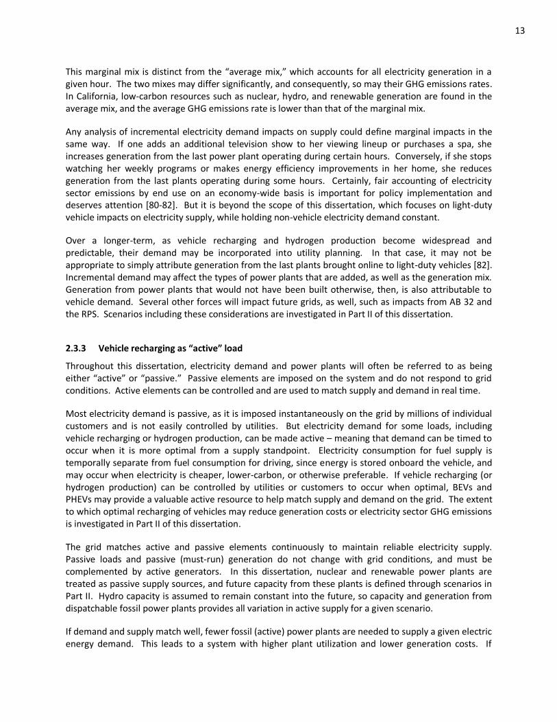
i Assessing Vehicle Electricity Demand Impacts on California ...

i

Assessing Vehicle Electricity Demand Impacts on California Electricity Supply

by

RYAN WILLIAM McCARTHY B.S. (University of California, San Diego) 2002

M.S. (University of California, Davis) 2005

DISSERTATION

Submitted in partial satisfaction of the requirements for the degree of

DOCTOR OF PHILOSOPHY

in

Civil and Environmental Engineering

in the

OFFICE OF GRADUATE STUDIES

of the

UNIVERSITY OF CALIFORNIA DAVIS

Approved:

Joan M. Ogden

Christopher Yang

Daniel Sperling

Committee in Charge

2009

ii

ABSTRACT

Achieving policy targets for reducing greenhouse gas (GHG) emissions from transportation will likely require significant adoption of battery-electric, plug-in hybrid, or hydrogen fuel cell vehicles. These vehicles use electricity either directly as fuel, or indirectly for hydrogen production or storage. As they gain share, currently disparate electricity and transportation fuels supply systems will begin to “converge.”

Several studies consider impacts of electric vehicle recharging on electricity supply or comparative GHG emissions among alternative vehicle platforms. But few consider interactions between growing populations of electric-drive vehicles and the evolution of electricity supply, especially within particular regional and policy contexts. This dissertation addresses this gap. It develops two modeling tools (EDGE-CA and LEDGE-CA) to illuminate tradeoffs and potential interactions between light-duty vehicles and electricity supply in California.

Near-term findings suggest natural gas-fired power plants will supply “marginal” electricity for vehicle recharging and hydrogen production. Based on likely vehicle recharging profiles, GHG emissions rates from these plants are more than 40% higher than the average from all generation supplying electricity demand in California and 65% higher than the estimated marginal electricity emissions rate in California’s Low Carbon Fuel Standard. Emissions from power plants supplying vehicle recharging are usually highest from 5pm-8pm, when they are 20% higher than their typical low value, from 2am-4am. Plug-in hybrid vehicles are 25-42% more efficient than conventional, gasoline hybrids, but reduce GHG emissions by less than 5%, because marginal electricity is currently much more carbon-intensive than gasoline in California (based on likely recharging profiles).

Over the long term, adding vehicle recharging or renewable generation to the grid can have important impacts on how electricity is supplied. Vehicle recharging shifts capacity and generation from poorly-utilized peaking power plants to more highly-utilized baseload plants with lower operating costs. Adding renewable generation has the opposite effect, which may be partially mitigated if vehicle recharging can be made to follow renewable generation. Achieving long-term targets for deep reductions in electricity sector GHG emissions requires significantly increasing renewable or nuclear generation and reducing per-capita electricity demand or avoiding new capacity from fossil power plants without carbon capture and sequestration.

iii

ACKNOWLEDGEMENTS

This research was funded by the California Energy Commission and the sponsors of the Sustainable Transportation Energy Pathways (STEPS) Program at the Institute of Transportation Studies at the University of California, Davis (ITS-Davis). I would like to thank those institutions, as well as CH2MHill, the National Science Foundation, and the sponsors of the Hydrogen Pathways Program at ITS-Davis for financial support in my graduate research and education.

Thanks are due to many others, whose shared wisdom and generosity have made for a wonderfully enriching graduate experience: Dr. Chris Yang and Prof. Joan Ogden for their caring guidance and mentoring throughout my research endeavors; Prof. Dan Sperling for his knowing insight and direction; Profs. Yueyue Fan and Alissa Kendall for their service on my qualifying exam committee; the ITS-Davis staff for making everything easy and enjoyable; and my friends who housed me as I traveled and wrote: Reilly; Kona; Mark, Lida, Yasmin, and Sasha; Nic; Nathan and Deborah; and Mike and Belinda.

As always, I am forever grateful for unwavering love and support from my friends and family – especially my parents, Sarah, Katherine, Mary, and Erica. You are my greatest blessing.

Finally, a shout out to my nieces and nephews: Claire, Rosalyn, Curran, Reid, and Wyatt. Your bright smiles, pure hearts, and inquisitive minds inspire me.

iv

TABLE OF CONTENTS

LIST OF TABLES ....................................................................................................................................... vi LIST OF FIGURES .....................................................................................................................................vii ABBREVIATIONS AND PARAMETERS ........................................................................................................ x 1. INTRODUCTION ................................................................................................................................ 1 2. BACKGROUND .................................................................................................................................. 5

2.1 Energy Policy in California ........................................................................................................ 5 2.2 Well-to-wheels vehicle GHG emissions ..................................................................................... 7

2.2.1 Vehicle Efficiency and Fuel Carbon Intensity ..................................................................... 8 2.3 Electricity Supply .................................................................................................................... 10

2.3.1 Electricity dispatch ......................................................................................................... 11 2.3.2 Marginal electricity and emissions .................................................................................. 12 2.3.3 Vehicle recharging as “active” load ................................................................................. 13 2.3.4 Integrating intermittent renewables on the grid ............................................................. 15

2.4 Literature Review ................................................................................................................... 17 PART I: MARGINAL GENERATION FOR NEAR-TERM VEHICLE ELECTRICITY DEMAND IN CALIFORNIA ...... 21 3. DOCUMENTATION OF THE ELECTRICITY DISPATCH FOR GREENHOUSE GAS EMISSIONS IN CALIFORNIA (EDGE-CA) MODEL ...................................................................................................... 22

3.1 Model Overview ..................................................................................................................... 22 3.1.1 Regional representation of California electricity supply .................................................. 23 3.1.2 Model outputs ................................................................................................................ 27

3.2 Power Plant Representation and Availability Module ............................................................. 29 3.2.1 Nuclear, geothermal, and biomass.................................................................................. 32 3.2.2 Wind .............................................................................................................................. 33 3.2.3 Solar ............................................................................................................................... 34 3.2.4 Hydro ............................................................................................................................. 35 3.2.5 Firm imports ................................................................................................................... 38 3.2.6 System imports............................................................................................................... 39 3.2.7 Dispatchable plants ........................................................................................................ 47 3.2.8 Additional generation ..................................................................................................... 48

3.3 Electricity Demand Module .................................................................................................... 49 3.3.1 Non-vehicle demand ...................................................................................................... 49 3.3.2 Vehicle demand .............................................................................................................. 50

3.4 Dispatch Module .................................................................................................................... 53 3.5 Costs ...................................................................................................................................... 58 3.6 Validation............................................................................................................................... 59 3.7 Discussion of Modeling Issues ................................................................................................ 63

4. NEAR-TERM VEHICLE AND FUEL PATHWAY COMPARISON .............................................................. 65 4.1 Electricity Supply in 2010 with No Vehicles ............................................................................. 65 4.2 Impacts of Vehicle Recharging on Electricity Demand ............................................................. 73 4.3 Marginal Electricity Supply in 2010 for Vehicle and Fuel Pathways ......................................... 75

4.3.1 Sensitivity of marginal electricity supply to hydro availability and demand location ........ 79 4.3.2 Comparison of EDGE-CA results to California’s Low Carbon Fuel Standard ...................... 82

4.4 Comparative Vehicle Pathway GHG Emissions in the Near Term ............................................. 83 4.5 Summary of Near-Term Findings ............................................................................................ 87

PART II: LONG-TERM VEHICLE ELECTRICITY DEMAND IMPACTS ON CALIFORNIA ELECTRICITY SUPPLY ... 90

v

5. DOCUMENTATION OF THE LONG-TERM ELECTRICITY DISPATCH MODEL FOR GREENHOUSE GAS EMISSIONS IN CALIFORNIA (LEDGE-CA) .......................................................................................... 91

5.1 Overview and Model Framework ........................................................................................... 92 5.2 Long-term Scenarios: Grid and Renewable Profiles ................................................................ 95 5.3 Future Non-Vehicle Electricity Demand Calculations .............................................................. 98 5.4 Representation of (Must-run) Renewable and Nuclear Capacity and Generation .................. 100 5.5 Long-term Scenarios: Vehicle Electricity Demand Profiles .................................................... 105 5.6 Representation of Hydro Generation .................................................................................... 108 5.7 Screening Curve Analysis for Optimal Fossil Capacity Additions ............................................ 108 5.8 Dispatch of Fossil Power Plants ............................................................................................ 114

6. LONG-TERM RESULTS: EVOLUTION OF CALIFORNIA ELECTRICITY SUPPLY (2020-2050) ................. 116 6.1 Long-term Results: No Added Renewables, No Vehicle Recharging (Category 1) .................. 117

6.1.1 Summary of category 1 results: Grid evolution without renewables or vehicle recharging ..................................................................................................................... 122

6.2 Long-term Results: Added Vehicle Electricity Demand, No New Renewables (Category 2) ... 123 6.2.1 Summary of category 2 results: Impact of vehicle recharging on fossil supply .............. 131

6.3 Long-term Results: Added Renewable Capacity, No Vehicle Recharging (Category 3) ........... 132 6.3.1 Summary of category 3 results: Impacts of renewable generation on fossil supply ....... 139

6.4 Long-term Results: Added Renewable Capacity and Vehicle Recharging (Category 4) .......... 140 6.4.1 Summary of Category 4 results: Interactions between renewable generation and vehicle recharging ..................................................................................................................... 154

6.5 Sensitivity Analysis of Long-term Results .............................................................................. 155 7. SUMMARY AND CONCLUSIONS ................................................................................................... 162

7.1 Methodological Contributions and Areas for Improvement .................................................. 162 7.2 Empirical Contributions and Areas for Future Work .............................................................. 163

REFERENCES ........................................................................................................................................ 175

vi

LIST OF TABLES Table 1. Vehicles compared in this dissertation, and assumed vehicle energy use. .................................. 7 Table 2. Studies investigating demand impacts from transportation on the electricity sector................ 19 Table 3. Resource mix by region in California, 2006. ............................................................................. 24 Table 4. Summary of existing power plants in California, as represented in EDGE-CA. ........................... 30 Table 5. Summary of references and methods used to represent power plant types in EDGE-CA model. ..................................................................................................................................... 31 Table 6. Description of power plants comprising firm imports. ............................................................. 38 Table 7. Assignment of zones in CAISO’s OASIS database that are interconnected to the CAISO control area to regions in EDGE-CA. ......................................................................................... 41 Table 8. Parameters investigated in regression modeling of system imports. ........................................ 41 Table 9. Regression coefficients for system imports from the Northwest. ............................................. 42 Table 10. Regression coefficients for system imports from the Southwest. ........................................... 44 Table 11. Distribution of net imports among California control areas. ................................................... 47 Table 12. Recent historical energy demand by balancing authority region in California. ........................ 49 Table 13. Vehicle and fuel efficiency and electricity demand assumptions used in near-term analysis. ................................................................................................................................. 51 Table 14. Timing profiles and vehicle and fuel pathways included in the near-term analysis. ................ 52 Table 15. Power plant operating cost parameters. ................................................................................ 59 Table 16. Validation of generation by energy source in EDGE-CA (TWh). ............................................... 60 Table 17. Comparison of reported natural gas-fired power plant heat rates and generation, 2005. ..................................................................................................................................... 62 Table 18. Vehicle demand and system load factors by scenario ............................................................ 75 Table 19. List of power plant types included in LEDGE-CA model. ......................................................... 94 Table 20. Components of scenarios investigated in Part II. .................................................................... 94 Table 21. Variables and baseline values included in sensitivity analysis in Part II. .................................. 94 Table 22. Description of grid profiles investigated in Part II. .................................................................. 96 Table 23. Description of renewable profiles in long-term electricity supply scenarios ........................... 97 Table 24. Renewable and nuclear power plant cost characteristics by year in LEDGE-CA. .................... 101 Table 25. Assumed capacity factors of renewable and nuclear power plants....................................... 102 Table 26. Cost and performance assumptions for new power plants built in California. ...................... 111 Table 27. Categorical order of electricity dispatch used in long-term electricity analysis. .................... 114 Table 28. Categorical representation of long-term results in this chapter............................................ 116 Table 29. Grid response to added vehicle electricity demand in the BAU (no IGCC) grid profile with the Current renewable mix. .......................................................................................... 125 Table 30. Grid response to added vehicle electricity demand in the Mixed technology grid profile with the Current renewable mix. .......................................................................................... 128 Table 31. Grid response to added vehicle electricity demand in the Low carbon grid profile with the Current renewable mix................................................................................................... 129 Table 32. Grid response to added vehicle electricity demand in 2050, BAU (no IGCC). ........................ 144 Table 33. Grid response to added vehicle electricity demand in 2050, Mixed technology .................... 147 Table 34. Grid response to added vehicle electricity demand in 2050, Low carbon.............................. 150

vii

LIST OF FIGURES Figure 1. Comparison of gasoline, electricity, and hydrogen fuel carbon intensity. .................................. 8 Figure 2. Well-to-wheel vehicle GHG emissions rates as a function of the lifecycle carbon intensity of electricity supply. ..................................................................................................................... 9 Figure 3. Illustration of active vehicle recharging impacts on active generation..................................... 14 Figure 4. Intermittent availability of California's wind and solar resources ............................................ 16 Figure 5. Median hourly demand and renewable generation load factors in California ......................... 17 Figure 6. Regions and transmission constraints included in EDGE-CA. ................................................... 23 Figure 7. Variations in definitions of electricity control areas ................................................................ 25 Figure 8. Framework of the EDGE-CA model. ........................................................................................ 26 Figure 9. Sample outputs from the EDGE-CA model. ............................................................................. 28 Figure 10. Historical distribution of nuclear, geothermal, and biomass generation................................ 33 Figure 11. Average hourly wind availability by month in the EDGE-CA model. ....................................... 34 Figure 12. Distribution of hourly solar insolation in Palm Springs, CA (August). ..................................... 35 Figure 13. Historical distribution of hydro generation ........................................................................... 36 Figure 14. Average hourly hydro generation by season and annual hydro availability, as represented in EDGE-CA. .............................................................................................................................. 37 Figure 15. Network model for the CAISO region .................................................................................... 40 Figure 16. Comparison of NW imports regression results and historical data. ....................................... 43 Figure 17. Comparison of SW imports regression results and historical data. ........................................ 44 Figure 18. Net NW and SW import duration curves for CAISO, and representation in EDGE-CA for California. ........................................................................................................................ 45 Figure 19. Monthly NW and SW imports into CAISO region, with representation in EDGE-CA for California. ............................................................................................................................. 46 Figure 20. Average monthly outages among dispatchable power plants in EDGE-CA. ............................ 48 Figure 21. Load duration curve used in 2010 dispatch modeling. .......................................................... 50 Figure 22. Representative monthly fuel demand at refueling stations. .................................................. 51 Figure 23. Representative hourly and daily fuel demand at refueling stations. ...................................... 52 Figure 24. Representative demand timing profiles for PHEV and BEV pathways. ................................... 53 Figure 25. Flow chart of logic in the EDGE-CA model. ............................................................................ 54 Figure 26. Representative statewide supply curve, including imports. ................................................... 55 Figure 27. Sample allocation of supply among regions. ......................................................................... 56 Figure 28. Sample regional supply curves. ............................................................................................. 57 Figure 29. Comparison of EDGE-CA inter-zonal transfers to CAISO data (2005-2007)............................. 61 Figure 30. Validation of greenhouse gas emissions rates. ...................................................................... 62 Figure 31. Relative market-clearing costs, compared to costs in CA-S. ................................................... 63 Figure 32. Monthly generation and average GHG emissions rates in 2010 from EDGE-CA simulation with no vehicle electricity demand and median hydro availability. ................................................ 66 Figure 33. Generation and average GHG emissions rate by region in 2010 from EDGE-CA simulation with no vehicle electricity demand and median hydro availability. ................................................ 67 Figure 34. Regional electricity cost duration curves in 2010 from EDGE-CA simulations with no vehicle electricity demand and median hydro availability. ................................................................. 68 Figure 35. Median hourly GHG emissions rates by month and regon in 2010 from EDGE-CA simulations with no vehicle elctricity demand and median hydro availability. .......................................... 69 Figure 36. Sensitivity of results from EDGE-CA simulations to assumed annual hydro availability (no added vehicle electricity demand). ........................................................................................ 72 Figure 37. Emissions rate from last generator operating in 2010 in EDGE-CA simulation with no added vehicle electricity demand and median annual hydro availability. ......................................... 73

viii

Figure 38. Sample impact of vehicle recharging on system electricity demand ...................................... 74 Figure 39. Marginal electricity GHG emissions rates by hour and month in 2010 for BEV recharging according to the Offpeak profile ........................................................................................... 76 Figure 40. Marginal electricity GHG emissions rates by hour and month in 2010 for BEV recharging according to the Load-level profile ........................................................................................ 77 Figure 41. Comparison of near-term marginal electricity mix and GHG emissions rates by vehicle and fuel pathway ......................................................................................................................... 78 Figure 42. Marginal electricity GHG emissions rates by hour, month, and region in 2010 for BEV recharging according to the Offpeak profile ......................................................................... 80 Figure 43. Sensitivity of near-term results to annual hydro availability and demand location. ............... 81 Figure 44. Comparison of marginal GHG emissions rates from EDGE-CA simulations and value in California’s Low Carbon Fuel Standard (and percentage increase). ....................................... 82 Figure 45. Well-to-wheels vehicle GHG emissions rates by energy source, based on marginal electricity mixes from EDGE-CA simulations for 2010 (median hydro availability). ................ 83 Figure 46. Well-to-wheels vehicle GHG emissions rates (gCO2-eq/mi) based on time of day and month of recharging............................................................................................................. 84 Figure 47. Vehicle GHG emissions rates as a function of vehicle energy intensity and fuel carbon intensity, based on marginal electricity mixes from EDGE-CA simulations for 2010. .............. 86 Figure 48. Framework of LEDGE-CA model for long-term electricity supply analysis. ............................. 93 Figure 49. Fraction of generation from renewables by supply scenario. ................................................ 98 Figure 50. Impact of load factor on California non-vehicle electricity demand (2050). ......................... 100 Figure 51. Map of capacity factors of wind generation from a Vestas V112-3.0 MW turbine based on median hourly wind speeds by region, as represented in LEDGE-CA .................................... 103 Figure 52. Relative solar thermal generation for representative wind and summer days. .................... 104 Figure 53. Fleet share and population of advanced vehicles in the long-term analysis. ........................ 105 Figure 54. Annual electric energy demand from vehicle recharging in long-term analysis.................... 106 Figure 55. Sample distribution of vehicle electricity demand for three recharging profiles. ................. 107 Figure 56. Sample screening curve analysis. ........................................................................................ 109 Figure 57. Assumed natural gas and coal prices in LEDGE-CA .............................................................. 112 Figure 58. Comparison of dispatchable plant capacity using costs from the EIA and the CEC. .............. 113 Figure 59. Assumed future capacity and emissions rates of existing fossil power plants. ..................... 113 Figure 60. Scenario capacity by power plant type and time segment (Current, No vehicles). ............... 118 Figure 61. Scenario capacity additions by time segment (Current, No vehicles). .................................. 119 Figure 62. Generation by power plant type and average GHG emissions rates by scenario (Current, No vehicles). ............................................................................................................................. 120 Figure 63. Generation costs by snapshot and scenario (Current, No vehicles). ..................................... 122 Figure 64. Duration curves in 2050 for load served by fossil power plants in scenarios with BAU (no IGCC) or Mixed technology grid profiles and Current renewable mix. ............................ 124 Figure 65. Vehicle recharging impacts on fossil capacity in 2050 for scenarios with Current renewable mix (percent change from the No vehicles case). ............................................... 130 Figure 66. Vehicle recharging impacts on fossil generation in 2050 for scenarios with Current renewable mix. .................................................................................................................. 131 Figure 67. Duration curves by renewable profile for fossil supply in 2050 in scenarios with BAU (no IGCC) and Mixed technology grid profiles. .................................................................... 133 Figure 68. System capacity in 2050 for scenarios with no vehicle demand. ......................................... 134 Figure 69. Change in fossil capacity in 2050 from added renewable generation in scenarios with No vehicles, compared to results with the Current renewable mix. ..................................... 135 Figure 70. Generation and average GHG emissions in 2050 for scenarios with no vehicle demand. ..... 136

ix

Figure 71. Change in fossil generation when renewable profiles are added to scenarios ..................... 137 Figure 72. Annualized generation costs in 2050 for scenarios with no vehicle demand. ....................... 138 Figure 73. Sample variation in Minimize fossil supply recharging profile by renewable mix. ................ 141 Figure 74. Demand and generation for selected scenarios with the Mixed technology grid profile on the peak electricity demand day in 2050. ...................................................................... 142 Figure 75. Map of median hourly GHG emissions rates in 2050, BAU (no IGCC). .................................. 145 Figure 76. Impact of vehicle recharging on system capacity in 2050, Mixed technology....................... 148 Figure 77. Impact of vehicle recharging on generation in 2050, Mixed technology. ............................. 148 Figure 78. Map of median hourly GHG emissions rates in 2050, Mixed technology. ............................ 149 Figure 79. Map of median hourly GHG emissions rates in 2050, Low carbon. ...................................... 151 Figure 80. Average electricity generation costs in 2050, by scenario. .................................................. 152 Figure 81. Average electricity GHG emissions rates in 2050, by scenario. ............................................ 153 Figure 82. Sensitivity of results in 2050 to load factor of non-vehicle electricity demand .................... 156 Figure 83. Sensitivity of results in 2050 to natural gas price ................................................................ 157 Figure 84. Effects of natural gas prices on screening curves in LEDGE-CA. ........................................... 158 Figure 85. Sensitivity of results in 2050 to $50/tonne CO2 tax ............................................................. 159 Figure 86. Sensitivity of select results in 2050 to non-vehicle demand load factor for scenarios with Offpeak or Minimize fossil supply recharging. ............................................................. 160 Figure 87. Summary of near-term well-to-wheels vehicle greenhouse gas emissions, based on marginal electricity generation mix for vehicle electricity demand timing profiles .............. 166 Figure 88. Median average GHG emissions rates in 2010 by region. .................................................... 168 Figure 89. Marginal electricity GHG emissions rates by hour and month in 2010 for BEV recharging according to the Offpeak profile. ........................................................................................ 169 Figure 90. Average electricity greenhouse gas emissions rates in 2050 for long-term scenarios in Part II of this dissertation. ............................................................................................................. 173

x

ABBREVIATIONS AND PARAMETERS A Wind turbine rotor-swept area (m2) AEO Annual Energy Outlook (EIA publication) AZ/NM/SNV Arizona/New Mexico/Southern Nevada Power Area BEV Battery-electric vehicle (all-electric) Cp Wind turbine coefficient of performance CA California CA-N Northern California supply area (north of Path 26) CA-S Southern California supply area (south of Path 15, excluding LADWP) CA/MX California/Mexico Power Area CAISO California Independent System Operator CCS Carbon capture and sequestration CEC California Energy Commission EDGE-CA Electricity Dispatch for Greenhouse gas Estimation in California CHP Combined heat and power CO2-eq CO2 equivalent (includes CO2, CH4, and N2O emissions) CPUC California Public Utilities Commission DSW Desert Southwest eGRID Emissions and Generation Resource Integrated Database (U.S. EPA database) EIA U.S. Energy Information Administration EPA U.S. Environmental Protection Agency EPRI Electric Power Research Institute ES&D Electric Supply and Demand (NERC database) FCV Fuel cell vehicle FERC Federal Energy Regulatory Commission GHG Greenhouse gas HEV (Conventional) Hybrid-electric vehicle ICE Internal combustion engine IGCC Integrated gasification combined cycle IID Imperial Irrigation District IOU Investor-owned utility LADWP Los Angeles Department of Water and Power Mer Merchant (power plant) NEEDS National Electric Energy Data System (U.S. EPA database) NERC North American Electric Reliability Corporation NGCC Natural gas combined-cycle NGCT Natural gas combustion turbine NGST Natural gas steam turbine NWPP Northwest Power Pool O&M Operations and maintenance OASIS Open Access Same-time Information System PG&E Pacific Gas & Electric PHEV Plug-in hybrid vehicle PHEVxx PHEV with xx miles of all-electric range PO Publicly-owned ρ Air density (1.225 kg/m3) RPS Renewable Portfolio Standard SCE Southern California Edison

xi

SDG&E San Diego Gas & Electric SMR Steam-methane reformation (for hydrogen production) SMUD Sacramento Municipal Utility District TID Turlock Irrigation District v Wind speed (m/s) VMT Vehicle-miles traveled WECC Western Electricity Coordinating Council

1

1. INTRODUCTION

In today’s energy system, supply chains for electricity and transportation fuels are largely independent from one another. But this paradigm could change. Several recent studies suggest that meeting 2050 goals for reducing greenhouse gas (GHG) emissions could require significant use of electric-drive vehicles, especially for light-duty applications [1-3]. As state and national governments adopt new energy solutions for economic, environmental, and security reasons, battery-electric vehicles (BEVs), hydrogen fuel cell vehicles (FCVs), and plug-in hybrid electric vehicles (PHEVs) could come to comprise a growing share of the vehicle mix.

Each of these vehicles, to various degrees, relies on electricity as fuel. Battery-electric vehicles completely use electricity. Fuel cell vehicles generate electricity onboard using stored hydrogen and a fuel cell. Hydrogen supply often relies on electricity from the grid, especially for production from electrolysis, or liquefaction and compression requirements for hydrogen distribution. Plug-in hybrids use both gasoline and electricity, and operate much like a conventional gasoline hybrid vehicle (HEV), but with a bigger battery that can be plugged in and recharged from the electric power grid. Several PHEV control strategies are possible that utilize the gasoline engine and battery-powered electric motor in different ways and under various conditions. In this dissertation, it is assumed that PHEVs operate as all-electric vehicles for some number of miles initially (20 or 40, designated PHEV20 or PHEV40), then as HEVs until they recharge.1 As vehicle recharging or hydrogen production place new demands on the electricity grid, the transportation and electricity sectors could begin to interact in radically new ways.

The electricity supply system (or “grid”) that powers these vehicles comprises a collection of power plants and transmission and distribution facilities that produces and delivers electricity to end users. Electricity cannot be practically stored,2 so the grid has evolved to supply fluctuating demands in real time. It does so using a suite of power plants of different size and type, which have different characteristics and fulfill different roles in the network. The composition of the grid varies significantly by time of day, season, and region, based on demand timing, resource availability, and energy policy.

Altogether, the grid is a dynamic supplier, matching supply and demand in real time. The types of power plants operating at any given time and the associated emissions and resource use depend on instantaneous demand. Anytime a light is turned on or off, or a vehicle begins or finishes recharging, the grid adapts to accommodate it. An operational power plant may generate more or less, or another plant may turn on or off. (With future “smart grids,” utilities might control demands to better match with supply, as well.) Each action has consequences for the operation of the system and affects the costs and emissions associated with electricity supply.

Electricity demand from vehicles, especially as it grows in quantity, must be considered within this context. Comparative emissions among vehicle types may vary significantly, depending on their impacts on electricity supply. Similarly, emissions may vary significantly for a single vehicle, depending on when and where it consumes electricity.

1 The all-electric range implies various technical and operational characteristics, which are discussed in Section 3.3.2. Other than the fraction of energy from electricity, however, PHEV20s and PHEV40s are treated identically in this analysis. 2 There are a number of electricity storage schemes that have been proposed and tested, including compressed air

storage, pumped hydro, batteries, and hydrogen. Aside from pumped hydro (most suitable sites for pumped hydro have already been exploited), none are used at large scale today.

2

California provides an ideal case study, as the state has recently adopted policies that will hasten adoption of advanced vehicles, increase renewable power generation, and reduce greenhouse gas emissions from the transportation and electricity sectors. The state will provide a testbed for new technologies and regulatory structures to be mimicked worldwide, if successful. Its policies are both near-term and far-reaching, and to be effective, require proper accounting of GHG emissions in the transportation and electricity sectors now, and decades into the future.

Several studies consider impacts from electric vehicles on electricity supply [4-7] or comparative greenhouse gas emissions among alternative vehicle platforms [8-15]. But few consider interactions between growing populations of electric-drive vehicles and the evolution of electricity supply, especially within the important regional and policy context of California. No studies compare interactions across vehicle platforms for a wide range of supply and demand conditions in the state using well-documented modeling techniques and assumptions that are available for public review. This dissertation begins to fill this gap. It develops two new modeling tools that simulate California electricity supply in the near term and decades into the future. These models offer a straightforward, transparent representation of electricity generation and capacity expansion in California that is appropriate for systems-level analysis.

In the near term, the Electricity Dispatch model for Greenhouse Gas Emissions in California (EDGE-CA) is developed to investigate electricity demand impacts from BEVs, PHEVs, and FCVs on power plant operation. California is divided into three regions, and individual power plants are “dispatched” to supply demand on an hourly basis, according to a merit order that minimizes the variable cost of generation statewide.

Among other outputs, EDGE-CA identifies the “marginal mix” of power plants that would not operate without added electricity demand from light-duty vehicles, while considering variations based on demand timing, location, and the availability of various power plants. Generation from these plants is attributed to vehicle electricity demand to compare lifecycle GHG emissions among vehicle platforms, while accurately accounting for the contribution from electricity supply.

The EDGE-CA model is subsequently modified to develop the Long-term EDGE-CA model (LEDGE-CA), which is applied to investigate the evolution of the California grid through 2050. This model simulates grid response to a number of scenarios relating to increased levels of vehicle recharging or renewable power generation, and the technical and social feasibility of new nuclear power or carbon capture and sequestration (CCS) technology. The LEDGE-CA model includes capacity additions and retirements over time, but represents hourly dispatch more simply. Unlike EDGE-CA, LEDGE-CA treats California as a single region and dispatches power plants categorically, rather than on a plant-by-plant basis.

The scenario approach and simplified representation of electricity dispatch in LEDGE-CA are appropriate for long-term analysis of the electricity sector. The power plants that will exist further-off in the future, and their operational strategies, depend on many uncertain parameters. The timing and composition of imported power will shift according to energy policy, population growth, and resource availability in California and neighboring states. Hydro power facilities may operate differently based on climatic factors affecting water storage. Future capacity of nuclear and hydro power is likely to be more a function of energy policy and social acceptance than economics. And distinctions in cost and efficiency among dispatchable power plants in the future are more difficult to identify than for the current grid. Given high-levels of uncertainty, plant-by-plant dispatch provides little additional information regarding vehicle demand impacts on future grids, and a simplified approach is appropriate for this type of analysis.

3

The objectives of this dissertation research fall generally into three categories: (1) estimating future vehicle and fuel electricity demands and their impact on overall electricity demand, (2) understanding the impact of demand timing on operation of the current California grid (daytime versus nighttime vehicle recharging, for example) and comparing GHG emissions across a wide range of vehicle and fuel pathways, and (3) understanding how large penetrations of electric-drive vehicles might impact the long-term evolution of the electricity sector. Several interesting and novel questions are addressed from each category, including:

1. What is the effect of increasing penetrations of advanced vehicles and alternative fuels on electricity demand in California?

How many alternative-fueled vehicles can the current California electricity grid support?

How do long-term vehicle electricity demand and timing scenarios affect electricity demand profiles and load factors?

2. How does operation of the existing and near-term electricity grid in California change in response to additional demand from light-duty vehicles?

What types of power plants will provide marginal electricity supply for vehicles and fuels initially? What are the associated GHG emissions rates? How do they compare to the value codified in California’s Low Carbon Fuel Standard (LCFS)?

How does the marginal mix affect vehicle GHG emissions? How do alternative vehicle emissions compare on a well-to-wheels basis?

How sensitive are electricity supply and GHG emissions rates to hydro availability and the location and timing of vehicle and fuel-related electricity demands in the near term?

3. How might the California electric grid evolve differently over time with additional demand from vehicles and fuels than it would otherwise?

What effect does increasing light-duty vehicle recharging have on electricity supply in California?

What effect does increasing renewable generation have on electricity supply in California?

To what extent can coordinated vehicle recharging (acting as active load) reduce costs associated with operating the grid and integrating passive generation from intermittent renewable sources?

The dissertation is organized as follows. Chapter 2 provides relevant background information and a discussion of previous research pertaining to electricity dispatch modeling and vehicle demand impacts on electricity supply. Chapters 3 and 4 encompass Part I of this analysis, and discuss marginal electricity generation for vehicles using the current California grid. Chapter 3 describes the methodology behind the EDGE-CA model, which is applied in Chapter 4 to compare vehicle and fuel pathway GHG emissions. The results presented in Chapter 4 are compared to the values included in the LCFS, and sensitivity to demand quantity, timing, location, and hydro availability is discussed. Part II of the dissertation comprises Chapters 5 and 6, which investigate evolution of the electricity sector and impacts of vehicle

4

recharging on California electricity supply through 2050. Chapter 5 describes the LEDGE-CA model and its methods, and results are presented in Chapter 6. The results especially focus on electricity costs and grid composition given high levels of intermittent wind or solar generation, and on impacts of vehicle recharging. The dissertation is concluded in Chapter 7, which summarizes results presented throughout the analysis in the context of the questions above and offers areas for future research.

5

2. BACKGROUND

This section provides relevant background information and literature review to provide context for this dissertation. First, a primer is provided regarding California energy policies that will shape future energy supply and demand in the state. Next, in Section 2.2, well-to-wheels analysis is described and the contribution of vehicle efficiency and fuel carbon intensity to well-to-wheels GHG emissions are explored. In Section 2.3, the composition and operation of the electricity grid is discussed. Elements comprising the grid are described, dispatch rules for operating different types of power plants are introduced, and marginal generation and GHG emissions are defined. The grid is also described as a network of “active” or “passive” generation and demand elements that must balance each other to match supply with demand. The active or passive nature of vehicle and hydrogen-related electricity demand and renewable power has important implications for integrating either onto the grid, as described in this section. Finally, in Section 2.4, literature pertaining to well-to-wheels analysis and vehicle electricity demand impacts on the current and future grids is reviewed, and this dissertation is put in the context of existing work.

2.1 Energy Policy in California

Historically, California has been a pioneer in energy and environmental policy. In the 1960s and 1970s it established vehicle emissions and building energy efficiency standards, which have been subsequently been implemented at the federal level and internationally [16-19]. Today, California continues to lead with progressive energy and environmental policy, and is beginning to establish policy frameworks for mitigating climate change emissions from vehicles and the electricity sector. State policies relevant to this dissertation are summarized below:

Global Warming Solutions Act (AB 32) – This act requires California to reduce its GHG emissions to 1990 levels by 2020, or about 25% below business as usual estimates [20]. An 80% reduction target by 2050 has been established through Executive Order [21]. A series of early actions under AB 32 have been developed, which include the Renewable Portfolio Standard and Low Carbon Fuel Standard, which are discussed below. It is expected that this policy may guide energy and environmental rulemaking for years to come in the state.

Low Carbon Fuel Standard (LCFS) – The LCFS was established through an Executive Order in 2007 [22] and has subsequently been adopted as an early action item under AB 32. The regulation directs refiners to reduce the carbon content of on-road transportation fuels in California by 10% in 2020, compared to conventional petroleum fuels [23]. In implementing the LCFS regulation, the California Air Resources Board (ARB) has developed estimates of lifecycle GHG emissions associated with various fuels. Gasoline is attributed a lifecycle GHG intensity of 96 gCO2/MJ (346 gCO2/kWh) [24]. Marginal electricity for vehicle recharging is assumed to be 79% from natural gas combined cycle (NGCC) power plants, and 21% from renewables, leading to a lifecycle GHG intensity of 104.7 gCO2/MJ (377 gCO2/kWh) [25]. In the Standard, the carbon intensity of electricity is divided by a factor of three to account for improved vehicle efficiency compared to gasoline engines, so electricity does count as a “low carbon” fuel, despite its higher GHG intensity initially *23+.

Renewable Portfolio Standard (RPS) – Mandates that 20% of electricity generation in the state come renewable resources by 2010 [26]. The target has been extended through an

6

Executive Order to require 33% of electricity generation to come from renewable resources by 2020 [27].

Fuel economy standards – California passed aggressive light-duty vehicle greenhouse gas emissions standards in 2002 (the “Pavley Bill,” or AB 1493) *28+, which have recently been harmonized with federal Corporate Average Fuel Economy Standards (or CAFÉ) [29]. The standard requires the light-duty vehicle fleet to have an average fuel economy of about 34 miles per gallon (mpg) by 2016, and includes incentives for BEVs, FCVs, and PHEVs.

Zero Emission Vehicle (ZEV) Mandate – The ZEV mandate was established in 1990 to encourage sales of zero-emission vehicles in California [34]. It requires increasing fractions of zero-emission vehicle sales among large automotive manufacturers in the state, but has been revised since its original adoption to allow manufacturers more flexibility in meeting the targets [30].

Alternative and Renewable Fuel and Vehicle Technology Program (AB 118) – AB 118 provides funding for air quality improvement projects related to vehicle and fuel technologies [31]. Many of the goals of the Investment Plan developed under AB 118 have been previously established in the State Alternative Fuels Plan (AB 1007) [32, 33] and California’s Strategy to Reduce Petroleum Dependence (AB 2076) *34, 35+. Among other projects, AB 118 partially funds the California Hydrogen Highway [36], which develops a network of hydrogen refueling stations throughout the state. As per Senate Bill 1505 (Environmental Standards for Hydrogen Production), hydrogen production in California must include 33% renewable content and have 30% lower well-to-wheel GHG emissions than conventional gasoline vehicles [37].

Other incentives for advanced vehicles – Several federal, state, and local incentives have been adopted to encourage purchasing advanced or alternative-fueled vehicles. The Alternative Fuel Motor Vehicle Tax Credit was enacted as part of the Energy Policy Act of 2005 [38] and provides a federal income tax credit of up to $4,000 dollars for qualifying alternative fueled vehicles – including hydrogen vehicles – purchased before December 31, 2010 [39]. The American Recovery and Reinvestment Act of 2009 includes federal income tax credits ranging from $2,500-7,500, depending on battery size, for the first 200,000 plug-in vehicles sold by a manufacturer. It also provides a tax credit of up to $4,000 for electric-drive conversion kits [40]. The Fuel Cell Motor Vehicle Tax Credit provides a $4,000 federal income tax credit through December 31, 2014 on qualifying FCVs [41]. Additional incentives include reduced insurance payments or registration fees, carpool lane exemptions, preferential parking, and others [42].

Electricity Greenhouse Gas Emission Performance Standards (SB 1368) – SB 1368 sets emissions standards on new baseload power plants serving electricity demand in California, stipulating that emissions rates must be no higher than 1,100 gCO2/MWh, which is about the level of a natural gas combined-cycle (NGCC) power plant. This law effectively outlaws new conventional coal-fired power plants from serving California electricity demand, but does not prevent utilities from utilizing coal-fired generation from existing contracts (mostly with out-of-state plants, as described in Section 3.2.5) [43].

7

2.2 Well-to-wheels vehicle GHG emissions

Greenhouse gas emissions are a key metric for comparing environmental performance of vehicles. Comparing energy use and emissions among distinct vehicle platforms requires analysis on a "well-to-wheels" basis. Well-to-wheels emissions include those upstream from the vehicle, from the "well-to-tank," as well as those that take place from the "tank-to-wheels." Emissions from conventional vehicles occur predominately from tank-to-wheels, during fuel combustion in the engine; only a small fraction of total emissions occurs during the extraction, refining, and transportation of petroleum to a vehicle's tank. In a PHEV, well-to-tank emissions from electricity generation contribute significantly to overall emissions. In the case of a BEV or FCV, emissions occur entirely upstream from the vehicle's "tank," during the production of electricity or hydrogen and delivery to the vehicle.

Previous well-to-wheels studies have investigated a number of advanced vehicle platforms and concluded that they will likely have much higher fuel economies than conventional internal combustion engine vehicles (ICEs) and conventional HEVs. Battery-electric vehicles may be more than three times as fuel-efficient as an ICE, and have more than twice the fuel economy of an HEV. Relative fuel economy gains from PHEVs depend on their operation, while fuel cell vehicles are typically more than twice as fuel-efficient as ICEs [10, 11, 14, 15, 44, 45].

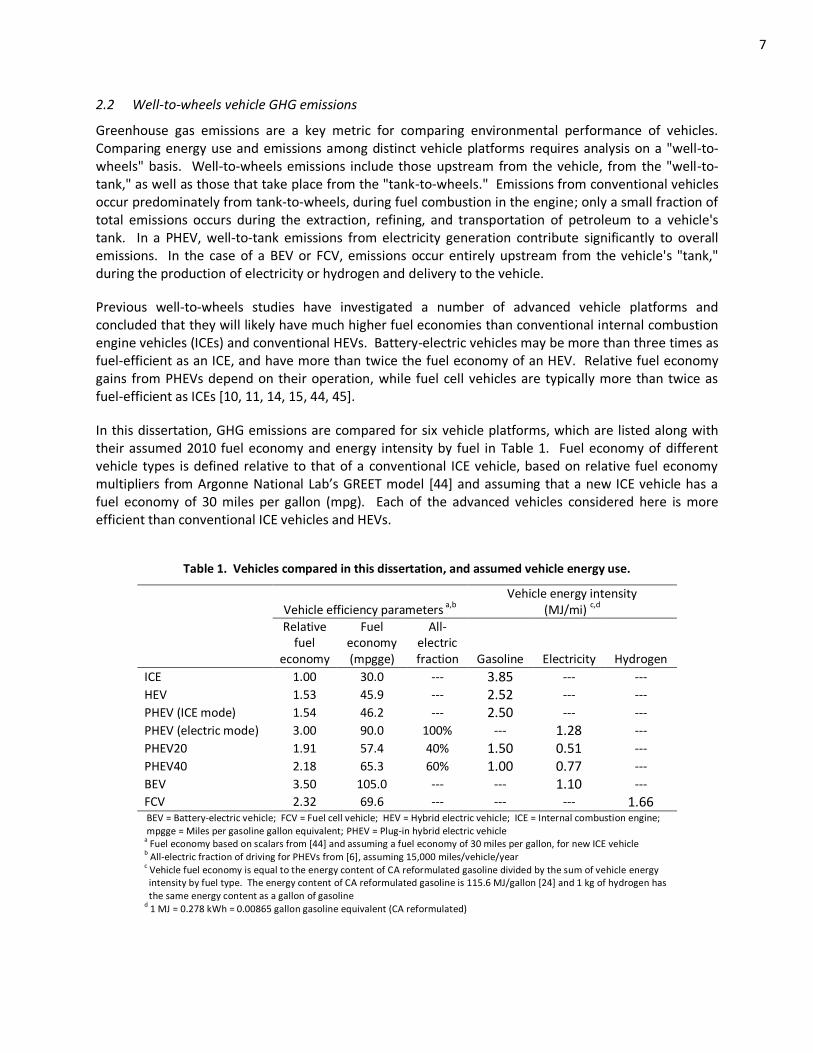
In this dissertation, GHG emissions are compared for six vehicle platforms, which are listed along with their assumed 2010 fuel economy and energy intensity by fuel in Table 1. Fuel economy of different vehicle types is defined relative to that of a conventional ICE vehicle, based on relative fuel economy multipliers from Argonne National Lab’s GREET model *44+ and assuming that a new ICE vehicle has a fuel economy of 30 miles per gallon (mpg). Each of the advanced vehicles considered here is more efficient than conventional ICE vehicles and HEVs.

Table 1. Vehicles compared in this dissertation, and assumed vehicle energy use.

Vehicle efficiency parameters a,b

Vehicle energy intensity (MJ/mi)

c,d

Relative fuel

economy

Fuel economy (mpgge)

All- electric fraction Gasoline Electricity Hydrogen

ICE 1.00 30.0 --- 3.85 --- ---

HEV 1.53 45.9 --- 2.52 --- ---

PHEV (ICE mode) 1.54 46.2 --- 2.50 --- ---

PHEV (electric mode) 3.00 90.0 100% --- 1.28 ---

PHEV20 1.91 57.4 40% 1.50 0.51 ---

PHEV40 2.18 65.3 60% 1.00 0.77 ---

BEV 3.50 105.0 --- --- 1.10 ---

FCV 2.32 69.6 --- --- --- 1.66 BEV = Battery-electric vehicle; FCV = Fuel cell vehicle; HEV = Hybrid electric vehicle; ICE = Internal combustion engine; mpgge = Miles per gasoline gallon equivalent; PHEV = Plug-in hybrid electric vehicle a Fuel economy based on scalars from [44] and assuming a fuel economy of 30 miles per gallon, for new ICE vehicle

b All-electric fraction of driving for PHEVs from [6], assuming 15,000 miles/vehicle/year

c Vehicle fuel economy is equal to the energy content of CA reformulated gasoline divided by the sum of vehicle energy

intensity by fuel type. The energy content of CA reformulated gasoline is 115.6 MJ/gallon [24] and 1 kg of hydrogen has the same energy content as a gallon of gasoline d 1 MJ = 0.278 kWh = 0.00865 gallon gasoline equivalent (CA reformulated)

8

The fuel economy of a PHEV depends on its fraction of all-electric drive. If it is low, then a PHEV operates much like an HEV, with similar fuel economy. If it is high, a PHEV has a fuel economy closer to that of a BEV, although somewhat lower due to the increased weight of the dual drive train. As represented here, the PHEV20 and PHEV40 vehicle types included in this dissertation have fuel economies that are 25% and 43% higher than those of conventional HEVs.

2.2.1 Vehicle Efficiency and Fuel Carbon Intensity

Well-to-wheels vehicle GHG emissions (gCO2/mi) can be defined as the product of vehicle energy intensity (MJ/mi) and well-to-tank fuel carbon intensity (gCO2/MJ). The use of advanced vehicle technologies and alternative fuels can help reduce GHG emissions by improving vehicle efficiency or fuel economy (that is, reducing energy intensity)3 and lowering fuel carbon intensity [2].

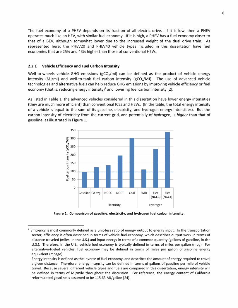
As listed in Table 1, the advanced vehicles considered in this dissertation have lower energy intensities (they are much more efficient) than conventional ICEs and HEVs. (In the table, the total energy intensity of a vehicle is equal to the sum of its gasoline, electricity, and hydrogen energy intensities). But the carbon intensity of electricity from the current grid, and potentially of hydrogen, is higher than that of gasoline, as illustrated in Figure 1.

0

50

100

150

200

250

300

350

Gasoline CA avg. NGCC NGCT Coal SMR Elec (NGCC)

Elec (NGCT)

Electricity Hydrogen

Fue

l car

bo

n in

ten

sity

(gC

O2/M

J)

Figure 1. Comparison of gasoline, electricity, and hydrogen fuel carbon intensity.

3 Efficiency is most commonly defined as a unit-less ratio of energy output to energy input. In the transportation

sector, efficiency is often described in terms of vehicle fuel economy, which describes output work in terms of distance traveled (miles, in the U.S.) and input energy in terms of a common quantity (gallons of gasoline, in the U.S.). Therefore, in the U.S., vehicle fuel economy is typically defined in terms of miles per gallon (mpg). For alternative-fueled vehicles, fuel economy may be defined in terms of miles per gallon of gasoline energy equivalent (mpgge). Energy intensity is defined as the inverse of fuel economy, and describes the amount of energy required to travel a given distance. Therefore, energy intensity can be defined in terms of gallons of gasoline per mile of vehicle travel. Because several different vehicle types and fuels are compared in this dissertation, energy intensity will be defined in terms of MJ/mile throughout the discussion. For reference, the energy content of California reformulated gasoline is assumed to be 115.63 MJ/gallon [24].

9

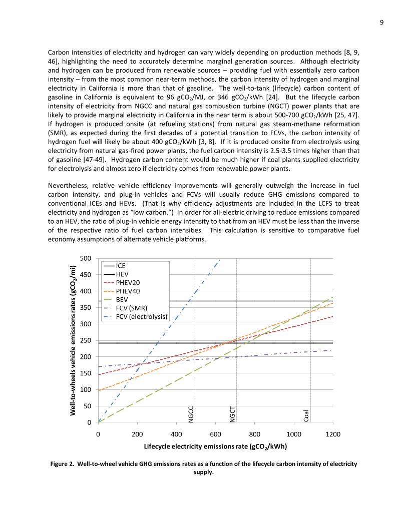
Carbon intensities of electricity and hydrogen can vary widely depending on production methods [8, 9, 46], highlighting the need to accurately determine marginal generation sources. Although electricity and hydrogen can be produced from renewable sources – providing fuel with essentially zero carbon intensity – from the most common near-term methods, the carbon intensity of hydrogen and marginal electricity in California is more than that of gasoline. The well-to-tank (lifecycle) carbon content of gasoline in California is equivalent to 96 gCO2/MJ, or 346 gCO2/kWh [24]. But the lifecycle carbon intensity of electricity from NGCC and natural gas combustion turbine (NGCT) power plants that are likely to provide marginal electricity in California in the near term is about 500-700 gCO2/kWh [25, 47]. If hydrogen is produced onsite (at refueling stations) from natural gas steam-methane reformation (SMR), as expected during the first decades of a potential transition to FCVs, the carbon intensity of hydrogen fuel will likely be about 400 gCO2/kWh [3, 8]. If it is produced onsite from electrolysis using electricity from natural gas-fired power plants, the fuel carbon intensity is 2.5-3.5 times higher than that of gasoline [47-49]. Hydrogen carbon content would be much higher if coal plants supplied electricity for electrolysis and almost zero if electricity comes from renewable power plants.

Nevertheless, relative vehicle efficiency improvements will generally outweigh the increase in fuel carbon intensity, and plug-in vehicles and FCVs will usually reduce GHG emissions compared to conventional ICEs and HEVs. (That is why efficiency adjustments are included in the LCFS to treat electricity and hydrogen as “low carbon.”) In order for all-electric driving to reduce emissions compared to an HEV, the ratio of plug-in vehicle energy intensity to that from an HEV must be less than the inverse of the respective ratio of fuel carbon intensities. This calculation is sensitive to comparative fuel economy assumptions of alternate vehicle platforms.

0

50

100

150

200

250

300

350

400

450

500

0 200 400 600 800 1000 1200

We

ll-to

-wh

eel

s ve

hic

le e

mis

sio

ns

rate

s (g

CO

2/m

i)

Lifecycle electricity emissions rate (gCO2/kWh)

ICEHEVPHEV20PHEV40BEVFCV (SMR)FCV (electrolysis)

Co

al

NG

CT

NG

CC

Figure 2. Well-to-wheel vehicle GHG emissions rates as a function of the lifecycle carbon intensity of electricity supply.

10

The impact of the GHG intensity of electricity supply on vehicle GHG emissions rates is illustrated in Figure 2, based on the assumptions included in this analysis (additional details are provided in Chapter 3). The figure compares vehicle GHG emissions rates as a function of electricity supply, and compares them to emissions from a conventional ICE vehicle and HEV. Note that the carbon intensity of gasoline and natural gas is constant, so vehicle emissions can be presented entirely as a function of electricity sector GHG emissions, according to the vehicle energy intensity values listed in Table 1. For reference, average emissions rates from coal, NGCC, and NGCT power plants are shown, as well [47]. It is unlikely that electricity supply would have much higher GHG emissions rates than those from the average coal power plant illustrated in the figure.

Based on these assumptions, BEVs and PHEVs will essentially always have lower GHG emissions than gasoline ICE vehicles. If the electricity mix for vehicle recharging has a GHG emissions rate that is no higher than the lifecycle rate for NGCT plants in California, these vehicles should have lower GHG emissions than conventional HEVs, as well. Battery-electric vehicles rely entirely on electricity, and if electricity sector GHG emissions are very low, so too are vehicle emissions. Plug-in hybrid electric vehicles will typically use gasoline for some portion of driving, and thus will not achieve zero emissions, regardless of electricity sector emissions rates. The emissions line for BEVs has a much steeper slope than those for PHEVs because BEVs have a higher electric energy intensity (listed in Table 1), making their emissions rates more sensitive to the carbon intensity of electricity supply.

Fuel cell vehicles using hydrogen from natural gas SMR have relatively low electric energy intensity, making them somewhat insensitive to the emissions rate of electric supply, and have lower GHG emissions rates than conventional hybrids regardless of the types of power plants supplying electricity for hydrogen supply. (The only electricity use in this pathway is for compressed hydrogen storage on vehicles.) If hydrogen is produced from electrolysis, however, electric energy intensity of the pathway is very high, and electricity supply must have very low GHG emissions to reduce vehicle emissions compared to conventional hybrids.

Clearly, achieving very low GHG emissions from these vehicles requires decarbonizing electricity supply. Even in the case of FCVs using hydrogen from SMR – a pathway with low electricity requirements – vehicle emissions are 20% lower if renewable (zero-carbon) electricity is used in the pathway, rather than coal-fired power plants. This partly motivates investigation of long-term, low carbon electricity scenarios, which are considered in Part II of this dissertation.

2.3 Electricity Supply

The electricity grid refers to the system of power plants, transmission, and distribution facilities that supply electricity demand. This dissertation focuses on the operation of power plants, as they respond to changes in demand.

Power plants are generally classified according to two categories:

Must-run (passive): Must-run resources, also described in this dissertation as “passive,” represent power plants whose output generation is taken whenever available. Generation from must-run resources is independent from demand, and these power plants do not ramp up or down – or turn on or off – in response to grid conditions. These resources may have constant and predictable output, or it may vary intermittently. In this dissertation, biomass, geothermal, and nuclear power plants are represented as must-run resources that operate

11

as “baseload” facilities, with essentially constant output.4 Some of the hydro resource operates as must-run, baseload generation, as well, to maintain minimum river flows or following the “run-of-the-river.” Wind and solar plants are also treated as must-run, but generation from these facilities may fluctuate significantly from one hour to the next (as illustrated in Figure 4). Energy storage may play a significant role in the future in “firming” generation from intermittent resources, to make output from these resources more predictable, or even dispatchable. Energy storage is beyond the scope of this dissertation, but has been investigated elsewhere [50-53]. Adding energy storage as a supplemental generation resource in the EDGE-CA or LEDGE-CA models is left for future work.

Dispatchable (active): Dispatchable resources, described in this dissertation as “active,” may change their output from hour to hour, and are “dispatched” as needed to match supply with demand. Most of the hydro resource and all fossil fuel-fired power plants in California are treated as dispatchable in the EDGE-CA and LEDGE-CA models.

Throughout this dissertation, “must-run” and “passive” are used interchangeably. “Dispatchable” and “active” are also used interchangeably.

2.3.1 Electricity dispatch

Electricity dispatch is a process used by utilities and grid operators to determine which power plants operate to meet demand at a given time. Generally, electricity dispatch aims to satisfy instantaneous electricity demand at the lowest cost, while satisfying several system constraints. A schedule of costs versus production levels is developed for each available generator, and – theoretically – plants are dispatched in order of increasing cost until generation requirements are met. Practically, dispatch is more complicated, and does not simply follow a cost-based merit order. Constraining factors extend dispatch beyond simply allocating generation to plants with the lowest variable costs or unit offers:

Contractual obligations

Environmental regulations

Plant availability, operational limits, ramp rates, and start-up costs

Reliability requirements

Transmission and distribution constraints

Utilities and grid operators have complicated optimization models to help determine dispatch order. A common modeling approach is through economic dispatch, which formulates an objective function that minimizes cost subject to constraints above [54]. Several solution algorithms have been implemented to

4 There are many different types of biomass-fired power plants, which may take various feedstocks and employ

various operating strategies. Many may, in fact, operate as dispatchable plants that can ramp up or down with demand. But biomass facilities comprise less than 2% of California generation currently, and are not a focus of the long-term scenarios analyzed in Part II. Therefore, for simplicity, biomass power plants are aggregated and treated as a single must-run resource, which is dispatched according to historical availability, as described in Section 3.2.1.

12

solve economic dispatch problems, including artificial intelligence theory [55-57], dynamic programming [58], and non-linear programming [59].

A handful of commercially-available models have been developed by consulting firms that are often licensed to utilities and planning organizations [49, 60-69]. Other studies represent electricity dispatch more simply, using representative daily or annual load profiles [70-78]. The EDGE-CA and LEDGE-CA models represent electricity dispatch with a level of rigor between the two. They use a straightforward, merit-order approach to dispatch power plants, which lacks system optimization and detailed representation of many grid elements that are included in proprietary software. But the models developed in this dissertation represent supply in greater detail than the latter set of studies, which do not account for variations in supply on a refined level.

The EDGE-CA and LEDGE-CA models provide useful insight regarding the operation of various types of power plants and affects from changes in electricity demand profiles, and provide a transparent representation of electric generation in California that is appropriate for systems-level and policy analysis related to demand impacts on electricity supply, resource use, and GHG emissions.

2.3.2 Marginal electricity and emissions

Characterizing upstream emissions for electricity and hydrogen fuels requires detailed electricity dispatch modeling to correctly identify the “marginal mix” of power plants supplying vehicle and fuel-related electricity demands that would not be operating otherwise. In the well-to-wheels GHG analysis presented in Chapter 4, the last power plants brought online in a given hour are attributed to the marginal mix for vehicle recharging or hydrogen production. The EDGE-CA model tracks dispatch order and identifies the last power plants brought online in a given hour to determine the marginal mix for light-duty vehicle demand.

Attributing electrons from particular power plants to specific end uses is impossible with current technology, which makes it a delicate exercise. The actual electricity supplying PHEV electricity may come from the “first” power plant dispatched – a nuclear plant, for example – rather than the last. But this analysis proposes to compare the decision to purchase and recharge a PHEV (for example) to purchasing and operating a gasoline ICE vehicle or HEV, from a GHG emissions perspective. A consequence of that decision is an increase in electricity demand at the time of vehicle recharging, which causes the last (marginal) power plant operating to generate a little more electricity than it would if the PHEV owner had decided to buy a gasoline HEV, instead.

If the aggregate, incremental demand from thousands of consumers choosing BEVs, PHEVs, or FCVs instead of gasoline vehicles exceeds the excess capacity of the last generator operating, additional plants are brought online and added to the marginal mix. As vehicle and fuel-related electricity demands grow, so do the number of marginal generators operating, and operation of the power grid adapts. The timing and quantity of imported power may change, as well as the timing of hydro generation, and generation from dispatchable, fossil-fired power plants adjusts accordingly.

By this definition, which is used in other studies as well [7, 79], marginal generators are often the most expensive plants operating in a given hour, and likely, the least efficient. In this analysis, generation from passive hydro, nuclear, or renewable power plants – which also have very low operating costs – is never on the margin. Instead, the marginal mix consists of generation from fossil-fired power plants, usually natural gas for California.

13

This marginal mix is distinct from the “average mix,” which accounts for all electricity generation in a given hour. The two mixes may differ significantly, and consequently, so may their GHG emissions rates. In California, low-carbon resources such as nuclear, hydro, and renewable generation are found in the average mix, and the average GHG emissions rate is lower than that of the marginal mix.

Any analysis of incremental electricity demand impacts on supply could define marginal impacts in the same way. If one adds an additional television show to her viewing lineup or purchases a spa, she increases generation from the last power plant operating during certain hours. Conversely, if she stops watching her weekly programs or makes energy efficiency improvements in her home, she reduces generation from the last plants operating during some hours. Certainly, fair accounting of electricity sector emissions by end use on an economy-wide basis is important for policy implementation and deserves attention [80-82]. But it is beyond the scope of this dissertation, which focuses on light-duty vehicle impacts on electricity supply, while holding non-vehicle electricity demand constant.

Over a longer-term, as vehicle recharging and hydrogen production become widespread and predictable, their demand may be incorporated into utility planning. In that case, it may not be appropriate to simply attribute generation from the last plants brought online to light-duty vehicles [82]. Incremental demand may affect the types of power plants that are added, as well as the generation mix. Generation from power plants that would not have been built otherwise, then, is also attributable to vehicle demand. Several other forces will impact future grids, as well, such as impacts from AB 32 and the RPS. Scenarios including these considerations are investigated in Part II of this dissertation.

2.3.3 Vehicle recharging as “active” load

Throughout this dissertation, electricity demand and power plants will often be referred to as being either “active” or “passive.” Passive elements are imposed on the system and do not respond to grid conditions. Active elements can be controlled and are used to match supply and demand in real time.

Most electricity demand is passive, as it is imposed instantaneously on the grid by millions of individual customers and is not easily controlled by utilities. But electricity demand for some loads, including vehicle recharging or hydrogen production, can be made active – meaning that demand can be timed to occur when it is more optimal from a supply standpoint. Electricity consumption for fuel supply is temporally separate from fuel consumption for driving, since energy is stored onboard the vehicle, and may occur when electricity is cheaper, lower-carbon, or otherwise preferable. If vehicle recharging (or hydrogen production) can be controlled by utilities or customers to occur when optimal, BEVs and PHEVs may provide a valuable active resource to help match supply and demand on the grid. The extent to which optimal recharging of vehicles may reduce generation costs or electricity sector GHG emissions is investigated in Part II of this dissertation.

The grid matches active and passive elements continuously to maintain reliable electricity supply. Passive loads and passive (must-run) generation do not change with grid conditions, and must be complemented by active generators. In this dissertation, nuclear and renewable power plants are treated as passive supply sources, and future capacity from these plants is defined through scenarios in Part II. Hydro capacity is assumed to remain constant into the future, so capacity and generation from dispatchable fossil power plants provides all variation in active supply for a given scenario.

If demand and supply match well, fewer fossil (active) power plants are needed to supply a given electric energy demand. This leads to a system with higher plant utilization and lower generation costs. If

14

demand does not match supply well, more fossil power plant capacity is needed, and plants are not utilized as well, resulting in relatively higher electricity costs. If electricity demand can be controlled (that is, can be made active) it can help to match the supply and demand, and reduce costs.

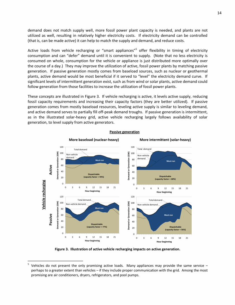
Active loads from vehicle recharging or “smart appliances”5 offer flexibility in timing of electricity consumption and can “defer” demand until it is convenient to supply. (Note that no less electricity is consumed on whole, consumption for the vehicle or appliance is just distributed more optimally over the course of a day.) They may improve the utilization of active, fossil power plants by matching passive generation. If passive generation mostly comes from baseload sources, such as nuclear or geothermal plants, active demand would be most beneficial if it served to “level” the electricity demand curve. If significant levels of intermittent generation exist, such as from wind or solar plants, active demand could follow generation from those facilities to increase the utilization of fossil power plants.

These concepts are illustrated in Figure 3. If vehicle recharging is active, it levels active supply, reducing fossil capacity requirements and increasing their capacity factors (they are better utilized). If passive generation comes from mostly baseload resources, leveling active supply is similar to leveling demand, and active demand serves to partially fill off-peak demand troughs. If passive generation is intermittent, as in the illustrated solar-heavy grid, active vehicle recharging largely follows availability of solar generation, to level supply from active generators.

Passive generation

More baseload (nuclear-heavy) More intermittent (solar-heavy)

Veh

icle

rec

har

gin

g

Act

ive

0

20

40

60

80

100

120

0 3 6 9 12 15 18 21

De

man

d o

r G

en

era

tio

n (

GW

)

Hour beginning

Must-run

Dispatchable(capacity factor = 94%)

Non-vehicle

demand

Total demand

0

20

40

60

80

100

120

0 3 6 9 12 15 18 21

De

man

d o

r G

en

era

tio

n (

GW

)

Hour beginning


Must-run

Non-vehicle

demand

Total demand

Pas

sive

0

20

40

60

80

100

120

0 3 6 9 12 15 18 21

De

man

d o

r G

en

era

tio

n (

GW

)

Hour beginning


Must-run

Non-vehicle demand

Total demand

0

20

40

60

80

100

120

0 3 6 9 12 15 18 21

De

man

d o

r G

en

era

tio

n (

GW

)

Hour beginning


Must-run

Non-vehicle demand

Total demand

Figure 3. Illustration of active vehicle recharging impacts on active generation.

5

Vehicles do not present the only promising active loads. Many appliances may provide the same service – perhaps to a greater extent than vehicles – if they include proper communication with the grid. Among the most promising are air conditioners, dryers, refrigerators, and pool pumps.

15

Energy storage will likely provide an important active resource to the grid in the future, as well. Importantly, it could serve to level generation from the solar-heavy passive resource illustrated in Figure 3. As previously discussed, consideration of energy storage is mostly excluded in this dissertation, except for its assumed minor role in supplementing future solar power plants, as represented in Figure 3 and described in Section 5.4. Energy storage could play a more significant role in leveling intermittent renewable supply, however.

2.3.4 Integrating intermittent renewables on the grid

Generation from wind and solar power plants can be highly intermittent, making it challenging to integrate onto the grid [83-85]. Many of the resources in California are far from demand centers, requiring significant transmission upgrades to access them [86]. Also, backup generation resources must be ready to come online to supplant lost renewable generation if the wind stops blowing or clouds obscure the sun. While energy storage may play a role in the future, to “firm” wind and solar generation and make their output less variable [50, 53], backup generation today is typically provided by natural gas power plants. In fact, based on current practices, replacing a significant fraction of natural gas generation with wind power may lead to more natural gas-fired power plants in the future than would be needed otherwise [87]. These plants would be small, poorly-utilized NGCT power plants, rather than larger, more highly utilized NGCC power plants that would otherwise operate. Predicting when these backup generators will be needed hours or days ahead of time complicates integration, as well [88].

Figure 4 depicts the level of intermittency in wind and solar resources in California in the month of August. Hourly generation from a Vestas 47 660 kW wind turbine in the Tehachapi wind region is shown along with hourly availability of solar power in the Palm Springs desert. The figure illustrates quartile values as well as the 5th and 95th percentiles. Clearly, wind is a highly variable resource in the region. At any given time, an average turbine may be generating anywhere from 0-80% of its 660 kW nameplate capacity. The median and quartile values demonstrate a clearer trend, which peaks in the late evening and dips in late morning.

The solar resource in the state is less variable. The quartile values span a tight range that approaches the daily maximum. The sun typically shines from about 5am until 7pm or 8pm, with relatively constant maximum insolation from about 9am to 3pm. Only on rare occasion does cloud cover limit solar availability in August.

Aside from differences in the degree of intermittency between solar and wind resources, differences appear in the median values, as well. Solar power peaks during the day, when electricity demand is higher, while wind generation peaks at night and even approaches zero during periods of the highest electricity demand. The median values of Tehachapi wind generation, Palm Springs solar insolation, and California electricity demand are shown in Figure 5 for the month of August. A combination of wind and solar generation may be able to match demand quite well.

Wind generation in the region is ill-suited for meeting peak electricity demands, but is high in the evening, when plug-in vehicles are likely to be charging. Assuming most people recharge their vehicles overnight, vehicle electricity demand matches wind availability well, even without adjusting the time of recharging. More active control of vehicle recharging may be helpful if the future grid were to include very high levels of solar generation, to defer vehicle loads until the renewable resource is available.

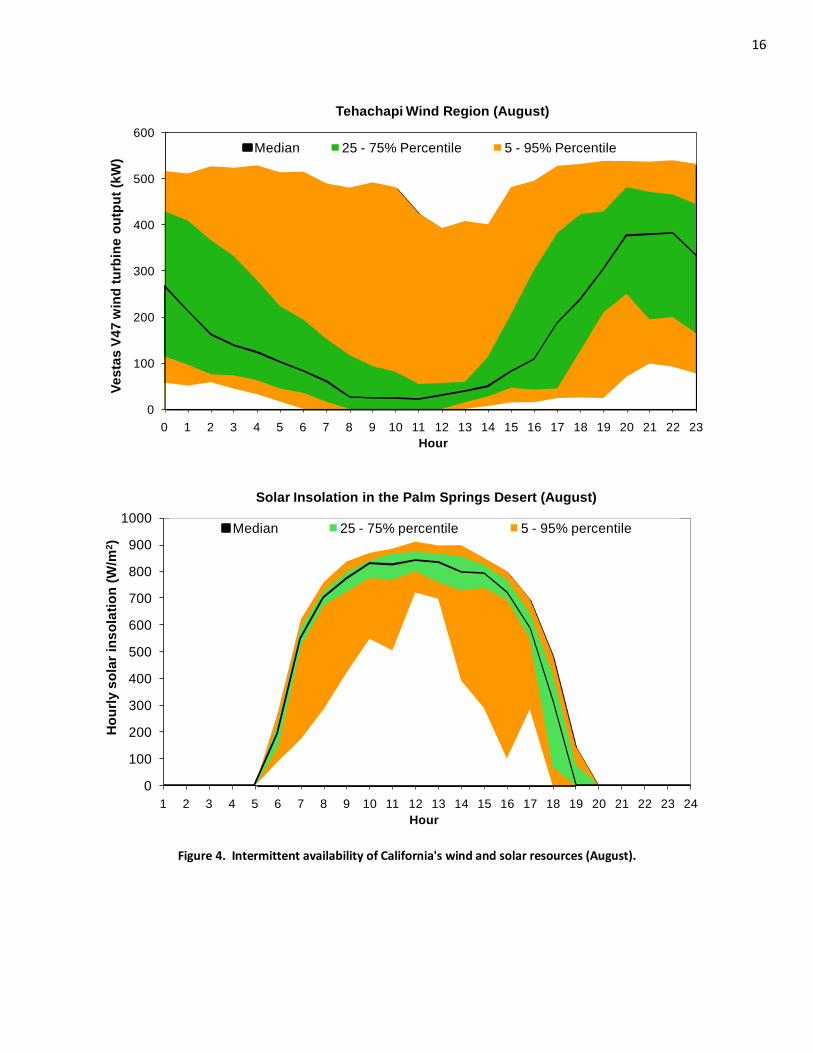
16

0

100

200

300

400

500

600

0 1 2 3 4 5 6 7 8 9 10 11 12 13 14 15 16 17 18 19 20 21 22 23

Ve

sta

sV

47

win

d t

urb

ine

ou

tpu

t (k

W)

Hour

Tehachapi Wind Region (August)

Median 25 - 75% Percentile 5 - 95% Percentile

0

100

200

300

400

500

600

700

800

900

1000

1 2 3 4 5 6 7 8 9 10 11 12 13 14 15 16 17 18 19 20 21 22 23 24

Ho

url

y s

ola

r in

so

lati

on

(W/m

2)

Hour

Solar Insolation in the Palm Springs Desert (August)

Median 25 - 75% percentile 5 - 95% percentile

Figure 4. Intermittent availability of California's wind and solar resources (August).

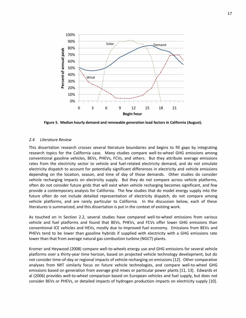
17

0%

10%

20%

30%

40%

50%

60%

70%

80%

90%

100%

0 3 6 9 12 15 18 21

Pe

rce

nt o

f a

nn

ua

l pe

ak

Begin hour

DemandSolar

Wind

Figure 5. Median hourly demand and renewable generation load factors in California (August).

2.4 Literature Review

This dissertation research crosses several literature boundaries and begins to fill gaps by integrating research topics for the California case. Many studies compare well-to-wheel GHG emissions among conventional gasoline vehicles, BEVs, PHEVs, FCVs, and others. But they attribute average emissions rates from the electricity sector to vehicle and fuel-related electricity demand, and do not simulate electricity dispatch to account for potentially significant differences in electricity and vehicle emissions depending on the location, season, and time of day of those demands. Other studies do consider vehicle recharging impacts on electricity supply. But they do not compare across vehicle platforms, often do not consider future grids that will exist when vehicle recharging becomes significant, and few provide a contemporary analysis for California. The few studies that do model energy supply into the future often do not include detailed representation of electricity dispatch, do not compare among vehicle platforms, and are rarely particular to California. In the discussion below, each of these literatures is summarized, and this dissertation is put in the context of existing work.

As touched on in Section 2.2, several studies have compared well-to-wheel emissions from various vehicle and fuel platforms and found that BEVs, PHEVs, and FCVs offer lower GHG emissions than conventional ICE vehicles and HEVs, mostly due to improved fuel economy. Emissions from BEVs and PHEVs tend to be lower than gasoline hybrids if supplied with electricity with a GHG emissions rate lower than that from average natural gas combustion turbine (NGCT) plants.

Kromer and Heywood (2008) compare well-to-wheels energy use and GHG emissions for several vehicle platforms over a thirty-year time horizon, based on projected vehicle technology development, but do not consider time-of-day or regional impacts of vehicle recharging on emissions [12]. Other comparative analyses from MIT similarly focus on future vehicle technologies, and compare well-to-wheel GHG emissions based on generation from average grid mixes or particular power plants [11, 13]. Edwards et al (2006) provides well-to-wheel comparison based on European vehicles and fuel supply, but does not consider BEVs or PHEVs, or detailed impacts of hydrogen production impacts on electricity supply [10].

18

Samaras and Meisterling (2008) compare lifecycle emissions from PHEVs to other vehicle platforms, but do not consider FCVs or impacts of recharging demand on the grid.

The GREET model, developed by Argonne National Laboratory [8, 44], has been applied to compare vehicle and fuel cycle emissions in several studies. A version of the model has been developed for California [89], which includes a representation of marginal electricity for vehicle recharging [25]. But this, too, is an average representation of electricity supply, which does not account for time-varying demand impacts on generation. And as discussed in Section 4.3.2, it likely misrepresents marginal generation for vehicles recharging in California in the near term.

Among analyses using the GREET model, Elgowainy et al (2009) provides a thorough analysis for PHEVs, but does not consider other vehicle platforms or impacts of variable recharging profiles on marginal electricity supply [79]. Brinkman et al (2005) also uses GREET, but does not consider BEVs or PHEVs in the comparison [14]. The LEM model, developed at UC Davis by Mark Delucchi, offers an alternative to GREET [9]. It represents marginal electricity for several regions and for weekends and weekdays, but does not include California-specific detail or account for time-varying demand impacts.

This dissertation addresses these gaps for the California case. Most well-to-wheels studies focus on vehicle technology or hydrogen supply, rather than detailing impacts on electricity supply. While this dissertation treats vehicle technology with less rigor than many of the studies reviewed here, it is informed by them (specifically, GREET [44]), and extends them to detail demand impacts from various vehicle and fuel platforms on electricity supply in California.

Other studies do detail demand impacts from vehicles on electricity supply when estimating energy and environmental impacts of vehicles (summarized in Table 2). The most complete analysis to date, EPRI and NRDC (2007) [6, 90], details electricity demand impacts from PHEVs on dispatch and grid evolution in the U.S. through 2050, including California detail. But it uses a proprietary dispatch model that is not open for public review, does not compare across vehicle platforms, and does not consider multiple recharging profiles. This dissertation intends to supplement and extend knowledge offered by the EPRI study and others, discussed below.

Several studies have looked at effects on the electricity sector associated with new demands from the transportation sector. It was a popular research topic in the 1990s for BEVs in light of California’s Zero Emission Vehicle (ZEV) Mandate and is reappearing in the literature for PHEVs. Then, the primary focus was on emission impacts of criteria pollutants. Today, studies focus more broadly on comparing on costs, resource use, and greenhouse gas emissions for various vehicle and fuel pathways.

The ZEV Mandate led many earlier studies to focus on California, especially Southern California. Ford considers the case of adding 1-2 million electric vehicles in the Southern California Edison service area, using the ELFIN model to simulate electricity supply in the region [91, 92]. A contemporaneous report by the CEC also used ELFIN (coupled with other models) to investigate marginal generation resources and criteria pollutant emissions associated with adding electric vehicles in the South Coast Air Basin [93]. These studies provide useful insights regarding interactions between BEV recharging and the California grid, but are outdated. California’s grid, vehicle technology, and energy policy have changed noticeably in the last two decades, and updated analysis is required to understand vehicle and grid interactions in the current and future contexts.

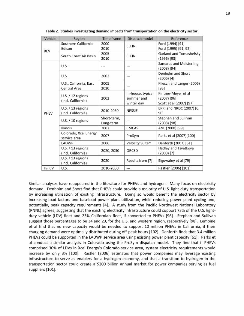
19

Table 2. Studies investigating demand impacts from transportation on the electricity sector.

Vehicle Region Time frame Dispatch model Reference

BEV

Southern California Edison

2000 2010

ELFIN Ford (1994) [91] Ford (1995) [91, 92]

South Coast Air Basin 2005 2010

ELFIN Garland and Tomashefsky (1996) [93]

PHEV

U.S. --- --- Samaras and Meisterling (2008) [94]

U.S. 2002 --- Denholm and Short (2006) [4]

U.S., California, East Central Area

2005 2020

--- Kliesch and Langer (2006) [95]

U.S. / 12 regions (incl. California)

2002 In-house; typical summer and winter day

Kintner-Meyer et al (2007) [96] Scott et al (2007) [97]


2010-2050 NESSIE EPRI and NRDC (2007) [6, 90]

U.S. / 10 regions Short-term, Long-term

--- Stephan and Sullivan (2008) [98]

Illinois 2007 EMCAS ANL (2008) [99]

Colorado, Xcel Energy service area

2007 ProSym Parks et al (2007)[100]

LADWP 2006 Velocity Suite® Danforth (2007) [61]


2020, 2030 ORCED Hadley and Tsvetkova (2008) [7]


2020 Results from [7] Elgowainy et al [79]

H2FCV U.S. 2010-2050 --- Rastler (2006) [101]

Similar analyses have reappeared in the literature for PHEVs and hydrogen. Many focus on electricity demand. Denholm and Short find that PHEVs could provide a majority of U.S. light-duty transportation by increasing utilization of existing infrastructure. Doing so would benefit the electricity sector by increasing load factors and baseload power plant utilization, while reducing power plant cycling and, potentially, peak capacity requirements [4]. A study from the Pacific Northwest National Laboratory (PNNL) agrees, suggesting that the existing electricity infrastructure could support 73% of the U.S. light-duty vehicle (LDV) fleet and 23% California’s fleet, if converted to PHEVs [96]. Stephan and Sullivan suggest those percentages to be 34 and 23, for the U.S. and western region, respectively [98]. Lemoine et al find that no new capacity would be needed to support 10 million PHEVs in California, if their charging demand were optimally distributed during off-peak hours [102]. Danforth finds that 3.4 million PHEVs could be supported in the LADWP service area using existing power plant capacity [61]. Parks et al conduct a similar analysis in Colorado using the ProSym dispatch model. They find that if PHEVs comprised 30% of LDVs in Xcel Energy’s Colorado service area, system electricity requirements would increase by only 3% [100]. Rastler (2006) estimates that power companies may leverage existing infrastructure to serve as enablers for a hydrogen economy, and that a transition to hydrogen in the transportation sector could create a $200 billion annual market for power companies serving as fuel suppliers [101].

20

Some analyses extend beyond demand analysis to investigate impacts on electricity supply and GHG emissions, as well. EPRI and NRDC present a thorough analysis considering PHEV demand impacts on the electricity sector through 2050 [6, 90]. They conduct a scenario analysis for the U.S. using NEMS, the U.S. EPA’s CMAQ model, and EPRI’s NESSIE model, which simulates power plant retirements, capacity expansion, and dispatch. They find that PHEVs reduce greenhouse gas emissions across all scenarios, and improve air quality in most parts of the country. This analysis does not compare demand impacts from BEVs or FCVs, however, and does not variations in the timing of vehicle recharging. The recharging profile used in the EPRI analysis is included in this dissertation, as the Offpeak profile (described in Sections 3.3.2 and 5.5).

The PNNL study considers dispatch, as well. The authors develop an aggregate dispatch model that they apply to 12 regions in the U.S., including California, for a typical summer and winter day. They find that PHEVs reduce greenhouse gas emissions in most parts of the country, but in regions with high fraction of coal generation, greenhouse gas emissions might actually increase [96, 97]. Their analysis uses GREET and treats dispatch simply. Parks et al use ProSym, a detailed but proprietary model, to simulate costs, emissions, and resource use associated with PHEVs in the Xcel service territory [100]. Hadley and Tsvetkova use the Oak Ridge Competitive Electricity Dispatch (ORCED) model to investigate impacts of PHEVs on electricity supply in 13 regions of the U.S., including California [7]. Their model dispatches power plants in merit order, like EDGE-CA and LEDGE-CA, using load duration curves, rather than continuous demand profiles. Load duration curves order hourly demands in decreasing order, over the course or a year (or other time period), and may miss some hourly-level interactions. Researchers at Argonne National Laboratory are investigating the impacts of high penetrations of PHEVs on electricity generation in Illinois [99], and recently conducted an analysis for 13 regions of the U.S. [79], using the GREET model and outputs from Hadley and Tsvetkova [7]. Other studies use accounting methods to estimate emissions and resource use associated with PHEVs operating in both near-term and long-term electricity markets [95, 98], which lack detailed dispatch modeling or comparison to hydrogen pathways and FCVs.

While there is a large body of work regarding electricity as a fuel for electric-drive vehicles, no study was found that investigates GHG emissions impacts of multiple vehicle types in California in the near and long term using detailed electricity sector modeling. Transparent, California-specific analysis of electricity (per-kWh) and vehicle (per-mile) GHG emissions is especially important in light of state policies that require detailed accounting of vehicle and fuel emissions. This dissertation begins to address this gap.

21

PART I: MARGINAL GENERATION FOR NEAR-TERM VEHICLE ELECTRICITY DEMAND IN CALIFORNIA

Chapters 3 and 4 of this dissertation consider impacts of vehicle recharging on the current grid in California. The primary focus of Part I is to identify the marginal electricity mix likely to supply vehicle and hydrogen-related electricity demands in the near term, and in turn, provide an accurate comparison of well-to-wheels emissions of advanced vehicles that accounts variations in their electricity demand profiles (and thus, the marginal mixes supplying them).

A set of scenarios are developed that describe the number of advanced vehicles, their daily and hourly electricity demand timing, and parameters for vehicle efficiency (fuel use) and energy use for hydrogen production and distribution. From these scenario parameters, hourly electricity demand profiles are developed for each pathway and added to projected hourly non-vehicle demands in 2010, to develop total electricity demand profiles representing a range of possible near-term operational conditions for BEVs, PHEVs, and FCVs.

The Electricity Dispatch model for Greenhouse gas Emissions in California (EDGE-CA) is developed to simulate operation of the current grid and electricity supply for these various demand scenarios. It accounts for the current mix of power plants supplying California, including imported power from neighboring states. The model allows high-level investigation of light-duty vehicle electricity demand impacts on the operation of the California grid. Specifically, it is applied to determine which power plants are likely to turn on or ramp up production to supply incremental electricity demand from light-duty vehicles; this set of generation would not occur without electricity demand from the light-duty sector. The GHG emissions of these power plants (the marginal mix) are accounted and attributed to a vehicle recharging or hydrogen production scenario.

Different scenarios and operating strategies are considered to understand impacts of annual hydro availability and incremental electricity demand location, quantity, and timing. The results presented in Chapter 4 address the first two research questions posed in the Introduction:

1. What is the effect of increasing penetrations of advanced vehicles and alternative fuels on electricity demand in California?


How do long-term vehicle electricity demand and timing scenarios affect electricity demand profiles and load factors?

2. How does operation of the existing and near-term electricity grid in California change in response to additional demand from light-duty vehicles?

What types of power plants will provide marginal electricity supply for vehicles and fuels initially? What are the associated GHG emissions rates? How do they compare to the value codified in California’s Low Carbon Fuel Standard (LCFS)?

How does the marginal mix affect vehicle GHG emissions? How do alternative vehicle emissions compare on a well-to-wheels basis?


22

3. DOCUMENTATION OF THE ELECTRICITY DISPATCH FOR GREENHOUSE GAS EMISSIONS IN CALIFORNIA (EDGE-CA) MODEL

3.1 Model Overview

The Electricity Dispatch model for Greenhouse gas Emissions in California (EDGE-CA) simulates near-term electricity supply in California on an hourly basis in order to estimate emissions from the sector and from marginal generation for vehicle and fuel demands. It is a spreadsheet-based accounting tool that determines capacity and allocates generation among available power plants to meet demand in three regions of California, including imported power from out of state.

The model includes three components. It calculates power plant availability, electricity demand, and dispatches power plants based on operating costs and transmission constraints to meet demand. For each of 8,760 hours in a year, EDGE-CA registers generation by power plant type, generating costs, and GHG emissions from electricity supply.

Importantly, the model tracks the last power plant dispatched. This “marginal” generator sets the market clearing cost for electricity, and its characteristics are attributable to incremental demand. When new demand from vehicles is imposed on an existing system, the characteristics of the marginal plants that would not operate otherwise determine the costs and emissions associated with using electricity as fuel.

From this accounting, comparative analyses are made. Impacts of demand timing on the operation of different types of power plants are investigated (hydroelectric and imported power are particularly interesting). Costs, emissions, and resource use are compared for different electricity demand profiles. And the model is applied to consider the effects of intermittent and variable availability of power plants on the system.

EDGE-CA is applied to look at operation of current and likely near-term grids in California. It represents all dispatchable, fossil-fired power plants in the state individually, and simulates generation from hydro and imported power plants according to their operation today. In this way, the model provides relatively accurate accounting of demand impacts on electricity supply in California in the near term.

The model is less appropriate for investigating long-term scenarios, and dispatch analysis is simplified for grids in 2020-2050, as discussed in Part II of this dissertation.

It is important to note the limitations of the EDGE-CA model. In reality, sophisticated decision-making algorithms are used by grid operators to dispatch generation optimally. Their models rely on proprietary data and software, and take into account several important considerations that are not included here, including:

Bilateral agreements and long-term contracts between generation companies and load serving entities,

Local transmission and distribution constraints,

Reliability constraints,

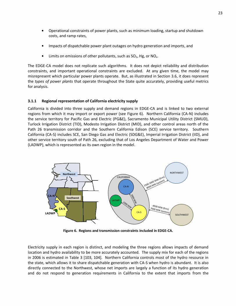
23

Operational constraints of power plants, such as minimum loading, startup and shutdown costs, and ramp rates,

Impacts of dispatchable power plant outages on hydro generation and imports, and

Limits on emissions of other pollutants, such as SO2, Hg, or NOx.

The EDGE-CA model does not replicate such algorithms. It does not depict reliability and distribution constraints, and important operational constraints are excluded. At any given time, the model may misrepresent which particular power plants operate. But, as illustrated in Section 3.6, it does represent the types of power plants that operate throughout the State quite accurately, providing useful metrics for analysis.

3.1.1 Regional representation of California electricity supply

California is divided into three supply and demand regions in EDGE-CA and is linked to two external regions from which it may import or export power (see Figure 6). Northern California (CA-N) includes the service territory for Pacific Gas and Electric (PG&E), Sacramento Municipal Utility District (SMUD), Turlock Irrigation District (TID), Modesto Irrigation District (MID), and other control areas north of the Path 26 transmission corridor and the Southern California Edison (SCE) service territory. Southern California (CA-S) includes SCE, San Diego Gas and Electric (SDG&E), Imperial Irrigation District (IID), and other service territory south of Path 26, excluding that of Los Angeles Department of Water and Power (LADWP), which is represented as its own region in the model.

SouthwestCA-N

Northwest

CA-S

LADWP

CALIFORNIA

CA-S

LADWP

CA-N

NORTHWEST

SOUTHWEST

Figure 6. Regions and transmission constraints included in EDGE-CA.

Electricity supply in each region is distinct, and modeling the three regions allows impacts of demand location and hydro availability to be more accurately accounted. The supply mix for each of the regions in 2006 is estimated in Table 3 [103, 104]. Northern California controls most of the hydro resource in the state, which allows it to share dispatchable generation with CA-S when hydro is abundant. It is also directly connected to the Northwest, whose net imports are largely a function of its hydro generation and do not respond to generation requirements in California to the extent that imports from the

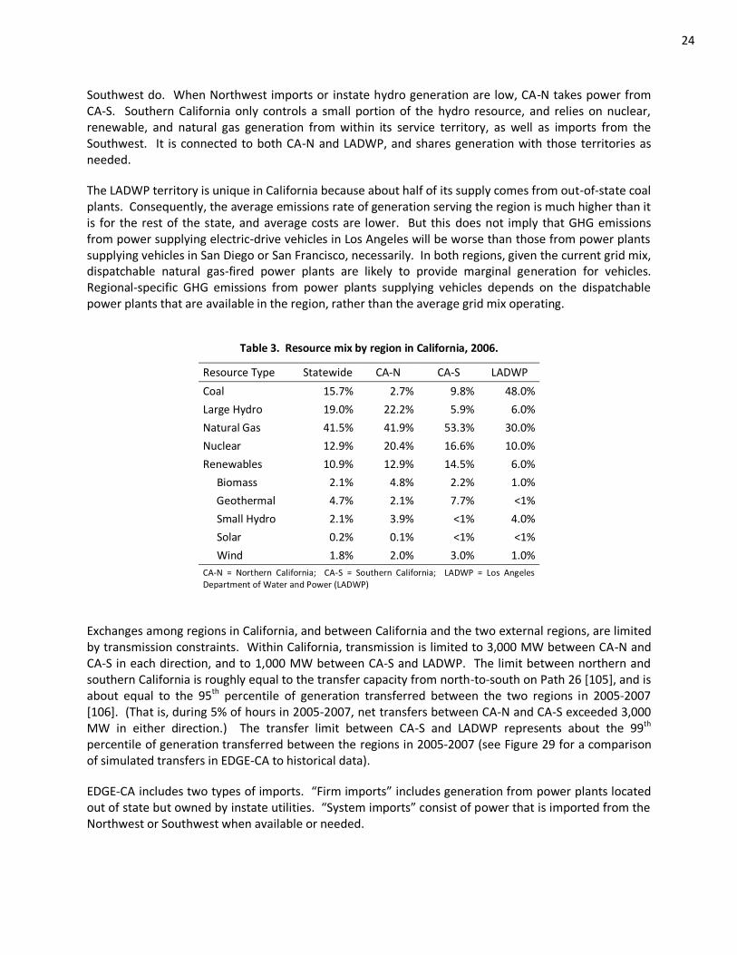
24

Southwest do. When Northwest imports or instate hydro generation are low, CA-N takes power from CA-S. Southern California only controls a small portion of the hydro resource, and relies on nuclear, renewable, and natural gas generation from within its service territory, as well as imports from the Southwest. It is connected to both CA-N and LADWP, and shares generation with those territories as needed.

The LADWP territory is unique in California because about half of its supply comes from out-of-state coal plants. Consequently, the average emissions rate of generation serving the region is much higher than it is for the rest of the state, and average costs are lower. But this does not imply that GHG emissions from power supplying electric-drive vehicles in Los Angeles will be worse than those from power plants supplying vehicles in San Diego or San Francisco, necessarily. In both regions, given the current grid mix, dispatchable natural gas-fired power plants are likely to provide marginal generation for vehicles. Regional-specific GHG emissions from power plants supplying vehicles depends on the dispatchable power plants that are available in the region, rather than the average grid mix operating.

Table 3. Resource mix by region in California, 2006.

Resource Type Statewide CA-N CA-S LADWP

Coal 15.7% 2.7% 9.8% 48.0%

Large Hydro 19.0% 22.2% 5.9% 6.0%

Natural Gas 41.5% 41.9% 53.3% 30.0%

Nuclear 12.9% 20.4% 16.6% 10.0%

Renewables 10.9% 12.9% 14.5% 6.0%

Biomass 2.1% 4.8% 2.2% 1.0%

Geothermal 4.7% 2.1% 7.7% <1%

Small Hydro 2.1% 3.9% <1% 4.0%

Solar 0.2% 0.1% <1% <1%

Wind 1.8% 2.0% 3.0% 1.0%

CA-N = Northern California; CA-S = Southern California; LADWP = Los Angeles Department of Water and Power (LADWP)

Exchanges among regions in California, and between California and the two external regions, are limited by transmission constraints. Within California, transmission is limited to 3,000 MW between CA-N and CA-S in each direction, and to 1,000 MW between CA-S and LADWP. The limit between northern and southern California is roughly equal to the transfer capacity from north-to-south on Path 26 [105], and is about equal to the 95th percentile of generation transferred between the two regions in 2005-2007 [106]. (That is, during 5% of hours in 2005-2007, net transfers between CA-N and CA-S exceeded 3,000 MW in either direction.) The transfer limit between CA-S and LADWP represents about the 99th percentile of generation transferred between the regions in 2005-2007 (see Figure 29 for a comparison of simulated transfers in EDGE-CA to historical data).

EDGE-CA includes two types of imports. “Firm imports” includes generation from power plants located out of state but owned by instate utilities. “System imports” consist of power that is imported from the Northwest or Southwest when available or needed.

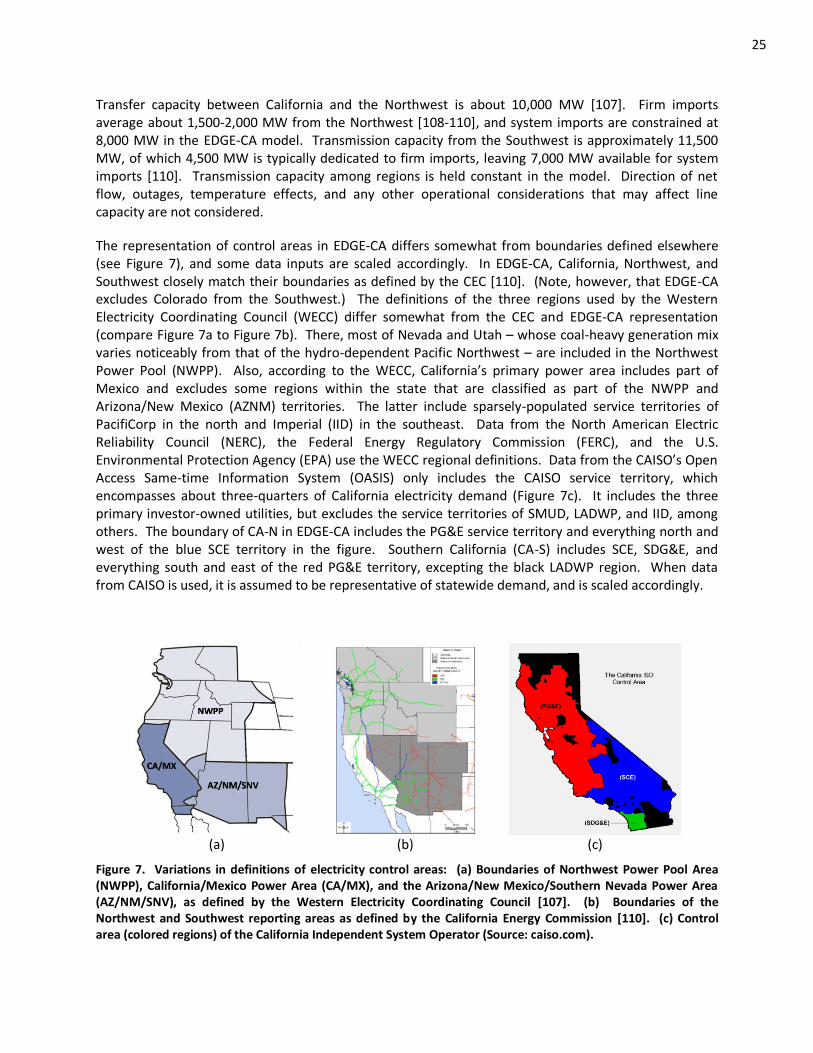
25

Transfer capacity between California and the Northwest is about 10,000 MW [107]. Firm imports average about 1,500-2,000 MW from the Northwest [108-110], and system imports are constrained at 8,000 MW in the EDGE-CA model. Transmission capacity from the Southwest is approximately 11,500 MW, of which 4,500 MW is typically dedicated to firm imports, leaving 7,000 MW available for system imports [110]. Transmission capacity among regions is held constant in the model. Direction of net flow, outages, temperature effects, and any other operational considerations that may affect line capacity are not considered.

The representation of control areas in EDGE-CA differs somewhat from boundaries defined elsewhere (see Figure 7), and some data inputs are scaled accordingly. In EDGE-CA, California, Northwest, and Southwest closely match their boundaries as defined by the CEC [110]. (Note, however, that EDGE-CA excludes Colorado from the Southwest.) The definitions of the three regions used by the Western Electricity Coordinating Council (WECC) differ somewhat from the CEC and EDGE-CA representation (compare Figure 7a to Figure 7b). There, most of Nevada and Utah – whose coal-heavy generation mix varies noticeably from that of the hydro-dependent Pacific Northwest – are included in the Northwest Power Pool (NWPP). Also, according to the WECC, California’s primary power area includes part of Mexico and excludes some regions within the state that are classified as part of the NWPP and Arizona/New Mexico (AZNM) territories. The latter include sparsely-populated service territories of PacifiCorp in the north and Imperial (IID) in the southeast. Data from the North American Electric Reliability Council (NERC), the Federal Energy Regulatory Commission (FERC), and the U.S. Environmental Protection Agency (EPA) use the WECC regional definitions. Data from the CAISO’s Open Access Same-time Information System (OASIS) only includes the CAISO service territory, which encompasses about three-quarters of California electricity demand (Figure 7c). It includes the three primary investor-owned utilities, but excludes the service territories of SMUD, LADWP, and IID, among others. The boundary of CA-N in EDGE-CA includes the PG&E service territory and everything north and west of the blue SCE territory in the figure. Southern California (CA-S) includes SCE, SDG&E, and everything south and east of the red PG&E territory, excepting the black LADWP region. When data from CAISO is used, it is assumed to be representative of statewide demand, and is scaled accordingly.

(a) (b) (c)

Figure 7. Variations in definitions of electricity control areas: (a) Boundaries of Northwest Power Pool Area (NWPP), California/Mexico Power Area (CA/MX), and the Arizona/New Mexico/Southern Nevada Power Area (AZ/NM/SNV), as defined by the Western Electricity Coordinating Council [107]. (b) Boundaries of the Northwest and Southwest reporting areas as defined by the California Energy Commission [110]. (c) Control area (colored regions) of the California Independent System Operator (Source: caiso.com).

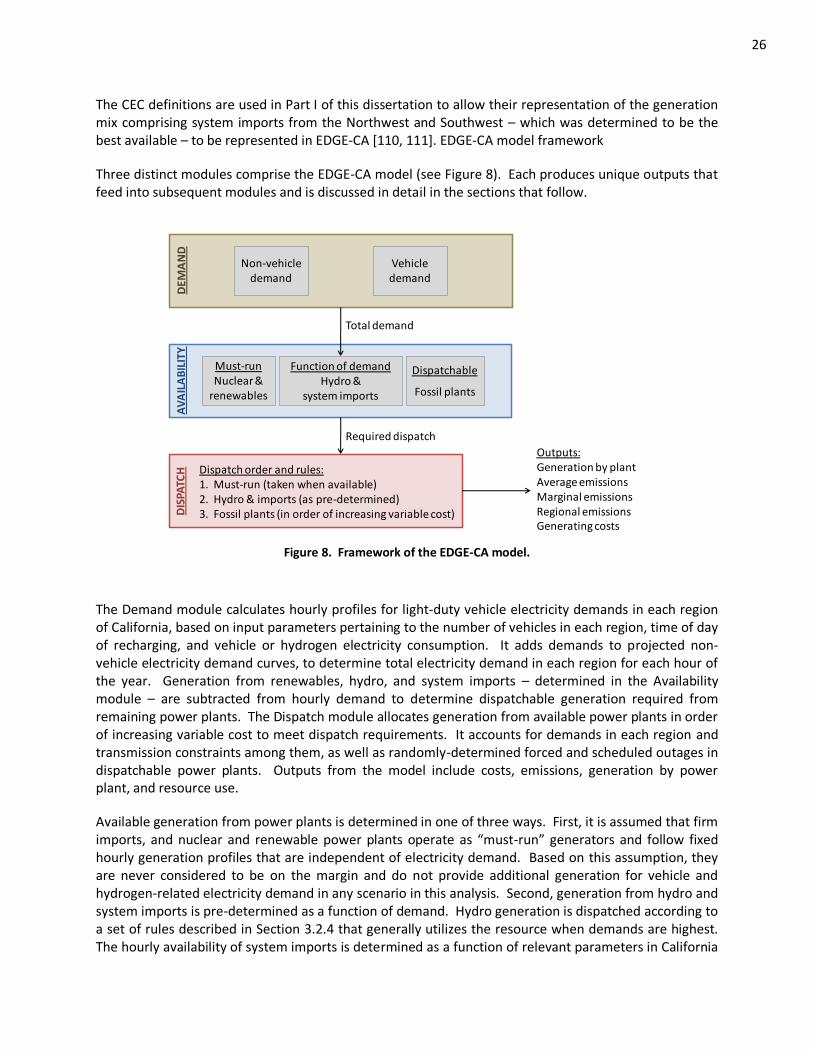
26

The CEC definitions are used in Part I of this dissertation to allow their representation of the generation mix comprising system imports from the Northwest and Southwest – which was determined to be the best available – to be represented in EDGE-CA [110, 111]. EDGE-CA model framework

Three distinct modules comprise the EDGE-CA model (see Figure 8). Each produces unique outputs that feed into subsequent modules and is discussed in detail in the sections that follow.

DEM

AN

D

Non-vehicle demand

Vehicle demand

AV

AIL

AB

ILIT

Y

Must-runNuclear &

renewables

Function of demandHydro &

system imports

DIS

PATC

H

Outputs:Generation by plantAverage emissionsMarginal emissionsRegional emissionsGenerating costs

Total demand

Dispatchable

Fossil plants

Dispatch order and rules:1. Must-run (taken when available)2. Hydro & imports (as pre-determined)3. Fossil plants (in order of increasing variable cost)

Required dispatch

Figure 8. Framework of the EDGE-CA model.

The Demand module calculates hourly profiles for light-duty vehicle electricity demands in each region of California, based on input parameters pertaining to the number of vehicles in each region, time of day of recharging, and vehicle or hydrogen electricity consumption. It adds demands to projected non-vehicle electricity demand curves, to determine total electricity demand in each region for each hour of the year. Generation from renewables, hydro, and system imports – determined in the Availability module – are subtracted from hourly demand to determine dispatchable generation required from remaining power plants. The Dispatch module allocates generation from available power plants in order of increasing variable cost to meet dispatch requirements. It accounts for demands in each region and transmission constraints among them, as well as randomly-determined forced and scheduled outages in dispatchable power plants. Outputs from the model include costs, emissions, generation by power plant, and resource use.

Available generation from power plants is determined in one of three ways. First, it is assumed that firm imports, and nuclear and renewable power plants operate as “must-run” generators and follow fixed hourly generation profiles that are independent of electricity demand. Based on this assumption, they are never considered to be on the margin and do not provide additional generation for vehicle and hydrogen-related electricity demand in any scenario in this analysis. Second, generation from hydro and system imports is pre-determined as a function of demand. Hydro generation is dispatched according to a set of rules described in Section 3.2.4 that generally utilizes the resource when demands are highest. The hourly availability of system imports is determined as a function of relevant parameters in California

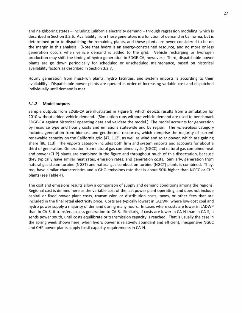
27

and neighboring states – including California electricity demand – through regression modeling, which is described in Section 3.2.6. Availability from these generators is a function of demand in California, but is determined prior to dispatching the remaining plants, and these plants are never considered to be on the margin in this analysis. (Note that hydro is an energy-constrained resource, and no more or less generation occurs when vehicle demand is added to the grid. Vehicle recharging or hydrogen production may shift the timing of hydro generation in EDGE-CA, however.) Third, dispatchable power plants are go down periodically for scheduled or unscheduled maintenance, based on historical availability factors as described in Section 3.2.7.

Hourly generation from must-run plants, hydro facilities, and system imports is according to their availability. Dispatchable power plants are queued in order of increasing variable cost and dispatched individually until demand is met.

3.1.2 Model outputs

Sample outputs from EDGE-CA are illustrated in Figure 9, which depicts results from a simulation for 2010 without added vehicle demand. (Simulation runs without vehicle demand are used to benchmark EDGE-CA against historical operating data and validate the model.) The model accounts for generation by resource type and hourly costs and emissions statewide and by region. The renewables category includes generation from biomass and geothermal resources, which comprise the majority of current renewable capacity on the California grid [47, 112], as well as wind and solar power, which are gaining share [86, 113]. The imports category includes both firm and system imports and accounts for about a third of generation. Generation from natural gas combined cycle (NGCC) and natural gas combined heat and power (CHP) plants are combined in the figure and throughout much of this dissertation, because they typically have similar heat rates, emission rates, and generation costs. Similarly, generation from natural gas steam turbine (NGST) and natural gas combustion turbine (NGCT) plants is combined. They, too, have similar characteristics and a GHG emissions rate that is about 50% higher than NGCC or CHP plants (see Table 4).

The cost and emissions results allow a comparison of supply and demand conditions among the regions. Regional cost is defined here as the variable cost of the last power plant operating, and does not include capital or fixed power plant costs, transmission or distribution costs, taxes, or other fees that are included in the final retail electricity price. Costs are typically lowest in LADWP, where low-cost coal and hydro power supply a majority of demand during many hours. In cases where costs are lower in LADWP than in CA-S, it transfers excess generation to CA-S. Similarly, if costs are lower in CA-N than in CA-S, it sends power south, until costs equilibrate or transmission capacity is reached. That is usually the case in the spring week shown here, when hydro power is relatively abundant and efficient, inexpensive NGCC and CHP power plants supply fossil capacity requirements in CA-N.

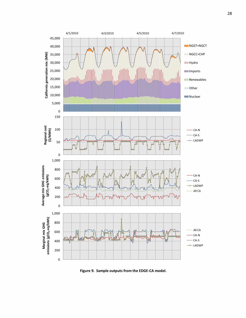
28

0

200

400

600

800

1,000

Mar

gin

al m

ix G

HG

e

mis

sio

ns

(gC

O2-e

q/k

Wh

)

All CA

CA-N

CA-S

LADWP

0

5,000

10,000

15,000

20,000

25,000

30,000

35,000

40,000

45,000

Cal

ifo

rnia

ge

ne

rati

on

mix

(M

W)

NGST+NGCT

NGCC+CHP

Hydro

Imports

Renewables

Other

Nuclear

4/1/2010 4/5/20104/3/2010 4/7/2010

0

50

100

150

Re

gio

nal

co

st

($/M

Wh

)

CA-N

CA-S

LADWP

0

200

400

600

800

1,000

Ave

rage

mix

GH

G e

mis

sio

ns

(g

CO

2-e

q/k

Wh

) CA-N

CA-S

LADWP

All CA

Figure 9. Sample outputs from the EDGE-CA model.

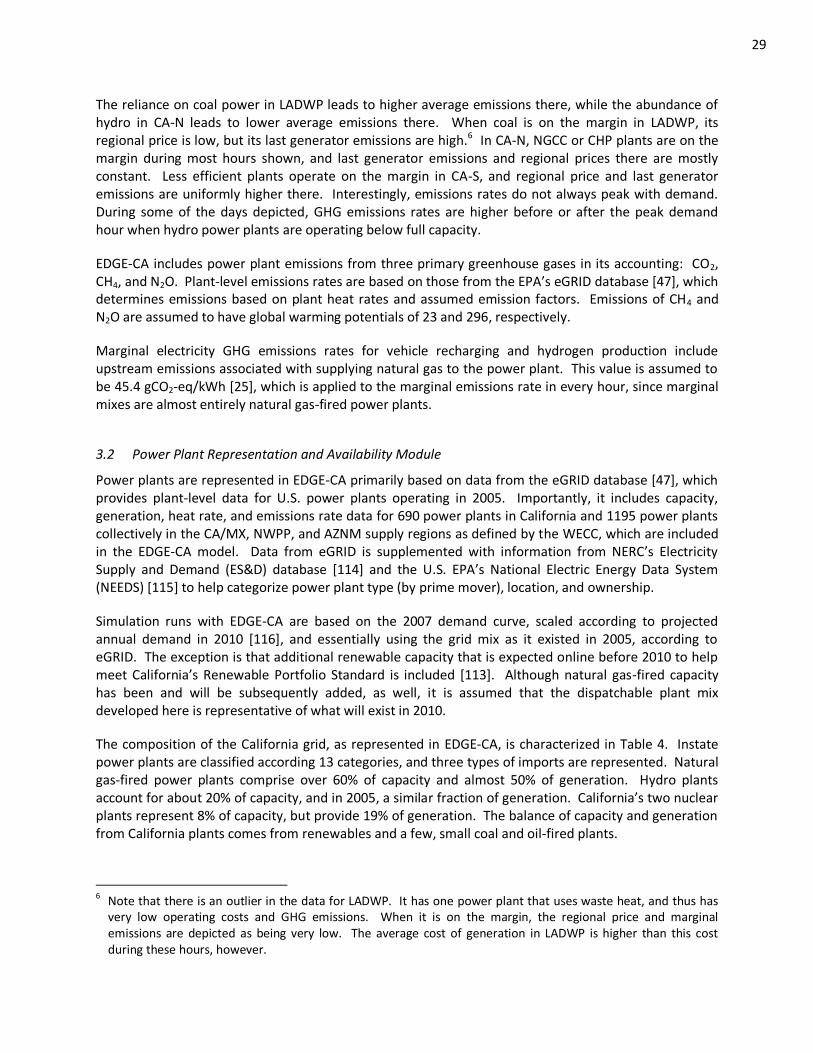
29

The reliance on coal power in LADWP leads to higher average emissions there, while the abundance of hydro in CA-N leads to lower average emissions there. When coal is on the margin in LADWP, its regional price is low, but its last generator emissions are high.6 In CA-N, NGCC or CHP plants are on the margin during most hours shown, and last generator emissions and regional prices there are mostly constant. Less efficient plants operate on the margin in CA-S, and regional price and last generator emissions are uniformly higher there. Interestingly, emissions rates do not always peak with demand. During some of the days depicted, GHG emissions rates are higher before or after the peak demand hour when hydro power plants are operating below full capacity.

EDGE-CA includes power plant emissions from three primary greenhouse gases in its accounting: CO2, CH4, and N2O. Plant-level emissions rates are based on those from the EPA’s eGRID database *47+, which determines emissions based on plant heat rates and assumed emission factors. Emissions of CH4 and N2O are assumed to have global warming potentials of 23 and 296, respectively.

Marginal electricity GHG emissions rates for vehicle recharging and hydrogen production include upstream emissions associated with supplying natural gas to the power plant. This value is assumed to be 45.4 gCO2-eq/kWh [25], which is applied to the marginal emissions rate in every hour, since marginal mixes are almost entirely natural gas-fired power plants.

3.2 Power Plant Representation and Availability Module

Power plants are represented in EDGE-CA primarily based on data from the eGRID database [47], which provides plant-level data for U.S. power plants operating in 2005. Importantly, it includes capacity, generation, heat rate, and emissions rate data for 690 power plants in California and 1195 power plants collectively in the CA/MX, NWPP, and AZNM supply regions as defined by the WECC, which are included in the EDGE-CA model. Data from eGRID is supplemented with information from NERC’s Electricity Supply and Demand (ES&D) database *114+ and the U.S. EPA’s National Electric Energy Data System (NEEDS) [115] to help categorize power plant type (by prime mover), location, and ownership.

Simulation runs with EDGE-CA are based on the 2007 demand curve, scaled according to projected annual demand in 2010 [116], and essentially using the grid mix as it existed in 2005, according to eGRID. The exception is that additional renewable capacity that is expected online before 2010 to help meet California’s Renewable Portfolio Standard is included *113+. Although natural gas-fired capacity has been and will be subsequently added, as well, it is assumed that the dispatchable plant mix developed here is representative of what will exist in 2010.

The composition of the California grid, as represented in EDGE-CA, is characterized in Table 4. Instate power plants are classified according 13 categories, and three types of imports are represented. Natural gas-fired power plants comprise over 60% of capacity and almost 50% of generation. Hydro plants account for about 20% of capacity, and in 2005, a similar fraction of generation. California’s two nuclear plants represent 8% of capacity, but provide 19% of generation. The balance of capacity and generation from California plants comes from renewables and a few, small coal and oil-fired plants.

6 Note that there is an outlier in the data for LADWP. It has one power plant that uses waste heat, and thus has

very low operating costs and GHG emissions. When it is on the margin, the regional price and marginal emissions are depicted as being very low. The average cost of generation in LADWP is higher than this cost during these hours, however.

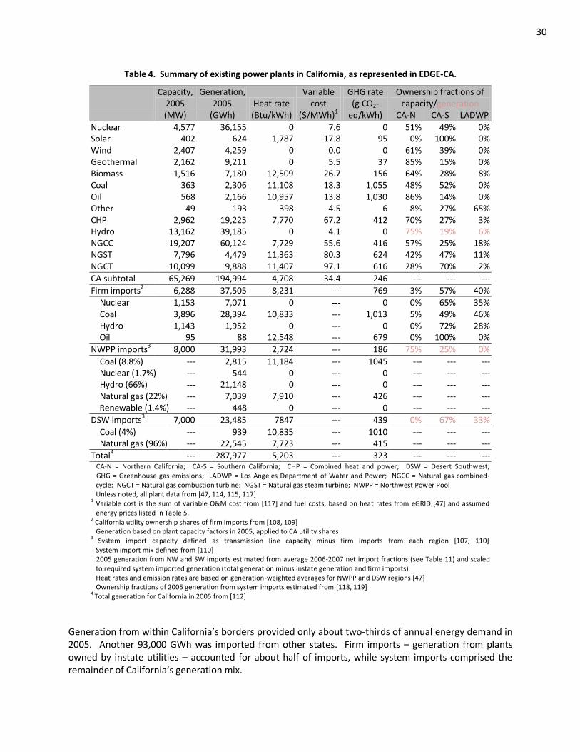
30

Table 4. Summary of existing power plants in California, as represented in EDGE-CA.

Capacity, 2005 (MW)

Generation,2005

(GWh) Heat rate (Btu/kWh)

Variable cost

($/MWh)1

GHG rate (g CO2-

eq/kWh)

Ownership fractions of capacity/generation

CA-N CA-S LADWP

Nuclear 4,577 36,155 0 7.6 0 51% 49% 0% Solar 402 624 1,787 17.8 95 0% 100% 0% Wind 2,407 4,259 0 0.0 0 61% 39% 0% Geothermal 2,162 9,211 0 5.5 37 85% 15% 0% Biomass 1,516 7,180 12,509 26.7 156 64% 28% 8% Coal 363 2,306 11,108 18.3 1,055 48% 52% 0% Oil 568 2,166 10,957 13.8 1,030 86% 14% 0% Other 49 193 398 4.5 6 8% 27% 65% CHP 2,962 19,225 7,770 67.2 412 70% 27% 3% Hydro 13,162 39,185 0 4.1 0 75% 19% 6% NGCC 19,207 60,124 7,729 55.6 416 57% 25% 18% NGST 7,796 4,479 11,363 80.3 624 42% 47% 11% NGCT 10,099 9,888 11,407 97.1 616 28% 70% 2%

CA subtotal

65,269 194,994 4,708 34.4 246 --- --- ---

Firm imports2 6,288 37,505 8,231 --- 769 3% 57% 40%

Nuclear 1,153 7,071 0 --- 0 0% 65% 35% Coal 3,896 28,394 10,833 --- 1,013 5% 49% 46% Hydro 1,143 1,952 0 --- 0 0% 72% 28% Oil 95 88 12,548 --- 679 0% 100% 0%

NWPP imports3 8,000 31,993 2,724 --- 186 75% 25% 0%

Coal (8.8%) --- 2,815 11,184 --- 1045 --- --- --- Nuclear (1.7%) --- 544 0 --- 0 --- --- --- Hydro (66%) --- 21,148 0 --- 0 --- --- --- Natural gas (22%) --- 7,039 7,910 --- 426 --- --- --- Renewable (1.4%) --- 448 0 --- 0 --- --- ---

DSW imports3 7,000 23,485 7847 --- 439 0% 67% 33%

Coal (4%) --- 939 10,835 --- 1010 --- --- --- Natural gas (96%) --- 22,545 7,723 --- 415 --- --- ---

Total4 --- 287,977 5,203 --- 323 --- --- --- CA-N = Northern California; CA-S = Southern California; CHP = Combined heat and power; DSW = Desert Southwest; GHG = Greenhouse gas emissions; LADWP = Los Angeles Department of Water and Power; NGCC = Natural gas combined- cycle; NGCT = Natural gas combustion turbine; NGST = Natural gas steam turbine; NWPP = Northwest Power Pool Unless noted, all plant data from [47, 114, 115, 117] 1 Variable cost is the sum of variable O&M cost from [117] and fuel costs, based on heat rates from eGRID [47] and assumed

energy prices listed in Table 5. 2 California utility ownership shares of firm imports from [108, 109]

Generation based on plant capacity factors in 2005, applied to CA utility shares 3

System import capacity defined as transmission line capacity minus firm imports from each region [107, 110] System import mix defined from [110] 2005 generation from NW and SW imports estimated from average 2006-2007 net import fractions (see Table 11) and scaled to required system imported generation (total generation minus instate generation and firm imports) Heat rates and emission rates are based on generation-weighted averages for NWPP and DSW regions [47] Ownership fractions of 2005 generation from system imports estimated from [118, 119] 4

Total generation for California in 2005 from [112]

Generation from within California’s borders provided only about two-thirds of annual energy demand in 2005. Another 93,000 GWh was imported from other states. Firm imports – generation from plants owned by instate utilities – accounted for about half of imports, while system imports comprised the remainder of California’s generation mix.

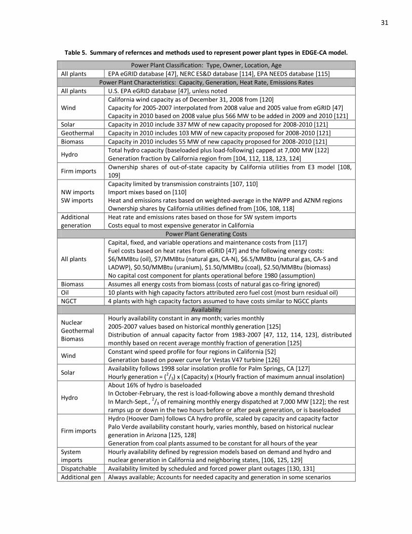
31

Table 5. Summary of refernces and methods used to represent power plant types in EDGE-CA model.

Power Plant Classification: Type, Owner, Location, Age

All plants EPA eGRID database [47], NERC ES&D database [114], EPA NEEDS database [115]

Power Plant Characteristics: Capacity, Generation, Heat Rate, Emissions Rates

All plants U.S. EPA eGRID database [47], unless noted

Wind California wind capacity as of December 31, 2008 from [120] Capacity for 2005-2007 interpolated from 2008 value and 2005 value from eGRID [47] Capacity in 2010 based on 2008 value plus 566 MW to be added in 2009 and 2010 [121]

Solar Capacity in 2010 include 337 MW of new capacity proposed for 2008-2010 [121]

Geothermal Capacity in 2010 includes 103 MW of new capacity proposed for 2008-2010 [121]

Biomass Capacity in 2010 includes 55 MW of new capacity proposed for 2008-2010 [121]

Hydro Total hydro capacity (baseloaded plus load-following) capped at 7,000 MW [122] Generation fraction by California region from [104, 112, 118, 123, 124]

Firm imports Ownership shares of out-of-state capacity by California utilities from E3 model [108, 109]

NW imports SW imports

Capacity limited by transmission constraints [107, 110] Import mixes based on [110] Heat and emissions rates based on weighted-average in the NWPP and AZNM regions Ownership shares by California utilities defined from [106, 108, 118]

Additional generation

Heat rate and emissions rates based on those for SW system imports Costs equal to most expensive generator in California

Power Plant Generating Costs

All plants

Capital, fixed, and variable operations and maintenance costs from [117] Fuel costs based on heat rates from eGRID [47] and the following energy costs: $6/MMBtu (oil), $7/MMBtu (natural gas, CA-N), $6.5/MMBtu (natural gas, CA-S and LADWP), $0.50/MMBtu (uranium), $1.50/MMBtu (coal), $2.50/MMBtu (biomass) No capital cost component for plants operational before 1980 (assumption)

Biomass Assumes all energy costs from biomass (costs of natural gas co-firing ignored) Oil 10 plants with high capacity factors attributed zero fuel cost (most burn residual oil)

NGCT 4 plants with high capacity factors assumed to have costs similar to NGCC plants

Availability

Nuclear Geothermal Biomass

Hourly availability constant in any month; varies monthly 2005-2007 values based on historical monthly generation [125] Distribution of annual capacity factor from 1983-2007 [47, 112, 114, 123], distributed monthly based on recent average monthly fraction of generation [125]

Wind Constant wind speed profile for four regions in California [52] Generation based on power curve for Vestas V47 turbine [126]

Solar Availability follows 1998 solar insolation profile for Palm Springs, CA [127] Hourly generation = (

2/3) x (Capacity) x (Hourly fraction of maximum annual insolation)

Hydro

About 16% of hydro is baseloaded In October-February, the rest is load-following above a monthly demand threshold In March-Sept., 2/3 of remaining monthly energy dispatched at 7,000 MW [122]; the rest ramps up or down in the two hours before or after peak generation, or is baseloaded

Firm imports

Hydro (Hoover Dam) follows CA hydro profile, scaled by capacity and capacity factor Palo Verde availability constant hourly, varies monthly, based on historical nuclear generation in Arizona [125, 128] Generation from coal plants assumed to be constant for all hours of the year

System imports

Hourly availability defined by regression models based on demand and hydro and nuclear generation in California and neighboring states, [106, 125, 129]

Dispatchable Availability limited by scheduled and forced power plant outages [130, 131]

Additional gen Always available; Accounts for needed capacity and generation in some scenarios

32

As mentioned above, power plants fall into three categories when determining availability on an average and marginal basis. First, generation from nuclear and renewable generators is assumed to be taken whenever available, and firm imports, nuclear, and renewable power plants do not provide marginal energy for vehicle and fuel demands. Second, availability of system imports and hydro power is pre-determined, but does change as a function of demand. System imports provide marginal generation according to the regression equations described in Section 3.2.6. Hydro power is assumed to be energy-constrained, and does not provide additional energy for marginal demands. But, the hourly distribution of hydro energy does change with demand, and in this way, the hydro resource affects the marginal electricity mix. Adding vehicles to the grid can alter the supply mix even during periods of zero vehicle demand, because the hydro resource may be distributed differently than if vehicle demand were not imposed on the system. Third, dispatchable (fossil) power plants are brought online as needed, and provide all other marginal generation.

Notes and references describing how power plant types are represented in EDGE-CA are summarized in Table 5 and detailed in the sections that follow.

3.2.1 Nuclear, geothermal, and biomass

Nuclear, geothermal, and biomass power plants are considered to be “must-run” baseload generators. Their average daily generation varies on a monthly basis, but is assumed to be constant on an hourly basis in a given month. Heat rates, emissions, and costs are based on the 2005 generation-weighted average characteristics of the plants within a category (see Table 4). Greenhouse gas emissions associated with biomass power generation come from natural gas co-firing in some biomass power plants.

These generators are dispatched first, independent of demand. They do not provide marginal generation for vehicle demands in EDGE-CA.

In backcasting simulations for 2005-2007, to validate the model (see Section 3.6), monthly generation from those years is distributed uniformly to determine hourly availability in a month. Otherwise, annual availability can vary based on the distribution of historical capacity factors from 1983-2007 for each of the generator types [47, 112, 114, 123]. Annual generation is distributed monthly based on average monthly fractions of annual generation from 2005-2007 for geothermal and biomass resources, and using average fractions from 2000-2008 for nuclear [125]. Simulations for 2010 include an additional 103 MW of geothermal capacity and 55 MW of new biomass capacity, which is expected to be added in California from 2008-2010 [121].

Figure 10 summarizes the distribution of annual and monthly generation for the three resources. Nuclear generation peaks in the summer months when electricity demand is high, and decreases in the spring for plant maintenance when demands are lower and hydro is plentiful. Since 1983, annual capacity factors have ranged from less than 68% to more than 109%, with a median value of 90%.

Availability of geothermal and biomass resources is fairly constant over the course of the year, but annual capacity factors vary noticeably. The annual capacity factor of geothermal resources has varied from 52% to 87%, with a median value of 62%, while that for biomass facilities (including the fraction of generation from natural gas co-firing) has ranged from 26% to 68%, with a median value of 48%.

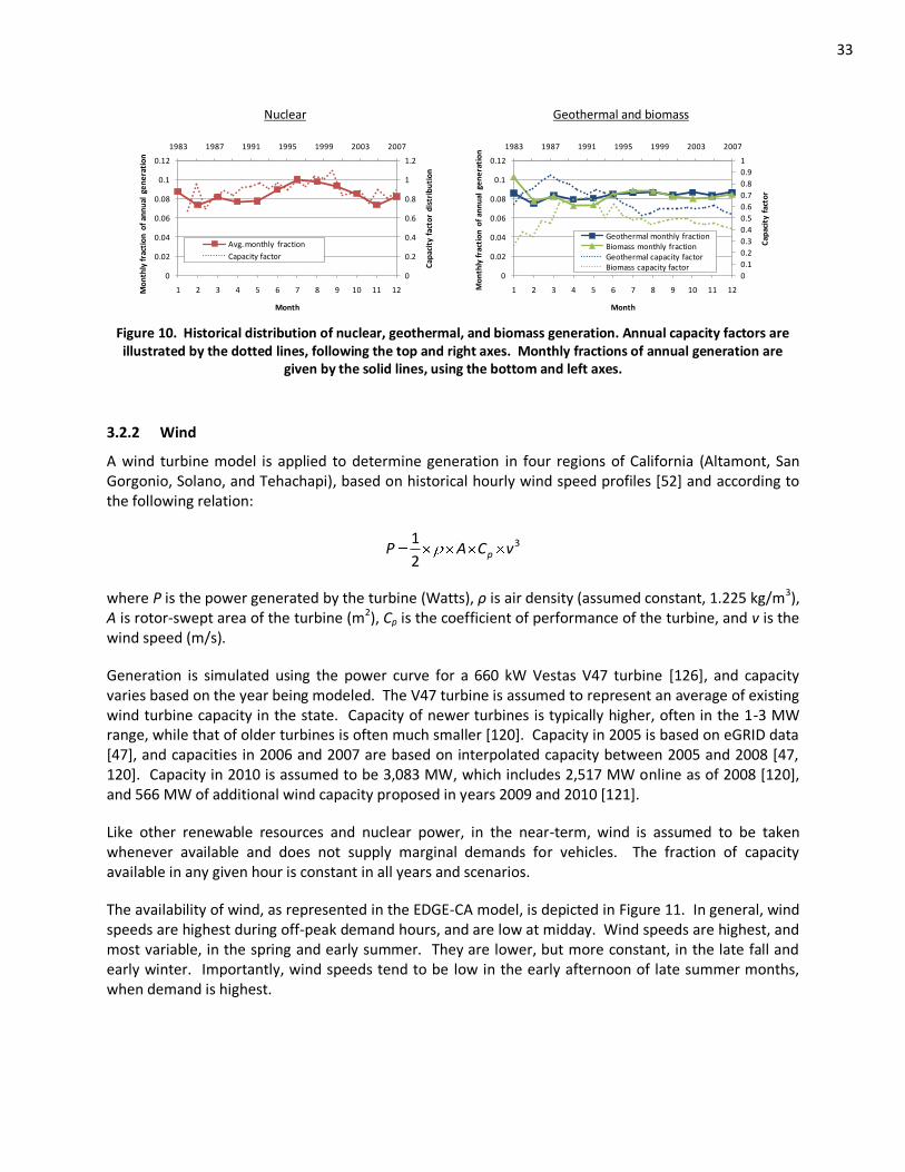
33

Nuclear Geothermal and biomass

1983 1987 1991 1995 1999 2003 2007

0

0.2

0.4

0.6

0.8

1

1.2

0

0.02

0.04

0.06

0.08

0.1

0.12

1 2 3 4 5 6 7 8 9 10 11 12

Cap

acit

y fa

cto

r d

istr

ibu

tio

n

Mo

nth

ly f

ract

ion

of

ann

ual

ge

ne

rati

on

Month

Avg. monthly fraction

Capacity factor

1983 1987 1991 1995 1999 2003 2007

0

0.1

0.2

0.3

0.4

0.5

0.6

0.7

0.8

0.9

1

0

0.02

0.04

0.06

0.08

0.1

0.12

1 2 3 4 5 6 7 8 9 10 11 12

Cap

acit

y fa

cto

r

Mo

nth

ly f

ract

ion

of

ann

ual

ge

ne

rati

on

Month

Geothermal monthly fractionBiomass monthly fractionGeothermal capacity factorBiomass capacity factor

Figure 10. Historical distribution of nuclear, geothermal, and biomass generation. Annual capacity factors are illustrated by the dotted lines, following the top and right axes. Monthly fractions of annual generation are

given by the solid lines, using the bottom and left axes.

3.2.2 Wind

A wind turbine model is applied to determine generation in four regions of California (Altamont, San Gorgonio, Solano, and Tehachapi), based on historical hourly wind speed profiles [52] and according to the following relation:

3

2

1vCAP p

where P is the power generated by the turbine (Watts), ρ is air density (assumed constant, 1.225 kg/m3), A is rotor-swept area of the turbine (m2), Cp is the coefficient of performance of the turbine, and v is the wind speed (m/s).

Generation is simulated using the power curve for a 660 kW Vestas V47 turbine [126], and capacity varies based on the year being modeled. The V47 turbine is assumed to represent an average of existing wind turbine capacity in the state. Capacity of newer turbines is typically higher, often in the 1-3 MW range, while that of older turbines is often much smaller [120]. Capacity in 2005 is based on eGRID data [47], and capacities in 2006 and 2007 are based on interpolated capacity between 2005 and 2008 [47, 120]. Capacity in 2010 is assumed to be 3,083 MW, which includes 2,517 MW online as of 2008 [120], and 566 MW of additional wind capacity proposed in years 2009 and 2010 [121].

Like other renewable resources and nuclear power, in the near-term, wind is assumed to be taken whenever available and does not supply marginal demands for vehicles. The fraction of capacity available in any given hour is constant in all years and scenarios.

The availability of wind, as represented in the EDGE-CA model, is depicted in Figure 11. In general, wind speeds are highest during off-peak demand hours, and are low at midday. Wind speeds are highest, and most variable, in the spring and early summer. They are lower, but more constant, in the late fall and early winter. Importantly, wind speeds tend to be low in the early afternoon of late summer months, when demand is highest.

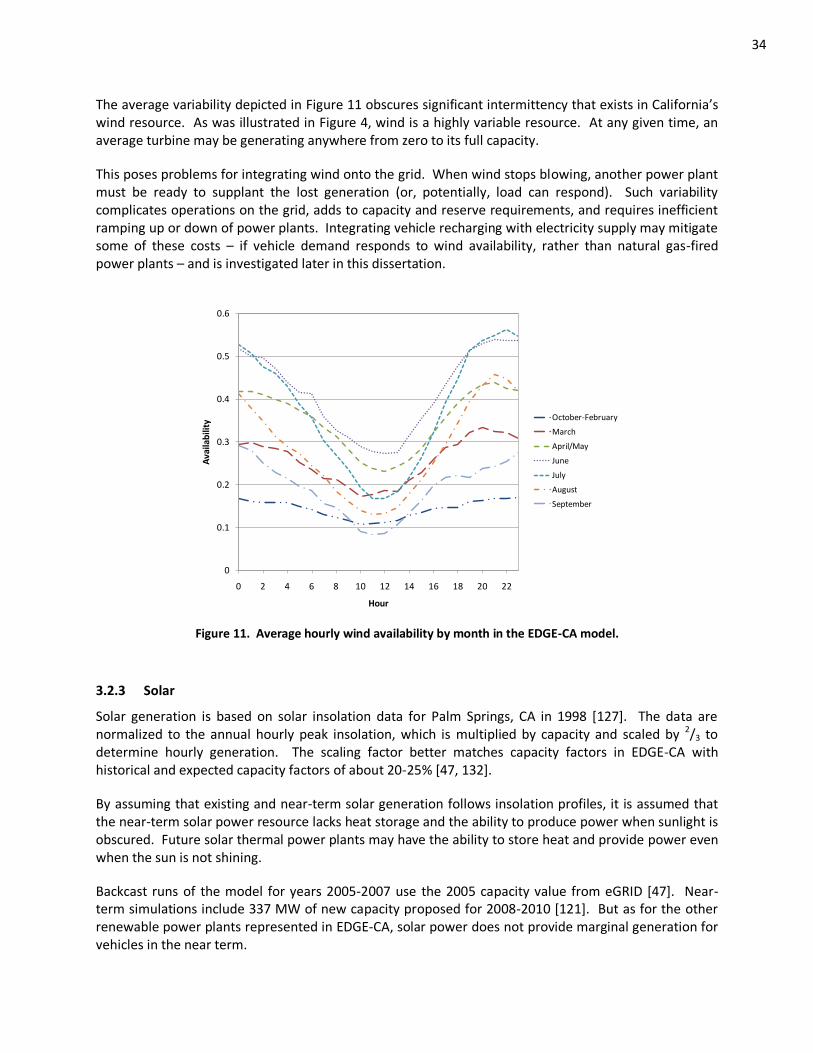
34

The average variability depicted in Figure 11 obscures significant intermittency that exists in California’s wind resource. As was illustrated in Figure 4, wind is a highly variable resource. At any given time, an average turbine may be generating anywhere from zero to its full capacity.

This poses problems for integrating wind onto the grid. When wind stops blowing, another power plant must be ready to supplant the lost generation (or, potentially, load can respond). Such variability complicates operations on the grid, adds to capacity and reserve requirements, and requires inefficient ramping up or down of power plants. Integrating vehicle recharging with electricity supply may mitigate some of these costs – if vehicle demand responds to wind availability, rather than natural gas-fired power plants – and is investigated later in this dissertation.

0

0.1

0.2

0.3

0.4

0.5

0.6

0 2 4 6 8 10 12 14 16 18 20 22

Ava

ilab

ility

Hour

October-February

March

April/May

June

July

August

September

Figure 11. Average hourly wind availability by month in the EDGE-CA model.

3.2.3 Solar

Solar generation is based on solar insolation data for Palm Springs, CA in 1998 [127]. The data are normalized to the annual hourly peak insolation, which is multiplied by capacity and scaled by 2/3 to determine hourly generation. The scaling factor better matches capacity factors in EDGE-CA with historical and expected capacity factors of about 20-25% [47, 132].

By assuming that existing and near-term solar generation follows insolation profiles, it is assumed that the near-term solar power resource lacks heat storage and the ability to produce power when sunlight is obscured. Future solar thermal power plants may have the ability to store heat and provide power even when the sun is not shining.

Backcast runs of the model for years 2005-2007 use the 2005 capacity value from eGRID [47]. Near-term simulations include 337 MW of new capacity proposed for 2008-2010 [121]. But as for the other renewable power plants represented in EDGE-CA, solar power does not provide marginal generation for vehicles in the near term.

35

Note that, in Table 4, there are operating costs and emissions associated with the solar resource. This reflects generation from the Solar Energy Generating Station (SEGS), which accounts for 400 MW of the 402 MW of solar power online in California. The SEGS facility is a solar thermal facility that can be fired with natural gas as needed, but about 85% of its generation comes from solar power [47]. Additional capacity added before 2010 is assumed to be free of GHG emissions and operating costs.

0

100

200

300

400

500

600

700

800

900

1000

0 1 2 3 4 5 6 7 8 9 10 11 12 13 14 15 16 17 18 19 20 21 22 23

Pal

m S

pri

ngs

so

lar

inso

lati

on

(W

/m2 )

Hour

25th-75th percentile

5th-95th percentile

Median

Figure 12. Distribution of hourly solar insolation in Palm Springs, CA (August).

The distribution of solar availability in August is illustrated in Figure 12. Like wind, solar power is intermittent, but to a lesser degree. The quartile values shown span a tight range that approaches the daily maximum. The sun typically shines from about 5am until 7pm or 8pm, with relatively constant maximum insolation from about 9am to 3pm. Only on rare occasion (less than 25% of the time) does cloud cover limit solar availability to a noticeable degree in August.

3.2.4 Hydro

Hydro power in California is modeled as an energy-constrained resource whose availability varies on a monthly basis reflecting seasonal river and reservoir levels. A portion of the resource runs at constant levels (varying monthly) reflecting run-of-the-river resources and minimum flow requirements from dams. It constitutes about 16% of in-state hydro generation, and is subsequently referred to as “baseload hydro” [133].

The remaining, “non-baseload,” resource can be dispatched as needed, and is modeled to generally minimize generation requirements from dispatchable natural gas-fired power plants. From October- February, when water storage levels have been drawn down, non-baseload hydro energy is assumed to be load-following. In each month, a statewide demand threshold is determined, above which additional power is generated. During the peak demand hour of the month, hydro generation is at peak capacity. Peak hydro capacity in California is assumed to be 7,000 MW in every month and for all hydro conditions

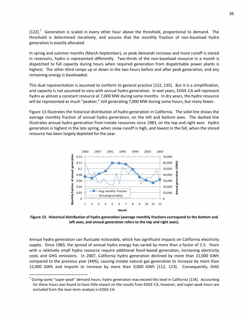
36

[122].7 Generation is scaled in every other hour above the threshold, proportional to demand. The threshold is determined iteratively, and assures that the monthly fraction of non-baseload hydro generation is exactly allocated.

In spring and summer months (March-September), as peak demands increase and more runoff is stored in reservoirs, hydro is represented differently. Two-thirds of the non-baseload resource in a month is dispatched to full capacity during hours when required generation from dispatchable power plants is highest. The other third ramps up or down in the two hours before and after peak generation, and any remaining energy is baseloaded.

This dual representation is assumed to conform to general practice [122, 135]. But it is a simplification, and capacity is not assumed to vary with annual hydro generation. In wet years, EDGE-CA will represent hydro as almost a constant resource at 7,000 MW during some months. In dry years, the hydro resource will be represented as much “peakier,” still generating 7,000 MW during some hours, but many fewer.

Figure 13 illustrates the historical distribution of hydro generation in California. The solid line shows the average monthly fraction of annual hydro generation, on the left and bottom axes. The dashed line illustrates annual hydro generation from instate resources since 1983, on the top and right axes. Hydro generation is highest in the late spring, when snow runoff is high, and lowest in the fall, when the stored resource has been largely depleted for the year.

1983 1987 1991 1995 1999 2003 2007

0

10,000

20,000

30,000

40,000

50,000

60,000

70,000

0

0.02

0.04

0.06

0.08

0.1

0.12

0.14

1 2 3 4 5 6 7 8 9 10 11 12

An

nu

al g

en

era

tio

n (

GW

h)

Mo

nth

ly f

ract

ion

of

ann

ual

ge

ne

rati

on

Month

Avg. monthly fraction

Annual generation

Figure 13. Historical distribution of hydro generation (average monthly fractions correspond to the bottom and left axes, and annual generation refers to the top and right axes).

Annual hydro generation can fluctuate noticeably, which has significant impacts on California electricity supply. Since 1983, the spread of annual hydro energy has varied by more than a factor of 2.5. Years with a relatively small hydro resource require additional fossil-based generation, increasing electricity costs and GHG emissions. In 2007, California hydro generation declined by more than 21,000 GWh compared to the previous year (44%), causing instate natural gas generation to increase by more than 12,000 GWh and imports to increase by more than 9,000 GWh [112, 123]. Consequently, GHG

7 During some “super-peak” demand hours, hydro generation may exceed this level in California [134]. Accounting

for these hours was found to have little impact on the results from EDGE-CA, however, and super-peak hours are excluded from the near-term analysis in EDGE-CA.

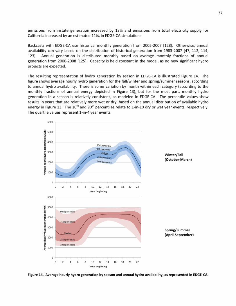
37

emissions from instate generation increased by 13% and emissions from total electricity supply for California increased by an estimated 11%, in EDGE-CA simulations.

Backcasts with EDGE-CA use historical monthly generation from 2005-2007 [128]. Otherwise, annual availability can vary based on the distribution of historical generation from 1983-2007 [47, 112, 114, 123]. Annual generation is distributed monthly based on average monthly fractions of annual generation from 2000-2008 [125]. Capacity is held constant in the model, as no new significant hydro projects are expected.

The resulting representation of hydro generation by season in EDGE-CA is illustrated Figure 14. The figure shows average hourly hydro generation for the fall/winter and spring/summer seasons, according to annual hydro availability. There is some variation by month within each category (according to the monthly fractions of annual energy depicted in Figure 13), but for the most part, monthly hydro generation in a season is relatively consistent, as modeled in EDGE-CA. The percentile values show results in years that are relatively more wet or dry, based on the annual distribution of available hydro energy in Figure 13. The 10th and 90th percentiles relate to 1-in-10 dry or wet year events, respectively. The quartile values represent 1-in-4 year events.

0

1000

2000

3000

4000

5000

6000

0 2 4 6 8 10 12 14 16 18 20 22

Ave

rage

ho

url

y h

ydro

ge

ne

rati

on

(M

Wh

)

Hour beginning

Winter/Fall (October-March)

0

1000

2000

3000

4000

5000

6000

0 2 4 6 8 10 12 14 16 18 20 22

Ave

rage

ho

url

y h

ydro

ge

ne

rati

on

(M

Wh

)

Hour beginning

10th percentile

25th percentile

Median

75th percentile

90th percentile

Spring/Summer (April-September)

Figure 14. Average hourly hydro generation by season and annual hydro availability, as represented in EDGE-CA.

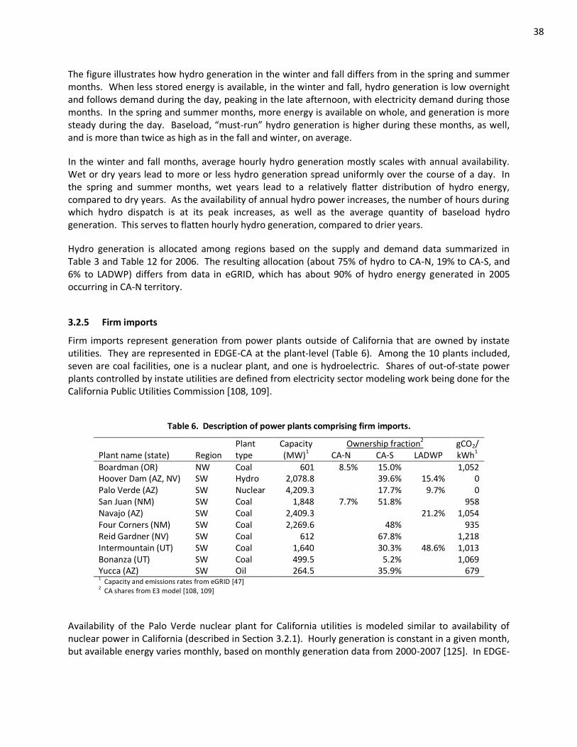
38

The figure illustrates how hydro generation in the winter and fall differs from in the spring and summer months. When less stored energy is available, in the winter and fall, hydro generation is low overnight and follows demand during the day, peaking in the late afternoon, with electricity demand during those months. In the spring and summer months, more energy is available on whole, and generation is more steady during the day. Baseload, “must-run” hydro generation is higher during these months, as well, and is more than twice as high as in the fall and winter, on average.

In the winter and fall months, average hourly hydro generation mostly scales with annual availability. Wet or dry years lead to more or less hydro generation spread uniformly over the course of a day. In the spring and summer months, wet years lead to a relatively flatter distribution of hydro energy, compared to dry years. As the availability of annual hydro power increases, the number of hours during which hydro dispatch is at its peak increases, as well as the average quantity of baseload hydro generation. This serves to flatten hourly hydro generation, compared to drier years.

Hydro generation is allocated among regions based on the supply and demand data summarized in Table 3 and Table 12 for 2006. The resulting allocation (about 75% of hydro to CA-N, 19% to CA-S, and 6% to LADWP) differs from data in eGRID, which has about 90% of hydro energy generated in 2005 occurring in CA-N territory.

3.2.5 Firm imports

Firm imports represent generation from power plants outside of California that are owned by instate utilities. They are represented in EDGE-CA at the plant-level (Table 6). Among the 10 plants included, seven are coal facilities, one is a nuclear plant, and one is hydroelectric. Shares of out-of-state power plants controlled by instate utilities are defined from electricity sector modeling work being done for the California Public Utilities Commission [108, 109].

Table 6. Description of power plants comprising firm imports.

Plant name (state) Region Plant type

Capacity (MW)1

Ownership fraction2 gCO2/kWh1 CA-N CA-S LADWP

Boardman (OR) NW Coal 601 8.5% 15.0% 1,052 Hoover Dam (AZ, NV) SW Hydro 2,078.8 39.6% 15.4% 0 Palo Verde (AZ) SW Nuclear 4,209.3 17.7% 9.7% 0 San Juan (NM) SW Coal 1,848 7.7% 51.8% 958 Navajo (AZ) SW Coal 2,409.3 21.2% 1,054 Four Corners (NM) SW Coal 2,269.6 48% 935 Reid Gardner (NV) SW Coal 612 67.8% 1,218 Intermountain (UT) SW Coal 1,640 30.3% 48.6% 1,013 Bonanza (UT) SW Coal 499.5 5.2% 1,069 Yucca (AZ) SW Oil 264.5 35.9% 679 1 Capacity and emissions rates from eGRID [47]

2 CA shares from E3 model [108, 109]

Availability of the Palo Verde nuclear plant for California utilities is modeled similar to availability of nuclear power in California (described in Section 3.2.1). Hourly generation is constant in a given month, but available energy varies monthly, based on monthly generation data from 2000-2007 [125]. In EDGE-

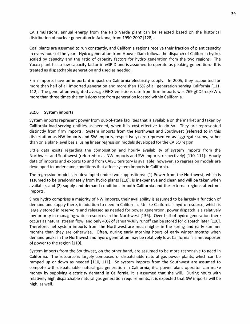
39

CA simulations, annual energy from the Palo Verde plant can be selected based on the historical distribution of nuclear generation in Arizona, from 1990-2007 [128].

Coal plants are assumed to run constantly, and California regions receive their fraction of plant capacity in every hour of the year. Hydro generation from Hoover Dam follows the dispatch of California hydro, scaled by capacity and the ratio of capacity factors for hydro generation from the two regions. The Yucca plant has a low capacity factor in eGRID and is assumed to operate as peaking generation. It is treated as dispatchable generation and used as needed.

Firm imports have an important impact on California electricity supply. In 2005, they accounted for more than half of all imported generation and more than 15% of all generation serving California [111, 112]. The generation-weighted average GHG emissions rate from firm imports was 769 gCO2-eq/kWh, more than three times the emissions rate from generation located within California.

3.2.6 System imports

System imports represent power from out-of-state facilities that is available on the market and taken by California load-serving entities as needed, when it is cost-effective to do so. They are represented distinctly from firm imports. System imports from the Northwest and Southwest (referred to in this dissertation as NW imports and SW imports, respectively) are represented as aggregate sums, rather than on a plant-level basis, using linear regression models developed for the CAISO region.

Little data exists regarding the composition and hourly availability of system imports from the Northwest and Southwest (referred to as NW imports and SW imports, respectively) [110, 111]. Hourly data of imports and exports to and from CAISO territory is available, however, so regression models are developed to understand conditions that affect system imports in California.

The regression models are developed under two suppositions: (1) Power from the Northwest, which is assumed to be predominately from hydro plants [110], is inexpensive and clean and will be taken when available, and (2) supply and demand conditions in both California and the external regions affect net imports.

Since hydro comprises a majority of NW imports, their availability is assumed to be largely a function of demand and supply there, in addition to need in California. Unlike California’s hydro resource, which is largely stored in reservoirs and released as needed for power generation, power dispatch is a relatively low priority in managing water resources in the Northwest [136]. Over half of hydro generation there occurs as natural stream flow, and only 40% of January-July runoff can be stored for dispatch later [110]. Therefore, net system imports from the Northwest are much higher in the spring and early summer months than they are otherwise. Often, during early morning hours of early winter months when demand peaks in the Northwest and hydro generation may be relatively low, California is a net exporter of power to the region [110].

System imports from the Southwest, on the other hand, are assumed to be more responsive to need in California. The resource is largely composed of dispatchable natural gas power plants, which can be ramped up or down as needed [110, 111]. So system imports from the Southwest are assumed to compete with dispatchable natural gas generation in California; if a power plant operator can make money by supplying electricity demand in California, it is assumed that she will. During hours with relatively high dispatchable natural gas generation requirements, it is expected that SW imports will be high, as well.

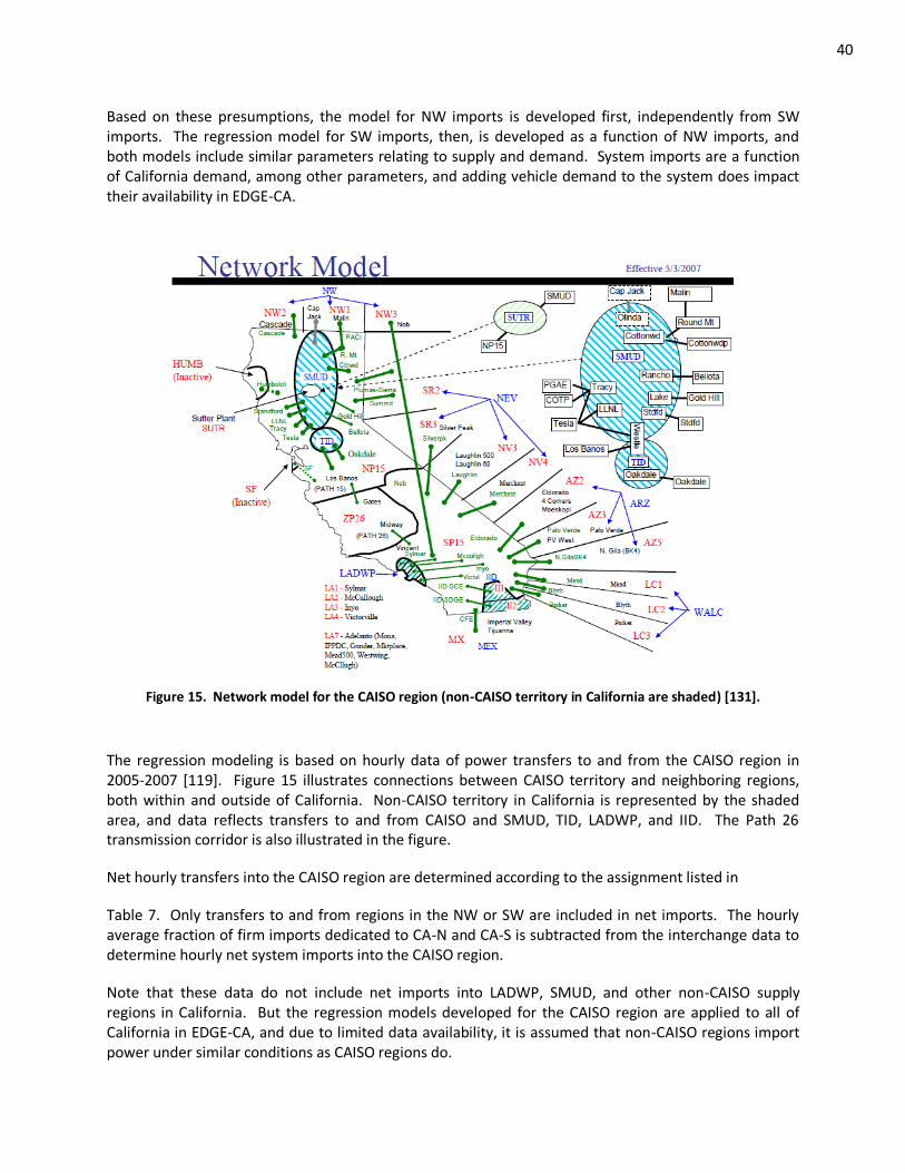
40

Based on these presumptions, the model for NW imports is developed first, independently from SW imports. The regression model for SW imports, then, is developed as a function of NW imports, and both models include similar parameters relating to supply and demand. System imports are a function of California demand, among other parameters, and adding vehicle demand to the system does impact their availability in EDGE-CA.

Figure 15. Network model for the CAISO region (non-CAISO territory in California are shaded) [131].

The regression modeling is based on hourly data of power transfers to and from the CAISO region in 2005-2007 [119]. Figure 15 illustrates connections between CAISO territory and neighboring regions, both within and outside of California. Non-CAISO territory in California is represented by the shaded area, and data reflects transfers to and from CAISO and SMUD, TID, LADWP, and IID. The Path 26 transmission corridor is also illustrated in the figure.

Net hourly transfers into the CAISO region are determined according to the assignment listed in

Table 7. Only transfers to and from regions in the NW or SW are included in net imports. The hourly average fraction of firm imports dedicated to CA-N and CA-S is subtracted from the interchange data to determine hourly net system imports into the CAISO region.

Note that these data do not include net imports into LADWP, SMUD, and other non-CAISO supply regions in California. But the regression models developed for the CAISO region are applied to all of California in EDGE-CA, and due to limited data availability, it is assumed that non-CAISO regions import power under similar conditions as CAISO regions do.

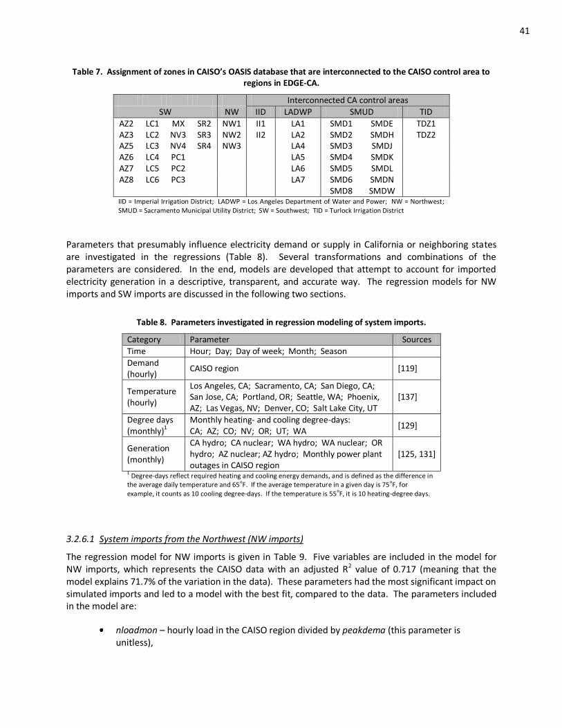
41

Table 7. Assignment of zones in CAISO’s OASIS database that are interconnected to the CAISO control area to regions in EDGE-CA.

Interconnected CA control areas

SW NW IID LADWP SMUD TID

AZ2 LC1 MX SR2 NW1 II1 LA1 SMD1 SMDE TDZ1 AZ3 LC2 NV3 SR3 NW2 II2 LA2 SMD2 SMDH TDZ2 AZ5 LC3 NV4 SR4 NW3 LA4 SMD3 SMDJ AZ6 LC4 PC1 LA5 SMD4 SMDK AZ7 LC5 PC2 LA6 SMD5 SMDL AZ8 LC6 PC3 LA7 SMD6 SMDN

SMD8 SMDW IID = Imperial Irrigation District; LADWP = Los Angeles Department of Water and Power; NW = Northwest; SMUD = Sacramento Municipal Utility District; SW = Southwest; TID = Turlock Irrigation District

Parameters that presumably influence electricity demand or supply in California or neighboring states are investigated in the regressions (Table 8). Several transformations and combinations of the parameters are considered. In the end, models are developed that attempt to account for imported electricity generation in a descriptive, transparent, and accurate way. The regression models for NW imports and SW imports are discussed in the following two sections.

Table 8. Parameters investigated in regression modeling of system imports.

Category Parameter Sources

Time Hour; Day; Day of week; Month; Season

Demand (hourly)

CAISO region [119]

Temperature (hourly)

Los Angeles, CA; Sacramento, CA; San Diego, CA; San Jose, CA; Portland, OR; Seattle, WA; Phoenix, AZ; Las Vegas, NV; Denver, CO; Salt Lake City, UT

[137]

Degree days (monthly)1

Monthly heating- and cooling degree-days: CA; AZ; CO; NV; OR; UT; WA

[129]

Generation (monthly)

CA hydro; CA nuclear; WA hydro; WA nuclear; OR hydro; AZ nuclear; AZ hydro; Monthly power plant outages in CAISO region

[125, 131]

1 Degree-days reflect required heating and cooling energy demands, and is defined as the difference in

the average daily temperature and 65oF. If the average temperature in a given day is 75

oF, for

example, it counts as 10 cooling degree-days. If the temperature is 55oF, it is 10 heating-degree days.

3.2.6.1 System imports from the Northwest (NW imports)

The regression model for NW imports is given in Table 9. Five variables are included in the model for NW imports, which represents the CAISO data with an adjusted R2 value of 0.717 (meaning that the model explains 71.7% of the variation in the data). These parameters had the most significant impact on simulated imports and led to a model with the best fit, compared to the data. The parameters included in the model are:

nloadmon – hourly load in the CAISO region divided by peakdema (this parameter is unitless),

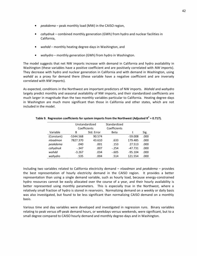
42

peakdema – peak monthly load (MW) in the CAISO region,

cahydnuk – combined monthly generation (GWh) from hydro and nuclear facilities in California,

wahdd – monthly heating degree-days in Washington, and

wahydro – monthly generation (GWh) from hydro in Washington.

The model suggests that net NW imports increase with demand in California and hydro availability in Washington (these variables have a positive coefficient and are positively correlated with NW imports). They decrease with hydro and nuclear generation in California and with demand in Washington, using wahdd as a proxy for demand there (these variable have a negative coefficient and are inversely correlated with NW imports).

As expected, conditions in the Northwest are important predictors of NW imports. Wahdd and wahydro largely predict monthly and seasonal availability of NW imports, and their standardized coefficients are much larger in magnitude than the two monthly variables particular to California. Heating degree-days in Washington are much more significant than those in California and other states, which are not included in the model.

Table 9. Regression coefficients for system imports from the Northwest (Adjusted R2 = 0.717).

Unstandardized

Coefficients Standardized Coefficients

Variable B Std. Error Beta t Sig.

(Constant) -5344.568 90.574 -59.008 .000 nloadmon 7827.370 43.610 .633 179.485 .000 peakdema .040 .001 .153 27.513 .000 cahydnuk -.347 .007 -.254 -47.731 .000 wahdd -3.267 .034 -.605 -95.104 .000 wahydro .535 .004 .514 121.554 .000

Including two variables related to California electricity demand – nloadmon and peakdema – provides the best representation of hourly electricity demand in the CAISO region. It provides a better representation than using a single demand variable, such as hourly load, because energy-constrained hydro resources cannot be easily allocated over the course of a year, and their hourly availability is better represented using monthly parameters. This is especially true in the Northwest, where a relatively small fraction of hydro is stored in reservoirs. Normalizing demand on a weekly or daily basis was also investigated, but found to be less significant than normalizing CAISO demand on a monthly basis.

Various time and day variables were developed and investigated in regression runs. Binary variables relating to peak versus off-peak demand hours, or weekdays versus weekends, were significant, but to a small degree compared to CAISO hourly demand and monthly degree-days and in Washington.

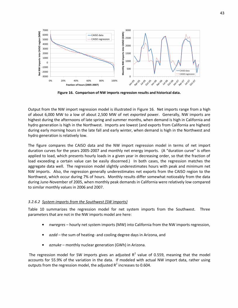
43

-3000

-2000

-1000

0

1000

2000

3000

4000

5000

6000

7000

0% 20% 40% 60% 80% 100%

Ne

t N

W im

po

rts

into

CA

ISO

re

gio

n (

MW

)

Fraction of hours (2005-2007)

CAISO data

CAISO regression

0

500

1000

1500

2000

2500

3000

Mo

nth

ly N

W im

po

rts

into

CA

ISO

(G

Wh

)

CAISO data

CAISO regression

Figure 16. Comparison of NW imports regression results and historical data.

Output from the NW import regression model is illustrated in Figure 16. Net imports range from a high of about 6,000 MW to a low of about 2,500 MW of net exported power. Generally, NW imports are highest during the afternoons of late spring and summer months, when demand is high in California and hydro generation is high in the Northwest. Imports are lowest (and exports from California are highest) during early morning hours in the late fall and early winter, when demand is high in the Northwest and hydro generation is relatively low.

The figure compares the CAISO data and the NW import regression model in terms of net import duration curves for the years 2005-2007 and monthly net energy imports. (A “duration curve” is often applied to load, which presents hourly loads in a given year in decreasing order, so that the fraction of load exceeding a certain value can be easily discerned.) In both cases, the regression matches the aggregate data well. The regression model slightly underestimates hours with peak and minimum net NW imports. Also, the regression generally underestimates net exports from the CAISO region to the Northwest, which occur during 7% of hours. Monthly results differ somewhat noticeably from the data during June-November of 2005, when monthly peak demands in California were relatively low compared to similar monthly values in 2006 and 2007.

3.2.6.2 System imports from the Southwest (SW imports)

Table 10 summarizes the regression model for net system imports from the Southwest. Three parameters that are not in the NW imports model are here:

nwregres – hourly net system imports (MW) into California from the NW imports regression,

azdd – the sum of heating- and cooling degree days in Arizona, and

aznuke – monthly nuclear generation (GWh) in Arizona.

The regression model for SW imports gives an adjusted R2 value of 0.559, meaning that the model accounts for 55.9% of the variation in the data. If modeled with actual NW import data, rather using outputs from the regression model, the adjusted R2 increases to 0.604.

44

Table 10. Regression coefficients for system imports from the Southwest (Adjusted R2 = 0.559).

Unstandardized

Coefficients Standardized Coefficients

B Std. Error Beta t Sig.

(Constant) -1997.655 89.791 -22.248 .000 nloadmon 4152.895 63.637 .482 65.259 .000 peakdema .111 .002 .604 69.057 .000 cahydnuk -.468 .005 -.491 -87.906 .000 nwregres -1.941 .049 -.317 -39.742 .000 azdd .335 .010 .162 33.467 .000 aznuke -.345 .006 -.418 -53.236 .000

Factors in California do dominate system imports from the Southwest, and have much more influence than they do on NW imports. The four parameters relating to California demand and supply (including imports from the Northwest) are the four with the highest magnitude beta values. Supply (aznuke) and demand (azdd) in the Southwest are significant, as well, but to a lesser extent than conditions in California. It does appear that California brings in power from the Southwest when it needs it – when demand in the state is high or supplies are low.

Peak SW import hours tend to occur during fall afternoons – when hydro availability from the Northwest is limited – with abnormally high temperatures and electricity demands. Peak net exports to the Southwest tend to occur during early mornings of late spring days when net imports from the Northwest are high.

As found for the NW imports estimation, the regression model for SW imports underestimates peak hourly net imports and net exports (see Figure 17). The difference at the tails of the distribution in the net SW import duration curve is more pronounced than for NW imports, partly because it relies on already-regressed data. The regression model for NW imports averages out the hourly distribution of imported power, and regressing again does so further.

-4000

-3000

-2000

-1000

0

1000

2000

3000

4000

5000

0% 20% 40% 60% 80% 100%

Ne

t SW

imp

ort

s in

to C

AIS

O r

egi

on

(M

W)


CAISO data

CAISO regression

-500

0

500

1000

1500

2000

2500

Mo

nth

ly S

W im

po

rts

into

CA

ISO

(G

Wh

)

CAISO data

CAISO regression

Figure 17. Comparison of SW imports regression results and historical data.

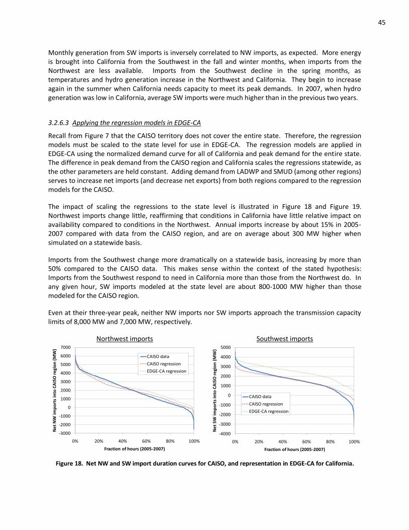
45

Monthly generation from SW imports is inversely correlated to NW imports, as expected. More energy is brought into California from the Southwest in the fall and winter months, when imports from the Northwest are less available. Imports from the Southwest decline in the spring months, as temperatures and hydro generation increase in the Northwest and California. They begin to increase again in the summer when California needs capacity to meet its peak demands. In 2007, when hydro generation was low in California, average SW imports were much higher than in the previous two years.

3.2.6.3 Applying the regression models in EDGE-CA

Recall from Figure 7 that the CAISO territory does not cover the entire state. Therefore, the regression models must be scaled to the state level for use in EDGE-CA. The regression models are applied in EDGE-CA using the normalized demand curve for all of California and peak demand for the entire state. The difference in peak demand from the CAISO region and California scales the regressions statewide, as the other parameters are held constant. Adding demand from LADWP and SMUD (among other regions) serves to increase net imports (and decrease net exports) from both regions compared to the regression models for the CAISO.

The impact of scaling the regressions to the state level is illustrated in Figure 18 and Figure 19. Northwest imports change little, reaffirming that conditions in California have little relative impact on availability compared to conditions in the Northwest. Annual imports increase by about 15% in 2005-2007 compared with data from the CAISO region, and are on average about 300 MW higher when simulated on a statewide basis.

Imports from the Southwest change more dramatically on a statewide basis, increasing by more than 50% compared to the CAISO data. This makes sense within the context of the stated hypothesis: Imports from the Southwest respond to need in California more than those from the Northwest do. In any given hour, SW imports modeled at the state level are about 800-1000 MW higher than those modeled for the CAISO region.

Even at their three-year peak, neither NW imports nor SW imports approach the transmission capacity limits of 8,000 MW and 7,000 MW, respectively.

Northwest imports Southwest imports

-3000

-2000

-1000

0

1000

2000

3000

4000

5000

6000

7000

0% 20% 40% 60% 80% 100%

Ne

t N

W im

po

rts

into

CA

ISO

re

gio

n (

MW

)


CAISO data

CAISO regression

EDGE-CA regression

-4000

-3000

-2000

-1000

0

1000

2000

3000

4000

5000

0% 20% 40% 60% 80% 100%

Ne

t SW

imp

ort

s in

to C

AIS

O r

egi

on

(M

W)


CAISO data

CAISO regression

EDGE-CA regression

Figure 18. Net NW and SW import duration curves for CAISO, and representation in EDGE-CA for California.

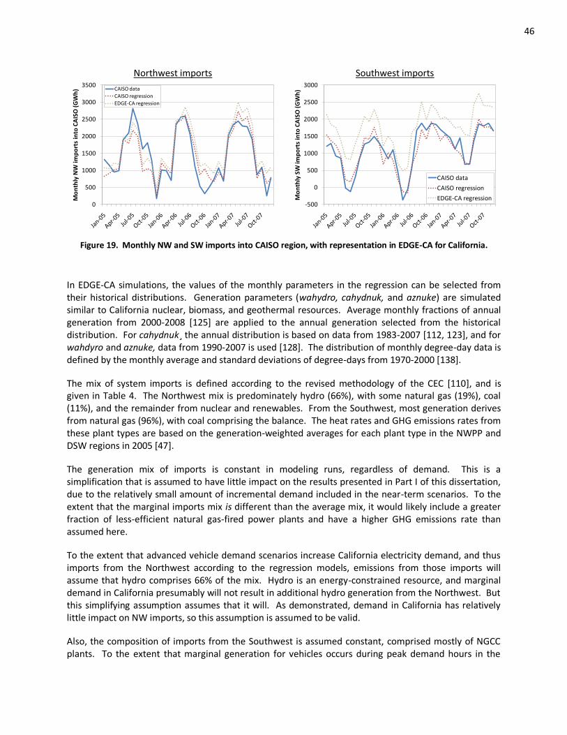
46

Northwest imports Southwest imports

0

500

1000

1500

2000

2500

3000

3500

Mo

nth

ly N

W im

po

rts

into

CA

ISO

(G

Wh

) CAISO data

CAISO regression

EDGE-CA regression

-500

0

500

1000

1500

2000

2500

3000

Mo

nth

ly S

W im

po

rts

into

CA

ISO

(G

Wh

)

CAISO data

CAISO regression

EDGE-CA regression

Figure 19. Monthly NW and SW imports into CAISO region, with representation in EDGE-CA for California.

In EDGE-CA simulations, the values of the monthly parameters in the regression can be selected from their historical distributions. Generation parameters (wahydro, cahydnuk, and aznuke) are simulated similar to California nuclear, biomass, and geothermal resources. Average monthly fractions of annual generation from 2000-2008 [125] are applied to the annual generation selected from the historical distribution. For cahydnuk¸ the annual distribution is based on data from 1983-2007 [112, 123], and for wahdyro and aznuke, data from 1990-2007 is used [128]. The distribution of monthly degree-day data is defined by the monthly average and standard deviations of degree-days from 1970-2000 [138].

The mix of system imports is defined according to the revised methodology of the CEC [110], and is given in Table 4. The Northwest mix is predominately hydro (66%), with some natural gas (19%), coal (11%), and the remainder from nuclear and renewables. From the Southwest, most generation derives from natural gas (96%), with coal comprising the balance. The heat rates and GHG emissions rates from these plant types are based on the generation-weighted averages for each plant type in the NWPP and DSW regions in 2005 [47].

The generation mix of imports is constant in modeling runs, regardless of demand. This is a simplification that is assumed to have little impact on the results presented in Part I of this dissertation, due to the relatively small amount of incremental demand included in the near-term scenarios. To the extent that the marginal imports mix is different than the average mix, it would likely include a greater fraction of less-efficient natural gas-fired power plants and have a higher GHG emissions rate than assumed here.

To the extent that advanced vehicle demand scenarios increase California electricity demand, and thus imports from the Northwest according to the regression models, emissions from those imports will assume that hydro comprises 66% of the mix. Hydro is an energy-constrained resource, and marginal demand in California presumably will not result in additional hydro generation from the Northwest. But this simplifying assumption assumes that it will. As demonstrated, demand in California has relatively little impact on NW imports, so this assumption is assumed to be valid.

Also, the composition of imports from the Southwest is assumed constant, comprised mostly of NGCC plants. To the extent that marginal generation for vehicles occurs during peak demand hours in the

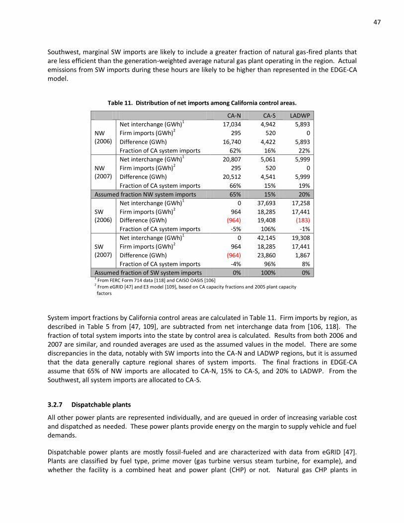
47

Southwest, marginal SW imports are likely to include a greater fraction of natural gas-fired plants that are less efficient than the generation-weighted average natural gas plant operating in the region. Actual emissions from SW imports during these hours are likely to be higher than represented in the EDGE-CA model.

Table 11. Distribution of net imports among California control areas.

CA-N CA-S LADWP

NW (2006)

Net interchange (GWh)1 17,034 4,942 5,893

Firm imports (GWh)2

295 520 0

Difference (GWh) 16,740 4,422 5,893

Fraction of CA system imports 62% 16% 22%

NW (2007)

Net interchange (GWh)1 20,807 5,061 5,999

Firm imports (GWh)2

295 520 0

Difference (GWh) 20,512 4,541 5,999

Fraction of CA system imports 66% 15% 19%

Assumed fraction NW system imports 65% 15% 20%

SW (2006)

Net interchange (GWh)1 0 37,693 17,258

Firm imports (GWh)2 964 18,285 17,441

Difference (GWh) (964) 19,408 (183)

Fraction of CA system imports -5% 106% -1%

SW (2007)

Net interchange (GWh)1 0 42,145 19,308

Firm imports (GWh)2

964 18,285 17,441

Difference (GWh) (964) 23,860 1,867

Fraction of CA system imports -4% 96% 8%

Assumed fraction of SW system imports 0% 100% 0% 1 From FERC Form 714 data [118] and CAISO OASIS [106]

2 From eGRID [47] and E3 model [109], based on CA capacity fractions and 2005 plant capacity

factors

System import fractions by California control areas are calculated in Table 11. Firm imports by region, as described in Table 5 from [47, 109], are subtracted from net interchange data from [106, 118]. The fraction of total system imports into the state by control area is calculated. Results from both 2006 and 2007 are similar, and rounded averages are used as the assumed values in the model. There are some discrepancies in the data, notably with SW imports into the CA-N and LADWP regions, but it is assumed that the data generally capture regional shares of system imports. The final fractions in EDGE-CA assume that 65% of NW imports are allocated to CA-N, 15% to CA-S, and 20% to LADWP. From the Southwest, all system imports are allocated to CA-S.

3.2.7 Dispatchable plants

All other power plants are represented individually, and are queued in order of increasing variable cost and dispatched as needed. These power plants provide energy on the margin to supply vehicle and fuel demands.

Dispatchable power plants are mostly fossil-fueled and are characterized with data from eGRID [47]. Plants are classified by fuel type, prime mover (gas turbine versus steam turbine, for example), and whether the facility is a combined heat and power plant (CHP) or not. Natural gas CHP plants in

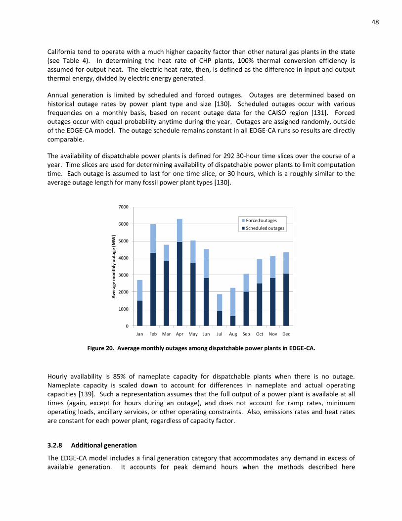
48

California tend to operate with a much higher capacity factor than other natural gas plants in the state (see Table 4). In determining the heat rate of CHP plants, 100% thermal conversion efficiency is assumed for output heat. The electric heat rate, then, is defined as the difference in input and output thermal energy, divided by electric energy generated.

Annual generation is limited by scheduled and forced outages. Outages are determined based on historical outage rates by power plant type and size [130]. Scheduled outages occur with various frequencies on a monthly basis, based on recent outage data for the CAISO region [131]. Forced outages occur with equal probability anytime during the year. Outages are assigned randomly, outside of the EDGE-CA model. The outage schedule remains constant in all EDGE-CA runs so results are directly comparable.

The availability of dispatchable power plants is defined for 292 30-hour time slices over the course of a year. Time slices are used for determining availability of dispatchable power plants to limit computation time. Each outage is assumed to last for one time slice, or 30 hours, which is a roughly similar to the average outage length for many fossil power plant types [130].

0

1000

2000

3000

4000

5000

6000

7000

Jan Feb Mar Apr May Jun Jul Aug Sep Oct Nov Dec

Ave

rage

mo

nth

ly o

uta

ge (

MW

)

Forced outages

Scheduled outages

Figure 20. Average monthly outages among dispatchable power plants in EDGE-CA.

Hourly availability is 85% of nameplate capacity for dispatchable plants when there is no outage. Nameplate capacity is scaled down to account for differences in nameplate and actual operating capacities [139]. Such a representation assumes that the full output of a power plant is available at all times (again, except for hours during an outage), and does not account for ramp rates, minimum operating loads, ancillary services, or other operating constraints. Also, emissions rates and heat rates are constant for each power plant, regardless of capacity factor.

3.2.8 Additional generation

The EDGE-CA model includes a final generation category that accommodates any demand in excess of available generation. It accounts for peak demand hours when the methods described here

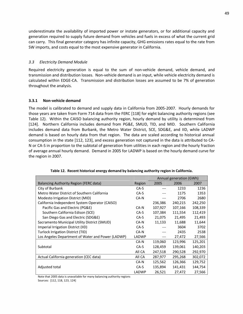
49

underestimate the availability of imported power or instate generators, or for additional capacity and generation required to supply future demand from vehicles and fuels in excess of what the current grid can carry. This final generator category has infinite capacity, GHG emissions rates equal to the rate from SW imports, and costs equal to the most expensive generator in California.

3.3 Electricity Demand Module

Required electricity generation is equal to the sum of non-vehicle demand, vehicle demand, and transmission and distribution losses. Non-vehicle demand is an input, while vehicle electricity demand is calculated within EDGE-CA. Transmission and distribution losses are assumed to be 7% of generation throughout the analysis.

3.3.1 Non-vehicle demand

The model is calibrated to demand and supply data in California from 2005-2007. Hourly demands for those years are taken from Form 714 data from the FERC [118] for eight balancing authority regions (see Table 12). Within the CAISO balancing authority region, hourly demand by utility is determined from [124]. Northern California includes demand from PG&E, SMUD, TID, and MID. Southern California includes demand data from Burbank, the Metro Water District, SCE, SDG&E, and IID, while LADWP demand is based on hourly data from that region. The data are scaled according to historical annual consumption in the state [112, 123], and excess generation not captured in the data is attributed to CA-N or CA-S in proportion to the subtotal of generation from utilities in each region and the hourly fraction of average annual hourly demand. Demand in 2005 for LADWP is based on the hourly demand curve for the region in 2007.

Table 12. Recent historical energy demand by balancing authority region in California.

Annual generation (GWh)

Balancing Authority Region (FERC data) Region 2005 2006 2007

City of Burbank CA-S --- 1233 1236 Metro Water District of Southern California CA-S --- 1175 1353 Modesto Irrigation District (MID) CA-N --- 2706 2680 California Independent System Operator (CAISO) 236,386 240,215 242,250 Pacific Gas and Electric (PG&E) CA-N 107,927 107,166 108,339 Southern California Edison (SCE) CA-S 107,384 111,554 112,419 San Diego Gas and Electric (SDG&E) CA-S 21,075 21,495 21,493 Sacramento Municipal Utility District (SMUD) CA-N 11,133 11,688 11,644 Imperial Irrigation District (IID) CA-S --- 3604 3702 Turlock Irrigation District (TID) CA-N --- 2435 2538 Los Angeles Department of Water and Power (LADWP) LADWP --- 27,472 27,566

Subtotal

CA-N 119,060 123,996 125,201

CA-S 128,459 139,061 140,203

All CA 247,518 290,528 292,970

Actual California generation (CEC data) All CA 287,977 295,268 302,072

Adjusted total

CA-N 125,562 126,366 129,752

CA-S 135,894 141,431 144,754

LADWP 26,521 27,472 27,566 Note that 2005 data is unavailable for many balancing authority regions Sources: [112, 118, 123, 124]

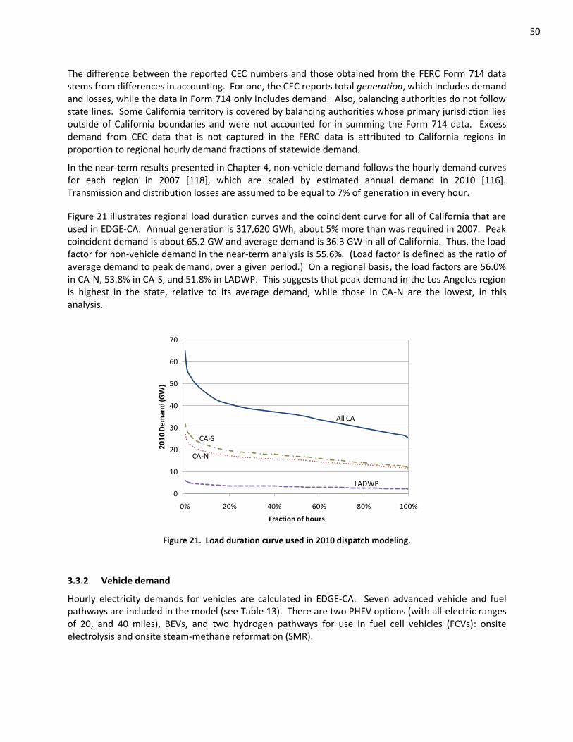
50

The difference between the reported CEC numbers and those obtained from the FERC Form 714 data stems from differences in accounting. For one, the CEC reports total generation, which includes demand and losses, while the data in Form 714 only includes demand. Also, balancing authorities do not follow state lines. Some California territory is covered by balancing authorities whose primary jurisdiction lies outside of California boundaries and were not accounted for in summing the Form 714 data. Excess demand from CEC data that is not captured in the FERC data is attributed to California regions in proportion to regional hourly demand fractions of statewide demand.

In the near-term results presented in Chapter 4, non-vehicle demand follows the hourly demand curves for each region in 2007 [118], which are scaled by estimated annual demand in 2010 [116]. Transmission and distribution losses are assumed to be equal to 7% of generation in every hour.

Figure 21 illustrates regional load duration curves and the coincident curve for all of California that are used in EDGE-CA. Annual generation is 317,620 GWh, about 5% more than was required in 2007. Peak coincident demand is about 65.2 GW and average demand is 36.3 GW in all of California. Thus, the load factor for non-vehicle demand in the near-term analysis is 55.6%. (Load factor is defined as the ratio of average demand to peak demand, over a given period.) On a regional basis, the load factors are 56.0% in CA-N, 53.8% in CA-S, and 51.8% in LADWP. This suggests that peak demand in the Los Angeles region is highest in the state, relative to its average demand, while those in CA-N are the lowest, in this analysis.

0

10

20

30

40

50

60

70

0% 20% 40% 60% 80% 100%

20

10

De

man

d (G

W)

Fraction of hours

All CA

CA-N

CA-S

LADWP

Figure 21. Load duration curve used in 2010 dispatch modeling.

3.3.2 Vehicle demand

Hourly electricity demands for vehicles are calculated in EDGE-CA. Seven advanced vehicle and fuel pathways are included in the model (see Table 13). There are two PHEV options (with all-electric ranges of 20, and 40 miles), BEVs, and two hydrogen pathways for use in fuel cell vehicles (FCVs): onsite electrolysis and onsite steam-methane reformation (SMR).

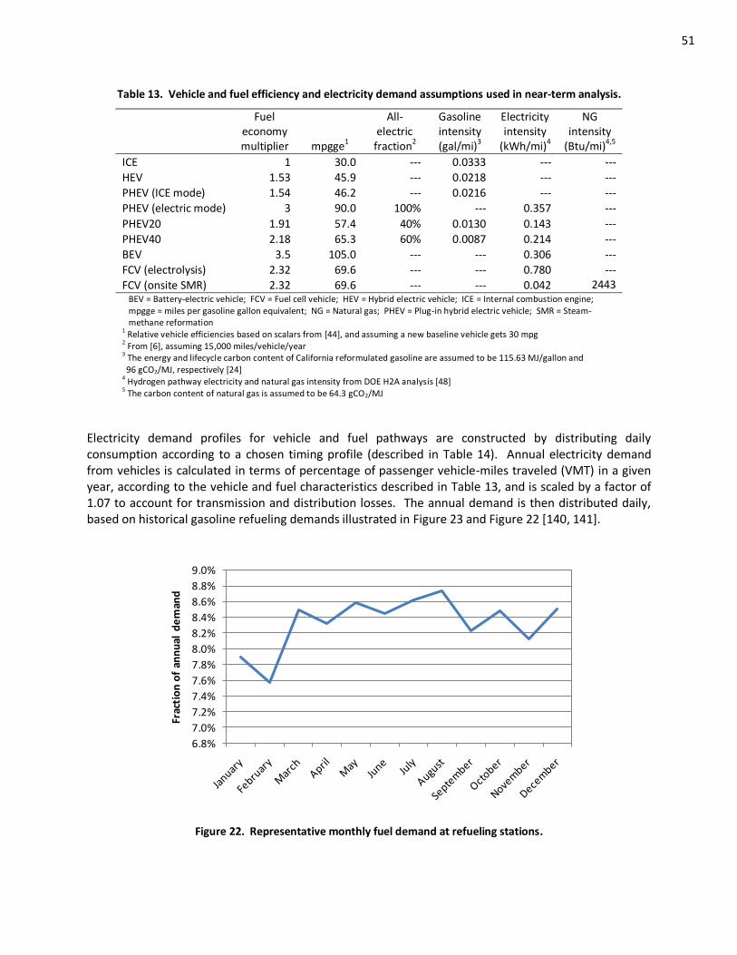
51

Table 13. Vehicle and fuel efficiency and electricity demand assumptions used in near-term analysis.

Electricity demand profiles for vehicle and fuel pathways are constructed by distributing daily consumption according to a chosen timing profile (described in Table 14). Annual electricity demand from vehicles is calculated in terms of percentage of passenger vehicle-miles traveled (VMT) in a given year, according to the vehicle and fuel characteristics described in Table 13, and is scaled by a factor of 1.07 to account for transmission and distribution losses. The annual demand is then distributed daily, based on historical gasoline refueling demands illustrated in Figure 23 and Figure 22 [140, 141].

6.8%

7.0%

7.2%

7.4%

7.6%

7.8%

8.0%

8.2%

8.4%

8.6%

8.8%

9.0%

Frac

tio

n o

f an

nu

al d

em

and

Figure 22. Representative monthly fuel demand at refueling stations.

Fuel economy multiplier

mpgge

1

All- electric

fraction2

Gasoline intensity (gal/mi)

3

Electricity intensity

(kWh/mi)4

NG intensity

(Btu/mi)4,5

ICE 1 30.0 --- 0.0333 --- ---

HEV 1.53 45.9 --- 0.0218 --- ---

PHEV (ICE mode) 1.54 46.2 --- 0.0216 --- ---

PHEV (electric mode) 3 90.0 100% --- 0.357 ---

PHEV20 1.91 57.4 40% 0.0130 0.143 ---

PHEV40 2.18 65.3 60% 0.0087 0.214 ---

BEV 3.5 105.0 --- --- 0.306 ---

FCV (electrolysis) 2.32 69.6 --- --- 0.780 ---

FCV (onsite SMR) 2.32 69.6 --- --- 0.042 2443 BEV = Battery-electric vehicle; FCV = Fuel cell vehicle; HEV = Hybrid electric vehicle; ICE = Internal combustion engine; mpgge = miles per gasoline gallon equivalent; NG = Natural gas; PHEV = Plug-in hybrid electric vehicle; SMR = Steam- methane reformation 1 Relative vehicle efficiencies based on scalars from [44], and assuming a new baseline vehicle gets 30 mpg

2 From [6], assuming 15,000 miles/vehicle/year

3 The energy and lifecycle carbon content of California reformulated gasoline are assumed to be 115.63 MJ/gallon and

96 gCO2/MJ, respectively [24] 4 Hydrogen pathway electricity and natural gas intensity from DOE H2A analysis [48]

5 The carbon content of natural gas is assumed to be 64.3 gCO2/MJ

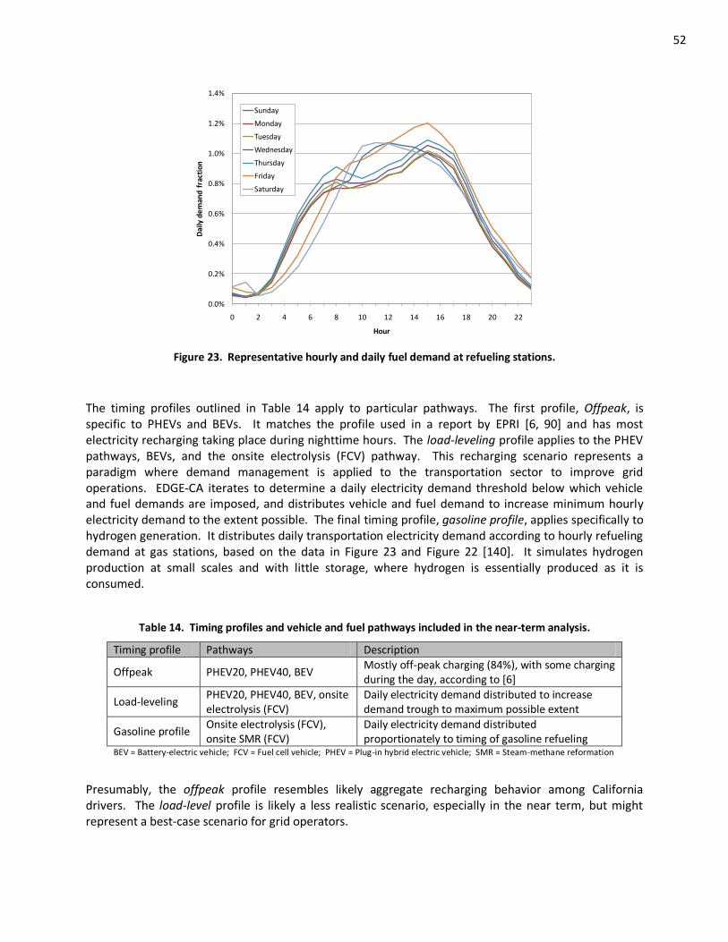
52

0.0%

0.2%

0.4%

0.6%

0.8%

1.0%

1.2%

1.4%

0 2 4 6 8 10 12 14 16 18 20 22

Dai

ly d

em

and

fra

ctio

n

Hour

Sunday

Monday

Tuesday

Wednesday

Thursday

Friday

Saturday

Figure 23. Representative hourly and daily fuel demand at refueling stations.

The timing profiles outlined in Table 14 apply to particular pathways. The first profile, Offpeak, is specific to PHEVs and BEVs. It matches the profile used in a report by EPRI [6, 90] and has most electricity recharging taking place during nighttime hours. The load-leveling profile applies to the PHEV pathways, BEVs, and the onsite electrolysis (FCV) pathway. This recharging scenario represents a paradigm where demand management is applied to the transportation sector to improve grid operations. EDGE-CA iterates to determine a daily electricity demand threshold below which vehicle and fuel demands are imposed, and distributes vehicle and fuel demand to increase minimum hourly electricity demand to the extent possible. The final timing profile, gasoline profile, applies specifically to hydrogen generation. It distributes daily transportation electricity demand according to hourly refueling demand at gas stations, based on the data in Figure 23 and Figure 22 [140]. It simulates hydrogen production at small scales and with little storage, where hydrogen is essentially produced as it is consumed.

Table 14. Timing profiles and vehicle and fuel pathways included in the near-term analysis.

Timing profile Pathways Description

Offpeak PHEV20, PHEV40, BEV Mostly off-peak charging (84%), with some charging during the day, according to [6]

Load-leveling PHEV20, PHEV40, BEV, onsite electrolysis (FCV)

Daily electricity demand distributed to increase demand trough to maximum possible extent

Gasoline profile Onsite electrolysis (FCV), onsite SMR (FCV)

Daily electricity demand distributed proportionately to timing of gasoline refueling

BEV = Battery-electric vehicle; FCV = Fuel cell vehicle; PHEV = Plug-in hybrid electric vehicle; SMR = Steam-methane reformation

Presumably, the offpeak profile resembles likely aggregate recharging behavior among California drivers. The load-level profile is likely a less realistic scenario, especially in the near term, but might represent a best-case scenario for grid operators.

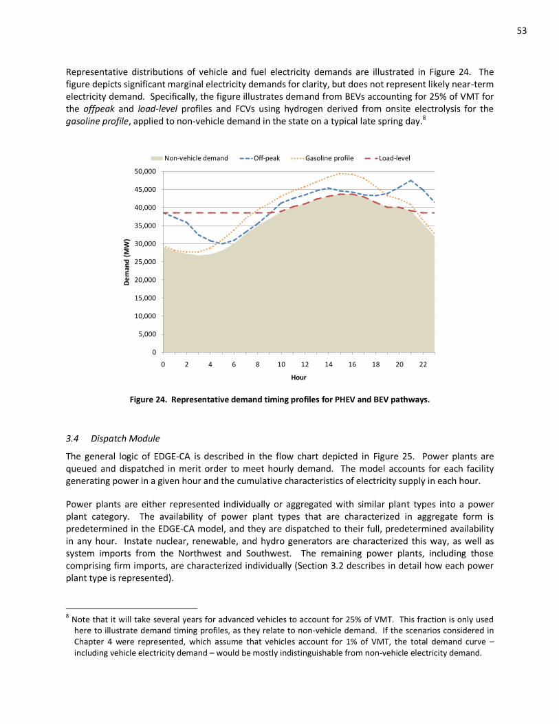
53

Representative distributions of vehicle and fuel electricity demands are illustrated in Figure 24. The figure depicts significant marginal electricity demands for clarity, but does not represent likely near-term electricity demand. Specifically, the figure illustrates demand from BEVs accounting for 25% of VMT for the offpeak and load-level profiles and FCVs using hydrogen derived from onsite electrolysis for the gasoline profile, applied to non-vehicle demand in the state on a typical late spring day.8

0

5,000

10,000

15,000

20,000

25,000

30,000

35,000

40,000

45,000

50,000

0 2 4 6 8 10 12 14 16 18 20 22

De

man

d (

MW

)

Hour

Non-vehicle demand Off-peak Gasoline profile Load-level

Figure 24. Representative demand timing profiles for PHEV and BEV pathways.

3.4 Dispatch Module

The general logic of EDGE-CA is described in the flow chart depicted in Figure 25. Power plants are queued and dispatched in merit order to meet hourly demand. The model accounts for each facility generating power in a given hour and the cumulative characteristics of electricity supply in each hour.

Power plants are either represented individually or aggregated with similar plant types into a power plant category. The availability of power plant types that are characterized in aggregate form is predetermined in the EDGE-CA model, and they are dispatched to their full, predetermined availability in any hour. Instate nuclear, renewable, and hydro generators are characterized this way, as well as system imports from the Northwest and Southwest. The remaining power plants, including those comprising firm imports, are characterized individually (Section 3.2 describes in detail how each power plant type is represented).

8 Note that it will take several years for advanced vehicles to account for 25% of VMT. This fraction is only used

here to illustrate demand timing profiles, as they relate to non-vehicle demand. If the scenarios considered in Chapter 4 were represented, which assume that vehicles account for 1% of VMT, the total demand curve – including vehicle electricity demand – would be mostly indistinguishable from non-vehicle electricity demand.

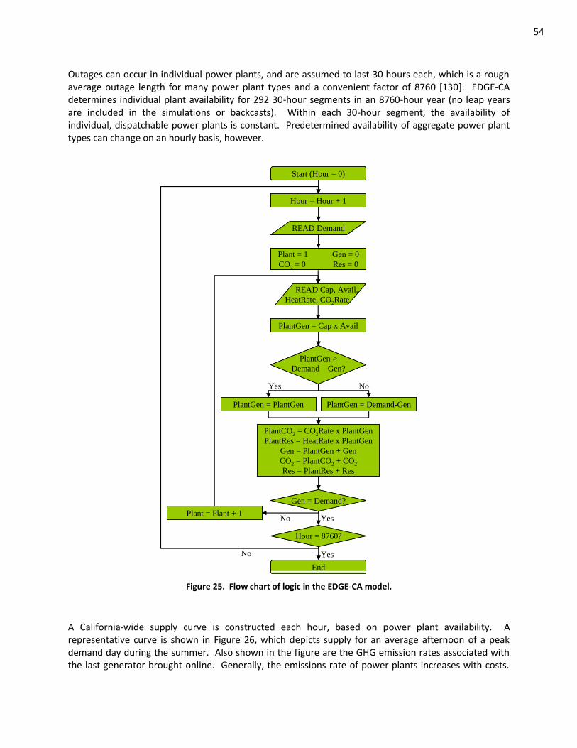
54

Outages can occur in individual power plants, and are assumed to last 30 hours each, which is a rough average outage length for many power plant types and a convenient factor of 8760 [130]. EDGE-CA determines individual plant availability for 292 30-hour segments in an 8760-hour year (no leap years are included in the simulations or backcasts). Within each 30-hour segment, the availability of individual, dispatchable power plants is constant. Predetermined availability of aggregate power plant types can change on an hourly basis, however.

Hour = Hour + 1Hour = Hour + 1

Plant = 1 Gen = 0

CO2 = 0 Res = 0

Plant = 1 Gen = 0

CO2 = 0 Res = 0

READ DemandREAD Demand

READ Cap, Avail,

HeatRate, CO2Rate

READ Cap, Avail,

HeatRate, CO2Rate

PlantGen = Cap x AvailPlantGen = Cap x Avail

PlantGen >

Demand – Gen?

PlantGen >

Demand – Gen?

PlantGen = Demand-GenPlantGen = Demand-GenPlantGen = PlantGenPlantGen = PlantGen

PlantCO2 = CO2Rate x PlantGen

PlantRes = HeatRate x PlantGen

Gen = PlantGen + Gen

CO2 = PlantCO2 + CO2

Res = PlantRes + Res

PlantCO2 = CO2Rate x PlantGen

PlantRes = HeatRate x PlantGen

Gen = PlantGen + Gen

CO2 = PlantCO2 + CO2

Res = PlantRes + Res

Hour = 8760?Hour = 8760?

Start (Hour = 0)Start (Hour = 0)

Gen = Demand?Gen = Demand?

Plant = Plant + 1Plant = Plant + 1

Yes

EndEnd

Yes

Yes

No

No

No

Figure 25. Flow chart of logic in the EDGE-CA model.

A California-wide supply curve is constructed each hour, based on power plant availability. A representative curve is shown in Figure 26, which depicts supply for an average afternoon of a peak demand day during the summer. Also shown in the figure are the GHG emission rates associated with the last generator brought online. Generally, the emissions rate of power plants increases with costs.

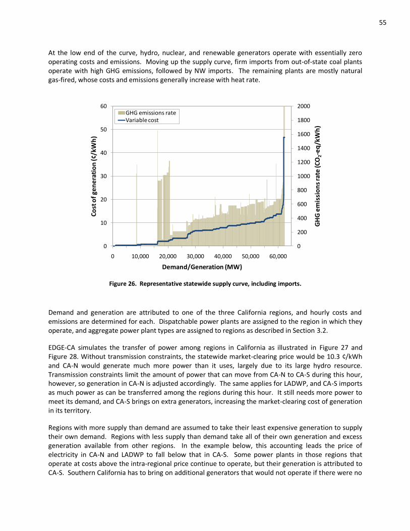
55

At the low end of the curve, hydro, nuclear, and renewable generators operate with essentially zero operating costs and emissions. Moving up the supply curve, firm imports from out-of-state coal plants operate with high GHG emissions, followed by NW imports. The remaining plants are mostly natural gas-fired, whose costs and emissions generally increase with heat rate.

0

200

400

600

800

1000

1200

1400

1600

1800

2000

0

10

20

30

40

50

60

0 10,000 20,000 30,000 40,000 50,000 60,000

GH

G e

mis

sio

ns

rate

(CO

2-e

q/k

Wh

)

Co

st o

f ge

ne

rati

on

(¢/k

Wh

)

Demand/Generation (MW)

GHG emissions rateVariable cost

Figure 26. Representative statewide supply curve, including imports.

Demand and generation are attributed to one of the three California regions, and hourly costs and emissions are determined for each. Dispatchable power plants are assigned to the region in which they operate, and aggregate power plant types are assigned to regions as described in Section 3.2.

EDGE-CA simulates the transfer of power among regions in California as illustrated in Figure 27 and Figure 28. Without transmission constraints, the statewide market-clearing price would be 10.3 ¢/kWh and CA-N would generate much more power than it uses, largely due to its large hydro resource. Transmission constraints limit the amount of power that can move from CA-N to CA-S during this hour, however, so generation in CA-N is adjusted accordingly. The same applies for LADWP, and CA-S imports as much power as can be transferred among the regions during this hour. It still needs more power to meet its demand, and CA-S brings on extra generators, increasing the market-clearing cost of generation in its territory.

Regions with more supply than demand are assumed to take their least expensive generation to supply their own demand. Regions with less supply than demand take all of their own generation and excess generation available from other regions. In the example below, this accounting leads the price of electricity in CA-N and LADWP to fall below that in CA-S. Some power plants in those regions that operate at costs above the intra-regional price continue to operate, but their generation is attributed to CA-S. Southern California has to bring on additional generators that would not operate if there were no

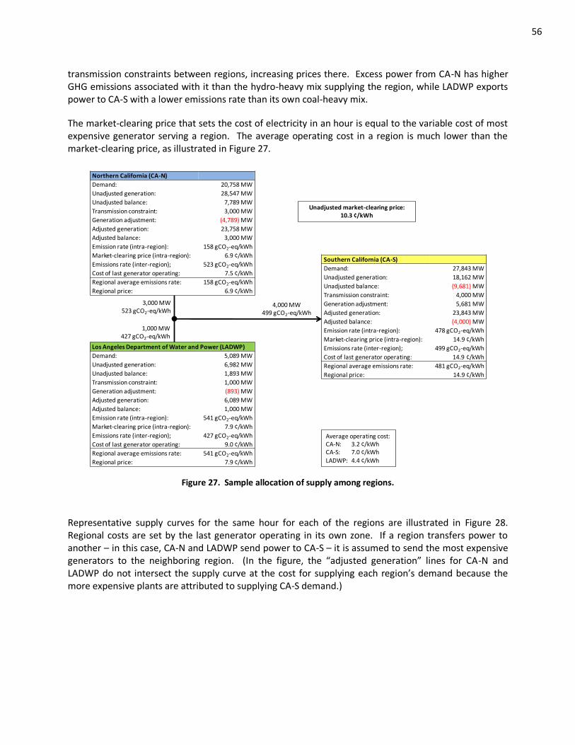
56

transmission constraints between regions, increasing prices there. Excess power from CA-N has higher GHG emissions associated with it than the hydro-heavy mix supplying the region, while LADWP exports power to CA-S with a lower emissions rate than its own coal-heavy mix.

The market-clearing price that sets the cost of electricity in an hour is equal to the variable cost of most expensive generator serving a region. The average operating cost in a region is much lower than the market-clearing price, as illustrated in Figure 27.

Unadjusted market-clearing price: 10.3 ¢/kWh

Northern California (CA-N)

Demand: 20,758 MW

Unadjusted generation: 28,547 MW

Unadjusted balance: 7,789 MW

Transmission constraint: 3,000 MW

Generation adjustment: (4,789) MW

Adjusted generation: 23,758 MW

Adjusted balance: 3,000 MW

Emission rate (intra-region): 158 gCO2-eq/kWh

Market-clearing price (intra-region): 6.9 ¢/kWh

Emissions rate (inter-region); 523 gCO2-eq/kWh

Cost of last generator operating: 7.5 ¢/kWh

Regional average emissions rate: 158 gCO2-eq/kWh

Regional price: 6.9 ¢/kWh

Los Angeles Department of Water and Power (LADWP)

Demand: 5,089 MW


Unadjusted balance: 1,893 MW


Generation adjustment: (893) MW


Adjusted balance: 1,000 MW







Southern California (CA-S)

Demand: 27,843 MW


Unadjusted balance: (9,681) MW


Generation adjustment: 5,681 MW


Adjusted balance: (4,000) MW







3,000 MW 523 gCO2-eq/kWh



Average operating cost:CA-N: 3.2 ¢/kWhCA-S: 7.0 ¢/kWhLADWP: 4.4 ¢/kWh

Figure 27. Sample allocation of supply among regions.

Representative supply curves for the same hour for each of the regions are illustrated in Figure 28. Regional costs are set by the last generator operating in its own zone. If a region transfers power to another – in this case, CA-N and LADWP send power to CA-S – it is assumed to send the most expensive generators to the neighboring region. (In the figure, the “adjusted generation” lines for CA-N and LADWP do not intersect the supply curve at the cost for supplying each region’s demand because the more expensive plants are attributed to supplying CA-S demand.)

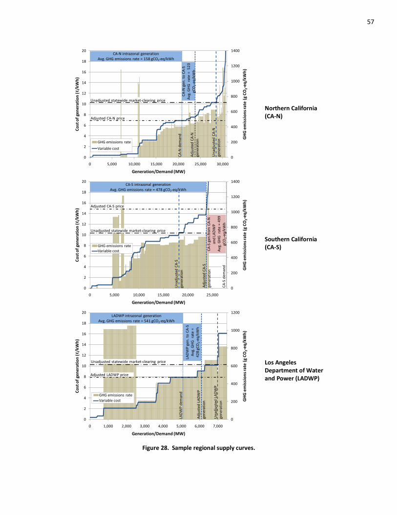
57

0

200

400

600

800

1000

1200

1400

0

2

4

6

8

10

12

14

16

18

20

0 5,000 10,000 15,000 20,000 25,000 30,000

GH

G e

mis

sio

ns

rate

(g

CO

2-e

q/k

Wh

)

Co

st o

f ge

ne

rati

on

(¢

/kW

h)

Generation/Demand (MW)

GHG emissions rate

Variable cost

Unadjusted statewide market-clearing price

CA

-N d

eman

d

Un

adju

sted

CA

-N

gen

erat

ion

CA-N intrazonal generationAvg. GHG emissions rate = 158 gCO2-eq/kWh

CA

-N g

en.

to C

A-S

A

vg.G

HG

ra

te =

5

23

gC

O2-e

q/k

Wh

Ad

just

ed C

A-N

ge

ner

atio

n

Adjusted CA-N price

(a) Northern California (CA-N)

0

200

400

600

800

1000

1200

1400

0

2

4

6

8

10

12

14

16

18

20

0 5,000 10,000 15,000 20,000 25,000

GH

G e

mis

sio

ns

rate

(g

CO

2-e

q/k

Wh

)

Co

st o

f ge

ne

rati

on

(¢

/kW

h)


GHG emissions rateVariable cost


CA

-S d

eman

d

Un

adju

sted

CA

-S

gen

erat

ion

CA-S intrazonal generationAvg. GHG emissions rate = 478 gCO2-eq/kWh

CA

-S g

en.f

rom

CA

-N

and

LA

DW

PA

vg.G

HG

ra

te =

49

9

gCO

2-e

q/k

Wh

Ad

just

ed C

A-S

ge

ner

atio

nAdjusted CA-S price

(b) Southern California (CA-S)

0

200

400

600

800

1000

1200

0

2

4

6

8

10

12

14

16

18

20

0 1,000 2,000 3,000 4,000 5,000 6,000 7,000

GH

G e

mis

sio

ns

rate

(g

CO

2-e

q/k

Wh

)

Co

st o

f ge

ne

rati

on

(¢

/kW

h)


GHG emissions rate

Variable cost


LAD

WP

dem

and

Un

adju

sted

LA

DW

P

gen

erat

ion

LADWP intrazonal generationAvg. GHG emissions rate = 541 gCO2-eq/kWh

LAD

WP

gen

. to

CA

-S

Avg

.GH

G

rate

=

42

8 g

CO

2-e

q/k

Wh

Ad

just

ed L

AD

WP

ge

ner

atio

n

Adjusted LADWP price

(c) Los Angeles Department of Water and Power (LADWP)

Figure 28. Sample regional supply curves.

58

Northern California generates about 10,000 MW from inexpensive and low GHG-intensive sources, mostly hydro and nuclear. Given the cost of electricity, it has a significant resource to share with CA-S, which relies heavily on dispatchable capacity to meet its demands in this hour. Without adjusting for transmission constraints, CA-N would have 7,789 MW of excess capacity. But it can only send 3,000 MW to CA-S, which increases the market-clearing cost relative to what it would be without transmission constraints.

The LADWP region supplies its own needs with a significant fraction of coal power, which it brings in from the Navajo and Intermountain power plants in Arizona and Utah, respectively. It, too, can generate more power at the statewide market-clearing cost than can be transmitted to regions that need it, and it curtails generation compared to the unconstrained case.

3.5 Costs

Hourly electricity supply costs are defined as the sum of the variable operating cost of the last plant brought online (the most expensive plant operating). These costs represent costs of electricity generation, rather than prices seen by consumers, which also include fixed costs, transmission and distribution costs, taxes, and other fees. The additional cost components may increase prices to consumers significantly. In 2007, for example, the average wholesale energy price for electricity in the CAISO supply area was about $49/MWh [131], while the average rate paid by all consumers in the three CAISO utility regions was $129-$166/MWh [142].

The variable costs presented in Table 4 are developed based on the parameters described in Table 15. Plant-level variable costs are the sum of fuel costs and variable operations and maintenance (O&M) costs, which are taken from [117]. Fuel costs are the product of heat rate, from the eGRID database [47], and the assumed energy costs listed in the table. Natural gas prices are set equal to $7/MMBtu in the CA-N region and $6.5/MMbtu in CA-S and LADWP, which is roughly equal to the average month-ahead price index from 2005-2007 for natural gas at the PG&E city gate and Southern California border, respectively [143]. Fuel costs are assumed to be constant over the course of the year.

A few exceptions are made in assigning variable costs when simulating the current CA grid. Ten plants in the Oil category have high capacity factors in 2005 that would not be realized in EDGE-CA simulations if the plants were queued according to the costs in Table 15. Those plants, which mostly burn residual oil, are assumed to have zero fuel costs, pushing them higher up in the dispatch order and increasing their capacity factor in EDGE-CA simulations. Also, four NGCT plants have unexpectedly high capacity factors in the eGRID data. These plants are attributed capital, fixed, and variable O&M costs for comparable NGCC plants instead, to push them higher up in the dispatch queue. Finally, in determining energy costs for biomass and solar facilities that are co-fired with natural gas, natural gas energy costs are excluded. This simplification does not impact electricity dispatch in EDGE-CA, however, since generation from biomass and solar facilities are predetermined in the model (as described above).

This costing methodology may misrepresent costs for some plants, as data for variable O&M costs are based on current technology. Older plants likely have different costs, and comparative costs among different plants of different vintages might even have different relative values. Also, much of the merchant capacity in the state was purchased from investor-owned utilities (IOU) in the late 1990s and early 2000s as part of deregulation.

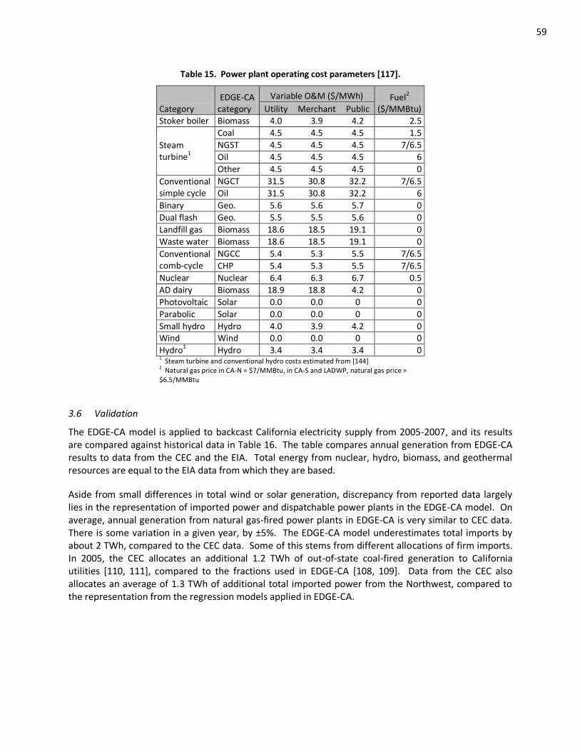
59

Table 15. Power plant operating cost parameters [117].

Category

EDGE-CA category

Variable O&M ($/MWh) Fuel2 ($/MMBtu) Utility Merchant Public

Stoker boiler Biomass 4.0 3.9 4.2 2.5

Steam turbine

1

Coal 4.5 4.5 4.5 1.5

NGST 4.5 4.5 4.5 7/6.5

Oil 4.5 4.5 4.5 6

Other 4.5 4.5 4.5 0

Conventional simple cycle

NGCT 31.5 30.8 32.2 7/6.5

Oil 31.5 30.8 32.2 6

Binary Geo. 5.6 5.6 5.7 0

Dual flash Geo. 5.5 5.5 5.6 0

Landfill gas Biomass 18.6 18.5 19.1 0

Waste water Biomass 18.6 18.5 19.1 0

Conventional comb-cycle

NGCC 5.4 5.3 5.5 7/6.5

CHP 5.4 5.3 5.5 7/6.5

Nuclear Nuclear 6.4 6.3 6.7 0.5

AD dairy Biomass 18.9 18.8 4.2 0

Photovoltaic Solar 0.0 0.0 0 0

Parabolic Solar 0.0 0.0 0 0

Small hydro Hydro 4.0 3.9 4.2 0 Wind Wind 0.0 0.0 0 0

Hydro1 Hydro 3.4 3.4 3.4 0 1 Steam turbine and conventional hydro costs estimated from [144]

2 Natural gas price in CA-N = $7/MMBtu, in CA-S and LADWP, natural gas price =

$6.5/MMBtu

3.6 Validation

The EDGE-CA model is applied to backcast California electricity supply from 2005-2007, and its results are compared against historical data in Table 16. The table compares annual generation from EDGE-CA results to data from the CEC and the EIA. Total energy from nuclear, hydro, biomass, and geothermal resources are equal to the EIA data from which they are based.

Aside from small differences in total wind or solar generation, discrepancy from reported data largely lies in the representation of imported power and dispatchable power plants in the EDGE-CA model. On average, annual generation from natural gas-fired power plants in EDGE-CA is very similar to CEC data. There is some variation in a given year, by ±5%. The EDGE-CA model underestimates total imports by about 2 TWh, compared to the CEC data. Some of this stems from different allocations of firm imports. In 2005, the CEC allocates an additional 1.2 TWh of out-of-state coal-fired generation to California utilities [110, 111], compared to the fractions used in EDGE-CA [108, 109]. Data from the CEC also allocates an average of 1.3 TWh of additional total imported power from the Northwest, compared to the representation from the regression models applied in EDGE-CA.

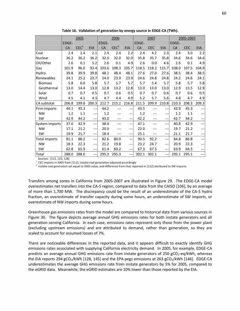
60

Table 16. Validation of generation by energy source in EDGE-CA (TWh).

2005 2006 2007 2005-2007

EDGE-

CA CEC1 EIA EDGE-

CA CEC2 EIA EDGE-

CA CEC EIA EDGE-

CA CEC EIA

Coal 2.4 2.4 2.1 2.4 2.4 2.2 2.4 4.2 2.3 2.4 3.0 2.2

Nuclear 36.2 36.2 36.2 32.0 32.0 32.0 35.8 35.7 35.8 34.6 34.6 34.6

Oil/Other 2.6 0.1 5.2 2.6 0.1 4.9 2.6 0.0 4.6 2.6 0.1 4.9

Gas 101.9 96.0 93.4 103.6 108.3 105.7 118.5 118.2 115.7 108.0 107.5 104.9

Hydro 39.8 39.9 39.8 48.1 48.4 48.1 27.6 27.0 27.6 38.5 38.4 38.5

Renewables 24.1 25.2 23.7 24.0 23.9 23.9 24.6 24.8 24.8 24.2 24.6 24.1

Biomass 5.8 6.0 5.8 5.7 5.7 5.7 5.7 5.4 5.7 5.8 5.7 5.8

Geothermal 13.0 14.4 13.0 12.8 13.2 12.8 13.0 13.0 13.0 12.9 13.5 12.9

Solar 0.7 0.7 0.5 0.7 0.6 0.5 0.7 0.7 0.6 0.7 0.6 0.5

Wind 4.5 4.1 4.3 4.7 4.4 4.9 5.2 5.7 5.6 4.8 4.7 4.9

CA subtotal 206.8 199.8 200.3 212.7 215.2 216.8 211.5 209.9 210.8 210.3 208.3 209.3

Firm imports 44.1 45.3 --- 44.2 --- --- 43.5 --- --- 43.9 45.3 ---

NW 1.2 1.1 --- 1.2 --- --- 1.2 --- --- 1.2 1.1 ---

SW 42.9 44.2 --- 43.0 --- --- 42.2 --- --- 42.7 44.2 ---

System imports 37.0 42.9 --- 38.4 --- --- 47.1 --- --- 40.8 42.9 ---

NW 17.1 21.2 --- 20.0 --- --- 22.0 --- --- 19.7 21.2 ---

SW 19.9 21.7 --- 18.4 --- --- 25.1 --- --- 21.1 21.7 ---

Total imports 81.1 88.2 --- 82.6 80.0 --- 90.5 92.2 --- 84.8 86.8 ---

NW 18.3 22.3 --- 21.2 19.8 --- 23.2 24.7 --- 20.9 22.3 ---

SW 62.8 65.9 --- 61.4 60.2 --- 67.3 67.5 --- 63.9 64.5 ---

Total 288.0 288.0 --- 295.3 295.3 --- 302.1 302.1 --- 295.1 295.1 --- Sources: [112, 123, 128] 1 CEC imports in 2005 from [111]; instate coal generation adjusted accordingly

2 Instate coal generation set equal to 2005 value, and difference from that reported in [112] attributed to SW imports

Transfers among zones in California from 2005-2007 are illustrated in Figure 29. The EDGE-CA model overestimates net transfers into the CA-S region, compared to data from the CAISO [106], by an average of more than 1,700 MW. The discrepancy could be the result of an underestimate of the CA-S hydro fraction, an overestimate of transfer capacity during some hours, an underestimate of SW imports, or overestimate of NW imports during some hours.

Greenhouse gas emissions rates from the model are compared to historical data from various sources in Figure 30. The figure depicts average annual GHG emissions rates for both instate generators and all generation serving California. In each case, emissions rates represent only those from the power plant (excluding upstream emissions) and are attributed to demand, rather than generation, so they are scaled to account for assumed losses of 7%.

There are noticeable differences in the reported data, and it appears difficult to exactly identify GHG emissions rates associated with supplying California electricity demand. In 2005, for example, EDGE-CA predicts an average annual GHG emissions rate from instate generators of 250 gCO2-eq/kWh, whereas the EIA reports 294 gCO2/kWh [128, 145] and the EPA pegs emissions at 263 gCO2/kWh [146]. EDGE-CA underestimates the average GHG emissions rate from instate generators by 5% for 2005, compared to the eGRID data. Meanwhile, the eGRID estimates are 10% lower than those reported by the EIA.

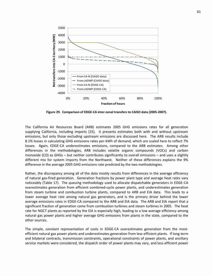
61

-4000

-3000

-2000

-1000

0

1000

2000

3000

4000

5000

0% 20% 40% 60% 80% 100%

Ne

t tra

nsf

ers

into

CA

-S te

rrit

ory

(MW

)

Fraction of hours

From CA-N (CAISO data)

From LADWP (CAISO data)

From CA-N (EDGE-CA)

From LADWP (EDGE-CA)

Figure 29. Comparison of EDGE-CA inter-zonal transfers to CAISO data (2005-2007).

The California Air Resources Board (ARB) estimates 2005 GHG emissions rates for all generation supplying California, including imports [25]. It presents estimates both with and without upstream emissions, but only those excluding upstream emissions are discussed here. The ARB results include 8.1% losses in calculating GHG emissions rates per-kWh of demand, which are scaled here to reflect 7% losses. Again, EDGE-CA underestimates emissions, compared to the ARB estimates. Among other differences in the methodologies, ARB includes volatile organic compounds (VOCs) and carbon monoxide (CO) as GHGs – but neither contributes significantly to overall emissions – and uses a slightly different mix for system imports from the Northwest. Neither of these differences explains the 9% difference in the average 2005 GHG emissions rate predicted by the two methodologies.

Rather, the discrepancy among all of the data mostly results from differences in the average efficiency of natural gas-fired generation. Generation fractions by power plant type and average heat rates vary noticeably (Table 17). The queuing methodology used to allocate dispatchable generators in EDGE-CA overestimates generation from efficient combined-cycle power plants, and underestimates generation from steam turbine and combustion turbine plants, compared to ARB and EIA data. This leads to a lower average heat rate among natural gas generators, and is the primary driver behind the lower average emissions rates in EDGE-CA compared to the ARB and EIA data. The ARB and EIA report that a significant fraction of generation came from combustion turbines and steam turbines in 2005. The heat rate for NGCT plants as reported by the EIA is especially high, leading to a low average efficiency among natural gas power plants and higher average GHG emissions from plants in the state, compared to the other sources.

The simple, constant representation of costs in EDGE-CA overestimates generation from the most-efficient natural gas power plants and underestimates generation from less-efficient plants. If long-term and bilateral contracts, transmission constraints, operational constraints of power plants, and ancillary service markets were considered, the dispatch order of power plants may vary, and less-efficient power

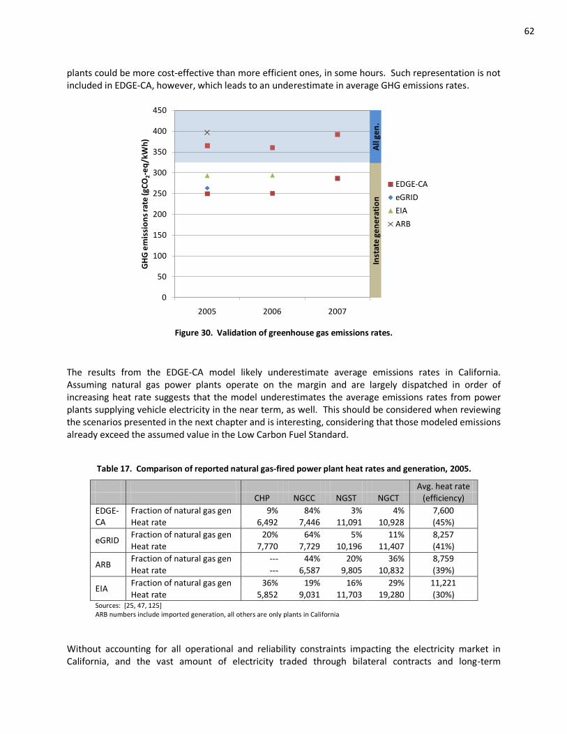
62

plants could be more cost-effective than more efficient ones, in some hours. Such representation is not included in EDGE-CA, however, which leads to an underestimate in average GHG emissions rates.

0

50

100

150

200

250

300

350

400

450

2005 2006 2007

GH

G e

mis

sio

ns

rate

(gC

O2-e

q/k

Wh

)

EDGE-CA

eGRID

EIA

ARB

Inst

ate

ge

ne

rati

on

All

ge

n.

Figure 30. Validation of greenhouse gas emissions rates.

The results from the EDGE-CA model likely underestimate average emissions rates in California. Assuming natural gas power plants operate on the margin and are largely dispatched in order of increasing heat rate suggests that the model underestimates the average emissions rates from power plants supplying vehicle electricity in the near term, as well. This should be considered when reviewing the scenarios presented in the next chapter and is interesting, considering that those modeled emissions already exceed the assumed value in the Low Carbon Fuel Standard.

Table 17. Comparison of reported natural gas-fired power plant heat rates and generation, 2005.

Avg. heat rate

CHP NGCC NGST NGCT (efficiency)

EDGE-CA

Fraction of natural gas gen 9% 84% 3% 4% 7,600

Heat rate 6,492 7,446 11,091 10,928 (45%)

eGRID Fraction of natural gas gen 20% 64% 5% 11% 8,257

Heat rate 7,770 7,729 10,196 11,407 (41%)

ARB Fraction of natural gas gen --- 44% 20% 36% 8,759

Heat rate --- 6,587 9,805 10,832 (39%)

EIA Fraction of natural gas gen 36% 19% 16% 29% 11,221

Heat rate 5,852 9,031 11,703 19,280 (30%) Sources: [25, 47, 125] ARB numbers include imported generation, all others are only plants in California

Without accounting for all operational and reliability constraints impacting the electricity market in California, and the vast amount of electricity traded through bilateral contracts and long-term

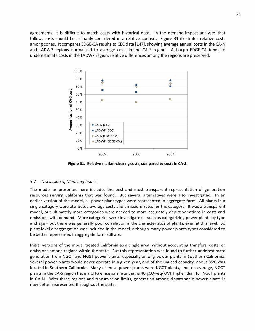
63

agreements, it is difficult to match costs with historical data. In the demand-impact analyses that follow, costs should be primarily considered in a relative context. Figure 31 illustrates relative costs among zones. It compares EDGE-CA results to CEC data [147], showing average annual costs in the CA-N and LADWP regions normalized to average costs in the CA-S region. Although EDGE-CA tends to underestimate costs in the LADWP region, relative differences among the regions are preserved.

0%

10%

20%

30%

40%

50%

60%

70%

80%

90%

100%

2005 2006 2007

Ave

rge

frac

tio

n o

f CA

-S c

ost

CA-N (CEC)

LADWP (CEC)

CA-N (EDGE-CA)

LADWP (EDGE-CA)

Figure 31. Relative market-clearing costs, compared to costs in CA-S.

3.7 Discussion of Modeling Issues

The model as presented here includes the best and most transparent representation of generation resources serving California that was found. But several alternatives were also investigated. In an earlier version of the model, all power plant types were represented in aggregate form. All plants in a single category were attributed average costs and emissions rates for the category. It was a transparent model, but ultimately more categories were needed to more accurately depict variations in costs and emissions with demand. More categories were investigated – such as categorizing power plants by type and age – but there was generally poor correlation in the characteristics of plants, even at this level. So plant-level disaggregation was included in the model, although many power plants types considered to be better represented in aggregate form still are.

Initial versions of the model treated California as a single area, without accounting transfers, costs, or emissions among regions within the state. But this representation was found to further underestimate generation from NGCT and NGST power plants, especially among power plants in Southern California. Several power plants would never operate in a given year, and of the unused capacity, about 85% was located in Southern California. Many of these power plants were NGCT plants, and, on average, NGCT plants in the CA-S region have a GHG emissions rate that is 40 gCO2-eq/kWh higher than for NGCT plants in CA-N. With three regions and transmission limits, generation among dispatchable power plants is now better represented throughout the state.

64

A version of the model was also developed where dispatch was simulated in the Northwest and Southwest, in addition to California. The aim was to more accurately capture hourly net imports, but ultimately the representation was less accurate than the regression models developed here. This representation also lacked transparency and simplicity, as many additional, often ill-defined parameters were included. Representing the hydro resource in the Northwest proved a key difficulty, since it does not operate as California’s and power generation is a low-priority use of the resource. Also, depicting trade among regions was difficult, and not transparent, without developing an optimization algorithm.

A stochastic version of the model was developed, to investigate impacts of uncertainty in power plant availability [148]. It was found that annual hydro generation had a far greater impact on the results than intermittent wind availability or uncertain power plant outage schedules. In the results presented in the next chapter, sensitivity to hydro generation is investigated, but power plant outages and hourly wind speeds remain constant.

Wind speeds were investigated to gauge their correlation to load and temperature. Maximum wind speeds were found to decline with peak load and temperature, but little correlation was found in quartile and median values. And minimum wind speed appears to increase with temperature and load, according to the wind speed profile used here. In the model results presented here, wind speed is independent of temperature or load, taken directly from a wind speed curve from 2003 [52]. Wind speed data are difficult to come by, however, and some data in this curve may be derived. That little correlation was found between wind speed and peak temperature or load in this data set does not imply that such correlation does not exist.

65

4. NEAR-TERM VEHICLE AND FUEL PATHWAY COMPARISON

Characterizing well-to-wheels emissions from electric vehicles or hydrogen FCVs requires understanding the marginal mix of generation that supplies electricity demands for vehicle recharging or hydrogen production. In Part I of this dissertation, the marginal mix is defined as generation equal to vehicle or fuel electricity demand from the last dispatchable, fossil power plants brought online in a given hour. This mix reflects additional generation from power plants that are brought online to supply incremental demand from BEVs, PHEVs, or FCVs. EDGE-CA assumes that current hydro, nuclear, and renewable power plants generate the same amount of electricity with or without vehicle and fuel electricity demands, and generation from these plant types does not contribute to the marginal mix. Thus, marginal mixes presented in this chapter will represent the most expensive fossil-fired power plants operating in a given hour, which are also likely to be among the least efficient. Coupled with the assumption that low-emitting hydro, nuclear, and renewable power plants do not supply marginal generation, the marginal GHG emissions rate for electricity supplying vehicle and fuel demands is usually higher than the average rate from all of the plants operating at a given time.

This chapter explores lifecycle marginal GHG emissions supplying light-duty vehicle demands from the current electricity grid in California and compares well-to-wheels vehicle emissions for various vehicle and fuel platforms. Although vehicle recharging will have minor impacts on grid operation in the near-term, when the number of plug-in vehicles on the road is relatively small, this analysis offers insight into marginal generation from the current grid and the resulting vehicle-level GHG emissions. The results are helpful to inform energy policy discussions relevant to the current state of affairs in California, such as the LCFS or vehicle-level GHG emission standards. Analysis of future grids, whose composition and operation may be more dramatically affected by vehicle recharging or capacity additions from renewable or other resources, is presented in Part II.

First, results are presented for average electricity supply in 2010 when no vehicle recharging is added to the grid. Then, vehicle and fuel electricity demands are added to the grid, based on the timing profiles developed in Section 3.3.2 and assuming that BEVs, PHEVs, or FCVs account for 1% of VMT. Results are presented and discussed for marginal electricity supplying these scenarios, and well-to-wheels GHG emissions are calculated and compared for vehicle and fuel pathways based on their marginal mix. Throughout this chapter, sensitivity of the results to annual hydro availability and location of vehicle and fuel demand is explored, and marginal electricity GHG emissions rates are compared to the assumed value in the LCFS rulemaking.

4.1 Electricity Supply in 2010 with No Vehicles

To begin, EDGE-CA is applied to consider California electricity supply in 2010 without vehicle electricity demand. Understanding grid operation without vehicle recharging helps to describe the capabilities (and shortcomings) of the EDGE-CA model, and provides context for understanding marginal generation when vehicle recharging is added.

The simulated California generation mix in 2010 is illustrated in Figure 32. The figure shows generation by power plant type and average GHG emissions rates for the entire state on a monthly basis. In July and August, generation increases by about 20% from the monthly average. Peaking NGST or NGCT power plants account for up to 10% of generation in August. But hydro generation and NW imports are also among their highest in the early summer months, and average GHG emissions rates in July are lower than they are in all other non-spring months. Average GHG emissions rates in August are similar to what they are in the fall and early winter, when demand is much lower, because hydro generation

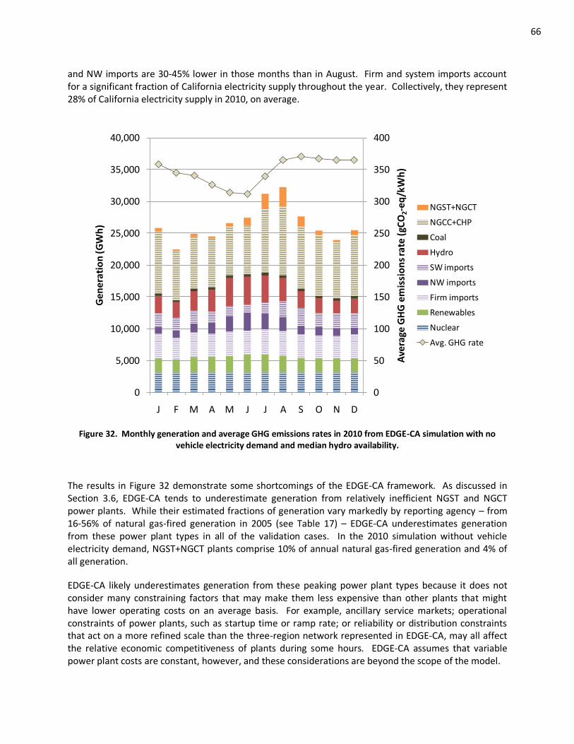
66

and NW imports are 30-45% lower in those months than in August. Firm and system imports account for a significant fraction of California electricity supply throughout the year. Collectively, they represent 28% of California electricity supply in 2010, on average.

0

50

100

150

200

250

300

350

400

0

5,000

10,000

15,000

20,000

25,000

30,000

35,000

40,000

J F M A M J J A S O N DA

vera

ge G

HG

em

issi

on

s ra

te (

gCO

2-e

q/k

Wh

)

Ge

ne

rati

on

(G

Wh

)

NGST+NGCT

NGCC+CHP

Coal

Hydro

SW imports

NW imports

Firm imports

Renewables

Nuclear

Avg. GHG rate

Figure 32. Monthly generation and average GHG emissions rates in 2010 from EDGE-CA simulation with no vehicle electricity demand and median hydro availability.

The results in Figure 32 demonstrate some shortcomings of the EDGE-CA framework. As discussed in Section 3.6, EDGE-CA tends to underestimate generation from relatively inefficient NGST and NGCT power plants. While their estimated fractions of generation vary markedly by reporting agency – from 16-56% of natural gas-fired generation in 2005 (see Table 17) – EDGE-CA underestimates generation from these power plant types in all of the validation cases. In the 2010 simulation without vehicle electricity demand, NGST+NGCT plants comprise 10% of annual natural gas-fired generation and 4% of all generation.

EDGE-CA likely underestimates generation from these peaking power plant types because it does not consider many constraining factors that may make them less expensive than other plants that might have lower operating costs on an average basis. For example, ancillary service markets; operational constraints of power plants, such as startup time or ramp rate; or reliability or distribution constraints that act on a more refined scale than the three-region network represented in EDGE-CA, may all affect the relative economic competitiveness of plants during some hours. EDGE-CA assumes that variable power plant costs are constant, however, and these considerations are beyond the scope of the model.

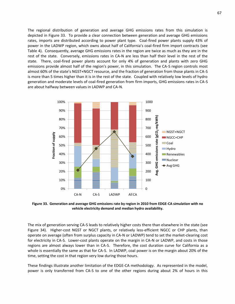
67

The regional distribution of generation and average GHG emissions rates from this simulation is depicted in Figure 33. To provide a clear connection between generation and average GHG emissions rates, imports are distributed according to power plant type. Coal-fired power plants supply 43% of power in the LADWP region, which owns about half of California’s coal-fired firm import contracts (see Table 4). Consequently, average GHG emissions rates in the region are twice as much as they are in the rest of the state. Conversely, emissions rates in CA-N are less than half their level in the rest of the state. There, coal-fired power plants account for only 4% of generation and plants with zero GHG emissions provide almost half of the region’s power, in this simulation. The CA-S region controls most almost 60% of the state’s NGST+NGCT resource, and the fraction of generation from those plants in CA-S is more than 5 times higher than it is in the rest of the state. Coupled with relatively low levels of hydro generation and moderate levels of coal-fired generation from firm imports, GHG emissions rates in CA-S are about halfway between values in LADWP and CA-N.

0

100

200

300

400

500

600

700

800

900

1000

0%

10%

20%

30%

40%

50%

60%

70%

80%

90%

100%

CA-N CA-S LADWP All CA

Avg

. GH

G e

mis

sio

ns

rate

(gC

O2-e

q/k

Wh

)

Fra

ctio

n o

f su

pp

ly NGST+NGCT

NGCC+CHP

Coal

Hydro

Renewables

Nuclear

Avg GHG

Figure 33. Generation and average GHG emissions rate by region in 2010 from EDGE-CA simulation with no vehicle electricity demand and median hydro availability.

The mix of generation serving CA-S leads to relatively higher costs there than elsewhere in the state (see Figure 34). Higher-cost NGST or NGCT plants, or relatively less-efficient NGCC or CHP plants, than operate on average (often from surplus capacity in CA-N or LADWP) tend to set the market-clearing cost for electricity in CA-S. Lower-cost plants operate on the margin in CA-N or LADWP, and costs in those regions are almost always lower than in CA-S. Therefore, the cost duration curve for California as a whole is essentially the same as that for CA-S. In LADWP, coal power is on the margin about 20% of the time, setting the cost in that region very low during those hours.

These findings illustrate another limitation of the EDGE-CA methodology. As represented in the model, power is only transferred from CA-S to one of the other regions during about 2% of hours in this

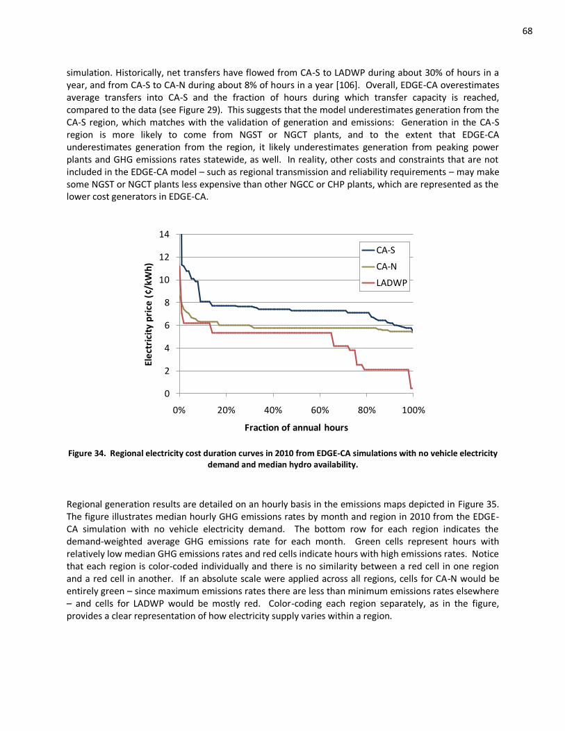
68

simulation. Historically, net transfers have flowed from CA-S to LADWP during about 30% of hours in a year, and from CA-S to CA-N during about 8% of hours in a year [106]. Overall, EDGE-CA overestimates average transfers into CA-S and the fraction of hours during which transfer capacity is reached, compared to the data (see Figure 29). This suggests that the model underestimates generation from the CA-S region, which matches with the validation of generation and emissions: Generation in the CA-S region is more likely to come from NGST or NGCT plants, and to the extent that EDGE-CA underestimates generation from the region, it likely underestimates generation from peaking power plants and GHG emissions rates statewide, as well. In reality, other costs and constraints that are not included in the EDGE-CA model – such as regional transmission and reliability requirements – may make some NGST or NGCT plants less expensive than other NGCC or CHP plants, which are represented as the lower cost generators in EDGE-CA.

0

2

4

6

8

10

12

14

0% 20% 40% 60% 80% 100%

Ele

ctri

city

pri

ce (

¢/kW

h)

Fraction of annual hours

CA-S

CA-N

LADWP

Figure 34. Regional electricity cost duration curves in 2010 from EDGE-CA simulations with no vehicle electricity demand and median hydro availability.

Regional generation results are detailed on an hourly basis in the emissions maps depicted in Figure 35. The figure illustrates median hourly GHG emissions rates by month and region in 2010 from the EDGE-CA simulation with no vehicle electricity demand. The bottom row for each region indicates the demand-weighted average GHG emissions rate for each month. Green cells represent hours with relatively low median GHG emissions rates and red cells indicate hours with high emissions rates. Notice that each region is color-coded individually and there is no similarity between a red cell in one region and a red cell in another. If an absolute scale were applied across all regions, cells for CA-N would be entirely green – since maximum emissions rates there are less than minimum emissions rates elsewhere – and cells for LADWP would be mostly red. Color-coding each region separately, as in the figure, provides a clear representation of how electricity supply varies within a region.

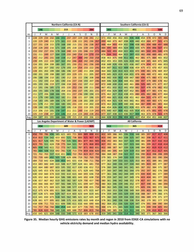
69

146

162 177 192 253 269

284 393

405 418 431 470 483 496

509

Hr. J F M A M J J A S O N D J F M A M J J A S O N D

0 228 229 234 232 166 151 237 237 229 238 241 212 471 450 456 452 443 406 408 454 478 472 485 486

1 220 229 240 213 173 161 222 228 222 241 236 267 490 460 473 467 438 409 440 453 484 477 501 473

2 227 231 228 215 170 168 200 215 231 236 238 267 488 464 493 459 432 398 438 481 494 488 497 488

3 234 228 243 216 171 168 205 218 226 239 230 271 484 495 489 455 424 393 435 475 494 496 507 472

4 233 232 237 231 178 164 240 223 235 246 232 272 484 502 493 450 422 401 432 481 502 495 500 470

5 231 211 249 227 164 159 233 240 254 239 270 259 474 504 502 464 415 397 433 482 490 489 481 470

6 242 212 245 231 168 158 212 247 284 240 250 258 458 463 475 448 411 401 462 481 475 484 465 452

7 239 205 222 220 167 162 202 246 269 242 240 256 452 455 453 435 426 419 442 469 485 469 471 445

8 224 201 204 208 180 167 201 230 251 241 236 249 458 448 426 436 425 436 447 474 494 472 466 453

9 225 202 207 192 192 179 193 219 254 233 222 246 459 447 411 422 409 436 459 475 472 470 457 455

10 228 201 202 199 184 186 196 227 240 211 204 244 464 442 420 413 423 433 475 490 481 476 469 457

11 200 201 199 208 180 187 203 229 225 211 205 247 470 445 423 419 434 431 476 486 480 472 465 458

12 206 188 194 210 181 190 212 226 222 196 208 248 468 442 430 402 439 447 480 496 475 480 472 456

13 211 192 193 214 181 190 216 237 234 193 207 246 469 446 428 404 444 451 480 497 479 480 478 462

14 205 193 196 219 177 194 218 245 232 197 212 247 472 448 430 414 443 461 486 505 485 475 477 457

15 212 191 196 185 173 205 220 252 236 199 211 248 467 451 432 412 441 450 482 507 478 476 482 452

16 203 191 183 178 166 204 216 243 237 195 201 231 477 456 429 409 437 452 481 509 477 481 474 461

17 211 177 206 168 166 195 211 237 236 190 194 223 475 462 427 414 438 455 480 495 482 486 477 464

18 213 179 190 165 162 182 211 238 221 207 196 225 477 466 421 416 438 451 462 484 501 479 477 462

19 218 183 195 189 166 176 197 236 228 201 200 227 475 464 421 428 443 441 461 491 489 483 475 459

20 221 179 212 192 164 180 191 231 220 210 202 228 473 462 415 409 440 446 464 487 499 481 483 464

21 228 190 195 171 160 160 195 218 233 219 205 232 466 454 426 406 421 426 455 479 482 476 494 463

22 213 206 210 191 158 147 211 211 249 216 219 243 475 440 437 400 432 435 414 472 475 491 495 478

23 225 219 238 207 154 146 213 214 224 243 228 251 477 437 438 423 436 417 400 463 473 478 503 479Avg. 204 187 201 191 166 166 199 215 219 203 206 223 444 428 413 396 404 401 427 454 454 451 448 437

454

506 558 611 768 820 872

925 311

323 335 347 383 395

419


0 856 799 786 496 585 621 683 721 800 889 888 832 402 389 386 365 336 316 348 385 397 417 417 408

1 814 810 534 542 653 692 521 738 800 925 907 875 403 390 384 363 338 325 347 382 398 417 417 411

2 821 817 526 595 702 750 535 501 801 877 865 905 406 392 383 363 337 323 344 381 399 417 416 413

3 823 795 551 624 728 775 564 521 767 875 868 893 407 392 381 365 337 323 344 381 399 417 418 414

4 805 498 543 611 722 773 567 521 787 871 860 831 402 388 387 367 339 326 348 384 402 419 419 412

5 765 484 508 553 692 741 528 713 779 859 836 820 393 380 395 369 329 319 353 389 407 412 417 405

6 721 702 702 537 614 651 465 722 763 823 817 794 384 368 387 358 322 317 356 390 413 398 398 399

7 735 739 680 492 505 538 629 696 719 762 769 793 379 365 374 349 320 319 355 392 399 392 390 394

8 684 710 642 634 500 455 641 631 658 708 711 766 377 363 349 333 331 325 353 383 401 389 381 390

9 653 683 682 640 610 588 617 597 624 661 681 734 377 362 340 336 337 334 360 385 403 385 377 387

10 632 664 680 687 603 595 592 617 630 636 652 713 376 360 344 340 341 341 365 387 392 384 375 387

11 625 645 653 676 614 600 580 631 671 629 645 708 377 360 347 340 342 344 370 392 397 382 376 388

12 630 650 660 674 610 592 610 615 660 693 636 718 377 361 346 342 344 349 373 400 404 381 377 389

13 635 652 663 664 614 586 588 601 643 692 638 730 379 359 347 342 347 349 376 403 404 381 377 390

14 636 657 667 662 610 565 582 587 629 700 657 740 380 361 346 342 348 352 378 407 397 381 380 391

15 650 666 666 667 597 582 588 571 631 699 647 742 380 363 346 339 346 352 377 407 398 381 380 390

16 655 675 671 669 623 584 588 577 638 698 655 718 380 362 345 336 344 352 375 405 396 383 372 384

17 612 675 674 691 611 564 580 599 621 675 615 647 375 360 353 334 336 349 369 395 401 385 366 376

18 597 628 671 668 529 567 614 603 623 644 619 641 374 359 349 335 329 339 358 388 387 379 366 375

19 613 641 650 673 518 565 562 585 621 617 635 647 375 360 343 339 334 334 353 386 389 379 371 377

20 628 661 677 695 602 588 575 616 605 633 648 654 378 361 340 336 338 336 354 382 379 381 377 379

21 658 698 711 715 611 606 590 611 616 666 690 666 382 364 352 336 326 324 347 374 391 388 390 384

22 715 757 756 744 484 454 640 637 677 726 745 705 388 374 371 345 320 313 346 373 399 398 405 392

23 785 828 820 766 540 530 689 688 757 806 815 766 396 380 385 358 323 311 348 376 398 410 417 401Avg. 650 645 621 604 548 550 548 571 619 683 678 692 359 345 341 326 314 312 340 365 371 367 365 366

689 365

215 451

Northern California (CA-N) Southern California (CA-S)

Los Angeles Department of Water & Power (LADWP) All California

Figure 35. Median hourly GHG emissions rates by month and regon in 2010 from EDGE-CA simulations with no vehicle elctricity demand and median hydro availability.

70

The relative GHG emissions rates indicated in the figure reflect relative differences in hourly generation mixes by time of day, season, and region. In general, on a statewide basis, average GHG emissions rates are lowest during spring and early summer months, when hydro generation and relatively low-emitting NW imports are most abundant. As demand tends to increase in the afternoon of late summer months, and generation from hydro and NW imports begins to taper, emissions rates increase. By August, and through January, average GHG emissions rates are relatively high. Emissions rates are among their highest values when baseload, coal-fired generation comprises its greatest share of supply. This happens during offpeak demand hours in the late evening and early morning of fall and early winter months, when hydro generation is low.

There is some variation in general operation of the grid on a regional basis. In CA-N or LADWP, which rely heavily on hydro or coal-fired power plants, respectively, median hourly GHG emissions rates may vary by more than ±30% from their annual average value. Emissions rates are most sensitive to the seasonal availability of hydro and NW imports in CA-N. Emissions rates are most sensitive to demand in LADWP, where coal-fired plants may provide most of the region’s power and resulting emissions rates may be very high during some offpeak hours. As demand increases in LADWP, during daytime hours, emissions rates tend to decline. Additional natural gas-fired and hydro generation supplement the average supply mix and reduce the generation shares from coal-fired plants with high GHG emissions rates. In CA-S, which relies less on hydro than CA-N and less on coal than LADWP, emissions rates are more steady. During any given hour, median emissions rates differ by less than ±15% of the region’s annual average value.

Relative average GHG emissions rates do not necessarily translate to relatively marginal GHG emissions rates. Despite higher average emissions rates in the LADWP region, marginal emissions rates there are often lower than they are in the rest of the state. When coal-fired power plants supply most of the power there, some of the region’s most efficient natural gas-fired generators – or even hydro plants – may be operating on the margin, in EDGE-CA simulations. Although emissions rates are lower in CA-N than in the rest of the state, the relative abundance of hydro there does not necessarily imply that the mix of dispatchable, fossil-fired generation is more efficient than that operating in the other regions of the state, at any given time. Emissions from the marginal generator supplying incremental demand cannot always be inferred from average emissions rates; they are sensitive to the magnitude, timing, and location of incremental demand.

Clearly, electricity supply in California (especially in CA-N) is sensitive to the annual availability of hydro energy. The impacts of hydro availability on electricity supply in 2010, as simulated in EDGE-CA, are depicted in Figure 36. The figure compares the percentage change in select results when annual available hydro energy is changed from its median value (37,557 GWh) to its 10th percentile value (24,235 GWh) or its 90th percentile value (50,879 GWh).

For reference, Figure 14 illustrates the effects of annual availability on hourly hydro generation. The difference in hydro generation between a median year and a 90th or a 10th percentile year is an average of about 1,500 MW/hour. Between the 90th and 10th percentile years, then, the average difference is about 3,000 MW/hour. During fall and winter months, the difference in hourly generation between a 90th percentile year and a 10th percentile year is greater during daytime hours than it is offpeak. The opposite holds in the spring and summer. Hourly hydro generation is more often at its peak capacity in EDGE-CA simulations during those months, and increasing hydro energy increases hydro generation overnight relatively more than it does during daytime hours. Therefore, electricity supply is less

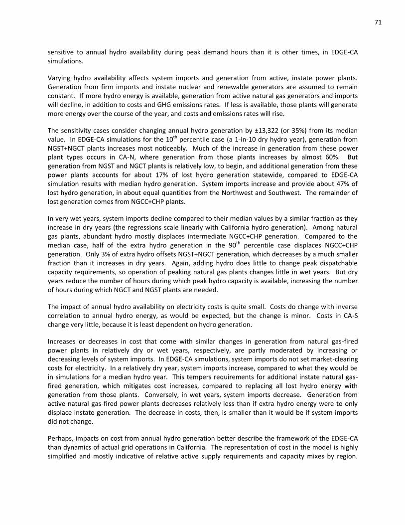
71

sensitive to annual hydro availability during peak demand hours than it is other times, in EDGE-CA simulations.

Varying hydro availability affects system imports and generation from active, instate power plants. Generation from firm imports and instate nuclear and renewable generators are assumed to remain constant. If more hydro energy is available, generation from active natural gas generators and imports will decline, in addition to costs and GHG emissions rates. If less is available, those plants will generate more energy over the course of the year, and costs and emissions rates will rise.

The sensitivity cases consider changing annual hydro generation by ±13,322 (or 35%) from its median value. In EDGE-CA simulations for the 10th percentile case (a 1-in-10 dry hydro year), generation from NGST+NGCT plants increases most noticeably. Much of the increase in generation from these power plant types occurs in CA-N, where generation from those plants increases by almost 60%. But generation from NGST and NGCT plants is relatively low, to begin, and additional generation from these power plants accounts for about 17% of lost hydro generation statewide, compared to EDGE-CA simulation results with median hydro generation. System imports increase and provide about 47% of lost hydro generation, in about equal quantities from the Northwest and Southwest. The remainder of lost generation comes from NGCC+CHP plants.

In very wet years, system imports decline compared to their median values by a similar fraction as they increase in dry years (the regressions scale linearly with California hydro generation). Among natural gas plants, abundant hydro mostly displaces intermediate NGCC+CHP generation. Compared to the median case, half of the extra hydro generation in the 90th percentile case displaces NGCC+CHP generation. Only 3% of extra hydro offsets NGST+NGCT generation, which decreases by a much smaller fraction than it increases in dry years. Again, adding hydro does little to change peak dispatchable capacity requirements, so operation of peaking natural gas plants changes little in wet years. But dry years reduce the number of hours during which peak hydro capacity is available, increasing the number of hours during which NGCT and NGST plants are needed.

The impact of annual hydro availability on electricity costs is quite small. Costs do change with inverse correlation to annual hydro energy, as would be expected, but the change is minor. Costs in CA-S change very little, because it is least dependent on hydro generation.

Increases or decreases in cost that come with similar changes in generation from natural gas-fired power plants in relatively dry or wet years, respectively, are partly moderated by increasing or decreasing levels of system imports. In EDGE-CA simulations, system imports do not set market-clearing costs for electricity. In a relatively dry year, system imports increase, compared to what they would be in simulations for a median hydro year. This tempers requirements for additional instate natural gas-fired generation, which mitigates cost increases, compared to replacing all lost hydro energy with generation from those plants. Conversely, in wet years, system imports decrease. Generation from active natural gas-fired power plants decreases relatively less than if extra hydro energy were to only displace instate generation. The decrease in costs, then, is smaller than it would be if system imports did not change.

Perhaps, impacts on cost from annual hydro generation better describe the framework of the EDGE-CA than dynamics of actual grid operations in California. The representation of cost in the model is highly simplified and mostly indicative of relative active supply requirements and capacity mixes by region.

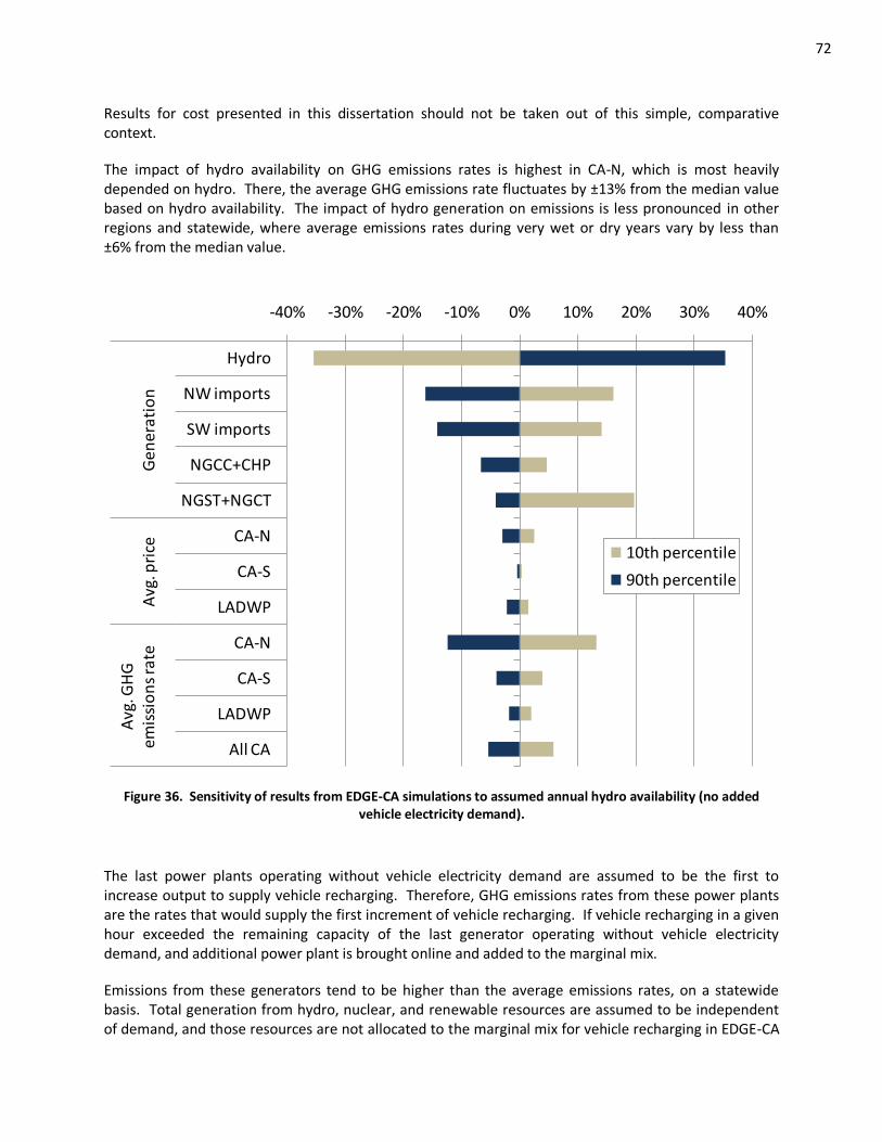
72

Results for cost presented in this dissertation should not be taken out of this simple, comparative context.

The impact of hydro availability on GHG emissions rates is highest in CA-N, which is most heavily depended on hydro. There, the average GHG emissions rate fluctuates by ±13% from the median value based on hydro availability. The impact of hydro generation on emissions is less pronounced in other regions and statewide, where average emissions rates during very wet or dry years vary by less than ±6% from the median value.

-40% -30% -20% -10% 0% 10% 20% 30% 40%

Hydro

NW imports

SW imports

NGCC+CHP

NGST+NGCT

CA-N

CA-S

LADWP

CA-N

CA-S

LADWP

All CA

Gen

erat

ion

Avg

. pri

ceA

vg. G

HG

em

issi

on

s ra

te

10th percentile

90th percentile

Figure 36. Sensitivity of results from EDGE-CA simulations to assumed annual hydro availability (no added vehicle electricity demand).

The last power plants operating without vehicle electricity demand are assumed to be the first to increase output to supply vehicle recharging. Therefore, GHG emissions rates from these power plants are the rates that would supply the first increment of vehicle recharging. If vehicle recharging in a given hour exceeded the remaining capacity of the last generator operating without vehicle electricity demand, and additional power plant is brought online and added to the marginal mix.

Emissions from these generators tend to be higher than the average emissions rates, on a statewide basis. Total generation from hydro, nuclear, and renewable resources are assumed to be independent of demand, and those resources are not allocated to the marginal mix for vehicle recharging in EDGE-CA

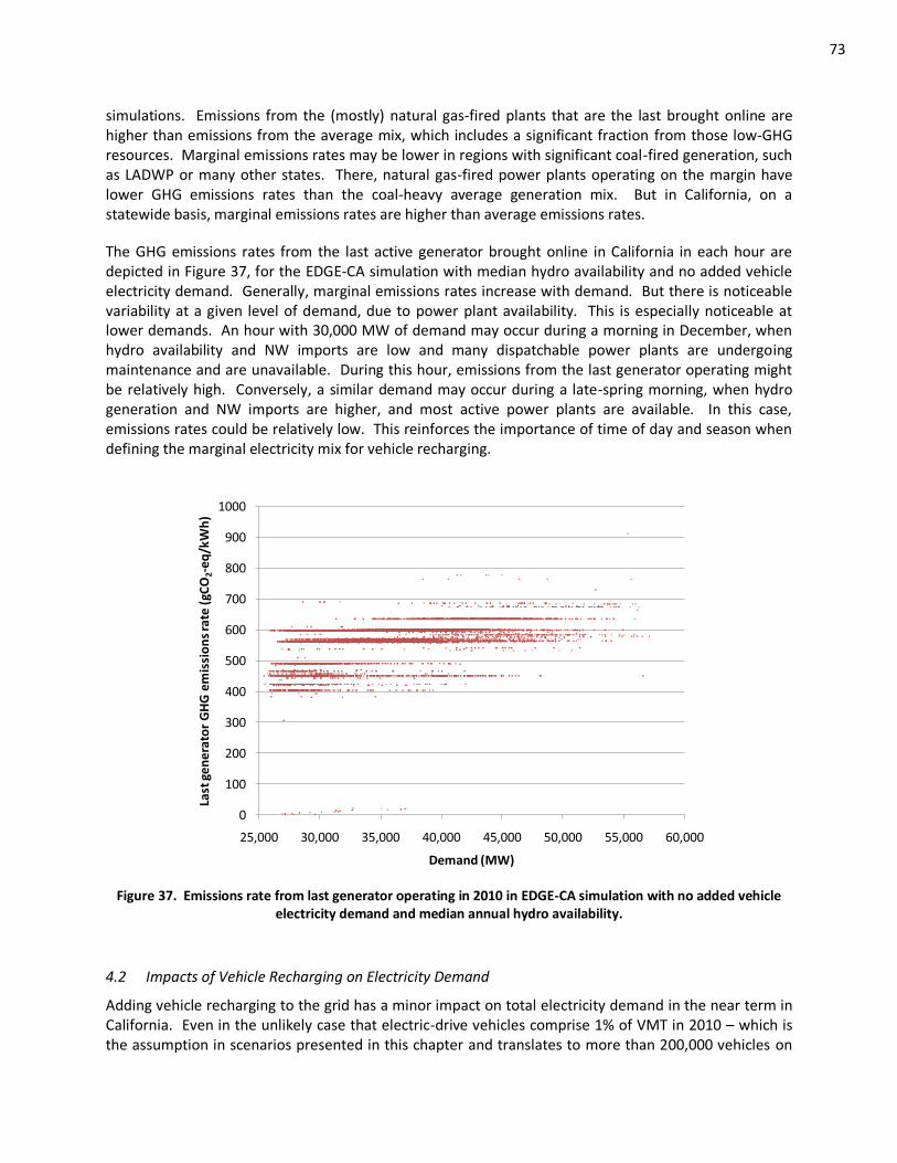
73

simulations. Emissions from the (mostly) natural gas-fired plants that are the last brought online are higher than emissions from the average mix, which includes a significant fraction from those low-GHG resources. Marginal emissions rates may be lower in regions with significant coal-fired generation, such as LADWP or many other states. There, natural gas-fired power plants operating on the margin have lower GHG emissions rates than the coal-heavy average generation mix. But in California, on a statewide basis, marginal emissions rates are higher than average emissions rates.

The GHG emissions rates from the last active generator brought online in California in each hour are depicted in Figure 37, for the EDGE-CA simulation with median hydro availability and no added vehicle electricity demand. Generally, marginal emissions rates increase with demand. But there is noticeable variability at a given level of demand, due to power plant availability. This is especially noticeable at lower demands. An hour with 30,000 MW of demand may occur during a morning in December, when hydro availability and NW imports are low and many dispatchable power plants are undergoing maintenance and are unavailable. During this hour, emissions from the last generator operating might be relatively high. Conversely, a similar demand may occur during a late-spring morning, when hydro generation and NW imports are higher, and most active power plants are available. In this case, emissions rates could be relatively low. This reinforces the importance of time of day and season when defining the marginal electricity mix for vehicle recharging.

0

100

200

300

400

500

600

700

800

900

1000

25,000 30,000 35,000 40,000 45,000 50,000 55,000 60,000

Last

ge

ne

rato

r G

HG

em

issi

on

s ra

te (

gCO

2-e

q/k

Wh

)

Demand (MW)

Figure 37. Emissions rate from last generator operating in 2010 in EDGE-CA simulation with no added vehicle electricity demand and median annual hydro availability.

4.2 Impacts of Vehicle Recharging on Electricity Demand

Adding vehicle recharging to the grid has a minor impact on total electricity demand in the near term in California. Even in the unlikely case that electric-drive vehicles comprise 1% of VMT in 2010 – which is the assumption in scenarios presented in this chapter and translates to more than 200,000 vehicles on

74

the road – vehicle and fuel electricity demands increase total demand by less than 1% in each scenario. If BEVs accounted for 1% of VMT, they would increase California electricity demand by less than 0.4%. This is 5 times less than the 1.8% average annual growth in California electricity demand that has occurred since 1983 [112]. It would take about 1 million BEVs to increase electricity demand by a similar amount.

Realistically, it will likely take several years for vehicle recharging demands in the state to grow to the level that would occur if 1% of VMT came from BEVs, and the near term impact of vehicle recharging on the grid will be much smaller. For reference, it took five years for 200,000 HEVs to be sold in the entire U.S. [149].

The impact of vehicle recharging on hourly electricity demands are represented in Figure 32Figure 38, for the scenarios with BEV recharging considered in this chapter. Indeed, it is difficult to discern the difference in demand timing for these pathways. Vehicle recharging only occurs from 2am-6am on this day, according to the Load-level profile. Vehicle electricity demands are relatively high during these hours – compared to Offpeak recharging – and level electricity demand to a small extent. Some vehicle recharging occurs during all hours of the day with the Offpeak profile – more overnight than during the day – but hourly vehicle recharging demands are very small relative to non-vehicle demand.

30.0

32.5

35.0

37.5

40.0

42.5

45.0

47.5

50.0

52.5

0 3 6 9 12 15 18 21

De

ma

nd

(GW

)

Hour beginning

Load-level

Offpeak

None

Figure 38. Sample impact of vehicle recharging on system electricity demand (1% of VMT from BEVs).

Electricity demand from vehicles accounting for 1% of VMT and its impact on total demand is described in Table 3. Average and peak hourly electricity demands for each pathway are listed, along with load factors, which are defined as the ratio of average to peak demand. Load factors describe variability in demand (constant demand would have a load factor of one). Pathways with Load-level demand timing have a low vehicle demand load factor, because most electricity demand occurs during a few hours. But

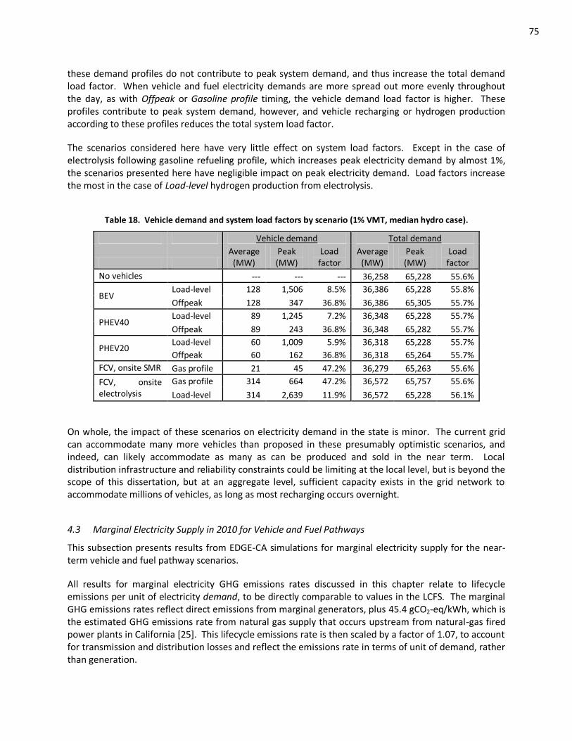
75

these demand profiles do not contribute to peak system demand, and thus increase the total demand load factor. When vehicle and fuel electricity demands are more spread out more evenly throughout the day, as with Offpeak or Gasoline profile timing, the vehicle demand load factor is higher. These profiles contribute to peak system demand, however, and vehicle recharging or hydrogen production according to these profiles reduces the total system load factor.

The scenarios considered here have very little effect on system load factors. Except in the case of electrolysis following gasoline refueling profile, which increases peak electricity demand by almost 1%, the scenarios presented here have negligible impact on peak electricity demand. Load factors increase the most in the case of Load-level hydrogen production from electrolysis.

Table 18. Vehicle demand and system load factors by scenario (1% VMT, median hydro case).

Vehicle demand Total demand

Average

(MW) Peak (MW)

Load factor

Average (MW)

Peak (MW)

Load factor

No vehicles --- --- --- 36,258 65,228 55.6%

BEV Load-level 128 1,506 8.5% 36,386 65,228 55.8%

Offpeak 128 347 36.8% 36,386 65,305 55.7%

PHEV40 Load-level 89 1,245 7.2% 36,348 65,228 55.7%

Offpeak 89 243 36.8% 36,348 65,282 55.7%

PHEV20 Load-level 60 1,009 5.9% 36,318 65,228 55.7%

Offpeak 60 162 36.8% 36,318 65,264 55.7%

FCV, onsite SMR Gas profile 21 45 47.2% 36,279 65,263 55.6%

FCV, onsite electrolysis

Gas profile 314 664 47.2% 36,572 65,757 55.6%

Load-level 314 2,639 11.9% 36,572 65,228 56.1%

On whole, the impact of these scenarios on electricity demand in the state is minor. The current grid can accommodate many more vehicles than proposed in these presumably optimistic scenarios, and indeed, can likely accommodate as many as can be produced and sold in the near term. Local distribution infrastructure and reliability constraints could be limiting at the local level, but is beyond the scope of this dissertation, but at an aggregate level, sufficient capacity exists in the grid network to accommodate millions of vehicles, as long as most recharging occurs overnight.

4.3 Marginal Electricity Supply in 2010 for Vehicle and Fuel Pathways

This subsection presents results from EDGE-CA simulations for marginal electricity supply for the near-term vehicle and fuel pathway scenarios.

All results for marginal electricity GHG emissions rates discussed in this chapter relate to lifecycle emissions per unit of electricity demand, to be directly comparable to values in the LCFS. The marginal GHG emissions rates reflect direct emissions from marginal generators, plus 45.4 gCO2-eq/kWh, which is the estimated GHG emissions rate from natural gas supply that occurs upstream from natural-gas fired power plants in California [25]. This lifecycle emissions rate is then scaled by a factor of 1.07, to account for transmission and distribution losses and reflect the emissions rate in terms of unit of demand, rather than generation.

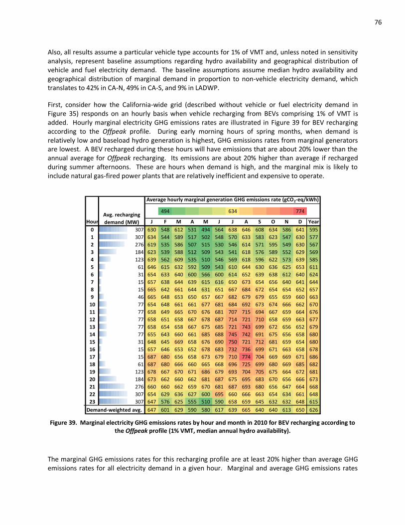
76

Also, all results assume a particular vehicle type accounts for 1% of VMT and, unless noted in sensitivity analysis, represent baseline assumptions regarding hydro availability and geographical distribution of vehicle and fuel electricity demand. The baseline assumptions assume median hydro availability and geographical distribution of marginal demand in proportion to non-vehicle electricity demand, which translates to 42% in CA-N, 49% in CA-S, and 9% in LADWP.

First, consider how the California-wide grid (described without vehicle or fuel electricity demand in Figure 35) responds on an hourly basis when vehicle recharging from BEVs comprising 1% of VMT is added. Hourly marginal electricity GHG emissions rates are illustrated in Figure 39 for BEV recharging according to the Offpeak profile. During early morning hours of spring months, when demand is relatively low and baseload hydro generation is highest, GHG emissions rates from marginal generators are lowest. A BEV recharged during these hours will have emissions that are about 20% lower than the annual average for Offpeak recharging. Its emissions are about 20% higher than average if recharged during summer afternoons. These are hours when demand is high, and the marginal mix is likely to include natural gas-fired power plants that are relatively inefficient and expensive to operate.

494

522 550 578 606

634 774

Hour J F M A M J J A S O N D Year

0 307 630 548 612 531 494 564 638 646 608 634 586 641 595

1 307 634 544 589 517 502 548 570 633 583 623 547 630 577

2 276 619 535 586 507 515 530 546 614 571 595 549 630 567

3 184 623 539 588 512 509 543 541 618 576 589 552 629 569

4 123 639 562 609 535 510 546 569 618 596 622 573 639 585

5 61 646 615 632 592 509 543 610 644 630 636 625 653 611

6 31 654 633 640 600 566 600 614 652 639 638 612 640 624

7 15 657 638 644 639 615 616 650 673 654 656 640 641 644

8 15 665 642 661 644 631 651 667 684 672 654 654 652 657

9 46 665 648 653 650 657 667 682 679 679 655 659 660 663

10 77 654 648 661 661 677 681 684 692 673 674 666 662 670

11 77 658 649 665 670 676 681 707 715 694 667 659 664 676

12 77 658 651 658 667 678 687 714 721 710 658 659 663 677

13 77 658 654 658 667 675 685 721 743 699 672 656 652 679

14 77 655 643 660 661 685 688 745 742 691 675 656 658 680

15 31 648 645 669 658 676 690 750 721 712 681 659 654 680

16 15 657 646 653 652 678 683 732 736 699 671 663 658 678

17 15 687 680 656 658 673 679 710 774 704 669 669 671 686

18 61 687 680 666 660 665 668 696 725 699 680 669 685 682

19 123 678 667 670 671 686 679 693 704 705 675 664 672 681

20 184 673 662 660 662 681 687 675 695 683 670 656 666 673

21 276 660 660 662 659 670 681 687 693 680 656 647 664 668

22 307 654 629 636 627 600 695 660 666 663 654 634 661 648

23 307 647 576 625 555 510 590 658 659 645 632 632 648 615

Demand-weighted avg. 647 601 629 590 580 617 639 665 640 640 613 650 626

Average hourly marginal generation GHG emissions rate (gCO2-eq/kWh)

Avg. recharging

demand (MW)

Figure 39. Marginal electricity GHG emissions rates by hour and month in 2010 for BEV recharging according to the Offpeak profile (1% VMT, median annual hydro availability).

The marginal GHG emissions rates for this recharging profile are at least 20% higher than average GHG emissions rates for all electricity demand in a given hour. Marginal and average GHG emissions rates

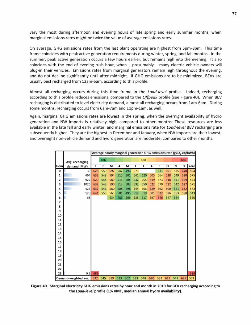
77

vary the most during afternoon and evening hours of late spring and early summer months, when marginal emissions rates might be twice the value of average emissions rates.

On average, GHG emissions rates from the last plant operating are highest from 5pm-8pm. This time frame coincides with peak active generation requirements during winter, spring, and fall months. In the summer, peak active generation occurs a few hours earlier, but remains high into the evening. It also coincides with the end of evening rush hour, when – presumably – many electric vehicle owners will plug-in their vehicles. Emissions rates from marginal generators remain high throughout the evening, and do not decline significantly until after midnight. If GHG emissions are to be minimized, BEVs are usually best recharged from 12am-5am, according to this profile.

Almost all recharging occurs during this time frame in the Load-level profile. Indeed, recharging according to this profile reduces emissions, compared to the Offpeak profile (see Figure 40). When BEV recharging is distributed to level electricity demand, almost all recharging occurs from 1am-6am. During some months, recharging occurs from 6am-7am and 11pm-1am, as well.

Again, marginal GHG emissions rates are lowest in the spring, when the overnight availability of hydro generation and NW imports is relatively high, compared to other months. These resources are less available in the late fall and early winter, and marginal emissions rate for Load-level BEV recharging are subsequently higher. They are the highest in December and January, when NW imports are their lowest, and overnight non-vehicle demand and hydro generation are moderate, compared to other months.

486

506 527 547 567

588 689


0 39 628 559 597 542 496 571 531 601 575 648 594

1 464 632 548 594 515 501 541 520 605 564 628 549 630 575

2 927 629 544 589 515 504 532 555 619 573 618 541 629 573

3 1026 632 543 590 513 503 532 550 622 579 612 542 627 571

4 423 637 546 580 508 498 544 566 629 592 600 521 632 573

5 120 641 555 565 501 495 512 519 601 622 586 553 588 543

6 68 534 486 505 535 517 597 646 547 524 550

7

8

9

10

11

12

13

14

15

16

17

18

19

20

21

22

23 0.2 689 689



Avg. recharging

demand (MW)

Figure 40. Marginal electricity GHG emissions rates by hour and month in 2010 for BEV recharging according to the Load-level profile (1% VMT, median annual hydro availability).

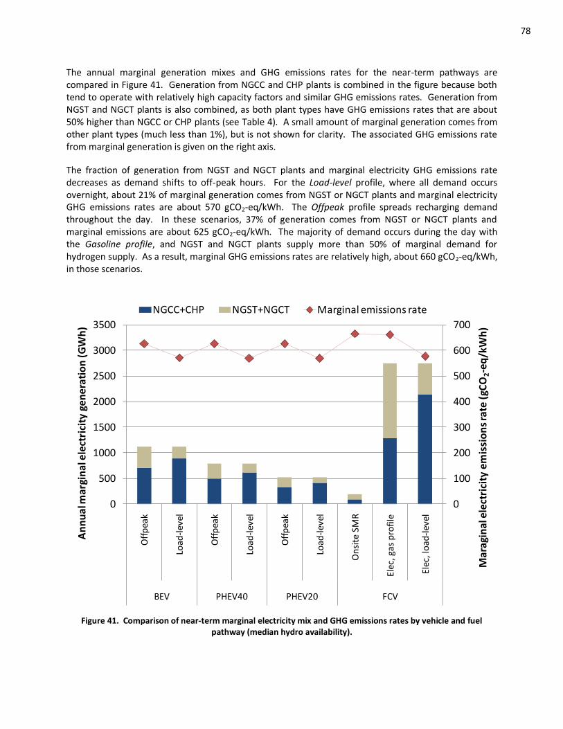
78

The annual marginal generation mixes and GHG emissions rates for the near-term pathways are compared in Figure 41. Generation from NGCC and CHP plants is combined in the figure because both tend to operate with relatively high capacity factors and similar GHG emissions rates. Generation from NGST and NGCT plants is also combined, as both plant types have GHG emissions rates that are about 50% higher than NGCC or CHP plants (see Table 4). A small amount of marginal generation comes from other plant types (much less than 1%), but is not shown for clarity. The associated GHG emissions rate from marginal generation is given on the right axis.

The fraction of generation from NGST and NGCT plants and marginal electricity GHG emissions rate decreases as demand shifts to off-peak hours. For the Load-level profile, where all demand occurs overnight, about 21% of marginal generation comes from NGST or NGCT plants and marginal electricity GHG emissions rates are about 570 gCO2-eq/kWh. The Offpeak profile spreads recharging demand throughout the day. In these scenarios, 37% of generation comes from NGST or NGCT plants and marginal emissions are about 625 gCO2-eq/kWh. The majority of demand occurs during the day with the Gasoline profile, and NGST and NGCT plants supply more than 50% of marginal demand for hydrogen supply. As a result, marginal GHG emissions rates are relatively high, about 660 gCO2-eq/kWh, in those scenarios.

0

100

200

300

400

500

600

700

0

500

1000

1500

2000

2500

3000

3500

Off

pea

k

Load

-lev

el

Off

pea

k

Load

-lev

el

Off

pea

k

Load

-lev

el

On

site

SM

R

Elec

, gas

pro

file

Elec

, lo

ad-l

evel

BEV PHEV40 PHEV20 FCV

Mar

agin

al e

lect

rici

ty e

mis

sio

ns

rate

(gC

O2-e

q/k

Wh

)

An

nu

al m

argi

nal

ele

ctri

city

ge

ne

rati

on

(G

Wh

)

NGCC+CHP NGST+NGCT Marginal emissions rate

Figure 41. Comparison of near-term marginal electricity mix and GHG emissions rates by vehicle and fuel pathway (median hydro availability).

79

Generally, as the quantity of electricity demand for a given charging profile increases, so does the fraction of marginal generation from NGST and NGCT plants and the marginal electricity GHG emissions rate. Thus, one would expect marginal emissions rates to be higher for BEV pathways than for PHEV pathways using the same charging profile.

But they are very similar in these results, due to the relatively small amount of marginal demand. During many hours, increased demand for BEV pathways is insufficient to add additional power plants to the marginal mix, compared to PHEV scenarios, and the same marginal generator operates in either case. When the demand difference is more noticeable, during off-peak hours, subsequent generators added to the marginal mix often have similar characteristics to those operating before them. California has a large stock of CHP and new NGCC plants that operate with similar emissions rates and are available on the margin when active generation requirements are low.

4.3.1 Sensitivity of marginal electricity supply to hydro availability and demand location

The previous results represent marginal supply on a statewide basis under typical conditions. But electricity supply is highly dynamic and emissions vary from average, depending on when and where hydrogen is produced or a vehicle is recharged.

Marginal emissions rates by region are illustrated in Figure 42 for the BEV, Offpeak pathway. The figure illustrates GHG emissions rates from the last generators operating in a region, averaged by hour and month. Relative differences in GHG emissions rates by time of day and month are similar for each of the regions. But typically, LADWP region has the lowest marginal GHG emissions rate, while CA-S has the highest, among the three regions.

Emissions rates are highest on a statewide basis, because they include the last generators operating statewide, regardless of region. During most hours, generators in CA-S are on the last brought online, and set the California-wide market-clearing cost and marginal emissions rate. But during some hours, especially in early mornings in April or August afternoons, plants in CA-N or LADWP are the last brought online in the state and have higher GHG emissions rates than the last plants operating in CA-S. As a result, the statewide marginal emissions rate is slightly higher than that in CA-S, on an average basis.

The differences depicted in the figure primarily help to describe differences in generation in each region over the course of the day and year. They do not accurately convey marginal emissions rates associated with incremental demand in a given region. Indeed, the last generators operating in a region – depicted in the figure – may be supplying demand in another region. And increasing demand in one region may lead to increasing supply in a different region, if available generation is less expensive there and sufficient transmission capacity exists. Therefore, considering marginal generation on a statewide basis is the most accurate representation of vehicle and fuel demand impacts on electricity supply. All of the results presented above, and below, reflect marginal generation and emissions on a statewide basis (as shown here in the “All California” graph for the BEV, Offpeak pathway). Figure 42 simply provides additional insight into regional supply and sets up the sensitivity analysis regarding the impact of demand location on marginal supply statewide.

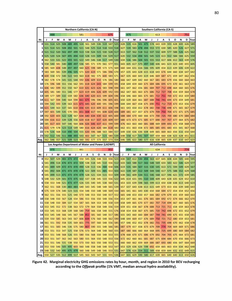
80

488

525 544 563

581

600 619 638 656

675 475

503 530 558 586

613

641 668 696 723

751

Hr. J F M A M J J A S O N D Year J F M A M J J A S O N D Year

0 531 514 525 508 489 495 524 561 549 536 519 547 525 628 535 616 501 475 574 643 639 593 628 600 626 589

1 521 514 521 508 492 501 521 548 525 514 518 533 518 627 539 583 478 494 553 572 630 585 620 526 627 571

2 521 512 520 502 497 499 513 538 524 515 530 528 517 613 537 562 518 512 537 532 609 577 588 526 625 562

3 525 520 524 507 495 494 510 528 533 509 534 529 517 620 532 534 494 501 545 523 613 552 584 584 625 559

4 562 533 531 522 493 501 522 549 546 538 517 549 530 634 536 586 504 501 555 553 617 606 612 563 639 576

5 558 540 581 540 489 497 536 585 571 570 561 577 551 643 605 617 575 497 540 606 641 623 623 640 655 605

6 585 569 608 548 497 497 560 625 598 589 573 575 569 660 644 631 616 566 595 609 654 613 639 606 639 622

7 583 569 581 539 496 505 571 620 619 571 586 596 570 657 635 643 628 615 618 643 676 644 660 634 647 642

8 600 558 572 540 522 543 563 618 582 575 600 583 571 667 635 660 643 619 646 669 687 671 659 647 662 656

9 582 578 574 541 531 544 592 636 609 610 576 586 580 666 647 649 642 660 667 681 683 679 656 660 664 663

10 576 596 588 551 556 562 591 618 624 643 584 599 591 658 644 659 660 675 684 686 695 673 670 661 663 670

11 606 582 599 552 550 567 610 631 623 626 583 598 594 661 647 662 656 681 684 707 712 698 664 660 665 676

12 605 581 580 551 546 577 623 619 606 626 609 592 593 662 647 665 663 675 686 712 727 708 654 659 664 678

13 589 577 589 532 559 582 636 640 620 615 599 604 596 658 646 660 665 675 681 722 751 700 672 653 659 680

14 611 567 594 540 564 594 661 675 596 596 596 605 601 650 639 664 661 687 688 746 741 694 673 659 649 681

15 594 542 593 539 563 615 671 645 620 600 591 596 599 644 644 667 658 675 690 751 712 719 673 653 656 679

16 621 544 563 537 565 610 656 635 613 609 611 606 598 661 643 650 652 678 682 730 736 698 671 665 667 679

17 597 601 549 535 570 591 651 668 617 591 608 620 600 689 681 657 657 673 679 709 750 704 672 671 675 685

18 592 620 603 522 528 567 634 640 634 630 622 605 600 688 684 670 660 666 673 700 725 700 680 670 684 684

19 594 616 612 539 528 556 620 618 617 637 620 609 597 680 673 673 671 685 677 690 707 707 677 664 675 682

20 585 617 603 547 546 564 606 626 646 637 611 599 599 676 663 663 660 681 688 669 699 693 671 658 668 674

21 615 579 578 523 514 549 580 616 624 620 584 618 583 662 651 663 658 672 685 685 691 683 655 641 667 668

22 578 526 568 510 490 504 555 620 596 588 563 584 557 649 630 636 636 608 649 665 669 663 656 616 650 644

23 542 512 546 511 488 493 543 602 547 567 523 580 539 648 558 617 541 507 597 659 660 638 623 628 651 611

Avg. 562 546 557 521 509 523 560 592 577 573 557 573 554 646 595 622 580 577 616 638 665 639 637 610 647 623

470

546 584 622

661

699 737 775 813

852 494

522 550 578 606

634

662 690 718 746

774


0 552 507 529 483 473 472 550 545 526 548 533 556 523 630 547 612 530 494 563 637 645 608 634 585 640 595

1 541 496 514 476 473 472 504 538 518 545 510 556 512 633 543 588 517 502 548 569 633 583 622 546 629 577

2 541 489 509 472 473 470 490 528 513 536 488 558 506 619 535 584 507 515 530 545 613 571 594 549 629 567

3 541 492 504 471 473 470 478 522 509 531 485 553 503 622 539 587 512 509 544 540 617 575 588 552 629 568

4 545 499 513 471 473 474 479 528 521 534 515 553 509 638 561 609 534 511 546 568 617 596 621 572 639 585

5 548 532 529 501 473 475 502 537 538 545 533 556 522 645 614 631 591 510 544 609 643 628 635 624 652 610

6 558 553 548 521 473 477 526 535 540 545 538 560 531 653 633 639 598 565 599 613 650 638 638 613 640 623

7 562 551 568 530 483 483 540 543 545 548 548 565 539 657 637 643 638 613 615 649 673 653 656 639 640 643

8 575 559 574 540 523 515 554 548 550 548 548 569 550 665 641 661 643 630 650 668 684 672 654 654 652 656

9 562 551 556 555 525 540 573 548 553 550 548 557 552 665 648 653 650 657 666 682 679 679 655 659 660 663

10 558 548 550 567 528 554 586 553 556 550 548 556 554 653 647 661 661 676 681 684 692 672 674 666 662 670

11 558 548 550 584 537 554 587 565 564 553 548 558 559 658 649 665 670 677 682 707 714 694 667 660 665 676

12 553 545 552 572 538 563 572 579 564 558 548 556 559 659 651 658 667 678 688 713 721 711 658 659 663 678

13 553 545 553 568 539 568 580 759 566 558 548 555 576 658 654 658 667 675 685 720 742 698 672 655 652 679

14 553 545 548 566 545 567 588 852 581 560 548 557 586 655 643 660 660 684 687 744 741 690 675 655 658 681

15 559 550 585 563 543 567 606 839 576 560 548 562 590 648 644 669 657 676 689 750 721 712 680 659 653 681

16 561 551 592 558 535 569 601 775 597 560 548 556 585 657 646 652 652 678 682 731 735 698 670 662 658 678

17 561 551 583 546 536 575 580 807 590 555 548 566 585 687 679 657 658 673 679 709 774 704 669 669 671 686

18 553 551 553 547 525 558 576 573 564 548 548 560 555 687 680 666 660 664 668 695 725 699 680 669 684 682

19 553 551 548 568 526 555 580 556 568 550 548 553 555 678 668 670 671 686 679 692 704 705 675 664 672 681

20 553 551 547 562 542 563 580 555 564 550 548 553 556 672 662 660 661 681 687 675 694 684 670 656 666 673

21 553 551 546 531 538 550 573 550 563 550 548 553 551 660 660 662 659 669 680 687 693 680 656 647 664 669

22 553 550 546 505 495 603 560 548 558 548 548 553 547 653 629 636 626 598 692 659 665 663 654 634 662 648

23 548 532 540 495 475 479 560 548 549 548 546 553 531 647 576 626 554 511 589 658 659 644 632 632 649 615

Avg. 550 527 535 512 499 517 545 563 543 547 531 555 536 647 601 629 590 580 617 639 665 640 640 613 650 626


Los Angeles Department of Water and Power (LADWP) All California

Figure 42. Marginal electricity GHG emissions rates by hour, month, and region in 2010 for BEV recharging according to the Offpeak profile (1% VMT, median annual hydro availability).

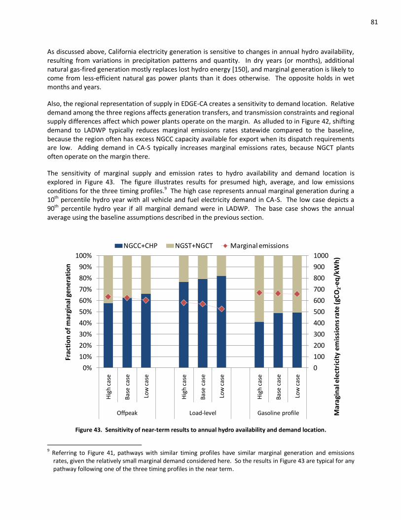
81

As discussed above, California electricity generation is sensitive to changes in annual hydro availability, resulting from variations in precipitation patterns and quantity. In dry years (or months), additional natural gas-fired generation mostly replaces lost hydro energy [150], and marginal generation is likely to come from less-efficient natural gas power plants than it does otherwise. The opposite holds in wet months and years.

Also, the regional representation of supply in EDGE-CA creates a sensitivity to demand location. Relative demand among the three regions affects generation transfers, and transmission constraints and regional supply differences affect which power plants operate on the margin. As alluded to in Figure 42, shifting demand to LADWP typically reduces marginal emissions rates statewide compared to the baseline, because the region often has excess NGCC capacity available for export when its dispatch requirements are low. Adding demand in CA-S typically increases marginal emissions rates, because NGCT plants often operate on the margin there.

The sensitivity of marginal supply and emission rates to hydro availability and demand location is explored in Figure 43. The figure illustrates results for presumed high, average, and low emissions conditions for the three timing profiles.9 The high case represents annual marginal generation during a 10th percentile hydro year with all vehicle and fuel electricity demand in CA-S. The low case depicts a 90th percentile hydro year if all marginal demand were in LADWP. The base case shows the annual average using the baseline assumptions described in the previous section.

0

100

200

300

400

500

600

700

800

900

1000

0%

10%

20%

30%

40%

50%

60%

70%

80%

90%

100%

Hig

h c

ase

Bas

e ca

se

Low

cas

e

Hig

h c

ase

Bas

e ca

se

Low

cas

e

Hig

h c

ase

Bas

e ca

se

Low

cas

e

Offpeak Load-level Gasoline profile Ma

ragi

na

l ele

ctri

city

em

issi

on

s ra

te (

gCO

2-e

q/k

Wh

)

Frac

tio

n o

f m

argi

nal

ge

ne

rati

on

NGCC+CHP NGST+NGCT Marginal emissions

Figure 43. Sensitivity of near-term results to annual hydro availability and demand location.

9 Referring to Figure 41, pathways with similar timing profiles have similar marginal generation and emissions

rates, given the relatively small marginal demand considered here. So the results in Figure 43 are typical for any pathway following one of the three timing profiles in the near term.

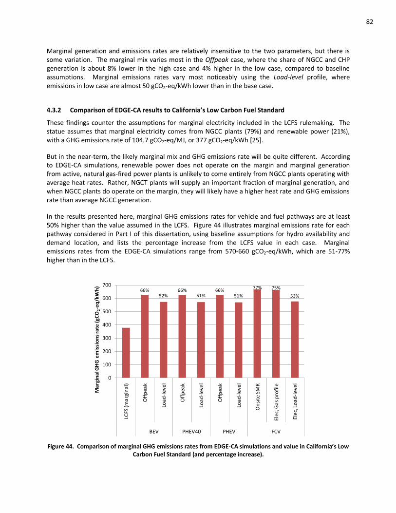
82

Marginal generation and emissions rates are relatively insensitive to the two parameters, but there is some variation. The marginal mix varies most in the Offpeak case, where the share of NGCC and CHP generation is about 8% lower in the high case and 4% higher in the low case, compared to baseline assumptions. Marginal emissions rates vary most noticeably using the Load-level profile, where emissions in low case are almost 50 gCO2-eq/kWh lower than in the base case.

4.3.2 Comparison of EDGE-CA results to California’s Low Carbon Fuel Standard

These findings counter the assumptions for marginal electricity included in the LCFS rulemaking. The statue assumes that marginal electricity comes from NGCC plants (79%) and renewable power (21%), with a GHG emissions rate of 104.7 gCO2-eq/MJ, or 377 gCO2-eq/kWh [25].

But in the near-term, the likely marginal mix and GHG emissions rate will be quite different. According to EDGE-CA simulations, renewable power does not operate on the margin and marginal generation from active, natural gas-fired power plants is unlikely to come entirely from NGCC plants operating with average heat rates. Rather, NGCT plants will supply an important fraction of marginal generation, and when NGCC plants do operate on the margin, they will likely have a higher heat rate and GHG emissions rate than average NGCC generation.

In the results presented here, marginal GHG emissions rates for vehicle and fuel pathways are at least 50% higher than the value assumed in the LCFS. Figure 44 illustrates marginal emissions rate for each pathway considered in Part I of this dissertation, using baseline assumptions for hydro availability and demand location, and lists the percentage increase from the LCFS value in each case. Marginal emissions rates from the EDGE-CA simulations range from 570-660 gCO2-eq/kWh, which are 51-77% higher than in the LCFS.

66%52%

66%51%

66%51%

77% 75%

53%

0

100

200

300

400

500

600

700

LCFS

(mar

gin

al)

Off

pea

k

Load

-lev

el

Off

pea

k

Load

-lev

el

Off

pea

k

Load

-lev

el

On

site

SM

R

Elec

, Gas

pro

file

Elec

, Lo

ad-l

evel

BEV PHEV40 PHEV FCV

Mar

gin

al G

HG

em

issi

on

s ra

te (

gCO

2-eq

/kW

h)

Figure 44. Comparison of marginal GHG emissions rates from EDGE-CA simulations and value in California’s Low Carbon Fuel Standard (and percentage increase).

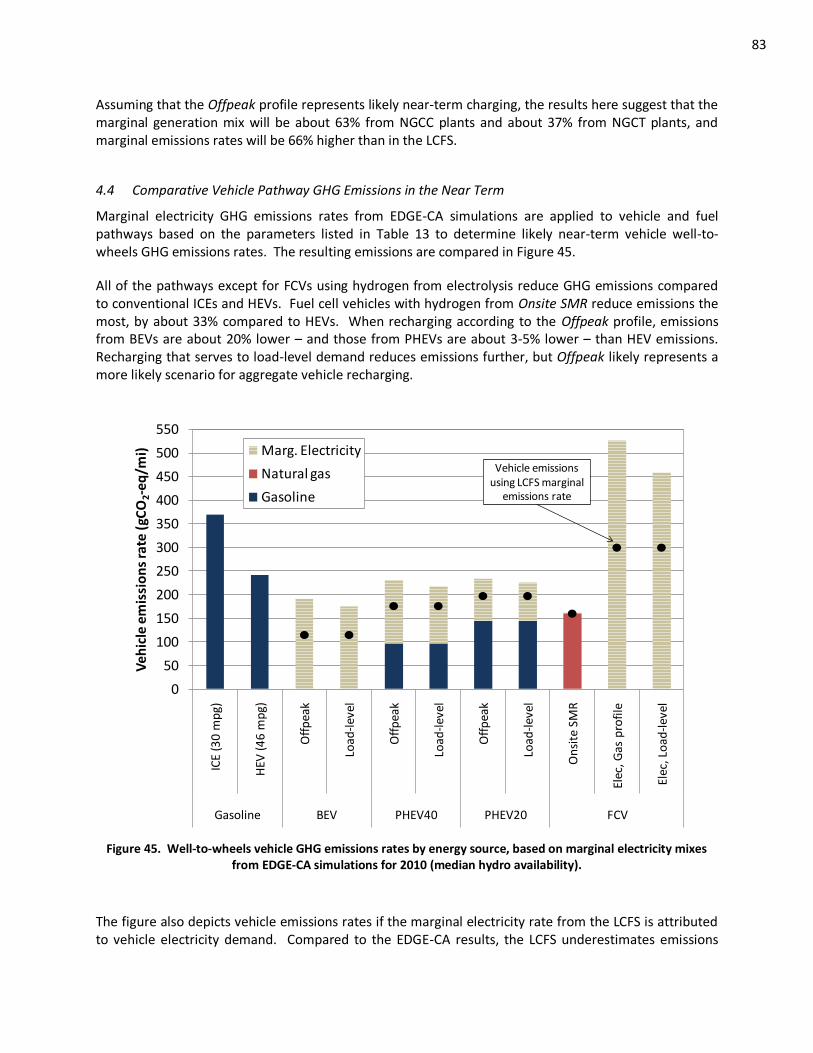
83

Assuming that the Offpeak profile represents likely near-term charging, the results here suggest that the marginal generation mix will be about 63% from NGCC plants and about 37% from NGCT plants, and marginal emissions rates will be 66% higher than in the LCFS.

4.4 Comparative Vehicle Pathway GHG Emissions in the Near Term

Marginal electricity GHG emissions rates from EDGE-CA simulations are applied to vehicle and fuel pathways based on the parameters listed in Table 13 to determine likely near-term vehicle well-to-wheels GHG emissions rates. The resulting emissions are compared in Figure 45.

All of the pathways except for FCVs using hydrogen from electrolysis reduce GHG emissions compared to conventional ICEs and HEVs. Fuel cell vehicles with hydrogen from Onsite SMR reduce emissions the most, by about 33% compared to HEVs. When recharging according to the Offpeak profile, emissions from BEVs are about 20% lower – and those from PHEVs are about 3-5% lower – than HEV emissions. Recharging that serves to load-level demand reduces emissions further, but Offpeak likely represents a more likely scenario for aggregate vehicle recharging.

0

50

100

150

200

250

300

350

400

450

500

550

ICE

(30

mp

g)

HEV

(4

6 m

pg)

Off

pea

k

Load

-lev

el

Off

pea

k

Load

-lev

el

Off

pea

k

Load

-lev

el

On

site

SM

R

Elec

, Gas

pro

file

Elec

, Lo

ad-l

evel

Gasoline BEV PHEV40 PHEV20 FCV

Veh

icle

em

issi

on

s ra

te (

gCO

2-eq

/mi) Marg. Electricity

Natural gas

Gasoline

Vehicle emissions using LCFS marginal

emissions rate

Figure 45. Well-to-wheels vehicle GHG emissions rates by energy source, based on marginal electricity mixes from EDGE-CA simulations for 2010 (median hydro availability).

The figure also depicts vehicle emissions rates if the marginal electricity rate from the LCFS is attributed to vehicle electricity demand. Compared to the EDGE-CA results, the LCFS underestimates emissions

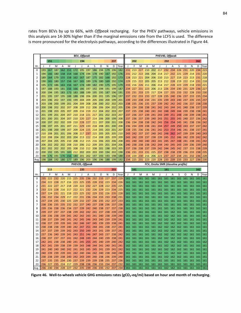
84

rates from BEVs by up to 66%, with Offpeak recharging. For the PHEV pathways, vehicle emissions in this analysis are 14-30% higher than if the marginal emissions rate from the LCFS is used. The difference is more pronounced for the electrolysis pathways, according to the differences illustrated in Figure 44.

151

160 168 177 185

194

203 211 220 228

237 202

208 214 220 226

232

238 244 250 256

262


0 193 167 187 162 151 172 195 197 186 194 179 196 182 231 213 227 210 202 217 232 234 226 231 220 234 223

1 194 166 180 158 154 168 174 194 178 190 167 192 176 231 212 222 206 204 214 217 232 221 229 214 231 220

2 189 164 179 155 158 162 167 187 175 182 168 192 173 228 213 221 204 206 210 213 227 219 223 213 231 218

3 190 165 180 157 156 167 165 189 176 180 169 192 174 229 215 222 205 205 213 212 228 219 222 214 231 218

4 195 172 186 163 156 167 174 189 182 190 175 195 179 233 216 226 211 206 214 217 228 223 229 218 233 221

5 197 188 193 181 156 166 186 197 192 194 191 199 187 234 227 231 223 206 213 226 234 230 231 229 236 227

6 200 194 195 183 173 183 188 199 195 195 187 196 191 235 231 233 225 217 224 227 235 233 232 228 233 230

7 201 195 197 195 188 188 198 206 200 201 195 196 197 237 232 233 233 227 228 235 240 236 237 233 235 234

8 203 196 202 197 193 199 204 209 205 200 200 199 201 239 233 238 234 231 235 239 243 240 237 235 235 237

9 203 198 200 199 201 204 209 208 208 200 202 202 203 238 235 236 235 237 239 242 242 242 236 237 238 238

10 200 198 202 202 207 208 209 212 206 206 204 202 205 236 234 238 238 241 242 243 244 241 240 238 237 239

11 201 198 203 205 207 209 216 219 212 204 202 203 207 237 235 238 240 241 242 248 249 244 239 238 238 241

12 201 199 201 204 207 210 218 221 217 201 202 203 207 237 236 237 239 241 243 249 251 248 238 239 238 241

13 201 200 201 204 207 210 220 227 214 206 200 199 208 237 236 237 239 240 243 251 255 245 240 237 236 242

14 200 197 202 202 209 210 228 227 211 207 200 201 208 236 234 238 238 242 243 256 254 245 241 238 236 242

15 198 197 205 201 207 211 229 220 218 208 201 200 208 236 234 239 238 241 244 257 249 250 243 237 237 242

16 201 198 200 199 207 209 224 225 214 205 203 201 207 238 235 236 236 241 242 253 254 246 241 238 237 241

17 210 208 201 201 206 208 217 237 215 205 205 205 210 243 242 237 237 240 242 248 262 247 239 239 240 243

18 210 208 204 202 203 204 213 222 214 208 205 209 209 243 242 239 237 238 239 245 252 246 242 239 242 242

19 207 204 205 205 210 208 212 215 216 206 203 206 208 241 240 240 240 243 241 245 247 248 241 238 241 242

20 206 202 202 202 208 210 206 212 209 205 201 204 206 240 238 238 238 242 244 240 245 243 239 236 239 240

21 202 202 202 202 205 208 210 212 208 201 198 203 205 237 236 238 237 239 242 244 245 242 237 233 238 239

22 200 192 195 191 183 212 202 203 203 200 194 202 198 236 231 233 231 225 237 238 238 239 236 233 238 235

23 198 176 191 170 156 180 201 202 197 193 193 198 188 234 220 230 216 206 223 237 237 234 231 232 236 228Avg. 198 184 192 180 177 189 196 203 196 196 188 199 192 234 225 231 223 220 228 233 239 233 233 227 236 230

215

219 223 227 231

235

239 243 247 251

255 161

161 161 161 161

161

162 162 162 162

162


0 235 222 232 220 215 225 235 236 232 233 227 237 229 161 161 161 161 161 161 161 161 161 161 161 161 161

1 234 222 228 217 216 223 225 235 228 232 223 234 226 161 161 161 161 161 161 161 161 161 161 161 161 161

2 231 222 227 217 218 220 222 232 227 228 222 235 225 161 161 161 161 161 161 161 161 161 161 161 161 161

3 233 223 228 216 217 222 221 232 226 229 223 234 225 161 161 161 161 161 161 161 161 161 161 161 161 161

4 237 224 231 221 218 223 225 232 229 232 226 235 228 161 161 161 161 161 161 161 161 161 161 161 161 161

5 236 232 234 229 217 222 231 236 234 233 233 238 231 161 161 161 161 161 161 161 161 161 161 161 161 161

6 237 234 235 230 225 229 232 237 236 235 232 237 233 161 161 161 161 161 161 161 161 161 161 161 161 161

7 238 236 235 235 232 232 237 240 237 238 236 237 236 161 161 161 161 161 161 161 161 161 161 161 161 161

8 239 236 238 236 234 237 239 242 240 238 237 237 238 161 161 161 161 161 161 161 161 161 161 161 161 161

9 239 237 237 237 238 239 242 242 241 237 238 239 239 161 161 161 161 161 161 161 162 161 161 161 161 161

10 238 236 238 239 241 242 242 243 241 240 238 239 240 161 161 161 161 161 161 162 162 161 161 161 161 161

11 238 237 239 240 241 242 245 246 243 240 239 239 241 161 161 161 161 161 162 162 162 162 161 161 161 161

12 238 237 239 239 241 242 246 247 245 239 239 238 241 161 161 161 161 161 162 162 162 162 161 161 161 161

13 238 238 238 239 240 242 247 251 244 241 238 237 241 161 161 161 161 161 162 162 162 162 161 161 161 161

14 237 237 239 239 242 243 250 249 243 241 239 237 241 161 161 161 161 162 162 162 162 162 161 161 161 161

15 237 236 240 239 241 243 251 246 247 243 237 238 242 161 161 161 161 161 162 162 162 162 162 161 161 161

16 238 237 237 237 241 242 248 249 244 240 239 238 241 161 161 161 161 161 162 162 162 162 161 161 161 161

17 242 241 238 238 240 241 245 255 245 240 239 240 242 162 161 161 161 161 161 162 162 162 161 161 161 162

18 242 241 239 238 239 239 243 248 244 241 240 241 241 162 161 161 161 161 161 162 162 162 161 161 161 161

19 241 240 240 240 242 241 243 245 245 241 239 241 242 161 161 161 161 162 161 162 162 162 161 161 161 161

20 240 239 239 239 241 242 240 244 242 240 238 240 240 161 161 161 161 161 162 161 162 162 161 161 161 161

21 238 238 239 238 240 242 243 244 240 238 236 239 240 161 161 161 161 161 161 162 162 162 161 161 161 161

22 237 235 235 234 230 237 239 239 239 238 235 237 236 161 161 161 161 161 161 161 161 161 161 161 161 161

23 236 227 235 224 217 229 238 238 236 233 234 237 232 161 161 161 161 161 161 161 161 161 161 161 161 161Avg. 236 230 234 228 227 232 235 239 236 235 232 237 234 161 161 161 161 161 161 162 162 161 161 161 161 161

BEV, Offpeak PHEV40, Offpeak

FCV, Onsite SMR (Gasoline profile)PHEV20, Offpeak

Figure 46. Well-to-wheels vehicle GHG emissions rates (gCO2-eq/mi) based on hour and month of recharging.

85

Emissions rates from a particular vehicle using electricity as fuel vary, depending on the vehicle is recharged or hydrogen is produced. Figure 46 illustrates how vehicle emissions vary, based on the time at which electricity was consumed for use onboard the vehicle. The figure compares vehicle emissions (in gCO2-eq/mile, on a lifecycle-basis) for BEVs, PHEVs, and FCVs with hydrogen production from onsite SMR. Note that in the emissions maps shown here – contrary to those shown elsewhere – the color-coding is based on a single scale that applies to all four pathways. This allows relative differences in emissions within a pathway and among pathways to be more clearly described, in this case.

The variation in vehicle GHG emissions rates for a particular pathway scales with electricity demand. Battery electric vehicles require the most electricity, of the pathways considered here, and see the most fluctuation in their emissions rate, depending on when the vehicle is recharged. Their emissions rate may vary by more than ±20%, on average, over the course of the year. If recharged at 5pm on an August afternoon, a BEV is likely to emit 23% more GHGs than it does on average, according to the Offpeak recharging profile. If recharged at midnight in May, emissions are likely to be similarly lower than the annual average. For an average day, as depicted in the “year” column, vehicle emissions vary by ±10% from the annual average.

Conversely, electricity contributes relatively little to hydrogen production in Onsite SMR. Vehicle emissions are essentially constant, regardless of when hydrogen is produced, and almost always lower than for the other pathways.

The variability of emissions for PHEVs is in between those of BEVs and FCVs using Onsite SMR, and emissions are more variable for PHEV40s than PHEV20s. Interestingly, if recharged during peak demand hours – during afternoons of most months – emissions from PHEV40s are slightly higher than those from PHEV20s. In those cases, the incremental improvement in efficiency from a PHEV20 to a PHEV40 does not outweigh the relative increase in carbon intensity associated with marginal electricity, compared to gasoline. This occurs during hours in which the marginal electricity emissions rate is greater than about 650 gCO2-eq/kWh.

The reduction in emissions found for these electric-drive vehicles is a result of improved vehicle efficiency, rather than reduced carbon-intensity of fuel. As assumed here, and listed in Table 13, electric-drive vehicles are 1.5-3.5 times more efficient than conventional gasoline ICEs. But the carbon content of marginal electricity in EDGE-CA simulations for these pathways – ranging from 570-665 gCO2-eq/kWh on an average annual basis – is 65-95% higher than that of gasoline.

The tradeoff between vehicle efficiency and fuel carbon intensity is explored for the pathways in further detail in Figure 47. The figure shows isolines for vehicle GHG emission rates, represented in terms of the product of vehicle energy intensity (MJ/mi) and fuel carbon intensity (gCO2/MJ). Vehicle emissions increase as vehicle energy intensity increases (moving to the right in the figure) or as fuel carbon intensity increases (moving up in the figure).

Each of the 11 vehicle, fuel, and timing pathways discussed in Part I of this dissertation is placed on the figure according to its intensity components. The conventional gasoline ICE and HEV vehicles are the most energy-intensive, and are furthest right in the figure. But gasoline also has the lowest fuel carbon intensity among any of the pathways considered and are placed lower than other pathways in the figure. Emissions from a conventional ICE vehicle (depicted by the black “X” in the figure) are 370 gCO2/mi, placing that symbol between the isolines for 350 gCO2/mi and 400 gCO2/mi. The emissions rate from an HEV is about 250 gCO2/mi, and its symbol is just below that isoline in the figure. Emissions

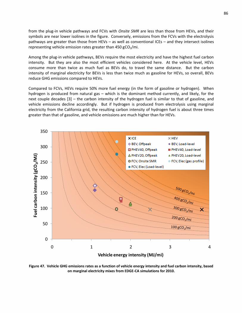
86

from the plug-in vehicle pathways and FCVs with Onsite SMR are less than those from HEVs, and their symbols are near lower isolines in the figure. Conversely, emissions from the FCVs with the electrolysis pathways are greater than those from HEVs – as well as conventional ICEs – and they intersect isolines representing vehicle emission rates greater than 450 gCO2/mi.

Among the plug-in vehicle pathways, BEVs require the most electricity and have the highest fuel carbon intensity. But they are also the most efficient vehicles considered here. At the vehicle level, HEVs consume more than twice as much fuel as BEVs do, to travel the same distance. But the carbon intensity of marginal electricity for BEVs is less than twice much as gasoline for HEVs, so overall, BEVs reduce GHG emissions compared to HEVs.

Compared to FCVs, HEVs require 50% more fuel energy (in the form of gasoline or hydrogen). When hydrogen is produced from natural gas – which is the dominant method currently, and likely, for the next couple decades [3] – the carbon intensity of the hydrogen fuel is similar to that of gasoline, and vehicle emissions decline accordingly. But if hydrogen is produced from electrolysis using marginal electricity from the California grid, the resulting carbon intensity of hydrogen fuel is about three times greater than that of gasoline, and vehicle emissions are much higher than for HEVs.

0

50

100

150

200

250

300

350

0 1 2 3 4

Fuel

car

bo

n in

ten

sity

(gC

O2/M

J)

Vehicle energy intensity (MJ/mi)

Figure 47. Vehicle GHG emissions rates as a function of vehicle energy intensity and fuel carbon intensity, based on marginal electricity mixes from EDGE-CA simulations for 2010.

87

4.5 Summary of Near-Term Findings

Part I of this dissertation considers the operation of the current grid and marginal and vehicle GHG emissions rates for scenarios including electricity demand from vehicle recharging or hydrogen production for about 200,000 advanced, light-duty vehicles in 2010. Specific results in this chapter should be considered within the context of the simplified modeling techniques used in EDGE-CA, and the vehicle and efficiency assumptions upon which the findings are founded. The results could be refined through more detailed modeling that includes many constraining factors that are beyond the scope of EDGE-CA. But several general conclusions and trends can be taken from the current analysis.

Clearly, comparing emissions among distinct alternatives requires analysis on a well-to-wheels basis. An important component of well-to-wheels analysis for many vehicle and fuel pathways is the marginal electricity mix and GHG emissions rates for incremental vehicle and fuel electricity demands. In this analysis, the marginal electricity mix represents generation from the set of the last active power plants brought online in California, equal to incremental demand. It is distinct from the average mix, which represents generation for all electricity demand on the system. In California, GHG emission rates from marginal generation are higher than average GHG emissions rates. In other regions with higher fractions of coal power, marginal emissions rates could be lower than average emissions rates.

The EDGE-CA model was developed to simulate electricity supply, based on the current composition of the grid, and identify the types of power plants that are likely to operate on the margin to supply near-term vehicle and fuel-related electricity demands. The model represents California in three regions, to more accurately represent electricity supply and demand in the state, but presents results for marginal supply on a statewide basis, because increasing demand in one region may lead to increasing generation in another. About 50% of generation in CA-N comes from low-carbon hydro, nuclear, or renewable resources, and average GHG emissions rates there are about half of the rate in CA-S and a third of the rate in the relatively coal-heavy LADWP region. Southern California lacks a significant hydro resource and tends to have the highest active generation requirements. In EDGE-CA, the region often receives power from CA-N and has the last generator operating in the state, setting the statewide market-clearing cost for electricity. As a result, natural gas-fired power plants in CA-S account for the majority of marginal mixes in EDGE-CA simulations.

During a given hour of the day or month of the year, the types of power plants operating on the margin and supplying vehicle recharging or hydrogen production depend on non-vehicle electricity demand and the availability of supply resources. Aside from the total level of demand, the availability of hydro power has the greatest impact on average and marginal generation mixes and emissions rates on the current grid. When less hydro energy is available – on an hourly, monthly, or annual basis – more active generation is required from instate plants or system imports, and average and marginal GHG emissions rates increase. Average electricity GHG emissions rates in California during in a 1-in-10 wet or dry year fluctuate by ±5% in EDGE-CA simulations, compared to those during a median hydro year. The impacts are most noticeable in CA-N, where average GHG emissions rates fluctuate by ±13%, based on hydro availability.

The impact of hydro availability on annual marginal generation and emissions is much smaller than it is on average generation and emissions. It has some effect, as well as demand location – in terms of the three California regions considered here – but collectively, they affect marginal emissions rates by less than ±8% from baseline values. Also, results are quite insensitive to quantity of marginal demand; marginal generation and emissions rates were similar for different vehicle or fuel pathways with a particular electricity demand timing profile.

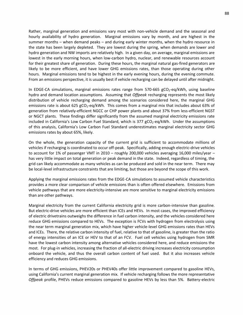
88

Rather, marginal generation and emissions vary most with non-vehicle demand and the seasonal and hourly availability of hydro generation. Marginal emissions vary by month, and are highest in the summer months – when demand peaks – and during early winter months, when the hydro resource in the state has been largely depleted. They are lowest during the spring, when demands are lower and hydro generation and NW imports are relatively high. In a given day, on average, marginal emissions are lowest in the early morning hours, when low-carbon hydro, nuclear, and renewable resources account for their greatest share of generation. During these hours, the marginal natural gas-fired generators are likely to be more efficient, and have lower GHG emissions rates, than those operating during other hours. Marginal emissions tend to be highest in the early evening hours, during the evening commute. From an emissions perspective, it is usually best if vehicle recharging can be delayed until after midnight.

In EDGE-CA simulations, marginal emissions rates range from 570-665 gCO2-eq/kWh, using baseline hydro and demand location assumptions. Assuming that Offpeak recharging represents the most likely distribution of vehicle recharging demand among the scenarios considered here, the marginal GHG emissions rate is about 625 gCO2-eq/kWh. This comes from a marginal mix that includes about 63% of generation from relatively-efficient NGCC or CHP power plants and about 37% from less-efficient NGST or NGCT plants. These findings differ significantly from the assumed marginal electricity emissions rate included in California’s Low Carbon Fuel Standard, which is 377 gCO2-eq/kWh. Under the assumptions of this analysis, California’s Low Carbon Fuel Standard underestimates marginal electricity sector GHG emissions rates by about 65%, likely.

On the whole, the generation capacity of the current grid is sufficient to accommodate millions of vehicles if recharging is coordinated to occur off-peak. Specifically, adding enough electric-drive vehicles to account for 1% of passenger VMT in 2010 – roughly 200,000 vehicles averaging 16,000 miles/year – has very little impact on total generation or peak demand in the state. Indeed, regardless of timing, the grid can likely accommodate as many vehicles as can be produced and sold in the near term. There may be local-level infrastructure constraints that are limiting, but those are beyond the scope of this work.

Applying the marginal emissions rates from the EDGE-CA simulations to assumed vehicle characteristics provides a more clear comparison of vehicle emissions than is often offered elsewhere. Emissions from vehicle pathways that are more electricity-intensive are more sensitive to marginal electricity emissions than are other pathways.

Marginal electricity from the current California electricity grid is more carbon-intensive than gasoline. But electric-drive vehicles are more efficient than ICEs and HEVs. In most cases, the improved efficiency of electric drivetrains outweighs the difference in fuel carbon intensity, and the vehicles considered here reduce GHG emissions compared to HEVs. The exception is FCVs with hydrogen from electrolysis using the near term marginal generation mix, which have higher vehicle-level GHG emissions rates than HEVs and ICEs. There, the relative carbon intensity of fuel, relative to that of gasoline, is greater than the ratio of energy intensities of an ICE or HEV to that of an FCV. Fuel cell vehicles using hydrogen from SMR have the lowest carbon intensity among alternative vehicles considered here, and reduce emissions the most. For plug-in vehicles, increasing the fraction of all-electric driving increases electricity consumption onboard the vehicle, and thus the overall carbon content of fuel used. But it also increases vehicle efficiency and reduces GHG emissions.

In terms of GHG emissions, PHEV20s or PHEV40s offer little improvement compared to gasoline HEVs, using California’s current marginal generation mix. If vehicle recharging follows the more representative Offpeak profile, PHEVs reduce emissions compared to gasoline HEVs by less than 5%. Battery-electric

89

vehicles and FCVs using hydrogen from onsite natural gas reformers improve emissions more, by 20-33%, respectively, compared to gasoline HEVs.

Over time, the carbon intensity of the grid will decrease, as energy policies promote renewable generation or impose costs on GHG emissions, and as older power plants are retired and replaced with newer, more efficient ones. In the future, the carbon content of electricity supplying vehicles and fuels could be much lower than it is currently. Long-term scenarios that include significant fractions of generation from low-carbon, passive, renewable resources are a focus of Part II of this dissertation.

90

PART II: LONG-TERM VEHICLE ELECTRICITY DEMAND IMPACTS ON CALIFORNIA ELECTRICITY SUPPLY

Whereas Part I of this dissertation compares vehicle pathway GHG emissions based on small amounts of marginal generation from the current grid, Part II considers changes to power plant capacity and grid operation when significant amounts of renewable generation or vehicle recharging are added over the long term. Long-term analysis is necessary to understand the broader impacts of vehicle recharging on a future grid shaped by new technologies, infrastructure constraints, and energy policies. Impacts of vehicle demand on electricity supply will be relatively minor at an aggregate level until several million plug-in vehicles are on the road [96, 100]. At that time, they may have an important impact on shaping the supply mix, which deserves analysis.

The primary focus of the long-term analysis is to understand interactions between vehicle electricity demand and electricity supply through 2050, given various potential future grid compositions. Specifically of interest are interactions among the active grid elements that respond to demand or supply availability and the passive grid elements that do not. For example, adding wind and solar power adds passive, intermittent generation that is taken whenever available. Adding vehicle recharging adds passive demand in some scenarios – if recharging is assumed to be independent of market signals related to grid conditions – and active demand in others, if recharging is coordinated to occur when it is optimal from a supply standpoint. Together, these may interact to affect the grid in a negative way, making power supply relatively inefficient and costly, or in a positive way, if supply and demand is well-matched. Capacity, generation, and costs are used as comparative metrics to convey how well supply and demand match in various scenarios.

Several scenarios that encompass various renewable generation and vehicle electricity demand profiles are investigated. Increasing levels of passive, renewable generation are imposed on the grid to determine impacts on active capacity requirements and electricity costs. Electricity demand from several million plug-in vehicles is added, as well, and various active and passive recharging timing profiles are considered, to understand the costs or benefits to the grid of vehicle recharging over the long term.

91

5. DOCUMENTATION OF THE LONG-TERM ELECTRICITY DISPATCH MODEL FOR GREENHOUSE GAS EMISSIONS IN CALIFORNIA (LEDGE-CA)

The methods used for modeling electricity supply over the long term in this analysis differ from those used to represent the current grid in Part I of this dissertation. The EDGE-CA model, described previously, is adapted to create the Long-term EDGE-CA model (LEDGE-CA). LEDGE-CA includes power plant retirements and capacity expansion, and represents dispatch in a simpler way. Grid profiles are developed that define demand and capacity and generation from hydro, nuclear, and renewable power plants. LEDGE-CA is applied to determine an optimal distribution of new capacity from coal-fired integrated gasification combined-cycle plants with carbon capture and sequestration (IGCC w/ CCS),10 NGCC plants (with and without CCS), and NGCT power plants, whose availability is defined by costs and other parameters in the scenarios. Finally, generation from all new and existing fossil power plants is dispatched hourly to supply remaining demand. The types of power plants represented in LEDGE-CA are listed in Table 19.

This analysis assumes that dispatchable (“active”) generation continues to come from fossil-based power plants, which offer flexible operation to match supply and demand on the grid. Hydro capacity and median annual available energy is assumed to remain constant through 2050. Hourly generation from hydro resources is represented in LEDGE-CA as it is in EDGE-CA. All other power plants (nuclear and renewable) are treated as must-run (“passive”). Contributions from bulk energy storage11 and non-vehicle electricity demand management are ignored. (Active demand management by utilities of vehicle recharging is implied in the Minimize fossil supply recharging profile, however.) except as implied by the active vehicle recharging scenarios. Further, it is assumed that SB 1368 holds and no new conventional coal-fired power plants are built to serve California electricity demand [117, 151].12

The detailed approach to dispatch modeling used for the near-term analysis is less appropriate for evaluating supply decades into the future, when demographics, technology, and policy are less certain. While hourly dispatch is still simulated in LEDGE-CA, it is practical to simplify the representation of the grid for long-term analysis. California is treated as a single region in LEDGE-CA, rather than three (as in EDGE-CA). Power plants are dispatched categorically, by power plant type and vintage, rather than on a plant-by-plant basis. And system imports are ignored.13 While imports will continue to supply California demand, it is assumed that hydro from the Northwest will be less available to California in the future, due to population and demand growth there, and system imports will increasingly mirror the mix of dispatchable, fossil-fired power plants within the state. Excluding imports, then, assumes that California ratepayers bear the costs of building sufficient capacity – even if it is located in neighboring states – to meet their electricity demand.

10 Although IGCC plants can operate without carbon capture and sequestration (CCS), throughout this dissertation,

IGCC plants serving California electricity demand are assumed to include CCS. 11 Bulk energy storage could be represented as another power plant type in LEDGE-CA that takes excess electricity

during low demand periods as an input and generates electricity during peak demand periods. This would be a helpful extension of the model, but is left for future work.

12 SB 1368 bans new, conventional coal power plants from serving California electricity demand. Specifically, it bans long-term contracts with power plants that have a higher GHG emissions rate than NGCC power plants. This prevents utilities from signing new firm import contracts with out-of-state coal facilities, but existing firm import contracts remain.

13 Firm imports are still included in LEDGE-CA, as they essentially represent instate power plants. Firm imports are mostly from coal-fired power plants, and all firm import contracts are assumed to expire after 2020 [108].

92

Snapshots of California electricity supply in 2020, 2035, and 2050 are presented and analyzed. The results in Chapter 6 illustrate capacity, generation, average and marginal GHG emissions, and system costs for various scenarios, which are used to compare value among scenarios with various demand levels and supply mixes. Finally, a sensitivity analysis is presented that explores the impacts of energy prices, CO2 prices, and shifting the timing of non-vehicle electricity demands (such as deferring loads with a “smart grid”) on the results.

5.1 Overview and Model Framework

The general framework of analysis for long-term electricity supply is illustrated in Figure 48. First, hourly non-vehicle electricity demands and generation from must-run (passive) nuclear and renewable power plants are calculated. In Step 2, hourly vehicle recharging demands are calculated and added to non-vehicle demand.14 This leads to an adjusted load profile (illustrated in Step 2b) that represents total electricity demand (non-vehicle and vehicle electricity demand) minus must-run generation, that is supplied by active hydro or fossil resources. Next, in Step 3, hourly hydro generation is allocated according to the methods described in Part I.15 It is assumed that hydro generation is dispatched to minimize fossil generation, rather than follow demand directly, so it is allocated after must-run generation has been subtracted from the demand curve. The difference between the adjusted load profile and hydro generation yields the “fossil supply profile,” which represents hourly generation required from fossil power plants. In Steps 4 and 5, LEDGE-CA uses screening curve analysis to determine optimal capacities of fossil power plants based on this demand profile and dispatches them on an hourly basis to supply all remaining demand. The sections that follow describe the methods underlying each of these steps in turn.

The power plants included in LEDGE-CA differ somewhat from those included in EDGE-CA. LEDGE-CA does not include system imports, but does include IGCC, new NGCC plants – with and without CCS – and new NGCT plants. The types of power plants included in the LEDGE-CA model are listed in Table 19. Must-run plants include nuclear and renewable plants, as well as a small component of hydro generation. Generation from these plants is allocated first in the LEDGE-CA model. The remaining power plants are dispatched in the order shown and by vintage. All coal-fired power plants are dispatched first, in decreasing order of age, which is a proxy for relative heat rate and operating cost. Then new NGCC power plants are dispatched, followed by generation from existing NGCC and CHP plants. Finally, peaking plants are dispatched – again, in inverse age order. The methods for allocating and dispatching fossil power plant capacity are detailed in the sections that follow.

14 Vehicle electricity demand profiles are calculated after must-run generation in LEDGE-CA because the timing of

recharging can be a function of hourly generation from must-run resources, in the Minimize fossil supply profile. This is the case in the illustration in Figure 48, where electricity demand from vehicles is actively controlled to level fossil supply. It is presumed to be coordinated by utilities to follow must-run generation and level the remaining demand curve. Passive vehicle electricity demands that do not respond to supply conditions are considered in this analysis as well, and are described in sections below.

15 Hydro includes a small must-run component and a larger, active component that follows demand. In the scenario illustrated in Figure 48, hydro generation is mostly constant on this representative day, since vehicle recharging has leveled the remaining demand curve to a significant extent.

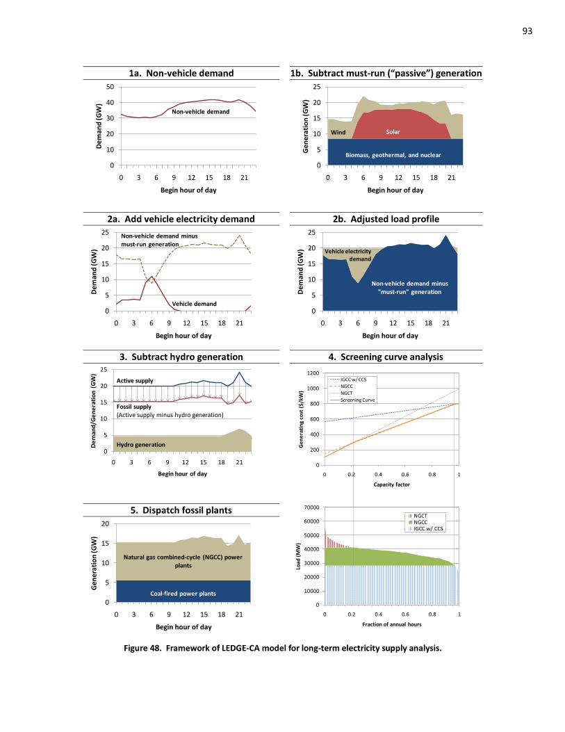
93

1a. Non-vehicle demand 1b. Subtract must-run (“passive”) generation

0

10

20

30

40

50

0 3 6 9 12 15 18 21

De

ma

nd

(G

W)

Begin hour of day

Non-vehicle demand

0

5

10

15

20

25

0 3 6 9 12 15 18 21

Ge

ne

rati

on

(GW

)

Begin hour of day

Biomass, geothermal, and nuclear

SolarWind

2a. Add vehicle electricity demand 2b. Adjusted load profile

0

5

10

15

20

25

0 3 6 9 12 15 18 21

De

ma

nd

(G

W)

Begin hour of day

Non-vehicle demand minus must-run generation

Vehicle demand

0

5

10

15

20

25

0 3 6 9 12 15 18 21

De

ma

nd

(G

W)

Begin hour of day

Non-vehicle demand minus "must-run" generation

Vehicle electricity demand

3. Subtract hydro generation 4. Screening curve analysis

0

5

10

15

20

25

0 3 6 9 12 15 18 21

De

man

d/G

en

era

tio

n (

GW

)

Begin hour of day

Active supply

Hydro generation

Fossil supply (Active supply minus hydro generation)

0

200

400

600

800

1000

1200

0 0.2 0.4 0.6 0.8 1

Ge

ne

rati

ng

cost

($

/kW

)

Capacity factor

IGCC w/ CCS

NGCC

NGCT

Screening Curve

0

10000

20000

30000

40000

50000

60000

70000

0 0.2 0.4 0.6 0.8 1

Load

(M

W)


NGCTNGCCIGCC w/ CCS

5. Dispatch fossil plants

0

5

10

15

20

0 3 6 9 12 15 18 21

Ge

ne

rati

on

(GW

)

Begin hour of day

Coal-fired power plants

Natural gas combined-cycle (NGCC) power plants

Figure 48. Framework of LEDGE-CA model for long-term electricity supply analysis.

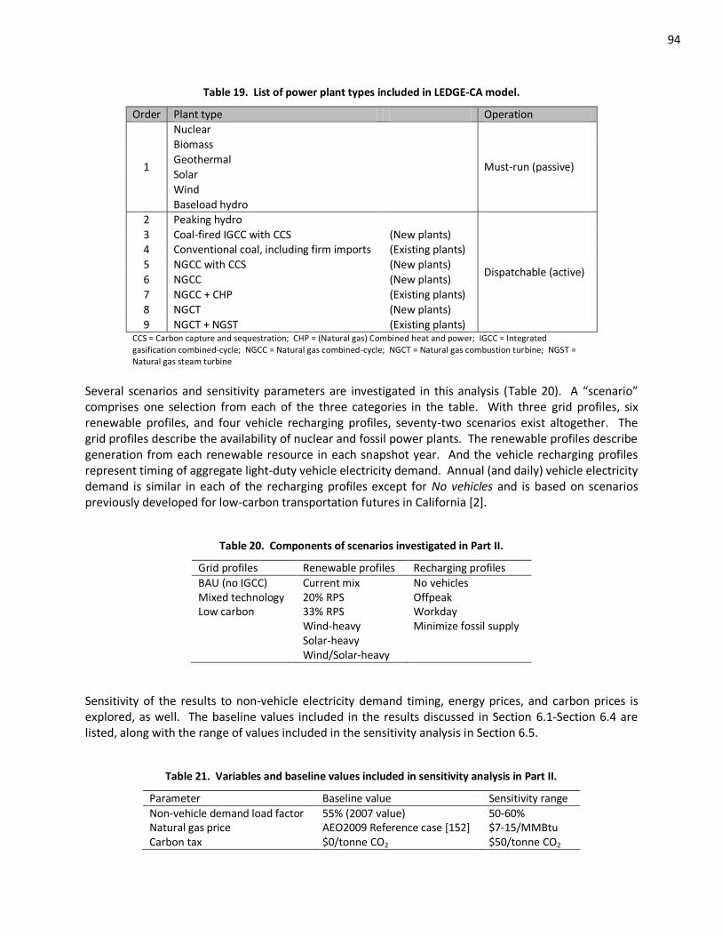
94

Table 19. List of power plant types included in LEDGE-CA model.

Order Plant type Operation

1

Nuclear

Must-run (passive)

Biomass

Geothermal

Solar

Wind

Baseload hydro

2 Peaking hydro

Dispatchable (active)

3 Coal-fired IGCC with CCS (New plants) 4 Conventional coal, including firm imports (Existing plants)

5 NGCC with CCS (New plants)

6 NGCC (New plants)

7 NGCC + CHP (Existing plants)

8 NGCT (New plants)

9 NGCT + NGST (Existing plants) CCS = Carbon capture and sequestration; CHP = (Natural gas) Combined heat and power; IGCC = Integrated gasification combined-cycle; NGCC = Natural gas combined-cycle; NGCT = Natural gas combustion turbine; NGST = Natural gas steam turbine

Several scenarios and sensitivity parameters are investigated in this analysis (Table 20). A “scenario” comprises one selection from each of the three categories in the table. With three grid profiles, six renewable profiles, and four vehicle recharging profiles, seventy-two scenarios exist altogether. The grid profiles describe the availability of nuclear and fossil power plants. The renewable profiles describe generation from each renewable resource in each snapshot year. And the vehicle recharging profiles represent timing of aggregate light-duty vehicle electricity demand. Annual (and daily) vehicle electricity demand is similar in each of the recharging profiles except for No vehicles and is based on scenarios previously developed for low-carbon transportation futures in California [2].

Table 20. Components of scenarios investigated in Part II.

Grid profiles Renewable profiles Recharging profiles

BAU (no IGCC) Current mix No vehicles Mixed technology 20% RPS Offpeak Low carbon 33% RPS Workday Wind-heavy Minimize fossil supply Solar-heavy Wind/Solar-heavy

Sensitivity of the results to non-vehicle electricity demand timing, energy prices, and carbon prices is explored, as well. The baseline values included in the results discussed in Section 6.1-Section 6.4 are listed, along with the range of values included in the sensitivity analysis in Section 6.5.

Table 21. Variables and baseline values included in sensitivity analysis in Part II.

Parameter Baseline value Sensitivity range

Non-vehicle demand load factor 55% (2007 value) 50-60% Natural gas price AEO2009 Reference case [152] $7-15/MMBtu Carbon tax $0/tonne CO2 $50/tonne CO2

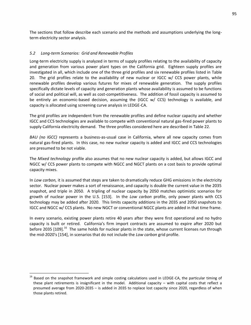
95

The sections that follow describe each scenario and the methods and assumptions underlying the long-term electricity sector analysis.

5.2 Long-term Scenarios: Grid and Renewable Profiles

Long-term electricity supply is analyzed in terms of supply profiles relating to the availability of capacity and generation from various power plant types on the California grid. Eighteen supply profiles are investigated in all, which include one of the three grid profiles and six renewable profiles listed in Table 20. The grid profiles relate to the availability of new nuclear or IGCC w/ CCS power plants, while renewable profiles develop various futures for mixes of renewable generation. The supply profiles specifically dictate levels of capacity and generation plants whose availability is assumed to be functions of social and political will, as well as cost-competitiveness. The addition of fossil capacity is assumed to be entirely an economic-based decision, assuming the (IGCC w/ CCS) technology is available, and capacity is allocated using screening curve analysis in LEDGE-CA.

The grid profiles are independent from the renewable profiles and define nuclear capacity and whether IGCC and CCS technologies are available to compete with conventional natural gas-fired power plants to supply California electricity demand. The three profiles considered here are described in Table 22.

BAU (no IGCC) represents a business-as-usual case in California, where all new capacity comes from natural gas-fired plants. In this case, no new nuclear capacity is added and IGCC and CCS technologies are presumed to be not viable.

The Mixed technology profile also assumes that no new nuclear capacity is added, but allows IGCC and NGCC w/ CCS power plants to compete with NGCC and NGCT plants on a cost basis to provide optimal capacity mixes.

In Low carbon, it is assumed that steps are taken to dramatically reduce GHG emissions in the electricity sector. Nuclear power makes a sort of renaissance, and capacity is double the current value in the 2035 snapshot, and triple in 2050. A tripling of nuclear capacity by 2050 matches optimistic scenarios for growth of nuclear power in the U.S. [153]. In the Low carbon profile, only power plants with CCS technology may be added after 2020. This limits capacity additions in the 2035 and 2050 snapshots to IGCC and NGCC w/ CCS plants. No new NGCT or conventional NGCC plants are added in that time frame.

In every scenario, existing power plants retire 40 years after they were first operational and no hydro capacity is built or retired. California’s firm import contracts are assumed to expire after 2020 but before 2035 [109].16 The same holds for nuclear plants in the state, whose current licenses run through the mid-2020’s *154+, in scenarios that do not include the Low carbon grid profile.

16

Based on the snapshot framework and simple costing calculations used in LEDGE-CA, the particular timing of these plant retirements is insignificant in the model. Additional capacity – with capital costs that reflect a presumed average from 2020-2035 – is added in 2035 to replace lost capacity since 2020, regardless of when those plants retired.

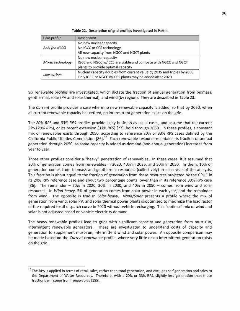
96

Table 22. Description of grid profiles investigated in Part II.

Grid profile Description

BAU (no IGCC) No new nuclear capacity No IGCC or CCS technology All new capacity from NGCC and NGCT plants

Mixed technology No new nuclear capacity IGCC and NGCC w/ CCS are viable and compete with NGCC and NGCT plants to provide optimal capacity

Low carbon Nuclear capacity doubles from current value by 2035 and triples by 2050 Only IGCC or NGCC w/ CCS plants may be added after 2020

Six renewable profiles are investigated, which dictate the fraction of annual generation from biomass, geothermal, solar (PV and solar thermal), and wind (by region). They are described in Table 23.

The Current profile provides a case where no new renewable capacity is added, so that by 2050, when all current renewable capacity has retired, no intermittent generation exists on the grid.

The 20% RPS and 33% RPS profiles provide likely business-as-usual cases, and assume that the current RPS (20% RPS), or its recent extension (33% RPS) [27], hold through 2050. In these profiles, a constant mix of renewables exists through 2050, according to reference 20% or 33% RPS cases defined by the California Public Utilities Commission [86].17 Each renewable resource maintains its fraction of annual generation through 2050, so some capacity is added as demand (and annual generation) increases from year to year.

Three other profiles consider a “heavy” penetration of renewables. In these cases, it is assumed that 30% of generation comes from renewables in 2020, 40% in 2035, and 50% in 2050. In them, 10% of generation comes from biomass and geothermal resources (collectively) in each year of the analysis. This fraction is about equal to the fraction of generation from these resources projected by the CPUC in its 20% RPS reference case and about two percentage points lower than in its reference 33% RPS case [86]. The remainder – 20% in 2020, 30% in 2030, and 40% in 2050 – comes from wind and solar resources. In Wind-heavy, 5% of generation comes from solar power in each year, and the remainder from wind. The opposite is true in Solar-heavy. Wind/Solar presents a profile where the mix of generation from wind, solar PV, and solar thermal power plants is optimized to maximize the load factor of the required fossil dispatch curve in 2020 without vehicle recharging. This “optimal” mix of wind and solar is not adjusted based on vehicle electricity demand.

The heavy-renewable profiles lead to grids with significant capacity and generation from must-run, intermittent renewable generators. These are investigated to understand costs of capacity and generation to supplement must-run, intermittent wind and solar power. An opposite comparison may be made based on the Current renewable profile, where very little or no intermittent generation exists on the grid.

17

The RPS is applied in terms of retail sales, rather than total generation, and excludes self generation and sales to the Department of Water Resources. Therefore, with a 20% or 33% RPS, slightly less generation than those fractions will come from renewables [155].

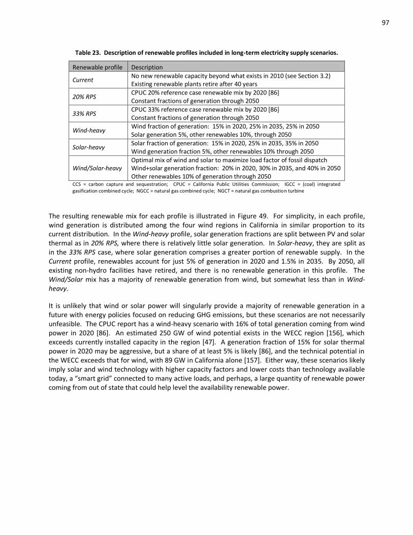
97

Table 23. Description of renewable profiles included in long-term electricity supply scenarios.

Renewable profile Description

Current No new renewable capacity beyond what exists in 2010 (see Section 3.2) Existing renewable plants retire after 40 years

20% RPS CPUC 20% reference case renewable mix by 2020 [86] Constant fractions of generation through 2050

33% RPS CPUC 33% reference case renewable mix by 2020 [86] Constant fractions of generation through 2050

Wind-heavy Wind fraction of generation: 15% in 2020, 25% in 2035, 25% in 2050 Solar generation 5%, other renewables 10%, through 2050

Solar-heavy Solar fraction of generation: 15% in 2020, 25% in 2035, 35% in 2050 Wind generation fraction 5%, other renewables 10% through 2050

Wind/Solar-heavy Optimal mix of wind and solar to maximize load factor of fossil dispatch Wind+solar generation fraction: 20% in 2020, 30% in 2035, and 40% in 2050 Other renewables 10% of generation through 2050

CCS = carbon capture and sequestration; CPUC = California Public Utilities Commission; IGCC = (coal) integrated gasification combined cycle; NGCC = natural gas combined cycle; NGCT = natural gas combustion turbine

The resulting renewable mix for each profile is illustrated in Figure 49. For simplicity, in each profile, wind generation is distributed among the four wind regions in California in similar proportion to its current distribution. In the Wind-heavy profile, solar generation fractions are split between PV and solar thermal as in 20% RPS, where there is relatively little solar generation. In Solar-heavy, they are split as in the 33% RPS case, where solar generation comprises a greater portion of renewable supply. In the Current profile, renewables account for just 5% of generation in 2020 and 1.5% in 2035. By 2050, all existing non-hydro facilities have retired, and there is no renewable generation in this profile. The Wind/Solar mix has a majority of renewable generation from wind, but somewhat less than in Wind-heavy.

It is unlikely that wind or solar power will singularly provide a majority of renewable generation in a future with energy policies focused on reducing GHG emissions, but these scenarios are not necessarily unfeasible. The CPUC report has a wind-heavy scenario with 16% of total generation coming from wind power in 2020 [86]. An estimated 250 GW of wind potential exists in the WECC region [156], which exceeds currently installed capacity in the region [47]. A generation fraction of 15% for solar thermal power in 2020 may be aggressive, but a share of at least 5% is likely [86], and the technical potential in the WECC exceeds that for wind, with 89 GW in California alone [157]. Either way, these scenarios likely imply solar and wind technology with higher capacity factors and lower costs than technology available today, a “smart grid” connected to many active loads, and perhaps, a large quantity of renewable power coming from out of state that could help level the availability renewable power.

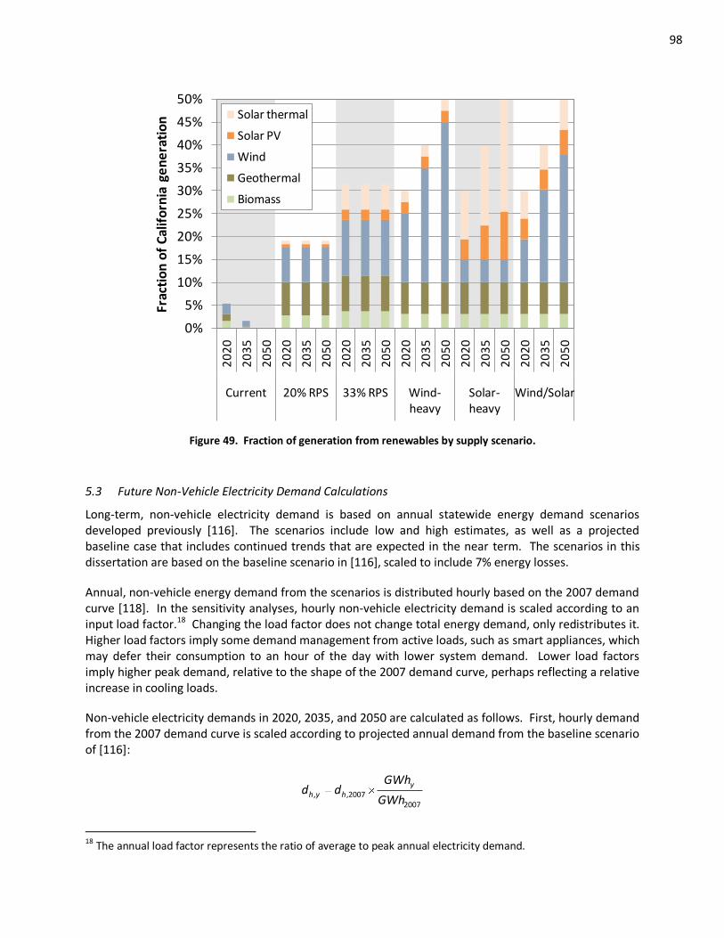
98

0%

5%

10%

15%

20%

25%

30%

35%

40%

45%

50%

20

20

20

35

20

50

20

20

20

35

20

50

20

20

20

35

20

50

20

20

20

35

20

50

20

20

20

35

20

50

20

20

20

35

20

50

Current 20% RPS 33% RPS Wind-heavy

Solar-heavy

Wind/Solar

Frac

tio

n o

f C

alif

orn

ia g

en

era

tio

n Solar thermal

Solar PV

Wind

Geothermal

Biomass

Figure 49. Fraction of generation from renewables by supply scenario.

5.3 Future Non-Vehicle Electricity Demand Calculations

Long-term, non-vehicle electricity demand is based on annual statewide energy demand scenarios developed previously [116]. The scenarios include low and high estimates, as well as a projected baseline case that includes continued trends that are expected in the near term. The scenarios in this dissertation are based on the baseline scenario in [116], scaled to include 7% energy losses.

Annual, non-vehicle energy demand from the scenarios is distributed hourly based on the 2007 demand curve [118]. In the sensitivity analyses, hourly non-vehicle electricity demand is scaled according to an input load factor.18 Changing the load factor does not change total energy demand, only redistributes it. Higher load factors imply some demand management from active loads, such as smart appliances, which may defer their consumption to an hour of the day with lower system demand. Lower load factors imply higher peak demand, relative to the shape of the 2007 demand curve, perhaps reflecting a relative increase in cooling loads.

Non-vehicle electricity demands in 2020, 2035, and 2050 are calculated as follows. First, hourly demand from the 2007 demand curve is scaled according to projected annual demand from the baseline scenario of [116]:

20072007,,

GWh

GWhdd

yhyh

18 The annual load factor represents the ratio of average to peak annual electricity demand.

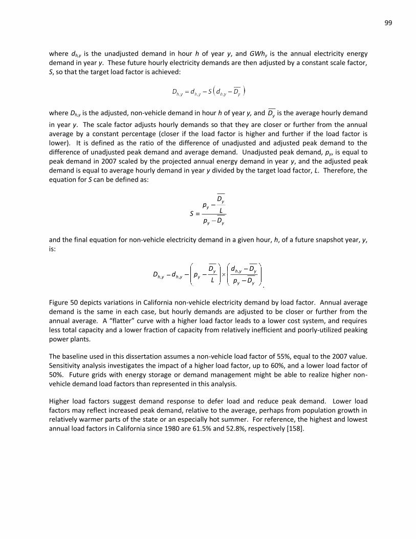
99

where dh,y is the unadjusted demand in hour h of year y, and GWhy is the annual electricity energy demand in year y. These future hourly electricity demands are then adjusted by a constant scale factor, S, so that the target load factor is achieved:

where Dh,y is the adjusted, non-vehicle demand in hour h of year y, and yD is the average hourly demand

in year y. The scale factor adjusts hourly demands so that they are closer or further from the annual average by a constant percentage (closer if the load factor is higher and further if the load factor is lower). It is defined as the ratio of the difference of unadjusted and adjusted peak demand to the difference of unadjusted peak demand and average demand. Unadjusted peak demand, py, is equal to peak demand in 2007 scaled by the projected annual energy demand in year y, and the adjusted peak demand is equal to average hourly demand in year y divided by the target load factor, L. Therefore, the equation for S can be defined as:

yy

yy

Dp

L

Dp

S

and the final equation for non-vehicle electricity demand in a given hour, h, of a future snapshot year, y, is:

yy

yyhyyyhyh

Dp

Dd

L

DpdD

,,,

.

Figure 50 depicts variations in California non-vehicle electricity demand by load factor. Annual average demand is the same in each case, but hourly demands are adjusted to be closer or further from the annual average. A “flatter” curve with a higher load factor leads to a lower cost system, and requires less total capacity and a lower fraction of capacity from relatively inefficient and poorly-utilized peaking power plants.

The baseline used in this dissertation assumes a non-vehicle load factor of 55%, equal to the 2007 value. Sensitivity analysis investigates the impact of a higher load factor, up to 60%, and a lower load factor of 50%. Future grids with energy storage or demand management might be able to realize higher non-vehicle demand load factors than represented in this analysis.

Higher load factors suggest demand response to defer load and reduce peak demand. Lower load factors may reflect increased peak demand, relative to the average, perhaps from population growth in relatively warmer parts of the state or an especially hot summer. For reference, the highest and lowest annual load factors in California since 1980 are 61.5% and 52.8%, respectively [158].

100

0

10

20

30

40

50

60

70

80

0 4 8 12 16 20

De

man

d (

GW

)

Hour

50% 55% 60%Load factor:

(a) Sample variation by load factor in daily California non- vehicle electricity demand (6/22/2050)

0

10

20

30

40

50

60

70

80

90

100

0% 20% 40% 60% 80% 100%

De

man

d (

GW

)

Percent of annual hours

(b) California load duration curves for non-vehicle electricity demand in 2050

Figure 50. Impact of load factor on California non-vehicle electricity demand (2050).

5.4 Representation of (Must-run) Renewable and Nuclear Capacity and Generation

The renewable and grid profiles dictate the fraction of total generation supplied by each renewable resource and the capacity of nuclear generation in the state. Hourly generation is then assigned in LEDGE-CA, according to the methods described below.

These resources are assigned zero GHG emissions rates and costs as listed in Table 24. Capital costs are amortized using a capital recovery factor of 15% in a snapshot year, and do not carry over into subsequent analysis periods.19 This is a simplifying assumption that allows all costs within one snapshot to be allocated that time period. Fixed and variable O&M costs are constant in all years, but variable costs may decline over time based on improvements in heat rate, which reduce energy costs because,

19

This is a simplification in the LEDGE-CA model to provide a simple, clear representation of power plant capacity additions and costs in each snapshot. In reality, it may take more than 15 years to capitalize many power plants, and LEDGE-CA could be improved in future work by including more thorough accounting of cumulative costs of generation for various scenarios.

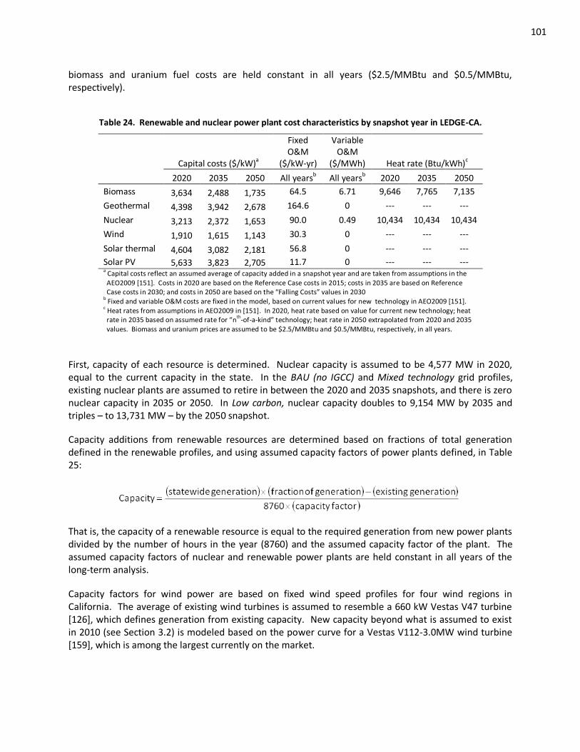
101

biomass and uranium fuel costs are held constant in all years ($2.5/MMBtu and $0.5/MMBtu, respectively).

Table 24. Renewable and nuclear power plant cost characteristics by snapshot year in LEDGE-CA.

Capital costs ($/kW)a

Fixed O&M

($/kW-yr)

Variable O&M

($/MWh) Heat rate (Btu/kWh)c

2020 2035 2050 All yearsb All yearsb 2020 2035 2050

Biomass 3,634 2,488 1,735 64.5 6.71 9,646 7,765 7,135

Geothermal 4,398 3,942 2,678 164.6 0 --- --- ---

Nuclear 3,213 2,372 1,653 90.0 0.49 10,434 10,434 10,434

Wind 1,910 1,615 1,143 30.3 0 --- --- ---

Solar thermal 4,604 3,082 2,181 56.8 0 --- --- ---

Solar PV 5,633 3,823 2,705 11.7 0 --- --- --- a Capital costs reflect an assumed average of capacity added in a snapshot year and are taken from assumptions in the

AEO2009 [151]. Costs in 2020 are based on the Reference Case costs in 2015; costs in 2035 are based on Reference Case costs in 2030; and costs in 2050 are based on the “Falling Costs” values in 2030 b Fixed and variable O&M costs are fixed in the model, based on current values for new technology in AEO2009 [151].

c Heat rates from assumptions in AEO2009 in [151]. In 2020, heat rate based on value for current new technology; heat

rate in 2035 based on assumed rate for “nth

-of-a-kind” technology; heat rate in 2050 extrapolated from 2020 and 2035 values. Biomass and uranium prices are assumed to be $2.5/MMBtu and $0.5/MMBtu, respectively, in all years.

First, capacity of each resource is determined. Nuclear capacity is assumed to be 4,577 MW in 2020, equal to the current capacity in the state. In the BAU (no IGCC) and Mixed technology grid profiles, existing nuclear plants are assumed to retire in between the 2020 and 2035 snapshots, and there is zero nuclear capacity in 2035 or 2050. In Low carbon, nuclear capacity doubles to 9,154 MW by 2035 and triples – to 13,731 MW – by the 2050 snapshot.

Capacity additions from renewable resources are determined based on fractions of total generation defined in the renewable profiles, and using assumed capacity factors of power plants defined, in Table 25:

That is, the capacity of a renewable resource is equal to the required generation from new power plants divided by the number of hours in the year (8760) and the assumed capacity factor of the plant. The assumed capacity factors of nuclear and renewable power plants are held constant in all years of the long-term analysis.

Capacity factors for wind power are based on fixed wind speed profiles for four wind regions in California. The average of existing wind turbines is assumed to resemble a 660 kW Vestas V47 turbine [126], which defines generation from existing capacity. New capacity beyond what is assumed to exist in 2010 (see Section 3.2) is modeled based on the power curve for a Vestas V112-3.0MW wind turbine [159], which is among the largest currently on the market.

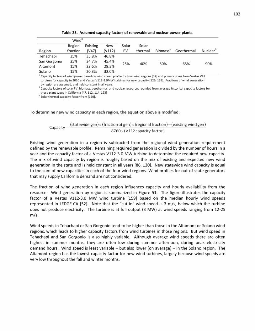
102

Table 25. Assumed capacity factors of renewable and nuclear power plants.

Winda

Region Region fraction

Existing (V47)

New (V112)

Solar PVb

Solar thermalc Biomassb Geothermalb Nuclearb

Tehachapi 35% 35.8% 46.8%

25% 40% 50% 65% 90% San Gorgonio 35% 34.7% 45.4% Altamont 15% 22.6% 29.3% Solano 15% 20.3% 32.0% a Capacity factors of wind power based on wind speed profile for four wind regions [52] and power curves from Vestas V47

turbines for capacity in 2010 and Vestas V112-3.0MW turbines for new capacity [126, 159]. Fractions of wind generation by region are assumed, and held constant in all years. b

Capacity factors of solar PV, biomass, geothermal, and nuclear resources rounded from average historical capacity factors for those plant types in California [47, 112, 114, 123] c Solar thermal capacity factor from [160].

To determine new wind capacity in each region, the equation above is modified:

Existing wind generation in a region is subtracted from the regional wind generation requirement defined by the renewable profile. Remaining required generation is divided by the number of hours in a year and the capacity factor of a Vestas V112-3.0 MW turbine to determine the required new capacity. The mix of wind capacity by region is roughly based on the mix of existing and expected new wind generation in the state and is held constant in all years [86, 120]. New statewide wind capacity is equal to the sum of new capacities in each of the four wind regions. Wind profiles for out-of-state generators that may supply California demand are not considered.

The fraction of wind generation in each region influences capacity and hourly availability from the resource. Wind generation by region is summarized in Figure 51. The figure illustrates the capacity factor of a Vestas V112-3.0 MW wind turbine [159] based on the median hourly wind speeds represented in LEDGE-CA *52+. Note that the “cut-in” wind speed is 3 m/s, below which the turbine does not produce electricity. The turbine is at full output (3 MW) at wind speeds ranging from 12-25 m/s.

Wind speeds in Tehachapi or San Gorgonio tend to be higher than those in the Altamont or Solano wind regions, which leads to higher capacity factors from wind turbines in those regions. But wind speed in Tehachapi and San Gorgonio is also highly variable. Although average wind speeds there are often highest in summer months, they are often low during summer afternoon, during peak electricity demand hours. Wind speed is least variable – but also lower (on average) – in the Solano region. The Altamont region has the lowest capacity factor for new wind turbines, largely because wind speeds are very low throughout the fall and winter months.

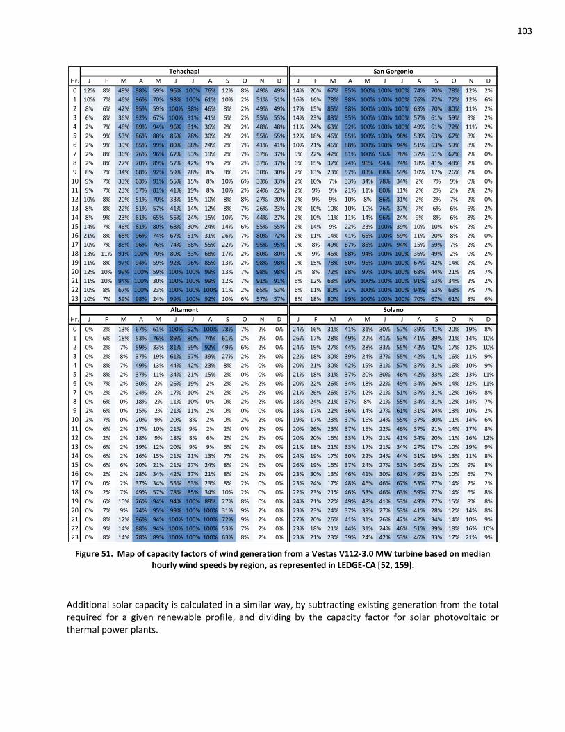
103


0 12% 8% 49% 98% 59% 96% 100% 76% 12% 8% 49% 49% 14% 20% 67% 95% 100% 100% 100% 74% 70% 78% 12% 2%

1 10% 7% 46% 96% 70% 98% 100% 61% 10% 2% 51% 51% 16% 16% 78% 98% 100% 100% 100% 76% 72% 72% 12% 6%

2 8% 6% 42% 95% 59% 100% 98% 46% 8% 2% 49% 49% 17% 15% 85% 98% 100% 100% 100% 63% 70% 80% 11% 2%

3 6% 8% 36% 92% 67% 100% 91% 41% 6% 2% 55% 55% 14% 23% 83% 95% 100% 100% 100% 57% 61% 59% 9% 2%

4 2% 7% 48% 89% 94% 96% 81% 36% 2% 2% 48% 48% 11% 24% 63% 92% 100% 100% 100% 49% 61% 72% 11% 2%

5 2% 9% 53% 86% 88% 85% 78% 30% 2% 2% 55% 55% 12% 18% 46% 85% 100% 100% 98% 53% 63% 67% 8% 2%

6 2% 9% 39% 85% 99% 80% 68% 24% 2% 7% 41% 41% 10% 21% 46% 88% 100% 100% 94% 51% 63% 59% 8% 2%

7 2% 8% 36% 76% 96% 67% 53% 19% 2% 7% 37% 37% 9% 22% 42% 81% 100% 96% 78% 37% 51% 67% 2% 0%

8 2% 8% 27% 70% 89% 57% 42% 9% 2% 2% 37% 37% 6% 15% 37% 74% 96% 94% 74% 18% 41% 48% 2% 0%

9 8% 7% 34% 68% 92% 59% 28% 8% 8% 2% 30% 30% 2% 13% 23% 57% 83% 88% 59% 10% 17% 26% 2% 0%

10 9% 7% 33% 63% 91% 55% 15% 8% 10% 6% 33% 33% 2% 10% 7% 33% 34% 78% 34% 2% 7% 9% 0% 0%

11 9% 7% 23% 57% 81% 41% 19% 8% 10% 2% 24% 22% 2% 9% 9% 21% 11% 80% 11% 2% 2% 2% 2% 2%

12 10% 8% 20% 51% 70% 33% 15% 10% 8% 8% 27% 20% 2% 9% 9% 10% 8% 86% 31% 2% 2% 7% 2% 0%

13 8% 8% 22% 51% 57% 41% 14% 12% 8% 7% 26% 23% 2% 10% 10% 10% 10% 76% 37% 7% 6% 6% 6% 2%

14 8% 9% 23% 61% 65% 55% 24% 15% 10% 7% 44% 27% 2% 10% 11% 11% 14% 96% 24% 9% 8% 6% 8% 2%

15 14% 7% 46% 81% 80% 68% 30% 24% 14% 6% 55% 55% 2% 14% 9% 22% 23% 100% 39% 10% 10% 6% 2% 2%

16 21% 8% 68% 96% 74% 67% 51% 31% 26% 7% 80% 72% 2% 11% 14% 41% 65% 100% 59% 11% 20% 8% 2% 0%

17 10% 7% 85% 96% 76% 74% 68% 55% 22% 7% 95% 95% 0% 8% 49% 67% 85% 100% 94% 15% 59% 7% 2% 2%

18 13% 11% 91% 100% 70% 80% 83% 68% 17% 2% 80% 80% 0% 9% 46% 88% 94% 100% 100% 36% 49% 2% 0% 2%

19 11% 8% 97% 94% 59% 92% 96% 85% 13% 2% 98% 98% 0% 15% 78% 80% 95% 100% 100% 67% 42% 14% 2% 2%

20 12% 10% 99% 100% 59% 100% 100% 99% 13% 7% 98% 98% 2% 8% 72% 88% 97% 100% 100% 68% 44% 21% 2% 7%

21 11% 10% 94% 100% 30% 100% 100% 99% 12% 7% 91% 91% 6% 12% 63% 99% 100% 100% 100% 91% 53% 34% 2% 2%

22 10% 8% 67% 100% 23% 100% 100% 100% 11% 2% 65% 53% 6% 11% 80% 91% 100% 100% 100% 94% 53% 63% 7% 7%

23 10% 7% 59% 98% 24% 99% 100% 92% 10% 6% 57% 57% 8% 18% 80% 99% 100% 100% 100% 70% 67% 61% 8% 6%


0 0% 2% 13% 67% 61% 100% 92% 100% 78% 7% 2% 0% 24% 16% 31% 41% 31% 30% 57% 39% 41% 20% 19% 8%

1 0% 6% 18% 53% 76% 89% 80% 74% 61% 2% 2% 0% 26% 17% 28% 49% 22% 41% 53% 41% 39% 21% 14% 10%

2 0% 2% 7% 59% 33% 81% 59% 92% 49% 6% 2% 0% 24% 19% 27% 44% 28% 33% 55% 42% 42% 17% 12% 10%

3 0% 2% 8% 37% 19% 61% 57% 39% 27% 2% 2% 0% 22% 18% 30% 39% 24% 37% 55% 42% 41% 16% 11% 9%

4 0% 8% 7% 49% 13% 44% 42% 23% 8% 2% 0% 0% 20% 21% 30% 42% 19% 31% 57% 37% 31% 16% 10% 9%

5 2% 8% 2% 37% 11% 34% 21% 15% 2% 0% 0% 0% 21% 18% 31% 37% 20% 30% 46% 42% 33% 12% 13% 11%

6 0% 7% 2% 30% 2% 26% 19% 2% 2% 2% 2% 0% 20% 22% 26% 34% 18% 22% 49% 34% 26% 14% 12% 11%

7 0% 2% 2% 24% 2% 17% 10% 2% 2% 2% 2% 0% 21% 26% 26% 37% 12% 21% 51% 37% 31% 12% 16% 8%

8 0% 6% 0% 18% 2% 11% 10% 0% 0% 2% 2% 0% 18% 24% 21% 37% 8% 21% 55% 34% 31% 12% 14% 7%

9 2% 6% 0% 15% 2% 21% 11% 2% 0% 0% 0% 0% 18% 17% 22% 36% 14% 27% 61% 31% 24% 13% 10% 2%

10 2% 7% 0% 20% 9% 20% 8% 2% 0% 2% 2% 0% 19% 17% 23% 37% 16% 24% 55% 37% 30% 11% 14% 6%

11 0% 6% 2% 17% 10% 21% 9% 2% 2% 0% 2% 0% 20% 26% 23% 37% 15% 22% 46% 37% 21% 14% 17% 8%

12 0% 2% 2% 18% 9% 18% 8% 6% 2% 2% 2% 0% 20% 20% 16% 33% 17% 21% 41% 34% 20% 11% 16% 12%

13 0% 6% 2% 19% 12% 20% 9% 9% 6% 2% 2% 0% 21% 18% 21% 33% 17% 21% 34% 27% 17% 10% 19% 9%

14 0% 6% 2% 16% 15% 21% 21% 13% 7% 2% 2% 0% 24% 19% 17% 30% 22% 24% 44% 31% 19% 13% 11% 8%

15 0% 6% 6% 20% 21% 21% 27% 24% 8% 2% 6% 0% 26% 19% 16% 37% 24% 27% 51% 36% 23% 10% 9% 8%

16 0% 2% 2% 28% 34% 42% 37% 21% 8% 2% 2% 0% 23% 30% 13% 46% 41% 30% 61% 49% 23% 10% 6% 7%

17 0% 0% 2% 37% 34% 55% 63% 23% 8% 2% 0% 0% 23% 24% 17% 48% 46% 46% 67% 53% 27% 14% 2% 2%

18 0% 2% 7% 49% 57% 78% 85% 34% 10% 2% 0% 0% 22% 23% 21% 46% 53% 46% 63% 59% 27% 14% 6% 8%

19 0% 6% 10% 76% 94% 94% 100% 89% 27% 8% 0% 0% 24% 21% 22% 49% 48% 41% 53% 49% 27% 15% 8% 8%

20 0% 7% 9% 74% 95% 99% 100% 100% 31% 9% 2% 0% 23% 23% 24% 37% 39% 27% 53% 41% 28% 12% 14% 8%

21 0% 8% 12% 96% 94% 100% 100% 100% 72% 9% 2% 0% 27% 20% 26% 41% 31% 26% 42% 42% 34% 14% 10% 9%

22 0% 9% 14% 88% 94% 100% 100% 100% 53% 7% 2% 0% 23% 18% 21% 44% 31% 24% 46% 51% 39% 18% 16% 10%

23 0% 8% 14% 78% 89% 100% 100% 100% 63% 8% 2% 0% 23% 21% 23% 39% 24% 42% 53% 46% 33% 17% 21% 9%

Tehachapi San Gorgonio

Altamont Solano

Figure 51. Map of capacity factors of wind generation from a Vestas V112-3.0 MW turbine based on median hourly wind speeds by region, as represented in LEDGE-CA [52, 159].

Additional solar capacity is calculated in a similar way, by subtracting existing generation from the total required for a given renewable profile, and dividing by the capacity factor for solar photovoltaic or thermal power plants.

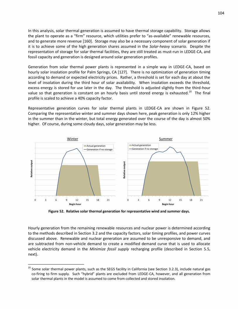
104

In this analysis, solar thermal generation is assumed to have thermal storage capability. Storage allows the plant to operate as a “firm” resource, which utilities prefer to “as-available” renewable resources, and to generate more revenue [160]. Storage may also be a necessary component of solar generation if it is to achieve some of the high generation shares assumed in the Solar-heavy scenario. Despite the representation of storage for solar thermal facilities, they are still treated as must-run in LEDGE-CA, and fossil capacity and generation is designed around solar generation profiles.

Generation from solar thermal power plants is represented in a simple way in LEDGE-CA, based on hourly solar insolation profile for Palm Springs, CA [127]. There is no optimization of generation timing according to demand or expected electricity prices. Rather, a threshold is set for each day at about the level of insolation during the third hour of solar availability. When insolation exceeds the threshold, excess energy is stored for use later in the day. The threshold is adjusted slightly from the third-hour value so that generation is constant on an hourly basis until stored energy is exhausted.20 The final profile is scaled to achieve a 40% capacity factor.

Representative generation curves for solar thermal plants in LEDGE-CA are shown in Figure 52. Comparing the representative winter and summer days shown here, peak generation is only 12% higher in the summer than in the winter, but total energy generated over the course of the day is almost 50% higher. Of course, during some cloudy days, solar generation may be less.

Winter Summer

0 3 6 9 12 15 18 21

Re

lati

ve o

utp

ut

Begin hour

Actual generation

Generation if no storage

0 3 6 9 12 15 18 21

Re

lati

ve o

utp

ut

Begin hour

Actual generation

Generation if no storage

Figure 52. Relative solar thermal generation for representative wind and summer days.

Hourly generation from the remaining renewable resources and nuclear power is determined according to the methods described in Section 3.2 and the capacity factors, solar timing profiles, and power curves discussed above. Renewable and nuclear generation are assumed to be unresponsive to demand, and are subtracted from non-vehicle demand to create a modified demand curve that is used to allocate vehicle electricity demand in the Minimize fossil supply recharging profile (described in Section 5.5, next).

20

Some solar thermal power plants, such as the SEGS facility in California (see Section 3.2.3), include natural gas co-firing to firm supply. Such “hybrid” plants are excluded from LEDGE-CA, however, and all generation from solar thermal plants in the model is assumed to come from collected and stored insolation.

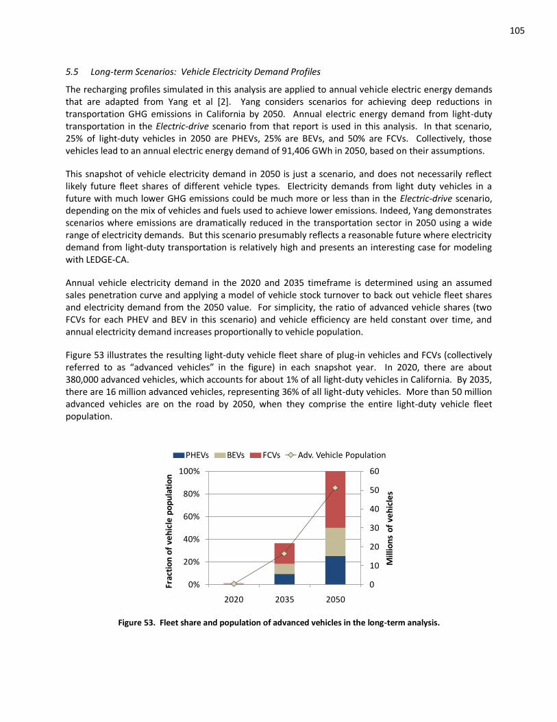
105

5.5 Long-term Scenarios: Vehicle Electricity Demand Profiles

The recharging profiles simulated in this analysis are applied to annual vehicle electric energy demands that are adapted from Yang et al [2]. Yang considers scenarios for achieving deep reductions in transportation GHG emissions in California by 2050. Annual electric energy demand from light-duty transportation in the Electric-drive scenario from that report is used in this analysis. In that scenario, 25% of light-duty vehicles in 2050 are PHEVs, 25% are BEVs, and 50% are FCVs. Collectively, those vehicles lead to an annual electric energy demand of 91,406 GWh in 2050, based on their assumptions.

This snapshot of vehicle electricity demand in 2050 is just a scenario, and does not necessarily reflect likely future fleet shares of different vehicle types. Electricity demands from light duty vehicles in a future with much lower GHG emissions could be much more or less than in the Electric-drive scenario, depending on the mix of vehicles and fuels used to achieve lower emissions. Indeed, Yang demonstrates scenarios where emissions are dramatically reduced in the transportation sector in 2050 using a wide range of electricity demands. But this scenario presumably reflects a reasonable future where electricity demand from light-duty transportation is relatively high and presents an interesting case for modeling with LEDGE-CA.

Annual vehicle electricity demand in the 2020 and 2035 timeframe is determined using an assumed sales penetration curve and applying a model of vehicle stock turnover to back out vehicle fleet shares and electricity demand from the 2050 value. For simplicity, the ratio of advanced vehicle shares (two FCVs for each PHEV and BEV in this scenario) and vehicle efficiency are held constant over time, and annual electricity demand increases proportionally to vehicle population.

Figure 53 illustrates the resulting light-duty vehicle fleet share of plug-in vehicles and FCVs (collectively referred to as “advanced vehicles” in the figure) in each snapshot year. In 2020, there are about 380,000 advanced vehicles, which accounts for about 1% of all light-duty vehicles in California. By 2035, there are 16 million advanced vehicles, representing 36% of all light-duty vehicles. More than 50 million advanced vehicles are on the road by 2050, when they comprise the entire light-duty vehicle fleet population.

0

10

20

30

40

50

60

0%

20%

40%

60%

80%

100%

2020 2035 2050

Mill

ion

s o

f ve

hic

les

Frac

tio

n o

f ve

hic

le p

op

ula

tio

n

PHEVs BEVs FCVs Adv. Vehicle Population

Figure 53. Fleet share and population of advanced vehicles in the long-term analysis.

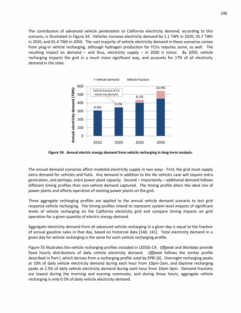
106

The contribution of advanced vehicle penetration to California electricity demand, according to this scenario, is illustrated in Figure 54. Vehicles increase electricity demand by 1.1 TWh in 2020, 35.7 TWh in 2035, and 91.4 TWh in 2050. The vast majority of vehicle electricity demand in these scenarios comes from plug-in vehicle recharging, although hydrogen production for FCVs requires some, as well. The resulting impact on demand – and thus, electricity supply – in 2020 is minor. By 2050, vehicle recharging impacts the grid in a much more significant way, and accounts for 17% of all electricity demand in the state.

0.0%0.3%

8.2%

16.9%

0

100

200

300

400

500

600

2010 2020 2035 2050An

nu

al e

lect

rici

ty d

em

and

(TW

h)

Vehicle demand Vehicle fraction

Vehicle fraction of CA electricity demand

Figure 54. Annual electric energy demand from vehicle recharging in long-term analysis.

The annual demand scenarios affect modeled electricity supply in two ways. First, the grid must supply extra demand for vehicles and fuels. Any demand in addition to the No vehicles case will require extra generation, and perhaps, extra power plant capacity. Second – importantly – additional demand follows different timing profiles than non-vehicle demand captured. The timing profile alters the ideal mix of power plants and affects operation of existing power plants on the grid.

Three aggregate recharging profiles are applied to the annual vehicle demand scenario to test grid response vehicle recharging. The timing profiles intend to represent system-level impacts of significant levels of vehicle recharging on the California electricity grid and compare timing impacts on grid operation for a given quantity of electric energy demand.

Aggregate electricity demand from all advanced vehicle recharging in a given day is equal to the fraction of annual gasoline sales in that day, based on historical data [140, 141]. Total electricity demand in a given day for vehicle recharging is the same for each vehicle recharging profile.

Figure 55 illustrates the vehicle recharging profiles included in LEDGE-CA. Offpeak and Workday provide fixed hourly distributions of daily vehicle electricity demand. Offpeak follows the similar profile described in Part I, which derives from a recharging profile used by EPRI [6]. Overnight recharging peaks at 10% of daily vehicle electricity demand during each hour from 10pm-2am, and daytime recharging peaks at 2.5% of daily vehicle electricity demand during each hour from 10am-3pm. Demand fractions are lowest during the morning and evening commutes, and during those hours, aggregate vehicle recharging is only 0.5% of daily vehicle electricity demand.

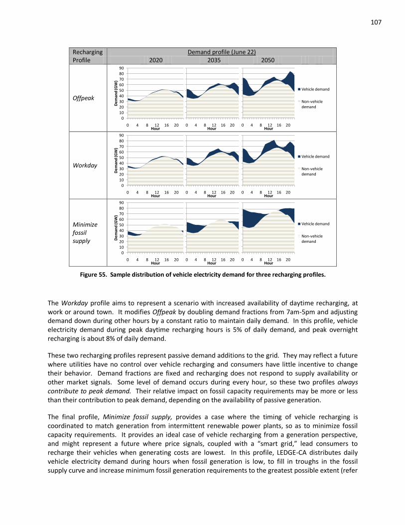
107

Recharging Demand profile (June 22) Profile 2020 2035 2050

Offpeak

0 4 8 12 16 20Hour

Vehicle demand

Non-vehicle demand

0 4 8 12 16 20Hour

0

10

20

30

40

50

60

70

80

90

0 4 8 12 16 20

De

man

d (G

W)

Hour

Workday

0 4 8 12 16 20Hour

Vehicle demand

Non-vehicle demand

0 4 8 12 16 20Hour

0

10

20

30

40

50

60

70

80

90

0 4 8 12 16 20

De

man

d (G

W)

Hour

Minimize fossil supply

0 4 8 12 16 20Hour

Vehicle demand

Non-vehicle demand

0 4 8 12 16 20Hour

0

10

20

30

40

50

60

70

80

90

0 4 8 12 16 20

De

man

d (G

W)

Hour

Figure 55. Sample distribution of vehicle electricity demand for three recharging profiles.

The Workday profile aims to represent a scenario with increased availability of daytime recharging, at work or around town. It modifies Offpeak by doubling demand fractions from 7am-5pm and adjusting demand down during other hours by a constant ratio to maintain daily demand. In this profile, vehicle electricity demand during peak daytime recharging hours is 5% of daily demand, and peak overnight recharging is about 8% of daily demand.

These two recharging profiles represent passive demand additions to the grid. They may reflect a future where utilities have no control over vehicle recharging and consumers have little incentive to change their behavior. Demand fractions are fixed and recharging does not respond to supply availability or other market signals. Some level of demand occurs during every hour, so these two profiles always contribute to peak demand. Their relative impact on fossil capacity requirements may be more or less than their contribution to peak demand, depending on the availability of passive generation.

The final profile, Minimize fossil supply, provides a case where the timing of vehicle recharging is coordinated to match generation from intermittent renewable power plants, so as to minimize fossil capacity requirements. It provides an ideal case of vehicle recharging from a generation perspective, and might represent a future where price signals, coupled with a “smart grid,” lead consumers to recharge their vehicles when generating costs are lowest. In this profile, LEDGE-CA distributes daily vehicle electricity demand during hours when fossil generation is low, to fill in troughs in the fossil supply curve and increase minimum fossil generation requirements to the greatest possible extent (refer

108

to Figure 48 for an illustration). Vehicle electricity demand may be distributed differently day-to-day, depending on the hourly distribution of non-vehicle demand and renewable generation. Based on the annual – and thus, daily – vehicle electricity demand scenario developed here, this profile never contributes to peak demand or fossil capacity requirements.

5.6 Representation of Hydro Generation

After vehicle recharging is added to the grid, hydro energy is dispatched based on the curve for total demand minus must-run generation. The hydro resource in California includes a relatively small fraction of baseload (must-run) generation, to satisfy ecological and other non-power requirements, but most of the resource can be stored and dispatched as needed, when demands and electricity prices are highest.

This analysis assumes that the future hydro system in California will operate in similar fashion to the way it does currently, and hydro resources are represented in LEDGE-CA as they are in EDGE-CA, described in Section 3.2.4. There is one exception, however. In EDGE-CA, peak hydro capacity is fixed at 7,000 MW, and “super-peak” hours – during which hydro generation may exceed that average peak generation level significantly [134] – are ignored. This simplification mostly shifts some NGCT generation from one hour to another (because hydro is energy-constrained), and was found to have little impact on the results in Part I. But when capacity expansion is included, in LEDGE-CA, accurately accounting for dependable hydro capacity is important. Therefore, super-peak hours are included in LEDGE-CA. They are defined as the 50 hours with the highest fossil supply requirement on an annual basis. During those hours, hydro generation is set to 11,000 MW in LEDGE-CA, which is roughly the dependable capacity of the resource (for short duration) in the state currently [134].

Including super-peak hours in LEDGE-CA does not necessarily reduce fossil capacity requirements by 4,000 MW, compared to what they would be without such representation. If demand during the 51st-peak hour is more or less than 4,000 MW lower than during the 1st peak demand hour, avoided capacity additions (through this methodological adjustment) will differ accordingly.

Certainly, hydro supply in California may change in the future. Climate change impacts, ecological concerns, population growth, and state and regional politics may contribute to a redesigned hydro power supply system in the future. But those speculative conditions are ignored in this long-term analysis.

Further, it is assumed that no new hydro capacity will be added, and none will be retired; hydro capacity is constant in each supply scenario in LEDGE-CA.

5.7 Screening Curve Analysis for Optimal Fossil Capacity Additions

After hydro generation is allocated, the hourly fossil supply profile is constructed. It represents the difference between total demand and generation from renewable, nuclear, and hydro resources, and is equal to the segment of hourly demand that must be supplied by coal- and natural gas-fired power plants. LEDGE-CA uses screening curve analysis to optimize fossil capacity to meet these demands.

By dispatching hydro, nuclear, and renewable generation before determining optimal capacity and dispatch of remaining generation, perfect foresight is assumed. In practice, planners cannot predict how much renewable generation will be available during peak demand hours. Rather, they size capacity in the system using capacity credits, which represent assumed availabilities of power plants during peak

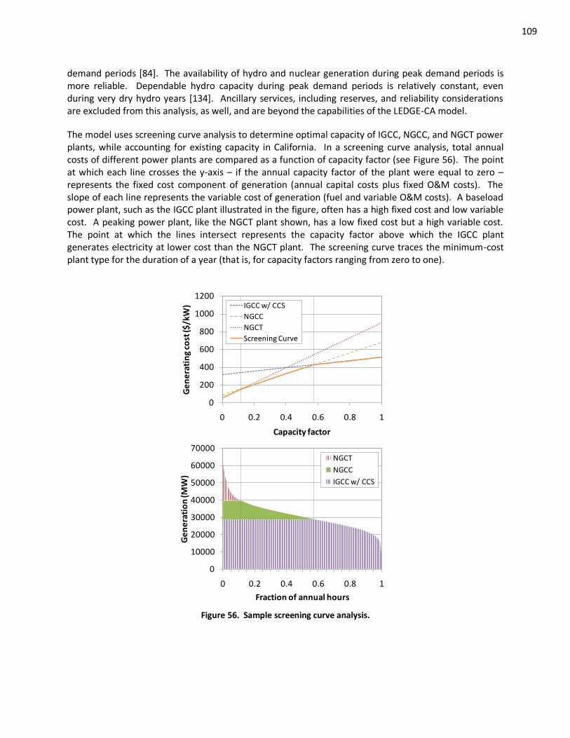
109

demand periods [84]. The availability of hydro and nuclear generation during peak demand periods is more reliable. Dependable hydro capacity during peak demand periods is relatively constant, even during very dry hydro years [134]. Ancillary services, including reserves, and reliability considerations are excluded from this analysis, as well, and are beyond the capabilities of the LEDGE-CA model.

The model uses screening curve analysis to determine optimal capacity of IGCC, NGCC, and NGCT power plants, while accounting for existing capacity in California. In a screening curve analysis, total annual costs of different power plants are compared as a function of capacity factor (see Figure 56). The point at which each line crosses the y-axis – if the annual capacity factor of the plant were equal to zero – represents the fixed cost component of generation (annual capital costs plus fixed O&M costs). The slope of each line represents the variable cost of generation (fuel and variable O&M costs). A baseload power plant, such as the IGCC plant illustrated in the figure, often has a high fixed cost and low variable cost. A peaking power plant, like the NGCT plant shown, has a low fixed cost but a high variable cost. The point at which the lines intersect represents the capacity factor above which the IGCC plant generates electricity at lower cost than the NGCT plant. The screening curve traces the minimum-cost plant type for the duration of a year (that is, for capacity factors ranging from zero to one).

0

200

400

600

800

1000

1200

0 0.2 0.4 0.6 0.8 1

Ge

ne

rati

ng

cost

($/k

W)

Capacity factor

IGCC w/ CCS

NGCC

NGCT

Screening Curve

0

10000

20000

30000

40000

50000

60000

70000

0 0.2 0.4 0.6 0.8 1

Ge

ne

rati

on

(MW

)


NGCT

NGCC

IGCC w/ CCS

Figure 56. Sample screening curve analysis.

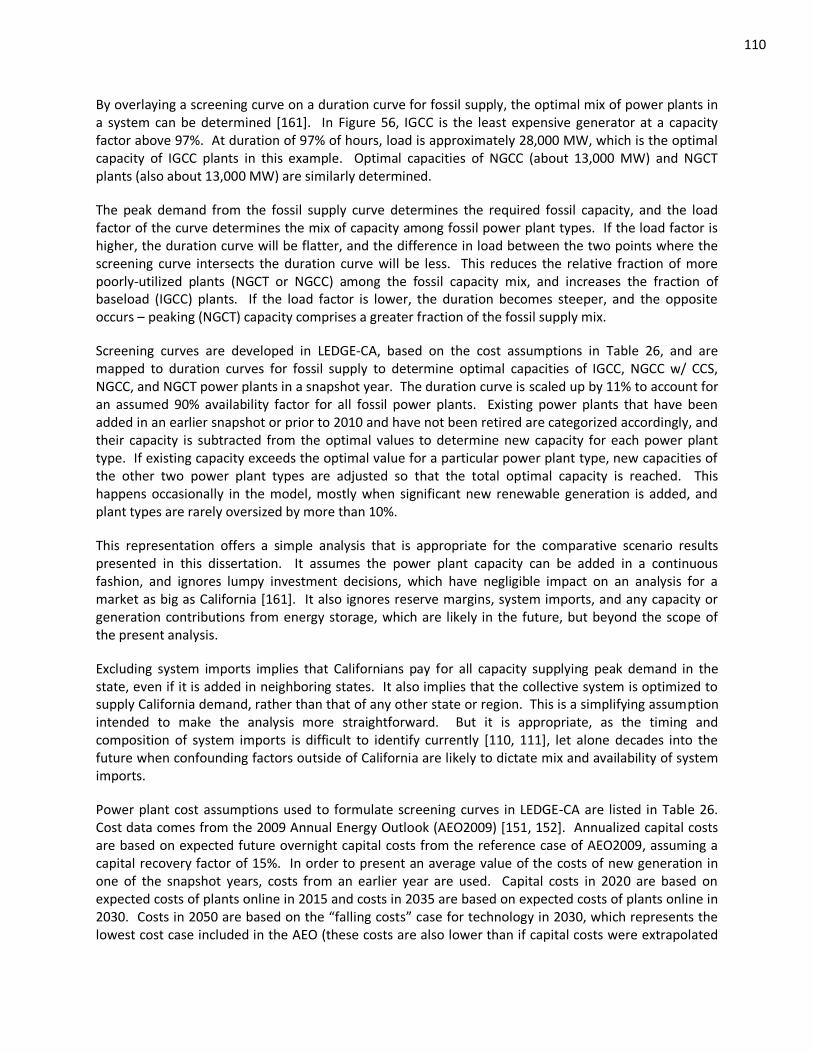
110

By overlaying a screening curve on a duration curve for fossil supply, the optimal mix of power plants in a system can be determined [161]. In Figure 56, IGCC is the least expensive generator at a capacity factor above 97%. At duration of 97% of hours, load is approximately 28,000 MW, which is the optimal capacity of IGCC plants in this example. Optimal capacities of NGCC (about 13,000 MW) and NGCT plants (also about 13,000 MW) are similarly determined.

The peak demand from the fossil supply curve determines the required fossil capacity, and the load factor of the curve determines the mix of capacity among fossil power plant types. If the load factor is higher, the duration curve will be flatter, and the difference in load between the two points where the screening curve intersects the duration curve will be less. This reduces the relative fraction of more poorly-utilized plants (NGCT or NGCC) among the fossil capacity mix, and increases the fraction of baseload (IGCC) plants. If the load factor is lower, the duration becomes steeper, and the opposite occurs – peaking (NGCT) capacity comprises a greater fraction of the fossil supply mix.

Screening curves are developed in LEDGE-CA, based on the cost assumptions in Table 26, and are mapped to duration curves for fossil supply to determine optimal capacities of IGCC, NGCC w/ CCS, NGCC, and NGCT power plants in a snapshot year. The duration curve is scaled up by 11% to account for an assumed 90% availability factor for all fossil power plants. Existing power plants that have been added in an earlier snapshot or prior to 2010 and have not been retired are categorized accordingly, and their capacity is subtracted from the optimal values to determine new capacity for each power plant type. If existing capacity exceeds the optimal value for a particular power plant type, new capacities of the other two power plant types are adjusted so that the total optimal capacity is reached. This happens occasionally in the model, mostly when significant new renewable generation is added, and plant types are rarely oversized by more than 10%.

This representation offers a simple analysis that is appropriate for the comparative scenario results presented in this dissertation. It assumes the power plant capacity can be added in a continuous fashion, and ignores lumpy investment decisions, which have negligible impact on an analysis for a market as big as California [161]. It also ignores reserve margins, system imports, and any capacity or generation contributions from energy storage, which are likely in the future, but beyond the scope of the present analysis.

Excluding system imports implies that Californians pay for all capacity supplying peak demand in the state, even if it is added in neighboring states. It also implies that the collective system is optimized to supply California demand, rather than that of any other state or region. This is a simplifying assumption intended to make the analysis more straightforward. But it is appropriate, as the timing and composition of system imports is difficult to identify currently [110, 111], let alone decades into the future when confounding factors outside of California are likely to dictate mix and availability of system imports.

Power plant cost assumptions used to formulate screening curves in LEDGE-CA are listed in Table 26. Cost data comes from the 2009 Annual Energy Outlook (AEO2009) [151, 152]. Annualized capital costs are based on expected future overnight capital costs from the reference case of AEO2009, assuming a capital recovery factor of 15%. In order to present an average value of the costs of new generation in one of the snapshot years, costs from an earlier year are used. Capital costs in 2020 are based on expected costs of plants online in 2015 and costs in 2035 are based on expected costs of plants online in 2030. Costs in 2050 are based on the “falling costs” case for technology in 2030, which represents the lowest cost case included in the AEO (these costs are also lower than if capital costs were extrapolated

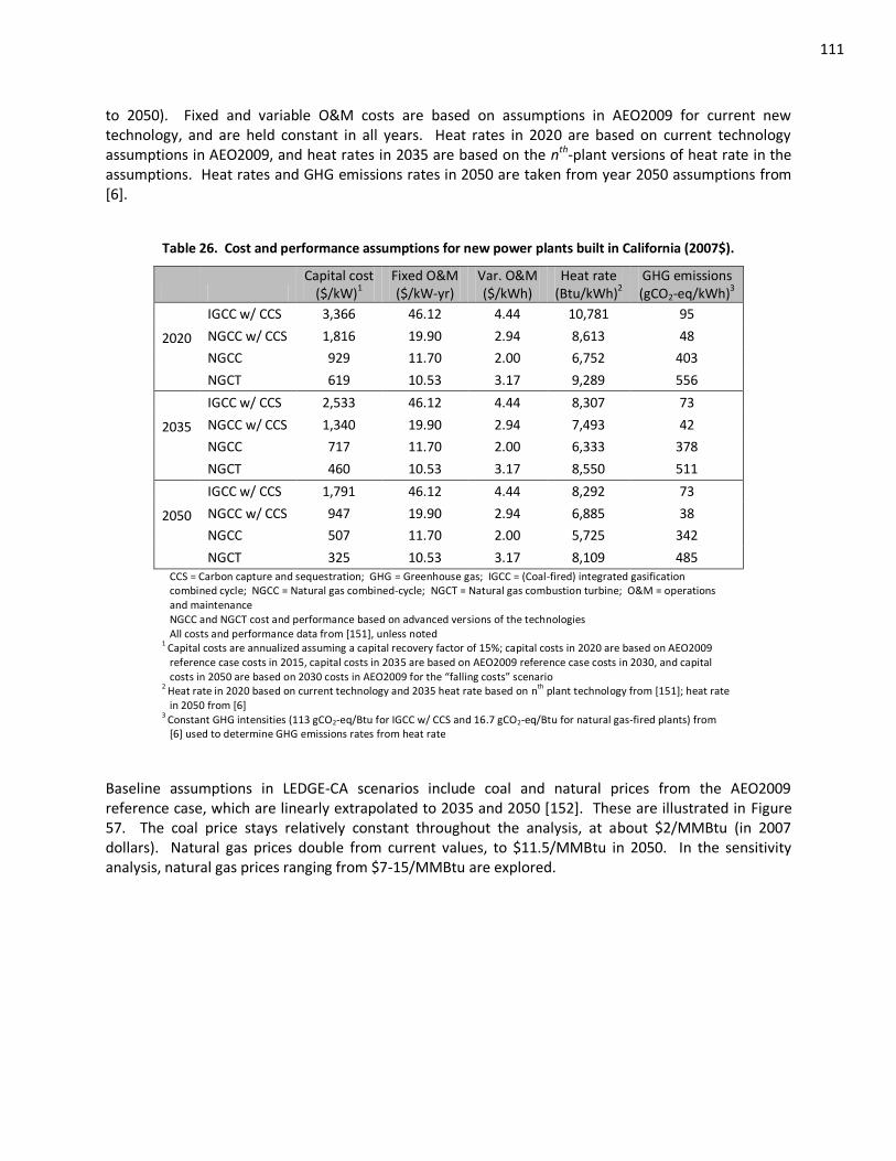
111

to 2050). Fixed and variable O&M costs are based on assumptions in AEO2009 for current new technology, and are held constant in all years. Heat rates in 2020 are based on current technology assumptions in AEO2009, and heat rates in 2035 are based on the nth-plant versions of heat rate in the assumptions. Heat rates and GHG emissions rates in 2050 are taken from year 2050 assumptions from [6].

Table 26. Cost and performance assumptions for new power plants built in California (2007$).

Capital cost

($/kW)1 Fixed O&M ($/kW-yr)

Var. O&M ($/kWh)

Heat rate (Btu/kWh)2

GHG emissions (gCO2-eq/kWh)3

2020

IGCC w/ CCS 3,366 46.12 4.44 10,781 95

NGCC w/ CCS 1,816 19.90 2.94 8,613 48

NGCC 929 11.70 2.00 6,752 403

NGCT 619 10.53 3.17 9,289 556

2035

IGCC w/ CCS 2,533 46.12 4.44 8,307 73

NGCC w/ CCS 1,340 19.90 2.94 7,493 42

NGCC 717 11.70 2.00 6,333 378

NGCT 460 10.53 3.17 8,550 511

2050

IGCC w/ CCS 1,791 46.12 4.44 8,292 73

NGCC w/ CCS 947 19.90 2.94 6,885 38

NGCC 507 11.70 2.00 5,725 342

NGCT 325 10.53 3.17 8,109 485 CCS = Carbon capture and sequestration; GHG = Greenhouse gas; IGCC = (Coal-fired) integrated gasification combined cycle; NGCC = Natural gas combined-cycle; NGCT = Natural gas combustion turbine; O&M = operations and maintenance NGCC and NGCT cost and performance based on advanced versions of the technologies All costs and performance data from [151], unless noted 1

Capital costs are annualized assuming a capital recovery factor of 15%; capital costs in 2020 are based on AEO2009 reference case costs in 2015, capital costs in 2035 are based on AEO2009 reference case costs in 2030, and capital costs in 2050 are based on 2030 costs in AEO2009 for the “falling costs” scenario 2

Heat rate in 2020 based on current technology and 2035 heat rate based on nth

plant technology from [151]; heat rate in 2050 from [6] 3

Constant GHG intensities (113 gCO2-eq/Btu for IGCC w/ CCS and 16.7 gCO2-eq/Btu for natural gas-fired plants) from [6] used to determine GHG emissions rates from heat rate

Baseline assumptions in LEDGE-CA scenarios include coal and natural prices from the AEO2009 reference case, which are linearly extrapolated to 2035 and 2050 [152]. These are illustrated in Figure 57. The coal price stays relatively constant throughout the analysis, at about $2/MMBtu (in 2007 dollars). Natural gas prices double from current values, to $11.5/MMBtu in 2050. In the sensitivity analysis, natural gas prices ranging from $7-15/MMBtu are explored.

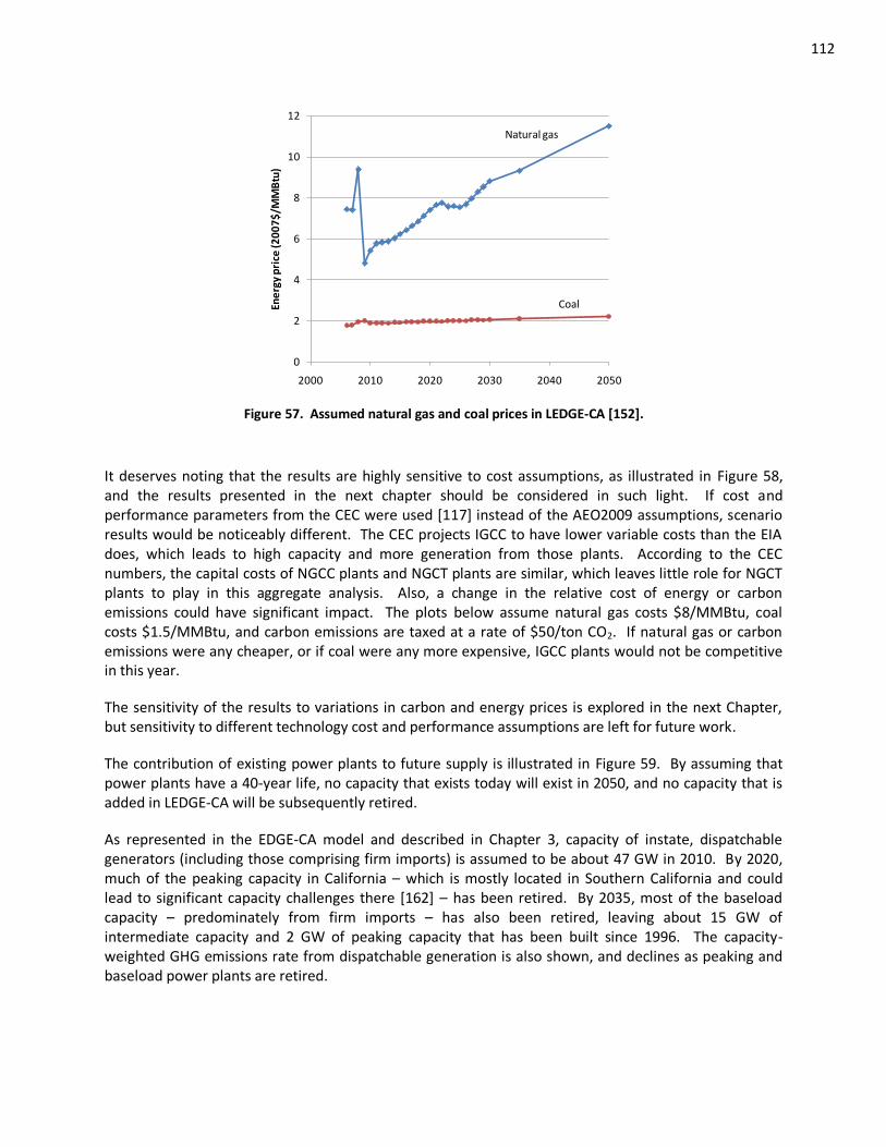
112

0

2

4

6

8

10

12

2000 2010 2020 2030 2040 2050

Ene

rgy

pri

ce (2

00

7$

/MM

Btu

)

Natural gas

Coal

Figure 57. Assumed natural gas and coal prices in LEDGE-CA [152].

It deserves noting that the results are highly sensitive to cost assumptions, as illustrated in Figure 58, and the results presented in the next chapter should be considered in such light. If cost and performance parameters from the CEC were used [117] instead of the AEO2009 assumptions, scenario results would be noticeably different. The CEC projects IGCC to have lower variable costs than the EIA does, which leads to high capacity and more generation from those plants. According to the CEC numbers, the capital costs of NGCC plants and NGCT plants are similar, which leaves little role for NGCT plants to play in this aggregate analysis. Also, a change in the relative cost of energy or carbon emissions could have significant impact. The plots below assume natural gas costs $8/MMBtu, coal costs $1.5/MMBtu, and carbon emissions are taxed at a rate of $50/ton CO2. If natural gas or carbon emissions were any cheaper, or if coal were any more expensive, IGCC plants would not be competitive in this year.

The sensitivity of the results to variations in carbon and energy prices is explored in the next Chapter, but sensitivity to different technology cost and performance assumptions are left for future work.

The contribution of existing power plants to future supply is illustrated in Figure 59. By assuming that power plants have a 40-year life, no capacity that exists today will exist in 2050, and no capacity that is added in LEDGE-CA will be subsequently retired.

As represented in the EDGE-CA model and described in Chapter 3, capacity of instate, dispatchable generators (including those comprising firm imports) is assumed to be about 47 GW in 2010. By 2020, much of the peaking capacity in California – which is mostly located in Southern California and could lead to significant capacity challenges there [162] – has been retired. By 2035, most of the baseload capacity – predominately from firm imports – has also been retired, leaving about 15 GW of intermediate capacity and 2 GW of peaking capacity that has been built since 1996. The capacity-weighted GHG emissions rate from dispatchable generation is also shown, and declines as peaking and baseload power plants are retired.

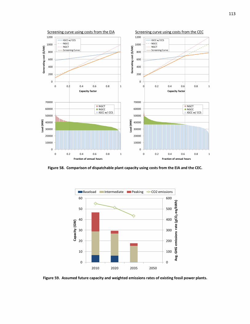
113

Screening curve using costs from the EIA Screening curve using costs from the CEC

0

200

400

600

800

1000

1200

0 0.2 0.4 0.6 0.8 1

Ge

ne

rati

ng

cost

($

/kW

)

Capacity factor

IGCC w/ CCS

NGCC

NGCT

Screening Curve

0

10000

20000

30000

40000

50000

60000

70000

0 0.2 0.4 0.6 0.8 1

Load

(M

W)


NGCTNGCCIGCC w/ CCS

0

200

400

600

800

1000

1200

0 0.2 0.4 0.6 0.8 1

Ge

ne

rati

ng

cost

($

/kW

)

Capacity factor

IGCC w/ CCS

NGCC

NGCT

Screening Curve

0

10000

20000

30000

40000

50000

60000

70000

0 0.2 0.4 0.6 0.8 1

Load

(M

W)


NGCTNGCCIGCC w/ CCS

Figure 58. Comparison of dispatchable plant capacity using costs from the EIA and the CEC.

0

100

200

300

400

500

600

0

10

20

30

40

50

60

2010 2020 2035 2050

Avg

. GH

G e

mis

sio

ns

rate

(gC

O2-

eq

/kW

h)

Cap

acit

y (G

W)

Baseload Intermediate Peaking CO2 emissions

Figure 59. Assumed future capacity and weighted emissions rates of existing fossil power plants.

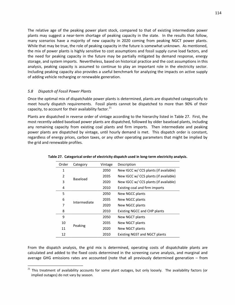
114

The relative age of the peaking power plant stock, compared to that of existing intermediate power plants may suggest a near-term shortage of peaking capacity in the state. In the results that follow, many scenarios have a majority of new capacity in 2020 coming from peaking NGCT power plants. While that may be true, the role of peaking capacity in the future is somewhat unknown. As mentioned, the mix of power plants is highly sensitive to cost assumptions and fossil supply curve load factors, and the need for peaking capacity in the future may be partially mitigated by demand response, energy storage, and system imports. Nevertheless, based on historical practice and the cost assumptions in this analysis, peaking capacity is assumed to continue to play an important role in the electricity sector. Including peaking capacity also provides a useful benchmark for analyzing the impacts on active supply of adding vehicle recharging or renewable generation.

5.8 Dispatch of Fossil Power Plants

Once the optimal mix of dispatchable power plants is determined, plants are dispatched categorically to meet hourly dispatch requirements. Fossil plants cannot be dispatched to more than 90% of their capacity, to account for their availability factor.21

Plants are dispatched in reverse order of vintage according to the hierarchy listed in Table 27. First, the most recently-added baseload power plants are dispatched, followed by older baseload plants, including any remaining capacity from existing coal plants and firm imports. Then intermediate and peaking power plants are dispatched by vintage, until hourly demand is met. This dispatch order is constant, regardless of energy prices, carbon taxes, or any other operating parameters that might be implied by the grid and renewable profiles.

Table 27. Categorical order of electricity dispatch used in long-term electricity analysis.

Order Category Vintage Description

1

Baseload

2050 New IGCC w/ CCS plants (if available)

2 2035 New IGCC w/ CCS plants (if available)

3 2020 New IGCC w/ CCS plants (if available)

4 2010 Existing coal and firm imports

5

Intermediate

2050 New NGCC plants

6 2035 New NGCC plants

7 2020 New NGCC plants

8 2010 Existing NGCC and CHP plants

9

Peaking

2050 New NGCT plants

10 2035 New NGCT plants

11 2020 New NGCT plants

12 2010 Existing NGST and NGCT plants

From the dispatch analysis, the grid mix is determined, operating costs of dispatchable plants are calculated and added to the fixed costs determined in the screening curve analysis, and marginal and average GHG emissions rates are accounted (note that all previously determined generation – from

21

This treatment of availability accounts for some plant outages, but only loosely. The availability factors (or implied outages) do not vary by season.

115

renewable, nuclear, and hydro facilities – are assumed to have zero GHG emissions). The cost calculations represent the total cost of generation in a given year, in 2007 dollars. Annualized capacity costs for all capacity added since the previous modeled year (2020 or 2035) are included, and other plants are assumed to be fully capitalized.

Results for the various supply and demand scenarios are presented and compared in the following chapter.

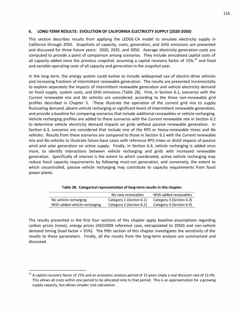
116

6. LONG-TERM RESULTS: EVOLUTION OF CALIFORNIA ELECTRICITY SUPPLY (2020-2050)

This section describes results from applying the LEDGE-CA model to simulate electricity supply in California through 2050. Snapshots of capacity, costs, generation, and GHG emissions are presented and discussed for three future years: 2020, 2035, and 2050. Average electricity generation costs are computed to provide a point of comparison among scenarios. They include annualized capital costs of all capacity added since the previous snapshot, assuming a capital recovery factor of 15%,22 and fixed and variable operating costs of all capacity and generation in the snapshot year.

In the long term, the energy system could evolve to include widespread use of electric-drive vehicles and increasing fractions of intermittent renewable generation. The results are presented incrementally to explore separately the impacts of intermittent renewable generation and vehicle electricity demand on fossil supply, system costs, and GHG emissions (Table 28). First, in Section 6.1, scenarios with the Current renewable mix and No vehicles are considered, according to the three non-renewable grid profiles described in Chapter 5. These illustrate the operation of the current grid mix to supply fluctuating demand, absent vehicle recharging or significant levels of intermittent renewable generation, and provide a baseline for comparing scenarios that include additional renewables or vehicle recharging. Vehicle recharging profiles are added to these scenarios with the Current renewable mix in Section 6.2 to determine vehicle electricity demand impacts on grids without passive renewable generation. In Section 6.3, scenarios are considered that include one of the RPS or heavy-renewable mixes and No vehicles. Results from these scenarios are compared to those in Section 6.1 with the Current renewable mix and No vehicles to illustrate future base cases with reference RPS mixes or distill impacts of passive wind and solar generation on active supply. Finally, in Section 6.4, vehicle recharging is added once more, to identify interactions between vehicle recharging and grids with increased renewable generation. Specifically of interest is the extent to which coordinated, active vehicle recharging may reduce fossil capacity requirements by following must-run generation, and conversely, the extent to which uncontrolled, passive vehicle recharging may contribute to capacity requirements from fossil power plants.

Table 28. Categorical representation of long-term results in this chapter.

No new renewables With added renewables

No vehicle recharging Category 1 (Section 6.1) Category 3 (Section 6.3) With added vehicle recharging Category 2 (Section 6.2) Category 4 (Section 6.4)

The results presented in the first four sections of this chapter apply baseline assumptions regarding carbon prices (none), energy prices (AEO2009 reference case, extrapolated to 2050) and non-vehicle demand timing (load factor = 55%). The fifth section of this chapter investigates the sensitivity of the results to these parameters. Finally, all the results from the long-term analysis are summarized and discussed.

22

A capital recovery factor of 15% and an economic analysis period of 15 years imply a real discount rate of 12.4%. This allows all costs within one period to be allocated only to that period. This is an approximation for a growing supply capacity, but allows simpler cost calculation.

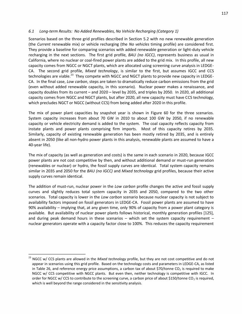
117

6.1 Long-term Results: No Added Renewables, No Vehicle Recharging (Category 1)

Scenarios based on the three grid profiles described in Section 5.2 with no new renewable generation (the Current renewable mix) or vehicle recharging (the No vehicles timing profile) are considered first. They provide a baseline for comparing scenarios with added renewable generation or light-duty vehicle recharging in the next sections. The first grid profile, BAU (no IGCC), represents business as usual in California, where no nuclear or coal-fired power plants are added to the grid mix. In this profile, all new capacity comes from NGCC or NGCT plants, which are allocated using screening curve analysis in LEDGE-CA. The second grid profile, Mixed technology, is similar to the first, but assumes IGCC and CCS technologies are viable.23 They compete with NGCC and NGCT plants to provide new capacity in LEDGE-CA. In the final case, Low carbon, steps are taken to dramatically reduce carbon emissions from the grid (even without added renewable capacity, in this scenario). Nuclear power makes a renaissance, and capacity doubles from its current – and 2020 – level by 2035, and triples by 2050. In 2020, all additional capacity comes from NGCC and NGCT plants, but after 2020, all new capacity must have CCS technology, which precludes NGCT or NGCC (without CCS) from being added after 2020 in this profile.

The mix of power plant capacities by snapshot year is shown in Figure 60 for the three scenarios. System capacity increases from about 70 GW in 2010 to about 100 GW by 2050, if no renewable capacity or vehicle electricity demand is added to the system. The coal capacity reflects capacity from instate plants and power plants comprising firm imports. Most of this capacity retires by 2035. Similarly, capacity of existing renewable generation has been mostly retired by 2035, and is entirely absent in 2050 (like all non-hydro power plants in this analysis, renewable plants are assumed to have a 40-year life).

The mix of capacity (as well as generation and costs) is the same in each scenario in 2020, because IGCC power plants are not cost competitive by then, and without additional demand or must-run generation (renewables or nuclear) or hydro, the fossil supply curves are identical. Total system capacity remains similar in 2035 and 2050 for the BAU (no IGCC) and Mixed technology grid profiles, because their active supply curves remain identical.

The addition of must-run, nuclear power in the Low carbon profile changes the active and fossil supply curves and slightly reduces total system capacity in 2035 and 2050, compared to the two other scenarios. Total capacity is lower in the Low carbon scenario because nuclear capacity is not subject to availability factors imposed on fossil generators in LEDGE-CA. Fossil power plants are assumed to have 90% availability – implying that, at any given time, only 90% of capacity from a power plant category is available. But availability of nuclear power plants follows historical, monthly generation profiles [125], and during peak demand hours in these scenarios – which set the system capacity requirement – nuclear generators operate with a capacity factor close to 100%. This reduces the capacity requirement

23 NGCC w/ CCS plants are allowed in the Mixed technology profile, but they are not cost competitive and do not

appear in scenarios using this grid profile. Based on the technology costs and parameters in LEDGE-CA, as listed in Table 26, and reference energy price assumptions, a carbon tax of about $70/tonne CO2 is required to make NGCC w/ CCS competitive with NGCC plants. But even then, neither technology is competitive with IGCC. In order for NGCC w/ CCS to contribute to the screening curve, a carbon price of about $150/tonne CO2 is required, which is well beyond the range considered in the sensitivity analysis.

118

from fossil generators slightly, compared to what would be needed if nuclear plants were simulated as fossil plants, and never generated more than 90% of capacity.24

0

10

20

30

40

50

60

70

80

90

100

110

2010 2020 2035 2050 2020 2035 2050 2020 2035 2050

BAU (no IGCC) Mixed tech Low carbon

Syst

em

cap

acit

y (G

W) NGCT

NGCC w/CCS

NGCC

IGCC w/CCS

Coal

Bio & geo

Solar

Wind

Nuclear

Hydro

Figure 60. Scenario capacity by power plant type and time segment (Current, No vehicles).

By 2035, the mix of capacity differs among the scenarios. Costs of IGCC power plants have declined, relative to those of natural gas-fired generation, and those plants begin to appear. In the Mixed technology and Low carbon scenarios, where it is allowed, IGCC comprises a significant fraction of capacity in 2035 and 2050. In the scenario for the BAU (no IGCC) grid profile, NGCC and NGCT plants account for all capacity and generation in 2050, aside from that coming from existing hydro facilities.

Capacity additions are broken out by year in Figure 61. For each scenario and time segment, roughly 30 GW of new capacity is required to replace retired generation and accommodate increasing demand. This is somewhat higher than in recent history – for reference, about 20 GW of capacity was added in the 15-year segment from 1990-2005 in California [47, 114] – likely because system imports are excluded from this analysis and non-hydro power plants all retire after 40 years.

By 2020, about 22 GW of NGCT capacity is added, and 8 GW of new NGCC capacity, under baseline assumptions. The current fleet of NGCT plants in the state – which is concentrated in Southern California – is relatively old. Absent adaptations from the grid that increase the load factor of the fossil supply curve or accommodate peak demands with energy storage or other resources, significant new

24

The annual capacity factor of nuclear power is, coincidentally, assumed to be 90%. But it varies monthly. It is greater than 90% during some months, including summer months when capacity requirements are set, and is less than 90% during other months.

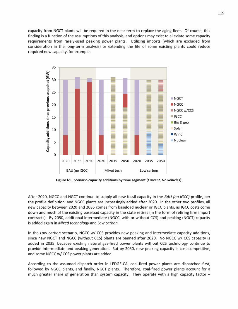
119

capacity from NGCT plants will be required in the near term to replace the aging fleet. Of course, this finding is a function of the assumptions of this analysis, and options may exist to alleviate some capacity requirements from rarely-used peaking power plants. Utilizing imports (which are excluded from consideration in the long-term analysis) or extending the life of some existing plants could reduce required new capacity, for example.

0

5

10

15

20

25

30

35

2020 2035 2050 2020 2035 2050 2020 2035 2050


Cap

acit

y ad

dit

ion

s si

nce

pre

vio

us

snap

sho

t (G

W)

NGCT

NGCC

NGCC w/CCS

IGCC

Bio & geo

Solar

Wind

Nuclear

Figure 61. Scenario capacity additions by time segment (Current, No vehicles).

After 2020, NGCC and NGCT continue to supply all new fossil capacity in the BAU (no IGCC) profile, per the profile definition, and NGCC plants are increasingly added after 2020. In the other two profiles, all new capacity between 2020 and 2035 comes from baseload nuclear or IGCC plants, as IGCC costs come down and much of the existing baseload capacity in the state retires (in the form of retiring firm import contracts). By 2050, additional intermediate (NGCC, with or without CCS) and peaking (NGCT) capacity is added again in Mixed technology and Low carbon.

In the Low carbon scenario, NGCC w/ CCS provides new peaking and intermediate capacity additions, since new NGCT and NGCC (without CCS) plants are banned after 2020. No NGCC w/ CCS capacity is added in 2035, because existing natural gas-fired power plants without CCS technology continue to provide intermediate and peaking generation. But by 2050, new peaking capacity is cost-competitive, and some NGCC w/ CCS power plants are added.

According to the assumed dispatch order in LEDGE-CA, coal-fired power plants are dispatched first, followed by NGCC plants, and finally, NGCT plants. Therefore, coal-fired power plants account for a much greater share of generation than system capacity. They operate with a high capacity factor –

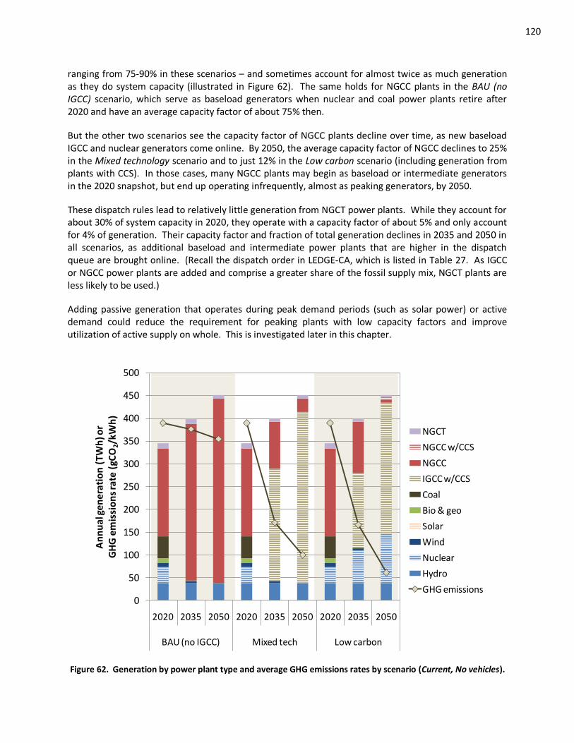
120

ranging from 75-90% in these scenarios – and sometimes account for almost twice as much generation as they do system capacity (illustrated in Figure 62). The same holds for NGCC plants in the BAU (no IGCC) scenario, which serve as baseload generators when nuclear and coal power plants retire after 2020 and have an average capacity factor of about 75% then.

But the other two scenarios see the capacity factor of NGCC plants decline over time, as new baseload IGCC and nuclear generators come online. By 2050, the average capacity factor of NGCC declines to 25% in the Mixed technology scenario and to just 12% in the Low carbon scenario (including generation from plants with CCS). In those cases, many NGCC plants may begin as baseload or intermediate generators in the 2020 snapshot, but end up operating infrequently, almost as peaking generators, by 2050.

These dispatch rules lead to relatively little generation from NGCT power plants. While they account for about 30% of system capacity in 2020, they operate with a capacity factor of about 5% and only account for 4% of generation. Their capacity factor and fraction of total generation declines in 2035 and 2050 in all scenarios, as additional baseload and intermediate power plants that are higher in the dispatch queue are brought online. (Recall the dispatch order in LEDGE-CA, which is listed in Table 27. As IGCC or NGCC power plants are added and comprise a greater share of the fossil supply mix, NGCT plants are less likely to be used.)

Adding passive generation that operates during peak demand periods (such as solar power) or active demand could reduce the requirement for peaking plants with low capacity factors and improve utilization of active supply on whole. This is investigated later in this chapter.

0

50

100

150

200

250

300

350

400

450

500

2020 2035 2050 2020 2035 2050 2020 2035 2050


An

nu

al g

en

era

tio

n (

TW

h) o

r

G

HG

em

issi

on

s ra

te (

gCO

2/k

Wh

)

NGCT

NGCC w/CCS

NGCC

IGCC w/CCS

Coal

Bio & geo

Solar

Wind

Nuclear

Hydro

GHG emissions

Figure 62. Generation by power plant type and average GHG emissions rates by scenario (Current, No vehicles).

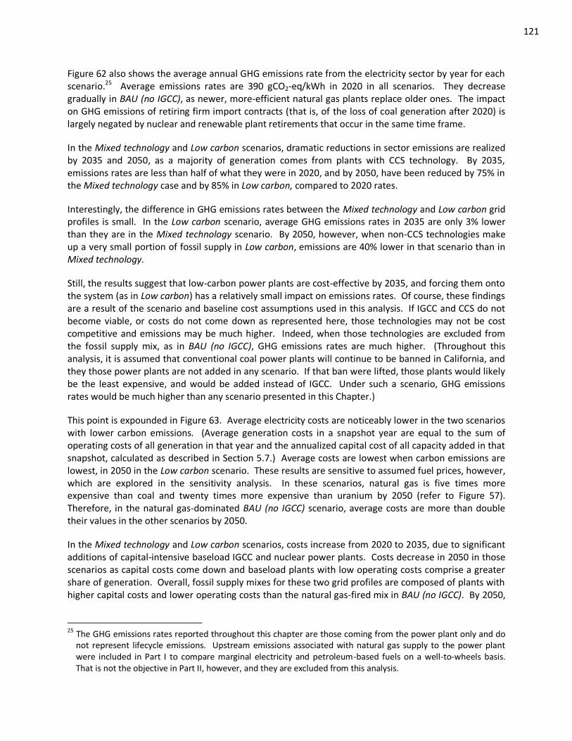
121

Figure 62 also shows the average annual GHG emissions rate from the electricity sector by year for each scenario.25 Average emissions rates are 390 gCO2-eq/kWh in 2020 in all scenarios. They decrease gradually in BAU (no IGCC), as newer, more-efficient natural gas plants replace older ones. The impact on GHG emissions of retiring firm import contracts (that is, of the loss of coal generation after 2020) is largely negated by nuclear and renewable plant retirements that occur in the same time frame.

In the Mixed technology and Low carbon scenarios, dramatic reductions in sector emissions are realized by 2035 and 2050, as a majority of generation comes from plants with CCS technology. By 2035, emissions rates are less than half of what they were in 2020, and by 2050, have been reduced by 75% in the Mixed technology case and by 85% in Low carbon, compared to 2020 rates.

Interestingly, the difference in GHG emissions rates between the Mixed technology and Low carbon grid profiles is small. In the Low carbon scenario, average GHG emissions rates in 2035 are only 3% lower than they are in the Mixed technology scenario. By 2050, however, when non-CCS technologies make up a very small portion of fossil supply in Low carbon, emissions are 40% lower in that scenario than in Mixed technology.

Still, the results suggest that low-carbon power plants are cost-effective by 2035, and forcing them onto the system (as in Low carbon) has a relatively small impact on emissions rates. Of course, these findings are a result of the scenario and baseline cost assumptions used in this analysis. If IGCC and CCS do not become viable, or costs do not come down as represented here, those technologies may not be cost competitive and emissions may be much higher. Indeed, when those technologies are excluded from the fossil supply mix, as in BAU (no IGCC), GHG emissions rates are much higher. (Throughout this analysis, it is assumed that conventional coal power plants will continue to be banned in California, and they those power plants are not added in any scenario. If that ban were lifted, those plants would likely be the least expensive, and would be added instead of IGCC. Under such a scenario, GHG emissions rates would be much higher than any scenario presented in this Chapter.)

This point is expounded in Figure 63. Average electricity costs are noticeably lower in the two scenarios with lower carbon emissions. (Average generation costs in a snapshot year are equal to the sum of operating costs of all generation in that year and the annualized capital cost of all capacity added in that snapshot, calculated as described in Section 5.7.) Average costs are lowest when carbon emissions are lowest, in 2050 in the Low carbon scenario. These results are sensitive to assumed fuel prices, however, which are explored in the sensitivity analysis. In these scenarios, natural gas is five times more expensive than coal and twenty times more expensive than uranium by 2050 (refer to Figure 57). Therefore, in the natural gas-dominated BAU (no IGCC) scenario, average costs are more than double their values in the other scenarios by 2050.

In the Mixed technology and Low carbon scenarios, costs increase from 2020 to 2035, due to significant additions of capital-intensive baseload IGCC and nuclear power plants. Costs decrease in 2050 in those scenarios as capital costs come down and baseload plants with low operating costs comprise a greater share of generation. Overall, fossil supply mixes for these two grid profiles are composed of plants with higher capital costs and lower operating costs than the natural gas-fired mix in BAU (no IGCC). By 2050,

25

The GHG emissions rates reported throughout this chapter are those coming from the power plant only and do not represent lifecycle emissions. Upstream emissions associated with natural gas supply to the power plant were included in Part I to compare marginal electricity and petroleum-based fuels on a well-to-wheels basis. That is not the objective in Part II, however, and they are excluded from this analysis.

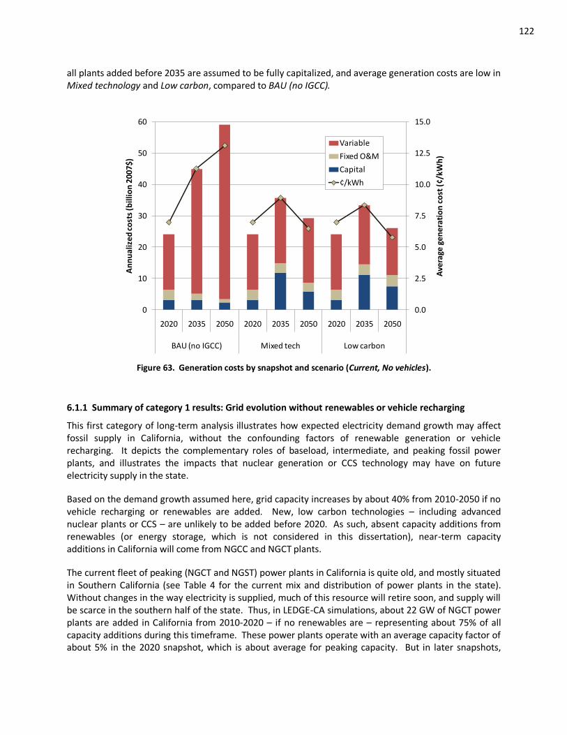
122

all plants added before 2035 are assumed to be fully capitalized, and average generation costs are low in Mixed technology and Low carbon, compared to BAU (no IGCC).

0.0

2.5

5.0

7.5

10.0

12.5

15.0

0

10

20

30

40

50

60

2020 2035 2050 2020 2035 2050 2020 2035 2050


Ave

rage

ge

ne

rati

on

co

st (

¢/k

Wh

)

An

nu

aliz

ed

co

sts

(bill

ion

20

07

$)

Variable

Fixed O&M

Capital

¢/kWh

Figure 63. Generation costs by snapshot and scenario (Current, No vehicles).

6.1.1 Summary of category 1 results: Grid evolution without renewables or vehicle recharging

This first category of long-term analysis illustrates how expected electricity demand growth may affect fossil supply in California, without the confounding factors of renewable generation or vehicle recharging. It depicts the complementary roles of baseload, intermediate, and peaking fossil power plants, and illustrates the impacts that nuclear generation or CCS technology may have on future electricity supply in the state.

Based on the demand growth assumed here, grid capacity increases by about 40% from 2010-2050 if no vehicle recharging or renewables are added. New, low carbon technologies – including advanced nuclear plants or CCS – are unlikely to be added before 2020. As such, absent capacity additions from renewables (or energy storage, which is not considered in this dissertation), near-term capacity additions in California will come from NGCC and NGCT plants.

The current fleet of peaking (NGCT and NGST) power plants in California is quite old, and mostly situated in Southern California (see Table 4 for the current mix and distribution of power plants in the state). Without changes in the way electricity is supplied, much of this resource will retire soon, and supply will be scarce in the southern half of the state. Thus, in LEDGE-CA simulations, about 22 GW of NGCT power plants are added in California from 2010-2020 – if no renewables are – representing about 75% of all capacity additions during this timeframe. These power plants operate with an average capacity factor of about 5% in the 2020 snapshot, which is about average for peaking capacity. But in later snapshots,

123

when more intermediate and baseload capacity is added, these power plants are even more poorly utilized.

Much of the existing baseload capacity supplying California is slated to retire in the 2020s. Included are the state’s two nuclear power plants and most firm import contracts supplying coal power from out-of-state. Coupled with the fact that peaking power plant capacity is almost entirely replaced from 2010-2020, capacity additions from 2020-2035 are mostly from baseload power plants, in LEDGE-CA. Technology costs are projected to decline sufficiently by the 2035 snapshot that IGCC w/ CCS accounts for all new fossil capacity in the Mixed technology and Low carbon grid profiles.

After 2035, the system is more balanced, and capacity additions reflect a mix of baseload, intermediate, and peaking power plants, if no renewables or vehicle recharging are added.

Without added renewable capacity, average emissions rates in 2020 are similar to their level today. Most generation supplying annual demand increases come from NGCC power plants, whose GHG emissions rate is similar to the current average in California. If natural gas-fired plants without CCS technology continue to provide all new capacity in the state, as in the BAU (no IGCC) grid profile, emissions rates gradually decline over time, as older power plants retire and are replaced with newer, more efficient ones.

Retiring firm import contracts, nuclear power plants, and renewable generators have little effect on average emissions rates over time. Coal-heavy firm imports are among the highest-emitting plants serving California, while nuclear and renewable generators operate with essentially zero GHG emissions. The average emissions rate from those sources collectively is roughly equal to the state’s current average. And because those plants retire in the same time period, between the 2020 and 2035 snapshots, their impact on emissions of these retirements essentially cancels out.

The impact on costs of retiring firm import contracts, nuclear plants, and renewable generators is noticeable, however. Those plants are assumed to be fully capitalized, and provide low-cost generation for California. When they retire after 2020, generation costs spike in the 2035 snapshot in all scenarios considered here (recall that plants are assumed to have a 40-year life span, and that generation costs in a snapshot year include operating costs from all power plants and capital costs for all plants added since the previous snapshot). If IGCC, CCS, and advanced nuclear technology become viable, GHG emissions and generating costs are lower in 2050. These power plants have high capital costs, but low operating costs. By 2050, a significant baseload resource exists that has been capitalized (all those plants added before 2035), and it offers low-cost generation for California ratepayers.

In addition to the assumed technology costs, these findings are highly sensitive to energy price assumptions. If natural gas prices do not increase as projected here, IGCC w/ CCS may not be cost-effective (see the discussion in Section 6.5), and significant contributions from renewable generators or carbon pricing might be required to achieve deep reductions in GHG emissions.

6.2 Long-term Results: Added Vehicle Electricity Demand, No New Renewables (Category 2)

Now, vehicle electricity demand is added to these scenarios without additional renewable generation to account for recharging impacts on fossil supply.

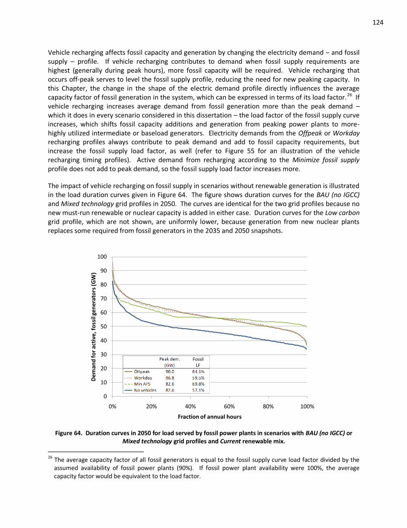
124

Vehicle recharging affects fossil capacity and generation by changing the electricity demand – and fossil supply – profile. If vehicle recharging contributes to demand when fossil supply requirements are highest (generally during peak hours), more fossil capacity will be required. Vehicle recharging that occurs off-peak serves to level the fossil supply profile, reducing the need for new peaking capacity. In this Chapter, the change in the shape of the electric demand profile directly influences the average capacity factor of fossil generation in the system, which can be expressed in terms of its load factor.26 If vehicle recharging increases average demand from fossil generation more than the peak demand – which it does in every scenario considered in this dissertation – the load factor of the fossil supply curve increases, which shifts fossil capacity additions and generation from peaking power plants to more-highly utilized intermediate or baseload generators. Electricity demands from the Offpeak or Workday recharging profiles always contribute to peak demand and add to fossil capacity requirements, but increase the fossil supply load factor, as well (refer to Figure 55 for an illustration of the vehicle recharging timing profiles). Active demand from recharging according to the Minimize fossil supply profile does not add to peak demand, so the fossil supply load factor increases more.

The impact of vehicle recharging on fossil supply in scenarios without renewable generation is illustrated in the load duration curves given in Figure 64. The figure shows duration curves for the BAU (no IGCC) and Mixed technology grid profiles in 2050. The curves are identical for the two grid profiles because no new must-run renewable or nuclear capacity is added in either case. Duration curves for the Low carbon grid profile, which are not shown, are uniformly lower, because generation from new nuclear plants replaces some required from fossil generators in the 2035 and 2050 snapshots.

0

10

20

30

40

50

60

70

80

90

100

0% 20% 40% 60% 80% 100%

Dem

and

for

acti

ve, f

oss

il ge

ner

ato

rs (G

W)


Fossil LF

Figure 64. Duration curves in 2050 for load served by fossil power plants in scenarios with BAU (no IGCC) or Mixed technology grid profiles and Current renewable mix.

26

The average capacity factor of all fossil generators is equal to the fossil supply curve load factor divided by the assumed availability of fossil power plants (90%). If fossil power plant availability were 100%, the average capacity factor would be equivalent to the load factor.

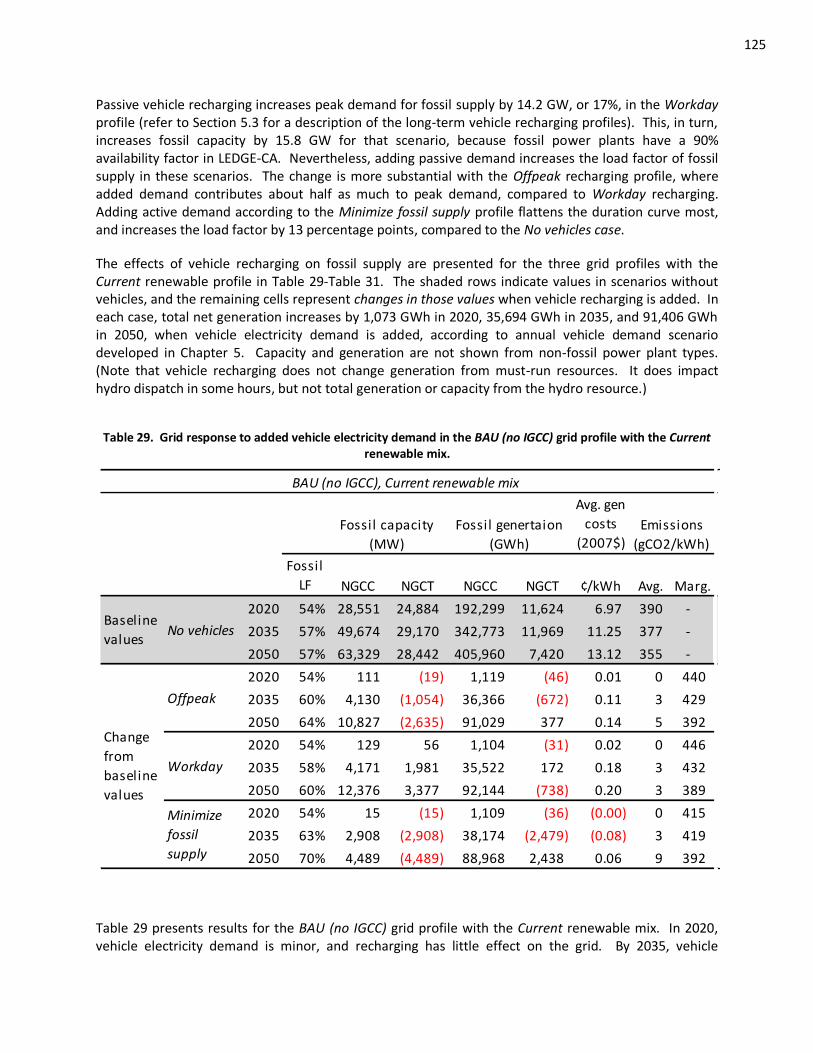
125

Passive vehicle recharging increases peak demand for fossil supply by 14.2 GW, or 17%, in the Workday profile (refer to Section 5.3 for a description of the long-term vehicle recharging profiles). This, in turn, increases fossil capacity by 15.8 GW for that scenario, because fossil power plants have a 90% availability factor in LEDGE-CA. Nevertheless, adding passive demand increases the load factor of fossil supply in these scenarios. The change is more substantial with the Offpeak recharging profile, where added demand contributes about half as much to peak demand, compared to Workday recharging. Adding active demand according to the Minimize fossil supply profile flattens the duration curve most, and increases the load factor by 13 percentage points, compared to the No vehicles case.

The effects of vehicle recharging on fossil supply are presented for the three grid profiles with the Current renewable profile in Table 29-Table 31. The shaded rows indicate values in scenarios without vehicles, and the remaining cells represent changes in those values when vehicle recharging is added. In each case, total net generation increases by 1,073 GWh in 2020, 35,694 GWh in 2035, and 91,406 GWh in 2050, when vehicle electricity demand is added, according to annual vehicle demand scenario developed in Chapter 5. Capacity and generation are not shown from non-fossil power plant types. (Note that vehicle recharging does not change generation from must-run resources. It does impact hydro dispatch in some hours, but not total generation or capacity from the hydro resource.)

Table 29. Grid response to added vehicle electricity demand in the BAU (no IGCC) grid profile with the Current renewable mix.

Avg. gen

costs

(2007$)

Fossil

LF NGCC NGCT NGCC NGCT ¢/kWh Avg. Marg.

2020 54% 28,551 24,884 192,299 11,624 6.97 390 -

2035 57% 49,674 29,170 342,773 11,969 11.25 377 -

2050 57% 63,329 28,442 405,960 7,420 13.12 355 -

2020 54% 111 (19) 1,119 (46) 0.01 0 440

2035 60% 4,130 (1,054) 36,366 (672) 0.11 3 429

2050 64% 10,827 (2,635) 91,029 377 0.14 5 392

2020 54% 129 56 1,104 (31) 0.02 0 446

2035 58% 4,171 1,981 35,522 172 0.18 3 432

2050 60% 12,376 3,377 92,144 (738) 0.20 3 389

2020 54% 15 (15) 1,109 (36) (0.00) 0 415

2035 63% 2,908 (2,908) 38,174 (2,479) (0.08) 3 419

2050 70% 4,489 (4,489) 88,968 2,438 0.06 9 392

Change

from

baseline

values

Offpeak

Workday

Minimize

fossil

supply

BAU (no IGCC), Current renewable mix

Fossil capacity

(MW)

Fossil genertaion

(GWh)

Emissions

(gCO2/kWh)

Baseline

valuesNo vehicles

Table 29 presents results for the BAU (no IGCC) grid profile with the Current renewable mix. In 2020, vehicle electricity demand is minor, and recharging has little effect on the grid. By 2035, vehicle

126

recharging has a greater impact on peak demand and increases fossil capacity by about 3.1 GW for Offpeak recharging and twice that in the Workday profile. In 2050, Offpeak and Workday recharging increase fossil capacity by 8.2 GW and 15.8 GW, respectively. In the Minimize fossil supply profile, vehicle electricity demand does not contribute to peak fossil supply requirements, and no new capacity is needed, compared to the baseline BAU (no IGCC) scenario. Compared to the other recharging profiles, the Minimize fossil supply profile has lower average electricity costs, because fossil power plants are better utilized.

In addition to the change in peak demand, vehicle recharging changes the shape of the fossil supply profile, affecting the fossil supply load factor, the mix of new fossil capacity as determined by the screening curve analysis in LEDGE-CA, and the distribution of generation among fossil plants according to the dispatch rules described in Section 5.8.

Offpeak and Minimize fossil supply reduce peaking capacity from NGCT plants and add to intermediate or baseload capacity from NGCC plants. In Offpeak, NGCT capacity declines by 9% and NGCC capacity increases by 17% in 2050. Minimize fossil supply shifts 16% of NGCT capacity to NGCC plants in 2050, increasing capacity of that resource by 7%. While Workday recharging also increases the load factor compared to No vehicles, it only does slightly, and NGCT capacity is also added to supply vehicle electricity demand. But because the load factor is higher than with No vehicles, NGCC plants account for a greater fraction of added fossil capacity than their share of fossil capacity with No vehicles. Overall, Workday recharging increases NGCT capacity by 12% and NGCC capacity by 20%, based on the BAU (no IGCC), Current supply profile.

In addition to shifting capacity from NGCT to NGCC, adding vehicle electricity demand increases generation from NGCC power plants. In all of the snapshots and scenarios considered in Table 29, NGCC power plants provide the vast majority – and often the entirety – of additional generation required compared to the No vehicles case.

The result of these shifts in capacity and generation are increased average capacity factors of fossil power plants in scenarios that include vehicle electricity demand. In this analysis, the average fossil capacity factor is equal to 90% of the fossil supply load factor, since all fossil power plants are assumed to have that availability. The impact is minimal in 2020, when electricity demand from vehicles accounts for a very small fraction of the total, but by 2050, average capacity factors are 63% in the Minimize fossil supply profile, compared to 51% in the baseline, No vehicles case. Vehicle electricity demand serves to increase average capacity factors in the other scenarios, as well, but to a lesser extent. Average capacity factors are 58% and 54% in 2050 in the scenarios including the Offpeak and Workday recharging profiles, respectively.27

This improvement in power plant utilization does not lead to lower average generation costs or GHG emissions, however. The cost of additional power plant capacity and generation to supply 91 TWh of electricity demand for vehicles in the 2050 snapshot exceeds $12 billion (in 2007 dollars) for all vehicle

27

These capacity factors are likely higher than would actually be realized in the power sector, and are provided simply for the sake of comparing scenarios. This analysis ignores reserve requirements, as well as many other constraining factors that affect electricity supply, which would likely lead to more overall capacity and lower utilization rates of power plants.

127

timing profiles applied to the BAU (no IGCC) grid profile.28 Assuming the energy content of California reformulated gasoline is 115.63 MJ/gallon [24], these additional costs range from an equivalent of $4.30/gallon gasoline in the Minimize fossil supply recharging profile to $4.60/gallon gasoline in the Workday profile, on an energy basis.29 Variable costs of power generation dominate the cost of electricity supply for vehicles, which in turn, are dominated by the price of natural gas and are highly sensitive to it, as explored in Section 6.5.

Average GHG emission rates change little when vehicle recharging is added to the grid in the BAU (no IGCC) profile. With No vehicles, average emissions rates are just below those from new NGCC plants in each year. Most additional generation supplying vehicle recharging comes from those plants, and the increase in demand has little effect on average GHG emissions rates. They increase slightly because the share of hydro generation decreases when electricity demand increases, since the resource is energy-constrained. Marginal emissions rates from the last generators supplying electricity equal to vehicle demand are somewhat higher, and represent a mix of NGCC and NGCT plants. They decrease over time as newer plants come online that have lower emissions rates than plants from an earlier vintage.

Many similar trends appear when vehicle recharging is imposed on the grid in the Mixed technology profile (Table 30). The effect of vehicle recharging on the fossil supply curve is the same as for the BAU (no IGCC) grid profile, since no nuclear or renewable generation is added in these scenarios. Therefore, total capacity in these scenarios is the same as in scenarios with the BAU (no IGCC) grid profile and peaking capacity shifts to intermediate or baseload capacity in a similar manner. In Mixed technology, IGCC w/ CCS plants comprise a significant share of supply and much of the avoided NGCT capacity shifts to IGCC w/ CCS when vehicle recharging is added. More NGCT capacity is avoided by 2050 with Offpeak and Minimize fossil supply recharging in the Mixed technology cases, compared to BAU (no IGCC), but average fossil plant utilization remains constant for a given recharging profile, since the same levels of total fossil capacity and generation are required for either grid profile.

Costs associated with providing electricity for vehicles are noticeably less in for the Mixed technology profile, because of less reliance on relatively expensive natural gas. In these scenarios, additional electricity sector costs for vehicle recharging range from $5.4-6.7 billion in 2050, equivalent to $1.91-2.31/gallon gasoline on an energy basis, in 2007 dollars. The increase in costs from vehicle recharging in Mixed technology also tend to be lower than those from scenarios with the BAU (no IGCC) grid profile, because more generation tends to shift from peaking to baseload plants in the Mixed technology profile.

Emissions rates vary more noticeably in these scenarios than for the BAU (no IGCC) profile, since there is a greater diversity of fossil power plants supplying demand. This is most noticeable in the snapshot for the year 2035, when IGCC power plants are first cost competitive for this grid profile.

The greatest increase in GHG emissions rates in that snapshot year comes in the Minimize fossil supply profile. With that recharging profile, no new fossil capacity is required, and in 2035, no more IGCC w/ CCS capacity exists than without vehicle recharging. Therefore, natural gas-fired power plants

28 Total incremental generation costs in a snapshot year (in billions) are not given in the table, but can be

determined by multiplying the average generation cost (¢/kWh) by total annual demand (451 TWh for non-vehicle electricity demand, plus 91 TWh for vehicle electricity demand, in 2050).

29 Recall that costs for a snapshot year reflect capital costs of power plants added since the previous snapshot, and operating costs of all generation in that year. The per-gallon gasoline cost represents a simple comparison, based on the costing methods in LEDGE-CA, and accounts for capital costs of power plants required to supply added vehicle recharging.

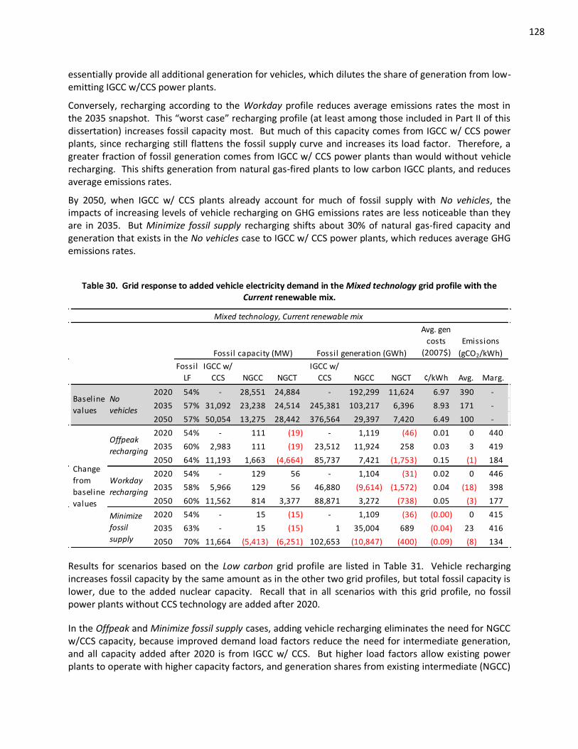
128

essentially provide all additional generation for vehicles, which dilutes the share of generation from low-emitting IGCC w/CCS power plants.

Conversely, recharging according to the Workday profile reduces average emissions rates the most in the 2035 snapshot. This “worst case” recharging profile (at least among those included in Part II of this dissertation) increases fossil capacity most. But much of this capacity comes from IGCC w/ CCS power plants, since recharging still flattens the fossil supply curve and increases its load factor. Therefore, a greater fraction of fossil generation comes from IGCC w/ CCS power plants than would without vehicle recharging. This shifts generation from natural gas-fired plants to low carbon IGCC plants, and reduces average emissions rates.

By 2050, when IGCC w/ CCS plants already account for much of fossil supply with No vehicles, the impacts of increasing levels of vehicle recharging on GHG emissions rates are less noticeable than they are in 2035. But Minimize fossil supply recharging shifts about 30% of natural gas-fired capacity and generation that exists in the No vehicles case to IGCC w/ CCS power plants, which reduces average GHG emissions rates.

Table 30. Grid response to added vehicle electricity demand in the Mixed technology grid profile with the Current renewable mix.

Avg. gen

costs

(2007$)

Fossil

LF

IGCC w/

CCS NGCC NGCT

IGCC w/

CCS NGCC NGCT ¢/kWh Avg. Marg.

2020 54% - 28,551 24,884 - 192,299 11,624 6.97 390 -

2035 57% 31,092 23,238 24,514 245,381 103,217 6,396 8.93 171 -

2050 57% 50,054 13,275 28,442 376,564 29,397 7,420 6.49 100 -

2020 54% - 111 (19) - 1,119 (46) 0.01 0 440

2035 60% 2,983 111 (19) 23,512 11,924 258 0.03 3 419

2050 64% 11,193 1,663 (4,664) 85,737 7,421 (1,753) 0.15 (1) 184

2020 54% - 129 56 - 1,104 (31) 0.02 0 446

2035 58% 5,966 129 56 46,880 (9,614) (1,572) 0.04 (18) 398

2050 60% 11,562 814 3,377 88,871 3,272 (738) 0.05 (3) 177

2020 54% - 15 (15) - 1,109 (36) (0.00) 0 415

2035 63% - 15 (15) 1 35,004 689 (0.04) 23 416

2050 70% 11,664 (5,413) (6,251) 102,653 (10,847) (400) (0.09) (8) 134

Baseline

values

No

vehicles

Change

from

baseline

values

Offpeak

recharging

Workday

recharging

Minimize

fossil

supply

Mixed technology, Current renewable mix

Fossil capacity (MW) Fossil generation (GWh)

Emissions

(gCO2/kWh)

Results for scenarios based on the Low carbon grid profile are listed in Table 31. Vehicle recharging increases fossil capacity by the same amount as in the other two grid profiles, but total fossil capacity is lower, due to the added nuclear capacity. Recall that in all scenarios with this grid profile, no fossil power plants without CCS technology are added after 2020.

In the Offpeak and Minimize fossil supply cases, adding vehicle recharging eliminates the need for NGCC w/CCS capacity, because improved demand load factors reduce the need for intermediate generation, and all capacity added after 2020 is from IGCC w/ CCS. But higher load factors allow existing power plants to operate with higher capacity factors, and generation shares from existing intermediate (NGCC)

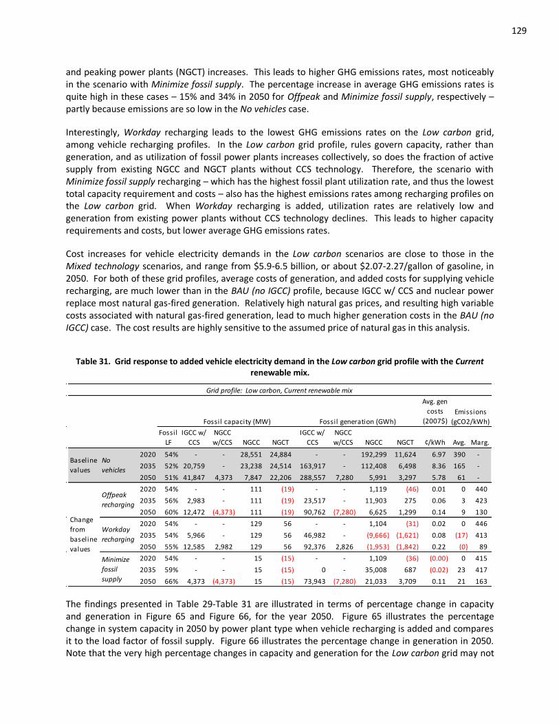
129

and peaking power plants (NGCT) increases. This leads to higher GHG emissions rates, most noticeably in the scenario with Minimize fossil supply. The percentage increase in average GHG emissions rates is quite high in these cases – 15% and 34% in 2050 for Offpeak and Minimize fossil supply, respectively – partly because emissions are so low in the No vehicles case.

Interestingly, Workday recharging leads to the lowest GHG emissions rates on the Low carbon grid, among vehicle recharging profiles. In the Low carbon grid profile, rules govern capacity, rather than generation, and as utilization of fossil power plants increases collectively, so does the fraction of active supply from existing NGCC and NGCT plants without CCS technology. Therefore, the scenario with Minimize fossil supply recharging – which has the highest fossil plant utilization rate, and thus the lowest total capacity requirement and costs – also has the highest emissions rates among recharging profiles on the Low carbon grid. When Workday recharging is added, utilization rates are relatively low and generation from existing power plants without CCS technology declines. This leads to higher capacity requirements and costs, but lower average GHG emissions rates.

Cost increases for vehicle electricity demands in the Low carbon scenarios are close to those in the Mixed technology scenarios, and range from $5.9-6.5 billion, or about $2.07-2.27/gallon of gasoline, in 2050. For both of these grid profiles, average costs of generation, and added costs for supplying vehicle recharging, are much lower than in the BAU (no IGCC) profile, because IGCC w/ CCS and nuclear power replace most natural gas-fired generation. Relatively high natural gas prices, and resulting high variable costs associated with natural gas-fired generation, lead to much higher generation costs in the BAU (no IGCC) case. The cost results are highly sensitive to the assumed price of natural gas in this analysis.

Table 31. Grid response to added vehicle electricity demand in the Low carbon grid profile with the Current renewable mix.

Avg. gen

costs

(2007$)

Fossil

LF

IGCC w/

CCS

NGCC

w/CCS NGCC NGCT

IGCC w/

CCS

NGCC

w/CCS NGCC NGCT ¢/kWh Avg. Marg.

2020 54% - - 28,551 24,884 - - 192,299 11,624 6.97 390 -

2035 52% 20,759 - 23,238 24,514 163,917 - 112,408 6,498 8.36 165 -

2050 51% 41,847 4,373 7,847 22,206 288,557 7,280 5,991 3,297 5.78 61 -

2020 54% - - 111 (19) - - 1,119 (46) 0.01 0 440

2035 56% 2,983 - 111 (19) 23,517 - 11,903 275 0.06 3 423

2050 60% 12,472 (4,373) 111 (19) 90,762 (7,280) 6,625 1,299 0.14 9 130

2020 54% - - 129 56 - - 1,104 (31) 0.02 0 446

2035 54% 5,966 - 129 56 46,982 - (9,666) (1,621) 0.08 (17) 413

2050 55% 12,585 2,982 129 56 92,376 2,826 (1,953) (1,842) 0.22 (0) 89

2020 54% - - 15 (15) - - 1,109 (36) (0.00) 0 415

2035 59% - - 15 (15) 0 - 35,008 687 (0.02) 23 417

2050 66% 4,373 (4,373) 15 (15) 73,943 (7,280) 21,033 3,709 0.11 21 163

Grid profile: Low carbon, Current renewable mix

Baseline

values

No

vehicles

Change

from

baseline

values

Offpeak

recharging

Workday

recharging

Minimize

fossil

supply


Emissions

(gCO2/kWh)

The findings presented in Table 29-Table 31 are illustrated in terms of percentage change in capacity and generation in Figure 65 and Figure 66, for the year 2050. Figure 65 illustrates the percentage change in system capacity in 2050 by power plant type when vehicle recharging is added and compares it to the load factor of fossil supply. Figure 66 illustrates the percentage change in generation in 2050. Note that the very high percentage changes in capacity and generation for the Low carbon grid may not

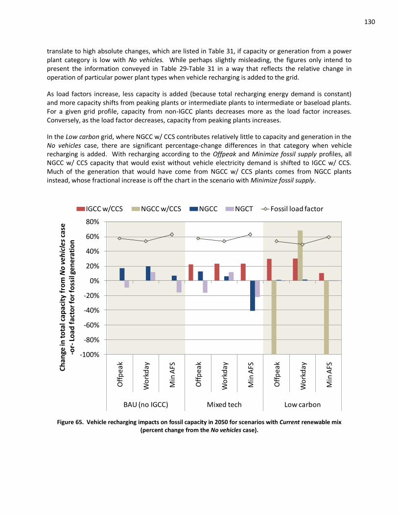
130

translate to high absolute changes, which are listed in Table 31, if capacity or generation from a power plant category is low with No vehicles. While perhaps slightly misleading, the figures only intend to present the information conveyed in Table 29-Table 31 in a way that reflects the relative change in operation of particular power plant types when vehicle recharging is added to the grid.

As load factors increase, less capacity is added (because total recharging energy demand is constant) and more capacity shifts from peaking plants or intermediate plants to intermediate or baseload plants. For a given grid profile, capacity from non-IGCC plants decreases more as the load factor increases. Conversely, as the load factor decreases, capacity from peaking plants increases.

In the Low carbon grid, where NGCC w/ CCS contributes relatively little to capacity and generation in the No vehicles case, there are significant percentage-change differences in that category when vehicle recharging is added. With recharging according to the Offpeak and Minimize fossil supply profiles, all NGCC w/ CCS capacity that would exist without vehicle electricity demand is shifted to IGCC w/ CCS. Much of the generation that would have come from NGCC w/ CCS plants comes from NGCC plants instead, whose fractional increase is off the chart in the scenario with Minimize fossil supply.

-100%

-80%

-60%

-40%

-20%

0%

20%

40%

60%

80%

Off

pea

k

Wo

rkd

ay

Min

AFS

Off

pea

k

Wo

rkd

ay

Min

AFS

Off

pea

k

Wo

rkd

ay

Min

AFS


Ch

ange

in t

ota

l cap

acit

y fr

om

No

veh

icle

s ca

se

-o

r-Lo

ad f

acto

r fo

r fo

ssil

gen

erat

ion

IGCC w/CCS NGCC w/CCS NGCC NGCT Fossil load factor

Figure 65. Vehicle recharging impacts on fossil capacity in 2050 for scenarios with Current renewable mix (percent change from the No vehicles case).

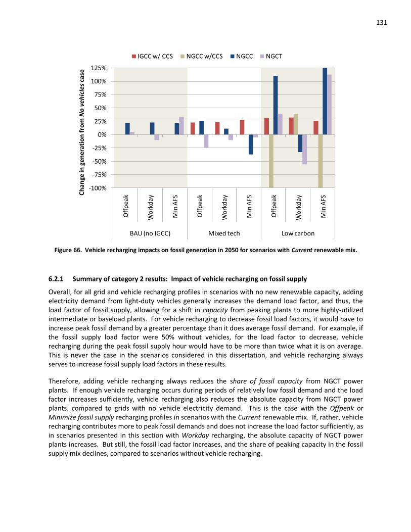
131

-100%

-75%

-50%

-25%

0%

25%

50%

75%

100%

125%

Off

pea

k

Wo

rkd

ay

Min

AFS

Off

pea

k

Wo

rkd

ay

Min

AFS

Off

pea

k

Wo

rkd

ay

Min

AFS


Ch

ange

in g

ener

atio

n f

rom

No

veh

icle

s ca

se

IGCC w/ CCS NGCC w/CCS NGCC NGCT

Figure 66. Vehicle recharging impacts on fossil generation in 2050 for scenarios with Current renewable mix.

6.2.1 Summary of category 2 results: Impact of vehicle recharging on fossil supply

Overall, for all grid and vehicle recharging profiles in scenarios with no new renewable capacity, adding electricity demand from light-duty vehicles generally increases the demand load factor, and thus, the load factor of fossil supply, allowing for a shift in capacity from peaking plants to more highly-utilized intermediate or baseload plants. For vehicle recharging to decrease fossil load factors, it would have to increase peak fossil demand by a greater percentage than it does average fossil demand. For example, if the fossil supply load factor were 50% without vehicles, for the load factor to decrease, vehicle recharging during the peak fossil supply hour would have to be more than twice what it is on average. This is never the case in the scenarios considered in this dissertation, and vehicle recharging always serves to increase fossil supply load factors in these results.

Therefore, adding vehicle recharging always reduces the share of fossil capacity from NGCT power plants. If enough vehicle recharging occurs during periods of relatively low fossil demand and the load factor increases sufficiently, vehicle recharging also reduces the absolute capacity from NGCT power plants, compared to grids with no vehicle electricity demand. This is the case with the Offpeak or Minimize fossil supply recharging profiles in scenarios with the Current renewable mix. If, rather, vehicle recharging contributes more to peak fossil demands and does not increase the load factor sufficiently, as in scenarios presented in this section with Workday recharging, the absolute capacity of NGCT power plants increases. But still, the fossil load factor increases, and the share of peaking capacity in the fossil supply mix declines, compared to scenarios without vehicle recharging.

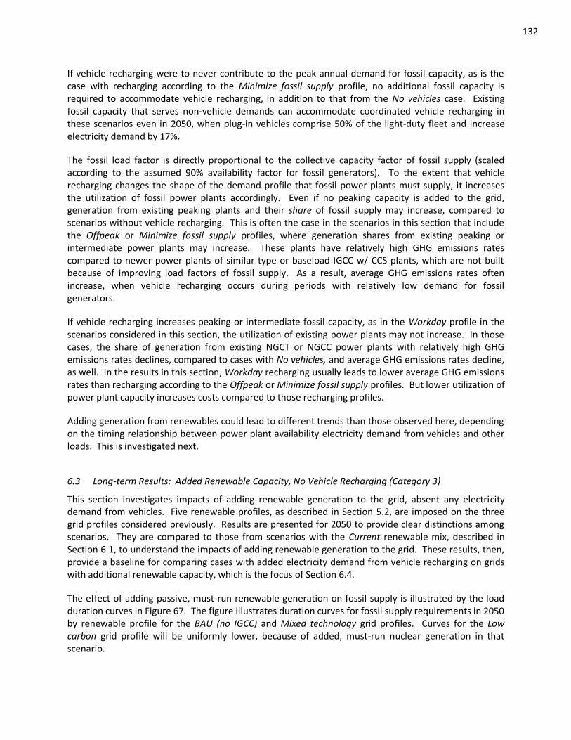
132

If vehicle recharging were to never contribute to the peak annual demand for fossil capacity, as is the case with recharging according to the Minimize fossil supply profile, no additional fossil capacity is required to accommodate vehicle recharging, in addition to that from the No vehicles case. Existing fossil capacity that serves non-vehicle demands can accommodate coordinated vehicle recharging in these scenarios even in 2050, when plug-in vehicles comprise 50% of the light-duty fleet and increase electricity demand by 17%.

The fossil load factor is directly proportional to the collective capacity factor of fossil supply (scaled according to the assumed 90% availability factor for fossil generators). To the extent that vehicle recharging changes the shape of the demand profile that fossil power plants must supply, it increases the utilization of fossil power plants accordingly. Even if no peaking capacity is added to the grid, generation from existing peaking plants and their share of fossil supply may increase, compared to scenarios without vehicle recharging. This is often the case in the scenarios in this section that include the Offpeak or Minimize fossil supply profiles, where generation shares from existing peaking or intermediate power plants may increase. These plants have relatively high GHG emissions rates compared to newer power plants of similar type or baseload IGCC w/ CCS plants, which are not built because of improving load factors of fossil supply. As a result, average GHG emissions rates often increase, when vehicle recharging occurs during periods with relatively low demand for fossil generators.

If vehicle recharging increases peaking or intermediate fossil capacity, as in the Workday profile in the scenarios considered in this section, the utilization of existing power plants may not increase. In those cases, the share of generation from existing NGCT or NGCC power plants with relatively high GHG emissions rates declines, compared to cases with No vehicles, and average GHG emissions rates decline, as well. In the results in this section, Workday recharging usually leads to lower average GHG emissions rates than recharging according to the Offpeak or Minimize fossil supply profiles. But lower utilization of power plant capacity increases costs compared to those recharging profiles.

Adding generation from renewables could lead to different trends than those observed here, depending on the timing relationship between power plant availability electricity demand from vehicles and other loads. This is investigated next.

6.3 Long-term Results: Added Renewable Capacity, No Vehicle Recharging (Category 3)

This section investigates impacts of adding renewable generation to the grid, absent any electricity demand from vehicles. Five renewable profiles, as described in Section 5.2, are imposed on the three grid profiles considered previously. Results are presented for 2050 to provide clear distinctions among scenarios. They are compared to those from scenarios with the Current renewable mix, described in Section 6.1, to understand the impacts of adding renewable generation to the grid. These results, then, provide a baseline for comparing cases with added electricity demand from vehicle recharging on grids with additional renewable capacity, which is the focus of Section 6.4.

The effect of adding passive, must-run renewable generation on fossil supply is illustrated by the load duration curves in Figure 67. The figure illustrates duration curves for fossil supply requirements in 2050 by renewable profile for the BAU (no IGCC) and Mixed technology grid profiles. Curves for the Low carbon grid profile will be uniformly lower, because of added, must-run nuclear generation in that scenario.

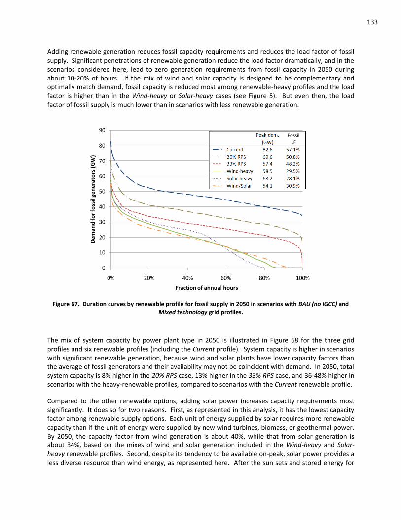
133

Adding renewable generation reduces fossil capacity requirements and reduces the load factor of fossil supply. Significant penetrations of renewable generation reduce the load factor dramatically, and in the scenarios considered here, lead to zero generation requirements from fossil capacity in 2050 during about 10-20% of hours. If the mix of wind and solar capacity is designed to be complementary and optimally match demand, fossil capacity is reduced most among renewable-heavy profiles and the load factor is higher than in the Wind-heavy or Solar-heavy cases (see Figure 5). But even then, the load factor of fossil supply is much lower than in scenarios with less renewable generation.

0

10

20

30

40

50

60

70

80

90

0% 20% 40% 60% 80% 100%

Dem

and

for

foss

il ge

ner

ato

rs (G

W)


Fossil LF

Figure 67. Duration curves by renewable profile for fossil supply in 2050 in scenarios with BAU (no IGCC) and Mixed technology grid profiles.

The mix of system capacity by power plant type in 2050 is illustrated in Figure 68 for the three grid profiles and six renewable profiles (including the Current profile). System capacity is higher in scenarios with significant renewable generation, because wind and solar plants have lower capacity factors than the average of fossil generators and their availability may not be coincident with demand. In 2050, total system capacity is 8% higher in the 20% RPS case, 13% higher in the 33% RPS case, and 36-48% higher in scenarios with the heavy-renewable profiles, compared to scenarios with the Current renewable profile.

Compared to the other renewable options, adding solar power increases capacity requirements most significantly. It does so for two reasons. First, as represented in this analysis, it has the lowest capacity factor among renewable supply options. Each unit of energy supplied by solar requires more renewable capacity than if the unit of energy were supplied by new wind turbines, biomass, or geothermal power. By 2050, the capacity factor from wind generation is about 40%, while that from solar generation is about 34%, based on the mixes of wind and solar generation included in the Wind-heavy and Solar-heavy renewable profiles. Second, despite its tendency to be available on-peak, solar power provides a less diverse resource than wind energy, as represented here. After the sun sets and stored energy for

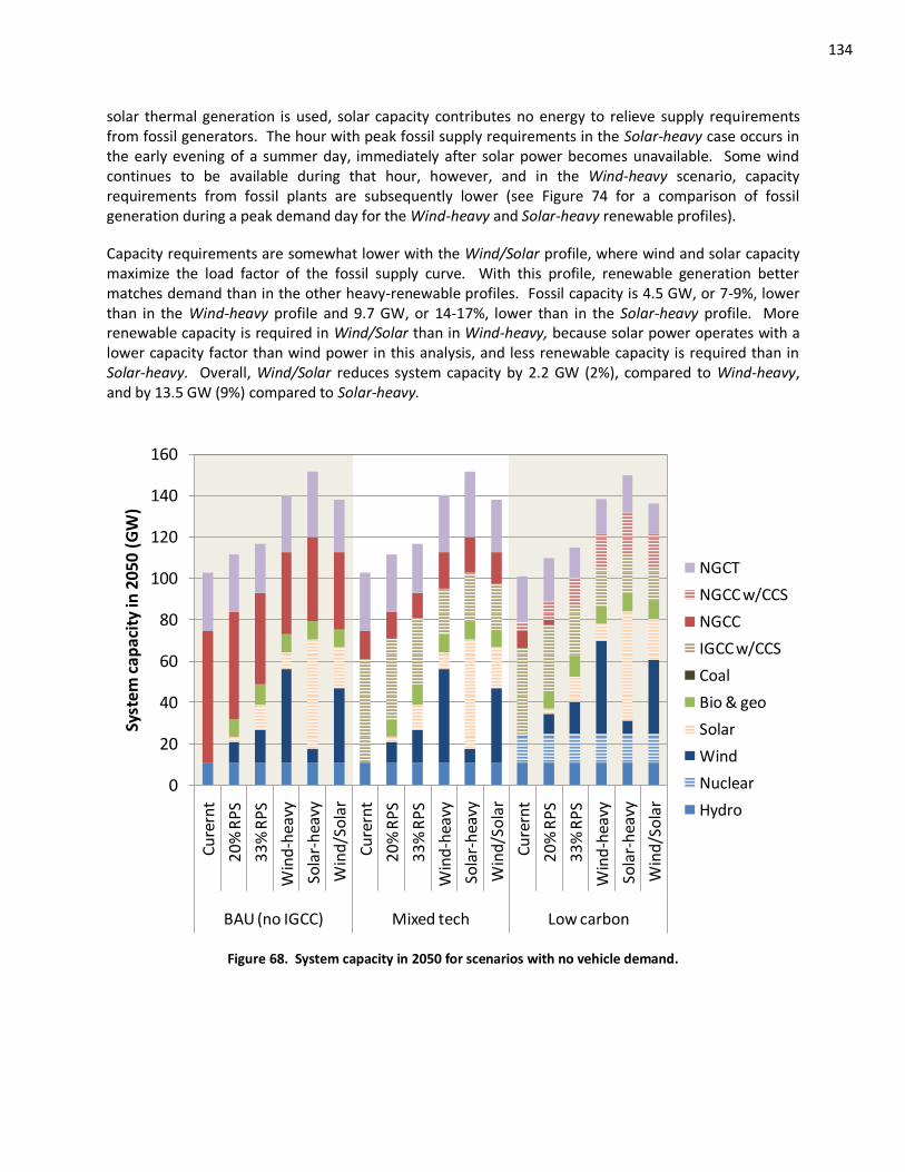
134

solar thermal generation is used, solar capacity contributes no energy to relieve supply requirements from fossil generators. The hour with peak fossil supply requirements in the Solar-heavy case occurs in the early evening of a summer day, immediately after solar power becomes unavailable. Some wind continues to be available during that hour, however, and in the Wind-heavy scenario, capacity requirements from fossil plants are subsequently lower (see Figure 74 for a comparison of fossil generation during a peak demand day for the Wind-heavy and Solar-heavy renewable profiles).

Capacity requirements are somewhat lower with the Wind/Solar profile, where wind and solar capacity maximize the load factor of the fossil supply curve. With this profile, renewable generation better matches demand than in the other heavy-renewable profiles. Fossil capacity is 4.5 GW, or 7-9%, lower than in the Wind-heavy profile and 9.7 GW, or 14-17%, lower than in the Solar-heavy profile. More renewable capacity is required in Wind/Solar than in Wind-heavy, because solar power operates with a lower capacity factor than wind power in this analysis, and less renewable capacity is required than in Solar-heavy. Overall, Wind/Solar reduces system capacity by 2.2 GW (2%), compared to Wind-heavy, and by 13.5 GW (9%) compared to Solar-heavy.

0

20

40

60

80

100

120

140

160

Cu

rern

t

20

% R

PS

33

% R

PS

Win

d-h

eavy

Sola

r-h

eavy

Win

d/S

ola

r

Cu

rern

t

20

% R

PS

33

% R

PS

Win

d-h

eavy

Sola

r-h

eavy

Win

d/S

ola

r

Cu

rern

t

20

% R

PS

33

% R

PS

Win

d-h

eavy

Sola

r-h

eavy

Win

d/S

ola

r


Syst

em

cap

acit

y in

20

50

(G

W)

NGCT

NGCC w/CCS

NGCC

IGCC w/CCS

Coal

Bio & geo

Solar

Wind

Nuclear

Hydro

Figure 68. System capacity in 2050 for scenarios with no vehicle demand.

135

The impact of renewable generation on grids with No vehicles is further explained in Figure 69. The figure illustrates the change in fossil capacity by power plant type in 2050 for each renewable and grid profile.

Adding renewable generation works opposite of the findings for adding vehicle recharging, which were discussed in Section 6.2. Must-run generation, both baseload or intermittent, reduces fossil capacity requirements and shifts capacity from baseload generators to intermediate or peaking power plants. This shift is more dramatic for renewable profiles that lead to lower fossil supply curve load factors. For example, in the Low carbon grid profile, which has the lowest fossil load factors, changes in fossil capacity are most significant, when renewable generation is added to the grid. In that grid profile, adding renewable generation reduces capacity from NGCC and NGCT plants that would otherwise be added in the 2020 snapshot. Those plants are not allowed to be added after 2020, so more NGCC w/ CCS is added in 2035 and 2050 when renewables are added, since that power plant type provides new “peaking” capacity in the Low carbon grid profile.

-30

-25

-20

-15

-10

-5

0

5

10

15

20

20

% R

PS

33

% R

PS

Win

d-h

eavy

Sola

r-h

eavy

Win

d/S

ola

r

20

% R

PS

33

% R

PS

Win

d-h

eavy

Sola

r-h

eavy

Win

d/S

ola

r

20

% R

PS

33

% R

PS

Win

d-h

eavy

Sola

r-h

eavy

Win

d/S

ola

r


Cap

acit

y ch

ange

fro

m C

urr

ent

ren

ew

able

mix

(G

W)


Figure 69. Change in fossil capacity in 2050 from added renewable generation in scenarios with No vehicles, compared to results with the Current renewable mix.

Although adding renewable generation tends to reduce NGCT capacity overall, its fraction of total fossil capacity tends to increase, because renewable generation decreases fossil supply load factors. The increase is most noticeable in the Solar-heavy profile, where the share of NGCT capacity increases by as much as 41%.

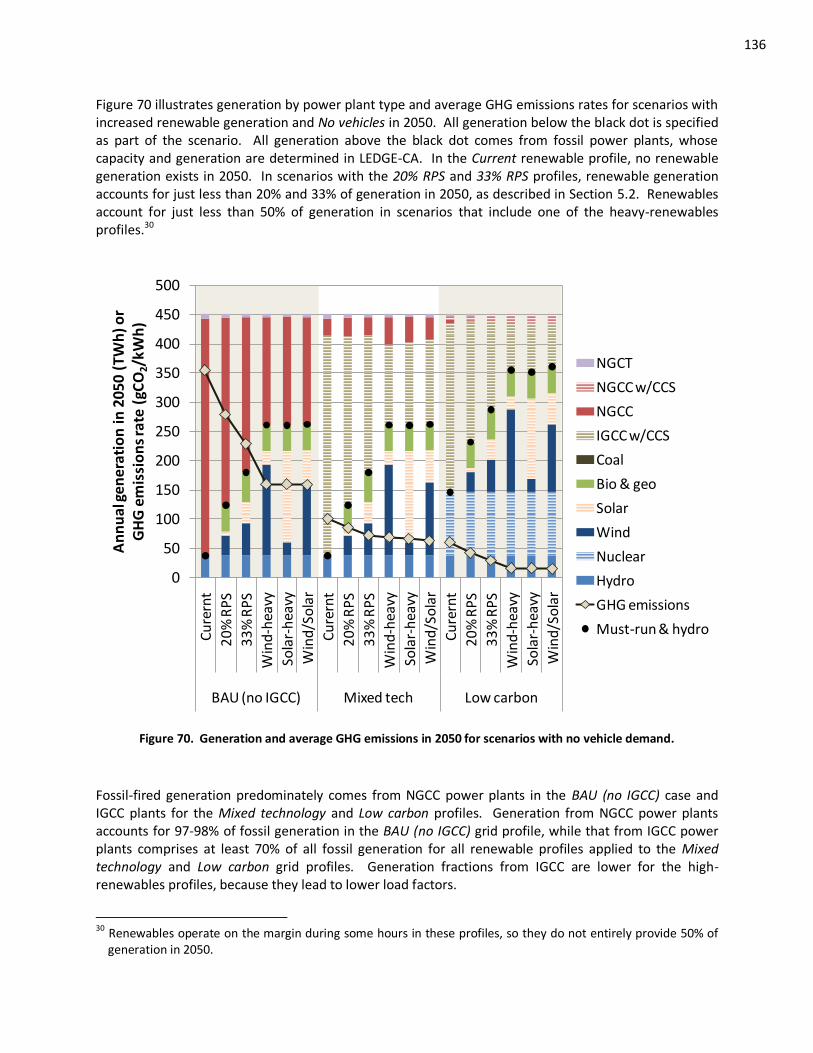
136

Figure 70 illustrates generation by power plant type and average GHG emissions rates for scenarios with increased renewable generation and No vehicles in 2050. All generation below the black dot is specified as part of the scenario. All generation above the black dot comes from fossil power plants, whose capacity and generation are determined in LEDGE-CA. In the Current renewable profile, no renewable generation exists in 2050. In scenarios with the 20% RPS and 33% RPS profiles, renewable generation accounts for just less than 20% and 33% of generation in 2050, as described in Section 5.2. Renewables account for just less than 50% of generation in scenarios that include one of the heavy-renewables profiles.30

0

50

100

150

200

250

300

350

400

450

500

Cu

rern

t

20

% R

PS

33

% R

PS

Win

d-h

eavy

Sola

r-h

eavy

Win

d/S

ola

r

Cu

rern

t

20

% R

PS

33

% R

PS

Win

d-h

eavy

Sola

r-h

eavy

Win

d/S

ola

r

Cu

rern

t

20

% R

PS

33

% R

PS

Win

d-h

eavy

Sola

r-h

eavy

Win

d/S

ola

r


An

nu

al g

en

era

tio

n in

20

50

(TW

h)

or

GH

G e

mis

sio

ns

rate

(gC

O2/k

Wh

)

NGCT

NGCC w/CCS

NGCC

IGCC w/CCS

Coal

Bio & geo

Solar

Wind

Nuclear

Hydro

GHG emissions

Must-run & hydro

Figure 70. Generation and average GHG emissions in 2050 for scenarios with no vehicle demand.

Fossil-fired generation predominately comes from NGCC power plants in the BAU (no IGCC) case and IGCC plants for the Mixed technology and Low carbon profiles. Generation from NGCC power plants accounts for 97-98% of fossil generation in the BAU (no IGCC) grid profile, while that from IGCC power plants comprises at least 70% of all fossil generation for all renewable profiles applied to the Mixed technology and Low carbon grid profiles. Generation fractions from IGCC are lower for the high-renewables profiles, because they lead to lower load factors.

30

Renewables operate on the margin during some hours in these profiles, so they do not entirely provide 50% of generation in 2050.

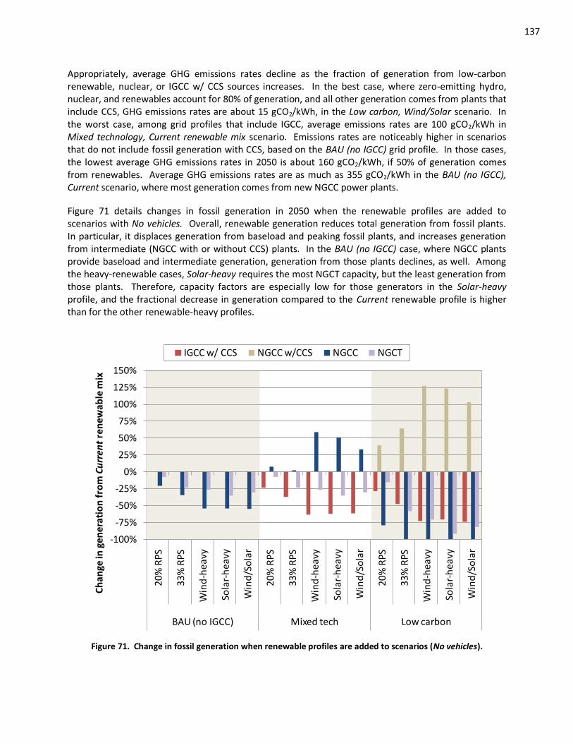
137

Appropriately, average GHG emissions rates decline as the fraction of generation from low-carbon renewable, nuclear, or IGCC w/ CCS sources increases. In the best case, where zero-emitting hydro, nuclear, and renewables account for 80% of generation, and all other generation comes from plants that include CCS, GHG emissions rates are about 15 gCO2/kWh, in the Low carbon, Wind/Solar scenario. In the worst case, among grid profiles that include IGCC, average emissions rates are 100 gCO2/kWh in Mixed technology, Current renewable mix scenario. Emissions rates are noticeably higher in scenarios that do not include fossil generation with CCS, based on the BAU (no IGCC) grid profile. In those cases, the lowest average GHG emissions rates in 2050 is about 160 gCO2/kWh, if 50% of generation comes from renewables. Average GHG emissions rates are as much as 355 gCO2/kWh in the BAU (no IGCC), Current scenario, where most generation comes from new NGCC power plants.

Figure 71 details changes in fossil generation in 2050 when the renewable profiles are added to scenarios with No vehicles. Overall, renewable generation reduces total generation from fossil plants. In particular, it displaces generation from baseload and peaking fossil plants, and increases generation from intermediate (NGCC with or without CCS) plants. In the BAU (no IGCC) case, where NGCC plants provide baseload and intermediate generation, generation from those plants declines, as well. Among the heavy-renewable cases, Solar-heavy requires the most NGCT capacity, but the least generation from those plants. Therefore, capacity factors are especially low for those generators in the Solar-heavy profile, and the fractional decrease in generation compared to the Current renewable profile is higher than for the other renewable-heavy profiles.

-100%

-75%

-50%

-25%

0%

25%

50%

75%

100%

125%

150%

20

% R

PS

33

% R

PS

Win

d-h

eavy

Sola

r-h

eavy

Win

d/S

ola

r

20

% R

PS

33

% R

PS

Win

d-h

eavy

Sola

r-h

eavy

Win

d/S

ola

r

20

% R

PS

33

% R

PS

Win

d-h

eavy

Sola

r-h

eavy

Win

d/S

ola

r


Ch

ange

in g

en

era

tio

n f

rom

Cu

rren

t re

ne

wab

le m

ix


Figure 71. Change in fossil generation when renewable profiles are added to scenarios (No vehicles).

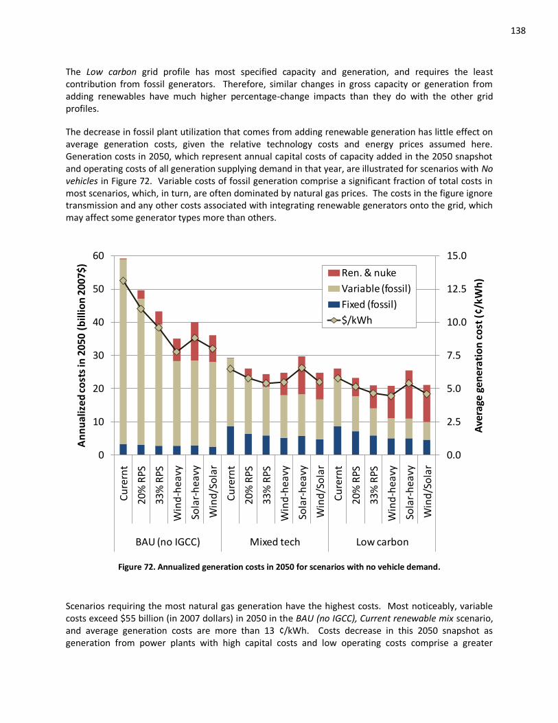
138

The Low carbon grid profile has most specified capacity and generation, and requires the least contribution from fossil generators. Therefore, similar changes in gross capacity or generation from adding renewables have much higher percentage-change impacts than they do with the other grid profiles.

The decrease in fossil plant utilization that comes from adding renewable generation has little effect on average generation costs, given the relative technology costs and energy prices assumed here. Generation costs in 2050, which represent annual capital costs of capacity added in the 2050 snapshot and operating costs of all generation supplying demand in that year, are illustrated for scenarios with No vehicles in Figure 72. Variable costs of fossil generation comprise a significant fraction of total costs in most scenarios, which, in turn, are often dominated by natural gas prices. The costs in the figure ignore transmission and any other costs associated with integrating renewable generators onto the grid, which may affect some generator types more than others.

0.0

2.5

5.0

7.5

10.0

12.5

15.0

0

10

20

30

40

50

60

Cu

rern

t

20%

RPS

33%

RPS

Win

d-h

eavy

Sola

r-h

eavy

Win

d/S

ola

r

Cu

rern

t

20%

RPS

33%

RPS

Win

d-h

eavy

Sola

r-h

eavy

Win

d/S

ola

r

Cu

rern

t

20%

RPS

33%

RPS

Win

d-h

eavy

Sola

r-h

eavy

Win

d/S

ola

r


Ave

rage

ge

ne

rati

on

co

st (

¢/kW

h)

An

nu

aliz

ed

co

sts

in 2

05

0 (

bill

ion

20

07

$)

Ren. & nuke

Variable (fossil)

Fixed (fossil)

$/kWh

Figure 72. Annualized generation costs in 2050 for scenarios with no vehicle demand.

Scenarios requiring the most natural gas generation have the highest costs. Most noticeably, variable costs exceed $55 billion (in 2007 dollars) in 2050 in the BAU (no IGCC), Current renewable mix scenario, and average generation costs are more than 13 ¢/kWh. Costs decrease in this 2050 snapshot as generation from power plants with high capital costs and low operating costs comprise a greater

139

fraction of supply. Renewable, nuclear, and IGCC w/ CCS power plants added in the 2020 and 2035 snapshots are assumed to be fully capitalized in 2050 and provide low-cost generation then. Older natural gas-fired power plants are also fully capitalized, but are relatively expensive because high natural gas prices lead to high variable costs.

Among the three high-renewable penetration scenarios, those with a greater fraction of solar generation have higher costs, since the technology has a lower capacity factor and is assumed to be more expensive than wind generation in LEDGE-CA (the costs of renewable generators are listed in Table 24). In fact, optimizing wind and solar capacity to minimize fossil capacity requirements does not reduce costs in the scenarios considered here. The costs of additional solar capacity, and additional renewable capacity overall, do not offset the costs of saved fossil capacity. Overall, costs are lowest in the Low carbon, Wind-heavy scenario, according to assumptions in this analysis.

Of course, these findings are a product of the technology and geography assumptions defined in the scenarios, and the insolation and wind speed data used to create renewable generation profiles. In any given hour, month, or year, aggregate generation from wind and solar in California could be very different than the profiles derived from fixed data that are used here. Solar facilities located outside of the Palm Springs Desert could create a more diverse mix of solar power than represented here. Technology advances may increase capacity factors of wind and solar generation. And demand response or energy storage could alleviate some requirements for fossil-fired power plant capacity to supplement passive renewable generation. These factors are not investigated in Part II of this dissertation, and are left for future work. The results presented here should be considered accordingly, within the context of the assumptions that shape them.

6.3.1 Summary of category 3 results: Impacts of renewable generation on fossil supply

Adding renewable generation to the grid has the opposite effect of vehicle recharging on fossil supply. Whether baseload (from nuclear, geothermal, or biomass) or intermittent (from wind or solar), passive generation reduces fossil capacity requirements and fossil supply load factors. Although it reduces load factors for fossil supply, making the mix of fossil power plants shift towards peaking plants, baseload must-run generation provides a predictable resource for the grid. Intermittent generation from wind or solar plants leads to more variable must-run supply, and thus, can lead to highly variable fossil supply, as well. This can lead to significant ramping requirements for fossil generators, which can be costly.

As more renewables are added, the fossil supply profile becomes more variable (its load factor decreases), and the share of fossil generation from baseload plants falls. Because the fossil supply curve becomes more variable, the share of fossil generation from peaking NGCT power plants increases, even though its overall capacity and generation declines.

Grids with significant fractions of generation from wind or solar plants have higher overall capacity, because those plants operate with lower capacity factors than the baseload fossil generators they mostly replace. Interestingly, even though solar generation tends to be better correlated with peak electricity demand than wind generation is, according to their representations in LEDGE-CA, adding solar power increases fossil capacity requirements compared to adding wind power. Grids with significant levels of solar power shift peak fossil demand periods from summer afternoons to summer evenings. Grids with significant levels of wind generation continue to see fossil generation peak during summer afternoons, but fossil capacity requirements are lower than in the Solar-heavy case. While some wind generation is available during peak fossil supply hours in summer afternoons, especially in the Altamont

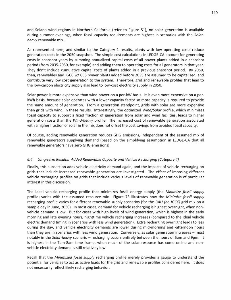
140

and Solano wind regions in Northern California (refer to Figure 51), no solar generation is available during summer evenings, when fossil capacity requirements are highest in scenarios with the Solar-heavy renewable mix.

As represented here, and similar to the Category 1 results, plants with low operating costs reduce generation costs in the 2050 snapshot. The simple cost calculations in LEDGE-CA account for generating costs in snapshot years by summing annualized capital costs of all power plants added in a snapshot period (from 2035-2050, for example) and adding them to operating costs for all generators in that year. They don’t include cumulative capital costs of plants added in a previous snapshot period. By 2050, then, renewables and IGCC w/ CCS power plants added before 2035 are assumed to be capitalized, and contribute very low cost generation to the system. Therefore, grid and renewable profiles that lead to the low-carbon electricity supply also lead to low-cost electricity supply in 2050.

Solar power is more expensive than wind power on a per-kW basis. It is even more expensive on a per-kWh basis, because solar operates with a lower capacity factor so more capacity is required to provide the same amount of generation. From a generation standpoint, grids with solar are more expensive than grids with wind, in these results. Interestingly, the optimized Wind/Solar profile, which minimizes fossil capacity to support a fixed fraction of generation from solar and wind facilities, leads to higher generation costs than the Wind-heavy profile. The increased cost of renewable generation associated with a higher fraction of solar in the mix does not offset the cost savings from avoided fossil capacity.

Of course, adding renewable generation reduces GHG emissions, independent of the assumed mix of renewable generators supplying demand (based on the simplifying assumption in LEDGE-CA that all renewable generators have zero GHG emissions).

6.4 Long-term Results: Added Renewable Capacity and Vehicle Recharging (Category 4)

Finally, this subsection adds vehicle electricity demand again, and the impacts of vehicle recharging on grids that include increased renewable generation are investigated. The effect of imposing different vehicle recharging profiles on grids that include various levels of renewable generation is of particular interest in this discussion.

The ideal vehicle recharging profile that minimizes fossil energy supply (the Minimize fossil supply profile) varies with the assumed resource mix. Figure 73 illustrates how the Minimize fossil supply recharging profile varies for different renewable supply scenarios (for the BAU (no IGCC) grid mix on a sample day in June, 2050). In most cases, demand for vehicle recharging is highest overnight, when non-vehicle demand is low. But for cases with high levels of wind generation, which is highest in the early morning and late evening hours, nighttime vehicle recharging increases (compared to the ideal vehicle electric demand timing in scenarios with less wind generation). Extra recharging overnight leads to less during the day, and vehicle electricity demands are lower during mid-morning and -afternoon hours than they are in scenarios with less wind generation. Conversely, as solar generation increases – most notably in the Solar-heavy scenario – recharging occurs entirely between the hours of 5am and 9pm. It is highest in the 7am-8am time frame, when much of the solar resource has come online and non-vehicle electricity demand is still relatively low.

Recall that the Minimized fossil supply recharging profile merely provides a gauge to understand the potential for vehicles to act as active loads for the grid and renewable profiles considered here. It does not necessarily reflect likely recharging behavior.

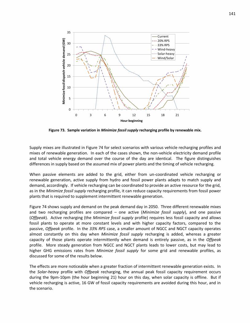
141

0

5

10

15

20

25

30

35

0 3 6 9 12 15 18 21

Min

imiz

e fo

ssil

dis

pat

ch v

eh

icle

de

man

d (G

W)

Hour beginning

Current20% RPS33% RPSWind-heavySolar-heavyWind/Solar

Figure 73. Sample variation in Minimize fossil supply recharging profile by renewable mix.

Supply mixes are illustrated in Figure 74 for select scenarios with various vehicle recharging profiles and mixes of renewable generation. In each of the cases shown, the non-vehicle electricity demand profile and total vehicle energy demand over the course of the day are identical. The figure distinguishes differences in supply based on the assumed mix of power plants and the timing of vehicle recharging.

When passive elements are added to the grid, either from un-coordinated vehicle recharging or renewable generation, active supply from hydro and fossil power plants adapts to match supply and demand, accordingly. If vehicle recharging can be coordinated to provide an active resource for the grid, as in the Minimize fossil supply recharging profile, it can reduce capacity requirements from fossil power plants that is required to supplement intermittent renewable generation.

Figure 74 shows supply and demand on the peak demand day in 2050. Three different renewable mixes and two recharging profiles are compared – one active (Minimize fossil supply), and one passive (Offpeak). Active recharging (the Minimize fossil supply profile) requires less fossil capacity and allows fossil plants to operate at more constant levels and with higher capacity factors, compared to the passive, Offpeak profile. In the 33% RPS case, a smaller amount of NGCC and NGCT capacity operates almost constantly on this day when Minimize fossil supply recharging is added, whereas a greater capacity of those plants operate intermittently when demand is entirely passive, as in the Offpeak profile. More steady generation from NGCC and NGCT plants leads to lower costs, but may lead to higher GHG emissions rates from Minimize fossil supply for some grid and renewable profiles, as discussed for some of the results below.

The effects are more noticeable when a greater fraction of intermittent renewable generation exists. In the Solar-heavy profile with Offpeak recharging, the annual peak fossil capacity requirement occurs during the 9pm-10pm (the hour beginning 21) hour on this day, when solar capacity is offline. But if vehicle recharging is active, 16 GW of fossil capacity requirements are avoided during this hour, and in the scenario.

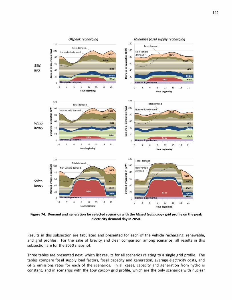
142

Offpeak recharging Minimize fossil supply recharging

33% RPS

0

20

40

60

80

100

120

0 3 6 9 12 15 18 21

De

man

d o

r G

en

era

tio

n (

GW

)

Hour beginning

NGCT

NGCC

IGCC

Hydro

Wind

Biomass & geothermal

Solar

Non-vehicle demand

Total demand

0

20

40

60

80

100

120

0 3 6 9 12 15 18 21

De

man

d o

r G

en

era

tio

n (

GW

)

Hour beginning

Hydro

WindBiomass & geothermal

Solar

NGCT

NGCC

Non-vehicle

demand

IGCC

Total demand

Wind-heavy

0

20

40

60

80

100

120

0 3 6 9 12 15 18 21

De

man

d o

r G

en

era

tio

n (

GW

)

Hour beginning

Hydro

Wind

Biomass & geothermalSolar

NGCT

NGCC

IGCC

Non-vehicle demand

Total demand

0

20

40

60

80

100

120

0 3 6 9 12 15 18 21

De

man

d o

r G

en

era

tio

n (

GW

)

Hour beginning

Hydro

Wind

Biomass & geothermalSolar

NGCT

NGCC

Non-vehicle demand

IGCC

Total demand

Solar-heavy

0

20

40

60

80

100

120

0 3 6 9 12 15 18 21

De

man

d o

r G

en

era

tio

n (

GW

)

Hour beginning

HydroWind


Solar

NGCT

NGCC

IGCC

Non-vehicle demand

Total demand

0

20

40

60

80

100

120

0 3 6 9 12 15 18 21

De

man

d o

r G

en

era

tio

n (

GW

)

Hour beginning

HydroWind


Solar

NGCT

NGCC

Non-vehicle

demand

IGCC

Total demand

Figure 74. Demand and generation for selected scenarios with the Mixed technology grid profile on the peak electricity demand day in 2050.

Results in this subsection are tabulated and presented for each of the vehicle recharging, renewable, and grid profiles. For the sake of brevity and clear comparison among scenarios, all results in this subsection are for the 2050 snapshot.

Three tables are presented next, which list results for all scenarios relating to a single grid profile. The tables compare fossil supply load factors, fossil capacity and generation, average electricity costs, and GHG emissions rates for each of the scenarios. In all cases, capacity and generation from hydro is constant, and in scenarios with the Low carbon grid profile, which are the only scenarios with nuclear

143

capacity in 2050, capacity and generation from nuclear is constant. Minimize fossil supply is abbreviated as “Min fossil” in each of the tables.

In all scenarios with a given renewable profile, adding vehicle electricity demand increases renewable capacity by a constant amount, because total electricity demand is constant. There are slight variations in wind and solar generation among scenarios with one of the three heavy-renewables profiles, however, which reflect excess wind or solar generation during hours in which must-run generation or hydro is on the margin. This occurs during a small fraction of hours in scenarios with very high capacities of wind or solar power, and leads some high-renewable scenarios to have slightly less than 50% of annual generation from renewables. It does not, however, have an impact on comparative costs or GHG emissions among scenarios, since wind and solar power are assumed to operate with zero variable cost and zero GHG emissions.

Table 32 lists results for the BAU (no IGCC) grid profile. All new non-renewable capacity and generation for vehicle electricity demand comes from NGCC and NGCT power plants, per the definition of the grid profile. Adding vehicle recharging increases the load factor of fossil supply and partially offsets the reduction in load factor that comes from adding renewable generation. The Solar-heavy renewable mix leads to the highest fossil capacity requirements and the lowest load factors for fossil supply, for the reasons described in Section 6.3.

Costs and GHG emissions rates always increase when vehicle recharging is added to scenarios including the BAU (no IGCC) grid profile, because added demand leads to increased capacity and generation from a similar mix of plants as operates without vehicle demand, and dilutes the fraction of generation from existing, low-cost and zero-emitting hydro facilities. Average generation costs increase by 0.5-7.0% and average GHG emissions rates increase by 1.0-5.1% when vehicle recharging is added. Cost increases from vehicle recharging follow the change in the fossil load factor. Active recharging allows a better match between intermittent renewables and demand, which lowers costs and GHG emissions, compared to passive recharging. Also, in this analysis, wind power is less expensive than solar power, and adding solar generation to accommodate new demands from vehicles increases costs more than adding wind power. Marginal emissions rates are lowest with high renewable generation, because NGCT plants comprise a smaller fraction of generation and because at times, renewable or hydro generation operates on the margin.

Offpeak recharging requires additional natural gas-fired capacity in each scenario with the BAU (no IGCC) grid profile. Except for with Wind/Solar renewable mix, all new fossil capacity comes from NGCC plants, and capacity from NGCT plants is less than in scenarios without Offpeak recharging. Interestingly, Offpeak recharging leads to fossil load factors and higher fossil capacity requirements than Workday recharging in the 33% RPS, Solar-heavy, or Wind/Solar renewable cases. Despite contributing more to peak non-vehicle demand, recharging according to the Workday profile better matches must-run generation and requires less fossil capacity than Offpeak recharging in these scenarios. Consequently, costs are slightly lower for Workday recharging with those renewable profiles, as well.

Fossil load factors are highest when vehicles recharge according to Minimize fossil supply and costs are lowest, among scenarios with vehicle recharging. Notably, generation from NGCT power plants increases when Minimize fossil supply is added to scenarios that do not include one of the three heavy-renewable profiles, and GHG emissions are higher than for the other two vehicle recharging profiles. For the high-renewable profiles, however, Minimize fossil supply recharging reduces average and marginal GHG emissions rates compared to the other recharging profiles.

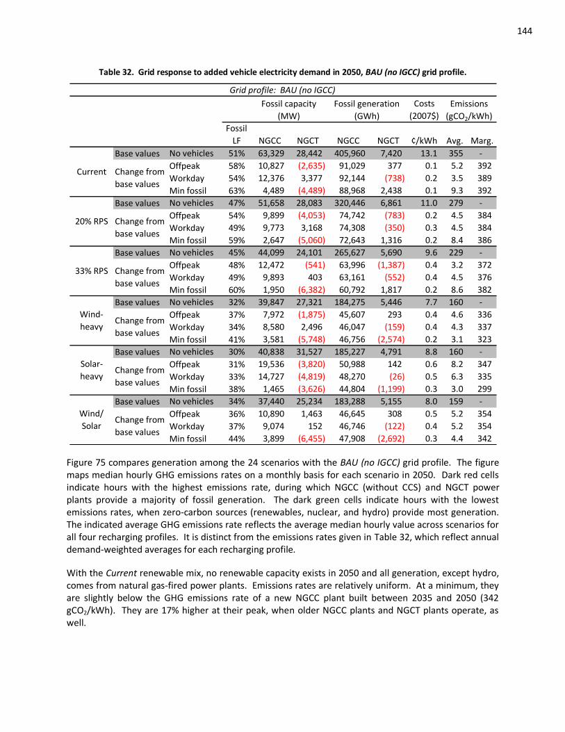
144

Table 32. Grid response to added vehicle electricity demand in 2050, BAU (no IGCC) grid profile.

Costs

(2007$)

Fossil

LF NGCC NGCT NGCC NGCT ¢/kWh Avg. Marg.

Base values No vehicles 51% 63,329 28,442 405,960 7,420 13.1 355 -

Offpeak 58% 10,827 (2,635) 91,029 377 0.1 5.2 392

Workday 54% 12,376 3,377 92,144 (738) 0.2 3.5 389

Min fossil 63% 4,489 (4,489) 88,968 2,438 0.1 9.3 392


Offpeak 54% 9,899 (4,053) 74,742 (783) 0.2 4.5 384

Workday 49% 9,773 3,168 74,308 (350) 0.3 4.5 384

Min fossil 59% 2,647 (5,060) 72,643 1,316 0.2 8.4 386


Offpeak 48% 12,472 (541) 63,996 (1,387) 0.4 3.2 372

Workday 49% 9,893 403 63,161 (552) 0.4 4.5 376

Min fossil 60% 1,950 (6,382) 60,792 1,817 0.2 8.6 382


Offpeak 37% 7,972 (1,875) 45,607 293 0.4 4.6 336

Workday 34% 8,580 2,496 46,047 (159) 0.4 4.3 337

Min fossil 41% 3,581 (5,748) 46,756 (2,574) 0.2 3.1 323


Offpeak 31% 19,536 (3,820) 50,988 142 0.6 8.2 347

Workday 33% 14,727 (4,819) 48,270 (26) 0.5 6.3 335

Min fossil 38% 1,465 (3,626) 44,804 (1,199) 0.3 3.0 299


Offpeak 36% 10,890 1,463 46,645 308 0.5 5.2 354

Workday 37% 9,074 152 46,746 (122) 0.4 5.2 354

Min fossil 44% 3,899 (6,455) 47,908 (2,692) 0.3 4.4 342

Solar-

heavyChange from

base values

Wind/

SolarChange from

base values

20% RPS Change from

base values

33% RPS Change from

base values

Wind-

heavyChange from

base values

Grid profile: BAU (no IGCC)

Fossil capacity

(MW)

Fossil generation

(GWh)

Emissions

(gCO2/kWh)

Current Change from

base values

Figure 75 compares generation among the 24 scenarios with the BAU (no IGCC) grid profile. The figure maps median hourly GHG emissions rates on a monthly basis for each scenario in 2050. Dark red cells indicate hours with the highest emissions rate, during which NGCC (without CCS) and NGCT power plants provide a majority of fossil generation. The dark green cells indicate hours with the lowest emissions rates, when zero-carbon sources (renewables, nuclear, and hydro) provide most generation. The indicated average GHG emissions rate reflects the average median hourly value across scenarios for all four recharging profiles. It is distinct from the emissions rates given in Table 32, which reflect annual demand-weighted averages for each recharging profile.

With the Current renewable mix, no renewable capacity exists in 2050 and all generation, except hydro, comes from natural gas-fired power plants. Emissions rates are relatively uniform. At a minimum, they are slightly below the GHG emissions rate of a new NGCC plant built between 2035 and 2050 (342 gCO2/kWh). They are 17% higher at their peak, when older NGCC plants and NGCT plants operate, as well.

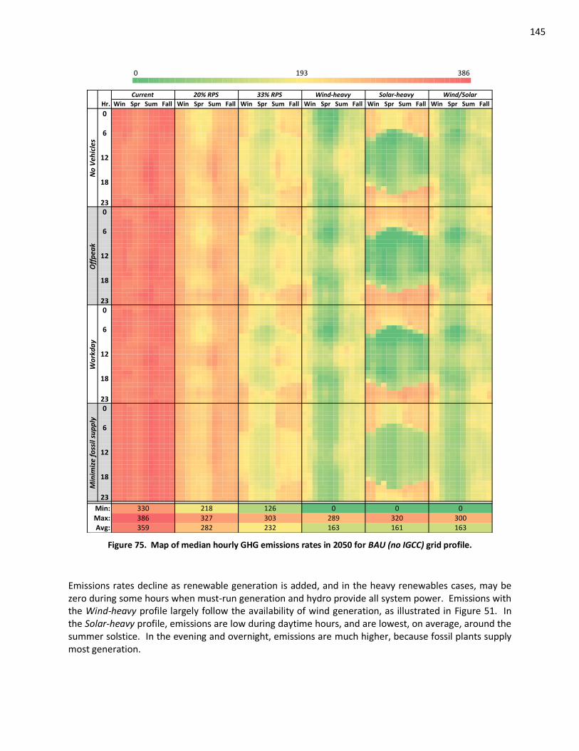
145

23 28 34 40 45 51 57 63 68 74 80 85 91 97 ## ## ## ## ## ## ## ## ## ## ## ## ## ## ## ## ## ## ## ## ## ## ## ## ## ## ## ## ## ## ## ## ## ## ## ## ## ## ## ## ## ## ## ## ## ## ## ## ## ##

Hr.

Min:Max:Avg:

Sum Fall WinSum

Current

Win Spr Sum Fall Win Spr Sum Fall Win Spr

No

Veh

icle

sO

ffp

eak

Wo

rkd

ay

Min

imiz

e fo

ssil

sup

ply

0

23

6

18

12

0

6

12

18

23

12

3860

18

23

6

12

18

230

6

FallSpr Sum Fall Win

0

386359

218

193 3860

Wind/SolarSolar-heavyWind-heavy33% RPS20% RPS

Spr SumFall Win Spr

126 0 0 0330327 303 289 320 300282 232 163 161 163

Figure 75. Map of median hourly GHG emissions rates in 2050 for BAU (no IGCC) grid profile.

Emissions rates decline as renewable generation is added, and in the heavy renewables cases, may be zero during some hours when must-run generation and hydro provide all system power. Emissions with the Wind-heavy profile largely follow the availability of wind generation, as illustrated in Figure 51. In the Solar-heavy profile, emissions are low during daytime hours, and are lowest, on average, around the summer solstice. In the evening and overnight, emissions are much higher, because fossil plants supply most generation.

146

As discussed in Part I, emissions tend to be lower in the spring and overnight (except for Solar-heavy) when non-vehicle demand is low and hydro generation is high, and they are higher in the fall and early winter months. There is little noticeable difference in emissions rates for scenarios with similar renewable profiles and different vehicle recharging profiles, but Minimize fossil supply does make hourly GHG emissions rates somewhat more uniform.

Table 33 lists results for scenarios including the Mixed technology grid profile. This grid profile includes capacity additions from IGCC power plants, and they account for most of the fossil capacity additions in the scenarios considered here. Since no new nuclear capacity is added in this grid profile and all new capacity comes from prescribed renewable mixes or fossil generators, the impact of vehicle recharging on fossil load factors in Mixed technology is the same as in BAU (no IGCC) and required fossil capacity and generation are the same as for scenarios listed in Table 32. When nuclear capacity and generation is added to the grid in scenarios with the Low carbon grid profile, discussed next, fossil capacity and generation requirements are reduced, as well as fossil supply curve load factors.

Costs and GHG emissions rates are lower for the Mixed technology grid profile than they are for BAU (no IGCC). Adding vehicle recharging decreases costs and GHG emissions rates in some cases, which was never the case for scenarios with the BAU (no IGCC) profile. Unlike the results presented in Table 32, marginal emissions rates for Mixed technology grids increase in scenarios that include heavy-renewable mixes, because there is a smaller fraction of IGCC capacity operating in those scenarios and natural gas-fired capacity is more likely to be on the margin.

Adding Offpeak recharging always increases total fossil capacity and generation, in equal amounts to similar scenarios with the BAU (no IGCC) grid profiles. Capacity from NGCT plants declines compared to the No vehicles case with all renewable profiles except Solar-heavy, where there is a huge increase in NGCC capacity and a decrease in IGCC capacity, compared to the base values. Relative changes in costs and GHG emissions rates among scenarios with Offpeak recharging and the Mixed technology grid profile generally match changes in fossil supply load factors. When load factors increase the most from Offpeak recharging – in the Current, 20% RPS, or Wind-heavy renewable profiles – cost increases are lower and emissions rates decline. In scenarios with the 33% RPS, Solar-heavy, or Wind/Solar renewable mix, where Offpeak recharging increases fossil supply load factors less, GHG emissions rates increase and cost increases are more significant, compared to No vehicles. These effects are most noticeable with the Solar-heavy renewable profile, where costs increase by 20% and average emissions rates increase by 50% with Offpeak recharging.

As is the case for the BAU (no IGCC) grid profile, Workday recharging increase fossil supply load factors more than Offpeak recharging does for the 33% RPS, Solar-heavy, or Wind/Solar renewables mixes. Workday recharging increases load factors most with the Solar-heavy or Wind/Solar renewable mixes. Despite this, costs and average GHG emissions rates increase most when Workday recharging is added with these renewable profiles. Notably, costs increase by 14% and GHG emissions rates increase by 33% with the Solar-heavy renewable mix. Average GHG emissions rates actually decrease with the other four renewable mixes when Workday recharging is imposed on the grid.

When vehicle recharging follows the Minimize fossil supply profile, no new fossil capacity is required. As for the BAU (no IGCC) grid profile, adding vehicle recharging actually reduces the total fossil capacity required, except with the Current renewable mix, where it remains constant. This leads to better utilization of fossil generators, whose average capacity factors increase proportionally to load factor, by

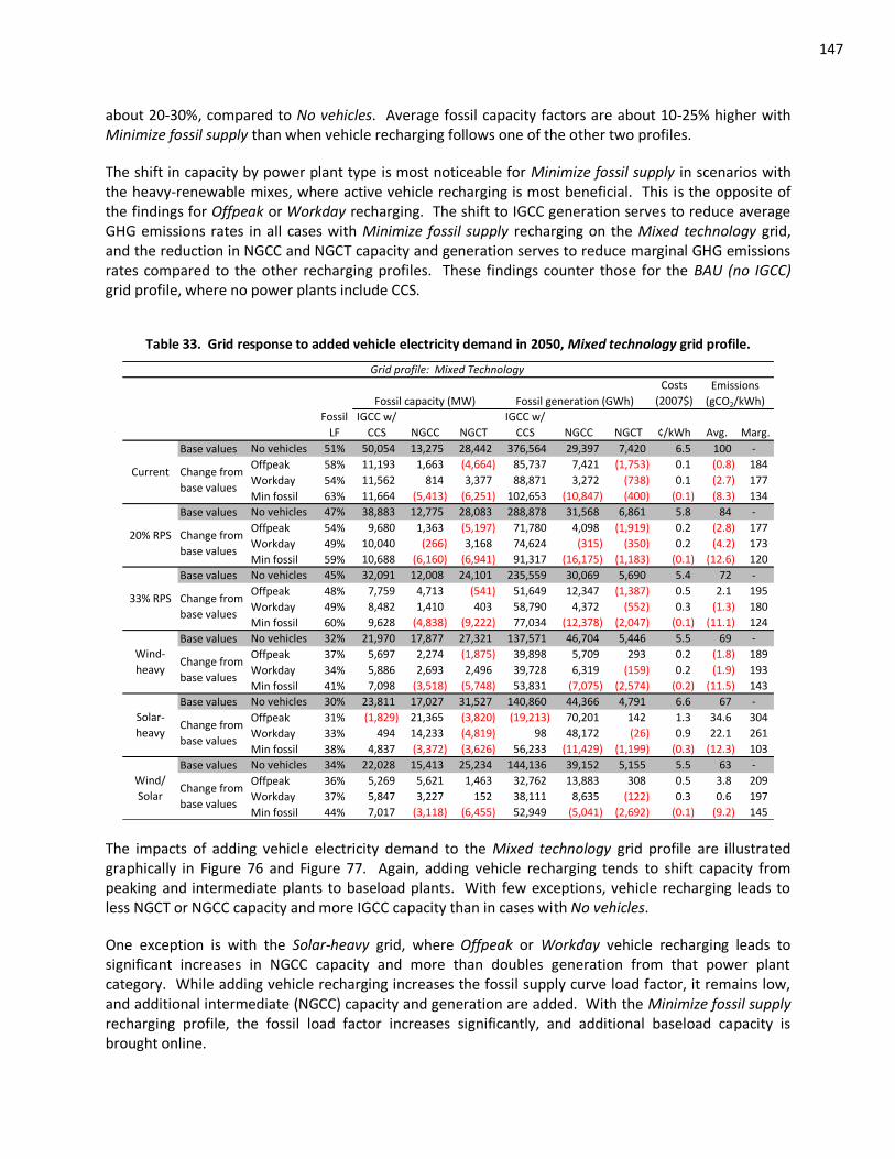
147

about 20-30%, compared to No vehicles. Average fossil capacity factors are about 10-25% higher with Minimize fossil supply than when vehicle recharging follows one of the other two profiles.

The shift in capacity by power plant type is most noticeable for Minimize fossil supply in scenarios with the heavy-renewable mixes, where active vehicle recharging is most beneficial. This is the opposite of the findings for Offpeak or Workday recharging. The shift to IGCC generation serves to reduce average GHG emissions rates in all cases with Minimize fossil supply recharging on the Mixed technology grid, and the reduction in NGCC and NGCT capacity and generation serves to reduce marginal GHG emissions rates compared to the other recharging profiles. These findings counter those for the BAU (no IGCC) grid profile, where no power plants include CCS.

Table 33. Grid response to added vehicle electricity demand in 2050, Mixed technology grid profile.

Costs

(2007$)

Fossil

LF

IGCC w/

CCS NGCC NGCT

IGCC w/


Base values No vehicles 51% 50,054 13,275 28,442 376,564 29,397 7,420 6.5 100 -

Offpeak 58% 11,193 1,663 (4,664) 85,737 7,421 (1,753) 0.1 (0.8) 184

Workday 54% 11,562 814 3,377 88,871 3,272 (738) 0.1 (2.7) 177

Min fossil 63% 11,664 (5,413) (6,251) 102,653 (10,847) (400) (0.1) (8.3) 134


Offpeak 54% 9,680 1,363 (5,197) 71,780 4,098 (1,919) 0.2 (2.8) 177

Workday 49% 10,040 (266) 3,168 74,624 (315) (350) 0.2 (4.2) 173

Min fossil 59% 10,688 (6,160) (6,941) 91,317 (16,175) (1,183) (0.1) (12.6) 120


Offpeak 48% 7,759 4,713 (541) 51,649 12,347 (1,387) 0.5 2.1 195

Workday 49% 8,482 1,410 403 58,790 4,372 (552) 0.3 (1.3) 180

Min fossil 60% 9,628 (4,838) (9,222) 77,034 (12,378) (2,047) (0.1) (11.1) 124


Offpeak 37% 5,697 2,274 (1,875) 39,898 5,709 293 0.2 (1.8) 189

Workday 34% 5,886 2,693 2,496 39,728 6,319 (159) 0.2 (1.9) 193

Min fossil 41% 7,098 (3,518) (5,748) 53,831 (7,075) (2,574) (0.2) (11.5) 143


Offpeak 31% (1,829) 21,365 (3,820) (19,213) 70,201 142 1.3 34.6 304

Workday 33% 494 14,233 (4,819) 98 48,172 (26) 0.9 22.1 261

Min fossil 38% 4,837 (3,372) (3,626) 56,233 (11,429) (1,199) (0.3) (12.3) 103


Offpeak 36% 5,269 5,621 1,463 32,762 13,883 308 0.5 3.8 209

Workday 37% 5,847 3,227 152 38,111 8,635 (122) 0.3 0.6 197

Min fossil 44% 7,017 (3,118) (6,455) 52,949 (5,041) (2,692) (0.1) (9.2) 145

Solar-

heavyChange from

base values

Wind/

SolarChange from

base values

20% RPS Change from

base values

33% RPS Change from

base values

Wind-

heavyChange from

base values

Grid profile: Mixed Technology


Emissions

(gCO2/kWh)

Current Change from

base values

The impacts of adding vehicle electricity demand to the Mixed technology grid profile are illustrated graphically in Figure 76 and Figure 77. Again, adding vehicle recharging tends to shift capacity from peaking and intermediate plants to baseload plants. With few exceptions, vehicle recharging leads to less NGCT or NGCC capacity and more IGCC capacity than in cases with No vehicles.

One exception is with the Solar-heavy grid, where Offpeak or Workday vehicle recharging leads to significant increases in NGCC capacity and more than doubles generation from that power plant category. While adding vehicle recharging increases the fossil supply curve load factor, it remains low, and additional intermediate (NGCC) capacity and generation are added. With the Minimize fossil supply recharging profile, the fossil load factor increases significantly, and additional baseload capacity is brought online.

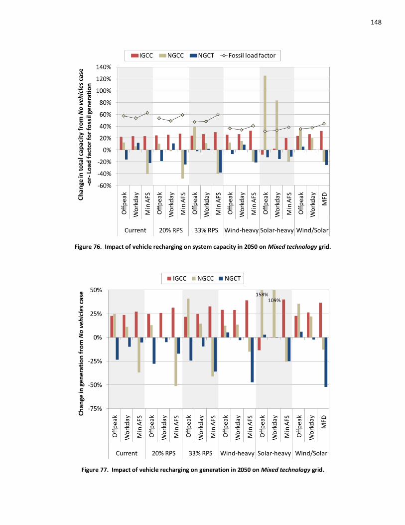
148

-60%

-40%

-20%

0%

20%

40%

60%

80%

100%

120%

140%

Off

pea

k

Wo

rkd

ay

Min

AFS

Off

pea

k

Wo

rkd

ay

Min

AFS

Off

pea

k

Wo

rkd

ay

Min

AFS

Off

pea

k

Wo

rkd

ay

Min

AFS

Off

pea

k

Wo

rkd

ay

Min

AFS

Off

pea

k

Wo

rkd

ay

MFD

Current 20% RPS 33% RPS Wind-heavy Solar-heavy Wind/Solar

Ch

ange

in t

ota

l cap

acit

y fr

om

No

veh

icle

s ca

se

-o

r-Lo

ad f

acto

r fo

r fo

ssil

gen

erat

ion

IGCC NGCC NGCT Fossil load factor

Figure 76. Impact of vehicle recharging on system capacity in 2050 on Mixed technology grid.

158%109%

-75%

-50%

-25%

0%

25%

50%

Off

pea

k

Wo

rkd

ay

Min

AFS

Off

pea

k

Wo

rkd

ay

Min

AFS

Off

pea

k

Wo

rkd

ay

Min

AFS

Off

pea

k

Wo

rkd

ay

Min

AFS

Off

pea

k

Wo

rkd

ay

Min

AFS

Off

pea

k

Wo

rkd

ay

MFD

Current 20% RPS 33% RPS Wind-heavy Solar-heavy Wind/Solar

Ch

ange

in g

en

era

tio

n f

rom

No

veh

icle

s ca

se

IGCC NGCC NGCT

Figure 77. Impact of vehicle recharging on generation in 2050 on Mixed technology grid.

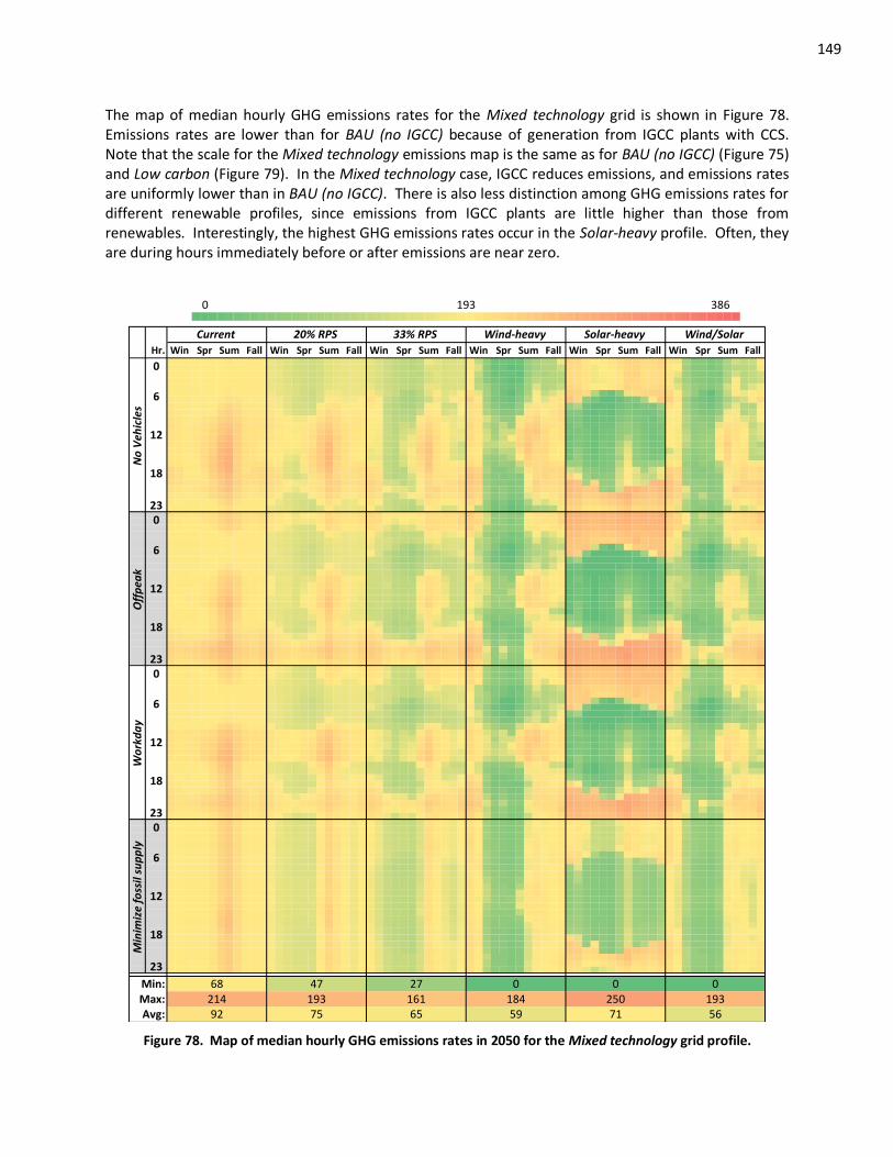
149

The map of median hourly GHG emissions rates for the Mixed technology grid is shown in Figure 78. Emissions rates are lower than for BAU (no IGCC) because of generation from IGCC plants with CCS. Note that the scale for the Mixed technology emissions map is the same as for BAU (no IGCC) (Figure 75) and Low carbon (Figure 79). In the Mixed technology case, IGCC reduces emissions, and emissions rates are uniformly lower than in BAU (no IGCC). There is also less distinction among GHG emissions rates for different renewable profiles, since emissions from IGCC plants are little higher than those from renewables. Interestingly, the highest GHG emissions rates occur in the Solar-heavy profile. Often, they are during hours immediately before or after emissions are near zero.

6 12 18 24 30 36 42 48 53 59 65 71 77 83 89 95 ## ## ## ## ## ## ## ## ## ## ## ## ## ## ## ## ## ## ## ## ## ## ## ## ## ## ## ## ## ## ## ## ## ## ## ## ## ## ## ## ## ## ## ## ## ## ## ##

Hr.

Min:Max:Avg: 5692 75 65 59 71

0214 193 161 184 250 19368 47 27 0 0

Min

imiz

e fo

ssil

sup

ply

0

6

12

18

23

Wo

rkd

ay

0

6

12

18

23

Off

pea

k

0

6

12

18

23

No

Veh

icle

s

0

6

12

18

23

Spr Sum FallFall Win Spr Sum Fall WinSpr Sum Fall Win Spr Sum

Wind/Solar

Win Spr Sum Fall Win Spr Sum Fall Win

Current 20% RPS 33% RPS Wind-heavy Solar-heavy

0 193 386

Figure 78. Map of median hourly GHG emissions rates in 2050 for the Mixed technology grid profile.

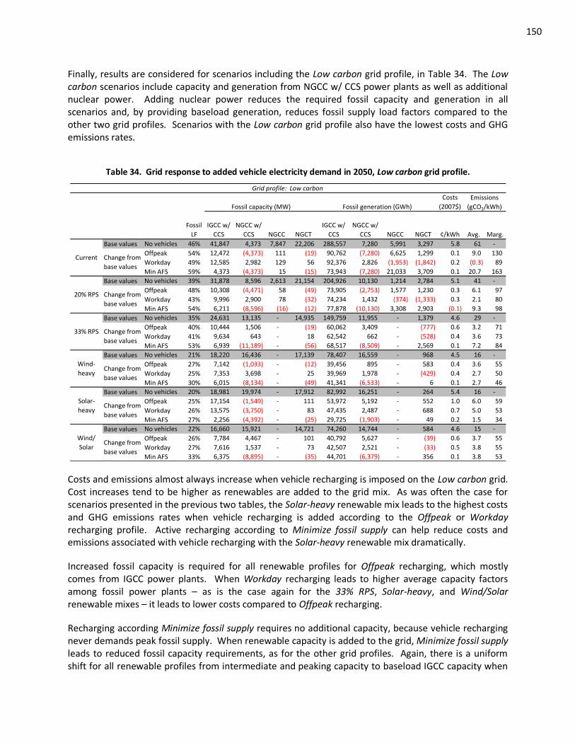
150

Finally, results are considered for scenarios including the Low carbon grid profile, in Table 34. The Low carbon scenarios include capacity and generation from NGCC w/ CCS power plants as well as additional nuclear power. Adding nuclear power reduces the required fossil capacity and generation in all scenarios and, by providing baseload generation, reduces fossil supply load factors compared to the other two grid profiles. Scenarios with the Low carbon grid profile also have the lowest costs and GHG emissions rates.

Table 34. Grid response to added vehicle electricity demand in 2050, Low carbon grid profile.

Costs

(2007$)

Fossil

LF

IGCC w/

CCS

NGCC w/

CCS NGCC NGCT

IGCC w/

CCS

NGCC w/


Base values No vehicles 46% 41,847 4,373 7,847 22,206 288,557 7,280 5,991 3,297 5.8 61 -

Offpeak 54% 12,472 (4,373) 111 (19) 90,762 (7,280) 6,625 1,299 0.1 9.0 130

Workday 49% 12,585 2,982 129 56 92,376 2,826 (1,953) (1,842) 0.2 (0.3) 89

Min AFS 59% 4,373 (4,373) 15 (15) 73,943 (7,280) 21,033 3,709 0.1 20.7 163

Base values No vehicles 39% 31,878 8,596 2,613 21,154 204,926 10,130 1,214 2,784 5.1 41 -

Offpeak 48% 10,308 (4,471) 58 (49) 73,905 (2,753) 1,577 1,230 0.3 6.1 97

Workday 43% 9,996 2,900 78 (32) 74,234 1,432 (374) (1,333) 0.3 2.1 80

Min AFS 54% 6,211 (8,596) (16) (12) 77,878 (10,130) 3,308 2,903 (0.1) 9.3 98

Base values No vehicles 35% 24,631 13,135 - 14,935 149,759 11,955 - 1,379 4.6 29 -

Offpeak 40% 10,444 1,506 - (19) 60,062 3,409 - (777) 0.6 3.2 71

Workday 41% 9,634 643 - 18 62,542 662 - (528) 0.4 3.6 73

Min AFS 53% 6,939 (11,189) - (56) 68,517 (8,509) - 2,569 0.1 7.2 84

Base values No vehicles 21% 18,220 16,436 - 17,139 78,407 16,559 - 968 4.5 16 -

Offpeak 27% 7,142 (1,033) - (12) 39,456 895 - 583 0.4 3.6 55

Workday 25% 7,353 3,698 - 25 39,969 1,978 - (429) 0.4 2.7 50

Min AFS 30% 6,015 (8,134) - (49) 41,341 (6,533) - 6 0.1 2.7 46


Offpeak 25% 17,154 (1,549) - 111 53,972 5,192 - 552 1.0 6.0 59

Workday 26% 13,575 (3,750) - 83 47,435 2,487 - 688 0.7 5.0 53

Min AFS 27% 2,256 (4,392) - (25) 29,725 (1,903) - 49 0.2 1.5 34


Offpeak 26% 7,784 4,467 - 101 40,792 5,627 - (39) 0.6 3.7 55

Workday 27% 7,616 1,537 - 73 42,507 2,521 - (33) 0.5 3.8 55

Min AFS 33% 6,375 (8,895) - (35) 44,701 (6,379) - 356 0.1 3.8 53

Solar-

heavyChange from

base values

Wind/

SolarChange from

base values

20% RPS Change from

base values

33% RPS Change from

base values

Wind-

heavyChange from

base values

Grid profile: Low carbon


Emissions

(gCO2/kWh)

Current Change from

base values

Costs and emissions almost always increase when vehicle recharging is imposed on the Low carbon grid. Cost increases tend to be higher as renewables are added to the grid mix. As was often the case for scenarios presented in the previous two tables, the Solar-heavy renewable mix leads to the highest costs and GHG emissions rates when vehicle recharging is added according to the Offpeak or Workday recharging profile. Active recharging according to Minimize fossil supply can help reduce costs and emissions associated with vehicle recharging with the Solar-heavy renewable mix dramatically.

Increased fossil capacity is required for all renewable profiles for Offpeak recharging, which mostly comes from IGCC power plants. When Workday recharging leads to higher average capacity factors among fossil power plants – as is the case again for the 33% RPS, Solar-heavy, and Wind/Solar renewable mixes – it leads to lower costs compared to Offpeak recharging.

Recharging according Minimize fossil supply requires no additional capacity, because vehicle recharging never demands peak fossil supply. When renewable capacity is added to the grid, Minimize fossil supply leads to reduced fossil capacity requirements, as for the other grid profiles. Again, there is a uniform shift for all renewable profiles from intermediate and peaking capacity to baseload IGCC capacity when

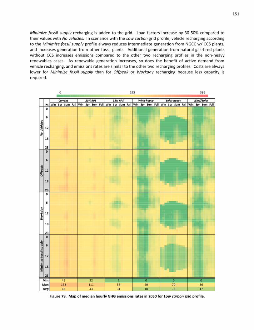
151

Minimize fossil supply recharging is added to the grid. Load factors increase by 30-50% compared to their values with No vehicles. In scenarios with the Low carbon grid profile, vehicle recharging according to the Minimize fossil supply profile always reduces intermediate generation from NGCC w/ CCS plants, and increases generation from other fossil plants. Additional generation from natural gas-fired plants without CCS increases emissions compared to the other two recharging profiles in the non-heavy renewables cases. As renewable generation increases, so does the benefit of active demand from vehicle recharging, and emissions rates are similar to the other two recharging profiles. Costs are always lower for Minimize fossil supply than for Offpeak or Workday recharging because less capacity is required.

6 12 18 24 30 36 42 48 53 59 65 71 77 83 89 95 ## ## ## ## ## ## ## ## ## ## ## ## ## ## ## ## ## ## ## ## ## ## ## ## ## ## ## ## ## ## ## ## ## ## ## ## ## ## ## ## ## ## ## ## ## ## ## ## ##

Hr.

Min:Max:Avg: 1765 43 31 18 18

0153 111 58 50 70 3645 22 7 0 0

Min

imiz

e fo

ssil

sup

ply

0

6

12

18

23

Wo

rkd

ay

0

6

12

18

23

Off

pea

k

0

6

12

18

23

No

Veh

icle

s

0

6

12

18

23

Spr Sum FallFall Win Spr Sum Fall WinSpr Sum Fall Win Spr Sum

Wind/Solar

Win Spr Sum Fall Win Spr Sum Fall Win

Current 20% RPS 33% RPS Wind-heavy Solar-heavy

0 193 386

Figure 79. Map of median hourly GHG emissions rates in 2050 for Low carbon grid profile.

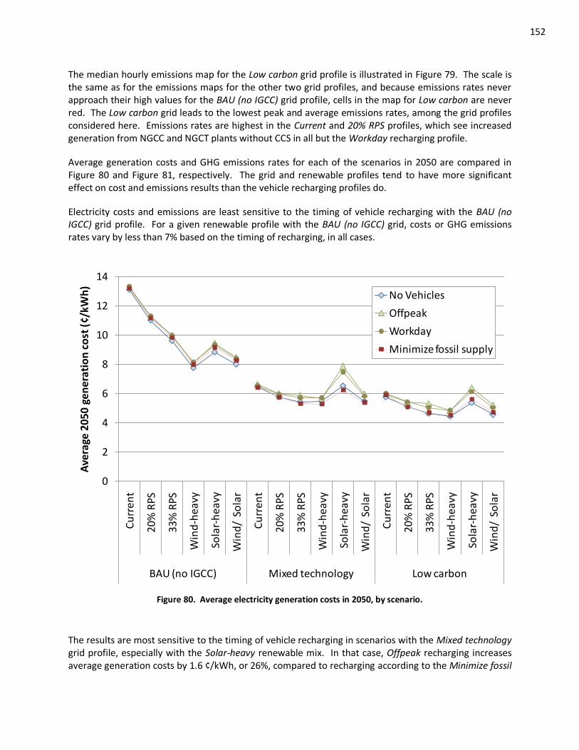
152

The median hourly emissions map for the Low carbon grid profile is illustrated in Figure 79. The scale is the same as for the emissions maps for the other two grid profiles, and because emissions rates never approach their high values for the BAU (no IGCC) grid profile, cells in the map for Low carbon are never red. The Low carbon grid leads to the lowest peak and average emissions rates, among the grid profiles considered here. Emissions rates are highest in the Current and 20% RPS profiles, which see increased generation from NGCC and NGCT plants without CCS in all but the Workday recharging profile.

Average generation costs and GHG emissions rates for each of the scenarios in 2050 are compared in Figure 80 and Figure 81, respectively. The grid and renewable profiles tend to have more significant effect on cost and emissions results than the vehicle recharging profiles do.

Electricity costs and emissions are least sensitive to the timing of vehicle recharging with the BAU (no IGCC) grid profile. For a given renewable profile with the BAU (no IGCC) grid, costs or GHG emissions rates vary by less than 7% based on the timing of recharging, in all cases.

0

2

4

6

8

10

12

14

Cu

rren

t

20

% R

PS

33

% R

PS

Win

d-h

eavy

Sola

r-h

eavy

Win

d/

So

lar

Cu

rren

t

20

% R

PS

33

% R

PS

Win

d-h

eavy

Sola

r-h

eavy

Win

d/

So

lar

Cu

rren

t

20

% R

PS

33

% R

PS

Win

d-h

eavy

Sola

r-h

eavy

Win

d/

So

lar

BAU (no IGCC) Mixed technology Low carbon

Ave

rage

20

50

ge

ne

rati

on

co

st (

¢/kW

h)

No Vehicles

Offpeak

Workday


Figure 80. Average electricity generation costs in 2050, by scenario.

The results are most sensitive to the timing of vehicle recharging in scenarios with the Mixed technology grid profile, especially with the Solar-heavy renewable mix. In that case, Offpeak recharging increases average generation costs by 1.6 ¢/kWh, or 26%, compared to recharging according to the Minimize fossil

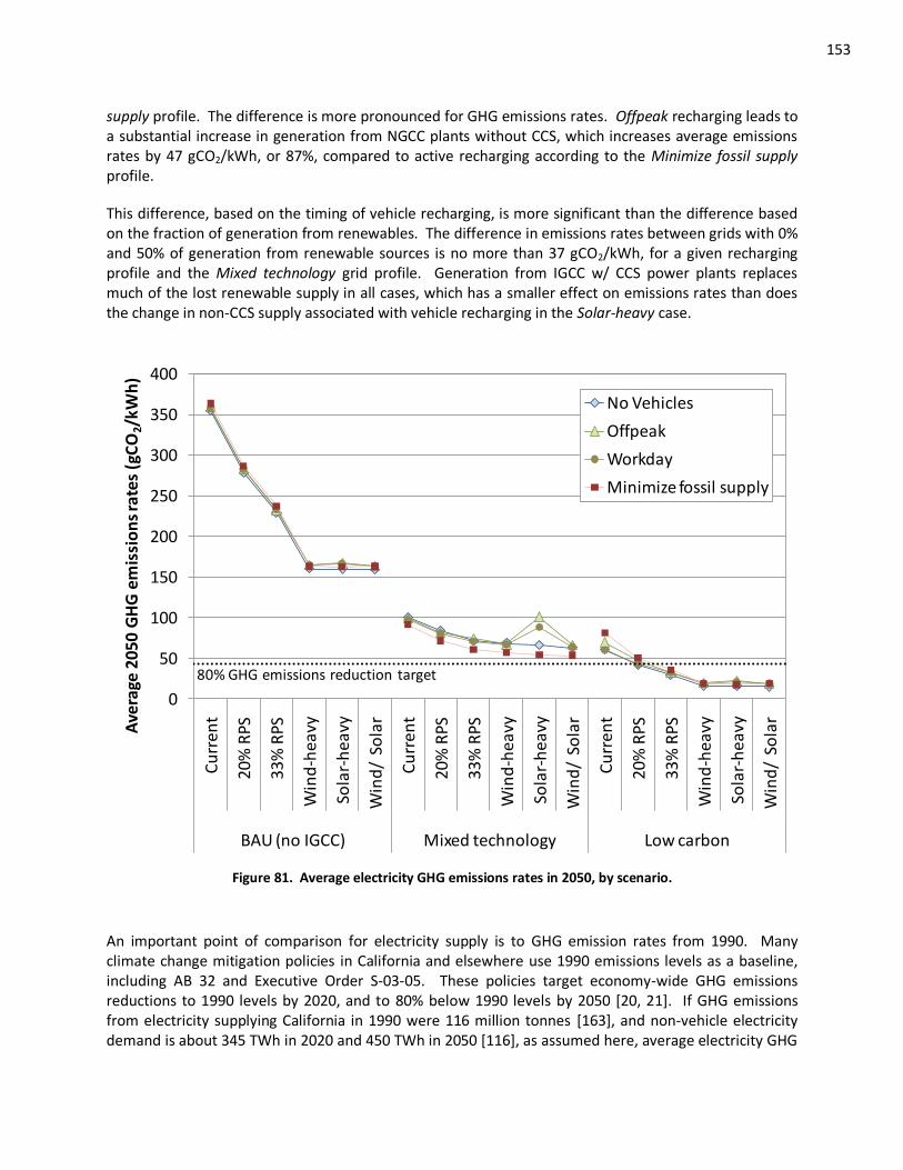
153

supply profile. The difference is more pronounced for GHG emissions rates. Offpeak recharging leads to a substantial increase in generation from NGCC plants without CCS, which increases average emissions rates by 47 gCO2/kWh, or 87%, compared to active recharging according to the Minimize fossil supply profile.

This difference, based on the timing of vehicle recharging, is more significant than the difference based on the fraction of generation from renewables. The difference in emissions rates between grids with 0% and 50% of generation from renewable sources is no more than 37 gCO2/kWh, for a given recharging profile and the Mixed technology grid profile. Generation from IGCC w/ CCS power plants replaces much of the lost renewable supply in all cases, which has a smaller effect on emissions rates than does the change in non-CCS supply associated with vehicle recharging in the Solar-heavy case.

0

50

100

150

200

250

300

350

400

Cu

rren

t

20%

RPS

33%

RPS

Win

d-h

eavy

Sola

r-h

eavy

Win

d/

So

lar

Cu

rren

t

20%

RPS

33%

RPS

Win

d-h

eavy

Sola

r-h

eavy

Win

d/

So

lar

Cu

rren

t

20%

RPS

33%

RPS

Win

d-h

eavy

Sola

r-h

eavy

Win

d/

So

lar


Ave

rage

205

0 G

HG

em

issi

on

s ra

tes

(gC

O2/

kWh

)

No Vehicles

Offpeak

Workday


80% GHG emissions reduction target

Figure 81. Average electricity GHG emissions rates in 2050, by scenario.

An important point of comparison for electricity supply is to GHG emission rates from 1990. Many climate change mitigation policies in California and elsewhere use 1990 emissions levels as a baseline, including AB 32 and Executive Order S-03-05. These policies target economy-wide GHG emissions reductions to 1990 levels by 2020, and to 80% below 1990 levels by 2050 [20, 21]. If GHG emissions from electricity supplying California in 1990 were 116 million tonnes [163], and non-vehicle electricity demand is about 345 TWh in 2020 and 450 TWh in 2050 [116], as assumed here, average electricity GHG

154

emissions rates for California have to be about 335 gCO2/kWh in 2020 and about 51 gCO2/kWh in 2050 to achieve the target in the electricity sector. If an additional 91 TWh of demand is added to the system from vehicle recharging in 2050, target GHG emissions rates fall to 43 gCO2/kWh.

In this analysis, none of the scenarios meet the targets without increasing renewable generation beyond current levels. If at least as much renewable generation as in the 20% RPS profile is added to scenarios, emissions rates meet the 2020 and 2050 targets for most scenarios based upon the Low carbon grid profile. Without a Low carbon grid, emissions rates in 2050 exceed the target value in all scenarios, although they are close with heavy renewables and the Mixed technology grid profile.

6.4.1 Summary of Category 4 results: Interactions between renewable generation and vehicle recharging

As observed from the results in Categories 2 and 3, adding vehicle recharging and renewable generation have opposing effects on fossil supply. When vehicle recharging is imposed on a grid with high levels of renewable generation, it can reduce the decline in utilization of fossil power plants that comes with renewables. This highlights a potential benefit of vehicle recharging.

In general, coordinating vehicle recharging with generation from intermittent renewables helps avoid additional fossil capacity and improves utilization of fossil power plants. The ideal timing of a vehicle recharging profile – to minimize fossil capacity – varies with the assumed resource mix and non-vehicle demand. If the grid evolves to include much more solar power, utilities may want to encourage daytime recharging during some days when fossil supply is not at its peak. They may want to strongly discourage vehicle recharging in the early evening, when the solar resource becomes unavailable and many fossil plants may need to ramp up very quickly. If wind generation comprises a significant fraction of supply, vehicle recharging in the early- and mid-evening hours may be beneficial from a generation standpoint. If future grids do not include a significant penetration of intermittent renewable resources, active vehicle recharging may have the most benefit on fossil supply the most by countering non-vehicle electricity demand. Non-vehicle electricity demand and intermittent renewable availability vary seasonally; so too does the optimal timing for active vehicle recharging.

By minimizing fossil capacity requirements, active vehicle recharging – as represented in Part II of this dissertation – always reduces costs of electricity supply, compared to other timing profiles for vehicle electricity demand. But emissions might be higher than if recharging follows a “less optimal” timing profile. By minimizing fossil capacity, coordinated vehicle recharging improves the utilization of existing fossil power plants. If these plants are relatively less-efficient, or have higher GHG emissions rates, than new plants that would be built otherwise, electricity GHG emissions may increase, compared to recharging vehicles in a way that requires more fossil capacity. In the Category 4 results, active vehicle recharging increases the share of generation from NGCT plants and average electricity emissions rates compared to passive recharging according to the Offpeak or Workday profiles, in scenarios with the BAU (no IGCC) or Low carbon grid profiles and no more than 33% of generation from renewables. In scenarios with any of the heavy-renewables profiles or the Mixed technology grid mix, active recharging reduces average electricity GHG emissions rates compared to scenarios with passive recharging according to the Offpeak or Workday recharging profiles.

Coordinated timing of vehicle recharging may be especially important for grids with a lot of solar generation. As represented here, the Solar-heavy renewable mix leads to wild fluctuations in electricity supply and emissions. Peak hourly emissions rates are often as high, or higher, than those for grids with

155

a much smaller fraction of generation from renewables. And they often occur in hours immediately before or after significant levels of solar generation is available, and emissions rates are very low. Active control of vehicle recharging on grids with significant levels of solar generation can reduce costs and emissions associated with supplying vehicle electricity demand dramatically.

6.5 Sensitivity Analysis of Long-term Results

The long-term results presented in this chapter reflect how renewables and vehicle recharging can shape the structure of electricity supply, but they are sensitive to the assumptions underlying the LEDGE-CA model. Of note, the shape of non-vehicle electricity demand and the relative cost of different power plant types may affect the results significantly. Sensitivity to these variables is explored by varying the load factor of non-vehicle electricity demand and by changing natural gas price and CO2 prices. The effect of changing each parameter is investigated in isolation, and presented graphically below. The sensitivities depicted in Figure 82-Figure 85 illustrate percentage changes in results for the 33% RPS renewable profile with No vehicles. In Figure 86, sensitivity to non-vehicle demand load factor is explored for some scenarios that include vehicle recharging or high levels of generation from intermittent renewables.

The sensitivity of the results to non-vehicle demand timing is investigated in Figure 82. Decreasing the load factor of non-vehicle electricity demand from the baseline value of 55% to 50%, as described in Section 5.3, reduces the fossil supply curve load factor by only 4% in the BAU (no IGCC) and Mixed technology grid profiles and 7% for the Low carbon profile. But if the non-vehicle demand load factor increases to 60%, the fossil supply load factor increases by 26% and 31%, respectively. As a result, total fossil capacity requirements (illustrated in Figure 68 with baseline assumptions) are 10 GW higher than with baseline assumptions if the non-vehicle load factor is 50% and about 8 GW lower if the non-vehicle load factor is 60%.

Changing the non-vehicle load factor affects the peaking capacity and generation in each scenario much more than baseload supply. For each grid profile, capacity from NGCT plants varies by ±25-50%. The absolute changes in NGCT capacity and generation are similar for each grid profile, but the percentage change is higher in Low carbon because baseline NGCT capacity and generation are lower than in the other two grid profiles.

For baseload generators, the percentage change in capacity is an order of magnitude lower than it is for NGCT plants. The variation in non-vehicle load factor reduces peak demands during relatively few hours more than it increases off-peak demand during many more hours. Thus, the effect of varying non-vehicle load factor on peak capacity is much more significant than the effect on baseload capacity. Total fossil capacity requirements, and NGCT capacity results from LEDGE-CA, then, are highly sensitive to input assumptions regarding non-vehicle electricity demand timing.

The effect of non-vehicle load factor on costs and emissions is smaller, but to the extent that changing non-vehicle demand shifts capacity and generation from peaking plants to baseload plants, it also serves to reduce costs and average GHG emissions rates. The effect on costs is more noticeable in the 2020 snapshot, when much of the NGCT capacity is added in these scenarios (not shown). But even then, the change in cost is relatively small compared to the change in fossil capacity.

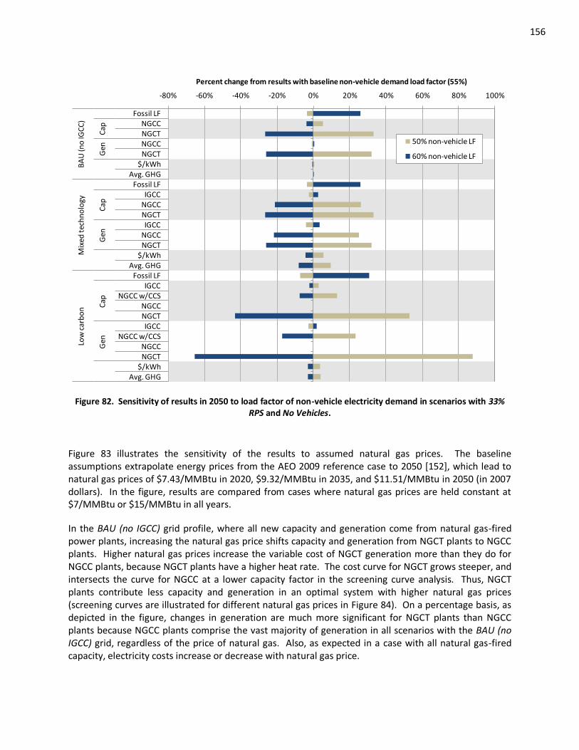
156

-80% -60% -40% -20% 0% 20% 40% 60% 80% 100%

Fossil LFNGCCNGCTNGCCNGCT

$/kWhAvg. GHG

Fossil LFIGCC

NGCCNGCTIGCC

NGCCNGCT

$/kWhAvg. GHG

Fossil LFIGCC

NGCC w/CCSNGCCNGCTIGCC

NGCC w/CCSNGCCNGCT

$/kWhAvg. GHG

Cap

Gen

Cap

Gen

Cap

Gen

BA

U (n

o IG

CC

)M

ixed

tec

hn

olo

gyLo

w c

arb

on

Percent change from results with baseline non-vehicle demand load factor (55%)

50% non-vehicle LF

60% non-vehicle LF

Figure 82. Sensitivity of results in 2050 to load factor of non-vehicle electricity demand in scenarios with 33% RPS and No Vehicles.

Figure 83 illustrates the sensitivity of the results to assumed natural gas prices. The baseline assumptions extrapolate energy prices from the AEO 2009 reference case to 2050 [152], which lead to natural gas prices of $7.43/MMBtu in 2020, $9.32/MMBtu in 2035, and $11.51/MMBtu in 2050 (in 2007 dollars). In the figure, results are compared from cases where natural gas prices are held constant at $7/MMBtu or $15/MMBtu in all years.

In the BAU (no IGCC) grid profile, where all new capacity and generation come from natural gas-fired power plants, increasing the natural gas price shifts capacity and generation from NGCT plants to NGCC plants. Higher natural gas prices increase the variable cost of NGCT generation more than they do for NGCC plants, because NGCT plants have a higher heat rate. The cost curve for NGCT grows steeper, and intersects the curve for NGCC at a lower capacity factor in the screening curve analysis. Thus, NGCT plants contribute less capacity and generation in an optimal system with higher natural gas prices (screening curves are illustrated for different natural gas prices in Figure 84). On a percentage basis, as depicted in the figure, changes in generation are much more significant for NGCT plants than NGCC plants because NGCC plants comprise the vast majority of generation in all scenarios with the BAU (no IGCC) grid, regardless of the price of natural gas. Also, as expected in a case with all natural gas-fired capacity, electricity costs increase or decrease with natural gas price.

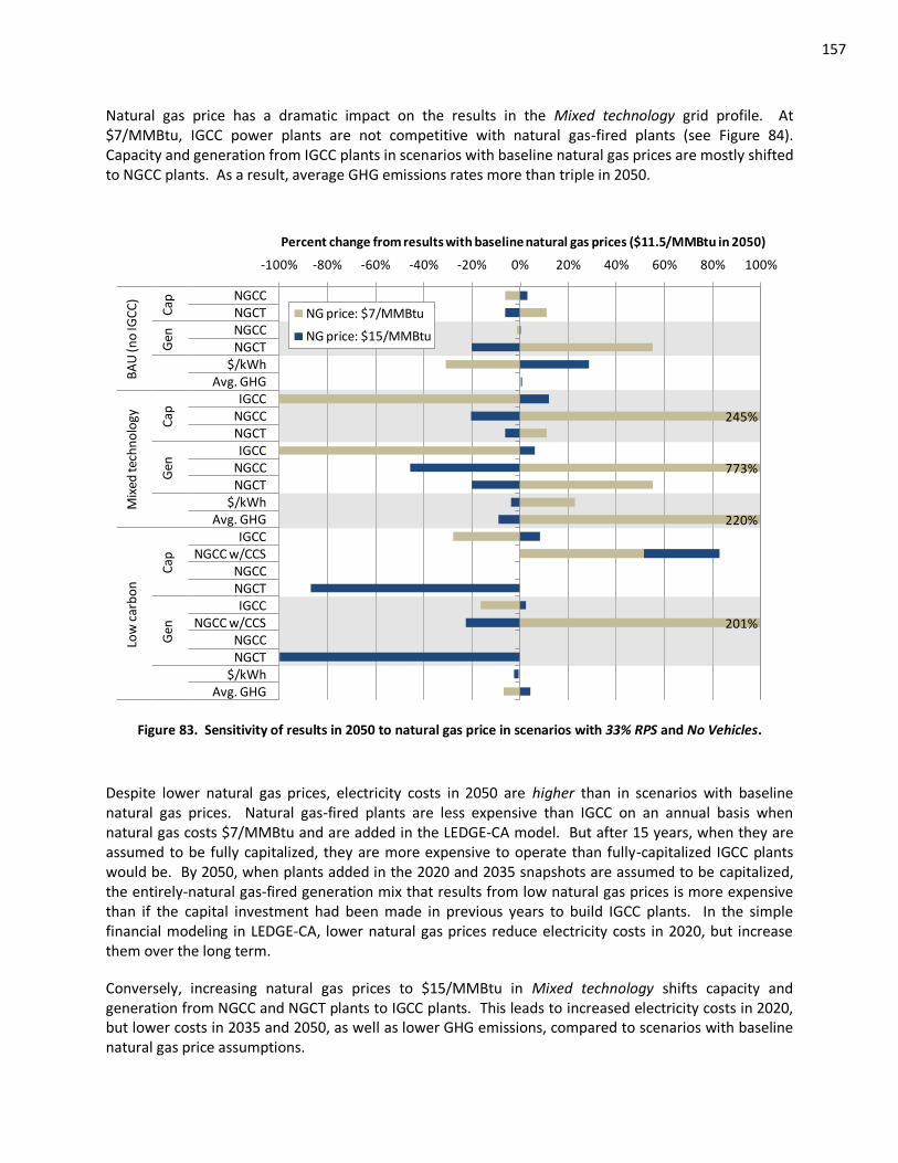
157

Natural gas price has a dramatic impact on the results in the Mixed technology grid profile. At $7/MMBtu, IGCC power plants are not competitive with natural gas-fired plants (see Figure 84). Capacity and generation from IGCC plants in scenarios with baseline natural gas prices are mostly shifted to NGCC plants. As a result, average GHG emissions rates more than triple in 2050.

245%

773%

220%

201%

-100% -80% -60% -40% -20% 0% 20% 40% 60% 80% 100%

NGCCNGCTNGCCNGCT

$/kWhAvg. GHG

IGCCNGCCNGCTIGCC

NGCCNGCT

$/kWhAvg. GHG

IGCCNGCC w/CCS

NGCCNGCTIGCC

NGCC w/CCSNGCCNGCT

$/kWhAvg. GHG

Cap

Gen

Cap

Gen

Cap

Gen

BA

U (n

o IG

CC

)M

ixed

tech

no

logy

Low

car

bo

n

Percent change from results with baseline natural gas prices ($11.5/MMBtu in 2050)

NG price: $7/MMBtu

NG price: $15/MMBtu

Figure 83. Sensitivity of results in 2050 to natural gas price in scenarios with 33% RPS and No Vehicles.

Despite lower natural gas prices, electricity costs in 2050 are higher than in scenarios with baseline natural gas prices. Natural gas-fired plants are less expensive than IGCC on an annual basis when natural gas costs $7/MMBtu and are added in the LEDGE-CA model. But after 15 years, when they are assumed to be fully capitalized, they are more expensive to operate than fully-capitalized IGCC plants would be. By 2050, when plants added in the 2020 and 2035 snapshots are assumed to be capitalized, the entirely-natural gas-fired generation mix that results from low natural gas prices is more expensive than if the capital investment had been made in previous years to build IGCC plants. In the simple financial modeling in LEDGE-CA, lower natural gas prices reduce electricity costs in 2020, but increase them over the long term.

Conversely, increasing natural gas prices to $15/MMBtu in Mixed technology shifts capacity and generation from NGCC and NGCT plants to IGCC plants. This leads to increased electricity costs in 2020, but lower costs in 2035 and 2050, as well as lower GHG emissions, compared to scenarios with baseline natural gas price assumptions.

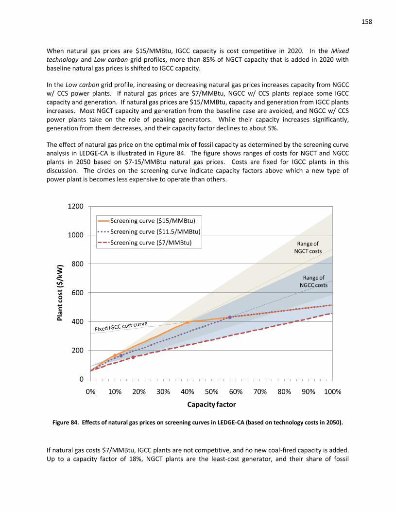
158

When natural gas prices are $15/MMBtu, IGCC capacity is cost competitive in 2020. In the Mixed technology and Low carbon grid profiles, more than 85% of NGCT capacity that is added in 2020 with baseline natural gas prices is shifted to IGCC capacity.

In the Low carbon grid profile, increasing or decreasing natural gas prices increases capacity from NGCC w/ CCS power plants. If natural gas prices are $7/MMBtu, NGCC w/ CCS plants replace some IGCC capacity and generation. If natural gas prices are $15/MMBtu, capacity and generation from IGCC plants increases. Most NGCT capacity and generation from the baseline case are avoided, and NGCC w/ CCS power plants take on the role of peaking generators. While their capacity increases significantly, generation from them decreases, and their capacity factor declines to about 5%.

The effect of natural gas price on the optimal mix of fossil capacity as determined by the screening curve analysis in LEDGE-CA is illustrated in Figure 84. The figure shows ranges of costs for NGCT and NGCC plants in 2050 based on $7-15/MMBtu natural gas prices. Costs are fixed for IGCC plants in this discussion. The circles on the screening curve indicate capacity factors above which a new type of power plant is becomes less expensive to operate than others.

0

200

400

600

800

1000

1200

0% 10% 20% 30% 40% 50% 60% 70% 80% 90% 100%

Pla

nt c

ost

($/

kW)

Capacity factor

Screening curve ($15/MMBtu)

Screening curve ($11.5/MMBtu)

Screening curve ($7/MMBtu) Range of NGCT costs

Range of NGCC costs

Figure 84. Effects of natural gas prices on screening curves in LEDGE-CA (based on technology costs in 2050).

If natural gas costs $7/MMBtu, IGCC plants are not competitive, and no new coal-fired capacity is added. Up to a capacity factor of 18%, NGCT plants are the least-cost generator, and their share of fossil

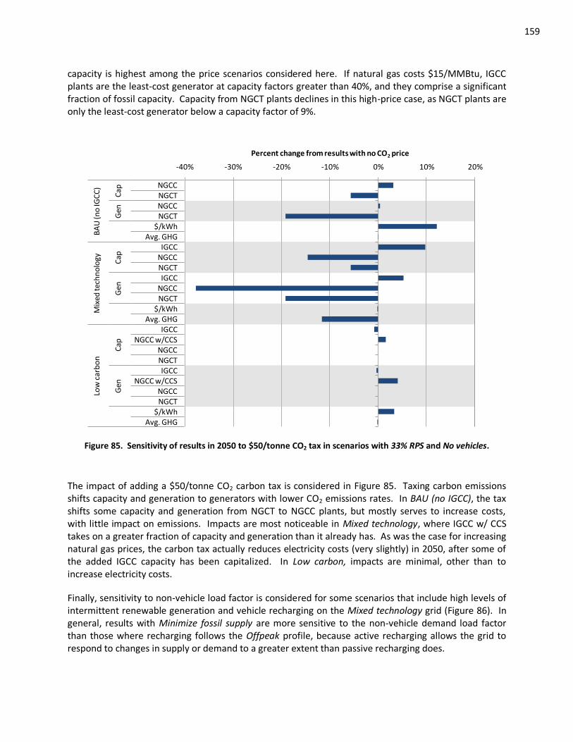
159

capacity is highest among the price scenarios considered here. If natural gas costs $15/MMBtu, IGCC plants are the least-cost generator at capacity factors greater than 40%, and they comprise a significant fraction of fossil capacity. Capacity from NGCT plants declines in this high-price case, as NGCT plants are only the least-cost generator below a capacity factor of 9%.

-40% -30% -20% -10% 0% 10% 20%

NGCCNGCTNGCCNGCT

$/kWhAvg. GHG

IGCCNGCCNGCTIGCC

NGCCNGCT

$/kWhAvg. GHG

IGCCNGCC w/CCS

NGCCNGCTIGCC

NGCC w/CCSNGCCNGCT

$/kWhAvg. GHG

Cap

Gen

Cap

Gen

Cap

Gen

BA

U (n

o IG

CC

)M

ixed

tech

no

logy

Low

car

bo

n

Percent change from results with no CO2 price

Figure 85. Sensitivity of results in 2050 to $50/tonne CO2 tax in scenarios with 33% RPS and No vehicles.

The impact of adding a $50/tonne CO2 carbon tax is considered in Figure 85. Taxing carbon emissions shifts capacity and generation to generators with lower CO2 emissions rates. In BAU (no IGCC), the tax shifts some capacity and generation from NGCT to NGCC plants, but mostly serves to increase costs, with little impact on emissions. Impacts are most noticeable in Mixed technology, where IGCC w/ CCS takes on a greater fraction of capacity and generation than it already has. As was the case for increasing natural gas prices, the carbon tax actually reduces electricity costs (very slightly) in 2050, after some of the added IGCC capacity has been capitalized. In Low carbon, impacts are minimal, other than to increase electricity costs.

Finally, sensitivity to non-vehicle load factor is considered for some scenarios that include high levels of intermittent renewable generation and vehicle recharging on the Mixed technology grid (Figure 86). In general, results with Minimize fossil supply are more sensitive to the non-vehicle demand load factor than those where recharging follows the Offpeak profile, because active recharging allows the grid to respond to changes in supply or demand to a greater extent than passive recharging does.

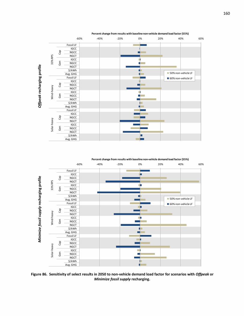
160

Off

pea

k re

char

gin

g p

rofi

le

-60% -40% -20% 0% 20% 40% 60%

Fossil LFIGCC

NGCCNGCTIGCC

NGCCNGCT

$/kWhAvg. GHG

Fossil LFIGCC

NGCCNGCTIGCC

NGCCNGCT

$/kWhAvg. GHG

Fossil LFIGCC

NGCCNGCTIGCC

NGCCNGCT

$/kWhAvg. GHG

Cap

Gen

Cap

Gen

Cap

Gen

33

% R

PS

Win

d-h

eavy

Sola

r-h

eavy


50% non-vehicle LF

60% non-vehicle LF

Min

imiz

e fo

ssil

sup

ply

re

char

gin

g p

rofi

le

-60% -40% -20% 0% 20% 40% 60%

Fossil LFIGCC

NGCCNGCTIGCC

NGCCNGCT

$/kWhAvg. GHG

Fossil LFIGCC

NGCCNGCTIGCC

NGCCNGCT

$/kWhAvg. GHG

Fossil LFIGCC

NGCCNGCTIGCC

NGCCNGCT

$/kWhAvg. GHG

Cap

Gen

Cap

Gen

Cap

Gen

33

% R

PS

Win

d-h

eavy

Sola

r-h

eavy


50% non-vehicle LF

60% non-vehicle LF

Figure 86. Sensitivity of select results in 2050 to non-vehicle demand load factor for scenarios with Offpeak or Minimize fossil supply recharging.

161

As observed in the sensitivity analysis for scenarios with No vehicles, illustrated in Figure 82, capacity and generation from peaking power plants (NGCT) are most sensitive to non-vehicle demand load factors. For a constant level or annual demand, and thus a constant average hourly demand, increasing the load factor serves to both decrease required fossil capacity and shift the mix of capacity from peaking plants to baseload plants. Thus, capacity from NGCT plants decreases significantly when the non-vehicle demand load factor is increased to 60%. Conversely, when the load factor decreases, total fossil capacity and the capacity share of peaking plants increases, and NGCT capacity increases significantly. When vehicle recharging is active, capacity and generation from NGCC plants is very sensitive to non-vehicle demand load factor, as well.

Often, the results are more sensitive in the scenarios with the 33% RPS renewable mix than they are in scenarios with higher levels of intermittent renewable generation because demand has a greater impact on the shape of the fossil supply curve (and its load factor). In the Wind-heavy and Solar-heavy scenarios, intermittent generation from wind or solar resources have an important impact on the supply curve for fossil generators, and changes to the shape of non-vehicle electricity demand have relatively smaller impacts on fossil supply.

162

7. SUMMARY AND CONCLUSIONS

This dissertation research investigates interactions between light-duty vehicle and fuel-related electricity demands and electricity supply in California. It estimates near-term marginal electricity mixes likely to supply electricity demand from BEV or PHEV recharging or from hydrogen production for use in FCVs. The resulting marginal electricity GHG emissions rates are attributed to vehicle and fuel pathways to compare vehicle emissions on a well-to-wheels basis, with detailed accounting of electricity supply for a broad range of vehicles in California.

This dissertation also considers evolution of electricity generation in California through 2050, when high levels of renewable generation may be incorporated on the grid or plug-in vehicle recharging may have significant impacts on California electricity supply and demand. Electricity supply over the long term is highly uncertain. It is investigated using dozens of scenarios pertaining to various renewable and other power plant mixes, and timing of vehicle recharging.

The concepts of active and passive grid elements are introduced, and frame the discussion of long-term vehicle recharging impacts on the grid. Passive elements are imposed on the grid and do not respond to market or system conditions. They include most current electricity demand and “must-run” generation from nuclear or renewable power plants that is assumed to be taken whenever available, in this analysis. Active elements represent loads that can be controlled by utilities to follow demand and passive generation, or hydro and fossil power plants that ramp up or down in response to system changes and are used to balance supply with demand.

Given the policy context in California, interactions between intermittent renewable generation and active vehicle recharging are particularly interesting. In the models developed as part of this dissertation, interactions and impacts of these elements on the grid are analyzed in terms of their affect on the composition of fossil supply. Capacities and generation from fossil power plants are a function of the portion of the demand profile that must be supplied by fossil generators, which represents the difference in total demand and generation from must-run or hydro power plants on an hourly basis. The quantity, timing, and location of vehicle recharging or renewable generation determine their impact on fossil supply profiles, and thus, their impact on generation costs and GHG emissions from the electricity sector.

7.1 Methodological Contributions and Areas for Improvement

Two simulation models are developed to investigate the research questions posed in this dissertation. EDGE-CA simulates operation of the current grid to identify near-term marginal electricity mixes. LEDGE-CA simulates evolution and operation of the California grid through 2050 to determine impacts of vehicle recharging and intermittent renewable generation on the structure and operation of future electricity supply in the state.

The modeling tools and results developed in this dissertation offer important methodological and empirical contributions that advance understanding of electricity supply and potential impacts of new demand from vehicles and fuels, especially in California. The vehicle recharging profiles provide insights regarding potential impacts of light-duty vehicles on the California grid, including optimal recharging from a utility and generation perspective, to match supply with demand.

Few detailed, hourly electricity dispatch models exist that are not proprietarily held and commercially licensed. While EDGE-CA and LEDGE-CA lack the detail of commercial software, they provide useful

163

tools appropriate for systems-level analysis of demand effects on electricity supply, and match well with current system operation.

They also provide helpful representations of aggregate availability and generation from power plant categories in California that is often lacking. The aggregate representations of wind, solar, and hydro generation in California that are developed in this dissertation (as described in Section 3.2) are interesting and novel. The regression models developed for system imports offer important insight into regional supply, demand, and power procurement decisions that are missing in the literature. The import models offer a starting point for understanding variables that affect the hourly availability of power from out-of-state. They deserve to be elaborated upon in future work.

While the models represent aggregate generation with reasonable accuracy, the representation of electricity supply could be improved. Simple costing methods are used and various operating constraints are excluded that may affect the relative economics of power plants in a given hour. Explicit representations of energy storage and demand management are not included in the models, but these resources will likely play important roles in electricity supply in the near and long term. Presumably, the dispatch order of fossil power plants could be made dynamic, and adjust to changes in relative power plant costs. This would lead to a more accurate representation of system costs and allow demand management and energy storage to be explored through optimization techniques. These efforts are left for future work.

7.2 Empirical Contributions and Areas for Future Work

This dissertation offers several empirical contributions, as well. They are discussed in this section in the context of the research questions posed in Chapter 1, and along with ideas for future research to improve upon them.

Question 1: What is the effect of increasing penetrations of advanced vehicles and alternative fuels on electricity demand in California?


From a high-level perspective, in terms of power plant capacity and generation (excluding implications for transmission and local distribution infrastructure), the grid can likely accommodate as many electric vehicles as can be manufactured and sold in the near term. Indeed, if 1 million BEVs were suddenly added to California roads, they would increase annual electricity demand by about 1.8% – the same amount that it already increases annually, without vehicle recharging. Based on likely timing of aggregate vehicle recharging (represented by the Offpeak profile in this dissertation), 1 million BEVs would increase projected peak demand in 2010 by about 350 MW, or 0.6%. If vehicle recharging follows a different profile, it would have a different impact on peak demand, and grid capacity.

Incremental impacts from vehicles on annual electricity demand in California likely will be much smaller. It will take several years for 1 million plug-in vehicles to be sold in the state, and many will likely be PHEVs, which use less electricity than BEVs.

164

How do long-term vehicle electricity demand and timing scenarios affect demand profiles and load factors?

Vehicle recharging changes total demand, the shape of the demand profile that must be supplied by fossil-fired power plants (total demand minus generation from hydro, nuclear, and renewable sources), and thus, the optimal mix of fossil generators. When vehicle recharging contributes to peak demand, more power plant capacity is needed. To the extent that vehicle recharging levels demand and makes the curve flatter, which it should, it allows fossil power plants to be more highly utilized. As the fossil supply curve becomes flatter, the optimal mix of fossil capacity shifts away from peaking and intermediate plants to baseload plants. If these plants have lower operating costs and GHG emissions rates than those that would exist otherwise – as will be the case if technology costs for CCS, IGCC, and nuclear plants drop sufficiently – average generation costs and GHG emissions rates can decline with increasing vehicle and fuel electricity demand.

In the scenarios considered in this dissertation, 91 TWh of light-duty vehicle electricity demand is added to the grid by 2050. This represents demand from a fleet of more than 50 million light-duty vehicles, composed of 50% FCVs, 25% BEVs, and 25% PHEVs. According to the projected non-vehicle electricity demand scenario, these vehicles increase annual California electricity demand by 17%, and peak demand by 8% (in the representative Offpeak profile). If vehicle recharging can be made active, controlled by utilities to avoid contributing to peak demand, no additional capacity is needed to supply these vehicles beyond what would be needed in 2050 to meet non-vehicle electricity demands.

The relative “peakiness” of demand and fossil supply are measured through load factors. Every scenario for vehicle recharging considered in this dissertation leads to higher demand load factors and increased utilization of fossil supply. Load factors increase the most if recharging provides active load to complement non-vehicle demand and match the availability of passive generation. But they also increase – to a lesser extent – if recharging is passive, and not controlled by utilities. Even in the worst case considered in this dissertation, where about 20% of recharging occurs from 12pm-5pm every day (according to the Workday profile), recharging increases average electricity demand more than peak demand, and increases load factors for demand and fossil supply.

The analysis only considers demand impacts in terms of power plant capacity. On a local-level, vehicle recharging may have important impacts on grid infrastructure that require upgrading equipment within a home or at the sub-station level. These interactions are beyond the scope of this dissertation, and are left for future work.

The empirical results from the analyses in this dissertation can be extended in future work by considering additional demand timing profiles. For example, aggregate recharging may include a mix of active and passive demands. It could be interesting to investigate the impacts from timing profiles that include some combination of those investigated here, or that represent actual, measured recharging behavior. Also, a more clear representation of future interactions between the transportation and electricity sectors would include all electricity demands from the transportation sector. Electrifying delivery trucks, rail systems, or truck stops – for example – could lead to more significant electricity demands and different timing profiles than the scenarios for light-duty vehicles considered here.

165

The analysis methods and tools presented in this dissertation can be applied to consider demand effects on electricity supply from any change in end use. Active or passive demand from plasma TVs, “smart” appliances, and controllable thermostats will likely have much more significant impacts on the grid in the near term than plug-in vehicles will. Their impacts on electricity supply in California can be investigated with the EDGE-CA and LEDGE-CA models, as well.

Question 2: How does operation of the existing and near-term electricity grid in California change in response to additional demand from light-duty vehicles?

What types of power plants will provide marginal electricity supply for vehicles and fuels initially? What are the associated GHG emissions rates? How do they compare to the value codified in the California’s Low Carbon Fuel Standard (LCFS)?

In the near-term, because electricity demand from vehicles and fuels is very small, operation of the grid changes very little. Mostly, vehicle recharging increases generation from natural gas-fired power plants in California. These plants are more expensive, and typically less efficient with higher GHG emissions rates, than the average of all natural gas-fired generation operating.

According to the Offpeak recharging profile, which is presumed to be the most likely near-term vehicle electricity demand scenario included in this dissertation, the marginal mix includes 63% NGCC or CHP power plants, and 37% NGST or NGCT power plants. Emissions rates from the latter two plant types are about 50% higher than NGCC or CHP plants. This leads to a marginal electricity emissions rate of about 625 gCO2-eq/kWh on a lifecycle basis.

Compared to these results, the LCFS significantly underestimates marginal emissions rates for vehicle electricity. The marginal emissions rate included in the LCFS is 377 gCO2-eq/kWh, or about 65% less than the results here. It assumes that about 20% of marginal electricity for vehicle recharging will come from renewable resources and the remainder from NGCC plants. The LCFS also includes a fuel efficiency multiplier to account for the improved vehicle efficiency of electric-drive vehicles, which makes electricity a “low carbon fuel” in the regulatory framework, and a much more attractive option than the 377 gCO2-eq/kWh would imply.

It is highly unlikely that renewable power will supply marginal electricity for vehicle recharging and fuel production in the near term. Additionally, these results indicate that marginal electricity from natural gas-fired power plants is not likely to come entirely from NGCC plants. Generation from the less-efficient NGST and NGCT plants constitutes an important part of marginal mixes in near-term scenarios. And to the extent that NGCC plants do supply marginal power, they are likely to be less efficient than the average of all NGCC plants operating.

If vehicle recharging flattens the demand and fossil supply profiles more than in the Offpeak profile, the fraction of generation from NGCC and CHP plants increases and marginal electricity emissions rates decline below 625 gCO2-eq/kWh. If vehicle recharging has the opposite effect, the fraction of generation from NGST and NGCT plants increases, along with marginal emissions rates. Regardless of the timing of vehicle recharging, however, marginal electricity GHG emissions rates are likely to be much higher than represented in the LCFS.

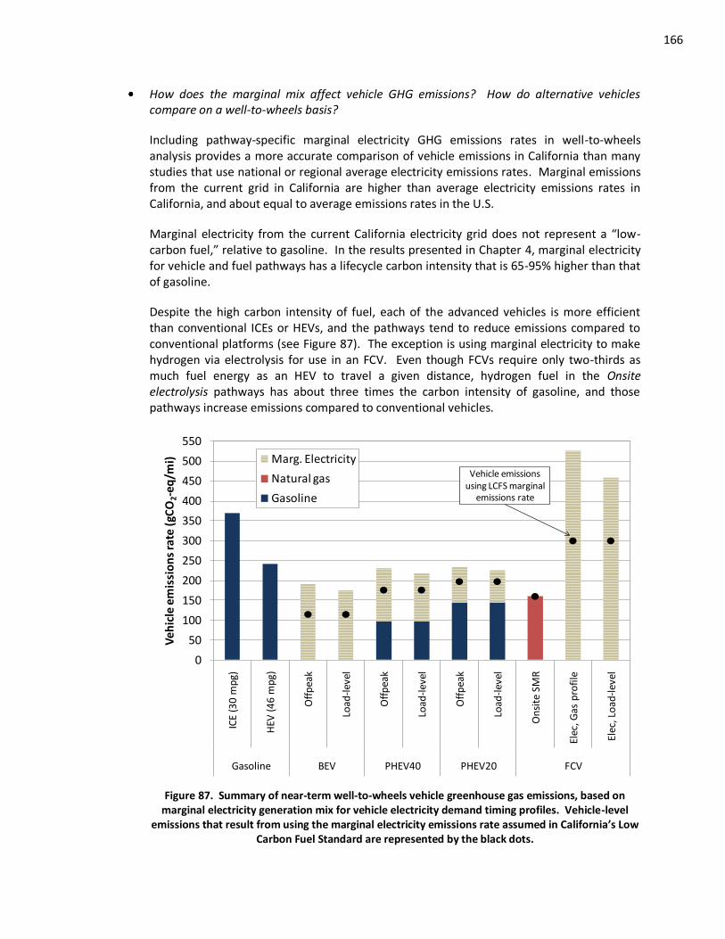
166

How does the marginal mix affect vehicle GHG emissions? How do alternative vehicles compare on a well-to-wheels basis?

Including pathway-specific marginal electricity GHG emissions rates in well-to-wheels analysis provides a more accurate comparison of vehicle emissions in California than many studies that use national or regional average electricity emissions rates. Marginal emissions from the current grid in California are higher than average electricity emissions rates in California, and about equal to average emissions rates in the U.S.

Marginal electricity from the current California electricity grid does not represent a “low-carbon fuel,” relative to gasoline. In the results presented in Chapter 4, marginal electricity for vehicle and fuel pathways has a lifecycle carbon intensity that is 65-95% higher than that of gasoline.

Despite the high carbon intensity of fuel, each of the advanced vehicles is more efficient than conventional ICEs or HEVs, and the pathways tend to reduce emissions compared to conventional platforms (see Figure 87). The exception is using marginal electricity to make hydrogen via electrolysis for use in an FCV. Even though FCVs require only two-thirds as much fuel energy as an HEV to travel a given distance, hydrogen fuel in the Onsite electrolysis pathways has about three times the carbon intensity of gasoline, and those pathways increase emissions compared to conventional vehicles.

0

50

100

150

200

250

300

350

400

450

500

550

ICE

(30

mp

g)

HEV

(4

6 m

pg)

Off

pea

k

Load

-lev

el

Off

pea

k

Load

-lev

el

Off

pea

k

Load

-lev

el

On

site

SM

R

Elec

, Gas

pro

file

Elec

, Lo

ad-l

evel

Gasoline BEV PHEV40 PHEV20 FCV

Veh

icle

em

issi

on

s ra

te (

gCO

2-eq

/mi) Marg. Electricity

Natural gas

Gasoline

Vehicle emissions using LCFS marginal

emissions rate

Figure 87. Summary of near-term well-to-wheels vehicle greenhouse gas emissions, based on marginal electricity generation mix for vehicle electricity demand timing profiles. Vehicle-level

emissions that result from using the marginal electricity emissions rate assumed in California’s Low Carbon Fuel Standard are represented by the black dots.

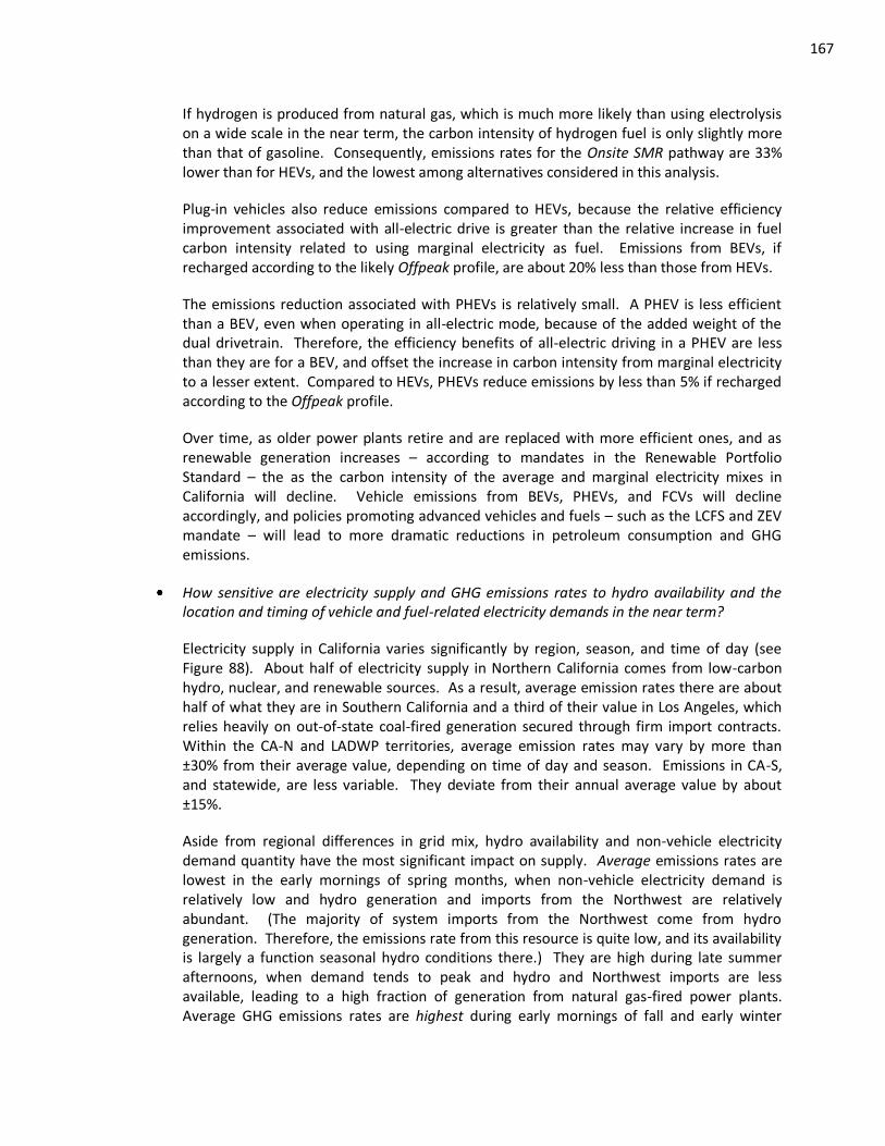
167

If hydrogen is produced from natural gas, which is much more likely than using electrolysis on a wide scale in the near term, the carbon intensity of hydrogen fuel is only slightly more than that of gasoline. Consequently, emissions rates for the Onsite SMR pathway are 33% lower than for HEVs, and the lowest among alternatives considered in this analysis.

Plug-in vehicles also reduce emissions compared to HEVs, because the relative efficiency improvement associated with all-electric drive is greater than the relative increase in fuel carbon intensity related to using marginal electricity as fuel. Emissions from BEVs, if recharged according to the likely Offpeak profile, are about 20% less than those from HEVs.

The emissions reduction associated with PHEVs is relatively small. A PHEV is less efficient than a BEV, even when operating in all-electric mode, because of the added weight of the dual drivetrain. Therefore, the efficiency benefits of all-electric driving in a PHEV are less than they are for a BEV, and offset the increase in carbon intensity from marginal electricity to a lesser extent. Compared to HEVs, PHEVs reduce emissions by less than 5% if recharged according to the Offpeak profile.

Over time, as older power plants retire and are replaced with more efficient ones, and as renewable generation increases – according to mandates in the Renewable Portfolio Standard – the as the carbon intensity of the average and marginal electricity mixes in California will decline. Vehicle emissions from BEVs, PHEVs, and FCVs will decline accordingly, and policies promoting advanced vehicles and fuels – such as the LCFS and ZEV mandate – will lead to more dramatic reductions in petroleum consumption and GHG emissions.


Electricity supply in California varies significantly by region, season, and time of day (see Figure 88). About half of electricity supply in Northern California comes from low-carbon hydro, nuclear, and renewable sources. As a result, average emission rates there are about half of what they are in Southern California and a third of their value in Los Angeles, which relies heavily on out-of-state coal-fired generation secured through firm import contracts. Within the CA-N and LADWP territories, average emission rates may vary by more than ±30% from their average value, depending on time of day and season. Emissions in CA-S, and statewide, are less variable. They deviate from their annual average value by about ±15%.

Aside from regional differences in grid mix, hydro availability and non-vehicle electricity demand quantity have the most significant impact on supply. Average emissions rates are lowest in the early mornings of spring months, when non-vehicle electricity demand is relatively low and hydro generation and imports from the Northwest are relatively abundant. (The majority of system imports from the Northwest come from hydro generation. Therefore, the emissions rate from this resource is quite low, and its availability is largely a function seasonal hydro conditions there.) They are high during late summer afternoons, when demand tends to peak and hydro and Northwest imports are less available, leading to a high fraction of generation from natural gas-fired power plants. Average GHG emissions rates are highest during early mornings of fall and early winter

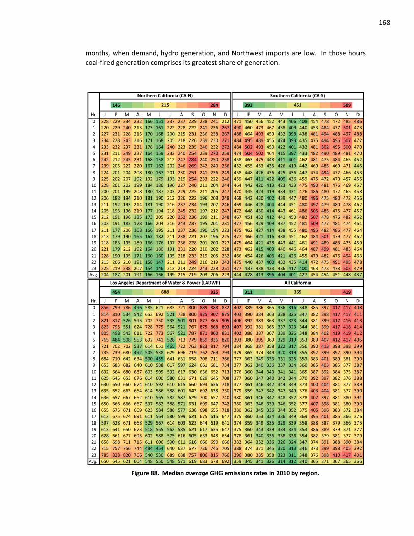
168

months, when demand, hydro generation, and Northwest imports are low. In those hours coal-fired generation comprises its greatest share of generation.

146

162 177 192 253 269

284 393

405 418 431 470 483 496

509


0 228 229 234 232 166 151 237 237 229 238 241 212 471 450 456 452 443 406 408 454 478 472 485 486

1 220 229 240 213 173 161 222 228 222 241 236 267 490 460 473 467 438 409 440 453 484 477 501 473

2 227 231 228 215 170 168 200 215 231 236 238 267 488 464 493 459 432 398 438 481 494 488 497 488

3 234 228 243 216 171 168 205 218 226 239 230 271 484 495 489 455 424 393 435 475 494 496 507 472

4 233 232 237 231 178 164 240 223 235 246 232 272 484 502 493 450 422 401 432 481 502 495 500 470

5 231 211 249 227 164 159 233 240 254 239 270 259 474 504 502 464 415 397 433 482 490 489 481 470

6 242 212 245 231 168 158 212 247 284 240 250 258 458 463 475 448 411 401 462 481 475 484 465 452

7 239 205 222 220 167 162 202 246 269 242 240 256 452 455 453 435 426 419 442 469 485 469 471 445

8 224 201 204 208 180 167 201 230 251 241 236 249 458 448 426 436 425 436 447 474 494 472 466 453

9 225 202 207 192 192 179 193 219 254 233 222 246 459 447 411 422 409 436 459 475 472 470 457 455

10 228 201 202 199 184 186 196 227 240 211 204 244 464 442 420 413 423 433 475 490 481 476 469 457

11 200 201 199 208 180 187 203 229 225 211 205 247 470 445 423 419 434 431 476 486 480 472 465 458

12 206 188 194 210 181 190 212 226 222 196 208 248 468 442 430 402 439 447 480 496 475 480 472 456

13 211 192 193 214 181 190 216 237 234 193 207 246 469 446 428 404 444 451 480 497 479 480 478 462

14 205 193 196 219 177 194 218 245 232 197 212 247 472 448 430 414 443 461 486 505 485 475 477 457

15 212 191 196 185 173 205 220 252 236 199 211 248 467 451 432 412 441 450 482 507 478 476 482 452

16 203 191 183 178 166 204 216 243 237 195 201 231 477 456 429 409 437 452 481 509 477 481 474 461

17 211 177 206 168 166 195 211 237 236 190 194 223 475 462 427 414 438 455 480 495 482 486 477 464

18 213 179 190 165 162 182 211 238 221 207 196 225 477 466 421 416 438 451 462 484 501 479 477 462

19 218 183 195 189 166 176 197 236 228 201 200 227 475 464 421 428 443 441 461 491 489 483 475 459

20 221 179 212 192 164 180 191 231 220 210 202 228 473 462 415 409 440 446 464 487 499 481 483 464

21 228 190 195 171 160 160 195 218 233 219 205 232 466 454 426 406 421 426 455 479 482 476 494 463

22 213 206 210 191 158 147 211 211 249 216 219 243 475 440 437 400 432 435 414 472 475 491 495 478

23 225 219 238 207 154 146 213 214 224 243 228 251 477 437 438 423 436 417 400 463 473 478 503 479Avg. 204 187 201 191 166 166 199 215 219 203 206 223 444 428 413 396 404 401 427 454 454 451 448 437

454

506 558 611 768 820 872

925 311

323 335 347 383 395

419


0 856 799 786 496 585 621 683 721 800 889 888 832 402 389 386 365 336 316 348 385 397 417 417 408

1 814 810 534 542 653 692 521 738 800 925 907 875 403 390 384 363 338 325 347 382 398 417 417 411

2 821 817 526 595 702 750 535 501 801 877 865 905 406 392 383 363 337 323 344 381 399 417 416 413

3 823 795 551 624 728 775 564 521 767 875 868 893 407 392 381 365 337 323 344 381 399 417 418 414

4 805 498 543 611 722 773 567 521 787 871 860 831 402 388 387 367 339 326 348 384 402 419 419 412

5 765 484 508 553 692 741 528 713 779 859 836 820 393 380 395 369 329 319 353 389 407 412 417 405

6 721 702 702 537 614 651 465 722 763 823 817 794 384 368 387 358 322 317 356 390 413 398 398 399

7 735 739 680 492 505 538 629 696 719 762 769 793 379 365 374 349 320 319 355 392 399 392 390 394

8 684 710 642 634 500 455 641 631 658 708 711 766 377 363 349 333 331 325 353 383 401 389 381 390

9 653 683 682 640 610 588 617 597 624 661 681 734 377 362 340 336 337 334 360 385 403 385 377 387

10 632 664 680 687 603 595 592 617 630 636 652 713 376 360 344 340 341 341 365 387 392 384 375 387

11 625 645 653 676 614 600 580 631 671 629 645 708 377 360 347 340 342 344 370 392 397 382 376 388

12 630 650 660 674 610 592 610 615 660 693 636 718 377 361 346 342 344 349 373 400 404 381 377 389

13 635 652 663 664 614 586 588 601 643 692 638 730 379 359 347 342 347 349 376 403 404 381 377 390

14 636 657 667 662 610 565 582 587 629 700 657 740 380 361 346 342 348 352 378 407 397 381 380 391

15 650 666 666 667 597 582 588 571 631 699 647 742 380 363 346 339 346 352 377 407 398 381 380 390

16 655 675 671 669 623 584 588 577 638 698 655 718 380 362 345 336 344 352 375 405 396 383 372 384

17 612 675 674 691 611 564 580 599 621 675 615 647 375 360 353 334 336 349 369 395 401 385 366 376

18 597 628 671 668 529 567 614 603 623 644 619 641 374 359 349 335 329 339 358 388 387 379 366 375

19 613 641 650 673 518 565 562 585 621 617 635 647 375 360 343 339 334 334 353 386 389 379 371 377

20 628 661 677 695 602 588 575 616 605 633 648 654 378 361 340 336 338 336 354 382 379 381 377 379

21 658 698 711 715 611 606 590 611 616 666 690 666 382 364 352 336 326 324 347 374 391 388 390 384

22 715 757 756 744 484 454 640 637 677 726 745 705 388 374 371 345 320 313 346 373 399 398 405 392

23 785 828 820 766 540 530 689 688 757 806 815 766 396 380 385 358 323 311 348 376 398 410 417 401Avg. 650 645 621 604 548 550 548 571 619 683 678 692 359 345 341 326 314 312 340 365 371 367 365 366

689 365

215 451


Los Angeles Department of Water & Power (LADWP) All California

Figure 88. Median average GHG emissions rates in 2010 by region.

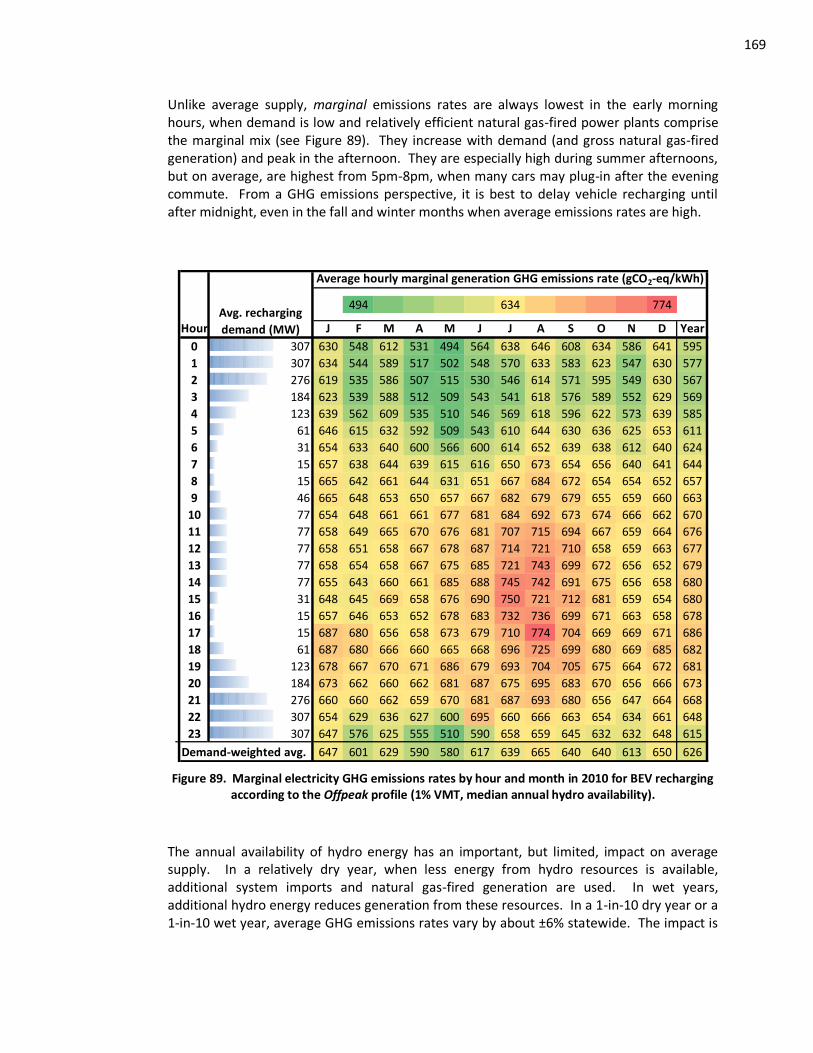
169

Unlike average supply, marginal emissions rates are always lowest in the early morning hours, when demand is low and relatively efficient natural gas-fired power plants comprise the marginal mix (see Figure 89). They increase with demand (and gross natural gas-fired generation) and peak in the afternoon. They are especially high during summer afternoons, but on average, are highest from 5pm-8pm, when many cars may plug-in after the evening commute. From a GHG emissions perspective, it is best to delay vehicle recharging until after midnight, even in the fall and winter months when average emissions rates are high.

494

522 550 578 606

634 774


0 307 630 548 612 531 494 564 638 646 608 634 586 641 595

1 307 634 544 589 517 502 548 570 633 583 623 547 630 577

2 276 619 535 586 507 515 530 546 614 571 595 549 630 567

3 184 623 539 588 512 509 543 541 618 576 589 552 629 569

4 123 639 562 609 535 510 546 569 618 596 622 573 639 585

5 61 646 615 632 592 509 543 610 644 630 636 625 653 611

6 31 654 633 640 600 566 600 614 652 639 638 612 640 624

7 15 657 638 644 639 615 616 650 673 654 656 640 641 644

8 15 665 642 661 644 631 651 667 684 672 654 654 652 657

9 46 665 648 653 650 657 667 682 679 679 655 659 660 663

10 77 654 648 661 661 677 681 684 692 673 674 666 662 670

11 77 658 649 665 670 676 681 707 715 694 667 659 664 676

12 77 658 651 658 667 678 687 714 721 710 658 659 663 677

13 77 658 654 658 667 675 685 721 743 699 672 656 652 679

14 77 655 643 660 661 685 688 745 742 691 675 656 658 680

15 31 648 645 669 658 676 690 750 721 712 681 659 654 680

16 15 657 646 653 652 678 683 732 736 699 671 663 658 678

17 15 687 680 656 658 673 679 710 774 704 669 669 671 686

18 61 687 680 666 660 665 668 696 725 699 680 669 685 682

19 123 678 667 670 671 686 679 693 704 705 675 664 672 681

20 184 673 662 660 662 681 687 675 695 683 670 656 666 673

21 276 660 660 662 659 670 681 687 693 680 656 647 664 668

22 307 654 629 636 627 600 695 660 666 663 654 634 661 648

23 307 647 576 625 555 510 590 658 659 645 632 632 648 615



Avg. recharging

demand (MW)

Figure 89. Marginal electricity GHG emissions rates by hour and month in 2010 for BEV recharging according to the Offpeak profile (1% VMT, median annual hydro availability).

The annual availability of hydro energy has an important, but limited, impact on average supply. In a relatively dry year, when less energy from hydro resources is available, additional system imports and natural gas-fired generation are used. In wet years, additional hydro energy reduces generation from these resources. In a 1-in-10 dry year or a 1-in-10 wet year, average GHG emissions rates vary by about ±6% statewide. The impact is

170

twice that in Northern California. The impact of annual hydro generation and location of vehicle recharging on marginal supply is quite small.

These trends are particular to California. Regions with more hydro may have more variation in supply and emissions rates, while others with fewer variable resources may see more steady supply. In regions with a significant fraction of generation from coal-fired plants, marginal emissions rates might be lower than average rates, if natural gas-fired plants operate on the margin with lower emissions rates than the coal-heavy average mix. In that case, off-peak recharging might be worst from an emissions perspective. An investigation of average and marginal supply in other regions, and comparison to California, would be an interesting extension of this research.

The GHG emissions rate for marginal electricity in the LCFS deserves to be re-assessed. Further analysis and discussion is required to develop an appropriate definition of marginal electricity and to improve the accuracy of the estimated GHG emissions rate. The impact of vehicle recharging on electricity dispatch should be considered in the rule-making.

Question 3: How might the California electric grid evolve differently over time with additional renewable generation or demand from vehicle recharging than it would otherwise?

Regardless of the level of vehicle recharging or renewable generation, an uneven distribution of plant age among power plant categories may have important impacts on future supply. The current fleet of peaking power plants in California is quite old. Unless energy storage or demand management can supplant the role of peaking generators, much of the existing capacity in the state will have to be replaced in the near term. In the simulations here, about 70% of fossil capacity added in the 2010-2020 timeframe comes from peaking, NGCT power plants. After 2020, much of the baseload capacity serving the state retires – including its two nuclear power plants and most firm import contracts – and the vast majority of capacity added in the 2020-2035 timeframe comes from baseload power plants. From 2035-2050, a more balanced mix of fossil generators is added in these scenarios.

According to the technology cost assumptions used in Part II of this dissertation, low-carbon generation is cost-effective in the 2020-2035 timeframe. Average electricity costs are lowest in scenarios with more IGCC or nuclear capacity and generation. This result stems largely from the relatively high price of natural gas assumed in this analysis, which make IGCC and CCS technologies more cost-effective than conventional natural gas-fired power plants when operating at high capacity factors. (Carbon prices have a very small impact on the results, compared to assumed technology costs and natural gas prices.) Consequently, in scenarios that assume that IGCC and CCS technology are cost-effective and technically feasible, GHG emissions rates reduce dramatically over time, even without adding renewable power to the grid. Carbon capture and sequestration technology is not cost effective if added to NGCC plants, however, and is not included in optimal capacity mixes unless natural gas-fired plants without CCS technology are banned.

These general findings hold in all scenarios considered here, but the level and timing of vehicle recharging or renewable generation have important impacts on future supply, as well.

What effect does increasing light-duty vehicle recharging have on electricity supply in California?

If vehicle recharging contributes to peak demand – in all likelihood, it will to some (probably small) extent – additional power plant capacity will be required. Some incremental capacity

171

may come from renewable generators, in proportion to the state’s Renewable Portfolio Standard, but much of it will come from fossil power plants. If vehicle recharging can be actively controlled to avoid contributing to peak demand, no additional capacity may be required.

Adding electricity demand from vehicle recharging also flattens the fossil supply profile, which shifts capacity from peaking or intermediate power plants to more highly-utilized baseload generators. In many of the long-term scenarios, especially if vehicle recharging is actively controlled by utilities, vehicle recharging reduces capacity of peaking power plants and increases capacity of baseload power plants. If NGCT plants provide peaking power, and IGCC w/ CCS provides baseload power, vehicle recharging may reduce electricity costs and GHG emissions, as well. In cases where vehicle recharging increases capacity from peaking power plants, its share of total fossil capacity still declines.

Based on these observations, the assumptions for marginal electricity in the LCFS make sense: Renewable capacity and generation do increase with vehicle electricity demand – if there is a binding Renewable Portfolio Standard – and recharging shifts capacity and generation from NGCT to NGCC plants. But these are long term observations that are unlikely to materialize before the 2020 timeframe and should not be included in the current standard. Utilities are unlikely to meet the 2010 RPS target on time, and may well struggle to meet the new 33% target by 2020. Until they do meet their targets, it is inappropriate to suggest that incremental demand increases the level of renewable generation in the state. Also, vehicle electricity demands are unlikely to affect capacity additions and procurement decisions until they grow to be significant, which will likely be after 2020. If the LCFS is to be extended beyond 2020 and complement policies targeting dramatic GHG reductions in the state, electricity supply is likely to be a much more important component than it is in the near term, and the regulation should be informed by long-term modeling in the vein of the analysis in Part II of this dissertation.

What effect does increasing renewable generation have on electricity supply in California?

Renewable power plants have the opposite effects on fossil supply as adding vehicle recharging. For one, adding renewable capacity reduces the required capacity of fossil plants. Total system capacity increases, however, because renewable plants included in these scenarios operate with relatively low capacity factors. Renewable generation also makes the fossil supply profile more “peaky,” and reduces its load factor. This shifts capacity and generation from baseload power plants to intermediate or peaking generators with lower capacity factors.

In scenarios with significant levels of generation from renewable resources, capacity and generation from peaking power plants are similar to their levels in scenarios with no added renewable capacity, and most avoided fossil capacity and generation comes from baseload power plants. If these are IGCC w/ CCS plants, the grid may already have relatively low GHG emissions rates, and adding renewables may have little effect on emissions. If those technologies are unavailable in the future – or remain too costly (perhaps because natural gas prices are lower than predicted here) – additional renewable generation will likely replace that from NGCC power plants and reduce GHG emissions substantially.

172

Compared to adding wind, solar power increases capacity requirements and reduces the fossil supply curve load factor. Adding significant solar capacity shifts peak fossil capacity requirements from the afternoon – when demand peaks – to early evening hours, after the sun sets. This could create a significant disconnect in fossil generation during the last hour of solar availability and the first hour without it, requiring fossil power plant capacity to ramp up very quickly, unless energy storage and demand management can complement solar generation. Wind is available more consistently throughout the day, and peak fossil capacity requirements are subsequently lower in Wind-heavy cases. If wind and solar capacities are optimally matched with demand, fossil capacity requirements reduce further.

To what extent can coordinated vehicle recharging (acting as active load) reduce costs associated with operating the grid and integrating passive generation from intermittent renewable sources?

Vehicle recharging can help mitigate some of the challenges associated with adding significant renewable generation to the electricity supply mix. Fossil supply profiles are flatter than in scenarios without vehicle recharging, but peakier than in scenarios without added renewable capacity.

Active vehicle recharging helps avoid the need for additional fossil capacity and improves utilization of fossil power plants, thus lowering costs. The extent to which it does, and whether or not active recharging increases or decreases costs and GHG emissions rates associated with electricity supply, depends on how well demand timing matches passive generation. If vehicle recharging matches passive generation well, it levels fossil supply and allows lower cost, more efficient power plants to provide a greater fraction of supply.

Active control of vehicle recharging may be especially important for grids with a lot of solar generation, to minimize ramping requirements of natural gas generators in the evening, and can reduce costs and emissions associated with supplying vehicle electricity demand dramatically. If the grid includes significant wind generation, less coordination of vehicle recharging may be required, since availability of wind better matches likely recharging of vehicles in the evening and early morning hours, anyways.

None of the long-term scenarios considered in this analysis meet California’s near-term or long-term GHG emissions targets without added renewable generation. If emissions reductions were applied uniformly throughout the economy, average electricity GHG emissions rates in California would have to be about 335 gCO2/kWh in 2020 and 43 gCO2/kWh in 2050, accounting for growth in vehicle and non-vehicle electricity demand. Coordinating vehicle recharging (as well as other demand management measures that are beyond the scope of this analysis) can reduce the costs associated with realizing these targets for electricity supply.

The targets can be reached if renewable generation increases above current levels, and if CCS or nuclear technologies are added to the system over the long term. In 2020, if renewables supply 20% of generation, GHG emissions are about equal to 1990 levels. With a 33% RPS, electricity sector emissions are about 18% below 1990 levels, and average GHG emissions rates are about 275 gCO2/kWh. In 2050, if 20% of generation comes from

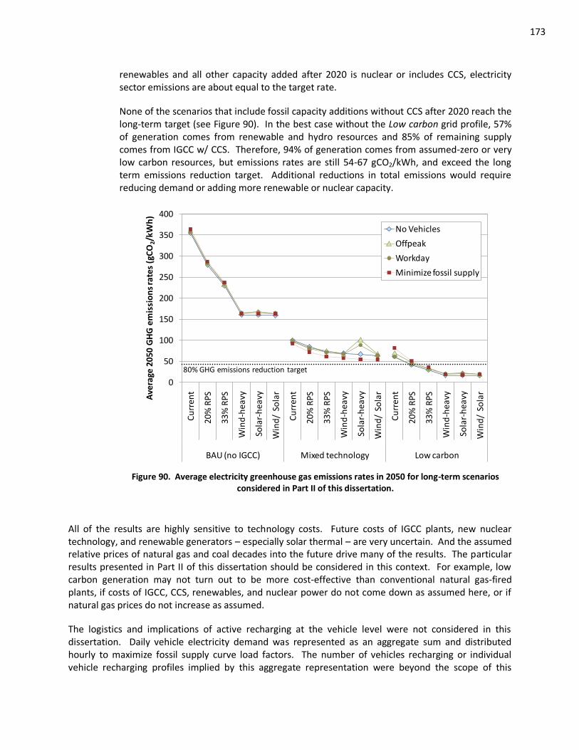
173

renewables and all other capacity added after 2020 is nuclear or includes CCS, electricity sector emissions are about equal to the target rate.

None of the scenarios that include fossil capacity additions without CCS after 2020 reach the long-term target (see Figure 90). In the best case without the Low carbon grid profile, 57% of generation comes from renewable and hydro resources and 85% of remaining supply comes from IGCC w/ CCS. Therefore, 94% of generation comes from assumed-zero or very low carbon resources, but emissions rates are still 54-67 gCO2/kWh, and exceed the long term emissions reduction target. Additional reductions in total emissions would require reducing demand or adding more renewable or nuclear capacity.

0

50

100

150

200

250

300

350

400

Cu

rren

t

20%

RPS

33%

RPS

Win

d-h

eavy

Sola

r-h

eavy

Win

d/

So

lar

Cu

rren

t

20%

RPS

33%

RPS

Win

d-h

eavy

Sola

r-h

eavy

Win

d/

So

lar

Cu

rren

t

20%

RPS

33%

RPS

Win

d-h

eavy

Sola

r-h

eavy

Win

d/

So

lar


Ave

rage

205

0 G

HG

em

issi

on

s ra

tes

(gC

O2/

kWh

)

No Vehicles

Offpeak

Workday


80% GHG emissions reduction target

Figure 90. Average electricity greenhouse gas emissions rates in 2050 for long-term scenarios considered in Part II of this dissertation.

All of the results are highly sensitive to technology costs. Future costs of IGCC plants, new nuclear technology, and renewable generators – especially solar thermal – are very uncertain. And the assumed relative prices of natural gas and coal decades into the future drive many of the results. The particular results presented in Part II of this dissertation should be considered in this context. For example, low carbon generation may not turn out to be more cost-effective than conventional natural gas-fired plants, if costs of IGCC, CCS, renewables, and nuclear power do not come down as assumed here, or if natural gas prices do not increase as assumed.

The logistics and implications of active recharging at the vehicle level were not considered in this dissertation. Daily vehicle electricity demand was represented as an aggregate sum and distributed hourly to maximize fossil supply curve load factors. The number of vehicles recharging or individual vehicle recharging profiles implied by this aggregate representation were beyond the scope of this

174

analysis, as were investigation of mechanisms for matching passive generation and active vehicle recharging. An examination of these factors would provide a more robust analysis and important contributions to further understanding of the extent to which light-duty vehicles may provide an active demand resource to the grid.

Future analysis should consider renewable-heavy scenarios in greater detail. Renewable profiles should be developed that reflect available resources in the state and represent likely long-term generation mixes. Potential contributions and impacts from adding more geothermal or biomass capacity should be evaluated. And alternative representations of intermittent resources should be explored, including wind farms with energy storage to firm the resource, or solar thermal plants that optimize storage and generation.

This dissertation addressed several questions pertaining to demand impacts on electricity supply and raised others, but only touches this broad, important field. Further analysis is needed understand how the sectors may evolve and complement one another in a resource- and climate-constrained future.

Increasing electricity use from light-duty vehicles is one of the most promising options to reduce petroleum consumption and GHG emissions from the transportation sector. If these issues remain policy and social objectives for some time, the transportation and electricity sectors will increasingly converge, and vehicle and fuel-related electricity demands could lead to lower-cost structure and operation of the electricity grid. Understanding the operation of the grid, and interactions to follow, is essential for policy and regulatory development. Several parameters influence the impact that electricity demand from the light-duty transportation sector may have on electricity supply, and in turn, how electricity supply affects the emissions profile of various vehicle platforms. Proper accounting of interactions and GHG emissions throughout the energy supply chain is necessary, and to the extent that this analysis or any other informs such decision-making, healthy discussion and scrutiny of its methods and findings is warranted.

175

REFERENCES

1. IEA (2008) Energy Technology Perspectives 2008 - Scenarios and Strategies to 2050, International Energy Agency, Paris.

2. Yang, C., D. McCollum, R. McCarthy, and W. Leighty (2009) Meeting an 80% reduction in greenhouse gas emissions from transportation by 2050: A case study in California, Transportation Research Part D: Transport and Environment, 14(3): p. 147-156.

3. NRC (2008) Transitions to Alternative Transportation Technologies - A Focus on Hydrogen, National Research Council.

4. Denholm, P. and W. Short (2006) An Evaluation of Utility System Impacts and Benefits of Optimally Dispatched Plug-In Hybrid Electric Vehicles, NREL/TP-620-40293, National Renewable Energy Laboratory.

5. EPRI (2007) Program on Technology Innovation: Economic Analysis of California Climate Initiatives: An Integrated Approach, Volume 1: Summary for Policymakers, 1014641, Electric Power Research Institute

6. EPRI and NRDC (2007) Environmental Assessment of Plug-In Hybrid Electric Vehicles, Volume 1: Nationwide Greenhouse Gas Emissions, 1015325, Electric Power Research Institute.

7. Hadley, S.W. and A. Tsvetkova (2008) Potential Impacts of Plug-in Hybrid Electric Vehicles on Regional Power Generation, ORNL/TM-2007/150, Oak Ridge National Laboratory.

8. ANL (2009) The Greenhouse Gases, Regulated Emissions, and Energy Use in Transportation (GREET) Model, Argonne National Laboratory.

9. Delucchi, M.A. (2003) A Lifecycle Emissions Model (LEM): Lifecycle Emissions from Transportation Fuels, Motor Vehicles, Transportation Modes, Electricity Use, Heating and Cooking Fuels, and Materials (Documentation of methods and data), UCD-ITS-RR-03-17, Institute of Transportation Studies, UC Davis.

10. Edwards, R., J.-F. Larive, V. Mahieu, and P. Rouveirolles (2006) Well-to-Wheels Analysis of Future Automotive Fuels and Powertrains in the European Context (Version 2b), European Commission.

11. Weiss, M.A., J.B. Heywood, E.M. Drake, A. Schafer, and F.F. AuYeung (2000) On the Road in 2020: A Life-Cycle Analysis of New Automobile Technologies, MIT EL 00-003, MIT Laboratory for Energy and the Environment.

12. Kromer, M. and J.B. Heywood (2007) Electric Powertrains: Opportunities and Challenges in the U.S. Light-Duty Vehicle Fleet, LFEE 2007-03 RP, MIT Laboratory for Energy and the Environment.

13. Bandivadekar, A., K. Bodek, L. Cheah, C. Evans, T. Groode, J.B. Heywood, E. Kasseris, M. Kromer, and M.A. Weiss (2008) On the Road in 2035: Reducing Transportation's Petroleum Consumption and GHG Emissions, LFEE 2008-05 RP, MIT Laboratory for Energy and the Environment.

14. Brinkman, N., M. Wang, T. Weber, and T. Darlington (2005) Well-to-Wheels Analysis of Advanced Fuel/Vehicle Systems - A North American Study of Energy Use, Greenhouse Gas Emissions, and Criteria Pollutant Emissions, Argonne National Laboratory.

15. Granovskii, M., I. Dincer, and M.A. Rosen (2006) Economic and environmental comparison of conventional, hybrid, electric and hydrogen fuel cell vehicles, Journal of Power Sources, 159(2): p. 1186-1193.

16. NRC (2006) State and Federal Standards for Mobile-Source Emissions, National Research Council, The National Academies Press, Washington, DC.

17. CEC (2006) 2005 Building Energy Efficiency Standards: Nonresidential Compliance Manual (4th Quarter Revisions), CEC-400-2005-006-CMF, California Energy Commission.

18. CEC (2006) 2005 Building Energy Efficiency Standards: Residential Compliance Manual (4th Quarter Revisions), CEC-400-2005-005-CMF, California Energy Commission.

19. ICC (2009) 2009 International Energy Conservataion Code, International Code Council, Inc.

176

20. (2006) AB 32: California Global Warming Solutions Act of 2006. 21. (2005) Executive Order S-3-05. 22. (2007) Executive Order S-01-07: Low Carbon Fuel Standard. 23. ARB (2009) Initial Statement of Reasons: Proposed Regulation to Implement the Low Carbon Fuel

Standard, California Air Resources Board. 24. ARB (2009) Detailed California-Modified GREET Pathway for California reformulated Gasoline

(CaRFG) (version 2.1), California Air Resources Board. 25. ARB (2009) Detailed California-Modified GREET Pathway for California Average and Marginal

Electricity (Version 2.1), California Air Resources Board. 26. (2006) SB 107: California Renewable Electricity Standard. 27. (2009) Executive Order S-21-09. 28. (2002) AB 1493: Vehicular emissions: Greenhouse gases. 29. EPA and DOT (2009) Proposed Rulemaking to Establish Light-Duty Vehicle Greenhouse Gas

Emission Standards and Corporate Average Fuel Economy Standards, Federal Register, 74(186): p. 49454-49502.

30. ARB (2003) California Exhaust Emission Standards and Test Procedures for 2005 and Subsequent Model Zero-Emission Vehicles, and 2001 and Subsequent Model Hybrid Electric Vehicles, in the Passenger Car, Light-Duty Truck, and Medium-Duty Vehicle Classes, California Air Resources Board.

31. (2007) AB 118: Energy Efficiency, Lower Carbon Fuels, and a Critical Investment in California's Economic and Transportation Future.

32. CEC and ARB (2007) State Alternative Fuels Plan, CEC-600-2007-011.CMF, California Energy Commissions and the California Air Resources Board.

33. (2005) AB 1007: State Alternative Fuels Plan. 34. CEC and ARB (2003) Reducing California's Petroleum Dependence, P600-03-005F, California

Energy Commission and California Air Resources Board. 35. (2000) AB 2076: Strategy to Reduce Petroleum Dependence, 36. ARB (2009) California Hydrogen Highway Network CaH2Net - Summer 2009 Update, California

Air Resources Board. 37. (2006) SB 1505: Environmental Standards for Hydrogen Production. 38. (2005) Energy Policy Act of 2005. 39. IRS (2009) Alternative Motor Vehicle Credit, Internal Revenue Service. 40. (2009) American Recovery and Reinvestment Act of 2009. 41. IRS (2008) IRS Explains How Manufacturers, Purchasers Can Take Advantage of Tax Credit for

Fuel Cell Vehicles, IF-2008-40, Internal Revenue Service. 42. ARB (2009) Drive Clean, California Air Resources Board. 43. (2006) SB 1368: Greenhouse Gas Emission Performance Standards. 44. Wang, M., Y. Wu, and A. Elgowainy (2007) Operating manual for GREET: Version 1.7,

ANL/ESD/05-3, Argonne National Laboratory. 45. Colella, W.G., M.Z. Jacobson, and D.M. Golden (2005) Switching to a U.S. hydrogen fuel cell

vehicle fleet: The resultant change in emissions, energy use, and greenhouse gases, Journal of Power Sources, 150: p. 150-181.

46. NRC (2004) The Hydrogen Economy: Opportunities, Costs, Barriers, and R&D Needs, National Research Council and National Academy of Engineering, The National Academies Press.

47. EPA, U.S. (2009) Emissions and Generation Resource Integrated Database (eGRID2007, Version 1.1), U.S. Environmental Protection Agency.

48. DOE,(2005), DOE H2A Production Analysis. Available from: http://www.hydrogen.energy.gov/h2a_production.html.

177

49. ANL (2008) Electricity Market Complex Adaptive System (EMCAS): Model Introduction, Argonne National Laboratory.

50. Greenblatt, J.B., S. Succar, D.C. Denkenberger, R.H. Williams, and R.H. Socolow (2007) Baseload wind energy: modeling the competition between gas turbines and compressed air energy storage for supplemental generation, Energy Policy, 35(3): p. 1474-1492.

51. Kempton, W., C.L. Archer, A. Dhanju, R.W. Garvine, and M.Z. Jacobson (2007) Large CO2 reductions via offshore wind power matched to inherent storage in energy end-uses, Geophysical Research Letters, 34(2): p. L02817.

52. Lipman, T.E., R. Ramos, and D.M. Kammen (2005) An Assessment of Battery and Hydrogen Energy Storage Systems Integrated with Wind Energy Resources in California, CEC-500-2005-136, California Energy Commission.

53. Denholm, P., G.L. Kulcinski, and T. Holloway (2005) Emissions and Energy Efficiency Assessment of Baseload Wind Energy Systems, Environmental Science & Technology, 39(6): p. 1903-1911.

54. Han, X.S. and H.B. Gooi (2007) Effective economic dispatch model and algorithm, International Journal of Electrical Power & Energy Systems, 29(2): p. 113-120.

55. Jayabarathi, T., K. Jayaprakash, D.N. Jeyakumar, and T. Raghunathan (2005) Evolutionary programming techniques for different kinds of economic dispatch problems, Electric Power Systems Research, 73(2): p. 169-176.

56. Cai, J., X. Ma, L. Li, and P. Haipeng (2007) Chaotic particle swarm optimization for economic dispatch considering the generator constraints, Energy Conversion and Management, 48(2): p. 645-653.

57. Chiou, J.-P. (2007) Variable scaling hybrid differential evolution for large-scale economic dispatch problems, Electric Power Systems Research, 77(3-4): p. 212-218.

58. Carraretto, C. and A. Zigante (2006) Interaction among competitive producers in the electricity market: An iterative market model for the strategic management of thermal power plants, Energy, 31(15): p. 3145-3158.

59. Martinez-Crespo, J., J. Usaola, and J.L. Fernandez (2007) Optimal security-constrained power scheduling by Benders decomposition, Electric Power Systems Research, 77(7): p. 739-753.

60. Decisions, G.E.,(Market Analytics Powered by ProSym (Product brochure). [accessed February 29, 2008]; Available from: http://www.globalenergy.com/cutsheets/products-ma-combined.pdf.

61. Danforth, J. (2007) Plug-In Hybrid Charging in Los Angeles: Analysis of the Load-Leveling Capacity for Charging Plug-In Hybrids in the Los Angeles Department of Water and Power Transmission Area, in Electric Vehicle Symposium, Anaheim, CA, December 3-5.

62. Consulting, L. UPLAN-NPM Network Power Model (Product brochure). [accessed February 29, 2008]; Available from: http://www.energyonline.com/Products/Uplane.aspx.

63. Associates, N. PROMOD IV (Product brochure). [accessed February 29, 2008]; Available from: http://www.newenergyassoc.com/solutions/product-index/powerbase-suite/promod-iv.

64. International, I. IPM - The Integrated Planning Model (Product brochure). [accessed February 29, 2008]; Available from: http://www.icfi.com/markets/energy/doc_files/ipmglobal.pdf.

65. Systems, I.E. PROPHET Electricity Market Model (Product brochure). [accessed February 29, 2008]; Available from: http://www.iesys.com.au/DNN/Default.aspx?tabid=457.

66. Exemplar, E. PLEXOS for Power Systems (Product brochure). [accessed February 29, 2008]; Available from: http://www.energyexemplar.com/main.asp?page=overview.

67. Coste, W.H. and G. Adams (2001) Proposal for Bulk Power Analytical Services, IREMM, Inc. 68. EPIS, I., AURORAxmp Electric Market Model (Product brochure). [accessed February 29, 2008];

Available from:

178

http://www.epis.com/Products/onesheets/AURORA%20Product%20Sheet%2004-16-2007.pdf. 69. International, C. MRN-NEEM (Product brochure). [accessed February 29, 20008]; Available from:

http://www.crai.com/ConsultingExpertise/Content.aspx?tID=828&subtID=842&tertID=8 70. Kennedy, S. (2005) Wind power planning: assessing long-term costs and benefits, Energy Policy,

33(13): p. 1661-1675. 71. Andrews, C.J. and S. Govil (1995) Becoming proactive about environmental risks : Regulatory

reform and risk management in the US electricity sector, Energy Policy, 23(10): p. 885-892. 72. Puller, S.L. (2005) Pricing and firm conduct in California's deregulated electricity market, Texas

A&M University. 73. Ford, A. (2001) Waiting for the boom: a simulation study of power plant construction in

California, Energy Policy, 29(11): p. 847-869. 74. Paul, A. and D. Burtraw (2002) The RFF Haiku Electricity Market Model, Resources for the Future. 75. Short, W., T. Ferguson, and M. Leifman (2006) Modeling of Uncertainties in Major Drivers in U.S.

Electricity Markets, NREL/CP-620-40451, National Renewable Energy Laboratory. 76. Mintzer, I., J.A. Leonard, and P. Schwartz (2003) U.S. Energy Scenarios for the 21st Century, Pew

Center on Global Climate Change. 77. Neubauer, F., E. Westman, and A. Ford (1997) Applying planning models to study new

competition, Energy Policy, 25(3): p. 273-280. 78. Hirst, E. and S. Hadley (1998) ORCED: A model to simulate the operations and costs of bulk-

power markets, ORNL/CON-464, Oak Ridge National Laboratory. 79. Elgowainy, A., A. Burnham, M. Wang, J. Molburg, and A. Rousseau (2009) Well-to-Wheels Energy

Use and Greenhouse Gas Emissions Analysis of Plug-in Hybrid Electric Vehicles, ANL/ESD/09-2, Argonne National Laboratory.

80. Price, L., C. Marnay, J. Sathaye, S. Murtishaw, D. Fisher, A. Phadke, and G. Franco (2002) Development of Methodologies for Calculating GHG Emissions from Electricity Generation for the California Climate Action Registry.

81. Sjödin, J. and S. Grönkvist (2004) Emissions accounting for use and supply of electricity in the Nordic market, Energy Policy, 32(13): p. 1555-1564.

82. Samaras, C. and K. Meisterling (2008) Life Cycle Assessment of Greenhouse Gas Emissions from Plug-in Hybrid Vehicles: Implications for Policy, Environmental Science and Technology, 42(9): p. 3170-3176.

83. Collaborative, C.W.E. (2004) California Renewables Portfolio Standard Renewable Generation Integration Cost Analysis: PHASE III: RECOMMENDATIONS FOR IMPLEMENTATION, P500-04-054, Public Interest Energy Research Program, California Energy Commission.

84. Collaborative, C.W.E. (2006) California Renewables Portfolio Standard Renewable Generation Cost Analysis: MULTI-YEAR ANALYSIS RESULTS AND RECOMMENDATIONS - FINAL REPORT, CEC-500-2006-064, California Energy Commission, PIER.

85. Davis, R.E. and B. Quach (2007) Intermittency Analysis Project: Appendix A: Intermittency Impacts of Wind and Solar Resources on Transmission Reliability, CEC-500-2007-081-APA, California Energy Commission, PIER Renewable Energy Technologies Program.

86. Douglas, P., E. Stoltzfus, A. Gillette, and J. Marks (2009) 33% Renewables Portfolio Standard: Implementation Analysis (Preliminary Results), California Public Utilities Commission.

87. NREL (2008) 20% Wind Energy by 2030: Increasing Wind Energy's Contribution to U.S. Electricity Supply, DOE/GO-102008-2567, National Renewable Energy Laboratory.

88. Piwko, R.J., X. Bai, K. Clark, G.A. Jordan, and N.W. Miller (2007) Intermittency Analysis Project: Appendix B: Impact of Intermittent Generation on Operation of California Power Grid, CEC-500-2007-081-APB, California Energy Commission, PIER Renewable Energy Technologies Program.

89. ARB (2009) Modified California-GREET Model, California Air Resources Board.

179

90. EPRI and NRDC (2007) Environmental Assessment of Plug-In Hybrid Electric Vehicles, Volume 2: United States Air Quality Analysis Based on AEO-2006 Assumptions for 2030, 1015326, Electric Power Research Institute.

91. Ford, A. (1994) Electric vehicles and the electric utility company, Energy Policy, 22(7): p. 555-570.

92. Ford, A. (1995) The impacts of large scale use of electric vehicles in southern California, Energy and Buildings, 22(3): p. 207-218.

93. Garland, J. and S. Tomashefsky (1996) Electric vehicle and power plant emissions update: South Coast Air Basin, California Energy Commission.

94. Samaras, C. and K. Meisterling (2008) Life Cycle Assessment of Greenhouse Gas Emissions from Plug-in Hybrid Vehicles: Implications for Policy, Environmental Sciene and Technology, In press.

95. Kliesch, J. and T. Langer (2006) Plug-In Hybrids: An Environmental and Economic Performance Outlook T061, American Council for an Energy-Efficient Economy.

96. Kintner-Meyer, M., K. Schneider, and R. Pratt (2007) Impacts assessment of plug-in hybrid vehicles on electric utilities and regioal U.S. power grids: Part 1: Technical analysis, Pacific Northwest National Laboratory.

97. Scott, M.J., M. Kintner-Meyer, D.B. Elliott, and W.M. Warwick (2007) Impacts assessment of plug-in hybrid vehicles on electric utilities and regional U.S. power grids: Part 2: Economic assessment, Pacific Northwest National Laboratory.

98. Stephan, C.H. and J. Sullivan (2008) Environmental and Energy Implications of Plug-In Hybrid-Electric Vehicles, Environmental Sciene and Technology, 42(4): p. 1185-1190.

99. ANL (2008) Impact of Plug-in Hybrid Electric Vehicles on the Electricity Market in Illinois, Argonne National Laboratory.

100. Parks, K., P. Denholm, and T. Markel (2007) Costs and Emissions Associated with Plug-In Hybrid Electric Vehicle Charging in the Xcel Energy Colorado Service Territory, NREL/TP-640-41410; TRN: US200720%%219, National Renewable Energy Laboratory.

101. Rastler, D. (2006) The roles and opportunities for power companies in the hydrogen-electric economy, EPRI.

102. Lemoine, D.M., D.M. Kammen, and A.E. Farrell (2008) An Innovation and Policy Agenda for Commercially Competitive Plug-in Hybrid Electric Vehicles, Environmental Research Letters, 3(1): p. 014003.

103. CEC (2008) Electricity Consumption by Entity, California Energy Commission. 104. CEC California Major Utilities' Resource Mix for 2006, California Energy Commission. 105. CEC (2007) Summer 2007 Electricity Supply and Demand Outlook, CEC-200-2007-005-SD,

California Energy Commission. 106. CAISO (2008) System Load and Resource Schedules (Hour Ahead Market), California Independent

System Operator. 107. WECC (2006) Information Summary, Western Electricity Coordinating Council. 108. Energy and Environmental Economics, I. (2007) Attributing Generator Emissions to LSEs

(Supporting documentation to the CPUC GHG modeling). 109. Energy and Environmental Economics, I. (2008) Generator Assignment in E3 Model.xls

(Supporting documentation to the CPUC GHG modeling). 110. Alvarado, A. and K. Griffin (2007) Revised Methodology to Estimate the Generation Resource Mix

of California Electricity Imports (Update to the May 2006 Staff Paper), CEC-700-2007-007, California Energy Commission.

111. Alvarado, A. (2006) Proposed methodology to estimate the generation resource mix of California electricity imports, California Energy Commission.

180

112. CEC (2007) 1983-2006 California Electricity Generation (spreadsheet), California Energy Commission.

113. EIA (2009) Proposed Nameplate Capacity by Year, Energy Source, and State (EIA-860), Energy Information Administration.

114. NERC (2007) Electricity Supply and Demand (ES&D 2007), North American Electric Reliability Corporation.

115. EPA, U.S. (2006) National Electric Energy Data System (NEEDS) 2006, U.S. Environmental Protection Agency.

116. McCarthy, R.W., C. Yang, and J.M. Ogden (2006) California energy demand scenario projections to 2050, UCD-ITS-RR-08-11, Institute of Transportation Studies, University of California, Davis.

117. Klein, J. and A. Rednam (2007) Comparative Costs of California Central Station Electricity Generation Technologies, CEC-200-2007-011, California Energy Commission, Electricity Supply Analysis Division.

118. FERC (2008) Form 714 - Annual Electric Balancing Authority Area and Planning Area Report, Federal Energy Regulatory Commission.

119. CAISO (2008) Open Access Same-Time Information System (OASIS), California Independent System Operator.

120. AWEA (2009) US Wind Energy Projects - California (As of 12/31/2008), American Wind Energy Association.

121. EIA (2009) Electric Power Annual 2007, Energy Information Administration. 122. Grygier, J. (2007) Pacific Gas and Electric Company, personal communication. 123. CEC (2008) 2007 Net System Power Report, CEC-200-2008-002-CMF, California Energy

Commission. 124. CAISO (2009) System Load by IOU, California Independent System Operator. 125. EIA (2009) Form EIA-906, EIA-920, and EIA-923 Databases, Energy Information Administration. 126. Smith, B., G. Randall, T. McCoy, and J. VandenBosche (2001) Power Performance Testing

Progress in the DOE/EPRI Turbine Verification Program, NREL/CP-500-30667, National Renewable Energy Laboratory.

127. NREL National Solar Radiation Data Base, National Renewable Energy Laboratory. 128. EIA (2009) Net Generation by State by Type of Producer by Energy Source (EIA-906), Energy

Information Administration. 129. NCDC (2008) Heating & Cooling Degree Day Data, National Climatic Data Center, NOAA Satellite

and Information Service. 130. NERC (2007) 2002-2006 Generating Availability Report, North American Electric Reliability

Corporation. 131. CAISO (2008) Market Issues & Performance: 2007 Annual Report, Department of Market

Monitoring, California Independent System Operator Corporation. 132. EIA (2006) Assumptions to the Annual Energy Outlook 2006, Energy Information Administration. 133. Gillette, J. (2007) California Energy Commission, personal communication. 134. Woodward, J. (2008) Dependable Hydro Capacity, California Energy Commission. 135. CEC (2004) Resource, Reliability and Environmental Concerns of Aging Power Plant Operations

and Retirements (Draft), CEC-100-04-005D, California Energy Commission. 136. Hirst, E. (2002) Integrating Wind Energy with the BPA Power System: Preliminary Study. 137. NCDC (2008) Integrated Surface Data, Hourly Global (DS3505), National Climatic Data Center,

NOAA Satellite and Information Service. 138. NCDC (2002) Divisional Normals and Standard Deviations of Temperature, Precipitation, and

Heating and Cooling Degree Days 1971-2000 (and previous normals periods) National Climatic Data Center, NOAA Satellite and Information Service.

181

139. EIA (2009) Table 2.2. Existing Capacity by Energy Source, Energy Information Administration. 140. Nexant (2005) Hydrogen Delivery Infrastructure Option Analysis. 141. EIA (2009) Petroleum Consumption/Sales Data and Analysis, Energy Information Administration. 142. CEC (2009) Utility-wide Weighted Average Retail Electricity Prices, California Energy Commission. 143. ICE (2009) ICE Month Ahead Natural Gas Price Report, Intercontinental Exchange. 144. EIA (2006) The Electricity Market Module of the National Energy Modeling System, Energy

Information Administration. 145. EIA (2009) U.S. Electric Power Industry Estimated Emissions by State (EIA-767 and EIA-906),

Energy Information Administration. 146. EPA (2008) eGRID Year 2005 Summary Tables, U.S. Environmental Protection Agency. 147. CEC (2009) Statewide Electricity Rates by Utility, Class and Other Data, California Energy

Commission. 148. McCarthy, R.W., C. Yang, and J.M. Ogden (2008) Interactions between hydrogen pathways and

electricity supply: A stochastic representation of the California power sector, NHA Annual Hydrogen Conference 2008, Sacramento, CA, March 30-April 3.

149. Gronich, S. (2006) 2010-2025 Scenario Analysis, DOE Hydrogen, Fuel Cells & Infrastructure Technologies Program.

150. McCarthy, R.W., C. Yang, and J.M. Ogden (2009) Interactions Between Electric-Drive Vehicles and the Power Sector in California, EVS 24, Stavanger, Norway, May 13-16.

151. EIA (2009) Assumptions to the Annual Energy Outlook 2009, DOE/EIA-0554(2009), Energy Information Administration.

152. EIA (2009) Annual Energy Outlook 2009, DOE/EIA-0383(2009), Energy Information Administration.

153. Deutch, J., E.J. Moniz, S. Ansolabehere, M. Driscoll, P.E. Gray, J.P. Holdren, P.L. Joskow, R.K. Lester, and N.E. Todreas (2003) The Future of Nuclear Power: An Interdisciplinary MIT Study, Massachusetts Institute of Technology.

154. McClary, S.C., R.B. Weisenmiller, H.L. Metha, and L.B. Norin (2007) Nuclear Power in California: 2007 Status Report, CEC-100-2007-005-F, California Energy Commission.

155. CEC (2009) Renewable Energy Transmission Initiative: RETI Phase 1B (Final Report), RETI-1000-2008-003-F, California Energy Commission.

156. Energy and Environmental Economics, I. (2007) Wind Resources, Cost, and Performance (Supporting documentation to the CPUC GHG modeling).

157. Energy and Environmental Economics, I. (2007) Concentrating Solar Power (CSP) Resources, Cost, and Performace (Supporting documentation to the CPUC GHG modeling).

158. CEC,(Historic Statewide California Electricity Demand. [accessed June 22, 2009]; Available from: http://energyalmanac.ca.gov/electricity/historic_peak_demand.html.

159. Vestas (2009) V112-3.0 MW Wind Turbine Product Brochure. 160. Stoddard, L., J. Abiecunas, and R. O'Connell (2006) Economic, Energy, and Environmental

Benefits of Concentrating Solar Power in California, NREL/SR-550-39291, National Renewable Energy Laboratory.

161. Stoft, S. (2002) Power System Economics: Designing Markets for Electricity, Wiley-IEEE Press. 162. CEC (2007) 2007 Integrated Energy Policy Report, CEC-100-2007-008-CMF, California Energy

Commission. 163. ARB (2007) California 1990 Greenhouse Gas Emissions Level and 2020 Emissions Limit, California

Air Resources Board.

i Assessing Vehicle Electricity Demand Impacts on California ...

Documents