EKSPLOATACJA I NIEZAWODNOSC – MAINTENANCE AND RELIABILITY VOL. 23, NO. 3, 2021 I TABLE OF CONTENTS Andrzej Gajek, Adam Kot, Piotr Strzępek Identification of the ESP sensors condition during the vehicle service life .............................................................................................................................. 405 Dragan Živanić, Nikola Ilanković, Ninoslav Zuber, Radomir Đokić, Nebojša Zdravković, Atila Zelić The analysis of influential parameters on calibration and feeding accuracy of belt feeders ............................................................................................... 413 Zdzisław Hryciów, Wiesław Krasoń, Józef Wysocki Evaluation of the influence of friction in a multi-leaf spring on the working conditions of a truck driver ......................................................................... 422 Piotr Sliż, Ewa Wycinka Identification of factors that differentiate motor vehicles that have experienced wear or failure of brake system components during the warranty service period ..................................................................................................................................................................................................................................... 430 Maysa Alshraideh, Shereen Ababneh, Elif Elcin Gunay, Omar Al-Araidah A fuzzy-TOPSIS model for maintenance outsourcing considering the quality of submitted tender documents ................................................................ 443 Dan Zhao, Yu-Xin Liu, Xun-Tao Ren, Jing-Zi Gao, Shao-Gang Liu, Li-Qiang Dong, Ming-Shen Cheng Fatigue life prediction of wire rope based on grey particle filter method under small sample condition.......................................................................... 454 Ireneusz Pielecha, Filip Szwajca Cooperation of a PEM fuel cell and a NiMH battery at various states of its charge in a FCHEV drive .................................................................................... 468 Lucyna Szaciłło, Marianna Jacyna, Emilian Szczepański, Mariusz Izdebski Risk assessment for rail freight transport operations ................................................................................................................................................................. 476 Hongyan Dui, Xiaoqian Zheng, Qian Qian Zhao, Yining Fang Preventive maintenance of multiple components for hydraulic tension systems .................................................................................................................. 489 Hui Liu, Ning-Cong Xiao An efficient method for calculating system non-probabilistic reliability index ...................................................................................................................... 498 Jan Famfulik, Michal Richtar, Jakub Smiraus, Petra Muckova, Branislav Sarkan, Pavel Dresler Internal combustion engine diagnostics using statistically processed Wiebe function......................................................................................................... 505 Chao Zhang, Yujie Qian, Hongyan Dui, Shaoping Wang, Rentong Chen, Mileta M. Tomovic Opportunistic maintenance strategy of a Heave Compensation System for expected performance degradation............................................................ 512 Javier Castilla-Gutiérrez, Juan Carlos Fortes Garrido, Jose Miguel Davila Martín, Jose Antonio Grande Gil Evaluation procedure for blowing machine monitoring and predicting bearing SKFNU6322 failure by power spectral density ................................... 522 Paweł Grabowski, Artur Jankowiak, Witold Marowski Fatigue lifetime correction of structural joints of opencast mining machinery...................................................................................................................... 530 Paweł Zdziebko, Adam Martowicz Study on the temperature and strain fields in gas foil bearings – measurement method and numerical simulations ................................................... 540 Arkadiusz Czarnuch , Marek Stembalski , Tomasz Szydłowski, Damian Batory Method of reconstructing dynamic load characteristics for durability test of heavy semitrailer under different road conditions ............................... 548 Zhiming Wang, Hao Yuan Enhancing machining accuracy reliability of multi-axis CNC machine tools using an advanced importance sampling method .................................... 559 Ryszard Machnik, Łukasz Więckowski Operational tests of an electrostatic precipitator reducing low dust emission from solid fuels combustion..................................................................... 569 Maciej Badora, Marzia Sepe, Marcin Bielecki, Antonino Graziano, Tomasz Szolc Predicting length of fatigue cracks by means of machine learning algorithms in the small-data regime......................................................................... 575 Anna Borucka, Dariusz Pyza Influence of meteorological conditions on road accidents. A model for observations with excess zeros. .......................................................................... 586 2021-3-wnetrze.indd 1 09.07.2021 16:03:29

Welcome message from author
This document is posted to help you gain knowledge. Please leave a comment to let me know what you think about it! Share it to your friends and learn new things together.
Transcript

Eksploatacja i NiEzawodNosc – MaiNtENaNcE aNd REliability Vol. 23, No. 3, 2021 I
Table Of COnTenTs
Andrzej Gajek, Adam Kot, Piotr StrzępekIdentification of the ESP sensors condition during the vehicle service life .............................................................................................................................. 405
Dragan Živanić, Nikola Ilanković, Ninoslav Zuber, Radomir Đokić, Nebojša Zdravković, Atila ZelićThe analysis of influential parameters on calibration and feeding accuracy of belt feeders ............................................................................................... 413
Zdzisław Hryciów, Wiesław Krasoń, Józef WysockiEvaluation of the influence of friction in a multi-leaf spring on the working conditions of a truck driver ......................................................................... 422
Piotr Sliż, Ewa WycinkaIdentification of factors that differentiate motor vehicles that have experienced wear or failure of brake system components during the warranty service period ..................................................................................................................................................................................................................................... 430
Maysa Alshraideh, Shereen Ababneh, Elif Elcin Gunay, Omar Al-AraidahA fuzzy-TOPSIS model for maintenance outsourcing considering the quality of submitted tender documents ................................................................ 443
Dan Zhao, Yu-Xin Liu, Xun-Tao Ren, Jing-Zi Gao, Shao-Gang Liu, Li-Qiang Dong, Ming-Shen ChengFatigue life prediction of wire rope based on grey particle filter method under small sample condition .......................................................................... 454
Ireneusz Pielecha, Filip SzwajcaCooperation of a PEM fuel cell and a NiMH battery at various states of its charge in a FCHEV drive .................................................................................... 468
Lucyna Szaciłło, Marianna Jacyna, Emilian Szczepański, Mariusz IzdebskiRisk assessment for rail freight transport operations ................................................................................................................................................................. 476
Hongyan Dui, Xiaoqian Zheng, Qian Qian Zhao, Yining FangPreventive maintenance of multiple components for hydraulic tension systems .................................................................................................................. 489
Hui Liu, Ning-Cong XiaoAn efficient method for calculating system non-probabilistic reliability index ...................................................................................................................... 498
Jan Famfulik, Michal Richtar, Jakub Smiraus, Petra Muckova, Branislav Sarkan, Pavel DreslerInternal combustion engine diagnostics using statistically processed Wiebe function ......................................................................................................... 505
Chao Zhang, Yujie Qian, Hongyan Dui, Shaoping Wang, Rentong Chen, Mileta M. TomovicOpportunistic maintenance strategy of a Heave Compensation System for expected performance degradation ............................................................ 512
Javier Castilla-Gutiérrez, Juan Carlos Fortes Garrido, Jose Miguel Davila Martín, Jose Antonio Grande GilEvaluation procedure for blowing machine monitoring and predicting bearing SKFNU6322 failure by power spectral density ................................... 522
Paweł Grabowski, Artur Jankowiak, Witold MarowskiFatigue lifetime correction of structural joints of opencast mining machinery...................................................................................................................... 530
Paweł Zdziebko, Adam MartowiczStudy on the temperature and strain fields in gas foil bearings – measurement method and numerical simulations ................................................... 540
Arkadiusz Czarnuch , Marek Stembalski , Tomasz Szydłowski, Damian BatoryMethod of reconstructing dynamic load characteristics for durability test of heavy semitrailer under different road conditions ............................... 548
Zhiming Wang, Hao YuanEnhancing machining accuracy reliability of multi-axis CNC machine tools using an advanced importance sampling method .................................... 559
Ryszard Machnik, Łukasz WięckowskiOperational tests of an electrostatic precipitator reducing low dust emission from solid fuels combustion ..................................................................... 569
Maciej Badora, Marzia Sepe, Marcin Bielecki, Antonino Graziano, Tomasz SzolcPredicting length of fatigue cracks by means of machine learning algorithms in the small-data regime ......................................................................... 575
Anna Borucka, Dariusz PyzaInfluence of meteorological conditions on road accidents. A model for observations with excess zeros. .......................................................................... 586
2021-3-wnetrze.indd 1 09.07.2021 16:03:29
Eksploatacja i NiEzawodNosc – MaiNtENaNcE aNd REliability Vol. 23, No. 3, 2021 405
(*) Corresponding author.E-mail addresses:
Eksploatacja i Niezawodnosc – Maintenance and ReliabilityVolume 23 (2021), Issue 3
journal homepage: http://www.ein.org.pl
Indexed by:
A. Gajek - [email protected], A. Kot - [email protected], P. Strzępek - [email protected]
The paper presents the proposals of extension of the periodic tests of the selected ESP sys-tem sensors: angular velocity sensor and lateral acceleration sensor using a universal diag-nostics tester and a plate stand (a wheel play detector unit). The idea of this approach is to evaluate the signals from the above sensors in terms of their amplitude and frequency in the case of known forcing at the plate stand. Knowledge of the amplitude and frequency of the plates excitation and the model of tested vehicle allows for predicting the response of vehi-cle. On this way the verification of sensors indications is possible. This article presents the flat model of a vehicle placed on the plate stand, simulation tests and the results of its vali-dation for three different vehicles. The results of the investigation show that the wheelbase of vehicle has a significant impact on the steady-state vibration amplitude. This conclusion is important in the practical application of this method to test the vehicle yaw rate sensor in the ESP system.
Highlights Abstract
Extension of periodic tests of the ESP selected • sensors is proposed.
The idea assumes using a universal diagnostics • tester and a wheel play detector unit.
The flat model of a vehicle placed on a wheel play • detector unit is presented.
The results of simulation are compared with the • ESP sensor signal.
Identification of the ESP sensors condition during the vehicle service life
Andrzej Gajek a, Adam Kot a*, Piotr Strzępek a
aCracow University of Technology, Department of Automotive Vehicles, Al. Jana Pawla II 37, 31-864 Cracow, Poland
Gajek A, Kot A, Strzępek. Identification of the ESP sensors condition during the vehicle service life. Eksploatacja i Niezawodnosc – Maintenance and Reliability 2021; 23 (3): 405–412, http://doi.org/10.17531/ein.2021.3.1.
Article citation info:
1. IntroductionModern motor vehicles are equipped with a number of systems re-
sponsible for reducing the likelihood of an undesirable road incident (e.g. collision). One of the most important and the most intensively developed by automotive engineers is Electronic Stability Program (ESP). The statistical research shows that ESP system can decrease the number of crash situations, associated with defensive maneuvers even about 8% [13]. The effectiveness of the track stabilization sys-tem increases by the recently developing integrated systems combin-ing ESP and AFS (Active Front Steering) [3] or ESP and TVD (Torque Vectoring Differential) [9]. Furthermore, the concepts of using ESP for diagnosing automotive damper defects appears in the literature [19]. Active car safety is particularly dependent on the correct opera-tion of systems that affect the operation of the braking system and the stabilization of the drive track. Currently, these tasks are included in the scope of duties of the mechatronic ESP system, whose operation is based on the analysis of signals from sensors located in the vehicle, which include among others: wheel speed sensors, yaw rate (vehicle angular velocity) sensor and lateral acceleration sensor, steering an-gle sensor. Assessment of the efficiency of these sensors during the vehicle service life is therefore important from the point of view of road safety. Thus, in last years there are papers deal with sensors di-agnosis and estimation their bias under normal driving conditions [16,
17, 18]. Considering the fact that the role of mechatronic systems in vehicles is growing very rapidly, it seems natural to state that periodic testing of vehicles should carefully take into account the control of these elements. Now the tests of these systems consist on verifying whether the on-board diagnostics system informs a possible malfunc-tion via the MIL lamp. This supervision concerns the efficiency of electrical and electronic systems. However, the condition of sensors during lifetime may also change in the mechanical field. Therefore, the control of the operation of the system as a whole is recommended especially in vehicles with extended service life and crashed.
The research and development works conducted in the field of extending vehicle inspection tests take into account the fact that ve-hicle assemblies have become mechatronic systems. Their operation depends both on the efficiency of the mechanical part of these sys-tems, tested on stationary stands, and on the efficiency of sensors and actuators. New test methods should take into account the need to test these elements. The proposed solutions in the field of safety system control include the use of computer testers [2] and external measure-ment tools for periodic tests at the PTI (Periodic Technical Inspection) [11]. The basic problem related to the direct application of diagnostic stands is the difficulty in obtaining data from vehicle controllers, sen-sors and actuators. This is due to the need to interfere with the car’s electrical system and driver software. In addition, car manufacturers
ESP sensors diagnostics, yaw rate sensor, testing of the mechatronic safety systems, inte-grated diagnostic.
Keywords
This is an open access article under the CC BY license (https://creativecommons.org/licenses/by/4.0/)
Eksploatacja i NiEzawodNosc – MaiNtENaNcE aNd REliability Vol. 23, No. 3, 2021406
do not provide information on both the location of the sensors and their characteristics (scale factors). Therefore, it becomes necessary to use specialized diagnostic testers connected to the vehicle’s IT sys-tem via the OBD socket. This facilitates and speeds up the process of acquiring data from sensors. On the other hand, the modification of the testers software requires the proper sampling frequency of sig-nals, because too low frequency hinders the qualitative assessment of the results. The above problems are currently being undertaken by research centers in the European Union [1, 2, 8]. It is proposed to modify the currently used diagnostic programs in order to standardize procedures, facilitate access to other systems and accelerate the per-formance of diagnostic tests [8]. The scope of obligatory control tests of active and passive safety systems is being developed as well as the requirements in this regard for diagnostic testers used at PTI stations [1, 2, 12]. This applies to testing brakes (roller stations) and engines (chassis braking) [4,5].
One of the proposals to extend the scope of periodic tests is to check the operation of the angular velocity and lateral acceleration sensors (usually built in an integrated form) of the ESP system. The determination of vehicle angular velocity is based on the Coriolis ef-fect acting on sensor’s vibrating element [10]. The lateral acceleration is calculated on the basis of an electric signal proportional to the mass displacement in the sensor [10]. Internal elements of the sensor are subject to forced vibrations. Its characteristics may change during the period of use, e.g. due to loosening of the fastening, overload during a collision of the vehicle, repairs of the body. These circumstances justify the need to test the sensors during the vehicle service life.
The article presents the method of testing the operation of the sen-sors of angular velocity and lateral acceleration of the ESP system (usually built in an integrated form) in bench conditions. A method of forcing a vehicle rotation on a plate stand was proposed, with the use of devices used so far in periodic technical tests. The idea of the proposed method is to evaluate the signals from the above sensors in terms of their amplitude and frequency, with the known rotation of the vehicle being forced on a plate stand for checking the looseness in the suspension (a wheel play detector unit). The course of the signals from the sensors is monitored in real time with a diagnostic tester and evaluated after the test.
The aim of the study was to show that the knowledge of the am-plitude and frequency of the excitation of the plate movement, i.e. the excitation acting on the vehicle and appropriate model of the ve-hicle allows predicting the vehicle’s response and verifying the val-ues measured by the sensors. This article presents the flat model of a vehicle with the front wheels placed on the diagnostic stand with two coaxially moving plates and the results of its validation for three different vehicles.
The hypothesis that needed to be proved is as follows: a flat model of the vehicle, taking into account the characteristics of the tires, sub-jected to excitation from the station’s plates with a known amplitude and excitation frequency can be used to determine body vibrations on the plate stand and to assess the correctness of the ESP rotational speed sensor indications.
The proposed test method is a new solution, not used so far [15]. It is applicable in Periodic Technical Inspections.
2. Mathematical modelThe developed model adopts a flat model of the vehicle whose
body rotates relative to the instantaneous center of rotation. This is illustrated schematically in Figure 1. The assumption of the vehicle’s rotational movement on the plate stand is justified because:
the plates are located only under the front axle wheels, –the rear axle wheels are free to roll during the measurement, –diagnostic plates reciprocate movement, whose amplitude is –small (up to 100 mm) relative to the distance of the plates from the center of rotation of the vehicle body.
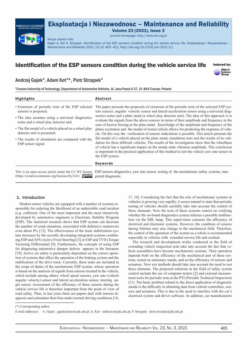
The hydraulically driven diagnostic plates reciprocate in a direc-tion perpendicular to the longitudinal axis of the vehicle. Under ideal conditions, the x coordinate associated with the plate can be described by the equation:
x A t= sin( )ω (1)
where:A - one-sided amplitude of the plate,ω - circular frequency of plate movement (ω = 2πf, f - frequency).
Considering the fact that the amplitude of the plate movement is small in relation to their distance from the instantaneous center of rotation of the vehicle and the wheels on the plates are unbraked, the model uses the angular coordinate α describing the kinematic forcing acting from the plates on the wheels as:
a xl e
Al e
t=+
=+
sin( ),ω (2)
where:x - displacement of plates,l - wheelbase of the vehicle,e - distance between the center of rotation of the body and the rear axle (e – in front of or behind the rear axle).
The angular velocity of excitation will be then:
αω
ω=+
=+
xl e
Al e
tcos( ). (3)
It is kinematic forcing on the vehicle’s wheels. The movement of the plates is transferred to the body through flexible tires and suspen-sion. Considering the above assumptions, the equation of the vehicle body movement will take the form:
ˆI k cop op α α α α α1 1 1 0+ − + − =( ) ( )ˆ (4)
where:I - moment of inertia of the vehicle relative to the instantaneous center of rotation,α1 - angular coordinate associated with the vehicle body,
Fig. 1. Flat model of the vehicle at the plate bench (diagnostic plates under the front axle wheels), c - distance between the center of mass and the rear axle, e - distance between the center of rotation and the rear axle, l - wheelbase
Eksploatacja i NiEzawodNosc – MaiNtENaNcE aNd REliability Vol. 23, No. 3, 2021 407
opk - equivalent coefficient of lateral damping of tire for rotary mo-tion,
opc - equivalent coefficient of lateral stiffness of tire for rotary mo-tion.
The analyzed model takes into account the stiffness and damping of the front axle tires (the impact of rear axle tires was omitted). Con-sidering the direction of loading resulting from the plate forcing, the flexibility of suspension elements was omitted. The subject literature provides information on the damping coefficients and lateral stiffness of a tyre for linear motion [6, 7]. Due to the fact that rotational motion is considered in this analysis, the following approximate relationships have been adopted for the above coefficients:
ˆ 22 ( ) ,op opk k l e= + (5)
ˆ 22 ( ) ,op opc c l e= + (6)
where:kop - tyre lateral damping coefficient,cop - tyre lateral stiffness coefficient.
They result from the following relationships for forces and mo-ments from the elasticity and damping of tires:
)(ˆ)()()()()(
)(ˆ)()()()()(
111
111
αααααα
αααααα
−⋅=+⋅−⋅+⋅=−⋅+⋅=
−⋅=+⋅−⋅+⋅=−⋅+=
opopkopopkop
opopcopopcop
kelelkMelkF
celelcMelcF
(7)
The constant ‘2’ in equations (5) and (6) results from the fact that the two wheels of the front axle are treated as a parallel combination of elastic and damping elements.
The moment of inertia I relative to the instantaneous center of rota-tion was determined on the basis of Steiner’s theorem:
I I m c eo= + +( )2 , (8)
where:Io - moment of inertia about the vertical axis passing through the ve-hicle’s center of mass,m - vehicle mass,c - as in Fig. 1.
The solution of equation (4) is angle α1, i.e. the angular coordinate associated with the vehicle body as a function of time. On its basis, the angular velocity (yaw rate) usually designated in the literature as Ѱ will be:
ψ α= 1. (9)
The lateral acceleration ay of the center of mass can be written as:
a x c ey − = + 1 1α ( ). (10)
3. Parameters of test vehicles with particular emphasis on tyre characteristics
Simulation analyzes and validation of the developed model were carried out for three passenger cars with different inertial and geomet-ric parameters. Table 1 contains a list of values significant from the model’s point of view.
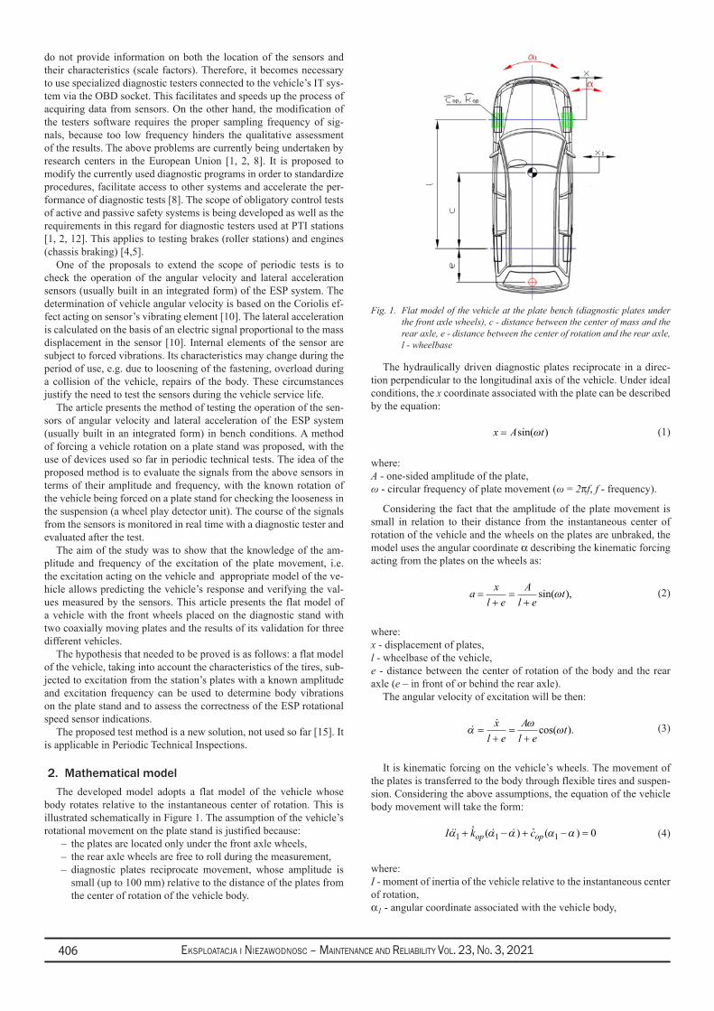
The lateral stiffness of the tyre was determined on a special stand for testing tyres under static conditions (Fig. 2). The movable plate under the rigidly mounted wheel can be moved perpendicular to the wheel disk.
This motion is carried out through a screw mechanism connected to the load plate by a force sensor. An inductive sensor is used to meas-ure displacement. Data is saved to the hard disk via an A/D converter. The construction of the stand allows applying any vertical load. The test was performed for the 205/55 R16 radial tyre with a pumping pressure of 2.2 bar. The specified vertical load was 3 kN, which cor-
Table 1. Selected mass and geometrical parameters of the tested cars (size symbols in accordance with the markings in the text)
Fiat Panda II Opel Astra G Renault Kadjar
l [m] 2,30 2,61 2,60
c [m] 1,14 1,56 1,3
m [kg] 1050 1165 1545
Io [kgm2] 1085 1586 2260
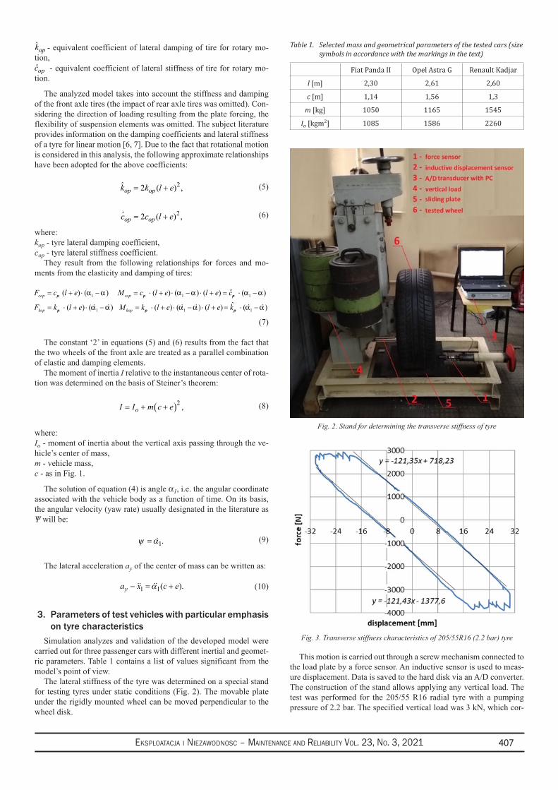
Fig. 3. Transverse stiffness characteristics of 205/55R16 (2.2 bar) tyre
Fig. 2. Stand for determining the transverse stiffness of tyre
Eksploatacja i NiEzawodNosc – MaiNtENaNcE aNd REliability Vol. 23, No. 3, 2021408
responds to a typical normal reaction for a front wheel car. The char-acteristics of the lateral stiffness of the tyre obtained in this way are presented in Fig. 3. The visible hysteresis loop results, among others, from exceeding the limit force of adhesion between the wheel and the plate. Regardless of the return of the applied force, the linear nature of the relationship between force and deformation was recorded. This allowed easy determination of the lateral stiffness coefficient of the tested tyre, whose value was:
cop = 121 N/mm.The presented stand does not allow for obtaining high plate speeds,
which means that the possibilities of determining the transversal damping factor are very limited. The value of this parameter was tak-en from the literature. The papers [6] and [7] contain numerous simu-lations and studies on lateral dynamics of tires. According to these data, the value of the lateral damping coefficient for tires of the same size as the tested tyre, loaded with a normal force of 3600 N and with a pump pressure of 2.75 bar is:
kop = 1770 kg/s.In turn, the lateral stiffness coefficient then takes the value of 126
N/mm. Bearing in mind similar (compared to the considered) tyre pa-rameters and almost identical values of the stiffness coefficient, in the course of further calculations the above value of the coefficient kop was adopted.
4. Simulation tests and model validationFig. 4 presents the influence of the position of the center of rota-
tion on the body deflection speed for sinusoidal forcing. The position of the center of rotation is represented by the parameter e (Fig. 1). Negative values e correspond to the shift towards the vehicle’s center of mass.
Shifting the center of rotation toward of the rear axle increases the amplitude of yaw angular velocity. For the center of rotation shifted by 1 m towards the center of mass, the amplitude increases almost twice (relative to the center of rotation on the rear axle). Shifting the center of rotation by the same value in the opposite direction results in a slight decrease in the amplitude from the initial value.
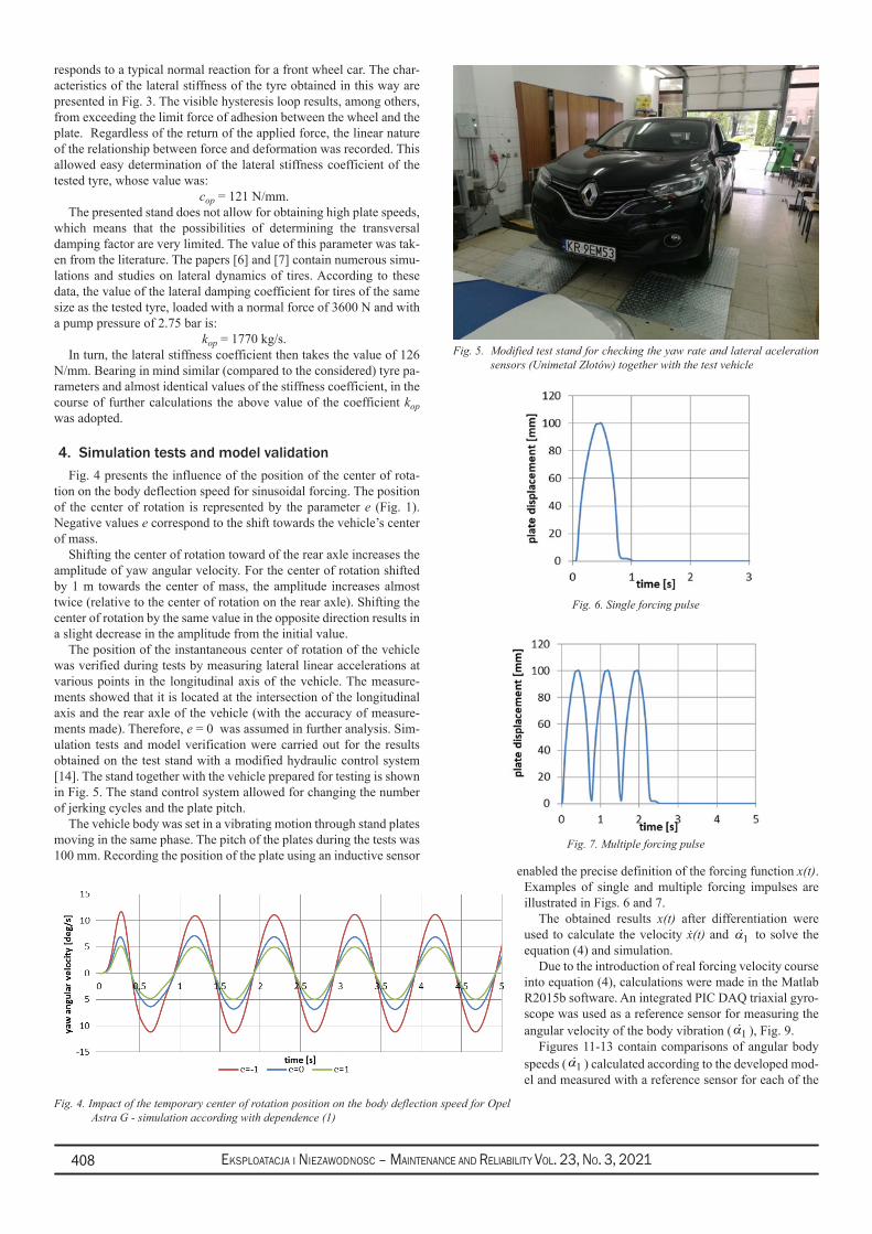
The position of the instantaneous center of rotation of the vehicle was verified during tests by measuring lateral linear accelerations at various points in the longitudinal axis of the vehicle. The measure-ments showed that it is located at the intersection of the longitudinal axis and the rear axle of the vehicle (with the accuracy of measure-ments made). Therefore, e = 0 was assumed in further analysis. Sim-ulation tests and model verification were carried out for the results obtained on the test stand with a modified hydraulic control system [14]. The stand together with the vehicle prepared for testing is shown in Fig. 5. The stand control system allowed for changing the number of jerking cycles and the plate pitch.
The vehicle body was set in a vibrating motion through stand plates moving in the same phase. The pitch of the plates during the tests was 100 mm. Recording the position of the plate using an inductive sensor
enabled the precise definition of the forcing function x(t). Examples of single and multiple forcing impulses are illustrated in Figs. 6 and 7.
The obtained results x(t) after differentiation were used to calculate the velocity ẋ(t) and α1 to solve the equation (4) and simulation.
Due to the introduction of real forcing velocity course into equation (4), calculations were made in the Matlab R2015b software. An integrated PIC DAQ triaxial gyro-scope was used as a reference sensor for measuring the angular velocity of the body vibration ( α1 ), Fig. 9.
Figures 11-13 contain comparisons of angular body speeds ( α1 ) calculated according to the developed mod-el and measured with a reference sensor for each of the
Fig. 4. Impact of the temporary center of rotation position on the body deflection speed for Opel Astra G - simulation according with dependence (1)
Fig. 6. Single forcing pulse
Fig. 7. Multiple forcing pulse
Fig. 5. Modified test stand for checking the yaw rate and lateral aceleration sensors (Unimetal Złotów) together with the test vehicle
Eksploatacja i NiEzawodNosc – MaiNtENaNcE aNd REliability Vol. 23, No. 3, 2021 409
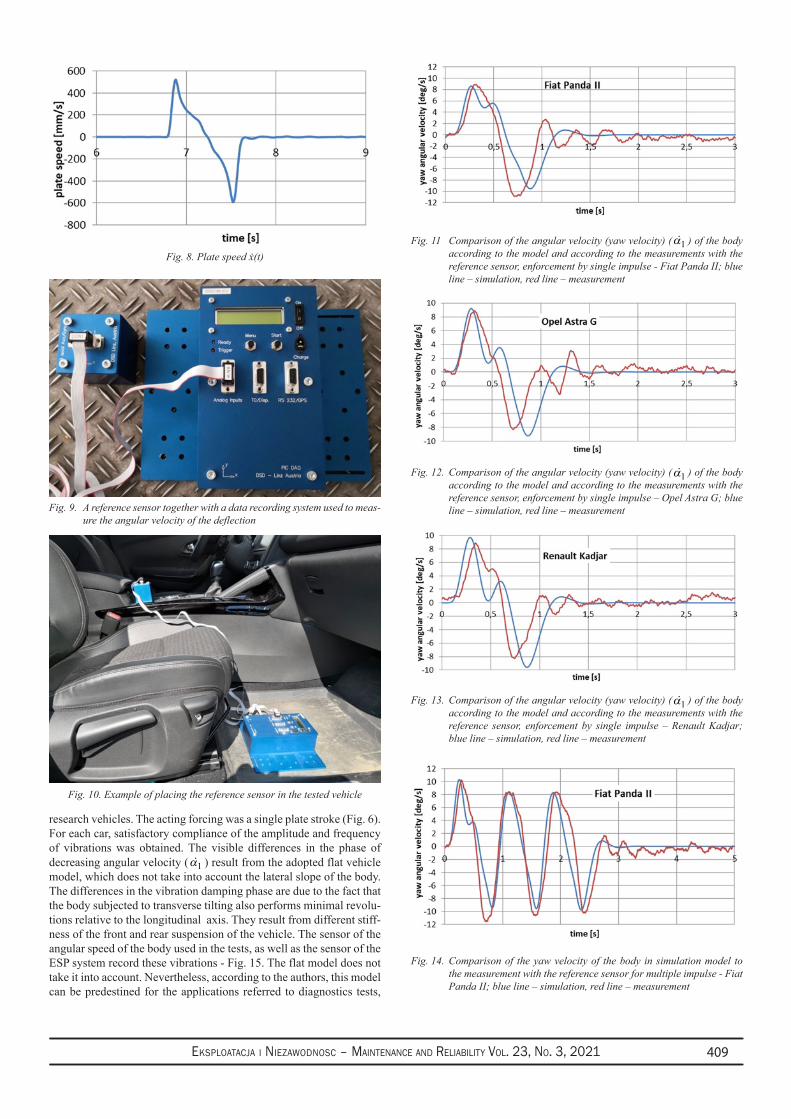
research vehicles. The acting forcing was a single plate stroke (Fig. 6). For each car, satisfactory compliance of the amplitude and frequency of vibrations was obtained. The visible differences in the phase of decreasing angular velocity ( α1 ) result from the adopted flat vehicle model, which does not take into account the lateral slope of the body. The differences in the vibration damping phase are due to the fact that the body subjected to transverse tilting also performs minimal revolu-tions relative to the longitudinal axis. They result from different stiff-ness of the front and rear suspension of the vehicle. The sensor of the angular speed of the body used in the tests, as well as the sensor of the ESP system record these vibrations - Fig. 15. The flat model does not take it into account. Nevertheless, according to the authors, this model can be predestined for the applications referred to diagnostics tests,
Fig. 8. Plate speed ẋ(t)Fig. 11 Comparison of the angular velocity (yaw velocity) ( α1 ) of the body
according to the model and according to the measurements with the reference sensor, enforcement by single impulse - Fiat Panda II; blue line – simulation, red line – measurement
Fig. 12. Comparison of the angular velocity (yaw velocity) ( α1 ) of the body according to the model and according to the measurements with the reference sensor, enforcement by single impulse – Opel Astra G; blue line – simulation, red line – measurement
Fig. 13. Comparison of the angular velocity (yaw velocity) ( α1 ) of the body according to the model and according to the measurements with the reference sensor, enforcement by single impulse – Renault Kadjar; blue line – simulation, red line – measurement
Fig. 9. A reference sensor together with a data recording system used to meas-ure the angular velocity of the deflection
Fig. 10. Example of placing the reference sensor in the tested vehicle
Fig. 14. Comparison of the yaw velocity of the body in simulation model to the measurement with the reference sensor for multiple impulse - Fiat Panda II; blue line – simulation, red line – measurement
Eksploatacja i NiEzawodNosc – MaiNtENaNcE aNd REliability Vol. 23, No. 3, 2021410
especially taking into account the measurement accuracy of sensors used in ESP systems.
Figure 14 presents an analogous comparison to the above for one of the research vehicles, where the excitation was a triple impulse (Fig. 7). Also in this case, an acceptable correlation was observed be-tween simulation and measurement, which confirms the usefulness of the proposed model.
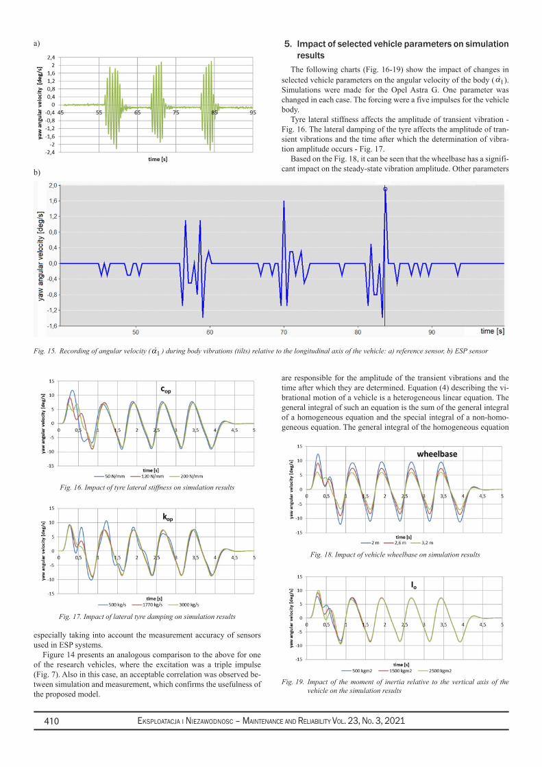
5. Impact of selected vehicle parameters on simulation results
The following charts (Fig. 16-19) show the impact of changes in selected vehicle parameters on the angular velocity of the body ( α1). Simulations were made for the Opel Astra G. One parameter was changed in each case. The forcing were a five impulses for the vehicle body.
Tyre lateral stiffness affects the amplitude of transient vibration - Fig. 16. The lateral damping of the tyre affects the amplitude of tran-sient vibrations and the time after which the determination of vibra-tion amplitude occurs - Fig. 17.
Based on the Fig. 18, it can be seen that the wheelbase has a signifi-cant impact on the steady-state vibration amplitude. Other parameters
are responsible for the amplitude of the transient vibrations and the time after which they are determined. Equation (4) describing the vi-brational motion of a vehicle is a heterogeneous linear equation. The general integral of such an equation is the sum of the general integral of a homogeneous equation and the special integral of a non-homo-geneous equation. The general integral of the homogeneous equation
Fig. 15. Recording of angular velocity ( α1 ) during body vibrations (tilts) relative to the longitudinal axis of the vehicle: a) reference sensor, b) ESP sensor
b)
a)
Fig. 16. Impact of tyre lateral stiffness on simulation results
Fig. 17. Impact of lateral tyre damping on simulation results
Fig. 18. Impact of vehicle wheelbase on simulation results
Fig. 19. Impact of the moment of inertia relative to the vertical axis of the vehicle on the simulation results

Eksploatacja i NiEzawodNosc – MaiNtENaNcE aNd REliability Vol. 23, No. 3, 2021 411
describes free (unforced) vibrations, so in the considered case their amplitude drops to 0 (due to tyre damping). As a result, specific body vibrations (α1) will tend to introduce α from the movement of the plates (the model assumes that the movement of the plates x forces the body to rotate through the wheels of the vehicle). According to the relationship (3), the vehicle parameter affecting the angular excitation speed ( α1 ) is the wheelbase. Assuming that the center of rotation is on the rear axle, it can be concluded that the amplitude of the angular speed of the body (yaw rate) will be a function of the wheelbase and the parameters of the plate movement (amplitude and frequency). This conclusion is important in the practical application of this method to test the vehicle angular velocity sensor in the ESP system. It should be noted that with known plate motion parameters, to evaluate the sensor operation, it is sufficient to know the wheelbase of the vehicle. For lateral acceleration, the position of the vehicle’s center of mass (parameter c in equation (10)) will also be relevant.
6. ConclusionThe analysis shows that the efficiency of the angular velocity sen-
sor and the ESP lateral acceleration sensor can be assessed using a diagnostic test stand for suspension tests. The experimental tests confirmed the postulated hypothesis that the developed model of the vehicle movement on the plate stand can be used to determine the body vibrations. The results of the vehicle angular velocity obtained computationally on the basis of the model can be a reference for the operation evaluation of the yaw rate sensor and the lateral accelera-tion sensor.
The vibratory motion of the vehicle body in the solid phase can be calculated on the basis of knowledge of the plate movement (ampli-tude and frequency), vehicle wheelbase, position of the lateral accel-eration sensor (to determine lateral acceleration) and the position of
the instantaneous center of rotation. The values of the amplitude and frequency of the vehicle body angular velocity and lateral accelera-tion obtained in this way should coincide with the values measured by the sensors of the ESP system.
The conducted tests have shown that the position of the instantane-ous center of rotation of the body is on the rear axle, or in its immedi-ate vicinity (e ≈ 0, Fig. 1). This determination will allow the practical application of this method for diagnosing the signal from the vehicle angular velocity sensor and the lateral acceleration sensor during the vehicle service life.
The extension of the periodic tests scope of used vehicles on ele-ments of the mechatronic systems (ABS, ESP), especially for vehicles with high mileage and repaired after accidents, has an impact on ac-tive safety in road traffic. The tests of the operation of these sensors in stand conditions allow for detecting mechanical malfunctions in the systems, e.g. loosening of sensor mounting, changes in their char-acteristics due to vibrations or weather conditions. These failures are not signalled by the on-board diagnostic system OBD but have an impact on the active safety systems of the vehicle. The costs reduction of such tests can be achieved by adapting stationary stands (a set of wheel play detectors) to cooperation with diagnostic testers.
AcknowledgementsThe work was created as part of the project: “UNILINE QUAN-
TUM - Integrated diagnostic line for testing the technical condition of the latest mechatronic safety systems in motor vehicles, including
ABS, ESP and suspension vibration damping efficiency, designed for vehicle control stations and car services” co-financed from EU funds European as part of the Intelligent Development Operational
Program, project number: POIR.01.01.01-00-0949/15.
References1. Buekenhoudt P. ECSS testing: concept and implementation of a wider interrogation of the electronic controlled safety system via OBD.
CITA Conference, Dubai: 2015. [https://citainsp.org/wp-content/uploads/2016/01/1.-Workshop-B2-Final-Presentation.pdf].2. CITA. ECSS: Study on a new performance test for electronic safety components at roadworthiness tests – Final Report: 2014.
[https://www.researchgate.net/profile/Pascal-Buekenhoudt/publication/344654916_ECSS_-_Study_on_a_new_performance_test_for_electronic_safety_components_at_roadworthiness_tests_-_final_report/ l inks/5f87078b458515b7cf7fc262/ECSS-Study-on-a-new-performance-test-for-electronic-safety-components-at-roadworthiness-tests-final-report.pdf].
3. Fan X, Zhao Z. Vehicle dynamics modeling and electronic stability program/active front steering sliding mode integrated control. Asian Journal of Control 2019; 21(5): 2364–2377, https://doi.org/10.1002/asjc.1822.
4. Gajek A. Directions for the development of periodic technical inspection for motor vehicles safety systems. The Archives of Automotive Engineering 2018; 80(2): 37-51, https://doi.org/10.14669/AM.VOL80.ART3.
5. Gajek A, Strzępek P, Dobaj K. Algorithms for diagnostics of the hydraulic pressure modulators of ABS/ESP systems in stand conditions. MATEC Web of Conferences 2018; 182: 1-9, https://doi.org/10.1051/matecconf/201818201020.
6. Hackl A, Hirshberg W, Lex C, Rill G. Experimental validation of a non-linear first-order tyre dynamics approach. The Dynamics of Vehicles on Roads and Tracks: 24th Symposium of the International Association for Vehicle System Dynamics 2016; 24: 443-452.
7. Hackl A, Hirshberg W, Lex C, Rill G. Tire dynamics: model validation and parameter identification. In Andreescu C, Clenci A. (eds): Proceedings of the European Automotive Congress EAEC-ESFA 2015. Springer, Cham: 2016: 219-232.
8. IDELSY. Initiative for Diagnosis of Electronic Systems in Motor Vehicles for Periodic Technical Inspection (PTI) - Final Report: 2006. [https://ec.europa.eu/transport/road_safety/sites/roadsafety/files/pdf/projects_sources/idelsy_management_summary.pdf].
9. Jaafari S, Shirazi K. Integrated Vehicle Dynamics Control Via Torque Vectoring Differential and Electronic Stability Control to Improve Vehicle Handling and Stability Performance. ASME Journal of Dynamic Systems, Measurement and Control 2018; 140(7): 1-13, https://doi.org/10.1115/1.4038657.
10. Kraft M, White N. MEMS for automotive and aerospace applications. Cambridge, UK, Woodhead Publishing Limited: 2013: 29-53.11. Pieniążek W, Janczur R, Gajek A, Wolak S. Verification of sensors for yaw rate and lateral acceleration in car ESP system. The Archives of
Automotive Engineering 2020; 88(2): 61-76, https://doi.org/10.14669/AM.VOL88.ART5.12. Taracido E. Capability analysis of different scanning tools to check ECSS. CITA Conference, Dubai: 2015. [https://citainsp.org/wp-content/
uploads/2016/01/1.-Workshop-B2-Final-Presentation.pdf].13. Tumasov A, Vashurin A, Toropov E, Moshkov P, Trusov Y. Estimation of influence of ESP on LCV active safety in condition of curvilinear
movement. In Proceedings of the International Conference on Vehicle Technology and Intelligent Transport Systems (VEHITS 2016), 118-123.
14. Unimetal Sp. z o.o. - information materials and technical specifications. [https://unimetal-moto.com/].15. Unimetal Sp.z o.o. The diagnostic method of controlling and checking the operation of the ABS or ESP/ESC pressure modulator for motor
vehicles. The patent application No P.436848 with Gajek A and Strzępek P. The Patent Office of the Republic of Poland 2021.

Eksploatacja i NiEzawodNosc – MaiNtENaNcE aNd REliability Vol. 23, No. 3, 2021412
16. Wu Y, Ahmed Q, Chen W, Tian W, Chen Q. Model-Based Fault Diagnosis of an Anti-Lock Braking System via Structural Analysis. Sensors 2018; 18(12): 1-23, https://doi.org/10.3390/s18124468.
17. Yongqiang Z, Kaicheng Z, Chang L, Xiang L. Development of the safety diagnosis system for VCU of pure electric vehicle. Journal of Physics: Conference Series 2020; 1605(012033): 1-10, https://doi.org/10.1088/1742-6596/1605/1/012033.
18. Zhang G, Yu Z, Wang J. Correction of contaminated yaw rate signal and estimation of sensor bias for an electric vehicle under normal driving conditions. Mechanical Systems and Signal Processing 2017; 87: 64-80, https://doi.org/10.1016/j.ymssp.2016.05.034.
Eksploatacja i NiEzawodNosc – MaiNtENaNcE aNd REliability Vol. 23, No. 3, 2021 413
(*) Corresponding author.E-mail addresses:
Eksploatacja i Niezawodnosc – Maintenance and ReliabilityVolume 23 (2021), Issue 3
journal homepage: http://www.ein.org.pl
Indexed by:
1. Introduction Given the technological importance and complex-
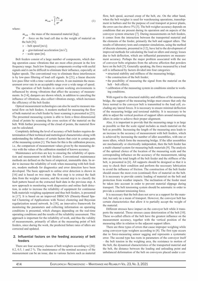
ity of measuring material flow, accelerated industrial development imposes the need for increase the level of accuracy of existing measuring devices. Material flow measurement occurs in many industries. Trans-port of certain material amount in a specified time interval between loading and unloading points is the transport task of belt conveyors [15]. Belt feeders, as shown on Figure 1, represent belt conveyors on which a design change has been made by placing one or more support idlers on the measuring bridge. Thus, during transport, the quantity, i.e., the flow of transported material can be measured.
The weight of the material on the belt is trans-ferred to the load cell - directly or via a lever sys-tem. In practice, the integration principle of flow determination is most often applied. The principle is based on the specific load with which the material and the belt act on the measuring bridge of the scale, so that the flow is calculated according to:
Continual material feeding represents a process of great importance for process industries. Feeding with belt feeders represents one of the most common methods. Belt feeders are devices that require little space, they are not expensive and, most importantly, they do not interrupt material flow while feeding. Calibration of belt feeders, as well as other measur-ing devices, is a prerequisite for measuring and achieving a defined level of measurement accuracy. On the other hand, the defined level of measurement accuracy is often difficult to achieve in practice due to the multitude of factors that affect the operation of belt feeders. Existing mathematical models indicate a number of influential factors on measurement ac-curacy. The paper presents the measurement procedure performed on a belt feeder in labora-tory conditions, with variable speeds and belt tensions and the known raised position of the measuring idler. Based on the obtained results, appropriate conclusions were made about the influences on calibration and measurement accuracy.
Highlights Abstract
Measurements on a belt feeder with variable speed • and belt tension.
PLC controled belt feeder with data monitoring, • visualization and processing.
Material calibration under operating conditions is • the most accurate calibration method.
Existing mathematical models for estimating • measurement errors do not cover all factors.
The speed and tension of the belt must be kept • within certain limits during feeding.
The analysis of influential parameters on calibration and feeding accuracy of belt feedersDragan Živanić a, Nikola Ilanković a,*, Ninoslav Zuber a, Radomir Đokić a, Nebojša Zdravković b, Atila Zelić a
a Faculty of Technical Sciences, University of Novi Sad, Trg Dositeja Obradovica 6, 21000 Novi Sad, Serbia b Faculty of Mechanical and Civil Engineering in Kraljevo, University of Kragujevac, Dositejeva 19, 36000 Kraljevo, Serbia
Živanić D, Ilanković N, Zuber N, Đokić R, Zdravković N, Zelić A. The analysis of influential parameters on calibration and feeding accu-racy of belt feeders. Eksploatacja i Niezawodnosc – Maintenance and Reliability 2021; 23 (3): 413–421, http://doi.org/10.17531/ein.2021.3.2.
Article citation info:
flat belt feeder, calibration methods, measurement errors.
Keywords
This is an open access article under the CC BY license (https://creativecommons.org/licenses/by/4.0/)
D. Živanić - [email protected], N. Ilanković - [email protected], N. Zuber - [email protected], R. Đokić - [email protected], N. Zdravković - [email protected], A. Zelić - [email protected]
Fig. 1. Belt feeder
Eksploatacja i NiEzawodNosc – MaiNtENaNcE aNd REliability Vol. 23, No. 3, 2021414
( )2
1
1t
wmt
Pvm dtgr
= ∫ (1)
where:
wmm – the mass of the measured material [kg];P – force on the load cell due to the weight of material on the belt [N];v – belt speed [m/s];g – gravitational acceleration [m/s2];r – scale span [m].
Belt feeders consist of a large number of components, which dur-ing operation cause vibrations that are most often present in the low frequency range. Such low frequency components overlap with useful signals and it can be difficult to eliminate their influence, especially at higher speeds. The conventional way to eliminate these interferences is by low-pass filtering of load cell signals. In [21], a linear discrete low-pass filter with a time variant is shown. It can maintain the meas-urement error rate in an acceptable range over a wide range of speed.
The operation of belt feeders in certain working environments is influenced by strong vibrations that affect the accuracy of measure-ments. In [14], dampers are shown which, in addition to canceling the influence of vibrations, also collect vibration energy, which increases the efficiency of the belt feeder.
Optical measurement technologies can also be used to measure ma-terial flow on belt feeders. A modern method for measuring the flow of bulk material on a belt feeder by laser scanning is presented in [23]. The presented measuring system is able to form a three-dimensional cloud of points by scanning the cross section of the material on the belt. With further processing of the cloud of points, the material flow can be calculated.
Completely defining the level of accuracy of belt feeders requires de-termination of their technical and metrological characteristics along with understanding the influence of certain factors that exist in certain parts of the measuring system [1]. The basis for this is the calibration process, i.e., the comparison of measurement values given by the measuring de-vice with the values of the calibration standard of known accuracy.
Maintenance activities are key to ensuring the reliability of opera-tion and measurement with belt feeders. Conventional maintenance methods are defined on the basis of empirical, immutable data. In or-der to increase the reliability of work when measuring with belt feed-ers, modern methods for diagnostics and error detection have been developed. The basic approach to online error detection is shown in [16] and is based on two steps: the first step is to extract the fault data from the weigher sensors, and the second step is to classify the fault pattern based on the extracted fault data in the previous step. A new approach to monitoring work diagnostics and online fault detec-tion, in order to increase the reliability of equipment for continuous bulk materials weighing equipment and thus belt feeders, is presented in [17]. It is based on an improved DBSCAN (Density-Based Spa-tial Clustering of Applications with Noise) clustering and Bayesian regularization neural network. In [18], an innovative framework for monitoring the parameters and collecting information on operating conditions is presented, which changes depending on the real-time operating conditions and the results of the reliability assessment. This approach is important for the reliability of work, and thus the validity of measurements, primarily of idlers at the measuring point of belt feeders, since during the work, the predicted failure rates of idlers are corrected and updated.
2. Influential factors on the feeding accuracy of belt feeders
There are four accuracy classes of belt weighers according to [20]: 0.2, 0.5, 1 and 2 %. The maintenance of the nominal accuracy of the measurement can be an issue, due to various factors such as material
flow, belt speed, accrued creep of the belt, etc. On the other hand, when the belt weigher is used for warehousing operations, transship-ment in harbors and for the purpose of coal transport at power plants, the error can rise above 5% [3]. The belt weigher accuracy depends on conditions that are present during its operation and on aspects of the conveyor system structure [7]. During measurements on belt feeders, it comes from the interaction between the transported material and the elements of the feeder, primarily the belt and support idlers. The results of laboratory tests and computer simulations, using the method of discrete elements, presented in [12], have led to the development of improved methods for calculating the load on idlers and energy losses due to belt deflection, which are influential parameters on measure-ment accuracy. Perhaps the major problem associated with the use of conveyor belts originates from the adverse affection that powders have on the belt [5]. Generally speaking, the force measured by a load cell is influenced by factors divided into four categories:
structural stability and stiffness of the measuring bridge;• the construction of the belt feeder;• the possibility of measuring the signal from the material on the • belt – belt effects;calibration of the measuring system in conditions similar to work-• ing conditions.
With regard to the structural stability and stiffness of the measuring bridge, the support of the measuring bridge must ensure that only the force normal to the conveyor belt is transmitted to the load cell, ex-cluding any lateral forces. It is necessary to ensure minimal deflection of the measuring bridge and torsional stability. It is necessary to be able to adjust the vertical position of support idlers around measuring idlers in order to achieve their proper alignment.
Also, it is important to provide that the measuring range is as large as possible so that the scale signal includes as much material on the belt as possible. Increasing the length of the measuring area leads to an increase in the accuracy of measurement with belt feeders, which is achieved by increasing the number of idler assemblies, with one or more idlers, which form the measuring bridge. If the idler assemblies are mechanically or electrically independent, then the belt feeder has a multi-channel system for measuring bulk materials [9]. The analysis of the optimal choice of the location of the measuring scale and the corresponding influence on the accuracy of the measurement, taking into account the total length of the belt feeder and the stiffness of the belt, is presented in [6]. All supports should be designed so that it is easy to check their condition and perform the necessary lubrication to avoid the influence of friction. The construction of the belt feeder should ensure the most even (continual) flow of material on the belt. It is necessary to provide centric loading of material on the belt and protection from weather impacts. The inclination of the feeder must be taken into account in order to prevent material slippage during transport. The belt tensioning system should be automatic in order to provide a constant tensioning force.
It is necessary that the belt does not serve as a support for the mate-rial, but only as a mean of transport. However, the conveyor belt has certain characteristics that allow it to partially accept the weight of the material.
Different stresses have impact on the conveyor belt while it trans-ports the material. Those stresses cause deterioration of the belt [10]. These so-called effects of the belt have the greatest influence on the measurement accuracy, together with the vertical position of the measuring idler in relation to the adjacent support idlers.
There are three types of errors that cause improper weighing while using conveyor-type weighers according to [8]. The first type occurs due to force-measuring sensor sagging and represents a systematic error. The second type has roots in parameters of the conveyor itself – the belt tension in the weighing area, the resistance to motion of the belt, the dynamical characteristics of the transported material and the belt, the distance between the loading and unloading point and unbalanced deformation of the belt on conveyors placed under a cer-
Eksploatacja i NiEzawodNosc – MaiNtENaNcE aNd REliability Vol. 23, No. 3, 2021 415
tain angle. These errors can be successfully minimized with a proper calibration procedure. The third type is consisted of errors that occur randomly due to various deviations of characteristics of the physical function of a conveyor-type weigher.
It has been experimentally determined that the belt behaves as a continuous and horizontal elastic beam supported by equally spaced supports. The combined action of the tensile force and stiffness-to-bending (IE) in the conveyor belt on misaligned measuring idlers leads to inaccurate signals from the scale. Mathematical models have been developed for ideal systems that have supports and measuring idlers at equal distances, with n rollers on a measuring platform, a uniform belt, etc. One such model, according to [11], defines the force P detected by the scale according to the following:
P nQLcos
TDL
EIDL
= + + [ ]0 102 500
312500 3. θ
N (2)
where:n – number of idlers on the measuring platform;Q – material mass per unit length [kg/m];L – spacing between idlers [m];T – tension in the belt at scale location [N];E – modulus of elasticity of belt carcass material [MPa];I – moment of inertia of carcass cross-section [cm4];D – vertical misalignment between measuring idlers and adja-cent support idlers [mm];θ – angle of conveyor inclination [deg].
The calibration procedure should take into account factors that af-fect the force detected by the scales that also exist during calibration. Assuming that the EI value does not change with the change in tensile force, the net value of the error (%Er) that occurs during operating conditions can be expressed as follows:
%* ** *
ErD T T cos
nQLT T
EAT T W
EAQR C R C R C b=−( )
−−
−−( )2 4
10000 100002. θ ***
3( ) (3)
where:* – tension effect on misalignment;** – speed measurement error;*** – error due to change in the belt weight per unit length due to stretch;
,RT CT – tension force in the belt at the scale under working conditions and during calibration [N];A – cross-sectional area of the carcass [m2];
bW – belt mass per unit length [kg/m].
The second mathematical model according to [4] is based on the principle of a simple beam. The force detected by the scale P can be expressed as:
P nQLcos
KDTcosL
= ± ( )0 102
0 2 4.
.θ
θ* ** (4)
KG
G
G L TcosEI p
=−
( ) =1
15
tanh; θ
(5)
where:* – the true belt load on the scale;• ** – measurement error caused by the beam effect of the belt;• K• – belt stiffness factor (od 1 do ∞); K=f(L, T, E, Ip)I• p – planar moment of inertia of a cross-section of the belt about its centroidal axis [cm4];
the sign „-“ is used for downward displacement and the sign „+“ is • used for an upward displacement of measuring idlers.
The modulus of elasticity of the belt carcass is determined accord-ing to [22].
It was experimentally determined that the modulus of elasticity of the belt carcass made from textile and nylon ranges from 275 ÷ 345 MPa, from rayon ranges from 690 ÷ 1050 MPa, and from steel cords is 7000 MPa. The measurement error caused by the behaviour of the belt as a simple beam can be represented as a percentage of the total load detected by the scale:
E
DKTcosL
nQL cos% = ⋅
0 2
0 102100
.
/ .
θ
θ (6)
The value %E varies depending on the support configuration of the scale. If the total vertical misalignment is consisted of the load cell deflection (D1) and structural deflection and initial installation misalignment (D2), then %E can be expressed as:
E KTnQL
D D% %= +( )[ ]0 0204 2 1 2. (7)
The measurement error is directly proportional to the product of the belt tensile force and the vertical misalignment of measuring idlers (DT). As the troughing angle of support idlers increases, the belt be-comes stiffer and the simple beam effect increases thus increasing the measurement error.
When loading the material on the belt, the direction of its move-ment does not coincide with the direction of movement of the belt. Therefore, it takes a certain amount of time, i.e., a certain distance for the material to reach the speed of the belt. In order for the material to reach the speed of the belt before it reaches the measuring range of the scale, the minimum required distance between the loading place and the scale is calculated according to:
X v v
g f cos sin W cA
V V
m
x ==
−
⋅ ⋅ ⋅ − +⋅ ⋅⋅
( )2
02
2 0 258
θ θρ
, (8)
where:
0v – initial material speed [m/s];c – cohesion [kg/m2].
3. Experimental setupIn order to examine the influence of certain factors listed in the
previous section, tests were performed on a horizontal belt feeder with a flat belt with lateral sides, which is located in the laboratory at the Faculty of Technical Sciences in Novi Sad (Figure 1). The belt feeder is controlled by the PLC and a variable frequency drive (VFD). The basic characteristics are:
belt width 540 mm with the height of lateral sides of 70 mm;• feeder length: • L = 3000 mm;AC motor power: • P = 0.75 kW;belt speed: • v = 0.2405 m/s at 50 Hz of power supply of VFD;max. material flow: 26 m• 3/h.
With the development of the IT system and its application in trans-port systems, it is possible to collect a lot of valuable information for technical, operational and diagnostic purposes. This enables adequate identification of the flow distribution of transported bulk material [19, 13]. Control and measuring devices have been added to the basic con-
Eksploatacja i NiEzawodNosc – MaiNtENaNcE aNd REliability Vol. 23, No. 3, 2021416
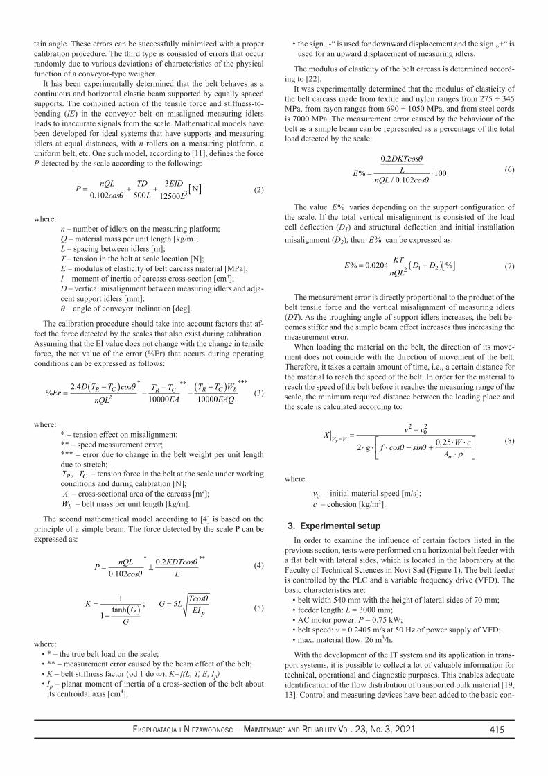
figuration of the belt feeder. The scheme of automation of the belt dispenser drive is shown on Figure 2.
HBM SPIDER 8 universal measurement amplifier has been used as an acquisition device. Figure 3 shows the connectors of measuring instruments on the SPIDER 8. Catman® Pro-fessional PC software has been used for data recording, visuali-zation and processing.
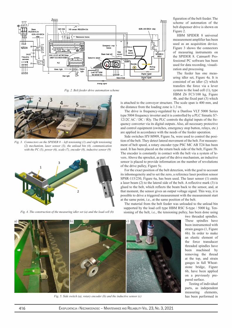
The feeder has one meas-uring idler set, Figure 4a. It is consisted of an idler (2) which transfers the force via a lever system to the load cell (1), type HBM Z6 FC3/100 kg, Figure 4b, and the fixed part (3) which
is attached to the conveyor structure. The scale span is 400 mm, and the distance from the loading zone is 1.3 m.
The drive is frequency-regulated by a Danfoss VLT 5000 Series type 5004 frequency inverter and it is controlled by a PLC Simatic S7-1212C AC / DC / Rly. The PLC controls the digital inputs of the fre-quency converter via its digital outputs. Also, all necessary protective and control equipment (switches, emergency stop button, relays, etc.) are applied in accordance with the needs of the feeder operation.
Side switches HY-M909, Figure 5a, were used to control the posi-tion of the belt. They detect lateral movement of the belt. For measure-ment of belt speed, a rotary encoder type PSC MC AB T24 has been used. It has been placed on the return back side of the belt, Figure 5b. The encoder is constantly in contact with the belt via a system of le-vers. Above the sprocket, as part of the drive mechanism, an inductive sensor is placed to provide information on the number of revolutions of the drive pulley, Figure 5c.
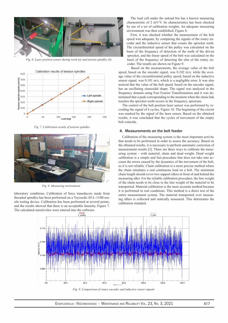
For the exact position of the belt detection, with the goal to account its inhomogeneity and to set the zero, a reference laser position sensor SPSR-115/230, Figure 6a, has been used. The laser sensor (1) emits a laser beam (2) to the lateral side of the belt. A reflective mark (3) is glued to the belt, which reflects the beam back to the sensor, and, at that moment, the sensor gives an output voltage signal. This way, it is possible to drive a triggered measurement with the measurement start at the same point, i.e., at the same position of the belt.
The material from the belt feeder was unloaded to the unload bin supported by the load cell type HBM RSC S-type / 5000 kg. Ten-sioning of the belt, i.e., the tensioning pulley, has been done using
two threaded spindles. These spindles have been instrumented with strain gauges (1, Figure 6b). In order to make an elastic element of the force transducer threaded spindles have been machined by removing the thread at the top, and strain gauges in full Wheat-stone bridge, Figure 6b, have been applied on a previously pre-pared surface.
Testing of individual parts, as independent measuring elements, has been performed in
Fig. 2. Belt feeder drive automation scheme
Fig. 4. The construction of the measuring idler set (a) and the load cell (b)
Fig. 3. Connectors on the SPIDER 8 – left tensioning (1) and right tensioning (2) mechanism, laser sensor (3), the unload bin (4), communication with the PC (5), power (6), scale (7), encoder (8), inductive sensor (9)
Fig. 5. Side switch (a), rotary encoder (b) and the inductive sensor (c)
b) c)a)
Eksploatacja i NiEzawodNosc – MaiNtENaNcE aNd REliability Vol. 23, No. 3, 2021 417
laboratory conditions. Calibration of force transducers made from threaded spindles has been performed on a Toyoseiki AT-L-118B ten-sile testing device. Calibration has been performed at several points, and the results showed that there is an acceptable linearity, Figure 7. The calculated sensitivities were entered into the software.
The load cell under the unload bin has a known measuring characteristic of 2 mV/V. Its characteristics has been checked by use of a set of calibration weights. An adequate measuring environment was then established, Figure 8.
First, it was checked whether the measurement of the belt speed was adequate, by comparing the signals of the rotary en-coder and the inductive sensor that counts the sprocket teeth. The circumferential speed of the pulley was calculated on the basis of the frequency of detection of the teeth of the driven sprocket, and the linear speed of the belt was calculated on the basis of the frequency of detecting the slits of the rotary en-coder. The results are shown on Figure 9.
Based on the measurements, the average value of the belt speed, based on the encoder signal, was 0.102 m/s; while the aver-age value of the circumferential pulley speed, based on the inductive sensor signal, was 0.101 m/s, which is a negligible error. It was also noticed that the value of the belt speed, based on the encoder signal, has an oscillating sinusoidal shape. The signal was analysed in the frequency domain using Fast Fourier Transformation and it was de-termined that a peak corresponding to the moment when the chain link touches the sprocket tooth occurs in the frequency spectrum.
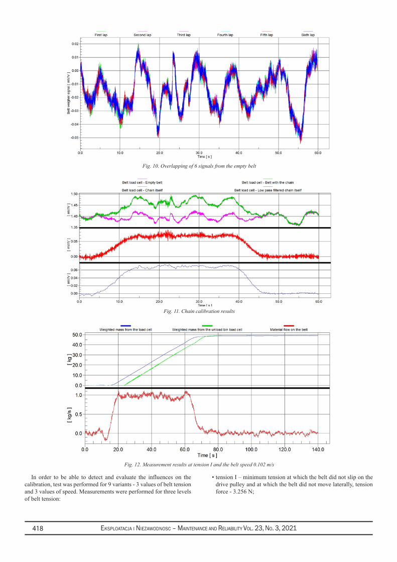
The control of the belt position laser sensor was performed by re-cording the signal of 6 cycles, Figure 10. The beginning of the circuit was marked by the signal of the laser sensor. Based on the obtained results, it was concluded that the cycles of movement of the empty belt coincide.
4. Measurements on the belt feederCalibration of the measuring system is the most important activity
that needs to be performed in order to assess the accuracy. Based on the obtained results, it is necessary to perform automatic correction of measurement results [2]. There are three ways to calibrate the meas-uring system – with material, chain and dead weight. Dead weight calibration is a simple and fast procedure that does not take into ac-count the errors caused by the dynamics of the movement of the belt, so it is not reliable. Chain calibration is a more precise method where the chain simulates a real continuous load on a belt. The minimum chain length should cover two support idlers in front of and behind the measuring idler. For the reliable calibration procedure, the line weight of the chain needs to be close to the line weight of the material to be transported. Material calibration is the most accurate method because it is performed in real conditions. This method is a direct test of the entire measurement system. The material transported over measur-ing idlers is collected and statically measured. This determines the calibration standard.
Fig. 6. Laser position sensor during work (a) and tension spindles (b)
Fig. 8. Measuring environment
Fig. 9. Comparison of rotary encoder and inductive sensor signals
Fig. 7. Calibration results of tension spindles
Eksploatacja i NiEzawodNosc – MaiNtENaNcE aNd REliability Vol. 23, No. 3, 2021418
In order to be able to detect and evaluate the influences on the calibration, test was performed for 9 variants - 3 values of belt tension and 3 values of speed. Measurements were performed for three levels of belt tension:
tension I – minimum tension at which the belt did not slip on the • drive pulley and at which the belt did not move laterally, tension force - 3.256 N;
Fig. 10. Overlapping of 6 signals from the empty belt
Fig. 11. Chain calibration results
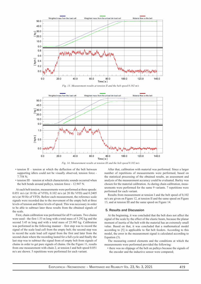
Fig. 12. Measurement results at tension I and the belt speed 0.102 m/s
Eksploatacja i NiEzawodNosc – MaiNtENaNcE aNd REliability Vol. 23, No. 3, 2021 419
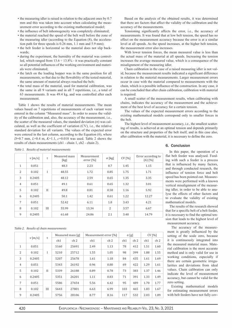
tension II – tension at which the deflection of the belt between • supporting idlers could not be visually observed, tension force - 7.758 N;tension III – tension at which characteristic sounds occurred when • the belt bends around pulleys, tension force - 12.947 N.
At each belt tension, measurements were performed at three speeds: 0.051 m/s (at 10 Hz of VFD), 0.102 m/s (at 20 Hz VFD) and 0.2405 m/s (at 50 Hz of VFD). Before each measurement, the reference scale signals were recorded due to the movement of the empty belt at three levels of tension and three levels of speed. This was necessary in order to be able to subtract later these results from the obtained signals of the scale.
First, chain calibration was performed for all 9 variants. Two chains were used - the first 1.53 m long with a total mass of 5.292 kg and the second 3.45 m long and with a total mass of 25.985 kg. Calibration was performed in the following manner – first step was to record the signal of the scale load cell from the empty belt; the second step was to record the scale load cell signal from the first and later from the second chain where the recording lasted for a full cycle and finally the last step was to subtract the signal from of empty belt from signals of chains in order to get pure signals of chains. On the Figure 11, results from one measurement with chain 2, at tension I and belt speed 0.051 m/s are shown. 5 repetitions were performed for each variant.
After that, calibration with material was performed. Since a larger number of repetitions of measurements were performed, based on the statistical processing of the obtained results, an assessment and analysis of the measurement accuracy could be evaluated. Barley was chosen for the material calibration. As during chain calibration, meas-urements were performed for the same 9 variants. 7 repetitions were performed for each variant.
Results from measurement at tension I and the belt speed of 0,102 m/s are given on Figure 12, at tension II and the same speed on Figure 13, and at tension III and the same speed on Figure 14.
5. Results and DiscussionAt the beginning, it was concluded that the belt does not affect the
signal of the scale by the effect of the elastic beam, because the planar moment of inertia of the belt with the material has an extremely small value. Based on that, it was concluded that a mathematical model according to [5] is applicable to flat belt feeders. According to this model, the error in the measurement signal is calculated according to Equation (3).
The measuring control elements and the conditions at which the measurements were performed provided the following:
there was no slippage of the belt on pulleys because the signals of • the encoder and the inductive sensor were compared;
Fig. 13. Measurement results at tension II and the belt speed 0.102 m/s
Fig. 14. Measurement results at tension III and the belt speed 0.102 m/s
Eksploatacja i NiEzawodNosc – MaiNtENaNcE aNd REliability Vol. 23, No. 3, 2021420
the measuring idler is raised in relation to the adjacent ones by 0.7 • mm and this was taken into account when calculating the meas-urement error according to the existing mathematical model;the influence of belt inhomogeneity was completely eliminated;• the material reached the speed of the belt well before the zone of • the measuring idler (according to the Equation (8), the accelera-tion path for three speeds is 0.26 mm, 1.1 mm and 5.9 mm);the belt feeder is horizontal so the material does not slip back-• wards;during the experiment, the humidity of the material was control-• led, which ranged from 13.6 ÷ 13.8% - it was practically constant so all potential influences of the working environment and materi-als were eliminated;the latch on the loading hopper was in the same position for all • measurements, so that due to the flowability of the tested material, the same amount of material always reached the belt;the total mass of the material, used for material calibration, was • the same in all 9 variants and in all 7 repetitions, i.e., a total of 63 measurements. It was 49.4 kg, and was controlled after each measurement.
Table 1 shows the results of material measurements. The mean values based on 7 repetitions of measurements of each variant were entered in the column “Measured mass”. In order to assess the valid-ity of the calibration and, also, the accuracy of the measurement, i.e., the scatter of the measured values, the standard deviation (σ) was cal-culated, as well as the coefficient of variation (CV), i.e., the relative standard deviation for all variants. The values of the expected error were entered in the last column, according to the Equation (6), where D=0.7 mm, L=0.4 m, K=1.1, c=0.018 was used. Table 2 shows the results of chain measurements (ch1 - chain 1, ch2 - chain 2).
Based on the analysis of the obtained results, it was determined that there are factors that affect the validity of the calibration and the accuracy of the measurements.
Tensioning significantly affects the error, i.e., the accuracy of measurements. It was found that at low belt tension, the speed has no effect on the measurement accuracy because the error is at a similar level at all speeds. As the speed increases, at the higher belt tension, the measurement error also increases.
With lower tension forces, the mean measured value is less than the actual mass of the material at all speeds. Increasing the tension increases the average measured value, which is a consequence of the misalignment of the measuring idler.
Chain calibration in the case of a raised measuring idler is not val-id, because the measurement results indicated a significant difference in relation to the material measurements. Larger measurement errors occur in case with the material compared to measurements with the chain, which is a possible influence of the construction. In any case, it can be concluded that after chain calibration, calibration with material is required.
A small scatter of the measurement results, when calibrating with chains, indicates the accuracy of the measurement and the achieve-ment of the best level of accuracy for a certain tension.
The values of the expected measurement errors according to the existing mathematical models correspond only to smaller forces in the belt.
The highest level of measurement accuracy, i.e., the smallest scatter-ing of results, is achieved at an optimal tension and depends primarily on the structure and properties of the belt itself, and in this case also, after calibration with the material, it is necessary to define the zero.
6. ConclusionIn this paper, the operation of a
flat belt feeder was analysed. Feed-ing with such a feeder is a process that is influenced by many factors, and through conducted research, the influence of tension force and belt speed has been pointed out. Measure-ments were performed with a known vertical misalignment of the measur-ing idler, in order to be able to ana-lyse the effects of other factors and to evaluate the validity of existing mathematical models.
The results of the research showed that for a specific belt of a belt feeder, it is necessary to find the optimal ten-sion that leads to the highest level of
measurement accuracy.The accuracy of the measure-
ment is greatly influenced by the setting of the scale zero, because it is continuously integrated into the measured material mass. Mate-rial calibration is the most accurate method and is only valid for use in working conditions, especially if there are certain geometric irregu-larities and deviations from ideal values. Chain calibration can only indicate the level of measurement accuracy, but cannot be valid for the zero setting.
Existing mathematical models for estimating measurement errors with belt feeders have not fully cov-
Table 1. Results of material measurements
v [m/s] t Measured mass [kg]
Measurement error [%] σ [kg] CV [%] Error according to
(6) [%]
1 0.051
I
48.3 2.23 0.7 1.45 1.15
2 0.102 48.55 1.72 0.85 1.75 1.71
3 0.2405 48.12 2.59 0.65 1.35 3.35
4 0.051
II
49.1 0.61 0.65 1.32 3.01
5 0.102 49.8 0.81 0.58 1.16 5.92
6 0.2405 50.1 1.42 0.61 1.22 12.27
7 0.051
III
52.42 6.11 1.8 3.43 4.21
8 0.102 55.99 13.34 2 3.57 6.67
9 0.2405 61.68 24.86 2.1 3.40 14.79
Table 2. Results of chain measurements
v [m/s] tMeasured mass [g] Measurement error [%] σ [g] CV [%]
ch1 ch 2 ch1 ch 2 ch1 ch 2 ch1 ch 2
1 0.051
I
5160 25691 2.49 1.13 78 412 1.51 1.60
2 0.102 5210 25712 1.55 1.05 98 399 1.88 1.55
3 0.2405 5207 25678 1.61 1.18 84 435 1.61 1.69
4 0.051
II
5343 26192 0.96 0.80 69 422 1.29 1.61
5 0.102 5339 26188 0.89 0.78 73 383 1.37 1.46
6 0.2405 5351 26201 1.11 0.83 71 391 1.33 1.49
7 0.051
III
5586 27654 5.56 6.42 95 489 1.70 1.77
8 0.102 5643 27801 6.63 6.99 103 465 1.83 1.67
9 0.2405 5756 28106 8.77 8.16 117 532 2.03 1.89

Eksploatacja i NiEzawodNosc – MaiNtENaNcE aNd REliability Vol. 23, No. 3, 2021 421
ReferencesAleksandrovic S, Jovic M. Analysis of Belt Weigher Accuracy Limiting Factors, International Journal of Coal Preparation and Utilization 1. 2011; 31(5): 223-241, https://doi.org/10.1080/19392699.2011.552896Aleksandrović S, Jović M. Testing and calibration of continuously operating belt weighers, Przegląd Elektrotechniczny 2011; 87(7): 276-2. 279.Bingying L, Yongxin L, Haitao W, Yuming M, Qiang H, Fangli G. Compensation of automatic weighing error of belt weigher based on BP 3. neural network. Measurement 2018; 128: 625–632, https://doi.org/10.1016/j.measurement.2018.07. 080Colijn H. Weighing and Proportioning of Bulk Solids. Bäch: Trans Tech Publications, 1975.4. Czuba W, Furmanik K. Analysis of a grain motion in the transfer area of the belt conveyor. Eksploatacja i Niezawodnosc – Maintenance and 5. Reliability 2013; 15(4): 390-396.Donis V. K, Rachkovskii A. E, Sin A. E. How the Conveyor Belt Length Affects Belt Weigher Accuracy, Measurement Techniques 2004; 6. 47(2): 163-167.Donis V.K, Rachkovski A.E, Sin V.M. How the Conveyor Belt Length Affects Belt Weigher Accuracy. Measurement Techniques 2004; 47(2): 7. 163-167. Galin I. A, Donis V. K. Calibration of continuous conveyor-type weighers using reference weights without stoppage of the production 8. process. Measurement Techniques 2014; 57(8): 884-890, https://doi.org/10.15866/ireme.v11i11.12237.Galin I. A. Verification of Continuous Multichannel Belt-Conveyor Weighers. Measurement Techniques 2016; 59(1): 34-40, https://doi.9. org/10.1007/s11018-016-0912-6Grinčová A, Marasová D. Experimental research and mathematical modelling as an effective tool of assessing failure of conveyor belts. 10. Eksploatacja i Niezawodnosc - Maintenance and Reliability 2014; 16(2): 229-235.Hyer F. A scientific approach to conveyor weighing. Master Thesis, Medison: University of Wisconsin, 1967.11. Ilic D, Wheeler C. Measurement and simulation of the bulk solid load on a conveyor belt during transportation. Powder Technology 2017; 12. 307: 190–202, https://doi.org/10.1016/j.powtec.2016.11.020Kacprzak M., Kulinowski P., Wędrychowicz D. Computerized information system used for management of mining belt conveyors operation. 13. Eksploatacja I Niezawodnosc - Maintenance and Reliability 2011; 2(50): 81-93.Krupenin V, Nerubenko G, Gurevych D. Improved performance of belt conveyor-feeder, Proceedings of 18th International Scientific 14. Conference Engineering for Rural Development 2019: 712-717, DOI: 10.22616/ERDev2019.18.N011 Kulinowski P. Simulation studies as the part of an integrated design process dealing with belt conveyor operation. Eksplotacja i Niezawodnosc 15. – Maintenance and Reliability 2013; 15(1): 83-88.Li W, Zhu Z, Jiang F, Zhou G, Chen G. Fault diagnosis of rotating machinery with a novel statistical feature extraction and evaluation 16. method. Mechanical Systems and Signal Processing 50-51: 414-426, http://dx.doi.org/10.1016/j.ymssp.2014. 05.034.Liang Z, Fei H, Yifei T, Dongbo L. Fault detection and diagnosis of belt weigher using improved DBSCAN and Bayesian Regularized Neural 17. Network. Mechanika 2015; 21(1): 70-77, http://dx.doi.org/10.5755/j01.mech.21.1.8560Liu X, He D, Lodewijks G, Pang Y, Mei J: Integrated decision making for predictive maintenance of belt conveyor systems. Reliability 18. Engineering and System Safety 2019; 188: 347–351, https://doi.org/10.1016/j.ress.2019.03.047.Mazurkiewicz D. Computer-aided maintenance and reliability management systems for conveyor belts. Eksploatacja i Niezawodnosc - 19. Maintenance and Reliability 2014; 16(3): 377-382.OIML R 50-1:2014 (E), Continuous totalizing automatic weighing instruments (belt weighers)-Part 1: Metrological and technical 20. requirements, 20-24.Pietrzak P, Meller M, Niedźwiecki M. Dynamic mass measurement in checkweighers using a discrete time-variant low-pass filter, Mechanical 21. Systems and Signal Processing 2014; 48(1-2): 67–76, http://dx.doi.org/10.1016/j.ymssp. 2014.02.013.Standard ISO 9856:2016. Conveyor belts — Determination of elastic and permanent elongation and calculation of elastic modulus: 15-17.22. Zeng F, Wu Q, Chu X, Yue Z. Measurement of bulk material flow based on laser scanning technology for the energy efficiency improvement 23. of belt conveyors. Measurement 2015; 75: 230–243 http://dx.doi.org/10.1016/j.measurement.2015. 05.041
ered all factors and can be applied to certain ranges of belt tension and speed. Also, they do not take into account all the specifics and features of the belt.
Finally, it can be concluded that during feeding with belt feeders, it is necessary to control the speed and tension of the belt and keep it
within certain limits, in order to be able to comply with the defined accuracy of measurement. Certainly, further research is necessary in order to analyse not just the influence of forces and speed, but also the characteristics of the belt of the belt feeder on the accuracy of measurements.

Eksploatacja i NiEzawodNosc – MaiNtENaNcE aNd REliability Vol. 23, No. 3, 2021422
(*) Corresponding author.E-mail addresses:
Eksploatacja i Niezawodnosc – Maintenance and ReliabilityVolume 23 (2021), Issue 3
journal homepage: http://www.ein.org.pl
Indexed by:
This article presents a simulation study of the suspension system in a vehicle that weighs approximately 12 tons (class N2). The authors have tested the influence of experimentally determined values of friction coefficients on the energy dissipated in the multi-leaf spring. The study was carried out using finite element analysis with LS-DYNA software. A nonlin-ear vibration model of the complete spring was developed, including the variable friction forces between the leafs. The model takes into account the sprung and unsprung mass of the chassis. Numerical tests were carried out using three different coefficients of friction (determined experimentally) for a selected speed of the car. Random realizations of the road micro-profile (type A, B, C) recommended by ISO 8608 were used. The results of the tests were presented in the form of acceleration curves in the vertical direction, comparative plots of daily vibration exposure A(8) and vibration transmission coefficient (T), and the distributions of RMS acceleration in frequency of one-third octave bands. This data was used to assess the quality of the vibration isolation system between the front suspension of the vehicle and the driver’s seat.
Highlights Abstract
Suspension with a 3D model of spring, leaf inter-• action mechanism and variable friction forces.
Evaluation of vibroisolation and energy dissipa-• tion in suspension models under changing driving conditions.
Estimation of the level of nuisance and limitation • of the permissible working time of the driver.
The results can be applied to the diagnosis, design • and testing of vehicle structures.
Evaluation of the influence of friction in a multi-leaf spring on the working conditions of a truck driverZdzisław Hryciów a, Wiesław Krasoń a*, Józef Wysocki a
a Military University of Technology, Faculty of Mechanical Engineering, ul. Gen. Sylwestra Kaliskiego 2, 00-908 Warsaw, Poland
Hryciów Z, Krasoń W, Wysocki J. Evaluation of the influence of friction in a multi-leaf spring on the working conditions of a truck driver. Eksploatacja i Niezawodnosc – Maintenance and Reliability 2021; 23 (3): 422–429, http://doi.org/10.17531/ein.2021.3.3.
Article citation info:
seat vibration, vibroisolation, experimental-simulation research methodology, Finite Ele-ment Method (FEM), static and kinetic friction coefficient.
Keywords
This is an open access article under the CC BY license (https://creativecommons.org/licenses/by/4.0/)
Z. Hryciów - [email protected], W. Krasoń - [email protected], J. Wysocki - [email protected]
1. IntroductionIn many areas of the world, dynamic and uncontrolled economic
development causes irreversible degradation of the environment (cli-mate change, pollution, degradation of natural water and land areas, including forest stands, etc.) [7]. Also, it can lead to the occurrence of pollution, in the form of smog, noise, vibration, etc. [5, 22]. Among the factors contributing to the creation of this pollution, road transport is shown to be the worst offender, despite the fact that it is also seen as an indicator of the economic development of the country [4]. The complex role of transport is an area of interest for many scientific and engineering communities, including civil engineering and transport, mechanical engineering and medical research teams [11].
A large number of vehicles are produced worldwide, and this is increasing every year [4]. The vehicles can be categorised in the N category (motor vehicles with at least four wheels, designed and con-structed for the carriage of goods), including N1 – vehicles designed and constructed for the carriage of goods and having a maximum total mass not exceeding 3.5 t; N2 – vehicles designed and constructed for the carriage of goods and having a maximum total mass exceeding 3,5 t but not exceeding 12 t and N3 – vehicles designed and constructed
for the carriage of goods and having the maximum total mass exceed-ing 12 t.
The number of professional drivers is also increasing, who, in or-der to perform their professional activities, must not only be assessed as competent to drive the specific type of transport vehicle but also, due to the maintenance of the highest standard of road traffic safety (which is the direction of development of modern transport in many countries), be subjected to appropriate working conditions [20].
In their daily work, vehicle drivers are subjected to various effects of the environment in which they perform their activities. These in-clude mechanical, physical, biological and chemical factors, which separately, and in combination, influence the functioning and reac-tions of the driver. The most adverse of them are vibration and noise – mechanical and physical hazards, respectively [12]. These hazards cause discomfort and sometimes – when excessively exposed – lead to the development of disease [13]. One area of the vehicle that com-bines both of these impacts is the suspension. Mechanical and acoustic waves are generated from the suspension. Friction plays a major role in their use, especially in the case of leaf springs. From an engineering point of view, due to friction, contact between components affects the
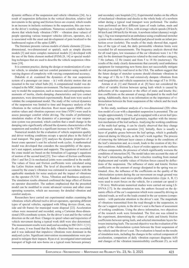
Eksploatacja i NiEzawodNosc – MaiNtENaNcE aNd REliability Vol. 23, No. 3, 2021 423
dynamic stiffness of the suspension and vehicle vibrations [24]. As a result of suspension deflection in the vertical direction, relative leaf movements in the spring and friction forces are created, which results in an increase in inelastic resistance in the suspension, this can wors-en the driver’s working conditions. Numerous scientific studies have shown that whole-body vibration (VBV – vibration dose values) of people operating various transport vehicles (drivers, operators, etc.) is associated with the onset and development of pain localized to the lumbosacral region of the spine (LBP).
The literature presents various models of elastic elements [2] (one-dimensional, two-dimensional or spatial), such as simple discrete models [3] and more complex numerical models [1] developed with the use of the finite element method (FEM) [8, 14] or special model-ling techniques that are used to describe the vehicle suspension vibra-tions [19].
It is common practice, during the design or modernization of a mo-tor vehicle, to simulate and test comfort parameters using models of varying degrees of complexity with varying computational accuracy.
Dukalski et al. examined the dynamics of the rear suspension system of a passenger car (mass ~ 1t ) with electric motors that are mounted in the rear wheel hubs [6]. A computational model was de-veloped in the MSC.Adams environment. The basic parameters neces-sary to model the suspension, such as masses and corresponding mass moments of inertia, elastic-damping characteristics and tyre contact parameters, were determined experimentally. Road tests were used to validate the computational model. The study of the vertical dynamics of the suspension was limited to time and frequency analysis of the vibrations in the vertical direction. Root mean square (RMS) accel-eration values and vibration exposure over time (VDV) were used to assess passenger comfort whilst driving. The results of preliminary simulation studies of the dynamics of a passenger car rear suspen-sion system was presented, which confirm that a small change in the damping ratio significantly affected the dynamic characteristics of the suspension and resulted in a significant increase in the VDV index.
Numerical models for the evaluation of vehicle suspension quality and driver working conditions occupy a special place in the field of road transport. The paper [23] analyses the dynamic properties of a forest crane operator’s seat for selected work cycles. A mathematical model was developed that considers the susceptibility of the opera-tor’s seat support, actuators and supports. The equations of motion of the crane model are based on the formalism of Lagrange’s equations of motion of the second kind [23]. Two values of friction coefficients (Set-1 and Set-2) in mechanical joints were considered in the model. The values of force and friction coefficients were calculated using the LuGre friction model. The level of discomfort to the operator caused by the crane’s vibration was estimated in accordance with the applicable standards for noise analysis and the impact of vibrations on the operator (N.V.H – Noise, Vibration and Harshness analyses). The simulation results obtained confirmed the large effect of friction on operator discomfort. The authors emphasized that the presented model can be modified to create advanced versions and other crane operating scenarios, which are necessary for detailed vibration and comfort analysis.
Researchers have carried out experimental studies examining the vibrations which affected twelve driver-operators, operating different types of special vehicles, equipped with lifting devices (front, rear, side and tilt frame) for municipal waste disposal [22]. Acceleration values were measured and recorded, using a Cartesian three-dimen-sional (3D) coordinate system, for the driver’s seat and for the vertical direction on the cab floor. Changes in speed values and trajectories of vehicle movement during a typical work shift were also determined. The measurement results were analysed according to ISO 2631-1 [11]. In all cases, it was found that the daily vibration limit was exceeded, and it was indicated that impulsive vibrations were dominant in the analysed cycles. Significant intervention recommendations were pro-posed to mitigate their impacts. Ryan et al. investigated interventional transport of high-risk new-borns on a typical route between primary
and secondary care hospitals [21]. Experimental studies on the effects of mechanical vibrations and shocks to the whole body of a newborn infant during a typical road transport were performed. The studies were performed on three different types of roads (urban, main and highway) on a length of 32 km, with average vehicle speeds (20 km/h; 60 km/h and 100 km/h) for 46 min. A newborn infant (dummy) weigh-ing 1.3 kg was transported in an ambulance using a traditional stretcher system with a mattress and a fluidized pad placed inside an infant pro-tection cover (isolette). The results of the study showed that, regard-less of the type of road, the daily permissible vibration limits were exceeded for all measurements. The frequency analysis showed that for all road types, low resonance of the car vibrations were 1 to 3 Hz and, for the dominant frequencies related to the road surface category, 7 Hz (urban), 12 Hz (main) and from 5 to 18 Hz (motorway). The results of the study clearly demonstrate that currently used ambulance equipment for transporting new-borns does not successfully mitigate the risk presented by road travel in the USA. The authors suggest that the future design of stretcher systems should eliminate vibrations in the range of 1 Hz to 3 Hz and extensively dampen vibrations from road irregularities and vehicle suspension in the range of 5 to 18 Hz.
Amrute et al. [1] and Hareesh et al. [8] have not considered the effect of variable friction between spring leafs which is caused by deflections of the suspension or the effect of static and kinetic fric-tion coefficients on the amount of energy dissipated in the multi-leaf spring. Additionally, there is no information on the importance of vi-broisolation between the front suspension of the vehicle and the truck driver’s seat.
In this study, nonlinear analysis of a two-dimensional (2D) vibra-tion model of a car with a dependent suspension is presented. The car weighs approximately 12 tons, and is equipped with a seven leaf (pro-totype) spring with mapped leaf geometry, together with the interac-tion mechanism of the leaf surfaces. Analysing the working conditions of the multi-leaf spring, it can be clearly observed that they change continuously during its operation [16]. Initially, there is usually a layer of graphite grease between the leaf springs, which is gradually removed during its lifecycle, as the leaf’s work together. The process of removing the lubricant layer causes a change in the conditions of the leaf’s interaction and, as a result, leads to the creation of dry fric-tion conditions. Additionally, a layer of oxides appears on the surfaces of these components, the presence of which significantly worsens the conditions of interaction [9]. The model takes into account the state of the leaf’s interacting surfaces, their velocities resulting from mutual displacement and variable values of friction forces caused by deflec-tions of the suspension. The influence of static and kinetic friction coefficients on the amount of energy dissipated in the spring was es-timated. Also, the influence of the coefficients on the quality of the vibroisolation system during the car movement on rough ground was analysed. Random road micro-profile characteristics (type A, B, C) were used to exert forces on the vehicle, for a constant car speed (v = 20 m/s). Multivariate numerical studies were carried out using LS-DYNA [17]. In the simulation tests, the authors focused on the dy-namic effects of the car’s suspension which were caused by driving on selected roads, as well as the loads created in the car systems (compo-nents) – with particular attention to the driver’s seat. The magnitude of vibrations transmitted from the road through to the suspension, to the car’s support system, to the driver’s seat is the basis of assessment of working conditions. Using the above information, two objectives of the research work were formulated. The first one was related to the experiment, determining the values of static and kinetic friction coefficients between spring leafs, and selected intermediate layers be-tween interacting leafs. The second objective was the evaluation of the quality of the vibroisolation system between the front suspension of the vehicle and the driver’s seat. The evaluation is based on the results of simulation tests, including the changes in the vertical component of acceleration, comparison of daily vibration exposure diagrams A(8) and changes of the vibration transmissibility coefficient (T), as well
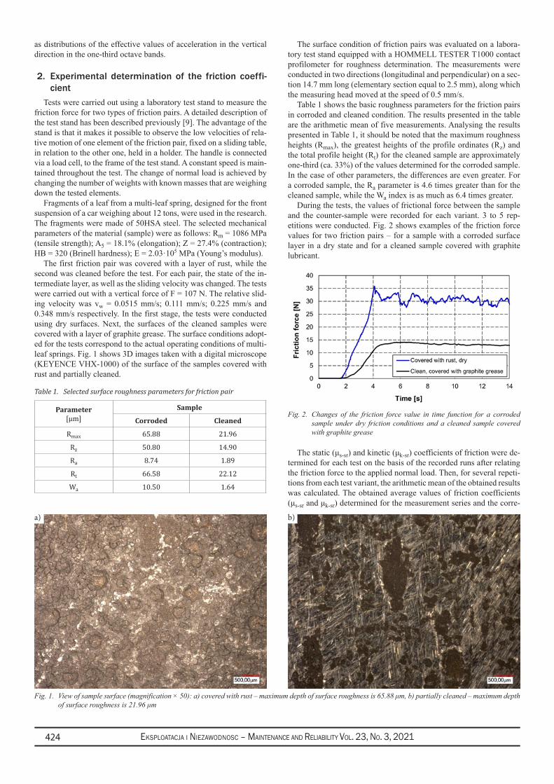
Eksploatacja i NiEzawodNosc – MaiNtENaNcE aNd REliability Vol. 23, No. 3, 2021424
as distributions of the effective values of acceleration in the vertical direction in the one-third octave bands.
2. Experimental determination of the friction coeffi-cient
Tests were carried out using a laboratory test stand to measure the friction force for two types of friction pairs. A detailed description of the test stand has been described previously [9]. The advantage of the stand is that it makes it possible to observe the low velocities of rela-tive motion of one element of the friction pair, fixed on a sliding table, in relation to the other one, held in a holder. The handle is connected via a load cell, to the frame of the test stand. A constant speed is main-tained throughout the test. The change of normal load is achieved by changing the number of weights with known masses that are weighing down the tested elements.
Fragments of a leaf from a multi-leaf spring, designed for the front suspension of a car weighing about 12 tons, were used in the research. The fragments were made of 50HSA steel. The selected mechanical parameters of the material (sample) were as follows: Rm = 1086 MPa (tensile strength); A5 = 18.1% (elongation); Z = 27.4% (contraction); HB = 320 (Brinell hardness); E = 2.03·105 MPa (Young’s modulus).
The first friction pair was covered with a layer of rust, while the second was cleaned before the test. For each pair, the state of the in-termediate layer, as well as the sliding velocity was changed. The tests were carried out with a vertical force of F = 107 N. The relative slid-ing velocity was vw = 0.0515 mm/s; 0.111 mm/s; 0.225 mm/s and 0.348 mm/s respectively. In the first stage, the tests were conducted using dry surfaces. Next, the surfaces of the cleaned samples were covered with a layer of graphite grease. The surface conditions adopt-ed for the tests correspond to the actual operating conditions of multi-leaf springs. Fig. 1 shows 3D images taken with a digital microscope (KEYENCE VHX-1000) of the surface of the samples covered with rust and partially cleaned.
The surface condition of friction pairs was evaluated on a labora-tory test stand equipped with a HOMMELL TESTER T1000 contact profilometer for roughness determination. The measurements were conducted in two directions (longitudinal and perpendicular) on a sec-tion 14.7 mm long (elementary section equal to 2.5 mm), along which the measuring head moved at the speed of 0.5 mm/s.
Table 1 shows the basic roughness parameters for the friction pairs in corroded and cleaned condition. The results presented in the table are the arithmetic mean of five measurements. Analysing the results presented in Table 1, it should be noted that the maximum roughness heights (Rmax), the greatest heights of the profile ordinates (Rz) and the total profile height (Rt) for the cleaned sample are approximately one-third (ca. 33%) of the values determined for the corroded sample. In the case of other parameters, the differences are even greater. For a corroded sample, the Ra parameter is 4.6 times greater than for the cleaned sample, while the Wa index is as much as 6.4 times greater.
During the tests, the values of frictional force between the sample and the counter-sample were recorded for each variant. 3 to 5 rep-etitions were conducted. Fig. 2 shows examples of the friction force values for two friction pairs – for a sample with a corroded surface layer in a dry state and for a cleaned sample covered with graphite lubricant.
Fig. 2. Changes of the friction force value in time function for a corroded sample under dry friction conditions and a cleaned sample covered with graphite grease
The static (μs-sr) and kinetic (μk-sr) coefficients of friction were de-termined for each test on the basis of the recorded runs after relating the friction force to the applied normal load. Then, for several repeti-tions from each test variant, the arithmetic mean of the obtained results was calculated. The obtained average values of friction coefficients (μs-sr and μk-sr) determined for the measurement series and the corre-
Table 1. Selected surface roughness parameters for friction pair
Parameter[μm]
Sample
Corroded Cleaned
Rmax 65.88 21.96
Rz 50.80 14.90
Ra 8.74 1.89
Rt 66.58 22.12
Wa 10.50 1.64
Fig. 1. View of sample surface (magnification × 50): a) covered with rust – maximum depth of surface roughness is 65.88 μm, b) partially cleaned – maximum depth of surface roughness is 21.96 μm
b)a)
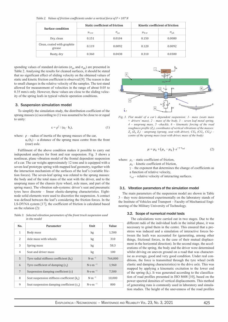
Eksploatacja i NiEzawodNosc – MaiNtENaNcE aNd REliability Vol. 23, No. 3, 2021 425
sponding values of standard deviations (σμs and σμk) are presented in Table 2. Analysing the results for cleaned surfaces, it should be stated that no significant effect of sliding velocity on the obtained values of static and kinetic friction coefficient is observed [9]. The reason is due to small changes in the relative velocity of the samples. The test stand allowed for measurement of velocities in the range of about 0.05 to 0.35 mm/s only. However, these values are close to the sliding veloc-ity of the spring leafs in typical vehicle operation conditions.
3. Suspension simulation model To simplify the simulation study, the distribution coefficient of the
sprung masses (ε) according to (1) was assumed to be close to or equal to unity:
ε = ρ2 / (af · br), (1)
where: ρ – radius of inertia of the sprung masses of the car, af (br) – a distance of the sprung mass centre from the front (rear) axle.
Fulfilment of the above condition makes it possible to carry out independent analyses for front and rear suspension. Fig. 3 shows a nonlinear, plane vibration model of the frontal dependent suspension of a car. The car weighs approximately 12 tons and is equipped with a seven-leaf prototype spring with mapped leaf geometry, together with the interaction mechanism of the surfaces of the leaf’s (variable fric-tion forces). The seven-leaf spring was related to the sprung masses: the body and of the total mass of the seat with the driver, and to the unsprung mass of the chassis (tyre wheel, axle mass, and part of the spring mass). The vibration sub-systems: driver’s seat and pneumatic tyres have discrete – linear elastic-damping characteristics. Eight-node solid elements were used to discretize the suspension. A contact was defined between the leaf’s considering the friction forces. In the LS-DYNA system [17], the coefficient of friction is calculated based on the relation (2):
µ µ µ µ γ= + −( ) ⋅ − ⋅k s k
ve rel (2)
where: µs – static coefficient of friction,µk – kinetic coefficient of friction,γ – the exponent that determines the change of coefficients as a function of relative velocity,vrel – relative velocity of interacting surfaces.
3.1. Vibration parameters of the simulation modelThe main parameters of the suspension model are shown in Table
3 – they were determined experimentally on the laboratory stands of the Institute of Vehicles and Transport – Faculty of Mechanical Engi-neering of the Military University of Technology.
3.2. Scope of numerical model tests The calculations were carried out in two stages. Due to the
different radii of the individual leafs in the initial phase, it was necessary to grind them in the centre. This ensured that a pre-stress was induced and a simulation of interactive forces be-tween the leafs was accounted for (generating, among other things, frictional forces, in the case of their mutual displace-ment in the horizontal direction). In the second stage, the accel-erations of the spring, the body and the driver were determined whilst driving on uneven ground on a road that was character-ise as average, good and very good condition. Under real con-ditions, the force is transmitted through the tyre wheel (with elastic and damping characteristics) to the drive axle. This was mapped by applying a kinematic excitation to the lower end of the spring (kt). It was generated according to the classifica-tion of road profiles presented in ISO 8608 [10], based on the power spectral densities of vertical displacements. This method of generating runs is commonly used in laboratory and simula-tion studies. The height of the unevenness of the road profiles
Table 2. Values of friction coefficients under a vertical force of F = 107 N
Surface conditionStatic coefficient of friction Kinetic coefficient of friction
µs-sr σµs µk-sr σµk
Dry, clean 0.151 0.0104 0.150 0.0080
Clean, coated with graphite grease 0.119 0.0092 0.120 0.0092
Rusty, dry 0.360 0.0438 0.310 0.0300
Table 3. Selected vibration parameters of the front truck suspension used in the model
No. Parameter Unit Value
1 Body mass kg 1,500
2 Axle mass with wheels kg 310
3 Spring mass kg 58.3
4 Seat and driver mass kg 100
5 Tyre radial stiffness coefficient (kt) N·m −1 764,000
6 Tyre coefficient of damping (ct) N·s·m −1 1,960
7 Suspension damping coefficient (c) N·s·m −1 7,500
8 Seat suspension stiffness coefficient (ks) N·m −1 10,000
9 Seat suspension damping coefficient (cs) N·s·m −1 800
Fig. 3. Flat model of a car’s dependent suspension: 1– mass (seats mass + drivers’ mass), 2 – mass of the body, 3 – seven leaf metal spring, 4 – unsprung mass, 5 –shackle, 6 – kinematic forcing of the road roughness profile (Zr), coordinates of vertical vibrations of the masses: Za (Zb, Zs) – unsprung (sprung, seat with driver), CGb (CGs, CGa) – centre of the sprung mass (seat with driver, mass of the body)
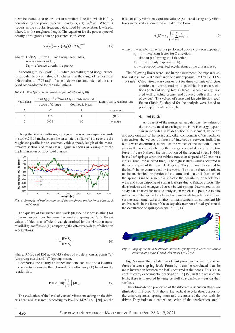
Eksploatacja i NiEzawodNosc – MaiNtENaNcE aNd REliability Vol. 23, No. 3, 2021426
h can be treated as a realization of a random function, which is fully described by the power spectral density Gd (Ω) [m3/rad]. Where Ω [rad/m] is the circular frequency described by the relation Ω = 2π/L, where L is the roughness length. The equation for the power spectral density of roughness can be presented as follows:
( ) ( )( )0 0/ wd dG G −Ω = Ω Ω Ω (3)
where: Gd (Ω0) [m3/rad] – road roughness index,w – waviness index, Ω0 – reference circular frequency.
According to ISO 8608 [10], when generating road irregularities, the circular frequency should be changed in the range of values from 0.069 rad/m to 17.77 rad/m. Table 4 shows the parameters of the ana-lysed roads adopted for the calculations.
Using the Matlab software, a programme was developed (accord-ing to ISO [10] and based on the parameters in Table 4) to generate the roughness profile for an assumed vehicle speed, length of the meas-urement section and road class. Figure 4 shows an example of the implementation of three road classes.
Fig. 4. Example of implementation of the roughness profile for a class A, B and C road
The quality of the suspension work (degree of vibroisolation) for different associations between the working spring leaf’s (different values of friction coefficient) was determined by the vibration trans-missibility coefficient (T) comparing the effective values of vibration accelerations:
b
a
RMSTRMS
= (4)
where: RMSa and RMSb – RMS values of accelerations at points “a” (unsprung mass) and “b” (sprung mass).
Comparing the quality of suspension, one can also use a logarith-mic scale to determine the vibroisolation efficiency (E) based on the relationship:
1E 20 logT
= ⋅
[dB] (5)
The evaluation of the level of vertical vibrations acting on the driv-er’s seat was assessed, according to PN-EN 14253+A1 [20], on the
basis of daily vibration exposure value A(8). Considering only vibra-tions in the vertical direction – it takes the form:
( )n
2z ws i
0 i 1
1A 8 k a tT =
= ⋅∑ (6)
where: n – number of activities performed under vibration exposure,kz = 1 – weighting factor for Z direction,ti – time of performing the i-th action,T0 – time of daily exposure (8 h),aws – frequency weighted acceleration of the driver’s seat.
The following limits were used in the assessment: the exposure ac-tion value (EAV) – 0.5 m/s2 and the daily exposure limit value (ELV) – 0.8 m/s2. Calculations were carried out for three variants of friction
coefficients, corresponding to possible friction associa-tions (states of spring leaf surfaces – clean and dry, cov-ered with graphite grease, and covered with a thin layer of oxides). The values of static and kinetic friction coef-ficient (Table 2) adopted for the analysis were based on prior experimental research.
4. ResultsAs a result of the numerical calculations, the values of
the stress reduced according to the H-M-H energy hypoth-esis in individual leaf, deflection/displacement, velocities
and accelerations of the spring and other components of the modelled suspension, the values of forces of interaction between individual leaf’s were determined, as well as the values of the individual ener-gies in the system (including the energy associated with the friction force). Figure 5 shows the distribution of the reduced stress H-M-H in the leaf springs when the vehicle moves at a speed of 20 m/s on a class C road (for selected time). The highest stress values occurred in the central part of the lower leaf spring. They are mainly caused by the leaf’s being compressed by the yoke. The stress values are related to the mechanical properties of the structural material from which the spring is made, which can indicate the possibility of accelerated wear and even chipping of spring leaf tips due to fatigue effects. The distributions and changes of stress in leaf springs determined in this study can be used for fatigue analysis, in which it is possible to take into account the applied load spectrum, material characteristics of leaf springs and numerical estimation of main suspension component life on this basis, in the form of the acceptable number of load cycles until the occurrence of spring damage [3, 17, 18].
Fig. 5. Map of the H-M-H reduced stress in spring leaf’s when the vehicle passes over a class C road with speed v = 20 m/s
Fig. 6 shows the distribution of unit pressures caused by contact forces between spring leafs. From it, it can be concluded that the main interaction between the leaf’s occurred at their ends. This is also confirmed by experimental observations in [15]. In these areas of the leafs, there is increased heating, as well as significant wear on their surfaces.
The vibroisolation properties of the different suspension stages are illustrated in Figure 7. It shows the vertical acceleration curves for the unsprung mass, sprung mass and the mass of the seat with the driver. They indicate a radical reduction of the acceleration ampli-
Table 4. Road parameters assumed for calculations [10]
Road classGd(Ω0) (10-6 m3/rad), Ω0 = 1 rad/m, w = 2
Road Quality Assessment Scope of Change Geometric Mean
A <2 1 very good
B 2–8 4 good
C 8–32 16 average
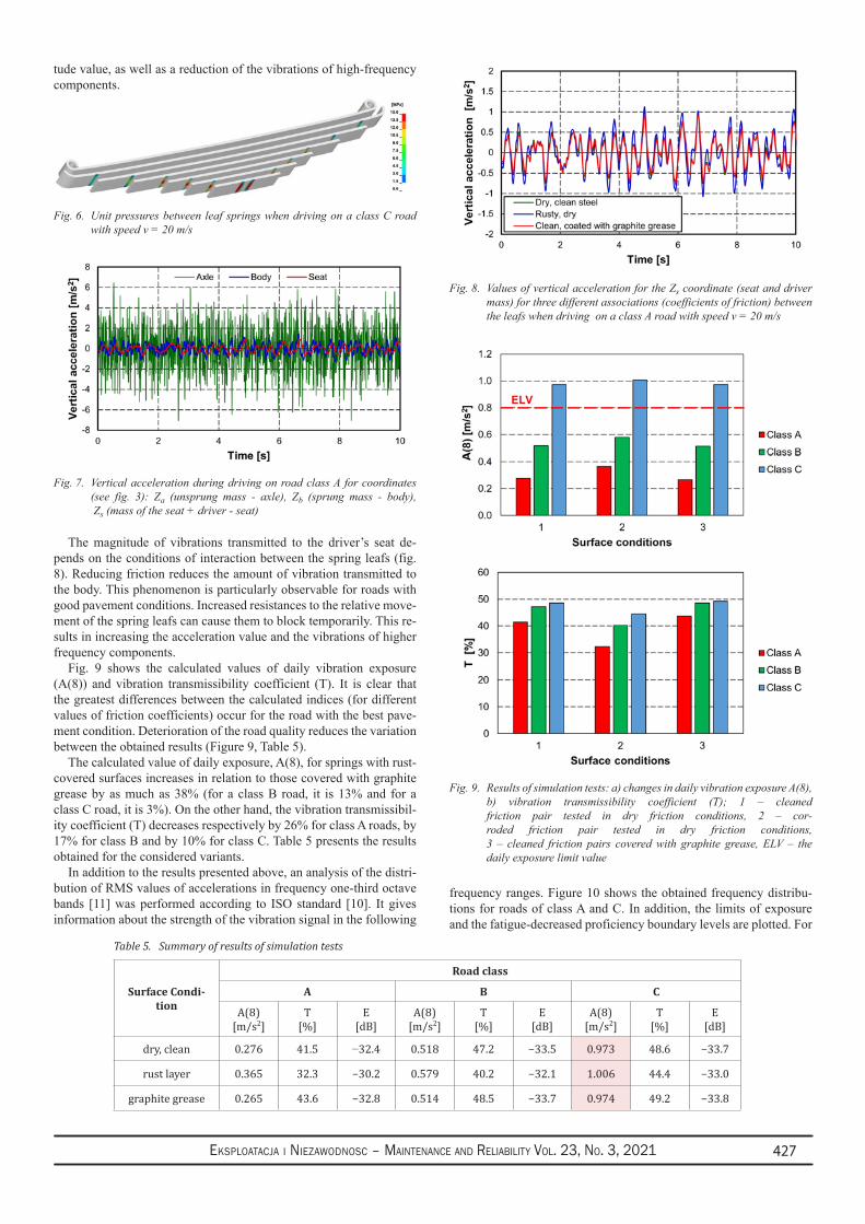
Eksploatacja i NiEzawodNosc – MaiNtENaNcE aNd REliability Vol. 23, No. 3, 2021 427
tude value, as well as a reduction of the vibrations of high-frequency components.
Fig. 6. Unit pressures between leaf springs when driving on a class C road with speed v = 20 m/s
Fig. 7. Vertical acceleration during driving on road class A for coordinates (see fig. 3): Za (unsprung mass - axle), Zb (sprung mass - body), Zs (mass of the seat + driver - seat)
The magnitude of vibrations transmitted to the driver’s seat de-pends on the conditions of interaction between the spring leafs (fig. 8). Reducing friction reduces the amount of vibration transmitted to the body. This phenomenon is particularly observable for roads with good pavement conditions. Increased resistances to the relative move-ment of the spring leafs can cause them to block temporarily. This re-sults in increasing the acceleration value and the vibrations of higher frequency components.
Fig. 9 shows the calculated values of daily vibration exposure (A(8)) and vibration transmissibility coefficient (T). It is clear that the greatest differences between the calculated indices (for different values of friction coefficients) occur for the road with the best pave-ment condition. Deterioration of the road quality reduces the variation between the obtained results (Figure 9, Table 5).
The calculated value of daily exposure, A(8), for springs with rust-covered surfaces increases in relation to those covered with graphite grease by as much as 38% (for a class B road, it is 13% and for a class C road, it is 3%). On the other hand, the vibration transmissibil-ity coefficient (T) decreases respectively by 26% for class A roads, by 17% for class B and by 10% for class C. Table 5 presents the results obtained for the considered variants.
In addition to the results presented above, an analysis of the distri-bution of RMS values of accelerations in frequency one-third octave bands [11] was performed according to ISO standard [10]. It gives information about the strength of the vibration signal in the following
frequency ranges. Figure 10 shows the obtained frequency distribu-tions for roads of class A and C. In addition, the limits of exposure and the fatigue-decreased proficiency boundary levels are plotted. For
Table 5. Summary of results of simulation tests
Surface Condi-tion
Road class
A B C
A(8)[m/s2]
T[%]
E[dB]
A(8)[m/s2]
T[%]
E[dB]
A(8)[m/s2]
T[%]
E[dB]
dry, clean 0.276 41.5 −32.4 0.518 47.2 −33.5 0.973 48.6 −33.7
rust layer 0.365 32.3 −30.2 0.579 40.2 −32.1 1.006 44.4 −33.0
graphite grease 0.265 43.6 −32.8 0.514 48.5 −33.7 0.974 49.2 −33.8
Fig. 8. Values of vertical acceleration for the Zs coordinate (seat and driver mass) for three different associations (coefficients of friction) between the leafs when driving on a class A road with speed v = 20 m/s
Fig. 9. Results of simulation tests: a) changes in daily vibration exposure A(8), b) vibration transmissibility coefficient (T); 1 – cleaned friction pair tested in dry friction conditions, 2 – cor-roded friction pair tested in dry friction conditions, 3 – cleaned friction pairs covered with graphite grease, ELV – the daily exposure limit value
b)
a)
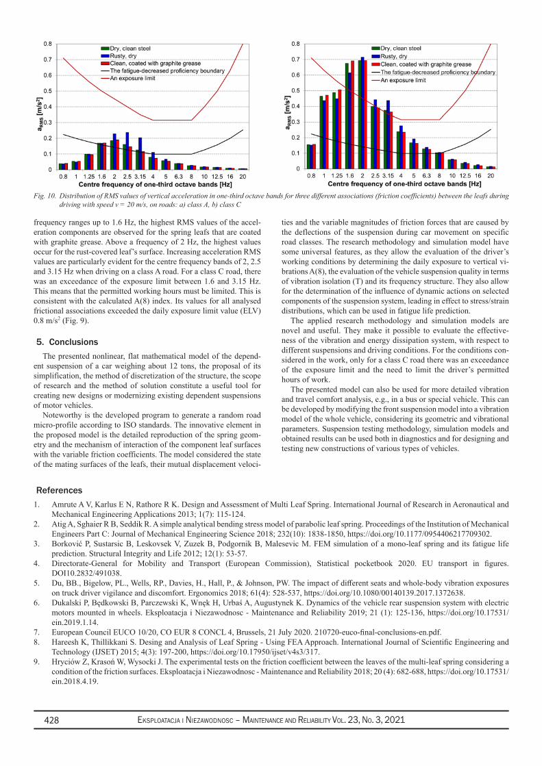
Eksploatacja i NiEzawodNosc – MaiNtENaNcE aNd REliability Vol. 23, No. 3, 2021428
frequency ranges up to 1.6 Hz, the highest RMS values of the accel-eration components are observed for the spring leafs that are coated with graphite grease. Above a frequency of 2 Hz, the highest values occur for the rust-covered leaf’s surface. Increasing acceleration RMS values are particularly evident for the centre frequency bands of 2, 2.5 and 3.15 Hz when driving on a class A road. For a class C road, there was an exceedance of the exposure limit between 1.6 and 3.15 Hz. This means that the permitted working hours must be limited. This is consistent with the calculated A(8) index. Its values for all analysed frictional associations exceeded the daily exposure limit value (ELV) 0.8 m/s2 (Fig. 9).
5. ConclusionsThe presented nonlinear, flat mathematical model of the depend-
ent suspension of a car weighing about 12 tons, the proposal of its simplification, the method of discretization of the structure, the scope of research and the method of solution constitute a useful tool for creating new designs or modernizing existing dependent suspensions of motor vehicles.
Noteworthy is the developed program to generate a random road micro-profile according to ISO standards. The innovative element in the proposed model is the detailed reproduction of the spring geom-etry and the mechanism of interaction of the component leaf surfaces with the variable friction coefficients. The model considered the state of the mating surfaces of the leafs, their mutual displacement veloci-
ties and the variable magnitudes of friction forces that are caused by the deflections of the suspension during car movement on specific road classes. The research methodology and simulation model have some universal features, as they allow the evaluation of the driver’s working conditions by determining the daily exposure to vertical vi-brations A(8), the evaluation of the vehicle suspension quality in terms of vibration isolation (T) and its frequency structure. They also allow for the determination of the influence of dynamic actions on selected components of the suspension system, leading in effect to stress/strain distributions, which can be used in fatigue life prediction.
The applied research methodology and simulation models are novel and useful. They make it possible to evaluate the effective-ness of the vibration and energy dissipation system, with respect to different suspensions and driving conditions. For the conditions con-sidered in the work, only for a class C road there was an exceedance of the exposure limit and the need to limit the driver’s permitted hours of work.
The presented model can also be used for more detailed vibration and travel comfort analysis, e.g., in a bus or special vehicle. This can be developed by modifying the front suspension model into a vibration model of the whole vehicle, considering its geometric and vibrational parameters. Suspension testing methodology, simulation models and obtained results can be used both in diagnostics and for designing and testing new constructions of various types of vehicles.
Fig. 10. Distribution of RMS values of vertical acceleration in one-third octave bands for three different associations (friction coefficients) between the leafs during driving with speed v = 20 m/s, on roads: a) class A, b) class C
References1. Amrute A V, Karlus E N, Rathore R K. Design and Assessment of Multi Leaf Spring. International Journal of Research in Aeronautical and
Mechanical Engineering Applications 2013; 1(7): 115-124.2. Atig A, Sghaier R B, Seddik R. A simple analytical bending stress model of parabolic leaf spring. Proceedings of the Institution of Mechanical
Engineers Part C: Journal of Mechanical Engineering Science 2018; 232(10): 1838-1850, https://doi.org/10.1177/0954406217709302.3. Borković P, Sustarsic B, Leskovsek V, Zuzek B, Podgornik B, Malesevic M. FEM simulation of a mono-leaf spring and its fatigue life
prediction. Structural Integrity and Life 2012; 12(1): 53-57.4. Directorate-General for Mobility and Transport (European Commission), Statistical pocketbook 2020. EU transport in figures.
DOI10.2832/491038.5. Du, BB., Bigelow, PL., Wells, RP., Davies, H., Hall, P., & Johnson, PW. The impact of different seats and whole-body vibration exposures
on truck driver vigilance and discomfort. Ergonomics 2018; 61(4): 528-537, https://doi.org/10.1080/00140139.2017.1372638.6. Dukalski P, Będkowski B, Parczewski K, Wnęk H, Urbaś A, Augustynek K. Dynamics of the vehicle rear suspension system with electric
motors mounted in wheels. Eksploatacja i Niezawodnosc - Maintenance and Reliability 2019; 21 (1): 125-136, https://doi.org/10.17531/ein.2019.1.14.
7. European Council EUCO 10/20, CO EUR 8 CONCL 4, Brussels, 21 July 2020. 210720-euco-final-conclusions-en.pdf.8. Hareesh K, Thillikkani S. Desing and Analysis of Leaf Spring - Using FEA Approach. International Journal of Scientific Engineering and
Technology (IJSET) 2015; 4(3): 197-200, https://doi.org/10.17950/ijset/v4s3/317.9. Hryciów Z, Krasoń W, Wysocki J. The experimental tests on the friction coefficient between the leaves of the multi-leaf spring considering a
condition of the friction surfaces. Eksploatacja i Niezawodnosc - Maintenance and Reliability 2018; 20 (4): 682-688, https://doi.org/10.17531/ein.2018.4.19.

Eksploatacja i NiEzawodNosc – MaiNtENaNcE aNd REliability Vol. 23, No. 3, 2021 429
10. ISO 8608: 2016. Mechanical vibration - Road surface profiles - Reporting of measured data, https://www.iso.org/standard/71202.html.11. ISO 2631-1: Mechanical vibration and shock - Evaluation of human exposure to whole-body vibration - Part 1: General requirements.
International Organization for Standarization, 2018.12. Jamroziak K, Kosobudzki M, Ptak J. Assessment of the comfort of passenger transport in special purpose vehicles. Eksploatacja i
Niezawodnosc - Maintenance and Reliability 2013; 15 (1): 25-30.13. Kim J H, Aulck L, Hughes M, Zigman M, Cavallari J, Dennerlein J T, Johnson P W. Whole Body Vibration Exposures in Long-
haul Truck Drivers. Proceedings of the Human Factors and Ergonomics Society Annual Meeting 2016; 59: 1274-1278, http://doi.org/10.1177/1541931215591205.
14. Kong Y S, Omar M Z, Chua L B, Abdullah S. Explicit Nonlinear Finite Element Geometric Analysis of Parabolic Leaf Springs under Various Loads. Hindawi Publishing Corporation The Scientific World Journal 2013; 2013(261926), 1-11, https://doi.org/10.1155/2013/261926.
15. Krason W, Wysocki J. Investigation of friction in dual leaf spring. Journal of Friction and Wear 2017; 38(3): 214-220, https://doi.org/10.3103/S1068366617030096.
16. Krason W, Wysocki J, Hryciow Z. Dynamics stand tests and numerical research of multi-leaf springs with regard to clearances and friction. Advances in Mechanical Engineering 2019; 11(5): 1-13, https://doi.org/10.1177/1687814019853353.
17. LS-DYNA, Keyword user's manual, Volume I, LS-DYNA R12, Livermore Software Technology (LST), AN Ansys Company, 07/17/20.18. MSC.Software, What is Fatigue Analysis? MSC Nastran, https://simulatemore.mscsoftware.com/what-is-fatigue-analysis-msc-nastran/
25.03.2021.19. Padmakar S, Seyd A H. Desing and Analysis of Leaf Spring for Tanker trailer suspension System. Global Journal of Advanced Engineering
Technologies 2015; 4(3): 240-250.20. PN-EN 14253+A1:2011, Mechanical vibrations - Measurement and calculation of occupational exposure to vibrations with a general effect
on the human body for the purposes of health protection, Practical guidelines, 2011. (in Polish)21. Ryan D M, Lokeh A, Hirschman D, Spector J, Parker R, Johnson P W. The effect of road type on neonate whole body vibration exposures
during ambulance transport. 7th American Conference on Human Vibration 2018; 76-77.22. Ryou H, Johnson P W. Whole-Body Vibration Exposures Among Solid Waste Collecting Truck Operators. Proceedings of the Human Factors
and Ergonomics Society Annual Meeting 2018; 62(1): 860-864, https://doi.org/10.1177/1541931218621196.23. Urbaś A, Szczotka M. The influence of the friction phenomenon on a forest crane operator's level of discomfort. Eksploatacja i Niezawodnosc
- Maintenance and Reliability 2019; 21 (2): 197-210, https://doi.org/10.17531/ein.2019.2.3.24. Zhou Z, Guo W, Shen T, Wang F, Ju J, Wang H, Song E. Research and Application on Dynamic Stiffness of Leaf Spring. SAE - China,
FISITA Proceedings of the FISITA 2012 World Automotive Congress. Lecture Notes in Electrical Engineering 2012; 198: 105-119, https://doi.org/10.1007/978-3-642-33795-6_10.
Eksploatacja i NiEzawodNosc – MaiNtENaNcE aNd REliability Vol. 23, No. 3, 2021430
(*) Corresponding author.E-mail addresses:
Eksploatacja i Niezawodnosc – Maintenance and ReliabilityVolume 23 (2021), Issue 3
journal homepage: http://www.ein.org.pl
Indexed by:
The paper focuses on issues related to selected automotive brakes with the aim of apply-ing the proposed methodology to other structural systems of this type. The main aim of the paper is to identify the factors that differentiate the course of wear and occurrence of a fault in brake system components of passenger cars and light commercial vehicles during the warranty service period. The following methods were used in this study: systematic litera-ture review, process analysis, and descriptive and inferential statistics, including analysis of variance and multiple classification analysis. As a result of an analysis of 295 brake system repairs, six differentiating factors that allowed for ex post analysis of the repairs were iden-tified. An analysis of the interaction of these factors made it possible to distinguish three groups of motor vehicles depending on the cause of failure of the braking system. Based on the data generated in the warranty process, it is possible to determine the factors that differ-entiate the occurrence of a fault and the course of brake disc and pad wear.
Highlights Abstract
The study was carried out on a complete sample of • 295 warranty repairs of X and Y brand vehicles
The study reproduced the actual process of diag-• nosis and repair of the brake system
An analysis of the operation process was carried • out using the process mining method
The identified factors that differentiate the course • of brake disc wear and failure were vehicle type, body type, vehicle make, and vehicle model.
Groups of factors that differentiate the vehicles • reported for brake system failure and wear were identified.
Identification of factors that differentiate motor vehicles that have experienced wear or failure of brake system components during the warranty service periodPiotr Sliż a,*, Ewa Wycinka b
a Katedra Organizacji i Zarządzania, Wydział Zarządzania, Uniwersytet Gdański, ul. Armii Krajowej 101, 81-824 Sopot b Department of Statistics, Faculty of Management, University of Gdansk, Armii Krajowej 101, 81-824 Sopot
Sliż P, Wycinka E. Identification of factors that differentiate motor vehicles that have experienced wear or failure of brake system compo-nents during the warranty service period. Eksploatacja i Niezawodnosc – Maintenance and Reliability 2021; 23 (3): 430–442, http://doi.org/10.17531/ein.2021.3.4.
Article citation info:
failure, warranty service, passenger vehicles, commercial vehicles, brake system, brake disc, wear, brake mechanism, wear factors, wear analysis.
Keywords
This is an open access article under the CC BY license (https://creativecommons.org/licenses/by/4.0/)
P. Śliż - [email protected], E. Wycinka - [email protected]
1. IntroductionAs a result of dynamic technological and technical development,
attempts are made to find material and construction solutions that have a positive and direct influence on the economic, environmental [5], design, and production aspects related to motor vehicles. They are aimed at developing solutions that reduce CO2 emissions [12] and fuel consumption [18], and replace internal combustion engines with electric units [11, 15]. There is a noticeable trend of improving such performance parameters in motor vehicles as acceleration and maxi-mum speed. As a result, this requires modification of current solutions and the design of new active and passive safety systems, with a clear emphasis on the design of the brake system. Assuming that the effec-tiveness of the brake system in motor vehicles has a significant effect on the speed of vehicles at the time of a collision and, as a result, on the consequences of the accident, this system should be indicated as one of the most important structural assemblies of vehicles [19]. Ac-cording to a report on the statistics of road accidents caused by vehicle defect factors in the UK in 2018 (1,443 accidents), as many as 36.10% of the defects were related to the brake system [8]. The statistics pre-sented provide the basis for discussions between representatives of
the research community and the business community concerning the design of structural solutions for the brake system based on the ac-quisition and analysis of data generated in the process of the use of vehicles [19].
A systematic literature review identified a research gap related the small number of publications that identify factors differentiating vehi-cles with wear or failure of brake system components. Efforts to find the factors that differentiate vehicles in which brake discs and pads have become worn out or faulty are particularly important during the first few years of vehicle use. This concerns anticipation of the costs related to safety, selection of subcontractors, indication of warranty costs, and determination of the extent and frequency of brake system checks and inspections. Attempts to analyze the wear of brake system components are found in the literature. In publication [19], the results of studies presented thus far were extended to include an assessment of the impact of vehicle operating conditions on the brake system wear. The present paper adopts a similar approach, which consists in measuring the thickness of the brake system mechanism compo-nents (brake discs and brake pads) at Authorized Service Stations (in Polish, ASO). The measurements were made in real operating con-ditions when symptoms of malfunction were indicated by the user,
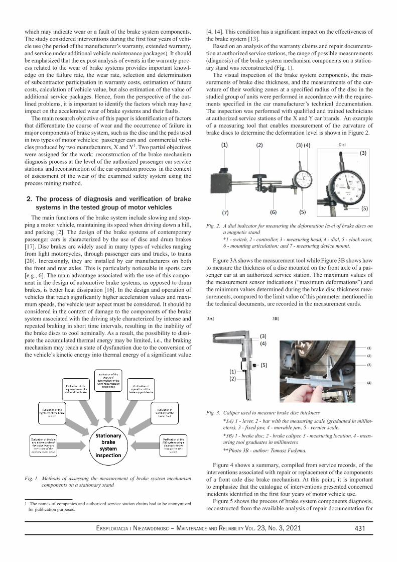
Eksploatacja i NiEzawodNosc – MaiNtENaNcE aNd REliability Vol. 23, No. 3, 2021 431
which may indicate wear or a fault of the brake system components. The study considered interventions during the first four years of vehi-cle use (the period of the manufacturer’s warranty, extended warranty, and service under additional vehicle maintenance packages). It should be emphasized that the ex post analysis of events in the warranty proc-ess related to the wear of brake systems provides important knowl-edge on the failure rate, the wear rate, selection and determination of subcontractor participation in warranty costs, estimation of future costs, calculation of vehicle value, but also estimation of the value of additional service packages. Hence, from the perspective of the out-lined problems, it is important to identify the factors which may have impact on the accelerated wear of brake systems and their faults.
The main research objective of this paper is identification of factors that differentiate the course of wear and the occurrence of failure in major components of brake system, such as the disc and the pads used in two types of motor vehicles: passenger cars and commercial vehi-cles produced by two manufacturers, X and Y1. Two partial objectives were assigned for the work: reconstruction of the brake mechanism diagnosis process at the level of the authorized passenger car service stations and reconstruction of the car operation process in the context of assessment of the wear of the examined safety system using the process mining method.
2. The process of diagnosis and verification of brake systems in the tested group of motor vehicles
The main functions of the brake system include slowing and stop-ping a motor vehicle, maintaining its speed when driving down a hill, and parking [2]. The design of the brake systems of contemporary passenger cars is characterized by the use of disc and drum brakes [17]. Disc brakes are widely used in many types of vehicles ranging from light motorcycles, through passenger cars and trucks, to trains [20]. Increasingly, they are installed by car manufacturers on both the front and rear axles. This is particularly noticeable in sports cars [e.g., 6]. The main advantage associated with the use of this compo-nent in the design of automotive brake systems, as opposed to drum brakes, is better heat dissipation [16]. In the design and operation of vehicles that reach significantly higher acceleration values and maxi-mum speeds, the vehicle user aspect must be considered. It should be considered in the context of damage to the components of the brake system associated with the driving style characterized by intense and repeated braking in short time intervals, resulting in the inability of the brake discs to cool nominally. As a result, the possibility to dissi-pate the accumulated thermal energy may be limited, i.e., the braking mechanism may reach a state of dysfunction due to the conversion of the vehicle’s kinetic energy into thermal energy of a significant value
1 The names of companies and authorized service station chains had to be anonymized for publication purposes.
[4, 14]. This condition has a significant impact on the effectiveness of the brake system [13].
Based on an analysis of the warranty claims and repair documenta-tion at authorized service stations, the range of possible measurements (diagnosis) of the brake system mechanism components on a station-ary stand was reconstructed (Fig. 1).
The visual inspection of the brake system components, the mea-surements of brake disc thickness, and the measurements of the cur-vature of their working zones at a specified radius of the disc in the studied group of units were performed in accordance with the require-ments specified in the car manufacturer’s technical documentation. The inspection was performed with qualified and trained technicians at authorized service stations of the X and Y car brands. An example of a measuring tool that enables measurement of the curvature of brake discs to determine the deformation level is shown in Figure 2.
Fig. 2. A dial indicator for measuring the deformation level of brake discs on a magnetic stand
*1 - switch, 2 - controller, 3 - measuring head, 4 - dial, 5 - clock reset, 6 - mounting articulation; and 7 - measuring device mount.
Figure 3A shows the measurement tool while Figure 3B shows how to measure the thickness of a disc mounted on the front axle of a pas-senger car at an authorized service station. The maximum values of the measurement sensor indications (“maximum deformations”) and the minimum values determined during the brake disc thickness mea-surements, compared to the limit value of this parameter mentioned in the technical documents, are recorded in the measurement cards.
Fig. 3. Caliper used to measure brake disc thickness *3A) 1 - lever, 2 - bar with the measuring scale (graduated in millim-
eters), 3 - fixed jaw, 4 - movable jaw, 5 - vernier scale. *3B) 1 - brake disc, 2 - brake caliper, 3 - measuring location, 4 - meas-
uring tool graduates in millimeters **Photo 3B - author: Tomasz Fudyma.
Figure 4 shows a summary, compiled from service records, of the interventions associated with repair or replacement of the components of a front axle disc brake mechanism. At this point, it is important to emphasize that the catalogue of interventions presented concerned incidents identified in the first four years of motor vehicle use.
Figure 5 shows the process of brake system components diagnosis, reconstructed from the available analysis of repair documentation for
Fig. 1. Methods of assessing the measurement of brake system mechanism components on a stationary stand
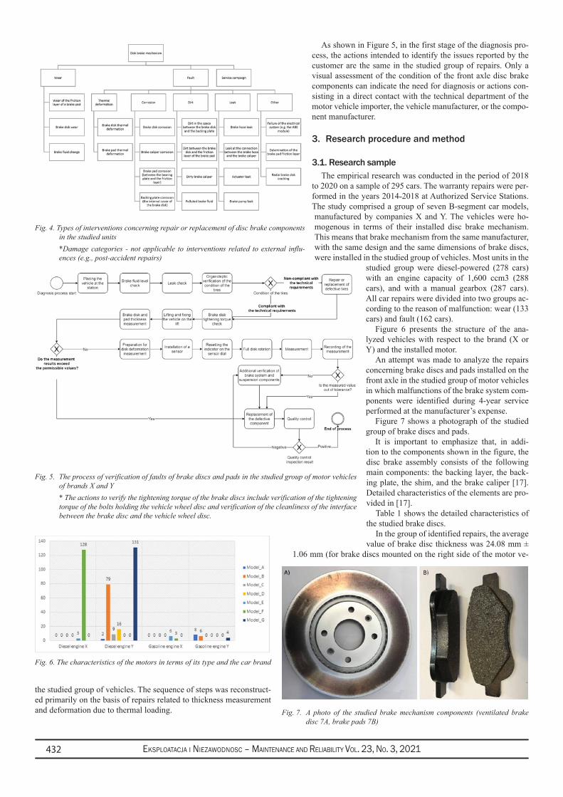
Eksploatacja i NiEzawodNosc – MaiNtENaNcE aNd REliability Vol. 23, No. 3, 2021432
the studied group of vehicles. The sequence of steps was reconstruct-ed primarily on the basis of repairs related to thickness measurement and deformation due to thermal loading.
As shown in Figure 5, in the first stage of the diagnosis pro-cess, the actions intended to identify the issues reported by the customer are the same in the studied group of repairs. Only a visual assessment of the condition of the front axle disc brake components can indicate the need for diagnosis or actions con-sisting in a direct contact with the technical department of the motor vehicle importer, the vehicle manufacturer, or the compo-nent manufacturer.
3. Research procedure and method
3.1. Research sampleThe empirical research was conducted in the period of 2018
to 2020 on a sample of 295 cars. The warranty repairs were per-formed in the years 2014˗2018 at Authorized Service Stations. The study comprised a group of seven B-segment car models, manufactured by companies X and Y. The vehicles were ho-mogenous in terms of their installed disc brake mechanism. This means that brake mechanism from the same manufacturer, with the same design and the same dimensions of brake discs, were installed in the studied group of vehicles. Most units in the
studied group were diesel-powered (278 cars) with an engine capacity of 1,600 ccm3 (288 cars), and with a manual gearbox (287 cars). All car repairs were divided into two groups ac-cording to the reason of malfunction: wear (133 cars) and fault (162 cars).
Figure 6 presents the structure of the ana-lyzed vehicles with respect to the brand (X or Y) and the installed motor.
An attempt was made to analyze the repairs concerning brake discs and pads installed on the front axle in the studied group of motor vehicles in which malfunctions of the brake system com-ponents were identified during 4-year service performed at the manufacturer’s expense.
Figure 7 shows a photograph of the studied group of brake discs and pads.
It is important to emphasize that, in addi-tion to the components shown in the figure, the disc brake assembly consists of the following main components: the backing layer, the back-ing plate, the shim, and the brake caliper [17]. Detailed characteristics of the elements are pro-vided in [17].
Table 1 shows the detailed characteristics of the studied brake discs.
In the group of identified repairs, the average value of brake disc thickness was 24.08 mm ±
1.06 mm (for brake discs mounted on the right side of the motor ve-
Fig. 4. Types of interventions concerning repair or replacement of disc brake components in the studied units
*Damage categories - not applicable to interventions related to external influ-ences (e.g., post-accident repairs)
Fig. 5. The process of verification of faults of brake discs and pads in the studied group of motor vehicles of brands X and Y
* The actions to verify the tightening torque of the brake discs include verification of the tightening torque of the bolts holding the vehicle wheel disc and verification of the cleanliness of the interface between the brake disc and the vehicle wheel disc.
Fig. 7. A photo of the studied brake mechanism components (ventilated brake disc 7A, brake pads 7B)
Fig. 6. The characteristics of the motors in terms of its type and the car brand
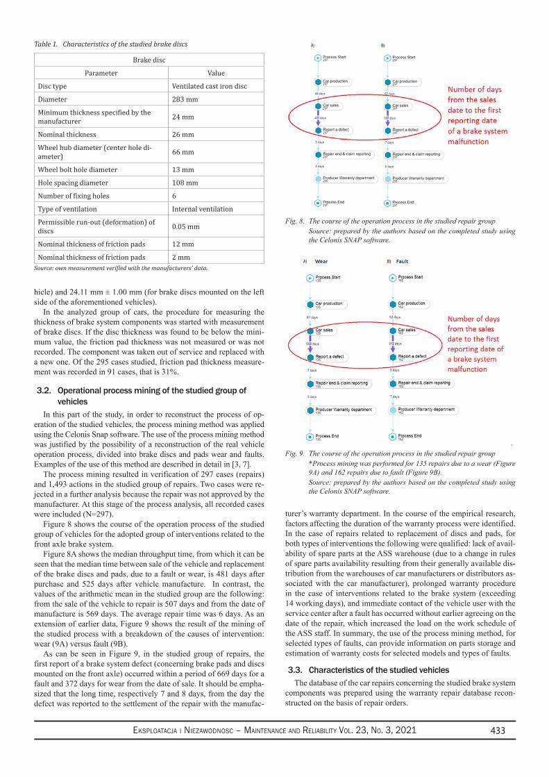
Eksploatacja i NiEzawodNosc – MaiNtENaNcE aNd REliability Vol. 23, No. 3, 2021 433
hicle) and 24.11 mm ± 1.00 mm (for brake discs mounted on the left side of the aforementioned vehicles).
In the analyzed group of cars, the procedure for measuring the thickness of brake system components was started with measurement of brake discs. If the disc thickness was found to be below the mini-mum value, the friction pad thickness was not measured or was not recorded. The component was taken out of service and replaced with a new one. Of the 295 cases studied, friction pad thickness measure-ment was recorded in 91 cases, that is 31%.
3.2. Operational process mining of the studied group of vehicles
In this part of the study, in order to reconstruct the process of op-eration of the studied vehicles, the process mining method was applied using the Celonis Snap software. The use of the process mining method was justified by the possibility of a reconstruction of the real vehicle operation process, divided into brake discs and pads wear and faults. Examples of the use of this method are described in detail in [3, 7].
The process mining resulted in verification of 297 cases (repairs) and 1,493 actions in the studied group of repairs. Two cases were re-jected in a further analysis because the repair was not approved by the manufacturer. At this stage of the process analysis, all recorded cases were included (N=297).
Figure 8 shows the course of the operation process of the studied group of vehicles for the adopted group of interventions related to the front axle brake system.
Figure 8A shows the median throughput time, from which it can be seen that the median time between sale of the vehicle and replacement of the brake discs and pads, due to a fault or wear, is 481 days after purchase and 525 days after vehicle manufacture. In contrast, the values of the arithmetic mean in the studied group are the following: from the sale of the vehicle to repair is 507 days and from the date of manufacture is 569 days. The average repair time was 6 days. As an extension of earlier data, Figure 9 shows the result of the mining of the studied process with a breakdown of the causes of intervention: wear (9A) versus fault (9B).
As can be seen in Figure 9, in the studied group of repairs, the first report of a brake system defect (concerning brake pads and discs mounted on the front axle) occurred within a period of 669 days for a fault and 372 days for wear from the date of sale. It should be empha-sized that the long time, respectively 7 and 8 days, from the day the defect was reported to the settlement of the repair with the manufac-
turer’s warranty department. In the course of the empirical research, factors affecting the duration of the warranty process were identified. In the case of repairs related to replacement of discs and pads, for both types of interventions the following were qualified: lack of avail-ability of spare parts at the ASS warehouse (due to a change in rules of spare parts availability resulting from their generally available dis-tribution from the warehouses of car manufacturers or distributors as-sociated with the car manufacturer), prolonged warranty procedure in the case of interventions related to the brake system (exceeding 14 working days), and immediate contact of the vehicle user with the service center after a fault has occurred without earlier agreeing on the date of the repair, which increased the load on the work schedule of the ASS staff. In summary, the use of the process mining method, for selected types of faults, can provide information on parts storage and estimation of warranty costs for selected models and types of faults.
3.3. Characteristics of the studied vehiclesThe database of the car repairs concerning the studied brake system
components was prepared using the warranty repair database recon-structed on the basis of repair orders.
Table 1. Characteristics of the studied brake discs
Brake disc
Parameter Value
Disc type Ventilated cast iron disc
Diameter 283 mm
Minimum thickness specified by the manufacturer 24 mm
Nominal thickness 26 mm
Wheel hub diameter (center hole di-ameter) 66 mm
Wheel bolt hole diameter 13 mm
Hole spacing diameter 108 mm
Number of fixing holes 6
Type of ventilation Internal ventilation
Permissible run-out (deformation) of discs 0.05 mm
Nominal thickness of friction pads 12 mm
Nominal thickness of friction pads 2 mmSource: own measurement verified with the manufacturers’ data.
Fig. 8. The course of the operation process in the studied repair group Source: prepared by the authors based on the completed study using
the Celonis SNAP software.
Fig. 9. The course of the operation process in the studied repair group *Process mining was performed for 135 repairs due to a wear (Figure
9A) and 162 repairs due to fault (Figure 9B). Source: prepared by the authors based on the completed study using
the Celonis SNAP software.

Eksploatacja i NiEzawodNosc – MaiNtENaNcE aNd REliability Vol. 23, No. 3, 2021434
Table 2 shows the characteristics of the variables in the relational database that was developed, on the basis of which the statistical anal-yses discussed in the next chapter of the paper were performed.
Using the collected empirical data, an attempt was made to conduct a statistical analysis of the factors that characterize the vehicles re-ported to the service center due to a fault or wear of the brake system. Seven factors were identified whose distributions were analyzed in the groups of vehicles in which, during the warranty period, brake discs and pads wear occurred and in the group of vehicles with faults:
Vehicle type • (car_type): passenger car or commercial vehicle.Vehicle brand • (brand): brand X or brand Y.Vehicle model • (model): 7 vehicle models were considered in the study.Engine type • (engine_type): diesel/spark ignition engine.Engine capacity • (engine_capacity): in the studied group of en-gines, engines with capacity of 1,200 ccm3 and 1,600 ccm3 were identified.Gearbox type • (gearbox_type): automatic gearbox or manual gearbox.Mileage • (mileage): expressed in kms, as read at the time of the fault report.Vehicle age (months): • counted in months of vehicle use, calcu-lated as the difference between the date the car was reported for service and the date of manufacture.
The structure of the sample is shown in Table 3.The hypothesis was put forward that the distributions of the above
variables differ in the group of cars in which a fault occurred and the group of cars in which the brake system elements were worn out. Both groups were analyzed separately and the hypothesis was verified by appropriate statistical tests.
Identification of the regularities that characterize the vehicles re-ported for service due to brake disc wear or fault should start with identification of the distributions of the variables that describe the ve-
hicles. These variables can be numerical (e.g., mileage, vehicle age, brake disc thickness, etc.) or non-numerical (e.g., car model, gearbox type, etc.). In the case of the numerical variables, the choice of the method of further analysis depends on the type of distribution of the respective variable [9].
When the variables have a normal distribution, the analysis can be carried out using parametric methods, while for other types of statistical distributions (often skewed ones) non-parametric methods are required. The assumption of equality of the empirical distribu-tion with the normal distribution is verified with one of the normality tests. In the present study, the Kolmogorov-Smirnov normality test with a Lilliefors correction was used [1]. Since distributions of all analyzed characteristics were not normal, the evaluation of the dif-ferences in the distributions of the numerical variables was obtained
Table 3. The structure of the sample according to selected factors
Variable Attribute N
Gearbox type
Manual 287
Semi Automatic 7
Automatic 1
Engine capacity1200 [cm3] 7
1600 [cm3] 288
Engine typeDiesel engine 278
Gasoline engine 17
Vehicle brandX 126
Y 169
Table 2. Characteristics of the studied variables
Variable Class Description
ID_case [character] A unique number of the warranty report that identifies the completed intervention (repair)
Prod_date [date, format = “%Y-%m-%d] The vehicle production date
Repair_date [date, format = “%Y-%m-%d] The date of the repair, the date on which the customer reported the fault to the authorized service station
Warranty_start [date, format = “%Y-%m-%d] The start date of the warranty period of the vehicle, also identified as the date of sale
Age [numeric] The number of the vehicle’s days in service, identified as the difference between Repair date and Warranty start
Mileage [numeric] The value of the mileage of the vehicle read at the time of the customer’s fault report
Brand [character] The brand of the vehicle
Model [character] The vehicle model
Claim_type [character] The report type (1 – manufacturer warranty, 2 - supplementary warranty, 3 - vehicle maintenance)
Cause [character] The code for the cause of the reported fault determined by the workshop at the authorized service station
Cause_wear [logical] Indication of wear of a brake system component (1-yes, 0-no)
Cause_deformation [logical]Indication of a fault of a brake system component (1-yes, 0-no)
Disc_R [numeric] The thickness of the right front brake disc [mm]
Disc_L [numeric] The thickness of the left front brake disc [mm]
Pads_front [numeric]The thickness of the front friction pads [mm]The minimum value from the external and internal measurement of the left and right pads.
Deformation_R [numeric] The value of the run-out of the right brake disc [mm]
Deformation_L [numeric] The value of the run-out of the left brake disc [mm]Source: prepared by the author.
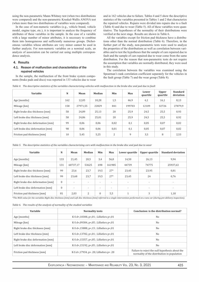
Eksploatacja i NiEzawodNosc – MaiNtENaNcE aNd REliability Vol. 23, No. 3, 2021 435
using the non-parametric Mann-Whitney test (when two distributions were compared) and the non-parametric Kruskal-Wallis ANOVA test (when more than two distributions of variables were compared).
In the case of non-numeric variables (e.g., vehicle brand, vehicle model, engine type, etc.), it is important to analyze the frequency of attributes of these variables in the sample. In the case of a variable with a large number of minor attributes, it is necessary to combine them into homogeneous and sufficiently numerous groups. Dichot-omous variables whose attributes are very minor cannot be used in further analysis. For non-numeric variables on a nominal scale, an analysis of association can be carried out using multiple correspon-dence analysis.
4. Results4.1. Reason of malfunction and characteristics of the
repaired vehiclesIn the sample, the malfunction of the front brake system compo-
nents (brake pads and discs) was reported in 133 vehicles due to wear
and in 162 vehicles due to failure. Tables 4 and 5 show the descriptive statistics of the variables presented in Tables 1 and 2 that characterize the repaired vehicles. Repairs were divided into repairs due to a fault (Table 4) and due to wear (Table 5). All of these variables were quan-titative. The hypotheses of the normality of their distributions were verified at the next stage. Results are shown in Table 6.
All the variables except for friction pad thickness have a distribu-tions other than the normal distribution (Table 6). Therefore, in the further part of the study, non-parametric tests were used to analyze the properties of the distributions as well as correlation between vari-ables and to test the hypotheses that the sample of cars repaired due to fault and the sample of cars repaired due to wear come from the same distribution. For the reason that non-parametric tests do not require the assumption that variables are normally distributed, they were used in this study.
The correlation between the variables was examined using the Spearman’s rank correlation coefficient separately for the vehicles in the fault group (Table 7) and the wear group (Table 8).
Table 4. The descriptive statistics of the variables characterizing vehicles with malfunction in the brake disc and pad due to fault
Variable N Mean Median Min Max Lower quartile
Upper quartile
Standard deviation
Age [months] 162 12,05 10,28 1,5 46,9 6,1 16,1 8,13
Mileage [km] 158 27971,55 22829 841 199703 12109 32726 27879,9
Right brake disc thickness [mm] 58 24,89 25,13 20 25,9 24,5 25,5 0,93
Left brake disc thickness [mm] 58 24,86 25,01 20 25,9 24,5 25,5 0,92
Right brake disc deformation [mm] 99 0,06 0,06 0,02 0,1 0,05 0,07 0,02
Left brake disc deformation [mm] 98 0,06 0,06 0,01 0,1 0,05 0,07 0,02
Friction pad thickness [mm] 10 5,45 5,25 2 9 3,5 8 2,53
Table 5. The descriptive statistics of the variables characterizing cars with malfunction in the brake disc and pad due to wear
Variable N Mean Median Min Max Lower quartile Upper quartile Standard deviation
Age [months] 133 21,45 20,5 3,4 56,8 14,50 26,13 9,94
Mileage [km] 131 60737,17 53625 698 161985 44739 74775 25937,63
Right brake disc thickness [mm] 99 23,6 23,7 19,5 27* 23,45 23,95 0,81
Left brake disc thickness [mm] 99 23,68 23,7 19,5 27* 23,45 24 0,76
Right brake disc deformation [mm] 0 - - - - - - -
Left brake disc deformation [mm] 0 - - - - - - -
Friction pad thickness [mm] 81 2,03 2 0 5,5 1 3 1,18*The MAX value for the variables Right disc thickness [mm] and Left disc thickness [mm] referred to a single intervention performed on a new car (during pre-delivery inspection).
Table 6. The results of the analysis of normality of the studied variables
Variable Normality tests Conclusion: is the distribution normal?
Age [months] K-S d=,10308, p<,01 ; Lilliefors p<,01 No
Mileage [km] K-S d=,09384, p<,05 ; Lilliefors p<,01 No
Right brake disc thickness [mm] K-S d=,15888, p<,15 ; Lilliefors p<,01 No
Left brake disc thickness [mm] K-S d=,13782, p<,01 ; Lilliefors p<,01 No
Right brake disc deformation [mm] K-S d=,15357, p<,05 ; Lilliefors p<,01 No
Left brake disc deformation [mm] K-S d=,15192, p<,05 ; Lilliefors p<,01 No
Friction pad thickness [mm] K-S d=,17934, p> .20; Lilliefors p> .20 Failure to reject the null hypothesis about the normality of the distribution in population
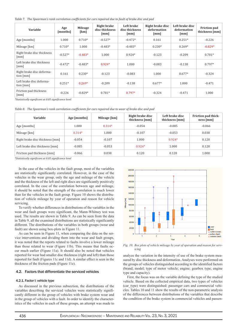
Eksploatacja i NiEzawodNosc – MaiNtENaNcE aNd REliability Vol. 23, No. 3, 2021436
In the case of the vehicles in the fault group, most of the variables are statistically significantly correlated. However, in the case of the vehicles in the wear group, only the age and mileage of the vehicle and the thickness of the left and right discs are significantly positively correlated. In the case of the correlation between age and mileage, it should be noted that the strength of the correlation is much lower than for the vehicles in the fault group. Figure 10 shows the distribu-tion of vehicle mileage by year of operation and reason for vehicle servicing.
To verify whether differences in distributions of the variables in the wear and fault groups were significant, the Mann-Whitney test was used. The results are shown in Table 9. As can be seen from the data in Table 9, all the examined distributions are statistically significantly different. The distributions of the variables in both groups (wear and fault) are shown using box-plots in Figure 11.
As can be seen in Figure 11, when comparing the data on the ser-vice interventions and dividing them into the wear and fault groups, it was noted that the reports related to faults involve a lower mileage than those related to wear (Figure 11b). This means that faults oc-cur much earlier (Figure 11a). It should also be noted that vehicles reported for wear had smaller disc thickness (right and left) than those reported for fault (Figures 11c and 11d). A similar effect is seen in the thickness of the friction pads (Figure 11e).
4.2. Factors that differentiate the serviced vehicles
4.2.1. Factor I: vehicle type As discussed in the previous subsection, the distributions of the
variables describing the serviced vehicles were statistically signifi-cantly different in the group of vehicles with brake system wear and in the group of vehicles with a fault. In order to identify the character-istics of the vehicles in each of these groups, an attempt was made to
analyze the variation in the intensity of use of the brake system mea-sured by disc thickness and deformation. Analyses were performed on the groups of vehicles distinguished according to the identified factors (brand; model; type of motor vehicle; engine; gearbox type; engine type and capacity).
First, the focus was on the variable defining the type of the studied vehicle. Based on the collected empirical data, two types of vehicles (car_type) were distinguished: passenger cars and commercial vehi-cles. Tables 10 and 11 show the results of the non-parametric analysis of the differences between distributions of the variables that describe the condition of the brake system in commercial vehicles and passen-
Table 8. The Spearman’s rank correlation coefficients for cars repaired due to wear of brake disc and pad
Variable Age [months] Mileage [km] Right brake disc thickness [mm]
Left brake disc thickness [mm]
Friction pad thick-ness [mm]
Age [months] 1.000 0.314* -0.054 -0.085 -0.066
Mileage [km] 0.314* 1.000 -0.107 -0.053 0.038
Right brake disc thickness [mm] -0.054 -0.107 1.000 0.924* 0.120
Left brake disc thickness [mm] -0.085 -0.053 0.924* 1.000 0.128
Friction pad thickness [mm] -0.066 0.038 0.120 0.128 1.000*Statistically significant at 0.05 significance level
Table 7. The Spearman’s rank correlation coefficients for cars repaired due to fault of brake disc and pad
Variable Age [months]
Mileage [km]
Right brake disc thickness
[mm]
Left brake disc thickness
[mm]
Right brake disc deformation
[mm]
Left brake disc deformation
[mm]
Friction pad thickness [mm]
Age [months] 1.000 0.710* -0.527* -0.472* 0.161 0.251* -0.226
Mileage [km] 0.710* 1.000 -0.483* -0.483* 0.230* 0.269* -0.829*
Right brake disc thickness [mm] -0.527* -0.483* 1.000 0.924* -0.123 -0.209 0.781*
Left brake disc thickness [mm] -0.472* -0.483* 0.924* 1.000 -0.083 -0.138 0.797*
Right brake disc deforma-tion [mm] 0.161 0.230* -0.123 -0.083 1.000 0.677* -0.324
Left brake disc deforma-tion [mm] 0.251* 0.269* -0.209 -0.138 0.677* 1.000 -0.471
Friction pad thickness [mm] -0.226 -0.829* 0.781* 0.797* -0.324 -0.471 1.000
*Statistically significant at 0.05 significance level
Fig. 10. Box plots of vehicle mileage by year of operation and reason for serv-icing
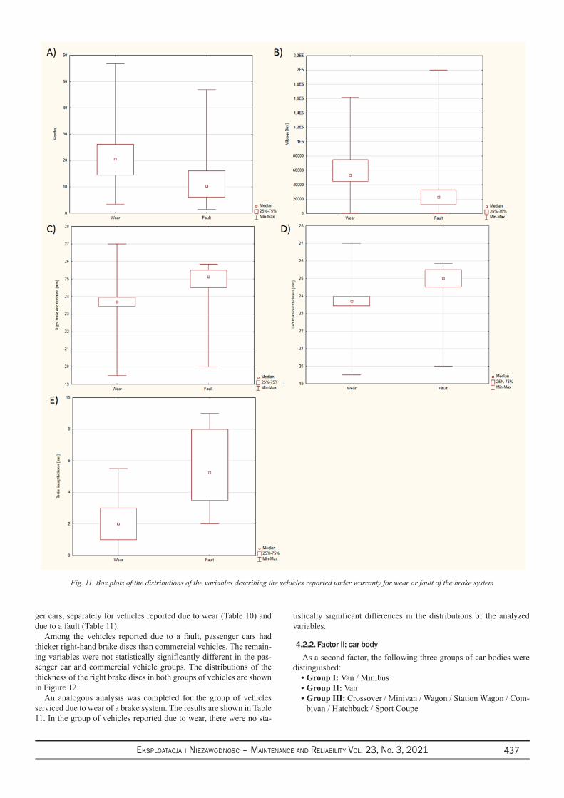
Eksploatacja i NiEzawodNosc – MaiNtENaNcE aNd REliability Vol. 23, No. 3, 2021 437
ger cars, separately for vehicles reported due to wear (Table 10) and due to a fault (Table 11).
Among the vehicles reported due to a fault, passenger cars had thicker right-hand brake discs than commercial vehicles. The remain-ing variables were not statistically significantly different in the pas-senger car and commercial vehicle groups. The distributions of the thickness of the right brake discs in both groups of vehicles are shown in Figure 12.
An analogous analysis was completed for the group of vehicles serviced due to wear of a brake system. The results are shown in Table 11. In the group of vehicles reported due to wear, there were no sta-
tistically significant differences in the distributions of the analyzed variables.
4.2.2. Factor II: car bodyAs a second factor, the following three groups of car bodies were
distinguished: Group I:• Van / MinibusGroup II:• Van Group III:• Crossover / Minivan / Wagon / Station Wagon / Com-bivan / Hatchback / Sport Coupe
Fig. 11. Box plots of the distributions of the variables describing the vehicles reported under warranty for wear or fault of the brake system
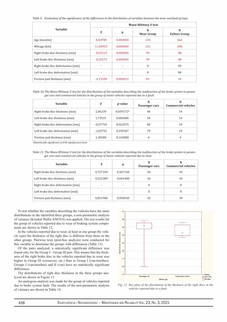
Eksploatacja i NiEzawodNosc – MaiNtENaNcE aNd REliability Vol. 23, No. 3, 2021438
To test whether the variables describing the vehicles have the same distributions in the identified three groups, a non-parametric analysis of variance (Kruskal Wallis ANOVA) was applied. The test results for the group of vehicles reported due to wear of braking system compo-nents are shown in Table 12.
In the vehicles reported due to wear, at least in one group (by vehi-cle type) the thickness of the right disc is different from those in the other groups. Pairwise tests (post-hoc analysis) were conducted for this variable to determine the groups with differences (Table 13).
Of the pairs analyzed, a statistically significant difference was found only for the Group I - Group III pair. This means that the thick-ness of the right brake disc in the vehicles reported due to wear was higher in Group III (crossover, etc.) than in Group I (van/minibus). Groups I (van/minibus) and II (van) have no statistically significant differences.
The distributions of right disc thickness in the three groups ana-lyzed are shown in Figure 13.
An analogous analysis was made for the group of vehicles reported due to brake system fault. The results of the non-parametric analysis of variance are shown in Table 14.
Table 10. The Mann-Whitney U test for the distributions of the variables describing the malfunction of the brake system in passen-ger cars and commercial vehicles in the group of motor vehicles reported due to a fault
Variable Z p-value N Passenger cars
N Commercial vehicles
Right brake disc thickness [mm] 2,06239 0,039172* 44 14
Left brake disc thickness [mm] 1,73531 0,082686 44 14
Right brake disc deformation [mm] -0,57754 0,563575 80 19
Left brake disc deformation [mm] -1,03792 0,299307 79 19
Friction pad thickness [mm] 1,38580 0,165808 6 4*Statistically significant at 0.05 significance level
Table 11. The Mann-Whitney U test for the distributions of the variables describing the malfunction of the brake system in passen-ger cars and commercial vehicles in the group of motor vehicles reported due to wear
Variable Z p N Passenger cars
N Commercial vehicles
Right brake disc thickness [mm] 0,727109 0,467160 56 43
Left brake disc thickness [mm] 0,522389 0,601400 56 43
Right brake disc deformation [mm] - - 0 0
Left brake disc deformation [mm] - - 0 0
Friction pad thickness [mm] 0,051986 0,958540 42 39
Table 9. Evaluation of the significance of the differences in the distribution of variables between the wear and fault groups
VariableMann-Whitney U test
Z p N Wear Group
N Failure Group
Age [months] 8,40788 0,000000 133 162
Mileage [km] 11,00955 0,000000 131 158
Right brake disc thickness [mm] -8,55215 0,000000 99 58
Left brake disc thickness [mm] -8,25575 0,000000 99 58
Right brake disc deformation [mm] - - 0 99
Left brake disc deformation [mm] - - 0 98
Friction pad thickness [mm] -4,15590 0,000032 81 10
Fig. 12. Box plots of the distribution of the thickness of the right discs in the vehicles reported due to a fault
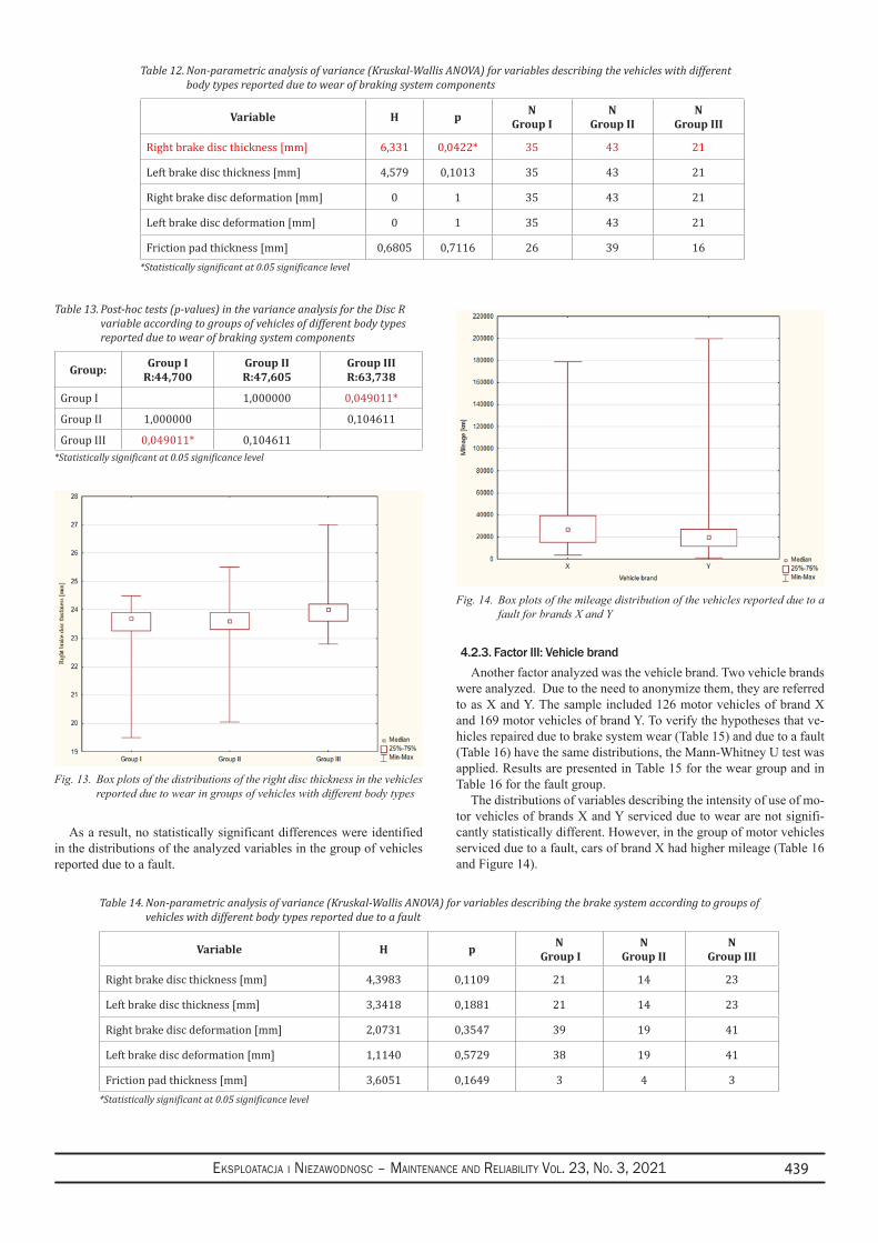
Eksploatacja i NiEzawodNosc – MaiNtENaNcE aNd REliability Vol. 23, No. 3, 2021 439
As a result, no statistically significant differences were identified in the distributions of the analyzed variables in the group of vehicles reported due to a fault.
4.2.3. Factor III: Vehicle brand Another factor analyzed was the vehicle brand. Two vehicle brands
were analyzed. Due to the need to anonymize them, they are referred to as X and Y. The sample included 126 motor vehicles of brand X and 169 motor vehicles of brand Y. To verify the hypotheses that ve-hicles repaired due to brake system wear (Table 15) and due to a fault (Table 16) have the same distributions, the Mann-Whitney U test was applied. Results are presented in Table 15 for the wear group and in Table 16 for the fault group.
The distributions of variables describing the intensity of use of mo-tor vehicles of brands X and Y serviced due to wear are not signifi-cantly statistically different. However, in the group of motor vehicles serviced due to a fault, cars of brand X had higher mileage (Table 16 and Figure 14).
Table 14. Non-parametric analysis of variance (Kruskal-Wallis ANOVA) for variables describing the brake system according to groups of vehicles with different body types reported due to a fault
Variable H p N Group I
NGroup II
N Group III
Right brake disc thickness [mm] 4,3983 0,1109 21 14 23
Left brake disc thickness [mm] 3,3418 0,1881 21 14 23
Right brake disc deformation [mm] 2,0731 0,3547 39 19 41
Left brake disc deformation [mm] 1,1140 0,5729 38 19 41
Friction pad thickness [mm] 3,6051 0,1649 3 4 3*Statistically significant at 0.05 significance level
Table 12. Non-parametric analysis of variance (Kruskal-Wallis ANOVA) for variables describing the vehicles with different body types reported due to wear of braking system components
Variable H p N Group I
N Group II
N Group III
Right brake disc thickness [mm] 6,331 0,0422* 35 43 21
Left brake disc thickness [mm] 4,579 0,1013 35 43 21
Right brake disc deformation [mm] 0 1 35 43 21
Left brake disc deformation [mm] 0 1 35 43 21
Friction pad thickness [mm] 0,6805 0,7116 26 39 16*Statistically significant at 0.05 significance level
Table 13. Post-hoc tests (p-values) in the variance analysis for the Disc R variable according to groups of vehicles of different body types reported due to wear of braking system components
Group: Group I R:44,700
Group II R:47,605
Group III R:63,738
Group I 1,000000 0,049011*
Group II 1,000000 0,104611
Group III 0,049011* 0,104611*Statistically significant at 0.05 significance level
Fig. 13. Box plots of the distributions of the right disc thickness in the vehicles reported due to wear in groups of vehicles with different body types
Fig. 14. Box plots of the mileage distribution of the vehicles reported due to a fault for brands X and Y
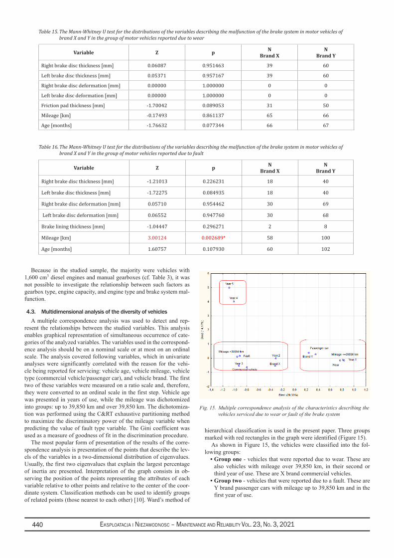
Eksploatacja i NiEzawodNosc – MaiNtENaNcE aNd REliability Vol. 23, No. 3, 2021440
Because in the studied sample, the majority were vehicles with 1,600 cm3 diesel engines and manual gearboxes (cf. Table 3), it was not possible to investigate the relationship between such factors as gearbox type, engine capacity, and engine type and brake system mal-function.
4.3. Multidimensional analysis of the diversity of vehiclesA multiple correspondence analysis was used to detect and rep-
resent the relationships between the studied variables. This analysis enables graphical representation of simultaneous occurrence of cate-gories of the analyzed variables. The variables used in the correspond-ence analysis should be on a nominal scale or at most on an ordinal scale. The analysis covered following variables, which in univariate analyses were significantly correlated with the reason for the vehi-cle being reported for servicing: vehicle age, vehicle mileage, vehicle type (commercial vehicle/passenger car), and vehicle brand. The first two of these variables were measured on a ratio scale and, therefore, they were converted to an ordinal scale in the first step. Vehicle age was presented in years of use, while the mileage was dichotomized into groups: up to 39,850 km and over 39,850 km. The dichotomiza-tion was performed using the C&RT exhaustive partitioning method to maximize the discriminatory power of the mileage variable when predicting the value of fault type variable. The Gini coefficient was used as a measure of goodness of fit in the discrimination procedure.
The most popular form of presentation of the results of the corre-spondence analysis is presentation of the points that describe the lev-els of the variables in a two-dimensional distribution of eigenvalues. Usually, the first two eigenvalues that explain the largest percentage of inertia are presented. Interpretation of the graph consists in ob-serving the position of the points representing the attributes of each variable relative to other points and relative to the center of the coor-dinate system. Classification methods can be used to identify groups of related points (those nearest to each other) [10]. Ward’s method of
hierarchical classification is used in the present paper. Three groups marked with red rectangles in the graph were identified (Figure 15).
As shown in Figure 15, the vehicles were classified into the fol-lowing groups:
Group one• - vehicles that were reported due to wear. These are also vehicles with mileage over 39,850 km, in their second or third year of use. These are X brand commercial vehicles.Group two• - vehicles that were reported due to a fault. These are Y brand passenger cars with mileage up to 39,850 km and in the first year of use.
Table 15. The Mann-Whitney U test for the distributions of the variables describing the malfunction of the brake system in motor vehicles of brand X and Y in the group of motor vehicles reported due to wear
Variable Z p NBrand X
N Brand Y
Right brake disc thickness [mm] 0.06087 0.951463 39 60
Left brake disc thickness [mm] 0.05371 0.957167 39 60
Right brake disc deformation [mm] 0.00000 1.000000 0 0
Left brake disc deformation [mm] 0.00000 1.000000 0 0
Friction pad thickness [mm] -1.70042 0.089053 31 50
Mileage [km] -0.17493 0.861137 65 66
Age [months] -1.76632 0.077344 66 67
Table 16. The Mann-Whitney U test for the distributions of the variables describing the malfunction of the brake system in motor vehicles of brand X and Y in the group of motor vehicles reported due to fault
Variable Z p NBrand X
NBrand Y
Right brake disc thickness [mm] -1.21013 0.226231 18 40
Left brake disc thickness [mm] -1.72275 0.084935 18 40
Right brake disc deformation [mm] 0.05710 0.954462 30 69
Left brake disc deformation [mm] 0.06552 0.947760 30 68
Brake lining thickness [mm] -1.04447 0.296271 2 8
Mileage [km] 3.00124 0.002689* 58 100
Age [months] 1.60757 0.107930 60 102
Fig. 15. Multiple correspondence analysis of the characteristics describing the vehicles serviced due to wear or fault of the brake system

Eksploatacja i NiEzawodNosc – MaiNtENaNcE aNd REliability Vol. 23, No. 3, 2021 441
Group three• - cars reported in the 4th and 5th year of use. The large distance of the two points constituting this group from the others indicates that there is no interaction with any of the other analyzed variables and their levels.
At this point, it is important to emphasize that the vehicles reported due to a fault were in the first year of use with low mileage (up to 39,850 km). At the same time, the thickness of the brake discs and friction pads in these vehicles was greater than in the vehicles reported due to wear (cf. Tables 4 and 5). Based on the results of the multiple correspondence analysis, it can also be concluded that reports of fault are involved with passenger cars of the Y brand. In contrast, the vehi-cles reported for wear were in their third or, more rarely, second year of use and had higher mileage. These were X brand commercial vehi-cles. In the commercial vehicles, the brake disc thickness was smaller than in passenger cars, which is related to the previous observations.
5. ConclusionsThe approach presented herein to the identification and analysis
of the factors that differentiate the course of wear and the occurrence of faults in brake system components in motor vehicles with the use of statistical methods is an original solution. It can be applied by both researchers studying similar problems and by organizations operating in the automotive sector.
As a result of the empirical process, three generalizing conclu-sions were formulated:
Vehicles reported for service due to brake system wear or fault 1. have different characteristics. Their identification makes it possible to predict which vehicles and at what time of use will be reported due to malfunction of the brake system. The distri-butions of analyzed variables that describe the intensity of use of vehicles are not normal, hence in their analysis it is neces-sary to use non-parametric measures. In particular, quartiles should be used in describing the central tendency rather than measures based on the arithmetic mean. The use of multiple correspondence analysis makes it possible to study of relation-ships between the factors that characterize the intensity of use of the vehicles.The results presented herein may have a positive impact on 2. the efficiency and effectiveness of activities associated with
the diagnosis and repairs of brake systems in motor vehicles. Moreover, the results obtained, in the utilitarian space, can provide new knowledge to car manufacturers regarding an analysis of the quality of the components and parts ordered as well as the selection of subcontractors (Original Equipment Manufacturers - OEM).The study outlines an area for improvement in the production 3. processes, selection of parts manufacturers, and diagnosis and repair of the described brake system components, in the con-text of the prediction of the costs related to parts wear and faults.The relationship between such characteristics of the studied 4. motor vehicles as vehicle type, body type, vehicle brand and model and the cause and time of reporting of a malfunction of brake system components was demonstrated.
At this point, it is necessary to outline the limitations of the em-pirical procedure carried out. First is a focus on a four-year service period of the studied group of vehicles. Second, possible errors exist in the measurement of the thickness and deformation of the studied group of brake system components, which were beyond the authors’ control. The authors outline new directions of research that focus on broadening the study by an attempt to enlarge the list of factors that differentiate the brake system components by adding variables de-scribing the steering system and the vehicle suspension. Additionally, the sample size and the observation period should be increased, taking into consideration repairs carried out in the warranty period, as well as paid repairs.
AcknowledgementsThe authors would like to acknowledge the many valuable and
insightful comments made by anonymous reviewers, which enhanced the substantial value of the paper and helped to give it its final
shape. Moreover, the authors would like to thank Mr. Maciej Fus-iewicz, the deputy manager of the authorized service station acting as a Renault COTECH and ZE-EV Expert, for substantial advice he
provided in the course of our work on the paper.
References1. Albright S C, Winston W L, Albright S C. Business analytics: data analysis and decision making. 5th edition. Stamford, CT, USA, Cengage
Learning: 2014.2. Bhane A B, Salodkar S M, Ramani H B. Braking System Approaching towards the Betterment and It's Consequences. International Research
Journal on Advanced Science Hub 2020; 2: 64-70, https://doi.org/10.47392/irjash.2020.236.3. Bitkowska A, Sliż P, Tenbrink C, Piasecka A. Application of Process Mining on the Example of an Authorized Passenger Car Service Station
in Poland. Foundations of Management 2020; 12(1): 125-136, https://doi.org/10.2478/fman-2020-0010.4. Breuer B, Bill K H. Menschliche Anforderungen. In Breuer B, Bill KH (eds): Bremsenhandbuch, Wiesbaden, Vieweg+Teubner Verlag: 2004:
38-48, https://doi.org/10.1007/978-3-322-99535-3_4.5. Dvadnenko V, Arhun S, Bogajevskiy A, Ponikarovska S. Improvement of economic and ecological characteristics of a car with a Start-Stop
system. International Journal of Electric and Hybrid Vehicles 2018; 10(3): 209, https://doi.org/10.1504/IJEHV.2018.097377.6. Ebrahimi N S, Kheybari M. Brake system design for sport cars using digital logic method. Automotive Science and Engineering 2017; 7(4):
2571-2582.7. Garcia C dos S, Meincheim A, Faria Junior E R et al. Process mining techniques and applications - A systematic mapping study. Expert
Systems with Applications 2019; 133: 260-295, https://doi.org/10.1016/j.eswa.2019.05.003.8. GOV.UK. Number of road accidents caused by vehicle defect factors in Great Britain (UK) in 2018. 2019.9. Hardy M, Bryman A.Handbook of data analysis. Los Angeles ; London, SAGE: 2009.10. Hjellbrekke J. Multiple correspondence analysis for the social sciences. Abingdon, Oxon ; New York, NY, Routledge, Taylor & Francis
Group: 2019.11. Jensen A F, Mabit S L. The use of electric vehicles: A case study on adding an electric car to a household. Transportation Research Part A:
Policy and Practice 2017; 106: 89-99, https://doi.org/10.1016/j.tra.2017.09.004.12. Likhanov V A, Rossokhin A V. Optimization of environmental performance of a car diesel engine running on natural gas by reducing carbon
black in the exhaust gas. IOP Conference Series: Materials Science and Engineering 2020; 862: 062046, https://doi.org/10.1088/1757-899X/862/6/062046.

Eksploatacja i NiEzawodNosc – MaiNtENaNcE aNd REliability Vol. 23, No. 3, 2021442
13. Milenkovic P, Jovanovic S, Jankovic A et al. The influence of brake pads thermal conductivity on passenger car brake system efficiency. Thermal Science 2010; 14(suppl.): 221-230, https://doi.org/10.2298/TSCI100505016M.
14. Nakanishi H. Development of aluminum metal matrix composites (Al-MMC) brake rotor and pad. JSAE Review 2002; 23(3): 365-370, https://doi.org/10.1016/S0389-4304(02)00203-5.
15. Ortar N, Ryghaug M. Should All Cars Be Electric by 2025? The Electric Car Debate in Europe. Sustainability 2019; 11(7): 1868, https://doi.org/10.3390/su11071868.
16. Owen C E, Eichhorn L, Eichhorn L. Shop manual for automotive brake systems. 5th ed. Clifton Park, NY, Delmar Cengage Learning: 2011.
17. Rashid A. Overview of disc brakes and related phenomena - a review. International Journal of Vehicle Noise and Vibration 2014; 10(4): 257, https://doi.org/10.1504/IJVNV.2014.065634.
18. Sivaraj G, Parammasivam K, Suganza G. Reduction of aerodynamic drag force for reducing fuel consumption in road vehicle using basebleed. Journal of Applied Fluid Mechanics 2018; 11(6): 1489-1495, https://doi.org/10.29252/jafm.11.06.29115.
19. Świderski A, Borucka A, Jacyna-Gołda I, Szczepański E. Wear of brake system components in various operating conditions of vehicle in the transport company. Eksploatacja i Niezawodnosc - Maintenance and Reliability 2018; 21(1): 1-9, https://doi.org/10.17531/ein.2019.1.1.
20. Yang Y-C, Chen W-L. A nonlinear inverse problem in estimating the heat flux of the disc in a disc brake system. Applied Thermal Engineering 2011; 31(14-15): 2439-2448, https://doi.org/10.1016/j.applthermaleng.2011.04.008.
Eksploatacja i NiEzawodNosc – MaiNtENaNcE aNd REliability Vol. 23, No. 3, 2021 443
(*) Corresponding author.E-mail addresses:
Eksploatacja i Niezawodnosc – Maintenance and ReliabilityVolume 23 (2021), Issue 3
journal homepage: http://www.ein.org.pl
Indexed by:
The paper provides a multiple-experts Fuzzy-TOPSIS decision-making model for the se-lection among maintenance contractors based on the quality of tendering documents. The study introduces a set of selection criteria utilizing benefit and cost criteria from literature. The proposed model aggregates subjective linguistic assessments of multiple experts that express their opinions on the degree of importance of criteria and allows multiple decision-makers to evaluate the compliance of contractors’ documents. For a case study, the model is applied to select among contractors tendering to maintain the heavy-duty cranes of an international steel company from literature. Several decision-making scenarios are investi-gated, and major changes in the final decision are observed. The changes in obtained results illustrate the need to better address uncertainties in rating and tendering an overqualified contractor at a higher cost.
Highlights Abstract
The study presents a Fuzzy-TOPSIS model for • solving the maintenance outsourcing problem.
The study integrates fuzzy opinions of experts on • the importance of selection criteria.
The study allows multiple decision-makers to in-• tegrate their fuzzy evaluations.
Disagreements among experts may result in a ma-• jor change to the final decision.
A fuzzy-TOPSIS model for maintenance outsourcing considering the quality of submitted tender documentsMaysa Alshraideh a, Shereen Ababneh a, Elif Elcin Gunay b, Omar Al-Araidah a,*a Industrial Engineering Department, Jordan University of Science and Technology, Irbid 22110, Jordan b Industrial Engineering Department, Sakarya University, Sakarya, Turkey
Alshraideh M, Ababneh S, Gunay EE, Al-Araidah O. A fuzzy-TOPSIS model for maintenance outsourcing considering the quality of submit-ted tender documents. Eksploatacja i Niezawodnosc – Maintenance and Reliability 2021; 23 (3): 443–453, http://doi.org/10.17531/ein.2021.3.5.
Article citation info:
contractor selection; maintenance outsourcing; MCDM; Fuzzy-TOPSIS; decision-making.
Keywords
This is an open access article under the CC BY license (https://creativecommons.org/licenses/by/4.0/)
1. IntroductionMaintenance plays a fundamental role in preserving the safety,
quality, and productivity of service for industrial and governmental facilities. Maintenance actions vary in complexity, and accordingly, the associated costs, time, skills, and machinery required to perform the job right the first time differ. Therefore, many companies out-source some or all of their maintenance activities to enhance value [1]. While selecting the maintenance services, the decision-maker (DM) must primarily consider the technical abilities of the maintenance contractors in addition to several other time and financial compliance attributes to guarantee maximum safety and quality for money.
The maintenance contractor selection process accounts for several technical and non-technical strategic and operational decision criteria based on the organization’s requirements such as price and payment terms, experience in similar work, ability to supply spare parts, etc. Since the adequate selection of the contractors directly influences maintenance performance, outsourcing is a crucial decision for any organization. Tendering is one of the most used selection methods to inform and invite maintenance contractors to apply and compete for the maintenance contract. Among the many obligations of the project owners, they should notify contractors of the process by which ten-
ders will be considered and selected. The selection process must be transparent, verifiable, and liable. Moreover, owners must provide clear and adequate documentation that specifies requirements and specifications. Consequently, interested contractors must adequately address all the information required by the project owners to ensure compliance, and they must provide evidence of professional capabili-ties to ensure safety, quality, and timely delivery [26].
The information presented in tender documents about contractors is evaluated by DMs, i.e., organizations, and then the best-fit contractor among alternatives is selected. Basically, the evaluation process in-cludes determining the selection criteria (e.g., price, experience), their relative importance, and selecting the best contractor that meets DM’s demand. Therefore, selecting the best maintenance contractor that fulfills DM’s need among possible alternatives is considered under multi-attribute decision-making problems [10]. The selection of the decision-making method is essential since it directly influences the performance of the maintenance. Additionally, evaluating the degree of compliance based on tender documents is rather vague, imprecise, or sometimes inconsistent since the evaluation depends on the subjec-tive judgments of the different DMs. Given the diverse backgrounds of the DMs, and their degree of influence on the decision, the great proximity of the candidate qualities makes the decision hard to agree
M. Alshraideh - [email protected], S. Ababneh - [email protected], E.E. Gunay - [email protected], O. Al-Araidah - [email protected]
Eksploatacja i NiEzawodNosc – MaiNtENaNcE aNd REliability Vol. 23, No. 3, 2021444
upon. These risks originated from subjective preferences of different DMs hamper the applicability of the deterministic approaches. In re-sponse, fuzzy logic is proposed as an alternative that allows incorpo-rating uncertain, vague information in the decision-making process. According to Jasiulewicz-Kaczmarek et al. [14], by combining fuzzy with AHP (analytical hierarchy process) and/or fuzzy with TOPSIS (technique for order preference by similarity to ideal solution), DMs can incorporate the specific requirements of their company in decid-ing key maintenance factors to enhance sustainability. Moreover, the authors declared that the opinions of multiple DMs on multiple crite-ria can be incorporated using Fuzzy-AHP, and that the use of Fuzzy-TOPSIS allows the rating of a large number of alternatives and find-ing the “best” alternative.
In this study, we present a multiple-criteria multiple-experts Fuzzy-TOPSIS model for evaluating the performance of the maintenance contractors. Given that tender documents are the main source of in-formation, tendering information is used to set the decision criteria. Accordingly, the degree of compliance of the provided information to requirements is set as the measure to select among contractors. In the proposed Fuzzy-TOPSIS model, Fuzzy logic is deployed to cap-ture the subjectivity in the evaluating the degree of compliance based on tender documents, and TOPSIS allows the rating of alternative contractors based on the trade-off among the different criteria. For a case study, the model is applied for the maintenance of the maritime heavy-duty cranes at the steel company. This study contributes to the literature both theoretically and practically in the following aspects. From the theoretical point of view, the study integrates experts’ pref-erences on criteria important to contractors’ selection. The resulting fuzzy set “better” addresses experts’ disagreements on the importance of criteria. The Fuzzy-TOPSIS model allows multiple DMs to inte-grate their uncertain evaluations of contractors’ documents. From the practical point of view, the study introduces various decision-making scenarios through a case study from literature to illustrate the usability of the solution methodology. Moreover, the study shows a potentially major change in the final decision due to the change in the evaluation process.
The remainder of this paper is structured as follows. Section 2 re-views the literature on maintenance contractor selection. Section 3 addresses the solution method, Fuzzy-TOPSIS. The application for maritime heavy-duty cranes is presented by a case study in Section 4. Finally, Section 5 concludes the paper.
2. Literature reviewMaintenance management plays a significant role in increasing
the organization’s assets by preventing failures and reducing possible hazards. Therefore, making appropriate maintenance decisions, in-cluding outsourcing, is key to enhance a company’s resilience [4]. In the literature, researchers utilized several combinations of decision-making tools to help DMs decide regarding outsourcing. Such tools include TOPSIS, AHP, analytical network process (ANP), decision-making trial and evaluation laboratory (DEMATEL), balanced score-card (BSC), and Fuzzy logic [12]. Several recent studies addressed the applications of these tools in outsourcing of parts supply in vehicle production [27] and [13], complex system building in aviation [22], software development [21], catering [8], hospitals [5], cast iron part supply used in manufacturing catalytic converters [18], airline retail industry [23], supplier selection in steel industry [3] and in mainte-nance contractor selection [11]. Moline and Coves [19] presented a review of literature until 2007 on supplier evaluation and selection. In a recent study, Jasiulewicz-Kaczmarek et al. [14] used the matrix of crossed impact multiplications applied to a classification (MIC-MAC), Fuzzy-AHP, and Fuzzy-TOPSIS in identifying the mainte-nance factors critical to enhance manufacturing sustainability.
Hammudah [10] proposed a TOPSIS model to select among con-tractors bidding for a contract to maintain maritime heavy-duty cranes
at a steel company. In its first phase, the study surveyed maintenance professionals from various companies to identify key criteria that guide the outsourcing decision. Key criteria were further filtered by company project, and maintenance managers and contractors were evaluated based on information they listed in their tender documents. The company officials divided the selection criteria into technical and non-technical criteria as they are itemized in the company’s mainte-nance tender. Information cards were used to summarize information about each contractor, and the proposed TOPSIS model was used to select the most competent contractor. Mahdi et al. [17] identified sev-eral qualifying factors for the selection. The factors include criteria concerning cash flows, managerial capability, equipment accessibil-ity, contractor’s business strategy, professional staff capability, and organizational structure, workforce scheduling, supply scheduling, access to the workforce, logistic capability, percentage, and type of work that is assigned to the contractor, quality control, equipment scheduling, and guarantee program. Singh and Tiong [25] suggested past performance, characteristics of the contractor’s company, poten-tial performance, financial capability, and specific project criteria. Hafeez et al. [9] proposed intellectual properties, physical assets, cul-tural capitals, quality, delivery time, and cost to distinguish among contractors. Darvish et al. [7] used criteria concerning equipment and technology, work experience, operations team knowledge and experi-ence, quality, financial stability, reputation, familiarity with the area and domestication, innovation, and creativity in contractor evaluation. Jaskowsk et al. [15] suggested using financial capacity, organization-al experience, labor and equipment, a managerial system including safety policy, quality system, and performance in previous projects. Lam and Yu [16] used quantitative criteria including current work-load, human resources and financial capacity, and qualitative criteria including environmental concern, equipment, and resources, manage-ment capacity, complaint history, safety aspects, quality management, past performance, and experience. In [2], Alzahrani and Emsley used quality, safety, environment, past performance, resources, experience, organization, management, and technical aspects, finance, and the type and size of previous projects. Nieto-Morote and Ruz-Vila [20] suggested using technical capacity, experience, staff qualifications, labor and equipment, method innovation, experience, and managerial capacity. Moreover, the authors used financial stability, credit and li-quidity, financial capability, past performance, previous relationship, reputation, and health and safety. [23] used cost, delivery time, product quality, cooperate social responsibility, and financial stability. In [13], the authors utilized criteria concerning product quality, cost, on-time delivery, brand name, environmental performance, manufacturing ca-pability, warranty, and quality of a relationship. [21] used cost, vendor reputation, recoverability, scalability, portability, requirement rate, technical support, quality, risk analysis, changeability, analyzability, and response time. Hua et al. [11] classified criteria into (1) financial perspective: maintenance cost and maintenance value, (2) customer perspective: before, during, and after maintenance customer services, (3) internal business perspective: serviceability, customer manage-ment and innovation ability, and (4) learning and growth perspective: human capital, information capital and organizational capital.
3. Research methodologyThe research methodology includes two phases. In the first phase,
the authors utilized the literature search (studies from [1-27]) to iden-tify the essential tendering criteria considered in the selecting a main-tenance contractor. Table 1 divides surveyed criteria into “Benefit cri-teria” and “Cost criteria” and provides descriptions of the specifics to be present in tender documents for each of the criteria. In phase two, the project owner is expected to evaluate each of the benefit criteria against the owner’s expected or minimum level of requirement for that criteria. On the other hand, the project owner is expected to evalu-ate each of the cost criteria against the owner’s expected or maximum limit of obligation the owner expects to bear. To this end, the multi-
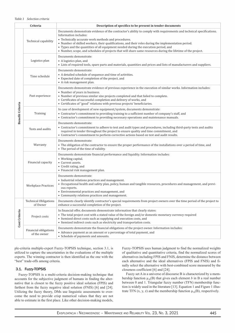
Eksploatacja i NiEzawodNosc – MaiNtENaNcE aNd REliability Vol. 23, No. 3, 2021 445
ple-criteria multiple-expert Fuzzy-TOPSIS technique, section 3.1, is utilized to capture the uncertainties in the evaluations of the multiple experts. The winning contractor is then identified as the one with the “best” trade-offs among criteria.
3.1. Fuzzy-TOPSISFuzzy-TOPSIS is a multi-criteria decision-making technique that
accounts for the subjective judgment of humans in finding the alter-native that is closest to the fuzzy positive ideal solution (FPIS) and farthest from the fuzzy negative ideal solution (FNIS) [6] and [24]. Utilizing the fuzzy theory, DMs use linguistic assessments to over-come the need to provide crisp numerical values that they are not able to estimate in the first place. Like other decision-making models,
Fuzzy-TOPSIS uses human judgment to find the normalized weights of qualitative and quantitative criteria, find the normalized scores of alternatives including FPIS and FNIS, determine the distance between each alternative and the ideal alternatives (FPIS and FNIS) and fi-nally select the alternative with best-combined score measured by the closeness coefficient [6] and [24].
Fuzzy set A in a universe of discourse B is characterized by a mem-bership function µA(B) that gives each element b in B a real number between 0 and 1. Triangular fuzzy number (TFN) membership func-tion is widely used in the literature [13]. Equation 1 and Figure 1 illus-trate TFN (x, y, z) and the membership function µA(B), respectively.
Table 1 Selection criteria
Criteria Description of specifics to be present in tender documents
Bene
fit C
rite
ria
Technical capability
Documents demonstrate evidence of the contractor’s ability to comply with requirements and technical specifications. Information includes:
Technically accurate work methods and procedures.•Number of skilled workers, their qualifications, and their roles during the implementation period.•Types and the quantities of all equipment needed during the execution period, and•Number, scope, and schedules of projects that will share same resources during the lifetime of the project.•
Logistics planDocuments demonstrate:
A logistics plan, and•Lists of required tools, spare parts and materials, quantities and prices and lists of manufacturers and suppliers.•
Time schedule
Documents demonstrate:A detailed schedule of sequence and time of activities.•Expected date of completion of the project, and•A risk management plan.•
Past experience
Documents demonstrate evidence of previous experience in the execution of similar works. Information includes: Number of years in business.•Number of previous similar size projects completed and that failed to complete.•Certificates of successful completion and delivery of works, and•Certificates of “good” relations with previous projects’ beneficiaries.•
TrainingIn case of development of new equipment/system, documents demonstrate:
Contractor’s commitment to providing training to a sufficient number of company’s staff, and •Contractor’s commitment to providing necessary operations and maintenance manuals.•
Tests and audits
Documents demonstrate:Contractor’s commitment to adhere to test and audit types and procedures, including third-party tests and audits •required in tender throughout the project to ensure quality and time commitment, andContractor’s commitment to perform corrective actions based on test and audit results.•
Warranty Documents demonstrate:
The obligation of the contractor to ensure the proper performance of the installations over a period of time, and•The period of the time of validity. •
Financial capacity
Documents demonstrate financial performance and liquidity. Information includes:Working capital.•Current assets.•Credit rating, and•Financial risk management plan.•
Workplace Practices
Documents demonstrate:Industrial relations practices and management.•Occupational health and safety plan, policy, human and tangible resources, procedures and management, and previ-•ous reports.Environmental practices and management, and•Community relations practices and management.•
Cost
Cri
teri
a
Technical Obligations of Owner
Documents clearly identify contractor’s special requirements from project owners over the time period of the project to enhance a successful completion of the project.
Project costs
In financial offer, documents demonstrate information that clearly states:The total project cost with a stated value of the foreign and/or domestic monetary currency required•Itemized direct costs such as supplying and execution costs, and•Itemized indirect costs such as electricity and transportation costs.•
Financial obligations of the owner
Documents demonstrate the financial obligations of the project owner. Information includes:Advance payment as an amount or a percentage of total payment, and•Schedule of payments and amounts.•
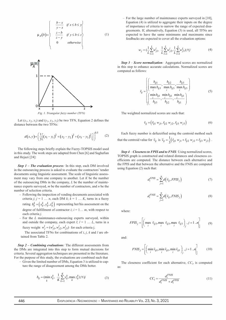
Eksploatacja i NiEzawodNosc – MaiNtENaNcE aNd REliability Vol. 23, No. 3, 2021446
( )
0
A
b x if x b yy xz bb if y b zz y
otherwise
µ
− ≤ ≤ − −
= ≤ ≤ −
(1)
Fig. 1. Triangular fuzzy number (TFN)
Let (x1, x2, x3) and (y1, y2, y3) be two TFN, Equation 2 defines the distance between the two TFNs:
( ) ( ) ( ) ( )0.5
22 21 1 2 2 3 3
1,3
d x y x y x y x y = − + − + − (2)
The following steps briefly explain the Fuzzy-TOPSIS model used in this study. The work steps are adapted from Chen [6] and Saghafian and Hejazi [24]:
Step 1 – The evaluation process: In this step, each DM involved in the outsourcing process is asked to evaluate the contractors’ tender documents using linguistic assessment. The scale of linguistic assess-ment may vary from one company to another. Let K be the number of the outsourcing DMs in the company, L be the number of mainte-nance experts surveyed, m be the number of contractors, and n be the number of selection criteria.
Following the inspection of vending documents associated with –criteria j; j = 1 … n, each DM k; k = 1 … K, turns in a fuzzy rating b x y zij
kijk
ijk
ijk= ( ), , representing her/his assessment on the
degree of fulfillment of contractor i; i = 1… m, with respect to each criteria j. For the – L maintenance-outsourcing experts surveyed, within and outside the company, each expert l; l = 1 … L, turns in a fuzzy weight
1 2 3)( , ,l l l lj j j jw w w w= for each criteria j.
The associated TFNs for combinations of i, j, k and l are ob-tained from Table 2.
Step 2 – Combining evaluations: The different assessments from the DMs are integrated into this step to form mutual decisions for criteria. Several aggregation techniques are presented in the literature. For the purpose of this study, the evaluations are combined such that
Given the limited number of DMs, Equation 3 is utilized to cap- –ture the range of disagreement among the DMs better.
1
1(min , , max ); K
k k kij ij ij ij
kk kb x y z ij
K == ∀∑ (3)
For the large number of maintenance experts surveyed in [10], –Equation (4) is utilized to aggregate their inputs on the degree of importance of criteria to narrow the range of expected disa-greements. If, alternatively, Equation (3) is used, all TFNs are expected to have the same minimums and maximums since feedbacks are expected to cover all the evaluation options:
1 2 31 1 1
1 1 1( , , ); L L L
l l Lj j j j
l l lw w w w j
L L L= = == ∀∑ ∑ ∑ (4)
Step 3 – Score normalization: Aggregated scores are normalized in this step to enhance accurate calculations. Normalized scores are computed as follows:
1 2 3
3 3 3
1 1 1
3 2 1
, ,max max max
min min min , ,
ij ij ij
ij ij iji i i
ij ij iji i i
ij ij ij
ij
b b bb b b
b b b
b b b
r
=
(5)
The weighted normalized scores are such that:
v r w r w r wij ij j ij j ij j= ( )1 1 2 2 3 3, , (6)
Each fuzzy number is defuzzified using the centroid method such
that the centroid value for ijv is v r w r w r wij ij j ij j ij j= + +( )13 1 1 2 2 3 3 .
Step 4 – Closeness to FPIS and to FNIS: Using normalized scores, TOPSIS graph is constructed and related distances and closeness co-efficients are computed. The distance between each alternative and the FPIS and that between the alternative and the FNIS are computed using Equation (2) such that:
d d v FPISiFPIS
j
nij j= ( )
=∑
1 , (7)
d d v FNISiFNIS
j
nij j= ( )
=∑
1 , (8)
where:
3 3 3max , max ,max , 1 ..j ij ij iji i i j
FPIS v v v j n = =
(9)
and:
1 1 1min , min ,min , 1 ..j ij ij iji ii j
FNIS v v v j n = =
(10)
The closeness coefficient for each alternative, CCi, is computed as:
FNISi
i FNIS FPISi i
dCCd d
=+
(11)
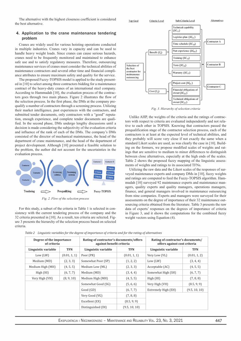
Eksploatacja i NiEzawodNosc – MaiNtENaNcE aNd REliability Vol. 23, No. 3, 2021 447
The alternative with the highest closeness coefficient is considered the best alternative.
4. Application to the crane maintenance tendering problem
Cranes are widely used for various hoisting operations conducted in multiple industries. Cranes vary in capacity and can be used to handle heavy weight loads. Since cranes can cause serious hazards, cranes need to be frequently monitored and maintained to enhance safe use and to satisfy regulatory measures. Therefore, outsourcing maintenance services of cranes must consider the technical abilities of maintenance contractors and several other time and financial compli-ance attributes to ensure maximum safety and quality for the service.
The proposed Fuzzy-TOPSIS model is applied to the study present-ed in [10] to select among three contractors bidding for a maintenance contract of the heavy-duty cranes of an international steel company. According to Hammudah [10], the evaluation process of the contrac-tors goes through two main phases. Figure 2 illustrates the flow of the selection process. In the first phase, the DMs at the company pre-qualify a number of contractors through a screening process. Utilizing their market intelligence, past experiences with the contractors, and submitted tender documents, only contractors with a “good” reputa-tion, enough experience, and complete tender documents are quali-fied. In the second phase, DMs undergo lengthy discussions until a decision is made considering the subjectivity of the evaluation criteria and influence of the rank of each of the DMs. The company’s DMs consisted of the director of mechanical maintenance, the head of the department of crane maintenance, and the head of the department of project development. Although [10] presented a feasible solution to the problem, the author did not account for the uncertainties in the evaluation process.
Fig. 2. Flow of the selection process
For this study, a subset of the criteria in Table 1 is selected in con-sistency with the current tendering process of the company and the 32 criteria presented in [10]. As a result, ten criteria are selected. Fig-ure 3 presents the hierarchy of the selection process based on selected criteria.
Unlike AHP, the weights of the criteria and the ratings of contrac-tors with respect to criteria are evaluated independently and not rela-tive to each other in TOPSIS. Knowing that contractors passed the prequalification stage of the contractor selection process, each of the contractors is at least at the expected level of technical abilities, and they probably will score very close if not exactly the same when a standard Likert scales are used, as was clearly the case in [10]. Build-ing on the formers, we propose modified scales of weights and rat-ings that are sensitive to medium to minor differences to distinguish between close alternatives, especially at the high ends of the scales. Table 2 shows the proposed fuzzy mapping of the linguistic assess-ments of weights and ratings to its associated TFNs.
Utilizing the raw data and the Likert scales of the responses of sur-veyed maintenance experts and company DMs in [10], fuzzy weights and ratings are computed to feed the Fuzzy-TOPSIS algorithm. Ham-mudah [10] surveyed 92 maintenance experts and maintenance man-agers, quality experts and quality managers, operations managers, finance, and general managers involved in maintenance outsourcing from nine companies. Experts and managers were surveyed for their assessments on the degree of importance of their 32 maintenance out-sourcing criteria obtained from the literature. Table 3 presents the raw data of experts’ responses on the degrees of importance of criteria in Figure 3, and it shows the computations for the combined fuzzy weight vectors using Equation (4).
Table 2 Linguistic variables for the degree of importance of criteria and for the rating of alternatives
Degree of the importance of criteria
Rating of contractor’s documents/offers against benefit criteria
Rating of contractor’s documents/ offers against cost criteria
Linguistic variable TFN Linguistic variable TFN Linguistic variable TFN
Low (LW) (0.01, 1, 1) Poor (PR) (0.01, 1, 1) Very Low (VL) (0.01, 1, 2)
Medium (MD) (2, 3, 3) Somewhat Poor (SP) (1, 2, 2) Low (LW) (3, 4, 4)
Medium High (MH) (4, 5, 5) Medium Low (ML) (2, 3, 3) Acceptable (AC) (4, 5, 5)
High (HI) (6, 7, 7) Medium (MD) (3, 4, 4) Somewhat High (SH) (6, 7, 7)
Very High (VH) (8, 9, 10) Medium High (MH) (4, 5, 5) High (HI) (7, 8, 8)
Somewhat Good (SG) (5, 6, 6) Very High (VH) (8.5, 9, 9)
Good (GD) (6, 7, 7) Extremely High (EH) (9.5, 10, 10)
Very Good (VG) (7, 8, 8)
Excellent (EX) (8.5, 9, 9)
Distinguished (DI) (9.5, 10, 10)
Fig. 3. Hierarchy of selection criteria
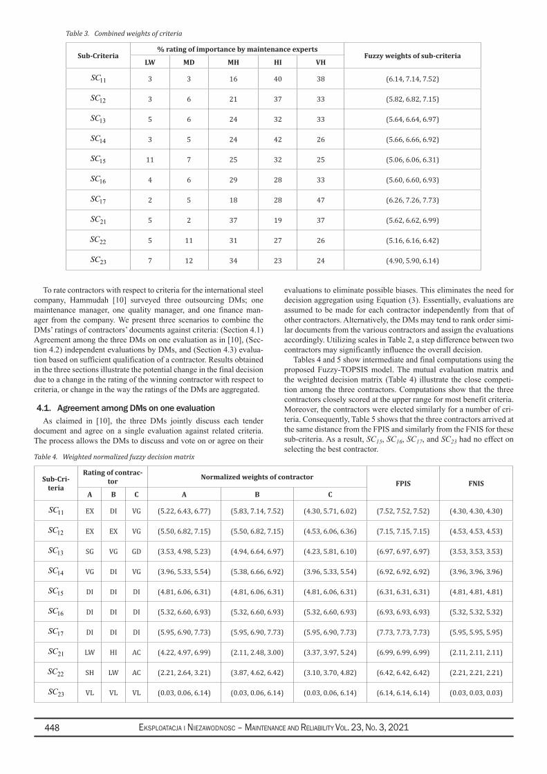
Eksploatacja i NiEzawodNosc – MaiNtENaNcE aNd REliability Vol. 23, No. 3, 2021448
To rate contractors with respect to criteria for the international steel company, Hammudah [10] surveyed three outsourcing DMs; one maintenance manager, one quality manager, and one finance man-ager from the company. We present three scenarios to combine the DMs’ ratings of contractors’ documents against criteria: (Section 4.1) Agreement among the three DMs on one evaluation as in [10], (Sec-tion 4.2) independent evaluations by DMs, and (Section 4.3) evalua-tion based on sufficient qualification of a contractor. Results obtained in the three sections illustrate the potential change in the final decision due to a change in the rating of the winning contractor with respect to criteria, or change in the way the ratings of the DMs are aggregated.
4.1. Agreement among DMs on one evaluationAs claimed in [10], the three DMs jointly discuss each tender
document and agree on a single evaluation against related criteria. The process allows the DMs to discuss and vote on or agree on their
evaluations to eliminate possible biases. This eliminates the need for decision aggregation using Equation (3). Essentially, evaluations are assumed to be made for each contractor independently from that of other contractors. Alternatively, the DMs may tend to rank order simi-lar documents from the various contractors and assign the evaluations accordingly. Utilizing scales in Table 2, a step difference between two contractors may significantly influence the overall decision.
Tables 4 and 5 show intermediate and final computations using the proposed Fuzzy-TOPSIS model. The mutual evaluation matrix and the weighted decision matrix (Table 4) illustrate the close competi-tion among the three contractors. Computations show that the three contractors closely scored at the upper range for most benefit criteria. Moreover, the contractors were elected similarly for a number of cri-teria. Consequently, Table 5 shows that the three contractors arrived at the same distance from the FPIS and similarly from the FNIS for these sub-criteria. As a result, SC15, SC16, SC17, and SC23 had no effect on selecting the best contractor.
Table 4. Weighted normalized fuzzy decision matrix
Sub-Cri-teria
Rating of contrac-tor Normalized weights of contractor
FPIS FNISA B C A B C
11SC EX DI VG (5.22, 6.43, 6.77) (5.83, 7.14, 7.52) (4.30, 5.71, 6.02) (7.52, 7.52, 7.52) (4.30, 4.30, 4.30)
12SC EX EX VG (5.50, 6.82, 7.15) (5.50, 6.82, 7.15) (4.53, 6.06, 6.36) (7.15, 7.15, 7.15) (4.53, 4.53, 4.53)
13SC SG VG GD (3.53, 4.98, 5.23) (4.94, 6.64, 6.97) (4.23, 5.81, 6.10) (6.97, 6.97, 6.97) (3.53, 3.53, 3.53)
14SC VG DI VG (3.96, 5.33, 5.54) (5.38, 6.66, 6.92) (3.96, 5.33, 5.54) (6.92, 6.92, 6.92) (3.96, 3.96, 3.96)
15SC DI DI DI (4.81, 6.06, 6.31) (4.81, 6.06, 6.31) (4.81, 6.06, 6.31) (6.31, 6.31, 6.31) (4.81, 4.81, 4.81)
16SC DI DI DI (5.32, 6.60, 6.93) (5.32, 6.60, 6.93) (5.32, 6.60, 6.93) (6.93, 6.93, 6.93) (5.32, 5.32, 5.32)
17SC DI DI DI (5.95, 6.90, 7.73) (5.95, 6.90, 7.73) (5.95, 6.90, 7.73) (7.73, 7.73, 7.73) (5.95, 5.95, 5.95)
21SC LW HI AC (4.22, 4.97, 6.99) (2.11, 2.48, 3.00) (3.37, 3.97, 5.24) (6.99, 6.99, 6.99) (2.11, 2.11, 2.11)
22SC SH LW AC (2.21, 2.64, 3.21) (3.87, 4.62, 6.42) (3.10, 3.70, 4.82) (6.42, 6.42, 6.42) (2.21, 2.21, 2.21)
23SC VL VL VL (0.03, 0.06, 6.14) (0.03, 0.06, 6.14) (0.03, 0.06, 6.14) (6.14, 6.14, 6.14) (0.03, 0.03, 0.03)
Table 3. Combined weights of criteria
Sub-Criteria% rating of importance by maintenance experts
Fuzzy weights of sub-criteriaLW MD MH HI VH
11SC 3 3 16 40 38 (6.14, 7.14, 7.52)
12SC 3 6 21 37 33 (5.82, 6.82, 7.15)
13SC 5 6 24 32 33 (5.64, 6.64, 6.97)
14SC 3 5 24 42 26 (5.66, 6.66, 6.92)
15SC 11 7 25 32 25 (5.06, 6.06, 6.31)
16SC 4 6 29 28 33 (5.60, 6.60, 6.93)
17SC 2 5 18 28 47 (6.26, 7.26, 7.73)
21SC 5 2 37 19 37 (5.62, 6.62, 6.99)
22SC 5 11 31 27 26 (5.16, 6.16, 6.42)
23SC 7 12 34 23 24 (4.90, 5.90, 6.14)
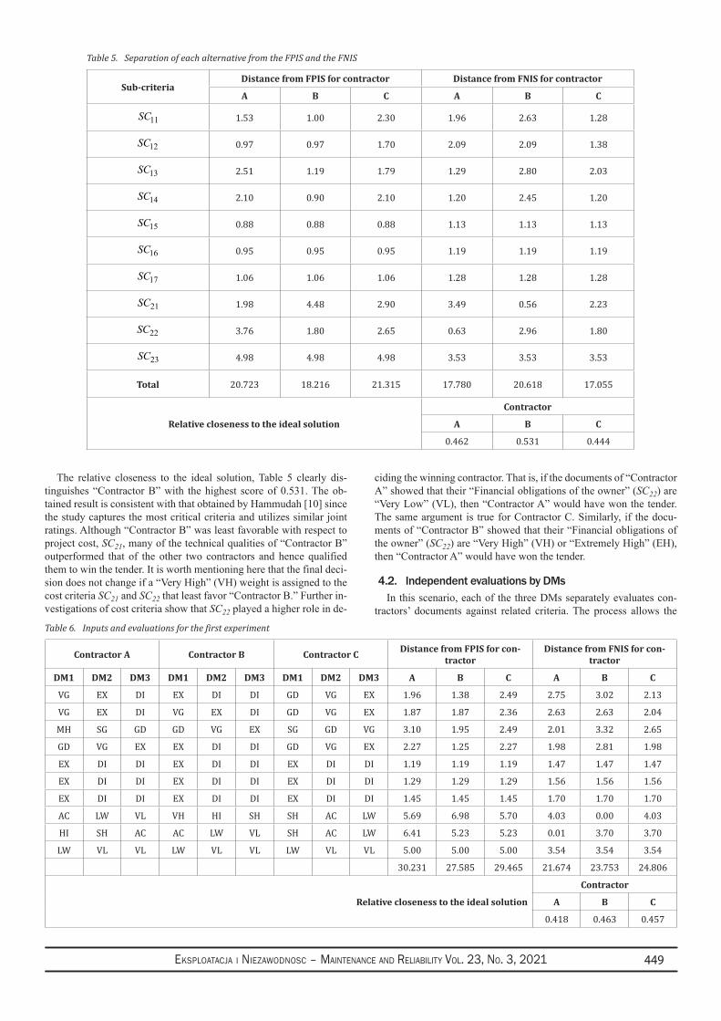
Eksploatacja i NiEzawodNosc – MaiNtENaNcE aNd REliability Vol. 23, No. 3, 2021 449
The relative closeness to the ideal solution, Table 5 clearly dis-tinguishes “Contractor B” with the highest score of 0.531. The ob-tained result is consistent with that obtained by Hammudah [10] since the study captures the most critical criteria and utilizes similar joint ratings. Although “Contractor B” was least favorable with respect to project cost, SC21, many of the technical qualities of “Contractor B” outperformed that of the other two contractors and hence qualified them to win the tender. It is worth mentioning here that the final deci-sion does not change if a “Very High” (VH) weight is assigned to the cost criteria SC21 and SC22 that least favor “Contractor B.” Further in-vestigations of cost criteria show that SC22 played a higher role in de-
ciding the winning contractor. That is, if the documents of “Contractor A” showed that their “Financial obligations of the owner” (SC22) are “Very Low” (VL), then “Contractor A” would have won the tender. The same argument is true for Contractor C. Similarly, if the docu-ments of “Contractor B” showed that their “Financial obligations of the owner” (SC22) are “Very High” (VH) or “Extremely High” (EH), then “Contractor A” would have won the tender.
4.2. Independent evaluations by DMsIn this scenario, each of the three DMs separately evaluates con-
tractors’ documents against related criteria. The process allows the Table 6. Inputs and evaluations for the first experiment
Contractor A Contractor B Contractor C Distance from FPIS for con-tractor
Distance from FNIS for con-tractor
DM1 DM2 DM3 DM1 DM2 DM3 DM1 DM2 DM3 A B C A B C
VG EX DI EX DI DI GD VG EX 1.96 1.38 2.49 2.75 3.02 2.13
VG EX DI VG EX DI GD VG EX 1.87 1.87 2.36 2.63 2.63 2.04
MH SG GD GD VG EX SG GD VG 3.10 1.95 2.49 2.01 3.32 2.65
GD VG EX EX DI DI GD VG EX 2.27 1.25 2.27 1.98 2.81 1.98
EX DI DI EX DI DI EX DI DI 1.19 1.19 1.19 1.47 1.47 1.47
EX DI DI EX DI DI EX DI DI 1.29 1.29 1.29 1.56 1.56 1.56
EX DI DI EX DI DI EX DI DI 1.45 1.45 1.45 1.70 1.70 1.70
AC LW VL VH HI SH SH AC LW 5.69 6.98 5.70 4.03 0.00 4.03
HI SH AC AC LW VL SH AC LW 6.41 5.23 5.23 0.01 3.70 3.70
LW VL VL LW VL VL LW VL VL 5.00 5.00 5.00 3.54 3.54 3.54
30.231 27.585 29.465 21.674 23.753 24.806
Relative closeness to the ideal solution
Contractor
A B C
0.418 0.463 0.457
Table 5. Separation of each alternative from the FPIS and the FNIS
Sub-criteriaDistance from FPIS for contractor Distance from FNIS for contractor
A B C A B C
11SC 1.53 1.00 2.30 1.96 2.63 1.28
12SC 0.97 0.97 1.70 2.09 2.09 1.38
13SC 2.51 1.19 1.79 1.29 2.80 2.03
14SC 2.10 0.90 2.10 1.20 2.45 1.20
15SC 0.88 0.88 0.88 1.13 1.13 1.13
16SC 0.95 0.95 0.95 1.19 1.19 1.19
17SC 1.06 1.06 1.06 1.28 1.28 1.28
21SC 1.98 4.48 2.90 3.49 0.56 2.23
22SC 3.76 1.80 2.65 0.63 2.96 1.80
23SC 4.98 4.98 4.98 3.53 3.53 3.53
Total 20.723 18.216 21.315 17.780 20.618 17.055
Relative closeness to the ideal solution
Contractor
A B C
0.462 0.531 0.444
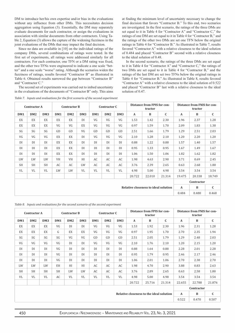
Eksploatacja i NiEzawodNosc – MaiNtENaNcE aNd REliability Vol. 23, No. 3, 2021450
DM to introduce her/his own expertise and/or bias in the evaluations without any influence from other DMs. This necessitates decision aggregation using Equation (3). Essentially, the DM may separately evaluate documents for each contractor, or assign the evaluations in association with similar documents from other contractors. Using Ta-ble 2, Equation (3) allows the capture of the widening fuzziness in the joint evaluations of the DMs that may impact the final decision.
Since no data are available in [10] on the individual ratings of the company DMs, several combinations of ratings were tested. In the first set of experiments, all ratings were addressed similarly for all contractors. For each contractor, one TFN or a DM rating was fixed, and the other two TFNs were engineered to indicate a one scale “bet-ter” and a one scale “worse” rating. Although the scenarios widen the fuzziness of ratings, results favored “Contractor B” as illustrated in Table 6. Obtained results narrowed the gap between “Contractor B” and “Contractor C.”
The second set of experiments was carried out to imbed uncertainty in the evaluations of the documents of “Contractor B” only. This aims
at finding the minimum level of uncertainty necessary to change the final decision that favors “Contractor B.” To this end, two scenarios are investigated. In the first scenario, the ratings of the three DMs are set equal to it in Table 4 for “Contractor A” and “Contractor C,” the ratings of one DM are set equal to it in Table 4 for “Contractor B,” and the ratings of the other two DMs are set one TFN below the original ratings in Table 4 for “Contractor B.” As illustrated in Table 7, results favored “Contractor A” with a relative closeness to the ideal solution of 0.484 and placed “Contractor B” second with a relative closeness to the ideal solution of 0.48.
In the second scenario, the ratings of the three DMs are set equal to it in Table 4 for “Contractor A” and “Contractor C,” the ratings of two DMs are set equal to it in Table 4 for “Contractor B,” and the ratings of the last DM are set two TFNs below the original ratings in Table 4 for “Contractor B.” As illustrated in Table 8, results favored “Contractor A” with a relative closeness to the ideal solution of 0.522 and placed “Contractor B” last with a relative closeness to the ideal solution of 0.47.
Table 7. Inputs and evaluations for the first scenario of the second experiment
Contractor A Contractor B Contractor C Distance from FPIS for con-tractor
Distance from FNIS for con-tractor
DM1 DM2 DM3 DM1 DM2 DM3 DM1 DM2 DM3 A B C A B C
EX EX EX EX EX DI VG VG VG 1.53 1.42 2.30 1.96 2.37 1.28
EX EX EX VG VG EX VG VG VG 0.97 1.59 1.70 2.09 1.83 1.38
SG SG SG GD GD VG GD GD GD 2.51 1.66 1.79 1.29 2.51 2.03
VG VG VG EX EX DI VG VG VG 2.10 1.28 2.10 1.20 2.20 1.20
DI DI DI EX EX DI DI DI DI 0.88 1.22 0.88 1.57 1.40 1.57
DI DI DI EX EX DI DI DI DI 0.95 1.33 0.95 1.67 1.49 1.67
DI DI DI EX EX DI DI DI DI 1.06 1.50 1.06 1.82 1.62 1.82
LW LW LW VH VH HI AC AC AC 1.98 4.63 2.90 3.71 0.69 2.45
SH SH SH AC AC LW AC AC AC 3.76 2.39 2.65 0.63 2.68 1.80
VL VL VL LW LW VL VL VL VL 4.98 5.00 4.98 3.54 3.54 3.54
20.722 22.010 21.314 19.475 20.338 18.749
Relative closeness to ideal solution
Contractor
A B C
0.484 0.480 0.468
Table 8. Inputs and evaluations for the second scenario of the second experiment
Contractor A Contractor B Contractor C Distance from FPIS for con-tractor
Distance from FNIS for con-tractor
DM1 DM2 DM3 DM1 DM2 DM3 DM1 DM2 DM3 A B C A B C
EX EX EX VG DI DI VG VG VG 1.53 1.92 2.30 1.96 2.31 1.28
EX EX EX G EX EX VG VG VG 0.97 1.95 1.70 2.70 2.35 1.94
SG SG SG SG VG VG GD GD GD 2.51 2.05 1.79 1.29 2.48 2.03
VG VG VG VG DI DI VG VG VG 2.10 1.76 2.10 1.20 2.15 1.20
DI DI DI VG DI DI DI DI DI 0.88 1.64 0.88 2.28 2.01 2.28
DI DI DI VG DI DI DI DI DI 0.95 1.79 0.95 2.46 2.17 2.46
DI DI DI VG DI DI DI DI DI 1.06 2.01 1.06 2.70 2.38 2.70
LW LW LW EH HI HI AC AC AC 1.98 4.70 2.90 3.88 0.83 2.63
SH SH SH SH LW LW AC AC AC 3.76 2.89 2.65 0.63 2.58 1.80
VL VL VL AC VL VL VL VL VL 4.98 5.00 4.98 3.54 3.54 3.54
20.722 25.716 21.314 22.655 22.788 21.876
Relative closeness to the ideal solution
Contractor
A B C
0.522 0.470 0.507
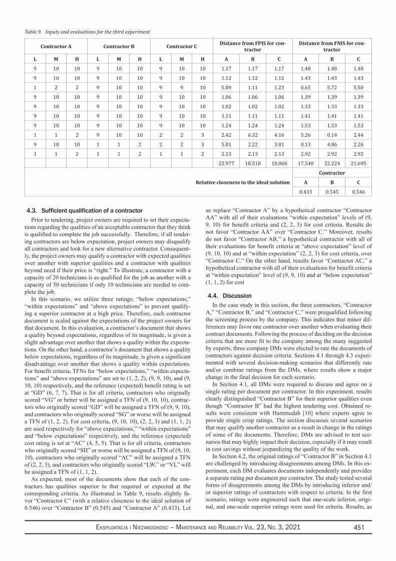
Eksploatacja i NiEzawodNosc – MaiNtENaNcE aNd REliability Vol. 23, No. 3, 2021 451
4.3. SufficientqualificationofacontractorPrior to tendering, project owners are required to set their expecta-
tions regarding the qualities of an acceptable contractor that they think is qualified to complete the job successfully. Therefore, if all tender-ing contractors are below expectation, project owners may disqualify all contractors and look for a new alternative contractor. Consequent-ly, the project owners may qualify a contractor with expected qualities over another with superior qualities and a contractor with qualities beyond need if their price is “right.” To illustrate, a contractor with a capacity of 20 technicians is as qualified for the job as another with a capacity of 50 technicians if only 10 technicians are needed to com-plete the job.
In this scenario, we utilize three ratings; “below expectations,” “within expectations” and “above expectations” to prevent qualify-ing a superior contractor at a high price. Therefore, each contractor document is scaled against the expectations of the project owners for that document. In this evaluation, a contractor’s document that shows a quality beyond expectations, regardless of its magnitude, is given a slight advantage over another that shows a quality within the expecta-tions. On the other hand, a contractor’s document that shows a quality below expectations, regardless of its magnitude, is given a significant disadvantage over another that shows a quality within expectations. For benefit criteria, TFNs for “below expectations,” “within expecta-tions” and “above expectations” are set to (1, 2, 2), (9, 9, 10), and (9, 10, 10) respectively, and the reference (expected) benefit rating is set at “GD” (6, 7, 7). That is for all criteria, contractors who originally scored “VG” or better will be assigned a TFN of (9, 10, 10), contrac-tors who originally scored “GD” will be assigned a TFN of (9, 9, 10), and contractors who originally scored “SG” or worse will be assigned a TFN of (1, 2, 2). For cost criteria, (9, 10, 10), (2, 2, 3) and (1, 1, 2) are used respectively for “above expectations,” “within expectations” and “below expectations” respectively, and the reference (expected) cost rating is set at “AC” (4, 5, 5). That is for all criteria, contractors who originally scored “SH” or worse will be assigned a TFN of (9, 10, 10), contractors who originally scored “AC” will be assigned a TFN of (2, 2, 3), and contractors who originally scored “LW,” or “VL” will be assigned a TFN of (1, 1, 2).
As expected, most of the documents show that each of the con-tractors has qualities superior to that required or expected at the corresponding criteria. As illustrated in Table 9, results slightly fa-vor “Contractor C” (with a relative closeness to the ideal solution of 0.546) over “Contractor B” (0.545) and “Contractor A” (0.433). Let
us replace “Contractor A” by a hypothetical contractor “Contractor AA” with all of their evaluations “within expectation” levels of (9, 9, 10) for benefit criteria and (2, 2, 3) for cost criteria. Results do not favor “Contractor AA” over “Contractor C.” Moreover, results do not favor “Contractor AB,” a hypothetical contractor with all of their evaluations for benefit criteria at “above expectation” level of (9, 10, 10) and at “within expectation” (2, 2, 3) for cost criteria, over “Contractor C.” On the other hand, results favor “Contractor AC,” a hypothetical contractor with all of their evaluations for benefit criteria at “within expectation” level of (9, 9, 10) and at “below expectation” (1, 1, 2) for cost
4.4. DiscussionIn the case study in this section, the three contractors, “Contractor
A,” “Contractor B,” and “Contractor C,” were prequalified following the screening process by the company. This indicates that minor dif-ferences may favor one contractor over another when evaluating their contract documents. Following the process of deciding on the decision criteria that are more fit to the company among the many suggested by experts, three company DMs were elected to rate the documents of contractors against decision criteria. Sections 4.1 through 4.3 experi-mented with several decision-making scenarios that differently rate and/or combine ratings from the DMs, where results show a major change in the final decision for each scenario.
In Section 4.1, all DMs were required to discuss and agree on a single rating per document per contractor. In this experiment, results clearly distinguished “Contractor B” for their superior qualities even though “Contractor B” had the highest tendering cost. Obtained re-sults were consistent with Hammudah [10] where experts agree to provide single crisp ratings. The section discusses several scenarios that may qualify another contractor as a result in change in the ratings of some of the documents. Therefore, DMs are advised to test sce-narios that may highly impact their decision, especially if it may result in cost savings without jeopardizing the quality of the work.
In Section 4.2, the original ratings of “Contractor B” in Section 4.1 are challenged by introducing disagreements among DMs. In this ex-periment, each DM evaluates documents independently and provides a separate rating per document per contractor. The study tested several forms of disagreements among the DMs by introducing inferior and/or superior ratings of contractors with respect to criteria. In the first scenario, ratings were engineered such that one-scale inferior, origi-nal, and one-scale superior ratings were used for criteria. Results, as
Table 9. Inputs and evaluations for the third experiment
Contractor A Contractor B Contractor C Distance from FPIS for con-tractor
Distance from FNIS for con-tractor
L M H L M H L M H A B C A B C
9 10 10 9 10 10 9 10 10 1.17 1.17 1.17 1.48 1.48 1.48
9 10 10 9 10 10 9 10 10 1.12 1.12 1.12 1.43 1.43 1.43
1 2 2 9 10 10 9 9 10 5.89 1.11 1.23 0.65 5.72 5.50
9 10 10 9 10 10 9 10 10 1.06 1.06 1.06 1.39 1.39 1.39
9 10 10 9 10 10 9 10 10 1.02 1.02 1.02 1.33 1.33 1.33
9 10 10 9 10 10 9 10 10 1.11 1.11 1.11 1.41 1.41 1.41
9 10 10 9 10 10 9 10 10 1.24 1.24 1.24 1.53 1.53 1.53
1 1 2 9 10 10 2 2 3 2.42 6.32 4.16 5.26 0.14 2.44
9 10 10 1 1 2 2 2 3 5.81 2.22 3.81 0.13 4.86 2.26
1 1 2 1 1 2 1 1 2 2.13 2.13 2.13 2.92 2.92 2.92
22.977 18.518 18.068 17.540 22.224 21.695
Relative closeness to the ideal solution
Contractor
A B C
0.433 0.545 0.546
Eksploatacja i NiEzawodNosc – MaiNtENaNcE aNd REliability Vol. 23, No. 3, 2021452
expected, favored “Contractor B” since they were rated “DI” in most of the benefit criteria and were rated “HI” in their worst cost criteria. In the second scenario, all of the ratings of “Contractor A” and “Con-tractor C” are set equal to original ratings. For “Contractor B,” one rating of is set equal to the original, and the other two ratings were set one-scale inferior to the original for all criteria. Results slightly favored “Contractor A” over “Contractor B,” which shows a form of disagreement among DMs that may result in a significant change in the decision. The last scenario, also, sets ratings of “Contractor A” and “Contractor C” to original. For “Contractor B,” two ratings were set equal to the original, and the third was set two-scales inferior to the original. Results significantly favored “Contractor A” over “Con-tractor B,” who came last. The scenario shows the significance of the “odd” rating that might be biased by the trade of the DM while evaluating documents from different trades. It is common to see such forms of disagreements among DMs in the many studies in the litera-ture where clusters of evaluations may be highly influenced by one or more outliers, which can be clearly seen through computed TFNs. Therefore, although disagreements are healthy, data must be cleaned, and clear outliers must be excluded.
Section 4.3 introduces a new scale to narrow the chances of fa-voring a contractor with superior qualities that will not significantly benefit the project owner. In a job setting, if a worker with two years of experience is considered qualified to complete the job, there will be no significant advantage to hiring a worker with more than two years of experience, especially at a higher rate of pay. In this scenario, rat-ings are set to slightly favor a contractor with qualities superior to ex-pected, while it largely penalizes the one with inferior qualities. Since all contractors in the study were prequalified, many scored similarly
for most of the criteria. The results of the scenario favored “Contrac-tor C” over the other two contractors mainly for their ratings in cost criteria. The change of the results calls upon DMs to look back to the screening stage where they might disqualify a contractor solely because others provided better documents.
5. ConclusionThe paper presents a Fuzzy-TOPSIS decision-making model for
selecting maintenance contractors based on the quality of submitted tender documents. The model allows multiple DMs with different in-fluences to use linguistic (Fuzzy) assessments to arrive at a common decision. The proposed model is applied to a case study from the lit-erature [10]. Several decision scenarios are tested, where each result qualified a different contractor for the job. Results obtained from the study scenarios illustrate a potentially major change in the decision based on the way the decision-making process is performed. This calls upon DMs to better address uncertainties in their ratings to avoid crisp over- or under-rating of qualities and costs. Moreover, DMs must en-sure a healthy disagreement to reduce potential biases and to prevent outsourcing mistakes, including tendering an over-qualified contrac-tor at a higher cost. Since only three DMs and three contractors were included in the study, future work will focus on conducting real-life experiments that will include more DMs and more contractors. More-over, future studies may utilize AHP, or ANP to captures dependen-cies, to obtain results based on relative comparisons. Furthermore, future studies will be conducted around several forms of disagreement among the DMs to better embed and control biases.
References1. Alsyouf I. Cost Effective Maintenance for Competitive Advantages. Acta Wexionensia 2004; 33: 1-98.2. Alzahrani J, Emsley M. The impact of contractors' attributes on construction project success: A post construction evaluation. International
Journal of Project Management 2012; 31: 313-322, https://doi.org/10.1016/j.ijproman.2012.06.006.3. Azimifard A, Moosavirad S, Ariafar S. Selecting sustainable supplier countries for Iran's steel industry at three levels by using AHP and
TOPSIS methods. Resources Policy 2018; 57: 30-44, https://doi.org/10.1016/j.resourpol.2018.01.002.4. Bukowski L, Werbińska-Wojciechowska S. Using fuzzy logic to support maintenance decisions according to Resilience-Based Maintenance
concept. Eksploatacja i Niezawodnosc - Maintenance and Reliability 2021; 23 (2): 294-307, https://doi.org/10.17531/ein.2021.2.9.5. Cebi F, Otay I. An Integrated Approach to Supplier Selection and Order Allocation Problem: A Case Study in a Hospital. Proceedings of the
17th International Working Seminar on Production Economics, Innsbruck, Austria 2012.6. Chen, C. Extensions of the TOPSIS for group decision-making under fuzzy environment. Fuzzy Sets and Systems 2000; 114: 1-9, https://
doi.org/10.1016/S0165-0114(97)00377-1.7. Darvish M, Yasaei M, Saeedi A. Application of the graph theory and matrix methods to contractor ranking. International Journal of Project
Management 2009; 27: 610-619, https://doi.org/10.1016/j.ijproman.2008.10.004.8. Fu Y. An integrated approach to catering supplier selection using AHP-ARASMCGP Methodology. Journal of Air Transport Management
2019; 75: 164-169, https://doi.org/10.1016/j.jairtraman.2019.01.011.9. Hafeez K, Malak N, Zhang Y. Outsourcing non-core assets and competences of a firm using AHP. Computers and Operations Research 2007;
34: 3592- 3608, https://doi.org/10.1016/j.cor.2006.01.004.10. Hammudah N. Multi Criteria Decision Making Model for Outsourcing Maintenance Services: A Case Study of Cranes Industry. Master
thesis, Isra University, Jordan 201411. Hua Y, Xiaoa S, Wena J, Li J. An ANP-multi-criteria-based methodology to construct maintenance networks for agricultural machinery cluster
in a balanced scorecard context. Computers and Electronics in Agriculture 2019; 158: 1-10, https://doi.org/10.1016/j.compag.2019.01.031.12. Hwang C, Yoon K. Multiple Attribute Decision Making: Methods and Applications. New York: Springer-Verlag 1981, https://doi.
org/10.1007/978-3-642-48318-9.13. Jain V, Sangaiah A, Sakhuja S, Thoduka N, Aggarwal R. Supplier selection using fuzzy AHP and TOPSIS: a case study in the Indian
automotive industry. Neural Computing and Applications 2018; 29: 555-564, https://doi.org/10.1007/s00521-016-2533-z.14. Jasiulewicz-Kaczmarek M, Antosz K, Wyczółkowski R, Mazurkiewicz D, Sun B, Qian C, Ren Y. Application of MICMAC, Fuzzy AHP,
and Fuzzy TOPSIS for Evaluation of the Maintenance Factors Affecting Sustainable Manufacturing. Energies 2021; 14: 1436, https://doi.org/10.3390/en14051436.
15. Jaskowsk P, Biruk S, Bucon R. Assessing contractor selection criteria weights with fuzzy AHP method application in group decision environment. Automation in Construction 2010; 19: 120-126, https://doi.org/10.1016/j.autcon.2009.12.014.
16. Lam K, Yu C. A multiple kernel learning-based decision support model for contractor pre-qualification. Automation in Construction 2011; 20: 531-536, https://doi.org/10.1016/j.autcon.2010.11.019.
17. Mahdi I, Riley M, Fereig S, Alex A. A multicriteria approach to contractor selection. Engineering Construction and Architectural Management 2002; 9: 29-37, https://doi.org/10.1108/eb021204.
18. Memari A, Dargib A, Jokara M, Robiah A, Abdul Rahim A. Sustainable supplier selection: A multi-criteria intuitionistic fuzzy TOPSIS

Eksploatacja i NiEzawodNosc – MaiNtENaNcE aNd REliability Vol. 23, No. 3, 2021 453
Method. Journal of Manufacturing Systems 2019; 50: 9-24, https://doi.org/10.1016/j.jmsy.2018.11.002.19. Moline J, Coves A. Supplier Evaluation and Selection: A Review of the literature since 2007. The 7th International Conference on Industrial
Engineering and Industrial Management, Spain 2013, https://doi.org/10.1007/978-3-319-04705-8_25.20. Nieto-Morote A, Ruz-Vila F. A fuzzy multi-criteria decision-making model for construction contractor prequalification. Automation in
Construction 2012; 25: 8-19, https://doi.org/10.1016/j.autcon.2012.04.004.21. Pankaj G, Mukesh K, Divya M. Multi-objective optimization framework for software maintenance, component evaluation and selection
involving outsourcing, redundancy and customer to customer relationship. Information Sciences 2019; 483: 21-52, https://doi.org/10.1016/j.ins.2019.01.017.
22. Poudeha H, Cheshmberah M, Torabi H, Gavareshki M, Reza H. Determining and prioritizing the factors influencing the outsourcing of Complex Product Systems R&D projects employing ANP and grey-DEMATEL method (case study: Aviation Industries Organization, Iran). Technology in Society 2019; 56: 57-68, https://doi.org/10.1016/j.techsoc.2018.09.005.
23. Rezaei J, Fahim P, Tavasszy L. Supplier selection in the airline retail industry using a funnel methodology: Conjunctive screening method and fuzzy AHP. Expert Systems with Applications 2014; 41: 8165-8179, https://doi.org/10.1016/j.eswa.2014.07.005.
24. Saghafian S, Hejazi S. Multi-criteria Group Decision Making Using a Modified Fuzzy TOPSIS Procedure. Proceedings of the 2005 International Conference on Computational Intelligence for Modelling, Control and Automation, and International Conference on Intelligent Agents, Web Technologies and Internet Commerce (CIMCA-IAWTIC'05), Vienna, Austria 2005
25. Singh D, Tiong R. Contractor Selection Criteria: Investigation of Opinions of Singapore Construction Practitioner. Journal of Construction Engineering and Management 2006; 132: 998-1008, https://doi.org/10.1061/(ASCE)0733-9364(2006)132:9(998).
26. Victorian Civil Construction Industry, Best Practice Guide for Tendering and Contract Management. http://www.wellington.vic.gov.au/files/a708f74e-1c2f-4365-8b53-a1d300a96e05/VCCI-Best-Practice-Guide-for-Tendering-and-Contract-Management.pdf 2008
27. Zhou F, Wang X, Goh M, Zhou L, He Y. Supplier portfolio of key outsourcing parts selection using a two-stage decision making framework for Chinese domestic auto-maker. Computers & Industrial Engineering 2019; 128: 559-575, https://doi.org/10.1016/j.cie.2018.12.014.
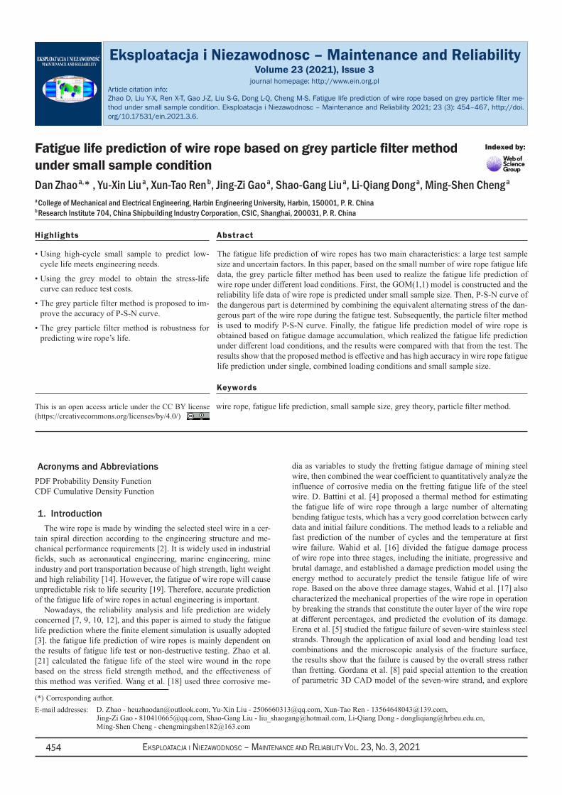
Eksploatacja i NiEzawodNosc – MaiNtENaNcE aNd REliability Vol. 23, No. 3, 2021454
(*) Corresponding author.E-mail addresses:
Eksploatacja i Niezawodnosc – Maintenance and ReliabilityVolume 23 (2021), Issue 3
journal homepage: http://www.ein.org.pl
Indexed by:
Acronyms and AbbreviationsPDF Probability Density Function CDF Cumulative Density Function
1. IntroductionThe wire rope is made by winding the selected steel wire in a cer-
tain spiral direction according to the engineering structure and me-chanical performance requirements [2]. It is widely used in industrial fields, such as aeronautical engineering, marine engineering, mine industry and port transportation because of high strength, light weight and high reliability [14]. However, the fatigue of wire rope will cause unpredictable risk to life security [19]. Therefore, accurate prediction of the fatigue life of wire ropes in actual engineering is important.
Nowadays, the reliability analysis and life prediction are widely concerned [7, 9, 10, 12], and this paper is aimed to study the fatigue life prediction where the finite element simulation is usually adopted [3]. the fatigue life prediction of wire ropes is mainly dependent on the results of fatigue life test or non-destructive testing. Zhao et al. [21] calculated the fatigue life of the steel wire wound in the rope based on the stress field strength method, and the effectiveness of this method was verified. Wang et al. [18] used three corrosive me-
dia as variables to study the fretting fatigue damage of mining steel wire, then combined the wear coefficient to quantitatively analyze the influence of corrosive media on the fretting fatigue life of the steel wire. D. Battini et al. [4] proposed a thermal method for estimating the fatigue life of wire rope through a large number of alternating bending fatigue tests, which has a very good correlation between early data and initial failure conditions. The method leads to a reliable and fast prediction of the number of cycles and the temperature at first wire failure. Wahid et al. [16] divided the fatigue damage process of wire rope into three stages, including the initiate, progressive and brutal damage, and established a damage prediction model using the energy method to accurately predict the tensile fatigue life of wire rope. Based on the above three damage stages, Wahid et al. [17] also characterized the mechanical properties of the wire rope in operation by breaking the strands that constitute the outer layer of the wire rope at different percentages, and predicted the evolution of its damage. Erena et al. [5] studied the fatigue failure of seven-wire stainless steel strands. Through the application of axial load and bending load test combinations and the microscopic analysis of the fracture surface, the results show that the failure is caused by the overall stress rather than fretting. Gordana et al. [8] paid special attention to the creation of parametric 3D CAD model of the seven-wire strand, and explore
The fatigue life prediction of wire ropes has two main characteristics: a large test sample size and uncertain factors. In this paper, based on the small number of wire rope fatigue life data, the grey particle filter method has been used to realize the fatigue life prediction of wire rope under different load conditions. First, the GOM(1,1) model is constructed and the reliability life data of wire rope is predicted under small sample size. Then, P-S-N curve of the dangerous part is determined by combining the equivalent alternating stress of the dan-gerous part of the wire rope during the fatigue test. Subsequently, the particle filter method is used to modify P-S-N curve. Finally, the fatigue life prediction model of wire rope is obtained based on fatigue damage accumulation, which realized the fatigue life prediction under different load conditions, and the results were compared with that from the test. The results show that the proposed method is effective and has high accuracy in wire rope fatigue life prediction under single, combined loading conditions and small sample size.
Highlights Abstract
Using high-cycle small sample to predict low-• cycle life meets engineering needs.
Using the grey model to obtain the stress-life • curve can reduce test costs.
The grey particle filter method is proposed to im-• prove the accuracy of P-S-N curve.
The grey particle filter method is robustness for • predicting wire rope’s life.
Fatigue life prediction of wire rope based on grey particle filter method under small sample conditionDan Zhao a,* , Yu-Xin Liu a, Xun-Tao Ren b, Jing-Zi Gao a, Shao-Gang Liu a, Li-Qiang Dong a, Ming-Shen Cheng a
a College of Mechanical and Electrical Engineering, Harbin Engineering University, Harbin, 150001, P. R. China b Research Institute 704, China Shipbuilding Industry Corporation, CSIC, Shanghai, 200031, P. R. China
Zhao D, Liu Y-X, Ren X-T, Gao J-Z, Liu S-G, Dong L-Q, Cheng M-S. Fatigue life prediction of wire rope based on grey particle filter me-thod under small sample condition. Eksploatacja i Niezawodnosc – Maintenance and Reliability 2021; 23 (3): 454–467, http://doi.org/10.17531/ein.2021.3.6.
Article citation info:
wire rope, fatigue life prediction, small sample size, grey theory, particle filter method.
Keywords
This is an open access article under the CC BY license (https://creativecommons.org/licenses/by/4.0/)
D. Zhao - [email protected], Yu-Xin Liu - [email protected], Xun-Tao Ren - [email protected], Jing-Zi Gao - [email protected], Shao-Gang Liu - [email protected], Li-Qiang Dong - [email protected], Ming-Shen Cheng - [email protected]
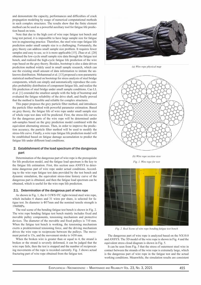
Eksploatacja i NiEzawodNosc – MaiNtENaNcE aNd REliability Vol. 23, No. 3, 2021 455
and demonstrate the capacity, performances and difficulties of crack propagation modeling by usage of numerical computational methods in such complex structures. The results show that the finite element method can be used as a powerful auxiliary tool for fatigue life predic-tion based on tests.
Note that due to the high cost of wire rope fatigue test bench and long test period, it is impossible to have large sample size for fatigue test in engineering practice. Therefore, the steel wire rope fatigue life prediction under small sample size is a challenging. Fortunately, the grey theory can address small sample size problem. It requires fewer samples and easy to use, so it is more applicable [15]. Zhao et al. [20] obtained the low-cycle small sample size data through the fatigue test bench, and realized the high-cycle fatigue life prediction of the wire rope based on the grey theory. Besides, bootstrap is also a data-driven prediction method widely used in small sample research, which can use the existing small amount of data information to imitate the un-known distribution. Mohammad et al. [13] proposed a non-parametric statistical method based on bootstrap for stress analysis of steel bridge components, which can simply and automatically reproduce the com-plex probability distribution of component fatigue life, and realize the life prediction of steel bridge under small sample conditions. Cao LL et al. [1] extended the smallest sample with the help of bootstrap and evaluated the fatigue reliability of the drive shaft, and finally proved that the method is feasible and reliable for complex structures.
This paper proposes the grey particle filter method, and introduces the particle filter method with powerful parameter estimation. Based on grey theory, the fatigue life of wire rope under small sample size of whole rope test data will be predicted. First, the stress-life curves for the dangerous parts of the wire rope will be determined under sub-samples based on the grey prediction model combined with the equivalent alternating stresses. Then, in order to improve the predic-tion accuracy, the particle filter method will be used to modify the stress-life curve. Finally, a wire rope fatigue life prediction model will be established based on fatigue damage accumulation to predict the fatigue life under different load conditions.
2. Establishment of the load spectrum of the dangerous part
Determination of the dangerous part of wire rope is the prerequisite for life prediction model, and the fatigue load spectrum is the key to the fatigue life estimation. First, this section uses ANSYS to deter-mine dangerous part of wire rope under actual conditions. Accord-ing to the wire rope fatigue test data provided by the test bench and dynamic simulation, the equivalent stress-time history curve of the dangerous part is obtained, and then the fatigue load spectrum can be obtained, which is useful for the wire rope life prediction.
2.1. Determination of the dangerous part of wire ropeAs shown in Fig. 1, the 6×31WS+FC right-twisted steel wire rope,
which includes 6 shares and 31 wires per share, is selected for fa-tigue test. Its diameter is Φ37mm and the nominal tensile strength is 1960MPa.
The real scene of the bending fatigue test bench is shown in Fig. 2. The wire rope bending fatigue test bench mainly includes fixed and movable pulley components, tensioning mechanism and protective devices. The diameter of the movable and fixed pulleys is 710 mm. When the fatigue test bench is working, the tensioning mechanism exerts a predetermined tensioning force, and the driving mechanism drives the wire rope to reciprocate between the pulleys. The move-ment period is 15s, and the movement stroke is 1430 mm.
When the broken wire is greater than or equal to 4, the strand is broken or the strand is severely deformed, it can be judged that the wire rope fails, then the test is stopped and the number of reciprocat-ing movements of the rope is recorded currently. Fig. 3 shows actual fracturing part of wire rope obtained from the fatigue test.
The dangerous part of wire rope is analyzed based on the NX10.0 and ANSYS. The 3D model of the wire rope is shown in Fig. 4 and the equivalent stress cloud diagram is shown in Fig. 5.
It can be seen from Fig. 5 that the stress of outermost steel wire in contact between the strands of the wire rope is extremely large, which is the dangerous part of wire rope in the fatigue test and the actual working conditions. Meanwhile, the simulation results are consistent
Fig. 1. Wire rope for test
(a) Wire rope physical map
(b) Wire rope section view
Fig. 2. Real Scene of wire rope bending fatigue test bench
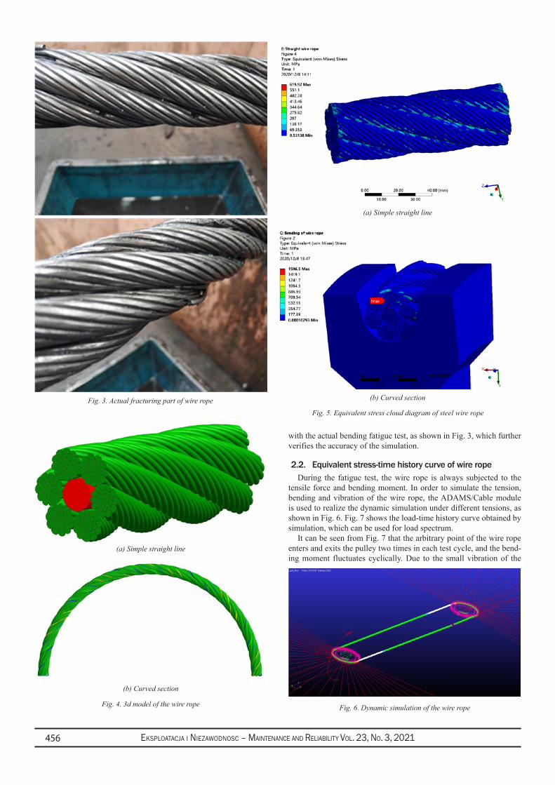
Eksploatacja i NiEzawodNosc – MaiNtENaNcE aNd REliability Vol. 23, No. 3, 2021456
with the actual bending fatigue test, as shown in Fig. 3, which further verifies the accuracy of the simulation.
2.2. Equivalent stress-time history curve of wire ropeDuring the fatigue test, the wire rope is always subjected to the
tensile force and bending moment. In order to simulate the tension, bending and vibration of the wire rope, the ADAMS/Cable module is used to realize the dynamic simulation under different tensions, as shown in Fig. 6. Fig. 7 shows the load-time history curve obtained by simulation, which can be used for load spectrum.
It can be seen from Fig. 7 that the arbitrary point of the wire rope enters and exits the pulley two times in each test cycle, and the bend-ing moment fluctuates cyclically. Due to the small vibration of the
Fig. 3. Actual fracturing part of wire ropeFig. 5. Equivalent stress cloud diagram of steel wire rope
Fig. 4. 3d model of the wire rope
(b) Curved section
(a) Simple straight line
Fig. 6. Dynamic simulation of the wire rope
(b) Curved section
(a) Simple straight line
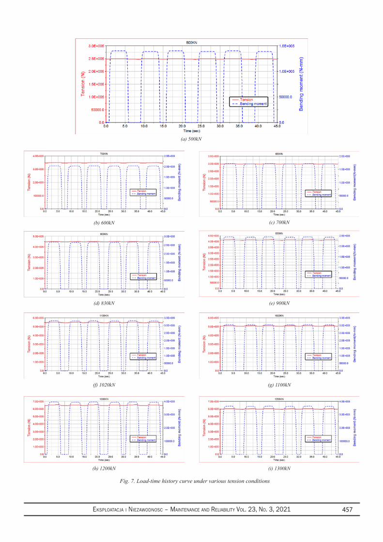
Eksploatacja i NiEzawodNosc – MaiNtENaNcE aNd REliability Vol. 23, No. 3, 2021 457
Fig. 7. Load-time history curve under various tension conditions
(b) 600kN
(d) 830kN
(f) 1020kN
(h) 1200kN
(c) 700kN
(e) 900kN
(g) 1100kN
(i) 1300kN
(a) 500kN
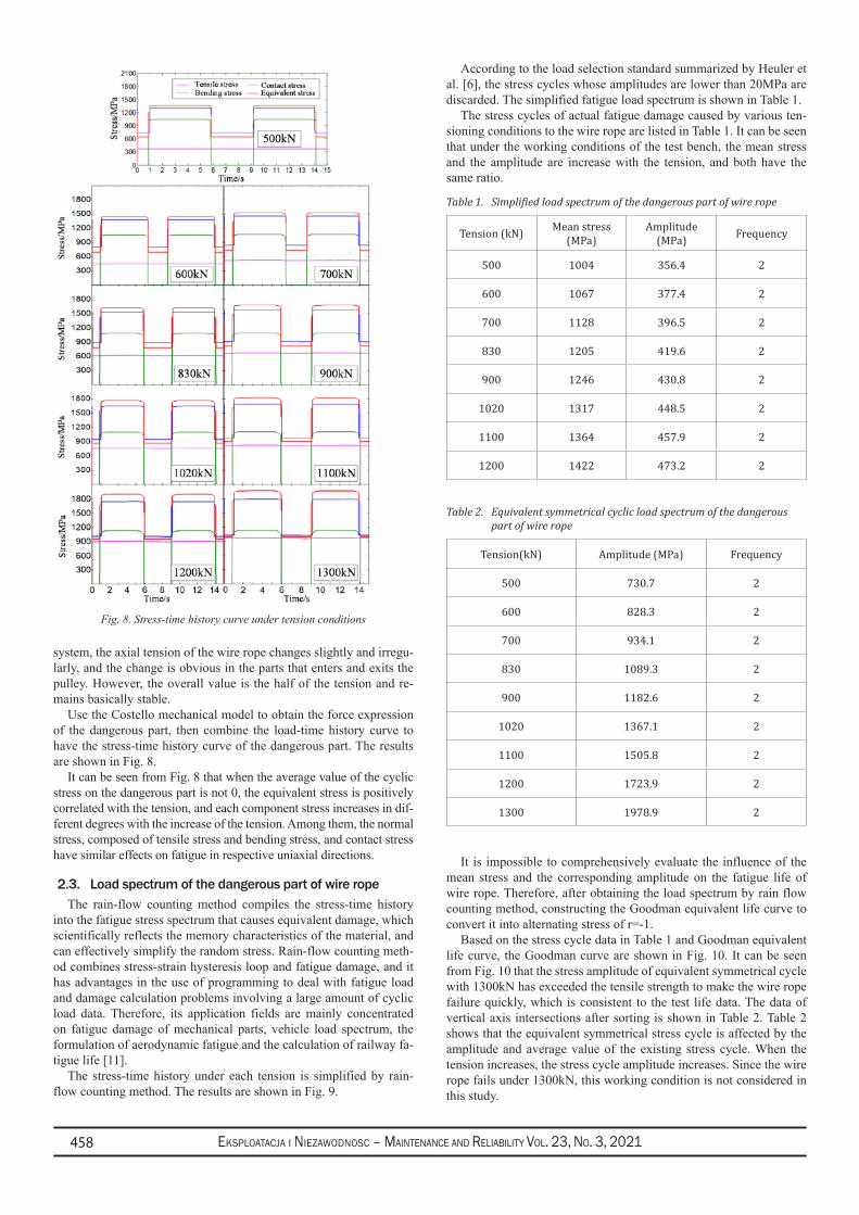
Eksploatacja i NiEzawodNosc – MaiNtENaNcE aNd REliability Vol. 23, No. 3, 2021458
system, the axial tension of the wire rope changes slightly and irregu-larly, and the change is obvious in the parts that enters and exits the pulley. However, the overall value is the half of the tension and re-mains basically stable.
Use the Costello mechanical model to obtain the force expression of the dangerous part, then combine the load-time history curve to have the stress-time history curve of the dangerous part. The results are shown in Fig. 8.
It can be seen from Fig. 8 that when the average value of the cyclic stress on the dangerous part is not 0, the equivalent stress is positively correlated with the tension, and each component stress increases in dif-ferent degrees with the increase of the tension. Among them, the normal stress, composed of tensile stress and bending stress, and contact stress have similar effects on fatigue in respective uniaxial directions.
2.3. Load spectrum of the dangerous part of wire ropeThe rain-flow counting method compiles the stress-time history
into the fatigue stress spectrum that causes equivalent damage, which scientifically reflects the memory characteristics of the material, and can effectively simplify the random stress. Rain-flow counting meth-od combines stress-strain hysteresis loop and fatigue damage, and it has advantages in the use of programming to deal with fatigue load and damage calculation problems involving a large amount of cyclic load data. Therefore, its application fields are mainly concentrated on fatigue damage of mechanical parts, vehicle load spectrum, the formulation of aerodynamic fatigue and the calculation of railway fa-tigue life [11].
The stress-time history under each tension is simplified by rain-flow counting method. The results are shown in Fig. 9.
According to the load selection standard summarized by Heuler et al. [6], the stress cycles whose amplitudes are lower than 20MPa are discarded. The simplified fatigue load spectrum is shown in Table 1.
The stress cycles of actual fatigue damage caused by various ten-sioning conditions to the wire rope are listed in Table 1. It can be seen that under the working conditions of the test bench, the mean stress and the amplitude are increase with the tension, and both have the same ratio.
It is impossible to comprehensively evaluate the influence of the mean stress and the corresponding amplitude on the fatigue life of wire rope. Therefore, after obtaining the load spectrum by rain flow counting method, constructing the Goodman equivalent life curve to convert it into alternating stress of r=-1.
Based on the stress cycle data in Table 1 and Goodman equivalent life curve, the Goodman curve are shown in Fig. 10. It can be seen from Fig. 10 that the stress amplitude of equivalent symmetrical cycle with 1300kN has exceeded the tensile strength to make the wire rope failure quickly, which is consistent to the test life data. The data of vertical axis intersections after sorting is shown in Table 2. Table 2 shows that the equivalent symmetrical stress cycle is affected by the amplitude and average value of the existing stress cycle. When the tension increases, the stress cycle amplitude increases. Since the wire rope fails under 1300kN, this working condition is not considered in this study.
Table 1. Simplified load spectrum of the dangerous part of wire rope
Tension (kN) Mean stress (MPa)
Amplitude (MPa) Frequency
500 1004 356.4 2
600 1067 377.4 2
700 1128 396.5 2
830 1205 419.6 2
900 1246 430.8 2
1020 1317 448.5 2
1100 1364 457.9 2
1200 1422 473.2 2
Table 2. Equivalent symmetrical cyclic load spectrum of the dangerous part of wire rope
Tension(kN) Amplitude (MPa) Frequency
500 730.7 2
600 828.3 2
700 934.1 2
830 1089.3 2
900 1182.6 2
1020 1367.1 2
1100 1505.8 2
1200 1723.9 2
1300 1978.9 2
Fig. 8. Stress-time history curve under tension conditions
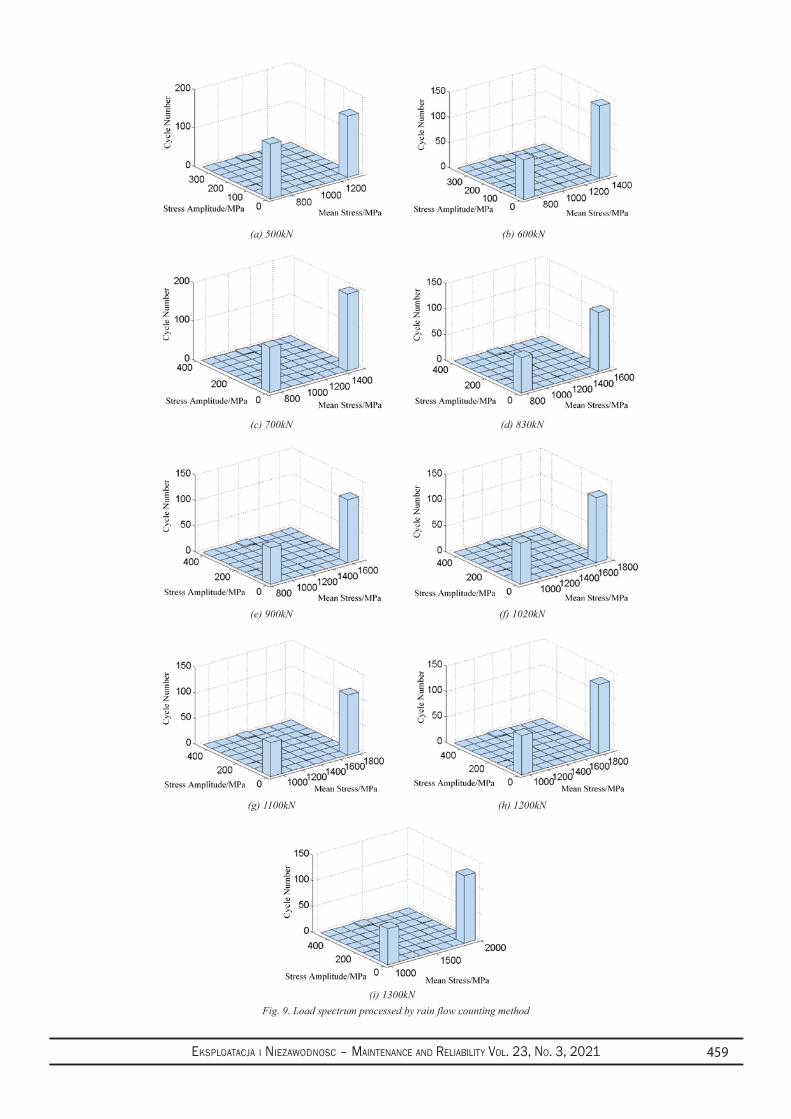
Eksploatacja i NiEzawodNosc – MaiNtENaNcE aNd REliability Vol. 23, No. 3, 2021 459
Fig. 9. Load spectrum processed by rain flow counting method
(c) 700kN
(e) 900kN
(g) 1100kN
(i) 1300kN
(a) 500kN
(d) 830kN
(f) 1020kN
(h) 1200kN
(b) 600kN
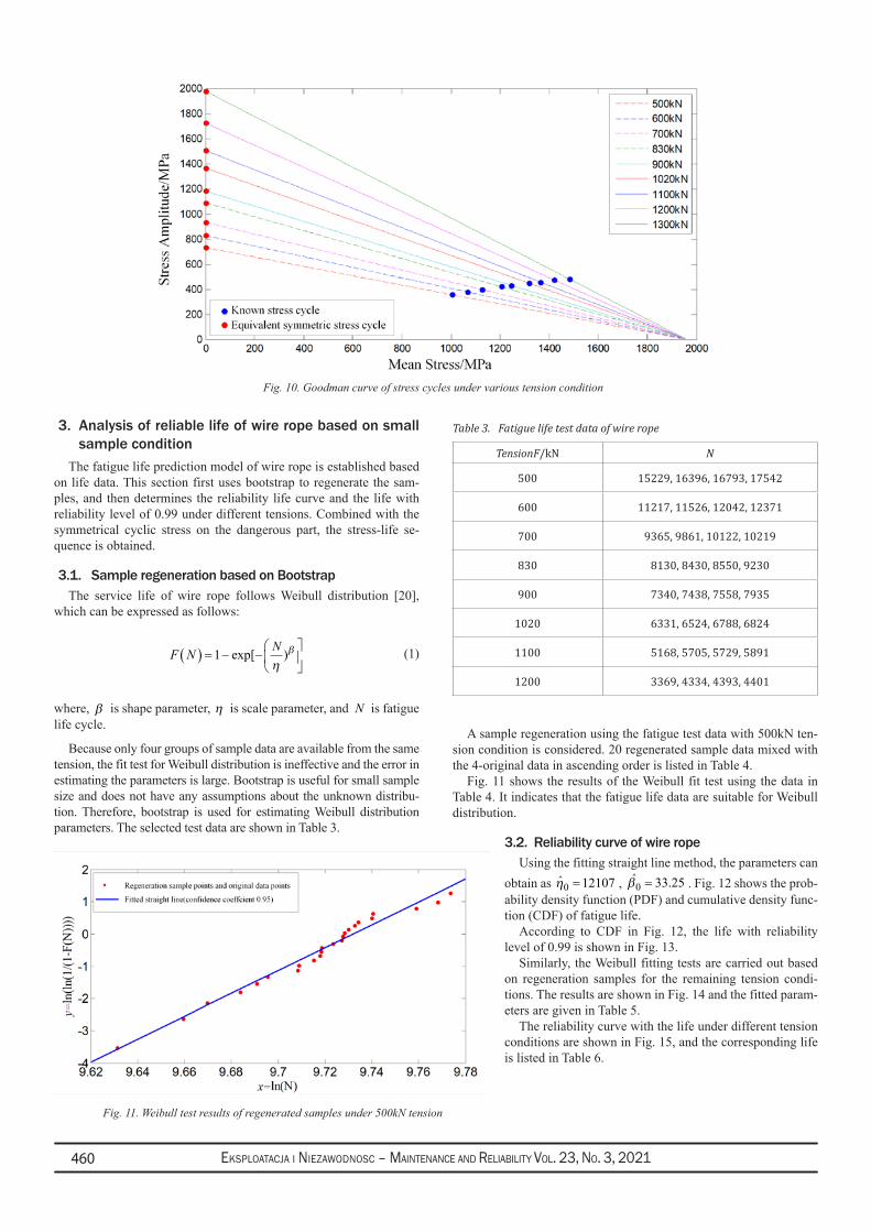
Eksploatacja i NiEzawodNosc – MaiNtENaNcE aNd REliability Vol. 23, No. 3, 2021460
3. Analysis of reliable life of wire rope based on small sample condition
The fatigue life prediction model of wire rope is established based on life data. This section first uses bootstrap to regenerate the sam-ples, and then determines the reliability life curve and the life with reliability level of 0.99 under different tensions. Combined with the symmetrical cyclic stress on the dangerous part, the stress-life se-quence is obtained.
3.1. Sample regeneration based on BootstrapThe service life of wire rope follows Weibull distribution [20],
which can be expressed as follows:
F N N( ) = − −
1 exp[ )
ηβ (1)
where, β is shape parameter, η is scale parameter, and N is fatigue life cycle.
Because only four groups of sample data are available from the same tension, the fit test for Weibull distribution is ineffective and the error in estimating the parameters is large. Bootstrap is useful for small sample size and does not have any assumptions about the unknown distribu-tion. Therefore, bootstrap is used for estimating Weibull distribution parameters. The selected test data are shown in Table 3.
A sample regeneration using the fatigue test data with 500kN ten-sion condition is considered. 20 regenerated sample data mixed with the 4-original data in ascending order is listed in Table 4.
Fig. 11 shows the results of the Weibull fit test using the data in Table 4. It indicates that the fatigue life data are suitable for Weibull distribution.
3.2. Reliability curve of wire ropeUsing the fitting straight line method, the parameters can
obtain as η0 12107=ˆ , β0 33 25= .ˆ . Fig. 12 shows the prob-ability density function (PDF) and cumulative density func-tion (CDF) of fatigue life.
According to CDF in Fig. 12, the life with reliability level of 0.99 is shown in Fig. 13.
Similarly, the Weibull fitting tests are carried out based on regeneration samples for the remaining tension condi-tions. The results are shown in Fig. 14 and the fitted param-eters are given in Table 5.
The reliability curve with the life under different tension conditions are shown in Fig. 15, and the corresponding life is listed in Table 6.
Fig. 10. Goodman curve of stress cycles under various tension condition
Fig. 11. Weibull test results of regenerated samples under 500kN tension
Table 3. Fatigue life test data of wire rope
TensionF/kN N
500 15229, 16396, 16793, 17542
600 11217, 11526, 12042, 12371
700 9365, 9861, 10122, 10219
830 8130, 8430, 8550, 9230
900 7340, 7438, 7558, 7935
1020 6331, 6524, 6788, 6824
1100 5168, 5705, 5729, 5891
1200 3369, 4334, 4393, 4401
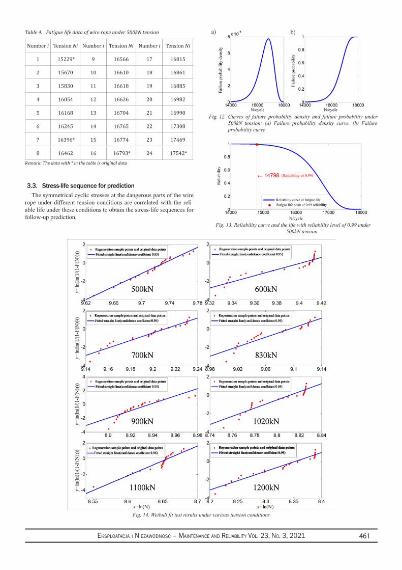
Eksploatacja i NiEzawodNosc – MaiNtENaNcE aNd REliability Vol. 23, No. 3, 2021 461
3.3. Stress-life sequence for predictionThe symmetrical cyclic stresses at the dangerous parts of the wire
rope under different tension conditions are correlated with the reli-able life under these conditions to obtain the stress-life sequences for follow-up prediction.
Table 4. Fatigue life data of wire rope under 500kN tension
Number i Tension Ni Number i Tension Ni Number i Tension Ni
1 15229* 9 16566 17 16815
2 15670 10 16610 18 16861
3 15830 11 16618 19 16885
4 16054 12 16626 20 16982
5 16168 13 16704 21 16990
6 16245 14 16765 22 17308
7 16396* 15 16774 23 17469
8 16462 16 16793* 24 17542*
Remark: The data with * in the table is original data
Fig. 12. Curves of failure probability density and failure probability under 500kN tension: (a) Failure probability density curve, (b) Failure probability curve
Fig. 13. Reliability curve and the life with reliability level of 0.99 under 500kN tension
Fig. 14. Weibull fit test results under various tension conditions
b)a)
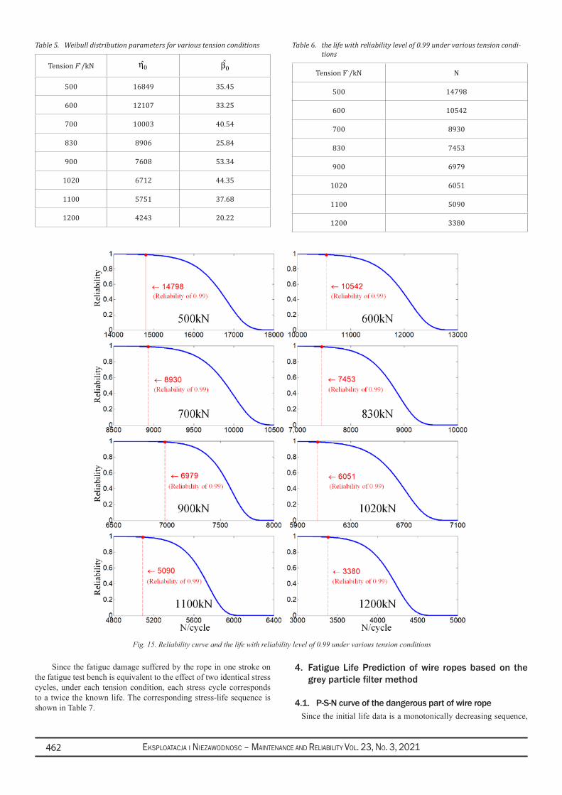
Eksploatacja i NiEzawodNosc – MaiNtENaNcE aNd REliability Vol. 23, No. 3, 2021462
Since the fatigue damage suffered by the rope in one stroke on the fatigue test bench is equivalent to the effect of two identical stress cycles, under each tension condition, each stress cycle corresponds to a twice the known life. The corresponding stress-life sequence is shown in Table 7.
4. Fatigue Life Prediction of wire ropes based on the grey particle filter method
4.1. P-S-N curve of the dangerous part of wire ropeSince the initial life data is a monotonically decreasing sequence,
Table 5. Weibull distribution parameters for various tension conditions
Tension F`/kN 0η 0β
500 16849 35.45
600 12107 33.25
700 10003 40.54
830 8906 25.84
900 7608 53.34
1020 6712 44.35
1100 5751 37.68
1200 4243 20.22
Table 6. the life with reliability level of 0.99 under various tension condi-tions
Tension F`/kN N
500 14798
600 10542
700 8930
830 7453
900 6979
1020 6051
1100 5090
1200 3380
Fig. 15. Reliability curve and the life with reliability level of 0.99 under various tension conditions
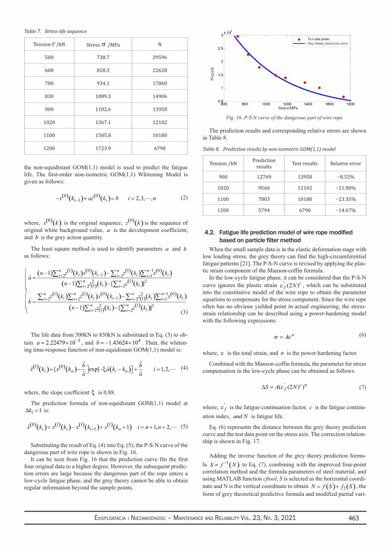
Eksploatacja i NiEzawodNosc – MaiNtENaNcE aNd REliability Vol. 23, No. 3, 2021 463
the non-equidistant GOM(1,1) model is used to predict the fatigue life. The first-order non-isometric GOM(1,1) Whitening Model is given as follows:
( )( ) ( )( )0 01 2,3, ,i ix k az k b i n−− + = =
(2)
where, ( )( )0x k is the original sequence, ( )( )0 z k is the sequence of original white background value, a is the development coefficient, and b is the grey action quantity.
The least square method is used to identify parameters a and b as follows:
( ) ( )( ) ( )( ) ( )( ) ( )( )( ) ( )( ) ( )( )
( )( ) ( )( ) ( )( ) ( )( ) ( )( )( ) ( )( ) ( )( )
11 0 1 012 2 1
12 212 2
11 1 0 021 12 2 2 1
12 212 2
1
1 [ ]
1 [ ]
n n ni i i ii i i
n ni ii i
n n n ni i i i ii i i i
n ni ii i
n z k x k z k x k
n z k z k
z k z k x k z k x k
n k
a
bz k z
−−= = =
= =
−−= = = =
= =
=
− −
− −
−
=− −
∑ ∑ ∑∑ ∑
∑ ∑ ∑ ∑∑ ∑
(3)
The life data from 500kN to 830kN is substituted in Eq. (3) to ob-tain 3 2.22479 10a −= × , and 41.43624 10b = − × . Then, the whiten-ing time-response function of non-equidistant GOM(1,1) model is:
( )( ) ( )( ) ( )1 0 1ˆ ˆ
ˆˆ
[ ˆexp[ ,2ˆ
,i n i nb bx k x k a k k ia a
ξ = − − − + =
(4)
where, the slope coefficient ξ is 0.88.
The prediction formula of non-equidistant GOM(1,1) model at 1ik∆ = is:
( )( ) ( )( ) ( )( ) ( )( )0 1 1 11 ˆ 1 1, 2,i i i nx k x k x k x k i n n+= − + + = + +
(5)
Substituting the result of Eq. (4) into Eq. (5), the P-S-N curve of the dangerous part of wire rope is shown in Fig. 16.
It can be seen from Fig. 16 that the prediction curve fits the first four original data to a higher degree. However, the subsequent predic-tion errors are large because the dangerous part of the rope enters a low-cycle fatigue phase, and the grey theory cannot be able to obtain regular information beyond the sample points.
The prediction results and corresponding relative errors are shown in Table 8.
4.2. Fatiguelifepredictionmodelofwireropemodifiedbasedonparticlefiltermethod
When the small sample data is in the elastic deformation stage with low loading stress, the grey theory can find the high-circumferential fatigue patterns [21]. The P-S-N curve is revised by applying the plas-tic strain component of the Manson-coffin formula.
In the low-cycle fatigue phase, it can be considered that the P-S-N curve ignores the plastic strain ε f
cN' ( )2 , which can be substituted into the constitutive model of the wire rope to obtain the parameter equations to compensate for the stress component. Since the wire rope often has no obvious yielded point in actual engineering, the stress-strain relationship can be described using a power-hardening model with the following expressions:
σ ε= A n (6)
where, ε is the total strain, and n is the power-hardening factor.
Combined with the Manson-coffin formula, the parameter for stress compensation in the low-cycle phase can be obtained as follows:
∆S A Nfc n= ( ( ) )'ε 2 (7)
where, ε f' is the fatigue continuation factor, c is the fatigue continu-
ation index, and N is fatigue life.
Eq. (6) represents the distance between the grey theory prediction curve and the test data point on the stress axis. The correction relation-ship is shown in Fig. 17.
Adding the inverse function of the grey theory prediction formu-la ( )1S f N−= to Eq. (7), combining with the improved four-point correlation method and the formula parameters of steel material, and using MATLAB function cftool, S is selected as the horizontal coordi-nate and N is the vertical coordinate to obtain ( ) ( )2N f S f S= + , the form of grey theoretical predictive formula and modified partial vari-
Table 8. Prediction results by non-isometric GOM(1,1) model
Tension /kN Prediction results Test results Relative error
900 12769 13958 −8.52%
1020 9560 12102 −21.00%
1100 7803 10180 −23.35%
1200 5794 6790 −14.67%
Table 7. Stress-life sequence
Tension F`/kN Stress σ /MPa N
500 730.7 29596
600 828.3 22628
700 934.1 17860
830 1089.3 14906
900 1182.6 13958
1020 1367.1 12102
1100 1505.8 10180
1200 1723.9 6790
Fig. 16. P-S-N curve of the dangerous part of wire rope
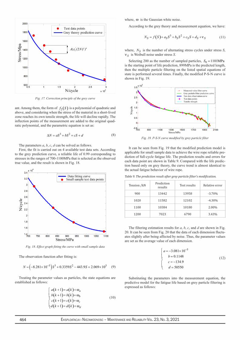
Eksploatacja i NiEzawodNosc – MaiNtENaNcE aNd REliability Vol. 23, No. 3, 2021464
ant. Among them, the form of ( )2f S is a polynomial of quadratic and above, and considering when the stress of the material in a short-lived zone reaches its own tensile strength, the life will decline rapidly. The inflection points of the measurement are added to the original quad-ratic polynomial, and the parametric equation is set as:
3 2N aS bS cS d∆ = + + + (8)
The parameters a, b, c, d can be solved as follows. First, the fit is carried out on 4 available test data sets. According
to the grey prediction curve, a reliable life of 0.99 corresponding to stresses in the ranges of 700-1100MPa that is selected as the observed true value, and the result is shown in Fig. 18.
Fig. 18. Effect graph fitting the curve with small sample data
The observation function after fitting is:
N S S S= − ×( ) + − + ×−8 281 10 0 3359 443 9 2 069 105 3 2 5. . . . (9)
Treating the parameter values as particles, the state equations are established as follows:
( ) ( )( ) ( )( ) ( )( ) ( )
1111
a
b
c
d
a k a kb k b kc k c kd k d k
ωωωω
+ = + + = + + = + + = +
(10)
where, ω is the Gaussian white noise.
According to the grey theory and measurement equation, we have:
( ) 3 2S S S S S SN f S a S b S c S d ν= + + + + + (11)
where, SN is the number of alternating stress cycles under stress S, Sν is Weibull noise under stress S.
Selecting 200 as the number of sampled particles, 0 1101MPaS = is the starting point of life prediction, 899MPa is the predicted length, then the multiple particle filtering on the listed spatial equations of state is performed several times. Finally, the modified P-S-N curve is shown in Fig. 19.
Fig. 19. P-S-N curve modified by grey particle filter
It can be seen from Fig. 19 that the modified prediction model is applicable for small sample data to achieve the wire rope reliable pre-diction of full-cycle fatigue life. The prediction results and errors for each data point are shown in Table 9. Compared with the life predic-tion based only on grey theory, the curve trend is almost identical to the actual fatigue behavior of wire rope.
The filtering estimation results for a, b, c, and d are shown in Fig. 20. It can be seen from Fig. 20 that the data of each dimension fluctu-ates slightly after being affected by noise. Thus, the parameter values are set as the average value of each dimension.
53.081 100.1148
134.950550
abcd
− = − ×
=
= − =
(12)
Substituting the parameters into the measurement equation, the predictive model for the fatigue life based on grey particle filtering is expressed as follows:
Table 9. The prediction result after grey particle filter’s modification.
Tension /kN Prediction results Test results Relative error
900 13442 13958 -3.70%
1020 11582 12102 -4.30%
1100 10384 10180 2.00%
1200 7023 6790 3.43%
Fig. 17. Correction principle of the grey curve
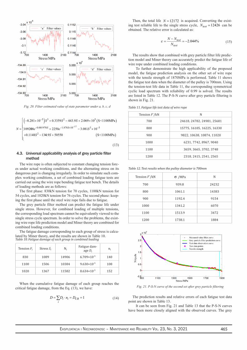
Eksploatacja i NiEzawodNosc – MaiNtENaNcE aNd REliability Vol. 23, No. 3, 2021 465
N
S S S
=
− ×( ) + − + × ( )−8 281 10 0 3359 443 9 2 069 10
1092
5 3 2 5. . . . S<1100MPa
000 2250 3 081 100 001978 1 878 10 3 5
2
17e e S
S
S S− − × −+ − ×
+ −
−. . .
0.1148 1344.9 S<1100MPaS + ( )
50550
(13)
4.3. Universalapplicabilityanalysisofgreyparticlefiltermethod
The wire rope is often subjected to constant changing tension forc-es under actual working conditions, and the alternating stress on its dangerous part is changing irregularly. In order to simulate such com-plex working conditions, a set of combined loading fatigue tests are carried out using the wire rope bending fatigue test bench. The details of loading methods are as follows:
The first phase: 830kN tension for 70 cycles, 1100kN tension for 54 cycles, and 1020kN tension for 76 cycles. The second phase: keep-ing the first phase until the steel wire rope fails due to fatigue.
The grey particle filter method can predict the fatigue life under single stress. However, for combined loading of multiple tensions, the corresponding load spectrum cannot be equivalently viewed to the single stress cycle spectrum. In order to solve the problems, the exist-ing wire rope life prediction model and Miner theory are combined for combined loading conditions.
The fatigue damage corresponding to each group of stress is calcu-lated by Miner theory, and the results are shown in Table 10.
When the cumulative fatigue damage of each group reaches the critical fatigue damage, from the Eq. (13), we have:
1i i CRi
D D n D= ⋅ = =∑ (14)
Then, the total life 12172N = is acquired. Converting the exist-ing test reliable life to the single stress cycle, 12426testN = can be obtained. The relative error is calculated as:
ε =−
= −N N
Ntest
test2 044. % (15)
The results show that combined with grey particle filter life predic-tion model and Miner theory can accurately predict the fatigue life of wire rope under combined loading conditions.
To further demonstrate the high applicability of the proposed model, the fatigue prediction analysis on the other set of wire rope with the tensile strength of 1870MPa is performed. Table 11 shows the fatigue test data when the diameter of the pulley is 700mm. Using the tension-test life data in Table 11, the corresponding symmetrical cyclic load spectrum with reliability of 0.99 is solved. The results are listed in Table 12. The P-S-N curve after grey particle filtering is shown in Fig. 21.
Fig. 21. P-S-N curve of the second set after grey particle filtering
The prediction results and relative errors of each fatigue test data point are shown in Table 13.
It can be seen from Fig. 21 and Table 13 that the P-S-N curves have been more closely aligned with the observed curves. The grey
Table 10. Fatigue damage of each group in combined loading
Tension Fi Stress Si NiFatigue dam-
age Dini
830 1089 14906 6.709×10⁻⁵ 140
1100 1506 10384 9.630×10⁻⁵ 108
1020 1367 11582 8.634×10⁻⁵ 152
Table 11. Fatigue life test data of wire rope
Tension F`/kN N
700 24618,24782,24981,25681
800 15775,16105,16225,16330
900 9822,10638,10874,11020
1000 6231,7742,8967,9040
1100 3659,3665,3702,3748
1200 2318,2415,2541,2565
Table 12. Test results when the pulley diameter is 700mm
Tension F`/kN σ /MPa N
700 939.8 24232
800 1061.1 14383
900 1192.4 9154
1000 1341.2 6070
1100 1513.9 3472
1200 1738.1 1884
Fig. 20. Filter estimated value of state parameter under a, b, c, d
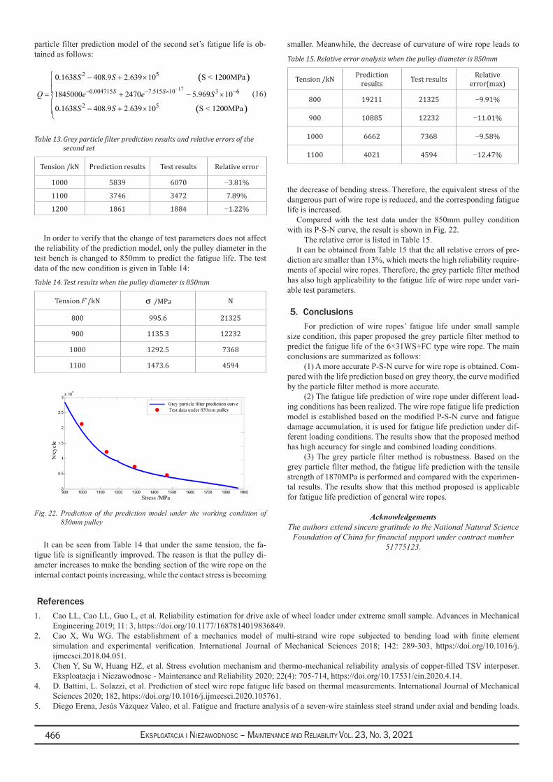
Eksploatacja i NiEzawodNosc – MaiNtENaNcE aNd REliability Vol. 23, No. 3, 2021466
particle filter prediction model of the second set’s fatigue life is ob-tained as follows:
( )
( )
17
2 5
0.004715 7.515 10 3 6
2 5
0.1638 408.9 2.639 10 S < 1200MPa
1845000 2470 5.969 10
0.1638 408.9 2.639 10 S < 1200MPa
S SQ
S S
e e S
S S
−− − × −
−
−
=
+ ×
+ ×
− +
×
(16)
In order to verify that the change of test parameters does not affect the reliability of the prediction model, only the pulley diameter in the test bench is changed to 850mm to predict the fatigue life. The test data of the new condition is given in Table 14:
It can be seen from Table 14 that under the same tension, the fa-tigue life is significantly improved. The reason is that the pulley di-ameter increases to make the bending section of the wire rope on the internal contact points increasing, while the contact stress is becoming
smaller. Meanwhile, the decrease of curvature of wire rope leads to
the decrease of bending stress. Therefore, the equivalent stress of the dangerous part of wire rope is reduced, and the corresponding fatigue life is increased.
Compared with the test data under the 850mm pulley condition with its P-S-N curve, the result is shown in Fig. 22.
The relative error is listed in Table 15.It can be obtained from Table 15 that the all relative errors of pre-
diction are smaller than 13%, which meets the high reliability require-ments of special wire ropes. Therefore, the grey particle filter method has also high applicability to the fatigue life of wire rope under vari-able test parameters.
5. ConclusionsFor prediction of wire ropes’ fatigue life under small sample
size condition, this paper proposed the grey particle filter method to predict the fatigue life of the 6×31WS+FC type wire rope. The main conclusions are summarized as follows:
(1) A more accurate P-S-N curve for wire rope is obtained. Com-pared with the life prediction based on grey theory, the curve modified by the particle filter method is more accurate.
(2) The fatigue life prediction of wire rope under different load-ing conditions has been realized. The wire rope fatigue life prediction model is established based on the modified P-S-N curve and fatigue damage accumulation, it is used for fatigue life prediction under dif-ferent loading conditions. The results show that the proposed method has high accuracy for single and combined loading conditions.
(3) The grey particle filter method is robustness. Based on the grey particle filter method, the fatigue life prediction with the tensile strength of 1870MPa is performed and compared with the experimen-tal results. The results show that this method proposed is applicable for fatigue life prediction of general wire ropes.
AcknowledgementsThe authors extend sincere gratitude to the National Natural Science
Foundation of China for financial support under contract number 51775123.
Table 14. Test results when the pulley diameter is 850mm
Tension F`/kN σ /MPa N
800 995.6 21325
900 1135.3 12232
1000 1292.5 7368
1100 1473.6 4594
Table 15. Relative error analysis when the pulley diameter is 850mm
Tension /kN Prediction results Test results Relative
error(max)
800 19211 21325 −9.91%
900 10885 12232 −11.01%
1000 6662 7368 −9.58%
1100 4021 4594 −12.47%
Table 13. Grey particle filter prediction results and relative errors of the second set
Tension /kN Prediction results Test results Relative error
1000 5839 6070 −3.81%
1100 3746 3472 7.89%
1200 1861 1884 −1.22%
Fig. 22. Prediction of the prediction model under the working condition of 850mm pulley
References1. Cao LL, Cao LL, Guo L, et al. Reliability estimation for drive axle of wheel loader under extreme small sample. Advances in Mechanical
Engineering 2019; 11: 3, https://doi.org/10.1177/1687814019836849.2. Cao X, Wu WG. The establishment of a mechanics model of multi-strand wire rope subjected to bending load with finite element
simulation and experimental verification. International Journal of Mechanical Sciences 2018; 142: 289-303, https://doi.org/10.1016/j.ijmecsci.2018.04.051.
3. Chen Y, Su W, Huang HZ, et al. Stress evolution mechanism and thermo-mechanical reliability analysis of copper-filled TSV interposer. Eksploatacja i Niezawodnosc - Maintenance and Reliability 2020; 22(4): 705-714, https://doi.org/10.17531/ein.2020.4.14.
4. D. Battini, L. Solazzi, et al. Prediction of steel wire rope fatigue life based on thermal measurements. International Journal of Mechanical Sciences 2020; 182, https://doi.org/10.1016/j.ijmecsci.2020.105761.
5. Diego Erena, Jesús Vázquez Valeo, et al. Fatigue and fracture analysis of a seven‐wire stainless steel strand under axial and bending loads.

Eksploatacja i NiEzawodNosc – MaiNtENaNcE aNd REliability Vol. 23, No. 3, 2021 467
Fatigue & Fracture of Engineering Materials & Structures 2019; 43(1):149-161, https://doi.org/10.1111/ffe.13096.6. Heuler P, Seeger T. A criterion for omission of variable amplitude loading histories. International Journal of Fatigue 1986; 8(4): 225-230,
https://doi.org/10.1016/0142-1123(86)90025-3.7. Huang T, Xiahou T, Li YF, et al. Assessment of wind turbine generators by fuzzy universal generating function. Eksploatacja i Niezawodnosc
- Maintenance and Reliability 2021; 23(2): 308-314, https://doi.org/10.17531/ein.2021.2.10.8. Kastratovic G, Vidanovic N, Grbovic A, et al. Numerical Simulation of Crack Propagation in Seven-Wire Strand. Computer and Experimental
Approaches in Materials Science and Engineering 2020; 90: 76-91, https://doi.org/10.1007/978-3-030-30853-7_5.9. Li YF, Huang HZ, Mi J, et al. Reliability analysis of multi-state systems with common cause failures based on Bayesian network and fuzzy
probability. Annals of Operations Research 2019; https://doi.org/10.1007/s10479-019-03247-6.10. Li YF, Liu Y, Huang T, et al. Reliability assessment for systems suffering common cause failure based on Bayesian networks and proportional
hazards model. Quality and Reliability Engineering International 2020; 36(7): 2509-2520, https://doi.org/10.1002/qre.2713.11. Liu G, Wang D, Hu Z. Application of the Rain-flow Counting Method in Fatigue. International Conference on Electronics 2016, https://doi.
org/10.2991/icence-16.2016.50.12. Mi J, Li YF, Peng W, et al. Reliability analysis of complex multi-state system with common cause failure based on evidential networks.
Reliability Engineering & System Safety 2018; 174: 71-81, https://doi.org/10.1016/j.ress.2018.02.021.13. Mohammad Reza Saberi, Ali Reza Rahai, Masoud Sanayei, et al. Steel Bridge Service Life Prediction Using Bootstrap Method. International
Journal of Civil Engineering 2017; 1A: 51-56, https://doi.org/10.1007/s40999-016-0036-z.14. Peterka P, Krešák J, et al. Failure analysis of hoisting steel wire rope. Engineering Failure Analysis 2014; 45(1):96-105, https://doi.
org/10.1016/j.engfailanal.2014.06.005.15. Tao YW, He LL, Zhang HW, et al. Research on fatigue life prediction method of tower crane based on grey system. Mechanical Science and
Technology 2012; 8: 1236-1240.16. Wahid A, Mouhib N, Kartouni A, et al. Energy method for experimental life prediction of central core strand constituting a steel wire rope.
Engineering Failure Analysis 2018; 97: 61-71, https://doi.org/10.1016/j.engfailanal.2018.12.005.17. Wahid A, Mouhib N, Ouardi A, et al. Experimental prediction of wire rope damage by energy method. Engineering Structures 2019; 201.
https://doi.org/10.1016/j.engstruct.2019.10979418. Wang D, Zhang D, Zhao W, et al. Quantitative analyses of fretting fatigue damages of mine rope wires in different corrosive media. Materials
Science & Engineering A 2014; 596(4): 80-88, https://doi.org/10.1016/j.msea.2013.12.047.19. Zhang D, Feng C, Chen K, et al. Effect of Broken Wire on Bending Fatigue Characteristics of Wire Ropes. International Journal of Fatigue
2017; 103: 456-465, https://doi.org/10.1016/j.ijfatigue.2017.06.024.20. Zhao D, Gao CX, Zhou Z, et al. Fatigue life prediction of the wire rope based on grey theory under small sample condition. Engineering
Failure Analysis 2020, 107(SI), https://doi.org/10.1016/j.engfailanal.2019.104237.21. Zhao D, Liu SG, Xu Q T, et al. Fatigue life prediction of wire rope based on stress field intensity method. Engineering Failure Analysis 2017;
81: 1-9, https://doi.org/10.1016/j.engfailanal.2017.07.019.
Eksploatacja i NiEzawodNosc – MaiNtENaNcE aNd REliability Vol. 23, No. 3, 2021468
E-mail addresses:
Eksploatacja i Niezawodnosc – Maintenance and ReliabilityVolume 23 (2021), Issue 3
journal homepage: http://www.ein.org.pl
Indexed by:
The development of electromobility is focused on the design and implementation of in-creasingly more effective electric drives. In such a system, apart from energy recovery, it is not possible to recharge the batteries while driving. Electric vehicles equipped with fuel cells and a battery (FCHEV – fuel cell hybrid electric vehicle) in a parallel configuration boast increased energy transfer capabilities. The article presents an energy flow analysis in a parallel hybrid drive system with fuel cells and a battery. The research was carried out on a 30 W vehicle made in 1:10 scale with a NiMH battery and a fuel cell with a proton exchange membrane (PEM). Increasing driving dynamics causes a 29% increase in energy consump-tion, 43.6% reduction of energy transfer from a fuel cell and a 23% increase of in the energy share intended for battery charging. Continuous operation of the system in full power mode ensures a much greater efficiency of energy transmission to the drive train (95%) compared to the system operating in dynamic driving conditions – 64–75%.
Highlights Abstract
Experimental analysis of energy flow in a hydro-• gen-electric propulsion system
Increasing driving dynamics significantly reduces • the share of energy from the fuel cell
Full power operation of the system leads to energy • transfer efficiency up to 95%
Variable driving conditions result in operation • with an efficiency of 64–75%
Cooperation of a PEM fuel cell and a NiMH battery at various states of its charge in a FCHEV driveIreneusz Pielecha a, Filip Szwajca a
a Poznan University of Technology, Faculty of Civil and Transport Engineering, ul. Piotrowo 3, 60-965 Poznan, Poland
Pielecha I, Szwajca F. Cooperation of a PEM fuel cell and a NiMH battery at various states of its charge in a FCHEV drive. Eksploatacja i Niezawodnosc – Maintenance and Reliability 2021; 23 (3): 468–475, http://doi.org/10.17531/ein.2021.3.7.
Article citation info:
hybrid drive, fuel cells, energy flow, vehicle drive energy management.
Keywords
This is an open access article under the CC BY license (https://creativecommons.org/licenses/by/4.0/)
I. Pielecha - [email protected], F. Szwajca - [email protected]
1. IntroductionThe search for substitutes for conventional fuels and vehicle
drives contributes to the development of hybrid drives and electric drives. The testing procedures for typical internal combustion propul-sion systems are increasingly more complicated (thanks to the intro-duction of stringent exhaust emission norms) and require both bench and road tests in real traffic conditions [7, 27]. The use of alternative drives (electric and hydrogen fuel) thus leads to a reduction in the environmental impact [24] and reduction of the carbon footprint of modern drive systems.
Hydrogen (H2) can be used as a fuel for propulsion systems in two basic ways. The first one consists of hydrogen combustion in internal combustion engine (ICE) and direct conversion of chemical energy into mechanical energy [8, 25]. The second one is the production of electricity using hydrogen fuel cells, which is then used to drive the vehicle’s electric motors [23]. In a parallel configuration with the bat-tery, this solution provides wide possibilities of energy transfer be-tween the individual drive system components.
Hydrogen-powered internal combustion engines can be used as single-fuel engines, or hydrogen can provide an additional dose of fuel when burned along with conventional fuel by using a direct or indirect injection system [17]. Hydrogen has several advantages when
it comes to its use in spark ignition engines. These include broad flam-mability limits, high auto-ignition temperature and minimal require-ments of the energy initiating the combustion process when compared to gasoline or methane, which is the main component of natural gas [13]. Thanks to this, it is possible to increase the engine thermal ef-ficiency by using lean mixtures combustion for example. Powering compression-ignition engines with pure hydrogen is problematic due to the high resistance to auto-ignition, however, using an additional source of energy or a very high compression ratio, this solution can be made applicable. A less problematic method of hydrogen combustion is the use of a dual-fuel combustion system, where a small pilot dose of diesel fuel plays the role of the combustion process initiator. The research results on hydrogen combustion in compression-ignition en-gines indicate a reduction in the exhaust emission of particulate mat-ter, hydrocarbons, as well as carbon monoxide and dioxide. On the other hand, it led to an increase in the share of nitrogen oxides [11].
The advantage of using conventional combustion engines com-pared to fuel cell systems is the low cost of engine adaptation to hy-drogen fuel [16] when compared to the price of fuel cells. Whereas other beneficial aspects of hydrogen energy sources clearly indicate the greater benefits of fuel cells, which are more efficient, do not emit toxic exhaust components, and their operation causes much lower noise emissions [29].
Eksploatacja i NiEzawodNosc – MaiNtENaNcE aNd REliability Vol. 23, No. 3, 2021 469
In [4] a comparison of fuel consumption and exhaust emissions of three types of vehicles equipped with two different sources of con-ventional propulsion was made, an internal combustion engine coop-erating with a fuel cell (ICE + PEMFC) and a fuel cell drive system (PEMFC – proton exchange membrane fuel cell) in WLTP (World-wide Harmonized Light-Duty Vehicles Test Procedure) and NEDC (New European Driving Cycle) tests. The lowest fuel consumption in terms of gasoline consumption was achieved using the PEMFC fuel cell and reached the value of 3.61 dm3/100 km in the NEDC test (fuel consumption by ICE and ICE + PEMFC vehicles was higher by 24.6% and 20.5%, respectively). Hybridizing the drive system power source significantly reduced the exhaust emissions of carbon monox-ide (CO), hydrocarbons (THC) and nitrogen oxides (NOx) compared to the conventional drive system (ICE).
Vehicles equipped with a fuel cell as an energy source are built from the main power source and the energy storage system (ESS). The maximum system power (in relation to the parallel drive) is then given by the formula [14]:
( ) ( )load FC sys ES sysP t P t P= + (t) (1)
Nickel-metal hydride (nickel-metal hydride) batteries are widely used in hybrid and electric drives, which are commonly being re-placed by lithium-ion (Li-Ion) batteries. The usefulness of hybrid drives in urban traffic conditions is confirmed both by their lower fuel consumption and by the effect they have on limiting the toxic exhaust emission components [4, 9, 28]. Nevertheless, NiMH batteries show better scalability in series connection, they do not require balancing of cells when connecting them, and have a greater voltage tolerance when charging. Li-Ion batteries are characterized by a higher voltage value of a single cell (2.3–4.8 V depending on the cathode and anode material [6]) compared to the voltage of 1.2 V in NiMH batteries. In addition, their electrical capacity is greater with the same size dimen-sions.
The general reactions during charging/discharging of batteries take the form
for NiMH [20]:•
MH + NiOOH M + Ni(OH)2 (2)
where M is a hydrogen absorbing alloy;
for Li-Ion [6]:• MaXb + (b.n) Li+ + (b.n) e– aM + bLinX (3)
where M is a transition metal or a mixture of such metals, X is an anion from the oxygen, halogen, nitrogen, phosphorus, sulfur group etc. or a combination of several such anions, and n is the oxidation state of X.
NiMH batteries used in hybrid vehicles contain: about 36% steel, 23% nickel, 18% plastic, 9% electrolyte, 7% rare earth elements (4% cobalt and 3% of other materials) [20].
Currently, from among various types of fuel cells, the PEM type fuel cells are the solution dedicated to automotive use, due to their low operating temperature (about 80°C) and relatively high efficien-cy. The theoretical value of their efficiency reaches 75.7% for air-hydrogen cells [18, 22].
The electrochemical reactions and processes on the electrodes can be denoted as [31]:
anode:•
H2 2H+ + 2e– (4)
cathode:• O2 + 4H+ + 4e– 2H2O (5)
total:•
H2 + ½O2 H2O (6)
The analysis by Akinyele et al. [2] indicates a high specific power value in excess of 1000 W/kg, a specific energy value of 100-450 Wh/kg and a power density of over 3.8 kW/m3 for PEM cells.
There are three configurations of energy storage systems in FCHEV vehicles [27]:
Fuel cell and ultracapacitor,• Fuel cell and an electrochemical battery,• Fuel cell, ultracapacitor and an electrochemical battery.•
The use of ultracapacitors increases costs and lowers fuel economy, as opposed to systems using batteries, e.g. Li-Ion. Connecting ult-racapacitors in parallel with batteries with appropriate optimization allows – apart from fuel economy – to extend the lifespan of the bat-teries [5].
Drive system design and control optimization efforts are currently pursued intensively. The simulations of hydrogen drive system opti-mization shows that it is possible to reduce the maximum cell current from 500 A to 100 A by using an ultracapacitor (in critical driving cycle situations, such as during acceleration). It also allows to reduce the battery pack’s output power by approx. 20%. As a result, the simu-lation predicts a 3.3% reduction in fuel consumption [9].
Khayyer and Famouri [21] proposed to use two smaller fuel cells instead of a single large one. The simulations were based on fuel cells with a power of 35 and 50 kW, respectively, and batteries with a rated power of 36 kW. This resulted in significant energy savings for driv-ing in urban conditions. On the other hand, the use of an island ge-netic model algorithm for the optimization of the energy management system (EMS), based on a fuzzy control system, allowed to achieve hydrogen consumption reduction by 1.1%–8.4% in four drive tests, which translated into an increase in range by 1.10–9.15 km per 100 km [32]. Similar effects were achieved by the use of EMS based on the prediction of traffic conditions and the use of the Hull Moving Average (HMA) algorithm and fuzzy logic, reducing hydrogen con-sumption by 0.1167 dm3/s [30].
Typical hybrid solutions using fuel cells and batteries require the voltage of both systems to be adjusted. The value of the fuel cell volt-age needs to be adjusted to the decreasing battery voltage during its discharge [1, 12]. Hence, various types of DC-DC regulators are used [3]. Their efficiency is usually highest at maximum load. Their maxi-mum performance capabilities are rarely achieved, especially when travelling in urban traffic conditions. There are many hybrid solutions that do not use such DC-DC converters. Such tests at a system voltage of 48 V were conducted by Shang et al. [26]. The work involved the use of a 3 kW fuel cell (43.2 V @ 70 A) and several battery variants: 4 × 12 V (lead-acid batteries), 16 × 3.4 V (Li-Ion batteries), 15 × 3.4 V (Li-Ion batteries). It has been found that the elimination of the DC-DC converter not only lowers the overall cost of the system, but also increases its efficiency. Unfortunately, the disadvantage of such a solution is the need to adjust the voltages of the cell stack, batteries and electric motors. It is also necessary to provide an appropriate bat-tery charge/discharge curve to the fuel cell discharge curve. Only then will such a system ensure high operational efficiency.
Howroyd and Chen carried out similar research on the cooperation between a cell and a battery without the use of DC-DC regulators [19]. In the system with PEM cells, diodes were used instead of the DC-DC converter. The hybrid system consisted of a Horizon H100 fuel cell with a power of 100 W and a Hyperion G3 3300 mAh battery (LiPo – Lithium-Polymer Battery) with a voltage of 9.6–12.6 V. The range of the common voltage curve was set at 12.8 to 16.8 V.
Analysis of three variants of drive systems [15] containing succes-sively a basic system, one expanded with an ultracapacitor, and one expanded with an ultracapacitor and a DC-DC converter. The high-est drive system efficiency (58.9%) was demonstrated for the variant
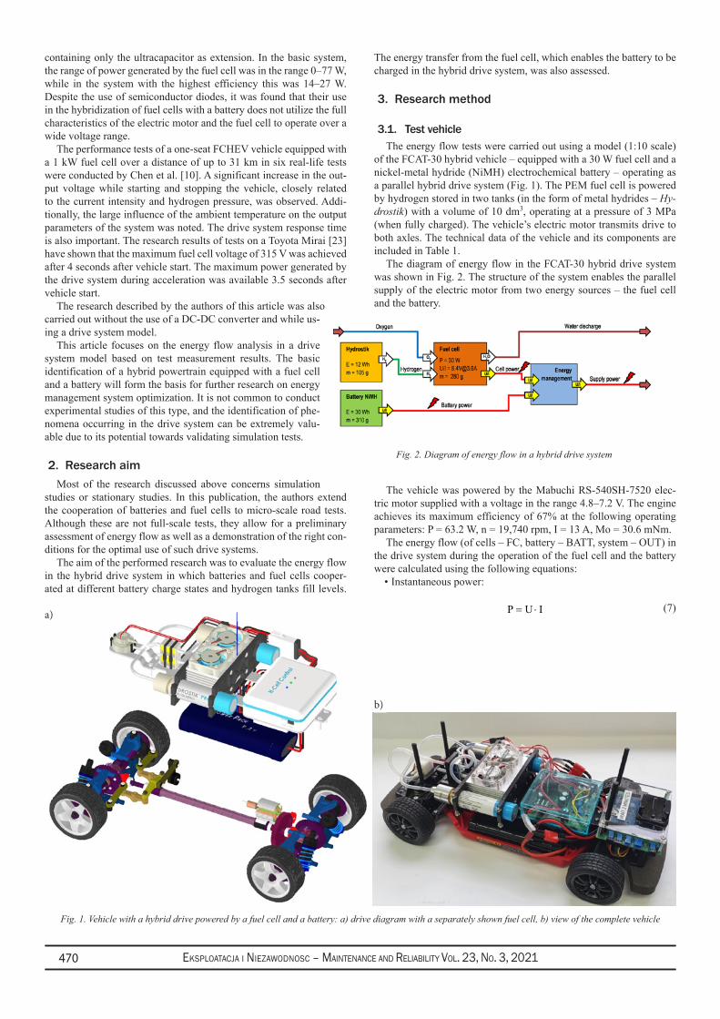
Eksploatacja i NiEzawodNosc – MaiNtENaNcE aNd REliability Vol. 23, No. 3, 2021470
containing only the ultracapacitor as extension. In the basic system, the range of power generated by the fuel cell was in the range 0–77 W, while in the system with the highest efficiency this was 14–27 W. Despite the use of semiconductor diodes, it was found that their use in the hybridization of fuel cells with a battery does not utilize the full characteristics of the electric motor and the fuel cell to operate over a wide voltage range.
The performance tests of a one-seat FCHEV vehicle equipped with a 1 kW fuel cell over a distance of up to 31 km in six real-life tests were conducted by Chen et al. [10]. A significant increase in the out-put voltage while starting and stopping the vehicle, closely related to the current intensity and hydrogen pressure, was observed. Addi-tionally, the large influence of the ambient temperature on the output parameters of the system was noted. The drive system response time is also important. The research results of tests on a Toyota Mirai [23] have shown that the maximum fuel cell voltage of 315 V was achieved after 4 seconds after vehicle start. The maximum power generated by the drive system during acceleration was available 3.5 seconds after vehicle start.
The research described by the authors of this article was also carried out without the use of a DC-DC converter and while us-ing a drive system model.
This article focuses on the energy flow analysis in a drive system model based on test measurement results. The basic identification of a hybrid powertrain equipped with a fuel cell and a battery will form the basis for further research on energy management system optimization. It is not common to conduct experimental studies of this type, and the identification of phe-nomena occurring in the drive system can be extremely valu-able due to its potential towards validating simulation tests.
2. Research aimMost of the research discussed above concerns simulation
studies or stationary studies. In this publication, the authors extend the cooperation of batteries and fuel cells to micro-scale road tests. Although these are not full-scale tests, they allow for a preliminary assessment of energy flow as well as a demonstration of the right con-ditions for the optimal use of such drive systems.
The aim of the performed research was to evaluate the energy flow in the hybrid drive system in which batteries and fuel cells cooper-ated at different battery charge states and hydrogen tanks fill levels.
The energy transfer from the fuel cell, which enables the battery to be charged in the hybrid drive system, was also assessed.
3. Research method
3.1. Test vehicleThe energy flow tests were carried out using a model (1:10 scale)
of the FCAT-30 hybrid vehicle – equipped with a 30 W fuel cell and a nickel-metal hydride (NiMH) electrochemical battery – operating as a parallel hybrid drive system (Fig. 1). The PEM fuel cell is powered by hydrogen stored in two tanks (in the form of metal hydrides – Hy-drostik) with a volume of 10 dm3, operating at a pressure of 3 MPa (when fully charged). The vehicle’s electric motor transmits drive to both axles. The technical data of the vehicle and its components are included in Table 1.
The diagram of energy flow in the FCAT-30 hybrid drive system was shown in Fig. 2. The structure of the system enables the parallel supply of the electric motor from two energy sources – the fuel cell and the battery.
The vehicle was powered by the Mabuchi RS-540SH-7520 elec-tric motor supplied with a voltage in the range 4.8–7.2 V. The engine achieves its maximum efficiency of 67% at the following operating parameters: P = 63.2 W, n = 19,740 rpm, I = 13 A, Mo = 30.6 mNm.
The energy flow (of cells – FC, battery – BATT, system – OUT) in the drive system during the operation of the fuel cell and the battery were calculated using the following equations:
Instantaneous power:•
P U I= ⋅ (7)
Fig. 1. Vehicle with a hybrid drive powered by a fuel cell and a battery: a) drive diagram with a separately shown fuel cell, b) view of the complete vehicle
b)
a)
Fig. 2. Diagram of energy flow in a hybrid drive system
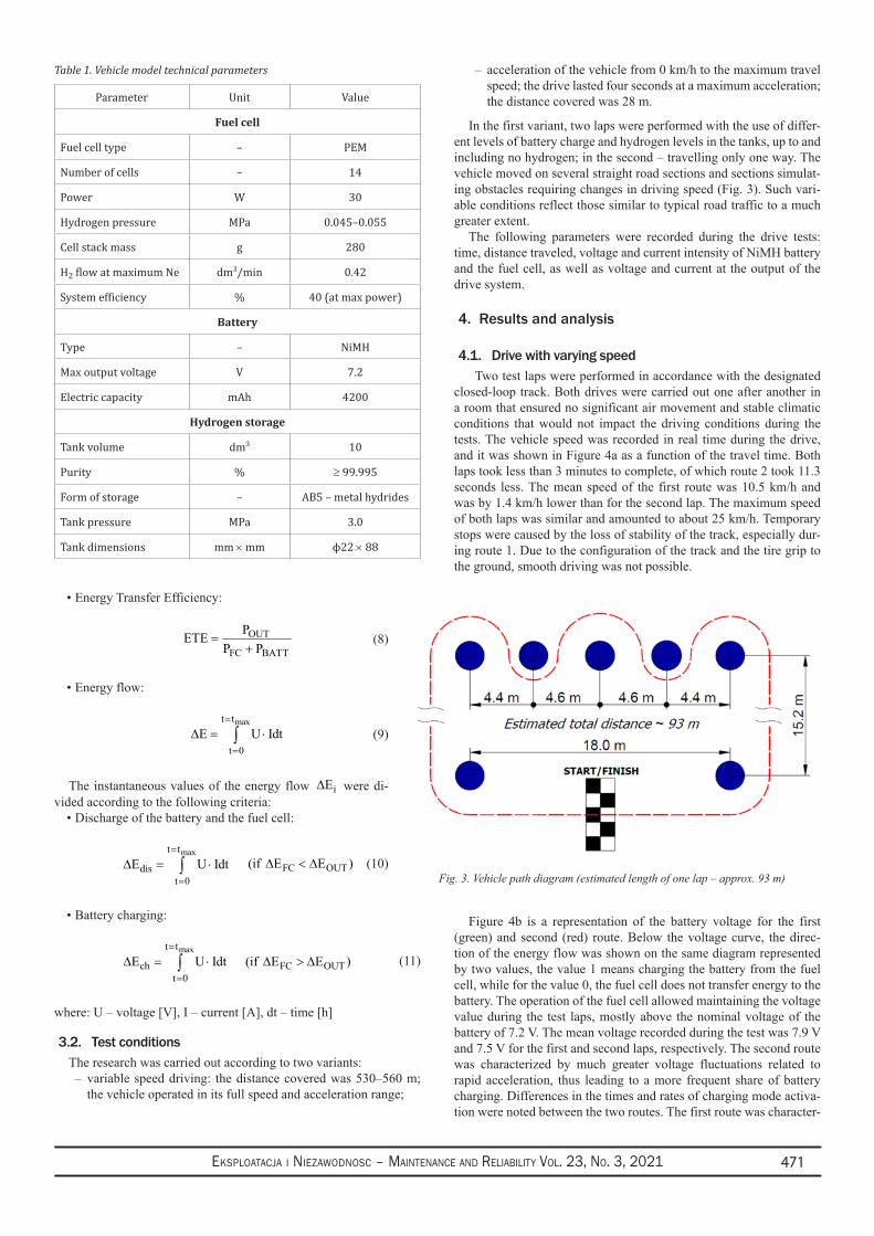
Eksploatacja i NiEzawodNosc – MaiNtENaNcE aNd REliability Vol. 23, No. 3, 2021 471
Energy Transfer Efficiency:•
OUT
FC BATT
PETEP P
=+
(8)
Energy flow:•
∆E U Idtt
t tmax= ⋅
=
=
∫0
(9)
The instantaneous values of the energy flow ∆Ei were di-vided according to the following criteria:
Discharge of the battery and the fuel cell:•
∆E U Idtdist
t tmax= ⋅
=
=
∫0
( )if E EFC OUT∆ ∆< (10)
Battery charging:•
∆ ∆ ∆E U Idt if E Echt
t t
FC OUTmax
= ⋅ >=
=
∫0
( ) (11)
where: U – voltage [V], I – current [A], dt – time [h]
3.2. Test conditionsThe research was carried out according to two variants:
variable speed driving: the distance covered was 530–560 m; –the vehicle operated in its full speed and acceleration range;
acceleration of the vehicle from 0 km/h to the maximum travel –speed; the drive lasted four seconds at a maximum acceleration; the distance covered was 28 m.
In the first variant, two laps were performed with the use of differ-ent levels of battery charge and hydrogen levels in the tanks, up to and including no hydrogen; in the second – travelling only one way. The vehicle moved on several straight road sections and sections simulat-ing obstacles requiring changes in driving speed (Fig. 3). Such vari-able conditions reflect those similar to typical road traffic to a much greater extent.
The following parameters were recorded during the drive tests: time, distance traveled, voltage and current intensity of NiMH battery and the fuel cell, as well as voltage and current at the output of the drive system.
4. Results and analysis
4.1. Drive with varying speedTwo test laps were performed in accordance with the designated
closed-loop track. Both drives were carried out one after another in a room that ensured no significant air movement and stable climatic conditions that would not impact the driving conditions during the tests. The vehicle speed was recorded in real time during the drive, and it was shown in Figure 4a as a function of the travel time. Both laps took less than 3 minutes to complete, of which route 2 took 11.3 seconds less. The mean speed of the first route was 10.5 km/h and was by 1.4 km/h lower than for the second lap. The maximum speed of both laps was similar and amounted to about 25 km/h. Temporary stops were caused by the loss of stability of the track, especially dur-ing route 1. Due to the configuration of the track and the tire grip to the ground, smooth driving was not possible.
Figure 4b is a representation of the battery voltage for the first (green) and second (red) route. Below the voltage curve, the direc-tion of the energy flow was shown on the same diagram represented by two values, the value 1 means charging the battery from the fuel cell, while for the value 0, the fuel cell does not transfer energy to the battery. The operation of the fuel cell allowed maintaining the voltage value during the test laps, mostly above the nominal voltage of the battery of 7.2 V. The mean voltage recorded during the test was 7.9 V and 7.5 V for the first and second laps, respectively. The second route was characterized by much greater voltage fluctuations related to rapid acceleration, thus leading to a more frequent share of battery charging. Differences in the times and rates of charging mode activa-tion were noted between the two routes. The first route was character-
Table 1. Vehicle model technical parameters
Parameter Unit Value
Fuel cell
Fuel cell type – PEM
Number of cells – 14
Power W 30
Hydrogen pressure MPa 0.045–0.055
Cell stack mass g 280
H2 flow at maximum Ne dm3/min 0.42
System efficiency % 40 (at max power)
Battery
Type – NiMH
Max output voltage V 7.2
Electric capacity mAh 4200
Hydrogen storage
Tank volume dm3 10
Purity % ≥ 99.995
Form of storage – AB5 – metal hydrides
Tank pressure MPa 3.0
Tank dimensions mm × mm ϕ22 × 88
Fig. 3. Vehicle path diagram (estimated length of one lap – approx. 93 m)
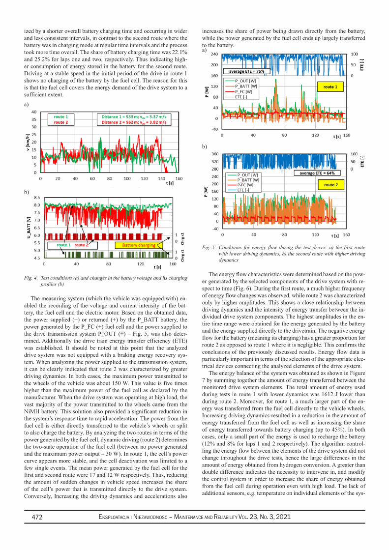
Eksploatacja i NiEzawodNosc – MaiNtENaNcE aNd REliability Vol. 23, No. 3, 2021472
ized by a shorter overall battery charging time and occurring in wider and less consistent intervals, in contrast to the second route where the battery was in charging mode at regular time intervals and the process took more time overall. The share of battery charging time was 22.1% and 25.2% for laps one and two, respectively. Thus indicating high-er consumption of energy stored in the battery for the second route. Driving at a stable speed in the initial period of the drive in route 1 shows no charging of the battery by the fuel cell. The reason for this is that the fuel cell covers the energy demand of the drive system to a sufficient extent.
Fig. 4. Test conditions (a) and changes in the battery voltage and its charging profiles (b)
The measuring system (which the vehicle was equipped with) en-abled the recording of the voltage and current intensity of the bat-tery, the fuel cell and the electric motor. Based on the obtained data, the power supplied (−) or returned (+) by the P_BATT battery, the power generated by the P_FC (+) fuel cell and the power supplied to the drive transmission system P_OUT (+) – Fig. 5, was also deter-mined. Additionally the drive train energy transfer efficiency (ETE) was established. It should be noted at this point that the analyzed drive system was not equipped with a braking energy recovery sys-tem. When analyzing the power supplied to the transmission system, it can be clearly indicated that route 2 was characterized by greater driving dynamics. In both cases, the maximum power transmitted to the wheels of the vehicle was about 150 W. This value is five times higher than the maximum power of the fuel cell as declared by the manufacturer. When the drive system was operating at high load, the vast majority of the power transmitted to the wheels came from the NiMH battery. This solution also provided a significant reduction in the system’s response time to rapid acceleration. The power from the fuel cell is either directly transferred to the vehicle’s wheels or split to also charge the battery. By analyzing the two routes in terms of the power generated by the fuel cell, dynamic driving (route 2) determines the two-state operation of the fuel cell (between no power generated and the maximum power output – 30 W). In route 1, the cell’s power curve appears more stable, and the cell deactivation was limited to a few single events. The mean power generated by the fuel cell for the first and second route were 17 and 12 W respectively. Thus, reducing the amount of sudden changes in vehicle speed increases the share of the cell’s power that is transmitted directly to the drive system. Conversely, Increasing the driving dynamics and accelerations also
increases the share of power being drawn directly from the battery, while the power generated by the fuel cell ends up largely transferred to the battery.
Fig. 5. Conditions for energy flow during the test drives: a) the first route with lower driving dynamics, b) the second route with higher driving dynamics
The energy flow characteristics were determined based on the pow-er generated by the selected components of the drive system with re-spect to time (Fig. 6). During the first route, a much higher frequency of energy flow changes was observed, while route 2 was characterized only by higher amplitudes. This shows a close relationship between driving dynamics and the intensity of energy transfer between the in-dividual drive system components. The highest amplitudes in the en-tire time range were obtained for the energy generated by the battery and the energy supplied directly to the drivetrain. The negative energy flow for the battery (meaning its charging) has a greater proportion for route 2 as opposed to route 1 where it is negligible. This confirms the conclusions of the previously discussed results. Energy flow data is particularly important in terms of the selection of the appropriate elec-trical devices connecting the analyzed elements of the drive system.
The energy balance of the system was obtained as shown in Figure 7 by summing together the amount of energy transferred between the monitored drive system elements. The total amount of energy used during tests in route 1 with lower dynamics was 1612 J lower than during route 2. Moreover, for route 1, a much larger part of the en-ergy was transferred from the fuel cell directly to the vehicle wheels. Increasing driving dynamics resulted in a reduction in the amount of energy transferred from the fuel cell as well as increasing the share of energy transferred towards battery charging (up to 45%). In both cases, only a small part of the energy is used to recharge the battery (12% and 8% for laps 1 and 2 respectively). The algorithm control-ling the energy flow between the elements of the drive system did not change throughout the drive tests, hence the large differences in the amount of energy obtained from hydrogen conversion. A greater than double difference indicates the necessity to intervene in, and modify the control system in order to increase the share of energy obtained from the fuel cell during operation even with high load. The lack of additional sensors, e.g. temperature on individual elements of the sys-
b)
a)
b)
a)
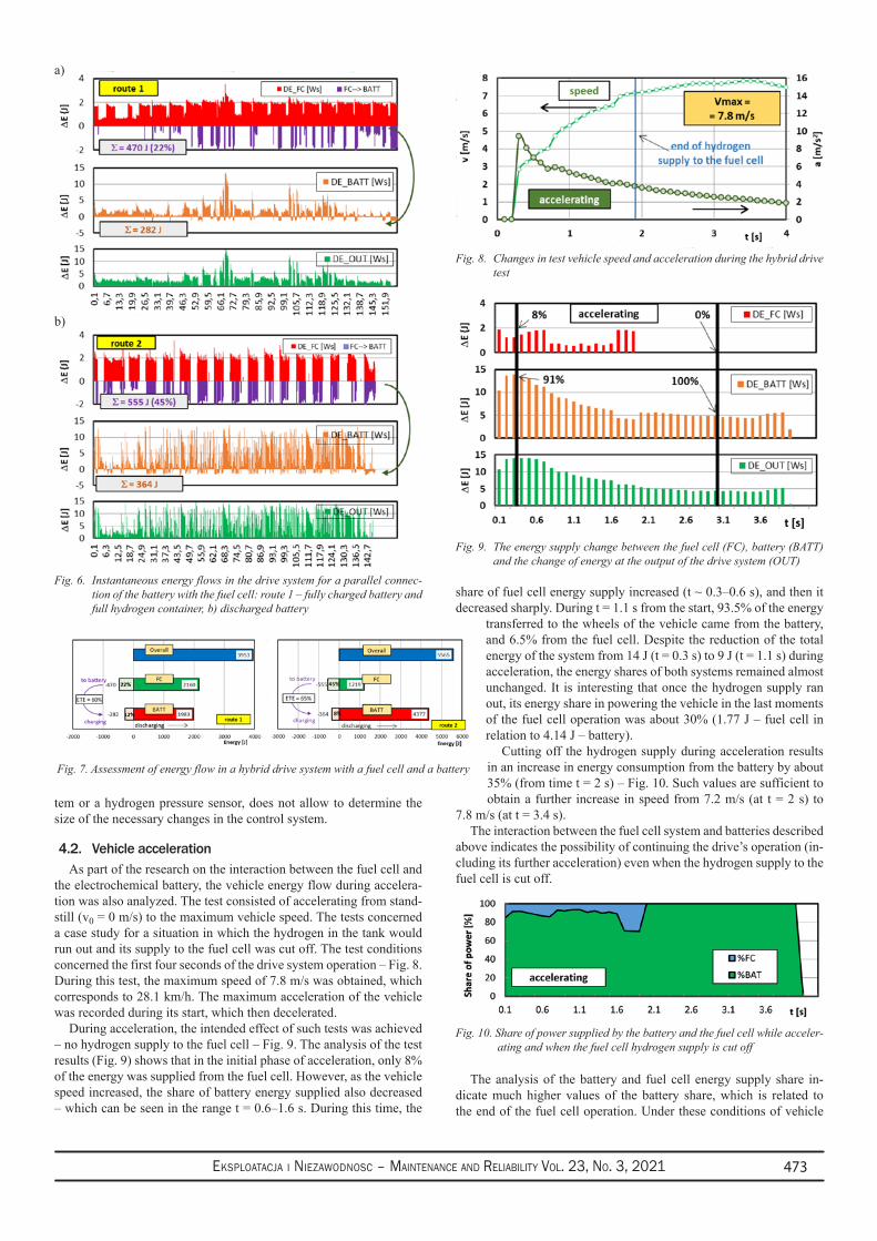
Eksploatacja i NiEzawodNosc – MaiNtENaNcE aNd REliability Vol. 23, No. 3, 2021 473
tem or a hydrogen pressure sensor, does not allow to determine the size of the necessary changes in the control system.
4.2. Vehicle accelerationAs part of the research on the interaction between the fuel cell and
the electrochemical battery, the vehicle energy flow during accelera-tion was also analyzed. The test consisted of accelerating from stand-still (v0 = 0 m/s) to the maximum vehicle speed. The tests concerned a case study for a situation in which the hydrogen in the tank would run out and its supply to the fuel cell was cut off. The test conditions concerned the first four seconds of the drive system operation – Fig. 8. During this test, the maximum speed of 7.8 m/s was obtained, which corresponds to 28.1 km/h. The maximum acceleration of the vehicle was recorded during its start, which then decelerated.
During acceleration, the intended effect of such tests was achieved – no hydrogen supply to the fuel cell – Fig. 9. The analysis of the test results (Fig. 9) shows that in the initial phase of acceleration, only 8% of the energy was supplied from the fuel cell. However, as the vehicle speed increased, the share of battery energy supplied also decreased – which can be seen in the range t = 0.6–1.6 s. During this time, the
share of fuel cell energy supply increased (t ~ 0.3–0.6 s), and then it decreased sharply. During t = 1.1 s from the start, 93.5% of the energy
transferred to the wheels of the vehicle came from the battery, and 6.5% from the fuel cell. Despite the reduction of the total energy of the system from 14 J (t = 0.3 s) to 9 J (t = 1.1 s) during acceleration, the energy shares of both systems remained almost unchanged. It is interesting that once the hydrogen supply ran out, its energy share in powering the vehicle in the last moments of the fuel cell operation was about 30% (1.77 J – fuel cell in relation to 4.14 J – battery).
Cutting off the hydrogen supply during acceleration results in an increase in energy consumption from the battery by about 35% (from time t = 2 s) – Fig. 10. Such values are sufficient to obtain a further increase in speed from 7.2 m/s (at t = 2 s) to
7.8 m/s (at t = 3.4 s).The interaction between the fuel cell system and batteries described
above indicates the possibility of continuing the drive’s operation (in-cluding its further acceleration) even when the hydrogen supply to the fuel cell is cut off.
Fig. 10. Share of power supplied by the battery and the fuel cell while acceler-ating and when the fuel cell hydrogen supply is cut off
The analysis of the battery and fuel cell energy supply share in-dicate much higher values of the battery share, which is related to the end of the fuel cell operation. Under these conditions of vehicle
b)
a)
Fig. 6. Instantaneous energy flows in the drive system for a parallel connec-tion of the battery with the fuel cell: route 1 – fully charged battery and full hydrogen container, b) discharged battery
Fig. 7. Assessment of energy flow in a hybrid drive system with a fuel cell and a battery
Fig. 9. The energy supply change between the fuel cell (FC), battery (BATT) and the change of energy at the output of the drive system (OUT)
Fig. 8. Changes in test vehicle speed and acceleration during the hybrid drive test
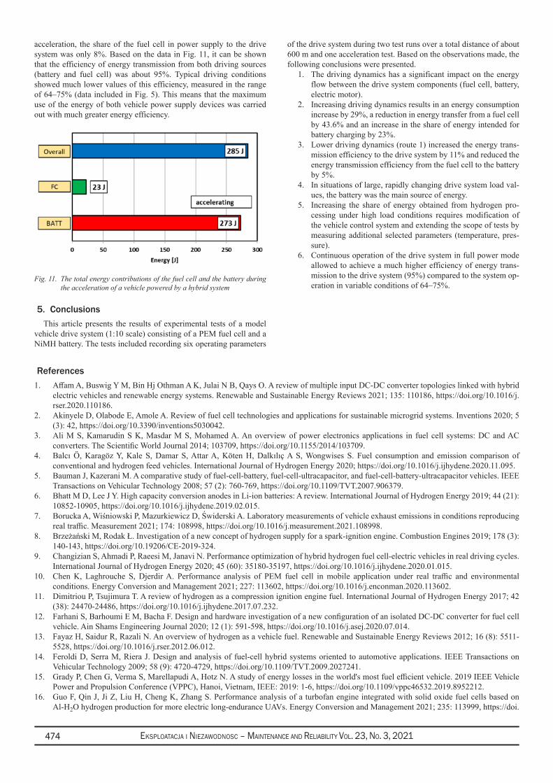
Eksploatacja i NiEzawodNosc – MaiNtENaNcE aNd REliability Vol. 23, No. 3, 2021474
acceleration, the share of the fuel cell in power supply to the drive system was only 8%. Based on the data in Fig. 11, it can be shown that the efficiency of energy transmission from both driving sources (battery and fuel cell) was about 95%. Typical driving conditions showed much lower values of this efficiency, measured in the range of 64–75% (data included in Fig. 5). This means that the maximum use of the energy of both vehicle power supply devices was carried out with much greater energy efficiency.
Fig. 11. The total energy contributions of the fuel cell and the battery during the acceleration of a vehicle powered by a hybrid system
5. ConclusionsThis article presents the results of experimental tests of a model
vehicle drive system (1:10 scale) consisting of a PEM fuel cell and a NiMH battery. The tests included recording six operating parameters
of the drive system during two test runs over a total distance of about 600 m and one acceleration test. Based on the observations made, the following conclusions were presented.
The driving dynamics has a significant impact on the energy 1. flow between the drive system components (fuel cell, battery, electric motor).Increasing driving dynamics results in an energy consumption 2. increase by 29%, a reduction in energy transfer from a fuel cell by 43.6% and an increase in the share of energy intended for battery charging by 23%.Lower driving dynamics (route 1) increased the energy trans-3. mission efficiency to the drive system by 11% and reduced the energy transmission efficiency from the fuel cell to the battery by 5%.In situations of large, rapidly changing drive system load val-4. ues, the battery was the main source of energy.Increasing the share of energy obtained from hydrogen pro-5. cessing under high load conditions requires modification of the vehicle control system and extending the scope of tests by measuring additional selected parameters (temperature, pres-sure). Continuous operation of the drive system in full power mode 6. allowed to achieve a much higher efficiency of energy trans-mission to the drive system (95%) compared to the system op-eration in variable conditions of 64–75%.
References1. Affam A, Buswig Y M, Bin Hj Othman A K, Julai N B, Qays O. A review of multiple input DC-DC converter topologies linked with hybrid
electric vehicles and renewable energy systems. Renewable and Sustainable Energy Reviews 2021; 135: 110186, https://doi.org/10.1016/j.rser.2020.110186.
2. Akinyele D, Olabode E, Amole A. Review of fuel cell technologies and applications for sustainable microgrid systems. Inventions 2020; 5 (3): 42, https://doi.org/10.3390/inventions5030042.
3. Ali M S, Kamarudin S K, Masdar M S, Mohamed A. An overview of power electronics applications in fuel cell systems: DC and AC converters. The Scientific World Journal 2014; 103709, https://doi.org/10.1155/2014/103709.
4. Balcı Ö, Karagöz Y, Kale S, Damar S, Attar A, Köten H, Dalkılıç A S, Wongwises S. Fuel consumption and emission comparison of conventional and hydrogen feed vehicles. International Journal of Hydrogen Energy 2020; https://doi.org/10.1016/j.ijhydene.2020.11.095.
5. Bauman J, Kazerani M. A comparative study of fuel-cell-battery, fuel-cell-ultracapacitor, and fuel-cell-battery-ultracapacitor vehicles. IEEE Transactions on Vehicular Technology 2008; 57 (2): 760-769, https://doi.org/10.1109/TVT.2007.906379.
6. Bhatt M D, Lee J Y. High capacity conversion anodes in Li-ion batteries: A review. International Journal of Hydrogen Energy 2019; 44 (21): 10852-10905, https://doi.org/10.1016/j.ijhydene.2019.02.015.
7. Borucka A, Wiśniowski P, Mazurkiewicz D, Świderski A. Laboratory measurements of vehicle exhaust emissions in conditions reproducing real traffic. Measurement 2021; 174: 108998, https://doi.org/10.1016/j.measurement.2021.108998.
8. Brzeżański M, Rodak Ł. Investigation of a new concept of hydrogen supply for a spark-ignition engine. Combustion Engines 2019; 178 (3): 140-143, https://doi.org/10.19206/CE-2019-324.
9. Changizian S, Ahmadi P, Raeesi M, Janavi N. Performance optimization of hybrid hydrogen fuel cell-electric vehicles in real driving cycles. International Journal of Hydrogen Energy 2020; 45 (60): 35180-35197, https://doi.org/10.1016/j.ijhydene.2020.01.015.
10. Chen K, Laghrouche S, Djerdir A. Performance analysis of PEM fuel cell in mobile application under real traffic and environmental conditions. Energy Conversion and Management 2021; 227: 113602, https://doi.org/10.1016/j.enconman.2020.113602.
11. Dimitriou P, Tsujimura T. A review of hydrogen as a compression ignition engine fuel. International Journal of Hydrogen Energy 2017; 42 (38): 24470-24486, https://doi.org/10.1016/j.ijhydene.2017.07.232.
12. Farhani S, Barhoumi E M, Bacha F. Design and hardware investigation of a new configuration of an isolated DC-DC converter for fuel cell vehicle. Ain Shams Engineering Journal 2020; 12 (1): 591-598, https://doi.org/10.1016/j.asej.2020.07.014.
13. Fayaz H, Saidur R, Razali N. An overview of hydrogen as a vehicle fuel. Renewable and Sustainable Energy Reviews 2012; 16 (8): 5511-5528, https://doi.org/10.1016/j.rser.2012.06.012.
14. Feroldi D, Serra M, Riera J. Design and analysis of fuel-cell hybrid systems oriented to automotive applications. IEEE Transactions on Vehicular Technology 2009; 58 (9): 4720-4729, https://doi.org/10.1109/TVT.2009.2027241.
15. Grady P, Chen G, Verma S, Marellapudi A, Hotz N. A study of energy losses in the world's most fuel efficient vehicle. 2019 IEEE Vehicle Power and Propulsion Conference (VPPC), Hanoi, Vietnam, IEEE: 2019: 1-6, https://doi.org/10.1109/vppc46532.2019.8952212.
16. Guo F, Qin J, Ji Z, Liu H, Cheng K, Zhang S. Performance analysis of a turbofan engine integrated with solid oxide fuel cells based on Al-H2O hydrogen production for more electric long-endurance UAVs. Energy Conversion and Management 2021; 235: 113999, https://doi.

Eksploatacja i NiEzawodNosc – MaiNtENaNcE aNd REliability Vol. 23, No. 3, 2021 475
org/10.1016/j.enconman.2021.113999.17. Gurz M, Baltacioglu E, Hames Y, Kaya K. The meeting of hydrogen and automotive: a review. International Journal of Hydrogen Energy
2017; 42 (36): 23334-23346, https://doi.org/10.1016/j.ijhydene.2017.02.124.18. Haseli Y. Maximum conversion efficiency of hydrogen fuel cells. International Journal of Hydrogen Energy 2018; 43 (18): 9015-9021,
https://doi.org/10.1016/j.ijhydene.2018.03.076.19. Howroyd S, Chen R. Powerpath controller for fuel cell & battery hybridisation. International Journal of Hydrogen Energy 2016; 41 (7):
4229-4238, https://doi.org/10.1016/j.ijhydene.2016.01.038.20. Innocenzi V, Ippolito N M, De Michelis I, Prisciandaro M, Medici F, Vegliò F. A review of the processes and lab-scale techniques for the treatment
of spent rechargeable NiMH batteries. Journal of Power Sources 2017; 362: 202-218, https://doi.org/10.1016/j.jpowsour.2017.07.034.21. Khayyer P, Famouri P. Application of two fuel cells in hybrid electric vehicles. SAE Paper 2008: 2008-01-2418, https://doi.org/10.4271/2008-
01-2418.22. Manoharan Y, Hosseini S E, Butler B, Alzhahrani H, Senior B T F, Ashuri T, Krohn J. Hydrogen fuel cell vehicles; current status and future
prospect. Applied Sciences 2019; 9 (11): 2296, https://doi.org/10.3390/app9112296.23. Pielecha I, Cieślik W, Szałek A. The use of electric drive in urban driving conditions using a hydrogen powered vehicle - Toyota Mirai.
Combustion Engines 2018; 172(1): 51-58, https://doi.org/10.19206/CE-2018-106.24. Pielecha I, Pielecha J. Simulation analysis of electric vehicles energy consumption in driving tests. Eksploatacja i Niezawodnosc - Maintenance
and Reliability 2020; 22 (1): 130-137, https://doi.org/10.17531/ein.2020.1.15.25. Rana K, Natarajan S, Jilakara S. Potential of hydrogen fuelled IC engine to achieve the future performance and emission norms. SAE Paper
2015: 2015-26-0050, https://doi.org/10.4271/2015-26-0050.26. Shang J, Kendall K, Pollet B G. Hybrid hydrogen PEM fuel cell and batteries without DC-DC converter. International Journal of Low-
Carbon Technologies 2016; 11 (2): 205-210, https://doi.org/10.1093/ijlct/ctt070.27. Sorlei I S, Bizon N, Thounthong P, Varlam M, Carcadea E, Culcer M, Iliescu M, Raceanu M. Fuel cell electric vehicles - a brief review of
current topologies and energy management strategies. Energies 2021; 14: 252, https://doi.org/10.3390/en14010252.28. Szumska E, Jurecki R, Pawełczyk M. Evaluation of the use of hybrid electric powertrain system in urban traffic conditions. Eksploatacja i
Niezawodnosc - Maintenance and Reliability 2020; 22 (1): 154-160, https://doi.org/10.17531/ein.2020.1.18.29. Verhelst S, Sierens R, Verstraeten S. A critical review of experimental research on hydrogen fueled SI engines. SAE Paper 2006: 2006-01-
0430, https://doi.org/10.4271/2006-01-0430.30. Yao G, Du C, Ge Q, Jiang H, Wang Y, Ait-Ahmed M, Moreau L. Traffic-condition-prediction-based HMA-FIS energy-management strategy
for fuel-cell electric vehicles. Energies 2019; 12: 4426, https://doi.org/10.3390/en12234426.31. Zhang J, Zhang H, Wu J, Zhang J. PEM Fuel Cell Fundamentals. PEM Fuel Cell Testing and Diagnosis, Elsevier: 2013: 1-42, https://doi.
org/10.1016/B978-0-444-53688-4.00001-2.32. Zhao Z, Wang T, Li M, Wang H, Wang Y. Optimization of fuzzy control energy management strategy for fuel cell vehicle power system using
a multi-islandgenetic algorithm. Energy Science & Engineering 2021; 9: 548-564, https://doi.org/10.1002/ese3.835.
Eksploatacja i NiEzawodNosc – MaiNtENaNcE aNd REliability Vol. 23, No. 3, 2021476
E-mail addresses:
Eksploatacja i Niezawodnosc – Maintenance and ReliabilityVolume 23 (2021), Issue 3
journal homepage: http://www.ein.org.pl
Indexed by:
1. IntroductionThe problem of risk assessment in railway transport is presented
next to risk analysis and risk evaluation as one of the stages of risk management in the whole railway system. The level of generality in dealing with adverse events in the process of freight transport by rail often results in an inadequate and insufficient response to the upset-ting of the acceptable level of risk by those involved in the process. It is common practice to react to the effects of rail incidents rather than prevent them from occurring. The groups of entities involved in ensuring safety in railway transport include rail operators, infrastruc-ture managers, users of sidings, rolling stock manufacturers, manu-facturers of devices and railway traffic control systems, designers and entities responsible for maintenance of rolling stock and railway in-frastructure facilities.
Risk assessment in the rail transport system can be seen as an ap-proach aimed at identifying risks at junctions and on railway lines, including risks arising from operational processes and the actions of other actors in the system whose task is to provide rail freight trans-port operations. Risk assessment also consists of risk analysis and evaluation.
Particularly relevant in this context is the risk profile R the so-called risk scenario representing the pattern of the risk distribution
probability and its consequences written in the form of the following pairs [53]:
R=(P1, S1), (P2, S2), …,(Pi, Si),…, (Pn, Sn) (1)
where:R – risk, Pi – probability of risk due to i-th factor,Si – effects of risk due to i-th factor,i – risk factor number; i = 1,...n.
Risks can come from internal sources resulting from the transport system under study and from external sources resulting from causes in its environment. A single risk may consequently generate multiple negative effects with varying degrees of impact. At the same time, one effect of risk implementation may have several causes.
Identification and analysis of adverse events allow for understand-ing and improving the weaknesses of the organisations operating within the railway system where such situations have been diagnosed. Positive aspects of studying this type of situations include:
effective accident prevention by learning from mistakes, –minimising the risks involved through proactive management, –elimination of repetition of potentially dangerous situations, –
The aim of this article is to assess the risk of performance of rail freight transport on the basis of an analysis of identified risk areas based on statistical data on the causes of acci-dents that occurred on the lines of railway transport in Poland. A critical review of selected scientific studies relating to the risk assessment process for identified areas of the railway system has been undertaken. Based on statistical data, the authors analysed the causes of accidents on railway lines in 2019 in Poland and determined the probability of occurrence of a given cause. In addition, the article calculates the probability of vehicle delays for dif-ferent emergency situations occurring in the performance of rail freight transport operations. This enabled the authors of the article to carry out a risk assessment of freight train delays on railway lines.
Highlights Abstract
Risk assessment for freight train delays on rail-• way lines.
Identification of causes of accidents on railway • lines and railway sidings in Poland.
Determination of the probability of a cause result-• ing in a railway accident.
Risk analysis of potential costs of delays resulting • from accidents in Poland in 2019.
Risk assessment for rail freight transport operations
Lucyna Szaciłło a, Marianna Jacyna a, Emilian Szczepański a, Mariusz Izdebski a
a Warsaw University of Technology Faculty of Transport, ul. Koszykowa 75, Warsaw, Poland
Szaciłło L, Jacyna M, Szczepański E, Izdebski M. Risk assessment for rail freight transport operations. Eksploatacja i Niezawodnosc – Maintenance and Reliability 2021; 23 (3): 476–488, http://doi.org/10.17531/ein.2021.3.8.
Article citation info:
risk assessment, railway transport risk, train delay risk level, causes of railway accidents.
Keywords
This is an open access article under the CC BY license (https://creativecommons.org/licenses/by/4.0/)
L. Szaciłło - [email protected], M. Jacyna - [email protected], E. Szczepański - [email protected], M. Izdebski - [email protected]
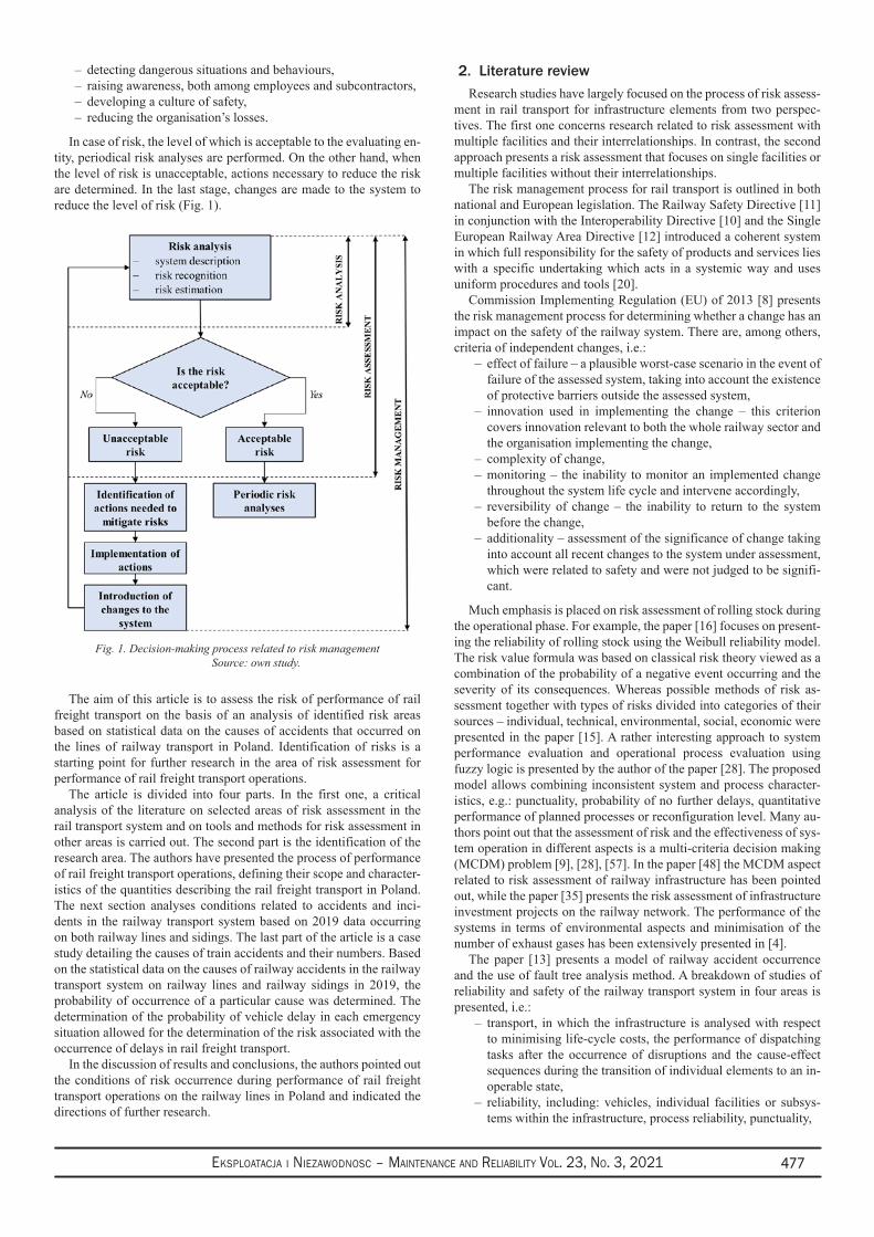
Eksploatacja i NiEzawodNosc – MaiNtENaNcE aNd REliability Vol. 23, No. 3, 2021 477
detecting dangerous situations and behaviours, –raising awareness, both among employees and subcontractors, –developing a culture of safety, –reducing the organisation’s losses. –
In case of risk, the level of which is acceptable to the evaluating en-tity, periodical risk analyses are performed. On the other hand, when the level of risk is unacceptable, actions necessary to reduce the risk are determined. In the last stage, changes are made to the system to reduce the level of risk (Fig. 1).
Fig. 1. Decision-making process related to risk management Source: own study.
The aim of this article is to assess the risk of performance of rail freight transport on the basis of an analysis of identified risk areas based on statistical data on the causes of accidents that occurred on the lines of railway transport in Poland. Identification of risks is a starting point for further research in the area of risk assessment for performance of rail freight transport operations.
The article is divided into four parts. In the first one, a critical analysis of the literature on selected areas of risk assessment in the rail transport system and on tools and methods for risk assessment in other areas is carried out. The second part is the identification of the research area. The authors have presented the process of performance of rail freight transport operations, defining their scope and character-istics of the quantities describing the rail freight transport in Poland. The next section analyses conditions related to accidents and inci-dents in the railway transport system based on 2019 data occurring on both railway lines and sidings. The last part of the article is a case study detailing the causes of train accidents and their numbers. Based on the statistical data on the causes of railway accidents in the railway transport system on railway lines and railway sidings in 2019, the probability of occurrence of a particular cause was determined. The determination of the probability of vehicle delay in each emergency situation allowed for the determination of the risk associated with the occurrence of delays in rail freight transport.
In the discussion of results and conclusions, the authors pointed out the conditions of risk occurrence during performance of rail freight transport operations on the railway lines in Poland and indicated the directions of further research.
2. Literature reviewResearch studies have largely focused on the process of risk assess-
ment in rail transport for infrastructure elements from two perspec-tives. The first one concerns research related to risk assessment with multiple facilities and their interrelationships. In contrast, the second approach presents a risk assessment that focuses on single facilities or multiple facilities without their interrelationships.
The risk management process for rail transport is outlined in both national and European legislation. The Railway Safety Directive [11] in conjunction with the Interoperability Directive [10] and the Single European Railway Area Directive [12] introduced a coherent system in which full responsibility for the safety of products and services lies with a specific undertaking which acts in a systemic way and uses uniform procedures and tools [20].
Commission Implementing Regulation (EU) of 2013 [8] presents the risk management process for determining whether a change has an impact on the safety of the railway system. There are, among others, criteria of independent changes, i.e.:
effect of failure – a plausible worst-case scenario in the event of –failure of the assessed system, taking into account the existence of protective barriers outside the assessed system,innovation used in implementing the change – this criterion –covers innovation relevant to both the whole railway sector and the organisation implementing the change,complexity of change, –monitoring – the inability to monitor an implemented change –throughout the system life cycle and intervene accordingly,reversibility of change – the inability to return to the system –before the change,additionality – assessment of the significance of change taking –into account all recent changes to the system under assessment, which were related to safety and were not judged to be signifi-cant.
Much emphasis is placed on risk assessment of rolling stock during the operational phase. For example, the paper [16] focuses on present-ing the reliability of rolling stock using the Weibull reliability model. The risk value formula was based on classical risk theory viewed as a combination of the probability of a negative event occurring and the severity of its consequences. Whereas possible methods of risk as-sessment together with types of risks divided into categories of their sources – individual, technical, environmental, social, economic were presented in the paper [15]. A rather interesting approach to system performance evaluation and operational process evaluation using fuzzy logic is presented by the author of the paper [28]. The proposed model allows combining inconsistent system and process character-istics, e.g.: punctuality, probability of no further delays, quantitative performance of planned processes or reconfiguration level. Many au-thors point out that the assessment of risk and the effectiveness of sys-tem operation in different aspects is a multi-criteria decision making (MCDM) problem [9], [28], [57]. In the paper [48] the MCDM aspect related to risk assessment of railway infrastructure has been pointed out, while the paper [35] presents the risk assessment of infrastructure investment projects on the railway network. The performance of the systems in terms of environmental aspects and minimisation of the number of exhaust gases has been extensively presented in [4].
The paper [13] presents a model of railway accident occurrence and the use of fault tree analysis method. A breakdown of studies of reliability and safety of the railway transport system in four areas is presented, i.e.:
transport, in which the infrastructure is analysed with respect –to minimising life-cycle costs, the performance of dispatching tasks after the occurrence of disruptions and the cause-effect sequences during the transition of individual elements to an in-operable state,reliability, including: vehicles, individual facilities or subsys- –tems within the infrastructure, process reliability, punctuality,
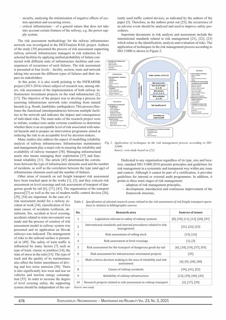
Eksploatacja i NiEzawodNosc – MaiNtENaNcE aNd REliability Vol. 23, No. 3, 2021478
security, analysing the minimisation of negative effects of sys- –tem operation and occurring errors, critical infrastructure – of a general nature that does not take –into account certain features of the railway, e.g. the power sup-ply system.
The risk assessment methodology for the railway infrastructure network was investigated in the DESTination RAIL project. Authors of the study [39] presented the process of risk assessment supporting railway network infrastructure managers in risk reduction for selected facilities by applying unified probability of failure con-nected with different state of infrastructure facilities and con-sequences of occurrence of such failures. The risk assessment is presented at four levels – facility, section, route and network taking into account the different types of failures and their im-pact on stakeholders.
At this point, it is also worth pointing to the INFRARISK project (2013-2016) whose subject of research was, among oth-ers, risk assessment of the implementation of both railway in-frastructure investment projects on the road infrastructure [2], [17]. The objective of the project was to develop a process for assessing infrastructure network risks resulting from natural hazards (e.g. floods, landslides, earthquakes). This process illus-trates the functional interdependencies between multiple facili-ties in the network and indicates the impact and consequences of individual risks. The main tasks of the research project were to initiate, conduct tests under extreme conditions to determine whether there is an acceptable level of risk associated with natu-ral hazards and to prepare an intervention programme aimed at reducing the risk to an acceptable level by decision makers.
Many studies also address the aspect of modelling reliability analysis of railway infrastructure. Infrastructure maintenance and management play a major role in ensuring the reliability and availability of railway transport [38]. Managing infrastructural assets also means managing their exploitation [57] and func-tional reliability [31]. The article [45] determined the correla-tions between the type of infrastructure elements used and the number of incidents, as well as the correlation between the type (and age) of infrastructure elements used and the number of failures.
Other areas of research on rail freight transport risk assessment have been touched upon in the works [1], [3], and they concern risk assessment on level crossings and risk assessment of transport of dan-gerous goods by rail [6], [37], [43]. The organisation of the transport process[27] as well as the use of modern traffic control devices [26], [29], [54] are important. In the case of a risk assessment model for a railway ac-cident at work [34], classification of five main causes of accidents (collision, de-railment, fire, accident at level crossing, accidents related to train movement) was made and the process of creation of risk assessment model in railway system was presented and its application on Slovak railways was indicated. The management of risks to the railroad surface is present-ed in [49]. The safety of train traffic is influenced by many factors [7] such as type of track: classic or jointless [14], the state of stress in the rails [33]. The type of track and the quality of its maintenance also affect the better smoothness of driv-ing and less noise emission [50]. There is also significantly less wear and tear on vehicles and traction energy consump-tion [55]. In order to increase the degree of level crossing safety, the supporting system should be independent of the cur-
rently used traffic control devices, as indicated by the authors of the paper [5]. Therefore, as the authors point out [25], the occurrence of an adverse event should be analysed and used to improve safety pro-cedures.
Important documents in risk analysis and assessment include the international standards related to risk management [21], [22], [23] which relate to the identification, analysis and evaluation of risks. The application of techniques in the risk management process according to ISO 31000 is shown in Figure 2.
Dedicated to any organisation regardless of its type, size and loca-tion, standard ISO 31000:2018 presents principles and guidelines for risk management in a systematic and transparent way within any issue and context. Although it cannot be part of a certification, it provides guidelines for internal or external audit programmes. In addition, it points to three main stages of risk management:
adoption of risk management principles, –development, introduction and continuous improvement of the –framework structure,
Fig. 2. Application of techniques in the risk management process according to ISO 31000
Source: own study based on [21]
Table 1. Specification of selected research areas related to the risk assessment of rail freight transport opera-tions in relation to bibliographic sources
No. Research area Sources of issues
1 Legislation relevant to safety of railway systems [8], [10], [11], [12], [20], [47]
2 International standards and internal procedures related to risk management [21], [22], [23]
3 Risk assessment of rolling stock [15], [16]
4 Risk assessment at level crossings [1], [3]
5 Risk assessment for the transport of dangerous goods by rail [6], [18], [19], [37], [43]
6 Risk assessment for infrastructure investment projects [35]
7 Multi-criteria decision making in the area of reliability and risk assessment [4], [9], [28], [48]
8 Causes of railway accidents [34], [41], [52]
9 Reliability of railway infrastructure [13], [39], [40], [45]
10 Research projects related to risk assessment in railway transport [2], [17], [39]Source: own study.
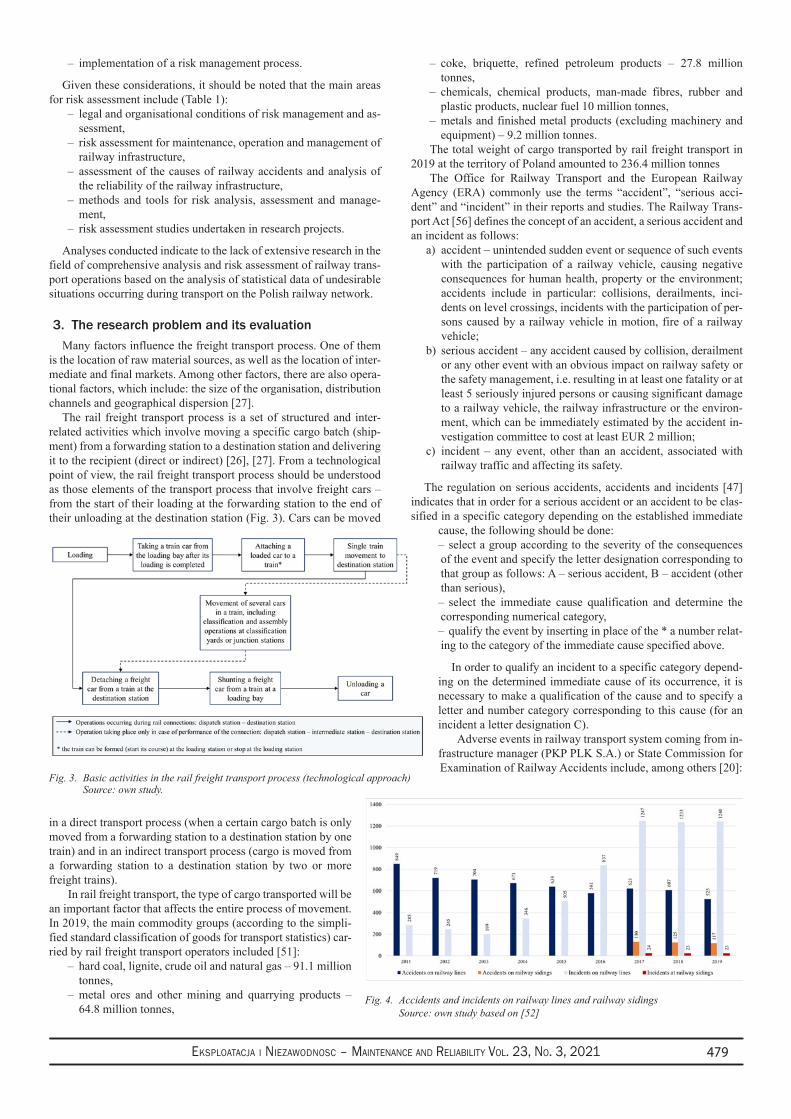
Eksploatacja i NiEzawodNosc – MaiNtENaNcE aNd REliability Vol. 23, No. 3, 2021 479
implementation of a risk management process. –
Given these considerations, it should be noted that the main areas for risk assessment include (Table 1):
legal and organisational conditions of risk management and as- –sessment,risk assessment for maintenance, operation and management of –railway infrastructure,assessment of the causes of railway accidents and analysis of –the reliability of the railway infrastructure,methods and tools for risk analysis, assessment and manage- –ment,risk assessment studies undertaken in research projects. –
Analyses conducted indicate to the lack of extensive research in the field of comprehensive analysis and risk assessment of railway trans-port operations based on the analysis of statistical data of undesirable situations occurring during transport on the Polish railway network.
3. The research problem and its evaluationMany factors influence the freight transport process. One of them
is the location of raw material sources, as well as the location of inter-mediate and final markets. Among other factors, there are also opera-tional factors, which include: the size of the organisation, distribution channels and geographical dispersion [27].
The rail freight transport process is a set of structured and inter-related activities which involve moving a specific cargo batch (ship-ment) from a forwarding station to a destination station and delivering it to the recipient (direct or indirect) [26], [27]. From a technological point of view, the rail freight transport process should be understood as those elements of the transport process that involve freight cars – from the start of their loading at the forwarding station to the end of their unloading at the destination station (Fig. 3). Cars can be moved
in a direct transport process (when a certain cargo batch is only moved from a forwarding station to a destination station by one train) and in an indirect transport process (cargo is moved from a forwarding station to a destination station by two or more freight trains).
In rail freight transport, the type of cargo transported will be an important factor that affects the entire process of movement. In 2019, the main commodity groups (according to the simpli-fied standard classification of goods for transport statistics) car-ried by rail freight transport operators included [51]:
hard coal, lignite, crude oil and natural gas – 91.1 million –tonnes,metal ores and other mining and quarrying products – –64.8 million tonnes,
coke, briquette, refined petroleum products – 27.8 million –tonnes,chemicals, chemical products, man-made fibres, rubber and –plastic products, nuclear fuel 10 million tonnes,metals and finished metal products (excluding machinery and –equipment) – 9.2 million tonnes.
The total weight of cargo transported by rail freight transport in 2019 at the territory of Poland amounted to 236.4 million tonnes
The Office for Railway Transport and the European Railway Agency (ERA) commonly use the terms “accident”, “serious acci-dent” and “incident” in their reports and studies. The Railway Trans-port Act [56] defines the concept of an accident, a serious accident and an incident as follows:
accident – unintended sudden event or sequence of such events a) with the participation of a railway vehicle, causing negative consequences for human health, property or the environment; accidents include in particular: collisions, derailments, inci-dents on level crossings, incidents with the participation of per-sons caused by a railway vehicle in motion, fire of a railway vehicle;serious accident – any accident caused by collision, derailment b) or any other event with an obvious impact on railway safety or the safety management, i.e. resulting in at least one fatality or at least 5 seriously injured persons or causing significant damage to a railway vehicle, the railway infrastructure or the environ-ment, which can be immediately estimated by the accident in-vestigation committee to cost at least EUR 2 million;incident – any event, other than an accident, associated with c) railway traffic and affecting its safety.
The regulation on serious accidents, accidents and incidents [47] indicates that in order for a serious accident or an accident to be clas-sified in a specific category depending on the established immediate
cause, the following should be done:select a group according to the severity of the consequences –
of the event and specify the letter designation corresponding to that group as follows: A – serious accident, B – accident (other than serious),
select the immediate cause qualification and determine the –corresponding numerical category,
qualify the event by inserting in place of the * a number relat- –ing to the category of the immediate cause specified above.
In order to qualify an incident to a specific category depend-ing on the determined immediate cause of its occurrence, it is necessary to make a qualification of the cause and to specify a letter and number category corresponding to this cause (for an incident a letter designation C).
Adverse events in railway transport system coming from in-frastructure manager (PKP PLK S.A.) or State Commission for Examination of Railway Accidents include, among others [20]:
Fig. 3. Basic activities in the rail freight transport process (technological approach) Source: own study.
Fig. 4. Accidents and incidents on railway lines and railway sidings Source: own study based on [52]
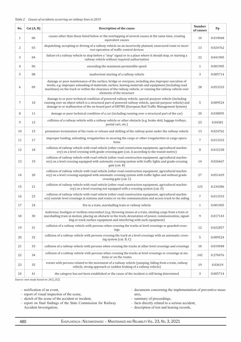
Eksploatacja i NiEzawodNosc – MaiNtENaNcE aNd REliability Vol. 23, No. 3, 2021480
notification of an event, –report of visual inspection of the scene, –sketch of the scene of the accident or incident, –report on final findings of the State Commission for Railway –Accident Investigation,
documents concerning the implementation of preventive meas- –ures,summary of proceedings, –facts directly related to a serious accident, –description of test and hearing records, –
Table 2. Causes of accidents occurring on railway lines in 2019
No. Cat (A, B) Description of the cause Numberof causes Pp
1 00 causes other than those listed below or the overlapping of several causes at the same time, creating equivalent causes 10 0.019048
2 03 dispatching, accepting or driving of a railway vehicle on an incorrectly planned, unsecured route or incor-rect operation of traffic control devices 13 0.024762
3 04 failure of a railway vehicle to stop before a “stop” signal or in a place where it should stop, or starting a railway vehicle without required authorisation 22 0.041905
4 06 exceeding the maximum permissible speed 1 0.001905
5 08 inadvertent starting of a railway vehicle 3 0.005714
6 09
damage or poor maintenance of the surface, bridge or overpass, including also improper execution of works, e.g. improper unloading of materials, surface, leaving materials and equipment (including road
machines) on the track or within the clearance of the railway vehicle, or running the railway vehicle over elements of the structure
28 0.053333
7 10damage to or poor technical condition of powered railway vehicle, special-purpose vehicle (including
running over an object which is a structural part of powered railway vehicle, special-purpose vehicle) and damage to or malfunction of the on-board part of ERTMS (European Rail Traffic Management System)
5 0.009524
8 11 damage or poor technical condition of a car (including running over a structural part of the car) 20 0.038095
9 13 collision of a railway vehicle with a railway vehicle or other obstacle (e.g. brake skid, luggage trolleys, postal cart, etc.) 23 0.04381
10 15 premature termination of the route or release and shifting of the railway point under the railway vehicle 13 0.024762
11 17 improper loading, unloading, irregularities in securing the cargo or other irregularities in cargo opera-tions 7 0.013333
12 18 collision of railway vehicle with road vehicle (other road construction equipment, agricultural machin-ery) on a level crossing with grade-crossing gate (cat. A according to the transit metric) 8 0.015238
13 19collision of railway vehicle with road vehicle (other road construction equipment, agricultural machin-ery) on a level crossing equipped with automatic crossing system with traffic lights and grade-crossing
gate (cat. B)14 0.026667
14 20collision of railway vehicle with road vehicle (other road construction equipment, agricultural machin-ery) on a level crossing equipped with automatic crossing system with traffic lights and without grade-
crossing gate (cat. C)27 0.051429
15 21 collision of railway vehicle with road vehicle (other road construction equipment, agricultural machin-ery) on a level crossing not equipped with a crossing system (cat. D) 123 0.234286
16 23 collision of railway vehicle with road vehicle (other road construction equipment, agricultural machin-ery) outside level crossings in stations and routes or on the communication and access track to the siding 7 0.013333
17 24 fire in a train, marshalling train or railway vehicle 1 0.001905
18 30malicious, hooligan or reckless misconduct (e.g. throwing stones at a train, stealing cargo from a train or
marshalling train in motion, placing an obstacle in the track, devastation of power, communication, signal-ling or track surface equipment and interfering with such equipment)
9 0.017143
19 31 collision of a railway vehicle with persons when crossing the tracks at level crossings or guarded cross-ings 12 0.022857
20 32 collision of a railway vehicle with persons crossing the track at a level crossings with an automatic cross-ing system (cat. B, C) 5 0.009524
21 33 collision of a railway vehicle with persons when crossing the tracks at other level crossings and crossings 10 0.019048
22 34 collision of a railway vehicle with persons when crossing the tracks at level crossings or crossings at sta-tions or on the routes 142 0.270476
23 35 events with persons related to the movement of a railway vehicle (jumping, falling from a train, railway vehicle, strong approach or sudden braking of a railway vehicle) 19 0.03619
24 41 the category has not been established or the cause of the incident is still being determined 3 0.005714
Source: own study based on: [41], [52].

Eksploatacja i NiEzawodNosc – MaiNtENaNcE aNd REliability Vol. 23, No. 3, 2021 481
analysis and conclusions –description of ad hoc preventive measures, –
recommended preventive measures to avoid such accidents or inci-dents in the future or to limit their consequences.
Figure 4 shows the number of accidents and incidents occurring on railway lines (2011-2019) and on railway sidings (2017-2019).
Since 2011 there has been a downward trend in the number of accidents on railway lines in Poland. In 2019 there were 525 ac-cidents on railway lines and for the corresponding group on railway sidings – 117.
As indicated in many publications [41]a serious accident is only possible if the following factors occur simultaneously:
a conscious or unconscious decision to misuse the system, –continuation of the system misuse, –disrupted train traffic (mainly serious accidents caused by the –traffic dispatcher),human error (driver or traffic dispatcher). –
For incidents on railway lines (Fig. 4), an increasing trend has been noticeable since 2014. This is due, among other things, to supervision activities that revealed the misclassification of some events which may have resulted in them not being included in official statistics. In 2019, 1240 incidents were recorded on railway lines while 23 incidents were recorded for the same group of incidents on railway sidings.
4. Risk analysis and assessment based on adverse events – case study
4.1. Identificationofadverseeventsontherailtransportnetwork
Publicly available statistical data on adverse events in the Polish railway transport system, provided by the Office for Railway Trans-port, do not distinguish between passenger and freight transport. Based on an analysis of documents [41], [52] causes of railway ac-cidents for categories A (serious accident) and B (other than serious accident) on railway lines in 2019 (Table 2) and for railway sidings (Table 3) were identified.
The probability of occurrence of a given cause in the railway trans-port system in 2019 (Pp) and the probability of effect, i.e. occurrence of train delay generated by a given emergency situation (Po) were determined on the basis of data analysis.
Out of all adverse events in the railway transport system, those reported by the Office for Railway Transport were singled out. The probability of causes listed in Tables 2 and 3 was calculated assuming that the number of train accidents in the system under study represents the same event space.
Table 3. Causes of accidents occurring on railway sidings in 2019
No. Cat (A, B) Description of the cause Number P
1 00 causes other than those listed below or the overlapping of several causes at the same time, creating equivalent causes 3 0.026315789
2 03 dispatching, accepting or driving of a railway vehicle on an incorrectly planned, unsecured route or incorrect operation of traffic control devices 17 0.149122807
3 04 failure of a railway vehicle to stop before a “stop” signal or in a place where it should stop, or starting a railway vehicle without required authorisation 6 0.052631579
4 07 carrying out a manoeuvre that creates a risk for the safety of train traffic 1 0.00877193
5 08 inadvertent starting of a railway vehicle 1 0.00877193
6 09
damage or poor maintenance of the surface, bridge or overpass, including also improper execution of works, e.g. improper unloading of materials, surface, leaving materials and equipment (including road
machines) on the track or within the clearance of the railway vehicle, or running the railway vehicle over elements of the structure
24 0.210526316
7 10
damage to or poor technical condition of powered railway vehicle, special-purpose vehicle (including running over an object which is a structural part of powered railway vehicle, special-purpose vehicle) and damage to or malfunction of the on-board part of ERTMS (European Rail Traffic Management Sys-
tem)
1 0.00877193
8 11 damage or poor technical condition of a car (including running over a structural part of the car) 6 0.052631579
9 12 failure or malfunction of signalling equipment 1 0.00877193
10 13 running over a railway vehicle or other obstacle (e.g. brake skid, luggage trolleys, postal cart, etc.) 26 0.228070175
11 15 premature termination of the route or release and shifting of the railway point under the railway vehi-cle 1 0.00877193
12 17 improper loading, unloading, irregularities in securing the cargo or other irregularities in cargo opera-tions 10 0.087719298
13 21 collision of railway vehicle with road vehicle (other road construction equipment, agricultural machin-ery) on a level crossing not equipped with a crossing system (cat. D) 12 0.105263158
14 23collision of railway vehicle with road vehicle (other road construction equipment, agricultural machin-
ery) outside level crossings in stations and routes or on the communication and access track to the siding
3 0.026315789
15 34 collision of a railway vehicle with persons when crossing the tracks at level crossings or crossings at stations or on the routes 1 0.00877193
16 35 events with persons related to the movement of a railway vehicle (jumping, falling from a train, railway vehicle, strong approach or sudden braking of a railway vehicle) 1 0.00877193
Source: own study based on: [41], [52].
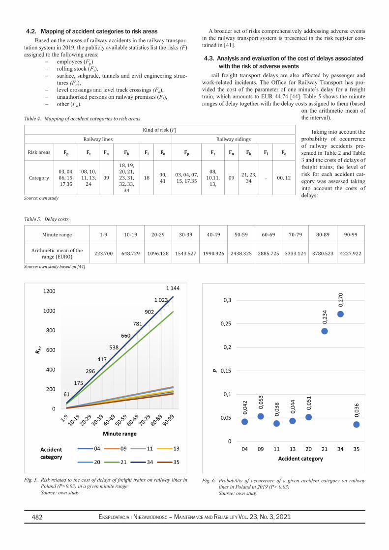
Eksploatacja i NiEzawodNosc – MaiNtENaNcE aNd REliability Vol. 23, No. 3, 2021482
4.2. Mappingofaccidentcategoriestoriskareas Based on the causes of railway accidents in the railway transpor-
tation system in 2019, the publicly available statistics list the risks (F) assigned to the following areas:
employees (− Fp)rolling stock (− Ft),surface, subgrade, tunnels and civil engineering struc-−tures (Fn),level crossings and level track crossings − (Fk),unauthorised persons on railway premises (− Fl),other (− Fo).
A broader set of risks comprehensively addressing adverse events in the railway transport system is presented in the risk register con-tained in [41].
4.3.Analysisandevaluationofthecostofdelaysassociatedwiththeriskofadverseevents
rail freight transport delays are also affected by passenger and work-related incidents. The Office for Railway Transport has pro-vided the cost of the parameter of one minute’s delay for a freight train, which amounts to EUR 44.74 [44]. Table 5 shows the minute ranges of delay together with the delay costs assigned to them (based
on the arithmetic mean of the interval).
Taking into account the probability of occurrence of railway accidents pre-sented in Table 2 and Table 3 and the costs of delays of freight trains, the level of risk for each accident cat-egory was assessed taking into account the costs of delays:
Table 4. Mapping of accident categories to risk areas
Kind of risk (F)
Railway lines Railway sidings
Risk areas Fp Ft Fn Fk Fl Fo Fp Ft Fn Fk Fl Fo
Category03, 04, 06, 15, 17,35
08, 10, 11, 13,
2409
18, 19, 20, 21, 23, 31, 32, 33,
34
18 00, 41
03, 04, 07, 15, 17.35
08, 10,11,
13,09 21, 23,
34 - 00, 12
Source: own study
Table 5. Delay costs
Minute range 1-9 10-19 20-29 30-39 40-49 50-59 60-69 70-79 80-89 90-99
Arithmetic mean of the range (EURO) 223.700 648.729 1096.128 1543.527 1990.926 2438.325 2885.725 3333.124 3780.523 4227.922
Source: own study based on [44]
Fig. 5. Risk related to the cost of delays of freight trains on railway lines in Poland (P>0.03) in a given minute range
Source: own study
Fig. 6. Probability of occurrence of a given accident category on railway lines in Poland in 2019 (P> 0.03)
Source: own study
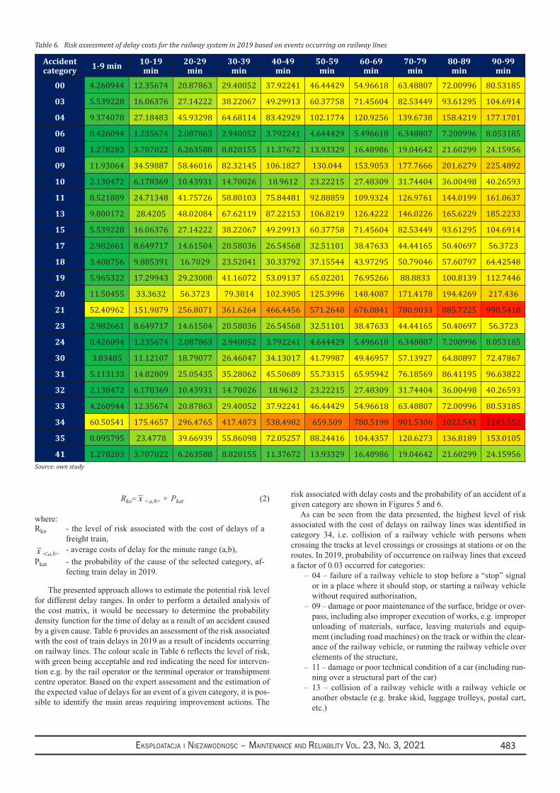
Eksploatacja i NiEzawodNosc – MaiNtENaNcE aNd REliability Vol. 23, No. 3, 2021 483
Rko= x <a,b> × Pkat (2)
where:Rko - the level of risk associated with the cost of delays of a
freight train,x <a,b> - average costs of delay for the minute range (a,b),
Pkat - the probability of the cause of the selected category, af-fecting train delay in 2019.
The presented approach allows to estimate the potential risk level for different delay ranges. In order to perform a detailed analysis of the cost matrix, it would be necessary to determine the probability density function for the time of delay as a result of an accident caused by a given cause. Table 6 provides an assessment of the risk associated with the cost of train delays in 2019 as a result of incidents occurring on railway lines. The colour scale in Table 6 reflects the level of risk, with green being acceptable and red indicating the need for interven-tion e.g. by the rail operator or the terminal operator or transhipment centre operator. Based on the expert assessment and the estimation of the expected value of delays for an event of a given category, it is pos-sible to identify the main areas requiring improvement actions. The
risk associated with delay costs and the probability of an accident of a given category are shown in Figures 5 and 6.
As can be seen from the data presented, the highest level of risk associated with the cost of delays on railway lines was identified in category 34, i.e. collision of a railway vehicle with persons when crossing the tracks at level crossings or crossings at stations or on the routes. In 2019, probability of occurrence on railway lines that exceed a factor of 0.03 occurred for categories:
04 – failure of a railway vehicle to stop before a “stop” signal –or in a place where it should stop, or starting a railway vehicle without required authorisation,09 – damage or poor maintenance of the surface, bridge or over- –pass, including also improper execution of works, e.g. improper unloading of materials, surface, leaving materials and equip-ment (including road machines) on the track or within the clear-ance of the railway vehicle, or running the railway vehicle over elements of the structure,11 – damage or poor technical condition of a car (including run- –ning over a structural part of the car)13 – collision of a railway vehicle with a railway vehicle or –another obstacle (e.g. brake skid, luggage trolleys, postal cart, etc.)
Table 6. Risk assessment of delay costs for the railway system in 2019 based on events occurring on railway lines
Accident category 1-9 min 10-19
min20-29
min30-39
min40-49
min50-59
min60-69
min70-79
min80-89
min90-99
min
00 4.260944 12.35674 20.87863 29.40052 37.92241 46.44429 54.96618 63.48807 72.00996 80.53185
03 5.539228 16.06376 27.14222 38.22067 49.29913 60.37758 71.45604 82.53449 93.61295 104.6914
04 9.374078 27.18483 45.93298 64.68114 83.42929 102.1774 120.9256 139.6738 158.4219 177.1701
06 0.426094 1.235674 2.087863 2.940052 3.792241 4.644429 5.496618 6.348807 7.200996 8.053185
08 1.278283 3.707022 6.263588 8.820155 11.37672 13.93329 16.48986 19.04642 21.60299 24.15956
09 11.93064 34.59887 58.46016 82.32145 106.1827 130.044 153.9053 177.7666 201.6279 225.4892
10 2.130472 6.178369 10.43931 14.70026 18.9612 23.22215 27.48309 31.74404 36.00498 40.26593
11 8.521889 24.71348 41.75726 58.80103 75.84481 92.88859 109.9324 126.9761 144.0199 161.0637
13 9.800172 28.4205 48.02084 67.62119 87.22153 106.8219 126.4222 146.0226 165.6229 185.2233
15 5.539228 16.06376 27.14222 38.22067 49.29913 60.37758 71.45604 82.53449 93.61295 104.6914
17 2.982661 8.649717 14.61504 20.58036 26.54568 32.51101 38.47633 44.44165 50.40697 56.3723
18 3.408756 9.885391 16.7029 23.52041 30.33792 37.15544 43.97295 50.79046 57.60797 64.42548
19 5.965322 17.29943 29.23008 41.16072 53.09137 65.02201 76.95266 88.8833 100.8139 112.7446
20 11.50455 33.3632 56.3723 79.3814 102.3905 125.3996 148.4087 171.4178 194.4269 217.436
21 52.40962 151.9879 256.8071 361.6264 466.4456 571.2648 676.0841 780.9033 885.7225 990.5418
23 2.982661 8.649717 14.61504 20.58036 26.54568 32.51101 38.47633 44.44165 50.40697 56.3723
24 0.426094 1.235674 2.087863 2.940052 3.792241 4.644429 5.496618 6.348807 7.200996 8.053185
30 3.83485 11.12107 18.79077 26.46047 34.13017 41.79987 49.46957 57.13927 64.80897 72.47867
31 5.113133 14.82809 25.05435 35.28062 45.50689 55.73315 65.95942 76.18569 86.41195 96.63822
32 2.130472 6.178369 10.43931 14.70026 18.9612 23.22215 27.48309 31.74404 36.00498 40.26593
33 4.260944 12.35674 20.87863 29.40052 37.92241 46.44429 54.96618 63.48807 72.00996 80.53185
34 60.50541 175.4657 296.4765 417.4873 538.4982 659.509 780.5198 901.5306 1022.541 1143.552
35 8.095795 23.4778 39.66939 55.86098 72.05257 88.24416 104.4357 120.6273 136.8189 153.0105
41 1.278283 3.707022 6.263588 8.820155 11.37672 13.93329 16.48986 19.04642 21.60299 24.15956Source: own study
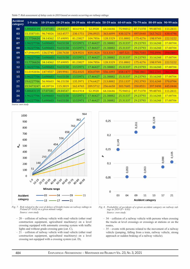
Eksploatacja i NiEzawodNosc – MaiNtENaNcE aNd REliability Vol. 23, No. 3, 2021484
20 – collision of railway vehicle with road vehicle (other road –construction equipment, agricultural machinery) on a level crossing equipped with automatic crossing system with traffic lights and without grade-crossing gate (cat. C),21 – collision of railway vehicle with road vehicle (other road –construction equipment, agricultural machinery) on a level crossing not equipped with a crossing system (cat. D),
34 – collision of a railway vehicle with persons when crossing –the tracks at level crossings or crossings at stations or on the routes,35 – events with persons related to the movement of a railway –vehicle (jumping, falling from a train, railway vehicle, strong approach or sudden braking of a railway vehicle).
Table 7. Risk assessment of delay costs in 2019 based on events occurring on railway sidings
Accident category 1-9 min 10-19 min 20-29 min 30-39 min 40-49 min 50-59 min 60-69 min 70-79 min 80-89 min 90-99 min
00 5.88683119 17.07181 28.84547 40.61914 52.3928 64.16646 75.94012 87.71378 99.48745 111.261103 33.3587101 96.74026 163.4577 230.1751 296.8925 363.6099 430.3274 497.0448 563.7622 630.479604 11.7736624 34.14362 57.69095 81.23827 104.7856 128.3329 151.8802 175.4276 198.9749 222.522207 1.96227706 5.690603 9.615158 13.53971 17.46427 21.38882 25.31337 29.23793 33.16248 37.0870408 1.96227706 5.690603 9.615158 13.53971 17.46427 21.38882 25.31337 29.23793 33.16248 37.0870409 47.0946495 136.5745 230.7638 324.9531 419.1424 513.3317 607.521 701.7103 795.8996 890.088910 1.96227706 5.690603 9.615158 13.53971 17.46427 21.38882 25.31337 29.23793 33.16248 37.0870411 11.7736624 34.14362 57.69095 81.23827 104.7856 128.3329 151.8802 175.4276 198.9749 222.522212 1.96227706 5.690603 9.615158 13.53971 17.46427 21.38882 25.31337 29.23793 33.16248 37.0870413 51.0192036 147.9557 249.9941 352.0325 454.0709 556.1093 658.1477 760.1861 862.2245 964.262915 1.96227706 5.690603 9.615158 13.53971 17.46427 21.38882 25.31337 29.23793 33.16248 37.0870417 19.6227706 56.90603 96.15158 135.3971 174.6427 213.8882 253.1337 292.3793 331.6248 370.870421 23.5473247 68.28724 115.3819 162.4765 209.5712 256.6658 303.7605 350.8551 397.9498 445.044423 5.88683119 17.07181 28.84547 40.61914 52.3928 64.16646 75.94012 87.71378 99.48745 111.261134 1.96227706 5.690603 9.615158 13.53971 17.46427 21.38882 25.31337 29.23793 33.16248 37.0870435 1.96227706 5.690603 9.615158 13.53971 17.46427 21.38882 25.31337 29.23793 33.16248 37.08704
Source: own study
Fig. 7. Risk related to the cost of delays of freight trains on railway sidings in Poland (P>0.03) in a given minute range
Source: own study
Fig. 8. Probability of accidents of a given accident category on railway sid-ings in 2019 (P> 0.03)
Source: own study.
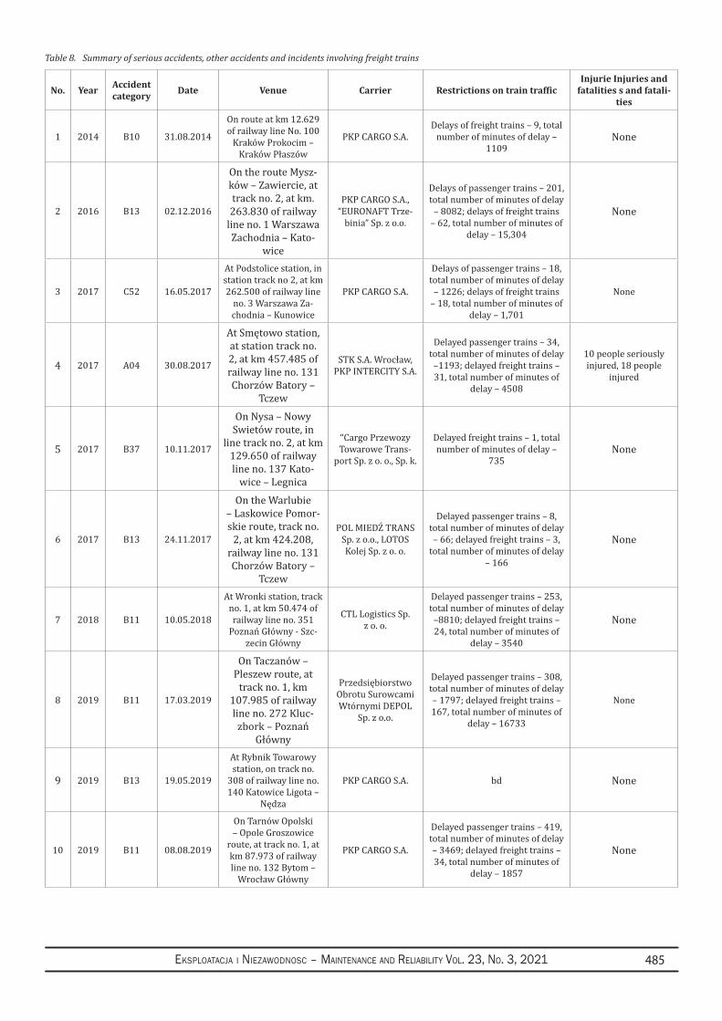
Eksploatacja i NiEzawodNosc – MaiNtENaNcE aNd REliability Vol. 23, No. 3, 2021 485
Table 8. Summary of serious accidents, other accidents and incidents involving freight trains
No. Year Accident category Date Venue Carrier Restrictions on train traffic
Injurie Injuries and fatalities s and fatali-
ties
1 2014 B10 31.08.2014
On route at km 12.629 of railway line No. 100
Kraków Prokocim – Kraków Płaszów
PKP CARGO S.A.Delays of freight trains – 9, total
number of minutes of delay – 1109
None
2 2016 B13 02.12.2016
On the route Mysz-ków – Zawiercie, at track no. 2, at km. 263.830 of railway
line no. 1 Warszawa Zachodnia – Kato-
wice
PKP CARGO S.A., “EURONAFT Trze-
binia” Sp. z o.o.
Delays of passenger trains – 201, total number of minutes of delay
– 8082; delays of freight trains – 62, total number of minutes of
delay – 15,304
None
3 2017 C52 16.05.2017
At Podstolice station, in station track no 2, at km 262.500 of railway line
no. 3 Warszawa Za-chodnia – Kunowice
PKP CARGO S.A.
Delays of passenger trains – 18, total number of minutes of delay
– 1226; delays of freight trains – 18, total number of minutes of
delay – 1,701
None
4 2017 A04 30.08.2017
At Smętowo station, at station track no. 2, at km 457.485 of railway line no. 131 Chorzów Batory –
Tczew
STK S.A. Wrocław, PKP INTERCITY S.A.
Delayed passenger trains – 34, total number of minutes of delay –1193; delayed freight trains – 31, total number of minutes of
delay – 4508
10 people seriously injured, 18 people
injured
5 2017 B37 10.11.2017
On Nysa – Nowy Swietów route, in
line track no. 2, at km 129.650 of railway line no. 137 Kato-
wice – Legnica
“Cargo Przewozy Towarowe Trans-
port Sp. z o. o., Sp. k.
Delayed freight trains – 1, total number of minutes of delay –
735None
6 2017 B13 24.11.2017
On the Warlubie – Laskowice Pomor-skie route, track no.
2, at km 424.208, railway line no. 131 Chorzów Batory –
Tczew
POL MIEDŹ TRANS Sp. z o.o., LOTOS Kolej Sp. z o. o.
Delayed passenger trains – 8, total number of minutes of delay – 66; delayed freight trains – 3,
total number of minutes of delay – 166
None
7 2018 B11 10.05.2018
At Wronki station, track no. 1, at km 50.474 of railway line no. 351
Poznań Główny - Szc-zecin Główny
CTL Logistics Sp. z o. o.
Delayed passenger trains – 253, total number of minutes of delay –8810; delayed freight trains – 24, total number of minutes of
delay – 3540
None
8 2019 B11 17.03.2019
On Taczanów – Pleszew route, at
track no. 1, km 107.985 of railway line no. 272 Kluc-
zbork – Poznań Główny
Przedsiębiorstwo Obrotu Surowcami Wtórnymi DEPOL
Sp. z o.o.
Delayed passenger trains – 308, total number of minutes of delay – 1797; delayed freight trains – 167, total number of minutes of
delay – 16733
None
9 2019 B13 19.05.2019
At Rybnik Towarowy station, on track no.
308 of railway line no. 140 Katowice Ligota –
Nędza
PKP CARGO S.A. bd None
10 2019 B11 08.08.2019
On Tarnów Opolski – Opole Groszowice
route, at track no. 1, at km 87.973 of railway line no. 132 Bytom –
Wrocław Główny
PKP CARGO S.A.
Delayed passenger trains – 419, total number of minutes of delay – 3469; delayed freight trains – 34, total number of minutes of
delay – 1857
None
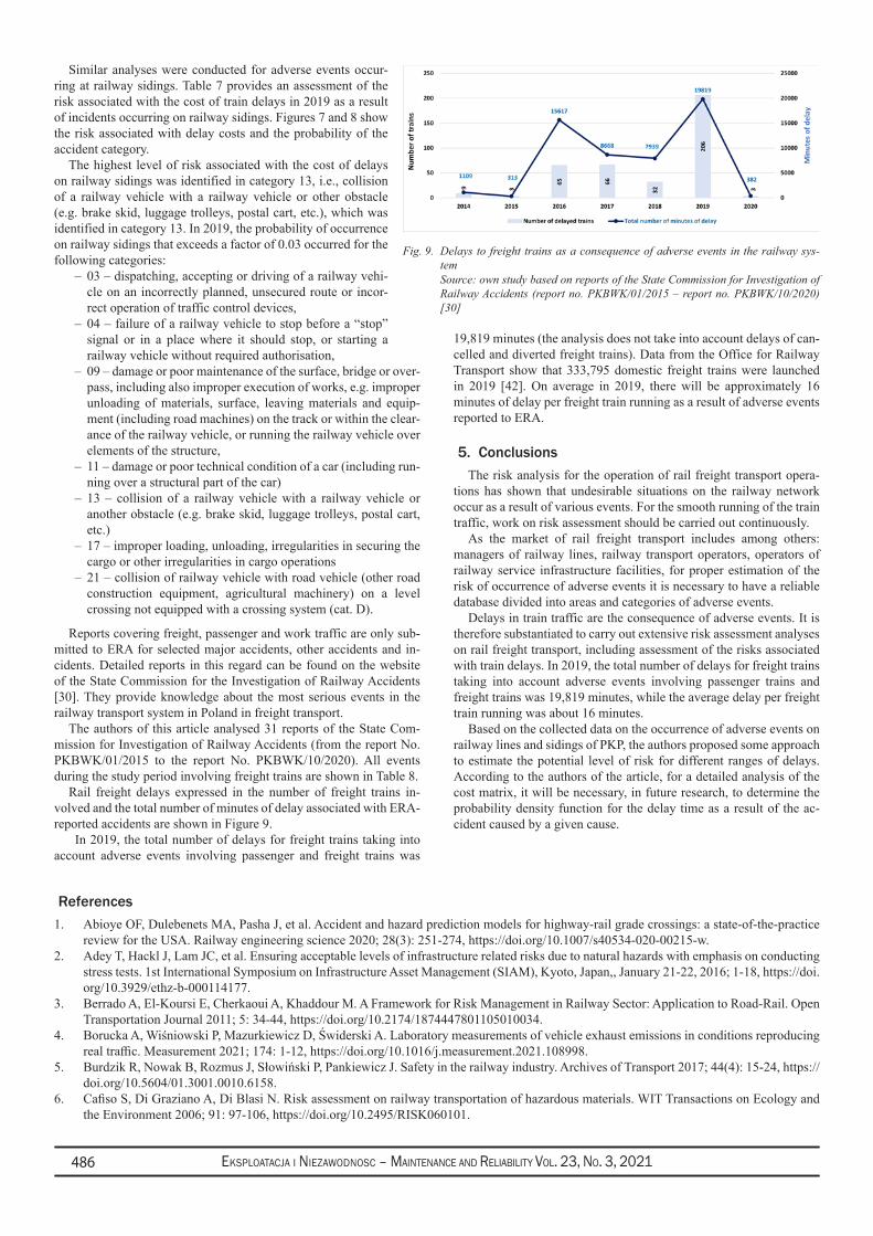
Eksploatacja i NiEzawodNosc – MaiNtENaNcE aNd REliability Vol. 23, No. 3, 2021486
Similar analyses were conducted for adverse events occur-ring at railway sidings. Table 7 provides an assessment of the risk associated with the cost of train delays in 2019 as a result of incidents occurring on railway sidings. Figures 7 and 8 show the risk associated with delay costs and the probability of the accident category.
The highest level of risk associated with the cost of delays on railway sidings was identified in category 13, i.e., collision of a railway vehicle with a railway vehicle or other obstacle (e.g. brake skid, luggage trolleys, postal cart, etc.), which was identified in category 13. In 2019, the probability of occurrence on railway sidings that exceeds a factor of 0.03 occurred for the following categories:
03 – dispatching, accepting or driving of a railway vehi- –cle on an incorrectly planned, unsecured route or incor-rect operation of traffic control devices,04 – failure of a railway vehicle to stop before a “stop” –signal or in a place where it should stop, or starting a railway vehicle without required authorisation,09 – damage or poor maintenance of the surface, bridge or over- –pass, including also improper execution of works, e.g. improper unloading of materials, surface, leaving materials and equip-ment (including road machines) on the track or within the clear-ance of the railway vehicle, or running the railway vehicle over elements of the structure,11 – damage or poor technical condition of a car (including run- –ning over a structural part of the car)13 – collision of a railway vehicle with a railway vehicle or –another obstacle (e.g. brake skid, luggage trolleys, postal cart, etc.)17 – improper loading, unloading, irregularities in securing the –cargo or other irregularities in cargo operations21 – collision of railway vehicle with road vehicle (other road –construction equipment, agricultural machinery) on a level crossing not equipped with a crossing system (cat. D).
Reports covering freight, passenger and work traffic are only sub-mitted to ERA for selected major accidents, other accidents and in-cidents. Detailed reports in this regard can be found on the website of the State Commission for the Investigation of Railway Accidents [30]. They provide knowledge about the most serious events in the railway transport system in Poland in freight transport.
The authors of this article analysed 31 reports of the State Com-mission for Investigation of Railway Accidents (from the report No. PKBWK/01/2015 to the report No. PKBWK/10/2020). All events during the study period involving freight trains are shown in Table 8.
Rail freight delays expressed in the number of freight trains in-volved and the total number of minutes of delay associated with ERA-reported accidents are shown in Figure 9.
In 2019, the total number of delays for freight trains taking into account adverse events involving passenger and freight trains was
19,819 minutes (the analysis does not take into account delays of can-celled and diverted freight trains). Data from the Office for Railway Transport show that 333,795 domestic freight trains were launched in 2019 [42]. On average in 2019, there will be approximately 16 minutes of delay per freight train running as a result of adverse events reported to ERA.
5. ConclusionsThe risk analysis for the operation of rail freight transport opera-
tions has shown that undesirable situations on the railway network occur as a result of various events. For the smooth running of the train traffic, work on risk assessment should be carried out continuously.
As the market of rail freight transport includes among others: managers of railway lines, railway transport operators, operators of railway service infrastructure facilities, for proper estimation of the risk of occurrence of adverse events it is necessary to have a reliable database divided into areas and categories of adverse events.
Delays in train traffic are the consequence of adverse events. It is therefore substantiated to carry out extensive risk assessment analyses on rail freight transport, including assessment of the risks associated with train delays. In 2019, the total number of delays for freight trains taking into account adverse events involving passenger trains and freight trains was 19,819 minutes, while the average delay per freight train running was about 16 minutes.
Based on the collected data on the occurrence of adverse events on railway lines and sidings of PKP, the authors proposed some approach to estimate the potential level of risk for different ranges of delays. According to the authors of the article, for a detailed analysis of the cost matrix, it will be necessary, in future research, to determine the probability density function for the delay time as a result of the ac-cident caused by a given cause.
Fig. 9. Delays to freight trains as a consequence of adverse events in the railway sys-tem
Source: own study based on reports of the State Commission for Investigation of Railway Accidents (report no. PKBWK/01/2015 – report no. PKBWK/10/2020) [30]
References1. Abioye OF, Dulebenets MA, Pasha J, et al. Accident and hazard prediction models for highway-rail grade crossings: a state-of-the-practice
review for the USA. Railway engineering science 2020; 28(3): 251-274, https://doi.org/10.1007/s40534-020-00215-w.2. Adey T, Hackl J, Lam JC, et al. Ensuring acceptable levels of infrastructure related risks due to natural hazards with emphasis on conducting
stress tests. 1st International Symposium on Infrastructure Asset Management (SIAM), Kyoto, Japan,, January 21-22, 2016; 1-18, https://doi.org/10.3929/ethz-b-000114177.
3. Berrado A, El-Koursi E, Cherkaoui A, Khaddour M. A Framework for Risk Management in Railway Sector: Application to Road-Rail. Open Transportation Journal 2011; 5: 34-44, https://doi.org/10.2174/1874447801105010034.
4. Borucka A, Wiśniowski P, Mazurkiewicz D, Świderski A. Laboratory measurements of vehicle exhaust emissions in conditions reproducing real traffic. Measurement 2021; 174: 1-12, https://doi.org/10.1016/j.measurement.2021.108998.
5. Burdzik R, Nowak B, Rozmus J, Słowiński P, Pankiewicz J. Safety in the railway industry. Archives of Transport 2017; 44(4): 15-24, https://doi.org/10.5604/01.3001.0010.6158.
6. Cafiso S, Di Graziano A, Di Blasi N. Risk assessment on railway transportation of hazardous materials. WIT Transactions on Ecology and the Environment 2006; 91: 97-106, https://doi.org/10.2495/RISK060101.

Eksploatacja i NiEzawodNosc – MaiNtENaNcE aNd REliability Vol. 23, No. 3, 2021 487
7. Ciszewski T, Nowakowski W, Chrzan M. Analysis of selected aspects of the railway safety in the European Union. AUTOBUSY - Technika, Eksploatacja, Systemy Transportowe 2018; 19(12): 378-381, https://doi.org/10.24136/atest.2018.416.
8. Commission Implementing Regulation (EU) No 402/2013 of 30 April 2013 on the common safety method for risk evaluation and assessment and repealing Regulation (EC) No 352/2009, http://data.europa.eu/eli/reg_impl/2013/402/oj.
9. Daniewski K, Kosicka E, Mazurkiewicz D. Analysis of the correctness of determination of the effectiveness of maintenance service actions. Management and Production Engineering Review 2018; 9(2): 20-25, https://doi.org/10.24425/119522.
10. Directive (EU) 2016/797 of the European Parliament and of the Council of 11 May 2016 on the interoperability of the rail system within the European Union, http://data.europa.eu/eli/dir/2016/797/oj.
11. Directive (EU) 2016/798 of the European Parliament and of the Council of 11 May 2016 on railway safety, http://data.europa.eu/eli/dir/2016/798/oj.
12. Directive 2012/34/EU of the European Parliament and of the Council of 21 November 2012 establishing a single European railway area, http://data.europa.eu/eli/dir/2012/34/oj.
13. Fourie CJ, Zhuwaki NT. A modelling framework for railway infrastructure reliability analysis. South African Journal of Industrial Engineering 2017; 28(4): 150-160, http://dx.doi.org/10.7166/28-4-1763.
14. Gołębiowski P, Kukulski J. Preliminary study of shaping the railway track geometry in terms of their maintenance costs and capacity. Archives of Transport 2020; 53(1): 115-128, https://doi.org/10.5604/01.3001.0014.1787.
15. Grenčík J, Galliková J, Volna P, Poprocký R. Use of risk assessment methods in maintenance for more reliable rolling stock operation. MATEC Web of Conferences 2018; 157, 04002: 1-11, https://doi.org/10.1051/matecconf/201815704002.
16. Grenčík J, Volna P, Galliková J. A novel methodology of risk assessment. Scientific Journals of the Maritime University of Szczecin 2020; 63(135): 17-22, https://doi.org/10.17402/435.
17. Hackl J, Lam JC, Adey B, Heitzler M. Novel indicators for identifying critical, INFRAstructure at RISK from Natural Hazards. D4.2 Final Model, Methodology and Information Exchange. ETH Zurich, 2016.
18. Huanga W, Zhanga Y, Koue X, el al. Railway dangerous goods transportation system risk analysis: An Interpretive Structural Modeling and Bayesian Network combining approach. Reliability Engineering and System Safety 2020; 204, 107220: 1-10, https://doi.org/10.1016/j.ress.2020.107220.
19. Huanga W, Zhanga Y, Yua Y, et al. Historical data-driven risk assessment of railway dangerous goods transportation system: Comparisons between Entropy Weight Method and Scatter Degree Method. Reliability Engineering and System Safety 2021; 205,107236: 1-8, https://doi.org/10.1016/j.ress.2020.107236 .
20. Instrukcja postępowania w sprawach poważnych wypadków, wypadków i incydentów w transporcie kolejowym Ir-8. Warszawa: PKP PLK S.A., 2016.
21. ISO 31000:2018. Risk Management. Guidelines.22. ISO Guide 73:2009 Risk management - Vocabulary.23. ISO/IEC 31010:2009 Risk management - Risk assessment techniques.24. Jacyna M, Gołębiowski P, Krześniak, M. Some aspects of heuristic algorithms and their application in decision support tools for freight railway
traffic organisation. Scientific Journal of Silesian University of Technology. Series Transport 2017; 96: 59-69, https://doi.org/10.20858/sjsutst.2017.96.6.
25. Jacyna M, Szczepański E, Izdebski M, et al. Characteristics of event recorders in Automatic Train Control systems. Archives of Transport 2018, 46(2): 61-70, https://doi.org/10.5604/01.3001.0012.2103.
26. Jacyna M, Gołębiowski P, Urbaniak M. Multi-option model of railway traffic organisation including the energy recuperation. In: Mikulski J. (eds) Challenge of Transport Telematics. TST 2016. Communications in Computer and Information Science 2016; 640: 199-210, https://doi.org/10.1007/978-3-319-49646-7_17.
27. Jacyna M, Krześniak M. Computer Support of Decision-Making for the Planning Movement of Freight Wagons on the Rail Network. In: Macioszek E, Sierpiński G. (eds) Recent Advances in Traffic Engineering for Transport Networks and Systems. TSTP 2017. Lecture Notes in Networks and Systems 2018; 21: 225-236, https://doi.org/10.1007/978-3-319-64084-6_21.
28. Jasiulewicz-Kaczmarek M, Antosz K, Wyczółkowski R, el al. Application of MICMAC, Fuzzy AHP, and Fuzzy TOPSIS for Evaluation of the Maintenance Factors Affecting Sustainable Manufacturing. Energies 2021; 14(5): 1-30, https://doi.org/10.3390/en14051436.
29. Kang R, Wang J, Cheng J, et al. (2019). Intelligent Forecasting of Automatic Train Protection System Failure Rate in China High-speed Railway. Eksploatacja i Niezawodnosc - Maintenance and Reliability 2019; 21(4): 567-576, https://doi.org/10.17531/ein.2019.4.5.
30. Komisja Badania Wypadków Kolejowych, https://www.gov.pl/web/mswia/raporty (accessed 19.04.2021).31. Konowrocki R, Chojnacki A. Analysis of rail vehicles' operational reliability in the aspect of safety against derailment based on various
methods of determining the assessment criterion. Eksploatacja i Niezawodnosc - Maintenance and Reliability 2020; 22(1): 73-85, https://doi.org/10.17531/ein.2020.1.9.
32. Kowalski M, Izdebski M, Żak J, Gołda P, Manerowski J. Planning and management of aircraft maintenance using a genetic algorithm. Eksploatacja i Niezawodnosc - Maintenance and Reliability 2021, 23(1): 143-153, https://doi.org/10.17531/ein.2021.1.15.
33. Kukulski J, Jacyna M, Gołębiowski P. Finite Element Method in Assessing Strength Properties of a Railway Surface and Its Elements. Symmetry-Basel 2019; 8(11): 1-29. http://doi.org/10.3390/sym11081014.
34. Leitner B. A General Model for Railway Systems Risk Assessment with the Use of Railway Accident Scenarios Analysis. Procedia Engineering 2017; 187: 150-159, https://doi.org/10.1016/j.proeng.2017.04.361.
35. Leśniak A, Janowiec F. Risk Assessment of Additional Works in Railway Construction Investments Using the Bayes Network. Sustainability 2019; 11(19): 1-15, https://doi.org/10.3390/su11195388.
36. Lin JT, Xu Q. Functional safety verification of train control procedure in train-centric CBTC by colored petri net. Archives of Transport 2020; 54(2): 43-58, https://doi.org/10.5604/01.3001.0014.2730.
37. Liu X. Development of a Risk Assessment Tool for Rail Transport of Flammable Energy Resources. Final report (CAIT-UTC-NC16). New Jersey: Department of Civil and Environmental Engineering Rutgers, The State University of New Jersey, 2016.
38. Niu HX, Hou T. Fast detection study of foreign object intrusion on railway track. Archives of Transport 2018; 47(3): 79-89, https://doi.org/10.5604/01.3001.0012.6510.
39. Papathanasiou N, Adey B, Burkhalter M, Martani C. D3.6 Risk Assessment Methodology. DESTination RAIL - Decision Support Tool for

Eksploatacja i NiEzawodNosc – MaiNtENaNcE aNd REliability Vol. 23, No. 3, 2021488
Rail Infrastructure Managers. Brussels, Belgium, 2018.40. Peace Ch. The reasonably practicable test and work health and safety related risk assessments. New Zealand Journal of Employment Relations
2017; 42(2): 61-78.41. Procedura nr SMS/MMS-PR-02 Ocena ryzyka technicznego i operacyjnego, PKP PLK S.A., 2015.42. Punktualność przewozów towarowych w 2019 r. https://www.utk.gov.pl/pl/raporty-i-analizy/analizy-i-monitoring/statystyka-przewozow-to/
dane-archiwalne/15700,Punktualnosc-przewozow-towarowych-w-2019-r.html (accessed 19.04.2021).43. Rahbar M, Bagheri M. Risk Assessment Framework for the Rail Transport of Hazardous Materials. Transportation Research Record Journal
of the Transportation Research Board 2015; 2411(1): 90-95, https://doi.org/10.3141/2411-11.44. Raport w sprawie bezpieczeństwa w 2019. Warszawa: Urząd Transportu Kolejowego, 2020.45. Restel FJ. Impact of infrastructure type on reliability of railway transportation system. Journal of KONBiN 2013; 1(25): 21-36, https://doi.
org/10.2478/jok-2013-0065.46. Restel FJ. The railway operation process evaluation method in terms of resilience analysis. Archives of Transport 2021; 57(1): 73-89, https://
doi.org/10.5604/01.3001.0014.7485.47. Regulation of the Minister of Infrastructure and Construction of 16 March 2016 on serious accidents, accidents and incidents in railway
transport (Journal of Laws of 2015, item 1297, 1741, 1753, 1777 and 1893).48. Simic V, Jovcic S, Soušek R. Picture Fuzzy MCDM Approach for Risk Assessment of Railway Infrastructure. Mathematics 2020; 8(12):
1-29, http://dx.doi.org/10.3390/math8122259.49. Smoczyński P, Kadziński A. Introduction to the risk management in the maintenance of railway tracks. Journal of Mechanical and Transport
Engineering 2016; 68(4): 65-80, https://doi.org/10.21008/j.2449-920X.2016.68.4.06.50. Sobota A, Żochowska R, Szczepański E, Gołda P. The influence of tram tracks on car vehicle speed and noise emission at four-approach
intersections located on multilane arteries in cities. Journal of Vibroengineering 2018; 20(6): 2453-2468, https://doi.org/10.21595/jve.2018.20087.
51. Sprawozdanie z funkcjonowania rynku transportu kolejowego w 2019 r. Warszawa: Urząd Transportu Kolejowego, 2020.52. Sprawozdanie ze stanu bezpieczeństwa w ruchu kolejowym w 2018 r. Warszawa: Urząd Transportu Kolejowego, 2019.53. Świerczek A. Zarządzanie ryzykiem transmisji zakłóceń we współdziałaniu przedsiębiorstw w łańcuchach dostaw. Katowice: Wydawnictwo
Uniwersytetu Ekonomicznego w Katowicach, 2012.54. Toruń A, Sokołowska L, Jacyna M. Communications-based train control system - Concept based on WiFi LAN network. Proceedings of 23rd
International Scientific Conference. Transport Means 2019: 911-915.55. Urbaniak M, Kardas-Cinal E, Jacyna M. Optimization of Energetic Train Cooperation. Symmetry-Basel 2019; 11(9): 1-19, http://doi.
org/10.3390/sym11091175.56. Act of 28 March 2003 on rail transport (Journal of Laws of 2019, item 710).57. Yu H, Zhang G, Ran Y, Li M, Wang Y. A comprehensive and practical reliability allocation method considering failure effects and reliability
costs. Eksploatacja i Niezawodnosc - Maintenance and Reliability 2018; 20(2): 244-251, https://doi.org/10.17531/ein.2018.2.09
Eksploatacja i NiEzawodNosc – MaiNtENaNcE aNd REliability Vol. 23, No. 3, 2021 489
(*) Corresponding author.E-mail addresses:
Eksploatacja i Niezawodnosc – Maintenance and ReliabilityVolume 23 (2021), Issue 3
journal homepage: http://www.ein.org.pl
Indexed by:
Automatically controlled hydraulic tension systems adjust the tension force of a conveyor belt under different working conditions. Failures of an automatically controlled hydraulic tension system influence the performance of conveyor belts. At present, the maintenance of automatically controlled hydraulic tension systems mainly considers the replacement of components when failures occur. Considering the maintenance cost and downtime, it is im-possible to repair all the failed components to improve the hydraulic tension system. One of the key problems is selecting the most valuable components for preventive maintenance. In this paper, preventive maintenance for multiple components in a hydraulic tension system is analyzed. An index is proposed to select more reliable preventive maintenance components to replace the original ones. A case study is given to demonstrate the proposed method. When the cost budget increases, there are three different variations in the number of compo-nents for selective preventive maintenance (SPM).
Highlights Abstract
Hydraulic tension system of conveyor belt is in-• troduced to SPM.
Preventive maintenance model for multiple com-• ponents is proposed.
Joint integrated importance measure (JIIM) is ap-• plied to a hydraulic tension system.
Maintenance plan of hydraulic tension is analysed • to optimize the system performance.
Preventive maintenance of multiple components for hydraulic tension systemsHongyan Dui a, Xiaoqian Zheng a, Qian Qian Zhao a, Yining Fang b,*a School of Management Engineering, Zhengzhou University, Zhengzhou 450001, China b Laboratory of Science and Technology on Integrated Logistics Support, College of Intelligent Sciences and Technology, National University of Defense Technology, Changsha 410073, PR China
Dui H, Zheng X, Zhao QQ, Fang Y. Preventive maintenance of multiple components for hydraulic tension systems. Eksploatacja i Nieza-wodnosc – Maintenance and Reliability 2021; 23 (3): 489–497, http://doi.org/10.17531/ein.2021.3.9.
Article citation info:
preventive maintenance; reliability; importance measure; maintenance cost.
Keywords
This is an open access article under the CC BY license (https://creativecommons.org/licenses/by/4.0/)
H. Dui - [email protected], X. Zheng - [email protected], Q. Q. Zhao - [email protected], Y. Fang - [email protected]
1. IntroductionIn recent years, with the development of automation technology
and increasing demand in industry, an automatically controlled hy-draulic tension system is increasingly being used in conveyor belts [26]. An automatically controlled hydraulic tension system is used to provide stable tension to a conveyor belt. Routine maintenance only considers the maintenance of faulty components and only in the event of obvious system failure. Preventive maintenance of other compo-nents can be carried out at the same time when the failure components are repaired. This saves the maintenance time, and the components that may fail can be replaced in advance before the next system failure to ensure long-term system reliability.
Many scholars have studied the maintenance of hydraulic systems [18, 20, 25], but few researchers focus on the preventive maintenance of hydraulic tension systems due to their high system complexity. A hydraulic tension system plays an important role in ensuring the stable transportation of a conveyor belt [18]. An automatically controlled hydraulic tension system is composed of a series of hydraulic compo-nents, such as a pump, relief valve, accumulator, and one-way valve. When the components in the system fail, they will reduce the system reliability and even cause the whole system to fail [20]. Because the
maintenance resources are limited, preventive maintenance is widely used as a reliability-centered maintenance strategy.
Jia and Cui [12] gave a joint maintenance strategy for safety-criti-cal hydraulic tension systems. Wu and Castrob [27] developed main-tenance policies for a system under condition monitoring. Zhao et al. [37] proposed an optimization model of an opportunistic maintenance strategy. Cai et al. [1] analyzed the system failure of engineering sys-tems based on Bayesian networks. Based on the expected value and variance of system reliability as an objective function, the optimiza-tion problem of selective maintenance bi-objective optimization prob-lem was modeled.
Jiang and Liu [11] developed a new selective maintenance model for systems that execute multiple consecutive missions. The preven-tive maintenance uses the optimal allocation of limited resources to improve the reliability of the system as much as possible under the constraints of cost resources. Wu and Zhou [30] analyzed a predictive maintenance policy with nonperiodic inspection. After the preventive maintenance, Jia et al. [14] studied the improvement of the reliabil-ity and safety of safety-critical hydraulic tension systems. Preventive maintenance can obtain strategies to maximize hydraulic tension sys-tem performance under cost constraints.
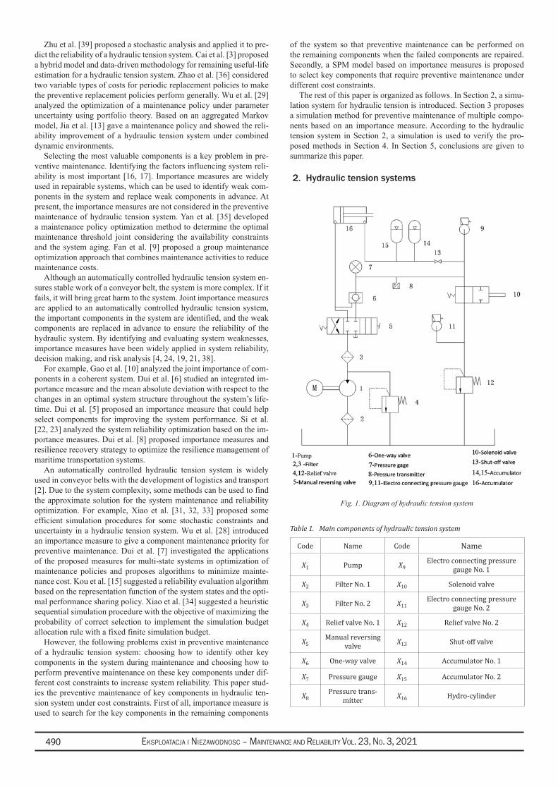
Eksploatacja i NiEzawodNosc – MaiNtENaNcE aNd REliability Vol. 23, No. 3, 2021490
Zhu et al. [39] proposed a stochastic analysis and applied it to pre-dict the reliability of a hydraulic tension system. Cai et al. [3] proposed a hybrid model and data-driven methodology for remaining useful-life estimation for a hydraulic tension system. Zhao et al. [36] considered two variable types of costs for periodic replacement policies to make the preventive replacement policies perform generally. Wu et al. [29] analyzed the optimization of a maintenance policy under parameter uncertainty using portfolio theory. Based on an aggregated Markov model, Jia et al. [13] gave a maintenance policy and showed the reli-ability improvement of a hydraulic tension system under combined dynamic environments.
Selecting the most valuable components is a key problem in pre-ventive maintenance. Identifying the factors influencing system reli-ability is most important [16, 17]. Importance measures are widely used in repairable systems, which can be used to identify weak com-ponents in the system and replace weak components in advance. At present, the importance measures are not considered in the preventive maintenance of hydraulic tension system. Yan et al. [35] developed a maintenance policy optimization method to determine the optimal maintenance threshold joint considering the availability constraints and the system aging. Fan et al. [9] proposed a group maintenance optimization approach that combines maintenance activities to reduce maintenance costs.
Although an automatically controlled hydraulic tension system en-sures stable work of a conveyor belt, the system is more complex. If it fails, it will bring great harm to the system. Joint importance measures are applied to an automatically controlled hydraulic tension system, the important components in the system are identified, and the weak components are replaced in advance to ensure the reliability of the hydraulic system. By identifying and evaluating system weaknesses, importance measures have been widely applied in system reliability, decision making, and risk analysis [4, 24, 19, 21, 38].
For example, Gao et al. [10] analyzed the joint importance of com-ponents in a coherent system. Dui et al. [6] studied an integrated im-portance measure and the mean absolute deviation with respect to the changes in an optimal system structure throughout the system’s life-time. Dui et al. [5] proposed an importance measure that could help select components for improving the system performance. Si et al. [22, 23] analyzed the system reliability optimization based on the im-portance measures. Dui et al. [8] proposed importance measures and resilience recovery strategy to optimize the resilience management of maritime transportation systems.
An automatically controlled hydraulic tension system is widely used in conveyor belts with the development of logistics and transport [2]. Due to the system complexity, some methods can be used to find the approximate solution for the system maintenance and reliability optimization. For example, Xiao et al. [31, 32, 33] proposed some efficient simulation procedures for some stochastic constraints and uncertainty in a hydraulic tension system. Wu et al. [28] introduced an importance measure to give a component maintenance priority for preventive maintenance. Dui et al. [7] investigated the applications of the proposed measures for multi-state systems in optimization of maintenance policies and proposes algorithms to minimize mainte-nance cost. Kou et al. [15] suggested a reliability evaluation algorithm based on the representation function of the system states and the opti-mal performance sharing policy. Xiao et al. [34] suggested a heuristic sequential simulation procedure with the objective of maximizing the probability of correct selection to implement the simulation budget allocation rule with a fixed finite simulation budget.
However, the following problems exist in preventive maintenance of a hydraulic tension system: choosing how to identify other key components in the system during maintenance and choosing how to perform preventive maintenance on these key components under dif-ferent cost constraints to increase system reliability. This paper stud-ies the preventive maintenance of key components in hydraulic ten-sion system under cost constraints. First of all, importance measure is used to search for the key components in the remaining components
of the system so that preventive maintenance can be performed on the remaining components when the failed components are repaired. Secondly, a SPM model based on importance measures is proposed to select key components that require preventive maintenance under different cost constraints.
The rest of this paper is organized as follows. In Section 2, a simu-lation system for hydraulic tension is introduced. Section 3 proposes a simulation method for preventive maintenance of multiple compo-nents based on an importance measure. According to the hydraulic tension system in Section 2, a simulation is used to verify the pro-posed methods in Section 4. In Section 5, conclusions are given to summarize this paper.
2. Hydraulic tension systems
Fig. 1. Diagram of hydraulic tension system
Table 1. Main components of hydraulic tension system
Code Name Code Name
X1 Pump X9Electro connecting pressure
gauge No. 1
X2 Filter No. 1 X10 Solenoid valve
X3 Filter No. 2 X11Electro connecting pressure
gauge No. 2
X4 Relief valve No. 1 X12 Relief valve No. 2
X5Manual reversing
valve X13 Shut-off valve
X6 One-way valve X14 Accumulator No. 1
X7 Pressure gauge X15 Accumulator No. 2
X8Pressure trans-
mitter X16 Hydro-cylinder
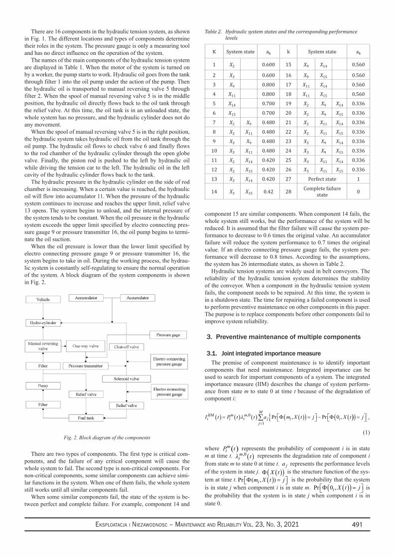
Eksploatacja i NiEzawodNosc – MaiNtENaNcE aNd REliability Vol. 23, No. 3, 2021 491
There are 16 components in the hydraulic tension system, as shown in Fig. 1. The different locations and types of components determine their roles in the system. The pressure gauge is only a measuring tool and has no direct influence on the operation of the system.
The names of the main components of the hydraulic tension system are displayed in Table 1. When the motor of the system is turned on by a worker, the pump starts to work. Hydraulic oil goes from the tank through filter 1 into the oil pump under the action of the pump. Then the hydraulic oil is transported to manual reversing valve 5 through filter 2. When the spool of manual reversing valve 5 is in the middle position, the hydraulic oil directly flows back to the oil tank through the relief valve. At this time, the oil tank is in an unloaded state, the whole system has no pressure, and the hydraulic cylinder does not do any movement.
When the spool of manual reversing valve 5 is in the right position, the hydraulic system takes hydraulic oil from the oil tank through the oil pump. The hydraulic oil flows to check valve 6 and finally flows to the rod chamber of the hydraulic cylinder through the open globe valve. Finally, the piston rod is pushed to the left by hydraulic oil while driving the tension car to the left. The hydraulic oil in the left cavity of the hydraulic cylinder flows back to the tank.
The hydraulic pressure in the hydraulic cylinder on the side of rod chamber is increasing. When a certain value is reached, the hydraulic oil will flow into accumulator 11. When the pressure of the hydraulic system continues to increase and reaches the upper limit, relief valve 13 opens. The system begins to unload, and the internal pressure of the system tends to be constant. When the oil pressure in the hydraulic system exceeds the upper limit specified by electro connecting pres-sure gauge 9 or pressure transmitter 16, the oil pump begins to termi-nate the oil suction.
When the oil pressure is lower than the lower limit specified by electro connecting pressure gauge 9 or pressure transmitter 16, the system begins to take in oil. During the working process, the hydrau-lic system is constantly self-regulating to ensure the normal operation of the system. A block diagram of the system components is shown in Fig. 2.
Fig. 2. Block diagram of the components
There are two types of components. The first type is critical com-ponents, and the failure of any critical component will cause the whole system to fail. The second type is non-critical components. For non-critical components, some similar components can achieve simi-lar functions in the system. When one of them fails, the whole system still works until all similar components fail.
When some similar components fail, the state of the system is be-tween perfect and complete failure. For example, component 14 and
component 15 are similar components. When component 14 fails, the whole system still works, but the performance of the system will be reduced. It is assumed that the filter failure will cause the system per-formance to decrease to 0.6 times the original value. An accumulator failure will reduce the system performance to 0.7 times the original value. If an electro connecting pressure gauge fails, the system per-formance will decrease to 0.8 times. According to the assumptions, the system has 26 intermediate states, as shown in Table 2.
Hydraulic tension systems are widely used in belt conveyors. The reliability of the hydraulic tension system determines the stability of the conveyor. When a component in the hydraulic tension system fails, the component needs to be repaired. At this time, the system is in a shutdown state. The time for repairing a failed component is used to perform preventive maintenance on other components in this paper. The purpose is to replace components before other components fail to improve system reliability.
3. Preventive maintenance of multiple components
3.1. Joint integrated importance measureThe premise of component maintenance is to identify important
components that need maintenance. Integrated importance can be used to search for important components of a system. The integrated importance measure (IIM) describes the change of system perform-ance from state m to state 0 at time t because of the degradation of component i:
I t P t t a m X t j X tiIIM
im
im
j
Mj i i( ) = ( ) ( ) ( )( ) = − (
=∑λ , Pr , Pr ,0
10Φ Φ ))( ) = j ,
(1)
where ( )miP t represents the probability of component i is in state
m at time t. λim t,0 ( ) represents the degradation rate of component i
from state m to state 0 at time t. ja represents the performance levels of the system in state j. Φ X t( )( ) is the structure function of the sys-tem at time t. Pr ( , )Φ m X t ji ( ) = is the probability that the system is in state j when component i is in state m. Pr ,Φ 0i X t j( )( ) = is the probability that the system is in state j when component i is in state 0.
Table 2. Hydraulic system states and the corresponding performance levels
K System state ak k System state ak
1 X2 0.600 15 X9 X14 0.560
2 X3 0.600 16 X9 X15 0.560
3 X9 0.800 17 X11 X14 0.560
4 X11 0.800 18 X11 X15 0.560
5 X14 0.700 19 X2 X9 X14 0.336
6 X15 0.700 20 X2 X9 X15 0.336
7 X2 X9 0.480 21 X2 X11 X14 0.336
8 X2 X11 0.480 22 X2 X11 X15 0.336
9 X3 X9 0.480 23 X3 X9 X14 0.336
10 X3 X11 0.480 24 X3 X9 X15 0.336
11 X2 X14 0.420 25 X3 X11 X14 0.336
12 X2 X15 0.420 26 X3 X11 X15 0.336
13 X3 X14 0.420 27 Perfect state 1
14 X3 X15 0.42 28 Complete failure state 0
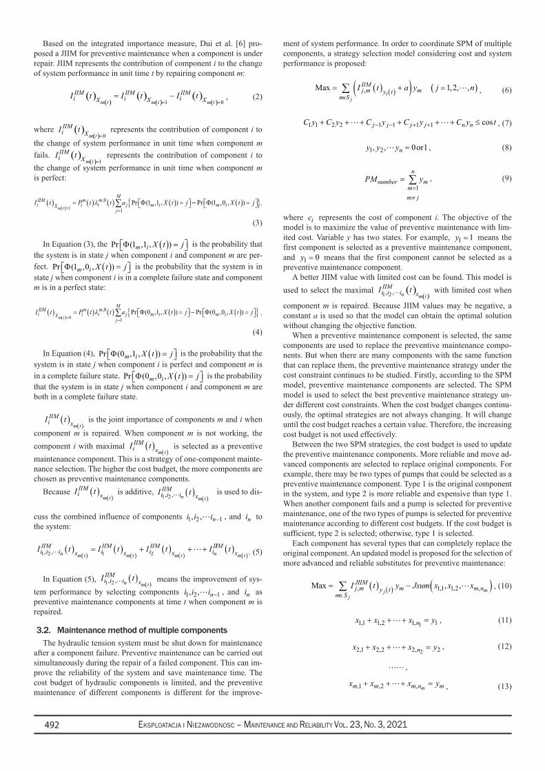
Eksploatacja i NiEzawodNosc – MaiNtENaNcE aNd REliability Vol. 23, No. 3, 2021492
Based on the integrated importance measure, Dui et al. [6] pro-posed a JIIM for preventive maintenance when a component is under repair. JIIM represents the contribution of component i to the change of system performance in unit time t by repairing component m:
( )( )
( )( )
( )( )1 0m t m t m t
IIM IIM IIMi i iX X XI t I t I t
= == − , (2)
where ( )( ) 0m t
IIMi XI t
= represents the contribution of component i to
the change of system performance in unit time when component m fails. ( )
( ) 1m t
IIMi XI t
= represents the contribution of component i to
the change of system performance in unit time when component m is perfect:
I t P t t a X t jiIIM
X im
im
j
Mj m im t
( ) = ( ) ( ) ( ) = ( )= =∑
1
0
11 1λ , Pr ( , , )Φ −− ( ) = Pr ( , , )Φ 1 0m i X t j .
(3)
In Equation (3), the Pr ( , , )Φ 1 1m i X t j( ) = is the probability that the system is in state j when component i and component m are per-fect. Pr ( , , )Φ 1 0m i X t j( ) = is the probability that the system is in state j when component i is in a complete failure state and component m is in a perfect state:
I t P t t a X t jiIIM
X im
im
j
Mj m im t
( ) = ( ) ( ) ( ) = ( )= =∑
0
0
10 1λ , Pr ( , , )Φ −− ( ) = Pr ( , , )Φ 0 0m i X t j .
(4)
In Equation (4), Pr ( , , )Φ 0 1m i X t j( ) = is the probability that the system is in state j when component i is perfect and component m is in a complete failure state. Pr ( , , )Φ 0 0m i X t j( ) = is the probability that the system is in state j when component i and component m are both in a complete failure state.
I tiIIM
xm t( )
( ) is the joint importance of components m and i when
component m is repaired. When component m is not working, the component i with maximal I ti
IIMxm t
( )( )
is selected as a preventive maintenance component. This is a strategy of one-component mainte-nance selection. The higher the cost budget, the more components are chosen as preventive maintenance components.
Because I tiIIM
xm t( )
( ) is additive, I ti i i
IIMxn m t1 2, , ( )
( ) is used to dis-
cuss the combined influence of components 1 2 1, , ni i i − , and ni to the system:
I t I t I t Ii i iIIM
x iIIM
x iIIM
x iI
n m t m t m t n1 2 1 2, , ( ) = ( ) + ( ) + +( ) ( ) ( )
IIMxt
m t( )
( ) . (5)
In Equation (5), I ti i iIIM
xn m t1 2, , ( )( )
means the improvement of sys-tem performance by selecting components 1 2 1, , ni i i − , and ni as preventive maintenance components at time t when component m is repaired.
3.2. Maintenance method of multiple components The hydraulic tension system must be shut down for maintenance
after a component failure. Preventive maintenance can be carried out simultaneously during the repair of a failed component. This can im-prove the reliability of the system and save maintenance time. The cost budget of hydraulic components is limited, and the preventive maintenance of different components is different for the improve-
ment of system performance. In order to coordinate SPM of multiple components, a strategy selection model considering cost and system performance is proposed:
Max = ( ) +( ) =( )∑ ( )m S
j mIIM
y t mj
iI t a y j n
, , , ,1 2 , (6)
1 1 2 2 1 1 1 1 cosj j j j n nC y C y C y C y C y t− − + ++ + + + + + ≤ , (7)
1 2, , 0 or1 ny y y = , (8)
1
nnumber m
mm j
PM y=≠
= ∑ , (9)
where ic represents the cost of component i. The objective of the model is to maximize the value of preventive maintenance with lim-ited cost. Variable y has two states. For example, 1 1y = means the first component is selected as a preventive maintenance component, and 1 0y = means that the first component cannot be selected as a preventive maintenance component.
A better JIIM value with limited cost can be found. This model is used to select the maximal ( )
( )1 2, , n m t
IIMi i i xI t
with limited cost when
component m is repaired. Because JIIM values may be negative, a constant a is used so that the model can obtain the optimal solution without changing the objective function.
When a preventive maintenance component is selected, the same components are used to replace the preventive maintenance compo-nents. But when there are many components with the same function that can replace them, the preventive maintenance strategy under the cost constraint continues to be studied. Firstly, according to the SPM model, preventive maintenance components are selected. The SPM model is used to select the best preventive maintenance strategy un-der different cost constraints. When the cost budget changes continu-ously, the optimal strategies are not always changing. It will change until the cost budget reaches a certain value. Therefore, the increasing cost budget is not used effectively.
Between the two SPM strategies, the cost budget is used to update the preventive maintenance components. More reliable and move ad-vanced components are selected to replace original components. For example, there may be two types of pumps that could be selected as a preventive maintenance component. Type 1 is the original component in the system, and type 2 is more reliable and expensive than type 1. When another component fails and a pump is selected for preventive maintenance, one of the two types of pumps is selected for preventive maintenance according to different cost budgets. If the cost budget is sufficient, type 2 is selected; otherwise, type 1 is selected.
Each component has several types that can completely replace the original component. An updated model is proposed for the selection of more advanced and reliable substitutes for preventive maintenance:
Max = ( ) − ( )∈
( )∑m S
j mJIIM
y t m m nj
j mI t y Jsum x x x, , , ,, ,11 1 2 , (10)
11,1 1,2 1, 1nx x x y+ + + = , (11)
22,1 2,2 2, 2nx x x y+ + + =
, (12)
,
,1 ,2 , mm m m n mx x x y+ + + = , (13)
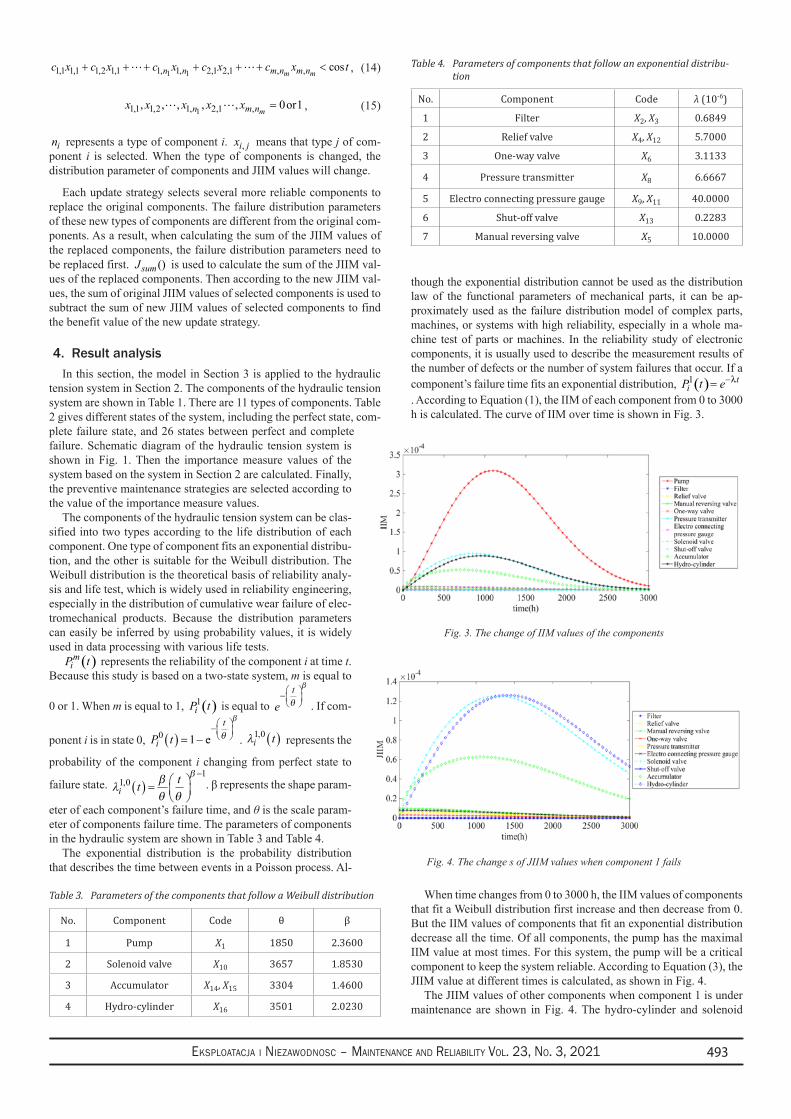
Eksploatacja i NiEzawodNosc – MaiNtENaNcE aNd REliability Vol. 23, No. 3, 2021 493
1 11,1 1,1 1,2 1,1 1, 1, 2,1 2,1 , , cosm mn n m n m nc x c x c x c x c x t+ + + + + + < , (14)
11,1 1,2 1, 2,1 ,, , , , , 0 or1 mn m nx x x x x = , (15)
in represents a type of component i. ,i jx means that type j of com-ponent i is selected. When the type of components is changed, the distribution parameter of components and JIIM values will change.
Each update strategy selects several more reliable components to replace the original components. The failure distribution parameters of these new types of components are different from the original com-ponents. As a result, when calculating the sum of the JIIM values of the replaced components, the failure distribution parameters need to be replaced first. ()sumJ is used to calculate the sum of the JIIM val-ues of the replaced components. Then according to the new JIIM val-ues, the sum of original JIIM values of selected components is used to subtract the sum of new JIIM values of selected components to find the benefit value of the new update strategy.
4. Result analysisIn this section, the model in Section 3 is applied to the hydraulic
tension system in Section 2. The components of the hydraulic tension system are shown in Table 1. There are 11 types of components. Table 2 gives different states of the system, including the perfect state, com-plete failure state, and 26 states between perfect and complete failure. Schematic diagram of the hydraulic tension system is shown in Fig. 1. Then the importance measure values of the system based on the system in Section 2 are calculated. Finally, the preventive maintenance strategies are selected according to the value of the importance measure values.
The components of the hydraulic tension system can be clas-sified into two types according to the life distribution of each component. One type of component fits an exponential distribu-tion, and the other is suitable for the Weibull distribution. The Weibull distribution is the theoretical basis of reliability analy-sis and life test, which is widely used in reliability engineering, especially in the distribution of cumulative wear failure of elec-tromechanical products. Because the distribution parameters can easily be inferred by using probability values, it is widely used in data processing with various life tests.
( )miP t represents the reliability of the component i at time t.
Because this study is based on a two-state system, m is equal to
0 or 1. When m is equal to 1, ( )1iP t is equal to e
t−
θ
β
. If com-
ponent i is in state 0, P ti
t0 1( ) = −
−
e θ
β
. λi t1 0, ( ) represents the
probability of the component i changing from perfect state to
failure state. λ βθ θ
β
i t t1 01
, ( ) =
−. β represents the shape param-
eter of each component’s failure time, and θ is the scale param-eter of components failure time. The parameters of components in the hydraulic system are shown in Table 3 and Table 4.
The exponential distribution is the probability distribution that describes the time between events in a Poisson process. Al-
though the exponential distribution cannot be used as the distribution law of the functional parameters of mechanical parts, it can be ap-proximately used as the failure distribution model of complex parts, machines, or systems with high reliability, especially in a whole ma-chine test of parts or machines. In the reliability study of electronic components, it is usually used to describe the measurement results of the number of defects or the number of system failures that occur. If a component’s failure time fits an exponential distribution, ( )1 t
iP t e λ−=. According to Equation (1), the IIM of each component from 0 to 3000 h is calculated. The curve of IIM over time is shown in Fig. 3.
When time changes from 0 to 3000 h, the IIM values of components that fit a Weibull distribution first increase and then decrease from 0. But the IIM values of components that fit an exponential distribution decrease all the time. Of all components, the pump has the maximal IIM value at most times. For this system, the pump will be a critical component to keep the system reliable. According to Equation (3), the JIIM value at different times is calculated, as shown in Fig. 4.
The JIIM values of other components when component 1 is under maintenance are shown in Fig. 4. The hydro-cylinder and solenoid
Table 3. Parameters of the components that follow a Weibull distribution
No. Component Code θ β
1 Pump X1 1850 2.3600
2 Solenoid valve X10 3657 1.8530
3 Accumulator X14, X15 3304 1.4600
4 Hydro-cylinder X16 3501 2.0230
Fig. 3. The change of IIM values of the components
Table 4. Parameters of components that follow an exponential distribu-tion
No. Component Code λ (10-6)
1 Filter X2, X3 0.6849
2 Relief valve X4, X12 5.7000
3 One-way valve X6 3.1133
4 Pressure transmitter X8 6.6667
5 Electro connecting pressure gauge X9, X11 40.0000
6 Shut-off valve X13 0.2283
7 Manual reversing valve X5 10.0000
Fig. 4. The change s of JIIM values when component 1 fails
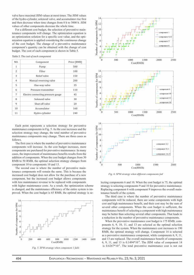
Eksploatacja i NiEzawodNosc – MaiNtENaNcE aNd REliability Vol. 23, No. 3, 2021494
valve have maximal JIIM values at most times. The JIIM values of the hydro-cylinder, solenoid valve, and accumulator rise first and then decrease when time changes from 0 h to 3000 h. JIIM values of other components decrease the whole time.
For a different cost budget, the selection of preventive main-tenance components will change. The optimization equation is an optimization solution for a specific cost value, and the opti-mization equation is applied considering the continuous change of the cost budget. The change of a preventive maintenance component’s quantity can be obtained with the change of cost budget. The cost of each component is shown in Table 5.
Each point represents a selection strategy for preventive maintenance components in Fig. 5. As the cost increases and the selection strategy may change, the total number of preventive maintenance components may change. There are three cases as follows.
The first case is where the number of preventive maintenance components will increase. As the cost budget increases, more components are purchased for preventive maintenance. In many cases, the improvement of maintenance benefits results from the addition of components. When the cost budget changes from 30 RMB to 50 RMB, the optimal selection strategy changes from component 10 to components 10 and 13.
The second case is where the number of preventive main-tenance components will remain the same. This is because the increased cost budget does not allow for the purchase of a new component, but the increased cost budget allows components with less maintenance revenue to be replaced with components with higher maintenance costs. As a result, the optimization scheme is changed, and the maintenance efficiency of the entire system is im-proved. When the cost budget is 65 RMB, the optimal strategy is se-
lecting components 6 and 10. When the cost budget is 75, the optimal strategy is selecting components 9 and 10 for preventive maintenance. Replacing component 6 with component 9 improves the overall main-tenance benefit of the system.
The third case is where the number of preventive maintenance components will be reduced, there are some components with high cost and high maintenance benefit, and their cost may be the sum of several other components. When the cost budget is sufficient, the maintenance benefit of selecting a component with high maintenance may be better than selecting several other components. That leads to a reduction in the number of preventive maintenance components.
When the preventive maintenance cost budget is 175 RMB, com-ponents 6, 9, 10, 11, and 13 are selected as the optimal selection strategy for the system. When the maintenance cost increases to 190 RMB, the optimal strategy will change. Component 14 is selected as a preventive maintenance component, while components 6, 9, 11, and 13 are replaced. The overall maintenance benefit of components 6, 9, 11, and 13 is 0.1494*10-4. The JIIM value of component 14 is 0.6267*10-4. The total preventive maintenance cost is not out
Table 5. The cost of each component
NO. Component Price (RMB)
1 Pump 500
2 Filter 100
3 Relief valve 150
4 Manual reversing valve 200
5 One-way valve 35
6 Pressure transmitter 110
7 Electro connecting pressure gauge 45
8 Solenoid valve 30
9 Shut-off valve 20
10 Accumulator 160
11 Hydro-cylinder 240
Fig. 5. SPM strategy when component 1 fails
Fig. 6. SPM strategy when different components fail

Eksploatacja i NiEzawodNosc – MaiNtENaNcE aNd REliability Vol. 23, No. 3, 2021 495
of range due to the constraints of the condition in the optimization model.
In general, the number of preventive maintenance components increases with the increase of cost. The relationships between the number of components and cost budget are shown in Fig. 6. The number of preventive maintenance components increases faster dur-ing repair of component 1. Because the cost of component 1 is 500 RMB, which is the highest of all components, more components can be used as preventive maintenance components at a lower cost.
When component 16 is repaired, the number of preventive mainte-nance components increases faster than with other components. The cost of component 16 is 240 RMB, which is the second most expen-sive component of all components. This is a normal phenomenon be-cause when repairing expensive components, there is no need to re-serve a high cost budget for preventive maintenance. The components with the same function in the system have the same SPM.
There are many strategies for SPM at different costs. The selection strategy of component 1 for preventive maintenance is shown in Ta-ble 6. In consideration of the preventive maintenance strategies when component 1 is repaired, the interval is selected when the cost budget is between 50 RMB and 65 RMB. According to data in Table 6, com-ponents 10 and 13 could be updated when the cost budget increases from 50 RMB to 65 RMB.
Component 10 has two types, and component 13 has three types. The costs of different types of components are shown in Table 7. The failure distribution parameters of different types of components are shown in Table 8. Type 1 means original components, which are se-lected to be replaced.
The strategy when the lower limit of the cost budget is 50 RMB is shown in Table 9. When the cost budget is 55 RMB, the optimal update strategy is to select type 2 of component 10 and type 1 of component 13. When the cost budget is 55 RMB, type 1 of compo-
nent 10 and type 3 of component 13 are se-lected. Since the update strategy is based on the selection strategy, the lower limit of the cost budget is 50 RMB. The number of SPM components is always 2, and components 10 and 13 are updated.
5. ConclusionsIn this paper, a preventive maintenance model for multiple com-
ponents was applied to a hydraulic tension system. According to the model analysis, the pump in this system is the most important com-ponent. When the cost budget increases, there are three different vari-ations in the number of components for SPM. When the cost budget is equal to 50 RMB, components 10 and 13 are selected. When the cost budget increases from 50 RMB to 65 RMB, different types of components 10 and 13 are selected to replace the original type to im-prove the system performance. Different components have different repair times. Therefore, it is necessary to add component repair time research to the model in future work.
AcknowledgementsThe authors gratefully acknowledge the financial support for this research from the National Natural Science Foundation of China
(72071182, U1904211), and the Ministry of Education’s Humanities and Social Sciences Planning Fund (20YJA630012).
Table 6. Selection strategy of component 1 for preventive maintenance
Cost Component
2 3 4 5 6 8 9 10 11 12 13 14 15 16
50 0 0 0 0 0 0 0 1 0 0 1 0 0 0
65 0 0 0 0 1 0 0 1 0 0 0 0 0 0
Table 7. The cost of different types of components
ComponentPrice (RMB)
Type 1(origin) Type 2 Type 3
10 30 35
13 20 23 25
Table 8. Parameters of components in hydraulic system
Component θ1 β1 θ2 β2
10 3657 1.8530 4657 1.3530
Component λ1610−( )
λ2
610−( )
λ3610−( )
13 0.2283 0.11 0.07
Table 9. Strategies under different cost budgets
Cost Number of SPM com-ponents
Component
10 13
50 2 Type 1 Type 1
53 2 Type 1 Type 2
55 2 Type 2 Type 1
58 2 Type 2 Type 2
60 2 Type 2 Type 3
ReferencesCai B P, Huang L, Xie M. Bayesian networks in fault diagnosis. IEEE Transactions on Industrial Informatics 2017; 13(5): 2227-2240, 1. https:/doi.org/10.1109/TII.2017.2695583.Cai B P, Yu L, Xie M. A dynamic-bayesian-network-based fault diagnosis methodology considering transient and intermittent faults. IEEE 2. Transactions on Automation Science and Engineering, 2017; 14(1): 276-285, https:/doi.org/10.1109/TASE.2016.2574875.Cai B P, Shao X Y, Liu Y H, Kong X D, Wang H F, Xu H Q, Ge W F. Remaining useful life estimation of structure systems under the 3. influence of multiple causes: subsea pipelines as a case study. IEEE Transactions on Industrial Electronics, 2020; 67(7): 5737-5747, https://doi.org/10.1109/TIE.2019.2931491.Cui J G, Ren Y, Xu B H, Yang D Z, Zeng S K. Reliability analysis of a multi-eso based control strategy for level adjustment control system 4. of quadruped robot under disturbances and failures. Eksploatacja i Niezawodnosc - Maintenance and Reliability, 2020; 22(1): 42-51, http://doi.org/10.17531/ein.2020.1.6.Dui H Y, Li S M, Xing L D, Liu H L. System performance-based joint importance analysis guided maintenance for repairable systems. 5. Reliability Engineering & System Safety, 2019; 186: 162-175, https://doi.org/10.1016/j.ress.2019.02.021.

Eksploatacja i NiEzawodNosc – MaiNtENaNcE aNd REliability Vol. 23, No. 3, 2021496
Dui H Y, Si S B, Yam RCM. Importance measures for optimal structure in linear consecutive-k-out-of-n systems. Reliability Engineering & 6. System Safety, 2018; 169: 339-350, https://doi.org/10.1016/j.ress.2017.09.015.Dui H Y, Wu S M, Zhao J B. Some extensions of the component maintenance priority. Reliability Engineering and System Safety, 2021; 214: 7. 107729.https:/doi.org/10.1016/j.ress.2021.107729.Dui H Y, Zheng X Q, Wu. S M. Resilience analysis of maritime transportation systems based on importance measures. Reliability Engineering 8. and System Safety, 2021; 209: 107461. https://doi.org/10.1016/j.ress.2021.107461.Fan D M, Zhang A B, Feng Q, Cai B P, Liu Y L, Ren Y. Group maintenance optimization of subsea Xmas trees with stochastic dependency. 9. Reliability Engineering & System Safety, 2021; 209: 107450, https://doi.org/10.1016/j.ress.2021.107450.Gao X L, Cui L R, Li J. L Analysis for joint importance of components in a coherent system. European Journal of Operational Research, 10. 2007; 182(1): 282-299, https://doi.org/10.1016/j.ejor.2006.07.022.Jiang T, Liu Y. Selective maintenance strategy for systems executing multiple consecutive missions with uncertainty. Reliability Engineering 11. & System Safety, 2020; 193: 106632, https://doi.org/10.1016/j.ress.2019.106632.Jia X J, Cui L R. Optimization of joint maintenance strategy for safety-critical systems with different reliability degrees. Expert Systems, 12. 2011; 28(3): 199-208, https://doi.org/10.1111/j.1468-0394.2011.00579.x.Jia X J, Xing L D, Song X Y. Aggregated Markov-based reliability analysis of multi-state systems under combined dynamic environments. 13. Quality and Reliability Engineering International, 2020; 36(3): 846-860, https://doi.org/10.1002/qre.2584.Jia X J, Xing L D, Li G. Copula-based reliability and safety analysis of safety‐critical systems with dependent failures. Quality and Reliability 14. Engineering International, 2018; 34(5): 928-938, https://doi.org/10.1002/qre.2301.Kou G, Xiao H, Cao M H, Lee L H. Optimal Computing Budget Allocation for the Vector Evaluated Genetic Algorithm in Multi-objective 15. Simulation Optimization. Automatica, 2021; 129: 109599. https://doi.org/10.1016/j.automatica.2021.109599.Kozłowski E, Kowalska B, Kowalski D, Mazurkiewicz D. Survival Function in the Analysis of the Factors Influencing the Reliability of 16. Water Wells Operation. Water Resources Management, 2019; 33: 4909–4921. https://doi.org/10.1007/s11269-019-02419-0.Kozłowski E, Mazurkiewcz D, Kowalska B, Kowalski D. Application of multidimensional scaling method to identify the factors influencing 17. on reliability of deep wells. In: Burduk A., Chlebus E., Nowakowski T., Tubis A. (eds) Intelligent Systems in Production Engineering and Maintenance. Advances in Intelligent Systems and Computing, 2018; 835: 56-65, https://doi.org/10.1007/978-3-319-97490-3_6.Lee T, Shin S, Cha S, Choi S. Fine position control of a vehicle maintenance lift system using a hydraulic unit activated by magnetorheological 18. valves. Journal of intelligent material systems and structures, 2019; 30(6): 896-907, https://doi.org/10.1177%2F1045389X19828497.Liu D, Wang S P, Tomovic M. Degradation modeling method for rotary lip seal based on failure mechanism analysis and stochastic process. 19. Eksploatacja i Niezawodnosc - Maintenance and Reliability, 2020; 22(3): 381-390, https://doi.org/10.17531/ein.2020.3.1.Mohammad J, Mohammad A, Reza K, Seyed H. Reliability-based maintenance scheduling of hydraulic system of rotary drilling machines. 20. International Journal of Mining Science and Technology, 2013; 23(5): 771-775, https://doi.org/10.1016/j.ijmst.2013.08.023.Mohammad R P, Sadigh R, Ashkan H. A simulation approach on reliability assessment of complex system subject to stochastic degradation and 21. random shock. Eksploatacja i Niezawodnosc - Maintenance and Reliability, 2020; 22(2): 370-379, https://doi.org/10.17531/ein.2020.2.20.Si S B, Liu M L, Jiang Z Y, Jin T D, Cai Z Q. System reliability allocation and optimization based on generalized birnbaum importance 22. measure. IEEE Transactions on Reliability, 2019; 68(3): 831-843, https://doi.org/10.1109/TR.2019.2897026.Si S B, Zhao J B, Cai Z Q, Dui H Y. Recent advances in system reliability optimization driven by importance measures. Frontiers of 23. Engineering Management, 2020; 7(3): 335-358, https://doi.org/10.1007/s42524-020-0112-6.Sun B, Li Y, Wang Z L, Li Z F, Xia Q, Ren Y, Feng Q, Yang D Z, Qian C. Physics-of-failure and computer-aided simulation fusion approach 24. with a software system for electronics reliability analysis. Eksploatacja i Niezawodnosc - Maintenance and Reliability, 2020; 22(2): 340-351, https://doi.org/10.17531/ein.2020.2.17.Teng R M, Liang J F, Wu G L, Wang D L, Wang X. An optimal preventive maintenance strategy for the hydraulic system of platform 25. firefighting vehicle based on the improved NSGA-II algorithm. Proceedings of the Institution of Mechanical Engineers Part O-Journal of Risk and Reliability, 2018; 233: 978-989, https://doi.org/10.1177%2F1748006X19849752.Wang T, Liu Y J. Dynamic response of platform-riser coupling system with hydro-pneumatic tensioner. Ocean Engineering, 2018; 166(15): 26. 172-181, https://doi.org/10.1016/j.oceaneng.2018.08.004.Wu S M, Castrob I T. Maintenance policy for a system with a weighted linear combination of degradation processes. European Journal of 27. Operational Research, 2020; 280(1): 124-133, https://doi.org/10.1016/j.ejor.2019.06.048.Wu S M, Chen Y, Wu Q T, Wang Z L. Linking component importance to optimization of preventive maintenance policy. Reliability 28. Engineering & System Safety, 2016; 146: 26-32, https://doi.org/10.1016/j.ress.2015.10.008.Wu S M, Coolen F, Liu B. Optimization of maintenance policy under parameter uncertainty using portfolio theory. IISE Transactions, 2016; 29. 49(7): 711-721, https://doi.org/10.1080/24725854.2016.1267881.Wu L, Zhou Q. Adaptive sequential predictive maintenance policy with nonperiodic inspection for hard failures. Quality and Reliability 30. Engineering International, 2021, 37(3), 1173-1185. https://doi.org/10.1002/qre.2788.Xiao H, Chen H, Lee L H. An efficient simulation procedure for ranking the top simulated designs in the presence of stochastic constraints. 31. Automatica, 2019; 103: 106-115, https://doi.org/10.1016/j.automatica.2018.12.008.Xiao H, Gao S, Lee L H. Simulation budget allocation for simultaneously selecting the best and worst subsets. Automatica, 2017; 84: 177-32. 127, https://doi.org/10.1016/j.automatica.2017.07.006.Xiao H, Gao S Y. Simulation budget allocation for selecting the top-m designs with input uncertainty. IEEE Transactions on Automatic 33. Control, 2018; 63(9): 3127-3134, https://doi.org/10.1109/TAC.2018.2791425.Xiao H, Lee L H, Morrice D J, Chen C H, Hu X. Ranking and selection for terminating simulation under sequential sampling. IISE 34. Transactions, 2021; 53(7): 735-750. https://doi.org/10.1080/24725854.2020.1785647.Yan S F, Ma B, Wang X, Chen J H, Zheng C S. Maintenance policy for oil-lubricated systems with oil analysis data. Eksploatacja i 35. Niezawodnosc - Maintenance and Reliability, 2020; 22(3): 455-464, https://doi.org/10.17531/ein.2020.3.8.Zhao X, Chen M, Nakagawa T. Replacement policies for a parallel system with shortage and excess costs. Reliability Engineering & System 36. Safety, 2016; 150: 89-95, https://doi.org/10.1016/j.ress.2016.01.008.Zhao X,37. Lv Z, He, Z, Wang W. Reliability and opportunistic maintenance for a series system with multi-stage accelerated damage in shock environments. Computers & Industrial Engineering, 2019; 137, 106029, https://doi.org/10.1016/j.cie.2019.106029.

Eksploatacja i NiEzawodNosc – MaiNtENaNcE aNd REliability Vol. 23, No. 3, 2021 497
Zhang C, Zhang Y. Common cause and load-sharing failures-based reliability analysis for parallel systems. Eksploatacja i Niezawodnosc - 38. Maintenance and Reliability, 2020; 22(1): 26-34. http://doi.org/10.17531/ein.2020.1.4.Zhu P, Guo Y, Si S, Han J. A stochastic analysis of competing failures with propagation effects in functional dependency gates. IISE 39. Transactions, 2017; 49(11), 1050-1064, https://doi.org/10.1080/24725854.2017.1342056.
Eksploatacja i NiEzawodNosc – MaiNtENaNcE aNd REliability Vol. 23, No. 3, 2021498
(*) Corresponding author.E-mail addresses:
Eksploatacja i Niezawodnosc – Maintenance and ReliabilityVolume 23 (2021), Issue 3
journal homepage: http://www.ein.org.pl
Indexed by:
Collecting enough samples is difficult in real applications. Several interval-based non-prob-abilistic reliability methods have been reported. The key of these methods is to estimate sys-tem non-probabilistic reliability index. In this paper, a new method is proposed to calculate system non-probabilistic reliability index. Kriging model is used to replace time-consuming simulations, and the efficient global optimization is used to determine the new training sam-ples. A refinement learning function is proposed to determine the best component (or per-formance function) during the iterative process. The proposed refinement learning function has considered two important factors: (1) the contributions of components to system non-probabilistic reliability index, and (2) the accuracy of the Kriging model at current iteration. Two stopping criteria are given to terminate the algorithm. The system non-probabilistic index is finally calculated based on the Kriging model and Monte Carlo simulation. Two numerical examples are given to show the applicability of the proposed method.
Highlights Abstract
A method for calculating system non-probabilistic • reliability index is proposed.
A refinement learning function is proposed to de-• termine the best component.
Two important factors for non-probabilistic reli-• ability index have been considered.
An efficient method for calculating system non-probabilistic reliability indexHui Liu a, Ning-Cong Xiao b,*a College of Medical Technology, Chengdu University of Traditional Chinese Medicine, No. 1166, Liutai Avenue, Wenjiang District, Chengdu 611137, China b School of Mechanical and Electrical Engineering, University of Electronic Science and Technology of China, No. 2006, Xiyuan Avenue, West Hi-Tech Zone, Chengdu 611731, China
Liu H, Xiao N-C. An efficient method for calculating system non-probabilistic reliability index. Eksploatacja i Niezawodnosc – Maintenance and Reliability 2021; 23 (3): 498–504, http://doi.org/10.17531/ein.2021.3.10.
Article citation info:
non-probabilistic model, non-probabilistic reliability index, system reliability, implicit functions, Kriging model.
Keywords
This is an open access article under the CC BY license (https://creativecommons.org/licenses/by/4.0/)
H. Liu - [email protected], NC Xiao - [email protected]
1. IntroductionReliability analysis is performed to estimate the system prob-
ability of failure and reliability sensitivity with consideration of uncertainties[25, 19, 34]. Traditionally, uncertainties are often mod-eled using random variables. To assess uncertainty effects on system performance, many probabilistic-based reliability analysis methods have been reported, such as the first/second order reliability methods (FORM/SORM)[20], saddle-point approximation-based method[6], and surrogate-based method [32]. These reliability methods are gen-erally based on probability theory, i.e., the parameter uncertainties are represented using random variables.
It is well known that sufficient samples (or data) are required to characterize a random variable. This requirement is difficult to satisfy in product early design stages. Therefore, existing probabilistic-based reliability analysis methods may encounter difficulties in this situa-tion. To resolve the problem, non-probabilistic reliability methods are explored. Convex models were first suggested for uncertainty analysis by Ben-Haim and Elishakoff in 1990s [1, 8]; subsequently, Ben-Haim[1, 2] introduced non-probabilistic reliability principles and corresponding theories; He demonstrated that probabilistic-based methods are sensitive to probabilistic model. The small model error
may lead to the large error of the result. Guo et al. [12] used interval variables to handle insufficient sample problems, and non-probabil-istic reliability index and corresponding model were developed. The non-probabilistic reliability index, which is similar to the reliability index in FORM, can be used to measure the reliability of a system. Subsequently, Guo et al. [13] proposed three kinds of possible ap-proaches to calculate non-probabilistic reliability index. Compared with probabilistic-based reliability methods, non-probabilistic reli-ability provides a new way to assess the reliability of a structure, and has received much attentions in past two decades. Jiang et al. [17] pro-posed a semi-analytic method to calculate non-probabilistic reliability index. Dong et al.[5] used interval non-probabilistic reliability method for analyzing jointed rock mass. Chen et al. [4] proposed a theoretical method for structures to conduct non-probabilistic reliability analysis. Jiang et al. [15] proposed a new method to model correlations among convex variables; then, the non-probabilistic reliability analysis was established. Xiao et al. [30] proposed a non-probabilistic reliability method for structural systems with interval variables; whereas the correlations among interval variables is determined by constraints. Nie and Li [22] proposed a direct integration method for systems with
Eksploatacja i NiEzawodNosc – MaiNtENaNcE aNd REliability Vol. 23, No. 3, 2021 499
non-probabilistic convex model. Yang et al. [33] proposed a convex model-based non-probabilistic reliability model for the bridge crane. Jiang et al. [14, 16]proposed a non-probabilistic reliability method for systems with correlated interval variables.
In general, interval variables have obvious advantages to address insufficient information or samples because only little information is required to determine their bounds. Thus, interval-based non-proba-bilistic reliability methods are useful compared with existing proba-bilistic methods for insufficient sample problems. For interval-based non-probabilistic reliability analysis methods, the key is to estimate system non-probabilistic reliability index. Based on existing litera-ture, there are generally two kinds of approaches that can be used, i.e., analytical approach and optimization-based approach. The former is computationally effective while its accuracy is low for highly nonlin-ear performance functions. The latter is extremely accurate while its compactional efficiency is low. Furthermore, performance functions, in general, are often implicit functions with time-consuming simula-tions in real applications. Thus, calculating non-probabilistic reliabil-ity index for systems with multiple failure modes and implicit func-tions is challenging, and existing approaches are generally difficult to implement. To address the problem, a new and effective method is proposed in this study to calculate non-probabilistic reliability index for systems with multiple failure modes and time-consuming simula-tions. A refinement learning function is proposed to determine the best component (or failure mode) during iterative process, and two stop-ping criteria are given to terminate the proposed algorithm. To avoid complex optimization process, the system non-probabilistic reliability index can be calculated based on the final kriging model and Monte Carlo simulation (MCS).
This paper is organized as follows. Section 2 gives a brief review of Kriging. Section 3 introduces interval-based non-probabilistic index model. The details of proposed method for calculating system non-probabilistic reliability index are presented in section 4. Two numeri-cal examples are investigated in section 5 to demonstrate the proposed method. Section 6 presents conclusion to close the paper.
2. Kriging modelKriging model is a Gaussian process that has been widely used
in reliability engineering [21, 24, 27, 28, 29, 31, 35, 36]. In general, Kriging model has two parts, i.e., a deterministic term and a stationary Gaussian process. It is expressed as follows [7]:
g zTsx f x x( ) = ( ) + ( )ββ (1)
where ( ) ( ) ( ) ( )1 2, , ,T
pf f f = f x x x x are the regression func-
tions, ββ = β β β1 2, , , pT
are the regression coefficients. ( )sz x is
a stochastic process with mean zero and covariance as follows:
Cov x x x xi j i jR, ,( ) = ( )σ 2 (2)
where ( )Cov is the covariance, σ 2 is the process variance, and ( )R
is the correlation function.
Given the training data, the unknown parameters ββ and σ 2 in
Eqs. (1) and (2), can be estimated based on maximum likelihood esti-mates, respectively. Finally, for a new unobserved point, x , the Krig-ing prediction is a normal distribution random variable as follows:
g g gx x x( ) ( ) ( )
~ , µ σ 2 (3)
where µg x( ) and ( ) ( )2 Varg gσ =
x x are Kriging mean prediction and Kriging variance, respectively. For further information of Kriging model, please see refs [3, 7, 9, 10] for details.
3. Non-probabilistic index modelBecause of insufficient samples in product early design stages,
probabilistic-based reliability methods are difficult to implement. Fortunately, interval variable can be used. An interval variable is de-fined as follows:
Y Y Y Y Y YL U L U,
= ∈ ≤ ≤( ) (4)
where is the real number, LY and UY are the lower and upper bounds of the interval variable, respectively. The midpoint Y and ra-dius rY can be, respectively, calculated as follows.:
2
L UY YY += ,
2
U Lr Y YY −= (5)
Let ( )Z g= Y with ( )1 2, , , nY Y Y=Y be the system perfor-mance function. Because ( )1 2, , , nY Y Y=Y are interval variables,
( )Z g= Y must be an interval variable with the midpoint Z and ra-dius rZ , respectively. The non-probabilistic index η can be defined as follows[12]:
η =ZZ r (6)
In Eq. (6), η >1 denotes that ( ), 1,2, ,L Ui i iY Y Y i n ∀ ∈ = , the
( ) 0g >Y . Then, the system is safe; η < −1 denotes that the system is failure; 1 1η− ≤ ≤ denotes that the system is in uncertain state. A larger value of η means that the system is more reliable. Several studies have indicated that the non-probabilistic index η is appro-priate to measure the state of structures. For more information of η , please see refs [12] and [16] for details. Based on Eqs. (5) and (6), the non-probabilistic index η can also be rewritten as follows:
η =+( )−( )
Z Z
Z Z
U L
U L (7)
According to Eq. (7), it is easy to know that the heart of calculating non-probabilistic index η is determining the lower and upper bounds of Z . In general, if all interval variables are mutually independent, the lower and upper bounds of Z can be calculated as follows:
( )min max
. .
L U
L U
Z Z g
s t
=
≤ ≤
Y
Y Y Y
(8)
In Eq. (8), several available optimization algorithms can be used to solve it. However, dependency of interval variables should be con-sidered in real applications. For example, functional dependency can be modeled by using both inequality and equality constraints. When functional dependency of interval variables is considered, Eq. (8) should be extended as follows:
Eksploatacja i NiEzawodNosc – MaiNtENaNcE aNd REliability Vol. 23, No. 3, 2021500
( )
( ) ( )
min max
. .0 1,2, ,
L U
jL U
Z Z g
s tf j m
=
≤ =
≤ ≤
Y
Y
Y Y Y
(5)
where ( ) ( )0 1,2, ,jf i m≤ = Y are inequality or equality con-straints.
In practical engineering, a system may have multiple components or failure modes. For a series system with k components (or failure modes) ( )1,2, ,ig i k= , the system non-probabilistic reliability in-dex can be expressed as follows:
η η η ηsys k= ( )min , , ,1 2 (9)
where ηi i k=( )1 2, , , is the thi non-probabilistic reliability index
of the corresponding component ig .
Similarly, the system non-probabilistic reliability index for a paral-lel system can be given by:
η η η ηsys k= ( )max , , ,1 2 (10)
In general, ( )( )1,2, ,i iZ g i k= =Y are often time-consuming im-plicit performance functions in real applications. Thus, using tradi-tional optimization methods for calculating system non-probabilistic reliability index is complex and may encounter difficulties.
4. Proposed method for calculating system non-proba-bilistic reliability index
It is noteworthy that when ( )( )1,2, ,i iZ g i k= =Y are time-consuming implicit functions, it is difficult to calculate system non-probabilistic reliability index. To resolve the foregoing, the efficient global optimization (EGO)[18] based on Kriging model can be used to find the global minimum and maximum values of ( )ig Y , respec-tively. The following steps are summarized. (1) constructing initial Kriging model based on a small number of training samples; (2) The EGO is used to find the best added training samples at each iteration; (3) The algorithm is terminated when the given stopping criterion is met. Subsequently, the global minimum or maximum values can be approximately determined based on the final Kriging model. The best added training samples at each iteration for finding the minimum and maximum values can be determined as follows [18]:
( )( )
*min min*max max
arg max EI
arg max EI
=
=
y y
y y (11)
where minEI and maxEI are the expected improvements with the fol-lowing expressions[23]:
EImin min min miny y y y y( ) = − ( )( ) − ( )( ) ( )
+ ( )g g gg g g gµ µ σ σ ϕ
Φ −− ( )( ) ( )
µ σ
g gy y
(12)
EImax max maxy y y y y y( ) = ( ) −( ) ( ) −( ) ( )
+ ( )µ µ σ σ ϕ µ
g g g g gg gΦ (( ) −( ) ( )
g gmax σ
y
(13)
where ϕ and Φ are the probability density function and cumulative density function of the standard normal distribution, respectively; µg y( )
and σg y( )
are the Kriging prediction and the standard devia-tion of Kriging variance, respectively; g g g j sjmin max min max , , ,= ( ) =( )y 1 , and s is the number of
current training samples. Note that if the functional dependency of in-terval variables is considered, Eq. (11) should be rewritten as follows:
y y
y
y Y Y
y Y Y
min*
min
max*
arg max
arg max
= ( )
=
∈ ( )≤
∈ ( )≤
f
f
j
j
0
0
EI
( )
EImax y (14)
Intuitively, Kriging model can be used to approximately determine the minimum and maximum values for each component (or failure mode), i.e., minEI strategy is used to construct Kriging model g∆for determining the global minimum value ( )( )min ming g∆≈ y , and
maxEI strategy is used to construct the other Kriging model g∇ for the global maximum value ( )( )max maxg g∇≈ y . Based on the available values of ming and maxg , the non-probabilistic reliability index can be calculated. However, this manner is not effective if a system in-volving k components (or failure modes). The reasons are as follows: (1) it is computationally expensive because all Kriging models are re-quired to accurately construct for calculating system non-probabilistic reliability index; (2) it is not effective because single training sample is added at each iteration. To address these issues, we proposed an efficient method for calculating system non-probabilistic reliability index.
For a series system with k components (or failure modes), the con-structed Kriging model and non-probabilistic reliability index of the thi component are denoted as ig and ηi , respectively. Based on Eq.
(9), the system non-probabilistic reliability index can be calculated as η η η ηsys k≈ ( )min , , ,
1 2 . It is easy to know that the system non-
probabilistic reliability index is mainly dependent on the minimum value of
η η η1 2, , , k( ) , the other indexes have no contribution to the
system non-probabilistic reliability index. Thus, the component (or failure mode) with the smaller non-probabilistic index is more impor-tant than others for a series system in the iterative process, and more training samples should be selected for it. Furthermore, more training samples should be selected for the component (or failure mode) with inaccurate Kriging model to yield accurate non-probabilistic reliabil-ity index. Thus, we propose a strategy for finding the best component at each iteration, which is called as refinement learning function. The above-mentioned two cases are needed to combine in the proposed refinement learning function. Thus, the proposed refinement learning function for series systems is defined as follows:
i SD gi k
i i*
, , ,arg min= ( )( )=1 2
η (15)
where * 1,2, ,i k∈ is the best component (or failure mode) that is needed to refine at current iteration, ηi is the non-probabilistic reli-ability index of the thi component at current iteration, and ( )iSD g
is used to measure the variance of ηi caused by ig . Furthermore, the optimization models in Eqs. (11) and (14) are difficult to directly solve. Thus, the EGO combined with the MCS are used to improve computational efficiency. Suppose that a MC candidate sample set with sn samples is denoted by cy , the ( )iSD g is defined as fol-lows:
SD gi gi
gi
g ci i i
( ) = ( ) + ( )( ) ( ) ( ) ( )σ σy y ymin* max* E Var (16)
Eksploatacja i NiEzawodNosc – MaiNtENaNcE aNd REliability Vol. 23, No. 3, 2021 501
where y ymin* arg minii cg( ) = ( ) , y ymax* arg maxi
i cg( ) = ( ) , E ( ) is
the expectation operator, Varig is the Kriging variance of the Kriging
model ig with Var g c g ci i
y y ( ) = ( )σ , and ( ) ( ) min* max*,i i
c∈y y y .
Based on the proposed refinement learning function, the best com-ponent (or failure mode) *i can be determined at each iteration. Two important factors having a major effect on the system non-probabilis-tic reliability index are considered, i.e., (1) the component (or failure mode) contribution to the system non-probabilistic reliability index, and (2) the accuracy of the Kriging models. The selected component (or failure mode) at each iteration has the following features, i.e., (1) it has generally the smaller non-probabilistic index than most com-ponents, (2) its Kriging model is generally less accurate than others, and (3) for both. Since non-probabilistic reliability index is dependent on the global minimum and maximum values of performance func-tion, the best two added training samples are selected at each iteration based on the EGO. These two samples have the maximum expected improvement on current minimum value and maximum value, respec-tively. These two training samples for the *thi component can be se-lected as follows:
y y
y
min*
min
max*
max
arg max
arg max
i ic
i
∗ ∗
∗
( ) ( )
( )
= ( )
=
EI
EIii
c
∗( ) ( )
y
(17)
where
EImin min mini
ci
g ci
g cg gi i
∗ ∗
∗
∗
∗
( ) ( ) ( )( ) = − ( )
− (y y yµ µ
Φ ))
( )
+
( ) − ( )
∗
∗
∗
∗
( )
σ
σ ϕ µ
g c
g ci
g c
i
i ig
y
y ymin
( )
∗
σg ci
y
,
g g j si
i j imin min , , , ,* *
∗( )= ( ) =( )y 1 2 ,
EImax max maxi
c g ci
g ci
i ig g
∗
∗
∗
∗
∗( ) ( ) (( ) = ( ) −
( ) −y y yµ µ
Φ ))
( )
( )
+
( ) ( ) −
∗
∗ ∗
∗
σ
σ ϕ µ
g c
g c g ci
i
i ig
y
y y max
( )
∗
σg ci
y
,
g g j si
i j imax max , , , ,* *
∗( ) = ( ) =( )y 1 2 , and *is is the number of
available training samples of the *thi component.
With the added two training samples at each iteration, the overall computational time is reduced compared with adding single sample point, and the Kriging model *i
g is also refined. When the given
stopping criteria are met, the proposed algorithm is terminated. The stopping criteria are given by:
max EI and max EImin maxi
ci
c
∗ ∗( ) ( ) ( )
≤ ( )
y yε1 ≤≤ ε2 (18)
where ε ε1 2, are two given small positive numbers such asε ε1 2
210= = − . Note that if the functional dependency of interval vari-ables is considered, Eq. (11) should be rewritten as follows:
y y
y
y y ymin*
min
max
arg maxi
f
im
m c j c
∗ ∗( )∈ ( )≤
( )= ( )
0
EI
**maxarg max
i
f
im
m c j c
∗ ∗( )∈ ( )≤
( )= ( )
y y yy
0EI
(19)
where my is the MC candidate set that satisfies the constraints, and
m c∈y y .
Similarly, the system non-probabilistic reliability index for a paral-lel system is calculated as η η η ηsys k≈ ( )max , , ,
1 2 ; thus, the refine-
ment learning function is defined as follows:
i SD gi k
i i*
, , ,arg max= × ( )( )=1 2
η (20)
Based on proposed refinement learning functions in Eqs. (15) and (20), the component (or failure mode) with the smaller/larger non-probabilistic index and inaccurate kriging model will be generally se-lected at the current iteration. It is noteworthy that the best component
*i is changeable instead of a determined value. The proposed method for calculating system non-probabilistic reliability index is summa-rized as follows:
Step 1: A large number of uniform distribution samples are generated within the interval variables using the MCS, and the generated MC sample set with sn samples is denoted as cy ;
Step 2: Finding the samples satisfy the constraints ( ) ( )0 1,2, ,jf j m≤ = y . The sample set is denoted as my , and
m c∈y y ;
Step 3: Selecting a small number of initial training samples sy from my , and calculating corresponding responses ( )s s=z g y , where ( )1 2, , , kg g g= g . Subsequently, constructing initial Kriging models ( )( )1,2, ,i iZ g i k= =
Y based on ( ),s sy z individually.
Step 4: Using the proposed refinement learning functions in Eq.(15) or Eq.(20) to find the best component (or failure mode). For a series system, Eq. (15) is used; for a parallel system, Eq. (20) is used.
Step 5: Using the Eqs. (17) or (19) to find the best two added train-ing samples for the *thi component (or failure mode), and the number of training samples of the *thi component is updated as * * 2
i is s= + ;
then, the corresponding Kriging model of the *thi component (or fail-ure mode), *i
g , is refined with the added two training samples.
Step 6: Checking the stopping criteria in Eq. (18). If they are met, proceed to Step 7; otherwise, goes back to step 4.
Step 7: Calculating non-probabilistic reliability index of each compo-nent (or failure mode) based on the final constructed Kriging models, these indexes are
ηi i k, , , ,= 1 2 .
Step 8: The system non-probabilistic reliability index is estimated as η η η ηsys k≈ ( )min , , ,
1 2
and η η η ηsys k≈ ( )max , , ,
1 2 for series and parallel systems, respectively.
4. Numerical examplesIn this section, two numeral examples are investigated to show the
applicability of the proposed method. This first is a parallel system; the second is a cantilever with three failure modes and is a series sys-tem. For each example, the system non-probabilistic reliability index calculated based on the true performance functions is reported as the benchmark for accuracy comparisons. It is noteworthy that all per-
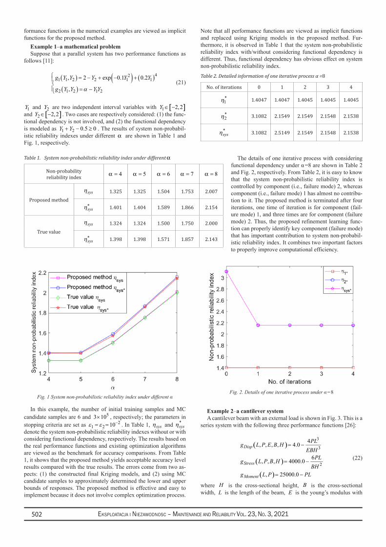
Eksploatacja i NiEzawodNosc – MaiNtENaNcE aNd REliability Vol. 23, No. 3, 2021502
formance functions in the numerical examples are viewed as implicit functions for the proposed method.
Example 1–a mathematical problem Suppose that a parallel system has two performance functions as
follows [11]:
g Y Y Y Y Y
g Y Y Y Y
1 1 2 2 12
14
2 1 2 1 2
2 0 1 0 2, exp . .
,
( ) = − + −( ) + ( )( ) = −
α (21)
1Y and 2Y are two independent interval variables with [ ]1 2,2Y ∈ −and [ ]2 2,2Y ∈ − . Two cases are respectively considered: (1) the func-tional dependency is not involved, and (2) the functional dependency is modeled as 1 2 0.5 0Y Y+ − ≥ . The results of system non-probabil-istic reliability indexes under different α are shown in Table 1 and Fig. 1, respectively.
Fig. 1 System non-probabilistic reliability index under different α
In this example, the number of initial training samples and MC candidate samples are 6 and 53 10× , respectively; the parameters in stopping criteria are set as ε ε1 2
210= = − . In Table 1, ηsys and ηsys
*
denote the system non-probabilistic reliability indexes without or with considering functional dependency, respectively. The results based on the real performance functions and existing optimization algorithms are viewed as the benchmark for accuracy comparisons. From Table 1, it shows that the proposed method yields acceptable accuracy level results compared with the true results. The errors come from two as-pects: (1) the constructed final Kriging models, and (2) using MC candidate samples to approximately determined the lower and upper bounds of responses. The proposed method is effective and easy to implement because it does not involve complex optimization process.
Note that all performance functions are viewed as implicit functions and replaced using Kriging models in the proposed method. Fur-thermore, it is observed in Table 1 that the system non-probabilistic reliability index with/without considering functional dependency is different. Thus, functional dependency has obvious effect on system non-probabilistic reliability index.
The details of one iterative process with considering functional dependency under α =8 are shown in Table 2 and Fig. 2, respectively. From Table 2, it is easy to know that the system non-probabilistic reliability index is controlled by component (i.e., failure mode) 2, whereas component (i.e., failure mode) 1 has almost no contribu-tion to it. The proposed method is terminated after four iterations, one time of iteration is for component (fail-ure mode) 1, and three times are for component (failure mode) 2. Thus, the proposed refinement learning func-tion can properly identify key component (failure mode) that has important contribution to system non-probabil-istic reliability index. It combines two important factors to properly improve computational efficiency.
Example 2–a cantilever systemA cantilever beam with an external load is shown in Fig. 3. This is a
series system with the following three performance functions [26]:
( )
( )
( )
3
3
2
4, , , , 4.0
6, , , 4000.0
, 25000.0
Disp
Stress
Moment
PLg L P E B HEBH
PLg L P B HBH
g L P PL
= −
= −
= −
(22)
where H is the cross-sectional height, B is the cross-sectional width, L is the length of the beam, E is the young’s modulus with
Table 1. System non-probabilistic reliability index under different α
Non-probabilityreliability index 4α = 5α = 6α = 7α = 8α =
Proposed method
ηsys 1.325 1.325 1.504 1.753 2.007
ηsys∗ 1.401 1.404 1.589 1.866 2.154
True value
ηsys 1.324 1.324 1.500 1.750 2.000
ηsys∗ 1.398 1.398 1.571 1.857 2.143
Table 2. Detailed information of one iterative process α =8
No. of iterations 0 1 2 3 4
η1* 1.4047 1.4047 1.4045 1.4045 1.4045
η2* 3.1082 2.1549 2.1549 2.1548 2.1538
ηsys* 3.1082 2.5149 2.1549 2.1548 2.1538
Fig. 2. Details of one iterative process under α =8
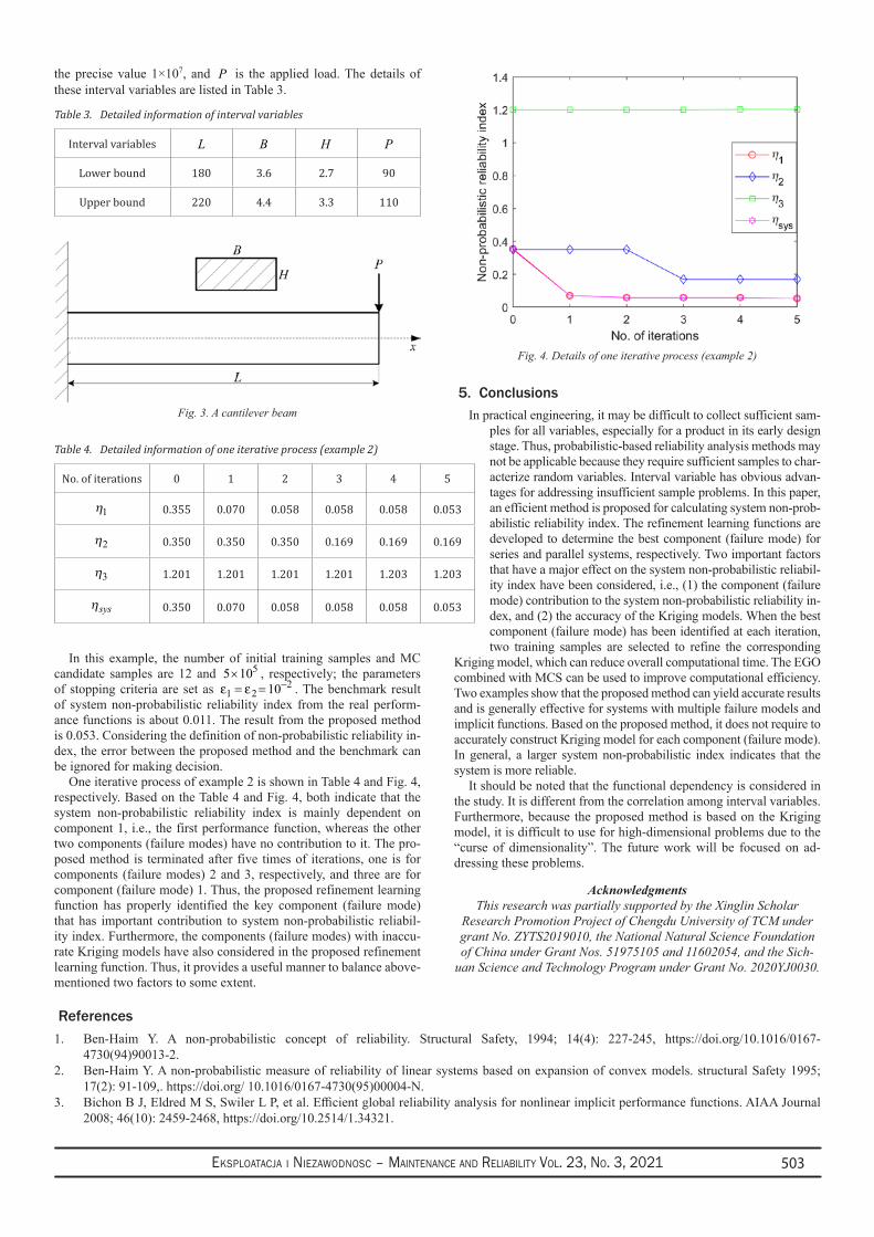
Eksploatacja i NiEzawodNosc – MaiNtENaNcE aNd REliability Vol. 23, No. 3, 2021 503
the precise value 1×10⁷, and P is the applied load. The details of these interval variables are listed in Table 3.
Fig. 3. A cantilever beam
In this example, the number of initial training samples and MC candidate samples are 12 and 55 10× , respectively; the parameters of stopping criteria are set as 2
1 2 10ε ε −= = . The benchmark result of system non-probabilistic reliability index from the real perform-ance functions is about 0.011. The result from the proposed method is 0.053. Considering the definition of non-probabilistic reliability in-dex, the error between the proposed method and the benchmark can be ignored for making decision.
One iterative process of example 2 is shown in Table 4 and Fig. 4, respectively. Based on the Table 4 and Fig. 4, both indicate that the system non-probabilistic reliability index is mainly dependent on component 1, i.e., the first performance function, whereas the other two components (failure modes) have no contribution to it. The pro-posed method is terminated after five times of iterations, one is for components (failure modes) 2 and 3, respectively, and three are for component (failure mode) 1. Thus, the proposed refinement learning function has properly identified the key component (failure mode) that has important contribution to system non-probabilistic reliabil-ity index. Furthermore, the components (failure modes) with inaccu-rate Kriging models have also considered in the proposed refinement learning function. Thus, it provides a useful manner to balance above-mentioned two factors to some extent.
5. ConclusionsIn practical engineering, it may be difficult to collect sufficient sam-
ples for all variables, especially for a product in its early design stage. Thus, probabilistic-based reliability analysis methods may not be applicable because they require sufficient samples to char-acterize random variables. Interval variable has obvious advan-tages for addressing insufficient sample problems. In this paper, an efficient method is proposed for calculating system non-prob-abilistic reliability index. The refinement learning functions are developed to determine the best component (failure mode) for series and parallel systems, respectively. Two important factors that have a major effect on the system non-probabilistic reliabil-ity index have been considered, i.e., (1) the component (failure mode) contribution to the system non-probabilistic reliability in-dex, and (2) the accuracy of the Kriging models. When the best component (failure mode) has been identified at each iteration, two training samples are selected to refine the corresponding
Kriging model, which can reduce overall computational time. The EGO combined with MCS can be used to improve computational efficiency. Two examples show that the proposed method can yield accurate results and is generally effective for systems with multiple failure models and implicit functions. Based on the proposed method, it does not require to accurately construct Kriging model for each component (failure mode). In general, a larger system non-probabilistic index indicates that the system is more reliable.
It should be noted that the functional dependency is considered in the study. It is different from the correlation among interval variables. Furthermore, because the proposed method is based on the Kriging model, it is difficult to use for high-dimensional problems due to the “curse of dimensionality”. The future work will be focused on ad-dressing these problems.
AcknowledgmentsThis research was partially supported by the Xinglin Scholar
Research Promotion Project of Chengdu University of TCM under grant No. ZYTS2019010, the National Natural Science Foundation of China under Grant Nos. 51975105 and 11602054, and the Sich-
uan Science and Technology Program under Grant No. 2020YJ0030.
Table 3. Detailed information of interval variables
Interval variables L B H P
Lower bound 180 3.6 2.7 90
Upper bound 220 4.4 3.3 110
Table 4. Detailed information of one iterative process (example 2)
No. of iterations 0 1 2 3 4 5
η1 0.355 0.070 0.058 0.058 0.058 0.053
η2 0.350 0.350 0.350 0.169 0.169 0.169
η3 1.201 1.201 1.201 1.201 1.203 1.203
ηsys 0.350 0.070 0.058 0.058 0.058 0.053
Fig. 4. Details of one iterative process (example 2)
References1. Ben-Haim Y. A non-probabilistic concept of reliability. Structural Safety, 1994; 14(4): 227-245, https://doi.org/10.1016/0167-
4730(94)90013-2.2. Ben-Haim Y. A non-probabilistic measure of reliability of linear systems based on expansion of convex models. structural Safety 1995;
17(2): 91-109,. https://doi.org/ 10.1016/0167-4730(95)00004-N.3. Bichon B J, Eldred M S, Swiler L P, et al. Efficient global reliability analysis for nonlinear implicit performance functions. AIAA Journal
2008; 46(10): 2459-2468, https://doi.org/10.2514/1.34321.

Eksploatacja i NiEzawodNosc – MaiNtENaNcE aNd REliability Vol. 23, No. 3, 2021504
4. Chen X Y, Fan J P, Bian X Y. Theoretical analysis of non-probabilistic reliability based on interval model. Acta Mechanica Solida Sinica 2017; 30: 638-646, https://doi.org/10.1016/j.camss.2017.11.003.
5. Dong L J, Sun D Y, Li X B, et al. Interval non-probabilistic reliability of surrounding jointed rock mass considering micro seismic loads in mining tunnels. Tunneling and Underground Space Technology 2018; 81: 326-335, https://doi.org/10.1016/j.tust.2018.06.034.
6. Du X. System reliability analysis with saddle-point approximation. Structural and Multidisciplinary Optimization 2010; 42: 193-208, https://doi.org/10.1007/s00158-009-0478-x.
7. Echard B, Gayton N, Lemaire M. AK-MCS: An active learning reliability method combining Kriging and Monte Carlo simulation. Structural Safety 2011; 33: 145-154, https://doi.org/10.1016/j.strusafe.2011.01.002.
8. Elishakoff I, Elisseeff P, Glegg S A L. Non-probabilistic, convex-theoretic modeling of scatter in material properties. AIAA Journal 1995; 32(4): 843-849, https://doi.org/10.2514/3.12062.
9. Fauriat W, Gayton N. AK-SYS: An adaptation of the AK-MCS method for system reliability. Reliability Engineering and System Safety 2014; 123: 137-144, https://doi.org/10.1016/j.ress.2013.10.010.
10. Forrester A I J, Sóbester A, Keane A J. Engineering design via surrogate modelling. Chicheste: John Wiley & Sons, 2008.11. Grooteman F. Adaptive radial-based importance sampling method for structural reliability. Structural Safety 2008; 30: 533-542,https://doi.
org/10.1016/j.strusafe.2007.10.002.12. Guo S X, Lu Z Z, Feng Y S. A non-probabilistic model of structural reliability based on interval analysis. Chinese Journal of Computational
Mechanics 2001; 18(1): 56-60. (In Chinese)13. Guo S X, Zhang L, Li Y. Procedures for computing the non-probabilistic reliability index of uncertain structures. Chinese Journal of
Computational Mechanics, 2005; 22(2): 227-231. (In Chinese)14. Jiang C, Fu C, Ni B, et al. Interval arithmetic operations for uncertainty analysis with correlated interval variables. Acta Mechanica Sinica
2016; 32: 743-752, https://doi.org/10.1007/s10409-015-0525-3.15. Jiang C, Han X, Lu G Y, et al. Correlation analysis of non-probabilistic convex model and corresponding structural reliability technique.
Computer Methods in Applied Mechanics and Engineering 2011; 200(33-36): 2528-2546, https://doi.org/10.1016/j.cma.2011.04.007.16. Jiang C, Zhang Q F, Han X et al. A non-probabilistic structural reliability analysis method based on a multidimensional parallelepiped convex
model. Acta Mechanica 2014; 225: 383-395, https://doi.org/10.1108/MMMS-06-2015-0033.17. Jiang T, Chen J J, Xu Y L. A semi-analytic method for calculating non-probabilistic reliability index based on interval models. Applied
Mathematical Modelling 2007; 31(7): 1362-1370, https://doi.org/10.1016/j.apm.2006.02.013.18. Jones D R, Schonlau M, Welch W J. Efficient global optimization of expensive black-box functions. Journal of Global Optimization 1998;
13: 455-492, https://doi.org/ 10.1023/A:1008306431147.19. Kumar V, Kumar G, Singh R K, et al. Degrading systems availability analysis: analytical semi-Markov approach. Eksploatacja i Niezawodnosc
- Maintenance and Reliability 2021; 23(1): 195-208, https://doi.org/10.17531/ein.2021.1.20.20. Lemaire M. Structural reliability. Hoboken: John Wiley & Sons, 2009.21. Meng Z, Zhang Z, Zhang D, et al. An active learning method combining Kriging and accelerated chaotic single loop approach (AK-
ACSLA) for reliability-based design optimization. Computer Methods in Applied Mechanics and Engineering 2019; 357: 112570, https://doi.org/10.1016/j.cma.2019.112570.
22. Nie X B, Li H B. A direct integration-based structural reliability analysis method using non-probabilistic convex model. Journal of Mechanical Science and Technology 2018; 32(11): 5063-5068, https://doi.org/10.1007/s12206-018-1002-2.
23. Schöbi R, Sudret B. Structural reliability analysis for p-boxes using multi-level meta-models. Probabilistic Engineering Mechanics 2017; 48: 27-38, https://doi.org/10.1016/ j.probengmech.2017.04.001.
24. Teixeira R, Nogal M, Connor A O, et al. Reliability assessment with density scanned adaptive kriging. Reliability Engineering and System Safety 2020; 199: 106908, https://doi.org/10.1016/j.ress.2020.106908.
25. Wang C, Matthies H G. Epistemic uncertainty-based reliability analysis for engineering system with hybrid evidence and fuzzy variables. Computer Methods in Applied Mechanics and Engineering 2019; 355: 438-455, https://doi.org/10.1016/j.cma.2019.06.036.
26. Wang L, Kodiyalam S. An efficient method for probabilistic and robust design with non-normal distributions. In Proceedings of the 43rd AIAA/ASME/ASCE/AHS/ASC Structures, Structural Dynamics, and Materials Conference, Denver, Colorado, 22–25, April, 2002.
27. Wang Z, Shafieezadeh A. On confidence intervals for failure probability estimates in kriging-based reliability analysis. Reliability Engineering and System Safety 2020; 196: 106758, https://doi.org/10.1016/j.ress.2019.106758.
28. Xiao M, Zhang J H, Gao L, et al. An efficient kriging-based subset simulation method for hybrid reliability analysis under random and interval variables with small failure probability. Structural and Multidisciplinary Optimization 2019; 59(6): 2077-2029, https://doi.org/10.1007/s00158-018-2176-z.
29. Xiao M, Zhang J H, Gao L. A system active learning Kriging method for system reliability-based design optimization with a multiple response model. Reliability Engineering and System Safety 2020; 199: 106935, https://doi.org/10.1016/j.ress.2020.106935.
30. Xiao N C, Huang H Z, Li Y F, et al. Non-probabilistic reliability sensitivity analysis of the model of structural systems with interval variables whose state of dependence is determined by constraints. Journal of Risk and Reliability 2013; 227(5): 491-498, https://doi.org/10.1177/1748006X13480742.
31. Xiao N C, Yuan K, Zhou C N. Adaptive kriging-based efficient reliability method for structural systems with multiple failure modes and mixed variables. Computer Methods in Applied Mechanics and Engineering 2020; 359:112649, https://doi.org/10.1016/ j.cma.2019.112649.
32. Xiao N C, Zuo M J, Zhou C. A new adaptive sequential sampling method to construct surrogate models for efficient reliability analysis. Reliability Engineering and System Safety 2018; 169: 330-338, https://doi.org/10.1016/j.ress.2017.09.008.
33. Yang Z M, Zhang Y J, Meng W J, et al. A convex model approach for structure non-probabilistic reliability analysis. Journal of Risk and Reliability 2017; 231(5): 508-515, https://doi.org/10.1177/1748006X17710817.
34. Zhang D Q, Zhang N, Ye N, et al. Hybrid learning algorithm of radial basis function networks for reliability analysis. IEEE Transaction on Reliability 2020; https://doi.org/10.1109/TR.2020.3001232.
35. Zhang X F, Wang L, Sørensen J D. REIF: A novel active learning function toward adaptive kriging surrogate models for structural reliability analysis. Reliability Engineering and System Safety 2019; 185: 440-454, https://doi.org/10.1016/j.ress.2019.01.014.
36. Zhou C, Xiao N C, Zuo M, et al. AK-PDF: an active learning method combining kriging and probability density function for efficient reliability analysis. Journal of Risk and Reliability 2020; 234(3): 536-549, https://doi.org/10.1177/1748006X19888421.
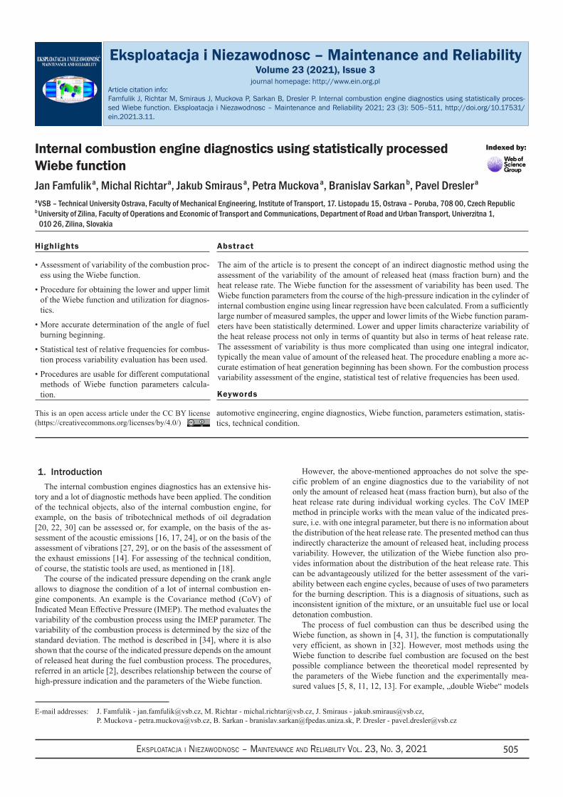
Eksploatacja i NiEzawodNosc – MaiNtENaNcE aNd REliability Vol. 23, No. 3, 2021 505
E-mail addresses:
Eksploatacja i Niezawodnosc – Maintenance and ReliabilityVolume 23 (2021), Issue 3
journal homepage: http://www.ein.org.pl
Indexed by:
1. IntroductionThe internal combustion engines diagnostics has an extensive his-
tory and a lot of diagnostic methods have been applied. The condition of the technical objects, also of the internal combustion engine, for example, on the basis of tribotechnical methods of oil degradation [20, 22, 30] can be assessed or, for example, on the basis of the as-sessment of the acoustic emissions [16, 17, 24], or on the basis of the assessment of vibrations [27, 29], or on the basis of the assessment of the exhaust emissions [14]. For assessing of the technical condition, of course, the statistic tools are used, as mentioned in [18].
The course of the indicated pressure depending on the crank angle allows to diagnose the condition of a lot of internal combustion en-gine components. An example is the Covariance method (CoV) of Indicated Mean Effective Pressure (IMEP). The method evaluates the variability of the combustion process using the IMEP parameter. The variability of the combustion process is determined by the size of the standard deviation. The method is described in [34], where it is also shown that the course of the indicated pressure depends on the amount of released heat during the fuel combustion process. The procedures, referred in an article [2], describes relationship between the course of high-pressure indication and the parameters of the Wiebe function.
However, the above-mentioned approaches do not solve the spe-cific problem of an engine diagnostics due to the variability of not only the amount of released heat (mass fraction burn), but also of the heat release rate during individual working cycles. The CoV IMEP method in principle works with the mean value of the indicated pres-sure, i.e. with one integral parameter, but there is no information about the distribution of the heat release rate. The presented method can thus indirectly characterize the amount of released heat, including process variability. However, the utilization of the Wiebe function also pro-vides information about the distribution of the heat release rate. This can be advantageously utilized for the better assessment of the vari-ability between each engine cycles, because of uses of two parameters for the burning description. This is a diagnosis of situations, such as inconsistent ignition of the mixture, or an unsuitable fuel use or local detonation combustion.
The process of fuel combustion can thus be described using the Wiebe function, as shown in [4, 31], the function is computationally very efficient, as shown in [32]. However, most methods using the Wiebe function to describe fuel combustion are focused on the best possible compliance between the theoretical model represented by the parameters of the Wiebe function and the experimentally mea-sured values [5, 8, 11, 12, 13]. For example, „double Wiebe“ models
The aim of the article is to present the concept of an indirect diagnostic method using the assessment of the variability of the amount of released heat (mass fraction burn) and the heat release rate. The Wiebe function for the assessment of variability has been used. The Wiebe function parameters from the course of the high-pressure indication in the cylinder of internal combustion engine using linear regression have been calculated. From a sufficiently large number of measured samples, the upper and lower limits of the Wiebe function param-eters have been statistically determined. Lower and upper limits characterize variability of the heat release process not only in terms of quantity but also in terms of heat release rate. The assessment of variability is thus more complicated than using one integral indicator, typically the mean value of amount of the released heat. The procedure enabling a more ac-curate estimation of heat generation beginning has been shown. For the combustion process variability assessment of the engine, statistical test of relative frequencies has been used.
Highlights Abstract
Assessment of variability of the combustion proc-• ess using the Wiebe function.
Procedure for obtaining the lower and upper limit • of the Wiebe function and utilization for diagnos-tics.
More accurate determination of the angle of fuel • burning beginning.
Statistical test of relative frequencies for combus-• tion process variability evaluation has been used.
Procedures are usable for different computational • methods of Wiebe function parameters calcula-tion.
Internal combustion engine diagnostics using statistically processed Wiebe functionJan Famfulik a, Michal Richtar a, Jakub Smiraus a, Petra Muckova a, Branislav Sarkan b, Pavel Dresler a
a VSB – Technical University Ostrava, Faculty of Mechanical Engineering, Institute of Transport, 17. Listopadu 15, Ostrava – Poruba, 708 00, Czech Republic b University of Zilina, Faculty of Operations and Economic of Transport and Communications, Department of Road and Urban Transport, Univerzitna 1, 010 26, Zilina, Slovakia
Famfulik J, Richtar M, Smiraus J, Muckova P, Sarkan B, Dresler P. Internal combustion engine diagnostics using statistically proces-sed Wiebe function. Eksploatacja i Niezawodnosc – Maintenance and Reliability 2021; 23 (3): 505–511, http://doi.org/10.17531/ein.2021.3.11.
Article citation info:
automotive engineering, engine diagnostics, Wiebe function, parameters estimation, statis-tics, technical condition.
Keywords
This is an open access article under the CC BY license (https://creativecommons.org/licenses/by/4.0/)
J. Famfulik - [email protected], M. Richtar - [email protected], J. Smiraus - [email protected], P. Muckova - [email protected], B. Sarkan - [email protected], P. Dresler - [email protected]
Eksploatacja i NiEzawodNosc – MaiNtENaNcE aNd REliability Vol. 23, No. 3, 2021506
are used in cases, as shown in [33], where the sophisticated „fitting“ method with weighting coefficients given in [6] is used to calculate the parameters of the Wiebe function. The calculation procedure is based on the average value of the high-pressure indication course obtained from a large number of cycles. The calculation of the parameters of the Wiebe function is then performed from this fictitious course. Ob-viously, this procedure does not allow to assess the variability of the combustion process. This procedure is suitable, for example, as an input to simulation calculations of internal combustion engines. In this way, it is possible to enrich the spectrum of methods already used for the diagnostics of internal combustion engines [19, 25].
Early diagnostic results allow to properly plan a preventive engine maintenance strategy and thus affect the maintenance costs. There-fore, it is an important tool of predictive diagnostics [15, 23].
The concept of the diagnostic method described in the article is based on a statistical assessment of the variance of values of the Wiebe function parameters. From a large number of cycles for the individual crankshaft rotation angles, an interval estimation of the amount of released heat at a predetermined confidence level α has been determined. The upper and lower estimate specify the limits, between which the values of the Wiebe function parameters of the standard (etalon) engine must be found.
The number of unsatisfactory engine cycles of the diagnosed en-gine has been further evaluated. If the test result exceeds the confi-dence level α, the diagnosed engine shows greater combustion pro-cess variability, than corresponds to the expected values, thus shows the poor technical condition of the engine.
2. Mathematical modelThe Wiebe function, is the default equation for description of the
course of a mixture burning in the internal combustion engine cylin-der, depending on the crank angle. The function is given by the equa-tion (1), but the derivation of the equation (1) defined by the equation (2) for course description of the function often has been used:
( ) ( )( )1
0
1
MAQ
F eQc
ϕ ϕϕϕ
ϕ
+− − ∆ = = − (1)
( ) ( )( )1
001
MM AA M
f eϕ ϕ
ϕϕ ϕϕϕ ϕ
+− − ∆ ⋅ + −
= ⋅ ⋅ ∆ ∆ (2)
The equation (1) describes the ratio of the gradually released heat Q (φ) depending on a crank angle φ, to the total amount of heat Qc released during one cycle. The Wiebe function contains the constant A given by the used fuel type, for gasoline (RON 95) A = 6.90 as de-scribed in [7]. Furthermore, the Wiebe function contains the shape parameter M, which characterizes the shape of the curve of the released heat. Function also contains angle ∆φ, which represents the time, when 95% of the heat has been released. The value of 95% is given by the fact, that the amount of released heat is very small at the beginning and the end of the cycle and thus the pressure changes in the cylinder are very small, and therefore difficult to measure [26]. The last parameter φ0 specifies the angle of displacement of the burn-ing beginning with respect to the top dead center (TDC).
3. Wiebe function parameters estimation The mathematical model aims to estimate the parameters ∆φ, φ0
and M of the Wiebe function using a linear regression and an experi-mentally obtained data. The procedure requires adjustments of equa-tion (1) to obtain a linear form (see equation (5)):
( )
( )10
1
MA
F eϕ ϕ
ϕϕ
+− − ∆ − = (3)
( )( )1
0ln(1 )M
F A ϕ ϕϕϕ
+ −
− − = ⋅ ∆ (4)
( ) ( ) ( ) ( )0ln ln(1 ) ln ln( ) 1 ln( ) 1F A M Mϕ ϕ ϕ ϕ− − − = − ⋅ + − ∆ ⋅ + (5)
Equation (5) with the line equation has been compared, (see equa-tion (6)) and the substitutions have been used (see equations (7) to (9)):
y k x q= ⋅ + (6)
( )ln ln 1 ( ) ln( )y F Aϕ= − − − (7)
( ) 01 ln( )k x M ϕ ϕ⋅ = + ⋅ − (8)
( )ln( ) 1q Mϕ= − ∆ ⋅ + (9)
It is now possible to create a table of values from experimentally obtained data. Data have a structure described in Tab.1. The graph of ordered values has been created, as shown in Fig. 1. In the graph in Fig. 1 the values ln (φ−φ0) on the x-axis have been plotted, when meanwhile φ0 = 0° has been considered, and the values of yi given by the substitution according to equation (7) on the y-axis have been plotted. Initial, very small values of released heat, in accordance the definition of ∆φ, in the graph have been not considered.
Where: i - serial number of the measurement [-] (φ−φ0) - crank angle [°] Qi - average amount of released heat [J] σi - standard deviation of released heat [J] F(φ) - Wiebe function of gradually released heat [%] QC - total amount of released heat in one cycle [J] yi - value of substitution at i-th measurement accord-
ing to equation (7) [-] n - number of engine cycles [-]
Table 1. Data structure for Wiebe function parameters estimation
i (φ−φ0) [°] Qi [J] σI [J] ( ) i
1F = Q / Q
n
i=ϕ ∑ C [%] ln (φ−φ0) [-] yi [-]
1 −1 −0.378 0.212 - - -
2 0 0.012 0.281 0.001 −6.908 −13.053
3 1 0.164 0.387 0.021 0.000 −10.404
4 2 0.731 0.649 0.11 0.693 −8.763
5 3 2.030 1.056 0.35 1.099 −7.587
6 4 2.905 1.452 0.69 1.386 −6.898
7 5 5.276 2.169 1.32 1.609 −6.251
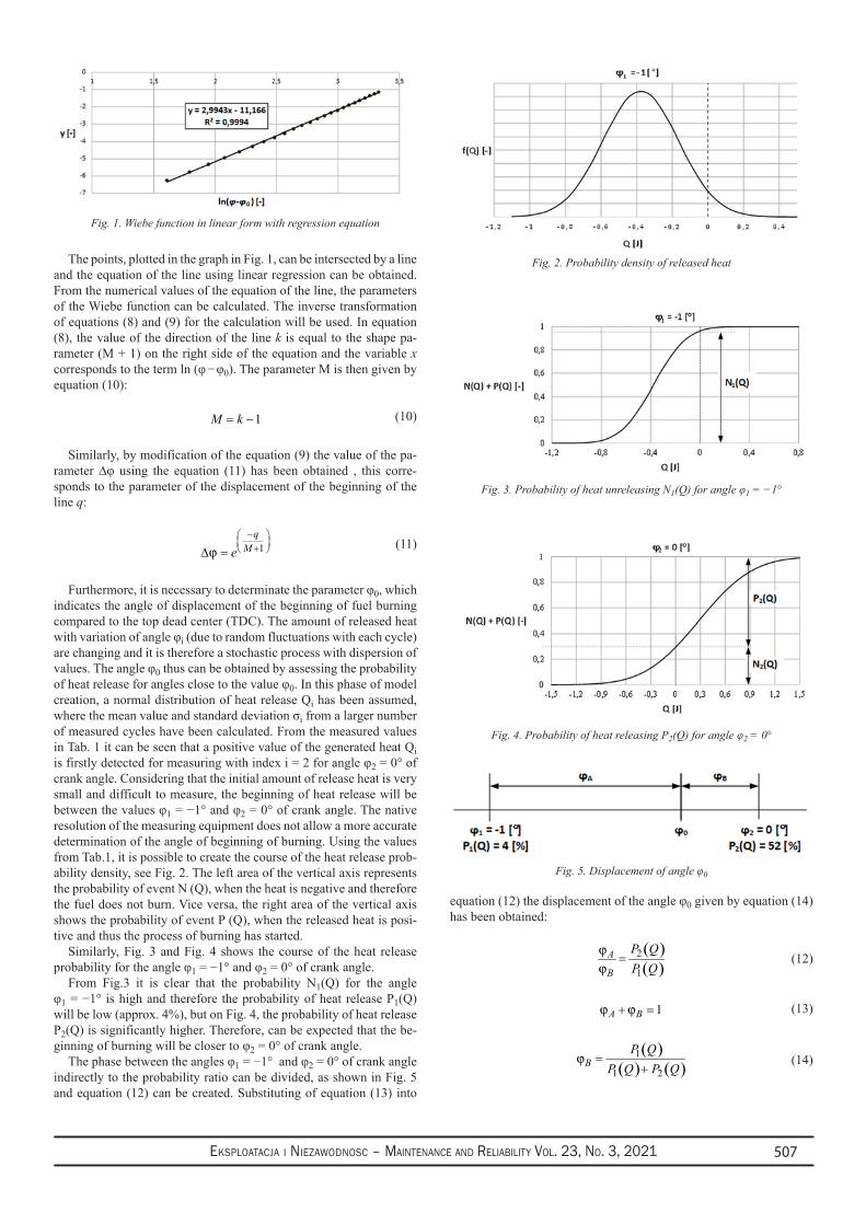
Eksploatacja i NiEzawodNosc – MaiNtENaNcE aNd REliability Vol. 23, No. 3, 2021 507
Fig. 1. Wiebe function in linear form with regression equation
The points, plotted in the graph in Fig. 1, can be intersected by a line and the equation of the line using linear regression can be obtained. From the numerical values of the equation of the line, the parameters of the Wiebe function can be calculated. The inverse transformation of equations (8) and (9) for the calculation will be used. In equation (8), the value of the direction of the line k is equal to the shape pa-rameter (M + 1) on the right side of the equation and the variable x corresponds to the term ln (φ − φ0). The parameter M is then given by equation (10):
1M k= − (10)
Similarly, by modification of the equation (9) the value of the pa-rameter ∆φ using the equation (11) has been obtained , this corre-sponds to the parameter of the displacement of the beginning of the line q:
1q
Meϕ−
+ ∆ = (11)
Furthermore, it is necessary to determinate the parameter φ0, which indicates the angle of displacement of the beginning of fuel burning compared to the top dead center (TDC). The amount of released heat with variation of angle φi (due to random fluctuations with each cycle) are changing and it is therefore a stochastic process with dispersion of values. The angle φ0 thus can be obtained by assessing the probability of heat release for angles close to the value φ0. In this phase of model creation, a normal distribution of heat release Qi has been assumed, where the mean value and standard deviation σi from a larger number of measured cycles have been calculated. From the measured values in Tab. 1 it can be seen that a positive value of the generated heat Qi is firstly detected for measuring with index i = 2 for angle φ2 = 0° of crank angle. Considering that the initial amount of release heat is very small and difficult to measure, the beginning of heat release will be between the values φ1 = −1° and φ2 = 0° of crank angle. The native resolution of the measuring equipment does not allow a more accurate determination of the angle of beginning of burning. Using the values from Tab.1, it is possible to create the course of the heat release prob-ability density, see Fig. 2. The left area of the vertical axis represents the probability of event N (Q), when the heat is negative and therefore the fuel does not burn. Vice versa, the right area of the vertical axis shows the probability of event P (Q), when the released heat is posi-tive and thus the process of burning has started.
Similarly, Fig. 3 and Fig. 4 shows the course of the heat release probability for the angle φ1 = −1° and φ2 = 0° of crank angle.
From Fig.3 it is clear that the probability N1(Q) for the angle φ1 = −1° is high and therefore the probability of heat release P1(Q) will be low (approx. 4%), but on Fig. 4, the probability of heat release P2(Q) is significantly higher. Therefore, can be expected that the be-ginning of burning will be closer to φ2 = 0° of crank angle.
The phase between the angles φ1 = −1° and φ2 = 0° of crank angle indirectly to the probability ratio can be divided, as shown in Fig. 5 and equation (12) can be created. Substituting of equation (13) into
equation (12) the displacement of the angle φ0 given by equation (14) has been obtained:
( )( )
2
1
A
B
P QP Q
ϕϕ
= (12)
1A Bϕ ϕ+ = (13)
( )
( ) ( )1
1 2B
P QP Q P Q
ϕ =+
(14)
Fig. 2. Probability density of released heat
Fig. 5. Displacement of angle φ0
Fig. 4. Probability of heat releasing P2(Q) for angle φ2 = 0°
Fig. 3. Probability of heat unreleasing N1(Q) for angle φ1 = −1°
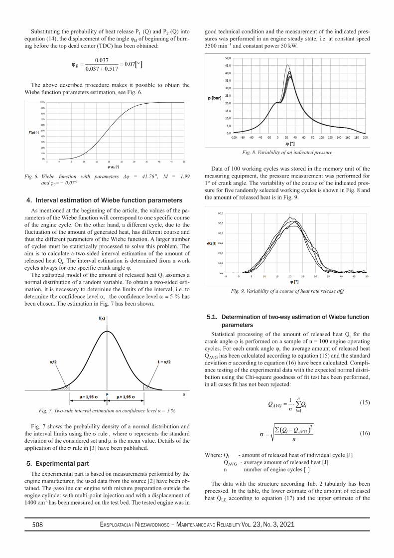
Eksploatacja i NiEzawodNosc – MaiNtENaNcE aNd REliability Vol. 23, No. 3, 2021508
Substituting the probability of heat release P1 (Q) and P2 (Q) into equation (14), the displacement of the angle φB of beginning of burn-ing before the top dead center (TDC) has been obtained:
[ ]0.037 0.07
0.037 0.517Bϕ = = °+
The above described procedure makes it possible to obtain the Wiebe function parameters estimation, see Fig. 6.
4. Interval estimation of Wiebe function parameters As mentioned at the beginning of the article, the values of the pa-
rameters of the Wiebe function will correspond to one specific course of the engine cycle. On the other hand, a different cycle, due to the fluctuation of the amount of generated heat, has different course and thus the different parameters of the Wiebe function. A larger number of cycles must be statistically processed to solve this problem. The aim is to calculate a two-sided interval estimation of the amount of released heat Qi. The interval estimation is determined from n work cycles always for one specific crank angle φ.
The statistical model of the amount of released heat Qi assumes a normal distribution of a random variable. To obtain a two-sided esti-mation, it is necessary to determine the limits of the interval, i.e. to determine the confidence level α, the confidence level α = 5 % has been chosen. The estimation in Fig. 7 has been shown.
Fig. 7 shows the probability density of a normal distribution and the interval limits using the σ rule , where σ represents the standard deviation of the considered set and µ is the mean value. Details of the application of the σ rule in [3] have been published.
5. Experimental partThe experimental part is based on measurements performed by the
engine manufacturer, the used data from the source [2] have been ob-tained. The gasoline car engine with mixture preparation outside the engine cylinder with multi-point injection and with a displacement of 1400 cm3, has been measured on the test bed. The tested engine was in
good technical condition and the measurement of the indicated pres-sures was performed in an engine steady state, i.e. at constant speed 3500 min−1 and constant power 50 kW.
Fig. 8. Variability of an indicated pressure
Data of 100 working cycles was stored in the memory unit of the measuring equipment, the pressure measurement was performed for 1° of crank angle. The variability of the course of the indicated pres-sure for five randomly selected working cycles is shown in Fig. 8 and the amount of released heat is in Fig. 9.
Fig. 9. Variability of a course of heat rate release dQ
5.1. Determination of two-way estimation of Wiebe function parameters
Statistical processing of the amount of released heat Qi for the crank angle φ is performed on a sample of n = 100 engine operating cycles. For each crank angle φ, the average amount of released heat QAVG has been calculated according to equation (15) and the standard deviation σ according to equation (16) have been calculated. Compli-ance testing of the experimental data with the expected normal distri-bution using the Chi-square goodness of fit test has been performed, in all cases fit has not been rejected:
1
1 nAVG i
iQ Q
n == ⋅ ∑ (15)
( )2i AVGQ Q
nσ
∑ −= (16)
Where: Qi - amount of released heat of individual cycle [J] QAVG - average amount of released heat [J] n - number of engine cycles [-]
The data with the structure according Tab. 2 tabularly has been processed. In the table, the lower estimate of the amount of released heat QLE according to equation (17) and the upper estimate of the
Fig. 6. Wiebe function with parameters Δφ = 41.76 °, M = 1.99 and φ0 = − 0.07 °
Fig. 7. Two-side interval estimation on confidence level α = 5 %
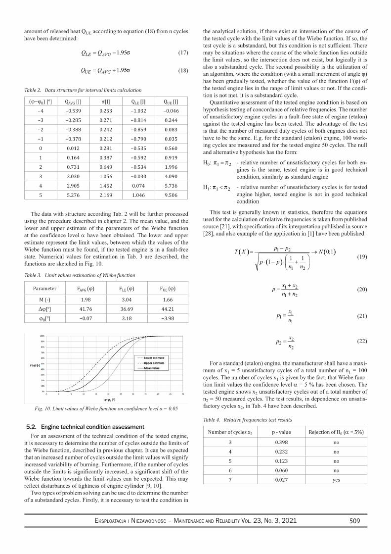
Eksploatacja i NiEzawodNosc – MaiNtENaNcE aNd REliability Vol. 23, No. 3, 2021 509
amount of released heat QUE according to equation (18) from n cycles have been determined:
1.95LE AVGQ Q σ= − (17)
1.95UE AVGQ Q σ= + (18)
The data with structure according Tab. 2 will be further processed using the procedure described in chapter 2. The mean value, and the lower and upper estimate of the parameters of the Wiebe function at the confidence level α have been obtained. The lower and upper estimate represent the limit values, between which the values of the Wiebe function must be found, if the tested engine is in a fault-free state. Numerical values for estimation in Tab. 3 are described, the functions are sketched in Fig. 10.
Fig. 10. Limit values of Wiebe function on confidence level α = 0.05
5.2. Engine technical condition assessmentFor an assessment of the technical condition of the tested engine,
it is necessary to determine the number of cycles outside the limits of the Wiebe function, described in previous chapter. It can be expected that an increased number of cycles outside the limit values will signify increased variability of burning. Furthermore, if the number of cycles outside the limits is significantly increased, a significant shift of the Wiebe function towards the limit values can be expected. This may reflect disturbances of tightness of engine cylinder [9, 10].
Two types of problem solving can be use d to determine the number of a substandard cycles. Firstly, it is necessary to test the condition in
the analytical solution, if there exist an intersection of the course of the tested cycle with the limit values of the Wiebe function. If so, the test cycle is a substandard, but this condition is not sufficient. There may be situations where the course of the whole function lies outside the limit values, so the intersection does not exist, but logically it is also a substandard cycle. The second possibility is the utilization of an algorithm, where the condition (with a small increment of angle φ) has been gradually tested, whether the value of the function F(φ) of the tested engine lies in the range of limit values or not. If the condi-tion is not met, it is a substandard cycle.
Quantitative assessment of the tested engine condition is based on hypothesis testing of concordance of relative frequencies. The number of unsatisfactory engine cycles in a fault-free state of engine (etalon) against the tested engine has been tested. The advantage of the test is that the number of measured duty cycles of both engines does not have to be the same. E.g. for the standard (etalon) engine, 100 work-ing cycles are measured and for the tested engine 50 cycles. The null and alternative hypothesis has the form:
H0: 1 2π π= - relative number of unsatisfactory cycles for both en-gines is the same, tested engine is in good technical condition, similarly as standard engine
H1: 1 2 π π< - relative number of unsatisfactory cycles is for tested engine higher, tested engine is not in good technical condition
This test is generally known in statistics, therefore the equations used for the calculation of relative frequencies is taken from published source [21], with specification of its interpretation published in source [28], and also example of the application in [1] have been published:
( )
( )( )1 2
1 2
0;11 11
p pT X N
p pn n
−= →
⋅ − ⋅ +
(19)
1 2
1 2
x xpn n
+=
+ (20)
11
1
xpn
= (21)
22
2
xpn
= (22)
For a standard (etalon) engine, the manufacturer shall have a maxi-mum of x1 = 5 unsatisfactory cycles of a total number of n1 = 100 cycles. The number of cycles x1 is given by the fact, that Wiebe func-tion limit values the confidence level α = 5 % has been chosen. The tested engine shows x2 unsatisfactory cycles out of a total number of n2 = 50 measured cycles. The test results, in dependence on unsatis-factory cycles x2, in Tab. 4 have been described.
Table 2. Data structure for interval limits calculation
(φ−φ0) [o] QAVG [J] σ[J] QLE [J] QUE [J]
−4 −0.539 0.253 −1.032 −0.046
−3 −0.285 0.271 −0.814 0.244
−2 −0.388 0.242 −0.859 0.083
−1 −0.378 0.212 −0.790 0.035
0 0.012 0.281 −0.535 0.560
1 0.164 0.387 −0.592 0.919
2 0.731 0.649 −0.534 1.996
3 2.030 1.056 −0.030 4.090
4 2.905 1.452 0.074 5.736
5 5.276 2.169 1.046 9.506
Table 3. Limit values estimation of Wiebe function
Parameter FAVG (φ) FLE (φ) FUE (φ)
M (-) 1.98 3.04 1.66
Δφ[o] 41.76 36.69 44.21
φ0[o] −0.07 3.18 −3.98
Table 4. Relative frequencies test results
Number of cycles x2 p - value Rejection of H0 (α = 5%)
3 0.398 no
4 0.232 no
5 0.123 no
6 0.060 no
7 0.027 yes
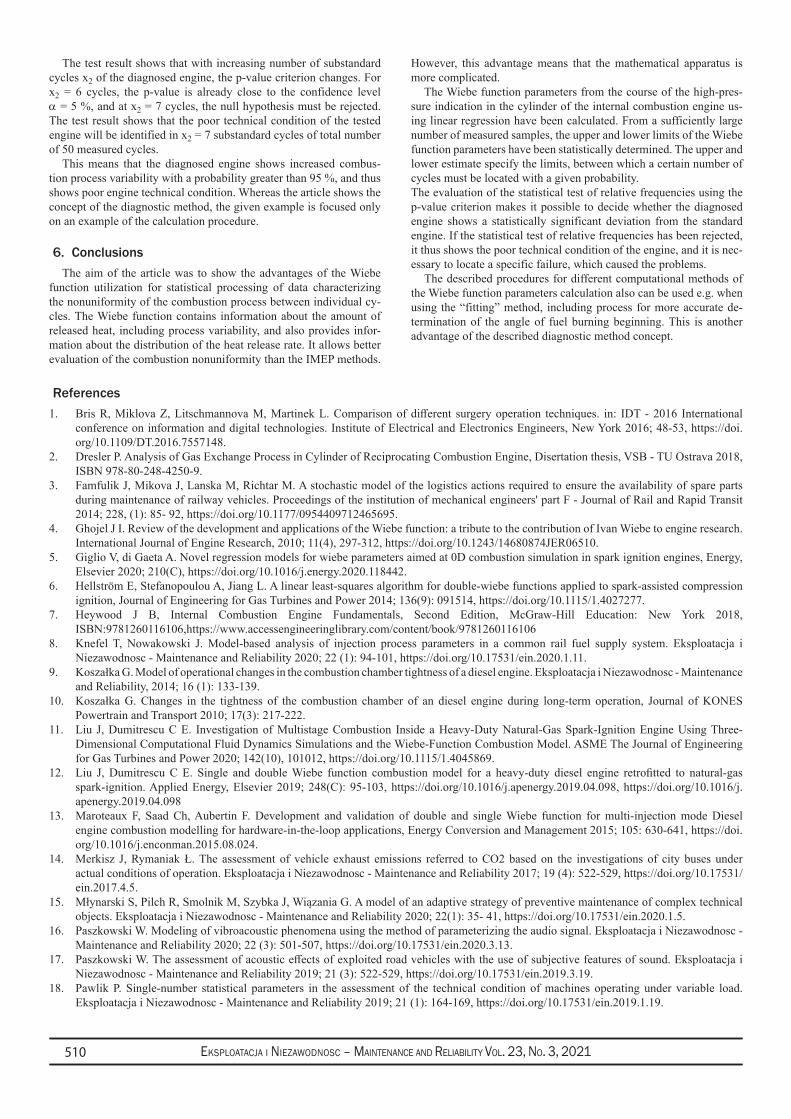
Eksploatacja i NiEzawodNosc – MaiNtENaNcE aNd REliability Vol. 23, No. 3, 2021510
References1. Bris R, Miklova Z, Litschmannova M, Martinek L. Comparison of different surgery operation techniques. in: IDT - 2016 International
conference on information and digital technologies. Institute of Electrical and Electronics Engineers, New York 2016; 48-53, https://doi.org/10.1109/DT.2016.7557148.
2. Dresler P. Analysis of Gas Exchange Process in Cylinder of Reciprocating Combustion Engine, Disertation thesis, VSB - TU Ostrava 2018, ISBN 978-80-248-4250-9.
3. Famfulik J, Mikova J, Lanska M, Richtar M. A stochastic model of the logistics actions required to ensure the availability of spare parts during maintenance of railway vehicles. Proceedings of the institution of mechanical engineers' part F - Journal of Rail and Rapid Transit 2014; 228, (1): 85- 92, https://doi.org/10.1177/0954409712465695.
4. Ghojel J I. Review of the development and applications of the Wiebe function: a tribute to the contribution of Ivan Wiebe to engine research. International Journal of Engine Research, 2010; 11(4), 297-312, https://doi.org/10.1243/14680874JER06510.
5. Giglio V, di Gaeta A. Novel regression models for wiebe parameters aimed at 0D combustion simulation in spark ignition engines, Energy, Elsevier 2020; 210(C), https://doi.org/10.1016/j.energy.2020.118442.
6. Hellström E, Stefanopoulou A, Jiang L. A linear least-squares algorithm for double-wiebe functions applied to spark-assisted compression ignition, Journal of Engineering for Gas Turbines and Power 2014; 136(9): 091514, https://doi.org/10.1115/1.4027277.
7. Heywood J B, Internal Combustion Engine Fundamentals, Second Edition, McGraw-Hill Education: New York 2018, ISBN:9781260116106,https://www.accessengineeringlibrary.com/content/book/9781260116106
8. Knefel T, Nowakowski J. Model-based analysis of injection process parameters in a common rail fuel supply system. Eksploatacja i Niezawodnosc - Maintenance and Reliability 2020; 22 (1): 94-101, https://doi.org/10.17531/ein.2020.1.11.
9. Koszałka G. Model of operational changes in the combustion chamber tightness of a diesel engine. Eksploatacja i Niezawodnosc - Maintenance and Reliability, 2014; 16 (1): 133-139.
10. Koszałka G. Changes in the tightness of the combustion chamber of an diesel engine during long-term operation, Journal of KONES Powertrain and Transport 2010; 17(3): 217-222.
11. Liu J, Dumitrescu C E. Investigation of Multistage Combustion Inside a Heavy-Duty Natural-Gas Spark-Ignition Engine Using Three-Dimensional Computational Fluid Dynamics Simulations and the Wiebe-Function Combustion Model. ASME The Journal of Engineering for Gas Turbines and Power 2020; 142(10), 101012, https://doi.org/10.1115/1.4045869.
12. Liu J, Dumitrescu C E. Single and double Wiebe function combustion model for a heavy-duty diesel engine retrofitted to natural-gas spark-ignition. Applied Energy, Elsevier 2019; 248(C): 95-103, https://doi.org/10.1016/j.apenergy.2019.04.098, https://doi.org/10.1016/j.apenergy.2019.04.098
13. Maroteaux F, Saad Ch, Aubertin F. Development and validation of double and single Wiebe function for multi-injection mode Diesel engine combustion modelling for hardware-in-the-loop applications, Energy Conversion and Management 2015; 105: 630-641, https://doi.org/10.1016/j.enconman.2015.08.024.
14. Merkisz J, Rymaniak Ł. The assessment of vehicle exhaust emissions referred to CO2 based on the investigations of city buses under actual conditions of operation. Eksploatacja i Niezawodnosc - Maintenance and Reliability 2017; 19 (4): 522-529, https://doi.org/10.17531/ein.2017.4.5.
15. Młynarski S, Pilch R, Smolnik M, Szybka J, Wiązania G. A model of an adaptive strategy of preventive maintenance of complex technical objects. Eksploatacja i Niezawodnosc - Maintenance and Reliability 2020; 22(1): 35- 41, https://doi.org/10.17531/ein.2020.1.5.
16. Paszkowski W. Modeling of vibroacoustic phenomena using the method of parameterizing the audio signal. Eksploatacja i Niezawodnosc - Maintenance and Reliability 2020; 22 (3): 501-507, https://doi.org/10.17531/ein.2020.3.13.
17. Paszkowski W. The assessment of acoustic effects of exploited road vehicles with the use of subjective features of sound. Eksploatacja i Niezawodnosc - Maintenance and Reliability 2019; 21 (3): 522-529, https://doi.org/10.17531/ein.2019.3.19.
18. Pawlik P. Single-number statistical parameters in the assessment of the technical condition of machines operating under variable load. Eksploatacja i Niezawodnosc - Maintenance and Reliability 2019; 21 (1): 164-169, https://doi.org/10.17531/ein.2019.1.19.
The test result shows that with increasing number of substandard cycles x2 of the diagnosed engine, the p-value criterion changes. For x2 = 6 cycles, the p-value is already close to the confidence level α = 5 %, and at x2 = 7 cycles, the null hypothesis must be rejected. The test result shows that the poor technical condition of the tested engine will be identified in x2 = 7 substandard cycles of total number of 50 measured cycles.
This means that the diagnosed engine shows increased combus-tion process variability with a probability greater than 95 %, and thus shows poor engine technical condition. Whereas the article shows the concept of the diagnostic method, the given example is focused only on an example of the calculation procedure.
6. ConclusionsThe aim of the article was to show the advantages of the Wiebe
function utilization for statistical processing of data characterizing the nonuniformity of the combustion process between individual cy-cles. The Wiebe function contains information about the amount of released heat, including process variability, and also provides infor-mation about the distribution of the heat release rate. It allows better evaluation of the combustion nonuniformity than the IMEP methods.
However, this advantage means that the mathematical apparatus is more complicated.
The Wiebe function parameters from the course of the high-pres-sure indication in the cylinder of the internal combustion engine us-ing linear regression have been calculated. From a sufficiently large number of measured samples, the upper and lower limits of the Wiebe function parameters have been statistically determined. The upper and lower estimate specify the limits, between which a certain number of cycles must be located with a given probability.The evaluation of the statistical test of relative frequencies using the p-value criterion makes it possible to decide whether the diagnosed engine shows a statistically significant deviation from the standard engine. If the statistical test of relative frequencies has been rejected, it thus shows the poor technical condition of the engine, and it is nec-essary to locate a specific failure, which caused the problems.
The described procedures for different computational methods of the Wiebe function parameters calculation also can be used e.g. when using the “fitting” method, including process for more accurate de-termination of the angle of fuel burning beginning. This is another advantage of the described diagnostic method concept.

Eksploatacja i NiEzawodNosc – MaiNtENaNcE aNd REliability Vol. 23, No. 3, 2021 511
19. Pielecha I, Skowron M, Mazanek A. Evaluation of the injectors operational wear process based on optical fuel spray analysis. Eksploatacja i Niezawodnosc - Maintenance and Reliability 2018;20 (1): 83- 89, https://doi.org/10.17531/ein.2018.1.11.
20. Rodrigues J, Costa I, Torr es Farinha J, Mendes M, Margalho L. Predicting motor oil condition using artificial neural networks and principal component analysis. Eksploatacja i Niezawodnosc - Maintenance and Reliability 2020; 22 (3): 440-448, https://doi.org/10.17531/ein.2020.3.6.
21. Salkind N J. Encyclopedia of research design (Vols. 1-0). Thousand Oaks, CA: SAGE Publications Inc. 2010, https://doi.org/10.4135/9781412961288.
22. Sejkorova M, Sarkan B, Caban J, Marczuk A. On relationship between infrared spectra of worn out engine oils and their kinematic viscosity. Przemysl Chemiczny, 2018; 97(1): 49-54, https://doi.org/10.15199/62.2018.1.5.
23. Sobaszek Ł, Gola A, Świć A. Time-based machine failure prediction in multi-machine manufacturing systems. Eksploatacja i Niezawodnosc - Maintenance and Reliability 2020; 22 (1): 52-62, https://doi.org/10.17531/ein.2020.1.7.
24. Sofer M, Kucera P, Mazancova E, Krejci L. Acoustic Emission and Fractographic Analysis of Seamless Steel Pressure Cylinders with Artificial Flaws Under Hydrostatic Burst Testing. Journal of Nondestructive Evaluation, Springer New York LLC 2019; 38(3), https://doi.org/10.1007/s10921-019-0627-0.
25. Stanik W, Jakóbiec J, Mazanek A. Engine tests for coking and contamination of modern multi-injection injectors of high-pressure fuel supplies compression-ignition engine. Eksploatacja i Niezawodnosc - Maintenance and Reliability 2018; 20 (1): 131-136, https://doi.org/10.17531/ein.2018.1.17.
26. Sui W, Hall M C. Combustion phasing modeling and control for compression ignition engines with high dilution and boost. Proceedings of the Institution of mechanical engineers Part D: Journal of Automobile Engineering, SAGE Publications Ltd. 2019; 233(7): 1834-1850, https://doi.org/10.1177/0954407018790176.
27. Tabaszewski M, Szymański GM. Engine valve clearance diagnostics based on vibration signals and machine learning methods. Eksploatacja i Niezawodnosc - Maintenance and Reliability 2020; 22 (2): 331- 339, https://doi.org/10.17531/ein.2020.2.16.
28. Valis D, Zak L. Vintr Z. Application of fuzzy inference system for analysis of oil field data to optimize combustion engine maintenance. Proceedings of the Institution of mechanical engineers Part D - Journal of Automobile Engineering, SAGE Publications Ltd. 2019; 2: 3736- 3745, https://doi.org/10.1177/0954407019833521.
29. Waliszyn A, Adamkiewicz A. A method of vibration damping for diesel engine cylinder liners to prevent the consequences of erosion. Eksploatacja i Niezawodnosc - Maintenance and Reliability 2018; 20 (3): 371- 377, https://doi.org/10.17531/ein.2018.3.4.
30. Wolak A, Zając G, Kumbar V. Evaluation of engine oil foaming tendency under urban driving conditions. Eksploatacja i Niezawodnosc - Maintenance and Reliability 2018; 20 (2): 229-235, https://doi.org/10.17531/ein.2018.2.07.
31. Wu Y-Y, Wang J H, Mir F M. Improving the Thermal Efficiency of the Homogeneous Charge Compression Ignition Engine by Using Various Combustion Patterns. Energies 2018; 11(11): 3002, https://doi.org/10.3390/en11113002.
32. Yang X, Zhu G G. A control-oriented hybrid combustion model of a homogeneous charge compression ignition capable spark ignition engine. Proceedings of the Institution of mechanical engineers Part D: Journal of Automobile Engineering, SAGE Publications Ltd, 380-1395, https://doi.org/10.1177/0954407012443334.
33. Yasar H, Soyhan H S, Walmsley H, Head B, Sorusbay C. Double-Wiebe function: An approach for single-zone HCCI engine modeling. Applied Thermal Engineering 2008; 28(11): 1284-1290, https://doi.org/10.1016/j.applthermaleng.2007.10.014.
34. Zhu O. A Study Model Predictive Control for Spark Ignition Engine Management and Testing. Dissertation thesis. 1760. Clemson University. 2015. https://tigerprints.clemson.edu/all_dissertations/1760.
Eksploatacja i NiEzawodNosc – MaiNtENaNcE aNd REliability Vol. 23, No. 3, 2021512
(*) Corresponding author.E-mail addresses:
Eksploatacja i Niezawodnosc – Maintenance and ReliabilityVolume 23 (2021), Issue 3
journal homepage: http://www.ein.org.pl
Indexed by:
In the marine industry, heave compensation systems are applied to marine equipment to compensate for the adverse effects of waves and the hydraulic system is usually used as the power system of heave compensation systems. This article introduces importance theory to the opportunistic maintenance (OM) strategy to provide guidance for the maintenance of heave compensation systems. The working principle of a semi-active heave compensation system and the specific working states of its hydraulic components are also first explained. Opportunistic maintenance is applied to the semi-active heave compensation system. More-over, the joint integrated importance measure (JIIM) between different components at differ-ent moments is analyzed and used as the basis for the selection of components on which to perform PM, with the ultimate goal of delaying the degradation of the expected performance of the system. Finally, compared with conditional marginal reliability importance (CMRI)-based OM, the effectiveness of JIIM-based OM is verified by the Monte Carlo method.
Highlights Abstract
An opportunity maintenance model is proposed • for semi-active heave compensation system.
The importance theory is applied into the oppor-• tunistic maintenance model.
The joint integrated importance measure between • different components is analyzed.
The JIIM is used as the basis for preventive main-• tenance of components.
The effectiveness of JIIM-based OM in terms of • expected system performance is verified.
Opportunistic maintenance strategy of a Heave Compensation System for expected performance degradationChao Zhang a,b,c,*, Yujie Qian a,c, Hongyan Dui d, Shaoping Wang a,c, Rentong Chen a, Mileta M. Tomovic e
a School of Automation Science and Electrical Engineering, Beihang University, Beijing 100083, China b Research Institute for Frontier Science, Beihang University, Beijing 100191, China c Ningbo Institute of Technology, Beihang University, Ningbo 315800, China d School of Management Engineering, Zhengzhou University, Zhengzhou 450001, China e Engineering Technology Department, Old Dominion University, Norfolk, VA 23529 USA
Zhang C, Qian Y, Dui H, Wang S, Chen R, Tomovic MM. Opportunistic maintenance strategy of a Heave Compensation System for expected performance degradation. Eksploatacja i Niezawodnosc – Maintenance and Reliability 2021; 23 (3): 512–521, http://doi.org/10.17531/ein.2021.3.12.
Article citation info:
opportunistic maintenance, importance measure, heave compensation, hydraulic system, Monte Carlo.
Keywords
This is an open access article under the CC BY license (https://creativecommons.org/licenses/by/4.0/)
C. Zhang - [email protected], Y. Qian - [email protected], H. Dui - [email protected], S. Wang - [email protected], R. Chen - [email protected], M. M. Tomovic - [email protected]
1. IntroductionHeave compensation systems keep offshore operation platforms
stable via active or passive compensation, thereby overcoming the adverse effects of sea wind, waves, ocean currents, etc., on offshore operations [6, 12]. Since 1970, the heave compensation systems have been developed rapidly, and have been widely used in offshore drilling platforms, offshore cranes, and underwater towing systems, thereby improving the accuracy and reliability of offshore operations [25, 28]. Rotary heave compensation systems are usually driven by a hydraulic motor to drive the winch, and while the compensation stroke is not limited, the control is difficult and characterized by low accuracy. A hydraulic cylinder is usually used as the actuator of linear heave compensation systems and is used in conjunction with a pulley block. Linear heave compensation systems have the advantages of high control accuracy and the convenient combination of active and passive control, but the compensation stroke is limited by the stroke of the hydraulic cylinder. In semi-active heave compensation sys-tem, the passive subsystem equilibrates the static load, and the active subsystem equilibrates the dynamic movement. Semi-active heave
compensation systems are characterized by the advantages of both passive and active heave compensation systems. Li et al. designed a semi-active heave compensation system for underwater heavy towing equipment on a supply ship, the load of which can reach several hun-dred tons [17]. The hydraulic system provides a high actuator power density, which fully meets the power requirements of the heave com-pensation system [20]. As the core of the heave compensation system, the hydraulic system determines the accuracy and efficiency of com-pensation, and its reliability affects the safe and reliable operation of the entire compensation system.
Maintenance strategy models and their optimization have always been an important branch of reliability engineering. Many scholars, such as Wang and Ahmad and Kamaruddin, have systematically re-viewed the related research in the maintenance field [1, 27]. Main-tenance strategies can be divided into three categories: corrective maintenance (CM), preventive maintenance (PM), and condition-based maintenance (CBM). PM refers to the maintenance of impor-tant components at regular intervals or at specified moments before failure, which is a type of active maintenance. The purpose of PM is to improve the reliability of the system and reduce the probability
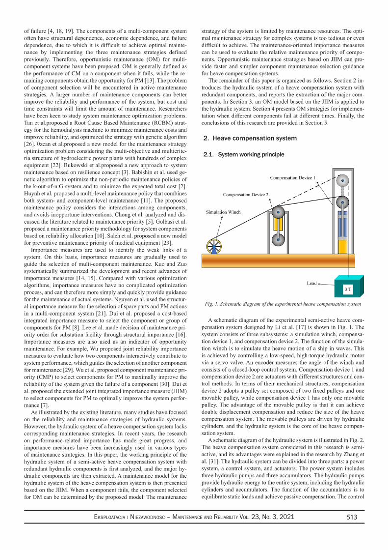
Eksploatacja i NiEzawodNosc – MaiNtENaNcE aNd REliability Vol. 23, No. 3, 2021 513
of failure [4, 18, 19]. The components of a multi-component system often have structural dependence, economic dependence, and failure dependence, due to which it is difficult to achieve optimal mainte-nance by implementing the three maintenance strategies defined previously. Therefore, opportunistic maintenance (OM) for multi-component systems have been proposed. OM is generally defined as the performance of CM on a component when it fails, while the re-maining components obtain the opportunity for PM [13]. The problem of component selection will be encountered in active maintenance strategies. A larger number of maintenance components can better improve the reliability and performance of the system, but cost and time constraints will limit the amount of maintenance. Researchers have been keen to study system maintenance optimization problems. Tan et al.proposed a Root Cause Based Maintenance (RCBM) strat-egy for the hemodialysis machine to minimize maintenance costs and improve reliability, and optimized the strategy with genetic algorithm [26]. Özcan et al.proposed a new model for the maintenance strategy optimization problem considering the multi-objective and multicrite-ria structure of hydroelectric power plants with hundreds of complex equipment [22]. Bukowski et al.proposed a new approach to system maintenance based on resilience concept [3]. Babishin et al. used ge-netic algorithm to optimize the non-periodic maintenance policies of the k-out-of-n:G system and to minimze the expected total cost [2].Huynh et al. proposed a multi-level maintenance policy that combines both system- and component-level maintenance [11]. The proposed maintenance policy considers the interactions among components, and avoids inopportune interventions. Chong et al. analyzed and dis-cussed the literature related to maintenance priority [5]. Golbasi et al. proposed a maintenance priority methodology for system components based on reliability allocation [10]. Saleh et al. proposed a new model for preventive maintenance priority of medical equipment [23].
Importance measures are used to identify the weak links of a system. On this basis, importance measures are gradually used to guide the selection of multi-component maintenance. Kuo and Zuo systematically summarized the development and recent advances of importance measures [14, 15]. Compared with various optimization algorithms, importance measures have no complicated optimization process, and can therefore more simply and quickly provide guidance for the maintenance of actual systems. Nguyen et al. used the structur-al importance measure for the selection of spare parts and PM actions in a multi-component system [21]. Dui et al. proposed a cost-based integrated importance measure to select the component or group of components for PM [8]. Lee et al. made decision of maintenance pri-ority order for substation facility through structural importance [16]. Importance measures are also used as an indicator of opportunity maintenance. For example, Wu proposed joint reliability importance measures to evaluate how two components interactively contribute to system performance, which guides the selection of another component for maintenance [29]. Wu et al. proposed component maintenance pri-ority (CMP) to select components for PM to maximally improve the reliability of the system given the failure of a component [30]. Dui et al. proposed the extended joint integrated importance measure (JIIM) to select components for PM to optimally improve the system perfor-mance [7].
As illustrated by the existing literature, many studies have focused on the reliability and maintenance strategies of hydraulic systems. However, the hydraulic system of a heave compensation system lacks corresponding maintenance strategies. In recent years, the research on performance-related importance has made great progress, and importance measures have been increasingly used in various types of maintenance strategies. In this paper, the working principle of the hydraulic system of a semi-active heave compensation system with redundant hydraulic components is first analyzed, and the major hy-draulic components are then extracted. A maintenance model for the hydraulic system of the heave compensation system is then presented based on the JIIM. When a component fails, the component selected for OM can be determined by the proposed model. The maintenance
strategy of the system is limited by maintenance resources. The opti-mal maintenance strategy for complex systems is too tedious or even difficult to achieve. The maintenance-oriented importance measures can be used to evaluate the relative maintenance priority of compo-nents. Opportunistic maintenance strategies based on JIIM can pro-vide faster and simpler component maintenance selection guidance for heave compensation systems.
The remainder of this paper is organized as follows. Section 2 in-troduces the hydraulic system of a heave compensation system with redundant components, and reports the extraction of the major com-ponents. In Section 3, an OM model based on the JIIM is applied to the hydraulic system. Section 4 presents OM strategies for implemen-tation when different components fail at different times. Finally, the conclusions of this research are provided in Section 5.
2. Heave compensation system
2.1. System working principle
Fig. 1. Schematic diagram of the experimental heave compensation system
A schematic diagram of the experimental semi-active heave com-pensation system designed by Li et al. [17] is shown in Fig. 1. The system consists of three subsystems: a simulation winch, compensa-tion device 1, and compensation device 2. The function of the simula-tion winch is to simulate the heave motion of a ship in waves. This is achieved by controlling a low-speed, high-torque hydraulic motor via a servo valve. An encoder measures the angle of the winch and consists of a closed-loop control system. Compensation device 1 and compensation device 2 are actuators with different structures and con-trol methods. In terms of their mechanical structures, compensation device 2 adopts a pulley set composed of two fixed pulleys and one movable pulley, while compensation device 1 has only one movable pulley. The advantage of the movable pulley is that it can achieve double displacement compensation and reduce the size of the heave compensation system. The movable pulleys are driven by hydraulic cylinders, and the hydraulic system is the core of the heave compen-sation system.
A schematic diagram of the hydraulic system is illustrated in Fig. 2. The heave compensation system considered in this research is semi-active, and its advantages were explained in the research by Zhang et al. [31]. The hydraulic system can be divided into three parts: a power system, a control system, and actuators. The power system includes three hydraulic pumps and three accumulators. The hydraulic pumps provide hydraulic energy to the entire system, including the hydraulic cylinders and accumulators. The function of the accumulators is to equilibrate static loads and achieve passive compensation. The control
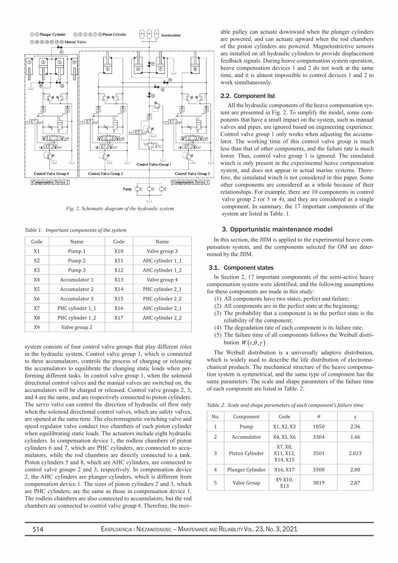
Eksploatacja i NiEzawodNosc – MaiNtENaNcE aNd REliability Vol. 23, No. 3, 2021514
system consists of four control valve groups that play different roles in the hydraulic system. Control valve group 1, which is connected to three accumulators, controls the process of charging or releasing the accumulators to equilibrate the changing static loads when per-forming different tasks. In control valve group 1, when the solenoid directional control valves and the manual valves are switched on, the accumulators will be charged or released. Control valve groups 2, 3, and 4 are the same, and are respectively connected to piston cylinders. The servo valve can control the direction of hydraulic oil flow only when the solenoid directional control valves, which are safety valves, are opened at the same time. The electromagnetic switching valve and speed regulator valve conduct two chambers of each piston cylinder when equilibrating static loads. The actuators include eight hydraulic cylinders. In compensation device 1, the rodless chambers of piston cylinders 6 and 7, which are PHC cylinders, are connected to accu-mulators, while the rod chambers are directly connected to a tank. Piston cylinders 5 and 8, which are AHC cylinders, are connected to control valve groups 2 and 3, respectively. In compensation device 2, the AHC cylinders are plunger cylinders, which is different from compensation device 1. The sizes of piston cylinders 2 and 3, which are PHC cylinders, are the same as those in compensation device 1. The rodless chambers are also connected to accumulators, but the rod chambers are connected to control valve group 4. Therefore, the mov-
able pulley can actuate downward when the plunger cylinders are powered, and can actuate upward when the rod chambers of the piston cylinders are powered. Magnetostrictive sensors are installed on all hydraulic cylinders to provide displacement feedback signals. During heave compensation system operation, heave compensation devices 1 and 2 do not work at the same time, and it is almost impossible to control devices 1 and 2 to work simultaneously.
2.2. Component listAll the hydraulic components of the heave compensation sys-
tem are presented in Fig. 2. To simplify the model, some com-ponents that have a small impact on the system, such as manual valves and pipes, are ignored based on engineering experience. Control valve group 1 only works when adjusting the accumu-lator. The working time of this control valve group is much less than that of other components, and the failure rate is much lower. Thus, control valve group 1 is ignored. The simulated winch is only present in the experimental heave compensation system, and does not appear in actual marine systems. There-fore, the simulated winch is not considered in this paper. Some other components are considered as a whole because of their relationships. For example, there are 10 components in control valve group 2 (or 3 or 4), and they are considered as a single component. In summary, the 17 important components of the system are listed in Table. 1.
3. Opportunistic maintenance modelIn this section, the JIIM is applied to the experimental heave com-
pensation system, and the components selected for OM are deter-mined by the JIIM.
3.1. Component statesIn Section 2, 17 important components of the semi-active heave
compensation system were identified, and the following assumptions for these components are made in this study:
All components have two states, perfect and failure;(1) All components are in the perfect state at the beginning;(2) The probability that a component is in the perfect state is the (3) reliability of the component; The degradation rate of each component is its failure rate;(4) The failure time of all components follows the Weibull distri-(5) bution W t, ,θ γ( ) .
The Weibull distribution is a universally adaptive distribution, which is widely used to describe the life distribution of electrome-chanical products. The mechanical structure of the heave compensa-tion system is symmetrical, and the same type of component has the same parameters. The scale and shape parameters of the failure time of each component are listed in Table. 2.
Table 1. Important components of the system
Code Name Code Name
X1 Pump 1 X10 Valve group 3
X2 Pump 2 X11 AHC cylinder 1_1
X3 Pump 3 X12 AHC cylinder 1_2
X4 Accumulator 1 X13 Valve group 4
X5 Accumulator 2 X14 PHC cylinder 2_1
X6 Accumulator 3 X15 PHC cylinder 2_2
X7 PHC cylinder 1_1 X16 AHC cylinder 2_1
X8 PHC cylinder 1_2 X17 AHC cylinder 2_2
X9 Valve group 2
Table. 2. Scale and shape parameters of each component’s failure time
No. Component Code θ γ
1 Pump X1, X2, X3 1850 2.36
2 Accumulator X4, X5, X6 3304 1.46
3 Piston CylinderX7, X8,
X11, X12, X14, X15
3501 2.023
4 Plunger Cylinder X16, X17 3300 2.00
5 Valve Group X9 X10, X13 3819 2.87
Fig. 2. Schematic diagram of the hydraulic system
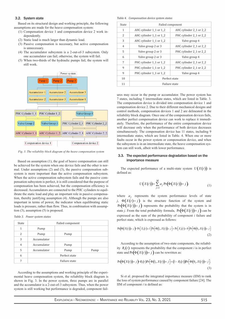
Eksploatacja i NiEzawodNosc – MaiNtENaNcE aNd REliability Vol. 23, No. 3, 2021 515
3.2. System stateBased on its structural design and working principle, the following
assumptions are made for the heave compensation system:Compensation device 1 and compensation device 2 work in-(1) dependently.Static load is much larger than dynamic load.(2) Passive compensation is necessary, but active compensation (3) is unnecessary.The accumulator subsystem is a 2-out-of-3 subsystem. Only (4) one accumulator can fail; otherwise, the system will fail.When two-thirds of the hydraulic pumps fail, the system will (5) still work.
Based on assumption (1), the goal of heave compensation can still be achieved for the system when one device fails and the other is nor-mal. Under assumptions (2) and (3), the passive compensation sub-system is more important than the active compensation subsystem. When the active compensation subsystem fails and the passive com-pensation subsystem is perfect, it is still considered that the purpose of compensation has been achieved, but the compensation efficiency is decreased. Accumulators are connected to the PHC cylinders to equil-ibrate the static load and play an important role in passive compensa-tion, thereby justifying assumption (4). Although the pumps are also important in terms of power, the indicator when equilibrating static loads is pressure, rather than flow. Thus, in combination with assump-tion (3), assumption (5) is proposed.
According to the assumptions and working principle of the experi-mental heave compensation system, the reliability block diagram is shown in Fig. 3. In the power system, three pumps are in parallel and the accumulator is a 2-out-of-3 subsystem. Thus, when the power system is still working but performance is degraded, component fail-
ures may occur in the pump or accumulator. The power system has 7 states, including 5 intermediate states, which are listed in Table. 3. The compensation device is divided into compensation device 1 and compensation device 2. Due to their different mechanical designs and control methods, compensation devices 1 and 2 are delineated in the reliability block diagram. Once one of the compensation devices fails, another perfect compensation device can work to replace it immedi-ately. Therefore, the performance of the entire compensation device will decrease only when the performance of both devices decreases simultaneously. The compensation device has 11 states, including 9 intermediate states, which are listed in Table. 4. When one or more faults occur in the power system or compensation device, and when the subsystem is in an intermediate state, the heave compensation sys-tem can still work, albeit with lower performance.
3.3. The expected performance degradation based on the importance measure
The expected performance of a multi-state system ( )( )U X t is defined as:
( )( ) ( )( )( )1
Pr ,M
jj
U X t a X t j=
= Φ =∑ (1)
where ja represents the system performance levels of state j, ( )( )X t jΦ = is the structure function of the system and
( )( )( )Pr X t jΦ = represents the probability that the system is in state j. From the total probability formula, ( )( )( )Pr X t jΦ = can be expressed as the sum of the probability of component i failure and perfect state, which is expressed as follows:
( )( )( ) ( ) ( )( ) ( ) ( )( )Pr = Pr 1 Pr 1 , Pr 0 Pr 0 ,i i i iX t j X t X t j X t X t j Φ = = Φ = + = Φ = (2)
According to the assumption of two-state components, the reliabil-ity ( )iR t represents the probability that the component i is in perfect state and ( )( )( )Pr X t jΦ = can be rewritten as:
( )( )( ) ( ) ( )( ) ( )( ) ( )( )Pr = Pr 1 , 1 Pr 0 , .i i i iX t j R t X t j R t X t j Φ = Φ = + − Φ = (3)
Si et al. proposed the integrated importance measure (IIM) to rank the loss of system performance caused by component failure [24]. The IIM of component i is defined as:
Table 3. Power system states
State Failed component
1 Pump
2 Pump Pump
3 Accumulator
4 Accumulator Pump
5 Accumulator Pump Pump
6 Perfect state
7 Failure state
Table 4. Compensation device system states
State Failed component
1 AHC cylinder 1_1 or 1_2 AHC cylinder 2_1 or 2_2
2 AHC cylinder 1_1 or 1_2 PHC cylinder 2_1 or 2_2
3 AHC cylinder 1_1 or 1_2 Valve group 4
4 Valve group 2 or 3 AHC cylinder 2_1 or 2_2
5 Valve group 2 or 3 PHC cylinder 2_1 or 2_2
6 Valve group 2 or 3 Valve group 4
7 PHC cylinder 1_1 or 1_2 AHC cylinder 2_1 or 2_2
9 PHC cylinder 1_1 or 1_2 PHC cylinder 2_1 or 2_2
9 PHC cylinder 1_1 or 1_2 Valve group 4
10 Perfect state
11 Failure state
Fig. 3. The reliability block diagram of the heave compensation system
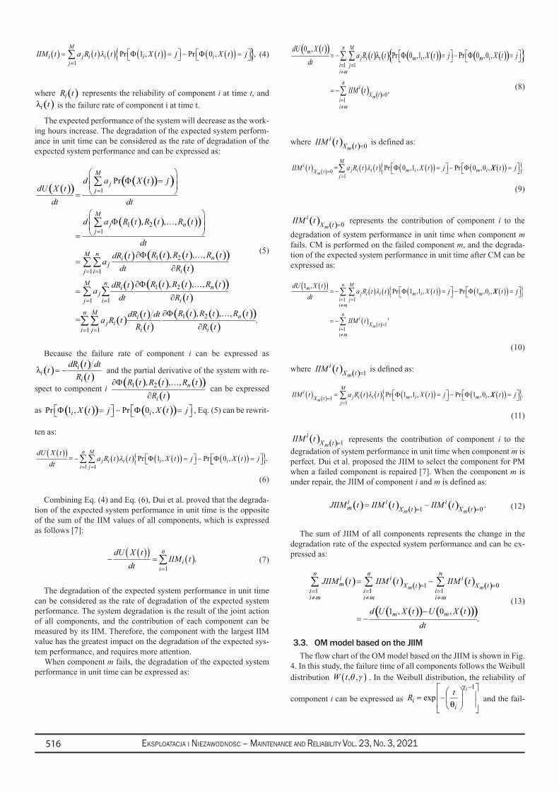
Eksploatacja i NiEzawodNosc – MaiNtENaNcE aNd REliability Vol. 23, No. 3, 2021516
IIM t a R t t X t j X t ji j i i i i( ) = ( ) ( ) ( )( ) = − ( )( ) = λ Pr , Pr ,Φ Φ1 0 =∑j
M
1, (4)
where ( )iR t represents the reliability of component i at time t, and ( )i tλ is the failure rate of component i at time t.
The expected performance of the system will decrease as the work-ing hours increase. The degradation of the expected system perform-ance in unit time can be considered as the rate of degradation of the expected system performance and can be expressed as:
( )( )( )( )( )
( ) ( ) ( )( )
( ) ( ) ( ) ( )( )( )
( ) ( ) ( ) ( )( )( )
( ) ( )( )
( ) ( ) ( )( )( )
1
1 21
1 2
1 1
1 2
1 1
1 2
1 1
Pr
, , ,
, , ,
, , ,
, , ,= .
Mj
j
Mj n
j
M n nij
ij i
M n nij
ij i
n M nij i
i ii j
d a X t jdU X t
dt dt
d a R t R t R t
dtR t R t R tdR t
adt R t
R t R t R tdR ta
dt R t
R t R t R tdR t dta R t
R t R t
=
=
= =
= =
= =
Φ = =
Φ =
∂Φ=
∂
∂Φ=
∂
∂Φ
∂
∑
∑
∑∑
∑ ∑
∑∑
(5)
Because the failure rate of component i can be expressed as
( ) ( )( )
ii
i
dR t dtt
R tλ = − and the partial derivative of the system with re-
spect to component i ( ) ( ) ( )( )
( )1 2, , , n
i
R t R t R tR t
∂Φ
∂
can be expressed
as ( )( ) ( )( )Pr 1 , Pr 0 ,i iX t j X t j Φ = − Φ = , Eq. (5) can be rewrit-
ten as:
dU X tdt
a R t t X t j X t jj i i i i( )( )
− ( ) ( ) ( )( ) = − ( )( ) == λ Pr , Pr ,Φ Φ1 0 ==∑∑j
M
i
n
11.
(6)
Combining Eq. (4) and Eq. (6), Dui et al. proved that the degrada-tion of the expected system performance in unit time is the opposite of the sum of the IIM values of all components, which is expressed as follows [7]:
−( )( )
= ( )=∑
dU X tdt
IIM tii
n
1. (7)
The degradation of the expected system performance in unit time can be considered as the rate of degradation of the expected system performance. The system degradation is the result of the joint action of all components, and the contribution of each component can be measured by its IIM. Therefore, the component with the largest IIM value has the greatest impact on the degradation of the expected sys-tem performance, and requires more attention.
When component m fails, the degradation of the expected system performance in unit time can be expressed as:
( )( ) ( ) ( ) ( )( ) ( )( )
( ) ( )
1 1
01
0 ,Pr 0 ,1 , Pr 0 ,0 ,
,m
n Mmj i i m i m i
i ji m
ni
X tii m
dU X ta R t t X t j X t j
dt
IIM t
λ= =≠
==≠
= − Φ = − Φ =
= −
∑ ∑
∑
(8)
where ( ) ( ) 0mi
X tIIM t = is defined as:
IIM t a R t t X t jiX t j i i m i m im
( ) ( ) ( ) ( )( ) = −( )=0 0 1 0 0= λ Pr , , Pr , ,Φ Φ XX t jj
M( )( ) =
=∑
1.
(9)
( ) ( ) 0mi
X tIIM t = represents the contribution of component i to the
degradation of system performance in unit time when component m fails. CM is performed on the failed component m, and the degrada-tion of the expected system performance in unit time after CM can be expressed as:
dU X tdt
a R t t X t jmj i i m i m i
11 1 1 0
,Pr , , Pr , ,
( )( )= − ( ) ( ) ( )( ) = −λ Φ Φ XX t j
IIM t
j
M
ii m
n
iX t
ii m
n
m
( )( ) =
= − ( )
==≠
( )==≠
∑∑
∑
11
11
'
(10)
where ( ) ( ) 1mi
X tIIM t = is defined as:
IIM t a R t t X t jiX t j i i m i m im
( ) = ( ) ( ) ( )( ) = −( )=1 1 1 1 0λ Pr , , Pr , ,Φ Φ XX t jj
M( )( ) =
=∑
1.
(11)
( ) ( ) 1mi
X tIIM t = represents the contribution of component i to the degradation of system performance in unit time when component m is perfect. Dui et al. proposed the JIIM to select the component for PM when a failed component is repaired [7]. When the component m is under repair, the JIIM of component i and m is defined as:
( ) ( ) ( ) ( ) ( )1 0 .m m
i i im X t X tJIIM t IIM t IIM t= == − (12)
The sum of JIIM of all components represents the change in the degradation rate of the expected system performance and can be ex-pressed as:
( ) ( ) ( ) ( ) ( )
( )( ) ( )( )( )
1 01 1 1
1 , 0 ,.
m m
n n ni i im X t X t
i i ii m i m i m
m m
JIIM t IIM t IIM t
d U X t U X t
dt
= == = =≠ ≠ ≠
= −
−= −
∑ ∑ ∑
(13)
3.3. OM model based on the JIIMThe flow chart of the OM model based on the JIIM is shown in Fig.
4. In this study, the failure time of all components follows the Weibull distribution W t, ,θ γ( ) . In the Weibull distribution, the reliability of
component i can be expressed as 1
expi
ii
tRγ
θ
− = −
and the fail-
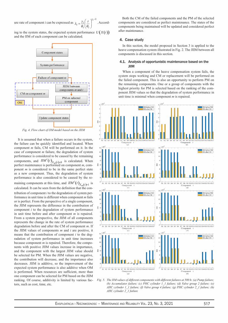
Eksploatacja i NiEzawodNosc – MaiNtENaNcE aNd REliability Vol. 23, No. 3, 2021 517
ure rate of component i can be expressed as λ γθ θ
γ
ii
i i
t i
=
−1. Accord-
ing to the system states, the expected system performance ( )( )U X t and the IIM of each component can be calculated.
Fig. 4. Flow chart of OM model based on the JIIM
It is assumed that when a failure occurs in the system, the failure can be quickly identified and located. When component m fails, CM will be performed on it. In the case of component m failure, the degradation of system performance is considered to be caused by the remaining components, and ( ) ( ) 0m
iX tIIM t = is calculated. When
perfect maintenance is performed on component m, com-ponent m is considered to be in the same perfect state as a new component. Thus, the degradation of system performance is also considered to be caused by the re-maining components at this time, and ( ) ( ) 1m
iX tIIM t = is
calculated. It can be seen from the definition that the con-tribution of component i to the degradation of system per-formance in unit time is different when component m fails or is perfect. From the perspective of a single component, the JIIM represents the difference in the contribution of component i to the degradation of system performance in unit time before and after component m is repaired. From a system perspective, the JIIM of all components represents the change in the rate of system performance degradation before and after the CM of component m. If the JIIM values of components m and i are positive, it means that the contribution of component i to the deg-radation of system performance in unit time increases because component m is repaired. Therefore, the compo-nents with positive JIIM values increase in importance, and the component with the largest JIIM value should be selected for PM. When the JIIM values are negative, the contribution will decrease, and the importance also decreases. JIIM is additive, so the improvement of the expected system performance is also additive when OM is performed. When resources are sufficient, more than one component can be selected for PM based on the JIIM ranking. Of course, additivity is limited by various fac-tors, such as cost, time, etc.
Both the CM of the failed components and the PM of the selected components are considered as perfect maintenance. The states of the components being maintained will be updated and considered perfect after maintenance.
4. Case studyIn this section, the model proposed in Section 3 is applied to the
heave compensation system illustrated in Fig. 2. The JIIM between all components is discussed in this section.
4.1. Analysis of opportunistic maintenance based on the JIIM
When a component of the heave compensation system fails, the system stops working and CM or replacement will be performed on the failed component. This is also an opportunity to perform PM on the remaining components. One or a group of components with the highest priority for PM is selected based on the ranking of the com-ponent JIIM values so that the degradation of system performance in unit time is minimal when component m is repaired.
Fig. 5. The IIM values of different components with different failures at 500 h: (a) Pump failure; (b) Accumulator failure; (c) PHC cylinder 1_1 failure; (d) Valve group 2 failure; (e) AHC cylinder 1_1 failure; (f) Valve group 4 failure; (g) PHC cylinder 2_1 failure; (h) AHC cylinder 2_1 failure
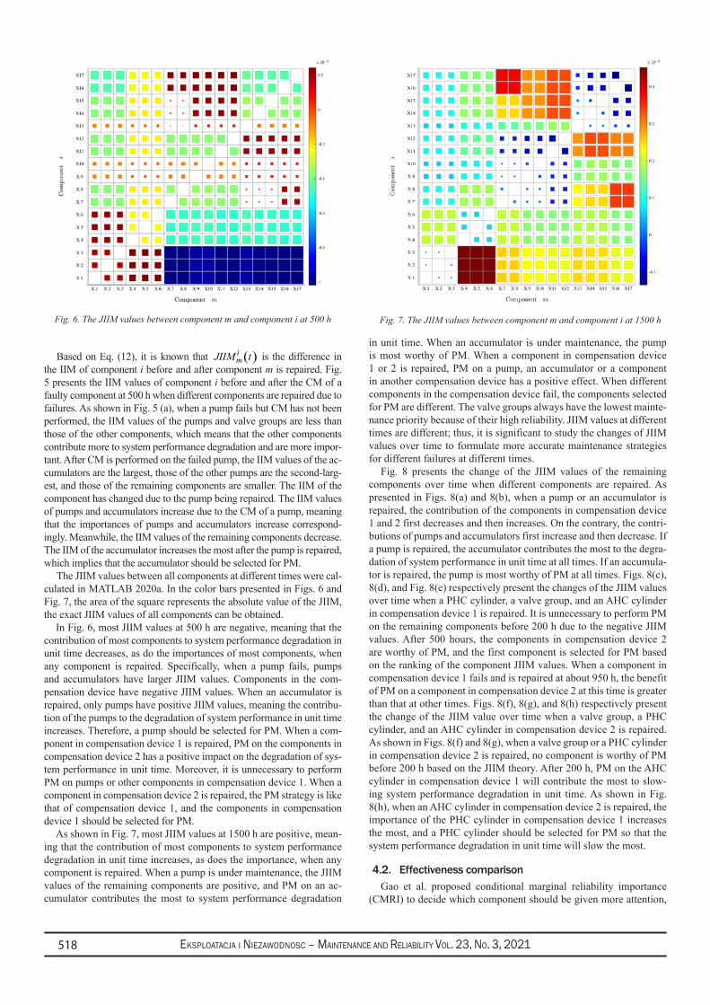
Eksploatacja i NiEzawodNosc – MaiNtENaNcE aNd REliability Vol. 23, No. 3, 2021518
Based on Eq. (12), it is known that ( )imJIIM t is the difference in
the IIM of component i before and after component m is repaired. Fig. 5 presents the IIM values of component i before and after the CM of a faulty component at 500 h when different components are repaired due to failures. As shown in Fig. 5 (a), when a pump fails but CM has not been performed, the IIM values of the pumps and valve groups are less than those of the other components, which means that the other components contribute more to system performance degradation and are more impor-tant. After CM is performed on the failed pump, the IIM values of the ac-cumulators are the largest, those of the other pumps are the second-larg-est, and those of the remaining components are smaller. The IIM of the component has changed due to the pump being repaired. The IIM values of pumps and accumulators increase due to the CM of a pump, meaning that the importances of pumps and accumulators increase correspond-ingly. Meanwhile, the IIM values of the remaining components decrease. The IIM of the accumulator increases the most after the pump is repaired, which implies that the accumulator should be selected for PM.
The JIIM values between all components at different times were cal-culated in MATLAB 2020a. In the color bars presented in Figs. 6 and Fig. 7, the area of the square represents the absolute value of the JIIM, the exact JIIM values of all components can be obtained.
In Fig. 6, most JIIM values at 500 h are negative, meaning that the contribution of most components to system performance degradation in unit time decreases, as do the importances of most components, when any component is repaired. Specifically, when a pump fails, pumps and accumulators have larger JIIM values. Components in the com-pensation device have negative JIIM values. When an accumulator is repaired, only pumps have positive JIIM values, meaning the contribu-tion of the pumps to the degradation of system performance in unit time increases. Therefore, a pump should be selected for PM. When a com-ponent in compensation device 1 is repaired, PM on the components in compensation device 2 has a positive impact on the degradation of sys-tem performance in unit time. Moreover, it is unnecessary to perform PM on pumps or other components in compensation device 1. When a component in compensation device 2 is repaired, the PM strategy is like that of compensation device 1, and the components in compensation device 1 should be selected for PM.
As shown in Fig. 7, most JIIM values at 1500 h are positive, mean-ing that the contribution of most components to system performance degradation in unit time increases, as does the importance, when any component is repaired. When a pump is under maintenance, the JIIM values of the remaining components are positive, and PM on an ac-cumulator contributes the most to system performance degradation
in unit time. When an accumulator is under maintenance, the pump is most worthy of PM. When a component in compensation device 1 or 2 is repaired, PM on a pump, an accumulator or a component in another compensation device has a positive effect. When different components in the compensation device fail, the components selected for PM are different. The valve groups always have the lowest mainte-nance priority because of their high reliability. JIIM values at different times are different; thus, it is significant to study the changes of JIIM values over time to formulate more accurate maintenance strategies for different failures at different times.
Fig. 8 presents the change of the JIIM values of the remaining components over time when different components are repaired. As presented in Figs. 8(a) and 8(b), when a pump or an accumulator is repaired, the contribution of the components in compensation device 1 and 2 first decreases and then increases. On the contrary, the contri-butions of pumps and accumulators first increase and then decrease. If a pump is repaired, the accumulator contributes the most to the degra-dation of system performance in unit time at all times. If an accumula-tor is repaired, the pump is most worthy of PM at all times. Figs. 8(c), 8(d), and Fig. 8(e) respectively present the changes of the JIIM values over time when a PHC cylinder, a valve group, and an AHC cylinder in compensation device 1 is repaired. It is unnecessary to perform PM on the remaining components before 200 h due to the negative JIIM values. After 500 hours, the components in compensation device 2 are worthy of PM, and the first component is selected for PM based on the ranking of the component JIIM values. When a component in compensation device 1 fails and is repaired at about 950 h, the benefit of PM on a component in compensation device 2 at this time is greater than that at other times. Figs. 8(f), 8(g), and 8(h) respectively present the change of the JIIM value over time when a valve group, a PHC cylinder, and an AHC cylinder in compensation device 2 is repaired. As shown in Figs. 8(f) and 8(g), when a valve group or a PHC cylinder in compensation device 2 is repaired, no component is worthy of PM before 200 h based on the JIIM theory. After 200 h, PM on the AHC cylinder in compensation device 1 will contribute the most to slow-ing system performance degradation in unit time. As shown in Fig. 8(h), when an AHC cylinder in compensation device 2 is repaired, the importance of the PHC cylinder in compensation device 1 increases the most, and a PHC cylinder should be selected for PM so that the system performance degradation in unit time will slow the most.
4.2. Effectiveness comparisonGao et al. proposed conditional marginal reliability importance
(CMRI) to decide which component should be given more attention,
Fig. 6. The JIIM values between component m and component i at 500 h Fig. 7. The JIIM values between component m and component i at 1500 h
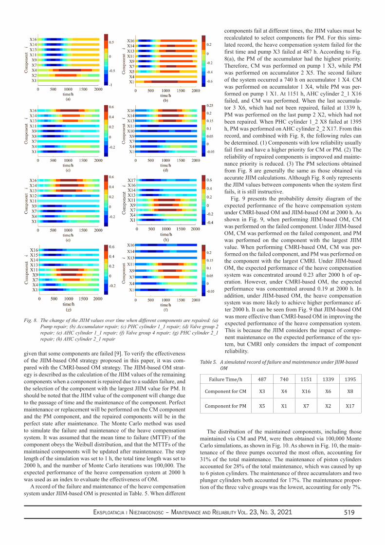
Eksploatacja i NiEzawodNosc – MaiNtENaNcE aNd REliability Vol. 23, No. 3, 2021 519
given that some components are failed [9]. To verify the effectiveness of the JIIM-based OM strategy proposed in this paper, it was com-pared with the CMRI-based OM strategy. The JIIM-based OM strat-egy is described as the calculation of the JIIM values of the remaining components when a component is repaired due to a sudden failure, and the selection of the component with the largest JIIM value for PM. It should be noted that the JIIM value of the component will change due to the passage of time and the maintenance of the component. Perfect maintenance or replacement will be performed on the CM component and the PM component, and the repaired components will be in the perfect state after maintenance. The Monte Carlo method was used to simulate the failure and maintenance of the heave compensation system. It was assumed that the mean time to failure (MTTF) of the component obeys the Weibull distribution, and that the MTTFs of the maintained components will be updated after maintenance. The step length of the simulation was set to 1 h, the total time length was set to 2000 h, and the number of Monte Carlo iterations was 100,000. The expected performance of the heave compensation system at 2000 h was used as an index to evaluate the effectiveness of OM.
A record of the failure and maintenance of the heave compensation system under JIIM-based OM is presented in Table. 5. When different
components fail at different times, the JIIM values must be recalculated to select components for PM. For this simu-lated record, the heave compensation system failed for the first time and pump X3 failed at 487 h. According to Fig. 8(a), the PM of the accumulator had the highest priority. Therefore, CM was performed on pump 1 X3, while PM was performed on accumulator 2 X5. The second failure of the system occurred a 740 h on accumulator 1 X4. CM was performed on accumulator 1 X4, while PM was per-formed on pump 1 X1. At 1151 h, AHC cylinder 2_1 X16 failed, and CM was performed. When the last accumula-tor 3 X6, which had not been repaired, failed at 1339 h, PM was performed on the last pump 2 X2, which had not been repaired. When PHC cylinder 1_2 X8 failed at 1395 h, PM was performed on AHC cylinder 2_2 X17. From this record, and combined with Fig. 8, the following rules can be determined. (1) Components with low reliability usually fail first and have a higher priority for CM or PM. (2) The reliability of repaired components is improved and mainte-nance priority is reduced. (3) The PM selections obtained from Fig. 8 are generally the same as those obtained via accurate JIIM calculations. Although Fig. 8 only represents the JIIM values between components when the system first fails, it is still instructive.
Fig. 9 presents the probability density diagram of the expected performance of the heave compensation system under CMRI-based OM and JIIM-based OM at 2000 h. As shown in Fig. 9, when performing JIIM-based OM, CM was performed on the failed component. Under JIIM-based OM, CM was performed on the failed component, and PM was performed on the component with the largest JIIM value. When performing CMRI-based OM, CM was per-formed on the failed component, and PM was performed on the component with the largest CMRI. Under JIIM-based OM, the expected performance of the heave compensation system was concentrated around 0.23 after 2000 h of op-eration. However, under CMRI-based OM, the expected performance was concentrated around 0.19 at 2000 h. In addition, under JIIM-based OM, the heave compensation system was more likely to achieve higher performance af-ter 2000 h. It can be seen from Fig. 9 that JIIM-based OM was more effective than CMRI-based OM in improving the expected performance of the heave compensation system. This is because the JIIM considers the impact of compo-nent maintenance on the expected performance of the sys-tem, but CMRI only considers the impact of component reliability.
The distribution of the maintained components, including those maintained via CM and PM, were then obtained via 100,000 Monte Carlo simulations, as shown in Fig. 10. As shown in Fig. 10, the main-tenance of the three pumps occurred the most often, accounting for 31% of the total maintenance. The maintenance of piston cylinders accounted for 28% of the total maintenance, which was caused by up to 6 piston cylinders. The maintenance of three accumulators and two plunger cylinders both accounted for 17%. The maintenance propor-tion of the three valve groups was the lowest, accounting for only 7%.
Fig. 8. The change of the JIIM values over time when different components are repaired: (a) Pump repair; (b) Accumulator repair; (c) PHC cylinder 1_1 repair; (d) Valve group 2 repair; (e) AHC cylinder 1_1 repair; (f) Valve group 4 repair; (g) PHC cylinder 2_1 repair; (h) AHC cylinder 2_1 repair
Table 5. A simulated record of failure and maintenance under JIIM-based OM
Failure Time/h 487 740 1151 1339 1395
Component for CM X3 X4 X16 X6 X8
Component for PM X5 X1 X7 X2 X17

Eksploatacja i NiEzawodNosc – MaiNtENaNcE aNd REliability Vol. 23, No. 3, 2021520
For components that account for a relatively high maintenance rate, more spare components can be prepared in advance.
5. Conclusion and future workIn this paper, JIIM-based OM was applied to the maintenance of a
semi-active heave compensation system to slow down the degradation of expected system performance. The JIIM is the difference between the IIM before and after the failed component is repaired, which is illustrated by bar graphs. In the case of different component failures at different times, the corresponding component for which PM should be performed is determined according to JIIM-based OM. Via the Monte Carlo method, it was verified that JIIM-based OM is superior to CMRI-based OM in slowing down the degradation of the expected
system performance. A typical component failure and repair record was analyzed, and the predicted maintenance percentages of various components were also illustrated by a pie chart.
Future work will include the development of multi-level mainte-nance strategies for CM and PM, and the economic dependence of the components will also be considered.
AcknowledgementsThe authors gratefully acknowledge the financial support for this
research from the National Key Research and Development Program of China (Grant No. 2019YFB2004504), the National Natural Sci-ence Foundation of China (Grant Nos. 51875015, 51620105010) and the Aviation Science Foundation (Grant No. 201902051001).
References1. Ahmad R, Kamaruddin S. An overview of time-based and condition-based maintenance in industrial application. Computers & Industrial
Engineering 2012; 63: 135-149, https://doi.org/10.1016/j.cie.2012.02.002.2. Babishin V, Hajipour Y, Taghipour S. Optimisation of non-periodic inspection and maintenance for multicomponent systems. Eksploatacja i
Niezawodnosc - Maintenance and Reliability 2018; 20 (2): 327-342, https://doi.org/10.17531/ein.2018.2.20.3. Bukowski L, Werbińska-Wojciechowska S. Using fuzzy logic to support maintenance decisions according to Resilience-Based Maintenance
concept. Eksploatacja i Niezawodnosc - Maintenance and Reliability 2021; 23: 294-307, https://doi.org/10.17531/ein.2021.2.9.4. Chen C, Wang C, Lu N, Jiang B, Xing Y. A data-driven predictive maintenance strategy based on accurate failure prognostics. Eksploatacja
i Niezawodnosc - Maintenance and Reliability 2021; 23: 387-394, https://doi.org/10.17531/ein.2021.2.19.5. Chong A K W, Mohammed A H, Abdullah M N, Rahman M S. Maintenance prioritization - a review on factors and methods. Journal of
Facilities Management 2019; 17 (1), 18-39, https://doi.org/10.1108/JFM-11-2017-0058.6. Do K D, Pan J. Nonlinear control of an active heave compensation system. Ocean Engineering 2008; 35: 558-571, https://doi.org/10.1016/j.
oceaneng.2007.11.005.7. Dui H Y, Li S M, Xing L D, Liu H L. System performance-based joint importance analysis guided maintenance for repairable systems.
Reliability Engineering & System Safety 2019; 186: 162-175, https://doi.org/10.1016/j.ress.2019.02.021.8. Dui H Y, Si S B and Yam R C M. A cost-based integrated importance measure of system components for preventive maintenance. Reliability
Engineering & System Safety 2017; 168: 98-104, https://doi.org/10.1016/j.ress.2017.05.025.9. Gao X L, Cui, L R, Li J L. Analysis for joint importance of components in a coherent system. European Journal of Operational Research
2007; 182: 282-299, https://doi.org/10.1016/j.ejor.2006.07.022.10. Golbasi O, Demirel N. Risk-based reliability allocation methodology to set a maintenance priority among system components: A case study
in Mining. Eksploatacja i Niezawodnosc - Maintenance and Reliability 2017; 19(2): 191-202, https://doi.org/10.17531/ein.2017.2.6.11. Huynh K T, Barros A, Bérenguer C. Multi-Level Decision-Making for The Predictive Maintenance of k-Out-of-n: F Deteriorating Systems.
IEEE Transactions on Reliability 2015; 64: 94-117, https://doi.org/10.1109/TR.2014.2337791.12. Kuechler S, Mahl T, Neupert J, Schneider K, Sawodny O. Active Control for an Offshore Crane Using Prediction of the Vessel's Motion.
IEEE/ASME Transactions on Mechatronics 2011; 16: 297-309, https://doi.org/10.1109/TMECH.2010.2041933.13. Kumar V, Kumar G, Singh RK, Soni U. Degrading systems availability analysis: analytical semi-Markov approach. Eksploatacja i
Niezawodnosc - Maintenance and Reliability 2021; 23 (1): 195-208, https://doi.org/10.17531/ein.2021.1.20.14. Kuo W, Zhu X. Relations and Generalizations of Importance Measures in Reliability. IEEE Transactions on Reliability 2012; 61: 956-674,
https://doi.org/10.1109/TR.2012.2194196.15. Kuo W, Zhu X. Some Recent Advances on Importance Measures in Reliability. IEEE Transactions on Reliability 2012; 61: 344-360, https://
doi.org/10.1109/TR.2012.2194196.16. Lee S H, Lee Y S, Kim J O. Decision of Maintenance Priority Order for Substation Facility through Structural Importance and Fault
Fig. 9. The probability density of the expected performance of the heave com-pensation system
Fig. 10. The distribution of maintained components

Eksploatacja i NiEzawodNosc – MaiNtENaNcE aNd REliability Vol. 23, No. 3, 2021 521
Analysis. Journal of the Korean Institute of Illuminating and Electrical Installation Engineers 2013; 27(4), 23-30, https://doi.org/10.5207/JIEIE.2013.27.4.023.
17. Li S Z, Wei J H, Guo K, Zhu W L. Nonlinear Robust Prediction Control of Hybrid Active-Passive Heave Compensator With Extended Disturbance Observer. IEEE Transactions on Industrial Electronics 2017; 64: 6684-6694, https://doi.org/10.1109/TIE.2017.2698358.
18. Lotovskyi E, Teixeira AP, Guedes Soares C. Availability analysis of an offshore oil and gas production system subjected to age-based preventive maintenance by Petri Nets. Eksploatacja i Niezawodnosc - Maintenance and Reliability 2020; 22: 627-637, https://doi.org/10.17531/ein.2020.4.6.
19. Młynarski S, Pilch R, Smolnik M, Szybka J, Wiązania G. A model of an adaptive strategy of preventive maintenance of complex technical objects. Eksploatacja i Niezawodnosc - Maintenance and Reliability 2020; 22: 35-41, https://doi.org/10.17531/ein.2020.1.5.
20. Nespoli A, Besseghini S, Pittaccio S, Villa E, Viscuso S. The high potential of shape memory alloys in developing miniature mechanical devices: A review on shape memory alloy mini-actuators. Sensors and Actuators A: Physical 2010; 158: 149-160, https://doi.org/10.1016/j.sna.2009.12.020.
21. Nguyen K A, Do P, Grall A. Condition-based maintenance for multi-component systems using importance measure and predictive information. International Journal of Systems Science: Operations & Logistics 2014; 1: 228-245, https://doi.org/10.1080/23302674.2014.983582.
22. Özcan E, Yumuşak R, Eren T. A novel approach to optimize the maintenance strategies: a case in the hydroelectric power plant. Eksploatacja i Niezawodnosc - Maintenance and Reliability 2021; 23: 324-337, https://doi.org/10.17531/ein.2021.2.12.
23. Saleh N, Sharawi A A, Abd Elwahed M, et al. Preventive maintenance prioritization index of medical equipment using quality function deployment. IEEE Journal of Biomedical and Health Informatics 2014; 19(3): 1029-1035, https://doi.org/10.1109/JBHI.2014.2337895.
24. Si S, Dui H, Zhao X, Zhang S, Sun, S. Integrated importance measure of component states based on loss of system performance. IEEE Transactions on Reliability 2012; 61: 192-202, https://doi.org/10.1109/TR.2011.2182394.
25. Southerland JR. Mechanical systems for ocean engineering. Naval Engineers Journal 1970; 82: 63-74, https://doi.org/10.1111/j.1559-3584.1970.tb04361.x.
26. Tan CM, Na rula U, La i LA, Pandey S, Tung JH, Li CY. Optimal maintenance strategy on medical instruments used for haemodialysis process. Eksploatacja i Niezawodnosc - Maintenance and Reliability 2019; 21: 318-328, https://doi.org/10.17531/ein.2019.2.17.
27. Wang H. A survey of maintenance policies of deteriorating systems. European Journal of Operational Research 2002; 139: 469-489, https://doi.org/10.1016/S0377-2217(01)00197-7.
28. Woodacre J K, Bauer R J, Irani R A. A review of vertical motion heave compensation systems. Ocean Engineering 2015; 104, 140-154, https://doi.org/10.1016/j.oceaneng.2015.05.004.
29. Wu, S. Joint importance of multistate systems. Computers & Industrial Engineering 2005; 49: 63-75, https://doi.org/10.1016/j.cie.2005.02.001.
30. Wu S, Chen Y, Wu Q, Wang, Z. Linking component importance to optimisation of preventive maintenance policy. Reliability Engineering & System Safety 2016; 146: 26-32, https://doi.org/10.1016/j.ress.2015.10.008.
31. Zhang C, Qian Y, Dui H, Wang S, Shi J. Component failure recognition and maintenance optimization for offshore heave compensation systems based on importance measures. Journal of Loss Prevention in the Process Industries 2020; 63, https://doi.org/10.1016/j.jlp.2019.103996.
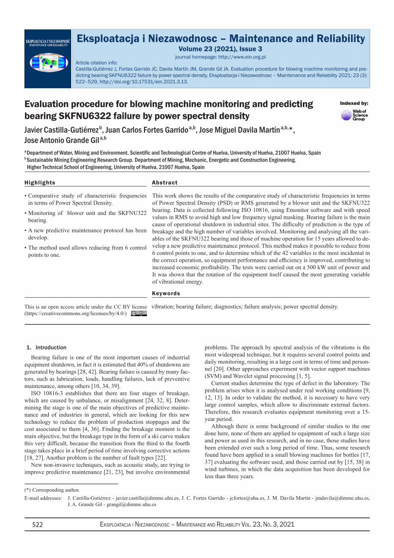
Eksploatacja i NiEzawodNosc – MaiNtENaNcE aNd REliability Vol. 23, No. 3, 2021522
(*) Corresponding author.E-mail addresses:
Eksploatacja i Niezawodnosc – Maintenance and ReliabilityVolume 23 (2021), Issue 3
journal homepage: http://www.ein.org.pl
Indexed by:
1. Introduction
Bearing failure is one of the most important causes of industrial equipment shutdown, in fact it is estimated that 40% of shutdowns are generated by bearings [28, 42]. Bearing failure is caused by many fac-tors, such as lubrication, loads, handling failures, lack of preventive maintenance, among others [10, 34, 39].
ISO 10816-3 establishes that there are four stages of breakage, which are caused by unbalance, or misalignment [24, 32, 8]. Deter-mining the stage is one of the main objectives of predictive mainte-nance and of industries in general, which are looking for this new technology to reduce the problem of production stoppages and the cost associated to them [4, 36]. Finding the breakage moment is the main objective, but the breakage type in the form of a ski curve makes this very difficult, because the transition from the third to the fourth stage takes place in a brief period of time involving corrective actions [18, 27]. Another problem is the number of fault types [22].
New non-invasive techniques, such as acoustic study, are trying to improve predictive maintenance [21, 23], but involve environmental
problems. The approach by spectral analysis of the vibrations is the most widespread technique, but it requires several control points and daily monitoring, resulting in a large cost in terms of time and person-nel [20]. Other approaches experiment with vector support machines (SVM) and Wavelet signal processing [1, 5].
Current studies determine the type of defect in the laboratory. The problem arises when it is analysed under real working conditions [9, 12, 13]. In order to validate the method, it is necessary to have very large control samples, which allow to discriminate external factors. Therefore, this research evaluates equipment monitoring over a 15-year period.
Although there is some background of similar studies to the one done here, none of them are applied to equipment of such a large size and power as used in this research, and in no case, those studies have been extended over such a long period of time. Thus, some research found have been applied in a small blowing machines for bottles [17, 37] evaluating the software used, and those carried out by [15, 38] in wind turbines, in which the data acquisition has been developed for less than three years.
Evaluation procedure for blowing machine monitoring and predicting bearing SKFNU6322 failure by power spectral densityJavier Castilla-Gutiérrez b, Juan Carlos Fortes Garrido a,b, Jose Miguel Davila Martín a,b,*, Jose Antonio Grande Gil a,b
a Department of Water, Mining and Environment. Scientific and Technological Centre of Huelva, University of Huelva, 21007 Huelva, Spain b Sustainable Mining Engineering Research Group. Department of Mining, Mechanic, Energetic and Construction Engineering. Higher Technical School of Engineering, University of Huelva, 21007 Huelva, Spain
Castilla-Gutiérrez J, Fortes Garrido JC, Davila Martín JM, Grande Gil JA. Evaluation procedure for blowing machine monitoring and pre-dicting bearing SKFNU6322 failure by power spectral density. Eksploatacja i Niezawodnosc – Maintenance and Reliability 2021; 23 (3): 522–529, http://doi.org/10.17531/ein.2021.3.13.
Article citation info:
This work shows the results of the comparative study of characteristic frequencies in terms of Power Spectral Density (PSD) or RMS generated by a blower unit and the SKFNU322 bearing. Data is collected following ISO 10816, using Emonitor software and with speed values in RMS to avoid high and low frequency signal masking. Bearing failure is the main cause of operational shutdown in industrial sites. The difficulty of prediction is the type of breakage and the high number of variables involved. Monitoring and analysing all the vari-ables of the SKFNU322 bearing and those of machine operation for 15 years allowed to de-velop a new predictive maintenance protocol. This method makes it possible to reduce from 6 control points to one, and to determine which of the 42 variables is the most incidental in the correct operation, so equipment performance and efficiency is improved, contributing to increased economic profitability. The tests were carried out on a 500 kW unit of power and It was shown that the rotation of the equipment itself caused the most generating variable of vibrational energy.
Highlights Abstract
Comparative study of characteristic frequencies • in terms of Power Spectral Density.
Monitoring of blower unit and the SKFNU322 • bearing.
A new predictive maintenance protocol has been • develop.
The method used allows reducing from 6 control • points to one.
vibration; bearing failure; diagnostics; failure analysis; power spectral density.
Keywords
This is an open access article under the CC BY license (https://creativecommons.org/licenses/by/4.0/)
J. Castilla-Gutiérrez - [email protected], J. C. Fortes Garrido - [email protected], J. M. Davila Martín - [email protected], J. A. Grande Gil - [email protected]
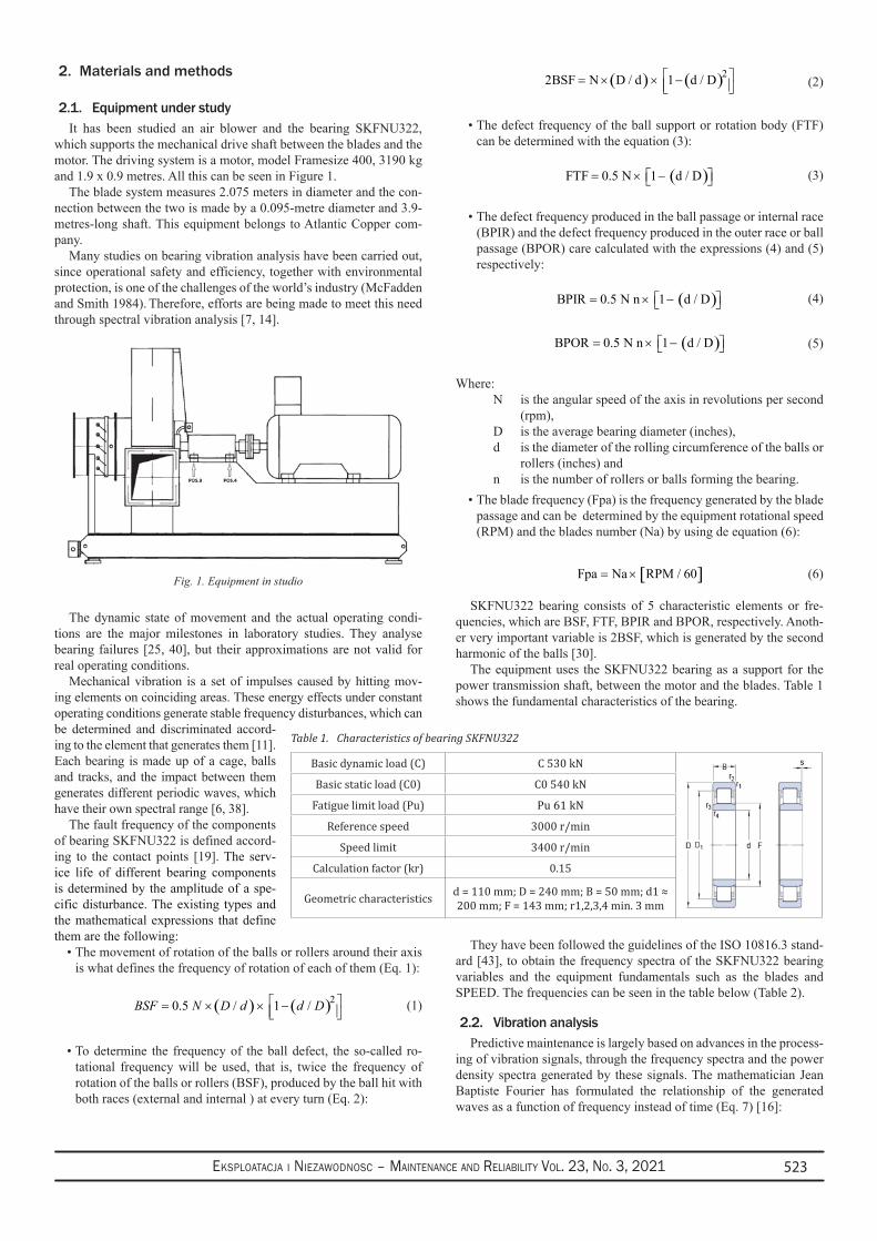
Eksploatacja i NiEzawodNosc – MaiNtENaNcE aNd REliability Vol. 23, No. 3, 2021 523
2. Materials and methods
2.1. Equipment under studyIt has been studied an air blower and the bearing SKFNU322,
which supports the mechanical drive shaft between the blades and the motor. The driving system is a motor, model Framesize 400, 3190 kg and 1.9 x 0.9 metres. All this can be seen in Figure 1.
The blade system measures 2.075 meters in diameter and the con-nection between the two is made by a 0.095-metre diameter and 3.9-metres-long shaft. This equipment belongs to Atlantic Copper com-pany.
Many studies on bearing vibration analysis have been carried out, since operational safety and efficiency, together with environmental protection, is one of the challenges of the world’s industry (McFadden and Smith 1984). Therefore, efforts are being made to meet this need through spectral vibration analysis [7, 14].
Fig. 1. Equipment in studio
The dynamic state of movement and the actual operating condi-tions are the major milestones in laboratory studies. They analyse bearing failures [25, 40], but their approximations are not valid for real operating conditions.
Mechanical vibration is a set of impulses caused by hitting mov-ing elements on coinciding areas. These energy effects under constant operating conditions generate stable frequency disturbances, which can be determined and discriminated accord-ing to the element that generates them [11]. Each bearing is made up of a cage, balls and tracks, and the impact between them generates different periodic waves, which have their own spectral range [6, 38].
The fault frequency of the components of bearing SKFNU322 is defined accord-ing to the contact points [19]. The serv-ice life of different bearing components is determined by the amplitude of a spe-cific disturbance. The existing types and the mathematical expressions that define them are the following:
The movement of rotation of the balls or rollers around their axis • is what defines the frequency of rotation of each of them (Eq. 1):
( ) ( )20.5 / 1 /BSF N D d d D = × × − (1)
To determine the frequency of the ball defect, the so-called ro-• tational frequency will be used, that is, twice the frequency of rotation of the balls or rollers (BSF), produced by the ball hit with both races (external and internal ) at every turn (Eq. 2):
( ) ( )22BSF N D / d 1 d / D = × × − (2)
The defect frequency of the ball support or rotation body (FTF) • can be determined with the equation (3):
( )FTF 0.5 N 1 d / D= × − (3)
The defect frequency produced in the ball passage or internal race • (BPIR) and the defect frequency produced in the outer race or ball passage (BPOR) care calculated with the expressions (4) and (5) respectively:
( )BPIR 0.5 N n 1 d / D= × − (4)
( )BPOR 0.5 N n 1 d / D= × − (5)
Where: N is the angular speed of the axis in revolutions per second
(rpm), D is the average bearing diameter (inches), d is the diameter of the rolling circumference of the balls or
rollers (inches) and n is the number of rollers or balls forming the bearing.
The blade frequency (Fpa) is the frequency generated by the blade • passage and can be determined by the equipment rotational speed (RPM) and the blades number (Na) by using de equation (6):
[ ]Fpa Na RPM / 60= × (6)
SKFNU322 bearing consists of 5 characteristic elements or fre-quencies, which are BSF, FTF, BPIR and BPOR, respectively. Anoth-er very important variable is 2BSF, which is generated by the second harmonic of the balls [30].
The equipment uses the SKFNU322 bearing as a support for the power transmission shaft, between the motor and the blades. Table 1 shows the fundamental characteristics of the bearing.
They have been followed the guidelines of the ISO 10816.3 stand-ard [43], to obtain the frequency spectra of the SKFNU322 bearing variables and the equipment fundamentals such as the blades and SPEED. The frequencies can be seen in the table below (Table 2).
2.2. Vibration analysisPredictive maintenance is largely based on advances in the process-
ing of vibration signals, through the frequency spectra and the power density spectra generated by these signals. The mathematician Jean Baptiste Fourier has formulated the relationship of the generated waves as a function of frequency instead of time (Eq. 7) [16]:
Table 1. Characteristics of bearing SKFNU322
Basic dynamic load (C) C 530 kN
Basic static load (C0) C0 540 kN
Fatigue limit load (Pu) Pu 61 kN
Reference speed 3000 r/min
Speed limit 3400 r/min
Calculation factor (kr) 0.15
Geometric characteristics d = 110 mm; D = 240 mm; B = 50 mm; d1 ≈ 200 mm; F = 143 mm; r1,2,3,4 min. 3 mm
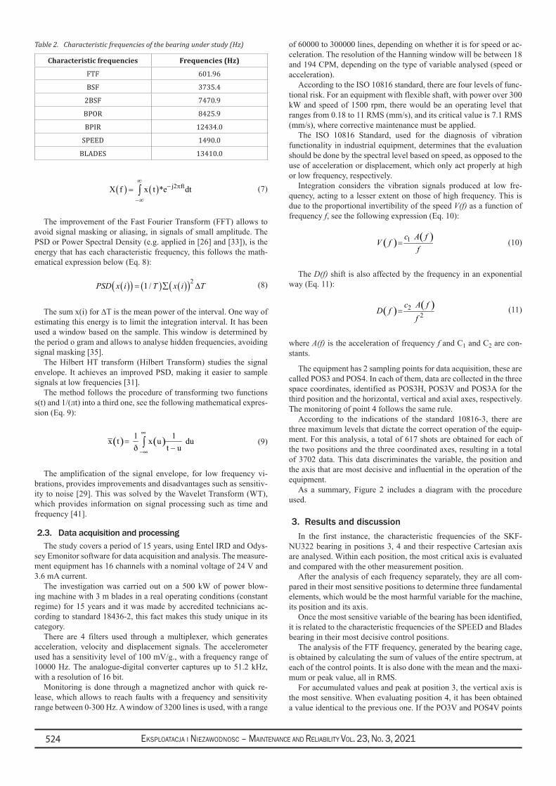
Eksploatacja i NiEzawodNosc – MaiNtENaNcE aNd REliability Vol. 23, No. 3, 2021524
X f x t *e dtj ft( ) = ( )−
−∫∞
∞2π (7)
The improvement of the Fast Fourier Transform (FFT) allows to avoid signal masking or aliasing, in signals of small amplitude. The PSD or Power Spectral Density (e.g. applied in [26] and [33]), is the energy that has each characteristic frequency, this follows the math-ematical expression below (Eq. 8):
PSD x i T x i T( )( ) = ( )∑ ( )( )1 2/ ∆ (8)
The sum x(i) for ∆T is the mean power of the interval. One way of estimating this energy is to limit the integration interval. It has been used a window based on the sample. This window is determined by the period o gram and allows to analyse hidden frequencies, avoiding signal masking [35].
The Hilbert HT transform (Hilbert Transform) studies the signal envelope. It achieves an improved PSD, making it easier to sample signals at low frequencies [31].
The method follows the procedure of transforming two functions s(t) and 1/(ᴫt) into a third one, see the following mathematical expres-sion (Eq. 9):
( ) ( )1 1x t x u duð t u
∞
∞−=
−∫ (9)
The amplification of the signal envelope, for low frequency vi-brations, provides improvements and disadvantages such as sensitiv-ity to noise [29]. This was solved by the Wavelet Transform (WT), which provides information on signal processing such as time and frequency [41].
2.3. Data acquisition and processingThe study covers a period of 15 years, using Entel IRD and Odys-
sey Emonitor software for data acquisition and analysis. The measure-ment equipment has 16 channels with a nominal voltage of 24 V and 3.6 mA current.
The investigation was carried out on a 500 kW of power blow-ing machine with 3 m blades in a real operating conditions (constant regime) for 15 years and it was made by accredited technicians ac-cording to standard 18436-2, this fact makes this study unique in its category.
There are 4 filters used through a multiplexer, which generates acceleration, velocity and displacement signals. The accelerometer used has a sensitivity level of 100 mV/g., with a frequency range of 10000 Hz. The analogue-digital converter captures up to 51.2 kHz, with a resolution of 16 bit.
Monitoring is done through a magnetized anchor with quick re-lease, which allows to reach faults with a frequency and sensitivity range between 0-300 Hz. A window of 3200 lines is used, with a range
of 60000 to 300000 lines, depending on whether it is for speed or ac-celeration. The resolution of the Hanning window will be between 18 and 194 CPM, depending on the type of variable analysed (speed or acceleration).
According to the ISO 10816 standard, there are four levels of func-tional risk. For an equipment with flexible shaft, with power over 300 kW and speed of 1500 rpm, there would be an operating level that ranges from 0.18 to 11 RMS (mm/s), and its critical value is 7.1 RMS (mm/s), where corrective maintenance must be applied.
The ISO 10816 Standard, used for the diagnosis of vibration functionality in industrial equipment, determines that the evaluation should be done by the spectral level based on speed, as opposed to the use of acceleration or displacement, which only act properly at high or low frequency, respectively.
Integration considers the vibration signals produced at low fre-quency, acting to a lesser extent on those of high frequency. This is due to the proportional invertibility of the speed V(f) as a function of frequency f, see the following expression (Eq. 10):
( ) ( )1 c A f
V ff
= (10)
The D(f) shift is also affected by the frequency in an exponential way (Eq. 11):
( ) ( )22
c A f
D ff
= (11)
where A(f) is the acceleration of frequency f and C1 and C2 are con-stants.
The equipment has 2 sampling points for data acquisition, these are called POS3 and POS4. In each of them, data are collected in the three space coordinates, identified as POS3H, POS3V and POS3A for the third position and the horizontal, vertical and axial axes, respectively. The monitoring of point 4 follows the same rule.
According to the indications of the standard 10816-3, there are three maximum levels that dictate the correct operation of the equip-ment. For this analysis, a total of 617 shots are obtained for each of the two positions and the three coordinated axes, resulting in a total of 3702 data. This data discriminates the variable, the position and the axis that are most decisive and influential in the operation of the equipment.
As a summary, Figure 2 includes a diagram with the procedure used.
3. Results and discussionIn the first instance, the characteristic frequencies of the SKF-
NU322 bearing in positions 3, 4 and their respective Cartesian axis are analysed. Within each position, the most critical axis is evaluated and compared with the other measurement position.
After the analysis of each frequency separately, they are all com-pared in their most sensitive positions to determine three fundamental elements, which would be the most harmful variable for the machine, its position and its axis.
Once the most sensitive variable of the bearing has been identified, it is related to the characteristic frequencies of the SPEED and Blades bearing in their most decisive control positions.
The analysis of the FTF frequency, generated by the bearing cage, is obtained by calculating the sum of values of the entire spectrum, at each of the control points. It is also done with the mean and the maxi-mum or peak value, all in RMS.
For accumulated values and peak at position 3, the vertical axis is the most sensitive. When evaluating position 4, it has been obtained a value identical to the previous one. If the PO3V and POS4V points
Table 2. Characteristic frequencies of the bearing under study (Hz)
Characteristic frequencies Frequencies (Hz)
FTF 601.96
BSF 3735.4
2BSF 7470.9
BPOR 8425.9
BPIR 12434.0
SPEED 1490.0
BLADES 13410.0
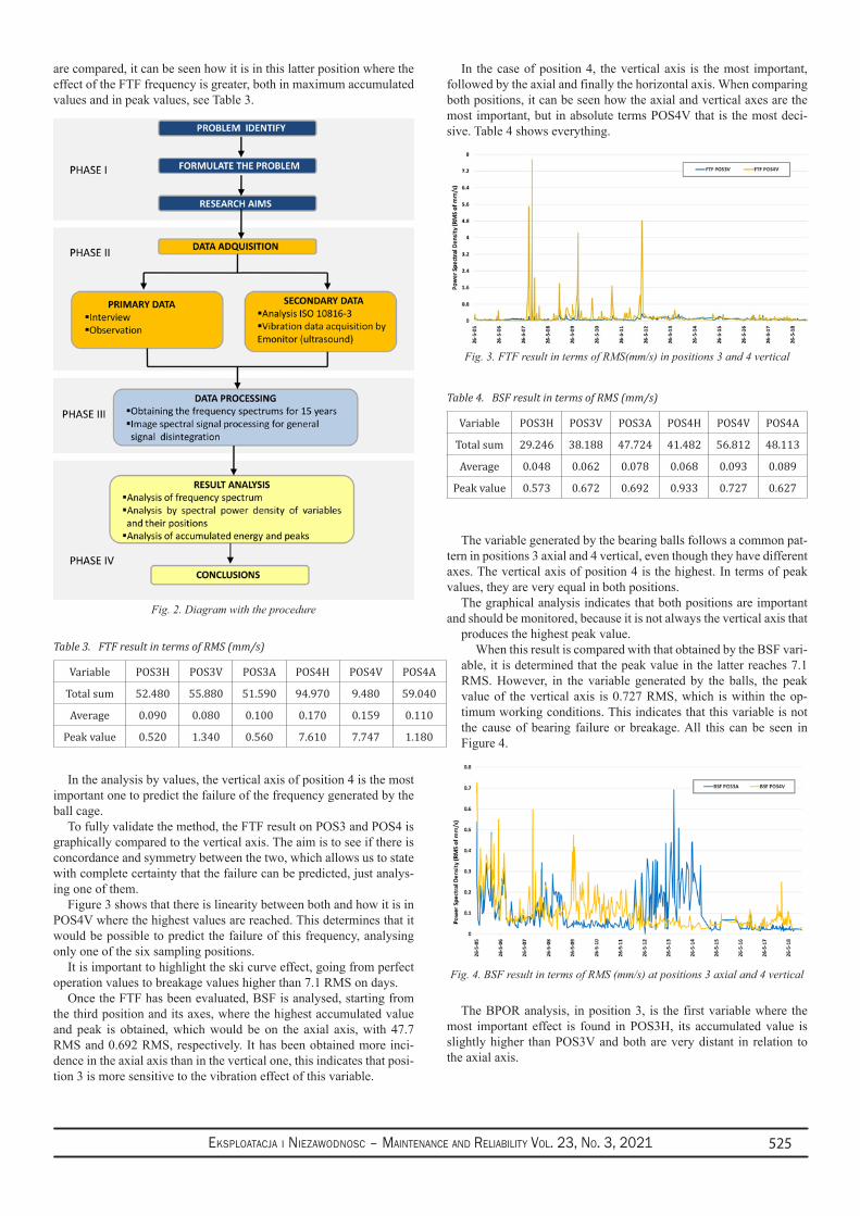
Eksploatacja i NiEzawodNosc – MaiNtENaNcE aNd REliability Vol. 23, No. 3, 2021 525
are compared, it can be seen how it is in this latter position where the effect of the FTF frequency is greater, both in maximum accumulated values and in peak values, see Table 3.
Fig. 2. Diagram with the procedure
In the analysis by values, the vertical axis of position 4 is the most important one to predict the failure of the frequency generated by the ball cage.
To fully validate the method, the FTF result on POS3 and POS4 is graphically compared to the vertical axis. The aim is to see if there is concordance and symmetry between the two, which allows us to state with complete certainty that the failure can be predicted, just analys-ing one of them.
Figure 3 shows that there is linearity between both and how it is in POS4V where the highest values are reached. This determines that it would be possible to predict the failure of this frequency, analysing only one of the six sampling positions.
It is important to highlight the ski curve effect, going from perfect operation values to breakage values higher than 7.1 RMS on days.
Once the FTF has been evaluated, BSF is analysed, starting from the third position and its axes, where the highest accumulated value and peak is obtained, which would be on the axial axis, with 47.7 RMS and 0.692 RMS, respectively. It has been obtained more inci-dence in the axial axis than in the vertical one, this indicates that posi-tion 3 is more sensitive to the vibration effect of this variable.
In the case of position 4, the vertical axis is the most important, followed by the axial and finally the horizontal axis. When comparing both positions, it can be seen how the axial and vertical axes are the most important, but in absolute terms POS4V that is the most deci-sive. Table 4 shows everything.
Fig. 3. FTF result in terms of RMS(mm/s) in positions 3 and 4 vertical
The variable generated by the bearing balls follows a common pat-tern in positions 3 axial and 4 vertical, even though they have different axes. The vertical axis of position 4 is the highest. In terms of peak values, they are very equal in both positions.
The graphical analysis indicates that both positions are important and should be monitored, because it is not always the vertical axis that
produces the highest peak value.When this result is compared with that obtained by the BSF vari-
able, it is determined that the peak value in the latter reaches 7.1 RMS. However, in the variable generated by the balls, the peak value of the vertical axis is 0.727 RMS, which is within the op-timum working conditions. This indicates that this variable is not the cause of bearing failure or breakage. All this can be seen in Figure 4.
The BPOR analysis, in position 3, is the first variable where the most important effect is found in POS3H, its accumulated value is slightly higher than POS3V and both are very distant in relation to the axial axis.
Table 3. FTF result in terms of RMS (mm/s)
Variable POS3H POS3V POS3A POS4H POS4V POS4A
Total sum 52.480 55.880 51.590 94.970 9.480 59.040
Average 0.090 0.080 0.100 0.170 0.159 0.110
Peak value 0.520 1.340 0.560 7.610 7.747 1.180
Table 4. BSF result in terms of RMS (mm/s)
Variable POS3H POS3V POS3A POS4H POS4V POS4A
Total sum 29.246 38.188 47.724 41.482 56.812 48.113
Average 0.048 0.062 0.078 0.068 0.093 0.089
Peak value 0.573 0.672 0.692 0.933 0.727 0.627
Fig. 4. BSF result in terms of RMS (mm/s) at positions 3 axial and 4 vertical
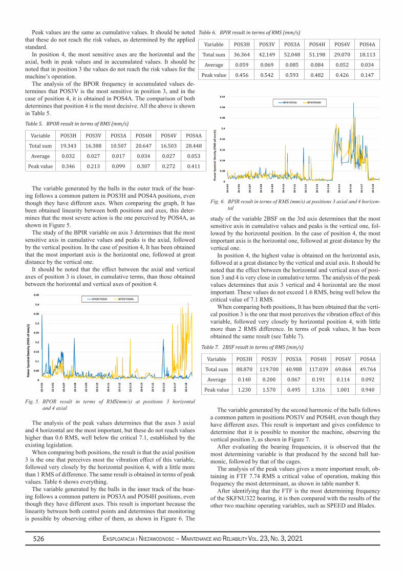
Eksploatacja i NiEzawodNosc – MaiNtENaNcE aNd REliability Vol. 23, No. 3, 2021526
Peak values are the same as cumulative values. It should be noted that these do not reach the risk values, as determined by the applied standard.
In position 4, the most sensitive axes are the horizontal and the axial, both in peak values and in accumulated values. It should be noted that in position 3 the values do not reach the risk values for the machine’s operation.
The analysis of the BPOR frequency in accumulated values de-termines that POS3V is the most sensitive in position 3, and in the case of position 4, it is obtained in POS4A. The comparison of both determines that position 4 is the most decisive. All the above is shown in Table 5.
The variable generated by the balls in the outer track of the bear-ing follows a common pattern in POS3H and POS4A positions, even though they have different axes. When comparing the graph, It has been obtained linearity between both positions and axes, this deter-mines that the most severe action is the one perceived by POS4A, as shown in Figure 5.
The study of the BPIR variable on axis 3 determines that the most sensitive axis in cumulative values and peaks is the axial, followed by the vertical position. In the case of position 4, It has been obtained that the most important axis is the horizontal one, followed at great distance by the vertical one.
It should be noted that the effect between the axial and vertical axes of position 3 is closer, in cumulative terms, than those obtained between the horizontal and vertical axes of position 4.
Fig. 5. BPOR result in terms of RMS(mm/s) at positions 3 horizontal and 4 axial
The analysis of the peak values determines that the axes 3 axial and 4 horizontal are the most important, but these do not reach values higher than 0.6 RMS, well below the critical 7.1, established by the existing legislation.
When comparing both positions, the result is that the axial position 3 is the one that perceives most the vibration effect of this variable, followed very closely by the horizontal position 4, with a little more than 1 RMS of difference. The same result is obtained in terms of peak values. Table 6 shows everything.
The variable generated by the balls in the inner track of the bear-ing follows a common pattern in POS3A and POS4H positions, even though they have different axes. This result is important because the linearity between both control points and determines that monitoring is possible by observing either of them, as shown in Figure 6. The
study of the variable 2BSF on the 3rd axis determines that the most sensitive axis in cumulative values and peaks is the vertical one, fol-lowed by the horizontal position. In the case of position 4, the most important axis is the horizontal one, followed at great distance by the vertical one.
In position 4, the highest value is obtained on the horizontal axis, followed at a great distance by the vertical and axial axis. It should be noted that the effect between the horizontal and vertical axes of posi-tion 3 and 4 is very close in cumulative terms. The analysis of the peak values determines that axis 3 vertical and 4 horizontal are the most important. These values do not exceed 1.6 RMS, being well below the critical value of 7.1 RMS.
When comparing both positions, It has been obtained that the verti-cal position 3 is the one that most perceives the vibration effect of this variable, followed very closely by horizontal position 4, with little more than 2 RMS difference. In terms of peak values, It has been obtained the same result (see Table 7).
The variable generated by the second harmonic of the balls follows a common pattern in positions POS3V and POS4H, even though they have different axes. This result is important and gives confidence to determine that it is possible to monitor the machine, observing the vertical position 3, as shown in Figure 7.
After evaluating the bearing frequencies, it is observed that the most determining variable is that produced by the second ball har-monic, followed by that of the cages.
The analysis of the peak values gives a more important result, ob-taining in FTF 7.74 RMS a critical value of operation, making this frequency the most determinant, as shown in table number 8.
After identifying that the FTF is the most determining frequency of the SKFNU322 bearing, it is then compared with the results of the other two machine operating variables, such as SPEED and Blades.
Table 5. BPOR result in terms of RMS (mm/s)
Variable POS3H POS3V POS3A POS4H POS4V POS4A
Total sum 19.343 16.388 10.507 20.647 16.503 28.448
Average 0.032 0.027 0.017 0.034 0.027 0.053
Peak value 0.346 0.213 0.099 0.307 0.272 0.411
Table 7. 2BSF result in terms of RMS (mm/s)
Variable POS3H POS3V POS3A POS4H POS4V POS4A
Total sum 88.870 119.700 40.988 117.039 69.864 49.764
Average 0.140 0.200 0.067 0.191 0.114 0.092
Peak value 1.230 1.570 0.495 1.316 1.001 0.940
Table 6. BPIR result in terms of RMS (mm/s)
Variable POS3H POS3V POS3A POS4H POS4V POS4A
Total sum 36.364 42.149 52.048 51.198 29.070 18.113
Average 0.059 0.069 0.085 0.084 0.052 0.034
Peak value 0.456 0.542 0.593 0.482 0.426 0.147
Fig. 6. BPIR result in terms of RMS (mm/s) at positions 3 axial and 4 horizon-tal
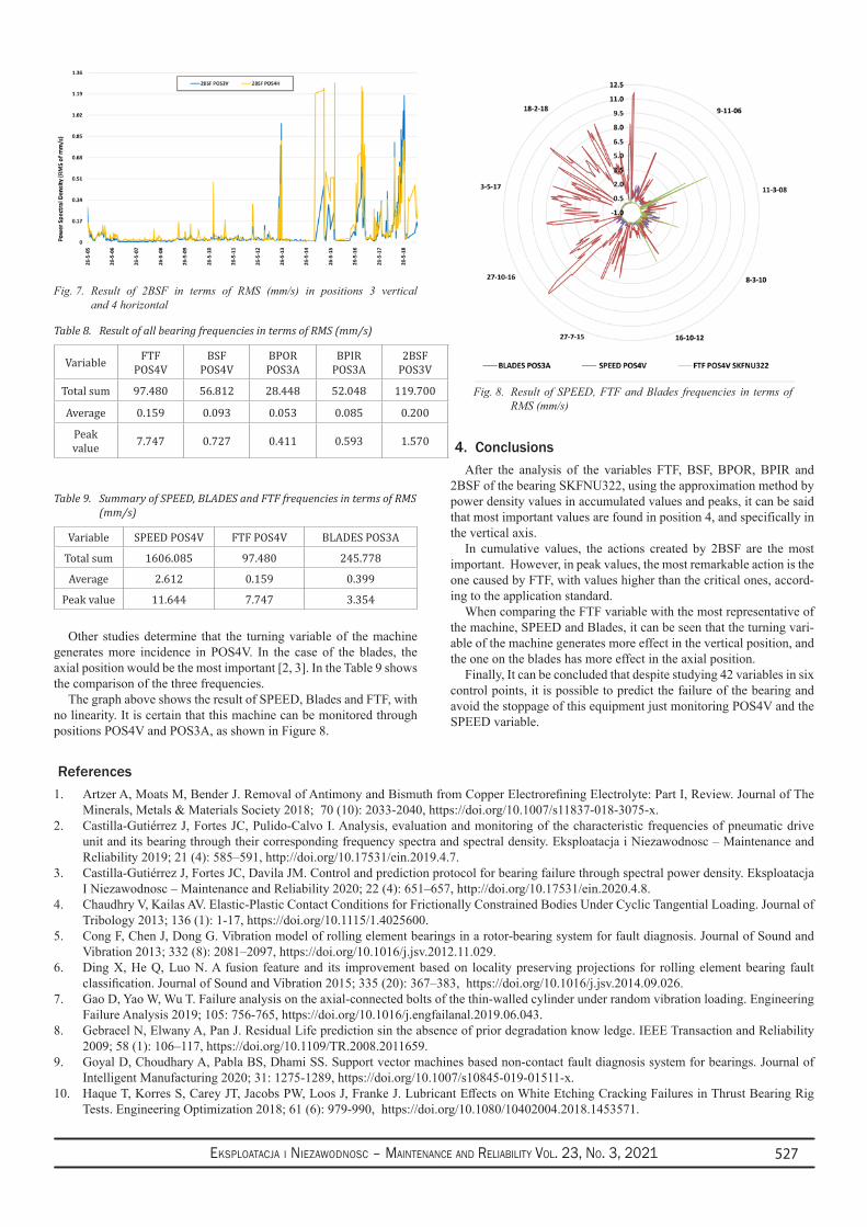
Eksploatacja i NiEzawodNosc – MaiNtENaNcE aNd REliability Vol. 23, No. 3, 2021 527
Other studies determine that the turning variable of the machine generates more incidence in POS4V. In the case of the blades, the axial position would be the most important [2, 3]. In the Table 9 shows the comparison of the three frequencies.
The graph above shows the result of SPEED, Blades and FTF, with no linearity. It is certain that this machine can be monitored through positions POS4V and POS3A, as shown in Figure 8.
4. ConclusionsAfter the analysis of the variables FTF, BSF, BPOR, BPIR and
2BSF of the bearing SKFNU322, using the approximation method by power density values in accumulated values and peaks, it can be said that most important values are found in position 4, and specifically in the vertical axis.
In cumulative values, the actions created by 2BSF are the most important. However, in peak values, the most remarkable action is the one caused by FTF, with values higher than the critical ones, accord-ing to the application standard.
When comparing the FTF variable with the most representative of the machine, SPEED and Blades, it can be seen that the turning vari-able of the machine generates more effect in the vertical position, and the one on the blades has more effect in the axial position.
Finally, It can be concluded that despite studying 42 variables in six control points, it is possible to predict the failure of the bearing and avoid the stoppage of this equipment just monitoring POS4V and the SPEED variable.
Table 8. Result of all bearing frequencies in terms of RMS (mm/s)
Variable FTF POS4V
BSF POS4V
BPOR POS3A
BPIR POS3A
2BSF POS3V
Total sum 97.480 56.812 28.448 52.048 119.700
Average 0.159 0.093 0.053 0.085 0.200
Peak value 7.747 0.727 0.411 0.593 1.570
Table 9. Summary of SPEED, BLADES and FTF frequencies in terms of RMS (mm/s)
Variable SPEED POS4V FTF POS4V BLADES POS3A
Total sum 1606.085 97.480 245.778
Average 2.612 0.159 0.399
Peak value 11.644 7.747 3.354
Fig. 8. Result of SPEED, FTF and Blades frequencies in terms of RMS (mm/s)
References1. Artzer A, Moats M, Bender J. Removal of Antimony and Bismuth from Copper Electrorefining Electrolyte: Part I, Review. Journal of The
Minerals, Metals & Materials Society 2018; 70 (10): 2033-2040, https://doi.org/10.1007/s11837-018-3075-x.2. Castilla-Gutiérrez J, Fortes JC, Pulido-Calvo I. Analysis, evaluation and monitoring of the characteristic frequencies of pneumatic drive
unit and its bearing through their corresponding frequency spectra and spectral density. Eksploatacja i Niezawodnosc – Maintenance and Reliability 2019; 21 (4): 585–591, http://doi.org/10.17531/ein.2019.4.7.
3. Castilla-Gutiérrez J, Fortes JC, Davila JM. Control and prediction protocol for bearing failure through spectral power density. Eksploatacja I Niezawodnosc – Maintenance and Reliability 2020; 22 (4): 651–657, http://doi.org/10.17531/ein.2020.4.8.
4. Chaudhry V, Kailas AV. Elastic-Plastic Contact Conditions for Frictionally Constrained Bodies Under Cyclic Tangential Loading. Journal of Tribology 2013; 136 (1): 1-17, https://doi.org/10.1115/1.4025600.
5. Cong F, Chen J, Dong G. Vibration model of rolling element bearings in a rotor-bearing system for fault diagnosis. Journal of Sound and Vibration 2013; 332 (8): 2081–2097, https://doi.org/10.1016/j.jsv.2012.11.029.
6. Ding X, He Q, Luo N. A fusion feature and its improvement based on locality preserving projections for rolling element bearing fault classification. Journal of Sound and Vibration 2015; 335 (20): 367–383, https://doi.org/10.1016/j.jsv.2014.09.026.
7. Gao D, Yao W, Wu T. Failure analysis on the axial-connected bolts of the thin-walled cylinder under random vibration loading. Engineering Failure Analysis 2019; 105: 756-765, https://doi.org/10.1016/j.engfailanal.2019.06.043.
8. Gebraeel N, Elwany A, Pan J. Residual Life prediction sin the absence of prior degradation know ledge. IEEE Transaction and Reliability 2009; 58 (1): 106–117, https://doi.org/10.1109/TR.2008.2011659.
9. Goyal D, Choudhary A, Pabla BS, Dhami SS. Support vector machines based non-contact fault diagnosis system for bearings. Journal of Intelligent Manufacturing 2020; 31: 1275-1289, https://doi.org/10.1007/s10845-019-01511-x.
10. Haque T, Korres S, Carey JT, Jacobs PW, Loos J, Franke J. Lubricant Effects on White Etching Cracking Failures in Thrust Bearing Rig Tests. Engineering Optimization 2018; 61 (6): 979-990, https://doi.org/10.1080/10402004.2018.1453571.
Fig. 7. Result of 2BSF in terms of RMS (mm/s) in positions 3 vertical and 4 horizontal
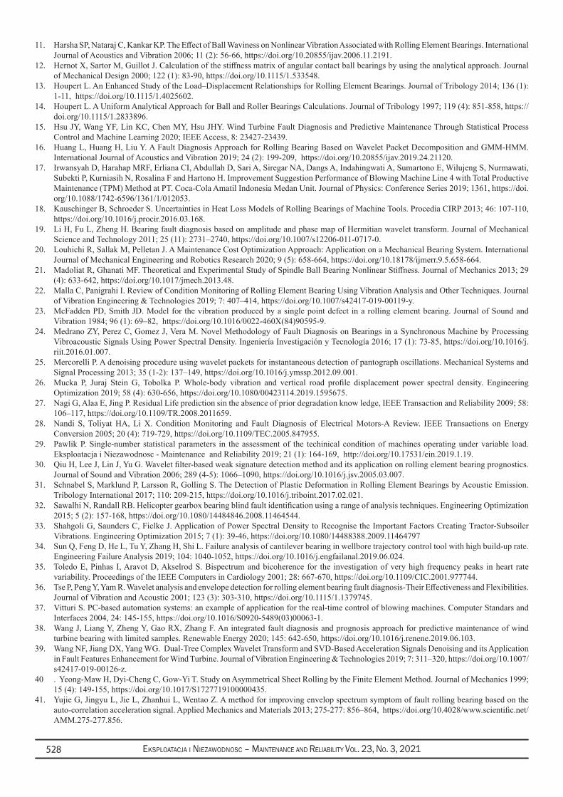
Eksploatacja i NiEzawodNosc – MaiNtENaNcE aNd REliability Vol. 23, No. 3, 2021528
11. Harsha SP, Nataraj C, Kankar KP. The Effect of Ball Waviness on Nonlinear Vibration Associated with Rolling Element Bearings. International Journal of Acoustics and Vibration 2006; 11 (2): 56-66, https://doi.org/10.20855/ijav.2006.11.2191.
12. Hernot X, Sartor M, Guillot J. Calculation of the stiffness matrix of angular contact ball bearings by using the analytical approach. Journal of Mechanical Design 2000; 122 (1): 83-90, https://doi.org/10.1115/1.533548.
13. Houpert L. An Enhanced Study of the Load–Displacement Relationships for Rolling Element Bearings. Journal of Tribology 2014; 136 (1): 1-11, https://doi.org/10.1115/1.4025602.
14. Houpert L. A Uniform Analytical Approach for Ball and Roller Bearings Calculations. Journal of Tribology 1997; 119 (4): 851-858, https://doi.org/10.1115/1.2833896.
15. Hsu JY, Wang YF, Lin KC, Chen MY, Hsu JHY. Wind Turbine Fault Diagnosis and Predictive Maintenance Through Statistical Process Control and Machine Learning 2020; IEEE Access, 8: 23427-23439.
16. Huang L, Huang H, Liu Y. A Fault Diagnosis Approach for Rolling Bearing Based on Wavelet Packet Decomposition and GMM-HMM. International Journal of Acoustics and Vibration 2019; 24 (2): 199-209, https://doi.org/10.20855/ijav.2019.24.21120.
17. Irwansyah D, Harahap MRF, Erliana CI, Abdullah D, Sari A, Siregar NA, Dangs A, Indahingwati A, Sumartono E, Wilujeng S, Nurmawati, Subekti P, Kurniasih N, Rosalina F and Hartono H. Improvement Suggestion Performance of Blowing Machine Line 4 with Total Productive Maintenance (TPM) Method at PT. Coca-Cola Amatil Indonesia Medan Unit. Journal of Physics: Conference Series 2019; 1361, https://doi.org/10.1088/1742-6596/1361/1/012053.
18. Kauschinger B, Schroeder S. Uncertainties in Heat Loss Models of Rolling Bearings of Machine Tools. Procedia CIRP 2013; 46: 107-110, https://doi.org/10.1016/j.procir.2016.03.168.
19. Li H, Fu L, Zheng H. Bearing fault diagnosis based on amplitude and phase map of Hermitian wavelet transform. Journal of Mechanical Science and Technology 2011; 25 (11): 2731–2740, https://doi.org/10.1007/s12206-011-0717-0.
20. Louhichi R, Sallak M, Pelletan J. A Maintenance Cost Optimization Approach: Application on a Mechanical Bearing System. International Journal of Mechanical Engineering and Robotics Research 2020; 9 (5): 658-664, https://doi.org/10.18178/ijmerr.9.5.658-664.
21. Madoliat R, Ghanati MF. Theoretical and Experimental Study of Spindle Ball Bearing Nonlinear Stiffness. Journal of Mechanics 2013; 29 (4): 633-642, https://doi.org/10.1017/jmech.2013.48.
22. Malla C, Panigrahi I. Review of Condition Monitoring of Rolling Element Bearing Using Vibration Analysis and Other Techniques. Journal of Vibration Engineering & Technologies 2019; 7: 407–414, https://doi.org/10.1007/s42417-019-00119-y.
23. McFadden PD, Smith JD. Model for the vibration produced by a single point defect in a rolling element bearing. Journal of Sound and Vibration 1984; 96 (1): 69–82, https://doi.org/10.1016/0022-460X(84)90595-9.
24. Medrano ZY, Perez C, Gomez J, Vera M. Novel Methodology of Fault Diagnosis on Bearings in a Synchronous Machine by Processing Vibroacoustic Signals Using Power Spectral Density. Ingeniería Investigación y Tecnología 2016; 17 (1): 73-85, https://doi.org/10.1016/j.riit.2016.01.007.
25. Mercorelli P. A denoising procedure using wavelet packets for instantaneous detection of pantograph oscillations. Mechanical Systems and Signal Processing 2013; 35 (1-2): 137–149, https://doi.org/10.1016/j.ymssp.2012.09.001.
26. Mucka P, Juraj Stein G, Tobolka P. Whole-body vibration and vertical road profile displacement power spectral density. Engineering Optimization 2019; 58 (4): 630-656, https://doi.org/10.1080/00423114.2019.1595675.
27. Nagi G, Alaa E, Jing P. Residual Life prediction sin the absence of prior degradation know ledge, IEEE Transaction and Reliability 2009; 58: 106–117, https://doi.org/10.1109/TR.2008.2011659.
28. Nandi S, Toliyat HA, Li X. Condition Monitoring and Fault Diagnosis of Electrical Motors-A Review. IEEE Transactions on Energy Conversion 2005; 20 (4): 719-729, https://doi.org/10.1109/TEC.2005.847955.
29. Pawlik P. Single-number statistical parameters in the assessment of the techinical condition of machines operating under variable load. Eksploatacja i Niezawodnosc - Maintenance and Reliability 2019; 21 (1): 164-169, http://doi.org/10.17531/ein.2019.1.19.
30. Qiu H, Lee J, Lin J, Yu G. Wavelet filter-based weak signature detection method and its application on rolling element bearing prognostics. Journal of Sound and Vibration 2006; 289 (4-5): 1066–1090, https://doi.org/10.1016/j.jsv.2005.03.007.
31. Schnabel S, Marklund P, Larsson R, Golling S. The Detection of Plastic Deformation in Rolling Element Bearings by Acoustic Emission. Tribology International 2017; 110: 209-215, https://doi.org/10.1016/j.triboint.2017.02.021.
32. Sawalhi N, Randall RB. Helicopter gearbox bearing blind fault identification using a range of analysis techniques. Engineering Optimization 2015; 5 (2): 157-168, https://doi.org/10.1080/14484846.2008.11464544.
33. Shahgoli G, Saunders C, Fielke J. Application of Power Spectral Density to Recognise the Important Factors Creating Tractor-Subsoiler Vibrations. Engineering Optimization 2015; 7 (1): 39-46, https://doi.org/10.1080/14488388.2009.11464797
34. Sun Q, Feng D, He L, Tu Y, Zhang H, Shi L. Failure analysis of cantilever bearing in wellbore trajectory control tool with high build-up rate. Engineering Failure Analysis 2019; 104: 1040-1052, https://doi.org/10.1016/j.engfailanal.2019.06.024.
35. Toledo E, Pinhas I, Aravot D, Akselrod S. Bispectrum and bicoherence for the investigation of very high frequency peaks in heart rate variability. Proceedings of the IEEE Computers in Cardiology 2001; 28: 667-670, https://doi.org/10.1109/CIC.2001.977744.
36. Tse P, Peng Y, Yam R. Wavelet analysis and envelope detection for rolling element bearing fault diagnosis-Their Effectiveness and Flexibilities. Journal of Vibration and Acoustic 2001; 123 (3): 303-310, https://doi.org/10.1115/1.1379745.
37. Vitturi S. PC-based automation systems: an example of application for the real-time control of blowing machines. Computer Standars and Interfaces 2004, 24: 145-155, https://doi.org/10.1016/S0920-5489(03)00063-1.
38. Wang J, Liang Y, Zheng Y, Gao RX, Zhang F. An integrated fault diagnosis and prognosis approach for predictive maintenance of wind turbine bearing with limited samples. Renewable Energy 2020; 145: 642-650, https://doi.org/10.1016/j.renene.2019.06.103.
39. Wang NF, Jiang DX, Yang WG. Dual-Tree Complex Wavelet Transform and SVD-Based Acceleration Signals Denoising and its Application in Fault Features Enhancement for Wind Turbine. Journal of Vibration Engineering & Technologies 2019; 7: 311–320, https://doi.org/10.1007/s42417-019-00126-z.
40 . Yeong-Maw H, Dyi-Cheng C, Gow-Yi T. Study on Asymmetrical Sheet Rolling by the Finite Element Method. Journal of Mechanics 1999; 15 (4): 149-155, https://doi.org/10.1017/S1727719100000435.
41. Yujie G, Jingyu L, Jie L, Zhanhui L, Wentao Z. A method for improving envelop spectrum symptom of fault rolling bearing based on the auto-correlation acceleration signal. Applied Mechanics and Materials 2013; 275-277: 856–864, https://doi.org/10.4028/www.scientific.net/AMM.275-277.856.

Eksploatacja i NiEzawodNosc – MaiNtENaNcE aNd REliability Vol. 23, No. 3, 2021 529
42. Zheng D, Chen W. Thermal performances on angular contact ball bearing of high speed spindle considering structural constraints under oil-air lubrication. Tribology International 2017; 109: 593–601, https://doi.org/10.1016/j.triboint.2017.01.035.
43. Zhou W, Habetler TG, Harley RG. Bearing Condition Monitoring Methods for Electric Machines: A General Review. IEEE International Symposium on Diagnostics for Electric Machines, Power Electronics and Drives 2007; 3-6, https://doi.org/10.1109/demped.2007.4393062.

Eksploatacja i NiEzawodNosc – MaiNtENaNcE aNd REliability Vol. 23, No. 3, 2021530
(*) Corresponding author.E-mail addresses:
Eksploatacja i Niezawodnosc – Maintenance and ReliabilityVolume 23 (2021), Issue 3
journal homepage: http://www.ein.org.pl
Indexed by:Fatigue lifetime correction of structural joints of opencast mining machineryPaweł Grabowski a,*, Artur Jankowiak a, Witold Marowski a
a Warsaw University of Technology, Institute of Vehicles and Construction Machinery Engineering, ul. Narbutta 84, 02-524 Warsaw, Poland
Grabowski P, Jankowiak A, Marowski W. Fatigue lifetime correction of structural joints of opencast mining machinery. Eksploatacja i Niezawodnosc – Maintenance and Reliability 2021; 23 (3): 530–539, http://doi.org/10.17531/ein.2021.3.14.
Article citation info:
Opencast mining machinery represents a group of large-scale individually manufactured technical objects operated with long-life requests. Since their manufacturers are obliged to provide product that will reach declared time of life, fatigue strength and durability condi-tions have to be taken into account for superstructures to meet the requirements. The paper highlights main problems occurring while assessing fatigue lifetime during design. Firstly, the short survey of current state of the art regarding the approach to this problem is pre-sented. Secondly, the most important reasons of unsatisfactory accuracy of the assessments are discussed. As a main objective of the study, the authors introduce the unique method of continuous fatigue lifetime correction for the welded superstructures during the machine lifecycle, as a remedy for this group of machinery. Furthermore, results and experience from adapting the approach in real object are presented, including fatigue lifetime correction due to the real intensity of loading acquired from a bucket-wheel excavator during its long-lasting operation. It is expected that proposed procedure can help to improve credibility of fatigue lifetime assessment of heavy earthmoving machinery.
Highlights Abstract
The novel comprehensive approach to fatigue de-•sign of welded superstructures was presented.
Functionality of the method has been developed •and verified on the real object remaining in op-eration.
Fatigue lifetime correction results for long-time •operated object was provided.
The procedure improves fatigue lifetime assess-•ments credibility and helps to provide requested lifetime.
The method aids maintenance of superstructure •providing information about its technical condi-tion.
fatigue life, lifetime assessment, supporting structure, welded joints, opencast mining machinery.
Keywords
This is an open access article under the CC BY license (https://creativecommons.org/licenses/by/4.0/)
P. Grabowski - [email protected], A. Jankowiak - [email protected], W. Marowski - [email protected]
1. Introduction
1.1. Background of the problemOpencast mining machines (wheel-bucket excavators, spreaders,
etc. – Fig. 1) that are commonly used for earthmoving work such as surface mining, transportation and dumping of material, are one of the largest and heaviest machines ever produced and their operational efficiency is also beyond any comparison – these affects their design and the way of operating. To provide economical efficiency, life cycle of this kind of objects has to be very specific and they should normally operate with long-life requests [37].
Conditions in which every individual machine is operated are unique – they strictly depend on geological structure, which is almost an individual feature of each mine, or may even differ a lot on various areas of the same mine. This is one of the most important reasons why the analyzed group of machines is manufactured in one-off or semi-one-off production scale – it results in their quite unique design, as well as in the operational characteristics (lifting capacity, efficiency, etc.)
The essential components of these objects are supporting struc-tures, which technical condition and durability determines not only the total lifetime of the whole machine, but usually also decides about safety and operating costs of the machinery.
At the same time, structural components usually undergo intensive, cyclic loading at variable courses. The load intensity and its high vari-ation during machine lifecycle causes that the load may be difficult to determine at the design stage. The problem becomes more visible when the requested lifetime is very long – reaching dozens of years.
Welding techniques that are applied to join structural components together make the structure very sensitive to the fatigue degradation process [36], which is often intensified by corrosion [1, 55], nearly always occurring in such a long time of usage. As a result, the fatigue lifetime of the structure is limited mainly by progress of fatigue degra-dation of welded structural joints [53]. The observable general rule in design is that these machines get more and more stressed, because of reducing cross-sections and using materials which, admittedly, have increasingly greater tensile strength, but its permissible fatigue stress range remains the same or grows slightly, which in addition, wors-ens work conditions (greater strains, vibratory sensitivity, etc.). All of
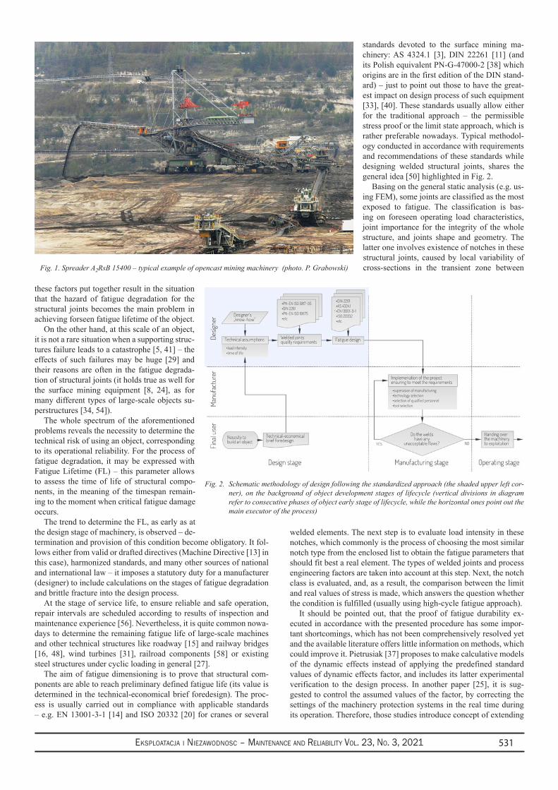
Eksploatacja i NiEzawodNosc – MaiNtENaNcE aNd REliability Vol. 23, No. 3, 2021 531
these factors put together result in the situation that the hazard of fatigue degradation for the structural joints becomes the main problem in achieving forseen fatigue lifetime of the object.
On the other hand, at this scale of an object, it is not a rare situation when a supporting struc-tures failure leads to a catastrophe [5, 41] – the effects of such failures may be huge [29] and their reasons are often in the fatigue degrada-tion of structural joints (it holds true as well for the surface mining equipment [8, 24], as for many different types of large-scale objects su-perstructures [34, 54]).
The whole spectrum of the aforementioned problems reveals the necessity to determine the technical risk of using an object, corresponding to its operational reliability. For the process of fatigue degradation, it may be expressed with Fatigue Lifetime (FL) – this parameter allows to assess the time of life of structural compo-nents, in the meaning of the timespan remain-ing to the moment when critical fatigue damage occurs.
The trend to determine the FL, as early as at the design stage of machinery, is observed – de-termination and provision of this condition become obligatory. It fol-lows either from valid or drafted directives (Machine Directive [13] in this case), harmonized standards, and many other sources of national and international law – it imposes a statutory duty for a manufacturer (designer) to include calculations on the stages of fatigue degradation and brittle fracture into the design process.
At the stage of service life, to ensure reliable and safe operation, repair intervals are scheduled according to results of inspection and maintenance experience [56]. Nevertheless, it is quite common nowa-days to determine the remaining fatigue life of large-scale machines and other technical structures like roadway [15] and railway bridges [16, 48], wind turbines [31], railroad components [58] or existing steel structures under cyclic loading in general [27].
The aim of fatigue dimensioning is to prove that structural com-ponents are able to reach preliminary defined fatigue life (its value is determined in the technical-economical brief foredesign). The proc-ess is usually carried out in compliance with applicable standards – e.g. EN 13001-3-1 [14] and ISO 20332 [20] for cranes or several
standards devoted to the surface mining ma-chinery: AS 4324.1 [3], DIN 22261 [11] (and its Polish equivalent PN-G-47000-2 [38] which origins are in the first edition of the DIN stand-ard) – just to point out those to have the great-est impact on design process of such equipment [33], [40]. These standards usually allow either for the traditional approach – the permissible stress proof or the limit state approach, which is rather preferable nowadays. Typical methodol-ogy conducted in accordance with requirements and recommendations of these standards while designing welded structural joints, shares the general idea [50] highlighted in Fig. 2.
Basing on the general static analysis (e.g. us-ing FEM), some joints are classified as the most exposed to fatigue. The classification is bas-ing on foreseen operating load characteristics, joint importance for the integrity of the whole structure, and joints shape and geometry. The latter one involves existence of notches in these structural joints, caused by local variability of cross-sections in the transient zone between
welded elements. The next step is to evaluate load intensity in these notches, which commonly is the process of choosing the most similar notch type from the enclosed list to obtain the fatigue parameters that should fit best a real element. The types of welded joints and process engineering factors are taken into account at this step. Next, the notch class is evaluated, and, as a result, the comparison between the limit and real values of stress is made, which answers the question whether the condition is fulfilled (usually using high-cycle fatigue approach).
It should be pointed out, that the proof of fatigue durability ex-ecuted in accordance with the presented procedure has some impor-tant shortcomings, which has not been comprehensively resolved yet and the available literature offers little information on methods, which could improve it. Pietrusiak [37] proposes to make calculative models of the dynamic effects instead of applying the predefined standard values of dynamic effects factor, and includes its latter experimental verification to the design process. In another paper [25], it is sug-gested to control the assumed values of the factor, by correcting the settings of the machinery protection systems in the real time during its operation. Therefore, those studies introduce concept of extending
Fig. 1. Spreader A2RsB 15400 – typical example of opencast mining machinery (photo. P. Grabowski)
Fig. 2. Schematic methodology of design following the standardized approach (the shaded upper left cor-ner), on the background of object development stages of lifecycle (vertical divisions in diagram refer to consecutive phases of object early stage of lifecycle, while the horizontal ones point out the main executor of the process)
Eksploatacja i NiEzawodNosc – MaiNtENaNcE aNd REliability Vol. 23, No. 3, 2021532
some steps of design process onto the further phases of the lifecy-cle. Such an approach has also been postulated by Jakubczak et al, in their studies [21]. In contrary to the considered group of machinery, elements of that approach are used to maintain the other group of fatigue loaded structures with a limited design service life – the civil engineering infrastructure, especially railway and roadway bridges [28], which in a way of design, operating and maintenance are quite comparable with superstructures of open-pit mining machinery. In this paper authors try to adapt and generalize a similar approach, by introducing the procedure of continuous fatigue lifetime correction, which is expected to be a helpful tool while designing load-bearing structures of large-scale individually manufactured machinery.
The proposed methodology requires the use of structural health monitoring system, which involves periodic read-outs of continuously recorded information from a net of sensors located on structural com-ponents of the supervised object. The acquired data are, in turn, inter-preted respectively to the structure technical condition. The data sent to and stored in the central unit enables a remote observation of an object technical condition [17]. The role of structural health monitor-ing recently becomes more and more popular in the diagnostics of en-gineering structures. In the literature one can find many publications about real time diagnostics applied to identify the technical condition of machinery bearing structures. For example, Sikora et al. [47] de-scribes a system for monitoring and diagnosing a gantry, which is ca-pable to acquire, visualize and monitor vibration levels of the gantry crucial structural components. The system equipped with a computing and analytical module enables the predictive maintenance due to the obtained vibration level assessment. Similar approach is presented by Rusińskietal.[43]toevaluatedynamicloadscorrespondingtocer-tain operational loading of surface mining equipment and, in turn, to carry out the modal analysis of the superstructure. Another paper [34] presents results of long-term load tests of bucket wheel excavator. The load carrying structure of the machinery is equipped with the moni-toring system in order to determine the real stress values in selected welded joints, to enable prediction of the structure health. In work [51] authors present an identification method of technical condition of complex geometry large-size objects taking into consideration the power line supporting structure. The presented technique is based on testing the correlation between the change of stress in the system and the change of modal parameters caused by damage.
1.2. Fatigue life assessments of welded joints in the ma-chinery structural components – difficulties and limita-tions of standardized procedures
In practice, design engineer has to face with many diverse diffi-culties making the actual fatigue lifetime of an object substantially different from the requested one. A number of papers manifests the problem of the impact of the external environment [52, 35], ageing [53, 55] and wear processes [36] or their combinations [10] on the technical system functioning. The problems, discussed in this section, are especially noticeable while considering the group of long-lasting large-scale one-off manufactured machinery [9, 39].
Significant doubts occur just when conditions of operating have to be assessed. Those remain almost unknown for the designer. Serv-ice conditions collected in the past represented in the form of various loading spectra may sometimes be available in manufacturer’s data-base for some similar objects, but in most cases they are not directly applicable, so the service conditions could only be assumed according to his engineering experience with similar objects, and drawing on the results of consultations with a final user, about how the user plans to operate and maintain the machinery. Bearing in mind the size of the equipment and the unique nature of the operating conditions in sur-face mining, there is little to no knowledge of the operating stresses at critical details [50].
Alternatively, for some groups of machines, this information may come from applicable standard recommendations. This is quite often
situation for calculating the classification group of cranes [59]. Nev-ertheless, such kind of “statistical truth” in many cases remains inap-plicable for the group of individually manufactured machinery, where the designer’s knowledge about working conditions of similar objects from the present generation is very limited.
For machinery with foreseen lifetime reaching 40-50 years (com-mon situation in the considered group), the real operating conditions may not reflect designer’s expectations [44, 45]. Furthermore, service conditions may also significantly change over time [7], so even if the characteristic is accurate for the initial stage of machine’s lifecycle, the conditions may change a lot in the future. As far as opencast ma-chines are concerned, the significant change of conditions may be just a result of different geological parameters of the successive layers of mined material.
The fact is that for some groups of machines the attempts to assess external loads occurring during object lifecycle may give satisfac-tory results. This approach is applied to cranes by calculating their classification group. However, an accurate determination of external load does not guarantee proper evaluation of its effects – it is almost impossible to determine results of these loads in individual structural joints (stresses in considered cross-sections). Moreover, foreseen number of load cycles usually may be assessed very approximately – in real conditions there may incidentally appear stresses of great amplitude or frequency, which completely change the character of operating (vibrations, resonance, etc.). Further complication of the problem is caused by gradual degradation of machines components (increasing clearances of knuckle joints, which tends to alternate the structure’s response to external impulses). Such a missed load spec-trum, substantially increases the differences between designed and real fatigue lifetime consumption ratio (the time necessary to obtain a critical damage).
Improper maintenance, usage prolongation beyond the designed lifetime of an object and variable degree of technical culture of an operator, as well as of a technical service, are another factors with random character, which influence onto machine structure fatigue lifetime in long time horizon is hard to determine. Working condi-tions of open-pit machines can be even more unpredictable, if some non-technical factors are considered – e.g. strictly political decisions. Great affect onto the whole branch will surely have the introduction of “green order”, which can cause sufficient alternation of costs structure in coal mines for maintenance of machinery, which will seem to be “abandoned” in future. Reducing subventions for repairs and modern-izations, while their growing necessity (because of objects increasing age), may be very important problem that technical services will have to face with in near future.
Another important difficulty, but of a different kind, is the right selection of fatigue resistance S-N curve of welded joints in order to evaluate its fatigue strength. Its value is significantly influenced by such factors as shape and local dimensions of a joint (quality of type), but also quality of conformance [14, 18] involving e.g. resid-ual stresses which stems from the manufacturing process [46]. The last one is difficult to determine unambiguously for the purpose of preparing fatigue assessment [4]. It is also problematic to obtain the form of welded joints determined by the designer, which may differ (sometimes considerably) in the real object (i.e. shape, manufacturing quality, or post-welding treatment). Stress of the structural joints or their material stress-life (S-N) curve may also be changed by major repairs or modernizations which are common processes in long-life operated machinery.
At last, durability condition itself – defined with usage of stress instead of operating time – may be inadequate for the purpose, be-coming another source of problems during the design of the FL of structural components. According to the aforementioned standard recommendations, stress in a welded joint has to be lower than the permissible stress range (or should not exceed the value correspond-ing to the limit state in case where this approach is regarded) for such joint. It means that fatigue lifetime is expressed indirectly, using only
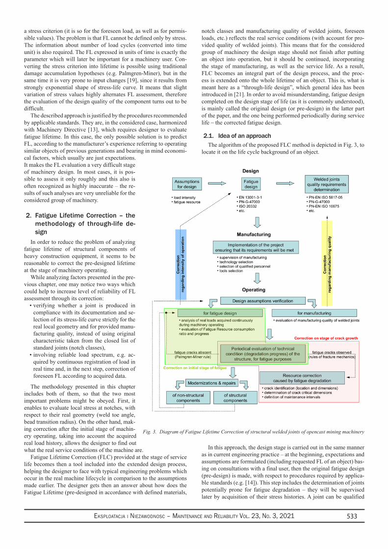
Eksploatacja i NiEzawodNosc – MaiNtENaNcE aNd REliability Vol. 23, No. 3, 2021 533
a stress criterion (it is so for the foreseen load, as well as for permis-sible values). The problem is that FL cannot be defined only by stress. The information about number of load cycles (converted into time unit) is also required. The FL expressed in units of time is exactly the parameter which will later be important for a machinery user. Con-verting the stress criterion into lifetime is possible using traditional damage accumulation hypotheses (e.g. Palmgren-Miner), but in the same time it is very prone to input changes [19], since it results from strongly exponential shape of stress-life curve. It means that slight variation of stress values highly alternates FL assessment, therefore the evaluation of the design quality of the component turns out to be difficult.
The described approach is justified by the procedures recommended by applicable standards. They are, in the considered case, harmonized with Machinery Directive [13], which requires designer to evaluate fatigue lifetime. In this case, the only possible solution is to predict FL, according to the manufacturer’s experience referring to operating similar objects of previous generations and bearing in mind economi-cal factors, which usually are just expectations. It makes the FL evaluation a very difficult stage of machinery design. In most cases, it is pos-sible to assess it only roughly and this also is often recognized as highly inaccurate – the re-sults of such analyses are very unreliable for the considered group of machinery.
2. Fatigue Lifetime Correction – the methodology of through-life de-sign
In order to reduce the problem of analyzing fatigue lifetime of structural components of heavy construction equipment, it seems to be reasonable to correct the pre-designed lifetime at the stage of machinery operating.
While analyzing factors presented in the pre-vious chapter, one may notice two ways which could help to increase level of reliability of FL assessment through its correction:
verifying whether a joint is produced in •compliance with its documentation and se-lection of its stress-life curve strictly for the real local geometry and for provided manu-facturing quality, instead of using original characteristic taken from the closed list of standard joints (notch classes),involving reliable load spectrum, e.g. ac-•quired by continuous registration of load in real time and, in the next step, correction of foreseen FL according to acquired data.
The methodology presented in this chapter includes both of them, so that the two most important problems might be obeyed. First, it enables to evaluate local stress at notches, with respect to their real geometry (weld toe angle, bead transition radius). On the other hand, mak-ing correction after the initial stage of machin-ery operating, taking into account the acquired real load history, allows the designer to find out what the real service conditions of the machine are.
Fatigue Lifetime Correction (FLC) provided at the stage of service life becomes then a tool included into the extended design process, helping the designer to face with typical engineering problems which occur in the real machine lifecycle in comparison to the assumptions made earlier. The designer gets then an answer about how does the Fatigue Lifetime (pre-designed in accordance with defined materials,
notch classes and manufacturing quality of welded joints, foreseen loads, etc.) reflects the real service conditions (with account for pro-vided quality of welded joints). This means that for the considered group of machinery the design stage should not finish after putting an object into operation, but it should be continued, incorporating the stage of manufacturing, as well as the service life. As a result, FLC becomes an integral part of the design process, and the proc-ess is extended onto the whole lifetime of an object. This is, what is meant here as a “through-life design”, which general idea has been introduced in [21]. In order to avoid misunderstanding, fatigue design completed on the design stage of life (as it is commonly understood), is mainly called the original design (or pre-design) in the latter part of the paper, and the one being performed periodically during service life – the corrected fatigue design.
2.1. Idea of an approachThe algorithm of the proposed FLC method is depicted in Fig. 3, to
locate it on the life cycle background of an object.
In this approach, the design stage is carried out in the same manner as in current engineering practice – at the beginning, expectations and assumptions are formulated (including requested FL of an object) bas-ing on consultations with a final user, then the original fatigue design (pre-design) is made, with respect to procedures required by applica-ble standards (e.g. [14]). This step includes the determination of joints potentially prone for fatigue degradation – they will be supervised later by acquisition of their stress histories. A joint can be qualified
Fig. 3. Diagram of Fatigue Lifetime Correction of structural welded joints of opencast mining machinery
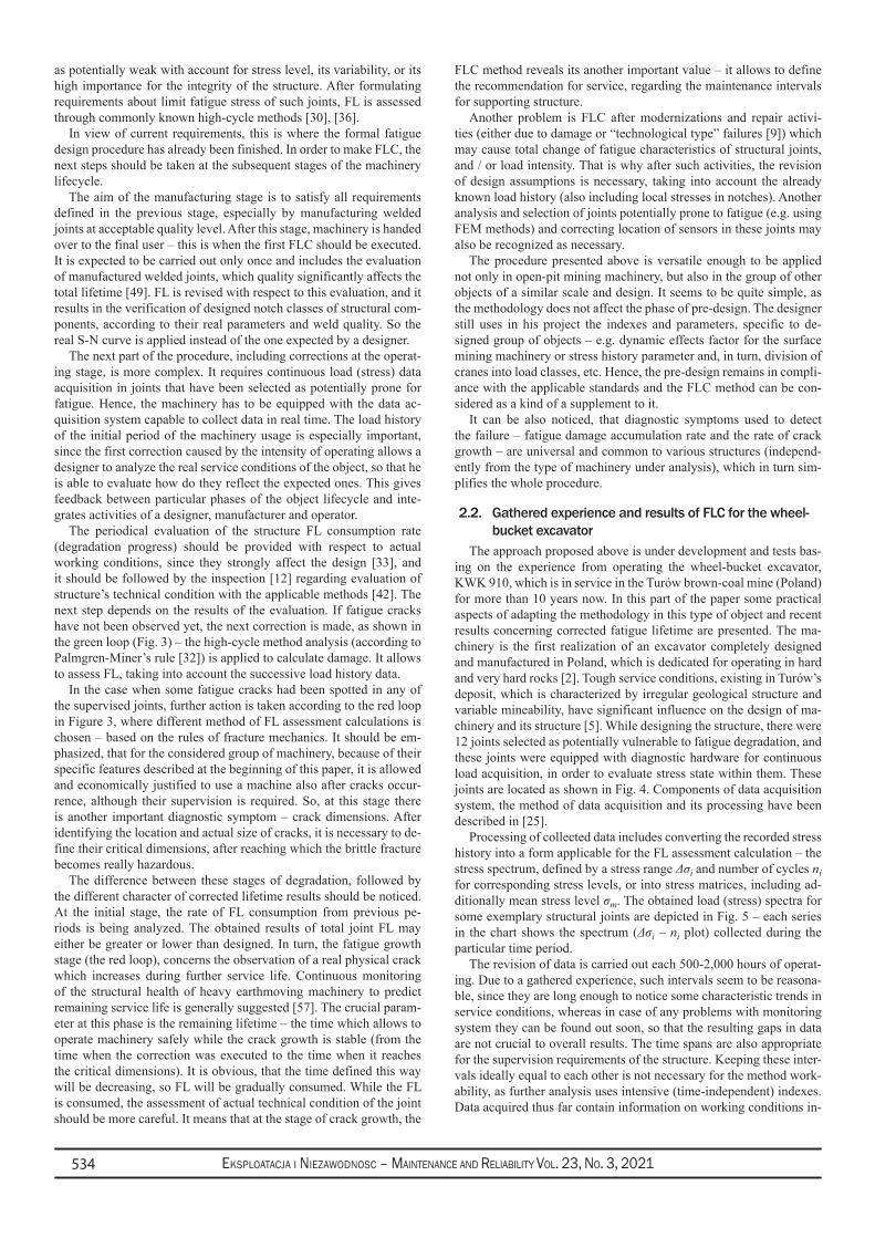
Eksploatacja i NiEzawodNosc – MaiNtENaNcE aNd REliability Vol. 23, No. 3, 2021534
as potentially weak with account for stress level, its variability, or its high importance for the integrity of the structure. After formulating requirements about limit fatigue stress of such joints, FL is assessed through commonly known high-cycle methods [30], [36].
In view of current requirements, this is where the formal fatigue design procedure has already been finished. In order to make FLC, the next steps should be taken at the subsequent stages of the machinery lifecycle.
The aim of the manufacturing stage is to satisfy all requirements defined in the previous stage, especially by manufacturing welded joints at acceptable quality level. After this stage, machinery is handed over to the final user – this is when the first FLC should be executed. It is expected to be carried out only once and includes the evaluation of manufactured welded joints, which quality significantly affects the total lifetime [49]. FL is revised with respect to this evaluation, and it results in the verification of designed notch classes of structural com-ponents, according to their real parameters and weld quality. So the real S-N curve is applied instead of the one expected by a designer.
The next part of the procedure, including corrections at the operat-ing stage, is more complex. It requires continuous load (stress) data acquisition in joints that have been selected as potentially prone for fatigue. Hence, the machinery has to be equipped with the data ac-quisition system capable to collect data in real time. The load history of the initial period of the machinery usage is especially important, since the first correction caused by the intensity of operating allows a designer to analyze the real service conditions of the object, so that he is able to evaluate how do they reflect the expected ones. This gives feedback between particular phases of the object lifecycle and inte-grates activities of a designer, manufacturer and operator.
The periodical evaluation of the structure FL consumption rate (degradation progress) should be provided with respect to actual working conditions, since they strongly affect the design [33], and it should be followed by the inspection [12] regarding evaluation of structure’s technical condition with the applicable methods [42]. The next step depends on the results of the evaluation. If fatigue cracks have not been observed yet, the next correction is made, as shown in the green loop (Fig. 3) – the high-cycle method analysis (according to Palmgren-Miner’s rule [32]) is applied to calculate damage. It allows to assess FL, taking into account the successive load history data.
In the case when some fatigue cracks had been spotted in any of the supervised joints, further action is taken according to the red loop in Figure 3, where different method of FL assessment calculations is chosen – based on the rules of fracture mechanics. It should be em-phasized, that for the considered group of machinery, because of their specific features described at the beginning of this paper, it is allowed and economically justified to use a machine also after cracks occur-rence, although their supervision is required. So, at this stage there is another important diagnostic symptom – crack dimensions. After identifying the location and actual size of cracks, it is necessary to de-fine their critical dimensions, after reaching which the brittle fracture becomes really hazardous.
The difference between these stages of degradation, followed by the different character of corrected lifetime results should be noticed. At the initial stage, the rate of FL consumption from previous pe-riods is being analyzed. The obtained results of total joint FL may either be greater or lower than designed. In turn, the fatigue growth stage (the red loop), concerns the observation of a real physical crack which increases during further service life. Continuous monitoring of the structural health of heavy earthmoving machinery to predict remaining service life is generally suggested [57]. The crucial param-eter at this phase is the remaining lifetime – the time which allows to operate machinery safely while the crack growth is stable (from the time when the correction was executed to the time when it reaches the critical dimensions). It is obvious, that the time defined this way will be decreasing, so FL will be gradually consumed. While the FL is consumed, the assessment of actual technical condition of the joint should be more careful. It means that at the stage of crack growth, the
FLC method reveals its another important value – it allows to define the recommendation for service, regarding the maintenance intervals for supporting structure.
Another problem is FLC after modernizations and repair activi-ties (either due to damage or “technological type” failures [9]) which may cause total change of fatigue characteristics of structural joints, and / or load intensity. That is why after such activities, the revision of design assumptions is necessary, taking into account the already known load history (also including local stresses in notches). Another analysis and selection of joints potentially prone to fatigue (e.g. using FEM methods) and correcting location of sensors in these joints may also be recognized as necessary.
The procedure presented above is versatile enough to be applied not only in open-pit mining machinery, but also in the group of other objects of a similar scale and design. It seems to be quite simple, as the methodology does not affect the phase of pre-design. The designer still uses in his project the indexes and parameters, specific to de-signed group of objects – e.g. dynamic effects factor for the surface mining machinery or stress history parameter and, in turn, division of cranes into load classes, etc. Hence, the pre-design remains in compli-ance with the applicable standards and the FLC method can be con-sidered as a kind of a supplement to it.
It can be also noticed, that diagnostic symptoms used to detect the failure – fatigue damage accumulation rate and the rate of crack growth – are universal and common to various structures (independ-ently from the type of machinery under analysis), which in turn sim-plifies the whole procedure.
2.2. Gathered experience and results of FLC for the wheel-bucket excavator
The approach proposed above is under development and tests bas-ing on the experience from operating the wheel-bucket excavator, KWK 910, which is in service in the Turów brown-coal mine (Poland) for more than 10 years now. In this part of the paper some practical aspects of adapting the methodology in this type of object and recent results concerning corrected fatigue lifetime are presented. The ma-chinery is the first realization of an excavator completely designed and manufactured in Poland, which is dedicated for operating in hard and very hard rocks [2]. Tough service conditions, existing in Turów’s deposit, which is characterized by irregular geological structure and variable mineability, have significant influence on the design of ma-chinery and its structure [5]. While designing the structure, there were 12 joints selected as potentially vulnerable to fatigue degradation, and these joints were equipped with diagnostic hardware for continuous load acquisition, in order to evaluate stress state within them. These joints are located as shown in Fig. 4. Components of data acquisition system, the method of data acquisition and its processing have been described in [25].
Processing of collected data includes converting the recorded stress history into a form applicable for the FL assessment calculation – the stress spectrum, defined by a stress range Δσi and number of cycles ni for corresponding stress levels, or into stress matrices, including ad-ditionally mean stress level σm. The obtained load (stress) spectra for some exemplary structural joints are depicted in Fig. 5 – each series in the chart shows the spectrum (Δσi – ni plot) collected during the particular time period.
The revision of data is carried out each 500-2,000 hours of operat-ing. Due to a gathered experience, such intervals seem to be reasona-ble, since they are long enough to notice some characteristic trends in service conditions, whereas in case of any problems with monitoring system they can be found out soon, so that the resulting gaps in data are not crucial to overall results. The time spans are also appropriate for the supervision requirements of the structure. Keeping these inter-vals ideally equal to each other is not necessary for the method work-ability, as further analysis uses intensive (time-independent) indexes. Data acquired thus far contain information on working conditions in-
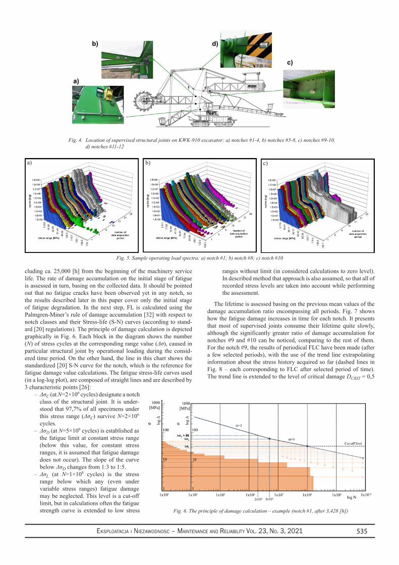
Eksploatacja i NiEzawodNosc – MaiNtENaNcE aNd REliability Vol. 23, No. 3, 2021 535
cluding ca. 25,000 [h] from the beginning of the machinery service life. The rate of damage accumulation on the initial stage of fatigue is assessed in turn, basing on the collected data. It should be pointed out that no fatigue cracks have been observed yet in any notch, so the results described later in this paper cover only the initial stage of fatigue degradation. In the next step, FL is calculated using the Palmgren-Miner’s rule of damage accumulation [32] with respect to notch classes and their Stress-life (S-N) curves (according to stand-ard [20] regulations). The principle of damage calculation is depicted graphically in Fig. 6. Each block in the diagram shows the number (N) of stress cycles at the corresponding range value (Δσ), caused in particular structural joint by operational loading during the consid-ered time period. On the other hand, the line in this chart shows the standardized [20] S-N curve for the notch, which is the reference for fatigue damage value calculations. The fatigue stress-life curves used (in a log-log plot), are composed of straight lines and are described by 3 characteristic points [26]:
Δσ – C (at N=2×10⁶ cycles) designate a notch class of the structural joint. It is under-stood that 97,7% of all specimens under this stress range (ΔσC) survive N=2×10⁶ cycles.Δσ – D (at N=5×10⁶ cycles) is established as the fatigue limit at constant stress range (below this value, for constant stress ranges, it is assumed that fatigue damage does not occur). The slope of the curve below ΔσD changes from 1:3 to 1:5.Δσ – L (at N=1×10⁸ cycles) is the stress range below which any (even under variable stress ranges) fatigue damage may be neglected. This level is a cut-off limit, but in calculations often the fatigue strength curve is extended to low stress
ranges without limit (in considered calculations to zero level). In described method that approach is also assumed, so that all of recorded stress levels are taken into account while performing the assessment.
The lifetime is assessed basing on the previous mean values of the damage accumulation ratio encompassing all periods. Fig. 7 shows how the fatigue damage increases in time for each notch. It presents that most of supervised joints consume their lifetime quite slowly, although the significantly greater ratio of damage accumulation for notches #9 and #10 can be noticed, comparing to the rest of them. For the notch #9, the results of periodical FLC have been made (after a few selected periods), with the use of the trend line extrapolating information about the stress history acquired so far (dashed lines in Fig. 8 – each corresponding to FLC after selected period of time). The trend line is extended to the level of critical damage DCRIT = 0,5
Fig. 4. Location of supervised structural joints on KWK-910 excavator: a) notches #1-4, b) notches #5-8, c) notches #9-10, d) notches #11-12
Fig. 5. Sample operating load spectra: a) notch #1; b) notch #8; c) notch #10
b) c)a)
Fig. 6. The principle of damage calculation – example (notch #1, after 3,428 [h])
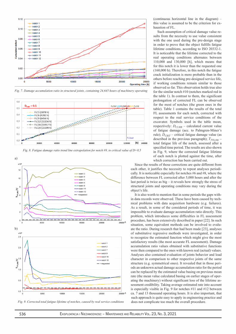
Eksploatacja i NiEzawodNosc – MaiNtENaNcE aNd REliability Vol. 23, No. 3, 2021536
(continuous horizontal line in the diagram) – this value is assumed to be the criterion for ex-haustion of FL.
Such assumption of critical damage value re-sults from the necessity to use value consistent with the one used during the pre-design stage in order to prove that the object fulfills fatigue lifetime conditions, according to ISO 20332-1. It is noticeable that the lifetime corrected to the real operating conditions alternates between 110,000 and 130,000 [h], which means that for this notch it is lower than the requested one (160,000 h). Therefore, in this notch the fatigue crack initialization is more probable than in the others before reaching pre-designed service life, if working conditions remain similar to those observed so far. This observation holds true also for the similar notch #10 (notches marked red in the table 1). In contrast to them, the significant prolongation of corrected FL can be observed for the most of notches (the green ones in the table). Table 1 contains the results of the total FL assessments for each notch, corrected with respect to the real service conditions of the excavator. Symbols used in the table mean, respectively: DCURR – calculated current value of fatigue damage (acc. to Palmgren-Miner’s rule); DCRIT – critical fatigue damage value (as described in the previous paragraph); TTTL(M) – total fatigue life of the notch, assessed after a specified time period. The results are also shown in Fig. 9, where the corrected fatigue lifetime of each notch is plotted against the time, after which correction has been carried out.
Since the results of those corrections are quite different from each other, it justifies the necessity to repeat analyses periodi-cally. It is noticeable especially for notches #6 and #8, where the difference between FL corrected after 5,000 hours and after the last period is twice as big – it reveals how strongly the stress of structural joints and operating conditions may vary during the object’s life.
It is also worth to mention that in some periods the gaps with-in data records were observed. These have been caused by tech-nical problems with data acquisition hardware (e.g. failures). As a result, in some of the considered periods of time, it was impossible to evaluate damage accumulation ratio directly. This problem, which introduces some difficulties in FL assessment procedure, has been extensively described in paper [22]. In such situation, some equivalent methods can be involved to evalu-ate the ratio. During research that had been made [23], analyses of substitutive regressive methods were investigated, in order to recognize the estimated function which might give the most satisfactory results (the most accurate FL assessment). Damage accumulation ratio values obtained with substitutive functions were then compared to the ones with known real (actual) values. Analyses also contained evaluation of joints behavior and load character in comparison to other respective joints of the same structure (e.g. symmetrical ones). It revealed that in those peri-ods an unknown actual damage accumulation ratio for the period can be replaced by the estimated value basing on previous mean rate (the mean value calculated basing on earlier stages of oper-ating the machinery) without significant loss of the lifetime as-sessment credibility. Taking average estimated rate into account is especially visible in Fig. 9 for notches #11 and #12 between ca. 7 and 13 thousand operating hours. It is also important, that such approach is quite easy to apply in engineering practice and does not complicate too much the overall procedure.
Fig. 7. Damage accumulation ratio in structural joints, containing 24,645 hours of machinery operating
Fig. 8. Fatigue damage ratio trend line extrapolation for notch #9, to critical value of D=0,5
Fig. 9. Corrected total fatigue lifetime of notches, caused by real service conditions
b)
a)
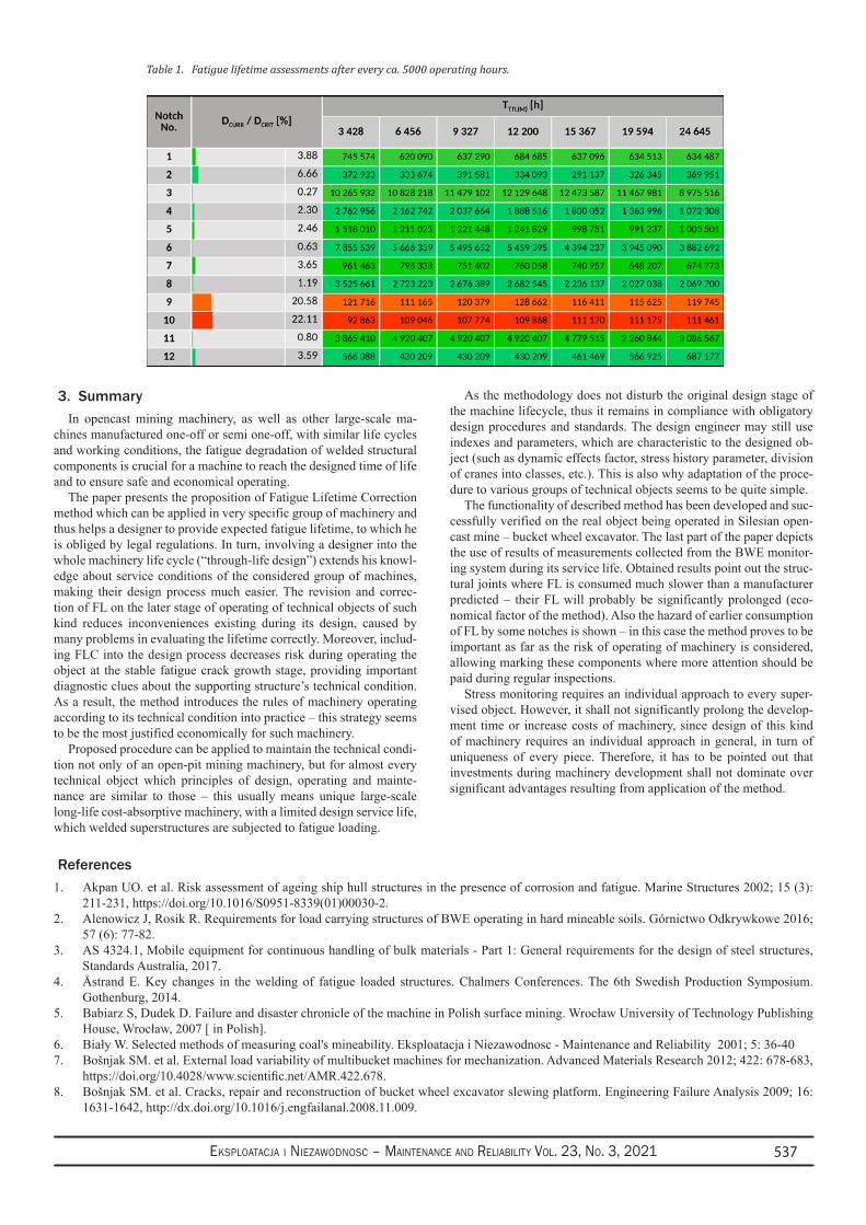
Eksploatacja i NiEzawodNosc – MaiNtENaNcE aNd REliability Vol. 23, No. 3, 2021 537
3. SummaryIn opencast mining machinery, as well as other large-scale ma-
chines manufactured one-off or semi one-off, with similar life cycles and working conditions, the fatigue degradation of welded structural components is crucial for a machine to reach the designed time of life and to ensure safe and economical operating.
The paper presents the proposition of Fatigue Lifetime Correction method which can be applied in very specific group of machinery and thus helps a designer to provide expected fatigue lifetime, to which he is obliged by legal regulations. In turn, involving a designer into the whole machinery life cycle (“through-life design”) extends his knowl-edge about service conditions of the considered group of machines, making their design process much easier. The revision and correc-tion of FL on the later stage of operating of technical objects of such kind reduces inconveniences existing during its design, caused by many problems in evaluating the lifetime correctly. Moreover, includ-ing FLC into the design process decreases risk during operating the object at the stable fatigue crack growth stage, providing important diagnostic clues about the supporting structure’s technical condition. As a result, the method introduces the rules of machinery operating according to its technical condition into practice – this strategy seems to be the most justified economically for such machinery.
Proposed procedure can be applied to maintain the technical condi-tion not only of an open-pit mining machinery, but for almost every technical object which principles of design, operating and mainte-nance are similar to those – this usually means unique large-scale long-life cost-absorptive machinery, with a limited design service life, which welded superstructures are subjected to fatigue loading.
As the methodology does not disturb the original design stage of the machine lifecycle, thus it remains in compliance with obligatory design procedures and standards. The design engineer may still use indexes and parameters, which are characteristic to the designed ob-ject (such as dynamic effects factor, stress history parameter, division of cranes into classes, etc.). This is also why adaptation of the proce-dure to various groups of technical objects seems to be quite simple.
The functionality of described method has been developed and suc-cessfully verified on the real object being operated in Silesian open-cast mine – bucket wheel excavator. The last part of the paper depicts the use of results of measurements collected from the BWE monitor-ing system during its service life. Obtained results point out the struc-tural joints where FL is consumed much slower than a manufacturer predicted – their FL will probably be significantly prolonged (eco-nomical factor of the method). Also the hazard of earlier consumption of FL by some notches is shown – in this case the method proves to be important as far as the risk of operating of machinery is considered, allowing marking these components where more attention should be paid during regular inspections.
Stress monitoring requires an individual approach to every super-vised object. However, it shall not significantly prolong the develop-ment time or increase costs of machinery, since design of this kind of machinery requires an individual approach in general, in turn of uniqueness of every piece. Therefore, it has to be pointed out that investments during machinery development shall not dominate over significant advantages resulting from application of the method.
Table 1. Fatigue lifetime assessments after every ca. 5000 operating hours.
References1. Akpan UO. et al. Risk assessment of ageing ship hull structures in the presence of corrosion and fatigue. Marine Structures 2002; 15 (3):
211-231, https://doi.org/10.1016/S0951-8339(01)00030-2.2. Alenowicz J, Rosik R. Requirements for load carrying structures of BWE operating in hard mineable soils. Górnictwo Odkrywkowe 2016;
57 (6): 77-82.3. AS 4324.1, Mobile equipment for continuous handling of bulk materials - Part 1: General requirements for the design of steel structures,
Standards Australia, 2017.4. Åstrand E. Key changes in the welding of fatigue loaded structures. Chalmers Conferences. The 6th Swedish Production Symposium.
Gothenburg, 2014.5. BabiarzS,DudekD.FailureanddisasterchronicleofthemachineinPolishsurfacemining.WrocławUniversityofTechnologyPublishing
House,Wrocław,2007[inPolish].6. BiałyW.Selectedmethodsofmeasuringcoal'smineability.EksploatacjaiNiezawodnosc-MaintenanceandReliability2001;5:36-407. Bošnjak SM. et al. External load variability of multibucket machines for mechanization. Advanced Materials Research 2012; 422: 678-683,
https://doi.org/10.4028/www.scientific.net/AMR.422.678.8. Bošnjak SM. et al. Cracks, repair and reconstruction of bucket wheel excavator slewing platform. Engineering Failure Analysis 2009; 16:
1631-1642, http://dx.doi.org/10.1016/j.engfailanal.2008.11.009.

Eksploatacja i NiEzawodNosc – MaiNtENaNcE aNd REliability Vol. 23, No. 3, 2021538
9. BošnjakSM.,ZrnićNĐ.Dynamics,failures,redesigningandenvironmentallyfriendlytechnologiesinsurfaceminingsystems.ArchivesofCivil and Mechanical Engineering 2012; 12: 348-359, http://dx.doi.org/10.1016/j.acme.2012.06.009.
10. Deng L,YanW, Nie L.A simple corrosion fatigue design method for bridges considering the coupled corrosion-overloading effect.Engineering Structures 2019; 178: 309-317, https://doi.org/10.1016/j.engstruct.2018.10.028.
11. DIN 22261-2, Excavators, spreaders and auxiliary equipment in brown coal opencast lignite mines - Part 2: Calculation Principles, German Institute for Standardization, 2015.
12. Dittrich W, Dralle HJ. Inspection of opencast mine equipment. World of Mining 2007; 59 (1): 22-26.13. Directive 2006/42/CE of The European Parliament, of The Council of 17th May 2006 on machinery, and amending Directive 95/16/CE
(recast)14. EN 13001-3-1, Cranes - General design - Part 3-1: Limit states and proof of competence of steel structures, 2018.15. FathallaE,TanakaY,MaekawaK.Remaining fatigue life assessmentof in-servicebridgedecksbaseduponartificialneuralnetworks.
Engineering Structures 2018; 171: 602-616, https://doi.org/10.1016/j.engstruct.2018.05.122.16. FrosethGT,RonnquistA.LoadmodelofhistorictrafficforfatiguelifeestimationofNorwegianrailwaybridges.EngineeringStructures
2019; 200, https://doi.org/10.1016/j.engstruct.2019.109626.17. GołaśA,IwaniecM,SzopaK.HasheddatatransferinSHMdistributedsystemswiththeuseofPowerLineCommunicationtechnology.Key
EngineeringMaterials2012;518:54-159,https://doi.org/10.4028/www.scientific.net/KEM.518.154.18. Hobbacher A. Recommendations for Fatigue Design of Welded Joints and Components. International Institute of Welding, document IIW-
1823-07 (ex XIII-2151r4-07/XV-1254r4-07), Paris, 2008.19. Huang B, Wang S, Geng S, Liu X. Improved numerical model for fatigue cumulative damage of mechanical structure considering load
sequence and interaction. Advances in Mechanical Engineering 2021; 13 (2): 1-9, https://doi.org/10.1177/1687814021995309.20. ISO 20332-1, Cranes - Proof of competence of steel structures - Part I: General, 2016.21. Jakubczak H, Jankowiak A, Sobczykiewicz W, Kowalczyk M. Technical basis of management with risk caused by fatigue cracking of load-
bearing constructions of working machines. Górnictwo Odkrywkowe 2011; 52 (3-4): 61-7022. Jankowiak A, Grabowski P, Kowalczyk M. Bearing structures fatigue. Resource assessment during long-lasting exploitation of machines.
Part 1 - loading data acquisition problems in long-lasting exploitation. Górnictwo Odkrywkowe 2018; 5: 15-25.23. Jankowiak A, Grabowski P, Kowalczyk M. Bearing structures fatigue. Resource assessment during long-lasting exploitation of machines.
Part 2 - substitutive methods of fatigue life assessment in long periods of time. Górnictwo Odkrywkowe 2018; vol. LVIV, 5: 26-32.24. JovančićP.D,IgnjatovićD,TanasijevićM,ManeskiT.Load-bearingsteelstructurediagnosticsonbucketwheelexcavatorforthepurpose
of failure prevention. Engineering Failure Analysis 2011; 18: 1203-1211, http://dx.doi.org/10.1016/j.engfailanal.2011.03.001.25. Kowalczyk M, Sobczykiewicz W. Problems of PEX exploitation project realization in the range of fatigue life of opencast mining machines
load-bearing structures. Górnictwo Odkrywkowe 2011; 52 (3-4): 71-79.26. Kowalewski J. Assessment of Remaining Fatigue Life for Surface Mining Equipment. Surface Mining. Braunkohle & Other Minerals 2001;
53 (4): 405-416.27. Kuhn B. Assessment of existing steel structures - Recommendations for estimation of the remaining fatigue life. 5th Fatigue Design
Conference, Fatigue Design 2013, Procedia Engineering 2013; 66: 3-11, https://doi.org/10.1016/j.proeng.2013.12.057.28. Kuhn B. et al. Assessment of existing steel structures: Recommendations for estimation of remaining fatigue life. Background documents
onsupporttheimplementation,harmonizationandfurtherdevelopmentoftheEurocodes-jointreport.JointResearchCenterScientificandTechnical Reports, 1st Edition, 2008, https://doi.org/10.1002/stco.200890018.
29. LovePED,etal.Whatgoesup,shouldn'tcomedown:learningfromconstructionandengineeringfailures.ProcediaEngineering2011;14:844-850, https://doi.org/10.1016/j.proeng.2011.07.107.
30. Maddox SJ. Review of fatigue assessment procedures for welded aluminium structures. International Journal of Fatigue 2003; 25 (2): 1359-1378, https://doi.org/10.1016/S0142-1123(03)00063-X.
31. May QA. et al. Prediction of remaining fatigue life of welded joints in wind turbine support structures considering strain measurements and a joint distribution of oceanographic data. Marine Structures 2019; 66: 307-322, https://doi.org/10.1016/j.marstruc.2019.05.002.
32. Miner M. Cumulative fatigue damage. Journal of Applied Mechanics 1945; 12: A159-A164, https://doi.org/10.1115/1.4009458.33. MoczkoP,PietrusiakD,RusińskiE.Materialhandlingandminingequipment-internationalstandardsrecommendationsfordesignand
testing. FME Transactions 2018; 46: 291-298, http://dx/doi.org/10.5937/fmet1803291M.34. Onichimiuk M, Wygoda M, Figiel A. Long-term load tests of opencast mining excavators. Górnictwo Odkrywkowe 2013; 54 (3-4): 24-29.35. Palin-Luc T et al. Fatigue crack initiation and growth on a steel in the very high cycle regime with water corrosion. Engineering Fracture
Mechanics 2010; 77 (11): 1953-1962, https://doi.org/10.1016/j.engfracmech.2010.02.015.36. Petinov S. In-service fatigue service reliability of structures. Solid Mechanics and Its Applications, vol. 251. Springer, 2018. ISBN 978-3-
319-89317-4.37. PietrusiakD.Evaluationoflarge-scaleload-caryingstructuresofmachineswiththeapplicationofthedynamiceffectsfactor.Eksploatacjai
Niezawodnosc - Maintenance and Reliability 2017; 19 (4): 542-551, https://doi.org/10.17531/ein.2017.4.7.38. PN-G-47000-2, Opencast mining - Bucket Wheel Excavators and Spreaders - Part 2: Calculation Fundamentals, 2011.39. RusińskiE.etal.Surfaceminingmachines:problemsofmaintenanceandmodernization.Springer,2017,ISBN978-3-319-47792-3.40. RusińskiE.etal.Guidelinesforthedesignofopencastminingmachines.GórnictwoOdkrywkowe2018;4:114-119.41. RusińskiE.etal.AnanalysisofthecausesofaBWEcounterweightboomsupportfracture.EngineeringFailureAnalysis2010;17:179-191,
https://doi.org/10.1016/j.engfailanal.2009.06.001.42. RusińskiE,CzmochowskiJ,PietrusiakD.Selectedproblemsindesigningandconstructingsurfaceminingmachinery.FMETransactions
2012; 40: 153-164.43. RusińskiE,MoczkoP,PietrusiakD.Lowfrequencyvibrationsofthesurfaceminingmachinescausedbyoperationalloadsanditsimpact
on durability. Proceedings of ISMA 2014, Leuven, 2014, ISBN 978-9-073-80291-9.44. Schmidt MJ. Structural failures on mobile materials handling equipment. Dissertation. University of Pretoria, 2014.45. Schmidt MJ, van Rensburg BWJ Avoiding structural failures on mobile bulk materials handling equipment. The Journal of The Southern
African Institute of Mining and Metallurgy 2015; 115: 179-184, https://doi.org/10.17159/2411-9717/2015/v115n3a2.46. Shen F, Zhao B, Li L, Chua C.K, Zhou K. Fatigue damage evolution and lifetime prediction of welded joints with the consideration of

Eksploatacja i NiEzawodNosc – MaiNtENaNcE aNd REliability Vol. 23, No. 3, 2021 539
residual stresses and porosity. International Journal of Fatigue 2017; 103: 272-279, https://doi.org/10.1016/j.ijfatigue.2017.06.014.47. SikoraM,SzczyrbaK,WróbelŁ,MichalakM.Monitoringandmaintenanceofagantrybasedonawirelesssystemformeasurementand
analysis of the vibration level. Eksploatacja i Niezawodnosc - Maintenance and Reliability, 2019; 21 (2): 341-350, https://doi.org/10.17531/ein.2019.2.19.
48. Siriwardane S, Ohga M, Dissanayake R, Taniwaki K. Application of New damage indicator-based sequential law for remaining fatigue life estimation of railway bridges. Journal of Constructional Steel Research 2008; 64: 228-237, https://doi.org/10.1016/j.jcsr.2007.06.002.
49. Sobczykiewicz W. Fatigue life of welded load carrying structures with respect to quality. Technology, Law and Insurance 1999, 4: 251-256, https://doi.org/10.1080/135993799348983.
50. Sobczykiewicz W, Kowalczyk M. Accomplishing the required fatigue life of load-carrying machine structures. Traditional approach. Górnictwo Odkrywkowe 2009; 50 (4-5): 115-122.
51. Szopa K, IwaniecM, Iwaniec J. Identification of technical condition of the overhead power line supporting structure. Eksploatacja iNiezawodnosc - Maintenance and Reliability 2019; 21 (1): 115-124, https://doi.org/10.17531/ein.2019.1.13.
52. Woch M. Reliability analysis of the PZL-130 Orlik TC-II aircraft structural component under real operating conditions. Eksploatacja i Niezawodnosc - Maintenance and Reliability 2017; 19 (2): 287-295, https://doi.org/10.17531/ein.2017.2.17.
53. XuS,WangH,LiA,WangY,SuL.Effectsofcorrosiononsurfacecharacterizationandmechanicalpropertiesofbutt-weldedjoints.Journalof Constructional Steel Research 2016; 126: 50-62, https://doi.org/10.1016/j.jcsr.2016.07.001.
54. Xu T. Fatigue of ship structural details: technical development and problems. Journal of Ship Research 1997; 41(4):318-331, https://doi.org/10.5957/jsr.1997.41.4.318.
55. Yang S et al.Approach for fatigue damage assessment of welded structure considering coupling effect between stress and corrosion.International Journal of Fatigue 2016; 88: 88-95, https://doi.org/10.1016/j.ijfatigue.2016.03.024.
56. Yin Y, Rondin G.Y, Obaia KH, Elwi AE. Fatigue life prediction of heavy mining equipment. Part 1: Fatigue load assessment and crack growth rate tests. Journal of Constructional Steel Research 2007; 63: 1494-1505, https://doi.org/10.1016/j.jcsr.2007.01.008.
57. Yin Y, Rondin G.Y, Obaia KH, Elwi AE. Fatigue life prediction of heavy mining equipment. Part 2: Behavior of corner crack in steel welded box section and remaining fatigue life determination. Journal of Constructional Steel Research 2008; 64: 62-71, https://doi.org/10.1016/j.jcsr.2007.04.003.
58. YouR,KaewunruenS.Evaluationof remaining fatigue life of concrete sleeperbasedonfield loading conditions.EngineeringFailureAnalysis 2019; 105: 70-86, https://doi.org/10.1016/j.engfailanal.2019.06.086.
59. Zaretski A.A. Calculating Life. 2001; Aug./Sept. HOIST.

Eksploatacja i NiEzawodNosc – MaiNtENaNcE aNd REliability Vol. 23, No. 3, 2021540
(*) Corresponding author.E-mail addresses:
Eksploatacja i Niezawodnosc – Maintenance and ReliabilityVolume 23 (2021), Issue 3
journal homepage: http://www.ein.org.pl
Indexed by:
1. IntroductionMost of the machines used in the industry require bearings to sup-
port shafts. It is necessary to support them to provide the capability of both carrying loads and allowing rotation. The lifespan of the ro-tating machineries strongly depends on the technical condition and operating parameters of the used shafts’ bearings. Hence, it should be noticed that a number of works related to the analysis of maintenance problems and ensuring the operational reliability of bearings have been published so far, e.g., [1, 14, 21]. In the work [8], the authors present a review of algorithms that enable the assessment of the bear-ing’s degradation based on machine learning. The authors also con-clude that there is still a lack of universal indicator that would allow for an unambiguous determination of the trend regarding bearing’s degradation. On the other hand, the work [23] deals with the issue of type selection of the bearing ensuring correct operation of high-speed systems.
In the present work, the authors focus their research efforts on a specific type of the bearings, namely the gas foil bearings (GFB)s, also known as air foil bearings. These bearings are a subgroup of the slide bearings. However, in contrary to the typical slide bearings, in which the lubricating medium is usually oil, GFBs make use of air
[15]. A general view of the bearing’s installation employing a GFB is schematically shown in Fig. 1A. The bearing’s bushing is fixed in the housing by means of the thrust rings. The characteristic components of a GFB are the top foil and bump foils [19]. A close-up view show-ing the bearing’s bushing, top and bump foils as well as the rotating shaft is shown in Fig. 1B.
In a GFB, the rotating shaft is supported by a top foil which, in turn, is held in a desired location in the bushing by the bump foils. The required gap between the shaft and the top foil is provided by the hydrodynamic pressure generated while developing the air film. Generation of this pressure is ensured by the fact that the air is drawn in (due to viscous effects) between the shaft and the top foil. A high rotational speed of the shaft with respect to the bearing’s bushing is required to form a continuous air film. Once achieved, the generated air film enables non-contact operation of the bearing, which refers to the nominal condition of its maintenance.
As mentioned, the developing air film creates a small clearance, several micrometers thick, between the surface of the shaft’s journal and the top foil. Through this gap, the air is continuously exchanged with the surroundings. Maintaining this gap is essential for the correct operation of the bearing [22]. However, the use of air as a lubricant in GFBs introduces certain limitations in terms of their use. The consid-
Study on the temperature and strain fields in gas foil bearings – measurement method and numerical simulations Paweł Zdziebko a,*, Adam Martowicz a
a AGH University of Science and Technology, Department of Robotics and Mechatronics, al. A. Mickiewicza 30, 30-059 Kraków, Poland
Zdziebko P, Martowicz A. Study on the temperature and strain fields in gas foil bearings – measurement method and numerical simula-tions. Eksploatacja i Niezawodnosc – Maintenance and Reliability 2021; 23 (3): 540–547, http://doi.org/10.17531/ein.2021.3.15.
Article citation info:
Gas foil bearings belong to the group of slide bearings and are used in devices in which op-eration at high rotational speeds of the shafts are of key importance, e.g., in gas turbines. The air film developed on the surface of the bearing’s top foil allows this structural component to be separated from the shaft. This ensures a non-contact operation of the bearing. In the case of the mentioned type of bearings, their resultant operational properties are influenced by both thermal and mechanical phenomena. The current work presents a model of a gas foil bearing developed making use of the Finite Element Method. The model takes into account thermomechanical couplings which are necessary for the correct simulation of the operation of physical components of the modeled system. The paper reports the results of numerical analyzes conducted for the elaborated model as well as the relevant conclusions concerning thermomechanical couplings present in gas foil bearings. The method for the experimental identification of the temperature and strain fields in the bearing’s top foil proposed to vali-date the numerical model is also presented.
Highlights Abstract
A method for measurement of the temperature and • strain fields in the bearing’s top foil making use of its specialized version equipped with sensors of the adequate physical quantities has been pro-posed.
A numerical model of a gas foil bearing has been • developed using the Finite Element Method, which takes into account thermomechanical cou-plings.
The obtained results of numerical calculations • have indicated the dominant directions of strains as well as temperature distribution in the bearing.
gas foil bearing, numerical analysis, thermomechanical couplings, Finite Element Method, temperature field, strain field.
Keywords
This is an open access article under the CC BY license (https://creativecommons.org/licenses/by/4.0/)
P. Zdziebko - [email protected], A. Martowicz - [email protected]
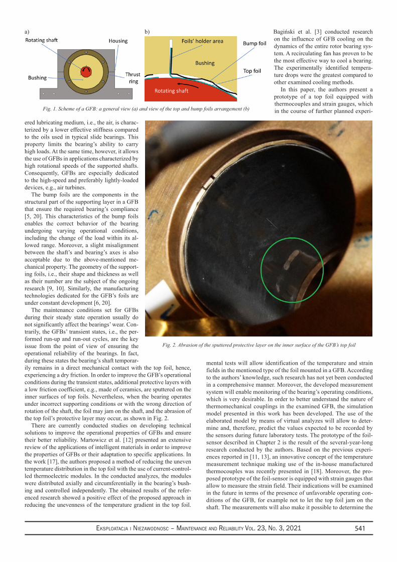
Eksploatacja i NiEzawodNosc – MaiNtENaNcE aNd REliability Vol. 23, No. 3, 2021 541
ered lubricating medium, i.e., the air, is charac-terized by a lower effective stiffness compared to the oils used in typical slide bearings. This property limits the bearing’s ability to carry high loads. At the same time, however, it allows the use of GFBs in applications characterized by high rotational speeds of the supported shafts. Consequently, GFBs are especially dedicated to the high-speed and preferably lightly-loaded devices, e.g., air turbines.
The bump foils are the components in the structural part of the supporting layer in a GFB that ensure the required bearing’s compliance [5, 20]. This characteristics of the bump foils enables the correct behavior of the bearing undergoing varying operational conditions, including the change of the load within its al-lowed range. Moreover, a slight misalignment between the shaft’s and bearing’s axes is also acceptable due to the above-mentioned me-chanical property. The geometry of the support-ing foils, i.e., their shape and thickness as well as their number are the subject of the ongoing research [9, 10]. Similarly, the manufacturing technologies dedicated for the GFB’s foils are under constant development [6, 20].
The maintenance conditions set for GFBs during their steady state operation usually do not significantly affect the bearings’ wear. Con-trarily, the GFBs’ transient states, i.e., the per-formed run-up and run-out cycles, are the key issue from the point of view of ensuring the operational reliability of the bearings. In fact, during these states the bearing’s shaft temporar-ily remains in a direct mechanical contact with the top foil, hence, experiencing a dry friction. In order to improve the GFB’s operational conditions during the transient states, additional protective layers with a low friction coefficient, e.g., made of ceramics, are sputtered on the inner surfaces of top foils. Nevertheless, when the bearing operates under incorrect supporting conditions or with the wrong direction of rotation of the shaft, the foil may jam on the shaft, and the abrasion of the top foil’s protective layer may occur, as shown in Fig. 2.
There are currently conducted studies on developing technical solutions to improve the operational properties of GFBs and ensure their better reliability. Martowicz et al. [12] presented an extensive review of the applications of intelligent materials in order to improve the properties of GFBs or their adaptation to specific applications. In the work [17], the authors proposed a method of reducing the uneven temperature distribution in the top foil with the use of current-control-led thermoelectric modules. In the conducted analyzes, the modules were distributed axially and circumferentially in the bearing’s bush-ing and controlled independently. The obtained results of the refer-enced research showed a positive effect of the proposed approach in reducing the unevenness of the temperature gradient in the top foil.
Bagiński et al. [3] conducted research on the influence of GFB cooling on the dynamics of the entire rotor bearing sys-tem. A recirculating fan has proven to be the most effective way to cool a bearing. The experimentally identified tempera-ture drops were the greatest compared to other examined cooling methods.
In this paper, the authors present a prototype of a top foil equipped with thermocouples and strain gauges, which in the course of further planned experi-
mental tests will allow identification of the temperature and strain fields in the mentioned type of the foil mounted in a GFB. According to the authors’ knowledge, such research has not yet been conducted in a comprehensive manner. Moreover, the developed measurement system will enable monitoring of the bearing’s operating conditions, which is very desirable. In order to better understand the nature of thermomechanical couplings in the examined GFB, the simulation model presented in this work has been developed. The use of the elaborated model by means of virtual analyzes will allow to deter-mine and, therefore, predict the values expected to be recorded by the sensors during future laboratory tests. The prototype of the foil-sensor described in Chapter 2 is the result of the several-year-long research conducted by the authors. Based on the previous experi-ences reported in [11, 13], an innovative concept of the temperature measurement technique making use of the in-house manufactured thermocouples was recently presented in [18]. Moreover, the pro-posed prototype of the foil-sensor is equipped with strain gauges that allow to measure the strain field. Their indications will be examined in the future in terms of the presence of unfavorable operating con-ditions of the GFB, for example not to let the top foil jam on the shaft. The measurements will also make it possible to determine the
Fig. 1. Scheme of a GFB: a general view (a) and view of the top and bump foils arrangement (b)
Fig. 2. Abrasion of the sputtered protective layer on the inner surface of the GFB’s top foil
b)a)
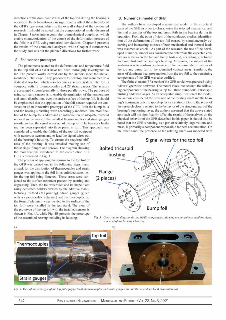
Eksploatacja i NiEzawodNosc – MaiNtENaNcE aNd REliability Vol. 23, No. 3, 2021542
directions of the dominant strains of the top foil during the bearing’s operation. Its deformations can significantly affect the reliability of the GFB’s operation, which is the overall subject of the conducted research. It should be noted that the computational model discussed in Chapter 3 takes into account thermomechanical couplings, which enable characterization of the course of the deformation process of the foils in a GFB using numerical simulations. Chapter 4 presents the results of the conducted analyzes, while Chapter 5 summarizes the study and sets out the planned directions for further work.
2. Foil-sensor prototypeThe phenomena related to the deformations and temperature field
in the top foil of a GFB have not been thoroughly investigated so far. The present works carried out by the authors meet the above-mentioned challenge. They proposed to develop and manufacture a dedicated top foil, which also becomes a sensor system. The foil is equipped with 18 thermocouples and 28 strain gauges. The sensors are arranged circumferentially in three parallel rows. The purpose of using so many sensors is to enable determination of the temperature and strain distributions over the entire surface of the top foil. It should be emphasized that the application of the foil-sensor required the con-struction of an innovative prototype of the GFB. Both the bump foils and the bearing’s bushing were accordingly modified. The modifica-tion of the bump foils addressed an introduction of adequate material removal in the areas of the installed thermocouples and strain gauges in order to lead the signal wires out of the top foil. The bearing’s bush-ing has been separated into three parts, in turn. This approach was considered to enable the folding of the top foil equipped with numerous sensors and to lead the signal wires out of the bearing’s housing. To ensure the required stiff-ness of the bushing, it was installed making use of thrust rings, flanges and screws. The diagram showing the modifications introduced to the construction of a GFB is presented in Fig. 3.
The process of applying the sensors to the top foil of the GFB was carried out in the following steps. First, a mask for the distribution of thermocouples and strain gauges was applied to the foil in its unfolded state, i.e., for the top foil being flattened. These areas were sub-jected to the surface treatment process by matting and degreasing. Then, the foil was rolled and its shape fixed using dedicated holders created by the additive manu-facturing method (3D printing). Strain gauges (glued with a cyanoacrylate adhesive) and thermocouples (in the form of platinum wires welded to the surface of the top foil) were installed in the test stand. The view of the prototype of the top foil with the installed sensors is shown in Fig. 4A, while Fig. 4B presents the prototype of the assembled bearing including its housing.
3. Numerical model of GFBThe authors have developed a numerical model of the structural
parts of the GFB in order to characterize the selected mechanical and thermal properties of the top and bump foils in the bearing during its operation. From the point of view of the conducted studies, identifica-tion of the deformation of the top foil caused by simultaneously oc-curring and interacting sources of both mechanical and thermal loads was assumed as crucial. As part of the research, the use of the devel-oped numerical model was considered to determine the expected con-tact areas between the top and bump foils and, accordingly, between the bump foil and the bearing’s bushing. Moreover, the subject of the analyzes was to confirm occurrence of the increased deformations of the top and bump foil in the identified contact areas. Similarly, the areas of dominant heat propagation from the top foil to the remaining components of the GFB was also verified.
The finite element (FE) mesh of the GFB model was prepared using Altair HyperMesh software. The model takes into account the follow-ing components of the bearing: a top foil, three bump foils, a tricuspid bushing and two flanges. As an acceptable simplification of the model, the authors considered the omission of the rotating shaft and the bear-ing’s housing in order to speed up the calculations. Due to the scope of the research closely related to the behavior of the structural part of the bearing’s supporting layer, the authors assumed that the above stated approach will not significantly affect the results of the analyzes on the physical behavior of the GFB described in this paper. It should also be noted that the GFB’s housing, as a part of relatively large volume and mass, is primarily a component responsible for heat accumulation. On the other hand, the presence of the rotating shaft was modeled with
Fig. 3. Construction diagram for the GFB’s components allowing to conveniently lead the signal wires out of the bearing’s housing
Fig. 4. View of the prototype of the top foil equipped with thermocouples and strain gauges (a) and the assembled GFB installation (b)
b)a)
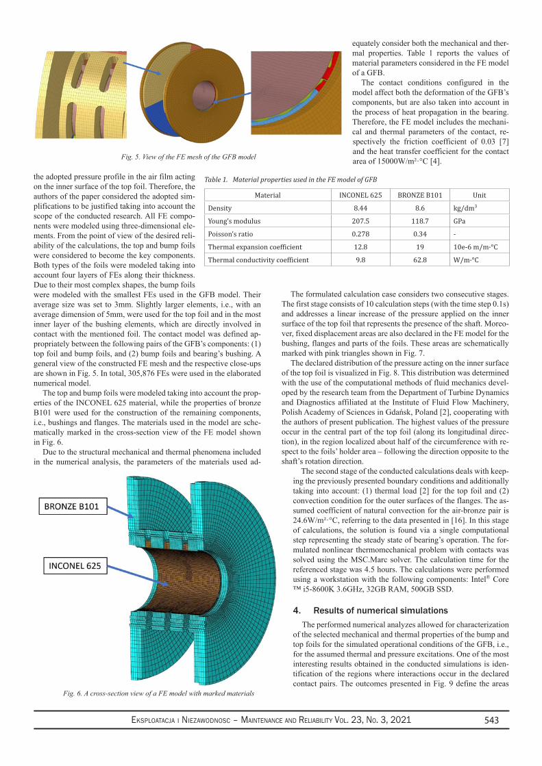
Eksploatacja i NiEzawodNosc – MaiNtENaNcE aNd REliability Vol. 23, No. 3, 2021 543
the adopted pressure profile in the air film acting on the inner surface of the top foil. Therefore, the authors of the paper considered the adopted sim-plifications to be justified taking into account the scope of the conducted research. All FE compo-nents were modeled using three-dimensional ele-ments. From the point of view of the desired reli-ability of the calculations, the top and bump foils were considered to become the key components. Both types of the foils were modeled taking into account four layers of FEs along their thickness. Due to their most complex shapes, the bump foils were modeled with the smallest FEs used in the GFB model. Their average size was set to 3mm. Slightly larger elements, i.e., with an average dimension of 5mm, were used for the top foil and in the most inner layer of the bushing elements, which are directly involved in contact with the mentioned foil. The contact model was defined ap-propriately between the following pairs of the GFB’s components: (1) top foil and bump foils, and (2) bump foils and bearing’s bushing. A general view of the constructed FE mesh and the respective close-ups are shown in Fig. 5. In total, 305,876 FEs were used in the elaborated numerical model.
The top and bump foils were modeled taking into account the prop-erties of the INCONEL 625 material, while the properties of bronze B101 were used for the construction of the remaining components, i.e., bushings and flanges. The materials used in the model are sche-matically marked in the cross-section view of the FE model shown in Fig. 6.
Due to the structural mechanical and thermal phenomena included in the numerical analysis, the parameters of the materials used ad-
equately consider both the mechanical and ther-mal properties. Table 1 reports the values of material parameters considered in the FE model of a GFB.
The contact conditions configured in the model affect both the deformation of the GFB’s components, but are also taken into account in the process of heat propagation in the bearing. Therefore, the FE model includes the mechani-cal and thermal parameters of the contact, re-spectively the friction coefficient of 0.03 [7] and the heat transfer coefficient for the contact area of 15000W/m²·°C [4].
The formulated calculation case considers two consecutive stages. The first stage consists of 10 calculation steps (with the time step 0.1s) and addresses a linear increase of the pressure applied on the inner surface of the top foil that represents the presence of the shaft. Moreo-ver, fixed displacement areas are also declared in the FE model for the bushing, flanges and parts of the foils. These areas are schematically marked with pink triangles shown in Fig. 7.
The declared distribution of the pressure acting on the inner surface of the top foil is visualized in Fig. 8. This distribution was determined with the use of the computational methods of fluid mechanics devel-oped by the research team from the Department of Turbine Dynamics and Diagnostics affiliated at the Institute of Fluid Flow Machinery, Polish Academy of Sciences in Gdańsk, Poland [2], cooperating with the authors of present publication. The highest values of the pressure occur in the central part of the top foil (along its longitudinal direc-tion), in the region localized about half of the circumference with re-spect to the foils’ holder area – following the direction opposite to the shaft’s rotation direction.
The second stage of the conducted calculations deals with keep-ing the previously presented boundary conditions and additionally taking into account: (1) thermal load [2] for the top foil and (2) convection condition for the outer surfaces of the flanges. The as-sumed coefficient of natural convection for the air-bronze pair is 24.6W/m²·°C, referring to the data presented in [16]. In this stage of calculations, the solution is found via a single computational step representing the steady state of bearing’s operation. The for-mulated nonlinear thermomechanical problem with contacts was solved using the MSC.Marc solver. The calculation time for the referenced stage was 4.5 hours. The calculations were performed using a workstation with the following components: Intel® Core ™ i5-8600K 3.6GHz, 32GB RAM, 500GB SSD.
4. Results of numerical simulationsThe performed numerical analyzes allowed for characterization
of the selected mechanical and thermal properties of the bump and top foils for the simulated operational conditions of the GFB, i.e., for the assumed thermal and pressure excitations. One of the most interesting results obtained in the conducted simulations is iden-tification of the regions where interactions occur in the declared contact pairs. The outcomes presented in Fig. 9 define the areas
Fig. 5. View of the FE mesh of the GFB model
Fig. 6. A cross-section view of a FE model with marked materials
Table 1. Material properties used in the FE model of GFB
Material INCONEL 625 BRONZE B101 Unit
Density 8.44 8.6 kg/dm3
Young’s modulus 207.5 118.7 GPa
Poisson’s ratio 0.278 0.34 -
Thermal expansion coefficient 12.8 19 10e-6 m/m·°C
Thermal conductivity coefficient 9.8 62.8 W/m·°C
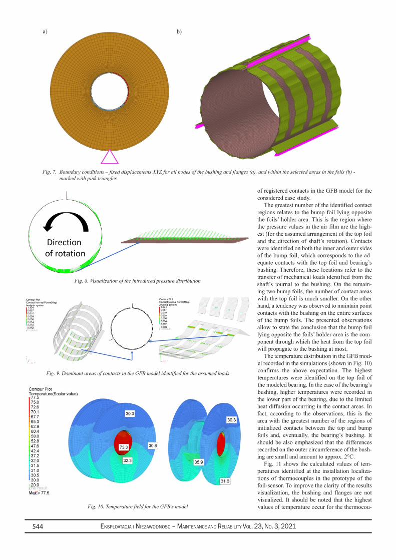
Eksploatacja i NiEzawodNosc – MaiNtENaNcE aNd REliability Vol. 23, No. 3, 2021544
of registered contacts in the GFB model for the considered case study.
The greatest number of the identified contact regions relates to the bump foil lying opposite the foils’ holder area. This is the region where the pressure values in the air film are the high-est (for the assumed arrangement of the top foil and the direction of shaft’s rotation). Contacts were identified on both the inner and outer sides of the bump foil, which corresponds to the ad-equate contacts with the top foil and bearing’s bushing. Therefore, these locations refer to the transfer of mechanical loads identified from the shaft’s journal to the bushing. On the remain-ing two bump foils, the number of contact areas with the top foil is much smaller. On the other hand, a tendency was observed to maintain point contacts with the bushing on the entire surfaces of the bump foils. The presented observations allow to state the conclusion that the bump foil lying opposite the foils’ holder area is the com-ponent through which the heat from the top foil will propagate to the bushing at most.
The temperature distribution in the GFB mod-el recorded in the simulations (shown in Fig. 10) confirms the above expectation. The highest temperatures were identified on the top foil of the modeled bearing. In the case of the bearing’s bushing, higher temperatures were recorded in the lower part of the bearing, due to the limited heat diffusion occurring in the contact areas. In fact, according to the observations, this is the area with the greatest number of the regions of initialized contacts between the top and bump foils and, eventually, the bearing’s bushing. It should be also emphasized that the differences recorded on the outer circumference of the bush-ing are small and amount to approx. 2°C.
Fig. 11 shows the calculated values of tem-peratures identified at the installation localiza-tions of thermocouples in the prototype of the foil-sensor. To improve the clarity of the results visualization, the bushing and flanges are not visualized. It should be noted that the highest values of temperature occur for the thermocou-
Fig. 7. Boundary conditions – fixed displacements XYZ for all nodes of the bushing and flanges (a), and within the selected areas in the foils (b) - marked with pink triangles
Fig. 8. Visualization of the introduced pressure distribution
Fig. 10. Temperature field for the GFB’s model
Fig. 9. Dominant areas of contacts in the GFB model identified for the assumed loads
b)a)
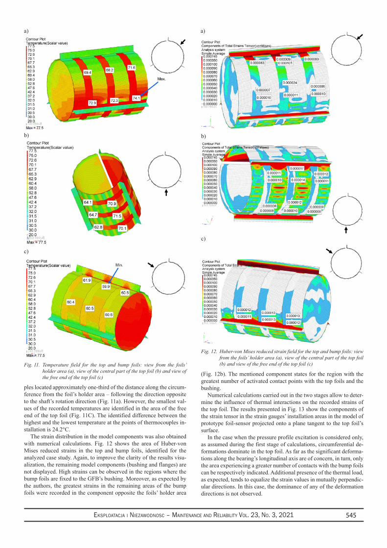
Eksploatacja i NiEzawodNosc – MaiNtENaNcE aNd REliability Vol. 23, No. 3, 2021 545
ples located approximately one-third of the distance along the circum-ference from the foil’s holder area – following the direction opposite to the shaft’s rotation direction (Fig. 11a). However, the smallest val-ues of the recorded temperatures are identified in the area of the free end of the top foil (Fig. 11C). The identified difference between the highest and the lowest temperature at the points of thermocouples in-stallation is 24.2°C.
The strain distribution in the model components was also obtained with numerical calculations. Fig. 12 shows the area of Huber-von Mises reduced strains in the top and bump foils, identified for the analyzed case study. Again, to improve the clarity of the results visu-alization, the remaining model components (bushing and flanges) are not displayed. High strains can be observed in the regions where the bump foils are fixed to the GFB’s bushing. Moreover, as expected by the authors, the greatest strains in the remaining areas of the bump foils were recorded in the component opposite the foils’ holder area
(Fig. 12b). The mentioned component states for the region with the greatest number of activated contact points with the top foils and the bushing.
Numerical calculations carried out in the two stages allow to deter-mine the influence of thermal interactions on the recorded strains of the top foil. The results presented in Fig. 13 show the components of the strain tensor in the strain gauges’ installation areas in the model of prototype foil-sensor projected onto a plane tangent to the top foil’s surface.
In the case when the pressure profile excitation is considered only, as assumed during the first stage of calculations, circumferential de-formations dominate in the top foil. As far as the significant deforma-tions along the bearing’s longitudinal axis are of concern, in turn, only the area experiencing a greater number of contacts with the bump foils can be respectively indicated. Additional presence of the thermal load, as expected, tends to equalize the strain values in mutually perpendic-ular directions. In this case, the dominance of any of the deformation directions is not observed.
Fig. 11. Temperature field for the top and bump foils: view from the foils’ holder area (a), view of the central part of the top foil (b) and view of the free end of the top foil (c)
Fig. 12. Huber-von Mises reduced strain field for the top and bump foils: view from the foils’ holder area (a), view of the central part of the top foil (b) and view of the free end of the top foil (c)
b)
a)
c)
b)
a)
c)
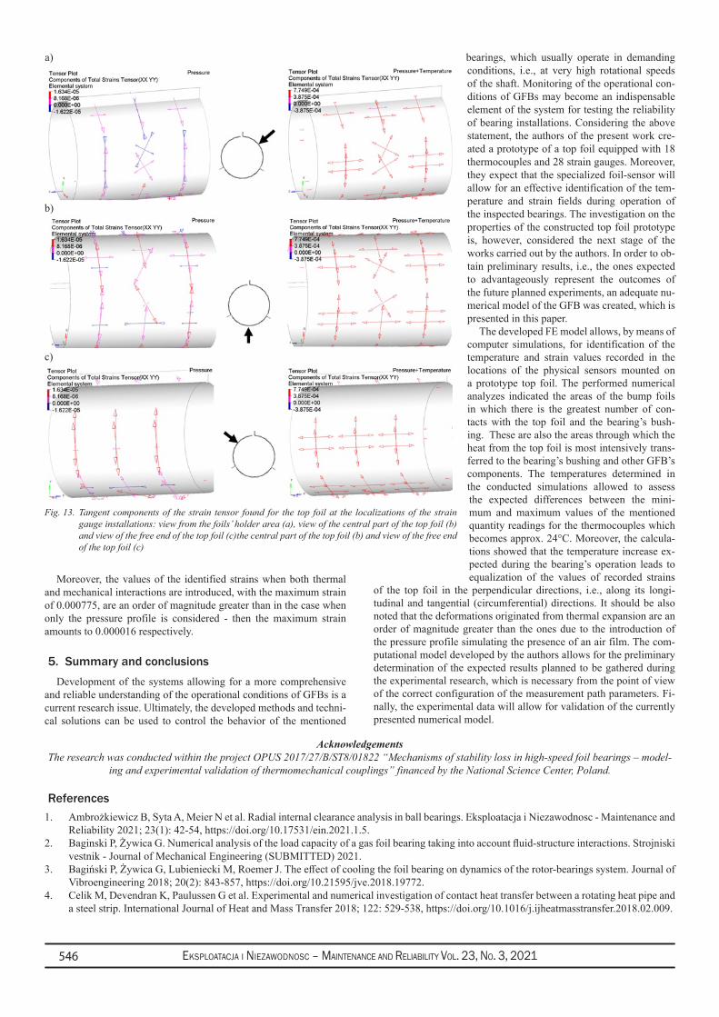
Eksploatacja i NiEzawodNosc – MaiNtENaNcE aNd REliability Vol. 23, No. 3, 2021546
Moreover, the values of the identified strains when both thermal and mechanical interactions are introduced, with the maximum strain of 0.000775, are an order of magnitude greater than in the case when only the pressure profile is considered - then the maximum strain amounts to 0.000016 respectively.
5. Summary and conclusionsDevelopment of the systems allowing for a more comprehensive
and reliable understanding of the operational conditions of GFBs is a current research issue. Ultimately, the developed methods and techni-cal solutions can be used to control the behavior of the mentioned
bearings, which usually operate in demanding conditions, i.e., at very high rotational speeds of the shaft. Monitoring of the operational con-ditions of GFBs may become an indispensable element of the system for testing the reliability of bearing installations. Considering the above statement, the authors of the present work cre-ated a prototype of a top foil equipped with 18 thermocouples and 28 strain gauges. Moreover, they expect that the specialized foil-sensor will allow for an effective identification of the tem-perature and strain fields during operation of the inspected bearings. The investigation on the properties of the constructed top foil prototype is, however, considered the next stage of the works carried out by the authors. In order to ob-tain preliminary results, i.e., the ones expected to advantageously represent the outcomes of the future planned experiments, an adequate nu-merical model of the GFB was created, which is presented in this paper.
The developed FE model allows, by means of computer simulations, for identification of the temperature and strain values recorded in the locations of the physical sensors mounted on a prototype top foil. The performed numerical analyzes indicated the areas of the bump foils in which there is the greatest number of con-tacts with the top foil and the bearing’s bush-ing. These are also the areas through which the heat from the top foil is most intensively trans-ferred to the bearing’s bushing and other GFB’s components. The temperatures determined in the conducted simulations allowed to assess the expected differences between the mini-mum and maximum values of the mentioned quantity readings for the thermocouples which becomes approx. 24°C. Moreover, the calcula-tions showed that the temperature increase ex-pected during the bearing’s operation leads to equalization of the values of recorded strains
of the top foil in the perpendicular directions, i.e., along its longi-tudinal and tangential (circumferential) directions. It should be also noted that the deformations originated from thermal expansion are an order of magnitude greater than the ones due to the introduction of the pressure profile simulating the presence of an air film. The com-putational model developed by the authors allows for the preliminary determination of the expected results planned to be gathered during the experimental research, which is necessary from the point of view of the correct configuration of the measurement path parameters. Fi-nally, the experimental data will allow for validation of the currently presented numerical model.
Fig. 13. Tangent components of the strain tensor found for the top foil at the localizations of the strain gauge installations: view from the foils’ holder area (a), view of the central part of the top foil (b) and view of the free end of the top foil (c)the central part of the top foil (b) and view of the free end of the top foil (c)
b)
a)
c)
References1. Ambrożkiewicz B, Syta A, Meier N et al. Radial internal clearance analysis in ball bearings. Eksploatacja i Niezawodnosc - Maintenance and
Reliability 2021; 23(1): 42-54, https://doi.org/10.17531/ein.2021.1.5.2. Baginski P, Żywica G. Numerical analysis of the load capacity of a gas foil bearing taking into account fluid-structure interactions. Strojniski
vestnik - Journal of Mechanical Engineering (SUBMITTED) 2021.3. Bagiński P, Żywica G, Lubieniecki M, Roemer J. The effect of cooling the foil bearing on dynamics of the rotor-bearings system. Journal of
Vibroengineering 2018; 20(2): 843-857, https://doi.org/10.21595/jve.2018.19772.4. Celik M, Devendran K, Paulussen G et al. Experimental and numerical investigation of contact heat transfer between a rotating heat pipe and
a steel strip. International Journal of Heat and Mass Transfer 2018; 122: 529-538, https://doi.org/10.1016/j.ijheatmasstransfer.2018.02.009.
AcknowledgementsThe research was conducted within the project OPUS 2017/27/B/ST8/01822 “Mechanisms of stability loss in high-speed foil bearings – model-
ing and experimental validation of thermomechanical couplings” financed by the National Science Center, Poland.

Eksploatacja i NiEzawodNosc – MaiNtENaNcE aNd REliability Vol. 23, No. 3, 2021 547
5. Gu Y, Ren G, Zhou M. A fully coupled elastohydrodynamic model for static performance analysis of gas foil bearings. Tribology International 2020; 147(October 2019): 106297, https://doi.org/10.1016/j.triboint.2020.106297.
6. Ha D N, Xu Y. High Precision Manufacturing for Air Foil Bearings. Proceedings of the 6th International Conference on Nanomanufacturing, nanoMan2018, 04-06 July 2018, Brunel University London, UK 2018.
7. Kiciński J, Żywica G, Rządkowski R, Drewczyński M. Modelowanie strukturalnej warstwy nośnej łożyska foliowego. Acta Mechanica et Automatica 2008; 2(1): 45-50.
8. Kumar S, Kumar P, Kumar G. Degradation assessment of bearing based on machine learning classification matrix. Eksploatacja i Niezawodnosc - Maintenance and Reliability 2021; 23(2): 395-404, https://doi.org/10.17531/ein.2021.2.20.
9. Lai T, Guo Y, Zhao Q et al. Numerical and experimental studies on stability of cryogenic turbo-expander with protuberant foil gas bearings. Cryogenics 2018; 96: 62-74, https://doi.org/10.1016/j.cryogenics.2018.10.009.
10. Liu W, Zhao X, Zhang T, Feng K. Investigation on the rotordynamic performance of hybrid bump-metal mesh foil bearings rotor system. Mechanical Systems and Signal Processing 2021; 147: 107076, https://doi.org/10.1016/j.ymssp.2020.107076.
11. Lubieniecki M, Roemer J, Martowicz A et al. A Multi-Point Measurement Method for Thermal Characterization of Foil Bearings Using Customized Thermocouples. Journal of Electronic Materials 2016; 45(3): 1473-1477, https://doi.org/10.1007/s11664-015-4082-0
12. Martowicz A, Roemer J, Kantor S et al. Gas foil bearing technology enhanced with smart materials. Applied Sciences (Switzerland) 2021, https://doi.org/10.3390/app11062757.
13. Martowicz A, Roemer J, Lubieniecki M et al. Experimental and numerical study on the thermal control strategy for a gas foil bearing enhanced with thermoelectric modules. Mechanical Systems and Signal Processing 2020, https://doi.org/10.1016/j.ymssp.2019.106581.
14. Mazurkow A, Witkowski W, Kalina A et al. The effect of oil feeding type and oil grade on the oil film bearing capacity. Eksploatacja i Niezawodnosc - Maintenance and Reliability 2021; 23(2): 381-386, https://doi.org/10.17531/ein.2021.2.18.
15. McAuliffe C, Dziorny P J. Bearing cooling arrangement for air cycle machine. 1992.16. Ochoa G V, Sanchez W E, Truyoll S D L H. Experimental and theoretical study on free and force convection heat transfer. Contemporary
Engineering Sciences 2017; 10(23): 1143-1152, https://doi.org/10.12988/ces.2017.79124.17. Roemer J, Lubieniecki M, Martowicz A, Uhl T. Multi-point control method for reduction of thermal gradients in foil bearings based on the
application of smart materials. 7th ECCOMAS Thematic Conference on Smart Structures and Materials SMART 2015.18. Roemer J, Zdziebko P, Martowicz A. Multifunctional bushing for gas foil bearing - Test rig architecture and functionalities. International
Journal of Multiphysics 2021; 15(1): 73-86, https://doi.org/10.21152/1750-9548.15.1.73.19. Samanta P, Murmu N C, Khonsari M M. The evolution of foil bearing technology. Tribology International 2019; 135(November 2018): 305-
323, https://doi.org/10.1016/j.triboint.2019.03.021.20. Shalash K, Schiffmann J. On the manufacturing of compliant foil bearings. Journal of Manufacturing Processes 2017; 25: 357-368, https://
doi.org/10.1016/j.jmapro.2016.12.021.21. Strzelecki S, Kuśmierz L, Ponieważ G. Thermal deformation of pads in tilting 5-pad jouranl bearing. Eksploatacja i Niezawodnosc 2008; 2:
12-16.22. Żywica G, Bagiński P, Kiciński J. Selected operational problems of high-speed rotors supported by gas foil bearings. Technische Mechanik
2017; 37(2-5): 339-346.23. Żywica G, Kaczmarczyk T Z. Experimental evaluation of the dynamic properties of an energy microturbine with defects in the rotating
system. Eksploatacja i Niezawodnosc - Maintenance and Reliability 2019; 21(4): 670-678, https://doi.org/10.17531/ein.2019.4.17.
Eksploatacja i NiEzawodNosc – MaiNtENaNcE aNd REliability Vol. 23, No. 3, 2021548
(*) Corresponding author.E-mail addresses:
Eksploatacja i Niezawodnosc – Maintenance and ReliabilityVolume 23 (2021), Issue 3
journal homepage: http://www.ein.org.pl
Indexed by:Method of reconstructing dynamic load characteristics for durability test of heavy semitrailer under different road conditionsArkadiusz Czarnuch a,c,*, Marek Stembalski b, Tomasz Szydłowski a, Damian Batory a
a Łódź University of Technology, ul. Stefanowskiego 1/15, 90-537 Lodz, Poland b Wroclaw University of Technology, ul. Lukasiewicza 5, 50-371 Wroclaw, Poland c Wielton S.A., ul. Rymarkiewicz 6, 98-300 Wielun, Poland
Czarnuch A, Stembalski M, Szydłowski T, Batory D. Method of reconstructing dynamic load characteristics for durability test of heavy semitrailer under different road conditions. Eksploatacja i Niezawodnosc – Maintenance and Reliability 2021; 23 (3): 548–558, http://doi.org/10.17531/ein.2021.3.16.
Article citation info:
The aim of the article is to present and validate a methodology for collecting road load data on a vehicle, driving on roads and analysis of a drive data signal under the wheel in the time domain, using FRF (Frequency Response Function) and the MTS 320 eight-poster inertia reacted road simulator. The elaborated drive data, was used to control the actuators forcing the movements of the wheels and the coupling part of the semi-trailer during durability tests. The road tests were carried out by registering physical variables in the time domain, by a set of sensors mounted on a vehicle. The data was collected from roads categorized as motorways, national and local roads. Differences between the variability of the parameters, collected on the roads and the variability of the drive data under the wheel, were determined for the particular types of roads, for loaded and unloaded vehicle. The obtained accuracy of reconstruction of the road load data conditions was as high as 97%. Therefore, the proposed method is suitable for reliable durability tests with use of the road simulator.
Highlights Abstract
Road data was recorded using real semitrailer • with a set of sensors.
Drive data was created and verified using the road • simulator.
Dynamic load characteristics of different road • conditions was made.
The reconstruction of the road load data condi-• tions was as high as 97%.
This methodology is valid for accelerated durabil-• ity test for different road conditions.
drive data, road load data, fatigue damage, durability, sensors.
Keywords
This is an open access article under the CC BY license (https://creativecommons.org/licenses/by/4.0/)
A. Czarnuch - [email protected], M. Stembalski - [email protected], T. Szydłowski - [email protected], D. Batory - [email protected]
1. IntroductionThe durability and reliability of road vehicles depend on many
factors. The basic factor is the quality of the manufactured vehicle, which comprises the vehicle structure, the materials used, the material joining technology and the production quality. The second (equally important) factor is the manner and conditions of vehicle use. For example in the case of brake system components, different roads and operating conditions have a significant influence on wear and reli-ability [22].
In the case of vehicles, their lifetime is specified by the manufac-turer, regarding the failure assumption. Paraforos et. al calculated this life time for agriculture vehicle. The authors state that the use of real road profiles is more appropriate than the use of an artificial profile to simulate the fatigue of real vehicles.[15]. On the other hand Kong et. al for this purpose used a particular component of the vehicle, indicat-ing the parameters for which the design of the spring leaf will meet the durability requirements. [10]. Vehicle lifetime is most often expressed by the covered mileage. But mileage, is not the only indicator of fa-tigue in actual operation [8]. There are many factors which affect du-rability, besides the kilometres travelled, such as the way the vehicle is driven, whether it is operated in accordance with the manufacturer’s guidelines, and varied environment in which the vehicles travel [5].
In order to confirm the assumed lifetime of their products, vehicle producers must carry out durability tests in conditions correspond-ing to the real ones. Nowadays the durability of manufactured ve-hicles is tested in two ways. The most popular way, especially for buses and trucks, is to test them on a specially designed proving ground track. This method of durability testing of buses is described and its results are presented by Kepka et al. [9]. In the article it was confirmed, that driving at testing ground around 100,000 [km] can demonstrate 1,000,000 [km] in real conditions. Kosobudzki et al. [12] analysed durability of suspension elements, to estimate their durability limited by the fatigue strength. The authors presented re-sults for short testing distance of 1 [km] at constant speed and con-ditions emphasizing that this was an initial analysis, which needed confirmation during longer runs under changing road conditions. The other method of durability testing consists of testing of com-plete vehicles on a road simulator test stand, where the conditions of simulation are based on acquired actual road data, as presented by Chindamo et al. [4]. Vehicle tests on four-post road simulator have been described, by Sharma et al. [19]. The authors described the test of the truck frame on four-post road simulator, presenting the limits of the station with regard to vertical excitation. The eight-poster road simulator was described by Stembalski et al. [20]. Herethe test
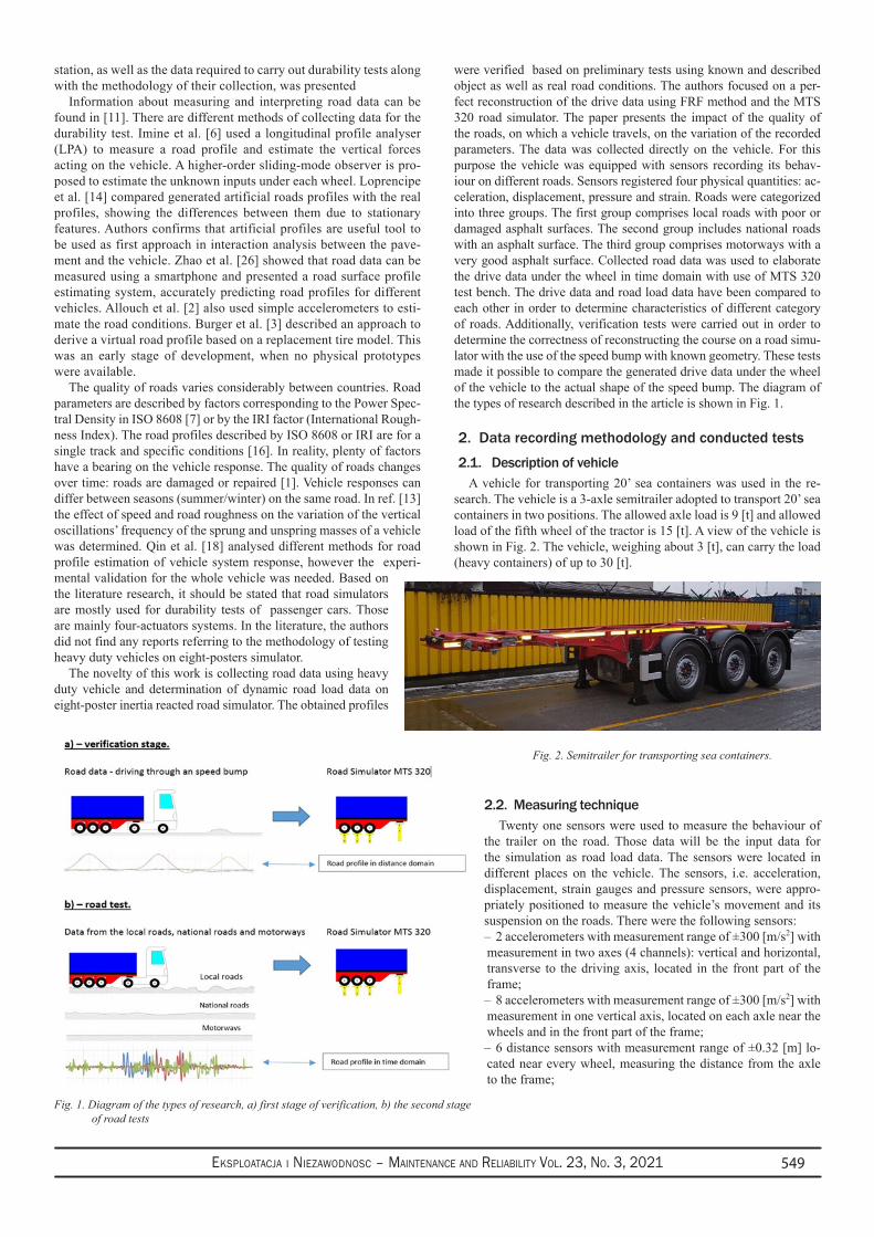
Eksploatacja i NiEzawodNosc – MaiNtENaNcE aNd REliability Vol. 23, No. 3, 2021 549
station, as well as the data required to carry out durability tests along with the methodology of their collection, was presented
Information about measuring and interpreting road data can be found in [11]. There are different methods of collecting data for the durability test. Imine et al. [6] used a longitudinal profile analyser (LPA) to measure a road profile and estimate the vertical forces acting on the vehicle. A higher-order sliding-mode observer is pro-posed to estimate the unknown inputs under each wheel. Loprencipe et al. [14] compared generated artificial roads profiles with the real profiles, showing the differences between them due to stationary features. Authors confirms that artificial profiles are useful tool to be used as first approach in interaction analysis between the pave-ment and the vehicle. Zhao et al. [26] showed that road data can be measured using a smartphone and presented a road surface profile estimating system, accurately predicting road profiles for different vehicles. Allouch et al. [2] also used simple accelerometers to esti-mate the road conditions. Burger et al. [3] described an approach to derive a virtual road profile based on a replacement tire model. This was an early stage of development, when no physical prototypes were available.
The quality of roads varies considerably between countries. Road parameters are described by factors corresponding to the Power Spec-tral Density in ISO 8608 [7] or by the IRI factor (International Rough-ness Index). The road profiles described by ISO 8608 or IRI are for a single track and specific conditions [16]. In reality, plenty of factors have a bearing on the vehicle response. The quality of roads changes over time: roads are damaged or repaired [1]. Vehicle responses can differ between seasons (summer/winter) on the same road. In ref. [13] the effect of speed and road roughness on the variation of the vertical oscillations’ frequency of the sprung and unspring masses of a vehicle was determined. Qin et al. [18] analysed different methods for road profile estimation of vehicle system response, however the experi-mental validation for the whole vehicle was needed. Based on the literature research, it should be stated that road simulators are mostly used for durability tests of passenger cars. Those are mainly four-actuators systems. In the literature, the authors did not find any reports referring to the methodology of testing heavy duty vehicles on eight-posters simulator.
The novelty of this work is collecting road data using heavy duty vehicle and determination of dynamic road load data on eight-poster inertia reacted road simulator. The obtained profiles
were verified based on preliminary tests using known and described object as well as real road conditions. The authors focused on a per-fect reconstruction of the drive data using FRF method and the MTS 320 road simulator. The paper presents the impact of the quality of the roads, on which a vehicle travels, on the variation of the recorded parameters. The data was collected directly on the vehicle. For this purpose the vehicle was equipped with sensors recording its behav-iour on different roads. Sensors registered four physical quantities: ac-celeration, displacement, pressure and strain. Roads were categorized into three groups. The first group comprises local roads with poor or damaged asphalt surfaces. The second group includes national roads with an asphalt surface. The third group comprises motorways with a very good asphalt surface. Collected road data was used to elaborate the drive data under the wheel in time domain with use of MTS 320 test bench. The drive data and road load data have been compared to each other in order to determine characteristics of different category of roads. Additionally, verification tests were carried out in order to determine the correctness of reconstructing the course on a road simu-lator with the use of the speed bump with known geometry. These tests made it possible to compare the generated drive data under the wheel of the vehicle to the actual shape of the speed bump. The diagram of the types of research described in the article is shown in Fig. 1.
2. Data recording methodology and conducted tests
2.1. Description of vehicleA vehicle for transporting 20’ sea containers was used in the re-
search. The vehicle is a 3-axle semitrailer adopted to transport 20’ sea containers in two positions. The allowed axle load is 9 [t] and allowed load of the fifth wheel of the tractor is 15 [t]. A view of the vehicle is shown in Fig. 2. The vehicle, weighing about 3 [t], can carry the load (heavy containers) of up to 30 [t].
Fig. 2. Semitrailer for transporting sea containers.
2.2. Measuring techniqueTwenty one sensors were used to measure the behaviour of
the trailer on the road. Those data will be the input data for the simulation as road load data. The sensors were located in different places on the vehicle. The sensors, i.e. acceleration, displacement, strain gauges and pressure sensors, were appro-priately positioned to measure the vehicle’s movement and its suspension on the roads. There were the following sensors:
2 accelerometers with measurement range of ±300 [m/s – 2] with measurement in two axes (4 channels): vertical and horizontal, transverse to the driving axis, located in the front part of the frame;
8 accelerometers with measurement range of ±300 [m/s – 2] with measurement in one vertical axis, located on each axle near the wheels and in the front part of the frame;
6 distance sensors with measurement range of ±0.32 [m] lo- –cated near every wheel, measuring the distance from the axle to the frame;
Fig. 1. Diagram of the types of research, a) first stage of verification, b) the second stage of road tests
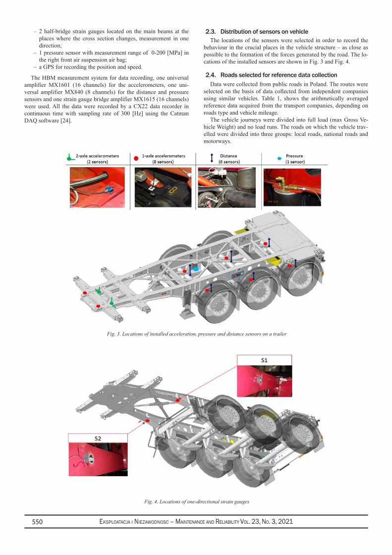
Eksploatacja i NiEzawodNosc – MaiNtENaNcE aNd REliability Vol. 23, No. 3, 2021550
2 half-bridge strain gauges located on the main beams at the –places where the cross section changes, measurement in one direction;1 pressure sensor with measurement range of 0-200 [MPa] in –the right front air suspension air bag;a GPS for recording the position and speed. –
The HBM measurement system for data recording, one universal amplifier MX1601 (16 channels) for the accelerometers, one uni-versal amplifier MX840 (8 channels) for the distance and pressure sensors and one strain gauge bridge amplifier MX1615 (16 channels) were used. All the data were recorded by a CX22 data recorder in continuous time with sampling rate of 300 [Hz] using the Catman DAQ software [24].
2.3. Distribution of sensors on vehicleThe locations of the sensors were selected in order to record the
behaviour in the crucial places in the vehicle structure – as close as possible to the formation of the forces generated by the road. The lo-cations of the installed sensors are shown in Fig. 3 and Fig. 4.
2.4. Roads selected for reference data collectionData were collected from public roads in Poland. The routes were
selected on the basis of data collected from independent companies using similar vehicles. Table 1, shows the arithmetically averaged reference data acquired from the transport companies, depending on roads type and vehicle mileage.
The vehicle journeys were divided into full load (max Gross Ve-hicle Weight) and no load runs. The roads on which the vehicle trav-elled were divided into three groups: local roads, national roads and motorways.
Fig. 3. Locations of installed acceleration, pressure and distance sensors on a trailer
Fig. 4. Locations of one-directional strain gauges
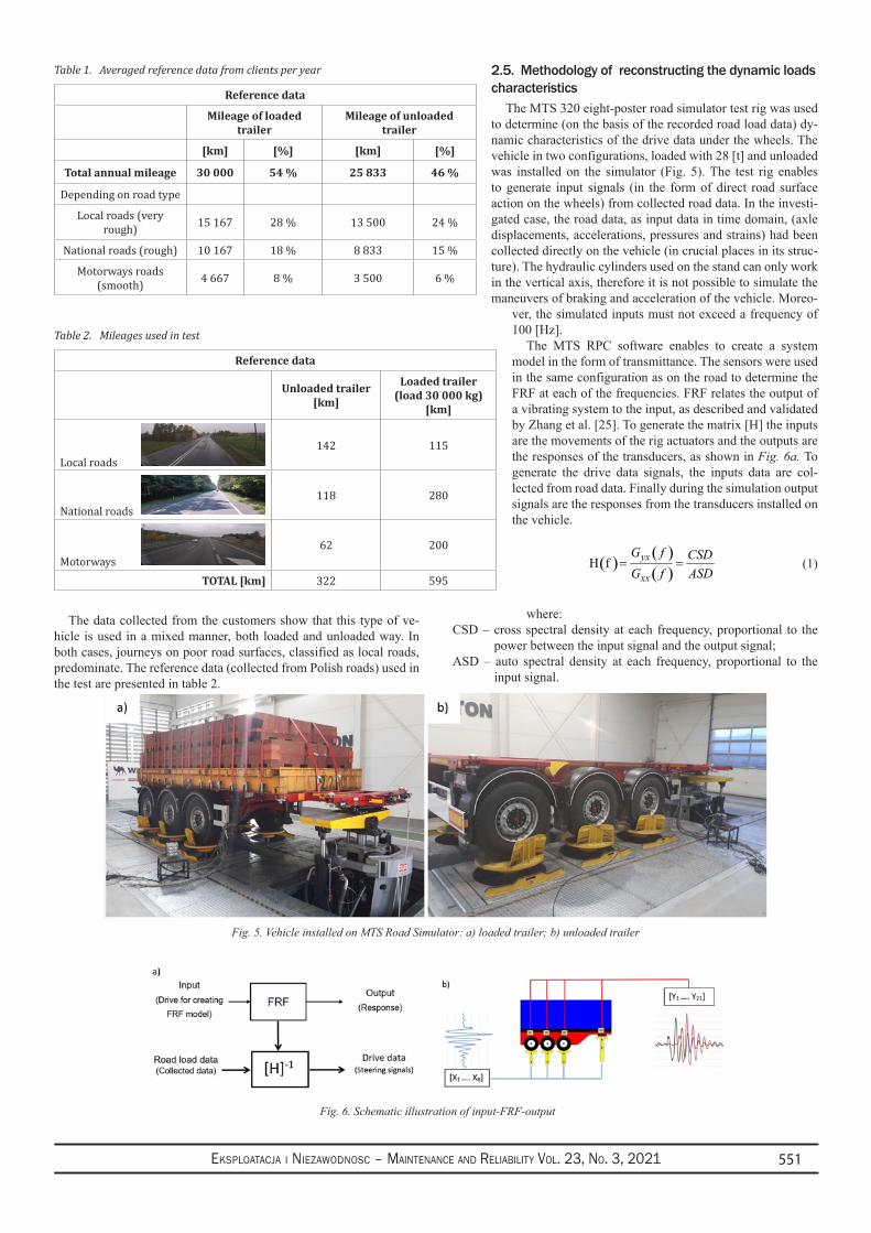
Eksploatacja i NiEzawodNosc – MaiNtENaNcE aNd REliability Vol. 23, No. 3, 2021 551
The data collected from the customers show that this type of ve-hicle is used in a mixed manner, both loaded and unloaded way. In both cases, journeys on poor road surfaces, classified as local roads, predominate. The reference data (collected from Polish roads) used in the test are presented in table 2.
2.5. Methodology of reconstructing the dynamic loads characteristics
The MTS 320 eight-poster road simulator test rig was used to determine (on the basis of the recorded road load data) dy-namic characteristics of the drive data under the wheels. The vehicle in two configurations, loaded with 28 [t] and unloaded was installed on the simulator (Fig. 5). The test rig enables to generate input signals (in the form of direct road surface action on the wheels) from collected road data. In the investi-gated case, the road data, as input data in time domain, (axle displacements, accelerations, pressures and strains) had been collected directly on the vehicle (in crucial places in its struc-ture). The hydraulic cylinders used on the stand can only work in the vertical axis, therefore it is not possible to simulate the maneuvers of braking and acceleration of the vehicle. Moreo-
ver, the simulated inputs must not exceed a frequency of 100 [Hz].
The MTS RPC software enables to create a system model in the form of transmittance. The sensors were used in the same configuration as on the road to determine the FRF at each of the frequencies. FRF relates the output of a vibrating system to the input, as described and validated by Zhang et al. [25]. To generate the matrix [H] the inputs are the movements of the rig actuators and the outputs are the responses of the transducers, as shown in Fig. 6a. To generate the drive data signals, the inputs data are col-lected from road data. Finally during the simulation output signals are the responses from the transducers installed on the vehicle.
( )( )( )
H f yx
xx
G f CSDG f ASD
= = (1)
where:CSD – cross spectral density at each frequency, proportional to the
power between the input signal and the output signal;ASD – auto spectral density at each frequency, proportional to the
input signal.
Table 1. Averaged reference data from clients per year
Reference data
Mileage of loaded trailer
Mileage of unloaded trailer
[km] [%] [km] [%]
Total annual mileage 30 000 54 % 25 833 46 %
Depending on road type
Local roads (very rough) 15 167 28 % 13 500 24 %
National roads (rough) 10 167 18 % 8 833 15 %
Motorways roads (smooth) 4 667 8 % 3 500 6 %
Table 2. Mileages used in test
Reference data
Unloaded trailer [km]
Loaded trailer (load 30 000 kg)
[km]
Local roads 142 115
National roads 118 280
Motorways 62 200
TOTAL [km] 322 595
Fig. 5. Vehicle installed on MTS Road Simulator: a) loaded trailer; b) unloaded trailer
Fig. 6. Schematic illustration of input-FRF-output
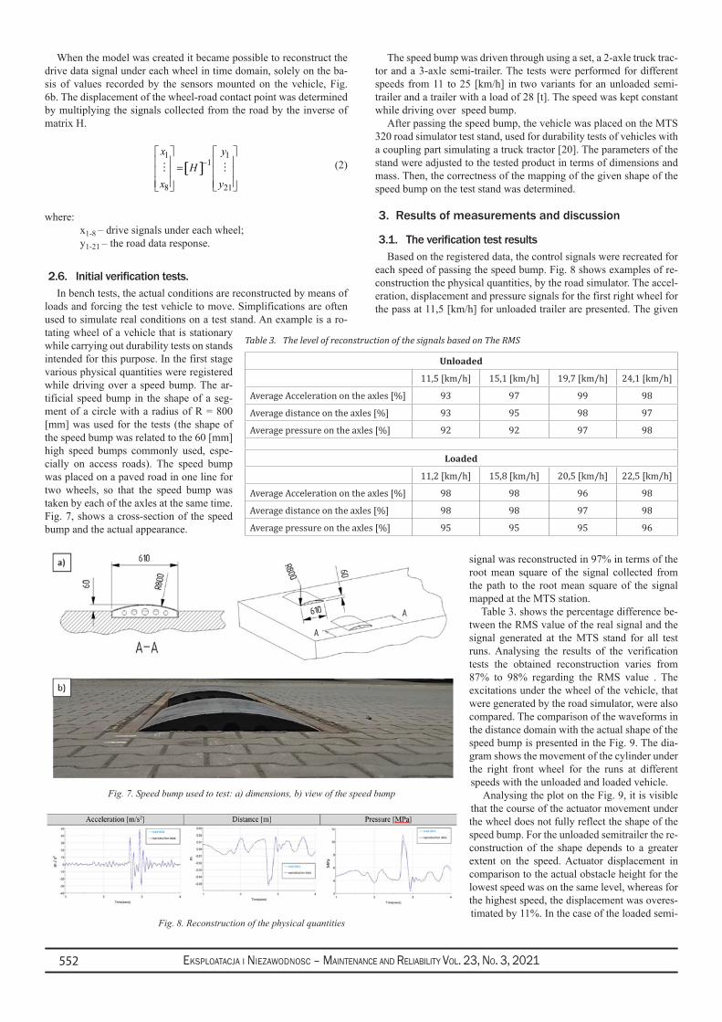
Eksploatacja i NiEzawodNosc – MaiNtENaNcE aNd REliability Vol. 23, No. 3, 2021552
When the model was created it became possible to reconstruct the drive data signal under each wheel in time domain, solely on the ba-sis of values recorded by the sensors mounted on the vehicle, Fig. 6b. The displacement of the wheel-road contact point was determined by multiplying the signals collected from the road by the inverse of matrix H.
[ ]1 1
1
8 21
x yH
x y
− =
(2)
where:x1-8 – drive signals under each wheel;y1-21 – the road data response.
2.6. Initialverificationtests.In bench tests, the actual conditions are reconstructed by means of
loads and forcing the test vehicle to move. Simplifications are often used to simulate real conditions on a test stand. An example is a ro-tating wheel of a vehicle that is stationary while carrying out durability tests on stands intended for this purpose. In the first stage various physical quantities were registered while driving over a speed bump. The ar-tificial speed bump in the shape of a seg-ment of a circle with a radius of R = 800 [mm] was used for the tests (the shape of the speed bump was related to the 60 [mm] high speed bumps commonly used, espe-cially on access roads). The speed bump was placed on a paved road in one line for two wheels, so that the speed bump was taken by each of the axles at the same time. Fig. 7, shows a cross-section of the speed bump and the actual appearance.
The speed bump was driven through using a set, a 2-axle truck trac-tor and a 3-axle semi-trailer. The tests were performed for different speeds from 11 to 25 [km/h] in two variants for an unloaded semi-trailer and a trailer with a load of 28 [t]. The speed was kept constant while driving over speed bump.
After passing the speed bump, the vehicle was placed on the MTS 320 road simulator test stand, used for durability tests of vehicles with a coupling part simulating a truck tractor [20]. The parameters of the stand were adjusted to the tested product in terms of dimensions and mass. Then, the correctness of the mapping of the given shape of the speed bump on the test stand was determined.
3. Results of measurements and discussion
3.1. TheverificationtestresultsBased on the registered data, the control signals were recreated for
each speed of passing the speed bump. Fig. 8 shows examples of re-construction the physical quantities, by the road simulator. The accel-eration, displacement and pressure signals for the first right wheel for the pass at 11,5 [km/h] for unloaded trailer are presented. The given
signal was reconstructed in 97% in terms of the root mean square of the signal collected from the path to the root mean square of the signal mapped at the MTS station.
Table 3. shows the percentage difference be-tween the RMS value of the real signal and the signal generated at the MTS stand for all test runs. Analysing the results of the verification tests the obtained reconstruction varies from 87% to 98% regarding the RMS value . The excitations under the wheel of the vehicle, that were generated by the road simulator, were also compared. The comparison of the waveforms in the distance domain with the actual shape of the speed bump is presented in the Fig. 9. The dia-gram shows the movement of the cylinder under the right front wheel for the runs at different speeds with the unloaded and loaded vehicle.
Analysing the plot on the Fig. 9, it is visible that the course of the actuator movement under the wheel does not fully reflect the shape of the speed bump. For the unloaded semitrailer the re-construction of the shape depends to a greater extent on the speed. Actuator displacement in comparison to the actual obstacle height for the lowest speed was on the same level, whereas for the highest speed, the displacement was overes-timated by 11%. In the case of the loaded semi-
Table 3. The level of reconstruction of the signals based on The RMS
Unloaded
11,5 [km/h] 15,1 [km/h] 19,7 [km/h] 24,1 [km/h]
Average Acceleration on the axles [%] 93 97 99 98
Average distance on the axles [%] 93 95 98 97
Average pressure on the axles [%] 92 92 97 98
Loaded
11,2 [km/h] 15,8 [km/h] 20,5 [km/h] 22,5 [km/h]
Average Acceleration on the axles [%] 98 98 96 98
Average distance on the axles [%] 98 98 97 98
Average pressure on the axles [%] 95 95 95 96
Fig. 7. Speed bump used to test: a) dimensions, b) view of the speed bump
Fig. 8. Reconstruction of the physical quantities
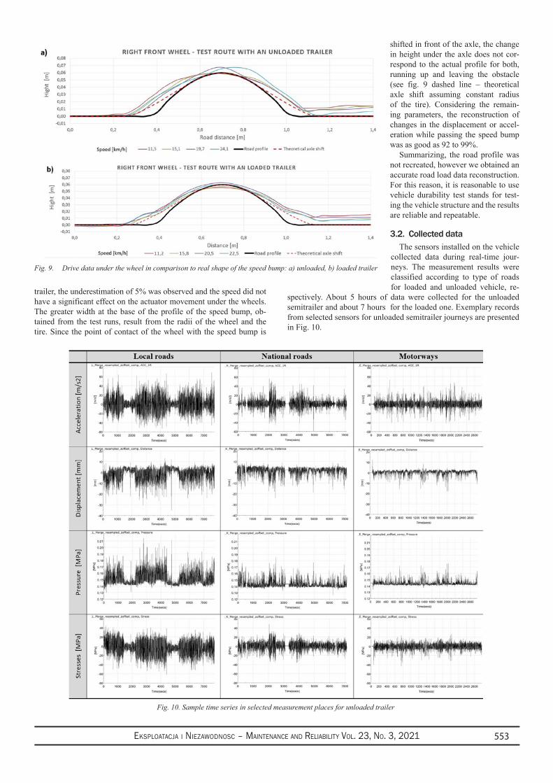
Eksploatacja i NiEzawodNosc – MaiNtENaNcE aNd REliability Vol. 23, No. 3, 2021 553
trailer, the underestimation of 5% was observed and the speed did not have a significant effect on the actuator movement under the wheels. The greater width at the base of the profile of the speed bump, ob-tained from the test runs, result from the radii of the wheel and the tire. Since the point of contact of the wheel with the speed bump is
shifted in front of the axle, the change in height under the axle does not cor-respond to the actual profile for both, running up and leaving the obstacle (see fig. 9 dashed line – theoretical axle shift assuming constant radius of the tire). Considering the remain-ing parameters, the reconstruction of changes in the displacement or accel-eration while passing the speed bump was as good as 92 to 99%.
Summarizing, the road profile was not recreated, however we obtained an accurate road load data reconstruction. For this reason, it is reasonable to use vehicle durability test stands for test-ing the vehicle structure and the results are reliable and repeatable.
3.2. Collected dataThe sensors installed on the vehicle
collected data during real-time jour-neys. The measurement results were classified according to type of roads for loaded and unloaded vehicle, re-
spectively. About 5 hours of data were collected for the unloaded semitrailer and about 7 hours for the loaded one. Exemplary records from selected sensors for unloaded semitrailer journeys are presented in Fig. 10.
Fig. 9. Drive data under the wheel in comparison to real shape of the speed bump: a) unloaded, b) loaded trailer
Fig. 10. Sample time series in selected measurement places for unloaded trailer
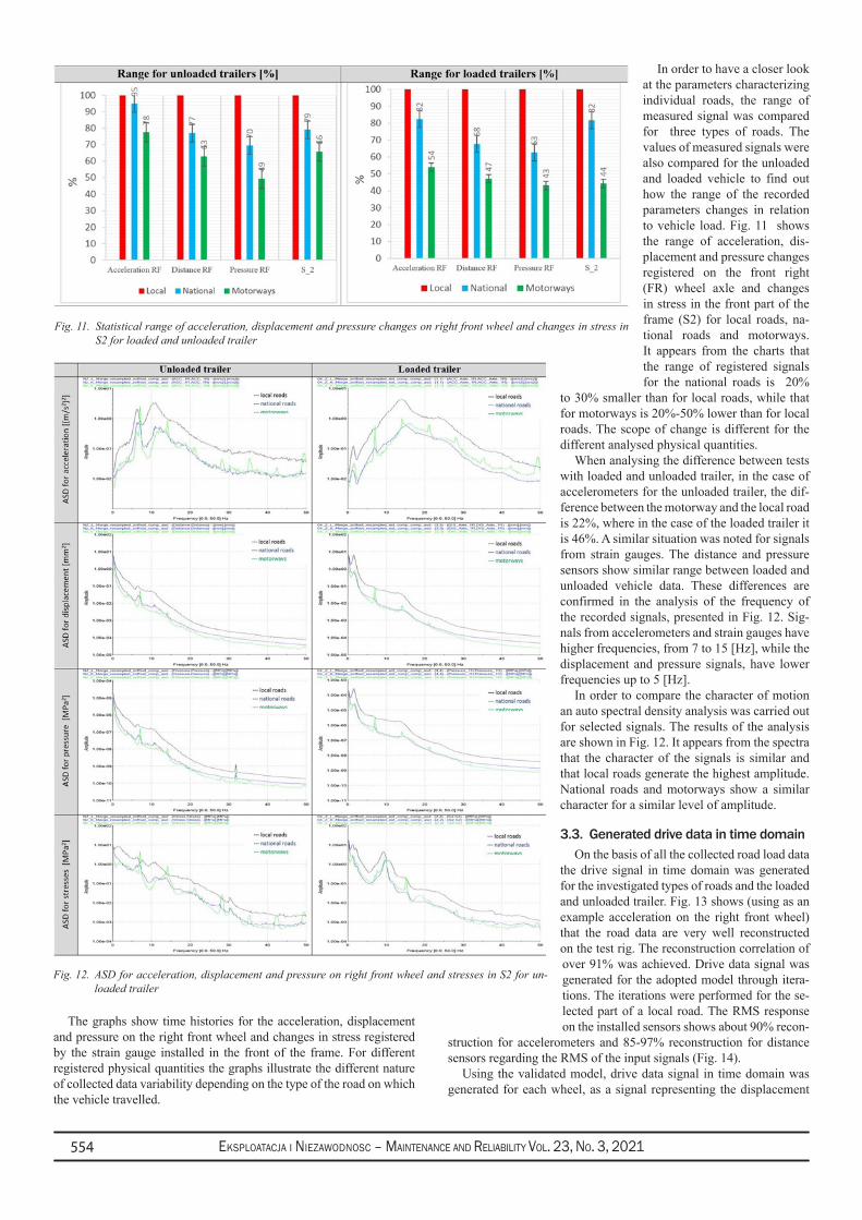
Eksploatacja i NiEzawodNosc – MaiNtENaNcE aNd REliability Vol. 23, No. 3, 2021554
The graphs show time histories for the acceleration, displacement and pressure on the right front wheel and changes in stress registered by the strain gauge installed in the front of the frame. For different registered physical quantities the graphs illustrate the different nature of collected data variability depending on the type of the road on which the vehicle travelled.
In order to have a closer look at the parameters characterizing individual roads, the range of measured signal was compared for three types of roads. The values of measured signals were also compared for the unloaded and loaded vehicle to find out how the range of the recorded parameters changes in relation to vehicle load. Fig. 11 shows the range of acceleration, dis-placement and pressure changes registered on the front right (FR) wheel axle and changes in stress in the front part of the frame (S2) for local roads, na-tional roads and motorways. It appears from the charts that the range of registered signals for the national roads is 20%
to 30% smaller than for local roads, while that for motorways is 20%-50% lower than for local roads. The scope of change is different for the different analysed physical quantities.
When analysing the difference between tests with loaded and unloaded trailer, in the case of accelerometers for the unloaded trailer, the dif-ference between the motorway and the local road is 22%, where in the case of the loaded trailer it is 46%. A similar situation was noted for signals from strain gauges. The distance and pressure sensors show similar range between loaded and unloaded vehicle data. These differences are confirmed in the analysis of the frequency of the recorded signals, presented in Fig. 12. Sig-nals from accelerometers and strain gauges have higher frequencies, from 7 to 15 [Hz], while the displacement and pressure signals, have lower frequencies up to 5 [Hz].
In order to compare the character of motion an auto spectral density analysis was carried out for selected signals. The results of the analysis are shown in Fig. 12. It appears from the spectra that the character of the signals is similar and that local roads generate the highest amplitude. National roads and motorways show a similar character for a similar level of amplitude.
3.3. Generated drive data in time domainOn the basis of all the collected road load data
the drive signal in time domain was generated for the investigated types of roads and the loaded and unloaded trailer. Fig. 13 shows (using as an example acceleration on the right front wheel) that the road data are very well reconstructed on the test rig. The reconstruction correlation of over 91% was achieved. Drive data signal was generated for the adopted model through itera-tions. The iterations were performed for the se-lected part of a local road. The RMS response on the installed sensors shows about 90% recon-
struction for accelerometers and 85-97% reconstruction for distance sensors regarding the RMS of the input signals (Fig. 14).
Using the validated model, drive data signal in time domain was generated for each wheel, as a signal representing the displacement
Fig. 11. Statistical range of acceleration, displacement and pressure changes on right front wheel and changes in stress in S2 for loaded and unloaded trailer
Fig. 12. ASD for acceleration, displacement and pressure on right front wheel and stresses in S2 for un-loaded trailer
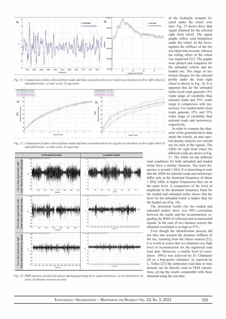
Eksploatacja i NiEzawodNosc – MaiNtENaNcE aNd REliability Vol. 23, No. 3, 2021 555
of the hydraulic actuator lo-cated under the wheel over time. Fig. 15 shows drive data signal obtained for the selected right front wheel. The signal graphs reflect road bumpiness under the wheel. In the inves-tigation the stiffness of the tire was taken into account, whereas the rolling effect of the wheel was neglected [21]. The graphs were plotted and compared for the unloaded vehicle and the loaded one. The range of sta-tistical changes for the selected profile under the front right wheel is shown in Fig. 16. It is apparent that for the unloaded trailer local roads generate 15% wider range of variability than national roads and 35% wider range in comparison with mo-torways. For loaded trailer local roads generate 25% and 55% wider range of variability than national roads and motorways, respectively.
In order to compare the char-acter of the generated drive data under the wheels, an auto spec-tral density analysis was carried out for each of the signals. The ASDs for right front wheel for different roads are shown in Fig. 17. The ASDs for the different
road conditions for both unloaded and loaded trailer have a similar character. The main fre-quency is around 1 [Hz]. It is interesting to note that the ASDs for national roads and motorways differ only at the dominant frequency of about 1 [Hz] while at higher frequencies they are at the same level. A comparison of the level of amplitude in the dominant frequency band for the loaded and unloaded trailer shows that the level for the unloaded trailer is higher than for the loaded one (Fig. 18).
The presented results (for the loaded and unloaded trailer) show over 90% correlation between the reality and the reconstruction, re-garding the RMS of collected and reconstructed signals. In the case of two distance sensors the obtained correlation is as high as 97%.
Even though the identification process did not take into account the dynamic stiffness of the tire, resulting from the wheel rotation [21], it is worth to notice that we obtained very high level of reconstruction for the registered road load data. Moreover, a similar level of corre-lation (98%) was achieved by D. Chindamo [4] on a four-poster simulator. As reported by L. Telloa [23] the elaborated road data in time domain can be directly used in FEM calcula-tions, giving the results comparable with those obtained using the real data.
Fig. 13. Comparison of data collected from roads and data reconstructed on test rig for acceleration on first right wheel of unloaded trailer: a) time series. b) spectrum
Fig. 13. Comparison of data collected from roads and data reconstructed on test rig for acceleration on first right wheel of unloaded trailer: a) time series. b) spectrum
Fig. 14. RMS response of selected sensors during generating drive signal iterations: a) accelerometers on axles, b) distance sensors on axles
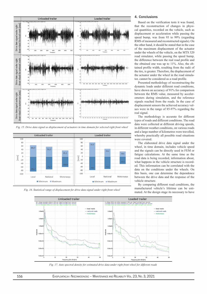
Eksploatacja i NiEzawodNosc – MaiNtENaNcE aNd REliability Vol. 23, No. 3, 2021556
4. ConclusionsBased on the verification tests it was found,
that the reconstruction of changes in physi-cal quantities, recorded on the vehicle, such as displacement or acceleration while passing the speed bump, was from 93 to 99% (regarding RMS of measured and reconstructed signals). On the other hand, it should be stated that in the case of the maximum displacement of the actuator under the wheels of the vehicle, on the MTS 320 road simulator, while passing the speed bump, the difference between the real road profile and the obtained one was up to 11%. Also, the ob-tained profile width, resulting from the radii of the tire, is greater. Therefore, the displacement of the actuator under the wheel in the road simula-tor, cannot be considered as a road profile.
Presented methodology of reconstructing the dynamic loads under different road conditions, have shown an accuracy of 91% for comparison between the RMS value, measured by acceler-ometers during simulation, and the reference signals reached from the roads. In the case of displacement sensors the achieved accuracy val-ues were in the range of 85-97% regarding the real signal.
The methodology is accurate for different types of roads and different conditions. The road data were collected at different driving speeds, in different weather conditions, on various roads and a large number of kilometres were travelled, whereby practically all possible road situations were covered.
The elaborated drive data signal under the wheel, in time domain, includes vehicle speed and the signals can be directly used in FEM or fatigue calculations. At the same time as the road data is being recorded, information about, what happens in the vehicle structure is record-ed. This information can be correlated with the data on the conditions under the wheels. On this basis, one can determine the dependence between the drive data and the response of the vehicle structure.
By comparing different road conditions, the manufactured vehicle’s lifetime can be esti-mated. At the design stage its necessary to have
Fig. 15. Drive data signal as displacement of actuators in time domain for selected right front wheel
Fig. 16. Statistical range of displacement for drive data signal under right front wheel
Fig. 17. Auto spectral density for estimated drive data under right front wheel for different roads
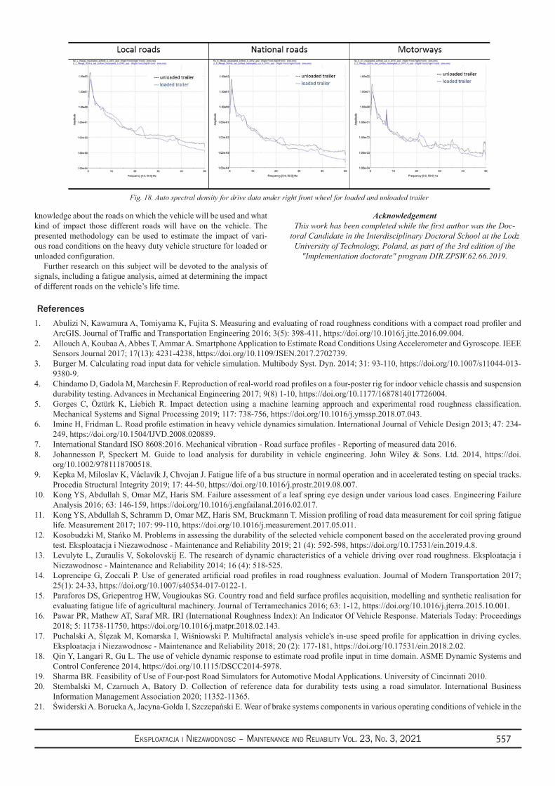
Eksploatacja i NiEzawodNosc – MaiNtENaNcE aNd REliability Vol. 23, No. 3, 2021 557
knowledge about the roads on which the vehicle will be used and what kind of impact those different roads will have on the vehicle. The presented methodology can be used to estimate the impact of vari-ous road conditions on the heavy duty vehicle structure for loaded or unloaded configuration.
Further research on this subject will be devoted to the analysis of signals, including a fatigue analysis, aimed at determining the impact of different roads on the vehicle’s life time.
AcknowledgementThis work has been completed while the first author was the Doc-
toral Candidate in the Interdisciplinary Doctoral School at the Lodz University of Technology, Poland, as part of the 3rd edition of the
"Implementation doctorate" program DIR.ZPSW.62.66.2019.
Fig. 18. Auto spectral density for drive data under right front wheel for loaded and unloaded trailer
References1. Abulizi N, Kawamura A, Tomiyama K, Fujita S. Measuring and evaluating of road roughness conditions with a compact road profiler and
ArcGIS. Journal of Traffic and Transportation Engineering 2016; 3(5): 398-411, https://doi.org/10.1016/j.jtte.2016.09.004.2. Allouch A, Koubaa A, Abbes T, Ammar A. Smartphone Application to Estimate Road Conditions Using Accelerometer and Gyroscope. IEEE
Sensors Journal 2017; 17(13): 4231-4238, https://doi.org/10.1109/JSEN.2017.2702739.3. Burger M. Calculating road input data for vehicle simulation. Multibody Syst. Dyn. 2014; 31: 93-110, https://doi.org/10.1007/s11044-013-
9380-9.4. Chindamo D, Gadola M, Marchesin F. Reproduction of real-world road profiles on a four-poster rig for indoor vehicle chassis and suspension
durability testing. Advances in Mechanical Engineering 2017; 9(8) 1-10, https://doi.org/10.1177/1687814017726004.5. Gorges C, Öztürk K, Liebich R. Impact detection using a machine learning approach and experimental road roughness classification.
Mechanical Systems and Signal Processing 2019; 117: 738-756, https://doi.org/10.1016/j.ymssp.2018.07.043.6. Imine H, Fridman L. Road profile estimation in heavy vehicle dynamics simulation. International Journal of Vehicle Design 2013; 47: 234-
249, https://doi.org/10.1504/IJVD.2008.020889.7. International Standard ISO 8608:2016. Mechanical vibration - Road surface profiles - Reporting of measured data 2016.8. Johannesson P, Speckert M. Guide to load analysis for durability in vehicle engineering. John Wiley & Sons. Ltd. 2014, https://doi.
org/10.1002/9781118700518.9. Kepka M, Miloslav K, Václavík J, Chvojan J. Fatigue life of a bus structure in normal operation and in accelerated testing on special tracks.
Procedia Structural Integrity 2019; 17: 44-50, https://doi.org/10.1016/j.prostr.2019.08.007.10. Kong YS, Abdullah S, Omar MZ, Haris SM. Failure assessment of a leaf spring eye design under various load cases. Engineering Failure
Analysis 2016; 63: 146-159, https://doi.org/10.1016/j.engfailanal.2016.02.017.11. Kong YS, Abdullah S, Schramm D, Omar MZ, Haris SM, Bruckmann T. Mission profiling of road data measurement for coil spring fatigue
life. Measurement 2017; 107: 99-110, https://doi.org/10.1016/j.measurement.2017.05.011.12. Kosobudzki M, Stańko M. Problems in assessing the durability of the selected vehicle component based on the accelerated proving ground
test. Eksploatacja i Niezawodnosc - Maintenance and Reliability 2019; 21 (4): 592-598, https://doi.org/10.17531/ein.2019.4.8.13. Levulyte L, Zuraulis V, Sokolovskij E. The research of dynamic characteristics of a vehicle driving over road roughness. Eksploatacja i
Niezawodnosc - Maintenance and Reliability 2014; 16 (4): 518-525.14. Loprencipe G, Zoccali P. Use of generated artificial road profiles in road roughness evaluation. Journal of Modern Transportation 2017;
25(1): 24-33, https://doi.org/10.1007/s40534-017-0122-1.15. Paraforos DS, Griepentrog HW, Vougioukas SG. Country road and field surface profiles acquisition, modelling and synthetic realisation for
evaluating fatigue life of agricultural machinery. Journal of Terramechanics 2016; 63: 1-12, https://doi.org/10.1016/j.jterra.2015.10.001.16. Pawar PR, Mathew AT, Saraf MR. IRI (International Roughness Index): An Indicator Of Vehicle Response. Materials Today: Proceedings
2018; 5: 11738-11750, https://doi.org/10.1016/j.matpr.2018.02.143.17. Puchalski A, Ślęzak M, Komarska I, Wiśniowski P. Multifractal analysis vehicle's in-use speed profile for applicattion in driving cycles.
Eksploatacja i Niezawodnosc - Maintenance and Reliability 2018; 20 (2): 177-181, https://doi.org/10.17531/ein.2018.2.02.18. Qin Y, Langari R, Gu L. The use of vehicle dynamic response to estimate road profile input in time domain. ASME Dynamic Systems and
Control Conference 2014, https://doi.org/10.1115/DSCC2014-5978.19. Sharma BR. Feasibility of Use of Four-post Road Simulators for Automotive Modal Applications. University of Cincinnati 2010.20. Stembalski M, Czarnuch A, Batory D. Collection of reference data for durability tests using a road simulator. International Business
Information Management Association 2020; 11352-11365.21. Świderski A. Borucka A, Jacyna-Gołda I, Szczepański E. Wear of brake systems components in various operating conditions of vehicle in the

Eksploatacja i NiEzawodNosc – MaiNtENaNcE aNd REliability Vol. 23, No. 3, 2021558
transport company. Eksploatacja i Niezawodnosc - Maintenance and Reliability 2019; 21 (1): 1-9, https://doi.org/10.17531/ein.2019.1.1.22. Steven R. Haeg. Dynamic FRF Response Comparison for Rolling and Non-rolling Tires. MTS Systems Corporation 2014.23. Telloa L, Castejona L, Malona H, Valladaresa D, Luqueb P, Mantarasb A. Development of a fatigue life prediction methodology for
welded steel semi-trailer components based on a new criterion. Engineering Failure Analysis 2020; 104268: 1-26, https://doi.org/10.1016/j.engfailanal.2019.104268.
24. Tianshuang Q. Signal Processing and Data Analysis. De Gruyter 2018.25. Zhang Q, Hou J, Duan Z, Jankowski Ł, Hu X. Road Roughness Estimation Based on the Vehicle Frequency Response Function. Actuators
2021; 10(5): 89, https://doi.org/10.3390/act10050089.26. Zhao B, Nagayama T, Xue K. Road profile estimation, and its numerical and experimental validation, by smartphone measurement of the
dynamic responses of an ordinary vehicle. Journal of Sound and Vibration 2019; 457: 92-117, https://doi.org/10.1016/j.jsv.2019.05.015.
Eksploatacja i NiEzawodNosc – MaiNtENaNcE aNd REliability Vol. 23, No. 3, 2021 559
E-mail addresses:
Eksploatacja i Niezawodnosc – Maintenance and ReliabilityVolume 23 (2021), Issue 3
journal homepage: http://www.ein.org.pl
Indexed by:Enhancing machining accuracy reliability of multi-axis CNC machine tools using an advanced importance sampling methodZhiming Wang a, Hao Yuan a
a School of Mechanical and Electronic Engineering, Lanzhou University of Technology, Lanzhou 730050, China
Wang Z, Yuan H. Enhancing machining accuracy reliability of multi-axis CNC machine tools using an advanced importance sampling me-thod. Eksploatacja i Niezawodnosc – Maintenance and Reliability 2021; 23 (3): 559–568, http://doi.org/10.17531/ein.2021.3.17.
Article citation info:
The purpose of this paper is to propose a general precision allocation method to improve machining performance of CNC machine tools based on certain design requirements. A comprehensive error model of machine tools is established by using the differential motion relation of coordinate frames. Based on the comprehensive error model, a reliability model is established by updating the primary reliability with an advanced importance sampling method, which is used to predict the machining accuracy reliability of machine tools. Be-sides, to identify and optimize geometric error parameters which have a great influence on machining accuracy reliability of machine tools, the sensitivity analysis of machining ac-curacy is carried out by improved first-order second-moment method. Taking a large CNC gantry guide rail grinder as an example, the optimization results show that the method is effective and can realize reliability optimization of machining accuracy.
Highlights Abstract
An accuracy allocation method for CNC machine • tools is proposed.
The error is presented by using the differential • motion matrix and reliability theory.
The machining accuracy reliability is given by an • advanced importance sampling method.
The effectiveness is validated by a CNC grinding • machine.
precision allocation, comprehensive error, machining accuracy reliability, sensitivity analy-sis, advanced importance sampling method.
Keywords
This is an open access article under the CC BY license (https://creativecommons.org/licenses/by/4.0/)
Z. Wang - [email protected], H. Yuan - [email protected]
Nomenclatureδxx Positioning error of the X-axisδyx Y direction of straightness error of the X-axisδzx Z direction of straightness error of the X-axisεxx Roll error of the X-axisεyx Pitch error of the X-axisεzx Yaw error of the X-axisδxy X direction of straightness error of the Y-axisδyy Positioning error of the Y-axisδzy Z direction of straightness error of the Y-axisεxy Pitch error of the Y-axisεyy Roll error of the Y-axisεzy Yaw error of the Y-axisδxz X direction of straightness error of the Z-axisδyz Y direction of straightness error of the Z-axisδzz Positioning error of the Z-axisεxz Pitch error of the Z-axisεyz Yaw error of the Z-axisεzz Roll error of the Z-axisSxz X and Z-axis perpendicularity errorSyz Y and Z-axis perpendicularity errorSxy X and Y-axis perpendicularity error
1. IntroductionCNC machine tools integrate many technologies, such as accuracy
machinery, electronics, electric drag, automatic control, automatic detection, fault diagnosis, and computer. It is a typical mechatronics product with high accuracy and efficiency [22]. Machining accuracy is critical to the quality and performance of machine tools and it is the first consideration of any manufacturer [20]. Machining accuracy reli-ability is the ability for machine tools can work normally to achieve the corresponding machining accuracy under specified conditions [14]. Its main influencing factors include geometric errors, thermal errors and cutting force errors, etc. Geometric errors and thermal er-rors are the main influencing factors, accounting for 45%-65% of the total errors. The higher the accuracy of machine tools, the bigger the proportion of geometric errors and thermal errors [12]. When the tem-perature changes to a stable state, the impact of geometric errors are the largest, accounting for about 40% of the total errors [5]. Large CNC gantry rail grinder has a wide range of travel and is suitable for heavy machinery, ships, and metallurgical equipment. This paper takes it as an example to analyze the relationship between geometric errors of components of the grinder and the reliability of grinding ac-curacy.
The accuracy design of machine tools includes two aspects: ac-curacy prediction and accuracy allocation [10]. Accuracy prediction
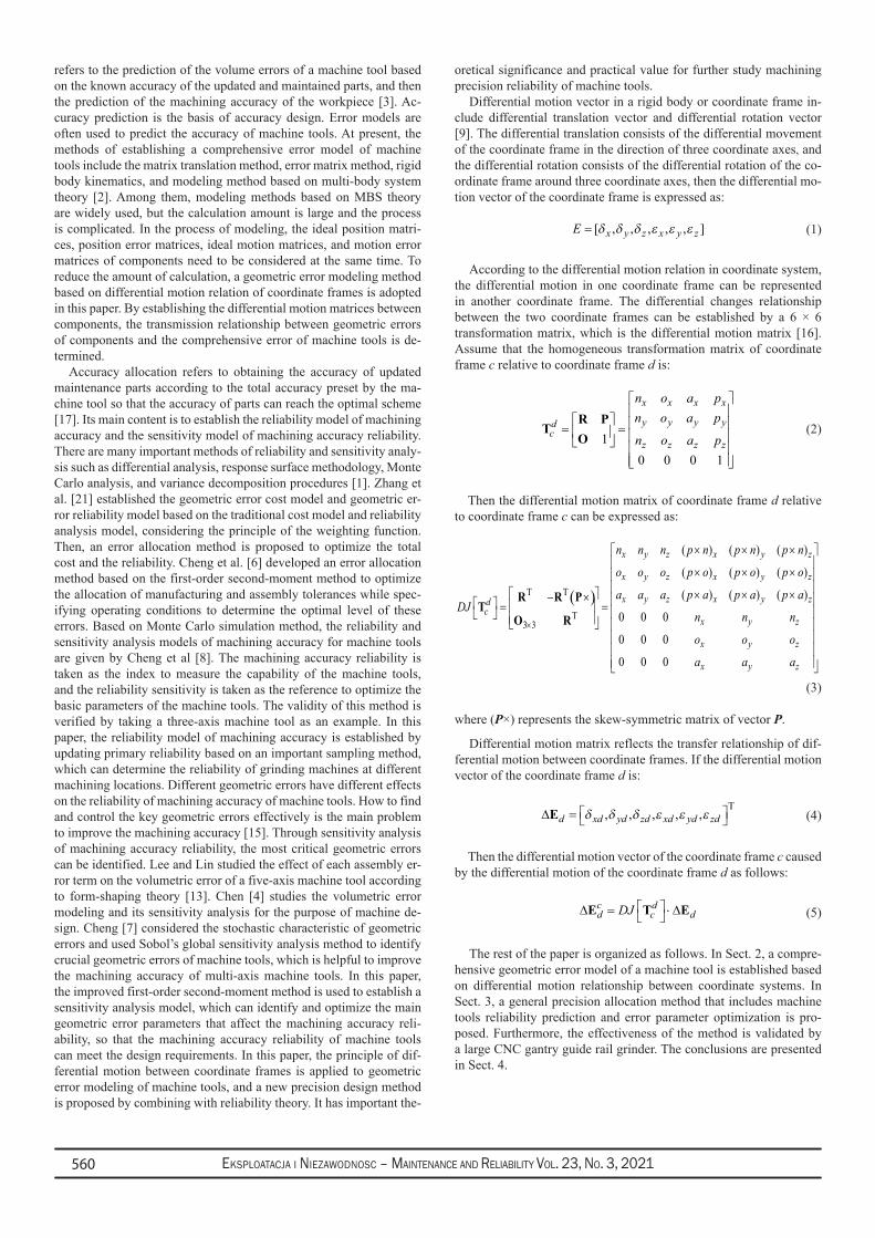
Eksploatacja i NiEzawodNosc – MaiNtENaNcE aNd REliability Vol. 23, No. 3, 2021560
refers to the prediction of the volume errors of a machine tool based on the known accuracy of the updated and maintained parts, and then the prediction of the machining accuracy of the workpiece [3]. Ac-curacy prediction is the basis of accuracy design. Error models are often used to predict the accuracy of machine tools. At present, the methods of establishing a comprehensive error model of machine tools include the matrix translation method, error matrix method, rigid body kinematics, and modeling method based on multi-body system theory [2]. Among them, modeling methods based on MBS theory are widely used, but the calculation amount is large and the process is complicated. In the process of modeling, the ideal position matri-ces, position error matrices, ideal motion matrices, and motion error matrices of components need to be considered at the same time. To reduce the amount of calculation, a geometric error modeling method based on differential motion relation of coordinate frames is adopted in this paper. By establishing the differential motion matrices between components, the transmission relationship between geometric errors of components and the comprehensive error of machine tools is de-termined.
Accuracy allocation refers to obtaining the accuracy of updated maintenance parts according to the total accuracy preset by the ma-chine tool so that the accuracy of parts can reach the optimal scheme [17]. Its main content is to establish the reliability model of machining accuracy and the sensitivity model of machining accuracy reliability. There are many important methods of reliability and sensitivity analy-sis such as differential analysis, response surface methodology, Monte Carlo analysis, and variance decomposition procedures [1]. Zhang et al. [21] established the geometric error cost model and geometric er-ror reliability model based on the traditional cost model and reliability analysis model, considering the principle of the weighting function. Then, an error allocation method is proposed to optimize the total cost and the reliability. Cheng et al. [6] developed an error allocation method based on the first-order second-moment method to optimize the allocation of manufacturing and assembly tolerances while spec-ifying operating conditions to determine the optimal level of these errors. Based on Monte Carlo simulation method, the reliability and sensitivity analysis models of machining accuracy for machine tools are given by Cheng et al [8]. The machining accuracy reliability is taken as the index to measure the capability of the machine tools, and the reliability sensitivity is taken as the reference to optimize the basic parameters of the machine tools. The validity of this method is verified by taking a three-axis machine tool as an example. In this paper, the reliability model of machining accuracy is established by updating primary reliability based on an important sampling method, which can determine the reliability of grinding machines at different machining locations. Different geometric errors have different effects on the reliability of machining accuracy of machine tools. How to find and control the key geometric errors effectively is the main problem to improve the machining accuracy [15]. Through sensitivity analysis of machining accuracy reliability, the most critical geometric errors can be identified. Lee and Lin studied the effect of each assembly er-ror term on the volumetric error of a five-axis machine tool according to form-shaping theory [13]. Chen [4] studies the volumetric error modeling and its sensitivity analysis for the purpose of machine de-sign. Cheng [7] considered the stochastic characteristic of geometric errors and used Sobol’s global sensitivity analysis method to identify crucial geometric errors of machine tools, which is helpful to improve the machining accuracy of multi-axis machine tools. In this paper, the improved first-order second-moment method is used to establish a sensitivity analysis model, which can identify and optimize the main geometric error parameters that affect the machining accuracy reli-ability, so that the machining accuracy reliability of machine tools can meet the design requirements. In this paper, the principle of dif-ferential motion between coordinate frames is applied to geometric error modeling of machine tools, and a new precision design method is proposed by combining with reliability theory. It has important the-
oretical significance and practical value for further study machining precision reliability of machine tools.
Differential motion vector in a rigid body or coordinate frame in-clude differential translation vector and differential rotation vector [9]. The differential translation consists of the differential movement of the coordinate frame in the direction of three coordinate axes, and the differential rotation consists of the differential rotation of the co-ordinate frame around three coordinate axes, then the differential mo-tion vector of the coordinate frame is expressed as:
E x y z x y z= [ , , , , , ]δ δ δ ε ε ε (1)
According to the differential motion relation in coordinate system, the differential motion in one coordinate frame can be represented in another coordinate frame. The differential changes relationship between the two coordinate frames can be established by a 6 × 6 transformation matrix, which is the differential motion matrix [16]. Assume that the homogeneous transformation matrix of coordinate frame c relative to coordinate frame d is:
TR POc
d
x x x x
y y y y
z z z z
n o a pn o a p
n o a p=
=
10 0 0 1
(2)
Then the differential motion matrix of coordinate frame d relative to coordinate frame c can be expressed as:
( )T T
T3 3
( ) ( ) ( )
( ) ( ) ( )
( ) ( ) ( )
0 0 0
0 0 0
0 0 0
x y z x y z
x y z x y z
x y z x y zdc
x y z
x y z
x y z
n n n p n p n p n
o o o p o p o p o
a a a p a p a p aDJ
n n n
o o o
a a a
×
× × ×
× × × × × ×− × = =
R R PT
O R
(3)
where (P×) represents the skew-symmetric matrix of vector P.
Differential motion matrix reflects the transfer relationship of dif-ferential motion between coordinate frames. If the differential motion vector of the coordinate frame d is:
∆Ed xd yd zd xd yd zd= δ δ δ ε ε ε, , , , ,T
(4)
Then the differential motion vector of the coordinate frame c caused by the differential motion of the coordinate frame d as follows:
∆ ∆E T Edc
cd
dDJ=
⋅ (5)
The rest of the paper is organized as follows. In Sect. 2, a compre-hensive geometric error model of a machine tool is established based on differential motion relationship between coordinate systems. In Sect. 3, a general precision allocation method that includes machine tools reliability prediction and error parameter optimization is pro-posed. Furthermore, the effectiveness of the method is validated by a large CNC gantry guide rail grinder. The conclusions are presented in Sect. 4.

Eksploatacja i NiEzawodNosc – MaiNtENaNcE aNd REliability Vol. 23, No. 3, 2021 561
2. Geometric error modeling of machine tool based on the differential motion relation of coordinate frames
2.1. Differential motion matrix of a machine toolWhen the differential transformation between coordinate frames is
applied to geometric error modeling of a machine tool, the influence of geometric errors of various parts of a machine tool on machining accuracy can be obtained and geometric error model can be estab-lished. Taking a large CNC gantry rail grinder as an example, the geo-metric error modeling process of this machine tool is presented using differential motion relation of coordinate frames.
The basis of geometric error modeling is to obtain the homogene-ous transformation matrices between each component of the machine tool. Firstly, the homogeneous transformation matrices of tool relative to any other component are established according to the order of open kinematic chain of the machine tool. The structure of the large CNC gantry rail grinder is shown in Figure 1 and the corresponding topo-logical structure is shown in Figure 2. The order of open kinematic chain is working table — X-axis — Bed — Z-axis — Y-axis — tool.
Fig. 1. Structure diagram of CNC gantry guide rail grinder
Fig. 2. Topological structure diagram
The components of the grinder are regarded as rigid bodies and their local coordinate frames are established. Based on the MBS the-ory, the homogeneous transformation matrices between the compo-nents of the grinder are established. The homogeneous transformation matrices of the working table relative to X-axis, the X-axis relative to
bed, the Z-axis relative to bed, the Y-axis relative to Z-axis, and the tool relative to Y-axis are respectively represented as:
1 0 0 0 1 0 0 1 0 0 00 1 0 0 0 1 0 0 0 1 0 0
, , ,0 0 1 0 0 0 1 0 0 0 10 0 0 1 0 0 0 1 0 0 0 1
1 0 0 0 1 0 0 00 1 0 0 1 0 0
, 0 0 1 0 0 0 1 00 0 0 1 0 0 0 1
X F FW X Z
Z YY T
x
z
y
= = = =
= = =
T E T T
T T E
(6)
Then the homogeneous transformation matrix of the bed relative to the X-axis coordinate frame can be indicated as:
1 0 00 1 0 00 0 1 00 0 0 1
XF
x− =
T (7)
where x, y, and z denote the moving distances of the X-axis, Y-axis and Z-axis respectively.
From the order of open kinematic chain of the grinder, the homoge-neous transformation matrices of the tool relative to other parts of the grinder can be obtained, which are expressed as:
W W X F Z YT X F Z Y TX X F Z Y
T F Z Y TF F Z YT Z Y TZ Z YT Y TY YT T
= ⋅ ⋅ ⋅ ⋅ = ⋅ ⋅ ⋅ = ⋅ ⋅
= ⋅
=
T T T T T T
T T T T T
T T T T
T T T
T T
(8)
From equations (3) and (8), the differential motion matrices of each axis of the grinder relative to the tool can be obtained, which are:
1 0 0 00 1 0 00 0 1 00 0 0 1 0 00 0 0 0 1 00 0 0 0 0 1
TX
z yz x
y xDJ
− − −
=
T (9)
1 0 0 0 00 1 0 0 0 00 0 1 0 00 0 0 1 0 00 0 0 0 1 00 0 0 0 0 1
TZ
y
yDJ
−
=
T (10)
1 0 0 0 0 00 1 0 0 0 00 0 1 0 0 00 0 0 1 0 00 0 0 0 1 00 0 0 0 0 1
TYDJ
=
T (11)
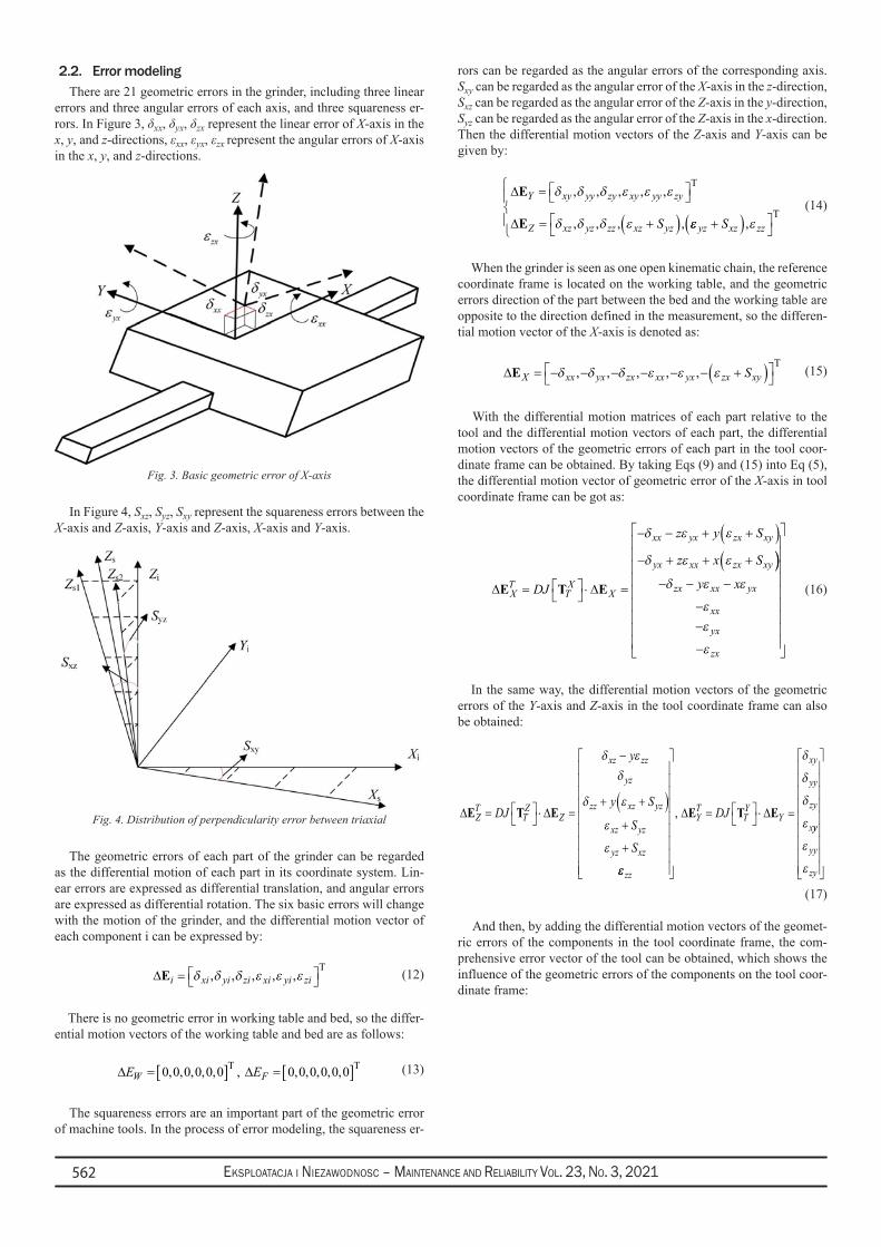
Eksploatacja i NiEzawodNosc – MaiNtENaNcE aNd REliability Vol. 23, No. 3, 2021562
2.2. Error modelingThere are 21 geometric errors in the grinder, including three linear
errors and three angular errors of each axis, and three squareness er-rors. In Figure 3, δxx, δyx, δzx represent the linear error of X-axis in the x, y, and z-directions, εxx, εyx, εzx represent the angular errors of X-axis in the x, y, and z-directions.
Fig. 3. Basic geometric error of X-axis
In Figure 4, Sxz, Syz, Sxy represent the squareness errors between the X-axis and Z-axis, Y-axis and Z-axis, X-axis and Y-axis.
Fig. 4. Distribution of perpendicularity error between triaxial
The geometric errors of each part of the grinder can be regarded as the differential motion of each part in its coordinate system. Lin-ear errors are expressed as differential translation, and angular errors are expressed as differential rotation. The six basic errors will change with the motion of the grinder, and the differential motion vector of each component i can be expressed by:
∆Ei xi yi zi xi yi zi= δ δ δ ε ε ε, , , , ,T (12)
There is no geometric error in working table and bed, so the differ-ential motion vectors of the working table and bed are as follows:
∆ ∆E EW F= [ ] = [ ]0 0 0 0 0 0 0 0 0 0 0 0, , , , , , , , , , ,T T (13)
The squareness errors are an important part of the geometric error of machine tools. In the process of error modeling, the squareness er-
rors can be regarded as the angular errors of the corresponding axis. Sxy can be regarded as the angular error of the X-axis in the z-direction, Sxz can be regarded as the angular error of the Z-axis in the y-direction, Syz can be regarded as the angular error of the Z-axis in the x-direction. Then the differential motion vectors of the Z-axis and Y-axis can be given by:
∆
∆
E
E
Y xy yy zy xy yy zy
Z xz yz zz xz yzS
=
= +( )
δ δ δ ε ε ε
δ δ δ ε
, , , , ,
, , , ,
T
εε εyz xz zzS+( )
,
T (14)
When the grinder is seen as one open kinematic chain, the reference coordinate frame is located on the working table, and the geometric errors direction of the part between the bed and the working table are opposite to the direction defined in the measurement, so the differen-tial motion vector of the X-axis is denoted as:
∆EX xx yx zx xx yx zx xyS= − − − − − − +( )
δ δ δ ε ε ε, , , , ,
T (15)
With the differential motion matrices of each part relative to the tool and the differential motion vectors of each part, the differential motion vectors of the geometric errors of each part in the tool coor-dinate frame can be obtained. By taking Eqs (9) and (15) into Eq (5), the differential motion vector of geometric error of the X-axis in tool coordinate frame can be got as:
∆ ∆E T EXT
TX
X
xx yx zx xy
yx xx zx xy
DJ
z y S
z x S
=
⋅ =
− − + +( )− + + +(δ ε ε
δ ε ε ))− − −
−−
−
δ ε ε
εε
ε
zx xx yx
xx
yx
zx
y x (16)
In the same way, the differential motion vectors of the geometric errors of the Y-axis and Z-axis in the tool coordinate frame can also be obtained:
∆ ∆E T EZT
TZ
Z
xz zz
yz
zz xz yz
xz yz
yz xz
DJ
y
y S
S
S
=
⋅ =
−
+ +( )+
+
δ εδ
δ ε
ε
ε
εε
δ
δ
δ
ε
zz
YT
TY
Y
xy
yy
zy
xDJ
=
⋅ =, ∆ ∆E T E
yy
yy
zy
ε
ε
(17)
And then, by adding the differential motion vectors of the geomet-ric errors of the components in the tool coordinate frame, the com-prehensive error vector of the tool can be obtained, which shows the influence of the geometric errors of the components on the tool coor-dinate frame:
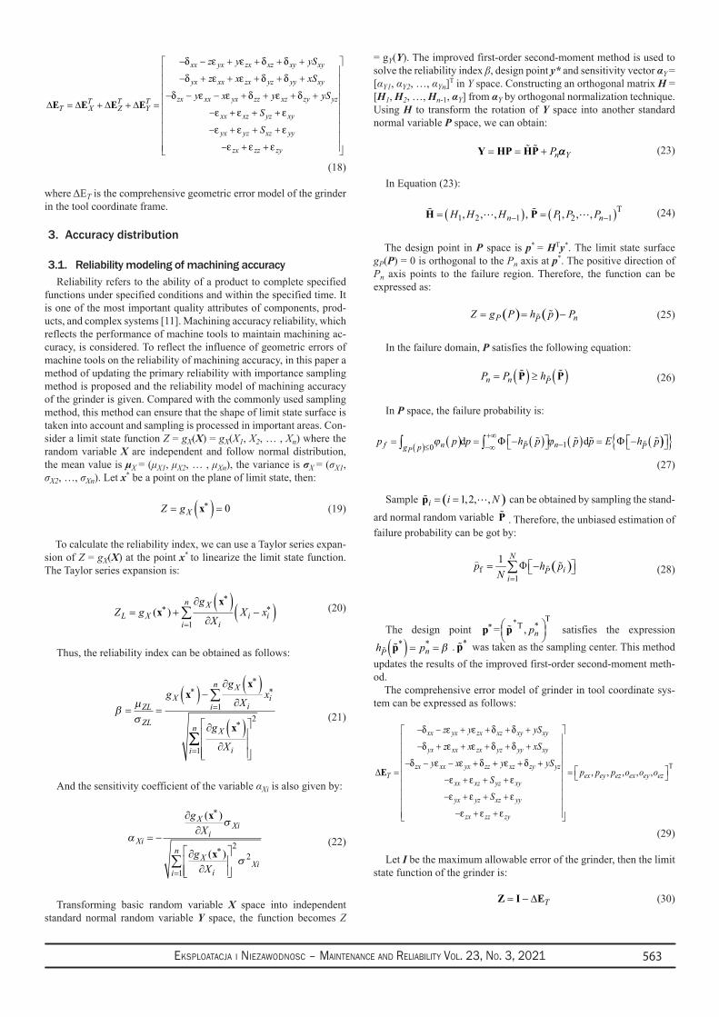
Eksploatacja i NiEzawodNosc – MaiNtENaNcE aNd REliability Vol. 23, No. 3, 2021 563
xx yx zx xz xy xy
yx xx zx yz yy xy
zx xx yx zz xz zy yzT T TT X Z Y
xx xz yz xy
yx yz xz yy
zx zz zy
z y yS
z x xS
y x y yS
S
S
δ ε ε δ δ
δ ε ε δ δ
δ ε ε δ ε δ
ε ε ε
ε ε ε
ε ε ε
− − + + + +
− + + + + + − − − + + + + ∆ = ∆ + ∆ + ∆ = − + + + − + + +
− + +
E E E E
(18)
where ΔET is the comprehensive geometric error model of the grinder in the tool coordinate frame.
3. Accuracy distribution
3.1. Reliability modeling of machining accuracyReliability refers to the ability of a product to complete specified
functions under specified conditions and within the specified time. It is one of the most important quality attributes of components, prod-ucts, and complex systems [11]. Machining accuracy reliability, which reflects the performance of machine tools to maintain machining ac-curacy, is considered. To reflect the influence of geometric errors of machine tools on the reliability of machining accuracy, in this paper a method of updating the primary reliability with importance sampling method is proposed and the reliability model of machining accuracy of the grinder is given. Compared with the commonly used sampling method, this method can ensure that the shape of limit state surface is taken into account and sampling is processed in important areas. Con-sider a limit state function Z = gX(X) = gX(X1, X2, … , Xn) where the random variable X are independent and follow normal distribution, the mean value is μX = (μX1, μX2, … , μXn), the variance is σX = (σX1, σX2, …, σXn). Let x* be a point on the plane of limit state, then:
Z gX= ( ) =∗x 0 (19)
To calculate the reliability index, we can use a Taylor series expan-sion of Z = gX(X) at the point x* to linearize the limit state function. The Taylor series expansion is:
Z gg
XX xL X
X
ii i
i
n= +
∂ ( )∂
−( )∗∗
∗
=∑( )x
x
1
(20)
Thus, the reliability index can be obtained as follows:
βµσ
= =( ) −
∂ ( )∂
∂ ( )∂
∗∗
∗
=
∗
=
∑ZL
ZL
XX
ii
i
n
X
ii
n
gg
Xx
g
X
xx
x
1
1∑∑
2 (21)
And the sensitivity coefficient of the variable αXi is also given by:
ασ
σ
Xi
X
iXi
X
iXi
i
n
gX
gX
= −
∂∂
∂∂
∗
∗
=∑
( )
( )
x
x2
2
1
(22)
Transforming basic random variable X space into independent standard normal random variable Y space, the function becomes Z
= gY(Y). The improved first-order second-moment method is used to solve the reliability index β, design point y* and sensitivity vector αY = [αY1, αY2, …, αYn]T in Y space. Constructing an orthogonal matrix H = [H1, H2, …, Hn-1, αY] from αY by orthogonal normalization technique. Using H to transform the rotation of Y space into another standard normal variable P space, we can obtain:
Y HP HP= = + Pn Yαα (23)
In Equation (23):
H P= ( ) = ( )− −H H H P P Pn n1 2 1 1 2 1, , , , , ,, T (24)
The design point in P space is p* = HTy*. The limit state surface gP(P) = 0 is orthogonal to the Pn axis at p*. The positive direction of Pn axis points to the failure region. Therefore, the function can be expressed as:
( ) ( )P nPZ g P h p P= = −
(25)
In the failure domain, P satisfies the following equation:
P P hn n P= ( ) ≥ ( )
P P (26)
In P space, the failure probability is:
p p p h p p p E h pf ng p P n PP= ( ) = − ( ) ( ) = − (( )≤ −∞
+∞−∫ ∫ϕ ϕ0 1d dΦ Φ
)) (27)
Sample ( )1,2, ,i i N= =p can be obtained by sampling the stand-ard normal random variable P . Therefore, the unbiased estimation of failure probability can be got by:
( )f1
1 ÖN
iPi
p h pN =
= − ∑
Φ (28)
The design point * T
T *= , np∗
p p satisfies the expressionh pP n
p* *( ) = = β . *p was taken as the sampling center. This method updates the results of the improved first-order second-moment meth-od.
The comprehensive error model of grinder in tool coordinate sys-tem can be expressed as follows:
T, , , , ,
xx yx zx xz xy xy
yx xx zx yz yy xy
zx xx yx zz xz zy yzT ex ey ez ex ey ez
xx xz yz xy
yx yz xz yy
zx zz zy
z y yS
z x xS
y x y ySp p p o o o
S
S
δ ε ε δ δ
δ ε ε δ δ
δ ε ε δ ε δ
ε ε ε
ε ε ε
ε ε ε
− − + + + +
− + + + + + − − − + + + + ∆ = = − + + + − + + +
− + +
E
(29)
Let I be the maximum allowable error of the grinder, then the limit state function of the grinder is:
T= − ∆Z I E (30)
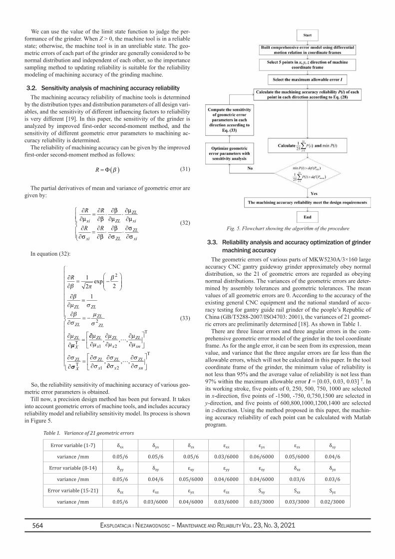
Eksploatacja i NiEzawodNosc – MaiNtENaNcE aNd REliability Vol. 23, No. 3, 2021564
We can use the value of the limit state function to judge the per-formance of the grinder. When Z > 0, the machine tool is in a reliable state; otherwise, the machine tool is in an unreliable state. The geo-metric errors of each part of the grinder are generally considered to be normal distribution and independent of each other, so the importance sampling method to updating reliability is suitable for the reliability modeling of machining accuracy of the grinding machine.
3.2. Sensitivity analysis of machining accuracy reliabilityThe machining accuracy reliability of machine tools is determined
by the distribution types and distribution parameters of all design vari-ables, and the sensitivity of different influencing factors to reliability is very different [19]. In this paper, the sensitivity of the grinder is analyzed by improved first-order second-moment method, and the sensitivity of different geometric error parameters to machining ac-curacy reliability is determined.
The reliability of machining accuracy can be given by the improved first-order second-moment method as follows:
R = ( )Φ β (31)
The partial derivatives of mean and variance of geometric error are given by:
ZL
xi ZL xi
ZL
xi ZL xi
R R
R R
β µµ β µ µ
β σσ β σ σ
∂ ∂ ∂ ∂ = ⋅ ⋅ ∂ ∂ ∂ ∂ ∂ ∂ ∂ ∂ = ⋅ ⋅∂ ∂ ∂ ∂
(32)
In equation (32):
∂∂
= −
∂∂
=
∂∂
= −
∂
∂=
R
ZL ZL
ZL
ZL
ZL
ZL
X
β πβ
βµ σβσ
µσ
µ
12 2
1
2
2
exp
µµT∂∂∂
∂∂
∂∂
∂
∂=
∂∂
∂
µµ
µµ
µµ
σ σσ
σ
ZL
x
ZL
x
ZL
xn
ZL
X
ZL
x
ZL
1 2
1
, , ,
,
T
Tσσ ∂∂∂∂
σ
σσx
ZL
xn2, ,
T
(33)
So, the reliability sensitivity of machining accuracy of various geo-metric error parameters is obtained.
Till now, a precision design method has been put forward. It takes into account geometric errors of machine tools, and includes accuracy reliability model and reliability sensitivity model. Its process is shown in Figure 5.
3.3. Reliability analysis and accuracy optimization of grinder machining accuracy
The geometric errors of various parts of MKW5230A/3×160 large accuracy CNC gantry guideway grinder approximately obey normal distribution, so the 21 of geometric errors are regarded as obeying normal distributions. The variances of the geometric errors are deter-mined by assembly tolerances and geometric tolerances. The mean values of all geometric errors are 0. According to the accuracy of the existing general CNC equipment and the national standard of accu-racy testing for gantry guide rail grinder of the people’s Republic of China (GB/T5288-2007/ISO4703: 2001), the variances of 21 geomet-ric errors are preliminarily determined [18]. As shown in Table 1.
There are three linear errors and three angular errors in the com-prehensive geometric error model of the grinder in the tool coordinate frame. As for the angle error, it can be seen from its expression, mean value, and variance that the three angular errors are far less than the allowable errors, which will not be calculated in this paper. In the tool coordinate frame of the grinder, the minimum value of reliability is not less than 95% and the average value of reliability is not less than 97% within the maximum allowable error I = [0.03, 0.03, 0.03] T. In its working stroke, five points of 0, 250, 500, 750, 1000 are selected in x-direction, five points of -1500, -750, 0,750,1500 are selected in y-direction, and five points of 600,800,1000,1200,1400 are selected in z-direction. Using the method proposed in this paper, the machin-ing accuracy reliability of each point can be calculated with Matlab program.
Table 1. Variance of 21 geometric errors
Error variable (1-7) δxx δyx δzx εxx εyx εzx δxy
variance /mm 0.05/6 0.05/6 0.05/6 0.03/6000 0.06/6000 0.05/6000 0.04/6
Error variable (8-14) δyy δzy εxy εyy εzy δxz δyz
variance /mm 0.05/6 0.04/6 0.05/6000 0.04/6000 0.04/6000 0.03/6 0.03/6
Error variable (15-21) δzz εxz εyz εzz Sxy Sxz Syz
variance /mm 0.05/6 0.03/6000 0.04/6000 0.03/6000 0.03/3000 0.03/3000 0.02/3000
Fig. 5. Flowchart showing the algorithm of the procedure
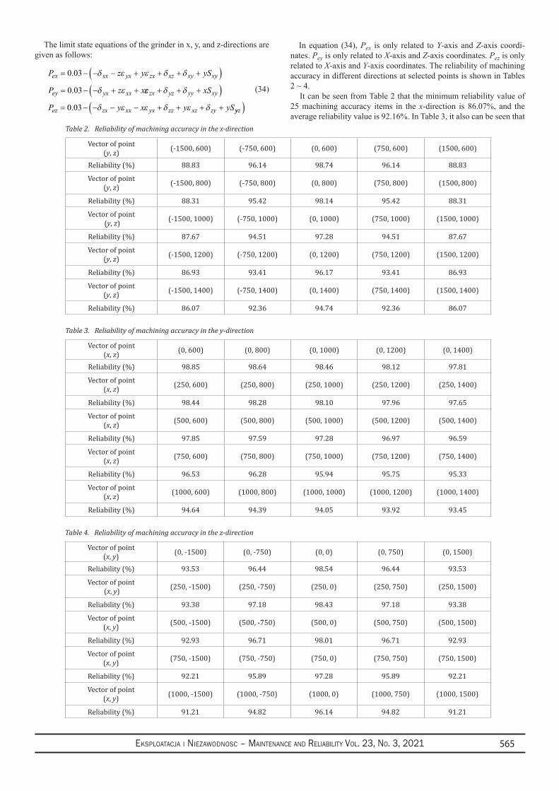
Eksploatacja i NiEzawodNosc – MaiNtENaNcE aNd REliability Vol. 23, No. 3, 2021 565
The limit state equations of the grinder in x, y, and z-directions are given as follows:
P z y yS
P z x
ex xx yx zx xz xy xy
ey yx xx
= − − − + + + +( )= − − + +
0 03
0 03
.
.
δ ε ε δ δ
δ ε εε δ δ
δ ε ε δ ε δ
zx yz yy xy
ez zx xx yx zz xz zy
xS
P y x y yS
+ + +( )= − − − − + + + +0 03. yyz( )
(34)
In equation (34), Pex is only related to Y-axis and Z-axis coordi-nates. Pey is only related to X-axis and Z-axis coordinates. Pez is only related to X-axis and Y-axis coordinates. The reliability of machining accuracy in different directions at selected points is shown in Tables 2 ~ 4.
It can be seen from Table 2 that the minimum reliability value of 25 machining accuracy items in the x-direction is 86.07%, and the average reliability value is 92.16%. In Table 3, it also can be seen that
Table 2. Reliability of machining accuracy in the x-direction
Vector of point(y, z) (-1500, 600) (-750, 600) (0, 600) (750, 600) (1500, 600)
Reliability (%) 88.83 96.14 98.74 96.14 88.83
Vector of point (y, z) (-1500, 800) (-750, 800) (0, 800) (750, 800) (1500, 800)
Reliability (%) 88.31 95.42 98.14 95.42 88.31
Vector of point (y, z) (-1500, 1000) (-750, 1000) (0, 1000) (750, 1000) (1500, 1000)
Reliability (%) 87.67 94.51 97.28 94.51 87.67
Vector of point (y, z) (-1500, 1200) (-750, 1200) (0, 1200) (750, 1200) (1500, 1200)
Reliability (%) 86.93 93.41 96.17 93.41 86.93
Vector of point (y, z) (-1500, 1400) (-750, 1400) (0, 1400) (750, 1400) (1500, 1400)
Reliability (%) 86.07 92.36 94.74 92.36 86.07
Table 3. Reliability of machining accuracy in the y-direction
Vector of point (x, z) (0, 600) (0, 800) (0, 1000) (0, 1200) (0, 1400)
Reliability (%) 98.85 98.64 98.46 98.12 97.81
Vector of point (x, z) (250, 600) (250, 800) (250, 1000) (250, 1200) (250, 1400)
Reliability (%) 98.44 98.28 98.10 97.96 97.65
Vector of point(x, z) (500, 600) (500, 800) (500, 1000) (500, 1200) (500, 1400)
Reliability (%) 97.85 97.59 97.28 96.97 96.59
Vector of point(x, z) (750, 600) (750, 800) (750, 1000) (750, 1200) (750, 1400)
Reliability (%) 96.53 96.28 95.94 95.75 95.33
Vector of point(x, z) (1000, 600) (1000, 800) (1000, 1000) (1000, 1200) (1000, 1400)
Reliability (%) 94.64 94.39 94.05 93.92 93.45
Table 4. Reliability of machining accuracy in the z-direction
Vector of point(x, y) (0, -1500) (0, -750) (0, 0) (0, 750) (0, 1500)
Reliability (%) 93.53 96.44 98.54 96.44 93.53
Vector of point (x, y) (250, -1500) (250, -750) (250, 0) (250, 750) (250, 1500)
Reliability (%) 93.38 97.18 98.43 97.18 93.38
Vector of point(x, y) (500, -1500) (500, -750) (500, 0) (500, 750) (500, 1500)
Reliability (%) 92.93 96.71 98.01 96.71 92.93
Vector of point (x, y) (750, -1500) (750, -750) (750, 0) (750, 750) (750, 1500)
Reliability (%) 92.21 95.89 97.28 95.89 92.21
Vector of point (x, y) (1000, -1500) (1000, -750) (1000, 0) (1000, 750) (1000, 1500)
Reliability (%) 91.21 94.82 96.14 94.82 91.21
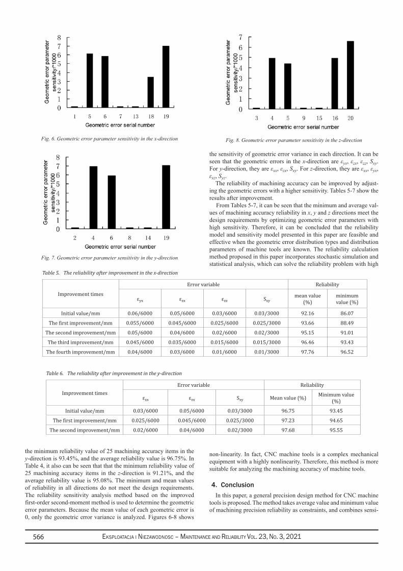
Eksploatacja i NiEzawodNosc – MaiNtENaNcE aNd REliability Vol. 23, No. 3, 2021566
the sensitivity of geometric error variance in each direction. It can be seen that the geometric errors in the x-direction are εyx, εzx, εzz, Sxy. For y-direction, they are εxx, εzx, Sxy. For z-direction, they are εxx, εyx, εxz, Syz.
The reliability of machining accuracy can be improved by adjust-ing the geometric errors with a higher sensitivity. Tables 5-7 show the results after improvement.
From Tables 5-7, it can be seen that the minimum and average val-ues of machining accuracy reliability in x, y and z directions meet the design requirements by optimizing geometric error parameters with high sensitivity. Therefore, it can be concluded that the reliability model and sensitivity model presented in this paper are feasible and effective when the geometric error distribution types and distribution parameters of machine tools are known. The reliability calculation method proposed in this paper incorporates stochastic simulation and statistical analysis, which can solve the reliability problem with high
non-linearity. In fact, CNC machine tools is a complex mechanical equipment with a highly nonlinearity. Therefore, this method is more suitable for analyzing the machining accuracy of machine tools.
4. ConclusionIn this paper, a general precision design method for CNC machine
tools is proposed. The method takes average value and minimum value of machining precision reliability as constraints, and combines sensi-
the minimum reliability value of 25 machining accuracy items in the y-direction is 93.45%, and the average reliability value is 96.75%. In Table 4, it also can be seen that that the minimum reliability value of 25 machining accuracy items in the z-direction is 91.21%, and the average reliability value is 95.08%. The minimum and mean values of reliability in all directions do not meet the design requirements. The reliability sensitivity analysis method based on the improved first-order second-moment method is used to determine the geometric error parameters. Because the mean value of each geometric error is 0, only the geometric error variance is analyzed. Figures 6-8 shows
Fig. 6. Geometric error parameter sensitivity in the x-direction
Table 5. The reliability after improvement in the x-direction
Improvement times
Error variable Reliability
εyx εzx εzz Sxymean value
(%)minimum value (%)
Initial value/mm 0.06/6000 0.05/6000 0.03/6000 0.03/3000 92.16 86.07
The first improvement/mm 0.055/6000 0.045/6000 0.025/6000 0.025/3000 93.66 88.49
The second improvement/mm 0.05/6000 0.04/6000 0.02/6000 0.02/3000 95.15 91.01
The third improvement/mm 0.045/6000 0.035/6000 0.015/6000 0.015/3000 96.46 93.43
The fourth improvement/mm 0.04/6000 0.03/6000 0.01/6000 0.01/3000 97.76 96.52
Table 6. The reliability after improvement in the y-direction
Improvement timesError variable Reliability
εxx εzx Sxy Mean value (%) Minimum value (%)
Initial value/mm 0.03/6000 0.05/6000 0.03/3000 96.75 93.45
The first improvement/mm 0.025/6000 0.045/6000 0.025/3000 97.23 94.65
The second improvement/mm 0.02/6000 0.04/6000 0.02/3000 97.68 95.55
Fig. 7. Geometric error parameter sensitivity in the y-direction
Fig. 8. Geometric error parameter sensitivity in the z-direction

Eksploatacja i NiEzawodNosc – MaiNtENaNcE aNd REliability Vol. 23, No. 3, 2021 567
tivity analysis of error parameters to optimize geometric error param-eters of machine tools. Some conclusions are drawn as follows:
Compared with the existing traditional method, the geometric 1. error modeling method based on the differential motion rela-tion between coordinate frames has less calculation and can clearly explain the geometric meaning of the geometric error of each part to the total error.Based on the comprehensive error model and advanced im-2. portance sampling method, the accuracy reliability model and
reliability sensitivity model of machine tools are given to opti-mize the machining accuracy reliability of machine tools.The effectiveness of the method proposed in this paper is val-3. idated by a large CNC gantry guide rail grinder, the results show that the machining accuracy reliability of the machine tool can be improved.
Table 7. The reliability after improvement in the z-direction
Improvement times
Error variable Reliability
εxx εyx εxz SyzMean value
(%)Minimum value (%)
Initial value/mm 0.06/6000 0.05/6000 0.03/6000 0.03/3000 95.08 91.21
The first improvement/mm 0.055/6000 0.045/6000 0.025/6000 0.025/3000 96.24 93.26
The second improvement/mm 0.05/6000 0.04/6000 0.02/6000 0.02/3000 97.06 94.69
The third improvement/mm 0.045/6000 0.035/6000 0.015/6000 0.015/3000 97.21 95.24
References1. Antonio CC, Hoffbauer LN. An approach for reliability-based robust design optimisation of angle-piy composite. Composite Structures
2009; 90(1): 53-59, https://doi.org/10.1016/j.compstruct.2009.01.008.2. Bohez ELJ, Ariyajunya B, Sinlapeecheewa C, Shein TMM, Lap DT, Belforte G. Systematic geometric rigid body error identification of
5-axis milling machines. Computer-Aided Design 2007; 39(4): 229-244, https://doi.org/10.1016/j.cad.2006.11.006.3. Cai LG, Zhang ZL, Cheng Q, Liu ZF, Gu PH. A geometric accuracy design method of multi-axis NC machine tool for improving
machining accuracy reliability. Eksploatacja i Niezawodnosc-Maintenance and Reliability 2015; 17(1): 143-155, https://doi.org/10.17531/ein.2015.1.19.
4. Chen GD, Liang YC, Sun YZ, Chen WQ, Wang B. Volumetric error modeling and sensitivity analysis for designing a five-axis ultra-precision machine too. The International Journal of Advanced Manufacturing Technology 2013; 68(9-12): 2525-2534, https://doi.org/10.1007/s00170-013-4874-4.
5. Cheng Q, Feng QN, Liu ZF, Gu PH, Cai LG. Fluctuation prediction of machining accuracy for multi-axis machine tool based on stochastic process theory. Proceedings of the Institution of Mechanical Engineers, Part C: Journal of Mechanical Engineering Science 2015; 229(14): 2534-2550, https://doi.org/10.1177/0954406214562633.
6. Cheng Q, Zhang ZL, Zhang GJ, Gu PH, Cai LG. Geometric accuracy allocation for multi-axis CNC machine tools based on sensitivity analysis and reliability theory. Proceedings of the Institution of Mechanical Engineers, Part C: Journal of Mechanical Engineering Science 2015; 229(6): 1134-1149, https://doi.org/10.1177/0954406214542491.
7. Cheng Q, Zhao HW, Zhang GJ, Gu PH, Cai LG. An analytical approach for crucial geometric errors identification of multi-axis machine tool based on global sensitivity analysis. The International Journal of Advanced Manufacturing Technology 2014; 75(1-4): 107-121, https://doi.org/10.1007/s00170-014-6133-8.
8. Cheng Q, Zhao HW, Zhao YS, Sun BW, Gu PH. Machining accuracy reliability analysis of multi-axis machine tool based on Monte Carlo simulation. Journal of Intelligent Manufacturing 2018; 29(1): 1-19, https://doi.org/10.1007/s10845-015-1101-1.
9. Fu GQ, Fu JZ, Xu YT, Chen ZC, Lai JT. Accuracy enhancement of five-axis machine tool based on differential motion matrix: Geometric error modeling, identification and compensation. International Journal of Machine Tools & Manufacture 2015; 89: 170-181, https://doi.org/10.1016/j.ijmachtools.2014.11.005.
10. Guo SJ, Mei XS, Jiang GD. Geometric accuracy enhancement of five-axis machine tool based on error analysis. The International Journal of Advanced Manufacturing Technology 2019; 105(1-4): 137-153, https://doi.org/10.1007/s00170-019-04030-4.
11. Huang B. Reliability theory of engineering structure and its application. Wuhan: Wuhan University of Technology Press 2019.12. Lee ES, Suh SH, Shon JW. A comprehensive method for calibration of volumetric positioning accuracy of CNC-machines. The International
Journal of Advanced Manufacturing Technology 1998; 14(1): 43-49, https://doi.org/10.1007/BF01179416.13. Lee RS, Lin YH. Applying bidirectional kinematics to assembly error analysis for five-axis machine tools with general orthogonal
configuration. The International Journal of Advanced Manufacturing Technology 2012; 62(9-12): 1261-1272, https://doi.org/10.1007/s00170-011-3860-y.
14. Niu P, Cheng Q, Chang WF, Song XM, Li YS. Sensitivity analysis of machining accuracy reliability considering partial correlation of geometric errors for Horizontal Machining Center. Proceedings of the Institution of Mechanical Engineers, part B 2021; 235(3): 455-465, https://doi.org/10.1177/0954405420958843.
15. Niu P, Cheng Q, Liu ZF, Chu HY. A machining accuracy improvement approach for a horizontal machining center based on analysis of geometric error characteristics. The International Journal of Advanced Manufacturing Technology 2021; 112: 2873-2887, https://doi.org/10.1007/s00170-020-06565-3.
16. Qi J, Yang W. Differential change construction based geometric error compensation for machine tools. Transactions of the Chinese Society for Agricultural Machinery 2016; 47(9): 398-405.
17. Wu HR, Zheng HL, Li XX, Wang WK, Xiang XP, Meng XP. A geometric accuracy analysis and tolerance robust design approach for a vertical machining center based on the reliability theory. Measurement 2020; 161: 107809, https://doi.org/10.1016/j.measurement.2020.107809.
18. Yu ZM, Liu ZJ, Ai YD, Xiong M. Geometric error model and precision distribution based on reliability theory for large CNC gantry

Eksploatacja i NiEzawodNosc – MaiNtENaNcE aNd REliability Vol. 23, No. 3, 2021568
guideway grinder. Journal of Mechanical Engineering 2013; 49(17): 142-151, https://doi.org/10.3901/JME.2013.17.142.19. Zhang C. Geometric error inversion and optimization of multi axis CNC machine tools based on robust design. Beijing: Beijing University
of Technology 2014.20. Zhang ZL, Cai LG, Cheng Q, Liu ZF, Gu PH. A geometric error budget method to improve machining accuracy reliability of multi-axis
machine tools. Journal of Intelligent Manufacturing 2019; 30(2): 495-519, https://doi.org/10.1007/s10845-016-1260-8.21. Zhang ZL, Liu ZF, Cai LG, Cheng Q, Qi Y. An accuracy design approach for a multi-axis NC machine tool based on reliability theory. The
International Journal of Advanced Manufacturing Technology 2016; 91(5-8): 1-20, https://doi.org/10.1007/s00170-016-9824-5.22. Zhang ZL, Liu ZF, Cheng Q, Qi Y, Cai LG. An approach of comprehensive error modeling and accuracy allocation for the improvement of
reliability and optimization of cost of a multi-axis NC machine tool. The International Journal of Advanced Manufacturing Technology 2016; 89(1-4): 1-19, https://doi.org/10.1007/s00170-016-8981-x.
23. Zhao CB. Application of SCM and PLC technology in CNC machine tool. Applied Mechanics and Materials 2014; 687-691: 22-25, https://doi.org/10.4028/www.scientific.net/AMM.687-691.22.
Eksploatacja i NiEzawodNosc – MaiNtENaNcE aNd REliability Vol. 23, No. 3, 2021 569
E-mail addresses:
Eksploatacja i Niezawodnosc – Maintenance and ReliabilityVolume 23 (2021), Issue 3
journal homepage: http://www.ein.org.pl
Indexed by:Operational tests of an electrostatic precipitator reducing low dust emission from solid fuels combustionRyszard Machnik a, Łukasz Więckowski b
a Faculty of Mechanical Engineering and Robotics, AGH University of Science and Technology, al. Mickiewicza 30, 30-059 Krakow, Poland b Faculty of Electrical Engineering, Automatics, Computer Science and Biomedical Engineering, , AGH University of Science and Technology, al. Mickiewicza 30, 30-059 Krakow, Poland
Machnik R, Więckowski Ł. Operational tests of an electrostatic precipitator reducing low dust emission from solid fuels combustion. Eksploatacja i Niezawodnosc – Maintenance and Reliability 2021; 23 (3): 569–574, http://doi.org/10.17531/ein.2021.3.18.
Article citation info:
The article presents the continuation of the research aimed at designing, manufacturing and selecting the operating parameters of the electrostatic precipitator for household applica-tions. The tests were carried out in the laboratory and real conditions. The object of the research was a pre-production prototype of the electrostatic precipitator installed in the flue gas duct of a single-family building. The source of exhaust gases was a coal-fired, low-tem-perature water heating boiler with a nominal power of 21 kW (old generation boiler-year of production: 2007). The obtained results showed that the adopted design of the electrostatic precipitator enables the reduction of dust emissions generated in the combustion of solid fuels in households at relatively low operating costs.
Highlights Abstract
An electrostatic precipitator was designed and • manufactured to reduce dust from low emission sources.
A microprocessor controller with the function of • monitoring device operating parameters through the LoRaWAN network was developed.
The required dedusting efficiency was achieved • with relatively low operating costs of the electro-static precipitator.
air protection, low emission, electrostatic precipitator, operating parameters.
Keywords
This is an open access article under the CC BY license (https://creativecommons.org/licenses/by/4.0/)
R. Machnik - [email protected], Ł. Więckowski - [email protected]
IntroductionSignificant exceedance of the standards for suspended dust con-
centrations from low emission sources is a significant problem. Low emission is defined as the emission of combustion products of solid, liquid or gaseous fuels into the atmosphere from sources located at a height not exceeding 40 m. Low emission is a source of many air pol-lutants, especially PM10 and PM2.5 [31]. The chemical composition of suspended dust PM10 and PM2.5 contains chemical components that are hazardous to health [6], which was pointed out in the recent report of the European Environment Agency [10]. Dust from solid fuel combustion contains organic compounds: polycyclic aromatic hydrocarbons, dioxins and heavy inorganic metals or their compounds [32], including particularly toxic mercury [33]. One of the significant sources of low dust and harmful gas emissions is the combustion proc-ess of low-quality coal in home furnaces or local boiler houses [3]. The source of dust is also burning biomass in stoves and fireplaces [5, 30]. Fuel combustion in outdated boilers is due to economic reasons. The reduction of dust emissions from the combustion of solid fuels by individual users is possible by replacing obsolete boilers with modern devices that meet emission standards or by equipping existing heating installations with relatively cheap, easy-to-use electrostatic precipita-tors. Electrostatic precipitators are commonly used in many industries [15, 21]. The leading sector of the economy that uses electrostatic
precipitators is energy. Industrial electrostatic precipitators are large-size devices [22] and their design solutions cannot be used to separate dust from low emission sources. Many design electrostatic precipita-tors for household use [28] have been developed, and new solutions are constantly sought. The device that generates large amounts of free ions (sonic-jet charger), presented in [18], to be used in the process of diffusive charging of dust particles deserves attention. Household electrostatic precipitators are often installed directly at the outlet of a power boiler [4, 11, 24], which is not always possible due to the cuba-ture of the boiler room. High flue gas temperature at the boiler outlet may cause accelerated corrosion of the electrostatic precipitator. An alternative is to place a tubular electrostatic precipitator in the flue gas duct (inside the chimney) [9]. Such a design solution was adopted by the authors [16]. This electrostatic precipitator is intended mainly for older generation boilers, which are fed with fuel with lower quality parameters than the fuels used in the new generation boilers.
The elaboration of the electrostatic precipitator design was preced-ed by testing the properties of dust pollutants emitted by household boilers. The theoretical level of dust emissions from the combustion of solid fuels (coal and biomass) in domestic boiler houses was deter-mined. As part of the research, analyses of the chemical composition, morphology and physicochemical properties of dust from coal com-bustion and biomass were carried out. Based on the research results,
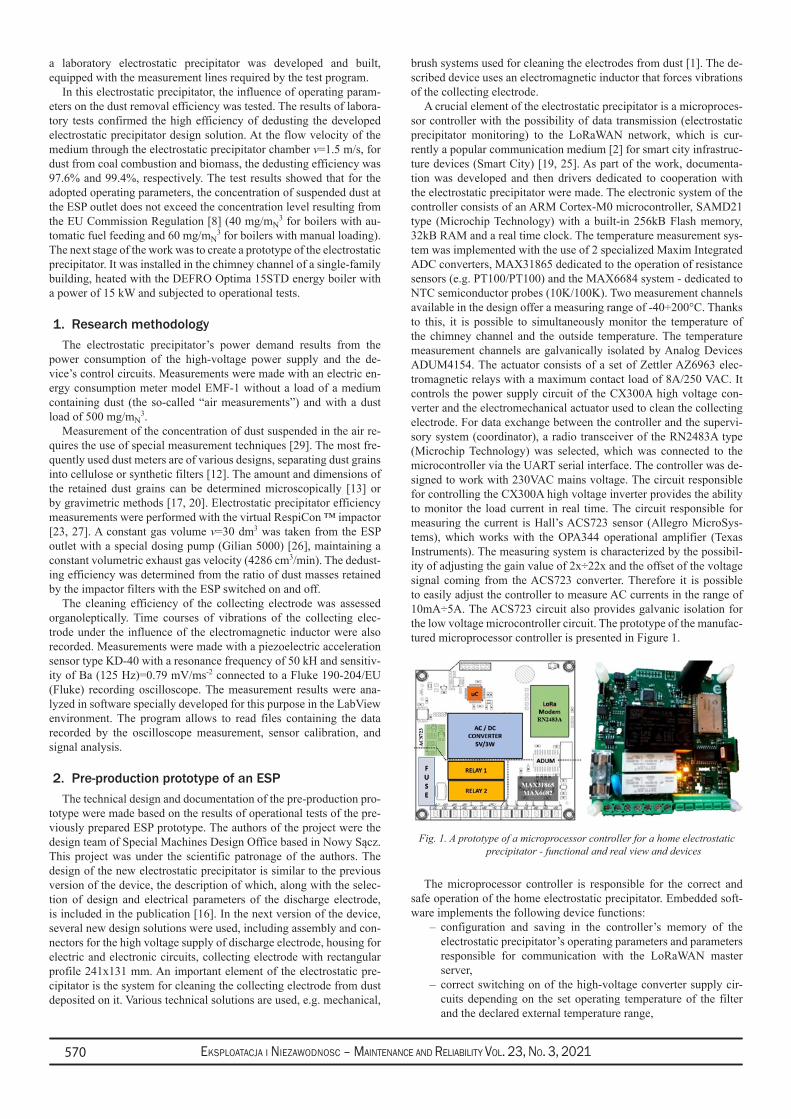
Eksploatacja i NiEzawodNosc – MaiNtENaNcE aNd REliability Vol. 23, No. 3, 2021570
a laboratory electrostatic precipitator was developed and built, equipped with the measurement lines required by the test program.
In this electrostatic precipitator, the influence of operating param-eters on the dust removal efficiency was tested. The results of labora-tory tests confirmed the high efficiency of dedusting the developed electrostatic precipitator design solution. At the flow velocity of the medium through the electrostatic precipitator chamber v=1.5 m/s, for dust from coal combustion and biomass, the dedusting efficiency was 97.6% and 99.4%, respectively. The test results showed that for the adopted operating parameters, the concentration of suspended dust at the ESP outlet does not exceed the concentration level resulting from the EU Commission Regulation [8] (40 mg/mN
3 for boilers with au-tomatic fuel feeding and 60 mg/mN
3 for boilers with manual loading). The next stage of the work was to create a prototype of the electrostatic precipitator. It was installed in the chimney channel of a single-family building, heated with the DEFRO Optima 15STD energy boiler with a power of 15 kW and subjected to operational tests.
1. Research methodologyThe electrostatic precipitator’s power demand results from the
power consumption of the high-voltage power supply and the de-vice’s control circuits. Measurements were made with an electric en-ergy consumption meter model EMF-1 without a load of a medium containing dust (the so-called “air measurements”) and with a dust load of 500 mg/mN
3.Measurement of the concentration of dust suspended in the air re-
quires the use of special measurement techniques [29]. The most fre-quently used dust meters are of various designs, separating dust grains into cellulose or synthetic filters [12]. The amount and dimensions of the retained dust grains can be determined microscopically [13] or by gravimetric methods [17, 20]. Electrostatic precipitator efficiency measurements were performed with the virtual RespiCon ™ impactor [23, 27]. A constant gas volume v=30 dm3 was taken from the ESP outlet with a special dosing pump (Gilian 5000) [26], maintaining a constant volumetric exhaust gas velocity (4286 cm3/min). The dedust-ing efficiency was determined from the ratio of dust masses retained by the impactor filters with the ESP switched on and off.
The cleaning efficiency of the collecting electrode was assessed organoleptically. Time courses of vibrations of the collecting elec-trode under the influence of the electromagnetic inductor were also recorded. Measurements were made with a piezoelectric acceleration sensor type KD-40 with a resonance frequency of 50 kH and sensitiv-ity of Ba (125 Hz)=0.79 mV/ms-2 connected to a Fluke 190-204/EU (Fluke) recording oscilloscope. The measurement results were ana-lyzed in software specially developed for this purpose in the LabView environment. The program allows to read files containing the data recorded by the oscilloscope measurement, sensor calibration, and signal analysis.
2. Pre-production prototype of an ESPThe technical design and documentation of the pre-production pro-
totype were made based on the results of operational tests of the pre-viously prepared ESP prototype. The authors of the project were the design team of Special Machines Design Office based in Nowy Sącz. This project was under the scientific patronage of the authors. The design of the new electrostatic precipitator is similar to the previous version of the device, the description of which, along with the selec-tion of design and electrical parameters of the discharge electrode, is included in the publication [16]. In the next version of the device, several new design solutions were used, including assembly and con-nectors for the high voltage supply of discharge electrode, housing for electric and electronic circuits, collecting electrode with rectangular profile 241x131 mm. An important element of the electrostatic pre-cipitator is the system for cleaning the collecting electrode from dust deposited on it. Various technical solutions are used, e.g. mechanical,
brush systems used for cleaning the electrodes from dust [1]. The de-scribed device uses an electromagnetic inductor that forces vibrations of the collecting electrode.
A crucial element of the electrostatic precipitator is a microproces-sor controller with the possibility of data transmission (electrostatic precipitator monitoring) to the LoRaWAN network, which is cur-rently a popular communication medium [2] for smart city infrastruc-ture devices (Smart City) [19, 25]. As part of the work, documenta-tion was developed and then drivers dedicated to cooperation with the electrostatic precipitator were made. The electronic system of the controller consists of an ARM Cortex-M0 microcontroller, SAMD21 type (Microchip Technology) with a built-in 256kB Flash memory, 32kB RAM and a real time clock. The temperature measurement sys-tem was implemented with the use of 2 specialized Maxim Integrated ADC converters, MAX31865 dedicated to the operation of resistance sensors (e.g. PT100/PT100) and the MAX6684 system - dedicated to NTC semiconductor probes (10K/100K). Two measurement channels available in the design offer a measuring range of -40÷200°C. Thanks to this, it is possible to simultaneously monitor the temperature of the chimney channel and the outside temperature. The temperature measurement channels are galvanically isolated by Analog Devices ADUM4154. The actuator consists of a set of Zettler AZ6963 elec-tromagnetic relays with a maximum contact load of 8A/250 VAC. It controls the power supply circuit of the CX300A high voltage con-verter and the electromechanical actuator used to clean the collecting electrode. For data exchange between the controller and the supervi-sory system (coordinator), a radio transceiver of the RN2483A type (Microchip Technology) was selected, which was connected to the microcontroller via the UART serial interface. The controller was de-signed to work with 230VAC mains voltage. The circuit responsible for controlling the CX300A high voltage inverter provides the ability to monitor the load current in real time. The circuit responsible for measuring the current is Hall’s ACS723 sensor (Allegro MicroSys-tems), which works with the OPA344 operational amplifier (Texas Instruments). The measuring system is characterized by the possibil-ity of adjusting the gain value of 2x÷22x and the offset of the voltage signal coming from the ACS723 converter. Therefore it is possible to easily adjust the controller to measure AC currents in the range of 10mA÷5A. The ACS723 circuit also provides galvanic isolation for the low voltage microcontroller circuit. The prototype of the manufac-tured microprocessor controller is presented in Figure 1.
Fig. 1. A prototype of a microprocessor controller for a home electrostatic precipitator - functional and real view and devices
The microprocessor controller is responsible for the correct and safe operation of the home electrostatic precipitator. Embedded soft-ware implements the following device functions:
configuration and saving in the controller’s memory of the –electrostatic precipitator’s operating parameters and parameters responsible for communication with the LoRaWAN master server,correct switching on of the high-voltage converter supply cir- –cuits depending on the set operating temperature of the filter and the declared external temperature range,
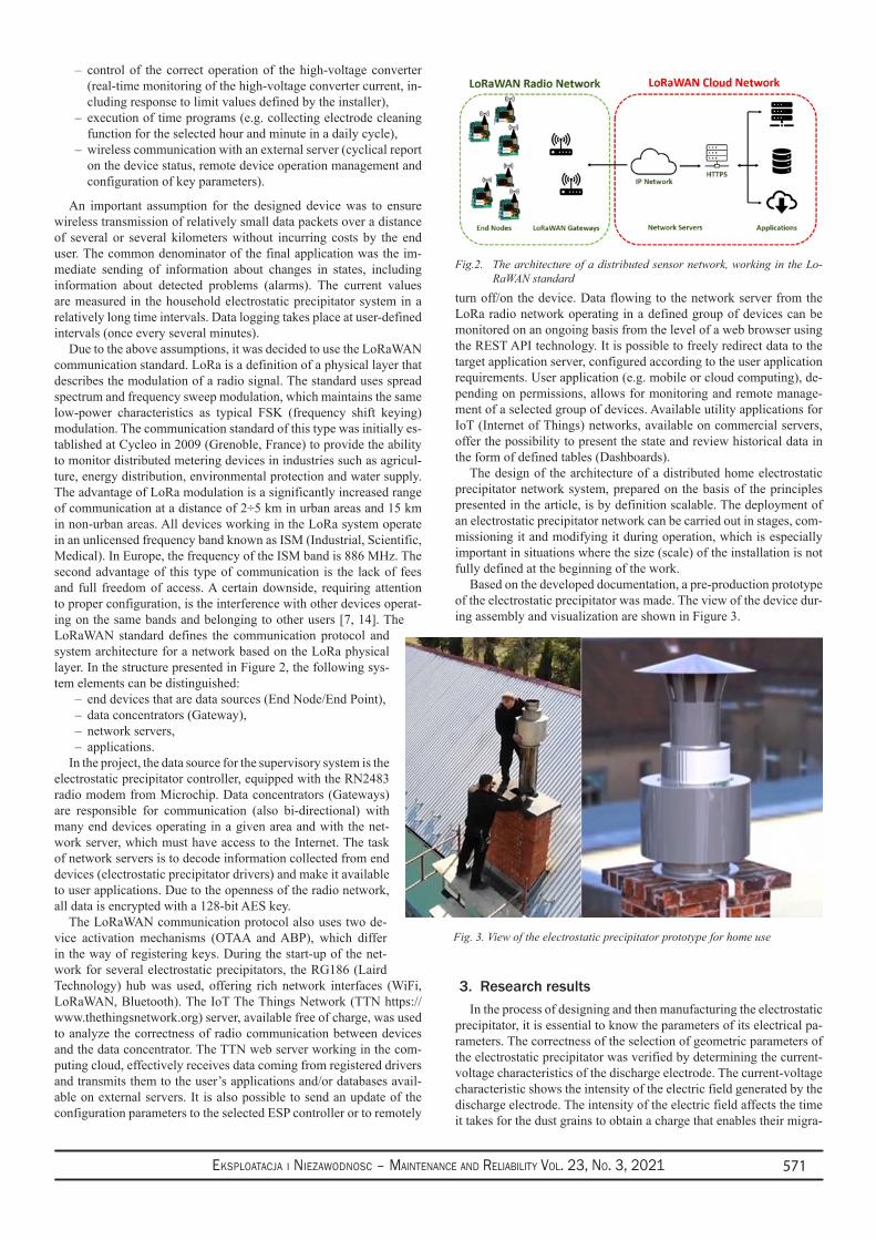
Eksploatacja i NiEzawodNosc – MaiNtENaNcE aNd REliability Vol. 23, No. 3, 2021 571
control of the correct operation of the high-voltage converter –(real-time monitoring of the high-voltage converter current, in-cluding response to limit values defined by the installer),execution of time programs (e.g. collecting electrode cleaning –function for the selected hour and minute in a daily cycle),wireless communication with an external server (cyclical report –on the device status, remote device operation management and configuration of key parameters).
An important assumption for the designed device was to ensure wireless transmission of relatively small data packets over a distance of several or several kilometers without incurring costs by the end user. The common denominator of the final application was the im-mediate sending of information about changes in states, including information about detected problems (alarms). The current values are measured in the household electrostatic precipitator system in a relatively long time intervals. Data logging takes place at user-defined intervals (once every several minutes).
Due to the above assumptions, it was decided to use the LoRaWAN communication standard. LoRa is a definition of a physical layer that describes the modulation of a radio signal. The standard uses spread spectrum and frequency sweep modulation, which maintains the same low-power characteristics as typical FSK (frequency shift keying) modulation. The communication standard of this type was initially es-tablished at Cycleo in 2009 (Grenoble, France) to provide the ability to monitor distributed metering devices in industries such as agricul-ture, energy distribution, environmental protection and water supply. The advantage of LoRa modulation is a significantly increased range of communication at a distance of 2÷5 km in urban areas and 15 km in non-urban areas. All devices working in the LoRa system operate in an unlicensed frequency band known as ISM (Industrial, Scientific, Medical). In Europe, the frequency of the ISM band is 886 MHz. The second advantage of this type of communication is the lack of fees and full freedom of access. A certain downside, requiring attention to proper configuration, is the interference with other devices operat-ing on the same bands and belonging to other users [7, 14]. The LoRaWAN standard defines the communication protocol and system architecture for a network based on the LoRa physical layer. In the structure presented in Figure 2, the following sys-tem elements can be distinguished:
end devices that are data sources (End Node/End Point), –data concentrators (Gateway), –network servers, –applications. –
In the project, the data source for the supervisory system is the electrostatic precipitator controller, equipped with the RN2483 radio modem from Microchip. Data concentrators (Gateways) are responsible for communication (also bi-directional) with many end devices operating in a given area and with the net-work server, which must have access to the Internet. The task of network servers is to decode information collected from end devices (electrostatic precipitator drivers) and make it available to user applications. Due to the openness of the radio network, all data is encrypted with a 128-bit AES key.
The LoRaWAN communication protocol also uses two de-vice activation mechanisms (OTAA and ABP), which differ in the way of registering keys. During the start-up of the net-work for several electrostatic precipitators, the RG186 (Laird Technology) hub was used, offering rich network interfaces (WiFi, LoRaWAN, Bluetooth). The IoT The Things Network (TTN https://www.thethingsnetwork.org) server, available free of charge, was used to analyze the correctness of radio communication between devices and the data concentrator. The TTN web server working in the com-puting cloud, effectively receives data coming from registered drivers and transmits them to the user’s applications and/or databases avail-able on external servers. It is also possible to send an update of the configuration parameters to the selected ESP controller or to remotely
turn off/on the device. Data flowing to the network server from the LoRa radio network operating in a defined group of devices can be monitored on an ongoing basis from the level of a web browser using the REST API technology. It is possible to freely redirect data to the target application server, configured according to the user application requirements. User application (e.g. mobile or cloud computing), de-pending on permissions, allows for monitoring and remote manage-ment of a selected group of devices. Available utility applications for IoT (Internet of Things) networks, available on commercial servers, offer the possibility to present the state and review historical data in the form of defined tables (Dashboards).
The design of the architecture of a distributed home electrostatic precipitator network system, prepared on the basis of the principles presented in the article, is by definition scalable. The deployment of an electrostatic precipitator network can be carried out in stages, com-missioning it and modifying it during operation, which is especially important in situations where the size (scale) of the installation is not fully defined at the beginning of the work.
Based on the developed documentation, a pre-production prototype of the electrostatic precipitator was made. The view of the device dur-ing assembly and visualization are shown in Figure 3.
3. Research resultsIn the process of designing and then manufacturing the electrostatic
precipitator, it is essential to know the parameters of its electrical pa-rameters. The correctness of the selection of geometric parameters of the electrostatic precipitator was verified by determining the current-voltage characteristics of the discharge electrode. The current-voltage characteristic shows the intensity of the electric field generated by the discharge electrode. The intensity of the electric field affects the time it takes for the dust grains to obtain a charge that enables their migra-
Fig. 3. View of the electrostatic precipitator prototype for home use
Fig.2. The architecture of a distributed sensor network, working in the Lo-RaWAN standard
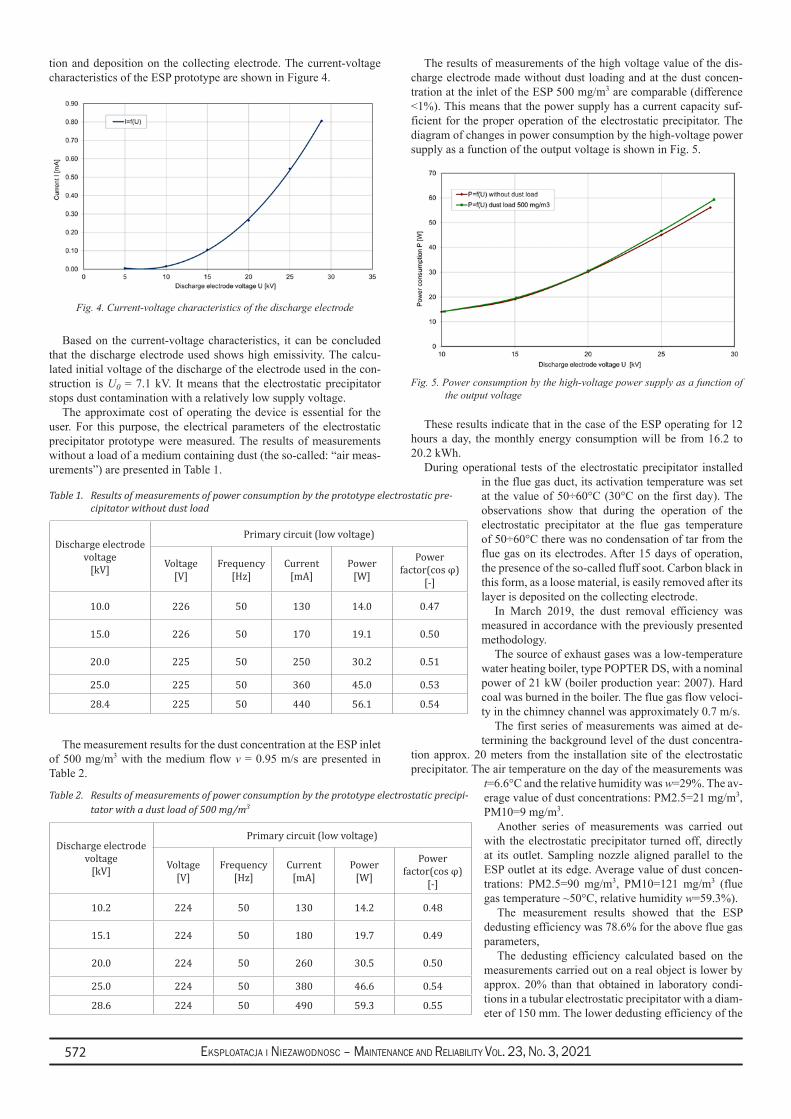
Eksploatacja i NiEzawodNosc – MaiNtENaNcE aNd REliability Vol. 23, No. 3, 2021572
tion and deposition on the collecting electrode. The current-voltage characteristics of the ESP prototype are shown in Figure 4.
Fig. 4. Current-voltage characteristics of the discharge electrode
Based on the current-voltage characteristics, it can be concluded that the discharge electrode used shows high emissivity. The calcu-lated initial voltage of the discharge of the electrode used in the con-struction is U0 = 7.1 kV. It means that the electrostatic precipitator stops dust contamination with a relatively low supply voltage.
The approximate cost of operating the device is essential for the user. For this purpose, the electrical parameters of the electrostatic precipitator prototype were measured. The results of measurements without a load of a medium containing dust (the so-called: “air meas-urements”) are presented in Table 1.
The measurement results for the dust concentration at the ESP inlet of 500 mg/m3 with the medium flow v = 0.95 m/s are presented in Table 2.
The results of measurements of the high voltage value of the dis-charge electrode made without dust loading and at the dust concen-tration at the inlet of the ESP 500 mg/m3 are comparable (difference <1%). This means that the power supply has a current capacity suf-ficient for the proper operation of the electrostatic precipitator. The diagram of changes in power consumption by the high-voltage power supply as a function of the output voltage is shown in Fig. 5.
Fig. 5. Power consumption by the high-voltage power supply as a function of the output voltage
These results indicate that in the case of the ESP operating for 12 hours a day, the monthly energy consumption will be from 16.2 to 20.2 kWh.
During operational tests of the electrostatic precipitator installed in the flue gas duct, its activation temperature was set at the value of 50÷60°C (30°C on the first day). The observations show that during the operation of the electrostatic precipitator at the flue gas temperature of 50÷60°C there was no condensation of tar from the flue gas on its electrodes. After 15 days of operation, the presence of the so-called fluff soot. Carbon black in this form, as a loose material, is easily removed after its layer is deposited on the collecting electrode.
In March 2019, the dust removal efficiency was measured in accordance with the previously presented methodology.
The source of exhaust gases was a low-temperature water heating boiler, type POPTER DS, with a nominal power of 21 kW (boiler production year: 2007). Hard coal was burned in the boiler. The flue gas flow veloci-ty in the chimney channel was approximately 0.7 m/s.
The first series of measurements was aimed at de-termining the background level of the dust concentra-
tion approx. 20 meters from the installation site of the electrostatic precipitator. The air temperature on the day of the measurements was
t=6.6°C and the relative humidity was w=29%. The av-erage value of dust concentrations: PM2.5=21 mg/m3, PM10=9 mg/m3.
Another series of measurements was carried out with the electrostatic precipitator turned off, directly at its outlet. Sampling nozzle aligned parallel to the ESP outlet at its edge. Average value of dust concen-trations: PM2.5=90 mg/m3, PM10=121 mg/m3 (flue gas temperature ~50°C, relative humidity w=59.3%).
The measurement results showed that the ESP dedusting efficiency was 78.6% for the above flue gas parameters,
The dedusting efficiency calculated based on the measurements carried out on a real object is lower by approx. 20% than that obtained in laboratory condi-tions in a tubular electrostatic precipitator with a diam-eter of 150 mm. The lower dedusting efficiency of the
Table 1. Results of measurements of power consumption by the prototype electrostatic pre-cipitator without dust load
Discharge electrode voltage
[kV]
Primary circuit (low voltage)
Voltage [V]
Frequency[Hz]
Current[mA]
Power[W]
Power factor(cos φ)
[-]
10.0 226 50 130 14.0 0.47
15.0 226 50 170 19.1 0.50
20.0 225 50 250 30.2 0.51
25.0 225 50 360 45.0 0.53
28.4 225 50 440 56.1 0.54
Table 2. Results of measurements of power consumption by the prototype electrostatic precipi-tator with a dust load of 500 mg/m3
Discharge electrode voltage
[kV]
Primary circuit (low voltage)
Voltage [V]
Frequency[Hz]
Current[mA]
Power[W]
Power factor(cos φ)
[-]
10.2 224 50 130 14.2 0.48
15.1 224 50 180 19.7 0.49
20.0 224 50 260 30.5 0.50
25.0 224 50 380 46.6 0.54
28.6 224 50 490 59.3 0.55
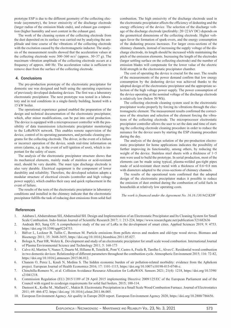
Eksploatacja i NiEzawodNosc – MaiNtENaNcE aNd REliability Vol. 23, No. 3, 2021 573
prototype ESP is due to the different geometry of the collecting elec-trode (asymmetry), the lower emissivity of the discharge electrode (larger radius of the emission blade ends), and exhaust gas composi-tion (higher humidity and soot content in the exhaust gas).
The work of the cleaning system of the collecting electrode from the dust deposited on its surface was carried out by analyzing the am-plitude and time course of the vibrations of the collecting electrode with the excitation caused by the electromagnetic inductor. The analy-sis of the measurement results showed that the acceleration values at the collecting electrode were 300÷360 m/s2 (approx. 30÷37 g). The maximum vibration amplitude of the collecting electrode occurs at a frequency of approx. 440 Hz. The acceleration value is sufficient to remove dust from the surface of the collecting electrode.
4. ConclusionsThe pre-production prototype of the electrostatic precipitator for
domestic use was designed and built using the operating experience of previously developed dedusting devices. The first was a laboratory electrostatic precipitator. The next prototype was tested in a labora-tory and in real conditions in a single-family building, heated with a 15 kW boiler.
The operational experience gained enabled the preparation of the design and technical documentation of the electrostatic precipitator, which, after minor modifications, can be put into serial production. The device is equipped with a microprocessor controller with the pos-sibility of data transmission (electrostatic precipitator monitoring) to the LoRaWAN network. This enables remote supervision of the device, control of its operating parameters, and periodic cleaning pro-grams for the collecting electrode. The driver, in the event of a failure or incorrect operation of the device, sends real-time information on errors (alarms, e.g. in the event of self-ignition of soot), which is im-portant for the safety of users.
The analysis of the electrostatic precipitator structure shows that its mechanical elements, mainly made of stainless or acid-resistant steel, should be very durable. The mast type discharge electrode is also very durable. Electrical equipment is the component of lower durability and reliability. Therefore, the developed solution adopts a modular structure of electrical circuits (controller and high voltage power supply), which enables their easy and quick replacement in the event of failure.
The results of the tests of the electrostatic precipitator in laboratory conditions and installed in the chimney indicate that the electrostatic precipitator fulfills the task of reducing dust emissions from solid fuel
combustion. The high emissivity of the discharge electrode used in the electrostatic precipitator affects the efficiency of dedusting and the energy efficiency of the device. The selection of the discharge volt-age of the discharge electrode (preferably: 20÷22 kV DC) depends on the geometrical dimensions of the collecting electrode. Higher volt-ages favor the formation of spark-overs, and the energy consumption of the dedusting process increases. For larger cross-sections of the chimney channels, instead of increasing the supply voltage of the dis-charge electrode, its length should be increased while maintaining the pitch of the emission elements. Increasing the length of the electrodes (larger settling surface on the collecting electrode) and the number of emission blades will compensate for the lower value of the electric field strength in the electrostatic precipitator chamber.
The cost of operating the device is crucial for the user. The results of the measurements of the power demand confirm that low energy consumption by the dedusting device was achieved thanks to the adopted design of the electrostatic precipitator and the appropriate se-lection of the high voltage power supply. The power consumption of the device operating at the nominal voltage of the discharge electrode is relatively low (below 50 Wh).
The collecting electrode cleaning system used in the electrostatic precipitator works properly by forcing its vibrations through the elec-tromagnetic element. The measurement results confirmed the correct-ness of the structure and selection of the element forcing the vibra-tions of the collecting electrode. The microprocessor electrostatic precipitator controller allows the user to set the date and time of start-ing the collecting electrode cleaning procedure in order to reduce the nuisance for the device users by starting the ESP cleaning procedure during the day.
The analysis of the design solution of the pre-production electro-static precipitator for home applications indicates the possibility of further improving its functionality, among others, by reducing the weight of the device. Stainless steel sheets with a thickness of 1÷5 mm were used to build the prototype. In serial production, most of the elements can be made using typical, plasma-welded gas-tight pipes made of acid-resistant sheet metal with a thickness of 0.6÷0.8 mm with diameters adapted to the cross-sections of chimney channels.
The results of the operational tests confirmed that the adopted design of the electrostatic precipitator makes it possible to reduce the emission of dust emitted during the combustion of solid fuels in households at relatively low operating costs.
The work is financed under the Agreement No. 16.16.130.942/KSW
References1. Adabara I, Abdurrahman SH, Abdurrashid SH. Design and Implementation of an Electrostatic Precipitator and Its Cleaning System for Small
Scale Combustion. Indo-Iranian Journal of Scientific Research 2017; 1: 213-224, https://www.researchgate.net/publication/3216826362. Andrade RO, Sang GY. A comprehensive study of the use of LoRa in the development of smart cities. Applied Sciences 2019; 9: 4753.
https://doi.org/10.3390/app9224753.3. Bäfver L, Leckner B, Tullin C, Berntsen M. Particle emissions from pellets stoves and modern and old-type wood stoves. Biomass and
Bioenergy 2011; 35: 3648-3655, https://doi.org/10.1016/j.biombioe.2011.05.027.4. Bologa A, Paur HR, Woletz K. Development and study of an electrostatic precipitator for small scale wood combustion. International Journal
of Plasma Environmental Science and Technology 2011; 5: 168-1735. Calvo AI, Martins V, Nunes T, Duarte M, Hillamo R, Teinilä K, Pont V, Castro A, Fraile R, Tarelho L, Alves C. Residential wood combustion
in two domestic devices: Relationship of different parameters throughout the combustion cycle. Atmospheric Environment 2015; 116: 72-82, https://doi.org/10.1016/j.atmosenv.2015.06.012.
6. Chanem O, Perez L, Knuli N, Medina S. The hidden economic burden of air pollution-related morbidity: evidence from the Aphekom project. European Journal of Health Economics 2016; 17: 1101-1115, https://doi.org/10.1007/s10198-015-0748-z.
7. Chinchilla-Romero N., et al. Collision Avoidance Resource Allocation for LoRaWAN. Sensors 2021; 21(4): 1218, https://doi.org/10.3390/s21041218.
8. Commission Regulation (EU) 2015/1189 of 28 April 2015 implementing Directive 2009/125/EC of the European Parliament and of the Council with regard to ecodesign requirements for solid fuel boilers. 2015; 100-114.
9. Dastoori K., Kolhe M., Mallard C., Makin B. Electrostatic Precipitation in a Small Scale Wood Combustion Furnace. Journal of Electrostatics 2011; 69: 466-472. https://doi.org/ 10.1016/j.elstat.2011.06.005.
10. European Environment Agency. Air quality in Europe 2020 report. European Environment Agency 2020, https://doi.org/10.2800/786656.

Eksploatacja i NiEzawodNosc – MaiNtENaNcE aNd REliability Vol. 23, No. 3, 2021574
11. Fischer, T., Grass N., Zouzou N., Dăscălescu L., Greil R., Hopf N. Smart home precipitator for biomass furnaces: Design considerations on a small scale electrostatic precipitator. Annual Meeting. IEEE Transactions on Industry Applications 2013; 50: 2219-2224, https://doi.org/10.1109/TIA.2013.2288430.
12. Görner P., Simon X., Wrobel R., Edmond K., Witschger O. Laboratory Study of Selected Personal Inhalable Aerosol Samplers. The Annals of occupational hygiene 2010; 54: 165-87, https://doi.org/10.1093/annhyg/mep079.
13. Harper M, Akbar MZ, Andrew ME. Comparison of wood-dust aerosol size-distributions collected by air samplers. Journal of Environmental Monitoring 2004; 6: 18-22, https://doi.org/10.1039/b312883k.
14. Heusse M, et al. Capacity of a LoRaWAN Cell. Proceedings of the 23rd International ACM Conference on Modeling, Analysis and Simulation of Wireless and Mobile Systems 2020, https://doi.org/10.1145/3416010.3423228.
15. Karwat B, Nocuń M, Machnik R, Niedźwiedzki J. Modelling and study the effect of selected design features for the operating parameters of industrial electrostatic precipitators. Eksploatacja i Niezawodnosc - Maintenance and Reliability 2016; 18(3): 325-332, doi:10.17531/ein.2016.3.2.
16. Karwat B, Machnik R, Niedźwiedzki J, Nogaj M. Selecting operating parameters of an electrostatic precipitator decreasing emission of solid fuels fly ashes. Eksploatacja i Niezawodnosc - Maintenance and Reliability 2018; 20(3): 495-501, https://doi.org/10.17531/ein.2018.3.20.
17. Koch W, Dunkhorst W, Lödding H, Thomassen Y, Skaugset N, Nikano A, Vincent J. Evaluation of the Respicon as a personal inhalable sampler in industrial environments. Journal of Environmental Monitoring 2002; 4: 657-662, https://doi.org/10.1039/B204985F.
18. Laitinen A, Karjalainen K, Virtanen A, Keskinen J, Aho M, Maunuksela J, Talka I. ESP for Small Scale Wood Combustion. Electrostatic Precipitation Springer, Berlin, Heidelberg 2009; 54-56, https://doi.org/10.1007/978-3-540-89251-9_8.
19. Manchini de Souza FV, Rabello RDS. LoRaWan: Low Cost Solution for Smart Cities. Smart and Digital Cities. Urban Computing. Springer, Cham. 2019, https://doi.org/10.1007/978-3-030-12255-3_11.
20. Mosquera J, Wagemans MJM, Aarnink AJA, Huynh TTT, de Gijsel P, Hol JMG. Guidelines to use the RespiCon unit for dust concentration measurements in practice. Agrotechnology & Food Innovations B.V. 2004.
21. Parker KR. Applied electrostatic precipitation. Blackie Academic & Professional. UK London 1997, https://doi.org/10.1007/978-94-009-1553-4_1.
22. Parker K. Electrical operation of electrostatic precipitators. The Institution of Electrical Engineers. UK London, 2003, https://doi.org/10.1049/PBPO041E.
23. Rando R, Poovey H, Mokadam D, Brisolara J. Field performance of the RespiCon™ for size-selective sampling of industrial wood processing dust. Journal of Occupational and Environmental Hygiene 2005; 2: 219-226, https://doi.org/10.1080/15459620590930309.
24. Ruttanachot C, Tirawanichakul Y, Tekasakul P. Application of electrostatic precipitator in collection of smoke aerosol particles from wood combustion. Aerosol and Air Quality Research 2011; 11: 90-98, https://doi.org/10.4209/aaqr.2010.08.0068.
25. Saari M, et al. LoRa-A survey of recent research trends. 41st International Convention on Information and Communication Technology, Electronics and Microelectronics (MIPRO). IEEE, 2018; 0872-0877, https://doi.org/10.23919/MIPRO.2018.8400161.
26. Sensidyne. Gilian 5000 Air Sampling Pump Operation Manual REF 360-0103-01 (Rev H) https://www.sensidyne.com/air-sampling-equipment/gilian-air-sampling-pumps/gilian-3500gilian-5000-air-sampling-pump/.
27. Tatum V, Ray AE, Rovell-Rixx D. Performance of the RespiCon™ Personal Aerosol Sampler in Forest Products Industry Workplaces. Journal of Occupational and Environmental Hygiene 2002; 63: 311-16, https://doi.org/10.1080/15428110208984719.
28. TU Graz. Survey on the present state of particle precipitation devices for residential biomass combustion with a nominal capacity up to 50 kW in IEA Bioenergy Task32 member countries. Graz University of Technology 2011, http://www.biosbioenergy.at/uploads/media/Filter-study-IEA-Dez-2011.pdf.
29. Vincent J. H. Aerosol sampling: science, standards, instrumentation and applications. John Wiley & Son 2007.30. Vicente ED, Alves C. A. An overview of particulate emissions from residential biomass combustion. Atmospheric Research 2018; 199:159-
185, https://doi.org/10.1016/j.atmosres.2017.08.027.31. WHO Air quality guidelines for Europe; second edition. WHO regional publications. European series 2000; 9.32. Wiinikka H., Grönberg C., Boman C. Emissions of heavy metals during fixed-bed combustion of six biomass fuels. Energy Fuels 2013; 27:
1073-1080, https://doi.org/10.1021/ef3011146.
Eksploatacja i NiEzawodNosc – MaiNtENaNcE aNd REliability Vol. 23, No. 3, 2021 575
(*) Corresponding author.E-mail addresses:
Eksploatacja i Niezawodnosc – Maintenance and ReliabilityVolume 23 (2021), Issue 3
journal homepage: http://www.ein.org.pl
Indexed by:
1. IntroductionIn the last decade repair intervals of certain parts of gas turbines,
which are installed in the combustor or turbine sections, have been extended by 100%. Constantly growing energy needs force operators of petrochemical and power plants to reduce downtime and maximize production. Many companies sign a Long-term Service Agreement with the engine’s OEM to assure seamless execution of the optimized maintenance plan, with availability and productivity guarantees. The value delivered by the manufacturer is based on the knowledge, expe-rience and data accumulated over the years. Combining this with se-lected operating parameters of the units allows to develop predictive models, which support data-driven decisions and provide actionable insights to the end users [6]. Due to the complexity of the analyzed system, numerous estimators are built and utilized, e.g., for diagnostic and anomaly detection [17, 13], classification [2], regression, or as a synthetic sensors [33]. A structured collection of such models reflect-ing part-to-part interactions and fed with operational data is referred to as the digital twin of the gas turbine [30].
Survival analysis for rotating equipment is typically carried out on limited datasets due to the low occurrence of failures, long duration
and high costs associated with the destructive tests. These constraints set Weibull analysis for years as the default method for forecasting failure probability and damage size [1]. Scientific papers on the cor-rect execution of regression analysis in the small-data regime [28] have not disappeared in the big data era. New contributions have been published [23, 14] and are needed to provide guidance on how to use machine learning algorithms, which were not so commonly used in the past, for predictive modeling based on small samples. Such stud-ies will be executed regardless of the growth of big data, but with the development of new data infrastructures the small data might be pooled and scaled more frequently [26].
Fatigue is among the most frequent causes of failures in mechani-cal systems. Deep knowledge of the fatigue crack growth mechanism is needed for the design and maintenance of gas turbines, especially with rising expectations regarding the efficiency and comprehensive optimization of the production process. Since the groundbreaking con-tribution of Paris and Erdogan [32], numerous fatigue crack growth equations have been published and these have been summarized well in [4]. For the most part, these models are based on experimental data and vary in complexity. There is no universal approach to fatigue life prediction; thus, for a particular problem, the optimal method should
Predicting length of fatigue cracks by means of machine learning algorithms in the small-data regimeMaciej Badora a,b,*, Marzia Sepe c, Marcin Bielecki b, Antonino Graziano c, Tomasz Szolc a
a Institute of Fundamental Technological Research, Polish Academy of Sciences, ul. Pawińskiego 5b, 02-106 Warsaw, Poland b Baker Hughes, BH Poland sp. z o.o., Aleja Krakowska 110/114, 02-256 Warsaw, Poland c Baker Hughes, Via Felice Matteucci 2, 50127 Florence, Italy
Badora M, Sepe M, Bielecki M, Graziano A, Szolc T. Predicting length of fatigue cracks by means of machine learning algorithms in the small-data regime. Eksploatacja i Niezawodnosc – Maintenance and Reliability 2021; 23 (3): 575–585, http://doi.org/10.17531/ein.2021.3.19.
Article citation info:
In this paper several statistical learning algorithms are used to predict the maximal length of fatigue cracks based on a sample composed of 31 observations. The small-data regime is still a problem for many professionals, especially in the areas where failures occur rarely. The analyzed object is a high-pressure Nozzle of a heavy-duty gas turbine. Operating parameters of the engines are used for the regression analysis. The following algorithms are used in this work: multiple linear and polynomial regression, random forest, kernel-based methods, AdaBoost and extreme gradient boosting and artificial neural networks. A substantial part of the paper provides advice on the effective selection of features. The paper explains how to process the dataset in order to reduce uncertainty; thus, simplifying the analysis of the results. The proposed loss and cost functions are custom and promote solutions accurately predicting the longest cracks. The obtained results confirm that some of the algorithms can accurately predict maximal lengths of the fatigue cracks, even if the sample is small.
Highlights Abstract
Machine learning algorithms can be utilized ef-• fectively in the small-data regime.
The length of fatigue cracks can be predicted • based on operational data of the engine.
The lowest root mean squared error (RMSE) is • achieved with the AdaBoost.R2 algorithm.
Small datasets should be processed in a fully con-• trolled manner to get valuable results.
A custom cost function may favor certain solu-• tions and drives capabilities of the model.
empirical models, fatigue cracks, predictive maintenance, regression analysis, small data, statistical learning, turbomachinery.
Keywords
This is an open access article under the CC BY license (https://creativecommons.org/licenses/by/4.0/)
M. Badora - [email protected], [email protected]; M. Sepe - [email protected];M. Bielecki - [email protected]; A. Graziano - [email protected]; T. Szolc - [email protected]
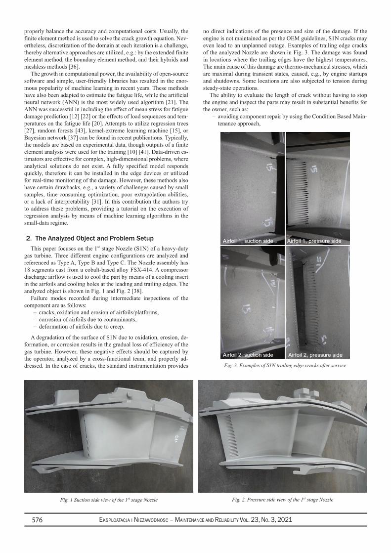
Eksploatacja i NiEzawodNosc – MaiNtENaNcE aNd REliability Vol. 23, No. 3, 2021576
properly balance the accuracy and computational costs. Usually, the finite element method is used to solve the crack growth equation. Nev-ertheless, discretization of the domain at each iteration is a challenge, thereby alternative approaches are utilized, e.g.: by the extended finite element method, the boundary element method, and their hybrids and meshless methods [36].
The growth in computational power, the availability of open-source software and simple, user-friendly libraries has resulted in the enor-mous popularity of machine learning in recent years. These methods have also been adapted to estimate the fatigue life, while the artificial neural network (ANN) is the most widely used algorithm [21]. The ANN was successful in including the effect of mean stress for fatigue damage prediction [12] [22] or the effects of load sequences and tem-peratures on the fatigue life [20]. Attempts to utilize regression trees [27], random forests [43], kernel-extreme learning machine [15], or Bayesian network [37] can be found in recent publications. Typically, the models are based on experimental data, though outputs of a finite element analysis were used for the training [10] [41]. Data-driven es-timators are effective for complex, high-dimensional problems, where analytical solutions do not exist. A fully specified model responds quickly, therefore it can be installed in the edge devices or utilized for real-time monitoring of the damage. However, these methods also have certain drawbacks, e.g., a variety of challenges caused by small samples, time-consuming optimization, poor extrapolation abilities, or a lack of interpretability [31]. In this contribution the authors try to address these problems, providing a tutorial on the execution of regression analysis by means of machine learning algorithms in the small-data regime.
2. The Analyzed Object and Problem SetupThis paper focuses on the 1st stage Nozzle (S1N) of a heavy-duty
gas turbine. Three different engine configurations are analyzed and referenced as Type A, Type B and Type C. The Nozzle assembly has 18 segments cast from a cobalt-based alloy FSX-414. A compressor discharge airflow is used to cool the part by means of a cooling insert in the airfoils and cooling holes at the leading and trailing edges. The analyzed object is shown in Fig. 1 and Fig. 2 [38].
Failure modes recorded during intermediate inspections of the component are as follows:
cracks, oxidation and erosion of airfoils/platforms, –corrosion of airfoils due to contaminants, –deformation of airfoils due to creep. –
A degradation of the surface of S1N due to oxidation, erosion, de-formation, or corrosion results in the gradual loss of efficiency of the gas turbine. However, these negative effects should be captured by the operator, analyzed by a cross-functional team, and properly ad-dressed. In the case of cracks, the standard instrumentation provides
no direct indications of the presence and size of the damage. If the engine is not maintained as per the OEM guidelines, S1N cracks may even lead to an unplanned outage. Examples of trailing edge cracks of the analyzed Nozzle are shown in Fig. 3. The damage was found in locations where the trailing edges have the highest temperatures. The main cause of this damage are thermo-mechanical stresses, which are maximal during transient states, caused, e.g., by engine startups and shutdowns. Some locations are also subjected to tension during steady-state operations.
The ability to evaluate the length of crack without having to stop the engine and inspect the parts may result in substantial benefits for the owner, such as:
avoiding component repair by using the Condition Based Main- –tenance approach,
Fig. 1 Suction side view of the 1st stage Nozzle Fig. 2. Pressure side view of the 1st stage Nozzle
Fig. 3. Examples of S1N trailing edge cracks after service
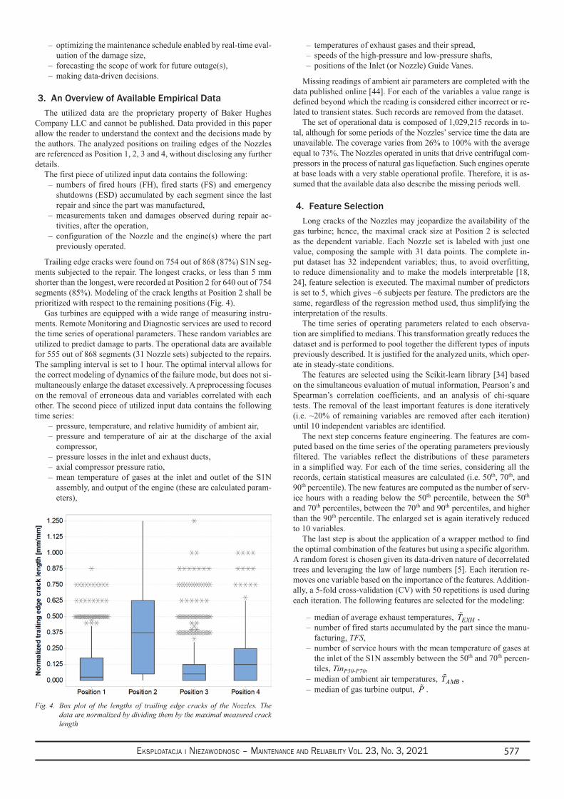
Eksploatacja i NiEzawodNosc – MaiNtENaNcE aNd REliability Vol. 23, No. 3, 2021 577
optimizing the maintenance schedule enabled by real-time eval- –uation of the damage size,forecasting the scope of work for future outage(s), –making data-driven decisions. –
3. An Overview of Available Empirical DataThe utilized data are the proprietary property of Baker Hughes
Company LLC and cannot be published. Data provided in this paper allow the reader to understand the context and the decisions made by the authors. The analyzed positions on trailing edges of the Nozzles are referenced as Position 1, 2, 3 and 4, without disclosing any further details.
The first piece of utilized input data contains the following:numbers of fired hours (FH), fired starts (FS) and emergency –shutdowns (ESD) accumulated by each segment since the last repair and since the part was manufactured,measurements taken and damages observed during repair ac- –tivities, after the operation,configuration of the Nozzle and the engine(s) where the part –previously operated.
Trailing edge cracks were found on 754 out of 868 (87%) S1N seg-ments subjected to the repair. The longest cracks, or less than 5 mm shorter than the longest, were recorded at Position 2 for 640 out of 754 segments (85%). Modeling of the crack lengths at Position 2 shall be prioritized with respect to the remaining positions (Fig. 4).
Gas turbines are equipped with a wide range of measuring instru-ments. Remote Monitoring and Diagnostic services are used to record the time series of operational parameters. These random variables are utilized to predict damage to parts. The operational data are available for 555 out of 868 segments (31 Nozzle sets) subjected to the repairs. The sampling interval is set to 1 hour. The optimal interval allows for the correct modeling of dynamics of the failure mode, but does not si-multaneously enlarge the dataset excessively. A preprocessing focuses on the removal of erroneous data and variables correlated with each other. The second piece of utilized input data contains the following time series:
pressure, temperature, and relative humidity of ambient air, –pressure and temperature of air at the discharge of the axial –compressor,pressure losses in the inlet and exhaust ducts, –axial compressor pressure ratio, –mean temperature of gases at the inlet and outlet of the S1N –assembly, and output of the engine (these are calculated param-eters),
temperatures of exhaust gases and their spread, –speeds of the high-pressure and low-pressure shafts, –positions of the Inlet (or Nozzle) Guide Vanes. –
Missing readings of ambient air parameters are completed with the data published online [44]. For each of the variables a value range is defined beyond which the reading is considered either incorrect or re-lated to transient states. Such records are removed from the dataset.
The set of operational data is composed of 1,029,215 records in to-tal, although for some periods of the Nozzles’ service time the data are unavailable. The coverage varies from 26% to 100% with the average equal to 73%. The Nozzles operated in units that drive centrifugal com-pressors in the process of natural gas liquefaction. Such engines operate at base loads with a very stable operational profile. Therefore, it is as-sumed that the available data also describe the missing periods well.
4. Feature SelectionLong cracks of the Nozzles may jeopardize the availability of the
gas turbine; hence, the maximal crack size at Position 2 is selected as the dependent variable. Each Nozzle set is labeled with just one value, composing the sample with 31 data points. The complete in-put dataset has 32 independent variables; thus, to avoid overfitting, to reduce dimensionality and to make the models interpretable [18, 24], feature selection is executed. The maximal number of predictors is set to 5, which gives ~6 subjects per feature. The predictors are the same, regardless of the regression method used, thus simplifying the interpretation of the results.
The time series of operating parameters related to each observa-tion are simplified to medians. This transformation greatly reduces the dataset and is performed to pool together the different types of inputs previously described. It is justified for the analyzed units, which oper-ate in steady-state conditions.
The features are selected using the Scikit-learn library [34] based on the simultaneous evaluation of mutual information, Pearson’s and Spearman’s correlation coefficients, and an analysis of chi-square tests. The removal of the least important features is done iteratively (i.e. ~20% of remaining variables are removed after each iteration) until 10 independent variables are identified.
The next step concerns feature engineering. The features are com-puted based on the time series of the operating parameters previously filtered. The variables reflect the distributions of these parameters in a simplified way. For each of the time series, considering all the records, certain statistical measures are calculated (i.e. 50th, 70th, and 90th percentile). The new features are computed as the number of serv-ice hours with a reading below the 50th percentile, between the 50th and 70th percentiles, between the 70th and 90th percentiles, and higher than the 90th percentile. The enlarged set is again iteratively reduced to 10 variables.
The last step is about the application of a wrapper method to find the optimal combination of the features but using a specific algorithm. A random forest is chosen given its data-driven nature of decorrelated trees and leveraging the law of large numbers [5]. Each iteration re-moves one variable based on the importance of the features. Addition-ally, a 5-fold cross-validation (CV) with 50 repetitions is used during each iteration. The following features are selected for the modeling:
median of average exhaust temperatures, – EXHT ,number of fired starts accumulated by the part since the manu- –facturing, TFS,number of service hours with the mean temperature of gases at –the inlet of the S1N assembly between the 50th and 70th percen-tiles, TinP50-P70,median of ambient air temperatures, – AMBT ,median of gas turbine output, – P .
Fig. 4. Box plot of the lengths of trailing edge cracks of the Nozzles. The data are normalized by dividing them by the maximal measured crack length
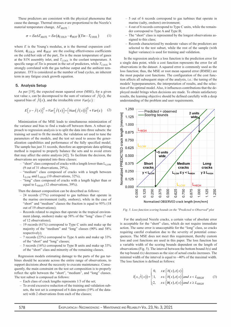
Eksploatacja i NiEzawodNosc – MaiNtENaNcE aNd REliability Vol. 23, No. 3, 2021578
These predictors are consistent with the physical phenomena that cause the damage. Thermal stresses σ are proportional to the Nozzle’s material temperature change, ∆TMATL :
σ α α φ φ= = −( ) −( )E T E Tin TMATL COLD HOT COOL∆ (1)
where E is the Young’s modulus, α is the thermal expansion coef-ficient, φCOLD and φHOT are the cooling effectiveness coefficients on the cold/hot side of the part, Tin is the mean temperature of gases at the S1N assembly inlet, and TCOOL is the coolant temperature. A specific range of Tin is present in the set of predictors, while TCOOL is strongly correlated with the gas turbine output and the ambient tem-perature. TFS is considered as the number of load cycles, an inherent term in any fatigue crack growth equation.
5. Analysis SetupAs per [19], the expected mean squared error (MSE), for a given
test value x, can be decomposed to the sum of variance of ( )f x , the squared bias of ( )f x , and the irreducible error Var ε( ) :
E y f x Var f x bias f x Var− ( ) = ( ) + ( )( ) + ( )2 2εˆˆ ˆ (2)
Minimization of the MSE leads to simultaneous minimization of the variance and bias to find a trade-off between them. A robust ap-proach to regression analysis is to split the data into three subsets: the training set used to fit the models, the validation set used to tune the parameters of the models, and the test set used to assess the gener-alization capabilities and performance of the fully specified model. The sample has just 31 records, therefore an appropriate data splitting method is required to properly balance the sets and to avoid errors that may affect the entire analysis [42]. To facilitate the decision, the observations are separated into three classes:
“short” class composed of cracks with a length lower than L – LOW (9 out of 31 observations, 29%),“medium” class composed of cracks with a length between –LLOW and LHIGH (10 observations, 32%),“long” class composed of cracks with a length higher than or –equal to LHIGH (12 observations, 39%).
Then the dataset composition can be described as follows:24 records (77%) correspond to gas turbines that operate in –the marine environment (salty, onshore), while in the case of “short” and “medium” classes the fraction is equal to 95% (18 out of 19 observations);Records related to engines that operate in the tropical environ- –ment (damp, onshore) make up 58% of the “long” class (7 out of 12 observations);19 records (61%) correspond to Type C units and make up the –majority of the “medium” and “long” classes (90% and 58% respectively);7 records (23%) correspond to Type A units and make up 33% –of the “short” and “long” classes;5 records (16%) correspond to Type B units and make up 33% –of the “short” class and minority of the remaining classes.
Regression models estimating damage to the parts of the gas tur-bines should be accurate across the entire range of observations, to support decisions about the necessity to execute maintenance. Conse-quently, the main constraint on the test set composition is to properly reflect the split between the “short”, “medium”, and “long” classes. The test subset is composed as follows:
Each class of crack lengths represents 1/3 of the set; –To avoid excessive reduction of the training and validation sub- –sets, the test set is composed of 6 data points (19% of the data-set) with 2 observations from each of the classes;
5 out of 6 records correspond to gas turbines that operate in –marine (salty, onshore) environment;4 out of 6 records correspond to Type C units, while the remain- –der correspond to Type A and Type B;The “short” class is represented by the longest observations as- –signed to this class;Records characterized by moderate values of the predictors are –selected to the test subset, while the rest of the sample (with higher variance) is used for training and validation.
In the regression analysis a loss function is the prediction error for a single data point, while a cost function represents the error for all observations in the dataset. A squared error is commonly used as the loss function; thus, the MSE or root mean squared error (RMSE) are the most popular cost functions. The configuration of the cost func-tion affects all subsequent steps of the analysis, i.e.: the tuning of the models’ hyperparameters, the interpretation of results, and the selec-tion of the optimal model. Also, it influences contributions that the de-ployed model brings when decisions are made. To obtain satisfactory results, the learning objective should be defined carefully with a deep understanding of the problem and user requirements.
For the analyzed Nozzle cracks, a certain value of absolute error is acceptable for the “short” class, which do not require immediate action. The same error is unacceptable for the “long” class, so cracks requiring careful evaluation due to the severity of potential conse-quences. The MSE does not meet this requirement, thereby custom loss and cost functions are used in this paper. The loss function has a variable width of the scoring bounds dependent on the length of observations (Fig. 5). The interval between the bottom bound b(x) and the top bound t(x) decreases as the size of actual cracks increases. The minimal width of the interval is equal to ~40% of the maximal width. The loss function is defined as follows:
l x f x
x b x t x
x b x t x and x L
xHIGH,
, ,
, ,
,( )( ) =
∉ ( ) ( ) ∈ ( ) ( ) <
∈
0
1
2 bb x t x and x LHIGH( ) ( ) ≥
,
ˆ (3)
Fig. 5. Loss function scoring bounds on the "Predicted vs Observed" plot
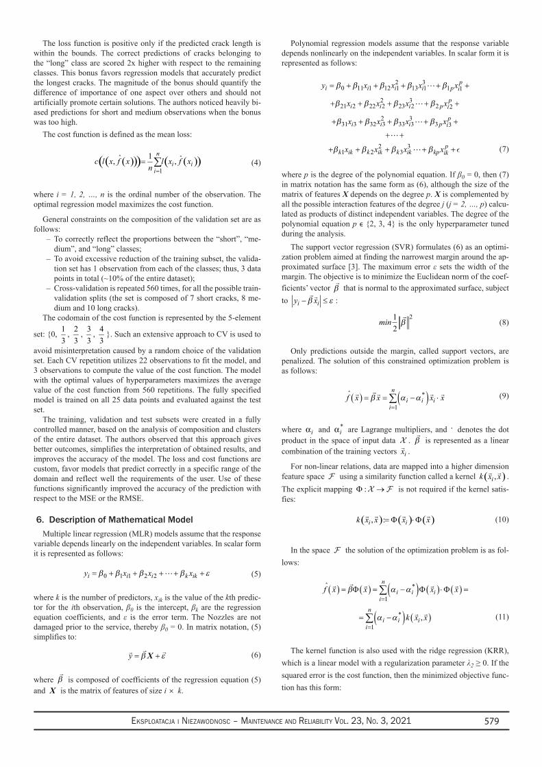
Eksploatacja i NiEzawodNosc – MaiNtENaNcE aNd REliability Vol. 23, No. 3, 2021 579
The loss function is positive only if the predicted crack length is within the bounds. The correct predictions of cracks belonging to the “long” class are scored 2x higher with respect to the remaining classes. This bonus favors regression models that accurately predict the longest cracks. The magnitude of the bonus should quantify the difference of importance of one aspect over others and should not artificially promote certain solutions. The authors noticed heavily bi-ased predictions for short and medium observations when the bonus was too high.
The cost function is defined as the mean loss:
( )( )( ) ( )( )1
1, ,n
i ii
c l x f x l x f xn =
= ∑ˆ ˆ (4)
where i = 1, 2, …, n is the ordinal number of the observation. The optimal regression model maximizes the cost function.
General constraints on the composition of the validation set are as follows:
To correctly reflect the proportions between the “short”, “me- –dium”, and “long” classes;To avoid excessive reduction of the training subset, the valida- –tion set has 1 observation from each of the classes; thus, 3 data points in total (~10% of the entire dataset);Cross-validation is repeated 560 times, for all the possible train- –validation splits (the set is composed of 7 short cracks, 8 me-dium and 10 long cracks).
The codomain of the cost function is represented by the 5-element
set: 0, 13
, 23
, 33
, 43
. Such an extensive approach to CV is used to
avoid misinterpretation caused by a random choice of the validation set. Each CV repetition utilizes 22 observations to fit the model, and 3 observations to compute the value of the cost function. The model with the optimal values of hyperparameters maximizes the average value of the cost function from 560 repetitions. The fully specified model is trained on all 25 data points and evaluated against the test set.
The training, validation and test subsets were created in a fully controlled manner, based on the analysis of composition and clusters of the entire dataset. The authors observed that this approach gives better outcomes, simplifies the interpretation of obtained results, and improves the accuracy of the model. The loss and cost functions are custom, favor models that predict correctly in a specific range of the domain and reflect well the requirements of the user. Use of these functions significantly improved the accuracy of the prediction with respect to the MSE or the RMSE.
6. Description of Mathematical ModelMultiple linear regression (MLR) models assume that the response
variable depends linearly on the independent variables. In scalar form it is represented as follows:
y x x xi i i k ik= + + + + +β β β β ε0 1 1 2 2 (5)
where k is the number of predictors, xik is the value of the kth predic-tor for the ith observation, β0 is the intercept, βk are the regression equation coefficients, and ε is the error term. The Nozzles are not damaged prior to the service, thereby β0 = 0. In matrix notation, (5) simplifies to:
y = +β εX (6)
where
β is composed of coefficients of the regression equation (5) and X is the matrix of features of size i × k.
Polynomial regression models assume that the response variable depends nonlinearly on the independent variables. In scalar form it is represented as follows:
y x x x xi i i i p i
p= + + + + +β β β β β0 11 1 12 12
13 13
1 1
+ + + + +β β β β21 2 22 2
223 2
32 2x x x xi i i p i
p
+ + + + +β β β β31 3 32 3
233 3
33 3x x x xi i i p i
p
+ + + + + + +β β β βk ik k ik k ik kp ik
px x x x1 22
33 (7)
where p is the degree of the polynomial equation. If β0 = 0, then (7) in matrix notation has the same form as (6), although the size of the matrix of features X depends on the degree p. X is complemented by all the possible interaction features of the degree j (j = 2, …, p) calcu-lated as products of distinct independent variables. The degree of the polynomial equation p ϵ 2, 3, 4 is the only hyperparameter tuned during the analysis.
The support vector regression (SVR) formulates (6) as an optimi-zation problem aimed at finding the narrowest margin around the ap-proximated surface [3]. The maximum error ε sets the width of the margin. The objective is to minimize the Euclidean norm of the coef-ficients’ vector
β that is normal to the approximated surface, subject to y xi i− ≤
β ε :
min 12
2β (8)
Only predictions outside the margin, called support vectors, are penalized. The solution of this constrained optimization problem is as follows:
f x x x xi
ni i i
( ) = = −( ) ⋅=∑β α α
1
*ˆ (9)
where iα and *iα are Lagrange multipliers, and ⋅ denotes the dot
product in the space of input data .
β is represented as a linear combination of the training vectors ix .
For non-linear relations, data are mapped into a higher dimension feature space using a similarity function called a kernel ( ),ik x x . The explicit mapping :Φ → is not required if the kernel satis-fies:
( ) ( ) ( ), :i ik x x x x= Φ ⋅Φ (10)
In the space the solution of the optimization problem is as fol-lows:
f x x x x
i
ni i i
( ) = ( ) = −( ) ( ) ⋅ ( ) ==∑β α αΦ Φ Φ
1
*ˆ
= −( ) ( )=∑i
ni i ik x x
1α α* , (11)
The kernel function is also used with the ridge regression (KRR), which is a linear model with a regularization parameter λ2 ≥ 0. If the squared error is the cost function, then the minimized objective func-tion has this form:
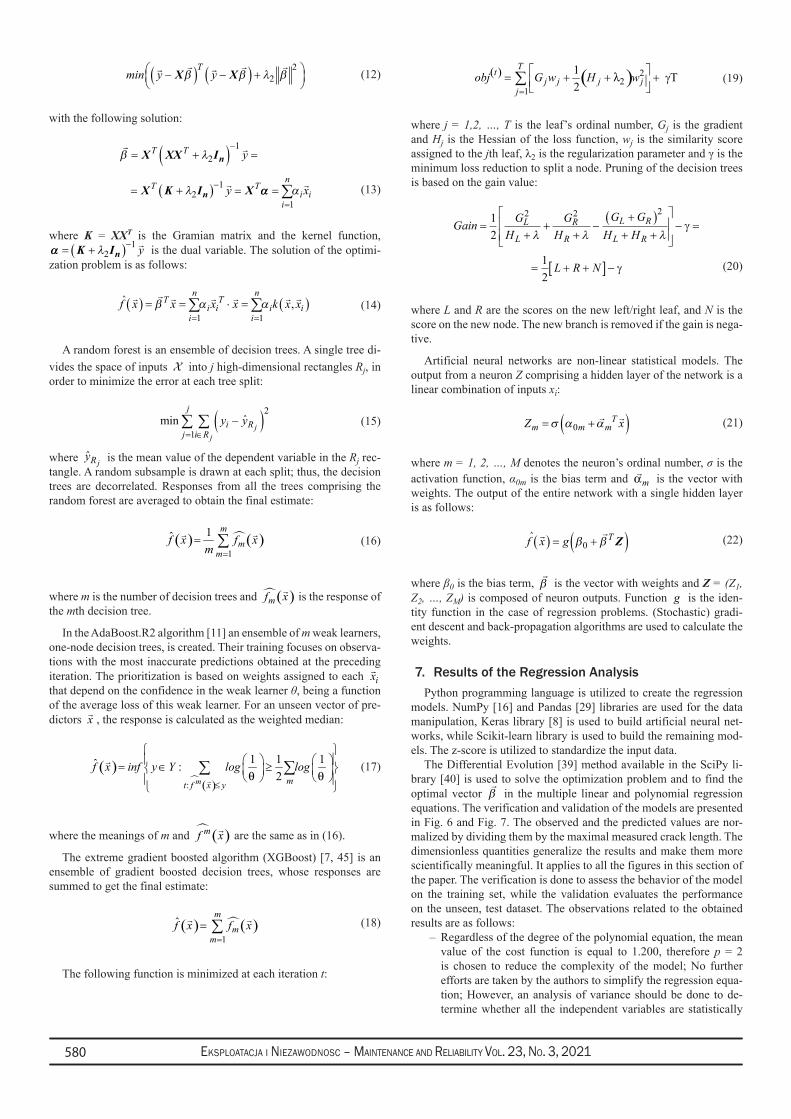
Eksploatacja i NiEzawodNosc – MaiNtENaNcE aNd REliability Vol. 23, No. 3, 2021580
min y yT
−( ) −( ) +
X Xβ β λ β2
2 (12)
with the following solution:
β λ= +( ) =−
X XX InT T y2
1
= +( ) = =−
=∑X K I Xn
T T
i
ni iy xλ α2
1
1
αα (13)
where K = XXT is the Gramian matrix and the kernel function, αα = +( )−K Inλ2
1 y is the dual variable. The solution of the optimi-zation problem is as follows:
f x x x x k x xT
i
ni i
T
i
ni i
( ) = = ⋅ = ( )= =∑ ∑β α α
1 1, (14)
A random forest is an ensemble of decision trees. A single tree di-vides the space of inputs into j high-dimensional rectangles Rj, in order to minimize the error at each tree split:
minj
j
i Ri R
jj
y y= ∈∑ ∑ −( )
1
2ˆ (15)
where ˆjRy is the mean value of the dependent variable in the Rj rec-
tangle. A random subsample is drawn at each split; thus, the decision trees are decorrelated. Responses from all the trees comprising the random forest are averaged to obtain the final estimate:
( ) ( )1
1ˆm
mm
f x f xm =
= ∑
(16)
where m is the number of decision trees and ( )mf x is the response of the mth decision tree.
In the AdaBoost.R2 algorithm [11] an ensemble of m weak learners, one-node decision trees, is created. Their training focuses on observa-tions with the most inaccurate predictions obtained at the preceding iteration. The prioritization is based on weights assigned to each ix that depend on the confidence in the weak learner θ, being a function of the average loss of this weak learner. For an unseen vector of pre-dictors x , the response is calculated as the weighted median:
( ) ( ):
2ˆ 1 1 1:
m mt f x y
f x inf y Y log logθ θ
≤
= ∈ ≥
∑ ∑
(17)
where the meanings of m and ( )mf x are the same as in (16).
The extreme gradient boosted algorithm (XGBoost) [7, 45] is an ensemble of gradient boosted decision trees, whose responses are summed to get the final estimate:
( ) ( )1
ˆm
mm
f x f x=
= ∑ (18)
The following function is minimized at each iteration t:
( ) ( ) 22
1
1 T2
Ttj j j j
jobj G w H wλ
=
= + + + γ ∑ (19)
where j = 1,2, …, T is the leaf’s ordinal number, Gj is the gradient and Hj is the Hessian of the loss function, wj is the similarity score assigned to the jth leaf, λ2 is the regularization parameter and γ is the minimum loss reduction to split a node. Pruning of the decision trees is based on the gain value:
Gain GH
GH
G GH H
L
L
R
R
L R
L R=
++
+−
+( )+ +
− =
12
2 2 2
λ λ λγ
= + +[ ] −12
L R N γ (20)
where L and R are the scores on the new left/right leaf, and N is the score on the new node. The new branch is removed if the gain is nega-tive.
Artificial neural networks are non-linear statistical models. The output from a neuron Z comprising a hidden layer of the network is a linear combination of inputs xi:
Z xm m mT= +( )σ α α0
(21)
where m = 1, 2, …, M denotes the neuron’s ordinal number, σ is the activation function, α0m is the bias term and mα is the vector with weights. The output of the entire network with a single hidden layer is as follows:
f x g T
( ) = +( )β β0 Zˆ (22)
where β0 is the bias term,
β is the vector with weights and Z = (Z1, Z2, …, ZM) is composed of neuron outputs. Function g is the iden-tity function in the case of regression problems. (Stochastic) gradi-ent descent and back-propagation algorithms are used to calculate the weights.
7. Results of the Regression AnalysisPython programming language is utilized to create the regression
models. NumPy [16] and Pandas [29] libraries are used for the data manipulation, Keras library [8] is used to build artificial neural net-works, while Scikit-learn library is used to build the remaining mod-els. The z-score is utilized to standardize the input data.
The Differential Evolution [39] method available in the SciPy li-brary [40] is used to solve the optimization problem and to find the optimal vector
β in the multiple linear and polynomial regression equations. The verification and validation of the models are presented in Fig. 6 and Fig. 7. The observed and the predicted values are nor-malized by dividing them by the maximal measured crack length. The dimensionless quantities generalize the results and make them more scientifically meaningful. It applies to all the figures in this section of the paper. The verification is done to assess the behavior of the model on the training set, while the validation evaluates the performance on the unseen, test dataset. The observations related to the obtained results are as follows:
Regardless of the degree of the polynomial equation, the mean –value of the cost function is equal to 1.200, therefore p = 2 is chosen to reduce the complexity of the model; No further efforts are taken by the authors to simplify the regression equa-tion; However, an analysis of variance should be done to de-termine whether all the independent variables are statistically
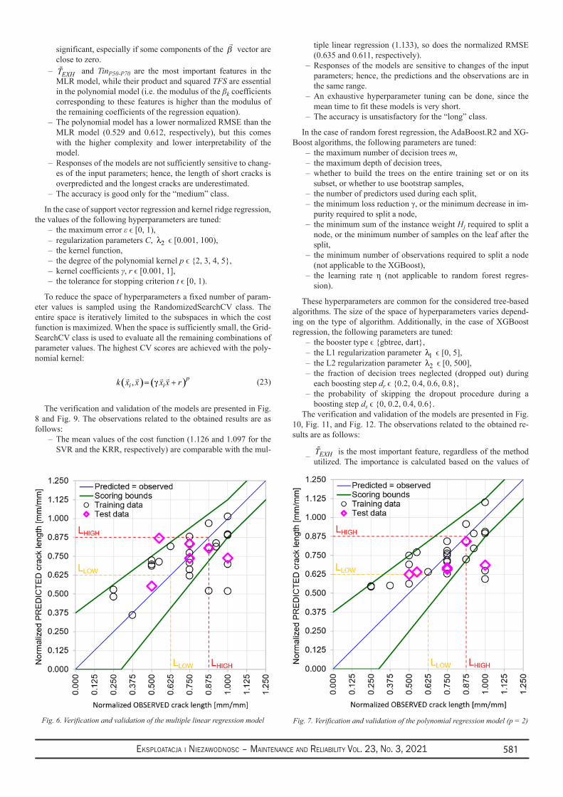
Eksploatacja i NiEzawodNosc – MaiNtENaNcE aNd REliability Vol. 23, No. 3, 2021 581
significant, especially if some components of the
β vector are close to zero.
EXHT – and TinP50-P70 are the most important features in the MLR model, while their product and squared TFS are essential in the polynomial model (i.e. the modulus of the βk coefficients corresponding to these features is higher than the modulus of the remaining coefficients of the regression equation).The polynomial model has a lower normalized RMSE than the –MLR model (0.529 and 0.612, respectively), but this comes with the higher complexity and lower interpretability of the model.Responses of the models are not sufficiently sensitive to chang- –es of the input parameters; hence, the length of short cracks is overpredicted and the longest cracks are underestimated.The accuracy is good only for the “medium” class. –
In the case of support vector regression and kernel ridge regression, the values of the following hyperparameters are tuned:
the maximum error – ε ϵ [0, 1),regularization parameters – C, 2λ ϵ [0.001, 100),the kernel function, –the degree of the polynomial kernel – p ϵ 2, 3, 4, 5,kernel coefficients – γ, r ϵ [0.001, 1],the tolerance for stopping criterion – t ϵ [0, 1).
To reduce the space of hyperparameters a fixed number of param-eter values is sampled using the RandomizedSearchCV class. The entire space is iteratively limited to the subspaces in which the cost function is maximized. When the space is sufficiently small, the Grid-SearchCV class is used to evaluate all the remaining combinations of parameter values. The highest CV scores are achieved with the poly-nomial kernel:
( ) ( ), pi ik x x x x rγ= + (23)
The verification and validation of the models are presented in Fig. 8 and Fig. 9. The observations related to the obtained results are as follows:
The mean values of the cost function (1.126 and 1.097 for the –SVR and the KRR, respectively) are comparable with the mul-
tiple linear regression (1.133), so does the normalized RMSE (0.635 and 0.611, respectively).Responses of the models are sensitive to changes of the input –parameters; hence, the predictions and the observations are in the same range.An exhaustive hyperparameter tuning can be done, since the –mean time to fit these models is very short.The accuracy is unsatisfactory for the “long” class. –
In the case of random forest regression, the AdaBoost.R2 and XG-Boost algorithms, the following parameters are tuned:
the maximum number of decision trees – m,the maximum depth of decision trees, –whether to build the trees on the entire training set or on its –subset, or whether to use bootstrap samples,the number of predictors used during each split, –the minimum loss reduction γ, or the minimum decrease in im- –purity required to split a node,the minimum sum of the instance weight – Hj required to split a node, or the minimum number of samples on the leaf after the split,the minimum number of observations required to split a node –(not applicable to the XGBoost),the learning rate η (not applicable to random forest regres- –sion).
These hyperparameters are common for the considered tree-based algorithms. The size of the space of hyperparameters varies depend-ing on the type of algorithm. Additionally, in the case of XGBoost regression, the following parameters are tuned:
the booster type ϵ gbtree, dart, –the L1 regularization parameter – 1λ ϵ [0, 5],the L2 regularization parameter – 2λ ϵ [0, 500],the fraction of decision trees neglected (dropped out) during –each boosting step dr ϵ 0.2, 0.4, 0.6, 0.8,the probability of skipping the dropout procedure during a –boosting step ds ϵ 0, 0.2, 0.4, 0.6.
The verification and validation of the models are presented in Fig. 10, Fig. 11, and Fig. 12. The observations related to the obtained re-sults are as follows:
EXHT – is the most important feature, regardless of the method utilized. The importance is calculated based on the values of
Fig. 6. Verification and validation of the multiple linear regression model Fig. 7. Verification and validation of the polynomial regression model (p = 2)
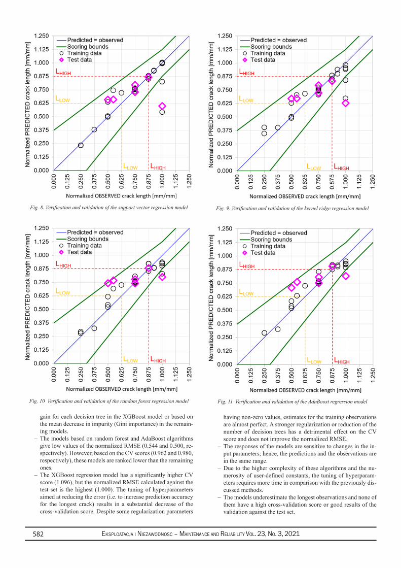
Eksploatacja i NiEzawodNosc – MaiNtENaNcE aNd REliability Vol. 23, No. 3, 2021582
gain for each decision tree in the XGBoost model or based on the mean decrease in impurity (Gini importance) in the remain-ing models.The models based on random forest and AdaBoost algorithms –give low values of the normalized RMSE (0.544 and 0.500, re-spectively). However, based on the CV scores (0.962 and 0.980, respectively), these models are ranked lower than the remaining ones.The XGBoost regression model has a significantly higher CV –score (1.096), but the normalized RMSE calculated against the test set is the highest (1.000). The tuning of hyperparameters aimed at reducing the error (i.e. to increase prediction accuracy for the longest crack) results in a substantial decrease of the cross-validation score. Despite some regularization parameters
having non-zero values, estimates for the training observations are almost perfect. A stronger regularization or reduction of the number of decision trees has a detrimental effect on the CV score and does not improve the normalized RMSE.The responses of the models are sensitive to changes in the in- –put parameters; hence, the predictions and the observations are in the same range.Due to the higher complexity of these algorithms and the nu- –merosity of user-defined constants, the tuning of hyperparam-eters requires more time in comparison with the previously dis-cussed methods.The models underestimate the longest observations and none of –them have a high cross-validation score or good results of the validation against the test set.
Fig. 8. Verification and validation of the support vector regression model
Fig. 10 Verification and validation of the random forest regression model
Fig. 9. Verification and validation of the kernel ridge regression model
Fig. 11 Verification and validation of the AdaBoost regression model
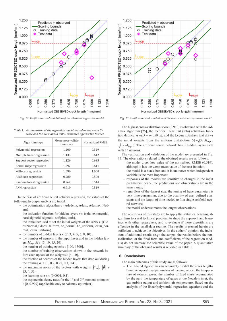
Eksploatacja i NiEzawodNosc – MaiNtENaNcE aNd REliability Vol. 23, No. 3, 2021 583
In the case of artificial neural network regression, the values of the following hyperparameters are tuned:
the optimization algorithm ϵ Adadelta, Adam, Adamax, Nad- –am,the activation function for hidden layers – σ ϵ relu, exponential, hard sigmoid, sigmoid, softplus, tanh,the initializer used to set the initial weights of the ANN ϵ Glo- –rotNormal, GlorotUniform, he_normal, he_uniform, lecun_nor-mal, lecun_uniform,the number of hidden layers ϵ 2, 3, 4, 5, 6, 8, 10, –the number of neurons in the input layer and in the hidden lay- –ers Minp, M ϵ 5, 10, 15, 20,the number of training epochs ϵ [100, 1300], –the number of training observations shown to the network be- –fore each update of the weights ϵ [4, 10],the fraction of neurons of the hidden layers that drop out during –the training dr ϵ 0, 0.2, 0.25, 0.3, 0.4,the maximum norm of the vectors with weights –
αm ,
β ϵ 3, 4, 5,the learning rate η ϵ [0.0001, 0.1], –the exponential decay rates for the 1 – st and 2nd moment estimates ϵ [0, 0.999] (applicable only to Adamax optimizer).
The highest cross-validation score (0.910) is obtained with the Ad-amax algorithm [25], the rectifier linear unit (relu) activation func-tion defined as σ(x) = max(0, x), and the Lecun initializer that draws the initial weights from the uniform distribution U( 3 / inpM− ,
3 / inpM ). The artificial neural network has 3 hidden layers each with 15 neurons.
The verification and validation of the model are presented in Fig. 13. The observations related to the obtained results are as follows:
the model gives low value of the normalized RMSE (0.519), –although it has the worst mean value of the cost function;the model is a black-box and it is unknown which independent –variable is the most important;responses of the models are sensitive to changes in the input –parameters; hence, the predictions and observations are in the same range;regardless of the dataset size, the tuning of hyperparameters is –very time-consuming, due to the quantity of user-defined con-stants and the length of time needed to fit a single artificial neu-ral network;the model underestimates the longest observations. –
The objectives of this study are to apply the statistical learning al-gorithms to a real technical problem, to share the approach and learn-ings with other researchers, and to evaluate if these algorithms are effective in the small-data regime. The results presented herein are sufficient to achieve the objectives. In the authors’ opinion, the inclu-sion of additional results (e.g.: the scripts, the results before the nor-malization, or the final form and coefficients of the regression mod-els) do not increase the scientific value of the paper. A quantitative summary of the obtained results is reported in Table 1.
8. ConclusionsThe main outcomes of this study are as follows:
The utilized algorithms can accurately predict the crack lengths –based on operational parameters of the engine, i.e.: the tempera-ture of exhaust gases, the number of fired starts accumulated by the part, the temperature of gases at the Nozzle’s inlet, the gas turbine output and ambient air temperature. Based on the analysis of the linear/polynomial regression equations and the
Fig. 12. Verification and validation of the XGBoost regression model Fig. 13. Verification and validation of the neural network regression model
Table 1. A comparison of the regression models based on the mean CV score and the normalized RMSE evaluated against the test set
Algorithm type Mean cross-valida-tion score Normalized RMSE
Polynomial regression 1.200 0.529
Multiple linear regression 1.133 0.612
Support vector regression 1.126 0.635
Kernel ridge regression 1.097 0.611
XGBoost regression 1.096 1.000
AdaBoost regression 0.980 0.500
Random forest regression 0.962 0.544
ANN regression 0.910 0.519
Eksploatacja i NiEzawodNosc – MaiNtENaNcE aNd REliability Vol. 23, No. 3, 2021584
values of gain/Gini importance, the median of the average ex-haust temperatures EXHT is the most important feature in the majority of the regression models.The polynomial regression model is the best model, considering –the cross-validation score and the normalized RMSE evaluated against the test set. Nevertheless, it is not sufficiently sensitive to changes in the input parameters. It underestimates the long-est observations as well, which is a common drawback with the created models. The AdaBoost regression model predicts these cracks with the lowest normalized RMSE. Before being used as a standalone support for data-driven decisions, the model should be subjected to further validation.The split into training, validation and test subsets was done –in a fully controlled manner, considering the clusters and the composition of the entire dataset. Each subset represents the sample in a quantitative and qualitative way. Such a consistent approach reduces ambiguity during the cross-validation, testing and interpretation of obtained results, especially in the case of small datasets.The (root) mean squared error should not be automatically cho- –sen as the cost function, as the results might be suboptimal from a business, risk management or other relevant perspective. A custom cost function better reflects the requirement of the user/customer and may favor certain solutions. In this paper, accu-rate predictions of the longest cracks are awarded with a bonus. The structure of the cost function drives the form and capabili-ties of the model.A variant of leave-p-out cross-validation is utilized, since the –usage of k-fold cross-validation provides unclear and hard-to-interpret results for the training set composed of 25 records. This is computationally feasible because of the effective feature selection and the small number of observations.None of the models outperforms the remainder. Some of them –are accurate for the “short” class, while others are better for the “long” class. Combining these models into an ensemble could improve the overall accuracy and better support data-driven de-cisions. None of the analyzed algorithms surpasses the others because of certain advantages or characteristics. The order of regression models in Table 1, resulting from the mean cross-
validation score, will change for a different dataset. Neverthe-less, finding the optimal structure and hyperparameters of the artificial neural network was the most complicated and time-consuming. In general, the short time needed to fit a model al-lows for an extensive tuning of hyperparameters and is one of the few benefits of small samples.Building conclusions on a small dataset can be reliable, but it –requires a rigorous approach and understanding of the decisions made throughout the entire analysis. The applicability domain must be defined for such models to limit extrapolation attempts and application of the model to items not covered by the train-ing set. If possible, results of the data-driven model should be compared with a different approach, e.g., the results of the finite element analysis. A staggered implementation of the regression model is suggested, preferably connected with checks of the hardware (e.g., borescope inspection of the analyzed Nozzles), data gathering, and subsequent update of the model.
The authors applied several known machine learning algorithms to predict the maximal length of fatigue cracks. The analyzed dataset was not created synthetically or obtained during an experiment, but it describes components that operated in the industrial gas turbines under variable operating conditions. The purpose was to assess if the data-hungry methods can provide valuable results for the inhomoge-neous sample composed of 31 observations only. The authors proved that the selected algorithms are effective in the small-date regime. The experience shared herein is universal and can support other research-ers and professionals working with similarly sized sets.
It is the first attempt of the authors to apply machine learning al-gorithms in the small-data regime. Further research will focus on techniques that combine physics-based descriptions of the analyzed phenomenon with empirical models, staying in the small-data regime. Physics-informed neural networks [35, 9] are examples of such hybrid models. This approach should assure the consistency of the outputs with the laws of physics, and improve the accuracy of the predictions and extrapolation capabilities. The ultimate objective of the research-ers is to propose a method of scaling the hybrid models and transfer-ring knowledge between domains.
References1. Abernethy RB. An Overview Of Weibull Analysis. The New Weibull Handbook: Reliability & Statistical Analysis for Predicting Life, Safety,
Risk, Support Costs, Failures, and Forecasting Warranty Claims, Substantiation and Accelerated Testing, Usin Weibull, Log Normal, Crow-AMSAA, Probit, and Kaplan-Meier Models, 5th edition. North Palm Beach, Florida, Robert B. Abernethy: 2004: 13-24.
2. Allegorico C, Mantini V. A Data-Driven Approach for on-line Gas Turbine Combustion Monitoring using Classification Models. PHM Society European Conference 2014, https://doi.org/10.36001/phme.2014.v2i1.1461.
3. Awad M, Khanna R. Support Vector Regression. In Awad M, Khanna R (eds): Efficient Learning Machines: Theories, Concepts, and Applications for Engineers and System Designers. Berkeley, CA, Apress: 2015: 67-80, https://doi.org/10.1007/978-1-4302-5990-9_4.
4. Beden S, Abdullah S, Ariffin AK. Review of Fatigue Crack Propagation Models for Metallic Components. European Journal of Scientific Research 2009.
5. Breiman L. Random Forests. Machine Learning 2001; 45(1): 5-32, https://doi.org/10.1023/A:1010933404324.6. Carlevaro F, Cioncolini S, Sepe M et al. Use of Operating Parameters, Digital Replicas and Models for Condition Monitoring and Improved
Equipment Health. Proceedings of the ASME Turbo Expo 2018: Turbomachinery Technical Conference and Exposition, Oslo, Norway, American Society of Mechanical Engineers Digital Collection: 2018, https://doi.org/10.1115/GT2018-76849.
7. Chen T, Guestrin C. XGBoost: A Scalable Tree Boosting System. Proceedings of the 22nd ACM SIGKDD International Conference on Knowledge Discovery and Data Mining, New York, NY, USA, ACM: 2016: 785-794, https://doi.org/10.1145/2939672.2939785.
8. Keras. [https://keras.io/].9. Dourado AD, Viana F. Physics-Informed Neural Networks for Bias Compensation in Corrosion-Fatigue. AIAA Scitech 2020 Forum, Orlando,
FL, American Institute of Aeronautics and Astronautics: 2020. doi:10.2514/6.2020-1149, https://doi.org/10.2514/6.2020-1149.10. Dresia K, Waxenegger-Wilfing G, Riccius J et al. Numerically Efficient Fatigue Life Prediction of Rocket Combustion Chambers using
Artificial Neural Networks. 2019.11. Drucker H. Improving Regressors Using Boosting Techniques. Proceedings of the 14th International Conference on Machine Learning
1997.12. Durodola JF, Ramachandra S, Gerguri S, Fellows NA. Artificial neural network for random fatigue loading analysis including the effect of
mean stress. International Journal of Fatigue 2018; 111: 321-332, https://doi.org/10.1016/j.ijfatigue.2018.02.007.13. Escobedo E, Arguello L, Sepe M et al. Enhanced Early Warning Diagnostic Rules for Gas Turbines Leveraging on Bayesian Networks.

Eksploatacja i NiEzawodNosc – MaiNtENaNcE aNd REliability Vol. 23, No. 3, 2021 585
Proceedings of the ASME Turbo Expo 2020: Turbomachinery Technical Conference and Exposition, American Society of Mechanical Engineers Digital Collection: 2021. doi:10.1115/GT2020-16082, https://doi.org/10.1115/GT2020-16082.
14. Faraway JJ, Augustin NH. When small data beats big data. Statistics & Probability Letters 2018; 136: 142-145, https://doi.org/10.1016/j.spl.2018.02.031.
15. Gan L, Zhao X, Wu H, Zhong Z. Estimation of remaining fatigue life under two-step loading based on kernel-extreme learning machine. International Journal of Fatigue 2021; 148: 106190, https://doi.org/10.1016/j.ijfatigue.2021.106190.
16. Harris CR, Millman KJ, van der Walt SJ et al. Array programming with NumPy. Nature 2020; 585(7825): 357-362, https://doi.org/10.1038/s41586-020-2649-2.
17. Iannitelli M, Allegorico C, Garau F, Capanni M. A Hybrid Model for on-line Detection of Gas Turbine Lean Blowout Events. PHM Society European Conference 2018, https://doi.org/10.36001/phme.2018.v4i1.405.
18. James G, Witten D, Hastie T, Tibshirani R. Linear Model Selection and Regularization. In James G, Witten D, Hastie T, Tibshirani R (eds): An Introduction to Statistical Learning: with Applications in R, New York, NY, Springer: 2013: 203-264, https://doi.org/10.1007/978-1-4614-7138-7_6.
19. James G, Witten D, Hastie T, Tibshirani R. Statistical Learning. In James G, Witten D, Hastie T, Tibshirani R (eds): An Introduction to Statistical Learning: with Applications in R, New York, NY, Springer: 2013: 15-57, https://doi.org/10.1007/978-1-4614-7138-7_2.
20. Jimenez-Martinez M, Alfaro-Ponce M. Fatigue damage effect approach by artificial neural network. International Journal of Fatigue 2019; 124: 42-47, https://doi.org/10.1016/j.ijfatigue.2019.02.043.
21. Kalayci CB, Karagoz S, Karakas Ö. Soft computing methods for fatigue life estimation: A review of the current state and future trends. Fatigue & Fracture of Engineering Materials & Structures 2020; 43(12): 2763-2785, https://doi.org/10.1111/ffe.13343.
22. Kalombo RB, Pestana MS, Freire Júnior RCS et al. Fatigue life estimation of an all aluminium alloy 1055 MCM conductor for different mean stresses using an artificial neural network. International Journal of Fatigue 2020; 140: 105814, https://doi.org/10.1016/j.ijfatigue.2020.105814.
23. Kamath C, Fan Y J. Regression with small data sets: a case study using code surrogates in additive manufacturing. Knowledge and Information Systems 2018; 57(2): 475-493, https://doi.org/10.1007/s10115-018-1174-1.
24. Karagiannopoulos M, Anyfantis D, Kotsiantis S B, Pintelas P E. Feature Selection for Regression Problems. Proceedings of HERCMA 2007, Athens, 2007.
25. Kingma DP, Ba J. Adam: A Method for Stochastic Optimization. 3rd International Conference on Learning Representations, ICLR 2015, San Diego, CA, USA, May 7-9, 2015, Conference Track Proceedings, San Diego, CA, USA, 2015.
26. Kitchin R, Lauriault T. Small data in the era of big data. GeoJournal 2015; 80: 463-475, https://doi.org/10.1007/s10708-014-9601-7.27. Liu X, Athanasiou CE, Padture NP et al. A machine learning approach to fracture mechanics problems. Acta Materialia 2020; 190: 105-112,
https://doi.org/10.1016/j.actamat.2020.03.016.28. Martens HA, Dardenne P. Validation and verification of regression in small data sets. Chemometrics and Intelligent Laboratory Systems
1998; 44(1): 99-121, https://doi.org/10.1016/S0169-7439(98)00167-1.29. McKinney W. Data Structures for Statistical Computing in Python. Proceedings of the 9th Python in Science Conference, Austin, Texas,
2010; 445: 56-61, https://doi.org/10.25080/Majora-92bf1922-00a.30. Michelassi V, Allegorico C, Cioncolini S et al. Machine Learning in Gas Turbines. Mechanical Engineering 2018; 140(09): S54-S55, https://
doi.org/10.1115/1.2018-SEP5.31. Nowell D, Nowell PW. A machine learning approach to the prediction of fretting fatigue life. Tribology International 2020; 141: 105913,
https://doi.org/10.1016/j.triboint.2019.105913.32. Paris P, Erdogan F. A Critical Analysis of Crack Propagation Laws. Journal of Basic Engineering 1963; 85(4): 528-533, https://doi.
org/10.1115/1.3656900.33. Pawełczyk M, Fulara S, Sepe M et al. Industrial gas turbine operating parameters monitoring and data-driven prediction. Eksploatacja i
Niezawodnosc - Maintenance and Reliability 2020; 22: 391-399, https://doi.org/10.17531/ein.2020.3.2.34. Pedregosa F, Varoquaux G, Gramfort A et al. Scikit-learn: Machine Learning in Python. Journal of Machine Learning Research 2011; 12:
2825-2860.35. Raissi M, Perdikaris P, Karniadakis GE. Physics-informed neural networks: A deep learning framework for solving forward and inverse
problems involving nonlinear partial differential equations. Journal of Computational Physics 2018; 378: 686-707, https://doi.org/10.1016/j.jcp.2018.10.045.
36. Rege K, Lemu H. A review of fatigue crack propagation modelling techniques using FEM and XFEM. IOP Conference Series Materials Science and Engineering 2017; 276: 012027, https://doi.org/10.1088/1757-899X/276/1/012027.
37. Rovinelli A, Sangid MD, Proudhon H, Ludwig W. Using machine learning and a data-driven approach to identify the small fatigue crack driving force in polycrystalline materials. npj Computational Materials 2018; 4(1): 1-10, https://doi.org/10.1038/s41524-018-0094-7.
38. Shanmugam M. Baker Hughes Company LLC: 2015.39. Storn R, Price K. Differential Evolution - A Simple and Efficient Heuristic for Global Optimization over Continuous Spaces. Journal of
Global Optimization 1997; 11: 341-359, https://doi.org/10.1023/A:1008202821328.40. Virtanen P, Gommers R, Oliphant TE et al. SciPy 1.0--Fundamental Algorithms for Scientific Computing in Python. Nature Methods 2020;
17(3): 261-272, https://doi.org/10.1038/s41592-019-0686-2.41. Wang B, Xie L, Song J et al. Curved fatigue crack growth prediction under variable amplitude loading by artificial neural network.
International Journal of Fatigue 2021; 142: 105886, https://doi.org/10.1016/j.ijfatigue.2020.105886.42. Xu Y, Goodacre R. On Splitting Training and Validation Set: A Comparative Study of Cross-Validation, Bootstrap and Systematic Sampling
for Estimating the Generalization Performance of Supervised Learning. Journal of Analysis and Testing 2018; 2(3): 249-262, https://doi.org/10.1007/s41664-018-0068-2.
43. Zhan Z, Li H. Machine learning based fatigue life prediction with effects of additive manufacturing process parameters for printed SS 316L. International Journal of Fatigue 2021; 142: 105941, https://doi.org/10.1016/j.ijfatigue.2020.105941.
44. Travel Weather Averages (Weatherbase). [https://www.weatherbase.com/].45. XGBoost Documentation - xgboost 1.4.0-SNAPSHOT documentation. [https://xgboost.readthedocs.io/].
Eksploatacja i NiEzawodNosc – MaiNtENaNcE aNd REliability Vol. 23, No. 3, 2021586
(*) Corresponding author.E-mail addresses:
Eksploatacja i Niezawodnosc – Maintenance and ReliabilityVolume 23 (2021), Issue 3
journal homepage: http://www.ein.org.pl
Indexed by:Influence of meteorological conditions on road accidents. A model for observations with excess zerosAnna Borucka a,*, Dariusz Pyza b
a Military University of Technology, Faculty of Security, Logistics and Management, ul. gen. Sylwestra Kaliskiego 2, 00 – 908 Warsaw, Poland b Warsaw University of Technology, Faculty of Transport, pl. Politechniki 1, 00-661 Warsaw, Poland
Borucka A, Pyza D. Influence of meteorological conditions on road accidents. A model for observations with excess zeros. Eksploatacja i Niezawodnosc – Maintenance and Reliability 2021; 23 (3): 586–592, http://doi.org/10.17531/ein.2021.3.20.
Article citation info:
Road accidents are one of the basic road safety determinants. Most research covers large territorial areas. The results of such research do not take into account the differences be-tween individual regions, which often leads to incorrect results and their interpretation. What makes it difficult to conduct analyses in a narrow territorial area is the small number of observations. The narrowing of the research area means that the number of accidents in time units is often very low. There are many zero observations in the data sets, which may affect the reliability of the research results. Such data are usually aggregated, which leads to information loss. The authors have therefore applied a model that addresses such problems. They proposed a method that does not require data aggregation and allows for the analysis of sets with an excess of zero observations. The presented model can be implemented in different territorial areas.
Highlights Abstract
Determining the influence of meteorological con-• ditions on the number of accidents.
More accurate analysis of accidents by limiting • the area (territory).
Solving the problem of excess zero observations • in the accident data set.
Applying Negative Binomial Hurdle Model in the • research on road accidents.
road accidents, excess zeros, road safety, meteorological conditions.
Keywords
This is an open access article under the CC BY license (https://creativecommons.org/licenses/by/4.0/)
A. Borucka - [email protected], D. Pyza - [email protected]
IntroductionRoad accidents are one of the basic sources of data for road safety
analysis [1, 5, 10]. However, it is very difficult to find their causes as there are numerous factors that affect them [25, 26]. The basic road safety analyses carried out in most countries concern the gen-eral trends in the number of accidents and casualties in relation to data characterizing a given area. However, determination of the ex-act causes of accidents requires much more advanced methods. The studies presented in the literature are of varied nature [10, 12]. Some of them are limited to evaluation of the impact of single variables such as driver drowsiness [22], driving speed before the incident [27], traffic jams [19, 29], driver’s gender [2], driving under the influence of alcohol or drugs [16], etc. In other publications, many variables are analyzed simultaneously. Singh [23], for example, evaluates the impact of inexperience and lack of skills characteristic of young driv-ers, while in the group of older drivers he emphasizes impairment of sight, cognitive functions and motor skills. Ashraf et al. [4] also take into account many different elements, considering, among other things, driver’s gender, experience, time of incident, observance of traffic rules [20].
There are a lot of publications on road accidents. All of them ana-lyze a limited number of factors, as it is not possible to take into ac-count all variables that affect the number of such incidents. Moreover, not all of them are identifiable or measurable, and some data are dif-ficult to obtain. These include, for example, detailed weather data, which in publicly available form concern only average measurement values for larger administrative areas and sometimes the whole coun-try. Such aggregated values are useless, as meteorological conditions may vary dramatically among distant regions.
Another problem in the analysis of road accidents is the availability of information in this area. In many countries, no accurate records are compiled for areas smaller than the whole country [6, 7], or the avail-able information is not complete [9, 28], so that only country-wide analyses are possible. Examples include the research conducted in Saudi Arabia [3], South Korea [4], India [21] or Poland [8, 11, 24].
The results of such research, however, do not take into account the differences between individual regions, which may occur even within a single country/region. They may result (e.g. when comparing small towns and large agglomerations) from different lifestyles, traffic vol-umes at different times of the day, different numbers of traffic users, the condition of road infrastructure, and even driver experience or driving culture. Analyses carried out within different areas allow to
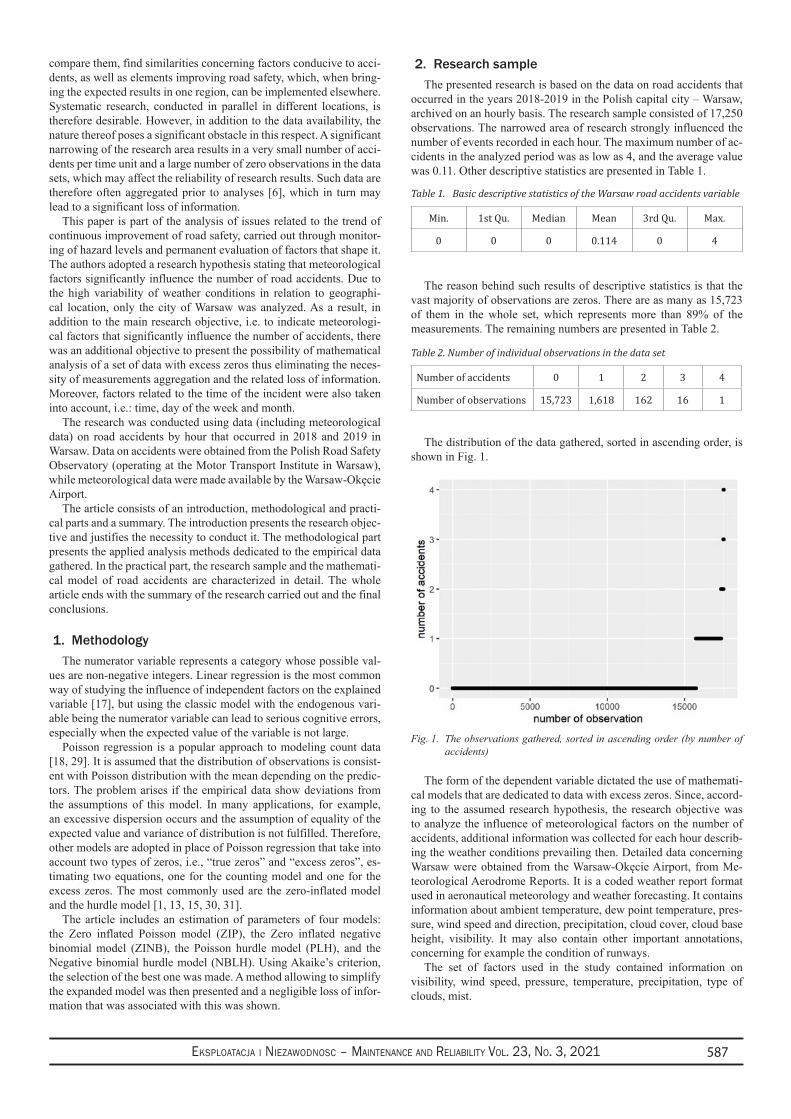
Eksploatacja i NiEzawodNosc – MaiNtENaNcE aNd REliability Vol. 23, No. 3, 2021 587
compare them, find similarities concerning factors conducive to acci-dents, as well as elements improving road safety, which, when bring-ing the expected results in one region, can be implemented elsewhere. Systematic research, conducted in parallel in different locations, is therefore desirable. However, in addition to the data availability, the nature thereof poses a significant obstacle in this respect. A significant narrowing of the research area results in a very small number of acci-dents per time unit and a large number of zero observations in the data sets, which may affect the reliability of research results. Such data are therefore often aggregated prior to analyses [6], which in turn may lead to a significant loss of information.
This paper is part of the analysis of issues related to the trend of continuous improvement of road safety, carried out through monitor-ing of hazard levels and permanent evaluation of factors that shape it. The authors adopted a research hypothesis stating that meteorological factors significantly influence the number of road accidents. Due to the high variability of weather conditions in relation to geographi-cal location, only the city of Warsaw was analyzed. As a result, in addition to the main research objective, i.e. to indicate meteorologi-cal factors that significantly influence the number of accidents, there was an additional objective to present the possibility of mathematical analysis of a set of data with excess zeros thus eliminating the neces-sity of measurements aggregation and the related loss of information. Moreover, factors related to the time of the incident were also taken into account, i.e.: time, day of the week and month.
The research was conducted using data (including meteorological data) on road accidents by hour that occurred in 2018 and 2019 in Warsaw. Data on accidents were obtained from the Polish Road Safety Observatory (operating at the Motor Transport Institute in Warsaw), while meteorological data were made available by the Warsaw-Okęcie Airport.
The article consists of an introduction, methodological and practi-cal parts and a summary. The introduction presents the research objec-tive and justifies the necessity to conduct it. The methodological part presents the applied analysis methods dedicated to the empirical data gathered. In the practical part, the research sample and the mathemati-cal model of road accidents are characterized in detail. The whole article ends with the summary of the research carried out and the final conclusions.
1. MethodologyThe numerator variable represents a category whose possible val-
ues are non-negative integers. Linear regression is the most common way of studying the influence of independent factors on the explained variable [17], but using the classic model with the endogenous vari-able being the numerator variable can lead to serious cognitive errors, especially when the expected value of the variable is not large.
Poisson regression is a popular approach to modeling count data [18, 29]. It is assumed that the distribution of observations is consist-ent with Poisson distribution with the mean depending on the predic-tors. The problem arises if the empirical data show deviations from the assumptions of this model. In many applications, for example, an excessive dispersion occurs and the assumption of equality of the expected value and variance of distribution is not fulfilled. Therefore, other models are adopted in place of Poisson regression that take into account two types of zeros, i.e., “true zeros” and “excess zeros”, es-timating two equations, one for the counting model and one for the excess zeros. The most commonly used are the zero-inflated model and the hurdle model [1, 13, 15, 30, 31].
The article includes an estimation of parameters of four models: the Zero inflated Poisson model (ZIP), the Zero inflated negative binomial model (ZINB), the Poisson hurdle model (PLH), and the Negative binomial hurdle model (NBLH). Using Akaike’s criterion, the selection of the best one was made. A method allowing to simplify the expanded model was then presented and a negligible loss of infor-mation that was associated with this was shown.
2. Research sampleThe presented research is based on the data on road accidents that
occurred in the years 2018-2019 in the Polish capital city – Warsaw, archived on an hourly basis. The research sample consisted of 17,250 observations. The narrowed area of research strongly influenced the number of events recorded in each hour. The maximum number of ac-cidents in the analyzed period was as low as 4, and the average value was 0.11. Other descriptive statistics are presented in Table 1.
The reason behind such results of descriptive statistics is that the vast majority of observations are zeros. There are as many as 15,723 of them in the whole set, which represents more than 89% of the measurements. The remaining numbers are presented in Table 2.
The distribution of the data gathered, sorted in ascending order, is shown in Fig. 1.
Fig. 1. The observations gathered, sorted in ascending order (by number of accidents)
The form of the dependent variable dictated the use of mathemati-cal models that are dedicated to data with excess zeros. Since, accord-ing to the assumed research hypothesis, the research objective was to analyze the influence of meteorological factors on the number of accidents, additional information was collected for each hour describ-ing the weather conditions prevailing then. Detailed data concerning Warsaw were obtained from the Warsaw-Okęcie Airport, from Me-teorological Aerodrome Reports. It is a coded weather report format used in aeronautical meteorology and weather forecasting. It contains information about ambient temperature, dew point temperature, pres-sure, wind speed and direction, precipitation, cloud cover, cloud base height, visibility. It may also contain other important annotations, concerning for example the condition of runways.
The set of factors used in the study contained information on visibility, wind speed, pressure, temperature, precipitation, type of clouds, mist.
Table 1. Basic descriptive statistics of the Warsaw road accidents variable
Min. 1st Qu. Median Mean 3rd Qu. Max.
0 0 0 0.114 0 4
Table 2. Number of individual observations in the data set
Number of accidents 0 1 2 3 4
Number of observations 15,723 1,618 162 16 1
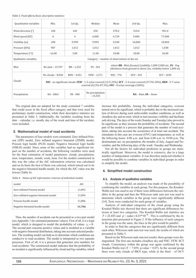
Eksploatacja i NiEzawodNosc – MaiNtENaNcE aNd REliability Vol. 23, No. 3, 2021588
The original data set adopted for the study contained 7 variables that could occur in the fixed effect category and that were used for preliminary model construction, while their descriptive statistics are presented in Table 3. Additionally, the variables resulting from the date – calendar, i.e. month, day of the week and time of the incident, were included.
3. Mathematical model of road accidentsThe parameters of four models were estimated: Zero inflated Pois-
son (ZIP) model, Zero inflated negative binomial (ZIMB) model, Poisson logit hurdle (PLH) model, Negative binomial logit hurdle (NBLH) model. Since some of the variables had no significant im-pact on the number of accidents, the following variables were used for the final estimation of model parameters: clouds, precipitation, mist, temperature, month, week, hour. For the models constructed in this way the value of the AIC information criterion was calculated and on its basis the best of them was selected, which turned out to be the negative binomial hurdle model, for which the AIC value was the lowest (Table 4).
Thus, the number of accidents can be presented as a two-part model (see Appendix 1 for estimated parameter values). First of all, it is a logit model, which is designed to model the probability of values 0iy = . The second part concerns positive values and is modeled as a variable with negative binomial distribution, taking into account selected predic-tors. The resulting model can help us to determine which conditions are conducive to road accidents. The model is interpreted as two separate processes. First of all, it is a process that generates zero numbers for road accidents. The constructed model indicates that the probability of no incident is significantly influenced by cloud and fog variables, which
increase this probability. Among the individual categories, overcast turned out to be significant, which is probably due to the increased cau-tion of drivers during such unfavorable weather conditions, as well as cloudless sky and no mist, which in turn increase visibility and facilitate safe driving. The days of the week (Sunday and Tuesday) also proved to be significant, as they increase the probability of accidents. The second part of the model is a process that generates the number of road acci-dents, taking into account the occurrence of at least one accident. The stimulants in this case are overcast (OVC) and temperature, as well as the following hours: 4:00 a.m. and from 6:00 a.m. to 10:00 p.m. The destimulants are: no precipitation, the months of July, August and No-vember, and the following days of the week: Tuesday and Wednesday.
Not all the factors for individual predictors in groups are statis-tically significant. Moreover, the model is extensive, due to a large number of independent variables. It was therefore analyzed whether it would be possible to combine variables in individual groups in order to simplify the model.
4. Simplified model construction
4.1. Analysis of qualitative variablesTo simplify the model, an analysis was made of the possibility of
combining the variables in each group. For this purpose, the Kruskal-Wallis test was used to see if there were differences between the vari-ables in the group and then the Wilcoxon rank sum test was used to determine which variables in the group were significantly different [14]. Tests were conducted for each group of variables.
Analysis of individual categories of the cloud group using the Kruskal-Wallis test showed that there are significant differences be-tween at least two categories. The Kruskal-Wallis test statistics are
22.433 T = and 4 4.33*10p value −− = . This is confirmed by the in-teraction plot presented in Figure 2. If the influence of each category in the group was the same, the lines in the plot would be parallel.
In order to find the categories that are significantly different from each other, Wilcoxon rank sum test was used, the results of which are presented in Table 5.
Based on the Wilcoxon rank sum test results, three groups were dis-tinguished. The first one includes cloudless sky and NSC, FEW, SCT clouds. Consistency within the group was again confirmed by the Kruskal-Wallis test (T = 7.059, p-value = 0.07). In the second group there were only clouds of BKN type, while in the third – of OCV
Table 4. Values of AIC information criterion of individual models
model AIC
Zero inflated Poisson model 11,892
Zero inflated negative binomial model 11,894
Poisson hurdle model 11,806
Negative binomial hurdle model 11,766
Table 3. Fixed effects/basic descriptive statistics
Quantitative variables Min. 1st Qu. Median Mean 3rd Qu. Max.
Wind direction [°] 100 160 250 278.2 310.0 901.0
Wind speed [KT] 0 4 6.000 6.729 9.000 77.000
Visibility [m] 180 9,999 9,999 9,340 10,000 10,004
Pressure [hPa] 987 1,012 1,012 1,012 1,012 1,038
Temperature [°C] -16.00 3.00 11.00 10.88 18.00 36.00
Qualitative variables Category – number of observations in the set
Mist No mist – 15,707 BR – 1,252 FG - 561 where BR - Mist (brume) (visibility 1,000-5,000 m) , FG - Fog (thickness from ground to above 2m, visibility below 1,000 m)
Clouds
No clouds – 8,030 BKN – 4,451 FEW – 2,271 NSC - 776 OCV - 343 SCT - 1649
NSC - no significant clouds. FEW - 1-2 octas covered (12.5-25%), SCT - 3-4 octas covered (37.5%-50%), BKN - 5-7 octas covered (62.5%-87.5%), OVC - 8 octas coverage (100%)
Precipitation RA - 2865 SN - 300 No precipitation - 14,355 RA – Rain, SN – Snow
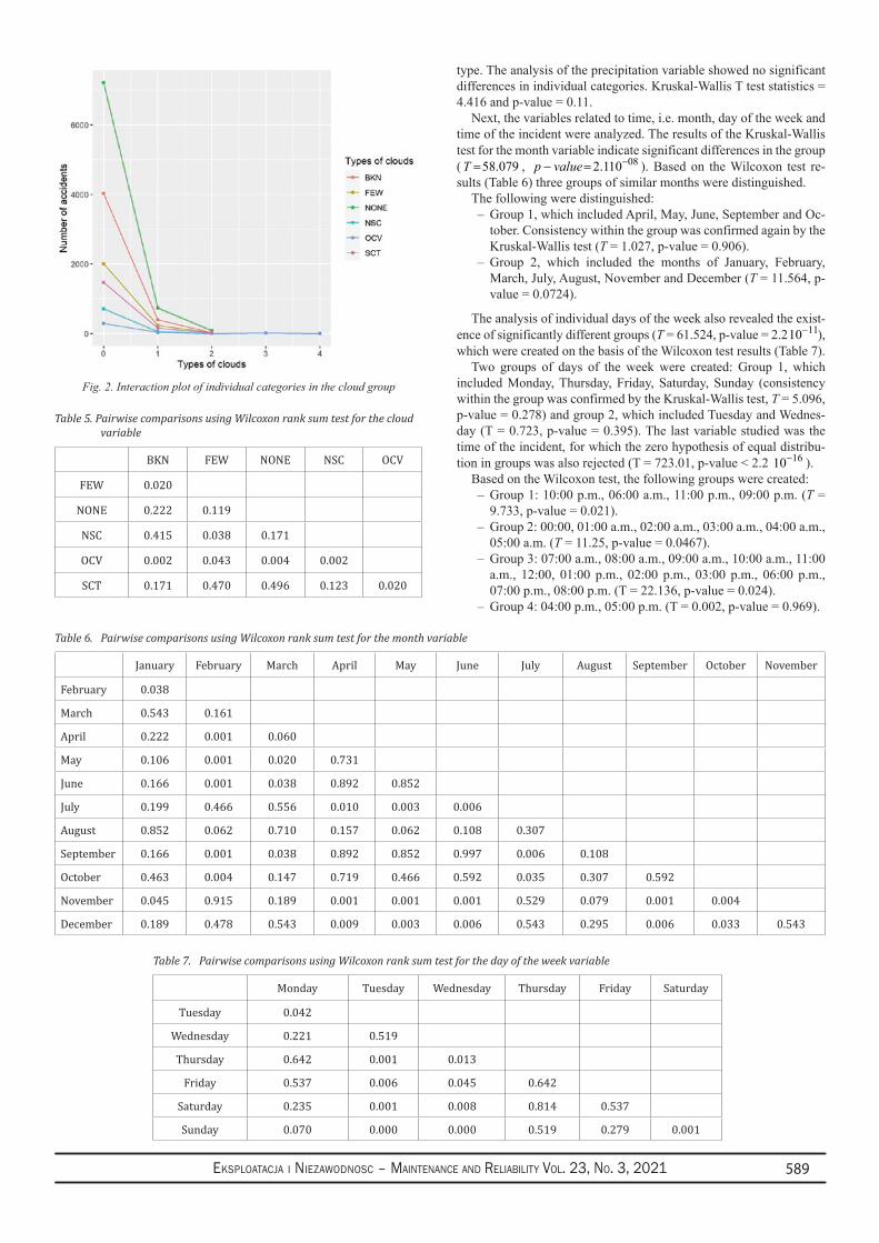
Eksploatacja i NiEzawodNosc – MaiNtENaNcE aNd REliability Vol. 23, No. 3, 2021 589
type. The analysis of the precipitation variable showed no significant differences in individual categories. Kruskal-Wallis T test statistics = 4.416 and p-value = 0.11.
Next, the variables related to time, i.e. month, day of the week and time of the incident were analyzed. The results of the Kruskal-Wallis test for the month variable indicate significant differences in the group ( 58.079T = , 08 2.11 0p value −− = ). Based on the Wilcoxon test re-sults (Table 6) three groups of similar months were distinguished.
The following were distinguished:Group 1, which included April, May, June, September and Oc- –tober. Consistency within the group was confirmed again by the Kruskal-Wallis test (T = 1.027, p-value = 0.906).Group 2, which included the months of January, February, –March, July, August, November and December (T = 11.564, p-value = 0.0724).
The analysis of individual days of the week also revealed the exist-ence of significantly different groups (T = 61.524, p-value = 2.2 1110− ), which were created on the basis of the Wilcoxon test results (Table 7).
Two groups of days of the week were created: Group 1, which included Monday, Thursday, Friday, Saturday, Sunday (consistency within the group was confirmed by the Kruskal-Wallis test, T = 5.096, p-value = 0.278) and group 2, which included Tuesday and Wednes-day (T = 0.723, p-value = 0.395). The last variable studied was the time of the incident, for which the zero hypothesis of equal distribu-tion in groups was also rejected (T = 723.01, p-value < 2.2 1610− ).
Based on the Wilcoxon test, the following groups were created:Group 1: 10:00 p.m., 06:00 a.m., 11:00 p.m., 09:00 p.m. ( – T = 9.733, p-value = 0.021).Group 2: 00:00, 01:00 a.m., 02:00 a.m., 03:00 a.m., 04:00 a.m., –05:00 a.m. (T = 11.25, p-value = 0.0467).Group 3: 07:00 a.m., 08:00 a.m., 09:00 a.m., 10:00 a.m., 11:00 –a.m., 12:00, 01:00 p.m., 02:00 p.m., 03:00 p.m., 06:00 p.m., 07:00 p.m., 08:00 p.m. (T = 22.136, p-value = 0.024).Group 4: 04:00 p.m., 05:00 p.m. (T = 0.002, p-value = 0.969). –
Table 5. Pairwise comparisons using Wilcoxon rank sum test for the cloud variable
BKN FEW NONE NSC OCV
FEW 0.020
NONE 0.222 0.119
NSC 0.415 0.038 0.171
OCV 0.002 0.043 0.004 0.002
SCT 0.171 0.470 0.496 0.123 0.020
Table 6. Pairwise comparisons using Wilcoxon rank sum test for the month variable
January February March April May June July August September October November
February 0.038
March 0.543 0.161
April 0.222 0.001 0.060
May 0.106 0.001 0.020 0.731
June 0.166 0.001 0.038 0.892 0.852
July 0.199 0.466 0.556 0.010 0.003 0.006
August 0.852 0.062 0.710 0.157 0.062 0.108 0.307
September 0.166 0.001 0.038 0.892 0.852 0.997 0.006 0.108
October 0.463 0.004 0.147 0.719 0.466 0.592 0.035 0.307 0.592
November 0.045 0.915 0.189 0.001 0.001 0.001 0.529 0.079 0.001 0.004
December 0.189 0.478 0.543 0.009 0.003 0.006 0.543 0.295 0.006 0.033 0.543
Table 7. Pairwise comparisons using Wilcoxon rank sum test for the day of the week variable
Monday Tuesday Wednesday Thursday Friday Saturday
Tuesday 0.042
Wednesday 0.221 0.519
Thursday 0.642 0.001 0.013
Friday 0.537 0.006 0.045 0.642
Saturday 0.235 0.001 0.008 0.814 0.537
Sunday 0.070 0.000 0.000 0.519 0.279 0.001
Fig. 2. Interaction plot of individual categories in the cloud group
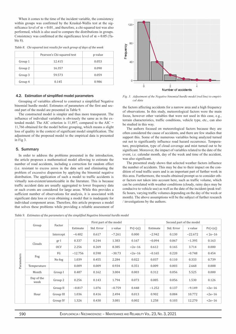
Eksploatacja i NiEzawodNosc – MaiNtENaNcE aNd REliability Vol. 23, No. 3, 2021590
When it comes to the time of the incident variable, the consistency within groups was confirmed by the Kruskal-Wallis test at the sig-nificance level of 0.01α = , and therefore, a chi-squared test was also performed, which is also used to compare the distributions in groups. Consistency was confirmed at the significance level of 0.05 α = (Ta-ble 8).
4.2. EstimationofsimplifiedmodelparametersGrouping of variables allowed to construct a simplified Negative
binomial hurdle model. Estimates of parameters of the first and sec-ond part of the model are presented in Table 9.
The constructed model is simpler and thus more transparent. The influence of individual variables is obviously the same as in the ex-tended model. The AIC criterion is 11,897, compared to the AIC = 11,766 obtained for the model before grouping, which means a slight loss of quality in the context of significant model simplification. The adjustment of the proposed model to the empirical data is presented in Fig 3.
5. SummaryIn order to address the problems presented in the introduction,
the article proposes a mathematical model allowing to estimate the number of road accidents, including a correction for random effect (i.e. resistant to excess zeros in the data set) and eliminating the problem of excessive dispersion by applying the binomial negative distribution. The application of such a model to traffic accidents is virtually non-existent/unnoticeable in the literature. This is because traffic accident data are usually aggregated to lower frequency data or such events are considered for large areas. While this provides a sufficient number of observations for analysis, it is associated with significant data loss or even obtaining a model that is inadequate for individual component areas. Therefore, this article proposes a model that solves these problems while providing a reliable assessment of
the factors affecting accidents for a narrow area and a high frequency of observations. In this study, meteorological factors were the main focus, however other variables that were not used in this case, e.g., terrain characteristics, traffic conditions, vehicle type, etc., can also be studied in this way.
The authors focused on meteorological factors because they are often considered the cause of accidents, and there are few studies that support this. Some of the numerous variables being analyzed turned out not to significantly influence road hazard occurrence. Tempera-ture, precipitation, type of cloud coverage and mist turned out to be significant. Moreover, the impact of variables related to the date of the event, i.e. calendar month, day of the week and time of the accident, was also significant.
The presented study shows that selected weather factors influence the number of accidents. This may be due to their impact on the con-dition of road traffic users and is an important part of further work in this area. Furthermore, the results obtained prompt us to consider oth-er factors not taken into account here, such as traffic volume, which can be correlated with weather conditions (cloudy, rainy days may be conducive to vehicle use) as well as the date of the incident (peak traf-fic hours, varying traffic volumes depending on the day of the week or month). The above assumptions will be the subject of further research / investigations by the authors.
Table 8. Chi-squared test results for each group of days of the week
Pearson’s Chi-squared test p-value
Group 1 12.415 0.053
Group 2 16.357 0.090
Group 3 59.573 0.059
Group 4 0.145 0.986
Table 9. Estimates of the parameters of the simplified Negative binomial hurdle model
Para
met
ers
Group FactorFirst part of the model Second part of the model
Estimate Std. Error z value Pr(>|z|) Estimate Std. Error z value Pr(>|z|)
Intercept −4.482 0.617 −7.261 0.000 −2.942 0.130 −22.672 < 2e−16
Cloudsgr I 0.337 0.244 1.383 0.167 −0.094 0.067 −1.395 0.163
OCV 2.256 0.269 8.385 <2e−16 0.612 0.165 3.714 0.000
FogFG −12.756 0.590 −30.73 <2e−16 −0.165 0.220 −0.748 0.454
No fog 1.039 0.455 2.284 0.022 0.037 0.110 0.333 0.739
Temperature 0.009 0.009 0.934 0.351 0.009 0.003 2.668 0.008
Month Group I 0.487 0.162 3.004 0.003 0.312 0.056 5.525 0.000
Day of the week Group 2 0.256 0.143 1.794 0.073 0.085 0.056 1.530 0.126
Hour
Group II −0.817 1.076 −0.759 0.448 −1.252 0.137 −9.149 <2e−16
Group III 1.036 0.416 2.494 0.013 0.902 0.084 10.772 <2e−16
Group IV 1.326 0.430 3.081 0.002 1.258 0.103 12.270 <2e−16
Fig. 3. Adjustment of the Negative binomial hurdle model (red line) to empiri-cal data
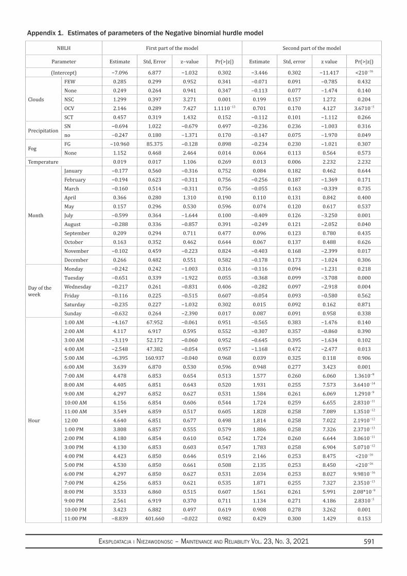
Eksploatacja i NiEzawodNosc – MaiNtENaNcE aNd REliability Vol. 23, No. 3, 2021 591
Appendix 1. Estimates of parameters of the Negative binomial hurdle model
NBLH First part of the model Second part of the model
Parameter Estimate Std, Error z−value Pr(>|z|) Estimate Std, error z value Pr(>|z|)
(Intercept) −7.096 6.877 −1.032 0.302 −3.446 0.302 −11.417 <210−16
Clouds
FEW 0.285 0.299 0.952 0.341 −0.071 0.091 −0.785 0.432None 0.249 0.264 0.941 0.347 −0.113 0.077 −1.474 0.140NSC 1.299 0.397 3.271 0.001 0.199 0.157 1.272 0.204OCV 2.146 0.289 7.427 1.1110−13 0.701 0.170 4.127 3.6710−5
SCT 0.457 0.319 1.432 0.152 −0.112 0.101 −1.112 0.266
PrecipitationSN −0.694 1.022 −0.679 0.497 −0.236 0.236 −1.003 0.316no −0.247 0.180 −1.371 0.170 −0.147 0.075 −1.970 0.049
FogFG −10.960 85.375 −0.128 0.898 −0.234 0.230 −1.021 0.307None 1.152 0.468 2.464 0.014 0.064 0.113 0.564 0.573
Temperature 0.019 0.017 1.106 0.269 0.013 0.006 2.232 2.232
Month
January −0.177 0.560 −0.316 0.752 0.084 0.182 0.462 0.644February −0.194 0.623 −0.311 0.756 −0.256 0.187 −1.369 0.171March −0.160 0.514 −0.311 0.756 −0.055 0.163 −0.339 0.735April 0.366 0.280 1.310 0.190 0.110 0.131 0.842 0.400May 0.157 0.296 0.530 0.596 0.074 0.120 0.617 0.537July −0.599 0.364 −1.644 0.100 −0.409 0.126 −3.250 0.001August −0.288 0.336 −0.857 0.391 −0.249 0.121 −2.052 0.040September 0.209 0.294 0.711 0.477 0.096 0.123 0.780 0.435October 0.163 0.352 0.462 0.644 0.067 0.137 0.488 0.626November −0.102 0.459 −0.223 0.824 −0.403 0.168 −2.399 0.017December 0.266 0.482 0.551 0.582 −0.178 0.173 −1.024 0.306
Day of the week
Monday −0.242 0.242 −1.003 0.316 −0.116 0.094 −1.231 0.218Tuesday −0.651 0.339 −1.922 0.055 −0.368 0.099 −3.708 0.000Wednesday −0.217 0.261 −0.831 0.406 −0.282 0.097 −2.918 0.004Friday −0.116 0.225 −0.515 0.607 −0.054 0.093 −0.580 0.562Saturday −0.235 0.227 −1.032 0.302 0.015 0.092 0.162 0.871Sunday −0.632 0.264 −2.390 0.017 0.087 0.091 0.958 0.338
Hour
1:00 AM −4.167 67.952 −0.061 0.951 −0.565 0.383 −1.476 0.1402:00 AM 4.117 6.917 0.595 0.552 −0.307 0.357 −0.860 0.3903:00 AM −3.119 52.172 −0.060 0.952 −0.645 0.395 −1.634 0.1024:00 AM −2.548 47.382 −0.054 0.957 −1.168 0.472 −2.477 0.0135:00 AM −6.395 160.937 −0.040 0.968 0.039 0.325 0.118 0.9066:00 AM 3.639 6.870 0.530 0.596 0.948 0.277 3.423 0.0017:00 AM 4.478 6.853 0.654 0.513 1.577 0.260 6.060 1.3610−9
8:00 AM 4.405 6.851 0.643 0.520 1.931 0.255 7.573 3.6410−14
9:00 AM 4.297 6.852 0.627 0.531 1.584 0.261 6.069 1.2910−9
10:00 AM 4.156 6.854 0.606 0.544 1.724 0.259 6.655 2.8310−11
11:00 AM 3.549 6.859 0.517 0.605 1.828 0.258 7.089 1.3510−12
12:00 4.640 6.851 0.677 0.498 1.814 0.258 7.022 2.1910−12
1:00 PM 3.808 6.857 0.555 0.579 1.886 0.258 7.326 2.3710−13
2:00 PM 4.180 6.854 0.610 0.542 1.724 0.260 6.644 3.0610−11
3:00 PM 4.130 6.853 0.603 0.547 1.783 0.258 6.904 5.0710−12
4:00 PM 4.423 6.850 0.646 0.519 2.146 0.253 8.475 <210−16
5:00 PM 4.530 6.850 0.661 0.508 2.135 0.253 8.450 <210−16
6:00 PM 4.297 6.850 0.627 0.531 2.034 0.253 8.027 9.9810−16
7:00 PM 4.256 6.853 0.621 0.535 1.871 0.255 7.327 2.3510−13
8:00 PM 3.533 6.860 0.515 0.607 1.561 0.261 5.991 2.08*10−9
9:00 PM 2.561 6.919 0.370 0.711 1.134 0.271 4.186 2.8310−5
10:00 PM 3.423 6.882 0.497 0.619 0.908 0.278 3.262 0.00111:00 PM −8.839 401.660 −0.022 0.982 0.429 0.300 1.429 0.153
Eksploatacja i NiEzawodNosc – MaiNtENaNcE aNd REliability Vol. 23, No. 3, 2021592
References1. Aga MA, Woldeamanuel BT, Tadesse M. Statistical modeling of number of human deaths per road traffic accident in Oromia region,
Ethiopia. PLoS one 2020; 16(5) e0251492, https://doi.org/10.1371/journal.pone.0251492.2. Al-Balbissi AH. Role of gender in road accidents. Traffic Injury Prevention 2003; 4(1): 64-73, https://doi.org/10.1080/15389580309857.3. Ansari S, Akhdar F, Mandoorah M, Moutaery K. Causes and effects of road traffic accidents in Saudi Arabia. Public health 2000; 114(1):
37-39, https://doi.org/10.1038/sj.ph.1900610.4. Ashraf I, Hur S, Shafiq M. Park Y. Catastrophic factors involved in road accidents: Underlying causes and descriptive analysis. PLoS one
2019; 14(10), e0223473, https://doi.org/10.1371/journal.pone.0223473.5. Borucka A, Kozłowski E, Oleszczuk P, Świderski A. Predictive analysis of the impact of the time of day on road accidents in Poland. Open
Engineering 2020; 11(1): 142-150, https://doi.org/10.1515/eng-2021-0017.6. Edwards JB. The temporal distribution of road accidents in adverse weather. Meteorological Applications: A Journal of Forecasting, Practical
Applications, Training Techniques and Modelling 1999; 6(1): 59-68, https://doi.org/10.1017/S1350482799001139.7. Elvik R, Mysen A. Incomplete accident reporting: meta-analysis of studies made in 13 countries. Transportation Research Record 1999;
1665(1), 133-140, https://doi.org/10.3141/1665-18.8. Frej D, Ludwinek K. Analysis of road accidents in 2002-2019 on the example of Poland. The Archives of Automotive Engineering - Archiwum
Motoryzacji 2020; 89(3): 5-18.9. Golias J, Yannis G. Dealing with lack of exposure data in road accident analysis. In 12th 557 International Conference: Traffic Safety on
Three Continents 2001, September; 558.10. Guzek M, Lozia Z. Computing Methods in the Analysis of Road Accident Reconstruction Uncertainty. Archives of Computational Methods
in Engineering 2020; 28: 2459-2476, https://doi.org/10.1007/s11831-020-09462-w.11. Jacyna M, Merkisz J. Proecological approach to modelling traffic organization in national transport system. Archives of Transport 2014;
30(2): 31-41, https://doi.org/10.5604/08669546.1146975.12. Jamroz K, Budzyński M, Romanowska A, Żukowska J, Oskarbski J, Kustra W. Experiences and challenges in fatality reduction on polish
roads. Sustainability 2019; 11(4): 959, https://doi.org/10.3390/su11040959.13. Kasin JA, Papastathopoulos I. A spatial Poisson hurdle model with application to wildfires. arXiv preprint arXiv:2007.00137, 2020.14. Kozłowski E, Mazurkiewicz D, Żabiński T, Prucnal S, Sęp J. Machining sensor data management for operation-level predictive model.
Expert Systems with Applications 2020; 159, 113600, https://doi.org/10.1016/j.eswa.2020.113600.15. Lukusa MT, Phoa FKH. A Horvitz-type estimation on incomplete traffic accident data analyzed via a zero-inflated Poisson model. Accident
Analysis & Prevention 2020; 134, 105235, https://doi.org/10.1016/j.aap.2019.07.011.16. Martin JL, Gadegbeku B, Wu D, Viallon V, Laumon B. Cannabis, alcohol and fatal road accidents. PLoS one 2017; 12(11), e0187320, https://
doi.org/10.1371/journal.pone.0187320.17. Mitkow S, Świderski A. Regression Model In Road Transport Services. Business Logistics in Modern Management 2019; 19: 263-27518. Pourhassan MR, Raissi S, Hafezalkotob A. A simulation approach on reliability assessment of complex system subject to stochastic
degradation and random shock. Eksploatacja i Niezawodnosc - Maintenance and Reliability 2020; 22 (2): 370-379, https://doi.org/10.17531/ein.2020.2.20.
19. Pyza D, Jachimowski R. Modelling of Parcels' Transport System. Proceedings of the International Scientific Conference Transport Means 2015; 22-23.
20. Pyza D, Jacyna-Gołda I, Gołda P, Gołebiowski P. Alternative Fuels and Their Impact on Reducing Pollution of the Natural Environment. Annual Set The Environment Protection 2018; 20: 819-836.
21. Rolison JJ, Regev S, Moutari S, Feeney A. What are the factors that contribute to road accidents? An assessment of law enforcement views, ordinary drivers' opinions, and road accident records. Accident Analysis & Prevention 2018; 115: 11-24, https://doi.org/10.1016/j.aap.2018.02.025.
22. Sagberg F. Road accidents caused by drivers falling asleep. Accident Analysis & Prevention 1999; 31(6): 639-649, https://doi.org/10.1016/S0001-4575(99)00023-8.
23. Singh SK. Road traffic accidents in India: issues and challenges. Transportation Research Procedia 2017; 25: 4708-4719, https://doi.org/10.1016/j.trpro.2017.05.484.
24. Świderski A, Borucka A, Skoczyński P. Characteristics and Assessment of the Road Safety Level in Poland with Multiple Regression Model, Transport Means - Proceedings of the International Conference 2018; Part I : 92-97.
25. Świderski A. Decision-Making Problems in the Standardization and Certification of Transport Services, Wydawnictwa Komunikacji i Łączności, 2019.
26. Świderski A. Modeling of transport processes in terms of seasonality of transport. Scientific Journal of Polish Naval Academy 2019; 216(1): 103-116, https://doi.org/10.2478/sjpna-2019-0008.
27. Taylor MC, Lynam DA, Baruya A. The effects of drivers' speed on the frequency of road accidents. Crowthorne: Transport Research Laboratory, 2000.
28. Trépanier M, Leroux MH, de Marcellis-Warin N. Cross-analysis of hazmat road accidents using multiple databases. Accident Analysis & Prevention, 2009; 41(6): 1192-1198, https://doi.org/10.1016/j.aap.2008.05.010.
29. Wang C, Quddus MA, Ison SG. Impact of traffic congestion on road accidents: a spatial analysis of the M25 motorway in England. Accident Analysis & Prevention, 2009; 41(4): 798-808, https://doi.org/10.1016/j.aap.2009.04.002.
30. Zhang X, Yi N. Fast zero-inflated negative binomial mixed modeling approach for analyzing longitudinal metagenomics data. Bioinformatics 2020; 36(8): 2345-2351, https://doi.org/10.1093/bioinformatics/btz973.
31. Zuur AF. Zero inflated models and generalized linear mixed models with R, 2012: 574.50182 Z8.

Editorial Board
Prof. Holm AltenbachOtto-von-Guericke-Universität, Magdeburg, GermanyProf. John AndrewsUniversity of Nottingham, Nottingham, UKProf. Karol AndrzejczakPoznań University of Technology, Poznań, PolandProf. Christophe BérenguerInstitut Polytechnique de Grenoble, Grenoble, FranceProf. Gintautas BureikaVilnius Gediminas Technical University, Vilnius, LithuaniaProf. Baoping CaiChina University of Petroleum, Quingdao, ChinaDr Alireza DaneshkhahWarwick Centre for Predictive Modelling University of Warwick, UKProf. Luis Andrade FerreiraUniversity of Porto, Porto, PortugalProf. Mitra FouladiradTroyes University of Technology, FranceDr Ilia FrenkelShamoon College of Engineering, Beer Sheva, IsraelProf. Olgierd HryniewiczSystems Research Institute of the Polish Academy of Science, Warsaw, PolandProf. Hong-Zhong HuangUniversity of Electronic Science and Technology of China, Chengdu, Sichuan, ChinaProf. Jerzy MerkiszPoznań University of Technology, Poznań, Poland
Prof. Gilbert De MeyUniversity of Ghent, BelgiumProf. Maria Francesca MilazzoUniversity of Messina, ItalyProf. Tomasz NowakowskiWrocław University of Technology, Wrocław, PolandProf. Marek OrkiszRzeszów University of Technology, Rzeszów, PolandProf. François PérèsTouluse University, Touluse, FranceProf. Yi RenBeihang University, Beijing, ChinaProf. Jan SzybkaAGH University of Science and Technology, Cracow, PolandProf. Marcin ŚlęzakMotor Transport Institute, Warsaw, PolandProf. Katsumi TanakaKyoto University, Kyoto, Japan Prof. David VališUniversity of Defence, Brno, Czech RepublicProf. Lesley WallsUniversity of Strathclyde, Glasgow, ScotlandProf. Min XieCity University of Hong Kong, Hong KongProf. Irina YatskivRiga Transport and Telecommunication Institute, Latvia
Editorial staff: Dariusz Mazurkiewicz, PhD, DSc (Eng), Associate Professor (Editor-in-Chief, Secretary of the Editorial Board) Tomasz Klepka, PhD, DSc (Eng), Associate Professor (Deputy Editor-in-Chief) Teresa Błachnio-Krolopp, MSc (Eng) (Editorial secretary) Andrzej Koma (Typesetting and text makeup) Krzysztof Olszewski, PhD (Eng) (Webmaster)Publisher: Polish Maintenance Society, Warsaw Scientific patronage: Polish Academy of Sciences Branch in LublinAddress for correspondence: “Eksploatacja i Niezawodność” – Editorial Office ul. Nadbystrzycka 36, 20-618 Lublin, Poland e-mail: [email protected] http://www.ein.org.pl/Circulation: 550 copies
Prof. Andrzej NiewczasChair of Editorial Board
The Journal is indexed and abstracted in the Journal Citation Reports (JCR Science Edition), Scopus, Science Citation Index Expanded (SciSearch®) and Index Copernicus International.
The Quarterly appears on the list of journals credited with a high impact factor by the Polish Ministry of Science and Higher Education and is indexed in the Polish Technical Journal Contents database – BAZTECH and the database of the Digital Library Federation.
All the scientific articles have received two positive reviews from independent reviewers.Our 2020 Impact Factor is 2.176
Task „Implementation of procedures ensuring the originality of scientific papers published in the quarterly „Eksploatacja i Niezawodność – Maintenance and Reliability” financed under contract 532/P-DUN/2018 from the funds of the Minister of Science and Higher Education for science dissemination activities.
Indexed by:

INFORMATION FOR AUTHORS
Terms and Conditions of Publication
The quarterly „Eksploatacja i Niezawodnosc - Maintenance and Reliability” publishes original papers written in English. Authors are strongly 1. recommended to have their manuscripts checked by a native English speaker or a professional language editing service before submission, in order to ensure that the language is acceptable. Submissions may be rejected due to low quality of the translation.The Quarterly welcomes all original submissions of articles that comply with its Aims and Scope. If a paper contains any material that has 2. already been published (e.g. figures), then this must be declared by referencing the source in the manuscript, and authors are responsible for obtaining relevant permissions to republish. Evidence of permission granted must be available upon request.All submissions should be made online via the peer-review system. Authors can use the „Articles” button to make a new submission or check 3. the status of their manuscript. New users will need to create an account.Submissions are made on the understanding that the manuscript has not been published elsewhere and is not currently under consideration by 4. another journal published by any other publisher.The submitting author is responsible for ensuring that the submission has been approved for publication by all co-authors. Submitting authors’ 5. responsibilities include especially the following issues: plagiarism, authorship, conflict of interest and misleading or misreporting of findings. In all cases, the Editorial Office reserves the rights to contact the authors’ institutions if serious misconduct has been identified, and to retract any articles in which serious misconduct has been identified.Each submission is checked for suitability when received by the Editorial Office, and may be rejected without review if it is outside the scope 6. of the journal, is obviously of insufficient quality, or is missing important sections. This ends the assessment procedure. Re-submission of a rejected manuscript is not possible.Reviewers are selected in accordance with the principle of avoiding conflict of interest (examples of conflicts of interest include a personal 7. relationship between reviewer and author, occupational subordination, direct scientific cooperation over the last two years prior to the review). The journal operates a single-blind peer review system.The review is provided in written form and concludes with an explicit recommendation to accept, revise or reject the paper for publication. 8. If a negative review is given, the submission is rejected, which ends the assessment procedure. Re-submission of a rejected manuscript is not possible.The Editor-in-Chief makes the publication decision after receiving at least two external reviewer reports with recommendations. On receiving 9. the required number of reviews, the Editors pass them immediately to authors. The Editors require that authors prepare answers to reviewers’ comments, which are then sent to the referees. The Editor-in-Chief will make a decision to accept, accept with minor revisions, accept with major revisions, or reject the paper for publication. The reasons for the decision will be communicated to the authors. When the decision of mi-nor/major revisions is made, and the authors do not revise their articles satisfactorily after receiving reviewer reports, then the Editor-in-Chief reserves the right to reject the article. When revised articles are received, they will either be sent out for further review or the Editor-in-Chief will make a decision depending on the level of revision requested.The time required for reviewing a manuscript and making a publication decision may vary a lot from one submission to the next since it is 10. sometimes difficult to find suitable reviewers, and there may be delays in receiving reviewer reports. The Editor-in-Chief and the Editorial Office try their best to minimize the time from submission to first decision. The journal aims to make the first decision within 7 days after the Editorial Office check and the second decision within 30 days after the review, but no guarantees can be made in this regard.Submissions with positive reviews are subjected to an originality check. Only those articles that have successfully passed the anti-plagiarism 11. test are finally accepted for publication.All accepted articles are published as open-access and distributed under the terms of the Creative Commons Attribution 4.0 International Li-12. cense, which permits unrestricted use, distribution, and reproduction in any medium, provided the original author and source are credited. Full texts of all printed articles are available on the website of the Quarterly.
FeesThe publication fee for one text is 410 EUR (1700 PLN for submissions from Polish institutions).
Technical requirementsAll papers must be submitted in a Microsoft Word document format. Drawings and photos should be submitted as separate graphic files in 1. *.tif, *.jpg or *.cdr format.A manuscript should include:2.
Names of authors, title, abstract, and keywords that should complement the title and abstract. The corresponding author should be indi-cated. Abstract should not exceed 1100 characters (including spaces) and must be divided into the following sections: Objectives, Methods, Results, and Conclusions.
Highlights (a short collection of bullet points that convey the core findings and provide researchers with a quick overview of the article in text form) - three to five bullet points should describe the essence of the study (e.g. results or conclusions) and highlight what is distinctive about it. Highlights should not exceed 90 characters (including spaces) in each bullet point.
The text in English with a clear division into sections (please, do not divide words in the text).
Tables, drawings, graphs, and photos included in the text should have descriptive English-language captions.
If this can be avoided, no formulae and symbols should be inserted into text paragraphs by means of a formula editor.
References (written in accordance with the enclosed reference format). Authors using the Mendeley and the Zotero citation plugins and styles support may download the required format file from the repository.
Author data should include first names and surnames along with scientific titles, affiliation, detailed postal address and official e-mail ad-dress.
Related Documents