Hypertree Decompositions and Tractable Queries

arX

iv:c

s/98

1202

2v1

[cs.

DB

] 28

Dec

199

8

Hypertree Decompositions and Tractable Queries

Georg Gottlob, Nicola Leone, Francesco Scarcello

Institut fur InformationssystemeTechnische Universitat WienPaniglgasse 16, 1040 Wien

E-mail: gottlob,leone,[email protected]

November 1998

DBAI-TR 98/21

HYPERTREE DECOMPOSITIONS AND TRACTABLE QUERIES

Georg Gottlob Nicola Leone Francesco Scarcello∗

Institut fur Informationssysteme,Technische Universitat Wien

A-1040 Wien, Paniglgasse 16, Austriagottlob,leone,[email protected]

DBAI-TR 98/21, November 1998

Abstract

Several important decision problems on conjunctive queries (CQs) are NP-complete in general butbecome tractable, and actually highly parallelizable, if restricted to acyclic or nearly acyclic queries. Ex-amples are the evaluation of Boolean CQs and query containment. These problems were shown tractablefor conjunctive queries of bounded treewidth [7], and of bounded degree of cyclicity [18, 17]. The sofar most general concept of nearly acyclic queries was the notion of queries of bounded query-width in-troduced by Chekuri and Rajaraman [7]. While CQs of bounded query width are tractable, it remainedunclear whether such queries are efficiently recognizable.Chekuri and Rajaraman [7] stated as an openproblem whether for each constantk it can be determined in polynomial time if a query has query width≤ k. We give a negative answer by proving this problem NP-complete (specifically, fork = 4). In orderto circumvent this difficulty, we introduce the new concept of hypertree decomposition of a query and thecorresponding notion of hypertree width. We prove: (a) for eachk, the class of queries with query widthbounded byk is properly contained in the class of queries whose hypertree width is bounded byk; (b)unlike query width, constant hypertree-width is efficiently recognizable; (c) Boolean queries of constanthypertree width can be efficiently evaluated.

∗Partially supported by theIstituto per la Sistemistica e l’Informaticaof the Italian National Research Council (ISI-CNR), undergrant n.224.07.5

Contents

1 Introduction and Overview of Results

1.1 Conjunctive Queries

One of the simplest but also one of the most important classesof database queries is the class ofconjunctivequeries (CQs). In this paper we adopt the logical representation of a relational database [29, 1], where datatuples are identified with logical ground atoms, and conjunctive queries are represented as datalog rules. Wewill, in the first place, deal withBooleanconjunctive queries (BCQs) represented by rules whose heads arevariable-free, i.e., propositional (see Example 1.1 below). From our results on Boolean queries, we are ableto derive complexity results on important database problems concerning general (not necessarily Boolean)conjunctive queries.

Example 1.1 Consider a relational database with the following relationschemas:

enrolled(Pers#,Course#,Reg Date)teaches(Pers#,Course#,Assigned)parent(Pers1, Pers2)

The BCQQ1 below checks whether some student is enrolled in a course taught by his/her parent.

Q1 : ans←enrolled(S,C,R) ∧ teaches(P,C,A) ∧ parent(P, S).

The following queryQ2 asks: Is there a professor who has a child enrolled in some course?

Q2 : ans←teaches(P,C,A) ∧ enrolled(S,C ′, R) ∧ parent(P, S).

Decision problems such as theevaluation problemof Boolean CQs, thequery-of-tupleproblem (i.e., check-ing whether a given tuple belongs to a CQ), and thecontainment problemfor CQs have been studied inten-sively. (For recent references, see [20, 7].) These problems – which are all equivalent via simple logspacetransformations (see [13]) – are NP-complete in the generalsetting but are polynomially solvable for a numberof syntactically restricted subclasses.

1.2 Acyclic Queries and Join Trees

Most prominent among the polynomial cases is the class ofacyclic queriesor tree queries[32, 3, 12, 33, 8,9, 10, 22]. A queryQ is acyclic if its associated hypergraphH(Q) is acyclic, otherwiseQ is cyclic. Thevertices ofH(Q) are the variables occurring inQ. Denote byatoms(Q) the set of atoms in the body ofQ,and byvar(A) the variables occurring in any atomA ∈ atoms(Q). The hyperedges ofH(Q) consist of allsetsvar(A), such thatA ∈ atoms(Q). We refer to the standard notion of cyclicity/acyclicity inhypergraphsused in database theory [21, 29, 1].

A join treeJT (Q) for a conjunctive queryQ is a tree whose vertices are the atoms in the body ofQ suchthat whenever the same variableX occurs in two atomsA1 andA2, thenA1 andA2 are connected inJT (Q),andX occurs in each atom on the unique path linkingA1 andA2. In other words, the set of nodes in whichX occurs induces a (connected) subtree ofJT (Q). We will refer to this condition as theConnectednessConditionof join trees.

Acyclic queries can be characterized in terms of join trees:A queryQ is acyclic iff it has a join tree [3, 2].

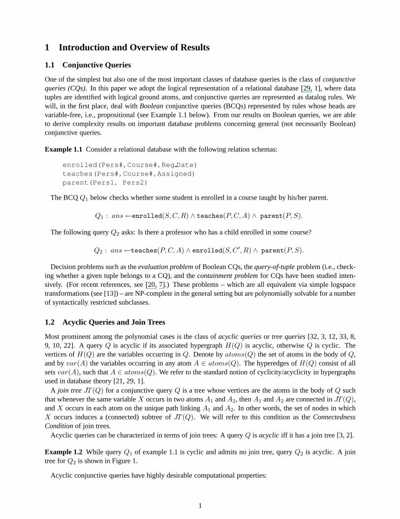
Example 1.2 While queryQ1 of example 1.1 is cyclic and admits no join tree, queryQ2 is acyclic. A jointree forQ2 is shown in Figure 1.

Acyclic conjunctive queries have highly desirable computational properties:

1

e(S,C’,R) t(P,C,A)

p(P,S)

Figure 1: A join tree ofQ2

(1) The problem BCQ of evaluating a Boolean conjunctive query can be efficiently solved if the input queryis acyclic. Yannakakis provided a (sequential) polynomialtime algorithm solving BCQ on acyclic conjunc-tive queries1 [32]. The authors of the present paper have recently shown that BCQ is highly parallelizable onacyclic queries, as it is complete for the low complexity class LOGCFL [13]. (2) Acyclicity is efficiently rec-ognizable, and a join tree of an acyclic query is efficiently computable. A linear-time algorithm for computinga join tree is shown in [28]; anLSL method has been provided in [13]. (3) The result of a (non-Boolean)acyclic conjunctive queryQ can becomputedin time polynomial in the combined size of the input instanceand of the output relation [32].

Intuitively, the efficient behaviour of Boolean acyclic queries is due to the fact that they can be evaluatedby processing the join tree bottom-up by performing upward semijoins, thus keeping small the size of theintermediate relations (that could become exponential if regular join were performed). This method is theBoolean version of Yannakakis evaluation algorithm for general conjunctive queries [32].

Acyclicity is a key-property responsible for the polynomial solvability of problems that are in general NP-hard such as BCQ [6] and other equivalent problems such as Conjunctive Query Containment [23, 7], ClauseSubsumption, and Constraint Satisfaction [20, 13]. (For a survey and detailed treatment see [13].)

1.3 Queries of Bounded Width

The tremendous speed-up obtainable in the evaluation of acyclic queries stimulated several research effortstowards the identification of wider classes of queries having the same desirable properties as acyclic queries.These studies identified a number of relevant classes of cyclic queries which are close to acyclic queries,because they can be decomposed via low width decompositionsto acyclic queries. The main classes ofpolynomially solvable bounded-width queries considered in database theory and in artificial intelligence are:

• The queries of bounded treewidth[7] (see also [20, 13]). These are queries, whose variable-atomincidence graph has treewidth bounded by a constant.2 The treewidth of a graph is a well-known mea-sure of its tree-likeness introduced by Robertson and Seymour in their work on graph minors [24]. Thisnotion plays a central role in algorithmic graph theory as well as in many subdisciplines of ComputerScience. We omit a formal definition. It is well-known that checking that a graph has treewidth≤ k

for a fixed constantk, and in the positive case, computing ak-width tree decomposition is feasible inlinear time [4].

• Queries of bounded degree of cyclicity[18, 17]. This is an interesting class of queries which alsoencompasses the class of acyclic queries. For space reasons, we omit a formal definition. For eachconstantk, checking whether a query has degree of cyclicity≤ k is feasible in polynomial time [18, 17].

1Note that, since both the databaseDB and the queryQ are part of an input-instance of BCQ, what we are consideringis thecombined complexityof the query [31].

2As pointed out in [20], the notion of treewidth of a query can be equivalently based on the Gaifman graph of a query, i.e., thegraph linking two variables by an edge if they occur togetherin a query-atom.

2

e(S,C,R) t(P,C,A)

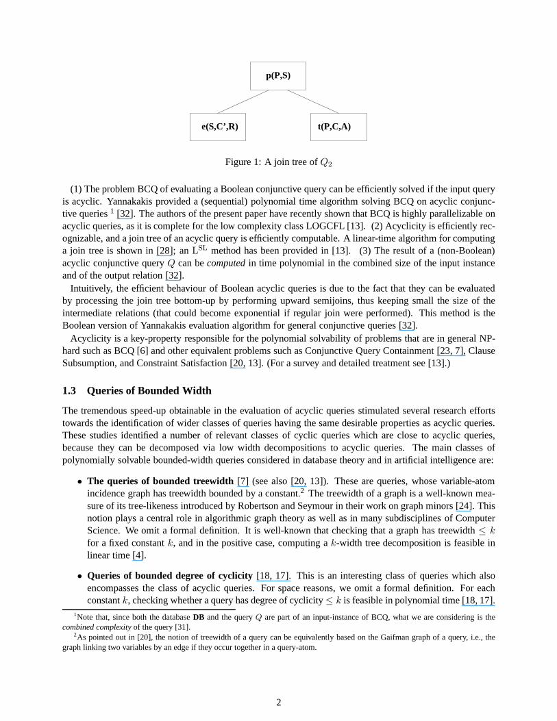
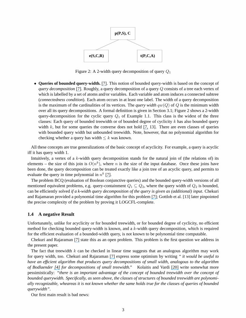
p(P,S), C

Figure 2: A 2-width query decomposition of queryQ1

• Queries of bounded query-width.[7]. This notion of bounded query-width is based on the concept ofquery decomposition[7]. Roughly, a query decomposition of a queryQ consists of a tree each vertex ofwhich is labelled by a set of atoms and/or variables. Each variable and atom induces a connected subtree(connectedness condition). Each atom occurs in at least one label. The width of a query decompositionis the maximum of the cardinalities of its vertices. Thequery widthqw(Q) of Q is the minimum widthover all its query decompositions. A formal definition is given in Section 3.1; Figure 2 shows a 2-widthquery-decomposition for the cyclic queryQ1 of Example 1.1. This class is the widest of the threeclasses: Each query of bounded treewidth or of bounded degree of cyclicity k has also bounded querywidth k, but for some queries the converse does not hold [7, 13]. There are even classes of querieswith bounded query width but unbounded treewidth. Note, however, that no polynomial algorithm forchecking whether a query has width≤ k was known.

All these concepts are true generalizations of the basic concept of acyclicity. For example, a query is acycliciff it has query width 1.

Intuitively, a vertex of ak-width query decomposition stands for the natural join of (the relations of) itselements – the size of this join isO(nk), wheren is the size of the input database. Once these joins havebeen done, the query decomposition can be treated exactly like a join tree of an acyclic query, and permits toevaluate the query in time polynomial innk [7].

The problem BCQ (evaluation of Boolean conjunctive queries) and the bounded query-width versions of allmentioned equivalent problems, e.g. query-containmentQ1 ⊆ Q2, where the query width ofQ2 is bounded,can be efficiently solvedif a k-width query decomposition of the query is given as (additional) input. Chekuriand Rajamaran provided a polynomial time algorithm for thisproblem [7]; Gottlob et al. [13] later pinpointedthe precise complexity of the problem by proving it LOGCFL-complete.

1.4 A negative Result

Unfortunately, unlike for acyclicity or for bounded treewidth, or for bounded degree of cyclicity, no efficientmethod for checking bounded query-width is known, and ak-width query decomposition, which is requiredfor the efficient evaluation of a bounded-width query, is notknown to be polynomial time computable.

Chekuri and Rajaraman [7] state this as an open problem. Thisproblem is the first question we address inthe present paper.

The fact that treewidthk can be checked in linear time suggests that an analogous algorithm may workfor query width, too. Chekuri and Rajaraman [7] express someoptimism by writing“ it would be useful tohave an efficient algorithm that produces query decompositions of small width, analogous to the algorithmof Bodlaender [4] for decompositions of small treewidth.”Kolaitis and Vardi [20] write somewhat morepessimistically:“there is an important advantage of the concept of bounded treewidth over the concept ofbounded querywidth. Specifically, as seen above, the classes of structures of bounded treewidth are polynomi-ally recognizable, wheareas it is not known whether the sameholds true for the classes of queries of boundedquerywidth”.

Our first main result is bad news:

3

Determining whether the query width of a conjunctive query is at most 4 is NP-complete.

The NP-completeness proof is rather involved and will be given in Section 3.2. We give a rough intuition inthis section. The proof led us to a better intuition about (i)why the problem is NP-complete, and (ii) how thiscould be redressed by suitably modifying the notion of querywidth. Very roughly, the source of NP-hardnesscan be pinpointed as follows. In order to obtain a query-decomposition of width bounded byk, it can beseen that it is implicitly required to proceed as follows. Atany step, the decomposition is guided by a setC of variables that still needs to be processed. Initially, i.e., at the root of the decomposition,C consists ofall variables that occur in the query. We then choose as root of the decomposition tree a hypernodeR of≤ k query atoms. By fixing this hypernode, we eliminate a set of variables, namely those which occur in theatoms ofR. The remaining set of variables disintegrates into connected components. We now expand thedecomposition tree by attaching children, and thus, in the long run, subtrees toR. It can be seen that eachsubtree rooted inR must correspond to one or more of the connected components and each component occursin exactly one subtree (otherwise the connectedness condition would be violated). In particular, since eachatom should be eventually covered, each remaining atom mustbe covered by some subtree, i.e., must occur insome subtree. This process goes on until all variables are eliminated and until all query atoms are eventuallycovered. The definition of query width requires that this covering beexact, i.e., that each atom containing avariable of a certain componentC occurs only in the subtree corresponding toC. (Again, the requirement ofexact covering is due to the connectedness condition.) The NP hardness is due to this requirement ofexactcovering. In our NP-completeness proof, we thus tried to reduce the problem ofEXACT COVERING BY3SETS to the query width problem. And this attempt was successful.

1.5 Hypertree Decompositions: Positive Results

To circumvent the high complexity of query-decompositions, we introduce a new concept of decomposition,which we callhypertree decomposition. The definition of hypertree decomposition (see Section 4) uses a moreliberal notion of covering. When choosing a setSC of components to be processed, the variables ofSC areno longer required to exactlycoincidewith the variables occurring in the labels of the decomposition-subtreecorresponding toSC, but it is sufficient that the former be a subset of the latter.Based on this more liberalnotion of decomposition, we define the corresponding notionof hypertree widthin analogy to the concept ofquery width.

We denote the query width of a query byqw(Q) and its hypertree width byhw(Q). We are able to provethe following results:

4

1. For each conjunctive queryQ it holds thathw(Q) ≤ qw(Q).

2. There exist queriesQ such thathw(Q) < qw(Q).

3. For each fixed constantk, the problems of determining whetherhw(Q) ≤ k and of computing(in the positive case) a hypertree decomposition of width≤ k are feasible in polynomial time.

4. For fixedk, evaluating a Boolean conjunctive queryQ with hw(Q) ≤ k is feasible in polynomialtime.

5. The result of a (non-Boolean) conjunctive queryQ of bounded hypertree-width can becomputedin time polynomial in the combined size of the input instanceand of the output relation.

6. Tasks 3 and 4 are not only polynomial, but are highly parallelizable. In particular, for fixedk,checking whetherhw(Q) ≤ k is in the parallel complexity classLOGCFL; computing a hyper-tree decomposition of widthk (if any) is in functionalLOGCFL, i.e., is feasible by a logspacetransducer that uses an oracle inLOGCFL; evaluatingQ wherehw(Q) ≤ k on a database iscomplete forLOGCFLunder logspace reductions.

Similar results hold for the equivalent problem of conjunctive query containmentQ1 ⊆ Q2, wherehw(Q2) ≤k, and for all other of the aforementioned equivalent problems.

Let us comment on these results. By statements 1 and 2, the concept of hypertree width is a proper general-ization of the notion of query width. By statement 3, constant hypertree-width is efficiently checkable, and bystatement 4, queries of constant hypertree width can be efficiently evaluated. In summary, this is truly goodnews. It means that the notion of constant hypertree width not only shares the desirable properties of constantquery-width, it also doesnotshare the bad properties of the latter, and, in addition, is amore general concept.

It thus turns out that the high complexity of determining constant query width is not, as one would usuallyexpect, the price for the generality of the concept. Rather,it is due to some peculiarity in its definition relatedto the exact covering paradigm. In the definition of hypertree width we succeeded to eliminate these problemswithout paying any additional charge, i.e., hypertree width comes as a freebie!

Statement 6 asserts that the main algorithmic tasks relatedto constant hypertree-width are in the verylow complexity class LOGCFL. This class consists of all decision problems that are logspace reducibleto a context-free language. An obvious example of a problem complete for LOGCFL is Greibach’s hardestcontext-free language [16]. There is a number of very interesting natural problems known to be LOGCFL-complete (see, e.g. [27, 26, 13]). The relationship betweenLOGCFL and other well-known complexity classesis summarized in the following chain of inclusions:

AC0 ⊆ NC1 ⊆ L ⊆ SL⊆ NL ⊆ LOGCFL⊆ AC1 ⊆ NC2 ⊆ P⊆ NP

HereL denotes logspace, ACi and NCi are logspace-uniformclasses based on the corresponding types ofBoolean circuits, SL denotes symmetric logspace, NL denotes nondeterministic logspace, P is polynomialtime, and NP is nondeterministic polynomial time. For the definitions of all these classes, and for referencesconcerning their mutual relationships, see [19].

Since LOGCFL⊆ AC1 ⊆ NC2, the problems in LOGCFL are all highly parallelizable. In fact, they aresolvable in logarithmic time by a CRCW PRAM with a polynomialnumber of processors, or inlog2-time byan EREW PRAM with a polynomial number of processors.

1.6 Structure of the Paper

Basic notions of database and complexity theory are given inSection 2. Section 3 deals with query decompo-sitions and includes the NP-completeness proof for the problem of deciding bounded query-width. The new

5

notions of hypertree decomposition and hypertree width areformally defined in Section 4, where also someexamples are given, and it is shown that bounded hypertree-width queries are efficiently evaluable. In Section5, the alternating algorithmk-decomp that checks whether a query has hypertree width≤ k is presented.This algorithm is shown to run on a logspace ATM having polynomially sized accepting computation trees,thus the problem is actually in LOGCFL. Finally, a short sketch of a deterministic polynomial algorithm (inform of a datalog program) for checking whether a query has hypertree width≤ k is given. In Section 6 thenotion of hypertree decomposition is shown to be the most general among the most important related notions,e.g., the notion of query decomposition.

2 Preliminaries

2.1 Databases and Queries

For a background on databases, conjunctive queries, etc., see [29, 1, 21]. We define only the most relevantconcepts here.

A relation schemaR consists of a name (name of the relation)r and a finite ordered list of attributes. Toeach attributeA of the schema, a countable domainDom(A) of atomic values is associated. Arelationinstance(or simply, arelation) over schemaR = (A1, . . . , Ak) is a finite subset of the cartesian productDom(A1) × · · · ×Dom(Ak). The elements of relations are calledtuples. A database schemaDS consistsof a finite set of relation schemas. Adatabase instance, or simply database, DB over database schemaDS = R1, . . . , Rm consists of relation instancesr1, . . . , rm for the schemasR1, . . . , Rm, respectively, anda finite universeU ⊆

⋃Ri(Ai

1,...,Ai

ki)∈DS(Dom(Ai

1)∪ · · · ∪Dom(Aiki

)) such that all data values occurring in

DB are fromU .In this paper we will adopt the standard convention [1, 29] ofidentifying a relational database instance

with a logical theory consisting of ground facts. Thus, a tuple 〈a1, . . . ak〉, belonging to relationr, will beidentified with the ground atomr(a1, . . . , ak). The fact that a tuple〈a1, . . . , ak〉 belongs to relationr of adatabase instanceDB is thus simply denoted byr(a1, . . . , ak) ∈ DB.

A (rule based)conjunctive queryQ on a database schemaDS = R1, . . . , Rm consists of a rule of theform

Q : ans(u)← r1(u1) ∧ · · · ∧ rn(un),

wheren ≥ 0, r1, . . . , rn are relation names (not necessarily distinct) ofDS; ans is a relation name not inDS;andu,u1, . . . ,un are lists of terms (i.e., variables or constants) of appropriate length. The set of variablesoccurring inQ is denoted byvar(Q). The set of atoms contained in the body ofQ is referred to asatoms(Q).Similarly, for any atomA ∈ atoms(Q), var(A) denotes the set of variables occurring inA; and for a set ofatomsR ⊆ atoms(Q), definevar(R) =

⋃A∈R var(A).

Theanswerof Q on a database instanceDB with associated universeU , consists of a relationans whosearity is equal to the length ofu, defined as follows.ans contains all tuplesans(u)ϑ such thatϑ : var(Q) −→U is a substitution replacing each variable invar(Q) by a value ofU and such that for1 ≤ i ≤ n, ri(ui)ϑ ∈DB. (For an atomA, Aϑ denotes the atom obtained fromA by uniformly substitutingϑ(X) for each variableX occurring inA.)

The conjunctive queryQ is aBoolean conjunctive query (BCQ)if its head atomans(u) does not containvariables and is thus a purely propositional atom.Q evaluates totrue if there exists a substitutionϑ such thatfor 1 ≤ i ≤ n, ri(ui)ϑ ∈ DB; otherwise the query evaluates tofalse.

The head literal in Boolean conjunctive queries is actuallyinessential, therefore we may omit it whenspecifying a Boolean conjunctive query.

Note that conjunctive queries as defined here correspond to conjunctive queries in the more classical settingof relational calculus, as well as to SELECT-PROJECT-JOIN queries in the classical setting of relational

6

algebra, or to simple SQL queries of the type

SELECT Ri1 .Aj1 , . . . Rik .AjkFROM R1, . . . Rn WHERE cond,

such thatcond is a conjunction of conditions of the formRi.A = Rj .B or Ri.A = c, wherec is a constant.A queryQ is acyclic [2, 3] if its associated hypergraphH(Q) is acyclic, otherwiseQ is cyclic. The vertices

of H(Q) are the variables occurring inQ. Denote byatoms(Q) the set of atoms in the body ofQ, and byvar(A) the variables occurring in any atomA ∈ atoms(Q). The hyperedges ofH(Q) consist of all setsvar(A), such thatA ∈ atoms(Q). We refer to the standard notion of cyclicity/acyclicity inhypergraphs usedin database theory [21, 29, 1].

A join treeJT (Q) for a conjunctive queryQ is a tree whose vertices are the atoms in the body ofQ suchthat whenever the same variableX occurs in two atomsA1 andA2, thenA1 andA2 are connected inJT (Q),andX occurs in each atom on the unique path linkingA1 andA2. In other words, the set of nodes in whichX occurs induces a (connected) subtree ofJT (Q) (connectedness condition).

Acyclic queries can be characterized in terms of join trees:A queryQ is acyclic iff it has a join tree [3, 2].

Example 2.1 While queryQ1 of example 1.1 is cyclic and admits no join tree, queryQ2 is acyclic. A jointree forQ2 is shown in Figure 1.

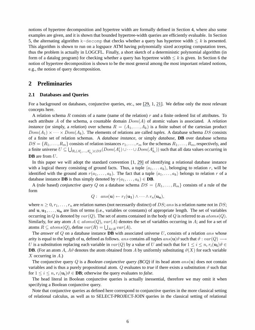
Consider the following queryQ3:

ans← r(Y,Z) ∧ g(X,Y ) ∧ s(Y,Z,U) ∧ s(Z,U,W ) ∧ t(Y,Z) ∧ t(Z,U)

A join tree forQ3 is shown in Figure 3.

s(Z,U,W) t(Z,U)

s(Y,Z,U)

r(Y,Z)

g(X,Y)

t(Y,Z)

Figure 3: A join tree ofQ3

Acyclic conjunctive queries have highly desirable computational properties:

1. The problem BCQ of evaluating a Boolean conjunctive querycan be efficiently solved if the input queryis acyclic. Yannakakis provided a (sequential) polynomialtime algorithm solving BCQ on acyclicconjunctive queries3 [32]. The authors of the present paper have recently shown that BCQ is highlyparallelizable on acyclic queries, as it is complete for thelow complexity class LOGCFL [13].

2. Acyclicity is efficiently recognizable, and a join tree ofan acyclic query is efficiently computable. Alinear-time algorithm for computing a join tree is shown in [28]; anLSL method has been provided in[13].

3. The result of a (non-Boolean) acyclic conjunctive queryQ can becomputedin time polynomial in thecombined size of the input instance and of the output relation [32].

3Note that, since both the databaseDB and the queryQ are part of an input-instance of BCQ, what we are consideringis thecombined complexityof the query [31].

7

Intuitively, the efficient behaviour of Boolean acyclic queries is due to the fact that they can be evaluatedby processing the join tree bottom-up by performing upward semijoins, thus keeping small the size of theintermediate relations (that could become exponential if regular join were performed). This method is theBoolean version of Yannakakis evaluation algorithm for general conjunctive queries [32].

Acyclicity is a key-property responsible for the polynomial solvability of problems that are in general NP-hard such as BCQ [6] and other equivalent problems such as Conjunctive Query Containment [23, 7], ClauseSubsumption, and Constraint Satisfaction [20, 13]. (For a survey and detailed treatment see [13].)

2.2 The class LOGCFL

LOGCFL consists of all decision problems that are logspace reducible to a context-free language. An obviousexample of a problem complete for LOGCFL is Greibach’s hardest context-free language [16]. There are anumber of very interesting natural problems known to be LOGCFL-complete (see, e.g. [13, 27, 26]). Therelationship between LOGCFL and other well-known complexity classes is summarized in the followingchain of inclusions:

AC0 ⊆ NC1 ⊆ L ⊆ SL⊆ NL ⊆ LOGCFL⊆ AC1 ⊆ NC2 ⊆ P⊆ NP

HereL denotes logspace, ACi and NCi are logspace-uniformclasses based on the corresponding types ofBoolean circuits, SL denotes symmetric logspace, NL denotes nondeterministic logspace, P is polynomialtime, and NP is nondeterministic polynomial time. For the definitions of all these classes, and for referencesconcerning their mutual relationships, see [19].

Since – as mentioned in the introduction – LOGCFL⊆ AC1 ⊆ NC2, the problems in LOGCFL are allhighly parallelizable. In fact, they are solvable in logarithmic time by a CRCW PRAM with a polynomialnumber of processors, or inlog2-time by an EREW PRAM with a polynomial number of processors.

In this paper, we will use an important characterization of LOGCFL by Alternating Turing Machines. Weassume that the reader is familiar with thealternating Turing machine (ATM)computational model introducedby Chandra, Kozen, and Stockmeyer [5]. Here we assume w.l.o.g. that the states of an ATM are partitionedinto existential and universal states.

As in [25], we define acomputation treeof an ATM M on a input stringw as a tree whose nodes are labeledwith configurations ofM on w, such that the descendants of any non-leaf labeled by a universal (existential)configuration include all (resp. one) of the successors of that configuration. A computation tree isacceptingif the root is labeled with the initial configuration, and allthe leaves are accepting configurations.

Thus, an accepting tree yields a certificate that the input isaccepted. A complexity measure consideredby Ruzzo [25] for the alternating Turing machine is the tree-size, i.e. the minimal size of an acceptingcomputation tree.

Definition 2.2 ([25]) A decision problemP is solved by an alternating Turing machineM within simulta-neoustree-size and space boundsZ(n) and S(n) if, for every “yes” instancew of P, there is at least oneaccepting computation tree forM on w of size (number of nodes)≤ Z(n), each node of which represents aconfiguration using space≤ S(n), wheren is the size ofw. (Further, for any “no” instancew of P there isno accepting computation tree forM .)

Ruzzo [25] proved the following important characterization of LOGCFL :

Proposition 2.3 (Ruzzo [25])LOGCFLcoincides with the class of all decision problems recognized by ATMsoperating simultaneously in tree-sizeO(nO(1)) and spaceO(log n).

3 Query Decompositions

8

t(Y,Z)

s(Z,W,X)

t(Z,X)

s(Y,Z,U)

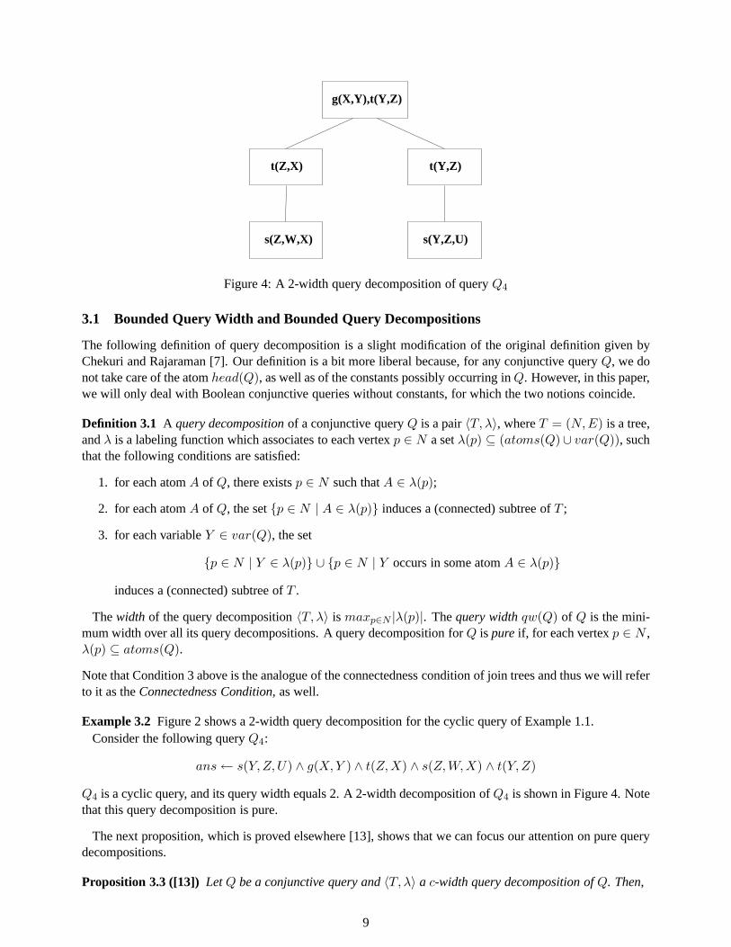
g(X,Y),t(Y,Z)

Figure 4: A 2-width query decomposition of queryQ4

3.1 Bounded Query Width and Bounded Query Decompositions

The following definition of query decomposition is a slight modification of the original definition given byChekuri and Rajaraman [7]. Our definition is a bit more liberal because, for any conjunctive queryQ, we donot take care of the atomhead(Q), as well as of the constants possibly occurring inQ. However, in this paper,we will only deal with Boolean conjunctive queries without constants, for which the two notions coincide.

Definition 3.1 A query decompositionof a conjunctive queryQ is a pair〈T, λ〉, whereT = (N,E) is a tree,andλ is a labeling function which associates to each vertexp ∈ N a setλ(p) ⊆ (atoms(Q)∪ var(Q)), suchthat the following conditions are satisfied:

1. for each atomA of Q, there existsp ∈ N such thatA ∈ λ(p);

2. for each atomA of Q, the setp ∈ N | A ∈ λ(p) induces a (connected) subtree ofT ;

3. for each variableY ∈ var(Q), the set

p ∈ N | Y ∈ λ(p) ∪ p ∈ N | Y occurs in some atomA ∈ λ(p)

induces a (connected) subtree ofT .

Thewidth of the query decomposition〈T, λ〉 is maxp∈N |λ(p)|. Thequery widthqw(Q) of Q is the mini-mum width over all its query decompositions. A query decomposition forQ is pure if, for each vertexp ∈ N ,λ(p) ⊆ atoms(Q).

Note that Condition 3 above is the analogue of the connectedness condition of join trees and thus we will referto it as theConnectedness Condition, as well.

Example 3.2 Figure 2 shows a 2-width query decomposition for the cyclic query of Example 1.1.Consider the following queryQ4:

ans← s(Y,Z,U) ∧ g(X,Y ) ∧ t(Z,X) ∧ s(Z,W,X) ∧ t(Y,Z)

Q4 is a cyclic query, and its query width equals 2. A 2-width decomposition ofQ4 is shown in Figure 4. Notethat this query decomposition is pure.

The next proposition, which is proved elsewhere [13], showsthat we can focus our attention on pure querydecompositions.

Proposition 3.3 ([13]) LetQ be a conjunctive query and〈T, λ〉 a c-width query decomposition ofQ. Then,

9

1. there exists a purec-width query decomposition〈T, λ′〉 of Q;

2. 〈T, λ′〉 is logspace computable from〈T, λ〉.

Thus, by Proposition 3.3, for any conjunctive queryQ, qw(Q) ≤ k if and only if Q has a purec-widthdecomposition, for somec ≤ k.

k-bounded-width queriesare queries whose query width is bounded by a fixed constantk > 0. The notionof bounded query-width generalizes the notion of acyclicity [7]. Indeed, acyclic queries are exactly theconjunctive queries of query width 1, because any join tree is a query decomposition of width 1.

Bounded-width queries share an important computational property with acyclic queries: BCQ can be effi-ciently solved on queries of k-bounded query-width, if a k-width query decomposition of the query is given as(additional) input. Chekuri and Rajamaran provided a polynomial time algorithm for this problem [7]; whileGottlob et al. pinpointed that the precise complexity of theproblem is LOGCFL.

Unfortunately, different from acyclicity, no efficient method for checking bounded query-width is known.In fact, we next prove that deciding whether a conjunctive query has a bounded-width query decompositionis NP-complete.

3.2 Recognizing bounded query-width isNP-complete

A k-element-vertexof a query decomposition(T, λ) is a vertexv of T such that|λ(v)| = k.

Lemma 3.4 LetQ be a query having variable setvar(Q) = Γ ∪Rest, where

Γ = Vij | 1 ≤ i < j ≤ 8,

and Rest is an arbitrary set of further variables. Assume the setatoms(Q) contains as subset a setΠ =P1, . . . , P8 of 8 atoms, where, for1 ≤ i ≤ 8, var(Pi) ∩ Γ = V1i, V2i, . . . , Vi−1 i, Vi i+1, . . . , Vi8, i.e.,

var(Pi) ∩ Γ =⋃

k<i

Vki ∪⋃

i<k

Vik.

and∀A ∈ atoms(Q)−Π : var(A) ∩ Γ = ∅.If Q admits a pure query decomposition(T, λ) of width 4, then there exist two adjacent4-element-vertices

p1 andp2 of T such thatλ(p1) ∪ λ(p2) = Π.

Proof. Assume this doesn’t hold. Letv be any vertex fromT such thatΓ ∩ var(v) 6= ∅. Let R = Π− λ(v).The atoms ofR must occur somewhere in the treeT . By theconnectedness condition, all atoms ofR mustoccur in the labels of some neighbours ofv. Moreover, by our assumption, the atoms ofR are not containedin the label of a single neighbour ofv. Thus, there exist two neighboursv1, v2 of v and two different atomsPi Pj ∈ R such thatPi ∈ λ(v1) − λ(v2) andPj ∈ λ(v2) − λ(v1). Assume, w.l.o.g., thati < j. ThenVij ∈ var(v1), Vij ∈ var(v2), but Vij 6∈ var(v). This, however, violates theconnectedness condition.Contradiction.

Definition 3.5 Let S be a set ofn elements. A3-partition Sa, Sb, Sc of S consists of three nonemptysubsetsSa, Sb, Sc ⊂ S such thatSa ∪ Sb ∪ Sc = S, andSx ∩ Sy = ∅ for x 6= y from a, b, c. The setsSa, Sb, Sc are referred to asclasses.

A 3-Partitioning-System (short3PS) Σ on a base setS is a set of 3-partitions ofS:

Σ = S1a, S1

b , S1c , S

2a, S2

b , S2c , . . . , S

ma , Sm

b , Smc ,

where∀σ, σ′ ∈ Σ: σ 6= σ′ ⇒ σ ∩ σ′ = ∅ (i.e., no class occurs in two or more elements ofΣ).We defineclasses(Σ) :=

⋃σ∈Σ σ. The base setS of Σ is referred-to asbase(Σ): base(Σ) =

⋃C∈classes(Σ) C.

10

A 3PS isstrict if for all S′, S′′, S′′′ ∈ classes(Σ) eitherS′, S′′, S′′′ = σ for someσ ∈ Σ orS′∪S ′′∪S′′′ ⊂S. In other words: the only way to obtainS as a union of three classes is via the specified 3-partitions of Σ;any other union of three classes results in a proper subset ofS.

A 3PSΣ is referred to as an(m,k)-3PSif |Σ| ≥ m and∀C ∈ classes(Σ) : |C| ≥ k.

Lemma 3.6 For eachm > 0 andk > 0 a strict (m,k)-3PS can be computed in polynomial time.

Proof. Fix m andk. We will construct a setS of the desired cardinalityn ≤ 27m3 + 2m + 3k such thatthere exists an(m,k)-3PS forS.

In order to constructS, first start with a setS0 of 2m elements. It is a trivial combinatorial fact that we canchoose at leastm different 3-partitions ofS0 (recall thatm > 3, thus the actual number of 3-partitions wecan build is much higher). Thus, letΣ0 be a (not necessarily strict) 3PS on base setS0, such that|Σ0| = m.We now basically have to achieve two goals: (1) we have to transformΣ0 to astrict 3PS, and, (2) we have tomake sure that all classes have at leastk elements.

In order to achieve goal (1), letNew be a set of27m3 fresh elements. Enumerate (e.g., in a FOR loop) allcombinations of three setsSi

x, Sjy, S

ℓz ∈ classes(Σ0) and check for each such triplet, whether it violates the

strictness-condition. If so, choose a fresh (i.e., so far unused) elementa from New, insert it intoS0 and useit as follows to redress the situation: For any setσ ∈ Σ0 in which neither ofSi

x, Sjy, S

ℓz occurs, inserta into

exactly one of the three classes (which one is irrelevant). This means that the so augmentedσ is a partitionof the newS0. On the other hand, for eachσ ∈ Σ0 such thatσ ∩ Si

x, Sjy, S

ℓz 6= ∅, choose a classC ∈ σ

such thatC 6∈ Six, S

jy, S

ℓz and inserta into C. It follows that the tripletSi

x, Sjy, S

ℓz no longer violates the

strictness condition w.r.t. the new setS0 (containinga), becausea is not in the unionSix ∪ S

jy ∪ Sℓ

z, and thusthis union is a strict subset ofS0. Note that this operation does never invalidate the strictness condition ofany other triplet. After we have repeated this procedure foreach triplet, we end-up with a strict 3PS for theresulting setS0. Call this resulting setS+ and denote the resulting strict 3PS byΣ+. Retain that the setS+

has less than2m + (3m)3 = 2m + 27m3 elements.In order to achieve goal (2), we simply add a setNew′ of 3k further fresh elements toS+, obtaining

S∗ = S+ ∪New′. We furthermore partitionNew′ into three setsO1, O2, andO3 of equal cardinalityk anddo the following for each 3-partitionσ = Ca, Cb, Cc of Σ+, where〈Ca, Cb, Cc〉 is any arbitrarily chosenorder of the elements ofσ: performCa := Ca ∪O1 andCb := Cb ∪O2 andCc := Cc ∪O3.

The resulting 3PSΣ is strict, has|Σ| = m, |base(Σ)| ≤ 27m3 + 2m + 3k, and each classC of classes(Σ)has|C| ≥ k. We are done. Note that our method for generating a strict 3PSworks in polynomial time.

Theorem 3.7 Deciding whether the query width of a conjunctive query is atmost4 is NP-complete.

Proof. 1. Membership.It is easy to see that if there exists a query decomposition ofwidth bounded by4, then there also exists one of polynomial size (in fact, by a simple restructuring technique we can alwaysremove identically labeled vertices from a decomposition tree, and thus for any conjunctive queryQ onlyO(|atoms(Q) ∪ var(Q)|4) need to be considered). Therefore, a query decomposition ofwidth ≤ k can befound by a nondeterministic guess followed by a polynomial correctness check. The problem is thus in NP.

2. Hardness.We transform the well-known NP-complete problemEXACT COVER BY 3-SETS (XC3C) [11]to the problem of deciding whether, for a conjunctive queryQ, qw(Q) ≤ 4 holds. An instance ofEXACTCOVER BY 3-SETS consists of a pairI = (R,∆) whereR is a set ofr = 3s elements, and∆ is a collectionof m 3-element subsets ofR. The question is whether we can selects subsets out of∆ such that they form apartition ofR.

Consider an instanceI = (R,∆) of XC3S. Let ∆ = Di|1 ≤ i ≤ m and letDi = Xia,X

ib,X

ic for

1 ≤ i ≤ m (note that fori 6= j, someXiα andY

jβ may coincide).

Generate a strict(m + 1, 2) 3PSΣ = σ0, σ1, . . . , σm on some base setS = base(Σ). By Lemma 3.6,this can be done in polynomial time. Letσi = Si

a, Sib, S

ic for 0 ≤ i ≤ m.

11

Identify each element ofS with a separate variable and establish a fixed precedence order ≺ among theelements (variables) ofS. If S′ is a subset ofS, andS′ = Z1, . . . , Zl, whereZ1 ≺ Z2 · · · ≺ Zl, thenwe will abbreviate the list of variablesZ1, . . . , Zl by S′ in query atoms. For example, instead of writingp(a,Z1, . . . , Zl, b), we writep(a, S′, b).

In order to transform the given instanceI = (R,∆) of XC3S to a conjunctive queryQ, let us first definethe following sets of variablesΓℓ andΠℓ

i , which are all taken to be disjoint from the variables inS.For0 ≤ ℓ ≤ s, let

Γℓ = V ℓij | 1 ≤ i < j ≤ 8,

and for (1 ≤ i ≤ 8), let

Πℓi = V ℓ

1i, Vℓ2i, . . . , V

ℓi−1 i, V

ℓi i+1, . . . , V

ℓi8.

Let S′a andS′′

a be two nonempty sets which partitionS0a . (Such a partition exists becauseS0

a contains atleast two elements.)

Define, for0 ≤ ℓ ≤ s the following sets of query atoms:

BLOCKAℓ = q(Πℓ

1, S′a, Zℓ), pa(Π

ℓ2, S

′′a), pb(Π

ℓ3, S

0b ), pc(Π

ℓ4, S

0c )

BLOCKBℓ = q(Πℓ

5, S′a, Yℓ), pa(Π

ℓ6, S

′′a), pb(Π

ℓ7, S

0b ), pc(Π

ℓ8, S

0c ),

where theYℓ andZℓ variables are distinct fresh variables not occurring in anypreviously defined set. Wefurther define

BLOCKSA =⋃

0≤ℓ≤s

BLOCKAℓ, BLOCKSB =

⋃

0≤ℓ≤s

BLOCKBℓ,

and BLOCKS = BLOCKSA ∪ BLOCKSB .

Define, for1 ≤ ℓ ≤ s:

LINK ℓ = link(Yℓ−1, Zℓ) and LINKS =⋃

1≤ℓ≤s

LINK ℓ.

Finally, define for each setDi = Xia,X

ib,X

ic of ∆, 1 ≤ i ≤ m, the set of atoms:

Ω[Di] = s(Xia, S

ia), s(X

ib, S

ib), s(X

ic, S

ic).

Let Ω =⋃

1≤i≤m Ω[Di], and denote byΩ(Di) the set of all atoms ofΩ in which some variable ofDi

occurs, i.e,Ω(Di) = s(X,α) ∈ Ω |X ∈ Di.

Let Q be the query whose atom-set isBLOCKS ∪ LINKS ∪ Ω.We claim thatQ has query width 4 iffI = (R,∆) is a positive instance ofEXACT COVER BY 3SETS.Let us first prove theif part. Assume that there exists 3-setsD1, . . . ,Ds ∈ ∆ which exactly coverR, i.e.,

which form a partition ofR. We describe a query-decomposition(T, λ) of Q.The rootva0 of T is labeled by the set of atomsBLOCKA

0. The root has as unique child a vertexvb0

labeled byBLOCKB0.

The decomposition tree is continued as follows. For each1 ≤ ℓ ≤ s, do the following.

• Create a vertexvcℓ labeled byLINK ℓ ∪ Ω[Dℓ], and attachvcℓ as a child tovbℓ−1.

• For each remaining atomA of Ω(Dℓ), we create a new vertex, label it withA, and attach it as a leafto vcℓ. (Note that these remaining atoms, if any, stem from other elements of∆, given that a variablemay occur in several 3-sets.)

12

• Then, create a vertexvaℓ of T , label it by the set of atomsBLOCKAℓ, and attach it as a child ofvcℓ.

The vertexVaℓ, in turn, has as only child a vertexvbℓ labeled byBLOCKBℓ.

It is not hard to check that(T, λ) is indeed a valid query decomposition.Let us now prove theonly-if part. Assume(T, λ) is a width 4 query decomposition of the above defined

queryQ. By Proposition 3.3, we also assume, w.l.o.g., that(T, λ) is a pure query decomposition. SinceQ isconnected, alsoT is connected.

We observe a number of relevant facts and make some assumptions.

FACT 1: By Lemma 3.4 for each0 ≤ ℓ ≤ s, there must exist adjacent verticesvaℓ and vbℓ such thatλ(vaℓ) ∪ λ(vbℓ) = BLOCKA

ℓ ∪ BLOCKBℓ.

FACT 2: It holds thatS ⊆ var(vaℓ) andS ⊆ var(vbℓ). In fact, if this were not the case, then both verticeswould miss variables fromS, but since all variables ofS occur together in other pairs of adjacentvertices, this would violate theconnectedness conditionand is thus impossible.

FACT 3: From the latter, and from the fact that the setsS′a, S

′′a , S0

b , andS0c form a partition ofS, it follows

that each of the verticesvaℓ andvbℓ contains aq atom, apa atom, apb atom, and apc atom. Withoutloss of generality, we can thus make the following assumption.

ASSUMPTION: For0 ≤ ℓ ≤ s we haveZℓ ∈ var(vaℓ) andYℓ ∈ var(vbℓ).

FACT 4: For1 ≤ ℓ ≤ s, there exists a vertexvcℓ that lies on the unique path fromvbℓ−1 to vaℓ such thatYℓ−1, Zℓ ⊆ var(vcℓ). This can be seen as follows. For any variableϑ, aϑ-path is a pathπ in T suchthat the variableϑ occurs in the labelλ(v) of any vertexv of π. The atomlink(Yℓ−1, Zℓ) must belongto the setλ(v′cℓ) of some vertexv′cℓ of T . Clearly, by theconnectednesscondition,v′cℓ is connected viaanYℓ−1-pathπb to vbℓ−1 and by anZℓ-pathπa to vaℓ. Let π denote the unique path fromvbℓ−1 to vaℓ.Thenπ, πa, andπb intersect at exactly one vertex. This is the desired vertexvcℓ.

FACT 5: For1 ≤ ℓ ≤ s, S ⊆ var(vcℓ). Trivial, becausevcℓ lies on a path fromvbℓ−1 to vaℓ andS ⊆var(vbℓ−1) andS ⊆ var(vaℓ). The fact follows by theconnectednesscondition.

FACT 6: For1 ≤ ℓ ≤ s link(Yℓ−1, Zℓ) belongs toλ(vcℓ) and there exists ani with 1 ≤ i ≤ m such thatΩ[Di] ⊆ λ(vcℓ); in summary,λ(vcℓ) = link(Yℓ−1, Zℓ) ∪ Ω[Di]. Let us prove this. By FACT 5 weknow that all variables inS must be covered byvcℓ. However, it also holds thatYℓ−1, Zℓ ⊆ var(vcℓ)(see FACT 4). To cover the latter variables, there are two alternative choices:

1. both atomsq(Πℓ−15 , S′

a, Yℓ−1) andq(Πℓ1, S

′a, Zℓ) belong toλ(vcℓ); or

2. the atomlink(Yℓ−1, Zℓ) belongs toλ(vcℓ).

Choice 1 is impossible: there exist no two other atomsA,B ∈ atoms(Q) such thatvar(A)∪var(B)∪S′

a = S. We are thus left with Choice 2. Since the atomlink(Yℓ−1, Zℓ) does not contain any variablefrom S, there must be three other atoms inλ(vcℓ) that together coverS. An inspection of the availableatoms shows that the only possibility of coveringS by three atoms is via some atom setΩ[Di] for1 ≤ i ≤ m. The fact is proved.

FACT 7: For1 ≤ i < j ≤ s it holds thatvai lies on the unique path inT from vci to vcj.

Consider the edgevai, vbi. If we cut this edge from the treeT , then we obtain two disconnected treesTa (containingvai) andTb (containingvbi). Sincevci is connected via aZi-path tovai, butZi does notoccur invar(vbi), it holds thatvci is contained inTa. On the other hand, by “iterative” application ofFact 4 and of theconnectedness conditionit follows that there is a pathπ from vbi to vcj such that foreach vertexv of π it holds thatvar(v)∩Bigvars 6= ∅, whereBigvars = Yh | i ≤ h < j∪Zh | i <

13

h < j. Sincevar(vai) ∩ Bigvars = ∅, π does not traversevai. It follows thatvci belongs toTb.Therefore, the unique path linkingvci to vcj goes through the edgevai, vbi, and thus contains thevertexvai.

FACT 8: For0 ≤ i < j ≤ s it holds thatvar(vci) ∩ var(vcj) = S. By Fact 7,vai lies on the unique pathfrom vci to vcj. Therefore by theconnectedness conditionit holds thatvar(vci)∩var(vcj) ⊆ var(vai).Moreover, by Fact 6, no variable fromvar(vai) − S is contained in bothvar(vci) andvar(vcj). Thusvar(vci) ∩ var(vcj) ⊆ S. On the other hand, by Fact 5,S ⊆ var(vci) andS ⊆ var(vcj), hence,S ⊆ var(vci) ∩ var(vcj). In summary, we obtainvar(vci) ∩ var(vcj) = S.

For each1 ≤ ℓ ≤ s, denote byDℓ the setDi such thatΩ[Di] ⊆ λ(vcℓ) (see Fact 6). By FACT 8 it followsthat the setsDℓ (1 ≤ ℓ ≤ s) are mutually disjoint. But then the union of these sets is ofcardinality3s = r,and hence the union must coincide withR. Thuss subsets out of∆ coverR and(R,∆) is a positive instanceof EXACT COVER BY 3-SETS.

4 Conjunctive Queries of Bounded Hypertree-Width

4.1 Hypertree Width

Let Q be a (conjunctive) query. Ahypertree forQ is a triple〈T, χ, λ〉, whereT = (N,E) is a rooted tree,and χ and λ are labeling functions which associate to each vertexp ∈ N two setsχ(p) ⊆ var(Q) andλ(p) ⊆ atoms(Q). If T ′ = (N ′, E′) is a subtree ofT , we defineχ(T ′) =

⋃v∈N ′ χ(v). We denote the set

of verticesN of T by vertices(T ), and the root ofT by root(T ). Moreover, for anyp ∈ N , Tp denotes thesubtree ofT rooted atp.

Definition 4.1 A hypertree decompositionof a conjunctive queryQ is a hypertree〈T, χ, λ〉 for Q whichsatisfies all the following conditions:

1. for each atomA ∈ atoms(Q), there existsp ∈ vertices(T ) such thatvar(A) ⊆ χ(p);

2. for each variableY ∈ var(Q), the setp ∈ vertices(T ) | Y ∈ χ(p) induces a (connected) subtree ofT ;

3. for each vertexp ∈ vertices(T ), χ(p) ⊆ var(λ(p));

4. for each vertexp ∈ vertices(T ), var(λ(p)) ∩ χ(Tp) ⊆ χ(p).

A hypertree decomposition〈T, χ, λ〉 of Q is acomplete decompositionof Q if, for each atomA ∈ atoms(Q),there existsp ∈ vertices(T ) such thatvar(A) ⊆ χ(p) andA ∈ λ(p).

Thewidth of the hypertree decomposition〈T, χ, λ〉 is maxp∈vertices(T )|λ(p)|. Thehypertree widthhw(Q)of Q is the minimum width over all its hypertree decompositions.

In analogy to join trees and query decompositions, we will refer to Condition 2 above as theConnectednessCondition. Note that, by Condition 1,χ(T ) = var(Q). Hence Condition 4 entails that, fors0 = root(T ),var(λ(s0)) = χ(s0).

Intuitively, the χ labeling selects the set of variables to be fixed in order to split the cycles and achieveacyclicity; λ(p) “covers” the variables ofχ(p) by a set of atoms. Thus, the relations associated to the atomsof λ(p) restrict the range of the variables ofχ(p). For the evaluation of queryQ, each vertexp of thedecomposition is replaced by a new atom whose associated database relation is the projection onχ(p) of thejoin of the relations inλ(p). This way, we obtain a join treeJT of an acyclic queryQ′ over databaseDB′

of sizeO(nk), wheren is the input size andk is the width of the hypertree decomposition. All the efficienttechniques available for acyclic queries can be then employed for the evaluation ofQ′.

14

More technically, Condition 1 and Condition 2 above extend the notion of tree decomposition [24] fromgraphs to hypergraphs (the hypergraph of a queryQ groups the variables of the same atom in one hyperedge[2]). Thus, the pair〈T, χ〉 of a hypertree decomposition〈T, χ, λ〉 of a conjunctive queryQ, can be seen asthe correspondent of a tree decomposition on the query hypergraph. However, the treewidth of〈T, χ〉 (i.e.,the maximum cardinality of theχ-labels of the vertices ofT ) is not an appropriate measure of the width ofthe hypertree decomposition, because a set ofm variables appearing in the same atom should count1 ratherthanm for the width. Thus,λ(p) provides a set of atoms which “covers”χ(p) and its cardinality gives themeasure of the width of vertexp. It is worthwhile noting that〈T, λ〉 may violate the classical connectednesscondition usually imposed on the variables of the join trees, as it is allowed that a variableX appears in bothλ(p) andλ(q) while it does not appear inλ(s), for some vertexs on the path fromp to q in T . However,this violation is not a problem, as the variables invar(λ(p))−χ(p) are meaningless and can be projected outbefore starting the query evaluation process, because the role of λ(p) is just that of providing a binding forthe variables ofχ(p).

P, S, C, A p, t

S, C, R e

X, X′, Y, Y ′, Xab, Xac, Xaf , Xbc, Xbf a, b

X′, Y ′, Xaf , Xbf , Z′ j, f

Y ′, Z′ hX′, Z′ g

X, Y, Xac, Xbc, Z j, c

Y, Z eX, Z d

J, X, Y, X′, Y ′ j

(a) (b)

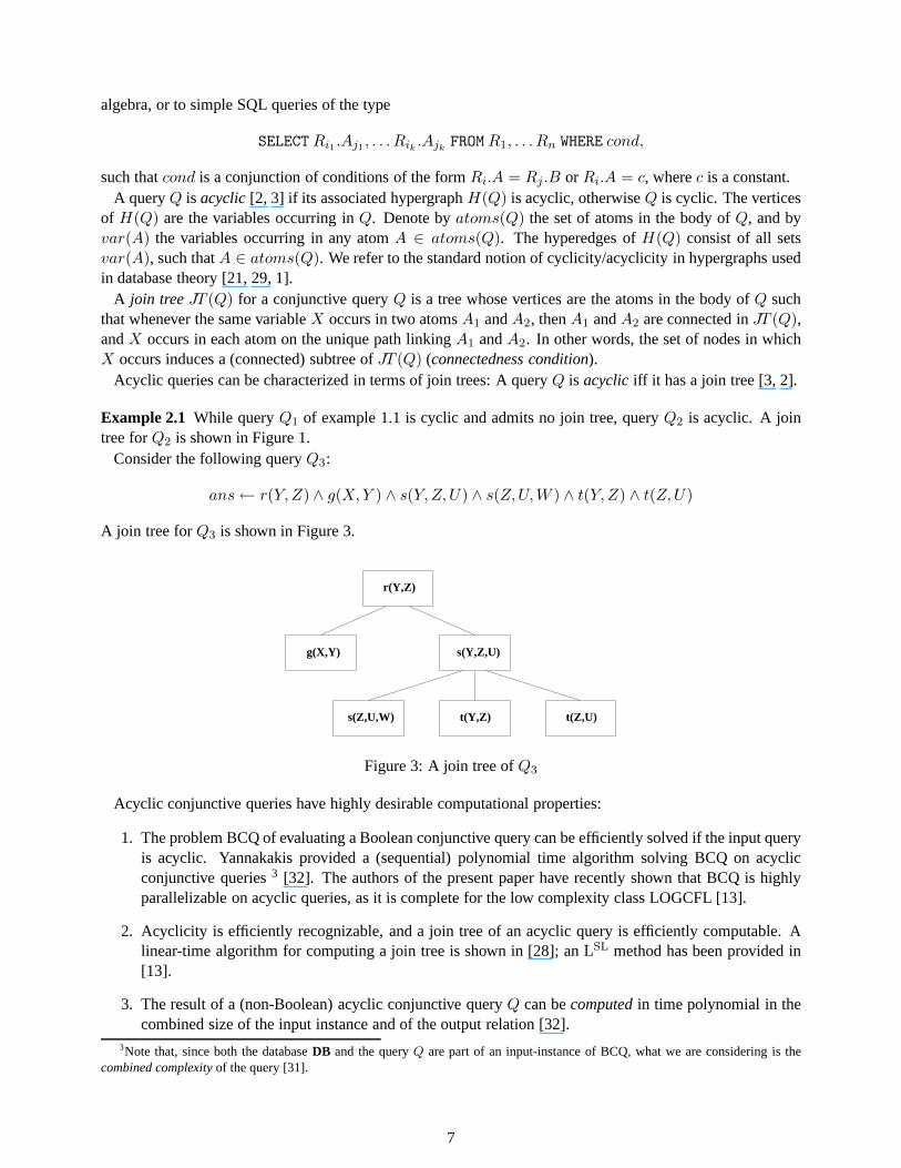
Figure 5: A 2-width hypertree decomposition of (a) queryQ1; and (b) queryQ5

Example 4.2 The hypertree width of the cyclic queryQ1 of Example 1.1 is 2; a (complete) 2-width hypertreedecomposition ofQ1 is shown in Figure 5.a.

Consider the following conjunctive queryQ5:

ans← a(Xab,X,X ′,Xac,Xaf ) ∧ b(Xab, Y, Y ′,Xbc,Xbf ) ∧ c(Xac,Xbc, Z) ∧ d(X,Z) ∧ e(Y,Z)∧∧f(Xaf ,Xbf , Z ′) ∧ g(X ′, Z ′) ∧ h(Y ′, Z ′) ∧ j(J,X, Y,X ′ , Y ′)

Q5 is clearly cyclic, and thushw(Q5) > 1 (as only acyclic queries have hypertree width equals 1). Figure 5shows a (complete) hypertree decomposition ofQ5 having width 2, hencehw(Q5) = 2.

Definition 4.1 does not require the presence of allquery atoms in a decompositionHD, as it is sufficientthat every atom is ”covered” by some vertexp of HD (i.e., its variables are included inχ(p)). However, everymissing atom can be easily added to complete decompositions.

Lemma 4.3 Given a conjunctive queryQ, everyk-width hypertree decomposition ofQ can be transformedin Logspace into ak-width complete hypertree decomposition ofQ.

Proof. Let Q be a conjunctive query andHD = 〈T, χ, λ〉 a hypertree decomposition ofQ. In order totransformHD into a complete decomposition, modifyHD as follows. For each atomA ∈ atoms(Q) suchthat no vertexq ∈ vertices(T ) satisfiesvar(A) ⊆ χ(q) andA ∈ λ(q), create a new vertexvA with λ(vA) :=A andχ(vA) = var(A), and attachvA as a new child of a vertexp ∈ vertex(T ) s.t. var(A) ⊆ χ(p). (ByCondition 1 of Definition 4.1 such ap must exist.)

This transformation is obviously feasible in Logspace.

The acyclic queries are precisely the queries of hypertree width one.

15

Theorem 4.4 A conjunctive queryQ is acyclic if and only ifhw(Q) = 1.

Proof. (Only if part.) If Q is an acyclic query, there exists a join treeJT (Q) for Q. Let T be a tree, andf a bijection fromvertices(JT (Q)) to vertices(T ) such that, for anyp, q ∈ vertices(JT (Q)), there is anedge betweenp andq in JT (Q) if and only if there is an edge betweenf(p) andf(q) in T . Moreover, letλ be the following labeling function: Ifp is a vertex ofJT (Q) andA is the atom ofQ associated top, thenλ(f(p)) = A. For any vertexp′ ∈ vertices(T ) defineχ(p′) = var(λ(p′)). Then,〈T, χ, λ〉 is clearly awidth 1 hypertree-decomposition ofQ.

(If part.) Let HD = 〈T, χ, λ〉 be a width 1 hypertree-decomposition ofQ. W.l.o.g., assume thatHD is acomplete hypertree decomposition. SinceHD has width 1, all theλ labels are singletons, i.e.,λ associate oneatom ofQ to each vertex ofT .

We next show how to trasformHD into a width 1 complete hypertree decomposition ofQ such that, forany vertexp ∈ vertices(T ), χ(p) = var(A), whereA = λ(p), andp is the unique vertex labeled with theatomA.

Choose any total ordering≺ of the vertices ofT . For any atomA ∈ atoms(Q), denote byv(A) the≺-leastvertex ofT such thatχ(v(A)) = var(A) andλ(v(A)) = A. The existence of such a vertex is guaranteedby definition of complete hypertree decomposition and by thehypothesis that everyλ label consists of exactlyone atom.

For any atomA ∈ atoms(Q), and for any vertexp 6= v(A) such thatλ(p) = A, perform the followingactions. For any childp′ of p, delete the edge betweenp andp′ and letp′ be a new child ofv(A), hencethe subtreeTp′ is now attached tov(A). Then, delete vertexp. By Condition 3 of Definition 4.1,χ(p) ⊆var(λ(p)). Sincevar(λ(p)) = var(A) = χ(v(A)), we getχ(p) ⊆ χ(v(A)). Then, it is easy to see that the(transformed) treeT satisfies the connectedness condition.

Eventually, we obtain a new hypertreeH ′ = 〈T ′, χ, λ〉 such thatvertices(T ′) ⊆ vertices(T ) andH ′ hasthe following properties: (i) for anyA ∈ atoms(Q), there exists exactly one vertexp = v(A) of T ′ such thatλ(p) = A andχ(p) = var(A); (ii) for any vertexp of T ′, p = v(A) holds, for someA ∈ atoms(Q); (iii)H ′ satisfies the connectedness condition. Thus,H ′ clearly corresponds to a join tree ofQ.

4.2 Efficient Query Evaluation

Lemma 4.5 Let Q be a Boolean conjunctive query over a databaseDB, andHD = 〈T, χ, λ〉 a hypertreedecomposition ofQ of widthk. Then, there existsQ′, DB′, JT such that:

1. Q′ is an acyclic (Boolean) conjunctive query answering ’yes’ on databaseDB′ iff the answer ofQ onDB is ’yes’.

2. ||〈Q′, DB′, JT 〉|| = O(||〈Q, DB,HD〉||k).

3. JT is a join tree of the queryQ′.

4. 〈Q′, DB′, JT 〉 is logspace computable from〈Q, DB,HD〉.

Proof. Let Q be a Boolean conjunctive query over a databaseDB, andHD = 〈T, χ, λ〉 a hypertree decom-position ofQ of width k. From Lemma 4.3, we can assume thatHD = 〈T, χ, λ〉 is a complete decompositionof Q. W.l.o.g., we also assumeQ does not contain any atomA such thatvar(A) = ∅.

Note thatQ evaluates totrue on DB if and only if 1A∈atoms(Q) rel(A) is a non-empty relation, whererel(A) denotes the relation ofDB associated to the atomA, and1 is the natural join operation (with commonvariables acting as join attributes).

For each vertexp ∈ vertices(T ) define a queryQ(p) and a databaseDB(p) as follows. For each atomA ∈ λ(p):

• If var(A) ⊆ χ(p), thenA occurs inQ(p) andrel(A) belongs toDB(p);

16

• if (var(A) ∩ χ(p)) 6= ∅, thenQ(p) contains a new atomA′ such thatvar(A′) = var(A) ∩ χ(p),andDB(p) contains the corresponding relationrel(A′), which is the projection ofrel(A) on the set ofattributes corresponding to the variables invar(A′);

Now, consider the following queryQ on the databaseDB =⋃

p∈vertices(T ) DB(p).

Q :∧

p∈vertices(T )

Q(p)

By the associative and commutative properties of natural joins, and by the fact thatHD is a completehypertree decomposition, it immediately follows thatQ on DB is equivalent toQ onDB.

We build 〈Q′, DB′, JT 〉 as follows. JT has exactly the same tree shape ofT . For each vertexp, there isprecisely one vertexp′ in JT , and one relationP ′ in DB′. p′ is an atom havingχ(p) as arguments and itscorresponding relationP ′ in DB′ is the result of the queryQ(p) onDB(p). Q′ is the conjunction of all vertices(atoms) ofJT . Q′ on DB′ is clearly equivalent toQ on DB, andJT is a join tree ofQ′. Moreover,||DB′|| =O(||DB||k), ||JT || = O(||HD||) and||Q′|| = O(||HD||); thus,||〈Q′, DB′, JT 〉|| = O(||〈Q, DB,HD〉||k).

The transformation is clearly feasible in Logspace.

Theorem 4.6 Given a databaseDB, a Boolean conjunctive queryQ, and a k-width hypertree decompositionof Q for a fixed constantk > 0, deciding whetherQ evaluates totrueonDB is LOGCFL-complete.

Theorem 4.7 Given a databaseDB, a (non-Boolean) conjunctive queryQ, and a k-width hypertree decom-position ofQ for a fixed constantk > 0, the answer ofQ on DB can becomputedin time polynomial in thecombined size of the input instance and of the output relation.

Remark. In this section we demonstrated that k-bounded hypertree-width queries are efficiently computable,once a k-width hypertree decomposition of the query is givenas (additional) input. In Section 5.2, we willstrenghten these results showing that providing the hypertree decomposition in input is unnecessary, as, dif-ferent from query decompositions, a hypertree decomposition can be computed very efficiently (inLLOGCFL,i.e., in functional LOGCFL).

5 Bounded Hypertree Decompositions are Efficiently Computable

5.1 Normal form

Let V ⊆ var(Q) be a set of variables, andX,Y ∈ var(Q) a pair of variables occurring inQ, thenX

is [V ]-adjacent toY if there exists an atomA ∈ atoms(Q) such thatX,Y ⊆ (var(A) − V ). A[V ]-path π from X to Y consists of a sequenceX = X0, . . . ,Xh = Y of variables and a sequence ofatomsA0, . . . , Ah−1 (h ≥ 0) such that:Xi is [V ]-adjacent toXi+1 andXi,Xi+1 ⊆ var(Ai), for eachi ∈ [0...h-1]. We denote byvar(π) (resp.atoms(π)) the set of variables (atoms) occurring in the sequenceX0, . . . ,Xh (A0, . . . , Ah−1).

Let V ⊆ var(Q) be a set of variables occurring in a queryQ. A set W ⊆ var(Q) of variables is[V ]-connected if∀X,Y ∈W there is a [V ]-path fromX toY . A [V ]-componentis a maximal [V ]-connectednon-empty set of variablesW ⊆ (var(Q)− V ).

Note that the variables inV do not belong to any [V ]-component (i.e.,V ∩C = ∅ for each [V ]-componentC).

Let C be a [V ]-component for some set of variablesV . We define:

atoms(C) := A ∈ atoms(Q) | var(A) ∩ C 6= ∅.

17

Note that, for any set of variablesV , and for every atomA ∈ atoms(Q) such thatvar(A) 6⊆ V , there existsexactly one [V ]-componentC of Q such thatA ∈ atoms(C).

Furthermore, letH = 〈T, χ, λ〉 be a hypertree ofQ and V ⊆ var(Q) a set of variables. We definevertices(V,H) = p ∈ vertices(T ) | χ(p) ∩ V 6= ∅.

For any vertexv of T , we will often usev as a synonym ofχ(v). In particular, [v]-component denotes[χ(v)]-component; the term [v]-path is a synonym of [χ(v)]-path; and so on.

Definition 5.1 A hypertree decompositionHD = 〈T, χ, λ〉 of a conjunctive queryQ is in normal form(NF)if for each vertexr ∈ vertices(T ), and for each childs of r, all the following conditions hold:

1. there is (exactly) one [r]-component Cr such thatχ(Ts) = Cr ∪ (χ(s) ∩ χ(r));

2. χ(s) ∩Cr 6= ∅, whereCr is the [r]-component satisfying Point 1;

3. var(λ(s)) ∩ χ(r) ⊆ χ(s).

Note that Condition 2 above entails that, for each vertexr ∈ vertices(T ), and for each childs of r,χ(s) 6⊆ χ(r). Indeed,Cr ∩ χ(r) = ∅, ands must contain some variable belonging to the [r]-componentCr.

Lemma 5.2 Let HD = 〈T, χ, λ〉 be a hypertree decomposition of a conjunctive queryQ. Let r be a ver-tex of T , let s be a child ofr, and letC be an [r]-component ofQ such thatC ∩ χ(Ts) 6= ∅. Then,vertices(C,HD) ⊆ vertices(Ts).

Proof. For any subtreeT ′ of T , let covered(T ′) denote the setA ∈ atoms(Q) | var(A) ⊆ χ(v) for somev ∈ vertices(T ′).

SinceC ∩ χ(Ts) 6= ∅, there exists a vertexp ∈ vertices(Ts) which also belongs tovertices(C,HD). Weproceed by contradiction. Assume there exists some vertexq ∈ vertices(C,HD) such thatq 6∈ vertices(Ts).By definition of vertices(C,HD), there exists a pair of variablesX,Y ⊆ C such thatX ∈ χ(p) andY ∈ χ(q). SinceX,Y ∈ C, there exists an [r]-path π from X to Y consisting of a sequence of variablesX = X0, . . . ,Xi,Xi+1, . . . ,Xℓ = Y , and a sequence of atomsA0, . . . , Ai, Ai+1, . . . , Aℓ−1.

Note thatY 6∈ χ(Ts). Indeed,Y 6∈ χ(r), hence any occurrence ofY in χ(v), for some vertexv of Ts, wouldviolate Condition 2 of Definition 4.1. Similarly,X only occurs as a variable inχ(Ts). As a consequence,A0 ∈ covered(Ts) (by Condition 1 of Definition 4.1) andAℓ−1 6∈ covered(Ts), hence the [r]-pathπ leavesTs, i.e.,atoms(π) 6⊆ covered(Ts).

Assume w.l.o.g. that the atomsAi, Ai+1 ∈ atoms(π) form the “frontier” of this path w.r.t. Ts, i.e.,Ai ∈ covered(Ts) andAi+1 6∈ covered(Ts), and consider the variableXi+1, which occurs in bothAi andAi+1. Xi+1 belongs toC, hence it does not occur inχ(r), and this immediately yields a contradiction toCondition 2 of Definition 4.1.

Lemma 5.3 LetHD = 〈T, χ, λ〉 be a hypertree decomposition of a conjunctive queryQ andr ∈ vertices(T ).If V is an [r]-connected set of variables invar(Q)−χ(r), thenvertices(V,HD) induces a (connected) sub-tree ofT .

Proof. We use induction on|V |.Basis.If |V | = 1, thenV is a singleton, and the statement follows from Condition 2 ofDefinition 4.1.Induction Step.Assume the statement is established for set of variables having cardinalitiesc ≤ h. Let

V be an [r]-connected set of variables such that|V | = h + 1, and letX ∈ V be any variable ofV suchthat V − X remains [r]-connected. (It is easy to see that such a variable exists.)By the induction hy-pothesis,vertices(V − X,HD) induces a connected subtree ofT . Moreover,X is a singleton, thusvertices(X,HD) induces a connected subtree ofT , too.

18

Since X ∈ V , V is [r]-connected, and |V | > 1, there exists a variableY ∈ V − X which is[r]-adjacent to X. Hence, there exists an atomA ∈ atoms(Q) such thatX,Y ⊆ var(A). By Con-dition 1 of Definition 4.1, there exists a vertexp ∈ vertices(T ) such thatvar(A) ⊆ χ(p). Note thatvertices(V,HD) = vertices(V − X,HD) ∪ vertices(X,HD), andp belongs to bothvertices(V −X,HD) andvertices(X,HD). Then, both sets induce connected subgraphs ofT that are, moreover,connected to each other via the vertexp. Thus,vertices(V,HD) induces a connected subgraph ofT , andhence a subtree, becauseT is a tree.

Theorem 5.4 For eachk-width hypertree decomposition of a conjunctive queryQ there exists ak-widthhypertree decomposition ofQ in normal form.

Proof. Let HD = 〈T, χ, λ〉 be anyk-width hypertree decomposition ofQ. We show how to transformHD

into ak-width hypertree decomposition in normal form.Assume there exist two verticesr ands s.t. s is a child ofr, ands violates any condition of Definition 5.1.

If s satisfies Condition 1, but violates Condition 2, thenχ(s) ⊆ χ(r) holds. In this case, simply eliminatevertexs from the tree as shown in Figure 6. It is immediate to see that this transformation is correct.

AssumeTs does not meet Condition 1 of Definition 5.1, and letC1, . . . , Ch be all the [r]-componentscontaining some variable occurring inχ(Ts). Hence,χ(Ts) ⊆ (

⋃1≤i≤h Ci ∪ χ(r)). For each [r]-component

Ci (1 ≤ i ≤ h), consider the set of verticesvertices(Ci,HD). Note that, by Lemma 5.3,vertices(Ci,HD)induces a subtree ofT , and by Lemma 5.2,vertices(Ci,HD) ⊆ vertices(Ts), hencevertices(Ci,HD)induces in fact a subtree ofTs.

For each vertexv ∈ vertices(Ci,HD) define a new vertexnew(v,Ci), and letλ(new(v,Ci)) = λ(v) andχ(new(v,Ci)) = χ(v)∩(Ci∪χ(r)). Note thatχ(new(v,Ci)) 6= ∅, because by definition ofvertices(Ci,HD),χ(v) contains some variable belonging toCi. Let Ni = new(v,Ci) | v ∈ vertices(Ci,HD). More-over, for anyCi (1 ≤ i ≤ h), let Ti denote the (directed) graph(Ni, Ei) such thatnew(p,Ci) is a child ofnew(q, Ci) iff p is is a child ofq in T . Ti is clearly isomorphic to the subtree ofTs induced byvertices(Ci,HD),henceTi is a tree, as well.

Now, transform the hypertree decompositionHD as follows. Delete every vertex invertices(Ts) fromT , and attach tor every treeTi for 1 ≤ i ≤ h. Intuitively, we replace the subtreeTs by the set of treesT1, . . . , Th. By construction,Ti contains a vertexnew(v,Ci) for each vertexv belonging tovertices(Ci,HD)(1 ≤ i ≤ h). Then, if we letchildren(r) denote the set of children ofr in the new treeT obtained afterthe transformation above, it holds that for anys′ ∈ children(r), there exists an [r]-componentC of Q suchthatvertices(Ts′) = vertices(C,HD), andχ(Ts′) ⊆ (C ∪ χ(r)). Furthermore, it is easy to verify that allthe conditions of Definition 4.1 are preserved during this transformation. As a consequence, Condition 2 ofDefinition 4.1 immediately entails that(χ(Ts′) ∩ χ(r)) ⊆ χ(s′). Hence,χ(Ts′) = C ∪ (χ(s′)∩ χ(r)). Thus,any child ofr satisfies both Condition 1 and Condition 2 of Definition 5.1.

Now, assume that some vertexv ∈ children(r) violates Condition 3 of Definition 5.1. Then, add to thelabelχ(v) the set of variablesvar(λ(v)) ∩ χ(r). Because variables inχ(r) induce connected subtrees ofT ,andχ(r) does not contain any variable occurring in some [r]-component, this further transformation neverinvalidates any other condition. Moreover, no new vertex islabeled by a set of atoms with cardinality greaterthank, then we get in fact a legalk-width hypertree decomposition.

Clearly, root(T ) cannot violate any of the normal form conditions, because ithas no parent inT . More-over, the transformations above never change the parentr of a violating vertexs. Thus, if we apply such atransformation to the children ofroot(T ), and iterate the process on the new children ofroot(T ), and so on,we eventually gets a newk-width hypertree decomposition〈T ′, λ′〉 of Q in normal form.

If HD = 〈T, χ, λ〉 is an NF hypertree decomposition of a conjunctive queryQ, we can associate a settreecomp(s) ⊆ var(Q) to each vertexs of T as follows.

• If s = root(T ), thentreecomp(s) = var(Q);

19

r

α

ββ

γ

δ

r

s

If χ(s) ⊆ χ(r)

α

γ δ

Figure 6: Normalizing a hypertree decomposition

• otherwise, letr be the father ofs in T ; then,treecomp(s) is the (unique) [r]-componentC such thatχ(Ts) = C ∪ (χ(s) ∩ χ(r)).

Note that, sinces ∈ vertices(Ts), alsoχ(Ts) = C ∪ χ(s) holds.

Lemma 5.5 Let HD = 〈T, χ, λ〉 be an NF hypertree decomposition of a conjunctive queryQ, v a vertex ofT , andW = treecomp(v)− χ(v). Then, for any [v]-componentC such that(C ∩W ) 6= ∅, C ⊆W holds.

Therefore, the setC = C ′ ⊆ var(Q) | C ′ is a [v]-component andC ′ ⊆ treecomp(v) is a partition oftreecomp(v)− χ(v).

Proof. Let C be a [v]-component such that(C ∩ W ) 6= ∅. We show thatC ⊆ W . Assume this isnot true, i.e.,C − W 6= ∅. By definition of treecomp(v), χ(Tv) = treecomp(v) ∪ χ(v). Hence, anyvariableY ∈ (C −W ) only occurs in theχ label of vertices not belonging tovertices(Tv). However,Cis a [v]-component, thereforeC ∩ χ(v) = ∅. As a consequence,vertices(C,HD) induces a disconnectedsubgraph ofT , and thus contradicts Lemma 5.3.

Lemma 5.6 Let HD = 〈T, χ, λ〉 be an NF hypertree decomposition of a conjunctive queryQ, andr be avertex ofT . Then,C = treecomp(s) for some childs of r if and only ifC is an [r]-component ofQ andC ⊆ treecomp(r).

Proof. (If part.) AssumeC is an [r]-component ofQ andC ⊆ treecomp(r). Let children(r) denote theset of the vertices ofT which are children ofr. BecauseC ⊆ (treecomp(r) − χ(r)), C must be includedin

⋃s∈children(r) χ(Ts). Moreover, for each subtreeTs of T such thats ∈ children(r), there is a (unique)

[r]-componenttreecomp(s) such thatχ(Ts) = treecomp(s) ∪ (χ(s) ∩ χ(r)). Therefore,C necessarilycoincides with one of these components, saytreecomp(s) for somes ∈ children(r).

(Only if part.) AssumeC = treecomp(s) for some childs of r, and letC ′ = treecomp(r). By definitionof treecomp(s), C is an [r]-component, then(C ∩ χ(r)) = ∅. SinceHD is in normal form,χ(Ts) =C∪(χ(s)∩χ(r)) andχ(Tr) = (C ′∪χ(r)). Moreover,s is a child ofr, thenvertices(Ts) ⊆ vertices(Tr) andthusχ(Ts) ⊆ χ(Tr). Therefore,C∪(χ(s)∩χ(r)) ⊆ χ(Tr), and hence we immediately getC ⊆ (C ′∪χ(r)).However,(C ∩ χ(r)) = ∅ and thusC ⊆ C ′.

Lemma 5.7 For any NF hypertree decompositionHD = 〈T, χ, λ〉 of a queryQ, |vertices(T )| ≤ |var(Q)|holds.

20

Proof. Follows from Lemma 5.6, Lemma 5.5, and Condition 2 of the normal form, which states that, for anyv ∈ vertices(T ), χ(v) ∩ treecomp(v) 6= ∅. Hence,treecomp(v) − χ(v) ⊂ treecomp(v) and thus, for anychild s of v in T , treecomp(s) is actually a proper subset oftreecomp(v).

Lemma 5.8 Let HD = 〈T, χ, λ〉 be an NF hypertree decomposition of a queryQ, s a vertex ofT , andC a set of variables such thatC ⊆ treecomp(s). Then,C is an [s]-component if and only ifC is a[var(λ(s))]-component.

Proof. Let V = var(λ(s)). By Condition 4 of Definition 4.1,(V ∩ χ(Ts)) ⊆ χ(s). SinceHD is in normalform, V satisfies the following property.

(1) (V ∩ treecomp(s)) ⊆ χ(s).

(Only if part.) AssumeC ⊆ treecomp(s) is an [s]-component. From Property 1 above,C ∩ V = ∅ holds.As a consequence, for any pair of variablesX,Y ⊆ C, X [s]-adjacent toY entailsX [V ]-adjacent toY .Hence,C is a [V ]-connected set of variables. Moreover,χ(s) ⊆ V . Then, any [V ]-connected set which is amaximal [s]-connected set is a maximal [V ]-connected set as well, and thusC is a [V ]-component.

(If part.) AssumeC ⊆ treecomp(s) is a [V ]-component. Sinceχ(s) ⊆ V , C is clearly [s]-connected.Thus,C ⊆ C ′, whereC ′ is an [s]-component and, by Lemma 5.5,C ′ ⊆ (treecomp(s)−χ(s)) holds. By the“only if” part of this lemma,C ′ is a [V ]-component, thereforeC cannot be a proper subset ofC ′, andC ′ = C

actually holds. Thus,C is an [s]-component.

5.2 A LOGCFL Algorithm Deciding k-bounded Hypertree-Width

Figure 7 shows the algorithmk-decomp, deciding whether a given conjunctive queryQ has ak-boundedhypertree-width decomposition. In that figure, we give a high level description of an alternating algorithm, tobe run on an alternating Turing machine (ATM). The details ofhow the algorithm can be effectively imple-mented on a logspace ATM will be given later (see Lemma 5.14).

To each computation treeτ of k-decomp on input queryQ, we associate a hypertreeδ(τ) = 〈T, χ, λ〉,called thewitness treeof τ , defined as follows: For any existential configuration ofτ corresponding to the“guess” of some setS ⊆ atoms(Q) during the computation ofk-decomposable(C,R), for some [var(R)]-componentC, (i.e., to Step 1 ofk-decomp), T contains a vertexs. In particular, the vertexs0 guessed at the initial callk-decomposable(var(Q), ∅), is the root ofT .

There is an edge between verticesr and s of T , wheres 6= s0, if S is guessed at Step 1 during thecomputation ofk-decomposable(C,R), for some [var(R)]-componentC (S andR are the (guessed) sets ofatoms ofτ corresponding tos andr in T , respectively). We will denoteC by comp(s), andr by father(s).Moreover, for the roots0 of T , we definecomp(s0) = var(Q).

The vertices ofT are labeled as follows.λ(s) = S (i.e.,λ(s) is the guessed setS of atoms correspondingto s), for any vertexs of T . If s0 = root(T ), let χ(s0) = var(λ(s0)); for any other vertexs, let χ(s) =var(λ(s)) ∩ (χ(r) ∪ C), wherer = father(s) andC = comp(s).

Lemma 5.9 For any given queryQ such thathw(Q) ≤ k, k-decomp acceptsQ. Moreover, for anyc ≤ k,eachc-width hypertree-decomposition ofQ in normal form is equal to some witness tree forQ.

Proof. LetHD = 〈T, χ, λ〉 be ac-width NF hypertree decomposition of a conjunctive queryQ, wherec ≤ k.We show that there exists an accepting computation treeτ for k-decomp on input queryQ such thatδ(τ) =〈T ′, χ′, λ′〉 “coincides” withHD. Formally, there exists a bijectionf : vertices(T ) → vertices(T ′) suchthat, for any pair of verticesp, q ∈ T , p is a child ofq in T iff f(p) is a child off(q) in T ′, λ(p) = λ′(f(p)),λ(q) = λ′(f(q)), χ(p) = χ′(f(p)), andχ(q) = χ′(f(q)).

To this aim, we impose tok-decomp on inputQ the following choices of setsS in Step 1:

21

ALTERNATING ALGORITHM k-decompInput: A non-empty QueryQ.Result: “Accept”, if Q hask-bounded hypertree width; “Reject”, otherwise.

Procedurek-decomposable(CR : SetOfVariables,R: SetOfAtoms)begin1) Guessa setS ⊆ atoms(Q) of k elements at most;2) Check that all the following conditions hold:

2.a) ∀P ∈ atoms(CR), (var(P ) ∩ var(R)) ⊆ var(S) and2.b) var(S) ∩ CR 6= ∅

3) If the check above failsThen Halt andReject; ElseLet C := C ⊆ var(Q) | C is a [var(S)]-component andC ⊆ CR;

4) If, for each C ∈ C, k-decomposable(C,S)Then AcceptElse Reject

end;

begin(* MAIN *)Accept if k-decomposable(var(Q), ∅)

end.

Figure 7:A non-deterministic algorithm decidingk-bounded hypertree-width

a) For the initial callk-decomposable(var(Q), ∅), the setS chosen in Step 1 isλ(root(T )).

b) Otherwise, for a callk-decomposable(CR , R), if R is the labelλ(r) of some vertexr, and if r has achild s such thattreecomp(s) = CR, then chooseS = λ(s) in Step 1.

We use structural induction on trees to prove that, for any vertex r ∈ vertex(T ), if we denotef(r) by r′, thefollowing equivalences hold:λ(r) = λ′(r′); treecomp(r) = comp(r′); andχ(r) = χ′(r′).

Basis:For r = root(T ), we setf(root(T )) := root(T ′). Thus, by choosingλ′(f(r)) = λ(r) as describedat Point a) above, all the equivalences trivially hold.

Induction Step:Assume that the equivalence holds for some vertexr ∈ vertices(T ). Then, we willshow that the statement also holds for every child ofr. Let r′ ∈ vertices(T ′) denotef(r), and lets beany child ofr in T . By Lemma 5.6 and Lemma 5.8, the [r]-componenttreecomp(s) coincides with some[var(λ′(r′))]-componentcomp(s′) corresponding to the callk-decomposable(comp(s′), λ′(r′)) that gener-ated a childs′ of r′, which we define to be the image ofs, i.e., we setf(s) := s′. SinceHD is ak-widthhypertree decomposition, and the induction hypothesis holds, it easily follows that, by choosingλ(s) = λ′(s′)as prescribed at Point b) above, no check performed in Step 2 of the callk-decomposable(comp(s′), λ′(r′))can fail.

Next we show thatχ(s) = χ′(s′). Let C = comp(s′) = treecomp(s), andV = var(λ(s)) = var(λ′(s′)).By Condition 4 of Definition 4.1,V ∩ χ(Ts) ⊆ χ(s) holds. SinceHD is in normal form, we can replaceχ(Ts) by C ∪ χ(s) according to Condition 1 of Definition 5.1, and we getV ∩ (C ∪ χ(s)) ⊆ χ(s). Hence,we obtain the following property

(1) V ∩ C ⊆ χ(s).

Now, considerχ′(s′). By definition of witness tree,χ′(s′) = V ∩ (χ′(r′) ∪ C) = V ∩ (χ(r) ∪ C). ByProperty(1) above,V ∩ C ⊆ χ(s). Moreover,HD is in NF, and Condition 3 of the normal form entailsthat(V ∩χ(r)) ⊆ χ(s). As a consequence,χ′(s′) ⊆ χ(s). We claim that this inclusionship cannot be proper.Indeed, by definition ofχ′(s′), if χ′(s′) ⊂ χ(s), there exists a variableY ∈ χ(s) which belongs neither

22

to χ(r), nor to C. However, this entails thatY belongs to some other [r]-component and thuss violatesCondition 1 of the normal form.

In summary,k-decomp acceptsQ with the accepting computation treeτ determined by the choices de-scribed above, and its witness treeδ(τ) is ac-width hypertree decomposition ofQ in normal form.

Lemma 5.10 Assume thatk-decomp accepts an input queryQ with an accepting computation treeτ andlet δ(τ) = 〈T, χ, λ〉 be the corresponding witness tree. Then, for any vertexs of T :

a) if s 6= root(T ), thencomp(s) is a [father(s)]-component;

b) for anyC ⊆ comp(s), C is an [s]-component if and only ifC is a [var(λ(s))]-component.

Proof. We use structural induction on the treeT .Basis: Both parts of the lemma trivially holds ifs is the root ofT . In fact, in this case, we haveχ(s) =

var(λ(s)), by definition of witness tree.Induction Step:Assume that the lemma holds for some vertexr ∈ vertices(T ). Then, we will show

that both parts hold for every child ofr. The induction hypothesis states that any [var(λ(r))]-componentincluded incomp(r) is an [r]-component included incomp(r), and vice versa. Moreover, ifr 6= root(T ),thencomp(r) is a [father(r)]-component; otherwise, i.e.,r is the root,comp(r) = var(Q), by definitionof witness tree. Lets ∈ vertices(T ) be a child ofr and letV = var(λ(s)). We first observe that, bydefinition of the variable labelingχ of the witness tree, it follows thatvar(λ(s)) ∩ comp(s) ⊆ χ(s). Hence,the following holds.Fact 1: (V − χ(s)) ∩ comp(s) = ∅.(Point a.) Immediately follows by the definition ofcomp(s) and by the induction hypothesis. Indeed,r

is the father ofs and by the induction hypothesis any [var(λ(r))]-component included incomp(r) is an[r]-component included incomp(r). Thus, in particular,comp(s) is an [r]-component.(Only if part, Point b.) Assume that a set of variablesC ⊆ comp(s) is an [s]-component. By Fact 1,C∩ (V −χ(s)) = ∅ holds, and for any pair of variablesX,Y ⊆ C, X [s]-adjacent toY entailsX [V ]-adjacent toY . Hence,C is a [V ]-connected set of variables. Moreover,χ(s) ⊆ V . Then, any [V ]-connected set whichis a maximal [s]-connected set is a maximal [V ]-connected set as well, and thusC is a [V ]-component.(If part, Point b.) We proceed by contradiction. AssumeC ⊆ comp(s) is a [V ]-component, butC is notan [s]-component, i.e.,C is not a maximal [s]-connected set of variables. Sinceχ(s) ⊆ V , C is clearly[s]-connected, then it is not maximal. That is, there exists a pair of variablesX ∈ C andY 6∈ C such thatX is [s]-adjacent toY , but X is not [var(λ(s))]-adjacent toY . Let A be any atom proving their adjacencyw.r.t. s, i.e.,X,Y ⊆ var(A) − χ(s). Hence, becauseX ∈ C andX is not [V ]-adjacent toY , it followsthat Y ∈ (V − χ(s)). By Fact 1,(V − χ(s)) ∩ comp(s) = ∅, thereforeY 6∈ comp(s). In summary,X ∈ comp(s) andY 6∈ comp(s). Moreover,comp(s) ⊆ comp(r), by Step 4 ofk-decomp. Hence, byinduction hypothesis,comp(s) is an [r]-component and thusX is not [r]-adjacent toY . Consider again theatom A. We getX,Y 6⊆ var(A) − χ(r). SinceX ∈ comp(s), the variableY must belong toχ(r).However, by definition of witness tree,Y ∈ χ(r) andY ∈ var(λ(s)) entail thatY ∈ χ(s), which is acontradiction.

Lemma 5.11 Assume thatk-decomp accepts an input queryQ with an accepting computation treeτ . Letδ(τ) = 〈T, χ, λ〉 be the corresponding witness tree, ands ∈ vertices(T ). Then, for each vertexv ∈ Ts :

χ(v) ⊆ comp(s) ∪ χ(s)comp(v) ⊆ comp(s)

Proof. We use induction on the distanced(v, s) between any vertexv ∈ vertices(Ts) ands. The basis istrivial, sinced(v, s) = 0 meansv = s.

Induction Step.Assume both statements hold for distancen. Let v ∈ vertices(Ts) be a vertex such thatdist(v, s) = n + 1. Let v′ be the father ofv in Ts. Clearly,dist(v′, s) = n, thus

23

(a) χ(v′) ⊆ (comp(s) ∪ χ(s)); and

(b) comp(v′) ⊆ comp(s).

v is generated by some callk-decomposable(comp(v), λ(v′ )). By the choice ofv and the definition of witnesstree, it must hold (a′) χ(v) ⊆ (comp(v)∪χ(v′)), and by Step 4 of the callk-decomposable(comp(v′), λ(father(v′)))we get (b′) comp(v) ⊆ comp(v′). By (a′) and (b′), we obtain (a′′) χ(v) ⊆ (comp(v′) ∪ χ(v′)). By (a′′), (b),and (a) we getχ(v) ⊆ (comp(s) ∪ χ(s)). Moreover, (b) and (b′) yield comp(v) ⊆ comp(s).

Lemma 5.12 If k-decomp accepts an input queryQ, thenhw(Q) ≤ k. Moreover, each witness tree forQ

is a c-width hypertree-decomposition ofQ in normal form, wherec ≤ k.

Proof. Assume thatτ is an accepting computation tree ofk-decomp on input queryQ. We show thatδ(τ) = 〈T, χ, λ〉 is an NFc-width hypertree decomposition ofQ, for somec ≤ k.

First, we will prove thatδ(τ) fulfils all the properties of Definition 4.1 and is thus a hypertree decompositionof Q.

Property 1: ∀A ∈ atoms(Q) ∃v ∈ vertices(T ) s.t. var(A) ⊆ χ(v).We first prove the following claim.CLAIM A: Let s be any vertex ofT , and letCr = comp(s). Then, for eachP ∈ atoms(Cr) it holds that

(a) ∀A ∈ (atoms(Q)− atoms(Cr)), (var(P ) ∩ var(A)) ⊆ χ(s); and

(b) eithervar(P ) ⊆ χ(s) or there exists an [s]-componentCs ⊆ Cr such thatP ∈ atoms(Cs).

Proof of Claim A. (Part a). We use structural induction on the treeT .Basis: Part (a) of the claim trivially holds ifs is the root ofT . In fact, in this case, we haveCr = comp(s) = var(Q) and henceatoms(Cr) = atoms(Q).Induction Step:Assume that Part (a) holds for some vertexs ∈ vertices(T ). Then, we will showthat the statement also holds for every child ofs. Let Cr = comp(s) andV = var(λ(s)). Theinduction hypothesis states that∀P ∈ atoms(Cr) and∀A 6∈ atoms(Cr), var(P ) ∩ var(A) ⊆χ(s). By Step 4 ofk-decomp, for each [V ]-componentC s.t. C ⊆ Cr, T contains a vertexqsuch thatcomp(q) = C andfather(q) = s. Moreover, by Lemma 5.10,C is an [s]-component.Let Cs be an [s]-component s.t.Cs ⊆ Cr, and letP ′ belong toatoms(Cs). By choice ofCs ⊆ Cr, P ′ also belongs toatoms(Cr). First note that,∀A 6∈ atoms(Cs), we have

(1) var(P ′) ∩ var(A) ⊆ χ(s).

Indeed, ifvar(A) ⊆ χ(s) (1) is trivial, and ifA 6∈ atoms(Cr), it follows from the inductionhypothesis. Otherwise, i.e. ifA contains some variable belonging to another [s]-componentincluded inCr, it immediately follows by definition of [s]-component. Now, for the compo-nentCs, Step 1 ofk-decomposable(Cs , λ(s)) guesses a vertexs′ such that,∀B ∈ atoms(Cs),(var(B) ∩ var(λ(s))) ⊆ var(λ(s′)). In particular,(var(P ′) ∩ var(λ(s))) ⊆ var(λ(s′)). Be-causeχ(s) ⊆ var(λ(s)), this yields(var(P ′) ∩ χ(s)) ⊆ (var(λ(s′)) ∩ χ(s)). By definition ofwitness tree,(var(λ(s′)) ∩ χ(s)) ⊆ χ(s′), hence we get(var(P ′)∩ χ(s)) ⊆ χ(s′). By combin-ing this result with relationship (1) above, we get that∀A 6∈ atoms(Cs) (var(P ′) ∩ var(A)) ⊆(var(P ′)∩ χ(s)) ⊆ χ(s′). Hence, Part (a) of the claim holds even fors′ and thus for every childof s in T .

(Part b). Let s be any vertex ofT , let Cr = comp(s), and letP belong toatoms(Cr). Assumethatvar(P ) 6⊆ χ(s) and thatP ∈ atoms(C ′

s), whereC ′s is an [s]-component not included inCr,

i.e.,C ′s 6⊆ Cr. Then, there exists a variableY ∈ C ′

s s.t. Y 6∈ Cr and there is an [s]-pathπ fromY to any variableX ∈ (var(P )− χ(s)).

24

Let A be an atom belonging to bothatoms(Cr) andatoms(C ′s). Then,var(A) − χ(r) ⊆ Cr

andvar(A) − χ(s) ⊆ Cs hold. As a consequence,(var(A) ∩ C ′s) ⊆ Cr. Indeed, if this is not

true, there exists a variableZ ∈ (var(A) − χ(s)) such thatZ ∈ χ(r). By the definition of theχlabeling of a witness tree, this entails thatZ ∈ (var(A)∩ var(λ(r))), butZ 6∈ var(λ(s)), whichcontradicts the fact thatA satisfies the condition checked at Step 2.a ofk-decomp, becauseτ isan accepting computation tree.

Therefore, there exist two atomsQ′, P ′ ⊆ atoms(π) belonging toatoms(C ′s) and adjacent

in π s.t. Q′ 6∈ atoms(Cr), P ′ ∈ atoms(Cr), andvar(Q′) ∩ var(P ′) 6⊆ χ(s). However, thiscontradicts Part (a) of the claim.⋄

Note that, by Lemma 5.10, in the Step 4 of any callk-decomposable(C, λ(r)) of an accepting computationof k-decomp, [s]-components included inC and [var(λ(s))]-components included inC coincide. Thus,Property 1 follows by inductive application of Part b of Claim A. In fact, Part (b) of the claim applied tothe roots0 of T , states that,∀A ∈ atoms(Q), either var(A) ⊆ χ(s0), or A ∈ atoms(CS) for some[S]-componentCS of Q that will be further treated in Step 4 of the algorithm. Thus,var(A) is coveredeventually by some chosen set of atomsS, i.e., there exists some vertexs of T , such thatλ(s) = S, andvar(A) ⊆ χ(s).

Property 2: For each variableY ∈ var(Q) the setv ∈ vertices(T ) | Y ∈ χ(v) induces a connectedsubtree ofT .

Assume that Property 2 does not hold. Then, there exists a variable Y ∈ var(Q) and two verticesv1

andv2 of T such thatY ∈ (χ(v1) ∩ χ(v2)) but the unique path fromv1 to v2 in T contains a vertexwsuch thatY 6∈ χ(w). W.l.o.g, assume thatv1 is adjacent tow and thatv2 is a descendant ofw in T , i.e.,v2 ∈ vertices(Tw). There are two possibilities to consider:

• v1 is a child ofw andv2 belongs to the subtreeTp of another childp of w. However, this would meanthat, by Step 4 ofk-decomp and by Lemma 5.11, the variables in setsV1 = (χ(v1)−χ(w)) andV2 =(χ(v2)− χ(w)) belong to distinct [w]-components. But this is not possible, becauseY ∈ (V1 ∩ V2).

• w is a child ofv1 andv2 belongs to the subtreeTw of T rooted atw. Then,λ(w) was chosen as setS

in Step 1 ofk-decomposable(C, λ(v1 )), whereC is a [v1]-component. Note thatY ∈ χ(v1) entailsY 6∈ C, by definition of [v1]-component. Sincev2 belongs to the subtreeTw, by Lemma 5.11 it holdsthatχ(v2) ⊆ (C ∪ χ(w)). This is a contradiction, becauseY ∈ χ(v2), butY belongs neither toχ(w),nor toC.

Property 3: ∀p ∈ vertices(T ), χ(p) ⊆ var(λ(p)).Follows by definition of theχ labeling of a witness tree.Property 4: ∀p ∈ vertices(T ), var(λ(p)) ∩ χ(Tp) ⊆ χ(p).Let v be any vertex inTp, and letV = var(λ(p)). By Lemma 5.11,χ(v) ⊆ comp(p) ∪ χ(p). Hence,

V ∩ χ(v) ⊆ V ∩ comp(p) ∪ χ(p), because Property 3 holds forp. However, by definition of witness tree,(V ∩ comp(p)) ⊆ χ(p), and thus(V ∩ χ(v)) ⊆ χ(p).

Thus,δ(τ) is a hypertree decomposition ofQ. Let c be the width ofδ(τ). Since Step 1 ofk-decomp onlychooses set of atoms having cardinality bounded byk, c ≤ k holds.

Moreover,δ(τ) is in normal form. Indeed, Condition 2 and Condition 3 of Definition 5.1 hold by Step 2.bof k-decomp, and by definition of theχ labeling of a witness tree. Finally, sinceδ(τ) is a hypertree de-composition, by Lemma 5.2, Lemma 5.11, and the definition of theχ labeling of a witness tree, we get thatCondition 1 holds forδ(τ), too.

By combining Lemma 5.9 and Lemma 5.12 we get:

Theorem 5.13 k-decomp accepts an input queryQ if and only ifhw(Q) ≤ k.

25

Lemma 5.14 k-decomp can be implemented on a logspace ATM having polynomially bounded tree-size.

Proof. Let us refer to logspace ATMs with polynomially bounded tree-size as LOGCFL-ATMs. We willoutline how the algorithmk-decomp can be implemented on an LOGCFL-ATMM .

We first describe the data-structures used byM . Instead of manipulating atoms directly,indicesof atomswill be used in order to meet the logarithmic space bound. Thus thei-th atom occurring in the given repre-sentation of the input queryQ will be represented by integeri. Sets of at mostk atoms,k-sets for short, arerepresented byk-tuples of integers; sincek is fixed, representing such sets requires logarithmic spaceonly.Variables are represented as integers, too.

If R is ak-set, then a [var(R)]-componentC is represented by a pair〈rep(R), f irst(C), whererep(R)is the representation of thek-setR, andfirst(C) is the smallest integer representing a variable of the com-ponentC. For example, the∅-componentvar(Q) is represented by the pair〈rep(∅), 1〉. It is thus clear that[var(R)]-components can be represented in logarithmic space, too.

The main data structures carried with each configuration ofM consist of (the representations of):

• ak-setR,4

• a [var(R)]-componentCR,

• ak-setS, and

• a [var(S)]-componentC.

Not all these items will contain useful data in all configurations. We do not describe further auxiliary logspacedata structures that may be used for control tasks and for other tasks such as counting or for performing someof the SL subtasks described below.

We are now ready to give a description of the computationM performs on an input queryQ.To facilitate the description, we will specify some subtasks of the computation, that are themselves solvable

in LOGCFL, as macro-steps without describing their corresponding computation (sub-)trees. We may imaginea macro-step as a special kind of configuration – termedoracle configuration– that acts as an oracle for thesubtask to be solved.

Each oracle configuration can benormalor converse.A normaloracle configuration has the following effect. If the subtask is negative, this configuration has no

children and amounts to a REJECT. Otherwise, its value (ACCEPT or REJECT) is identical to the value of itsunique successor configuration.

A converseoracle configuration has the following effect. If the subtask is negative, this configuration hasno children and amounts to an ACCEPT. Otherwise, its value (ACCEPT or REJECT) is identical to the valueof its unique successor configuration.

From the definition of logspace ATM with polynomial tree-size, it follows that any polynomially tree-sizedlogspace ATMM with LOGCFL oracle configurations (where an oracle configuration contributes 1 to thesize of an accepting subtree) is equivalent to a standard logspace ATM having polynomial tree size.

M is started withR initialized to the empty set andCR having valuevar(Q).We describe the evolution ofM corresponding to a procedure callk-decomposable(CR , R).Instruction 1 is performed by guessing an arbitraryk-setS of atoms.The “Guess” phase of Instruction 1 is implemented by an existential configuration of the ATM. (Actually,

it is implemented by a subtree of existential configurations, given that a single existential configuration canonly guess one bit; note however, that each accepting computation tree will contain only one branch of thissubtree.)

4The separate representation ofR is actually slightly redundant, given thatR also occurs in the description of the[R]-componentCR.

26

Checking Step 2 is in symmetric logspace (SL). The most difficult task is to enumerate atoms ofatoms(CR),which in turn – as most substantial subtask – requires to enumerate the variables ofCR. Remember thatCR

is given in the form〈rep(R), i〉 as described above. Thus, enumeratingCR amounts to cycling over all vari-ablesj and checking whetherj is [R]-connected toi. The latter subtask is easily seen to be in SL because itessentially amounts to a connectedness-test of two vertices in an undirected graph. It follows that the entirechecking-task of Instruction 2 is in SL. Since SL⊆ LOGCFL, this correspond to a LOGCFL-subtask. Wecan thus assume that the checking-task is performed by some normal oracle configuration. If the oracle com-putation fails at some branch, the branch ends in a REJECT, otherwise, the guessedk-setS corresponding tothat branch satisfies all the conditions checked by Step 2 ofk-decomp.

Steps 3 and 4 together intuitively correspond to a “big” universal configuration that universally quantifiesover all subtrees corresponding to the procedure callsk-decomposable(C,S) for all C ∈ C. This could berealized as follows. First, a subtree of universal configurations enumerates all candidatesCi = 〈rep(S), i〉 for1 ≤ i ≤ |var(Q)|, for [var(S)]-components. Each branch of this subtree (of polynomial depth) computesexactly one candidateCi. Each such branch is expanded by a converse oracle configuration checking whetherCi is effectively a [var(S)]-component contained inCR. Thus, branches that do not correspond to such acomponent are terminated with an ACCEPT configuration (theyare of no interest), while all other branchesare further expanded. Each branchCi of the latter type is expanded by the subtree corresponding to therecursive callk-decomposable(Ci , S).

We have thus completely described a logspace ATMM with oracle configurations that implementsk-decomp.It is easy to see that this machine has polynomial accepting computation trees. In fact, this is seen from thefact that there exist only a polynomial number of choices forsetS in Step 1, and that no such set is chosentwice in any accepting computation tree.

From the lemmas above and Proposition 2.3, we obtain the following theorem.

Theorem 5.15 Deciding whether a conjunctive queryQ hask-bounded hypertree-width is inLOGCFL.

In fact, the following proposition states that an acceptingcomputation tree of a bounded-treesize logspaceATM can becomputedin (the functional version of) LOGCFL.

Proposition 5.16 ([14]) LetM be a bounded-treesize logspace ATM recognizing a languageA. It is possibleto construct aLLOGCFL transducerT which for each inputw ∈ A outputs a single (polynomially-sized)accepting tree forM andw.

By Lemma 5.9 and Lemma 5.12, we have a one-to-one correspondence between the NF k-width hypertreedecompositions and accepting computation trees ofk-decomp. Thus, by Proposition 5.16, we get thathypertree decompositions are efficientlycomputable.

Theorem 5.17 Computing ak-bounded hypertree decomposition (if any) of a conjunctivequery Q is inLLOGCFL, i.e., in functionalLOGCFL.

Since LOGCFL is closed underLLOGCFL reductions [14], the two following statements follow from thetheorem above and Theorem 4.6 and Theorem 4.7, respectively.

Corollary 5.18 Deciding whether a k-bounded hypertree-width queryQ evaluates totrueon a databaseDBis LOGCFL-complete.

Corollary 5.19 The answer of a (non-Boolean) k-bounded hypertree-width queryQ can becomputedin timepolynomial in the combined size of the input instance and of the output relation.

27

5.3 A Datalog Program Recognizing Queries ofk-bounded Hypertree-Width

In this section we show a straightforward polynomial-time implementation of the LOGCFL algorithm above.In particular, we reduce (in polynomial time) the problem ofdeciding whether there exists ak-boundedhypertree-width decomposition of a given conjunctive query Q to the problem of solving a Datalog program.

First, we associate an identifier (e.g., some constant number) to eachk-vertex (non empty subset ofQconsisting ofk atoms at most)R for Q, and to each [R]-componentC for anyk-vertexR of Q. Moreover,we have a new identifierroot which intuitively will be the root of any possible tree-decomposition, and anew identifiervarQ which encodes the set of all the variables of the query and hence is seen as a componentincluding any subset ofvar(Q).

Then, we compute the following relations:5

• k-vertex(·): Contains a tuple〈R〉 for eachk-vertexR of Q.

• component(·, ·): Contains a tuple〈CR, R〉 for each [R]-componentCR of somek-vertexR.Moreover, it contains the tuple〈varQ, root〉.

• meets-condition(·, ·, ·): Contains any tuple〈S,R,CR〉 s.t.S andR arek-vertices,CR is an [R]-component,and the following conditions hold:var(S) ∩ CR 6= ∅, and∀P ∈ atoms(CR) var(P ) ∩ var(R) ⊆var(S).Moreover, it contains a tuple〈S, root, varQ〉 for anyk-vertexS.

• subset(·, ·): Encodes the standard set-inclusion relationship between[R]-components ofQ.

LetP be the following Datalog program:

1. k-decomposable(R,CR )← k-vertex(S), meets-conditions(S,R,CR ), ¬ undecomposable(S,CR )

2. undecomposable(S,CR )← component(CS , S), subset(CS , CR), ¬ k-decomposable(S,CS ).

It is easy to see thathw(Q) ≤ k if and only ifP |= k-decomposable(root, varQ).Note thatP is locally stratified on the base relations to which it is applied, and it is clearly evaluable in

polynomial time.

6 Bounded Hypertree-Width vs Related Notions

Many relevant cyclic queries are – in a precise sense – close to acyclic queries because they can be decomposedvia low bandwidth decompositions to acyclic queries.

The main classes of bounded-width queries considered in database theory and in artificial intelligence arethe following:

• Queries of bounded treewidth.Treewidth is the best-known graph theoretic measure of tree-similarity.The concept of treewidth is based on the notion oftree-decompositionof a graph. The concept oftreewidth is easily generalized to hypergraphs and thus to conjunctive queries. Conjunctive queries ofbounded treewidth can be answered in polynomial time [7]. For each fixedk, deciding whether a queryhas treewidthk is in LOGCFL.

• Queries of bounded degree of cyclicity. This concept was introduced by Gyssens et al. [18, 17] and isbased on the notion ofhinge-tree decomposition. The smaller the degree of cyclicity of a hypergraph,the more the hypergraph resembles an acyclic hypergraph. Hypergraphs of bounded treewidth havealso bounded degree of cyclicity, but not vice-versa. Queries of bounded degree of cyclicity can berecognized and processed in polynomial time [17].

5For the sake of clarity, we directly refer to objects by meansof their associated identifiers (which we also use as logicalterms inthe program).

28

• Queries of bounded query-width.This notion is based on the concept ofquery decomposition[7].Any hinge-tree decomposition of widthk is also a query decomposition of widthk, but not vice-versa.Thus query decompositions are the most general (i.e., most liberal) decompositions. It follows fromresults in [7] that queries of bounded query-width can be answered in polynomial time, once a querydecomposition is given.

Thus, the class of queries of bounded query-width is the widest of the above mentioned classes of tractablecyclic queries. We next show that this class is properly included in the class of queries of bounded hypertree-width. More precisely, we show that everyk-width query-decomposition corresponds to an equivalentk-widthhypertree-decomposition, but the converse is not true, in general. Recall thathw(Q) andqw(Q) denote thehypertree width and the query width of a conjunctive queryQ.

Theorem 6.1

a) For each conjunctive queryQ it holds thathw(Q) ≤ qw(Q).

b) There exist queriesQ such thathw(Q) < qw(Q).

Proof. (Point a.) Let Q be a conjunctive query and〈T, λ〉 a query decomposition ofQ. W.l.o.g., assumeQ is pure (i.e., labels contain only atoms, see Section 3.1). Then,(T, χ, λ) is a hypertree decomposition ofQ, where, for any vertexv of T , χ(v) consists of the set of variablesvar(λ(v)) occurring in the atomsλ(v).Indeed, because the properties of query decompositions holds for〈T, λ〉, 〈T, χ, λ〉 verifies Condition 1 and 2of Definition 4.1. Condition 3 and 4 follows immediately, asχ(p) = var(λ(p)) by construction. Therefore,hw(Q) ≤ qw(Q).

(Point b.) The queryQ4 of Example 4.2 has no query decompositions of width 2, and it is easy to see thatqw(Q4) = 3. However,hw(Q4) = 2, as witnessed by the hypertree decomposition shown in Figure 5.

Acknowledgment

We thank Cristinel Mateis for his useful comments on an earlier version of this paper.

References

[1] S. Abiteboul, R. Hull, V. Vianu.Foundations of Databases, Addison-Wesley Publishing Company, 1995.

[2] C. Beeri, R. Fagin, D. Maier, and M. Yannakakis. On the Desiderability of Acyclic Database Schemes.Journal of ACM, 30(3):479–513, 1983.

[3] P.A. Bernstein, and N. Goodman. The power of natural semijoins. SIAM J. Computing, 10(4):751–771,1981.

[4] H. L. Bodlaender. A linear-time algorithm for finding tree-decompositions of small treewidth.SIAMJournal on Computing, 25(6):1305-1317, 1996.

[5] A.K. Chandra, D.C. Kozen, and L.J. Stockmeyer. Alternation. Journal of ACM, 26:114–133, 1981.

[6] A.K. Chandra and P.M. Merlin. Optimal Implementation ofConjunctive Queries in relational Databases.In In ACM Symp. on Theory of Computing (STOC’77), pp.77–90, 1977.

[7] Ch. Chekuri and A. Rajaraman. Conjunctive Query Containment Revisited. InProc. International Con-ference on Database Theory 1997 (ICDT’97), Delphi, Greece,Jan. 1997, Springer LNCS, Vol. 1186,pp.56–70, 1997.

29

[8] A. D’Atri, and M. Moscarini. Recognition algorithms anddesign methodologies for acyclic databaseschemes. InAdvances in Computing Research, 3:43–68, P. Kannellakis, JAI press, London, 1986.

[9] R. Fagin. Degrees of acyclicity for hypergraphs and relational database schemes.J. ACM, 30(3):514–550, 1983.

[10] R. Fagin, A.O. Mendelzon, and J.D. Ullman. A simplified universal relation assumption and its proper-ties.ACM Trans. on Database Systems, 7(3):343–360, 1982.

[11] M.R. Garey and D.S. Johnson.Computers and Intractability. A Guide to the Theory ofNP-completeness.Freeman and Comp., NY, USA, 1979.

[12] N. Goodman, and O. Shmueli. Tree queries: a simple classof relational queries.ACM Trans. onDatabase Systems, 7(4):653–677, 1982.

[13] G. Gottlob, N. Leone, and F. Scarcello. The Complexity of Acyclic Con-junctive Queries. Technical Report DBAI-TR-98/17, available on the web as:http://www.dbai.tuwien.ac.at/staff/gottlob/acyclic.ps, or by email fromthe authors. An extended abstract concerning part of this work has been published inProc. of the IEEESymposium on Foundations of Computer Science (FOCS’98), pp.706–715, Palo Alto, CA, 1998.

[14] G. Gottlob, N. Leone, and F. Scarcello. Computing LOGCFL Cer-tificates. Technical Report DBAI-TR-98/19, available on the web as:http://www.dbai.tuwien.ac.at/staff/gottlob/certificates.ps, or by emailfrom the authors.

[15] G. Gottlob, N. Leone, and F. Scarcello. Hypertree Decompositions andTractable Queries. Technical Report DBAI-TR-98/21, available on the web as:http://www.dbai.tuwien.ac.at/staff/gottlob/hypertrees.ps, or by emailfrom the authors.

[16] S.H. Greibach. The Hardest Context-Free Language.SIAM Journal on Comput., 2(4):304–310, 1973.

[17] M. Gyssens, P.G. Jeavons, and D.A. Cohen. Decomposing constraint satisfaction problems usingdatabase techniques.Artificial Intelligence, 66:57–89, 1994.

[18] M. Gyssens, and J. Paradaens. A Decomposition Methodology for Cyclic Databases. InAdvances inDatabase Theory, volume 2, pp. 85-122. Plenum Press New York, NY, 1984.

[19] D. S. Johnson. A Catalog of Complexity Classes. In J. vanLeeuwen, editor,Handbook of TheoreticalComputer Science, volume A, chapter 2, pp.67–161. Elsevier Science Publishers B.V. (North-Holland),1990.

[20] Ph. G. Kolaitis andf M. Y. Vardi. Conjunctive-Query Containment and Constraint Satisfaction. To appearin: Proc. of Symp. on Principles of Database Systems (PODS’98), 1998.

[21] D. Maier.The Theory of Relational Databases, Rochville, Md, Computer Science Press, 1986.

[22] C.H. Papadimitriou and M. Yannakakis. On the Complexity of Database Queries. InProc. of Symp. onPrinciples of Database Systems (PODS’97), pp.12–19, Tucson, Arizona, 1997.

[23] X. Qian. Query Folding. InProc. Internatl. Conf. on Data Engineering, New Orleans, Louisiana, Feb.26-March 1, 1996 (ICDE’96, pp.48–55, 1996.

[24] N. Robertson and P.D. Seymour. Graph Minors II. Algorithmic Aspects of Tree-Width.J. Algorithms,7:309-322, 1986.

30

[25] W.L. Ruzzo. Tree-Size Bounded Alternation.Journal of Computer and System Sciences, 21:218–235,1980.

[26] S. Skyum and L.G. Valiant. A complexity theory based on Boolean algebra.J. Assoc. Comput. Mach.,32:484–502, 1985.

[27] I.H. Sudborough. Time and Tape Bounded Auxiliary Pushdown Automata. InMathematical Foundationsof Computer Science 1977, LNCS 53, Springer-Verlag, pp.493–503, 1977.

[28] R.E. Tarjan, and M. Yannakakis. Simple linear-time algorithms to test chordality of graphs, test acyclic-ity of hypergraphs, and selectively reduce acyclic hypergraphs.SIAM J. Computing, 13(3):566-579,1984.

[29] J.D. Ullman.Principles of Database and Knowledge Base Systems, Vol II, Computer Science Press,Rockville, MD, 1989.

[30] J.D. Ullman. Information integration using logical views. InDatabase Theory - ICDT’97, LNCS 1186,pp. 19–40, Springer-Verlag, 1997.

[31] M. Vardi. Complexity of Relational Query Languages. InProc. of 14th ACM STOC, pp. 137–146, 1982.

[32] M. Yannakakis. Algorithms for Acyclic Database Schemes. In Proc. of Int. Conf. on Very Large DataBases (VLDB’81), pp. 82–94, C. Zaniolo and C. Delobel Eds., Cannes, France, 1981.

[33] C.T. Yu, and M.Z. Ozsoyoglu. On determining tree-querymembership of a distributed query.Infor,22(3):261–282, 1984.

31