Hydrodynamic fluctuation-induced forces in incompressible fluid layers

arX

iv:1

310.

1965

v4 [

cond

-mat

.sta

t-m

ech]

18

Dec

201

5

Hydrodynamic fluctuation-induced forces in confined fluids

Christopher Monahan,1 Ali Naji,2 Ronald Horgan,3 Bing-Sui Lu,4 and Rudolf Podgornik4, 5, 6

1Department of Physics and Astronomy, University of Utah, Salt Lake City, Utah 84112, USA∗

2School of Physics, Institute for Research in Fundamental Sciences (IPM), Tehran 19395-5531, Iran3DAMTP, Centre for Mathematical Sciences, University of Cambridge, Cambridge, CB3 0WA, United Kingdom

4Department of Theoretical Physics, J. Stefan Institute, SI-1000 Ljubljana, Slovenia5Department of Physics, Faculty of Mathematics and Physics,

University of Ljubljana, SI-1000 Ljubljana, Slovenia6Department of Physics, University of Massachusetts, Amherst, MA 01003, USA

We study thermal, fluctuation-induced hydrodynamic interaction forces in a classical, compress-ible, viscous fluid confined between two rigid, planar walls with no-slip boundary conditions. Wecalculate hydrodynamic fluctuations using the linearized, stochastic Navier-Stokes formalism of Lan-dau and Lifshitz. The mean fluctuation-induced force acting on the fluid boundaries vanishes in thissystem, so we evaluate the two-point, time-dependent force correlations. The equal-time correlationfunction of the forces acting on a single wall gives the force variance, which we show to be finiteand independent of the plate separation at large inter-plate distances. The equal-time, cross-plateforce correlation, on the other hand, decays with the inverse inter-plate distance and is independentof the fluid viscosity at large distances; it turns out to be negative over the whole range of plateseparations, indicating that the two bounding plates are subjected to counter-phase correlations.We show that the time-dependent force correlations exhibit damped temporal oscillations for smallplate separations and a more irregular oscillatory behavior at large separations. The long-rangehydrodynamic correlations reported here represent a “secondary Casimir effect”, because the meanfluctuation-induced force, which represents the primary Casimir effect, is absent.

PACS numbers: 47.35.-i,05.40.-a,05.20.Jj

I. INTRODUCTION

The Casimir effect [1] is the most important exampleof a slew of phenomena usually referred to as fluctuation-induced interactions, their phenomenology extendingfrom cosmology on the one side to nanoscience on theother [2–9]. The general idea tying these diverse phenom-ena together is that the confining surfaces constrain thequantum and thermal field fluctuations, inducing long-range interactions between these boundaries [3, 4]. Forelectromagnetic fields, these confinement effects lead tothe Casimir-van der Waals interactions that can be de-rived within the specific framework of QED, and quan-tum field theory more generally [6]. Inspired by theclose analogy between thermal fluctuations in fluids andquantum fluctuations in electromagnetism, Fisher and deGennes predicted the existence of long-range fluctuationforces in other types of critical condensed matter systems[10] and the terms “Casimir” or “Casimir-like effect” nowdenote a range of other non-electromagnetic fluctuation-induced forces [3, 9].Beyond detailed measurements of the Casimir-van der

Waals interactions [6], attention has been directed towardCasimir-like forces engendered by density fluctuations inthe vicinity of the vapor-liquid critical point [8, 11, 12];in binary liquid mixtures near the critical demixing point

∗ Current address: New High Energy Theory Center, Rutgers, The

State University of New Jersey, 136 Frelinghuysen Road, Piscat-

away, NJ 08854-8019

[13, 14]; and in thin polymer [15–17] and liquid crystallinefilms [18, 19]. Most recently, several studies have ex-amined fluctuation-induced interactions for the Casimir-Lifshitz force out of thermal equilibrium [20, 21], for thetemporal relaxation of the thermal Casimir or van derWaals force [22], and for nonequilibrium steady states influids [23–25], where fluctuations are anomalously largeand long-range.It is instructive to recall that the original 1955 deriva-

tion of the electromagnetic Casimir-van der Waals inter-actions by Lifshitz [26] was not fundamentally rooted inQED but rather in stochastic electrodynamics, first for-mulated by Rytov [27]. In stochastic electrodynamics,Maxwell’s equations are augmented by fluctuating dis-placement current sources [28]. This leads to two coupledelectrodynamic Langevin-type equations, for each of thefundamental electrodynamic fields, that are then solvedwith standard boundary conditions. The interactionforce is obtained by averaging the Maxwell stress ten-sor and taking into account the statistical properties ofthe fluctuating sources [29]. This paradigmatic Lifshitz-route to fluctuation-induced interactions later becamedisfavored as other formal approaches gained strength [6],but appears to be reborn in recent endeavors regardingnon-equilibrium fluctuation-induced interactions [23, 24].In fact, in the Dean-Gopinathan method there exists amapping of the non-equilibrium problem characterizedby dissipative dynamics onto a corresponding static (Lif-shitz) partition function provided by the Laplace trans-form of the time-dependent force and the static partitionfunction [30, 31].Based on the success of stochastic electrodynamics,

2

Landau and Lifshitz proposed by analogy the stochasticdissipative hydrodynamic equations [32], augmenting thelinearized Navier-Stokes equations with fluctuating heatflow vector and fluctuating stress tensor [25, 33]. Thisleads to three coupled hydrodynamic equations involvingthe fundamental hydrodynamic fields of mass density, ve-locity and local temperature, which can now be solved indifferent contexts. In the absence of thermal conductiv-ity, this system further reduces to a Langevin-type equa-tion for the velocity field, involving the stress tensor fluc-tuations, and a continuity equation for the mass densityfield. Since the fundamental hydrodynamic equations arenon-linear, the derivation of fluctuating Landau-Lifshitzhydrodynamics already involves heavy linearity Ansatze

and the possible generalization to a full non-linear fluc-tuating hydrodynamics is not clear [34, 35].

Although fluctuating electrodynamics is based on lin-ear Maxwell’s equations with stresses quadratic in thefield and fluctuating hydrodynamics stems from non-linear Navier-Stokes equations with stresses linear in ve-locities, the general similarity between these approachesmight nevertheless lead one to assume that, in confinedgeometries, there should exist Casimir-like hydrodynamicfluctuation forces. But this notion is at odds with thestandard decomposition of the classical partition func-tion into momentum and configurational parts. This de-composition has far-reaching consequences, which wereclearly understood as far back as van der Waals’ thesis[36]. While there is an analogy between the description offluctuations in these two areas of physics, caution shouldbe exercised when trying to translate results from onefield directly into the other. We will show that theredoes exist a type of Casimir effect in the hydrodynamiccontext, but that this effect has fundamentally differentproperties from the conventional Casimir effect.

The first step in bringing together the Casimir force inelectrodynamics and its putative counterpart in hydro-dynamics was made by Jones [37]. Inspired by the obvi-ous analogy between electrodynamics and hydrodynam-ics, Jones investigated the possible existence of a long-ranged, fluctuation-induced, effective force generated byconfining boundaries in a fluid. He showed that in lin-earized hydrodynamics the net (mean) stochastic forcevanishes, which led him to introduce a next-to-leading or-der formalism. The status of this formalism, however, isnot entirely clear, because there are linearity assumptionsrooted deep within fluctuational hydrodynamics [25, 33].Within the context of this next-to-leading order formal-ism, Jones demonstrated that long-range forces could ex-ist in a semi-infinite fluid or around an immersed spher-ical body, and would be strongest in incompressible flu-ids, with much weaker forces in compressible fluids. Thisresult is at odds with the momentum decomposition ofthe classical partition function and should be consideredan artifact of the next-to-leading order analysis of thestochastic equations governing the hydrodynamic fieldevolution.

Chan and White [38], therefore, reconsidered the whole

calculation. They concentrated on the planar geome-try of two hard walls immersed in a fluid and arguedthat hydrodynamic fluctuations could give rise to a re-pulsive force in incompressible fluids, but that this forcewould vanish for classical compressible fluids. Since anincompressibility Ansatz does not translate directly intothe interaction potential in the classical partition func-tion [39], this fictional case could lead to a fluctuation-induced interaction that would not be contrary to theargument based on the momentum decomposition of theclassical partition function. The repulsive fluctuation-induced force would also in itself not be that hard toenvision since the existence of a repulsive force in thecontext of van der Waals interactions is well-establishedand was originally proposed in Ref. [40]. The vanishingof the fluctuation-induced force for classical compressiblefluids is based on a rough argument of analytic continua-tion of the viscosities into the infinite frequency domain[38]. While this latter argument is appropriate in electro-dynamics, because an infinite frequency corresponds tothe vacuum, it is not reasonable in hydrodynamics, wherethe whole basis of the continuum hydrodynamic theorybreaks down before any such limit could be enforced [33].

Therefore, both approaches to the problem of hydro-dynamic Casimir-like interactions have strong limitationsand subsequent developments failed to conclusively proveeither point of view [41].

In this paper, we revisit the question of the existenceof long-range, fluctuation-induced forces in classical flu-ids. We work strictly within the framework of linearizedstochastic hydrodynamics and rather than consideringthe net force, which is zero trivially, we study the forcecorrelators. In other words, we focus on the question: Inwhat way do boundary conditions and statistical prop-erties of the fluctuating hydrodynamic stresses affect thestatistical properties (correlators) of the random forcesacting on the bounding surfaces?

We formulate a general approach to this problem byconsidering a fluid of arbitrary compressibility, boundedbetween two plane-parallel, hard walls with no-slipboundary conditions. Thermal fluctuations lead tospatio-temporal variations in the pressure and velocityfields that can be calculated using the linearized, stochas-tic Navier-Stokes formalism of Landau and Lifshitz [32].Within this approach, we derive analytical expressionsfor the time-dependent correlators (for both the same-plate and the cross-plate correlators) of the fluctuation-induced forces acting on the walls. In particular, we ex-press the variance of these forces in terms of frequencyintegrals that have simple plate-separation dependencein the small and large plate-separation limits.

Our results do not depend upon the next-to-leadingorder formalism of Jones [37], nor do they depend on theunrealistic validity of analytic continuation of the vis-cosities in the whole frequency domain [38]. We showthat, while the mean force vanishes, the variance of thefluctuation-induced normal force is finite and dependson the separation between the bounding surfaces. We

3

call this the secondary Casimir effect, because the pri-mary Casimir effect refers to the average value of thefluctuation-induced force (which is zero here) and notstrictly its variance. Both quantities have been investi-gated in other Casimir-like situations [22, 42] and in dis-ordered charged systems [43–45]. The equal-time, cross-plate force correlation exhibits long-range behavior thatis independent of the fluid viscosity and decays propor-tional to the inverse plate separation. Finally, we findthat the time-dependent correlators exhibit damped os-cillatory behavior for small plate separations that be-comes irregular at large distances.In Sec. II, we outline the stochastic formalism of Lan-

dau and Lifshitz and the strategy of our calculation ofhydrodynamic fluctuation-induced forces in the generalcase of compressible fluids. Sections III and IV presentthe main steps of our calculation. We show results forthe equal-time force correlators and the two-point, time-dependent correlators in Sections V and VI, respectively.We conclude our discussions in Sec. VII.

II. FORMALISM

We consider the hydrodynamic fluctuations in a New-tonian fluid at rest and in the absence of heat trans-fer. These fluctuations are described by the stochasticLandau-Lifshitz equations [32]

η∇2v +

(η3+ ζ

)∇(∇ · v)−∇p

− ρ

(∂v

∂t+ v · ∇v

)= −∇ · S, (1)

∂ρ

∂t+∇ · (ρv) = 0, (2)

where v = v(r; t), p = p(r; t) and ρ = ρ(r; t) are the ve-locity, pressure and density fields and η and ζ are theshear and bulk viscosity coefficients, respectively [46].The randomly fluctuating microscopic degrees of free-dom are driven by the random stress tensor S = S(r; t),which is assumed to have a Gaussian distribution withzero mean 〈Sij(r; t)〉 = 0 and the two-point correlator

〈Skl(r; t)Smn(r′; t′)〉 = 2kBTδ(r− r

′)δ(t− t′)

×[η(δkmδln + δknδlm

)−(2η

3− ζ

)δklδmn

]. (3)

Here the subindices (i, j, k, . . .) denote the Cartesian com-ponents (x, y, z), kB is Boltzmann’s constant and 〈· · · 〉denote an equilibrium ensemble average at temperatureT . We do not consider any possible relaxation effects,which would formally correspond to frequency-dependentviscosities, but these effects can be easily incorporated[32]. Denoting the frequency Fourier transform by a tilde,i.e.,

f(ω) =

∫dt eiωtf(t), (4)

we have 〈Sij(r;ω)〉 = 0 and⟨Skl(r;ω) S

∗mn(r

′;ω′)⟩= 4πkBTδ(r− r

′)δ(ω − ω′)

×[η(δkmδln + δknδlm

)−(2η

3− ζ

)δklδmn

], (5)

which hold independent of the boundary conditions im-posed on the fluid system.Before proceeding further, we should note that this

form of fluctuating hydrodynamics is analogous to theRytov fluctuating electrodynamics [26], where the basicequations for the electric and magnetic fields are

∇×E(r, t) = − ∂B(r, t)

∂t, (6)

∇×H(r, t) =∂D(r, t)

∂t+

∂K(r, t)

∂t, (7)

supplemented by ∇ · D(r, t) = 0 and ∇ · B(r, t) = 0and appropriate boundary conditions. In this case, thefluctuating random polarization, K(r; t), has Gaussian

properties with⟨Ki(r;ω)

⟩= 0, and

⟨Ki(r;ω) K

∗j (r

′;ω′)⟩= kBT

εI(ω)

ωδijδ(r− r

′)δ(ω − ω′),

(8)where we have assumed a dispersive dielectric responsefunction ε(ω) = εR(ω) + iεI(ω). We can immediately seethe similarity between Eqs. (1)-(5) and Eqs. (6)-(8).Thus, the stochastic approach to hydrodynamics is

very close to Lifshitz’s original analysis of the electromag-netic problem [26], provided one fully takes into accountthe basic differences between the Maxwell equations andthe Navier-Stokes equations [38]: The former are linearin the fields with stresses quadratic in the fields, whilethe latter are non-linear in the fields with stresses lin-ear in the fields. This difference leads to some importantdistinctions and precludes directly applying results fromelectrodynamics to the hydrodynamic domain.

A. Linearized stochastic hydrodynamics

For vanishing random stress tensor, the equilibrium so-lution of Eqs. (1) and (2) is v = 0, p = p0 and ρ = ρ0,corresponding to a fluid at rest at constant temperature,T , with uniform pressure, p0, and density, ρ0. The ran-dom stress tensor, S, is of order kBT and, consequently,macroscopically small. Thus, the corresponding fluctua-tions in the velocity, pressure and density fields are alsomacroscopically small. Therefore we introduce a lin-earized treatment of the Landau-Lifshitz equations, bysetting v = v

(1), p = p0 + p(1) and ρ = ρ0 + ρ(1), wherethe superscript (1) denotes a term of order S.We assume local equilibrium, which enables us to relate

the density and pressure as

p(1) = c20ρ(1), with c20 =

(∂p

∂ρ

)

0

. (9)

4

Here c0 is the adiabatic speed of sound, so that ρ0c20

equals the inverse adiabatic compressibility (Newton-Laplace equation). Eqs. (1) and (2) can be linearizedas

η∇2v(1) +

(η3+ ζ

)∇(∇ · v(1)

)

−∇p(1) − ρ0∂v(1)

∂t= −∇ · S, (10)

∂ρ(1)

∂t+ ρ0∇ · v(1) = 0. (11)

or, in the frequency domain and using Eq. (9) [47],

η∇2v(1) +

(η3+ ζ

)∇(∇ · v(1)

)

− c20∇ρ (1) + iωρ0v(1) = −∇ · S, (12)

∇ · v(1) − iω

ρ0ρ (1) = 0. (13)

We now introduce transverse and longitudinal compo-nents of the velocity fluctuations v

(1), which we denotevT and v

L, respectively. We have dropped the super-script (1) for notational simplicity, i.e., v(1) = v

T + vL,

with

∇ · vT = 0 and ∇× vL = 0. (14)

The random force density vector Σ = −∇ · S can bedecomposed into transverse and longitudinal componentsas well, using Σ = Σ

T +ΣL, where

∇ ·ΣT = 0 and ∇×ΣL = 0. (15)

These random force density vector components have zeromean and zero cross correlations. Their self-correlationsfollow from Eq. (3) as

⟨ΣL

i (r;ω) ΣLj (r

′;ω′)⟩= 4πkBT

(4η

3+ ζ

)∇i∇′

j

× δ(r− r′)δ(ω + ω′), (16)

⟨ΣT

i (r;ω) ΣTj (r

′;ω′)⟩= 4πkBTη

(∇k∇′

kδij −∇i∇′j

)

× δ(r− r′)δ(ω + ω′). (17)

The stochastic Landau-Lifshitz equations can thus bewritten as

η∇2vL +

(η3+ ζ

)∇(∇ · vL

)

− c20∇ρ (1) + iωρ0vL = Σ

L, (18)

η∇2vT + iωρ0v

T = ΣT, (19)

∇ · vL − iω

ρ0ρ (1) = 0. (20)

We may simplify Eqs. (18)-(20) by using the vectoridentity

∇j∇j vLi = ∇j∇j v

Li +∇j

(∇iv

Lj −∇j v

Li

)= ∇i∇j v

Lj

(21)

for the curl-free longitudinal component and by substi-tuting Eq. (20) into Eq. (18) to obtain

[4η

3+ ζ +

iρ0c20

ω

]∇2

vL + iωρ0v

L = ΣL, (22)

η∇2vT + iωρ0v

T = ΣT. (23)

We have now decoupled the transverse and longitu-dinal components of the velocity fluctuations. Eqs. (22)and (23) are nothing but the Langevin equations for eachcomponent of the velocity field in the frequency domain.In fact, Eq. (22) is a scalar equation for the longitudinalcomponent of the velocity fluctuation [33].The density field fluctuations can be obtained from the

longitudinal component of the velocity field fluctuations,

ρ (1)(r;ω) = − iρ0ω

∇ · vL(r;ω). (24)

III. MEAN INTERACTION FORCE

To obtain the net effective interaction force betweenthe fluid’s confining boundaries, we integrate the fluctu-ating hydrodynamic stress tensor, σij = σij(r; t), overthe bounding surfaces, Γ, i.e.,

⟨Fi(t)

⟩=

∫

Γ

⟨σij(r; t)

⟩dAj , (25)

where the fluctuating hydrodynamic stress tensor, whichis [32]

σij = η[∇ivj +∇jvi

]−[(

2η

3− ζ

)∇kvk + p

]δij + Sij ,

(26)can be written up to first order in the field fluctuations

as σij = −p0δij + σ(1)ij , with

σ(1)ij = η

[∇iv

(1)j +∇jv

(1)i

]

−[(

2η

3− ζ

)∇kv

(1)k + c20ρ

(1)

]δij + Sij . (27)

The stress tensor is linear in the fluid fluctuations,which are themselves linear in the random stress tensorand, thus, their ensemble averages vanish

⟨vT(r; t)

⟩=⟨

vL(r; t)

⟩= 0 and

⟨ρ(1)(r; t)

⟩= 0. As a result, at first or-

der in field fluctuations, the net fluctuation-induced forceacting on the fluid boundaries must vanish, irrespectiveof the geometry of the fluid system, i.e.,

⟨F (1)

i (t)⟩= 0. (28)

We note that the mean force at leading order stems from

the equilibrium pressure and is simply F (0)z = −p0A. We

exclude this contribution in the rest of our discussionand focus on the statistical properties of the force at firstorder in the field fluctuations.

5

In what follows, we limit our discussion to the plane-parallel geometry of two rigid walls of arbitrarily largesurface area, A. We assume that the walls are locatedalong the z axis at z = 0 and z = L at a separationdistance of L and that the fluid velocity satisfies no-slipboundary conditions on the walls.

IV. TWO-POINT, TIME-DEPENDENT

CORRELATIONS OF THE FORCE

Although, as we have already noted, the mean inter-plate force due to hydrodynamic fluctuations in the fluidlayer must vanish, its variance or correlation functionsneed not and do not. In this Section, we study the two-point, time-dependent correlators, including the vari-ance, of the forces that act on the boundaries in thetwo-wall geometry. In this plane-parallel geometry, weare primarily concerned with the force perpendicular tothe plane boundaries, in which case the two-point, time-dependent force correlator is given by

C(z, z′; t, t′) =⟨F (1)

z (z; t)F (1)z (z′; t′)

⟩

=

∫∫

A

〈σzz(r; t)σzz(r′; t′)〉 dxdy dx′ dy′, (29)

where the integrals run over the surface areasA of the twowalls that are located at z = 0 and z = L. Throughoutthis paper, we use an uppercase C to denote correlationfunctions of the normal forces acting on the fluid bound-aries and a lowercase c to refer to correlation functionsof the fluctuating hydrodynamic fields. We express theformer quantity in terms of the latter ones (see AppendixA). In the present case, the correlators of the velocity anddensity fluctuations are given by

cTTij (r, r′; t, t′) =

⟨vTi (r; t)v

Tj (r

′; t′)⟩, (30)

cLLij (r, r′; t, t′) =⟨vLi (r; t)v

Lj (r

′; t′)⟩, (31)

cρρ(r, r′; t, t′) =⟨ρ(1)(r; t)ρ(1)(r′; t′)

⟩. (32)

The cross-correlation function of the transverse and lon-gitudinal components of the velocity vanishes by con-struction. Furthermore, the transverse velocity and den-sity fluctuations are independent fields, with vanishingcross-correlation function. Therefore, the only other cor-relation function we need is the density-velocity cross-correlator,

cLρi (r, r′; t, t′) =⟨vLi (r; t)ρ

(1)(r′; t′)⟩. (33)

Not all of these correlators contribute to the time-dependent correlator of the forces between the two hardboundaries. In Appendices B and D, we show that thecontributions to the normal force correlator generated bythe correlation function of the transverse velocity fieldand by the correlation function between the velocity anddensity fields vanish for our geometry. Therefore, apply-ing the formulae of the previous Section, we can write

the time-dependent force correlator as the sum of threeterms (see Appendix A for details),

C(z, z′; t, t′) =2∑

i=0

Pi(z, z′; t, t′). (34)

Defining the dimensionless parameter

χ = 4/3 + ζ/η, (35)

we can write the first term as

P0(z, z′; t, t′) ≡ 2kBTηχAδ(z − z′)δ(t− t′). (36)

This contribution stems directly from the integration ofthe random stress correlator, 〈Szz(r; t)Szz(r

′; t′)〉, overthe bounding surfaces; this term vanishes unless z = z′

and t = t′, in which case it reduces to an irrelevant con-stant that will be dropped in the rest of our analysis.The two other terms are

P1(z, z′; t, t′) ≡

(4η

3+ ζ

)2 ∫∫

A

dxdy dx′ dy′

×∇z∇′zc

LLzz (r, r

′; t, t′), (37)

P2(z, z′; t, t′) ≡ c40

∫∫

A

dxdy dx′ dy′cρρ(r, r′; t, t′). (38)

We note that, in the above, we have used Eq. (24), whichrelates the density fluctuations to the fluctuations of thelongitudinal components of the velocity.With this expression in hand, we can see that we need

to determine the correlation functions of the density fieldsand the longitudinal component of the velocity fields. Weproceed via the following steps [32]:

1. Obtain the Green functions of Eq. (22);

2. Express the fluctuating fields and their correlationfunctions in terms of the Green functions above;

3. Integrate the resulting expressions over the bound-aries of the fluid according to Eqs. (37) and (38).

A. Green functions

In the present model with no-slip walls, the velocityand, therefore, the corresponding Green function shouldvanish at the boundaries. Translational invariance in thetwo (transverse) directions perpendicular to the z-axisprompts us to search for Green functions of the form

G(r, r′′;ω) =1

(2π)2

∫d2k eik·(s−s

′′)G(z, z′′;k;ω), (39)

where r = (s, z), with s = (x, y), and k = (kx, ky). Thelongitudinal Green function corresponding to Eq. (22) isa solution of the following equation:

[∇2

z −m2]GL(z, z′′;k;ω) =

iλ2

ωρ0δ(z − z′′), (40)

6

where m2 = k2+λ2 and we have defined the longitudinal

decay constant λ as

λ2 = − iω2ρ0(4η/3 + ζ)ω + iρ0c20

. (41)

The solution of Eq. (40) is well known [48–50], andwith no-slip boundary conditions at z = 0 and z = L,the Green function is obtained as

GL(z, z′′;k;ω) = g L1 e

−mz + g L2 e

m(z−L)

− iλ2

2mωρ0e−m|z−z′′|, (42)

where

g L1 =

iλ2

2mωρ0csch(mL) sinh(m(L − z′′)), (43)

g L2 =

iλ2

2mωρ0csch(mL) sinh(mz′′), (44)

are constants of integration that satisfy the no-slipboundary conditions.

B. Characteristic scales and dimensionless

parameters

We simplify the following analysis by introducing di-mensionless parameters that characterize the fluid andthe plane-parallel geometry of our system. There aretwo length scales that can be used for this purpose: Themacroscopic plate separation, L, and the microscopicscale at which the continuum hydrodynamic descriptionbreaks down, which we denote a. There are two charac-teristic vorticity frequencies associated with each of theselength scales [48],

ω0 =η

L2ρ0and ω∞ =

η

a2ρ0. (45)

The inverse frequencies, ω−10 and ω−1

∞ , correspond to thetime that vorticity requires to diffuse a certain distance,in this case L or a, respectively. We also define the di-mensionless parameter γ, which is given by

γ =c20

L2ω20

=

(Lρ0c0η

)2

. (46)

This parameter is the squared ratio of the vorticity timescale and the typical compression time scale in which apropagating sound wave travels a distance L [48].To facilitate our later discussions, we introduce the

dimensionless ratios

u =ω

ω0γand u∞ =

ω∞

ω0γ, (47)

and define the function

fm(u) =u2−m

1 + χ2u2. (48)

We can now express the real and imaginary parts of thelongitudinal decay constant, λ, as

ℓ+ = λRL =ω0γL

c0

|u|√2

√[1−

√f2(u)

]√f2(u), (49)

ℓ− = λIL = −ω0γL

c0

u√2

√[1 +

√f2(u)

]√f2(u). (50)

The vorticity frequency scale ω0 marks the boundarybetween the low-frequency propagative regime, for whichω < ω0γ (or u < 1) and sound waves propagate withspeed c ∼ |λ−1

I |, and the high-frequency diffusive regime,for which ω > ω0γ (or u > 1) and viscosity effects dampcompression perturbations [48]. Furthermore, the dimen-sionless ratio u∞ can be expressed in terms of a newlength scale δ:

u∞ =δ2

a2where δ =

η

ρ0c0=

c0ω0γ

. (51)

This length scale characterizes the boundary between thepropagative and diffusive regimes at ω0γ. We can alsodefine a characteristic time scale,

t0 = δ/c0, (52)

associated with this boundary. Finally, then, we canwrite ℓ+ and ℓ− as

ℓ+ =L

δ

|u|√2

√[1−

√f2(u)

]√f2(u), (53)

ℓ− = − L

δ

u√2

√[1 +

√f2(u)

]√f2(u). (54)

For any reasonable choice of realistic parameters for afluid far from the critical point, we have u ≪ 1, i.e., wework in the propagative regime. In this case, the plateseparation of a realistic experiment satisfies L/δ ≫ 1.For liquids close to the critical point, or polymers in solu-tion, however, the crossover frequency can be much lowerand, therefore, we can have u ≫ 1. In this case, the sys-tem is in the diffusive regime and the crossover lengthscale, δ, may be macroscopic.

C. Correlation functions

Now that we have explicit expressions for the Greenfunction solutions in hand, we turn to the correlationfunctions cLLzz and cρρ, which enter in Eqs. (34)-(38), andexpress these correlation functions in terms of the cor-responding Green functions. Here, we simply sketch thederivation for cLLzz , as an example, and leave the detailsof the corresponding calculation of cρρ to Appendix C.The longitudinal velocity fluctuations are given in

terms of the longitudinal Green function as

vLi (r; t) =

∫dt′′

∫d3r′′ GL(r, r′′; t−t′′)ΣL

i (r′′; t′′). (55)

7

We require the correlation function

⟨vLi (r; t)v

Lj (r

′; t′)⟩=

∫dt′′

∫dt′′′

∫d3r′′

∫d3r′′′

×GL(r, r′′; t− t′′)GL(r′, r′′′; t′ − t′′′)

×⟨ΣL

i (r′′; t′′)ΣL

j (r′′′; t′′′)

⟩. (56)

Recalling the stochastic properties of the random stresstensor, Eq. (16), we obtain

cLLij (r, r′; t, t′) = 2kBTηχ

∫dt′′

∫d3r′′

×∇′′i G

L(r, r′′; t− t′′)∇′′jG

L(r′, r′′; t′ − t′′). (57)

We now introduce a Fourier representation of theGreen functions

cLLij (r, r′; t, t′) = 2kBTηχ

∫dt′′

∫d3r′′

×∫

dω

2πe−iω(t−t′′)∇′′

i GL(r, r′′;ω)

×∫

dω′

2πe−iω′(t′−t′′)∇′′

j GL(r′, r′′;ω′). (58)

The integral over t′′ generates a Dirac delta function forthe frequencies, δ(ω + ω′), and therefore one of the fre-quency integrals is trivial:

cLLij (r, r′; t, t′) = 2kBTηχ

∫dω′

2πeiω

′(t−t′)

×∫

d3r′′∇′′i G

L(r, r′′;−ω′)∇′′j G

L(r′, r′′;ω′).

(59)

In principle, we could substitute our explicit expressionfor the Green function, Eq. (42), into this correlationfunction and attempt to directly calculate the integralsat this stage. We will see, however, that this is not themost straightforward approach: Spatial integrations overthe fluid boundary will simplify our task considerably.We also take advantage of the fact that we only requirethe components of the velocity fields perpendicular tothe plane boundaries. Therefore, we set i = j = z inour expression for the correlation function, cLLij (r, r′; t, t′),and use the translational-invariant structure of the Greenfunction, Eq. (39), to write

cLLzz (r, r′; t, t′) = 2kBTηχ

∫dω′

2πeiω

′(t−t′)

×∫

d3r′′∫

d2k

(2π)2eik·(s−s

′′)∇′′z G

L(z, z′′;k;−ω′)

×∫

d2k′

(2π)2eik

′·(s′−s′′)∇′′

z GL(z′, z′′;k′;ω′). (60)

The double integral over s′′ generates a wavenumber

Dirac delta function, δ(k + k′), that enables us to carry

out one of the wavenumber integrals immediately and,thus, obtain

cLLzz (r, r′; t, t′) = 2kBTηχ

∫dω′

2πeiω

′(t−t′)

×∫

dz′′∫

d2k

(2π)2eik·(s−s

′)∇′′z G

L(z, z′′;k;−ω′)

×∇′′z G

L(z′, z′′;−k;ω′). (61)

Analogous arguments apply to the density correlationfunction, which is (see Appendix C)

cρρ(r, r′; t, t′) =kBT

πρ20ηχ

∫dω′

ω′2eiω

′(t−t′)

∫dz′′

×∫

d2k

(2π)2eik·(s−s

′)(∇z∇′′

z + k2)GL(z, z′′;k;−ω′)

×(∇′

z∇′′z + k

2)GL(z′, z′′;−k;ω′). (62)

D. Spatial integration over surface boundaries

Our final step is to integrate the correlation functions,Eqs. (61) and (62), over the boundaries of the fluid ac-cording to Eqs. (34)-(38). These integrals give our finalresult for the time-dependent correlators of the force act-ing on the fluid boundaries.

The double integrals over (x, y) and (x′, y′) inEqs. (34)-(38) lead to a Dirac delta function over thetransverse wavenumbers, (2π)2Aδ(k). Thus, we canwrite these equations in terms of the Green function as

P1(z, z′; t, t′) =

kBT

πη3χ3A

∫dω′ cos[ω′(t− t′)]

×∫

dz′′∇z∇′′z G

L(z, z′′;0;−ω′)∇′z∇′′

z GL(z′, z′′;0;ω′),

(63)

P2(z, z′; t, t′) =

kBT

πρ20ηχc

40A

∫dω′

ω′ 2cos[ω′(t− t′)]

×∫

dz′′∇z∇′′z G

L(z, z′′;0;−ω′)∇′z∇′′

z GL(z′, z′′;0;ω′).

(64)

These frequency integrals run over the frequency rangeω ∈ [−ω∞, ω∞] and the spatial integral is over z ∈ [0, L].In writing the above relations, we have used the factthat the integrands involved in calculating P1 and P2

(see Eqs. (61) and (62)) have odd imaginary parts, whichthus vanish, leading to the factor cos[ω′(t− t′)] from the

real part of the exponential factor eiω′(t−t′). We also

note that GL ∗(z′, z′′;0;ω′) = GL(z′, z′′;0;−ω′), whichfollows from the reality of GL(z′, z′′;0; t). Therefore, asexpected, the final correlators are purely real.

Carrying out the derivatives and the remaining spatial

8

integral is fairly straightforward. The results are

P1(z, z′; t, t′) =

kBT

π

ρ0c20 A

Lχ3

[W0(z, z

′; τ)

+ LV0(z, z′; τ)δ(z − z′)

], (65)

P2(z, z′; t, t′) =

kBT

π

ρ0c20 A

Lχ[W2(z, z

′; τ)

+ LV2(z, z′; τ)δ(z − z′)

]. (66)

The relevant frequency integrals are given by (see Ap-pendix E)

Wm(0, 0; τ) = 2

∫ u∞

0

du fm(u) cos[uτ ]

× 1

cosh[2ℓ+]− cos[2ℓ−]

[(ℓ2

2ℓ−− 2ℓ−

)sin[2ℓ−]

+

(ℓ2

2ℓ+− 2ℓ+

)sinh[2ℓ+]

], (67)

Wm(0, L; τ) = 2

∫ u∞

0

du fm(u) cos[uτ ]

× 1

cosh[2ℓ+]− cos[2ℓ−]

[(ℓ2

ℓ−− 4ℓ−

)cosh[ℓ+] sin[ℓ−]

+

(ℓ2

ℓ+− 4ℓ+

)cos[ℓ−] sinh[ℓ+]

], (68)

and

Vm(0, 0; τ) = 2

∫ u∞

0

du fm(u) cos[uτ ]. (69)

In these equations ℓ2 = ℓ2+ + ℓ2−, where we have definedℓ+ and ℓ− in Eqs. (53) and (54) and the function fm(u)in Eq. (48). The dimensionless time parameter is

τ = (t− t′)/t0, (70)

with t0 the characteristic microscopic timescale definedin Eq. (52). We have used the symmetry of the integrandto integrate over the positive real axis up to the dimen-sionless microscopic cutoff, u∞, of Eqs. (47) and (51). Tosimplify these expressions further, we note that

V2(0, 0; τ) + χ2V0(0, 0; τ) =2

τsin[u∞τ ]. (71)

Putting together all of these results, from Eqs. (34)and (63)-(71), we find

C(0, 0; t, t′) = kBT

π

ρ0c20A

Lχ

[2L

τsin[u∞τ ]δ(0)

+ χ2W0(0, 0; τ) +W2(0, 0; τ)

], (72)

C(0, L; t, t′) = kBT

π

ρ0c20A

Lχ

×[χ2W0(0, L; τ) +W2(0, L; τ)

]. (73)

These are our final results: The same-plate and thecross-plate correlators of the normal force, expressed interms of the four frequency integrals Wm(0, 0; τ) andWm(0, L; τ) where m = 0, 2. Thus, while the averagefluctuation-induced force between the bounding surfacesvanishes identically (see Sec. III), the correlation func-tions of the force show a pronounced dependence on theinter-plate separation and the time difference.

The same-plate correlator of the normal force,C(0, 0; t, t′) in Eq. (72), contains three terms. The firstcontribution is local in space and therefore proportionalto the Dirac delta function. Comparing this first termto P0(z, z

′; t, t′) in Eq. (36) indicates that this contri-bution to C(0, 0; t, t′) is related to the integral of therandom stress correlator, Eq. (3), across the boundingsurfaces, but with the hydrodynamic coupling neverthe-less fully taken into account. Incorporating the hydro-dynamic coupling leads to non-locality in time, while lo-cality in space is preserved at leading order. In contrast,P0(z, z

′; t, t′) is local both in time and in space, becausethis term follows directly from the correlator of the ran-dom stress tensor without any hydrodynamic couplingand has, therefore, been dropped from our present anal-ysis. The other two terms in C(0, 0; t, t′) are different innature. They are non-local both in time and in space.They correspond to self-correlations mediated by the hy-drodynamic interaction between the boundaries, leadingto separation-dependent contributions to the same-plate,normal force correlator. These two terms present a non-trivial generalization of the normal force correlator thathydrodynamically couples the boundaries. We now de-fine these contributions to be the excess correlator,

∆C(0, 0; t, t′) ≡ kBT

π

ρ0c20 A

Lχ

×[χ2W0(0, 0; τ) +W2(0, 0; τ)

], (74)

which we investigate in detail in the following sections.

The cross-plate correlator of the normal force inEq. (73) does not contain any local terms. In fact, itis purely non-local and does not include any hydrody-namic self-interactions. The cross-plate correlator is dueentirely to hydrodynamic interactions across the fluid be-tween the boundaries, and thus naturally depends on theboundary separation.

In summary, for the same-plate force correlator, wehave identified a trivial term that is local in space andnon-trivial terms that are non-local in space and cor-respond to self-correlations mediated by the hydrody-namic coupling between the boundaries. This leads tothe separation-dependent excess same-plate force corre-lator. On the other hand, the cross-plate force correlatorcontains no local terms, as expected, and stems entirelyfrom hydrodynamic interactions between the boundingsurfaces.

9

TABLE I. Representative ranges of physical parameters in arealistic fluid; see the text for definitions.

Parameter Description Range

L Plate separation 10−6 to 10−3 mδ Propagative-diffusive boundary 10−9 to 10−6 ma Microscopic cutoff 10−9 mη Shear viscosity 10−4 to 1 Pa·sζ Bulk viscosity 10−4 to 1 Pa·s

V. RESULTS FOR EQUAL-TIME FORCE

CORRELATORS

Our task now is to explore and evaluate the frequencyintegrals that appear in Eqs. (72)-(74). We start by con-sidering the equal-time correlators that follow from theseequations by setting τ = 0 or, equivalently, t = t′, i.e.,

∆C(0, 0) = kBT

π

ρ0c20 A

Lχ

[χ2W0(0, 0) +W2(0, 0)

], (75)

C(0, L) = kBT

π

ρ0c20 A

Lχ

[χ2W0(0, L) +W2(0, L)

],

(76)

where we have set C(z, z′) ≡ C(z, z′; t, t) and Wm(z, z′) ≡Wm(z, z′; τ = 0). We note that ∆C(0, 0) is, in fact, theexcess force variance.The dimensionless integrals, Wm(z, z′), are functions

of just three dimensionless ratios: The ratio of thefluid viscosities, ζ/η, which enters through χ, definedin Eq. (35); the ratio of the plate separation to thepropagative-diffusive boundary length scale L/δ; and theratio of the propagative-diffusive boundary length scaleto the microscopic cutoff scale, u∞ = (δ/a)2.We tabulate our choices for these parameters, which

correspond to a range of reasonable physical values, inTable I. For the case of confined fluids, relevant in par-ticular for our analysis, experiments and simulations onnano-slit confined water suggest that the bulk viscosityis recovered at boundary surface separations larger thanapproximately one nanometer [51–53]. To be on the safeside, we therefore take one nanometer as the implied mi-croscopic cutoff a, but also indicate in Fig. 1(c) how theequal-time force correlators depend on this cutoff throughthe dimensionless parameter u∞.We evaluate the frequency integrals Wm(z, z′) numer-

ically and plot the excess force variance, ∆C(0, 0), as afunction of L/δ for ζ/η =1, 3, 5 and 10 in Figs. 1(a) and1(b) (solid curves). The cross-plate correlator, C(0, L),is shown by dashed curves in Fig. 1(b), where, for thesake of comparison, the curves for ∆C(0, 0) are replot-ted. In the figures, we plot the force correlators in unitsof (kBT/π) · (ρ0c20 A).Figs. 1(a) and 1(b) show that both ∆C(0, 0) and C(0, L)

become negative at small separations, L/δ ≪ 1, and

(a)

(b)

(c)

FIG. 1. (Color online) (a) Equal-time, excess same-plate forcecorrelator (or force variance), ∆C(0, 0), as defined in Eq. (75),plotted as a function of L/δ for fixed u∞ = (δ/a)2 = 1 andζ/η = 1, 3, 5 and 10 (top to bottom). (b) Same as (a) but herewe plot the equal-time, cross-plate force correlator C(0, L) asdefined in Eq. (76) (dashed curves) and compare it with theequal-time, excess same-plate force correlator (solid curves).(c) Comparison of equal-time, excess same-plate force cor-relator, ∆C(0, 0) (solid curves), and equal-time, cross-plateforce correlator, C(0, L) (dashed curves), plotted as a func-tion of L/δ for fixed ζ/η = 3 and u∞ = 0.1, 1.0, 5.0 and 10.0(top to bottom). We plot the force correlators in units of(kBT/π) · (ρ0c

20 A).

eventually diverge when L/δ → 0. In this limit, thecurves for both these correlators overlap and, thus, theyare approximated by the same limiting form. At largeseparations, L/δ ≫ 1, the cross-plate correlator tends tozero while the excess same-plate correlator tends to a con-stant depending on the viscosity parameters. Therefore,the cross-plate correlator remains negative over the wholerange of separations, indicating that the two boundingsurfaces are subjected to counter-phase correlations. Theexcess same-plate correlator, on the other hand, can benegative (for intermediate to large values of ζ/η) or posi-tive (for sufficiently small ζ/η). Thus, when the two cor-

10

(a)

(b)

FIG. 2. (Color online) (a) Ratio of full numerical results of∆C(0, 0) to the analytic limiting behavior of Eq. (77), shownon the graph by R∆C(0,0), as a function of L/δ for L/δ ≤ 1

and ζ/η = 1, 3, 5, 10 and 20. We fix u∞ = (δ/a)2 = 1. (b)Same as (a) but for C(0, L).

relators are compared, as in Fig. 1(b), one can see that,at small to intermediate separations, the cross-plate cor-relator (dashed curves) is larger in magnitude than theexcess same-plate correlator (solid curves); while, at largeseparations, it can become smaller than the latter. Thedifference between these two quantities decreases withincreasing ζ/η.In addition, Fig. 1(c) demonstrates that the two cor-

relators overlap for the whole range of plate separationsfor small u∞, illustrated by the overlap of the solid anddashed blue curves at u∞ = 0.1. For large u∞, suchas at u∞ = 10.0, indicated by the solid red and dashedyellow curves, these correlators deviate significantly. Atlarge plate separations, the same-plate correlator tendsto a value that is independent of the plate separation, inagreement with the analytic result of Eq. (78), while thecross-plate correlator becomes independent of u∞ anddecays with the separation, in agreement with Eq. (79).

A. Analytic limits

Beyond these numerical results, we can analyticallycalculate the small and large plate-separation limitsand the limits of vanishing and infinite speed of sound(Burger’s and incompressible limits, respectively). Tostudy the small and large plate-separation cases, we firstnote that the frequency integrals of Eqs. (67) and (68)depend on L/δ through ℓ+ and ℓ−, which are both linearin this ratio (see Eqs. (53) and (54)).

FIG. 3. (Color online) Ratio of full numerical results of C(0, L)to the analytic limiting behavior of Eq. (79), shown on thegraph by RC(0,L), as a function of L/δ for L/δ ≫ 1 and

ζ/η = 1, 3, 5, 10 and 20. We fix u∞ = (δ/a)2 = 1.

Thus, in the small separation limit, L/δ ≪ 1, we canexpand the frequency integrands as Taylor series in L/δfor both Wm(0, 0) and Wm(0, L) and keep terms up tolinear order in L/δ. The resulting integrals are trivial,giving

∆C(0, 0)≃C(0, L)≃ − kBT

π

2 (4η/3 + ζ) ηA

ρ0a2L. (77)

These expressions agree with the full numerical resultsfor L/δ ≪ 1, as we illustrate in Fig. 2. This figure showsthe ratio of the full numerical result to the analytic ap-proximation of Eq. (77) for ∆C(0, 0) (panel a) and C(0, L)(panel b). The plots show that the ratio in both casestends to unity as L/δ becomes sufficiently small, but thedomain of validity of the analytic approximation dependsstrongly on the ratio ζ/η and increases with increasingζ/η.In the large separation limit, L/δ ≫ 1, the force vari-

ance reduces to the semi-infinite fluid result (see Ap-pendix F),

∆C(0, 0) L/δ→∞=

kBT

π

2ρ20c30A

ηχ

[2√z∞ − 1

z∞

+8√2

3

z∞(3 − z∞)√z∞ − 1

sin4(1

2arctan(z2∞ − 1)

)], (78)

where z∞ =√

1 + x2∞ and x∞ = χu∞ = χη2/(a2ρ20c

20).

The corresponding equal-time, cross-plate correlatortends to zero in the large plate-separation limit as

C(0, L)≃ − kBT

π

πρ0c20A

L. (79)

This limiting behavior is independent of the ratio ζ/η,as is clearly demonstrated by the plots of the ratio ofthe full numerical result to the analytic approximation ofEq. (79) in Fig. 3. However, the exact value of L/δ be-yond which Eq. (79) is a reasonable approximation doesdepend on ζ/η.

11

In the incompressible fluid limit, we consider the lead-ing contributions for c0 → ∞, giving

∆C(0, 0) c0→∞= C(0, L) c0→∞

= −kBT

π

2 (4η/3 + ζ) ηA

ρ0a2L.

(80)There is a correspondence between the incompressiblefluid limit and the small plate-separation limiting resultof Eq. (77): At small separations, the fluid behaves as ifit were incompressible.

In the limit of vanishing adiabatic speed of sound(“Burger’s limit”), c0 → 0, on the other hand, bothC(0, 0) and C(0, L) tend to zero as c20.

VI. RESULTS FOR TIME-DEPENDENT

CORRELATORS

We now turn to the two-point, time-dependent corre-lators of the normal forces acting on the walls, which wecompute numerically using Eqs. (72) and (73) for thesame-plate and the cross-plate correlators, C(0, 0; t, t′)and C(0, L; t, t′), respectively.We plot the behavior of the excess force correlator,

Eq. (74), as a function of the rescaled time difference,τ = (t− t′)/t0, for rescaled inter-plate separations L/δ =1, 4 and 10 in Fig. 4(a). In Fig. 4(b), we show the time-dependent behavior of the same quantity for ζ/η = 1, 3, 5and 10.

As seen in these figures, ∆C(0, 0; t, t′) exhibits adamped oscillatory behavior in τ . For L/δ . 3, theseoscillations are well described by a function of the formα sin(u∞τ)/τ , where α is a function of the viscosity ra-tio, ζ/η, the dimensionless cutoff, u∞, and the rescaledplate separation, L/δ. For L/δ & 3, this simple behaviorbreaks down, although ∆C(0, 0; t, t′) remains oscillatorywith an amplitude that gradually decreases for large τ .For the example of water at room temperature, with theplate separation L/δ = 1, ζ/η = 3 and cutoff u∞ = 1, wefind α = −8.5(3).

The cross-plate force correlator shows a similar time-dependent behavior as the excess same-plate correlator,and the onset of irregular oscillations occurs for similarvalues of L/δ. We compare the same-plate (solid curves)and cross-plate (dashed curves) correlators in Fig. 5.

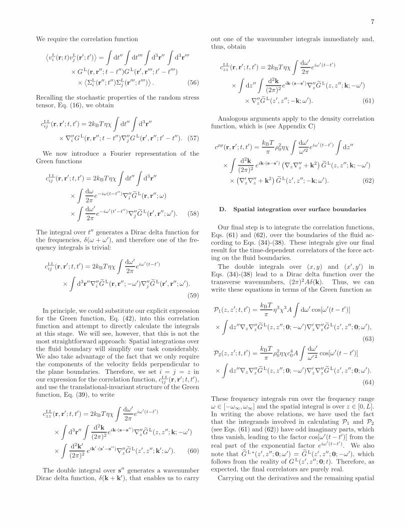
We plot the difference between the excess same-platecorrelator and the cross-plate correlator, defined as δC ≡∆C(0, 0; t, t′) − C(0, L; t, t′), in Fig. 6. This plot showsthat the two correlators exhibit similar period of oscilla-tions for a wide range of viscosities, especially at small tointermediate inter-plate separations. In the special caseof equal-time correlators with τ = 0, one can see a non-monotonic behavior for the two correlators in Fig. 6(a):At small inter-plate separations, δC|τ=0 is positive andincreases by increasing L/δ, but this trend changes ataround L/δ ≃ 3, and then tends to zero for large L/δ.

(a)

(b)

FIG. 4. (Color online) (a) Time-dependent, excess same-plateforce correlator, ∆C(0, 0; t, t′), as defined in Eq. (72), plottedas a function of the rescaled time difference, τ = (t − t′)/t0,for fixed u∞ = (δ/a)2 = 1, ζ/η = 3 and L/δ = 1, 4 and 10, asindicated on the graph. (b) Same as (a) but here we show theresults for fixed u∞ = (δ/a)2 = 1, L/δ = 4 and ζ/η = 1, 3, 5and 10.

FIG. 5. (Color online) Time-dependent, excess same-plate force correlator, ∆C(0, 0; t, t′) (solid curves), comparedwith the time-dependent cross-plate correlator, C(0, L; t, t′)(dashed curves), for fixed u∞ = (δ/a)2 = 1, ζ/η = 3 and attwo different rescaled inter-plate separations, L/δ = 4 and 10,as indicated on the graph.

VII. CONCLUSION AND DISCUSSION

We have revisited the problem of long-range,fluctuation-induced (or Casimir-like) hydrodynamic in-teractions within the context of Landau-Lifshitz’s lin-ear, stochastic hydrodynamics in a classical, compress-ible, viscous fluid confined between two rigid, planarwalls with no-slip boundary conditions and in the ab-sence of heat transfer. We show conclusively that, at

12

(a)

(b)

FIG. 6. (Color online) (a) The difference between the ex-cess same-plate and the cross-plate force correlators definedas δC ≡ ∆C(0, 0; t, t′) − C(0, L; t, t′), plotted as a functionof the rescaled time difference, τ = (t − t′)/t0, for fixedu∞ = (δ/a)2 = 1 and ζ/η = 3, and L/δ = 1, 4 and 10.(b) Fixed L/δ = 4 and ζ/η = 1, 3, 5 and 10 as indicated onthe graph.

this level and within the pertinent approximations, thereis no standard or primary Casimir effect manifest in theaverage value of the interaction force between the fluidboundaries. Nevertheless, we show that there does exista secondary Casimir effect in the variance of the nor-

mal force as well as in the cross-correlation function ofthe normal force between the bounding surfaces. Fluc-tuations in such effective fluctuation-induced forces havebeen investigated in other Casimir-like contexts [22, 42]and in disordered charged systems [43–45].We derive general expressions for the two-point, time-

dependent, force correlations and, thus, show that:

1. The variance of the fluctuation-induced force is fi-nite and independent of the separation between thebounding surfaces for large separations;

2. The equal-time, cross-plate force correlation ex-hibits a long-range decay with the inverse plate sep-aration that is independent of the fluid viscosities;

3. The time-dependent force correlations exhibit adamped oscillatory behavior for small and inter-mediate inter-plate separations that grows more ir-regular at large separations.

Our calculation is based on the Landau-Lifshitz lin-ear stochastic hydrodynamics and, therefore, does notinclude putative non-linear effects [37]. If such effectscould be brought into the fold, they would have to be

considered consistently for all variables. Moreover, wefind that incorporating compressibility does not com-pletely obliterate all fluctuation effects, contrary to pre-vious attempts, based on contour integration in the com-plex plane, that required the limiting behavior of hydro-dynamics at infinite frequencies [38]. In fact, our calcu-lation explicitly includes the scale at which the macro-scopic hydrodynamics breaks down. The limit of van-ishing compressibility is non-trivial and has to be takencarefully, because it can never be derived from a realisticinter-particle potential with infinite stiffness [39].

We interpret the non-zero hydrodynamic force corre-lations predicted in this work as a modification of thethermal stochastic force correlations that act on a Brow-nian particle in a fluid. Since the force correlator de-pends on the separation between the particles, the bath-mediated force fluctuations between the particles wouldmodify the particles’ Langevin dynamics and thus, inprinciple, should be detectable [54, 55]. The separationdependence of the normal force cross-correlation functionrepresents an interesting case of colloidal bodies which donot interact directly, but are driven by correlated noisesources that can provide an alternative mechanism whichcan produce non-trivial, ordered steady states [56]. Wehave considered infinite bounding surfaces, so our resultsare not strictly applicable to the case of finite particles,but our calculation can be straightforwardly generalizedto include a spherical geometry, which would also ad-mit an analytic, albeit much more complicated, solution.Moreover, we intend to include the effects of heat transferin a future calculation.

For experimental verification of our results, we againnote that one would have to generalize our calculationto the case of two spheres in a fluctuating hydrodynamicmedium. This is different from the existing analysis offluctuations of two unconnected, but hydrodynamicallyinteracting spheres [55], a problem in some sense dual toours. In order to exploit this connection, our first stepwill be to calculate the cross-correlation function for twospherical particles.

ACKNOWLEDGMENTS

This work has been partially funded by the U.S. De-partment of Energy. C.M. was supported in part bythe U.S. National Science Foundation under Grant NSFPHY10-034278. A.N. acknowledges partial support fromthe Royal Society, the Royal Academy of Engineering,and the British Academy. B.-S.L. and R.P. also acknowl-edge the financial support of the Agency for researchand development of Slovenia (ARRS) under the bilateralSLO-A Grant No. N1-0019. We acknowledge illuminat-ing discussions with M. Kardar in the KITP program onThe Theory and Practice of Fluctuation-Induced Interac-

tions (2008). R.P. would like to thank Joel Cohen for hiscareful reading of the manuscript and for his comments.

13

Appendix A: Derivation of the force correlator,

Eq. (34)

In this Appendix, we derive the explicit expression,Eq. (34), for the force correlator defined in terms of thestress tensor in Eq. (29). Our starting point is the generalexpression

⟨F (1)

i (t)F (1)j (t)

⟩=

∫∫

Γ

⟨σ(1)ik (r; t)σ

(1)jl (r′; t)

⟩dAkdA

′l,

(A1)where repeated subindices are summed over. In princi-ple, this equation represents nine components of the forcevariance, each of which has nine contributions. For thiswork, we are interested in only the i = j = z componentof the force acting on the plane parallel to the boundaries.We thus have

C(z, z′; t, t′) =⟨F (1)

z (z; t)F (1)z (z′; t′)

⟩

=

∫∫

A

⟨σ(1)zz (r; t)σ

(1)zz (r

′; t′)⟩dAzdA

′z , (A2)

where A is the surface area for each of the plates anddAz = dxdy and dA′

z = dx′dy′. The first-order stresstensor is given by

σ(1)ij (r; t) = η

(∇iv

(1)j (r; t) +∇jv

(1)i (r; t)

)(A3)

−[(

2η

3− ζ

)∇kv

(1)k (r; t) + c20ρ

(1)(r; t)

]δij + Sij(r; t).

In calculating the force correlator, which follows by in-serting (A3) into (A2), we realize that we are ultimatelyinterested in these correlation functions evaluated at theboundaries with no-slip boundary conditions. Therefore,the terms that contain a derivative with respect to thetransverse directions acting on the velocity field will van-ish. On the other hand, the spatial (surface) integralover the transverse correlation function cTT

zz (r, r′; t, t′) =⟨vTz (r; t)v

Tz (r

′; t′)⟩also vanishes (see Appendix B). It is

also straightforward to show that the terms containingcross correlations between the random stress tensor andother fluctuating fields vanish; this is because these termsturn out to be proportional to ∇zδ(z− z′), which is zerofor z 6= z′ and can also be set to zero for z = z′ by us-ing a standard regularization scheme (e.g., by consideringthe Dirac delta function as a limiting form of a Gaussianfunction). Hence, the expression for the force correlator

is:

C(z, z′; t, t′) =∫∫

A

dAzdA′z

{〈Szz(r; t)Szz(r

′; t′)〉

+

(4η

3+ ζ

)2

∇z∇′z

⟨v(1)z (r; t)v(1)z (r′; t′)

⟩

−(4η

3+ ζ

)c20∇z

⟨v(1)z (r; t)ρ(1)(r′; t′)

⟩

−(4η

3+ ζ

)c20∇′

z

⟨ρ(1)(r; t)v(1)z (r′; t′)

⟩

+ c40

⟨ρ(1)(r; t)ρ(1)(r′; t′)

⟩}. (A4)

Finally, the contributions from the correlation functionsbetween the density and velocity fields (third and fourthterms in Eq. (A4)) cancel out (see App. D). Therefore,we find

C(z, z′; t, t′) = P0(z, z′; t, t′)

+

∫∫

A

dAzdA′z

{c40c

ρρ(r, r′; t, t′)

+ η2χ2∇z∇′zc

LLzz (r, r

′; t, t′)}, (A5)

where P0(z, z′; t, t′) = 2kBTηχAδ(z−z′)δ(t−t′) and χ =

(4/3 + ζ/η). This is nothing but Eq. (34).

Appendix B: Transverse velocity correlator does not

contribute

The derivation of the correlation function for the trans-verse velocity fields largely follows that for the longitu-dinal components (Sec. IVC). In terms of the stochasticstress, the transverse velocity correlation function is

⟨vTi (r; t)v

Tj (r

′; t′)⟩=

∫dt′′

∫dt′′′

∫d3r′′

∫d3r′′′

×GT(r, r′′; t− t′′)GT(r′, r′′′; t′ − t′′′)

×⟨ΣT

i (r′′; t′′)ΣT

j (r′′′; t′′′)

⟩. (B1)

Here, the transverse Green function satisfies

[∇2

z − q2]GT(z, z′′;k;ω) =

1

ηδ(z − z′′), (B2)

where q2 = (k2−iωρ0/η). The solution for parallel-planeboundaries is

GT(z, z′′;k;ω) = g T1 e−qz + g T

2 eq(z−L) − 1

2ηqe−q|z−z′′|,

(B3)with constants of integration given by

g T1 =

1

2qηcsch(qL) sinh(q(L − z′′)), (B4)

g T2 =

1

2qηcsch(qL) sinh(qz′′). (B5)

14

Recalling the stochastic properties of the stress tensor,which are

⟨ΣT

i (r; t)ΣTj (r

′; t′)⟩= 2kBTη

(∇k∇′

kδij −∇i∇′j

)

× δ(r− r′)δ(t− t′) (B6)

in the time domain, we can immediately carry out oneof the time integrals and one of the the spatial integrals.Moreover, we are only concerned with the i = j = zcomponent, which leads to

cTTzz (r, r′; t, t′) = 2kBTη

∫dt′′

∫d3r′′ (B7)

×{∇′′

kGT(r, r′′; t− t′′)∇′′

kGT(r′, r′′; t′ − t′′)

−∇′′zG

T(r, r′′; t− t′′)∇′′zG

T(r′, r′′; t′ − t′′)

}.

Integrating by parts, this becomes

cTTzz (r, r′; t, t′) = −2kBTη

∫dt′′

∫d3r′′ (B8)

×[(

∇′′ 2 −∇′′z2)GT(r, r′′; t− t′′)

]GT(r′, r′′; t′ − t′′).

Moving to the frequency representation and substitut-ing the translation-invariant form of the Green function,analogous to Eq. (39), we obtain

cTTzz (r, r′; t, t′) = 2kBTη

∫dω′

2πeiω

′(t−t′)

∫dz′′

∫d2k

(2π)2

× eik·(s−s′)k2GT(z, z′′;k;−ω′)GT(z′, z′′;−k;ω′).

(B9)

Here, we have integrated over x′′ and y′′, which generatesa wavenumber delta function δ(k+k

′) that simplifies oneof the wavenumber integrals.We calculate the force variance, C(z, z′; t, t′), by inte-

grating the velocity correlation function over the bound-aries of the fluid, i.e. over x, x′, y, and y′ (see Eq. (34)).The only dependence on these variables occurs in theexponential function eik·(s−s

′). Thus, this integral gen-erates a second wavenumber Dirac delta function, δ(k).It is now straightforward to see that the wavenumber in-tegral vanishes: The product of the Green functions atk = 0 is finite and consequently the factor of k2 ensuresthat the integral vanishes.

Appendix C: Derivation of the density correlator

Here, we calculate the correlation function of the den-sity fields, cρρ, given in Eq. (62). We start with thecontinuity equation, Eq. (11), which can be written as

ρ(1)(r; t) + ρ0∇ · vL(r; t) = 0, (C1)

where the dot indicates a time derivative. From here weconstruct the correlation function

⟨ρ(1)(r; t)ρ(1)(r′; t′)

⟩= ρ20 ∇i∇′

j

⟨vLi (r; t)v

Lj (r

′; t′)⟩.

(C2)

By introducing Fourier components, we can cast theleft-hand side of this equation into the form

⟨ρ(1)(r; t)ρ(1)(r′; t′)

⟩=

∫dω

2π

∫dω′

2πe−i(ωt+ω′t′)

×⟨˜ρ (1)(r;ω)˜ρ (1)(r′;ω′)

⟩. (C3)

The correlation function of the right-hand side ofEq. (C2) is given by

cLLij (r, r′; t, t′) = 2kBTηχ

∫dω

2π

∫dω′e−i(ωt+ω′t′) (C4)

× δ(ω + ω′)

∫d3r′′∇iG

L(r, r′′;ω)∇′jG

L(r′, r′′;ω′).

Combining Eqs. (C2), (C3) and (C4), we write

⟨˜ρ (1)(r;ω)˜ρ (1)(r′;ω′)⟩= 4πkBTρ

20ηχδ(ω + ω′)

×∫

d3r′′∇i∇′′i G

L(r, r′′;ω)∇′j∇′′

j GL(r′, r′′;ω′). (C5)

Then, substituting this result into Eq. (C3) gives

⟨ρ(1)(r; t)ρ(1)(r′; t)

⟩= 4πkBTρ

20ηχ

∫dω′eiω

′(t−t′) (C6)

×∫

d3r′′∇i∇′′i G

L(r, r′′;−ω′)∇′j∇′′

j GL(r′, r′′;ω′).

Several more steps are needed. First of all, we note thatfor the Fourier components of the density field, we have

⟨ρ (1)(r;ω)ρ (1)(r′;ω′)

⟩= −4πkBTρ

20ηχ

δ(ω + ω′)

ωω′

×∫

d3r′′∇i∇′′i G

L(r, r′′;ω)∇′j∇′′

j GL(r′, r′′;ω′), (C7)

and, therefore, we finally find

cρρ(r, r′; t, t′) =kBT

πρ20ηχ

∫dω′

ω′2eiω

′(t−t′) (C8)

×∫

d3r′′∇i∇′′i G

L(r, r′′;−ω′)∇′j∇′′

j GL(r′, r′′;ω′).

Here, the relevant derivatives are given by

∇i∇′′i G

L(r, r′′;ω′) =

∫d2k

(2π)2eik·(s−s

′′)

×(k2 +∇z∇′′

z

)GL(z, z′′;k;ω′). (C9)

The force variance, C(z, z′; t, t′), follows by integratingthe velocity correlation function over the boundaries ofthe fluid, i.e. over x, x′, y, and y′ (see Eq. (34)). The onlydependence on these variables occurs in the exponentialfunction eik·(s−s

′) and consequently this integral gener-ates a Dirac delta function over the transverse wavenum-bers, (2π)2Aδ(k+ k

′). This leads directly to Eq. (62).

15

Appendix D: Density-velocity cross-correlator does

not contribute

To calculate the density-velocity cross-correlator,

cLρi (r, r′; t, t′), we first construct the cross-correlationfunction⟨vLi (r; t)ρ

(1)(r′, t′)⟩= −ρ0∇′

j

⟨vLi (r; t) v

Lj (r

′; t′)⟩. (D1)

Following a similar line of reasoning to that for thedensity-density correlation function, we can write

⟨vLi (r;ω)˜ρ (1)(r′;ω′)

⟩= −4πkBTρ0ηχδ(ω + ω′)

×∫

d3r′′∇′′i G

L(r, r′′;ω)∇′j∇′′

j GL(r′, r′′;ω′). (D2)

This equation leads to

⟨vLi (r;ω)ρ

(1)(r′;ω′)⟩= 4πikBTρ0ηχ

δ(ω + ω′)

ω′

×∫

d3r′′∇′′i G

L(r, r′′;ω)∇′j∇′′

j GL(r′, r′′;ω′). (D3)

Thus, we obtain

cLρi (r, r′; t, t′) = ikBT

πρ0ηχ

∫dω′

ω′eiω

′(t−t′)

×∫

d3r′′∇′′i G

L(r, r′′;−ω′)∇′j∇′′

j GL(r′, r′′;ω′). (D4)

We now introduce the translational invariant form of theGreen function and take i = z. The double spatial inte-gral generates a double wavenumber Dirac delta function,giving

cLρz (r, r′; t, t′) = ikBT

πρ0ηχ

∫dω′

ω′eiω

′(t−t′)

×∫

dz′′∫

d2k

(2π)2eik·(s−s

′)∇′′z G

L(z, z′′;k;−ω′)

×(k2 +∇′

z∇′′z

)GL(z′, z′′;−k;ω′). (D5)

Now, following the line of reasoning of the previoussection, the double integrals over (x, y) and (x′, y′) inthe full contribution to the force correlator generate aDirac delta function over the transverse wavenumbers,(2π)2Aδ(k). Therefore, we can write this contribution interms of the Green functions as∫∫

A

dAzdA′z ∇zc

Lρz (r, r′; t, t′) = −kBT

πρ0ηχA

×∫

dω′

ω′sin[ω′(t− t′)]

∫dz′′∇z∇′′

z GL(z, z′′;0;−ω′)

×∇′z∇′′

z GL(z′, z′′;0;ω′). (D6)

Since this expression is odd with respect to changing (z, t)to (z′, t′) and vice versa, it follows that the contributionsto the force correlator from the correlation functions be-tween the density and velocity fields (third and fourthterms) in Eq. (A4) vanish, i.e.,∫∫

A

dAzdA′z

[∇zc

Lρz (r, r′; t, t′) +∇′

zcLρz (r′, r; t′, t)

]= 0.

(D7)

Appendix E: Derivation of the frequency integrals

In this Appendix, we derive Eqs. (72) and (73) as wellas Eqs. (67) and (68).

1. Same-plate force correlator, Eq. (72)

We start with the first contribution to the force corre-lation function, which is given in Eq. (63):

P1(z, z′; t, t′) =

kBT

πη3χ3A

∫dω′ cos[ω′(t− t′)] (E1)

×∫

dz′′∇z∇′′z G

L(z, z′′;0;−ω′)∇′z∇′′

z GL(z′, z′′;0;ω′).

The explicit expressions for the derivatives appearing onthe right-hand side of the above equation are

∇z∇′′z G

L(z, z′′;0;−ω) =−ω

2[iρ0c20 − (4η/3 + ζ)ω](E2)

×[− 2δ(z − z′′) + λ∗e−λ∗|z−z′′| + λ∗ csch(λ∗L)

×(cosh(λ∗(L − z′′))e−λ∗z + cosh(λ∗z′′)eλ

∗(z−L))]

,

∇′z∇′′

z GL(z′, z′′;0;ω) =

ω

2[iρ0c20 + (4η/3 + ζ)ω](E3)

×[− 2δ(z′ − z′′) + λe−λ|z′−z′′| + λ csch(λL)

×(cosh(λ(L − z′′))e−λz′

+ cosh(λz′′)eλ(z′−L)

)],

where we have used the fact that m = λ when k2 = 0

and we note that λ∗ = λ(−ω).Now, in principle, we could multiply together the re-

sults and integrate over z′′. It is simpler, however, to lookahead a little. We know that, for the force variance at asingle plate, we will ultimately evaluate this correlationfunction at z = z′ = 0, so then these derivatives become

∇z∇′′z G

L(0, z′′;0;−ω) =−ω

2[iρ0c20 − (4η/3 + ζ)ω]

×[− 2δ(0− z′′) + λ∗e−λ∗z′′

+ λ∗ csch(λ∗L)

×(cosh(λ∗(L− z′′)) + cosh(λ∗z′′)e−λ∗L

) ], (E4)

∇′z∇′′

z GL(0, z′′;0;ω) =

ω

2[iρ0c20 + (4η/3 + ζ)ω]

×[− 2δ(0− z′′) + λe−λz′′

+ λ csch(λL)

×(cosh(λ(L − z′′)) + cosh(λz′′)e−λL

) ]. (E5)

Here, we have simplified the expressions using |−z′′| = z′′

for z′′ in the range [0, L].

16

The key simplification now is to notice that we cancollect together many of the exponential terms, whichsimplify to give

∇z∇′′z G

L(0, z′′;0;−ω) =−ω

[iρ0c20 − (4η/3 + ζ)ω]

×[λ∗ cosh[λ∗(L− z′′)] csch[λ∗L]− δ(0− z′′)

], (E6)

∇′z∇′′

z GL(0, z′′;0;ω) =

ω

[iρ0c20 + (4η/3 + ζ)ω]

×[λ cosh[λ(L− z′′)] csch[λL]− δ(0 − z′′)

]. (E7)

Let us now use this result in our full expression, giving

P1(0, 0; t, t′) =

kBT

πη3χ3A

∫dω ω2 cos[ω(t− t′)]

ρ20c40 + (4η/3 + ζ)

2ω2

×∫ L

0

dz′′[λ∗ cosh[λ∗(L − z′′)] csch[λ∗L]− δ(0− z′′)

]

×[λ cosh[λ(L − z′′)] csch[λL]− δ(0− z′′)

]

=kBT

πη3χ3A

∫dω ω2 cos[ω(t− t′)]

ρ20c40 + (4η/3 + ζ)

2ω2

×[ |λ|2 (λR sin[2λIL] + λI sinh[2λRL])

2λIλR (cosh[2λRL]− cos[2λIL])

− 2 (λI sin[2λIL] + λR sinh[2λRL])

(cosh[2λRL]− cos[2λIL])+ δ(0)

]. (E8)

We note that, in the L → ∞ limit, this result reducesto the expression for the semi-infinite fluid, Eq. (F3), animportant cross-check of our results. We now express ourresult in terms of the dimensionless parameters ℓ+, ℓ−,χ, γ, and τ = (t − t′)/t0, the dimensionless variable uand the function fm(u) (see Sec. IVB):

P1(0, 0; t, t′) =

kBT

πρ0c

20χ

3A

L2

∫ u∞

0

du f0(u) cos[uτ ]

×{

1

cosh[2ℓ+]− cos[2ℓ−]

[(ℓ2

2ℓ−− 2ℓ−

)sin[2ℓ−]

+

(ℓ2

2ℓ+− 2ℓ+

)sinh[2ℓ+]

]+ Lδ(0)

}. (E9)

Here, ℓ2 = ℓ2+ + ℓ2− and we have used the fact that theintegrand is symmetric in the frequency to rewrite theregion of integration over the positive real axis only, upto the dimensionless cutoff, u∞ = δ2/a2. We now define

W0(0, 0; τ) = 2

∫ u∞

0

du f0(u) cos[uτ ]

× 1

cosh[2ℓ+]− cos[2ℓ−]

[(ℓ2

2ℓ−− 2ℓ−

)sin[2ℓ−]

+

(ℓ2

2ℓ+− 2ℓ+

)sinh[2ℓ+]

](E10)

and

V0(0, 0; τ) = 2

∫ u∞

0

du f0(u) cos[uτ ], (E11)

and thus we have

P1(0, 0; t, t′) =

kBT

πρ0c

20χ

3A

L

×[W0(0, 0; τ) + LV0(0, 0; τ)δ(0)

]. (E12)

Now, we turn to the second contribution, P2(0, 0; t, t′).

The derivatives with respect to x and y will ultimatelybring down factors of kx and ky. When we integrateover the spatial directions, the Dirac delta functions inwavenumber will remove these terms. The result is thendirectly related to the equation above, except that thereis an extra denominator of ω2. We thus find

P2(0, 0; t, t′) =

kBT

πρ0c

20χ

A

L2

∫ u∞

0

du f2(u) cos[uτ ]

×{

1

cosh[2ℓ+]− cos[2ℓ−]

[(ℓ2

2ℓ−− 2ℓ−

)sin[2ℓ−]

+

( |λ|22ℓ+

− 2ℓ+

)sinh[2ℓ+]

]+ Lδ(0)

}, (E13)

or, in terms of the frequency integrals W2, Eq. (67), andV2, Eq. (69), we have

P2(0, 0; t, t′) =

kBT

πρ0c

20χ

A

L

×[W2(0, 0; τ) + LV2(0, 0; τ)δ(0)

]. (E14)

This, too, reduces to the expression for the semi-infinitefluid, Eq. (F4), in the L → ∞ limit.Finally, putting together Eqs. (E12) and (E14) and

using Eq. (71), we obtain Eq. (72).

2. Cross-plate force correlator, Eq. (73)

Here we derive Eq. (73), our final integral expres-sion for the cross-plate force correlator. We start fromEqs. (E1), (E3) and (E4) again, but now we need to eval-uate one of the derivatives at z′ = L,

∇z∇′′z G

L(0, z′′;0;−ω) =−ω

2[iρ0c20 − (4η/3 + ζ)ω]

×[− 2δ(0− z′′) + λ∗e−λ∗z′′

+ λ∗ csch(λ∗L)

×(cosh(λ∗(L− z′′)) + cosh(λ∗z′′)e−λ∗L

)],

(E15)

∇′z∇′′

z GL(L, z′′;0;ω) =

ω

2[iρ0c20 + (4η/3 + ζ)ω]

×[− 2δ(L− z′′) + λe−λ(L−z′′) + λ csch(λL)

×(cosh(λ(L − z′′))e−λL + cosh(λz′′)

) ]. (E16)

17

Once again we can simplify matters by writing

∇z∇′′z G

L(0, z′′;0;−ω) =−ω

iρ0c20 − (4η/3 + ζ)ω

×[λ∗ cosh[λ∗(L− z′′)] csch[λ∗L]− δ(0− z′′)

], (E17)

but, in this case, Eq. (E16) becomes

∇′z∇′′

z GL(L, z′′;0;ω) =

ω

iρ0c20 + (4η/3 + ζ)ω

×[λ cosh[λz′′] csch[λL]− δ(L − z′′)

]. (E18)

Therefore, the first contribution to the force correlatorbetween the two plates is

P1(0, L; t, t′) =

kBT

πη3χ3A

∫dω ω2 cos[ω(t− t′)]

ρ20c40 + (4η/3 + ζ)

2ω2

×∫ L

0

dz′′[λ∗ cosh[λ∗(L− z′′)] csch[λ∗L]− δ(0 − z′′)

]

×[λ cosh[λz′′] csch[λL]− δ(L− z′′)

]

=kBT

πη3χ3A

∫dω ω2 cos[ω(t− t′)]

ρ20c40 + (4η/3 + ζ)

2ω2

×[ |λ|2 (λR cosh[λRL] sin[λIL] + λI cos[λIL] sinh[λRL])

λIλR (cosh[2λRL]− cos[2λIL])

− 4 (λI cosh[λRL] sin[λIL] + λR cos[λIL] sinh[λRL])

cosh[2λRL]− cos[2λIL]

].

(E19)

We now express our result in terms of the dimensionlessparameters as before, giving

P1(0, L; t, t′) =

kBT

πρ0c

20χ

3A

L2

∫ u∞

0

du f0(u) cos[uτ ]

× 1

cosh[2ℓ+]− cos[2ℓ−]

[(ℓ2

ℓ−− 4ℓ−

)cosh[ℓ+] sin[ℓ−]

+

(ℓ2

ℓ+− 4ℓ+

)cos[ℓ−] sinh[ℓ+]

]. (E20)

As in the case of the same-plate force correlator, theother contribution, P2(0, L; t, t

′), is very simply relatedto P1(0, L; t, t

′). We can write the result immediately as

P2(0, L; t, t′) =

kBT

πρ0c

20χ

A

L2

∫ u∞

0

du f2(u) cos[uτ ]

× 1

cosh[2ℓ+]− cos[2ℓ−]

[(ℓ2

ℓ−− 4ℓ−

)cosh[ℓ+] sin[ℓ−]

+

(ℓ2

ℓ+− 4ℓ+

)cos[ℓ−] sinh[ℓ+]

]. (E21)

Now, putting together Eqs. (E20) and (E21) and defining

the frequency integral

Wm(0, L; τ) = 2

∫ u∞

0

du fm(u) cos[uτ ]

× 1

cosh[2ℓ+]− cos[2ℓ−]

[(ℓ2

ℓ−− 4ℓ−

)cosh[ℓ+] sin[ℓ−]

+

(ℓ2

ℓ+− 4ℓ+

)cos[ℓ−] sinh[ℓ+]

], (E22)

we obtain Eq. (73).In the large plate-separation limit, L → ∞, these cor-

relators vanish, in accordance with the results of Ap-pendix F 1.

Appendix F: Time correlators for simple geometries

In this Appendix, we derive the time-dependent cor-relators for two simple geometries: A semi-infinite fluidwith a single hard-wall boundary and an infinite fluid.The semi-infinite fluid is the limiting case for the two-wall geometry in the limit of infinite plate separationand we have confirmed, both analytically and numeri-cally, that our results for the two-wall geometry reduceto the semi-infinite fluid results.

1. Semi-infinite fluid

The Green function solution of Eq. (40) for a semi-infinite fluid, with an infinite hard-wall boundary at z =0, is

GL(z, z′′;k;ω) =iλ2

2mωρ0

[e−m(z+z′′) − e−m|z−z′′|

],

(F1)where now z′′ > 0. Once again, we substitute this resultinto Eqs. (63) and (64). The derivative we require thistime is

∇z∇′′z G

L(z, z′′;k;ω) =iλ2

2ωρ0

[me−m(z+z′′) +me−m|z−z′′|

− 2δ(z − z′′)]. (F2)

Carrying out the spatial integrals over z′′, from zero toinfinity, we obtain

P1(0, 0; t, t′) =

kBT

π

η3χ3A

ρ20

∫dω′

ω′ 2|λ|4 cos[ω′(t− t′)]

×[ |λ|22λR

− 2λR + δ(0)], (F3)

P2(0, 0; t, t′) =

kBT

πηχc40A

∫dω′

ω′ 4|λ|4 cos[ω′(t− t′)]

×[ |λ|22λR

− 2λR + δ(0)]. (F4)

18

We can carry out these frequency integrals for theequal time case, with t = t′, by first transforming tothe dimensionless variables, x = ηχω/(ρ0c

20) and τx =

(t − t′)ρ0c20/(ηχ), and then defining tan θ = x. We ob-

tain

P1(0, 0) =kBT

π2ρ0c

20A

{δ(0)

∫ x∞

0

dxx2

x2 + 1

+ρ0c0√2ηχ

∫ θ∞

0

dθ tan3 θ

(2 cos θ − 1

)√sec θ − 1

}

=kBT

π2ρ0c

20A

{δ(0)

(x∞ − arctanx∞

)

+8√2ρ0c03ηχ

z∞(3− z∞)√z∞ − 1

sin4(1

2arctan(z2∞ − 1)

)},

(F5)

and

P2(0, 0) =kBT

π2ρ0c

20A

{δ(0)

∫ x∞

0

dx

x2 + 1

+ρ0c0√2ηχ

∫ θ∞

0

dθ tan θ

(2 cos θ − 1

)√sec θ − 1

}

=kBT

π2ρ0c

20A

{δ(0) arctanx∞ +

2ρ0c0ηχ

√z∞ − 1

z∞

}.

(F6)

Here, θ∞ = arctanx∞ and z∞ =√1 + x2

∞ are bothfunctions of the dimensionless cutoff x∞ = η2χ/(a2ρ20c

20).

The equal-time correlator for a semi-infinite fluid isthen given by

C(0, 0) = kBT

π2ρ0c

20A

{x∞ · δ(0) + ρ0c0

ηχ

[2√z∞ − 1

z∞

+8√2

3

z∞(3− z∞)√z∞ − 1

sin4(1

2arctan(z2∞ − 1)

)]}, (F7)

which is Eq. (78).The corresponding time-dependent, cross-plate force

correlator vanishes for the semi-infinite fluid geometry,dropping to zero as 1/L.

2. Infinite fluid

The Green function solution of Eq. (40) for an infinitefluid, i.e., vanishing Green function at z → ±∞, is

GL(z, z′′;k;ω) = − iλ2

2mωρ0e−m|z−z′′|, (F8)

where m2 = k2 +λ2 and λ is the longitudinal decay con-

stant defined in Eq. (41). We will substitute this resultinto Eqs. (63) and (64). The derivative we require is

∇z∇′′z G

L(z, z′′;k;ω) =iλ2

2ωρ0

[me−m|z−z′′|

− 2δ(z − z′′)]. (F9)

For an infinite fluid, the spatial integral runs from neg-ative infinity to positive infinity and we assume that wedetermine the time correlator at z = z′ = 0. Carryingout the spatial integral, we obtain

P1(0, 0; t, t′) =

kBT

π

η3χ3A

ρ20

∫dω′

ω′ 2|λ|4 cos[ω′(t− t′)]

×[ |λ|24λR

− λR + δ(0)

], (F10)

P2(0, 0; t, t′) =

kBT

πηχc40A

∫dω′

ω′ 4|λ|4 cos[ω′(t− t′)]

×[ |λ|24λR

− λR + δ(0)

]. (F11)

By comparing these results to Eqs. (F3) and (F4), weimmediately see that this result is simply half that of thesemi-infinite fluid. Therefore, we have

C(0, 0; t, t′)∣∣∣∣infinite

=1

2C(0, 0; t, t′)

∣∣∣∣semi−infinite

. (F12)

[1] H.B.G. Casimir, Proc. K. Ned. Akad. Wet. 51, 793(1948).

[2] V.M. Mostepanenko and N.N. Trunov, The Casimir Ef-fect and Its Applications (Clarendon, Oxford, 1997).

[3] M. Kardar and R. Golestanian, Rev. Mod. Phys. 71, 1233(1999).

[4] M. Bordag, U. Mohideen and V.M. Mostepanenko,Phys. Rep. 353, 2 (2001).

[5] V.A. Parsegian, Van der Waals Forces: A Handbook forBiologists, Chemists, Engineers, and Physicists (Cam-bridge University Press, 2005).

[6] M. Bordag, G.L. Klimchitskaya, U. Mohideen andV.M. Mostepanenko, Advances in the Casimir Effect(Oxford University Press, New York, 2009).

[7] D.A.R. Dalvit, P.W. Milonni, D. Roberts, F.S.S. Rosa,Casimir Physics, Lecture Notes in Physics, Vol. 834,(Springer-Verlag, Berlin, 2011).

[8] M. Krech, The Casimir Effect in Critical Systems (WorldScientific, Singapore, 1994).

[9] R. French et al., Rev. Mod. Phys. 82, 1887 (2010).[10] M.E. Fisher and P.G. de Gennes, C. R. Acad. Sci. Paris

B 287, 207 (1978).[11] M. Krech, J. Phys. Condens. Matter 11, 391 (1999).[12] M. Krech, Phys. Rev. E 56, 1642 (1997).[13] C. Hertlein, L. Helden, A. Gambassi, S. Dietrich and C.

Bechinger, Nature 451, 172 (2008).[14] M. Fukuto, Y.F. Yano, and P.S. Pershan,

Phys. Rev. Lett. 94, 135702 (2005).

19

[15] E. Schaeffer and U. Steiner, Eur. Phys. J. E 8, 347 (2002).[16] M.D. Morariu, E. Schaeffer and U. Steiner,

Phys. Rev. Lett. 92, 156102 (2004).[17] M.D. Morariu, E. Schaeffer and U. Steiner,

Eur. Phys. J. E 12, 375 (2003).[18] A. Ajdari, L. Peliti and J. Prost, Phys. Rev. Lett. 66,

1481 (1991).[19] H. Li and M. Kardar, Phys. Rev. Lett. 67, 3275 (1991).[20] M. Antezza, L.P. Pitaevskii, S. Stringari, and V.B. Sve-

tovoy, Phys. Rev. A 77, 022901 (2008).[21] M. Kruger, T. Emig and M. Kardar, Phys. Rev. Lett. 106

201404 (2011).[22] D.S. Dean, V.A. Parsegian, and R. Podgornik,

Phys. Rev. A 87, 032111 (2013).[23] T.R. Kirkpatrick, J.M. Ortiz de Zarate, J.V. Sengers,

Phys. Rev. Lett. 110, 235 (2013).[24] T.R. Kirkpatrick, J.M. Ortiz de Zarate and J.V. Sengers,

Phys. Rev. E 89, 022145 (2014).[25] J.M. Ortiz de Zarate and J.V. Sengers, Hydrodynamic

Fluctuations in Fluids and Fluid Mixtures (Elsevier, Am-sterdam, 2006).

[26] E.M. Lifshitz, Sov. Phys. JETP 2, 73 (1956).[27] S.M. Rytov, Theory of Electric Fluctuations and Thermal

Radiation (AFCRC-TR Air Force Cambridge ResearchCenter, Bedford, 1959)

[28] F.S.S. Rosa, D.A.R. Dalvit, and P.W. Milonni, Phys.Rev. A 81, 033812 (2010).

[29] A. Narayanaswamy and Yi Zheng, Phys. Rev. A 88,012502 (2013).

[30] D.S. Dean and A. Gopinathan, Phys. Rev. E 81, 041126(2010).

[31] D.S. Dean and A. Gopinathan, J. Stat. Mech. L08001(2009).

[32] L.D. Landau and E.M. Lifshitz, Statistical Physics, Part2, 1st Ed. (Butterworth-Heinemann, Woburn, 1996).

[33] D. Forster, Hydrodynamic Fluctuations, Broken Symme-try, and Correlation Functions (W.A. Benjamin, Read-ing, 1975).

[34] H. Spohn, J. Phys. A: Math. Gen. 16, 4275 (1983).[35] J. Tailleur, J. Kurchan, and V. Lecomte, J. Phys. A:

Math. Theor. 41, 505001 (2008).[36] J.S. Rowlinson, Cohesion: A Scientific History of In-

termolecular Forces (Cambridge University Press, Cam-bridge, 2002).

[37] R.B. Jones, Physica A 105, 395 (1981).[38] D.Y.C. Chan, L.R. White, Physica A 122, 505 (1983).[39] N.G. van Kampen and J.J. Lodder, Constraints, Am. J.

Phys. 52, 419-424 (1984).[40] I.E. Dzyaloshinskii, E.M. Lifshitz, and L.P. Pitaevskii,

Sov. Phys. Uspekhi 4, 153 (1961).[41] B.I. Ivlev, J. Phys. Condens. Matter 14, 4829 (2002).[42] D. Bartolo, A. Ajdari, J-B. Fournier, and R. Golestanian,

Phys. Rev. Lett. 89, 230601 (2002).[43] A. Naji, D.S. Dean, J. Sarabadani, R. Horgan, R. Pod-

gornik, Phys. Rev. Lett. 104, 060601 (2010).[44] D.S. Dean, A. Naji and R. Podgornik, Phys. Rev. E 83,

011102 (2011).[45] A. Naji, J. Sarabadani, D.S. Dean and R. Podgornik,

Eur. Phys. J. E 35, 24 (2012).[46] We note the typographic error in Eq. (2.1) of Ref. [38], a

missing occurrence of the field v.[47] Here we note a typographic error in Eq. (2.11) of [38],

corresponding to a factor of 1/ρ0 missing from Eq. (13)above.

[48] A. Erbas, R. Podgornik and R.R. Netz, Eur. Phys. J. E32, 147 (2010).

[49] S. Kim and S. Karrila Microhydrodynamics, 1st Ed.(Dover, Mineola, 2005).

[50] J. Schwinger, L.L. Deraad Jr., K.A. Milton, W. Tsai andJ. Norton, Classical Electrodynamics (Westview, Boul-der, 1998).

[51] U. Raviv, P. Laurat and J. Klein, Nature 413, 5154(2001).

[52] U. Raviv and J. Klein, Science 297, 1540 (2002).[53] Y. Leng and P.T. Cummings, Phys. Rev. Lett. 94, 026101

(2005).[54] C. De Bacco, F. Baldovin, E. Orlandini, and K. Seki-

moto, Phys. Rev. Lett. 112, 180605 (2014).[55] J. von Hansen, A. Mehlich, B. Pelz, M. Rief, and R.R.

Netz, Rev. Sci. Inst. 83, 095116 (2012).[56] S. Lise, A. Maritan and M.R. Swift, J. Phys. A: Math.

Gen. 32, 5251 (1999).