Equivalence of Fluctuation Splitting and Finite … of Fluctuation Splitting and ... to extend fluctuation splitting to the Euler system ... The equivalence of fluctuation splitting

NASA/TM-97-206271

Equivalence of Fluctuation Splittingand Finite Volume for One-Dimensional

Gas Dynamics

William A. Wood

Langley Research Center Hampton, Virginia

National Aeronautics andSpace Administration

Langley Research CenterHampton, Virginia 23581-2199

October 1997

https://ntrs.nasa.gov/search.jsp?R=19980010522 2018-05-28T18:48:54+00:00Z

Available from the following:

NASA Center for AeroSpace Information (CASI)

800 Elkridge Landing Road

Linthicum Heights, MD 21090 2934

(301) 621-0390

National Technical Information Service (NTIS)

5285 Port Royal Road

Springfield, VA 22161-2171

(703) 487-4650

Abstract

The equivalence of the discretized equations resulting from both fluctuation

splitting and finite volume schemes is demonstrated in one dimension. Scalar

equations are considered for advection, diffusion, and combined advection/diffu-

sion. Analysis of systems is performed h)r tile Euler and Navier-Stokes equations

of gas dynamics. Non-unifornl mesh-point distributions are included in the

analyses.

Nomenclature

Geometric and independent variables

i

Zref

n

S

t

2"

Ff_

Coml)utational indicie

Non-dimensionalizing reference length

Edge or element lengthNormal vector

Distance vector

Generalized volume

Time

Physical coordinate, normalized by Lr,, IPerimeter of control volume

Generalized integration volume

Dependent variables

A

A

a

Cp

(¥

E

C

F

f

H

h

M

P

qR

8

T

U

V

Flux Jacobian in (:onservative variables

Flux Jacobian in auxiliary variables

Sound speedSpecific heat at, constant pressure

St)ecific heat at, constant volmne

Total energy

Internal energyFlux functionNumerical flux

Total enthalpySpecific enthalpy

Subsonic or sut)ersonic matrix dissipationPressure

Heal, flow

Area-weighted residual

EntropyTemperatureConserved variables

Cartesian velocities

Primitive variables

WXX

Z

A

P¢I,

#T

Auxiliary variables

Matrix of right eigenvectors

Right eigenvectors in auxiliary variablesParameter vector

Thermal conductivity

Wavespeed

Eigenvalue matrix

Density

Artificial dissipation functionElemental fluctuation

Fluctuation of auxiliary variables formulation

Elemental artificial dissipation

Artificial dissipation in auxiliary variables formulation

Coefficient of viscosity

Stress component

Auxiliary symbols

I

M_

p,qP,.

(

7

Identity matrix

Symmetric averaging function

Arguments of limiter

Prandtl number, Pr(air) = 0.72

Gas constant, _(air) = 287 J/(kg-K)Limiter bound

Eigenvalue limiting parameter

Ratio of specific heats, "y(diatomic) = 1.4Finite element shape functionLimiter function

Operators

V 2

A

V5

5_

Gradient

Laplacian, V _ = V -

Forward difference, Aix = xi+l - xiBackward difference, Vix = xi - xi-1

Central difference, _x = 1_(xi+l - x.)Second central difference, 5"_x = A'_ix = VAix = Xi+l - 2xi + xi-t

Acronyms

COE Contributions from other elementsLHS Left-hand side

RHS Right-hand side

Subscripts

E Element

k Left-hand state

R Right-hand state

U Upwind2U Second-order upwind

Superscripts

i Inviscid

v Vis('ous

Over[mrs are used to represent cell-average values. Vector symbols indicate

vectors spanning multiple spatial dimensions. Boht face is used for vectors and

tensors of systems. Subscripts of variables is short-hand for differentiation. Hatsdenote refit vectors. Tildes denote Roe-averaged quantities.

Introduction

Finite volume flux-difference-split schemes, in particular the Roe scheme[l, 2]

with a MUSCL[3] second-order extension, are well established for the solutionof one-dimensional gas dynamics, with textbooks written on the subject[4]. Thediscretization of these schemes on general unstructured domains is well covered

by Bart hi5].Fluctuation splitting concepts have been introduced for the solution of scalar

advection problems in two dimensions[6, 7, 8], and are aligned with finite ele-

ment concepts, as opposed to finite volumes. Notable work has been done by

Sidflkove_r[9, 10, 11] to extend fluctuation splitting to the Euler system of equa-

tions for gas dynamics.The current paper systeinatieally establishes the equivalence of the dis-

cretized equations resulting from both fluctuation splitting and finite volumetreatments of the Navier-Stokes equations in one dimension on non-uniforln

meshes. The fluctuation splitting development is performed as quadrature over

discrete elements, in contrast to the usual treatment which resorts to a flux for-

mula via the divergence theorem. Scalar equations are considered first, covering

advection, diffusion, and combined advection/diffusion. Then the Euler system

is considered, equating Roe's wave-decomposition procedure with Sidilkover's

modified auxiliary equations approach. Diseretization of viscous and conduc-

tive terms completes the analysis for the Navier-Stokes equations.

The equivalence of fluctuation splitting and finite volume in one dimension

serves as a prelude to multidimensional analysis, where the methods differ. Re-

sults by Sidilkover[12] suggest there may be definite advantages to fluctuation

splitting over finite volume for the nmltidimensional Euler equations. How-

ever, other researchers[13] have not found an advantage in fluctuation splitting,though their treatment of the Euler equations differs significantly from that of

Sidilkow,r.

Lineardatarepresentation

X X X

1i 23 i-!2 i+_

Nodesx-axis

i-1 i i+l

(boundary)

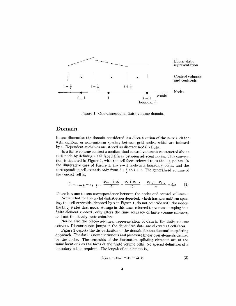
Figure 1: One-dimensional finite volume domain.

Control volumesand centroids

Domain

In one dimension the domain considered is a discretization of the x-axis, either

with uniform or non-uniform spacing between grid nodes, which are indexed

by i. Dependent variables are stored as discreet nodal values.In a finite volume context a median-dual control volume is constructed about

each node by defining a (:ell face halfway between adjacent nodes. This conven-1

tion is depicted in Figure 1, with the cell faces referred to as the ±3 points. Inthe illustrative case of Figure 1, the i + 1 node is a boundary point, and the

corresponding cell extends only from i + _ to i + 1. The generalized volume ofthe control cell is,

Si _- xi_-£-2 - xi-½ -

Xi+l • xi xi _xi_l xiT] - xi_ ]

2 2 2- 5_x (1)

There is a one-to-one correspondence between the nodes and control volumes.

Notice that for the nodal distribution depicted, which has non-uniform spac-

ing, the cell centroids, denoted by x in Figure 1, do not coincide with the nodes.

Barth[5] states that nodal storage in this case, referred to as mass lumping in a

finite element context, only alters the time accuracy of finite volume schemes,and not the steady state solutions.

Notice also the piecewise-linear representation of data in the finite volume

context. Discontinuous jumps in the dependent data are allowed at cell faces.

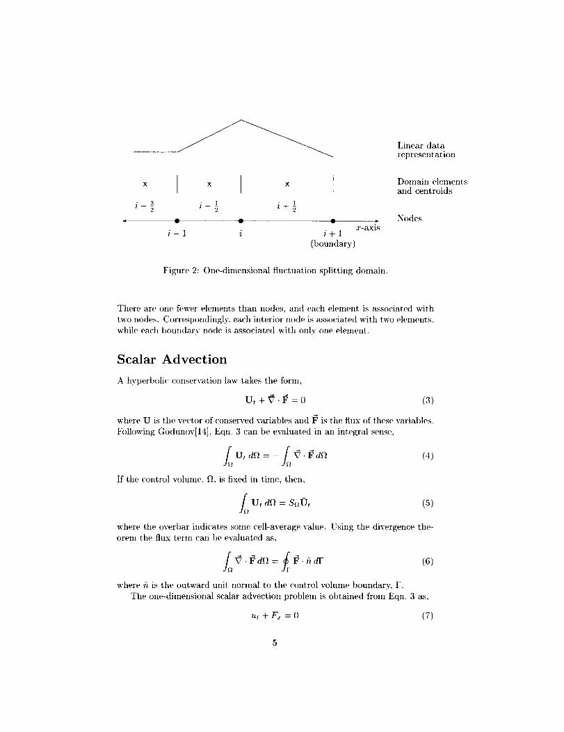
Figure 2 depicts the discretization of the domain for the fluctuation splitting

approach. The data is now continuous and piecewise linear over elements defined

by the nodes. The centroids of the fluctuation splitting elements are at the

same locations as the faces of the finite volume cells. No special definition of a

boundary cell is required. The length of an element is,

_i,i+l = Xi+l -- Xi _ AiX (2)

Linear datarepresentation

x x x Domain elementsand centroids

1i 23 i_L.2 i+:j

Nodesx-axis

i-1 i i+1

(boundary)

Figure 2: One-dimensional fluctuation splitting domain.

There are one fewer elements than nodes, and each element is associated with

two nodes. Correspondingly each interior node is associated with two elenmnts,

while each boundary node is associated with only one element.

Scalar Advection

A hyperl)olic conservation law takes tim form,

Ut + V-1 _ = 0 (3)

where U is the vector of conserved variables and 17 is the flux of these variables.

Following Godunov[14], Eqn. 3 can be evaluated in an integral sense,

f_ Ut d_ = - _ V . F d_ (4)

If the control volume, fL is fixed in time, then,

Ut df_ = SnlO't (5)

where the overbar indicates some cell-average value. Using the divergence the-orem the flux term can he evaluated as,

_ V - l_df_ = fr 1_ • fi dF (6)

where fi is the outward unit normal to the control volume boundary, F.

The one-dimensional scalar advection problem is obtained from Eqn. 3 as,

ut + F£ = 0 (7)

whichcanbewrittenfor acontrolcellas,

Fri.h, (S)face

Linear Advection

Linear advection is obtained from Eqn. 7 by choosing F = Au. The advectionspeed, A, is taken to be constant.

Finite Volume

Equation 8 is expressed for the finite volume about node i with mass lumpingto the node as,

Siui, = Fi_½ - Fi+½ _- fi-½ - fi+½ = Ri (9)

where the numerical flux, f, is a difference expression approximating the exactflux function, F. Choosing,

Fi + Fi+l (10)fi+½ -- 2

results in a second-order central difference scheme,

Ri = -5iF (11)

The first-order upwind CIR[15] scheme is obtained by the choice,

fi+_. - A +21AIui + _-[-_,ui+l (12)

_ F_ + F_+I I_1Aiu (13)2 2

giving,

Ri = -SiF + _-5]u (14)

The first-order upwind is then seen to be the same as a central distribution plus

an artificial dissipation term,

I'Xl_?u (15)q_u= 2 '

Second-order upwind is constructed following the MUSCL concept of van

Leer[3], where a linear reconstruction is performed on each finite volume. The

numerical flux of Eqn. 12 is modified to be,

L+½ - _ +2IxluL + _-_uR (16)

6

whereuL is the reconstructed conserved variable on the left side of the cell face

and uR is the reconstructed variable oil the right side of the cell face. Following

Barth[5], a limited reconstruction is performed on each cell as,

wo_. = u, + _>_(_u)_. cj_._ (17)

The gradient is evaluated as a central difference,

(Vu)/= W (18)

The limiter function, g', is employed to provide monotonicity of the solution,

based upon positivity arguments. The limiter takes the form,

.(:)where

Ili± 1 -- U i

P- 2 ' q = (Vu)i " ri+ ½

The more restrictive of the + choices is used for V!'. Some popular limiters are

presented in the appendix.The discrete numerical flux (Eqn. 16) expands to,

( gi.i+l \ A-IAt ( !'2 i+' 5i+1u_(19)+2I_1 < + v>,_5___a:,) + _ ?/i+1 --'_:i+' _%7+1 ,]

F,+F,+,2 IAIA:,+2 (g&(F+lAb)---S,+, + (F-lAb

leading to,Ri = -6iF + _u + R2U

where the second-order correction is,

I{20

:i-I i

4

t_i,i+l

4

Wi- l x _"'i 0s-777_o,_, (F+ IAlu) - _a,(F-lab

(_ &(F+l_'lu) - _t/'i+'5_+_(F- [AbO

The residual (Eqn. 20) can be rearranged as,

1 [ 1/)i-1 !=, ( 1_"i+ 1/{, : -aw - g Lle'-'"s7-,:'-2i-I-- 2V'iFf-' -t- :i,i+l i+l

Wi+, ]+ 2"@iFi+l - gi,i+l ST+IFi+2 + gP2u

(20)

(21)

@i- 1"_-- -- gi-l,i-- Fi

Si-_]

(22)

where the artificial dissipation is now,

_ [ (gi,i+l - gi-l,i) ui-1¢i-i ¢i

'I'2o = 'I'u + [-_,_I,_S-ZT_,,i_2_ + g

( <-, ,/',+1] ¢,+ gi-l,is--777_1 + gi,i+l Si+I / ui -- -_i (gi,i+l -- gi-l,i) Ui+l

_)i+1 ]

-- gi,i+l ='---ui+2! (23)b'i+ _ J

Oil a uniform grid and without limiting, the second-order residual (Eqn. 22)reduces to a low-truncation-error central difference minus fourth-order dissipa-tion,

1 -- i+21 -_- (-ui-2 -F 4ui-1 - 6ui + 4Ui+l -- Ui+2)Ri = _ (-/7/-2 + 6Fi-1 6Fi+, + F '+ I)_[

(24)

Fluctuation splitting

In the fluctuation splitting framework Eqn. 8 is evaluated over each domainelement, without recourse to the divergence theorem. The element fluctuation

is defined as,

S_t = 0e = - 1o F_ dft (25)

Assuming piecewise linear data, the fiuctuation for the (:ell bounded by xi andxi+l is evaluated as,

[xi+_ ) _iu= u. dg = --_ti,i+ 1 Ai x_gi'i+l --_,.'xl

Tile elemental update, the LHS of Eqn. 25, is formed as,

AiF (26)

ui + ui+l) gi, ISnftt = gci+l -2- t -- 2 (ui' + "tli+l' ) = ¢i,i+l(27)

Partitioning the fluctuation into halves and distributing equally to the nodesyields the elemental update formula,

gi,i+l Oi,i+l gi,i+l ¢i,i+l

2 Ui'- 2 ' T ui+I' -- 2 (28)

Assembling all the elemental contributions to the nodal updates, it is clear each

interior node will receive fluctuation signals from the elements adjacent to theleft and right. The nodal update is formed as the sum of these fluctuationcontributions,

ti-l,i gi,i+l ti-l,i + _i,i+l ¢i-l,i ¢i,i+l (29)2 Uit + T uit -- 2 Ui' = Si?2i' -- 2 +

or_

Oi-l,i -]- Oi,i+l (30)Sittit -h- 2

A popular nomenclature convention for Eqns. 28 and 30 is to describe the ele-

mental distribution formula as,

O_,i+, + COE, Si+,ui+l, + 0i,,+1Sin;, +-- _ - _ + COE (31)

where COE indicates a sum of similar contributions from other elements joiningat that node.

Expanding the nodal update fornmla (Eqn. 30),

-_TiF- AiF

Siui, - 2 - 6iF (32)

which is the identical central discretization as for finite volume (Eqn. 11).

An upwind scheme can be constructed by introducing artificial dissipation

in order to redistribute the fluctuation,

O_ = sign(A)OE (33)

The upwind distrilmtion formula becomes,

Si.u h ÷ OE-2 O_ +COE= Oi.i+l(1--2sign(A)) +COE

E + COE = + COE (34)Si+llti+lt _ OF + O' Oi,i+l (1 + sign(A))2 2

Using the fluctuation definition (Eqn. 26) the nodal ul)date is obtained as,

s_,,_, = (A + IAI)V;,, (A - IAI)_,, _ 6_r + I'_132,_ (35)2 2 2 '

which is identical to the first-order upwind discretization for finite volume

(Eqn. 14).A second-order scheme is easily obtained by adding the exact sanle fiIfite

volume correction, R2o (Eqn. 21), to the nodal update formula (Eqn. 35).

Non-linear Advection

Non-linear advection is obtained from Eqn. 7 by choosing the flux to be

Define the Jacobian of the flux,

so that,

F = -- (36)2

A = F,, (37)

OF OF OuF_ - - - F,,u_ = Au_

Ox Ou Ox

Equation 7 may be rearranged in non-conservation form,

ut + F_ = ut + Au_ =0 (38)

Finite volume

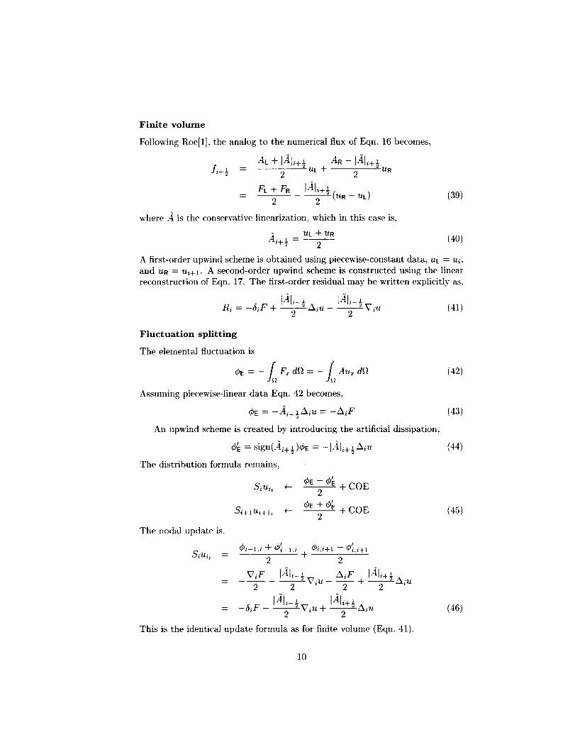
Following Roe[l], the analog to the numerical flux of Eqn. 16 becomes,

AR -I-_1/+½}'Aili+- } ttL + UR

AL +

fi+½ = 2 2

FL+FR 1"41/+3-- 2 2 (UR - UL) (39)

where ,4 is the conservative linearization, which in this case is,

jii+_ __ UL n t" UR (40)- 2

A first-order upwind scheme is obtained using pieeewise-constant data, ur = ui,

and Un = ui+l. A second-order upwind scheme is constructed using the linearreconstruction of Eqn. 17. The first-order residual may be written explicitly as,

Ri = -6iF + _Aiu IZali-½ Viu (41)z 2

Fluctuation splitting

The elemental fluctuation is

0E=--_ F, dft = - £ Au_. df_ (42)

Assuming piecewise-linear data Eqn. 42 becomes,

(be = -Ai+ ½Aiu = -AiF (43)

An upwind scheme is created by introducing the artificial dissipation,

_b_ = sign(_4i+ ½)0E = --1.4[i+ ½Aiu (44)

The distribution formula remains,

Siui, + OE--O'= +COE2

Si+I_/+lt + (_g nt- 0/= _1_ COE (45)

2

The nodal update is,

Siuit

ff)i-l,i -1- ¢ti-l,i Oi,i+l -- (_,i+1

= +2 2

_ ViF 1"4li-½Viu - _,____Fr+ IAl_+½_x_u2 2 2 2

= -5iF IAI,_}2Viu + _Aiu

This is the identical update formula as for finite volume (Eqn. 41).

(46)

10

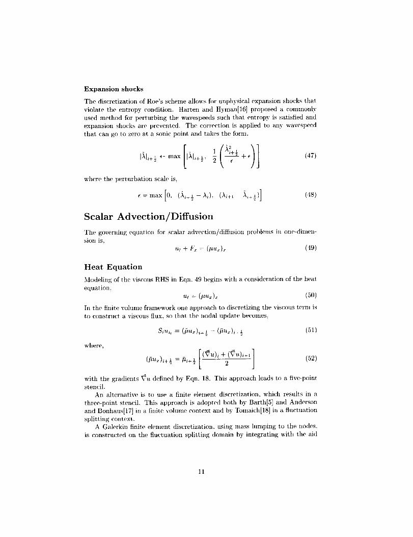
Expansionshocks

The discretization of Roe's scheme allows for unphysical expansion shocks that

violate tile entropy condition. Harten and Hyman[16] proposed a c<)mmonly

used method for perturbing tile wavespeeds such that entropy is satisfied and

expansion shocks are prevented. The correction is applied to any wavespeed

that can go to zero at a sonic point and takes the form,

[ )]+--max -- + e (47)

where the perturbation scale is

• = max [0,t (A_+½ - A_), (Ai+[ - Ai+½)] (48)

Scalar Advection/Diffusion

The governing equation for scalar advection/diffusion problems in one-dimen-

sion is,

ut + F_ = (ttu_)._ (49)

Heat Equation

Modeling of the viscous RHS in Eqn. 49 begins with a consideration of the heat

equation,ut = (m_)_ (50)

In the finite volume framework one approach to discretizing the viscous term is

to construct a viscous flux, so that the nodal update becomes,

SdLi, = (ftUx)i+½ - (#u_)__½ (51)

where,

(pu_)_+ ½ = I-L_+½ 2 (52)

with the gradients Vu defined by Eqn. 18. This approach leads to a five-point

stencil.An alternative is to use a finite element discretization, which results in a

three-point stencil. This approach is adopted both by Barth[5] and Anderson

and Bonhaus[17] in a finite volume context and by Tomaich[18] in a fluctuation

splitting context.A Gaterkin finite element discretization, using mass lumping to the nodes,

is constructed on the fluctuation splitting domain by integrating with the aid

11

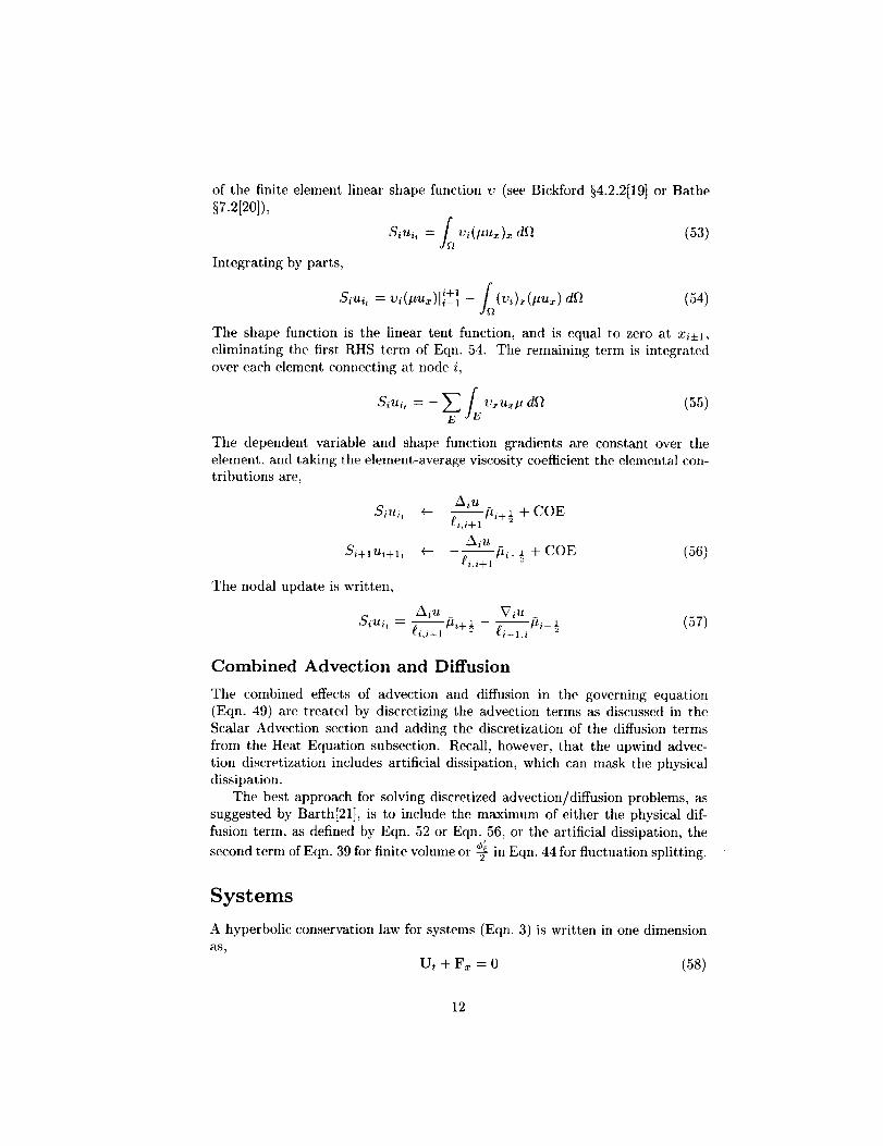
of thefiniteelementlinear shape function v (see Bickford §4.2.2119] or Bathe§7.2120]),

Siui, = fo vi(_u_)_ d_ (53)

Integrating by parts,

Siui t i+1= vi(#u,)li_ 1 - (v_),(llu,) da (54)

The shape fimction is the linear tent function, and is equal to zero at xi+l,

eliminating the first RHS term of Eqn. 54. The remaining term is integrated

over each element connecting at node i,

Siui, = - _E £ v._uxpd" (55)

The dependent variable and shape function gradients are constant over theelement, and taking the element-average viscosity coefficient the elemental con-tributions are,

Aiu _Si'ai, +"- ,; ILl+½ "-F COE

_i,i+l

/'kill _

Si+I ?/,/-t-1, *{ t'i,i+l pi+l + COE (56)

The nodal update is written,

Aiu _ _;iu _

Siui' -- gi,i+l Ill-l-1 gi_l,i _li-1 z (57)

Combined Advection and Diffusion

The combined effects of advection and diffusion in the governing equation(Eqn. 49) are treated by discretizing ttle advection terms as discussed in tile

Scalar Advection section and adding the diseretization of the diffusion terms

from ttle Heat Equation subsection. Recall, however, that the upwind advee-

tion discretization includes artificial dissipation, which can mask the physicaldissipation.

The best approach for solving discretized advection/diffusion problems, mssuggested by Barth[21], is to include the maximum of either the physical dif-

fusion term, as defined by Eqn. 52 or Eqn. 56, or the artificial dissipation, the

second term of Eqn. 39 for finite volume or @ in Eqn. 44 for fluctuation splitting.

Systems

A hyperbolic conservation law for systems (Eqn. 3) is written in one dimension

as_

ut + F_ = 0 (SS)

12

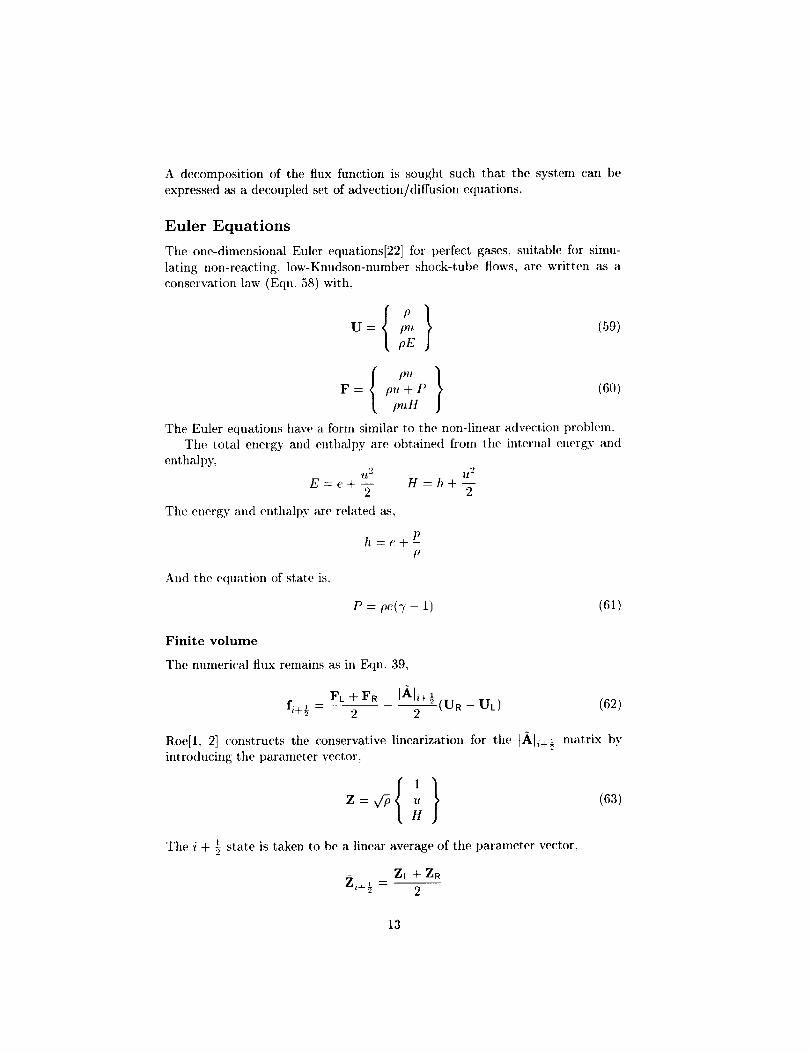
A decompositionof theflux functionis soughtsuchthat thesystemcanbeexpressedasadeeoupledsetofadvection/diffusionequations.

Euler Equations

The one-dimensional Euler equations[22] for perfect gases, suitable for simu-

lating non-reacting, low-Knudson-number shock-tube flows, are written as a

conservation law (Eqn. 58) with,

U = pu (59)

pE

{p}F = pu + P (60)puH

The Euler equations have a form similar to the non-linear advection problem.

The total energy and enthalpy are obtained from tile internal energy and

enthalpy,_2 U 2

E=c+-- H=h+--2 2

The energy and enthalpy are related as,

h = e + -pP

And the equation of state is,

P= pe(_- 1) (61)

Finite volume

The numerical flux remains as in Eqn. 39,

Ikl,++ (UR - Ut.) (62)FL + FRf_++ = " 2 2

the conservative linearization for tile {-_li+½ matrix byRoe[1 2] constructs

introducing the parameter vector,

{'}Z = _ - (63)H

!The i + _ state is taken to be a linear average of tile parameter vector,

EL nc ZR

Z,+½ - 2

13

Takingthevelocityandtotalenthalpyfromtheparametervector,

Zo Z3_=_ /_=-- (64)

and defining the Roe-density,

the Jacobian matrix is formed as,

(65)

Jhl = XlhlX -1 (66)

The eigenvalues are,

A=diag(u, u+a, u-a)

The right eigenvectors are,

(67)

{1} {1} {1}X II) ---- U X [2) ----- U "_ a X (3) = u -- (t

,,2 H + ua H - uaT

(68)

The product X-1 (UR -- Uu) is evaluated via the characteristic variables,

2fi2dp-2dP }1 dP + [)fidu

X-I(UR - UL) = X-IdU = _a 2 dP - Dadu(69)

Tile sound speed is,

.)Ir-

a 2 _ 7P _ 7(7- 1)e = (_- 1)h = (7- 1)(H- --_-) (70)P

Also note tile grouping Ddu can be constructed as,

_du = 21dz2 - _'2dZl (71)

As for the scalar cause, first-order spatial accuracy is obtained by taking the

right state to be i + 1 and the left, state at i. Higher-order accuracy is obtained

using gradient reconstruction (Eqn. 17) applied either to each of the conserved

variables (Eqn.59) or each of the primitive variables, which are,

V= uP

(72)

The nodal update is still formed as in Eqn. 9. The residual remains as

expressed in Eqn. 41, but for systems rather than scalar quantities.

14

Fluctuation splitting

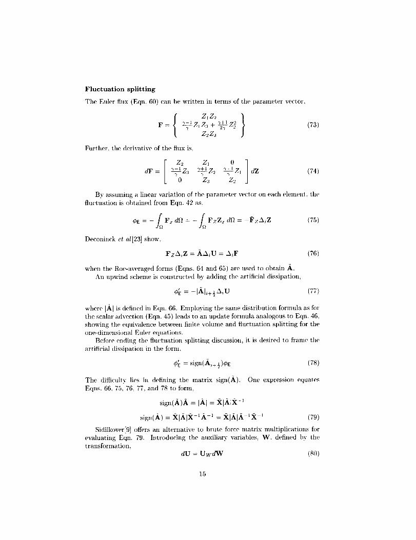
The Euler flux (Eqn. 60) can be written in terms of the parameter vector,

F = _ Z1 Z3 -}- _ .

Z2 Za

Further, tim derivative of the flux is,

dF = ._AZ3 Z_tA_ -._ _'2 Zl

0 Za Z_

dZ

(73)

(74)

By assunfing a linear variation of the parameter vector on each elenmnt, the

fluctuation is obtained from Eqn. 42 as,

OE =- f F, dl_=- f_ FzZzdf_=-_'zAiZ (75)

Deconinck et a1123] show,

F'zAiZ = AAiU = AiF (76)

when the Roe-averaged forms (Eqns. 64 and 65) are used to obtain A.

An upwind scheme is constructed by adding the artificial dissipation,

¢_ = -I]k.li+ ½AiU (77)

where []t[ is defined in Eqn. 66. Employing the same distribution formula as for

the scalar advection (Eqn. 45) leads to an update fornmla analogous to Eqn. 46,showing the equivalence between finite volume and fluctuation splitting for the

one-dimensional Euler equations.

Before ending the fluctuation splitting discussion, it is desired to frame the

artificial dissipation in the form,

4i'_ = sign(]ti+ ½)0e (78)

The difficulty lies in defining the matrix sign(it). One expression equates

Eqns. 66, 75, 76, 77, and 78 to form,

sign(A)_, = IAI = 5[IAIX-'

sign(A) = ZI_-IZ_-'a-' = RIAIA-'R-' (79)

Sidilkover[9] offers an alternative to brute force matrix multiplications forevaluating Eqn. 79. Introducing the auxiliary variables, W, defined by the

transformation,dU = UwdW (80)

15

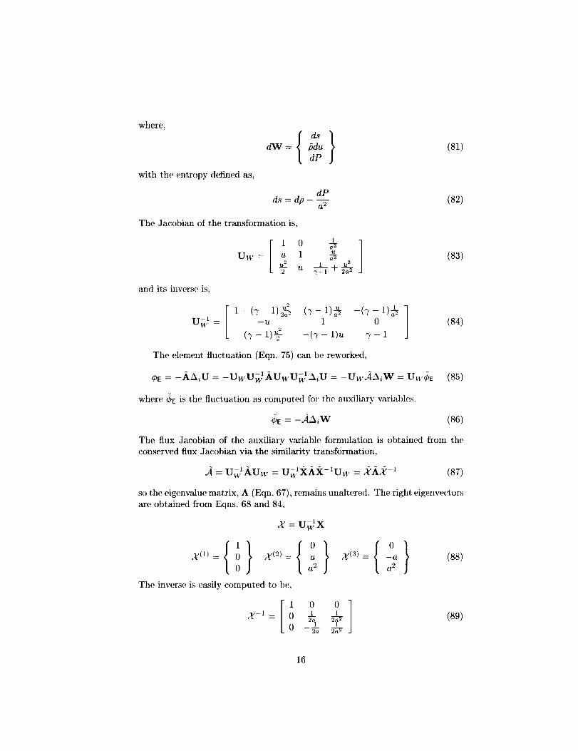
where,

with theentropydefinedas,

dW = [_dudP

dP

ds = do - -j

The Jacobian of the transformation is,

and its inverse is,

[ l]1 0

Uw = u 1 _ u2

(81)

(82)

(83)

1-(_f-1)_. (7-1)_ -('y-1)_ ]U_ = -u 1 0 J (84)(_- 1)@ -(7 - 1)u _ 1

The element fluctuation (Eqn. 75) can be reworked,

OE = --_kAiU = -UwU_IAUwU_IAi U = -Uw_AiW = UU'OE (85)

where ¢_E is the fluctuation as computed for the auxiliary variables,

CE = -AAiW (86)

The flux Jacobian of the auxiliary variable formulation is obtained from tile

conserved flux Jacobian via the similarity transformation,

A _-- u_lfikUB T --- U_IxAx-1uB , = 2A2 -1 (87)

so the eigenvalue matrix, A (Eqn. 67), remains unaltered. The right eigenvectors

are obtained from Eqns. 68 and 84,

x = u_x

{1} {o} {o}X (_) = 0 ,¥(2) = a X (3) = -a (88)0 a2 a 2

The inverse is easily computed to be,

[lO01 ' (89)X -1 = 0 2-_-0 2_

16

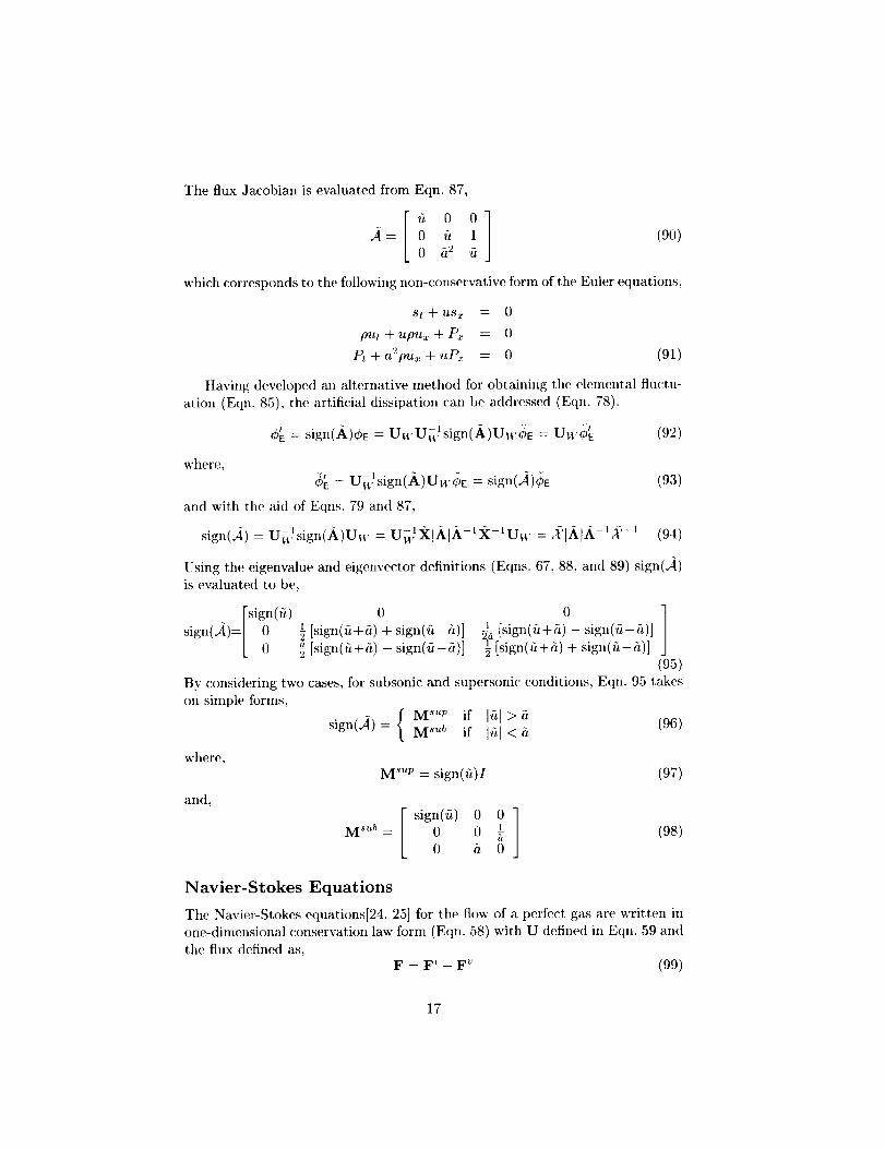
Theflux Jacobian is evaluated from Eqn. 87,

E 00].A= 0 fi 1 (90)0 5,2 _,

which corresponds to tile following non-conservative form of the Euler equations,

st + USx = 0

put + upu_ + P., = 0

Pl +a='pUx +uPx = 0 (91)

Having developed an alternative method for obtaining the elemental fluctu-

ation (Eqn. 85), tile artificial dissipation can be addressed (Eqn. 78).

0_ = sign(A)OE = UwU_sign(h)Uw0E = Uw_ (92)

where,

_[ = U_> sign(h)U,vSE = sign(A)4E (93)

and with the aid of Eqns. 79 and 87,

sign(A) = U_>sign(h)Uw = Ui_>XlAIA-lX-IUv = ,('IAIA-I,_ '-_ (94)

Using the eigenvalue and eigenvector definitions (Eqns. 67, 88, and 89) sign(.A)

is evaluated to be,

sign(A)=

sign(,-,) o o ]t [sign('h+h) + sign(fi-h)] _ [sign(fi+fi) - sign(fi-h)] ]0 :_

0 ._ [sign(_+fi) - sign(fi-5)] ½ [sign(f,+h) + sign(i,-a)](95)

By considering two cases, fi)r subsonic and supersonic conditions, Eqn. 95 takes

on simple forms,

M""" if I,-,I> a (96)sign(A) = M,ub if Ifil < h

where,

and,

M "_'p = sign(fi)I (97)

sign(fi) 0 0 ]1 (98)M _b = 0 0

0 fi 0

Navier-Stokes Equations

The Navier-Stokes equations[24, 25] for the flow of a perfect gas are written inone-dimensional conservation law form (Eqn. 58) with U defined in Eqn. 59 and

the flux defined as,F = F i - F v (99)

17

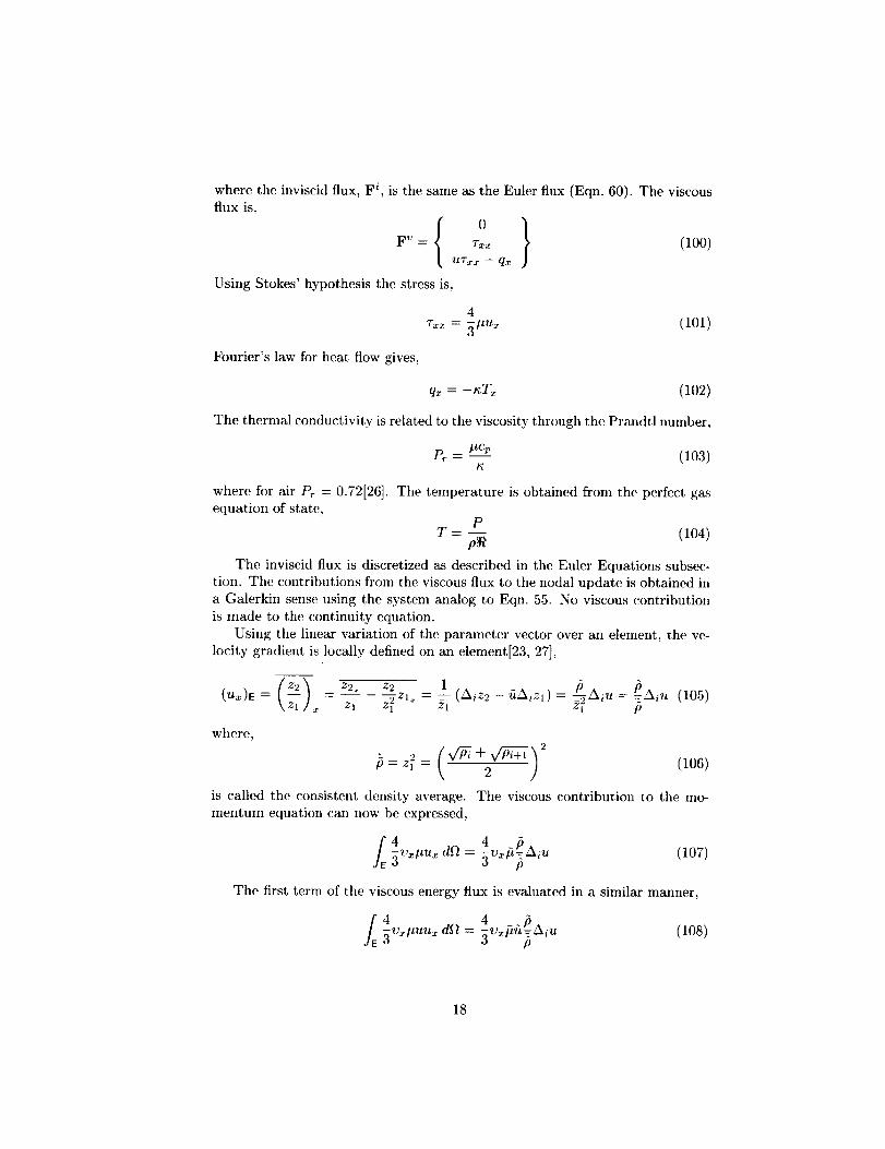
wheretheinviscidflux,F i, is the same as the Euler flux (Eqn. 60). The viscousflux is,

{o)F" = 7xx (100)

Urxx - q,

Using Stokes' hypothesis the stress is,

4

rxx = 5ttu. (101)

Fourier's law for heat flow gives,

qx = -_T_ (102)

Tile thermal conductivity is related to the viscosity through the Prandtl number,

Pr- #cp (103)t_

where for air Pr = 0.72126]. Tile temperature is obtained from the perfect gasequation of state,

P

T p_ (104)

The inviscid flux is discretized as described in the Euler Equations subsec-

tion. Tile contributions from the viscous flux to the nodal update is obtained in

a Galerkin sense using the system analog to Eqn. 55. No viscous contribution

is made to the continuity equation.

Using the linear variation of the parameter vector over an element, the ve-

locity gradient is locally defined on an element[23, 27],

(u,)e = z2 _ zfl__ z2 1 (Aiz2 - _Aizl) = A_u = Aiu (105)z, z_Zl_ = -_

where,

= = (106)

is called the consistent density average. The viscous contribution to the mo-

mentum equation can now be expressed,

_4 45v_ttUx d_ = 5Vxft_Aiu (lO7)

The first term of the viscous energy flux is evaluated in a similar manner,

fE 4 b5 v_#uux4 d_ = 5v_#'SpAiU (108)

18

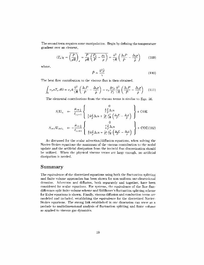
Thesecondtermrequiressomemanipulation.Beginbydefiningthetemperaturegradientoveranelement,

where,

Theheatflowcontribution to the viscous flux is then obtained,

(109)

(110)

(111)

The elemental contributions from the viscous terms is similar to Eqn. 56,

/ ° }I ° }/2i+ "_ :_ + COE(ll2)

Si+lU/+lt _-- (i,i+l ,_?A /_i_t4 ~iS/ q_ cv52p,,"_ (_ _ _)

As discussed for the scalar advection/diffusion equations, when solving the

Navier-Stokes equations the maximum of the viscous contribution to the nodalupdate and the artificial dissipation from the inviscid flux discretization should

t)e utilized. When the physical viscous terlns are large enough, no artificialdissipation is needed.

Summary

The equivalence of the discretized equations using both the fluctuation splittingand finite volume approaches has been shown for non-uniform one-dimensional

domains. Advection and diffusion, both separately and together, have been

considered for scalar equations. For systems, the equivalence of the Roe flux-

difference-split finite volume scheme and Sidilkover's fluctuation splitting scheine

for Euler equations is shown. Finally, viscous diffusion and conduction terms are

modele(t an(t inchlde(l, establishing the equivalence for the discretized Navier-Stokes equations. The strong link established in one dimension can serve as a

prelude to multidimensional analysis of fluctuation splitting and finite volume

as applied to viscous gas dynamics.

19

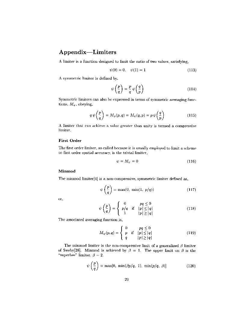
Appendix--Limiters

A limiter is a function designed to limit the ratio of two values, satisfying,

_/_(0) = 0, _b(1) = 1 (113)

A symmetric limiter is defined by,

= q _/, (114)

Symmetric limiters can also be expressed in terms of symmetric averaging func-tions, M_, obeying,

q_/_(q) =M_,(p,q)=M_.(q,p)= p_/_(q) (115)

A limiter that can achieve a value greater than unity is termed a compressivelimiter.

First Order

The first order linfiter, so called because it is usually employed to limit a scheme

to first order spatial accuracy, is the trivial limiter,

W = M¢,, = 0 (116)

Minmod

The minmod limiter[4] is a non-compressive, symmetric limiter defined as,

or_

0

(117)

pq_<0

Ipl<_lq

Jpl>_lq(118)

The associated averaging function .is,

0 pq__Ol_l¢,(p,q) = p if IPl < Iq (119)

q lPl>_lq

The minmod limiter is the non-compressive limit of a generalized _ limiter

of Sweby[28]. Minmod is achieved by fl = 1. The upper limit on /3 is the"superbee" limiter, _ = 2.

(P_ = max[0, min(flp/q, 1), min(p/q, /3)] (120)\q/

2O

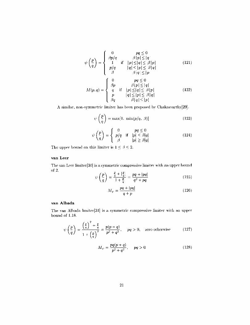
0 pq <_ 0

LTp/q ,LTiPI <-Iql

V){£}--- 1 if Ipl<lql< /3[pl\q] P/q Iq]-< II'1-< ,_lql

/_ /Tlql _<Ipl

0 pq<_O

/Jp /_lpl <-lqlM(p,q) = q if IPl <lql <_ _lpl

v Iql < Ipl ___2lql& /_lql _<Ipl

(121)

(122)

A similar, non-symnmtric limiter has been proposed by Chakravarthy[29],

_/" tq)= max[O, min(plq, f3)]

0 pq <_ 0,U_ \,tI =(P) plq if Ipl < /_lq,f_ Ipl > Olql

The upper bound oil this limiter is 1 < /3 < 2.

(123)

(124)

van Leer

The van Leer limiter[30] is a symmetric compressive linfiter with an upper boundof 2.

,_,,, _ u _ Pq + IPql (125)

1 + _q q2 + pq

pq + ImlAI_, - (126)

q+p

van Albada

The van Albada linfiter[31] is a symmetric compressive limiter with an ut)per

bound of 1.18.

_2) -- 2 p2 q_ q2 ' Pq > O, zero otherwise (127)

Pq(P+ q)

M_,,- p2+q2 ' Pq >0 (128)

21

References

[1] Roe, P. L., "Approximate Riemann Solvers, Parameter Vectors, and Differ-ence Schemes," Journal of Computational Physics, Vol. 43, October 1981,

pp. 357 372.

[2] Roe, P. L., "Characteristic-Based Schemes for the Euler Equations," An-

nual Review of Fluid Mechanics, Vol. 18, 1986, pp. 337-365.

[3] van Leer, B., "Towards the Ultimate Conservative Scheme. V. A Second-

Order Sequel to Godunov's Method," Journal of Computational Physics,

Vol. 32, 1979, pp. 101 136.

[4] Hirsch, C., Numerical Computation of Internal and External FlowsVolume 2: Computational Methods ]or Inviscid and Viscous Flows, John

Wiley & Sons Ltd., 1990.

[5] Barth, T. J., "Aspects of Unstructured Grids and Finite-Volume Solvers for

the Euler and Navier-Stokes Equations," Computational Fluid Dynamics,No. 1994 04 in Lecture Series, von Karman Institute for Fluid Dynamics,1994.

[6] Deconinck, H., Struijs, R., and Roe, P. L., "Fluctuation Splitting for Mul-tidimensional Convection Problems: An Alternative to Finite Volume and

Finite Element Methods," Computational Fluid Dynamics, No. 1990-03 in

Lecture Series, von Karman Institute for Fluid Dynamics, Mar. 1990.

[7] Hirsch, C., "A General Analysis of Two-Dimensional Convection Schemes,"

Computational Fluid Dynamics, Lecture Series 1991-01, von Karman In-stitute for Fluid Dynamics, Feb. 1991.

[8] Deconinck, H., Struijs, R., Bourgois, G., and Roe, P. L., "Compact Ad-

vection Schemes oll Unstructured Grids," Computational Fluid Dynamics,

No. 1993-04 in Lecture Series, von Karman Institute for Fluid Dynamics,Mar. 1993.

[9] Sidilkover, D., "A Genuinely Multidimensional Upwind Scheme and Effi-cient Multigrid Solver for the Compressible Euler Equations," Report 94

84, ICASE, USA, Nov. 1994.

[10] Sidilkover, D., "Multidimensional Upwinding and Multigrid," AIAA Paper

95 1759, Jun. 1995.

[11] Sidilkover, D. and Roe, P. L., "Unification of Some Advection Schemes ill

Two Dimensions," Report 95 10, ICASE, Hampton, Feb. 1995.

[12] Sidilkover, D., "Some Approaches Towards Constructing Optimally Effi-cient Multigrid Solvers for the Inviscid Flow Equations," Report 97--39,

ICASE, Hampton, Aug. 1997.

22

[13]Deconinck,H.,Paill_re,H.,Struijs,R.,andRoe,P.L., "MultidimensionalUpwindSchemesBasedoil Fluctuation-SplittingforSystemsof Conserva-tionLaws,"Computational Mechanics, Vol. 11, 1993, pp. 323 340.

[14] Godunov, S. K., "A Difference Method for the Numerical Calculation of

Discontinuous Solutions of Hydrodynamic Equations," Matematichaskiy

Sbor_ik, Vol. 47(89), No. 3, Mar. 1959, pp. 271 306.

[15] Courant, R., Isaacson, E., and Reeves, M., "On the Solution of NonlinearHyperbolic Differential Equations by Finite Differences," Pure and Applied

Mathematics, Vol. 5, 1952, pp. 243 255.

[16] Harten, A. and Hyman, J. M., "Self Adjusting Grid Methods for One-Dimensional Hyperbolic Conservation Laws," ,lou_,al of Computational

Physics, Vol. 50, 1983, pp. 235-269.

[17] Anderson, W. K. and Bonhaus, D. L., "An Implicit Upwind Algorithnl

for Computing Turbulent Flows on Unstructured Grids," Computers and

Fluids, Vol. 23, No. 1, Jan. 1994, pp. 1 21.

[18] Toinaich, G. T., A Genuinely Multi-Dimensional Upwindin9 Algorithm

for the Navier-Stokes Equations on Unstructured Grids Using a Com-

pact, Highly-Parallelizable Spatial Discretization, Ph.D. thesis, University

of Michigan, USA, 1995.

[19] Bickford, W. B., A First Course in the Finite Element Method, Richar(t

D. Irwin, Inc., Boston, 1990.

[20] Bathe, K.-J., Finite Element Procedures in Engineering Analysis, Pr(,ntice-

Hall, Inc., Englewood Cliffs, USA, 1982.

[21] Barth, T. ,]., "Recent Developments in High Order K-Exact Reconstructionon Unstructured Meshes," AIAA Paper 93 0668, Jan. 1993.

[22] Euler, L., "Princit)es G6nbxaux du Mouvenmnt des Fluides," Historical

Academy of Berlin, Opera Omnia H, Vol. 12, 1755, pp. 54 92.

[23] Deconinck, H., Roe, P. L., and Struijs, R., "A Multidimensional Generaliza-tion of Roe's Flux Difference Splitter for the Euler Equations," Computers

and Fluids, Vol. 22, No. 2/3, 1993, pp. 215 222.

[24] Navier, M., "Mfmoire sur les lois du Mouvement des Fhfides," Mdmoire del'Acaddmie des Sciences, Vol. 6, 1827, pp. a89.

[25] Stokes, G. G., "On the Theories of the Internal Friction of Fhfids in Mo-tion," Trans. Cambridge Philosophical Society, Vol. 8, 1849, pp. 227 319.

[26] Anderson, D. A., Tannehill, .I.C., and Pletcher, R. H., Computational FluidMechanics and Heat Transfer, Taylor and Francis, 1984.

23

[27]Struijs,R., Deconinck,H., de Palma,P., Roe,P., andPowell,K. G.,"Progresson MultidimensionalUpwindEulerSolversfor UnstructuredGrids,"AIAAPaper91-1550,Jun.1991.

[28]Sweby,P.K., "HighResolutionSchemesUsingFluxLimitersforHyperbolicConservationLaws,"SIAM Journal of Numerical Analysis, Vol. 21, 1984,

pp. 995-1011.

[29] Chakravarthy, S. R. and Osher, S., "High Resolution Applications of theOsher Upwind Scheme for the Euler Equations," AIAA Paper 83 1943,Jun. 1983.

[30] van Leer, B., "Towards the Ultimate Conservative Scheme. II. Monotonic-

ity and Conservation Combined in a Second Order Scheme," Journal o]Computational Physics, Vol. 14, 1974, pp. 361-370.

[31] van Albada, G. D., van Leer, B., and Roberts, W. W., "A Comparative

Study of Computational Methods in Cosmic Gas Dynamics," Report 81

24, ICASE, NASA Langley Research Center, Hampton, Virginia, August1981.

24

REPORT DOCUMENTATION PAGE Form ApprovedOMB No. 0704-0188

Public reporting burden for this collection of information is estimated to average 1 hour per response, including the time for reviewing instructions, searching existing data sources,

gathering and maintaining the data needed, end completing end reviewing the collection of information. Send comments regarding this burden estimate or any other 8.spec'tof thiscollection of information, including suggestions for reducing this burden, to Washington Headquarters Services, Directorate for Information Operations and Reports, 1215 Jefferson Davis

Highway, Suite 1204, Arlington, VA 22202.-4302, end to the Office of Management and Budget, Paperwork Reduction Project (0704-0188), Washington, DC 20503.

1. AGENCY USE ONLY (Leave blank) 2. REPORT DATE 3. REPORT TYPE AND DATES COVERED

October 1997 Technical Memorandum

4. TrrLE AND SUbii/LE 5. FUNDING NUMBERS

Equivalence of Fluctuation Splitting and Finite Volume for WU 242-80-01-01One-Dimensional Gas Dynamics

6. AUTHOR(S)

William A. Wood

7.PERFORMINGORGANIZATIONNAME(S)ANDADDRESS(ES)NASA Langley Research CenterHampton, VA 23681-2199

9.SPONSORING/MONiiuMINGAGENCYNAME(S)ANDADDRESS(ES)National Aeronautics and Space AdministrationWashington, DC 20546-0001

11. SUPPLEMENTARY NOTES

8. PERFORMING ORGANIZATION

REPORT NUMBER

L-17677

10. SPONSORING/MONITORINGAGENCY REPORT NUMBER

NAS/VTM-97-206271

12a. D,S t MvBUTION/AVAILABILITY STATEMENT

Unclassified-UnlimitedSubject Category 64 Distribution: NonstandardAvailability: NASA CASI (301) 621-0390

12b, DISTRIBUTION CODE

13. ABSTRACT (Maximum 200 words)

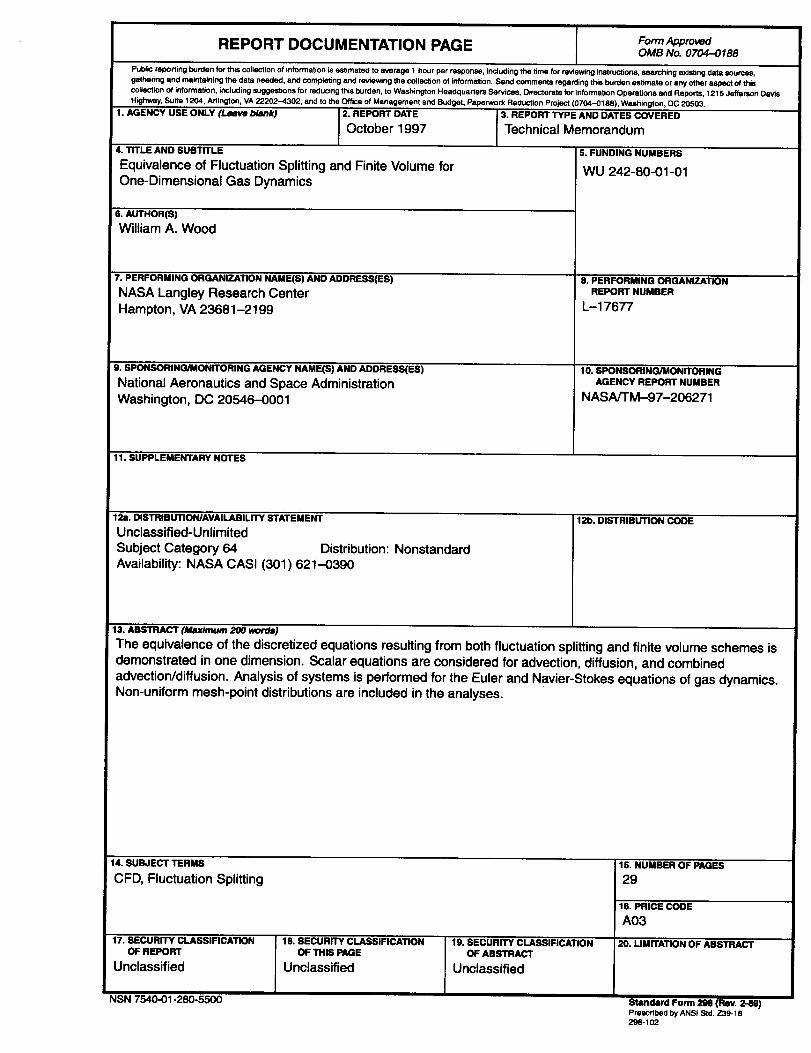
The equivalence of the discretized equations resulting from both fluctuation splittingand finite volume schemes isdemonstrated in one dimension. Scalar equations are considered for advection, diffusion, and combinedadvection/diffusion. Analysis of systems is performed for the Euler and Navier-Stokes equations of gas dynamics.Non-uniform mesh-point distributionsare included in the analyses.

14. SUBJECT IP'HMS

CFD, Fluctuation Splitting

17. SECURI-i-_ CLASSIFICATIONOF REPORT

Unclassified

NSN 7540-01-280-5500

18. SECURITY CLASSIFICATIONOF THIS PAGE

Unclassified

19. SECURITY CLASSIFICATIONOF ABSTRACT

Unclassified

15. NUMBER OF PAGES

29

16. PRICE CODE

A03

20. LIMITATION OF ABSTRACT

Stlmclllrd Form m (Rev. 2-89)Prescribed by ANSI SKI. Z39-18298-102