ERDC/CHL TR-08-15 Wave Climate and Littoral Sediment Transport Study for Virginia Beach, VA – Rudee Inlet to Cape Henry Hydraulic Model Study Michael J. Briggs and Edward F. Thompson September 2008 Coastal and Hydraulics Laboratory Approved for public release; distribution is unlimited.

Welcome message from author
This document is posted to help you gain knowledge. Please leave a comment to let me know what you think about it! Share it to your friends and learn new things together.
Transcript

ERD
C/CH
L TR
-08-
15
Wave Climate and Littoral Sediment Transport Study for Virginia Beach, VA – Rudee Inlet to Cape Henry Hydraulic Model Study
Michael J. Briggs and Edward F. Thompson September 2008
Coas
tal a
nd H
ydra
ulic
s La
bora
tory
Approved for public release; distribution is unlimited.

ERDC/CHL TR-08-15 September 2008
Wave Climate and Littoral Sediment Transport Study for Virginia Beach, VA – Rudee Inlet to Cape Henry Hydraulic Model Study
Michael J. Briggs and Edward F. Thompson Coastal and Hydraulics Laboratory U.S. Army Engineer Research and Development Center 3909 Halls Ferry Road Vicksburg, MS 39180-6199
Final report Approved for public release; distribution is unlimited.
Prepared for U.S. Army Engineer District, Norfolk Norfolk, VA 23510
Under Hydraulic Model Study LGF20L

ERDC/CHL TR-08-15 ii
Abstract: The Norfolk District is preparing an Environmental Assess-ment for the use of sand sources off the coast of Cape Henry for future maintenance of the Virginia Beach, VA, shoreline. The primary purpose is to maintain a buffer for hurricane protection for structures landward of the existing beach. The Cape Henry Borrow Area is being considered as a sand source. The plan borrow scenario involves removing approximately 34.2 M cu yd of material from the borrow area over a period of 50 years. The study provided wave climate and potential longshore transport infor-mation and analysis for two bathymetric cases: existing bathymetry and planned excavation from the Cape Henry Borrow Area. These two cases bracket the range of expected conditions over the next 50 years and enable assessment of potential project impacts on littoral transport patterns along adjacent beaches during this time frame.
DISCLAIMER: The contents of this report are not to be used for advertising, publication, or promotional purposes. Citation of trade names does not constitute an official endorsement or approval of the use of such commercial products. All product names and trademarks cited are the property of their respective owners. The findings of this report are not to be construed as an official Department of the Army position unless so designated by other authorized documents. DESTROY THIS REPORT WHEN NO LONGER NEEDED. DO NOT RETURN IT TO THE ORIGINATOR.

ERDC/CHL TR-08-15 iii
Contents Figures and Tables..................................................................................................................................v
Preface..................................................................................................................................................viii
Unit Conversion Factors........................................................................................................................ix
1 Introduction..................................................................................................................................... 1 Background .............................................................................................................................. 1 Need and objective .................................................................................................................. 3 Study approach ........................................................................................................................ 3
2 Offshore Wave Climate .................................................................................................................. 7 WIS hindcasts........................................................................................................................... 7 Wave climate ............................................................................................................................ 9
3 Numerical Model ..........................................................................................................................12 Objectives and approach .......................................................................................................12 Model description...................................................................................................................12
Wave model ................................................................................................................................12 Grids............................................................................................................................................13
Nearshore wave transformation............................................................................................15 Incident wave conditions ...........................................................................................................15 STWAVE output...........................................................................................................................16
Littoral transport .................................................................................................................... 17 Wave time history at nearshore monitoring stations ...............................................................17 Calculation of breaking wave conditions ..................................................................................19 Calculation of longshore transport rates ..................................................................................19
4 Wave Transformation ...................................................................................................................21 Wave transformation examples for existing and Plan 1 bathymetry ...................................21 Influence of borrow area on wave conditions at beaches north and south of Cape Henry borrow area ........................................................................................................25
Wave heights ..............................................................................................................................25 Wave directions..........................................................................................................................31
5 Littoral Transport Potential .........................................................................................................34 Existing bathymetry ................................................................................................................34 Comparisons to previous studies with existing bathymetry.................................................36 Plan 1 borrow area bathymetry .............................................................................................38 Changes in longshore transport between cases ..................................................................38
6 Summary and Conclusions..........................................................................................................45
References............................................................................................................................................51

ERDC/CHL TR-08-15 iv
Appendix A: STWAVE Input Wave Parameters .................................................................................53
Appendix B: Average Annual Longshore Transport Rates for Existing Bathymetry.....................54
Appendix C: Average Annual Longshore Transport Rates for Plan 1 with Borrow Area..............81
Appendix D: Average Annual Changes in Longshore Transport Rates Between Plan 1 and Existing Bathymetry,.......................................................................................................... 108
Report Documentation Page

ERDC/CHL TR-08-15 v
Figures and Tables
Figures
Figure 1. Study area location map............................................................................................................ 1 Figure 2. Proposed portion of Cape Henry borrow area used in current study.................................... 2 Figure 3. Bathymetry for existing conditions. .......................................................................................... 4 Figure 4. Plan 1 modified existing bathymetry with borrow pit.............................................................. 4 Figure 5. Model extent and existing depth contours in study area ....................................................... 6 Figure 6. Locations of WIS Stations, NDBC Buoys and CMAN gages in study area ............................ 8 Figure 7. Percent occurrence histogram of wave direction, period, and height for Station 197, 1990 to 1999..................................................................................................................... 10 Figure 8. Wave height rose, WIS Station 197, 1990 to 1999..............................................................11 Figure 9. Wave period rose, WIS Station 197, 1990 to 1999. ............................................................11 Figure 10. Monitoring station locations relative to Cape Henry borrow area.....................................18 Figure 11a. Wave transformation for existing bathymetry and Event 1..............................................23 Figure 11b. Difference in wave height between Plan 1 with borrow area and existing bathymetry for Event 1 ............................................................................................................................23 Figure 12a. Wave transformation for existing bathymetry and Event 2.............................................. 24 Figure 12b. Difference in wave height between Plan 1 with borrow area and existing bathymetry for Event 2 ............................................................................................................................ 24 Figure 13a. Wave transformation for existing bathymetry and Event 3..............................................26 Figure 13b. Difference in wave height between Plan 1 with borrow area and existing bathymetry for Event 3 ............................................................................................................................26 Figure 14a. Wave transformation for existing bathymetry and Event 4.............................................. 27 Figure 14b. Difference in wave height between Plan 1 with borrow area and existing bathymetry for Event 4 ............................................................................................................................ 27 Figure 15a. Wave transformation for existing bathymetry and Event 5..............................................28 Figure 15b. Difference in wave height between Plan 1 with borrow area and existing bathymetry for Event 5 ............................................................................................................................28 Figure 16a. Wave transformation for existing bathymetry and Event 6..............................................29 Figure 16b. Difference in wave height between Plan 1 with borrow area and existing bathymetry for Event 6 ............................................................................................................................29 Figure 17a. Event wave height at monitoring stations, existing bathymetry.......................................30 Figure 17b. Impact of borrow area on wave height at monitoring stations, Plan 1 – existing bathymetry. ...............................................................................................................................................30 Figure 18a. Event wave direction at monitoring stations, existing bathymetry. .................................32 Figure 18b. Impact of borrow area on wave direction at monitoring stations, Plan 1 – existing bathymetry. .................................................................................................................................32 Figure 19. 10-year average annual longshore transport rates, existing bathymetry.........................35 Figure 20. Comparison of historical resort beach sand nourishment with predicted average net and gross transport rates................................................................................................... 37

ERDC/CHL TR-08-15 vi
Figure 21. 10-year average annual longshore transport rates, Plan 1 borrow area..........................39 Figure 22. Comparison of existing and Plan 1 10-year average net transport rates.........................40 Figure 23. Impact of borrow area on average annual longshore transport rates, Plan 1 – existing bathymetry. ................................................................................................................................. 41 Figure 24. Impact of borrow area on annual net longshore transport rates, Plan 1 – existing bathymetry. .................................................................................................................................42 Figure 25. Change in net transport between Plan 1 and existing with standard deviation for existing bathymetry. ...........................................................................................................44 Figure B1. Average annual south longshore transport rates for monitoring stations, existing bathymetry. .................................................................................................................................55 Figure B2. Average annual north longshore transport rates for monitoring stations, existing bathymetry. .................................................................................................................................55 Figure B3. Average annual net longshore transport rates for monitoring stations, existing bathymetry................................................................................................................................................56 Figure B4. Average annual gross longshore transport rates for monitoring stations, existing bathymetry ..................................................................................................................................56 Figure C1. Average annual south longshore transport rates for monitoring stations, Plan 1 with borrow area.......................................................................................................................................82 Figure C2. Average annual north longshore transport rates for monitoring stations, Plan 1 with borrow area.......................................................................................................................................82 Figure C3. Average annual net longshore transport rates for monitoring stations, Plan 1 with borrow area.......................................................................................................................................83 Figure C4. Average annual gross longshore transport rates for monitoring stations, Plan 1 with borrow area.......................................................................................................................................83 Figure D1. Average annual change in southerly longshore transport rates for monitoring stations, Plan 1 – Existing bathymetry. ................................................................................................109 Figure D2. Average annual change in northerly longshore transport rates for monitoring stations, Plan 1 – Existing bathymetry. ................................................................................................109 Figure D3. Average annual change in net longshore transport rates for monitoring stations, Plan 1 – Existing bathymetry. ................................................................................................110 Figure D4. Average annual change in gross longshore transport rates for monitoring stations, Plan 1 – Existing bathymetry. ................................................................................................110
Tables
Table 1. Specifications for STWAVE grids............................................................................................... 14 Table 2. Directional spectral wave parameters. .................................................................................... 16 Table 3. Monitoring station STWAVE location coordinates...................................................................18 Table 4. Wave transformation events..................................................................................................... 21 Table 5. Annual longshore transport statistics, existing bathymetry, 1990–1999, 1,000 cu yd/yr. .........................................................................................................................................35 Table 6. Annual longshore transport statistics, Plan 1 bathymetry, 1990–1999, 1,000 cu yd/yr..........................................................................................................................................39 Table 7. Annual longshore transport statistics, changes between Plan 1 and existing cases, 1990–1999, 1,000 cu yd/yr ......................................................................................................42 Table A1. STWAVE wave parameters. .....................................................................................................53

ERDC/CHL TR-08-15 vii
Table B1. Southern longshore transport rates, existing bathymetry, 1990–1999, 1,000 cu yd/yr. ......................................................................................................................................... 57 Table B2. Northern longshore transport rates, existing bathymetry, 1990–1999, 1,000 cu yd/yr..........................................................................................................................................63 Table B3. Net longshore transport rates, existing bathymetry, 1990–1999, 1,000 cu yd/yr. .........................................................................................................................................69 Table B4. Gross longshore transport rates, existing bathymetry, 1990–1999, 1,000 cu yd/yr. ......................................................................................................................................... 74 Table C1. Southern longshore transport rates, Plan 1, 1990–1999, 1,000 cu yd/yr. .....................84 Table C2. Northern longshore transport rates, Plan 1, 1990–1999, 1,000 cu yd/yr.......................90 Table C3. Net longshore transport rates, Plan 1, 1990–1999, 1,000 cu yd/yr. ...............................96 Table C4. Gross longshore transport rates, Plan 1, 1990–1999, 1,000 cu yd/yr. .........................102 Table D1. Southern longshore transport rates, change = P1 – Ex, 1990–1999, 1,000 cu yd/yr. .......................................................................................................................................111 Table D2. Northern longshore transport rates, change = P1 – Ex, 1990–1999, 1,000 cu yd/yr. .......................................................................................................................................117 Table D3. Net longshore transport rates, change = P1 – Ex, 1990–1999, 1,000 cu yd/yr...........123 Table D4. Gross longshore transport rates, change = P1 – Ex, 1990–1999, 1,000 cu yd/yr. .......................................................................................................................................129

ERDC/CHL TR-08-15 viii
Preface
This study was authorized by the U.S. Army Engineer District, Norfolk, and was conducted by personnel of the Harbors, Entrances, and Structures Branch, Coastal and Hydraulics Laboratory (CHL), of the U.S. Army Engi-neer Research and Development Center (ERDC). The study was conducted during the period June 2003 through October 2003. Deborah R. Painter, U.S. Army Engineer District, Norfolk, oversaw progress of the study.
Dr. Michael J. Briggs, Harbors and Entrances Group, Harbors, Entrances, and Structures Branch, CHL, was point of contact for the study. This report was prepared by Dr. Briggs and Dr. Edward F. Thompson, Harbors and Entrances Group, CHL. Leonette J. Thomas, also of Harbors and Entrances Group, CHL, assisted with the preparation of the report. Direct supervision was provided by Dennis G. Markle, currently with the Information Technology Laboratory, ERDC. General supervision was provided by Thomas W. Richardson, Director, CHL, and Dr. James R. Houston, Director, ERDC.
COL Gary E. Johnston was Commander and Executive Director of ERDC. Dr. James R. Houston was Director.

ERDC/CHL TR-08-15 ix
Unit Conversion Factors
Multiply By To Obtain
cubic feet 0.02831685 cubic meters
cubic yards 0.7645549 cubic meters
degree 0.01745329 radians
feet 0.3048 meters
inches 2.54 centimeters
gallons 3.785 liters
miles (nautical) 1,852 meters
square feet 0.09290304 square meters

ERDC/CHL TR-08-15 1
1 Introduction Background
The U.S. Army Corps of Engineers, Norfolk District (CENAO), is preparing an Environmental Assessment for the use of sand sources off the coast of Cape Henry for future maintenance of the Virginia Beach, VA, shoreline. The primary purpose of the project is to maintain a buffer for hurricane protection for structures landward of the existing beach.
The study area along the Virginia coast extends along Cape Henry from Rudee Inlet in the south to 89th Street in the north (Figure 1). The beaches experience active movement of littoral sediment in both northward and southward directions, depending on incident wave conditions. The net impact of littoral transport can emerge as sediment accretion in some coastal areas and erosion in other areas.
Figure 1. Study area location map (Cape Henry borrow area shown in green).

ERDC/CHL TR-08-15 2
The Cape Henry borrow area is being considered as a sand source. It is a roughly triangular-shaped area, located adjacent to Virginia Beach, VA, and the Atlantic Ocean Navigation Channel. The plan borrow scenario involves removing approximately 34.2 M cu yd (million cubic yards) of material from the borrow area over a period of 50 years. Plan borrow activities will deepen the existing bottom in the seaward portion of the Cape Henry borrow area by 14 ft (Figure 2). Because significant changes to the Cape Henry borrow area will alter local wave conditions and may affect littoral transport patterns along nearby beaches, analysis of wave transfor-mation and estimates of potential longshore transport were developed for existing and with-project scenarios.
Use of offshore sand sources will modify the bathymetry affecting waves as they approach Virginia Beach. Depending on characteristics of the borrow areas and proximity to shore, the effect on wave climate may extend to the beach and alter littoral transport along the beach. The purpose of the pro-posed work is to assess the potential impacts of offshore sand removal on nearby beaches.
Figure 2. Proposed portion of Cape Henry borrow area used in current study
(shown in yellow).

ERDC/CHL TR-08-15 3
Need and objective
The use of the Cape Henry borrow area as a sand source may affect littoral transport patterns along nearby beaches landward of this area. CENAO needs information about the magnitude and extent of these impacts along Virginia Beach.
In response to this need, the study objective is to provide wave climate and potential longshore transport information and analysis for two bathyme-tric cases: existing bathymetry and with planned excavation from the Cape Henry borrow area. These two cases will bracket the range of expected conditions over the next 50 years and enable assessment of potential project impacts on littoral transport patterns along adjacent beaches.
Study approach
The study described in this report was performed by the U.S. Army Engi-neer Research and Development Center, Coastal and Hydraulics Labora-tory (CHL). The approach consisted of the following components:
• Determine appropriate offshore wave climate for the study area. • Obtain digital bathymetry. • Use a numerical model to transform offshore wave conditions to
coastal areas for two bathymetric configurations. • Estimate littoral transport potential along the coast, including differ-
ences resulting from the two configurations.
Offshore wind-wave and swell climate was represented by Wave Informa-tion Studies (WIS) hindcast information covering the 10-year time period 1990–99. The WIS information compared very favorably with National Data Buoy Center (NDBC) data from NDBC Station 44014. The WIS infor-mation offered some advantages over NDBC Station 44014 for this study as discussed in Chapter 2, Offshore Wave Climate.
Digital bathymetry was obtained from the National Oceanic and Atmo-spheric Administration (NOAA) for the study area. Two bathymetric con-figurations were modeled:
1. Existing Bathymetry (Figure 3). Existing offshore bathymetry within the study area.
2. Plan 1: Existing Bathymetry with Borrow Pit (Figure 4). Modified off-shore bathymetry to include proposed pit in Cape Henry borrow area.

ERDC/CHL TR-08-15 4
Figure 3. Bathymetry for existing conditions.
Figure 4. Plan 1 modified existing bathymetry with borrow pit.

ERDC/CHL TR-08-15 5
Wave transformation from deep to shallow water depths was performed with the finite difference STWAVE (STeady-State Spectral WAVE) model. It includes the coastal processes of refraction, shoaling, and depth-limited wave breaking. The STWAVE model is contained in the SMS (Surface-Water Modeling System 2000): a comprehensive graphical user interface (GUI) for model conceptualization, mesh generation, statistical interpre-tation, and visual examination of surface water model simulation results.
The model domain extended north into the mouth of Chesapeake Bay and south to near False Cape (Virginia and North Carolina border), beyond expected plan impacts (Figure 5). The computer program VaBeach_QCalc provided the tool for calculating potential longshore transport rates. Development of numerical model grids, model output stations, longshore sediment transport calculation procedures, and other aspects of the modeling approach are described in Chapter 3.
Study results are presented in Chapters 4 and 5. Nearshore wave trans-formation results are summarized in Chapter 4. Littoral transport results needed for assessing borrow-area impact on erosion and accretion of adjacent beaches are presented in Chapter 5. Conclusions are given in Chapter 6. This chapter is followed by references cited in the report.

ERDC/CHL TR-08-15 6
Figure 5. Model extent and existing depth contours (meters) in study area; model
output stations shown as red squares.
ERDC/CHL TR-08-15 7
2 Offshore Wave Climate
Determination of the incident wave climate is a critical first step in near-shore wave transformation and littoral transport studies. Ideally, a long-term, high-quality hindcast is available with at least a few years of con-current directional wave measurements in the same area to validate the hindcast. This study used a relatively recent 10-year hindcast, as discussed in the following paragraphs.
WIS hindcasts
The Wave Information Studies (WIS) have developed wave information along U.S. coasts by computer simulation of past wind and wave condi-tions. This type of simulation is termed a hindcast. The present hindcast information base consists of two 20-yr periods and one 10-year period. WIS produced the first period, covering years 1956–75, in the early 1980s (Corson et al. 1982). The second period, covering years 1976–95, was pro-duced in the mid-1990s (Brooks and Brandon 1995). The last period of 10 years from 1990–99 is the most recent and reliable since it was pro-duced using an improved wave hindcast model and results were evaluated against an extensive array of wave measurements that were not available during the two previous time periods. The WIS hindcasts and comparisons with gauge data are easily accessible by Internet for CENAO review at http://www.frf.usace.army.mil/wis/.
The 1990–99 WIS parameters are available at 1-hr intervals over the 10-year period. At each 1-hr interval, a number of wave parameters are given. Parameters typically used to represent waves are significant wave height, Hm0, peak spectral wave period, Tp, and mean direction at the peak frequency, θ .
Two WIS stations, 197 and 199, are available for analysis within the study area (Figure 6). Station 197 is located 11.5 nm offshore at latitude 36.92 N and longitude 75.75 W in a water depth of 17 m (56 ft). WIS Station 199 is located at latitude 36.83 N and longitude 75.75 W in a depth of 19 m (62 ft). It is a little further south and in deeper water than Station 197. After some comparisons, Station 197 was selected since it is directly off-shore from the beaches and thought to be more representative of the study area.

ERDC/CHL TR-08-15 8
Figure 6. Locations of WIS Stations, NDBC Buoys and CMAN gages in study area. Gage 197 is
marked with an arrow and gage 199 is to the south.
The WIS wave information was compared to data from three gage sites in the general location of the study area (Figure 6). The three sites were (1) National Weather Service National Data Buoy Center (NDBC) Buoy 44014 (includes wave direction data), (2) Coastal-Marine Automated Network (CMAN) station at Chesapeake Light, CHLV2 (does not include wave direction), and (3) nearshore CHL gage, VA001, near Virginia Beach. The NDBC Buoy 44014 is significantly further offshore than the other wave gages and the WIS stations. The Virginia Beach gage was a direc-tional nearshore pressure gage array in 8-m water depth operated by CHL. Additional information and data are available at http://sandbar.wes.army.mil/public_html/pmab2web/htdocs/va001.html.
Time history comparisons between the two offshore gage locations and the nearest WIS grid points are available via the WIS Web site. These
197

ERDC/CHL TR-08-15 9
comparisons were reviewed over the full ten-year time period. Several individual storms (i.e., October 1991) were examined in close detail and showed good agreement. Overall, the WIS information appears to give a very good representation of local offshore wave climate over the 10-year time period. Based on these results, WIS Station 197 was selected to provide wave climate information of this study since: (a) Station 197 is significantly closer to the study area than NDBC Buoy 44014 and can be used directly as incident waves for STWAVE modeling; (b) hourly wave information, including wave direction, is available over the full 10-year period with no gaps; and (c) WIS hindcasts compare well with available gauge data. One advantage of (a) is that most WIS wave cases are propa-gating toward shore, while NDBC Buoy 44014, the other possible source of offshore wave direction information, includes a number of cases of waves traveling offshore. If NDBC Buoy 44014 data were used, these cases would be considered as “calms” relative to the Virginia Beach coast. In reality, there is always wave energy propagating toward an exposed coast such as Virginia Beach.
Wave climate
The 10-year time history from 1990 to 1999 for WIS Station 197 was reviewed and summarized using the program NEMOS (Nearshore Evolution Modeling System), a part of the CEDAS (Coastal Engineering Design and Analysis System). The Web page for the CEDAS is located at http://chl.erdc.usace.army.mil/cedas.
Figure 7 is a percent occurrence histogram of wave direction, period, and height. Direction bands are 10 deg increments from 22 deg to 132 deg, equivalent to ±50 deg on either side of the normal to the shore. Waves approaching the coast from directions outside this arc are not a significant consideration because they will be refracted greatly and reduced in height before breaking at the shore. Approximately 4.1 percent of the waves occur below 22 deg and 8.3 percent above 132 deg. The most common direction band, with 12.2 percent of the cases, is between 72 to 82 deg, with a mean of 76.3 deg, approximately perpendicular to shore. The middle numbers listed in each band are the averages or means for the band. Wave periods range from 1 to 23 sec, with 2-sec bands. The most commonly occurring wave period band, with 39.9 percent of the cases, is 3 to 5 sec. The overall mean peak wave period is 6.7 sec. The standard deviation of wave period is 3 sec.

ERDC/CHL TR-08-15 10
0.9
1.9
2.9
3.9
5.0
5.7
7.0
0.5
1.5
2.5
3.5
4.5
5.5
6.5
7.5
Wav
e H
eigh
t (m
)
72.0
8.7 1.3 0.4 0.1 0.0 0.0
2.0
4.0
6.0
7.9
9.9
11.9
13.9
15.7
17.9
20.0
22.0
1.0
3.0
5.0
7.0
9.0
11.0
13.0
15.0
17.0
19.0
21.0
23.0
Wav
e Pe
riod
(sec
)
0.0
39.9
21.5 16.0 11.5 7.8 2.4 0.7 0.1 0.0 0.0
27.2
37.3
47.0
57.0
68.6
76.3
87.9
96.4
108.
0
116.
6
126.
8
22.0
32.0
42.0
52.0
62.0
72.0
82.0
92.0
102.
0
112.
0
122.
0
132.
0
Wav
e D
irect
ion
(deg
)
1.7 2.0 2.1 2.0 3.312.2 8.6 6.5 7.7 10.0 7.5
Percent Occurrence
Figure 7. Percent occurrence histogram of wave direction, period, and height for Station 197,
1990 to 1999
Significant wave heights are shown from 0.5 to 7.5 m, in seven bands of 1 m bandwidth. Approximately 17.5 percent of the waves have heights less than 0.5 m. These were not considered in the analysis since they are below the threshold for significant sediment transport. Seventy-two percent of the cases fall in the 0.5-m to 1.5-m band. Overall mean significant height is 0.9 m, with a standard deviation of 0.6 m. The highest significant wave height is 5.8 m, with corresponding peak period of 12.3 sec and direction of 88 deg azimuth.
Figure 8 shows a significant wave height rose diagram. The concentric rings represent percent occurrence of up to 9 percent. Thicker bars repre-sent smaller wave heights, as indicated in the legend. Wave directions are directions from which the waves are traveling, the same as meteorological conventions. A wave period rose is shown in Figure 9. Concentric rings represent up to 12 percent occurrence. Thicker bars represent smaller wave periods. The difference in percentage scales for the two rose dia-grams is due to the filtering of the data to include only the ranges of wave period, height, and direction listed above.

ERDC/CHL TR-08-15 11
0.5 - 1.51.5 - 2.52.5 - 3.53.5 - 4.54.5 - 5.55.5 - 6.56.5 - 7.5
Width Legend
90
60
30
0330
300
270
24021
0 180
150
120
0 2 4 7 9
Percent OccurrenceWave Direction (deg)
vs.Wave Height (m)
Figure 8. Wave height rose, WIS Station 197, 1990 to 1999.
1.0 - 3.03.0 - 5.05.0 - 7.07.0 - 9.0
9.0 - 11.011.0 - 13.013.0 - 15.015.0 - 17.017.0 - 19.019.0 - 21.021.0 - 23.0
Width Legend
90
60
30
0330
300
270
240
210 180
150
120
0 3 6 9 12
Percent OccurrenceWave Direction (deg)
vs.Wave Period (sec)
Figure 9. Wave period rose, WIS Station 197, 1990 to 1999.

ERDC/CHL TR-08-15 12
3 Numerical Model Objectives and approach
The numerical model studies had two main objectives:
1. Develop the numerical model application to represent the study area adequately.
2. Use the numerical model to estimate wave conditions and littoral trans-port along Virginia Beach with existing and Plan 1 excavated offshore bathymetry in the Cape Henry borrow area.
The numerical model used for the study, STWAVE, is the standard CHL tool for studies of wave transformation over broad areas of complex, shallow nearshore bathymetry. The wave transformation model is described in the following section, including a general description of the STWAVE model and implementation of the model for the Virginia Beach study.
As part of the study procedures, a suite of incident wave conditions must be specified at the seaward boundary of the area covered by STWAVE. Incident waves are determined by consideration of the hindcast wave climate seaward of the study area. This setup for STWAVE and the type of output produced is described in the section on “Nearshore wave transformation.”
The final section of this chapter describes the study approach for esti-mating littoral transport rates and quantities. STWAVE transformation results are used to first estimate breaking wave conditions along the coast. Then, breaking wave information is fed into the calculation of potential longshore transport rates.
Model description
Wave model
The numerical wave model STWAVE is a steady-state, finite-difference model used in the calculation of wave growth and transformation (Smith et al. 2001). Typically, the model area covers a rectangular domain with maximum dimension of about 26 nm or less, including regions with

ERDC/CHL TR-08-15 13
complex, shallow water depths. Typical model grid resolution is 200 m (600 ft) or less. Recently, the model has been extended to include a capa-bility for using a large-area, coarse grid to feed into a smaller-area fine grid (Smith and Smith 2002). This nesting capability can be helpful for near-shore wave transformation studies, but it was not considered necessary for the present study.
The STWAVE model is interfaced with commercially available Corps of Engineers-supported software to assist in preparing model grids and other inputs and in displaying model results. This software-assisted pre- and post-processing is needed in any practical application.
More information on STWAVE is available through the CHL Internet Web site at: http://chl.erdc.usace.army.mil/chl. The software package for pre- and post-processing is part of the Surface-Water Modeling System (SMS). More information on SMS software is available through the STWAVE model Web site.
Grids
The WIS information from Station 197 was used to characterize the off-shore wave climate. Station 197 is approximately 21 km (11.3 nm) from the Virginia Beach coast, in nominal water depth of 17 m (56 ft). The STWAVE model was configured to estimate wave transformation between Station 197 and the Virginia Beach coast.
The National Oceanic and Atmospheric Administration (NOAA), National Geophysical Data Center (NGDC), 3-arc-second Coastal Relief Model data-base provided existing bathymetry for a large coastal area, including the study area. This bathymetric database is more fully described at Internet address http://www.ngdc.noaa.gov/mgg/coastal/coastal.html. This digital bathymetry was input to the SMS.
The numerical model domain is a rectangle. For this study, the rectangular boundary was aligned approximately parallel to the Virginia Beach coast-line (Figure 5). The model offshore boundary was extended seaward far enough to encompass the most relevant shallow areas and shoal features seaward of the Virginia Beach coast and outside the entrance to Chesa-peake Bay. Lateral boundaries were extended well past the study area to accommodate the range of incident wave directions affecting the study area. The south lateral boundary nearly reaches False Cape, Virginia, and

ERDC/CHL TR-08-15 14
the north boundary falls near the tip of Cape Charles, on the north side of the Chesapeake Bay entrance. The model domain extends 15 km (8 nm) in the offshore direction and 47 km (25 nm) alongshore. Water depth along the seaward grid boundary is about 11–17 m (35–55 ft).
A finite-difference grid for STWAVE was constructed over the model domain using SMS. Parameters for creating the grid in SMS are given in Table 1. Resolution is 50 m (164 ft), which has sufficed in previous, similar studies and is reasonable relative to the 3-sec (92.5-m or 304-ft) resolu-tion of the NGDC bathymetric database. The grid was built in the State Plane coordinate system (Horizontal System: State Plane NAD 83 [US] and State Plane Zone: Virginia South – 4502, Vertical System: NAVD 88 [US]) in units of meters, as required for STWAVE modeling. Model bathymetry for the existing bathymetry grid in the study area is shown in Figures 3 and 5.
Table 1. Specifications for STWAVE grids.
Parameter Value Cell size 50 m (164 ft) Origin x (state plane) 3,734,096 m (12,250,934 ft) Origin y (state plane) 1,086,681 m (3,565,215 ft) Angle of rotation 193 deg Length x 15,000 m (49,212 ft) Length y 47,000 m (154,199 ft) Number of cells 282,000 Number of land cells 11,310 Number of ocean cells 270,690 No. of I’s (columns) 300 No. of J’s (rows) 940
The grid with existing bathymetry was modified to include the proposed borrow area excavations to a uniform depth of 4.3 m (14 ft) below the existing bottom over an area of approximately 66M sq ft (Figure 4). The location and depth of excavation to be modeled were specified by CENAO to represent anticipated borrow activities over a 50-year time period.
The STWAVE model coverage area is typical of a relatively large regional wave transformation study. The possibility of extending the seaward boundary further seaward or nesting the nearshore grid into a

ERDC/CHL TR-08-15 15
large-domain, coarse resolution offshore grid was considered. Advantages would include encompassing more of the irregular bathymetry on the wide continental shelf along the study coast and reaching out to the WIS station used for incident wave conditions. The grid would need to extend seaward another 6.3 km (3.5 nm) to reach the WIS station and considerably further to encompass irregular bottom features. The computational load and com-plications associated with such an effort did not seem warranted in the present study, in part because bottom depth changes within 9–13 nm seaward of the grid boundary are relatively mild and disorganized.
The STWAVE model cannot simulate waves coming from directions that are highly oblique to the grid orientation, because STWAVE is a half-plane model (i.e., only considers a 180 deg window of incident energy). When mean wave directions exceed about 60 deg (for typical directional spread-ing), energy is “lost” owing to the half-plane assumption. Thus, model grid orientation was selected to minimize the occurrence of highly oblique wave angles in regions of interest.
The range of directions in the incident wave climate is greater than can be modeled effectively by a single STWAVE grid. However, in studies focused on nearshore concerns, such as longshore sediment transport as in the present study, a single grid can suffice, since highly oblique offshore waves would be greatly refracted and attenuated by natural processes before arriving at the study site.
Nearshore wave transformation
Incident wave conditions
A range of wind wave and swell conditions incident to Virginia Beach was considered in STWAVE modeling. A representative range of significant wave heights, peak wave periods, and mean wave directions that are a con-cern at the coast was included, based on the hindcast wave climate. The wave parameters modeled are given in Table 2. Every combination of the three wave parameters was modeled in STWAVE, giving a total of 495 wave conditions (5 heights × 9 periods × 11 directions). These conditions provide reasonable coverage of the wave climate. Directions were chosen to cover the full directional exposure of the coast, in 10-deg increments.

ERDC/CHL TR-08-15 16
Table 2. Directional spectral wave parameters.
Parameter No. Units Values Wave period 9 sec 4, 6, 8, 10, 12, 14, 16, 18, 20 Wave height 5 m 1, 2, 3, 4, 5 Wave direction 11 deg 27, 37, 47, 57, 67,77, 87, 97, 107, 117, 127
For each STWAVE input height/period/direction combination, SMS was used to generate a directional wave spectrum in water depth appropriate to the grid seaward boundary (16 m or 52 ft). Spectral frequencies ranged from 0.04 Hz to 0.33 Hz in 0.01-Hz intervals to cover frequencies corre-sponding to one-half to three-times the peak frequency. Spectral direction components covered ±85 deg from normal incidence to the grid, in 5-deg increments. The directional spectrum consists of a Texel Marsden Arsloe (TMA) frequency spectrum and a Cosn spreading function. Spectral wave parameters were selected for each wave based on wave period, a standard approach for practical CHL studies. For the TMA spectrum, frequency spreading is a function of the γ parameter that varied between 3.3 (broad) to 8 (narrow). For the directional Cosn spreading function, the “n” parameter ranged from 4 (broad) to 30 (narrow). These spectra formed the incident wave input for STWAVE nearshore transformation simulations. A listing of all parameters used for each of the 45 height-period cases is contained in Appendix A.
One water level was used for all simulations, corresponding to the mean lower low water (MLLW). NOAA National Ocean Service data for the National Tidal Datum Epoch (1983–2001) were examined for stations near the study area. The Rudee Inlet Station, which is representative of the study area, shows a difference between mean sea level (MSL) and MLLW of only 0.56 m (1.8 ft). MLLW was chosen for simulations to insure that possible impacts of the offshore borrow area would be evident. The overall effect of the borrow pit on longshore transport may be slightly amplified in the study owing to the choice of water level.
STWAVE output
The main output from STWAVE runs consists of two types of information. Wave field or “wav” files of significant wave height, peak period, and peak direction over the grid are produced first for each incident wave case. These relatively large files are useful for visualizing wave transformation over the entire grid. Second, height/period/direction information is saved

ERDC/CHL TR-08-15 17
as “selhts” files at selected monitoring stations in the grid, providing another, much more condensed output. Station output in shallow water along the coast was needed for this study, as discussed in the following sections.
Littoral transport
The approach to estimating potential littoral transport was to: (a) use STWAVE results to create a 10-year time history of near-breaking wave parameters at each nearshore station; (b) transform the near-breaking waves to a point at which breaking begins, using the assumption of locally, straight, parallel bottom contours; and (c) compute potential longshore transport rate from that breaking wave height and angle. With considera-tion of the 10-year incident wave time history, annual potential transport rates can then be calculated. Details of the approach are given in the following paragraphs.
Wave time history at nearshore monitoring stations
Monitoring stations for saving STWAVE wave parameters to be used in littoral transport estimation were selected with two primary objectives. First, the stations should be shoreward of all significant effects of irregular bathymetry (including proposed project-related changes in bathymetry), so that STWAVE will have included these effects in wave transformation. Second, stations should be seaward of the nearshore surf zone, so that STWAVE has not yet invoked breaking limits on wave height and the breaking wave height and angle needed for calculating longshore transport rates can be estimated accurately.
A nearshore monitoring station was selected for every alongshore grid cell adjacent to study area beaches. Stations were placed around the 6 m (20 ft) contour, where bottom contours were reasonably parallel to the shoreline. The selection of the 6-m contour is not exact, so including the larger 5-m wave height cases even though they might have experienced some breaking offshore from this location was felt to be satisfactory. Station 1 was located south of Rudee Inlet and Station 236 was positioned near 89th Street (Figure 10). The distance between stations is 50 m, the same as the STWAVE grid spacing. Table 3 lists the “i” and “j” indices corresponding to the STWAVE grid cell locations for each of the major stations. Thus, Stations 35 through 236 cover the study area.

ERDC/CHL TR-08-15 18
Figure 10. Monitoring station locations relative to Cape Henry borrow area.
Table 3. Monitoring station STWAVE location coordinates.
Station No. STWAVE i STWAVE j Comment 1 284 555 Beginning station 35 282 521 Rudee Inlet 50 283 506 100 284 456 150 285 406 200 284 356 236 283 320 89th Street
Stations 1 through 34, south of Rudee Inlet, were included to provide some overlap with previous studies focused on the coast south of Rudee Inlet (e.g., Kelley et al. 2001).
Results at nearshore monitoring stations from the 495 STWAVE runs were used to transform the WIS 10-year time history of offshore waves into a 10-year time history of nearshore waves at each station via a post-processing program called VaBeach_Timehist. The procedure consisted of the following basic steps:

ERDC/CHL TR-08-15 19
• compute the ratio of significant wave height parameter at each moni-toring station to incident wave height for every station and every incident wave condition run in STWAVE;
• compute similar ratios for peak period and direction parameters; • associate each wave case in the 10-year WIS time history with the
STWAVE run which most nearly matches the incident wave parameters; and
• apply (i.e., multiply) the transformation ratios from STWAVE to each WIS wave case to create a 10-year time history at each nearshore station.
Calculation of breaking wave conditions
A “shoreline” angle was specified for each nearshore station to establish the orientation of the straight, parallel bottom contours to be used in calculating wave breaking conditions. An average shoreline angle of 77 deg azimuth was estimated from available charts (Chart #12221, Chesapeake Bay Entrance). This approximation fits well for the study area, which consists of a nearly straight coastline and exceptionally straight, parallel bottom contours between the nearshore monitoring stations (about 6-m depth) and the point at which waves will break.
A computer program, VaBeach_QCalc, was adapted from previous studies to iteratively calculate breaking wave heights and angles. Inputs to the program include nearshore station 10-year time history and shoreline angles. The breaking criterion (for monochromatic waves) used was HB =0.78 d, where d = water depth.
Calculation of longshore transport rates
Potential longshore transport rates are also calculated in program VaBeach_Qcalc. The 10-year time history of breaking waves at each nearshore monitoring station is used to calculate a corresponding time history of hourly potential longshore transport rate at each station. Potential longshore transport rates Q are calculated as
. sin( α )B BQ KH= 2 5 2 (1)

ERDC/CHL TR-08-15 20
where:
K = constant αB = breaking wave angle relative to bottom contours.
When HB is in meters and Q in m3/day, the generally accepted value of K is 5,100 (Equation 6-7b of USACE 1992). Program calculations were done in metric units with Q expressed in m3/sec. The corresponding constant is K = 0.0590. The equivalent K = 0.0772 for engineering units of cu yd/yr when HB is expressed in units of feet.
In recent past studies along the U.S. Atlantic Coast using the same model-ing approach as in this study, longshore transport rates produced by the above equation were unreasonably large (Thompson et al. 1999; Cialone and Thompson 2000). Calibration to documented longshore transport produced a value of K = 0.023 in both studies. That value was also used in this study, producing longshore transport estimates consistent with avail-able information, as is discussed in Chapter 5.
Following standard convention, longshore transport directed to the right of an observer on the beach facing the ocean is positive (southward trans-port in this study), and transport toward the left is negative (northward transport in this study).
Contributions during each year in the time history of wave conditions are combined to give annual north and south potential longshore transport rates. Net potential longshore transport rates are determined as the sum of north and south magnitude rates, since northward transport is negative. Gross potential longshore transport rates are the combined absolute mag-nitudes of north and south transport rates. Annual longshore transport rates from all 10 years of wave information can be combined to give aver-age annual rates and standard deviations, which provide a helpful measure of expected variability between years.

ERDC/CHL TR-08-15 21
4 Wave Transformation
The objective of this chapter is to present model results showing the influ-ence of nearshore bathymetry on wave transformation and the impact of the deepened borrow area on wave patterns in Plan 1. The presentation is focused on a representative sample of the most commonly occurring wave conditions. These conditions illustrate key nearshore wave transformation effects and help explain the relative changes in potential longshore transport presented in Chapter 5.
Wave transformation examples for existing and Plan 1 bathymetry
Six of the 495 incident wave events were chosen to illustrate wave trans-formation patterns (Table 4). These six events include two wave periods and three wave directions for a significant wave height of 1 m. The 1-m significant height is approximately equal to the mean significant height at Virginia Beach. The two wave periods are representative of sea and swell waves during storms. The 77-deg wave direction is perpendicular to shore and the other two directions are 40 deg north and south of shore-perpendicular.
Table 4. Wave transformation events.
Event Height, m Period, sec Direction, deg 1 37 2 77 3
8
117 4 37 5 77 6
1.0
12
117
Figures 11 through 16 illustrate wave transformation and differences in wave heights between Plan 1 and existing bathymetries for the six events. The top plot in each figure shows wave transformation over the existing bathymetry. The bottom plot is the difference in wave heights between the modified Plan 1 (P1) with the borrow pit and the existing (Ex) bathymetry (i.e., P1 – Ex). For the wave transformation plot, contours range from 0 to 1.2 m, with a contour interval of 0.05 m. For the wave height differ-ences plot, contours range from –0.16 to 0.12 m, with a contour interval of

ERDC/CHL TR-08-15 22
0.02 m. The monitoring stations and annotation about relative locations are listed on each figure. The borrow area is shown in yellow or green (depending on the background color to improve readability) on both plots for reference.
Figure 11a is for Event 1 with Tp = 8 sec, Hs = 1 m, and waves from the northeast (i.e., θ = 37 deg). Waves in the vicinity of the Cape Henry borrow area are generally smaller than the incident 1-m wave height. Significant wave refraction does not occur until the waves are closer to shore, well shoreward of the borrow area. Wave heights in the nearshore area for this event are lower generally than for the other events. Figure 11b shows the difference in wave heights between Plan 1 and existing bath-ymetry for Event 1. Positive values indicate that the Plan 1 wave heights are higher than existing bathymetry heights for this case. Green areas are predominant, indicating no significant change. Differences range from -0.05 to 0.04 m, a very small change in wave heights resulting from Plan 1. Although not shown within the scale of Figure 11b, waves are slightly higher within the borrow area and present a “fan-shaped” area north and south of the borrow area. There is a slight decrease in wave height at the southerly end of the borrow area. Thus, Plan 1 bathymetry results in a shadow area of slightly lower wave heights on the lee side of the borrow area. The shadow extends all the way to the coast.
Figures 12a and 12b are for Event 2, with Tp = 8 sec, Hs = 1 m, and wave direction perpendicular to the beach (i.e., θ = 77 deg). In general, wave heights for this wave direction are the highest for the three wave direc-tions, with the predominant values greater than 0.95 m (Figure 12a). There is a noticeable increase in wave height northeast of the borrow area. Shoals north of the navigation channel cause this wave increase. Fig-ure 12b illustrates differences in wave heights for Event 2. Wave height differences range from –0.05 to 0.06 m, similar to Event 1. The Plan 1 wave heights tend to be slightly higher inside and north of the borrow area. They are slightly lower to the south and in a large shadow area to the west of the borrow area.

ERDC/CHL TR-08-15 23
Figure 11a. Wave transformation for existing bathymetry and Event 1: Tp = 8 sec, HS = 1 m, Dir = 37 deg.
Figure 11b. Difference in wave height between Plan 1 with borrow area and existing bathymetry for Event 1: Tp = 8 sec, HS = 1 m, Dir = 37 deg.

ERDC/CHL TR-08-15 24
Figure 12a. Wave transformation for existing bathymetry and Event 2: Tp = 8 sec, HS = 1 m, Dir = 77 deg.
Figure 12b. Difference in wave height between Plan 1 with borrow area and existing bathymetry for Event 2: Tp = 8 sec, HS = 1 m, Dir = 77 deg.

ERDC/CHL TR-08-15 25
Figures 13a and 13b are for Event 3, with Tp = 8 sec, Hs = 1 m, and wave direction from the southeast (i.e., θ = 117 deg). In general, wave heights are divided about the borrow area and the navigation channel, with higher heights to the northeast and lower values southwest. Wave heights are higher than those from Event 1, but lower than those from Event 2. As for Event 2, there is a large area of shoaling (i.e., increased wave heights) just northeast of the borrow area and navigation channel. Wave height differ-ences for this Event are shown in Figure 13b. In general, the existing bath-ymetry wave heights are higher than the Plan 1 values, with most of the contours ranging from –0.10 to 0.06 m. The Plan 1 wave heights are higher than existing bathymetry at the northern end of the borrow area. The existing bathymetry wave heights are higher (i.e., negative differ-ences) in the lee and to the west of the borrow area, projecting all the way to near Station 210 and north.
Figures 14–16 are for Events 4–6 with Tp = 12 sec. The wave transforma-tion patterns are similar for the Tp = 8 sec cases, but wave height changes are more pronounced for the longer period events. This is caused by the longer period waves (with correspondingly longer wavelength) feeling the bottom and being modified by the bathymetry more strongly in the modeled area. The wave height difference plots also exhibit similar patterns as the Tp = 8 sec cases. They are more intense, however, with larger differences between the Plan 1 and existing bathymetry cases.
Influence of borrow area on wave conditions at beaches north and south of Cape Henry borrow area
The impact of the dredged borrow area on incident wave conditions can be evaluated by examining changes in wave height and direction at the near-shore monitoring stations along the 6-m contour. These changes correlate closely to potential littoral transport differences presented in Chapter 5.
Wave heights
Figures 17a and 17b show calculated wave heights for existing bathymetry and changes in wave height at the 236 monitoring stations for the six wave events (Table 4). The changes represent wave heights for Plan 1 with the borrow pit minus existing bathymetry values for each event. The nominal 1-m incident wave height leads to nearshore wave heights that may be interpreted directly as transformation functions and/or fractional changes caused by sheltering, refraction, and shoaling.

ERDC/CHL TR-08-15 26
Figure 13a. Wave transformation for existing bathymetry and Event 3: Tp = 8 sec, HS = 1 m, Dir = 117 deg.
Figure 13b. Difference in wave height between Plan 1 with borrow area and existing bathymetry for Event 3: Tp = 8 sec, HS = 1 m, Dir = 117 deg.

ERDC/CHL TR-08-15 27
Figure 14a. Wave transformation for existing bathymetry and Event 4: Tp = 8 sec, HS = 1 m, Dir = 37 deg.
Figure 14b. Difference in wave height between Plan 1 with borrow area and existing bathymetry for Event 4: Tp = 8 sec, HS = 1 m, Dir = 37 deg.

ERDC/CHL TR-08-15 28
Figure 15a. Wave transformation for existing bathymetry and Event 5: Tp = 8 sec, HS = 1 m, Dir = 77 deg.
Figure 15b. Difference in wave height between Plan 1 with borrow area and existing bathymetry for Event 5: Tp = 8 sec, HS = 1 m, Dir = 77 deg.

ERDC/CHL TR-08-15 29
Figure 16a. Wave transformation for existing bathymetry and Event 6: Tp = 8 sec, HS = 1 m, Dir = 117 deg.
Figure 16b. Difference in wave height between Plan 1 with borrow area and existing bathymetry for Event 6: Tp = 8 sec, HS = 1 m, Dir = 117 deg.

ERDC/CHL TR-08-15 30
Figure 17a. Event wave height at monitoring stations, existing bathymetry.
Figure 17b. Impact of borrow area on wave height at monitoring stations,
Plan 1 – existing bathymetry.

ERDC/CHL TR-08-15 31
Wave heights range from approximately 0.8 to 1.2 m for the six events (Figure 17a). In general for the existing bathymetry, Event 1 (Tp = 8 sec, θ = 37 deg) has the lowest wave heights and Event 5 (Tp = 12 sec,
θ = 77 deg) the highest. Changes in wave height range from approximately –0.12 to 0.03 m. Again, positive values indicate higher wave heights for the Plan 1 cases. In general, the wave heights are reduced by the proposed Plan 1 owing to the borrow area. Events 5 and 6 are affected significantly in this manner. Plan 1 heights are higher for Event 6 (i.e., positive increase) between about stations 100 to 174, however. These patterns were also evident in the previous figures of wave height and difference contours (Figures 11 to 16). The length of coast covered by the borrow area stretches roughly from Station 100 to 236 (perpendicular projections of the borrow area boundaries to shore). For the northeast (i.e., θ = 37 deg) cases, how-ever, the effect of the borrow area can stretch all the way to Rudee Inlet at Station 35. The impact of the borrow area on the northern stations is stronger for the southeast cases (i.e., θ = 117 deg). In general, the amount of positive change in wave height is relatively small for Plan 1. Thus, wave height changes caused by the Plan 1 borrow area are relatively small, and in most cases are reduced. However, even small changes can impact longshore sediment transport significantly, since that is based on the breaking wave height raised to the power 2.5.
Wave directions
Figures 18a and 18b illustrate wave direction for existing bathymetry and changes in wave direction at the 236 monitoring stations for the six wave events. In Figure 18a the curves are grouped by incident wave direction (i.e., θ = 37, 77, and 117 deg) pairs for the two wave periods (i.e., Tp = 8 and 12 sec). Wave direction does not appear to be changed significantly by either wave period for the existing bathymetry. In general, wave direction decreases toward the north, becoming more southerly. Figure 18b shows the change in wave direction for the six events. The change in wave direc-tion is defined as before, positive values indicate that Plan 1 values are larger than the existing bathymetry. Changes appear to be minor, varying from –1.5 to 1 deg. The curves shown in the figure are curve fit to the data using a smoothing spline routine because of the small variation in the data.

ERDC/CHL TR-08-15 32
Figure 18a. Event wave direction at monitoring stations, existing bathymetry.
Figure 18b. Impact of borrow area on wave direction at monitoring stations,
Plan 1 – existing bathymetry.

ERDC/CHL TR-08-15 33
In summary, a predictor of potential littoral transport differences is to examine the changes in wave height and direction at the 236 monitoring stations. Wave heights range from approximately 0.8 to 1.2 m for the six events. In general for the existing bathymetry, Event 1 (Tp = 8 sec, θ = 37 deg) has the lowest wave heights and Event 5 (Tp = 12 sec,
θ = 77 deg) the highest. Changes in wave height range from approximately –0.12 to 0.03 m (positive values indicate higher wave heights for the Plan 1 cases). The impact of the borrow area on the northern stations is stronger for the southeast waves. In general, wave height changes resulting from Plan 1 are relatively small, and in most cases are reduced. Wave direction does not appear to be changed significantly by either wave period for the existing bathymetry. Differences in wave direction between existing and Plan 1 are insignificant (i.e., varying from –1.5 to 1 deg). In general, wave direction decreases toward the north, becoming more southerly.

ERDC/CHL TR-08-15 34
5 Littoral Transport Potential
The objective of this chapter is to present model simulations of potential longshore sediment transport, based on the 10-year time history of waves (1990–1999). Potential annual impacts of the Plan 1 borrow area on littoral transport are considered in terms of comparisons with the existing bathymetry. Although average annual littoral transport quantities are given, emphasis is on differences in the estimated littoral transport induced by the borrow area. All simulations were performed with the programs discussed in Chapter 3. Implications for beach erosion and accretion are discussed in Chapter 6.
Existing bathymetry
Potential longshore transport rates for the existing bathymetry case are shown in Figure 19. Rates are given in units of cubic yards per year (cu yd/yr) for the 10-year average at each of the 236 monitoring stations. Simulation results are shown for transport to the south, north, net transport (sum of magnitudes for south and north transport rates, since north is negative), and gross (sum of absolute values of south and north transport rates). The color-coordinated vertical lines are the standard error bars for each curve, indicative of plus or minus one standard devi-ation of annual estimates about the 10-year average lines.
Southerly transport is relatively constant along the study coast, averaging about 97,000 cu yd/yr for all stations. Northerly transport decreases from a maximum of 399,000 cu yd/yr in the south (Station 12) to 143,000 cu yd/yr in the north (Station 232), with an average of 288,000 cu yd/yr. Net transport decreases from 315,000 cu yd/yr at Station 12 in the south to a minimum of 18,000 cu yd/yr at the northern Station 236 near the Chesapeake Bay entrance. The average net transport rate is 191,000 cu yd/yr to the north for all monitoring stations. It decreases with distance north after about Station 85, with another break in slope around Station 170. Gross transport rate decreases more or less continuously south to north along the study coast from a maximum of 484,000 cu yd/yr at Station 12 to a low of 253,000 cu yd/yr at Station 233. The average gross transport rate is 385,000 cu yd/yr for all monitoring stations. Table 5 lists statistics for the existing bathymetry case for south, north, net, and gross longshore transport rates.

ERDC/CHL TR-08-15 35
Figure 19. 10-year average annual longshore transport rates, existing bathymetry.
Table 5. Annual longshore transport statistics, existing bathymetry, 1990–1999, 1,000 cu yd/yr.
Year 10-Year 1 2 3 4 5 6 7 8 9 10 Ave Std
South Min 29 63 81 95 124 63 61 101 48 86 75 28Max 50 113 158 166 192 111 112 160 83 144 129 43Ave 40 81 118 120 161 76 82 124 58 110 97 36Std 3 6 11 8 9 6 6 7 4 7 7 2
North Min -271 -218 -465 -385 -429 -511 -485 -202 -432 -604 -399 38Max -116 -72 -157 -140 -154 -163 -184 -89 -163 -191 -143 133Ave -202 -142 -318 -280 -318 -357 -355 -147 -319 -438 -288 96Std 30 28 61 50 58 73 61 21 56 88 52 21
Net Min -238 -146 -372 -284 -304 -441 -416 -89 -379 -518 -315 51Max -72 36 -6 25 36 -58 -77 65 -85 -48 -18 132Ave -161 -61 -200 -160 -157 -281 -273 -23 -261 -328 -191 99Std 32 32 69 55 61 78 66 25 59 92 57 18
Gross Min 160 167 291 280 320 258 279 225 234 312 253 56Max 303 289 559 493 567 580 553 315 486 696 484 139Ave 242 222 437 400 479 433 437 271 377 548 385 108Std 28 24 55 45 56 69 57 19 53 85 49 19

ERDC/CHL TR-08-15 36
Minimum, maximum, average, and standard deviations are included for each year, the 10-year average and standard deviation. The standard devi-ations show the natural variability from year to year and for the 10-year averages.
Comparisons to previous studies with existing bathymetry
The overall study objective is to quantify the impact, if any, of planned off-shore borrow activities on potential longshore transport at Virginia Beach. Since the impact is expected to be small or insignificant, this study is not intended to develop a comprehensive sediment budget for the study area. For example, Rudee Inlet interrupts longshore transport and sediment is routinely bypassed to the beach north of the inlet. This interruption is not represented in the study results. However, historical data on the volume of sand needed to nourish Virginia Beach, including Rudee Inlet bypassing activities, gives a useful comparison to present study results. CENAO pro-vided annual nourishment volumes for the 10-year study period, 1990 to 1999. The historical field data are compared to annual average longshore transport values for all model monitoring stations (Figure 20). The data fall between model gross and net transport volumes for most years and more nearly match gross than net transport. Although the data do not allow for a definitive comparison, the general level of agreement helps to validate model results.
In their analysis of sediment processes along the outer banks of North Carolina, Inman and Dolan (1989) discuss the presence of a longshore transport nodal point near False Cape, VA, the vicinity of the VA/NC bor-der, with net transport toward the north along beaches north of the node and toward the south along beaches further south. Citing earlier studies, they estimate the net transport rate in the vicinity of Rudee Inlet as 209,300 cu yd/yr (160,000 cu m/yr). Estimates of annual net and gross longshore transport rates are also given for the stretch of coast between Cape Henry and Cape Hatteras, NC. Although the estimates are very coarse spatially and are based on early WIS hindcasts for the years 1956–75, they are reasonably consistent with present study results.

ERDC/CHL TR-08-15 37
Figure 20. Comparison of historical resort beach sand nourishment with predicted
average net and gross transport rates.
More recent numerical model studies were performed to evaluate the impact of planned borrow activities at Sandbridge Shoals, VA, which lies between Rudee Inlet and False Cape (Kelley and Ramsey 2001; Kelley et al. 2001). These studies used numerical model technology similar to the present study but with only eleven representative incident wave condi-tions. Potential longshore transport estimates were generated along a stretch of coast that encompassed Rudee Inlet and approximately the southern one-third of the present study area. From this study, smoothed transport rates around and north of Rudee Inlet are 200,000 cu m/yr southward, 320,000 cu m/yr northward, 120,000 cu m/yr net, and 680,100 cu yd/yr (520,000 cu m/yr) gross. Northward rates are reason-ably comparable to the present study results. Southward rates are higher than the present study results. The discrepancy in southward transport rates may be attributed to the proximity of numerical grid northern boundaries in the Sandbridge Shoals studies. Southward longshore trans-port predictions along coasts near the northern grid boundaries may lose accuracy, because waves coming from the north and northwest directions are not fully accommodated in the grid.

ERDC/CHL TR-08-15 38
In conjunction with the present study, available information about long-shore transport rates was discussed with Professor David Basco, Old Dominion University, Norfolk, VA. Professor Basco confirmed that a net transport rate of around 200,000 cu yd/yr northward in the vicinity of Rudee Inlet is generally accepted, which is consistent with the present study results. He also indicated that there is considerable historical data that could be addressed if more detailed studies are needed in the future.
Plan 1 borrow area bathymetry
Figure 21 is a plot of the 10-year average longshore transport rates for Plan 1 with the borrow pit. The south, north, net, and gross longshore transport rates are shown, similar to Figure 19 for the existing bathymetry case. The statistical error bars are again shown on each curve. Table 6 summarizes transport rate statistics for the Plan 1 bathymetry, analogous to Table 5 for the existing bathymetry case.
In general, longshore transport rates for south, north, net, and gross are similar for the Plan 1 bathymetry cases. Southerly transport remains rela-tively constant along the study coast, averaging the same as the existing case (97,000 cu yd/yr) for all stations. Northerly transport decreases from a maximum of 397,000 cu yd/yr at Station 12 to 120,000 cu yd/yr in the north at Station 232, with an average of 282,000 cu yd/yr. Net transport decreases from 312,000 cu yd/yr at Station 12 in the south to a minimum of 4,000 cu yd/yr at the northern Station 236. The average net transport rate is 185,000cu yd/yr to the north, a slight decrease from the existing case. Gross transport rate decreases more or less continuously south to north along the study coast from a maximum of 483,000 cu yd/yr at Station 12 to a low of 230,000 cu yd/yr at Station 232. The average gross transport rate is 379,000 cu yd/yr for all monitoring stations, again down slightly from the existing case.
Changes in longshore transport between cases
Comparing Figures 19 and 21 for the existing and Plan 1 cases, it appears that longshore transport rates show little change for the transport in the southerly direction. There are some changes for the north, net, and gross transport rates, however, especially farther to the north. To highlight this fact, the two 10-year average net curves for existing and Plan 1 cases (from Figures 19 and 21, respectively) are overlain in Figure 22.

ERDC/CHL TR-08-15 39
Figure 21. 10-year average annual longshore transport rates, Plan 1 borrow area.
Table 6. Annual longshore transport statistics, Plan 1 bathymetry, 1990–1999, 1,000 cu yd/yr
Year 10-Year
1 2 3 4 5 6 7 8 9 10 Ave Std South
Min 29 63 83 96 124 63 61 101 48 86 76 28Max 50 112 156 167 192 112 113 161 84 145 129 43Ave 40 81 119 120 161 76 82 124 58 110 97 36Std 3 6 10 8 9 6 6 7 4 7 6 2
North Min -269 -215 -461 -382 -428 -508 -481 -200 -430 -603 -397 31Max -99 -64 -133 -117 -129 -129 -154 -77 -139 -157 -120 132Ave -199 -139 -311 -275 -312 -349 -349 -145 -314 -428 -282 94Std 35 29 67 57 66 84 70 24 63 100 59 24
Net Min -237 -143 -367 -282 -302 -439 -412 -88 -377 -516 -312 46Max -54 44 14 47 58 -24 -45 78 -59 -16 4 132Ave -158 -58 -192 -155 -150 -273 -267 -21 -255 -319 -185 97Std 37 33 74 62 69 89 74 28 66 103 63 21
Gross Min 143 159 269 257 294 224 250 213 210 280 230 50Max 302 288 557 491 567 578 551 315 484 695 483 139Ave 239 219 430 395 473 425 431 269 372 538 379 106Std 34 26 62 52 64 80 67 22 60 97 56 21

ERDC/CHL TR-08-15 40
Figure 22. Comparison of existing and Plan 1 10-year average net transport rates.
The small differences in net transport between the existing and Plan 1 cases are highlighted. The transport rates begin to diverge around Sta-tion 174, decreasing to the north for the Plan 1 bathymetry case, relative to the existing case. If a control volume is drawn around Stations 170 to 236 on Figure 22, for both existing and Plan 1 scenarios, accumulation occurs within the control volume since more sediment is entering in the south than leaving the control volume at the northern perimeter. Moreover, since the net transport is smaller for Plan 1, especially at the northern perimeter, it will accumulate more sediment than the existing case. Thus, the main impact of the borrow area is to decrease the amount of net north-ward longshore transport up to 32,000 cu yd/yr between Stations 170 and 236. This will tend to promote sand retention along this section of the shoreline.
This change in net transport is again demonstrated in Figure 23. It shows the changes between Plan 1 and existing cases (i.e., Change = Plan 1 – Existing) for the south, north, net, and gross transport rates (analogous to Figures 19 and 21). The statistical error bars (i.e., standard errors of the estimates) are again shown for reference. As noted above, the changes in southward transport are insignificant. Northward changes are not visible

ERDC/CHL TR-08-15 41
Figure 23. Impact of borrow area on average annual longshore transport rates,
Plan 1 – existing bathymetry.
since they are overlain by the net changes. Changes for north, net, and gross transport from approximately Station 160 to 236 show a clear impact of borrow activities. Note that the net transport is the sum of the southerly (positive) transport and the northerly (negative) transport. A positive net transport change (i.e., P1 – Ex) then implies that Plan 1 reduces northerly and net transport relative to the existing bathymetry. Net transport rate changes decrease (i.e., positive differences) to the north up to approxi-mately 32,000 cu yd/yr near Station 220 and then decrease to about 23,000 cu yd/yr at Station 236. Changes in net transport rates are positive along nearly the entire affected coast, indicating a pit-induced reduction of northerly transport. This reduction in transport rate implies more accum-ulation of sediment along the northern part of the study coast due to the borrow area. Table 7 again summarizes the statistics for the changes between Plan 1 and existing cases for south, north, net, and gross trans-port rates.
The curves in Figure 23 are for the 10-year average transport rates. The variation in the net transport rate changes for each of the years in the 10-year time period is shown in Figure 24. The minimum and maximum range of change in net transport rates is between 10,000 cu yd/yr at

ERDC/CHL TR-08-15 42
Table 7. Annual longshore transport statistics, changes between Plan 1 and existing cases, 1990–1999, 1,000 cu yd/yr
Year 10-Year Desc. 1 2 3 4 5 6 7 8 9 10 Ave Std
South Min -1 -2 -5 -2 -3 -1 -1 -2 -1 -3 -1 0 Max 1 2 5 3 5 2 3 3 1 4 2 1 Ave 0 0 0 0 0 0 0 0 0 0 0 1 Std 0 1 2 1 1 1 1 1 0 1 1 0
North Min -4 -3 -4 -5 -7 -11 -7 -2 -4 -11 -5 0 Max 24 11 31 32 36 51 42 15 34 54 32 14 Ave 3 3 7 5 6 8 6 2 6 10 6 3 Std 7 3 8 9 10 14 12 4 9 14 9 3
Net Min -4 -3 -6 -6 -9 -11 -8 -4 -5 -12 -7 0 Max 24 11 29 32 37 50 42 16 33 56 32 14 Ave 3 3 7 5 7 8 6 2 6 10 6 4 Std 6 3 8 9 10 14 12 4 9 15 9 3
Gross Min -25 -12 -34 -32 -35 -53 -42 -15 -34 -53 -33 0 Max 5 2 4 4 5 10 7 2 4 9 4 14 Ave -3 -3 -7 -5 -6 -8 -6 -2 -6 -9 -5 3 Std 7 3 9 8 10 15 12 4 9 14 9 3
Figure 24. Impact of borrow area on annual net longshore transport rates,
Plan 1 – existing bathymetry.

ERDC/CHL TR-08-15 43
Station 145 to 56,000 cu yd/yr to the north at the peak near Station 220. These curves illustrate that the impact of Plan 1 on the net longshore transport rate can vary considerably from year to year. They also show how the gradient (i.e., the rate of change of the transport rate or slope of the transport rate) varies from year to year. Drawing a control volume around stations 150 to 200 and looking at the gradient between stations illustrates this point. A steeper gradient for the change in net transport implies decreasing transport to the north between southerly and northerly stations for Plan 1 relative to the existing case. Thus, sediment may be better retained in the north part of the study area for Plan 1 during years when the gradient of net transport changes is steep.
Average annual longshore transport rate curves from 1990 to 1999 are contained in Appendix B for south, north, net, and gross transports for the existing bathymetry case. Plots for Plan 1 are contained in Appendix C. Appendix D contains the plots for the change condition, Plan 1 – Existing bathymetry. Because some of the change values are relatively small, they are shown to two decimal place accuracy while still being divided by 1,000 as in the other appendices.
Although the Plan 1 borrow excavation clearly appears to impact potential longshore transport in the northern part of the study area, considering whether this impact is significant is important. Consideration of annual variations that naturally occur owing to year-to-year wave climate varia-tions gives a useful perspective. Figure 25 shows the standard deviation σ of the annual net transport for the existing bathymetry over the 10-year period along with the average net transport difference curve repeated from Figure 23. For the coastline most impacted by borrow activities, around Station 220, natural year-to-year variations in existing annual net trans-port rate, as represented by σ, are 3–4 times as large as differences induced by the proposed borrow activities.

ERDC/CHL TR-08-15 44
Figure 25. Change in net transport between Plan 1 and existing with standard
deviation for existing bathymetry.

ERDC/CHL TR-08-15 45
6 Summary and Conclusions
1. The U.S. Army Corps of Engineers, Norfolk District (CENAO), is preparing an Environmental Assessment for the use of sand sources off the coast of Cape Henry for future maintenance of the Virginia Beach, VA, shoreline. The primary purpose of the project is to maintain a buffer for hurricane protection for structures landward of the existing beach.
2. The Cape Henry borrow area is being considered as a sand source. It is a roughly triangular-shaped area, located adjacent to Virginia Beach, VA, and the Atlantic Ocean Navigation Channel. The plan borrow scenario involves removing approximately 34.2 M cu yd of material from the borrow area over a period of 50 years. Plan borrow activities will deepen the existing bottom in the seaward portion of the Cape Henry borrow area by 4.3 m (14 ft) over an area of approximately 66M sq ft.
3. The study objective is to provide wave climate and potential longshore transport information and analysis for two bathymetric cases: existing bathymetry and Plan 1 with planned excavation from the Cape Henry borrow area. These two cases will bracket the range of expected conditions over the next 50 years and enable assessment of potential project impacts on littoral transport patterns along adjacent beaches. Thus, the overall objective is to quantify the impact, if any, of planned offshore borrow activ-ity on potential longshore transport at Virginia Beach. Since the impact was expected to be small or insignificant, this study is not intended to develop a comprehensive sediment budget for the study area. For example, Rudee Inlet interrupts longshore transport and sediment is routinely bypassed to the beach north of the inlet. This interruption is not repre-sented in the study results.
4. Offshore wind wave and swell climate was represented by Wave Informa-tion Studies (WIS) hindcast information covering the 10-year time period 1990–99. WIS Station 197 (13 miles from the Virginia Beach coast in nominal water depth of 56 ft MLLW) was selected for comparisons since it is directly offshore from the beaches and more representative for the study area. The WIS wave information compared favorably to data from three gage sites in the general location of the study area. The WIS information is more complete than the gage records.
5. The 10-year wave data were summarized using the program NEMOS (Nearshore Evolution Modeling System), a part of the CEDAS (Coastal Engineering Design and Analysis System). The most common direction

ERDC/CHL TR-08-15 46
band, with 12.2 percent of the cases, is between 72 to 82 deg, with a mean of 76.3 deg, approximately perpendicular to shore. The most commonly occurring wave period band, with 39.9 percent of the cases, is 3 to 5 sec. The overall mean peak wave period is 6.7 sec. The standard deviation of wave period is 3 sec. Seventy-two percent of the cases fall in the 0 to 1 m band. Overall mean significant height is 0.9 m, with a standard deviation of 0.6 m. The highest significant wave height is 5.8 m, with corresponding peak period of 12.3 sec and direction of 88 deg azimuth.
6. Wave transformation from deep to intermediate water depths was per-formed with the finite difference STWAVE (Spectral Wave) model. It includes the coastal processes of refraction, shoaling, and depth-limited wave breaking. The STWAVE model is contained in the SMS (Surface Water Modeling System).
7. The model domain extended north into the mouth of Chesapeake Bay and south to near False Cape (Virginia and North Carolina border), beyond expected plan impacts. The STWAVE model was configured to estimate wave transformation between WIS Station 197 and the Virginia Beach coast. The model domain extends 15 km (8 nm) in the offshore direction and 47 km (25 nm) alongshore.
8. One water level was used for all simulations, corresponding to the MLLW. The Rudee Inlet Station, which is representative of the study area, shows a difference between MSL and MLLW of only 0.56 m (1.8 ft). MLLW was chosen for simulations to ensure that possible impacts of the offshore borrow area would be evident. The overall effect of the borrow pit on longshore transport may be slightly amplified in the study owing to the choice of water level.
9. Digital bathymetry, with 3-arc-second Coastal Relief Model database resolution, was obtained from the National Oceanic and Atmospheric Administration (NOAA) for the study area. A finite difference grid for STWAVE was constructed over the model domain using SMS. Resolution is 50 m (164 ft), which has sufficed in previous, similar studies and is reasonable relative to the 3-sec (92.5-m or 304-ft) resolution of the NGDC bathymetric database. The grid was built in the State Plane coordinate system.
10. Based on the hindcast wave climate, a representative range of five signifi-cant wave heights (Hs = 1, 2, 3, 4, and 5m), nine peak wave periods (Tp = 4, 6, 8, 10, 12, 14, 16, 18, and 20 sec), and eleven peak wave direc-tions (θ = 27, 37, 47, 57, 67, 77, 87, 97, 107, 117, and 127 deg) were included in the STWAVE modeling. A total of 495 wave conditions (5 heights × 9 periods × 11 directions) were modeled as directional wave
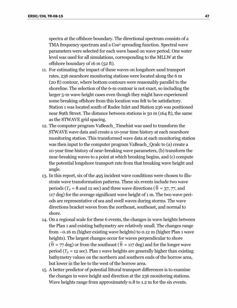
ERDC/CHL TR-08-15 47
spectra at the offshore boundary. The directional spectrum consists of a TMA frequency spectrum and a Cosn spreading function. Spectral wave parameters were selected for each wave based on wave period. One water level was used for all simulations, corresponding to the MLLW at the offshore boundary of 16 m (52 ft).
11. For estimating the impact of these waves on longshore sand transport rates, 236 nearshore monitoring stations were located along the 6 m (20 ft) contour, where bottom contours were reasonably parallel to the shoreline. The selection of the 6-m contour is not exact, so including the larger 5-m wave height cases even though they might have experienced some breaking offshore from this location was felt to be satisfactory. Station 1 was located south of Rudee Inlet and Station 236 was positioned near 89th Street. The distance between stations is 50 m (164 ft), the same as the STWAVE grid spacing.
12. The computer program VaBeach_Timehist was used to transform the STWAVE wave data and create a 10-year time history at each nearshore monitoring station. This transformed wave data at each monitoring station was then input to the computer program VaBeach_Qcalc to (a) create a 10-year time history of near-breaking wave parameters, (b) transform the near-breaking waves to a point at which breaking begins, and (c) compute the potential longshore transport rate from that breaking wave height and angle.
13. In this report, six of the 495 incident wave conditions were chosen to illu-strate wave transformation patterns. These six events include two wave periods (Tp = 8 and 12 sec) and three wave directions (θ = 37, 77, and 117 deg) for the average significant wave height of 1 m. The two wave peri-ods are representative of sea and swell waves during storms. The wave directions bracket waves from the northeast, southeast, and normal to shore.
14. On a regional scale for these 6 events, the changes in wave heights between the Plan 1 and existing bathymetry are relatively small. The changes range from –0.16 m (higher existing wave heights) to 0.12 m (higher Plan 1 wave heights). The largest changes occur for waves perpendicular to shore (θ = 77 deg) or from the southeast (θ = 117 deg) and for the longer wave period (Tp = 12 sec). Plan 1 wave heights are generally higher than existing bathymetry values on the northern and southern ends of the borrow area, but lower in the lee to the west of the borrow area.
15. A better predictor of potential littoral transport differences is to examine the changes in wave height and direction at the 236 monitoring stations. Wave heights range from approximately 0.8 to 1.2 m for the six events.

ERDC/CHL TR-08-15 48
In general for the existing bathymetry, Event 1 (Tp = 8 sec, θ = 37 deg) has
the lowest wave heights and Event 5 (Tp = 12 sec, θ = 77 deg) the highest. Changes in wave height range from approximately –0.12 to 0.03 m (posi-tive values indicate higher wave heights for the Plan 1 cases). The impact of the borrow area on the northern stations is stronger for the southeast waves. In general, wave height changes due to Plan 1 are relatively small, and in most cases are reduced. Wave direction does not appear to be significantly changed by either wave period for the existing bathymetry. Differences in wave direction between existing and Plan 1 are insignificant. In general, wave direction decreases toward the north, becoming more southerly.
16. Contributions during each year in the time history of wave conditions are combined to give annual north and south potential longshore transport rates. Net potential longshore transport rates are determined as the sum in magnitude between north and south rates, since northward transport is negative. Gross potential longshore transport rates are the combined abso-lute magnitudes of north and south transport rates. Annual longshore transport rates from all 10 years of wave information can be combined to give average annual rates and standard deviations, which provide a helpful measure of expected variability between years.
17. For existing bathymetry transport rates averaged over 10 years, southerly transport is relatively constant, averaging about 97,000 cu yd/yr for all stations. Northerly transport decreases from a maximum of 399,000 cu yd/yr in the south to 143,000 cu yd/yr in the north, with an average of 288,000 cu yd/yr. Net transport to the north decreases from 315,000 cu yd/yr in the south to a minimum of 18,000 cu yd/yr in the north, near the Chesapeake Bay entrance. The average net transport rate is 191,000 cu yd/yr to the north for all monitoring stations. It decreases with distance north after about Station 85. Gross transport rate decreases more or less continuously south to north along the study coast from a maximum of 484,000 cu yd/yr to a low of 253,000 cu yd/yr. The average gross trans-port rate is 385,000 cu yd/yr for all monitoring stations.
18. The existing bathymetry case was compared to available information about longshore transport rates along the study coast, which helped validate the model estimates of annual transport rates.
19. In general, 10-year average longshore transport rates for Plan 1 are similar to the existing bathymetry. Southerly transport stays the same and nor-therly transport decreases from a maximum of 397,000 cu yd/yr in the south to 120,000 cu yd/yr in the north, with an average of 282,000 cu yd/yr. Net transport decreases from 312,000 cu yd/yr in the

ERDC/CHL TR-08-15 49
south to a minimum of 4,000 cu yd/yr in the north. The average net trans-port rate is 185,000 cu yd/yr to the north, a slight decrease from the exist-ing case. Gross transport rate decreases more or less continuously south to north along the study coast from a maximum of 483,000 cu yd/yr to a low of 230,000 cu yd/yr in the north. The average gross transport rate is 379,000 cu yd/yr for all monitoring stations, again down slightly from the existing case. These differences are certainly within the uncertainty of transport predictions.
20. Changes between Plan 1 and existing longshore transport rates were investigated. There is little change in the southward transport along the entire length of shoreline within this study. Changes are more pronounced, however, farther to the north, especially for the net and gross transport rates. The transport rates begin to diverge around Station 174, decreasing to the north for the Plan 1 bathymetry case. Thus, the main impact of the borrow area is to decrease the amount of net northward longshore trans-port north of Station 174 by up to 32,000 cu yd/yr. Changes in transport rates are positive along nearly the entire affected coast, indicating a pit-induced reduction of northerly transport. This reduction in transport rate implies more accumulation of sediment along the northern part of the study coast owing to the borrow area.
21. Analyses and conclusions to this point were based on the changes in the 10-year average transport rates. Examining the individual years shows that the minimum and maximum range in change in net transport rates are between 10,000 cu yd/yr to 56,000 cu yd/yr to the north at the peak near Station 220. This gives a wider range on the potential longshore transport rates resulting from the Plan 1 borrow excavation. The gradients of the transport rates (or rate of change in transport rates) are variable from year to year. The gradient is important in the prediction of where the sediment goes along the shoreline and how the shoreline might change with time. The purpose of this study was focused on differences between existing and Plan 1 transport and how significant these differences are relative to the borrow site impact.
22. Although the Plan 1 borrow excavation clearly appears to impact potential longshore transport in the northern part of the study area, considering whether this impact is significant is important. Consideration of annual variations that naturally occur resulting from year-to-year wave climate variations gives a useful perspective. For the coastline most impacted by borrow activities, around Station 220, natural year-to-year variations in existing annual net transport rate are 3–4 times as large as differences induced by the proposed borrow activities.

ERDC/CHL TR-08-15 50
23. Partial excavation of the borrow area could cause local “hot spots” within the project area, especially near the end points. Although it is not possible to predict the formation or likelihood of these hot spots at this time, the possibility that they might occur over the life of the project should be noted.
24. Finally, these projections are based on a change over a 50-year duration. In this time, the probability that the beach and nearshore bathymetry will change and adapt incrementally to the changes that will be occurring over a 50-year period should be expected. The study predictions do not assume any infilling of the borrow area during this time. This is probably a con-servative approach.

ERDC/CHL TR-08-15 51
References Bodge, K. R. 1989. A literature review of the distribution of longshore sediment transport
across the surf zone. Journal of Coastal Research 5(2):307–328.
Boon, J. D. 1997. Wave climate and wave monitoring in lower Chesapeake Bay. Proceed-ings, 3rd International Symposium on Ocean Wave Measurement and Analysis, ASCE, 2:1076–1087. Virginia Beach, VA.
Brooks, R. M., and W. A. Brandon. 1995. Hindcast wave information for the U.S. Atlantic Coast: Update 1976–1993 with hurricanes. WIS Report 33. Vicksburg, MS: U.S. Army Engineer Waterways Experiment Station.
Cialone, M. A., and E. F. Thompson. 2000. Wave climate and littoral sediment transport potential, Long Beach Island, New Jersey. Technical Report ERDC/CHL TR-00-21. Vicksburg, MS: U.S. Army Engineer Research and Development Center.
Corson, W. D., D. T. Resio, R. M. Brooks, B. A. Ebersole, R. E. Jensen, D. S. Ragsdale, and B. A. Tracy. 1982. Atlantic coast hindcast, Phase II wave information. WIS Report 6. Vicksburg, MS: U.S. Army Engineer Waterways Experiment Station.
Farnsworth, K. L., and J. D. Boon. 1997. Response modes of the Chesapeake Bay wave field. Ocean Wave Measurement and Analysis, ASCE, 1469–1477.
Goldsmith, V., S. C. Sturm, and G. R. Thomas. 1977. Beach erosion and accretion at Virginia Beach, Virginia, and vicinity. Miscellaneous Report MR-77-12. Fort Belvoir, VA: U.S. Army Engineer Coastal Engineering Research Center.
Inman, D. L., and R. Dolan, R. 1989. The outer banks of North Carolina: Budget of sediment and inlet dynamics along a migrating barrier system. Journal of Coastal Research 5(2):193–237.
Jensen, R. E. 1983. Methodology for the calculation of a shallow-water wave climate. WIS Report 8. Vicksburg, MS: U.S. Army Engineer Waterways Experiment Station.
Kelley, S. W., and J. S. Ramsey. 2001. Cumulative impacts from dredging at Sandbridge Shoals, Virginia. Mashpee, MA: Applied Coastal Research and Engineering, Inc.
Kelley, S. W., J. S. Ramsey, and M. R. Byrnes. 2001. Numerical wave model analysis Sandbridge Shoal: Proposed Spring 2002 Sandbridge Beach, Virginia renourishment. Prepared under MMS Contract Number 1435-01-99-CT-30993. Mashpee, MA: Applied Coastal Research and Engineering, Inc.
NEMOS. 2000. Nearshore Evolution Modeling System, Version 1.01C. Vicksburg, MS: Veri-Tech, Inc.
Smith, J. M., and S. J. Smith. 2002. Grid nesting with STWAVE. Coastal and Hydraulics Engineering Technical Note ERDC/CHL CHETN-I-66. Vicksburg, MS: U.S. Army Engineer Research and Development Center.

ERDC/CHL TR-08-15 52
Smith, J. M., A. R. Sherlock, and D. T. Resio. 2001. STWAVE: Steady-state spectral wave model, Report 1, User’s manual for STWAVE Version 3.0. Instruction Report CHL-99-1. Vicksburg, MS: U.S. Army Engineer Waterways Experiment Station.
SMS. 2000. Surface-Water Modeling System. Version 7.1. Provo, UT: Brigham Young University.
Thompson, E. F., and M. B. Gravens (in preparation). Wave climate and littoral sediment transport potential for Brunswick County beaches, North Carolina–Cape Fear to Long Beach. Draft Technical Report. Vicksburg, MS: U.S. Army Engineer Research and Development Center.
Thompson, E. F., L. L. Lin, and D. L. Jones. 1999. Wave climate and littoral sediment transport potential, Cape Fear River entrance and Smith Island to Ocean Isle Beach, North Carolina. Technical Report CHL-99-18. Vicksburg, MS: U.S. Army Engineer Research and Development Center.
U.S. Army Corps of Engineers (USACE). 1992. Coastal littoral transport. Engineer Manual EM 1110-2-1502. Washington, DC: U.S. Army Corps of Engineers.

ERDC/CHL TR-08-15 53
Appendix A: STWAVE Input Wave Parameters Table A1. STWAVE wave parameters.
Index H, m T, sec γ n 1 4 3.30 4 2 6 3.30 4 3 8 3.30 4 4 10 3.30 4 5 12 4.00 10 6 14 5.00 16 7 16 6.00 20 8 18 7.00 26 9
1.00
20 8.00 30 10 4 3.30 4 11 6 3.30 4 12 8 3.30 4 13 10 3.30 4 14 12 4.00 10 15 14 5.00 16 16 16 6.00 20 17 18 7.00 26 18
2.00
20 8.00 30 19 4 3.30 4 20 6 3.30 4 21 8 3.30 4 22 10 3.30 4 23 12 4.00 10 24 14 5.00 16 25 16 6.00 20 26 18 7.00 26 27
3.00
20 8.00 30 28 4 3.30 4 29 6 3.30 4 30 8 3.30 4 31 10 3.30 4 32 12 4.00 10 33 14 5.00 16 34 16 6.00 20 35 18 7.00 26 36
4.00
20 8.00 30 37 4 3.30 4 38 6 3.30 4 39 8 3.30 4 40 10 3.30 4 41 12 4.00 10 42 14 5.00 16 43 16 6.00 20 44 18 7.00 26 45
5.00
20 8.00 30

ERDC/CHL TR-08-15 54
Appendix B: Average Annual Longshore Transport Rates for Existing Bathymetry1
1 This appendix contains figures and tables for south, north, net, and gross longshore transport rates.

ERDC/CHL TR-08-15 55
Figure B1. Average annual south longshore transport rates for monitoring stations,
existing bathymetry.
Figure B2. Average annual north longshore transport rates for monitoring stations,
existing bathymetry.

ERDC/CHL TR-08-15 56
Figure B3. Average annual net longshore transport rates for monitoring stations,
existing bathymetry
Figure B4. Average annual gross longshore transport rates for monitoring stations,
existing bathymetry

ERDC/CHL TR-08-15 57
Table B1. Southern longshore transport rates, existing bathymetry, 1990–1999, 1,000 cu yd/yr.
Year 10-Year
Station 1 2 3 4 5 6 7 8 9 10 Ave Std
1 39 79 116 117 162 72 79 123 56 108 95 36
2 38 78 113 115 159 71 78 120 55 106 93 36
3 37 77 109 114 155 70 76 119 55 105 92 35
4 36 76 107 113 153 70 76 118 55 103 91 34
5 36 74 104 110 149 69 74 115 54 101 89 33
6 36 74 104 109 148 69 74 115 53 101 88 33
7 34 71 101 106 145 67 71 111 52 98 86 33
8 33 69 96 103 139 66 68 108 51 93 83 31
9 31 65 89 98 130 64 64 103 49 89 78 29
10 29 63 83 95 124 63 61 101 48 86 75 28
11 29 64 81 97 124 64 61 102 49 86 76 28
12 33 71 93 108 140 69 68 114 53 97 85 32
13 36 77 105 115 153 71 74 120 56 105 91 35
14 40 79 115 117 161 72 79 123 57 109 95 36
15 38 75 110 112 154 70 76 117 54 104 91 35
16 35 70 103 105 145 66 71 109 51 95 85 32
17 34 68 96 101 137 66 67 106 50 92 82 30
18 32 68 92 102 136 66 67 108 51 92 82 30
19 35 72 101 107 146 69 71 113 53 98 87 33
20 36 74 103 109 149 70 72 116 54 100 88 33
21 37 76 108 114 155 71 75 119 55 103 91 35
22 37 77 109 115 158 72 77 121 56 105 93 36
23 38 79 111 117 160 73 78 123 57 108 94 36
24 38 80 112 118 161 73 79 124 57 109 95 36
25 39 80 113 119 162 74 79 125 57 110 96 36
26 40 81 118 120 166 73 82 126 57 110 97 37
27 40 79 117 117 162 72 79 122 56 108 95 36
28 39 75 110 110 153 69 75 115 54 102 90 34
29 36 71 104 106 147 67 72 111 52 97 86 33
30 35 71 100 106 144 68 70 111 53 97 86 32
31 35 73 103 109 148 70 72 115 54 100 88 33
32 35 74 103 110 150 70 73 116 54 101 89 33
33 34 73 101 110 148 70 72 115 54 99 88 33
34 34 75 102 113 150 71 73 118 55 102 89 34
35 36 78 106 118 155 74 77 122 58 108 93 35
36 38 78 111 118 159 73 78 123 57 107 94 36
37 38 78 111 116 158 72 78 121 56 107 94 36
38 38 77 111 114 157 71 76 119 55 105 92 35
39 38 75 109 112 154 71 75 117 54 103 91 34
(Sheet 1 of 6)

ERDC/CHL TR-08-15 58
Year 10-Year
Station 1 2 3 4 5 6 7 8 9 10 Ave Std
40 36 74 107 111 152 70 74 116 54 100 89 34
41 36 75 108 112 155 71 75 118 55 102 91 35
42 37 78 109 116 159 73 77 122 56 105 93 36
43 38 81 113 119 162 75 79 125 58 110 96 37
44 39 83 116 122 167 76 82 128 59 113 99 38
45 40 84 120 123 172 76 84 130 59 114 100 39
46 37 79 110 119 158 73 79 123 57 107 94 36
47 35 75 103 112 149 71 73 117 55 102 89 34
48 33 75 102 113 148 71 74 117 55 103 89 34
49 35 78 106 118 156 74 77 123 58 107 93 36
50 37 80 111 119 161 74 79 124 57 108 95 36
51 37 80 112 120 162 74 80 126 58 109 96 37
52 38 83 115 123 165 76 81 127 59 114 98 38
53 40 86 121 127 172 77 85 133 61 117 102 39
54 40 85 120 125 171 76 85 131 60 115 101 39
55 40 83 118 121 167 75 82 128 58 113 98 38
56 39 83 118 123 167 75 83 128 59 113 99 38
57 39 82 118 121 167 75 82 128 58 112 98 38
58 39 81 115 120 164 74 80 126 57 111 97 37
59 38 79 112 118 161 73 79 124 57 109 95 36
60 37 80 112 119 161 73 79 125 57 110 95 37
61 39 84 116 124 167 76 82 130 59 114 99 38
62 41 86 124 128 175 77 87 133 60 119 103 40
63 42 87 126 127 176 77 86 133 60 119 103 40
64 42 84 124 124 173 75 85 130 59 116 101 39
65 41 83 121 122 170 75 83 129 58 113 100 38
66 40 82 119 120 167 74 82 127 57 112 98 38
67 40 82 118 121 166 74 82 127 58 112 98 38
68 40 82 120 121 168 74 83 128 58 112 99 38
69 41 83 122 123 169 74 83 128 58 114 100 38
70 41 83 122 122 170 74 83 128 58 114 100 39
71 41 81 121 120 168 74 82 127 57 111 98 38
72 40 80 115 117 162 73 79 123 56 109 95 36
73 39 79 114 117 159 72 78 122 56 108 94 36
74 39 80 117 118 164 73 81 124 56 109 96 37
75 41 82 120 122 167 75 83 127 58 113 99 38
76 42 82 123 121 169 74 83 126 58 113 99 38
77 41 82 121 121 169 74 83 126 58 113 99 38
78 40 81 120 120 168 74 82 127 58 111 98 38
79 41 82 121 122 170 75 83 129 58 113 99 38
(Sheet 2 of 6)

ERDC/CHL TR-08-15 59
Year 10-Year
Station 1 2 3 4 5 6 7 8 9 10 Ave Std
80 41 85 123 126 173 76 85 132 59 115 102 39
81 43 88 130 130 178 78 89 135 61 121 105 41
82 45 90 134 132 182 81 92 138 63 123 108 41
83 46 88 134 129 180 79 90 135 61 120 106 40
84 43 83 125 122 169 74 84 127 58 113 100 38
85 41 80 120 117 165 72 80 123 56 109 96 37
86 40 81 117 120 165 74 81 125 57 111 97 37
87 41 80 120 119 166 73 81 125 57 111 97 37
88 40 79 118 117 162 73 80 123 56 109 96 37
89 40 79 117 117 161 72 79 122 56 108 95 36
90 40 80 118 119 164 74 82 125 57 110 97 37
91 41 81 120 121 166 75 82 126 58 111 98 37
92 42 83 123 123 169 76 84 128 59 114 100 38
93 42 84 125 123 170 76 85 129 59 115 101 38
94 43 84 125 123 170 76 85 129 59 115 101 38
95 43 84 127 124 173 76 86 129 59 115 102 39
96 45 86 131 127 176 78 88 132 60 118 104 40
97 44 88 134 130 179 80 90 134 62 121 106 41
98 44 86 130 125 174 77 88 131 60 118 103 39
99 42 84 126 124 171 77 85 129 59 115 101 38
100 41 82 121 122 166 76 84 127 58 113 99 37
101 40 81 119 120 163 75 82 125 58 110 97 37
102 39 80 117 119 161 75 81 124 58 110 96 36
103 40 80 118 120 162 75 82 125 58 110 97 37
104 40 81 119 120 163 75 82 125 58 111 97 37
105 39 80 118 119 163 75 81 124 58 110 97 37
106 39 80 117 119 162 74 82 124 57 110 96 37
107 39 81 118 122 164 76 83 127 59 113 98 37
108 40 82 120 122 164 76 83 127 59 113 99 37
109 41 83 121 123 166 77 84 128 59 114 100 37
110 43 84 127 125 170 77 86 130 59 116 102 38
111 43 84 125 124 169 77 85 129 59 116 101 38
112 42 82 123 122 168 77 84 128 59 113 100 38
113 42 83 123 122 168 76 84 128 59 113 100 38
114 42 84 125 125 171 78 86 130 60 115 102 38
115 44 86 129 127 175 79 88 132 60 119 104 39
116 45 86 131 128 175 79 89 133 61 119 105 39
117 44 85 131 126 174 78 87 130 60 117 103 39
118 44 83 128 124 169 77 85 128 59 115 101 38
119 42 80 122 118 162 75 82 123 57 110 97 36
(Sheet 3 of 6)

ERDC/CHL TR-08-15 60
Year 10-Year
Station 1 2 3 4 5 6 7 8 9 10 Ave Std
120 41 78 120 117 160 74 80 121 57 108 96 36
121 40 77 118 115 158 73 79 119 56 106 94 35
122 39 75 115 113 155 72 78 118 55 104 92 35
123 38 74 110 111 151 72 75 116 54 102 90 34
124 38 76 112 115 154 73 78 119 56 104 93 34
125 39 78 117 117 159 75 80 122 57 108 95 36
126 41 80 120 119 163 76 82 124 58 110 97 37
127 41 84 125 126 169 79 86 130 60 116 102 38
128 42 85 126 126 170 79 87 131 61 116 102 38
129 42 82 121 121 164 76 84 127 59 111 99 37
130 39 78 116 116 159 74 80 121 57 107 95 36
131 37 76 109 113 153 72 76 118 55 104 91 34
132 37 76 109 114 153 72 77 120 55 105 92 34
133 38 77 111 116 155 73 79 120 56 107 93 35
134 38 77 111 116 155 73 79 121 56 107 93 35
135 38 78 112 117 157 73 79 122 56 106 94 35
136 38 77 112 117 156 73 79 122 56 106 94 35
137 38 76 110 115 153 72 78 119 56 105 92 34
138 37 75 108 113 151 71 76 118 55 103 91 34
139 37 76 109 114 152 72 77 119 56 104 92 34
140 37 76 109 115 152 73 78 120 56 104 92 34
141 39 79 116 118 159 75 81 123 57 109 96 36
142 41 80 119 119 162 76 83 125 58 110 97 36
143 41 80 119 119 162 75 82 124 58 109 97 36
144 41 79 119 118 162 75 82 123 58 108 96 36
145 39 78 117 117 160 73 80 122 56 107 95 36
146 39 78 116 117 160 73 80 122 56 107 95 36
147 38 78 115 116 159 73 80 121 56 107 94 36
148 39 79 117 119 162 75 81 123 58 109 96 36
149 41 83 121 123 166 78 84 128 59 113 100 37
150 43 83 125 124 169 77 85 129 60 115 101 38
151 42 83 124 122 167 77 84 127 59 114 100 37
152 42 82 122 122 167 77 84 127 59 113 99 37
153 42 83 123 124 168 78 86 129 60 114 101 38
154 42 83 124 124 168 77 85 128 59 115 101 38
155 42 83 123 124 168 77 86 128 59 114 100 38
156 42 84 124 125 169 78 86 129 60 115 101 38
157 42 83 124 124 169 77 86 129 59 115 101 38
158 41 81 121 121 164 76 83 126 59 111 98 37
159 41 79 119 120 162 75 82 123 57 111 97 36
(Sheet 4 of 6)

ERDC/CHL TR-08-15 61
Year 10-Year
Station 1 2 3 4 5 6 7 8 9 10 Ave Std
160 41 79 117 118 160 75 81 123 58 109 96 36
161 40 78 117 117 159 75 80 122 57 108 95 35
162 40 77 114 116 156 74 79 121 57 107 94 35
163 39 76 112 115 153 74 78 120 56 105 93 34
164 39 76 112 115 152 74 78 119 56 105 93 34
165 39 76 111 115 152 74 78 119 56 105 92 34
166 38 75 110 113 150 73 77 117 55 103 91 33
167 38 74 109 112 149 72 76 117 55 103 90 33
168 38 75 111 113 151 72 77 118 55 104 91 34
169 39 74 111 111 149 71 76 116 55 102 90 33
170 38 72 106 110 146 71 74 114 54 100 89 32
171 37 73 105 109 145 71 74 114 54 100 88 32
172 38 73 105 110 146 71 74 115 54 100 89 32
173 38 74 106 111 148 72 75 116 55 101 90 33
174 38 74 110 111 151 72 76 117 55 102 90 33
175 38 75 110 112 151 72 76 117 55 102 91 33
176 39 75 112 113 152 72 77 118 55 104 92 34
177 40 76 112 114 153 72 78 119 56 104 93 34
178 40 76 113 114 154 73 78 119 56 104 93 34
179 40 76 113 114 154 73 78 119 56 104 93 34
180 39 77 113 115 155 73 78 120 56 105 93 34
181 40 78 118 117 160 74 80 122 57 108 95 36
182 41 81 120 120 162 76 83 125 58 110 98 36
183 43 84 125 123 166 77 85 128 59 114 100 37
184 44 85 128 125 170 79 87 130 60 115 102 38
185 43 85 129 125 170 78 87 129 60 115 102 38
186 43 83 128 124 169 77 86 127 59 114 101 38
187 40 79 119 117 157 75 80 121 57 107 95 35
188 39 77 114 115 153 74 79 120 57 106 93 34
189 39 79 117 118 156 76 81 121 57 108 95 35
190 40 81 122 121 162 77 83 124 58 110 98 36
191 41 82 124 122 163 78 84 126 60 111 99 37
192 40 81 122 120 161 76 82 123 58 109 97 36
193 43 84 128 124 167 79 86 127 60 112 101 37
194 43 86 131 126 169 80 88 130 61 116 103 38
195 43 87 131 127 169 80 88 129 61 116 103 38
196 43 86 131 126 167 80 87 128 61 115 102 37
197 43 85 129 124 165 79 86 127 60 113 101 37
198 44 87 134 126 168 81 88 128 61 115 103 37
199 44 86 133 126 167 80 87 128 61 115 103 37
(Sheet 5 of 6)

ERDC/CHL TR-08-15 62
Year 10-Year
Station 1 2 3 4 5 6 7 8 9 10 Ave Std
200 44 87 134 127 169 81 88 129 62 116 104 38
201 45 87 133 127 169 81 88 129 62 115 104 38
202 43 84 129 125 167 79 87 127 60 113 101 37
203 43 84 128 124 165 79 86 126 60 112 101 37
204 43 84 128 124 165 79 86 126 60 112 101 37
205 43 83 127 122 163 78 85 124 59 111 100 36
206 42 81 124 119 160 76 83 122 58 108 97 36
207 41 79 119 117 155 75 81 120 57 107 95 34
208 40 77 116 115 153 74 79 118 56 105 93 34
209 40 77 116 116 154 74 80 119 57 106 94 34
210 42 81 121 120 159 77 83 123 59 109 97 35
211 42 82 125 121 161 78 84 124 59 110 99 36
212 42 81 124 119 159 77 83 121 58 109 97 35
213 41 80 121 119 158 76 83 121 58 107 96 35
214 41 81 119 120 158 77 83 123 59 108 97 35
215 41 82 120 122 160 78 84 125 59 109 98 35
216 42 84 123 124 163 79 85 127 60 113 100 36
217 44 87 130 128 169 83 89 131 63 116 104 37
218 45 88 133 130 169 83 89 131 63 116 105 38
219 45 89 133 129 168 84 89 131 63 117 105 37
220 43 86 130 128 166 82 88 129 62 114 103 37
221 43 85 128 125 163 81 86 127 61 112 101 36
222 44 88 131 128 165 85 88 129 64 115 104 36
223 45 92 138 133 171 88 92 133 65 119 108 38
224 46 96 143 136 172 90 94 135 68 121 110 38
225 47 96 146 138 174 92 96 136 69 122 111 38
226 45 93 140 133 169 89 93 132 67 119 108 37
227 45 92 138 133 168 89 92 132 67 118 107 37
228 45 93 137 134 167 90 93 132 68 119 108 37
229 45 94 138 136 166 92 93 134 68 119 109 37
230 45 96 140 138 167 95 95 135 71 121 110 37
231 45 96 138 139 167 95 95 136 71 121 111 37
232 44 95 136 140 167 95 95 136 71 122 110 37
233 44 95 134 140 166 95 95 137 71 122 110 37
234 44 96 135 143 169 97 97 140 72 125 112 37
235 46 101 142 151 178 102 103 147 76 131 118 40
236 50 113 158 166 192 111 112 160 83 144 129 43
(Sheet 6 of 6)

ERDC/CHL TR-08-15 63
Table B2. Northern longshore transport rates, existing bathymetry, 1990–1999, 1,000 cu yd/yr.
Year 10-Year
Station 1 2 3 4 5 6 7 8 9 10 Ave Std
1 -249 -172 -388 -342 -381 -460 -441 -179 -386 -535 -353 120
2 -233 -162 -366 -322 -361 -428 -414 -169 -365 -505 -333 113
3 -226 -159 -355 -311 -348 -412 -400 -163 -351 -485 -321 108
4 -220 -156 -348 -303 -340 -401 -389 -160 -344 -474 -314 105
5 -216 -156 -347 -299 -335 -394 -383 -158 -338 -465 -309 103
6 -213 -154 -344 -296 -333 -390 -379 -156 -334 -461 -306 102
7 -209 -154 -342 -294 -332 -385 -373 -153 -332 -460 -303 102
8 -207 -154 -342 -296 -334 -385 -372 -154 -333 -462 -304 102
9 -211 -161 -356 -306 -345 -394 -382 -157 -343 -480 -314 106
10 -221 -175 -378 -321 -360 -414 -400 -165 -361 -505 -330 111
11 -254 -209 -453 -381 -429 -486 -465 -191 -425 -604 -390 133
12 -271 -218 -465 -385 -427 -511 -485 -202 -432 -599 -399 131
13 -262 -196 -426 -358 -396 -484 -458 -192 -404 -554 -373 122
14 -244 -175 -386 -332 -369 -446 -428 -177 -375 -512 -344 113
15 -230 -162 -354 -307 -338 -415 -401 -166 -348 -470 -319 104
16 -219 -156 -348 -304 -340 -404 -390 -160 -343 -473 -314 105
17 -223 -165 -368 -318 -357 -415 -402 -164 -359 -500 -327 111
18 -234 -177 -385 -330 -366 -434 -418 -173 -371 -515 -340 113
19 -238 -180 -400 -346 -389 -446 -433 -175 -390 -548 -355 122
20 -237 -178 -396 -342 -384 -444 -429 -175 -385 -540 -351 120
21 -234 -176 -391 -339 -380 -442 -426 -172 -382 -536 -348 119
22 -235 -175 -391 -335 -378 -441 -423 -171 -380 -528 -346 118
23 -235 -175 -387 -333 -372 -439 -422 -172 -378 -524 -344 116
24 -238 -177 -392 -334 -374 -443 -426 -173 -379 -526 -346 117
25 -239 -175 -388 -333 -372 -446 -427 -174 -378 -521 -345 116
26 -234 -169 -376 -322 -362 -433 -416 -169 -366 -506 -335 113
27 -224 -161 -361 -314 -353 -412 -400 -162 -356 -493 -324 110
28 -216 -155 -353 -312 -354 -404 -393 -158 -352 -497 -320 111
29 -215 -158 -358 -314 -359 -405 -392 -157 -355 -505 -322 113
30 -220 -163 -368 -323 -369 -416 -401 -161 -366 -521 -331 116
31 -224 -169 -378 -329 -373 -422 -409 -165 -373 -528 -337 117
32 -219 -163 -371 -320 -368 -412 -399 -161 -365 -518 -330 115
33 -220 -169 -377 -323 -368 -414 -401 -163 -367 -519 -332 115
34 -228 -178 -390 -330 -372 -429 -414 -170 -374 -522 -341 115
35 -236 -179 -388 -325 -363 -435 -416 -173 -370 -508 -339 111
36 -229 -169 -371 -317 -354 -423 -406 -168 -361 -494 -329 109
37 -228 -166 -368 -316 -354 -420 -405 -166 -360 -494 -328 109
38 -227 -166 -370 -322 -362 -421 -409 -166 -365 -508 -332 113
39 -229 -169 -379 -329 -372 -426 -413 -167 -372 -521 -338 116
(Sheet 1 of 6)

ERDC/CHL TR-08-15 64
Year 10-Year
Station 1 2 3 4 5 6 7 8 9 10 Ave Std
40 -227 -167 -376 -327 -370 -423 -411 -166 -371 -521 -336 116
41 -225 -168 -376 -328 -370 -422 -409 -165 -372 -521 -336 116
42 -223 -168 -373 -322 -365 -417 -404 -164 -365 -512 -331 114
43 -215 -161 -359 -309 -350 -400 -388 -158 -351 -491 -318 109
44 -206 -155 -348 -299 -341 -385 -373 -152 -340 -475 -307 105
45 -206 -157 -351 -301 -348 -387 -375 -151 -343 -486 -310 108
46 -199 -151 -332 -280 -316 -368 -356 -147 -318 -440 -291 97
47 -209 -162 -352 -296 -332 -389 -374 -155 -336 -464 -307 102
48 -219 -172 -368 -306 -342 -406 -389 -162 -348 -479 -319 105
49 -224 -175 -377 -314 -352 -420 -399 -166 -358 -494 -328 108
50 -226 -174 -382 -323 -363 -427 -407 -166 -367 -511 -335 113
51 -235 -180 -396 -335 -378 -443 -424 -172 -382 -535 -348 118
52 -240 -182 -397 -335 -376 -449 -428 -175 -382 -529 -349 117
53 -237 -176 -388 -330 -373 -443 -422 -172 -377 -524 -344 116
54 -234 -172 -382 -328 -370 -437 -418 -169 -374 -521 -341 116
55 -232 -171 -380 -326 -369 -433 -416 -168 -372 -520 -339 116
56 -230 -169 -373 -320 -360 -423 -410 -167 -365 -505 -332 112
57 -225 -165 -369 -317 -359 -414 -402 -163 -362 -501 -328 111
58 -227 -168 -375 -324 -369 -422 -409 -165 -368 -517 -334 115
59 -232 -172 -387 -332 -376 -431 -416 -169 -376 -525 -341 116
60 -235 -175 -390 -334 -377 -437 -422 -172 -379 -527 -345 117
61 -240 -178 -392 -334 -376 -442 -427 -174 -381 -525 -347 116
62 -234 -169 -378 -326 -367 -430 -415 -169 -371 -511 -337 113
63 -228 -164 -371 -324 -370 -422 -410 -165 -369 -514 -334 115
64 -226 -164 -374 -326 -372 -421 -408 -163 -370 -519 -334 116
65 -232 -171 -387 -334 -384 -431 -420 -167 -382 -538 -345 120
66 -236 -175 -392 -337 -385 -438 -425 -171 -384 -540 -348 120
67 -234 -173 -384 -331 -373 -432 -418 -170 -375 -520 -341 115
68 -229 -167 -375 -323 -370 -423 -409 -166 -369 -514 -334 114
69 -227 -164 -371 -323 -368 -419 -407 -164 -367 -512 -332 114
70 -226 -164 -372 -325 -372 -420 -409 -164 -370 -518 -334 116
71 -232 -171 -385 -335 -386 -432 -420 -168 -383 -539 -345 120
72 -238 -175 -396 -342 -392 -442 -430 -172 -389 -548 -353 122
73 -241 -176 -392 -339 -383 -442 -430 -174 -385 -537 -350 119
74 -234 -169 -378 -329 -372 -431 -419 -169 -375 -522 -340 116
75 -229 -163 -367 -319 -362 -418 -407 -165 -363 -503 -329 112
76 -223 -158 -362 -317 -364 -410 -400 -161 -361 -507 -326 113
77 -221 -158 -361 -318 -365 -409 -399 -160 -363 -511 -327 114
78 -227 -166 -375 -328 -378 -421 -411 -165 -376 -531 -338 118
79 -233 -169 -381 -335 -382 -430 -420 -168 -381 -537 -344 119
(Sheet 2 of 6)

ERDC/CHL TR-08-15 65
Year 10-Year
Station 1 2 3 4 5 6 7 8 9 10 Ave Std
80 -233 -167 -378 -329 -375 -428 -416 -168 -376 -523 -339 116
81 -228 -161 -363 -317 -360 -413 -405 -164 -362 -501 -327 111
82 -217 -150 -342 -301 -346 -393 -385 -155 -344 -478 -311 107
83 -208 -144 -330 -295 -341 -378 -372 -149 -338 -475 -303 106
84 -209 -146 -336 -303 -348 -381 -376 -150 -346 -488 -308 109
85 -223 -161 -367 -325 -375 -412 -403 -161 -373 -527 -333 117
86 -235 -170 -384 -338 -386 -432 -424 -170 -386 -542 -347 121
87 -232 -167 -381 -332 -382 -427 -417 -168 -379 -531 -342 118
88 -226 -164 -370 -322 -369 -415 -406 -164 -367 -514 -332 114
89 -225 -162 -367 -319 -366 -412 -403 -163 -364 -508 -329 113
90 -225 -163 -367 -318 -363 -411 -402 -163 -362 -504 -328 112
91 -224 -161 -363 -317 -362 -408 -401 -162 -361 -502 -326 112
92 -225 -159 -359 -316 -360 -409 -401 -162 -360 -501 -325 112
93 -223 -157 -357 -315 -358 -407 -399 -160 -357 -500 -323 112
94 -224 -157 -358 -316 -360 -409 -401 -161 -360 -504 -325 112
95 -223 -156 -355 -313 -357 -410 -398 -161 -357 -499 -323 112
96 -219 -150 -347 -308 -354 -400 -391 -157 -351 -491 -317 110
97 -202 -134 -309 -272 -311 -361 -353 -144 -312 -429 -283 96
98 -201 -136 -316 -282 -324 -367 -359 -145 -322 -450 -290 101
99 -207 -142 -327 -290 -333 -377 -369 -148 -332 -464 -299 104
100 -208 -144 -329 -291 -333 -378 -370 -150 -333 -463 -300 103
101 -209 -145 -331 -291 -334 -379 -370 -151 -333 -464 -301 103
102 -210 -145 -330 -290 -332 -378 -371 -151 -332 -459 -300 102
103 -211 -145 -330 -291 -332 -379 -371 -151 -332 -460 -300 102
104 -209 -143 -328 -291 -333 -375 -369 -151 -332 -461 -299 103
105 -208 -144 -328 -291 -336 -373 -368 -150 -335 -466 -300 103
106 -211 -147 -336 -296 -340 -380 -374 -152 -339 -473 -305 105
107 -211 -149 -336 -293 -335 -377 -372 -153 -336 -462 -302 102
108 -209 -144 -328 -290 -332 -375 -369 -151 -329 -459 -299 102
109 -205 -141 -320 -282 -323 -365 -360 -148 -323 -444 -291 98
110 -201 -137 -317 -280 -324 -361 -356 -145 -320 -447 -289 100
111 -202 -139 -318 -283 -328 -363 -360 -145 -325 -456 -292 101
112 -205 -140 -323 -289 -335 -371 -365 -147 -330 -469 -297 105
113 -208 -146 -333 -295 -343 -378 -372 -150 -338 -478 -304 107
114 -212 -147 -338 -300 -348 -386 -379 -153 -342 -482 -309 108
115 -213 -146 -335 -297 -343 -385 -378 -153 -339 -476 -306 106
116 -207 -140 -324 -288 -333 -372 -367 -149 -329 -459 -297 102
117 -204 -134 -317 -284 -330 -367 -361 -146 -324 -455 -292 102
118 -203 -134 -315 -285 -330 -367 -360 -146 -324 -457 -292 102
119 -204 -138 -320 -288 -333 -368 -364 -147 -330 -463 -296 104
(Sheet 3 of 6)

ERDC/CHL TR-08-15 66
Year 10-Year
Station 1 2 3 4 5 6 7 8 9 10 Ave Std
120 -206 -139 -321 -289 -333 -369 -366 -148 -330 -464 -296 103
121 -203 -138 -318 -286 -329 -363 -361 -147 -326 -457 -293 102
122 -200 -137 -313 -283 -324 -356 -356 -145 -323 -451 -289 100
123 -204 -141 -322 -290 -332 -367 -364 -148 -330 -464 -296 103
124 -206 -142 -324 -288 -333 -371 -366 -149 -330 -461 -297 102
125 -204 -140 -319 -283 -326 -362 -360 -147 -324 -451 -292 100
126 -200 -137 -313 -280 -323 -357 -355 -145 -320 -448 -288 99
127 -188 -125 -286 -255 -292 -330 -328 -136 -291 -401 -263 89
128 -187 -124 -287 -256 -295 -330 -328 -134 -292 -405 -264 90
129 -184 -124 -287 -257 -297 -327 -326 -133 -294 -409 -264 91
130 -189 -131 -299 -268 -309 -338 -336 -137 -306 -428 -274 95
131 -199 -140 -318 -281 -325 -360 -354 -145 -321 -452 -289 100
132 -203 -142 -321 -283 -326 -363 -358 -148 -323 -449 -292 99
133 -198 -138 -314 -276 -318 -352 -350 -143 -314 -437 -284 96
134 -197 -137 -313 -275 -318 -350 -349 -143 -315 -439 -284 97
135 -200 -140 -317 -279 -322 -355 -353 -145 -319 -444 -287 98
136 -199 -140 -318 -279 -323 -356 -353 -145 -320 -445 -288 98
137 -199 -140 -317 -279 -322 -355 -351 -145 -317 -443 -287 98
138 -199 -140 -316 -277 -319 -354 -351 -145 -316 -438 -286 96
139 -201 -142 -318 -278 -317 -355 -353 -147 -316 -434 -286 95
140 -202 -141 -315 -277 -317 -356 -352 -147 -315 -435 -286 95
141 -198 -135 -307 -272 -311 -348 -347 -144 -309 -425 -280 94
142 -195 -132 -302 -271 -311 -345 -344 -142 -307 -427 -278 94
143 -195 -134 -303 -272 -314 -345 -344 -142 -310 -432 -279 95
144 -194 -134 -304 -273 -313 -344 -344 -141 -312 -433 -279 96
145 -193 -134 -304 -273 -313 -345 -344 -140 -312 -435 -279 96
146 -194 -135 -308 -274 -314 -344 -345 -141 -312 -434 -280 96
147 -194 -136 -308 -273 -314 -343 -345 -141 -313 -435 -280 96
148 -196 -137 -310 -275 -316 -346 -347 -143 -315 -436 -282 96
149 -193 -133 -301 -271 -310 -339 -341 -141 -310 -426 -277 94
150 -191 -128 -295 -270 -307 -331 -337 -138 -308 -422 -273 93
151 -192 -133 -300 -272 -311 -334 -340 -140 -312 -430 -276 95
152 -193 -135 -304 -272 -311 -336 -341 -141 -313 -430 -277 94
153 -189 -127 -292 -263 -302 -327 -331 -137 -303 -415 -268 92
154 -182 -124 -283 -255 -292 -314 -321 -133 -293 -399 -260 88
155 -179 -123 -279 -252 -288 -308 -315 -131 -289 -392 -256 86
156 -178 -123 -278 -250 -287 -307 -313 -130 -288 -391 -254 86
157 -177 -122 -278 -250 -286 -306 -311 -129 -287 -391 -254 86
158 -178 -123 -281 -253 -291 -308 -316 -130 -291 -400 -257 88
159 -184 -128 -291 -262 -301 -321 -326 -135 -301 -414 -266 91
(Sheet 4 of 6)

ERDC/CHL TR-08-15 67
Year 10-Year
Station 1 2 3 4 5 6 7 8 9 10 Ave Std
160 -188 -131 -298 -265 -307 -328 -332 -138 -306 -420 -271 92
161 -186 -131 -296 -264 -305 -326 -331 -136 -303 -419 -270 92
162 -186 -129 -293 -263 -303 -323 -329 -136 -302 -417 -268 92
163 -189 -133 -301 -267 -308 -328 -334 -138 -308 -423 -273 92
164 -190 -135 -303 -268 -308 -331 -335 -139 -308 -421 -274 92
165 -188 -131 -298 -263 -306 -328 -331 -137 -303 -415 -270 91
166 -187 -131 -296 -261 -302 -325 -328 -137 -300 -410 -268 90
167 -188 -132 -299 -263 -305 -328 -332 -137 -303 -414 -270 91
168 -191 -135 -306 -269 -311 -334 -337 -140 -308 -423 -275 93
169 -194 -138 -311 -276 -318 -342 -344 -142 -315 -435 -281 96
170 -197 -141 -317 -283 -324 -350 -352 -145 -322 -447 -288 98
171 -203 -147 -328 -289 -332 -359 -361 -149 -330 -457 -296 100
172 -205 -148 -331 -291 -336 -363 -366 -151 -333 -461 -298 101
173 -207 -148 -333 -292 -337 -365 -366 -151 -333 -460 -299 101
174 -207 -147 -329 -290 -334 -365 -365 -151 -330 -457 -298 100
175 -206 -146 -325 -289 -331 -364 -364 -151 -326 -455 -296 99
176 -207 -144 -323 -288 -327 -363 -363 -151 -325 -446 -294 98
177 -208 -144 -324 -290 -329 -365 -365 -151 -327 -448 -295 99
178 -208 -145 -325 -291 -332 -366 -367 -151 -330 -454 -297 100
179 -210 -147 -328 -294 -333 -369 -371 -153 -333 -456 -299 100
180 -211 -147 -328 -293 -332 -369 -372 -154 -332 -454 -299 100
181 -211 -144 -324 -290 -329 -367 -369 -152 -329 -450 -296 99
182 -212 -142 -320 -290 -325 -368 -370 -154 -328 -447 -296 98
183 -209 -139 -314 -282 -319 -360 -362 -151 -320 -435 -289 96
184 -204 -132 -300 -274 -310 -347 -352 -147 -310 -421 -280 93
185 -197 -127 -290 -266 -301 -337 -340 -142 -302 -409 -271 90
186 -194 -124 -286 -263 -298 -331 -336 -139 -299 -406 -268 90
187 -190 -122 -276 -247 -278 -319 -321 -137 -281 -377 -255 82
188 -190 -123 -276 -247 -278 -320 -323 -138 -283 -379 -256 83
189 -189 -122 -275 -247 -278 -317 -323 -137 -284 -379 -255 83
190 -191 -122 -277 -252 -285 -321 -326 -138 -287 -388 -259 85
191 -191 -122 -277 -253 -287 -319 -325 -139 -289 -389 -259 85
192 -191 -123 -279 -255 -289 -318 -325 -139 -290 -389 -260 85
193 -194 -125 -283 -262 -293 -318 -332 -141 -299 -395 -264 86
194 -193 -123 -279 -257 -288 -313 -327 -140 -292 -385 -260 84
195 -188 -119 -268 -247 -277 -301 -317 -136 -283 -368 -250 80
196 -183 -114 -260 -240 -268 -291 -307 -133 -274 -355 -243 77
197 -178 -112 -253 -232 -260 -281 -298 -131 -266 -343 -235 74
198 -173 -109 -246 -228 -253 -269 -292 -127 -261 -333 -229 72
199 -168 -106 -237 -220 -243 -257 -281 -123 -253 -320 -221 68
(Sheet 5 of 6)

ERDC/CHL TR-08-15 68
Year 10-Year
Station 1 2 3 4 5 6 7 8 9 10 Ave Std
200 -163 -104 -233 -215 -238 -249 -273 -121 -247 -313 -216 67
201 -162 -105 -234 -216 -239 -249 -272 -121 -247 -312 -216 66
202 -164 -107 -236 -217 -241 -253 -275 -122 -248 -317 -218 67
203 -161 -104 -232 -211 -237 -247 -269 -119 -243 -309 -213 66
204 -157 -102 -226 -206 -229 -242 -263 -116 -236 -301 -208 64
205 -157 -102 -227 -206 -230 -241 -263 -116 -236 -301 -208 64
206 -157 -105 -231 -207 -233 -242 -265 -117 -238 -305 -210 64
207 -157 -108 -233 -209 -234 -245 -265 -118 -240 -309 -212 65
208 -157 -108 -234 -208 -234 -246 -266 -118 -241 -308 -212 65
209 -158 -108 -235 -208 -234 -247 -266 -119 -240 -307 -212 64
210 -160 -109 -238 -213 -239 -251 -271 -120 -245 -315 -216 66
211 -157 -105 -232 -205 -232 -246 -265 -117 -237 -304 -210 64
212 -148 -98 -217 -196 -220 -231 -251 -111 -224 -287 -198 61
213 -147 -98 -216 -195 -218 -229 -249 -109 -224 -288 -197 61
214 -150 -100 -222 -200 -225 -236 -255 -112 -228 -299 -203 63
215 -156 -104 -233 -209 -235 -250 -266 -116 -240 -314 -212 67
216 -161 -107 -238 -213 -240 -257 -273 -119 -245 -318 -217 68
217 -161 -105 -234 -211 -237 -254 -270 -119 -240 -312 -214 66
218 -159 -101 -227 -205 -229 -247 -265 -117 -233 -303 -209 64
219 -156 -99 -223 -201 -225 -243 -260 -115 -230 -294 -205 63
220 -157 -99 -222 -202 -225 -242 -260 -116 -230 -296 -205 63
221 -158 -101 -224 -203 -227 -244 -262 -117 -232 -299 -207 63
222 -157 -99 -220 -197 -218 -240 -257 -116 -226 -282 -201 60
223 -150 -93 -206 -186 -203 -225 -244 -112 -212 -260 -189 55
224 -141 -85 -188 -171 -186 -207 -225 -105 -195 -234 -174 49
225 -133 -81 -178 -162 -175 -192 -211 -100 -184 -221 -164 46
226 -130 -79 -175 -159 -173 -188 -209 -97 -183 -221 -162 46
227 -130 -80 -176 -158 -173 -188 -208 -98 -182 -219 -161 45
228 -129 -79 -172 -155 -168 -184 -204 -97 -179 -211 -158 44
229 -125 -76 -165 -151 -164 -177 -198 -94 -173 -204 -153 42
230 -121 -74 -161 -146 -159 -172 -192 -92 -168 -199 -148 41
231 -118 -73 -158 -143 -156 -166 -188 -90 -165 -194 -145 40
232 -116 -72 -158 -141 -154 -163 -184 -89 -163 -191 -143 39
233 -116 -72 -157 -140 -154 -163 -184 -89 -164 -192 -143 39
234 -118 -75 -160 -141 -156 -165 -186 -90 -165 -195 -145 40
235 -123 -78 -167 -144 -160 -170 -190 -94 -170 -199 -149 40
236 -124 -77 -164 -141 -156 -169 -188 -95 -168 -192 -147 38
(Sheet 6 of 6)

ERDC/CHL TR-08-15 69
Table B3. Net longshore transport rates, existing bathymetry, 1990–1999, 1,000 cu yd/yr.
Year 10-Year
Station 1 2 3 4 5 6 7 8 9 10 Ave Std
1 -209 -93 -272 -225 -219 -388 -362 -56 -329 -427 -258 122
2 -195 -84 -253 -207 -202 -357 -337 -49 -309 -398 -239 115
3 -188 -82 -246 -197 -193 -342 -323 -44 -296 -380 -229 110
4 -183 -81 -241 -190 -187 -331 -314 -41 -289 -371 -223 107
5 -180 -82 -243 -189 -186 -325 -309 -42 -284 -364 -220 105
6 -177 -80 -240 -186 -185 -322 -305 -41 -281 -360 -218 104
7 -174 -83 -240 -188 -187 -318 -302 -42 -280 -362 -218 103
8 -174 -86 -246 -193 -195 -319 -304 -45 -282 -369 -221 103
9 -181 -96 -266 -208 -214 -331 -318 -54 -294 -391 -235 106
10 -192 -112 -296 -226 -236 -351 -338 -65 -312 -419 -255 110
11 -225 -145 -372 -284 -304 -422 -404 -89 -377 -518 -314 132
12 -238 -146 -372 -277 -286 -441 -416 -88 -379 -503 -315 132
13 -226 -120 -321 -243 -243 -413 -383 -72 -348 -449 -282 124
14 -204 -96 -271 -214 -208 -374 -349 -54 -318 -404 -249 116
15 -193 -87 -244 -196 -184 -346 -325 -50 -294 -366 -228 107
16 -183 -86 -245 -199 -195 -338 -319 -50 -291 -377 -228 107
17 -189 -98 -271 -217 -220 -350 -336 -58 -308 -408 -246 111
18 -201 -108 -292 -228 -229 -367 -352 -65 -320 -423 -259 114
19 -202 -107 -299 -239 -243 -377 -362 -62 -337 -450 -268 122
20 -201 -104 -293 -233 -235 -374 -357 -59 -331 -440 -263 120
21 -198 -100 -284 -225 -225 -371 -350 -52 -327 -434 -257 120
22 -198 -98 -282 -220 -220 -369 -346 -50 -324 -424 -253 119
23 -197 -96 -276 -216 -212 -367 -344 -49 -321 -416 -249 118
24 -200 -98 -279 -216 -213 -370 -347 -50 -322 -417 -251 118
25 -200 -94 -275 -214 -210 -373 -348 -49 -320 -411 -249 118
26 -194 -88 -258 -202 -196 -359 -335 -43 -309 -396 -238 115
27 -184 -82 -244 -197 -191 -341 -321 -41 -301 -385 -229 112
28 -178 -81 -243 -203 -201 -335 -319 -42 -299 -396 -230 112
29 -179 -87 -254 -208 -211 -338 -320 -46 -303 -408 -235 113
30 -185 -91 -267 -217 -224 -347 -331 -50 -313 -424 -245 116
31 -189 -96 -276 -220 -224 -351 -337 -50 -319 -428 -249 117
32 -184 -89 -267 -211 -218 -342 -326 -45 -310 -417 -241 115
33 -186 -95 -276 -214 -220 -344 -329 -48 -313 -420 -244 115
34 -194 -103 -288 -217 -222 -357 -340 -52 -319 -420 -251 116
35 -200 -101 -282 -207 -208 -361 -339 -51 -312 -400 -246 113
36 -192 -91 -260 -199 -195 -350 -328 -45 -305 -387 -235 112
37 -190 -88 -257 -200 -196 -347 -327 -44 -304 -386 -234 111
38 -189 -89 -259 -209 -205 -349 -333 -47 -310 -402 -239 114
39 -191 -94 -270 -217 -218 -356 -338 -50 -318 -418 -247 116
(Sheet 1 of 6)

ERDC/CHL TR-08-15 70
Year 10-Year
Station 1 2 3 4 5 6 7 8 9 10 Ave Std
40 -191 -93 -269 -217 -218 -353 -337 -50 -317 -421 -247 117
41 -189 -93 -268 -215 -216 -351 -334 -48 -317 -419 -245 117
42 -186 -90 -264 -206 -206 -344 -326 -42 -309 -407 -238 115
43 -177 -80 -246 -189 -188 -324 -309 -32 -293 -382 -222 110
44 -167 -72 -231 -176 -174 -309 -292 -23 -281 -362 -209 107
45 -165 -73 -231 -178 -176 -310 -291 -21 -284 -372 -210 109
46 -163 -72 -222 -161 -157 -295 -277 -24 -261 -332 -196 99
47 -174 -88 -249 -184 -184 -319 -301 -38 -282 -362 -218 103
48 -185 -98 -267 -193 -194 -335 -316 -44 -293 -376 -230 106
49 -189 -96 -270 -196 -195 -347 -322 -43 -300 -387 -234 111
50 -189 -94 -271 -203 -202 -353 -328 -42 -310 -403 -240 115
51 -198 -99 -284 -215 -216 -368 -344 -46 -324 -426 -252 120
52 -202 -99 -283 -212 -210 -373 -346 -47 -323 -415 -251 119
53 -197 -91 -267 -203 -201 -365 -337 -39 -316 -408 -242 119
54 -194 -87 -262 -203 -199 -360 -334 -38 -314 -406 -240 118
55 -192 -88 -262 -205 -202 -358 -335 -40 -314 -408 -240 118
56 -191 -86 -255 -197 -193 -348 -327 -39 -306 -393 -234 114
57 -186 -83 -250 -196 -192 -340 -320 -36 -304 -389 -230 113
58 -188 -87 -260 -204 -205 -349 -329 -39 -311 -407 -238 116
59 -194 -93 -274 -213 -215 -357 -337 -45 -320 -416 -247 117
60 -198 -95 -278 -215 -216 -364 -343 -47 -322 -417 -249 118
61 -201 -94 -275 -211 -209 -366 -344 -44 -322 -411 -248 118
62 -193 -83 -254 -198 -192 -352 -328 -35 -310 -392 -234 116
63 -186 -77 -246 -197 -194 -346 -323 -31 -309 -395 -230 117
64 -184 -80 -250 -202 -200 -346 -324 -33 -312 -403 -233 117
65 -191 -88 -267 -212 -213 -357 -337 -38 -323 -425 -245 121
66 -196 -93 -274 -217 -219 -364 -343 -44 -327 -428 -251 121
67 -194 -91 -266 -210 -206 -358 -336 -43 -317 -408 -243 117
68 -189 -84 -256 -202 -202 -349 -327 -38 -311 -402 -236 116
69 -187 -82 -249 -200 -199 -345 -324 -36 -309 -398 -233 116
70 -185 -82 -250 -202 -201 -346 -325 -36 -312 -404 -234 117
71 -192 -90 -264 -215 -218 -359 -338 -41 -326 -428 -247 121
72 -198 -95 -281 -225 -230 -370 -351 -49 -333 -439 -257 123
73 -202 -97 -278 -222 -224 -370 -352 -52 -329 -429 -256 120
74 -195 -89 -261 -211 -208 -358 -338 -45 -319 -413 -244 118
75 -188 -80 -247 -197 -194 -343 -324 -38 -305 -390 -231 114
76 -181 -76 -239 -196 -195 -335 -317 -34 -303 -394 -227 114
77 -181 -76 -239 -197 -197 -335 -316 -34 -306 -399 -228 115
78 -187 -85 -255 -208 -210 -346 -328 -38 -318 -420 -240 119
79 -192 -87 -260 -213 -212 -355 -336 -39 -323 -424 -244 121
(Sheet 2 of 6)

ERDC/CHL TR-08-15 71
Year 10-Year
Station 1 2 3 4 5 6 7 8 9 10 Ave Std
80 -192 -82 -255 -203 -202 -351 -331 -37 -317 -408 -238 118
81 -185 -73 -233 -188 -182 -335 -316 -28 -301 -380 -222 114
82 -171 -60 -208 -169 -164 -312 -293 -17 -282 -356 -203 110
83 -162 -56 -196 -166 -161 -300 -282 -14 -276 -354 -197 108
84 -166 -64 -211 -181 -178 -306 -292 -23 -288 -375 -209 110
85 -182 -81 -247 -208 -210 -339 -323 -39 -316 -417 -236 118
86 -194 -89 -267 -218 -222 -358 -343 -45 -328 -431 -249 121
87 -192 -86 -261 -213 -216 -354 -336 -43 -322 -421 -244 119
88 -187 -84 -252 -204 -207 -342 -326 -41 -310 -405 -236 115
89 -186 -83 -250 -203 -205 -339 -324 -41 -308 -400 -234 114
90 -185 -82 -248 -199 -199 -337 -321 -38 -305 -394 -231 113
91 -183 -79 -243 -197 -195 -333 -319 -35 -304 -391 -228 113
92 -184 -76 -236 -192 -191 -333 -317 -33 -301 -387 -225 113
93 -181 -73 -232 -191 -188 -331 -314 -32 -299 -385 -223 113
94 -181 -73 -233 -193 -189 -333 -316 -32 -301 -389 -224 114
95 -180 -71 -228 -189 -184 -334 -313 -31 -299 -384 -221 114
96 -174 -64 -216 -182 -178 -322 -303 -25 -290 -373 -213 112
97 -158 -46 -174 -142 -131 -281 -263 -10 -250 -308 -177 100
98 -158 -50 -186 -156 -150 -290 -271 -13 -263 -332 -187 104
99 -164 -58 -202 -166 -162 -301 -284 -19 -273 -349 -198 106
100 -167 -62 -207 -170 -167 -302 -287 -23 -274 -350 -201 105
101 -169 -64 -212 -171 -171 -304 -289 -25 -275 -354 -203 105
102 -171 -65 -213 -171 -171 -304 -289 -27 -274 -350 -204 104
103 -171 -65 -212 -171 -170 -304 -289 -26 -275 -350 -203 104
104 -169 -63 -209 -171 -170 -300 -287 -25 -274 -351 -202 104
105 -169 -64 -211 -172 -173 -298 -287 -26 -278 -356 -203 105
106 -172 -68 -220 -176 -179 -306 -293 -28 -282 -363 -209 106
107 -172 -68 -218 -170 -171 -301 -289 -27 -277 -350 -204 104
108 -169 -62 -208 -168 -168 -299 -286 -24 -271 -346 -200 104
109 -164 -58 -199 -159 -157 -288 -275 -20 -263 -331 -191 101
110 -158 -53 -191 -155 -154 -284 -270 -15 -261 -331 -187 102
111 -159 -55 -193 -159 -158 -285 -274 -17 -266 -340 -191 103
112 -162 -58 -200 -167 -168 -294 -281 -19 -271 -356 -198 106
113 -166 -63 -210 -173 -175 -302 -288 -22 -279 -365 -204 108
114 -170 -64 -213 -175 -177 -308 -293 -23 -283 -367 -207 109
115 -169 -60 -206 -170 -168 -307 -291 -21 -278 -357 -203 108
116 -162 -54 -192 -160 -158 -293 -278 -16 -268 -340 -192 104
117 -160 -50 -186 -158 -156 -289 -273 -16 -264 -338 -189 104
118 -160 -51 -187 -161 -161 -290 -274 -18 -265 -342 -191 104
119 -162 -58 -198 -170 -171 -293 -283 -24 -273 -353 -199 105
(Sheet 3 of 6)

ERDC/CHL TR-08-15 72
Year 10-Year
Station 1 2 3 4 5 6 7 8 9 10 Ave Std
120 -165 -60 -200 -172 -174 -295 -286 -27 -274 -357 -201 104
121 -162 -61 -200 -171 -171 -290 -282 -27 -270 -351 -199 103
122 -161 -62 -199 -170 -170 -284 -279 -27 -268 -347 -197 101
123 -166 -67 -211 -178 -180 -296 -288 -33 -275 -362 -206 103
124 -168 -66 -213 -173 -178 -297 -288 -30 -274 -357 -205 104
125 -164 -62 -202 -166 -167 -288 -280 -26 -266 -344 -196 101
126 -159 -57 -194 -161 -160 -281 -273 -20 -262 -338 -190 101
127 -147 -41 -162 -129 -123 -251 -242 -6 -231 -285 -162 92
128 -144 -39 -161 -129 -125 -251 -241 -4 -232 -289 -161 93
129 -143 -42 -166 -136 -133 -251 -243 -6 -235 -298 -165 93
130 -150 -54 -183 -151 -150 -264 -256 -16 -249 -321 -180 96
131 -162 -64 -209 -169 -173 -288 -278 -26 -266 -348 -198 101
132 -165 -66 -212 -169 -173 -291 -281 -28 -267 -345 -200 101
133 -160 -61 -202 -160 -163 -279 -272 -23 -259 -330 -191 98
134 -159 -60 -202 -159 -162 -277 -270 -23 -259 -333 -190 98
135 -162 -62 -205 -162 -166 -282 -274 -23 -262 -337 -194 99
136 -161 -62 -206 -162 -166 -283 -274 -23 -264 -339 -194 100
137 -161 -63 -207 -164 -169 -283 -274 -25 -262 -338 -195 99
138 -162 -65 -208 -165 -168 -282 -275 -27 -261 -335 -195 98
139 -164 -66 -210 -164 -165 -283 -275 -28 -261 -330 -195 97
140 -164 -65 -206 -163 -165 -283 -274 -27 -260 -331 -194 97
141 -159 -56 -191 -154 -152 -273 -266 -22 -252 -316 -184 95
142 -154 -52 -183 -151 -149 -269 -261 -17 -249 -317 -180 96
143 -154 -54 -184 -154 -152 -270 -263 -18 -253 -323 -182 97
144 -153 -55 -186 -155 -151 -269 -263 -18 -254 -325 -183 97
145 -154 -56 -187 -156 -154 -272 -264 -19 -256 -328 -185 98
146 -156 -57 -192 -157 -154 -271 -265 -20 -255 -326 -185 97
147 -156 -58 -193 -157 -155 -270 -265 -20 -257 -328 -186 97
148 -156 -57 -193 -157 -154 -271 -266 -19 -257 -327 -186 98
149 -152 -50 -180 -148 -144 -262 -257 -13 -251 -313 -177 96
150 -148 -45 -170 -146 -138 -254 -251 -9 -248 -308 -172 96
151 -149 -50 -176 -150 -144 -257 -255 -12 -252 -316 -176 96
152 -151 -52 -182 -150 -145 -259 -257 -14 -254 -317 -178 96
153 -147 -44 -169 -139 -134 -249 -245 -8 -243 -301 -168 94
154 -140 -41 -159 -131 -124 -236 -236 -5 -234 -284 -159 90
155 -137 -40 -156 -128 -120 -231 -230 -3 -230 -278 -155 89
156 -136 -39 -154 -126 -118 -229 -227 -1 -228 -276 -153 89
157 -135 -39 -154 -126 -118 -229 -225 -1 -227 -276 -153 88
158 -137 -43 -160 -132 -127 -232 -232 -4 -233 -289 -159 90
159 -144 -49 -172 -142 -139 -246 -244 -11 -243 -303 -169 92
(Sheet 4 of 6)

ERDC/CHL TR-08-15 73
Year 10-Year
Station 1 2 3 4 5 6 7 8 9 10 Ave Std
160 -148 -53 -181 -147 -147 -253 -251 -15 -248 -311 -175 94
161 -146 -53 -179 -147 -146 -251 -250 -14 -246 -310 -174 93
162 -146 -53 -179 -147 -147 -249 -249 -15 -246 -310 -174 93
163 -149 -57 -188 -152 -154 -254 -256 -18 -252 -317 -180 94
164 -151 -58 -191 -153 -156 -257 -257 -20 -252 -316 -181 93
165 -150 -55 -187 -149 -154 -254 -254 -18 -247 -310 -178 92
166 -149 -56 -186 -148 -152 -252 -252 -20 -245 -307 -177 91
167 -150 -58 -190 -151 -156 -256 -256 -21 -248 -311 -180 92
168 -153 -60 -195 -155 -161 -262 -260 -23 -253 -320 -184 94
169 -155 -64 -200 -164 -169 -271 -269 -26 -260 -333 -191 96
170 -159 -69 -210 -173 -178 -279 -277 -31 -268 -346 -199 98
171 -166 -74 -223 -180 -187 -288 -287 -35 -276 -357 -207 100
172 -168 -75 -226 -181 -190 -292 -292 -35 -279 -361 -210 102
173 -169 -75 -227 -181 -188 -293 -291 -35 -278 -359 -210 102
174 -168 -73 -219 -179 -183 -294 -289 -35 -275 -355 -207 101
175 -167 -72 -215 -177 -180 -293 -288 -34 -271 -352 -205 100
176 -168 -68 -212 -175 -175 -291 -286 -33 -270 -342 -202 99
177 -168 -68 -212 -175 -175 -293 -287 -32 -272 -344 -203 100
178 -168 -69 -212 -176 -177 -294 -289 -32 -274 -349 -204 101
179 -170 -70 -215 -179 -178 -296 -293 -33 -277 -352 -206 102
180 -172 -70 -215 -179 -177 -296 -293 -33 -275 -350 -206 101
181 -171 -66 -206 -173 -169 -293 -289 -30 -272 -343 -201 101
182 -171 -62 -200 -169 -163 -293 -287 -28 -270 -337 -198 101
183 -166 -56 -189 -158 -152 -283 -277 -23 -261 -321 -189 98
184 -160 -48 -172 -150 -140 -269 -265 -17 -250 -306 -178 96
185 -153 -42 -162 -141 -131 -259 -254 -13 -242 -294 -169 94
186 -151 -40 -158 -139 -129 -254 -251 -12 -240 -292 -167 93
187 -150 -44 -157 -130 -122 -245 -241 -16 -224 -270 -160 86
188 -151 -45 -161 -132 -125 -246 -244 -18 -226 -273 -162 86
189 -150 -43 -158 -130 -122 -242 -242 -16 -226 -271 -160 86
190 -150 -41 -155 -132 -124 -244 -243 -14 -229 -278 -161 89
191 -150 -39 -153 -131 -124 -241 -241 -13 -229 -278 -160 88
192 -151 -41 -157 -136 -128 -242 -243 -16 -233 -280 -163 88
193 -151 -42 -154 -138 -126 -239 -246 -14 -239 -283 -163 89
194 -149 -37 -148 -130 -119 -233 -240 -11 -230 -269 -157 87
195 -144 -32 -137 -121 -109 -220 -230 -7 -222 -252 -147 84
196 -140 -29 -129 -114 -101 -211 -220 -5 -213 -239 -140 81
197 -136 -27 -124 -108 -94 -201 -212 -4 -205 -230 -134 79
198 -128 -22 -113 -102 -85 -188 -204 1 -200 -218 -126 77
199 -124 -20 -104 -95 -76 -177 -194 4 -192 -206 -118 74
(Sheet 5 of 6)

ERDC/CHL TR-08-15 74
Year 10-Year
Station 1 2 3 4 5 6 7 8 9 10 Ave Std
200 -119 -17 -98 -88 -70 -168 -185 8 -185 -197 -112 72
201 -118 -18 -101 -88 -69 -168 -184 8 -185 -197 -112 72
202 -121 -22 -106 -92 -74 -174 -189 5 -188 -204 -116 73
203 -118 -20 -104 -87 -71 -168 -183 7 -183 -196 -112 71
204 -114 -18 -99 -82 -64 -163 -177 10 -176 -188 -107 70
205 -114 -19 -100 -84 -67 -163 -178 8 -177 -191 -108 69
206 -115 -24 -107 -88 -73 -166 -182 5 -180 -196 -113 69
207 -116 -28 -114 -92 -79 -170 -185 2 -183 -202 -117 69
208 -118 -31 -118 -94 -81 -172 -187 0 -185 -203 -119 69
209 -118 -31 -119 -92 -80 -172 -186 1 -183 -201 -118 69
210 -117 -28 -117 -93 -79 -174 -188 3 -187 -206 -119 71
211 -115 -23 -108 -84 -70 -168 -181 7 -178 -195 -111 70
212 -107 -18 -92 -76 -61 -154 -168 11 -166 -178 -101 66
213 -106 -18 -95 -76 -60 -153 -166 12 -166 -181 -101 66
214 -109 -20 -103 -80 -67 -159 -172 11 -170 -191 -106 68
215 -115 -23 -112 -87 -75 -172 -182 9 -181 -204 -114 72
216 -119 -23 -114 -90 -77 -177 -188 7 -185 -205 -117 73
217 -116 -18 -104 -83 -68 -171 -182 12 -177 -196 -110 72
218 -114 -13 -94 -76 -60 -164 -175 14 -170 -187 -104 71
219 -112 -11 -89 -72 -57 -159 -170 15 -167 -177 -100 69
220 -114 -13 -93 -74 -59 -160 -172 13 -167 -182 -102 69
221 -116 -16 -96 -78 -64 -163 -176 9 -170 -186 -106 69
222 -113 -12 -89 -69 -53 -155 -168 13 -163 -167 -98 67
223 -105 -1 -67 -53 -32 -138 -152 22 -146 -141 -81 64
224 -94 10 -44 -35 -14 -116 -131 30 -127 -113 -63 60
225 -86 15 -32 -24 -2 -100 -116 36 -116 -99 -52 57
226 -85 14 -35 -26 -4 -99 -116 34 -116 -102 -53 57
227 -85 12 -38 -25 -5 -99 -116 34 -114 -102 -54 56
228 -84 14 -35 -21 -1 -94 -112 36 -111 -93 -50 55
229 -81 18 -27 -15 2 -85 -104 39 -105 -85 -44 54
230 -76 22 -20 -8 8 -77 -97 43 -97 -78 -38 53
231 -74 24 -20 -4 12 -71 -92 46 -94 -73 -35 52
232 -72 23 -22 -1 13 -68 -89 47 -92 -69 -33 51
233 -72 23 -24 1 12 -67 -89 48 -93 -71 -33 51
234 -74 21 -25 2 14 -68 -89 49 -93 -71 -33 52
235 -77 24 -24 7 18 -68 -88 54 -95 -67 -32 54
236 -74 36 -6 25 36 -58 -77 65 -85 -48 -18 56
(Sheet 6 of 6)

ERDC/CHL TR-08-15 75
Table B4. Gross longshore transport rates, existing bathymetry, 1990–1999, 1,000 cu yd/yr.
Year 10-Year
Station 1 2 3 4 5 6 7 8 9 10 Ave Std
1 288 252 504 459 543 532 520 302 442 644 449 128
2 271 240 479 437 520 499 492 289 420 611 426 122
3 263 235 464 424 503 483 476 282 406 590 413 116
4 256 232 456 416 493 471 465 278 398 577 404 114
5 251 230 452 409 484 463 457 273 391 566 398 111
6 248 228 447 405 481 459 452 271 387 562 394 111
7 243 225 443 401 477 452 444 265 384 557 389 111
8 240 223 438 399 473 451 440 262 383 555 386 110
9 242 226 445 404 475 458 446 259 392 569 392 114
10 250 238 461 416 484 478 461 266 409 591 405 117
11 282 272 534 477 553 550 526 293 474 689 465 139
12 303 289 559 493 567 580 553 315 486 696 484 138
13 298 273 531 472 549 555 532 311 460 659 464 129
14 283 254 501 449 530 519 507 300 431 621 440 122
15 268 237 465 419 492 485 477 283 402 574 410 112
16 254 226 452 409 485 470 460 269 394 568 399 113
17 256 233 464 419 493 481 469 270 409 592 409 118
18 266 245 477 432 502 500 485 280 422 607 422 120
19 273 252 502 453 535 515 503 288 443 647 441 130
20 273 252 498 451 532 514 501 290 439 641 439 128
21 271 252 499 452 536 513 501 291 438 639 439 128
22 271 253 500 451 535 513 499 293 436 633 438 127
23 273 254 499 450 533 512 500 295 434 633 438 125
24 276 257 504 451 535 516 505 297 435 635 441 126
25 278 255 502 452 533 520 506 299 435 631 441 125
26 275 250 493 442 528 506 498 295 423 616 433 122
27 264 240 478 430 515 484 479 284 412 602 419 119
28 255 230 463 422 507 473 468 273 406 599 410 120
29 250 229 462 421 506 473 463 268 407 602 408 122
30 254 234 468 428 513 484 472 272 419 618 416 125
31 260 243 481 438 521 492 481 280 427 628 425 126
32 255 238 474 430 517 482 472 277 419 619 418 125
33 254 242 478 433 516 484 473 278 421 617 420 124
34 262 253 492 443 522 500 487 288 429 624 430 124
35 272 257 494 443 517 509 493 295 427 616 432 120
36 267 248 482 435 513 496 485 291 418 601 423 118
37 266 245 479 432 512 492 482 287 416 601 421 118
38 266 243 481 436 519 492 485 285 420 613 424 122
39 266 244 488 440 525 497 488 284 427 623 428 125
(Sheet 1 of 6)

ERDC/CHL TR-08-15 76
Year 10-Year
Station 1 2 3 4 5 6 7 8 9 10 Ave Std
40 263 242 483 438 523 493 485 282 425 621 425 125
41 261 243 484 440 525 493 484 283 426 623 426 125
42 260 246 482 438 524 490 481 285 422 617 425 123
43 253 242 472 428 512 475 468 283 408 601 414 119
44 245 239 464 421 508 461 455 280 399 588 406 117
45 246 241 471 425 520 463 459 282 402 600 411 120
46 236 230 442 398 474 442 435 270 375 547 385 107
47 243 237 455 408 481 460 448 271 391 566 396 111
48 252 247 470 419 489 477 463 279 403 582 408 113
49 259 253 483 432 508 494 477 289 415 601 421 118
50 263 253 493 442 524 501 487 291 425 619 430 123
51 272 260 508 456 540 517 504 298 440 644 444 128
52 278 264 512 459 541 524 509 302 441 642 447 127
53 277 262 509 458 545 520 507 305 437 641 446 126
54 274 257 502 454 541 513 503 301 433 636 441 126
55 272 253 498 448 536 507 498 296 430 633 437 126
56 269 252 491 442 526 498 493 294 423 618 431 122
57 264 248 487 438 526 489 484 291 420 614 426 121
58 266 249 490 443 532 496 489 290 426 628 431 125
59 269 252 499 450 537 504 494 292 433 634 436 126
60 272 255 503 453 538 511 501 296 437 637 440 127
61 279 261 508 458 542 518 509 304 440 640 446 126
62 275 255 502 454 542 507 502 302 431 630 440 124
63 271 251 497 452 546 499 496 298 429 633 437 126
64 268 248 498 450 545 496 493 293 429 635 436 127
65 273 254 508 457 554 506 503 296 440 651 444 131
66 277 256 511 457 552 511 506 298 442 652 446 130
67 274 255 502 451 539 505 500 297 432 632 439 125
68 269 249 495 445 538 497 492 294 426 626 433 125
69 268 247 493 445 538 494 490 292 425 626 432 125
70 268 247 495 447 542 495 492 292 428 632 434 127
71 273 252 506 455 554 506 502 294 441 651 444 131
72 278 255 511 459 554 515 509 295 446 657 448 132
73 279 255 506 455 543 514 508 297 441 645 444 128
74 274 248 495 447 536 504 500 294 432 631 436 126
75 270 245 488 440 529 492 490 291 421 616 428 122
76 265 240 485 438 532 484 483 287 418 620 425 124
77 262 240 482 439 534 483 482 286 421 624 425 125
78 268 247 495 449 546 495 493 292 433 643 436 129
79 273 252 502 457 552 505 503 297 440 650 443 130
(Sheet 2 of 6)

ERDC/CHL TR-08-15 77
Year 10-Year
Station 1 2 3 4 5 6 7 8 9 10 Ave Std
80 275 252 501 455 548 504 501 300 436 639 441 127
81 271 249 493 447 539 492 493 299 423 622 433 123
82 262 240 476 433 527 473 476 294 407 601 419 119
83 254 232 465 424 521 457 462 283 399 595 409 119
84 251 229 461 425 517 455 460 277 404 601 408 121
85 263 241 486 443 540 484 482 284 429 636 429 128
86 275 252 502 457 551 506 504 295 443 653 444 131
87 273 247 500 451 547 500 498 292 436 642 439 129
88 266 243 488 439 532 487 485 287 423 622 427 125
89 265 241 484 436 527 484 482 285 420 616 424 123
90 265 243 485 437 528 485 484 288 419 615 425 122
91 265 242 483 438 528 483 484 288 419 613 424 122
92 267 242 482 439 529 485 485 290 419 615 425 122
93 265 241 481 438 528 482 483 289 416 616 424 123
94 266 241 483 439 530 484 485 290 419 619 426 123
95 266 240 483 438 531 485 484 290 416 615 425 123
96 264 236 479 435 530 478 479 289 411 610 421 122
97 247 222 443 403 490 441 443 279 374 549 389 108
98 245 221 447 407 499 444 446 276 382 568 394 113
99 249 225 453 414 504 454 454 277 391 579 400 115
100 249 226 450 413 499 453 454 277 391 576 399 114
101 249 226 450 411 497 453 452 276 391 575 398 114
102 250 225 448 409 493 453 452 276 389 569 396 112
103 250 225 448 410 495 454 453 276 390 571 397 113
104 249 224 447 411 497 451 452 276 390 572 397 113
105 247 224 446 410 498 447 449 275 393 576 397 114
106 250 227 453 415 502 454 456 277 396 583 401 116
107 251 230 454 415 500 453 455 280 395 575 401 113
108 250 226 448 411 497 452 452 278 388 572 397 113
109 246 224 441 405 489 442 444 276 382 558 391 109
110 244 222 444 405 495 439 442 275 380 563 391 112
111 245 222 443 407 497 440 445 274 385 572 393 113
112 247 223 447 411 503 447 449 275 389 582 397 116
113 249 228 456 418 511 455 456 278 397 591 404 118
114 255 231 463 424 518 463 464 284 402 597 410 119
115 256 231 464 424 517 464 466 285 399 594 410 118
116 252 226 455 417 508 451 456 282 391 577 401 115
117 248 219 448 410 503 445 448 276 384 572 396 115
118 247 217 444 409 499 444 445 274 383 572 393 114
119 246 217 442 406 496 443 446 270 387 572 393 115
(Sheet 3 of 6)

ERDC/CHL TR-08-15 78
Year 10-Year
Station 1 2 3 4 5 6 7 8 9 10 Ave Std
120 246 217 441 406 493 442 446 269 387 572 392 114
121 243 215 436 400 487 435 440 266 382 564 387 112
122 239 213 428 396 479 428 434 263 378 555 381 111
123 242 216 432 401 483 439 439 264 384 566 387 113
124 245 218 436 403 487 444 443 269 386 566 390 112
125 243 219 435 401 485 437 441 269 381 559 387 111
126 240 217 433 400 486 432 437 269 378 558 385 111
127 229 209 411 380 461 409 414 266 351 517 365 101
128 229 209 413 382 466 409 415 265 353 521 366 102
129 226 206 408 378 461 404 410 260 352 521 362 103
130 228 209 414 384 467 411 416 258 363 535 369 106
131 236 215 427 394 478 432 431 263 376 555 381 110
132 240 218 430 397 479 436 435 267 378 554 384 109
133 236 215 425 392 473 424 429 264 370 543 377 107
134 234 215 424 391 473 423 427 264 371 546 377 108
135 238 217 429 396 479 429 433 267 375 550 381 108
136 237 217 429 396 479 429 432 266 376 551 381 109
137 236 216 428 393 475 427 429 264 373 548 379 108
138 236 215 424 390 469 425 428 262 371 540 376 106
139 238 218 427 392 469 427 430 266 372 538 378 105
140 239 217 425 392 469 428 430 266 371 540 378 105
141 237 214 423 391 470 423 427 267 367 533 375 104
142 236 212 421 390 473 421 427 266 365 536 375 106
143 236 214 422 391 476 421 426 266 368 541 376 107
144 235 213 423 390 474 419 426 264 369 542 376 107
145 233 212 421 389 473 418 424 262 369 542 374 107
146 233 214 423 391 474 417 425 263 368 541 375 107
147 233 214 423 390 473 416 424 262 369 542 375 107
148 235 216 427 394 478 421 429 266 373 545 378 108
149 235 215 422 394 476 417 425 269 369 539 376 106
150 233 212 420 394 476 409 422 267 368 537 374 106
151 234 215 424 395 478 412 424 267 371 544 376 107
152 235 217 425 394 478 413 425 268 372 542 377 106
153 231 211 415 386 470 404 416 265 362 529 369 104
154 224 208 407 378 460 391 406 261 353 515 360 101
155 221 206 403 375 456 385 401 260 349 506 356 99
156 220 206 402 375 456 385 399 259 347 506 356 99
157 219 206 402 374 455 383 397 258 346 505 355 99
158 219 204 402 374 455 384 399 255 350 512 355 101
159 225 207 411 381 463 397 409 258 358 525 363 104
(Sheet 4 of 6)

ERDC/CHL TR-08-15 79
Year 10-Year
Station 1 2 3 4 5 6 7 8 9 10 Ave Std
160 229 210 415 384 467 404 413 261 363 529 367 104
161 227 208 413 381 464 401 411 258 361 527 365 104
162 225 206 407 379 459 397 408 256 359 524 362 103
163 228 210 413 382 461 401 412 259 364 528 366 103
164 229 211 414 383 461 405 413 259 365 526 366 103
165 227 207 409 378 458 401 409 256 359 520 362 102
166 225 206 405 374 452 397 405 254 355 513 359 100
167 226 206 408 376 454 400 408 254 358 516 361 102
168 229 209 417 382 462 406 414 258 363 527 367 104
169 232 212 421 387 467 413 420 258 370 536 372 106
170 235 213 423 392 471 420 426 259 376 547 376 108
171 240 219 433 398 478 429 435 264 384 557 384 110
172 243 221 437 402 482 435 440 266 387 560 387 110
173 244 222 439 403 485 436 442 268 387 561 389 111
174 245 221 438 402 484 437 441 268 385 559 388 110
175 244 221 435 400 481 436 440 268 381 557 386 109
176 246 219 435 401 479 435 439 268 381 550 385 108
177 247 220 437 404 482 438 443 270 383 552 388 108
178 247 221 437 405 486 439 445 270 386 558 390 110
179 249 223 441 408 487 441 449 272 389 561 392 110
180 251 224 441 408 487 442 450 274 388 559 392 109
181 250 223 441 408 488 441 449 275 386 558 392 109
182 253 223 440 410 488 444 452 279 386 557 393 108
183 252 223 438 405 485 438 446 280 380 550 390 106
184 247 217 428 399 479 426 439 277 371 536 382 104
185 240 211 419 392 471 415 427 271 362 524 373 102
186 237 207 414 386 467 408 422 267 358 519 368 102
187 229 201 395 364 435 394 402 258 338 484 350 93
188 229 200 390 363 430 395 402 257 340 485 349 92
189 229 201 391 365 434 393 404 259 341 486 350 93
190 231 203 399 373 447 399 409 262 345 498 357 96
191 232 204 400 375 450 397 409 264 348 500 358 96
192 231 204 400 375 449 394 407 262 348 498 357 96
193 236 209 411 386 459 397 418 268 360 507 365 98
194 236 208 410 383 457 393 415 270 353 501 363 96
195 231 205 399 374 446 381 405 266 345 484 354 92
196 226 200 392 366 436 371 394 261 335 470 345 89
197 221 196 382 356 425 360 384 257 326 456 336 86
198 217 196 380 355 421 350 379 255 323 449 332 85
199 212 192 370 346 411 338 368 251 314 435 324 82
(Sheet 5 of 6)

ERDC/CHL TR-08-15 80
Year 10-Year
Station 1 2 3 4 5 6 7 8 9 10 Ave Std
200 208 191 367 342 407 330 361 250 309 429 319 80
201 207 192 367 343 408 329 361 249 309 427 319 80
202 208 191 365 341 408 331 362 249 308 430 319 81
203 204 188 361 335 402 326 355 245 303 421 314 79
204 200 186 354 330 395 321 349 242 296 413 309 77
205 200 185 354 329 394 319 348 240 295 412 308 77
206 199 187 355 327 392 319 347 239 296 413 307 77
207 198 187 352 326 389 320 346 238 298 415 307 77
208 197 184 350 323 387 320 345 236 297 413 305 77
209 197 185 351 324 387 321 346 238 296 413 306 77
210 202 190 359 333 398 328 354 243 304 424 313 79
211 200 187 357 326 393 324 349 241 296 414 309 78
212 190 179 341 315 380 307 334 232 282 396 296 75
213 188 178 337 313 376 306 331 230 281 395 294 74
214 191 181 341 320 383 314 337 235 287 407 300 76
215 198 186 353 330 395 327 349 241 300 423 310 80
216 203 191 361 337 403 336 358 246 306 431 317 81
217 205 193 364 339 405 337 359 250 303 428 318 80
218 203 189 360 335 398 330 354 249 297 419 313 78
219 201 188 356 330 393 326 349 246 293 411 309 76
220 200 186 352 329 391 324 348 245 292 410 308 76
221 201 186 352 328 389 326 349 244 293 411 308 76
222 201 187 351 326 383 324 345 246 290 397 305 73
223 195 185 344 319 374 313 336 245 277 379 297 69
224 187 181 331 307 358 297 319 240 263 355 284 64
225 179 177 323 299 349 284 307 235 253 342 275 62
226 175 173 316 292 342 277 301 229 251 340 270 62
227 175 172 314 291 341 277 300 230 249 337 269 61
228 173 172 309 289 335 274 297 229 247 330 265 59
229 170 171 304 286 330 269 291 228 242 324 261 58
230 166 170 301 284 326 266 287 227 239 319 259 57
231 163 169 296 282 323 262 283 226 237 316 256 56
232 161 167 294 280 320 259 280 225 234 312 253 56
233 160 167 291 280 320 258 279 225 234 314 253 56
234 162 171 296 284 325 262 284 230 237 320 257 57
235 169 179 309 296 337 272 293 241 246 330 267 58
236 174 190 322 307 349 280 300 255 251 337 276 59
(Sheet 6 of 6)

ERDC/CHL TR-08-15 81
Appendix C: Average Annual Longshore Transport Rates for Plan 1 with Borrow Area1
1 This appendix contains figures and tables for south, north, net, and gross longshore transport rates.

ERDC/CHL TR-08-15 82
Figure C1. Average annual south longshore transport rates for monitoring stations,
Plan 1 with borrow area.
Figure C2. Average annual north longshore transport rates for monitoring stations,
Plan 1 with borrow area.

ERDC/CHL TR-08-15 83
Figure C3. Average annual net longshore transport rates for monitoring stations,
Plan 1 with borrow area.
Figure C4. Average annual gross longshore transport rates for monitoring stations,
Plan 1 with borrow area.

ERDC/CHL TR-08-15 84
Table C1. Southern longshore transport rates, Plan 1, 1990–1999, 1,000 cu yd/yr.
Year 10-Year
Station 1 2 3 4 5 6 7 8 9 10 Ave Std
1 41 81 119 120 167 73 82 125 57 111 98 38
2 39 79 116 117 161 72 79 122 56 108 95 36
3 37 77 112 115 158 71 77 120 55 106 93 36
4 37 77 108 114 154 70 76 119 55 105 92 35
5 36 76 107 113 153 70 76 118 54 104 91 35
6 36 74 105 110 150 69 74 116 54 101 89 34
7 35 73 105 108 147 68 73 113 53 100 87 33
8 33 69 97 104 140 66 69 109 51 94 83 31
9 31 66 90 99 131 64 65 104 49 90 79 29
10 29 63 83 96 124 63 62 101 48 86 76 28
11 29 64 83 97 126 64 61 103 49 87 76 28
12 33 73 96 109 143 70 69 114 54 100 86 32
13 37 78 108 116 155 72 76 121 57 106 93 35
14 40 80 117 118 162 73 80 124 57 109 96 37
15 38 77 112 113 156 70 77 119 55 105 92 35
16 36 71 105 107 147 67 72 111 52 97 87 33
17 34 69 98 103 140 67 69 108 51 95 83 31
18 33 69 95 104 140 67 68 109 51 93 83 31
19 36 73 103 108 147 69 71 114 53 99 87 33
20 36 75 106 112 153 71 75 118 55 102 90 34
21 37 77 110 114 157 72 76 120 56 104 92 35
22 38 79 112 117 160 73 78 122 57 108 94 36
23 38 80 112 118 162 73 79 124 57 109 95 36
24 39 80 113 118 162 73 79 124 57 110 95 36
25 40 82 118 121 166 74 82 127 58 112 98 37
26 41 82 120 121 168 74 82 126 58 113 98 38
27 41 79 119 117 164 72 80 122 56 109 96 37
28 39 76 113 111 156 69 76 116 54 103 91 35
29 36 72 106 108 149 68 72 113 52 98 87 33
30 35 72 105 107 148 68 72 112 53 98 87 33
31 35 74 107 110 152 70 74 116 54 101 89 34
32 36 74 107 111 153 71 74 117 55 102 90 34
33 35 74 103 111 149 70 73 116 54 100 89 34
34 34 76 104 114 151 72 74 119 56 102 90 34
35 36 78 109 119 157 74 78 123 58 109 94 36
36 38 80 112 119 160 74 80 124 57 108 95 36
37 39 79 113 117 159 73 79 122 56 108 94 36
38 39 78 113 115 159 72 78 121 56 107 94 36
39 38 76 110 112 154 71 75 117 55 103 91 34
(Sheet 1 of 6)

ERDC/CHL TR-08-15 85
Year 10-Year
Station 1 2 3 4 5 6 7 8 9 10 Ave Std
40 37 75 109 111 153 70 75 117 54 101 90 34
41 37 76 109 113 155 71 76 119 55 102 91 35
42 38 79 111 117 160 73 78 123 57 106 94 36
43 38 82 114 120 164 75 81 126 58 111 97 37
44 40 83 119 123 169 76 83 129 59 114 100 38
45 41 84 122 124 172 76 85 131 59 115 101 39
46 37 79 112 119 160 74 79 124 57 108 95 36
47 35 75 105 113 151 71 75 117 55 103 90 34
48 34 75 102 113 149 71 74 118 55 103 90 34
49 36 79 110 120 160 74 79 124 58 108 95 36
50 37 80 112 120 161 74 80 125 57 110 96 37
51 38 81 114 121 163 75 80 126 58 111 97 37
52 38 83 115 124 166 76 82 129 59 114 99 38
53 40 86 121 128 173 78 86 133 61 117 102 39
54 40 85 122 127 173 77 85 132 60 116 102 39
55 40 83 119 122 168 75 83 128 58 113 99 38
56 39 83 118 123 166 75 82 127 59 113 99 38
57 40 82 119 122 168 75 83 127 58 113 99 38
58 39 82 118 121 167 74 82 126 58 112 98 38
59 38 80 113 119 161 74 79 124 57 109 95 36
60 38 80 113 119 161 74 79 125 57 110 96 37
61 39 84 118 124 167 76 83 130 59 115 99 38
62 41 86 124 128 175 77 87 133 60 120 103 40
63 43 88 130 129 179 77 88 134 61 120 105 41
64 42 84 124 124 173 75 85 130 59 116 101 39
65 41 83 122 122 170 74 83 129 58 113 100 39
66 40 81 120 120 167 73 82 127 57 112 98 38
67 40 81 119 120 166 74 82 127 57 112 98 38
68 41 82 121 123 170 74 84 128 58 113 99 38
69 41 83 122 123 170 75 84 129 58 113 100 38
70 42 83 123 123 170 75 84 129 58 115 100 39
71 41 81 120 119 167 73 82 126 57 111 98 38
72 40 80 116 117 162 73 79 123 56 109 96 36
73 39 79 114 116 160 72 78 122 56 108 95 36
74 40 80 117 118 164 73 81 125 57 110 96 37
75 41 82 121 122 167 75 83 127 58 113 99 38
76 42 83 123 122 169 75 84 127 58 113 99 38
77 41 82 122 122 168 75 83 127 58 113 99 38
78 41 82 121 121 168 75 83 127 58 112 99 38
79 41 82 121 122 170 75 83 128 58 113 99 38
(Sheet 2 of 6)

ERDC/CHL TR-08-15 86
Year 10-Year
Station 1 2 3 4 5 6 7 8 9 10 Ave Std
80 42 84 124 126 172 77 86 131 59 116 102 39
81 44 88 130 130 178 80 89 136 62 121 106 40
82 45 90 135 132 182 80 92 138 62 123 108 41
83 46 88 134 129 180 78 90 134 61 120 106 41
84 43 83 125 121 169 74 84 127 58 113 100 38
85 41 80 120 118 165 73 81 123 57 110 97 37
86 40 81 120 119 166 74 81 125 57 111 97 37
87 41 81 121 120 165 74 82 125 57 111 98 37
88 40 79 118 117 162 73 80 122 56 109 96 36
89 40 79 118 117 162 73 80 122 56 108 96 36
90 40 80 118 118 163 74 81 124 57 110 97 37
91 41 81 120 120 166 75 82 126 58 111 98 37
92 42 83 123 123 168 76 84 128 59 114 100 38
93 42 84 124 123 169 76 85 128 59 114 100 38
94 43 83 125 123 170 75 84 128 59 115 100 38
95 44 84 128 125 173 77 86 130 60 116 102 39
96 45 85 131 126 175 78 88 132 60 117 104 39
97 44 88 134 130 179 80 90 134 61 120 106 40
98 44 85 130 125 173 77 87 130 60 117 103 39
99 43 83 126 123 170 77 85 128 59 115 101 38
100 41 82 121 121 165 75 83 126 58 113 99 37
101 40 80 118 119 162 74 81 124 57 110 97 36
102 39 79 117 119 160 74 81 123 57 109 96 36
103 40 80 118 119 162 75 82 124 58 110 97 36
104 40 80 119 119 162 75 82 125 58 110 97 36
105 39 79 118 118 162 74 81 123 57 109 96 36
106 39 79 116 119 161 74 81 123 57 110 96 36
107 39 81 118 121 164 76 82 126 58 112 98 37
108 40 81 119 121 163 76 83 126 58 112 98 37
109 41 82 121 122 165 77 84 127 59 113 99 37
110 43 83 124 124 168 77 85 129 59 114 101 38
111 43 82 124 123 168 77 84 127 59 113 100 38
112 42 82 123 121 166 76 83 126 58 112 99 37
113 42 81 122 121 167 76 84 127 59 112 99 37
114 42 84 125 124 170 77 85 130 60 114 101 38
115 43 85 128 126 173 78 87 131 60 117 103 39
116 44 86 131 127 174 79 88 131 61 118 104 39
117 44 84 131 125 172 78 87 129 60 116 103 39
118 43 82 127 123 167 77 84 127 59 114 100 38
119 42 78 121 117 160 74 81 122 56 108 96 36
(Sheet 3 of 6)

ERDC/CHL TR-08-15 87
Year 10-Year
Station 1 2 3 4 5 6 7 8 9 10 Ave Std
120 41 78 120 116 158 74 80 120 56 107 95 35
121 40 76 117 114 156 72 78 118 55 105 93 35
122 39 74 114 112 153 72 77 116 55 103 91 34
123 38 73 109 110 150 71 75 115 54 101 90 33
124 38 75 112 113 153 73 77 118 55 103 92 34
125 39 78 116 116 157 74 80 121 57 106 94 35
126 40 79 119 118 161 75 81 123 58 109 96 36
127 42 83 125 125 168 79 86 129 60 115 101 38
128 42 84 126 125 168 79 86 129 60 115 101 38
129 42 81 121 120 162 76 83 125 58 110 98 36
130 39 77 116 115 157 73 79 119 56 105 94 35
131 37 75 108 111 151 71 76 117 55 102 90 34
132 37 76 110 114 153 72 77 119 55 103 91 34
133 38 76 113 115 155 72 78 119 55 105 93 35
134 38 77 113 115 156 73 78 119 56 105 93 35
135 38 77 114 116 157 73 79 121 56 107 94 35
136 38 77 114 116 156 74 79 121 56 107 94 35
137 38 76 111 114 152 73 77 119 56 104 92 34
138 37 75 108 112 149 72 76 117 55 102 90 33
139 37 75 108 113 150 72 76 118 55 103 91 34
140 38 77 111 116 153 74 78 120 56 106 93 34
141 39 78 116 117 158 75 80 122 57 107 95 35
142 41 79 119 118 160 75 81 123 58 108 96 36
143 41 79 119 118 161 75 81 123 57 109 96 36
144 40 78 117 117 159 75 80 122 57 107 95 35
145 39 77 116 116 158 74 80 121 57 106 95 35
146 39 78 116 116 158 74 80 121 57 106 94 35
147 39 78 116 116 159 74 80 121 57 107 95 36
148 39 79 117 117 160 74 81 122 57 108 95 36
149 41 82 121 122 165 78 84 127 59 113 99 37
150 43 83 124 123 167 77 85 128 59 113 100 37
151 42 82 123 122 166 77 84 127 59 113 99 37
152 42 82 122 121 165 77 84 126 59 112 99 37
153 42 83 123 124 167 78 85 128 60 115 101 37
154 42 83 126 124 169 78 86 128 60 115 101 38
155 42 83 126 124 170 78 86 128 60 116 101 38
156 42 83 124 125 168 79 86 129 60 114 101 38
157 43 83 125 124 168 78 86 129 60 114 101 38
158 42 81 123 122 165 77 84 126 59 112 99 37
159 41 79 120 119 161 75 82 123 58 110 97 36
(Sheet 4 of 6)

ERDC/CHL TR-08-15 88
Year 10-Year
Station 1 2 3 4 5 6 7 8 9 10 Ave Std
160 41 79 120 120 161 76 82 123 58 110 97 36
161 41 78 119 118 159 75 81 123 57 109 96 36
162 40 77 115 115 156 74 79 119 56 106 94 35
163 39 76 112 115 154 73 78 119 56 105 93 34
164 39 76 112 115 153 74 78 119 56 105 93 34
165 39 76 111 114 151 73 77 118 56 105 92 34
166 38 75 110 113 150 73 76 117 55 103 91 33
167 38 75 110 113 149 73 77 117 55 103 91 33
168 38 75 112 113 151 73 77 118 56 103 92 34
169 39 75 112 112 150 73 76 116 55 102 91 33
170 38 73 109 109 148 71 75 113 54 100 89 33
171 37 72 107 109 147 71 74 113 54 99 88 32
172 37 73 107 110 149 71 75 115 54 100 89 33
173 38 74 108 110 149 72 75 115 54 101 90 33
174 38 75 110 112 150 72 76 116 55 101 90 33
175 39 76 112 114 151 74 77 118 56 104 92 34
176 39 76 112 114 151 74 77 118 56 104 92 33
177 40 77 113 114 153 74 78 120 56 104 93 34
178 39 77 112 114 153 73 78 119 56 104 93 34
179 39 76 112 114 152 73 78 119 56 103 92 34
180 39 78 115 115 156 74 79 121 57 106 94 35
181 40 79 117 118 159 75 81 122 57 107 95 36
182 41 80 119 119 163 75 82 124 58 109 97 36
183 43 84 126 123 167 78 85 128 60 113 101 37
184 43 84 128 125 169 78 86 129 60 114 102 38
185 43 85 130 125 170 79 87 129 60 114 102 38
186 43 85 130 124 168 78 86 128 60 114 102 38
187 39 79 118 117 157 74 80 120 57 107 95 35
188 39 78 116 115 154 75 79 120 56 105 94 34
189 39 79 118 117 157 75 81 121 57 107 95 35
190 41 82 124 121 163 77 84 125 59 110 99 36
191 41 83 125 123 165 78 85 126 60 111 100 37
192 40 81 121 119 160 76 82 123 58 109 97 36
193 42 84 126 124 167 79 86 127 60 114 101 37
194 43 85 130 126 169 80 87 129 61 116 103 38
195 43 86 131 126 168 80 87 129 61 116 103 38
196 43 86 131 126 168 80 87 129 61 115 103 38
197 42 85 129 125 166 79 86 126 61 112 101 37
198 44 87 134 126 169 81 88 128 61 115 103 38
199 44 86 131 126 167 80 87 128 61 115 102 37
(Sheet 5 of 6)

ERDC/CHL TR-08-15 89
Year 10-Year
Station 1 2 3 4 5 6 7 8 9 10 Ave Std
200 44 86 130 127 169 80 88 129 62 114 103 37
201 44 85 129 126 168 79 87 128 61 114 102 38
202 43 84 128 124 167 79 86 127 60 113 101 37
203 43 84 127 124 166 79 86 126 60 113 101 37
204 43 84 126 124 166 78 86 126 60 113 101 37
205 43 83 126 123 164 78 85 125 59 111 100 36
206 42 81 121 119 158 76 82 123 58 109 97 35
207 40 77 116 116 155 74 80 119 56 106 94 34
208 40 77 115 115 153 74 80 118 56 104 93 34
209 40 78 115 116 154 74 80 119 57 105 94 34
210 41 80 119 119 159 76 82 123 58 109 97 35
211 42 81 121 122 161 77 84 125 59 110 98 36
212 42 81 122 121 160 77 84 123 59 109 98 36
213 41 79 118 119 158 76 83 122 58 108 96 35
214 40 80 117 119 159 77 82 123 58 108 96 35
215 41 81 118 120 160 77 83 124 59 109 97 35
216 42 83 122 125 165 79 86 128 61 113 100 37
217 43 86 128 128 169 81 89 131 62 116 103 38
218 45 88 132 130 170 84 90 133 64 118 105 38
219 44 88 132 130 170 83 90 132 63 117 105 38
220 44 86 129 127 166 82 88 129 62 115 103 37
221 42 85 128 126 164 81 87 128 62 114 102 36
222 43 87 129 128 166 83 89 129 63 115 103 37
223 45 92 138 134 171 87 93 134 66 119 108 38
224 46 96 144 139 175 92 96 137 69 124 112 39
225 46 96 144 137 173 92 95 136 69 123 111 38
226 45 94 141 136 171 90 94 134 68 121 109 38
227 44 93 137 135 168 90 93 133 68 120 108 37
228 44 93 137 136 167 91 93 133 68 120 108 37
229 45 94 138 137 167 92 94 134 69 121 109 37
230 45 96 138 138 167 94 96 135 70 122 110 37
231 44 95 138 140 167 94 96 135 71 123 110 37
232 44 95 137 140 167 95 96 136 71 123 110 37
233 44 95 134 141 165 96 96 137 72 124 110 36
234 44 97 134 143 168 97 97 140 73 126 112 37
235 46 101 140 150 176 101 102 146 76 132 117 39
236 50 112 156 167 192 112 113 161 84 145 129 43
(Sheet 6 of 6)

ERDC/CHL TR-08-15 90
Table C2. Northern longshore transport rates, Plan 1, 1990–1999, 1,000 cu yd/yr.
Year 10-Year
Station 1 2 3 4 5 6 7 8 9 10 Ave Std
1 -247 -171 -386 -340 -379 -458 -438 -178 -383 -530 -351 119
2 -233 -162 -364 -321 -360 -426 -414 -169 -364 -501 -331 112
3 -225 -158 -355 -310 -347 -413 -399 -163 -351 -485 -321 108
4 -220 -156 -349 -303 -340 -401 -389 -160 -344 -474 -314 105
5 -215 -154 -344 -297 -334 -392 -382 -157 -337 -464 -307 103
6 -213 -153 -340 -295 -332 -389 -378 -155 -334 -461 -305 102
7 -208 -152 -340 -292 -331 -383 -372 -152 -330 -459 -302 102
8 -207 -153 -342 -295 -333 -385 -372 -153 -332 -461 -303 102
9 -211 -160 -354 -304 -343 -393 -381 -156 -342 -480 -312 106
10 -221 -175 -377 -320 -359 -414 -399 -165 -360 -504 -329 110
11 -253 -207 -450 -379 -428 -484 -463 -190 -424 -603 -388 132
12 -269 -215 -461 -382 -424 -508 -481 -200 -430 -595 -397 130
13 -261 -195 -425 -355 -395 -483 -456 -191 -402 -553 -372 122
14 -243 -173 -381 -330 -367 -443 -427 -176 -373 -510 -342 113
15 -229 -159 -350 -306 -336 -415 -400 -166 -346 -467 -317 104
16 -218 -155 -345 -302 -338 -401 -388 -159 -341 -472 -312 105
17 -222 -163 -363 -315 -354 -414 -401 -163 -355 -496 -324 110
18 -233 -176 -383 -329 -365 -433 -418 -172 -371 -514 -339 113
19 -238 -177 -396 -345 -388 -445 -432 -174 -389 -547 -353 122
20 -235 -176 -392 -340 -382 -443 -427 -173 -383 -538 -349 120
21 -233 -173 -389 -335 -379 -439 -421 -170 -378 -531 -345 118
22 -234 -174 -388 -333 -375 -438 -421 -171 -377 -526 -344 117
23 -234 -175 -387 -331 -372 -438 -422 -171 -376 -523 -343 116
24 -237 -174 -386 -332 -372 -441 -423 -173 -376 -524 -344 116
25 -238 -173 -384 -331 -370 -443 -424 -173 -374 -518 -343 115
26 -234 -168 -374 -321 -361 -432 -415 -169 -365 -505 -334 112
27 -223 -157 -353 -312 -352 -408 -398 -161 -352 -490 -321 109
28 -216 -155 -352 -310 -353 -403 -392 -157 -350 -496 -318 111
29 -214 -157 -355 -313 -357 -403 -391 -157 -355 -505 -321 113
30 -218 -161 -365 -320 -366 -413 -398 -160 -362 -517 -328 116
31 -222 -165 -372 -323 -368 -417 -403 -163 -367 -519 -332 116
32 -219 -163 -368 -319 -367 -410 -398 -161 -363 -517 -328 115
33 -217 -164 -369 -319 -364 -411 -397 -161 -362 -514 -328 114
34 -226 -173 -384 -326 -369 -426 -410 -167 -370 -518 -337 115
35 -236 -179 -387 -324 -362 -434 -416 -172 -370 -507 -339 111
36 -229 -169 -370 -315 -353 -421 -406 -167 -359 -493 -328 109
37 -228 -166 -365 -314 -353 -418 -404 -165 -358 -492 -326 109
38 -226 -164 -368 -318 -360 -418 -406 -164 -362 -503 -329 112
39 -227 -165 -373 -326 -368 -422 -410 -166 -368 -513 -334 115
(Sheet 1 of 6)

ERDC/CHL TR-08-15 91
Year 10-Year
Station 1 2 3 4 5 6 7 8 9 10 Ave Std
40 -227 -168 -375 -327 -370 -423 -411 -166 -371 -520 -336 116
41 -224 -166 -375 -325 -369 -420 -407 -164 -368 -518 -334 115
42 -222 -165 -369 -320 -362 -415 -402 -163 -362 -507 -329 113
43 -215 -160 -357 -307 -349 -397 -387 -157 -350 -487 -317 108
44 -206 -152 -343 -296 -338 -383 -372 -150 -338 -473 -305 105
45 -205 -153 -346 -299 -345 -385 -372 -150 -341 -481 -308 107
46 -200 -151 -331 -280 -316 -367 -357 -147 -318 -439 -291 96
47 -207 -160 -347 -291 -329 -384 -369 -153 -332 -457 -303 100
48 -218 -169 -364 -304 -340 -405 -388 -161 -346 -477 -317 104
49 -222 -170 -368 -309 -345 -414 -395 -163 -350 -484 -322 107
50 -225 -170 -377 -320 -361 -423 -405 -164 -364 -508 -332 113
51 -233 -177 -393 -332 -375 -439 -420 -169 -377 -526 -344 117
52 -239 -181 -396 -333 -374 -447 -426 -174 -379 -525 -348 116
53 -237 -174 -386 -329 -370 -441 -421 -171 -374 -522 -343 116
54 -233 -171 -380 -326 -368 -433 -416 -169 -371 -515 -338 114
55 -231 -168 -377 -323 -367 -428 -412 -167 -369 -512 -335 114
56 -228 -165 -366 -316 -356 -419 -404 -165 -361 -497 -328 110
57 -225 -163 -365 -317 -359 -415 -402 -163 -360 -500 -327 111
58 -225 -163 -368 -319 -364 -418 -404 -163 -363 -508 -330 113
59 -231 -170 -381 -328 -374 -427 -415 -167 -375 -524 -339 116
60 -236 -176 -390 -335 -378 -437 -424 -172 -381 -529 -346 117
61 -239 -176 -389 -331 -373 -438 -424 -173 -379 -524 -345 116
62 -234 -168 -375 -325 -367 -428 -415 -169 -370 -509 -336 113
63 -228 -163 -371 -323 -369 -420 -410 -165 -368 -514 -333 115
64 -226 -163 -371 -325 -373 -419 -408 -163 -370 -518 -334 116
65 -229 -167 -379 -330 -379 -426 -414 -165 -375 -527 -339 118
66 -233 -169 -384 -332 -380 -432 -418 -168 -378 -530 -342 118
67 -233 -169 -379 -326 -370 -429 -415 -169 -371 -515 -338 114
68 -230 -166 -375 -324 -370 -423 -411 -166 -370 -515 -335 115
69 -228 -164 -372 -322 -369 -419 -408 -164 -367 -513 -333 114
70 -228 -164 -373 -325 -373 -421 -410 -164 -370 -519 -334 116
71 -230 -166 -378 -332 -381 -428 -415 -166 -377 -530 -340 119
72 -237 -171 -385 -339 -387 -439 -426 -170 -385 -543 -348 121
73 -238 -171 -384 -336 -378 -440 -426 -172 -381 -530 -346 118
74 -235 -167 -378 -328 -372 -430 -417 -169 -374 -517 -339 115
75 -228 -159 -358 -316 -357 -414 -404 -164 -359 -498 -326 111
76 -223 -154 -353 -315 -358 -406 -399 -160 -358 -500 -323 112
77 -222 -159 -361 -317 -366 -408 -400 -160 -363 -511 -327 114
78 -227 -162 -373 -326 -377 -420 -409 -164 -373 -525 -335 118
79 -232 -165 -379 -331 -381 -428 -416 -167 -380 -533 -341 119
(Sheet 2 of 6)

ERDC/CHL TR-08-15 92
Year 10-Year
Station 1 2 3 4 5 6 7 8 9 10 Ave Std
80 -234 -167 -378 -328 -374 -428 -416 -168 -375 -522 -339 116
81 -228 -158 -360 -315 -358 -414 -402 -164 -359 -499 -326 111
82 -217 -146 -339 -301 -345 -392 -384 -154 -342 -477 -310 107
83 -208 -141 -328 -293 -339 -377 -370 -149 -334 -471 -301 106
84 -209 -146 -336 -303 -349 -381 -376 -151 -347 -488 -309 109
85 -223 -161 -368 -324 -374 -412 -403 -161 -371 -525 -332 117
86 -234 -169 -385 -336 -386 -432 -421 -169 -384 -538 -346 120
87 -231 -165 -373 -329 -377 -423 -414 -166 -374 -525 -338 117
88 -226 -160 -364 -321 -367 -412 -405 -163 -364 -509 -329 113
89 -226 -159 -359 -318 -362 -409 -402 -163 -361 -502 -326 111
90 -224 -158 -358 -316 -358 -409 -399 -161 -358 -497 -324 111
91 -225 -158 -359 -317 -359 -409 -400 -161 -359 -500 -325 111
92 -223 -157 -357 -313 -356 -406 -398 -161 -357 -496 -322 110
93 -222 -156 -357 -313 -358 -406 -396 -161 -356 -498 -322 111
94 -223 -156 -358 -315 -360 -408 -398 -161 -358 -501 -324 112
95 -224 -154 -354 -312 -358 -407 -397 -160 -355 -497 -322 111
96 -219 -148 -342 -307 -350 -398 -390 -157 -348 -486 -314 109
97 -203 -132 -307 -272 -309 -360 -354 -144 -310 -425 -282 95
98 -202 -136 -316 -282 -323 -365 -359 -145 -321 -446 -290 100
99 -209 -142 -327 -291 -336 -377 -371 -149 -332 -466 -300 104
100 -210 -144 -330 -292 -335 -379 -372 -150 -333 -465 -301 104
101 -210 -145 -329 -291 -332 -379 -372 -151 -332 -462 -300 103
102 -211 -145 -329 -290 -330 -379 -372 -152 -331 -459 -300 102
103 -211 -143 -327 -290 -330 -378 -372 -152 -331 -459 -299 102
104 -209 -142 -325 -289 -330 -374 -369 -151 -330 -458 -298 102
105 -208 -142 -325 -290 -334 -373 -368 -150 -332 -463 -299 103
106 -211 -147 -337 -295 -340 -379 -373 -153 -339 -468 -304 104
107 -212 -146 -330 -292 -334 -379 -373 -153 -333 -462 -301 102
108 -210 -145 -328 -289 -330 -375 -370 -152 -330 -455 -298 101
109 -205 -140 -318 -282 -320 -365 -359 -148 -319 -439 -289 97
110 -203 -138 -317 -282 -323 -362 -358 -146 -321 -444 -289 99
111 -202 -138 -318 -284 -328 -363 -359 -146 -324 -452 -291 101
112 -205 -141 -326 -290 -336 -372 -367 -148 -332 -468 -299 104
113 -210 -145 -333 -297 -344 -381 -374 -151 -339 -478 -305 107
114 -215 -147 -339 -302 -347 -389 -382 -154 -345 -482 -310 108
115 -215 -147 -338 -299 -343 -386 -381 -154 -340 -474 -308 105
116 -209 -138 -321 -289 -330 -374 -369 -150 -328 -455 -296 102
117 -206 -135 -316 -283 -327 -367 -362 -147 -323 -451 -292 101
118 -204 -135 -315 -284 -328 -366 -362 -147 -323 -454 -292 102
119 -206 -137 -319 -289 -332 -371 -365 -148 -329 -461 -296 103
(Sheet 3 of 6)

ERDC/CHL TR-08-15 93
Year 10-Year
Station 1 2 3 4 5 6 7 8 9 10 Ave Std
120 -207 -140 -322 -290 -334 -371 -368 -149 -331 -464 -297 104
121 -204 -139 -319 -286 -330 -366 -363 -148 -328 -460 -294 102
122 -203 -138 -316 -286 -328 -362 -361 -146 -327 -456 -292 101
123 -206 -143 -326 -292 -335 -373 -368 -150 -333 -467 -299 104
124 -208 -143 -327 -292 -333 -373 -369 -150 -333 -460 -299 102
125 -205 -141 -319 -286 -325 -364 -363 -149 -324 -450 -293 99
126 -200 -138 -314 -281 -323 -359 -357 -146 -322 -449 -289 100
127 -191 -126 -289 -257 -293 -335 -332 -137 -294 -402 -266 89
128 -189 -125 -288 -258 -295 -333 -330 -136 -294 -405 -265 90
129 -186 -124 -289 -259 -299 -332 -330 -134 -296 -412 -266 92
130 -192 -133 -302 -271 -312 -344 -342 -139 -310 -435 -278 96
131 -202 -142 -322 -286 -328 -366 -361 -147 -325 -455 -293 101
132 -206 -144 -324 -287 -326 -370 -365 -149 -325 -450 -295 100
133 -200 -138 -312 -278 -318 -357 -354 -145 -317 -441 -286 98
134 -200 -137 -312 -278 -319 -355 -352 -144 -316 -442 -286 98
135 -202 -139 -317 -282 -323 -361 -358 -146 -320 -445 -289 99
136 -203 -140 -318 -283 -324 -362 -359 -147 -321 -447 -290 99
137 -202 -139 -314 -281 -321 -361 -357 -146 -320 -445 -288 98
138 -203 -140 -315 -281 -321 -361 -357 -147 -320 -443 -289 98
139 -204 -141 -316 -280 -317 -361 -359 -148 -320 -438 -288 96
140 -205 -141 -317 -279 -317 -364 -358 -149 -319 -438 -289 96
141 -201 -136 -306 -274 -310 -354 -351 -146 -311 -427 -282 94
142 -198 -132 -304 -274 -311 -350 -348 -144 -310 -427 -280 95
143 -197 -134 -303 -275 -315 -350 -348 -143 -312 -436 -281 96
144 -197 -135 -309 -277 -320 -354 -352 -143 -316 -444 -285 99
145 -196 -134 -306 -277 -317 -351 -350 -142 -314 -440 -283 98
146 -196 -134 -307 -275 -316 -350 -348 -142 -314 -440 -282 98
147 -196 -134 -306 -276 -317 -349 -349 -142 -315 -438 -282 97
148 -198 -136 -308 -278 -318 -351 -351 -143 -317 -440 -284 97
149 -197 -133 -304 -275 -315 -347 -347 -142 -313 -433 -281 96
150 -193 -128 -296 -273 -311 -338 -342 -139 -311 -429 -276 95
151 -194 -131 -299 -275 -312 -338 -344 -141 -314 -431 -278 95
152 -196 -132 -302 -275 -315 -343 -346 -142 -314 -435 -280 96
153 -191 -127 -292 -266 -304 -331 -336 -138 -305 -417 -271 92
154 -185 -123 -281 -256 -293 -319 -325 -134 -293 -403 -261 89
155 -182 -121 -276 -253 -290 -312 -319 -132 -289 -398 -257 88
156 -179 -119 -273 -251 -287 -309 -316 -130 -288 -394 -255 87
157 -179 -118 -272 -250 -286 -308 -314 -130 -287 -393 -254 87
158 -179 -120 -276 -254 -291 -311 -318 -130 -292 -400 -257 89
159 -186 -126 -289 -263 -302 -324 -329 -135 -301 -416 -267 92
(Sheet 4 of 6)

ERDC/CHL TR-08-15 94
Year 10-Year
Station 1 2 3 4 5 6 7 8 9 10 Ave Std
160 -190 -129 -294 -267 -307 -329 -335 -138 -306 -421 -271 93
161 -189 -126 -288 -265 -304 -326 -333 -136 -304 -418 -269 92
162 -187 -126 -289 -264 -304 -323 -331 -137 -302 -417 -268 92
163 -190 -130 -294 -268 -308 -329 -336 -139 -306 -423 -272 93
164 -191 -132 -295 -268 -308 -332 -338 -140 -307 -421 -273 92
165 -189 -128 -293 -264 -303 -328 -333 -138 -301 -412 -269 91
166 -187 -126 -287 -261 -298 -325 -329 -136 -297 -407 -265 90
167 -188 -127 -289 -262 -300 -326 -330 -137 -299 -408 -267 90
168 -191 -129 -293 -267 -305 -332 -337 -139 -303 -416 -271 92
169 -194 -133 -298 -274 -312 -337 -343 -142 -310 -428 -277 94
170 -197 -136 -306 -281 -318 -344 -351 -144 -319 -437 -283 96
171 -202 -139 -315 -286 -325 -353 -359 -148 -325 -448 -290 99
172 -204 -142 -319 -288 -327 -357 -362 -150 -328 -451 -293 99
173 -205 -141 -317 -288 -326 -356 -361 -150 -327 -446 -292 98
174 -205 -140 -316 -287 -325 -355 -361 -149 -326 -443 -291 97
175 -206 -140 -314 -285 -323 -357 -361 -150 -324 -441 -290 97
176 -204 -138 -311 -283 -321 -354 -358 -149 -320 -439 -288 96
177 -204 -138 -311 -284 -321 -353 -359 -148 -322 -440 -288 97
178 -205 -138 -311 -284 -322 -355 -360 -149 -323 -441 -289 97
179 -205 -137 -310 -284 -320 -353 -360 -149 -322 -440 -288 97
180 -206 -137 -311 -284 -320 -353 -361 -150 -323 -438 -288 96
181 -206 -137 -309 -282 -318 -352 -359 -150 -321 -434 -287 95
182 -206 -137 -308 -281 -315 -351 -357 -150 -319 -430 -285 94
183 -204 -132 -298 -275 -308 -342 -351 -148 -311 -418 -279 91
184 -197 -127 -288 -265 -299 -329 -339 -143 -301 -403 -269 88
185 -190 -121 -277 -255 -287 -313 -325 -137 -291 -388 -258 85
186 -187 -119 -270 -251 -282 -307 -320 -135 -286 -379 -254 83
187 -181 -116 -259 -237 -266 -297 -307 -132 -270 -358 -242 78
188 -182 -117 -259 -238 -266 -297 -307 -132 -270 -357 -243 77
189 -183 -117 -261 -239 -269 -297 -309 -133 -273 -361 -244 78
190 -183 -116 -263 -241 -270 -295 -309 -133 -276 -360 -245 78
191 -184 -117 -262 -242 -268 -293 -309 -134 -276 -357 -244 77
192 -182 -117 -260 -242 -267 -288 -307 -133 -277 -355 -243 76
193 -184 -119 -262 -246 -271 -287 -311 -135 -283 -361 -246 77
194 -183 -117 -259 -241 -265 -282 -307 -134 -277 -351 -242 75
195 -179 -112 -250 -233 -256 -271 -296 -131 -269 -336 -233 72
196 -173 -110 -243 -225 -247 -260 -287 -128 -260 -325 -226 69
197 -170 -108 -237 -219 -240 -254 -280 -125 -252 -313 -220 66
198 -164 -104 -229 -215 -234 -243 -271 -121 -247 -304 -213 64
199 -159 -102 -223 -209 -226 -233 -262 -118 -239 -293 -206 61
(Sheet 5 of 6)

ERDC/CHL TR-08-15 95
Year 10-Year
Station 1 2 3 4 5 6 7 8 9 10 Ave Std
200 -154 -100 -218 -202 -219 -226 -255 -115 -233 -281 -200 59
201 -155 -100 -220 -203 -220 -226 -255 -115 -234 -284 -201 60
202 -156 -103 -223 -204 -223 -228 -257 -116 -235 -288 -203 60
203 -152 -101 -220 -199 -219 -224 -252 -114 -229 -283 -199 59
204 -147 -98 -215 -193 -213 -218 -244 -111 -223 -274 -194 57
205 -147 -100 -214 -193 -213 -218 -245 -111 -223 -276 -194 57
206 -148 -102 -218 -195 -215 -221 -248 -112 -225 -278 -196 58
207 -148 -103 -219 -195 -215 -221 -246 -112 -225 -282 -196 58
208 -147 -104 -219 -194 -215 -220 -246 -112 -225 -281 -196 58
209 -148 -105 -222 -192 -215 -220 -246 -112 -223 -280 -196 57
210 -148 -104 -221 -193 -217 -220 -248 -112 -225 -284 -197 58
211 -145 -100 -215 -188 -211 -216 -241 -110 -218 -273 -192 56
212 -136 -94 -202 -177 -198 -201 -225 -103 -206 -254 -179 52
213 -132 -92 -199 -173 -194 -197 -221 -101 -202 -251 -176 52
214 -135 -95 -203 -178 -201 -202 -228 -103 -208 -262 -182 54
215 -140 -99 -210 -183 -208 -210 -234 -106 -214 -271 -187 56
216 -143 -99 -213 -186 -209 -213 -238 -108 -216 -273 -190 56
217 -141 -97 -208 -182 -205 -209 -234 -106 -212 -265 -186 55
218 -139 -92 -200 -176 -196 -201 -226 -104 -204 -252 -179 52
219 -137 -90 -195 -173 -192 -197 -222 -103 -200 -248 -176 51
220 -136 -90 -193 -171 -190 -194 -220 -102 -199 -244 -174 50
221 -137 -91 -194 -172 -191 -195 -222 -104 -200 -244 -175 50
222 -133 -88 -188 -166 -184 -189 -214 -101 -192 -233 -169 47
223 -126 -82 -176 -155 -171 -176 -202 -97 -180 -214 -158 43
224 -120 -76 -163 -143 -158 -163 -188 -92 -167 -194 -146 39
225 -112 -71 -151 -135 -145 -150 -176 -86 -156 -177 -136 36
226 -109 -70 -149 -133 -143 -147 -173 -84 -155 -176 -134 36
227 -110 -70 -150 -133 -144 -146 -173 -85 -154 -177 -134 35
228 -107 -68 -146 -129 -140 -143 -168 -83 -150 -173 -131 34
229 -105 -67 -142 -125 -136 -139 -164 -82 -146 -168 -127 33
230 -103 -65 -137 -121 -133 -134 -159 -80 -143 -162 -124 32
231 -101 -65 -135 -119 -130 -131 -157 -79 -141 -159 -122 31
232 -99 -64 -133 -117 -129 -129 -154 -77 -139 -157 -120 31
233 -99 -64 -135 -117 -129 -129 -154 -78 -139 -158 -120 31
234 -100 -66 -138 -119 -131 -131 -156 -79 -141 -160 -122 32
235 -103 -68 -142 -122 -135 -136 -160 -81 -144 -166 -126 32
236 -105 -68 -142 -120 -133 -136 -158 -83 -142 -161 -125 31
(Sheet 6 of 6)

ERDC/CHL TR-08-15 96
Table C3. Net longshore transport rates, Plan 1, 1990–1999, 1,000 cu yd/yr.
Year 10-Year
Station 1 2 3 4 5 6 7 8 9 10 Ave Std
1 -207 -90 -267 -220 -211 -385 -356 -53 -326 -419 -253 122
2 -194 -83 -249 -205 -198 -354 -335 -46 -308 -393 -237 114
3 -188 -81 -243 -195 -189 -342 -322 -43 -296 -378 -228 110
4 -183 -80 -240 -189 -186 -330 -313 -41 -289 -369 -222 107
5 -179 -78 -236 -184 -181 -321 -306 -38 -282 -360 -217 105
6 -177 -78 -235 -185 -182 -320 -304 -39 -280 -359 -216 104
7 -173 -79 -235 -184 -184 -315 -300 -39 -277 -359 -215 103
8 -174 -84 -244 -191 -193 -319 -303 -44 -281 -367 -220 103
9 -179 -94 -264 -205 -212 -329 -316 -52 -292 -390 -233 106
10 -192 -111 -294 -224 -235 -350 -338 -64 -311 -417 -254 110
11 -224 -143 -367 -282 -302 -419 -402 -88 -375 -516 -312 132
12 -237 -143 -365 -273 -281 -439 -412 -86 -377 -495 -311 131
13 -225 -118 -317 -239 -240 -411 -380 -69 -345 -446 -279 124
14 -203 -93 -265 -212 -205 -370 -348 -52 -317 -401 -246 116
15 -191 -82 -238 -193 -180 -345 -323 -47 -291 -362 -225 107
16 -182 -84 -239 -195 -192 -334 -316 -47 -288 -375 -225 107
17 -188 -94 -265 -212 -214 -347 -332 -55 -304 -401 -241 111
18 -201 -107 -288 -225 -225 -366 -350 -63 -320 -421 -257 114
19 -202 -104 -294 -237 -240 -376 -361 -60 -336 -448 -266 122
20 -199 -101 -286 -228 -229 -372 -352 -55 -328 -436 -259 120
21 -196 -97 -280 -221 -223 -367 -345 -50 -323 -428 -253 119
22 -196 -95 -277 -216 -215 -365 -343 -48 -321 -418 -249 118
23 -196 -95 -275 -213 -210 -365 -343 -47 -319 -413 -248 118
24 -199 -94 -273 -213 -210 -368 -344 -48 -320 -414 -248 118
25 -198 -91 -267 -210 -204 -369 -342 -46 -316 -406 -245 118
26 -193 -86 -254 -200 -193 -358 -333 -42 -308 -392 -236 115
27 -182 -78 -234 -194 -188 -336 -318 -39 -296 -381 -225 111
28 -177 -79 -238 -199 -197 -333 -315 -40 -297 -393 -227 112
29 -178 -85 -250 -205 -208 -335 -319 -44 -302 -407 -233 113
30 -183 -89 -260 -213 -219 -344 -327 -47 -309 -419 -241 115
31 -186 -91 -266 -213 -217 -347 -330 -47 -313 -418 -243 116
32 -184 -89 -262 -208 -214 -339 -324 -44 -308 -414 -238 115
33 -182 -90 -267 -209 -215 -341 -324 -44 -308 -414 -239 115
34 -192 -98 -280 -212 -218 -354 -335 -49 -314 -416 -247 116
35 -200 -101 -279 -205 -205 -360 -337 -50 -312 -398 -245 113
36 -191 -89 -258 -196 -193 -347 -326 -43 -302 -385 -233 112
37 -189 -87 -252 -197 -194 -345 -325 -43 -302 -384 -232 111
38 -187 -86 -255 -203 -202 -346 -328 -43 -306 -396 -235 113
39 -190 -89 -263 -214 -213 -351 -335 -49 -314 -410 -243 115
(Sheet 1 of 6)

ERDC/CHL TR-08-15 97
Year 10-Year
Station 1 2 3 4 5 6 7 8 9 10 Ave Std
40 -190 -93 -266 -216 -217 -353 -336 -49 -317 -419 -246 116
41 -187 -90 -266 -212 -214 -348 -332 -46 -313 -415 -242 116
42 -185 -87 -258 -203 -203 -342 -324 -40 -305 -401 -235 114
43 -177 -78 -243 -187 -185 -322 -306 -31 -292 -376 -220 109
44 -166 -68 -224 -173 -169 -306 -288 -21 -278 -359 -205 107
45 -164 -68 -225 -175 -172 -308 -287 -19 -281 -366 -207 109
46 -164 -72 -219 -161 -156 -294 -278 -23 -261 -331 -196 99
47 -172 -85 -242 -179 -178 -313 -295 -35 -278 -354 -213 102
48 -184 -94 -262 -191 -192 -334 -314 -44 -291 -374 -228 106
49 -186 -90 -257 -189 -185 -339 -316 -39 -293 -376 -227 109
50 -188 -90 -265 -200 -200 -349 -326 -39 -307 -398 -236 114
51 -195 -96 -279 -211 -213 -364 -339 -43 -319 -415 -247 118
52 -201 -98 -281 -209 -208 -371 -345 -46 -320 -411 -249 118
53 -197 -88 -264 -201 -197 -363 -335 -37 -313 -405 -240 119
54 -193 -86 -258 -199 -195 -356 -331 -37 -311 -399 -236 117
55 -191 -85 -258 -201 -199 -353 -329 -39 -311 -399 -236 116
56 -190 -82 -248 -193 -190 -344 -321 -38 -302 -384 -229 112
57 -186 -81 -246 -195 -191 -340 -319 -36 -302 -387 -228 113
58 -186 -81 -250 -199 -197 -344 -322 -37 -305 -397 -232 115
59 -193 -91 -268 -210 -213 -354 -336 -43 -318 -415 -244 118
60 -198 -96 -277 -215 -217 -363 -344 -47 -324 -418 -250 118
61 -200 -92 -271 -207 -207 -362 -341 -43 -319 -410 -245 118
62 -192 -81 -251 -196 -192 -351 -328 -35 -310 -389 -233 116
63 -185 -76 -241 -194 -190 -343 -321 -30 -307 -394 -228 117
64 -184 -78 -247 -200 -200 -344 -323 -33 -311 -402 -232 117
65 -188 -84 -257 -207 -209 -352 -330 -37 -317 -414 -240 119
66 -192 -88 -264 -212 -213 -359 -337 -42 -321 -418 -244 119
67 -193 -88 -260 -206 -204 -356 -333 -42 -314 -403 -240 116
68 -189 -84 -254 -201 -201 -349 -328 -38 -312 -402 -236 116
69 -187 -81 -251 -199 -199 -344 -324 -35 -309 -400 -233 116
70 -186 -80 -250 -201 -203 -346 -326 -36 -311 -404 -234 117
71 -189 -85 -258 -213 -213 -355 -333 -41 -320 -419 -243 120
72 -197 -91 -269 -222 -225 -366 -347 -48 -329 -434 -253 122
73 -199 -92 -269 -219 -219 -368 -347 -49 -325 -422 -251 120
74 -195 -88 -261 -209 -208 -357 -336 -45 -317 -407 -242 117
75 -187 -77 -237 -194 -190 -339 -321 -37 -301 -385 -227 113
76 -181 -72 -229 -193 -190 -331 -315 -33 -300 -387 -223 113
77 -181 -76 -239 -196 -197 -333 -317 -33 -305 -398 -228 115
78 -186 -80 -252 -205 -209 -345 -326 -37 -315 -414 -237 118
79 -191 -83 -257 -210 -211 -353 -333 -39 -322 -420 -242 120
(Sheet 2 of 6)

ERDC/CHL TR-08-15 98
Year 10-Year
Station 1 2 3 4 5 6 7 8 9 10 Ave Std
80 -193 -83 -254 -202 -202 -351 -331 -37 -316 -406 -237 118
81 -184 -70 -230 -185 -180 -334 -313 -28 -297 -378 -220 114
82 -171 -57 -204 -169 -164 -312 -292 -17 -280 -355 -202 110
83 -162 -54 -194 -164 -159 -299 -280 -15 -273 -351 -195 108
84 -166 -63 -211 -181 -181 -306 -292 -24 -289 -375 -209 110
85 -182 -81 -248 -206 -209 -340 -322 -38 -314 -416 -236 117
86 -194 -88 -265 -217 -221 -358 -340 -45 -327 -427 -248 120
87 -190 -84 -252 -209 -212 -349 -333 -41 -317 -414 -240 118
88 -186 -81 -245 -203 -205 -339 -325 -41 -308 -401 -233 114
89 -186 -80 -241 -201 -200 -336 -322 -41 -305 -393 -230 113
90 -184 -78 -240 -197 -195 -335 -318 -37 -301 -387 -227 112
91 -184 -77 -239 -196 -193 -335 -318 -35 -301 -389 -227 113
92 -182 -75 -234 -190 -188 -331 -314 -33 -298 -382 -223 112
93 -180 -73 -232 -190 -189 -330 -312 -32 -297 -384 -222 112
94 -181 -73 -233 -192 -190 -333 -314 -33 -300 -386 -223 113
95 -180 -70 -226 -187 -185 -330 -311 -31 -296 -381 -220 113
96 -174 -62 -210 -180 -175 -320 -302 -25 -287 -369 -211 111
97 -159 -45 -174 -143 -131 -281 -264 -11 -248 -305 -176 99
98 -159 -50 -186 -157 -150 -288 -272 -15 -261 -329 -187 102
99 -166 -58 -201 -168 -166 -301 -286 -21 -273 -351 -199 106
100 -169 -62 -209 -171 -170 -304 -289 -24 -275 -352 -202 105
101 -170 -65 -211 -172 -170 -305 -290 -27 -275 -352 -204 105
102 -172 -66 -212 -171 -170 -304 -291 -29 -274 -349 -204 104
103 -172 -63 -210 -171 -169 -304 -290 -28 -274 -349 -203 104
104 -169 -62 -206 -170 -168 -299 -287 -26 -273 -348 -201 104
105 -169 -63 -207 -172 -172 -299 -288 -27 -275 -354 -203 104
106 -172 -69 -221 -176 -179 -305 -292 -29 -282 -359 -208 105
107 -172 -65 -212 -170 -170 -303 -290 -27 -274 -350 -203 104
108 -170 -64 -209 -168 -166 -298 -287 -26 -271 -344 -200 103
109 -164 -58 -197 -159 -155 -288 -275 -21 -261 -326 -190 100
110 -160 -55 -193 -158 -155 -285 -273 -18 -261 -330 -189 101
111 -159 -56 -194 -161 -160 -286 -274 -18 -265 -339 -191 102
112 -163 -60 -203 -169 -170 -296 -284 -22 -273 -356 -200 106
113 -168 -63 -211 -176 -177 -305 -291 -24 -281 -366 -206 108
114 -172 -64 -214 -178 -178 -312 -297 -25 -285 -368 -209 109
115 -172 -62 -209 -173 -170 -307 -294 -23 -279 -356 -205 107
116 -165 -53 -190 -162 -157 -295 -280 -19 -267 -337 -192 104
117 -161 -51 -185 -158 -155 -289 -275 -18 -263 -334 -189 103
118 -160 -53 -188 -161 -161 -290 -277 -20 -264 -340 -191 103
119 -164 -58 -198 -172 -172 -296 -284 -27 -272 -353 -200 104
(Sheet 3 of 6)

ERDC/CHL TR-08-15 99
Year 10-Year
Station 1 2 3 4 5 6 7 8 9 10 Ave Std
120 -166 -62 -202 -174 -175 -297 -289 -29 -275 -358 -203 105
121 -164 -63 -202 -173 -174 -294 -285 -30 -272 -355 -201 103
122 -164 -64 -202 -174 -175 -290 -284 -30 -272 -353 -201 102
123 -169 -69 -216 -182 -185 -302 -293 -35 -279 -366 -210 104
124 -170 -68 -216 -178 -180 -301 -292 -33 -277 -357 -207 103
125 -166 -63 -204 -169 -168 -290 -284 -28 -268 -343 -198 101
126 -160 -59 -195 -163 -162 -284 -276 -23 -264 -341 -193 101
127 -149 -43 -165 -131 -125 -256 -246 -8 -234 -287 -164 93
128 -146 -41 -162 -133 -126 -254 -244 -7 -234 -290 -164 93
129 -145 -44 -168 -139 -137 -256 -247 -9 -238 -302 -168 94
130 -153 -56 -186 -156 -156 -272 -263 -20 -254 -329 -185 98
131 -165 -68 -214 -174 -177 -295 -285 -30 -270 -353 -203 102
132 -169 -68 -215 -173 -173 -298 -288 -31 -270 -347 -203 101
133 -162 -61 -199 -163 -163 -285 -277 -26 -261 -336 -193 99
134 -162 -60 -199 -163 -164 -283 -274 -25 -261 -337 -193 99
135 -164 -62 -203 -166 -166 -288 -279 -25 -264 -338 -196 100
136 -165 -63 -204 -166 -167 -289 -279 -26 -265 -340 -196 100
137 -164 -63 -204 -166 -169 -288 -280 -27 -263 -341 -196 100
138 -166 -65 -208 -169 -172 -289 -281 -30 -265 -341 -199 99
139 -167 -66 -208 -167 -167 -288 -282 -31 -265 -335 -198 98
140 -166 -65 -205 -164 -164 -290 -280 -29 -262 -332 -196 98
141 -161 -58 -190 -157 -152 -279 -270 -24 -254 -319 -187 96
142 -157 -53 -185 -156 -151 -275 -266 -21 -253 -319 -184 97
143 -156 -54 -184 -157 -154 -275 -267 -20 -255 -327 -185 98
144 -157 -56 -191 -161 -160 -280 -271 -21 -259 -338 -189 100
145 -157 -57 -190 -161 -158 -278 -270 -21 -258 -334 -188 99
146 -157 -57 -191 -159 -158 -276 -269 -21 -257 -334 -188 99
147 -157 -57 -190 -160 -158 -275 -269 -21 -259 -332 -188 99
148 -159 -57 -191 -161 -158 -277 -271 -21 -260 -332 -189 99
149 -155 -51 -182 -152 -150 -270 -263 -15 -254 -320 -181 98
150 -151 -46 -172 -150 -144 -260 -257 -12 -252 -316 -176 97
151 -152 -49 -176 -153 -147 -261 -260 -14 -255 -319 -179 97
152 -154 -51 -180 -154 -150 -266 -262 -16 -255 -324 -181 98
153 -149 -43 -168 -142 -137 -253 -250 -10 -245 -303 -170 95
154 -143 -40 -154 -133 -124 -241 -239 -6 -233 -288 -160 91
155 -139 -38 -150 -129 -120 -234 -233 -4 -229 -283 -156 90
156 -137 -36 -149 -126 -119 -230 -230 -1 -228 -279 -154 90
157 -136 -35 -148 -126 -118 -230 -229 -1 -227 -278 -153 90
158 -137 -39 -153 -132 -126 -234 -235 -4 -232 -288 -158 91
159 -145 -47 -169 -144 -141 -249 -247 -11 -244 -305 -170 93
(Sheet 4 of 6)

ERDC/CHL TR-08-15 100
Year 10-Year
Station 1 2 3 4 5 6 7 8 9 10 Ave Std
160 -149 -49 -174 -147 -146 -254 -253 -15 -248 -311 -174 94
161 -148 -48 -169 -147 -145 -251 -252 -14 -247 -309 -173 94
162 -147 -49 -173 -149 -147 -249 -252 -17 -246 -310 -174 93
163 -151 -54 -181 -153 -154 -256 -258 -20 -250 -318 -180 94
164 -152 -56 -183 -154 -154 -258 -260 -21 -251 -316 -180 94
165 -151 -53 -182 -149 -151 -255 -255 -20 -246 -307 -177 92
166 -149 -51 -177 -148 -148 -252 -252 -20 -242 -304 -174 91
167 -150 -52 -179 -149 -151 -253 -253 -20 -243 -306 -176 91
168 -153 -54 -181 -153 -154 -258 -259 -22 -248 -312 -180 93
169 -155 -59 -187 -162 -163 -264 -266 -25 -254 -326 -186 95
170 -159 -63 -197 -172 -171 -273 -276 -30 -265 -337 -194 97
171 -165 -67 -209 -177 -179 -282 -285 -34 -272 -349 -202 99
172 -167 -69 -212 -178 -179 -286 -287 -35 -274 -351 -204 100
173 -167 -67 -209 -177 -177 -285 -286 -34 -273 -346 -202 99
174 -167 -65 -205 -175 -175 -283 -285 -33 -271 -342 -200 99
175 -167 -64 -202 -172 -172 -283 -284 -32 -268 -337 -198 98
176 -165 -62 -200 -169 -170 -280 -281 -31 -264 -336 -196 98
177 -165 -61 -198 -169 -168 -279 -281 -29 -265 -336 -195 98
178 -166 -61 -199 -170 -169 -281 -283 -30 -267 -337 -196 99
179 -166 -61 -198 -170 -168 -280 -283 -29 -266 -336 -196 99
180 -167 -60 -195 -169 -164 -279 -281 -29 -266 -332 -194 98
181 -166 -58 -192 -164 -159 -277 -278 -27 -263 -327 -191 97
182 -165 -56 -188 -162 -153 -276 -275 -25 -261 -321 -188 97
183 -161 -48 -172 -152 -141 -264 -266 -20 -251 -305 -178 95
184 -154 -43 -160 -140 -129 -251 -253 -14 -241 -289 -167 92
185 -146 -36 -146 -130 -118 -234 -239 -9 -231 -274 -156 89
186 -143 -34 -140 -127 -114 -229 -235 -7 -226 -265 -152 87
187 -142 -37 -141 -121 -109 -223 -226 -12 -214 -251 -148 82
188 -143 -39 -144 -123 -112 -223 -227 -13 -214 -251 -149 81
189 -144 -38 -144 -122 -112 -222 -228 -13 -216 -254 -149 82
190 -143 -34 -139 -120 -107 -218 -225 -8 -217 -250 -146 82
191 -143 -35 -136 -119 -104 -214 -225 -8 -216 -246 -145 82
192 -142 -36 -139 -123 -107 -212 -226 -10 -219 -246 -146 81
193 -142 -36 -136 -122 -104 -209 -225 -8 -223 -248 -145 82
194 -140 -32 -129 -115 -96 -202 -220 -5 -216 -235 -139 80
195 -136 -26 -119 -107 -88 -191 -209 -1 -208 -220 -130 77
196 -130 -24 -113 -99 -79 -180 -200 1 -198 -210 -123 75
197 -127 -23 -108 -95 -74 -174 -193 1 -191 -200 -119 72
198 -119 -18 -95 -89 -65 -162 -183 7 -185 -188 -110 71
199 -115 -16 -91 -83 -59 -152 -175 10 -178 -178 -104 68
(Sheet 5 of 6)

ERDC/CHL TR-08-15 101
Year 10-Year
Station 1 2 3 4 5 6 7 8 9 10 Ave Std
200 -111 -14 -88 -75 -50 -146 -167 13 -172 -166 -98 66
201 -111 -15 -91 -77 -52 -147 -168 13 -173 -170 -99 67
202 -112 -19 -95 -79 -56 -150 -171 10 -175 -175 -102 67
203 -109 -17 -93 -75 -53 -146 -166 13 -169 -170 -98 66
204 -104 -14 -89 -69 -47 -140 -158 16 -163 -162 -93 64
205 -104 -17 -88 -70 -49 -141 -160 15 -163 -164 -94 64
206 -107 -21 -97 -76 -57 -145 -166 11 -167 -169 -99 64
207 -108 -26 -103 -79 -61 -147 -166 7 -168 -175 -103 63
208 -108 -27 -105 -78 -62 -146 -167 6 -169 -177 -103 63
209 -108 -28 -107 -76 -61 -146 -165 7 -167 -175 -103 63
210 -107 -24 -102 -74 -58 -144 -165 11 -167 -175 -101 64
211 -103 -19 -94 -66 -50 -138 -157 15 -159 -163 -93 63
212 -94 -13 -80 -56 -38 -124 -141 20 -147 -145 -82 59
213 -92 -13 -80 -54 -36 -121 -138 21 -144 -144 -80 58
214 -95 -15 -86 -59 -42 -126 -145 20 -149 -154 -85 60
215 -99 -18 -92 -63 -49 -133 -152 18 -155 -162 -90 62
216 -101 -16 -91 -61 -45 -134 -152 20 -155 -160 -89 63
217 -97 -10 -81 -55 -36 -127 -145 25 -150 -149 -83 62
218 -94 -4 -68 -46 -26 -117 -136 28 -140 -135 -74 60
219 -92 -2 -63 -43 -22 -114 -133 29 -137 -131 -71 60
220 -93 -4 -64 -45 -24 -112 -132 26 -137 -129 -71 58
221 -95 -6 -67 -46 -27 -114 -135 24 -138 -131 -73 58
222 -90 -1 -59 -37 -18 -105 -126 28 -129 -118 -66 56
223 -82 10 -38 -21 0 -90 -109 37 -114 -96 -50 55
224 -74 20 -19 -4 17 -71 -92 45 -98 -70 -35 52
225 -66 25 -7 3 28 -59 -81 50 -87 -54 -25 50
226 -64 24 -8 3 28 -56 -80 50 -87 -55 -25 50
227 -66 22 -13 2 24 -56 -80 48 -87 -57 -26 49
228 -63 25 -9 7 27 -52 -75 50 -82 -53 -22 48
229 -61 27 -4 12 31 -47 -70 52 -77 -47 -18 47
230 -58 31 1 18 34 -40 -64 55 -73 -40 -14 47
231 -56 31 2 21 37 -37 -61 56 -70 -37 -11 46
232 -54 32 3 23 38 -35 -58 58 -68 -34 -9 46
233 -55 31 -1 24 37 -33 -58 59 -68 -35 -10 46
234 -56 31 -4 25 37 -35 -59 61 -68 -34 -10 46
235 -57 33 -2 29 41 -35 -58 65 -68 -34 -9 48
236 -55 44 14 47 58 -24 -45 78 -59 -16 4 51
(Sheet 6 of 6)

ERDC/CHL TR-08-15 102
Table C4. Gross longshore transport rates, Plan 1, 1990–1999, 1,000 cu yd/yr.
Year 10-Year
Station 1 2 3 4 5 6 7 8 9 10 Ave Std
1 288 252 506 460 546 531 520 304 440 641 449 128
2 272 242 480 438 521 498 494 291 420 609 426 121
3 263 236 467 425 505 484 476 283 407 591 414 117
4 256 233 457 417 494 471 466 279 398 579 405 114
5 252 229 451 411 487 462 458 275 391 568 398 112
6 248 227 446 405 481 458 453 271 388 562 394 111
7 244 225 444 400 478 451 445 265 383 558 389 111
8 240 223 439 399 474 450 440 262 383 555 386 110
9 242 226 445 403 475 457 446 260 391 570 392 114
10 250 238 460 416 483 477 461 266 408 590 405 117
11 283 272 533 476 554 548 525 293 473 689 464 139
12 302 288 557 491 567 578 551 315 484 695 483 138
13 298 273 534 472 551 555 533 312 458 659 464 129
14 283 254 498 448 530 516 507 300 430 619 438 122
15 268 235 462 419 492 485 476 284 400 572 409 112
16 255 226 450 409 485 469 460 270 393 569 399 113
17 256 232 461 418 494 480 469 271 406 590 408 118
18 266 245 478 433 504 500 486 281 423 607 422 120
19 273 250 499 453 535 515 503 289 443 646 441 130
20 271 252 497 452 535 513 502 291 438 640 439 128
21 270 250 499 449 536 510 498 290 434 635 437 128
22 272 253 500 450 535 511 499 293 434 634 438 127
23 273 254 499 449 534 511 501 295 433 632 438 125
24 276 254 499 450 534 514 502 297 433 634 439 125
25 278 255 502 452 536 517 505 300 432 629 441 124
26 274 250 493 442 529 505 497 295 423 618 433 122
27 264 236 472 429 515 480 478 283 408 600 416 119
28 255 230 465 421 509 472 468 273 404 598 410 120
29 251 229 461 420 506 471 464 269 407 603 408 122
30 253 232 470 427 514 481 470 272 415 615 415 125
31 257 238 479 433 520 488 477 279 421 621 421 125
32 255 238 475 430 520 481 473 278 417 619 419 125
33 251 239 472 430 513 482 470 277 416 614 416 123
34 261 249 487 440 520 498 484 286 426 620 427 123
35 272 258 496 444 520 509 494 295 427 616 433 120
36 267 249 482 435 513 495 486 291 416 602 424 118
37 266 244 478 431 512 491 482 288 414 600 421 118
38 265 242 481 434 519 491 484 285 418 610 423 121
39 265 240 482 439 522 493 486 283 423 617 425 124
(Sheet 1 of 6)

ERDC/CHL TR-08-15 103
Year 10-Year
Station 1 2 3 4 5 6 7 8 9 10 Ave Std
40 264 243 483 438 523 493 486 283 425 622 426 125
41 261 241 484 438 524 491 483 283 423 620 425 125
42 260 244 480 437 522 488 480 285 418 613 423 122
43 253 242 471 427 513 472 467 283 408 598 413 118
44 245 235 462 419 507 459 455 279 397 586 404 117
45 246 237 468 423 517 461 457 280 400 596 408 119
46 237 231 443 399 477 441 436 271 376 547 386 107
47 242 235 452 404 480 454 444 270 387 560 393 110
48 252 245 466 418 489 477 462 279 401 580 407 113
49 258 249 478 429 505 488 474 287 408 593 417 116
50 262 251 489 440 523 497 485 289 422 619 428 123
51 270 258 506 453 538 514 500 296 435 638 441 127
52 277 264 512 457 540 523 508 303 438 640 446 126
53 277 260 507 457 543 519 507 304 435 639 445 126
54 274 256 502 453 541 510 501 301 431 630 440 125
55 271 252 496 446 535 503 495 295 428 626 434 124
56 267 248 484 439 523 494 486 293 419 609 426 120
57 265 246 483 438 527 490 484 291 418 612 425 121
58 264 245 487 440 530 492 485 289 420 620 427 124
59 269 250 494 447 535 501 494 291 432 633 435 126
60 274 256 503 454 540 511 503 297 438 639 441 127
61 278 260 506 456 540 514 507 302 438 639 444 126
62 275 254 499 453 542 505 501 302 430 629 439 124
63 272 251 501 451 548 497 498 299 428 634 438 126
64 268 247 496 449 545 494 493 293 429 634 435 127
65 271 250 501 452 549 501 497 294 433 641 439 129
66 273 251 504 452 547 506 500 295 435 642 440 129
67 273 251 497 447 536 503 497 295 429 627 435 124
68 271 249 496 447 540 498 495 294 428 628 435 125
69 269 247 494 445 538 494 492 293 425 626 432 125
70 269 247 496 448 543 496 494 293 428 633 435 127
71 271 247 499 451 548 501 497 292 434 641 438 129
72 277 250 501 456 548 511 506 293 441 652 444 131
73 277 250 498 452 538 512 504 294 437 639 440 127
74 274 247 495 446 536 503 499 294 430 627 435 125
75 268 241 479 438 524 489 487 290 416 610 424 121
76 265 237 476 436 527 481 483 287 416 613 422 123
77 263 241 483 439 534 482 483 287 421 624 426 125
78 268 243 494 446 545 494 492 290 431 637 434 129
79 272 247 500 453 550 502 499 295 438 646 440 130
(Sheet 2 of 6)

ERDC/CHL TR-08-15 104
Year 10-Year
Station 1 2 3 4 5 6 7 8 9 10 Ave Std
80 276 252 502 455 547 505 502 300 435 638 441 127
81 271 246 490 445 536 494 491 299 421 620 431 123
82 262 236 473 433 527 472 476 292 405 600 418 119
83 253 229 463 421 519 456 460 283 395 591 407 118
84 252 229 462 424 518 455 460 277 404 601 408 121
85 263 241 488 442 539 485 483 285 427 635 429 128
86 275 250 505 455 552 505 501 294 441 650 443 131
87 272 246 494 448 543 497 496 291 431 636 435 127
88 267 239 482 438 529 485 485 285 420 618 425 124
89 266 238 477 435 523 482 482 285 417 610 421 122
90 265 238 476 434 521 482 481 286 414 607 420 121
91 265 239 479 437 525 484 482 287 416 610 423 122
92 265 240 480 436 524 482 482 289 415 610 422 121
93 265 240 481 436 527 482 481 289 415 612 423 122
94 266 240 483 438 530 484 483 289 417 615 424 123
95 267 238 482 436 530 485 484 290 415 613 424 122
96 264 233 473 433 525 476 478 288 408 603 418 121
97 247 220 441 402 488 440 444 278 371 545 388 107
98 246 221 446 407 497 441 447 276 381 563 392 112
99 252 225 453 414 506 454 456 277 391 580 401 116
100 250 226 451 413 500 454 455 276 391 578 400 115
101 250 225 447 410 494 453 453 275 390 571 397 113
102 250 224 446 409 491 453 453 275 389 568 396 112
103 251 223 445 409 492 453 454 276 389 568 396 112
104 249 222 443 408 492 449 451 275 388 568 394 112
105 247 221 443 409 495 448 449 273 389 573 395 114
106 250 226 453 414 500 453 454 276 396 578 400 115
107 251 226 449 413 497 455 455 279 391 574 399 113
108 251 226 447 410 493 451 453 278 388 567 396 111
109 246 223 439 404 484 441 443 275 378 551 389 108
110 245 221 442 406 491 439 443 275 380 558 390 110
111 244 221 442 406 495 440 443 273 383 565 391 112
112 248 223 448 411 502 448 451 275 390 580 398 116
113 252 226 455 418 510 457 458 278 398 590 404 118
114 257 231 463 426 517 466 467 284 404 596 411 119
115 259 232 466 425 515 464 468 285 400 591 411 117
116 253 224 452 417 504 453 457 281 389 573 400 114
117 250 219 447 408 499 445 449 276 383 567 394 113
118 247 217 442 407 495 443 446 273 382 568 392 113
119 247 215 440 405 493 445 446 270 385 569 392 114
(Sheet 3 of 6)

ERDC/CHL TR-08-15 105
Year 10-Year
Station 1 2 3 4 5 6 7 8 9 10 Ave Std
120 248 217 441 406 492 445 448 269 387 571 392 114
121 244 215 436 400 486 438 442 265 383 565 387 113
122 241 213 430 399 481 433 438 262 381 559 384 112
123 244 216 435 402 484 445 442 264 387 568 389 113
124 247 219 439 405 486 446 446 268 388 563 391 112
125 245 218 435 402 482 439 443 269 381 556 387 110
126 241 216 433 399 484 434 438 268 379 558 385 111
127 233 209 414 382 461 414 418 267 355 517 367 101
128 231 208 413 383 463 412 416 265 354 519 367 102
129 228 205 410 378 461 408 413 260 354 522 364 103
130 231 209 418 386 469 417 421 259 366 540 372 107
131 239 217 430 397 479 438 437 264 379 557 384 111
132 244 219 434 400 478 442 441 268 380 554 386 109
133 238 214 425 392 473 430 432 264 372 546 378 108
134 237 214 424 393 475 428 430 264 372 547 378 108
135 241 217 431 398 480 434 437 267 376 552 383 109
136 242 217 432 399 480 436 438 267 378 554 384 110
137 240 215 425 395 473 434 434 265 376 549 381 108
138 240 215 423 393 470 433 433 263 375 545 379 107
139 241 217 424 393 467 433 435 266 375 541 379 106
140 243 218 428 395 470 438 437 269 375 543 381 106
141 240 214 422 391 468 429 431 268 368 534 377 104
142 239 211 422 392 471 426 429 266 368 535 376 105
143 238 213 422 393 475 425 429 266 369 545 377 107
144 238 213 426 394 479 429 432 265 373 551 380 109
145 236 212 422 393 475 425 430 264 371 547 377 109
146 235 212 423 391 474 424 428 263 370 546 377 108
147 235 212 422 392 475 423 428 263 372 545 377 108
148 237 214 425 395 478 425 432 266 375 547 379 108
149 238 215 425 397 480 425 432 269 372 546 380 108
150 236 211 420 396 478 415 427 267 370 542 376 107
151 237 213 421 397 478 415 429 268 373 544 377 107
152 238 214 424 397 480 420 430 268 373 547 379 108
153 233 210 415 390 471 410 421 266 365 532 371 104
154 227 206 407 380 462 398 410 262 353 518 362 102
155 224 204 402 378 459 391 405 261 349 514 359 101
156 221 203 397 375 456 387 402 260 348 508 356 100
157 221 201 397 375 455 386 400 259 347 507 355 100
158 221 201 399 376 456 388 402 256 351 512 356 101
159 227 206 410 383 463 399 411 258 359 526 364 104
(Sheet 4 of 6)

ERDC/CHL TR-08-15 106
Year 10-Year
Station 1 2 3 4 5 6 7 8 9 10 Ave Std
160 230 208 414 387 468 405 417 261 363 531 369 105
161 229 204 408 383 463 402 414 259 361 527 365 104
162 227 202 404 380 460 398 410 256 359 523 362 103
163 229 206 406 383 462 403 414 258 362 528 365 104
164 230 208 407 383 461 405 416 259 363 527 366 103
165 228 204 404 378 454 402 410 257 357 516 361 101
166 225 201 397 373 448 398 405 253 353 510 356 100
167 226 202 400 374 449 399 407 254 354 511 358 100
168 230 204 405 380 456 405 414 257 359 519 363 102
169 233 208 410 386 462 410 419 258 365 530 368 104
170 235 209 415 391 466 415 425 257 373 536 372 106
171 239 211 422 394 472 424 432 261 379 547 378 108
172 242 215 426 398 476 428 436 265 383 550 382 109
173 243 214 425 398 475 428 437 265 382 547 381 107
174 243 214 426 398 475 428 436 265 381 545 381 107
175 245 215 427 399 474 430 438 268 380 545 382 107
176 243 214 423 396 472 427 435 267 376 543 380 106
177 244 214 424 398 474 427 437 268 378 544 381 106
178 245 214 423 398 475 428 438 269 379 545 381 107
179 244 214 422 398 473 427 438 268 379 543 381 106
180 245 215 426 399 476 427 440 270 379 544 382 106
181 246 216 427 400 477 426 439 272 378 541 382 106
182 247 217 427 401 478 427 440 274 376 539 382 105
183 247 215 425 397 475 420 435 276 370 531 379 103
184 240 211 415 390 468 407 425 272 361 517 371 100
185 233 207 407 380 457 391 412 266 351 502 361 97
186 230 203 399 376 450 385 406 263 346 493 355 95
187 220 195 378 354 423 372 387 252 327 465 337 89
188 221 195 375 353 420 372 386 252 327 462 336 88
189 222 196 379 357 426 373 389 254 330 468 339 89
190 224 198 386 363 433 373 393 258 335 470 343 90
191 225 200 387 365 433 371 394 261 337 469 344 89
192 222 198 381 361 427 364 389 256 335 464 340 88
193 226 203 389 370 438 366 397 263 343 475 347 90
194 226 203 389 367 434 362 395 263 338 467 344 88
195 222 198 381 359 425 351 384 260 330 451 336 84
196 216 196 374 352 415 340 374 256 321 440 328 82
197 212 192 365 344 406 333 366 252 312 425 321 79
198 208 191 363 341 403 324 359 250 308 419 317 78
199 202 188 354 335 393 313 349 245 300 408 309 75
(Sheet 5 of 6)
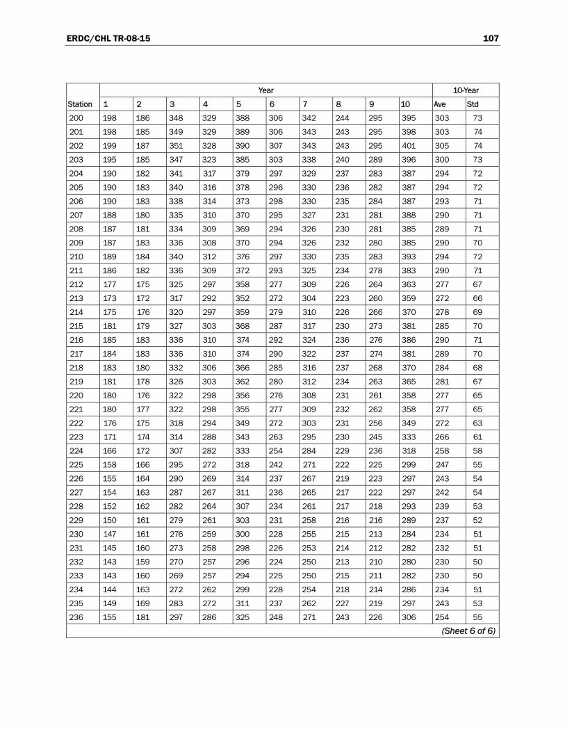
ERDC/CHL TR-08-15 107
Year 10-Year
Station 1 2 3 4 5 6 7 8 9 10 Ave Std
200 198 186 348 329 388 306 342 244 295 395 303 73
201 198 185 349 329 389 306 343 243 295 398 303 74
202 199 187 351 328 390 307 343 243 295 401 305 74
203 195 185 347 323 385 303 338 240 289 396 300 73
204 190 182 341 317 379 297 329 237 283 387 294 72
205 190 183 340 316 378 296 330 236 282 387 294 72
206 190 183 338 314 373 298 330 235 284 387 293 71
207 188 180 335 310 370 295 327 231 281 388 290 71
208 187 181 334 309 369 294 326 230 281 385 289 71
209 187 183 336 308 370 294 326 232 280 385 290 70
210 189 184 340 312 376 297 330 235 283 393 294 72
211 186 182 336 309 372 293 325 234 278 383 290 71
212 177 175 325 297 358 277 309 226 264 363 277 67
213 173 172 317 292 352 272 304 223 260 359 272 66
214 175 176 320 297 359 279 310 226 266 370 278 69
215 181 179 327 303 368 287 317 230 273 381 285 70
216 185 183 336 310 374 292 324 236 276 386 290 71
217 184 183 336 310 374 290 322 237 274 381 289 70
218 183 180 332 306 366 285 316 237 268 370 284 68
219 181 178 326 303 362 280 312 234 263 365 281 67
220 180 176 322 298 356 276 308 231 261 358 277 65
221 180 177 322 298 355 277 309 232 262 358 277 65
222 176 175 318 294 349 272 303 231 256 349 272 63
223 171 174 314 288 343 263 295 230 245 333 266 61
224 166 172 307 282 333 254 284 229 236 318 258 58
225 158 166 295 272 318 242 271 222 225 299 247 55
226 155 164 290 269 314 237 267 219 223 297 243 54
227 154 163 287 267 311 236 265 217 222 297 242 54
228 152 162 282 264 307 234 261 217 218 293 239 53
229 150 161 279 261 303 231 258 216 216 289 237 52
230 147 161 276 259 300 228 255 215 213 284 234 51
231 145 160 273 258 298 226 253 214 212 282 232 51
232 143 159 270 257 296 224 250 213 210 280 230 50
233 143 160 269 257 294 225 250 215 211 282 230 50
234 144 163 272 262 299 228 254 218 214 286 234 51
235 149 169 283 272 311 237 262 227 219 297 243 53
236 155 181 297 286 325 248 271 243 226 306 254 55
(Sheet 6 of 6)

ERDC/CHL TR-08-15 108
Appendix D: Average Annual Changes in Longshore Transport Rates Between Plan 1 and Existing Bathymetry1,2
1 This appendix contains Figures and tables for south, north, net, and gross longshore transport rates. 2 Values in tables show two decimal-place accuracy to better highlight difference because of small
values of numbers.

ERDC/CHL TR-08-15 109
Figure D1. Average annual change in southerly longshore transport rates
for monitoring stations, Plan 1 – Existing bathymetry.
Figure D2. Average annual change in northerly longshore transport rates
for monitoring stations, Plan 1 – Existing bathymetry.

ERDC/CHL TR-08-15 110
Figure D3. Average annual change in net longshore transport rates for monitoring
stations, Plan 1 – Existing bathymetry.
Figure D4. Average annual change in gross longshore transport rates for monitoring
stations, Plan 1 – Existing bathymetry.

ERDC/CHL TR-08-15 111
Table D1. Southern longshore transport rates, change = P1 – Ex, 1990–1999, 1,000 cu yd/yr.
Year 10-Year
Station 1 2 3 4 5 6 7 8 9 10 Ave Std
1 1.16 1.51 3.44 3.06 5.45 0.91 2.90 2.72 0.58 2.37 2.41 1.46
2 0.71 1.17 2.40 1.96 2.14 0.61 1.81 1.95 0.54 1.62 1.49 0.68
3 0.21 0.90 3.19 1.24 2.90 0.60 0.90 0.85 0.47 1.11 1.24 1.00
4 0.19 0.95 1.15 0.88 1.13 0.41 0.59 0.79 0.31 2.34 0.87 0.61
5 0.66 1.45 2.95 3.38 3.95 1.28 2.14 2.80 0.72 2.51 2.18 1.13
6 0.28 0.55 1.74 0.95 1.22 0.30 0.73 0.82 0.21 0.62 0.74 0.47
7 0.80 2.05 3.24 2.06 2.18 1.13 1.67 1.93 1.02 1.99 1.81 0.70
8 0.50 0.74 1.27 0.96 1.22 0.20 0.75 0.57 0.23 0.93 0.74 0.37
9 0.62 1.05 1.27 1.11 1.04 0.56 1.35 1.45 0.74 1.01 1.02 0.30
10 0.07 0.22 0.26 0.37 0.43 0.07 0.27 0.30 0.12 0.34 0.25 0.13
11 0.55 0.44 1.54 0.52 1.47 0.14 0.48 0.56 0.26 0.89 0.69 0.47
12 0.07 1.14 3.04 1.10 2.59 0.33 0.92 0.76 0.23 2.93 1.31 1.13
13 0.52 1.15 3.60 1.31 2.56 0.69 1.85 1.49 0.78 1.25 1.52 0.94
14 0.35 1.01 1.76 0.62 0.93 0.19 0.82 1.04 0.13 0.89 0.77 0.48
15 0.42 1.65 1.37 1.77 1.99 0.43 0.77 1.89 0.73 1.25 1.23 0.60
16 0.99 1.37 1.88 1.80 1.40 0.92 1.38 2.04 0.77 1.57 1.41 0.43
17 0.48 1.32 1.80 1.90 3.17 1.09 1.88 1.95 1.00 2.51 1.71 0.78
18 0.34 0.54 2.94 1.72 3.19 0.26 1.25 0.90 0.20 1.05 1.24 1.07
19 0.16 0.74 1.19 1.14 1.30 0.29 0.44 1.10 0.44 0.63 0.74 0.41
20 0.59 1.37 2.92 3.17 3.96 0.72 2.69 2.30 0.84 1.65 2.02 1.16
21 0.33 0.57 1.97 0.65 1.38 0.57 1.03 0.77 0.19 0.92 0.84 0.53
22 1.05 1.51 2.66 1.36 2.10 0.85 1.50 1.27 0.38 3.54 1.62 0.92
23 0.68 0.74 1.01 0.79 1.28 0.43 1.25 1.10 0.15 1.19 0.86 0.37
24 0.25 0.54 0.49 0.53 0.61 0.21 0.49 0.59 0.10 0.52 0.43 0.18
25 1.11 1.76 4.44 2.12 4.23 0.52 2.25 2.06 0.80 1.69 2.10 1.31
26 0.17 0.93 2.30 1.18 2.01 0.44 0.60 0.25 0.26 3.20 1.13 1.04
27 0.62 0.43 1.64 0.60 1.61 0.26 0.76 0.43 0.12 1.22 0.77 0.54
28 0.54 0.84 3.43 1.46 3.21 0.38 1.87 1.33 0.33 1.27 1.47 1.10
29 0.45 1.12 1.61 1.41 1.66 0.45 0.63 1.42 0.47 1.09 1.03 0.49
30 0.36 0.35 4.63 1.42 3.39 0.34 1.39 1.15 0.38 1.29 1.47 1.44
31 0.26 0.25 3.96 1.16 3.41 0.32 1.44 0.84 0.20 1.16 1.30 1.34
32 0.22 0.32 3.42 1.60 3.45 0.58 1.57 1.33 0.45 1.48 1.44 1.18
33 0.43 0.79 1.70 1.07 1.06 0.47 1.06 1.31 0.63 1.10 0.96 0.39
34 0.25 0.65 1.59 0.76 0.58 0.30 1.06 0.64 0.52 0.46 0.68 0.39
35 0.36 0.41 2.80 1.26 2.75 0.17 1.70 0.56 0.15 0.83 1.10 1.01
36 0.71 1.32 1.40 1.47 0.95 1.00 1.45 1.52 0.76 1.15 1.17 0.30
37 0.51 0.70 1.92 0.89 0.68 0.49 0.86 0.94 0.20 0.83 0.80 0.45
38 0.72 1.36 2.08 1.82 1.90 1.09 1.84 2.11 0.85 1.75 1.55 0.51
39 0.17 0.40 0.64 0.63 0.83 0.16 0.44 0.02 0.07 0.75 0.41 0.30
(Sheet 1 of 6)
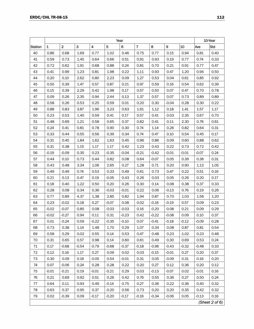
ERDC/CHL TR-08-15 112
Year 10-Year
Station 1 2 3 4 5 6 7 8 9 10 Ave Std
40 0.86 0.68 1.69 0.77 1.02 0.46 0.75 0.77 0.15 0.94 0.81 0.40
41 0.59 0.73 1.45 0.64 0.66 0.51 0.91 0.93 0.19 0.77 0.74 0.33
42 0.72 0.62 1.91 0.68 0.88 0.24 0.81 0.70 0.21 0.91 0.77 0.47
43 0.41 0.99 1.23 0.81 1.98 0.22 1.11 0.93 0.47 1.20 0.94 0.50
44 0.20 0.10 2.62 0.80 2.23 0.09 1.27 0.53 0.04 0.61 0.85 0.92
45 0.50 0.39 1.47 0.57 0.87 0.21 0.97 0.59 0.16 0.54 0.62 0.39
46 0.15 0.39 2.29 0.42 1.98 0.17 0.57 0.50 0.07 0.47 0.70 0.78
47 0.09 0.26 2.35 0.94 2.44 0.13 1.37 0.57 0.07 0.73 0.89 0.89
48 0.58 0.26 0.53 0.25 0.59 0.01 0.20 0.30 -0.04 0.28 0.30 0.22
49 0.88 0.83 3.87 1.96 3.23 0.63 1.61 1.12 0.18 1.41 1.57 1.17
50 0.23 0.53 1.40 0.59 0.41 0.17 0.57 0.41 0.03 2.35 0.67 0.70
51 0.48 0.69 1.21 0.58 0.65 0.37 0.82 0.41 0.11 2.30 0.76 0.61
52 0.24 0.41 0.81 0.78 0.90 0.30 0.74 1.14 0.26 0.82 0.64 0.31
53 0.33 0.44 0.55 0.56 0.39 0.34 0.74 0.47 0.10 0.54 0.45 0.17
54 0.31 0.45 1.84 1.62 1.63 0.45 0.96 0.86 0.09 0.60 0.88 0.62
55 0.31 0.38 1.15 1.17 1.17 0.42 1.23 0.43 0.22 0.73 0.72 0.42
56 -0.19 -0.09 0.35 0.23 -0.35 -0.04 -0.21 -0.42 -0.01 -0.01 -0.07 0.24
57 0.44 0.10 0.73 0.44 0.82 0.08 0.64 -0.07 0.05 0.39 0.36 0.31
58 0.43 0.48 3.34 1.06 2.65 0.27 1.28 0.71 0.20 0.90 1.13 1.05
59 0.49 0.49 0.74 0.53 0.33 0.49 0.61 0.73 0.47 0.22 0.51 0.16
60 0.21 0.13 0.47 0.19 -0.05 0.43 0.26 0.03 0.05 0.26 0.20 0.17
61 0.18 0.40 1.22 0.50 0.20 0.26 0.30 0.14 0.08 0.38 0.37 0.33
62 0.28 0.08 0.34 0.36 -0.03 -0.01 0.22 0.06 -0.13 0.76 0.19 0.26
63 0.77 0.89 4.37 1.38 2.85 0.82 1.94 0.87 0.70 1.03 1.56 1.20
64 0.23 -0.02 0.18 0.27 -0.07 0.08 0.02 -0.16 -0.19 0.57 0.09 0.23
65 -0.02 -0.07 0.85 0.08 -0.03 -0.03 0.16 -0.20 -0.08 0.21 0.09 0.29
66 -0.02 -0.27 0.94 0.11 0.31 -0.23 0.42 -0.22 -0.08 0.09 0.10 0.37
67 0.01 -0.24 0.59 -0.22 -0.35 -0.10 0.07 -0.41 -0.18 -0.12 -0.09 0.28
68 0.73 0.38 1.14 1.48 1.70 0.29 1.07 0.34 0.08 0.87 0.81 0.54
69 0.58 0.29 0.02 0.55 0.14 0.53 0.47 0.48 0.23 -1.02 0.23 0.48
70 0.31 0.65 0.57 0.98 0.14 0.60 0.61 0.49 0.30 0.69 0.53 0.24
71 0.17 -0.68 -0.54 -0.79 -0.68 -0.37 -0.18 -0.96 -0.43 -0.32 -0.48 0.33
72 0.12 0.16 1.17 0.27 0.09 0.02 0.03 -0.15 -0.01 0.27 0.20 0.37
73 0.30 0.09 0.16 -0.05 0.54 -0.01 0.31 0.05 -0.09 0.31 0.16 0.20
74 0.07 -0.06 0.24 0.28 0.28 0.22 0.20 0.27 0.12 0.36 0.20 0.12
75 -0.01 -0.21 0.19 -0.01 -0.21 0.29 0.03 -0.13 -0.07 0.02 -0.01 0.16
76 0.21 0.69 0.92 0.51 0.26 0.42 0.76 0.55 0.36 0.27 0.50 0.24
77 0.64 0.11 0.93 0.49 -0.14 0.75 0.27 0.36 0.22 0.36 0.40 0.32
78 0.63 0.37 0.95 0.37 -0.20 0.56 0.73 0.20 0.20 0.35 0.42 0.32
79 0.02 -0.39 0.09 -0.17 -0.20 -0.17 -0.16 -0.34 -0.06 0.05 -0.13 0.16
(Sheet 2 of 6)

ERDC/CHL TR-08-15 113
Year 10-Year
Station 1 2 3 4 5 6 7 8 9 10 Ave Std
80 0.42 -0.20 0.89 0.33 -0.49 0.86 0.56 -0.06 -0.08 0.55 0.28 0.47
81 0.66 -0.08 0.22 0.60 -0.53 1.09 0.50 0.35 0.69 0.04 0.35 0.46
82 -0.09 -0.33 0.51 -0.45 -0.05 -0.36 0.09 -0.81 -0.34 0.00 -0.18 0.36
83 -0.02 -0.45 -0.05 -0.38 0.04 -0.25 -0.19 -0.52 -0.23 0.07 -0.20 0.21
84 0.19 -0.19 0.20 -0.22 -0.51 0.30 -0.04 -0.39 -0.05 -0.12 -0.08 0.26
85 0.27 -0.24 0.65 0.55 -0.06 0.47 0.95 0.35 0.21 0.10 0.32 0.35
86 0.04 -0.45 2.44 -0.31 1.10 -0.08 0.17 -0.56 -0.17 -0.16 0.20 0.91
87 0.67 0.21 0.87 0.51 -0.21 0.94 0.75 0.38 0.28 0.57 0.50 0.34
88 0.33 0.01 0.36 -0.24 -0.53 0.35 0.12 -0.57 -0.19 -0.12 -0.05 0.34
89 0.49 0.07 1.00 0.68 0.61 0.76 1.09 0.14 0.05 0.31 0.52 0.37
90 -0.04 -0.52 -0.27 -0.72 -1.28 -0.01 -0.60 -0.94 -0.28 -0.33 -0.50 0.40
91 -0.06 -0.16 0.05 -0.27 -0.46 -0.05 -0.13 -0.42 -0.17 -0.35 -0.20 0.17
92 -0.01 -0.38 -0.15 -0.29 -0.56 -0.01 -0.18 -0.50 -0.13 -0.13 -0.23 0.19
93 0.11 -0.38 -0.11 -0.20 -1.27 0.01 -0.15 -0.48 -0.08 -0.78 -0.33 0.42
94 -0.08 -0.57 -0.30 -0.63 -0.32 -0.36 -0.36 -0.94 -0.24 -0.49 -0.43 0.24
95 0.86 0.21 0.77 0.54 -0.49 1.35 0.28 0.26 0.64 0.48 0.49 0.49
96 0.36 -0.57 0.05 -0.45 -0.76 0.00 0.00 -0.43 -0.07 -1.76 -0.36 0.60
97 -0.06 -0.55 -0.32 -0.41 -0.58 -0.17 -0.32 -0.60 -0.19 -0.32 -0.35 0.18
98 -0.10 -0.61 -0.57 -0.58 -0.95 -0.21 -0.43 -0.82 -0.19 -0.57 -0.50 0.27
99 0.35 -0.34 0.40 -0.63 -0.92 -0.09 -0.11 -0.85 -0.23 -0.54 -0.30 0.45
100 -0.02 -0.13 -0.35 -0.38 -0.71 -0.28 -0.42 -0.77 -0.10 -0.17 -0.33 0.25
101 -0.09 -0.52 -0.44 -0.72 -1.03 -0.37 -0.39 -0.84 -0.36 -0.66 -0.54 0.27
102 -0.01 -0.82 -0.50 -0.58 -0.82 -0.22 -0.27 -0.81 -0.24 -0.72 -0.50 0.30
103 0.21 -0.12 -0.37 -0.42 -0.84 0.14 -0.15 -0.61 -0.11 -0.60 -0.29 0.34
104 0.16 -0.47 -0.47 -0.71 -1.04 -0.29 -0.39 -0.95 -0.33 -0.84 -0.54 0.36
105 -0.03 -0.67 0.13 -0.87 -1.20 -0.32 -0.44 -1.17 -0.37 -0.75 -0.57 0.44
106 0.00 -0.62 -0.52 -0.49 -1.04 -0.16 -0.45 -0.89 -0.23 -0.68 -0.51 0.32
107 -0.04 -0.72 0.09 -0.82 -0.96 -0.09 -0.54 -0.68 -0.36 -0.70 -0.48 0.36
108 -0.09 -0.71 -0.60 -0.83 -1.04 -0.25 -0.19 -0.83 -0.40 -0.85 -0.58 0.33
109 -0.03 -0.78 0.05 -1.10 -1.24 -0.41 -0.56 -1.09 -0.39 -0.99 -0.65 0.46
110 -0.12 -1.22 -2.09 -0.98 -2.68 -0.26 -0.84 -1.37 -0.23 -2.53 -1.23 0.94
111 -0.47 -1.33 -0.67 -1.31 -1.57 -0.53 -0.84 -1.70 -0.49 -2.82 -1.17 0.74
112 0.13 -0.91 -0.84 -1.10 -1.55 -0.41 -0.66 -1.51 -0.50 -1.10 -0.85 0.51
113 0.16 -1.17 -0.81 -0.99 -1.42 -0.35 -0.61 -1.18 -0.42 -0.83 -0.76 0.47
114 -0.03 -0.16 -0.44 -0.55 -0.86 -0.45 -0.60 -0.79 -0.12 -0.95 -0.49 0.32
115 -0.09 -0.60 -0.54 -0.86 -1.88 -0.19 -0.63 -1.03 -0.23 -1.38 -0.74 0.56
116 -0.14 -0.51 -0.61 -0.90 -1.20 -0.19 -0.52 -1.15 -0.40 -0.87 -0.65 0.37
117 0.05 -0.79 0.22 -0.88 -1.22 -0.46 -0.32 -1.27 -0.34 -1.06 -0.61 0.52
118 -0.18 -1.04 -1.14 -1.23 -1.86 -0.43 -1.16 -1.42 -0.48 -1.12 -1.01 0.50
119 -0.24 -1.04 -1.03 -1.38 -1.94 -0.43 -0.95 -1.64 -0.48 -1.65 -1.08 0.58
(Sheet 3 of 6)

ERDC/CHL TR-08-15 114
Year 10-Year
Station 1 2 3 4 5 6 7 8 9 10 Ave Std
120 0.03 -0.86 -0.77 -0.94 -1.37 -0.19 -0.48 -1.09 -0.35 -1.02 -0.70 0.44
121 -0.49 -1.12 -0.85 -1.07 -1.76 -0.64 -0.76 -1.57 -0.63 -1.36 -1.02 0.43
122 -0.16 -0.90 -0.50 -1.22 -1.98 -0.43 -0.69 -1.46 -0.49 -1.40 -0.92 0.57
123 -0.26 -0.89 -0.67 -1.06 -1.70 -0.28 -0.62 -1.34 -0.43 -1.11 -0.83 0.47
124 0.15 -1.03 -0.21 -1.48 -1.32 -0.44 -0.60 -1.57 -0.48 -1.05 -0.80 0.57
125 -0.15 -0.86 -0.89 -0.96 -1.87 -0.21 -0.53 -1.15 -0.34 -1.16 -0.81 0.53
126 -0.14 -1.03 -0.80 -1.47 -2.17 -0.56 -1.00 -1.69 -0.52 -1.56 -1.10 0.62
127 0.57 -0.75 -0.04 -0.52 -1.14 0.37 -0.13 -0.60 0.30 -0.78 -0.27 0.57
128 -0.20 -0.98 -0.66 -1.38 -1.82 -0.49 -0.63 -1.47 -0.48 -1.16 -0.93 0.52
129 -0.05 -0.87 -0.23 -1.23 -1.48 -0.53 -0.74 -1.48 -0.39 -1.11 -0.81 0.51
130 0.19 -1.18 -0.01 -1.64 -2.16 -0.70 -1.08 -1.90 -0.51 -1.51 -1.05 0.79
131 0.03 -0.77 -0.93 -1.44 -1.49 -0.56 -0.63 -1.36 -0.53 -1.43 -0.91 0.51
132 0.01 -0.71 0.44 -0.50 -0.64 -0.45 -0.45 -1.33 -0.47 -1.12 -0.52 0.50
133 0.03 -0.63 1.36 -1.26 -0.32 -0.34 -1.00 -1.30 -0.31 -1.65 -0.54 0.86
134 -0.12 -0.44 1.22 -0.73 0.39 -0.13 -0.51 -1.14 -0.21 -1.24 -0.29 0.72
135 -0.05 -0.27 2.25 -0.65 0.20 0.17 -0.50 -1.28 -0.32 0.32 -0.01 0.93
136 0.34 -0.09 2.62 -0.22 0.05 0.91 0.01 -0.73 0.27 1.21 0.44 0.94
137 0.38 -0.29 0.36 -0.32 -1.36 0.89 -0.24 -0.25 0.34 -0.62 -0.11 0.63
138 0.34 -0.10 -0.05 -0.87 -1.21 0.36 -0.56 -0.92 -0.28 -0.78 -0.41 0.54
139 0.10 -0.56 -0.59 -1.17 -1.63 -0.08 -0.75 -1.36 -0.45 -1.16 -0.76 0.56
140 0.81 0.52 2.14 0.98 0.62 0.91 0.60 0.44 0.55 1.18 0.88 0.50
141 0.08 -1.02 -0.17 -1.06 -0.51 -0.38 -0.31 -1.00 -0.50 -1.19 -0.61 0.43
142 -0.19 -0.81 -0.56 -1.50 -2.01 -0.82 -1.31 -1.71 -0.46 -1.93 -1.13 0.65
143 -0.04 -0.53 0.13 -0.72 -1.40 -0.40 -0.59 -1.52 -0.58 -0.14 -0.58 0.54
144 -0.27 -0.80 -1.54 -1.21 -2.24 -0.41 -1.15 -1.36 -0.33 -1.66 -1.10 0.64
145 0.36 -0.70 -0.73 -0.51 -1.18 0.50 -0.04 -0.18 0.32 -0.51 -0.27 0.55
146 -0.02 -0.59 0.48 -0.72 -1.91 0.70 -0.39 -0.59 0.23 -0.96 -0.38 0.77
147 0.35 -0.41 0.96 0.26 -0.66 1.00 0.19 0.19 0.36 -0.37 0.19 0.55
148 -0.33 -0.87 -0.12 -1.18 -2.07 -0.50 -0.89 -1.09 -0.58 -1.65 -0.93 0.60
149 0.07 -0.33 0.03 -0.47 -0.87 -0.05 0.19 -0.90 0.02 0.35 -0.19 0.43
150 -0.35 -0.87 -0.61 -1.15 -2.34 0.00 -0.88 -1.45 -0.50 -1.51 -0.97 0.68
151 -0.14 -0.53 -0.92 -0.49 -0.97 -0.36 -0.14 -0.61 -0.50 -1.43 -0.61 0.40
152 -0.08 -0.47 0.05 -0.37 -1.21 -0.15 0.03 -0.92 -0.01 -1.01 -0.42 0.47
153 0.05 -0.05 0.39 -0.06 -1.11 0.85 -0.26 -0.53 0.32 0.74 0.03 0.59
154 0.09 -0.42 2.65 0.02 0.92 0.92 0.09 -0.37 0.30 -0.47 0.37 0.94
155 0.14 -0.02 2.87 0.42 1.41 1.22 0.31 -0.05 0.49 1.58 0.84 0.93
156 0.10 -0.20 0.42 -0.04 -0.52 1.02 -0.19 -0.26 0.43 -0.48 0.03 0.48
157 0.08 -0.10 0.59 0.24 -0.03 1.06 -0.22 -0.15 0.45 -0.20 0.17 0.42
158 0.47 0.21 2.19 1.03 0.99 1.17 0.76 0.30 0.65 0.63 0.84 0.57
159 0.18 0.43 1.14 -0.37 -1.17 -0.02 -0.29 -0.08 0.19 -0.85 -0.08 0.65
(Sheet 4 of 6)

ERDC/CHL TR-08-15 115
Year 10-Year
Station 1 2 3 4 5 6 7 8 9 10 Ave Std
160 0.32 0.37 3.01 1.37 1.10 0.29 1.15 -0.04 0.30 1.30 0.92 0.89
161 0.27 0.44 2.62 0.67 -0.04 0.62 0.89 0.48 0.33 1.33 0.76 0.75
162 -0.06 -0.04 1.62 -0.79 0.35 -0.11 -0.17 -1.26 -0.44 -0.55 -0.15 0.77
163 -0.76 -0.38 0.24 -0.51 0.54 -0.31 -0.04 -1.10 -0.46 -0.44 -0.32 0.47
164 -0.09 -0.16 0.34 -0.51 0.69 -0.08 0.12 -0.43 -0.23 0.24 -0.01 0.36
165 0.02 -0.36 -0.15 -0.41 -0.45 -0.13 -0.18 -0.42 -0.24 -0.41 -0.27 0.16
166 -0.16 0.20 0.46 -0.61 -0.22 0.07 -0.21 -0.47 -0.11 -0.13 -0.12 0.31
167 0.21 0.87 1.27 0.64 -0.27 1.23 0.38 0.33 0.69 0.32 0.57 0.48
168 0.26 0.38 0.90 0.15 0.11 1.21 0.43 0.04 0.52 -0.05 0.39 0.40
169 0.11 0.83 0.94 0.60 0.44 1.46 0.57 0.38 0.66 0.53 0.65 0.37
170 -0.16 0.36 2.85 -0.22 1.26 0.42 0.03 -0.68 0.07 -0.57 0.33 1.04
171 -0.25 -0.49 1.51 -0.41 1.32 -0.21 0.02 -1.29 -0.28 -0.75 -0.08 0.87
172 -0.22 -0.36 1.89 -0.43 2.58 -0.16 0.53 -0.29 -0.22 -0.06 0.33 1.05
173 -0.06 0.05 2.38 -0.62 0.74 0.00 -0.04 -0.88 -0.20 -0.43 0.09 0.92
174 -0.27 0.77 0.55 0.06 -0.66 0.58 -0.02 -0.26 0.20 -0.38 0.06 0.47
175 0.45 1.31 2.09 2.06 0.68 1.69 1.07 1.39 1.07 1.89 1.37 0.57
176 0.07 0.55 0.05 0.50 -0.80 1.36 0.21 0.25 0.49 -0.34 0.23 0.57
177 -0.09 0.59 0.26 -0.01 -0.40 1.21 -0.24 0.53 0.46 0.08 0.24 0.47
178 -0.24 0.48 -0.49 -0.14 -1.62 0.86 -0.25 0.21 0.31 -0.66 -0.15 0.69
179 -0.16 -0.01 -0.74 -0.40 -1.99 0.66 -0.43 0.12 0.30 -0.86 -0.35 0.74
180 -0.07 0.69 2.36 0.55 1.12 1.18 0.83 0.26 0.50 1.15 0.86 0.66
181 -0.21 0.32 -0.12 0.36 -0.64 0.65 0.27 0.06 0.50 -0.27 0.09 0.40
182 -0.33 -0.33 -0.38 -0.83 0.38 -0.34 -0.19 -0.79 -0.46 -0.79 -0.41 0.36
183 -0.11 0.18 1.82 -0.41 0.20 0.69 0.03 -0.19 0.29 -1.05 0.15 0.75
184 -0.73 -0.50 -0.43 -0.16 -0.42 -0.19 -0.47 -0.89 -0.55 -1.27 -0.56 0.33
185 -0.09 0.71 1.68 -0.26 -0.46 0.56 -0.07 -0.07 0.00 -0.51 0.15 0.67
186 0.21 1.23 1.46 0.81 -0.25 0.92 0.26 0.66 1.08 0.01 0.64 0.56
187 -0.81 0.44 -0.37 -0.65 0.24 -0.08 -0.32 -0.89 -0.38 -0.11 -0.29 0.43
188 -0.43 0.61 1.53 -0.27 1.03 0.05 0.09 -0.05 -0.10 -0.71 0.18 0.69
189 -0.34 0.26 1.03 -0.56 0.69 -0.31 -0.11 -0.67 -0.41 -0.56 -0.10 0.58
190 0.02 0.94 1.43 0.85 0.85 0.29 0.95 0.69 1.02 -0.26 0.68 0.51
191 -0.13 0.48 1.58 0.90 1.45 0.31 0.97 0.55 0.50 0.16 0.68 0.55
192 -0.40 -0.14 -1.12 -0.41 -0.43 -0.36 -0.23 -0.34 0.01 -0.37 -0.38 0.30
193 -0.69 0.01 -2.22 0.04 0.25 -0.04 0.24 -0.04 -0.16 1.43 -0.12 0.91
194 -0.62 -0.29 -1.00 -0.46 -0.18 -0.11 -0.11 -0.47 -0.26 -0.28 -0.38 0.27
195 -0.53 -0.67 -0.42 -0.32 -0.29 -0.12 -0.13 -0.13 -0.17 -0.53 -0.33 0.20
196 -0.27 0.49 -0.59 0.59 0.56 -0.02 0.10 0.75 0.51 0.06 0.22 0.43
197 -0.14 0.02 -0.43 0.35 0.35 -0.14 0.16 -0.26 0.22 -0.27 -0.01 0.27
198 0.01 -0.18 0.45 -0.02 1.42 0.12 0.07 0.19 0.06 0.07 0.22 0.45
199 -0.45 0.04 -2.00 0.14 0.07 -0.11 -0.10 0.01 0.11 -0.05 -0.23 0.64
(Sheet 5 of 6)

ERDC/CHL TR-08-15 116
Year 10-Year
Station 1 2 3 4 5 6 7 8 9 10 Ave Std
200 -0.69 -0.83 -4.68 -0.70 0.01 -1.06 -0.20 -0.28 -0.20 -1.53 -1.02 1.37
201 -1.22 -1.72 -3.46 -1.00 -0.82 -1.17 -0.88 -0.63 -1.38 -0.85 -1.31 0.82
202 -0.05 -0.38 -1.38 -0.22 -0.27 0.07 -0.52 -0.13 0.01 0.05 -0.28 0.43
203 -0.06 -0.28 -1.40 0.04 0.83 -0.23 -0.01 0.35 0.15 0.29 -0.03 0.58
204 0.13 0.12 -1.35 0.11 0.40 -0.25 -0.14 0.58 0.22 0.52 0.03 0.55
205 0.18 0.46 -0.97 0.21 0.81 -0.10 0.05 0.97 0.39 0.63 0.26 0.55
206 -0.40 -0.32 -3.46 -0.41 -1.51 -0.03 -0.29 0.72 0.37 0.65 -0.47 1.23
207 -0.91 -2.11 -2.71 -1.16 -0.59 -0.86 -0.42 -1.20 -1.05 -0.37 -1.14 0.74
208 -0.14 0.28 -1.09 0.37 0.10 0.29 0.23 0.42 0.33 -1.04 -0.02 0.57
209 -0.15 0.48 -0.74 0.14 0.48 -0.40 0.13 0.28 0.32 -0.98 -0.04 0.51
210 -1.24 -0.76 -1.84 -1.20 -0.31 -0.39 -0.61 -0.30 -0.55 0.16 -0.70 0.58
211 -0.88 -0.79 -3.71 0.26 -0.36 -0.70 0.07 0.55 0.16 0.31 -0.51 1.23
212 -0.31 0.30 -1.79 1.31 0.93 -0.02 0.85 1.55 0.73 -0.02 0.35 0.96
213 -0.35 -0.75 -2.85 0.49 -0.29 -0.57 0.15 0.76 0.19 0.79 -0.24 1.06
214 -0.70 -0.53 -2.05 -0.65 0.69 -0.79 -0.21 -0.31 -0.66 0.25 -0.50 0.72
215 -0.68 -0.92 -2.72 -1.37 -0.50 -0.92 -0.80 -0.47 -0.55 0.09 -0.88 0.75
216 -0.61 -0.48 -0.72 0.84 1.32 -0.19 0.40 1.29 0.59 -0.31 0.21 0.78
217 -0.80 -0.96 -2.73 -0.44 0.05 -1.35 -0.16 -0.50 -0.97 -0.09 -0.79 0.81
218 0.04 -0.09 -0.98 0.53 1.12 0.51 0.56 1.18 0.41 1.90 0.52 0.79
219 -0.53 -0.40 -1.51 0.65 2.04 -0.32 0.49 1.02 0.13 0.37 0.19 0.97
220 0.37 -0.19 -0.38 -0.89 0.29 -0.58 -0.01 -0.08 -0.16 1.01 -0.06 0.53
221 -0.22 0.28 -0.27 1.36 1.10 0.01 0.71 1.14 0.39 1.63 0.61 0.68
222 -0.85 -0.88 -2.12 0.06 0.85 -1.43 0.24 0.13 -0.49 0.66 -0.38 0.95
223 -0.11 -0.12 -0.57 1.03 0.77 -0.88 0.28 0.58 0.17 -0.12 0.10 0.59
224 -0.39 0.50 0.19 3.07 2.19 1.36 1.46 2.39 0.77 2.74 1.43 1.16
225 -0.52 -0.40 -1.44 -0.20 -0.62 -0.46 -0.58 0.22 -0.02 1.02 -0.30 0.64
226 0.24 0.46 0.44 2.21 1.68 1.05 1.10 2.34 0.50 2.28 1.23 0.84
227 -0.65 0.37 -1.23 1.89 -0.07 1.12 0.68 1.01 0.37 2.06 0.55 1.04
228 -0.46 0.55 -0.48 1.65 0.03 1.13 0.58 1.01 0.55 1.53 0.61 0.75
229 0.27 0.15 -0.16 0.84 0.93 -0.07 0.94 0.75 0.91 1.31 0.59 0.50
230 -0.09 -0.30 -2.09 0.40 -0.24 -0.79 0.72 -0.27 -0.41 1.32 -0.17 0.91
231 -0.36 -0.79 -0.33 0.33 -0.19 -0.89 0.35 -0.78 -0.45 1.26 -0.19 0.66
232 -0.20 0.40 0.47 0.41 0.23 -0.64 0.61 -0.37 0.25 1.39 0.26 0.57
233 0.23 0.48 0.54 0.60 -0.71 0.47 0.74 0.43 0.74 1.77 0.53 0.60
234 -0.03 0.61 -1.62 0.35 -1.75 -0.06 0.20 0.10 0.86 1.47 0.01 1.01
235 -0.32 -0.34 -2.26 -1.02 -1.88 -0.61 -0.93 -0.89 0.13 0.55 -0.76 0.85
236 0.14 -0.61 -1.87 0.80 -0.81 1.07 1.14 0.54 0.69 0.33 0.14 0.96
(Sheet 6 of 6)

ERDC/CHL TR-08-15 117
Table D2. Northern longshore transport rates, change = P1 – Ex, 1990–1999, 1,000 cu yd/yr.
Year 10-Year
Station 1 2 3 4 5 6 7 8 9 10 Ave Std
1 1.37 1.61 1.86 2.47 2.34 2.05 2.71 1.01 3.10 5.18 2.37 1.17
2 0.36 -0.06 1.63 0.66 1.62 1.98 0.18 0.13 0.58 3.85 1.09 1.20
3 0.27 0.41 0.25 0.61 0.95 -0.33 0.98 0.30 -0.19 0.21 0.35 0.42
4 0.17 0.02 -0.26 -0.07 -0.20 -0.10 0.15 -0.19 0.15 0.10 -0.02 0.16
5 0.30 2.46 3.62 1.33 1.42 1.90 0.75 1.20 1.06 1.14 1.52 0.94
6 -0.01 1.27 3.54 0.62 1.19 1.74 0.43 0.83 -0.10 0.62 1.01 1.05
7 0.42 1.86 2.11 2.12 1.19 1.80 0.37 1.28 2.10 0.96 1.42 0.68
8 0.32 0.93 0.45 0.98 0.48 0.38 0.09 0.80 0.84 1.16 0.64 0.35
9 0.64 1.23 1.18 1.87 1.18 1.69 0.76 0.86 1.35 0.65 1.14 0.42
10 0.13 -0.06 0.96 0.67 1.02 0.76 0.44 0.58 1.02 1.19 0.67 0.41
11 0.43 1.20 3.40 1.35 0.74 2.46 1.82 0.62 1.31 0.97 1.43 0.91
12 1.28 2.39 4.20 3.29 2.14 2.48 3.48 1.36 2.01 4.57 2.72 1.13
13 0.52 1.01 0.85 2.23 0.75 1.07 1.23 1.00 2.42 1.21 1.23 0.62
14 0.64 1.56 4.93 2.10 1.43 3.40 0.51 1.15 1.42 2.12 1.93 1.34
15 0.99 3.12 4.48 1.23 2.33 0.51 1.52 0.72 2.69 2.68 2.03 1.25
16 0.37 0.57 3.59 1.98 1.51 2.82 1.66 1.16 1.85 0.90 1.64 1.00
17 0.71 2.59 5.07 2.81 2.53 1.39 1.88 0.94 3.52 4.55 2.60 1.46
18 0.28 0.34 1.61 0.48 0.99 0.76 0.15 0.59 0.02 1.04 0.62 0.48
19 -0.08 2.23 4.23 0.79 1.29 0.81 0.62 0.44 0.49 1.18 1.20 1.23
20 1.80 1.71 3.97 1.96 1.74 1.52 1.70 1.87 1.78 2.33 2.04 0.71
21 1.41 2.82 2.30 3.50 1.18 3.12 4.35 1.41 4.19 5.18 2.95 1.38
22 0.69 1.57 2.70 2.04 2.37 2.70 1.37 0.93 2.62 2.21 1.92 0.74
23 0.57 0.29 0.17 1.57 0.62 1.01 0.56 1.00 1.92 1.69 0.94 0.61
24 0.66 3.48 5.70 1.96 2.18 1.64 2.50 0.72 2.36 2.13 2.33 1.44
25 1.08 1.72 4.00 2.04 1.67 3.36 3.40 1.53 3.21 3.59 2.56 1.05
26 0.22 0.82 1.98 1.16 1.15 0.77 1.06 0.50 0.68 0.96 0.93 0.47
27 1.04 4.10 7.74 2.27 1.58 3.87 2.11 1.52 4.13 3.15 3.15 1.97
28 0.48 0.71 1.03 2.33 1.01 1.36 1.67 0.78 1.99 1.98 1.33 0.63
29 0.41 0.30 2.78 1.67 1.83 2.22 0.50 0.16 0.53 0.79 1.12 0.93
30 1.41 2.15 2.53 2.63 2.49 3.06 3.00 1.23 4.28 4.21 2.70 1.01
31 2.76 4.44 6.02 5.58 4.13 4.54 5.73 1.85 5.78 8.65 4.95 1.89
32 0.06 0.08 2.18 1.41 0.88 2.20 0.50 0.59 1.97 1.32 1.12 0.82
33 2.83 4.39 7.48 3.81 4.16 2.38 3.86 1.89 5.27 4.72 4.08 1.59
34 1.91 4.53 6.54 3.74 3.30 2.58 4.11 2.34 4.32 4.13 3.75 1.33
35 -0.18 0.06 0.77 0.51 0.47 1.02 0.26 0.42 0.01 0.86 0.42 0.39
36 0.27 0.57 0.83 1.65 0.99 1.94 0.60 0.84 2.38 0.80 1.08 0.68
37 0.29 0.92 3.21 1.57 1.62 1.61 1.01 0.73 2.23 1.52 1.47 0.82
38 1.22 1.75 2.07 4.01 1.52 2.46 3.36 1.61 3.28 4.49 2.58 1.14
39 1.35 4.36 6.43 2.22 3.72 4.37 2.60 1.74 3.76 7.41 3.80 1.96
(Sheet 1 of 6)

ERDC/CHL TR-08-15 118
Year 10-Year
Station 1 2 3 4 5 6 7 8 9 10 Ave Std
40 -0.26 -0.25 1.21 0.58 0.42 0.42 0.14 -0.18 0.43 0.28 0.28 0.45
41 0.88 2.70 1.40 2.44 1.13 2.36 1.55 0.93 3.20 3.10 1.97 0.89
42 0.60 2.57 4.22 1.96 2.73 2.22 1.85 0.86 3.75 4.94 2.57 1.40
43 0.24 1.00 2.50 1.54 1.21 2.48 1.65 0.27 0.45 4.16 1.55 1.23
44 0.48 3.27 4.88 2.30 2.83 2.18 1.90 1.77 2.14 2.57 2.43 1.13
45 0.95 4.07 5.31 2.33 3.29 2.25 2.42 1.79 2.13 4.89 2.94 1.41
46 -0.94 -0.79 1.24 -0.20 -0.34 1.18 -0.84 -0.08 -0.43 0.96 -0.02 0.84
47 1.55 2.45 5.20 4.92 2.98 5.81 4.85 2.12 4.06 7.43 4.14 1.85
48 0.30 2.99 4.37 1.49 1.13 0.48 1.26 0.68 2.08 2.07 1.69 1.25
49 2.51 4.95 9.36 4.98 6.55 6.74 4.43 2.50 7.23 9.56 5.88 2.48
50 0.72 3.25 5.48 2.67 1.76 3.42 1.95 1.99 2.99 2.86 2.71 1.27
51 2.05 2.56 3.42 3.79 2.96 3.50 4.00 2.38 5.29 8.05 3.80 1.76
52 0.71 0.85 1.17 2.46 1.36 1.88 1.15 0.49 2.70 3.44 1.62 0.97
53 0.35 1.64 2.31 1.21 3.01 1.71 0.93 0.85 2.72 2.26 1.70 0.87
54 0.54 1.41 1.69 2.72 1.84 3.69 2.29 0.60 2.16 6.65 2.36 1.78
55 1.14 2.10 2.96 3.09 2.59 5.24 4.38 1.15 2.58 7.95 3.32 2.07
56 1.82 4.03 7.16 4.19 3.55 3.86 6.09 1.48 3.99 8.88 4.51 2.28
57 -0.27 1.85 4.01 0.49 0.59 -0.52 0.64 -0.13 1.59 1.70 0.99 1.35
58 1.98 4.72 6.95 4.26 4.85 4.50 5.27 1.54 5.58 9.01 4.87 2.16
59 1.09 1.90 5.51 3.09 2.18 3.47 0.83 1.77 1.19 0.89 2.19 1.47
60 -1.09 -1.04 0.42 -0.73 -1.31 0.75 -1.57 -0.23 -1.37 -1.51 -0.77 0.82
61 1.48 1.80 3.38 3.05 2.27 4.10 2.51 1.30 2.48 1.02 2.34 0.98
62 0.29 1.29 3.30 1.19 0.21 1.66 0.53 -0.14 0.74 1.86 1.09 1.01
63 -0.08 0.64 0.20 1.59 0.70 2.28 0.04 0.20 1.26 -0.04 0.68 0.80
64 -0.02 1.47 2.18 1.13 -0.15 1.83 0.27 0.21 0.41 1.19 0.85 0.82
65 2.45 4.22 8.45 4.84 4.58 5.12 6.09 2.01 6.72 10.52 5.50 2.59
66 3.59 5.43 8.80 5.07 5.74 5.45 6.50 2.75 6.20 9.84 5.94 2.13
67 1.13 3.94 5.00 4.10 2.51 2.28 2.74 1.14 3.39 4.93 3.11 1.40
68 -1.29 0.15 0.15 -0.94 -0.97 -0.48 -1.76 -0.13 -1.46 -1.20 -0.79 0.68
69 -0.71 0.64 -1.36 0.52 -0.25 0.46 -1.21 0.04 0.64 -0.78 -0.20 0.77
70 -1.31 0.58 -0.31 0.18 -1.26 -0.03 -1.14 -0.74 0.43 -0.42 -0.40 0.70
71 2.62 4.95 7.25 3.28 5.14 4.29 4.97 1.61 5.84 9.06 4.90 2.18
72 1.00 4.40 10.99 3.32 5.36 3.80 3.89 1.52 4.21 4.80 4.33 2.71
73 2.32 4.89 8.24 3.19 4.79 2.61 4.32 2.81 3.82 6.43 4.34 1.86
74 -0.23 1.33 -0.12 1.48 0.19 0.73 1.20 0.08 1.82 4.84 1.13 1.49
75 1.47 3.24 9.37 2.50 4.50 4.08 3.00 1.00 4.44 5.38 3.90 2.37
76 0.13 3.99 9.06 2.28 5.19 3.79 1.52 0.84 2.72 6.52 3.60 2.74
77 -0.79 -0.32 -0.72 0.63 -0.58 1.34 -1.06 -0.07 0.16 -0.19 -0.16 0.72
78 0.14 4.35 2.39 2.55 1.42 1.01 2.08 1.37 2.70 5.89 2.39 1.67
79 1.08 4.10 2.95 3.97 1.31 2.83 3.90 0.94 1.40 3.83 2.63 1.32
(Sheet 2 of 6)

ERDC/CHL TR-08-15 119
Year 10-Year
Station 1 2 3 4 5 6 7 8 9 10 Ave Std
80 -1.10 -0.27 -0.04 0.64 0.69 -0.17 -0.48 -0.16 1.23 1.47 0.18 0.80
81 0.50 3.27 3.12 2.43 2.02 -0.67 2.50 -0.21 2.83 1.91 1.77 1.40
82 -0.22 3.28 3.16 0.09 0.36 0.95 0.59 0.84 1.90 0.59 1.15 1.23
83 0.28 2.93 2.19 2.02 2.26 1.13 2.11 -0.26 3.37 3.60 1.96 1.26
84 -0.50 0.45 -0.40 0.33 -1.70 -0.22 0.03 -0.37 -0.33 0.13 -0.26 0.60
85 0.28 -0.06 -1.38 1.39 0.92 -0.59 0.02 -0.06 2.02 1.48 0.40 1.04
86 0.35 1.19 -0.69 1.58 0.03 0.61 2.89 0.31 1.32 3.49 1.11 1.29
87 1.51 1.81 7.85 2.89 4.38 4.20 2.49 1.43 5.32 6.12 3.80 2.16
88 0.04 3.56 6.64 1.23 1.97 2.54 1.03 1.04 2.57 4.43 2.50 1.95
89 -0.40 3.48 7.88 1.66 4.29 2.67 0.76 0.44 2.96 6.49 3.02 2.65
90 0.58 4.54 8.48 2.15 5.78 2.19 2.81 1.57 4.36 7.43 3.99 2.61
91 -0.41 2.80 4.23 0.82 2.75 -1.01 1.35 0.09 2.80 2.27 1.57 1.68
92 1.88 1.61 2.09 2.75 3.94 2.95 3.35 0.43 3.02 5.20 2.72 1.32
93 0.65 0.23 -0.12 1.44 0.33 0.64 2.32 -0.21 1.75 2.46 0.95 0.98
94 0.32 0.36 -0.15 0.67 -0.35 0.32 2.28 -0.04 1.67 3.34 0.84 1.20
95 -0.21 1.55 1.76 1.72 -0.24 2.10 0.98 0.63 2.38 2.77 1.34 1.03
96 -0.09 2.56 5.39 1.59 3.93 2.32 1.12 0.36 3.00 5.17 2.54 1.88
97 -0.89 1.87 1.17 0.16 1.33 0.65 -0.39 0.03 2.02 3.74 0.97 1.36
98 -1.00 0.01 -0.23 -0.19 1.02 2.32 -0.67 -0.70 1.28 4.19 0.60 1.63
99 -1.98 0.25 -0.30 -1.25 -2.32 0.04 -2.49 -1.01 -0.13 -1.74 -1.09 1.02
100 -1.46 -0.02 -1.13 -0.74 -1.85 -1.09 -1.69 -0.37 -0.92 -1.46 -1.07 0.58
101 -1.00 0.20 1.94 -0.36 1.46 -0.16 -1.42 -0.50 1.03 2.80 0.40 1.36
102 -0.82 0.31 1.32 0.25 1.36 -0.31 -1.24 -0.57 0.60 0.92 0.18 0.90
103 -0.84 1.79 2.67 0.41 2.07 0.55 -0.57 -0.62 0.81 1.85 0.81 1.25
104 -0.26 1.49 3.39 1.90 3.46 1.67 0.69 -0.13 2.01 3.46 1.77 1.39
105 0.09 2.22 3.07 0.65 1.91 -0.61 -0.38 0.31 3.42 2.95 1.36 1.52
106 0.15 -0.07 -0.79 0.63 0.70 1.10 1.04 -0.05 0.30 4.29 0.73 1.37
107 -0.42 3.08 5.53 0.77 1.56 -2.06 -0.53 0.24 3.68 0.14 1.20 2.29
108 -1.16 -0.65 0.35 0.84 2.67 0.70 -0.84 -0.94 -0.39 3.64 0.42 1.61
109 0.11 0.50 1.79 0.32 3.18 0.07 0.29 0.29 3.27 5.68 1.55 1.91
110 -1.83 -0.83 -0.07 -1.53 1.30 -0.70 -2.11 -1.23 -0.31 3.13 -0.42 1.59
111 0.46 0.26 0.45 -0.18 -0.07 -0.18 0.92 -0.11 1.73 4.53 0.78 1.44
112 -0.95 -1.20 -2.38 -0.69 -1.11 -1.32 -2.72 -1.06 -1.52 0.91 -1.20 0.98
113 -2.27 1.00 0.04 -1.51 -0.28 -2.46 -2.63 -1.09 -1.28 0.21 -1.03 1.24
114 -2.44 0.17 -0.66 -2.20 0.19 -3.53 -2.86 -1.01 -2.09 0.54 -1.39 1.43
115 -2.25 -1.54 -2.72 -1.90 0.07 -0.50 -2.83 -1.10 -0.86 2.22 -1.14 1.51
116 -1.89 1.43 2.64 -1.02 2.44 -2.33 -1.61 -0.94 1.47 3.91 0.41 2.22
117 -1.33 -0.69 1.15 0.55 2.88 0.35 -1.39 -1.06 0.84 4.26 0.56 1.86
118 -0.43 -0.68 0.49 0.69 1.99 0.41 -1.76 -0.58 0.99 2.90 0.40 1.36
119 -1.66 0.97 1.29 -0.38 1.06 -2.54 -0.59 -1.13 0.84 2.14 0.00 1.49
(Sheet 3 of 6)

ERDC/CHL TR-08-15 120
Year 10-Year
Station 1 2 3 4 5 6 7 8 9 10 Ave Std
120 -1.40 -0.73 -0.79 -1.00 -0.03 -2.29 -2.38 -0.66 -0.86 -0.13 -1.03 0.79
121 -1.44 -0.75 -1.05 -0.60 -0.57 -3.54 -2.31 -1.01 -1.68 -2.91 -1.59 1.02
122 -2.61 -0.91 -2.76 -3.52 -3.74 -5.90 -4.87 -1.36 -3.66 -4.90 -3.42 1.57
123 -2.00 -1.31 -4.24 -2.36 -3.25 -5.77 -4.09 -1.47 -3.17 -3.50 -3.11 1.38
124 -1.81 -1.25 -2.86 -3.23 -0.38 -2.77 -3.15 -1.10 -2.63 1.16 -1.80 1.42
125 -1.66 -0.39 -0.90 -2.52 1.11 -2.02 -2.86 -1.23 -0.90 1.38 -1.00 1.41
126 -0.75 -0.73 -1.05 -0.65 -0.32 -2.67 -2.08 -1.02 -1.84 -1.26 -1.24 0.74
127 -3.20 -1.23 -3.07 -2.03 -1.47 -5.04 -3.71 -1.46 -3.26 -1.46 -2.59 1.26
128 -2.02 -0.83 -0.73 -1.92 0.55 -2.83 -1.94 -1.45 -1.95 0.11 -1.30 1.06
129 -2.32 -0.22 -2.27 -1.91 -1.61 -4.58 -3.52 -1.37 -2.50 -2.65 -2.30 1.19
130 -3.07 -1.17 -3.45 -3.19 -3.68 -6.69 -5.63 -2.18 -4.14 -6.40 -3.96 1.79
131 -3.15 -2.69 -4.18 -4.05 -2.50 -6.41 -6.55 -1.96 -3.35 -3.10 -3.79 1.56
132 -3.43 -1.73 -3.27 -3.24 0.12 -7.14 -6.41 -1.74 -1.90 -1.21 -3.00 2.27
133 -1.97 0.42 1.59 -1.84 -0.28 -5.51 -4.18 -1.62 -2.38 -3.97 -1.98 2.18
134 -3.07 0.39 1.34 -2.67 -1.79 -5.35 -3.45 -1.16 -1.34 -2.87 -2.00 1.94
135 -2.79 0.37 -0.55 -3.09 -0.78 -5.48 -4.47 -0.90 -1.60 -1.42 -2.07 1.85
136 -4.22 -0.31 -0.36 -3.73 -1.01 -6.55 -5.25 -1.80 -1.55 -2.34 -2.71 2.13
137 -2.88 0.56 3.20 -2.21 1.03 -5.87 -5.39 -1.48 -2.32 -1.65 -1.70 2.78
138 -3.80 0.30 0.76 -3.62 -2.16 -7.40 -5.82 -1.78 -3.71 -5.82 -3.30 2.65
139 -3.59 0.53 1.94 -2.01 0.25 -5.70 -6.13 -1.48 -3.58 -3.86 -2.36 2.69
140 -2.77 -0.03 -1.21 -1.83 0.09 -8.19 -6.08 -1.91 -3.19 -2.18 -2.73 2.59
141 -2.52 -1.38 0.72 -1.81 0.84 -5.64 -4.30 -1.77 -1.98 -2.12 -2.00 1.96
142 -3.04 0.21 -1.31 -2.99 -0.09 -5.06 -3.84 -1.69 -2.97 -0.92 -2.17 1.69
143 -1.93 -0.02 -0.43 -2.15 -0.81 -4.80 -3.88 -1.10 -1.61 -3.61 -2.04 1.59
144 -3.10 -0.39 -4.38 -4.62 -7.07 -10.51 -7.33 -1.68 -4.21 -10.79 -5.41 3.48
145 -2.91 -0.30 -2.38 -3.78 -3.47 -6.39 -5.33 -1.78 -2.00 -5.25 -3.36 1.88
146 -1.54 1.25 0.89 -1.43 -1.84 -5.96 -3.59 -0.79 -1.84 -6.33 -2.12 2.54
147 -1.74 1.42 2.11 -2.41 -2.50 -6.13 -3.97 -0.36 -2.30 -3.40 -1.93 2.46
148 -2.29 1.08 1.77 -2.82 -2.15 -5.09 -4.08 -0.95 -2.49 -3.74 -2.08 2.18
149 -3.14 0.13 -2.66 -3.53 -4.81 -7.93 -6.46 -1.62 -3.22 -7.33 -4.06 2.57
150 -2.80 -0.19 -1.27 -2.76 -4.06 -6.53 -5.29 -1.37 -3.42 -6.47 -3.42 2.18
151 -2.61 1.69 1.33 -2.37 -1.45 -3.59 -4.61 -1.36 -2.31 -1.13 -1.64 1.97
152 -2.81 2.17 1.87 -3.48 -3.70 -6.93 -4.92 -1.15 -1.38 -5.54 -2.59 3.00
153 -2.03 0.25 0.09 -3.29 -1.45 -4.50 -4.73 -1.44 -2.19 -2.27 -2.16 1.68
154 -2.52 1.53 2.42 -1.82 -0.93 -5.77 -3.81 -0.83 -0.07 -3.36 -1.52 2.49
155 -2.84 1.58 3.20 -1.60 -1.55 -4.25 -3.91 -1.06 -0.14 -5.89 -1.65 2.75
156 -1.18 3.44 5.24 -0.52 -0.75 -1.74 -2.52 -0.36 -0.42 -3.03 -0.18 2.58
157 -1.57 4.56 5.74 -0.34 0.19 -2.17 -2.96 -0.56 0.21 -2.07 0.10 2.87
158 -1.23 3.69 4.64 -0.81 0.21 -2.62 -2.85 -0.59 -0.32 0.16 0.03 2.42
159 -1.54 2.11 2.15 -1.52 -1.13 -2.65 -2.63 -0.07 -0.20 -1.27 -0.67 1.70
(Sheet 4 of 6)

ERDC/CHL TR-08-15 121
Year 10-Year
Station 1 2 3 4 5 6 7 8 9 10 Ave Std
160 -1.22 2.70 3.42 -1.69 -0.52 -0.93 -2.43 -0.06 0.06 -0.71 -0.14 1.85
161 -2.40 4.49 7.38 -0.83 0.95 -0.49 -2.30 0.08 -0.49 0.59 0.70 3.04
162 -1.50 3.77 4.56 -1.64 -0.15 -0.57 -2.17 -0.95 -0.17 0.31 0.15 2.26
163 -1.58 3.58 6.78 -0.75 0.10 -1.91 -2.06 -0.50 1.84 -0.14 0.54 2.80
164 -1.28 2.87 7.84 -0.65 0.95 -0.98 -2.54 -0.59 1.44 -0.15 0.69 2.94
165 -1.07 3.25 5.20 -0.10 3.03 -0.61 -1.41 -1.34 1.99 3.51 1.25 2.42
166 0.23 4.32 8.69 0.16 4.08 -0.75 -0.31 0.19 2.54 3.38 2.25 2.96
167 0.15 4.81 9.96 1.69 4.74 2.58 1.87 0.17 4.21 5.50 3.57 2.95
168 0.15 5.62 12.64 1.88 6.02 2.42 0.40 0.61 4.37 7.64 4.18 3.95
169 -0.08 4.66 12.34 1.81 5.76 5.06 1.74 0.72 5.44 6.81 4.43 3.65
170 -0.43 5.02 10.06 1.20 6.13 5.51 1.10 1.12 2.83 9.78 4.23 3.70
171 1.26 7.53 12.77 3.42 7.05 5.51 2.63 1.43 4.93 9.25 5.58 3.67
172 1.25 6.31 11.95 3.02 8.51 6.20 4.19 1.12 4.62 9.96 5.71 3.61
173 1.49 7.55 16.20 4.16 10.80 8.76 5.00 1.51 5.50 14.22 7.52 5.02
174 1.36 7.47 13.13 3.70 8.58 9.95 4.59 2.12 4.41 13.91 6.92 4.42
175 -0.41 6.54 10.79 3.23 7.52 7.89 3.40 0.95 2.09 13.26 5.53 4.42
176 2.53 5.64 12.02 5.18 6.28 9.11 4.38 2.02 4.72 6.74 5.86 2.97
177 3.47 5.90 13.11 6.06 7.73 12.02 6.17 2.87 5.88 8.31 7.15 3.30
178 2.49 7.31 13.49 6.42 9.57 11.49 6.63 1.98 6.90 12.71 7.90 3.94
179 4.93 9.51 18.49 9.55 12.64 15.39 10.68 3.99 10.08 16.49 11.17 4.70
180 5.34 9.14 17.09 9.47 11.99 15.93 11.10 3.86 9.11 15.96 10.90 4.46
181 4.55 7.35 14.37 8.16 10.82 15.36 10.12 2.88 8.32 16.02 9.79 4.45
182 6.00 5.71 12.46 8.46 10.00 17.10 12.54 3.82 9.56 16.69 10.24 4.50
183 4.72 7.32 15.46 7.16 10.73 17.74 10.98 3.66 9.75 17.36 10.49 5.01
184 6.39 5.61 11.93 9.46 11.03 18.19 13.04 3.92 9.14 18.03 10.67 4.85
185 6.77 5.21 13.77 11.54 13.65 24.27 14.88 4.14 11.22 20.64 12.61 6.43
186 6.86 4.95 16.06 11.18 15.96 24.10 15.67 4.14 13.31 26.81 13.90 7.57
187 8.35 6.29 16.61 9.33 12.16 21.69 14.76 5.26 10.52 19.51 12.45 5.56
188 8.26 6.07 16.14 9.64 11.38 22.95 16.33 5.36 12.53 22.32 13.10 6.23
189 6.20 5.19 13.40 8.00 8.84 19.86 13.90 3.78 10.88 17.88 10.79 5.40
190 7.36 5.67 14.35 10.88 15.26 26.27 16.73 4.87 11.25 28.05 14.07 7.97
191 6.80 4.48 15.33 11.23 18.64 26.07 15.73 4.44 12.01 31.29 14.60 8.90
192 9.16 5.28 18.51 13.23 21.90 30.54 17.89 5.61 13.08 33.95 16.91 9.75
193 9.16 5.91 20.35 15.75 21.53 30.47 20.63 5.60 16.40 33.48 17.93 9.46
194 9.78 5.34 19.82 15.63 22.77 30.87 20.14 6.39 14.28 34.37 17.94 9.70
195 9.03 6.34 18.10 14.28 21.25 29.75 21.16 5.82 14.29 32.45 17.25 9.15
196 9.69 4.66 16.93 14.85 21.25 30.66 19.71 5.77 14.17 29.80 16.75 8.94
197 8.59 3.91 16.36 12.61 19.41 26.97 17.99 5.46 13.86 30.45 15.56 8.64
198 9.26 4.93 17.42 13.04 19.15 26.68 20.85 5.74 14.29 29.87 16.12 8.34
199 8.80 4.31 14.80 11.80 17.64 24.75 18.72 5.51 14.22 27.68 14.82 7.68
(Sheet 5 of 6)

ERDC/CHL TR-08-15 122
Year 10-Year
Station 1 2 3 4 5 6 7 8 9 10 Ave Std
200 9.07 4.10 14.63 12.98 19.33 22.91 18.37 5.47 13.66 31.92 15.24 8.36
201 7.92 4.54 13.95 12.46 18.33 22.36 17.05 5.63 12.91 27.55 14.27 7.31
202 8.60 3.87 12.66 12.96 17.54 24.06 17.96 5.34 12.75 28.39 14.41 7.79
203 8.94 3.14 12.18 12.45 17.62 22.47 16.89 5.19 14.05 25.57 13.85 7.10
204 9.77 3.62 11.51 13.74 16.39 23.67 18.94 5.65 13.28 26.41 14.30 7.29
205 9.71 2.31 12.20 13.34 16.85 22.42 18.03 5.37 13.45 25.76 13.94 7.20
206 8.85 3.37 12.87 12.92 17.65 21.03 16.56 5.00 12.62 26.61 13.75 7.09
207 9.64 4.65 14.01 14.21 18.71 24.78 18.74 6.17 15.40 27.03 15.33 7.32
208 9.81 3.62 14.57 14.84 18.21 26.35 19.86 6.09 15.75 26.79 15.59 7.71
209 10.12 2.63 13.47 16.48 18.27 26.59 20.18 6.15 16.49 26.98 15.74 7.97
210 11.69 4.84 17.41 19.73 21.48 30.65 23.19 7.96 20.00 30.63 18.76 8.65
211 12.71 4.70 17.13 17.56 20.64 30.44 24.19 7.52 18.71 31.77 18.54 8.84
212 12.79 4.38 14.47 18.98 22.15 30.13 25.59 7.98 18.34 33.12 18.79 9.26
213 14.39 5.46 17.33 21.31 24.51 32.57 27.44 8.45 21.16 37.13 20.98 10.02
214 14.90 4.79 18.78 22.62 24.39 33.92 26.86 8.72 20.88 36.91 21.28 10.13
215 16.49 5.81 23.06 25.48 27.18 39.68 31.15 10.19 26.51 42.13 24.77 11.63
216 18.07 7.60 24.37 27.95 30.93 43.72 35.03 11.19 29.73 44.74 27.33 12.45
217 20.06 8.67 25.68 28.91 31.86 45.23 36.58 13.24 27.42 47.18 28.48 12.53
218 20.25 9.01 26.82 29.08 33.14 46.24 38.46 12.76 29.55 50.38 29.57 13.34
219 19.67 8.96 28.09 28.44 33.23 45.45 37.43 12.42 29.80 45.81 28.93 12.50
220 20.74 9.28 29.24 30.38 35.41 47.83 39.35 13.52 30.94 52.33 30.90 13.80
221 21.36 9.66 29.25 30.58 35.75 49.06 40.47 13.58 31.56 54.32 31.56 14.28
222 24.27 11.34 31.47 31.70 34.10 51.29 42.10 15.11 33.67 48.64 32.37 13.03
223 23.63 11.40 29.41 31.14 31.67 48.90 41.86 15.02 32.01 45.58 31.06 12.24
224 20.52 9.40 24.70 28.31 28.05 43.99 37.22 12.80 28.08 39.98 27.30 11.17
225 20.79 10.29 26.59 26.93 30.11 42.06 35.08 13.46 28.64 43.87 27.78 10.98
226 20.21 9.33 25.90 25.99 30.17 41.69 35.46 13.05 28.01 44.81 27.46 11.40
227 20.51 9.81 26.00 25.55 29.34 41.54 34.94 13.52 27.21 42.67 27.11 10.79
228 21.29 10.46 26.24 26.33 27.64 41.07 36.14 13.44 28.82 38.84 27.03 10.09
229 19.69 9.47 23.91 25.96 27.49 38.15 33.59 12.34 26.70 36.70 25.40 9.56
230 18.64 8.73 23.16 24.93 26.18 37.37 32.58 12.15 25.16 36.28 24.52 9.49
231 17.69 7.94 22.65 23.99 25.26 35.04 30.71 11.19 24.63 35.20 23.43 9.16
232 17.58 8.17 24.40 23.31 24.93 34.03 30.04 11.58 24.24 33.67 23.20 8.64
233 17.38 8.10 22.48 23.01 25.22 33.46 30.02 11.11 24.51 34.10 22.94 8.72
234 18.50 8.83 22.19 22.46 24.71 33.98 29.97 11.67 24.28 35.32 23.19 8.66
235 19.83 9.50 24.04 22.81 24.45 33.68 30.77 12.42 26.41 32.95 23.69 8.08
236 18.77 9.23 22.31 21.23 23.07 32.43 30.06 11.82 25.50 31.05 22.55 7.77
(Sheet 6 of 6)

ERDC/CHL TR-08-15 123
Table D3. Net longshore transport rates, change = P1 – Ex, 1990–1999, 1,000 cu yd/yr.
Year 10-Year
Station 1 2 3 4 5 6 7 8 9 10 Ave Std
1 2.53 3.12 5.30 5.53 7.79 2.95 5.61 3.73 3.68 7.56 4.78 1.88
2 1.07 1.10 4.03 2.63 3.75 2.59 1.99 2.09 1.12 5.48 2.58 1.45
3 0.48 1.31 3.44 1.85 3.85 0.28 1.88 1.15 0.28 1.32 1.58 1.23
4 0.36 0.97 0.90 0.81 0.92 0.31 0.74 0.60 0.46 2.45 0.85 0.61
5 0.95 3.92 6.57 4.71 5.37 3.17 2.90 4.00 1.78 3.65 3.70 1.64
6 0.27 1.82 5.28 1.57 2.41 2.05 1.16 1.64 0.11 1.23 1.76 1.44
7 1.23 3.91 5.35 4.19 3.38 2.93 2.04 3.20 3.12 2.95 3.23 1.13
8 0.83 1.67 1.72 1.94 1.70 0.58 0.84 1.37 1.07 2.09 1.38 0.52
9 1.27 2.28 2.44 2.98 2.22 2.25 2.10 2.31 2.08 1.66 2.16 0.45
10 0.19 0.17 1.22 1.04 1.45 0.83 0.71 0.88 1.14 1.54 0.92 0.47
11 0.98 1.64 4.94 1.87 2.21 2.59 2.30 1.19 1.57 1.86 2.11 1.11
12 1.35 3.54 7.24 4.40 4.73 2.81 4.39 2.12 2.24 7.50 4.03 2.08
13 1.03 2.16 4.46 3.54 3.30 1.76 3.09 2.50 3.20 2.46 2.75 0.98
14 1.00 2.58 6.69 2.72 2.36 3.59 1.33 2.19 1.55 3.00 2.70 1.61
15 1.41 4.76 5.84 3.00 4.31 0.94 2.29 2.60 3.43 3.93 3.25 1.52
16 1.35 1.93 5.48 3.78 2.91 3.74 3.04 3.20 2.62 2.47 3.05 1.13
17 1.19 3.91 6.87 4.70 5.70 2.47 3.76 2.89 4.52 7.06 4.31 1.88
18 0.62 0.87 4.54 2.20 4.18 1.02 1.40 1.49 0.22 2.08 1.86 1.45
19 0.08 2.97 5.42 1.93 2.58 1.10 1.06 1.54 0.93 1.81 1.94 1.48
20 2.39 3.08 6.89 5.13 5.70 2.24 4.39 4.17 2.63 3.98 4.06 1.53
21 1.73 3.39 4.27 4.15 2.57 3.69 5.37 2.19 4.38 6.09 3.78 1.37
22 1.74 3.07 5.35 3.40 4.47 3.56 2.87 2.21 3.00 5.75 3.54 1.29
23 1.25 1.03 1.17 2.35 1.90 1.44 1.81 2.10 2.07 2.88 1.80 0.58
24 0.91 4.02 6.19 2.49 2.80 1.86 2.99 1.32 2.47 2.66 2.77 1.49
25 2.19 3.48 8.45 4.16 5.90 3.88 5.65 3.59 4.01 5.28 4.66 1.74
26 0.39 1.74 4.29 2.35 3.17 1.21 1.65 0.74 0.94 4.16 2.06 1.39
27 1.66 4.53 9.38 2.87 3.18 4.13 2.88 1.95 4.25 4.37 3.92 2.17
28 1.02 1.56 4.46 3.79 4.23 1.74 3.54 2.11 2.32 3.25 2.80 1.21
29 0.86 1.42 4.39 3.08 3.49 2.67 1.13 1.58 0.99 1.88 2.15 1.20
30 1.77 2.51 7.16 4.04 5.88 3.40 4.39 2.38 4.66 5.50 4.17 1.71
31 3.02 4.70 9.98 6.73 7.54 4.86 7.17 2.69 5.97 9.81 6.25 2.51
32 0.29 0.39 5.59 3.01 4.34 2.78 2.07 1.92 2.42 2.80 2.56 1.61
33 3.25 5.18 9.18 4.87 5.21 2.86 4.92 3.20 5.89 5.81 5.04 1.82
34 2.16 5.18 8.12 4.50 3.87 2.88 5.17 2.98 4.85 4.59 4.43 1.66
35 0.18 0.47 3.57 1.77 3.22 1.19 1.95 0.98 0.16 1.69 1.52 1.18
36 0.97 1.88 2.23 3.12 1.93 2.94 2.05 2.35 3.14 1.95 2.26 0.67
37 0.80 1.63 5.12 2.46 2.29 2.10 1.88 1.67 2.42 2.35 2.27 1.12
38 1.94 3.11 4.15 5.83 3.42 3.55 5.21 3.72 4.13 6.24 4.13 1.31
39 1.52 4.76 7.07 2.86 4.55 4.53 3.04 1.76 3.84 8.16 4.21 2.13
(Sheet 1 of 6)

ERDC/CHL TR-08-15 124
Year 10-Year
Station 1 2 3 4 5 6 7 8 9 10 Ave Std
40 0.60 0.43 2.90 1.35 1.44 0.87 0.90 0.59 0.58 1.22 1.09 0.73
41 1.47 3.43 2.85 3.09 1.79 2.87 2.46 1.87 3.39 3.87 2.71 0.79
42 1.32 3.19 6.12 2.65 3.61 2.46 2.67 1.56 3.95 5.85 3.34 1.62
43 0.66 1.99 3.74 2.36 3.18 2.71 2.76 1.20 0.92 5.36 2.49 1.42
44 0.69 3.37 7.51 3.10 5.06 2.27 3.17 2.30 2.18 3.18 3.28 1.86
45 1.46 4.46 6.78 2.90 4.16 2.45 3.39 2.38 2.29 5.42 3.57 1.64
46 -0.78 -0.40 3.54 0.22 1.64 1.35 -0.27 0.42 -0.37 1.43 0.68 1.32
47 1.63 2.71 7.55 5.86 5.41 5.94 6.22 2.69 4.14 8.17 5.03 2.17
48 0.88 3.25 4.90 1.74 1.71 0.49 1.46 0.98 2.05 2.35 1.98 1.30
49 3.39 5.78 13.23 6.94 9.78 7.37 6.04 3.62 7.40 10.96 7.45 3.12
50 0.95 3.79 6.88 3.27 2.17 3.59 2.52 2.40 3.02 5.21 3.38 1.67
51 2.54 3.25 4.62 4.37 3.61 3.87 4.82 2.80 5.40 10.34 4.56 2.22
52 0.95 1.26 1.98 3.24 2.26 2.19 1.89 1.63 2.95 4.26 2.26 0.99
53 0.68 2.08 2.86 1.76 3.40 2.05 1.67 1.32 2.83 2.79 2.14 0.83
54 0.85 1.86 3.53 4.34 3.47 4.14 3.26 1.46 2.25 7.25 3.24 1.82
55 1.45 2.48 4.12 4.26 3.77 5.66 5.61 1.58 2.81 8.68 4.04 2.20
56 1.63 3.95 7.51 4.41 3.20 3.83 5.88 1.06 3.98 8.86 4.43 2.42
57 0.17 1.95 4.74 0.94 1.42 -0.44 1.27 -0.21 1.63 2.09 1.36 1.48
58 2.41 5.20 10.29 5.33 7.51 4.77 6.55 2.25 5.79 9.91 6.00 2.70
59 1.58 2.38 6.25 3.62 2.50 3.96 1.44 2.50 1.66 1.11 2.70 1.55
60 -0.87 -0.92 0.88 -0.54 -1.37 1.18 -1.31 -0.20 -1.32 -1.24 -0.57 0.93
61 1.67 2.20 4.59 3.56 2.47 4.36 2.81 1.44 2.56 1.40 2.70 1.14
62 0.58 1.37 3.65 1.55 0.17 1.65 0.74 -0.08 0.61 2.62 1.29 1.15
63 0.69 1.53 4.58 2.97 3.55 3.11 1.99 1.07 1.96 0.99 2.24 1.27
64 0.21 1.44 2.35 1.40 -0.22 1.91 0.29 0.06 0.21 1.76 0.94 0.92
65 2.42 4.16 9.30 4.92 4.54 5.09 6.25 1.81 6.64 10.72 5.59 2.78
66 3.57 5.16 9.74 5.18 6.05 5.22 6.92 2.52 6.12 9.93 6.04 2.36
67 1.13 3.71 5.59 3.87 2.16 2.18 2.80 0.73 3.20 4.81 3.02 1.54
68 -0.56 0.53 1.29 0.54 0.73 -0.19 -0.69 0.21 -1.38 -0.33 0.02 0.79
69 -0.13 0.94 -1.34 1.07 -0.11 0.99 -0.74 0.52 0.86 -1.80 0.03 1.03
70 -1.00 1.23 0.26 1.16 -1.13 0.57 -0.54 -0.25 0.73 0.27 0.13 0.84
71 2.79 4.27 6.71 2.49 4.46 3.92 4.79 0.66 5.41 8.74 4.42 2.26
72 1.12 4.56 12.16 3.59 5.45 3.82 3.92 1.36 4.20 5.07 4.53 3.04
73 2.61 4.97 8.40 3.14 5.33 2.60 4.63 2.86 3.73 6.74 4.50 1.93
74 -0.15 1.27 0.13 1.76 0.47 0.95 1.40 0.35 1.94 5.19 1.33 1.53
75 1.46 3.03 9.57 2.49 4.29 4.37 3.03 0.88 4.37 5.40 3.89 2.44
76 0.33 4.68 9.98 2.80 5.45 4.22 2.28 1.39 3.08 6.79 4.10 2.82
77 -0.15 -0.21 0.21 1.12 -0.73 2.08 -0.79 0.29 0.39 0.17 0.24 0.85
78 0.77 4.72 3.34 2.92 1.22 1.57 2.82 1.57 2.90 6.24 2.81 1.68
79 1.10 3.71 3.04 3.80 1.10 2.66 3.73 0.61 1.34 3.88 2.50 1.32
(Sheet 2 of 6)

ERDC/CHL TR-08-15 125
Year 10-Year
Station 1 2 3 4 5 6 7 8 9 10 Ave Std
80 -0.68 -0.46 0.85 0.97 0.20 0.69 0.08 -0.22 1.15 2.03 0.46 0.83
81 1.16 3.19 3.35 3.02 1.48 0.42 2.99 0.15 3.52 1.95 2.12 1.26
82 -0.31 2.95 3.67 -0.35 0.31 0.60 0.67 0.03 1.55 0.59 0.97 1.36
83 0.26 2.48 2.14 1.64 2.30 0.88 1.91 -0.77 3.14 3.67 1.76 1.33
84 -0.32 0.26 -0.20 0.10 -2.21 0.08 -0.02 -0.76 -0.39 0.01 -0.34 0.72
85 0.55 -0.30 -0.73 1.94 0.86 -0.11 0.96 0.29 2.23 1.59 0.73 0.98
86 0.39 0.74 1.75 1.27 1.13 0.53 3.06 -0.25 1.15 3.32 1.31 1.13
87 2.19 2.02 8.71 3.40 4.16 5.13 3.24 1.81 5.59 6.69 4.29 2.24
88 0.37 3.57 6.99 0.99 1.44 2.88 1.15 0.47 2.37 4.31 2.45 2.07
89 0.09 3.55 8.89 2.34 4.90 3.43 1.85 0.57 3.02 6.80 3.54 2.72
90 0.55 4.02 8.22 1.44 4.49 2.17 2.22 0.63 4.09 7.10 3.49 2.61
91 -0.46 2.64 4.29 0.55 2.29 -1.06 1.23 -0.33 2.63 1.91 1.37 1.69
92 1.87 1.23 1.93 2.46 3.38 2.94 3.17 -0.06 2.89 5.07 2.49 1.38
93 0.76 -0.15 -0.24 1.24 -0.94 0.64 2.16 -0.69 1.67 1.69 0.61 1.08
94 0.24 -0.22 -0.46 0.04 -0.67 -0.05 1.92 -0.97 1.43 2.86 0.41 1.24
95 0.65 1.76 2.52 2.27 -0.73 3.45 1.27 0.89 3.02 3.25 1.83 1.33
96 0.27 1.99 5.45 1.14 3.17 2.32 1.12 -0.07 2.93 3.41 2.17 1.66
97 -0.95 1.32 0.85 -0.25 0.75 0.48 -0.70 -0.57 1.83 3.41 0.62 1.34
98 -1.10 -0.60 -0.79 -0.77 0.07 2.10 -1.10 -1.52 1.09 3.62 0.10 1.66
99 -1.63 -0.09 0.10 -1.88 -3.24 -0.04 -2.60 -1.86 -0.36 -2.28 -1.39 1.20
100 -1.48 -0.15 -1.48 -1.12 -2.56 -1.37 -2.11 -1.14 -1.01 -1.63 -1.41 0.65
101 -1.08 -0.32 1.50 -1.08 0.43 -0.53 -1.82 -1.34 0.67 2.14 -0.14 1.29
102 -0.83 -0.51 0.83 -0.33 0.54 -0.53 -1.52 -1.37 0.36 0.21 -0.32 0.79
103 -0.63 1.66 2.30 -0.01 1.24 0.69 -0.72 -1.23 0.69 1.25 0.53 1.14
104 -0.10 1.02 2.92 1.19 2.41 1.38 0.30 -1.08 1.67 2.62 1.23 1.27
105 0.06 1.55 3.19 -0.22 0.72 -0.93 -0.82 -0.86 3.05 2.20 0.79 1.61
106 0.15 -0.70 -1.32 0.14 -0.34 0.93 0.59 -0.94 0.06 3.61 0.22 1.38
107 -0.46 2.36 5.63 -0.05 0.60 -2.15 -1.07 -0.45 3.33 -0.56 0.72 2.36
108 -1.24 -1.36 -0.26 0.01 1.63 0.45 -1.03 -1.77 -0.79 2.80 -0.16 1.44
109 0.08 -0.28 1.85 -0.78 1.93 -0.34 -0.26 -0.80 2.88 4.69 0.90 1.85
110 -1.96 -2.05 -2.16 -2.50 -1.38 -0.95 -2.94 -2.60 -0.54 0.60 -1.65 1.09
111 -0.01 -1.06 -0.22 -1.48 -1.64 -0.70 0.08 -1.81 1.24 1.71 -0.39 1.19
112 -0.82 -2.10 -3.22 -1.79 -2.67 -1.73 -3.37 -2.57 -2.02 -0.19 -2.05 1.00
113 -2.11 -0.18 -0.77 -2.50 -1.70 -2.82 -3.24 -2.27 -1.70 -0.62 -1.79 1.00
114 -2.47 0.01 -1.11 -2.74 -0.66 -3.97 -3.46 -1.80 -2.21 -0.42 -1.88 1.33
115 -2.34 -2.14 -3.26 -2.75 -1.81 -0.68 -3.47 -2.12 -1.09 0.84 -1.88 1.29
116 -2.03 0.92 2.03 -1.91 1.25 -2.52 -2.12 -2.09 1.08 3.04 -0.24 2.09
117 -1.28 -1.49 1.37 -0.33 1.67 -0.11 -1.71 -2.33 0.50 3.20 -0.05 1.75
118 -0.61 -1.72 -0.66 -0.54 0.13 -0.02 -2.92 -2.00 0.51 1.78 -0.61 1.35
119 -1.90 -0.07 0.26 -1.76 -0.88 -2.97 -1.54 -2.77 0.35 0.49 -1.08 1.30
(Sheet 3 of 6)

ERDC/CHL TR-08-15 126
Year 10-Year
Station 1 2 3 4 5 6 7 8 9 10 Ave Std
120 -1.37 -1.60 -1.56 -1.94 -1.40 -2.48 -2.86 -1.75 -1.21 -1.15 -1.73 0.56
121 -1.92 -1.88 -1.90 -1.67 -2.34 -4.17 -3.07 -2.58 -2.31 -4.27 -2.61 0.94
122 -2.77 -1.81 -3.26 -4.74 -5.72 -6.33 -5.56 -2.82 -4.15 -6.30 -4.34 1.62
123 -2.25 -2.19 -4.91 -3.41 -4.94 -6.05 -4.71 -2.81 -3.60 -4.61 -3.95 1.29
124 -1.66 -2.27 -3.07 -4.71 -1.70 -3.21 -3.75 -2.67 -3.10 0.11 -2.60 1.32
125 -1.82 -1.25 -1.79 -3.48 -0.76 -2.23 -3.39 -2.38 -1.24 0.22 -1.81 1.14
126 -0.89 -1.76 -1.84 -2.12 -2.50 -3.24 -3.08 -2.71 -2.36 -2.82 -2.33 0.71
127 -2.63 -1.98 -3.11 -2.55 -2.61 -4.67 -3.83 -2.06 -2.97 -2.24 -2.87 0.84
128 -2.23 -1.81 -1.39 -3.30 -1.27 -3.32 -2.58 -2.92 -2.43 -1.06 -2.23 0.83
129 -2.37 -1.09 -2.50 -3.14 -3.09 -5.12 -4.26 -2.85 -2.89 -3.76 -3.11 1.10
130 -2.88 -2.35 -3.46 -4.83 -5.84 -7.40 -6.71 -4.08 -4.65 -7.91 -5.01 1.91
131 -3.12 -3.46 -5.11 -5.49 -3.99 -6.97 -7.18 -3.31 -3.88 -4.54 -4.71 1.46
132 -3.42 -2.45 -2.83 -3.74 -0.52 -7.59 -6.86 -3.07 -2.38 -2.33 -3.52 2.14
133 -1.94 -0.21 2.95 -3.10 -0.59 -5.85 -5.18 -2.93 -2.69 -5.62 -2.52 2.74
134 -3.19 -0.05 2.56 -3.40 -1.40 -5.47 -3.96 -2.30 -1.56 -4.11 -2.29 2.31
135 -2.84 0.10 1.70 -3.74 -0.58 -5.31 -4.97 -2.18 -1.92 -1.10 -2.08 2.22
136 -3.88 -0.40 2.27 -3.96 -0.96 -5.64 -5.24 -2.53 -1.27 -1.13 -2.27 2.44
137 -2.50 0.27 3.56 -2.53 -0.32 -4.98 -5.63 -1.73 -1.98 -2.27 -1.81 2.61
138 -3.46 0.20 0.71 -4.49 -3.37 -7.04 -6.38 -2.69 -3.99 -6.60 -3.71 2.65
139 -3.48 -0.02 1.35 -3.18 -1.38 -5.78 -6.88 -2.84 -4.04 -5.01 -3.13 2.55
140 -1.96 0.48 0.93 -0.85 0.71 -7.28 -5.48 -1.47 -2.64 -1.00 -1.85 2.68
141 -2.44 -2.40 0.54 -2.87 0.33 -6.01 -4.61 -2.77 -2.48 -3.31 -2.60 1.97
142 -3.23 -0.61 -1.87 -4.49 -2.10 -5.88 -5.15 -3.40 -3.43 -2.84 -3.30 1.58
143 -1.97 -0.55 -0.30 -2.87 -2.21 -5.19 -4.47 -2.63 -2.19 -3.76 -2.61 1.56
144 -3.37 -1.18 -5.92 -5.84 -9.30 -10.92 -8.49 -3.04 -4.54 -12.46 -6.51 3.67
145 -2.56 -1.00 -3.11 -4.29 -4.65 -5.89 -5.37 -1.96 -1.69 -5.76 -3.63 1.80
146 -1.56 0.66 1.37 -2.15 -3.74 -5.26 -3.98 -1.37 -1.62 -7.29 -2.49 2.63
147 -1.38 1.01 3.07 -2.15 -3.15 -5.13 -3.78 -0.18 -1.94 -3.77 -1.74 2.48
148 -2.62 0.21 1.65 -4.00 -4.21 -5.60 -4.97 -2.04 -3.07 -5.40 -3.01 2.40
149 -3.06 -0.20 -2.63 -4.01 -5.69 -7.97 -6.27 -2.52 -3.20 -6.98 -4.25 2.41
150 -3.14 -1.06 -1.89 -3.91 -6.40 -6.53 -6.17 -2.82 -3.92 -7.97 -4.38 2.27
151 -2.75 1.15 0.41 -2.86 -2.42 -3.95 -4.75 -1.97 -2.81 -2.55 -2.25 1.79
152 -2.89 1.69 1.92 -3.86 -4.91 -7.08 -4.90 -2.07 -1.39 -6.55 -3.00 3.11
153 -1.98 0.20 0.48 -3.36 -2.57 -3.65 -5.00 -1.97 -1.87 -1.53 -2.12 1.66
154 -2.43 1.11 5.07 -1.80 -0.01 -4.85 -3.72 -1.20 0.23 -3.83 -1.14 2.92
155 -2.70 1.57 6.07 -1.18 -0.14 -3.03 -3.60 -1.11 0.35 -4.31 -0.81 3.05
156 -1.08 3.24 5.66 -0.56 -1.27 -0.72 -2.70 -0.63 0.01 -3.51 -0.16 2.71
157 -1.49 4.45 6.33 -0.10 0.16 -1.11 -3.18 -0.72 0.66 -2.27 0.27 2.96
158 -0.76 3.89 6.84 0.22 1.20 -1.45 -2.10 -0.29 0.33 0.80 0.87 2.66
159 -1.36 2.54 3.29 -1.88 -2.29 -2.67 -2.92 -0.15 -0.01 -2.11 -0.76 2.17
(Sheet 4 of 6)

ERDC/CHL TR-08-15 127
Year 10-Year
Station 1 2 3 4 5 6 7 8 9 10 Ave Std
160 -0.91 3.07 6.43 -0.32 0.58 -0.64 -1.28 -0.10 0.36 0.59 0.78 2.32
161 -2.13 4.93 10.00 -0.16 0.91 0.13 -1.41 0.56 -0.16 1.92 1.46 3.57
162 -1.56 3.73 6.19 -2.43 0.20 -0.68 -2.34 -2.21 -0.60 -0.23 0.01 2.82
163 -2.34 3.21 7.02 -1.26 0.64 -2.22 -2.09 -1.60 1.38 -0.59 0.22 2.99
164 -1.38 2.71 8.18 -1.16 1.63 -1.07 -2.42 -1.01 1.22 0.09 0.68 3.07
165 -1.05 2.89 5.05 -0.51 2.58 -0.73 -1.59 -1.76 1.75 3.10 0.97 2.39
166 0.07 4.52 9.15 -0.46 3.86 -0.68 -0.51 -0.28 2.42 3.25 2.13 3.18
167 0.36 5.68 11.23 2.33 4.47 3.81 2.25 0.50 4.90 5.82 4.14 3.17
168 0.41 6.00 13.54 2.04 6.13 3.63 0.83 0.64 4.90 7.59 4.57 4.06
169 0.03 5.49 13.28 2.40 6.21 6.52 2.31 1.09 6.10 7.33 5.08 3.85
170 -0.59 5.38 12.91 0.97 7.38 5.93 1.13 0.44 2.90 9.21 4.57 4.38
171 1.01 7.04 14.28 3.01 8.37 5.29 2.64 0.14 4.65 8.49 5.49 4.23
172 1.03 5.96 13.85 2.59 11.09 6.04 4.72 0.83 4.40 9.90 6.04 4.35
173 1.43 7.60 18.58 3.53 11.55 8.76 4.96 0.63 5.29 13.79 7.61 5.69
174 1.09 8.24 13.67 3.77 7.92 10.53 4.57 1.86 4.62 13.53 6.98 4.54
175 0.04 7.84 12.88 5.29 8.20 9.58 4.47 2.35 3.16 15.14 6.90 4.76
176 2.60 6.19 12.07 5.68 5.48 10.47 4.59 2.27 5.21 6.40 6.10 3.08
177 3.38 6.49 13.38 6.05 7.32 13.23 5.93 3.40 6.34 8.39 7.39 3.48
178 2.25 7.79 13.01 6.27 7.94 12.35 6.38 2.19 7.22 12.05 7.75 3.84
179 4.78 9.50 17.75 9.15 10.65 16.05 10.25 4.11 10.39 15.63 10.82 4.53
180 5.27 9.82 19.45 10.02 13.11 17.11 11.94 4.12 9.61 17.11 11.76 5.06
181 4.34 7.67 14.25 8.52 10.19 16.00 10.39 2.95 8.82 15.75 9.89 4.45
182 5.67 5.38 12.09 7.63 10.38 16.76 12.35 3.04 9.10 15.90 9.83 4.54
183 4.61 7.50 17.29 6.75 10.93 18.43 11.01 3.46 10.04 16.32 10.63 5.28
184 5.66 5.11 11.50 9.30 10.60 18.00 12.57 3.03 8.59 16.76 10.11 4.86
185 6.67 5.92 15.45 11.28 13.20 24.84 14.81 4.07 11.22 20.13 12.76 6.46
186 7.07 6.18 17.52 12.00 15.71 25.01 15.93 4.80 14.38 26.82 14.54 7.45
187 7.55 6.72 16.24 8.68 12.41 21.61 14.45 4.37 10.15 19.41 12.16 5.69
188 7.84 6.68 17.67 9.38 12.41 23.00 16.41 5.32 12.43 21.61 13.28 6.20
189 5.85 5.45 14.43 7.44 9.53 19.55 13.79 3.11 10.47 17.31 10.69 5.44
190 7.38 6.62 15.78 11.72 16.11 26.56 17.68 5.56 12.27 27.79 14.75 7.75
191 6.66 4.96 16.91 12.14 20.09 26.39 16.70 5.00 12.52 31.45 15.28 8.92
192 8.76 5.14 17.38 12.82 21.48 30.18 17.66 5.27 13.10 33.58 16.54 9.69
193 8.47 5.92 18.13 15.79 21.78 30.43 20.86 5.56 16.24 34.91 17.81 9.79
194 9.15 5.04 18.82 15.17 22.59 30.75 20.04 5.92 14.03 34.09 17.56 9.78
195 8.50 5.68 17.68 13.96 20.96 29.63 21.03 5.69 14.12 31.92 16.92 9.19
196 9.42 5.15 16.35 15.44 21.80 30.63 19.81 6.52 14.68 29.86 16.97 8.81
197 8.45 3.94 15.93 12.95 19.76 26.83 18.15 5.20 14.08 30.18 15.55 8.61
198 9.27 4.76 17.87 13.02 20.56 26.80 20.92 5.94 14.34 29.94 16.34 8.45
199 8.35 4.34 12.79 11.94 17.71 24.64 18.63 5.52 14.33 27.63 14.59 7.70
(Sheet 5 of 6)

ERDC/CHL TR-08-15 128
Year 10-Year
Station 1 2 3 4 5 6 7 8 9 10 Ave Std
200 8.38 3.27 9.95 12.29 19.34 21.85 18.17 5.19 13.46 30.40 14.23 8.30
201 6.70 2.83 10.49 11.45 17.50 21.19 16.17 5.01 11.54 26.70 12.96 7.48
202 8.55 3.49 11.28 12.74 17.28 24.13 17.44 5.21 12.77 28.44 14.13 7.90
203 8.88 2.86 10.78 12.49 18.45 22.24 16.88 5.54 14.20 25.85 13.82 7.23
204 9.90 3.74 10.17 13.85 16.79 23.42 18.79 6.23 13.50 26.93 14.33 7.32
205 9.89 2.77 11.23 13.55 17.66 22.32 18.09 6.34 13.84 26.39 14.21 7.17
206 8.45 3.05 9.41 12.51 16.14 21.00 16.27 5.72 12.99 27.26 13.28 7.25
207 8.73 2.54 11.29 13.05 18.12 23.92 18.32 4.97 14.35 26.66 14.19 7.77
208 9.67 3.91 13.48 15.21 18.30 26.64 20.09 6.51 16.07 25.74 15.56 7.54
209 9.97 3.12 12.73 16.62 18.75 26.19 20.31 6.43 16.80 26.00 15.69 7.71
210 10.45 4.08 15.57 18.53 21.17 30.26 22.58 7.67 19.45 30.79 18.05 8.89
211 11.83 3.90 13.42 17.82 20.28 29.74 24.26 8.07 18.87 32.08 18.03 9.05
212 12.47 4.68 12.68 20.30 23.08 30.11 26.44 9.52 19.06 33.10 19.15 9.27
213 14.04 4.70 14.47 21.80 24.22 32.00 27.59 9.21 21.36 37.92 20.73 10.31
214 14.20 4.26 16.74 21.97 25.07 33.13 26.65 8.40 20.23 37.16 20.78 10.33
215 15.81 4.89 20.34 24.11 26.68 38.77 30.35 9.73 25.96 42.22 23.89 11.79
216 17.46 7.13 23.65 28.79 32.25 43.53 35.43 12.47 30.31 44.43 27.54 12.45
217 19.26 7.71 22.95 28.48 31.91 43.88 36.42 12.74 26.46 47.09 27.69 12.70
218 20.29 8.93 25.84 29.61 34.26 46.75 39.02 13.93 29.96 52.29 30.09 13.71
219 19.14 8.56 26.57 29.10 35.26 45.13 37.92 13.44 29.92 46.18 29.12 12.64
220 21.10 9.09 28.86 29.49 35.70 47.24 39.34 13.44 30.78 53.34 30.84 13.94
221 21.14 9.94 28.98 31.94 36.85 49.07 41.18 14.72 31.95 55.95 32.17 14.47
222 23.42 10.46 29.34 31.76 34.95 49.86 42.34 15.23 33.18 49.30 31.99 13.17
223 23.51 11.29 28.84 32.17 32.44 48.02 42.14 15.60 32.18 45.47 31.17 12.08
224 20.13 9.91 24.89 31.38 30.25 45.35 38.67 15.19 28.85 42.72 28.73 11.58
225 20.27 9.89 25.14 26.73 29.49 41.60 34.50 13.68 28.62 44.89 27.48 11.13
226 20.44 9.79 26.33 28.19 31.85 42.73 36.56 15.39 28.51 47.09 28.69 11.62
227 19.86 10.18 24.77 27.44 29.27 42.66 35.62 14.53 27.58 44.73 27.66 11.20
228 20.83 11.01 25.76 27.97 27.66 42.20 36.72 14.45 29.37 40.37 27.64 10.33
229 19.95 9.62 23.75 26.81 28.42 38.08 34.53 13.09 27.61 38.01 25.99 9.71
230 18.56 8.43 21.08 25.34 25.94 36.58 33.31 11.88 24.75 37.60 24.35 9.79
231 17.32 7.15 22.33 24.31 25.07 34.15 31.06 10.41 24.18 36.46 23.24 9.54
232 17.39 8.57 24.87 23.72 25.16 33.39 30.65 11.21 24.49 35.06 23.45 8.82
233 17.61 8.58 23.01 23.61 24.51 33.93 30.76 11.54 25.25 35.87 23.47 8.94
234 18.47 9.43 20.57 22.81 22.96 33.92 30.16 11.77 25.14 36.79 23.20 8.83
235 19.52 9.16 21.78 21.78 22.57 33.08 29.84 11.52 26.54 33.49 22.93 8.23
236 18.91 8.62 20.44 22.03 22.25 33.50 31.20 12.36 26.19 31.37 22.69 8.17
(Sheet 6 of 6)

ERDC/CHL TR-08-15 129
Table D4. Gross longshore transport rates, change = P1 – Ex, 1990–1999, 1,000 cu yd/yr.
Year 10-Year
Station 1 2 3 4 5 6 7 8 9 10 Ave Std
1 -0.21 -0.11 1.58 0.60 3.11 -1.14 0.19 1.70 -2.51 -2.81 0.04 1.86
2 0.35 1.23 0.78 1.30 0.52 -1.36 1.63 1.82 -0.04 -2.24 0.40 1.31
3 -0.06 0.48 2.94 0.62 1.95 0.93 -0.08 0.55 0.66 0.90 0.89 0.92
4 0.02 0.92 1.41 0.95 1.33 0.51 0.43 0.99 0.16 2.24 0.90 0.66
5 0.36 -1.01 -0.67 2.05 2.53 -0.62 1.39 1.60 -0.35 1.37 0.66 1.27
6 0.29 -0.72 -1.80 0.33 0.03 -1.44 0.29 -0.01 0.32 0.00 -0.27 0.78
7 0.38 0.19 1.14 -0.06 0.99 -0.67 1.30 0.65 -1.08 1.03 0.39 0.80
8 0.18 -0.19 0.82 -0.02 0.74 -0.19 0.66 -0.23 -0.61 -0.24 0.09 0.49
9 -0.02 -0.18 0.09 -0.76 -0.14 -1.14 0.59 0.59 -0.61 0.36 -0.12 0.58
10 -0.06 0.28 -0.70 -0.30 -0.59 -0.68 -0.16 -0.28 -0.90 -0.85 -0.42 0.38
11 0.12 -0.76 -1.86 -0.83 0.73 -2.32 -1.33 -0.06 -1.04 -0.08 -0.74 0.94
12 -1.22 -1.26 -1.16 -2.19 0.45 -2.16 -2.56 -0.60 -1.78 -1.65 -1.41 0.88
13 0.00 0.13 2.75 -0.93 1.81 -0.38 0.62 0.49 -1.64 0.04 0.29 1.26
14 -0.29 -0.55 -3.16 -1.48 -0.51 -3.22 0.32 -0.11 -1.29 -1.23 -1.15 1.21
15 -0.56 -1.48 -3.11 0.54 -0.34 -0.08 -0.75 1.17 -1.96 -1.43 -0.80 1.25
16 0.62 0.80 -1.71 -0.17 -0.11 -1.90 -0.28 0.88 -1.09 0.67 -0.23 1.03
17 -0.24 -1.27 -3.27 -0.91 0.64 -0.30 0.01 1.01 -2.52 -2.05 -0.89 1.39
18 0.06 0.20 1.33 1.24 2.20 -0.50 1.10 0.31 0.18 0.01 0.61 0.82
19 0.23 -1.49 -3.05 0.35 0.01 -0.51 -0.18 0.66 -0.04 -0.55 -0.46 1.09
20 -1.22 -0.34 -1.05 1.21 2.22 -0.80 0.99 0.42 -0.93 -0.68 -0.02 1.17
21 -1.08 -2.25 -0.33 -2.86 0.20 -2.55 -3.32 -0.64 -4.00 -4.26 -2.11 1.57
22 0.36 -0.06 -0.04 -0.68 -0.28 -1.85 0.13 0.34 -2.25 1.33 -0.30 1.06
23 0.11 0.45 0.84 -0.78 0.67 -0.58 0.70 0.10 -1.77 -0.50 -0.08 0.82
24 -0.41 -2.94 -5.21 -1.43 -1.57 -1.43 -2.00 -0.13 -2.26 -1.61 -1.90 1.42
25 0.02 0.04 0.44 0.07 2.56 -2.84 -1.14 0.52 -2.41 -1.90 -0.46 1.62
26 -0.05 0.11 0.32 0.02 0.86 -0.32 -0.46 -0.25 -0.41 2.23 0.21 0.81
27 -0.42 -3.66 -6.10 -1.67 0.03 -3.62 -1.35 -1.09 -4.01 -1.93 -2.38 1.91
28 0.06 0.13 2.41 -0.87 2.20 -0.98 0.21 0.55 -1.66 -0.71 0.13 1.33
29 0.04 0.82 -1.17 -0.26 -0.17 -1.77 0.13 1.25 -0.06 0.30 -0.09 0.87
30 -1.05 -1.80 2.10 -1.21 0.90 -2.72 -1.60 -0.08 -3.89 -2.92 -1.23 1.81
31 -2.49 -4.19 -2.06 -4.42 -0.72 -4.22 -4.29 -1.01 -5.58 -7.48 -3.65 2.09
32 0.16 0.24 1.24 0.19 2.57 -1.62 1.07 0.74 -1.53 0.16 0.32 1.24
33 -2.40 -3.60 -5.79 -2.74 -3.10 -1.91 -2.80 -0.58 -4.64 -3.62 -3.12 1.44
34 -1.66 -3.88 -4.95 -2.98 -2.72 -2.28 -3.04 -1.69 -3.80 -3.66 -3.07 1.04
35 0.55 0.35 2.03 0.75 2.29 -0.85 1.44 0.14 0.15 -0.03 0.68 0.97
36 0.44 0.75 0.57 -0.18 -0.04 -0.94 0.86 0.68 -1.62 0.36 0.09 0.81
37 0.22 -0.22 -1.29 -0.68 -0.94 -1.12 -0.15 0.21 -2.03 -0.69 -0.67 0.71
38 -0.50 -0.40 0.02 -2.19 0.38 -1.37 -1.52 0.50 -2.42 -2.74 -1.02 1.19
39 -1.18 -3.96 -5.79 -1.59 -2.89 -4.22 -2.16 -1.72 -3.69 -6.66 -3.39 1.83
(Sheet 1 of 6)

ERDC/CHL TR-08-15 130
Year 10-Year
Station 1 2 3 4 5 6 7 8 9 10 Ave Std
40 1.11 0.92 0.48 0.18 0.60 0.04 0.61 0.95 -0.28 0.66 0.53 0.44
41 -0.28 -1.97 0.05 -1.80 -0.47 -1.85 -0.64 0.00 -3.01 -2.33 -1.23 1.09
42 0.13 -1.94 -2.31 -1.28 -1.85 -1.99 -1.04 -0.16 -3.54 -4.03 -1.80 1.32
43 0.17 -0.01 -1.27 -0.72 0.77 -2.26 -0.54 0.66 0.02 -2.96 -0.61 1.23
44 -0.28 -3.17 -2.26 -1.50 -0.60 -2.09 -0.62 -1.25 -2.09 -1.96 -1.58 0.90
45 -0.45 -3.69 -3.84 -1.77 -2.42 -2.04 -1.46 -1.21 -1.97 -4.35 -2.32 1.26
46 1.09 1.17 1.05 0.63 2.32 -1.01 1.41 0.59 0.50 -0.49 0.73 0.94
47 -1.46 -2.19 -2.85 -3.98 -0.54 -5.68 -3.48 -1.55 -3.99 -6.70 -3.24 1.93
48 0.27 -2.73 -3.84 -1.24 -0.54 -0.46 -1.06 -0.39 -2.11 -1.80 -1.39 1.25
49 -1.63 -4.12 -5.49 -3.02 -3.32 -6.11 -2.83 -1.38 -7.05 -8.15 -4.31 2.30
50 -0.49 -2.72 -4.07 -2.08 -1.35 -3.25 -1.38 -1.59 -2.96 -0.51 -2.04 1.19
51 -1.57 -1.88 -2.21 -3.21 -2.30 -3.12 -3.17 -1.97 -5.18 -5.75 -3.04 1.41
52 -0.46 -0.45 -0.36 -1.68 -0.46 -1.58 -0.41 0.65 -2.44 -2.62 -0.98 1.05
53 -0.01 -1.20 -1.76 -0.65 -2.62 -1.37 -0.18 -0.37 -2.61 -1.72 -1.25 0.95
54 -0.23 -0.96 0.14 -1.10 -0.21 -3.24 -1.33 0.25 -2.08 -6.06 -1.48 1.93
55 -0.83 -1.72 -1.81 -1.92 -1.42 -4.82 -3.14 -0.73 -2.36 -7.22 -2.60 2.01
56 -2.01 -4.12 -6.81 -3.96 -3.90 -3.90 -6.30 -1.90 -4.01 -8.89 -4.58 2.17
57 0.72 -1.75 -3.28 -0.05 0.23 0.61 0.00 0.06 -1.54 -1.32 -0.63 1.29
58 -1.55 -4.24 -3.61 -3.20 -2.20 -4.23 -3.99 -0.82 -5.38 -8.11 -3.73 2.06
59 -0.60 -1.41 -4.77 -2.56 -1.85 -2.98 -0.22 -1.03 -0.71 -0.67 -1.68 1.40
60 1.30 1.17 0.05 0.91 1.26 -0.31 1.83 0.26 1.43 1.77 0.97 0.73
61 -1.30 -1.40 -2.16 -2.55 -2.07 -3.85 -2.22 -1.15 -2.40 -0.64 -1.97 0.90
62 -0.01 -1.21 -2.96 -0.84 -0.24 -1.68 -0.31 0.21 -0.88 -1.11 -0.90 0.93
63 0.85 0.25 4.17 -0.21 2.15 -1.46 1.90 0.67 -0.57 1.08 0.88 1.59
64 0.26 -1.49 -2.00 -0.85 0.08 -1.75 -0.25 -0.37 -0.60 -0.61 -0.76 0.76
65 -2.47 -4.29 -7.60 -4.76 -4.61 -5.15 -5.92 -2.22 -6.81 -10.31 -5.41 2.41
66 -3.61 -5.69 -7.86 -4.96 -5.42 -5.68 -6.08 -2.97 -6.28 -9.74 -5.83 1.94
67 -1.12 -4.18 -4.41 -4.32 -2.86 -2.37 -2.67 -1.54 -3.57 -5.05 -3.21 1.31
68 2.01 0.23 0.99 2.42 2.67 0.77 2.83 0.47 1.54 2.08 1.60 0.94
69 1.30 -0.35 1.39 0.03 0.39 0.07 1.68 0.43 -0.41 -0.24 0.43 0.77
70 1.61 0.07 0.87 0.80 1.40 0.63 1.75 1.23 -0.13 1.11 0.93 0.62
71 -2.45 -5.62 -7.79 -4.06 -5.83 -4.66 -5.15 -2.57 -6.27 -9.38 -5.38 2.15
72 -0.89 -4.25 -9.82 -3.04 -5.27 -3.77 -3.85 -1.67 -4.21 -4.53 -4.13 2.40
73 -2.02 -4.80 -8.08 -3.25 -4.25 -2.62 -4.01 -2.76 -3.91 -6.11 -4.18 1.81
74 0.30 -1.39 0.36 -1.20 0.09 -0.51 -1.01 0.19 -1.69 -4.48 -0.93 1.46
75 -1.48 -3.46 -9.18 -2.51 -4.70 -3.80 -2.97 -1.13 -4.52 -5.37 -3.91 2.30
76 0.08 -3.30 -8.15 -1.77 -4.93 -3.37 -0.76 -0.29 -2.35 -6.24 -3.11 2.68
77 1.44 0.43 1.65 -0.14 0.44 -0.59 1.34 0.43 0.06 0.55 0.56 0.72
78 0.49 -3.97 -1.43 -2.18 -1.63 -0.45 -1.35 -1.17 -2.49 -5.54 -1.97 1.73
79 -1.06 -4.50 -2.86 -4.14 -1.51 -3.00 -4.06 -1.28 -1.47 -3.78 -2.76 1.33
(Sheet 2 of 6)

ERDC/CHL TR-08-15 131
Year 10-Year
Station 1 2 3 4 5 6 7 8 9 10 Ave Std
80 1.52 0.07 0.94 -0.31 -1.18 1.03 1.04 0.09 -1.31 -0.92 0.10 1.02
81 0.16 -3.35 -2.90 -1.83 -2.55 1.77 -2.00 0.56 -2.14 -1.87 -1.42 1.67
82 0.13 -3.60 -2.66 -0.54 -0.41 -1.30 -0.50 -1.66 -2.24 -0.59 -1.34 1.19
83 -0.30 -3.38 -2.24 -2.40 -2.23 -1.38 -2.30 -0.26 -3.60 -3.53 -2.16 1.21
84 0.69 -0.65 0.60 -0.55 1.18 0.52 -0.08 -0.02 0.28 -0.24 0.17 0.58
85 0.00 -0.18 2.04 -0.85 -0.98 1.06 0.93 0.41 -1.82 -1.38 -0.08 1.21
86 -0.32 -1.64 3.13 -1.89 1.06 -0.68 -2.73 -0.87 -1.48 -3.65 -0.91 1.92
87 -0.84 -1.59 -6.98 -2.39 -4.59 -3.26 -1.75 -1.05 -5.04 -5.55 -3.30 2.12
88 0.29 -3.55 -6.28 -1.47 -2.50 -2.19 -0.91 -1.61 -2.76 -4.54 -2.55 1.88
89 0.89 -3.42 -6.88 -0.99 -3.68 -1.92 0.34 -0.30 -2.91 -6.18 -2.50 2.63
90 -0.62 -5.06 -8.75 -2.87 -7.06 -2.20 -3.40 -2.52 -4.64 -7.76 -4.49 2.66
91 0.35 -2.97 -4.18 -1.09 -3.21 0.96 -1.48 -0.50 -2.97 -2.62 -1.77 1.69
92 -1.89 -1.99 -2.24 -3.03 -4.50 -2.96 -3.53 -0.93 -3.15 -5.33 -2.96 1.30
93 -0.54 -0.62 0.01 -1.64 -1.60 -0.63 -2.47 -0.28 -1.83 -3.24 -1.28 1.05
94 -0.40 -0.93 -0.15 -1.30 0.02 -0.68 -2.65 -0.90 -1.91 -3.82 -1.27 1.21
95 1.08 -1.35 -0.99 -1.18 -0.25 -0.75 -0.70 -0.38 -1.74 -2.29 -0.85 0.92
96 0.45 -3.13 -5.34 -2.04 -4.68 -2.33 -1.12 -0.79 -3.06 -6.94 -2.90 2.25
97 0.84 -2.42 -1.49 -0.58 -1.90 -0.82 0.07 -0.63 -2.22 -4.06 -1.32 1.41
98 0.91 -0.62 -0.34 -0.39 -1.96 -2.53 0.25 -0.12 -1.47 -4.76 -1.10 1.65
99 2.33 -0.59 0.69 0.62 1.40 -0.13 2.38 0.16 -0.09 1.20 0.80 1.02
100 1.44 -0.12 0.78 0.36 1.14 0.81 1.27 -0.39 0.82 1.28 0.74 0.61
101 0.91 -0.72 -2.38 -0.36 -2.50 -0.21 1.03 -0.34 -1.39 -3.47 -0.94 1.48
102 0.81 -1.14 -1.82 -0.84 -2.18 0.09 0.97 -0.24 -0.83 -1.64 -0.68 1.08
103 1.05 -1.91 -3.04 -0.83 -2.91 -0.41 0.41 0.01 -0.92 -2.45 -1.10 1.42
104 0.41 -1.97 -3.87 -2.61 -4.50 -1.96 -1.08 -0.82 -2.34 -4.31 -2.30 1.59
105 -0.12 -2.89 -2.94 -1.52 -3.11 0.29 -0.05 -1.48 -3.79 -3.69 -1.93 1.56
106 -0.15 -0.55 0.27 -1.11 -1.74 -1.26 -1.49 -0.84 -0.53 -4.96 -1.24 1.44
107 0.39 -3.80 -5.44 -1.58 -2.53 1.98 -0.01 -0.92 -4.04 -0.85 -1.68 2.28
108 1.07 -0.07 -0.95 -1.67 -3.71 -0.94 0.66 0.11 -0.01 -4.49 -1.00 1.83
109 -0.14 -1.27 -1.73 -1.42 -4.42 -0.49 -0.85 -1.39 -3.65 -6.68 -2.20 2.07
110 1.71 -0.39 -2.01 0.55 -3.98 0.44 1.27 -0.15 0.08 -5.65 -0.81 2.37
111 -0.93 -1.59 -1.12 -1.13 -1.51 -0.35 -1.76 -1.60 -2.22 -7.35 -1.95 1.96
112 1.08 0.29 1.54 -0.41 -0.44 0.91 2.06 -0.45 1.03 -2.01 0.36 1.20
113 2.42 -2.17 -0.86 0.51 -1.14 2.11 2.01 -0.09 0.85 -1.05 0.26 1.58
114 2.40 -0.33 0.22 1.65 -1.05 3.08 2.26 0.22 1.97 -1.49 0.89 1.58
115 2.16 0.94 2.17 1.05 -1.95 0.31 2.20 0.07 0.63 -3.61 0.40 1.88
116 1.76 -1.94 -3.25 0.12 -3.64 2.13 1.09 -0.21 -1.87 -4.77 -1.06 2.39
117 1.38 -0.10 -0.94 -1.44 -4.09 -0.80 1.07 -0.21 -1.19 -5.32 -1.16 2.10
118 0.25 -0.37 -1.63 -1.92 -3.85 -0.85 0.60 -0.84 -1.46 -4.02 -1.41 1.55
119 1.42 -2.01 -2.32 -1.00 -3.01 2.11 -0.36 -0.51 -1.32 -3.79 -1.08 1.85
(Sheet 3 of 6)

ERDC/CHL TR-08-15 132
Year 10-Year
Station 1 2 3 4 5 6 7 8 9 10 Ave Std
120 1.42 -0.13 0.02 0.06 -1.34 2.11 1.90 -0.42 0.51 -0.89 0.32 1.16
121 0.95 -0.37 0.20 -0.47 -1.19 2.90 1.54 -0.56 1.05 1.56 0.56 1.26
122 2.44 0.01 2.27 2.29 1.76 5.47 4.17 -0.10 3.16 3.50 2.50 1.72
123 1.74 0.42 3.57 1.30 1.55 5.49 3.47 0.14 2.73 2.39 2.28 1.61
124 1.96 0.22 2.65 1.75 -0.93 2.32 2.55 -0.47 2.15 -2.22 1.00 1.72
125 1.51 -0.47 0.02 1.57 -2.97 1.80 2.33 0.07 0.56 -2.54 0.19 1.79
126 0.61 -0.31 0.25 -0.82 -1.85 2.11 1.07 -0.67 1.31 -0.30 0.14 1.17
127 3.77 0.48 3.03 1.51 0.33 5.41 3.58 0.86 3.56 0.68 2.32 1.77
128 1.82 -0.15 0.06 0.54 -2.37 2.35 1.31 -0.02 1.47 -1.27 0.38 1.45
129 2.27 -0.65 2.04 0.68 0.13 4.05 2.78 -0.10 2.10 1.54 1.48 1.46
130 3.26 -0.01 3.44 1.56 1.51 5.99 4.55 0.28 3.63 4.89 2.91 2.01
131 3.18 1.92 3.25 2.61 1.01 5.85 5.92 0.60 2.82 1.67 2.88 1.81
132 3.44 1.02 3.71 2.73 -0.77 6.70 5.96 0.41 1.43 0.09 2.47 2.50
133 2.00 -1.04 -0.22 0.58 -0.04 5.17 3.18 0.32 2.07 2.33 1.43 1.87
134 2.95 -0.84 -0.12 1.93 2.17 5.22 2.94 0.02 1.13 1.63 1.70 1.78
135 2.74 -0.64 2.80 2.43 0.97 5.64 3.96 -0.38 1.28 1.74 2.05 1.91
136 4.55 0.23 2.98 3.51 1.07 7.45 5.27 1.07 1.82 3.55 3.15 2.22
137 3.26 -0.84 -2.84 1.89 -2.39 6.75 5.15 1.23 2.66 1.04 1.59 3.08
138 4.14 -0.40 -0.81 2.75 0.94 7.75 5.26 0.86 3.42 5.05 2.90 2.75
139 3.68 -1.09 -2.53 0.84 -1.88 5.62 5.38 0.12 3.13 2.70 1.60 2.94
140 3.57 0.55 3.35 2.82 0.53 9.10 6.67 2.35 3.74 3.36 3.60 2.60
141 2.59 0.36 -0.89 0.76 -1.36 5.26 3.99 0.77 1.47 0.94 1.39 2.06
142 2.86 -1.02 0.74 1.49 -1.92 4.25 2.53 -0.03 2.52 -1.01 1.04 2.02
143 1.88 -0.51 0.57 1.43 -0.58 4.40 3.29 -0.41 1.03 3.47 1.46 1.79
144 2.82 -0.41 2.84 3.41 4.83 10.09 6.18 0.32 3.88 9.13 4.31 3.40
145 3.27 -0.41 1.65 3.27 2.29 6.89 5.29 1.59 2.32 4.74 3.09 2.10
146 1.52 -1.84 -0.41 0.70 -0.07 6.66 3.20 0.20 2.07 5.37 1.74 2.66
147 2.09 -1.83 -1.15 2.66 1.84 7.13 4.16 0.55 2.65 3.03 2.11 2.57
148 1.96 -1.95 -1.88 1.65 0.08 4.59 3.20 -0.14 1.91 2.09 1.15 2.11
149 3.21 -0.46 2.69 3.06 3.94 7.88 6.66 0.72 3.25 7.68 3.86 2.79
150 2.45 -0.68 0.66 1.61 1.72 6.53 4.42 -0.07 2.91 4.95 2.45 2.30
151 2.47 -2.22 -2.25 1.88 0.49 3.23 4.46 0.75 1.81 -0.30 1.03 2.20
152 2.73 -2.64 -1.82 3.11 2.49 6.78 4.95 0.23 1.36 4.53 2.17 2.97
153 2.09 -0.30 0.31 3.23 0.34 5.35 4.47 0.91 2.51 3.02 2.19 1.88
154 2.61 -1.95 0.22 1.84 1.85 6.70 3.90 0.46 0.36 2.89 1.89 2.37
155 2.97 -1.60 -0.33 2.02 2.96 5.46 4.22 1.01 0.64 7.48 2.48 2.74
156 1.28 -3.64 -4.82 0.48 0.22 2.77 2.33 0.10 0.85 2.55 0.21 2.54
157 1.65 -4.66 -5.15 0.58 -0.22 3.22 2.73 0.41 0.24 1.88 0.07 2.85
158 1.70 -3.48 -2.45 1.84 0.78 3.78 3.61 0.89 0.97 0.47 0.81 2.30
159 1.73 -1.68 -1.01 1.15 -0.04 2.63 2.35 -0.01 0.40 0.42 0.59 1.39
(Sheet 4 of 6)

ERDC/CHL TR-08-15 133
Year 10-Year
Station 1 2 3 4 5 6 7 8 9 10 Ave Std
160 1.54 -2.33 -0.41 3.05 1.63 1.22 3.58 0.03 0.24 2.01 1.06 1.74
161 2.66 -4.06 -4.76 1.50 -0.99 1.11 3.19 0.40 0.83 0.74 0.06 2.63
162 1.44 -3.81 -2.94 0.84 0.49 0.46 2.00 -0.31 -0.27 -0.86 -0.29 1.84
163 0.82 -3.96 -6.55 0.24 0.43 1.60 2.02 -0.60 -2.30 -0.30 -0.86 2.68
164 1.19 -3.04 -7.50 0.14 -0.26 0.90 2.65 0.16 -1.67 0.39 -0.70 2.85
165 1.09 -3.61 -5.35 -0.31 -3.47 0.48 1.22 0.91 -2.23 -3.91 -1.52 2.47
166 -0.39 -4.11 -8.23 -0.77 -4.30 0.83 0.10 -0.67 -2.65 -3.50 -2.37 2.75
167 0.06 -3.94 -8.69 -1.05 -5.02 -1.34 -1.49 0.17 -3.52 -5.18 -3.00 2.80
168 0.11 -5.25 -11.75 -1.73 -5.91 -1.21 0.03 -0.58 -3.85 -7.70 -3.78 3.89
169 0.19 -3.83 -11.40 -1.21 -5.32 -3.60 -1.17 -0.34 -4.78 -6.28 -3.78 3.48
170 0.26 -4.65 -7.21 -1.42 -4.87 -5.10 -1.07 -1.80 -2.77 -10.35 -3.90 3.21
171 -1.51 -8.02 -11.26 -3.84 -5.73 -5.72 -2.61 -2.72 -5.21 -10.00 -5.66 3.24
172 -1.47 -6.67 -10.06 -3.44 -5.93 -6.36 -3.66 -1.40 -4.85 -10.02 -5.39 3.06
173 -1.55 -7.50 -13.82 -4.78 -10.06 -8.77 -5.04 -2.38 -5.70 -14.65 -7.42 4.44
174 -1.63 -6.70 -12.58 -3.64 -9.23 -9.38 -4.60 -2.38 -4.21 -14.29 -6.87 4.35
175 0.85 -5.23 -8.70 -1.17 -6.85 -6.20 -2.34 0.44 -1.01 -11.37 -4.16 4.13
176 -2.47 -5.08 -11.97 -4.69 -7.08 -7.75 -4.17 -1.77 -4.22 -7.09 -5.63 2.96
177 -3.56 -5.31 -12.86 -6.06 -8.13 -10.82 -6.41 -2.34 -5.43 -8.23 -6.91 3.19
178 -2.73 -6.83 -13.98 -6.56 -11.19 -10.63 -6.88 -1.76 -6.59 -13.38 -8.05 4.15
179 -5.09 -9.52 -19.23 -9.94 -14.62 -14.72 -11.11 -3.87 -9.78 -17.36 -11.52 4.98
180 -5.41 -8.45 -14.74 -8.91 -10.87 -14.74 -10.27 -3.60 -8.60 -14.80 -10.04 3.89
181 -4.77 -7.03 -14.49 -7.79 -11.46 -14.71 -9.84 -2.82 -7.82 -16.29 -9.70 4.48
182 -6.33 -6.05 -12.84 -9.29 -9.63 -17.44 -12.73 -4.61 -10.03 -17.49 -10.64 4.49
183 -4.83 -7.15 -13.64 -7.58 -10.53 -17.04 -10.94 -3.85 -9.46 -18.40 -10.34 4.86
184 -7.12 -6.10 -12.36 -9.63 -11.45 -18.39 -13.52 -4.81 -9.69 -19.31 -11.24 4.86
185 -6.86 -4.50 -12.08 -11.79 -14.11 -23.71 -14.96 -4.22 -11.21 -21.15 -12.46 6.46
186 -6.65 -3.73 -14.60 -10.37 -16.20 -23.18 -15.41 -3.47 -12.23 -26.80 -13.27 7.72
187 -9.16 -5.85 -16.98 -9.97 -11.92 -21.77 -15.08 -6.15 -10.90 -19.62 -12.74 5.45
188 -8.69 -5.47 -14.61 -9.91 -10.35 -22.90 -16.24 -5.41 -12.63 -23.03 -12.92 6.34
189 -6.54 -4.93 -12.36 -8.56 -8.15 -20.17 -14.02 -4.45 -11.29 -18.44 -10.89 5.42
190 -7.34 -4.73 -12.92 -10.03 -14.40 -25.98 -15.79 -4.17 -10.24 -28.32 -13.39 8.21
191 -6.93 -4.00 -13.75 -10.33 -17.19 -25.76 -14.76 -3.89 -11.51 -31.14 -13.93 8.91
192 -9.55 -5.42 -19.63 -13.64 -22.33 -30.90 -18.12 -5.95 -13.07 -34.32 -17.29 9.82
193 -9.86 -5.90 -22.57 -15.70 -21.28 -30.51 -20.39 -5.65 -16.56 -32.04 -18.05 9.21
194 -10.40 -5.63 -20.82 -16.09 -22.95 -30.98 -20.25 -6.86 -14.54 -34.65 -18.32 9.62
195 -9.56 -7.01 -18.53 -14.60 -21.54 -29.87 -21.29 -5.95 -14.46 -32.97 -17.58 9.12
196 -9.95 -4.17 -17.52 -14.26 -20.69 -30.68 -19.61 -5.03 -13.66 -29.74 -16.53 9.09
197 -8.73 -3.89 -16.79 -12.26 -19.06 -27.11 -17.83 -5.72 -13.64 -30.73 -15.58 8.67
198 -9.25 -5.11 -16.97 -13.06 -17.73 -26.57 -20.78 -5.55 -14.23 -29.80 -15.90 8.26
199 -9.25 -4.27 -16.80 -11.66 -17.56 -24.87 -18.82 -5.50 -14.11 -27.73 -15.06 7.70
(Sheet 5 of 6)

ERDC/CHL TR-08-15 134
Year 10-Year
Station 1 2 3 4 5 6 7 8 9 10 Ave Std
200 -9.76 -4.93 -19.32 -13.68 -19.32 -23.97 -18.57 -5.75 -13.86 -33.45 -16.26 8.64
201 -9.14 -6.26 -17.42 -13.46 -19.15 -23.53 -17.92 -6.26 -14.29 -28.39 -15.58 7.23
202 -8.66 -4.24 -14.03 -13.18 -17.81 -23.99 -18.49 -5.47 -12.74 -28.35 -14.70 7.70
203 -9.00 -3.42 -13.58 -12.41 -16.79 -22.70 -16.90 -4.84 -13.89 -25.28 -13.88 7.01
204 -9.64 -3.49 -12.86 -13.62 -15.99 -23.92 -19.08 -5.08 -13.07 -25.89 -14.27 7.30
205 -9.53 -1.86 -13.17 -13.12 -16.03 -22.52 -17.98 -4.40 -13.06 -25.13 -13.68 7.28
206 -9.26 -3.68 -16.34 -13.32 -19.16 -21.06 -16.86 -4.28 -12.25 -25.95 -14.22 7.15
207 -10.55 -6.77 -16.72 -15.37 -19.30 -25.64 -19.16 -7.37 -16.45 -27.41 -16.47 6.93
208 -9.95 -3.34 -15.67 -14.47 -18.11 -26.06 -19.63 -5.67 -15.42 -27.83 -15.61 7.91
209 -10.27 -2.15 -14.21 -16.34 -17.79 -26.99 -20.06 -5.87 -16.17 -27.96 -15.78 8.26
210 -12.94 -5.60 -19.25 -20.93 -21.79 -31.04 -23.80 -8.26 -20.55 -30.46 -19.46 8.45
211 -13.58 -5.49 -20.84 -17.30 -21.00 -31.15 -24.12 -6.98 -18.55 -31.45 -19.05 8.79
212 -13.10 -4.07 -16.25 -17.67 -21.22 -30.15 -24.73 -6.43 -17.61 -33.14 -18.44 9.34
213 -14.74 -6.21 -20.18 -20.83 -24.81 -33.14 -27.29 -7.69 -20.97 -36.35 -21.22 9.85
214 -15.61 -5.32 -20.83 -23.28 -23.70 -34.71 -27.06 -9.03 -21.54 -36.66 -21.78 9.97
215 -17.17 -6.72 -25.78 -26.85 -27.68 -40.60 -31.95 -10.66 -27.06 -42.04 -25.65 11.52
216 -18.68 -8.08 -25.09 -27.12 -29.60 -43.91 -34.64 -9.90 -29.14 -45.05 -27.12 12.49
217 -20.86 -9.63 -28.41 -29.35 -31.81 -46.58 -36.74 -13.74 -28.39 -47.26 -29.28 12.40
218 -20.22 -9.10 -27.81 -28.55 -32.02 -45.73 -37.90 -11.58 -29.13 -48.48 -29.05 13.02
219 -20.20 -9.36 -29.60 -27.79 -31.19 -45.76 -36.95 -11.40 -29.67 -45.44 -28.74 12.44
220 -20.37 -9.46 -29.62 -31.27 -35.12 -48.40 -39.37 -13.60 -31.10 -51.32 -30.96 13.68
221 -21.58 -9.38 -29.52 -29.22 -34.65 -49.05 -39.76 -12.44 -31.17 -52.68 -30.95 14.11
222 -25.13 -12.22 -33.59 -31.65 -33.24 -52.72 -41.86 -14.98 -34.16 -47.98 -32.75 12.97
223 -23.74 -11.52 -29.98 -30.11 -30.90 -49.78 -41.59 -14.45 -31.84 -45.71 -30.96 12.43
224 -20.91 -8.90 -24.50 -25.24 -25.86 -42.63 -35.76 -10.41 -27.31 -37.25 -25.88 10.87
225 -21.31 -10.69 -28.03 -27.12 -30.73 -42.53 -35.67 -13.24 -28.66 -42.85 -28.08 10.86
226 -19.97 -8.87 -25.46 -23.78 -28.48 -40.64 -34.36 -10.71 -27.51 -42.53 -26.23 11.23
227 -21.17 -9.43 -27.23 -23.66 -29.41 -40.41 -34.26 -12.52 -26.84 -40.62 -26.56 10.46
228 -21.74 -9.91 -26.72 -24.68 -27.61 -39.95 -35.56 -12.42 -28.27 -37.32 -26.42 9.91
229 -19.42 -9.32 -24.07 -25.12 -26.55 -38.21 -32.65 -11.58 -25.79 -35.39 -24.81 9.44
230 -18.73 -9.02 -25.25 -24.53 -26.42 -38.16 -31.86 -12.41 -25.58 -34.96 -24.69 9.28
231 -18.05 -8.73 -22.98 -23.66 -25.45 -35.93 -30.36 -11.96 -25.08 -33.94 -23.61 8.81
232 -17.78 -7.77 -23.93 -22.89 -24.70 -34.67 -29.44 -11.96 -23.99 -32.29 -22.94 8.50
233 -17.15 -7.62 -21.94 -22.40 -25.93 -33.00 -29.28 -10.69 -23.77 -32.33 -22.41 8.54
234 -18.53 -8.22 -23.81 -22.10 -26.46 -34.04 -29.77 -11.58 -23.42 -33.84 -23.18 8.61
235 -20.15 -9.84 -26.30 -23.83 -26.33 -34.29 -31.71 -13.31 -26.28 -32.40 -24.44 8.02
236 -18.63 -9.84 -24.18 -20.43 -23.88 -31.37 -28.93 -11.28 -24.81 -30.72 -22.41 7.48
(Sheet 6 of 6)
REPORT DOCUMENTATION PAGE Form Approved
OMB No. 0704-0188 Public reporting burden for this collection of information is estimated to average 1 hour per response, including the time for reviewing instructions, searching existing data sources, gathering and maintaining the data needed, and completing and reviewing this collection of information. Send comments regarding this burden estimate or any other aspect of this collection of information, including suggestions for reducing this burden to Department of Defense, Washington Headquarters Services, Directorate for Information Operations and Reports (0704-0188), 1215 Jefferson Davis Highway, Suite 1204, Arlington, VA 22202-4302. Respondents should be aware that notwithstanding any other provision of law, no person shall be subject to any penalty for failing to comply with a collection of information if it does not display a currently valid OMB control number. PLEASE DO NOT RETURN YOUR FORM TO THE ABOVE ADDRESS.
1. REPORT DATE (DD-MM-YYYY) September 2008
2. REPORT TYPE Final report
3. DATES COVERED (From - To)
5a. CONTRACT NUMBER
5b. GRANT NUMBER
4. TITLE AND SUBTITLE
Wave Climate and Littoral Sediment Transport Study for Virginia Beach, VA - Rudee Inletto Cape Henry, Hydraulic Model Study
5c. PROGRAM ELEMENT NUMBER
5d. PROJECT NUMBER
5e. TASK NUMBER
6. AUTHOR(S)
Michael J. Briggs and Edward F. Thompson
5f. WORK UNIT NUMBER LGF20L
7. PERFORMING ORGANIZATION NAME(S) AND ADDRESS(ES) 8. PERFORMING ORGANIZATION REPORT NUMBER
U.S. Army Engineer Research and Development Center Coastal and Hydraulics Laboratory 3909 Halls Ferry Road Vicksburg, MS 39180-6199
ERDC/CHL TR-08-15
9. SPONSORING / MONITORING AGENCY NAME(S) AND ADDRESS(ES) 10. SPONSOR/MONITOR’S ACRONYM(S)
11. SPONSOR/MONITOR’S REPORT NUMBER(S)
U.S. Army Engineer District, Norfolk 803 Front Street Norfolk, VA 23510
12. DISTRIBUTION / AVAILABILITY STATEMENT
Approve for public release; distribution is unlimited.
13. SUPPLEMENTARY NOTES
14. ABSTRACT
The Norfolk District is preparing an Environmental Assessment for the use of sand sources off the coast of Cape Henry for future maintenance of the Virginia Beach, VA, shoreline. The primary purpose is to maintain a buffer for hurricane protection for structures landward of the existing beach. The Cape Henry Borrow Area is being considered as a sand source. The plan borrow scenario involves removing approximately 34.2 M cu yd of material from the borrow area over a period of 50 years. The study provided wave climate and potential longshore transport information and analysis for two bathymetric cases: existing bathymetry and planned excavation from the Cape Henry Borrow Area. These two cases bracket the range of expected conditions over the next 50 years and enable assessment of potential project impacts on littoral transport patterns along adjacent beaches during this time frame.
15. SUBJECT TERMS Cape Henry Borrow area Environmental assessment
50 year time period Hurricane protection Littoral sediment transport
Littoral transport patterns Sand sources Virginia Beach
Wave climate
16. SECURITY CLASSIFICATION OF: 17. LIMITATION OF ABSTRACT
18. NUMBER OF PAGES
19a. NAME OF RESPONSIBLE PERSON
a. REPORT
UNCLASSIFIED b. ABSTRACT
UNCLASSIFIED c. THIS PAGE
UNCLASSIFIED 144 19b. TELEPHONE NUMBER (include area code)
Standard Form 298 (Rev. 8-98) Prescribed by ANSI Std. 239.18
Related Documents