PNL-6206 Vol. 11 UC-85 HYDRA-Il: A Hydrothermal Analysis Computer Code Volume If User's Manual September 1987 Prepared for the U.S. Department of Energy under Contract DE-AC06-76RLO 1830 z 71~ C CZ Pacific Northwest Laboratory Operated for the U.S. Department of Energy by Battelle Memorial Institute EUS OE ~bf ~ O R ~FD C-

Welcome message from author
This document is posted to help you gain knowledge. Please leave a comment to let me know what you think about it! Share it to your friends and learn new things together.
Transcript
PNL-6206 Vol. 11UC-85
HYDRA-Il: A Hydrothermal Analysis Computer Code
Volume If
User's Manual
September 1987
Prepared for the U.S. Department of Energyunder Contract DE-AC06-76RLO 1830
z71~
C
CZPacific Northwest LaboratoryOperated for the U.S. Department of Energyby Battelle Memorial Institute
EUS OE~bf ~ O R ~FD C-
DISCLAIMER
This report was prepared as an account of work sponsored by an agency of theUnited States Government. Neither the United States Government nor any agencythereof, nor Battelle Memorial Institute, nor any of their employees, makes anywarranty, expressed or implied, or assumes any legal liability or responsibility forthe accuracy, completeness, or usefulness of any information, apparatus, product,or process disclosed, or represents that its use would not infringe privately ownedrights. Reference herein to any specific commercial product, process, or service bytrade name, trademark, manufacturer, or otherwise, does not necessarily consti-tute or imply its endorsement, recommendation, or favoring by the United StatesGovernment of any agency thereof, or Battelle Memorial Institute. The views andopinions of authors expressed herein do not necessarly state or reflect those of theUnited States Government or any agency thereof, or Battelle Memorial Institute.
PACIFIC NORTHWEST LABORATORYoperated by
BATTELLE MEMORIAL INSTITUTEfor the
UNITED STATES DEPARTMENT OF ENERGYunder Contract DE-AC06-76RLO 1830
Printed in the United States of AmericaAvailable from
National Technical Information ServiceUnited States Department of Commerce
5285 Port Royal RoadSpringfield, Virginia 22161
NTIS Price CodesMicrofiche AO1
Printed Copy
PricePages Codes
001-025 A02026-050 A03051-075 A04076-100 A05101-125 A06126-150 A07151-175 A08176-200 A09201-225 A010226-250 A011251-275 A012276-300 A013
SUMMARY
HYDRA-II is a hydrothermal computer code capable of three-dimensional
analysis of coupled conduction, convection, and thermal radiation problems.
This code is especially appropriate for simulating the steady-state performance
of spent fuel storage systems. The code has been evaluated for this applica-
tion for the U.S. Department of Energy's Commercial Spent Fuel Management
Program.
HYDRA-II provides a finite-difference solution in Cartesian coordinates to
the equations governing the conservation of mass, momentum, and energy. A
cylindrical coordinate system may also be used to enclose the Cartesian coor-
dinate system. This exterior coordinate system is useful for modeling cylin-
drical cask bodies.
The difference equations for conservation of momentum incorporate direc-
tional porosities and permeabilities that are available to model solid struc-
tures whose dimensions may be smaller than the computational mesh. The
equation for conservation of energy permits modeling of orthotropic physical
properties and film resistances. Several automated methods are available to
model radiation transfer within enclosures and from fuel rod to fuel rod.
The documentation of HYDRA-II is presented in three separate volumes.
Volume I - Equations and Numerics describes the basic differential equations,
illustrates how the difference equations are formulated, and gives the solution
procedures employed. This volume, Volume II - User's Manual, contains code
flow charts, discusses the code structure, provides detailed instructions for
preparing an input file, and illustrates the operation of the code by means of
a sample problem. The final volume, Volume III - Verification/Validation
Assessments, provides a comparison between the analytical solution and the
numerical simulation for problems with a known solution. This volume also
documents comparisons between the results of simulations of single- and multi-
assembly storage systems and actual experimental data.
iii
ACKNOWLEDGMENTS
The authors express their appreciation to the U.S. Department of Energy
for sponsoring this work. Appreciation is extended also to G. H. Beeman, D. R.
Oden, Jr., and D. F. Newman of the Commercial Spent Fuel Management Program
Office at Pacific Northwest Laboratory for their support of this activity.
Project management was provided by J. M. Creer. A. J. Currie and T. S.
Ceckiewicz provided technical editing support. The text of this document was
initially processed by E. C. Darby. Final text processing was done under
supervision of S. E. Kesterson.
v
CONTENTS
SUMMARY ....................................................... ...... 0 iii
ACKNOWLEDGMENTS ............... ..................... iv
1.0 INTRODUCTION ................................................... 1.1
2.0 CODE OVERVIEW ............... ................................... 2.1
2.1 CODE STRUCTURE AND SOLUTION SEQUENCE ...................... 2.1
2.2 CODE CONVENTIONS ....... 60000 SO 00000000 ............... 0...... 2.8
2.3 SUBROUTINE DESCRIPTIONS .......................... 2.9
3.0 PROGRAM MAIN ................ .................................. 3.1
3.1 PARAMETER STATEMENT INFORMATION ............. ............... 3.1
3.2 INPUT FORMAT ........................... ................. 3.1
3.2.1 Descriptive Text for the Application ............. 3.1
3.2.2 Run Control Information ............................ 3.3
3.2.3 Print Plane Options ....... ......................... 3.6
3.2.4 Specification of Output ...... ...................... 3.7
4.0 SUBROUTINE GRID ............. ..... *. 4.1
4.1 GRID FUNCTIONS .............. ....................*......... 4.1
4.1.1 Choosing the Grid ....... ........................... 4.5
4.1.2 Simulations Using Only a Rectangular Grid .......... 4.14
4.2 PARAMETER STATEMENT INFORMATION ............. .............. 4.14
4.3 INPUT FORMAT .................... 00000000000000000000000000 4.16
4.3.1 Overview .... ....................................... 4.16
4.3.2 Symmetry and Interface Regions. Input Block 1 ..... 4.17
4.3.3 Rectangular Grid Computational Region DefinitionGrid. Input Block 2 ............... 0................ 4.18
vii
4.3.4 Cartesian and Radial Mesh Spacings.Input Block 3 ...................................... 4.23
5.0 SUBROUTINE PROP ......................................................... 5.1
5.1 PROP FUNCTIONS ........................................ 5.1
5.1.1 Simple Isotropic or Orthotropic Conduction Model ... 5.13
5.1.2 Parallel Conduction Model .......................... 5.13
5.1.3 Series Conduction Model ............................ 5.14
5.1.4 Array of Cylinders or Fuel Assembly Model .......... 5.14
5.1.5 Conduction Through Films ........................... 5.15
5.1.6 Cask End Convection and Radiation .................. 5.16
5.2 PARAMETER STATEMENT INFORMATION ............. .............. 5.20
5.3 INPUT FORMAT ................. ............................. 5.21
5.3.1 XOverview .*......................................... 5.21
5.3.2 Thermal Resistance Print Specifications.PROP Input Block 1 .o............................... 5.21
5.3.3 Cartesian Cask End Convection Specifications ... .... 5.22
5.3.4 Material Conductivity Polynomial CoefficientSets. PROP Input Block 3 .......................... 5.24
5.3.5 Parallel, Isotropic, and Orthotropic ConductionModels. PROP Input Block 4 ......... ................ 5.26
5.3.6 Series Conduction Models. PROP Input Block 5 ...... 5.30
5.3.7 Fuel Assembly Conduction-Radiation Models.PROP Input Block 6 ................................. 5.34
5.3.8 Assignment of Resistance to Cell Locations.PROP Input Block 7 ................................. 5.35
6.0 SUBROUTINE THERM . .............................................. 6.1
6.1 THERM FUNCTIONS ........................................... 6.1
6.1.1 Numerical Procedure ....... ......................... 6.2
viii

6.1.2 Heat Source ............ .......................... 6.2
6.1.3 Setting or Resetting Temperature ................... 6.3
6.2 PARAMETER STATEMENT INFORMATION ............. .............. 6.6
6.3 INPUT FORMAT ................. o.......................... .. 6.6
6.3.1 Overview ........................................... 6.6
6.3.2 Numerical Procedure and Printout Options ........... 6.6
6.3.3 Heat Source Specifications ... ...................... 6.9
6.3.4 Initial Temperatures on the Rectangular Grid .... ... 6.12
6.3.5 Temperature Modification Specifications ... oo......... 6.15
7.0 SUBROUTINE REBT .... ............................................ 7.1
7.1 REBT FUNCTIONS .... . ......................................... 7.1
7.2 PARAMETER STATEMENT INFORMATION ...oo........ ................ 7.5
7.3 INPUT FORMAT oo o...............e....................ooeo .oo 7.6
7.3.1 Overview ..... o .o.o.0..................... 7.6
7.3.2 REBT Options Input Block .... ....................... 7.6
8.0 SUBROUTINE PROPS o........o.o.o. . ****oe* oooooooooooo oo............... 8.1
8.1 PROPS FUNCTIONS *oo***....o*[email protected].*CSSO.. oo.o..........SSo 8.1
8.2 PARAMETER STATEMENT INFORMATION ........................... 8.2
8.3 INPUT FORMAT ......... oooooo..............................* 8.3
8.3.1 Overview ..... 0000.... 00...........................* 8.3
8.3.2 Thermal Resistance Print Specifications.PROPS Input Block 1 ..o ............. ...........*..... 8.4
8.3.3 Convection Specifications for Cask Side andCylindrical Grid End Regions. PROPS InputBlock 2 ........ .............0....................... 8.5
8.3.4 Materials Conductivity Polynomial CoefficientSets. PROPS Input Block 3 ......................... 8.6
ix

8.3.5 Parallel, Isotropic, and Orthotropic ConductionModels. PROPS Input Block 4 ....................... 8.7
8.3.6 Series Conduction Models. PROPS Input Block 5 ..... 8.10
8.3.7 Assignment of Resistance to Cell Locations.PROPS Input Block 6 ................................ 8.12
9.0 SUBROUTINE TSIDE ............ 9.1
9.1 TSIDE FUNCTIONS ........................................... 9.1
9.2 PARAMETER STATEMENT INFORMATION ........................... 9.2
9.3 INPUT FORMAT ................ .............................. 9.2
9.3.1 Overview ........................................... 9.2
9.3.2 TSIDE Input Block .................................. 9.2
10.0 SUBROUTINE TBND ............ ..... e..e...........o..o.o.oo.. o o... 10.1
10.1 PARAMETER STATEMENT INFORMATION ...... oo....o............... 10.1
11.1 PARAMETER STATEMENT INFORMATION .......................... 11.3
11 S2 INPUT FORMAT .. ............. ..oo...o.o......o.....oo.o...o 11.4
11.2.1 Overview .........................................o 11.4
11.2.2 Set INFO Switch ............ 000*0................ 11.4
11.2.3 Define Regions ........ o....................... 11.7
11.2.4 K-Cell Identifiers ........... o ........... o. 11.10
11.2.5 I-Cell Identifiers ........ oo................*.... 11.11
11.2.6 J-Cell Identifiers .. ~~~o.~ .. . ~oo 11.12
11.2.7 H Array .o.................................... 11.14
11.2.8 Input Example When RADC Is Not Used 11.19
12.0 SUBROUTINE RADP . ...... 12.1
x
12.1 PARAMETER STATEMENT INFORMATION ............ ............... 12.2
12.2 INPUT FORMAT .. g.............. *0 . *................. 12.2
12.2.1 Overview ..... 12.2
12.2.2 I-Direction Radiation Heat Transfer Mode ...... 12.4
12.2.3 J-Direction Radiation Heat Transfer Mode 12.4
12.2.4 K-Direction Radiation Heat Transfer Mode ......... 12.8
12.2.5 Input Example When RADP Is Not Used....*,.**.*# 12.9
13.0 SUBROUTINE RADR ................................................ 13.1
13.1 PARAMETER STATEMENT INFORMATION ...... e........oo .eoe. 13.3
13.2 INPUT FORMAT ................ ............................. 13.4
13.2.1 Overview 13.4
13.2.2 Descriptive, Introductory Text Input 13.4
13.2.3 H Array Input 13.5
13.2.4 LREG Array Input Section 13.12
13.2.5 LT4 Array Input . . . .. 13.17
13.2.6 Discussion of Input Example 13.19
13.2.7 Input Example When RADR Is Not Used 13.20
14.0 SUBROUTINE REBA ................................................ 14.1
14.1 REBA FUNCTIONS ....................................... 14.1
14.2 PARAMETER STATEMENT INFORMATION ............ .. oogegeeeooeo 14.2
14.3 INPUT FORMAT ....... oeo........ go.....e.e.ge....eoo.eeo 000 14.2
14.3.1 Overview ...... g 00000 .. o..e... gooccoogge .... e 000s 14.2
14.3.2 REBA Input Block .. e .......e ... ................. 14.2
15.0 SUBROUTINE QINFO ............................................... 15.1
16.0 SUBROUTINE HYDRO ........... 16.1
xi
16.1 PARAMETER STATEMENT INFORMATION ............ e.............. 16.2
16.2 INPUT FORMAT ................ 16.3
16.2.1 Run Control Information ........................... 16.3
16.2.2 Monitor Cells for Mass Flux ..... ................. 16.6
16.2.3 Viscosity Specifications ....... *.................. 16.8
17.0 SUBROUTINE PINIT ........... .................................... 17.1
17.1 PARAMETER STATEMENT INFORMATION .......................... 17.2
17.2 INPUT FORMAT .......... *.......@ *...... ..... 17.2
18.0 SUBROUTINE PROPM ........... .................................... 18.1
18.1 PARAMETER STATEMENT INFORMATION .......................... 18.6
18.2 INPUT FORMAT .... ............. 18.6
18.2.1 Overview ......................................... 18.6
18.2.2 "Global" Setting of PERMX, PERMY, and PERMZ ...... 18.6
18.2.3 Block Loading Arrays AX, AY, AZ, AXI, AYI, AZI,POR, PERMX, PERMY, and PERMZ .. o ....... 606006*40 18.7
19.0 SUBROUTINES MOMX, MOMY, AND MOMZ ............ ................... 19.1
19.1 PARAMETER STATEMENT INFORMATION .......................... 19.1
19.2 INPUT FORMAT ............................................. 19.1
20.0 SUBROUTINE PDG 000000000000000000000000000000000000............. 20.1
20.1 PARAMETER STATEMENT INFORMATION .......................... 20.2
20.2 INPUT FORMAT ....................................... 20.2
20.2.1 Overview ........ ................................. 20.2
21.0 SUBROUTINE PITER ...... 021.1
21.1 PARAMETER STATEMENT INFORMATION ..... 21.3
21.2 INPUT FORMAT ............... 21.3
21.2.1 Overview ......................................... 21.3
xii
22.0 SUBROUTINE PILES ..e........0 22.1
22.1 PARAMETER STATEMENT INFORMATION ............. e............. 22.2
22.2 INPUT FORMAT .......... ................................... 22.2
22.2.1 Overview .... .....0.............000000000........0 22.2
23.0 SUBROUTINE REBS ............ ... oo...o........oo.ooo.oo ...oooooo. 23.1
23.1 REBS FUNCTIONS *****s****** 005505505055000050............. 23.1
23.2 PARAMETER STATEMENT INFORMATION o .......... o. 99ooose 23.1
23.3 INPUT FORMAT **................o.oo***s** 005 00000000.......oo 23.1
24.0 SUBROUTINE REBQ ........ o...o... ........... ...... o...s.. 24.1
24.1 REBQ FUNCTIONS ......... o........... 0.o. 00. 24.1
24.2 PARAMETER STATEMENT INFORMATION .......................... 24.4
24.3 INPUT FORMAT ..... o ......... e**...o.eo..........oo....oo00 24.5
24.3.1 Overview 24.5
24.3.2 Printout and Execution Options ................... 24.6
24.3.3 KREG Partition Specifications .0......0........... 24.7
24.3.4 JREG Partition Specifications .................... 24.13
24.3.5 IREG Partition Specifications .................... 24.18
25.0 SUBROUTINE CROUT o000..0.0..o.......... .......ooeooo............e 25.1
25.1 PARAMETER STATEMENT INFORMATION ....... o.. ... .............. 25.1
25.2 INPUT FORMAT o....................................o00000000 25.1
26.0 SUBROUTINE AF ........ o ......o.o..o .. o.o..e.oe........e.eo...... 26.1
26.1 PARAMETER STATEMENT INFORMATION ............ ............... 26.1
26.2 INPUT FORMAT ..... ........................................ 26.1
26.2.1 Overview ..... ........... 0......................... 26.1
27.0 SUBROUTINE AVG ............ o...o....o..o.oee.eo..e...o...o.e 27.1
27.1 PARAMETER STATEMENT INFORMATION .......... 27.1
xiii
27.2 INPUT FORMAT ............................................. 27.1
27.2.1 Overview *5 see...... ................. ... 27.1
28.0 SUBROUTINE PRINTL .... .... .. e.. e......o..........oo ........o. 28.1
28.1 PARAMETER STATEMENT INFORMATION .... o ....... *.oo...o..... 28.1
28.2 INPUT FORMAT ............. .... ................. o........... 28.1
29.0 SAMPLE PROBLEM ........ ......................................... 29.1
29.1 CONFIGURATION ... e.....e ..... e.e.c.......... 29.1
29.2 COMPUTATIONAL MODEL see......e.e. c........g .......... 29.7
29.3 COMPUTER SIMULATIONS .... e..................29.12
29.3.1 Base Case Run 29.12
29.3.2 Base-Case Run Extension .. ... e8ee*e9ee0e6e 29.21
29.3.3 Invoke REBA ................. ........ ee......0eec. 29.21
29.3.4 Invoke REBT 29.22
29.3.5 Timing Runs 29.24
REFERENCES .......... e..... egceee.e.......... oe..........e .... R.1
APPENDIX A - SAMPLE PROBLEM INPUT ..... ............................... A.1
APPENDIX B - SAMPLE PROBLEM OUTPUT .eece.................... .... - B.1
xiv
FIGURES
2.1 HYDRA-II Overall Structure ............................. ...... 2.3
2.2 Outer Loop for Energy and Momentum Equation Solution ......... 2.4
2.3 Energy Equation Solution Loop .......... 2.5
2.4 Momentum and Continuity Equation Solution Loop 2.7
4.1 Alignment of Mesh and Physical Features and ProperInterfacing of Cartesian and Cylindrical Grid Regions 4.2
4.2 Mesh Orientation and Interfacing Principles .................. 4.3
4.3 Rectangular and Cylindrical Grid Regions for CaskSimulation, Showing Possible Stepped Variations inOuter Cask Radius 4.4
4.4 Potential Modeling Region for Rectangular-Grid-OnlySimulation 4..5...
4.5 Some Nodalization Principles and Available Models 4.8
4.6 Series and Parallel Conduction Models ........ o ... ......... 4.10
4.7 Subroutine GRID Input Blocks 1 and 2 for MeshShown in Figure 4.2c 4.12
4.8 Ranges of Axial Indices in Energy Momentum Equationsfor Sample Cask Nodalization with KP = 31, KBP = 2,and KTP = 3 4.13
4.9 Nodalization in X-Y Plane on a Region Treatable inRectangular-Grid-Only Simulation 4.15
4.10 Sample Input for Rectangular-Grid-Only Simulation forMesh of Figure 4.9 4.16
5.1 Heat Transfer Model Schematics ...... 5.7
5.2 Parallel and Series Heat Transfer Examples o..oofooeoee 5.12
6.1 Regions Where Temperature is Set or Reset by Inputto THERM o...6.5
7.1 Qualitative Plot of Maximum Divergence Error in aK-Layer Versus Number of Iterations in REBT ........ 30....... 7.3
xv
7.2 Schematic Behavior of Maximum Temperature Change 16TI PerTime-Step Before and After REST Call ............... 0..........6 7.4
7.3 Schematic Behavior of Maximum Temperature Change 16TI PerTime-Step for Varying XDTIME Values in a REBT Call ........... 7.5
11.1 RADC Regions Superimposed on the TransverseComputational Mesh ............... 11.5
11.2 Axial Computational Mesh and Alignment of Meshwith Physical Cask Features ....................... . .......... 11.6
11.3 RADC Enclosure 4 Blow-up Showing Modeled and ImageSections ..................... ** g.e...... 11.20
12.1 Typical RADP "Floating Region" Simulating RadiationHeat Transfer in the K-Direction ............................. 12.5
12.2 Transverse Computational Mesh and Alignment of Meshwith Physical Cask Features - RADP Regions Shown ............. 12.6
12.3 Axial Computational Mesh and Alignment of Mesh withPhysical Cask Features - RADP KBEG and KEND Indices Shown .... 12.7
13.1 Placement of I and J Grid-Lines for HYDRA-II CellsWhen Spent Fuel Rods Are Modeled ............................. 13.2
13.2 RADR Example Grid ............ ................................ 13.2
13.3 RADR Heat Transfer Coefficient Notation ............ 0.......... 13.9
13.4 Transverse Computational Mesh Illustrating I-Cell andJ-Cell Levels of the RADR Model .............................. 13.15
13.5 Axial Computational Mesh Illustrating K-Cell Levelsof the RADR Model ............................................ 13.16
18.1 Cellular Locations for No-Slip Boundary Conditions ............ 18.3
18.2 Obstructed Flow Path .................................... g*e.. 18.4
24.1 Coarse Mesh for a K-Plane .................................... 24.2
24.2 Coarse Mesh for a J-Plane .................................... 24.3
29.1 Sample Problem Computational Mesh - Plan View ................ 29.2
29.2 Sample Problem Computational Mesh - Elevation View ........... 29.3
29.3 Sample Problem Computational Mesh - Elevation View ........... 29.4
xvi
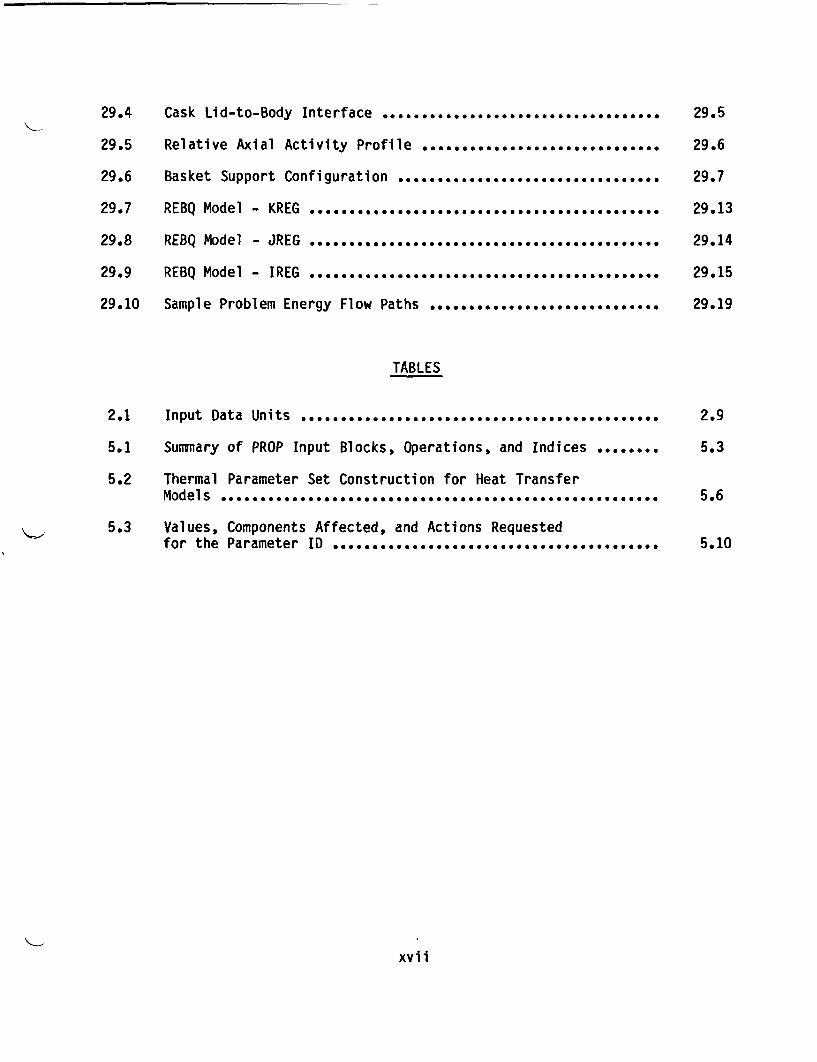
29.4 Cask Lid-to-Body Interface ................................... 29.5
29.5 Relative Axial Activity Profile ............... ................ 29.6
29.6 Basket Support Configuration ................................. 29.7
29.7 REBQ Model - KREG ............................................ 29.13
29.8 REBQ Model - JREG ........................................... 29.14
29.9 REBQ Model - IREG .................................... . . .... 29.15
29.10 Sample Problem Energy Flow Paths ....... ...................... 29.19
TABLES
2.1 Input Data Units . ............................................ 2.9
5.1 Summary of PROP Input Blocks, Operations, and Indices ........ 5.3
5.2 Thermal Parameter Set Construction for Heat TransferModels ......................0....... ... 0....................... 5.6
5.3 Values, Components Affected, and Actions Requestedfor the Parameter ID ...... .............................0 0...0 5.10
xvii
1.0 INTRODUCTION
Implementation of spent fuel dry storage systems is required in the late
1980s because several at-reactor storage basins will attain maximum capacity
(DOE 1986). The Nuclear Waste Policy Act of 1982 (NWPA) assigns the U.S.
Department of Energy (DOE) the responsibility for assisting utilities with
their spent fuel storage problems. One of the provisions of the NWPA is that
DOE shall provide generic research and development of alternative spent fuel
storage systems to assist utilities in their licensing activities.
One of the important requirements for storage systems is that they dissi-
pate heat while maintaining the temperature of the stored materials below
established limits. The thermal performance of a storage system can be
assessed by a comprehensive testing program. Such testing programs are typ-
ically time-consuming and expensive. Analysis tools (e.g., computer codes),
while not intended to entirely supplant testing methods, can perform a valuable
service. Appropriately qualified computer codes can provide predictions of
thermal performance as a function of system design and operating conditions.
Moreover, when tests are to be performed, computer codes can help select test
conditions, spent fuel decay heat generation rates, and instrumentation place-
ments, as well as aid in interpreting test data.
HYDRA-II, developed by the Pacific Northwest Laboratory (PNL), is a com-
puter code for heat transfer and fluid flow analysis. An enhanced version of
HYDRA-I (McCann 1980), it is a member of the HYDRA family of general purpose
codes collectively capable of transient three-dimensional analysis of coupled
conduction, convection, and radiation problems. This current version is espe-
cially appropriate for simulating the steady-state performance of spent fuel
storage systems of current interest. A specialized version was deemed appro-
priate for two reasons: 1) it provides a reasonable level of generality for
most potential users without the unwelcome burden of excess complexity and
cost, and 2) it permits public availability of the code in a timely fashion.
The documentation of HYDRA-II is presented in three separate volumes.
Volume I - Equations and Numerics describes the basic differential equations,
illustrates how the difference equations are formulated, and gives the solution
1.1
procedures employed. This volume, Volume II - User's Manual, contains code
flow charts, discusses the code structure, provides detailed instructions for
preparing an input file, and illustrates the operation of the code by means of
a model problem. The final volume, Volume III - Verification/Validation
Assessments, provides a comparison between the analytical solution and the
numerical simulation for problems with a known solution. This volume also
documents comparisons between the results of simulations of single- and multi-
assembly storage systems and actual experimental data.
A detailed overview of the HYDRA-I1 code is presented in Chapter 2.0. The
code structure and solution sequence are described and illustrated with flow
charts. General guidance on conventions to be followed in preparing the input
file is also provided. Chapters 3.0 through 28.0 present specific descriptions
of the code's individual subroutines. Each of these chapters contains the
FORTRAN PARAMETERS and information needed to prepare the input file relevant to
a specific subroutine. Chapter 29.0 contains a sample problem illustrating
many characteristics of a typical spent fuel cask. The complete input file is
included in Appendix A, and selected output is described in Appendix B. Code
setup and operation, as well as output interpretation, are explained and
illustrated using the sample problem.
1.2
2.0 CODE OVERVIEW
HYDRA-II provides a finite-difference solution in Cartesian coordinates to
the equations governing the conservation of mass, momentum, and energy. A
cylindrical coordinate system may also be used to enclose the Cartesian coor-
dinate system. This exterior coordinate system is useful for modeling cylin-
drical cask bodies. When both coordinate systems are invoked, the code will
automatically align the two systems and enforce conservation of energy at their
interface.
The difference equations for conservation of momentum are enhanced by the
incorporation of directional porosities and permeabilities that aid in modeling
solid structures whose dimensions may be smaller than the computational mesh.
The specification of inflow and outflow boundary conditions has been eliminated
as appropriate for sealed storage systems. The equation for conservation of
energy permits modeling of orthotropic physical properties and film resis-
tances. Several automated procedures are available to model radiation transfer
within enclosures and from fuel rod to fuel rod. An implicit solution algorithm
is used for both the momentum and energy equations to ease time-step limita-
tions and stability requirements.
HYDRA-II has been designed to provide a user-oriented input interface,
which eliminates the need for internal code changes. Any application for which
the code is an appropriate choice can be completely described through the con-
struction of an input file. The user may optionally request a formatted echo
of the input file to confirm that the intended parameters are actually those
used by the code. A selectable commentary monitoring the progress of the code
toward a steady-state solution is available, as is a summary of energy
balances. Finally, a tape may be written at the conclusion of a run if the
user wishes to restart the solution from its most recent point.
2.1 CODE STRUCTURE AND SOLUTION SEQUENCE
HYDRA-II is intended for steady-state applications. The method used by
the code to approach steady state is similar to a transient simulation that
ultimately converges to the steady-state condition. Starting from specified
2.1
initial conditions, the solution will evolve through time using automatically
selected time-steps for both the energy and the momentum equations. Because
only a steady-state solution is desired, the time-dependent terms for the
energy, momentum, and continuity equations have been modified to accelerate
convergence. Therefore, before it reaches steady state, the evolving solution
will not correspond exactly to an actual transient solution, and the numerical
values of the time-steps do not represent real time.
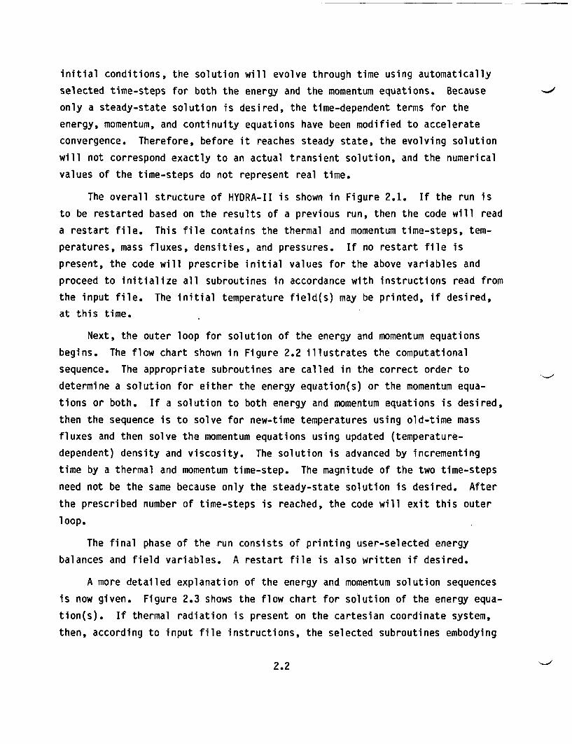
The overall structure of HYDRA-II is shown in Figure 2.1. If the run is
to be restarted based on the results of a previous run, then the code will read
a restart file. This file contains the thermal and momentum time-steps, tem-
peratures, mass fluxes, densities, and pressures. If no restart file is
present, the code will prescribe initial values for the above variables and
proceed to initialize all subroutines in accordance with instructions read from
the input file. The initial temperature field(s) may be printed, if desired,
at this time.
Next, the outer loop for solution of the energy and momentum equations
begins. The flow chart shown in Figure 2.2 illustrates the computational
sequence. The appropriate subroutines are called in the correct order to
determine a solution for either the energy equation(s) or the momentum equa-
tions or both. If a solution to both energy and momentum equations is desired,
then the sequence is to solve for new-time temperatures using old-time mass
fluxes and then solve the momentum equations using updated (temperature-
dependent) density and viscosity. The solution is advanced by incrementing
time by a thermal and momentum time-step. The magnitude of the two time-steps
need not be the same because only the steady-state solution is desired. After
the prescribed number of time-steps is reached, the code will exit this outer
loop.
The final phase of the run consists of printing user-selected energy
balances and field variables. A restart file is also written if desired.
A more detailed explanation of the energy and momentum solution sequences
is now given. Figure 2.3 shows the flow chart for solution of the energy equa-
tion(s). If thermal radiation is present on the Cartesian coordinate system,
then, according to input file instructions, the selected subroutines embodying
2.2
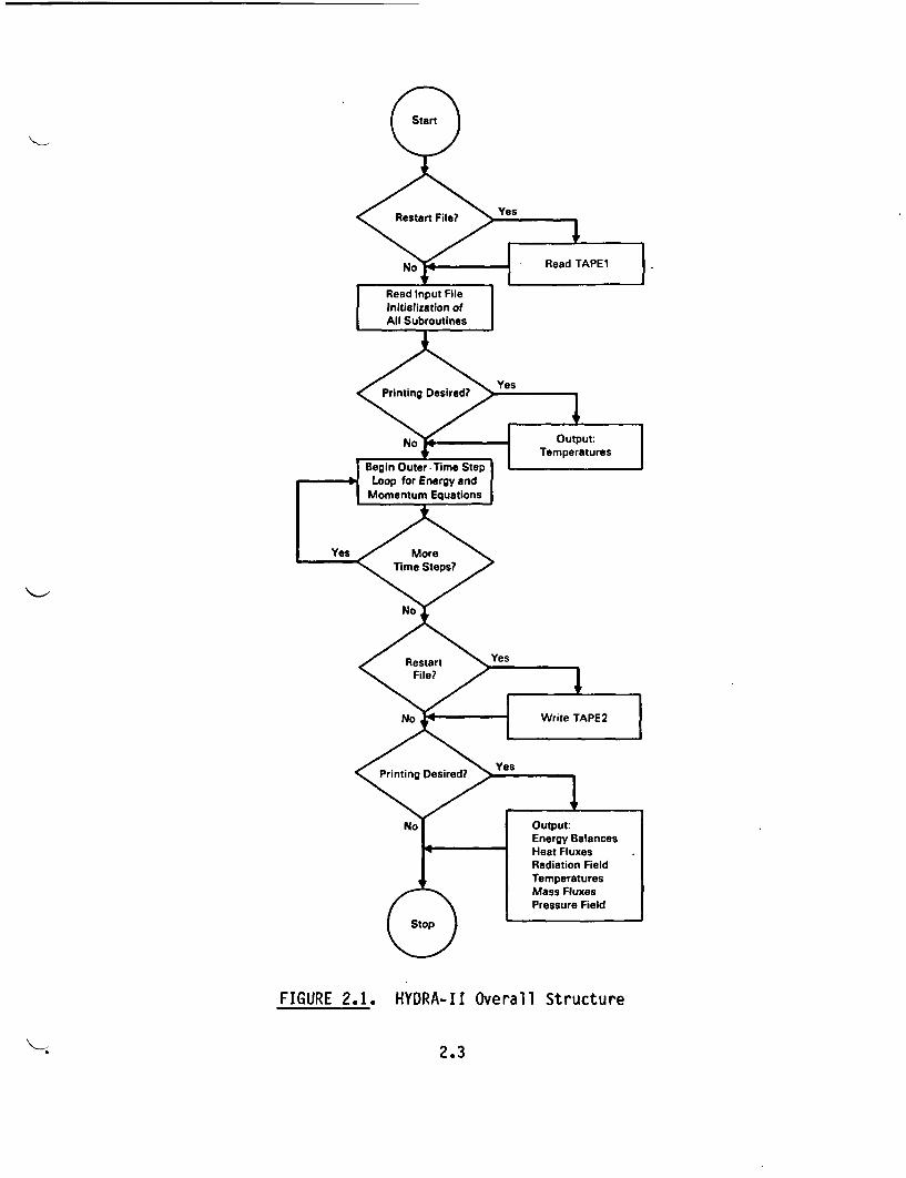
FIGURE 2.1. HYDRA-1I Overall Structure
2.3
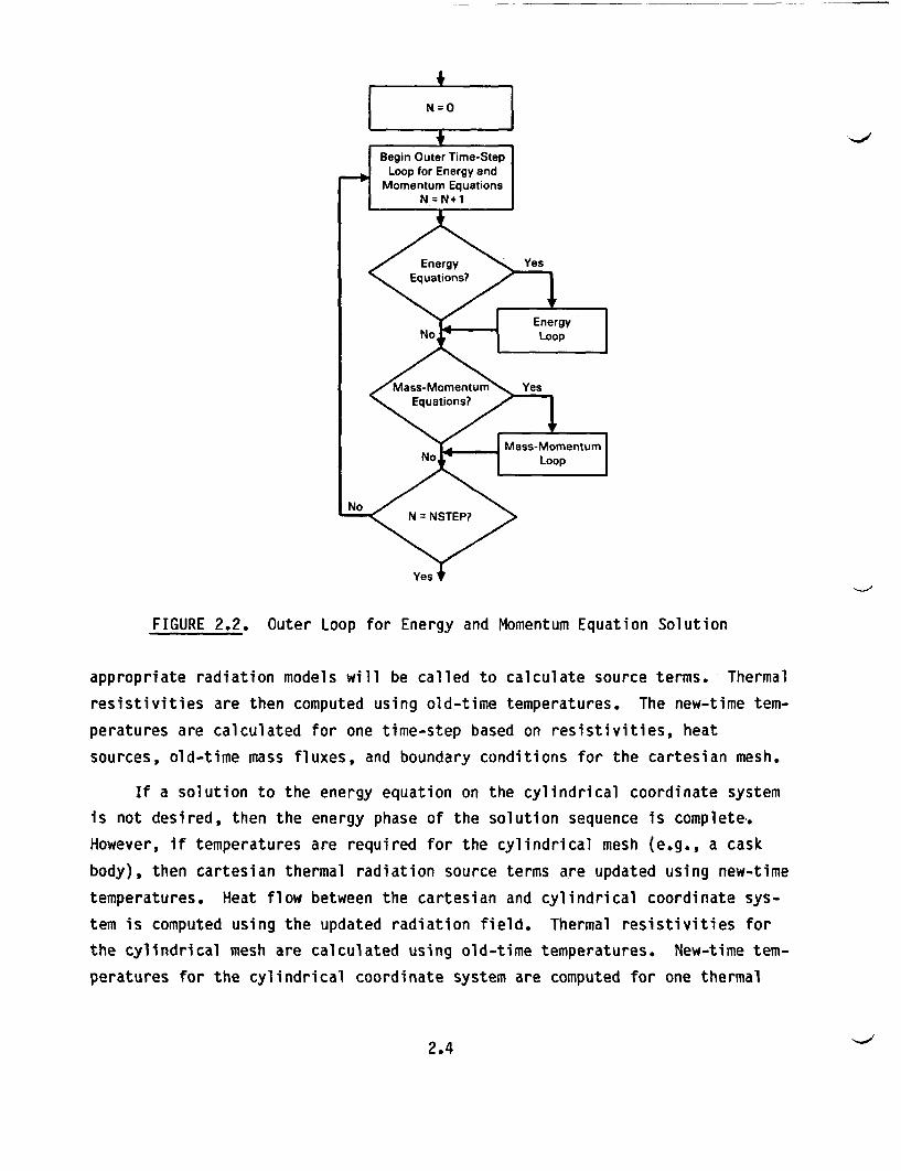
FIGURE 2.2. Outer Loop for Energy and Momentum Equation Solution
appropriate radiation models will be called to calculate source terms. Thermal
resistivities are then computed using old-time temperatures. The new-time tem-
peratures are calculated for one time-step based on resistivities, heat
sources, old-time mass fluxes, and boundary conditions for the Cartesian mesh.
If a solution to the energy equation on the cylindrical coordinate system
is not desired, then the energy phase of the solution sequence is complete.
However, if temperatures are required for the cylindrical mesh (e.g., a cask
body), then Cartesian thermal radiation source terms are updated using new-time
temperatures. Heat flow between the Cartesian and cylindrical coordinate sys-
tem is computed using the updated radiation field. Thermal resistivities for
the cylindrical mesh are calculated using old-time temperatures. New-time tem-
peratures for the cylindrical coordinate system are computed for one thermal
2.4
FIGURE 2.3. Energy Equation Solution Loop
2.5
time-step, based on resistivities and boundary conditions. One boundary condi-
tion is the prescribed energy exchange between the two coordinate systems; the
other boundary condition is the ambient temperature. The temperatures on the
interface between the two coordinate systems are updated as a final step to
ensure continuous temperatures and enforce conservation of energy.
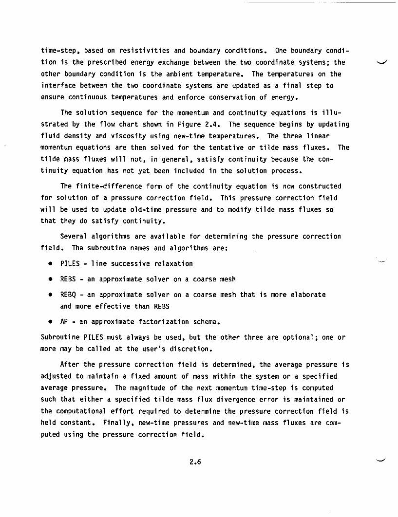
The solution sequence for the momentum and continuity equations is illu-
strated by the flow chart shown in Figure 2.4. The sequence begins by updating
fluid density and viscosity using new-time temperatures. The three linear
momentum equations are then solved for the tentative or tilde mass fluxes. The
tilde mass fluxes will not, in general, satisfy continuity because the con-
tinuity equation has not yet been included in the solution process.
The finite-difference form of the continuity equation is now constructed
for solution of a pressure correction field. This pressure correction field
will be used to update old-time pressure and to modify tilde mass fluxes so
that they do satisfy continuity.
Several algorithms are available for determining the pressure correction
field. The subroutine names and algorithms are:
* PILES - line successive relaxation
* REBS - an approximate solver on a coarse mesh
* REBQ - an approximate solver on a coarse mesh that is more elaborate
and more effective than REBS
* AF - an approximate factorization scheme.
Subroutine PILES must always be used, but the other three are optional; one or
more may be called at the user's discretion.
After the pressure correction field is determined, the average pressure is
adjusted to maintain a fixed amount of mass within the system or a specified
average pressure. The magnitude of the next momentum time-step is computed
such that either a specified tilde mass flux divergence error is maintained or
the computational effort required to determine the pressure correction field is
held constant. Finally, new-time pressures and new-time mass fluxes are com-
puted using the pressure correction field.
2.6
FIGURE 2.4. Momentum and Continuity Equation Solution Loop
2.7
2.2 CODE CONVENTIONS
This section contains some general information about the HYDRA-II source,
as well as conventions to be observed in preparing the input file.
The source for HYDRA-II is written in ANSI FORTRAN 77. Extensions that
might be installation-specific have been avoided. The code has been run on
CDC-7600, VAX 11/780, and CRAY machines, and verified to produce essentially
the same results (minor changes relating to word length on the VAX were
needed). Because the code version anticipated for public release has been run
extensively on CRAY machines, the internal coding has been structured to favor
vector machines.
The source uses FORTRAN PARAMETER statements to dimension arrays. Each
new application will require redimensioning. This is easily accomplished with
a line editor. Redimensioning is required because certain economies in com-
puter memory are more easily achieved and are commonly necessary for large-
scale simulations.
Almost every subroutine reads some information from the input file during
initialization, even if that subroutine may not be subsequently used. The
information read by a particular subroutine is most relevant to the function of
the respective subroutine. Certain data of global use are read by a few sub-
routines and then propagated by means of COMMON blocks.
List-directed reads are used almost exclusively in the source. The few
formatted reads in HYDRA-II read only some descriptive text for echoing to the
output file. The physical input file is separated into logical sections, each
dealing with a particular subroutine or special activity within a subroutine.
The section boundaries begin with an integer and then a slash followed by iden-
tifying text. For example,
1/HYDRO/MONITOR/MX
The first integer, which will be either 0 or 1, acts as a flag to either echo
succeeding input lines to the output file (1) or not (0). The slash terminates
reading of the record. The text (in this example) identifies the lines to
2.8
follow as being read by subroutine HYDRO and related to monitoring selected
mass fluxes in the x-direction. The text is very helpful in searching for a
desired section of input with the aid of a line editor.
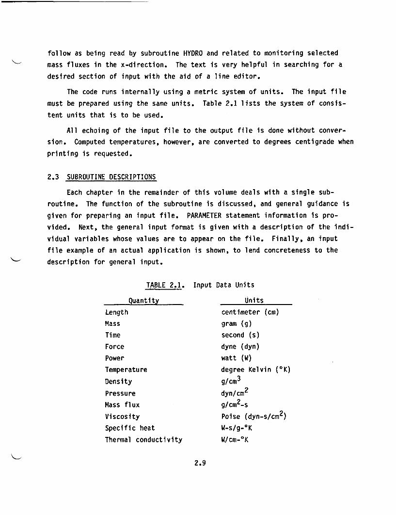
The code runs internally using a metric system of units. The input file
must be prepared using the same units. Table 2.1 lists the system of consis-
tent units that is to be used.
All echoing of the input file to the output file is done without conver-
sion. Computed temperatures, however, are converted to degrees centigrade when
printing is requested.
2.3 SUBROUTINE DESCRIPTIONS
Each chapter in the remainder of this volume deals with a single sub-
routine. The function of the subroutine is discussed, and general guidance is
given for preparing an input file. PARAMETER statement information is pro-
vided. Next, the general input format is given with a description of the indi-
vidual variables whose values are to appear on the file. Finally, an input
file example of an actual application is shown, to lend concreteness to the
description for general input.
TABLE 2.1.
Quantity
Length
Mass
Ti me
Force
Power
Temperature
Density
Pressure
Mass flux
Viscosity
Specific heat
Thermal conductivity
Input Data Units
Units
centimeter (cm)
gram (g)
second (s)
dyne (dyn)
watt (W)
degree Kelvin (OK)
g/cm3
dyn/cm2
g/cm2-s
Poise (dyn-s/cm2)
W-s/g-OK
W/cm-°K
2.9
3.0 PROGRAM MAIN
Program MAIN functions primarily as an executive that calls appropriate
subroutines as they are needed according to the requirements of the applica-
tion. Program MAIN also reads and writes restart tapes (if required) and con-
trols many of the printing options.
3.1 PARAMETER STATEMENT INFORMATION
Program MAIN requires the specification of parameters IP, JP, KP, ISP,
JSP, KBP, and KTP. These parameters define the overall computational mesh and
are described in Chapter 4.0, Subroutine GRID. Two additional parameters are
required for specification of printing options:
* NPLA1P - Most three-dimensional arrays may be printed in their
entirety (the default condition). It may be
desirable, at times, that only selected k-planes be
printed, to reduce the amount of output. NPLA1P-1 is
the maximum number of k-planes that can be selected
for any printing option. If no options are desired
(other than the default), then NPLA1P should be set to
1.
* NPLA2P - This parameter designates
ing options. The default
constitute an option. If
NPLA2P should be set to 1.
the maximum number of print-
printing condition does not
no options are desired, then
3.2 INPUT FORMAT
3.2.1 Descriptive Text for the Application
A user may optionally insert text to be printed on the output file that
describes the application.
3.1
General Input Format
NECHOLINESTEXT
.
TEXT
General Input Description
* NECHO - Echoing switch for this section of input. If input is
to be echoed, then NECHO = 1; otherwise, 0.
* LINES - The number of lines of text that follow and that are
to be read from the input file.
* TEXT - Text that the user wishes to have printed on the out-
put file. Each line of text may be up to 48
characters long.
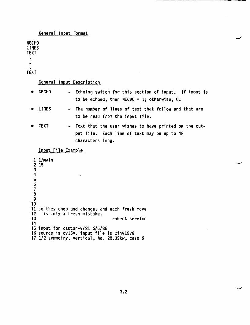
Input File Example
1 1/main2 153456789
1011 so they chop and change, and each fresh move12 is inly a fresh mistake.13 robert service1415 input for castor-v/21 6/6/8516 source is cvl5v, input file is cinvl5v617 1/2 symmetry, vertical, he, 28.09kw, case 6
3.2
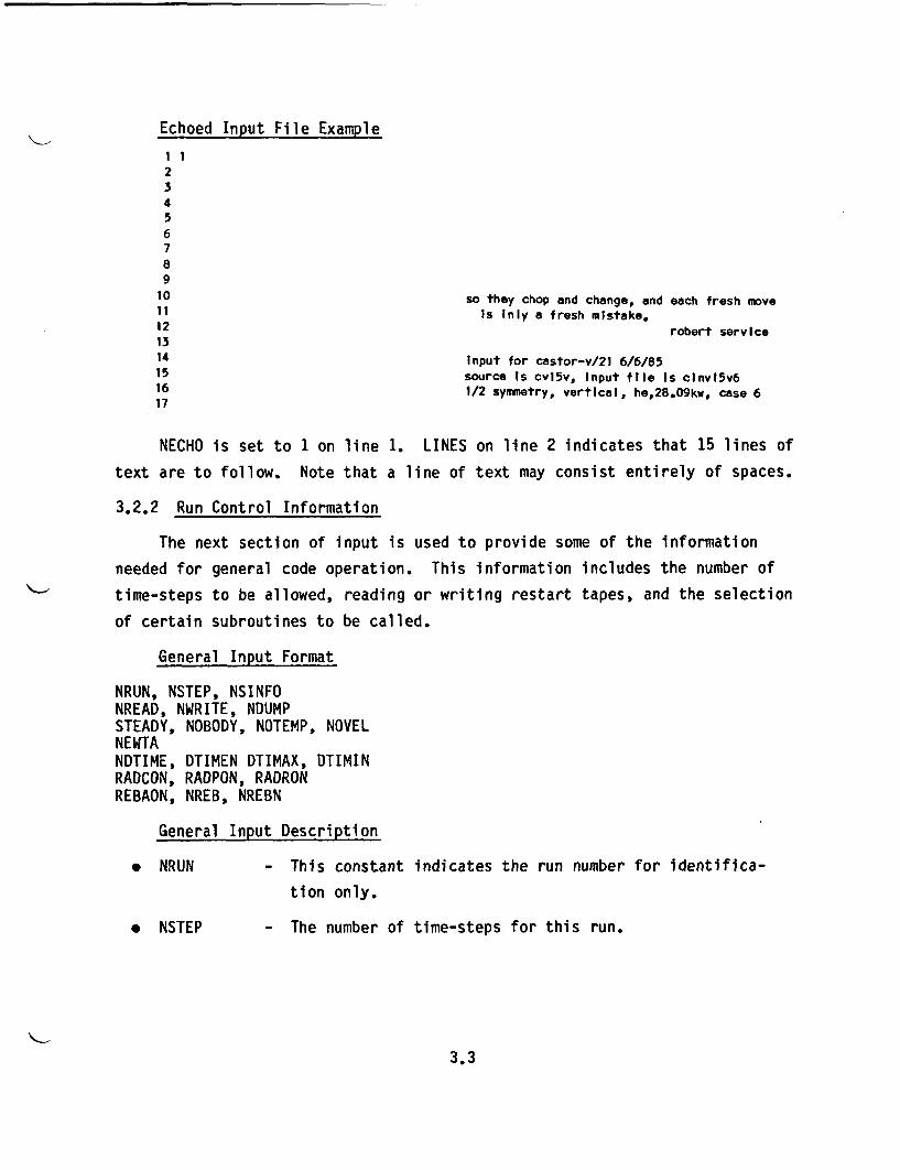
Echoed Input File Example
112345678910 so they chop and change, and each fresh move11 Is Inly a fresh mistake.12 robert service
14 Input for castor-v/21 6/6/8515 source Is cv15v, Input file Is cinvI5v616 1/2 symmetry, vertical, he,28.09kw, case 6
NECHO is set to 1 on line 1. LINES on line 2 indicates that 15 lines of
text are to follow. Note that a line of text may consist entirely of spaces.
3.2.2 Run Control Information
The next section of input is used to provide some of the information
needed for general code operation. This information includes the number of
time-steps to be allowed, reading or writing restart tapes, and the selection
of certain subroutines to be called.
General Input Format
NRUN, NSTEP, NSINFONREAD, NWRITE, NDUMPSTEADY, NOBODY, NOTEMP, NOVELNEWTANDTIME, DTIMEN DTIMAX, DTIMINRADCON, RADPON, RADRONREBAON, NREB, NREBN
General Input Description
* NRUN - This constant indicates the run number for identifica-
tion only.
* NSTEP - The number of time-steps for this run.
3.3
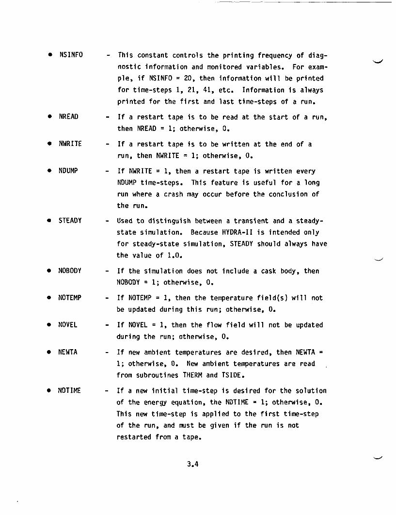
* NSINFO
* NREAD
* NWRITE
- This constant controls the printing frequency of diag-
nostic information and monitored variables. For exam-
ple, if NSINFO = 20, then information will be printed
for time-steps 1, 21, 41, etc. Information is always
printed for the first and last time-steps of a run.
- If a restart tape is to be read at the start of a run,
then NREAD = 1; otherwise, 0.
- If a restart tape is to be written at the end of a
run, then NWRITE = 1; otherwise, 0.
* NDUMP
* STEADY
* NOBODY
* NOTEMP
* NOVEL
* NEWTA
* NDTIME
- If NWRITE = 1, then a restart tape is written every
NDUMP time-steps. This feature is useful for a long
run where a crash may occur before the conclusion of
the run.
- Used to distinguish between a transient and a steady-
state simulation. Because HYDRA-II is intended only
for steady-state simulation, STEADY should always have
the value of 1.0.
- If the simulation does not include a cask body, then
NOBODY = 1; otherwise, 0.
- If NOTEMP = 1, then the temperature field(s) will not
be updated during this run; otherwise, 0.
- If NOVEL = 1, then the flow field will not be updated
during the run; otherwise, 0.
- If new ambient temperatures are desired, then NEWTA =
1; otherwise, 0. New ambient temperatures are read
from subroutines THERM and TSIDE.
- If a new initial time-step is desired for the solution
of the energy equation, the NDTIME = 1; otherwise, 0.
This new time-step is applied to the first time-step
of the run, and must be given if the run is not
restarted from a tape.
3.4
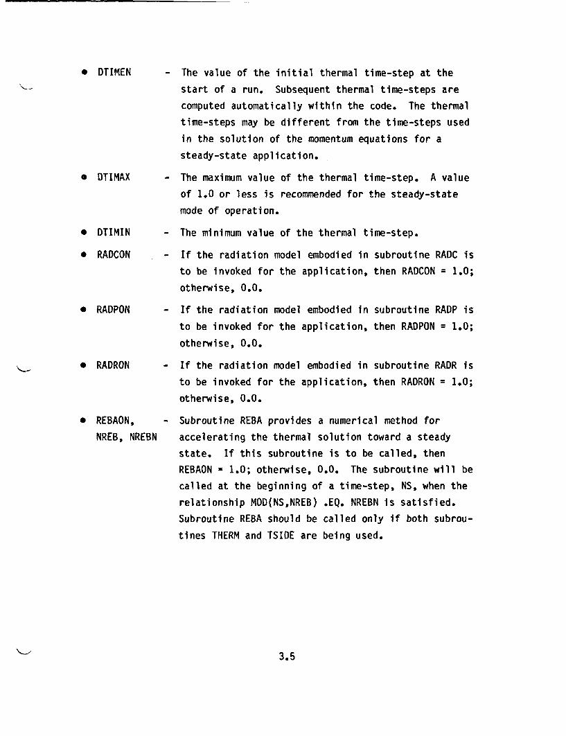
* DTIMEN
* DTIMAX
* DTIMIN
* RADCON
- The value of the initial thermal time-step at the
start of a run. Subsequent thermal time-steps are
computed automatically within the code. The thermal
time-steps may be different from the time-steps used
in the solution of the momentum equations for a
steady-state application.
- The maximum value of the thermal time-step. A value
of 1.0 or less is recommended for the steady-state
mode of operation.
- The minimum value of the thermal time-step.
- If the radiation model embodied in subroutine RADC is
to be invoked for the application, then RADCON = 1.0;
otherwise, O.O.
* RADPON
* RADRON
- If the radiation model embodied in
to be invoked for the application,
otherwise, O.O.
- If the radiation model embodied in
to be invoked for the application,
otherwise, O.O.
subroutine RADP is
then RADPON = 1.0;
subroutine RADR is
then RADRON = 1.0;
* REBAON,
NREB, NREBN
Subroutine REBA provides a numerical method for
accelerating the thermal solution toward a steady
state. If this subroutine is to be called, then
REBAON = 1.0; otherwise, O.O. The subroutine will be
called at the beginning of a time-step, NS, when the
relationship MOD(NS,NREB) .EQ. NREBN is satisfied.
Subroutine REBA should be called only if both subrou-
tines THERM and TSIDE are being used.
3.5
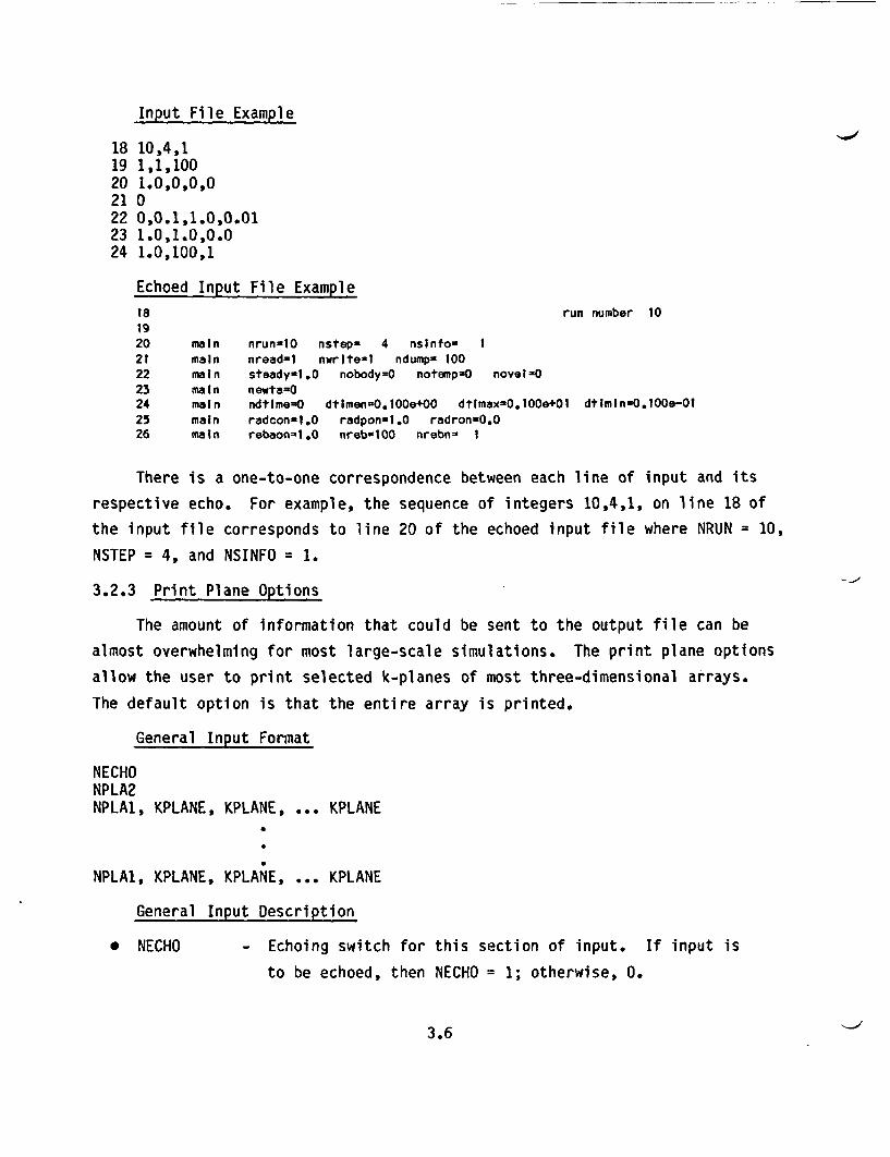
Input File Example
18 10,4,119 1,1,10020 1.0,0,0,021 022 0,0.1,1.0,0.0123 1.0,1.0,0.024 1.0,100,1
Echoed Input File Example
is run number 101920 main nrun10 nstepa 4 nsinfoo 121 main nread-1 nwriteal ndumpm 10022 main steady-l.0 nobody=O notempnO novel-23 main newta=O24 main ndtlme=O dtImen=O.10Oe+00 dtlmax=0.tOOe1Ol dtiminwO.100e-0125 main radcon-1.0 radpon-1.0 radron-0.026 main rebaon-1.0 nreb-100 nrebn- 1
There is a one-to-one correspondence between each line of input and its
respective echo. For example, the sequence of integers 10,4,1, on line 18 of
the input file corresponds to line 20 of the echoed input file where NRUN = 10,
NSTEP = 4, and NSINFO = 1.
3.2.3 Print Plane Options
The amount of information that could be sent to the output file can be
almost overwhelming for most large-scale simulations. The print plane options
allow the user to print selected k-planes of most three-dimensional arrays.
The default option is that the entire array is printed.
General Input Format
NECHONPLA2NPLA1, KPLANE, KPLANE, ... KPLANE
NPLA1, KPLANE, KPLANE, ... KPLANE
General Input Description
* NECHO - Echoing switch for this section of input. If input is
to be echoed, then NECHO = 1; otherwise, 0.
3.6
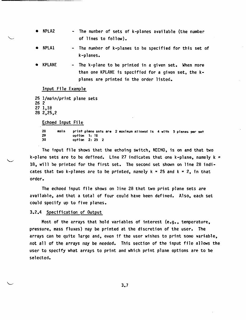
* NPLA2 - The number of sets of k-planes available (the number
of lines to follow).
* NPLA1 - The number of k-planes to be specified for this set of
k-planes.
* KPLANE - The k-plane to be printed in a given set. When more
than one KPLANE is specified for a given set, the k-
planes are printed in the order listed.
Input File Example
25 1/main/print plane sets26 227 1,1828 2,25,2
Echoed Input File
28 main print plane sets are 2 maximum allowed Is 4 with 5 planes per set29 option I: 1830 optIon 2: 25 2
The input file shows that the echoing switch, NECHO, is on and that two
k-plane sets are to be defined. Line 27 indicates that one k-plane, namely k =
18, will be printed for the first set. The second set shown on line 28 indi-
cates that two k-planes are to be printed, namely k = 25 and k = 2, in that
order.
The echoed input file shows on line 28 that two print plane sets are
available, and that a total of four could have been defined. Also, each set
could specify up to five planes.
3.2.4 Specification of Output
Most of the arrays that hold variables of interest (e.g., temperature,
pressure, mass fluxes) may be printed at the discretion of the user. The
arrays can be quite large and, even if the user wishes to print some variable,
not all of the arrays may be needed. This section of the input file allows the
user to specify what arrays to print and which print plane options are to be
selected.
3.7
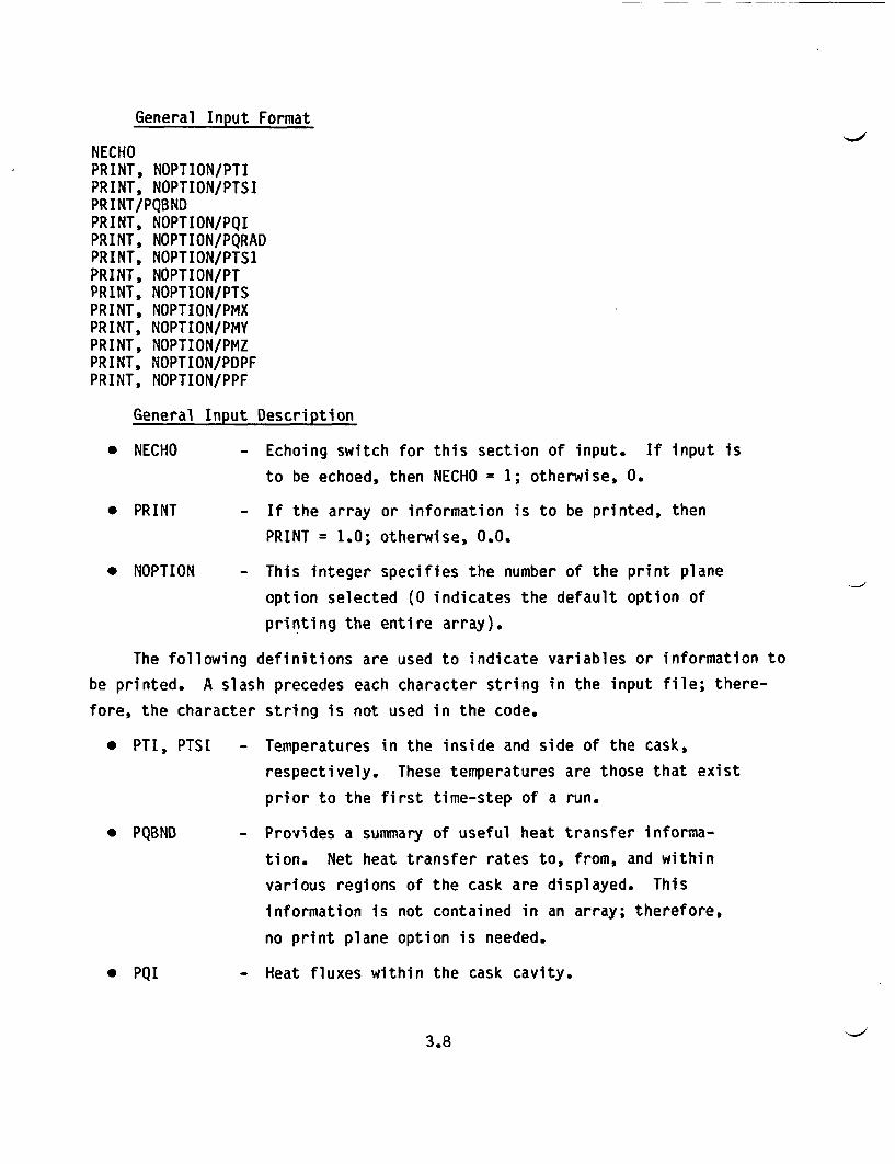
General Input Format-J
NECHOPRINT, NOPTION/PTIPRINT, NOPTION/PTSIPRINT/PQBNDPRINT, NOPTION/PQIPRINT, NOPTION/PQRADPRINT, NOPTION/PTS1PRINT, NOPTION/PTPRINT, NOPTION/PTSPRINT, NOPTION/PMXPRINT, NOPTION/PMYPRINT, NOPTION/PMZPRINT, NOPTION/PDPFPRINT, NOPTION/PPF
General Input Description
* NECHO
* NOPTION
- Echoing switch for this section of input. If input is
to be echoed, then NECHO = 1; otherwise, 0.
- If the array or information is to be printed, then
PRINT = 1.0; otherwise, O.O.
- This integer specifies the number of the print plane
option selected (O indicates the default option of
printing the entire array).
The following definitions are used to indicate variables or information to
be printed. A slash precedes each character string in the input file; there-
fore, the character string is not used in the code.
* PTI, PTSI
* PQBND
* PQI
- Temperatures in the inside and side of the cask,
respectively. These temperatures are those that exist
prior to the first time-step of a run.
- Provides a summary of useful heat transfer informa-
tion. Net heat transfer rates to, from, and within
various regions of the cask are displayed. This
information is not contained in an array; therefore,
no print plane option is needed.
- Heat fluxes within the cask cavity.
3.8
* PQRAD
* PTS1
- Radiation heat transfer to each cell within the cask
cavity. This is a summary of radiation source
strength computed by subroutines RADC, RADP, and/or
RADR.
- Heat flow into each cell of the side of the cask from
the inside.
* PT, PTS
* PMX, PMY,
PMZ
* PDPF
* PPF
- Temperature in the inside and side of the cask,
respectively.
- Mass fluxes in the x-, y-, and z-directions,
respectively.
- The change in the pressure field for the last time-
step.
- The pressure field.
Input File Example
29 1/main/print30 0.0,0/pti31 0.0,0/ptsi32 1.0/pqbnd33 1.0,1/pqi34 0.0,0/pqrad35 0.0,0/ptsl36 1.0,0/pt37 1.0,0/pts38 1.0,2/pmx39 0.0,0/pmy40 1.0,0/pmz41 0.0,0/pdpf42 0.0,0/ppf
arrays or info
3.9
-
Echoed Input File Example
32 main print arrays or Info33 ptl0.0 nptl= 034 ptsl=0.0 nptsi- 035 pqbndl.036 pqIl.0 npql- 137 pqrad-O.0 npqrada 038 ptsl-O.0 nptsli- 039 pt-l.0 npt- 040 ptsol.0 npts- 041 pmxal.O npmx- 242 pmynO.0 npmy- 043 pmz*l.O npmz- 044 pdpfO.0 npdpf- 045 ppf=O.0 nppf- 0
Line 29 on the input file shows that NECHO has been set to 1; therefore,
the echoed input file is printed as shown. Line 30 on the input file shows
that PRINT is set to 0.0 for PTI, so initial temperatures inside the cask are
not to be printed. Line 32 on the input file shows that PRINT is set to 1.0
for PQBND; hence, a summary of heat transfer information will be printed. Line
38 shows that PRINT is set to 1.0 and that print plane option 2 is desired for
PMX (mass fluxes in the x-direction). This specification results in printing
of k-planes 25 and 2 in this order.
3.10
4.0 SUBROUTINE GRID
Subroutine GRID allows the user to set up the computational grid for a
HYDRA-I1 application.
4.1 GRID FUNCTIONS
A full hydrothermal model with conduction, radiation, and single-phase
fluid flow on a rectangular grid for a three-dimensional region is available.
In addition, a coupled calculation of the temperature field is optionally
available on a cylindrical grid in a region enclosing the rectangular grid.
The two grid types have a cylindrical interface surface where coded connection
techniques impose some constraints on user grids. This hybrid grid configura-
tion and computational model is useful for modeling an interior rectangular
array of fuel rods and supporting structure within a cylindrical cask body.
Quarter-plane and half-plane symmetry can be treated. Computations can also be
performed on a rectangular grid alone without a surrounding cylindrical grid.
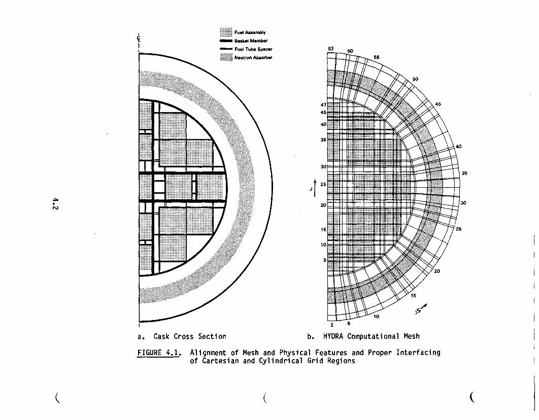
Figure 4.1a shows a typical cross-section of a spent fuel cask. The fuel
assemblies are stored within the cask in configurations most readily described
in rectangular coordinates. Figure 4.1b shows a realistic hybrid nodalization
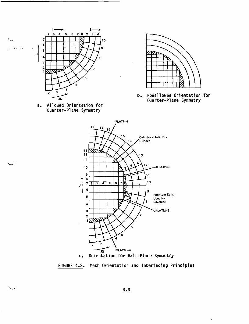
of the cask of Figure 4.1a. Figure 4.2 illustrates some of the grid inter-
facing principles of the nodalization of the two grid regions in a simpler geo-
metry. Rectangular grid indices in the x-y plane are I and J, with nodaliza-
tions 1(I1IP and 1CJ0JP. The radial grid index is IS, with nodalization
1'IS<ISP. The azimuthal sector index is JS, with nodalizatlon 14JS<JSP.
Two features are assumed for the full hybrid rectangular-cylindrical grid
model as currently coded: 1) there is no computed flow in the cylindrical grid
region, and 2) the inner surface of the cylindrical grid region is a circular
cylinder. The interface conditions between rectangular and cylindrical grid
regions assume that heat flow from the rectangular region enters the cylin-
drical region at the inner radius of the second radial cell in the azimuthal
sectors. Consistent coding of this energy flow imposes constraints on both the
cylindrical and the rectangular grids. A rectangular grid interface cell (I,J)
must have a unique connection to an azimuthal sector, as illustrated in
4.1
0 ,,.,Fuel Assmbly
anno B asket Member!Fuel Tube Spacer 63 60
Neutron Absorber _
4 56
... _ , , \ : \ .. _ .... ..... :::
... ..,, ,,i: .......... : ::........36 _ _._
"'_ ,,,,. ........... i\1 ......... .................. \ .......... ... .. . .... .0_\r@<W
rr ss* I. iiii .Cll . . .. g s Iij1iii. 5..i-iiiiiiii.-.i....... I . .... t.5_.. El1|_iii 3iiiiiiiiLiiiiii|XJ0 _|rE*~ .- 1
~~~~~~~~~~~~._ j ~i..iiiiiiiIX,,:X . .....I .
.-. -. 1. '. . ,,. ..... _1.. l. .....i i i i li. i. ..iii ./........ii iii i..iiiti ;
.. . ... .. . ... .. .. ...................... 6. . .
1J.. .... ..... .. . ... . /.
/~ i~~. .....
FIGRE4.1 A ignen of Mes ..... ....lFetrsad rpr Inefcn
FIUR 41 Aigmetof Cartsia and Cylind ical Feaure aei nds rprInefcn
( (
IS ---5 6 7 8 2 3 4
10
JI9
42 3
Jsb. Nonallowed Orientation for
Quarter-Plane Symmetrya. Allowed Orientation for
Quarter-Plane Symmetry
IFLATP=4
JI
IFLATM =4
c. Orientation for Half-Plane Symmetry
FIGURE 4.2. Mesh Orientation and Interfacing Principles
4.3
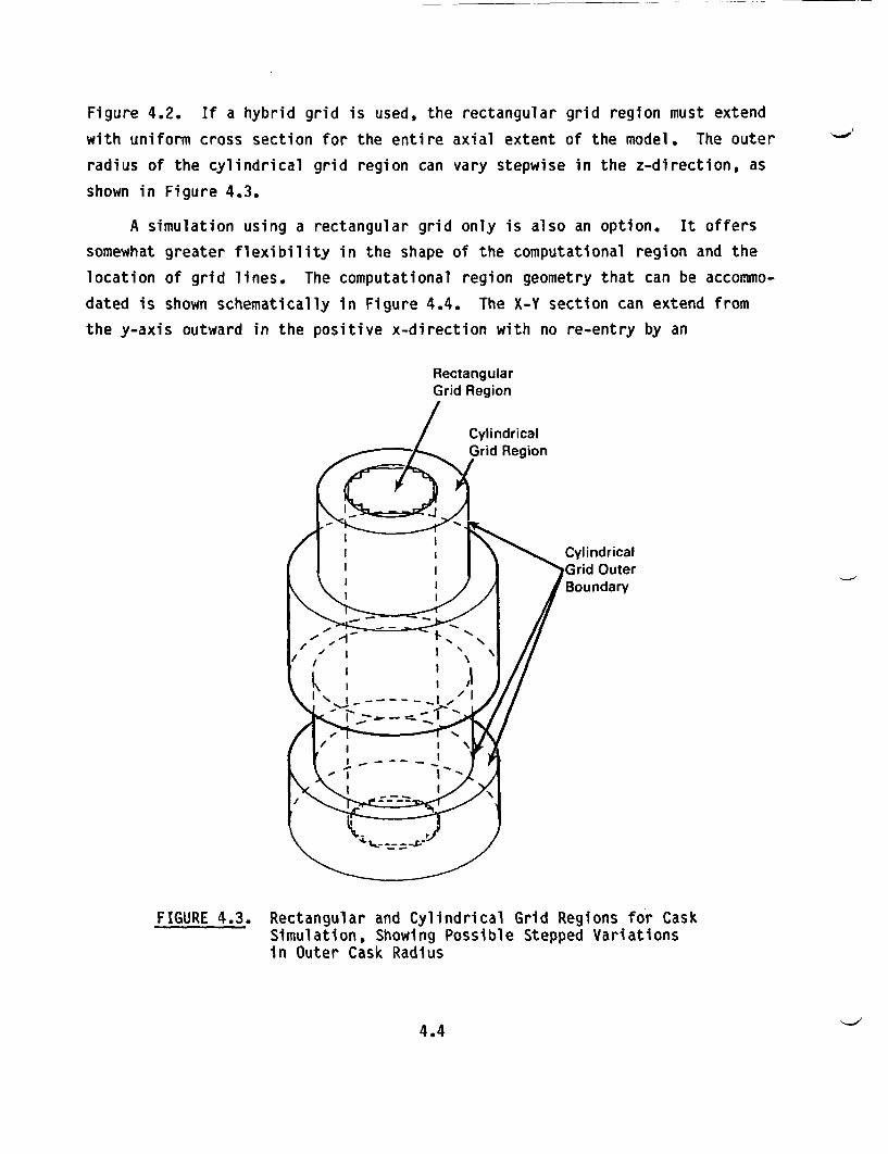
Figure 4.2. If a hybrid grid is used, the rectangular grid region must extend
with uniform cross section for the entire axial extent of the model. The outer
radius of the cylindrical grid region can vary stepwise in the z-direction, as
shown in Figure 4.3.
A simulation using a rectangular grid only is also an option. It offers
somewhat greater flexibility in the shape of the computational region and the
location of grid lines. The computational region geometry that can be accommo-
dated is shown schematically in Figure 4.4. The X-Y section can extend from
the y-axis outward in the positive x-direction with no re-entry by an
RectangularGrid Region
FIGURE 4.3. Rectangular and Cylindrical Grid Regions for CaskSimulation, Showing Possible Stepped Variationsin Outer Cask Radius
4.4
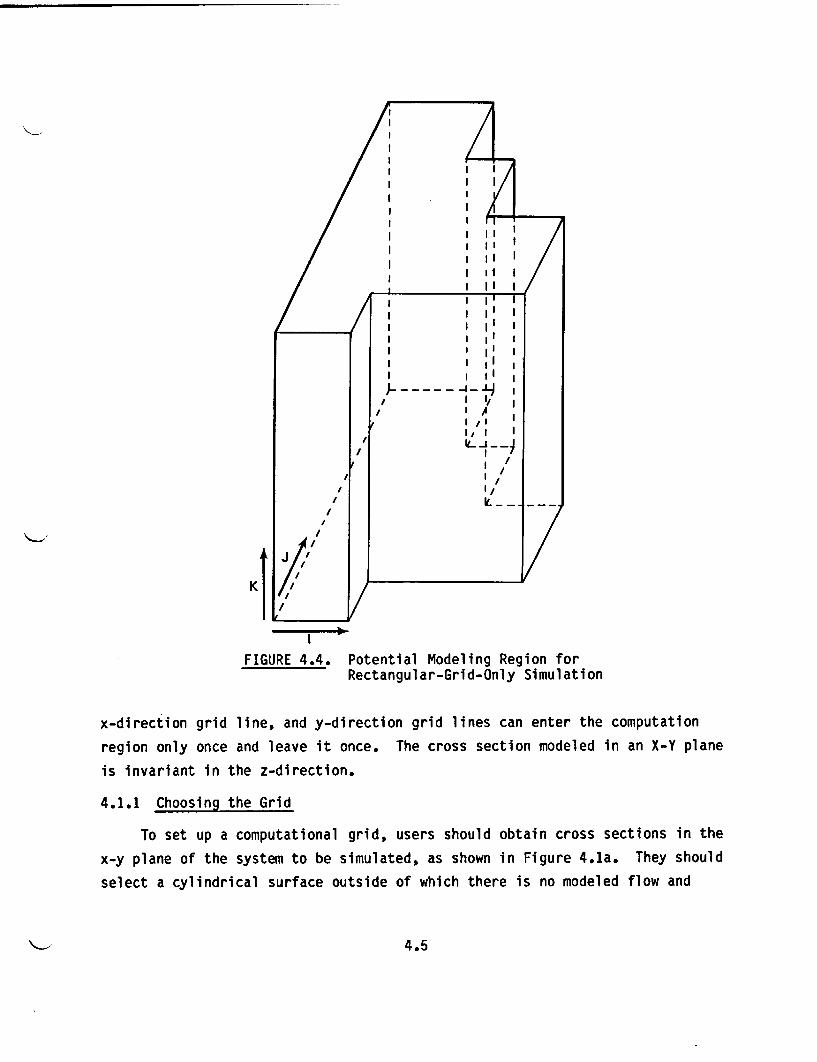
FIGURE 4.4. Potential Modeling Region forRectangular-Grid-Only Simulation
x-direction grid line, and y-direction grid lines can enter the computation
region only once and leave it once. The cross section modeled in an X-Y plane
is invariant in the z-direction.
4.1.1 Choosing the Grid
To set up a computational grid, users should obtain cross sections in the
x-y plane of the system to be simulated, as shown in Figure 4.1a. They should
select a cylindrical surface outside of which there is no modeled flow and
4.5
which lends itself to the transition to cylindrical mesh. The active computa-
tional cells (as opposed to phantom cells) for the rectangular mesh will all -
lie inside this interface surface. The computational cells are those on which
the field variable is computed in the solution algorithm for that grid type.
The phantom cells are those used to supply boundary conditions for the solution
on that grid type.
Although phantom cells experience no change in their field variables in
executing the solution procedure on their own grid type, the temperature vari-
able for phantom cells at the rectangular-cylindrical grid region interface
will be altered in solving the energy equation alternately on the rectangular
and cylindrical grid regions while advancing the solution through a time-step.
The conditions imposed are continuity of temperature and conservation of
energy. The coded method of achieving these conditions sets specific require-
ments on the setup of the grid, the specification of the rectangular grid com-
putation region, and the designation of the interface cells, as will be
explained here.
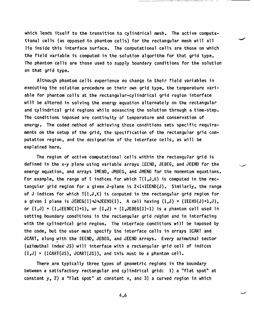
The region of active computational cells within the rectangular grid is
defined in the x-y plane using variable arrays IEEND, JEBEG, and JEEND for the
energy equation, and arrays IMEND, JMBEG, and JMEND for the momentum equations.
For example, the range of I indices for which T(I,J,K) is computed in the rec-
tangular grid region for a given J-plane is 2<I4IEEND(J). Similarly, the range
of J indices for which T(I,J,K) is computed in the rectangular grid region for
a given I plane is JEBEG(I)J JEEND(I). A cell having (I,J) = (IEEND(J)+1,J),
or (1,J) = (I,JEEND(I)+1), or (1,J) = (I,JEBEG(I)-1) is a phantom cell used in
setting boundary conditions in the rectangular grid region and in interfacing
with the cylindrical grid region. The interface conditions will be imposed by
the code, but the user must specify the interface cells in arrays ICART and
JCART, along with the IEEND, JEBEG, and JEEND arrays. Every azimuthal sector
(azimuthal index JS) will interface with a rectangular grid cell of indices
(I,J) = (ICART(JS), JCART(JS)), and this must be a phantom cell.
There are typically three types of geometric regions in the boundary
between a satisfactory rectangular and cylindrical grid: 1) a "flat spot" at
constant y, 2) a "flat spot" at constant x, and 3) a curved region in which
4.6
every x-direction grid line must intersect a y-direction grid line on the
cylindrical interface. These three region types on the boundary can be seen in
Figure 4.1b. They can also be seen in the grid layout of Figure 4.2, which
shows the allowed orientations for quarter-plane and half-plane symmetry
simulations. This arrangement of "flats" and curves recognizes two require-
ments: 1) some accommodation is necessary to join a rectangular grid to a
cylindrical grid, and 2) each azimuthal sector should give or receive an appro-
priate share of the total heat transfer with respect to the rectangular grid.
In a representative x-y plane cross section, the user must superimpose on
the interior region a tentative orthogonal network or grid. An early step is
to select the flat parts of the boundary of the rectangular computational grid,
using some discretion about the amount of gap that can be tolerated between the
rectangular grid and the cylindrical interface. Grid lines that penetrate per-
pendicularly through these flat side boundaries can be chosen primarily to
optimize resolution of physical detail. By contrast, grid lines (x- or
y-direction) that intersect the cylinder interface without intersecting a flat
boundary must intersect a perpendicular grid line (y or x) at the interface
cylinder, and this imposes some constraints on their location. For example,
the right boundary of the grid columns I = 2 or I = 3 in Figure 4.2 can be
chosen to optimize resolution in the x-direction in the region 2W4, whereas
the grid boundary between I = 5 and I = 6 must meet an x-direction grid line at
the interface, like the one between J = 2 and J = 3.
Grid lines should pass along the major material boundaries. In choosing
them, the user should keep in mind the models available to describe the heat
transfer phenomena: flow in the available open spaces, radiative transfer from
cell to cell by rods, radiative exchange among cells facing interior enclo-
sures, conduction from cell to cell through homogeneous materials and laminar
composites, and inhibition of conduction from cell to cell by film resistances.
Grid lines should be inserted as needed to represent the physical phenomena.
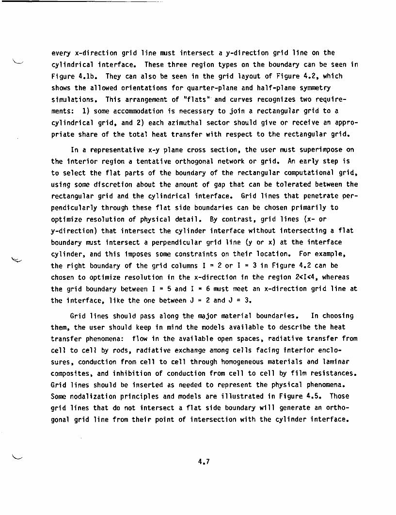
Some nodalization principles and models are illustrated in Figure 4.5. Those
grid lines that do not intersect a flat side boundary will generate an ortho-
gonal grid line from their point of intersection with the cylinder interface.
4.7
Grid Lines Chosen to FollowMaterial Boundaries Solid 1 Gap Solid 2
a. Grid Lines Chosen toFollow MaterialBoundaries
Il l
b. Radiation Across NarrowGap Modeled with Inter-Cell Film Resistance
- - I
I f1
- 4 p __-
c. Two-Dimensional RadiationEnclosure (Infinite inZ-Di rection)
d. Array of CylindersModeled as OrthotropicContinuum
e. Array of CylindersModeled as One perCell Column inZ-Direction
FIGURE 4.5. Some Nodalization Principles and Available Models
4.8

Users should insert the obvious choices of grid lines following material
boundaries and draw in the requisite orthogonal grid lines intersecting them on
the cylindrical interface for those not intersecting the flat boundary regions.
The grid may then be excessively detailed for available memory or desired com-
putational speed. A reduction in the number of grid lines may be possible
without serious loss of accuracy if composite models are used for conduction
and partial-flow blockage models are used for flow. These techniques may lead
to local reduction of spatial resolution without significant loss of accuracy
on a larger scale.
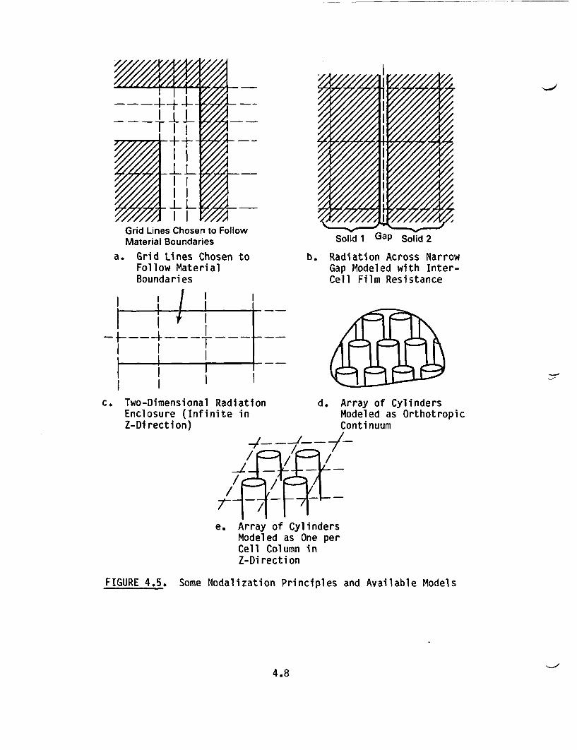
The series and parallel laminar composite conduction models for heat flow
allow some opportunity to economize on grid cells. Consider an interface
between material 1 and material 2 as shown in Figure 4.6. One would prefer to
make a cell boundary coincide with the material interface, as shown in Fig-
ure 4.6a. The desirability of fitting cell boundaries to a material interface
in the y-direction, the requirement that x and y grid lines intersect on the
cylindrical interface on the curved part of the rectangular grid boundary, and
a need to reduce the number of computational cells may require grid lines as
shown in Figure 4.6b. A medium-straddling cell such as the (I,J) cell of Fig-
ure 4.6b can be considered as having series conduction through layers in the
x-direction and parallel conduction in the y-direction as shown in Figure 4.6c.
The approximate laminar composite model is shown schematically in Figure 4.6d.
The input for laminar composite conduction is described in Chapter 5.0, but its
availability is described here to aid nodalization. If one of two media within
a computational cell contains a fluid, some use of directional permeabilities,
directional surface porosities, directional velocity-dependent drag coef-
ficients, and altered viscosities may be appropriate to model flow effects.
The preceding discussion and Figure 4.2 should indicate both the reasons
and the method for assigning IEEND, JEBEG, JEEND, ICART, and JCART values.
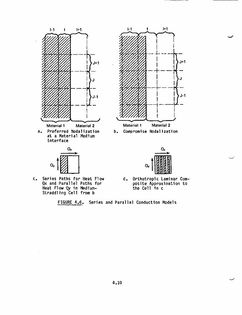
Specifically, the rules for assigning IEEND(J) values are:
4.9
1-1 I 1+1
7 1Material 1 Material 2
a. Preferred Nodalizationat a Material MediumInterface
Material 1 Material 2b. Compromise Nodalization
Qx0~
QYI
d. Orthotropic Laminar Com-posite Approximation tothe Cell in c
c. Series Paths for Heat FlowQx and Parallel Paths forHeat Flow Qy in Medium-Straddling Cell from b
FIGURE 4.6. Series and Parallel Conduction Models
4.10
* J = 1 - IEEND(1) = 1
* J = 2 to JFLATM, i.e., along curved boundary - Set IEEND(J)
to one less than the I index of the cell bisected by
the interface curve.
* J = JFLATM to JFLATP - Set IEEND(J) to one less than the I value of
the cells that extend from the "flat" boundary there
to the cylindrical interface curve.
* J = JFLATP+1 to JP-1 - Set IEEND(J) to one less than the I index of
the cell bisected by the interface curve.
* J =JP - IEEND(JP) = 1.
JEBEG and JEEND(I) values should be assigned according to:
* I = 1 to IFLATM - JEBEG(I) = 2
* I = 1 to IFLATP - JEEND(I) = the J value of layer below "flat" upper
boundary, that is JEEND(I) = JP-1
* I = IFLATM+1 to I = the I index just left of the "flat" right
boundary
- JEBEG(I) = one more than the J value of the cell
bisected by the interface curve
- JEEND(I) = one less than the J value of the cell
bisected by the interface curve.
In the most correct nodalization, the I index just left of the flat right
boundary will be IP-1.
The ICART(JS) and JCART(JS) values are the I and J indices, respectively,
of the phantom cell to which the JS azimuthal sector connects. The lowest
active computational sector is JS = 2, and it should be connected to the cell
(I,J) = (ICART(2),JCART(2)) = 2,1. The subsequent ICART and JCART values can
be read directly from a user diagram analogous to Figure 4.2. Figure 4.7 shows
input data appropriate to Figure 4.2.
The limits of the computational region for the momentum equations are set
in the arrays IMEND, JMBEG, and JMEND, and they are related to the choices for
the energy equation. The momentum equations apply only to the rectangular
4.11
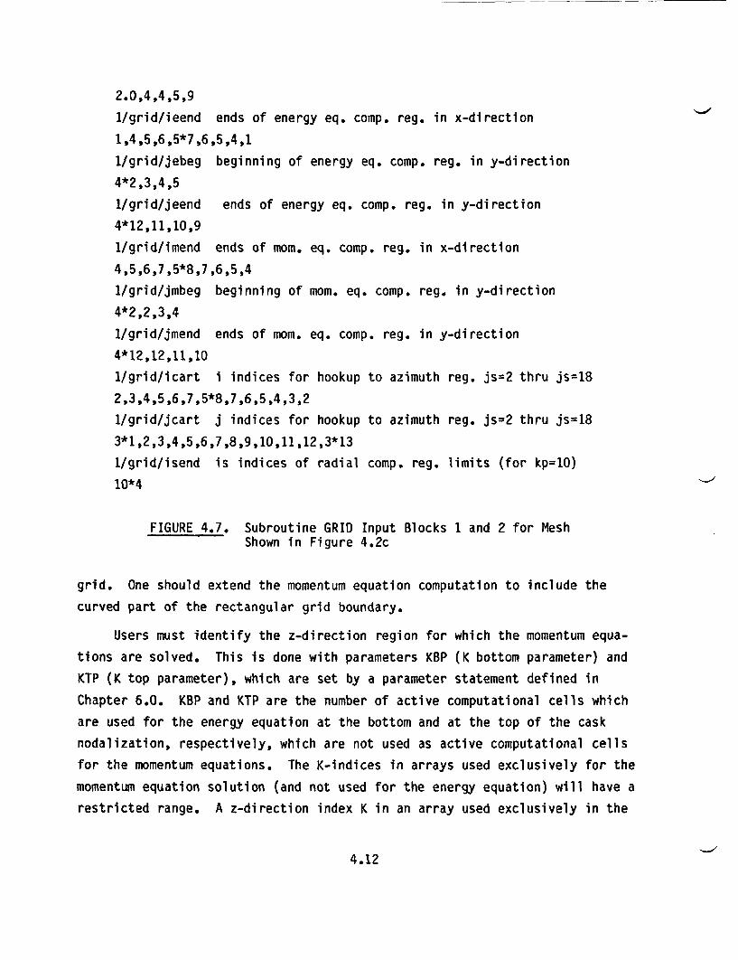
2.0,4,4,5,9
1/grid/ieend ends of energy eq. comp. reg. in x-direction
1,4,5,6,5*7,6,5,4,1
1/grid/jebeg beginning of energy eq. comp. reg. in y-direction
4*2,3,4,5
1/grid/jeend ends of energy eq. comp. reg. in y-direction
4*12,11,10,9
1/grid/imend ends of mom. eq. comp. reg. in x-direction
4,5,6,7,5*8,7,6,5,4
1/grid/jmbeg beginning of mom. eq. comp. reg. in y-direction
4*2,2,3,4
1/grid/jmend ends of mom. eq. comp. reg. in y-direction
4*12,12,11,10
1/grid/icart i indices for hookup to azimuth reg. js=2 thru js=18
2,3,4,5,6,7,5*8,7,6,5,4,3,2
1/grid/jcart j indices for hookup to azimuth reg. js=2 thru js=18
3*1,2,3,4,5,6,7,8,9,10,11,12,3*13
1/grid/isend is indices of radial comp. reg. limits (for kp=10)
10*4
FIGURE 4.7. Subroutine GRID Input Blocks 1 and 2 for MeshShown in Figure 4.2c
grid. One should extend the momentum equation computation to include the
curved part of the rectangular grid boundary.
Users must identify the z-direction region for which the momentum equa-
tions are solved. This is done with parameters KBP (K bottom parameter) and
KTP (K top parameter), which are set by a parameter statement defined in
Chapter 6.0. KBP and KTP are the number of active computational cells which
are used for the energy equation at the bottom and at the top of the cask
nodalization, respectively, which are not used as active computational cells
for the momentum equations. The K-indices in arrays used exclusively for the
momentum equation solution (and not used for the energy equation) will have a
restricted range. A z-direction index K in an array used exclusively in the
4.12
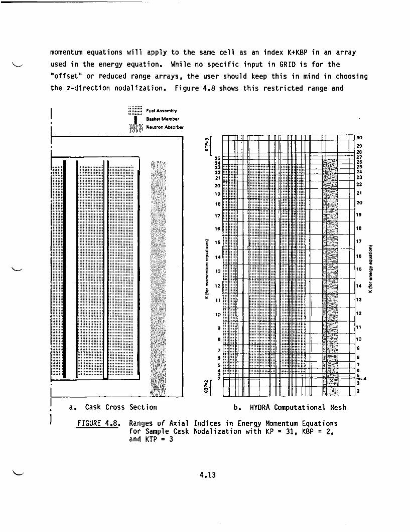
momentum equations will apply to the same cell as an index K+KBP in an array
used in the energy equation. While no specific input in GRID is for the
"offset" or reduced range arrays, the user should keep this in mind in choosing
the z-direction nodalization. Figure 4.8 shows this restricted range and
I.....:: -,Fuel Assembly
Basket Member
Neutron Absorber
wI__
2524232221
20
19
18
17
..... ...... .. .... . ...
..... ...... ...... ..... .. .... .
.. ... . ..... ..... .. .... . ..
.... .. .... ... ... .......
MI 1::::I:
..... ...... .. .... .
... . ..... ...... .. .... ...... ..... .. .... ...... .....
16
30
29282726252423
22
21
20
19
18
17E.2
16 §
g15 >
C
14 9
13
12
1 1
C0
E
E02v
15
14
13
12
1 1
lo PET1 11 11:::T1.1:v.''-S--;-l 11 Il:::::;:'::-'A''ll lI::::g:R'-R-l l 11 Rat:-:-::.:] I:::,:::i:, ,,
9 ..... ..... .. .. .... -l r: :.:........ X:::z: 11
.11 1t-:.. v.....-it~I - - I ---- -I, .,.,- i i - t r -T::;A2::.;;..T; :;;; ; -- :: :-I
::::: ::::: :: :::: : .. i;:--- ----- -- 11 11 .... I.a . ...
7
6
5432
:3 11::A124:1
10
la
8
7-'--:: ....... .. .[ V- .-t..... I- 1 1'-'l--'1'1 1 11-----1 - i iI
-L1 1 1 ; TV nIIIII
iAL
ml"IIIII IIII 11 II .. :1 1 1-
32I1
.1
I 1 1. A s As 1. I, , .,. ..>.......-.........
I a. Cask Cross Section b. HYDRA Computational Mesh
FIGURE 4.8. Ranges of Axial Indices in Energy Momentum Equationsfor Sample Cask Nodalization with KP = 31, KBP = 2,and KTP = 3
4.13
K-offset for a real cask nodalization. The K-nodalization and KBP and KTP
parameters for the cask shown in Figure 4.8 were chosen to model the conduction
at the solid cask ends without a meaningless fluid flow calculation there.
4.1.2 Simulations Using Only a Rectangular Grid
Computations in a cylindrical grid region can be bypassed by setting
NOBODY = 1 in the input to MAIN. For a simulation with no cylindrical region,
nodalization for radial regions can be minimal, say ISP = 3. The boundary of
the rectangular grid, however, still determines the number of azimuthal nodes
required.
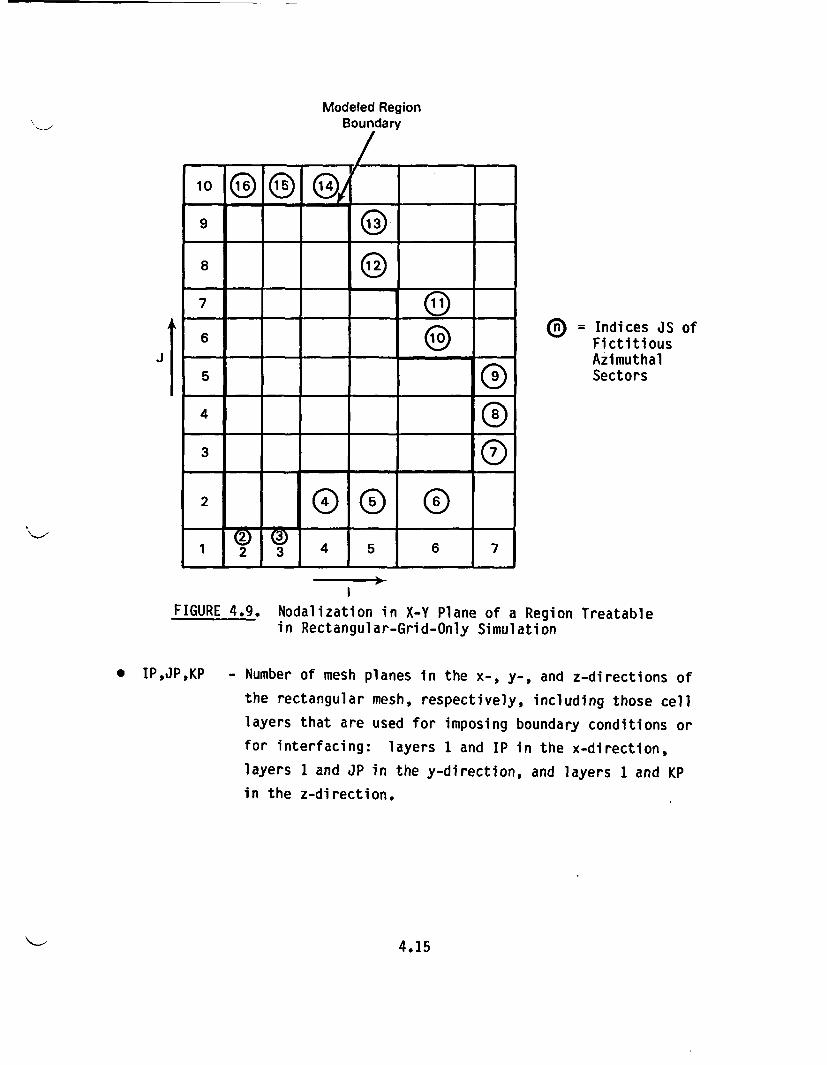
Figure 4.9 illustrates an X-Y nodalization for a geometry allowed in a
rectangular-grid-only computation. The active computational region, shown by
the dark outline in Figure 4.4, is defined in input using the arrays IEEND,
JEBEG, JEEND, IMEND, JMBEG, and JMEND. Cells bounding the active computation
region have a boundary condition or phantom cell role. The indices JS of the
fictitious azimuthal sectors connecting to the boundary cells are shown
circled. For a rectangular-grid-only simulation (NOBODY = 1), it is appropri-ate to set the dimensioning parameter JSP (number of azimuthal sectors,
including phantoms) to two more than the number of phantom boundary cells in
one X-Y plane to the right of the cell layer I = 1. Figure 4.10 illustrates a
possible set of input for GRID Input Blocks 1 and 2 for the geometry of
Figure 4.9.
A rectangular-grid-only simulation offers somewhat greater freedom in the
choice of grid lines than does a hybrid grid. Code input does not currently
allow a completely arbitrary specification of initial temperatures for a rec-
tangular grid alone. If that is needed, it can be provided by fairly simple
supplementary coding.
4.2 PARAMETER STATEMENT INFORMATION
Subroutine GRID requires the specification of the following parameters:
4.14
Modeled RegionBoundary
JA
0 = Indices JS ofFictitiousAzimuthalSectors
FIGURE 4.9. Nodalization in X-Y Plane of a Region Treatablein Rectangular-Grid-Only Simulation
0 IP,JP,KP - Number of mesh planes in the x-, y-, and z-directions of
the rectangular mesh, respectively, including those cell
layers that are used for imposing boundary conditions or
for interfacing: layers 1 and IP in the x-direction,
layers 1 and JP in the y-direction, and layers 1 and KP
in the z-direction.
4.15
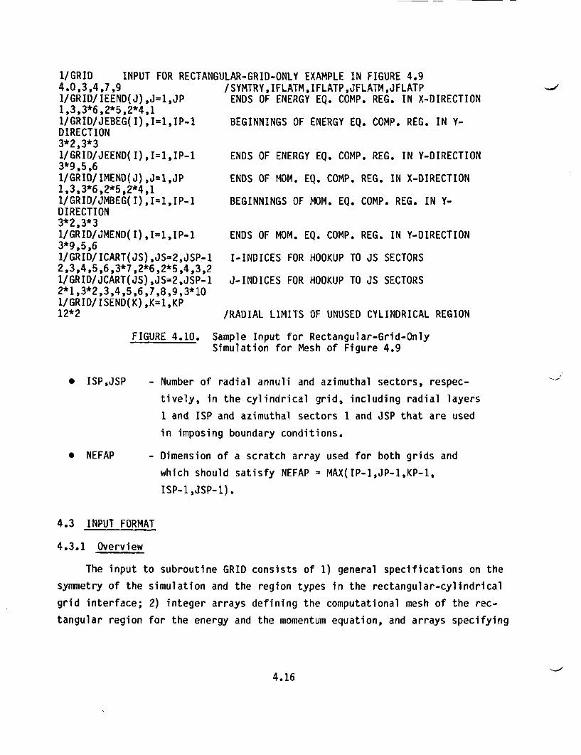
1/GRID INPUT FOR RECTANGULAR-GRID-ONLY EXAMPLE IN FIGURE 4.94.0,3,4,7,91/GRID/IEEND(J),J=1,JP1,3,3*6,2*5,2*4,11/GRID/JEBEG(I),I=1,IP-1DIRECTION3*2,3*31/GRID/JEEND(I),I=1,IP-13*9,5,61/GRID/ IMEND(J) ,J=1,JP1,3,3*6,2*5,2*4,11/GRID/JMBEG(I),I=1,IP-1DIRECTION3*2,3*31/GRID/JMEND(I),I=1,IP-13*9,5,61/GRID/ICART(JS),JS=2,JSP-12,3,4,5,6,3*7,2*6,2*5,4,3,21/GRID/JCART(JS),JS=2,JSP-12*1,3*2,3,4,5,6,7,8,9,3*101/GRID/ISEND(K),K=1,KP12*2
/SYMTRY,IFLATM,IFLATP,JFLATM,JFLATPENDS OF ENERGY EQ. COMP. REG. IN X-DIRECTION
BEGINNINGS OF ENERGY EQ. COMP. REG. IN Y-
ENDS OF ENERGY EQ. COMP. REG. IN Y-DIRECTION
ENDS OF MOM. EQ. COMP. REG. IN X-DIRECTION
BEGINNINGS OF MOM. EQ. COMP. REG. IN Y-
ENDS OF MOM. EQ. COMP. REG. IN Y-DIRECTION
I-INDICES FOR HOOKUP TO JS SECTORS
J-INDICES FOR HOOKUP TO JS SECTORS
/RADIAL LIMITS OF UNUSED CYLINDRICAL REGION
FIGURE 4.10. Sample Input for Rectangular-Grid-OnlySimulation for Mesh of Figure 4.9
* ISPJSP
* NEFAP
- Number of radial annuli and azimuthal sectors, respec-
tively, in the cylindrical grid, including radial layers
I and ISP and azimuthal sectors 1 and JSP that are used
in imposing boundary conditions.
- Dimension of a scratch array used for both grids and
which should satisfy NEFAP = MAX(IP-1,JP-1,KP-1,
ISP-i,JSP-1).
4.3 INPUT FORMAT
4.3.1 Overview
The input to subroutine GRID consists of 1) general specifications on the
symmetry of the simulation and the region types in the rectangular-cylindrical
grid interface; 2) integer arrays defining the computational mesh of the rec-
tangular region for the energy and the momentum equation, and arrays specifying
4.16
the rectangular grid cells that interface with cylindrical grid sectors; and 3)
arrays of mesh spacings for the rectangular and cylindrical meshes.
4.3.2 Symmetry and Interface Regions. Input Block 1
General Input Format
NECHOSYMTRY,IFLATM,IFLATP,JFLATM,JFLATP
General Input Description
* NECHO - Echoing switch for this section of input.
to be echoed, then NECHO = 1; otherwise 0.
If input is
* SYMTRY
* IFLATM
* IFLATP
* JFLATM
- Number of quadrants in modeled region: 1.0 for quarter-
plane symmetry, and 2.0 for half-plane symmetry.
- The value of the highest I index in the rectangular grid
for the flat part of the rectangular computational grid
boundary at the lower constant y-value. See Figure 4.2.
- The value of the highest I index in the rectangular grid
for the flat part of the rectangular computational grid
boundary at the higher constant y-value. See Figure 4.2.
- The value of the lowest J index in the rectangular
for the flat part of the rectangular computational
boundary at constant x-value. See Figure 4.2.
grid
grid
* JFLATP - The value of the highest J index in the rectangular grid
for the flat part of the rectangular computational grid
boundary at constant x-value. See Figure 4.2.
Note: The grid shown in Figure 4.1 has IP = 25, JP = 48, ISP = 8, and JSP =
64, with the x-direction layer at I = 1 and the radial layer IS = 8 not
shown. The phantom azimuthal sectors JS = 1 and JS = JSP = 64 are also
not shown. This example also has IFLATM = 9, IFLATP = 9, JFLATM = 17,
and JFLATP = 32. Because of the amount of detail and the fineness of
the mesh in places, it is useful to also examine the grid shown in
4.17
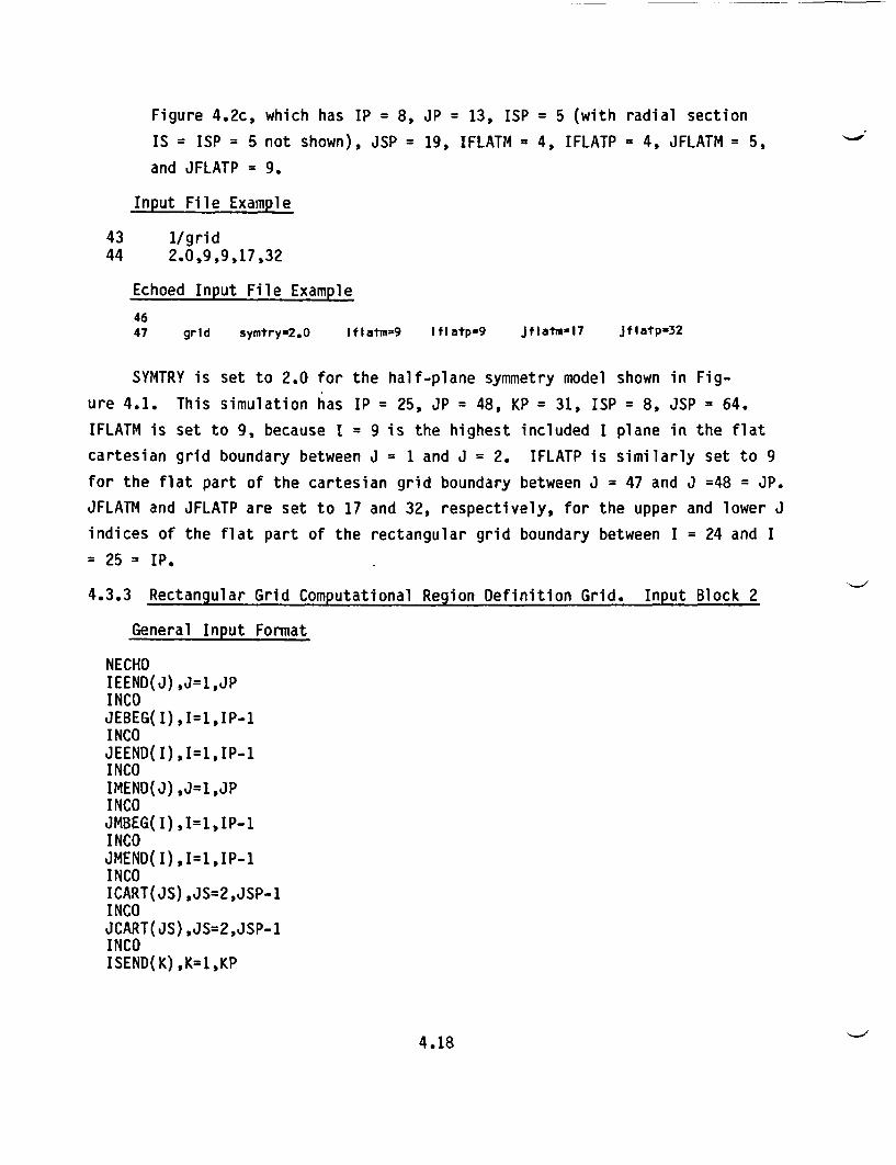
Figure 4.2c, which has IP = 8, JP = 13, ISP = 5 (with radial section
IS = ISP = 5 not shown), JSP = 19, IFLATM = 4, IFLATP = 4, JFLATM = 5,
and JFLATP = 9.
Input File Example
43 1/grid44 2.0,9,9,17,32
Echoed Input File Example
4647 grld symtry=2.0 Iflatm=9 IflatpO9 Jflatm=17 Jflatp=32
SYMTRY is set to 2.0 for the half-plane symmetry model shown in Fig-
ure 4.1. This simulation has IP = 25, JP = 48, KP = 31, ISP = 8, JSP = 64.
IFLATM is set to 9, because I = 9 is the highest included I plane in the flatCartesian grid boundary between J = 1 and J = 2. IFLATP is similarly set to 9
for the flat part of the Cartesian grid boundary between J = 47 and J =48 = JP.JFLATM and JFLATP are set to 17 and 32, respectively, for the upper and lower J
indices of the flat part of the rectangular grid boundary between I = 24 and I
= 25 = IP.
4.3.3 Rectangular Grid Computational Region Definition Grid. Input Block 2
General Input Format
NECHOIEEND(J),J=1,JPINCOJEBEG(I),I=1,IP-1INCOJEEND(I),I=1,IP-1INCOIMEND(J) ,J=1,JPINCOJMBEG( I) ,I=1,IP-1INCOJMEND( I) ,I=1,IP-1INCOICART(JS) ,JS=2,JSP-1INCOJCART(JS),JS=2,JSP-1INCOISEND(K),K=1,KP
4.18
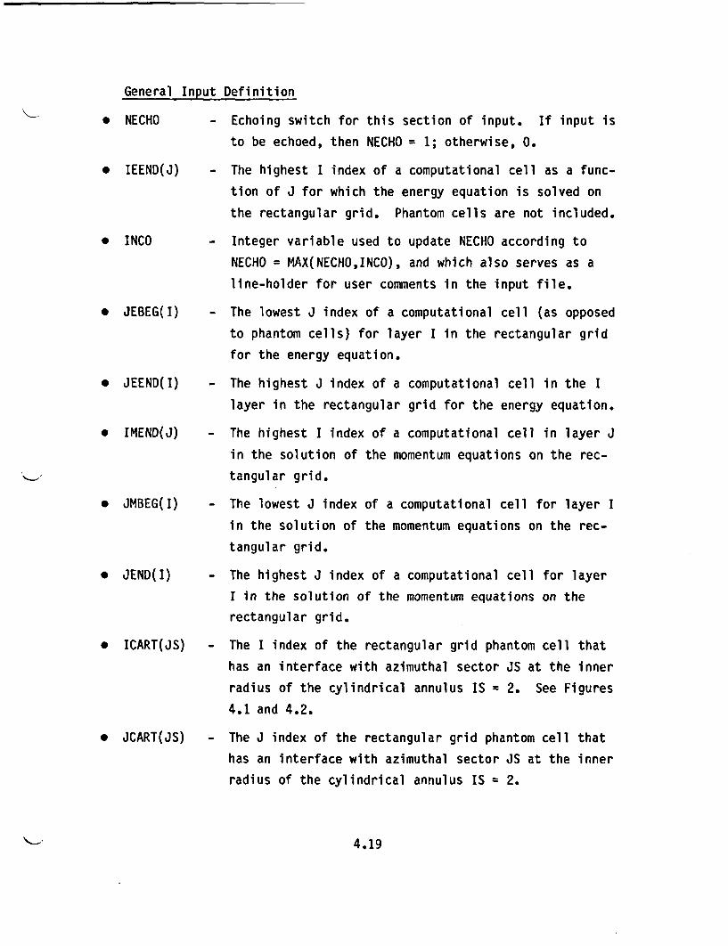
General Input Definition
* NECHO
* IEEND(J)
* INCO
* JEBEG(I)
- Echoing switch for this section of input. If input is
to be echoed, then NECHO = 1; otherwise, 0.
- The highest I index of a computational cell as a func-
tion of J for which the energy equation is solved on
the rectangular grid. Phantom cells are not included.
- Integer variable used to update NECHO according to
NECHO = MAX(NECHO,INCO), and which also serves as a
line-holder for user comments in the input file.
- The lowest J index of a computational cell (as opposed
to phantom cells) for layer I in the rectangular grid
for the energy equation.
* JEEND(I)
* IMEND(J)
* JMBEG(I)
* JEND(I)
* ICART(JS)
* JCART(JS)
- The highest J index of a computational cell in the I
layer in the rectangular grid for the energy equation.
- The highest I index of a computational cell in layer J
in the solution of the momentum equations on the rec-
tangular grid.
- The lowest J index of a computational cell for layer I
in the solution of the momentum equations on the rec-
tangular grid.
- The highest J index of a computational cell for layer
I in the solution of the momentum equations on the
rectangular grid.
- The I index of the rectangular grid phantom cell that
has an interface with azimuthal sector JS at the inner
radius of the cylindrical annulus IS = 2. See Figures
4.1 and 4.2.
- The J index of the rectangular grid phantom cell that
has an interface with azimuthal sector JS at the inner
radius of the cylindrical annulus IS = 2.
4.19
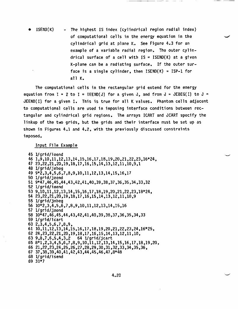
* ISEND(K) - The highest IS index (cylindrical region radial index)
of computational cells in the energy equation in the
cylindrical grid at plane K. See Figure 4.3 for an
example of a variable radial region. The outer cylin-
drical surface of a cell with IS = ISEND(K) at a given
K-plane can be a radiating surface. If the outer sur-
face is a single cylinder, then ISEND(K) = ISP-1 for
all K.
The computational cells in the rectangular grid extend for the energy
equation from I = 2 to I = IEEND(J) for a given J, and from J = JEBEG(I) to J =
JEEND(I) for a given I. This is true for all K values. Phantom cells adjacent
to computational cells are used in imposing interface conditions between rec-
tangular and cylindrical grid regions. The arrays ICART and JCART specify the
linkup of the two grids, but the grids and their interface must be set up as
shown in Figures 4.1 and 4.2, with the previously discussed constraints
imposed.
Input File Example
45 1/grid/ieend46 1,9,10,11,12,13,14,15,16,17,18,19,20,21,22,23,16*24,47 23,22,21,20,19,18,17,16,15,14,13,12,11,10,9,148 1/grid/jebeg49 9*2,3,4,5,6,7,8,9,10,11,12,13,14,15,16,1750 1/grid/jeend51 9*47,46,45,44,43,42,41,40,39,38,37,36,35,34,33,3252 1/grid/imend53 9,10,11,12,13,14,15,16,17,18,19,20,21,22,23,18*24,54 23,22,21,20,19,18,17,16,15,14,13,12,11,10,955 1/grid/jmbeg56 10*2,3,4,5,6,7,8,9,10,11,12,13,14,15,1657 1/grid/jmend58 10*47,46,45,44,43,42,41,40,39,38,37,36,35,34,3359 1/grid/icart60 2,3,4,5,6,7,8,9,61 10,11,12,13,14,15,16,17,18,19,20,21,22,23,24,16*25,62 24,23,22,21,20,19,18,17,16,15,14,13,12,11,10,63 9,8,7,6,5,4,3,2 64 1/grid/jcart65 8*1,2,3,4,5,6,7,8,9,10,11,12,13,14,15,16,17,18,19,20,66 21,22,23,24,25,26,27,28,29,30,31,32,33,34,35,36,67 37,38,39,40,41,42,43,44,45,46,47,8*4868 1/grid/isend69 31*7
4.20
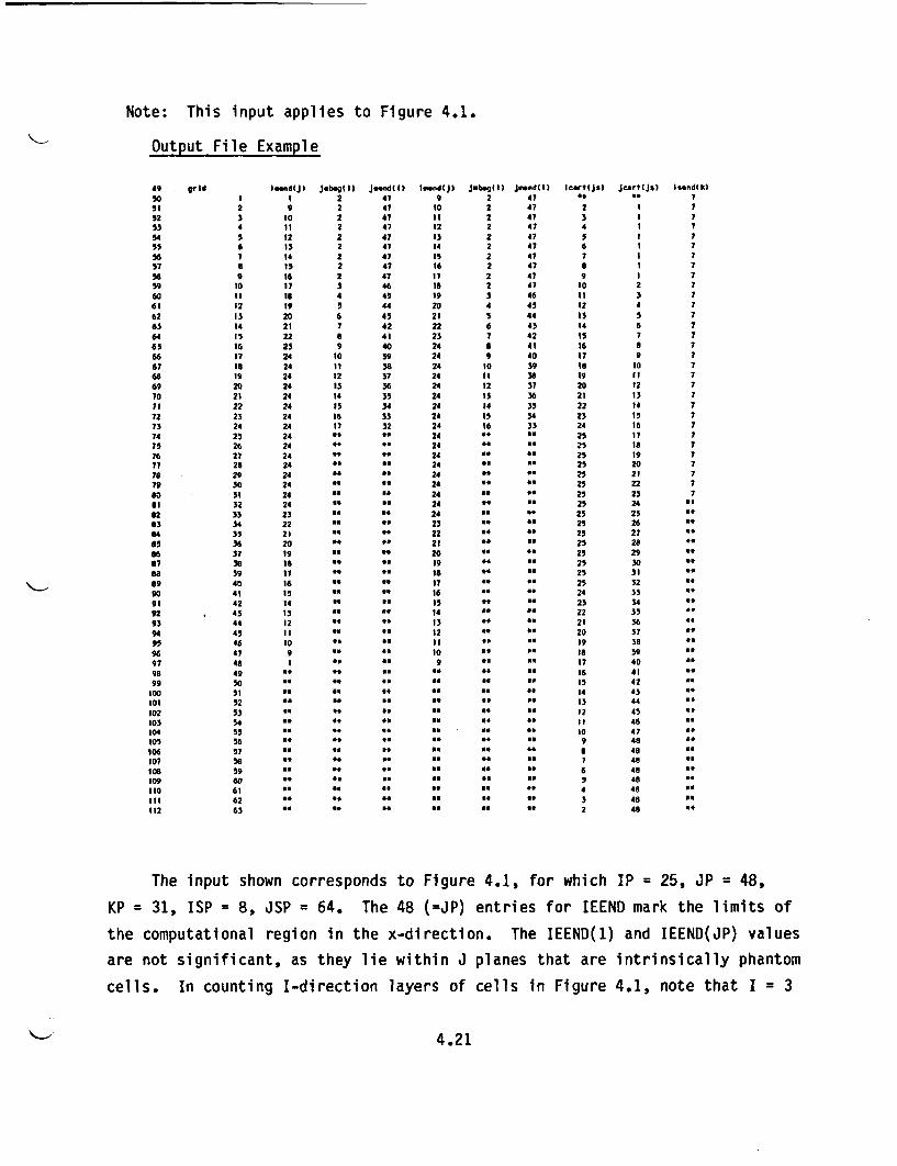
Note: This input applies to Figure 4.1.
Output File Example
49 grid leend~j) jeobgll ) Je.nd(l) loondCjl Jmbog(I) j..rnd(l) leart(js) JeartCjs) l.n"( k)s0 I I 2 41 2 41 No 7.33 2 9 2 47 10 2 47 2 7
32 3 tO 2 417 3 2 41 3 I 753 4 Il 2 47 12 2 47 4 1 154 5 12 2 47 33 2 47 5 3753 6 33 2 47 14 2 47 6 I1 7
36 7 I14 2 47 35 2 47 7 I757 8 I 2 47 16 2 447 8 736 9 16 2 47 I7 2 47 9I I
5910 17 3 46 la 2 47 30 2 780 II l 4 45 19 3 46 II 3 761 32 19 5 4 20 4 45 32 4 7
62 13 20 6 I3 21 5 44 13 5 763 14 21 7 42 22 6 43 14 6 764 IS 22 6 41 23 7 42 Is 7 763 16 23 9 40 24 6 41 16 S 766 17 24 10 39 24 9 40 17 9 7
636 24 33 3 24 0 39 1 0 7619 2 2 37 24 33 36 1 I
69 20 24 13 36 24 12 37 20 12 770 21 24 14 35 24 13 36 21 13 771 22 24 35 34 24 14 35 22 14 772 23 24 36 33 24 IS 34 23 35 773 24 24 37 32 24 16 33 24 16 174 25 24 4 24 No No 25 17 I73 26 24 ** 24 ' * 25 16776 27 24 24 1 23 19: 777 28 24 24 25 20 771 29 24 24 25 21 779 30 24 24 25 22 7so 31 24 4424 *253 23 783I 32 24 24 ' 25 2462 33 23 44 24 4 ~ ~ 25 25
8334 22 4 23 2 26641 35 21 No 232 00' 25 2785 36 20 of 21 44 " 23 288663 19 NO 20 NO . 25 2987 36 IS o 19 N of 23 30Be 39 17 No Is * 25 3169 40 16 14 4 7 4 ~ ~ 25 3290 4I3 16 24 33 4
91 42 14 15 ' i 23 54 4
92 * 43 13 so 14 22 3593 44 12 : No 13 to a* 21 36 N94 45 33 N2 to *2 20 37 o93 46 30 *0 4' 33 19 38 N96 47 9 No 44 30 No No I38 59 OR
97 46 I No 49 44 * 17 409849 ' 4 * 6 41
969 530 ':4 -3 42too SI* 4 4 43I01 52 '13 44102 331 2 45303 54 No 33 46
305 56 S.4t 9 45106 57 8 48107 36 44 48
Ie59 4 44 4 46 48109 60 No 4 5 48
I30 6 44 4 * 444 48
112 63 O . N4o4 D. to 2 48 s
The input shown corresponds to Figure 4.1, for which IP= 25, JP= 48,
KP= 31, ISP = 8, JSP = 64. The 48 (=JP) entries for IEEND mark the limits of
the computational region in the x-direction. The IEEND(1) and IEEND(JP) values
are not significant, as they lie within J planes that are intrinsically phantom
cells. In counting I-direction layers of cells in Figure 4.1, note that I = 3
4.21

corresponds to an extremely thin layer. Note IEEND(2) is set to 9, making the
cell (I,J) = (10,2) a phantom cell. This is appropriate because the cell (I,J)
= (10,2) is bisected by the cylinder and is appropriate for interfacing withthe azimuthal sector JS = 10. The energy computations in the rectangular grid
for J = 2 through J = 16 stop one short of a bisected interface cell in the
I-direction. Energy computations for J = 17 through J = 32 stop at I = 24,
leaving the cells at I = 25 in the region between this flat part of the rec-
tangular grid boundary and the cylinder interface as phantom cells connecting
to the azimuthal sectors JS = 25 through JS = 40.
The JEBEG and JEEND arrays give upper and lower J indices for the rec-
tangular grid computational region, leaving the interface cell at either end
(upper and lower) for interfaces. The IP-1 entries in either of these two
arrays (for I = 1 to IP-1) specify these limits, whose correspondence to Fig-
ure 4.1 should be noted.
The computational limits for the momentum equation are similarly defined
in IMEND, JMBEG, and JMEND. Note that the choices make the momentum equation
computational region somewhat larger. The cells on the curved part of the
interface boundary can be treated as having a partial flow area, with a zero
flow condition on the next outward computational cell.
The ISEND(K) are set to 7 (=ISP-1) for all K indices, indicating that all
radial regions in the cylindrical grid out to the phantom layer at IS = ISP = 8are to be included, and that the cask exterior is a cylinder.
The echoed output of these arrays uses a running multipurpose integer
index in a column on the left, i.e., the integer is I, J, JS, or K as needed,
followed by columns to report IEEND(J), JEBEG(I), JEEND(I), IMEND(J), JMBEG(I),
JMEND(I), ICART(JS), JCART(JS), or ISEND(K).
For convenience to users in seeing the region definitions and interface
hookup input, a possible set of input for GRID Input Blocks 1 and 2 for the
mesh shown in Figure 4.2c is presented in Figure 4.7.
4.22
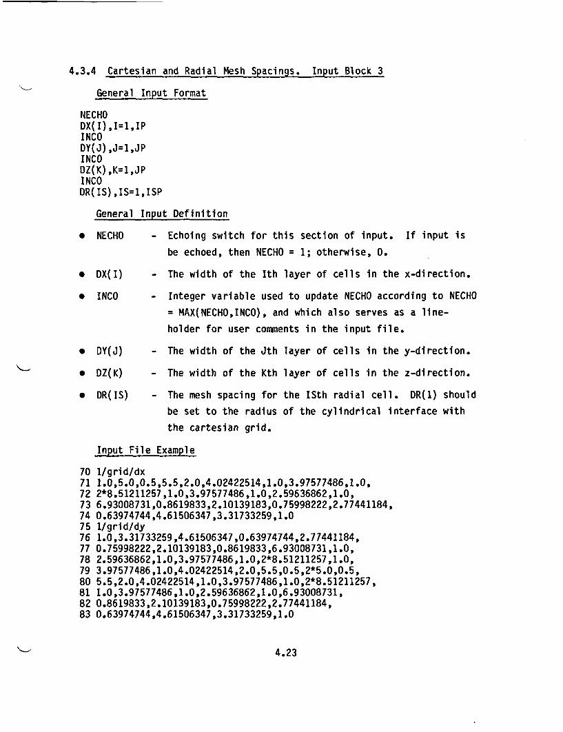
4.3.4 Cartesian and Radial Mesh Spacings. InputBlock 3. .
General Input Format
NECHODX(I),I=1,IPINCODY(J),J=1,JPINCODZ(K) ,K=1,JPINCODR(IS),IS=1,ISP
General Input Definition
* NECHO - Echoing switch for this section of input. If input is
be echoed, then NECHO = 1; otherwise, 0.
* DX(I) - The width of the Ith layer of cells in the x-direction.
* INCO - Integer variable used to update NECHO according to NECHO
= MAX(NECHO,INCO), and which also serves as a line-
holder for user comments in the input file.
* DY(J) - The width of the Jth layer of cells in the y-direction.
* DZ(K) - The width of the Kth layer of cells in the z-direction.
* DR(IS) - The mesh spacing for the ISth radial cell. DR(1) should
be set to the radius of the cylindrical interface with
the Cartesian grid.
Input File Example
70 1/grid/dx71 1.0,5.0,0.5,5.5,2.0,4.02422514,1.0,3.97577486,1.0,72 2*8.51211257,1.0,3.97577486,1.0,2.59636862,1.0,73 6.93008731,0.8619833,2.10139183,0.75998222,2.77441184,74 0.63974744,4.61506347,3.31733259,1.075 1/grid/dy76 1.0,3.31733259,4.61506347,0.63974744,2.77441184,77 0.75998222,2.10139183,0.8619833,6.93008731,1.0,78 2.59636862,1.0,3.97577486,1.0,2*8.51211257,1.0,79 3.97577486,1.0,4.02422514,2.0,5.5,0.5,2*5.0,0.5,80 5.5,2.0,4.02422514,1.0,3.97577486,1.0,2*8.51211257,81 1.0,3.97577486,1.0,2.59636862,1.0,6.93008731,82 0.8619833,2.10139183,0.75998222,2.77441184,83 0.63974744,4.61506347,3.31733259,1.0
4.23
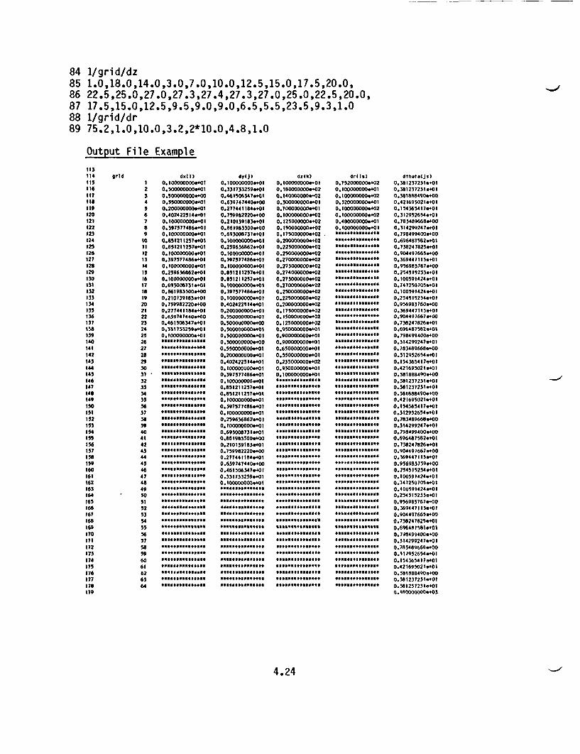
84 1/grid/dz85 1.0,18.0,14.0,3.0,7.0,10.0,12.5,15.0,17.5,20.0,86 22.5,25.0,27.0,27.3,27.4,27.3,27.0,25.0,22.5,20.0,87 17.5,15.0,12.5,9.5,9.0,9.0,6.5,5.5,23.5,9.3,1.088 1/grid/dr89 75.2,1.0,10.0,3.2,2*10.0,4.8,1.0
Output File Example
113.,.
11,
116It?#is119120121122123124125126127128129150151152'3313413513613715319140141142143144145146147ids149101511321531"4'3,15615715819160161162163164165166167168169170171172173174175176177178179
grid 6xt I)
2 0.1000000000+012 0.500000000..013 0.500000000.+004 0.2000000000+01
6 0.402422514.4017 0.100000000.0I0a 0.3975774860+019 0.1000000000+0l
to 0.651211237.401,II 0.8512112579+01I2 0.I000000000+0113 0.3973774860+0114 O.l0000O04,0+0115 0.259636862.40116 0. 1000000009O0117 0.69300673104011is 0.861983300.00019 0.210139183&+0l20 0.759982220.+0021 0.2714411840+012.2 0.6397474400+0023 0.461506347.40124 0.3`1533259.40123 0.100000000.0I0262728
32 **33 ..... ff*34 v.**0f** ... t00.S
37 tt*ffttttW
39 f....fn
40 ff~ffff*fffff
484243 *t*ttfff**
47 *.tf.fff..
4930 ... 0*ft*ft... ftftf
52 ft.....ft ntoof
560
62 *ff.04-0 .... f... d
63 f~tttf~tf~tt
64 tfft**tt*f
dyli) dztk)0.100000000.401 0. I000000000+0l0.331733259e+01 0.180000000.4020.461506347*4-01 0.140000000-4020.6397474400+00 0.3000000000+010.277441154.401 0.100000000.4010.759982220.400 0.100000000.4020.2101391830+01 0.125000000.4020.861983300e+00 0.1500000000+020.6930087310+01 0.11350000000+020.100000000.0+0 0.200000000.4020.259636862.401 0.2250000000+020.1000000000+O1 0.250OOO0000.4020.397571486.401 0.270000O0040020.1000000000+01 0.2130000000+020.831211257e401 0.214000000o4020.831211257a" 1 0.2750000000+020.1O000000040) 0.2100000000+020.391377486e401 0.2500000000+020.1000000009+01 0.2250000000+020.402422514.'401 0.2OO0000000+20.2O0000000&401 0.175000000.4020.550000000.401 0.1500000000+020.500000000.+00 0.1250000000+020.5000000000+01 0.9500000000+010.3000000000+0 I 0.9000000000+010.500000000.400 0.9000000000+010.5500000000+0l 0.650000000*4010.200000000.401 0.5300000000+0 I0.4024225140401 0.255000000.+020.1000000000+01 0.950000000.4010.397377486.+01 0.IO0000000.401
0.851211257.4e *t+tttfffOlff*
OAVMZ12570401 doom...ttftttt*f0. 0000.tI ftfttO()O**0tftfO I0.597317486.0I00.100000000.0I 10.2539636862.4010.I000000000+0I * *10.693006731.401 fptttttteft.
0.2101391830+01 f~tffffff~fff
0.759982220.400 a ... a ..... f 0ftf
0.639747440.+00 .*o ... foot l0.461506347.401 of...**..a0.331733259*401 .0*.. 0060.100000000*41f+fOi *fff~ff~
...f.... so . ...fft t*ftt*so .. .0
ft....*ft..ftMftf .*t.* fltt..n.....*0
*.to .f...ftft....d ft* ... fQ*fttffttffttf
.....ft... ..f.f f.f...ft*0..f.f..dom
r( I.s)0.752000000.+020.100000000.+010.100000000.+020.3200000000+0l0.1000000006+020.100000000e+020.480000000-+010.1000000000+01
of, ... " f.s.**ft
......ftt.........
so ftf...ftftft.0.0.
ft .ftt.....f tf.f
**dffv**fN#*sfo
t....doomf.....
. f..... on
ft0..f....ft.tf.
v*avft oftm*ftfft*§o
otf.f t. ft f... f. Omftf
fft.f...f tf. doom.
ft..Of..s f.. f.. f..
dth.tatJs)
0.381237231.400.381237231.400.3818884900+000.421695021.400.154365417e+010.3129526544+010.785489668.+000.314299247.+010.798499400e.000.696481562.0+0.738247825*+010.9044976650+000.3694471134+010.956983767+.000.2545152330+010.100591424 +010.74725070501+l0.100591424.400.2545152344+010.956983?60.4000.3694471130+010.9044976670+00
0.738247826e+0I0.696457582.40i0.7984994000+000.51429924710010.783489668e+000.312952654.+010.154365417*+010.421695021*+00.3818884900+000.3812372310+010.381237231&+010.581888490.+000.4216950210+010.154565417*+010.3129526540+010.783489668e+000.3142992470+010.798499400.+000.696487582*+010.7582478260+010.9044976670+000.5694471130+010.9569837590+000.254515234.+010.100591424.400.741250705-+0t0.1005914240+010.254515235.+010.9569837670+000.369447113.+010.9044976650+D00.758247825.+01
0.696481581WOI0.798499400.4000.514299247.4010.7854896680+000.312952654.0+0.1543654110+010.421693021&+0I0.3818884900+000.381237231e+010.381237231.+010. 180000000e+03
4.24
The rectangular and cylindrical mesh spacings are both specified by this
set of input. The azimuthal mesh is determined by the rectangular mesh and by
the linkup prescribed by the ICART and JCART arrays and the mesh parameters
IFLATM, IFLATP, JFLATM, and JFLATP, as can be seen in Figures 4.1 and 4.2.
Although the thicknesses of the phantom cell layers set by DX(I), DZ(1),
DZ(KP), DR(ISP), etc., are not critical for the boundary conditions usually
imposed, they are not completely arbitrary, either. For example, if insulated
boundary conditions are desired to impose symmetry about the constant x-plane
between the I = 1 and I = 2 layers, then the product of the x-direction
resistivity and the half-thickness of the I = 1 layer should be orders of mag-
nitude greater than that for real conduction paths.
The echoed output of these arrays of mesh spacing information uses a
running multipurpose integer index in a column on the left; i.e., the integer
is I, J, K, IS, or JS as needed, followed by columns with DX(I), DY(J), DZ(K)
DR(IS), and DTHETA(JS). The angular mesh spacing array, DTHETA(JS), is
reported in degrees.
4.25
5.0 SUBROUTINE PROP
Subroutine PROP sets resistances to heat transfer in the rectangular grid
region.
5.1 PROP FUNCTIONS
PROP treats heat transfer that is mathematically equivalent to conduction
on a finite mesh. Emission and reabsorption of radiation over short distances
within and between cells, as well as temperature dependence of true conduction,
can be incorporated into thermal resistances by PROP using effective thermal
conductivity polynomials. Explicit radiation models, like that among several
surfaces facing an enclosure or among fuel pins treated discretely, are treated
elsewhere in radiation routines RADC, RADP, and RADR.
At each time-step, PROP updates the resistances to heat transfer using
current temperatures and previously stored sets of numbers referred to here as
thermal parameter sets. These thermal parameter sets contain numbers that
specify some features of the heat transfer model. For most models, these
features include the temperature-dependence of the thermal conductivity of a
comprising material or composite.
Heat transfer models available in PROP include:
* conduction in isotropic or orthotropic substances
• conduction through layered composites offering parallel conduction
paths
* conduction through layered composites offering series conduction
paths
* conduction and radiation among arrays of cylinders having axes in the
z-direction (treated as a continuum)
* normal conduction through single or series films between cells,
including gaps with combined radiation and conduction
* parallel heat transfer by radiation and by forced or natural
convection from cask ends.
5.1
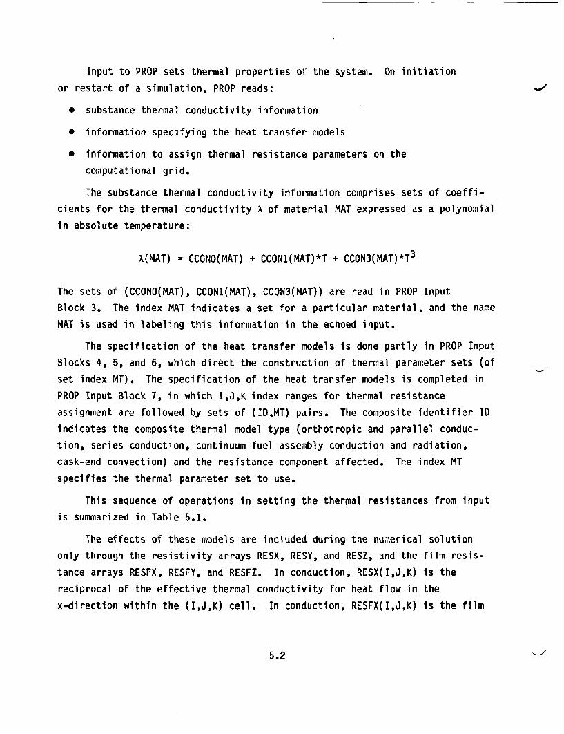
Input to PROP sets thermal properties of the system. On initiation
or restart of a simulation, PROP reads:
* substance thermal conductivity information
* information specifying the heat transfer models
* information to assign thermal resistance parameters on the
computational grid.
The substance thermal conductivity information comprises sets of coeffi-
cients for the thermal conductivity A of material MAT expressed as a polynomial
in absolute temperature:
A(MAT) = CCONO(MAT) + CCON1(MAT)*T + CCON3(MAT)*T3
The sets of (CCONO(MAT), CCON1(MAT), CCON3(MAT)) are read in PROP Input
Block 3. The index MAT indicates a set for a particular material, and the name
MAT is used in labeling this information in the echoed input.
The specification of the heat transfer models is done partly in PROP Input
Blocks 4, 5, and 6, which direct the construction of thermal parameter sets (of
set index MT). The specification of the heat transfer models is completed in
PROP Input Block 7, in which I,J,K index ranges for thermal resistance
assignment are followed by sets of (ID,MT) pairs. The composite identifier ID
indicates the composite thermal model type (orthotropic and parallel conduc-
tion, series conduction, continuum fuel assembly conduction and radiation,
cask-end convection) and the resistance component affected. The index MT
specifies the thermal parameter set to use.
This sequence of operations in setting the thermal resistances from input
is summarized in Table 5.1.
The effects of these models are included during the numerical solution
only through the resistivity arrays RESX, RESY, and RESZ, and the film resis-
tance arrays RESFX, RESFY, and RESFZ. In conduction, RESX(I,J,K) is the
reciprocal of the effective thermal conductivity for heat flow in the
x-direction within the (I,J,K) cell. In conduction, RESFX(I,J,K) is the film
5.2
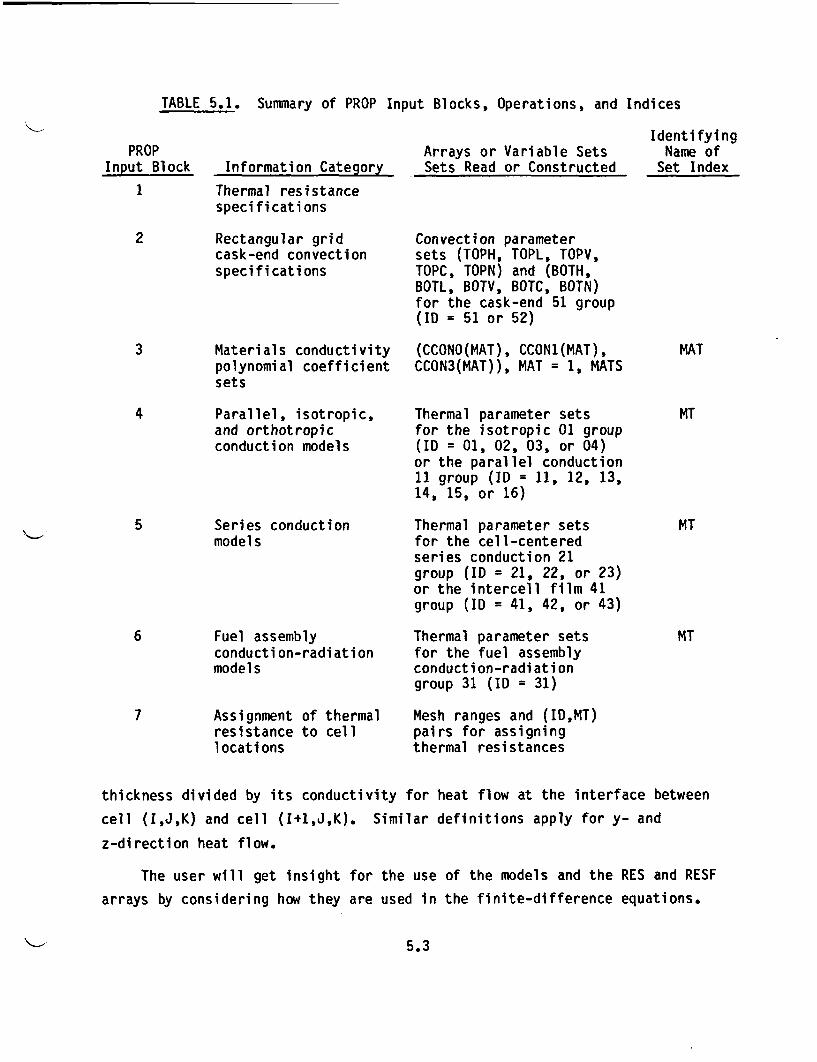
TABLE 5.1. Summary of PROP Input Blocks, Operations, and Indices
PROPInput Block
1
Information Category
Thermal resistancespecifications
Arrays or Variable SetsSets Read or Constructed
IdentifyingName of
Set Index
2 Rectangular gridcask-end convectionspecifications
3 Materials conductivitypolynomial coefficientsets
4 Parallel, isotropic,and orthotropicconduction models
Convection parametersets (TOPH, TOPL, TOPV,TOPC, TOPN) and (BOTH,BOTL, BOTV, BOTC, BOTN)for the cask-end 51 group(ID = 51 or 52)
(CCONO(MAT), CCON1(MAT),CCON3(MAT)), MAT = 1, MATS
Thermal parameter setsfor the isotropic 01 group(ID = 01, 02, 03, or 04)or the parallel conduction11 group (ID = 11, 12, 13,14, 15, or 16)
Thermal parameter setsfor the cell-centeredseries conduction 21group (ID = 21, 22, or 23)or the intercell film 41group (ID = 41, 42, or 43)
Thermal parameter setsfor the fuel assemblyconduction-radiationgroup 31 (ID = 31)
MAT
MT
MT
MT
5 Series conductionmodels
6 Fuel assemblyconduction-radiationmodels
7 Assignment of thermalresistance to celllocations
Mesh ranges and (ID,MT)pairs for assigningthermal resistances
thickness divided by its conductivity for heat flow at the interface between
cell (I,J,K) and cell (I+1,J,K). Similar definitions apply for y- and
z-direction heat flow.
The user will get insight for the use of the models and the RES and RESF
arrays by considering how they are used in the finite-difference equations.
5.3
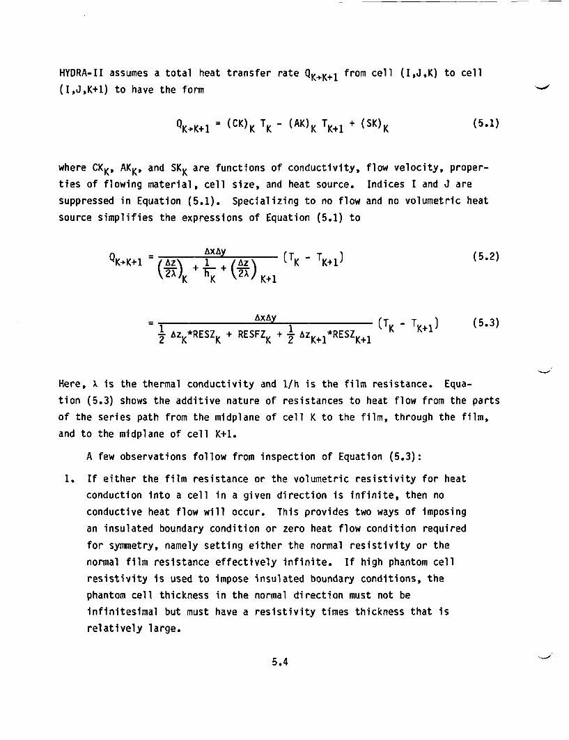
HYDRA-II assumes a total heat transfer rate QK+K+1 from cell (I,J,K) to cell
(I,J,K+1) to have the form
QKK1 (CK)K TK - (AK)K TK+j + (SK)K (5.1)
where CKK, AKK, and SKK are functions of conductivity, flow velocity, proper-
ties of flowing material, cell size, and heat source. Indices I and J are
suppressed in Equation (5.1). Specializing to no flow and no volumetric heat
source simplifies the expressions of Equation (5.1) to
K - AXAy (T - T. ) (5.2)QK-01 (AZ) + ; + /AZ K K+1
1 AXAY 1 (TK - TK+1) (5.3)2 AzK*RESZK + RESFZ K + 2 AZK+1*RESZ K+1
Here, x is the thermal conductivity and 1/h is the film resistance. Equa-
tion (5.3) shows the additive nature of resistances to heat flow from the parts
of the series path from the midplane of cell K to the film, through the film,
and to the midplane of cell K+1.
A few observations follow from inspection of Equation (5.3):
1. If either the film resistance or the volumetric resistivity for heat
conduction into a cell in a given direction is infinite, then no
conductive heat flow will occur. This provides two ways of imposing
an insulated boundary condition or zero heat flow condition required
for symmetry, namely setting either the normal resistivity or the
normal film resistance effectively infinite. If high phantom cell
resistivity is used to impose insulated boundary conditions, the
phantom cell thickness in the normal direction must not be
infinitesimal but must have a resistivity times thickness that is
relatively large.
5.4

2. If the effective resistivity within a cell for conduction in a
particular direction is zero, the effect is equivalent to moving the
cell center temperature to the cell boundary in that direction. This
should be used in setting a temperature boundary condition at the
edge of the computation region; i.e., set the resistivity in the
phantom cell to zero and the phantom cell temperature to the value
desired at the edge of the adjacent computational cell.
3. Resistances to heat transfer by processes other than conduction can
be modeled by appropriate temperature-dependent choices of
resistivity and/or film resistance parameters, as we will show for
specific cases.
The process of setting the RESX, RESY, RESZ, RESFX, RESFY, and RESFZ
variables in subroutine PROP occurs in phases for these models. Descriptive
input for these models is read in PROP in a series of input blocks. PROP Input
Block 2 specifies some parameters needed for the cask end convection models.
Input Block 3 specifies a number of sets of polynomial coefficients for
conductivity of substances, the sets CCONO(MAT), CCON1(MAT), and CCON3(MAT) for
MAT = 1 to MATS. Subsequent input blocks 4, 5, and 6 specify the construction
of thermal parameter sets for use in the heat transfer models. These thermal
parameters include the arrays CO(MT), C1(MT), C3(MT), and selected others for
the specific models. Most commonly, the set CO(MT), C1(MT), and C3(MT) is a
set of polynomial coefficients for a conduction-related variable. A final
block of input to PROP gives final specifications for the construction of the
resistance-related arrays according to these models, including the mesh
locations at which they apply. The actual setting of resistance arrays is done
at each time-step, using the latest temperatures, the constructed thermal
parameter sets, and the resistance assignment directive sets.
Table 5.2 provides summary information for construction of the thermal
parameter sets needed in the thermal models. It should be referred to in the
following discussions of models and of input data. Figure 5.1 shows schematic
5.5
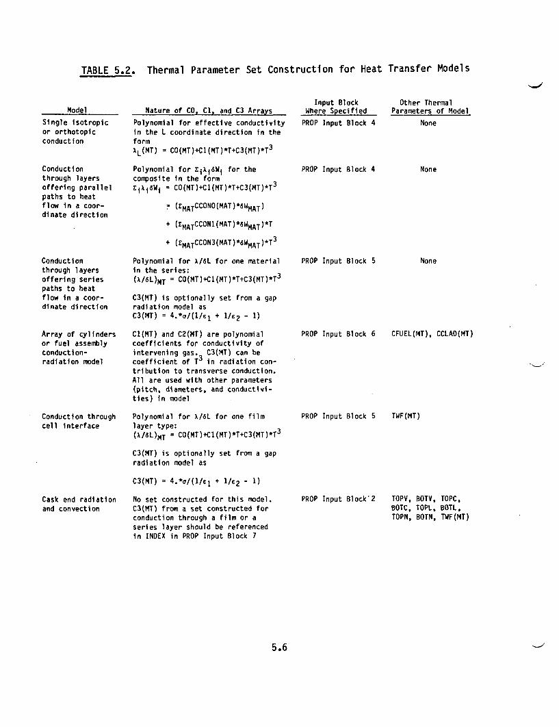
TABLE 5.2. Thermal Parameter Set Construction for Heat Transfer Models
Model
Single isotropicor orthotopicconduction
Nature of CO, CI, and C3 ArraysInput Block
Where SpecifiedPROP Input Block 4
Other ThermalParameters of Model
NonePolynomial for effective conductivity
in the L coordinate direction in theformXL(MT) = CO(MT)+Cl(MT)*T+C3(MT)*T
3
Conductionthrough layersoffering parallelpaths to heatflow in a coor-dinate direction
Conductionthrough layersoffering seriespaths to heatflow in a coor-dinate direction
Polynomial for EAi6iWi for thecomposite in the form
E jP Wi = CO(MT)+C1(MT)*T+C3(MT)*T 3
=(EMATCCONO(MAT)*6WMAT)
+ (ZMATCCONl(MAT)*aWMAT)*T
+ (EMATCCON3(MAT)*6WMAT)*T 3
Polynomial for A/6I for one materialin the series:(A/6L)MT = CO(MT)+Cl(MT)*T+C3(MT)*T 3
C3(MT) is optionally set from a gapradiation model asC3(MT) = 4.*a/(l/e1 + 1/42 - 1)
C1(MT) and C2(NT) are polynomialcoefficients for conductivity ofintervening gas. C3(MT) can becoefficient of T3 in radiation con-
tribution to transverse conduction.All are used with other parameters(pitch, diameters, and conductivi-
ties) in model
PROP Input Block 4 None
PROP Input Block 5 None
Array of cylindersor fuel assemblyconduction-radiation model
PROP Input Block 6 CFUEL(MT), CCLAO(MT)
Conduction throughcell interface
Polynomial for A/aL for one film
layer type:(A/6L)MT = CO(MT)+Cl(MT)*T+C3(MT)*T3
C3(MT) is optionally set from a gap
radiation model as
C3(MT) = 4.*a/(l/c 1 + lIe2 - 1)
PROP Input Block 5 TWF(MT)
Cask end radiationand convection
No set constructed for this model.C3(MT) from a set constructed forconduction through a film or aseries layer should be referencedin INDEX in PROP Input Block 7
PROP Input Block 2 TOPV, BOTV, TOPC,BOTC, TOPL, BOTL,TOPN, BOTN, TWF(MT)
5.6
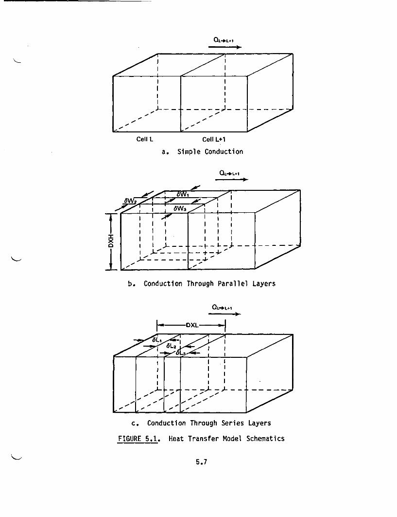
QL-sL+1
/I /lIi I
J- _ _ _ _ _ _ _ J _
Cell L Cell L+1
a. Simple Conduction
QL-10L+la. 0.+
WMIVW 00: LV
_ _. -
= iI I_11-151,11-1,109, ; , 6W3 -
1
rrI I I I I II I I I I II I I I I I
II L.- .. -- i- -- J- - - -
I -I - - + 4- -- - - - - -Jt
l ll, . F |
__________________________________ 1'� S.-
b. Conduction Through Parallel Layers
QL-L+1
|H DXL--,|
c. Conduction Through Series Layers
FIGURE 5.1. Heat Transfer Model Schematics
5.7
Fuel OD
Cladding ODT0i2
Id. Conduction and Radiation in Fuel Assembly
QL-*L+1
e. Conduction Through Cell Interface Films
Layer KPI T(KP) = TAmbient
Emittance E2
Emittance E,QKP-10-KP
f. Cask Top Radiation and Convection
FIGURE 5.1. (contd)
5.8
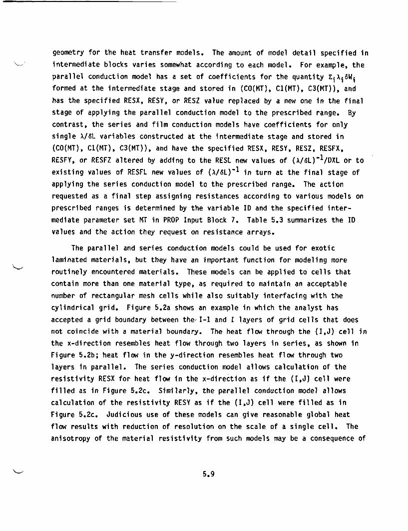
geometry for the heat transfer models. The amount of model detail specified in
intermediate blocks varies somewhat according to each model. For example, the
parallel conduction model has a set of coefficients for the quantity E.X1s6W
formed at the intermediate stage and stored in (CO(MT), C1(MT), C3(MT)), and
has the specified RESX, RESY, or RESZ value replaced by a new one in the final
stage of applying the parallel conduction model to the prescribed range. By
contrast, the series and film conduction models have coefficients for only
single X/6L variables constructed at the intermediate stage and stored in
(CO(MT), C1(MT), C3(MT)), and have the specified RESX, RESY, RESZ, RESFX,
RESFY, or RESFZ altered by adding to the RESL new values of (X/6L)-1 /DXL or to
existing values of RESFL new values of (A/6L)-1 in turn at the final stage of
applying the series conduction model to the prescribed range. The action
requested as a final step assigning resistances according to various models on
prescribed ranges is determined by the variable ID and the specified inter-
mediate parameter set MT in PROP Input Block 7. Table 5.3 summarizes the ID
values and the action they request on resistance arrays.
The parallel and series conduction models could be used for exotic
laminated materials, but they have an important function for modeling more
routinely encountered materials. These models can be applied to cells that
contain more than one material type, as required to maintain an acceptable
number of rectangular mesh cells while also suitably interfacing with the
cylindrical grid. Figure 5.2a shows an example in which the analyst has
accepted a grid boundary between the' I-1 and I layers of grid cells that does
not coincide with a material boundary. The heat flow through the (I,J) cell in
the x-direction resembles heat flow through two layers in series, as shown in
Figure 5.2b; heat flow in the y-direction resembles heat flow through two
layers in parallel. The series conduction model allows calculation of the
resistivity RESX for heat flow in the x-direction as if the (I,J) cell were
filled as in Figure 5.2c. Similarly, the parallel conduction model allows
calculation of the resistivity RESY as if the (I,J) cell were filled as in
Figure 5.2c. Judicious use of these models can give reasonable global heat
flow results with reduction of resolution on the scale of a single cell. The
anisotropy of the material resistivity from such models may be a consequence of
5.9
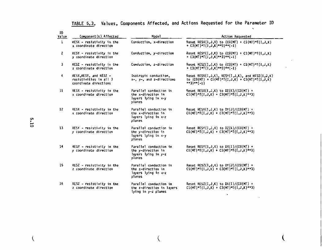
TABLE 5.3. Values, Components Affected, and Actions Requested for the Parameter ID
IDValue
I
Component(s) Affected Model
RESX - resistivity in thex coordinate direction
(A
0)
2 RESY - resistivity in they coordinate direction
3 RESZ - resistivity in thez coordinate direction
4 RESX,RESY, and RESZ -resistivities in all 3coordinate directions
11 RESX - resistivity in thex coordinate direction
12 RESX - resistivity in thex coordinate direction
13 RESY - resistivity in they coordinate direction
14 RESXY - resistivity in they coordinate direction
15 RESZ - resistivity in thez coordinate direction
16 RESZ - resistivity in thez coordinate direction
Conduction, x-direction
Conduction, y-direction
Conduction, z-direction
Isotropic conduction,x-, y-, and z-directions
Parallel conduction inthe x-direction inlayers lying in x-yplanes
Parallel conduction inthe x-direction inlayers lying in x-zplanes
Parallel conduction inthe y-direction inlayers lying in x-yplanes
Parallel conduction inthe y-direction inlayers lying in y-zplanes
Parallel conduction inthe z-direction inlayers lying in x-zplanes
Parallel conduction inthe z-direction in layerslying in y-z planes
Action Requested
Reset RESX(I,J,K) to (CO(MT) + C1(MT)*T(I,J,K)+ C3(MT)*T(I,J,K)**3)**(-1)
Reset RESY(I,J,K) to (CO(MT) + C1(MT)*T(I,J,K)+ C3(MT)*T(I,J,K)**3)**(-1)
Reset RESZ(I,J,K) to (CO(MT) + C1(MT)*T(I,J,K)+ C3(MT)*T(I,J,K)**3)**(-1)
Reset RESX(I,J,K), RESY(I,J,K), and RESZ(I,J,K)to (CO(MT) + C1(MT)*T(I,J,K) + C3(MT)*T(I,J,K)**3)**(-1)
Reset RESX(I,J,K) to DZ(K)/(CO(MT) +C1(MT)*T(I,J,K) + C3(MT)*T(I,J,K)**3)
Reset RESX(I,J,K) to DY(J)/(CO(MT) +C1(MT)*T(I,J,K) + C3(MT)*T(I,J,K)**3)
Reset RESY(I,J,K) to DZ(K)/(CO(MT) +C1(MT)*T(I,J,K) + C3(MT)*T(I,J,K)**3)
Reset RESY(I,J,K) to DX(I)/(CO(MT) +C1(MT)*T(I,J,K) + C3(MT)*T(I,J,K)**3)
Reset RESZ(I,J,K) to DY(J)/(CO(MT) +CI(MT)*T(I,J,K) + C3(MT)*T(I,J,K)**3)
Reset RESZ(I,J,K) to DX(I)/(CO(MT) +C1(MT)*T(I,JK) + C3(MT)*T(I,J,K)**3)
K (
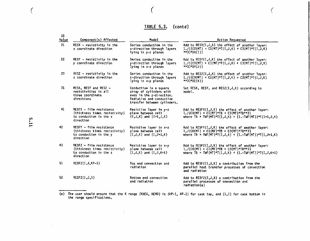
( ( (
TABLE 5.3. (contd)
IDValue
21
Component(s) Affected
RESX - resistivity in thex coordinate direction
Ln
PS
22 RESY - resistivity in they coordinate direction
23 RESZ - resistivity in thez coordinate direction
31 RESX, RESY and RESZ -resistivities in allthree coordinatedirections
41 RESFX - film resistance(thickness times resistivity)to conduction in the xdirection
42 RESFY - film resistance(thickness times resistivity)to conduction in the ydirection
43 RESFZ - film resistance(thickness times resistivity)to conduction in the zdirection
51 RESFZ(I,J,KP-1)
52 RESFZ(I,J,1)
Model
Series conduction in thex-direction through layerslying in y-z planes
Series conduction in they-direction through layerslying in x-z planes
Series conduction in thez-direction through layerslying in x-y planes
Conduction in a squarearray of cylinders withaxes in the z-direction.Radiative and conductivetransfer between cylinders.
Resistive layer in y-zplane between cell(I,J,K) and (I+1,J,K)
Resistive layer in x-zplane between cell(I,J,K) and (1,J+1,K)
Resistive layer in x-yplane hetween cell(I,J,K) and (I,J,K+1)
Top end convection andradiation
Bottom end convectionand radiation
Action Requested
Add to RESX(I,J,K) the effect of another layer:1./((CO(MT) + C1(MT)*T(I,J,K) + C3(MT)*T(I,J,K)**3)*DX(I))
Add to RESY(I,J,K) the effect of another layer:1./((CO(MT) + C1(MT)*T(I,J,K) + C3(MT)*T(I,J,K)**3)*DY(J))
Add to RESZ(I,J,K) the effect of another layer:1./((CO(MT) + C1(MT)*T(I,J,K) + C3(MT)*T(I,JK)**3)*DZ(K))
Set RESX, RESY, and RESZ(I,J,K) according tomodel.
Add to RESFX(I,J,K) the effect of another layer:1./(CO(MT) + C1(MT)*TB + C3(MT)*TB**3)where TB = TWF(MT)*T(I,J,K) + (1.-TWF(MT))*T(I+1,J,K)
Add to RESFY(I,J,K) the effect of another layer:1./(CO(MT) + C1(MT)*TB + C3(MT)*TB**3)where TB = TWF(MT)*T(I,J,K) + (1.-TWF(MT))*T(I,J+1,K)
Add to RESFZ(I,J,K) the effect of another layer:1./(CO(MT) + C1(MT)*TB + C3(MT)*TB**3)where TB = TWF(MT)*T(I,J,K) + (1.-TWF(MT))*T(I,J,K+1)
Add to RESFZ(I,J,K) a contribution from theparallel heat transfer processes of convectionand radiation
Add to RESFZ(I,J,K) a contribution from theparallel processes of convection andradiation(a)
(a) The user should ensure that the Kthe range specifications.
range (KBEG, KEND) is (KP-1, KP-1) for cask top, and (1,1) for cask bottom in
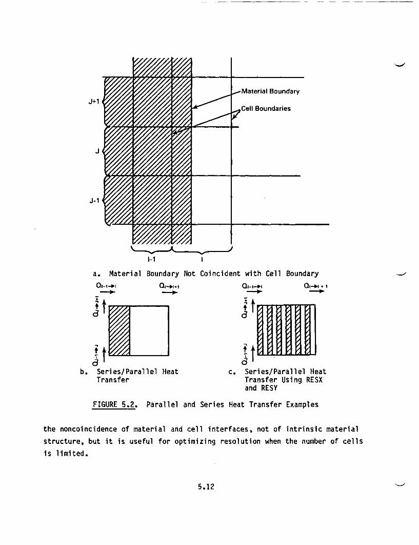
A/~
J+1
J-1
mmMaterial Boundary
Cell Boundaries
4 I 401
_- - - - - -I-
1-1 I
a. Material Boundary Not Coincident with Cell Boundary
-,
Qi-1-*1 0 -. +
dt ta3
d t wrm Ib. Series/Parallel Heat
Transfer
t tf aRN H IIc. Series/Parallel Heat
Transfer Using RESXand RESY
FIGURE 5.2. Parallel and Series Heat Transfer Examples
the noncoincidence of material and cell interfaces, not of intrinsic material
structure, but it is useful for optimizing resolution when the number of cells
is limited.
5.12
5.1.1 Simple Isotropic or Orthotropic Conduction Model
Subroutine PROP reads sets of polynomial coefficients CCONO, CCON1, and
CCON3 for calculating conductivity X of substance MAT at temperature T from
X(MAT) = CCONO(MAT)+CCON1(MAT)*T+CCON3(MAT)*T 3 (5.4)
These CCON type substance conductivity coefficient sets are read in PROP Input
Block 3. These substance conductivity coefficients can subsequently be used to
set arrays of coefficients CO(MT), C1(MT), and C3(MT) for polynomials that give
either conduction-related parameters with a similar three-term polynomial or
some other set of information used in setting RES or RESF type arrays. For
simple isotropic or orthotropic conduction in material MT, the values (CO(MT),
C1(MT), C3(MT)) will be set directly to (CCONO(MAT), CCON1(MAT), CCON3(MAT)),
where MAT is a designated index for the thermal parameter set MT.
5.1.2 Parallel Conduction Model
For a set of layers that offer parallel paths for conduction in the L
direction, the effective resistivity RL is
RL = W/(zSAj6W) (5.5)
where Ai is the conductivity of the ith material in the composite and SW1 is
its width. W is the width of the cell in the direction normal to the parallel
planes of the composite. It is usually the case that
W = E16WI (5.6)
The polynomial coefficient sets for the Ai are input in PROP Input Block 3
in the CCONO, CCON1, and CCON3 arrays and subsequently used in setting the
polynomial coefficients CO, C1, and C3 for zajWj The variables SWj are input
as WIDTH in PROP Input Block 4, along with the list of material property sets
determining the Xi to use in the ZXi6Wj sum. PROP Input Block 4 directs the
construction of polynomial coefficients for EXi6W1 .
5.13

5.1.3 Series Conduction Model
For a set of layers offering series conduction paths in the L-direction
through a computational cell, the effective resistivity in the L-direction is
RL = (hi ) DXL (5.7)
where DXL is the computational cell length in the L-direction, Xi is the
conductivity of the ith material in the composite, and SLi is the path length
per computational cell supplied by the ith material. The variables 6Li for
series layers are read as WIDTH in PROP Input Block 5, along with the index of
the set of coefficients for the xi previously read in PROP Input Block 3. PROP
Input Block 5 directs construction of polynomial coefficients for the quanti-
ties Xi/6Li. The direction of conduction and the orientation of the slabs is
specified later by the variable ID read in the array INDEX in PROP Input
Block 7. The coefficient sets for quantities of the form Xi/6Li can also be
used in the construction of film resistances for interfaces between cells. An
option is available for construction of the cubic term in the series for Xi/6Li
according to a radiation model (see discussion of conduction through films).
5.1.4 Array of Cylinders or Fuel Assembly Model
The fuel assembly model constructs effective resistivities RESX, RESY, and
RESZ for an array of cylinders having axes in the z-direction stored in a
square pattern in the x-y plane. The cylinders are assumed to be composed of a
circular cylinder core and annular clad, each region having its own character-
istic conductivity. Resistivity RESZ is computed on the assumption of parallel
conduction paths in the cylinder core, cladding, and intervening gas.
Transverse resistivities RESX and RESY are computed on the basis of a two-
dimensional model that includes conduction in the cylinder core, cladding, and
gas, as well as radiative heat transfer among the cylinders.
It should be noted that the radiative heat transfer among an array of fuel
cylinders may, under special conditions, be treated by a more precise model
(subroutine RADR) elsewhere in the code. For most practical purposes, RADR
will require a region of the Cartesian mesh with one cylinder per cell column
5.14
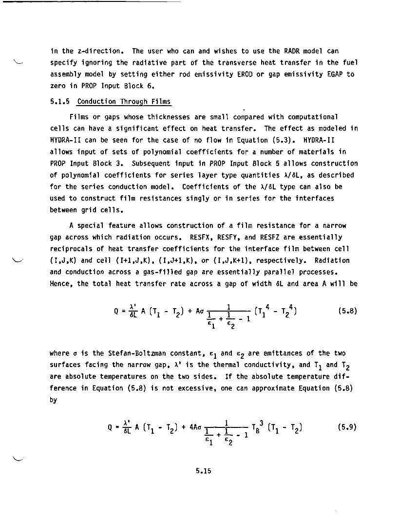
in the z-direction. The user who can and wishes to use the RADR model can
specify ignoring the radiative part of the transverse heat transfer in the fuel
assembly model by setting either rod emissivity EROD or gap emissivity EGAP to
zero in PROP Input Block 6.
5.1.5 Conduction Through Films
Films or gaps whose thicknesses are small compared with computational
cells can have a significant effect on heat transfer. The effect as modeled in
HYDRA-II can be seen for the case of no flow in Equation (5.3). HYDRA-II
allows input of sets of polynomial coefficients for a number of materials in
PROP Input Block 3. Subsequent input in PROP Input Block 5 allows construction
of polynomial coefficients for series layer type quantities X/6L, as described
for the series conduction model. Coefficients of the X/6L type can also be
used to construct film resistances singly or in series for the interfaces
between grid cells.
A special feature allows construction of a film resistance for a narrow
gap across which radiation occurs. RESFX, RESFY, and RESFZ are essentially
reciprocals of heat transfer coefficients for the interface film between cell
(IJ,K) and cell (I+1,J,K), (I,J+1,K), or (I,JK+1), respectively. Radiation
and conduction across a gas-filled gap are essentially parallel processes.
Hence, the total heat transfer rate across a gap of width 6L and area A will be
Q =-dALA (TI - T2) + Aa 1 1 (T1 T2 ) (5.8)-+ -1
1 2
where a is the Stefan-Boltzman constant, e and E2 are emittances of the two
surfaces facing the narrow gap, A' is the thermal conductivity, and T1 and T2
are absolute temperatures on the two sides. If the absolute temperature dif-
ference in Equation (5.8) is not excessive, one can approximate Equation (5.8)
by
Q A (T1 - T2) + 4Aa 1 1 TB3 (T1 - T2) (5.9)
1 2
5.15
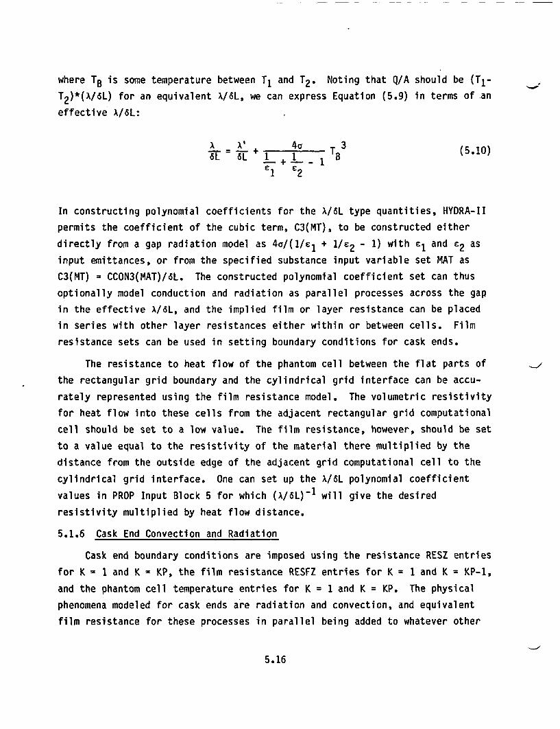
where TB is some temperature between T, and T2. Noting that Q/A should be (T1-
T2)*(X/SL) for an equivalent X/SL, we can express Equation (5.9) in terms of an
effective A/6L:
1+ + 1 T 1 3B (5.10)e1 E2
In constructing polynomial coefficients for the X/6L type quantities, HYDRA-I1
permits the coefficient of the cubic term, C3(MT), to be constructed either
directly from a gap radiation model as 4a/(1/£1 + 1/£2 - 1) with e1 and £2 as
input emittances, or from the specified substance input variable set MAT as
C3(MT) = CCON3(MAT)/6L. The constructed polynomial coefficient set can thus
optionally model conduction and radiation as parallel processes across the gap
in the effective X/6L, and the implied film or layer resistance can be placed
in series with other layer resistances either within or between cells. Film
resistance sets can be used in setting boundary conditions for cask ends.
The resistance to heat flow of the phantom cell between the flat parts of
the rectangular grid boundary and the cylindrical grid interface can be accu-
rately represented using the film resistance model. The volumetric resistivity
for heat flow into these cells from the adjacent rectangular grid computational
cell should be set to a low value. The film resistance, however, should be set
to a value equal to the resistivity of the material there multiplied by the
distance from the outside edge of the adjacent grid computational cell to the
cylindrical grid interface. One can set up the X/6L polynomial coefficient
values in PROP Input Block 5 for which (A/6L)-l will give the desired
resistivity multiplied by heat flow distance.
5.1.6 Cask End Convection and Radiation
Cask end boundary conditions are imposed using the resistance RESZ entries
for K = 1 and K = KP, the film resistance RESFZ entries for K = 1 and K = KP-1,
and the phantom cell temperature entries for K = 1 and K = KP. The physical
phenomena modeled for cask ends are radiation and convection, and equivalent
film resistance for these processes in parallel being added to whatever other
5.16
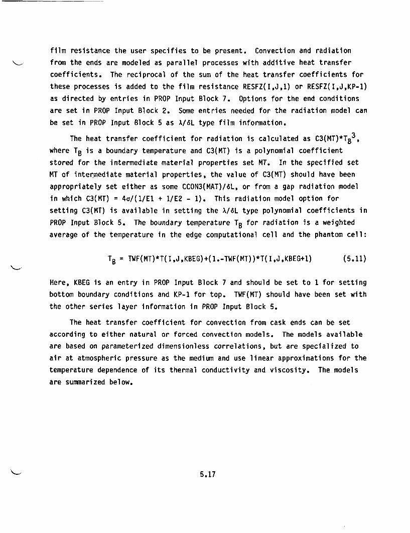
film resistance the user specifies to be present. Convection and radiation
from the ends are modeled as parallel processes with additive heat transfer
coefficients. The reciprocal of the sum of the heat transfer coefficients for
these processes is added to the film resistance RESFZ(I,J,1) or RESFZ(IJ,KP-1)
as directed by entries in PROP Input Block 7. Options for the end conditions
are set in PROP Input Block 2. Some entries needed for the radiation model can
be set in PROP Input Block 5 as I/6L type film information.
The heat transfer coefficient for radiation is calculated as C3(MT)*TB3,
where TB is a boundary temperature and C3(MT) is a polynomial coefficient
stored for the intermediate material properties set MT. In the specified set
MT of intermediate material properties, the value of C3(MT) should have been
appropriately set either as some CCON3(MAT)/6L, or from a gap radiation model
in which C3(MT) = 4a/(1/E1 + 1/E2 - 1). This radiation model option for
setting C3(MT) is available in setting the X/6L type polynomial coefficients in
PROP Input Block 5. The boundary temperature TB for radiation is a weighted
average of the temperature in the edge computational cell and the phantom cell:
TB = TWF(MT)*T(I,J,KBEG)+(1.-TWF(MT))*T(I,J,KBEG+1) (5.11)
Here, KBEG is an entry in PROP Input Block 7 and should be set to 1 for setting
bottom boundary conditions and KP-1 for top. TWF(MT) should have been set with
the other series layer information in PROP Input Block 5.
The heat transfer coefficient for convection from cask ends can be set
according to either natural or forced convection models. The models available
are based on parameterized dimensionless correlations, but are specialized to
air at atmospheric pressure as the medium and use linear approximations for the
temperature dependence of its thermal conductivity and viscosity. The models
are summarized below.
5.17
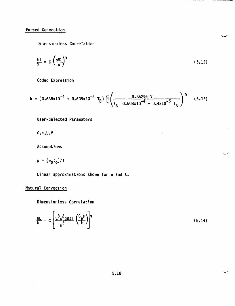
Forced Convection
Dimensionless Correlation
hL = C (PVL)n (5.12)
Coded Expression
h = (0.688xlO 4 + 0.635x10 6 T) CL 0.35296 L -(5.13)B 0.608x1O + 0.4x1O nB
User-Selected Parameters
C,n,L,V
Assumptions
p = (poTo)/T
Linear approximations shown for P and k.
Natural Convection
Dimensionless Correlation
hL- L3 2 BAT (C.)]n (5.14)
5.18
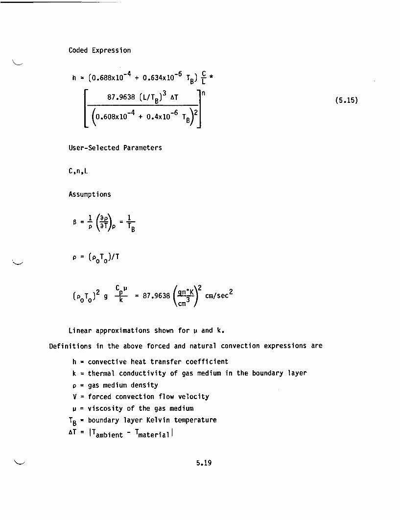
Coded Expression
h =(0.688x1O 4 + 0.6341+O6 TB) (.5
87.9638 (L/T B)3 AT n (5.15)
L(0. 608x1O 4 + 0.41lO 6 TB)2]
User-Selected Parameters
C,n,L
Assumptions
=1 (ap = 1
P = (poT 0 )/T
( ) g o = 87.9638 ( 3 ) cm/sec2
Linear approximations shown for P and k.
Definitions in the above forced and natural convection expressions are
h = convective heat transfer coefficient
k = thermal conductivity of gas medium in the boundary layer
p = gas medium density
V = forced convection flow velocity
P = viscosity of the gas medium
TB = boundary layer Kelvin temperature
AT = ITambient - Tmateriall
5.19
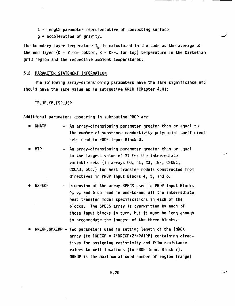
L = length parameter representative of convecting surface
g = acceleration of gravity.
The boundary layer temperature TB is calculated in the code as the average of
the end layer (K = 2 for bottom, K = KP-1 for top) temperature in the Cartesian
grid region and the respective ambient temperatures.
5.2 PARAMETER STATEMENT INFORMATION
The following array-dimensioning parameters have the same significance and
should have the same value as in subroutine GRID (Chapter 4.0):
IP,JP,KP,ISP,JSP
Additional parameters appearing in subroutine PROP are:
* NMATP
* MTP
* NSPECP
* NREGPNPAIRF
- An array-dimensioning parameter greater than or
the number of substance conductivity polynomial
sets read in PROP Input Block 3.
equal tocoefficient
- An array-dimensioning parameter greater than or equal
to the largest value of MT for the intermediate
variable sets (in arrays CO, C1, C3, TWF, CFUEL,
CCLAD, etc.) for heat transfer models constructed from
directives in PROP Input Blocks 4, 5, and 6.
A,
Dimension of the array SPECS used in PROP Input Blocks
4, 5, and 6 to read in end-to-end all the intermediate
heat transfer model specifications in each of the
blocks. The SPECS array is overwritten by each of
those input blocks in turn, but it must be long enough
to accommodate the longest of the three blocks.
Two parameters used in setting length of the INDEX
array (to INDEXP = 7*NREGP+2*NPAIRP) containing direc-
tives for assigning resistivity and film resistance
values to cell locations (in PROP Input Block 7).
NREGP is the maximum allowed number of region (range)
5.20
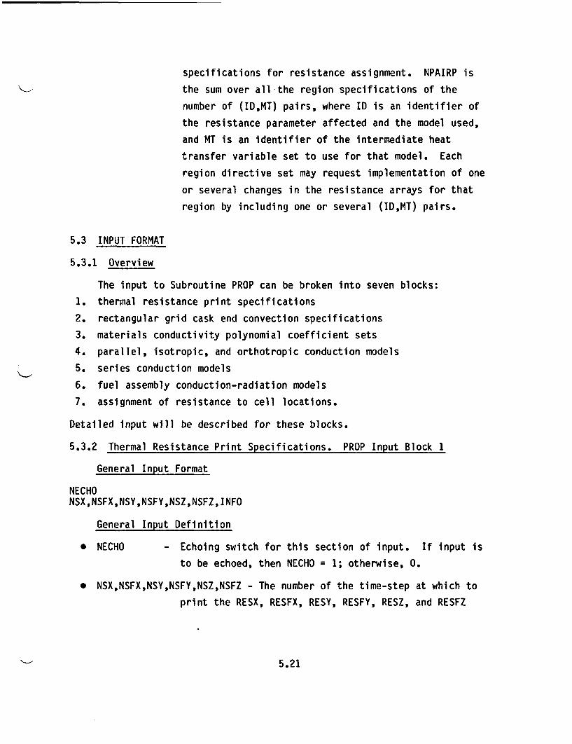
specifications for resistance assignment. NPAIRP is
the sum over all the region specifications of the
number of (ID,MT) pairs, where ID is an identifier of
the resistance parameter affected and the model used,
and MT is an identifier of the intermediate heat
transfer variable set to use for that model. Each
region directive set may request implementation of one
or several changes in the resistance arrays for that
region by including one or several (ID,MT) pairs.
5.3 INPUT FORMAT
5.3.1 Overview
The input to Subroutine PROP can be broken into seven blocks:
1. thermal resistance print specifications
2. rectangular grid cask end convection specifications
3. materials conductivity polynomial coefficient sets
4. parallel, isotropic, and orthotropic conduction models
5. series conduction models
6. fuel assembly conduction-radiation models
7. assignment of resistance to cell locations.
Detailed input will be described for these blocks.
5.3.2 Thermal Resistance Print Specifications. PROP Input Block 1
General Input Format
NECHONSX,NSFX,NSY,NSFY,NSZ,NSFZ,INFO
General Input Definition
* NECHO - Echoing switch for this section of input. If input is
to be echoed, then NECHO = 1; otherwise, 0.
* NSX,NSFX,NSY,NSFY,NSZ,NSFZ - The number of the time-step at which to
print the RESX, RESFX, RESY, RESFY, RESZ, and RESFZ
5.21
arrays, respectively. A negative entry suppresses
printing of that array.
* INFO - Integer flag variable that, if equal to 1, requests
printing of each resistivity or film resistivity array
at its designated (by NSX, NSFX, etc.) time-step. No
printing occurs if INFO = 0.
Input File Example
90 1/prop91 -1,-1,-1,-1,-1,-1,0
Echoed Input File Example
180 prop nsx -1 nsfx- -1 nsfy- -1 nszo -1 nsf z- -1 Info- 0
The echoing of input is requested by setting NECHO = 1; the remainder ofthe input line serves for comment. The printout of the RESL and RESFL (with L
= x, y, or z) has been doubly suppressed, with INFO = 0 and NSX, NSFX, NSY,
etc., set to -1. The user is advised to obtain these resistance array
printouts (INFO = 1, NSX = 1, etc.) at least once in an early execution, to
verify correctness of thermal model geometry and input.
5.3.3 Cartesian Cask End Convection Specifications
General Input Format
TOPH,TOPL,TOPV,TOPC,TOPNBOTH,BOTL,BOTV,BOTC,BOTN
General Input Definition
* TOPH - Floating point flag variable that, if equal to 1.0,
indicates a top end convective model is forthcoming.
(Note: The line should contain five entries, even if
TOPH = O.O.)
* TOPL - Length L to use in the forced convection [Equation
(5.12)] or the natural convection [Equation (5.14)]
heat transfer correlations for the cask top.
5.22
* TOPV - Velocity to use in forced convection heat transfer
correlation for top cask end. Setting TOPV = 0.0 with
TOPH = 1.0 invokes the natural rather than forced
convection model.
* TOPC - Constant C to use for the top cask end heat transfer
correlation in either forced convection [Equation
(5.12), TOPV > 0.0] or natural convection [Equation
(5.14), TOPV = 0.0].
* TOPN - Exponent n to use for the top cask end heat transfer
correlation in either forced convection [Equation
(5.12), TOPV > 0.0) or natural convection [Equation
(5.14), TOPV = 0.0].
* BOTH,BOTL,BOTV,BOTC,BOTN - Values of convection flag, L, V, C, and n,
respectively, for the cask bottom, analogous to TOPH,
TOPL, TOPV, TOPC, and TOPN, respectively, for the cask
top.
The complete specification of cask end thermal conditions will require
entries elsewhere in PROP, such as radiation parameters or surface film
resistances in Input Block 5 and resistance assignments in Input Block 7.
Input File Example
92 1.0,220.0,0.0,0.14,0.33393 1.0,220.0,0.0,0.27,0.25
Echoed Input File Example
182183 prop toph=1.0 toplO0.220e+03 topvMO.OOOe+OO topc=0.140e+00 topn=0.333e+00184 prop both=1.0 botl=0.220e+03 botv0.000e+00 botc0.270e+00 botn=0.250e+00
This input specifies that convection models are to be used on both the top
and the bottom surfaces, because both TOPH and BOTH are set to 1.0. The length
parameter in the convection correlation is set to 220 cm, on the order of the
cask diameter. Setting velocity parameters TOPV and BOTV to zero specifies
that the convection is natural, not forced. The coefficient C and the power n
in the natural convection correlation, Equation (5.15), are specified as
5.23
(TOPC = 0.14, TOPN = 0.333) for the top and (BOTC = 0.27, BOTN = 0.25) for the
bottom. Values for C and n should be taken from the heat transfer literature.
5.3.4 Material Conductivity Polynomial Coefficient Sets. PROP Input Block 3
General Input Format
NECHONMATTEXTCCONO(1),CCON1(1)CCON3(1)TEXTCCONO(2),CCON1(2),CCON3(2)
* * 0
TEXTCCONO(NMAT),CCON1(NMAT),CCON3(NMAT)
General Input Definition
* NECHO - Echoing switch for this section of input. If input is
to be echoed, then NECHO = 1; otherwise, 0.
* NMAT - Number of sets of substance effective conductivity
polynomial coefficients forthcoming.
* TEXT - Up to 40 characters of labeling information (5A8) for
the next polynomial coefficient set.
* CCONO(MAT),CCON1(MAT),CCON3(MAT) - The MATth set of polynomial
coefficients for representing an effective substance
thermal conductivity X(MAT) as
X(MAT) = CCONO(MAT)+CCON1(MAT)*T+CCON3(MAT)*T3.
These substance property sets are stored temporarily and are available to
construct intermediate property sets (CO(MT), C1(MT), C3(MT)) for repeated use
in setting resistance variables on the mesh according to the heat transfer
models. The CO(MT), C1(MT), C3(MT) sets are saved and used for updating
resistance variables as temperature changes.
Input File Example
94 1/prop/cconO,cconl,ccon395 9
5.24
96979899
100101102103104105106107108109110111112113
186
187188189190191192193194195196197
low conductivity0.le-20,0.0,0.0high conductivityO.le+20,0.0,0.0helium (backfill gas)0.52e-3,0.32e-5,0.0sst0.09215,0.1465e-3,0.0boron steel (radionox)0.079,0.21e-3,0.0nodular cast iron0.5162,-0.3205e-3,0.0epoxy (not used)0.15e-2,0.0,0.0nitrogen (not used)0.075e-3,0.6167e-6,0.0air (not used)0.6880e-4,0.6340e-6,0.0
Echoedpropprop
Input File Examplenmat- 9 maximum current dimension for nmat is 20cconOcconl ,ccon3 material thermal conductivity, W/cm-k
kMmat). cconO(mat)+ cconl(mat)'t+ ccon3(mat)*tthtI (O.10OOe-20)+(0.0000e+00)'t+(0.0000e+00)*t~tt low conductivity2 (0.1OOOe+20)+(0.OOOOe0+O)*t+(O.OOOOeOO*t0ttt high conductivity3 (0.52OOe-03)+(0.3200e-05)*t+(0.0000e+00)etetet helium (backfill gas)4 (0.9215e-01)+(0.1465e-03)*t+(0.0000e+00)*t'tt sst5 (0.7900e_01)+(0.2100e-03)*t+(0.0000e+00)*ttt boron steel (radlonox)6 (0.5162e+00)+(-.3205e-03)*t+(0.0000e+00)*tett nodular cast iron7 (0.15O0e-02)+(0.0000e+00)*t+(0.0000 +00)ttt epoxy (not used)8 (0.7500_-04)+(0.6167e-06)*t+(0.OOOOe+O0)*t'tt nitrogen (not used)9 (0.6880e-04)+(0.6340e-06)*t+(0.0000e+00)*titet air (not used)
The input requests echoing of the nine material conductivity polynomial
coefficient sets forthcoming. First descriptive text, then the list of three
coefficients, appears for each of the nine sets. Note that some input sets may
not be subsequently referenced.
The echoed input specifies the number of such sets NMAT, and also gives
the current number, NMATP, of such sets that can be accommodated. The coeffi-
cient sets are printed out in a form that suggests their use, followed by the
labeling text for that set.
5.25
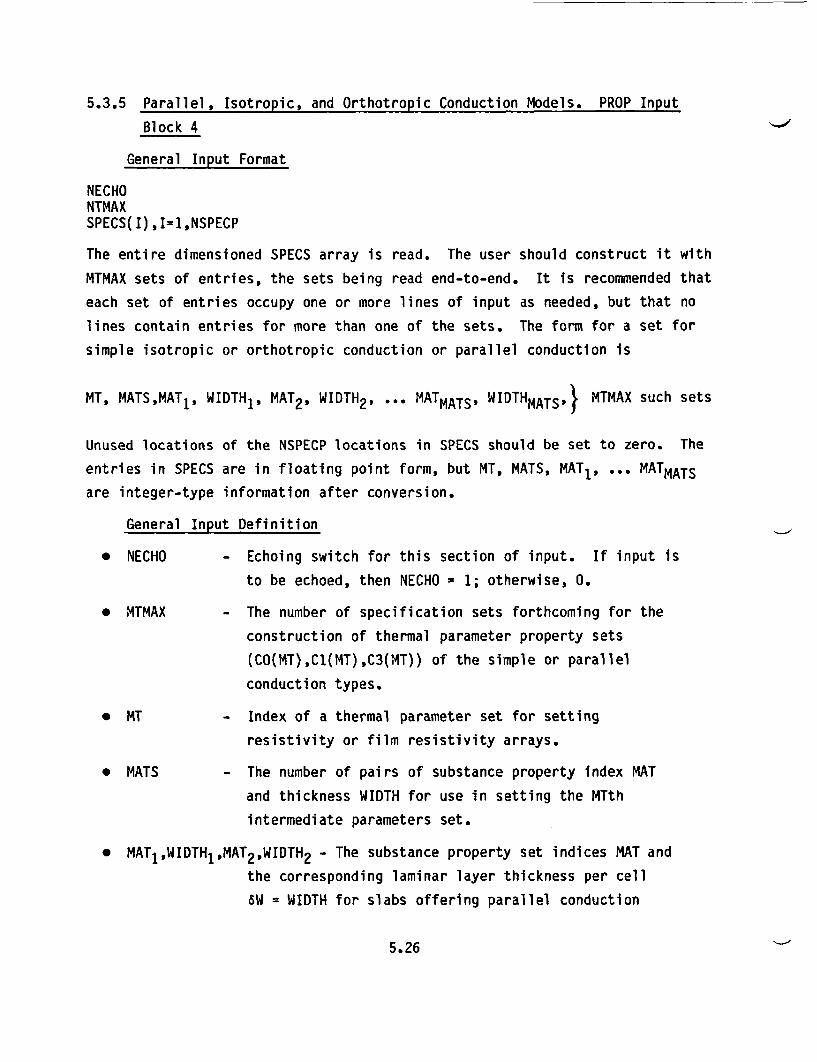
5.3.5 Parallel, Isotropic, and Orthotropic Conduction Models. PROP Input
Block 4
General Input Format
NECHONTMAXSPECS(I),I=1,NSPECP
The entire dimensioned SPECS array is read. The user should construct it with
MTMAX sets of entries, the sets being read end-to-end. It is recommended that
each set of entries occupy one or more lines of input as needed, but that no
lines contain entries for more than one of the sets. The form for a set for
simple isotropic or orthotropic conduction or parallel conduction is
MT, MATSMAT1, WIDTHJ, MAT2, WIDTH2, a** MATMATS, WIDTHMATS,} MTMAX such sets
Unused locations of the NSPECP locations in SPECS should be set to zero. The
entries in SPECS are in floating point form, but MT, MATS, MATI, ... MATMATS
are integer-type information after conversion.
General Input Definition
* NECHO - Echoing switch for this section of input. If input is
to be echoed, then NECHO = 1; otherwise, 0.
* MTMAX - The number of specification sets forthcoming for the
construction of thermal parameter property sets
(CO(MT),C1(MT),C3(MT)) of the simple or parallel
conduction types.
* MT - Index of a thermal parameter set for setting
resistivity or film resistivity arrays.
* MATS - The number of pairs of substance property index MAT
and thickness WIDTH for use in setting the MTth
intermediate parameters set.
* MAT,,WIDTH,,MAT2,WIDTH2 - The substance property set indices MAT and
the corresponding laminar layer thickness per cell
SW = WIDTH for slabs offering parallel conduction
5.26
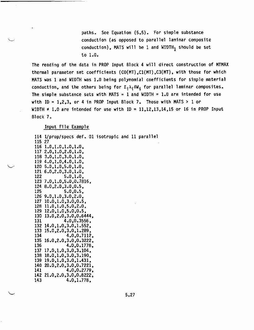
paths. See Equation (5.5). For simple substance
conduction (as opposed to parallel laminar composite
conduction), MATS will be 1 and WIDTH, should be set
to 1.0.
The reading of the data in PROP Input Block 4 will direct construction of MTMAX
thermal parameter set coefficients (CO(MT),C1(MT),C3(MT), with those for which
MATS was 1 and WIDTH was 1.0 being polynomial coefficients for simple material
conduction, and the others being for EiXi6Wi for parallel laminar composites.
The simple substance sets with MATS = 1 and WIDTH = 1.0 are intended for use
with ID = 1,2,3, or 4 in PROP Input Block 7. Those with MATS > 1 or
WIDTH * 1.0 are intended for use with ID = 11,12,13,14,15 or 16 in PROP Input
Block 7.
Input File Example
114115116117118119120121122123124125126127128129130131132133134135136137138139140141142143
1/prop/specs def. 01271.0,1.0,1.0,1.0,2.0,1.0,2.0,1.0,3.0,1.0,3.0,1.0,4.0,1.0,4.0,1.0,5.0,1.0,5.0,1.0,6.0,2.0,3.0,1.0,
5.0,1.0,7.0,1.0,5.0,0.7816,8.0,2.0,3.0,0.5,
5.0,0.5,9.0,1.0,3.0,2.0,10.0,1.0,3.0,0.5,11.0,1.0,5.0,2.0,12.0,1.0,5.0,0.5,13.0,2.0,3.0,0.6444,
4.0,0.3556,14.0,1.0,3.0,1.552,15.0,2.0,3.0,1.289,
4.0,0.7112,16.0,2.0,3.0,0.3222,
4.0,0.1778,17.0,1.0,3.0,3.104,18.0,1.0,3.0,3.190,19.0,1.0,3.0,1.431,20.0,2.0,3.0,0.7221,
4.0,0.2779,21.0,2.0,3.0,0.8222,
4.0,1.778,
isotropic and 11 parallel
5.27
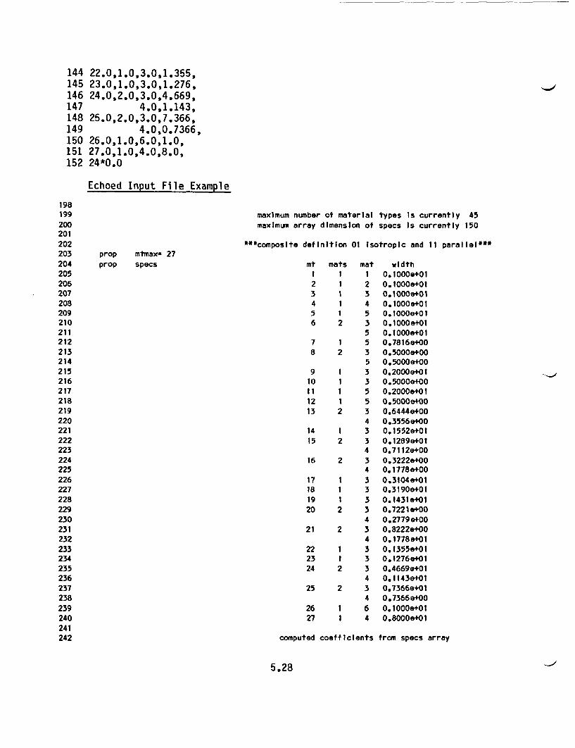
144145146147148149150151152
22.0,1.0,3.0,1.355,23.0,1.0,3.0,1.276,24.0,2.0,3.0,4.669,
4.0,1.143,25.0,2.0,3.0,7.366,
4.0,0.7366,26.0,1.0,6.0,1.0,27.0,1.0,4.0,8.0,24*0.0
Echoed Input File Example
198199200201202203204205206207208209210211212213214215216217218219220221222223224225226227228229230231232233234235236237238239240241242
maximum number of material types Is currently 45maximum array dimension of specs Is currently 150
***composite definition 01 Isotropic and 11 parallel***prop mtmaxm 27prop specs mt mats mat width
I I t 0.1000e+012 1 2 0.tOOOe+013 1 3 0.1000e+014 1 4 0.lOOOe+015 1 5 0.1000e+016 2 3 0.1000e+01
5 0.lOOOe+Ot7 1 5 0.7816e+008 2 3 0.5000e+00
5 0.5000e+009 1 3 0.2000e+0t
10 1 3 0.5000e+0011 1 5 0.2000e+0112 1 5 0.5000e+0013 2 3 0.6444e+00
4 0.3556e+0014 1 3 0.1552e+0115 2 3 0.1289e+01
4 0.7112e+0016 2 3 0.3222e+00
4 0.1778e+0017 1 3 0.3104e+0118 1 3 0.3190e+0119 1 3 0.1431e+0120 2 3 0.7221e+00
4 0.2779e+0021 2 3 0.8222e+00
4 0.1778e+O122 1 3 0.1355e+0123 1 3 0.1276e+0124 2 3 0.4669e+01
4 0.1143e+0125 2 3 0.7366e+01
4 0.7366e+0026 1 6 0.tOOOe+0127 1 4 0.8000e+01
computed coefficients from specs array
5.28
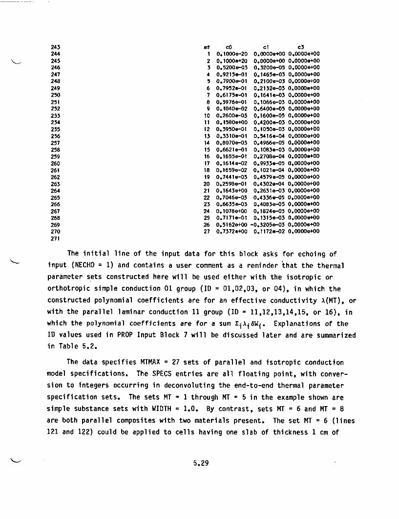
243244245246247248249250251252253254255256257258259260261262263264265266267268
Mt cOI 0.10OOe-202 0.1000e+203 0.5200e-034 0.9215e-015 0.7900e-016 0.7952e-017 0.6175e-018 0.3976e-019 0.1040e-02
10 0.2600e-0311 0.1580e+0012 0.3950e-0113 0.3310e-0114 0.8070e-0315 0.6621e-0116 0.1655e-0117 0.1614e-0218 0.1659e-0219 0.7441e-0320 0.2598e-0121 0.1643e+0022 0.7046e-0323 0.6635e-0324 0.10780+0025 0.7171e-01
cl c30.0000e+00 0.0000e+000.00000+00 0.OOOOe+000.3200e-05 0.0000e+000.1465e-03 0.OOOOe+000.2100e-03 0.0000e+000.2132e-03 0.0000e+000.1641e-03 0.0000e+000.1066e-03 0.0000e+000.6400e-05 0.0000e+000.1600e-05 0.0000e+000.4200e-03 0.0000e+000.1050e-03 0.0000e+000.5416e-04 0.0000e+000.4966e-05 0.0000e+000.1083e-03 0.0000e+000.2708e-04 0.0000e+000.9933e-05 0.0000e+000.1021e-04 0.0000e+000.4579e-05 0.0000e+000.4302e-04 0.0000+000.2631e-03 0.0000e+000.4336e-05 0.0000e+000.4083e-05 0.0000e+000.1824e-03 O.OOOOe+000.1315e-03 0.0000e+00
269 26 0.5162e+00 -0.3205e-03 0.00006+00270 27 0.7372e+00 0.1172e-02 0.0000e+00271
The initial line of the input data for this block asks for echoing of
input (NECHO = 1) and contains a user comment as a reminder that the thermal
parameter sets constructed here will be used either with the isotropic or
orthotropic simple conduction 01 group (ID = 01,02,03, or 04), in which the
constructed polynomial coefficients are for an effective conductivity A(MT), or
with the parallel laminar conduction 11 group (ID = 11,12,13,14,15, or 16), in
which the polynomial coefficients are for a sum riAi6Wi. Explanations of the
ID values used in PROP Input Block 7 will be discussed later and are summarized
in Table 5.2.
The data specifies MTMAX = 27 sets of parallel and isotropic conduction
model specifications. The SPECS entries are all floating point, with conver-
sion to integers occurring in deconvoluting the end-to-end thermal parameter
specification sets. The sets MT = 1 through MT = 5 in the example shown are
simple substance sets with WIDTH = 1.0. By contrast, sets MT = 6 and MT = 8
are both parallel composites with two materials present. The set MT = 6 (lines
121 and 122) could be applied to cells having one slab of thickness 1 cm of
5.29
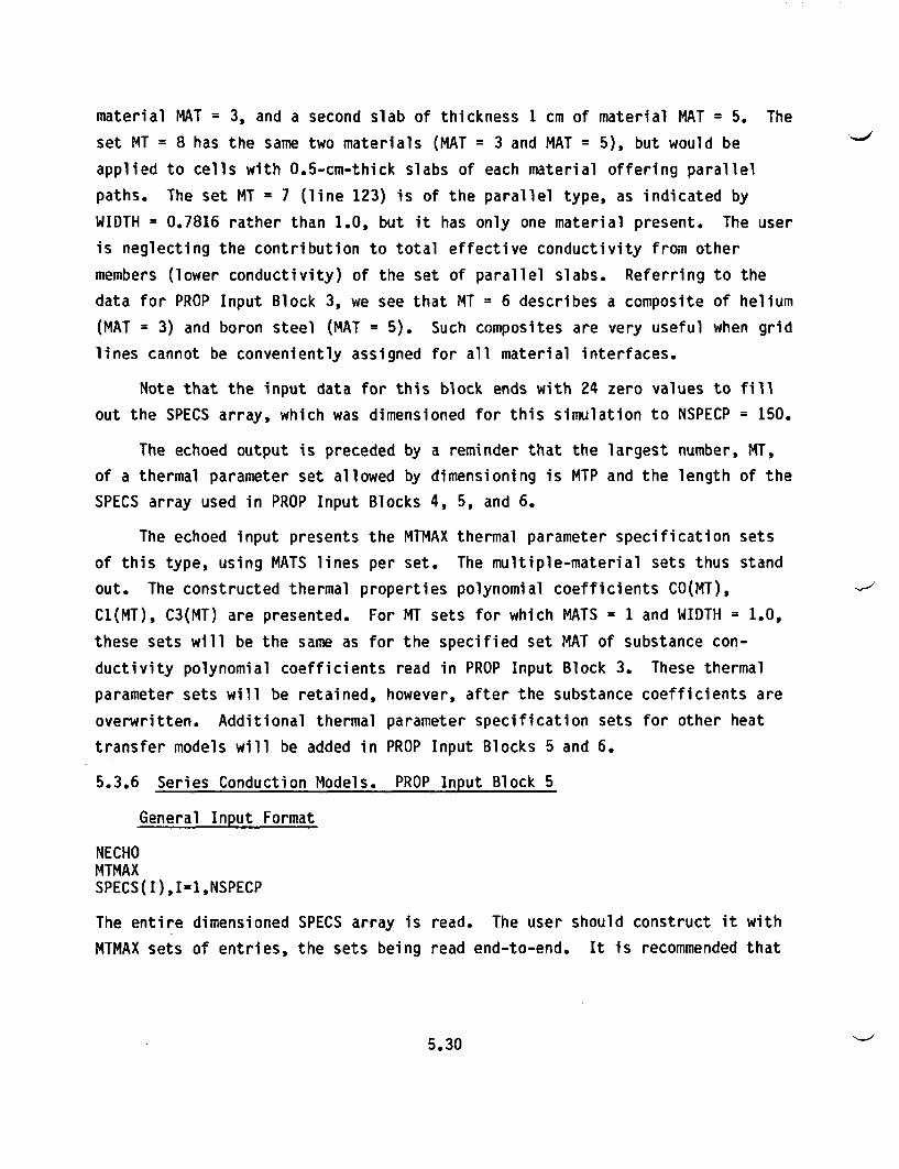
material MAT = 3, and a second slab of thickness 1 cm of material MAT = 5. The
set MT = 8 has the same two materials (MAT = 3 and MAT = 5), but would be
applied to cells with 0.5-cm-thick slabs of each material offering parallel
paths. The set MT = 7 (line 123) is of the parallel type, as indicated by
WIDTH = 0.7816 rather than 1.0, but it has only one material present. The user
is neglecting the contribution to total effective conductivity from other
members (lower conductivity) of the set of parallel slabs. Referring to the
data for PROP Input Block 3, we see that MT = 6 describes a composite of helium
(MAT = 3) and boron steel (MAT = 5). Such composites are very useful when grid
lines cannot be conveniently assigned for all material interfaces.
Note that the input data for this block ends with 24 zero values to fill
out the SPECS array, which was dimensioned for this simulation to NSPECP = 150.
The echoed output is preceded by a reminder that the largest number, MT,
of a thermal parameter set allowed by dimensioning is MTP and the length of the
SPECS array used in PROP Input Blocks 4, 5, and 6.
The echoed input presents the MTMAX thermal parameter specification sets
of this type, using MATS lines per set. The multiple-material sets thus stand
out. The constructed thermal properties polynomial coefficients CO(MT),
C1(MT), C3(MT) are presented. For MT sets for which MATS = 1 and WIDTH = 1.0,
these sets will be the same as for the specified set MAT of substance con-
ductivity polynomial coefficients read in PROP Input Block 3. These thermal
parameter sets will be retained, however, after the substance coefficients are
overwritten. Additional thermal parameter specification sets for other heat
transfer models will be added in PROP Input Blocks 5 and 6.
5.3.6 Series Conduction Models. PROP Input Block 5
General Input Format
NECHOMTMAXSPECS(I),I=1,NSPECP
The entire dimensioned SPECS array is read. The user should construct it with
MTMAX sets of entries, the sets being read end-to-end. It is recommended that
5.30
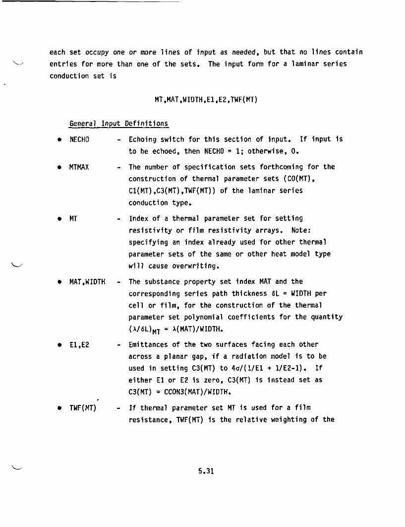
each set occupy one or more lines of input as needed, but that no lines contain
entries for more than one of the sets. The input form for a laminar series
conduction set is
MT,MAT,WIDTH,E1,E2,TWF(MT)
General Input Definitions
* NECHO
* MTMAX
* MT
- Echoing switch for this section of input. If input is
to be echoed, then NECHO = 1; otherwise, 0.
- The number of specification sets forthcoming for the
construction of thermal parameter sets (CO(MT),
Cl(MT),C3(MT),TWF(MT)) of the laminar series
conduction type.
- Index of a thermal parameter set for setting
resistivity or film resistivity arrays. Note:
specifying an index already used for other thermal
parameter sets of the same or other heat model type
will cause overwriting.
* MAT,WIDTH - The substance property set index MAT and the
corresponding series path thickness 6L = WIDTH per
cell or film, for the construction of the thermal
parameter set polynomial coefficients for the quantity
(A/6L)MT = X(MAT)/WIDTH.
* El,E2 - Emittances of the two surfaces facing each other
across a planar gap, if a radiation model is to be
used in setting C3(MT) to 4a/(1/El + 1/E2-1). If
either El or E2 is zero, C3(MT) is instead set as
C3(MT) = CCON3(MAT)/WIDTH.
* TWF(MT) - If thermal parameter set MT is used for a film
resistance, TWF(MT) is the relative weighting of the
5.31
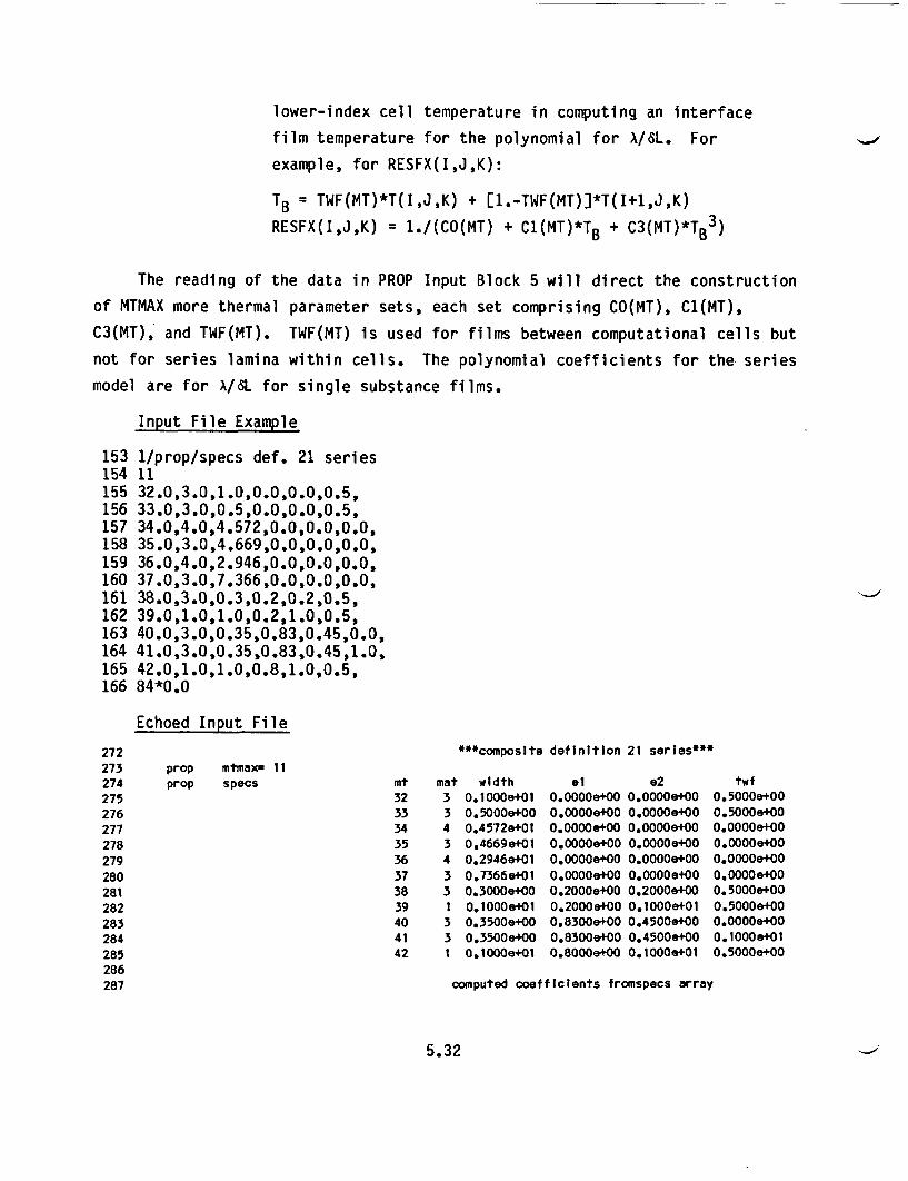
lower-index cell temperature in computing an interface
film temperature for the polynomial for A/SL. For
example, for RESFX(I,J,K):
TB = TWF(MT)*T(I,J,K) + [1.-TWF(MT)]*T(I+1,J,K)
RESFX(I,J,K) = 1./(CO(MT) + C1(MT)*TB + C3(MT)*TB3)
The reading of the data in PROP Input Block 5 will direct the construction
of MTMAX more thermal parameter sets, each set comprising CO(MT), C1(MT),
C3(MT), and TWF(MT). TWF(MT) is used for films between computational cells but
not for series lamina within cells. The polynomial coefficients for the series
model are for A/SL for single substance films.
Input File Example
153 1/prop/specs def. 21 series154 11155 32.0,3.0,1.0,0.0,0.0,0.5,156 33.0,3.0,0.5,0.0,0.0,0.5,157 34.0,4.0,4.572,0.0,0.0,0.0,158 35.0,3.0,4.669,0.0,0.0,0.0,159 36.0,4.0,2.946,0.0,0.0,0.0,160 37.0,3.0,7.366,0.0,0.0,0.0,161 38.0,3.0,0.3,0.2,0.2,0.5,162 39.0,1.0,1.0,0.2,1.0,0.5,163 40.0,3.0,0.35,0.83,0.45,0.0,164 41.0,3.0,0.35,0.83,0.45,1.0,165 42.0,1.0,1.0,0.8,1.0,0.5,166 84*0.0
Echoed Input File
272 ***composite definition 21 series***273 prop mtmax- 11274 prop specs mt mat width el e2 twf275 32 3 0.1000e+01 0.OOOOa+00 0.OOOOe+00 0.5000e+00276 33 3 0.5000e+00 0.0000e+00 O.OOOOe+00 0.5000a+00277 34 4 0.4572e+01 O.OOOOe+00 0.OOOOe+00 0.OOOOe+00278 35 3 0.4669e+01 O.OOOOe+00 O.OOOOe+00 O.OOOOe+00279 36 4 0.2946e+01 O.OOOOe+00 0.OOOOa+00 O.OOOOe+00280 37 3 0.7366e+01 O.OOOOa+00 0.OOOOe+00 O.OOOOe+00281 38 3 0.3000e+00 0.2000e+00 0.2000e+00 0.5000e+00282 39 1 O.lOOOe+01 0.2000a+00 0.lOOOe+01 0.5000e+00283 40 3 0.3500e+00 0.8300e+00 0.4500e+00 O.OOOOe+00284 41 3 0.3500a+00 0.8300e+00 0.4500e+00 0.lOOOe+01285 42 1 0.1000e+01 0.8000e+00 0.1000e+01 0.5000e+00286287 computed coefficients fromspecs array
5.32
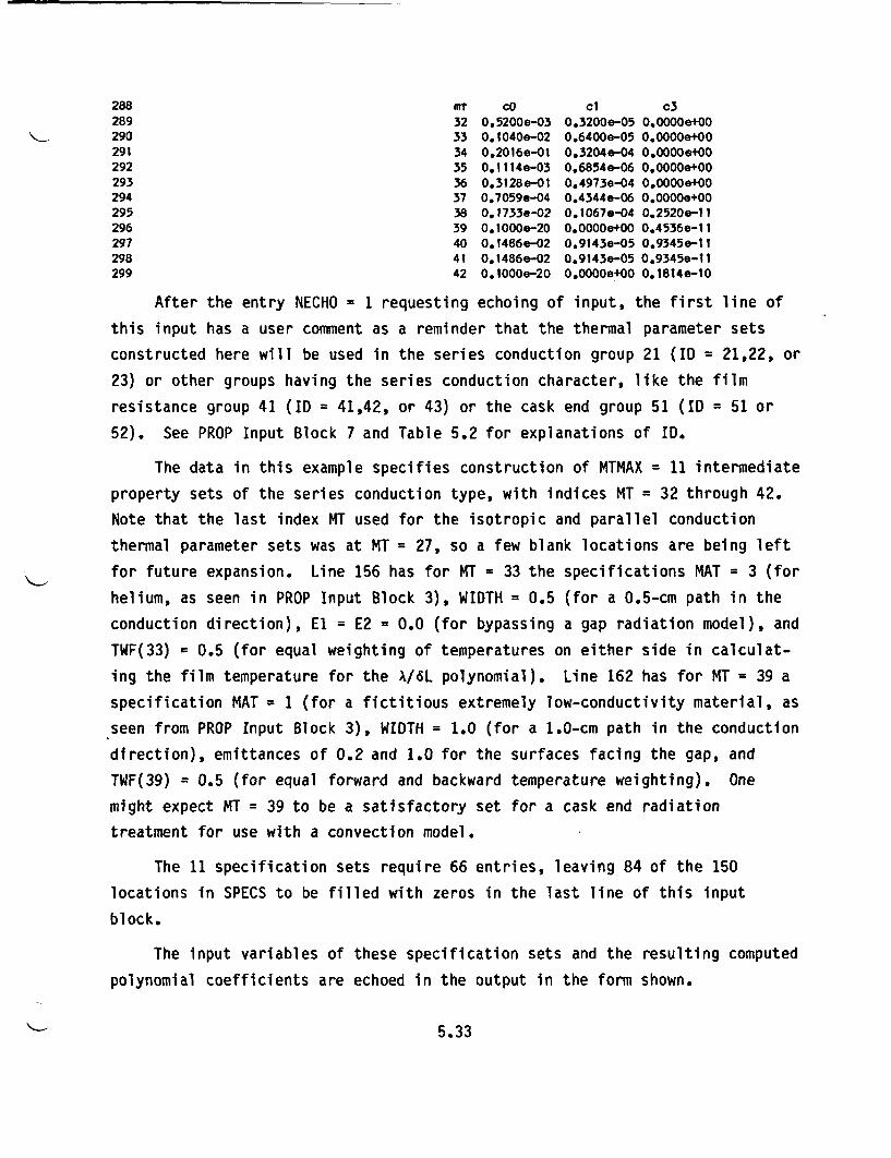
288 mt cO C1 c3289 32 0.5200e-03 0.3200e-05 0.0000e+00290 33 0.1040e-02 0.6400e-05 0.OOOOe+00291 34 0.2016e-01 0.3204e-04 0.0000e+00292 35 0.1114e-03 0.6854e-06 0.0000e+00293 36 0.3128e-01 0.4973e-04 0.0000e+00294 37 0.7059e-04 0.4344e-06 0.0000e+00295 38 0.1733e-02 0.1067e-04 0.2520.-1l296 39 0.10OOe-20 0.0000e+00 0.4536e-11297 40 0.1486e-02 0.9143e-05 0.9345e-11298 41 0.1486e-02 0.9143e-05 0.9345e-11299 42 0.1000e-20 0.0000e+00 0.1814e-10
After the entry NECHO = 1 requesting echoing of input, the first line of
this input has a user comment as a reminder that the thermal parameter sets
constructed here will be used in the series conduction group 21 (ID = 21,22, or
23) or other groups having the series conduction character, like the film
resistance group 41 (ID = 41,42, or 43) or the cask end group 51 (ID = 51 or
52). See PROP Input Block 7 and Table 5.2 for explanations of ID.
The data in this example specifies construction of MTMAX = 11 intermediate
property sets of the series conduction type, with indices MT = 32 through 42.
Note that the last index MT used for the isotropic and parallel conduction
thermal parameter sets was at MT = 27, so a few blank locations are being left
for future expansion. Line 156 has for MT = 33 the specifications MAT = 3 (for
helium, as seen in PROP Input Block 3), WIDTH = 0.5 (for a 0.5-cm path in the
conduction direction), El = E2 = 0.0 (for bypassing a gap radiation model), and
TWF(33) = 0.5 (for equal weighting of temperatures on either side in calculat-
ing the film temperature for the A/6L polynomial). Line 162 has for MT = 39 a
specification MAT = 1 (for a fictitious extremely low-conductivity material, as
seen from PROP Input Block 3), WIDTH = 1.0 (for a 1.0-cm path in the conduction
direction), emittances of 0.2 and 1.0 for the surfaces facing the gap, and
TWF(39) = 0.5 (for equal forward and backward temperature weighting). One
might expect MT = 39 to be a satisfactory set for a cask end radiation
treatment for use with a convection model.
The 11 specification sets require 66 entries, leaving 84 of the 150
locations in SPECS to be filled with zeros in the last line of this input
block.
The input variables of these specification sets and the resulting computed
polynomial coefficients are echoed in the output in the form shown.
5.33
5.3.7 Fuel Assembly Conduction-Radiation Models. PROP Input Block 6
General Input Format
NECHOMTMAXSPECS(I),I=1,NSPECP
The entire dimensioned array SPECS is read. SPECS comprises MTMAX sets of
entries making up the fuel assembly thermal parameter sets construction
directives and having the form (after conversion from floating point to integer
form as needed):
MT,MTA,FUELOD,CLADOD,PITCH,CFUEL,CCLAD,EROD,EGAP
General Input Definition
* NECHO - Integer flag variable that, if positive, directs
echoing of forthcoming input in the output.
* MTMAX - Number of specification sets forthcoming for
construction of thermal parameter sets
(CO(MT),C1(MT),C3(MT), X1(MT),X2(MT),
Z1(MT),Z2(MT),Z3(MT)) of the fuel assembly type.
* MT - Index of the thermal property set being constructed.
* MTA - Index of a previously set thermal parameter set of the
simple conduction type for calculating conductivity of
the gas between the square array of cylinders.
ECO(MT) gets set to CO(MTA), C1(MT) to C1(MTA)].
* FUELOD - Outside diameter of the fuel pellets.
* CLADOD - Outside diameter of the fuel cladding.
* PITCH - Distance between corresponding points on adjacent fuel
rods in the array.
* CFUEL - Thermal conductivity of the fuel.
* CCLAD - Thermal conductivity of the cladding.
5.34
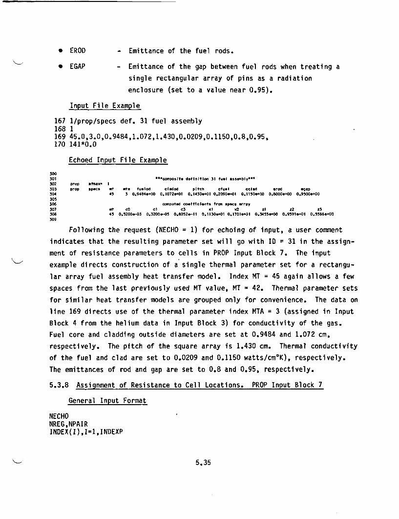
* EROD - Emittance of the fuel rods.
* EGAP - Emittance of the gap between fuel rods when treating a
single rectangular array of pins as a radiation
enclosure (set to a value near 0.95).
Input File Example
167 1/prop/specs def. 31 fuel assembly168 1169 45.0,3.0,0.9484,1.072,1.430,0.0209,0.1150,0.8,0.95,170 141*0.0
Echoed Input File Example
300301 ***composite definition 31 fuel assembly"*302 prop atmax. I303 prop specs Mt ata fuelod cladod pitch cfuel cclad erod egap304 45 5 0.9484.+00 0.1072.401 0.1430.401 0.2090_-01 0.1150.+00 0.8000e+00 0.9500.400305306 computed coefficients from specs array307 Mt co cl c3 xl la 21 z2 z3308 45 0.5200e-03 0.3200.-05 0.8052.-l 0.1130e401 0.1701.401 0.3455.400 0.9591.0I 0.5586.00309
Following the request (NECHO = 1) for echoing of input, a user comment
indicates that the resulting parameter set will go with ID = 31 in the assign-
ment of resistance parameters to cells in PROP Input Block 7. The input
example directs construction of a single thermal parameter set for a rectangu-
lar array fuel assembly heat transfer model. Index MT = 45 again allows a few
spaces from the last previously used MT value, MT = 42. Thermal parameter sets
for similar heat transfer models are grouped only for convenience. The data on
line 169 directs use of the thermal parameter index MTA = 3 (assigned in Input
Block 4 from the helium data in Input Block 3) for conductivity of the gas.
Fuel core and cladding outside diameters are set at 0.9484 and 1.072 cm,
respectively. The pitch of the square array is 1.430 cm. Thermal conductivity
of the fuel and clad are set to 0.0209 and 0.1150 watts/cm0 K), respectively.
The emittances of rod and gap are set to 0.8 and 0.95, respectively.
5.3.8 Assignment of Resistance to Cell Locations. PROP Input Block 7
General Input Format
NECHONREG,NPAIRINDEX(I),I=1,INDEXP
5.35
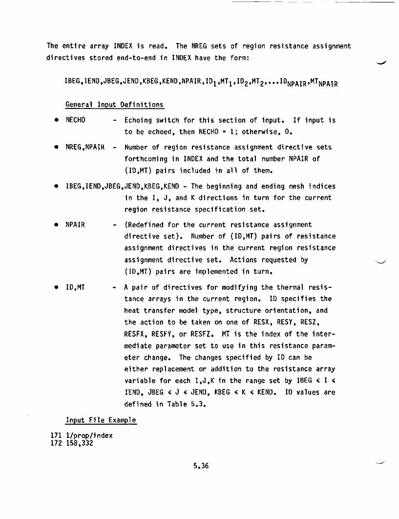
The entire array INDEX is read. The NREG sets of region resistance assignment
directives stored end-to-end in INDEX have the form:
IBEGIENDJBEGJENDKBEGKENDNPAIRID ,MTIID2,MT2,..eIDNPAIR,MTNPAIR
General Input Definitions
* NECHO - Echoing switch for this section of input. If input is
to be echoed, then NECHO = 1; otherwise, 0.
* NREG,NPAIR - Number of region resistance assignment directive sets
forthcoming in INDEX and the total number NPAIR of
(ID,MT) pairs included in all of them.
* IBEG,IEND,JBEG,JEND,KBEG,KEND - The beginning and ending mesh indices
in the I, J, and K directions in turn for the current
region resistance specification set.
* NPAIR - (Redefined for the current resistance assignment
directive set). Number of (ID,MT) pairs of resistance
assignment directives in the current region resistance
assignment directive set. Actions requested by
(ID,MT) pairs are implemented in turn.
* ID,MT - A pair of directives for modifying the thermal resis-
tance arrays in the current region. ID specifies the
heat transfer model type, structure orientation, and
the action to be taken on one of RESX, RESY, RESZ,
RESFX, RESFY, or RESFZ. MT is the index of the inter-
mediate parameter set to use in this resistance param-
eter change. The changes specified by ID can be
either replacement or addition to the resistance array
variable for each I,J,K in the range set by IBEG < I 4
IEND, JBEG < J < JEND, KBEG 4 K c KEND. ID values are
defined in Table 5.3.
Input File Example
171 1/prop/index172 158,332
5.36
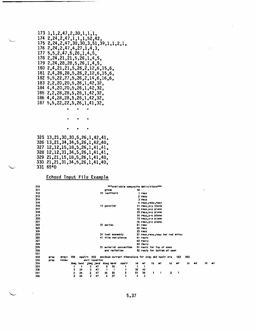
173 1,1,2,47,2,30,1,1,1,174 2,24,2,47,1,1,1,52,42,175 2,24,2,47,30,30,3,51,39,1,1,2,1,176 2,24,2,47,4,27,1,4,3,177 5,5,2,47,5,26,1,4,5,178 2,24,21,21,5,26,1,4,5,179 2,24,28,28,5,26,1,4,5,180 2,4,21,21,5,26,2,12,6,15,6,181 2,4,28,28,5,26,2,12,6,15,6,182 5,5,22,27,5,26,2,14,6,16,6,183 2,2,20,20,5,26,1,42,32,184 4,4,20,20,5,26,1,42,32,185 2,2,28,28,5,26,1,42,32,186 4,4,28,28,5,26,1,42,32,187 5,5,22,22,5,26,1,41,32,
* * S
* * a
* * 0
325 13,21,30,30,5,26,1,42,41,326 13,21,34,34,5,26,1,42,40,327 12,12,15,18,5,26,1,41,41,328 12,12,31,34,5,26,1,41,41,329 21,21,15,18,5,26,1,41,40,330 21,21,31,34,5,26,1,41,40,331 65*0
Echoed Input File Example
310 "availablo composite definitlons"*
311 group Id
312 01 Isotropic I rasx
313 2 res314 3 rasz
315 4 rasxyrytesz
316 11 parallel It rassxx-y plano
317 12 resxx-z plane
318 13 resy,x-y plane
319 14 rasy.y-z plans
320 15 resz,x-z plane
321 16 resz.y-z plane
322 21 series 21 resx
323 22 resy
324 23 resz
325 31 fuel assembly 31 resx,resy,resz for rod array
326 41 film resIstance 41 restx
327 42 resty
328 43 restz
329 51 exterior convection 51 rastz for top of cask
330 and radIatIon 52 restz for bottom of cask
331332 prop nrag- 158 npalr- 332 maximum current dimensions for nreg and npalr are 165 340
333 prop Index call location334 Ibeg lend Jbeg Jend kbeg lend npalr Id at Id *t Id at Id at Id at
335 1 1 2 47 2 50 I I 1336 2 24 2 47 1 1 1 52 42
337 2 24 2 47 30 30 3 513 9 1 1 2 1
338 2 24 2 47 4 27 1 4 3
5.37
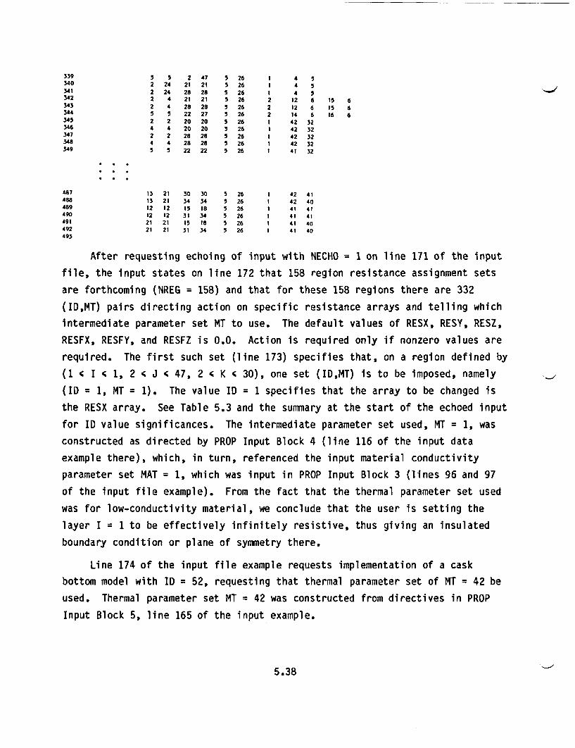
339 5 5 2 47 5 26 1 4 5340 2 24 21 21 5 26 1 4 5341 2 24 28 28 5 26 1 4 5342 2 4 21 21 5 26 2 12 6 is 6343 2 4 28 28 5 26 2 12 6 15 6344 5 5 22 27 5 26 2 14 6 16 6345 2 2 20 20 5 26 1 42 32346 4 4 20 20 5 26 1 42 32347 2 2 28 28 5 26 1 42 32348 4 4 28 28 5 26 1 42 32349 5 5 22 22 5 26 1 41 32
487 13 21 30 30 5 26 1 42 41488 13 21 34 34 5 26 1 42 40489 12 12 15 18 5 26 1 41 41490 12 12 31 34 5 26 1 41 41491 21 21 15 18 5 26 1 41 40492 21 21 31 34 5 26 1 41 40493
After requesting echoing of input with NECHO = 1 on line 171 of the input
file, the input states on line 172 that 158 region resistance assignment sets
are forthcoming (NREG = 158) and that for these 158 regions there are 332
(ID,MT) pairs directing action on specific resistance arrays and telling which
intermediate parameter set MT to use. The default values of RESX, RESY, RESZ,
RESFX, RESFY, and RESFZ is O.O. Action is required only if nonzero values are
required. The first such set (line 173) specifies that, on a region defined by
(1 < I < 1, 2 < J c 47, 2 < K 4 30), one set (ID,MT) is to be imposed, namely
(ID = 1, MT = 1). The value ID = 1 specifies that the array to be changed is
the RESX array. See Table 5.3 and the summary at the start of the echoed input
for ID value significances. The intermediate parameter set used, MT = 1, was
constructed as directed by PROP Input Block 4 (line 116 of the input data
example there), which, in turn, referenced the input material conductivity
parameter set MAT = 1, which was input in PROP Input Block 3 (lines 96 and 97
of the input file example). From the fact that the thermal parameter set used
was for low-conductivity material, we conclude that the user is setting the
layer I = 1 to be effectively infinitely resistive, thus giving an insulated
boundary condition or plane of symmetry there.
Line 174 of the input file example requests implementation of a cask
bottom model with ID = 52, requesting that thermal parameter set of MT = 42 be
used. Thermal parameter set MT = 42 was constructed from directives in PROP
Input Block 5, line 165 of the input example.
5.38
Line 175 of the input file example requests implementation of two (ID,MT)
resistance assignment pairs on its range (2 c I c 24, 2 cJ c 47, 30 c K c 30),
namely (ID,MT) = (1,1) and (ID,MT) = (2,1). Thus, both RESX and RESY are set
to large values on this range.
The echoed input summarizes this information.
5.39
6.0 SUBROUTINE THERM
Subroutine THERM solves the energy equation on the rectangular grid.
6.1 THERM FUNCTIONS
THERM reads input specifying initial temperatures, heat sources, and
numerical procedure options during initiation or restart of a simulation. If
solution of the energy equation on the rectangular grid is requested, THERM is
called at each time-step to advance the temperature solution.
The actions performed by THERM in the solution sequence include the
following:
1. THERM sets the connector arrays for the energy equation. These are
the coefficients that relate temperature to heat flow rates, mass
fluxes, and heat sources.
2. THERM executes an algorithm that advances the temperatures on the
rectangular computational grid through a time-step.
3. If requested, THERM prints monitoring information, including the
location and amount of the largest temperature change in each time-
step and the temperature in cells designated for temperature
printout.
4. THERM makes tentative adjustments in the time-step by comparing the
maximum temperature change and a user-specified maximum target
temperature change.
The algorithm used in THERM for advancing the temperature through a time-
step is discussed in Volume I - Equations and Numerics (McCann 1987). To carry
on this and its other functions in solving the energy equation on the rectan-
gular grid, THERM is called at initialization or restart to read input to guide
the solution and to set or reset temperatures.
Actions performed by THERM in the initialization or restart operation
include:
1. THERM reads certain options for numerical procedures and printouts.
6.1
2. THERM reads specifications for heat sources.
3. THERM reads specifications for initial temperatures on the rectan-
gular grid region and the rectangular-cylindrical grid interface,
including ambient temperatures at cask top and bottom.
4. THERM modifies or resets the temperature distribution according to
user input, as may be desired in a restart.
6.1.1 Numerical Procedures
If a solution for both temperatures and flows is requested, calls from
MAIN to the flow-solving routines are interspersed with the calls to the energy
equation-solving routines (such as THERM and REBT for the rectangular grid,
TSIDE for the cylindrical grid, and TBND or REBA for their connection). The
algorithm in REBT solves the energy equation on slab partitions of the rec-
tangular grid region, and its calling sequence is specified in input to THERM.
The use of REBA, a solver of the energy equations on both grids, is specified
in MAIN. The periodic use of REBT and REBA in the solution of the energy equa-
tions accelerates convergence, particularly as steady state is approached. See
the guidance for the use of REBT in Chapter 7.0 and for REBA in Chapter 14.0.
6.1.2 Heat Sources
The technique for specifying heat sources has been designed especially for
heat generating spent fuel assemblies. As a result, the input specifications
are relatively simple. Three items of information are required: the toal heat
generation rate of a fuel assembly; the locations of reduced heat generation
within a fuel assembly, such as instrumentation tubes; and the relative axial
activity of the fuel assembly. The longitudinal axis of each fuel assembly is
in the z-direction.
The total heat being generated in a single column of cells, assumed to
extend in the z-direction from K = 2 to K = KP-1, can be expressed as
QC (IJ)_ Q9 W(IJ)DX(I)DY(J) (6.1)Sz W(I,J)DX(I)DY(J) (
6.2
where QC(I,J) is the total heat generation in a column I,J
Qg is the total heat generation in the fuel assembly (group power)
W(IJ) is a relative weighting factor for heat generation within the
fuel assembly (group).
Different group powers and weighting factors may be specified for each fuel
assembly. The weighting factor is automatically halved for phantom cells on
the curved boundary.
The axial distribution of heat generation is determined from the relative
activity curve for a spent fuel assembly. The heat generation sources used in
the code are computed as
C KA DZ jKQGEN(I,JK) =Q (IJ) Zk RA(K)DZ(K7 (6.2)
where QGEN(I,JK) is the total heat generation in cell I,J,K
RA(K) is the relative activity as a function of K.
The code assigns the same relative activity curve to all fuel assemblies. The
relative activity data specified on the input file need not be normalized; the
code does this automatically.
It can be seen from the preceding discussion that a completely arbitrary
distribution of heat sources cannot be specified in this version of the code.
The basic restriction is that heat generation sources be expressed in the form
Q(I,J,K) = FXY(I,J)*FZ(K) (6.3)
6.1.3 Setting or Resetting Temperatures
Subroutine THERM can set the initial temperature on the rectangular grid
and its interface with the cylindrical grid in a new simulation, or it can
alter or reset them in a restart.
To set or reset the temperature distribution with input, the user supplies
temperatures TS1(JS,K) on the cylindrical interface between rectangular and
cylindrical grid regions, where JS is the azimuthal sector index and K is the
6.3
axial plane index. An array of temperatures, TCEN(K), on a user-specified
axial "center line" in the rectangular grid is also read. An array, TCAN(K),
of azimuthal average interface temperatures is calculated as
TCAN(K) = z TS1(JS,K)*DTHETA(JS)/E DTHETA(JS) (6.4)iS JS
These arrays can be used to reset temperatures in three regions as indicated in
Figure 6.1 according to options as follows:
1. NEWT = 1. Set an initial temperature distribution in the rectangular
grid computational region (but not the phantom cells) according to
T(I,J,K) = TCEN(K) + (TCAN(K) - TCEN(K))*(FAC/FACMX)
where FAC = (REAL(I) - 1.5)2 + (REAL(J) - CENJ)2
and FACMX is the largest value of FAC in the rectangular grid com-
putational region.
2. NEWTC = 1. Reset temperatures in the rectangular grid phantom cells
at the cylindrical grid interface as
T(ICART(JS),JCART(JS),K) = TS1(JS,K)
for azimuthal indices JS in the range 2 J OS 4 JSP-1 and axial
indices K in the range 2 ' K ' KP-1.
3. NEWTA = 1. Reset cask end ambient temperatures in the rectangular
grid region as
T(IJ,1) = TCAN(1)
T(I,J,KP) = TCAN(KP)
The azimuthal average value TCAN(1) of TS1(JS,1) becomes the cask
bottom ambient temperature, and the average value TCAN(KP) of
TS1(JS,KP) becomes the cask top ambient temperature.
These temperatures will be altered in the subsequent calculations with two
exceptions:
1. The cask end ambient temperatures T(I,J,1) and T(I,J,KP) will be held
constant.
6.4
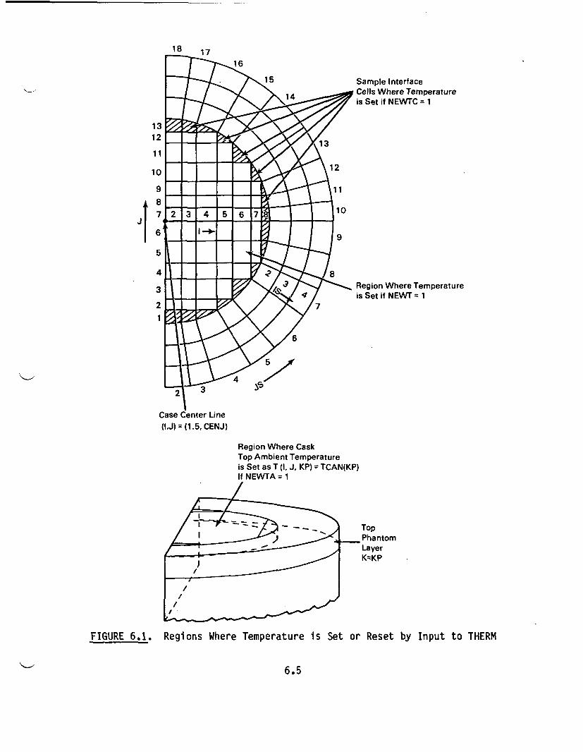
18 17
1312
1 1
10
9
I
Sample Interface14 _Cells Where Temperature
is Set if NEWTC = 1
M Region Where temperature/ t / ~is Set if NEWT-
2.2
1 /
Region Where CaskTop Ambient Temperatureis Set as T (I. J, KP) =TCAN(KP)If NEWTA = 1
\/\/
TopPhantomLayerK=KP
Case Center Line(1,J) = (1.5, CENJ)
FIGURE 6.1. Regions Where Temperature is Set or Reset by Input to THERM
6.5
2. If the calculation involves the rectangular grid only (as indicated
by NOBODY = 1), the temperatures will be constant on the boundary
cells of the rectangular grid.
6.2 PARAMETER STATEMENT INFORMATION
Dimensioning parameters required by THERM include IP, JP, KP, ISP, JSP,
NEFAP. These were discussed in Chapter 4.0. Also needed by THERM are:
* KBP,KTP - The number of K-planes at cask bottom and top, respec-
tively, which are active computational cells for the
energy equation but not for the flow equations. See
Figure 4.8.
* MONTP - Dimensioning parameter that must equal or exceed the
number of computational cells for which temperature is
to be monitored.
6.3 INPUT FORMAT
6.3.1 Overview
The input for THERM is discussed in four sections: 1) numerical procedure
and printout options, 2) heat source specifications, 3) initial temperature
specifications, and 4) temperature modifications or reset specifications.
6.3.2 Numerical Procedure and Printout Options
General Input Format
NECHOTHETA, SPHTF, DTEMAXREBON, NREB, NREBNNECHOMONTIMONT(M), JMONT(M), KMONT(M)) Lines for M=1 through MONT+1,
J (with IMONT(MONT+1)=O
General Input Description
* NECHO - Echoing switch for this section of input. If input is
to be echoed, then NECHO = 1; otherwise, 0.
6.6
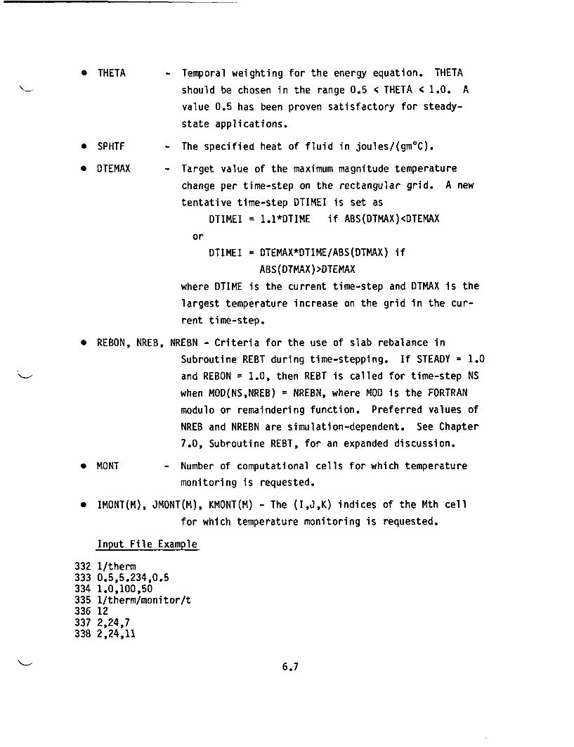
* THETA
* SPHTF
- Temporal weighting for the energy equation. THETA
should be chosen in the range 0.5 < THETA < 1.0. A
value 0.5 has been proven satisfactory for steady-
state applications.
- The specified heat of fluid in joules/(gm0 C).
* OTEMAX Target value of the maximum magnitude temperature
change per time-step on the rectangular grid. A new
tentative time-step DTIMEI is set as
DTIMEI = 1.1*DTIME if ABS(DTMAX)<DTEMAX
or
DTIMEI = DTEMAX*DTIME/ABS(DTMAX) if
ABS(DTMAX)>DTEMAX
where DTIME is the current time-step and DTMAX is the
largest temperature increase on the grid in the cur-
rent time-step.
* REBON, NREB, NREBN - Criteria for the use of slab rebalance in
Subroutine REBT during time-stepping. If STEADY = 1.0
and REBON = 1.0, then REBT is called for time-step NS
when MOD(NS,NREB) = NREBN, where MOD is the FORTRAN
modulo or remaindering function. Preferred values of
NREB and NREBN are simulation-dependent. See Chapter
7.0, Subroutine REBT, for an expanded discussion.
* MONT - Number of computational cells for which temperature
monitoring is requested.
* IMONT(M), JMONT(M), KMONT(M) - The (I,J,K) indices of the Mth cell
for which temperature monitoring is requested.
Input File Example
332333334335336337338
1/therm0.5,5.234,0.51.0,100,501/therm/monitor/t122,24,72,24,11
6.7

339 2,24,15340 2,24,16341 2,24,18342 2,24,22343 2,41,7344 2,41,11345 2,41,15346 2,41,16347 2,41,18348 2,41,22349 0,0,0
Echoed Input File Example
494 therm theta-0.5 sphtf=0.5234e+01 dtemax-0.500e+00
495 therm rebon-1.0 nreb-100 nrebn= 50496
497 therm monitor cells=12 maximum number currently allowed Is 12498 m I J k499 1 2 24 7
500 2 2 24 11501 3 2 24 15
502 4 2 24 16503 5 2 24 18504 6 2 24 22505 7 2 41 7
506 8 2 41 11507 9 2 41 15
508 10 2 41 16509 11 2 41 18
510 12 2 41 22511
Echoed input is requested with NECHO = 1 on line 332 of the input. THETA,
SPHTF, and DTEMAX are set to 0.5, 5.234, and 0.5, respectively. One of the
requirements for use of a coarse mesh rebalance of the energy equation, REBON =
1.0, is met. The input specifies rebalancing at time-steps NS = 50, 150, 250,
etc. Monitoring of the temperature in the list of 12 cells is requested. Line
349 has a zero first entry, indicating the end of the list of cells for
monitoring.
The echoed output confirms these numbers, and also compares the numbers
MONT of cells requested for temperature printouts with the number currently
allowed by dimensions.
6.8
6.3.3 Heat Source Specifications
General Input Format
NECHOQWTFAC,IBEG,IEND,JBEG,JEND - Repeated until IBEG = 0 is encounteredNECHOGRPPOW,IBEG,IEND,JBEG,JEND - Repeated until IBEG = 0 is encounteredNECHORELACT(K),K=2,KP-1NECHOPQGEN
General Input Description
* NECHO - Echoing switch for this section of input. If input is
to be echoed, then NECHO = 1; otherwise, 0.
* QWTFAC - The relative weighting factor per unit area for each
heat source in the range
JBEG 4 J 4 JEND
IBEG 4 I c MIN(IEND,IMEND(J))
The range is thus restricted to the computational and
phantom cells for the energy equation. QWTFAC is
automatically reduced by one half if the cell is a
phantom cell on the curved part of the Cartesian boun-
dary. The default value of QWTFAC is zero.
IBEG,IEND,JBEG,JEND - Range specifications of the form
JBEG 4 J < JEND
IBEG c I c MIN(IEND,IMEND(J))
* GRPPOW - Total power in watts for the heat source in the region
defined by the range specification on the same line
and in the K direction by 2 4 K < KP-1. The default
value of GRPPOW is zero.
* RELACT(K) - The relative activity at each K-plane. Normalization
is arbitrary.
* PQGEN - Floating point flag variable that, if equal to 1.0,
requests printout of the heat source array
QGEN(I,J,K). No printing occurs if PQGEN = O.O.
6.9

Input File Example
350 1/therm/q weighting factor351 1.0,2,4,2,9352 1.0,2,4,13,16353 1.0,2,4,22,27354 1.0,2,4,33,36355 1.0,2,4,40,47356 1.0,8,11,5,13357 1.0,8,11,15,18358 1.0,8,11,31,34359 1.0,8,11,36,44360 1.0,10,13,22,27361 1.0,17,24,22,27362 1.0,13,21,15,18363 1.0,13,21,31,34364 0.0,4*0365 1/therm/group power366 552.5,2,4,2,9367 552.5,2,4,13,16368 505.0,2,4,22,27369 552.5,2,4,33,36370 552.5,2,4,40,47371 1783.0,8,11,5,13372 993.0,8,11,15,18373 993.0,8,11,31,34374 1783.0,8,11,36,44375 1105.0,10,13,22,27376 1105.0,17,24,22,27377 1783.0,13,21,15,18378 1783.0,13,21,31,34379 0.0,4*0380 1/therm/relact381 4*0.0,0.5,0.72,0.94,1.12,1.19,1.23,5*1.24,382 1.23,1.21,1.16,1.03,0.83,0.61,0.44,0.26,6*0.0383 1/therm/pqgen384 0.0
Echoed Input File Example
512 therm q weighting cell location513 factor Ibeg lend Jbeg Jend514 0.lOOOe+01 2 4 2 9515 0.1000e+O1 2 4 13 16516 O.1000e+01 2 4 22 27517 0.1000e+01 2 4 33 36518 0.1000.+01 2 4 40 47519 D.lOOOe+01 8 11 5 13520 0.1000.+01 8 11 15 18521 0.1000.+01 8 11 31 34522 0.1000O01 8 11 36 44523 0.1000.+01 10 13 22 27
6.10
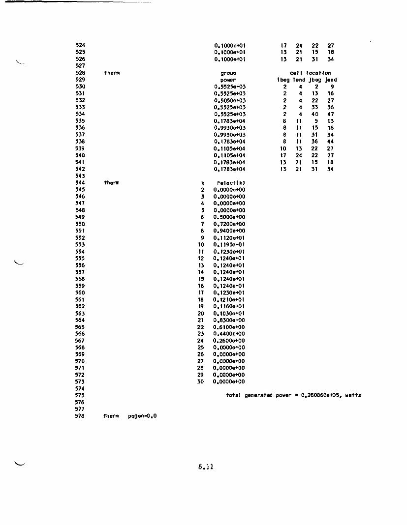
524 0.1000e+01 17 24 22 27
525 O.1000e+O 13 21 15 18
526 0.1000e+01 13 21 31 34
527528 therm group cell location
529 power Ibeg lend Jbeg Jend
530 0.5525e+03 2 4 2 9
531 0.5525e+03 2 4 13 16
532 0.5050e+03 2 4 22 27
533 0.55259+03 2 4 33 36
534 0.5525e+03 2 4 40 47
535 0.1783e+04 8 11 5 13
536 0.9930e+03 8 11 15 18
537 0.9930e+03 8 11 31 34
538 0.1783e+04 8 11 36 44
539 0.1105e+04 10 13 22 27
540 0.1105e+04 17 24 22 27
541 0.1783e+04 13 21 15 18
542 0.1783e+04 13 21 31 34
543544 therm k relact(k)
545 2 0.0000e+00
546 3 0.0000e+00547 4 0.OOOOe+00
548 5 0.OOOOe+00
549 6 0.5000e+00
550 7 0.7200e+00551 8 0.9400e+00
552 9 0.1120e+01
553 10 0.1190e+01
554 11 0.1230e+01555 12 0.1240e+01
556 13 0.1240e+01
557 14 0.1240e+01
558 15 0.1240e+01
559 16 0.1240e+01
560 17 0.1230e+01
561 18 0.1210e+01
562 19 0.1160e+01
563 20 0.1030e+01
564 21 0.8300e+00
565 22 0.6100e+00
566 23 0.4400e+00
567 24 0.2600e+00
568 25 0.0000+00
569 26 0.0000e+00
570 27 0.0000e+00571 28 0.0000+00
572 29 0.0000e+00
573 30 0.0000e+00
574575 total generated power * 0.280860e+05, watts
576577578 therm pqgen=O.0
6.11
-
The Q weighting factor is equal to 1.0 for 13 regions in the rectangular
grid. These regions correspond to the fuel assembly regions in Figure 4.1. In
this example, group powers for the entire axial extent of the 13 fuel assem-
blies of Figure 4.1 are set to values varying from 505 watts to 1783 watts.
The relative activities at axial positions from K = 2 to K = KP-1 = 30 are set
in the RELACT(K) array. Normalization of the input for RELACT(K) is arbitrary.
In this example, non-negligible heat sources are from the axial positions K = 6
to K = 24.
The echoed input shows the Q weighting factors by region, the group powers
by region, and the relative activity by position in the Z-direction. The total
power shown is calculated for the entire cask (i.e., four quadrants), and not
just the modeled region. Because PQGEN was set to zero, the final QGEN (I,J,K)
heat source per cell was not printed.
6.3.4 Initial Temperatures on the Rectangular Grid
General Input Format
NECHONEWT, CENJTCEN(K), K=2, KP-1NECHONEWTC, INFO[TS1(JS,K),JS=2,JSP-1],K=1,KP
General Input Description
* NECHO - Echoing switch for this section of input. If input is
to be echoed, then NECHO = 1; otherwise, 0.
* NEWT - An integer variable that, if equal to 1, requests
setting of temperatures on the rectangular grid based
on input temperatures TS1(JS,K) on the cylindrical
interface and TCEN(K) on the cask centerline. If NEWT
= 0, then temperatures are not reset.
* CENJ - A floating point number for the J index along which
"cask center line" temperatures TCEN(K) are
specified. The floating point number for the I index
is at I = 1.5.
6.12
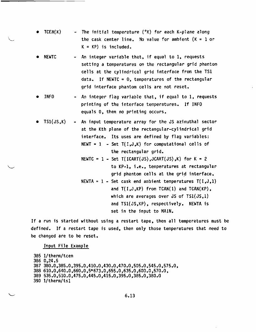
* TCEN(K)
* NEWTC
* INFO
* TS1(JS,K)
- The initial temperature (0K) for each K-plane along
the cask center line. No value for ambient (K = 1 or
K = KP) is included.
- An integer variable that, if equal to 1, requests
setting a temperatures on the rectangular grid phantom
cells at the cylindrical grid interface from the TS1
data. If NEWTC = 0, temperatures of the rectangular
grid interface phantom cells are not reset.
- An integer flag variable that, if equal to 1, requests
printing of the interface temperatures. If INFO
equals 0, then no printing occurs.
- An input temperature array for the JS azimuthal sector
at the Kth plane of the rectangular-cylindrical grid
interface. Its uses are defined by flag variables:
NEWT = 1 - Set T(I,J,K) for computational cells of
NEWTC = 1 -
NEWTA = 1 -
the rectangular grid.
Set T(ICART(JS),JCART(JS),K) for K = 2
to KP-1, i.e., temperatures at rectangular
grid phantom cells at the grid interface.
Set cask end ambient temperatures T(I,J,1)
and T(IJ,KP) from TCAN(1) and TCAN(KP),
which are averages over JS of TS1(JS,1)
and TS1(JS,KP), respectively. NEWTA is
set in the input to MAIN.
If a run is started without using a restart tape, then all temperatures must be
defined. If a restart tape is used, then only those temperatures that need to
be changed are to be reset.
Input File Example
385 1/therm/tcen386 0,24.5387 380.0,385.0,395.0,410.0,430.0,470.0,505.0,545.0,575.0,388 610.0,640.0,660.0,5*673.0,655.0,635.0,600.0,570.0,389 535.0,510.0,475.0,445.0,415.0,395.0,385.0,380.0390 1/therm/tsl
6.13
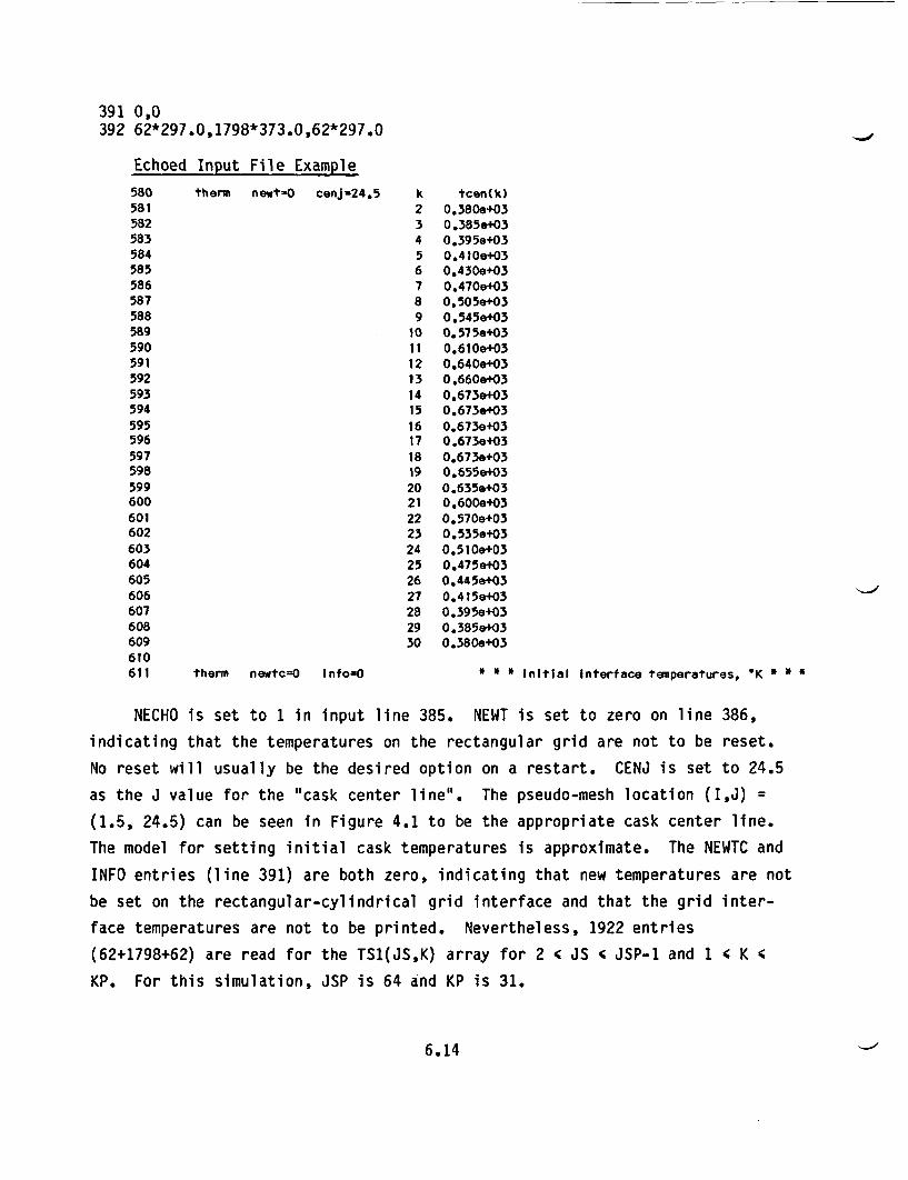
391 0,0392 62*297.0,1798*373.0,62*297.0
Echoed Input File Example
580 therm newt-O cenJ-24.5581582583584585586587588589590591592593594595596597598599600601602603604605606607608609610611 therm newtc=0 Info=0
k tcen(k)2 0.380e+033 0.385.+034 0.395e+035 0.410.+036 0.430e+037 0.470e+038 0.505e+039 0.545e+03
10 0.5759+0311 0.6109+0312 0.640e+0313 0.660.40314 0.6739+0315 0.673e+0316 0.673e40317 0.673e+0318 0.673e+0319 0.655e40320 0.635e+0321 0.600e+0322 0.5709+0323 0.535.+0324 0.510e+0325 0.475.40326 0.445e+0327 0.415e+0328 0.395e+0329 0.3859+0330 0.380e+03
Initial Interface tenperatures, *OK * * *
NECHO is set to 1 in input line 385. NEWT is set to zero on line 386,
indicating that the temperatures on the rectangular grid are not to be reset.
No reset will usually be the desired option on a restart. CENJ is set to 24.5
as the J value for the "cask center line". The pseudo-mesh location (I,J) =
(1.5, 24.5) can be seen in Figure 4.1 to be the appropriate cask center line.
The model for setting initial cask temperatures is approximate. The NEWTC and
INFO entries (line 391) are both zero, indicating that new temperatures are not
be set on the rectangular-cylindrical grid interface and that the grid inter-
face temperatures are not to be printed. Nevertheless, 1922 entries
(62+1798+62) are read for the TS1(JS,K) array for 2 4 JS < JSP-1 and 1 < K 4
KP. For this simulation, JSP is 64 and KP is 31.
6.14
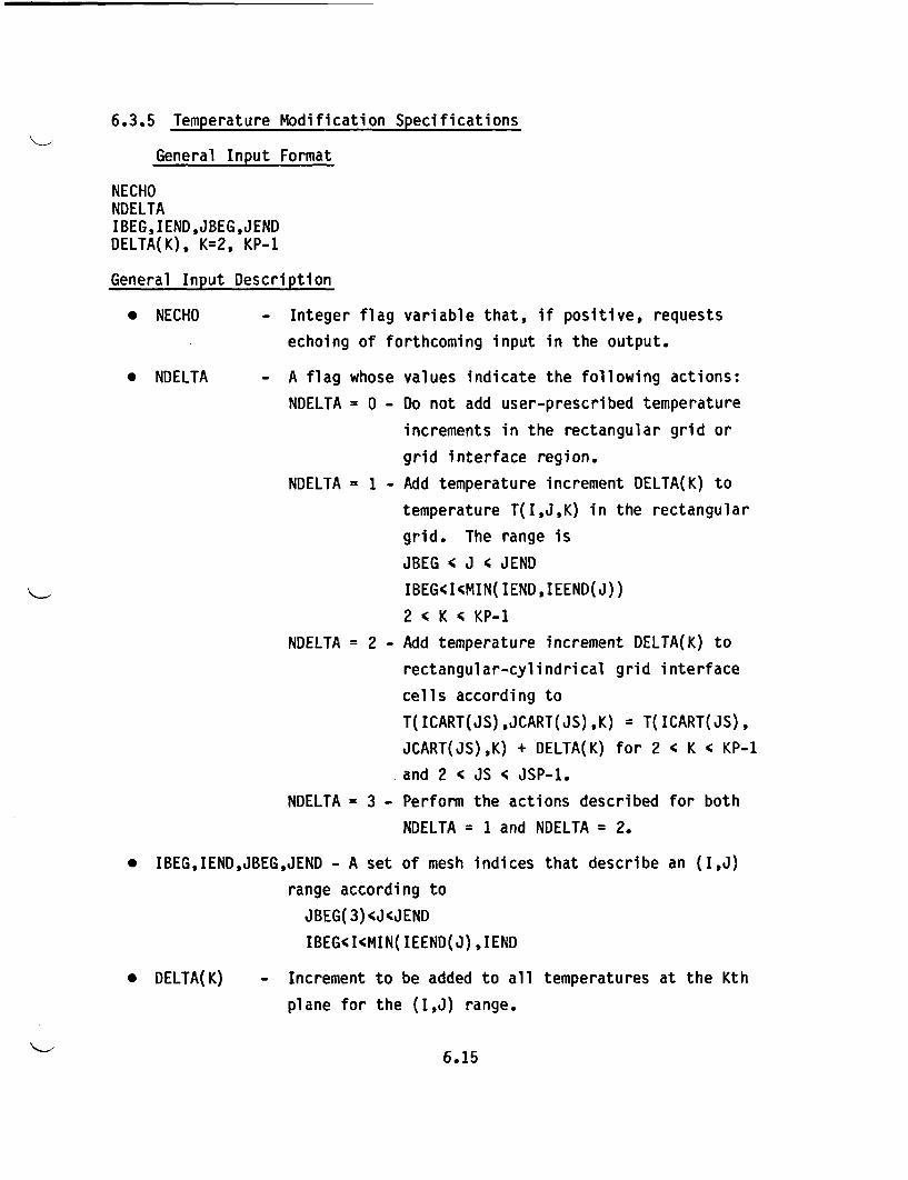
6.3.5 Temperature Modification Specifications
General Input Format
NECHONDELTAIBEG,IEND,JBEG,JENDDELTA(K), K=2, KP-1
General Input Description
* NECHO - Integer flag variable that, if positive, requests
echoing of forthcoming input in the output.
* NDELTA - A flag
NDELTA
whose
= O -
NDELTA = 1 -
N3ELTA = 2 -
NDELTA = 3 -
values indicate the following actions:
Do not add user-prescribed temperature
increments in the rectangular grid or
grid interface region.
Add temperature increment DELTA(K) to
temperature T(I,J,K) in the rectangular
grid. The range is
JBEG 4 J ' JEND
IBEG4I4MIN(IEND,IEEND(J))
2 < K < KP-1
Add temperature increment DELTA(K) to
rectangular-cylindrical grid interface
cells according to
T(ICART(JS),JCART(JS),K) = T(ICART(JS),
JCART(JS),K) + DELTA(K) for 2 4 K 4 KP-1
and 2 4 JS 4 JSP-1.
Perform the actions described for both
NDELTA = 1 and NDELTA = 2.
* IBEG,IEND,JBEG,JEND - A set of mesh indices that describe an (I,J)
range according to
JBEG(3) JcJEND
IBEG<'IMIN(IEEND(J),IEND
* DELTA(K) - Increment to be added to all temperatures at the Kth
plane for the (I,J) range.
6.15
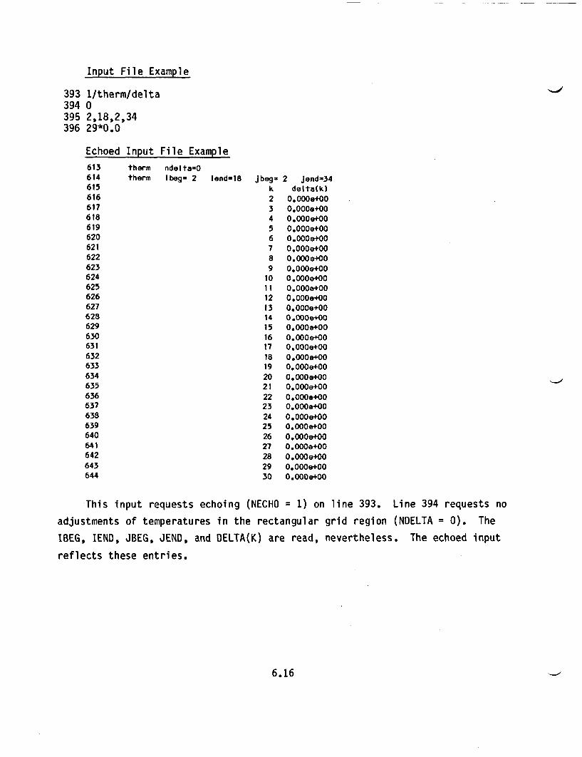
Input File Example
393394395396
1/therm/delta02,18,2,3429*0.0
Echoed Input File Example
613614615616617618619620621622623624625626627628629630631632633634635636637638639640641642643644
therm ndelta-0therm Ibeg- 2 Iend-18 Jbegn
k23456789
101112131415161718192021222324252627282930
2 Jend-34delta(k)
0.0008+000.000e+00.000e+000.000+000.0008+000.000e+000.000s+000.OOOe+000.000+000.000e+000.000+000.OOOe+000 .000e+000.000e+000.000+000.OOOe+000.000e+000.000e+000.000e+000.OOOe+000.000e+00.000+000.000e+000.000e+000.000e+000.000e+000.000+000.0008+000.OOOe+OO
This input requests echoing (NECHO = 1) on line 393. Line 394 requests no
adjustments of temperatures in the rectangular grid region (NDELTA = 0). The
IBEG, IEND, JBEG, JEND, and DELTA(K) are read, nevertheless.
reflects these entries.
The echoed input
6.16
7.0 SUBROUTINE REBT
Subroutine REBT provides an optional numerical procedure intended to
accelerate convergence of the solution of the energy equation toward steady
state on the rectangular grid.
7.1 REBT FUNCTIONS
REBT solves the energy equation on a coarser mesh, specifically, on three
slab partitions of the rectangular grid region. REBT is made available because
the algorithm used in THERM reduces small long-range errors slowly as steady
state is approached. Long-range errors are departures from the exact solution
over distances much larger than the mesh spacing.
The prescription for calling REBT is provided by the user in the input to
subroutine THERM. Additional minimal but rather important input for this con-
vergence acceleration scheme is read by subroutine REBT during an initiation or
restart. To use REBT judiciously, it is helpful to review some of the features
of the solution for the physical system and of the energy equation in sub-
routine THERM.
HYDRA-II is set up to find steady-state conditions, using time-stepping to
generate the approach to steady state. The finite-difference formulation in
HYDRA-II discussed in Volume I (McCann 1987) presents the energy equation in a
form relating temperature change 6T(I,J,K) in the (I,J,K) cell during time-step
St to the net energy flow into the (I,J,K) cell and energy sources there. Sub-
routine REBT, by contrast, solves a comparable energy equation on a coarser
mesh for some time increment, St = XDTIME, adding the temperature change ST
found for a coarse region to the T(I,J,K) for all the (I,J,K) points within the
region. REBT actually uses three coarse meshes, each a set of slabs. In the
first coarse mesh, there is a slab for each I value. Each temperature incre-
ment 6T(I) found in this coarse mesh solution is added to all the T(I,J,K) for
that I value. A similar procedure is followed in a coarse mesh with a slab for
each J value and in a coarse mesh with a slab for each K value.
Because the user is seeking only a steady-state solution for the coupled
system of heat and mass flow, the time-step in REBT need not be the same as
7.1
that being used in THERM. Nor does it matter that the energy and flow equa-
tions are not advanced in near-synchronous fashion, so long as the steady-state
solution is economically obtained. Although the algorithm in REBT allows arbi-
trarily large time-steps in the linearized energy equation, nonlinearities will
limit the preferred time-step size. Nonlinearities arise because the radiation
rates, the material properties, and the flow rates are dependent on the tem-
perature. The choice of input to REBT (and the pattern of calling REBT set in
THERM) should be based primarily on these considerations. The procedure within
REBT is applicable only if a steady state is desired, as the user should indi-
cate by setting STEADY = 1.0 in the input to Program MAIN.
The use of the coarser mesh solution in REBT will usually introduce short-
range error (departures from the true solution over distances of a few cell
lengths) while reducing the long-wavelength error. The user should expect this
in evaluating the effectiveness of REBT.
It is recommended that the user follow this procedure to use REBT
effectively:
1. Perform one or more HYDRA-II runs in which the solution for the com-
posite system is allowed to proceed through enough time-steps that
the temperature change per time-step becomes small before applying
REBT. The velocities and material properties should have attained
some measure of realism, but convergence will probably not have been
reached, as indicated by heat balance information printed by QINFO.
Create a restart file at this point.
2. Set the time-step St = XDTIME in REBT to some value in the approxi-
mate range 100 to 108. Select a trial number NMAX of times to
execute the three directions of slab solutions in REBT at each call,
say NMAX-15. Run a restart case through a time-step in which REBT is
called. The pattern of calls to REBT is set in THERM by input vari-
ables NREB and NREBN. INFO should be set to 1 or 2 in REBT for this
restart, to get printout of the maximum divergence error total for a
slab (labeled DIMAX, DJMAX, or DKMAX) following the I-, J-, or K-slab
coarse solutions. Plot one or more of DIMAX, DJMAX, or DKMAX as a
function of iteration number in REBT. Choose a value of NMAX for
7.2
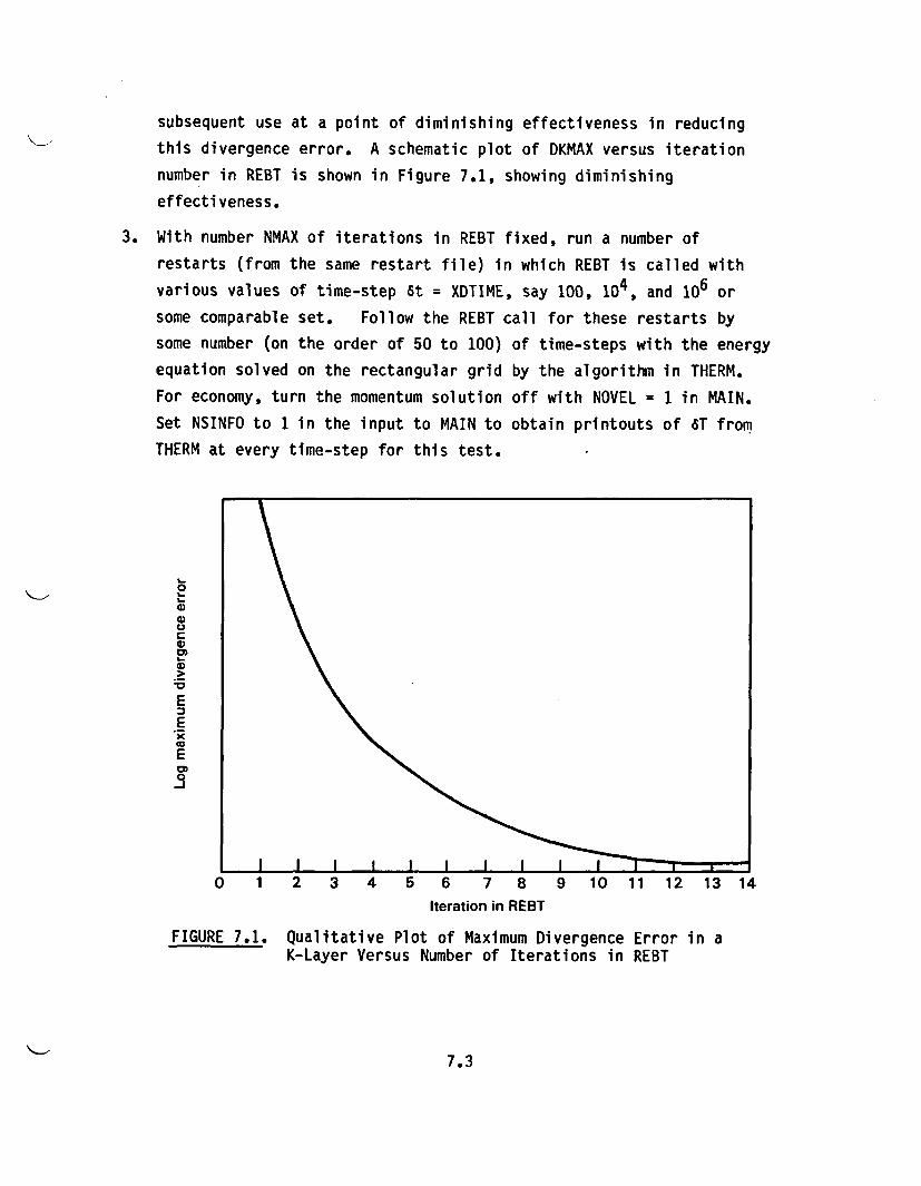
subsequent use at a point of diminishing effectiveness in reducing
this divergence error. A schematic plot of DKMAX versus iteration
number in REBT is shown in Figure 7.1, showing diminishing
effectiveness.
3. With number NMAX of iterations in REBT fixed, run a number of
restarts (from the same restart file) in which REBT is called with
various values of time-step St = XDTIME, say 100, 104, and 106 or
some comparable set. Follow the REBT call for these restarts by
some number (on the order of 50 to 100) of time-steps with the energy
equation solved on the rectangular grid by the algorithm in THERM.
For economy, turn the momentum solution off with NOVEL = 1 in MAIN.
Set NSINFO to 1 in the input to MAIN to obtain printouts of ST from
THERM at every time-step for this test.
0
U
EE
E0,0
-j
0 1 2 3 4 5 6 7
Iteration in
8 9 10 11 12 13 14
REBT
FIGURE 7.1. Qualitative Plot of Maximum Divergence Error in aK-Layer Versus Number of Iterations in REBT
7.3
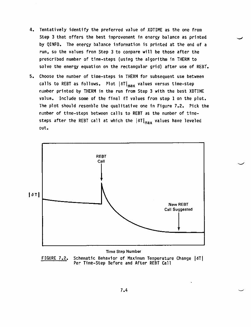
4. Tentatively identify the preferred value of XDTIME as the one from
Step 3 that offers the best improvement in energy balance as printed
by QINFO. The energy balance information is printed at the end of a
run, so the values from Step 3 to compare will be those after the
prescribed number of time-steps (using the algorithm in THERM to
solve the energy equation on the rectangular grid) after use of REBT.
5. Choose the number of time-steps in THERM for subsequent use between
calls to REBT as follows. Plot I6Timax values versus time-step
number printed by THERM in the run from Step 3 with the best XDTIME
value. Include some of the final 6T values from step 1 on the plot.
The plot should resemble the qualitative one in Figure 7.2. Pick the
number of time-steps between calls to REBT as the number of time-
steps after the REBT call at which the ISTImax values have leveled
out.
16TI
FIGURE 7.2.
Time Step Number
Schematic Behavior of Maximum Temperature Change 1ST!Per Time-Step Before and After REBT Call
7.4
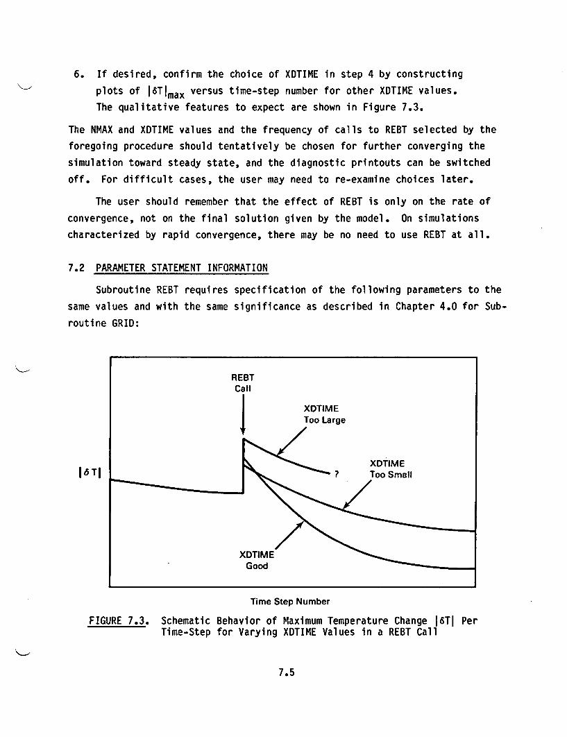
6. If desired, confirm the choice of XDTIME in step 4 by constructing
plots of I6TImax versus time-step number for other XDTIME values.
The qualitative features to expect are shown in Figure 7.3.
The NMAX and XDTIME values and the frequency of calls to REBT selected by the
foregoing procedure should tentatively be chosen for further converging the
simulation toward steady state, and the diagnostic printouts can be switched
off. For difficult cases, the user may need to re-examine choices later.
The user should remember that the effect of REBT is only on the rate of
convergence, not on the final solution given by the model. On simulations
characterized by rapid convergence, there may be no need to use REBT at all.
7.2 PARAMETER STATEMENT INFORMATION
Subroutine REBT requires specification of the following parameters to the
same values and with the same significance as described in Chapter 4.0 for Sub-
routine GRID:
REBTCall
XDTIMEToo Large
6 TXDTIME
XDTIMEGood
Time Step Number
FIGURE 7.3. Schematic Behavior of Maximum Temperature Change 16TI PerTime-Step for Varying XDTIME Values in a REBT Call
7.5
* IP,JP,KP,NEFAP
The following parameters required by REBT were discussed in Chapter 4.0,
Subroutine GRID, and defined in Chapter 6.0, Subroutine THERM:
* KBP,KTP
7.3 INPUT FORMAT
7.3.1 Overview
The input to REBT is minimal, but good choices for the key variables
XDTIME and NMAX should be based on previous experience or on systematic studies
described in Section 7.1. If REBT is to be used, set STEADY = 1.0 in MAIN and
REBON = 1.0 in THERM. The pattern of calls to the REBT procedure is set by
variables NREB and NREBN in THERM.
7.3.2 REBT Options Input Block
General Input Format
NECHOXDTIME,NMAX,INFO
General Input Description
o NECHO - Echoing switch for this section of input. If input is
to be echoed, then NECHO = 1; otherwise, 0.
* XDTIME - The time-step to be used in the solution of the energy
equation on the three slab partitions of the rectangular
grid region.
* NMAX - The number of three-direction sweeps used in solving the
slab representation of the energy equation on the rec-
tangular grid on a call to REBT.
* INFO - Input variable to control the level of printout at each
of the NMAX iterations in a call to REBT.
INFO = 0 No divergence error printout
INFO = 1 Print the maximum sum of divergence
errors encountered for a slab in each of
7.6
the slab orientations and the index of
the slab. Print after all three slab
solutions are done. Labels will be
(DIMAX,ID), (DJMAX,JD) and (DKMAX,KD)
for the three slab orientations.
INFO = 2 Print the maximum sum of divergence
errors for any slab after the tempera-
ture adjustment based on the slab solu-
tion has been made, and the slab
location at which it occurred. Print
immediately after each slab solution is
done.
Input File Example
397 1/rebt398 1.0e+5,12,1
Echoed Input File Example
645646 rebt xdtime=O.1OOe+06 nmax 12 Infohl
In this example, echo of input is requested on line 397 of the input file
with NECHO = 1. A time-step XDTIME = 1.OE+5 is set on input line 398, and
NMAX = 12 slab iterations is requested. Printout at one time of maximum diver-
gence error encountered and its location during the three slab solutions is
requested with INFO = 1. The output echoes these values.
7.7
8.0 SUBROUTINE PROPS
Subroutine PROPS sets heat transfer properties for the simulation in the
cylindrical grid region, much as Subroutine PROP does for the rectangular grid.
8.1 PROPS FUNCTIONS
The effects of heat transfer models used by PROPS are imposed exclusively
through the three thermal resistivity arrays RESX, RESY, and RESZ, and the
three film resistance arrays RESFX, RESFY, and RESFZ. These X-, Y-, and
Z-labeled arrays now apply to the r, 0, and z directions and have meanings for
the cylindrical grid as follows:
* RESX - R-direction resistivity
* RESY - 0-direction resistivity
* RESZ - Z-direction resistivity
* RESFX - R-direction film resistance
* RESFY - 0-direction film resistance
* RESFZ - Z-direction film resistance.
Subroutine PROPS reads input and sets up intermediate parameter sets
related to heat transfer models for the cylindrical grid. It reads mesh loca-
tion information assigning resistance array values on the cylindrical grid
according to these models. The actual assignment of values to resistance
arrays is done during each time-step using the latest temperatures for
temperature-dependent properties.
The heat transfer models available in PROPS include 1) simple isotropic
or orthotropic conduction in substances, 2) conduction through layered com-
posites offering parallel paths, 3) conduction through layered composites
offering series paths, 4) normal conduction through single or series films
between cells, and 5) parallel heat transfer by radiation and by forced or
natural convection from cask ends and sides. The model for conduction through
a film at a cell interface can include a contribution equivalent to radiation
across a gap. For an understanding of the models, see Chapter 5.0. The
changes in the definitions and relationships from those of Chapter 5.0 for the
conversion to cylindrical coordinates need not generally concern the user in
supplying input.
8.1
Consistent interfacing of the cylindrical and rectangular grid regions
requires that the radial resistivity in the first radial phantom cell,
RESX(IS = 1,JS,K), be set to a large number.
The user should also know that any resistivity or film resistance com-
ponent not defined for a mesh location will have the default value of zero.
8.2 PARAMETER STATEMENT INFORMATION
The following dimension-setting parameters have the same significance and
should have the same value as in Subroutine GRID (Chapter 4.0):
IP,JP,KP,ISP,JSP
The following dimension-setting parameters play an analogous role to parameters
of the same name used in PROP for the rectangular grid, but their numerical
values should be set in PROPS according to the need there:
* NMATP - An array-dimensioning parameter greater than or equal to
the number of substance conductivity polynomial coefficient
sets read in PROPS Input Block 3.
* MTP - An array-dimensioning parameter greater than or equal
to the largest value of MT for the intermediate vari-
able sets (in arrays CO, C1, C3, TWF, CFUEL, CCLAD,
etc.) for heat transfer models constructed from direc-
tives in PROPS Input Blocks 4 and 5.
* NSPECP - Dimension of the array SPECS used in PROPS Input
Blocks 4 and 5 to read end-to-end all the intermediate
heat transfer model specifications in each of the
blocks. The SPECS array is overwritten by each of
those input blocks in turn, so it must be long enough
to accommodate the longer of them.
* NREGP,NPAIRP - Two parameters used in setting length of the INDEX
array (to INDEXP = 7*NREGP+2*NPAIRP) containing direc-
tives for assigning resistivity and film resistance
8.2
values to cell locations in the cylindrical grid.
NREGP is the maximum allowed number of region (range)
specifications. NPAIRP is the sum over all regions of
the number of (ID,MT) pairs, where ID is an identifier
of the resistance parameter affected and the model
used, and MT is an identifier of the intermediate heat
transfer variable to use for that model. Each region
directive set may request implementation of one or
several changes in the resistance arrays by including
one or several (ID,MT) pairs.
8.3 INPUT FORMAT
8.3.1 Overview
The input to Subroutine PROPS separates into six blocks:
1. thermal resistance print specifications for the cylindrical grid
2. convection specifications for cask side and for cylindrical grid
parts of top and bottom
3. materials conductivity polynomial coefficient sets
4. parallel, isotropic, and orthotropic conduction models
5. series conduction models
6. assignment of resistance to cell locations.
The material conductivity polynomial coefficients read in Input Block 3 are
overwritten after their use in setting up intermediate parameter sets in Input
Blocks 4 and 5. The intermediate parameter sets constructed in response to
Input Blocks 4 and 5 are retained as local variables for use in assigning
resistances to cell locations at each time-step with most recent temperatures,
as directed in PROPS Input Block 6.
8.3
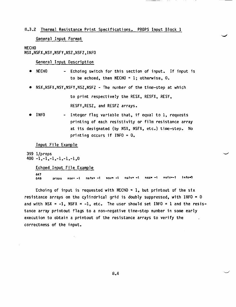
8.3.2 Thermal Resistance Print Specifications. PROPS Input Block 1
General Input Format
NECHONSX,NSFX,NSY,NSFY,NSZ,NSFZ,INFO
General Input Description
* NECHO - Echoing switch for this section of input. If input is
to be echoed, then NECHO = 1; otherwise, 0.
* NSX,NSFX,NSY,NSFY,NSZ,NSFZ - The number of the time-step at which
to print respectively the RESX, RESFX, RESY,
RESFY,RESZ, and RESFZ arrays.
* INFO - Integer flag variable that, if equal to 1, requests
printing of each resistivity or film resistance array
at its designated (by NSX, NSFX, etc.) time-step. No
printing occurs if INFO = 0.
Input File Example
399 I/props400 -1,-1,-1,-1,-1,-1,0
Echoed Input File Example
647648 props nsx- -1 nsftx -i nsv -1 nsfv- -1 nsz- -1 nsfz--l InfoaI
Echoing of input is requested with NECHO = 1, but printout of the six
resistance arrays on the cylindrical grid is doubly suppressed, with INFO = 0
and with NSX = -1, NSFX = -1, etc. The user should set INFO = 1 and the resis-
tance array printout flags to a non-negative time-step number in some early
execution to obtain a printout of the resistance arrays to verify the
correctness of the input.
8.4
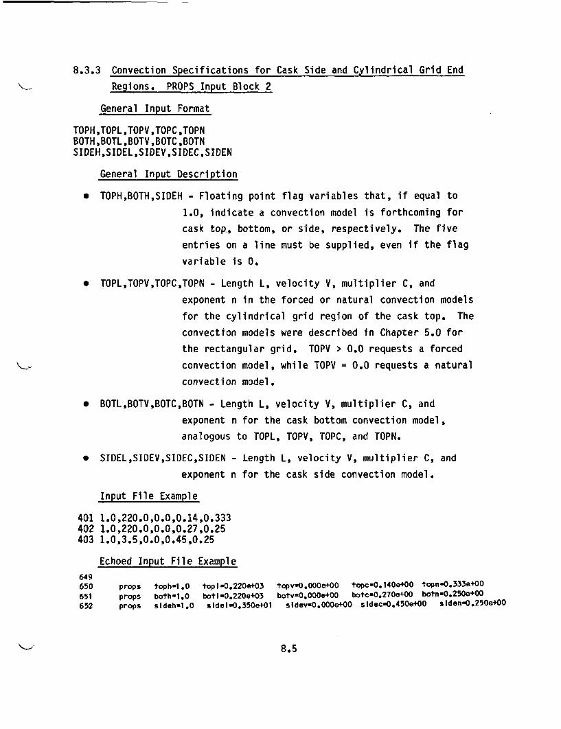
8.3.3 Convection Specifications for Cask Side and Cylindrical Grid End
Regions. PROPS Input Block 2
General Input Format
TOPH,TOPL,TOPV,TOPC,TOPNBOTH,BOTL,BOTV,BOTC,BOTNSIDEH,SIDEL,SIDEV,SIDEC,SIDEN
General Input Description
* TOPH,BOTH,SIDEH - Floating point flag variables that, if equal to
1.0, indicate a convection model is forthcoming for
cask top, bottom, or side, respectively. The five
entries on a line must be supplied, even if the flag
variable is 0.
* TOPL,TOPV,TOPC,TOPN - Length L, velocity V, multiplier C, and
exponent n in the forced or natural convection models
for the cylindrical grid region of the cask top. The
convection models were described in Chapter 5.0 for
the rectangular grid. TOPV > 0.0 requests a forced
convection model, while TOPV = 0.0 requests a natural
convection model.
* BOTL,BOTV,BOTC,BOTN - Length L, velocity V, multiplier C, and
exponent n for the cask bottom convection model,
analogous to TOPL, TOPV, TOPC, and TOPN.
* SIDEL,SIDEV,SIDEC,SIDEN - Length L, velocity VY multiplier C, and
exponent n for the cask side convection model.
Input File Example
401 1.0,220.0,0.0,0.14,0.333402 1.0,220.0,0.0,0.27,0.25403 1.0,3.5,0.0,0.45,0.25
Echoed Input File Example
649650 props tophl .0 topl-0.220e+03 topvO.OOOe+OO topc=O.140e+00 topnuO.333e+00651 props both=1.O botl0.220e+03 botviO.OOOe+OO botcuO.270e+00 botn-0.250e+00652 props sideh=1.0 sIdeI=0.350e+O1 sidev=O.OOOe+OO sIdec=0.450e+00 sIdenzO.250e+00
8.5
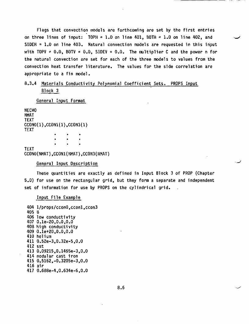
Flags that convection models are forthcoming are set by the first entries
on three lines of input: TOPH = 1.0 on line 401, BOTH = 1.0 on line 402, and
SIDEH = 1.0 on line 403. Natural convection models are requested in this input
with TOPY = 0.0, BOTY = 0.0, SIDEV = 0.0. The multiplier C and the power n for
the natural convection are set for each of the three models to values from the
convection heat transfer literature. The values for the side correlation are
appropriate to a fin model.
8.3.4 Materials Conductivity Polynomial Coefficient Sets. PROPS Input
Block 3
General Input Format
NECHONMATTEXTCCONO(1),CCON1(1),CCON3(1)TEXT
TEXTCCONO(NMAT),CCON1(NMAT),CCON3(NMAT)
General Input Description
These quantities are exactly as defined in Input Block 3 of PROP (Chapter
5.0) for use on the rectangular grid, but they form a separate and independent
set of information for use by PROPS on the cylindrical grid.
Input File Example
404 1/props/cconO,cconl,ccon3405 8406 low conductivity407 O.le-20,0.0,0.0408 high conductivity409 O.le+20,0.0,0.0410 helium411 0.52e-3,0.32e-5,0.0412 sst413 0.09215,0.1465e-3,0.0414 nodular cast iron415 0.5162,-0.3205e-3,0.0416 air417 0.688e-4,0.634e-6,0.0
8.6
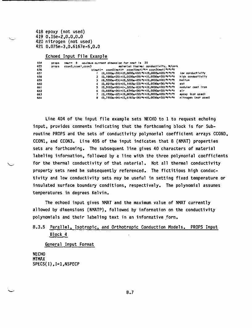
418 epoxy (not used)419 0.15e-2,0.0,0.0420 nitrogen (not used)421 0.075e-3,0.6167e-6,0.0
Echoed Input File Example654 props nmat- 8 maximum current dimension for nmat Is 20655 props ccon0,cconIccon3 material thermal conductivity, W/cm-k656 k(met)- cconO(mat)+ cconltmat)t+ ccon3(met)*ttt657 1 CO.lOOOe-20)4(0.0000e+00) t+(0.0000e+00) 't'tt low conductivity658 2 (0.1000e+20)+(0.0000e+00)*t+(0.0000e+00)*t~t't high conductivity659 3 (O.5200O-03)+(O.3200e-O5)0t+(0.OOOeeOO)*t~tt hellum660 4 (0.9215e-01)+(0.1
465e-03) t+(0.0000e+00)*t't't sst
661 5 (0.5l62e9+0)+(-.3205e-O3)*t+(0.0OOOe+OO)*tt't nodular cast Iron662 6 (0.6880e-04)+(0.6340e-06)*t+(0.0000e+00)*tstt air663 7 (0.1500e-02)+(0.0000e+00)*t+(0.0000e+O0)*t*tit epoxy (not used)664 8 (0.750De-04)+(0.6167e-06)'t+(0.0000e+00)*t'tt nitrogen (not used)
Line 404 of the input file example sets NECHO to 1 to request echoing
input, provides comments indicating that the forthcoming block is for Sub-
routine PROPS and the sets of conductivity polynomial coefficient arrays CCONO,
CCON1, and CCON3. Line 405 of the input indicates that 8 (NMAT) properties
sets are forthcoming. The subsequent line gives 40 characters of material
labeling information, followed by a line with the three polynomial coefficients
for the thermal conductivity of that material. Not all thermal conductivity
property sets need be subsequently referenced. The fictitious high conduc-
tivity and low conductivity sets may be useful in setting fixed temperature or
insulated surface boundary conditions, respectively. The polynomial assumes
temperatures in degrees Kelvin.
The echoed input gives NMAT and the maximum value of NMAT currently
allowed by dimensions (NMATP), followed by information on the conductivity
polynomials and their labeling text in an informative form.
8.3.5 Parallel, Isotropic, and Orthotropic Conduction Models. PROPS Input
Block 4
General Input Format
NECHOMTMAXSPECS(I),1=1,NSPECP
8.7
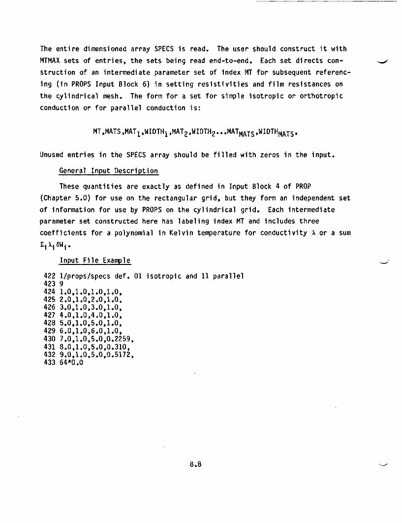
The entire dimensioned array SPECS is read. The user should construct it with
MTMAX sets of entries, the sets being read end-to-end. Each set directs con-
struction of an intermediate parameter set of index MT for subsequent referenc-
ing (in PROPS Input Block 6) in setting resistivities and film resistances on
the cylindrical mesh. The form for a set for simple isotropic or orthotropic
conduction or for parallel conduction is:
MTMATSMATjWIDTH1MAT2,WIDTH2..MATMATSWIDTHMATS,
Unused entries in the SPECS array should be filled with zeros in the input.
General Input Description
These quantities are exactly as defined in Input Block 4 of PROP
(Chapter 5.0) for use on the rectangular grid, but they form an independent set
of information for use by PROPS on the cylindrical grid. Each intermediate
parameter set constructed here has labeling index MT and includes three
coefficients for a polynomial in Kelvin temperature for conductivity X or a sum
i XisW1.
Input File Example
422 1/props/specs def. 01 isotropic and 11 parallel423 9424 1.0,1.0,1.0,1.0,425 2.0,1.0,2.0,1.0,426 3.0,1.0,3.0,1.0,427 4.0,1.0,4.0,1.0,428 5.0,1.0,5.0,1.0,429 6.0,1.0,6.0,1.0,430 7.0,1.0,5.0,0.2259,431 8.0,1.0,5.0,0.310,432 9.0,1.0,5.0,0.5172,433 64*0.0
8.8
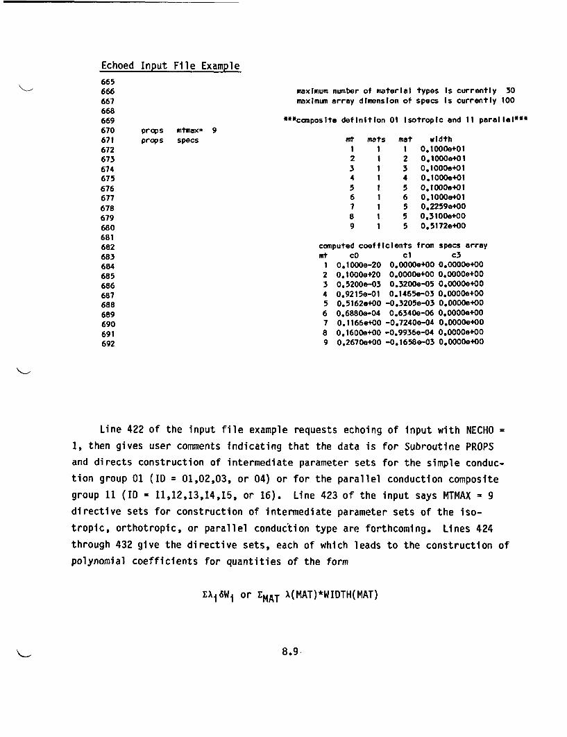
Echoed Input File Example665666 maximum number of material types Is currently 30667 maximum array dimension of specs Is currently 100668669 ***composite definition 01 Isotropic and 11 parallel***670 props ntmaxn 9671 props specs Mt mats mat width672 1 1 1 0.1000.+01673 2 1 2 0.1000e+01674 3 1 3 0.lOOOe+01675 4 1 4 0.1000e+01676 5 1 5 0.OOOe+01677 6 1 6 0.1000e+01
678 7 1 5 0,2259e+00679 8 1 5 0.3100e+00680 9 1 5 0.5172e+00681682 computed coefficients from specs array683 Mt cO cl c3684 1 0.lOOOe-20 0.0000e+00 0.0000.+00685 2 0.1000e+20 0.0000e+00 0.OOOOe+00686 3 0.5200e-03 0.3200e-05 0.0000e+00687 4 0.9215e-01 0.1465e-05 0.0000e+00688 5 0.5162.+00 -0.3205e-03 0.0000e+00689 6 0.6880e-04 0.6340e-06 0.0000e+00690 7 0.1166e400 -0.7240e-04 0.0000e400691 8 0.1600.+00 -0.9936e-04 0.0000e+00692 9 0.2670e+00 -0.1658e-03 0.0000e+00
Line 422 of the input file example requests echoing of input with NECHO =
1, then gives user comments indicating that the data is for Subroutine PROPSand directs construction of intermediate parameter sets for the simple conduc-
tion group 01 (ID = 01,02,03, or 04) or for the parallel conduction composite
group 11 (ID = 11,12,13,14,15, or 16). Line 423 of the input says MTMAX = 9
directive sets for construction of intermediate parameter sets of the iso-
tropic, orthotropic, or parallel conduction type are forthcoming. Lines 424
through 432 give the directive sets, each of which leads to the construction of
polynomial coefficients for quantities of the form
Ek Wj ior EMAT X(MAT)*WIDTH(MAT)
8.9
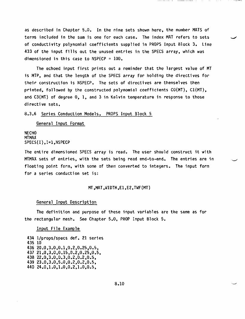
as described in Chapter 5.0. In the nine sets shown here, the number MATS of
terms included in the sum is one for each case. The index MAT refers to sets
of conductivity polynomial coefficients supplied in PROPS Input Block 3. Line
433 of the input fills out the unused entries in the SPECS array, which was
dimensioned in this case to NSPECP = 100.
The echoed input first prints out a reminder that the largest value of MT
is MTP, and that the length of the SPECS array for holding the directives for
their construction is NSPECP. The sets of directives are themselves then
printed, followed by the constructed polynomial coefficients CO(MT), C1(MT),
and C3(MT) of degree 0, 1, and 3 in Kelvin temperature in response to those
directive sets.
8.3.6 Series Conduction Models. PROPS Input Block 5
General Input Format
NECHOMTMAXSPECS(I),1=1,NSPECP
The entire dimensioned SPECS array is read. The user should construct it with
MTMAX sets of entries, with the sets being read end-to-end. The entries are in
floating point form, with some of them converted to integers. The input form
for a series conduction set is:
MT,MAT,WIDTH,E1,E2,TWF(MT)
General Input Description
The definition and purpose of these input variables are the same as for
the rectangular mesh. See Chapter 5.0, PROP Input Block 5.
Input File Example
434 1/props/specs def. 21 series435 10436 20.0,3.0,0.1,0.2,0.25,0.5,437 21.0,3.0,0.15,0.2,0.25,0.5,438 22.0,3.0,0.3,0.2,0.2,0.5,439 23.0,3.0,5.0,0.2,0.2,0.5,440 24.0,1.0,1.0,0.2,1.0,0.5,
8.10
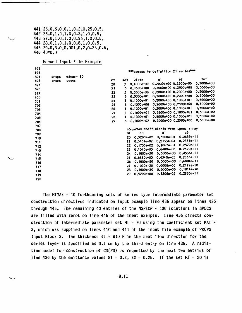
441442443444445446
25.0,6.0,0.1,0.2,0.25,0.5,26.0,1.0,1.0,0.3,1.0,0.5,27.0,1.0,1.0,0.96,1.0,0.5,28.0,1.0,1.0,0.8,1.0,0.5,29.0,3.0,0.001,0.2,0.25,0.5,40*0.0
Echoed Input File Example
693694695696697698699700701702703704705706707708709710711712713714715716717718719720
*"*composite definitIon 21 serIes***props mtmax= 10props specs Mt mat
20 321 322 323 324 125 626 127 128 129 3
width0.1000.+00
0.1500.+000.3000G+000.5000e+010.I000e+010. 1000e+000.1000.+01
0.1000l+010.1000.+010. I OOOe-02
el e20.2000.+00 0.25008+000.2000e+00 0.2500e+000.2000e+00 0.2000e+000.2000e+00 0.2000e4000.2000e+00 0.1000e+010.2000e+00 0.2500e+000.3000.+00 0.1000e4010.9600e+00 0.1000.+010.8000e+00 0.1000e+010.2000e.00 0.2500e400
twf0.5000e+000.5000.+000.5000e+000.5000.+000.5000.+000.50006+000.5000.+000.5000e+000.5000e+000.50000+00
canputed coefficients from specs arrayMt cO
20 0.5200e-0221 0.3467e-0222 0.1733e-0223 0.1040e-0324 0.10OOe-2025 0.6880e-0326 0.1000-e2027 0.100Oe-2028 0.1000-e2029 0.5200e+00
cl0.3200-e040.2133e3040.1067e.040.6400e-060.0000e+000.6340e-050.0000.+000.0000e+000.0000e+000.3200-e02
c30.2835e- 1I0.2835.-i 10.2520e-i 10.2520-i110.4536e- 1I0.2835e- 1I0.6804e- 1I0.2177e-100.1814.-100.2835e-I I
The MTMAX = 10 forthcoming sets of series type intermediate parameter set
construction directives indicated on input example line 435 appear on lines 436
through 445. The remaining 40 entries of the NSPECP = 100 locations in SPECS
are filled with zeros on line 446 of the input example. Line 436 directs con-
struction of intermediate parameter set MT = 20 using the coefficient set MAT =
3, which was supplied on lines 410 and 411 of the input file example of PROPS
Input Block 3. The thickness 6L = WIDTH in the heat flow direction for the
series layer is specified as 0.1 cm by the third entry on line 436. A radia-
tion model for construction of C3(20) is requested by the next two entries of
line 436 by the emittance values El = 0.2, E2 = 0.25. If the set MT = 20 is
8.11
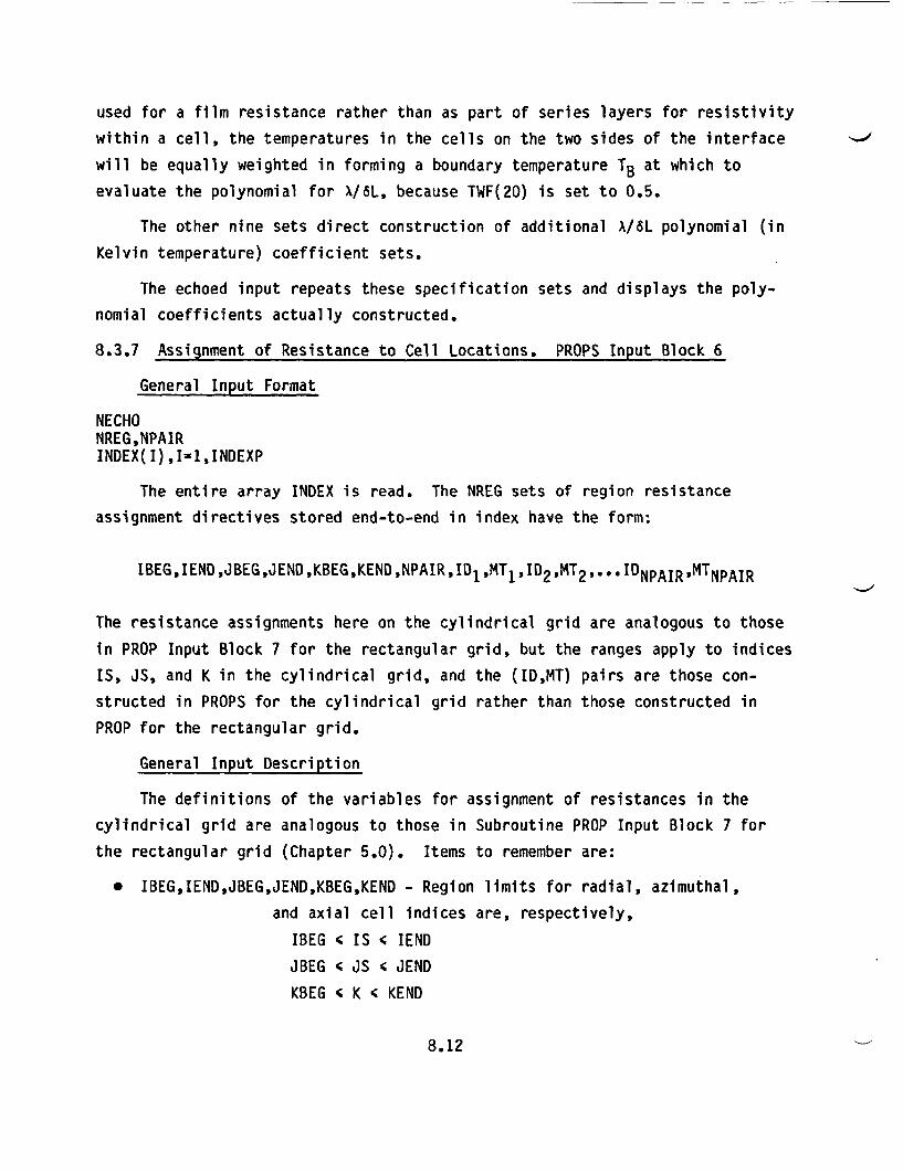
used for a film resistance rather than as part of series layers for resistivity
within a cell, the temperatures in the cells on the two sides of the interface
will be equally weighted in forming a boundary temperature TB at which to
evaluate the polynomial for X/6L, because TWF(20) is set to 0.5.
The other nine sets direct construction of additional A/8L polynomial (in
Kelvin temperature) coefficient sets.
The echoed input repeats these specification sets and displays the poly-
nomial coefficients actually constructed.
8.3.7 Assignment of Resistance to Cell Locations. PROPS Input Block 6
General Input Format
NECHONREG,NPAIRINDEX(I),I=1,INDEXP
The entire array INDEX is read. The NREG sets of region resistance
assignment directives stored end-to-end in index have the form:
IBEG,IEND,JBEG,JEND,KBEG,KEND,NPAIR,ID1,MTID2,MT2,...IDNPAIR,MTNPAIR
The resistance assignments here on the cylindrical grid are analogous to those
in PROP Input Block 7 for the rectangular grid, but the ranges apply to indices
IS, JS, and K in the cylindrical grid, and the (ID,MT) pairs are those con-
structed in PROPS for the cylindrical grid rather than those constructed in
PROP for the rectangular grid.
General Input Description
The definitions of the variables for assignment of resistances in the
cylindrical grid are analogous to those in Subroutine PROP Input Block 7 for
the rectangular grid (Chapter 5.0). Items to remember are:
* IBEG,IEND,JBEG,JEND,KBEG,KEND - Region limits for radial, azimuthal,
and axial cell indices are, respectively,
IBEG 4 IS 4 IEND
JBEG ' JS 4 JEND
KBEG 4 K 4 KEND
8.12
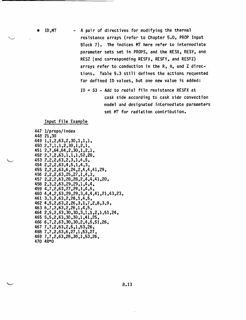
* ID,MT - A pair of directives for modifying the thermal
resistance arrays (refer to Chapter 5.0, PROP Input
Block 7). The indices MT here refer to intermediate
parameter sets set in PROPS, and the RESX, RESY, and
RESZ (and corresponding RESFX, RESFY, and RESFZ)
arrays refer to conduction in the R, 6, and Z direc-
tions. Table 5.3 still defines the actions requested
for defined ID values, but one new value is added:
ID = 53 - Add to radial film resistance RESFX at
cask side according to cask side convection
model and designated intermediate parameters
set MT for radiation contribution.
Input File Example
447 1/props/index448 21,30449 1,1,2,63,2,30,1,1,1,450 2,7,1,1,2,30,1,2,1,451 2,7,64,64,2,30,1,2,1,452 2,7,2,63,1,1,1,52,28,453 2,2,2,63,2,3,1,4,5,454 2,2,2,63,4,5,1,4,3,455 2,2,2,63,6,24,2,4,4,41,29,456 2,2,2,63,25,27,1,4,3,457 2,2,2,63,28,28,2,4,4,41,20,458 2,3,2,63,29,29,1,4,4,459 4,7,2,63,27,29,1,4,5,460 4,4,2,63,29,29,3,4,4,41,21,43,23,461 3,3,2,63,2,28,1,4,5,462 4,5,2,63,2,26,3,1,7,2,8,3,9,463 6,7,2,63,2,26,1,4,5,464 2,5,2,63,30,30,3,1,1,2,1,51,24,465 5,5,2,63,30,30,1,41,25,466 6,7,2,63,30,30,2,4,5,51,26,467 7,7,2,63,2,5,1,53,26,468 7,7,2,63,6,27,1,53,27,469 7,7,2,63,28,30,1,53,26,470 48*0
8.13
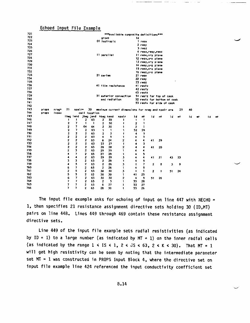
721722723724725726727728729730731732733734735736737738739740741742743744745746747748749750751752753754755756757758759760761762763764765766
Echoed Input File Example.*%avallable composite definitlons***
group Id01 Isotropic I reosx
2 rosy3 resz4 resx,resy,resz
11 parallel 11 resx,x-y plans12 resx,x-z plane13 resy,x-y plans14 resy,y-z plane15 resz,x-z plane16 resz,y-z plane
21 series 21 resx22 rosy23 resz
41 film resIstance 41 resfx42 resfy43 resfz
51 exterior convection 51 resfz for top of caskand radiation 52 resfz for bottom of cask
53 resfx for side of cask
npalr- 30 maxlmum current dimensions for nreg and npalr are
cell locatIonprops nraegprops Index
21 25 40
Ibeg
2
22222222
44346256777
leand
77722222374357557777
jbeg Jend2 631 I
64 642 632 632 632 632 632 632 632 632 632 632 632 632 632 632 632 632 632 63
kbeg kend2 302 302 30l l2 34 56 24
25 2728 2829 2927 2929 292 282 262 26
30 3030 3030 302 56 27
28 30
npal r
2
2
I
3
3
2
Id
2252444444444
4
41
4535353
Mt Id Mt Id Mt Id mt Id Mt
I
2853434454575
2525
262726
41 29
41 20
41 21
2 8
2 1
51 26
43 23
3 9
51 24
The input file example asks for echoing of input on line 447 with NECHO =
1, then specifies 21 resistance assignment directive sets holding 30 (ID,MT)
pairs on line 448. Lines 449 through 469 contain these resistance assignment
directive sets.
Line 449 of the input file example sets radial resistivities (as indicated
by ID = 1) to a large number (as indicated by MT = 1) on the inner radial cells
(as indicated by the range 1 ' IS ' 1, 2 4 JS 4 63, 2 4 K 4 30). That MT = 1
will get high resistivity can be seen by noting that the intermediate parameter
set MT = 1 was constructed in PROPS Input Block 4, where the directive set on
input file example line 424 referenced the input conductivity coefficient set
8.14
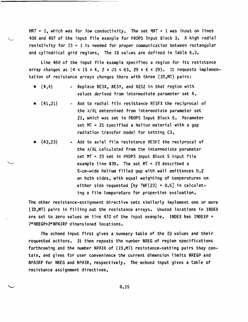
MAT = 1, which was for low conductivity. The set MAT = 1 was input on lines
406 and 407 of the input file example for PROPS Input Block 3. A high radial
resistivity for IS = 1 is needed for proper communication between rectangular
and cylindrical grid regions. The ID values are defined in Table 5.3.
Line 460 of the input file example specifies a region for its resistance
array changes as (4 < IS < 4, 2 < JS < 63, 29 < K 4 29). It requests implemen-
tation of resistance arrays changes there with three (ID,MT) pairs:
* (4,4) - Replace RESX, RESY, and RESZ in that region with
values derived from intermediate parameter set 4.
* (41,21)
* (43,23)
Add to radial film resistance RESFX the reciprocal of
the X/6L determined from intermediate parameter set
21, which was set in PROPS Input Block 5. Parameter
set MT = 21 specified a helium material with a gap
radiation transfer model for setting C3.
- Add to axial film resistance RESFZ the reciprocal of
the X/6L calculated from the intermediate parameter
set MT = 23 set in PROPS Input Block 5 input file
example line 439. The set MT = 23 described a
5-cm-wide helium filled gap with wall emittances 0.2
on both sides, with equal weighting of temperatures on
either side requested [by TWF(23) = 0.5] in calculat-
ing a film temperature for properties evaluation.
The other resistance-assignment directive sets similarly implement one or more
(ID,MT) pairs in filling out the resistance arrays. Unused locations in INDEX
are set to zero values on line 470 of the input example. INDEX has INDEXP =
7*NREGP+2*NPAIRP dimensioned locations.
The echoed input first gives a summary table of the ID values and their
requested actions. It then repeats the number NREG of region specifications
forthcoming and the number NPAIR of (ID,MT) resistance-setting pairs they con-
tain, and gives for user convenience the current dimension limits NREGP and
NPAIRP for NREG and NPAIR, respectively. The echoed input gives a table of
resistance assignment directives.
8.15
9.0 SUBROUTINE TSIDE
Subroutine TSIDE is used to solve the energy equation on the cylindrical
grid region.
9.1 TSIDE FUNCTIONS
TSIDE reads input specifying initial temperatures, boundary temperatures,
numerical procedure options, and printout options during initiation or restart
of a simulation. If solution of the energy equation in the cylindrical grid
region is requested, TSIDE is called at each time-step to advance the
temperature solution.
The actions by TSIDE in the solution sequence include:
1. TSIDE sets the connector arrays for the energy equation on the
cylindrical grid. These are the coefficients that relate heat flows
to temperatures and heat sources.
2. TSIDE executes an algorithm that advances the temperature on the
cylindrical grid through a time-step.
3. If requested, TSIDE prints monitoring information, including the
location and magnitude of the greatest temperature change on the
cylindrical grid for the current time-step, and also the temperatures
in cells specified by the user for monitoring.
4. TSIDE makes a tentative adjustment in the time-step by comparing the
maximum temperature change and a user-specified target maximum
temperature change.
The algorithm used in TSIDE for advancing the temperature on the cylindri-
cal grid through a time-step is discussed in Volume I - Equations and Numerics
(McCann 1987). The imposition of continuity conditions between the rectangular
and cylindrical grid regions, achieved with subroutine TBND supplementing TSIDE
and THERM, is discussed in Chapter 2.0, Code Overview.
9.1
TSIDE is called at setup or restart to read input to guide the solution
and to set or reset temperatures. Actions by TSIDE during setup or restart
include:
1. reading certain numerical procedure options, printout options, and
temperature monitoring options
2. reading and implementing options for setting or altering the initial
temperature distribution and ambient temperature.
9.2 PARAMETER STATEMENT INFORMATION
Subroutine TSIDE requires specification of the following parameters, which
were discussed in Chapter 4.0, Subroutine GRID:
IP,JP,KP,ISP,JSP,NEFAP,KBP,KTP
Subroutine TSIDE also requires specification of the parameter
* MONTSP - Number of cells in the cylindrical grid that can be
specified by the user for monitoring the temperature
during time-stepping.
9.3 INPUT FORMAT
9.3.1 Overview
The input read by TSIDE will be described in Section 9.3.2. Other input
available to TSIDE includes the initial temperature for the cylindrical grid
that was read in THERM.
9.3.2 TSIDE Input Block
General Input Format
NECHONEWTS,TSAMB,DTEMAXNECHOMONTSIMONTS(M),JMONTS(M),KMONTS(M) Repeated for M=1 to MONTS+1, with
{IMONT(MONTS+1)=O
9.2
NECHONDELTADELTA(K),K=2,KP-1
General Input Description
* NECHO
* NEWTS
* TSAMB
- Echoing switch for this section of input. If input is
to be echoed, then NECHO = 1; otherwise, 0.
- An integer flag for initializing or resetting side
(cask body or cylindrical grid) temperatures. If
NEWTS = 1, cylindrical grid temperatures TS are set to
the initial interface temperatures read in THERM. If
NEWTS = 0, cylindrical grid temperatures are not
reset.
- The cask-side ambient temperature. If resetting side
ambient temperature is requested by NEWTA = 1 (set in
MAIN) or NEWTS = 1, the cask-side ambient temperatures
are set as:
TS(IS,JS,K) = TSAMB
for the cells defined by the ranges
24JSQ3SP-1
ISEND(K)+1<IS<ISP
2<KKP-1
This is the region radially beyond the active
computational cells.
* DTEMAX
* MONTS
The target maximum temperature change per time-step
for the cylindrical grid. A tentative new time-step
DTIMES is set as:
DTIMES = 1.1*DTIME if DTMAX < DTEMAX
DTIMES = DTIME*DTEMAX/DTMAX if DTMAX>DTEMAX
DTIME is the current time-step, and DTMAX is the
magnitude of the largest temperature change in the
cylindrical grid in the current time-step.
The number of cells in the cylindrical grid region for
which temperature monitoring is requested.
9.3
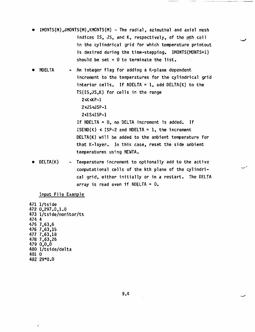
* IMONTS(M),JMONTS(M),KMONTS(M) - The radial, azimuthal and axial mesh
indices IS, JS, and K, respectively, of the mth cell
in the cylindrical grid for which temperature printout
is desired during the time-stepping. IMONTS(MONTS+1)
should be set = 0 to terminate the list.
* NDELTA
* DELTA(K)
- An integer flag for adding a K-plane dependent
increment to the temperatures for the cylindrical grid
interior cells. If NDELTA = 1, add DELTA(K) to the
TS(ISJS,K) for cells in the range
2<K<KP-1
24JS<JSP-1
2cIS4ISP-1
If NDELTA = 0, no DELTA increment is added. If
ISEND(K) ' ISP-2 and NDELTA = 1, the increment
DELTA(K) will be added to the ambient temperature for
that K-layer. In this case, reset the side ambient
temperatures using NEWTA.
- Temperature increment to optionally add to the active
computational cells of the kth plane of the cylindri-
cal grid, either initially or in a restart. The DELTA
array is read even if NDELTA = 0.
Input File Example
471 1/tsidi472 0,297.(473 1/tsidi474 4475 7,63,6476 7,63,1!477 7,63,11478 7,63,21479 0,0,0480 1/tsidi481 0482 29*0.0
0,1/.0le/monitor/ts
53'6
ae/delta
9.4
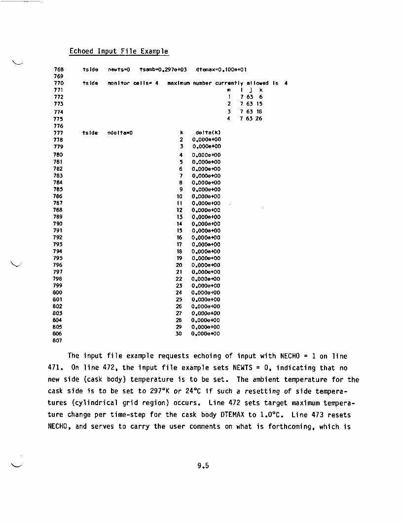
Echoed Input File Example
768769770771772773774775776777778779780781782783784785786787788789790791792793794795796797798799800801802803804805806807
tside newts=o tsamb=0.297e+03 dtemax=0.1OOe+0I
tside monitor cells= 4
tside ndelta=O
maximum number currently allowed Is 4m I J k1 763 62 763 153 763 184 763 26
k delta(k)2 0.000e+003 0.OOOe+004 0.OOOe+005 0.OOOe+006 0.OOOe+007 0.000e+008 0.0000e+09 0.OOOe+00
10 0.0000e+011 0.OOOe+0012 0.0000e+013 0.OOOe+0014 0.000.e+015 0.000e+0016 0.000.e+017 0.OOOe+0018 0.0000e+019 0.OOOe+0020 0.0000e+021 0.000e+0022 0.000e+0023 0 .000e+0024 0.000e+0025 0.OOOe+0026 0.0000e+027 0.000e+O028 0.0000e+029 0.OOOe+0030 0.000e+00
The input file example requests echoing of input with NECHO = 1 on line
471. On line 472, the input file example sets NEWTS = 0, indicating that no
new side (cask body) temperature is to be set. The ambient temperature for the
cask side is to be set to 297 0K or 24'C if such a resetting of side tempera-
tures (cylindrical grid region) occurs. Line 472 sets target maximum tempera-
ture change per time-step for the cask body DTEMAX to 1.0%. Line 473 resets
NECHO, and serves to carry the user comments on what is forthcoming, which is
9.5
the list of cells to be monitored for the cask body. Line 474 specifies that
monitoring of four temperatures is requested, and they are listed by their
indices in lines 475 through 478. Line 479 terminates this list of monitored
cells with its leading zero. Line 480 resets NECHO. Lines 481 and 482 set
NDELTA to 0, then set the 29 entries (for K = 2 through 30 in a simulation with
KP = 31) for DELTA(K) to zero, doubly indicating that no manual increment of
the temperatures in the active computational cells of the cylindrical grid
region is desired.
The output example echoes this input and also provides a reminder on line
770 of the number of monitor cells in the cylindrical grid region currently
allowed by dimensioning.
9.6
10.0 SUBROUTINE TBND
Subroutine TBND provides the means to couple the solution of the energy
equation within the interior of a cask to that of the exterior side of the cask
body. A Cartesian coordinate system is used for the interior of a cask and a
cylindrical coordinate system is used for the side portion of the cask body. A
cross section of a cask and the corresponding computational mesh is illustrated
in Figure 4.1. Although the temperatures are determined implicitly within each
region, the coupling between the two regions is explicit. This explicit
coupling is done within subroutine TBND in such a way that temperature is
continuous across the boundary and energy is conserved.
New-time temperatures are determined in the interior region using old-time
boundary temperatures. Heat fluxes from the interior to the boundary are then
determined. These heat fluxes are used as a boundary condition to calculate
new-time exterior side temperatures. Finally, the temperatures on the boundary
between the interior and exterior regions are updated to satisfy conservation
of energy across the boundary. If there is no body to the cask, then neither
subroutine TSIDE nor subroutine TBND is called.
10.1 PARAMETER STATEMENT INFORMATION
Subroutine TBND requires the specification of parameter IP, JP, KP, ISP,
JSP, NEFAP, KBP, and KTP. These parameters define the overall computational
mesh and are described in Chapter 4.0, Subroutine GRID. No additional
parameters are needed for Subroutine TBND.
10.2 INPUT FORMAT
The operation of subroutine TBND is automatic, and input file specifica-
tions are not required.
10.1
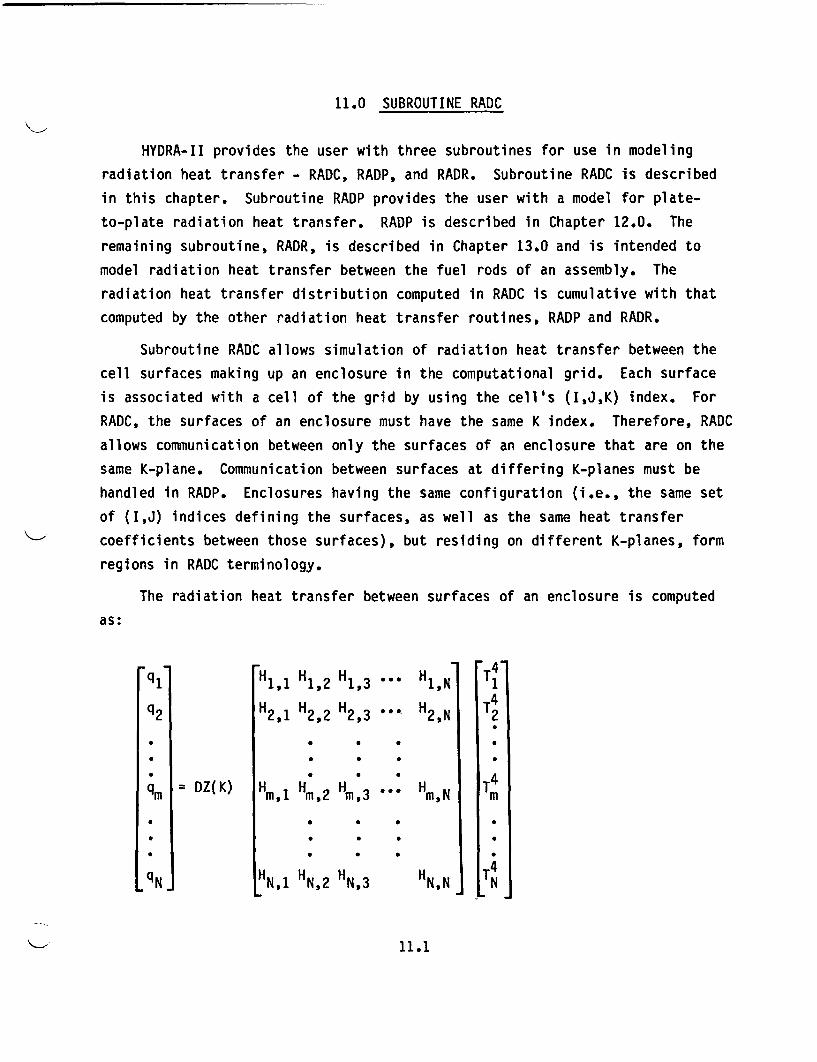
11.0 SUBROUTINE RADC
HYDRA-II provides the user with three subroutines for use in modeling
radiation heat transfer - RADC, RADP, and RADR. Subroutine RADC is described
in this chapter. Subroutine RADP provides the user with a model for plate-
to-plate radiation heat transfer. RADP is described in Chapter 12.0. The
remaining subroutine, RADR, is described in Chapter 13.0 and is intended to
model radiation heat transfer between the fuel rods of an assembly. The
radiation heat transfer distribution computed in RADC is cumulative with that
computed by the other radiation heat transfer routines, RADP and RADR.
Subroutine RADC allows simulation of radiation heat transfer between the
cell surfaces making up an enclosure in the computational grid. Each surface
is associated with a cell of the grid by using the cell's (I,J,K) index. For
RADC, the surfaces of an enclosure must have the same K index. Therefore, RADC
allows communication between only the surfaces of an enclosure that are on the
same K-plane. Communication between surfaces at differing K-planes must be
handled in RADP. Enclosures having the same configuration (i.e., the same set
of (I,J) indices defining the surfaces, as well as the same heat transfer
coefficients between those surfaces), but residing on different K-planes, form
regions in RADC terminology.
The radiation heat transfer between surfaces of an enclosure is computed
as:
H1 1 H1,2 H1,3 *-- H1,N T1H H HT 4
q2 H2,1 H2 2 2,3 H2,N 2
qm DZ(K) Hm 1 HM,2 Hm13 - , TEW
q Z H H H H T4
N ,1 N,2 N,3 N,N N
11.1
The radiation heat transfer received by the mth surface of the enclosure is
represented by qm. Each surface of the enclosure is assigned an index. These
indices range sequentially from 1 to N. The correlation between these indices
and the corresponding (I,J,K) indices of the computational cell is made in the
input to RADC. The format for providing this information is discussed in
Sections 11.2.3, 11.2.4, and 11.2.5.
DZ(K) represents the local DZ length segment which is common to all
surfaces of this enclosure. It makes up half of the information necessary to
compute the effective area of each of the surfaces. The other length segment
is embedded in the radiation heat transfer coefficient, H.
The radiation heat transfer coefficients, Hmn, are generated by the user
and provided as input to RADC as discussed in Section 11.2.6. The constituent
H's must include the effect of surface emissivity, shape factor, and Stefan-
Boltzmann constant (a = 5.67e-12 W/cm2 .K4), in addition to carrying the other
length segment representing the surface area. Since each enclosure of a RADC
region has the same set of radiation heat transfer coefficients, there must be
as many H matrices as there are regions in the RADC model. Each H matrix must
be symmetric to ensure conservation of energy (i.e., Hm n = Hn m). The
diagonal elements of these matrices account for reradiation from the receiving
surface to the other surfaces of the region. Therefore, they must equal the
negative of the sum of the off-diagonal row-element H's. More compactly
stated,
NH E Hm,m n=1 mn
n•m
As a general note, the information required to construct the H arrays can
be very lengthy and dominates the RADC input section. Therefore, the user
should configure the regions of the RADC model to take maximum advantage of any
symmetries present in the geometry in an effort to reduce the number of H
11.2
arrays required. The effect of symmetries resulting from the application of
boundary conditions requires special consideration. This is discussed in
Section 11.2.7.
The temperatures used to represent the surfaces in the RADC computation
are those of the corresponding (I,J,K) cells. These temperatures are actually
located at the center of the cell. Therefore, the user must reference a cell
surface to the cell that best represents the temperature of that surface. RADC
is intended to model radiation heat transfer between solid surfaces, however.
Consequently, the user must choose a cell that is consistent with both of these
considerations.
11.1 PARAMETER STATEMENT INFORMATION
Aside from the overall grid specification information IP, JP, KP, KBP, and
KTP (described in Chapter 4.0), RADC requires information pertaining to the
limiting number of surfaces and regions in the model. The required data are as
follows:
* NREGP - An array dimension greater than or equal to the
maximum number of RADC regions in the model.
* KCELLP - An array dimension greater than or equal to the
maximum number of K indices in a K-plane identifier.
* IDKP - An array dimension greater than or equal to the
maximum number of K-plane identifiers in the model.
* NSURFP - An array dimension greater than or equal to the
maximum number of surfaces in any region.
* IDIP - An array dimension greater than or equal to the
maximum number of I-cell identifiers.
* IDJP - An array dimension greater than or equal to the
maximum number of J-cell identifiers.
* IDHP - An array dimension greater than or equal to the
maximum number of H identifiers.
11.3
Each of these parameters must be set, as a minimum, to a value of 1 (even when
RADC is not used).
11.2 INPUT FORMAT
11.2.1 Overview
Generally speaking, the input to subroutine RADC can be divided into six
subsections:
* set info switch
* define regions
* load K-plane identifiers
* load I-cell identifiers
* load J-cell identifiers
* load H array.
A detailed discussion of the input requirements for each of these subsections
is provided in the following text. This discussion references the RADC radia-
tion model for the sample problem presented previously in Chapter 4.0. The
plan and elevation views illustrating the computational mesh and RADC regions
are presented in Figures 11.1 and 11.2, respectively. The input for Region 4
will be discussed in detail. Therefore, an enlarged view of this region is
provided in Figure 11.1.
11.2.2 Set INFO Switch
General Input Format
NECHOINFO
General Input Description
* NECHO - Echoing switch for this section of input. If
NECHO = 1, an echo of the input for this section will
be provided in the output; if NECHO = 0, this echoing
will not be provided.
11.4

I
II
; ..... .. Fuel Assembly
i Basket Member
Fuel Tube Spacer
Neutron Absorber
::::__., .. ....... ,__ ....
..... _.., '.........
' \ ' ~~. '\e. ...........
.......... ...,, :..'::::: _ ::::::::::::................ '.:...::-,
....' ... ..... .... ...._- --- ..... .'..'. . '.'. :f ......... ...
..... _ .-.- '..'.-'.....'.-.'.... -..-. m
...... _.. .., '....
~~~~~~......'''.., ........I
! .. j /.,~~~ , Og
!. ~~~et .l, Reg
.8 .
WNI I
4LIX 1:i:fi-..:. :IIWWW��4w w ww w! ; W : 4 1 10 ml a 4 H 1
. .
II N\~ .. . . .Eq='
I.Radom="Xx
2 I' 4
ail of RADCion 4
FIGURE 11.1. RADC Regions Superimposed on the TransverseComputational Mesh
11.5

I..:: u Fuel Assembly
Basket Member
gW Neutron Absorber
111111 1
K=26
II II �iz izz
�i�iI�tjJ II
Cc:::::: ................
...............
...............
................
............
................
...............
...............
Il: - :t L1 JI ;...- 5-.I
jj::::::::::::j::jj i.... . . ... -F -
... .... .. . ..F G R 11. 2. Axi l* C mpu ati nn . .A g . . o M. . . .... ... :,I .. . .: ..
_...n.. .... . .-. _.... .. .'.'. .. l.... . .,1 [ -
...., '.... ...., .__
.. * g'8=.3. ......-
.. : ;... ,,.3 ... : S.. .*
K=5 =-_ .
I
FIGURE 11.2. Axial Computational Mesh and Alignment of Mesh
with Physical Cask Features
11.6
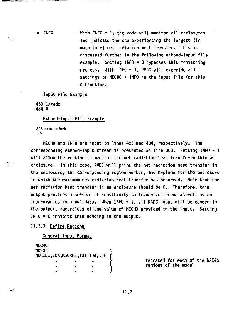
* INFO - With INFO = 1, the code will monitor all enclosures
and indicate the one experiencing the largest (in
magnitude) net radiation heat transfer. This is
discussed further in the following echoed-input file
example. Setting INFO = 0 bypasses this monitoring
process. With INFO = 1, RADC will override all
settings of NECHO 4 INFO in the input file for this
subroutine.
Input File Example
483 1/radc484 0
Echoed-Input File Example
808 radc InfozO809
NECHO and INFO are input on lines 483 and 484, respectively. The
corresponding echoed-input stream is presented as line 808. Setting INFO = 1
will allow the routine to monitor the net radiation heat transfer within an
enclosure. In this case, RADC will print the net radiation heat transfer in
the enclosure, the corresponding region number, and K-plane for the enclosure
in which the maximum net radiation heat transfer has occurred. Note that the
net radiation heat transfer in an enclosure should be 0. Therefore, this
output provides a measure of sensitivity to truncation error as well as to
inaccuracies in input data. When INFO = 1, all RADC input will be echoed in
the output, regardless of the value of NECHO provided in the input. Setting
INFO = 0 inhibits this echoing in the output.
11.2.3 Define Regions
General Input Format
NECHONREGSNKCELL,IDK,NSURFS,IDI,IDJ,IDH
repeated for each of the NREGSregions of the model
11.7
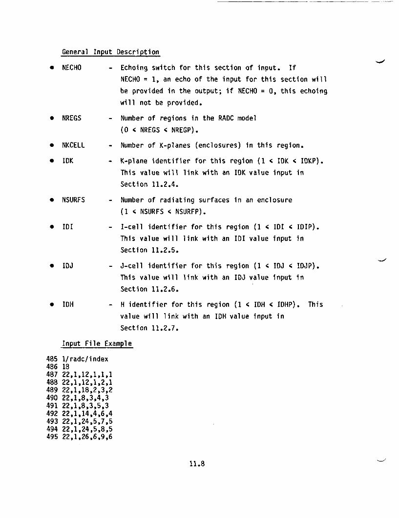
General Input Description
* NECHO - Echoing switch for this section of input. If
NECHO = 1, an echo of the input for this section will
be provided in the output; if NECHO = 0, this echoing
will not be provided.
* NREGS - Number of regions in the RADC model
(O 4 NREGS < NREGP).
* NKCELL - Number of K-planes (enclosures) in this region.
* IDK - K-plane identifier for this region (1 < IDK < IDKP).
This value will link with an IDK value input in
Section 11.2.4.
* NSURFS - Number of radiating surfaces in an enclosure
(1 < NSURFS < NSURFP).
* IDI - I-cell identifier for this region (1 4 IDI ' IDIP).
This value will link with an IDI value input in
Section 11.2.5.
* IDJ - J-cell identifier for this region (1 < IDJ ' IDJP).
This value will link with an IDJ value input in
Section 11.2.6.
* IDH - H identifier for this region (1 4 IDH < IDHP). This
value will link with an IDH value input in
Section 11.2.7.
Input File Example
485 1/radc/index486 18487 22,1,12,1,1,1488 22,1,12,1,2,1489 22,1,18,2,3,2490 22,1,8,3,4,3491 22,1,8,3,5,3492 22,1,14,4,6,4493 22,1,24,5,7,5494 22,1,24,5,8,5495 22,1,26,6,9,6
11.8
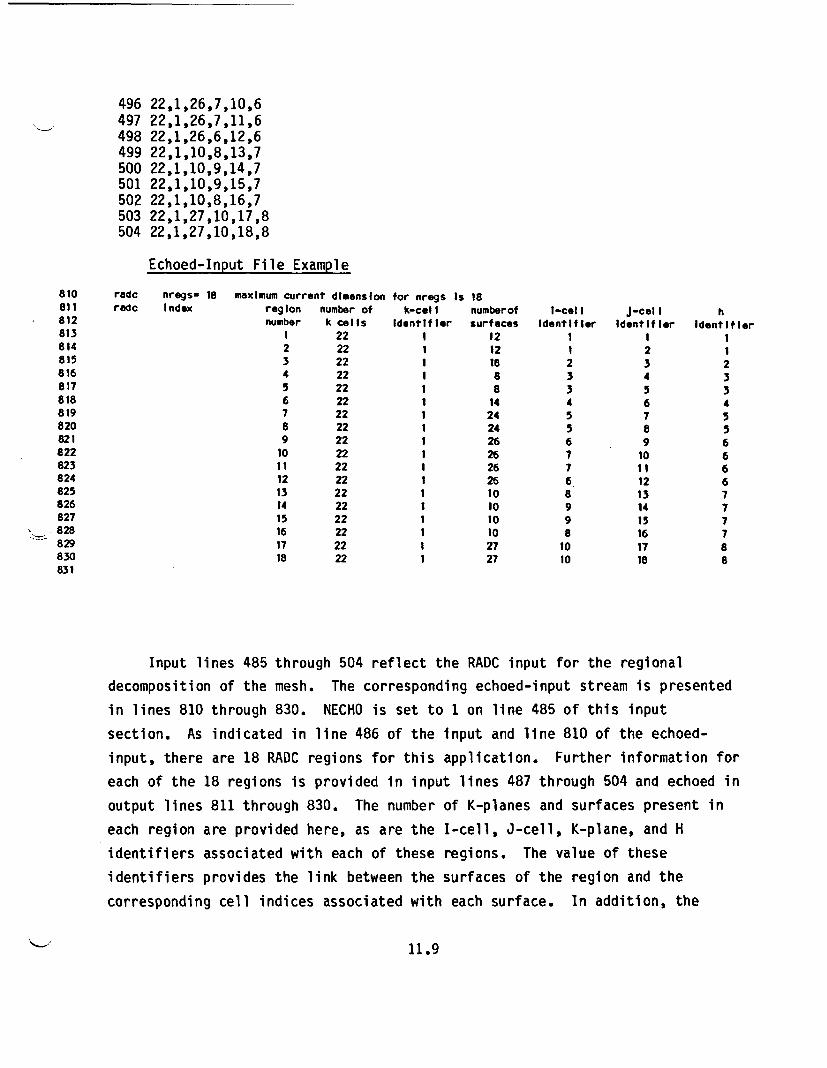
496 22,1,26,7,10,6497 22,1,26,7,11,6498 22,1,26,6,12,6499 22,1,10,8,13,7500 22,1,10,9,14,7501 22,1,10,9,15,7502 22,1,10,8,16,7503 22,1,27,10,17,8504 22,1,27,10,18,8
Echoed-Input File Example
810 radc nregs- 18 maximum current dimension for nregs Is 18811 radc Index rag Ion number of k-cel I numberof i-call J-cel I h812 number k cells Identifier surfaces Identifier Identifier Identifier813 1 22 1 12 1 1 1814 2 22 1 12 1 2 1815 3 22 1 18 2 3 2816 4 22 1 8 3 4 3817 5 22 1 8 3 5 3818 6 22 1 14 4 6 4819 7 22 1 24 5 7 5820 8 22 1 24 5 8 5821 9 22 1 26 6 9 6822 10 22 1 26 7 10 6823 11 22 1 26 7 11 6824 12 22 1 26 6 12 6825 13 22 1 10 8 13 7826 14 22 1 10 9 14 7827 15 22 1 10 9 15 7828 16 22 1 10 8 16 7829 17 22 1 27 10 17 8830 18 22 1 27 10 18 8831
Input lines 485 through 504 reflect the RADC input for the regional
decomposition of the mesh. The corresponding echoed-input stream is presented
in lines 810 through 830. NECHO is set to 1 on line 485 of this input
section. As indicated in line 486 of the input and line 810 of the echoed-
input, there are 18 RADC regions for this application. Further information for
each of the 18 regions is provided in input lines 487 through 504 and echoed in
output lines 811 through 830. The number of K-planes and surfaces present in
each region are provided here, as are the I-cell, J-cell, K-plane, and H
identifiers associated with each of these regions. The value of these
identifiers provides the link between the surfaces of the region and the
corresponding cell indices associated with each surface. In addition, the
11.9
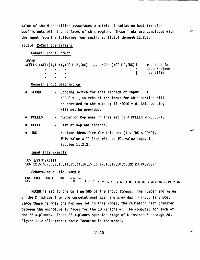
value of the H identifier associates a matrix of radiation heat transfer
coefficients with the surfaces of this region. These links are completed with
the input from the following four sections, 11.2.4 through 11.2.7.
11.2.4 K-Cell Identifiers
General Input Format
NECHOKCELLS,KCELL(1,IDK),KCELL(2,IDK), ... ,KCELL(KCELLS,IDK) repeated for
each K-plane. .identifier
General Input Description
* NECHO - Echoing switch for this section of input. If
NECHO = 1, an echo of the input for this section will
be provided in the output; if NECHO = 0, this echoing
will not be provided.
* KCELLS - Number of K-planes in this set (1 ' KCELLS 4 KCELLP).
* KCELL - List of K-plane indices.
* IDK - K-plane identifier for this set (1 < IDK < IDKP).
This value will link with an IDK value input in
Section 11.2.3.
Input File Example
505 1/radc/kcell506 22,5,6,7,8,9,10,11,12,13,14,15,16,17,18,19,20,21,22,23,24,25,26
Echoed-Input File Example
832 radc kcel I Idk k-ce Is:833 1 22 : 5 6 7 8 9 10 11 12 13 14 15 16 17 18 19 20 21 22 23 24 25 26
NECHO is set to one on line 505 of the input stream. The number and value
of the K indices from the computational mesh are provided in input line 506.
Since there is only one K-plane set in this model, the radiation heat transfer
between the enclosure surfaces for the 18 regions will be computed for each of
the 22 K-planes. These 22 K-planes span the range of K indices 5 through 26.
Figure 11.2 illustrates their location in the model.
11.10

11.2.5 I-Cell Identifiers
General Input Format
NECHONSURFS,ICELL(1,IDI),ICELL(2,IDI), ... ,ICELL(NSURFS,IDI)
* *
* * 0
* * s
General Input Description
repeated foreach I-cellidentifier
* NECHO - Echoing switch for this section of input. If
NECHO = 1, an echo of the input for this section will
be provided in the output; if NECHO = 0, this echoing
will not be provided.
* NSURFS
* ICELL
* IDI
- Number of surfaces in this set (1 4 NSURFS 4 NSURFP).
- List of I-cell indices.
- I-cell identifier for this set (1 ' IDI ' IDIP). This
value will link with an IDI value input in
Section 11.2.3.
Input File Example
507 1/radc/icell508 12,2,3,4,3*5,4,3,2,3*1509 18,6,7,8,6*9,8,7,6,6*5510 8,2,3,4,5,4,3,2,1511 14,15,6*16,15,6*14512 24,6,6*7,8,9,10,11,12,11,10,9,8,7,6,6*5513 26,6,12*7,6,12*5514 26,25,24,23,22,21,20,19,18,17,16,15,14,13,12,13,14,15,16,17,18,19,20,21,515 22,23,24516 10,8,9,10,11,11,10,9,8,7,7517 10,2*25,24,23,4*22,23,24518 27,13,14,15,16,17,18,19,20,21,21,20,19,18,17,16,15,14,13,9*12
Echoed-Input File Example
835836837838839840
radc Icell Idl I-cel Is:1 12 : 2 3 4 52 18 : 6 7 8 93 8 : 2 3 4 54 14 : 15 16 16 165 24 : 6 7 7 I
55 4 3 2 1 1 199 9 9 9 8 7 6 5 5 5 5 5 543 2 116 16 16 15 14 14 14 14 14 147 7 7 8 9 10 11 121110 9 8 7 6 5 5 5 5 5 5
11.11
841 6 26 6 7 7 7 7 7 7 7 7 7 7 7 7 6 5 5 5 5 5 5 5 5 5 5 5 5842 7 26 : 25 24 23 22 21 20 19 18 17 16 15 14 13 12 13 14 15 16 17 18 19 20 21 22 23 24843 8 10 : 8 9 10 11 11 10 9 8 7 7844 9 10 :25 25 24 23 22 22 22 22 23 24845 10 27 : 13 14 15 16 17 18 19 20 21 21 20 19 18 17 16 15 14 13 12 12 12 12 12 12 12 12 12846
The information for each I-cell identifier is provided next in input lines
507 through 518. NECHO has again been set to 1 on line 507. The number of
surfaces and mesh indices are provided for each of the 10 I-cell identifier
sets (IDI) in lines 508 through 518. The echoed-input stream for this data is
presented in lines 835 through 845. The number of surfaces represented in this
I-cell set is presented first in a line of input (e.g., 8 surfaces will be
represented by I-cell set 3 on input line 510). This is followed by the I-cell
indices associated with each of the surfaces of the set (e.g., I = 2,3,4,...
for I-cell set 3 on input line 510). Note that the IDI values for the I-cellgroups are not explicitly provided in the input. HYDRA-II loads the value of
NSURFS and each of the corresponding NSURFS I-cell indices into one IDI group
before incrementing IDI and beginning to load the next IDI group.
11.2.6 J-Cell Identifiers
General Input Format
NECHONSURFS,JCELL(1,IDJ),JCELL(2,IDJ), ... ,JCELL(NSURFS,IDJ) repeated for
each J-cell. . identifier
General Input Description
* NECHO - Echoing switch for this section of input. If
NECHO = 1, an echo of the input for this section will
be provided in the output; if NECHO = 0, this echoing
will not be provided.
* NSURFS - Number of surfaces in this set (1 c NSURFS 4 NSURFP).
* JCELL - List of J-cell indices.
11.12
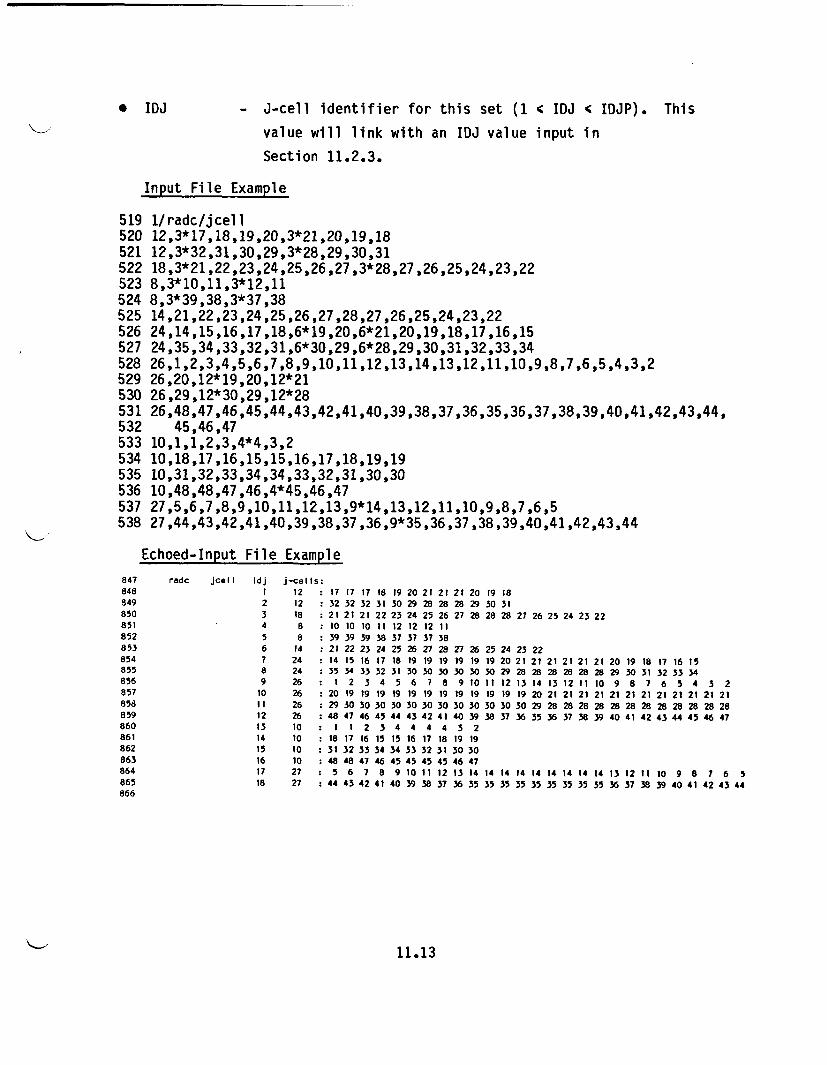
* IDJ - J-cell identifier for this set (1 c IDJ c IDJP). This
value will link with an IDJ value input in
Section 11.2.3.
Input File Example
519 1/radc/jcell520 12,3*17,18,19,20,3*21,20,19,18521 12,3*32,31,30,29,3*28,29,30,31522 18,3*21,22,23,24,25,26,27,3*28,27,26,25,24,23,22523 8,3*10,11,3*12,11524 8,3*39,38,3*37,38525 14,21,22,23,24,25,26,27,28,27,26,25,24,23,22526 24,14,15,16,17,18,6*19,20,6*21,20,19,18,17,16,15527 24,35,34,33,32,31,6*30,29,6*28,29,30,31,32,33,34528 26,1,2,3,4,5,6,7,8,9,10,11,12,13,14,13,12,11,10,9,8,7,6,5,4,3,2529 26,20,12*19,20,12*21530 26,29,12*30,29,12*28531 26,48,47,46,45,44,43,42,41,40,39,38,37,36,35,36,37,38,39,40,41,42,43,44,532 45,46,47533 10,1,1,2,3,4*4,3,2534 10,18,17,16,15,15,16,17,18,19,19535 10,31,32,33,34,34,33,32,31,30,30536 10,48,48,47,46,4*45,46,47537 27,5,6,7,8,9,10,11,12,13,9*14,13,12,11,10,9,8,7,6,5538 27,44,43,42,41,40,39,38,37,36,9*35,36,37,38,39,40,41,42,43,44
Echoed-Input File Example
847848849850
851852853854855
856857858859860861862863864865866
radc jcell Idj J-cells:
I 12 17 t7 17 18 19 20 21 21 21 20 19 182 12 :32 32 32 31 0 29 28 28 28 29 30 313 18 21 21 21 22 23 24 25 26 27 28 28 28
4 8 10 10 10 11 12 12 12 11
5 8 :39 39 39 38 37 37 37 38
6 14 :21 22 23 24 25 26 27 28 27 26 25 24
7 24 :14 15 16 17 18 19 19 19 19 19 19 208 24 :35 34 33 32 31 30 30 30 30 30 30 29
9 26 :1 2 3 4 5 6 7 8 9 10 11 1210 26 :20 19 19 19 19 19 19 19 19 19 19 19
11 26 :29 30 30 30 30 30 30 30 30 30 30 30
12 26 :48 47 46 45 44 43 42 41 40 39 38 3713 10 :I 1 2 3 4 4 4 4 3 2
.14 10 :18 17 16 15 15 16 17 18 19 1915 10 :31 32 33 34 34 33 32 31 30 30
16 10 :48 48 47 46 45 45 45 45 46 4717 27 : 5 6 7 8 9 10 11 12 13 14 14 1418 27 :44 43 42 41 40 39 38 37 36 35 35 35
27 26 25 24 23 22
23 2221 21 21 21 21 21 2028 28 28 28 28 28 2913 14 13 12 11 10 919 20 21 21 21 21 2130 29 28 28 28 28 2836 35 36 37 38 39 40
19 18 17 16 1 530 31 32 33 348 7 6 5 4 3 2
21 21 21 21 21 21 2128 28 28 28 28 28 2841 42 43 44 45 46 47
14 14 14 14 14 14 13 12 11 10 9 8 7 6 535 35 35 35 35 35 36 37 38 39 40 41 42 43 44
11.13
The J-cell identifier information is provided next in input lines 519
through 538. The format for this input is the same as that for the I-cell
identifiers. That is, line 519 indicates NECHO has been set to a value of 1.
Information for each of the 18 J-cell identifiers is provided next in input
lines 520 through 538 and has been echoed in output lines 848 through 865. The
number of surfaces and their corresponding J-cell indices are provided for each
J-cell set in this input stream. For example, J-cell set 4 represents eight
surfaces with J indices 10, 11, and 12. As with IDI in the previous section,
the IDJ group identifier numbers are assigned internally in HYDRA-II.
At this point, the code has all the necessary index information to
associate an (I,J,K) cell index with each of the surfaces modeled. For
example, the (I,J,K) indices associated with the eight surfaces of region 4
are (2,10,K), (3,10,K), (4,10,K), (5,11,K), (4,12,K), (3,12,K), (2,12,K), and
(1,11,K). As specified by the K-plane set provided on input line 506, K takes
on the values 5 through 26 in this RADC model.
It remains to associate a radiation heat transfer coefficient with each of
the interacting surface pairs of the model. This information is provided next.
11.2.7 H Array
General Input Format
NECHONSURFSH(1,1,IDH),H(1,2,IDH), ... ,H(1,NSURFS,IDH),
H(NSURFS,1,IDH),H(NSURFS,2,IDH), ... ,H(NSURFS,NSURFS,IDH)
repeated foreachH-identifierset
General Input Description
* NECHO
* NSURFS
- Echoing switch for this section of input. If
NECHO = 1, an echo of the input for this section will
be provided in the output; if NECHO = 0, this echoing
will not be provided.
- Number of surfaces represented in this H identifier
set (1 ' NSURFS ' NSURFP).
11.14
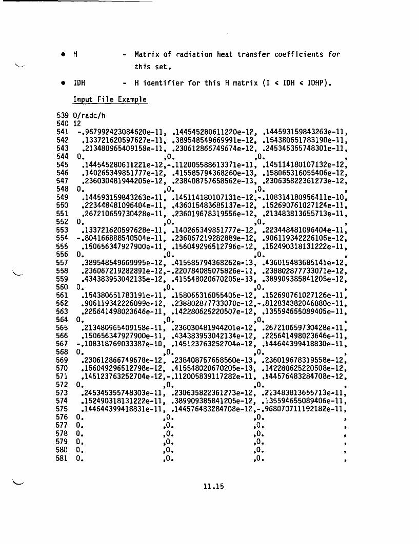
* H - Matrix of radiation heat transfer coefficients for
this set.
* IDH - H identifier for this H matrix (1 IDH < IDHP).
Input File Example
539 0/radc/h540 12541 -.967992423084620e-11, .144545280611220e-12, .144593159843263e-11,542 .133721620597627e-11, .389548549669991e-12, .154380651783190e-11,543 .213480965409158e-11, .230612866749674e-12, .245345355748301e-11,544 0. ,0. ,0.545 .144545280611221e-12,-.112005588613371e-11, .145114180107132e-12,546 .140265349851777e-12, .415585794368260e-13, .158065316055406e-12,547 .236030481944205e-12, .238408757658562e-13, .230635822361273e-12,548 0. ,0. ,0.549 .144593159843263e-11, .145114180107131e-12,-.108314180956411e-10,550 .223448481096404e-11, .436015483685137e-12, .152690761027124e-11,551 .267210659730428e-11, .236019678319556e-12, .213483813655713e-11,552 0. ,0. ,0.553 .133721620597628e-11, .140265349851777e-12, .223448481096404e-11,554 -.804166888540504e-11, .236067219282889e-12, .906119342226106e-12,555 .150656347927900e-11, .156049296512796e-12, .152490318131222e-11,556 0. ,0. ,0.557 .389548549669995e-12, .415585794368262e-13, .436015483685141e-12,558 .236067219282891e-12,-.220784085075826e-11, .238802877733071e-12,559 .434383953042135e-12, .415548020670205e-13, .389909385841205e-12,560 0. ,0. ,0.561 .154380651783191e-11, .158065316055405e-12, .152690761027126e-11,562 .906119342226099e-12, .238802877733070e-12,-.812834382046880e-11,563 .225641498023646e-11, .142280625220507e-12, .135594655089405e-11,564 0. ,0. 0.565 .213480965409158e-11, .236030481944201e-12, .267210659730428e-11,566 .150656347927900e-11, .434383953042134e-12, .225641498023646e-11,567 -.108318769033387e-10, .145123763252704e-12, .144644399418830e-11,568 0. ,O. ,0.569 .230612866749678e-12, .238408757658560e-13, .236019678319558e-12,570 .156049296512798e-12, .415548020670205e-13, .142280625220508e-12,571 .145123763252704e-12,-.112005839117282e-11, .144576483284708e-12,572 0. ,0. ,0.573 .245345355748303e-11, .230635822361273e-12, .213483813655713e-11,574 .152490318131222e-11, .389909385841205e-12, .135594655089406e-11,575 .144644399418831e-11, .144576483284708e-12,-.968070711192182e-11,576 0. ,0. ,0.577 0. ,0. ,0.578 0. ,0. ,0.579 0. ,0. ,0.580 0. ,0. ,0.581 0. 90. O0
11.15
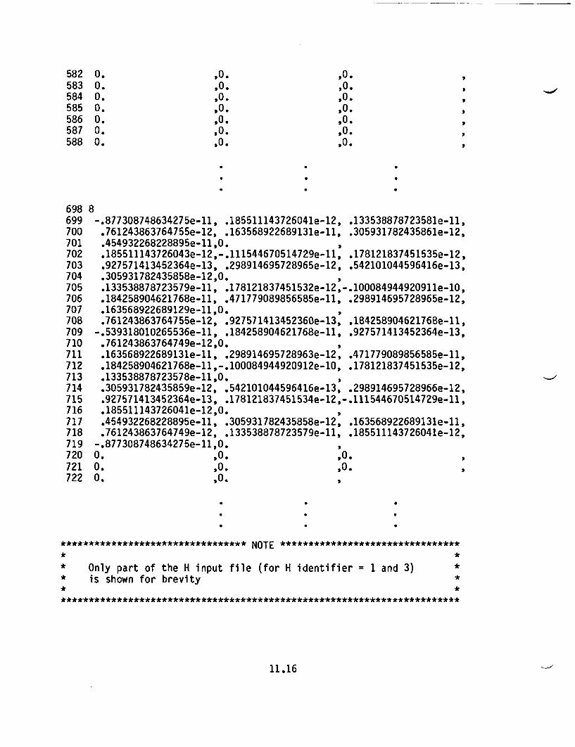
582 0. '0 '°.583 0. ,0. ,0.584 0. ,0. ,0.585 0. ,O. ,0.586 0. ,0. ,0.587 0. ,0. ,0.588 0. ,0. ,0.
698 8699 -. 877308748634275e-11, .185511143726041e-12, .133538878723581e-11,700 .761243863764755e-12, .163568922689131e-11, .305931782435861e-12,701 .45493226822889Se-11 ,0.702 .185511143726043e-12,-.111544670514729e-11, .178121837451535e-12,703 .927571413452364e-13, .298914695728965e-12, .542101044596416e-13,704 .305931782435858e-12,0.705 .133538878723579e-11, .178121837451532e-12,-.100084944920911e-10,706 .184258904621768e-11, .471779089856585e-11, .298914695728965e-12,707 .163568922689129e-11,0.708 .761243863764755e-12, .927571413452360e-13, .184258904621768e-11,709 -. 539318010265536e-11, .184258904621768e-11, .927571413452364e-13,710 .761243863764749e-12,0.711 .163568922689131e-11, .298914695728963e-12, .471779089856585e-11,712 .184258904621768e-11,-.100084944920912e-10, .178121837451535e-12,713 .133538878723578e-11,0.714 .305931782435859e-12, .542101044596416e-13, .298914695728966e-12,715 .927571413452364e-13, .178121837451534e-12,-.111544670514729e-11,716 .185511143726041e-12,0.717 .454932268228895e-11, .305931782435858e-12, .163568922689131e-11,718 .761243863764749e-12, .133538878723579e-11, .185511143726041e-12,719 -. 877308748634275e-11,0.720 0. ,0. ,0.721 0. ,0. ,0.722 0. ,0. 9
********************************* NOTE ********************************* *
* Only part of the H input file (for H identifier = 1 and 3) ** is shown for brevity ** *
11.16

Part of the input file for the radiation heat transfer coefficients is
provided in lines 539 through 588 and lines 698 through 722. This input is
typically quite lengthy for enclosures having many surfaces. Therefore, only
portions of it are presented here. Input line 539 indicates the setting of
NECHO to zero for this section. Input lines 540 through 588 correspond to the
data provided for the first H set (H identifier, IDH = 1). This array of
radiation heat transfer coefficients represents a region composed of 12
surfaces (ref., input line 540). Therefore, there are 144 elements in this H
array (12 x 12). The array is loaded by rows (i.e., updating the second index
most rapidly). Consequently, the radiation heat transfer coefficients from the
first through twelfth surfaces to the first surface are loaded first. Those
from the first through twelfth surfaces to the second surface are loaded next,
and so on. The H identifiers on input lines 487 and 488 (and in the echoed-
input lines 813 and 814) indicate that this H array is used for regions 1 and 2
of the RADC model.
The regional input provided in lines 487 through 504 above indicated that
there are eight such H arrays in this RADC model. Therefore, the input to this
section must have eight corresponding sets of data similar in format to that
provided in input lines 540 through 588.
Data for the third H array (H identifier, IDH = 3) are presented in input
lines 698 through 722. Input line 698 indicates that this array represents the
radiation heat transfer coefficients between eight surfaces. Therefore, this
array contains 64 elements (8 x 8). As with the first H array, this array is
loaded by rows.
The format for the H array input, as well as the connection between this
input and the information provided for I-cell, J-cell, and K-plane specifi-
cations, is best illustrated by an example. Therefore, the following discus-
sion pertains to region 4 of the model. The computational mesh associated with
this region is illustrated in the detail of Figure 11.1.
Region 4 represents an eight-surface enclosure at each of the 22 K-planes
corresponding to K indices 5 through 26. At each of these K-planes, radiation
heat transfer will be computed between the eight surfaces represented by the I-
cell and J-cell identifiers 3 and 4, respectively. The (I,J) pairs defining
11.17
the cells of this enclosure are identified by association with these I-cell and
J-cell identifiers as (2,10), (3,10), (4,10), (5,11), (4,12), (3,12), (2,12),
and (1,11). The H identifier is 3 for this region. Therefore, the correspond-
ing radiation heat transfer coefficients for this region are provided in the
third array of H data provided (input lines 698 through 722). The radiation
heat transfer coefficient for reradiation from the surface associated with cell
(2,10,K) to the seven other surfaces of this enclosure is input first. The
radiation heat transfer coefficient for energy received by (2,10,K) from the
surface associated with cell (3,10,K) is presented next in the input file,
followed by that for (4,10,K) to (2,10,K), and so on. As indicated by the K
index, these values are used for radiation heat transfer in this enclosure at
each of the 22 K-planes of the model. The code internally scales these coef-
ficients by the appropriate DZ(K). The other length scale of the area element
must be incorporated in the radiation heat transfer coefficient.
To further illustrate the structure of the input file format, consider the
specific interaction between nodes (5,11,K) and (3,10,K). The radiation heat
transfer coefficient used for the energy radiated by the surface at (3,10,K) to
the surface at (5,11,K) has the value 0.92757...e-13. Cell (5,11,K) represents
the fourth surface element of an enclosure in region 4. Cell (3,10,K) repre-
sents the second surface element of an enclosure in region 4. Therefore, the
radiation heat transfer coefficient for energy received by (5,11,K) from
(3,10,K) is stored in H4 ,2 (i.e., the second element of the fourth row in this
H array). Since the array is loaded by rows, this corresponds to the twenty-
sixth entry to the array (viz., the second entry on input line 708). To
illustrate the symmetry required of the matrix of radiation heat transfer
coefficients, this value must equal that representing transfer from (5,11,K) to
(3,10,K). The value is stored in element H2 ,4, the fourth element in the
second row. This is the twelfth value entered in the H array, viz., the first
entry on input line 703. Comparison of these two values indicates that they
are equal. The radiation heat transfer coefficient used to model reradiation
from (5,11,K) to the adjoining surfaces of the enclosure has the value
-0.53931...e-11 (the diagonal element on the fourth row of this array, H4 ,4).
This value equals the negative of the sum of the other radiation heat transfer
11.18

coefficients from (5,11,K). These same coefficients are used for each of the
22 K-planes, 5 through 26 (with the appropriate rescaling by DZ(K)).
Frequently, symmetries are present in the problem configuration. The
presence of these symmetries should be exploited in the model to reduce the
amount of input and execution time required by the simulation. However, when
invoking these symmetries, the user must be certain to include the effects of
image cells (i.e., the reflection of model cells about a line of symmetry) when
generating the input. In particular, the RADC radiation heat transfer coeffi-
cients must reflect the presence of these symmetries. A typical situation
exhibiting this is illustrated in Figure 11.3. In this figure, the modeled
section is represented on the right of the line-of-symmetry, and its image is
to the left of the line-of-symmetry. The participating surfaces of the RADC
enclosure and their images are indicated by the boxed numbers. To properly
model the radiation heat transfer in this enclosure, the user must generate
radiation heat transfer coefficients that include the presence of the image
section. For example, the radiation heat transfer coefficient between surfaces
1 and 7 should also include the effect of radiation from the image of surface 7
(surface 7) to surface 1. Similarly, the interaction between surfaces 3 and 4
should include that between surfaces 3' and 4' also. Surfaces 1' through 7'
are not, of course, explicitly included in the RADC model. Their effect is
lumped into the surface in the modeled section and its corresponding radiation
heat transfer coefficients.
11.2.8 Input Example When RADC Is Not Used
If routine RADC is not used in the simulation, then only lines 483 through
486, 505, 507, 519, and 539 need be provided in the input stream. The input
might look like the following in this case:
483 1/radc484 0485 1/radc/index486 0505 O/radc/kcell507 O/radc/icell519 0/radc/jcell539 O/radc/h
11.19
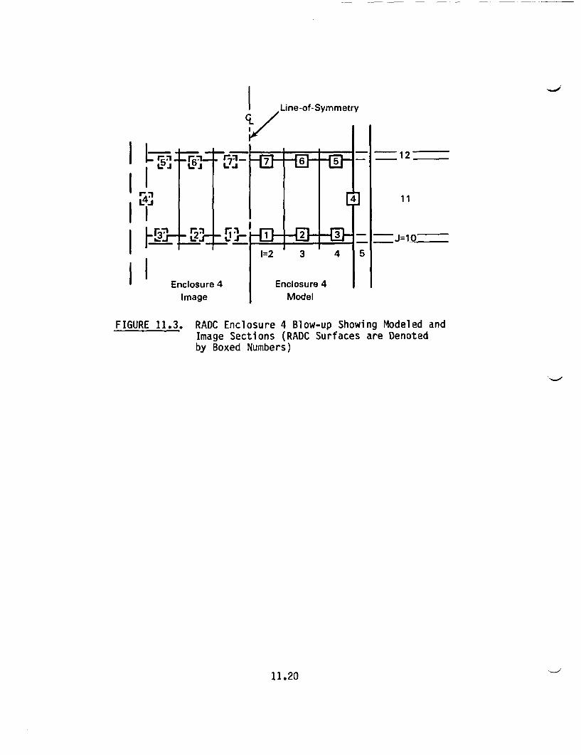
I Line-of-Symmetry
IC/ I
I
I
I
I
I
S-I
L4 .J
gr"L,
_ I I I_
l 4
Enclosure 4
-0-
E
_ 12 _ _
1 1
-J=Io --04-0-_ _.- _- I
1=2 3 4 5
Enclosure 4ModelImage
FIGURE 11.3. RADC Enclosure 4 Blow-up Showing Modeled andImage Sections (RADC Surfaces are Denotedby Boxed Numbers)
11.20

12.0 SUBROUTINE RADP
HYDRA-II provides the user with three subroutines for radiation heat
transfer - RADC, RADP, and RADR. Subroutine RADC is described in Chapter
11.0. RADC allows the user to simulate radiation heat transfer between the
surfaces of an enclosure in the computational domain. The cells associated
with these surfaces must share the same K index for RADC to be applicable.
Subroutine RADP is described in this chapter. The remaining subroutine, RADR,
is described in Chapter 13.0 and is intended to model radiation heat transfer
between the fuel rods of an assembly. The radiation heat transfer distribution
computed in RADP is cumulative with that computed by the other radiation heat
transfer routines, RADC and RADR.
RADP computes the radiative heat transfer received by the mth cell surface
from the nth cell surface using
cYA [T4 -T4jq (m,n) = am[Tn -MT:
RADP[(1/e 2) -1 + (1/cl)]
where e and £2 are the emissivities of the two communicating cell surfaces, a
is the Stefan-Boltzmann constant (= 5.67e-12 W/cm2.K4), and Am is the
appropriate surface area of cell m. A shape factor of 1.0 is assumed between
the two surfaces. Therefore, the radiation heat transfer is equivalent to that
between two essentially infinite parallel planes.
RADP is designed to compute the radiation heat transfer between the cells
on two computational mesh planes. These planes may be separated in any one of
the three coordinate directions (viz., I, J, or K). Two of the three cell
indices must be the same for any pair of communicating cells. Therefore, the
transfer of energy is either between the cells associated with indices (I,J,K)
and (L,J,K), between (I,J,K) and (I,M,K), or between (I,J,K) and (I,J,N). RADP
will sweep over a user-specified range of the two variable indices, computing
the radiation heat transfer between each pair of communicating cells in that
range. The range of indices constitutes a region of the computational domain.
12.1
Radiation heat transfer is between two cell surfaces. Any one cell
surface is shared by either of two cells. In addition, the temperatures T4 and
T4 in the above relationship are those associated with the center of cells m
and n. Therefore, care must be exercised when assigning cell indices to the
surfaces exchanging energy. When the RADP model is set up, the participating
cells should be chosen to accurately represent both the temperature and thermal
properties of the interacting surfaces.
12.1 PARAMETER STATEMENT INFORMATION
Aside from the overall computational mesh specification information IP,
JP, and KP, and the bottom- and top-side mesh information KBP and KTP
(described in Chapter 4.0), RADP requires information pertaining to the
limiting number of regions in the model. The required data are as follows:
* IREGP - An array dimension greater than or equal to the
maximum number of IREG regions (see Section 12.2.2).
* JREGP - An array dimension greater than or equal to the
maximum number of JREG regions (see Section 12.2.3).
* KREGP - An array dimension greater than or equal to the
maximum number of KREG regions (see Section 12.2.4).
IREGP, JREGP, and KREGP must, as a minimum, be set to a value of one (even when
RADP is not used).
12.2 INPUT FORMAT
12.2.1 Overview
Generally speaking, the input to subroutine RADP can be divided into three
subsections:
* load arrays for heat transfer between cells separated in the
I-direction
* load arrays for heat transfer between cells separated in the
J-direction
12.2
* load arrays for heat transfer between cells separated in the
K-direction.
A detailed discussion of the input requirements for each of these subsections
is provided in the following text.
General Input Format
The general format for input to this routine is as follows:
input line n : NECHOinput line (n+1) : NREGSinput line (n+2) : El e2 IBEG, IEND, JBEG, JEND, KBEG, KEND
* * S
* * .
input line (n+2+NREGS-1): e1, £2, IBEG, IEND, JBEG, JEND, KBEG, KEND.
General Input Description
* NECHO - Echoing switch for this section of input. If
NECHO = 1, an echo of the input for this section will
be provided in the output; if NECHO = 0, this echoing
will not be provided.
* NREGS - The number of regions modeled in this subsection.
* e1 and £2 - Emissivities of the communicating surfaces.
* IBEG - Beginning value for the I index range.
* IEND - Ending value for the I index range.
* JBEG - Beginning value for the J index range.
* JEND - Ending value for the J index range.
* KBEG - Beginning value for the K index range.
* KEND - Ending value for the K index range.
The pairs (IBEG,IEND), (JBEG,JEND), and (KBEG,KEND) represent the index
ranges for the surfaces of this region. RADP will loop (in the FORTRAN sense)
over any two of the three pairs of indices to compute the radiation heat
transferred between the third pair of indices. The index for one cell is
composed from the two running indices and the "BEG" value of the third index.
12.3
The index for the second cell of the pair is composed from the same two running
indices and the "END" value of the third index. For example, consider two
cells separated in the K-direction. Each cell has running indices I and J
where IBEG < I ' IEND and JBEG c J < JEND. Each pair of interacting cells will
then have indices (I,J,KBEG) and (I,J,KEND). This configuration is illustrated
in Figure 12.1.
This routine is perhaps best understood by means of an example problem.
Therefore, the use of RADP in modeling the sample problem presented in
Chapter 4.0 is discussed in Sections 12.2.2 through 12.2.4. Figures 12.2 and
12.3 illustrate the location of the regions modeled in the following input.
The input line numbers are used to call out the location of the corresponding
region on Figure 12.2.
12.2.2 I-Direction Radiation Heat Transfer Mode
Input File Example
1507 1/radp/iregs1508 0
Echoed-Input File Example
867 radp Iregsm 0 maximum current dimension for Iregs Is 1868
Those regions of the computational mesh for which the RADP surfaces are
separated in the I-direction are input first. The corresponding input for the
sample problem is shown here as input lines 1507 and 1508. On input line 1507,
the value of NECHO is set to 1. Input line 1508 provides the value of the
number of IREG regions in the RADP model. For this model, there are none, so 0
is entered. The echoed-input lines for this section are shown here as output
lines 867 and 868.
12.2.3 J-Direction Radiation Heat Transfer Mode
Input File Example
1509 1/radp/jregs1510 0
12.4
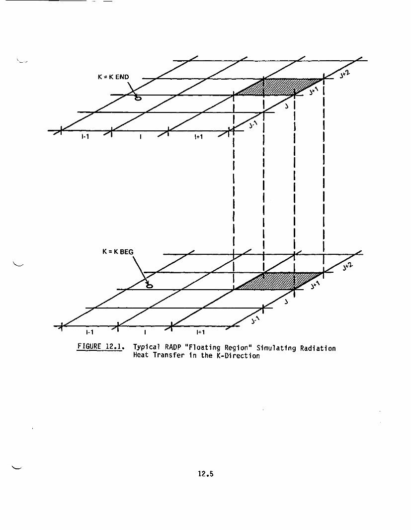
,1111� I"- vr'1K= K ENI -
0 I~In p -
1,1�� L.,��I !
Lr-1 -I I .. I 1+1
alI iI Il lI
II
I iI I
II
I II
I II II II II I
IK=K BEG
I hiI / I I 3l----- ----i --------
I I
L,,�< I
I I-1 I-1 -I I 1+1 -
FIGURE 12.1. Typical RADP "Floating Region" Simulating RadiationHeat Transfer in the K-Direction
12.5
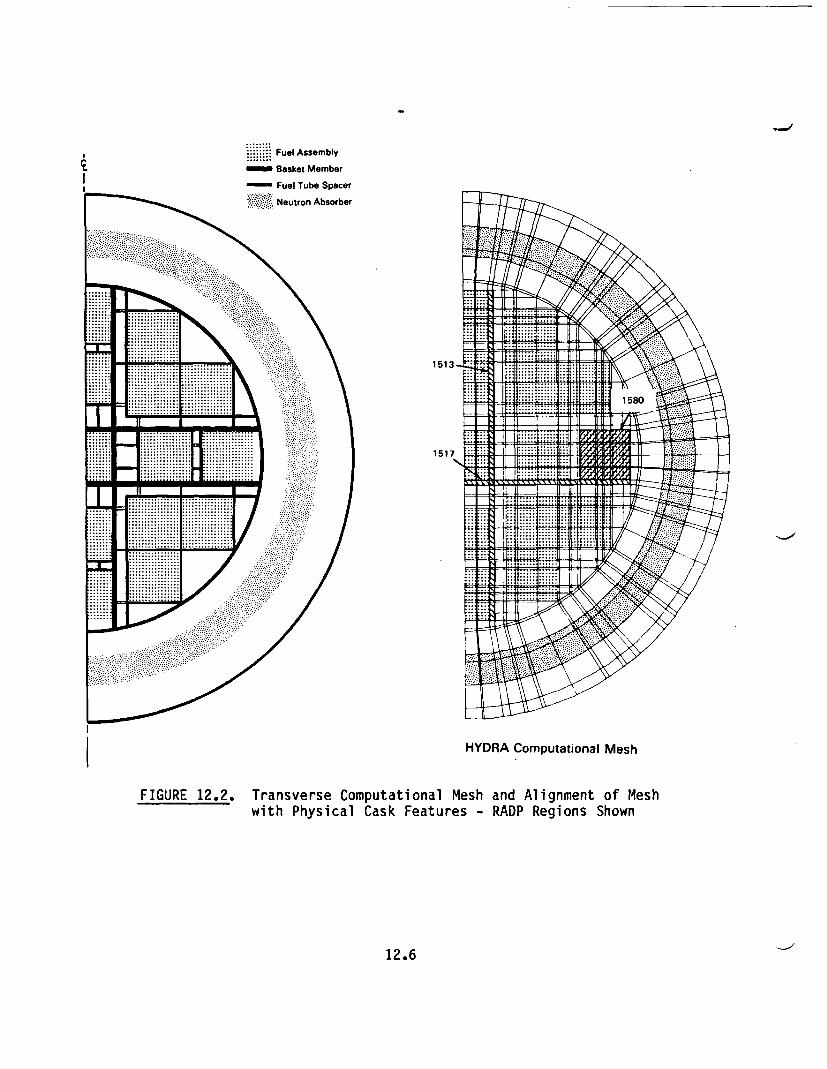
1513
1517
I HYDRA Computational Mesh
FIGURE 12.2. Transverse Computational Mesh and Alignment of Meshwith Physical Cask Features - RADP Regions Shown
12.6

In. :::. Fuel Assembly
|I Basket Member
I W Neutron Absorber
K=28
K=26 =
...... ................ ...............
............... ...............
...... ................ ..............
...............................
............... ..................... ................ ...............
4:4
.uFii
.,I.
. r
, *
1I:::=
OK- z
_
[] I i
<
, !.4p. -
_r-
, > .a ,t'z.-.-.-. -
; 'x'
i.
_=--i
_
i:::::i::::::":: t::::":1t:"::$:W :_ Il - R lr-n---r-_ _ l -1II I II: -1_ _ ll
_ - _-------w: : 1
H:::::1::;;:T; � :;;; ; ; ;;�;i:::::.:::::: :: I :::: : : ::. :111
l ll_ _ F_ 11::::§:t:|::e:1 11raT -1. . . .. .1
. ....
I-4 .17 ......
.. [ 1 .:i:-:
-
K=5_
K=3
i-. 1- ...I
�\\N�\\Nk�\N¶NNk\XN� M�uh fl \ X*NSN -- - L' ,
1 FTT117ll71H l FHI 1I F. % ':::':'
IRl
I
FIGURE 12.3. Axial Computational Mesh and Alignment of Meshwith Physical Cask Features - RADP KBEG andKEND Indices Shown
12.7

Echoed-Input File Example
869 radp Jregs= 0 maximum current dimension for Jregs Is 1870
Those regions of the computational mesh for which the RADP surfaces are
separated in the J-direction are input next. The corresponding input for the
sample problem is shown here as input lines 1509 and 1510. On input line 1509,
the value of NECHO is set to 1. Input line 1510 provides the value of the
number of JREG regions in the RADP model. For this model, there are none, so 0
is entered. The echoed-input lines for this section are shown here as output
lines 869 and 870.
12.2.4 K-Direction Radiation Heat Transfer Mode
Input File Example
1511 1/radp/kregs1512 681513 0.4,0.25,5,5,2,47,26,28
* *
* *
1517 0.4,0.25,2,24,21,21,26,28
* *
1580 0.8,0.25,17,24,22,27,3,5
871872873874
878
941
Echoed-Input File Example
radp kregs- 68 maximum current dimension for kregs Is 682 radp region emittances
- Ibeg Ie1 0.400 0.250 5
i 5 0.400 0.250 2
68 0.800 0.250 17 2
cell location)nd jbeg Jend kbeg kend5 2 47 26 28
24 21 21
24 22 27
26 28
3 5
12.8
Finally, those regions of the computational mesh for which the RADP
surfaces are separated in the K-direction are input. The corresponding input
for the example problem is shown as input lines 1511 through 1580. On input
line 1511 the value of NECHO is set to 1. Input line 1512 indicates that there
are 68 KREG regions in the RADP model. Input line 1580 is typical of the input
lines in this routine. Here, el and e2 are set to a value of 0.8 and 0.25,
respectively. Since this input is in the third subsection of input provided to
this routine, the routine will sweep over the I and J index ranges, computing
the radiation heat transfer between the surface pairs at (I,J,3) and (I,J,5)
for each I and J in the ranges 17 < I < 24 and 22 0 J < 27. The surface area,
A, will be computed as DX(I)*DY(J). The echoed-input lines for these lines are
shown in lines 871 through 874, line 878, and line 941.
12.2.5 Input Example When RADP Is Not Used
If routine RADP is not used in the simulation, the following input must
still be provided:
1507 1/radp/iregs1508 01509 1/radp/jregs1510 01511 1/radp/kregs1512 0
12.9
13.0 SUBROUTINE RADR
HYDRA-II provides the user with three subroutines for use in modeling
radiation heat transfer - RADC, RADP, and RADR. Subroutine RADC is described
in Chapter 11.0. RADC allows the user to simulate radiation heat transfer
between the surfaces of an enclosure in the computational domain. The cells
associated with these surfaces must share the same K index for RADC to be
applicable. Subroutine RADP provides the user with a model for plate-to-plate
radiation heat transfer. RADP is described in Chapter 12.0. Subroutine RADR
is described in this chapter. The radiation heat transfer computed in RADR is
cumulative with that computed by the other radiation heat transfer routines,
RADC and RADP.
RADR provides the user with a method for computing rod-to-rod radiation
heat transfer in a fuel assembly. Each computational cell of the RADR model
contains only one spent fuel rod. The cell surfaces on any K-plane are
configured so as not to "cut" the spent fuel rod boundaries; hence, the cell-
to-cell nature of the radiation heat transfer mode in this routine (contrasted
with the surface-to-surface structure of RADC). This idea is illustrated in
Figure 13.1.
The routine is structured to compute the radiation heat transfer between
the cell associated with index (I,JK) and any of its 24 neighboring cells in
the range It2 and Jt2. This region-of-influence is shown schematically in
Figure 13.2. The center cell [index (I,J,K)] is the receiver cell. The
generic" cell in this region-of-influence is identified by the roman indices
(IJ,K) to differentiate it from the center cell (I,J,K). The surrounding
24 cells of this region are the transmitter cells "seen" by the center cell.
The region-of-influence "floats" over the range of cells specified in the RADR
model. In addition, RADR computes the radiation heat transfer between these
cells for a user-specified range of K-planes. As in the RADC subroutine, RADR
does not allow radiation heat transfer between cells having different K-plane
indices. This mode of exchange may be modeled using subroutine RADP.
In general, the proper computation of radiation heat transfer coefficients
can get very involved. This is particularly true in cases where there are many
13.1
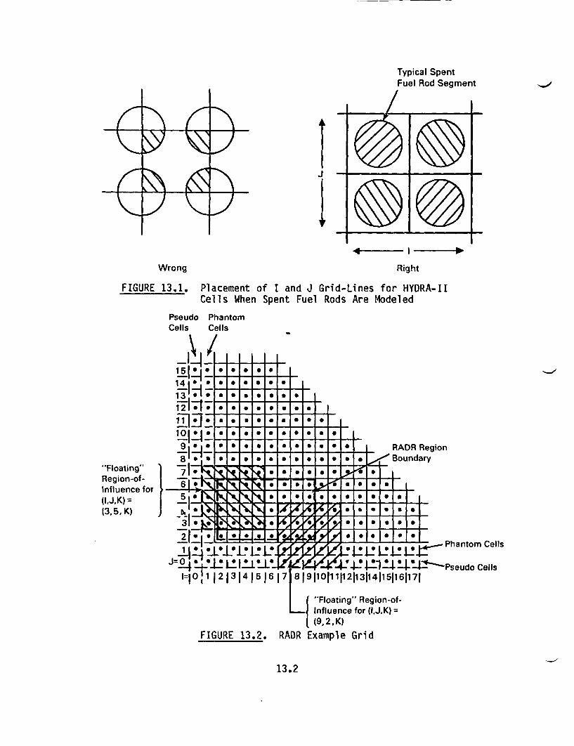
Typical SpentFuel Rod Segment
/A L
�,,v V\")6:��
2 K'-'I9
4 - I P
Wrong Right
FIGURE 13.1. Placement of I and J Grid-Lines for HYDRA-IICells When Spent Fuel Rods Are Modeled
Pseudo PhantomCells Cells
1-I .I
14 i;3
D 1 0 1 0 1 0 1 0
O i -0 i I i E L L L0 1 0 1 0 1 0 1 0 1 0 1 0 1 0 1
0-FO i - -.
9t,.*Itt~tII@TT-Ie@T I8a . * *I- I 1011 A* - I l t -
RADR Region/ Boundary
Region-of-Influence for(1,J,K) =(3,5, K) J
- I1 I I - A T -
*1 . * I.I I - - - . . .,* 01 . . 1 *
0~ * *rJE.. r*1.--.
1 * L L! L !J= 0 1*2 L!I 1 I "
I 10 1 12 1314 1516 17
_ _. I. L Phantom Cells
t4''V L-i 14 * -*4- l Pseudo Cells8 19110111112113141151161171
L{ "Floating" Region-of-Influence for (1,J,K) =(9,2,K)
FIGURE 13.2. RADR Example Grid
13.2
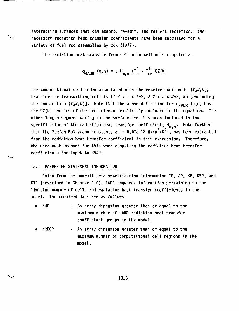
interacting surfaces that can absorb, re-emit, and reflect radiation. The
necessary radiation heat transfer coefficients have been tabulated for a
variety of fuel rod assemblies by Cox (1977).
The radiation heat transfer from cell n to cell m is computed as
q (mn) Hmn (Tn - Tm) DZ(K)
The computational-cell index associated with the receiver cell m is (I,J,K);
that for the transmitting cell is (I-2 I c I+2, J-2 4 J 4 J+2, K) [excluding
the combination (I,J,K)]. Note that the above definition for qRADR (m,n) has
the DZ(K) portion of the area element explicitly included in the equation. The
other length segment making up the surface area has been included in the
specification of the radiation heat transfer coefficient, Hmn@ Note further
that the Stefan-Boltzmann constant, a (= 5.67e-12 W/cm2 K4), has been extracted
from the radiation heat transfer coefficient in this expression. Therefore,
the user must account for this when computing the radiation heat transfer
coefficients for input to RADR.
13.1 PARAMETER STATEMENT INFORMATION
Aside from the overall grid specification information IP, JP, KP, KBP, and
KTP (described in Chapter 4.0), RADR requires information pertaining to the
limiting number of cells and radiation heat transfer coefficients in the
model. The required data are as follows:
* NHP - An array dimension greater than or equal to the
maximum number of RADR radiation heat transfer
coefficient groups in the model.
* NREGP - An array dimension greater than or equal to the
maximum number of computational cell regions in the
model.
13.3
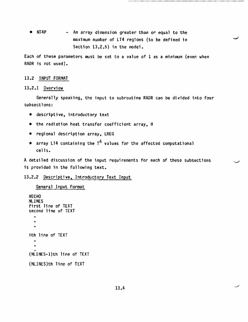
* NT4P - An array dimension greater than or equal to the
maximum number of LT4 regions (to be defined in
Section 13.2.5) in the model.
Each of these parameters must be set to a value of 1 as a minimum (even when
RADR is not used).
13.2 INPUT FORMAT
13.2.1 Overview
Generally speaking, the input to subroutine RADR can be divided into four
subsections:
* descriptive, introductory text
* the radiation heat transfer coefficient array, H
* regional description array, LREG
* array LT4 containing the T4 values for the affected computational
cells.
A detailed discussion of the input requirements for each of these subsections
is provided in the following text.
13.2.2 Descriptive, Introductory Text Input
General Input Format
NECHOWLINESfirst line of TEXTsecond line of TEXT
ith line of TEXT
.LNES-1th line of TEXT
(NLINES)th line of TEXT
13.4
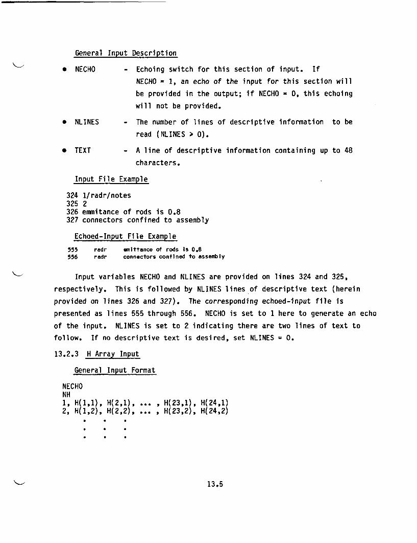
General Input Description
* NECHO - Echoing switch for this section of input. If
NECHO = 1, an echo of the input for this section will
be provided in the output; if NECHO = 0, this echoing
will not be provided.
* NLINES - The number of lines of descriptive information to be
read (NLINES > 0).
* TEXT - A line of descriptive information containing up to 48
characters.
Input File Example
324 1/radr/notes325 2326 emmitance of rods is 0.8327 connectors confined to assembly
Echoed-Input File Example
555 radr emittance of rods Is 0.8556 radr connectors confined to assembly
Input variables NECHO and NLINES are provided on lines 324 and 325,
respectively. This is followed by NLINES lines of descriptive text (herein
provided on lines 326 and 327). The corresponding echoed-input file is
presented as lines 555 through 556. NECHO is set to 1 here to generate an echo
of the input. NLINES is set to 2 indicating there are two lines of text to
follow. If no descriptive text is desired, set NLINES = 0.
13.2.3 H Array Input
General Input Format
NECHONH1, H(1,1), H(2,1), ... , H(23,1), H(24,1)2, H(1,2), H(2,2), ... , H(23,2), H(24,2)
13.5
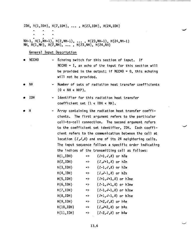
IDH, H(1,IDH), H(2,IDH), ... , H(23,IDH), H(24,IDH)
NH-1,*H(1,NH-1), H(2,NH-1), ... , H(23,NH-1), H(24,NH-1)
NH, H(1,NH), H(2,NH). ... , H(23,NH), H(24,NH)
General Input Description
* NECHO - Echoing switch for this section of input. If
NECHO = 1, an echo of the input for this section will
be provided in the output; if NECHO = 0, this echoing
will not be provided.
* NH - Number of sets of radiation heat transfer coefficients
(O c NH < NHP).
* IDH - Identifier for this radiation heat transfer
coefficient set (1 IDH 4 NH).
* H - Array containing the radiation heat transfer coeffi-
cients. The first argument refers to the particular
cell-to-cell connection. The second argument refers
to the coefficient set identifier, IDH. Each coeffi-
cient refers to the communication between the cell at
location (I,JK) and one of its 24 neighboring cells.
The input sequence follows a specific order indicating
the indices of the transmitting cell as follows:
H(1,IDH) => (I+1,J,K) or h2e
H(2,IDH) => (I,J+1,K) or h2n
H(3,IDH) => (I-1,J,K) or h2w
H(4,IDH) => (I,J-1,K) or h2s
H(5,IDH) => (I+1,J+1,K) or h3ne
H(6,IDH) => (I-1,J+l,K) or h3nw
H(7,IDH) => (I-l,J-1,K) or h3sw
H(8,IDH) => (I+l,J-1,K) or h3se
H(9,IDH) => (I+2,JJ,K) or h4e
H(10,IDH) => (I,J+2,K) or h4n
H(11,IDH) => (I-2,J,K) or h4w
13.6
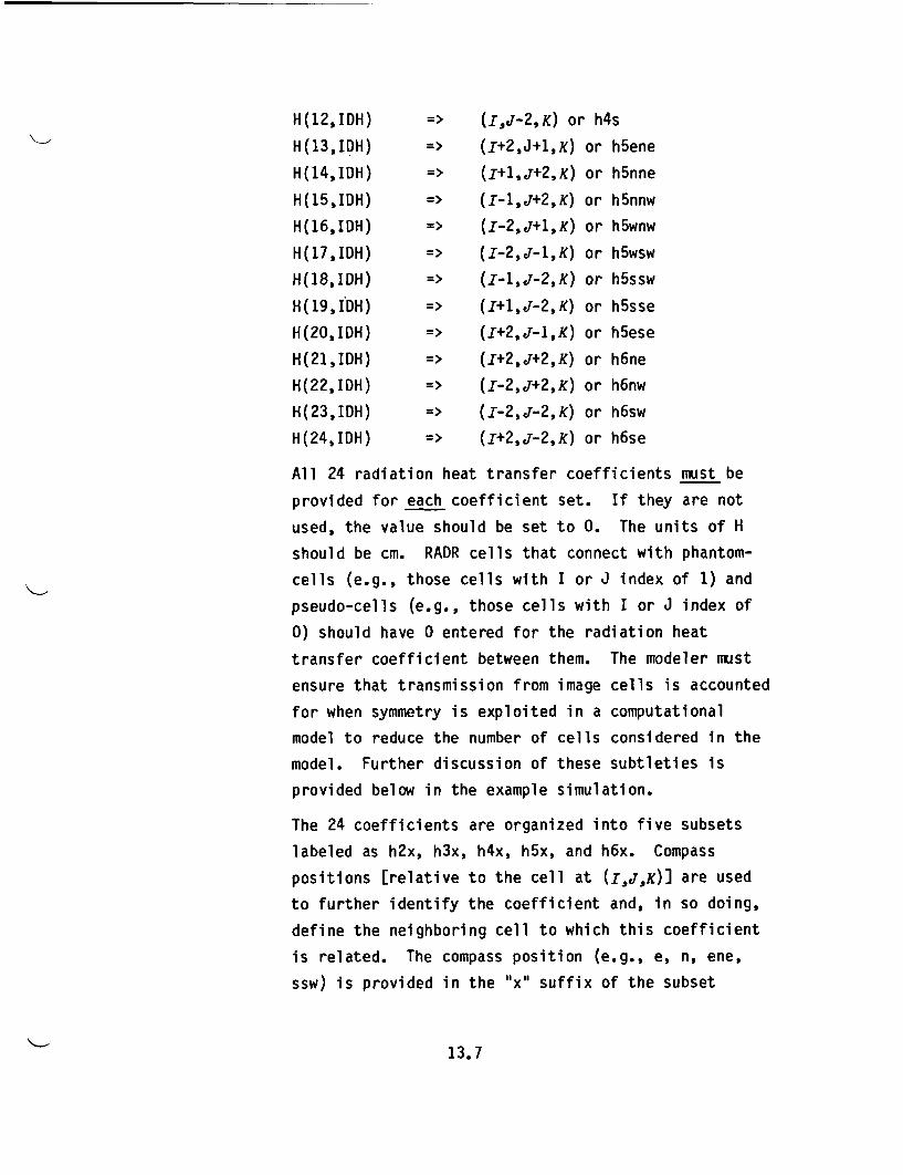
H(12,IDH)
H(13,IDH)
H(14,IDH)
H(15,IDH)
H(16,IDH)
H(17,IDH)
H(18,IDH)
H(19,IDH)
H(20, IDH)
H(21,IDH)
H(22, IDH)
H(23,IDH)
H(24,IDH)
=> (UJ-2,K) or h4s
=> (I+2,J+1,K) or h5ene
=> (I+1,,j+2,K) or h5nne
=> (I-1,J+2,K) or h5nnw
=> (I-2,J+1,K) or h5wnw
=> (I-2,J-1,K) or h5wsw
=> (I-1,J-2,K) or h5ssw
=> (I+1,J-2,K) or h5sse
=> (I+2,J-1,K) or h5ese
=> (I+2,J+2,K) or h6ne
=> (I-2,j+2,K) or h6nw
=> (I-2,J-2,K) or h6sw
=> (I+2,J-2,K) or h6se
All 24 radiation heat transfer coefficients must be
provided for each coefficient set. If they are not
used, the value should be set to 0. The units of H
should be cm. RADR cells that connect with phantom-
cells (e.g., those cells with I or J index of 1) and
pseudo-cells (e.g., those cells with I or J index of
0) should have 0 entered for the radiation heat
transfer coefficient between them. The modeler must
ensure that transmission from image cells is accounted
for when symmetry is exploited in a computational
model to reduce the number of cells considered in the
model. Further discussion of these subtleties is
provided below in the example simulation.
The 24 coefficients are organized into five subsets
labeled as h2x, h3x, h4x, h5x, and h6x. Compass
positions [relative to the cell at (I,J,K)] are used
to further identify the coefficient and, in so doing,
define the neighboring cell to which this coefficient
is related. The compass position (e.g., e, n, ene,
ssw) is provided in the "x" suffix of the subset
13.7
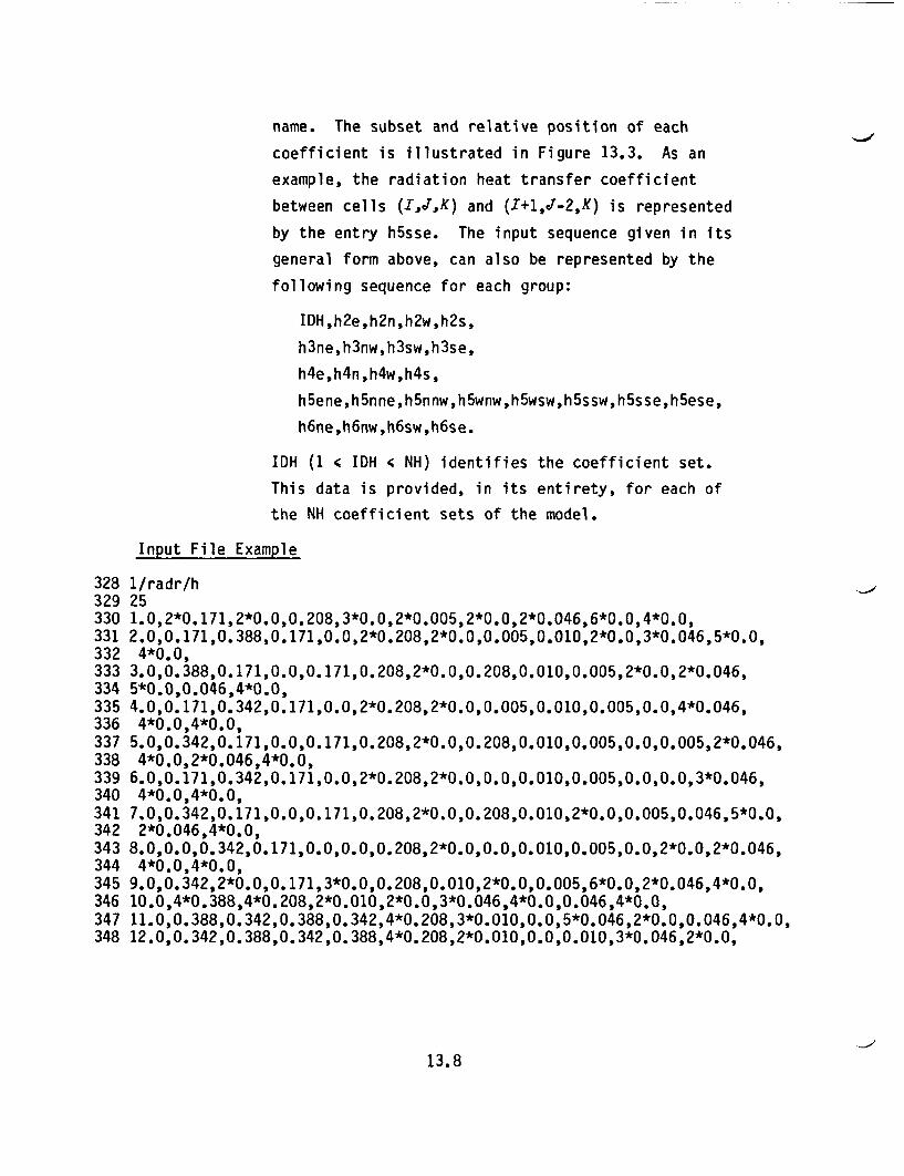
name. The subset and relative position of each
coefficient is illustrated in Figure 13.3. As an
example, the radiation heat transfer coefficient
between cells (IJK) and (I+1,J-2,X) is represented
by the entry h5sse. The input sequence given in its
general form above, can also be represented by the
following sequence for each group:
IDH,h2e,h2n,h2w,h2s,
h3ne,h3nw,h3sw,h3se,
h4e,h4n,h4w,h4s,
h5ene,h5nne,h5nnw,h5wnw,h5wsw,h5ssw,h5sse,h5ese,
h6ne,h6nw,h6sw,h6se.
IDH (1 4 IDH 4 NH) identifies the coefficient set.
This data is provided, in its entirety, for each of
the NH coefficient sets of the model.
Input File Example
328 1/radr/h329 25330 1.0,2*0.171,2*0.0,0.208,3*0.0,2*0.005,2*0.0,2*0.046,6*0.0,4*0.0,331 2.0,0.171,0.388,0.171,0.0,2*0.208,2*0.0,0.005,0.010,2*0.0,3*0.046,5*0.0,332 4*0.0,333 3.0,0.388,0.171,0.0,0.171,0.208,2*0.0,0.208,0.010,0.005,2*0.0,2*0.046,334 5*0.0,0.046,4*0.0,335 4.0,0.171,0.342,0.171,0.0,2*0.208,2*0.0,0.005,0.010,0.005,0.0,4*0.046,336 4*0.0,4*0.0,337 5.0,0.342,0.171,0.0,0.171,0.208,2*0.0,0.208,0.010,0.005,0.0,0.005,2*0.046,338 4*0.0,2*0.046,4*0.0,339 6.0,0.171,0.342,0.171,0.0,2*0.208,2*0.0,0.0,0.010,0.005,0.0,0.0,3*0.046,340 4*0.0,4*0.0,341 7.0,0.342,0.171,0.0,0.171,0.208,2*0.0,0.208,0.010,2*0.0,0.005,0.046,5*0.0,342 2*0.046,4*0.0,343 8.0,0.0,0.342,0.171,0.0,0.0,0.208,2*0.0,0.0,0.010,0.005,0.0,2*0.0,2*0.046,344 4*0.0,4*0.0,345 9.0,0.342,2*0.0,0.171,3*0.0,0.208,0.010,2*0.0,0.005,6*0.0,2*0.046,4*0.0,346 10.0,4*0.388,4*0.208,2*0.010,2*0.0,3*0.046,4*0.0,0.046,4*0.0,347 11.0,0.388,0.342,0.388,0.342,4*0.208,3*0.010,0.0,5*0.046,2*0.0,0.046,4*0.0,348 12.0,0.342,0.388,0.342,0.388,4*0.208,2*0.010,0.0,0.010,3*0.046,2*0.0,
13.8
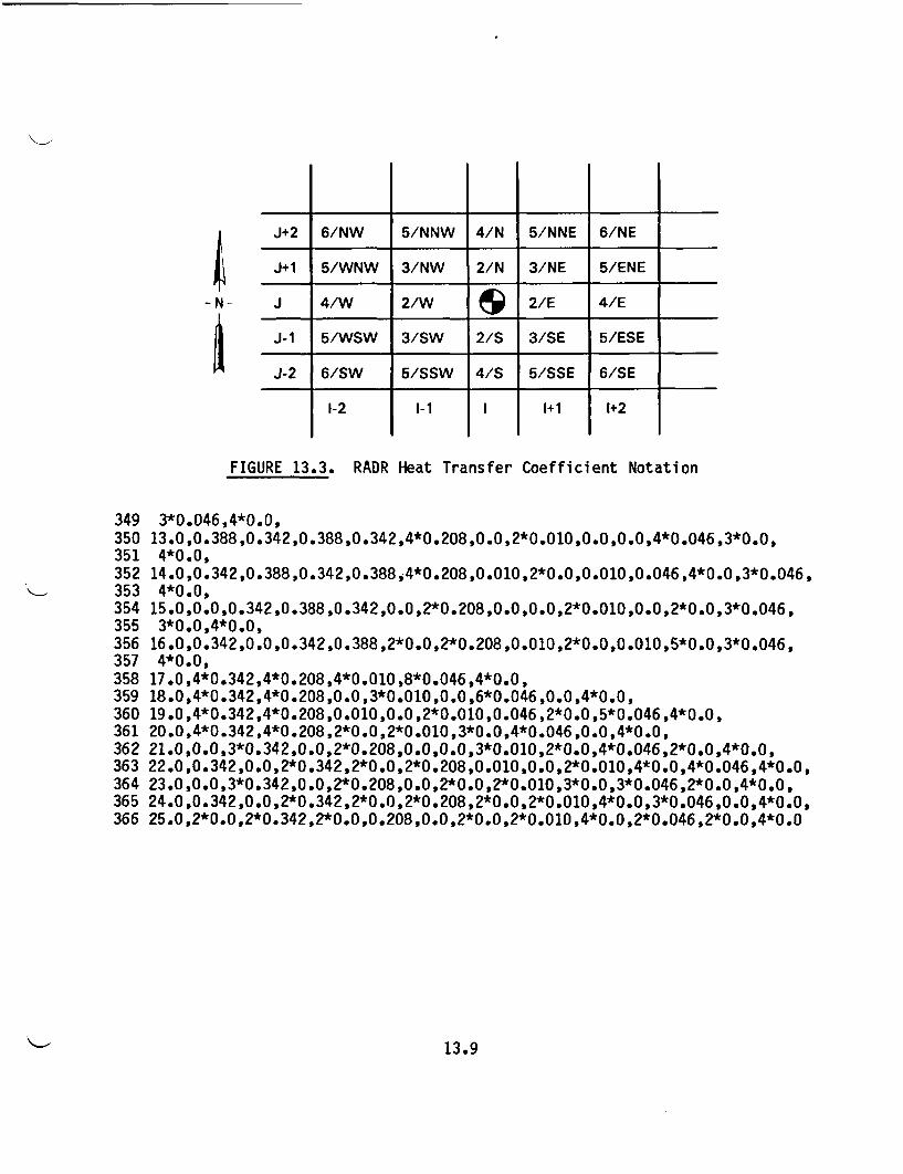
-N-
J+2 6/NW 5/NNW 4/N I5/NNE 6/NE
J+1 5/WNW 3/NW 2/N 3/NE 5/ENE
J 4/W 2/W 2/E 4/E
J-1 5/WSW 3/SW 2/S 3/SE 5/ESE
J-2 6/SW 5/SSW 4/S 5/SSE 6/SE
1-2 1-1 I I 1+1 I 1+2 I
FIGURE 13.3. RADR Heat Transfer Coefficient Notation
349 3*0.046,4*0.0,350 13.0,0.388,0.342,0.388,0.342,4*0.208,0.0,2*0.010,0.0,0.0,4*0.046,3*0.0,351 4*0.0,352 14.0,0.342,0.388,0.342,0.388,4*0.208,0.010,2*0.0,0.010,0.046,4*0.0,3*0.046,353 4*0.0,354 15.0,0.0,0.342,0.388,0.342,0.0,2*0.208,0.0,0.0,2*0.010,0.0,2*0.0,3*0.046,355 3*0.0,4*0.0,356 16.0,0.342,0.0,0.342,0.388,2*0.0,2*0.208,0.010,2*0.0,0.010,5*0.0,3*0.046,357 4*0.0,358 17.0,4*0.342,4*0.208,4*0.010,8*0.046,4*0.0,359 18.0,4*0.342,4*0.208,0.0,3*0.010,0.0,6*0.046,0.0,4*0.0,360 19.0,4*0.342,4*0.208,0.010,0.0,2*0.010,0.046,2*0.0,5*0.046,4*0.0,361 20.0,4*0.342,4*0.208,2*0.0,2*0.010,3*0.0,4*0.046,0.0,4*0.0,362 21.0,0.0,3*0.342,0.0,2*0.208,0.0,0.0,3*0.010,2*0.0,4*0.046,2*0.0,4*0.0,363 22.0,0.342,0.0,2*0.342,2*0.0,2*0.208,0.010,0.0,2*0.010,4*0.0,4*0.046,4*0.0,364 23.0,0.0,3*0.342,0.0,2*0.208,0.0,2*0.0,2*0.010,3*0.0,3*0.046,2*0.0,4*0.0,365 24.0,0.342,0.0,2*0.342,2*0.0,2*0.208,2*0.0,2*0.010,4*0.0,3*0.046,0.0,4*0.0,366 25.0,2*0.0,2*0.342,2*0.0,0.208,0.0,2*0.0,2*0.010,4*0.0,2*0.046,2*0.0,4*0.0
13.9
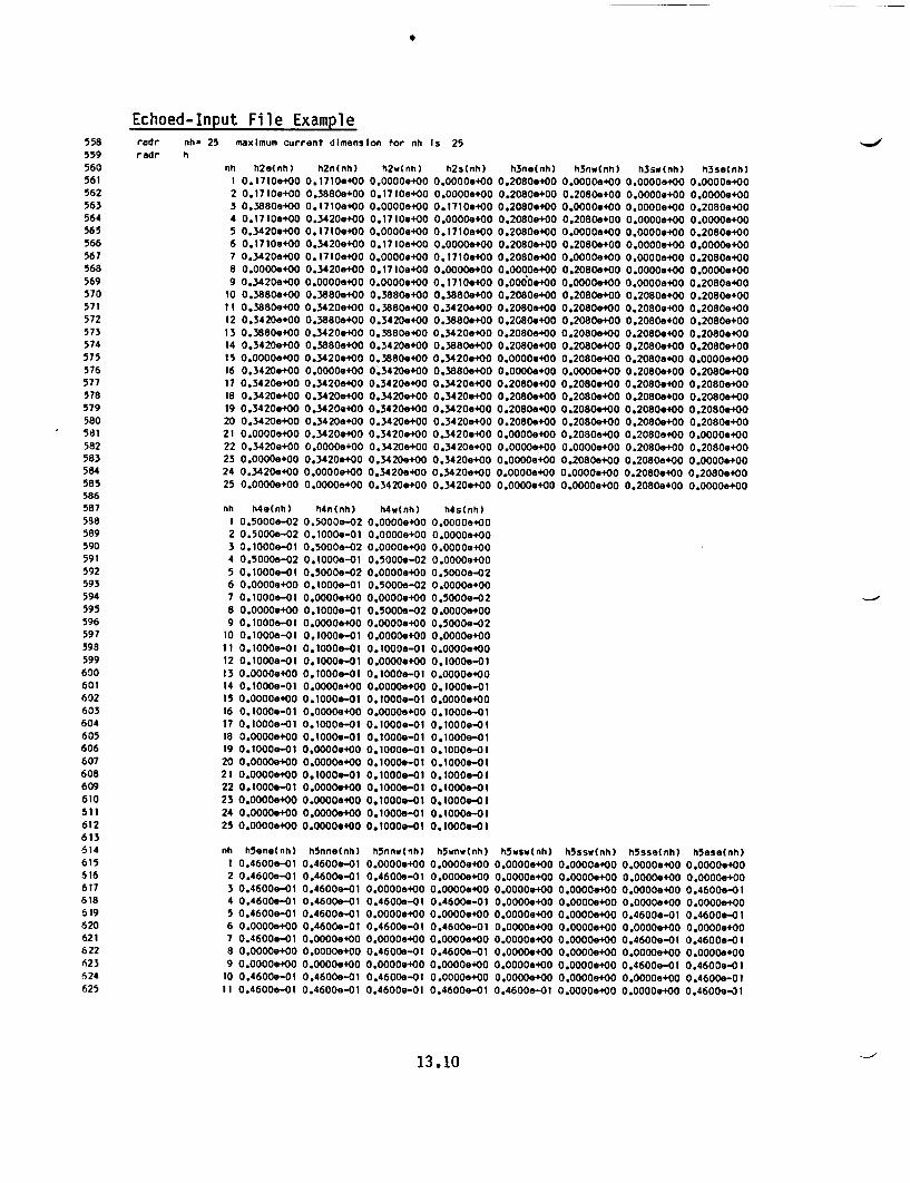
Echoed-Input File Example558 radr nh- 25 maximum current dimension for nh Is 25559 radr h560 nh h2e(nh) h2n(nh) h2wtnh) h2s(nh) h3ne(nh) h3nw(nh) h3sw(nh) h3se(nh)561 1 0.1710e+00 0.1710e+00 0.0000e+00 O.OOOOe4OO 0.2080e+00 0.0000e+00 0.0000.+00 0.0000.+00562 2 0.1710e+00 0.3880e+00 0.1710.+00 0.0000.+00 0.2080e+00 0.2080e+00 0.0000e+00 O.0000e+00563 3 0.3880e400 0.1710.+00 0.0000.e00 0.1710.400 0.2080e400 0.0000.+00 0.0000+400 0.2080e+00564 4 0.1710e+00 0.3420.+00 0.1710.+00 0.0000e+00 0.2080e+00 0.2080e+00 0.0000e+00 0.0000e+00565 5 0.3420.400 0.1710e400 0.0000.+00 0.1710.+00 0.2080e+00 0.0000e+00 0.0000.400 0.2080e400566 6 0.1710e+00 0.3420e+00 0.1710e+00 0.0000+00 0.2080e+00 0.2080e+00 0.0000+00 0.0000e+00567 7 0.3420e+00 0.1710e+00 0.0000e+00 0.1710e.00 0.2080e+00 O.OOOOe4OO 0.0000e+00 0.2080e.+00568 8 0.0000e+00 0.3420e+00 0.1710.+00 0.0000e+00 0.0000+00 0.2080.+00 0.0000.+00 0.0000e+00569 9 0.3420.+00 0.0000e+00 0.0000.e00 0.1710.+00 O.OO.00 0.00o.4oe+00 0.0000.400 0.2080.400570 10 0.3880e+00 0.3880e+00 0.3880e+00 0.3880e+00 0.2080e+00 0.2080e+00 0.2080e+00 0.2080e+00571 11 0.3880e+00 0.3420e+00 0.38809400 0.3420e+00 0.2080.+00 0.2080.+00 0.2080.+00 0.2080e+00572 12 0.3420e+00 0.3880e+00 0.3420e+00 0.3880.+00 0.2080.+00 0.2080e+00 0.2080e+00 0.2080e+00573 13 0.3880e+00 0.3420e+00 0.3880e+00 0.3420.+00 0.2080e+00 0.2080e+00 0.2080e400 0.2080.400574 14 0.3420.+00 0.3880e+00 0.3420e+00 0.3880.+00 0.2080e+00 0.2080e+00 0.2080e+00 0.2080e+00575 15 0.0000e+00 0.3420e+00 0.3880e+00 0.3420e+00 0.0000e+00 0.2080.400 0.2080e+00 0.0000.+00576 16 0.3420e+00 0.0000+00 0.3420e+00 0.3880.+00 0.0000+00 0.0000e+00 0.2080e+00 0.2080e+00577 17 0.3420e400 0.3420*400 0.3420e+00 0.3420e400 0.2080.400 0.2080.400 0.2080.400 0.2080e+00578 18 0.3420e+00 0.3420e+00 0.3420e+00 0.3420e+00 0.2080.+00 0.2080e+00 0.2080e+00 0.2080.+00579 19 0.3420.+00 0.3420.400 0.3420e400 0.3420e400 0.2080e400 0.2080e+00 0.2080.400 0.2080.+00580 20 0.3420.+00 0.3420e+00 0.3420e+00 0.3420e+00 0.2080.+00 0.20800+00 0.2080.+00 0.2080.+00581 21 0.0000e+00 0.3420e+00 0.3420e400 0.3420.e00 0.0000e+00 0.2080e.00 0.2080e+00 0.0000e+00582 22 0.3420e+00 0.0000e+00 0.3420.+00 0.3420e+00 0.0000e+00 0.0000e+00 0.2080.+00 0.2080e+00583 23 0.0000e+00 0.3420e+00 0.3420e+00 0.3420e+00 0.0000e+00 0.2080e+00 0.2080e+00 0.0000e+00584 24 0.3420e+00 0.0000.+00 0.3420.400 0.3420e+00 0.0000.400 0.0000e+00 0.2080e+00 0.2080.+00585 25 0.0000e+00 0.0000e+00 0.3420e+00 0.3420e+00 0.OOOOe+00 0.0000e+00 0.2080.+00 0.0000e+00586587 nh h4e(nh) h4n(nh) h4w(nh) h4s(nh)598 1 0.50009-02 0.5000e-02 0.0000.+00 0.0000e+00589 2 0.5000e-02 0.lOOOe-Ol 0.0000e+00 0.0000e+00
590 3 0.1000l-Ol 0.5000e-02 0.0000.+00 0.0000e+00591 4 0.50009-02 0.10OOe-Ol 0.5000e-02 0.0000+00592 5 0.1000l-Ol 0.5000e-02 0.0000400 0.5000-02593 6 0.0000e+00 0.10OOe-01 0.50009-02 0.0000,+00594 7 0.10OOe-Ol 0.0000.+00 0.0000.400 0.5000e-02595 8 0.0000.+00 0.1000l-Ol 0.5000e-02 0.0000e+00596 9 0.1000.-0l O.OOOOe4OO 0.0000+400 0.5000e-02597 10 0.1000e-O 0.10OOe-OI 0.0000e+00 0.0000e+00598 11 0.10OOe-01 0.1000l-OI 0.1000e-OI 0.0000e400599 12 0.10OOe-Ol 0.1000.-Ol 0.0000.+00 0.1000l-OI
600 13 O.OOOOe4OO 0.1000e-Ol 0.10OOe-OI 0.0OOe400601 14 0.1000.-0l 0.00000+00 0.00000+00 0.1000.e-a602 15 0.0000e+00 0.1000e-Ol 0.1000l-OI 0.0000e+00603 16 0.10OOe-01 0.0000e+00 0.0000e+00 0.1000,e-O604 17 0.1000.-Ol 0.1000l-OI 0.1000l-OI 0.1000le-O605 18 0.0000.+00 0.1000l-OI 0.1000l-OI 0.1000le-O606 19 0.1000l-Ol 0.0000.400 0.1000_-01 0.1000.-a607 20 0.0000.+00 0.0000e+00 0.1000l-OI 0.1000l-OI608 21 0.0000.4e00 0.1000l-OI 0.1000l-Ol 0.1000.-a609 22 0.100Oo-01 0.0000e+00 0.1000e-Ol 0.1000e-Ol610 23 0.0000.e00 0.00OOe+00 0.1000l-Ol 0.1000e-Ol511 24 0.0000O+00 0.0000.+00 0.1000e-Ol 0.1000e-Ol612 25 0.0000e+00 0.0000.+00 0.1000.-01 0.1000le-O
613614 nh h5ene(nh) h5nne(nhl h5nnw(nh) h5wnw(nh) h5wsw(nh) h5ssw(nh) h5sse(nh) h5eselnh)615 1 0.4600e-01 0.4600e-01 0.0000+00 0.0000.+00 0.0000.400 0.0000.+00 0.0000.+00 0.0000+00516 2 0.4600.-01 0.4600e-01 0.4600.-Ol 0.0000.+00 0.0000e+00 0.0000e+00 0.0000e+00 0.0000.+00617 3 0.4600e-0l 0.4600e-Ol 0.0000.400 0.0000e+00 0.0000.+00 0.0000e+00 0.0000.400 0.4600.-a1618 4 0.4600.-01 0.4600.-01 0.4600.-01 0.4600e-Ol 0.0000.+00 0.0000e+00 0.0000e+00 0.0000e+00619 5 0.4600e-01 0.4600e-01 0.00004e00 0.0000.+00 0.0000e+00 0.0000.400 0.4600.-01 0.4600.-01620 6 0.0000.+00 0.4600e-0l 0.4600.-01 0.4600e-01 0.0000.+00 0.0000e+00 0.0000e+00 0.0000e+00621 7 0.4600.- 0.0000.400 0.0000.+00 0.0000.+00 0.0000O+00 O.OOOOe4OO 0.4600e-01 0.4600.-a1622 8 0.0000e+00 0.0000.+00 0.4600.-01 0.4600e-01 0.0000e+00 0.0000e+00 0.0000e+00 0.0000e+00623 9 0.0000e+00 0.0000.+00 0.0000.+00 0.0000.400 0.0000.+00 O.OOOOe4OO 0.4600e-01 0.4600.-01624 10 0.4600.-01 0.4600e-0l 0.4600.-01 0.0000e+00 0.0000e+00 0.0000e+00 0.00000+00 0.4600.-01625 11 0.4600e-01 0.4600e-01 0.4600e-01 0.4600e-01 0.4600e-Ol O.OOOOe4OO 0.0000e+00 0.4600e-01
13.10
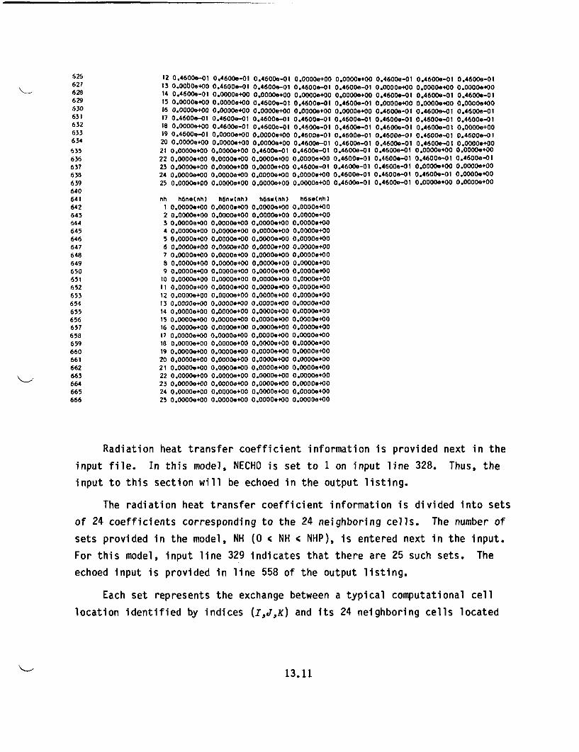
626627628629S30631632633634
635636637638639640641642643644645646647648649650651652653654655656657658659660661662663664665666
12 0.4600e-0l 0.4600e-01 0.4600e-01 0.00000+00 0.0000+00 0.4600e-0113 O.OObOe+oO 0.4600.-01 0.4600e-01 0.4600e-01 0.4600e-01 0.0000+0014 0.4600e-01 0.0000e+00 0.0000.+00 0.0000e+00 0.0000e+00 0.4600e-0115 0.0000e+00 0.0000.+00 0.4600e-01 0.4600e-01 0.4600e-01 0.0000o+0016 0.0000e+00 0.0000e+00 0.00000+00 0.0000.+00 0.0000.+00 0.4600e-Ot17 0.4600e-o0 0.4600e-01 0.4600e-01 0.4600e-01 0.4600e-01 0.4600e-0118 0.0000e+00 0.4600e-Ot 0.4600e-01 0.4600e-01 0.4600e-01 0.46000-0119 0.4600e- 0.0000.+00 0.0000O+00 0.4600e-01 0.4600e-01 0.4600e-0120 0.0000e+00 0.0000e+00 O.OOOOe+OO 0.4600e-01 0.4600e-01 0.46000-0121 0.0000e+00 0.0000e+00 0.46000-01 0.4600e-01 0.4600e-01 0.4600e-0122 0.0000e+00 0.0000e+00 0.0000e+00 0.0000e+00 0.4600e-01 0.4600e-0123 0.0000e+00 0.0000e+00 0.0000e+00 0.4600e-01 0.4600e-01 0.4600e-0124 O.OOOOe4OO 0.0000e+00 0.0000e+00 0.0000e+00 0.4600e-01 0.4600e-0125 0.0000e+00 0.0000e+00 0.0000e+00 0.0000e+00 0.4600e-01 0.4600e-01
0.46000-01 0.4600e-010.0000.+00 0.0000+000.4600e-01 0.4600e-010.0000e+00 0.0000.+000.4600e-Ot 0.46008-010.4600e-01 0.4600.-010.4600e-01 0.0000e+000.4600e-01 0.4600.-a10.4600e-01 0.0000e+000.0000.e00 0.00000+000.4600e-01 0.4600e-010.0000.+00 0.00000+000.4600e-01 0.0000e+000.0000e+00 0.0000e+00
nh h6ne(nh) h6nw(nh) h6sw(nh) h6se(nh)I 0.00Oe+00 0.0000.+00 0.0000.+00 0.0000e+002 0.00000+00 0.0000.+00 0.00000+00 0.0000e+003 0.0000+00 0.0000e+00 0.0000e+00 0.0000e+004 0.0000e+00 0.0000e+00 0.0000e+00 0.0000e+005 0.0000e+00 0.0000e+00 0.0000e+00 0.0000e+006 0.0000.+00 0.00000+00 0.0000e+00 0.0000.+007 0.0000e+00 0.0000e+00 0.0000e+00 0.0000e+008 0.OOOOe+00 0.0000e+00 0.0000.+00 0.0000e+009 0.0000e400 0.0000oe+00 0.0000e+00 0.0000+0010 0.00000+00 0.00000+00 0.0000.+00 0.0000e+0011 0.0000e+00 0.00OOe+00 0.0000e+00 0.0000e+0012 0.0000e+00 0.0000e+0013 0.0000e+00 0.0000e+0014 0.0000e+00 0.0000e+0015 0.0000e+00 0.0000e+0016 0.0000e+00 0.0000e+0017 0.0000e+00 0.0000e+0018 0.0000e+00 0.0000e+0019 0.0000+00 O.OOOe+00
20 0.0000e+00 0.0000e+0021 0.0000.+00 0.0000+0022 0.0000e+00 0.0000e+0023 0.0000.+00 O.OOOOe+OO24 0.0000e+00 0.0000e+0025 0.0000e+00 0.0000.+00
0.0000e+00 0.0000e+000.0000+00 0.000 004000.0000+00 0.0000e+000.0000e+00 0.0000e+000.0000e+00 0.0000+000.0000e+00 0.0000e+000.0000e+00 0.0000e+000.0000e+00 0.0000e+000.0000+00 0.OOOOe+000.0000.400 0.0000e+000.0000.+00 0.00000+000.0000.400 0.0000.4000.0000e+00 0.0000e+000.0000e+00 0.0000e400
Radiation heat transfer coefficient information is provided next in the
input file. In this model, NECHO is set to 1 on input line 328. Thus, the
input to this section will be echoed in the output listing.
The radiation heat transfer coefficient information is divided into sets
of 24 coefficients corresponding to the 24 neighboring cells. The number of
sets provided in the model, NH (O ' NH 4 NHP), is entered next in the input.
For this model, input line 329 indicates that there are 25 such sets. The
echoed input is provided in line 558 of the output listing.
Each set represents the exchange between a typical computational cell
location identified by indices (IJ,K) and its 24 neighboring cells located
13.11
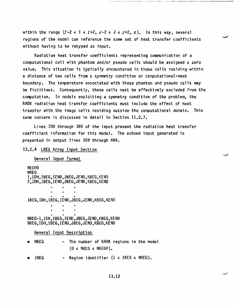
within the range (I-2 < I < I+2, J-2 c J < J+2, K). In this way, several
regions of the model can reference the same set of heat transfer coefficients
without having to be retyped as input.
Radiation heat transfer coefficients representing communication of a
computational cell with phantom and/or pseudo cells should be assigned a zero
value. This situation is typically encountered in those cells residing within
a distance of two cells from a symmetry condition or computational-mesh
boundary. The temperature associated with these phantom and pseudo cells may
be fictitious. Consequently, these cells must be effectively excluded from the
computation. In models exploiting a symmetry condition of the problem, the
RADR radiation heat transfer coefficients must include the effect of heat
transfer with the image cells residing outside the computational domain. This
same concern is discussed in detail in Section 11.2.7.
Lines 330 through 366 of the input present the radiation heat transfer
coefficient information for this model. The echoed input generated is
presented in output lines 559 through 666.
13.2.4 LREG Array Input Section
General Input Format
NECHONREG1,IDH,IBEG,IEND,JBEG,JEND,KBEG,KEND2, IDH,IBEG,IEND,JBEG,JEND,KBEG,KEND
IREG, IDH, IBEG, IEND,JBEG,JEND,KBEG,KEND
NREG-1, IONIBEGIENDJBEGJENDKBEG,KENDNREG,IDH,IBEG,IEND,JBEG,JEND,KBEG,KEND
General Input Description
* NREG - The number of RADR regions in the model
(O NREG < NREGP).
* IREG - Region identifier (1 4 IREG 4 NREG).
13.12
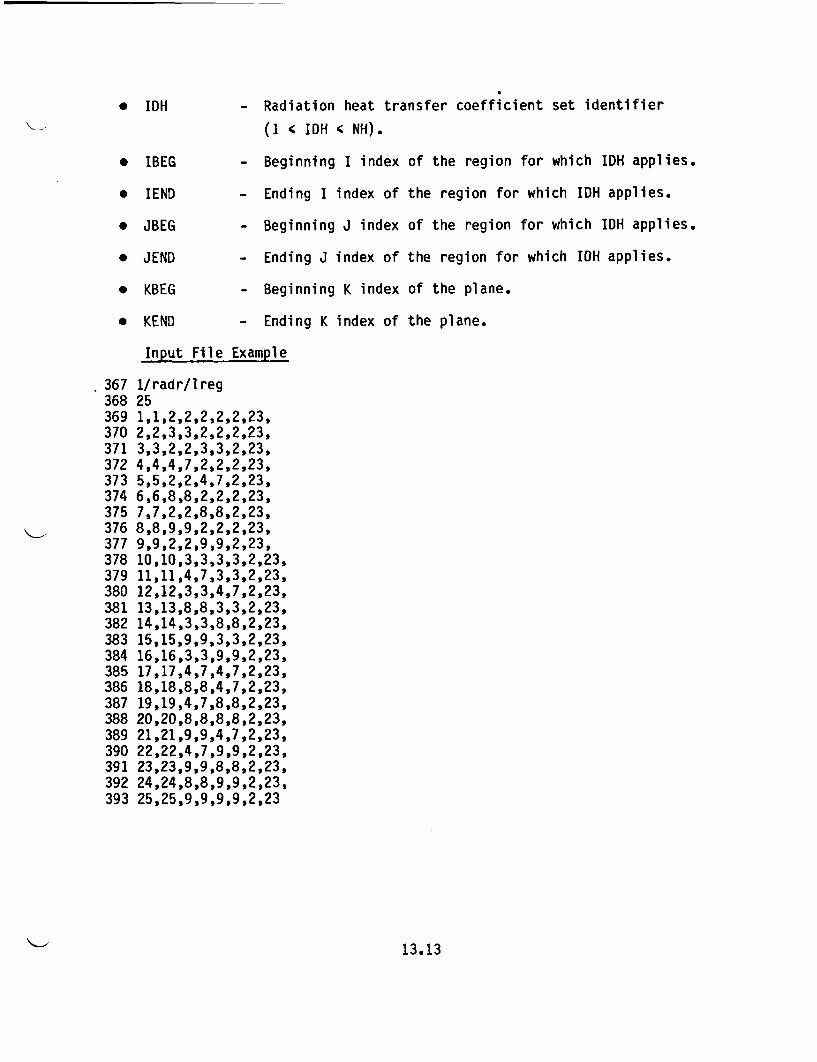
* IDH - Radiation heat transfer coefficient set identifier
(1 < IDH < NH).
* IBEG - Beginning I index of the region for which IDH applies.
* IEND - Ending I index of the region for which IDH applies.
* JBEG - Beginning J index of the region for which IDH applies.
* JEND - Ending J index of the region for which IDH applies.
* KBEG - Beginning K index of the plane.
* KEND - Ending K index of the plane.
Input File Example
367 1/radr/lreg368 25369 1,1,2,2,2,2,2,23,370 2,2,3,3,2,2,2,23,371 3,3,2,2,3,3,2,23,372 4,4,4,7,2,2,2,23,373 5,5,2,2,4,7,2,23,374 6,6,8,8,2,2,2,23,375 7,7,2,2,8,8,2,23,376 8,8,9,9,2,2,2,23,377 9,9,2,2,9,9,2,23,378 10,10,3,3,3,3,2,23,379 11,11,4,7,3,3,2,23,380 12,12,3,3,4,7,2,23,381 13,13,8,8,3,3,2,23,382 14,14,3,3,8,8,2,23,383 15,15,9,9,3,3,2,23,384 16,16,3,3,9,9,2,23,385 17,17,4,7,4,7,2,23,386 18,18,8,8,4,7,2,23,387 19,19,4,7,8,8,2,23,388 20,20,8,8,8,8,2,23,389 21,21,9,9,4,7,2,23,390 22,22,4,7,9,9,2,23,391 23,23,9,9,8,8,2,23,392 24,24,8,8,9,9,2,23,393 25,25,9,9,9,9,2,23
13.13
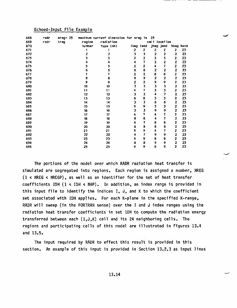
Echoed-Input File Example
668 radr nreg= 25 maximum current dimension for nreg Is 25669 radr Ireg region radiation call location670 number type (nh) Ibeg lend Jbeg jend kbeg kend671 1 1 2 2 2 2 2 23672 2 2 3 3 2 2 .2 23673 3 3 2 2 3 3 2 23674 4 4 4 7 2 2 2 23675 5 5 2 2 4 7 2 23676 6 6 8 8 2 2 2 23677 7 7 2 2 8 8 2 23678 8 8 9 9 2 2 2 23679 9 9 2 2 9 9 2 23680 10 10 3 3 3 3 2 23681 11 11 4 7 3 3 2 23682 12 12 3 3 4 7 2 23683 13 13 8 8 3 3 2 23684 14 14 3 3 8 8 2 23685 15 15 9 9 3 3 2 23686 16 16 3 3 9 9 2 23687 17 17 4 7 4 7 2 23688 18 18 8 8 4 7 2 23689 19 19 4 7 8 8 2 23690 20 20 8 8 8 8 2 23691 21 21 9 9 4 7 2 23692 22 22 4 7 9 9 2 23693 23 23 9 9 8 8 2 23694 24 24 8 8 9 9 2 23695 25 25 9 9 9 9 2 23
The portions of the model over which RADR radiation heat transfer is
simulated are segregated into regions. Each region is assigned a number, NREG
(1 < NREG c NREGP), as well as an identifier for the set of heat transfer
coefficients IDH (1 c IDH < NHP). In addition, an index range is provided in
this input file to identify the indices I, J, and K to which the coefficient
set associated with IDH applies. For each K-plane in the specified K-range,
RADR will sweep (in the FORTRAN sense) over the I and J index ranges using the
radiation heat transfer coefficients in set IDH to compute the radiation energy
transferred between each (I,J,K) cell and its 24 neighboring cells. The
regions and participating cells of this model are illustrated in Figures 13.4
and 13.5.
The input required by RADR to effect this result is provided in this
section. An example of this input is provided in Section 13.2.3 as input lines
13.14
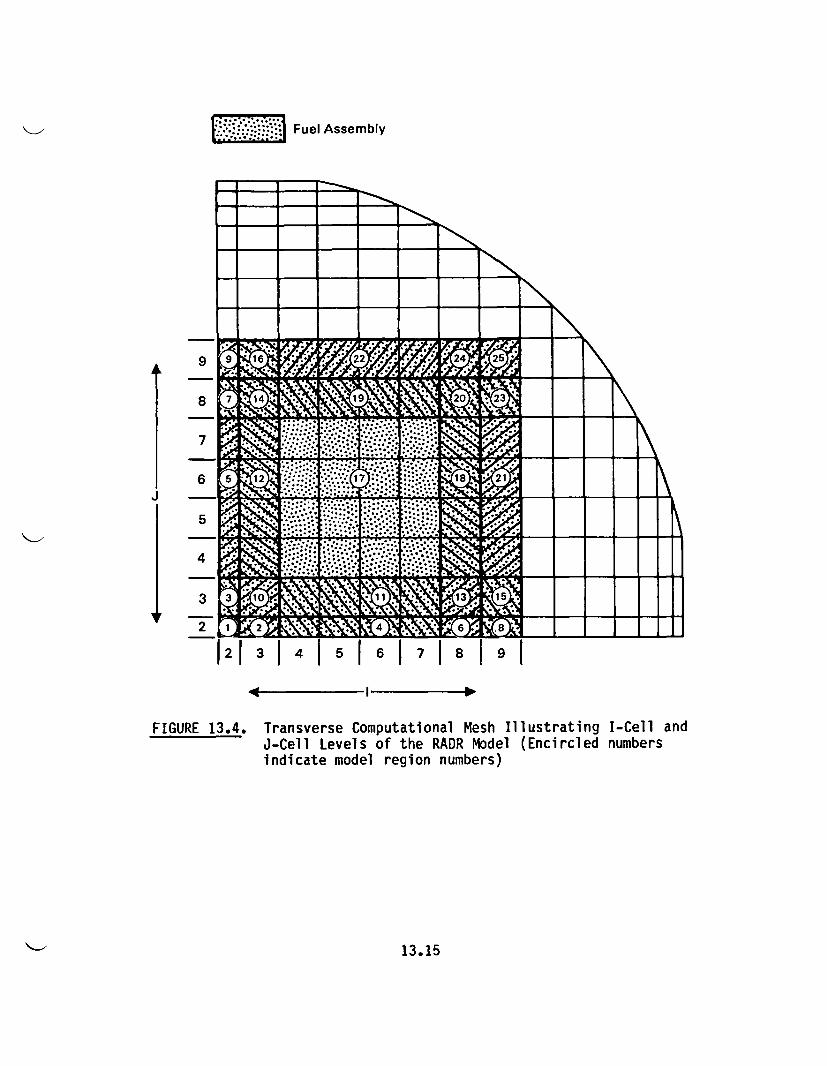
Fuel Assembly
I
FIGURE 13.4. Transverse Computational Mesh Illustrating I-Cell andJ-Cell Levels of the RADR Model (Encircled numbersindicate model region numbers)
13.15
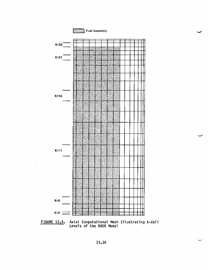
.. : Fuel Assembly
K=24
K=21
K=1 6
K=11
K=6
K=3 -
C _ ... ..... I I I 1 1
.... ., . .. 'm r l
... ... . . ,..m . I I 1 1
,.. .. 0 ... W n.... ...E..g . ......
.. ........ ..WW
FIGURE 13.5. Axial Computational Mesh Illustrating K-CellLevels of the RADR Model
13.16
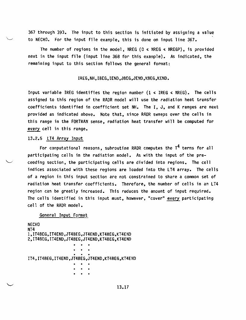
367 through 393. The input to this section is initiated by assigning a value
to NECHO. For the input file example, this is done on input line 367.
The number of regions in the model, NREG (O < NREG 4 NREGP), is provided
next in the input file (input line 368 for this example). As indicated, the
remaining input to this section follows the general format:
IREG,NH,IBEG,IEND,JBEG,JEND,KBEG,KEND.
Input variable IREG identifies the region number (1 < IREG < NREG). The cells
assigned to this region of the RADR model will use the radiation heat transfer
coefficients identified in coefficient set NH. The I, J, and K ranges are next
provided as indicated above. Note that, since RADR sweeps over the cells in
this range in the FORTRAN sense, radiation heat transfer will be computed for
every cell in this range.
13.2.5 LT4 Array Input
For computational reasons, subroutine RADR computes the T4 terms for all
participating cells in the radiation model. As with the input of the pre-
ceeding section, the participating cells are divided into regions. The cell
indices associated with these regions are loaded into the LT4 array. The cells
of a region in this input section are not constrained to share a common set of
radiation heat transfer coefficients. Therefore, the number of cells in an LT4
region can be greatly increased. This reduces the amount of input required.
The cells identified in this input must, however, "cover" every participating
cell of the RADR model.
General Input Format
NECHONT41,IT4BEG,IT4END,JT4BEG,JT4END,KT4BEG,KT4END2,IT4BEG,IT4END,JT4BEG,JT4END,KT4BEG,KT4END
IT4,IT4BEG,IT4END,JT4BEG,JT4END,KT4BEG,KT4END* *
* * .
* * .
13.17
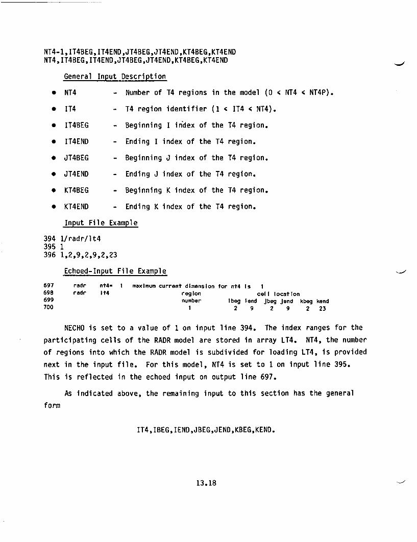
NT4-1,IT4BEG,IT4END,JT4BEG,JT4END,KT4BEG,KT4ENDNT4,IT4BEG,IT4END,JT4BEG,JT4END,KT4BEG,KT4END
General Input Description
* NT4 - Number of T4 regions in the model (O < NT4 < NT4P).
* 1T4 - T4 region identifier (1 < IT4 < NT4).
* IT4BEG - Beginning I index of the T4 region.
* IT4END - Ending I index of the T4 region.
* JT4BEG - Beginning J index of the T4 region.
* JT4END - Ending J index of the T4 region.
* KT4BEG - Beginning K index of the T4 region.
* KT4END - Ending K index of the T4 region.
Input File Example
394 1/radr/lt4395 1396 1,2,9,2,9,2,23
Echoed-Input File Example
697 radr nt4 1 maximum current dimension for nt4 Is 1698 radr It4 region cell location699 number Ibeg lend Jbeg Jend kbeg kend700 1 2 9 2 9 2 23
NECHO is set to a value of 1 on input line 394. The index ranges for the
participating cells of the RADR model are stored in array LT4. NT4, the number
of regions into which the RADR model is subdivided for loading LT4, is provided
next in the input file. For this model, NT4 is set to 1 on input line 395.
This is reflected in the echoed input on output line 697.
As indicated above, the remaining input to this section has the general
form
IT4,IBEG,IEND,JBEG,JEND,KBEG,KEND.
13.18
IT4 (1 4 IT4 4 NT4) is the region number for this set of indices comprising
the computational cells (I,J,K) where IBEG 4 I IEND, JBEG 4 J 4 JEND, and
KBEG 4 K 4 KEND. This input is presented in input line 396 for the model
discussed herein. The corresponding echoed input is presented in output lines
698 through 700.
13.2.6 Discussion of Input Example
To aid understanding of the interconnection between the input sections of
this routine, consider LREG region number 1 in Figure 13.4. This region
represents a portion of the computational domain swept-out by cells (2,2,2 4
K 4 23) - essentially a pencil of cells located at (I = 2, J = 2) and covering
K planes 2 through 23. RADR will compute the radiation heat transfer between
each of the neighboring 24 cells in the range (O I < 4, 0 < J 4 4, K) and the
cell at (2,2,K) for each of the 22 K-planes. The radiation heat transfer
coefficients used in these computations are carried in the first coefficient
set (NH = 1). Thus, for example, the radiation heat transfer coefficient used
for communication between cells (2,4,K) and (2,2,K) is identified as h4n(1) =
0.005; that between cells (4,4,K) and (2,2,K) is h6ne = 0. Initialization of
the T4 temperatures for the participating cells of this region are "covered" in
LT4 region number 1. Note that the phantom cells (index I or J = 1) and some
pseudo-cells (index I or J = 0) are included in the LREG region. These cells
are not "covered" by the LT4 region. The "temperature" for each of these cells
is therefore set to zero by the initialization procedure. However, their
effect is excluded from the RADR model by the zero entries in the radiation
heat transfer coefficients h2w(1), h2s(1), h3nw(1), h3sw(1), h3se(1), h4w(1),
h4s(1), h5nnw(1), h5wnw(1), h5wsw(1), h5ssw(1), h5sse(1), h5ese(1), h6nw(1),
h6sw(1), and h6se(1). Due to the quarter symmetry exploited in this problem,
some of these cell locations do coincide with image cells. For example,
coefficient h3ne(1) must include the effect of the communication between cell
(3,3,K) and (2,2,K) and its image energy-flow path, (1,1,K) and (2,2,K).
As in subroutine RADC, the matrix of heat transfer coefficients must be
symmetric to ensure energy conservation. For example, the radiation heat
transfer coefficient used in computing the energy received by the cell at
13.19

(8,8,K) from the cell at (7,6,K) [h5ssw(20) = 0.046] must equal that used in
computing the energy received by cell (7,6,K) from cell (8,8,K) [h5nne(17) =
0.046].
13.2.7 Input Example When RADR Is Not Used
If subroutine RADR is not used in the simulation, then only the following
lines of input are required:
1/radr01/radr/h01/radr/lreg01/radr/lt40
13.20
14.0 SUBROUTINE REBA
Subroutine REBA provides an optional procedure for acceleration of the
energy equation solution when a steady state is sought.
14.1 REBA FUNCTIONS
REBA solves steady-state energy balance equations on a coarse mesh made up
of three regions in each of the KP-2 active computational K-planes. The three
regions at a given K-plane are the rectangular grid region, the interface
cells, and the cylindrical grid region.
The merits and constraints of a coarse-mesh solution of the energy equa-
tion in accelerating progress toward steady state were discussed in Chap-
ter 7.0, Subroutine REBT. Some admonitions there are also applicable to use of
REBA. Use of REBA should be deferred until enough time-steps are taken that
properties and flows have "settled down" somewhat to near-physical values. The
axially coupled three-radial-region solutions in REBA are sufficiently effec-
tive, however, in achieving a rough temperature distribution that its use is
recommended for simulations that use both the rectangular and cylindrical grid
features.
The pattern of calls to REBA is set in Program MAIN by input variables
REBAON, NREB, and NREBN. The user may find it advantageous to monitor the
progress toward the steady-state solution before and after use of REBA by look-
ing at the maximum temperature change per time-step, and also by looking at
power balance information that can be calculated and printed by Subroutine
QINFO. See Chapters 15.0 and 29.0 for the QINFO features.
A feature provided in REBA to avoid potential overcompensation is a maxi-
mum allowable magnitude for the temperature change from the REBA coarse-mesh
solution. If in a given K-plane a temperature change ST' is calculated for one
of the three regions, the amount of temperature change ST added to the evolving
temperatures for that region is
ST = SIGN(MIN(ABS(ST'),DTMAX),6T')
14.1
where the FORTRAN SIGN function gives the algebraic sign of the second argument
(6T' in this case) to the magnitude of the first argument (the smaller of 16T'I
and DTMAX, in this case).
A printout option in REBA allows displaying "divergence error" quantities.
In REBA, a divergence error for a cell is calculated by net heat flow into the
cell, which should be zero in steady state. The divergence error quantities
printable in REBA are the sums of divergence errors over the regions (rec-
tangular, boundary, and cylindrical) of a K-plane. The largest sum for any
K-plane for each region can be printed.
14.2 PARAMETER STATEMENT INFORMATION
Parameters appearing in subroutine REBA that were discussed in Chap-
ter 4.0, Subroutine GRID, include:
IP,JP,KP,ISP,JSP,KBP,KTP
Additional dimensioning parameters in subroutine REBA that are discussed in
Chapter 25.0, Subroutine CROUT, include:
ICRP,JCRP
14.3 INPUT FORMAT
14.3.1 Overview
The schedule for calls to REBA is set in Program MAIN. The input here
sets a maximum allowable temperature change from the coarse grid solution, and
also sets the level of printout desired.
14.3.2 REBA Input Block
General Input Format
NECHODTMAX,INFO
14.2
General Input Description
* NECHO - Echoing switch for this section of input. If input isto be echoed, then NECHO = 1; otherwise, 0.
* DTMAX - The upper bound on the magnitude of the temperaturechange to add for any of the three regions at aK-plane from the coarse-mesh solution.
* INFO - An integer flag variable for printout of results. IfINFO = 1, REBA will report the K-plane at which thedivergence error sum is largest for each of the threeregions (rectangular grid, interface cells, cylin-drical grid) and the value of that divergence errorsum. Note that calculating this information takessome (though not major) effort, so it should be doneonly as needed. If INFO = 0, this information is notreported.
Input File Example
1591 1/reba1592 20.0,1
Echoed Input File Example
949950 reba dtmaxz0.200e+02 Info=1951
The input file asks for echoing (line 1591), sets maximum temperaturechange in a region to 20C (line 1592), and asks for a printout of divergenceerror information with INFO = 1 on line 1592. A typical line of divergenceerror information printed in response to INFO = 1 on a call to REBA is:
reba Info-1 dtmax-0.37ie-01 dimax. 0.402e-01 ki-30 dbmax-0.t33e-01 kb.I5 dsmax- 0.386e-08 ks- 3
This REBA printout line gives the maximum temperature change DTMAX thatactually occurred in the current call to REBA, the maximum divergence errorDIMAX for the interior (rectangular grid) region, the K-plane KI = 30 where itoccurred, the maximum divergence error DBMAX for the boundary or interface
14.3

region, the K-plane KB = 15 where it occurred, the maximum divergence DSMAX on
the side or cylindrical grid region, and the K-plane KS = 3 where it occurred.
14.4
15.0 SUBROUTINE QINFO
At the conclusion of a run, a user may optionally print net heat flows to
various portions of the cask and heat fluxes in the inside of the cask. Sub-
routine QINFO implements the process of determining heat flows using geometri-
cal information and current temperatures and thermal resistances.
15.1 PARAMETER STATEMENT INFORMATION
Subroutine QINFO requires the specification of parameters IP, JP, KP, KBP,
and KTP. These parameters define the overall computational mesh and are des-
cribed in Chapter 4.0, Subroutine GRID. No additional parameters are needed in
Subroutine QINFO.
15.2 INPUT FORMAT
Subroutine QINFO does not read information from the input file. No user
attention is required other than selecting appropriate input file options as
described in Chapter 3.0, Program MAIN.
15.1
16.0 SUBBROUTINE HYDRO
This subroutine serves as a gateway to all other subroutines required for
the solution of the fluid momentum and continuity equations. Subroutine HYDRO
is always called in the initialization phase of a run to set a number of con-
stants and arrays. If a momentum solution is desired, then this subroutine is
called once each time-step to update temperature-dependent properties, call
other subroutines, and provide diagnostic information.
The first operation undertaken in this subroutine is to read the input
file. The information contained on the input file includes:
* minimum and maximum allowed values of the momentum time-step
* reference pressure, temperature, and density for the gas within the
cask
* gravitational vector orientation with respect to the cask
* temperature dependence of gas viscosity
* viscosity specifications to account for fluid flow obstructions and
free-slip boundary conditions
* provision to monitor selected mass fluxes during a run.
The above information must be on the input file even if a momentum solution is
not desired, to satisfy list-directed read requirements. If no momentum solu-
tion is desired, such as for a conduction-only application, then the informa-
tion on the input file need not represent a physically realizable system.
There are certain other control parameters on the input file that relate
to simulating transient applications. This documented version of the code is,
however, intended for only steady-state applications. To allow for potential
future extension of the code and its documentation, input specifications relat-
ing to a transient mode of operation have been retained. In the general input
descriptions in this chapter, parameters related to the transient mode are
identified, a brief indication of the function given, and the appropriate value
to be used is provided.
16.1
If a solution to the momentum and continuity equations is desired (enabled
by setting NOVEL = 0 in Program MAIN), then subroutine HYDRO will call the
appropriate subroutines once each time-step. The calling sequence is:
* subroutine MOMX, MOMY, and MOMZ (Chapter 19.0) for solution of tilde
mass fluxes - Tilde mass fluxes are tentative mass fluxes that do not
yet satisfy continuity because they are based on old-time pressures.
* subroutine PDG (Chapter 20.0) for computation of the divergence error
of the tilde mass fluxes and construction of the discrete form of the
continuity equation
* subroutine PITER (Chapter 21.0), which directs the solution of the
continuity equation expressed in terms of pressure changes.
After satisfaction of the pressure (continuity) equation, the pressure
changes are returned to subroutine HYDRO to update the tilde mass fluxes so
that they satisfy conservation of mass. The next momentum time-step is com-
puted automatically based on the current time-step, the tilde mass-flux con-
tinuity error, and the computational effort required to satisfy the pressure
(continuity) equation. The new time-step may be adjusted up or down to meet
the specified optimum tilde mass-flux continuity error and specified optimum
computational cycles for the pressure equation. Finally, those mass fluxes
designated for monitoring are sent to the output file.
16.1 PARAMETER STATEMENT INFORMATION
Subroutine HYDRO requires the specification of parameters IP, JP, KP, KBP,
and KTP. These parameters define the overall computational mesh and are des-
cribed in Chapter 4.0, Subroutine GRID. Four additional parameters, local to
this subroutine, are required for specification of fluid viscosities and
printing options:
* NREGP - This parameter is used to dimension an array that
holds information about regions of computational
cells requiring special treatment of viscosity.
The details of this special treatment are given in
Section 16.2.3. NREGP should be greater than or equal
16.2
to the number of regions. If no special regions are
required, then NREGP should equal 1.
* MONMXP,
MONMYP,
MONMZP
- Three parameters, each greater than or equal to 1,
that allow storage for mass fluxes mx, my, and/or mz
to be monitored at designated computational cells.
For example, if MONMXP = 4, then it is possible to
print mass fluxes in the x-direction every time-step
at up to four different locations. See Section 16.2.2
for further details.
16.2 INPUT FORMAT
16.2.1 Run Control Information
This section of input provides some of the information needed for opera-
tion of the momentum solution. Basic gas properties and gravitational vector
orientation are also specified here. The input file must be constructed as
shown, to satisfy list-directed read requirements--even if no momentum solution
is required.
General Input Format
NECHOCONVEK,EPSCON,MITMAX,THETAM,WM,ESTPFNDTYME,DTYMEN,DTYMAXNEWGAS,NEWVEL,EXTRAVPFREF,TFREF,DFREFGX,GY,GZCVISA,CVISB
General Input Description
* NECHO
* CONVEK
- Echoing switch for this section of input. If input is
to be echoed, then NECHO = 1; otherwise, 0.
- The convection of momentum terms may be deleted from
the linear momentum equations if desired. The terms
deleted are V.(0fi) where t is the velocity and A is
16.3
the mass flux. The terms are included if CONVEK =
1.0; they are deleted if CONVEK = O.O.
* EPSCON - The maximum allowable continuity error to
if both momentum and continuity equations
satisfied each time-step. This option is
transient applications; therefore, EPSCON
set equal to O.O.
be permitted
are to be
intended for
should be
0 MITMAX - The maximum number of solution cycles permitted to
satisfy both momentum and continuity equations each
time-step. This option is intended for transient
applications; therefore, MITMAX should be set equal to
0.
0 THETAM - New-time tilde mass fluxes may be computed based on a
mixture of old-time mass fluxes and new-time tilde
mass fluxes. THETAM sets the relative weighting and
should have the value of 0.5 for steady-state applica-
tions.
* WM
* ESTPF
A weighting factor in the momentum equations intended
for switching between transient and steady-state modes
of operation. A value of 1.0 is to be used for the
steady-state mode.
This constant is used to estimate new-time pressures
according to the expression
p = p + estpf * St Id (p - old)
The momentum equations and the continuity (pressure)
equation are not solved simultaneously; thus, the
coupling is explicit. Slight underrelaxation is, at
times, beneficial for stability. The value shown on
16.4
the input file example for estpf, -0.05, is usually
satisfactory. A best value is application-specific,
and, if necessary, is determined by trial.
* NDTYME - If a new momentum time-step is desired at the start of
a run, then ndtyme = 1; otherwise, ndtyme = 0. If the
run is started without a restart tape, then ndtyme =
1.
* DTYMEN - The value of the new initial momentum time-step.
* DTYMAX
* NEWGAS
* NEWVEL
* EXTRAV
* PFREF,
TFREF,
DFREF
- The maximum value of the momentum time-step. DTYMAX
will normally not exceed 1.0, and may be less for
steady-state applications.
- A switch that enables changing gas properties at the
start of a run for transient applications. NEWGAS
should be set to 0 for steady-state applications.
- This constant, if equal to 1, will set all mass fluxes
to zero at the start of any run. No action is taken
if NEWVEL equals 0.
- If EXTRAV has a value different from 1.0, then all
mass fluxes are reset at the start of any run accord-
ing to the expression m = EXTRAV * m. The new mass
fluxes still satisfy continuity.
- Reference pressure, temperature, and density for
the gas, used in the code to compute density according
to an equation of state,
reT f P
16.5
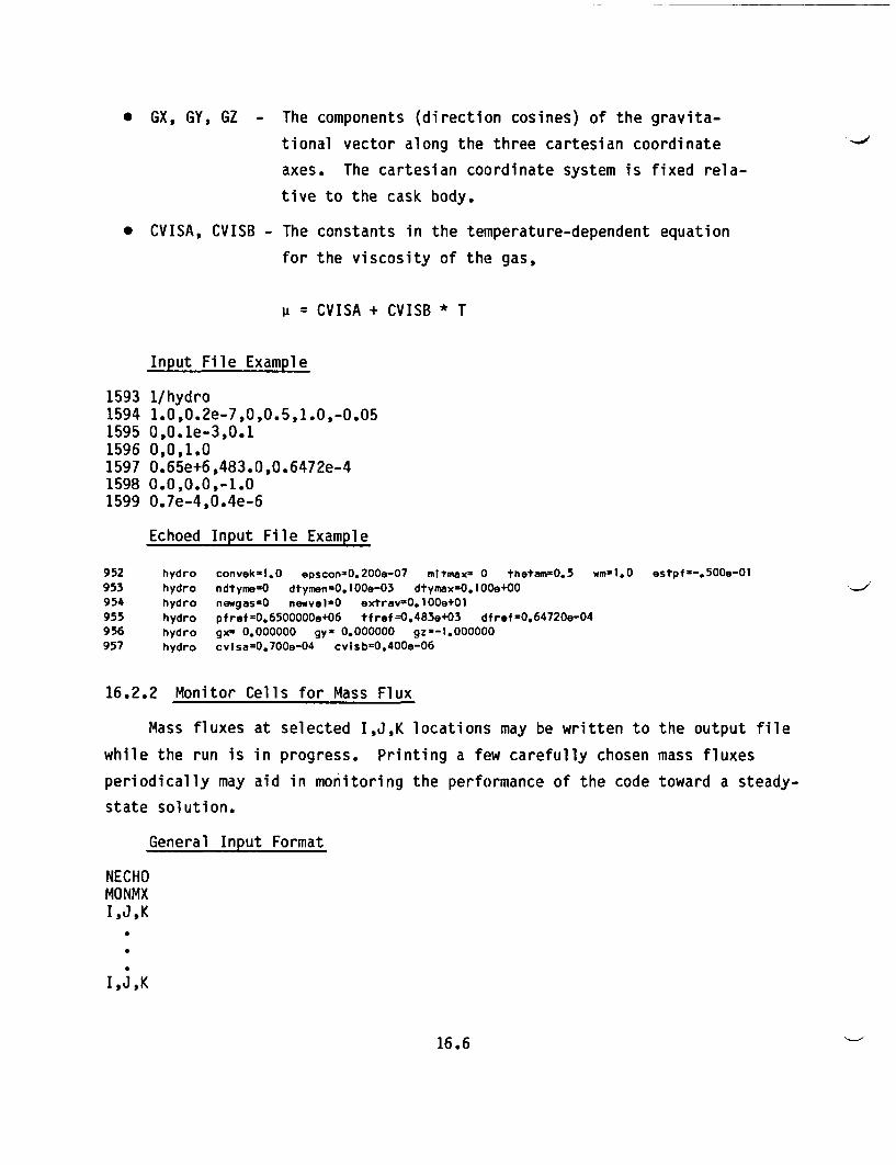
* GX, GY, GZ - The components (direction cosines) of the gravita-
tional vector along the three cartesian coordinate
axes. The cartesian coordinate system is fixed rela-
tive to the cask body.
* CVISA, CVISB - The constants in the temperature-dependent equation
for the viscosity of the gas,
P = CVISA + CVISB * T
Input File Example
1593 1/hydro1594 1.0,0.2e-7,0,0.5,1.0,-0.051595 0,0.le-3,0.11596 0,0,1.01597 0.65e+6,483.0,0.6472e-41598 0.0,0.0,-1.01599 0.7e-4,0.4e-6
Echoed Input File Example
952 hydro convekt1.0 epscon-0.200e-07 mitmax- 0 thetamn0.5 wmal.0 estpf=-.500e-01953 hydro ndtyme=O dtymen=0.100e-03 dtymax0.100e+00954 hydro newgas.0 newvelO eoxtrav*0.100e+01955 hydro pfref-O.6500000e+06 tfref-0.483e+03 dfref-0.64720e-04956 hydro gx= 0.000000 gy 0.000000 gz -1.000000957 hydro cvIsa=0.700e-0 4 cvisb=0.400e-06
16.2.2 Monitor Cells for Mass Flux
Mass fluxes at selected I,J,K locations may be written to the output file
while the run is in progress. Printing a few carefully chosen mass fluxes
periodically may aid in monitoring the performance of the code toward a steady-
state solution.
General Input Format
NECHOMONMXI,J,K
I,J,K
16.6
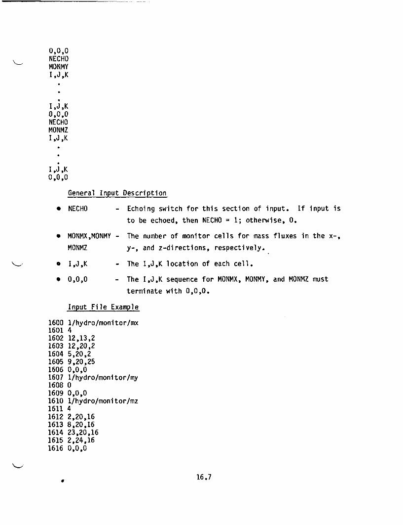
OO0ONECHOMONMYI,J,K
I,J,K0,0,0NECHOMONMZIJ,K
I ,J,KO,0,0
.
S
16001601160216031604160516061607160816091610161116121613161416151616
General Input Description
NECHO - Echoing switch for this section of input. If input is
to be echoed, then NECHO = 1; otherwise, 0.
MONMX,MONMY - The number of monitor cells for mass fluxes in the x-,
MONMZ y-, and z-directions, respectively.
I,J,K - The I,J,K location of each cell.
0,0,0 - The I,J,K sequence for MONMX, MONMY, and MONMZ must
terminate with 0,0,0.
Input File Example
1/hydro/monitor/mx412,13,212,20,25,20,29,20,25O,0,01/hydro/monitor/my0O,0,01/hydro/monitor/mz42,20,168,20,1623,20,162,24,160,0,0
16.7
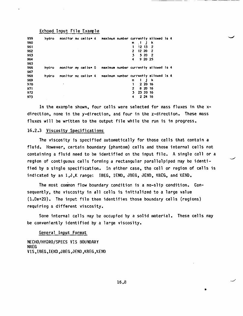
Echoed Input File Example
959 hydro monitor mx cells= 4 maximum number currently allowed Is 4960 m *t J k961 1 12 13 2962 2 12 20 2963 3 5 20 2964 4 9 20 25
965966 hydro monitor my cells- 0 maximum number currently allowed Is 4
967968 hydro monitor mz cellso 4 maximum number currently allowed Is 4
969 m I J k970 1 2 20 16
971 2 8 20 16972 3 23 20 16
973 4 2 24 16
In the example shown, four cells were selected for mass fluxes in the x-
direction, none in the y-direction, and four in the z-direction. These mass
fluxes will be written to the output file while the run is in progress.
16.2.3 Viscosity Specifications
The viscosity is specified automatically for those cells that contain a
fluid. However, certain boundary (phantom) cells and those internal cells not
containing a fluid need to be identified on the input file. A single cell or a
region of contiguous cells forming a rectangular parallelpiped may be identi-
fied by a single specification. In either case, the cell or region of cells is
indicated by an I,J,K range: IBEG, IEND, JBEG, JEND, KBEG, and KEND.
The most common flow boundary condition is a no-slip condition. Con-
sequently, the viscosity in all cells is initialized to a large value
(1.Oe+20). The input file then identifies those boundary cells (regions)
requiring a different viscosity.
Some internal cells may be occupied by a solid material. These cells may
be conveniently identified by a large viscosity.
General Input Format
NECHO/HYDRO/SPECS VIS BOUNDARYNREGVIS,IBEG,IEND,JBEG,JEND,KBEG,KEND
16.8
S
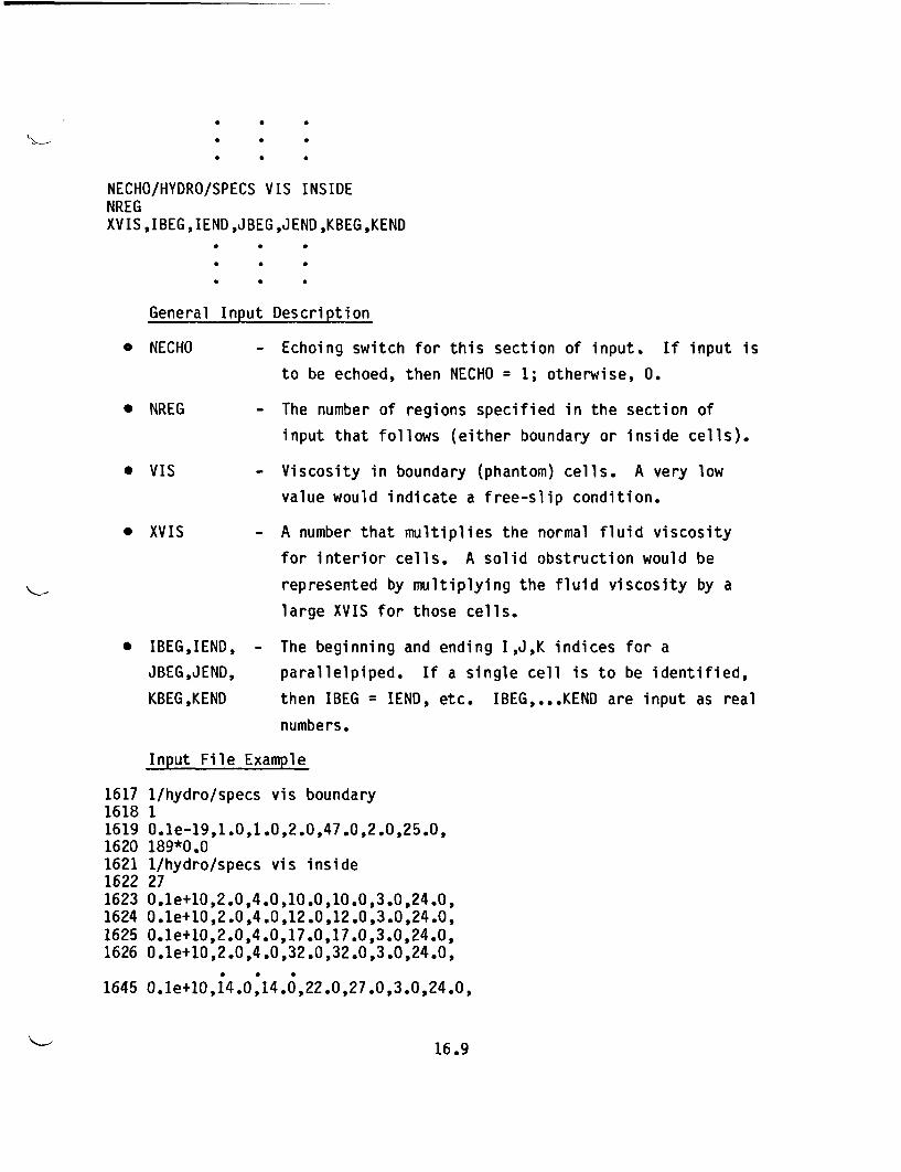
NECHO/HYDRO/SPECS VIS INSIDENREGXVIS,IBEG,IEND,JBEG,JEND,KBEG,KEND
* .
General Input Description
* NECHO - Echoing switch for this section of input. If input is
to be echoed, then NECHO = 1; otherwise, 0.
* NREG - The number of regions specified in the section of
input that follows (either boundary or inside cells).
* VIS - Viscosity in boundary (phantom) cells. A very low
value would indicate a free-slip condition.
* XVIS - A number that multiplies the normal fluid viscosity
for interior cells. A solid obstruction would be
represented by multiplying the fluid viscosity by a
large XVIS for those cells.
* IBEG,IEND, - The beginning and ending I,J,K indices for a
JBEG,JEND, parallelpiped. If a single cell is to be identified,
KBEG,KEND then IBEG = IEND, etc. IBEG,...KEND are input as real
numbers.
Input File Example
1617 1/hydro/specs vis boundary1618 11619 0.le-19,1.0,1.0,2.0,47.0,2.0,25.0,1620 189*0.01621 1/hydro/specs vis inside1622 271623 0.le+10,2.0,4.0,10.0,10.0,3.0,24.0,1624 0.le+10,2.0,4.0,12.0,12.0,3.0,24.0,1625 0.le+10,2.0,4.0,17.0,17.0,3.0,24.0,1626 O.le+10,2.0,4.0,32.0,32.0,3.0,24.0,
* . .
1645 O.le+10,14.0,14.0,22.0,27.0,3.0,24.0,
16.9
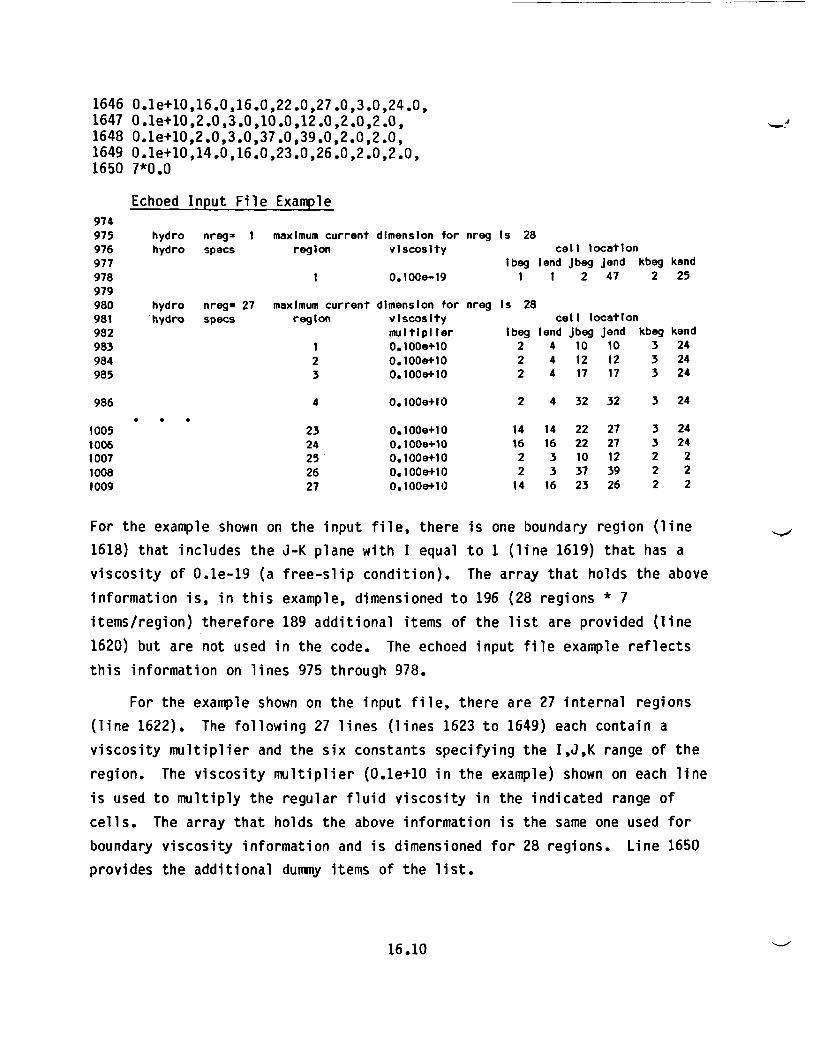
16461647164816491650
0.le+10,16.0,16.0,22.0,27.0,3.0,24.0,O.le+10,2.0,3.0,10.0,12.0,2.0,2.0,0.le+10,2.0,3.0,37.0,39.0,2.0,2.0,0.le+10,14.0,16.0,23.0,26.0,2.0,2.0,7*0.0
Echoed Input File Example974975976977978979980981982983984985
hydro nreg= Ihydro specs
maximum current dimension forregion viscosity
nreg Is 28call location
ibeg lend Jbeg Jend kbeg kend1 1 2 47 2 25I
hydro nreg- 27hydro specs
maximum currentregion
O.100s-19
dimension forviscositymultiplier0.1008+100.lOOe+100. lOOs+10
nreg Is 28cell location
Ibeg lend Jbeg Jend kbeg2 4 10 10 32 4 12 12 32 4 17 17 3
123
kend242424
986 4* * a
10051006100710081009
2324252627
0.l OOe+1 0
0.100e+100.1008+100.1OOe+100. OOe+100.OOe+10
2 4 32 32
14 14 22 2116 16 22 272 3 10 122 3 37 3914 16 23 26
3 24
3 243 242 22 22 2
For the example shown on the input file, there is one boundary region (line
1618) that includes the J-K plane with I equal to 1 (line 1619) that has a
viscosity of 0.1e-19 (a free-slip condition). The array that holds the above
information is, in this example, dimensioned to 196 (28 regions * 7
items/region) therefore 189 additional items of the list are provided (line
1620) but are not used in the code. The echoed input file example reflects
this information on lines 975 through 978.
For the example shown on the input file, there are 27 internal regions
(line 1622). The following 27 lines (lines 1623 to 1649) each contain a
viscosity multiplier and the six constants specifying the I,J,K range of the
region. The viscosity multiplier (0.le+10 in the example) shown on each line
is used to multiply the regular fluid viscosity in the indicated range of
cells. The array that holds the above information is the same one used for
boundary viscosity information and is dimensioned for 28 regions. Line 1650
provides the additional dummy items of the list.
16.10
17.0 SUBROUTINE PINIT
Subroutine PINIT initializes the pressure field assuming a static (zero
velocity) flow field within the domain. Consequently, the equation for the
pressure (obtained by setting each of the velocity component terms in the
momentum equations to zero), is solved initially. This equation is
- Vp + P+ = 0 (17.1)
PINIT sets up the matrix and vector components for the discrete form of this
equation. The actual solution for the pressure is performed in subroutines
PITER and PILES. Typically, HYDRA-II computes the gas properties using an
equation of state to relate pressure, density, and temperature. However, for
the purposes of the pressure initialization process in this routine only, the
fluid density is assumed constant.
HYDRA-II provides two options for setting the average pressure:
1. Set the desired average pressure directly.
2. Set the fluid mass in the domain.
Option 1 uses the reference fluid density, DFREF, specified as input to sub-
routine HYDRO in the computation for the pressure field. After Equation (17.1)
is solved, each nodal pressure is adjusted by a constant amount so that the
average pressure over the field equals FIXEDP if a value FIXEDP > 0.0 is input
to subroutine AVG. If the mass of the system is set as the constraint (option
2 above - invoked when FIXEDM > 0.0 is input to subroutine AVG), the cell den-
sity is adjusted to produce this specified mass. The cell pressures are sub-
sequently adjusted to be consistent with this density and the specified initial
temperature. In this case, the presence of any porous media, which have been
specified by the user to occupy some or all of the fluid cells (through the
input to subroutine PROPM), is accounted for to reduce the effective volume of
the domain.
The pressure field resulting from this initialization process is a func-
tion of, among other things, the orientation of the gravitational field vector,
17.1
4, relative to the computational domain's coordinate system. The direction
cosines defining the orientation of the gravitational field vector are GX, GY,
and GZ. These direction cosines are provided by the user as input to sub-
routine HYDRO. Vector 4 is then defined as
= (GX * + GY J + GZ k) | (17.2)
where *, J, and k are the unit vectors in the x-, y-, and z-directions of the
coordinate system, respectively, and 141 is the magnitude of the acceleration
due to gravity (= 980.665 cm/sec2 in HYDRA-lI).
Subroutine PINIT is not accessed in the event of:
1. a restart run (NREAD = 1 as input to MAIN)
2. no momentum-equation solution desired (NOVEL = 1 as input to MAIN).
In the first event, the pressure field is obtained from restart data. The
pressure field is irrelevant for the second event.
17.1 PARAMETER STATEMENT INFORMATION
Subroutine PINIT requires the specification of parameters IP, JP, KP, KBP,
and KTP. These data define the overall computational mesh and are described in
Chapter 4.0.
17.2 INPUT FORMAT
Subroutine PINIT does not require input data.
17.2
18.0 SUBROUTINE PROPM
The grid information has been provided in subroutine GRID, and much of the
thermo-fluid property information obtained through input to subroutine HYDRO.
Therefore, solution of the momentum equations in HYDRA-II requires only some
additional input regarding embedded flow obstructions. This information per-
tains to area blockages, cell porosities, and cell permeabilities. Two models
are available to the user for representing subgrid scale flow obstructions.
Flow paths in which a permeable substance is present may be modeled using a
Darcy-flow relationship. This Darcy-flow model may be used to represent the
entire range of permeability, from virtually unobstructed to essentially
plugged paths. For those flow paths occupied in part by an impermeable
obstruction, HYDRA-II allows the user to reduce the effective flow area to
simulate an orifice-induced pressure gradient.
Flow through porous media can be modeled by using any one of the PERMO,
PERMX, PERMY, and/or PERMZ input options provided in this routine. The
pressure gradient experienced from cell-to-cell as a result of the presence of
this porous media is modeled using the Darcy-flow relationship,
Vp p*PERMI m (18.1)
where p, il, and p are the pressure, viscosity, and density of the fluid in the
cell, respectively, i is the mass flux vector, and PERMI is the permeability
coefficient (with I = X, Y, or Z representing pressure gradients in the x-, y-,
or z-direction, respectively). Orthotropic permeability can be modeled by
specifying different values for the PERMX, PERMY, and PERMZ coefficients
associated with a given cell. The permeability for each physical cell of the
computational mesh is initialized to the input value PERMO. This value applies
to PERMX, PERMY, and PERMZ. Therefore, each cell is initially isotropic. The
prescribed permeability may then be overwritten with input to PERMX, PERMY,
and/or PERMZ as desired, to introduce directional preference in the model. An
impermeable cell is represented by a very small permeability coefficient. Con-
versely, a very porous cell is represented by a large permeability-coefficient.
18.1
The appropriate value to be assigned to PERMI at input may be estimated
from an order-of-magnitude analysis of the affected terms in the momentum equa-
tions. For example, an order-of-magnitude study of the ratio of Darcy-flow
induced pressure gradient to the viscous shear-stress gradient indicates that
these two terms will be of comparable importance if the permeability, PERMI, is
on the order of the square of the mesh size. Mathematically stated,
PERMI 62 (18.2)
where 6 is the characteristic cell size. Therefore, for cases in which Darcy-
flow modeling is desired, the permeability coefficient, PERMI, should be set to
a value on the order of the square of the local mesh size. To model both vir-
tually-impermeable and very permeable cells with this Darcy-flow model, PERMI
should be represented as follows:
* PERMI << 62 (or << (6Imin)2 in the global case) for virtually
impermeable cells.
* PERMI >> 62 for permeable cells (or >> (Slmax)2 for globally very
permeable cells.
"Plugging" of cells may be instituted either by the above process (i.e.,
specifying PERMI << 62) or by setting the cell viscosity to a relatively large
value. There is a subtle, but important, difference in these two approaches.
When using the cell viscosity to "plug" a cell, the blockage is assumed to
occur over the entire cell. The no-slip condition will then be effectively
applied at the cell faces. On the other hand, using the permeability
coefficient to "plug" a cell results in an induced drag that affects the mass
flow rates across the cell interfaces. The "no-slip" condition is therefore
effectively applied at the location of the mass flow rates, and is centered on
the surface of the cell interfaces. This amounts to adding an additional half-
a-cell width to the location of the "no-slip" condition. These ideas are illu-
strated in Figure 18.1. PERMI may be used to "plug" a cell in any or all of
the coordinate directions independently. On the other hand, using viscosity to
"*plug" a cell precludes flow through the cell in any direction.
18.2
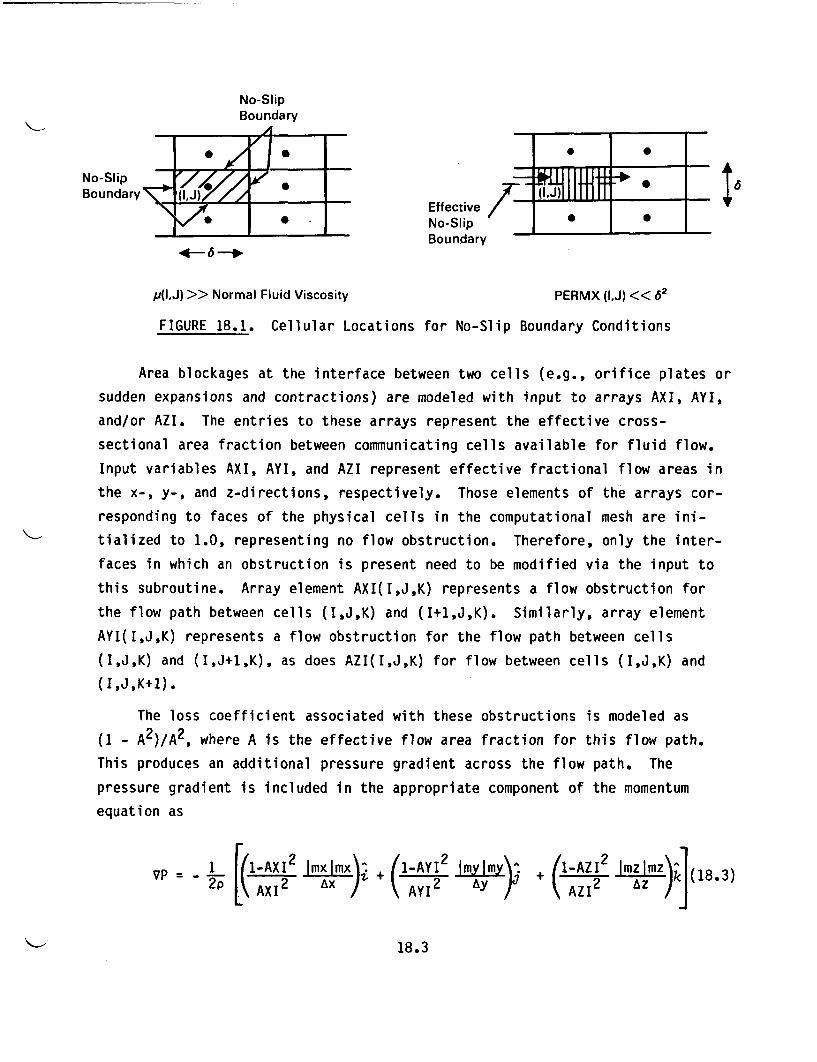
No-SlipBoundary
A
1,2I2 dilNo-Slip
0 0
EffectiveNo-SlipBoundary
6
lvo*. ; ' 1
p(lJ) >> Normal Fluid Viscosity PERMX (1,J) << 62
FIGURE 18.1. Cellular Locations for No-Slip Boundary Conditions
Area blockages at the interface between two cells (e.g., orifice plates or
sudden expansions and contractions) are modeled with input to arrays AXI, AYI,
and/or AZI. The entries to these arrays represent the effective cross-
sectional area fraction between communicating cells available for fluid flow.
Input variables AXI, AYI, and AZI represent effective fractional flow areas in
the x-, y-, and z-directions, respectively. Those elements of the arrays cor-
responding to faces of the physical cells in the computational mesh are ini-
tialized to 1.0, representing no flow obstruction. Therefore, only the inter-
faces in which an obstruction is present need to be modified via the input to
this subroutine. Array element AXI(I,J,K) represents a flow obstruction for
the flow path between cells (I,J,K) and (I+1,J,K). Similarly, array element
AYI(I,J,K) represents a flow obstruction for the flow path between cells
(I,J,K) and (I,J+1,K), as does AZI(I,J,K) for flow between cells (I,J,K) and
(I,J,K+1).
The loss coefficient associated with these obstructions is modeled as
(1 - A2)/A2, where A is the effective flow area fraction for this flow path.
This produces an additional pressure gradient across the flow path. The
pressure gradient is included in the appropriate component of the momentum
equation as
VP 2p AI ImxImx\ + 1-AYI2 Imylmy\ + -AZI2 Imz 3mzkl )VP = - L j(1- x + k 1 .3VP I. xi2 Ax / AYI2 Ay Kq AZI2 AZ 1~ 83
18.3
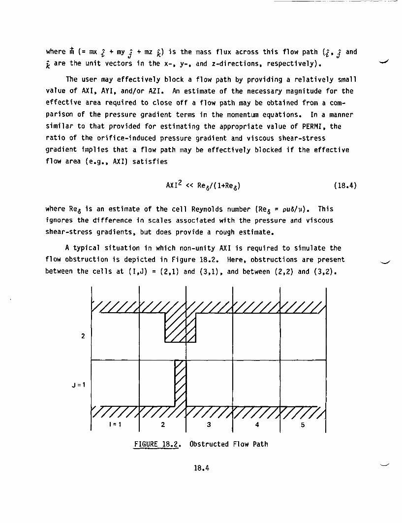
where i (= mx + my J + mz k) is the mass flux across this flow path ( and
are the unit vectors in the x-, y-, and z-directions, respectively).
The user may effectively block a flow path by providing a relatively small
value of AXI, AYI, and/or AZI. An estimate of the necessary magnitude for the
effective area required to close off a flow path may be obtained from a com-
parison of the pressure gradient terms in the momentum equations. In a manner
similar to that provided for estimating the appropriate value of PERMI, the
ratio of the orifice-induced pressure gradient and viscous shear-stress
gradient implies that a flow path may be effectively blocked if the effective
flow area (e.g., AXI) satisfies
AXI2 << Rea/(1+ReS) (18.4)
where Rea is an estimate of the cell Reynolds number (Re= puS/"). This
ignores the difference in scales associated with the pressure and viscous
shear-stress gradients, but does provide a rough estimate.
A typical situation in which non-unity AXI is required to simulate the
flow obstruction is depicted in Figure 18.2. Here, obstructions are present
between the cells at (I,J) = (2,1) and (3,1), and between (2,2) and (3,2).
.a2ZL� �z222 7////,XZZL22
J=1
4.
2
4 4 4.
I7=71tP -., -
//////4 5
FIGURE 18.2. Obstructed Flow Path
18.4
These obstructions reduce the effective flow area by 100% and 60%, respec-
tively. The corresponding input would be 10-6 (an entry of 0.0 would produce a
division-by-zero error) for the AXI associated with the path (2,1) +- (3,1),
and 0.4 for the AXI associated with the path (2,2) {+ (3,2).
With regard to the input variables AXI, AYI, and AZI, the presence of a
flow obstruction implies that:
* a restriction to flow exists in one or more of the coordinate
directions
* a no-slip condition be imposed for flow in directions parallel to the
obstruction surface.
The first item is addressed by specifying values for AXI, AYI, and/or AZI that
are in the range 0 < AXI, AYI, AZI < 1. The second item is addressed in the
coding of HYDRA-II. The momentum equation viscous-stress terms representing
drag to the flow in directions parallel to the obstruction surface are scaled
in the code to represent the no-slip condition imposed by the obstruction. For
example, when AXI * 1.0, the flow rates in the y- and z-directions will experi-
ence an additional drag at the cell interface due to the presence of this
obstruction.
The free-volume fraction of a cell can be modified from its default value
with the input to array POR. Values of 0.0 4 POR(I,J,K) 4 1.0 indicate that
the effective free volume of the cell associated with index (I,J,K) is
VOL(I,J,K) = POR(I,J,K)*DX(I)*DY(J)*DZ(K) (18.5)
where DX, DY, and DZ are the mesh sizes for the cell. For steady-state
applications, the volume influences the results for only those cases in which a
fixed mass is specified for the computational domain (FIXEDM > 0 as input to
subroutine AVG). When the average pressure is specified for the computational
domain (FIXEDP > 0 as input to subroutine AVG), POR has no effect on the com-
putation. Array POR is initialized to 0.0 for those cells outside the hydro-
dynamic portion of the computational domain, to 0.5 for those cells lying on
the interface between the Cartesian and cylindrical meshes (to simulate the
18.5
cells whose volumes are partially occupied by the domain enclosure), and to 1.0
for those cells located entirely within the hydrodynamic portion of the
computational domain.
As a final note, the effective loss coefficient for pressure-drop calcula-
tions is independent of flow speed (or, equivalently, flow rate) in the porous-
media model. On the other hand, the effective loss coefficient in modeling
flow obstructions with AXI, for example, is linearly dependent on the flow
speed. Therefore, by judiciously combining the two models and their coeffi-
cients, the user may simulate a segment of the drag curve for flow around a
body (e.g., cylinder or sphere). Attempts can then be made to match the
coefficients to produce the experimentally observed drag coefficient variation
in the Reynolds number range of interest.
18.1 PARAMETER STATEMENT INFORMATION
Only the overall grid specification information IP, JP, KP, KBP, and KTP
(described in Chapter 4.0) is required as PARAMETER information in PROPM.
18.2 INPUT FORMAT
18.2.1 Overview
Generally speaking, the input to subroutine PROPM can be divided into two
subsections:
* "iglobal" setting of the PERMX, PERMY, and PERMZ arrays
* loading of arrays AX, AY, AZ, AXI, AYI, AZI, and POR, as well as the
resetting of arrays PERMX, PERMY, and PERMZ by mesh blocks.
The input requirements for each of these subsections is provided in
Section 18.2.2.
18.2.2 "Global" Setting of PERMX, PERMY, and PERMZ
General Input Format
NECHOPERMO
18.6
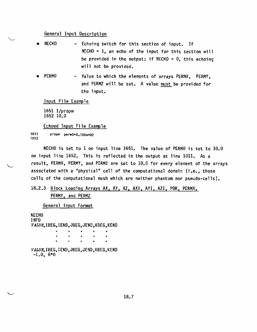
General Input Description
* NECHO - Echoing switch for this section of input. If
NECHO = 1, an echo of the input for this section will
be provided in the output; if NECHO = 0, this echoing
will not be provided.
* PERMO - Value to which the elements of arrays PERMX, PERMY,
and PERMZ will be set. A value must be provided for
the input.
Input File Example
1651 1/propm1652 10.0
Echoed Input File Example
1011 propm permo=o.lOOe+021012
NECHO is set to 1 on input line 1651. The value of PERMO is set to 10.0
on input line 1652. This is reflected in the output as line 1011. As a
result, PERMX, PERMY, and PERMZ are set to 10.0 for every element of the arrays
associated with a "physical" cell of the computational domain (i.e., those
cells of the computational mesh which are neither phantom nor pseudo-cells).
18.2.3 Block Loading Arrays AX, AY, AZ, AXI, AYI, AZI, POR, PERMX,
PERMY, and PERMZ
General Input Format
NECHOINFOVALUE, IBEG,IEND,JBEG,JEND,KBEG,KEND
VALUE, IBEG,IEND,JBEG,JEND,KBEG,KEND-1.0, 6*0
18.7
General Input Description
* NECHO - Echoing switch for this section of input. If
NECHO = 1, an echo of the input for this section will
be provided in the output; if NECHO = 0, this echoing
will not be provided.
* INFO - Switch to print the output file for the entire con-
tents of the array associated with this input section
(e.g., AXI or PERMY). Setting INFO = 1 will generate
this output listing; INFO = 0 will not.
* VALUE - Quantity to be loaded into this block of AX, AY, AZ,
AXI, AYI, AZI, POR, PERMX, PERMY, or PERMZ. A block
is defined as those cells covered by a sweep through
the I, J, and K index ranges. Loading is terminated
for a set of blocks with the sequence -1.0, 6*0. Up
to 1000 blocks may be loaded in each set. The AX set
of blocks is loaded first, followed by the AY, AZ,
AXI, AYI, AZI, POR, PERMX, PERMY, and PERMZ sets.
Loading in this order is essential. Input to arrays
AX, AY, and AZ has no significance to the steady-state
solution obtained by HYDRA-II. Therefore, no input is
provided to these arrays. As indicated in the sample
input presented in this section, only the terminator
sequence is provided as input to these arrays. The
input variable "VALUE" corresponds to a multiplier
when loading array POR. The affected elements of
array POR are set equal to the product of the input
value of POR multiplied by the cell volume
POR(I,J,K) = VALUE*DX(I)*DY(J)*DZ(K).
The volumes of those hydrodynamic cells lying on the
interface between Cartesian and cylindrical meshes are
halved to account for the cell bisection produced by
this interface.
18.8
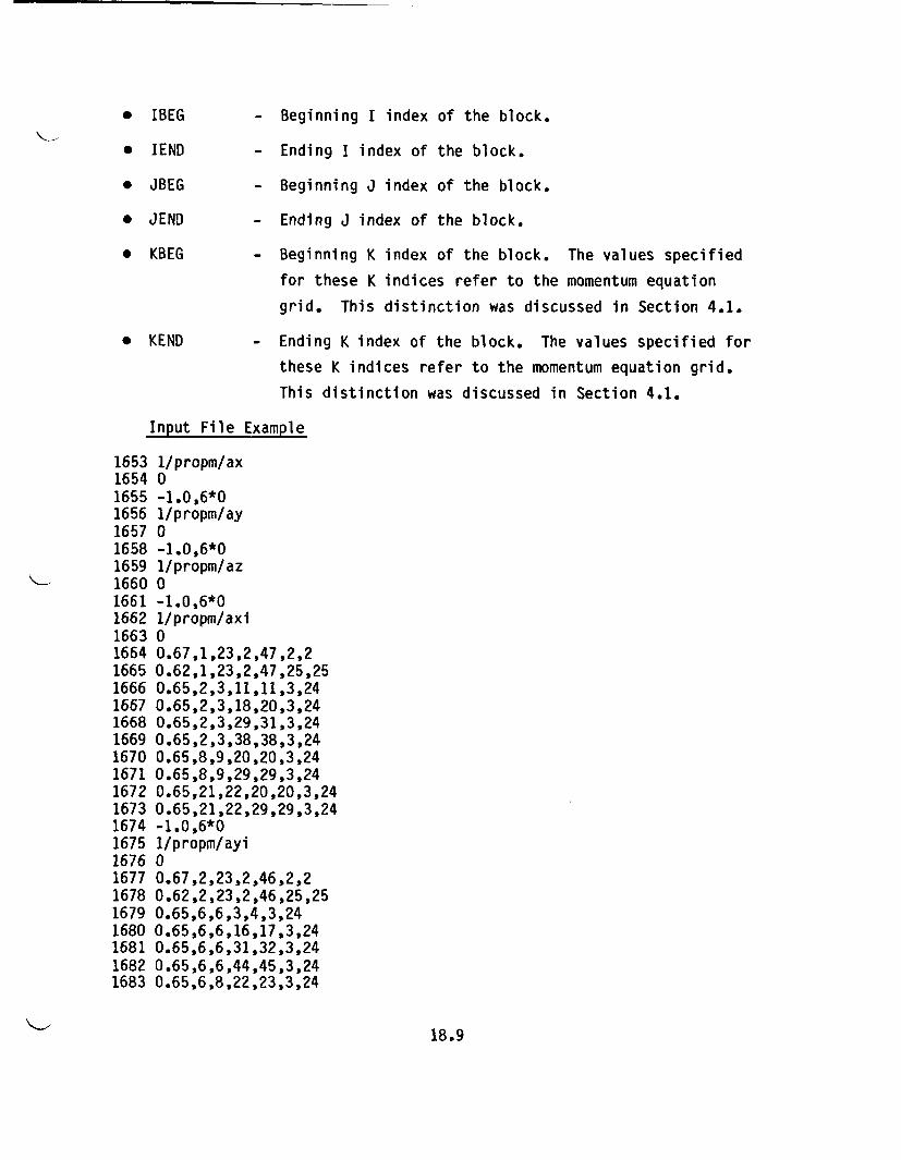
* IBEG - Beginning I index of the block.
* IEND - Ending I index of the block.
* JBEG - Beginning J index of the block.
* JEND - Ending J index of the block.
* KBEG - Beginning K index of the block. The values specified
for these K indices refer to the momentum equation
grid. This distinction was discussed in Section 4.1.
* KEND - Ending K index of the block. The values specified for
these K indices refer to the momentum equation grid.
This distinction was discussed in Section 4.1.
Input File Example
1653 1/propm/ax1654 01655 -1.0,6*01656 1/propm/ay1657 01658 -1.0,6*01659 1/propm/az1660 01661 -1.0,6*01662 1/propm/axi1663 01664 0.67,1,23,2,47,2,21665 0.62,1,23,2,47,25,251666 0.65,2,3,11,11,3,241667 0.65,2,3,18,20,3,241668 0.65,2,3,29,31,3,241669 0.65,2,3,38,38,3,241670 0.65,8,9,20,20,3,241671 0.65,8,9,29,29,3,241672 0.65,21,22,20,20,3,241673 0.65,21,22,29,29,3,241674 -1.0,6*01675 1/propm/ayi1676 01677 0.67,2,23,2,46,2,21678 0.62,2,23,2,46,25,251679 0.65,6,6,3,4,3,241680 0.65,6,6,16,17,3,241681 0.65,6,6,31,32,3,241682 0.65,6,6,44,45,3,241683 0.65,6,8,22,23,3,24
18.9
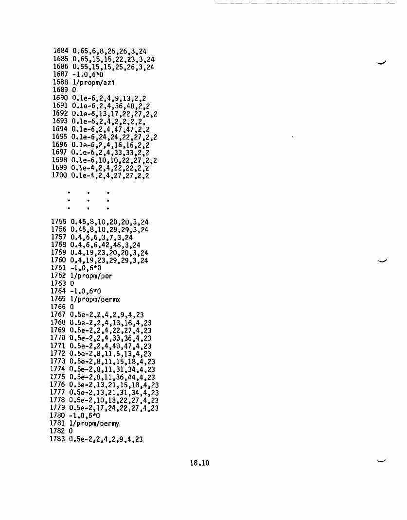
1684 0.65,6,8,25,26,3,241685 0.65,15,15,22,23,3,241686 0.65,15,15,25,26,3,241687 -1.0,6*01688 1/propm/azi1689 01690 O.le-6,2,4,9,13,2,21691 O.le-6,2,4,36,40,2,21692 O.le-6,13,17,22,27,2,21693 O.le-6,2,4,2,2,2,2,1694 O.le-6,2,4,47,47,2,21695 0.le-6,24,24,22,27,2,21696 O.le-6,2,4,16,16,2,21697 O.le-6,2,4,33,33,2,21698 O.le-6,10,10,22,27,2,21699 O.le-4,2,4,22,22,2,21700 O.le-4,2,4,27,27,2,2
* .
* .
* *
1755 0.45,8,10,20,20,3,241756 0.45,8,10,29,29,3,241757 0.4,6,6,3,7,3,241758 0.4,6,6,42,46,3,241759 0.4,19,23,20,20,3,241760 0.4,19,23,29,29,3,241761 -1.0,6*01762 1/propm/por1763 01764 -1.0,6*01765 1/p ropm/permx1766 01767 O.Se-2,2,4,2,9,4,231768 0.5e-2,2,4,13,16,4,231769 0.5e-2,2,4,22,27,4,231770 0.5e-2,2,4,33,36,4,231771 0.5e-2,2,4,40,47,4,231772 0.5e-2,8,11,5,13,4,231773 0.5e-2,8,11,15,18,4,231774 0.5e-2,8,11,31,34,4,231775 0.5e-2,8,11,36,44,4,231776 0.5e-2,13,21,15,18,4,231777 0.5e-2,13,21,31,34,4,231778 0.5e-2,10,13,22,27,4,231779 0.5e-2,17,24,22,27,4,231780 -1.0,6*01781 1/propm/permy1782 01783 0.5e-2,2,4,2,9,4,23
18.10
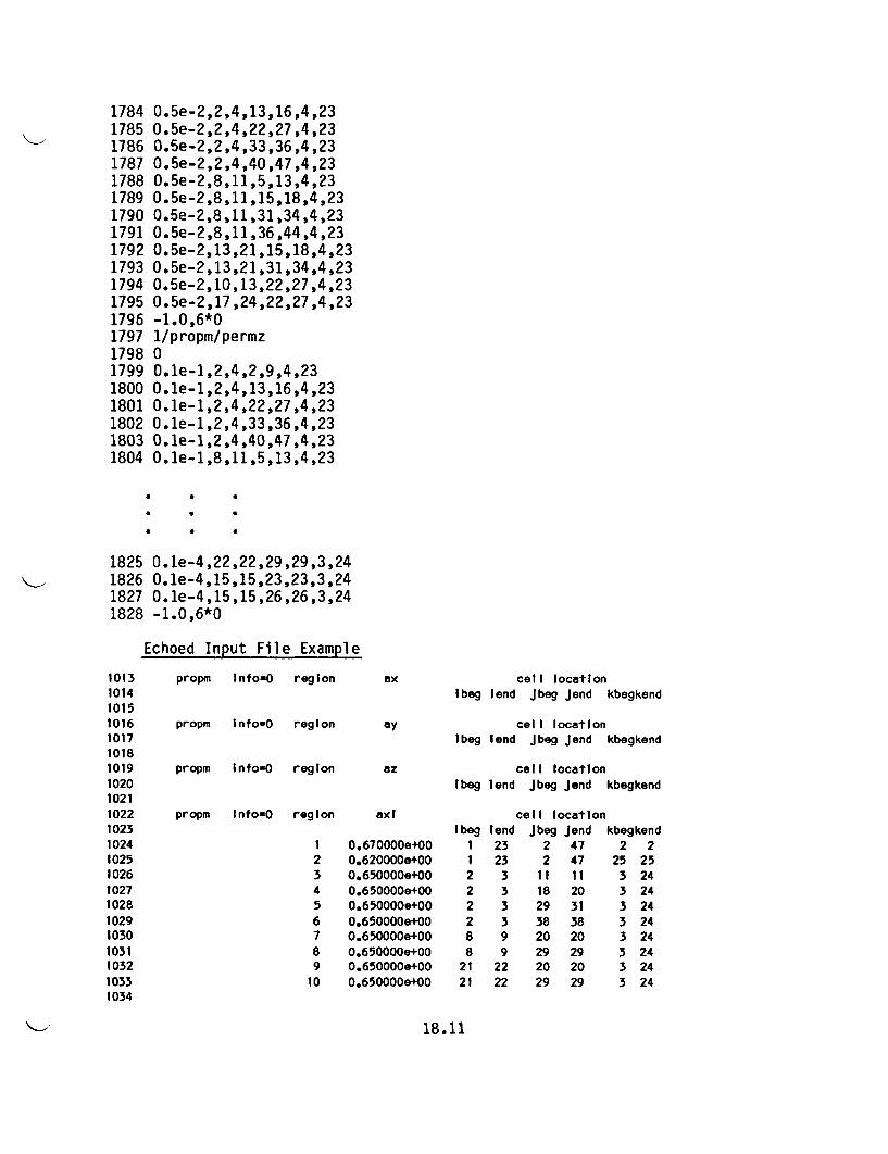
1784 0.5e-2,2,4,13,16,4,231785 0.5e-2,2,4,22,27,4,231786 0.5e-2,2,4,33,36,4,231787 0.5e-2,2,4,40,47,4,231788 0.5e-2,8,11,5,13,4,231789 0.5e-2,8,11,15,18,4,231790 0.5e-2,8,11,31,34,4,231791 0.5e-2,8,11,36,44,4,231792 0.5e-2,13,21,15,18,4,231793 0.5e-2,13,21,31,34,4,231794 0.5e-2,10,13,22,27,4,231795 0.5e-2,17,24,22,27,4,231796 -1.0,6*01797 1/propm/permz1798 01799 0.le-1,2,4,2,9,4,231800 0.le-1,2,4,13,16,4,231801 0.le-1,2,4,22,27,4,231802 O.le-1,2,4,33,36,4,231803 0.le-1,2,4,40,47,4,231804 0.le-1,8,11,5,13,4,23
1825182618271828
0.le-4,22,22,29,29,3,240.le-4,15,15,23,23,3,240.le-4,15,15,26,26,3,24-1.0,6*0
Echoed Input File Example
1013101410151016101710181019102010211022102310241025102610271028102910301031103210331034
propm Info=0 region
propm info-0 region
propm lnfo=0 region
ax
ay
az
cell locationibeg lend Jbeg Jend kbegkend
cell locationIbeg lend Jbeg Jend kbegkend
cell locationIbeg lend Jbeg Jend kbegkend
propm Info=0 region axi
1 0.670000e+002 0.620000e+003 0.650000e+004 0.650000e+005 0.650000e+006 0.650000e+007 0.650000e+008 0.650000e+009 0.650000e+00
10 0.650000e+00
I beg
12222882121
cell locationlend Jbeg jend kbegkend23 2 47 2 223 2 47 25 253 11 11 3 243 18 20 3 243 29 31 3 243 38 38 3 249 20 20 3 249 29 29 3 24
22 20 20 3 2422 29 29 3 24
18.11
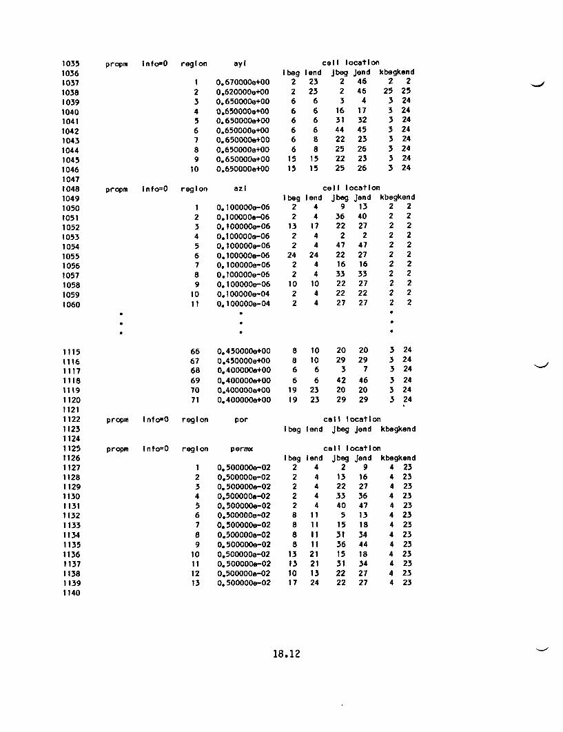
10351036103710381039104010411042104310441045104610471048104910501051105210531054105510561057105810591060
11151116111711181119112011211122112311241125112611271128112911301131113211331134113511361137113811391140
propm InfosO resglon ayl
1 0.670000e+002 0.620000e+003 0.650000e+004 0.650000e+005 0.650000e+006 0.650000e+007 0. 650000e+008 0.650000e+009 0.650000e+00
10 0.650000e+00
sglon azi
cell locationIbeg lend Jbeg Jend kbegkend
2 23 2 46 2 22 23 2 46 25 256 6 3 4 3 246 6 16 17 3 246 6 31 32 3 246 6 44 45 3 246 8 22 23 3 246 8 25 26 3 24
15 15 22 23 3 2415 15 25 26 3 24
cell locationtbeg lend Jbeg Jend kbegkend
2 4 9 13 2 22 4 36 40 2 2
13 17 22 27 2 22 4 2 2 2 22 4 47 47 2 2
24 24 22 27 2 22 4 16 16 2 22 4 33 33 2 2
10 10 22 27 2 22 4 22 22 2 22 4 27 27 2 2
propm lnfo=O re
1 0,1OOOOe-062 0.lOOOOOe-063 0.lOOOOOe-064 0.lOOOOOe-065 0.lOOOOOe-066 0.lOOOOOe-067 0.lOOOOOe-068 0.lOOOOOe-069 0.100000e-06
10 0,10000Oe-0 4
11 0. lOOOOOe-04
66 0.450000e+0067 0.450000e+0068 0.400000e+0069 0.400000e+0070 0,400000e+0071 0,400000e+00
8 10 20 208 10 29 296 6 3 76 6 42 46
19 23 20 2019 23 29 29
3 243 243 243 243 243 24
propm Info0O regIon
propm Info=0 regIon
por
permx
1 0.500000e-022 0.500000e-023 0. 500000e-024 0.5000OOe-025 0.500000e-026 0.500000e-027 0.5000OOe-028 0.5000OOe-029 0.500000e-02
10 0.500000e-0211 0.5000OOe-0212 0.500000e-0213 0.5000OOe-02
cell locationIbeg lend Jbeg Jend kbegkend
cell locationIbeg lend Jbeg Jend kbegkend
2 4 2 9 4 232 4 13 16 4 232 4 22 27 4 232 4 33 36 4 232 4 40 47 4 238 11 5 13 4 238 11 15 18 4 238 11 31 34 4 238 11 36 44 4 23
13 21 15 18 4 2313 21 31 34 4 2310 13 22 27 4 2317 24 22 27 4 23
18.12
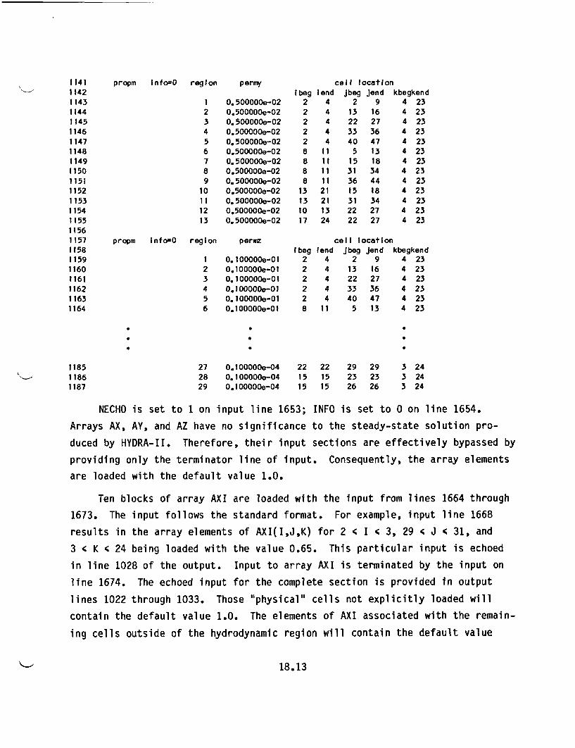
114111421143114411451146114711481149115011511152115311541155115611571158115911601161116211631164
propm lnfo=O region
23456789
10111213
propm lnfo=0 region
permy
0.500000e-020.500000e-020.500000e-020.500000e-020.5000e-02
0.500000e-020.500000e-020.500000e-020.500000e-020.500000e-020.500000e-020.500000e-020.500000e-02
perne
I beg22222888813131017
2beg222228
I enc44444
1 11 11 11 121211324
lend44444
11
cell locationI Jbeg Jend 1
2 913 1622 2733 3640 475 1315 1831 3436 4415 1831 3422 2722 27
(begkend4 234 234 234 234 234 234 234 234 234 234 234 234 23
I 0.100000e-OI2 0.lOOOOOe-013 0.lOOOOOe-014 0.IOOOOOe-O15 0.lOOOOOe-016 0.lOOOOOe-01
cell locationI Jbeg Jend kbegkend
2 9 4 2313 16 4 2322 27 4 2333 36 4 2340 47 4 235 13 4 23
.
.
118511861187
27 0.lOOOOOe-0428 0.IOOOOOe-04
29 0.lOOOOOe-04
22 22 29 29 3 2415 15 23 23 3 2415 15 26 26 3 24
NECHO is set to 1 on input line 1653; INFO is set to 0 on line 1654.
Arrays AX, AY, and AZ have no significance to the steady-state solution pro-
duced by HYDRA-II. Therefore, their input sections are effectively bypassed by
providing only the terminator line of input. Consequently, the array elements
are loaded with the default value 1.0.
Ten blocks of array AXI are loaded with the input from lines 1664 through
1673. The input follows the standard format. For example, input line 1668
results in the array elements of AXI(I,J,K) for 2 4 I 4 3, 29 ' J 4 31, and
3 4 K < 24 being loaded with the value 0.65. This particular input is echoed
in line 1028 of the output. Input to array AXI is terminated by the input on
line 1674. The echoed input for the complete section is provided in output
lines 1022 through 1033. Those "physical" cells not explicitly loaded will
contain the default value 1.0. The elements of AXI associated with the remain-
ing cells outside of the hydrodynamic region will contain the default value
18.13
0.0. Ten blocks of array AYI are loaded with the input from lines 1677 through
1686. Input to this array is terminated with the information provided on line
1687. The echoed input for this section is provided in lines 1035 through
1046. The same defaults apply here as for array AXI.
Seventy-one blocks of array AZI are loaded with the input from lines 1690
through 1761. The corresponding echoed-input is provided in lines 1048 through
1120. Again, the same default values apply here as for array AXI. The POR
array multiplier is loaded next in the sequence. However, in this example the
default values are sufficient (defaults to 1.0). Therefore, only the section
terminator line is provided, input line 1764.
PERMX, PERMY, and PERMZ are loaded next. Input lines 1765 through 1828
reflect the values specified for each block. For example, the array elements
PERMX(I,J,K) for 10 < I 4 13, 22 < J < 27, and 4 < K < 23 are loaded with the
value 0.005 on line 1778 of the input. Those "physical" cells not covered in
the input to these sections are defaulted to PERMO.
18.14
19.0 SUBROUTINES MOMX, MOMY, AND MOMZ
The terms of the momentum equations are evaluated in subroutines MOMX,
MOMY, and MOMZ using the methods discussed in Volume I - Equations and Numerics
(McCann 1987). Subroutine MOMX evaluates the terms of the x-component momentum
equation; MOMY, the y-component; and MOMZ the z-component. The x-, y-, and z-
momentum equation terms are evaluated using pressures obtained from the pre-
vious time-step. Consequently, the momentum subroutines produce a mass-flux
field that will not, in general, satisfy continuity. For this reason, these
mass fluxes are tentative and are denoted by a tilde, mi. This part of the cal-
culation is thus termed the "tilde phase." Mass conservation is enforced by
subsequently modifying the pressure field using the tilde-phase mass-flux
field. The final mass fluxes for this time-step are then computed using the
tilde-phase mass fluxes and the modified pressure field.
19.1 PARAMETER STATEMENT INFORMATION
Subroutines MOMX, MOMY, and MOMZ require the specification of parameters
IP, JP, KP, KBP, KTP, and NEFAP. These data define the overall computational
mesh and are described in the discussion of subroutine GRID in Chapter 4.0. No
additional parameters are needed for these three subroutines.
19.2 INPUT FORMAT
Subroutines MOMX, MOMY, and MOMZ do not require input data.
19.1
20.0 SUBROUTINE PDG
Subroutine PDG performs two functions. First, PDG sets up the coefficient
matrix required to obtain a solution for the pressure-correction field. The
elements comprising this coefficient matrix are identified in Chapter 9.0 of
Volume I - Equations and Numerics (McCann 1987). This matrix is used in
obtaining a first-pass solution in PDG. It is also employed in subroutines
PILES, REBS, REBQ, and AF to obtain a solution to the pressure-correction
field. The first-pass solution is generated in PDG using a variant of the
Douglas and Gunn algorithm (1964). The modification to this algorithm employs
a user-supplied weighting parameter, WP. This parameter is used to artifi-
cially weight the diagonal elements of the coefficient matrix. The effect of
this weighting is to enhance the convergence properties of the algorithm.
Subroutine PDG also allows the user to monitor the cell mass imbalance
during the solution process. Monitoring is controlled by switch NSINFO (set in
MAIN). This constant controls the printing frequency of diagnostic information
and monitored variables. For example, if NSINFO = 20, then information will be
printed for time-steps 1, 21, 41, etc. Information is always printed for the
first and last time-steps of a run. The output provided in this process is:
* the time-step number
* the momentum time-step
* the I, J, and K indices of the cell experiencing the largest tilde-
phase mass imbalance
* the tilde-phase mass imbalance for this cell.
In addition, the largest component mass-flux corrections and their correspond-
ing computational-mesh indices are provided in the output.
The magnitude of the largest continuity error is used to suggest a momen-
tum time-step adjustment to subroutine HYDRO. This is done in an effort to
maintain the optimum tilde-phase continuity error for the next time-step.
20.1
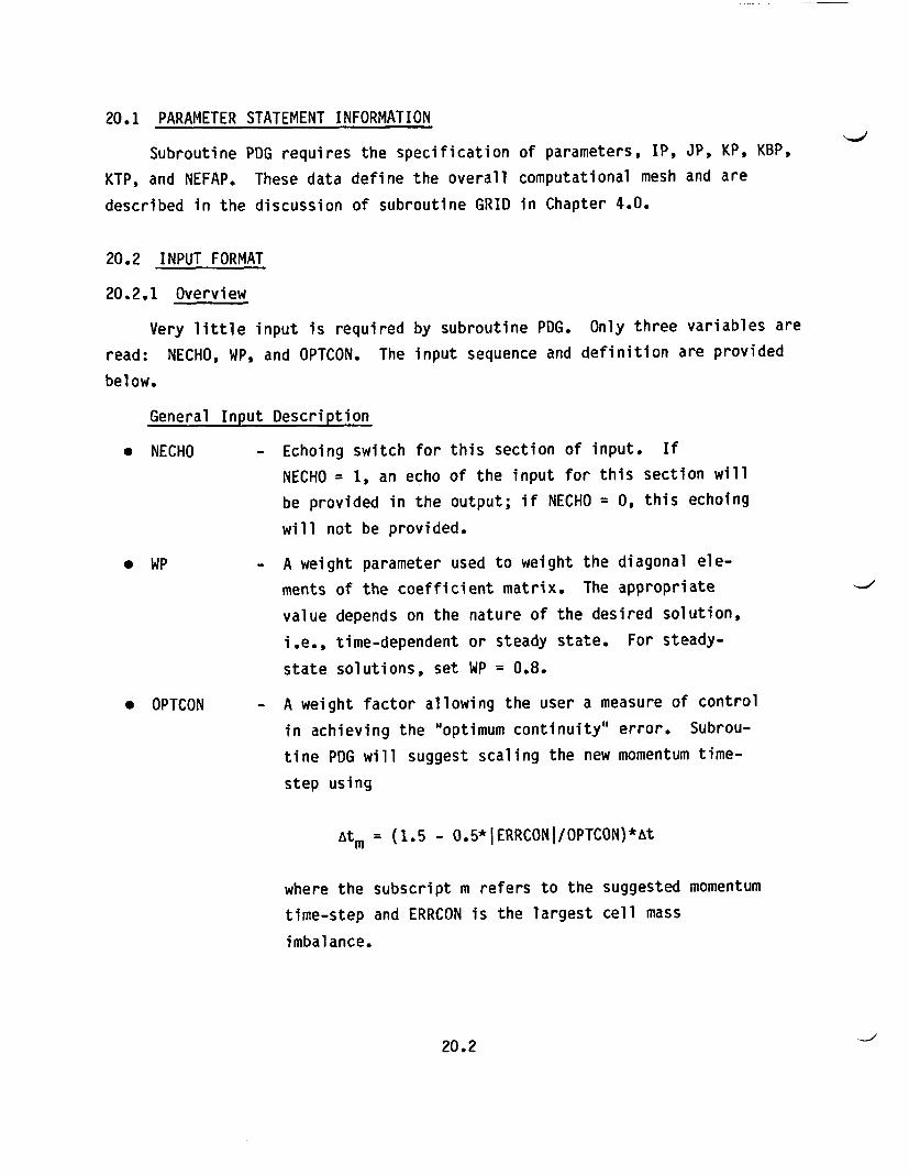
20.1 PARAMETER STATEMENT INFORMATION
Subroutine PDG requires the specification of parameters, IP, JP, KP, KBP,
KTP, and NEFAP. These data define the overall computational mesh and are
described in the discussion of subroutine GRID in Chapter 4.0.
20.2 INPUT FORMAT
20.2.1 Overview
Very little input is required by subroutine PDG. Only three variables are
read: NECHO, WP, and OPTCON. The input sequence and definition are provided
below.
General Input Description
* NECHO - Echoing switch for this section of input. If
NECHO = 1, an echo of the input for this section will
be provided in the output; if NECHO = 0, this echoing
will not be provided.
* WP - A weight parameter used to weight the diagonal ele-
ments of the coefficient matrix. The appropriate
value depends on the nature of the desired solution,
i.e., time-dependent or steady state. For steady-
state solutions, set WP = 0.8.
* OPTCON - A weight factor allowing the user a measure of control
in achieving the "optimum continuity" error. Subrou-
tine PDG will suggest scaling the new momentum time-
step using
Atm = (1.5 - 0.5*IERRCONI/OPTCON)*At
where the subscript m refers to the suggested momentum
time-step and ERRCON is the largest cell mass
imbalance.
20.2

General Input Format
NECHOWP,OPTCON
Input File Example
1829 1/pdg 11830 0.8,0.5e-5
Echoed-Input File Example
1189 pdg wp=0.80 optcon-0.500e-051190
NECHO has been set to 1 on input line 1829. Input line 1830 indicates
that WP has been set to a value of 0.8 and OPTCON to a value of 0.5e-5.
20.3
21.0 SUBROUTINE PITER
Subroutine PITER serves as a traffic control routine directing program
flow to the various methods available for solving the Poisson equation for the
pressure-correction field. HYDRA-II provides the user with a number of
approaches to generate the solution to the Poisson equation:
* Coarse-mesh subroutines REBS and REBQ adjust the interim pressure-
correction field solution to reduce long-wavelength errors. These
routines are discussed in Chapters 23.0 and 24.0.
* Subroutine AF uses an approximate-factorization technique. AF is
discussed in Chapter 26.0.
* Subroutine PILES performs line successive relaxation iterations.
PILES is discussed in Chapter 22.0.
Subroutine PITER allows the user to tailor the solution scheme to suit the
requirements of the specific problem at hand. PITER starts with the pressure-
correction field estimate obtained in subroutine PDG. An optimum sequence for
solving the pressure equation cannot be prescribed a priori for a particular
simulation. The user can cautiously try using REBQ along with PILES, and
possibly AF or REBS in a sequence found workable for similar problems. The use
of REBQ, REBS, or AF should be interspersed with the use of PILES with, at
least initially, setting the printout option INFO = 1 in PILES. The divergence
error, DMAX, for each direction of line-successive-relaxation sweeps in PILES
should be examined, and the maximum number of three-direction line-
successive-relaxation sweeps (NMAX) in PILES should be set to ensure that:
1. the short wavelength error is being reduced sufficiently in PILES so
that the divergence error is smaller than it was before the call to
REBQ or to a combination of REBQ, AF, and REBS
2. the iterations within PILES are not continuing past a point of
diminishing returns (i.e., the divergence error is no longer being
removed effectively).
21.1
In some cases it may be desirable to systematically explore the efficacy
of REBS, REBQ, and AF patterns, with PILES in the pressure correction
solution. This can be done with a sequence as follows:
1. Run HYDRA-II through some number of time-steps, possibly using only
PILES or some previously successful combination of PILES, REBS, REBQ,
and AF, but terminating with PILES. Create a restart file.
2. Run a succession of restart cases from this restart file in which one
of the routines REBS, REBQ, or AF is called, followed by a call to
PILES with a fairly high number of inner iterations (NMAX) and with
INFO = 1 to get divergence error printouts. Consider the pattern of
divergence errors (printed in PILES), noting which of the routines
preceding the call to PILES are effective in reducing the divergence
error. Note that some routines (particularly REBS and REBQ) may
initially increase the divergence error by increasing short
wavelength error while reducing long wavelength error. PILES is
effective for reducing short wavelength error.
3. Select some of the more promising routines from among REBS, REBQ, and
AF, based on the tests in Step 2. Use them in combinations, with or
without calls to PILES between them, and do further comparisons of
divergence error patterns. PILES should be called in the sequence,
of course, since only it, and possibly AF, can produce converged
solutions on the fine mesh. Always note the number of iterations in
PILES needed to show a net improvement in the divergence error,
paying particular attention to the diminishing returns phenomenon.
Select a pattern of calls to PILES, REBS, REBQ, and AF for further
use in seeking convergence, along with a number of iterations in
PILES (NMAX).
4. With the sequence (specified in NORDER in the input to PITER) chosen
by this procedure, and with the selected number of inner iterations
in PILES (NMAX), advance the simulation through additional time-
steps, stopping and restarting as appropriate. Reduce the level of
printout when confidence is gained that the sequence of procedures is
effective.
21.2
The number of techniques employed to obtain the interim solutions are
completely specified by the user with input variable NORDA. The sequence in
which each technique is employed in the process is specified by the user with
input to array NORDER(I) for I = 1,2, ... ,NORDA. The following is a list of
allowable NORDER settings and the corresponding routines invoked:
NORDER(I) Routine Invoked
1 line successive relaxation - PILES
2 coarse-mesh solver - REBS
3 coarse-mesh solver - REBQ
4 approximate factorization - AF
Subroutine PITER sweeps through the first NORDA elements of array NORDER;
therefore, the solution technique associated with the value of NORDER(1) will
be employed first. This is followed by invocation of the scheme associated
with NORDER(2), and so on up to NORDER(NORDA).
Convergence is not necessarily assured with one passage through the set of
schemes invoked by NORDER. Therefore, PITER allows the user to specify, via
the input variable NMAX, the number of times this set of schemes will be called
by subroutine PITER during each pass through PITER.
21.1 PARAMETER STATEMENT INFORMATION
Subroutine PITER requires the specification of one parameter, NORDAP.
This parameter sets the maximum number of elements which can be contained in
array NORDER. The elements of NORDER specify which methods are employed in the
calling sequence of subroutine PITER.
21.2 INPUT FORMAT
21.2.1 Overview
The input to subroutine PITER serves primarily to direct the calling
sequence to the various solution algorithms available.
21.3
General Input Format
NECHONOPT,NMAXREBSON,REBQONAFONNECHONORDANORDER(1),NORDER(2), ... , NORDER(NORDA)
General Input Description
* NECHO - Echoing switch for this section of input. If
NECHO = 1, an echo of the input for this section will
be provided in the output; if NECHO = 0, this echoing
will not be provided.
* NOPT - The desired optimum number of passes through
subroutine PITER. Subroutine PITER will suggest
appropriate scaling of the momentum time-step to the
calling routine, HYDRO, based on the convergence
history of the pressure solution. The scaling is
based on the number of PITER passes required for
convergence, ITER. ITER is set tQ the value NMAX if
no convergence is obtained in this pass through
subroutine PITER. The suggested time-step is computed
as
Atp = MAX(1.5 - 0.5*REAL(ITER)/REAL(NOPT),0.1)*At
NOPT should be set to a value less than or equal to
NMAX. Therefore, the suggested time-step scaling can
range from 0.1 for difficult convergence situations to
an asymptote of 1.5.
* NMAX - Maximum iterations allowed in each pass through PITER.
* REBSON, - Initialization switches for subroutines REBS, REBQ,
REBQON and AF, respectively. If any of these routines are
AFON to be employed in the set of iteration schemes, the
21.4
corresponding switch for that routine should be set to
1.0. Otherwise, set the switch to 0.0.
* NORDA
* NORDER
- Total number of routines employed in each pass through
PITER. If one routine is used more than once in the
set, it should be counted as many times as it is
invoked.
- Array containing the identification numbers for the
solution schemes. Their storage order corresponds to
the sequence in which the routines will be invoked in
the iteration. The identification number for the
various routines is provided in the above text. There
must be NORDAP entries provided in the input - even
if NORDA < NORDAP. NORDER(I) for I = NORDA+1,
NORDA+2, ... , NORDAP may be set to any value.
Input File Example
1831 1/piter1832 4,201833 0.0,1.0,1.01834 1/piter/norder1835 31836 3,4,1,0
11911192119311941195
Echoed-Input File Example
piter nopt=4 nmax=20piter rebson-0.0 rebqon-l.0 afon=1 .0
piter norda= 3 maximum current dimension for norda Is 4piter norder 3 4 1 0
NECHO has been set to 1 on
set to 4 and NMAX is set to 20.
iterations allowed in each pass
input line 1831. On input line 1832, NOPT is
Therefore, there will be a maximum of 20
through PITER.
Input line 1833 indicates that, of the three switchable schemes, only REBQ
and AF will be employed in this set. Subroutine PILES will be the last sub-
routine invoked in this set of schemes. NECHO has been set to 1 on input line
1834. Input line 1835 indicates that there will be three schemes employed in
the set; therefore, each scheme (viz., REBQ, AF, and PILES) will be invoked
21.5
only once per iteration. The sequence in which these schemes are employed is
provided on input line 1836. This line indicates that REBQ will be invoked
first, followed by AF and PILES. Note that four entries are provided for array
NORDER, even though only three are non-zero. With NORDAP = 4 and NORDA = 3,
four entries are required for input, but only the first three are used. The
remaining one is ignored.
This input sequence has been echoed in output lines 1191 through 1195.
21.6
22.0 SUBROUTINE PILES
Subroutine PILES solves the Poisson equation for the pressure correction
field using a line-successive-relaxation iteration scheme. This Poisson
equation is obtained by seeking the pressure-field correction that will produce
a mass balance for each cell of the computational mesh.
The line-successive-relaxation iteration is performed in three passes--one
corresponding to each of the three coordinate directions. If the user-
specified value for INFO is > 1, the routine searches for the largest solution
residual (in magnitude) and its (I,J,K) index location at the beginning of the
first two of the three passes. PILES always searches for these values at the
beginning of the third step, regardless of the value of INFO. If INFO is set
to a value greater than 0, PILES will print the iteration count, together with
the largest residual and its (I,J,K) index location at the first and second
passes in the iteration. The time-step number (NS, updated in MAIN) and switch
NSINFO (also set in MAIN) control whether or not this printout is produced at
the end of the third pass. For example, if NSINFO = 20, then information will
be printed at time-steps 1, 21, 41, etc. Information is always printed for the
first and last time-steps of a run, NS = 1 and NSTEP, respectively.
Convergence is tested at the conclusion of the third pass in each
iteration. When the largest residual (in magnitude) is less than the user-
specified convergence criterion, EPSD, the algorithm has converged. PILES will
then return to subroutine PITER. If no convergence is obtained after NMAX
iterations have been performed, PILES will set a flag before returning to
PITER. This flag indicates to subroutine PITER, the lack of convergence in
PILES. HYDRA-II uses this information to determine whether momentum time-step
adjustment is required.
The iteration scheme requires the user to specify a relaxation parameter,
OMEGA. This relaxation parameter may assume a value in the range
0 < OMEGA < 2
22.1

OMEGA < 1 corresponds to underrelaxation; OMEGA > 1 corresponds to over-
relaxation. As with the familiar successive overrelaxation (SOR) methods,
there exists a value for OMEGA which will produce the largest asymptotic
reduction in error. Unfortunately, the exact value for this optimal OMEGA is
very problem-specific and is usually determined by numerical experiment in most
simulations.
22.1 PARAMETER STATEMENT INFORMATION
Subroutine PILES requires the specification of parameters IP, JP, KP, KBP,
KTP, and NEFAP. These data define the overall computational mesh and are
described in the discussion of subroutine GRID in Chapter 4.0.
22.2 INPUT FORMAT
22.2.1 Overview
The input to subroutine PILES sets the parameters of the line successive-
relaxation scheme. Specifically, the convergence criterion (EPSD), relaxation
factor (OMEGA), and number of iterations per pass through PILES (NMAX), are
defined by the user through the input to this routine.
General Input Format
NECHOEPSD,OMEGA,NMAX,INFO
General Input Description
* NECHO - Echoing switch for this section of input. If
NECHO = 1, an echo of the input for this section willbe provided in output; if NECHO = 0, this echoing will
not be provided.
* EPSD - Convergence criterion. The appropriate value to use
is problem-dependent. A "loose" convergence criterion
effectively produces sources and sinks of mass in the
problem. These mass sources and sinks are amplified
22.2
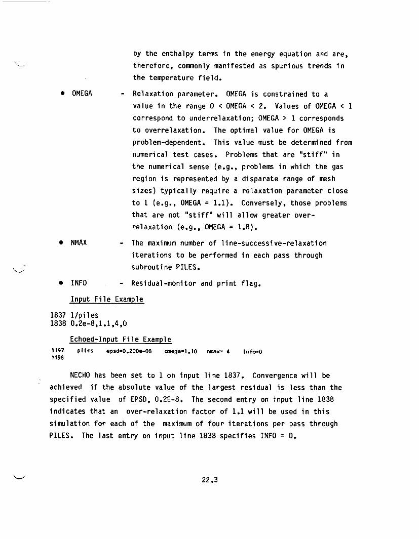
by the enthalpy terms in the energy equation and are,
therefore, commonly manifested as spurious trends in
the temperature field.
* OMEGA - Relaxation parameter. OMEGA is constrained to a
value in the range 0 < OMEGA < 2. Values of OMEGA < 1
correspond to underrelaxation; OMEGA > 1 corresponds
to overrelaxation. The optimal value for OMEGA is
problem-dependent. This value must be determined from
numerical test cases. Problems that are "stiff" in
the numerical sense (e.g., problems in which the gas
region is represented by a disparate range of mesh
sizes) typically require a relaxation parameter close
to 1 (e.g., OMEGA = 1.1). Conversely, those problems
that are not "stiff" will allow greater over-
relaxation (e.g., OMEGA = 1.8).
* NMAX - The maximum number of line-successive-relaxation
iterations to be performed in each pass through
subroutine PILES.
* INFO - Residual-monitor and print flag.
Input File Example
1837 1/piles1838 0.2e-8,1.1,4,0
Echoed-Input File Example
1197 piles epsd=0.200e-08 ornega=1.10 nmax- 4 Info=O1198
NECHO has been set to 1 on input line 1837. Convergence will be
achieved if the absolute value of the largest residual is less than the
specified value of EPSD, 0.2E-8. The second entry on input line 1838
indicates that an over-relaxation factor of 1.1 will be used in this
simulation for each of the maximum of four iterations per pass through
PILES. The last entry on input line 1838 specifies INFO = 0.
22.3
23.0 SUBROUTINE REBS
Subroutine REBS is one member of the set of subroutines (PILES, REBS,
REBQ, and AF) that can be called upon by subroutine PITER to solve a Poisson
equation for the pressure correction field.
23.1 REBS FUNCTIONS
If requested for use, REBS solves the Poisson equation three times on slab
representations of the rectangular grid, for slabs lying in planes of constant
I, J, and K in turn. The SP(I) calculated for the I-slab case is applied to
computational cells in that I-plane, and similarly for the J-plane and K-plane
solutions.
REBS does not read input, and it executes rapidly. It is used without
user control in setting up the static pressure field when initiating a simu-
lation. REBS is effective for numerically-easy problems. Its effectiveness in
the pressure-correction equation solution sequence can be monitored by noting
the divergence error for the pressure equation as printed by PILES before and
after REBS application. REBS will generally introduce some short-wavelength
error (which PILES is effective in removing) while reducing long-wavelength
error. Allow enough line-successive-relaxation sweeps in PILES between REBS
calls to ensure that the short-wavelength error is reduced and net progress
toward a solution is made.
23.2 PARAMETER STATEMENT INFORMATION
Dimensioning parameters set in REBS include IP,JP,KP. These were defined
in Chapter 4.0, subroutine GRID, and have the same meanings and should have the
same values here. Also set are KBP,KTP which were discussed in Chapter 4.0 and
defined in Chapter 6.0, subroutine THERM.
23.3 INPUT FORMAT
Subroutine REBS does not read input.
23.1
24.0 SUBROUTINE REBQ
Subroutine REBQ is another member of the set of subroutines (PILES, REBS,
REBQ, and AF) that can be called by subroutine PITER to aid in solving a
Poisson equation for the pressure correction field.
24.1 REBQ FUNCTIONS
REBQ solves the pressure correction equation on three different user-
defined coarse partitions of the rectangular grid. These coarse mesh solutions
are used to improve the estimate of the pressure correction field on the fine
mesh. REBQ has proved an effective tool for expediting convergence in the
pressure correction field, even for difficult simulations with intricate flow
patterns. It is effective in removing long-wavelength error, and it should be
interspersed with techniques like those of subroutine PILES or AF that are
effective against short-wavelength error.
REBQ is noteworthy for the flexibility and ease with which the coarse mesh
can be defined. For the first of the three coarse meshes (the KREG mesh), the
X-Y boundaries are defined identically for each K-plane. The coarse mesh can
be a fairly arbitrary set of rectangles bounded by X- and Y-grid lines. Such a
set is shown in Figure 24.1. The user must define the X-Y bounds of the
cells. The flow computational region with phantom planes extends from K = 1 to
K = KP-KBP-KTP.
The second of the three coarse meshes (the JREG mesh) is defined iden-
tically for each J-plane. The coarse cells within a J-plane are a fairly arbi-
trary set of rectangles bounded by X- and Z-grid lines, with the user defining
the bounds and interfaces. An example of a partition of a J-plane is shown in
Figure 24.2. Similarly, for the third or IREG simulation, each coarse cell
defined within a single I-plane is bounded by Y- and Z-grid lines.
The specification of any of these three coarse meshes requires
identifying:
1. the bounds of the coarse cells within a single plane
2. the other coarse cells with which each one has an interface
24.1
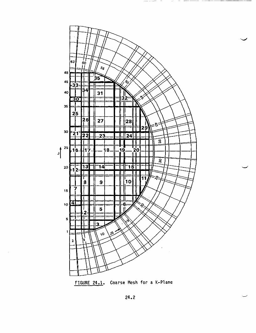
48
15
35 25 lr [ ~ /\
I2L 27 - 28 X30$ _= _
F1I 2 42 .1. C2 r Mes 24 f a . a
I5 1 C E :2 - 4 9 220 = 14 -1 _ E_ ;=
10 =6,F_ (
FIGURE 24.1. Coarse Mesh for a K-Plane
24.2
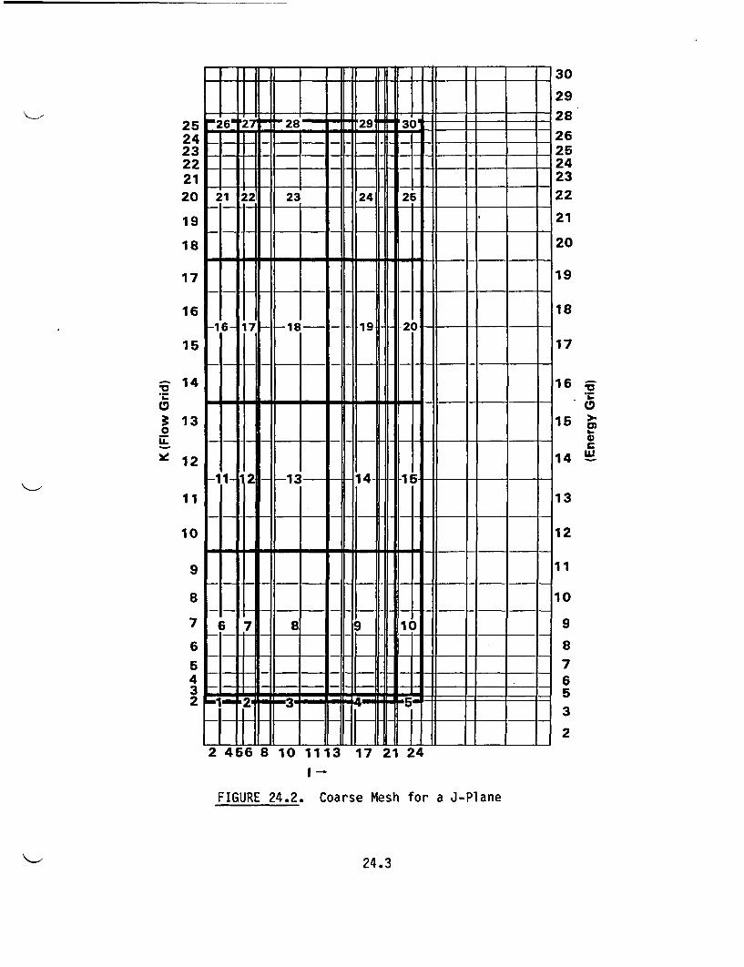
252423222120
19
18
17
26 2I 28 w 291 L+30 -
22 24 25
25I
30
29
28
2625242322
21
20
19- _ -"I- _ _--II-- - I_ _ _
16
15
I-1 5-1171- -18-I- .. ,19 1-20 _ I _ _
I
;a
CD
0
14
13
12
11
10
9
8
7
6
5432
_ T_ 0- I HII Al
tt ~- _- t 1
18
17
16 :-.,
15 >0c
14 W
13
12
11
10
9
8
765
3
2
2 456 8 10 1113 17 21 24
I -
FIGURE 24.2. Coarse Mesh for a J-Plane
24.3
3. the orientation of the interface between any two contacting cells.
The code limits the coarse computational cells to the computational region of
the rectangular grid. The user can define these cells with rectangular grid
index ranges, allowing the HYDRA-II coding to restrict the defined coarse cells
to the rectangular grid flow region along the curved parts of the boundary.
It is practical to use on the order of 30 or 40 computational cells in
each plane for each of the three coarse meshes. It is suggested that the
coarse cells be chosen to give a fair representation of the physical phenomena
occurring. Experience to date indicates that this selection is not critical,
as benefits from REBQ can be obtained with a variety of coarse meshes.
24.2 PARAMETER STATEMENT INFORMATION
The following array-dimensioning parameters have the same significance and
should have the same value as in Chapter 4.0 (subroutine GRID):
* IP, JP, KP, NEFAP
The following array dimensioning parameters were discussed in Chapter 4.0
(subroutine GRID) and were defined in Section 6.2 (subroutine THERM):
* KBP, KTP
The following array dimensioning parameters are defined in Chapter 25.0
(subroutine CROUT):
* ICRP, JCRP
Additional dimensioning parameters required are:
* KREGP - Maximum value of KREG allowed by dimensioning, where
KREG is the number of coarse cells in a K-plane for
the first coarse mesh pressure correction solution
(the KREG solution).
* JREGP - Maximum value of JREG allowed by dimensioning, where
JREG is the number of cells in a J-plane for the
second coarse mesh pressure correction solution (the
JREG solution).
24.4
---
* IREGP - Maximum value of IREG allowed by dimensioning, where
IREG is the number of cells in an I-plane for the
third coarse mesh pressure correction solution (the
IREG solution).
* KBIDAP - The length of the array KBID, used to store the cell
interface information for the KREG partition. The
KBID array stores, for each coarse cell of the KREG
mesh, a list of pairs of numbers for interfaces with
other coarse cells not already specified. The pair
for an interface comprises the neighbor cell number
and a number specifying the orientation of their
interface plane.
* JBIDAP - The length of the array JBID, used to store the cell
interface information for the JREG partition,
analogous to KBIDAP for the KREG partition.
* IBIDAP - The length of the array IBID, used to store the cell
interface information for the IREG partition,
analogous to KBIDAP for the KREG partition.
24.3 INPUT FORMAT
24.3.1 Overview
The REBQ input can be considered in four blocks:
1. specifications on the level of printout and execution options for the
pressure correction solutions on the REBQ type partitions of the flow
regi on
2. cell geometry and interfaces in the I-J planes (planes of constant K)
for the KREG partition
3. cell geometry and interfaces in the I-K planes (planes of constant J)
for the JREG partition
4. cell geometry and interfaces in the J-K planes (planes of constant I)
for the IREG partition.
24.5
24.3.2 Printout and Execution Options
General Input Format
NECHONMAX, INFOKBOUND, JBOUND, IBOUNDAKKMIN, AJJMIN, AIIMIN
General Input Description
* NECHO - Echoing switch for this section of input. If input is
to be echoed, then NECHO = 1; otherwise, 0.
* NMAX - Number of times to cycle through the approximate
solution on the three coarse' region partitions on a
call to REBQ. The preferred value is simulation-
dependent, and should be chosen by setting NMAX
initially to 3 with INFO set to 1. Observe the
printed divergence error and adjust the value of NMAX
if necessary to an observed point of diminishing
returns on the divergence error reduction.
* INFO - Flag for the level of printout desired. If INFO = 1,print divergence error maxima and location before each
of the three coarse partition solutions at each of the
NMAX iterations. If INFO = 2, print divergence error
maxima and location before and after each of these
coarse partition solutions at each of the NMAX
iterations. If INFO = 3, print also the coefficient
matrices for the coarse partitions. If INFO = 0,
bypass printing. After choosing and verifying a
satisfactory value of NMAX, it is desirable to set
INFO = 0.
* KBOUND, JBOUND IBOUND - Index of a phantom (boundary) plane related
to inflow and outflow conditions. This version of
HYDRA-II is restricted to no-flow boundaries;
therefore, KBOUND, JBOUND, and IBOUND should each be
equal to 1.
24.6
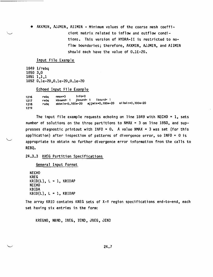
* AKKMIN, AJJMIN, AIIMIN - Minimum values of the coarse mesh coeffi-
cient matrix related to inflow and outflow condi-
tions. This version of HYDRA-II is restricted to no-
flow boundaries; therefore, AKKMIN, AJJMIN, and AIIMIN
should each have the value of 0.1E-20.
Input File Example
1849 1/rebq1850 3,01851 1,1,11852 0.le-20,0.1e-20,0.1e-20
Echoed Input File Example
1216 rebq nmax=3 Info=O1217 rebq kbound= 1 jbound= 1 lbound= 11218 rebq akkmln=O.lOOe-20 JJmntn=O.lOOe-20 aliminO.lOOe-201219
The input file example requests echoing on line 1849 with NECHO = 1, sets
number of solutions on the three partitions to NMAX = 3 on line 1850, and sup-
presses diagnostic printout with INFO = 0. A value NMAX = 3 was set (for this
application) after inspection of patterns of divergence error, so INFO = 0 is
appropriate to obtain no further divergence error information from the calls to
REBQ.
24.3.3 KREG Partition Specifications
General Input Format
NECHOKREGKRID(L), L = 1, KRIDAPNECHOKBIDAKBID(L), L = 1, KBIDAP
The array KRID contains KREG sets of X-Y region specifications end-to-end, each
set having six entries in the form:
KREGNO, NBND, IBEG, IEND, JBEG, JEND
24.7
The array KBID contains data sets stored end-to-end, each set having the
form:
KREGA, KREGB1, MBTYP1, KREGB2, MBTYP2, ... , KREGBNBND(KREGA),
MBTYPNBND( KREGA)
Each set in KBID has as a leading entry a region number KREGA that was one of
the regions KREGNO specified in KRID. This is followed by NBND(KREGA) pairs of
integers, where NBND(KREGA) was the second entry for set KREGA in KRID. Each
pair (KREGBi, MBTYPi) of these integers has as first entry a number KREGB of
another region in the X-Y plane that adjoins region KREGA, and as second entry
a number MBTYP (-1, +1, -2, or +2) that tells whether region KREGB is in the -X
(MBTYP = -1), +X (MBTYP = +1), -Y (MBTYP = -2), or +Y (MBTYP = +2) direction
from region KREGA.
KREGB is specified
in the list of regi
An interface should be specified only once. If region
as adjoining region KREGA, then KREGA should not be included
ons adjoining KREGB.
General Input Description
* NECHO
* KREG
* KRID
* KREGNO
- Echoing switch for this section of input. If input is
to be echoed, then NECHO = 1; otherwise, 0.
- Number of coarse computational cells in an X-Y plane
at each K-plane.
- Array defining the coarse cells in the X-Y plane for
each K-plane. The data entries for the regions follow
each other end-to-end, the six entries for each region
being:
KREGNO, NBND, IBEG, IEND, JBEG, JEND
- Number of a region in the X-Y plane for the KREG
computation. The region numbers and their
accompanying six-entry data sets must appear
consecutively with indices KREGNO running 1 through
KREG without omissions.
24.8
* NBND - Number of interfaces in the I-d plane for cell KREGNO
not previously specified for some other cell. See
forthcoming discussion for (KREGB, MBTYP) pairs.
* IBEG, IEND, JBEG, JEND - The beginning and end in the I-direction,
followed by the beginning and end in the J-direction,
of the included fine mesh cells for cell KREGNO in the
coarse KREG partition of the X-Y plane. The KREG
coarse cells are further restricted to the active
computational region for the momentum equations
defined the IMEND, JMBEG, and JMEND arrays.
* KBIDA - The number of active entries (individual numbers)
forthcoming in the KBID array (which is dimensioned to
KBIDAP).
* KBID - The array of sets of information on the interfaces of
the cells of the KREG partition, stored end-to-end as
previously indicated, each set having the form:
KREGA, KREGB1, MBTYP1, KREGB2, MBTYP2,
KREGBNBND(KREGA). MBTYPNBND(KREGA)
* KREGB, MBTYP - The index of a cell having an interface with cell
KREGA, and a specification of its relative position.
The values of MBTYP and their meanings are:
MBTYP Direction of KREGB From KREGA Interface Plane
-1 -X Y-Z
+1 +X Y-Z
-2 -Y X-Z
+2 +Y X-Z
The interface between two regions should be specified only
once in the KBID array, which is achieved if the region
index KREGB is always greater than KREGA in the sets in
KBID.
24.9
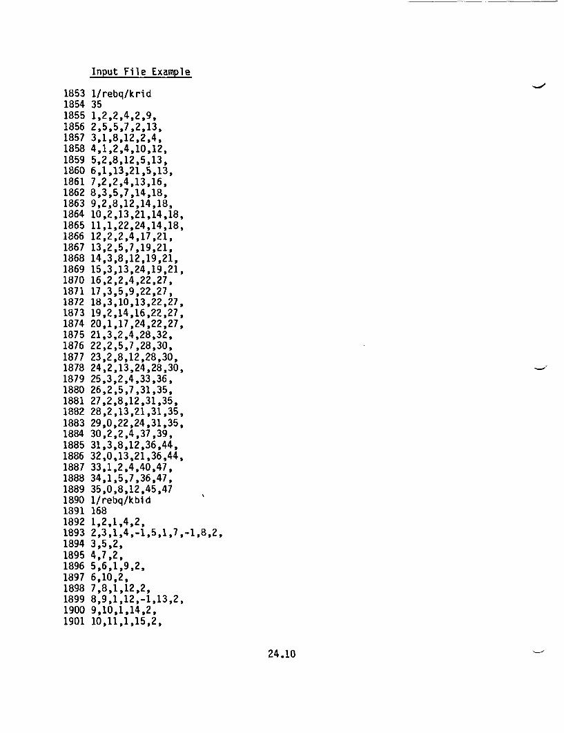
Input File Example
1853 1/rebq/krid1854 351855 1,2,2,4,2,9,1856 2,5,5,7,2,13,1857 3,1,8,12,2,4,1858 4,1,2,4,10,12,1859 5,2,8,12,5,13,1860 6,1,13,21,5,13,1861 7,2,2,4,13,16,1862 8,3,5,7,14,18,1863 9,2,8,12,14,18,1864 10,2,13,21,14,18,1865 11,1,22,24,14,18,1866 12,2,2,4,17,21,1867 13,2,5,7,19,21,1868 14,3,8,12,19,21,1869 15,3,13,24,19,21,1870 16,2,2,4,22,27,1871 17,3,5,9,22,27,1872 18,3,10,13,22,27,1873 19,2,14,16,22,27,1874 20,1,17,24,22,27,1875 21,3,2,4,28,32,1876 22,2,5,7,28,30,1877 23,2,8,12,28,30,1878 24,2,13,24,28,30,1879 25,3,2,4,33,36,1880 26,2,5,7,31,35,1881 27,2,8,12,31,35,1882 28,2,13,21,31,35,1883 29,0,22,24,31,35,1884 30,2,2,4,37,39,1885 31,3,8,12,36,44,1886 32,0,13,21,36,44,1887 33,1,2,4,40,47,1888 34,1,5,7,36,47,1889 35,0,8,12,45,471890 1/rebq/kbid1891 1681892 1,2,1,4,2,1893 2,3,1,4,-1,5,1,7,-1,8,2,1894 3,5,2,1895 4,7,2,1896 5,6,1,9,2,1897 6,10,2,1898 7,8,1,12,2,1899 8,9,1,12,-1,13,2,1900 9,10,1,14,2,1901 10,11,1,15,2,
24.10
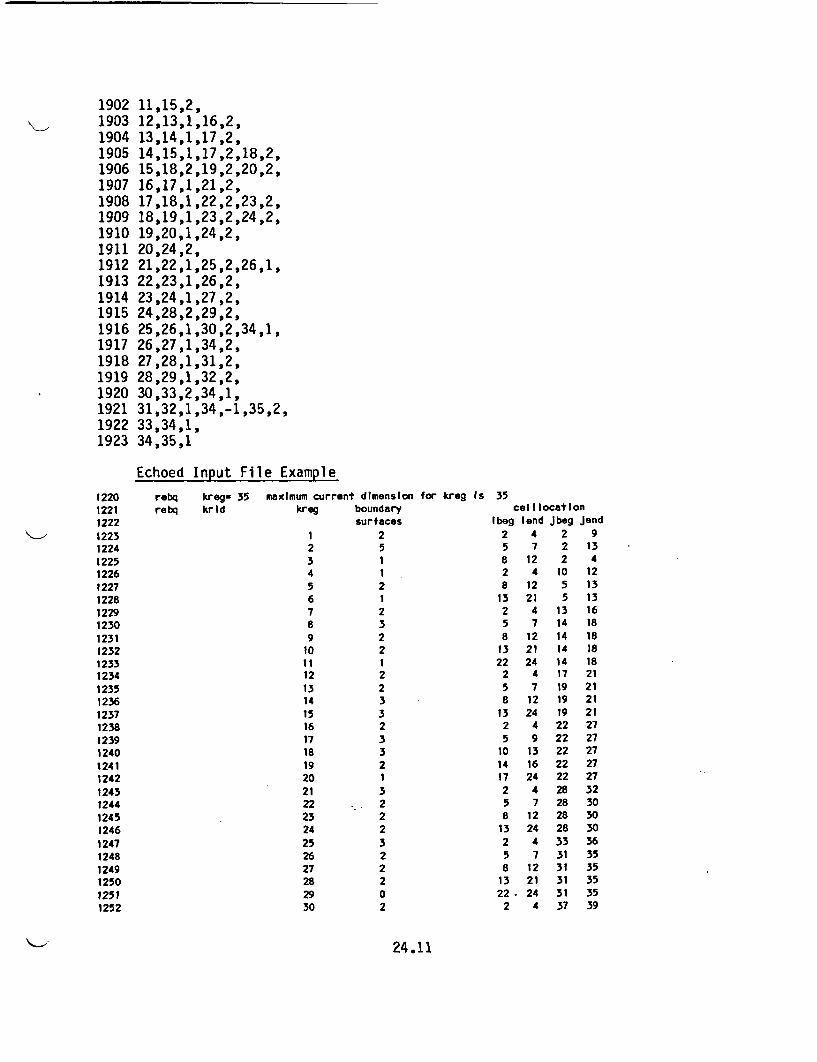
1902190319041905190619071908190919101911191219131914191519161917191819191920192119221923
11,15,2,12,13,1,16,2,13,14,1,17,2,14,15,1,17,2,18,2,15,18,2,19,2,20,2,16,17,1,21,2,17,18,1,22,2,23,2,18,19,1,23,2,24,2,19,20,1,24,2,20,24,2,21,22,1,25,2,26,1,22,23,1,26,2,23,24,1,27,2,24,28,2,29,2,25,26,1,30,2,34,1,26,27,1,34,2,27,28,1,31,2,28,29,1,32,2,30,33,2,34,1,31,32,1,34,-1,35,2,33,34,1,34,35,1
Echoed
rebqrebq
-
I nput
kreg.kr Id
122012211222122312241225122612271228122912301231123212331234123512361237123812391240124112421243124412451246124712481249125012511252
File Example
35 maximum current dimensionkreg boundary
surfaces1 22 53 14 15 26 17 28 39 2
10 211 112 213 214 315 316 217 318 319 220 121 322 223 224 225 326 227 228 229 030 2
for kreg Is 35cell location
Ibeg lend jbeg Jend2 4 2 95 7 2 138 12 2 42 4 10 128 12 5 13
13 21 5 132 4 13 165 7 14 188 12 14 18
13 21 14 1822 24 14 18
2 4 17 215 7 19 218 12 19 21
13 24 19 212 4 22 275 9 22 27
10 13 22 2714 16 22 2717 24 22 272 4 28 325 7 28 308 12 28 30
13 24 28 302 4 33 365 7 31 358 12 31 35
13 21 31 3522- 24 31 35
2 4 37 39
24.11
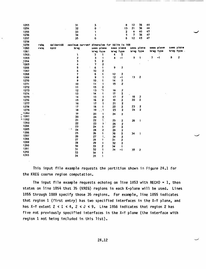
1253125412551256125712581259
3132333435
30
0
8 12 36 4413 21 36 442 4 40 475 7 36 478 12 45 47
rebq kbida-168 maximum current dimension for kbida Is 1681260 rebq kbid12611262N1263126412651266126712681269127012711272127312741275127612771278127912801281128212831284128512861287128812891290129112921293
kreg sees plane sees plane sees plane sees plane sees plane
12345678910311213141 5161718
192021222324
2526272830313334
kreg23576
108910.111513141518171819
2024222324282627282933323435
type
1
22
2
1
2
1
1
2'-I2
1~
2
kreg type4 24 -1
kreg type kreg type
5 1 7 -1
kreg type .
8 2
9 2
12 212 -114 215 2
16 217 217 219 221 222 223 2
24 2
25 226 227 229 230 234 231 232 234 134 -1
13 2
18 220 2
23 224 2
26 1
34 1
35 2
This input file example reques-
the KREG coarse region computation.
ts the partition shown in Figure 24.1 for
The input file example requests echoing on line 1853 with NECHO = 1, then
states on line 1854 that 35 (KREG) regions in each K-plane will be used. Lines
1855 through 1889 specify those 35 regions. For example, line 1855 indicates
that region 1 (first entry) has two specified interfaces in the X-Y plane, and
has X-Y extent 2 c I c 4, 2 < J < 9. Line 1856 indicates that region 2 has
five not previously specified interfaces in the X-Y plane (the interface with
region 1 not being included in this list).
24.12
Line 1890 of the input example introduces the forthcoming KBID array data
by again setting NECHO'to 1 with accompanying comments. Line 1891 promises 168
forthcoming numbers to specify the interfaces between the KREG type cells, and
these 168 entries in the KBID array appear in lines 1892 through 1923. Line
1892 indicates that cell 1 (first number) sees cell 2 (second number) on its
positive X side (as specified by the third number, 1), and sees cell 4 (fourth
number) on its +Y side (as specified by the fifth number, 2). Recall that two
pairs of bounding cells for cell 1 had been specified by the second entry NBND
= 2 for cell 1 on line 1855. Line 1893 gives five new interfaces for cell 2,
but does not give the 1-2 interface, which was specified on line 1892. No
trailing zeros appear in this KBID array data because the array was dimensioned
exactly to KBIDAP = 168.
The echoed input gives the KREG information in tabular form.
24.3.4 JREG Partition Specifications
General Input Format
NECHOJREGJRID(L), L = 1, JRIDAPNECHOJBIDAJBID(L), L = 1, JBIDAP
General Input Description
* NECHO - Echoing switch for this section of input, if input is
to be echoed, then NECHO = 1; otherwise, 0.
* JREG - Number of coarse computational cells in the X-Z plane
for each J-plane.
* JRID - Array defining the coarse cells in the X-Z plane for
each J-plane. The data entries for the regions follow
consecutively end-to-end, with the six entries for
each region being
JREGNO, NBND, IBEG, IEND, KBEG, KEND
24.13
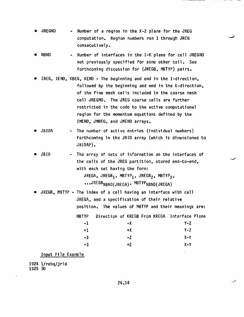
* JREGNO
* NBND
- Number of a region in the X-Z plane for the JREG
computation. Region numbers run 1 through JREG
consecutively.
- Number of interfaces in the I-K plane for cell JREGNO
not previously specified for some other cell. See
forthcoming discussion for (JREGB, MBTYP) pairs.
* IBEG, IEND, KBEG, KEND - The beginning and end in the I-direction,
followed by the beginning and end in the K-direction,
of the fine mesh cells included in the coarse mesh
cell JREGNO. The JREG coarse cells are further
restricted in the code to the active computational
region for the momentum equations defined by the
IMEND, JMBEG, and JMEND arrays.
* JBIDA - The number of active entries (individual numbers)
forthcoming in the JBID array (which is dimensioned to
JBIDAP).
* JBID - The array of sets of information on the interfaces of
the cells of the JREG partition, stored end-to-end,
with each set having the form:
JREGA, JREGB1, MBTYP 1, JREGB2, MBTYP2,
...JREGBNBND(JREGA). MBTYPNBND(JREGA)
* JREGB, MBTYP - The index of a cell having an interface with cell
JREGA, and a specification of their relative
position. The values of MBTYP and their meanings are:
MBTYP
-1
+1
-3
+3
Direction of KREGB From KREGA Interface Plane
-X yz
+X Y-Z
-Z X-Y
+Z X-Y
Input File Example
1924 1/rebq/jrid1925 30
24.14
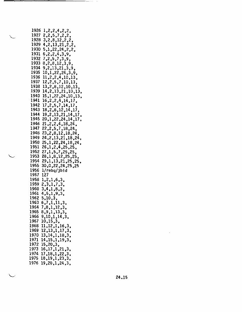
1926 1,2,2,4,2,2,1927 2,2,5,7,2,2,1928 3,2,8,12,2,2,1929 4,2,13,21,2,2,1930 5,1,22,24,2,2,1931 6,2,2,4,3,9,1932 7,2,5,7,3,9,1933 8,2,8,12,3,9,1934 9,2,13,21,3,9,1935 10,1,22,24,3,9,1936 11,2,2,4,10,13,1937 12,2,5,7,10,13,1938 13,2,8,12,10,13,1939 14,2,13,21,10,13,1940 15,1,22,24,10,13,1941 16,2,2,4,14,17,1942 17,2,5,7,14,17,1943 18,2,8,12,14,17,1944 19,2,13,21,14,17,1945 20,1,22,24,14,17,1946 21,2,2,4,18,24,1947 22,2,5,7,18,24,1948 23,2,8,12,18,24,1949 24,2,13,21,18,24,1950 25,1,22,24,18,24,1951 26,1,2,4,25,25,1952 27,1,5,7,25,25,1953 28,1,8,12,25,25,1954 29,1,13,21,25,25,1955 30,0,22,24,25,251956 1/rebq/jbid1957 1271958 1,2,1,6,3,1959 2,3,1,7,3,1960 3,4,1,8,3,1961 4,5,1,9,3,1962 5,10,3,1963 6,7,1,11,3,1964 7,8,1,12,3,1965 8,9,1,13,3,1966 9,10,1,14,3,1967 10,15,3,1968 11,12,1,16,3,1969 12,13,1,17,3,1970 13,14,1,18,3,1971 14,15,1,19,3,1972 15,20,3,1973 16,17,1,21,3,1974 17,18,1,22,3,1975 18,19,1,23,3,1976 19,20,1,24,3,
24.15
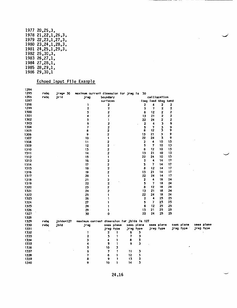
1977 20,25,3,1978 21,22,1,26,3,1979 22,23,1,27,3,1980 23,24,1,28,3,1981 24,25,1,29,3,1982 25,30,3,1983 26,27,1,1984 27,28,1,1985 28,29,1,1986 29,30,1
Echoed Input File Example
12941295129612971298129913001301130213031304130513061307130813091310131113121313131413151316131713181319132013211322132313241325132613271328132913301331133213351334133513361337133813391340
rebq Jreg= 30 maximum current dimension for Jreg Is 30rebq jrid jreg boundary cell1cation
surfaces Ibeg lend kbeg kend1 2 2 4 2 22 2 5 7 2 23 2 8 12 2 24 2 13 21 2 25 1 22 24 2 26 2 2 4 3 97 2 5 7 3 98 2 8 12 3 99 2 13 21 3 9
10 1 22 24 3 911 2 2 4 10 1312 2 5 7 10 1313 2 8 12 10 1314 2 13 21 10 1315 1 22 24 10 1316 2 2 4 14 1717 2 5 7 14 1718 2 8 12 14 1719 2 13 21 14 1720 1 22 24 14 1721 2 2 4 18 2422 2 5 7 18 2423 2 8 12 18 2424 2 13 21 18 2425 1 22 24 18 2426 1 2 4 25 2527 1 5 7 25 2528 1 8 12 25 2529 1 13 21 25 2530 0 22 24 25 25
rebq JbIda=127 maximum current dimension for Jbida Is 127rebq JbId jreg sees plane sees plane sees plane sees plane sees plane
jreg type jreg type Jreg type jreg type Jreg type1 2 1 6 32 3 1 7 33 4 1 8 34 5 1 9 356789
10 37 18 19 1
10 1
11 312 313 314 3
24.16
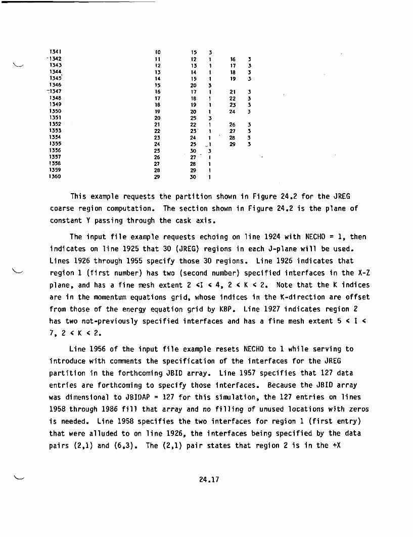
1341 10 15 3-1342 11 12 1 16 3
1343 12 13 1 17 31344 13 14 1 18 31345 14 15 1 19 31346 15 20 3
-:1347 16 17 1 21 31348 17 18 1 22 31349 i1 19 1 23 31350 19 20 1 24 31351 20 25 31352 21 22 1 26 31353 22 23 1 27 31354 23 24 1 28 31355 24 25 1 29 31356 25 30 31357 26 27 11358 27 28 11359 28 29 11360 29 30 1
This example requests the partition shown in Figure 24.2 for the JREG
coarse region computation. The section shown in Figure 24.2 is the plane of
constant Y passing through the cask axis.
The input file example requests echoing on line 1924 with NECHO = 1, thenindicates on line 1925 that 30 (JREG) regions in each J-plane will be used.
Lines 1926 through 1955 specify those 30 regions. Line 1926 indicates that
region 1 (first number) has two (second number) specified interfaces in the X-Z
plane, and has a fine mesh extent 2 4I 4 4, 2 < K ' 2. Note that the K indices
are in the momentum equations grid, whose indices in the K-direction are offset
from those of the energy equation grid by KBP. Line 1927 indicates region 2has two not-previously specified interfaces and has a fine mesh extent 5 < I <
7, 2 < K < 2.
Line 1956 of the input file example resets NECHO to 1 while serving to
introduce with comments the specification of the interfaces for the JREG
partition in the forthcoming JBID array. Line 1957 specifies that 127 data
entries are forthcoming to specify those interfaces. Because the JBID array
was dimensional to JBIDAP = 127 for this simulation, the 127 entries on lines1958 through 1986 fill that array and no filling of unused locations with zeros
is needed. Line 1958 specifies the two interfaces for region 1 (first entry)
that were alluded to on line 1926, the interfaces being specified by the data
pairs (2,1) and (6,3). The (2,1) pair states that region 2 is in the +X
24.17
direction from region 1, while the (6,3) pair states that region 6 is in the +Z
direction from region 1 in the JREG partition.
Line 1959 of the input file example specifies the two not-previously
specified interfaces of JREG cell 2. Cell 2 (first number) has an interface
with cell 3 (second number) on its +X (third number, +1) side, and with cell 7
(fourth number) on its +Z (fifth number, +3) side.
The echoed input summarizes the information on the JREG partition and
interfaces in tabular form.
24.3.5 IREG Partition Specifications
General Input Format
NECHOIREGIRID(L), L = 1, IRIDAPNECHOIBIDAIBID(L), L = 1, IBIDAP
General Input Description
* NECHO - Echoing switch for this section of input. If input is
to be echoed, then NECHO = 1; otherwise, 0.
* IREG - Number of coarse computational cells in a Y-Z plane at
each I-plane.
* IRID - Array defining the coarse cells in a Y-Z plane for
each I-plane. The data entries for the regions follow
consecutively end-to-end, the six entries for each
region being:
IREGNO, NBND, JBEG, JEND, KBEG, KEND
* IREGNO - Number of a region in the Y-Z plane for the IREG
computation. Region numbers run 1 through IREG
consecutively.
* NBND - Number of interfaces in the J-K plane for cell IREGNO
not previously specified for some other cell. See
forthcoming discussion of (IREG, MBTYP) pairs.
24.18
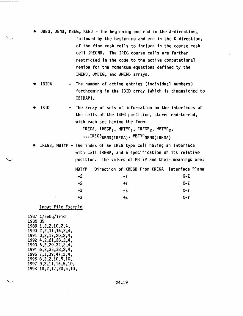
* JBEG, JEND, KBEG, KEND - The beginning and end in the J-direction,
followed by the beginning and end in the K-direction,
of the fine mesh cells to include in the coarse mesh
cell IREGNO. The IREG coarse cells are further
restricted in the code to the active computational
region for the momentum equations defined by the
IMEND, JMBEG, and JMEND arrays.
* IBIDA - The number of active entries (individual numbers)
forthcoming in the IBID array (which is dimensioned to
IBIDAP).
* IBID - The array of sets of information on the interfaces of
the cells of the IREG partition, stored end-to-end,
with each set having the form:
IREGA, IREGB1, MBTYP1, IREGB2, MBTYP2,
...IREGBNBND(IREGA). MBTYPNBND(IREGA)
* IREGB, MBTYP - The index of an IREG type cell having an interface
with cell IREGA, and a specification of its relative
position. The values of MBTYP and their meanings are:
MBTYP
-2
+2
-3
+3
Direction of KREGB From KREGA Interface Plane
-Y X-Z
+Y X-Z
-Z X-Y
+Z X-Y
198719881989199019911992199319941995199619971998
Input File Example
1/rebq/irid351,2,2,10,2,4,2,2,11,16,2,4,3,2,17,20,2,4,4,2,21,28,2,4,5,2,29,32,2,4,6,2,33,38,2,4,7,1,39,47,2,4,8,2,2,10,5,10,9,2,11,16,5,10,10,2,17,20,5,10,
24.19
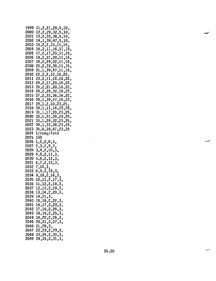
1999 11,2,21,28,5,10,2000 12,2,29,32,5,10,2001 13,2,33,38,5,10,2002 14,1,39,47,5,10,2003 15,2,2,10,11,15,2004 16,2,11,16,11,15,2005 17,2,17,20,11,15,2006 18,2,21,28,11,15,2007 19,2,29,32,11,15,2008 20,2,33,38,11,15,2009 21,1,39,47,11,15,2010 22,2,2,10,16,22,2011 23,2,11,16,16,22,2012 24,2,17,20,16,22,2013 25,2,21,28,16,22,2014 26,2,29,32,16,22,2015 27,2,33,38,16,22,2016 28,1,39,47,16,22,2017 29,1,2,10,23,25,2018 30,1,11,16,23,25,2019 31,1,17,20,23,25,2020 32,1,21,28,23,25,2021 33,1,29,32,23,25,2022 34,1,33,38,23,25,2023 35,0,39,47,23,252024 1/rebq/ibid2025 1502026 1,2,2,8,3,2027 2,3,2,9,3,2028 3,4,2,10,3,2029 4,5,2,11,3,2030 5,6,2,12,3,2031 6,7,2,13,3,2032 7,14,3,2033 8,9,2,15,3,2034 9,10,2,16,3,2035 10,11,2,17,3,2036 11,12,2,18,3,2037 12,13,2,19,3,2038 13,14,2,20,3,2039 14,21,3,2040 15,16,2,22,3,2041 16,17,2,23,3,2042 17,18,2,24,3,2043 18,19,2,25,3,2044 19,20,2,26,3,2045 20,21,2,27,3,2046 21,28,3,2047 22,23,2,29,3,2048 23,24,2,30,3,2049 24,25,2,31,3,
24.20
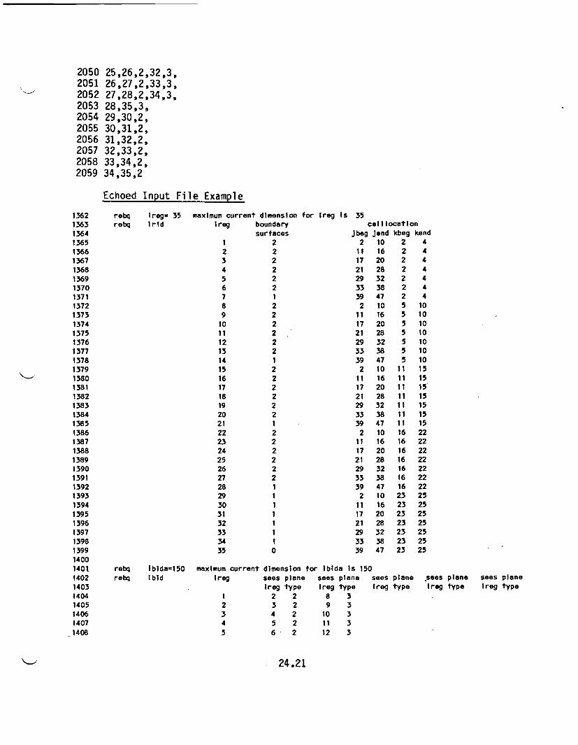
2050 25,26,2,32,3,2051 26,27,2,33,3,2052 27,28,2,34,3,2053 28,35,3,2054 29,30,2,2055 30,31,2,2056 31,32,2,2057 32,33,2,2058 33,34,2,2059 34,35,2
Echoed Input File Example
13621363136413651366136713681369137013711372137313741375137613771378137913801381138213831384138513861387138813891390139113921393139413951396139713981399140014011402140314041405140614071408
rebq Ireg- 35 maximum current dimension for Ireg Is 35
rebq Irld Ireg boundary cellocationsurfaces Jbeg Jend kbeg kend
1 2 2 10 2 4
2 2 11 16 2 4
3 2 17 20 2 4
4 2 21 28 2 45 2 29 32 2 4
6 2 33 38 2 4
7 1 39 47 2 4
8 2 2 10 5 10
9 2 11 16 5 10
10 2 17 20 5 10
11 2 21 28 5 10
12 2 29 32 5 10
13 2 33 38 5 10
14 1 39 47 5 10
15 2 2 10 11 15
16 2 11 16 11 15
17 2 17 20 11 15
18 2 21 28 11 15
19 2 29 32 11 15
20 2 33 38 11 15
21 1 39 47 11 15
22 2 2 10 16 22
23 2 11 16 16 22
24 2 17 20 16 22
25 2 21 28 16 22
26 2 29 32 16 22
27 2 33 38 16 22
28 1 39 47 16 22
29 1 2 10 23 25
30 1 11 16 23 25
31 1 17 20 23 25
32 1 21 28 23 25
33 1 29 32 23 25
34 1 33 38 23 25
35 0 39 47 23 25
rebq Ibida=150 maximum current dimension for Ibida Is 150
rebq Ibid Ireg sees plane sees plans sees plane sees plane sees plane
ireg type Ireg type Ireg type Ireg type Ireg type
1 2 2 8 32 3 2 9 3
3 4 2 10 34 5 2 11 3
5 6 2 12 3
24.21
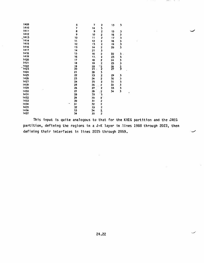
1409 6 7 2 13 31410 7 14 3
1411 8 9 2 15 31412 9 10 2 16 3
.1413 10 11 2 17 3-1414 iI 12 2 18 31415 12 13 2 19 31416 13 14 2 20 31417 14 21 31418 15 16 2 22 351419 16 17. 2 23 3
1420 17 18 2 24 31421 18 19 2 25 31422 19 20 2 26 31423 20 2T z 7 3'1424 21 28 31425 22 23 2 29 31426 23 24 2 30 31427 24 25 2 31 31428 25 26 2 32 31429 26 27 2 33 31430 27 28 .? 34 31431 28 35 31432 29 30 21433 30 31 21434 31 32 21435 32 33 21436 33 34 21437 34 35 2
This input is quite analogous to that for the KREG partition and the JREG
partition, defining the regions in a J-K layer in lines 1988 through 2023, then
defining their interfaces in lines 2025 through 2059.
24.22
25.0 SUBROUTINE CROUT
Subroutine CROUT employs a direct method for the solution of linear matrix
equations associated with subroutines REBA and REBQ. The Crout method is used
to solve matrix equations of the form
AX = B
where A is an m by m square matrix and X and B each have m rows and n
columns. A discussion of the Crout method may be found in Westlake (1968).
25.1 PARAMETER STATEMENT INFORMATION
The dimension of arrays A and B are specified by two parameters:
* ICRP - Row and column dimension of A and rows of B. If
subroutine REBA is used, then ICRP = 3. If subroutine
REBQ is used, then ICRP = MAX(IREG,JREG,KREG). If
both subroutines are used, then ICRP must equal the
largest of the above two dimensions.
* JCRP - Number of columns of B. If subroutine REBA is used,
then JCRP = 4. If subroutine REBQ is used, then JCRP
= ICRP. If both subroutines are used, then JCRP must
equal the largest of the above two dimensions.
25.2 INPUT FORMAT
Subroutine CROUT does not read the input file.
25.1
26.0 SUBROUTINE AF
Subroutine AF solves a Poisson equation (derived in Volume I - Equations
and Numerics, Chapter 9.0) for the pressure-correction field. It is one of the
set of subroutines (viz., PILES, REBS, REBQ, and AF) that can be called upon by
subroutine PITER to produce this solution. The method employed in this routine
is effectively an approximate factorization of the pressure-correction-field
matrix operator. Since the factorization is approximate, the exact solution is
not obtained in one pass through the algorithm. The user must specify the num-
ber of times the routine will cycle through the algorithm in each pass through
the subroutine. This is done with input variable NMAX.
Subroutine AF also allows the user to monitor the convergence history of
this algorithm. By setting input variable INFO = 1, AF will print the follow-
ing information: iteration count, the value of the current pressure-correction
at the (I,J,K) mesh location corresponding to the cell experiencing the largest
right-hand-side residual (in absolute value), the right-hand-side residual at
cell (I,J,K), and the I, J, and K cell indices for this "worst-case" cell.
With INFO = 1, this information is provided after entering AF just prior to
commencement of the iteration (for which case the iteration count and the
largest right-hand-side residual are printed as having values of 0), and once
again for each of the NMAX iterations. If this output is not desired, specify
INFO = 0 in the input.
26.1 PARAMETER STATEMENT INFORMATION
Subroutine AF requires the specification of parameters IP, JP, KP, KBP,
and KTP. These data define the overall computational mesh and are described in
the discussion of subroutine GRID in Chapter 4.0.
26.2 INPUT FORMAT
26.2.1 Overview
Very little input is required by subroutine AF. Only three variables are
read--NECHO, NMAX, and INFO. The input sequence and definition is provided
below.
26.1
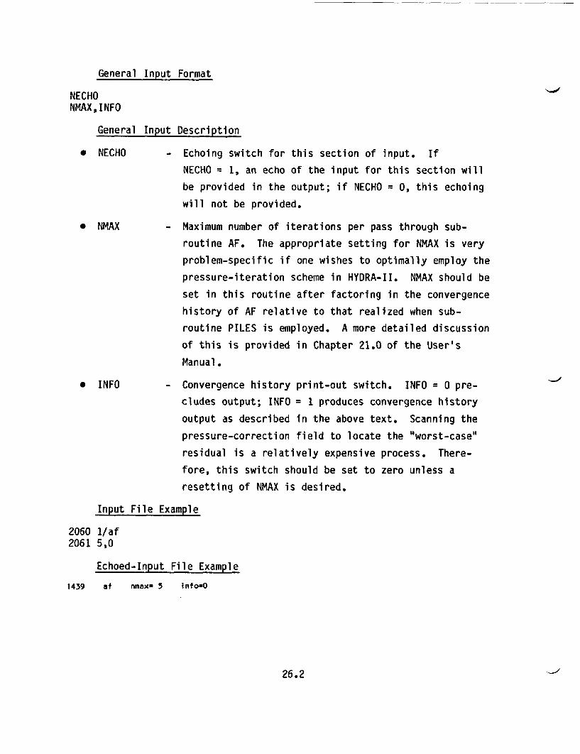
General Input Format
NECHONMAX,INFO
General Input Description
* NECHO - Echoing switch for this section of input. If
NECHO = 1, an echo of the input for this section will
be provided in the output; if NECHO = 0, this echoing
will not be provided.
* NMAX - Maximum number of iterations per pass through sub-
routine AF. The appropriate setting for NMAX is very
problem-specific if one wishes to optimally employ the
pressure-iteration scheme in HYDRA-II. NMAX should be
set in this routine after factoring in the convergence
history of AF relative to that realized when sub-
routine PILES is employed. A more detailed discussion
of this is provided in Chapter 21.0 of the User's
Manual.
* INFO - Convergence history print-out switch. INFO = 0 pre-cludes output; INFO = 1 produces convergence history
output as described in the above text. Scanning the
pressure-correction field to locate the "worst-case"
residual is a relatively expensive process. There-
fore, this switch should be set to zero unless a
resetting of NMAX is desired.
Input File Example
2060 1/af2061 5,0
Echoed-Input File Example
1439 at nmax- 5 Info=O
26.2

NECHO is set to 1 on input line 2060. NMAX and INFO are set to 5 and 0,
respectively, on input line 2061. With NECHO set to 1, these input data are
echoed in the output on line 1439.
26.3
27.0 SUBROUTINE AVG
Subroutine AVG computes the pressure adjustment required to satisfy the
user-specified constraint of either fixed total fluid mass or fixed average
pressure for the system. In either case, AVG takes advantage of the indeter-
minacy of the pressure field defined by the momentum equations. This indeter-
minacy allows the pressure field to be shifted by a spatially-uniform amount in
every cell of the computational mesh to effect the desired mass or average-
pressure constraint.
The choice of one or the other is determined by the user with a positive
input for FIXEDM (for fixed total system mass) or FIXEDP (for fixed average
system pressure). If either of the options is NOT desired, the corresponding
input should be zero.
27.1 PARAMETER STATEMENT INFORMATION
Subroutine AVG requires the specification of parameters IP, JP, KP, KBP,
and KTP. These data define the overall computational mesh and are described in
the discussion of subroutine GRID in Chapter 4.0.
27.2 INPUT FORMAT
27.2.1 Overview
Very little input is required by subroutine AVG. Only three variables are
read--NECHO, FIXEDM, and FIXEDP. The input sequence and definition is provided
below.
General Input Format
NECHOFIXEDM,FIXEDP
General Input Description
* NECHO - Echoing switch for this section of input. If
NECHO = 1, an echo of the input for this section will
be provided in the output; if NECHO = 0, this echoing
will not be provided.
27.1
* FIXEDM
* FIXEDP
- Flag to indicate whether or not the system mass is
fixed and, if so, at what value. If this option is
not to be used, set FIXEDM = 0.0; otherwise, set
FIXEDM = desired system mass in grams.
- Flag to indicate whether or not the system is operat-
ing at fixed average pressure. If this option is not
to be used, set FIXEDP = 0.0; otherwise, set FIXEDP =
desired average system pressure in dyn/cm2.
Input File Example
2062 1/avg2063 0.0,0.496e+6
Echoed-Input File Example
1441 avg f ixedmO.OOOOOOOe+OO f Ixedp=0.4960000e+06
NECHO is set to 1 on input line 2062. FIXEDM and FIXEDP have been set to
0 grams and 496000 dyn/cm2, respectively. Therefore, this simulation will
operate with a fixed average pressure.
27.2

28.0 SUBROUTINE PRINTL
Subroutine PRINTL is called from numerous locations to print array vari-
ables, according to user options or code defaults. PRINTL prints the triply-
dimensioned variable in its call list. No user attention to PRINTL is required
except to the dimensioning parameters.
28.1 PARAMETER STATEMENT INFORMATION
Subroutine PRINTL requires the specification of parameters IP and JP that
define the computational mesh and are described in Chapter 4.0, Subroutine
GRID. Two additional parameters, NPLA1P and NPLA2P, are required for speci-
fication of printing options. These are described in Chapter 3.0, Program
MAIN.
28.2 INPUT FORMAT
Subroutine PRINTL does not read user input.
28.1
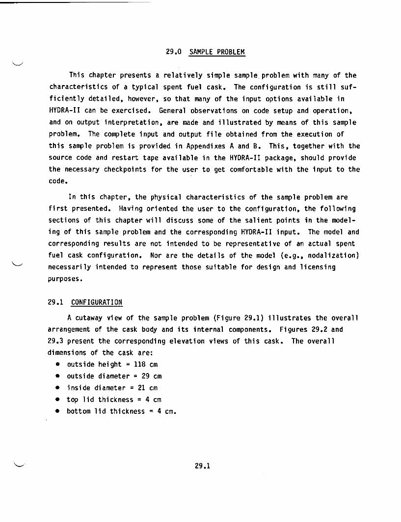
29.0 SAMPLE PROBLEM
This chapter presents a relatively simple sample problem with many of the
characteristics of a typical spent fuel cask. The configuration is still suf-
ficiently detailed, however, so that many of the input options available in
HYDRA-II can be exercised. General observations on code setup and operation,
and on output interpretation, are made and illustrated by means of this sample
problem. The complete input and output file obtained from the execution of
this sample problem is provided in Appendixes A and B. This, together with the
source code and restart tape available in the HYDRA-II package, should provide
the necessary checkpoints for the user to get comfortable with the input to the
code.
In this chapter, the physical characteristics of the sample problem are
first presented. Having oriented the user to the configuration, the following
sections of this chapter will discuss some of the salient points in the model-
ing of this sample problem and the corresponding HYDRA-II input. The model and
corresponding results are not intended to be representative of an actual spent
fuel cask configuration. Nor are the details of the model (e.g., nodalization)
necessarily intended to represent those suitable for design and licensing
purposes.
29.1 CONFIGURATION
A cutaway view of the sample problem (Figure 29.1) illustrates the overall
arrangement of the cask body and its internal components. Figures 29.2 and
29.3 present the corresponding elevation views of this cask. The overall
dimensions of the cask are:
* outside height = 118 cm
* outside diameter = 29 cm
* inside diameter = 21 cm
* top lid thickness = 4 cm
* bottom lid thickness = 4 cm.
29.1

I
-6-
49
3
is36
is74
55
FIGURE 29.1. Sample Problem Computational Mesh - Plan View
The top and bottom lids are welded to the side of the cask, leaving a slight
1-mm gap between the lid and cask side, as shown in the detail drawing of
Figure 29.4. The entire cask body is constructed of nodular cast iron.
Spent fuel rods are stored in a 9x9 square array within the cask. The
physical parameters for this array are:
* rod diameter = 1.072 cm
* pitch-to-diameter ratio = 1.334
* rod height = 100 cm.
The modeled portion of the rod array generates 290 watts of decay heat. There-
fore, the full rod array produces 1160 watts (4 x 290) of decay heat. The
relative activity profile for each rod is presented in Figure 29.5. Several of
29.2
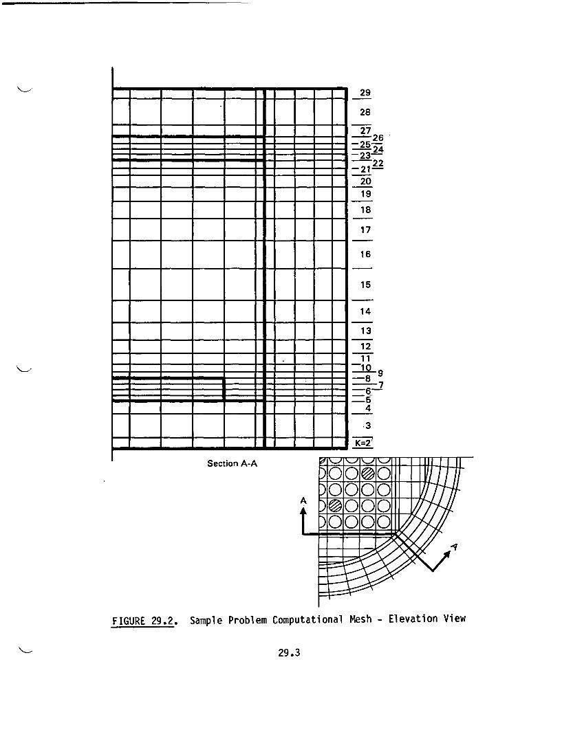
I~~~~ I 1Tl1T TI |~ [_ I F| f W I i
I A I I* * * *
I_0 j I | _li_
29
28
27-252231 24-2-
20
19
18
17
16
15
14
13
121 1
-8 9=-7
-54
.3
-k=-2'
Section A-A
i
e \J~-IIII I 1111 1. I 11 - -
c 010100) O 010.0 m>
F 0
FIGURE 29.2. Sample Problem Computational Mesh - Elevation View
29.3
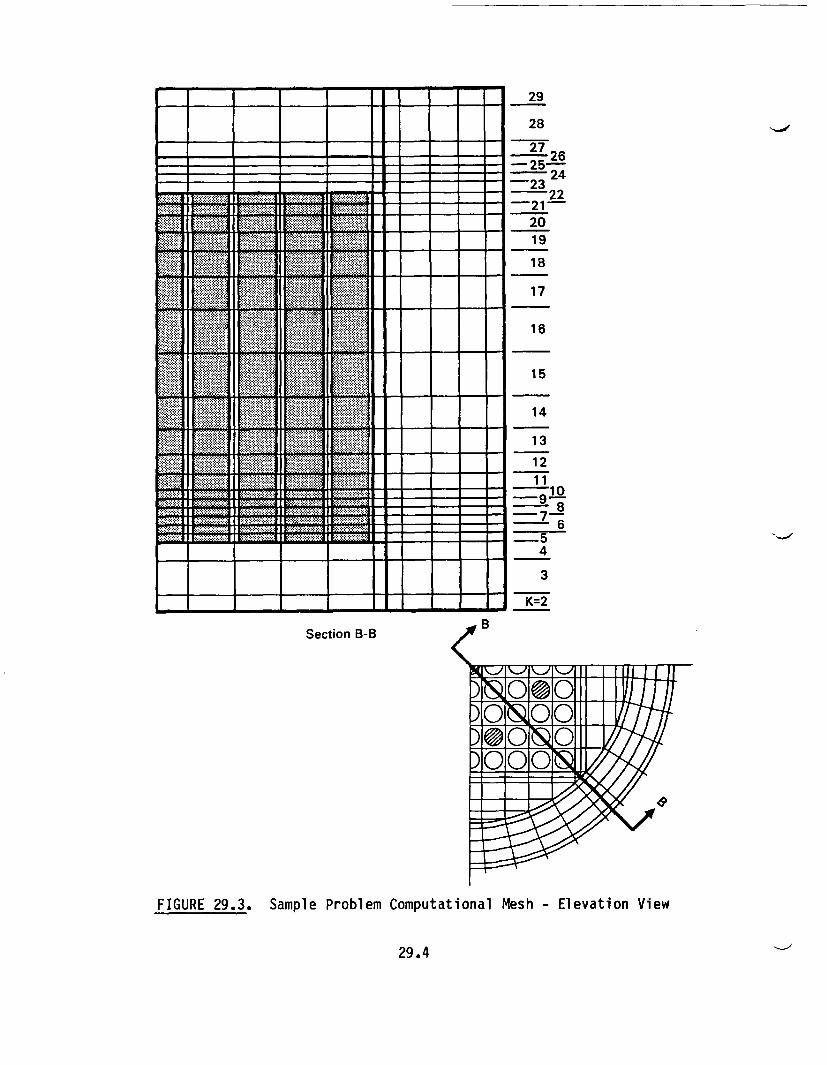
29
28
27 26-25--224
2322
21-2019
18
17
16
15
14
13
121 1-10-9-Il
-7- 86
- 5~4
3
K=2
Section B-B
FIGURE 29.3. Sample Problem Computational Mesh - Elevation View
29.4
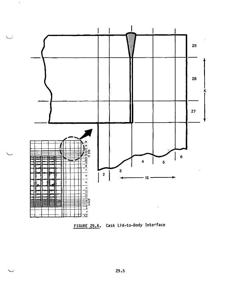
28
27
~29
522- -23
-- 20 I19
14
13
12
4
3
FIGURE 29.4. Cask Lid-to-Body Interface
29.5
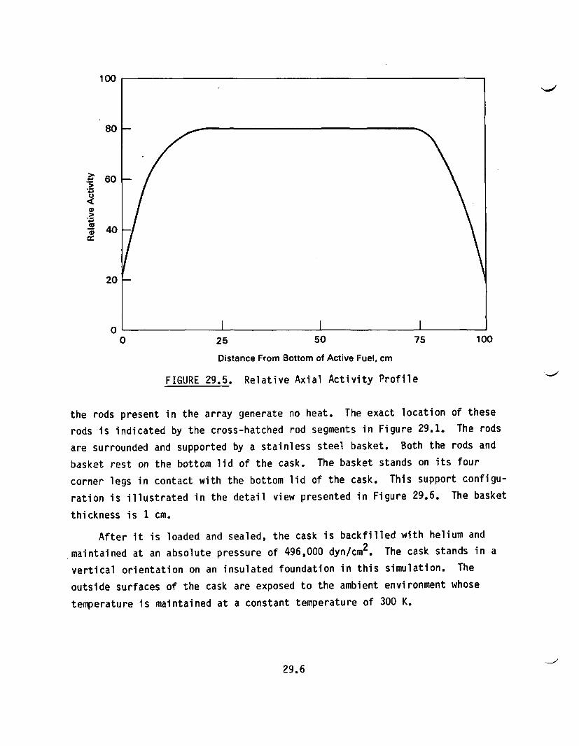
100
80 -
60 -
40
C.,
240
20
0 25 50 75 100
Distance From Bottom of Active Fuel, cm
FIGURE 29.5. Relative Axial Activity Profile
the rods present in the array generate no heat. The exact location of these
rods is indicated by the cross-hatched rod segments in Figure 29.1. The rods
are surrounded and supported by a stainless steel basket. Both the rods and
basket rest on the bottom lid of the cask. The basket stands on its four
corner legs in contact with the bottom lid of the cask. This support configu-
ration is illustrated in the detail view presented in Figure 29.6. The basket
thickness is 1 cm.
After it is loaded and sealed, the cask is backfilled with helium and
maintained at an absolute pressure of 496,000 dyn/cm2. The cask stands in a
vertical orientation on an insulated foundation in this simulation. The
outside surfaces of the cask are exposed to the ambient environment whose
temperature is maintained at a constant temperature of 300 K.
29.6
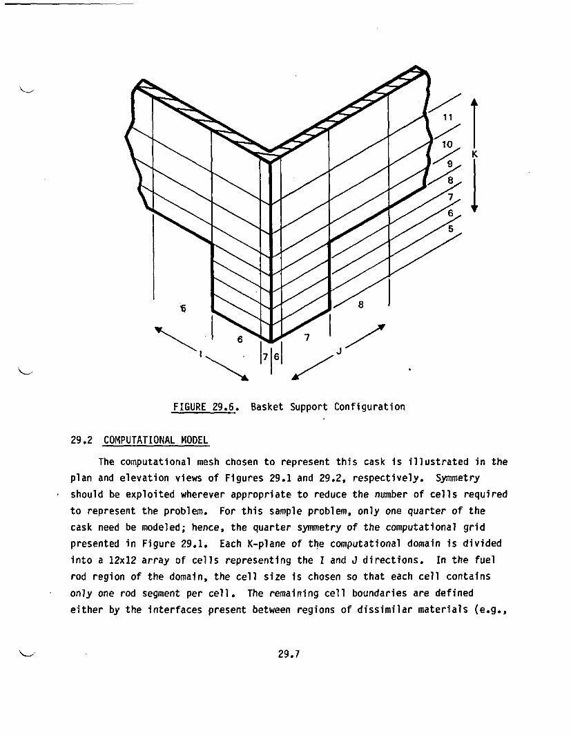
11
FIGURE 29.6. Basket Support Configuration
29.2 COMPUTATIONAL MODEL
The computational mesh chosen to represent this cask is illustrated in theplan and elevation views of Figures 29.1 and 29.2, respectively. Symmetryshould be exploited wherever appropriate to reduce the number of cells requiredto represent the problem. For this sample problem, only one quarter of thecask need be modeled; hence, the quarter symmetry of the computational gridpresented in Figure 29.1. Each K-plane of the computational domain is dividedinto a 12x12 array of cells representing the I and J directions. In the fuelrod region of the domain, the cell size is chosen so that each cell containsonly one rod segment per cell. The remaining cell boundaries are definedeither by the interfaces present between regions of dissimilar materials (e.g.,
29.7

helium and stainless steel), or to provide sufficient nodalization to ade-
quately represent the physics of the problem. Thus, regions where large
gradients in either temperature or velocity are anticipated should be repre-
sented with many cells of a scale adequate to capture these gradients.
Because of the Cartesian grid used to represent the interior of the cask
and the cask's cylindrical configuration, not all of the cells in the 12x12
array are activated in the model. The column of cells represented by I = 1 and
J = 1, 2, 3, ..., 12, and the row of cells at I = 2, 3, ..., 12 and J = 12 are
phantom cells used to represent the symmetry boundary conditions. The extent
of the active cells to be used in the model in obtaining a solution to the
momentum and energy equations is represented, in the usual way, by specifica-
tion of the "beg" and "end" values for the I and J indices of the active cells.
This information is provided as input to subroutine GRID. The cell sizes
(viz., DX(I) and DY(J)) are also provided as input to this subroutine. As
noted in Figure 29.1 and in the input to subroutine GRID, a small portion of
the cask interior represented by cells (I,J) = (2,1), (3,1), (12,10), and
(12,11) is not explicitly represented by the active cells of the Cartesian
region. However, the influence of these regions is still incorporated in the
model. This will be done in the input to subroutine PROP.
The azimuthal cell spacing in the cylindrical grid is set by the points-
of-intersection of the cartesian-region computational grid lines with the cask
body inner surface. Phantom cells for this region of the model are represented
by the row of cells at IS = 1 and JS = 1, 2, 3, ..., 14 as well as IS = 7, JS =
1, 2, 3, ..., 14. The fact that the outside of the cask has constant radius at
all elevations is represented by the uniformity of input to array ISEND(K) for
K= 1 through 30. As with the cartesian-grid information, this data is provided
in the input to subroutine GRID.
The input pertaining to material properties of the Cartesian region is
provided as input to subroutine PROP. For the most part, this input is rela-
tively straightforward and reflects the information necessary to set the
thermal resistances represented by the cells. However, the thermal resistance
of the regions represented by the cells at (I,J) = (2,1), (3,1), (12,10), and
(12,11) are incorporated as equivalent film resistances in the input to this
29.8
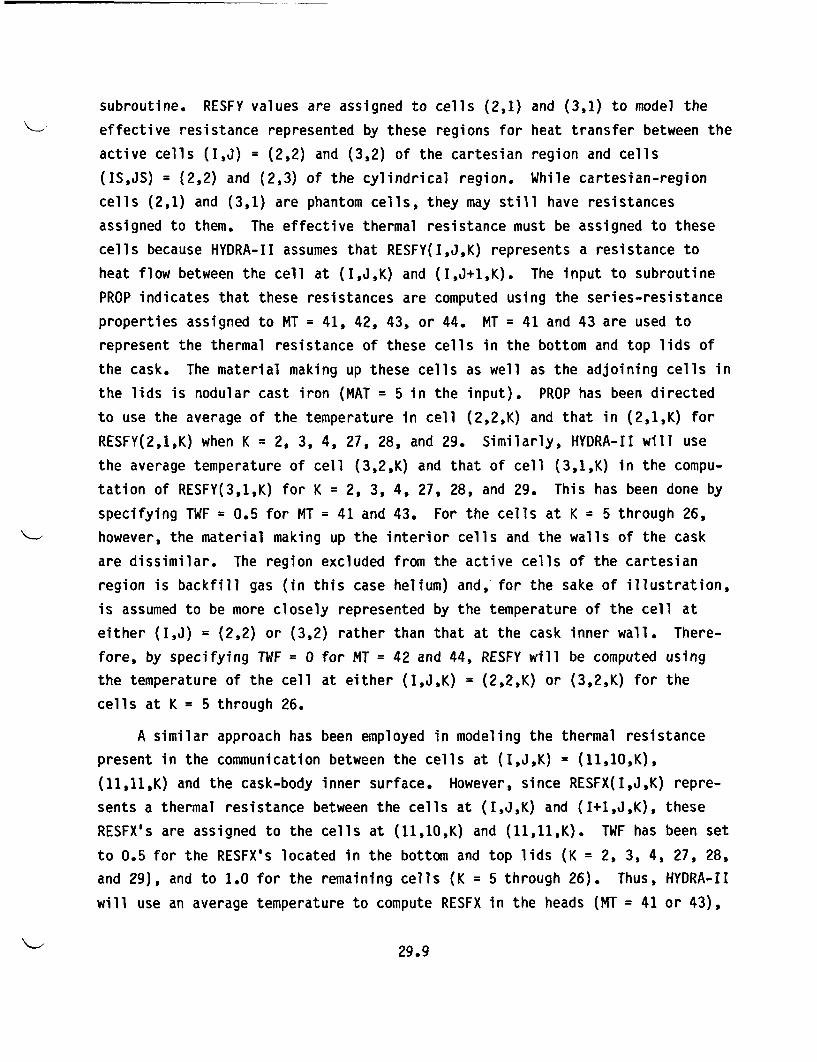
subroutine. RESFY values are assigned to cells (2,1) and (3,1) to model the
effective resistance represented by these regions for heat transfer between the
active cells (I,J) = (2,2) and (3,2) of the Cartesian region and cells
(IS,JS) = (2,2) and (2,3) of the cylindrical region. While cartesian-region
cells (2,1) and (3,1) are phantom cells, they may still have resistances
assigned to them. The effective thermal resistance must be assigned to these
cells because HYDRA-II assumes that RESFY(I,J,K) represents a resistance to
heat flow between the cell at (I,J,K) and (I,J+1,K). The input to subroutine
PROP indicates that these resistances are computed using the series-resistance
properties assigned to MT = 41, 42, 43, or 44. MT = 41 and 43 are used to
represent the thermal resistance of these cells in the bottom and top lids of
the cask. The material making up these cells as well as the adjoining cells in
the lids is nodular cast iron (MAT = 5 in the input). PROP has been directed
to use the average of the temperature in cell (2,2,K) and that in (2,1,K) for
RESFY(2,1,K) when K = 2, 3, 4, 27, 28, and 29. Similarly, HYDRA-II will use
the average temperature of cell (3,2,K) and that of cell (3,1,K) in the compu-
tation of RESFY(3,1,K) for K = 2, 3, 4, 27, 28, and 29. This has been done by
specifying TWF = 0.5 for MT = 41 and 43. For the cells at K = 5 through 26,
however, the material making up the interior cells and the walls of the cask
are dissimilar. The region excluded from the active cells of the Cartesian
region is backfill gas (in this case helium) and, for the sake of illustration,
is assumed to be more closely represented by the temperature of the cell at
either (I,J) = (2,2) or (3,2) rather than that at the cask inner wall. There-
fore, by specifying TWF = 0 for MT = 42 and 44, RESFY will be computed using
the temperature of the cell at either (I,J,K) = (2,2,K) or (3,2,K) for the
cells at K = 5 through 26.
A similar approach has been employed in modeling the thermal resistance
present in the communication between the cells at (I,J,K) = (11,1O,K),
(11,11,K) and the cask-body inner surface. However, since RESFX(I,J,K) repre-
sents a thermal resistance between the cells at (I,J,K) and (I+1,J,K), these
RESFX's are assigned to the cells at (11,10,K) and (11,11,K). TWF has been set
to 0.5 for the RESFX's located in the bottom and top lids (K = 2, 3, 4, 27, 28,
and 29), and to 1.0 for the remaining cells (K = 5 through 26). Thus, HYDRA-It
will use an average temperature to compute RESFX in the heads (MT = 41 or 43),
29.9
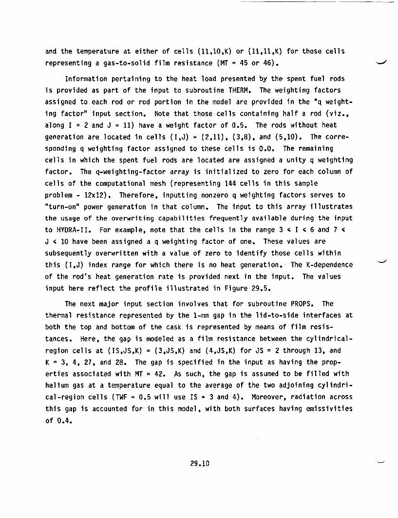
and the temperature at either of cells (11,10,K) or (11,11,K) for those cells
representing a gas-to-solid film resistance (MT = 45 or 46).
Information pertaining to the heat load presented by the spent fuel rods
is provided as part of the input to subroutine THERM. The weighting factors
assigned to each rod or rod portion in the model are provided in the "q weight-
ing factor" input section. Note that those cells containing half a rod (viz.,
along I = 2 and J = 11) have a weight factor of 0.5. The rods without heat
generation are located in cells (I,J) = (2,11), (3,8), and (5,10). The corre-
sponding q weighting factor assigned to these cells is 0.0. The remaining
cells in which the spent fuel rods are located are assigned a unity q weighting
factor. The q-weighting-factor array is initialized to zero for each column of
cells of the computational mesh (representing 144 cells in this sample
problem - 12x12). Therefore, inputting nonzero q weighting factors serves to
"turn-on" power generation in that column. The input to this array illustrates
the usage of the overwriting capabilities frequently available during the input
to HYDRA-II. For example, note that the cells in the range 3 4 I < 6 and 7 (
J < 10 have been assigned a q weighting factor of one. These values are
subsequently overwritten with a value of zero to identify those cells within
this (I,J) index range for which there is no heat generation. The K-dependence
of the rod's heat generation rate is provided next in the input. The values
input here reflect the profile illustrated in Figure 29.5.
The next major input section involves that for subroutine PROPS. The
thermal resistance represented by the 1-mm gap in the lid-to-side interfaces at
both the top and bottom of the cask is represented by means of film resis-
tances. Here, the gap is modeled as a film resistance between the cylindrical-
region cells at (IS,JS,K) = (3,JS,K) and (4,JS,K) for JS = 2 through 13, and
K = 3, 4, 27, and 28. The gap is specified in the input as having the prop-
erties associated with MT = 42. As such, the gap is assumed to be filled with
helium gas at a temperature equal to the average of the two adjoining cylindri-
cal-region cells (TWF = 0.5 will use IS = 3 and 4). Moreover, radiation across
this gap is accounted for in this model, with both surfaces having emissivities
of 0.4.
29.10
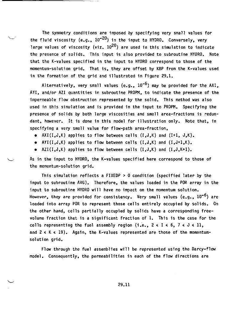
The symmetry conditions are imposed by specifying very small values for
the fluid viscosity (e.g., 10-20) in the input to HYDRO. Conversely, very
large values of viscosity (viz. 1020) are used in this simulation to indicate
the presence of solids. This input is also provided to subroutine HYDRO. Note
that the K-values specified in the input to HYDRO correspond to those of the
momentum-solution grid. That is, they are offset by KBP from the K-values used
in the formation of the grid and illustrated in Figure 29.1.
Alternatively, very small values (e.g., 10-6) may be provided for the AXI,
AYI, and/or AZI quantities in subroutine PROPM, to indicate the presence of the
impermeable flow obstruction represented by the solid. This method was also
used in this simulation and is provided in the input to PROPM. Specifying the
presence of solids by both large viscosities and small area-fractions is redun-
dant, however. It is done in this model for illustration only. Note that, in
specifying a very small value for flow-path area-fraction,
* AXI(I,J,K) applies to flow between cells (I,J,K) and (1+1, J,K).
* AYI(I,J,K) applies to flow between cells (I,J,K) and (I,J+1,K).
* AZI(I,J,K) applies to flow between cells (I,J,K) and (I,J,K+1).
As in the input to HYDRO, the K-values specified here correspond to those of
the momentum-solution grid.
This simulation reflects a FIXEDP > 0 condition (specified later by the
input to subroutine AVG). Therefore, the values loaded in the POR array in the
input to subroutine HYDRO will have no impact on the momentum solution.
However, they are provided for consistency. Very small values (e.g., 10-6) are
loaded into array POR to represent those cells entirely occupied by solids. On
the other hand, cells partially occupied by solids have a corresponding free-
volume fraction that is a significant fraction of 1. This is the case for the
cells representing the fuel assembly region (i.e., 2 c I ' 6, 7 c J 4 11,
and 2 ( K 4 19). Again, the K-values represented are those of the momentum-
solution grid.
Flow through the fuel assemblies will be represented using the Darcy-flow
model. Consequently, the permeabilities in each of the flow directions are
29.11
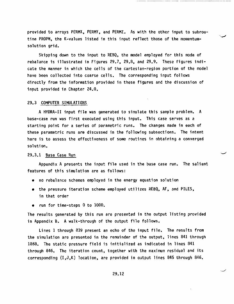
provided to arrays PERMX, PERMY, and PERMZ. As with the other input to subrou-
tine PROPM, the K-values listed in this input reflect those of the momentum-
solution grid.
Skipping down to the input to REBQ, the model employed for this mode of
rebalance is illustrated in Figures 29.7, 29.8, and 29.9. These figures indi-
cate the manner in which the cells of the cartesian-region portion of the model
have been collected into coarse cells. The corresponding input follows
directly from the information provided in these figures and the discussion of
input provided in Chapter 24.0.
29.3 COMPUTER SIMULATIONS
A HYDRA-II input file was generated to simulate this sample problem. A
base-case run was first executed using this input. This case serves as a
starting point for a series of parametric runs. The changes made in each of
these parametric runs are discussed in the following subsections. The intent
here is to assess the effectiveness of some routines in obtaining a converged
solution.
29.3.1 Base Case Run
Appendix A presents the input file used in the base case run. The salient
features of this simulation are as follows:
* no rebalance schemes employed in the energy equation solution
* the pressure iteration scheme employed utilizes REBQ, AF, and PILES,
in that order
* run for time-steps 0 to 1000.
The results generated by this run are presented in the output listing provided
in Appendix B. A walk-through of the output file follows.
Lines 1 through 839 present an echo of the input file. The results from
the simulation are presented in the remainder of the output, lines 841 through
1868. The static pressure field is initialized as indicated in lines 841
through 846. The iteration count, together with the maximum residual and its
corresponding (I,J,K) location, are provided in output lines 845 through 846.
29.12
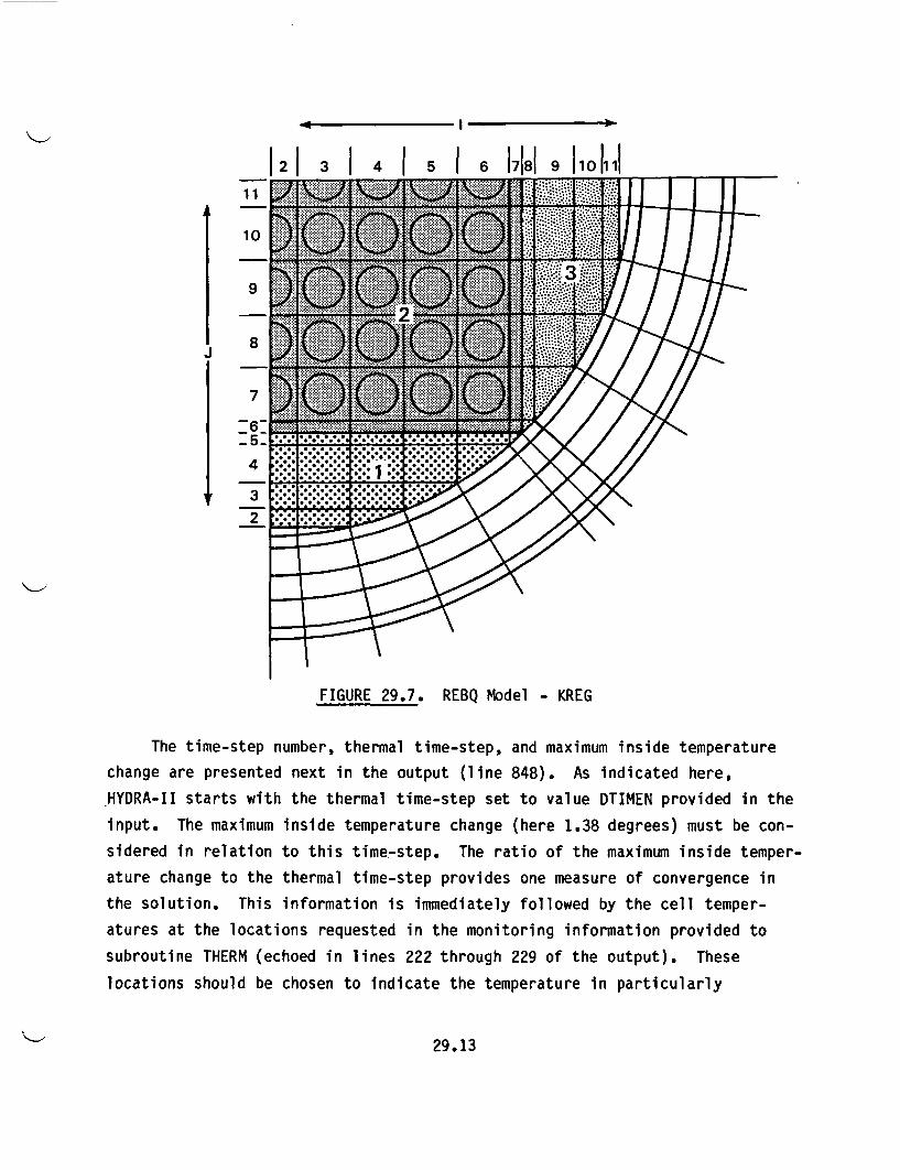
Il- b
FIGURE 29.7. REBQ Model - KREG
The time-step number, thermal time-step, and maximum inside temperature
change are presented next in the output (line 848). As indicated here,
HYDRA-II starts with the thermal time-step set to value DTIMEN provided in the
input. The maximum inside temperature change (here 1.38 degrees) must be con-
sidered in relation to this time-step. The ratio of the maximum inside temper-
ature change to the thermal time-step provides one measure of convergence in
the solution. This information is immediately followed by the cell temper-
atures at the locations requested in the monitoring information provided to
subroutine THERM (echoed in lines 222 through 229 of the output). These
locations should be chosen to indicate the temperature in particularly
29.13
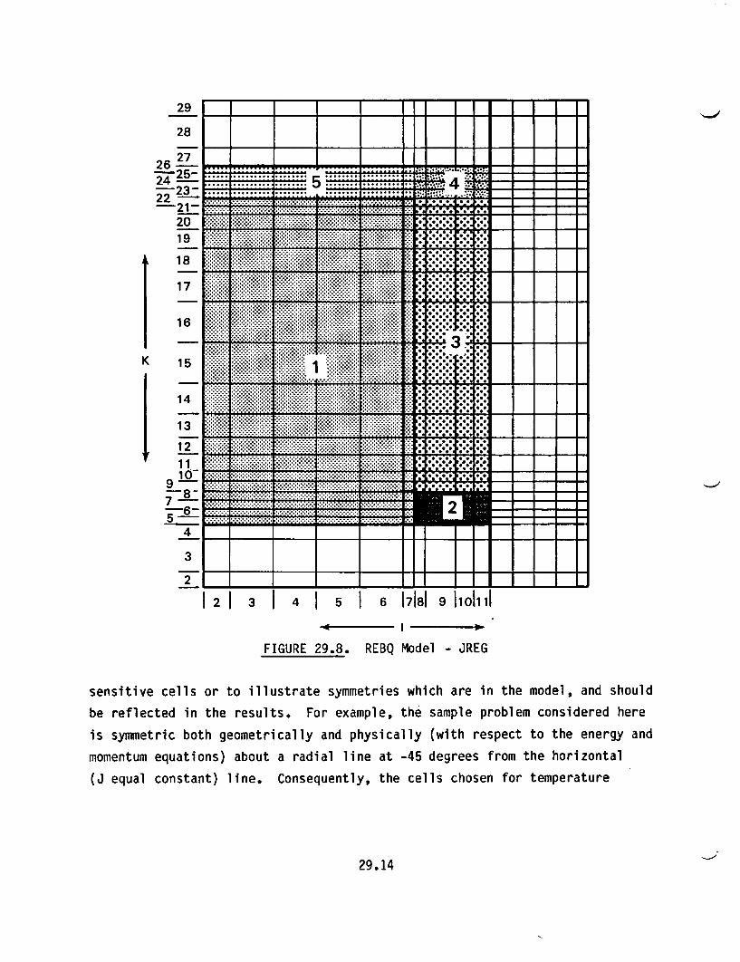
29
28
26 2724 25--23-
22 -
2019
18
17
16
K 115
14
13
121 1
910-9-
5-
I I II TI T li II
I+ I I I I IIII III2 1 1 1 1 1 1 1 1 1
23 I I I Il- - I121 3 4 J 5 1 6
FIGURE 29.8. REBQ
17181 9 1101111
Model - JREG
sensitive cells or to illustrate symmetries which are in the model, and should
be reflected in the results. For example, the sample problem considered here
is symmetric both geometrically and physically (with respect to the energy and
momentum equations) about a radial line at -45 degrees from the horizontal
(J equal constant) line. Consequently, the cells chosen for temperature
29.14

EI _-- I I'I I I I
IL _ L 11X 1 1 I 1I I I I II
- - -
- - -- - --- -.
I- I =I
I7 -
I
29
28
27Z-225
-23
2019
18
17
16
15
14
13
1211
-l9- 8 --7-6 -
54
_ - -_ . .
I =I I
I
lI I I 32= =-__ I I -1 1 M1it i i i
11I'10| 9 18171 6 1 5 4 3 1 2
.j
FIGURE 29.9. REBQ Model - IREG
monitoring in this simulation should exhibit this symmetry. The temperatures
listed on lines 849 and 850 of the output do exhibit this symmetry [e.g.,
T(3,4,10) = T(9,10,10)].
The maximum temperature change in the cylindrical-grid region of the model
is listed next in the output. The ratio of this value to the thermal time-step
provides a measure of the convergence of the solution. The following line of
29.15
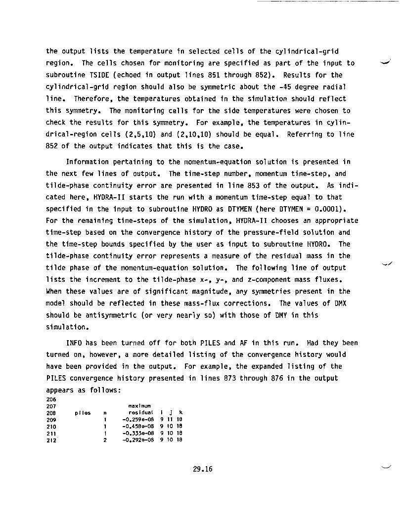
the output lists the temperature in selected cells of the cylindrical-grid
region. The cells chosen for monitoring are specified as part of the input to
subroutine TSIDE (echoed in output lines 851 through 852). Results for the
cylindrical-grid region should also be symmetric about the -45 degree radial
line. Therefore, the temperatures obtained in the simulation should reflect
this symmetry. The monitoring cells for the side temperatures were chosen to
check the results for this symmetry. For example, the temperatures in cylin-
drical-region cells (2,5,10) and (2,10,10) should be equal. Referring to line
852 of the output indicates that this is the case.
Information pertaining to the momentum-equation solution is presented in
the next few lines of output. The time-step number, momentum time-step, and
tilde-phase continuity error are presented in line 853 of the output. As indi-
cated here, HYDRA-II starts the run with a momentum time-step equal to that
specified in the input to subroutine HYDRO as DTYMEN (here DTYMEN = 0.0001).
For the remaining time-steps of the simulation, HYDRA-II chooses an appropriate
time-step based on the convergence history of the pressure-field solution and
the time-step bounds specified by the user as input to subroutine HYDRO. The
tilde-phase continuity error represents a measure of the residual mass in the
tilde phase of the momentum-equation solution. The following line of output
lists the increment to the tilde-phase x-, y-, and z-component mass fluxes.
When these values are of significant magnitude, any symmetries present in the
model should be reflected in these mass-flux corrections. The values of DMX
should be antisymmetric (or very nearly so) with those of DMY in this
simulation.
INFO has been turned off for both PILES and AF in this run. Had they been
turned on, however, a more detailed listing of the convergence history would
have been provided in the output. For example, the expanded listing of the
PILES convergence history presented in lines 873 through 876 in the output
appears as follows:206207 maximum208 plies n residual I J k209 1 -0.259e-08 9 11 18210 1 -0.458e-08 9 10 18211 1 -0.333e-08 9 10 18212 2 -0.292e-08 9 10 18
29.16
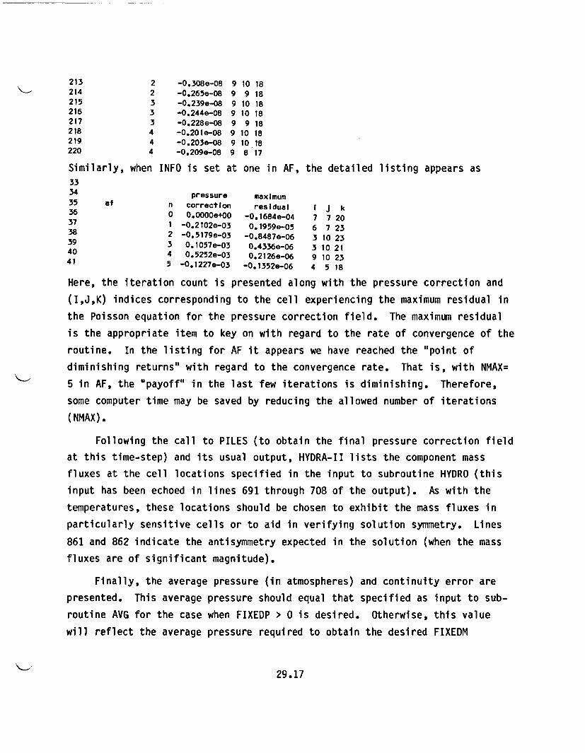
213 2 -0.308e-08 9 10 18214 2 -0.265e-08 9 9 18215 3 -0.239e-08 9 10 18216 3 -0.244e-08 9 10 18217 3 -0.228e-08 9 9 18218 4 -0.201e-08 9 10 18219 4 -0.203e-08 9 10 18220 4 -0.209e-08 9 8 17
Similarly, when INFO is set at one in AF, the detailed listing appears as3334 pressure maximum35 af n correction residual I J k36 0 O.OOOOe+00 -0.1684e-04 7 7 2037 1 -0.2102e-03 0.1959e-05 6 7 2338 2 -0.5179e-03 -0.8487e-06 3 10 2339 3 0.1057e-03 0.4336e-06 3 10 2140 4 0.5252e-03 0.2126e-06 9 10 2341 5 -0.1227e-03 -0.1352e-06 4 5 18
Here, the iteration count is presented along with the pressure correction and
(I,J,K) indices corresponding to the cell experiencing the maximum residual in
the Poisson equation for the pressure correction field. The maximum residual
is the appropriate item to key on with regard to the rate of convergence of the
routine. In the listing for AF it appears we have reached the "point of
diminishing returns" with regard to the convergence rate. That is, with NMAX=
5 in AF, the "payoff" in the last few iterations is diminishing. Therefore,
some computer time may be saved by reducing the allowed number of iterations
(NMAX).
Following the call to PILES (to obtain the final pressure correction field
at this time-step) and its usual output, HYDRA-II lists the component mass
fluxes at the cell locations specified in the input to subroutine HYDRO (this
input has been echoed in lines 691 through 708 of the output). As with the
temperatures, these locations should be chosen to exhibit the mass fluxes in
particularly sensitive cells or to aid in verifying solution symmetry. Lines
861 and 862 indicate the antisymmetry expected in the solution (when the mass
fluxes are of significant magnitude).
Finally, the average pressure (in atmospheres) and continuity error are
presented. This average pressure should equal that specified as input to sub-
routine AVG for the case when FIXEDP > 0 is desired. Otherwise, this value
will reflect the average pressure required to obtain the desired FIXEDM
29.17
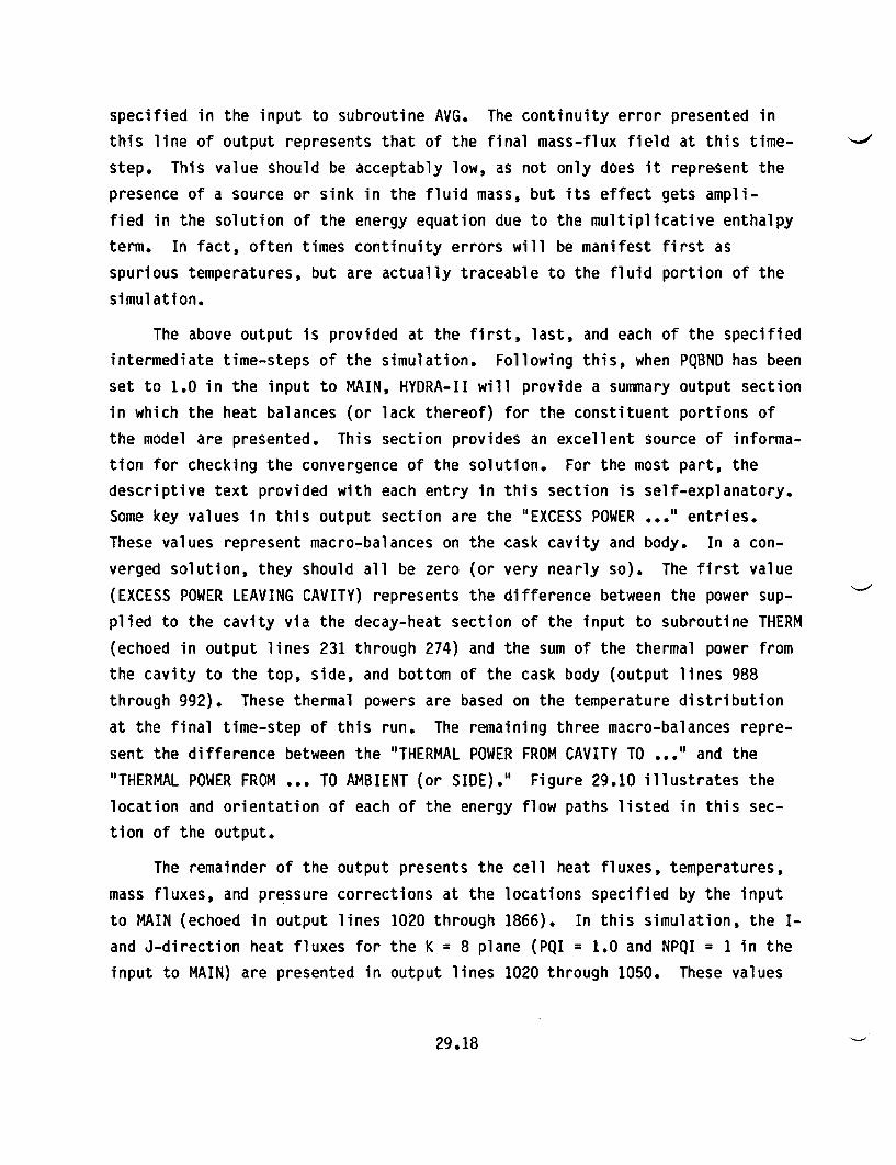
specified in the input to subroutine AVG. The continuity error presented in
this line of output represents that of the final mass-flux field at this time-
step. This value should be acceptably low, as not only does it represent the
presence of a source or sink in the fluid mass, but its effect gets ampli-
fied in the solution of the energy equation due to the multiplicative enthalpy
term. In fact, often times continuity errors will be manifest first as
spurious temperatures, but are actually traceable to the fluid portion of the
simulation.
The above output is provided at the first, last, and each of the specified
intermediate time-steps of the simulation. Following this, when PQBND has been
set to 1.0 in the input to MAIN, HYDRA-II will provide a summary output section
in which the heat balances (or lack thereof) for the constituent portions of
the model are presented. This section provides an excellent source of informa-
tion for checking the convergence of the solution. For the most part, the
descriptive text provided with each entry in this section is self-explanatory.
Some key values in this output section are the "EXCESS POWER ..." entries.
These values represent macro-balances on the cask cavity and body. In a con-
verged solution, they should all be zero (or very nearly so). The first value
(EXCESS POWER LEAVING CAVITY) represents the difference between the power sup-
plied to the cavity via the decay-heat section of the input to subroutine THERM
(echoed in output lines 231 through 274) and the sum of the thermal power from
the cavity to the top, side, and bottom of the cask body (output lines 988
through 992). These thermal powers are based on the temperature distribution
at the final time-step of this run. The remaining three macro-balances repre-
sent the difference between the "THERMAL POWER FROM CAVITY TO ..." and the
"THERMAL POWER FROM ... TO AMBIENT (or SIDE)." Figure 29.10 illustrates the
location and orientation of each of the energy flow paths listed in this sec-
tion of the output.
The remainder of the output presents the cell heat fluxes, temperatures,
mass fluxes, and pressure corrections at the locations specified by the input
to MAIN (echoed in output lines 1020 through 1866). In this simulation, the I-
and J-direction heat fluxes for the K = 8 plane (PQI = 1.0 and NPQI = 1 in the
input to MAIN) are presented in output lines 1020 through 1050. These values
29.18
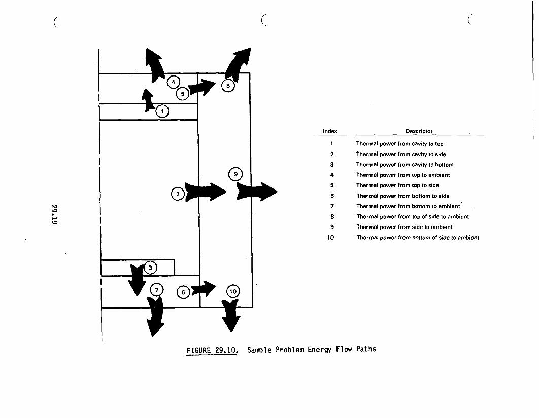
( (
Index Descriptor
1 Thermal power from cavity to top
2 Thermal power from cavity to side
3 Thermal power from cavity to bottom9 4 Thermal power from top to ambient
5 Thermal power from top to side(2 6 Thermal power from bottom to side
% 7 Thermal power from bottom to ambient* 8 Thermal power from top of side to ambient
9 Thermal power from side to ambient
10 Thermal power from bottom of side to ambient
FIGURE 29.10. Sample Problem Energy Flow Paths
provide and excellent check of the symmetry properties that should result from
this simulation. The I-component heat-flux matrix should be antisymmetric with
the J-component heat-flux matrix in this simulation. Therefore, the I = 7 out-put column for the I-direction heat flux values should equal the negative of
J = 5 output column for the J-direction heat flux values (recall that the heat
flux in the ith column of output for the I-direction heat flux component repre-
sents the heat flux between the cells at I and I+1; those in the jth row of
output for the J-direction heat flux component represent that between the cells
at J and J+1). The K-direction heat fluxes for the K = 8 plane are provided
next in the output (lines 1053 through 1066). These results should be symme-
tric. For example, the I = 9 column of results should equal the results
presented in the J = 4 column.
The cartesian-region temperatures are presented next in the output (output
lines 1069 through 1519). This results from setting PT = 1.0 in the input to
MAIN. With NPT = 0, the cell temperatures (in degrees Centigrade) are printed
for each (I,J,K) value in the cartesian-region grid. These results should also
exhibit the symmetry inherent in the model [e.g., the ith column should equal
the J = (13 - ith) row at any K-plane].
With PTS = 1.0 and NPTS= 0 set in MAIN, the temperatures (in degrees Cen-tigrade) for each cell of the cylindrical-region grid are presented next in the
output. As with the cartesian-region temperatures, these results should also
exhibit the symmetry inherent in the model. The temperatures listed for the
K = 1 and K = 30 planes represent those of the ambient (set with the initial
interface temperature in the input to subroutine THERM). The temperatures
listed in the jth column of entries should equal those of the (15 - jth) column
for each K-plane.
The x- and z-component mass fluxes are presented next in the output file.
With both NPMX and NPMY set to 2 in MAIN, these results will be listed for the
K = 2 and 10 planes only. Without the y-component mass fluxes, only the
z-component mass fluxes can be checked for symmetry here. As with the
K-direction heat flux output, the ith column of data should equal the (13 -
ith) row of data for symmetry.
29.20
Finally, the pressure change results are presented. These values repre-
sent the amount of correction applied to the pressure field in the last
time-step.
29.3.2 Base-Case Run Extension
The results from the preceeding base-case run indicated that convergence
was not obtained in the first 1000 time-steps (EXCESS POWER LEAVING CAVITY =
-78.7 watts). Therefore, for this case the same model and simulation param-
eters (e.g., no energy-equation rebalance routines invoked) were utilized to
extend the run an additional 1000 time steps (i.e., time steps 1001 through
2000) using the restart tape generated by the base-case run. This involved
changes to the following variables in the input file and the corresponding rou-
tine in which they appear:
*NREAD = 1 in MAIN
*NEWTA = 0 in MAIN
*NDTIME = 0 in MAIN
*NEWT = 0 in THERM
*NEWTC = 0 in THERM
*NEWTS = 0 in TSIDE
*NDTYME = 0 in HYDRO.
This simulation produced the following "EXCESS POWER" values:
* EXCESS POWER LEAVING CAVITY -0.507e+02
* EXCESS POWER LEAVING TOP -0.353e+02
* EXCESS POWER LEAVING SIDE -0.586e+03
* EXCESS POWER LEAVING BOTTOM -0.558e+02.
Clearly, with this iteration scheme, the problem still has not converged.
29.3.3 Invoke REBA
This simulation represents an extension to the base-case run for 1000
time-steps (i.e., time-steps 1001 through 2000) as was done for the preceeding
case. However, in this simulation the REBA routine was invoked (by setting
29.21
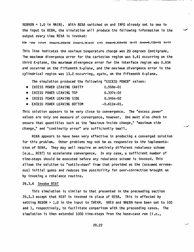
REBAON = 1.0 in MAIN). With REBA switched on and INFO already set to one in
the input to REBA, the simulation will produce the following information in the
output every time REBA is invoked:
839 reba Info-1 dtmax-O.200e+02 dlmax-O.541e+01 k13 dbmaxw0.934s+00 kb-15 dsmax=0.152&+02 ks-15
This line indicates the maximum temperature change was 20 degrees Centigrade.
The maximum divergence error for the Cartesian region was 5.41 occurring on the
third K-plane, the maximum divergence error for the interface region was 0.934
and occurred on the fifteenth K-plane, and the maximum divergence error in the
cylindrical region was 13.2 occurring, again, on the fifteenth K-plane.
The simulation produced the following "EXCESS POWER" values:
* EXCESS POWER LEAVING CAVITY 0.558e-01
* EXCESS POWER LEAVING TOP 0.337e-02
* EXCESS POWER LEAVING SIDE 0.346e-02
* EXCESS POWER LEAVING BOTTOM -0.611e-01.
This solution appears to be very close to convergence. The "excess power"
values are only one measure of convergence, however. One must also check to
ensure that quantities such as the "maximum inside change," "maximum side
change," and "continuity error" are sufficiently small.
REBA appears to have been very effective in producing a converged solution
for this problem. Other problems may not be as responsive to the implementa-
tion of REBA. They may well require an entirely different rebalance scheme
(e.g., REBT) to accelerate convergence. In any case, a sufficient number of
time-steps should be executed before any rebalance.scheme is invoked. This
allows the solution to "settle-down" from that provided as the (assumed errone-
ous) initial guess and reduces the possibility for over-correction brought on
by invoking a rebalance routine.
29.3.4 Invoke REBT
This simulation is similar to that presented in the preceeding section
29.3.3 except that REBT is invoked in place of REBA. This is effected by
setting REBON = 1.0 in the input to THERM. NREB and NREBN have been set to 100
and 1, respectively, to facilitate comparison with the preceeding cases. The
simulation is then extended 1000 time-steps from the base-case run (i.e.,
29.22
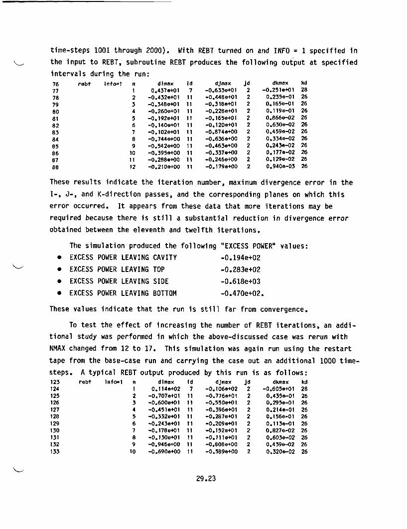
time-steps 1001 through 2000). With REBT turned on and INFO = 1 specified in
the input to REBT, subroutine REBT produces the following output at specified
intervals during the run:76 rebt Info=1 n dimax77 1 0.437e+0178 2 -0.432e+0179 3 -0.348e+0180 4 -0.260e+0181 5 -0.192e+0182 6 -0.140e+0183 7 -0.102e+0184 8 -0.744e+0085 9 -0.542e+0086 10 -0.395e+0087 11 -0.288e+0088 12 -0.210e+00
Id71 11 11 11 11 11 11 11 11 11 11 1
dJmax-0.633e+01-0.448e+01-0.318e+01-0.228e+01-0.165e+01-0.120e+01-0.874e+00-0.636.+00-0.463.+00-0.337e+00-0.246e+00-0.179e+00
Jd222222222222
dkmax-0.251e+01
0.235e-010. 165e-0 10.119e-010.866e-020.630e-020.459e-020.334e-020.243e-020.177e-020.129e-020.940e-03
kd282626262626262626262626
These results indicate the iteration number, maximum divergence error in the
I-, J-, and K-direction passes, and the corresponding planes on which this
error occurred. It appears from these data that more iterations may be
required because there is still a substantial reduction in divergence error
obtained between the eleventh and twelfth iterations.
The simulation produced the following
* EXCESS POWER LEAVING CAVITY
* EXCESS POWER LEAVING TOP
* EXCESS POWER LEAVING SIDE
* EXCESS POWER LEAVING BOTTOM
"EXCESS POWER" values:
-0.194e+02
-0.283e+02
-0.618e+03
-0.470e+02.
These values indicate that the run is still far from convergence.
To test the effect of increasing the number of REBT iterations, an addi-
tional study was performed in which the above-discussed case was rerun with
NMAX changed from 12 to 17. This simulation was again run using the restart
tape from the base-case run and carrying the case out an additional 1000 time-
steps. A typical REBT output produced by this run is as follows:123 rebt Info=1 n dimax Id dJmax Jd dkmax kd124 1 0.114e+02 7 -0.106e+02 2 -0.605e+01 28125 2 -0.707e+01 11 -0.776e+01 2 0.435e-01 26126 3 -0.600e+01 11 -0.550e+01 2 0.295e-01 26127 4 -0.451e+01 11 -0.396e+01 2 0.214e-01 26128 5 -0.332e+01 11 -0.287e+01 2 0.156e-01 26129 6 -0.243e+01 11 -0.209e+01 2 0.113e-01 26130 7 -0.178e+01 11 -0.152e+01 2 0.827e-02 26131 8 -0.130e+01 11 -0.111e+01 2 0.603e-02 26132 9 -0.946e+00 11 -0.808e+00 2 0.439e-02 26133 10 -0.690e+00 11 -0.589e+00 2 0.320e-02 26
29.23
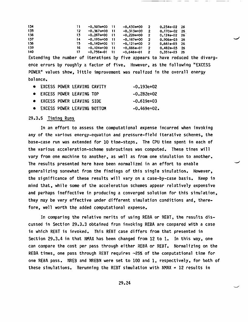
134 11 -0.503e+00 11 -0.430e+00 2 0.234e-02 26135 12 -0.367e+00 11 -0.313e+00 2 0.170e-02 26136 13 -0.267e+00 11 -0.228e+00 2 0.1240-02 26137 14 -0.195e+00 11 -0.167e+00 2 0.906e-03 26138 15 -0.142e+00 11 -0.121e+00 2 0.661e-03 26139 16 -0.104e+00 11 -0.886e-01 2 0.482e-03 26140 17 -0.756e-01 11 -0.646e-01 2 0.351e-03 26
Extending the number of iterations by five appears to have reduced the diverg-
ence errors by roughly a factor of five. However, as the following "EXCESS
POWER" values show, little improvement was realized in the overall energy
balance.
* EXCESS POWER LEAVING CAVITY -0.193e+02
* EXCESS POWER LEAVING TOP -0.282e+02
* EXCESS POWER LEAVING SIDE -0.619e+03
* EXCESS POWER LEAVING BOTTOM -0.469e+02.
29.3.5 Timing Runs
In an effort to assess the computational expense incurred when invoking
any of the various energy-equation and pressure-field iterative schemes, the
base-case run was extended for 10 time-steps. The CPU time spent in each of
the various acceleration-scheme subroutines was computed. These times will
vary from one machine to another, as well as from one simulation to another.
The results presented here have been normalized in an effort to enable
generalizing somewhat from the findings of this single simulation. However,
the significance of these results will vary on a case-by-case basis. Keep in
mind that, while some of the acceleration schemes appear relatively expensive
and perhaps ineffective in producing a converged solution for this simulation,
they may be very effective under different simulation conditions and, there-
fore, well worth the added computational expense.
In comparing the relative merits of using REBA or REBT, the results dis-
cussed in Section 29.3.3 obtained from invoking REBA are compared with a case
in which REBT is invoked. This REBT case differs from that presented in
Section 29.3.4 in that NMAX has been changed from 12 to 1. In this way, one
can compare the cost per pass through either REBA or REBT. Normalizing on the
REBA times, one pass through REBT requires -25% of the computational time for
one REBA pass. NREB and NREBN were set to 100 and 1, respectively, for both of
these simulations. Rerunning the REBT simulation with NMAX = 12 results in
29.24
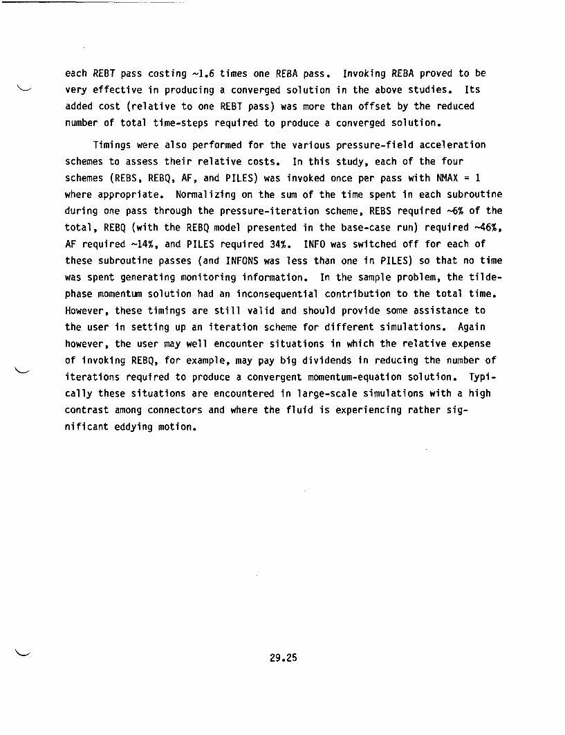
each REBT pass costing -1.6 times one REBA pass. Invoking REBA proved to be
very effective in producing a converged solution in the above studies. Its
added cost (relative to one REBT pass) was more than offset by the reduced
number of total time-steps required to produce a converged solution.
Timings were also performed for the various pressure-field acceleration
schemes to assess their relative costs. In this study, each of the four
schemes (REBS, REBQ, AF, and PILES) was invoked once per pass with NMAX = 1
where appropriate. Normalizing on the sum of the time spent in each subroutine
during one pass through the pressure-iteration scheme, REBS required -6% of the
total, REBQ (with the REBQ model presented in the base-case run) required -46%,
AF required -14%, and PILES required 34%. INFO was switched off for each of
these subroutine passes (and INFONS was less than one in PILES) so that no time
was spent generating monitoring information. In the sample problem, the tilde-
phase momentum solution had an inconsequential contribution to the total time.
However, these timings are still valid and should provide some assistance to
the user in setting up an iteration scheme for different simulations. Again
however, the user may well encounter situations in which the relative expense
of invoking REBQ, for example, may pay big dividends in reducing the number of
iterations required to produce a convergent momentum-equation solution. Typi-
cally these situations are encountered in large-scale simulations with a high
contrast among connectors and where the fluid is experiencing rather sig-
nificant eddying motion.
29.25
REFERENCES
Cox, R. L. 1977. Radioactive Heat Transfer in Arrays of Parallel Cylinders.ORNL-5239, Oak Ridge National Laboratory, Oak Ridge, Tennessee.
DOE. 1986. Spent Fuel Storage Requirements. DOE/RL-86-5, U.S. Department ofEnergy, Richland Operations Office, Richland, Washington.
Douglas, J., and J. Gunn. 1964. "A General Formulation of AlternatingDirection Methods." I. Numer. Math. 6:428.
McCann, R. A. 1987. HYDRA-II: A Hydrothermal Analysis Computer Code,Volume I - Equations and Numerics. PNL-6206 Vol. I, Pacific NorthwestLaboratory, Richland, Washington.
McCann, R. A. 1980. HYDRA-I: A Three Dimensional Finite Difference Code forCalculating the Thermohydraulic Performance of a Fuel Assembly ContainedWithin a Canister. PNL-3367, Pacific Northwest Laboratory, Richland,Washington.
Westlake, J. R. 1968. A Handbook of Numerical Matrix Inversion and Solutionof Linear Equations. John Wiley & Sons, Inc., New York, New York.
R .1

APPENDIX A
SAMPLE PROBLEM INPUT
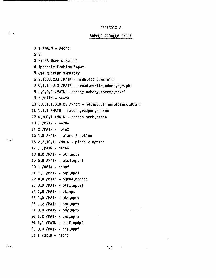
APPENDIX A
SAMPLE PROBLEM INPUT
1 1 /MAIN - necho
2 3
3 HYDRA User's Manual
4 Appendix Problem Input
5 Use quarter symmetry
6 1,1000,200 /MAIN - nrun,nstep,nsinfo
7 0,1,1000,0 /MAIN - nread,nwrite,ndump,ngraph
8 1,0,0,0 /MAIN - steady,nobody,notemp,novel
9 1 /MAIN - newta
10 1,0.1,1.0,0.01 /MAIN - ndtime,dtimen,dtimax,dtimin
11 1,1,1 /MAIN - radcon,radpon,radron
12 0,100,1 /MAIN - rebaon,nreb,nrebn
13 1 /MAIN - necho
14 2 /MAIN - npla2
15 1,8 /MAIN - pla
16 2,2,10,16 /MAIN
17 1 /MAIN - necho
18 0,0 /MAIN - pti
19 0,0 /MAIN - pts
20 1 /MAIN - pqbnd
21 1,1 /MAIN - pqi
22 0,0 /MAIN - pqr.
23 0,0 /MAIN - pts
24 1,0 /MAIN - pt,i
25 1,0 /MAIN - pts
26 1,2 /MAIN - pmx
27 0,0 /MAIN - pmy
28 1,2 /MAIN - pmz
29 1,1 /MAIN - pdpl
30 0,0 /MAIN - ppf
31 1 /GRID - necho
ne 1 opti
- plane
,npti
inptsi
,npqi
ad,npqrad
1,nptsl
npt
,npts
,npmx
;npmy
,npmz
f,npdpf
,nppf
on
2 option
A.1
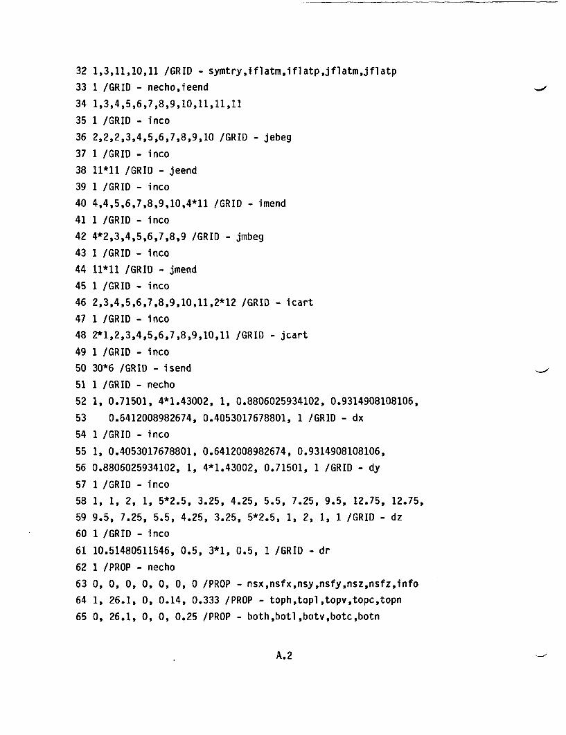
32 1,3,11,10,11 /GRID - symtry,iflatm,iflatp,jflatm,jflatp
33 1 /GRID - necho,ieend
34 1,3,4,5,6,7,8,9,10,11,11,11
35 1 /GRID - inco
36 2,2,2,3,4,5,6,7,8,9,10 /GRID - jebeg
37 1 /GRID - inco
38 11*11 /GRID - jeend
39 1 /GRID - inco
40 4,4,5,6,7,8,9,10,4*11 /GRID - imend
41 1 /GRID - inco
42 4*2,3,4,5,6,7,8,9 /GRID - jmbeg
43 1 /GRID - inco
44 11*11 /GRID - jmend
45 1 /GRID - inco
46 2,3,4,5,6,7,8,9,10,11,2*12 /GRID - icart
47 1 /GRID - inco
48 2*1,2,3,4,5,6,7,8,9,10,11 /GRID - jcart
49 1 /GRID - inco
50 30*6 /GRID - isend
51 1 /GRID - necho
52 1, 0.71501, 4*1.43002, 1, 0.8806025934102, 0.9314908108106,
53 0.6412008982674, 0.4053017678801, 1 /GRID - dx
54 1 /GRID - inco
55 1, 0.4053017678801, 0.6412008982674, 0.9314908108106,
56 0.8806025934102, 1, 4*1.43002, 0.71501, 1 /GRID - dy
57 1 /GRID - inco
58 1, 1, 2, 1, 5*2.5, 3.25, 4.25, 5.5, 7.25, 9.5, 12.75, 12.75,
59 9.5, 7.25, 5.5, 4.25, 3.25, 5*2.5, 1, 2, 1, 1 /GRID - dz
60 1 /GRID - inco
61 10.51480511546, 0.5, 3*1, 0.5, 1 /GRID - dr
62 1 /PROP - necho
63 0, 0, 0, 0, 0, 0, 0 /PROP - nsx,nsfx,nsy,nsfy,nsz,nsfz,info
64 1, 26.1, 0, 0.14, 0.333 /PROP - toph,topl,topv,topc,topn
65 0, 26.1, 0, 0, 0.25 /PROP - both,botl,botv,botc,botn
A.2
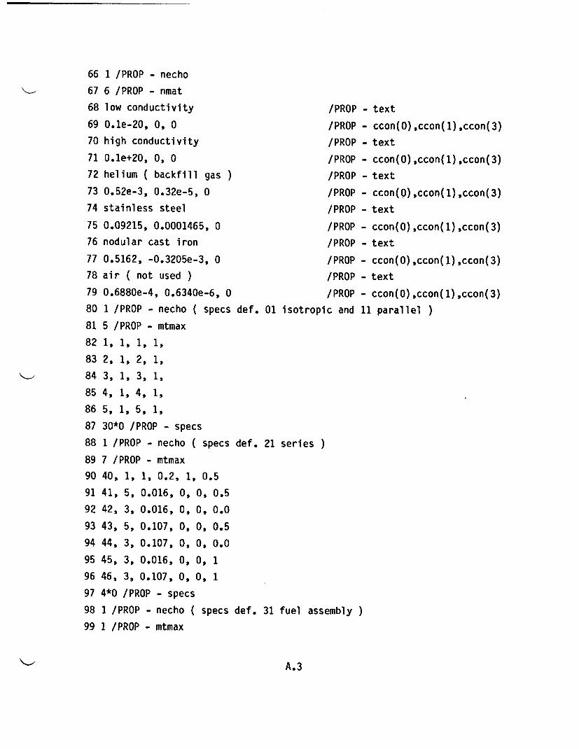
66 1 /PROP - necho
67 6 /PROP - nmat
68 low conductivity
69 0.le-20, 0, 0
70 high conductivity
71 0.le+20, 0, 0
72 helium ( backfill gas )
73 0.52e-3, 0.32e-5, 0
74 stainless steel
75 0.09215, 0.0001465, 0
76 nodular cast iron
77 0.5162, -0.3205e-3, 0
78 air ( not used )
79 0.6880e-4, 0.6340e-6, 0
80 1 /PROP - necho ( specs
81 5 /PROP - mtmax
82 1, 1, 1, 1,
83 2, 1, 2, 1,
84 3, 1, 3, 1,
85 4, 1, 4, 1,
86 5, 1, 5, 1,
87 30*0 /PROP - specs
88 1 /PROP - necho ( specs
89 7 /PROP - mtmax
90 40, 1, 1, 0.2, 1, 0.5
91 41, 5, 0.016, 0, 0, 0.5
92 42, 3, 0.016, 0, 0, 0.0
93 43, 5, 0.107, 0, 0, 0.5
94 44, 3, 0.107, 0, 0, 0.0
95 45, 3, 0.016, 0, 0, 1
96 46, 3, 0.107, 0, 0, 1
97 4*0 /PROP - specs
98 1 /PROP - necho ( specs
99 1 /PROP - mtmax
/PROP
/PROP
/PROP
/PROP
/PROP
/PROP
/PROP
/PROP
/PROP
/PROP
/PROP
/PROP
- text
- ccon(O),ccon(l),ccon(3)
- text
- ccon(O),ccon(l),ccon(3)
- text
- ccon(O)
- text
- ccon(O)
- text
- ccon(0)
- text
- ccon(0)
,ccon(l) ,ccon(3)
,ccon(l) ,ccon(3)
,ccon(l) ,ccon(3)
,ccon(1) ,ccon(3)
def. 01 isotropic and 11 parallel )
def. 21 series )
def. 31 fuel assembly )
A.3
100 47, 3, 0.9484, 1.072, 1.43002, 0.0209, 0.115, 0, 0
101 41*0 /PROP - specs
102 1 /PROP - necho
103 24, 24 /PROP - nreg,npair
104 1,1, 2,11, 2,29, 1,1,1,
105 2,11, 12,12, 2,29, 1,2,1,
106 2,11, 2,11, 5,26, 1,4,3,
107 2,7, 6,6, 5,22, 1,4,4,
108 7,7, 7,11, 5,22, 1,4,4,
109 2,5, 6,6, 5,8, 1,4,3,
110 7,7, 8,11, 5,8, 1,4,3,
111 2,6, 7,11, 5,22, 1,31,47,
112 2,11, 2,11, 2,4, 1,4,5,
113 2,11, 2,11, 27,29, 1,4,5,
114 2,11, 2,11, 1,1, 1,3,1,
115 2,11, 2,11, 29,29, 1,51,40,
116 2,2, 1,1, 2,4, 1,42,41
117 2,2, 1,1, 5,26, 1,42,42
118 2,2, 1,1, 27,29, 1,42,41
119 3,3, 1,1, 2,4, 1,42,43
120 3,3, 1,1, 5,26, 1,42,44
121 3,3, 1,1, 27,29, 1,42,43
122 11,11, 10,10, 2,4, 1,41,43
123 11,11, 10,10, 5,26, 1,41,46
124 11,11, 10,10, 27,29, 1,41,43
125 11,11, 11,11, 2,4, 1,41,41
126 11,11, 11,11, 5,26, 1,41,45
127 11,11, 11,11, 27,29, 1,41,41
128 791*0 /PROP - index
129 1 /THERM - necho
130 0.5, 5.234, 0.5 /THERM - theta,sphtf,dtemax
131 0, 100, 50 /THERM - rebon,nreb,nrebn
132 1 /THERM - necho
133 8 /THERM - mont
A.4
134
135
136
137
138
139
140
141
142
143
144
145
146
147
148
149
150
151
152
153
154
155
156
157
158
159
160
161
162
163
164
165
166
167
2,2,10
3,4,10
5,6,10
5,7,10
11,11,10
9,10,10
7,8,10
6,8,10
0,0,0 /THERM - (ij,k) locations
1 /THERM - necho
0.5, 2,2,7,11
0.5, 3,6,11,11
1, 3,6,7,10
0, 2,2,11,11
0, 3,3,8,8
0, 5,5,10,10
0, 4*0 /THERM - q weighting factor,ibeg,iend,jbeg,jend
1 /THERM - necho
290., 2,6,7,11
0.,0,0,0,0 /THERM - group power,ibeg,iend,jbeg,jend
1 /THERM - necho
3*0, 29.5, 44.5, 57, 65, 71, 75, 78, 6*80,
78.5, 69, 55, 39, 24.5, 7*0 /THERM - relact(k)
1 /THERM - necho
0 /THERM - pqgen
1 /THERM - necho
1,11.5
321, 323, 325, 356, 398, 433, 456, 473, 484, 492,
6*498, 494, 467, 428, 383, 342, 337, 332, 328,
324, 320, 315, 310 /THERM - newt,cenj,tcen(k)
1 /THERM - necho
1, 0
12*300, 336*320, 12*300 /THERM - newtc,cenj,tsl(j,k)
1 /THERM - necho
A.5
168
169
170
171
172
173
174
175
176
177
178
179
180
181
182
183
184
185
186
187
188
189
190
191
192
193
194
195
196
197
198
199
200
201
0 /THERM - ndelta
2,6,2,13 /THERM - loc
29*0 /THERM - delta
1 /REBT - necho
O.le+6, 12, 1 /REBT - xdtime,nmax,info
1 /PROPS - necho
0, 0, 0, 0, 0, 0, 0 /PROPS - nsx,nsfx,nsy,nsfy,nsz,nsfz,info
1, 26.1, 0, 0.14, 0.333 /PROP - toph,topl,topv,topc,topn
0, 26.1, 0, 0, 0.25 /PROP - both,botl,botv,botc,botn
1, 118.0, 0, 0.10, 0.333 /PROPS - sideh,sidel,sidev,sidec,siden
1 /PROPS - necho
6 /PROPS - nmat
low conductivity /PROPS - text
O.le-20, 0, 0 /PROPS - cconO,cconl,ccon3
high conductivity /PROPS - text
0.le+20, 0, 0 /PROPS - cconO,cconl,ccon3
helium ( backfill gas ) /PROPS - text
0.52e-3, 0.32e-5, 0 /PROPS - cconO,cconl,ccon3
stainless steel /PROPS - text
0.09215, 0.0001465, 0 /PROPS - cconO,cconl,ccon3
nodular cast iron /PROPS - text
0.5162, -0.3205e-3, 0 /PROPS - cconO,cconl,ccon3
air ( not used ) /PROPS - text
0.6880e-4, 0.6340e-6, 0 /PROPS - cconO,cconl,ccon3
1 /PROPS - necho
5 /PROPS - mtmax ( specs def. 01 isotropic and 11 parallel )
1, 1, 1, 1,
2, 1, 2, 1,
3, 1, 3, 1,
4, 1, 4, 1,
5, 1, 5, 1,
80*0 /PROPS - specs
1 /PROPS - necho
2 /PROPS - mtmax ( specs def. 21 series )
A. 6
202 41, 1, 1, 0.2, 1, 0.5
203 42, 3, 0.1, 0.4, 0.4, 0.5
204 88*0 /PROPS - specs
205 1 /PROPS - necho
206 9,9 /PROPS - nreg,npair
207 2,6, 2,13, 2,29, 1,4,5
208 1,1, 2,13, 2,29, 1,1,1
209 2,6, 1,1, 2,29, 1,2,1
210 2,6, 14,14, 2,29, 1,2,1
211 6,6, 2,13, 2,29, 1,53,41
212 2,6, 2,13, 1,1, 1,3,1
213 2,6, 2,13, 29,29, 1,51,41
214 3,3, 2,13, 27,28, 1,41,42
215 3,3, 2,13, 3,4, 1,41,42
216 174*0 /PROPS - index
217 1 /TSIDE - necho
218 1, 300, 5 /TSIDE - newts,tsamb,dtemax
219 1 /TSIDE - necho
220 4 /TSIDE - monts
221 2, 5, 10
222 2, 10, 10
223 4, 5, 10
224 4, 10, 10
225 0, 0, 0 /TSIDE - incol,inco2,inco3
226 1 /TSIDE - necho
227 0
228 28*0 /TSIDE - ndelta,delta
229 1 /RADC - necho
230 0 /RADC - info
231 1 /RADC - necho
232 2 /RADC - nregs
233 18,1,12,1,1,1
234 18,1,12,2,2,1 /RADC - nkcell,idk,nsurfs,idi,idj,idh
235 1 /RADC - necho
A. 7
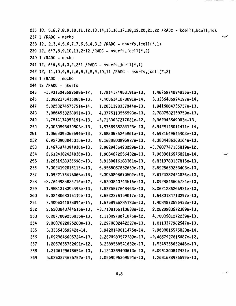
236
237
238
239
240
241
242
243
244
245
246
247
248
249
250
251
252
253
254
255
256
257
258
259
260
261
262
263
264
265
266
267
268
269
18, 5,6,7,8,9,10,11,12,13,14,15,16,17,18,19,20,21,22 /RADC - kcells,kcell,idk
1 /RADC - necho
12, 2,3,4,5,6,7,7,6,5,4,3,2 /RADC - nsurfs,icell(*,l)
12, 6*7,8,9,10,11,2*12 /RADC - nsurfs,icell(*,2)
1 /RADC - necho
12, 6*6,5,4,3,2,2*1 /RADC - nsurfs,jcell(*,l)
12, 11,10,9,8,7,6,6,7,8,9,10,11 /RADC - nsurfs,jcell(*,2)
1 /RADC - necho
12 /RADC - nsurfs
-1.9315045692589e-12,
1.0922176415065e-13,
5.0253274575751e-14,
3.0864550228951e-13,
1.7814174953191e-13,
2.3030898670503e-13,
1.0569095369594e-13,
6.9273903046315e-13,
1.4676974094936e-13,
2.6124382424036e-13,
1.2631628926698e-13,
7.3024192016115e-13,
1.0922176415065e-13,
-3.7649985826716e-12,
1.9581318305493e-13,
5.0848068315119e-13,
7.4006341878094e-14,
2.6203843744515e-13,
6.0877889258035e-13,
2.8037622095288e-13,
3.33564059942e-14,
1.0928846605724e-13,
1.2067655762691e-12,
1.2136129618654e-13,
5.0253274575752e-14,
1.7814174953191e-13,
7.4006341878091e-14,
1.2031398337844e-13,
4.3775113556598e-13,
-3.7133637277021e-12,
1.5758935284123e-13,
2.6880575245861e-13,
8.1680503895927e-13,
2.9629436490029e-13,
1.9084872556432e-13,
3.9130616188361e-13,
5.9565067832659e-13,
2.3030898670502e-13,
2.6203843744515e-13,
7.6226577648453e-13,
3.6532275159017e-13,
1.5758935284123e-13,
-3.7138156110638e-12,
1.1130978871075e-12,
2.2970032442227e-13,
6.9428148011475e-14,
2.2620983572389e-13,
3.2389558541632e-13,
1.1243369400613e-13,
1.0569095369594e-13,
1.4676974094935e-13,
3.3356405994197e-14,
1.9416884735737e-13,
2.7887582358759e-13,
2.962943649003e-13,
6.9428148011471e-14,
4.5921549645403e-13,
4.3834485368104e-13,
-3.7607747156819e-12,
7.9638816576821e-14,
6.8319780127815e-13,
2.5926639253403e-13,
2.6124382424036e-13,
1.0928846605724e-13,
8.0621286265921e-13,
1.5480184713297e-13,
1.9084872556433e-13,
2.2620983572389e-13,
4.7003581272239e-13,
1.0113377982547e-13,
7.9638816576823e-14,
-2.4867927816087e-12,
1.5345365652446e-13,
5.0961300842421e-14,
1.2631628926699e-13,
A.8
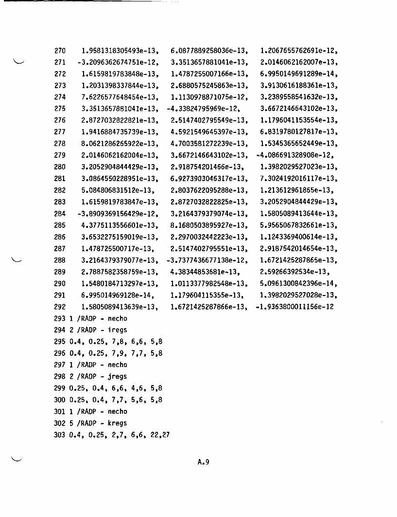
270
271
272
273
274
275
276
277
278
279
280
281
282
283
284
285
286
287
288
289
290
291
292
293
294
295
296
297
298
299
300
301
302
1.9581318305493e-13,
-3.2096362674751e-12,
1.6159819783848e-13,
1.2031398337844e-13,
7.6226577648454e-13,
3.3513657881041e-13,
2.8727032822821e-13,
1.9416884735739e-13,
8.0621286265922e-13,
2.0146062162004e-13,
3.2052904844429e-13,
3.0864550228951e-13,
5.084806831512e-13,
1.6159819783847e-13,
-3.8909369156429e-12,
4.3775113556601e-13,
3.6532275159019e-13,
1.478725500717e-13,
3.2164379379077e-13,
2.7887582358759e-13,
1.5480184713297e-13,
6.995014969128e-14,
1.5805089413639e-13,
1 /RADP - necho
2 /RADP - iregs
0.4, 0.25, 7,8, 6,6, 5,8
0.4, 0.25, 7,9, 7,7, 5,8
1 /RADP - necho
2 /RADP - jregs
0.25, 0.4, 6,6, 4,6, 5,8
0.25, 0.4, 7,7, 5,6, 5,8
1 /RADP - necho
5 /RADP - kregs
6.0877889258036e-13,
3.3513657881041e-13,
1.4787255007166e-13,
2.6880575245863e-13,
1.1130978871075e-12,
-4.33824795969e-12,
2.5147402795549e-13,
4.5921549645397e-13,
4.7003581272239e-13,
3.6672146643102e-13,
2.918754201466e-13,
6.9273903046317e-13,
2.8037622095288e-13,
2.8727032822825e-13,
3.2164379379074e-13,
8.1680503895927e-13,
2.2970032442223e-13,
2.5147402795551e-13,
-3.7377436677138e-12,
4.38344853681e-13,
1.0113377982548e-13,
1.179604115355e-13,
1.6721425287866e-13,
1.2067655762691e-12,
2.0146062162007e-13,
6.9950149691289e-14,
3.9130616188361e-13,
3.2389558541632e-13,
3.6672146643102e-13,
1.1796041153554e-13,
6.8319780127817e-13,
1.5345365652449e-13,
-4.086691328908e-12,
1.3982029527023e-13,
7.3024192016117e-13,
1.213612961865e-13,
3.2052904844429e-13,
1.5805089413644e-13,
5.956506783266le-13,
1.1243369400614e-13,
2.9187542014654e-13,
1.6721425287865e-13,
2.59266392534e-13,
5.0961300842396e-14,
1.3982029527028e-13,
-1.9363800011156e-12
303 0.4, 0.25, 2,7, 6,6, 22,27
A. 9
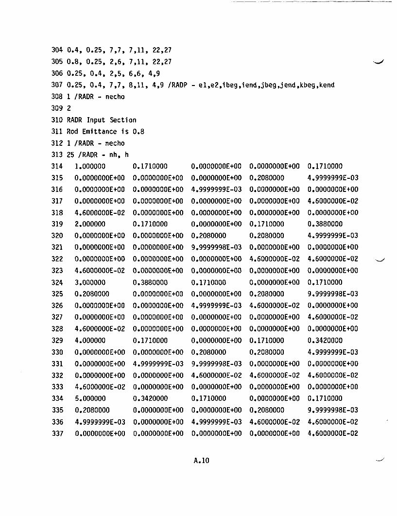
304
305
306
307
308
309
310
311
312
313
314
315
316
317
318
319
320
321
322
323
324
325
326
327
328
329
330
331
332
333
334
335
336
337
0.4, 0.25, 7,7, 7,11, 22,27
0.8, 0.25, 2,6, 7,11, 22,27
0.25, 0.4, 2,5, 6,6, 4,9
0.25, 0.4, 7,7, 8,11, 4,9 /RADP - el,e2,ibeg,iend,jbeg,jend,kbeg,kend
1 /RADR - necho
2
RADR Input Section
Rod Emittance is 0.8
1 /RADR - necho
25 /RADR - nh, h
1.000000 0.1710000
0.OOOOOOOE+00 O.OOOOOOOE+00
O.OOOOOOOE+00 O.OOOOOOOE+00
O.OOOOOOOE+00 O.OOOOOOOE+00
4.6000000E-02 O.OOOOOOOE+00
2.000000 0.1710000
O.OOOOOOOE+00 O.OOOOOOOE+00
O.OOOOOOOE+00 O.OOOOOOOE+00
O.OOOOOOOE+00 O.OOOOOOOE+00
4.6000000E-02 O.OOOOOOOE+00
3.000000 0.3880000
0.2080000 O.OOOOOOOE+00
O.OOOOOOOE+00 O.OOOOOOOE+00
O.OOOOOOOE+00 O.OOOOOOOE+00
4.6000000E-02 O.OOOOOOOE+00
4.000000 0.1710000
O.OOOOOOOE+00 O.OOOOOOOE+00
O.OOOOOOOE+00 4.9999999E-03
O.OOOOOOOE+00 O.OOOOOOOE+00
4.6000000E-02 O.OOOOOOOE+00
5.000000 0.3420000
0.2080000 O.OOOOOOOE+00
4.9999999E-03 O.OOOOOOOE+00
O.OOOOOOOE+00 O.OOOOOOOE+00
O.OOOOOOOE+00
O.OOOOOOOE+00
4.9999999E-03
O.OOOOOOOE+00
O.OOOOOOOE+00
O.OOOOOOOE+00
0.2080000
9.9999998E-03
O.OOOOOOOE+00
O.OOOOOOOE+00
0.1710000
O.OOOOOOOE+00
4.9999999E-03
O.OOOOOOOE+00
O.OOOOOOOE+00
O.OOOOOOOE+00
0.2080000
9.9999998E-03
4.6000000E-02
O.OOOOOOOE+00
0.1710000
O.OOOOOOOE+00
4.9999999E-03
O.OOOOOOOE+00
O.OOOOOOOE+00
0.2080000
O.OOOOOOOE+00
O.OOOOOOOE+00
O.OOOOOOOE+00
0.1710000
0.2080000
O.OOOOOOOE+00
4.6000000E-02
O.OOOOOOOE+00
O.OOOOOOOE+00
0.2080000
4.6000000E-02
O.OOOOOOOE+00
O.OOOOOOOE+00
0.1710000
0.2080000
O.OOOOOOOE+00
4.6000000E-02
O.OOOOOOOE+00
O.OOOOOOOE+00
0.2080000
4.6000000E-02
O.OOOOOOOE+00
0.1710000
4.9999999E-03
O.OOOOOOOE+00
4.6000000E-02
O.OOOOOOOE+00
0.3880000
4.9999999E-03
O.OOOOOOOE+00
4.6000000E-02
O.OOOOOOOE+00
0.1710000
9.9999998E-03
O.OOOOOOOE+00
4.6000000E-02
O.OOOOOOOE+00
0.3420000
4.9999999E-03
O.OOOOOOOE+00
4.6000000E-02
O.OOOOOOOE+00
0.1710000
9.9999998E-03
4.6000000E-02
4.6000000E-02
A. 10
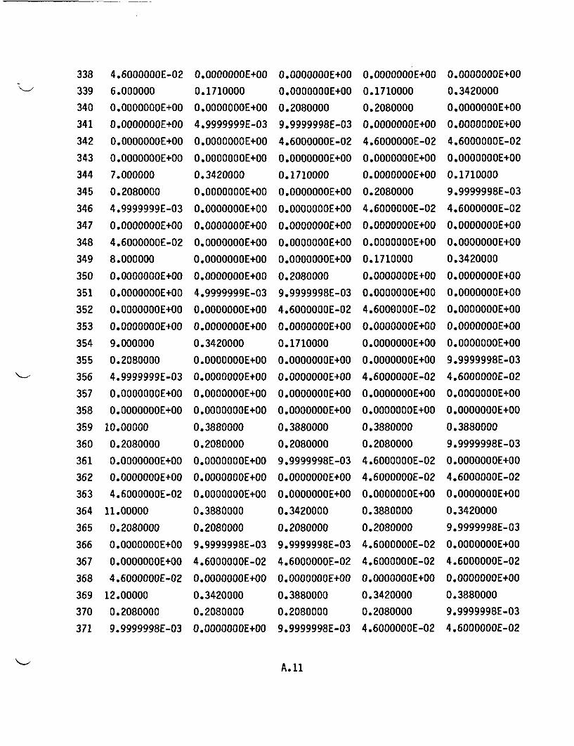
338
339
340
341
342
343
344
345
346
347
348
349
350
351
352
353
354
355
356
357
358
359
360
361
362
363
364
365
366
367
368
369
370
371
4.6000000E-02
6.000000
O.OOOOOOOE+OO
O.OOOOOOOE+00
O.OOOOOOOE+00
O.OOOOOOOE+00
7.000000
0.2080000
4.9999999E-03
O.OOOOOOOE+00
4.6000000E-02
8.000000
O.OOOOOOOE+00
O.OOOOOOOE+00
O.OOOOOOOE+00
O.OOOOOOOE+00
9.000000
0.2080000
4.9999999E-03
O.OOOOOOOE+00
O.OOOOOOOE+00
10.00000
0.2080000
O.OOOOOOOE+00
O.OOOOOOOE+00
4.6000000E-02
11.00000
0.2080000
O.OOOOOOOE+00
O.OOOOOOOE+OO
4.6000000E-02
12.00000
0.2080000
9.9999998E-03
O.OOOOOOOE+00
0.1710000
O.OOOOOOOE+00
4.9999999E-03
O.OOOOOOOE+00
O.OOOOOOOE+00
0.3420000
O.OOOOOOOE+00
O.OOOOOOOE+00
O.OOOOOOOE+00
O.OOOOOOOE+00
O.OOOOOOOE+00
O.OOOOOOOE+00
4.9999999E-03
O.OOOOOOOE+00
O.OOOOOOOE+00
0.3420000
O.OOOOOOOE+00
O.OOOOOOOE+00
O.OOOOOOOE+00
O.OOOOOOOE+00
0.3880000
0.2080000
O.OOOOOOOE+00
O.OOOOOOOE+00
O.OOOOOOOE+00
0.3880000
0.2080000
9.9999998E-03
4.6000000E-02
O.OOOOOOOE+00
0.3420000
0.2080000
O.OOOOOOOE+00
O.OOOOOOOE+00
O.OOOOOOOE+00
0.2080000
9.9999998E-03
4.6000000E-02
O.OOOOOOOE+00
0.1710000
O.OOOOOOOE+00
O.OOOOOOOE+00
O.OOOOOOOE+00
O.OOOOOOOE+00
O.OOOOOOOE+00
0.2080000
9.9999998E-03
4.6000000E-02
O.OOOOOOOE+00
0.1710000
O.OOOOOOOE+00
O.OOOOOOOE+00
O.OOOOOOOE+00
O.OOOOOOOE+00
0.3880000
0.2080000
9.9999998E-03
O.OOOOOOOE+00
O.OOOOOOOE+00
0.3420000
0.2080000
9.9999998E-03
4.6000000E-02
O.OOOOOOOE+00
0.3880000
0.2080000
9.9999998E-03
O.OOOOOOOE+00
0.1710000
0.2080000
O.OOOOOOOE+00
4.6000000E-02
O.OOOOOOOE+00
O.OOOOOOOE+00
0.2080000
4.6000000E-02
O.OOOOOOOE+00
O.OOOOOOOE+00
0.1710000
O.OOOOOOOE+00
O.OOOOOOOE+00
4.6000000E-02
O.OOOOOOOE+00
O.OOOOOOOE+00
O.OOOOOOOE+00
4.6000000E-02
O.OOOOOOOE+00
O.OOOOOOOE+00
0.3880000
0.2080000
4.6000000E-02
4.6000000E-02
O.OOOOOOOE+00
0.3880000
0.2080000
4.6000000E-02
4.6000000E-02
O.OOOOOOOE+00
0.3420000
0.2080000
4.6000000E-02
O.OOOOOOOE+00
0.3420000
O.OOOOOOOE+00
O.OOOOOOOE+00
4.6000000E-02
O.OOOOOOOE+00
0.1710000
9.9999998E-03
4.6000000E-02
O.OOOOOOOE+00
O.OOOOOOOE+00
0.3420000
O.OOOOOOOE+00
O.OOOOOOOE+00
O.OOOOOOOE+00
O.OOOOOOOE+00
O.OOOOOOOE+00
9.9999998E-03
4.6000000E-02
O.OOOOOOOE+00
O.OOOOOOOE+00
0.3880000
9.9999998E-03
O.OOOOOOOE+00
4.6000000E-02
O.OOOOOOOE+00
0.3420000
9.9999998E-03
O.OOOOOOOE+00
4.6000000E-02
O.OOOOOOOE+00
0.3880000
9.9999998E-03
4.6000000E-02
A.11
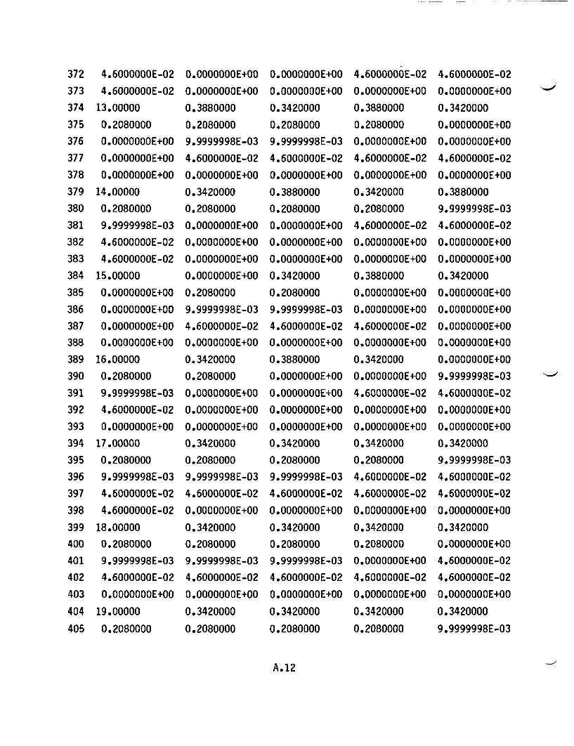
372
373
374
375
376
377
378
379
380
381
382
383
384
385
386
387
388
389
390
391
392
393
394
395
396
397
398
399
400
401
402
403
404
405
4.6000000E-02
4.6000000E-02
13.00000
0.2080000
O.OOOOOOOE+00
O.OOOOOOOE+00
O.OOOOOOOE+00
14.00000
0.2080000
9.9999998E-03
4.6000000E-02
4.6000000E-02
15.00000
O.OOOOOOOE+00
O.OOOOOOOE+00
O.OOOOOOOE+00
O.OOOOOOOE+00
16.00000
0.2080000
9.9999998E-03
4.6000000E-02
O.OOOOOOOE+00
17.00000
0.2080000
9.9999998E-03
4.6000000E-02
4.6000000E-02
18.00000
0.2080000
9.9999998E-03
4.6000000E-02
O.OOOOOOOE+00
19.00000
0.2080000
O.OOOOOOOE+00
O.OOOOOOOE+00
0.3880000
0.2080000
9.9999998E-03
4.6000000E-02
O.OOOOOOOE+00
0.3420000
0.2080000
O.OOOOOOOE+00
O.OOOOOOOE+00
O.OOOOOOOE+00
O.OOOOOOOE+00
0.2080000
9.9999998E-03
4.6000000E-02
O.OOOOOOOE+00
0.3420000
0.2080000
O.OOOOOOOE+00
O.OOOOOOOE+00
O.OOOOOOOE+00
0.3420000
0.2080000
9.9999998E-03
4.6000000E-02
O.OOOOOOOE+00
0.3420000
0.2080000
9.9999998E-03
4.6000000E-02
O.OOOOOOOE+00
0.3420000
0.2080000
O.OOOOOOOE+00
O.OOOOOOOE+00
0.3420000
0.2080000
9.9999998E-03
4.6000000E-02
O.OOOOOOOE+00
0.3880000
0.2080000
O.OOOOOOOE+00
O.OOOOOOOE+00
O.OOOOOOOE+00
0.3420000
0.2080000
9.9999998E-03
4.6000000E-02
O.OOOOOOOE+00
0.3880000
O.OOOOOOOE+00
O.OOOOOOOE+00
O.OOOOOOOE+00
O.OOOOOOOE+00
0.3420000
0.2080000
9.9999998E-03
4.6000000E-02
O.OOOOOOOE+00
0.3420000
0.2080000
9.9999998E-03
4.6000000E-02
O.OOOOOOOE+00
0.3420000
0.2080000
4.6000000E-02
O.OOOOOOOE+00
0.3880000
0.2080000
O.OOOOOOOE+00
4.6000000E-02
O.OOOOOOOE+00
0.3420000
0.2080000
4.6000000E-02
O.OOOOOOOE+00
O.OOOOOOOE+00
0.3880000
O.OOOOOOOE+00
O.OOOOOOOE+00
4.6000000E-02
O.OOOOOOOE+00
0.3420000
O.OOOOOOOE+00
4.6000000E-02
O.OOOOOOOE+00
O.OOOOOOOE+00
0.3420000
0.2080000
4.6000000E-02
4.6000000E-02
O.OOOOOOOE+00
0.3420000
0.2080000
O.OOOOOOOE+00
4.6000000E-02
O.OOOOOOOE+00
0.3420000
0.2080000
4.6000000E-02
O.OOOOOOOE+00
0.3420000
O.OOOOOOOE+00
O.OOOOOOOE+00
4.6000000E-02
O.OOOOOOOE+00
0.3880000
9.9999998E-03
4.6000000E-02
O.OOOOOOOE+00
O.OOOOOOOE+00
0.3420000
O.OOOOOOOE+00
O.OOOOOOOE+00
O.OOOOOOOE+00
O.OOOOOOOE+00
O.OOOOOOOE+00
9.9999998E-03
4.6000000E-02
O.OOOOOOOE+00
O.OOOOOOOE+00
0.3420000
9.9999998E-03
4.6000000E-02
4,6000000E-02
O.OOOOOOOE+00
0.3420000
O.OOOOOOOE+00
4.6000000E-02
4.6000000E-02
O.OOOOOOOE+00
0.3420000
9.9999998E-03
A. 12
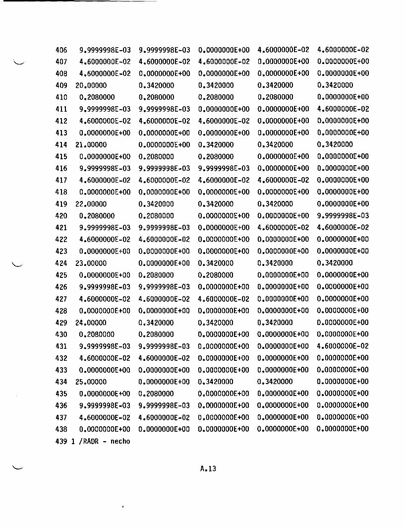
406 9.9999998E-03 9.9999998E-03 O.OOOOOOOE+00 4.6000000E-02 4.6000000E-02
407
408
409
410
411
412
413
414
415
416
417
418
419
420
421
422
423
424
425
426
427
428
429
430
431
432
433
434
435
436
437
438
439
4.6000000E-02
4.6000000E-02
20.00000
0.2080000
9.9999998E-03
4.6000000E-02
O.OOOOOOOE+00
21.00000
O.OOOOOOOE+00
9.9999998E-03
4.6000000E-02
O.OOOOOOOE+00
22 .00000
0.2080000
9.9999998E-03
4.6000000E-02
O.OOOOOOOE+00
23.00000
O.OOOOOOOE+00
9.9999998E-03
4.6000000E-02
O.OOOOOOOE+00
24.00000
0.2080000
9.9999998E-03
4.6000000E-02
O.OOOOOOOE+00
25.000000
O.OOOOOOOE+00
9.9999998E-03
4.6000000E-02
O.OOOOOOOE+00
1 /RADR - necho
4.6000000E-02
O.OOOOOOOE+00
0.3420000
0.2080000
9.9999998E-03
4.6000000E-02
O.OOOOOOOE+00
O.OOOOOOOE+00
0.2080000
9.9999998E-03
4.6000000E-02
O.OOOOOOOE+00
0.3420000
0.2080000
9.9999998E-03
4.6000000E-02
O.OOOOOOOE+00
O.OOOOOOOE+00
0.2080000
9.9999998E-03
4.6000000E-02
O.OOOOOOOE+00
0.3420000
0.2080000
9.9999998E-03
4.6000000E-02
O.OOOOOOOE+00
O.OOOOOOOE+00
0.2080000
9.9999998E-03
4.6000000E-02
O.OOOOOOOE+00
4.6000000E-02
O.OOOOOOOE+00
0.3420000
0.2080000
O.OOOOOOOE+00
4.6000000E-02
O.OOOOOOOE+00
0.3420000
0.2080000
9.9999998E-03
4.6000000E-02
O.OOOOOOOE+00
0.3420000
O.OOOOOOOE+00
O.OOOOOOOE+00
O.OOOOOOOE+00
O.OOOOOOOE+00
0.3420000
0.2080000
O.OOOOOOOE+00
4.6000000E-02
O.OOOOOOOE+00
0.3420000
O.OOOOOOOE+00
O.OOOOOOOE+00
O.OOOOOOOE+00
O.OOOOOOOE+00
0.3420000
O.OOOOOOOE+00
O.OOOOOOOE+00
O.OOOOOOOE+00
O.OOOOOOOE+00
0 .OOOOOOOE+00
0.OOOOOOOE+00
0.3420000022080000
0.OOOOOOOE+00O.OOOOOOOE+00
O.OOOOOOOE+00
0.3420000
0.OOOOOOOE+00
O.OOOOOOOE+00
4.60000OOE-02
O.OOOOOOOE+00
0.3420000
O.OOOOOOOE+00
4.6000000E-02
O.OOOOOOOE+00
0 .OOOOOOOE+00
0.3420000
O.OOOOOOOE+00
0.OOOOOOOE+00
O.OOOOOOOE+00O.OOOOOOOE+00
0.3420000O.OOOOOOOE+00
O.OOOOOOOE+00
O.OOOOOOOE+00
O.OOOOOOOE+00
0.3420000
O.OOOOOOOE+00
O.OOOOOOOE+00
O.OOOOOOOE+00
O.OOOOOOOE+00
O.OOOOOOOE+00
O.OOOOOOOE+00
0.3420000
O.OOOOOOOE+00
4.6000000E-02
O.OOOOOOOE+00
O.OOOOOOOE+00
0.3420000
O.OOOOOOOE+00
O.OOOOOOOE+00
O.OOOOOOOE+00
O.OOOOOOOE+00
O.OOOOOOOE+00
9.9999998E-03
4.6000000E-02
O.OOOOOOOE+00
O.OOOOOOOE+00
0.3420000
O.OOOOOOOE+00
O.OOOOOOOE+00
O.OOOOOOOE+00
O.OOOOOOOE+00
O.OOOOOOOE+00
O.OOOOOOOE+00
4.6000000E-02
O.OOOOOOOE+00
O.OOOOOOOE+00
O.OOOOOOOE+00
O.OOOOOOOE+00
O.OOOOOOOE+00
O.OOOOOOOE+00
O.OOOOOOOE+00
A.13
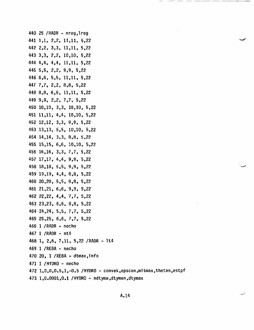
440 25 /RADR - nreg,lreg
441 1,1, 2,2, 11,11, 5,22
442 2,2, 3,3, 11,11, 5,22
443 3,3, 2,2, 10,10, 5,22
444 4,4, 4,4, 11,11, 5,22
445 5,5, 2,2, 9,9, 5,22
446 6,6, 5,5, 11,11, 5,22
447 7,7, 2,2, 8,8, 5,22
448 8,8, 6,6, 11,11, 5,22
449 9,9, 2,2, 7,7, 5,22
450 10,10, 3,3, 10,10, 5,22
451 11,11, 4,4, 10,10, 5,22
452 12,12, 3,3, 9,9, 5,22
453 13,13, 5,5, 10,10, 5,22
454 14,14, 3,3, 8,8, 5,22
455 15,15, 6,6, 10,10, 5,22
456 16,16, 3,3, 7,7, 5,22
457 17,17, 4,4, 9,9, 5,22
458 18,18, 5,5, 9,9, 5,22
459 19,19, 4,4, 8,8, 5,22
460 20,20, 5,5, 8,8, 5,22
461 21,21, 6,6, 9,9, 5,22
462 22,22, 4,4, 7,7, 5,22
463 23,23, 6,6, 8,8, 5,22
464 24,24, 5,5, 7,7, 5,22
465 25,25, 6,6, 7,7, 5,22
466 1 /RADR - necho
467 1 /RADR - nt4
468 1, 2,6, 7,11, 5,22 /RADR - 1t4
469 1 /REBA - necho
470 20, 1 /REBA - dtmax,info
471 1 /HYDRO - necho
472 1,0,0,0.5,1,-0.5 /HYDRO - convek,epscon,mitmax,thetam,estpf
473 1,0.0001,0.1 /HYDRO - ndtyme,dtymen,dtymax
A. 14
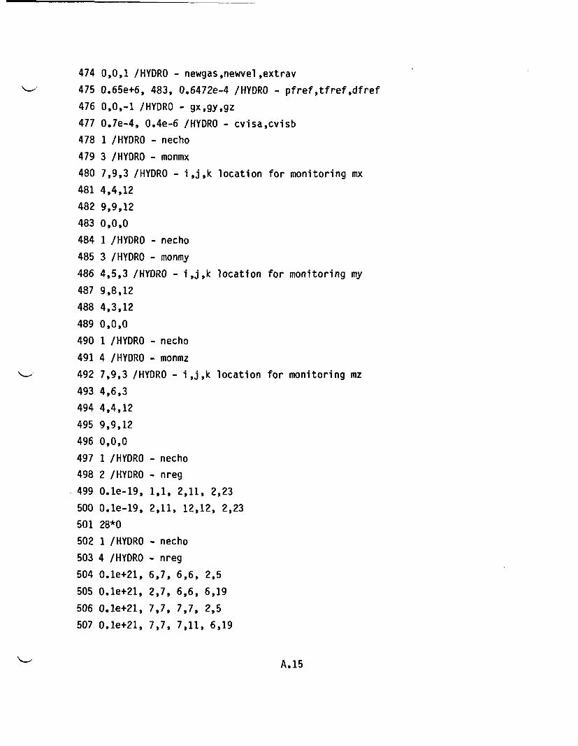
474 0,0,1 /HYDRO - newgas,newvel,extrav
475 0.65e+6, 483, 0.6472e-4 /HYDRO - pfref,tfref,dfref
476 0,0,-1 /HYDRO - gx,gy,gz
477 0.7e-4, 0.4e-6 /HYDRO - cvisa,cvisb
478 1 /HYDRO - necho
479 3 /HYDRO - monmx
480 7,9,3 /HYDRO - i,j,k location for monitoring mx
481 4,4,12
482 9,9,12
483 0,0,0
484 1 /HYDRO - necho
485 3 /HYDRO - monmy
486 4,5,3 /HYDRO - i,j,k location for monitoring my
487 9,8,12
488 4,3,12
489 0,0,0
490 1 /HYDRO - necho
491 4 /HYDRO - monmz
492 7,9,3 /HYDRO - i,j,k location for monitoring mz
493 4,6,3
494 4,4,12
495 9,9,12
496 0,0,0
497 1 /HYDRO - necho
498 2 /HYDRO - nreg
499 0.le-19, 1,1, 2,11, 2,23
500 0.le-19, 2,11, 12,12, 2,23
501 28*0
502 1 /HYDRO - necho
503 4 /HYDRO - nreg
504 0.le+21, 6,7, 6,6, 2,5
505 0.le+21, 2,7, 6,6, 6,19
506 O.le+21, 7,7, 7,7, 2,5
507 O.le+21, 7,7, 7,11, 6,19
A. 15
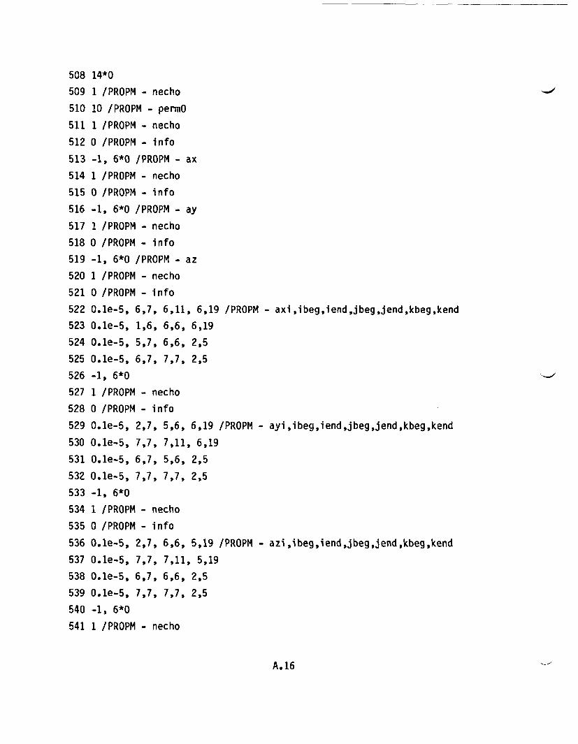
508 14*0
509 1 /PROPM - necho
510 10 /PROPM - pernm
511 1 /PROPM - necho
512 0 /PROPM - info
513 -1, 6*0 /PROPM - ax
514 1 /PROPM - necho
515 0 /PROPM - info
516 -1, 6*0 /PROPM - ay
517 1 /PROPM - necho
518 0 /PROPM - info
519 -1, 6*0 /PROPM - az
520 1 /PROPM - necho
521 0 /PROPM - info
522 O.le-5, 6,7, 6,11, 6,19 /PROPM - axi,ibeg,iend,jbeg,jend,kbeg,kend
523 O.le-5, 1,6, 6,6, 6,19
524 O.le-5, 5,7, 6,6, 2,5
525 O.le-5, 6,7, 7,7, 2,5
526 -1, 6*0
527 1 /PROPM - necho
528 0 /PROPM - info
529 O.le-5, 2,7, 5,6, 6,19 /PROPM - ayi,ibeg,iend,jbeg,jend,kbeg,kend
530 O.le-5, 7,7, 7,11, 6,19
531 O.le-5, 6,7, 5,6, 2,5
532 O.le-5, 7,7, 7,7, 2,5
533 -1, 6*0
534 1 /PROPM - necho
535 0 /PROPM - info
536 O.le-5, 2,7, 6,6, 5,19 /PROPM - azi,ibeg,iend,jbeg,jend,kbeg,kend
537 O.le-5, 7,7, 7,11, 5,19
538 O.le-5, 6,7, 6,6, 2,5
539 O.le-5, 7,7, 7,7, 2,5
540 -1, 6*0
541 1 /PROPM - necho
A. 16
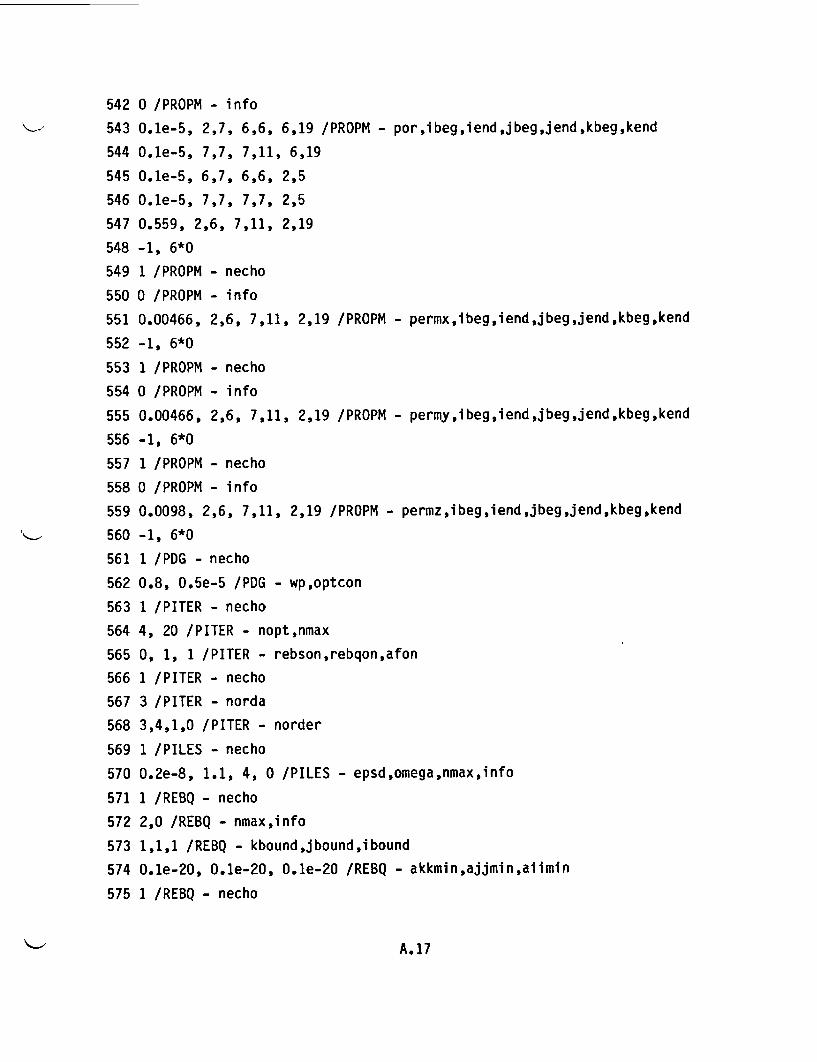
542
543
544
545
546
547
548
549
550
551
552
553
554
555
556
557
558
559
560
561
562
563
564
565
566
567
568
569
570
571
572
573
574
575
0 /PROPM - info
O.le-5, 2,7, 6,6, 6,19 /PROPM - por,ibeg,iend,jbeg,jend,kbeg,kend
O.le-5, 7,7, 7,11, 6,19
O.le-5, 6,7, 6,6, 2,5
O.le-5, 7,7, 7,7, 2,5
0.559, 2,6, 7,11, 2,19
-1, 6*0
1 /PROPM - necho
0 /PROPM - info
0.00466, 2,6, 7,11, 2,19 /PROPM - permx,ibeg,iend,jbeg,jend,kbeg,kend
-1, 6*0
1 /PROPM - necho
0 /PROPM - info
0.00466, 2,6, 7,11, 2,19 /PROPM - permy,ibeg,iend,jbeg,jend,kbeg,kend
-1, 6*0
1 /PROPM - necho
0 /PROPM - info
0.0098, 2,6, 7,11, 2,19 /PROPM - permz,ibeg,iend,jbeg,jend,kbeg,kend
-1, 6*0
1 /PDG - necho
0.8, 0.5e-5 /PDG - wp,optcon
1 /PITER - necho
4, 20 /PITER - nopt,nmax
0, 1, 1 /PITER - rebson,rebqon,afon
1 /PITER - necho
3 /PITER - norda
3,4,1,0 /PITER - norder
1 /PILES - necho
0.2e-8, 1.1, 4, 0 /PILES - epsd,omega,nmax,info
1 /REBQ - necho
2,0 /REBQ - nmax,info
1,1,1 /REBQ - kbound,jbound,ibound
O.le-20, O.le-20, O.le-20 /REBQ - akkmin,ajjmin,aiimin
1 /REBQ - necho
A. 17
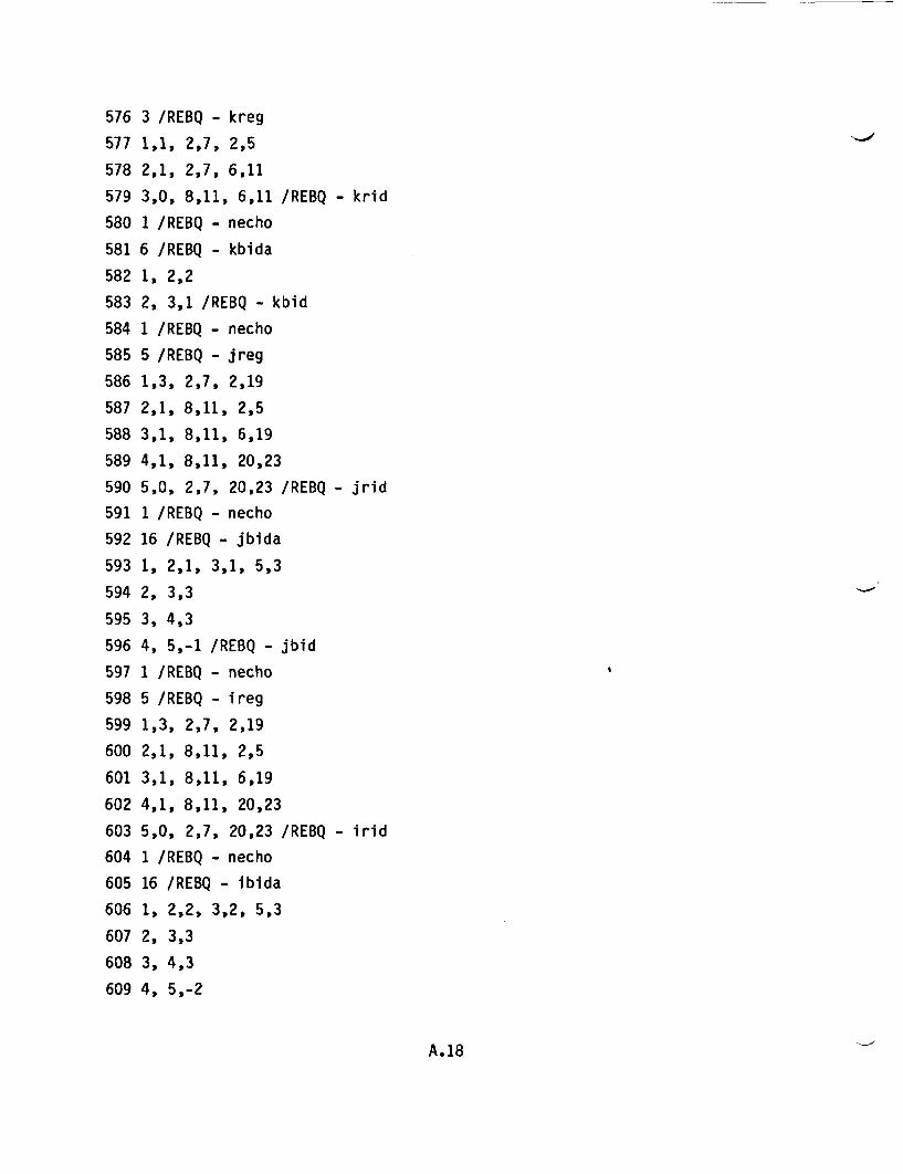
576 3 /REBQ - kreg
577 1,1, 2,7, 2,5
578 2,1, 2,7, 6,11
579 3,0, 8,11, 6,11 /REBQ - krid
580 1 /REBQ - necho
581 6 /REBQ - kbida
582 1, 2,2
583 2, 3,1 /REBQ - kbid
584 1 /REBQ - necho
585 5 /REBQ - jreg
586 1,3, 2,7, 2,19
587 2,1, 8,11, 2,5
588 3,1, 8,11, 6,19
589 4,1, 8,11, 20,23
590 5,0, 2,7, 20,23 /REBQ - jrid
591 1 /REBQ - necho
592 16 /REBQ - jbida
593 1, 2,1, 3,1, 5,3
594 2, 3,3
595 3, 4,3
596 4, 5,-1 /REBQ - jbid
597 1 /REBQ - necho
598 5 /REBQ - ireg
599 1,3, 2,7, 2,19
600 2,1, 8,11, 2,5
601 3,1, 8,11, 6,19
602 4,1, 8,11, 20,23
603 5,0, 2,7, 20,23 /REBQ - irid
604 1 /REBQ - necho
605 16 /REBQ - ibida
606 1, 2,2, 3,2, 5,3
607 2, 3,3
608 3, 4,3
609 4, 5,-2
A. 18

610 1 /AF - necho
611 5,0 /AF - nmax,info
612 1 /AVG - necho
613 0, 0.496e+6 /AVG - fixedm,fixedp*
A. 19

APPENDIX B
SAMPLE PROBLEM OUTPUT
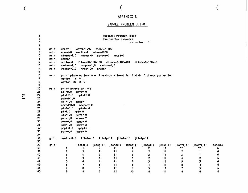
( ( (APPENDIX B
SAMPLE PROBLEM OUTPUT
456789
101112131415161718192021
w 222324252627282930313233343536373839404142434445
Appendix Problem InputUse quarter symmetry
run number I
mainmaInmainmalnmaInmainmaIn
nrun= 1 nstepul000nread=0 nwriteslsteady=1.0 nobody=0newta lndtimeal dtimen-0.1radcon=1 .0 radpon=lrebaon=0.0 nreb=100
nsInfo- 200ndump=1000
notemp-0 novel=0
00e+00 dtimax=0.100e+01.0 radron=1.0
nrebn= 1
dtIml n=0.100e-01
main print plane options areoption 1: 8option 2: 2 10
main print arrays or Infopti-0.0 npti- 0ptsI0.0 nptsl 0pqbnd-1.0pqilz.0 npqln 1pqrad-0.0 npqrad- 0ptslO0.0 nptsl= 0pt-1.0 npt- 0pts=l.0 npts= 0pmx-l.0 npmx 2pmy-0.0 npmy- 0pmz=l.0 npmz- 2pdpf-1.0 npdpfu 1ppf-0.0 nppf- 0
2 maximum al lowed Is 4 with 5 planes per option
grid symtryal.0 Iflatmz 3 Iflatpull Jflatm=10 Jflatp=ll
grid
2345678
Ieend(J)13456789
Jebeg(I )22234567
Jeend( I )1111111111111111
Imend(J) Jmbeg(I)4 24 25678910
223456
Jmend(I )11I 1111111111111
I cart(J s)**
2345678
Jcart(Js)F**
23456
Isend~k)66666666
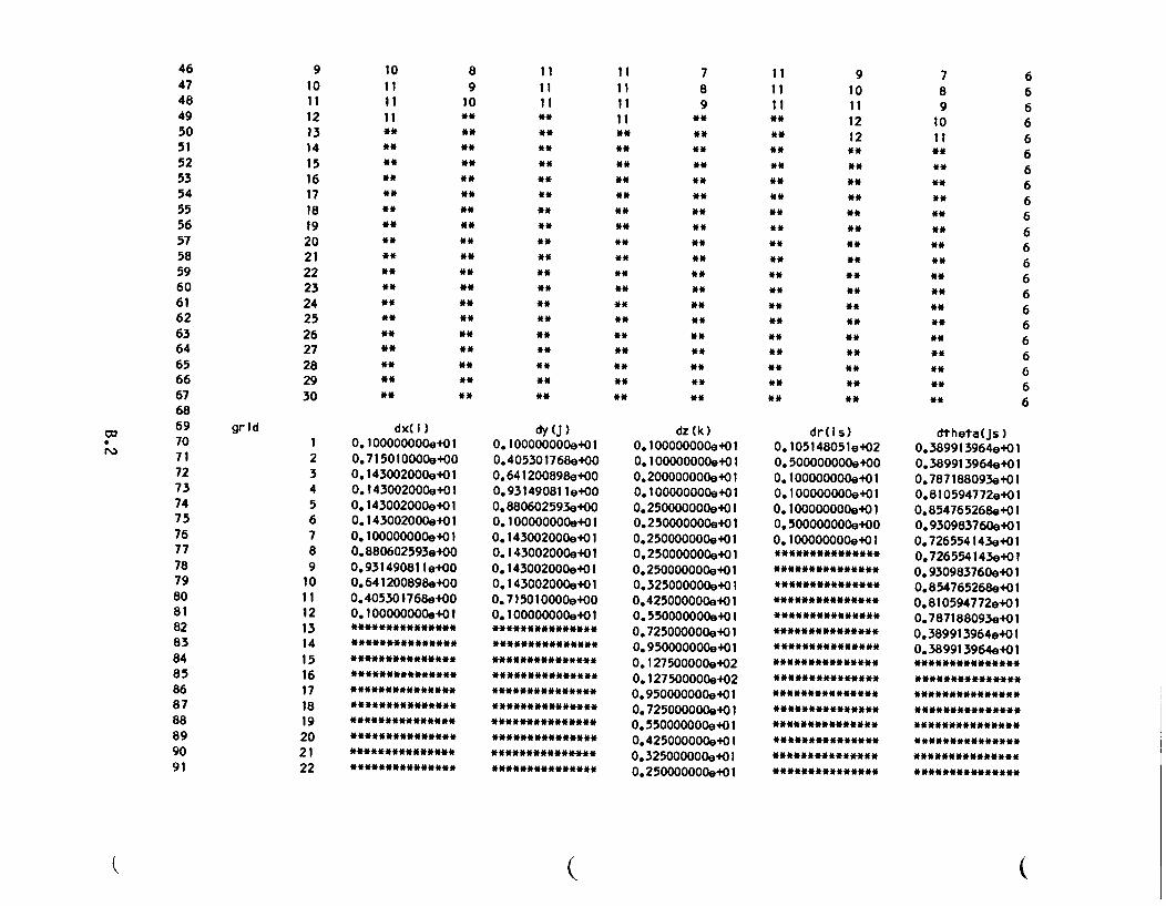
464748495051525354555657585960616263646566676869
w 70rla 71
7273747576777879808182838485868788899091
910I 112131415161718192021222324252627282930
10111 111**
**
**
**
**
**
**
**
**
**
**
**
**
**
**
**
89
10
**
**
**
**
**
**
**
**
**
**
**
**
**
1 111
**
**
**
**
**
**
**
**
**
**
**
**
**
**
**
**
**
**
dy (J )0.100000000I+010.405301768e+000.641200898e+000.93149081 1e+000.880602593e+000. 100000000l+010.143002000e+010.143002000.4010.143002000e+010.143002000.+010.715010000e+000.100000000.401
I1II1II1II1I
789
**
**
**
**
**
**
***
***
1 11111
**
**
**
**
**
910I11212**
**
**
**
**
**
** **
**
**
**
**
**
**
**
**
**
**
**
**
**
**
**
**
**
**
**
**
**
**
**
**
**
**
**
**
**
**
**
**
**
789
10I I
11
**
**
**
**
**
**
**
6666666666666666666666
grId dx( I )I 0.100000000e+012 0.715010000e+003 0.143002000e+014 0.143002000.+015 0.143002000a+016 0.14 3 0 0 2 0 0 0e+017 0. 1000000004+018 0.880602593e+009 0.931490811,+00
10 0.641200898e+0011 0.405301768e+0012 0.1000000004+0113 ***************14 ***************15 **********16 ***************17 **************18 **************19 ***************
20 *************21 **************22 **************
** *
dz(k)0.1000000004+010. 100000000.4+010.200000000.+010.100000000e+010.250000000.4010.250000000e+010.250000000.4010.250000000.+010.250000000e4010.325000000.+010.425000000.+010.550000000.+010.725000000e+010.950000000.+010.127500000,+020.127500000.+020.950000000e+010.725000000.+010.550000000e+010.425000000.+010.325000000.+010.250000000.+01
dr(Is)0.105148051e+020.500000000e+000.1000000004+010.100000000e+010.100000000e+010.500000000e+000.1000000004+01
****** * * **III** **
******** *1******1
dtheta(Js)0.389913964e+010.389913964e+010.787188093e+010.810594772e+010.854765268e+010.930983760e+010.726554143e+010.726554143e+010.930983760e+010.854765268e+010.810594772e+010.787188093e+010.389913964e+010.389913964e+01******** *******1*
I******1I * *1****
**1**1* *1** *****
II III * *1* 1* *1* I
1*1* 1* II I * * *1* 1
I * *1* I *1* 1* *1* I
( (
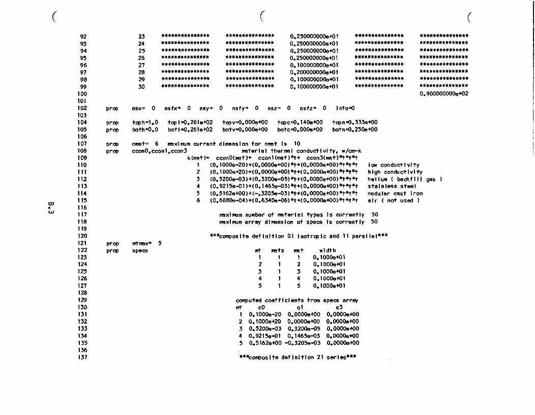
( ( (9293949596979899
100101102103104105106107108109110111112113114115
w 116W117
118119120121122123124125126127128129130131132133134135136137
2324252627282930
ftftftftftft ** * ft ** ** *
ft*ft ** ft ** ftft ftftft ft ft
ftftftft* ftft ftft * ft ft ftft ft
ftftftftftftftftftftftftftft*
ftftftft*ftftftftftftftftftft
** ftft ft ft ft ft ft ftft ft ft ft ft
ftft ft *ft ft ft ftftftft ftft ft ft
ft ftftftftftftftftftft *ft ft ft
ftftftftftftftftftftft*ftftft
ftftftftft**ftftftftftftftft
ftftft ftft ft ft ft ftftft ftftft ft
ftftftftftftftftftftftftftftft
ftftftftftftftftftftftftftftft
ft ftftftftft ftft ftft ft ftft ft ft
ftftftftftftftftftftftftftftft
0.250000000e+010.250000000e+010.250000000e+010.250000000e+010.100000000e+Ol0,200000000e+010.100000000e+010.1000000001e+O
ft ftftftftftft *ftft ftft* ft ft
ftftftft ftft ftft ft ftft ft ftft *
ft ftft ft ft ft ftft ft ftftftft ft ft
ft ftft ft ft ftftftft ftftftft ft ft
*ft ft ftft ft*ftft ftftftft ft ft
ft*ftftftftftftftftftftftftft
ftftftftftftftftftftftftftftft
ftftftftft*ftftftftftftft*ft
*************ttfttf fft**
***************t fftft tf f
***tf f************fft t
********tftftftftf**f*****f
f******fff*****tf****
************ttttff***
***tt tf****f**** f****f
*******ttfttf********t
0.900000000e+02
prop nsx= 0 nsfxm 0 nsy 0 nsfy- 0 nsz= 0 nsfz- 0 Info=O
prop toph=l.0 topilO. 2 61e+02
prop both=0.0 botl-0.261e+02topv=0.000.+00botv40.OOOe+00
topc=0.140e+00botc=0.000e+00
topn-O. 3 3 3 e+00botn-0.250.+00
prop nmat= 6 maximum current dimension for nmat Is 10prop cconO,cconl,ccon3 material thermal conductivity, w/cm-k
k(mat)u cconO(mat)+ ccon1(mat)*t+ ccon3(mat)*t*t*tI (0.10O0e-20)+(0.0000e+00)*t+(0.0000e+00)*tft*t2 (0.1000e+20)+(0.0000e+00)*t+(0.0000e+00)*t*t*t3 (0.5200e-03)+(0.3200e-05)*t+(0.0000e+00)*t*t*t4 (0.9215e-01)+(0.1465e-03)*t+(0.0000e+00)*t*t*t5 (0.5162e+00)+(-.3205e-03)*t+(0.0000e+00)*t*t*t6 (0.6880e-04)+(0.6340e-06)*t+(0.0000e+00)*t*ft*t
low conductivityhigh conductivityhelium ( backfill gas )stainless steelnodular cast Ironair ( not used )
maximum number of material types Is currently 50maximum array dimension of specs Is currently 50
prop mtmaxr 5prop specs
***composite definition 01 Isotropic and 11 parallel***
mt mats mat width1 1 1 0.1000e+012 1 2 0.1000l+013 1 3 0.1000e+014 1 4 0.1000.+015 1 5 0.1000l+01
computed coefficients frommt cO cl
1 0.1000e-20 0.0000e+002 0.1000l+20 0.0000e+003 0.5200e-03 0.32009-054 0.9215e-01 0.1465e-035 0.5162e+00 -0.3205e-03
specs arrayc3
O.OOOOe4OO0.0000+000.0000e4000.0000e+000.0000.+00
*"*composite definition 21 series***

138139140141142143144145146147148149150151152153154155156157158159160161
w 1624> 163
164165166167168169170171172173174175176177178179180181182183
prop mtmax= 7prop specs mt mnt width el e2
40 1 0.1000o+O1 0.2000e+00 0.1000.+0141 5 0.1600e-Ol 0.0000.+00 0.0000e+0042 3 0.1600e-01 0.0000e400 0.0000e+0043 5 0.1070.+00 0.0000.+00 0.0000.+0044 3 0.1070e400 0.0000O+00 0.0000e+0045 3 0.1600e-01 0.0000e+00 0.0000O+0046 3 0.1070e+00 0.0000e+00 0.0000e+00
twf0.5000e+000.5000.4000.00004+000.5000.+000.00004+000.l000e+010. 1000.+0 1
computed coefficients from specs arraymt cO cl c340 0.1000e-20 0.0000e+00 0.4536e-1141 0.3226e+02 -0.2003.-01 0.0000e+0042 0.3250.-01 0.2000.-03 0.0000e+0043 0.4824e+01 -0.2995e-02 0.0000+0044 0.4860e-02 0.2991e-04 0.0000e+0045 0.3250e-01 0.2000e-03 0.0000.+0046 0.4860e-02 0.2991e-04 0.0000+00
***composite definitIon 31 fuel assembly***prop mtmax- 1prop specs mt mta fuelod cladod pitch cfuel cclad erod egap
47 3 0.9484e+00 0.1072e+01 0.1430e+01 0.2090.-01 0.1150e+00 0.0000e+00 0.0000+00
mt cO47 0.5200e-03
computed coefficients from specs arraycl c3 xl x2 zI z2 z3
0.3200e-OS 0.0000+00 0.1130e+01 0.1701e+01 0.3455e+00 0.9591e-01 0.5586e+00
***avallable composite definitions***group Id
01 Isotropic I resx2 resy3 resz
11 parallel4 resxresy,resz11 resx, x-y plane12 resx, x-z plane13 resy, x-y plane14 resy, y-z plane15 resz, x-z plane16 resz, y-z plane21 resx22 rosy23 resz31 resx,resy,resz for rod array41 resfx
21 series
31 fuel assembly41 film resistance
k., C (

( ( (184185186187188189190191192193194195196197198199200201202203204205206207
* 208Ln 209
210211212213214215216217218219220221222223224225226227228229
42 resfy43 resfz
51 exterior convection 51 resfz for top of caskand radiation 52 resfz for bottom of cask
prop nreg= 24 npalr- 24 maximum current dimensions for nreg and npalr are 25 30prop Index cell location
ibeg lend jbeg Jend kbeg kend1 1 2 11 2 292 11 12 12 2 292 11 2 11 5 262 7 6 6 5 227 7 7 11 5 222 5 6 6 5 87 7 8 11 5 82 6 7 11 5 222 11 2 11 2 42 11 2 11 27 292 11 2 11 1 12 11 2 11 29 292 2 1 1 2 42 2 1 1 5 262 2 1 1 27 293 3 1 1 2 43 3 1 1 5 263 3 1 1 27 29
11 11 10 to 2 411 11 10 10 5 26it 11 10 10 27 2911 11 11 11 2 411 11 11 11 5 2611 11 11 11 27 29
npa I rIIIIIIIIIIIIIIIII1111111
Id mt1 12 14 34 44 44 34 3
31 474 54 53 1
51 4042 4142 4242 4142 4342 4442 4341 4341 4641 4341 4141 4541 41
Id mt Id mt Id mt Id mt
therm theta=0.5 sphtf-0.5234e+01 dtemax-0.500e+00therm rebon-0.0 nreb=100 nrebno 50
therm monitor cells* 8 neximum number currently allowed Is 12m I J k1 2 2 102 3 4 103 5 6 104 5 7 105 11 11 106 9 10 107 7 8 108 6 8 10
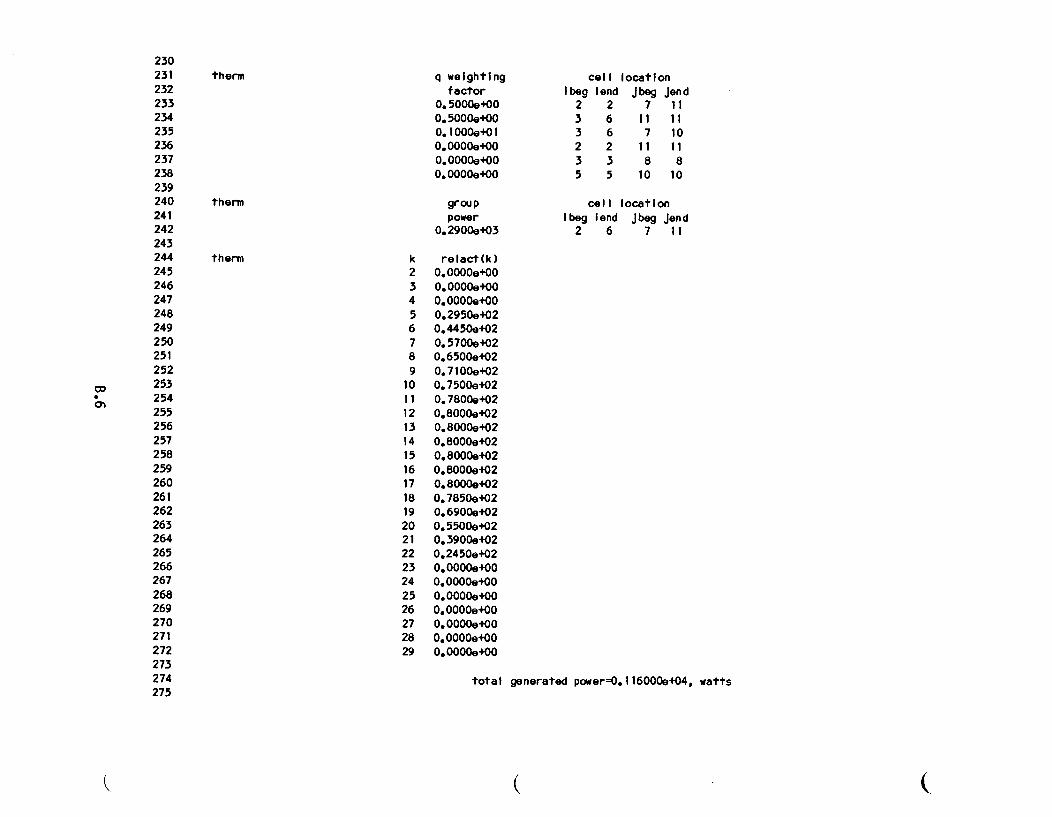
230231232233234235236237238239240241242243244245246247248249250251252
co 253* 254
255256257258259260261262263264265266267268269270271272273274275
therm q weightingfactor
0.5000e+000.5000e+000.1000l+010.0000.+000.0000+000.0000e+00
cell locationIbeg lend Jbeg Jend
2 2 7 113 6 11 113 6 7 102 2 11 113 3 8 85 5 10 10
cell locationIbeg lend Jbeg Jend
2 6 7 11
therm grou ppower
0.2900e+03
therm k reIact(k)2 0.0000O+00
3 0. 0000O+004 0. 0000e+005 0.2950e8026 0.44509+027 0.5700e+028 0.6500e+029 0.7100e+02
10 0.7500e+0211 0.78009+0212 0.80008+0213 0.80009+0214 0.8000e+0215 0.8000e+0216 0.8000e+0217 0.8000e+0218 0.7850e+0219 0.69008+0220 0.5500e+0221 0.3900e+0222 0.2450e+0223 0. 00008+0024 0. 00008400
25 0.00004+0026 0. 0000e+0027 0.0000840028 0. 0000e+00
29 0. 0000e+00
total generated power=0.116000e+04, watts
( (.
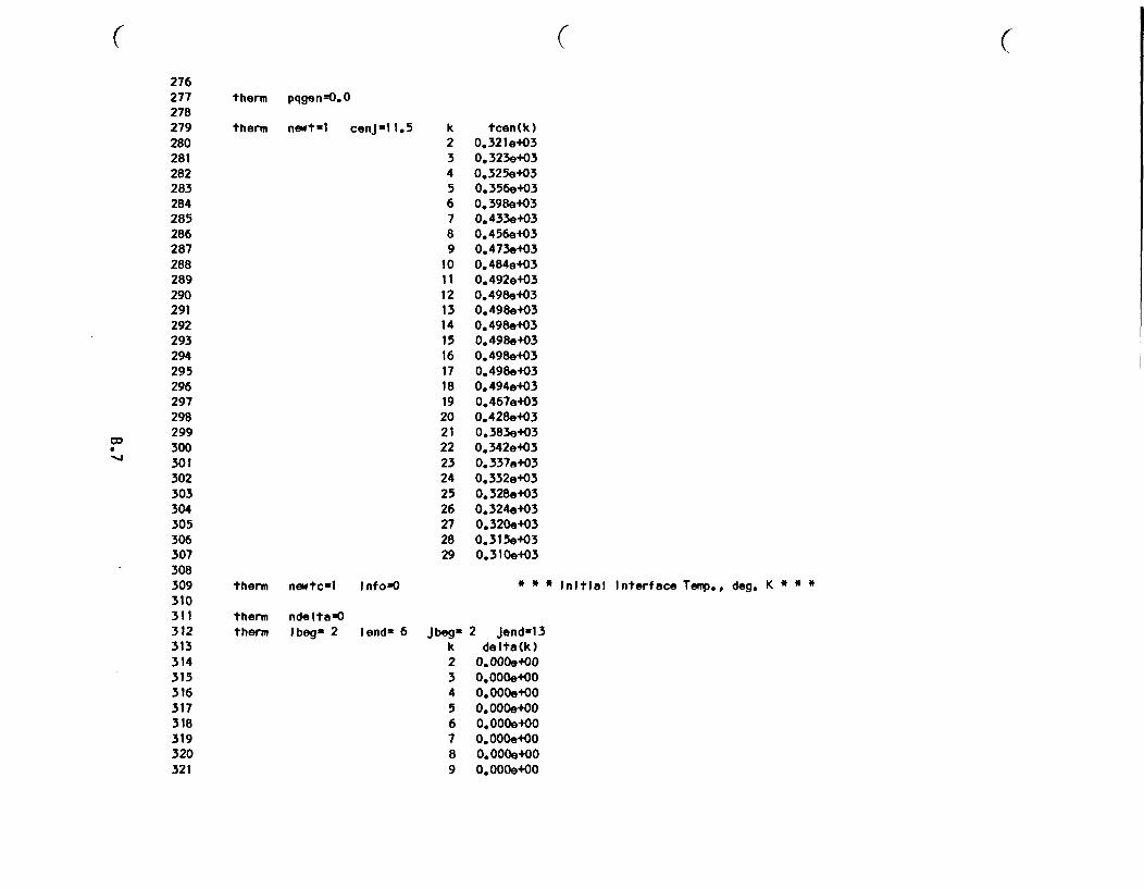
( ( (276277278279280281282283284285286287288289290291292293294295296297298299
* 300Ili 301
302303304305306307308309310311312313314315316317318319320321
therm pqgen-0.0
therm newt=1 cenJ-11.5 k tcen(k)2 0.321e+033 0.323e+034 0.325e+035 0.356e+036 0.398e+037 0.433e+038 0.456e+039 0.473e+03
10 0.484e+0311 0.492e+0312 0.498e+0313 0.498e+0314 0.498.+0315 0.498e+0316 0.498e+0317 0.498e+0318 0.494e+0319 0.467e+0320 0.428e+0321 0.383e+0322 0.342e+0323 0.3379+0324 0.332e+0325 0.328e+0326 0.324e+0327 0.320e+0328 0.315e+0329 0.310e+03
therm newtc-l InfowO * * * Initial Interface Temp., deg. K * * *
therm ndelta"Otherm Ibegs 2 Iend= 6 Jbegx
k23456789
2 Jend-l3delta(k)
0.000.+000.000+000.000.+000.000e+OO0.0000+O0.000+000.000.+000.000+00
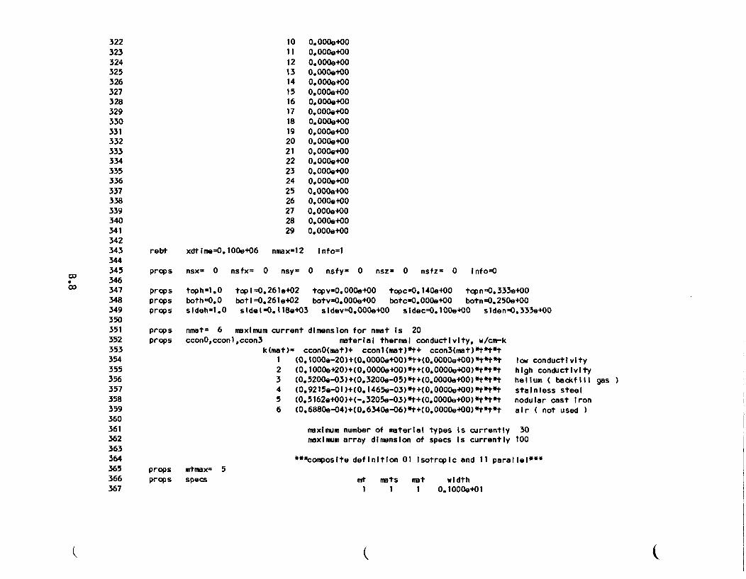
322323324325326327328329330331332333334335336337338339340341342343344345
w 346Co 347
348349350351352353354355356357358359360361362363364365366367
10 0.000e+0011 0.0000+0012 0,000.+0013 0,0004+0014 0.000.+0015 0.000.+0016 0,000.+0017 0.000.+0018 0.000.+0019 0.000.+0020 0.000e+0021 0.0000e+022 0.000+40023 0,000e+0024 0.000e+0025 0.000+0026 0.0000+0027 0.000e+0028 0.000e+OO29 0.000+00
rebt xdtime=0.100o+06 nmax*12 Info=l
props nsx- 0 nsfx= 0 nsy- 0 nsfyz 0 nszz 0 nsfz= 0 Info=O
propspropsprops
tophz1.0both=0.0sidehwl.O
topl=0.261e+02 topv0. 000.+00 topc-O.140e+00 topn=0.333e+00botl=0. 2 61e+02 botvu0.000+e00 botc-0.000e+00 botn=0.250e+00sidel=0.118e+03 sidevO.000e+00 sidec=O.i00e+00 siden=0.333e+00
props nmat= 6 maximum current dimension for nmat Is 20props cconO,cconl,ccon3 material thermal conductivity, w/cm-k
k(mat)- cconO(mat)+ cconl(mat)*t+ ccon3(mat)*t*t*tI (0.10OOe-20)+(0.0000e+00)*t+(0.0000e+00)*t*t*t2 (0,1000e+20)+(0,0000e+00)*t+(0.0000e+00)*t*t*t3 (0.5200e-03)+(0.3200e-05)*t+(0.0000e+00)*t*t*t4 (0.9215e-01)+(0.1465e-03)*t+(0.0000e+00)*t*t*t5 (0,5162e+00)+(-,3205e-03)*t+(0,0000e+00)*t*t*t6 (0,6880e-04)+(0,6340e-06)*t+(0,0000e+00)*t*t*t
low conductivityhigh conductivityhelIum ( backfill gas )stainless steelnodular cast Ironair ( not used )
maximum number of material types Is currently 30maximum array dimension of specs Is currently 100
props mtmax= 5props specs
***composite definition 01 Isotropic and 11 parallel***
mt mats mat widthI I I 0.1000+01
(
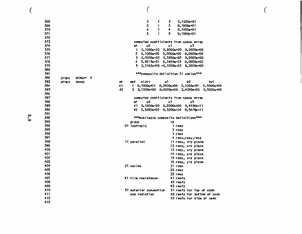
( ( (368369370371372373374375376377378379380381382383384385386387388389390391
* 392to 393
394395396397398399400401402403404405406407408409410411412413
2 1 2 0.lOOOe+013 1 3 0.1000e+014 1 4 0.lOOOe+015 1 5 0.1000e+01
computed coefficients from specs arraymt cO cl c31 0.1OOOe-20 0.0000e+00 0.0000e+002 0.lOOOe+20 0.0000e+00 0.0000+003 0.5200e-03 0.3200e-05 0.0000e+004 0.9215e-Ol 0.1465e-03 0.0000e+005 0.5162e+00 -0.3205e-03 0.0000e+00
**Acomposite definition 21 series***props mtmax- 2props specs Mt mat width el e2
41 1 0.1000.+01 0.2000e+00 0.1000.+0142 3 0.1000l+00 0.4000e+00 0.4000e+00
twf0.5000.+000.5000e+00
computed coefficients from specs arraymt cO cl c341 0.1000e-20 0.0000.+00 0.4536e-1142 0.5200e-02 0.3200e-04 0.5670e-11
***avaliable composite defInitions***
group01 Isotropic
11 parallel
21 series
41 film resistance
- 51 exterior convectionand radiation
Id1 resx2 resy3 resz4 resx,resy,resz11 resx, x-y plane12 resx, x-z plane13 resy, x-y plane14 resy, y-z plane15 resz, x-z plane16 resz, y-z plano21 resx22 resy23 resz41 resfx42 resfy43 resfz51 resfz52 resfz53 resfx
for top of caskfor bottom of caskfor side of cask
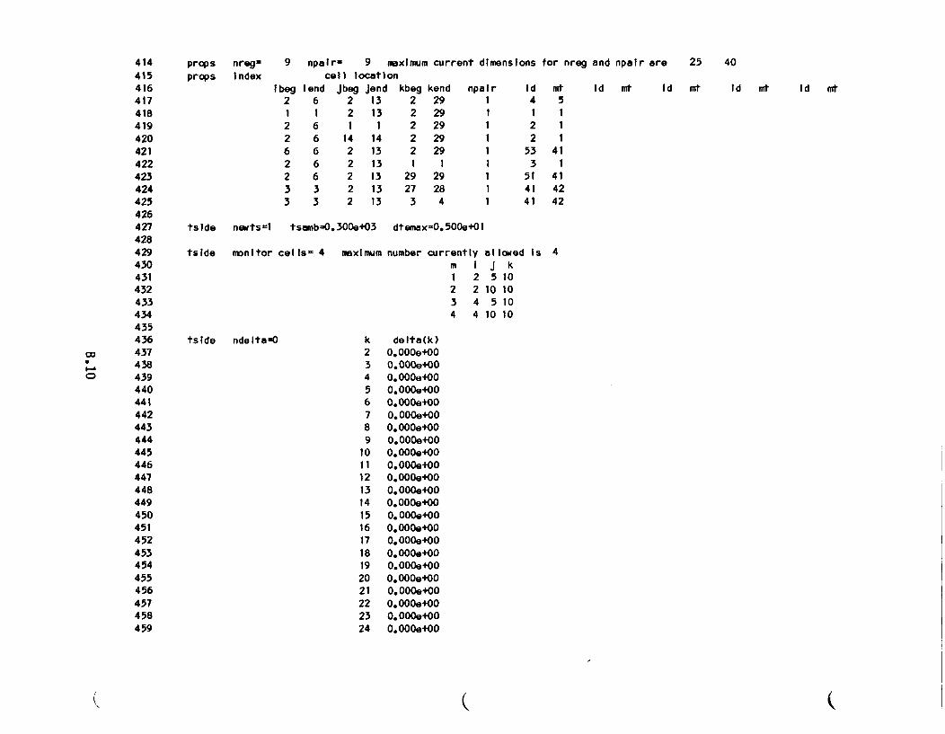
414415416417418419420421422423424425426427428429430431432433434435436
w 437*- 438o 439
440441442443444445446447448449450451452453454455456457458459
props nreg'props Index
9 npalr= 9 m xlmum current dimenslons for nreg and npalr are 25 40cell location
Ibeg lend Jbeg Jend kbeg kend2 6 2 13 2 291 1 2 13 2 292 6 1 1 2 292 6 14 14 2 296 6 2 13 2 292 6 2 13 1 12 6 2 13 29 293 3 2 13 27 283 3 2 13 3 4
npair111111111
Id mt4 51 12 12 1
53 413 1
51 4141 4241 42
Id mt Id mt Id mt Id mt
tside newtsal tsamb-0.300e+03 dtemax-0.5009e01
tside monitor cells= 4 maxlmum number currently alloIed Is 4m I J k1 2 5 102 2 10 103 4 5 104 4 10 10
tsIde ndelta=0 k delta(k)2 0.OOOe+003 0.000e+004 0.000Oe005 0.000e+006 0.000e+007 0.000e+008 0.000e+009 0.000e+00
10 0.0004+0011 .000e+0012 0.000Oe0013 0.000e+0014 0.000e+0015 0.000e+0016 0.000e+0017 0.000e+0018 0.000e+0019 0.000.+0020 0.000e+0021 0.000e+0022 0.000e+0023 0.000e+0024 0.000e+00
(
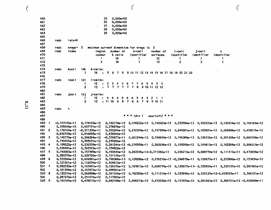
( ( (460461462463464465466467468
25 0.000e+0026 0.000e+0027 0.000+0028 0.000e+OO29 0.000e+00
radc
radc
Info'°
nregs= 2 nexlmum current dimension for nregs is 2469 radc Index470
region number of k-cell number of i-cell J-ce I I h
471472473474475476477478479480481482483484485
486487488489490491492493494495496497498499500501502503504505
number
2
k cells1818
Identifier surfaces1 121 12
Identifler
2
Identifier Identifier1 12 1
radc kcell Idk k-cells:1 18 : 5 6 7 8
radc Icell Idi i-cells:1 12 : 2 3 4 52 12 : 7 7 7 7
radc Jcell IdJ J-cells:1 12 : 6 6 6 62 12 : 11 10 9 8
9 10 11 12 13 14 15 16 17 18 19 20 21 22
6 7 7 6 5 4 3 27 7 8 9 10 11 12 12
6 6 5 4 3 2 1 17 6 6 7 8 9 10 11
radc h
2
3
4
5
6
7
8
9
-0.193150e-110.308646e-120.178142e-120.692739e-120.146770e-120.730242.-120.109222e-120.508481e-120.740063e-130.280376.-120.333564.-130.121361e-120.502533e-130.161598e-120.120314e-120.287270e-120.194169e-12
0.178142e-120.437751e-12
-0.371336e-110.816805e-120.296294e-120.595651e-120.230309e-i 20.365323e-120.157589.-120.229700e-120.694281e-130.112434e-120.105691e-120.147873e-120.268806.-120.251474e-120.459215e-12
0.146770e-10.278876e-10.296294.-i0.438345e-1
-0.376077e-i0.259266e-i0.261244e-i0.154802e-i0.190849e-i0.101134,-i0.796388e-i0.509613e-i0.126316e-i0.69950le-I0.391306e-i0.117960e-10.683198e-I
* * * Idh- 1 nsurfsi12 * * *
2 0.109222e-12 0.7400639-1322 0.230309e-12 0.157589e-1221 0.261244e-12 0.1908499-1222 -0.376500.-11 0.262038e-1222 0.262038e-12-0.371382.-1123 0.109288e-12 0.2262109-1232 0.195813e-12 0.608779e-1232 0.762266e-12 0.111310.-li22 0.806213e-12 0.470036e-12
0.333564e-13
0.694281e-13
0.796388e-13
0.109288e-12
0.226210e-12
-0.248679e-i1
0.120677e-ii-
0.323896e-12
0.153454e-12
0.502533e-13 0.120314e-12
0.105691e-12 0.268806e-12
0.126316e-12 0.391306e-12
0.195813e-12 0.762266e-12
0.608779e-12 0.111310e-11
0.120677e-il 0.323896e-12
0.320964e-il 0.335137e-12
0.335137e-12-0.433825e-il
0.20146le-12 0.36672le-12
0.194169e-12
0.459215e-12
0.683198e-12
0.806213e-12
0.470036.-12
0.153454e-12
0.201461e-12
0.366721e-12
-0.408669e-i1
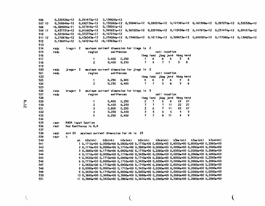
506507 10508509 11510511 12512513514515516517518519520521522523524525526527528529530531
532533534535536537538539540541542543544545546547548549550551
0.320529e-120.308646e-12
-0.389094e-110.437751e-i 20.321644e-120.278876.-120.15805le-12
0.291875e-120.692739e-120.321644e-120.81 6805e-i 2
-0.373774e-110.4383459-12
0.139820e-120.730242e-12 0.508481e-12 0.280376e-12 0.121361e-120.158051e-120.595651.-12 0.365323e-12 0.229700e-12 0.112434e-120.167214e-120.259266e-12 0.1548029-12 0.101134e-12 0.509613e-13
0.161598e-12
0.147873e-12
0.69950Ie-i 3
0.287270.-12 0.320529,-12
0.251474e-12 0.291875e-12
0.117960.-12 0.139820e-120.167214e-12 -0.193638e-11
radpradp
Iregsw 2 maximum current dimension for Iregs Is 2region emittances cell location
Ibeg lend Jbeg Jend kbeg kend7 8 6 6 5 87 9 7 7 5 8
1 0.400 0.2502 0.400 0.250
radpradp
jregsw 2 maximum current dimension for Jregs Is 2region emittances cell location
Ibeg lend Jbeg Jend kbeg kend6 6 4 6 5 87 7 5 6 5 8
1 0.250 0.4002 0.250 0.400
radpradp
kregsw 5 maximum current dimension for kregs Is 5region emittances
1 0.4002 0.4003 0.8004 0.2505 0.250
radr RADR Input Sectionradr Rod Emittance Is 0.8
radr nh- 25 maximum current dimensradr h
0.2500.2500.2500.4000.400
I beg27227
cell locationlend Jbeg jend I7 6 67 7 116 7 115 6 67 8 if
kbeg2222224
kend272727
94 9
ion for nh Is 25
nh h2e(nh)1 0.1710e+002 0.1710e+003 0.3880e+004 0.1710e+005 0.3420e+006 0.1710e+007 0.3420e+008 0.0000.+009 0.3420e+0010 0.3880e+0011 0.3880e+00
h2n(nh)0.00004+000.0000.+000.171Oe+000.0000.+000.1710.+000.0000.+000.1710e+00
h2w(nh)0.0000e+000.1710+000.0000e+000.1710e+000.00004+000.1710e+000.0000+00
h2s(nh)0.1710e+000.3880.+000.1710e+000.3420e+000.17 10e+000.3420e+000. 1710e+000.3420e+000.O0000+000.3880e+000.3420e+00
h3ne(nh) h3nw(nh) h3sw(nh)0.0000e+00 0.0000,+00 0.0000+000.0000e+00 0.0000e+00 0.2080e+000.2080e+00 0.0000e+00 0.0000e+000.0000.+00 0.0000e+00 0.2080.+000.2080e+00 0.0000+00 0.0000e+000.0000.+00 0.0000e+00 0.2080.+000.2080e+00 0.0000+00 0.0000.e+000.0000.+00 0.0000e+00 0.2080e+000.2080e+00 0.0000e+00 0.0000e+000.2080e+00 0.2080.+00 0.2080e4000.2080e+00 0.2080e+00 0.2080e+00
h3se(nh)0.2080e+000.2080e+000.2080e+000.2080.+000.2080e+000.2080.+000.2080e+000.0000.4000.0000+000.2080e+000.2080e+00
0.0000O+00 0.1710e+000.1710e+00 0.0000e+000.3880.+00 0.3880e+000.3420e+00 0.3880e+00
y (
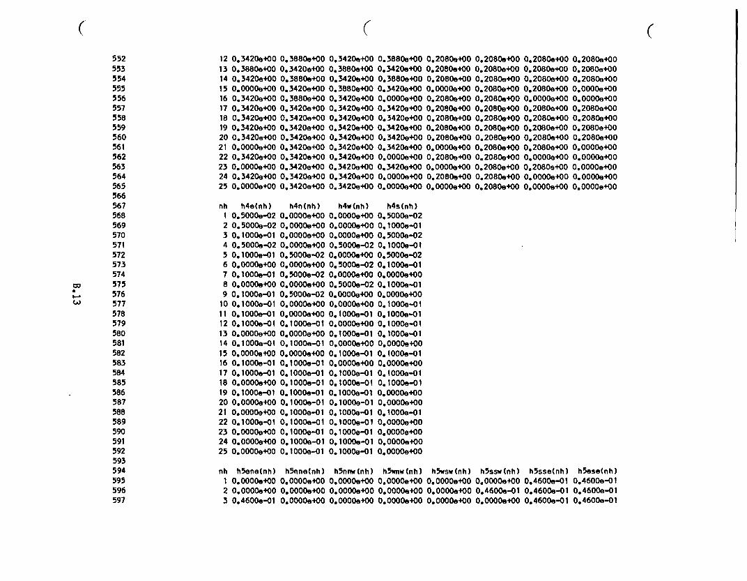
( ( (
552553554555556557558559560561562563564565566567568569570571572573574
w 575576
wA 577
578579580581582583584585586587588589590591592593594595596597
12 0.3420e+00 0.3880e+0013 0.3880e+00 0.3420e+0014 0.3420.+00 0.3880e+0015 0.00004+00 0.3420e+0016 0.3420e+00 0.3880e+0017 0.3420e+00 0.3420.+0018 0.3420e+00 0.3420e+0019 0.3420e+00 0.3420e+0020 0.3420e+00 0.3420e+0021 0.0000.e00 0.3420.+0022 0.3420e+00 0.3420e+0023 0.0000.+00 0.3420e+0024 0.3420.+00 0.3420e+0025 0.0000+00 0.3420e+00
nh h4e(nh) h4n(nh)1 0.5000e-02 0.0000e+002 0.5000.-02 0.00004+003 0. 1000.-01 0.00004+004 0.50009-02 0.0000.+005 0.10OOe-01 0.5000e-026 0.0000e+00 0.0000.+007 0.10OOe-01 0.50004-028 0.0000.+00 0.0000.+009 0.10OOe-01 0.5000e-0210 0.1000.-01 O.OOOOe+0011 0.1000e-01 0.0000.+0012 0.1000.-01 0.1000.-0113 0.0000e400 0.0000e+0014 0.1000e-01 0.1000e-0115 0.0000e+00 0.0000e+0016 0.1000.-01 0.1000.-0117 0.1000e-.01 0.1OOe-0118 0.0000.400 0. 1000l-0119 0.1OOe-01 0.1OOe-0120 0.0000e+00 0.1000e-0121 0.0000e+00 0. 10OOe-0122 0.1000.-01 0.1000e-0123 0.0000e+00 0.1000e-Ol24 0.00004+00 0.1000.-0125 0.0000e+00 0.1000.e01
0.3420e+000.3880a+000.3420e+000.3880e+000.3420e+000.3420e+000.3420e+000.3420e+000.3420e+000.3420e+000.3420.+000.3420e+000.3420e+000.3420e+00
h4w(nh)0.0000+00O.OOOOe+000.0000e+000.5000.-020.0000.+000.5000e-020.00004+000.5000e-020.0000e+000.0000e+00O.1 OOOe-010.00004+00O. I OOOe-010.0000.+000.10004-010.0000.+000.1000.-010. 1 OOOe-010.1000-010. 1000l-010. 1000.-010.1000-010. 1000.-010.1000.-010. 0OOOe-01
0.3880e+00 0.2080e+000.3420e+00 0.2080e+000.3880e+00 0.2080e+000.3420e+00 0.0000.+000.0000e+00 0.2080e4000.3420e+00 0.2080.+000.3420e+00 0.2080e+000.3420e+00 0.2080e+000.3420e+00 0.2080e+000.3420e+00 0.0000e+000.0000+00 0.2080e+000.3420e+00 0.0000e+000.00004+00 0.2080e+000.0000+00 0.0000e+00
0.2080e+000.2080e+000.2080.+000.2080e+000.2080.+000.2080e+000.2080e+000.2080e+000.2080e+000.2080e+000.2080e+000.2080e+000.2080e+000.2080e+00
0.2080e+00 0.2080e+000.2080.+00 0.2080.+000.2080e+00 0.2080e+000.2080e+00 0.0000.e000.0000+00 0.0000+000.2080e+00 0.2080e+000.2080e+00 0.2080e+000.2080e+00 0.2080e+000.2080.+00 0.2080.+000.2080e+00 0.0000e+000.0000e+00 0.0000+000.2080e+00 0.0000e+000.00004+00 0.00004+000.0000+00 0.0000e+00
h4s(nh)0.5000.-020. 0OOOe-010.5000.-020. 1000.4-010.5000e-020.1000.-010.0000+000. 1000.-010.0000.e000. 1000.-010.10004-010. 10004-010.10004-01O.OOOOe+000. 1000.-01O.OOOOe+000. I OOOe-0-0.1000.-010.0000e+OO0.0000e+OO0.100Oe-0 00.0000e+000.0000e+000.0000.+00O.OOOOe+OO
nh h5ene(nh) h5nne(nh) h5nnw(nh) h5wnw(nh) h5wsw(nh) h5ssw(nh) h5sse(nh) h5ese(nh)
1 0.0000.+00 0.0000e+00 0.0000.+00 0.0000e+00 0.0000e+00 0.0000.+00 0.4600.-01 0.4600e-01
2 0.0000.+00 0.0000.+00 0.0000e+00 0.0000e+00 0.0000e+00 0.4600.-01 0.4600e-01 0.4600e-01
3 0.4600e-01 0.0000e+00 0.0000e+00 0.0000+00 0.0000+00 0.0000e+00 0.4600e-01 0.4600e-01
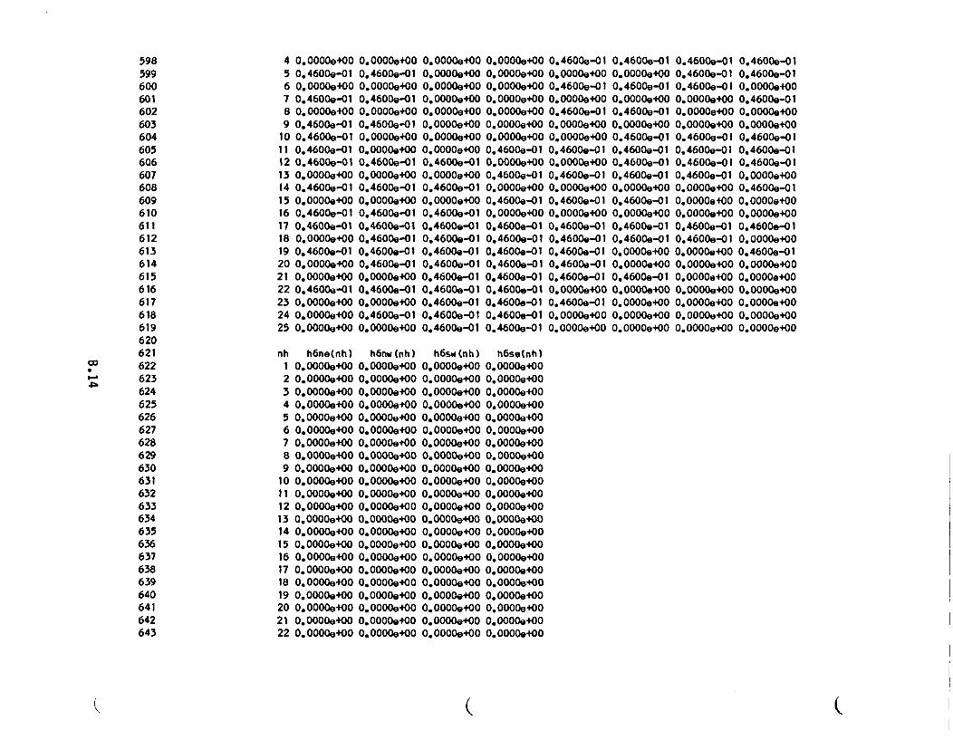
598599600601602603604605606607608609610611612613614615616617618619620621622
I-' 623624625626627628629630631632633634635636637638639640641642643
4 0.0000O+005 0.4600e-016 O.OOOOe4007 0.4600e-018 0.0000.+009 0.4600e-Ol
10 0.4600.-0111 0.4600e-0l12 0.4600.-0113 0.0000e+0014 0.4600e-0l15 0.00004+0016 0.4600e-0l17 0.4600e-0118 0.0000e+0019 0.4600.-al20 0.0000e+0021 0.0000e+0022 0.4600e-al23 0.0000e+0024 0.0000O+0025 0.0000@+00
0.00004e+0 0.0000OO000.460e-01 00.00004+000.00004+00 0.00004+000.460e-01 00.00004+000.00004+00 0.00004+000.4600e-al 0.0000e+000.0000e+00 0.0000+00
nh h6ne(nh)1 0.0000e+002 0.0000e+003 0.0000.+004 0.0000.+005 0.OOOOe+006 0.0000e+007 0.0000e+008 0.0000.+009 0.0000.+00
10 0.00004+0011 0.00004+0012 0.0000e+0013 0.0000e+0014 0.0000O+0015 0.0000e+0016 0.00004+0017 0.0000@+0018 0.0000.+0019 0.0000.+0020 0.0000.+0021 0.0000OO0022 0.0000e+00
0.00004+000.4600e-010.0000e+000.4600.-010.00004+000.4600.-a10.4600e-a10.4600.-a10.4600.-a10.4600.-010.0000.+000.4600e-010.0000+000.4600e-al0.0000e+00
h6nzw(nh)0.00004+000.00004+000.00004+000.00004+000.00004+00O.OOOOe+000.00004+000.00004+000.00004+000.00004+000.0000Oe000.0000.+000.0000.e000.00004+000.0000+000.00004+000.00004+000.0000OO000.00004+000.00004+000.00004+000.00004+00
0.0000+000.4600e-010.00004+000.4600e-al0.0000+000.4600e-al0.4600e-010.4600e-al0.4600.-a10.4600.-010.4600e-a10.4600e-010.4600e-a10.4600.-010.4600e-al
h6sw (nh)0.00004+000.00004+000.00004+000.00004+000.0000OO000.00004+000.00004+000.0000.+000.00004+000.00004+000.00004+000.00004+000.0000.+000.00004+000.0000.+000.0000e+000.0000.+000.0000.+000.0000.+000.00004+000.0000,+000.00004+00
0.0000e+00 0.4600e-01 0.4600.-010.0000.+00 0.00004+00 0.0000OO000.0000e+00 0.4600e-al 0.4600e-al0.0000.+00 0.0000.+00 0.0000.+000.0000.+00 0.4600e-al 0.4600.-010.0000+00 0.00004+00 0.0000OO000.0000e+00 0.0000e+00 0.4600.-010.4600e-01 0.4600.-01 0.4600.-010.0000O+00 0.0000.+00 0.4600e-al0.4600.-01 0.4600e-al 0.4600.-al0.00004+00 0.00004+00 0.00004+000.4600e-al 0.4600e-al 0.4600e-alO.OOOOe.00 0.0000+00 0.0000e+000.4600e-al 0.4600e-01 0.4600e-al0.4600.-01 0.4600.-01 0.4600.-010.4600.-01 0.4600e-01 0.0000.+000.4600.-01 0.4600.-01 0.0000.4000.4600e-al 0.4600.-01 0.4600e-010.4600e-al 0.0000e+00 0.0000e+000.4600e-01 0.4600e-al 0.0000e+000.4600.-01 0.0000e+00 0.0000.+000.4600.-01 0.0000e+00 0.00000e+0
0.4600e-O10.4600.-010.4600e-al0.0000.+000.00000e+O0.O0000+000.4600e-al0.4600.-010.4600e-010.4600.-a100000e+000.0000.+000.00004+000.4600e-0l0.4600.-010.0000e+OO0.00004+000.0000,+000.O0000+000.0000.+000.0000.+000.0000,+00
0.4600.-010.4600.-a10.0000.+000.4600.-010.0000.+000.0000.+000.4600e-al0.4600.-010.4600.-alO.OOOOe4OO0.4600.-010.0000+000.0000.+000.4600e-al0.0000.+000.4600e-010.0000.+000.0000,+000.00004+000.0000.+000.0000.+00O.OOOOe+00
h6se(nh)0.0000e+000.0000.+000.0000.+000.0000.+000.0000.+000.0000.+000.0000.+000.00004+000.0000.+000.0000.+000.0000,+000.00000e+O0.0000+000.0000.+000.0000.+000.0000.+000.0000.+000.O0000+000.O0000+000.0000.+000.00004+000.0000.+00
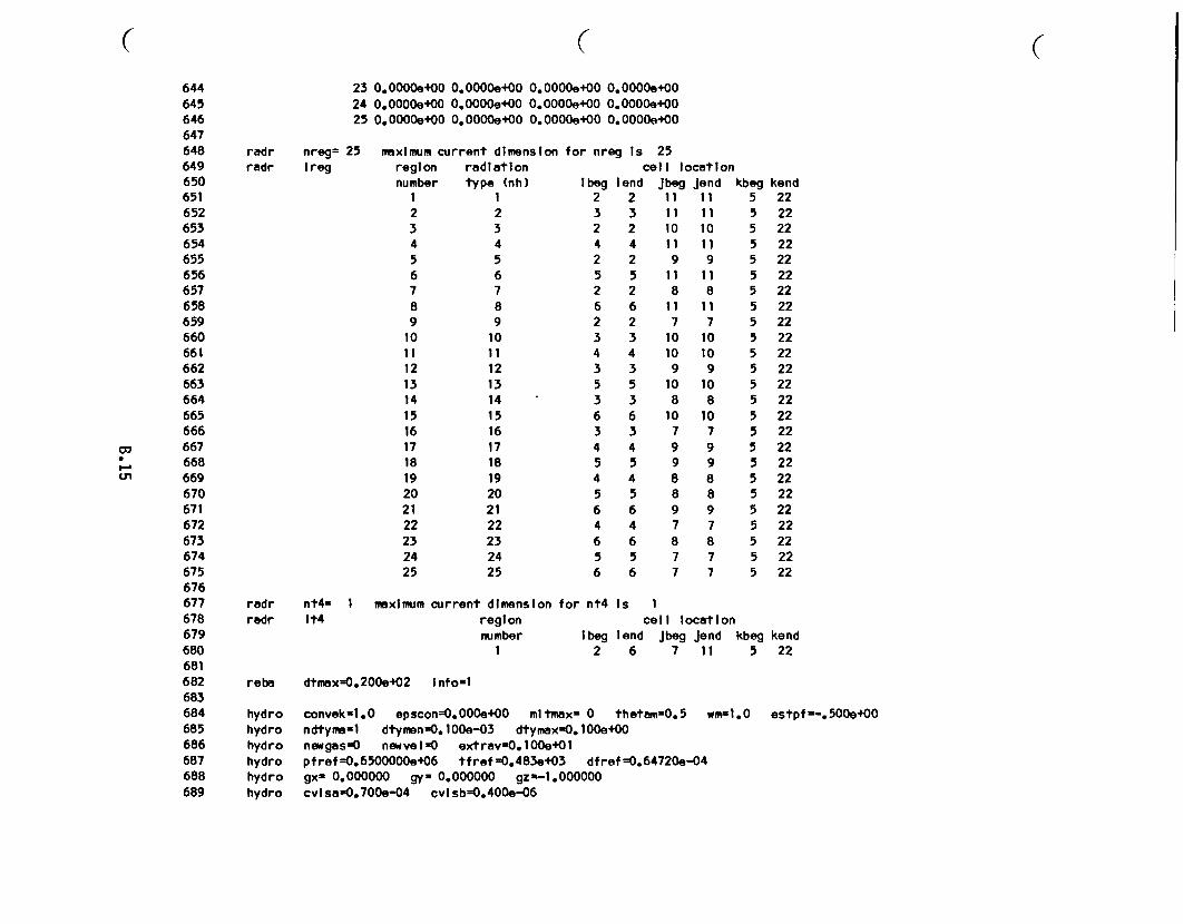
( ( C644645646647648649650651652653654655656657658659660661662663664665666
667668669670671672673674675676677678679680681682683684685686687688689
23 0.0000e+00 0.OOOOe+0024 0.0000e+00 0.0000e+0025 0.0000e+00 0.0000e+00
0.0000+00 0.0000+000.0000e+00 0.0000e+000.0000e+00 0.0000e+00
radr nreg= 25radr Ireg
mexlmum current dimension for nreg Is 25regionnumber
23456789
10111213141516171819202122232425
radiationtype (nh)
1
23456789
10111213141516171819202122232425
cell locationIbeg lend
2 23 32 24 42 25 52 26 62 23 34 43 35 53 36 63 34 45 54 45 56 64 46 65 56 6
Jbeg111110119
118
117
1010
9108
107998897877
Jend111110119
118
117
1010
9108
107998897877
kbeg5555555555555555555555555
kend222222
2222
2222
2222
22222222
22
2222
2222
2222
22
22
2222
22
radr nt4radr It4
1 maximum current dimension forregionnumber
I
r nt4 Is 1cell locatIon
Ibeg lend Jbeg Jend kbeg kend
2 6 7 11 5 22
reba dtmax-0.2004e+2 Info-I
hydrohydrohydrohydrohydrohydro
convek-1.0 epscon=0.000e+OO mitmax- 0 thetam=0.5 wm=l.0 estpf--.500e400
ndtyme=l dtymen40. 100-03 dtymaxO.100.e+Oonewgas=O newvel=O extrav0.100le+Olpfref=40.6500000e+06 tfref=0.483e+03 dfref=0.64720e-04gx= 0.000000 gyt 0.000000 gza-1.000000
cvisaO0.700e-04 cvisb=0.400a-06
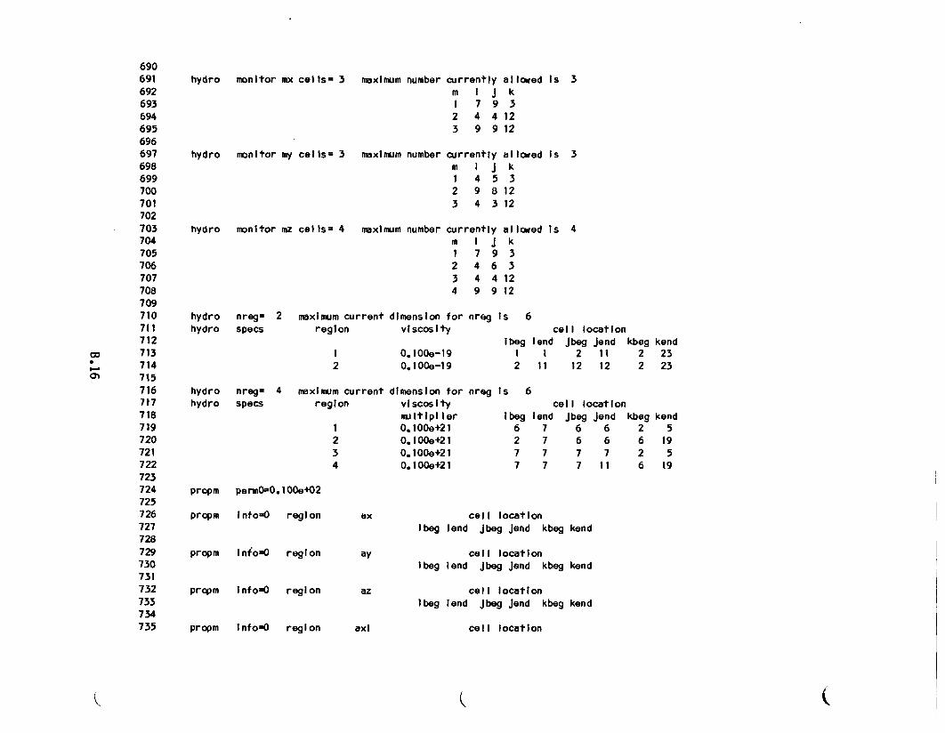
690691692693694695696697698699700701702703704705706707708709710711712
w 713*_ 7140) 715
716717718719720721722723724725726727728729730731732733734735
hydro monitor mx cells- 3
hydro monitor my cells- 3
hydro monitor mz cel ls- 4
maximum number
maximum number
currently alIowed Is 3m I J k1 7 9 32 4 4 123 9 9 12
currently alicwed Is 3m I J k1 4 5 32 9 8 123 4 3 12
maximum number currently allowed Is 4m I J k1 7 9 32 4 6 33 4 4 124 9 9 12
hydro nreg= 2 maximum current dimension fchydro specs region viscosity
)r nreg I s 6
2
hydrohydro
nrega 4 maximum currentspecs region
0. lOOe-l90.lOOe-19
dimension forviscositymu Iltipl ler0. lOOe+210.lOOe+210. 100e+210.lOOe+21
234
cell locationIbeg lend Jbeg Jend kbeg kend
1 1 2 11 2 232 11 12 12 2 23
nreg Is 6
IIcell location
beg lend Jbeg jend 16 7 6 62 7 6 67 7 7 77 7 7 11
,beg2626
kend5
19519
propm permOsO. 10 0l+02
propm I nfo=O regi on
propm Info=O region
prcpm Info-O region
propm InfoO region
ax
ay
cell locationIbeg lend jbeg Jend kbeg kend
cell locationIbeg lend jbeg Jend kbeg kend
celi locationIbeg lend Jbeg jend kbeg kend
axI cell location
K (
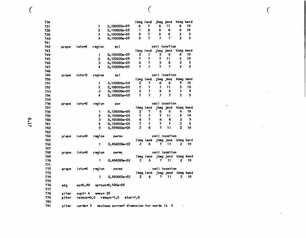
C ( (736737738739740741742743744745746747748749750751752753754755756757758759
cT 760F'& 761
762763764765766767768769770771772773774775776777778779780781
1 0.100000e-052 0.100000.-053 0.100000l-054 0.100000.-05
I beg6
56
Ibeg2767
lend7677
Jbeg6667
jend11667
kbeg6622
propm Info=O region ayI
1 0.100000e-052 0.100000.-053 0.100000l-054 0.100000e-05
cell locationiend Jbeg jend kbeg7 5 6 67 7 11 67 5 6 27 7 7 2
propm Info=0 region az I cell location
kend191955
kend1919
55
kend191955
ken d1919
55
19
1 0.100000.-052 0.100000e-OS3 0.100000e-054 O.100000e-05
I beg Ilen(2 77 76 77 7
d JI jeg Jend kbeg6 6 57 11 56 6 27 7 2
propm Info=0 region por
1 0.lOOOOOe-052 0.100000.-053 0.100000l-054 0.100000l-055 0.559000.+00
cell locationIbeg lend jbeg jend kbeg
2 7 6 6 67 7 7 11 66 7 6 6 27 7 7 7 22 6 7 11 2
propm Info-O regIon permx
1 0.466000e-02
propm Info=0 region permy
cell locationIbeg lend Jbeg jend kbeg kend
2 6 7 11 2 19
cell locationIbeg lend jbeg Jend kbeg kend
2 6 7 11 2 19
cell locationIbeg lend Jbeg Jend kbeg kend
2 6 7 11 2 19
1 0.4660009-02
propm Info-0 region permz
1 0.980000e-02
pdg wpO0.80 optcon=0.5009-05
piterpiter
nopt= 4 neax- 20rebson-0.0 rebqonzl.0 afon=l.0
piter nordan 3 maximum current dimension for norda Is 4
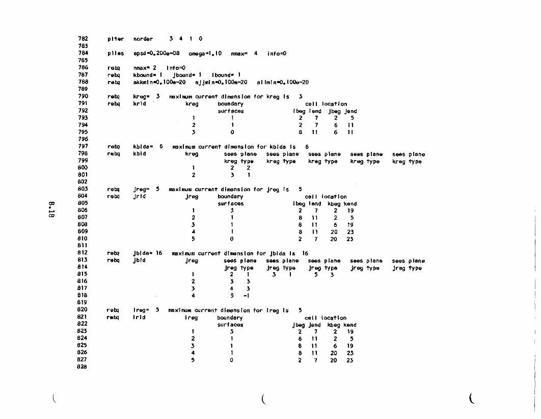
782783784785786787788789790791792793794795796797798799800801802803804
w 805806
00 807808809810811812813814815816817818819820821822823824825826827828
piter norder 3 4 1 0
plies epsd=0.200e-08 omega-l.10 nmax 4 info=O
rebArebqrebq
nmaxw 2 Info=0kboundw 1 Jbound= 1 lbounds Iakkmln=0.lOOe-20 aJJmln=O.100e-20 al Imln=O.100e-20
rebq kreg- 3 maximum current dimension for kreg Is 3rebq krld kreg boundary cell location
surfaces
23
rebq kbidam 6 mmximum currentrebq kbid kreg
2
0
Ibeg lend Jbeg jend2 7 2 52 7 6 118 11 6 11
dimension for kbida Isees plane sees plakreg type kreg typ
2 23 1
rebq Jreg= 5 mmximum current dimension for Jreg Isrebq Jrld Jreg boundary
surfaces1 3
s 6ne sees plane sees plane sees planele kreg type kreg type kreg type
5cell location
Ibeg lend kbeg kend2 7 2 198 11 2 58 11 6 198 11 20 232 7 20 23
2345 I
rebq Jbidaw 16rebq Jbid
maxlimum currentJreg
dimension for Jbida Is 16sees plane sees plane sjreg type Jreg type
2 1 3 13 34 35 -I
sees planeJreg type
5 3
sees plane sees planeJreg type jreg type
234
rebq Ireg 5 maximum current dimension for Ireg Isrebq Irld Ireg boundary
I2345
surfaces3
1
0
5cell location
jbeg jend kbeg kend2 7 2 198 11 2 58 11 6 198 11 20 232 7 20 23
(
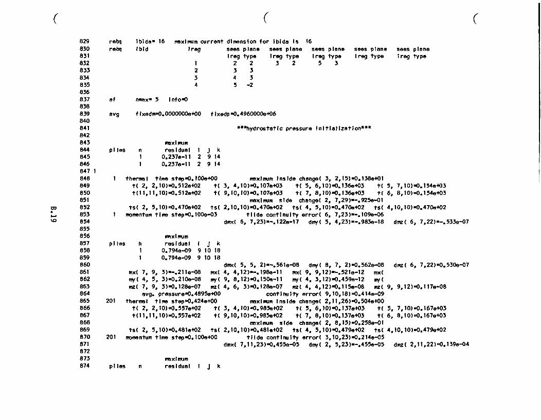
( ( (829830831832833834835836837838839840841842843844845846847 1848849850851852853854855856857858859860861862863864865866867868869870871872873874
rebq IbIda= 16 maxImum current dimension for Ibida Is 16rebq Ibid Ireg sees plane sees plane s
Ireg type Ireg type It 2 2 3 2
sees planereg type5 3
sees plane sees planeIreg type Ireg type
234
34
33
5 -2
at nmax= 5 Info=O
avg fixedm=0.OOOOOOOe+00 fIxedp-0.4960000e+06
***hydrostatic pressure Initialization***
maximumpiles n residual I J k
1 0.237e-11 2 9 141 0.237e-11 2 9 14
I thermal time stepu0.lOOe+OOt( 2, 2,10)-0.512e402 t(t(11,11,10)-0.512e+02 t(
ts( 2, 5,10)-0.470e+02 ts(I momentum time step0.100e-03
maxlmumpiles h residual I J k
1 0.794e-09 9 10 181 0.794e-09 9 10 18
mx( 7, 9, 3)=-.211e-08 mx(my( 4, 5, 3)=0.210e-08 my(mz( 7, 9, 3)=0.128e-07 mz(
avg. pressure-0.4895e+00201 thermal time step=0.424e+00
t( 2, 2,10)20.557e+02 t(t(11,11,10)-0.557e+02 t(
ts( 2, 5,10)-0.481e+02 ts(201 momentum time step=0.lOOe+00
maximumIOles n residual I I k
maximum Inside change( 3, 2,15)-0.138e+013, 4,10)-0.107e+03 t( 5, 6,10)-0.136e+03 t(9,10,10)i0.107e+03 t( 7, 8,10)-0.136e+03 t(
maximum side change( 2, 7,29)--.925e-012,10,10)-0.470e+02 ts( 4, 5,10)-0.470e402 ts(
tilde continuity error( 6, 7,23)=-.109e-06dmx( 6, 7,23)*-.122e-17 doyC 5, 4,23)=-.983e-18
dmx( 5, 5, 2)U-.561e-08 dmyC 8, 7, 2)=0.562e-084, 4,12)=-.198e-11 mx( 9, 9,12)=-.521e-12 mx(9, 8,12)-0.150e-11 my( 4, 3,12)-0.459a-12 my(4, 6, 3)-0.128e-07 mz( 4, 4,12)-0.115e-08 mz(
continuity error( 9,10,18)=0.414e-09maximum Inside change( 2,11,26)u0.504e+00
3, 4,10)i0.985e+02 t( 5, 6,10)-0.137e+03 t(9,10,10)u0.985e+02 t( 7, 8,10)wO.137e+03 t(
5, 7,10)u0.154e4036, 8,10)-0.154e+03
4,10,10)-0.470e+02
dmz( 6, 7,22)=-.533e-07
dmz( 6, 7,22)-0.530e-07
9, 9,12)-0.117e-08
5, 7,10)-0.167e+036, 8,10)u0.167e+03
maximum side change( 2, 8,15)-0.258e-012,10,10)=0.481e+02 ts( 4, 5,10)-0.479e+02 ts( 4,10,10)u0.479e402
tilde continuity error( 3,10,23)=0.214e-05dmx( 7,11,23)-0.455e-05 dmy( 2, 5,23)--.455e-05 dmz( 2,11,22)-0.139e-04
* z
875876877878879880881882883884885886887888889890891892893894895896897
w 898ra 899o 900
901902903904905906907908909910911912913914915916917918919920
I -0.333e-08 9 10 184 -0.2099-08 9 8 17
maximumpiles n residual I J k
I -0.772e-10 9 10 181 -0.7729-10 9 10 18
mx( 7, 9, 3)=-.862e-04 mx(my( 4, 5, 3)O0.862e-04 my(mz( 7, 9, 3)-0.519e-03 mz(
avg. pressure 0. 4 895e+00401 thermal time step=0.iOOef0O
t( 2, 2,10)a0.602e+02 t(t(ll,ll,lO)sO.602e+02 t(
ts( 2, 5,10)s0.528e+02 ts(401 momentum time step0. 100e+00
maximumpiles n residual I J k
I -0.216e-09 10 10 231 -0,216e-09 10 10 23
mx( 7, 9, 3)u-.840e-04 mx(my( 4, 5, 3)m0.840e-04 my(mz( 7, 9, 3)-0.513e-03 mz(
avg. pressure-O.4895e+00601 thermal time step0.100e+01
t( 2, 2,10)m0.6549+02 t(t(11,11,10)-0.654e+02 t(
ts( 2, 5,10)w0.579e402 ts(601 momentum time stepO:.100e+00
dmx( 3,10,23)s0.331e-06 dmy( 3, 9,23)=-.3 31e-06 dmz( 3,10,22)--.470e-064, 4,12)=0.194e-06 mx( 9, 9,12)-0.668e-07 mx(9, 8,12)=-.194e-06 my( 4, 3,12)--.668e-07 my(4, 6, 3)-0.519e-03 mz( 4, 4,12)--.15le-04 mz( 9, 9,12)=-.151e-04
continuity error( 9,10,18)=-.409e-10maximum Inside change( 2, 6,22)-0.833e-01
3, 4,10)-0.104e+03 t( 5, 6,10)-0.144e+03 t( 5, 7,10)=0.174e+039,10,10)=0.104e+03 t( 7, 8,10)-0.144.403 t( 6, 8,10)-0.174 e+03
maximum side change( 2, 7,15)-0.510e-012,10,10)-0.528e+02 ts( 4, 5,10)0.525e+02 ts( 4,10,10)-0.525e+02
tilde continuity error( 3,10,23)=0.188e-06dmx( 7,11,20)--.257e-06 dmy( 2, 5,20)u0.257e-06 dmz( 8,11,19)sO. 437e-06
dmx( 5,10,23)-0.1979-07 dmyC 3, 7,23)-.197e-07 dmz( 3,10, 2 2 )=-. 6 2 2 e-074, 4,12)-0.6389-06 mx( 9, 9,12)s0.228e-06 mx(9, 8,12)--.638e-06 my( 4, 3,12)--.228e-06 my(4, 6, 3)s0.513e-03 mz( 4, 4,12)-.102e-04 mz( 9, 9,12)=-.102e-04
continuity error( 9,10,22)--.119e-09maximum Inside change( 2, 6,15)-0.447e-01
3, 4,10)-0.109e+03 t( 5, 6,10)-0.150e+03 t( 5, 7,10)-0.180e+039,10,10)s0.109e+03 t( 7, 8,10)s0. 150e+03 t( 6, 8,10)s0.180e+03
maximum side change( 2, 2,15)s0.446e-012,10,10)=0.579e+02 ts( 4, 5,10)-0.576e+02 ts( 4,10,10)u0.576e+02
tilde continuity error( 4,10,23)u0.820e-07dmx( 7, 9,23)=0.509e-07 dmy( 4, 5,23)-.509e-07 dmz( 6, 4,11)=0.172e-06
dmx( 5,10,23)0.613e-08 dmy( 3, 7,23)--.613e-08 dmz( 5, 4,12)=-.393e-0 7
4, 4,12)-0.692e-06 mx( 9, 9,12)-0.244e-06 mx(9. 8,12 )=-.692e-06 my( 4, 3,12)=-.244e-06 my(4, 6, 3)c0.497t-03 mz( 4, 4,12)-.117e-04 mz 9, 9,12)--.117e-04
continuity error( 9,10,18)--.989e-10
maximumpiles n residual
I -0.182e-091 -0.182e-09
I J k9 10 189 10 18
mx( 7, 9, 3)=-.810e-04 mx(my( 4, 5, 3)=0.810e-04 my(mz( 7, 9, 3)s0.497e-03 mz(
avg. pressure-0.4895e+00
K ( (
( ( (921922923924925926927928929930931932933934935936937938939940941942943
w 944;la 945I- 946
947948949950951952953954955 1956957958959960961962963964965966
801 thermal time step=0.100e+01t( 2, 2,10)-0.706e+02 t(t(11,11,10)20.706e+02 t(
ts( 2, 5,10)20.631e+02 ts(801 momentum time step=0.lOOe+00
maximum Inside change( 2, 2,15)m0.387e-013, 4,10)-0.114e+03 t( 5, 6,10)-0.155e+03 t(9,10,10)=0.114e+03 t( 7, 8,10)20.155e+03 t(
maximum side change( 2, 2,15)=0.391e-012,10,10)-0.631e+02 ts( 4, 5,10)i0.628e+02 ts(
tilde continuity error( 6,10,20)=-.538e-07dmx( 7,11, 5)=-.389e-07 dmyI 2, 5, 5)*0.389e-07
5, 7,10)=0.184e+036, 8,10)=0.184e+03
4,10,10)=-0.628e+02
dmz( 6, 4,11)=0.147e-06
meximumpiles n residual I J k
1 -0.303e-09 9 10 181 -0.303e-09 9 10 18
mx( 7, 9, 3)=-.779e-04 mx(myC 4, 5, 3)=0.779e-04 my(mzC 7, 9, 3)=0.478e-03 mz(
avg. pressurenO.4895e+001000 thermal time step-0.100e+Ol
t( 2, 2,10)=0.757e+02 t(t(11,11,10)-0.757e+02 tl
ts( 2, 5,10)20.682e+02 ts(1000 momentum time step0.lOOe+00
dmx( 7,10, 5)=-.199e-08 dmy( 3, 5, 5)z0.199e-08 dmz( 5, 4,12)--.'4, 4,12)=0.660e-06 mx( 9, 9,12)=0.232e-06 mx(9, 8,12)"-.660e-06 my( 4, 3,12)=-.232e-06 my(4, 6, 3)-0.478e-03 mz( 4, 4,12)--.136e-04 mz( 9, 9,12)=-.136e-04
continuity error( 9,10,18)=-.164e-09maximum Inside change( 2, 2,15)20.339e-01
3, 4,10)-0.119e+03 t 5, 6,10)-0.160e+03 tl 5, 7,10)0.189e+039,10,10)=0.119e+03 t( 7, 8,10)=0.160e403 t( 6, 8,10)=0.189e+03
maximum side change( 2, 2,15)20.344e-012,10,10)u0.682e+02 tsC 4, 5,10)m0.679e+02 tsC 4,10,10)=0.679e+02
tilde continuity error( 6, 7,20)=-.545e-07dmxC 7,11, 5)=-.391e-07 dmy( 2, 5, 5)=0.391e-07 dmz( 9, 7,11)20.1
305e-07
1239-06
maximumpiles n residual
1 -0.363e-091 -0. 363e-09
I J k9 10 189 10 18
mx( 7, 9, 3)=-.749e-04 mxCmy( 4, 5, 3)=0.749e-04 my(mz( 7, 9, 3)20.459e-03 mz(
avg. pressure20.4895e+00
dmx( 7,10, 5)=-.194e-08 dmy( 3, 5, 5)20.194e-084, 4,12)=0.613e-06 mx( 9, 9,12)20.216e-06 mx(9, 8,12)=-.613e-06 my( 4, 3,12)=-.216e-06 my(4, 6, 3)u0.459e-03 mz( 4, 4,12)--.152e-04 mz(
continuity error( 9,10,18)=-.195e-09
dmz( 6, 7,20)=-. 2 83e-07
9, 9,12)-.152e-04
* * * thermal power balance summary, watts * * *
thermal power from Inside to side at level k2928272625242322
-. 165139e401-. 434836e+01-. 716536e4010.378800e+010.227392e+010.130187e+010.205785e+010.177996e+02

967968969970971972973974975976977978979980981982983984985986987988989990
* 991992993994995996997998999
1000100110021003100410051006100710081009101010111012
thermal
thermal
thermal
thermal
thermal
thermal
thermal
thermal
thermal
thermal
thermal
thermal
power
power
power
power
power
power
power
power
power
power
power
from
from
from
from
f rom
from
from
from
from
from
from
cavity to top
cavity to side
cavity to bottom
cavity
top to ambient
top to side
bottom to side
bottom to ambient
top of side to ambient
side to ambient
bottom of side to ambien1
21 0.247999.+0220 0.354332e+0219 0.513323e+0218 0.752517e+0217 0.105157.+0516 0.140924e40315 0.1420449+0314 0.108947 e+0313 0.817615e+0212 0.592768e+0211 0.4284619+0210 0.302628e+029 0.2110109+028 0.174653e+027 0.114181e+026 0.670351e+015 0.251733e+014 0.788006e+013 0.103409+022 0.693509.+01
0.198252e+02
0.984463e403
0.770241e+02
0.108131e+04
0.515122e+01
-. 131651e+02
0.251631e402
0.241767e-16
0.462020e+01
0.252627e+03
t 0.210228e-16
it 0.262399e+03power from outside surface to amblei
excess power leaving cavity -. 787e+02
K K
( ( (1013101410151016101710181019 11020102110221023102410251026102710281029103010311032103310341035 11036
r* 1037103810391040104110421043104410451046104710481049105010511052 1105310541055105610571058
excess power leaving top
excess power leaving side
excess power leaving bottom
-.278e+02
-.739e+03
-. 519e+02
* * * Inside heat flux In i-direction, watts/sq. cm * * *
plane k- 8
J I= 111-0.426e-18-0.116e-01 0.149e-01 0.376e-0110-0.428e-18-0.129e-01 0.15le-01 0.509e-019-0.417e-18-0.126e-01 0.673e-02 0.294e-018-0.391e-18 0.522e-02-0.146e-01 0.238e-017-0.362e-18-0.125e-01 0.441e-02 0.315e-016-0.293e-18 0.166e-01 0.581e-01 0.945e-Ol5-0.256e-18 0.149e-01 0.5 0 0e-01 0.912e-014-0.219e-18 0.121e-01 0.352e-01 0.589e-013-0.176e-18 0.743e-02 0.213e-01 0.293e-012-0.143e-18 0.1OOe-02 0.132e-01 0.000e+00
0.381e-010.247e-010.435e-Ol0.508e-010.803e-010.350e-010.904e-010.682e-01
0. 7 4 9e-010.779e-01
0.802e-010.762e-010. 14 9e+000.206e+000.451e-010. OOOe+00
0.485e+00 0.429e+000.473e+00 0.411e+000.419e+00 0.334e+000.303e+00 0.194e+000.826e-01 0.507e-010.199e+00 0.000e+000.000e+00 0.000.e000.000e+00
0. 192e+000. 179e+000. 129e+000.648e-010.000e+000.000e+00
0.770e-010.695e-010.566e-010.000e+000.000e+00
0. 534e-0 10.442e-01
0.000e+000.000e+00
0.0004+00 0.000,+000.000e+00
* * * Inside heat flux In J-directlon, watts/sq. cm * * *
plane km 8
J 1= 211 0.426e-18 0.428e-18 0.417e-18 0.391e-18 0.362e-18 0.293e-18 0.256e-18 0.219e-18 0.176e-18 0.143e-18
10 0.116e-01 0.129e-01 0.126e-01-0.522e-02 0.125e-01-0.166e-01-0.149e-01-0.121e-01-0.743e-02-0.l00e-02
9-0.149e-01-0.15le-01-0.673e-02 0.146e-01-0.44le-02-0.581e-01-0.500e-01-0.352,-01-0.213e-01-0.132e-01
8-0.376e-01-0.509e-01-0.294e-01-0.238e-01-0.315e-01-0.945e-01-0.912e-01-0.589e-01-0.293.- 0.000e+00
7-0.381e-01-0.247e-01-0.435e-01-0.508e-01-0.803e-01-0.350e-01-0.904e-01-0.682e-01 0.000e+00
6-0.749e-01-0.779e-01-0.802e-01-0.762e-01-0.149.+00-0.206e+00-0.451e-01 0.000e+00
5-0.485e+00-0.473e+00-0.419e+00-0.303e+00-0.826e-01-0.1994+00 0.000e+004-0.4 2 9e+00-0.411e+00-0. 3 34e+00-0.194e+00-0.507.-al 0.0004+00
3-0.192e+00-0.179e+00-0.129e+00-0.648e-O0 0.0004+002-0.770e-01-0.695e-01-0.566e-al 0.000e+001-0.534e-01-0.442e-01 0.000e+00 0.000O400
* * * Inside heat flux In k-direction, watts/sq. cm * * *
plane ku 8J I= 2
11-0.129e+00-0.128e+00-0.116e+00-0.905e-01-0.263e-01-0.229e-al 0.827e+00 0.376e+00-0.365e+00-0.316e+00
10-0.128e+00-0.128e+00-0.116e+00-0.873e-01-0.254e-01-0.217e-al 0.788e+00 0.309e+00-0.400e+00-0.314e+00
1059106010611062106310641065106610671068 11069107010711072107310741075107610771078107910801081
co 1082r~o 10834> 1084
10851086108710881089109010911092109310941095109610971098109911001101110211031104
9-0.116e+00-0.116e+00-0.107e+00-0.861 e-01-0.235e-01-0.199e-01 0.598e+00-0.21 0e-01-0.569e+00-0.123e+008-0.905e-01-0.873e-01-0.861e-0 1-0.758e-01-0.375e-01-0.235e-01 0.252e+00-0.492e+00-0.203e+00 0.000+00
7-0.263e-01-0.254e-01-0.235e-01-0.375e-01-0.105e+00-0.132e+01-0.175e+00-0.282.+00 0.000O+OO
6-0.229e-01-0.217e-01-0.199e-01-0.235e-01-0.132e+01-0.12 1 e+01-0. 1 49e+00 0.000+00
5 0.827e+00 0.788e+00 0.598e+00 0.252e+00-0.175e+00-0.149e+00 0.000+004 0.376e+00 0.309e+00-0.21 le-01-0.492e+00-0.282e+00 O.OOOe+OO3-0.365e+00-0.400e+00-0.569e+00-0.203.+00 0.000e+002-0.316e+00-0.314e+00-0.123e.00 0.000+00
* * * inside temperature, c * * *
plane k=30J 1 2
12 0.000+00 0+000.e+00 0.000e+00 0.000.400 0.000e+00 0.000e+011 0.270e+02 0.270e+0210 0.270.+02 0.2709+029 0.27 0e+02 0.270e+028 0.270e+02 0.2709+027 0.270e+02 0.270e4026 0.270e+02 0.270e+025 0.270,+02 0.270e+024 0.270.+02 0.270e+023 0.270.+02 0.270e+022 0.270.+02 0.270.+021 0.000+00 0.000+00
J - 212 0.000e+00 0.000e+00
0.270e+02 0.270e+020.270e+02 0.270e+020.270e402 0.270e+020.270e+02 0.270e+020.270.e02 0.270e4020.270e+02 0.270e+020.270.e02 0.270e4020.270e+02 0.270.+020.270e+02 0.270e+020.270e+02 0.0004+OO0.000.+00 0.0004+00
0.270e+02 0.270e+020.270e+02 0.270e+020.270e+02 0.270+4020.270e+02 0.270.+020.270,+02 0.270e+020.270e+02 0.270e+020.270e+02 0.270e+020.270e+02 0.0000e+00.000+00
0.O000+000.270e+020.270e+020. 270e+020.270.+020.270e+020.270e+020.000+400
0.000+000.270e+020.270e+020.270e+020.270.+020.270.+020.000e+00
0.000e+00 0.000e+00 0.000.+000.270.+02 0.270e+02 0.0000e+00.270.+02 0.270e+02 0.0000e+00.270.402 0.270e+02 0.0004000.270e+02 0.0000e+00.000+00
plane k-29
0.000e+00 0.000.+0011 0.516e+0210 0.516e+029 0.516e+028 0.515e+027 0.515e+026 0.515e+02
5 0.514e+024 0.5149+023 0.514,+022 0.515e+021 0.515e+02
0. 516e+020. 516e+020.516e+020.516,+020.5 15e+020.515e+020. 5159+020.515e+0209515e+020.515a+020.515e+02
0.516.+020.516.+020.516e+020.516e+020. 515e+020. 515e+020.515e+020.515e+020.515e+020.516e+020. OOOe+00
0.515e+020.516,+020.516e+020.516e+020.516e+020. 516e+020.516.+020.516,+020. 516e4020.000.+000.OOOe+00
0.000e+00 0.000+000.515e+02 0.515e4020.515e+02 0.515e+02
0.515e+02 0.515e+020.516e+02 0.516e+020.516e+02 0.516e+020.516e+02 0.516e+020.516.+02 0.517e+020.517e+02 0.000e0oo0.000e+00
0.000e+OO0. 514e+020.515e+020.515.+020. 516e+020. 516e+020.517e+020.000.+00
0.0004+00 0.000e+00 0.000e+00 0.000+000.514e+02 0.514e+02 0.515e+02 0.515e+020.515,+02 0.515e+02 0.515e+02 0.515.+020.515e+02 0.515e+02 0.516e+02 0.000e+000.516e+02 0.516e+02 0.0000e+00.517e402 0.000+000.000+00
J I= 212 0.0004+00 0.000.+0011 0.517e+02 0.517e+02
plane k=28
0.0004+00 0.0004+00 0.0004+00 0.0004+00 0.0004+00 0.0004+00 0.0004+00 0.0004+00 0.000+000.517e+02 0.516e+02 0.516e+02 0.515e402 0.515e+02 0.515e402 0.515e+02 0.516e+02 0.516e+02
Q (
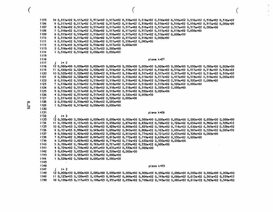
( ( (1105110611071108110911101t111112
10 0.517e+029 0.517e+028 0.5169+027 0.516e+026 0.515e+025 0.515e+024 0.5159+023 0.515e+02
0.517e+020.517e+020. 517e+020.516e+020.516e+020.515e+020.516e+020.516e+02
0.517e,020.517e+020.517e+020. 516e+020.516e+020.516e+020.516e+020.516e,020.517e+020. OOOe+00
0.517e+020. 517,4020.517e+020.517e+020.516,+020.517e+020. 517e+020.517e+020.000+000.000e+00
0.516e+02 0.516e+02 0.5169+02 0.516e+0 2 0.516e,02 0.516,+02 0.516e+02
0.516e+02 0.5169+02 0.516e+02 0.516e+02 0.516e+02 0.517e402 O.OOOe00
0.517e+02 0.516e+02 0.517e+02 0.517e+02 0.517e+02 0.0004+00
0.517e+02 0.517e+02 0.517e+02 0.518e+02 0.000O400
0.517e+02 0.517e+02 0.518e+02 0.000e+00
0.517e+02 0.518e+02 0.000e+000.518e+02 0.000e+000.000+00
1113 2 0.5169+02 0.516e+021114 1 0.516e+02 0.516e+021115111611171118111911201121112211231124112511261127
wo 1128;la 1129Iun 1130
11311132113311341135113611371138113911401141114211431144114511461147114811491150
plane k=27
J 1212 0.0004+00 0.000e+00 0.000e+0011 0.520e+02 0.520e+02 0.520e+0210 0.520e+02 0.520e+02 0.520e+029 0.520e+02 0.520e+02 0.519e.028 0.519e+02 0.519e+02 0.519e+027 0.518e+02 0.518e+02 0.518e+026 0.517e+02 0.517e+02 0.518e+025 0.516e+02 0.517e+02 0.517e+024 0.516e+02 0.517e+02 0.517e+023 0.517e+02 0.517e+02 0.518e+022 0.518,+02 0.518e+02 0.519e+021 0.518e+02 0.519e402 0.0004+00
J 1-212 0.0004+00 0.000e+00 0.0004+0011 0.109,+03 0.107e+03 0.101e+0310 0.107,+03 0.105e+03 0.9969+029 0.1014+03 0.996e402 0.949e+028 0.938e+02 0.929e+02 0.896e+027 0.874,+02 0.868e,02 0.845e+026 0.830e+02 0.825e+02 0.8069+025 0.788e+02 0.784e+02 0.763e+024 0.724e+02 0.719e+02 0.691e+023 0.634e+02 0.632e+02 0.597e+022 0.560e+02 0.565e+02 0.529e+02
1 0.528e+02 0.528e+02 0.000e+00
J 1=212 0.0004+00 0.0004+00 0.000o+00
11 0.123e+03 0.120e+03 0.109e+0310 0.120e+03 0.117e+03 0.106e+03
0.000+000.519e+020. 519e+020. 519e+020.519e+020.518,+020. 518e+020. 518e+020.519,+020.520e+020.0004+000.000e00
0.0004+00 0.000,400 0.000e+00 0.000e+00 0.000e+00 0.000e+00 0.000e+00
0.518e+02 0.517e+02 0.516e+02 0.516e+02 0.517e+02 0.518e+02 0.518e+02
0.518,+02 0.5179+02 0.517e+02 0.517e+02 0.517e+02 0.518e+02 0.519e+02
0.518e+02 0.518e+02 0.517e+02 0.517e+02 0.518e+02 0.519e+02 0.000e+00
0.518e+02 0.518e+02 0.518e+02 0.519e+02 0.520e+02 0.0004+00
0.518e+02 0.518e+02 0.519e+02 0.520e+02 0.000e+00
0.518e+02 0.519e+02 0.520e+02 0.0004+00
0.519e+02 0.520e+02 0.0004e000.520e+02 0.000e+000.000e+00
plane k-26
0.0004+000.938e+020.929,+020.896e+020.856e+020. 813e+020.774e+020.721e+020.631e+020.529e+020.000e000.000+00
0.0004+000.874e+020.868e+020.845e+020.813e+020. 772e+020.719e+020.639e+020.530e+020.0004+00
0.000+000.830e+020.825e+020.806e+020.774e+020.719e4020.630.+020.530e+020.000+00
0.0004O000.788,+020.784e+020.763e+020.721,e+020.639e+020.5309+020.000e00
0.000,e00 0.0004+00 0.000e+00 0.0004+00
0.724e+02 0.634e402 0.560e+02 0.528e+02
0.719e+02 0.632e+02 0.565e+02 0.528e+02
0.691e+02 0.597e+02 0.529e+02 0.000e+00
0.631,+02 0.529e+02 0.0004+000.530e+02 0.000e+000.000+00
plane k=25
0.0004+000.965e+020.951,+02
0.0004+00 0.0004+00 0.0004+00 0.0004+00 0.0004+00 0.000e00 0.0004+00
0.866e+02 0.804e,+02 0.749,+02 0.686e+02 0.613e+02 0.561e+02 0.539e+02
0.859e+02 0.799e+02 0.745e+02 0.681e+02 0.6129+02 0.565e+02 0.540e+02
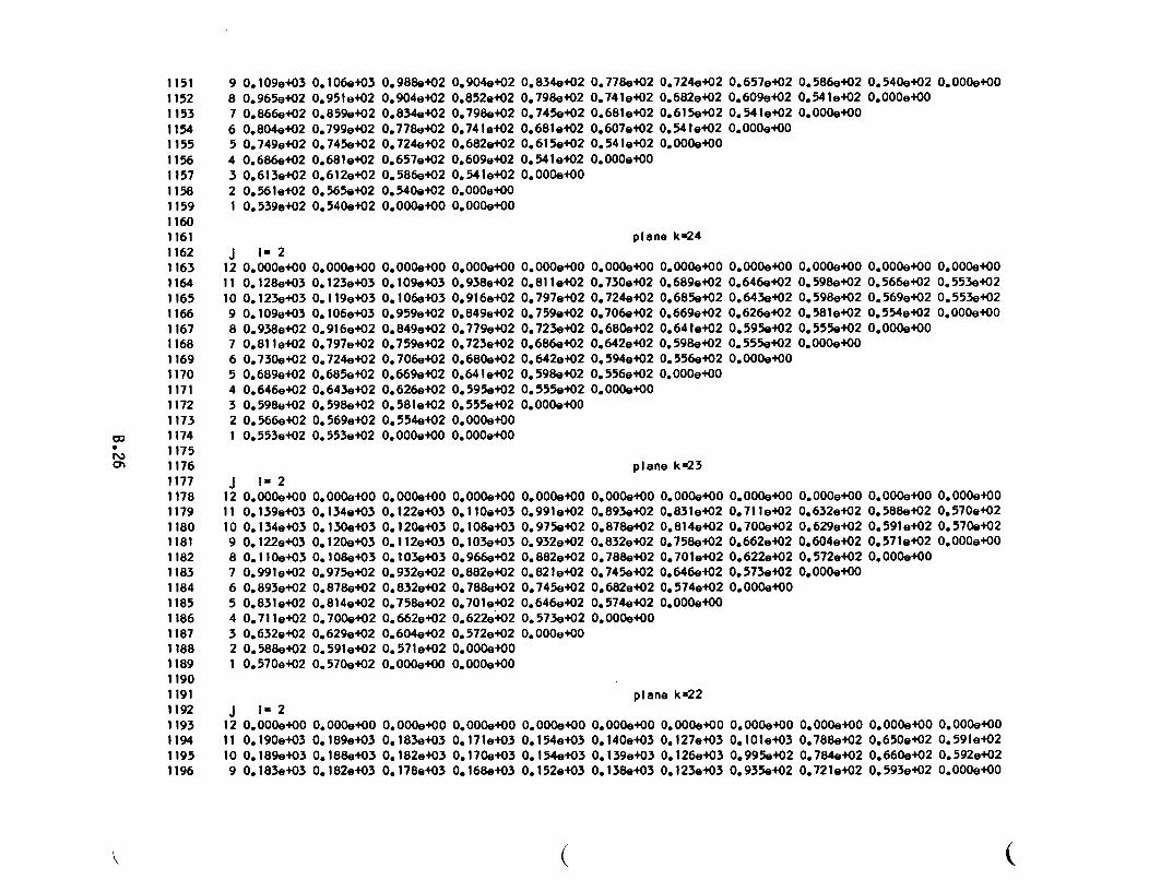
115111521153115411551156115711581159116011611162116311641165116611671168116911701171117211731174
* 1175117611771178117911801181118211831184118511861187118811891190119111921193119411951196
9 0.109e+038 0.965e+027 0.866e+026 0.804.+025 0.749e+024 0.686e+023 0.613e+022 0.561,+021 0.539e+02
J In212 0.000e+0011 0.128e+0310 0.123e+039 0. 109e+038 0.938e+027 0.81 le+026 0.730.+025 0.689e4024 0.646.+023 0.598e+022 0.566e+021 0.553e+02
J 1-212 0.0004+0011 0.139e+0310 0.134e+039 0.122e+038 0.110e+037 0.991e4026 0.893e+025 0.831e+024 0.71 1e+023 0.632e+022 0.588.+021 0.570e+02
J 1=212 0.000e+0011 0.190e+0310 0.189e+039 0.183e+03
0. 106e+030.951,+020.859e+020.799.+020.745.+020. 681e+020.612e+020.565e+020.540e+02
0.988e+020.904,+020.834e+020.778e+020.724e+020.657.+020.586e+020.540.+020.000e+00
0.904e+02 0.834e+02 0.778e+02 0.724e+020.852e+02 0.798e+02 0.741e+02 0.682e+020.798e+02 0.7459+02 0.681e+02 0.615e+020.741e+02 0.681e+02 0.607,402 0.541,+020.682e+02 0.615e+02 0.541e+02 0.0000e+00.609,402 0.541e+02 0.0000e+00.541e+02 0.000.+000.000,+000.000e+00
0.657e402 0.586e+02 0.540.+02 0.000e+OO0.609e402 0.54le+02 0.000e+OO0.541e+02 0.000e+OO0.000+00
plane k=24
0.000.+000.123e+030.119,+030.106,+030.916e+020.797e+020.724e+020.685e+020.643e+020.598e+020.569e+020.553e+02
0.000.+000. 109e+030.106e+030.959,+020.849e+020.759e+020.706e+020.669,+020.626.+020.581e+020.554e+020.000+00
0.0004+00 0.0004+00 0.0004+00 0.0000e+00.938e402 0.811,+02 0.7309402 0.689e+020.916e+02 0.797e+020.849e402 0.759e+020.779e+02 0.723e+020.723e+02 0.686e+020.680.+02 0.642e+020.641,+02 0.598e+020.595.+02 0.555e+020.555e+02 0.000e+000.000.+000.000,+00
0.724e+02 0.685e+020.706.+02 0.669e4020.680e+02 0.641,+020.642,402 0.598e+020.594e+02 0.556e+020.556e+02 0.0000e+00.000+00
0.000.+000.646,+020.643e+020.626e+020.595e+020.555.+020.000+00
0.000e+000.598e+020.598e+020. 581,e+020.555.+020.000.+00
0.O000+000.566e+020.569e+020.554,4020.000e+00
0.000.+000.553e+020.553e+020.000+00
plane k-23
0. OOOe+OO0.134e+030.130e+030.120e+030.108e4030.975e+020.878e+020. 814,4020.700.+020.629,+020.591e+020.570e+02
0.000+000.122e+030. 120e+030.112e+030.103e+030.932,+020.832e+020.758.4020.662e+020.604e4020. 571e+020.000+00
0.000.+000.11 Oe+030.108e+030.103.+030.966e+020.882,+020.788e+020.701e+020.622e,020.572,+020.000.+000. 000e+00
0. 000e+000. 991 e4O20.975e+020.932e+020.882e+020. 82 1e+020.745e+020.646.+020.573e+020.000+00
0.0004+00 0.0004+00 0.0004+00 0.000,+000.893e+02 0.831e+02 0.711e+02 0.632e+020.878e+02 0.814e+02 0.700e+02 0.629e+020.832,402 0.758e+02 0.662e+02 0.604,+020.788e+02 0.701.+02 0.622e+02 0.572e+020.745.402 0.646e+02 0.573e+02 0.O000+000.682,+02 0.5749+02 0.000e+OO0.574e+02 0.000e+OO0.000.+00
0.000e+000.588.+020.591 e+020. 571 e+020. OOOe+OO
0.000.+000. 570e+020.570.+020.000+00
plane k-22
0.000.+000.189e+030.188e+030.182e+03
0.000e+000.183e+030.182e+030.178e+03
0.000e+000.171e+030. 170.+030.168e+03
0.000.+000. 154e+030. 154e+030.152e+03
0.0004+00 0.000e+OO 0.0004+00 0.000+00 0.000.0e+O0 0.000+000.140e+03 0.127e+03 0.101e+03 0.788e+02 0.650e+02 0.591e+020.139e+03 0.126e+03 0.995.+02 0.784e+02 0.660e+02 0.592e+020.138e+03 0.123e+03 0.935e+02 0.721e+02 0.593e+02 0.000,+00
K ( (
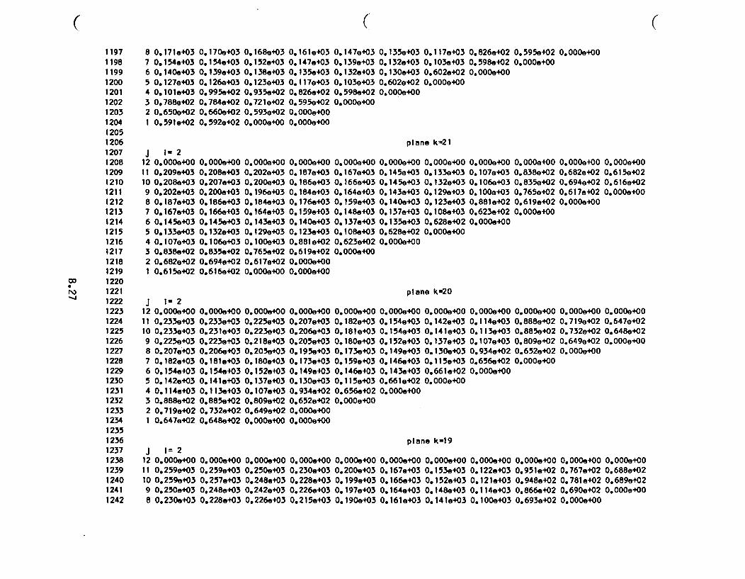
( ( (11971198119912001201120212031204120512061207120812091210121112121213121412151216121712181219
wo 1220;l 12214 1222
12231224122512261227122812291230123112321233123412351236123712381239124012411242
8 0.171e+037 0. 154e+036 0.140e4035 0.127e+034 0.101e+033 0.788e+022 0.650e+021 0.591e402
J 1= 212 0.000e+0011 0.209e+0310 0.208e+039 0.202e+038 0.187e+037 0.167e+036 0.145e+035 0.133e+034 0.107e+033 0.838e+022 0.682e+021 0.615.+02
J t-212 0.000+0011 0.233e+0310 0.233e+039 0.225e+038 0.207e+037 0.182,+036 0.154e+035 0.142e+034 0.114e+033 0.888e+022 0.719e+021 0.647e+02
0.170.+030. 154e+030. 139e+030.126e+030. 995e+020.784e4020.660e+020.592e+02
0.168.+03 0.161e+03 0.147e+03 0.135.+03 0.117e+03 0.826e+02 0.595e+02 0.000e+000.152e+03 0.147e+03 0.139e+03 0.132e+03 0.103e+03 0.598e+02 0.000e+000.138e+03 0.135e+03 0.132e+03 0.130e+03 0.602e+02 0.000e+000.123e+03 0.117e+03 0.103e+03 0.602e+02 0.000e+000.935.+02 0.8269+02 0.598e+02 0.0004+000.721e+02 0.595e+02 0.000e+000.593e+02 0.000e+000.000e+00 0.000e+00
plane k-21
0.000+000.208e+030.207e+030.200e+030.186e+030.166e+030.145e+030.132e+030. 106e+030.835e+020.694e+020.616e402
0.000+000.202e+030.200.+030.196e+030.184e+030.164,+030.143e+030.129e+030. 100e+030.765.+020. 617e+020.0004+00
O.OOO4e+0 0.000.0e+ 0.000.e+0 0.000,400 0.000e+000.187,+03 0.167e+03 0.145e+03 0.133e+03 0.107,+030.1864+03 0.166e+03 0.145e+03 0.132e+03 0.106e+030.184e+03 0.164e+03 0.143e+03 0.129e+03 0.100e+03
0. 000e+000.838e+020.835e+020.765e+02
0.000.+000.682e+020. 694e+020.617e+02
0.000,+000.615e+020.616e+020.000+00
0.176e+030. 159e+030.140e+030.123e+030.881 e+020.619,+020.0004+000.000,+00
0.159e+03 0.140e+03 0.123e+03 0.881e+02 0.619e+02 0.0004+000.148e+03 0.137e+03 0.108e+03 0.623e402 0.000e+000.137e+03 0.135e+03 0.628e+02 0.0004+000.108e+03 0.628e+02 0.000e+000.623e+02 0.000e+000.000e+00
plane k=20
0.000.+000.233.+030.231e+030.223.+030.206e+030.181e+030. 154e+030.141,+030.113.+030.885e+02
0.000.+000.225e+030.223.4030. 2 18e+030.205e+030.180.+030.152,+030.137e+030.107e+030.809e+02
0.000.+000. 207e+030.206e+030.205e+030.195e+030.173e+030.149e+030.130e+030. 934e+020.652e+020. OOOe+000. OO00040
0.000.+000.1824+030.181e+030.180e+030.173e+030.159e+030.146e+030. 115e+030.656e+02O.OOOe+00
0.0004+00 0.0004+00 0.0004+00 0.0004+00 0.0004+000.154e+03 0.142e+03 0.114e+03 0.888e+02 0.719e+020.154,+03 0.141e+03 0.113e403 0.885e+02 0.732e+020.152e+03 0.137e+03 0.107e+03 0.809e+02 0.649e+020.149e+03 0.130e+03 0.934e+02 0.652e+02 0.000e+000.146e+03 0.115e+03 0.656e+02 0.000e+000.143.403 0.661e+02 0.000.+000.661e402 0.000e+000.000O400
0.000.+000.647e+020.648e+020.000+00
0.732e+02 0.649,+020.648e+02 0.000+00
plane kui9J I- 2
12 0.000e+00 0.000e+00 0.000e+0011 0.259e+03 0.259e+03 0.250e+0310 0.259e+03 0.257e+03 0.248e+039 0.250e+03 0.248e+03 0.242e+038 0.230e+03 0.228e+03 0.226e+03
0.000.+000. 230e+030.228e+030. 226e+030.215e+03
0.000.+000.200e+030. 199e+030.197e+030.1 90e+03
0.000.+000.167e+030.166e+030.164e+030.161e403
0.000.+000. 153e+030. 152e+030.148e+030.141,+03
0.000.+000.122e+030.12 1,+030. 114e4030. 1 00e+03
0.000+000.951e+020.948e+020.866e+020.693e+02
0.000.+00 0.000.+000.767e+02 0.688e+020.781,+02 0.689e+020.690e+02 0.000,+000.000e+00
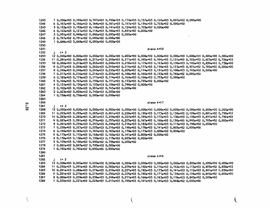
12431244124512461247124812491250125112521253125412551256125712581259126012611262126312641265
1266* 1267oo 1268
12691270127112721273127412751276127712781279128012811282128312841285128612871288
7 0.200e4036 0. 167e+035 0.153e+034 0.12294033 0.95194022 0.7679+021 0.688e+02
j 1=212 0.000.+0011 0.281e+0310 0.280e+039 0.271e+038 0.249e+037 0.217e+036 0.180e+035 0.164e+034 0.131e+033 0.102e+032 0.823e+021 0.738e+02
J 1.212 0.000e+0011 0.293e+0310 0.293e+039 0.283e+038 0.261e+037 0.228e+036 0.190e+035 0.173e+034 0.139e+033 0.109e+032 0.881e+021 0.792e+02
J 1=212 0.000.+0011 0.292e+0310 0.291.+039 0.281e+038 0.2609+037 0.229e+03
0.199e+030.166e+030.152e+030.121e+030.948e+020.781,4020.689e+02
0.197e+030. 164e+030.148e+030.114e+030.866e+020.690e+020.000.+00
0.190.+030.161e+030. 14 1e+030. 00e+030.693e+020.000+000.000+00
0.174e+030.157e+030.124e+030.697e4020.000OO00
0.157e+03 0.1244+03 0.697e+02 0.0004+000.154e+03 0.703e+02 0.000e+000.703e+02 0.000e+000.000e+00
plane k=18
0.000.+000.280e+030.278.+030.269e+030.248.+030.216e+030.179e+030.163,4030.130.+030.102e+030.839,+020.738e+02
0.000+000.2714e+030.269e+030.262e+030.245e+030.214e4030.177e+030.1594+030.123e+030.931e+020.740,+020.000,+00
0.000.+000.249e+030.248e+030.245.+030.233e+030.205e+030.174e+030. 151e+030. 1 08e+030. 743e+020.0004+000.0004+00
0.000.+000.217e+030.216e+030. 214e+030.205e+030.188e+030.169e+030.153e+030.748e+020. 000,400
0.000.+000.180e+030.179e+030. 177e+030.174e+030.169e+030.166e+030.755,4020.000e+00
0.0004+00 0.0004+00 0.0004e+0 0.000e+000.164e+03 0.131e+03 0.102e+03 0.823e+020.163e+03 0.130e+03 0.102,+03 0.839e+020.159e+03 0.123.+03 0.931e+02 0.740.+020.151e+03 0.108e+03 0.743e+02 0.0004+000.133e+03 0.748e+02 0.0004+000.755e+02 0.0004+000.000e+00
0.000+000.738e+020.738e+020.000e+00
plane k=17
0.000.e000.293e+030.290e4030.281e+030.25994030.227e+030.189.4030.172e4030.138e+030.108.e030.897e+020.792e+02
0.000.4000.283e+030.281e+030.274e+030.257e,030.225e+030.187e+030. 168e+030.130e.030.992,+020.795e+020. 000e+00
0.000.+000.261e+030.259e+030.257e+030.244e+030.216e+030.183e+030.160e+030.115e+030.798e+020.O000+000.000e+00
0.000.+000.228e+030.227e+030.225e+030.216e+030.198e+030.178e+030.141e+030.803e+020.000e+OO
0.000.+000. 190,+030.189,+030.187e+030.183e+030, 178e+030.175,+030.809e+020.000.+00
0.0004+00 0.000e+OO 0.0004+00 0.0004+00 0.0004+000.173,+03 0.139e+03 0.109e+03 0.8819+02 0.792e+020.172e+03 0.138e+03 0.108e+03 0.897e+02 0.792e+020.168e+03 0.130e+03 0.992e+02 0.795e+02 0.0000e+00.160e+03 0.115e+03 0.798e+02 0.0000e+00.141e+03 0.803e+02 0.000e+000.809e+02 0.0000e+00.000e+0
plane k=16
0.000.+000.291,+030.288e+030.279e+030.259.+030.227e+03
0.000.4000.281,+030.279e.030.273e+030.256e+030.225e+03
0.000e+000.260e+030.259e+030.256e+030.244e+030.217e+03
0.000.+000.229e+030.227e+030.225e+030.217e+030.199e+03
0.000.+000.192e+030.192,+030.190e+030.186e+030.181e+03
0.000e+OO 0.000.+00 0. OOOe+OO 0.000.+00 0.000.+000.176e+03 0.142e+03 0.113e+03 0.925e+02 0.838e+020.175,+03 0.141e+03 0.112e+03 0.941e+02 0.838,+020.171e+03 0.134e+03 0.104e+03 0.840e+02 0.000e+OO0.163e+03 0.119,403 0.843e+02 0.0000e+00.144e+03 0.8489+02 0.000+00
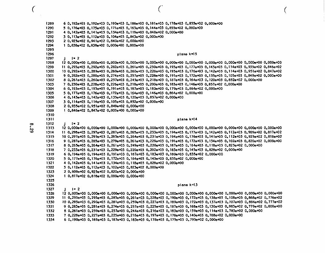
( C (128912901291129212931294129512961297129812991300130113021303130413051306130713081309131013111312
r* 1313131413151316131713181319132013211322132313241325132613271328132913301331133213331334
6 0.192e+035 0.176e+034 0.142.+033 0.113e+032 0.925e+021 0.838e+02
J 1=212 0.000e+0011 0.293e+0310 0.292e+039 0.282e+038 0.261e+037 0.230e+036 0. 193e+035 0.177e+034 0.143e+033 0.114e+03
0. 192e+030.175e+030.141e4030.112,+030.94 1e+020.838e402
0.190.+030.171e+030.134e+030.104,4030.840e+020.OOOe+00
0.186e+03 0.181e+03 0.178e+03 0.855e+02 0.000O4000.163e+03 0.144e+03 0.855e402 0.0004+000. 19e+030.843e+020. OOOe+000. OOOe+00
0.848.+02 0.000O4000.000e+00
plane k-15
0.000.+000.292e+030.289e+030.280e+030.260.+030.228e+030.193e+030.176e+030.142e+030.114e+03
0.000.+000.282e+030.280e+030.274e+030.257e+030.226e+030. 191e+030. 172e+030. 135e+030.105e+03
0.000e+000.261,e+030.260e+030.257e+030.245e+030.218e+030.187.+030. 164e+030.120e+030.852e+020.000.+000.000e+00
0.0004+00 0.0004+00 0.0004+00 0.OOOe+000.230,+03 0.193e+03 0.177e+03 0.143e+030.228e+03 0.193e+03 0.176e+03 0.142e+030.226e+03 0.191.+03 0.172e+03 0.135e+030.218e,03 0.187e+03 0.164,+03 0.120.+030.200e+03 0.183e+03 0.146e+03 0.857e+020.183e+03 0.179e+03 0.864e402 0.000e+000.146e+03 0.864e+02 0.000e+000.857e+02 0.0004+000.000e+00
0.0004+000. 114e+030. 114e+030.105,+030.852e+020.000e+00
0.000.+000.935e+020.951e+020.849e+020. OOOe+00
0.000.+000.846e+020.847e+020.000e+00
2 0.935e+02 0.951e+02 0.849e+021 0.846e+02 0.847e+02 0.000e+00
J 1-212 0.000e+00 0.0004+00 O.OOOe+0011 0.298,+03 0.297e+03 0.287e+0310 0.297e+03 0.295,+03 0.285e+039 0.287e+03 0.285e+03 0.279e+038 0.265e+03 0.264e+03 0.261e+037 0.233e+03 0.231e+03 0.229e+036 0.194e+03 0.194e+03 0.191e+035 0.177e+03 0.1769+03 0.172e+034 0.142e+03 0.141e+03 0.134e+033 0.112e+03 0.112e+03 0.102e+032 0.909e+02 0.925e+02 0.820e+021 0.817e+02 0.818e+02 0.000e+00
plane k-14
0.000.+000.265e+030.264e+030.261e+030.249e+030.220e+030.187e+030.164,+030. 118e+030. 823e+020.0004+000.000+00
0.000OO000.233,+030.231e+030.229e+030.220e+030.202e+030.183e+030.145e+030.828e+020.000,400
0.0004+000.194e+030.194e+030. 191e+030.187e+030.183e+030.180.+030.835e+02O.OOOe+00
0.000e+00 0.0004+00 0.000e+00 0.0004+00 0.0004+000.177e+03 0.142e+03 0.112e+03 0.909e+02 0.817e+020.176e+03 0.141e+03 0.112e+03 0.925e+02 0.818e+020.172e+03 0.134e+03 0.102,+03 0.820e+02 0.000e+000.164e+03 0.118e+03 0.823e+02 0.000e+000.145e+03 0.828e+02 0.000e+000.835e+02 0.000,4000.000e+00
plane k=13J 1-2
12 0.000e+0011 0.293e+0310 0.293e+039 0.283e+038 0.261e+037 0.228e+036 0.190e+03
0.000.+00 0.000.+000.293e+03 0.283e+030.290e+03 0.281e+030.281e+03 0.274e+030.259e+03 0.257e+030.227,+03 0.225e+03
0. 000e+000. 261 e+030.259e+030.257e+030.244,+030.216e+03
0.000.+000.228e+030.227e+030. 225e+030. 216e+030.197e+030.178e+03
0. 000e+000.1 90e+030. 189e+030.187e+030.183,+030.178e+030. 175e+03
0.000.+000.172e+030.172e+030.168e+030.159e+030.140e+030.795.+02
0.000.4000.138e4030.137e+030.130e+030.114e+030.788e+020.000e+00
0. OOOe+000.108e+030.107e,030.983e+020.783e+020.000+00
0.000.+000. 868e+020.884e+020.779e+020.000.+00
0.000.+000.776e+020. 777e+020.000+00
0. 189e+03 0.187e+03 0.183e+03
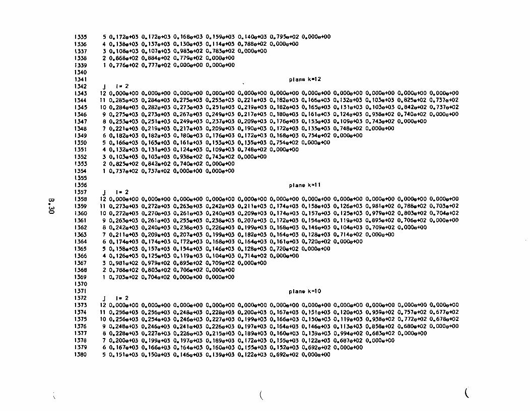
133513361337133813391340134113421343134413451346134713481349135013511352135313541355135613571358
( 1359o 1360
13611362136313641365136613671368136913701371137213731374137513761377137813791380
5 0.172e+034 0.138e+033 0.108e+032 0.868e+021 0.776e+02
J -s212 0.000e+0011 0.285e+0310 0.284e+039 0.275e+038 0.253e+037 0.221,+036 0.182e+035 0.166e+034 0.132e+033 0.103e+032 0.825e+021 0.737,+02
J 1 212 0.000e+0011 0.273e+0310 0.272 e+039 0.263e+038 0.242e+037 0.21 1e+036 0.174e+035 0.158e+034 0.126e+033 0.981,+022 0.788e+021 0.703e+02
J 1 212 0.000e+0011 0.2569+0310 0.256,+039 0.248e+038 0.228e+037 0.200e+036 0. 167e+035 0.151e+03
0.172e+03 0.168e+030.137e+03 0.130e+030.107e+03 0.983e+020.884e+02 0.779e4020.777e+02 0.000a+00
0.159,+03 0.140e403 0.795e+02 0.000e+000.114,+03 0.788e+02 0.000,4000.783e+02 0.0004000.000e+000.000+00
plane k=12
0.000a+00 0.000e+00 0.000e+00 0.000e+00 0.000e+00 0.000e+000.284e+03 0.275e+03 0.253e+03 0.2219+03 0.182e+03 0.166e+030.282e+03 0.273e+030.273e+03 0.267e+030.251e+03 0.249e+030.219e+03 0.217e+030.182e+03 0.180.+030.165e+03 0.161e+030.131,+03 0.1249+030.103,+03 0.938e+020.842e+02 0.740e+02
0.251e+03 0.2199403 0. 182e+03 0.1659+030.2499+03 0.217e+03 0.180e+03 0.161e+030.237e+03 0.209e+03 0.176e+03 0.153e+030.209e+03 0.190e+03 0.172,+03 0.135.+030.176e+03 0.172e+03 0.168.+03 0.754e+020.153e+03 0.135,+03 0.7549+02 0.000e+000.109e+03 0.748e+02 0.000e+000.743e+02 0.000e+000.000.+00
0.000.+000.132e+030.131,+030.124,+030.109e4030.748e+020.000.+00
0.000.+000.103e+030. 103e+030.938e+020.743e+020.000e+00
0.000+00 0.000.e000.825e+02 0.737e+020.842e+02 0.737e+020.740e+02 0.000e+000.000+00
0.737e+02 0.000e+00 0.000+00
plane k-l I
0.000e+00 0.000e+000.2729+03 0.263e+030.270e+03 0.261e+030.261e+03 0.255e+030.240e+03 0.238e+030.209e+03 0.207e+030.174e+03 0.172,+030.157,+03 0.154e+030.125e+03 0.119e+03
0.000e+00 0.000e+00 0.000e+00 0.000e+000.2429+03 0.211,+03 0.174e+03 0.158e+030.240.+03 0.209e+03 0.174e+03 0.157e+030.238e+03 0.207e+03 0.172e+03 0.154e+030.226e+03 0.199e+03 0.168e+03 0.146e+030.199,+03 0.182e+03 0.164e+03 0.128e+030.168e+03 0.164e+03 0.161e+03 0.720e+020.146e+03 0.128.+03 0.720e+02 O.OOOe,000.104,+03 0.714e+02 0.000e+00
0.000.+000.126e+030.125e+030.119e+030.104e+030. 714e+020.000+00
0.000.+000.981e+020.979e+020.895e+020.709e+020.000+00
0.000e+000.788.+020.803e+020.706e+020.000e+00
0.000+000.703e+020. 704e+020. OOOe+00
0.979e+02 0.895e+02 0.709,+02 O.OOOe+000.803e+02 0.706e+02 0.000e+000.7049+02 0.000e+00 O.OOOe+00
plane k=10
0.000OO00 0.000+000.256e+03 0.248e+030.254e+03 0.246e+030.246e+03 0.241e+030.227e+03 0.226e+030.199e+03 0.197e+030.166e+03 0.164e+030.150e+03 0.146e+03
0.000e+00 0.000e+00 0.000e+00 0.000e+000.228.+03 0.200,+03 0.167,+03 0.151e+030.227e+03 0.199e+03 0.166e+03 0.150e+030.226,+03 0.197e+03 0.164e+03 0.146e+030.215,+03 0.189e+03 0.160e+03 0.139e+030.189e+03 0.1729+03 0.155e+03 0.122e+030.160e+03 0.155e+03 0.152e+03 0.6929+020.139e+03 0.122e+03 0.692e+02 O.OOOe+00
0.000e+000. 120e+030. 119e+030.113,+030.994,+020. 687e+020.000e+00
0.000e+000.939e4020.938e+020.858e+020.683e+020.000e+00
0.000,+000.757e+020.772e+020.680e+020.000.+00
0.000.+000.677e4020.678e+020.000e+00
(
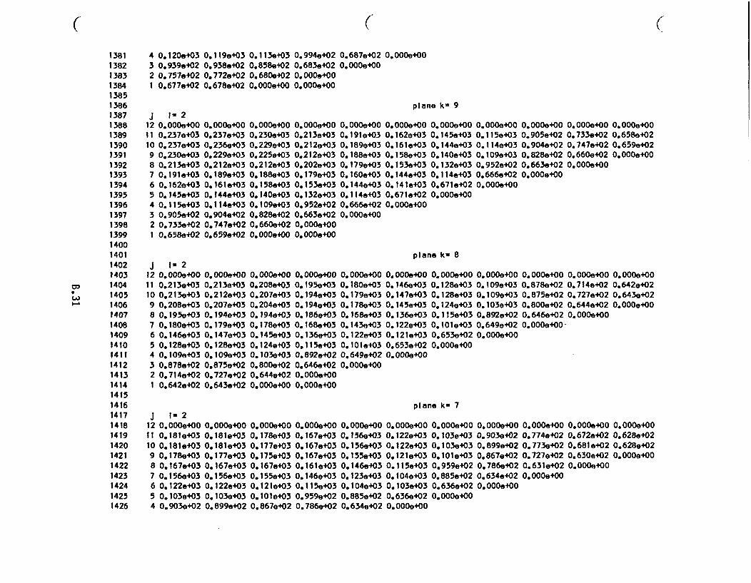
( ( (138113821383138413851386138713881389139013911392139313941395139613971398139914001401140214031404
La 140514061407140814091410141114121413141414151416141714181419142014211422142314241425
4 0.120e+033 0.939e4022 0.757e+021 0.677e+02
J 1-212 0.000+0011 0.237e+0310 0.237e+039 0.230e+038 0.213e+037 0.191e+036 0.162e+035 0.145e+034 0.115e+033 0.905e+022 0.733e+021 0.658e+02
J I=212 0.000+0011 0.213e+0310 0.213e+039 0.208e+038 0.195e+037 0.180e+036 0.146e+035 0.128e+034 0.109e+033 0.878e+022 0.714e+021 0.642e+02
0.119e+03 0.113.+03 0.994e+02 0.687e+02 0.000+000.938et02 0.858et02 0.683e+02 0.000e+000.772e+02 0.680e.02 0.000,+000.678e+02 0.000,e00 0.000e+00
plane km 9
0.000.+000.237e+030.236e+030. 229e+030.212e+030.189e+030.161e+030.144e+030.114e+030.904et020.747e+020.659e+02
0.0004+00 0.0004+00 0.000.+000.230e+03 0.213e+03 0.191e+030.229e+03 0.212e+03 0.189e+030.225e,03 0.212e+03 0.188e+030.212e+03 0.202e+03 0.179e+030.188e+03 0.179e+03 0.160e+030.158e403 0.153e+03 0.144e+030.140.+03 0.132e+03 0.114e+030.109e,03 0.952e+02 0.666e+020.828e+02 0.663e+02 0.000e+000.660.+02 0.000e+OO0.000e00 0.000+00
0. OOOe+OO0.162e+030.161,+030. 158e+030.153e+030.144e+030.141 ,+030.671e+020.000+00
0. OOOe+OO0.145e+030. 144e+030.140e+030.132e+030. 114e+030.6714e+020.OOOe+00
0.000,+000. 115e+030. 114e+030. 109e+030.952e+020.666e+020.000+00
0.000e+OO0.905e+020.904e+020.828e+020.663e+020.000+00
0. OOOe+OO0. 733e+020.747e+020.660e+020.000.+00
0.000,+000.658e4020.659.+020.000e+0
plane km 8
0. OOOe+OO0. 213e+030.212e+030.207e+030.194e+030.179e+030.147e+030.128e+030. 109,+030.875e+020.727e+020.643e+02
0.0004+00 0.000e+OO 0.0004+00 0.0004+00 0.000e+OO 0.0004+00 0.0004+00 0.0004+00 0.000+000.208e+03 0.195e+03 0.180e+03 0.146e+03 0.128e+03 0.109e+03 0.878e+02 0.714e+02 0.642e+020.207e+030.204e+030.194e+030.178e+030.145e+030.124e+030.103e+030.800e+020.644e+020.000,+00
0.194,+03 0.179e+03 0.147,+03 0.128e+03 0.109e+030.194e+03 0.178e+03 0.145e+03 0.124e+03 0.103e+030. 186e+03 0.168e+03 0.136e+03 0.115e+03 0.892e+020.168e+03 0.143e+03 0.122e+03 0.101e+03 0.649e+020.136e+03 0.122e+03 0.121,+03 0.653e+02 0.0000e+00.115e+03 0.101e+03 0.653e+02 0.000e+000.892,+02 0.649e+02 0.000.+000.6469+02 0.0000e+00.000e+OO0.000,+00
0.875e+020.800e+020.646e+020. 0004+00
0.727e+02 0.643e+020.644e+02 0.000e+000.000e+00
plane km 7J I=2
12 0.000e+00tt 0.181,+0310 0.181,+039 0.178e+038 0. 167e+037 0.156,+036 0.122e+035 0. 103e+03
0.000.+000.181.+030.181 e+030.177e+030.167e+030. 156e+030.122e+030.103e+03
0.000.+000.178e+030. 177e+030. 175e+030. 167e+030. 155e+030. 121e+030. 101e+030.867e+02
0. OOOe+OO0.167,+030. 167e+030. 167e+030. 161e+030. 146e+030. 15e+030.959e+020. 786e+02
0.0004+00 0.000.+00 0.0004+00 0.000.400 0 .OOe+OO 0.0004+00 0.000e+OO0.156e+03 0.122e+03 0.103e+03 0.903et02 0.774e+02 0.672e+02 0.628e+020.156e403 0.122,+03 0.103e+03 0.8999+02 0.773.+02 0.681e+02 0.628e+020.155e+03 0.121e+03 0.101e+03 0.867e+02 0.727e+02 0.630e+02 O.OOOe4OO0.146,403 0.115e+03 0.959e+02 0.786e+02 0.631e+02 0.0000e+00.123,+03 0.104e+03 0.885e+02 0.634e402 0.000e+OO0.104,+03 0.103e+03 0.636e+02 0.000.+000.885e402 0.6369+02 0.0000e+00.634e+02 0.0000e+01426 4 0.903.402 0.899e+02
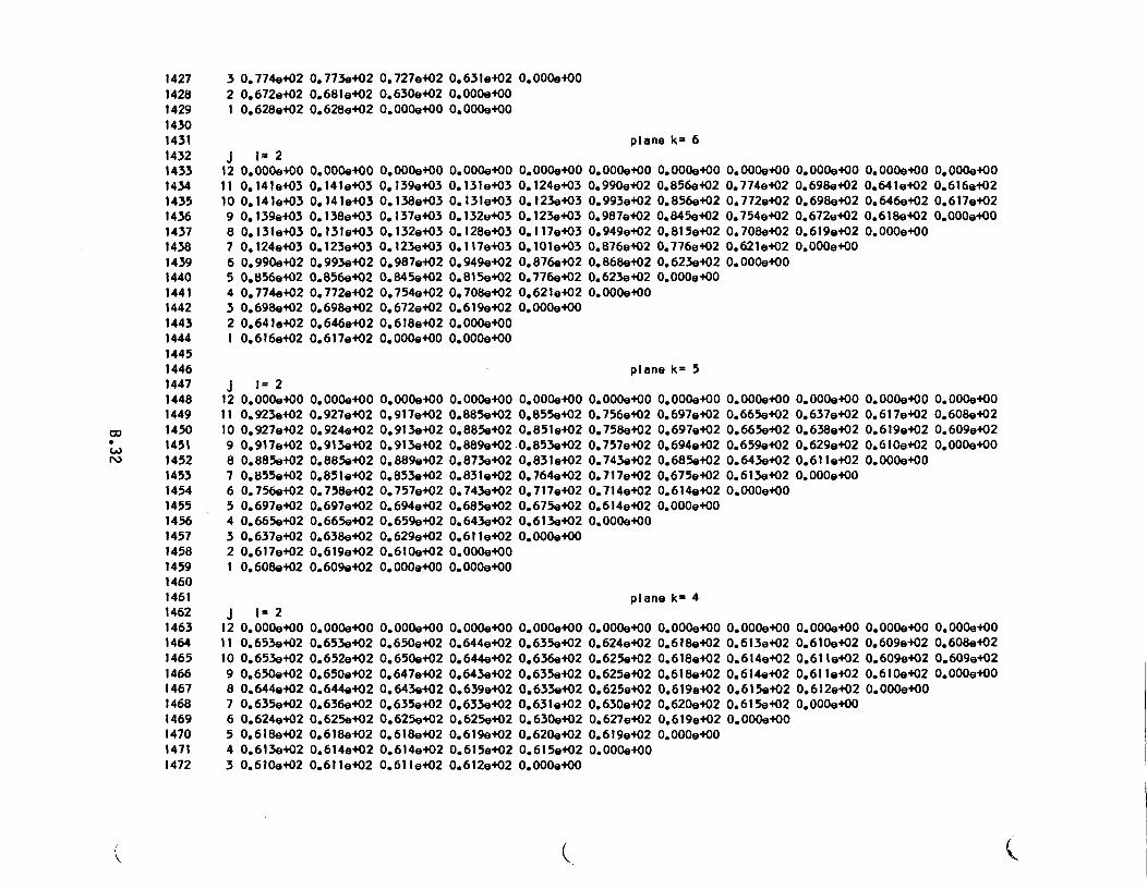
14271428142914301431143214331434143514361437143814391440144114421443144414451446144714481449
1450* 1451PO 1452
14531454145514561457145814591460146114621463146414651466146714681469147014711472
3 0.774e+022 0.672.+021 0.628e+02
J In212 0.000e,0011 0.1 41e+0310 0.1 4 1e+039 0.139e+038 0.131e+037 0.124e+036 0.990e+025 0.856,+024 0.774e+023 0.698e+022 0.641.+021 0.616e+02
J 1=212 0.000e+0011 0.923e+0210 0.927e+029 0.917e+028 0.885e+027 0.855,+026 0.756e+025 0.697,+024 0.665e+023 0.637e+022 0.617e+021 0.608et02
j 1=212 0.000e+0011 0.653e+0210 0.653e+029 0.650e+028 0.644e+027 0.635e+026 0.624e+025 0.618e+024 0.613e+023 0.61Oe+02
0.773e+020.681,+020.628e+02
0.727e+020.630e+020.000e+00
0.631e+02 0.000e+000.000.+000.000e+00
plane ku 6
0.000.+000.141e+030. 141 e+030. 138e+030.131e+030. 123e+030.993.+020.856.+020.772e+020.698e+020.646e+020.617e+02
0.000.+000.139e+030.138e+030.137e+030.132e+030.123e4030.987e+020.845e,020.754e+020.672e+020.618e+020.000,+00
0.000.+000.131e+030.131e+030.132e+030.128e+030. 117e+030. 949e+020.815e+020. 708e+020. 619e+020.000e+000.000e+00
0.000.+000.124e+030.123e+030.123.+030.117e+030.101e+030.876e+020.776e.020.621e+020.000e+00
0.000.+000. 990e+020. 993e+020.987e+020. 949e+020.876.+020.868e+020.623.4020.000e+00
0.000e+00 0.000e+00 0.000e+00 0.000e+00 0.000e+000.856e+02 0.774e+02 0.698e+02 0.641,+02 0.616e+020.856e+02 0.772e+02 0.698e+02 0.646e+02 0.6179+020.845e+02 0.754e+02 0.672e+02 0.618e+02 0.000e+000.815e+02 0.708e+02 0.619e+02 0.000e+000.776e+02 0.621e+02 0.000e+000.623e402 0.000e+000.000,+00
plane k= 5
0.000.+000.927e4020.924e+020.913e+020.885e+020.851,+020.758e+020.697e+020.665e+020.638e+020.619,+020.609e+02
0.000.+000. 917e4020. 913e+020.913e+020.889e4020.853e+020.757e+020.694e+020.659e+020.629,4020.610e+020.000e+00
0.000.+000.885e+020.885e+020.889e+020.873e+020.831,+020.743e+020.685e+020.643e+020.611e+020.000e4000.000+00
0.000e+OO0.855e+020.851e+02.0.853e+020.831,e+020. 764e+020. 717e+020.675e4020.613e+020.000+00
0.000e+000.756e+020.758e+020.757e+020.743e+020.717e+020. 714e+020. 614e+020.000e+OO
0.000,+000.697,+020.697,+020.694e+020.685e+020.675e+020. 614e+020.000+00
0.000.+000.665e+020.665e4020.659e4020.643e4020.613e+020.000e+00
0.000e+00 0.000e+O0 0.000e+000.637,402 0.617e+02 0.6089+020.638e+02 0.619e+02 0.609e+020.629e+02 0.610e+02 0.000+000.611e+02 0.0000e+00.000,+00
plane k= 4
0.000.+000.653e+020.652e+020.650e+020.644e+020.636e+020.625e+020.618e+020.614e+020.611e+02
0.000.+000.650e+020.650e+020.647e+020.643e+020.635e+020.625e+020. 618e+02
0. OOOe+OO0. 644e+020.644e+020.643e+020.639e+020.633e+020.625e+020. 619e+02
0.000.+00 0.000.+000.635e+02 0.624e+020.636e+02 0.625e+020.635e+02 0.625e+020.633e402 0.625e+020.631e+02 0.6309+020.630.+02 0.627e+020.620e+02 0.619e+020.615e+02 0.000e+OO0.000e+00
0.O000+000.618e+020.618e+020.618e+020.619,4020.620e+020.619e+020.000+00
O.OOOe4OO0.613e+020.614e+020.614,+020.615e+020.615e+020.000+00
0.000.+000.61 Oe+020.61 le+020.611e+020.612e+020.000+00
0.000.+00 0.000e+OO0.609,+02 0.608e+020.609,+02 0.609e+020.610.+02 0.000,+000.000,+00
0.614e+02 0.615e+020.611e+02 0.612e+02
(,.
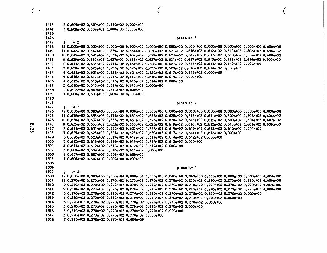
( ( (1473147414751476147714781479148014811482148314841485148614871488148914901491149214931494149514961497149814991500150115021503150415051506150715081509151015111512151315141515151615171518
2 0.609e+02 0.609e402 0.610e+02 0.000e+01 0.608e+02 0.6099+02 0.000O+00 0. 000e+00
plane k= 3J =X2
12 0.000e+00 0.000+0011 0.642e+02 0.642e+0210 0.642e+02 0.641e+029 0.639e+02 0.639e+028 0.634e+02 0.634e+027 0.628e+02 0.628e+026 0.621e+02 0.6219+025 0.616e+02 0.6179+024 0.612e+02 0.6139+023 0.6109402 0.610e4022 0.608e+02 0.609,+021 0.608e+02 0.608e+02
J 1=212 0.000e+00 0.000+0011 0.638.+02 0.638e+0210 0.638e+02 0.637e+029 0.635e+02 0.635e+028 0.631e+02 0.631e+027 0.625e+02 0.625e+026 0.620e+02 0.6209+025 0.615e+02 0.616e+024 0.611e+02 0.612e+023 0.609,+02 0.609e+022 0.607.+02 0.607e+021 0.606e+02 0.607e402
0.000.+000.639e+020.639e+020.637e+020.633e+020.627e+020.621e+020.617e+020. 6 13e+020.61 le+020.610.+020. 000,+00
0. 000e+000.634e+020.634e+020.633e+020.630.+020.626e+020.621e+020.617e+020. 613e4020.612e+020. 000e+000. 000e+00
0.OOOe+00 0 0.0004+00 0.0004+00 0.000400 0.0004+00 0.0004+00 0.000.+00
0.628e402 0.621e+02 0.616e+02 0.612e+02 0.610e+02 0.608e+02 0.608e402
0.628e+02 0.6219+02 0.617e+02 0.613e+02 0.610e+02 0.609,+02 0.608e+02
0.627,+02 0.621e+02 0.617e+02 0.613,+02 0.61 1e+02 0.610e+02 0.000,+000.626e402 0.621e+02 0.617e+02 0.613e+02 0. 6 l2e+02 0.0000e+0
0.623e+02 0.6209+02 0.616e+02 0.614e+02 0.0000e+0
0.620e+02 0.617e+02 0.615e+02 0.000.+000.616e+02 0.615.402 0.000e+000.614e+02 0.000.4000.000e+00
plane k- 2
0.000.+000.635e+020.635e+020.633e+020.630e+020.625e+020.619,+020.616e+020. 612e+020.610e+020.608,+020.000,400
0.000.+000.631e4020.631e+020.630e+020.627,+020.623e+020.619e+020.615e+020. 612e+020.610,+020.000e+OO0.000+00
0. OOOe+OO0.625e+020.625e+020.625,+020.623e+020. 620e+020. 617e+020. 614e+020.612e+020. OOOe+00
0.000.+00 0. OOOe+OO 0.000.+00 0.000.400 0.000.400 0.000.+000.620e+02 0.615e+02 0.611e+02 0.609e+02 0.607e+02 0.606e+020.620,+02 0.616e+02 0.612e+02 0.609e+02 0.607e+02 0.607e+020.619,+02 0.616e+02 0.612e+02 0.610e+02 0.608e+02 0.000,+000.619,+02 0.615e+02 0.612e+02 0.6109+02 0.000+000.617e+02 0.614e+02 0.612e402 0.000e+000.614,+02 0.612,402 0.0000e+00.612e+02 0.000e+000.000,+00
plane k= IJ 1=2
12 0.000.+OO 0.000.400 0.000.+0011 0.270e+02 0.270e+02 0.2709+0210 0.270.+02 0.270e+02 0.270.+029 0.270e+02 0.270e+02 0.270e+028 0.270.+02 0.2709+02 0.2709+027 0.270e+02 0.270e+02 0.270e+026 0.270e+02 0.270e+02 0.270e+025 0.270e+02 0.270e+02 0.270e+024 0.270.+02 0.270e+02 0.2709+023 0.270e+02 0.270e+02 0.270e+022 0.270.+02 0.270e+02 0.2709+02
0.000.+000.270e4020.270.+020.270e+020.270e+020.270e+020.270.+020.270e+020.270.+020.270e+020.000e+OO
0. OOOe+OO0.270e+020.270e+020.270e+020.270e+020.270e+020.270.4020.270e+020.270.+020. 000e+00
0.O000+000.270e+020.270.+020.270e+020. 270e+020.270e+020.270.+020.270,+020. OOOe+OO
0.000e+OO0. 270e+020.270e+020. 270e+020.270e+020.270e+020.270e+020.000,+00
0.000.+000.270e+020.270.+020. 270e+020.270e+020.270e4020.000e+00
0.000e+00 0.0004+00 0.000e+OO0.270e+02 0.270e+02 0.000,+000.270.+02 0.270.+02 0.0000e+00.270e+02 0.270e+02 0.000e+OO0.270e+02 0.000.+000.000e+0
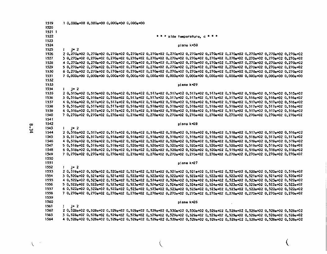
151915201521 11522152315241525152615271528152915301531153215331534153515361537153815391540154115421543
-> 154415451546154715481549155015511552155315541555155615571558155915601561156215631564
I 0.000e+OO 0.000e+00 0.000e+00 0.000+00
* * * side temperature, c * * *
plane kw30I J-22 0.2709+023 0.270e+024 0.270.+025 0.270e+026 0.270.+027 0.000e+00
I J=22 0 515e+02
3 0.516e+024 0.516e+025 0.516e+026 0.516e+027 0.270e+02
I J-22 0.516e+023 0. 517e+024 0.519e+025 0. 518e+026 0.518e+027 0.270.+02
I J=22 0. 5 19e+02
3 0.520e+024 0.522,+025 0.522.+026 0.522e+027 0.270,+02
I J=22 0.528e+023 0.528e+024 0.528e+02
0.270.+020.270e+020.270.+020.270e4020.270.+020.000+00
0.270.+020.270e+020.270+020.270e+020.270.+020.000,+00
0.270e+020.270e4020.270.+020.270.+020.270.4020.O000+00
0.270e+020.270e4020.270e+020.270e+020.270e+020.000.+00
0.270.+020.270e+020.270.+020. 270e+020.270.+020.000+00
0.270e+02 0.2709+02 0.270e+02 0.270e+02 0.270e+02 0.270.+020.270.+02 0.270e+02 0.2709+02 0.270e+02 0.270,+02 0.270,+020.270.+02 0.2709+02 0.270.+02 0.270e+02 0.270e+02 0.270e+020.270e+02 0.2709+02 0.270e+02 0.2709+02 0.270,+02 0.270e+020.270e402 0.270e+02 0.270e+02 0.270e+02 0.270e+02 0.270e+020.000,+00 0.000,+00 0.000,+00 0.000.+00 0.000,+00 0.000+00
plane k=29
0. 515e+020. 516e+020.517e+020.517e+020. 517e+020.270e+02
0.516e+020. 516e+020.517e+020. 517e+020.517,+020.270e+02
0.516e+020.517,+020.518e+020. 518e+020.517e+020. 270e+02
0.517e+020.517e+020.518,+020.518e+020.518e+020.270e+02
0. 517e+020. 517e+020.518e+020.518e+020.518,+020.270e+02
0.517e+02 0.517e+02 0.516e+02 0.516e+020.517e+02 0.517e+02 0.517e402 0.516e+020.518e+02 0.518,+02 0.518e+02 0.5179+020.518e402 0.518e+02 0.518e402 0.517,+020.518e402 0.518e+02 0.517e+02 0.5179+020.270.402 0.270e+02 0.270e+02 0.270e+02
0.515.+02 0.515e+020.516e+02 0.516e4020.517e+02 0.516e+020.517e+02 0.516e+020.517,+02 0.516e+020.270e+02 0.270e+02
plane k=28
0.517,+020. 517e+020.519.+020.519 e+020.518e+020.270e+02
0. 517e+020.518e+020.519,+020. 519e+020.519e+020.270e+02
0.518e+020. 518e+020.520.+020.520e+020. 519e+020. 270e+02
0.518e+020.518e+020.520.+020.520e4020.520.+020.270e+02
0.518e+020. 518e+020.520e+020.520e+020.520e+020. 270e+02
0.518,+02 0.518e+02 0.518e+02 0.517e+02 0.517.+02 0.516e+020.518e+02 0.5189+02 0.518e+02 0.518e+02 0.517e+02 0.517e+020.520.402 0.520e+02 0.520e+02 0.519e+02 0.519e+02 0.519e+020.520e+02 0.5209402 0.520e+02 0.519e+02 0.5199+02 0.518e+020.520e+02 0.520e+02 0.519e+02 0.519e+02 0.518,+02 0.518e+020.270e+02 0.270e+02 0.270e+02 0.270e+02 0.270e+02 0.270e+02
plane k=27
0.520e+020.521 e+020.523e+020.522e+020.522e+020.270e+02
0.520e+020.521 e+020. 523e+020.523e+020.522e+020.270e+02
0.521.+020.522e+020.523e+020.523e+020.523e+020.270e+02
0.521e+020.522,+020.524e+020.524e+020.523.+020.270,+02
0. 521 e+020.522e+020. 524e+020.524e+020.523e+020.270e+02
0.521e+02 0.521e+02 0.521e+02 0.520e+02 0.5209+02 0.519e+020.522,+02 0.522e+02 0.522e+02 0.521e+02 0.521e+02 0.520e+020.524e+02 0.524e+02 0.523.+02 0.523e+02 0.523e+02 0.522e+020.524,+02 0.524e+02 0.523,402 0.523e+02 0.522e+02 0.522e+020.523.+02 0.5239+02 0.523e+02 0.522e+02 0.522,+02 0.522e+020.270.+02 0.270e+02 0.270e+02 0.270e+02 0.270e+02 0.270e+02
plane k=26
0. 528e+020.528,+020.528e+02
0.529e+020. 529e+020.529e+02
0.529e+020.529e+020.529e+02
0.529e+020. 529e+020. 529e+02
0.530e+020.529e4020.529e+02
0.530e+02 0.529e402 0.529e+02 0.529e+02 0.528e+02 0.528e+020.529,+02 0.529e+02 0.529e+02 0.529e+02 0.528e+02 0.528e+020.529e+02 0.529e+02 0.529e+02 0.529e+02 0.528e+02 0.528e+02
K K (
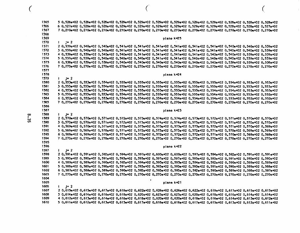
( ( (1565156615671568156915701571157215731574157515761577157815791580158115821583158415851586158715881589159015911592159315941595159615971598159916001601160216031604160516061607160816091610
5 0.528e+026 0.527e+027 0.270.+02
I J=22 0.539e+023 0.539e+024 0.539e+025 0. 539e+026 0.538e+027 0.270e+02
0.528e+02 0.528e+020.528e+02 0.528e4020.270e+02 0.2709402
0.529e+020.529e+020.270e+02
0.529e+02 0.529e+02 0.529e+02 0.529e+02 0.529e+02 0.528e+02 0.528e+02 0.528e+020.529e402 0.529e+02 0.529e+02 0.529e+02 0.529e+02 0.528e+02 0.528.+02 0.527e+020.270e+02 0.270e+02 0.270e+02 0.2709+02 0.2709+02 0.270e+02 0.270e+02 0.2709+02
plans k-25
0.540.+02 0.540e+020.540e+02 0.540e+020.539e+02 0.5409+020.5399+02 0.540e.020.539e+02 0.539e+020.270e+02 0.270e+02
0.54 1e+020. 541 e+020.540.+020.540e+020.540.+020.270e+02
0. 541 +4020.541 e+020.54 1e+020.540e+020.540e+020.270e402
0.541e+02 0.541e+02 0.541e+02 0.541e+02 0.540e+02 0.5409+02 0.539e+020.541e+02 0.541e+02 0.541e+02 0.541e+02 0.540e+02 0.540e+02 0.539e+020.541e+02 0.541e+02 0.541e+02 0.540e+02 0.540,+02 0.539e+02 0.539e+020.541e+02 0.541e+02 0.540e+02 0.540e+02 0.5409+02 0.539e+02 0.539e+020.540.+02 0.540e+02 0.540e+02 0.540e+02 0.539e+02 0.539e+02 0.538e+020.270e+02 0.270e+02 0.270e+02 0.270e+02 0.270e+02 0.270e+02 0.270e+02
plans k=24I Ju22 0.553e+02 0.553e+02 0.554e+023 0.553e+02 0.553e+02 0.554e+024 0.553e+02 0.553e+02 0.554e+025 0.552e+02 0.553e+02 0.553e+026 0.552e+02 0.552e+02 0.5539+027 0.270e+02 0.270e+02 0.270e+02
I J=22 0.570e+02 0.570e+02 0.571e+023 0.570e+02 0.570e+02 0.571e+024 0.569e+02 0.570e+02 0.571,+025 0.569e+02 0.569e+02 0.570e+026 0.568e+02 0.569e+02 0.570.+027 0.270e+02 0.2709+02 0.270e402
I J-22 0.591e+02 0.591e+02 0.592e+023 0.590e+02 0.590e+02 0.591e+024 0.589e+02 0.589e+02 0.5909+025 0.588e+02 0.589e+02 0.590e+026 0.587e+02 0.588e+02 0.589e+027 0.270e+02 0.270e+02 0.270e+02
I J=22 0.615e+02 0.615e+02 0.617e+023 0.614e+02 0.614e402 0.616e4024 0.612e+02 0.613e+02 0.614e+025 0.61 1e+02 0.612e+02 0.613e+02
0.555e+020.555e+020.554e+020.554e+020.554e+020. 270e+02
0.555e+020.555e+020. 555e+020. 555e+020.554e+020.270e+02
0.555e+02 0.555e+02 0.555e+02 0.5559+02 0.554e+02 0.553e+02 0.553.+020.555e+02 0.555e+02 0.555e+02 0.555e+02 0.554e+02 0.553e+02 0.553e+020.555e+02 0.555.+02 0.555e+02 0.554e+02 0.554e+02 0.553e+02 0.553e+020.555e+02 0.555,402 0.555e+02 0.554e+02 0.553e+02 0.553e+02 0.552e+020.554e402 0.554e+02 0.554e+02 0.554e+02 0.553e+02 0.552e+02 0.552e+020.270e+02 0.270e+02 0.270e+02 0.270e+02 0.270e+02 0.270e+02 0.270e+02
plane k-23
0. 572e+020.572e+020.572,+020. 571 e+020. 571 e+020. 270e+02
0.573e+020.573e+020. 573e+020.572,+020.572e+020.270e+02
0.574,+020.574e+020.573e+020. 573e+020.572e+020. 270e+02
0.574e+020.574e+020.573e+020.573e+020. 572e+020. 270e+02
0.573e+02 0.572e+02 0.571e+02 0.570.+02 0.570e+020.573e+02 0.572e+02 0.571e+02 0.570e+02 0.570e+020.573e+02 0.572e+02 0.571e+02 0.570e+02 0.569e+020.572e+02 0.571e+02 0.570e+02 0.569e+02 0.569e+020.572e+02 0.571e+02 0.570e+02 0.569e+02 0.568e+020.270e+02 0.270e+02 0.270e+02 0.270e+02 0.270e+02
plane k-22
0.594e+020.593e4020.592,+020.591e+020.590e+020.270e+02
0.597e+020.595e4020.594e+020.593e+020.592e+020.270e+02
0.600e+020.597e+020.595e+020.593e+020.593e+020.270e+02
0.600e+020. 597e+020.595e+020.593e+020.5939+020.270e402
0.597e+02 0.594.+020.595e+02 0.593e+020.594e+02 0.592e+020.593e+02 0.591e+020.592e+02 0.590.+020.270e+02 0.270e+02
0.592e+02 0.591e+02 0.591e+020.591e+02 0.590e+02 0.590e+020.590e+02 0.589e+02 0.589e+020.590e+02 0.589e+02 0.588e+020.589e+02 0.588e+02 0.587e+020.270e+02 0.270e+02 0.270e+02
plane k-21
0.619e+020. 6 18e+020.616e,020.615e+02
0.622e+020.620e+020.618e+020.617e+02
0.626e+020.623e+020.620e+020.618e+02
0.626e+020.623e+020.620e+020.618e402
0.622e+020.620e+020.618e+020.617e+02
0. 619e+020.618e+020.616,+020.615e+02
0.617e+02 0.615e+02 0.615e+020.616e+02 0.614e402 0.614e+020.614e+02 0.613.+02 0.6129+020.613e+02 0.612e+02 0.611e+02
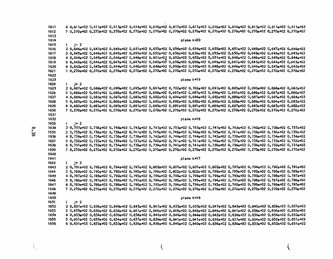
16111612161316141615161616171618161916201621162216231624162516261627162816291630163116321633
wu 16341635163616371638163916401641164216431644164516461647164816491650165116521653165416551656
6 0.611e+02 0.6114e02 0.613e+02 0.6149+02 0.616e+02 0.617e+02 0.6179+02 0. 616e+02 0.614e+02 0.613e+02 0.6119+02 0.611e+027 0.270e+02 0.270e+02 0.270e+02 0.270e+02 0.2709+02 0.270,+02 0.270e+02 0.2 70e+02 0.2709e0 2 0.27 0e+02 0.270e+02 0.270e+02
plane k-20I J=22 0.646e+02 0.6 4 7e+02 0.649o+023 0.645e+02 0.6 4 6e+02 0.64894024 0.644e+02 0.645e+02 0.646,+025 0.643e+02 0.644e+02 0.6459+026 0.6429+02 0.6439+02 0.644e+027 0.270e+02 0.270e+02 0.270,402
I J=22 0.687e+02 0.688e+02 0.6909+023 0.686e+02 0.687e+02 0.688e+024 0.684e+02 0.685e+02 0.6879+025 0.683e+02 0.684e+02 0.686e4026 0.682e+02 0.683e+02 0.6859+027 0.2709+02 0.270e+02 0.270e+02
I J-22 0.737e+02 0.738e+02 0.7409+023 0.735e+02 0.736e+02 0.738e+024 0.734e+02 0.734e+02 0.736,4025 0.732e+02 0.733e+02 0.735e+026 0.7319+02 0.732e+02 0.734e+027 0.270e+02 0.270,402 0.270e+02
I J-22 0.791e+02 0.792e+02 0.794e+023 0.789e,02 0.790e+02 0.792e+024 0.787,+02 0.788e+02 0.790e+025 0.786e+02 0.787e+02 0.788e+026 0.785e+02 0.786e+02 0.788e,+027 0.270e+02 0.270e+02 0.270e+02
I J=22 0.837,+02 0.838,+02 0.840e+023 0.835e+02 0.836e+02 0.838e+024 0.833e+02 0.8349+02 0.836e+025 0.831e+02 0.832e+02 0.834e,026 0.831e+02 0.832e+02 0.8339+02
0.651,+02 0.6559+02 0.6599402 0.659e+02 0.655e+020.650,402 0.6539+02 0.656e+02 0.656e402 0.653e+020.648e+02 0.651,+02 0.652e+02 0.6529+02 0.651e+020.647e+02 0.649e+02 0.650e+02 0.650e+02 0.6499+020.646e+02 0.6489+02 0.650e+02 0.650e+02 0.648e+020.270e+02 0.270e+02 0.270e+02 0.270e+02 0.270e402
0.651,+020.650.+020.648e+020.647e+020.6 4 6e+0 20.270e+02
0.6499+020.648,+020.646,+020.645e+020.644e+020. 270e+02
0.647e+020.646e+020.645e+020.644e+020.643.+020.270e+02
0.646e+020.645e+020.644e+020.643e+020.642e+020.270e+02
plane k-19
0.693e+02 0.697e+02 0.702e+02 0.702e+020.691e+02 0.694e+02 0.697e+02 0.697e4020.689,+02 0.692e+02 0.6949+02 0.694e+020.688e+02 0.690e+02 0.692,+02 0.692e+020.687e+02 0.689e+02 0.691e+02 0.691e+020.270e+02 0.270e+02 0.270e+02 0.270e+02
0.697e+020.694e+020.692e+020. 690e+020.689e+020.270e402
0.693e+020.691e+020.689e+020.688e+020.687e+020.270e+02
0.690,+020.688,+020.687e+020.686,+020.685e+020.270e+02
0.688e+020.687e+020.685e+020.684e+020.683e+020.270e,402
0.687e+020.686e+020.684e+020.683e+020.682e+020.270e+02
plane k=18
0.743e+02 0.747e+02 0.753e+02 0.753e+02 0.747,+020.741,+02 0.745e+02 0.748e+02 0.748e+02 0.745e+020.739e+02 0.742,+02 0.744,+02 0.7449+02 0.742,4020.737e+02 0.740e+02 0.741,+02 0.741,402 0.740e+020.736e+02 0.739e+02 0.741,+02 0.741e+02 0.739e,020.270e+02 0.270e+02 0.270e+02 0.270,+02 0.270e,02
0.743e+020.741e+020. 739e+020.737e+020.736e+020.270e+02
0.740e.020.738e+020.736,+020.735e+020.734e+020.270e+02
0.738e+020. 736e+020.734.+020.733e+020. 732e+020.270e+02
0.737e+020.735e+020.734,+020 732e+020.731e+020.270e+02
plane k-17
0.797e+02 0.802e+02 0.807e+02 0.8079+02 0.802e+02 0.797e+020.795e+02 0.799e402 0.802e+02 0.802e+02 0.799e+02 0.795e+020.793,+02 0.7969+02 0.798.+02 0.798e+02 0.796e402 0.793,+020.791e+02 0.794e+02 0.795e+02 0.795e+02 0.794e+02 0.791e+020.790e+02 0.793e+02 0.794e+02 0.794,+02 0.793e+02 0.790e+020.270e+02 0.270e,02 0.270e+02 0.270e+02 0.270e+02 0.270e+02
0.794e+020. 792e+020.790e+020.788e+020.788e+020.270e+02
0.792e+020.790e+020.788e+020.787,+020.786e+020.270,+02
0. 791 e+020.789e+020.787e4020.786e+020.785e+020.270e+02
plane kw16
0.843e+02 0.847e+02 0.853e+02 0.853e+02 0.8479+02 0.843e+02 0.840e+02 0.838e+020.841e+02 0.844e+02 0.848e+02 0.848e+02 0.844e+02 0.841e402 0.838e+02 0.836e+020.838e+02 0.842e+02 0.844e+02 0.844e+02 0.8429+02 0.838e+02 0.836,+02 0.8349+020.837e+02 0.839e+02 0.841,e+02 0.841,+02 0.839,+02 0.837e+02 0.834e+02 0.832e+020.836e+02 0.838,+02 0.840.+02 0.840e+02 0.838e+02 0.8369+02 0.833e+02 0.8329+02
0.837e+020.835e+020.833e+020.831e+020.831,+02
( (

( ( (1657165816591660166116621663166416651666166716681669167016711672167316741675167616771678167916801681168216831684168516861687168816891690169116921693169416951696169716981699170017011702
7 0.2709+02 0.270e+02 0.270e+02 0.2709+02 0.270e+02 0.270e+02 0.270e+02 0.270e+02 0.270e+02 0.270e+02 0.270e+02 0.270e+02
plane k-15I J- 22 0.846e+023 0.844e+024 0.842e+025 0.840e+02
6 0.8399+027 0.270e+02
I J- 22 0.816e+023 0.815e+024 0.813e+025 0.811e+026 0.810e+027 0.270e+02
I J= 22 0.776e+023 0.774e+024 0.772e+025 0.770e+026 0.7709+027 0.2709+02
I J= 22 0.736e+023 0.734e+024 0.733e4025 0.731e+026 0.730.+027 0.270e+02
0.846e+020.845e+020.843e+020.841e+020.840e+020.270e402
0.849e+020.847et020.845e4020.843e+020.842e4020.270e+02
0.852e+020.850e+020. 847e+020.846e+020.845e+020. 270e+02
0.856e+02 0.862e+02 0.862e+02 0.856e+02 0.852e+02 0.8499+02 0.846,+02 0.846e+020.853e+02 0.857e+02 0.857e+02 0.853e+02 0.850e+02 0.847e+020.850e+02 0.853e+02 0.853a+02 0.850e+02 0.847e+02 0.845e+020.848e.02 0.850e+02 0.850e+02 0.848e+02 0.846e+02 0.843e+020.847,+02 0.849e+02 0.849e+02 0.847e+02 0.845e+02 0.842e+020.270e+02 0.270e+02 0.270e402 0.270e+02 0.270e+02 0.270e+02
0.845e+020.843e+020.841e+020.840e+020. 270e+02
0.844,4020.842e+020.840e,020.839e+020.270e+02
plane k=14
0.817e+020.815,4020.813a+020. 812e+020.81le+020. 270e+02
0.819e+020. 817e+020.815e+020.814e,020.813e+020. 270e+02
0.823.+020.820,+020.818,+020.816e+020.815e+020. 270e+02
0.827e+02 0.8339+02 0.833.+02 0.827e+02 0.823e+02 0.819e+020.824,+02 0.828e+02 0.828e+02 0.824e+02 0.820e+02 0.817e+020.821e+02 0.824e+02 0.824e402 0.821e+02 0.818e+02 0.815e+020.819e+02 0.821e+02 0.821e+02 0.819e+02 0.816e+02 0.814e+020.818e+02 0.820e+02 0.820e+02 0.818e+02 0.8)5e+02 0.813e+020.270e+02 0.270e+02 0.270e+02 0.270e+02 0.270e+02 0.270e+02
0.817e+020.815e+020.813e+4020. 812e+020.811+020.270e+02
0.816e+020.815e+020. 81 3e+020. 811e+020.810e+020. 270e+02
plane kW13
0. 776e+020.775e+020.773e+020.771e+020.771,+020.270e+02
0.779e+020.777e+020.775e+020.773e+020.772e+020.270e+02
0.782e+020.780e+020.778e+020.776e+020.775,+020.270e+02
0.787e+02 0.792e+02 0.792e+02 0.787e+02 0.7829+02 0.779e+020.784e+02 0.787e+02 0.787e402 0.784e+02 0.780e+02 0.777e+020.781e+02 0.783e402 0.783e402 0.781e+02 0.778e+02 0.7759+020.7799402 0.780e402 0.780,e02 0.779e+02 0.776e402 0.773e4020.778e+02 0.779e+02 0.779e402 0.778e402 0.775e+02 0.772e4020.270,e02 0.270e+02 0.270e+02 0.270,e02 0.2709402 0.270e402
0.776+4020.775e4020. 773e+020.771e+020. 771e4020.270e+02
0.776e4020.774e4020.772e4020.770e4020.770e4020.270e402
plane k=12
0.737e4020.735e4020.733e4020.732 e4020.73le4020.270e+02
0.739e+020.737e4020.735e+020.734e4020.753e+020.270e+02
0.742,4020.740e4020.738,4020.736e+020.736e+020.270e402
0.747e402 0.752e402 0.752e402 0.747,402 0.742e+02 0.739e+02 0.737e+02 0.736e+020.744e402 0.747e+02 0.747e402 0.744e+02 0.740e402 0.737e402 0.735e402 0.734e4020.741e4020.739e+020.738e4020.270e+02
0.743,+02 0.743e+02 0.741,402 0.738e402 0.735e402 0.733e+02 0.733e4020.741e+02 0.741e402 0.739e402 0.736e402 0.734,402 0.732e+02 0.731e4020.740e402 0.740e+02 0.738,402 0.736e+02 0.733.402 0.731,e02 0.730e4020.270e+02 0.270e+02 0.270,e02 0.270e402 0.270,+02 0.270e402 0.270e402
plane k-llI J- 22 0.703e+02 0.703e+02 0.705.4023 0.701e+02 0.702e402 0.704e4024 0.700.+02 0.700e+02 0.702e4025 0.698e402 0.699.402 0.701e4026 0.697e+02 0.698e402 0.700e+027 0.270e402 0.270e+02 0.270e402
0.708e+020.707e4020. 705e4020.703e+020.702,+020.270e+02
0. 713e+020. 71Oe4020.708.+020.706e4020.705e+020.270,402
0.718e+020. 713e+020. 71Oe+020.707e4020.706.+020.270e402
0. 718,402 0.713e.02 0. 708e+02 0. 705e+02 0. 703e+02 0.7039+020.713a+02 0.7104e02 0.707e+02 0.704e402 0.702e402 0.701e4020.710.402 0.708e402 0.705e402 0.702e402 0.700e+02 0.700.4020.707e402 0.706e402 0.703,402 0.701,402 0.699e+02 0.698e4020.706e402 0.705e402 0.702e402 0.700e402 0.698,402 0.697e+020.270,e02 0.270e+02 0.270,e02 0.270,402 0.270e+02 0.270e402
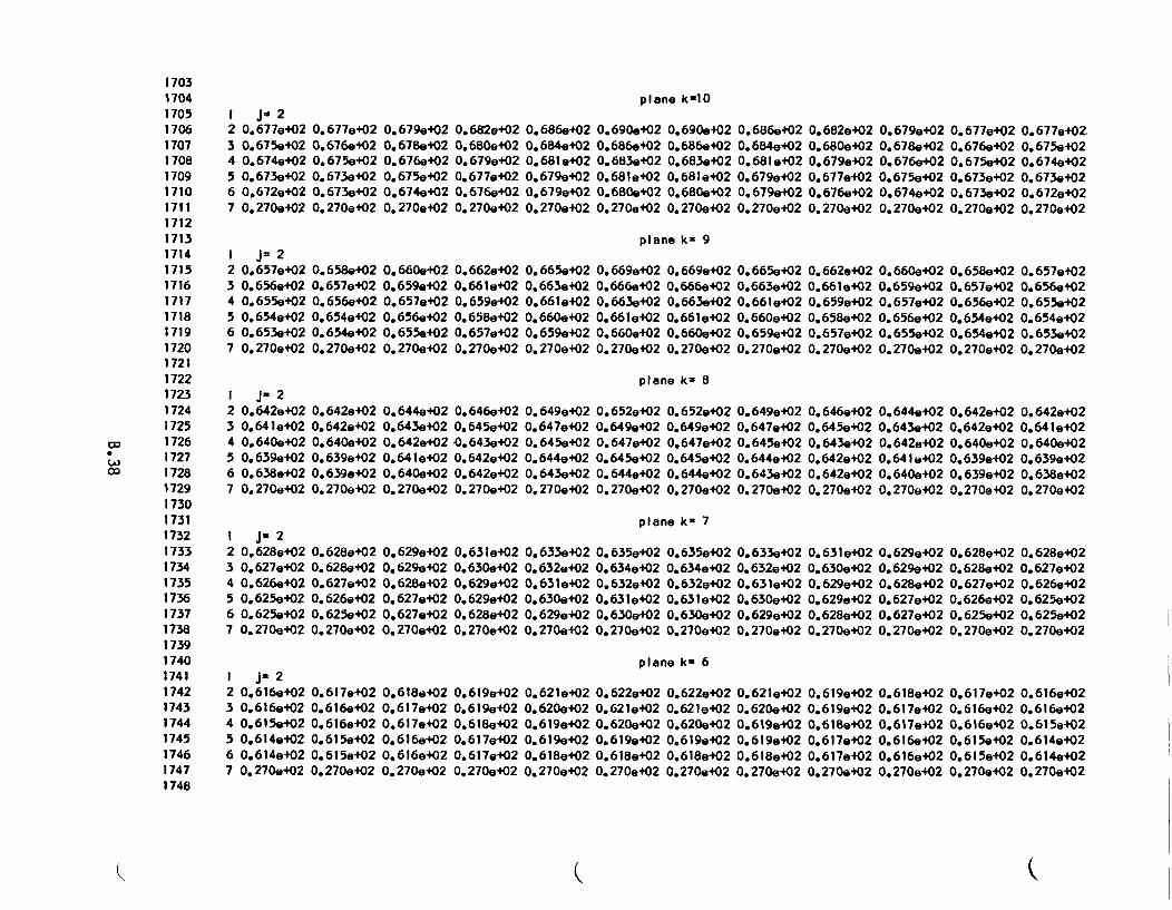
170317041705170617071708170917101711171217131714171517161717171817191720172117221723172417251726
*) 172700 1728
17291730173117321733173417351736173717381739174017411742174317441745174617471748
plane kl10I J 22 0.677e+02 0.677e+02 0.679e+023 0.675e+02 0.676.+02 0.678e+024 0.674e+02 0.675e+02 0.6769+025 0.673e+02 0.673e+02 0.675e+026 0.672e+02 0.673e+02 0.674e+027 0.270e+02 0.270e+02 0.2709+02
0.682e+02 0.686e+02 0.690e+02 0.690.+020.680e+02 0.684e+02 0.686e+02 0.686.+020.679e+02 0.681.+02 0.683e+02 0.683e+020.677,+02 0.679e+02 0.681e+02 0.681e4020.676.+02 0.679e+02 0.680.402 0.680e+020.2709+02 0.270e+02 0.270e+02 0.270e+02
0.686e+020.684e+020.681 e+020.679,+020.679e+020.270e+02
0.682e+020.680e+020.679e+020.677e+020.676e+020.270e+02
0.679e+020.678e4020.676.+020.675e+020.674e+020.270e+02
0.677e+020.676e4020.675e+020.673e+020.673e+020.270e+02
0.677e+02.0.675e+020.674e+020.673e+020.672e+020.270e+02
plane km 9I J=22 0.657e+02 0.658e+02 0.660e+02 0.662,+02 0.665e+02 0.669e+023 0.656e+02 0.657e+02 0.659e+02 0.661e+02 0.663e+02 0.666e.024 0.655e+02 0.656e+02 0.657e+02 0.659e+02 0.661e+02 0.663e+025 0.654e+02 0.654e+02 0.656e+02 0.658e+02 0.660.+02 0.661e+026 0.653.+02 0.6549+02 0.655e+02 0.657,+02 0.659e+02 0.660e+027 0.270e+02 0.270e+02 0.270e+02 0.270.402 0.270e+02 0.270e+02
0.669e+020.666e+020.663e+020.661e+020.660e+020.270e+02
0.665e4020.663e+020.661e+020.660e+020.659e+020.270,+02
0.662e+020.661e+020.659e+020.658e+020.657e+020. 270e+02
0.660e+020.659e+020.657e+020.656e+020.655e+020.270e+02
0.658e+02 0.657e+020.657e402 0.656e+020.656e+02 0.655e+020.654e+02 0.6549+020.654.+02 0.6539+020.270e+02 0.270e+02
plane km 8I Ju22 0.642e+02 0.642e+02 0.6449+02 0.646.+02 0.649e+02 0.652e+023 0.641e+02 0.642e+02 0.643e+02 0.645e+02 0.647e+02 0.649e+024 0.640e+02 0.640e+02 0.642e+02 4.643e+02 0.645e+02 0.647,+025 0.639e+02 0.639,+02 0.641e+02 0.642e+02 0.644e+02 0.645e+026 0.638e+02 0.639,+02 0.6409+02 0.642e+02 0.643e+02 0.644e+027 0.270e+02 0.270e+02 0.270e+02 0.270e+02 0.270e+02 0.270e+02
0.652e+020. 649e+020.647e+020.645e+020.644,+020.270e+02
0.649e+020.647e+020.645.+020.644,4020.643e+020.270e+02
0.646e+02 0.644e+02 0.642e+02 0.642e+020.645e+02 0.643e+02 0.642e+02 0.641e+020.643e+02 0.642e+02 0.640e+02 0.640e+020.642e+02 0.641e+02 0.639e+02 0.639e+020.642e+02 0.640e+02 0.639e+02 0.638e+020.270e+02 0.270e+02 0.270e+02 0.270e+02
plane km 7I J- 22 0.628e+02 0.628e+02 0.629e+02 0.631e+02 0.633e+02 0.635e+023 0.627e+02 0.628.+02 0.629,+02 0.630.+02 0.632e+02 0.634e+024 0.626e+02 0.627,+02 0.628e+02 0.629,+02 0.631e+02 0.632e+025 0.625e+02 0.6269+02 0.627,+02 0.629e+02 0.630e+02 0.631e+026 0.625a+02 0.625e+02 0.627,+02 0.628e+02 0.629e+02 0.630e+027 0.270e+02 0.270e+02 0.270e+02 0.270e+02 0.270e+02 0.27Oe.02
0.635e+020.634e+020.632e+020.631e+020.630e+020.270e+02
0.633e+020.632e+020.631e+020.630e+020.629e+020.270e+02
0.631e+020.630e+020.629e+020.629e+020.628e+020.270e+02
0.629e+02 0.628e+02 0.628e+020.629e+02 0.628e+02 0.627e+020.628e+02 0.627e+02 0.626e+020.627e+02 0.626e+02 0.625e+020.627e+02 0.625e+02 0.625e+020.270e+02 0.2709+02 0.270e+02
plane km 6I j-22 0.616e+023 0.616e+024 0.615e+025 0.614e+026 0.614e+027 0.270e+02
0.617,+020. 616e+020.616,4020.615e+020. 615,+020. 270,+02
0.618,+02 0.619,+020.6179+02 0.619e+020.617e+02 0.618e+020.616e+02 0.617e+020.616e+02 0.617e+020.270,e02 0.270e+02
0.6214e+020.620e+020.619e+020.619e+020.618e+020.270e+02
0.622e+020.621,e+020.620e+020.619,+020. 618e+020.270e+02
0.622e+020.6214e+020.620e+020.619e+020.618e+020.270e+02
0.621e+020.620e+020.619e+020. 619e+020.618e+020.270e402
0.619e+02 0.618,+02 0.617e+02 0.616e+020.619,+02 0.617e+02 0.616e+02 0.616e+020.618,+02 0.6179+02 0.6169402 0.615,+020.617e+02 0.616e+02 0.615e402 0.614e+020.617,+02 0.616e+02 0.615e+02 0.614,+020.270e+02 0.270e+02 0.270e+02 0.2709+02
(.
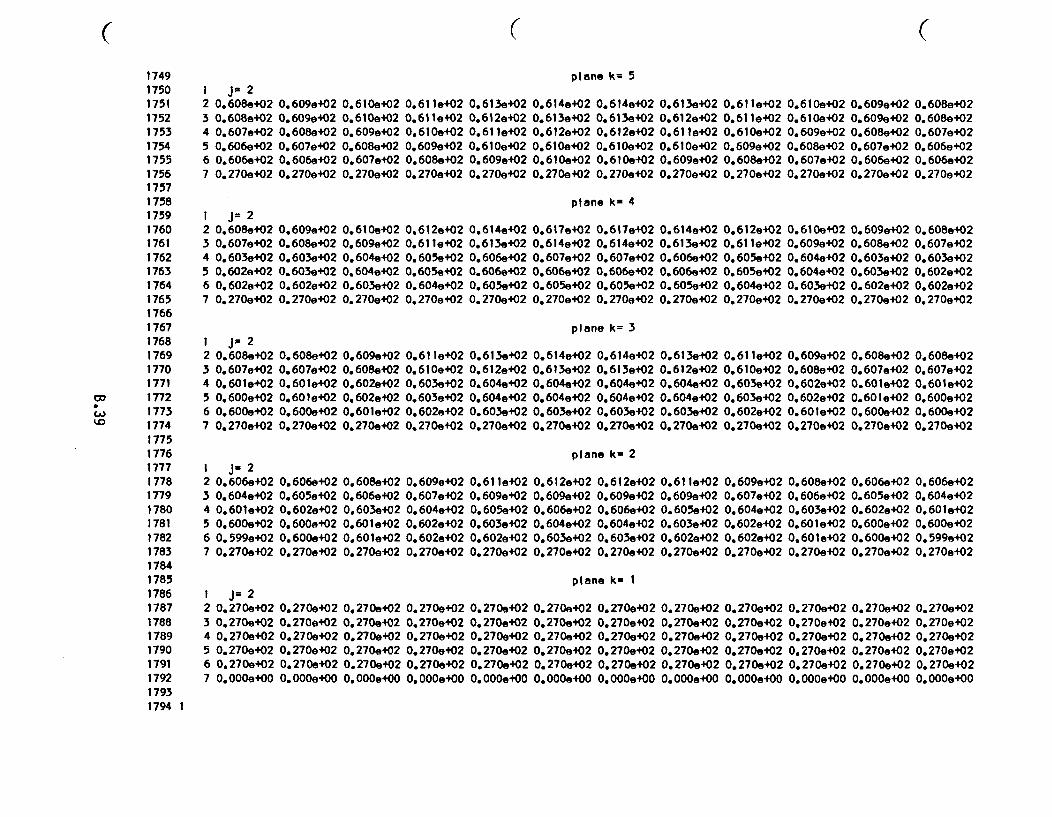
( ( (1749175017511752175317541755175617571758175917601761176217631764176517661767176817691770177117721773177417751776177717781779178017811782178317841785178617871788178917901791179217931794 1
plane k= 5I jm 22 0.6089+023 0.6089+024 0.607e+025 0.606e+026 0.606e+027 0.270e+02
I Jp22 0.608e+023 0.607e+024 0.603e+025 0.602e+026 0.602e+027 0.270e+02
I J- 22 0.608e+023 0.607e+024 0.601e+025 0.600e+026 0.600e+027 0.270e+02
I J-22 0.6069+023 0.604e+024 0.601e+025 0.600e+026 0.599e+027 0.270e+02
0.609,+020.609e+020.608e+020.607e+020.606.+020. 270,+02
0.610e+02 0.611,+02 0.613e+02 0.614e+02 0.6149+02 0.613e+020.610,t02 0.611e,02 0.612e+02 0.613e+02 0.613e+02 0.612e+020.609e+02 0.610e+02 0.611e+02 0.612e+02 0.612e+02 0.611e+020.6089402 0.609e+02 0.610e+02 0.610e+02 0.610e+02 0.610e4020.607e+02 0.608e+02 0.6099+02 0.610e+02 0.6109+02 0.609e+020.2 70e+02 0.270e+02 0.2 7 0e+02 0.270e+02 0.270e+02 0.270e+02
0.61 le+020.61 le+020. 61 Oe+020.6099+020.608e+020.270e+02
0.610.e+020.610.4020.609e+020.608e+020.607e+020.270e+02
0.609e+020.609e+020.608e+020.607e+020.606.+020.2 70e+02
0.608e+020.608e+020.607e+020.606e+020.606e+020.270e+02
plane k- 4
0.609,+020.608e+020.603e+020.603e+020.602e+020.270e+02
0.610e+02 0.612e+02 0.614e+02 0.617e+02 0.617,+02 0.614,4020.609e+02 0.611e+02 0.613e+02 0.614e+02 0.614e+02 0.613e+020.604e+02 0.605e+02 0.606.+02 0.607e+02 0.607e+02 0.606e+020.604e+02 0.605e+02 0.606,402 0.606e402 0.606.402 0.606.+020.6039+02 0.604e+02 0.605.+02 0.605e+02 0.605e+02 0.605.+020.270e+02 0.270e+02 0.270e+02 0.270e+02 0.270e+02 0.270e402
0.612e+020.611 e4O20.605e+020.605e+020. 604e+020.270e+02
0.610e+020.609e+020.604e+020.604e+020.603.+020.270e+02
0.609e+020.608e+020.603e+020.603e+020.602e+020.270e+02
0. 608e+020.607e+020.603e+020.602e+020.602e+020.270e+02
plane k= 3
0.608e+020.607e+020.601e+020.601e+020.600e+020.270e+02
0.609,+02 0.61 1e+02 0.613e+02 0.614e+02 0.614e+02 0.6139+020.608e+02 0.610e+02 0.612,+02 0.613,402 0.613e+02 0.612e+020.602,+02 0.603e402 0.604e+02 0.604e+02 0.604e+02 0.604e+020.602,402 0.603e+02 0.604e+02 0.604e+02 0.604e+02 0.604e+020.601e+02 0.602e+02 0.603e+02 0.603e+02 0.603.+02 0.603e+020.270e+02 0.270e+02 0.270e+02 0.270e+02 0.270e+02 0.2709+02
0.61 1e+020. 610e+020.603e+020.603e+020.602e+020.270e+02
0.609e+020.608e+020.602,+020.602e+020.601e+020.270e+02
0.608e+020.607e+020.601,+020.601e+020.600.+020.270e+02
0.608e+020. 607e,020.601e+020.600e+020.600e+020.270e+02
plane k= 2
0.606e+020.6054020.602e+020.600e+020.600.+020.270e+02
0.608e+020.606e+020.603.+020.601e+020.601,+020.270,+02
0.609e+020.607e+020.604e+020.602e+020.602e+020.270e+02
0.61 1e+020.609e+020.605e+020.603e+020.602e+020.270e+02
0.612e+02 0.612,+02 0.611e+02 0.609,+02 0.608e+02 0.606e+02 0.606e+020.609e+02 0.6099+02 0.609e+02 0.6079+02 0.606e+02 0.605e+02 0.604e+020.606e+02 0.606e+02 0.605.+02 0.604e+02 0.603e+02 0.602e+02 0.601e+020.604e+02 0.604e+02 0.603e+02 0.602e+02 0.601e+02 0.600e+02 0.600e+020.603,+02 0.603e+02 0.602e+02 0.602e+02 0.601e+02 0.6009+02 0.599e+020.270e+02 0.270e+02 0.270e+02 0.270e+02 0.270e+02 0.270e+02 0.270e+02
plane km II J=22 0.270e+02 0.270e+02 0.270.+023 0.270e+02 0.270e+02 0.270e+024 0.270.+02 0.2709+02 0.270.+025 0.270e+02 0.270,e02 0.270e+026 0.270.+02 0.2709+02 0.270e+027 0.000e+00 0.000e+00 0.000e+OO
0.270.+020.270e+020.270e+020.270e+020.270.4020.000,+00
0.270.+020.270e+020.270e+020.270e+020.270.4020. OOOe+OO
0.270.+020.270e+020.270.+020.270e+020.270e+020. OOOe+OO
0.270.+020.270e,020.270e+020.270e+020.270.+020.000,+00
0.270e+020.270e+020.270.+020.270e+020.2704+020.000,+00
0.270e+02 0.270.+02 0.270e+02 0.270e+020.270e+02 0.270e+02 0.270e+02 0.270e+020.270.+02 0.270e+02 0.270.+02 0.270.+020.270e+02 0.270e+02 0.270e+02 0.270,+020.2709+02 0.270e+02 0.270e+02 0.270.+020.000e+00 0.000e+00 O.OOOe4OO 0.000e+00
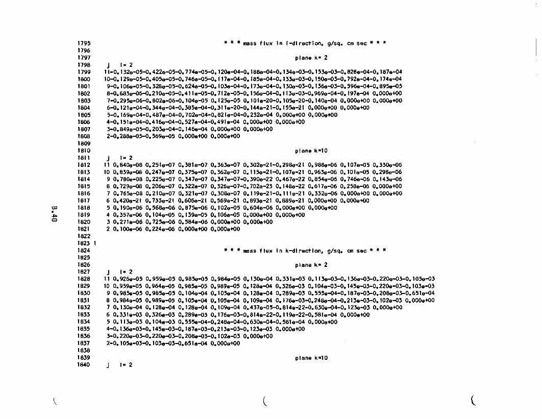
17951796179717981799t80018011802180318041805180618071808180918101811181218131814181518161817181818191820182118221823 118241825182618271828182918301831183218331834183518361837183818391840
* * * mass flux In 1-directlon, g/sq. cm sec * * *
plane km 2
J - 211-0. 132e-05-0.422e-05-0.774e-05-0.120e-04-0.188e-04-0.134e-03-0.153e-03-0.828e-04-0.187e-0410-0.129e-05-0.405e-05-0.746e-05-0.117e-0
4-0.185e-04-0.133e-03-0.150e-03-0.792e-04-0.174e-049-0.106e-05-0. 3 28e-05-0.624a-05-0.103e-04-0.173e-04-0.130e-03-0.136e-03-0.596e-04-0.895e-058-0.683e-06-0.21Oe-05-0. 4 1le-05-0.712e-05-0.156e-04-0.113e-03-0. 9 69e-0 4 -0.197e-04 0.0004e+07-0.295e-06-0.802e-06-0.10 4e-05 0.125a-05 0.10le-20-0.105e-20-0.140e-04 0.000e+00 0.0000e+06-0.121e-04-0.344e-04-0.385e-04-0.311 e20-0.144e-21-0.155e-21 0.000e+00 0.000.4005-0.169e-04 -0.487e-04-0.70 2e-04-0.821e-04-0.232e-04 0.000e+00 0.000+004-0.151e-04-0.416 e-0 4-0.527e-04-0.491e-04 0.000e+00 0.000e+003-0.849e-05-0.203e-04-0.146e-04 0.000e+00 0.000e+02-0.288e-05-0.569e-05 0.000e+00 0.000e+0
plane k=10J - 2
11 0.840e-08 0. 2 5le-07 0.381e-O7 0.363e-07 0.302e-21-0.298a-2110 0.839a-08 0.247e-07 0.375e-07 0.362e-07 0.115e-21-0.107e-219 0.780e-08 0.225e-07 0.347e-07 0.347e-07-0.390e-22 0.467e-228 0.729e-08 0.206e-07 0.322e-07 0.326e-07-0.702e-23 0.148e-227 0.765e-08 0.210e-07 0.321e-07 0.308e-07 0.1199-21-0.111e-216 0.420e-21 0.733e-21 0.606e-21 0.569e-21 0.893e-21 0.889e-215 0.190e-06 0.568e-06 0.875e-06 0.102e-05 0.604e-06 0.000.+004 0.357e-O6 0.104e-05 0.139e-O5 0.106e-05 0.000e+00 0.000,+003 0.271e-06 0.725e-06 0.584e-06 0.0004+00 0.000e+OO2 0.100e-06 0.224e-06 0.000e+00 0.000.e+0
0. 988e-060.963e-060.854e-060.617e-060.332e-060.OOOe+000.000+00
0.107e-050.101-050.1746e-060. 258e-060.000.+000.000.+00
0. 330e-060. 298e-060. 143e-060.000+4000.000.+00
* * * mass flux In k-direction, g/sq. cm sec * * *
plane km 2J 1. 211 0.926e-05 0.959e-05 0.985e-05 0.984.-05 0.130e-04 0.3319-03 0.113e-03-0.136e-03-0.220e-03-0.105e-0310 0.959e-05 0.964e-05 0.985e-05 0.989e-05 0.128e-04 0.326e-03 0.104e-03-0.145e-03-0.220e-03-0.103e-039 0.985.-05 0.985e-05 0.104e-04 0.105e-04 0.128e-04 0.289e-03 0.555e-04-0.187e-03-0.208e-03-0.651e-048 0.984e-05 0.989e-05 0.105e-04 0.105e-04 0.109e-04 0.176e-03-0.248e-04-0.213e-03-0.102e-03 0.000+007 0.130e-04 0.128e-04 0.128e-04 0.109e-04 0.437e-05-0.814e-22-0.630e-04-0.123e4-3 0.0000e+06 0.3319-03 0.326e-03 0.289e-03 0.176e-03-0.814e-22-0.119e-22-0.581e-04 0.0000e+05 0.113e-03 0.104e-03 0.555e-04-0.248e-04-0.630e-04-0.581e-04 0.0000e+04-0.136e-03-0.145e-03-0.187e-03-0.213e-03-0.123e-03 0.aOO0e+03-0.220e-03-0.220e-03-0.208e-03-0.102e-03 0.0000e+02-0.105e-03-0.103e-03-0.651e-04 0.aOOe+OO
plane k=10j 2
K
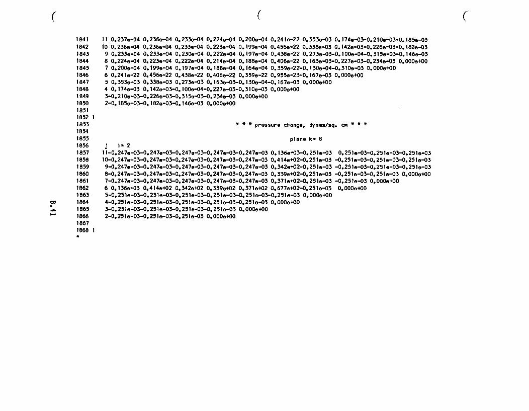
( ( (
184118421843184418451846184718481849185018511852 118531854185518561857185818591860186118621863
w 18641865186618671868 1*
11 0.237e-0410 0.236e-049 0.233e-048 0.224e-047 0.200e-046 0.24 1e-225 0.353e-034 0.174e-03
0. 236e-040,236e-040. 233e-040. 223e-040. 199e-040. 456e-220. 338e-03
0.233e-04 0.224e-04 0.200e-04 0.241e-22 0.353e-03 0.174e-03-0.210e-03-0.185e-030.233e-04 0.223e-04 0.199e-04 0.456e-22 0.338e-03 0.142e-03-0.226e-03-0.182e-030.230e-04 0.222e-04 0.197e-04 0.438e-22 0.273e-03-0.lOOe-04-0.315e-03-0.1 4 6e-030.222e-04 0.214 e-04 0.188e-04 0.406e-22 0.163e-03-0.227e-03-0.234e-03 0.OOOe+000.197e-04 0.188e-04 0.164e-04 0.359e-22-0.130e-04-0.310e-03 0.000e+000.438e-22 0.406e-22 0.359e-22 0.955e-23-0.167e-03 0.OOOe+000.273e-03 0.163e-03-0.130e-04-0.167e-03 0.OOOe+00
0.1 4 2e-03-0. 1OOe-04-0.227e-03-0.310e-03 0.OOOe+003-0.21 Oe-03-0.226e-03-0.315e-03-0.23 4e-03 0. OOOe+002-0.185e-03-0.182e-03-0.146e-03 O.OOOe+OO
* * * pressure change, dynes/sq. cm * * *
plane k= 8j 1i2
11-0.247e-03-0.247e-03-0.247e-03-0.247e-03-0.247e-03 0.136e+03-0.25 le-03 0.25 le-03-0.25 le-03-0.25 le-0310-0.247e-03-0.247e-03-0.247e-03-0.247e-03-0.247e-03 0.414e+02-0.251 e-03 -0.251 e-03-0.251 e-03-0.251 e-039-0. 2 47e-03-0.247e-03-0.247e-03-0.247e-03-0. 2 47e-03 0.342e+02-0.25 le-03 -0.25 le-03-0.25 le-03-0.251e-038-0.247e-03-0.247e-03-0.247e-03-0.247e-03-0.247e-03 0.339e+02-0.251 e-03 -0.25 1e-03-0.251 e-03 0. OOOe+007-0.247e-03-0.247e-03-0.247e-03-0.247e-03-0.247e-03 0.371 e+02-0.251 e-03 -0.25 le-03 0. OOOe+OO6 0.136e+03 0.414e+02 0.342e+02 0.339e+02 0.371e+02 0.677e+02-0.251e-03 0.000+005-0.251e-03-0.251e-03-0.25le-03-0.251e-03-0.251e-03-0.251e-03 0. OOOe+004-0.251e-03-0.251e-03-0.25 le-03-0.251 e-03-0.251 e-03 0.000e+003-0.251e-03-0.25 le-03-0.251e-03-0.25le-03 0. OOOe+002-0.251 e-03-0.251 e-03-0.251 e-03 0. OOOe+00
PNL-6206 Vol. IIUC-85
DISTRIBUTION
No. ofCopies
No. ofCopies
OFFSITE
77 DOE Technical Information Center
H. J. HaleU.S. Department of EnergyOffice of Civilian Radioactive
Waste ManagementRW-33Washington, DC 20585
L. BarrettU.S. Department of EnergyOffice of Civilian Radioactive
Waste ManagementRW-33Washington, DC 20585
J. EpsteinU.S. Department of EnergyOffice of Civilian Radioactive
Waste ManagementRW-32Washington, DC 20585
K. A. KleinU.S. Department of EnergyOffice of Civilian Radioactive
Waste ManagementRW-32Washington, DC 20585
D. E. ShelorU.S. Department of EnergyOffice of Civilian RadioactiveWaste Management
RW-32Washington, DC 20585
H. SteinburgU.S. Department of EnergyOffice of Storage and
Transportation SystemsRW-331000 Independence AvenueWashington, DC 20585
W. StringfieldU.S. Department of EnergyOffice of Civilian Radioactive
Waste ManagementRW-32Washington, DC 20585
J. S. FinucaneU.S. Department ofEnergy Information
Admini strationEI-53
Energy
Washington, DC 20585
M. FisherU.S. Department of EnergyIdaho Operations Office550 2nd StreetIdaho Falls, ID 83401
K. G. GolliherU.S. Department of EnergyAlbuquerque Operations OfficeP.O. Box 5400Albuquerque, NM 87115
C. J. DaukowskiU.S. Department of EnergyAttention: Defense ProgramsSan Francisco Operations Office1333 BroadwayOakland, CA 94612
Distr-1
No. ofCopies
No. ofCopies
C. MatthewsU.S. Department of EnergyOak Ridge National LaboratoryP.O. Box EOak Ridge, TN 37830
M. KunichU.S. Department of EnergyNevada Operations OfficeP.O. Box 14100Las Vegas, NV 89114
N. H. DavisonU.S. Nuclear Regulatory
Commi ssi onOffice of Nuclear Materials
Safety and SafeguardsWashington, DC 20555
C. FeldmanU.S. Nuclear Regulatory
CommissionOffice of Nuclear RegulatoryResearch
MS 1130-SSWashington, DC 20555
W. LakeU.S. Nuclear RegulatoryCommission
Office of Nuclear MaterialsSafety and Safeguards
MS 396-SSWashington, DC 20555
C. H. PetersonU.S. Nuclear RegulatoryCommission
Office of Nuclear MaterialSafety and Safeguards
MS 623-SSWashington, DC 20555
J. RobertsU.S. Nuclear Regulatory
CommissionOffice of Nuclear Material
Safety and SafeguardsMS 396-SSWashington, DC 20555
L. C. RuseU.S. Nuclear Regulatory
CommissionOffice of Spent Fuel
Storage InstallationDivision of Fuel Cycle and
Material SafetyWashington, DC 20555
J. A. CarrBattelle Memorial InstituteOffice of Nuclear Waste
Isolation505 King AvenueColumbus, OH 43201
Technical LibraryBattelle Memorial InstituteOffice of Nuclear Waste
Isolation505 King AvenueColumbus, OH 43201
L. J. JardineBechtel NationalPO. Box 3965San Francisco, CA 94119
R. KunitaCarolina IP.O. Box ]Raleigh, I
Power & Light1551NC 27602
I'o.
Inc.C. K. AndersonCombustion Engineering,1000 Prospect Hill RoadWindsor, CT 06095
Distr-2
No. ofCopies
T. GrantEbasco Services IncorporatedTwo World Trade CenterNew York, NY 10048
M. F. JensenEG&GP.O. Box 1625Idaho Falls, ID 83415
P. E. EggersEggers Ridihalgh Partners, Inc.1445 Summit StreetColumbus, OH 43201
FLUOR Engineers, Inc.Advanced Technology DivisionP.O. Box C-11944Santa Anna, CA 92711-1944
E. E. VoilandGeneral Electric CompanyNuclear Fuel & Services Division7555 E. Collins RoadMorris, IL 60450
R. AndersonGeneral Nuclear Services, Inc.135 Darling DriveAvon, CT 06001
W. R. JuergensBrooks and Perkins12633 Inkster RoadLivonia, MI 48150
L. B. BallouLawrence Livermore National
LaboratoryP.O. Box 808Livermore, CA 94550
M. W. SchwartzLawrence Livermore National
LaboratoryP.O. Box 808Livermore, CA 94550
No. ofCopies
C. E. WalterLawrence Livermore National
LaboratoryP.O. Box 808Livermore, CA 94550
H. LowenbergLowenberg Associates10901 Rosemont DriveRockville, MD 20852
J. HoustonNuclear Assurance Corporation5720 Peach Tree ParkwayNorcross, GA 30092
R. T. HaelsigNuclear Packaging Inc.1010 S. 336th StreetFederal Way, WA 98003
L. E. WilesNumerical Applications,825 Goethals DriveRichland, WA 99352
Inc.
B. LehnertNUTECH Engineers145 Martinvale LaneSan Jose, CA 95116
C. V. ParksOak Ridge National LaboratoryP.O. Box XOak Ridge, TN 37831
D. WoodsRalph M. Parsons Co.100 West Walnut StreetPasadena, CA 91124
J. V. MasseyReedy and Associates103 Albright WayLos Gatos, CA 95030
Distr-3
No. ofCopies
No. ofCopies
T. L. SandersSandia NationalAlbuquerque, NM
Laboratory87115
M. E. MasonTransnuclear, Inc.1 N. BroadwayWhite Plains, NY 10601
TRW Exploration/PROP.O. Box 441807Houston, TX 77244-1807
C. E. KingUranium Mgt. Corp.175 Curtner Ave. MC 620San Jose, CA 95125
M. L. SmithVirginia Electric Power Co.P.O. Box 26666Richmond, VA 23261
K. L. BasehoreVirginia Electric and Power Co.Power Station EngineeringThe Electric BuildingP.O. Box 5647th and FranklinRichmond, VA 23204
D. L. LarkinWashington Public Power Supply
SystemP.O. Box 968Richland, WA 99352
R. 0. AndersonNorthern States Power Company15 S. 15th StreetMinneapolis, MN 55401
G. SwindlehurstDuke Power CompanyP.O. Box 33189422 S. Church StreetCharlotte, NC 28242
D. HamiltonMiddle South Services, Inc.Box 61000New Orleans, LA 70161
G. R. BondManager, Nuclear FuelsGeneral Public Utilities, NUC100 Interpace ParkwayParsippany, NJ 07054
J. R. RatliffTennessee Valley Authority409 Krystal BuildingChattanooga, TN 37401
B. RiceTexas Utilities Generating Co.Skyway Tower400 North Olive StreetLD81Dallas, TX 75201
H. E. BlissNuclear Fuel ServicesCommonwealth Edison72 West Adams StreetP.O. Box 767Chicago, IL 60690
R. T. HarrisNortheast UtilitiesP.O. Box 270Hartford, CN 06101
A. LadieuYankee Atomic Electric Company1671 Worcester RoadFramingham, MA 01701
D. S. RoweRowe and AssociatesSuite 2002050 112th Avenue NEBellevue, WA 98007
Distr-4
No. ofCopies
No. ofCopies
Y. HsiiDivision of Systems IntegrationOffice of Nuclear RegulationU.S. Nuclear Regulatory
CommissionWashington, DC 20555
L. PhillipsDivision of Systems IntegrationOffice of Nuclear RegulationU.S. Nuclear Regulatory
CommissionWashington, DC 20555
L. AgeeElectric Power Research
InstituteP.O. Box 10412Palo Alto, CA 94303
R. LambertElectric Power Research
InstituteP.O. Box 10412Palo Alto, CA 94303
G. S. SrikantiahElectric Power Research
InstituteP.O. Box 10412Palo Alto, CA 94303
R. RiceEG&G Idaho, Inc.P.O. Box 1625Idaho Falls, ID 83415
C. R. BolmgrenWestinghouse Electric Corp.Nuclear Waste DepartmentP.O. Box 3912Pittsburgh, PA 15230
D. KleinMechanical Engineering
DepartmentUniversity of TexasAustin, TX 78712
B. A. ChinMechanical Engineering Dept.247 Wilmore LabsAuburn UniversityAuburn, AL 36849
ONSITE
4 DOE Richland Operations Office
J. P. CollinsD. E. CrouterM. S. KarolD. L. Oleson
3
42
Westinghouse Hanford Company
C. L. BrownG. T. HarperR. E. Stover
Pacific Northwest Laboratory
G. H. BeemanD. J. BradleyJ. L. BraitmanJ. M. CutaJ. M. Creer (5)L. R. DoddR. E. EinzigerM. D. FreshleyC. M. HeebA. B. Johnson, Jr.B. M. JohnsonL. T. LakeyD. L. LessorN. J. LombardoP. S. LoweryR. A. McCann (10)T. E. MichenerD. R. RectorC. W. StewartR. A. StokesD. S. TrentC. L. WheelerTechnical Report Files (5)Publishing Coordination (2)
Distr-5
Related Documents