Hybrid Velocity/Force Control for Robot Navigation in Compliant Unknown Environments Dushyant Palejiya and Herbert G. Tanner Abstract We combine a “hybrid” force/position control scheme with a po- tential field approach into a novel method for collision recovery and navigation in unknown environments. It can be implemented both on manipulators and mobile robots. The use of force sensors allows us to locally sense the environment and design a dynamic control law. Mul- tiple Lyapunov functions are used to establish asymptotic stability of the closed loop system. The switching conditions and stability criteria are established under reasonable assumptions on the type of obstacles present in the environment. Extensive simulation results are presented to illustrate the system behavior under designed control scheme, and verify its stability, collision recovery and navigation properties. 1

Welcome message from author
This document is posted to help you gain knowledge. Please leave a comment to let me know what you think about it! Share it to your friends and learn new things together.
Transcript
Hybrid Velocity/Force Control for Robot
Navigation in Compliant Unknown
Environments
Dushyant Palejiya and Herbert G. Tanner
Abstract
We combine a “hybrid” force/position control scheme with a po-
tential field approach into a novel method for collision recovery and
navigation in unknown environments. It can be implemented both on
manipulators and mobile robots. The use of force sensors allows us to
locally sense the environment and design a dynamic control law. Mul-
tiple Lyapunov functions are used to establish asymptotic stability of
the closed loop system. The switching conditions and stability criteria
are established under reasonable assumptions on the type of obstacles
present in the environment. Extensive simulation results are presented
to illustrate the system behavior under designed control scheme, and
verify its stability, collision recovery and navigation properties.
1

1 Introduction
1.1 Motivation and Overview
We address the problem of steering a redundant manipulator or a mobile
robot inside partially unknown environment. The environment is assumed to
contain compliant objects and the robot is required to use only its force/torque
sensors in order to navigate. Motivation for this approach comes primarily
from the need for coping with uncertainty in robotic search and rescue op-
erations. Contrary to the case of industrial environments, where the envi-
ronment can be structured and regulated, in calamity situations uncertainty
prevails. when a robotic snake or a tethered mobile robot dives into pile
of debris, there is little hope of getting gps signals, getting enough light for
image processing, or using ultrasound sensors in such confined environments.
In such cases, most perception mechanisms fail, and robots could be forced
to adopt the approach of one “walking in the dark,” touching surrounding
objects toward the destination. Then convergence (which can be understood,
for instance, as the robot reaching humans trapped under ruins or collapsed
mine tunnels in finite time), is more important than protecting the hardware
from collisions with the environment.
A challenging aspect of the problem at hand is that it consists of two
different and equally difficult subproblems: the robot should plan and control
its motion, and recover from unexpected (or avoid expected) collisions with
objects. In the latter case, such objects may not be considered compliant
when compared to, say, cardboard, but wood or plaster will definitely be
more compliant than steel. Our approach is to bring together two different
2

methodologies, each coping with one of these two particular subproblems,
into a single, coherent, and provably convergent robot control scheme.
The control scheme we present in this paper is hybrid. It combines a com-
ponent that aligns the robots velocity along the field produced by an artifi-
cial potential function, with a component that regulates contact force, using
measurements provided by a force/torque sensor. Besides controlling veloc-
ity, instead of position, our hybrid scheme is different from what is widely
known as “hybrid force/position control,” introduced in35; the proposed hy-
brid scheme has two distinct modes of operation, and there is intermittent
switching between the two, when specific conditions (guards) are satisfied.
Not only do we have different closed loop dynamics different in each mode,
but the state vectors are also different.
The contribution of this work is the use of force sensors for robot navi-
gation in an unknown environment, offering guarantees of convergence to a
desired configuration and recovery from collisions. We regard collisions not
as undesirable events, but as opportunities to learn about the environment
and discover a path that will bring the system closer to its goal. Our stability
analysis not only ensures that the system will recover safely, but that it will
also reach its destination, if a feasible path exists and the physical limitations
of the mechanism are not exceeded.
1.2 Related Work
Hybrid systems30,3 are characterized by the interaction of continuous dy-
namics and discrete-valued dynamics. Typically, the continuous dynamics
describes the system at a detailed concrete level, while some discrete logic
3

(utilizing both discrete and continuous variables) regulates the system at a
higher level. Ensuring stability in hybrid systems (especially during switch-
ing) is very important, since it is well known that switching between stable
systems can result to instability25. There is considerable work in the area of
stability for hybrid systems25, and one of the prevailing techniques is that
of multiple Lyapunov functions4. This is the method of choice for us to
establish the stability of our hybrid control scheme.
In the robotics literature, “hybrid force control” typically refers to the
superposition of position and force control signals, in an approach initially
proposed by35. Hybrid position/force controllers partition the task-space
into position controlled directions and force controlled directions using nat-
ural constraints. The latter is a concept introduced in Reference31: along
the normal directions of these surfaces, the velocity is zero (position con-
straint), while the force is zero along tangential directions (force constraint).
Specifying a desired velocity along an unconstrained direction and/or a de-
sired force along a constrained direction gives rise to an artificial constraint.
The basic idea of the hybrid force/position approach is to enforce only the
artificial constraints. Reference8 raised questions about the orthogonality as-
sumption between position and force controlled subspaces. Literature is rich
with extensions of the original hybrid force/position scheme that modify the
orthogonality condition and improve the overall system performance, such as
the Dynamic Hybrid Force/Position Control 43, the Operational Space Con-
trol 15, the Hybrid Impedance Control 41, and the Hybrid scheme with force
sensor 10.
The latter approach10 utilizes force sensor measurements to partition the
4
workspace into force and position controlled directions. The controller of The
parallel force/position control 6,38 combines the force and position controller
into a single control law, so that unpredicted contact forces are accommo-
dated. The parallel scheme has inspired in part our approach. Our original
ambition was to extend this methodology so that motion planning can be
done within the control loop. However, we had to abandon the idea of com-
bining the motion (velocity) and force controller into a single construction
because of stability concerns.
Besides force sensors, other sensors such as sensitive skins28, vision9
and strain gauges1 are also used for collision detection. Given an accurate
robot dynamics model, it is possible to detect collision by comparing the
actual torque (based on actuator currents) with the model-based calculated
torque39. The authors in27 use an approach for collision detection that relies
on the robot dynamical model, without making use of sensors. However,
since the exact magnitude and the direction of the contact force cannot be
identified, the obstacle location cannot be determined.
The problem of navigating in an unknown environment is first addressed
in29, with application to mobile robots, without addressing the issue of inte-
grating path-planning to lower level robot control. Behavior based control5,2
is an another approach for robot navigation in unstructured environments,
where a specific behavior is reactively selected from a pre-defined set based on
sensor information.44 have combined fuzzy logic controllers with such reactive
behavioral schemes19,21,23, to provide a smooth transition between different
behaviors and prevent unstable oscillations, and integrate multiple sensors20.
Low-level reactive control is combined with high-level path-planning by22 us-
5
ing a neural network.
An inherent limitation of reactive approaches is that it is extremely diffi-
cult to predict the overall system behavior resulting from the superposition
of several elementary behaviors. Navigation functions36, however, produce
artificial potential fields which do not have from local minima, a known limi-
tation of the original potential field method16, and can therefore offer formal
convergence guarantees. Performance comes at a price, and the assumption of
a perfectly known environment prevents the direct application of this method
to the problem at hand. To address this issue, article26, presents a kinematic
controller based on a navigation function, which could steer a mobile robot
in unknown environments using range sensors. The controller switches when
an obstacle is detected. Our approach is along this line of thought, with the
difference being that instead of using range sensors, the robot will have to
physically touch the obstacle and recover from the collision.
2 Problem Statement and Assumptions
We seek a control scheme that can be applied to planar mobile robots and
redundant manipulators equipped with the force sensors, alike. This control
law should enable the robot to:
• Converge to the destination configuration, and
• Regulate contact forces while navigating amongst known and unknown
obstacles.
6

The robot is assumed to be described by dynamic equations of the form:
M(x)x + C(x, x)x + G(x) = u − f, (1)
where x ∈ R2 is the vector of the mobile robot’s or the manipulator’s end
effector position; M(x) ∈ R2×2 is the inertia matrix; C(x, x) ∈ R
2×2 is the
matrix of Coriolis and centrifugal force terms; G(x) ∈ R2 is the vector of
gravitational terms; u ∈ R2 is the input force vector, and f ∈ R
2 is the
force applied to the end effector or to the mobile robot’s surface by the
environment. The reason why we restrict the present analysis to the planar
case will be explained in Section 3.3.
Given destination configuration xD in the task-space of a robot, the dy-
namics of which are given by (1), we need to find a feedback control law u(x)
such that:
• the robot approaches xD asymptotically from almost1 all initial config-
urations if xD is reachable, and
• the contact forces are bounded to a desired level.
We assume that the robots can obtain force measurements by means
of force/torque sensors. A mobile robot is assumed to have a force sensor
behind its front bumper. A manipulator is supposed to have a force sensor
at its end effector. In the latter case, note that collisions can occur between
intermediate arm links and obstacles, even if no force is measured at the end
effector. This is an inherent limitation, resulting from our assumption that
the robot uses a single force sensor. Future extensions of this work include
1The word “almost” allows the exclusion of a subset of the space with measure zero.
7

modifications to the navigation scheme, so explored workspace safety is taken
into account in motion planning.
The obstacles in the environment are assumed to occupy compact regions
of the workspace, and their surface is smooth with no sharp edges. Mobile
robots, on the other hand, are assumed as point objects. Sphere approxima-
tions of mobile robots shapes can be directly accounted for by “growing” the
obstacles by the corresponding radius18. Manipulators are represented in the
workspace as a series of control points along their links. In this approach,
collisions between manipulator links and obstacles are in theory possible; a
more thorough approach to real-time collision avoidance for multi-link mech-
anisms, has to take into account the whole volume of the robot42. It is
possible to use a formulation such as the one described by42 with the pro-
posed approach, but this is beyond the scope of this work. Our focus here is
on control design and stability. Any improvement on the collision prediction
component of our strategy will only bring benefits in terms of safety.
3 Force/Potential Field Control
Given a fairly accurate model of the system, (1) can be transformed into
those of a linear second order system:
x = us, (2)
by means of a feedback linearizing input:
u = M(x)us + C(x, x)x + G(x) + f, (3)
8
Initial configuration
Obstacle
Goal configuration
Obstacle
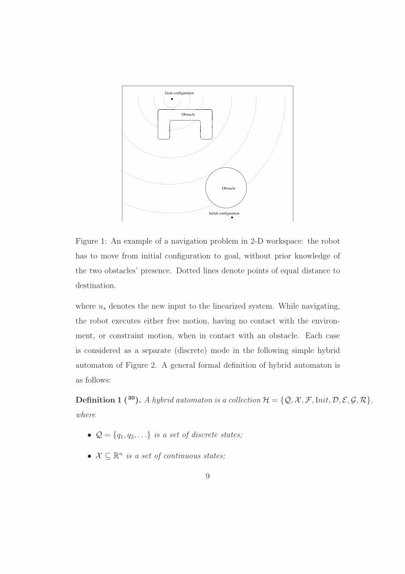
Figure 1: An example of a navigation problem in 2-D workspace: the robot
has to move from initial configuration to goal, without prior knowledge of
the two obstacles’ presence. Dotted lines denote points of equal distance to
destination.
where us denotes the new input to the linearized system. While navigating,
the robot executes either free motion, having no contact with the environ-
ment, or constraint motion, when in contact with an obstacle. Each case
is considered as a separate (discrete) mode in the following simple hybrid
automaton of Figure 2. A general formal definition of hybrid automaton is
as follows:
Definition 1 (30). A hybrid automaton is a collection H = {Q,X ,F , Init,D, E ,G,R},
where
• Q = {q1, q2, . . .} is a set of discrete states;
• X ⊆ Rn is a set of continuous states;
9

no−contact contact
modemode
Gnc = true
Gc = true
Figure 2: The hybrid system describing the closed loop dynamics of the
system. The predicates Gnc and Gc correspond to the guards on the no-
contact and contact modes, respectively, that force transitions. Part of the
control design problem is to define Gnc and Gc.
• F(·, ·) : Q×X → Rn is a vector field;
• Init ⊆ Q× X is a set of initial states;
• D : Q → P (X ), is a domain;
• E ⊆ Q×Q is a set of edges;
• G : E → P (X ) is a guard;
• R : E × X → P (X ) is a reset map.
The set P (·) denotes the power set (set of all subsets). We refer to (q, x) ∈
Q× X as the state of H.
10

3.1 No-Contact Mode
During free motion, the robot follows the negated gradient of a navigation
function, constructed on the known workspace. To account for the non-
point, multi-link structure of the manipulator, we define control points along
its links. Proximity of the robot to obstacles is assessed by considering all
distances between control points and workspace obstacles. Our navigation
function has the following form17
φ =γ(x)
exp(β(x)1/κ). (4)
The terms involved in the above expression are defined as follows:
• Function β is the product of several functions,
β =∏
c=1,...,po=0,...,q
βco, (5)
each encoding the proximity between a control point on the system c,
and a known obstacle o. These functions are given as17 βco = (1 −
λ (‖xc−xo‖2−d2)4
(‖xc−xo‖2−d2)4+1)
sign(d−‖xc−xo‖)+12 , with d being the distance to which the
presence of the obstacle is being “felt” by the robot, and λ = 1+d8
d8 .
The workspace boundary is taken into account as an additional obstacle
(obstacle 0) and is expressed as βc0 = (1−λ (‖xc‖−R)2−d2)4
(‖xc‖−R)2−d2)4+1)
sign(d−(R−‖xo‖))+12 .
The part of the workspace occupied by obstacles is defined as B , {xc ∈
R2 | β(xc) ≤ 0}.
• Function γ is a nonnegative function that encodes the proximity to the
destination configuration, γ(x) = ‖x − xD‖2.
11
• Parameter κ is a tuning constant, which is adjusted based on the geom-
etry of the (known) workspace according to17, to make (4) a navigation
function.
Obstacle functions are equal to one in the region where ‖xc−xo‖ > d, thus
making the effect of obstacles local. Thus, obstacle points can potentially be
included “on the fly” into the navigation function, and the tuning parameter
κ can be adjusted accordingly, without having to change the structure of ϕ.
The potential field based controller used for steering the robot during the
no-contact phase of its motion is given as:
us = −KDx −∇φ, (6)
where −∇φ is the negative gradient of (4), and KD > 0 is the gain of the
viscous damping term.
3.2 Contact Mode
When a collision between the robot and an obstacle occurs, contact forces
are exerted by the obstacle to the robot, which are assumed normal to the
obstacle surface. A force sensor measures the contact forces along different
directions: −f = [f1, f2]T . The force that the robot exerts on the the object
can be expressed compactly as f = fη, where f , ‖f‖ is the measured
force’s magnitude, and η , −1ff for f 6= 0 denotes the direction, normal to
the obstacle’s surface, along which the robot exerts a force. A tangential
direction is chosen to form an orthonormal basis in R2: τ ∈ span(η)⊥, and
[η, τ ] ∈ SO(2). This coordinate frame will be called the constraint frame.
12

X
Xo
f
Figure 3: Force exerted to the obstacle surface resulting to local deformation
according to the contact model (7).
We adopt a linear spring contact model, which describes an obstacle as a
compliant, frictionless surface:
f = K(x − x0) (7)
where x ∈ R is the position of the contact point along η, x0 ∈ R is the
position, along η, the contact point would have if the obstacle surface were
undeformed, and K ∈ R is the stiffness constant of the surface. High ob-
stacle stiffness allows us to neglect local deformations at the contact point.
Equation (7) applies along the normal to the surface direction.
Figure 3 shows the contact force due to surface deformation. The com-
pliant contact model (7) is used to express the desired contact force, fd:
fd = K(xfd− x0), (8)
where xfd∈ R is the position of the end effector along η, producing the
desired contact force fd according to (7). Combining (7) with (8):
∆f = fd − f = K(xfd− x). (9)
13

The control law for the contact mode is defined as follows40:
us = − KDx︸︷︷︸
damping
+ KDvd τ︸ ︷︷ ︸
velocity feedforward
+ KF ∆f η + KI
∫ t2
t1
∆f dσ η
︸ ︷︷ ︸
force control
, (10)
where vd is a constant reference speed in the tangential direction. The limits
of the integral t1, and t2 are the time instants when the contact was initiated
and terminated, respectively. Parameters KD, KF , and KI are positive scalar
feedback gains.
Along the normal direction η, the control law (10) attempts to stabilize
the contact force to the reference fd. A nonzero f maintains contact between
the robot and the obstacle is maintained. Along the tangential direction τ
the feedforward and damping terms, form a PD velocity controller, which
stabilizes the end effector velocity x to the reference vd.
3.3 Switching Conditions
The detection of a nonzero contact force marks the transition from free mo-
tion to contact with an obstacle. This event forces a control law switch, from
(6) to (10), to alleviate the effects of the collision. The transition to free
motion, however, cannot be arbitrary because the stability may be affected.
Let us denote xh the point on the obstacle boundary where contact is
initiated. Let xe be the point at which the transition from contact-mode
control to no-contact-mode control is to take place. The (forced) “guard”
that triggers the transitions from contact to no-contact will include:
(φ(xe) ≤ φ(xh)) ∧ (−∇φ(xe)Tη < 0). (11)
14

η
η
−∇φ
−∇φ
xD
xe
xh
Figure 4: The contact entry and exit points, xh and xe, on obstacle’s surface,
and relative alignment with the potential field gradient.
The first condition in (11) ensures that the system’s configuration at xe
is “closer” to the destination than the configuration xh where contact was
initiated (as measured by the potential function φ). Thus, each time the
system is reset to no-contact mode, the value of φ is decreased compared to
all values φ has obtained previously during free motion. The second condi-
tion requires that the obstacle surface normal is (partially) aligned with the
direction for free motion, −∇φ. This will indicate that the obstacle is not
obstructing the path to destination (at least locally), and that the system can
move in the free space for at least some minimum (dwell) time before switch-
ing back to contact mode. The condition, illustrated in Figure 4, eliminates
the possibility of Zeno executions in the hybrid system.
For the class of obstacles considered, the transition from contact to no-
contact mode happens in finite time:
15

Proposition 1. In a two-dimensional workspace, a system (2) under control
law (10) will satisfy Gc in finite time.
Proof. The control law (10) forces the system to slide continuously, along a
curve c(t) on the obstacle’s boundary. Since each obstacle defines a compact
set, B, its boundary ∂B and any continuous curve on it, c(t) ∈ ∂B, is also
compact. The continuous function φ will therefore assume a minimum value
φ(xb) at c(t) = xb. Sliding along the obstacle boundary with a nonzero speed,
the robot will eventually reach xb, satisfying the first condition in (11). Note
that xb minimizes φ globally on B, because the destination is not covered by
the obstacle – otherwise it would be unreachable. If −∇φ pointed inward
at xb, there would be points in B with smaller values of φ than φ(xb); a
contradiction. Therefore, −∇φ points outward at xb. Since η points inward,
(η is the direction along which the robot exerts a force on the obstacle), we
will have −∇φ(xb)T η(xb) < 0. Thus at xb, the second inequality in (11) will
also be satisfied.
3.4 Redundancy Resolution in Contact Mode
In the control schemes of the previous sections, only the task space coor-
dinates of the systems are being controlled. Depending on the degree of
redundancy, the system may possess additional degrees of freedom. In this
section, redundancy is exploited so that links of the redundant manipula-
tor avoid collisions with known (or newly discovered) obstacles. We need
to meet two objectives: (i) maintain contact between the end effector and
the obstacles; (ii) avoid contact between the arm links and already detected
obstacles. Simultaneously satisfying both objectives may be infeasible, and
16

therefore they have to be prioritized. In this approach, maintaining contact
between end-effector and obstacle is assigned higher priority, since the focus
is on convergence of the robot to the destination. The task-space acceleration
x can be written in terms of joint space coordinates θ as x = Jθ + J θ, where
θ ∈ Rn and θ ∈ R
n are joint space acceleration and velocity, respectively,
and J ∈ R2×n is the manipulator’s Jacobian, which is a function of θ.
It is well known33,11 that redundancy resolution schemes resolved at the
acceleration level, can cause divergence and instability because of built-up of
joint space velocities. We circumvent this problem by including an integrator
in our task space control law (10), to generate reference task space velocities
xd, instead of accelerations:
xd =
∫ t2
t1
[
−KDx + KDvd τ +
(
KF ∆f + KI
∫ t2
t1
∆f dσ
)
η
]
dt. (12)
Now the task space reference velocity xd is given in joint space coordinates
using the general solution involving the pseudoinverse32 of J , J†:
θd = J†xd + (I − J†J)h, (13)
where (I − J†J) is the projection matrix to the null space of J , and h is a
vector utilized to encode the secondary objective:
h = Ko∂β(x)
∂θ, (14)
where β(x) is the obstacle function defined in (5) and Ko is the positive gain.
The reference joint space acceleration is now defined as:
θd = J†(xd − J θd). (15)
17

The manipulator torques needed to realize this reference acceleration is:
T = M(θ)(θd + Kvj(θd − θ)) + C(θ, θ)θ + G(θ) + JT f,
where Kvj is the positive gain, yielding the closed loop joint space dynamics:
(θd − θ) + Kvj(θd − θ) = 0. (16)
4 Continuous Closed Loop Dynamics
4.1 Contact Mode
Using (9), the closed loop system during contact (10) is expressed in standard
state-space form:
x1
x2
x3
︸ ︷︷ ︸
y
=
0 −ηT 0
KF Kη −KD KIKη
1 0T 0
︸ ︷︷ ︸
A
x1
x2
x3
︸ ︷︷ ︸
y
, (17)
where 0 denotes the (3×1) vector of zeros. Symbols x1, x3, and x2 express the
coordinates of a (4×1) state vector y. They are given as x1 , xfd−x, the force
error translated into displacement through the contact model; x2 , x−vd τ ,
the velocity error; and x3 ,∫ t2
t1x1 dσ, the force error integral.
Equation (17) describes the closed loop system in the case of mobile
robots, but for robotic manipulators redundancy resolution imposes different
dynamics on the task and joint spaces. The task-space control law defined
in (10) ensures that contact between the robot and the obstacle is main-
tained; the joint-space control law (16) implements (10) by performing col-
lision avoidance in the null space of the manipulator’s Jacobian. Combining
18

(16), (10) yields the closed loop system dynamics:
x1
x2
x3
=
0 −ηT 0
KFKη −KD KIKη
1 0T 0
x1
x2
x3
+
0
Kvj(θd − θ)
0
(18)
θd = J†(xd + vdτ) + (I − J†J)h,
where xd and h are given by (12) and (14), respectively. Equation (18)
describes the dynamics of a linear system that is perturbed by the term
Kvj(θd − θ). As a prelude of what follows, we will regard this term as a
perturbation term, that will be made to converge to zero sufficiently fast.
4.2 No-Contact Mode
In no-contact mode, no force-related state variables are defined. Since there
is no contact, fd = 0 and therefore x ≡ x2. Equations (3), (6) yield the
following closed loop system:
x2 = −KDx2 −∇φ(x) (19)
5 Stability Analysis
Lyapunov stability theory for switched systems imposes conditions not only
on each admissible dynamics, but also on the switching signal25,4,13,12. This
Section refines the switching conditions of Section 3.3 to establish the stabil-
ity of the hybrid system defined in Section 3. We follow a multiple Lyapunov
function approach.
19

5.1 Contact Mode
The following proposition states that the (unperturbed) closed loop dynamics
of the contact mode (that is, equation (17)) is exponentially stable:
Proposition 2. There exists a choice of gains KD, KF , KI that makes the
origin of the system (17) exponentially stable.
Proof. Consider the Lyapunov function candidate for (17) :
Vc =1
2yTPy, (20)
where P is the symmetric matrix defined as:
P ,
KD + KFK − 1 −ηT KIK + KD
−η I −η
KIK + KD −ηT KIK + KFK
, (21)
and KD, KF , K are positive scalars. Expanding (20):
Vc =1
2[ x1x2 ]T
[KD−1 −ηT
−η 12I
]
[ x1x2 ] +
K
2[ x1x3 ]T
[KF KI
KI KI
][ x1x3 ] +
1
2[ x2x3 ]T
[12I −η
−ηT KF K
]
[ x2x3 ] .
(22)
If we assume that
KD > 2λmax + 1 = 3, KF > KI +KD
K, KF >
2
K, (23)
where λmax = 1 is the maximum eigenvalue of ηηT , then each matrix in (22)
will be positive definite. Then there will be c1 and c2 for which c1‖y‖2 ≤
Vc ≤ c2‖y‖2. The derivative of Vc along (17) is:
Vc = −(KF K − KIK − KD)x21 − xT
2 (KDI − ηηT )x2 − KIKx23 < 0, (24)
20

which is negative definite due to (23). Then (24) yields:
Vc ≤− (KF K − KIK − KD)x12 − (KD − λmax)‖x2‖
2 − KIKx23
− min{KFK − KIK − KD, KD − λmax, KIK}‖y‖2,
which establishes the exponential stability of (17).
5.2 No-Contact Mode
By means of an appropriate Lyapunov function, we show that in the no-
contact mode, the destination configuration is an almost globally asymptot-
ically stable equilibrium of the closed loop dynamics . The characterization
“almost” is included to exclude a subset of the state space with measure zero,
that contains unstable equilibria36:
Proposition 3. If KD > 0, then the system (19) is (almost globally) asymp-
totically stable at the destination.
Proof. Consider Vnc = 12‖x‖+φ(x) as Lyapunov function candidate for (19).
The derivative of Vnc along the trajectories of (19) is:
Vnc = −KD‖x‖2 − xT∇φ + ∇φT x = −KD‖x‖
2. (25)
which is negative semi-definite because KD > 0. Note that Vnc is positive
definite, since φ(x) is positive everywhere except for the destination xD. Its
levels sets, therefore, define compact subsets of the state space, which are
also invariant due to (25). By the invariance principle, the system converges
to the largest invariant set in the region where Vnc(x) = 0 ⇒ x = 0 for
all t > 0. The dynamics in this set are obtained from (19) substituting for
21
x = x = 0: ∇φ(x) = 0, which is true at xD and a set of isolated (unstable)
critical points of the navigation function φ. The system converges to these
unstable equilibria only by flowing along a set of measure zero.
5.3 Switching Conditions for Stability
To establish the stability of the closed loop hybrid system depicted in Fig-
ure 2, we will apply a classic result in switched systems concerning multiple
Lyapunov functions4. A switching system is defined as a collection of sub-
systems24: x = fσ(x), where σ[0,∞) → P is a piecewise constant function
taking values in a finite subset P ⊂ N. The swiching function σ(t) indicates
which subsystem, say p, is active at time t:
x(t) = fp(x(t)). (26)
The stability of the switched system (26) can be established as follows:
Theorem 4 (4). If for each p in P the system (26) is asymptotically stable,
i.e., for each p, x(t) → 0 as t → ∞ when x(t) = fp(x(t)), ∀t ≥ t0, and
there is a family of Lyapunov functions, Vp, for all p, such that for any two
switching times tj and tk with j < k we have:
Vp(x(tj)) − Vp(x(tk)) > 0 (27)
Then system x = fσ(x) is asymptotically stable.
Let T = {t0, t1, t2, . . .} be a strictly increasing sequence of switching times
and let NC(T ) (C(T )) denote the sequence of switching instants at which the
system enters into no-contact mode (contact mode). If the system is initially
in free space, NC(T ) = {t0, t2, t4, . . .} and C(T ) = {t1, t3, . . .}.
22

5.3.1 Switching from Contact to No-contact Mode
According to Theorem 4, one of the conditions for the stability of a hybrid
system is that the Lyapunov functions do not increase at switching instants.
The following proposition establishes that the switching from contact to no-
contact mode, does not allow the Lyapunov function of the no-contact control
mode to increase, compared to its values at the previous switching instant.
Proposition 5. For any two switching times tk ∈ NC(T ) and tj ∈ C(T )
such that k − j = 1, if (i) φ(x(tk)) < φ(x(tj)), and (ii) ‖x2(tk)‖ < ‖x2(tj)‖,
then Vnc(x(tj)) − Vnc(x(tk)) > 0.
Proof. Given that x ≡ x2 at switching instant tk, for the Lyapunov func-
tion of the no-contact mode we have Vnc(x(tk)) = 12‖x2(tk)‖2 + φ(x(tk)) <
12‖x2(tj)‖2 + φ(x(tj)) = Vnc(x(tj)).
5.3.2 Switching from No-contact to Contact Mode
When an obstacle is detected by means of the force sensor, the control law
switches from no-contact to contact mode. At switching instant tj , the con-
tact mode Lyapunov function in (22) becomes
Vc(x(tj)) = (KD + KFK − 1)x21(tj) − 2x1(tj)η
T x2(tj) + ‖x2(tj)‖2, (28)
since x3(tj) = 0 at tj ∈ C(T ). Obstacle surface deformation x1 depends on
the impact velocity x2. Conservation of energy during impact yields
xT2 (tj)Mx2(tj) = Kx2
1(tj) ⇒ x1(tj) =
√
x2(tj)T Mx2(tj)
K, (29)
and substituting (29) into (28) we obtain Vc(x(tj)) = (KD+KF K−1)x2(tj)T Mx2(tj)
K−
2√
x2(tj )T Mx2(tj )
KηT x2(tj) + ‖x2(tj)‖2.
23

Proposition 6. For any two switching times tj , tk ∈ C(T ) with k > j, if
‖x2(tk)‖
‖x2(tj)‖<
3λ(M)√
K(KD + KF K − 1)λ(M) + K, (30)
where λ(M) is a lower bound on the smallest eigenvalue of M and λ(M) is an
upper bound on the largest eigenvalue of M , then Vc(x(tj)) − Vc(x(tk)) > 0.
Proof. Conditions (23) imply that KD + KFK − 1 > KD + 1 > 4. In view of
this fact, Vc at the contact instant can be lower bounded as follows (dropping
the dependence on tj for brevity):
Vc >4xT
2 Mx2
K− 2
√
xT2 Mx2
K‖x2‖ + ‖x2‖
2
>
(√
xT2 Mx2
K− ‖x2‖
)2
+3xT
2 Mx2
K>
3λmin(M)
K‖x2‖
2, (31)
where λ(M) is a lower bound on the minimum eigenvalue of the positive
definite inertia matrix M . Similarly, defining λ(M) to be an upper bound
on the maximum eigenvalue of M , we can bound Vc(x(tj)) from above:
Vc <(KD + KFK − 1)xT
2 Mx2
K+ 2
√
(KD + KF K − 1)xT2 Mx2
K‖x2‖ + ‖x2‖
2
<
√
(KD + KF K − 1)λ(M)
K+ 1
‖x2‖2. (32)
Note now that if (30) is true we can write: Vc(tk)(32)<
(√(KD+KF K−1)λmax(M)
K+ 1
)
‖x2(tk)‖2(30)< 3λ(M)
K‖x2(tj)‖2
(31)< Vc(tj).
24

We define the guards for the hybrid system of Figure 2 as follows:
Gnc : fd 6= 0 (33a)
Gc :
φ(x(tk)) < φ(x(tj)),
− η(x(tk))T∇φ(x(tk)) < 0, and
‖x2(tk)‖
‖x2(tj)‖<
3λ(M)√
K(KD + KFK − 1)λ(M) + K< 1,
(33b)
The additional condition imposed on the direction of the potential field, en-
sures that the transition to no-contact mode will not be followed immediately
by a transition to contact mode. Thus the set of conditions (33) not only
ensure stability but decrease chattering.
Gausian noise of variance σ2 can be taken into account in control design,
by creating a “deadzone region” around f = 0 of width ±3σ, which corre-
sponds to a confidence interval for f = 0 at a level approximately equal to
99%. Thus, the switching condition for the guard Gnc in (33a) is modified
to: |f| > 3σ. In this way, transitions to contact mode will only be triggered
whenever a statistically significant (nonzero) value for f is detected. It will
be demonstrated in Section 6.1.2, that even without this measure, the closed
loop system maintains its stability properties.
If the conditions of Propositions 5 and 6, were satisfied, and if the hybrid
system of Figure 2, had closed loop dynamics given by (17) and (19) in the
contact and no-contact mode respectively, then it would be asymptotically
stable. In the following section we will address the fact that (17) only ex-
presses the ideal dynamics in the contact mode, that is, the behavior of the
system if the task space coordinates were controlled directly. This is the
case for a mobile robot, but not for a redundant manipulator. The proposed
25
redundancy resolution scheme imposes a perturbation to (17) and results in
a full state space model in the contact mode which is described by (18). The
subject of the next section is to show that (18) converges very quickly to (17)
(in a singular perturbations sense) and therefore the stability of the closed
loop hybrid system can be established.
5.4 Closed Loop Hybrid Dynamics
Based on Definition 1 we are now ready to define the hybrid automaton
shown in Figure 2:
The hybrid automaton H describing the closed loop dynamics is the fol-
lowing collection: H = {Q,X ,F , Init,D, E ,G,R}, where
• Discrete states Q = {c, nc};
• Continuous states of the form z = (x, x1, x2, x3) in X ⊂ R6 ;
• Domain, which depending on whether the system is in contact with
an obstacle in B, is defined as D = {z ∈ R6‖x ∈ B}, if q = c, or
D = {(x, x2) ∈ R4 | x /∈ B}, if q = nc.
• Dynamics based on the closed loop equations for each mode, (18) and
(19): F is given by (18) if q = c, or by (19), if q = nc.
• Initial set in the free space: Init = {(nc, z) | z ∈ X}
• E = Q×Q is the edges set;
• Guards G defined in (33);
26
• and reset map setting some states to zero at each transition:
R =
(x, x2) → (x, x1, x2, x3) = (x, 0, x2, 0), for e = (nc, c)
(x, x1, x2, x3) → (x, x2), x1 = x3 = 0, for e = (c, nc).
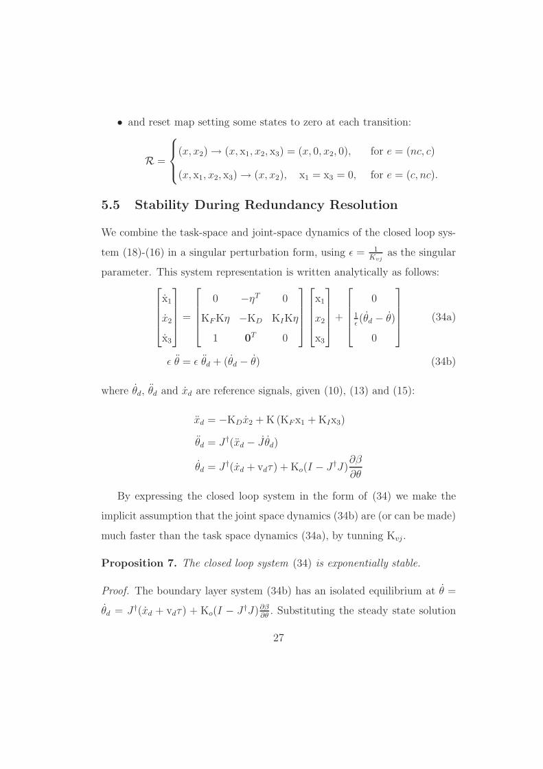
5.5 Stability During Redundancy Resolution
We combine the task-space and joint-space dynamics of the closed loop sys-
tem (18)-(16) in a singular perturbation form, using ǫ = 1Kvj
as the singular
parameter. This system representation is written analytically as follows:
x1
x2
x3
=
0 −ηT 0
KFKη −KD KIKη
1 0T 0
x1
x2
x3
+
0
1ǫ(θd − θ)
0
(34a)
ǫ θ = ǫ θd + (θd − θ) (34b)
where θd, θd and xd are reference signals, given (10), (13) and (15):
xd = −KDx2 + K (KFx1 + KIx3)
θd = J†(xd − J θd)
θd = J†(xd + vdτ) + Ko(I − J†J)∂β
∂θ
By expressing the closed loop system in the form of (34) we make the
implicit assumption that the joint space dynamics (34b) are (or can be made)
much faster than the task space dynamics (34a), by tunning Kvj .
Proposition 7. The closed loop system (34) is exponentially stable.
Proof. The boundary layer system (34b) has an isolated equilibrium at θ =
θd = J†(xd + vdτ) + Ko(I − J†J)∂β∂θ
. Substituting the steady state solution
27

of (34b) in (34a) we obtain the reduced system dynamics (17), which was
shown in Proposition 2 to be exponentially stable. Invoking Theorem 11.4
in14, the combined system (34) is shown to be exponentially stable, provided
that Kvj > 0.
6 Simulation Results
We consider a point-mass mobile robot and a 3-link manipulator inside the
planar workspace, similar to that of Figure 1. The task is to move from an ini-
tial configuration to a destination, without having any knowledge about the
existence, shape, and location of obstacles. We present two sets of simulation
results, one for each type of system. In addition to verifying the convergence
properties of the proposed control scheme, we also investigate the robust-
ness of the closed loop scheme to measurement noise, workspace complexity,
navigation method singularities, and model parameter uncertainty.
Tests with varying environment stiffness have also been conducted, but
are not included due to space limitations. Increased stiffness naturally pro-
duces more pronounced force transients, but stability is not affected. The
interested reader is referred to34.
6.1 Mobile Robot Simulations
6.1.1 Navigation and Force Regulation
Consider an example of the navigation problem where a robot is required
to move in a two-dimensional unknown workspace containing a disk and a
Π-shaped obstacle. Both obstacles are assumed to be of cardboard mate-
28

0.3 0.35 0.4 0.45 0.5 0.55 0.6 0.65
0.25
0.3
0.35
0.4
0.45
0.5
0.55
0.6
x
y
Figure 5: A mobile robot moves from (0.6, 0.25) to (0.37, 0.6), sliding along
the surface of a disk and Π shaped unknown obstacles.
rial, which has an approximate stiffness of 104 N/m. Figure 5 shows the
path of the mobile robot, starting at x = (0.6, 0.25) and converging to
xD = (0.37, 0.6). The navigation function used in this example is a quadratic
function of the Euclidean distance from xD, since no prior knowledge about
obstacles in the workspace is assumed. The robot deviates from the straight-
line path to goal to follow the obstacle boundaries. Its velocity variation
along this path is shown in Figure 6. Figures 6-7 show the evolution of the
mobile robot’s state during the period of 100 simulation seconds after ini-
tialization: During a small time interval within the first 10 seconds of the
motion, the robot encounters the disk-shaped obstacle. Contact-mode mo-
tion is indicated by gray background in Figure 7. At that time, the velocity
of the robot drops abruptly due to collision, as shown in in Figure 6, and
stabilized to a reference speed vd, set to a percentage of the speed at impact,
29

0 20 40 60 80 1000
0.01
0.02
0.03
0.04
0.05
0.06
0.07
time
Ve
locity n
orm
m
/se
c
Figure 6: The 1-norm of the mo-
bile robot’s velocity vector. Regions
of “depression” are associated with
reduced velocity after collision with
obstacles.
0 20 40 60 80 1000.25
0.3
0.35
0.4
0.45
0.5
0.55
0.6
0.65
time (second)
po
sitio
n (
m)
data1
data2
x position
y position
contact
no−contact
goal point
Figure 7: Evolution of the mobile
robot’s x and y coordinates, from
initial point to destination. Shaded
regions indicate sliding along an ob-
stacle’s boundary.
along the obstacle surface. When the switching conditions (33b) of the guard
Gc are satisfied, the robot’s velocity quickly converges to the potential field
at the exit point, after which it continues to decrease due to the action of the
damping term in (6). In the case of the mobile robot, where the inertia ma-
trix M is a constant scalar, the switching conditions (33b) are significantly
simplified to the point that we can easily track the transition by observing
the magnitudes of the entry and exit velocity in the contact mode. The sec-
ond column of Table 1 indicates how the guard (33b) evaluates true at the
exit point on disk obstacle surface. We see that the value of the navigation
function is smaller at the exit point xe, that the exit velocity ‖x2e‖ is smaller
than the velocity when the robot first hit the obstacle, and that the potential
field direction points toward the exterior of the obstacle, along −η.
30

Switching Criteria Disk obstacle Π obstacle
φ(xh) 0.9692 0.0266
φ(xe) 0.6617 0.0192
‖x2h‖ 0.0314 0.0071
‖x2e‖ 0.0278 0.0034
−∇φ(xe)T η −1.0534 × 10⁻⁵ −5.008 × 10⁻⁵
Table 1: Satisfying the conditions of Gc, in the scenario of Figure 5.
6.1.2 The Effect of Measurement Noise
In the preceding example, force regulation was performed under the assump-
tion that force measurements reflected the exerted forces accurately. How-
ever, force measurements are notoriously noisy. To simulate a realistic sensor
model, force measurements are contaminated with Gaussian noise.
Noise is assumed a random signal, following a normal distribution with
zero mean and a certain variance σ2. We have adopted a value for the
standard deviation σ based on the experimental data collected and analyzed
by Reference37. The values borrowed from37 turned out to be too small
to affect our control laws, so we conservatively adjusted them by a level of
magnitude and used σ = 0.001 N for our first simulation. In a subsequent
simulation test, we increased σ to 0.005 N.
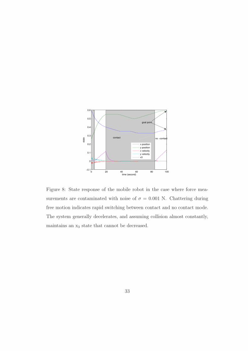
Figure 8 shows the state response of the mobile robot system when force
measurements are contaminated by noise with standard deviation equal to
σ = 0.001 N. While moving in free space, the controller switches rapidly
between contact and no-contact mode, perceiving measurement noise as a
nonzero value for f. This fast switching impacts the velocity dynamics, be-
31

cause in the two modes, velocity is being controlled differently. In Figure 8
this effect is shown as chattering for the duration of the collision free motion.
The guard conditions for switching back to no-contact mode are satisfied
throughout this interval, allowing the rapid switching between modes. Due
to the limited time spend in “contact mode” and the erroneous interpreta-
tion of the noise signal, the contact mode state variable x3 =t2∫
t1
x1ds cannot
be decreased. Once true contact is made, however, approximately after 20
simulation seconds, the conditions of Gc are no longer satisfied. This forces
the system to remain in contact mode, allowing the x3 state to decrease.
As velocity decreases with time because of damping, chattering during free
motion subsides (in terms of velocity magnitude); this is why at the later
stages of motion, close to destination, it is hardly observable in Figure 8.
The overall effect of unmodelled measurement noise is performance degra-
dation and slower speed. It can be observed in Figure 8 that the robot spends
more time in contact with obstacles and convergence to destination is decel-
erated, without however a significant effect on the system’s stability.
6.1.3 Navigation in Cluttered Environments
Workspace complexity does not affect the stability properties of the hybrid
control law. This is demonstrated in the following simulation test, where the
disk-shaped obstacle is replaced by a maze-shaped obstacle. Figure 9 shows
the path of the mobile robot, starting from a configuration inside the maze,
and converging to the destination point at coordinates (0.4, 0.6). The robot
follows the contour of the maze, switching between contact and no-contact
mode several times. In Table 2 there are three different exit points at the
32
0 20 40 60 80 100−0.1
0
0.1
0.2
0.3
0.4
0.5
0.6
time (second)
sta
te
x position
y position
x velocity
y velocity
x3
contact no −contact
goal point
Figure 8: State response of the mobile robot in the case where force mea-
surements are contaminated with noise of σ = 0.001 N. Chattering during
free motion indicates rapid switching between contact and no contact mode.
The system generally decelerates, and assuming collision almost constantly,
maintains an x3 state that cannot be decreased.
33

Criteria Maze obstacle Π obstacle
φ(xh) 0.3554 0.2526 0.2098 0.0202
φ(xe) 0.3175 0.2519 0.1647 0.0201
‖x2h‖ 0.0251 0.0232 0.0193 0.0060
‖x2e‖ 0.0142 0.0121 0.0166 0.0059
−∇φ(xe)Tη −5.283 × 10⁻⁴ -0.0051 −3.255 × 10⁻⁴ -0.0024
Table 2: Evaluations indicating the satisfaction of the switching conditions
for Gc in the scenario depicted in Figure 9.
surface of the maze obstacle, and the value of φ(xe) at each point suggests
that the robot is “closer” (as measured by the potential function) to the goal
than it was at the time when the last collision occurred.
Figure 10 shows the evolution of the contact force during contact, demon-
strating that the contact-mode control law is successful in regulating the con-
tact force to a desired level of 0.1 N. Spikes on the force graph correspond
to collision events.
6.1.4 Potential Field Singularities
The direction along which the robot slides on the obstacle boundary depends
on the how the vector normal to the obstacle surface, η, and the potential field
direction −∇φ align at the point of contact. This is measured by their inner
product, −ηT∇φ, and in theory when this product vanishes (the potential
field direction being normal to the obstacle surface at xh) there is no way to
determine a direction of motion. In practice, however, this is rarely the case.
The reason is that numerical errors (or noise during experimental imple-
34

0.3 0.4 0.5 0.6 0.70.25
0.3
0.35
0.4
0.45
0.5
0.55
0.6
0.65
0.7
Figure 9: Mobile robot navigation in a workspace with a maze of unknown
shape. The x and y coordinates are measured on the horizontal and vertical
axes, respectively. The goal configuration has coordinates (0.4, 0.6).
0 20 40 60 80 1000
0.2
0.4
0.6
0.8
1
1.2
1.4
time (second)
forc
e (
N)
Figure 10: The contact force is regulated to 0.1 N during the contact phases
in the simulation scenario described in Figure 9.
35
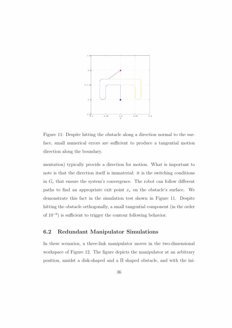
Figure 11: Despite hitting the obstacle along a direction normal to the sur-
face, small numerical errors are sufficient to produce a tangential motion
direction along the boundary.
mentation) typically provide a direction for motion. What is important to
note is that the direction itself is immaterial: it is the switching conditions
in Gc that ensure the system’s convergence. The robot can follow different
paths to find an appropriate exit point xe on the obstacle’s surface. We
demonstrate this fact in the simulation test shown in Figure 11. Despite
hitting the obstacle orthogonally, a small tangential component (in the order
of 10−6) is sufficient to trigger the contour following behavior.
6.2 Redundant Manipulator Simulations
In these scenarios, a three-link manipulator moves in the two-dimensional
workspace of Figure 12. The figure depicts the manipulator at an arbitrary
position, amidst a disk-shaped and a Π shaped obstacle, and with the ini-
36

tial and goal configurations marked by points at locations (0.6, 0.25) and
(0.375, 0.6), respectively. Circles along the manipulator body indicate the
position of the rotational joints, and control points for collision avoidance
have been defined along the manipulator links at regular intervals of 0.025 m.
The lengths of link 1, 2, and 3 are 0.4 m, 0.3 m and 0.1 m, respectively.
Figure 13 is a superposition of snapshots showing the manipulator con-
figuration at different time instances. The path of the manipulator, from
initial configuration to goal, is also marked. As shown in an intermediate
snapshot in Figure 13, the use of control points cannot eliminate the possi-
bility of unexpected collision between the links of the robot and the obstacles
completely: the tip of link 3 is shown to have “entered” the interior of the
Π shaped obstacle, toward its right “leg.” However, the collision avoidance
control component is indeed active and manifests itself in Figure 14 which
shows the evolution of the manipulator’s joint angles. In Figure 14 we see a
fast change in joint angle θ3 at approximately t = 2 s, t = 32 s, and t = 45 s.
The stability of joint velocities is demonstrated in Figure 16, which also
shows a (bounded) velocity increase during motion in free space. The end
effector force during the contact mode operation is regulated at the reference
value of 0.1 N as shown in Figure 15.
6.2.1 Sensitivity to Model Parameter Variations
One of the main concerns when performing computed-torque type compensa-
tion is the fact that a robot model is rarely perfect, and consequently terms
do not cancel completely as they are supposed to in theory. In this sec-
tion we investigate the sensitivity of the closed loop system to uncertainty
37

0 0.1 0.2 0.3 0.4 0.5 0.6 0.7 0.8−0.1
0
0.1
0.2
0.3
0.4
0.5
0.6
0.7
X
Y
Figure 12: The 3-link manipulator
considered, at a random configuration
in a workspace with a disk and a Π
shaped unknown obstacles.
0 0.1 0.2 0.3 0.4 0.5 0.6 0.7 0.8−0.1
0
0.1
0.2
0.3
0.4
0.5
0.6
0.7
x
y
Figure 13: Snapshots of different
manipulator configurations along its
path from initial to goal position.
0 10 20 30 40 50 60 70 80−2
−1.5
−1
−0.5
0
0.5
1
1.5
time (second)
sta
te
data1
data2
joint 1
joint 2
joint 3
Figure 14: Joint angle trajectories.
Shaded regions correspond to time in-
tervals when the end effector is in con-
tact with obstacles.
0 10 20 30 40 50 60 70 800
0.5
1
1.5
2
2.5
3
time (second)
forc
e (
N)
Figure 15: During the contact phase,
the exerted force is regulated at 0.1 N.
38

0 10 20 30 40 50 60 70−1
−0.5
0
0.5
time (second)
join
t velo
city (
rad/s
)
joint 1
joint 2
joint 3
Figure 16: Trajectories of the joint angle rates. Collision avoidance maneu-
vers are performed for the control points, resulting in local and temporal
increase of joint velocities.
in the parameters of the manipulator dynamics. We do so by artificially in-
troducing errors in terms of link length and mass and we monitor how the
performance of the system is affected. Table 3 lists the nominal values for the
model parameter, along with the adjusted parameter values used for control
implementation during our simulation tests.
Figures 17, 18 and 19 show the state response of the system when the
controller is implemented using parameter values which are 10%, 20% and
50% off their nominal values, respectively. There are no significant differ-
ences in the trajectory profiles, apart from minor changes during transient
phases. We attribute the seeming immunity of the system to such parameter
variations to the action of the integral control during force regulation, and
the use of potential fields for navigation.
39

Length (m) Mass (kg)
Nominal 10 % 20 % 50 % Nominal 10 % 20 % 50 %
value error error error value error error error
Link 1 0.4 0.44 0.48 0.6 1 1.1 1.2 1.5
Link 2 0.3 0.33 0.36 0.45 1 1.1 1.2 1.5
Link 3 0.1 0.11 0.12 0.15 1 1.1 1.2 1.5
Table 3: Dynamic model parameters for the 3-link manipulator. Nominal val-
ues are used to implement the manipulator model during simulation. Modi-
fied values (with errors) are used for controller implementation.
0 10 20 30 40 50 60 70−2
−1.5
−1
−0.5
0
0.5
1
1.5
time (second)
sta
te
data1
data2
joint 2 position
joint 3 position
joint 1 position
joint 1 velocity
joint 2 velocity
joint 3 velocity
goal
Figure 17: State Response with 10 % error in the dynamic model parameters
40

0 10 20 30 40 50 60 70−2
−1.5
−1
−0.5
0
0.5
1
1.5
time (second)
sta
te
data1
data2
joint 1 position
joint 2 position
joint 3 position
joint 1 velocity
joint 2 velocity
joint 3 velocity
goal
Figure 18: State Response with 20 % error in the dynamic model parameters
0 10 20 30 40 50 60 70−2
−1.5
−1
−0.5
0
0.5
1
1.5
time (second)
sta
te
data1
data2
joint 1 position
joint 2 position
joint 3 position
joint 1 velocity
joint 2 velocity
joint 3 velocity
Figure 19: State Response with 50 % error in the dynamic model parameters
41

7 Concluding Remarks
We presented a hybrid control scheme for mobile robots and redundant ma-
nipulators equipped with force sensors, which allows them to navigate in an
unknown environment and recover from unexpected collisions. The control
law consists of two discrete modes, a non-contact mode, for motion in the
free space, and a contact mode, for sliding along the surface of obstacles
discovered after collision. Switching conditions between the two modes are
designed to ensure the stability of the closed loop system. The contact mode
control law features a velocity control action and a pi force control action.
The non-contact mode combines path-planning and control action into a sin-
gle control law by means of artificial potential fields. Force measurements are
utilized for force regulation, obstacle detection and switching decisions. We
exploited the kinematic redundancy of the manipulator to avoid collisions
with obstacles discovered during execution.
The stability of the force/potential field control scheme is analyzed in a
multiple Lyapunov function framework, under the assumption of a compli-
ant environment. Switching conditions from the contact to no-contact mode
and selection criteria for feedback gains are established to prove asymptotic
stability for the system. Numerical simulations demonstrate the convergence
properties of the closed loop system. The latter is also tested against mea-
surement noise and model parameter variations, and results reveal some ro-
bustness, which could be a result of integral control action for force regulation
and potential field for motion planning. Further work is needed to determine
the source and the extend of these properties. These preliminary simulation
studies are promising, and seem to encourage further experimental testing.
42

References
1. V. Feliu A. Garcia and J.A. Somolinos. Experimental testing of a gauge
based collision detection mechanism for a new three-degree-of-freedom
flexible robot. Journal of Robotic Systems, 20:271–284, 2003.
2. Ronald C. Arkin and Robin R. Murphy. Autonomous navigation in a
manufacturing environment. IEEE Transactions on Robotics and Au-
tomation, 6:445–454, 1990.
3. Michael S. Branicky. Studies in Hybrid Systems: Modeling, Analysis,
and Control. PhD thesis, Massachusetts Institute of Technology, 1995.
4. Michael S. Branicky. Multiple lyapunov functions and other analysis
tools for switched and hybrid systems. IEEE Transactions on Automatic
Control, 43(4):475–482, 1998.
5. R.A. Brooks. A robust layered control system for a mobile robot. IEEE
Journal of Robotics and Automation, RA-2:14–23, 1986.
6. S. Chiaverini and L. Sciavicco. The parallel approach to force/position
control of robotic manipulators. IEEE Transactions on Robotics and
Automation, 9:361–373, 1993.
7. S. Chiaverini and B. Siciliano. On the stability of a force/position control
scheme for robot manipulators. In Proceedings of IFAC Robot Control,
pages 183–188, 1991.
8. J. Duffy. The fallacy of modern hybrid control theory that is based on
43

’orthogonal complements’ of twist and wrench spaces. Journal of Robotic
Systems, 7:139–144, 1990.
9. D. M. Ebert and D.D. Henrich. Safe human-robot-cooperation: Image
based collision detection for industrial robots. In Proceedings of 2002
IEEE International Conference on Intelligent Robots and Systems, pages
1826–1831, 2002.
10. Q. Wei H. Zhang, Z. Zhen and W. Chang. The position/force control
with self-adjusting select-matrix for robot manipulators. In Proceedings
of 2001 IEEE International Conference on Robotics and Automation,
pages 3932–3936, 2001.
11. J. Hollerbach and K. Suh. Redundancy resolution of manipulators
through torque optimization. IEEE Journal of Robotics and Automa-
tion, RA-3:308–316, 1987.
12. Mikael Johansson and Anders Rantzer. Computation of piecewise
quadratic Lyapunov functions. In Proceedings of IEEE Conference on
Decision and Control, pages 3515–3520, 1997.
13. Mikael Johansson and Anders Rantzer. Computation of piecewise
quadratic Lyapunov functions for hybrid systems. IEEE Transactions
on Automatic Control, 43:555–559, 1998.
14. Hassan Khalil. Nonlinear Systems. Pearson Education, 2000.
15. O. Khatib. A unified approach for motion and force control of robot
manipulators: The operational space formulations. IEEE Journal of
Robotics and Automation, 3:43–53, 1987.
44

16. Oussama Khatib. Real-time obstacle avoidance for manipulators and
mobile robots. The International Journal of Robotics Research, 5(1):
90–98, 1986.
17. Amit Kumar and Herbert Tanner. Formation stabilization and collision
avoidance of multiple agents using navigation functions. IEEE Transac-
tions on Robotics, 2005. submitted.
18. J.C. Latombe. Robot Motion Planning. Kluwer Academic Publishers,
Boston, MA, 1991.
19. W. Li. Fuzzy logic based perception-action behavior control of a mobile
robot in uncertain environments. In Proceedings of IEEE World Congress
on Computation Intelligence, pages 1626–1631, 1994.
20. W. Li. Fuzzy logic based robot navigation in uncertain environments
by multisensor integration. In Proceedings of 1994 IEEE International
Conference on Multisensor Fusion and Integration for Intelligent Sys-
tems, pages 439–446, 1994.
21. W. Li. Perception-action behavior control of a mobile robot in uncer-
tain environments using fuzzy logic. In Proceedings of 1994 IEEE Inter-
national Conference on Intelligent Robots and Systems, pages 439–446,
1994.
22. W. Li. A hybrid nuero-fuzzy system for sensor based robot navigation
in uncertain environments. In Proceedings of 1994 American Control
Conference, pages 2749–2753, 1995.
45
23. W. Li and K.Z. He. Sensor-based robot navigation in uncertain envi-
ronments using fuzzy logic. In Proceedings of 1994 ASME International
Computers in Engineering Conference, pages 813–818, 1994.
24. Daniel Liberzon. Switching in Systems and Control. Birkhauser, 2003.
25. Daniel Liberzon and A. Stephen Morse. Basic problems in stability and
design of switched systems. IEEE Control Systems Magazine, 19(5):
59–70, 1999.
26. Savvas G. Loizou, Herbert G. Tanner, Vijay Kumar, and Kostas Kyri-
akopoulos. Closed loop motion planning and control for mobile robots
in uncertain environment. In 42th IEEE Conference on Decision and
Control, volume 18, pages 2010–2015, Maui Hawaii, 2003.
27. Alessandro De Luca and Raffaella Mattone. Sensorless robot collision
detection and hybrid force/motion control. In Proceedings of 2005 IEEE
International Conference on Robotics and Automation, pages 1011–1016,
2005.
28. V. Lumelsky and E. Cheung. Real-time collision avoidance in teleop-
erated whole-sensitive robot arm manioulator. IEEE Transactions on
System, Man, Cybernetics, 23:194–203, 1993.
29. Vladimir J. Lumelsky and Alexander A. Stepanov. Path-planning strate-
gies for a point mobile automaton moving amidst unknown obstacles of
arbitrary shape. Algorithmica, 2:403–430, 1987.
30. John Lygeros. Lecture notes on hybrid systems, February 2004. Notes
for an ENSIETA short course.
46

31. M. T. Mason. Compliance and force control for computer controlled
manipulators. IEEE Transactions on System, Man, Cybernetics, 6:418–
432, 1981.
32. Y. Nakamura. Advanced Robotics: Redundancy and Optimization.
Addition-Wesley, 1991.
33. Kevin A. O’Neil. Divergence of linear acceleration-based redundancy
resolution schemes. IEEE Transactions on Robotics and Automation,
18:625–631, 2002.
34. Dushyant Palejiya. Force/potential field controller for robot navigation
in compliant unknown environment. Master’s thesis, The University of
New Mexico, 2005.
35. M. H. Raibert and J. J. Craig. Hybrid position/force control of manip-
ulator. ASME Journal of Dynamic Systems, Measurement and Control,
103:126–133, 1981.
36. Elon Rimon and Daniel E. Koditschek. Exact robot navigtion using
artificial potential functions. IEEE Transactions on Robotics and Au-
tomation, 8(5):501–518, 1992.
37. J. Roy and L.Whitcomb. Adaptive force control of position/velocity con-
trolled robots: Theory and experiment. IEEE Transactions on Robotics
and Automation, 18:121–137, 2002.
38. B.Siciliano S. Chiaverini and L.Sciavicco. Force/position regulation of
compliant robot manipulators. IEEE Transactions on Automatic Con-
trol, 39(3):647–651, 1994.
47
39. T. Murakami S. Takakura and K. Ohnishi. An approach to collision
detection and recovery motion in industrial robot. In Proceedings of
15th Annual Conference of IEEE Industrial Electronics Society, pages
421–426, 1989.
40. B. Sicilliano and L. Villani. Robot Force Control. Kluwer Academic
Publishers, 1999.
41. M. Spong and R. Anderson. Hybrid impedance control of robotic ma-
nipulators. IEEE Journal of Robotics and Automation, 4:549–556, 1988.
42. H. G. Tanner, S. G. Loizou, and K. J. Kyriakopoulos. Nonholonomic nav-
igation and control of multiple mobile manipulators. IEEE Transactions
on Robotics and Automation, 19(1):53–64, February 2003.
43. T. Yoshikawa. Dynamic hybrid position/force control of robot
manipulators—description of hand constrains and calculation of joint
driving force. IEEE Journal of Robotics and Automation, 3:386–392,
1987.
44. L.A. Zadeh. Fuzzy sets. Information and Control, 8:338–353, 1965.
48
Related Documents