Algorithmica (1995) 13:472-501 Algorithmica 1995 Springer-Verlag New York Inc. Landmark-Based Robot Navigation s A. Lazanas 2 and J.-C. Latombe 2 Abstract. Achieving goals despite uncertainty in control and sensing may require robots to perfor~a complicated motion planning and execution monitoring. This paper describes a reduced version of the general planning problem in the presence of uncertainty and a complete polynomial algorithm solving it. The planar computes a guaranteed plan (for given uncertainty bounds) by backchaining omnidirec- tional backprojections of the goal until the set of possible initial positions of the robot is fully contained. The algorithm assumes that landmarks are scattered across the workspace, that robot control and position sensing are perfect within the fields of influence of these landmarks (the regions in which the landmarks can be sensed by the robot), and that control is imperfect and sensing null outside these fields. The polynomialityand completeness of the algorithm derive from these simplifying assumptions, whose satisfaction may require the robot and/or its workspace to be specifically engineered. This leads us to view robot/workspace engineering as a means to make planning problems tractable. A computer program embedding the planner was implemented, along with navigation techniques and a robot simulator. Several examples run with this program are presented in this paper. Nonimplemented extensions of the planner are also discussed. Key Words. Motion planning, Mobile robot navigation, Uncertainty, Landmark. 1. Introduction. To operate in the real world robots must deal with errors in control and sensing. Several motion planners have been proposed which address this issue (e.g., [24], [32], [111 [20]; [16], [25], [27], and [12]). Many of them, however, embed tacit or unclear assumptions, causing them to be unreliable in practice. In this paper, as in [25], [27], and [12], we represent uncertainty by bounded regions describing ranges of errors. A correct plan is one whose execution is guaranteed to achieve the goal, whenever actual errors (at execution time) are within the uncertainty bounds. A sound planner is one which only generates correct plans. A complete planner is one which generates a correct plan whenever one exists, and returns failure otherwise. Very few complete planners have been proposed so far. Most of them take exponential time in some measure of the size of the input problem (e.g., [4] and [9]), which makes them virtually inapplicable. In fact, it has been shown that these planners attack problems which are inherently intractable [5]. 1 This research was partially funded by DARPA contract DAAA21-89-C0002 and ONR Contract N00014-92-J-1809. 2 Robotics Laboratory, Department of Computer Science, Stanford University, Stanford, CA 94305, USA. [email protected] and [email protected]. Received October 21, 1992; revised June 16, 1993. Communicated by J.-D. Boissonnat.

Welcome message from author
This document is posted to help you gain knowledge. Please leave a comment to let me know what you think about it! Share it to your friends and learn new things together.
Transcript
Algorithmica (1995) 13:472-501 Algorithmica �9 1995 Springer-Verlag New York Inc.
Landmark-Based Robot Navigation s
A. Lazanas 2 and J.-C. L a t o m b e 2
Abstract. Achieving goals despite uncertainty in control and sensing may require robots to perfor~a complicated motion planning and execution monitoring. This paper describes a reduced version of the general planning problem in the presence of uncertainty and a complete polynomial algorithm solving it. The planar computes a guaranteed plan (for given uncertainty bounds) by backchaining omnidirec- tional backprojections of the goal until the set of possible initial positions of the robot is fully contained. The algorithm assumes that landmarks are scattered across the workspace, that robot control and position sensing are perfect within the fields of influence of these landmarks (the regions in which the landmarks can be sensed by the robot), and that control is imperfect and sensing null outside these fields. The polynomiality and completeness of the algorithm derive from these simplifying assumptions, whose satisfaction may require the robot and/or its workspace to be specifically engineered. This leads us to view robot/workspace engineering as a means to make planning problems tractable. A computer program embedding the planner was implemented, along with navigation techniques and a robot simulator. Several examples run with this program are presented in this paper. Nonimplemented extensions of the planner are also discussed.
Key Words. Motion planning, Mobile robot navigation, Uncertainty, Landmark.
1. Introduction. To opera te in the real wor ld robo t s mus t deal with er rors in con t ro l and sensing. Several mo t ion p lanners have been p r o p o s e d which address this issue (e.g., [24], [32], [111 [20]; [16], [25], [27], and [12]). M a n y of them, however, embed taci t or unclear assumpt ions , causing them to be unre l iab le in practice.
In this paper , as in [25], [27], and [12], we represent uncer ta in ty by b o u n d e d regions descr ibing ranges of errors. A correct plan is one whose execut ion is gua ran teed to achieve the goal, whenever ac tua l e r rors (at execut ion time) are within the uncer ta in ty bounds . A sound planner is one which only generates correct plans. A complete p lanner is one which generates a correct p lan whenever one exists, and re turns failure otherwise. Very few comple te p lanners have been p r o p o s e d so far. Mos t of them take exponent ia l t ime in some measure of the size of the input p rob l em (e.g., [4] and [9]), which makes them vir tual ly inappl icable . In fact, it has been shown tha t these p lanners a t t ack p rob lems which are inherent ly in t rac tab le [5].
1 This research was partially funded by DARPA contract DAAA21-89-C0002 and ONR Contract N00014-92-J-1809. 2 Robotics Laboratory, Department of Computer Science, Stanford University, Stanford, CA 94305, USA. [email protected] and [email protected].
Received October 21, 1992; revised June 16, 1993. Communicated by J.-D. Boissonnat.
Landmark-Based Robot Navigation 473
In this paper we achieve polynomiality by both making assumptions in the problem formulation that eliminate the source of intractability, and using algor- ithmic techniques that take advantage of these assumptions. The key underlying notion is that of a landmark area, an "island of perfection" in the robot configuration space where we consider position sensing and motion control to be fully accurate. Outside any such area, we assume that control is imperfect and position sensing null. This notion of a landmark area approximately corresponds to the "field of influence" of a physical feature: if the robot is in this field, it can sense and identify the feature, and use this information to determine its position with high accuracy (actually, we assume full accuracy). A feature may be pre- existing (e.g., the corner made by two walls) or specifically provided to help robot navigation (e.g., a radio beacon or a magnetic device buried in the ground).
Given a set of landmark areas scattered across configuration space, a set of obstacles with which the robot should not collide, an initial region where the robot is known to be prior to execution, and a goal region where we would like the robot to go, the planning problem is to generate a set of motion commands whose execution guarantees that the robot will move into the goal and stop there. Our planning algorithm solves this problem by iteratively constructing a growing set of landmark areas from which the robot can reliably attain the goal. This set initially contains the landmark areas intersecting the goal region. Then new landmark areas are added, from which the robot can reliably attain landmark areas already in the set by executing a single move. The algorithm terminates successfully as soon as it is possible for the robot to attain some landmark area (any one) in this set by a single move from the initial region. It terminates with failure when no new landmark areas can be added to the set and the condition for success is still unsatisfied.
The algorithm constructs the set of landmark areas from which the robot can reliably attain the goal by comprising omnidirectional backprojections. The directional backprojection of a set of landmark areas, for a given direction of motion d, is the largest region in configuration space from which the robot is guaranteed to attain one of these areas by moving along d, despite control uncertainty. The omnidirectional backprojection is the disjoint union of directional backprojections over all possible directions of motion, indexed by the direction of motion. For a robot represented as a point in the plane, we show that the omnidirectional backprojection is sufficiently representedl as far as planning is concerned, by a finite number of directional backprojections..The planner derived from this result is complete. Its time complexity is polynomial in the number and complexity of the landmark areas and the obstacles. The plans it generates minimize the number of motions that have to be executed in the worst case.
Landmarks require the workspace to include appropriate features and the robot to be equipped with sensors able to detect them. Our planning algorithm thus illustrates the interplay between engineering and algorithmic complexity in robo- tics. As software becomes more critical in modern robots, the importance of this interplay will increase. The tractability of robot programming will more and more be a major consideration in robot design and workspace engineeringu The question is not "How can we avoid engineering?", but "How can we reduce its cost?"
474 A. Lazanas and J.-C. Latombe
Interestingly, once a motion plan has been generated by our planner, the assump- tion that control and sensing are perfect in landmark areas can be relaxed to some extent, while keeping the plan correct. Furthermore, we show that simple varia- tions of our planner can handle other sorts of landmark areas that do not require perfect sensing and control, without losing completeness and polynomiality.
In Section 2 (Related Work) we relate our work to previous research. In Section 3 (Planning Problem) we precisely state the class of problems solved by our planner and we illustrate this statement with an example. In Section 4 (Directional Backchaining) we present a first-cut planning method based on the concept of directional baekprojection. However, this method does not provide an efficient way to select directions of motior~. In Section 5 (Omnidirectional Baekchaining) we address this issue and we present the actual planning algorithm. In Section 6 (Experimental Results) we show a series of examples run with the implemented planner. For simplification, Sections 4-6 assume that there are no obstacles in the robot's workspace. In Section 7 (Dealing with Obstacles) we extend the planning method to deal with obstacles, and we present additional experimental results. In Section 8 (Discussion and Extensions) we discuss our assumptions and we describe nonimplemented extensions of the planner aimed at eliminating the most restric- tive ones.
2. Related Work. Motion planning with uncertainty has been a research topic in robotics for almost two decades. Various approaches have been proposed, including skeleton refinement [24], [32], inductive learning from experiments [113, iterative removal of contacts [20], [161 and preimage backchaining [253, [27], [12]. The first three of these approaches operate in two phases: a motion plan is first generated assuming no uncertainty and then transformed to deal with uncertainty. Instead, preimage backchaining takes uncertainty into account throughout the whole planning process. It can thus tackle problems where uncertainty shapes the structure of a plan to the extent that it cannot be generated by transforming an initial one produced under the no-uncertainty assumption. Our work is a direct continuation of a series of work on preimage backchaining. We focus most of the following discussion on this series.
Preimage backchaining considers the following class of motion-planning prob- lems [253: A plan is a sequence (more generally, an algorithm) of motion commands, each defined by a commanded direction of motion d and a termination condition TC. When the robot executes such a command in free space, it moves along a direction contained at each instant in a cone of half-angle 0 about d and stops as soon as TC becomes true. (In contact with an obstacle, the robot may stop or slide, depending on the particular control law that is used. In this paper we simply forbid contacts with obstacles, though our algorithm can be easily adapted to handle compliant'motions as well.) The angle 0 is the largest expected control error and models the directional uncertainty of the robot. The termination condition TC is a boolean function of sensory data s. At any one time, these data measure physical parameters (e.g., the robot position) with some error. The actual parameter vector lies anywhere in a region ~//(s) modelling the robot's sensory
Landmark-Based Robot Navigation 475
uncertainty. A planning problem is specified by a workspace model, an initial region, a goal region, the directional uncertainty 0, and the sensing uncertainty q/.
The above problem formulation admits many variants. For example, time may be introduced and uncertainty in the robot velocity considered, allowing the construction of more sophisticated termination conditions [27], [12]. The work- space model (e.g., the location and the shape of the obstacles) may also be subject to errors, yielding a third type of uncertainty [8]. For the sake of simplicity do not discuss these variants here (see [18]).
The preimage of a goal region for a given motion command M = (d, TC) is the set of all points in the robot's configuration space such that if the robot starts executing the command from any one of these points, it is guaranteed to reach the goal and stop in it. Preimage backchaining consists of constructing a sequence of motion commands Mi, i = 1 . . . . , n, such that if P, is the preimage of the goal for M,, if P,_ 1 is the preimage of P, for M,_ 1, and so on, then 1~ 1 contains the initial region.
One source of difficulty in computing preimages is the possible interaction between goal reachability and goal recognizability. The robot must both reach the goal (despite directional uncertainty) and stop in the goal (despite sensing uncertainty). Goal recognition, hence the termination condition of a command, may depend on the region from where the command is executed. This region, which is precisely the preimage of the goal for that command, also depends on the termination condition. This recursive dependence was noted in [25]. Neverthe- less, Canny [4] described a complete planner with very few restrictive assumptions in it. This planner generates an r-step plan by reducing the input problem to deciding the satisfiability of a semialgebraic formula with 2r alternating existential and universal quantifiers. Such a decision takes double exponential time in r. Moreover, the smallest r for which a plan may exist grows with the complexity of the environment. Actually, various forms of the above motion-planning problem have been proven intrinsically hard [5], [28].
At the expense of completeness, Erdmann [12] suggested that goal reachability and recognizability be treated separately by identifying a subset of the goal, called a kernel, such that when this subset is attained, goal achievement can be recognized (by TC) independently of the way it has been achieved. He defined the backprojection of a region R for a direction of motion d as the set of all points such that, if the robot moves along d with directional uncertainty 0, starting at any one of these points, it is guaranteed to reach R. He proposed an O(n log n) algorithm to compute backprojections in the plane when the obstacles are polygons bounded by n edges. Hence, a preimage of a goal can be computed as the backprojection of its kernel. An implemented planner based on this technique is described in [19].
Once the kernel of a goal has been identified, a remaining issue is the selection of the commanded direction of motion to attain this kernel, since the back- projection of the kernel varies when the direction changes. The planner described in [19] only considers a finite number of regularly spaced directions; hence, it is incomplete, and usually not very efficient. Donald [9] considered the disjoint union of backprojections of a region R over all possible directions of motion. For a point
476 A. Lazanas and J.-C. Latombe
robot moving in the plane, he showed that this set is sufficiently described by a polynomial number of backprojections. He used this result to propose an O(n 4 log n) algorithm to generate one-step (single motion command) plans. Briggs [2] reduced the time complexity of this algorithm to O(n 2 log n). Hutchinson and Fox [17], [14] extended the algorithm to exploit visual constraints and allow visual compliant motions.
One remaining difficulty to construct a multistep planner is backchaining. The difficulty comes from the fact that backchaining introduces a twofold variation: when the commanded direction of motion varies, both the backprojection of the current kernel and the kernel of this backprojection (which will be used at the next backchaining iterations)vary. In this paper we deal with this difficulty by introducing landmark areas. We show that backchaining is then reduced to computing iteratively a relatively small set of backprojections for a growing set of landmark regions. This result directly yields a polynomial planning algorithm. This planner is also complete relative to a well-defined class of problems. Previously, Friedman [151 had proposed another polynomial multistep planner for a compliant point robot in a polygonal workspace by assuming that sensing exactly detects when the robot traverses line segments joining the vertices of the workspace.
Our notion of a landmark corresponds to a recognizable feature of the workspace that induces a field of influence (the landmark area). If the robot lies in this field, it senses the landmark and uses this information to determine its location. Related notions have been previously introduced in the literature with the same or different names, e.g., landmarks [23], atomic regions [3], signature neighborhoods [26], and perceptual equivalent classes [10], [6]. Over the past decade, there has also been a substantial amount of work at reducing position-
sensing errors while a robot is moving. For example, for mobile robots, many techniques have been proposed to combine the estimates provided by both dead-reckoning and environmental sensing (e.g., see Eli, [7], [22], and [33]). These techniques address the problem of tracking a selected motion plan as well as possible, not the problem of generating this plan. The goal of planning in the presence of uncertainty considered in this paper is to make sure that executing the plan will reveal enough information to guarantee reliable execution.
3. Planning Problem. In this section we precisely state the class of problems solved by our planning algorithm. We illustrate this statement with a specific example.
3.1. Statement. The robot is a point 3 moving in a plane, the workspace, contain- ing stationary forbidden circular regions, the obstacle disks. The robot can move in either one of two control modes, the perfect and the imperfect modes.
3 Hence, the robot workspace and configuration space coincide.
Landmark-Based Robot Navigation 477
The perfect control mode can also be used in some stationary circular areas of the workspace called the landmark disks, where the robot also has perfect position sensing. Some of these disks may intersect, creating larger areas, called landmark areas, through which the robot can move in the perfect control mode. A motion command in the perfect control mode, called a P-command, is described by a sequence of via points such that all the via points are in the same landmark area, any two consecutive via points are in the same landmark disk, and any two nonconsecutive via points are in different landmark disks. The robot can start executing the command only when it is in the landmark disk containing the first via point. It executes the command by moving through the successive Via points and stops when it reaches the last one.
A motion command in the imperfect control mode, called an 1-command, is described by a pair (d, ~ ) , where d e S 1 is a direction in the plane, called the commanded direction of motion, and ~ is a set of landmark disks, called the termination set of the command. This command can be executed anywhere in the plane, outside the obstacle disks. The robot then follows a path whose tangent at any point makes an angle with the direction d that is no greater than some prespecified angle 0 ~ (0, n/2), called the directional uncertainty. The robot stops as soon as it enters a landmark disk in ~ .
The robot has no sense of time, which means that the modulus of its velocity is irrelevant to the planning problem.
The initial position of the robot is known to be anywhere in a specified initial region J that consists of one or several disks. Each initial-region disk may, or may not, be disjoint from the landmark areas. The robot must move into a given goal region f#o, which is any subset, connected or not, of the workspace whose intersection with the landmark disks is easily computable. The problem is to generate a correct motion plan made up of I- and P-commands to achieve f#o from J . The robot is not allowed to collide with any of the obstacles.
The number of landmark disks is finite and equal to I. The number of obstacle disks is also finite and in O(l). The number of initial-region disks is small enough to be considered constant. The goal region is such that its intersection with landmark disks can be computed in O(l) time. Hence, I is used to measure the size of the input problem.
The above problem is a simplification of a real mobile-robot navigation problem, but it is not oversimplified and captures most of its fundamental aspects. In Section 8 we see that the most restricting assumptions can be eliminated or alleviated, so that the methods described in this paper provide a solid foundation for real mobile-robot navigat ion.
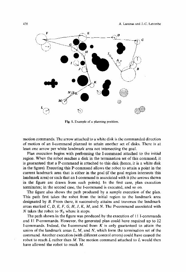
3.2. Example. Figure 1 illustrates the previous description with an example run using the implemented planner. The workspace contains 23 landmark disks (white or grey) forming 19 landmark areas, and 25 obstable disks (black). The directional uncertainty 0 is set to 0.09 rad. The initial and goal regions are two small disks designated by J and go, respectively.
The white landmark disks are those with which the planner has associated
478 A. Lazanas and J.-C. Latombe
J
~
O
D ~ ' , , C
. . . . . . . . . / "
@
Fig. 1. Example of a planning problem.
motion commands. The arrow attached to a white disk is the commanded direction of motion of an I-command planned to attain another set of disks. There is at least one arrow per white landmark area not intersecting the goal.
Plan execution begins with performing the I-command attached to the initial region. When the robot reaches a disk in the termination set of this command, it is guaranteed that a P-command is attached to this disk (hence, it is a white disk in the figure). Executing this P-command allows the robot to attain a point in the current landmark area that is either in the goal (if the goal region intersects this landmark area) or such that an I-command is associated with it (the arrows shown in the figure are drawn from such points). In the first case, plan execution terminates; in the second case, the I-command is executed, and so on.
The figure also shows the path produced by a sample execution of the plan. This path first takes the robot from the initial region to the landmark area designated by B. From there, it successively attains and traverses the landmark areas marked C, D, E, F, G, H, J, K, M, and N. The P-command associated with N takes the robot to f9 o where it stops.
The path shown in the figure was produced by the execution of 11 1-commands and 11 P-commands. However, the generated plan could have required up to 12 I-commands. Indeed, the I-command from K is only guaranteed to attain the union of the landmark areas L, M, and N, which form the termination set of the command. Another execution (with different control errors) could have caused the robot to reach L rather than M. The motion command attached to L would then have allowed the robot to reach M.
Landmark-Based Robot Navigation 479
4. Direct ional Backchaining. In this section and the next three we assume for simplification that the workspace contains no obstacle disks. Obstacles are introduced in Section 7.
4.1. Directional Backprojection of a Goal Consider a goal region ft. We define the extension of f# as the largest set of landmark disks such that, if the robot is in any one of them, it can attain the goal by executing a single P-command. Thus, the extension of f#, denoted by E(f#), is the set of all the landmark areas having a nonzero intersection with f#. The disks in E(f~) are called the extension disks. The other landmark disks are called the intermediate-goal disks.
The directional backprojection of E(f#), for any given d ~ S ~, is the region B(f#, d) defined as the largest subset of the workspace such that if the robot executes the 1-command (d, E(f#)) from any position in B(f#, d), then it is guaranteed to reach E(fr and thus to stop in E(~). From the entry point in the extension, the robot can attain fr by executing a P-command. Note that E(fr c B(fr d). Hence, if the robot is already in E(fr the I-command (d, E(fr immediately terminates.
There is no larger region than B(fr d) from where the robot is guarantee to attain fr recognizably by executing one I-command along d followed by one P-command. Indeed, if the robot executes the I-command (d, E(fr from any position outside this region, it is not guaranteed to reach E(fr From some positions, it may be guaranteed to reach fr but since it may not enter any landmark disk intersecting fr it may not recognize goal achievement and it may thus traverse the goal without stopping.
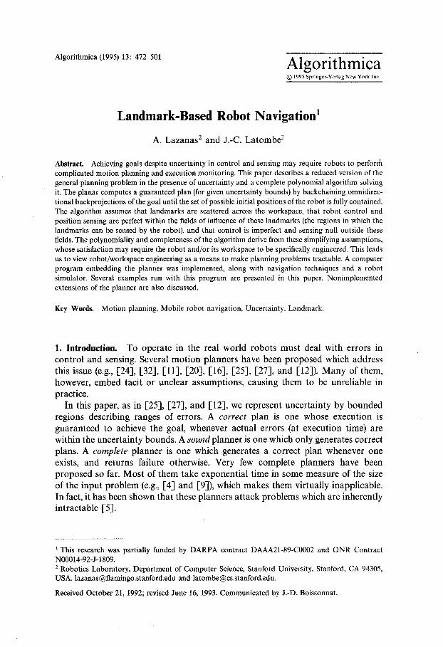
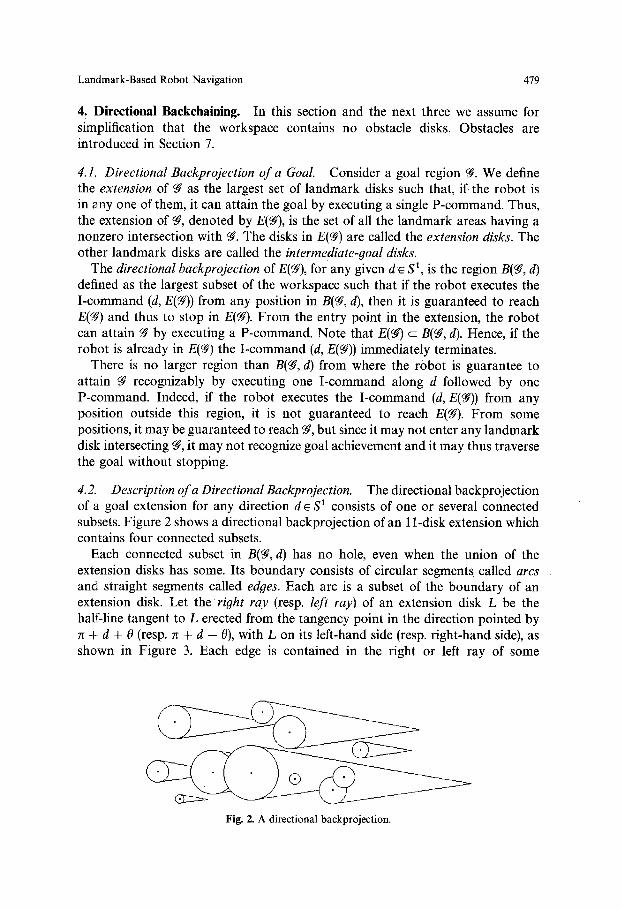
4.2. Description of a Directional Backprojection. The directional backprojection of a goal extension for any direction d ~ S 1 consists of one or several connected subsets. Figure 2 shows a directional backprojection of an 11-disk extension which contains four connected subsets.
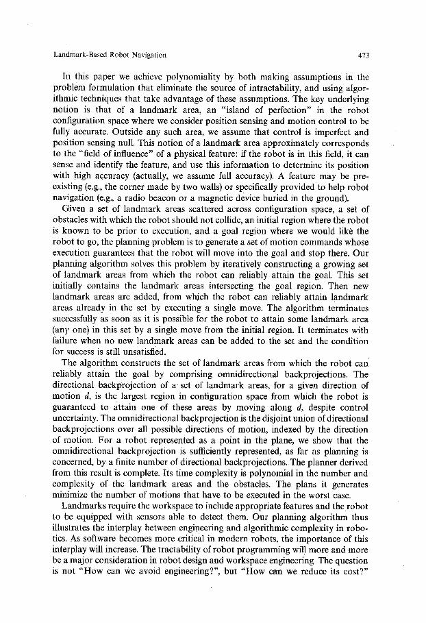
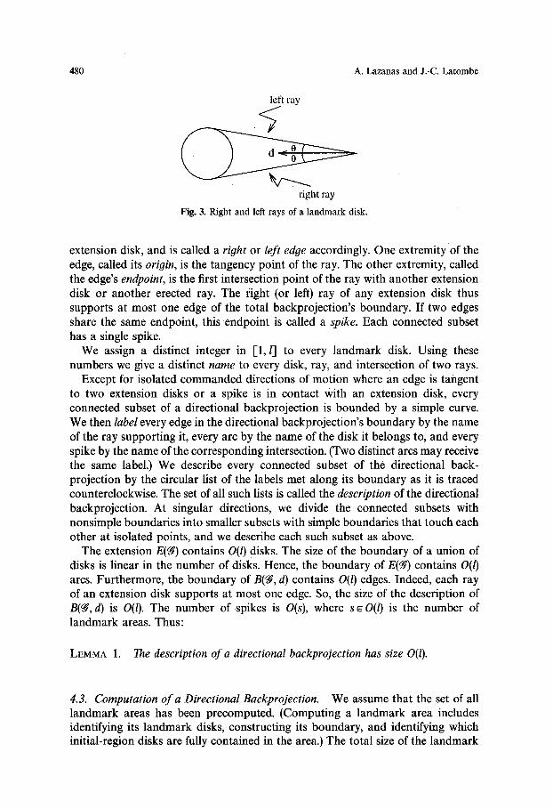
Each connected subset in B(fr d) has no hole, even when the union of the extension disks has some. Its boundary consists of circular segments called arcs and straight segments called edges. Each arc is a subset of the boundary of an extension disk. Let the right ray (resp. left ray) of an extension disk L be the half-line tangent to L erected from the tangency point in the direction pointed by n + d + 0 (resp. n + d - 0), with L on its left-hand side (resp. right-hand side), as shown in Figure 3. Each edge is contained in the right or left ray of some
Fig. 2. A directional backprojection.
480 A. Lazanas and J.-C. Latombe
left ray
fight ray
Fig. 3. Right and left rays of a landmark disk.
extension disk, and is called a right or left edge accordingly. One extremity o f the edge, called its origin, is the tangency point of the ray. The other extremity, called the edge's endpoint, is the first intersection point of the ray with another extension disk or another erected ray. The right (or left) ray of any extension disk thus supports at most one edge of the total backprojection's boundary. If two edges share the same endpoint, this endpoint is called a spike. Each connected subset has a single spike.
We assign a distinct integer in [1,/7 to every landmark disk. Using these numbers we give a distinct name to every disk, ray, and intersection of two rays.
Except for isolated commanded directions of motion where an edge is tangent to two extension disks or a spike is in contact With an extension disk, every connected subset of a directional backprojection is bounded by a simple curve. We then label every edge in the directional backprojection's boundary by the name of the ray supporting it, every arc by the name of the disk it belongs to, and every spike by the name of the corresponding intersection. (Two distinct arcs may receive the same label.) We describe every connected subset of the directional back- projection by the circular list of the labels met along its boundary as it is traced counterclockwise. The set of all such lists is called the description of the directional backprojection. At singular directions, we divide the connected subsets with nonsimple boundaries into smaller subsets with simple boundaries that touch each other at isolated points, and we describe each such subset as above.
The extension E(ff) contains O(/) disks. The size of the boundary of a union of disks is linear in the number of disks. Hence, the boundary of E(fr contains O(/) arcs. Furthermore, the boundary of B((#, d) contains O(/) edges. Indeed, each ray of an extension disk supports at most one edge. So, the size of the description of B(f~, d) is O(/). The number of spikes is O(s), where s ~ O(/) is the number of landmark areas. Thus:
LEMMA 1. The description of a directional backprojection has size O(I).
4.3. Computation of a Directional Backprojection. We assume that the set of all landmark areas has been precomputed. (Computing a landmark area includes identifying its landmark disks, constructing its boundary, and identifying which initial-region disks are fully contained in the area.) The total size of the landmark
Landmark-Based Robot Navigation 481
areas' boundaries is O(l). A simple divide-and-conquer does the precomputation in time O(l log 2 l) and space 0(/) [29].
To compute B(N, d) we erect the 0(/) rays tangent to the precomputed boundary of E((r and pointing along the directions ~ + d _+ 0. We construct the boundary of every connected subset of B(ff, d) by sweeping a line perpendicular to d, in the direction of d + re. Each ray is interrupted where it first intersects an extension disk or another ray. This sweep algorithm requires that 0 < re/2, in order to guarantee tha t the robot motion always projects positively on the direction d.
LEMMA 2. The description of a directional backprojection & computed in time O(l log l) and spac e O(l).
4.4. Backchaining. Assume that we select d o such that the directional back- projection of the problem's goal go contains the initial region J . We then have a motion plan to achieve the goal: from its initial position J , the robot can attain the extension E(ffo) by executing the I-command (do, E((qo)); then, by switching to the perfect control mode, it can reach the goal without leaving E((r
However, in general, such a "one-step" motion plan does not exist. If E((r is empty, so is B((r o, d) for any de $1; in this case if J r fro, the planner can safely return failure. If the extension E(fqo) is not empty and the backprojection B(fr o, do), for the selected direction do, does not contain J , we can treat B((r do) as an intermediate goal (r and try to produce a motion plan to achieve it from J . This means that we compute the extension E((r and, if it is a proper superset of E((r the backprojection B((ql, dO for some direction d l~ S ~. If we select dl such that B((r d~) contains J , we then have a two-step motion plan to achieve (r otherwise, we can consider B((q~, da) as a new intermediate goal (r and so on. The whole process is called directional backchaining.
The backchaining process requires that every newly computed backprojection be checked for containment of the initial region J . If it does not contain J , the new backprojection must also be checked for intersection with landmark disks not in the current goal's extension. These computations can be incorporated in the sweep-line algorithm that constructs the directional backprojection. During the sweep we can remove any intermediate-goal disk from further consideration, as soon as we detect that it is intersected by an edge of the directional back- projection being computed. With this simplification, the time complexity of the sweep-line algorithm remains O(l log l).
Let LA be a landmark area in E(ffo) and let G be an arbitrary point selected in LA c~ (go, called a 9oal point. We construct a tree, called the P-command tree of LA, whose nodes are all the disks in LA. The root of the tree is the disk containing G and any two disks related by a link of the tree overlap. (Any tree verifying these properties is adequate.) We select a via point in the intersection of every disk other than the root with its immediate parent in the tree. The P-command tree of LA will be used at execution time to select the P-command to be executed when the robot enters a disk in LA. The P-command will simply be the sequence of via points collected by tracing the path in the tree between the
482 A. Lazanas and J.-C. Latombe
entered disk and the root, with the goal point G added at the end of the sequence. A P-command tree is constructed for every landmark area in E(~o).
Consider now the extension E(ffi) of an intermediate goal ffi (i > 0). In every landmark area LA ~_ E(ffi)kE(ff~_ 1), we pick a disk that has a nonzero intersection with ffi and a point in this intersection. This point is called the exit point of LA. In the same way as above, we construct the P-command tree of LA, with the disk containing the exit point as the root. At execution time, if the robot attains this exit point, the generated plan prescribes to switch immediately to executing the I-command (d i_ 1, E((ff i - 1))"
A straightforward computation of all the P-command trees takes 0(12) time in total.
5. Omnidirectional Backehaining. In order to transform directional backchaining into an effective planning algorithm, we need a method for choosing a direction of motion at every iteration of the backchaining process. This issue leads to the notion of an omnidirectional backprojection.
5.1. Omnidirectional Backprojection of a Goal We call the omnidirectional back- projection of a goal ff the disjoint union of all directional backprojections over d e S 1, i.e., the three-dimensional set Un~s, (B(ff, d) x d) c R 2 • S 1. We denote this set by OB(ff).
(Remark on terminology: Erdmann [12] defines the nondirectional back- projection of a goal as the union of all directional backprojections of this goal over d ~ S 2. The nondirectional backprojection is thus the two-dimensional set Ua~s~ B(fr d). It is the region from where the robot can reach fr by a single move in some direction. Donald [9] employs the same name for the disjoint union of all directional backprojections over d, but the terminology is counterintuitive. Instead, we use the name "omnidirectional backprojection.")
At every iteration of the planning process, we wish to compute the omnidirec- tional backprojection of the current goal in order to answer the following two questions:
�9 Does d exist such that the initial region J is contained in the directional backprojection B(ff, d)?
�9 What are all the intermediate-goal disks that are intersected by a directional backprojection in OB(ff)?
If the answer to the first question is yes, the planning problem is solved. If it is no, the second question tells us which landmark disks, if any, have to be inserted in the new extension for the next backchaining iteration. If there are no such disks, the planner returns failure.
We show below that answering the above questions only requires computing a finite number of directional backprojections in OB(ff). Indeed, although there are infinitely many possible values of d, the answers to the above questions change only at a finite number of directions, called critical directions.
Landmark-Based Robot Navigation 483
Let (de, . . . . . dcp) by the cyclic list of all critical directions in Counterclockwise order and let 11 . . . . , Ip be the intervals between them, with Ii = (d~,, d~,+,modp ). For any interval Ii, let d,~, be any direction in I~. The above two questions can be answered by computing the directional backprojections B(ff, d) for all d ~ {d .... d~,, d,c . . . . . . de,}. In the following we call the set of these backprojections the discrete omnidirectional backprojection. We denote it by DOB((#).
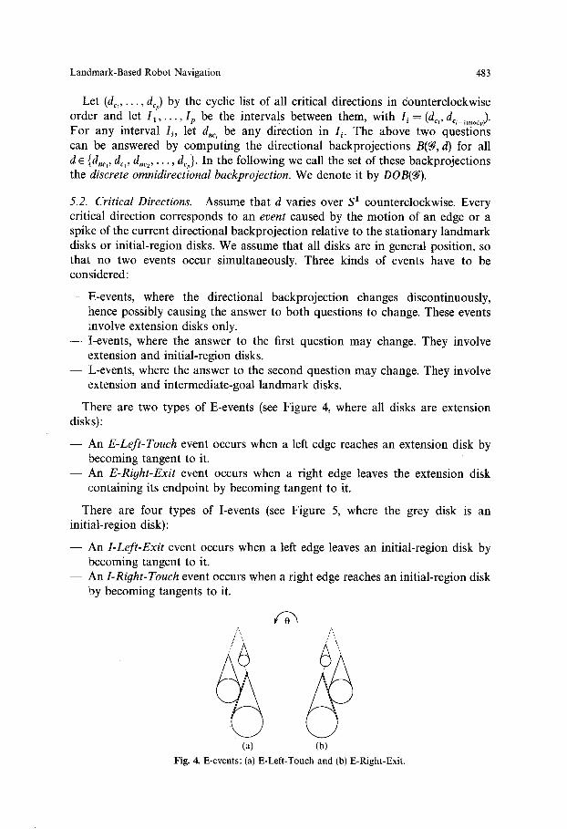
5.2. Critical Directions. Assume that d varies over S 1 counterclockwise. Every critical direction corresponds to an event caused by the motion of an edge or a spike of the current directional backprojection relative to the stationary landmark disks or initial-region disks. We assume that all disks are in general position, so that no two events occur simultaneously. Three kinds of events have to be considered:
--E-events, where the directional backprojection changes discontinuously, hence possibly causing the answer to both questions to change. These events involve extension disks only.
- - I-events, where the answer to the first question may change. They involve extension and initial-region disks. L-events, where the answer to the second question may change. They involve extension and intermediate-goal landmark disks.
There are two types of E-events (see Figure 4, where all disks are extension disks):
- - An E-Left-Touch event occurs when a left edge reaches an extension disk by becoming tangent to it. An E-Right-Exi t event occurs when a right edge leaves the extension disk containing its endpoint by becoming tangent to it.
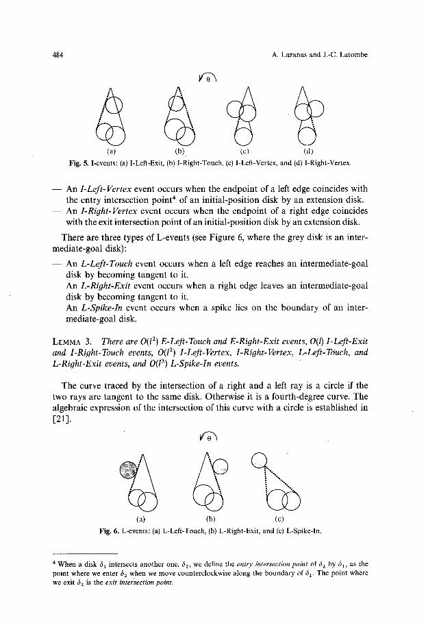
There are four types of I-events (see Figure 5, where the grey disk is an initial-region disk):
- - An I-Lef t-Exit event occurs when a left edge leaves an initial-region disk by becoming tangent to it.
- - An I-Right-Touch event occurs when a right edge reaches an initial-region disk by becoming tangents to it.
A / \
(a)
A
( b )
Fig. 4. E-events: (a) E-Left-Touch and (b) E-Right-Exit.
484 A. Lazanas and J.-C. Latombe
(a) (b) (c) (d)
Fig. 5. I-events: (a) I-Left-Exit, (b) I-Right-Touch, (c) I-Left-Vertex, and (d) I-Right-Vertex.
- - An I-Left- Vertex event occurs when the endpoint of a left edge coincides with the entry intersection point* of an initial-position disk by an extension disk.
- - An I-Right-Vertex event occurs when the endpoint of a right edge coincides with the exit intersection point of an initial-position disk by an extension disk.
There are three types of L-events (see Figure 6, where the grey disk is an inter- mediate-goal disk):
- - An L-Left-Touch event occurs when a left edge reaches an intermediate-goal disk by becoming tangent to it.
- - An L-Right-Exit event occurs when a right edge leaves an intermediate-goal disk by becoming tangent to it.
- - An L-Spike-In event occurs when a spike lies on the boundary of an inter- mediate-goal disk.
LEMMA 3. There are O(I 2) E-Left-Touch and E-Right-Exit events, O(l) I-Left-Exit and I-Right-Touch events, O(F) I-Left-Vertex, I-Right-Vertex, L-Left-Touch, and L-Right-Exit events, and O(l 3) L-Spike-In events.
The curve traced by the intersection of a right and a left ray is a circle if the two rays are tangent to the same disk. Otherwise it is a fourth-degree curve. The algebraic expression of the intersection of this curve with a circle is established in [21].
(a) (b) (c) Fig. 6. L-events: (a) L-Left-Touch, (b) L-Right-Exit, and (c) L-Spike-In.
4 When a disk 61 intersects another one, 62, we define the entry intersection point of 62 by 31, as the point where we enter 62 when we move counterclockwise along the boundary of 61 . The point where we exit 32 is the exit intersection point.
Landmark-Based Robot Navigation 485
5.3. Plannino Method. If J c fr the robot is already in the goal and the planner has nothing to do. In general, however, the planner computes the extension E(fr If this extension is empty, the planner returns failure. Otherwise, it associates a P-command to reach a goal point with every landmark disk in this extension. If J c E(f~o) , the planner returns success.
Let us assume that I r E(f#o). The planner then computes the discrete omni- directional backprojection DOB(~o). IfDOB(f#o) contains a directional backprojec- tion B(fr d) that includes J , then the planner attaches the I-command (d, E(fr to J and returns success. Otherwise, for every landmark area LA r E(fr that has a non-zero intersection with a directional backprojection B(fr d) in DOB(f#o), an exit point is arbitrarily selected in LA n B(f9 o, d) and the I-command (d, E(f#o)) is attached to this point. (If the same area LA intersects several directional backprojections, only one intersection is used to produce the I-command.) The union of the directional backprojections in OB(fgo) is now considered as an intermediate goal f~l-
The extension E(f~I) is a by-product of the above computation. By construction, E(fr ~-E(f#o). If E(f#0 = E(fr no directional backprojection of E(f#l) can possibly intersect a landmark disk that is not already in E(f#l); hence, the planner terminates with failure. Otherwise, every landmark area in E(fgO\E(fgo) contains one disk L with an exit point and an I-command attached to it. With every other disk in the landmark area, the planner associates a P-command to reach the exit point in L. If d c E(f#0, the planner returns success, else it computes the discrete omnidirectional backprojection of E(fr and so on.
During this backchaining process, the set of landmark areas in the extensions of the successive goals increases monotonically. At every iteration, either there is a new landmark area in the extension, and the planner proceeds further, or there is no new area, and the planner terminates with failure. The planner terminates with success whenever it has constructed an extension E(f#,) containing J or a discrete omnidirectional backprojection DOB(fr that includes a directional back- projection containing J . The number of iterations is bounded by the number s of landmark areas. Thus, n < s. Every iteration of the backchaining process requires computing O(P) directional backprojections. The computation of a directional backprojection takes time O(l log/) (see Section 4.3). Hence, the above planning algorithm has time complexity O(sl 4 log l).
5.4. Plan Execution. Assume that the planner returns success after computing an omnidirectional backprojection OB(f#,) that contains J . The generated plan can be regarded as a nonordered collection of reaction rules [30]. Each rule is a motion command whose execution is conditional to the entry of the robot into a region of the workspace, either the initial region, or a landmark disk, or an exit point:
- - The rule associated with J is the I-command (d,, E(fr where d, is such that J c B(CS,, d,). The rule associated with a landmark disk is a P-command to attain the exit point or the goal point of the landmark area to which the disk belongs.
486 A. Lazanas and J.-C. Latombe
- - The rule attached to the exit point of each landmark area LA contained in E(Cgffi+l)\E((ffi) , for any i t [0, n - 1], is an I-command (dl, E(fffl)), where dl is such that LA n B(f#i, dl) is a nonempty region containing the exit point.
The plan is executed as follows: The robot first executes the I-command associated with the initial region. This command guarantees that the robot will stop in a landmark disk with a P-command attached to it. Then the robot executes this P-command, and attains a goal point or an exit point. If it attains a goal point, the execution of the plan is terminated. If it attains an exit point, the I-command attached to this point is executed. This command leads the robot to a new landmark disk, and so on.
An exit point was selected by the planner in a landmark area when this area intersected a directional backprojection for the first time. Later, the planner never changed the command attached to this point. Therefore, when the robot executes the I-command (d~, E(fr from the exit point of some landmark area LA, no landmark disk in LA can possibly be in the termination set E(~) of this command. Thus, since E(fr c E(fr c "" c E(~r the robot cannot terminate its motion in the same landmark area twice by executing the plan. Hence, it is guaranteed to reach fr after executing an alternate sequence of I- and P-commands whose length is smaller than or equal to 2(n + 1).
If the planner re turns success when E(fr contains ~, the generated plan is essentially the same as above, except that it does not include a rule associated with J, since the robot will already be in a landmark area having a P-command attached to it.
If the planner returns failure, it still delivers a plan as a set of reaction rules associated with all landmark areas from where the goal can be achieved reliably. However, the plan is incomplete, since no command is attached to the initial region. The plan can nevertheless be useful. For example, the robot controller may then decide to execute a random motion until the robot enters a landmark area with a command attached to it (see 1-21]).
5.5. Completeness and Optimality. By construction, every I-command in a plan is guaranteed to reach a landmark disk in its termination set. Since the robot cannot terminate in the same landmark area twice (see the previous subsection), the execution of a plan eventually leads the robot to stop in the goal. Hence, the plans generated by the planner are correct. The planner is sound.
Let us say that a plan has k steps if it contains exactly k I-commands. The extension E(fgl) of any goal fCl is the maximal subset of the workspace from which the robot can reliably achieve ffl in zero steps. The set Ue~ooB(~r i.e., the union of the extensions of the directional backprojections in DOB(fgi), is the maximal subset of landmark disks from which the robot can reliably achieve fql in at most one step. Hence, E(fr for any i > 0, is the maximal set of landmark disks from which the robot can reliably achieve fr in at most i steps. The largest set of landmark disks from where the planner can reliably achieve fro is computed in at most s backchaining iterations. By definition of the I-events, if a directional backprojecfion of this set contains the initial region, the planner will find one
Landmark-Based Robot Navigation 487
(perhaps before the last iteration). Thus, if f~o can be reliably achieved from J, the planner is guaranteed to terminate with success. If @o cannot be reliably achieved, backchaining terminates with failure after at most s iterations. Thus, the planner is complete.
Let a motion plan be optimal if the maximal number of steps required by its execution is minimal over all correct motion plans. The maximal number of steps for a plan produced by our algorithm is equal to the number of backchaining iterations before an extension or a backprojection contains the initial region. By definition of the omnidirectional backprojections, the number of iterations is equal to the minimal number of steps that is required to achieve the goal in the worst case. Hence, our algorithm generates optimal plans. Furthermore, after the execution of any sequence of steps, the subset of the motion plan that may still be used to attain the problem's goal is also optimal.
THEOREM 1. 7he plannin9 algorithm is complete and #enerates optimal plans.
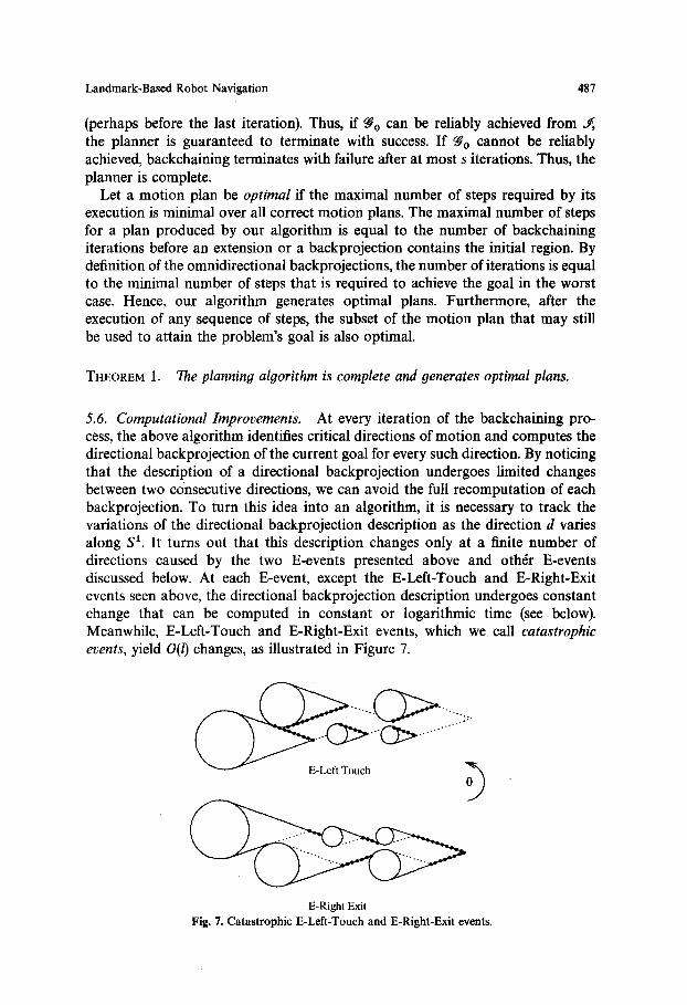
5.6. Computational Improvements. At every iteration of the backchaining pro- cess, the above algorithm identifies critical directions of motion and computes the directional backprojection of the current goal for every such direction. By noticing that the description of a directional backprojection undergoes limited changes between two consecutive directions, we can avoid the full recomputation of each backprojection. To turn this idea into an algorithm, it is necessary to track the variations of the directional backprojection description as the direction d varies along S ~. It turns out that this description changes only at a finite number of directions caused by the two E-events presented above and other E-events discussed below. At each E-event, except the E-Left-Touch and E-Right-Exit events seen above, the directional backprojection description undergoes constant change that can be computed in constant or logarithmic time (see below). Meanwhile, E-Left-Touch and E-Right-Exit events, which we call catastrophic events, yield O(l) changes, as illustrated in Figure 7.
E-Left Touch 0 ~
E-Right Exit Fig. 7. Catastrophic E-Left-Touch and E-Right-Exit events.
488 A. Lazanas and J.-C. Latombe
Hence, the planner can use a sweep algorithm to compute the discrete omni- directional backprojection. This algorithm scans all potential critical directions in counterclockwise order start ing at some noncritical directions where it computes the directional backprojection from scratch. During the sweep, it stops at every critical direction. At noncatastrophic E-events it simply updates the description of the directional backprojection in constant or logarithmic time. At E-Left-Touch or E-Right-Exit it recomputes the directional backprojection from scratch. At every I-event it uses the current backprojection description to determine if the backprojection contains J . This can be done in a straightforward way in time O(l log/). At every L-event the intersected intermediate-goal disk, if any, is identified in constant time.
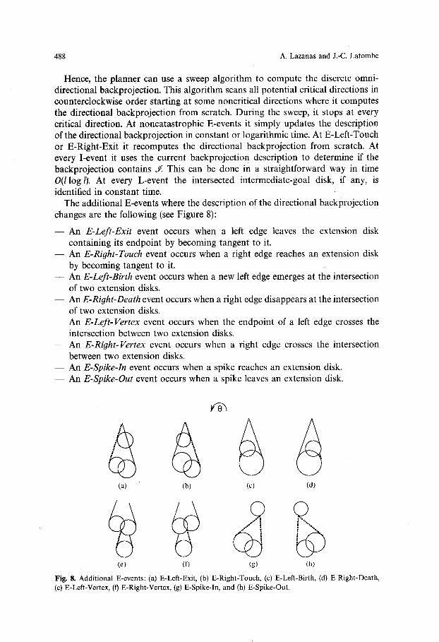
The additional E-events where the description of the directional backprojection changes are the following (see Figure 8):
- - An E-Left-Exit event occurs when a left edge leaves the extension disk containing its endpoint by becoming tangent to it.
- - An E-Right-Touch event occurs when a right edge reaches an extension disk by becoming tangent to it.
- - An E-Left-Birth event occurs when a new left edge emerges at the intersection of two extension disks.
- - An E-Right-Death event occurs when a right edge disappears at the intersection of two extension disks.
- - An E-Left-Vertex event occurs when the endpoint of a left edge crosses the intersection between two extension disks.
- - An E-Right-Vertex event occurs when a right edge crosses the intersection between two extension disks.
- - An E-Spike-In event occurs when a spike reaches an extension disk. - - An E-Spike-Out event occurs when a spike leaves an extension disk.
(a) (b)
(e) (f)
(c) (d)
(g) (h)
Fig. 8. Additional E-events: (a) E-Left-Exit, (b) E-Right-Touch, (c) E-Left-Birth, (d) E-Right-Death, (e) E-Left-Vertex, (f) E-Right-Vertex, (g) E-Spike-In, and (h) E-Spike-Out.
Landmark-Based Robot Navigation
11
23
r2
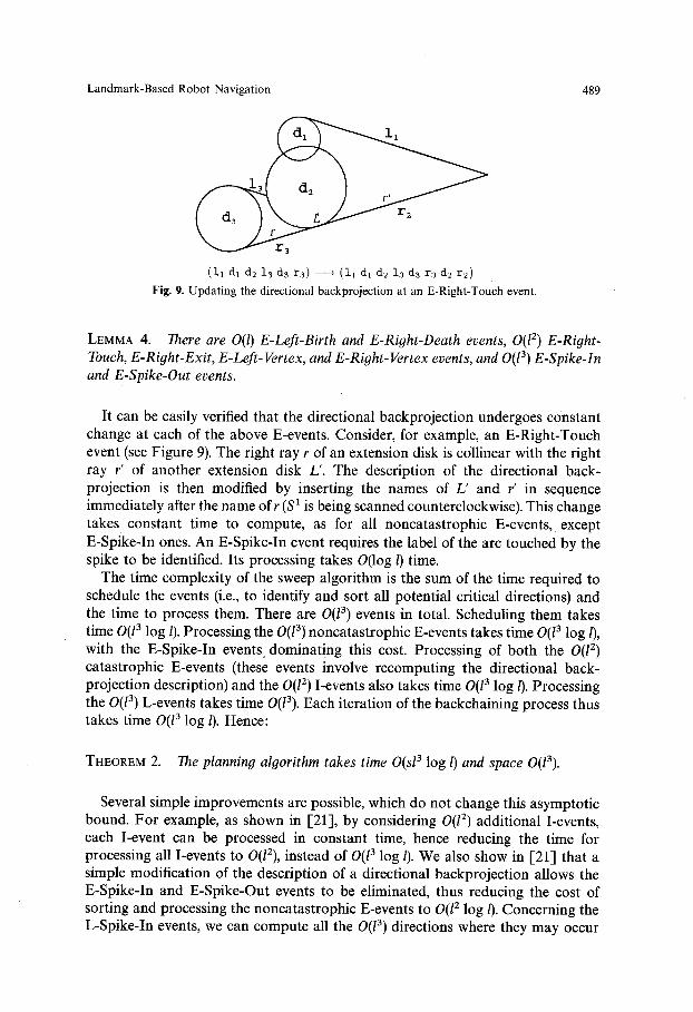
(11 dl d:~ 1:3 d3 r3) ----+ (ii dl d~ 13 d3 r:~ d~ r~)
Fig. 9. Updating the directional backprojection at an E-Right-Touch event.
489
LEMMA 4. There are O(l) E-Left-Birth and E-Right-Death events, O(I 2) E-Right- Touch, E-Right-Exit, E-Left-Vertex, and E-Right-Vertex events, and O(l 3) E-Spike-In and E-Spike-Out events.
It can be easily verified that the directional backprojection undergoes constant change at each of the above E-events. Consider, for example, an E-Right-Touch event (see Figure 9). The right ray r Of an extension disk is collinear with the right ray r' of another extension disk L'. The description of the directional back- projection is then modified by inserting the names of L' and r' in sequence immediately after the name of r (S 1 is being scanned counterclockwise). This change takes constant time to compute, as for all noncatastrophic E-events, except E-Spike-In ones. An E-Spike-In event requires the label of the arc touched by the spike to be identified. Its processing takes O(log/) time.
The time complexity of the sweep algorithm is the sum of the time required to schedule the events (i.e., to identify and sort all potential critical directions) and the time to process them. There are O(l a) events in total. Scheduling them takes time O(l 3 log/). Processing the O(l 3) noncatastrophic E-events takes time O(l 3 log l), with the E-Spike-In events dominating this cost. Processing of both the O(l 2) catastrophic E-events (these events involve recomputing the directional back- projection description) and the O(l 2) I-events also takes time O(l 3 log/). Processing the O(l 3) L-events takes time 0(13). Each iteration of the backchaining process thus takes time O(l 3 log/). Hence:
THEOREM 2. The planning algorithm takes time O(sl a log 1) and space 0(13).
Several simple improvements are possible, which do not change this asymptotic bound. For example, as shown in [-21], by considering O(l 2) additional I-events, each I-event can be processed in constant time, hence reducing the time for processing all I-events to O(12), instead of O(l 3 log/). We also show in [21] that a simple modification of the description of a directional backprojection allows the E-Spike-In and E-Spike-Out events to be eliminated, thus reducing the cost of sorting and processing the noncatastrophic E-events to O(l 2 log/). Concerning the L-Spike-In events, we can compute all the O(l 3) directions where they may occur
490 A. Lazanas and J.-C. Latombe
in advance, so that we sort them only once and reuse this result at every backchaining iteration. We thus reduce the total time for sorting and processing the L-Spike-In events to O(sl3). The O(sl 3 log/) time complexity of the planner is then only dominated by the processing of the O(/2) catastrophic E-events.
6. Experimental Results. We have implemented the above planning algorithm, along with navigation techniques and a robot simulator, in C on a DECstation 5000. The implemented planner incorporates two significant improvements:
(1) During the computation of an omnidirectional backprojection, it does not discard an intermediate-goal disk L as soon as this disk intersects a directional backprojection. Instead, it determines the intervals of all directions at which the directional backprojection intersects L, computes the intersection of L with the directional backprojection at the midpoint of each such interval, and keeps the intersection having the biggest area. This intersection is called the exit region of L.
(2) Several exit regions, each in a unique disk, may be generated in the same landmark area. With each disk in such a landmark area, the planner associates a P-command leading to one exit region constructed in the area. When several exit regions are available, it selects the region that allows the generation of the P-command containing the smallest number of via points.
The purpose of the first modification is to allow some errors in control and sensing in the landmark areas (see Section 8.2). The second modification avoids planning P-commands through long sequences of disks in a landmark area when this is not necessary. (However, it is only a heuristic, since it does not take the radii of the landmark disks into account.)
Below we present examples of plans generated by the implemented planner, along with their simulated execution. In all the figures (for instance, see Figure 11) white disks are landmark disks that intersect the omnidirectional back- projections computed by the planner, except the last one, i.e., the one that includes the initial region (if such a backprojection exists). Grey disks are the other landmark disks and no command is attached to them. In all examples there is a single initial-region disk designated by J, and a single goal-region disk designated by fro.
Whenever the robot enters a new landmark area L that is part of the termination set of the I-command currently being executed (then the disks in L are necessarily white), it shifts to executing a P-command leading to a point (the exit point) selected in an exit region in L; as soon as it enters the exit region containing the exit point, it abandons the P-command and shifts to executing the corresponding I-command attached to the exit point. The exit region constructed in every white disk, if there is one such region, is shown in the figures (except when it covers the whole disk), together with the direction of the I-command attached to the selected exit point. The termination sets of the I-commands are not shown in the figures, but can be inferred from the drawings.
L a n d m a r k - B a s e d Robo t N a v i g a t i o n 491
�9 ~.: :,., F!7i~)
- " ' A - - : - ' j ',
, (::9 "<: • ,._~ ~<:) ~" -h B . _ . . / I . . . .
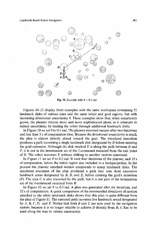
Fig. 10. Example wi th 0 = 0.1 tad.
Figures 10-12 display three examples with the same workspace containing 51 landmark disks of various sizes and the same initial and goal regions, but with increasing directional uncertainty 0. These examples show that, when uncertainty grows, the planner returns more and more sophisticated plans, as it attempts to reduce uncertainty by leading the robot through additional landmark disks.
In Figure 10 we set 0 to 0.1 rad. The planner returned success after two iterations and less than 3 s of computation time. Because the directional uncertainty is small, the plan is almost directly aimed toward the goal. The simulated execution produces a path traversing a single landmark disk designated by D before entering the goal extension. Although the disk marked E is along the path between D and F, it is not in the termination set of the I-command executed from the exit point of D. The robot traverses E without shifting to another motion command.
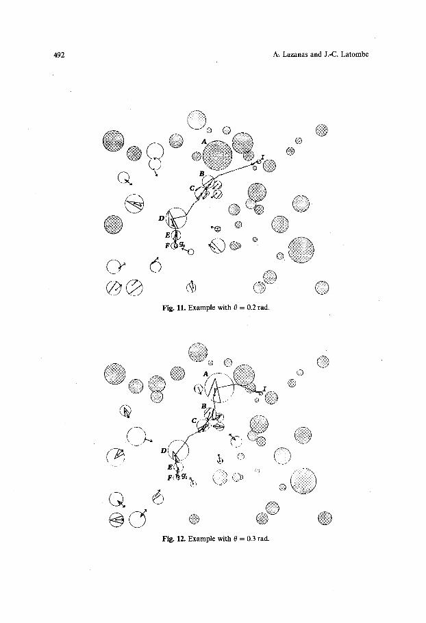
In Figure 11 we set 0 to 0.2 rad. It took four iterations of the-planner, and 19 s of computation, before the initial region was included in a backprojection. In the process the planner attached motion commands to many landmark disks. The simulated execution of the plan produced a path that uses three successive landmark areas designated by B, D, and E, before entering the goal's extension (F). The area C is also traversed by the path, but it is not part of the termination set of the I-command executed from B.
In Figure 12 we set 0 to 0.3 rad. A plan was generated after six iterations, and 52 s of computation. A quick comparison of the commanded directions of motion attached to the white landmark disks shows that this plan is quite different from the plan of Figure 11. The executed path traverses five landmark aread designated by A, B, C, D, and E. Notice that both B and C are now used by the navigation system, because it is no longer reliable to achieve D directly from B; C has to be used along the way to reduce uncertainty.
492 A. Lazanas and J.-C. Latombe
,.,,5 ~,~,~ | @
@ " ' ~J E~
Fi
{--2~ c5 @@
~'o
|
@ <~15
@ {} @
@ @
@
@
Fig. 11. Example with 0 = 0.2 rad.
(f-~X
@
F(1
.... ~ , ~ ~
{.~
�9 L . - - " 0
�9
@
@
@ _ |
Fig. 12. Example with 0 = 0.3 rad.
Landmark-Based Robot Navigation 493
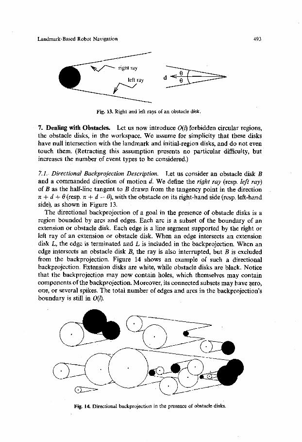
Fig. 13. Right and left rays of an obstacle disk.
7. Dealing with Obstacles. Let us now introduce O(/) forbidden circular regions, the obstacle disks, in the workspace. We assume for simplicity that these disks have null intersection with the landmark and initial-region disks, and do not even touch them. (Retracting this assumption presents no particular difficulty, but increases the number of event types to be considered.)
7.1. Directional Backprojection Description. Let us consider an obstacle disk B and a commanded direction of motion d. We define the right ray (resp. left ray) of B as the half-line tangent to B drawn from the tangency point in the direction n + d + 0 (resp. n + d - 0), with the obstacle on its right-hand side (resp. left-hand side), as shown in Figure 13.
The directional backprojection of a goal in the presence of obstacle disks is a region bounded by arcs and edges. Each arc is a subset of the boundary of an extension or obstacle disk. Each edge is a line segment supported by the right or left ray of an extension or obstacle disk. When an edge intersects an extension disk L, the edge is terminated and L is included in the backprojection. When an edge intersects an obstacle disk B, the ray is also interrupted, but B is excluded from the backprojection. Figure 14 shows an example of such a directional backprojection. Extension disks are white, while obstacle disks are black. Notice that the backprojection may now contain holes, which themselves may contain components of the backprojection. Moreover, its connected subsets may have zero, one, or several spikes. The total number of edges and arcs in the backprojection's boundary is still in 0(/).
Fig. 14. Directional backprojection in the presence of obstacle disks.
494 A. Lazanas and J.-C. Latombe
We construct the description of a directional backprojection very much in the same way as when there are no obstacles. We simply give a name to every obstacle disk so that we can label the various edges and arcs of the backprojection's boundary that arise from the presence of the obstacles. Although there are more types of labels to handle, the computation of this description still takes time 0(I log/).
LEMMA 5. The description of a directional backprojection in the presence of 0(I) obstacles is computed in time O(l log/) and space O(1).
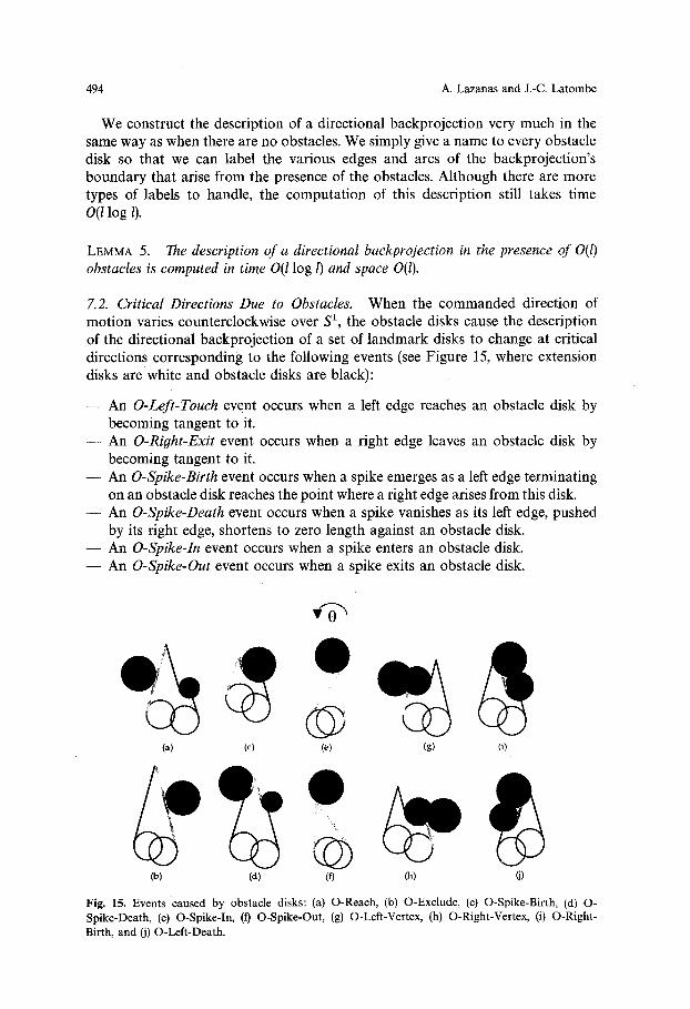
7.2. Critical Directions Due to Obstacles. When the commanded direction of motion varies counterclockwise over S 1, the obstacle disks cause the description of the directional backprojection of a set of landmark disks to change at critical directions corresponding to the following events (see Figure 15, where extension disks are white and obstacle disks are black):
- - An O-Left-Touch event occurs when a left edge reaches an obstacle disk by becoming tangent to it.
- - An O-Right-Exit event occurs when a right edge leaves an obstacle disk by becoming tangent to it.
- - An O-Spike-Birth event occurs when a spike emerges as a left edge terminating on an obstacle disk reaches the point where a right edge arises from this disk.
- - An O-Spike-Death event occurs when a spike vanishes as its left edge, pushed by its right edge, shortens to zero length against an obstacle disk.
- - An O-Spike-In event occurs when a spike enters an obstacle disk. - - An O-Spike-Out event occurs when a spike exits an obstacle disk.
(a)
Co)
(c) (g) (i)
(d) (h) O)
�9 (f)
Fig. 15. Events caused by obstacle disks: (a) O-Reach, (b) O-Exclude, (c) O-Spike-Birth, (d) O- Spike-Death, (e) O-Spike-In, (I) O-Spike-Out, (g) O-Left-Vertex, (h) O-Right-Vertex, (i) O-Right- Birth, and (j) O-Left-Death.
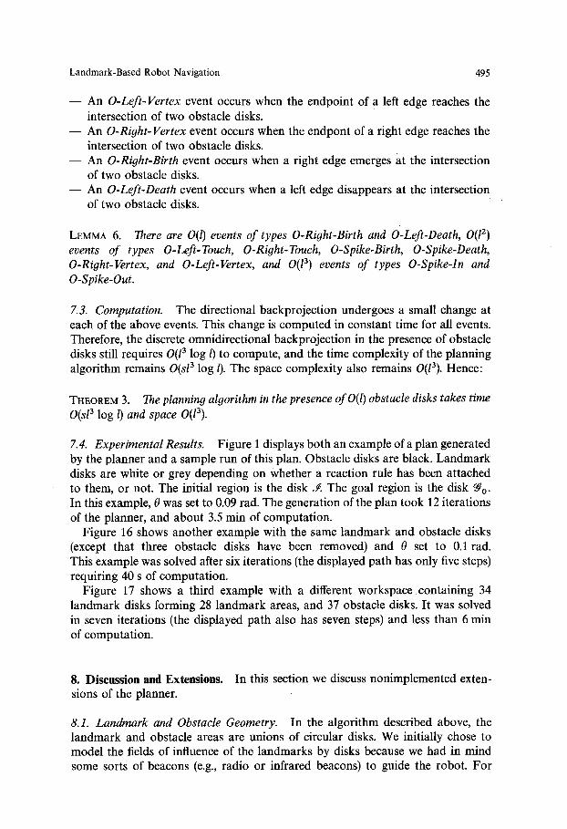
Landmark-Based Robot Navigation 495
- - An O-Left-Vertex event occurs when the endpoint of a left edge reaches the intersection of two obstacle disks.
- - An O-Rioht- Vertex event occurs when the endpont of a right edge reaches the intersection of two obstacle disks.
- - An O-Right-Birth event occurs when a right edge emerges at the intersection of two obstacle disks.
- - An O-Left-Death event occurs when a left edge disappears at the intersection of two obstacle disks.
LEMMA 6. There are O(1) events of types O-Right-Birth and O-Left-Death, O(l 2) events of types O-Left-Touch, O-Right-Touch, O-Spike-Birth, O-Spike-Death, O-Right-Vertex, and O-Left-Vertex, and O(l a) events of types O-Spike-In and O-Spike-Out.
7.3. Computation. The directional backprojection undergoes a small change at each of the above events. This change is computed in constant time for all events. Therefore, the discrete omnidirectional backprojection in the presence of obstacle disks still requires O(l 3 log/) to compute, and the time complexity of the planning algorithm remains O(sl 3 log/). The space complexity also remains O(13). Hence:
THEOREM 3. The planning algorithm in the presence of O(l) obstacle disks takes time O(sl 3 log/) and space O(/3).
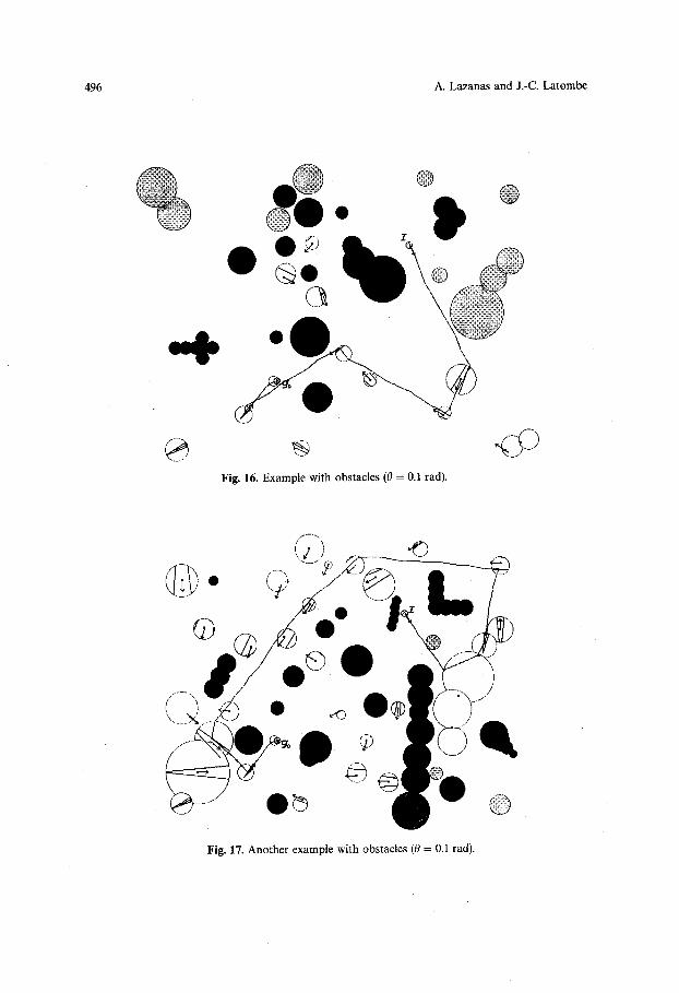
7.4. Experimental Results. Figure 1 displays both an example of a plan generated by the planner and a sample run of this plan. Obstacle disks are black. Landmark disks are white or grey depending on whether a reaction rule has been attached to them, or not. The initial region is the disk J. The goal region is the disk f#o. In this example, 0 was set to 0.09 rad. The generation of the plan took 12 iterations of the planner, and about 3.5 min of computation.
Figure 16 shows another example with the same landmark and obstacle disks (except that three obstacle disks have been removed) and 0 set to 0.1 rad. This example was solved after six iterations (the displayed path has only five steps) requiring 40 s of computation.
Figure 17 shows a third example with a different workspace containing 34 landmark disks forming 28 landmark areas, and 37 obstacle disks. It was solved in seven iterations (the displayed path also has seven steps) and less than 6 min of computation.
8. Discussion a n d E x t e n s i o n s . In this section we discuss nonimplemented exten- sions of the planner.
8.1. Landmark and Obstacle Geometry. In the algorithm described above, the landmark and obstacle areas are unions of circular disks. We initially chose to model the fields of influence of the landmarks by disks because we had in mind some sorts of beacons (e.g., radio or infrared beacons) to guide the robot. For
iu
1/ "~
!
) <<
--"
, --
J/"
M=:
,,lq,,
+ 0 g g +
5 II p~
@
0 II
,I, @
~i O
~
@
I
Landmark-Based Robot Navigation 497
uniformity, we made the same choice for the obstacles. However, most natural landmarks do not entail circular fields of influence. We can approximate any landmarks or obstacle area by a collection of overlapping disks, but the number of these disks grows quickly with the precision of the approximation, yielding longer computation.
Our algorithm can be easily adapted to deal with landmark and obstacle areas described as generalized polygonal regions bounded by straight and circular edges. In this extension, for any commanded direction of motion, we can still define the right and left rays of a landmark or an obstacle area. If the area is not convex, it may have several right and/or left rays. While the origin of the right or left ray of a circular contour varies continuously as the commanded direction of motion rotates, the origin of the right or left ray of a polygonal contour remains anchored at a fixed vertex, except at critical directions where it jumps from one vertex of the contour to another. These directions (which are parallel to the straight edges of the generalized polygonal contours of the landmark and obstacle areas) are additional critical directions to be treated by the planner. Also, if an extension landmark area and an obstacle area touch each other, we may have to erect a ray whose origin is an intersection point of the two contours. The origin of such a ray remains stationary for a subrange of orientations d. The curves traced by the spikesare not more complicated than in the pure circular case and their degrees remain no greater than 4.
Although several small adaptations have to be carefully made, our planning method thus extends to the case where landmark and obstacle areas are bounded by straight edges and circular arcs and may touch each other. If the workspace contains s landmark areas bounded by O(1) edges and arcs and the obstacle areas are bounded by O(/) edges and arcs, the time complexity of the planner remains O(sl 3 log l).
Representing landmark and obstacle areas as generalized polygons is a very realistic model for most applications. In particular, if the robot is an omnidirec- tional circular robot moving among polygonal obstacles, shrinking the robot to its centerpoint and growing the obstacles isotropically by the robot's radius yields such generalized polygonal regions.
In a similar way, the algorithm can be extended to allow compliant motions on obstacle edges. Additional critical directions must be considered by the planner, but complexity bounds remain unchanged. Allowing compliance significantly enlarges the set of problems that admit correct plans.
8.2. Uncertainty in Landmark Areas. Perhaps the less realistic assumption in the problem definition of Section 3 is that control and position sensing are perfect in landmark areas, while sensing is null outside any such area. Below, we first argue that this assumption is reasonable. We then show that it can be relaxed to some extent.
A typical mobile robot uses two techniques to estimate its position continuously, dead-reckoning and environmental sensing. Environmental sensing provides perti- nent information only when some characteristic features of the workspace ("land-
498 A. Lazanas and J.-C. Latombe
marks") are visible by the sensors. Then the robot knows its position with a good accuracy. When no or few features are visible, the robot relies on dead-reackoning, which yields cumulative errors that we model by the directional uncertainty. Our assumption that sensing outside landmark areas is null is perhaps conservative, but it does not prevent the robot's navigation system from using all available sensing information at execution time to determine the robot's current position better. In the worst case this may lead the planner to return failure, while reliable paths exist in practice.
On the contrary, the assumption that control is perfect in the landmark areas is anticonservative; but if we choose safe features to create landmark disks, it is a reasonable one. To some extent, most workspaces can be engineered to include such features. Landmark areas with sharp boundaries can be obtained by introdu- cing artificial landmarks and/or thresholding an estimate of the sensing un- certainty. For example, the notion of a "sensory uncertainty field" (SUF) is introduced in [31]. At every possible point q in the configuration space, the SUF estimates the range of possible errors in the sensed configuration that the naviga- tion system would compute by matching the sensory data against a prior model of the workspace, if the robot was at q. The SUF is computed at planning time from a model of the robot's sensing system.
More interestingly, however, it can be noticed that perfect control and sensing in landmark areas are not strictly needed. Indeed, once the robot enters a landmark area it is sufficient that it reaches an exit region of nonzero measure prior to executing the next I-command. (If the landmark area intersects the goal, the "exit region" is the intersection with the goal.) For example, the maximal sensing error allowed in a landmark area could be half the radius of the largest disk fully contained in an exit region. Thus, although the planner assumed perfect sensing in landmark areas, we can now create these areas by engineering the workspace in such a way that the sensors just provide the information that is needed by the plan (see [13] for a similar idea). However, maximal errors in landmark areas seem to depend on the plan itself, so that they can only be computed once a plan has been generated assuming no such errors.
8.3. Other Types of Landmarks. Other, perhaps more realistic types of land- marks, which only require simple adaptations of our planning algorithm, can be defined.
An example of another type of landmark area is a region L containing a subregion C, such that if the robot ever enters L, it knows that it is in L and it can reliably navigate into C; when it enters C, it recognizes the achievement of C. This definition does not require perfect control in L, nor perfect position sensing. For example, consider a wall w and the corner it makes with another wall. The wall w induces an area L, such that if the robot is in L, its proximity sensor can sense the wall (we assume that w cannot be confused with another object). If the robot moves along w, parallel to it (e.g., using proximity sensing), toward the corner, it will eventually reach a small region C from where it can sense the corner.
A landmark area (L, C) as above can be treated by our algorithm as follows: In order for a directional backprojection to "intersect" this landmark area, it has
Landmark-Based Robot Navigation 499
to contain C fully (yielding events similar to the I-events used for containment of the initial region). When this is the case the whole region L can be inserted in the goal extension used at the next backchaining iteration.
A particular case of the above landmark is when C = L. For example, a characteristic feature defines an area L from where it can be sensed. If the feature is not sufficient to allow the robot to determine its location or navigate into a subregion of L, we can simply set C -- L. Then the only information used by the planner is: if the robot ever enters L, it will know it.
9. Conclusion. This paper describes a complete polynomial planning algorithm for mobile-robot navigation in the presence of uncertainty. The algorithm addres- ses a class of problems where landmarks create regions in the configuration space where both control and position sensing are perfect. Outside these regions sensing is null; control, which relies on dead-reckoning, is imperfect, but directional errors are bounded. Although this class of problems is a simplification of real mobile- robot planning problems, by no means is it oversimplified.
A computer program embedding the planning algorithm was implemented, along with navigation techniques and a robot simulator. This program was run with many different examples, some of which were presented in this paper. The planner is reasonably fast. In its present form it assumes that all landmark and obstacle areas are described as unions of disks. However, extending the planner to accept a more general geometry (generalized polygonal areas) is rather straight- forward. Other interesting extensions (uncertainty in landmark areas, new types of landmark areas) are possible. The relative time efficiency of the planner suggests that our complexity bounds are not tight.
So far, most algorithms to plan motion strategies under uncertainty were either exponential in the size of the input problem; unsound, and/or incomplete. Such algorithms may be interesting from a theoretical point of view, but their computa- tional complexity or lack of reliability prevent them from being applied to real-world problems. Our work shows that it is possible to identify a restricted, but still realistic, subclass of planning problems that can be solved in polynomial time. This subclass is obtained through assumptions whose satisfaction may require prior engineering of the robot and/or its workspace. In our case this implies
+ the creation of adequate landmarks, either by taking advantage of the natural features of the workspace, or introducing artificial beacons, or using specific sensors. We call this type of simplification engineering for planning tractability.
Engineering the robot and the workspace has its own cost and we would like to minimize it. Therefore, future research should aim at finding more general classes of problems than the one solved by the current planner, but requiring less engineering and still solvable in polynomial time. It should also investigate the following "inverse" problem: Given our planning method, and the description of a family of tasks (e.g., the set of all possible initial and goal regions), how do we minimally engineer the workspace? For instance: What is the minimal number of landmarks that we should place in the workspace and where should we place them, so that every possible problem admits a correct plan?
5OO
Acknowledgment. comments.
A. Lazanas and J.-C. Latombe
The author thanks Leo Guibas for his encouragement and
References
[1] Ayache, N., Artificial Vision for Mobile Robots: Stereo Vision and Multisensory Perception, MIT Press, Cambr!dge~ MA, 1991.
[2] Briggs, A. J., An efficient Algorithm for One-Step Planar Compliant Motion Planning with Uncertainty, Proc. 5th Annual ACM Symp. on Computational Geometry, Saarbruchen, 1989, pp. 187-196.
[3] Buckley, S. J., Planning and Teaching Compliant Motion Strategies, Ph.D. Dissertation, Depart- ment of Electrical Engineering and Computer Science, MIT, Cambridge, MA, 1986.
[4] Canny, J. F., On Computability of Fine Motion Plans, Proc. IEEE Internat. Conf. on Robotics and Automation, Scottsdale, AZ, 1989, pp. 177-182.
[5] Canny, J. F., and Reif, J., New Lower Bound Techniques for Robot Motion Planning Problems, Proc. 27th IEEE Symp. on Foundations of Computer Science, Los Angeles, CA, 1987, pp. 49-60.
[6] Christiansen, A., Mason, M., and Mitchell, T. M., Learning Reliable Manipulation Strategies Without Initial Physical Models, Proc. IEEE Internat. Conf. on Robotics and Automation, Cincinnati, OH, 1990, pp. 1224-1230.
[7] Crowley, J. L., World Modeling and Position Estimation for a Mobile Robot Using Ultrasonic Ranging, Proc. IEEE Internat. Conf. on Robotics and Automation, Scottsdale, AZ, 1989, pp. 674-680.
[8] Donald, B. R., A Geometric Approach to Error Detection and Recovery for Robot Motion Planning with Uncertainty, Artificial Intelligence J., 37(1-3) (1988), 223-271.
[9] Donald, B. R., The Complexity of Planar Compliant Motion Planning Under Uncertainty, Algorithmica, 5 (1990), 353 382.
[10] Donald, B. R., and Jennings, J., Sensor Interpretation and Task-Directed Planning Using Perceptual Equivalence Classes, Proc. IEEE Internal. Cotf on Robotics and Automation, Sacramento, CA, 1991, pp. 190-197.
[11] Dufay, B., and Latombe, J. C., An Approach to Automatic Robot Programming Based on Inductive Learning, Internat. J. Robotics Res., 3(4) (1984), 3-20.
[12] Erdmann, M., On Motion Planning with Uncertainty, Technical Report 810, Artificial Intelligence Laboratory, MIT, Cambridge, MA, 1984.
[13] Erdmann, M., Towards Task-Level Planning." Action-Based Sensor Design, Technical Report CMU-CS-92-116, Department of Computer Science, Carnegie Mellon University, Pittsburgh, PA, February 1992.
[14] Fox, A., and Hutchinson, S., Exploiting Visual Constraints in the Synthesis of Uncertainty- Tolerant Motion Plans, Technical Report UIUC-BI-AI-RCV-92-05, The University of Illinois at Urbana-Champaign, Urbana, IL, October 1992.
[15] Friedman, J., Computational Aspects of Compliant Motion Planning, Ph.D. Dissertation, Techni- cal Report No. STAN-CS-91-1368, Department of Computer Science, Stanford University, Stanford, CA, 1991.
[16] Gottschlich, S. N., and Kak, A. C., Dealing with Uncertainty in CAD-Based Assembly Motion Planning, Proc. 9th Nat. Conf. on ArtificialIntelligence, Anaheim, CA, July 1991, pp. 646-652.
[17] Hutchinson, S., Exploiting Visual Constraints in Robot Motion Planning, Proc. IEEE Internat. Conf. of Robotics and Automation, Sacramento, CA, 1991, pp. 1722-1727.
[18] Latombe, J. C., Robot Motion Planning, Kluwer, Boston, MA, 1991. [19] Latombe, J. C., Lazanas, A., and Shekhar, S., Robot Motion Planning with Uncertainty in
Control and Sensing, Artificial Intelligence J., 52(1) (1991), 1-47. [20] Laugier, C., and Th6veneau, P., Planning Sensor-Based Motions for Part-Mating Using
Geometric Reasoning Techniques, Proc. European Conf on Artificial Intelligence , Brighton, 1986.
[21] Lazanas, A., and Latombe, J. C., Landmark-Based Robot Navigation, Technical Report STAN- CS-92-1428, Department of Computer Science, Stanford University, Stanford, CA, 1992.
Landmark-Based Robot Navigation 501
[22] Leonard, J. J., and Durrant-Whyte, H. F., Mobile Robot Localization by Tracking Geometric Beacons, IEEE Trans. Robotics Automat., 7(3) (1991), 376-382.
[23] Levitt, T. S., Lawton, D. T., Chelberg, D. M., and Nelson, P. C., Qualitative Navigation, Proc. Image Understanding Workshop, Los Angeles, CA, 1987, pp. 447465.
[24] Lozano-P6rez, T., The Design of a Mechanical Assembly System, Technical Report AI-TR 397, Artificial Intelligence Laboratory, MIT, Cambridge, MA, 1976.
[25] Lozano-P6rez, T., Mason, M. T., and Taylor, R. H., Automatic Synthesis of Fine-Motion Strategies for Robots, Internat. J. Robotics Res., 3(1) (1984), 3-24.
[26] Mahadevan, S., and Connell, J., Automatic Programming of Behavior-Based Robots Using Reinforcement Learning, Research Report, IBM T.J. Watson Research Center, Yorktown Heights, NY, 1990.
[27] Mason, M. T., Automatic Planning of Fine Motions: Correctness and Completeness, Proc. IEEE Internat. Conf. on Robotics and Automation, Atlanta, GA, 1984, pp. 492-503.
[28] Natarajan, B. K., The Complexity of Fine Motion Planning, Internat. J. Robotics Res., 7(2) (1988), 36-42.
[29] Preparata, F. P., and Shamos, M. I., Computational Geometry." An Introduction, Springer-Verlag, New York, 1985.
[30] Schoppers, M. J., Representation and Automatic Synthesis of Reaction Plans, Ph.D. Dissertation, Department of Computer Science, University of Illinois at Urbana-Champaign, Urbana, IL, 1989.
[31] Takeda, H., and Latombe, J. C., Sensory Uncertainty Field for Mobile Robot Navigation, Proc. IEEE Internat. Conf. on Robotics and Automation, Nice, 1992, pp. 2465-2472.
[32] Taylor, R. H., Synthesis of Manipulator Control Programs from Task-Level Specifications, Ph.D. Dissertation, Department of Computer Science, Stanford University, Stanford, CA, 1976.
[33] Zhang, Z., and Faugeras, O., A 3D World Model Builder with a Mobile Robot, The Internat. J. of Robotics Res., 11(4) (1992), 269-285.
Related Documents