How to fit nonlinear plant growth models and calculate ...guianaplants.stir.ac.uk/paine/pubs/Paine et al_MEE_2012.pdf · How to ﬁt nonlinear plant growth models and calculate growth

How to fit nonlinear plant growth models and calculategrowth rates: an update for ecologists

C. E. Timothy Paine1*, Toby R. Marthews1,2, Deborah R. Vogt1, Drew Purves3, Mark Rees4,

Andy Hector1 and Lindsay A. Turnbull1

1Institute of Evolutionary Biology and Environmental Studies, University of Zurich, Winterthurerstrasse 190, CH-8057

Switzerland; 2Oxford University Centre for the Environment, South Parks Road, Oxford OX1 3QY, UK; 3Computational

Ecology and Environmental Science Group, Microsoft Research, Cambridge CB3 0FB, UK; and 4Department of

Animal and Plant Sciences, University of She!eld, Western Bank, She!eld S10 2TN, UK

Summary

1. Plant growth is a fundamental ecological process, integrating across scales from physiology tocommunity dynamics and ecosystem properties. Recent improvements in plant growth modelling

have allowed deeper understanding and more accurate predictions for a wide range of ecologicalissues, including competition among plants, plant–herbivore interactions and ecosystem function-ing.

2. One challenge in modelling plant growth is that, for a variety of reasons, relative growth rate(RGR) almost universally decreases with increasing size, although traditional calculations assume

that RGR is constant. Nonlinear growth models are flexible enough to account for varying growthrates.

3. We demonstrate a variety of nonlinear models that are appropriate for modelling plant growthand, for each, show how to calculate function-derived growth rates, which allow unbiased compari-

sons among species at a common time or size. We show how to propagate uncertainty in estimatedparameters to express uncertainty in growth rates. Fitting nonlinear models can be challenging, so

we present extensive worked examples and practical recommendations, all implemented inR.4. The use of nonlinear models coupled with function-derived growth rates can facilitate the testingof novel hypotheses in population and community ecology. For example, the use of such techniques

has allowed better understanding of the components of RGR, the costs of rapid growth and thelinkage between host and parasite growth rates.We hope this contribution will demystify nonlinear

modelling and persuademore ecologists to use these techniques.

Key-words: mixed-effects models, nonlinear regression, relative growth rate, R language

Motivation

The purpose of this contribution is to update ecologists regard-

ing recent advances in plant growth modelling, which allow a

deeper understanding of ecological processes thanwas possible

with traditional approaches. The methods we develop are gen-

eral and may be applied to a wide range of organisms. The

advance they represent is made evident by the insight they have

provided into a wide variety of ecological subjects. Recent

applications of these techniques include assessing the relation-

ship between seed size and growth rates (Turnbull et al. 2008),

documenting trade-o!s between growth and survival (Rose

et al. 2009), quantifying the costs of investment in chemical

defence (Paul-Victor et al. 2010; Zust et al. 2011), assessing the

e!ects of hemi-parasitic plants on their hosts (Hautier et al.

2010) and partitioning the components of relative growth rate

(RGR) (Rees et al. 2010). These studies illustrate particular

aspects of the approach advocated in this contribution, but

here, we synthesize them to provide a general framework suit-

able formany applications.

Three factors make the time ripe for a review of nonlinear

growth models. There is a growing consensus that traditional

approaches to modelling growth, rooted as they are in linear

and exponential models, are inadequate. Statistical software

has matured to the point that implementation of nonlinear

models is increasingly within the grasp of ecologists. Finally,

the relevance of metabolic theory, the only widely accepted

theoretical model of plant growth (West, Brown & Enquist

1999), continues to be actively debated (e.g. Muller-Landau*Correspondence author. E-mail: [email protected] site: http://www.respond2articles.com/MEE/

Methods in Ecology and Evolution 2012, 3, 245–256 doi: 10.1111/j.2041-210X.2011.00155.x

! 2011 The Authors. Methods in Ecology and Evolution ! 2011 British Ecological Society

et al. 2006). Thus, there is a pressing need to fit empirical mod-

els, particularly nonlinear ones. We hope through this contri-

bution to encourage more ecologists to take advantage of

nonlinearmodels for growth.

Background

Growth, the ontogenetic change in the biomass of an organ-

ism, links scales of biology from physiology andmetabolism to

community dynamics (McMahon & Bonner 1983). An under-

standing of growth is therefore essential to understand a host

of ecological processes, including competition, plant–herbivore

interactions, interactions between plants and their abiotic envi-

ronment and local community dynamics (Kobe 1999; Tanner

et al. 2005; Muller-Landau et al. 2006). The details of plant

growth tend, however, to be ignored in many ecological stud-

ies. Most dynamic global vegetation models, for example, leap

from resource availability to ecosystem processes, with little

consideration of how individual physiology or height-struc-

tured competition for light a!ect the conversion of those

resources into biomass (Purves & Pacala 2008).

Traditional analyses of growth are rooted in the statistics

of linear regression, which limits the range of models that can

be fit (Causton & Venus 1981; Hunt 1982; Charles-Edwards,

Doley & Rimmington 1986; Poorter 1989). Linear models

assume constant absolute growth rate (AGR, g day)1), and

exponential (loglinear) models assume constant RGR

(g g)1 day)1). These assumptions limit their utility, as both

AGR and RGR vary with environmental conditions and over

ontogeny. Many studies of plant growth rates dispense with

curve fitting entirely and calculate absolute and RGRs directly

from a small number of observations of biomass. AGR is tra-

ditionally calculated as (Mt ) Mt)Dt) ⁄Dt, and RGR as

ln(Mt ⁄Mt)Dt) ⁄Dt, where M indicates biomass at successive

times t (Ho!mann&Poorter 2002), and only two observations

per species are required. When measurements are available at

more than two time points, RGR can be estimated as the slope

of a linear regression of log-transformed size vs. time. These

calculations have been widely used in ecology (for one of many

examples, see Paine et al. 2008), but are predicated on the

rarely tenable assumption that growth is exponential. Tradi-

tional calculations confound RGR with initial size and fail to

capture the temporal dynamics of growth (Rees et al. 2010).

In particular, growth models need to account for the univer-

sal decrease in RGR that occurs as plants increase in biomass.

This decrease results from a combination of factors, including

an accumulation of non-photosynthetic biomass in the form of

stems and roots, self-shading of leaves and decreases in local

concentrations of soil nutrients. In broad terms, respiration

cost scales with whole-plant biomass, whereas carbon acquisi-

tion scales with photosynthetic biomass. Thus, the rate of bio-

mass accumulation, as a fraction of total biomass, slows as

plants grow (Hunt 1982; South 1995). Only when light is plen-

tiful and nutrients are continually replenished, such as algae

growing in a chemostat, would RGR not be expected to slow

through time. To maintain a constant RGR, as an organism

grows would require an ever-increasing AGR, which is made

impractical by limitations of available resources and by

geometrical considerations. Contrastingly, AGR can remain

constant or even increase (e.g. Sillett et al. 2010), although not

at a rate that would allow a constant or increasingRGR.

We illustrate two cases of slowing growth, and the inade-

quacy of traditional calculations of RGR, in Fig. 1. Applying

an exponential model of growth, the slopes of the line segments

indicate RGR on these semi-log plots. The solid line segments

indicate the slopes that would be inferred were these plants to

grow exponentially during every census interval. The heavy

dashed lines indicate the constant RGR that would be inferred

by fitting a model of exponential growth to all of the data. It is

evident from the di!erences in slopes among census intervals

that the traditional approach fails to capture the decrease in

RGR through time. Traditional calculations of growth rates

should not be used when temporal growth dynamics are

of interest, or initial sizes vary among experimental units.

The best way to accommodate temporal variation in growth

rates is with nonlinear growthmodels.

!

!!

!!!

! !!!

!

!!!

!!!!! !

Biom

ass

(g)

0 50 100 150 2000·01

0·1

0·51

510

Days since sowing

(a) Cerastium

!!!!!!!!!!!!

!!!!!!

!! !! !!

0 20 40 60 800·0001

0·001

0·01

0·1

15

15 (b) Holcus

Fig. 1. The traditional calculation of relative growth rate, ln(Mt ⁄Mt)Dt) ⁄ Dt is predicated on an assumption of exponential growth and is inappro-priate in most circumstances. Line segments indicate the growth trajectory assumed by the traditional calculation, fitted for each census intervalfor (a) Cerastium di!usum and (b) Holcus lanatus. Their colours are arbitrary, but vary to highlight the di!erent growth rates among intervals.The dashed lines indicate the growth trajectory assumed by a exponential model of growth. Neither of the traditional approaches captures thetemporal variation in growth rates. Note that theY-axes are log transformed. See text (‘Data sets’) for details of the underlying data.

246 C. E. T. Paine et al.

! 2011 The Authors. Methods in Ecology and Evolution ! 2011 British Ecological Society, Methods in Ecology and Evolution, 3, 245–256

Many of the complexities of plant growth have long been

appreciated, and nonlinear growth models, therefore, have a

long history (Gompertz 1825; von Bertalan!y 1938; Blackman

1919; Hunt 1982). Only recently, however, have statistical soft-

ware and nonlinear model fitting advanced to the point, where

a wide range of models can be explored in realistically complex

experiments (Pinheiro & Bates 2000; Ritz & Streibig 2008).

Using nonlinear models does not preclude calculating growth

rates. Rather, AGR is the derivative with respect to time of the

function used to predict biomass, and RGR is simply AGR

divided by current biomass (Table 1). Growth rates calculated

in this way have the attractive property of capturing age- and

size-dependent growth. In this paper, we show how growth

rates can be derived from any di!erentiable growth function

and expressed as functions of time or biomass.

We begin with a brief survey of some of the functional forms

commonly used for growth analysis, updating earlier reviews

(Hunt 1981, 1982; Heinen 1999; Thornley & France 2007). We

do not attempt to enumerate all conceivablemodels, but rather

we concentrate on the basic forms at the core of themost popu-

lar models (Table 1). They balance, to varying degrees, the

objectives of realism, predictability and generality and also

vary in the data necessary for their parameterization (Hilborn

&Mangel 1997). These models can be applied to the growth of

any organism (Ricklefs 2010), but we emphasize botanical

examples, as we are ecologists mostly working with plants. We

do not discuss the relationships among models (Causton &

Venus 1981; Tjørve&Tjørve 2010) nor the techniques of fitting

fixed and random e!ects in them, as these topics are elegantly

presented elsewhere (Pinheiro & Bates 2000; Bolker 2008; Ritz

& Streibig 2008; Bolker et al. 2009). We present the models in

continuous-time formulations, although discrete-time versions

exist for many (Thornley & France 2007). To facilitate their

implementation, we demonstrate how to obtain the best-fit

parameters for all models using nonlinear least squares. We

then show, for all functional forms, how AGR and RGR can

be calculated as functions of both time and mass, including

uncertainty in our estimates of those rates. We use biomass as

a response variable, although any response variable allometri-

cally related to biomass can be analysed in the same frame-

work. These techniques are implemented in the nls, gnls and

nlsList functions of the R statistical language and environment

(R Development Core Team 2011; Pinheiro et al. 2009). Sev-

eral of the more flexible model forms are di"cult to fit to noisy

ecological data, often requiring ad hoc modifications to the

fitting routines. In the interest of making this contribution as

useful as possible, we illustrate extensive troubleshooting tech-

niques. The approach we recommend is documented in an R

script (Appendix S1).

Data sets

We illustrate the various functional forms and approaches

using two data sets (Fig. 1). In the first, Turnbull et al. (2008)

grew nine species of sand-dune annuals from seed under five

dilutions of fertilizer. All seeds were grown outdoors initially,

with half transferred to a cool glasshouse after 5 weeks. Three

individuals per treatment combination were sacrificed and

individual biomass measured at each of seven census intervals

over the course of 198 days. In this study, we focus on the

growth ofCerastium di!usum L. (Caryophyllaceae) in unfertil-

ized greenhouse conditions. We also compare the growth of

Cerastium with that of Geranium molle L. (Geraniaceae).

Because the growth of these plants in the unfertilized treatment

showed a clear asymptote at the end of the growing season, we

use these data to illustrate the asymptotic models.

As part of a study on parasitic plants, Hautier et al. (2010)

grew nine species of grass from seed as host plants in a glass-

house under three levels of shading. Three replicate plants were

sacrificed at eight time points over the course of 83 days. In this

study, we use the aboveground biomass of Holcus lanatus L.

(Poaceae) grown under unshaded conditions. We use these

data to illustrate the non-asymptotic forms, and, after log-

transforming biomass, also use them to fit asymptotic models.

Species are henceforth, referred to by their generic names.

Types of growth models

Growth models can be classified under two broad headings:

those that assume that an asymptotic final size exists and those

that do not. The idea of asymptotic final size is somewhat

problematic for individual plants (Hunt 1982), but is well-

established in zoology and for the resource-limited growth of

populations (McMahon & Bonner 1983). Plant size may

approach an asymptote because of limiting belowground

resources or ontogenetic changes, such as the onset of flower-

ing. Choosing between asymptotic and non-asymptotic func-

tional forms depends in part upon the response variable of

interest and the time scale of the study. For example, canopy

trees may be considered to grow asymptotically in terms of

height, even as their girth and biomass may increase without

limit (Thomas 1996; Chave et al. 2003; Muller-Landau et al.

2006; Sillett et al. 2010). Asymptotic models are also appropri-

ate for analyses that include the entire lifespan, as is frequently

the case for studies of annual plants. Non-asymptotic models

make the implicit (and in the extreme case, unrealistic)

assumption that growth continues indefinitely. Even so, they

can be appropriate for modelling the initial stages of the life-

span, such as seedlings of long-lived trees. This is not an abso-

lute dichotomy, however. Biomass can be log transformed,

allowing non-asymptotic forms to be fit, usually with the

added benefit of reducing heteroscedasticity (Fig. 1, e.g. Rees

et al. 2010). We include models that can be fitted within a lin-

ear model framework for completeness and to illustrate that

their performance is frequently poor. We provide details of all

model forms in Table 1, and a table of alternative parameter-

izations inAppendix S2.

Linear forms – non-asymptotic

(LOG- ) L INEAR MODELS

In linear models, AGR is constant, i.e. the same quantity of

biomass is added in each unit of time (Table 1, Fig. 2a). Thus,

Nonlinear plant growth models 247


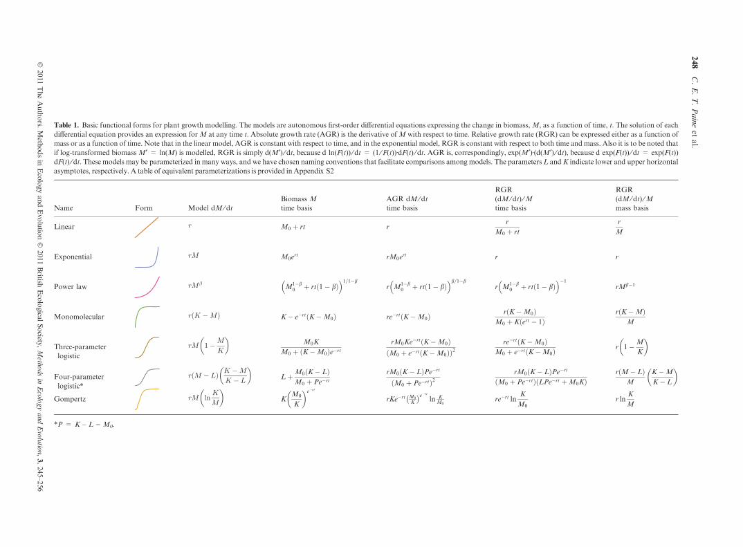
Table 1. Basic functional forms for plant growth modelling. The models are autonomous first-order di!erential equations expressing the change in biomass,M, as a function of time, t. The solution of eachdi!erential equation provides an expression forM at any time t. Absolute growth rate (AGR) is the derivative ofM with respect to time. Relative growth rate (RGR) can be expressed either as a function ofmass or as a function of time. Note that in the linear model, AGR is constant with respect to time, and in the exponential model, RGR is constant with respect to both time andmass. Also it is to be noted thatif log-transformed biomass M¢ = ln(M) is modelled, RGR is simply d(M¢) ⁄ dt, because d ln(F(t)) ⁄ dt = (1 ⁄F(t))ÆdF(t) ⁄ dt. AGR is, correspondingly, exp(M¢)Æ(d(M¢) ⁄ dt), because d exp(F(t)) ⁄ dt = exp(F(t))dF(t) ⁄ dt. These models may be parameterized in many ways, and we have chosen naming conventions that facilitate comparisons among models. The parameters L andK indicate lower and upper horizontalasymptotes, respectively. A table of equivalent parameterizations is provided in Appendix S2

Name Form Model dM ⁄ dtBiomass Mtime basis

AGR dM ⁄ dttime basis

RGR(dM ⁄ dt) ⁄Mtime basis

RGR(dM ⁄ dt) ⁄Mmass basis

Linear r M0 ! rt rr

M0 ! rt

r

M

Exponential rM M0ert rM0ert r r

Power law rM!M1"b

0 ! rt#1" b$! "1=1"b

r M1"b0 ! rt#1" b$

! "b=1"br M1"b

0 ! rt#1" b$! ""1

rMb"1

Monomolecular r K "M# $ K" e"rt K"M0# $ re"rt K"M0# $ r K"M0# $M0 ! K ert " 1# $

r K"M# $M

Three-parameterlogistic

rM 1"MK

# $M0K

M0 ! K"M0# $e"rtrM0Ke"rt K"M0# $M0 ! e"rt K"M0# $# $2

re"rt K"M0# $M0 ! e"rt K"M0# $ r 1"M

K

# $

Four-parameterlogistic*

r M " L# $ K "MK " L

# $L!M0 K" L# $

M0 ! Pe"rtrM0 K" L# $Pe"rt

M0 ! Pe"rt# $2rM0 K" L# $Pe"rt

M0 ! Pe"rt# $ LPe"rt !M0K# $r M" L# $

M

K"M

K" L

# $

Gompertz rM lnK

M

# $K

M0

K

# $e"rt

rKe"rt M0

K

% &e"rtln K

M0re"rt ln

K

M0r ln

K

M

*P = K – L ) M0.

248C.E.T.Paine

etal.

!2011

TheAuthors.

Meth

odsin

Ecology

andEvo

lutio

n!

2011British

Ecological

Society,

Methods

inEcology

andEvolution,

3,245–256

biomass acquisition is independent of current biomass. This

assumption is implausible, as biomass acquisition should

depend on leaf area, and hence biomass at least initially, when

resources are unlikely to be limiting. There are two parameters

in the linear model: M0, initial biomass, and r, the absolute

increase in biomass per unit time. A problemwith the standard

linear model is that it frequently predicts negative biomass at

early time points (Fig. 2a). This biologically impossible predic-

tion may be avoided by constraining the intercept to pass

through the origin (M0 = 0). In such a ‘no-intercept’ linear

model, biomass is always positive (Fig. 2a), and seed mass is

implicitly ignored.With only one parameter, r, the no-intercept

model is less flexible than the standard linear model, so it is no

surprise that it fits the data even less well. In this example, the

no-intercept model has lower R2 and higher Akaike Informa-

tion Criterion (AIC) than does the linear model, even as it

retains the implausible assumption that the rate of biomass

acquisition remains constant over time. Owing to their notable

defects, linearmodels appear rarely in the current growth-anal-

ysis literature and are included here primarily for complete-

ness.

Fitting a linear regression to the logarithm of biomass

yields the exponential (loglinear) model, in which the rate

of biomass acquisition is proportional to current biomass

(Blackman 1919). In the unlikely event that neither envi-

ronmental nor physiological factors slow the rate of bio-

mass acquisition, the exponential model may be

appropriate (for example, in the initial portion of a plant’s

lifespan). There are two parameters: M0, initial biomass,

and r, the relative growth rate. The exponential model is

the only one, in which the estimated parameter r is equiva-

lent to RGR, and constant with respect to time and bio-

mass (Fig. 2g,j). The AIC and R2 of the exponential

model are far superior to either of the linear fits (Fig. 2a).

However, the exponential model is only appropriate when

growth is unconstrained (e.g. algal blooms) and is not flex-

ible enough to account for the slowing of biomass acquisi-

tion that can occur with increasing structural biomass. In

contrast to the linear models, exponential models are fre-

quently used to analyse growth data. Although they may

be useful in cases where growth is authentically exponen-

tial, we generally discourage their use in favour of more

flexible nonlinear models.

POLYNOMIAL

In the polynomial model, growth follows a smooth curve,

potentially of great complexity (Poorter 1989; Heinen

1999). They were once widely used because they can be fit

in a linear model framework. However, polynomial func-

tions tend to make spurious upward or downward predic-

tions, especially at the extremes of the data. Furthermore,

it is di"cult to determine the proper order of polynomial

to use and to interpret the model parameters. We discour-

age the use of polynomial models and present no results

for them.

Nonlinear forms – non-asymptotic

POWER LAW (AKA ALLOMETRY)

A power-law model allows RGR to slow with increasing time

and biomass, according to the value of the exponent b(Fig. 2g,j). b = 0 yields the linear model, 0 > b > 1 corre-

sponds to progressive decreases in RGR, b = 1 yields the

exponential model (RGR is constant through time), and

b > 1 corresponds to the case of RGR increasing with

increasing biomass. Recently, the metabolic theory of ecology

has focused attention on power-law functions for their ability

to predict relationships among many aspects of individual sur-

vival and growth. Specifically, it predicts that biomass AGR

should scale with (biomass)3 ⁄ 4 and that diameter AGR should

scale with (diameter)1 ⁄ 3 (West, Brown & Enquist 1999). A test

of these predictions was conducted in 10 tropical rainforests,

encompassing>1.7 million trees, but were only upheld in one

forest (Muller-Landau et al. 2006). Among the non-asymp-

totic models, the power law is preferred in terms of R2 and

AIC. It e!ectively captures the rapid initial growth and the

slowing over time (Fig. 2a). Despite continuing discussion

regarding the value of the exponent b to be expected from the-

ory, the power law is frequently useful for non-asymptotic

data, as it allowsRGR to decrease as biomass increases.

Nonlinear forms – asymptotic

MONOMOLECULAR (AKA MITSCHERLICH)

The monomolecular model was originally derived from

physical chemistry, where it describes the progress of first-

order chemical reactions (Richards 1959; Zeide 1993;

Heinen 1999). There is no point of inflection; unlike the

other asymptotic forms it is always concave-down.

Correspondingly, AGR is fastest initially, and slows there-

after (Fig. 2e). It can be appropriate, therefore, for log-

transformed data (Fig. 2c) but it can predict negative bio-

mass at early time points for untransformed data (Fig. 2b).

In the limit, as the asymptotic mass (K) approaches zero,

the monomolecular becomes the exponential. It has been

occasionally applied to plant growth (Scanlan & Burrows

1990; Paul-Victor et al. 2010) and is implemented in R

with the SSasymp function (Pinheiro & Bates 2000).

THREE-PARAMETER LOGISTIC (AKA VERHULST,

AUTOCATALYTIC GROWTH) AND FOUR-PARAMETER

LOGISTIC

The logistic is the most commonly utilized asymptotic form

(Winsor 1932; Fresco 1973; Hunt 1982; Zeide 1993; Heinen

1999). In the three-parameter version, the lower horizontal

asymptote is fixed at 0 and the inflection point – the time at

which AGR is maximized – falls rigidly at M = K ⁄2. Four-parameter versions loosen one or the other of these strictures

(Nelder 1961; R function SSfpl in Pinheiro & Bates 2000). The



Model R2 !AICPower!law 0·94 0·0Exponential 0·90 12·5Linear 0·85 25·0Linear no!int 0·55 39·6

Holcus (untransformed)Model R2 !AICLogistic 0·77 0·0Gompertz 0·82 1·04!p Logistic 0·77 1·9Monomolecular 0·80 33·2

CerastiumModel R2 !AIC4!p Logistic 0·998 0·0Gompertz 0·986 13·2Monomolecular 0·994 20·2Logistic 0·777 55·4

Holcus (log"transformed)

0 20 40 60 80

0

5

10

15

Biom

ass

(g)

(a)

0 50 100 150 200

0

2

4

6

8

10

12

Days since sowing

(b)

0 20 40 60 80

0·001

0·01

0·1

1

515 (c)

0 20 40 60 800·0

0·2

0·4

0·6

0·8

1·0

AGR

(g"1

#day

"1)

(d)

0 50 100 150 2000·00

0·05

0·10

0·15

Days since sowing

(e)

0 20 40 60 800·0

0·2

0·4

0·6

0·8

1·0 (f)

0 20 40 60 80

0·00

0·05

0·10

0·15

0·20

0·25

0·30

0·35

RG

R(g

#g"1

#day

"1)

(g)

0 50 100 150 200

0·00

0·05

0·10

0·15

0·20

Days since sowing

(h)

0 20 40 60 80

0·00

0·05

0·10

0·15

0·20

0·25

0·30

0·35 (i)

0 5 10 150·00

0·05

0·10

0·15

0·20

0·25

0·30

0·35

RG

R( g

# g"1

# day

"1)

(j)

0 1 2 3 4 5 60·00

0·05

0·10

0·15

0·20

Biomass (g)

(k)

0 5 10 150·00

0·05

0·10

0·15

0·20

0·25

0·30

0·35 (l)



five-parameter version provides maximum flexibility and alle-

viating both restrictions (Gottschalk & Dunn 2005; Appen-

dix S2). The three-parameter version collapses to the

exponential in the limit as K approaches infinity. For some

data sets, the additional flexibility of the four-parameter ver-

sion greatly increases the variance explained by the model

(Fig. 2c), although the three-parameter version provides a

more parsimonious and equally adequate fit in other situations

(Fig. 2b). The three- and four-parameter logistic models are

implemented inRwith the SSlogis andSSfpl functions, respec-

tively (Pinheiro&Bates 2000).

GOMPERTZ

In theGompertzmodel, RGRdeclines exponentially over time

(Fig. 2e, Heinen 1999; Gompertz 1825; Winsor 1932; Zeide

1993). The Gompertz model di!ers from the three-parameter

logistic in that the inflection point of the former occurs at

approximately 37% of the asymptotic mass K (Winsor 1932),

whereas in the latter, the inflection point occurs at one-half the

maximal biomass (Fig. 2e, Hunt 1982). The Gompertz and

logistic models provide similar fits to the Cerastium data. The

three-parameter logistic is preferred on the basis of AIC,

whereas theGompertz is preferred on the basis ofR2 (Fig. 2b).

Like the logistic, the Gompertz model can be generalized to

allow non-zero initial masses and variation in the inflection

point (Winsor 1932). It is implemented in R with the SSgom-

pertz function (Pinheiro&Bates 2000).

Calculating and comparing growth rates

Many ecological analyses require estimations of absolute

and relative growth rates. Once the best functional form has

been selected, AGR and RGR can be calculated on the basis

of time or mass (Table 1). For proper inference, the uncer-

tainty surrounding the estimated growth rates must be quan-

tified. If experimental groups (such as species or treatment

levels) only vary in a single parameter, then the standard

error of the growth rate is simply the standard error for that

parameter, and comparisons are easily made. However, if

groups vary in two or more parameters, then the covariance

among parameters must be accounted for to generate confi-

dence intervals for the growth rates. We present the method

of population prediction intervals, which is easily imple-

mented and is considered reliable, although it lacks a strong

statistical justification. Bolker (2008) reviews this and other

techniques of error propagation, including the delta method.

To calculate population prediction intervals, we first examine

the square-root transformed likelihood profiles for each

parameter to check that they are approximately V-shaped,

and thus that the corresponding sampling intervals are

approximately multivariate normal (Appendix S1). If this is

the case, we randomly draw parameter combinations from a

multivariate normal distribution centred on the maximum-

likelihood parameter estimates and variance–covariance esti-

mates (as determined by the R functions nls, gnls or nlsList).

These sets of parameter combinations are used to calculate

replicates of the desired growth rate using the expressions in

Table 1. Confidence intervals for a significance threshold acan be extracted by taking the a ⁄2 and (1 ) a) ⁄2 quantiles

at every point in time (or biomass). For comparisons among

experimental groups, for example between a wild type and

various mutants, it is frequently more interpretable to calcu-

late the di!erence in growth rates and compare that di!er-

ence to zero, corresponding to the null expectation of no

di!erence between groups (see Zust et al. 2011). This can be

accomplished with population prediction intervals, except

that one calculates di!erences in growth rates between

groups, rather than the growth rates themselves.

The fluctuating nature of growth rates derived from nonlin-

ear growth models encourages a reconsideration of compari-

sons of growth rates (whether AGR or RGR) among

experimental groups. Rather than comparing point estimates

of growth rates, one compares time-(or biomass-) specific

functions. For example, the best form for modellingCerastium

and Geranium growth was the three-parameter logistic. Using

the traditional approach, one could hypothesize that their

growth rates would di!er. Using function-derived growth

rates, we can refine this hypothesis, testing the degree to which

they di!er in terms of the timing and magnitude of peak AGR

and RGR. To visualize these comparisons, we plot biomass,

AGR andRGR as functions of time andmass for both species

(Fig. 3). In this case, the peak AGR ofGeranium precedes that

of Cerastium by 46 days and is 29% greater in magnitude

(Fig. 3b). In themiddle of the growing season,Cerastium has a

37% greater RGR than does Geranium (Fig. 3c). The di!er-

ences in magnitude are significant, as the confidence intervals

around the di!erences in AGR and RGR between species do

not overlap zero (Appendix S3). Time-based comparisons of

RGR can be misleading, however, as physiological and envi-

ronmental conditions change over time, and experimental

groups may vary widely in initial size (Britt et al. 1991). Di!er-

ences in initial size among groups are especially common when

comparisons are made among species (Turnbull et al. 2008;

Fig. 2. Biomass trajectories predicted by the non-asymptotic models for (a) untransformed Holcus lanatus and by asymptotic models for (b)Cerastium di!usum and (c) log-transformed Holcus lanatus. The dashed lines in (b) indicate the predicted asymptotic biomass for each model.For the Cerastium data, the predictions from the three- and four-parameter logistic models are almost equivalent. Models are sorted by DAIC.Absolute and relative growth rates (RGRs) are derived from functions given in Table 1. (d) Absolute growth rate (AGR) is constant for linearmodels and increases monotonically for exponential and power-law models. (e, f) AGR is concave-down for logistic and Gompertz functions,and monotonically decreasing (Cerastium) or increasing (Holcus) for monomolecular. RGRmay be expressed as a function of (g–i) time or (j–l)biomass. For the exponential function, RGR is constant with respect to (h) time and (k) biomass, whereas RGR varies with time and biomass forall other functions. For the three- and four-parameter logistic functions, (j) RGR decreases linearly with biomass. Growth rates for linear andmonomolecularmodels, both of which predict negative biomass at early time points, are shown only for positive biomass.



Rees et al. 2010). Thus, it can be more illuminating to express

RGR on the basis of biomass, rather than that of time.

Standardized for mass, Geranium has a significantly greater

RGR than does Cerastium (Fig. 3d, Appendix S3). Analysing

RGR on a biomass basis corrects for variation in initial size,

which can be substantial.

It is important to carefully select the times or biomasses at

which growth rates are compared among experimental groups.

For example, Paul-Victor et al. (2010) compared RGR among

inbred recombinant lines ofArabidopsis thaliana at the average

mass of plants half-way through their experiment, whereas

Rees et al. (2010) compared growth rates at the smallest size

common to all studied species. Here, at a common size of 5 g,

Geranium has a greater RGR than does Cerastium (Fig. 3d,

Appendix S3). The choice of comparison times is particularly

important when values of two ormoremodel parameters di!er

among experimental groups, because crossovers in growth

rates among experimental units may then occur (e.g. Hautier

et al. 2010). For example, Cerastium and Geranium di!er in

both initial and asymptotic biomass (M0 and K, respectively),

and their AGR trajectories correspondingly intersect (Fig. 3b).

Comparisons performed at di!erent times would therefore

lead to di!erent conclusions. Compared at day 75, Geranium

had significantly greater AGR, whereas at day 100, Ceras-

tium’s AGR was significantly greater (Fig. 3b, Appendix S3).

These patterns are not obvious in the trajectory of biomass

through time (Fig. 3a). For these reasons, we recommend plot-

ting AGR and RGR against time or biomass to allow a more

holistic understanding of the variation in growth rates as time

passes and biomass increases (Heinen 1999; Hautier et al.

2010).

Troubleshooting

The approach we advocate for modelling growth does not dif-

fer substantially from that for any other statistical analysis, but

fitting nonlinearmodels is rathermore involved than fitting lin-

ear models. In this section, we describe some techniques that

can be used to avoid common pitfalls. The steps we describe

are implemented in anR script (Appendix S1).

STUDY DESIGN

In planning your study, several simple considerations can

facilitate the subsequent analysis. Frequently, measures of

biomass (or allometrically related variables, such as height or

diameter, Muller-Landau et al. 2006) are made on many

individuals at relatively few time points (e. g., Paine et al.

2008). One of the easiest ways to increase the reliability of

parameter estimates is to take the opposite approach: mea-

sure relatively few individuals at each of many time points,

particularly during times of rapid changes in growth. For

example, more frequent measurements in the early stages of

the Cerastium study may have reduced our uncertainty in

0 50 100 150 2000

5

10

15

20

25

Days since sowing

Bio

mas

s (g

)

GeraniumrCerastiumr

(a)

0 50 100 150 2000·00

0·05

0·10

0·15

0·20

Days since sowing

AG

R (

g pe

r da

y)

(b)

0 50 100 150 2000·00

0·02

0·04

0·06

0·08

0·10

0·12

0·14

Days since sowing

RG

R( g

# g"1

#day

"1)

(c)

0 2 4 6 8 100·00

0·02

0·04

0·06

0·08

0·10

0·12

0·14

Predicted biomass (g)

RG

R( g

# g"1

#day

"1)

(d)

Fig. 3. Observed and predicted values from a three-parameter logistic model for (a) biomass, (b) absolute growth rate (AGR), (c) relative growthrate (RGR) on a time basis and (d) RGR on a biomass basis of Cerastium di!usum and Geranium molle. Grey curves indicate 95% confidencebands for biomass and growth rates, as derived from population prediction intervals. Confidence bounds can be generated for any growth func-tion (Appendix S1), but are suppressed for clarity in other figures.



the estimate of RGR during that period (Fig. 3c,d). Just as

important, however, is that the number of individuals sam-

pled at any time point be su"cient to capture the variation

in sizes at that time, and that, they be drawn in such a way

(e.g. randomly) to be representative of that variation. When

nondestructive measurements are used, individuals are often

measured repeatedly through time and should be, therefore,

represented by a random-e!ects term in the model. In such

studies, the number of individuals sampled at each time

should be large enough to provide a reasonable number of

groups for this term. Note that the examples in this contri-

bution were derived from destructively harvested plants.

Accordingly, each individual was observed only once, moot-

ing the issue of correlated observations on individuals

through time. Balancing number of sampling times with the

number of individuals to sample at each time is a topic in

study design that deserves careful consideration. Finally, the

timing of observations should be tailored to the expected

growth rates of the plants studied, as well as the error inher-

ent to the measurement technique. For example, more fre-

quent measurements of diameter growth of large trees can

be made with dendrometer bands than with tape measures,

owing to their greater precision.

Recommendation

To enhance reliability in parameter estimation, measure rela-

tivelyfewindividualsper timepointanduserelativelymanytime

points, while sampling individuals representatively and adher-

ing to the requirements ofmixed-e!ectsmodels.Makeobserva-

tionsmorefrequently inperiodsofrapidchanges ingrowth.

GET TO KNOW THE DATA

Plotting the data, understanding the natural history of the sys-

tem and considering the attributes of the various functional

forms are essential to select an appropriate model (South

1995). Carefully examine the raw data before selecting a

growth model. Together with knowledge of the study system,

graphics can indicate which model(s) is most appropriate for

the data. Examination of diagnostic plots can aid in identifying

mis-specified models (Appendix S3; Fig. 2). Log-transforming

biomass permits the application of a wide variety of additional

models (Fig. 2c). Generalized additive models can also be

applied when the biomass trajectory conforms to no simple

parametric form (Katsanevakis 2007;Wood 2006), and the use

of the predict.gam function in the packagemgcv can permit the

calculation of function-derived growth rates.

Recommendation

Make graphs early and often. The importance of this step can-

not be overstated. Avoid polynomial functions (too di"cult to

interpret parameters) and linear or exponential functions (too

simplistic). Use flexible nonlinear forms, such as the power-law

or four-parameter logistic. Consider log-transforming biomass

when growth rates are of primary interest.

CHOOSE AMONG MODELS

Through experience, we have found that inappropriate func-

tional forms often fail to converge or yield unreasonable

parameter estimates. A common pitfall is to attempt to fit

overly complicated models. The smaller or noisier the data set,

the simpler the model should be: i.e. avoid over-parameteriza-

tion. Exploring di!erent model specifications is essential for

selecting the most parsimonious model. The ‘params’ and

‘fixed’ arguments of the gnls and nlme functions, respectively,

provide important tools formodel selection, as they can specify

which parameters are to vary among treatment groups and

which are to be global. Several di!erent models may be almost

equally good, particularly if the data are noisy. It is frequently

desirable to choose a model with biologically interpretable

parameters. The models presented here include only very basic

forms, however. Given su"cient data, these models may be

combined with others to test more elaborate ecological

hypotheses. As examples, Godoy, Monterubbianesi &

Tognetti (2008) combined Gompertz models to model the

biphasic double-sigmoid growth of highbush blueberries

(Vaccinium corymbosum L.), and Damgaard & Weiner (2008)

model the growth ofChenopodium albumL. (Chenopodiaceae)

with the Birch function, a generalization of the logistic that

allows initially exponential growth to slow.

Recommendation

Use the simplest possible model that captures the essence of

your data. For models with roughly equal fits, use biological

relevance to arbitrate.

HETEROSCEDASTIC ITY

Because growth is essentially amultiplicative process, variation

in genetic and environmental conditions increases the variation

among individuals in biomass through time. Thus, heterosce-

dasticity is a frequent problem in modelling plant growth.

There are two principal approaches to reduce heteroscedas-

ticity. The first is to model the logarithm of biomass, rather

than biomass itself. A logarithmic transformation will often

reduce heteroscedasticity, because multiplicative relationships

become additive following transformation (Fig. 2b,c). Log

transformation, however, can complicate the biological inter-

pretation of some model parameters, although if the estima-

tion of growth rates is the main objective, this does not pose a

major problem. It is to be noted that models fit to transformed

and untransformed data cannot be compared unless appropri-

ate steps are taken to accommodate the change in scale (Burn-

ham & Anderson 2002; Weiss 2010). An alternative approach

to reducing heteroscedasticity is to model the variance in bio-

mass explicitly, for example as a power or exponential function

of the mean (Pinheiro & Bates 2000). In fitting curves to the

Cerastium data, we modelled the variance in biomass as an

exponential function of predicted biomass. This reduced,

although did not entirely eliminate, heteroscedasticity (Appen-

dix S3). If many nondestructive measures are made on the



same individuals, then the error structure of the model fit must

take this into account. One can fit a mixed-e!ect model for

repeated-measures data with the function nlme, specifying indi-

viduals as a random e!ect, and indicating the within-group

correlation structure with the ‘correlation’ argument (see Pin-

heiro&Bates 2000 for details).

Recommendation

Account for heteroscedasticity in your data and ⁄or repeatedmeasures with an appropriate transformation and ⁄or variancemodelling (Pinheiro&Bates 2000).

CONVERGENCE FAILURE

Even appropriate models sometimes fail to converge on

reasonable parameter estimates. The easiest way to avoid

problems is to use a nonlinear model for which self-starting

routines exist. These routines, which are available in R for the

majority of models presented here, facilitate model conver-

gence by selecting sensible starting estimates for parameters

and computing derivatives analytically (Pinheiro & Bates

2000). Fitting routines will fail if parameter values lead to non-

numeric predictions. For example, in the Gompertz model, as

asymptotic biomass (K) approaches zero, divide-by-zero

errors become common. Some errors of this type may be

avoided by bounding parameter values away from zero. Care

should be taken when using bounded methods, however, that

the estimated parameter values are not at, or close to, the

bounded limits. Such a situation usually indicates a mis-speci-

fiedmodel or bounds. In somemodels, certain parameters may

take only positive values (such as the power law, where b, bio-logically, should be>0). This can be achieved by exponentiat-

ing the parameter in the model, then subsequently log

transforming the best-fit parameter value. R’s grofit package

may facilitate model fitting in certain cases, and for some

mixed-e!ects models, the functions in the lme4 package con-

verge more readily than do those of nlme (Kahm et al. 2010;

Bates,Maechler &Bolker 2011).

Further problem-solving techniques may be called for in

extreme cases, particularly for the power-law model, which

seems particularly prone to convergence failures. The first is

to fix the value of one parameter, typically the initial mass

M0, and fit only the rate and scaling exponent, r and b. Thistechnique was employed in the original analysis of the

Holcus data set, where the value of M0 was determined by

germinating a large sample of seeds on filter paper and using

the average initial seedling biomass as the mass on day 0

(0.0606 mg, Hautier et al. 2010). This approach can also be

used in the linear model to avoid predictions of negative bio-

mass. Another option is to use a brute-force search to deter-

mine the most likely combination of parameters, given the

data. In this technique, the likelihood of all possible parame-

ter combinations within a plausible volume of parameter

space is evaluated (Fig. 4). Brute-force searches can be iter-

ated to generate parameter estimates of any desired preci-

sion, but are prohibitively slow for parameter-rich models.

A third option is to use general-purpose optimization meth-

ods, such as that implemented in the R function nlminb. As

nlminb has convergence criteria that di!er from those in nls,

the former sometimes converges in cases where the latter

fails. We used these techniques after nls failed to converge

$

r

0·2 0·3 0·4 0·5 0·6 0·7 0·80·00

0·05

0·10

0·15

0·20 (a)

$

M0

0·2 0·3 0·4 0·5 0·6 0·7 0·80·0001

0·001

0·01

0·1

0·5 (b)

r

M0

0·00 0·05 0·10 0·15 0·200·0001

0·001

0·01

0·1

0·5 (c)

Fig. 4. Three slices through the three-dimensional volume of parame-ter space for the power-law model showing the likelihood surface foreach of pairwise combination of parameters, as determined throughan iterated brute-force search. Contour lines indicate the likelihoodof each parameter combination, given the data and the specifiedmodel. The ‘X’s indicate the most likely combination of parameters.Note that theY-axes in panels (b) and (c) are log transformed.



for the power-law model and arrived at parameter estimates

that di!ered by no more than 2.3%. The grid search also

illuminated one possible cause of the failure of nls to con-

verge: substantial uncertainty in the estimate of b (Fig. 4a).

Recommendation

Be persistent. Use these hints to determine the most likely

parameter values, given your data and model. The payo!, in

terms of biological plausibility and additional insight, will be

worth it.

PROPAGATE UNCERTAINTY

The ecological significance of a model frequently lies in the

growth rates it predicts, rather than the parameter values them-

selves. In these circumstances, it is essential that growth rates

be properly calculated.

Recommendation

Derive absolute and RGRs from fitted nonlinear functions.

Propagate uncertainty from the parameter estimates to the

function-derived growth rates. Allow ecological hypotheses

and natural history to guide your choice of times and biomas-

ses for comparison of growth rates among experimental

groups.

Future directions

The models presented in this contribution may be extended in

many ways. One objective is the development of fitting rou-

tines for highly flexible forms, such as those pioneered by von

Bertalan!y (1938, 1957) and others (see Thornley & France

2007).With four parameters, the von Bertalan!ymodel allows

rapid initial growth to slow, without imposing strict asymp-

totic conditions. This model is also valued because its parame-

ters are biologically interpretable (Thornley & France 2007).

There are two components – one for anabolism (i.e. synthesis,

taken to follow a power law) and one for catabolism (i.e. deg-

radation, taken as exponential, Appendix S2). Furthermore,

the vonBertalan!ymodel collapses to all the othermodels pre-

sented here, depending upon the values of its parameters

(Tjørve & Tjørve 2010). In theory, therefore, a von Bertalan!y

model could fit a wide variety of growth data sets. However, it

is so flexible that it can be very di"cult to fit to data, because

di!erent combinations of parameter values can produce very

similar growth curves. Markov chain Monte Carlo (MCMC)

or similarmethodsmay be necessary to obtain reliable parame-

ter estimates for this model (Hilborn & Mangel 1997; Bolker

2008; Lichstein et al. 2010), but this is beyond the scope of this

contribution.

An active avenue of research is in the development of

mechanistic models of plant growth. These models consider

growth algorithmically or as an iterative process of carbon

acquisition, allocation to various compartments and bio-

mass gain (Tilman 1988; Grimm & Railsback 2005). They

are set up as a system of (potentially nonlinear) equations.

This allows for an enormously flexible framework that can

accommodate multiple compartments (e.g. roots, stems and

leaves), changes in environmental conditions, latent vari-

ables such as the rate of photosynthate allocation to roots

and leaves, and losses of biomass through time (Turnbull

et al. 2008). These aspects cannot easily be accommodated

in the nonlinear regression framework we advocate. The

development of individual-based mechanistic models is

described in detail by Grimm & Railsback (2005). Such

models generally require the use of MCMC for parameter

estimation and should be more widely employed, as they

become easier to implement.

Conclusion

The analysis of plant growth and the determination of robust

estimates of parameter values and growth rates are an impor-

tant area of ecological research. Advice on the mechanics of

curve fitting is, however, dispersed throughout the academic

literature and progressing quickly, as new statistical techniques

become available. Updating earlier reviews with practical

advice, we have briefly summarized some of the basic func-

tional forms for growth, discussed the derivation of growth

rates from functional forms and advocated the propagation of

uncertainty from model parameters to estimated growth rates.

We hope that the methodological review and synthesis

presented here will facilitate the study of growth rates by

ecologists.

Acknowledgements

We thank Yann Hautier for providing the Holcus data set, and thank him,Camille Guilbaud, Xuefei Li and Christopher Philipson for helpful discussions.We thank two anonymous reviewers for their comments and suggestions, whichstrengthened themanuscript.

References

Bates, D., Maechler, M. & Bolker, B. (2011) lme4: Linear mixed-e!ects modelsusing S4 classes. R package version 0.999375-39.

von Bertalan!y, L. (1938) A quantitative theory of organic growth. Humanbiology, 10, 181–213.

von Bertalan!y, L. (1957) Quantitative laws in metabolism and growth. TheQuarterly Review of Biology, 32, 217–231.

Blackman, V.H. (1919) The compound interest law and plant growth.Annals ofBotany, os-33, 353–360.

Bolker, B. (2008) Ecological Models and Data in R. Princeton University Press,Princeton, NJ.

Bolker, B.M., Brooks,M.E., Clark, C.J., Geange, S.W., Poulsen, J.R., Stevens,M.H.H. &White, J.-S.S. (2009) Generalized linear mixedmodels: a practicalguide for ecology and evolution.Trends in Ecology & Evolution, 24, 127–135.

Britt, J., Mitchell, R., Zutter, B., South, D., Gjerstad, D. & Dickson, J. (1991)The influence of herbaceous weed control and seedling diameter on six yearsof loblolly pine growth – a classical growth analysis approach. Forest Sci-ence, 37, 655–668.

Burnham, K.P. & Anderson, D.R. (2002) Model Selection and MultimodelInference: A Practical Information-Theoretic Approach. Springer Verlag,NewYork.

Causton, D. & Venus, J. (1981)The Biometry of Plant Growth. EdwardArnold,London.

Charles-Edwards, D., Doley, D. & Rimmington, G. (1986) Modelling PlantGrowth and Development. Academic Press Australia, North Ryde,NSW.



Chave, J., Condit, R., Lao, S., Caspersen, J., Foster, R. & Hubbell, S. (2003)Spatial and temporal variation of biomass in a tropical forest: results from alarge census plot in Panama. Journal of Ecology, 91, 240–252.

Damgaard, C. & Weiner, J. (2008) Modeling the growth of individuals incrowded plant populations. Journal of Plant Ecology, 1, 111–116.

Fresco, L.F.M. (1973) Model for plant-growth – estimation of parameters oflogistic function.Acta Botanica Neerlandica, 22, 486–489.

Godoy, C., Monterubbianesi, G. & Tognetti, J. (2008) Analysis of highbushblueberry (Vaccinium corymbosum L.) fruit growth with exponential mixedmodels.Scientia Horticulturae, 115, 368–376.

Gompertz, B. (1825) On the nature of the function expressive of the law ofhumanmortality, and on a newmode of determining the value of life contin-gencies. Philosophical Transactions of the Royal Society of London, 115, 513–583.

Gottschalk, P.G. & Dunn, J.R. (2005) The five-parameter logistic: a character-ization and comparisonwith the four-parameter logistic.Analytical biochem-istry, 343, 54–65.

Grimm, V. & Railsback, S. (2005) Individual-Based Modeling and Ecology.PrincetonUniversity Press, Princeton, NJ.

Hautier, Y., Hector, A., Vojtech, E., Purves, D. & Turnbull, L.A. (2010) Mod-elling the growth of parasitic plants. Journal of Ecology, 98, 857–866.

Heinen,M. (1999)Analytical growth equations and theirGenstat 5 equivalents.Netherlands Journal of Agricultural Science, 47, 67–89.

Hilborn, R. &Mangel,M. (1997)The Ecological Detective: ConfrontingModelswith Data. PrincetonUniversity Press, Princeton, NJ.

Ho!mann, W. & Poorter, H. (2002) Avoiding bias in calculations of relativegrowth rate.Annals of Botany, 90, 37–42.

Hunt, R. (1981) The fitted curve in plant growth studies.Mathematics and PlantPhysiology (eds D.A. Rose & D.A. Charles-Edwards), pp. 283–298. Aca-demic Press, London.

Hunt, R. (1982)Plant Growth Curves: The Functional Approach to Plant GrowthAnalysis. EdwardArnold, London.

Kahm, M., Hasenbrink, G., Lichtenberg-Frate, H., Ludwig, J. & Kschischo,M. (2010) grofit: Fitting Biological Growth Curves with R. Journal of Statis-tical Software, 33, 1–21.

Katsanevakis, S. (2007) Growth andmortality rates of the fanmussel Pinna no-bilis in Lake Vouliagmeni (Korinthiakos Gulf, Greece): a generalized addi-tivemodelling approach.Marine Biology, 152, 1319–1331.

Kobe, R.K. (1999) Light gradient partitioning among tropical tree speciesthrough di!erential seedlingmortality and growth.Ecology, 80, 187–201.

Lichstein, J.W., Dusho!, J., Ogle, K., Chen, A., Purves, D.W., Caspersen, J.P.& Pacala, S.W (2010) Unlocking the forest inventory data: relating individ-ual tree performance to unmeasured environmental factors. EcologicalApplications, 20, 684–699.

McMahon, T.A. & Bonner, J.T. (1983) On Size and Life. Scientific AmericanBooks,NewYork,NewYork.

Muller-Landau, H.C., Condit, R., Chave, J., Thomas, S.C., Bohlman, S.A.,Bunyavejchewin, S., Davies, S.J., Foster, R.B., Gunatilleke, C.V.S.,Gunatilleke, I.A.U.N., Harms, K.E., Hart, T.B., Hubbell, S.P., Itoh, A.,Kassim, A.R., Lafrankie, J.V., Lee, H.S., Losos, E.C., Makana, J.-R.,Ohkubo, T., Sukumar, R., Sun, I.-F., Supardi, M.N.N., Tan, S., Thompson,J., Valencia, R., Munoz, G.V., Wills, C., Yamakura, T., Chuyong, G.,Dattaraja, H.S., Esufali, S., Hall, P., Hernandez, C., Kenfack, D., Kirati-prayoon, S., Suresh, H.S., Thomas, D.W., Vallejo, M. &Ashton, P.S. (2006)Testing metabolic ecology theory for allometric scaling of tree size, growthandmortality in tropical forests.Ecology Letters, 9, 575–588.

Nelder, J.A. (1961) The fitting of a generalization of the logistic curve. Biomet-rics, 17, 89–110.

Paine, C.E.T., Harms, K.E., Schnitzer, S.A. & Carson,W.P. (2008)Weak com-petition among tropical tree seedlings: implications for species coexistence.Biotropica, 40, 432–440.

Paul-Victor, C., Zust, T., Rees, M., Kliebenstein, D.J. & Turnbull, L.A. (2010)A new method for measuring RGR can uncover the costs of defensive com-pounds inArabidopsis thaliana.New Phytologist, 187, 1102–1111.

Pinheiro, J. & Bates, D. (2000) Mixed-E!ects Models in S and S-PLUS.Springer Verlag, NewYork.

Pinheiro, J., Bates, D., DebRoy, S. & Sarkar, D. (2009) nlme: Linear and Non-linearMixed E!ectsModels. R package version 3.1-86.

Poorter, H. (1989) Plant growth analysis: towards a synthesis of the classicaland the functional approach.Physiologia Plantarum, 75, 237–244.

Purves, D. & Pacala, S. (2008) Predictive models of forest dynamics. Science,320, 1452–1453.

RDevelopment Core Team (2011)R: ALanguage and Environment for Statisti-cal Computing. R Foundation for Statistical Computing, Vienna, Austria.

Rees, M., Osborne, C.P., Woodward, F.I., Hulme, S.P., Turnbull, L.A. & Tay-lor, S.H. (2010) Partitioning the components of relative growth rate: howimportant is plant size variation?TheAmericanNaturalist, 176, E152–E161.

Richards, F.J. (1959) A flexible growth function for empirical use. Journal ofExperimental Botany, 10, 290–300.

Ricklefs, R.E. (2010) Embryo growth rates in birds and mammals. FunctionalEcology, 24, 588–596.

Ritz, C. & Streibig, J. (2008) Nonlinear Regression with R. Springer Verlag,NewYork.

Rose, K.E., Atkinson, R.L., Turnbull, L.A. & Rees, M. (2009) The costs andbenefits of fast living.Ecology Letters, 12, 1379–1384.

Scanlan, J.C. & Burrows, W.H. (1990) Woody overstorey impact on herba-ceous understorey in Eucalyptus spp. communities in central Queensland.Austral Ecology, 15, 191–197.

Sillett, S.C., Van Pelt, R., Koch, G.W., Ambrose, A.R., Carroll, A.L., Antoine,M.E. &Mifsud, B.M. (2010) Increasing wood production through old age intall trees. Forest Ecology andManagement, 259, 976–994.

South, D.B. (1995) Relative growth rates: a critique. South African ForestryJournal, 173, 43–48.

Tanner, E.V.J., Teo, V.K., Coomes,D.A. &Midgley, J.J. (2005) Pair-wise com-petition-trials amongst seedlings of ten dipterocarp species; the role of initialheight, growth rate and leaf attributes. Journal of Tropical Ecology, 21, 317–328.

Thomas, S. (1996) Asymptotic height as a predictor of growth and allometriccharacteristics in Malaysian rain forest trees. American Journal of Botany,83, 556–566.

Thornley, J. & France, J. (2007)Mathematical Models in Agriculture: Quantita-tive Methods for the Plant, Animal and Ecological Sciences. CAB Interna-tional, Oxon. UK.

Tilman, D. (1988) Plant Strategies and the Dynamics and Structure of PlantCommunities. PrincetonUniversity Press, Princeton,NJ.

Tjørve, E. & Tjørve, K.M.C. (2010) A unified approach to the Richards-modelfamily for use in growth analyses: why we need only two model forms. Jour-nal of Theoretical Biology, 267, 417–425.

Turnbull, L.A., Paul-Victor, C., Schmid, B. & Purves, D.W. (2008) Growthrates, seed size, and physiology: do small-seeded species really grow faster?Ecology, 89, 1352–1363.

Weiss, J. (2010) Course notes Ecology 145—Statistical Analysis. Available at:http://www.unc.edu/courses/2006spring/ecol/145/001/docs/lectures/lec-ture18.htm [accessed 6 July 2011].

West, G., Brown, J. & Enquist, B. (1999) A general model for the structure andallometry of plant vascular systems.Nature, 400, 664–667.

Winsor, C.P. (1932) The Gompertz curve as a growth curve. Proceedings of theNational Academy of Sciences of the United States of America, 18, 1–8.

Wood, S.N. (2006)Generalized Additive Models: An Introduction with R. Chap-man&Hall, BocaRaton, FL.

Zeide, B. (1993) Analysis of growth equations. Forest Science, 39, 594–616.Zust, T., Joseph, B., Shimizu, K.K., Kliebenstein, D.J. & Turnbull, L.A. (2011)

Using knockout mutants to reveal the growth costs of defensive traits. Pro-ceedings of the Royal Society B, 278, 2598–2603.

Received 16 February 2011; accepted 19 July 2011Handling Editor: Robert Freckleton

Supporting Information

Additional Supporting Information may be found in the online

version of this article.

Appendix S1.R script.

Appendix S2.Table of equivalent parameterizations of functions.

Appendix S3. Supplemental figures.

As a service to our authors and readers, this journal provides support-

ing information supplied by the authors. Such materials may be

re-organized for online delivery, but are not copy-edited or typeset.

Technical support issues arising from supporting information (other

thanmissing files) should be addressed to the authors.



How to fit nonlinear plant growth models and calculate ...guianaplants.stir.ac.uk/paine/pubs/Paine et al_MEE_2012.pdf · How to ﬁt nonlinear plant growth models and calculate growth

Documents