Horizontal Wavenumber Spectra of Vertical Vorticity - Munin

1. IntroductionThe terrestrial atmosphere between tropospheric and thermospheric altitudes contains a diversity of fluid motions, that range from large periods (up to around 30 days), large horizontal extent (thousands of kilometers), namely planetary waves (McCormack et  al.,  2014; Rossby, 1939), to small-to-medium scale oscillations like gravity waves (GWs) (Hines, 1988) or stratified turbulence regimes (Billant & Chomaz, 2001; Lindborg, 2006). A typical way to discern the intrinsic nature of the motion is to separate the horizontal velocity wind vectors into a rotational and a divergent component using the Helmholtz decomposition (Lindborg, 2014). The comparison between the two components, or different estimates associated with them, allows us to build a notion of how the fluid propagates and determines the dominant physical processes.

For example, at synoptic and planetary scales (>1,000 km) in the lower atmosphere, the rotational component is dominant. From general circulation models, it was found that its energy content, is about 100 times larger than the energy content of the divergent component (e.g., Augier & Lindborg, 2013). For smaller horizontal scales, in the tens to hundreds of kilometers (mesoscales), the relative importance is not clear. Many simulations, as well as observational studies, have been carried out in the upper troposphere and lower stratosphere (UTLS) with dissim-ilar results in such a range of horizontal scales (Callies et al., 2016; Hamilton et al., 2008). Hamilton et al. (2008) estimated that the rotational component was more than three times larger than the divergent component near the troposphere. In addition, Skamarock et al. (2014) found the same order of magnitude for the two components in the 8.5–10.5 km tropospheric altitude range and a clearly dominant divergent component (five times larger than the rotational component) in the 16–18 km altitude range. These results highlight the importance of studying

Abstract Specular meteor radars (SMRs) have significantly contributed to the understanding of wind dynamics in the mesosphere and lower thermosphere (MLT). We present a method to estimate horizontal correlations of vertical vorticity (Qzz) and horizontal divergence (P) in the MLT, using line-of-sight multistatic SMRs velocities, that consists of three steps. First, we estimate 2D, zonal, and meridional correlation functions of wind fluctuations (with periods less than 4 hr and vertical wavelengths smaller than 4 km) using the wind field correlation function inversion (WCFI) technique. Then, the WCFI's statistical estimates are converted into longitudinal and transverse components. The conversion relation is obtained by considering the rotation about the vertical direction of two velocity vectors, from an east-north-up system to a meteor-pair-dependent cylindrical system. Finally, following a procedure previously applied in the upper troposphere and lower stratosphere to airborne wind measurements, the longitudinal and transverse spatial correlations are fitted, from which Qzz, P, and their spectra are directly estimated. The method is applied to a special Spread spectrum Interferometric Multistatic meteor radar Observing Network data set, obtained over northern Germany for seven days in November 2018. The results show that in a quasi-axisymmetric scenario, P was more than five times larger than Qzz for the horizontal wavelengths range given by ∼50–400 km, indicating a predominance of internal gravity waves over vortical modes of motion as a possible explanation for the MLT mesoscale dynamics during this campaign.

POBLET ET AL.

© 2022. The Authors. Earth and Space Science published by Wiley Periodicals LLC on behalf of American Geophysical Union.This is an open access article under the terms of the Creative Commons Attribution-NonCommercial-NoDerivs License, which permits use and distribution in any medium, provided the original work is properly cited, the use is non-commercial and no modifications or adaptations are made.

Horizontal Wavenumber Spectra of Vertical Vorticity and Horizontal Divergence of Mesoscale Dynamics in the Mesosphere and Lower Thermosphere Using Multistatic Specular Meteor Radar ObservationsFacundo L. Poblet1  , Jorge L. Chau1  , J. Federico Conte1  , Victor Avsarkisov1  , Juha Vierinen2  , and Harikrishnan Charuvil Asokan1,3 

1Leibniz Institute of Atmospheric Physics at the University of Rostock, Kühlungsborn, Germany, 2Arctic University of Norway, Tromsø, Norway, 3Laboratoire de Mécanique des Fluides et d’Acoustique, UMR5509, Université de Lyon, CNRS, ÉCole Centrale de Lyon, INSA de Lyon, Université Claude Bernard Lyon 1, Écully, France

Key Points:• We investigate the horizontal

correlation functions of vertical vorticity and horizontal divergence for mesoscale wind fluctuations in the mesosphere and lower thermosphere

• 2D zonal and meridional correlation functions and 1D longitudinal and transverse correlation functions as a function of horizontal lags are analyzed

• The divergence dominated over the vorticity during November 2018 in northern Germany

Correspondence to:F. L. Poblet,[email protected]

Citation:Poblet, F. L., Chau, J. L., Conte, J. F., Avsarkisov, V., Vierinen, J., & Charuvil Asokan, H. (2022). Horizontal wavenumber spectra of vertical vorticity and horizontal divergence of mesoscale dynamics in the mesosphere and lower thermosphere using multistatic specular meteor radar observations. Earth and Space Science, 9, e2021EA002201. https://doi.org/10.1029/2021EA002201

Received 25 DEC 2021Accepted 16 AUG 2022

Author Contributions:Conceptualization: Facundo L. Poblet, Victor AvsarkisovFormal analysis: Facundo L. Poblet, Jorge L. Chau, J. Federico Conte, Victor Avsarkisov, Juha Vierinen, Harikrishnan Charuvil AsokanFunding acquisition: Jorge L. ChauInvestigation: Facundo L. Poblet, Jorge L. ChauMethodology: Facundo L. PobletProject Administration: Jorge L. Chau

10.1029/2021EA002201RESEARCH ARTICLE

1 of 16

Earth and Space Science

POBLET ET AL.

10.1029/2021EA002201

2 of 16

the mesoscale dynamics in other regions of the atmosphere, to have a broader picture of rotational and divergent components in this range of scales.

Observationally, Lindborg (2007) presented a method to quantify the information of the two vector components given by the Helmholtz decomposition. It consists of calculating the vertical component of the two-point corre-lation tensor of vorticity and the two-point correlation of horizontal divergence. To estimate these functions, the author used one-dimensional longitudinal and transverse structure function components, calculated from velocity measurements in the UTLS, using the Measurement of Ozone and Water Vapor by Airbus In-Service Aircraft database of commercial flight measurements (Marenco et al., 1998). The results showed that the two functions and their spectra had similar orders of magnitude, for horizontal scales up to a couple of hundred kilometers.

Performing such analysis from observations at mesosphere and lower thermosphere (MLT) altitudes poses the difficulty that to obtain correlation or structure functions for displacements of at least several hundreds of kilom-eters in horizontal directions, the full three-dimensional velocity vector with good horizontal coverage, should be known beforehand, which is not the case. To tackle this problem, Vierinen et al. (2019) introduced the wind field correlation function inversion (WCFI) technique. WCFI uses an indirect way to calculate wind-field correlation functions without previously knowing the complete velocity vectors. The technique has been implemented on line-of-sight multistatic Specular meteor radar (SMR) velocities to calculate six independent components of the velocity correlation tensor, distributed either in time lags, horizontal or vertical displacements. The method is particularly useful when a dense data set of meteor detections is available.

Monostatic SMRs have been proven to be an essential tool to study mesoscale phenomena in the MLT region. In particular, they are useful for characterizing the evolution of GW-driven momentum fluxes and variances in time and altitude (e.g., Andrioli et al., 2015; Conte et al., 2021; Placke et al., 2011). This characterization can be significantly improved with the usage of multistatic SMR configurations (Conte et al., 2022), since they allow a significant increase in meteor detections per unit time (e.g., Chau et al., 2017; Stober & Chau, 2015).

This work introduces a novel approach for calculating longitudinal and transverse horizontal correlation functions in the MLT. With them, and the formalism developed by Lindborg (2007), the relative importance of internal GWs and vortical modes of motion to explain MLT mesoscale variations can be established. So far, the role of vorticity has been poorly quantified in the MLT mesoscales. Since GW breaking is a primary source of vorticity, it cannot be insignificant. Also, many different mechanisms of coupling between atmospheric regions, like spon-taneous imbalances or secondary GWs require non-zero vorticity (e.g., Kogure et al., 2020; Vadas et al., 2003; Vadas & Fritts, 2002). Then, this study aims to quantify the mesoscale vorticity in the MLT, in terms of its spatial correlation.

The technique is demonstrated with Spread spectrum Interferometric Multistatic meteor radar Observing Network (SIMONe) 2018, which was conducted over Northern Germany in November of 2018. SIMONe 2018 led to the detailed characterization of different aspects of the MLT wind field, documented in several publications so far (e.g., Charuvil Asokan et al., 2022; Vargas et al., 2021; Vierinen et al., 2019; Volz et al., 2021).

This article is organized as follows. Section 2 briefly describes the derivation of the two-point correlation of vertical vorticity and horizontal divergence as was originally done by Lindborg (2007), and their relation to the longitudinal and transverse correlation functions. Section 3 describes the data set and the methodology to obtain the correlation estimates. Section 4 presents the results on the 2D correlation functions, the functional fits used to represent the trends, and the calculation of Lindborg's functions. Section 5 discusses the main points, and Section 6 presents the scope of this work and treats the possible extension of the technique to other applications.

2. Two-Point Correlation of Vertical Vorticity (Qzz) and Horizontal Divergence (P) - DefinitionsThe Reynolds decomposition of the MLT wind field (u)

𝐮𝐮 = 𝐔𝐔 + 𝐮𝐮′ (1)

into its mean wind U  =  ⟨u⟩ and fluctuating wind u′ part is frequently used to study the wind in different spatio-temporal scales. From Equation  1, one would expect that ⟨u′⟩  =  0, where ⟨⋯⟩ denotes an ensemble average or expected value. In practice, due to the presence of intermittency, the separation into the mean and

Software: Facundo L. Poblet, Juha Vierinen, Harikrishnan Charuvil AsokanSupervision: Jorge L. Chau, J. Federico ConteValidation: Facundo L. Poblet, Juha Vierinen, Harikrishnan Charuvil AsokanVisualization: Facundo L. PobletWriting – original draft: Facundo L. PobletWriting – review & editing: Facundo L. Poblet, Jorge L. Chau, J. Federico Conte, Victor Avsarkisov, Juha Vierinen, Harikrishnan Charuvil Asokan

Earth and Space Science

POBLET ET AL.

10.1029/2021EA002201

3 of 16

fluctuating parts is always strongly dependent on the averaging procedure, and so the mean wind represents different dynamics when it is averaged over 1 month, 24 hr or 30 min, for example,

The fluctuations u′ can be used to define the two-point correlation tensor of the wind velocity fluctuations 𝐴𝐴 𝐴𝐴′

𝑖𝑖𝑖𝑖 ,

that for points separated by s and determined at position r is

𝑅𝑅′

𝑖𝑖𝑖𝑖(𝐫𝐫, 𝐬𝐬) = ⟨𝑢𝑢′𝑖𝑖(𝐫𝐫)𝑢𝑢′

𝑖𝑖(𝐫𝐫 + 𝐬𝐬)⟩. (2)

Here, the indices i, j = 1, 2, 3; and refer to the components of u′, given by 𝐴𝐴 𝐮𝐮′=

(𝑢𝑢′1, 𝑢𝑢′

2, 𝑢𝑢′

3

) . The analogous expres-

sion for the vorticity vector ζ = ∇r × u′ is

𝑄𝑄𝑖𝑖𝑖𝑖(𝐫𝐫, 𝐬𝐬) = ⟨𝜁𝜁𝑖𝑖(𝐫𝐫)𝜁𝜁𝑖𝑖(𝐫𝐫 + 𝐬𝐬)⟩, (3)

where Qij is the two-point correlation tensor of the vorticity. If the velocity field is considered homogeneous in horizontal planes, the correlation does not depend on the position, but only on the horizontal separation. Then, for a given altitude z = z0 we have 𝐴𝐴 𝐴𝐴′

𝑖𝑖𝑖𝑖= 𝐴𝐴′

𝑖𝑖𝑖𝑖(𝑧𝑧0, 𝐬𝐬) and Qij = Qij(z0, s).

The relation between 𝐴𝐴 𝐴𝐴′

𝑖𝑖𝑖𝑖 and Qij can be derived by inserting in Equation 3 the ζ components ζi as a function of

𝐴𝐴 𝐴𝐴′𝑖𝑖 and applying the derivative definition assuming homogeneity. Batchelor (1953, p. 38 Equation 3.2.1) gives an

elegant solution, that for the vertical component of Qij, that is, Q33 is

𝑄𝑄33 = −𝜀𝜀3𝑖𝑖𝑖𝑖𝜀𝜀3𝑗𝑗𝑗𝑗𝜕𝜕2𝑅𝑅′

𝑖𝑖𝑗𝑗

𝜕𝜕s𝑖𝑖𝜕𝜕s𝑗𝑗, (4)

with summation over repeated indices. In this case, the indices i, j refer to the separation vector components s =  (s1, s2, s3) and k, l = 1, 2, 3 to the components of the velocity correlation tensor. The symbol ɛijk is the Levi-Civita tensor that accounts for the permutations. Lindborg (2007) expanded Equation 4 into a local cylindri-cal coordinate system (sh, ϕ, sz), where sh and sz are the horizontal and vertical distance between two points; and ϕ is the angle between the direction of sh and a predefined horizontal direction. He found that for a fixed altitude

𝑄𝑄𝑧𝑧𝑧𝑧 (𝑠𝑠ℎ) =1

𝑠𝑠ℎ

𝜕𝜕𝜕𝜕′

𝐿𝐿𝐿𝐿

𝜕𝜕𝑠𝑠ℎ−

1

𝑠𝑠2ℎ

𝜕𝜕

𝜕𝜕𝑠𝑠ℎ

(

𝑠𝑠2ℎ

𝜕𝜕𝜕𝜕′

𝑇𝑇𝑇𝑇

𝜕𝜕𝑠𝑠ℎ

)

. (5)

In this expression, the notation has been changed to 𝐴𝐴 𝐴𝐴′

11= 𝐴𝐴′

𝑠𝑠ℎ𝑠𝑠ℎ= 𝐴𝐴′

𝐿𝐿𝐿𝐿 , 𝐴𝐴 𝐴𝐴′

22= 𝐴𝐴′

𝜙𝜙𝜙𝜙= 𝐴𝐴′

𝑇𝑇𝑇𝑇 and Q33 = Qzz. For 𝐴𝐴 𝐴𝐴′

𝐿𝐿𝐿𝐿

and 𝐴𝐴 𝐴𝐴′

𝑇𝑇𝑇𝑇 , this is done to be consistent with the commonly used terminology (Batchelor, 1953; Buell, 1960; King

et al., 2015a, 2015b) that refers to the correlations in the sh direction (usually referred to as “along-track” direc-tion) as longitudinal correlation functions 𝐴𝐴 𝐴𝐴′

𝐿𝐿𝐿𝐿 , and to the correlations in the ϕ direction as transverse or lateral

correlation functions 𝐴𝐴 𝐴𝐴′

𝑇𝑇𝑇𝑇 . These two functions are defined with the velocity components in these directions as

𝐴𝐴 𝐴𝐴′

𝐿𝐿𝐿𝐿(𝐫𝐫, 𝐬𝐬) = ⟨𝑢𝑢′

𝐿𝐿(𝐫𝐫)𝑢𝑢′

𝐿𝐿(𝐫𝐫 + 𝐬𝐬)⟩ and 𝐴𝐴 𝐴𝐴′

𝑇𝑇𝑇𝑇(𝐫𝐫, 𝐬𝐬) = ⟨𝑢𝑢′

𝑇𝑇(𝐫𝐫)𝑢𝑢′

𝑇𝑇(𝐫𝐫 + 𝐬𝐬)⟩ , for the most general case of a non-homogeneous

medium. In the case of Qzz, the intention is to preserve the original notation introduced by Lindborg (2007). An important hypothesis assumed to derive Equation 5 is axisymmetry, that is when all statistical quantities are invariant under rotations of s and so derivatives with respect to ϕ vanish. The same equation can be obtained using a Cartesian decomposition of the vectors, as it is presented in Appendix A.

Similarly, the divergence 𝐴𝐴 ∇ℎ ⋅ 𝐮𝐮′

ℎ can be used to define the two-point correlation function of horizontal divergence

P (Lindborg, 2007) as

𝑃𝑃 = ⟨(∇ℎ ⋅ 𝐮𝐮

′

ℎ(𝐫𝐫)

) (∇ℎ ⋅ 𝐮𝐮

′

ℎ(𝐫𝐫 + 𝐬𝐬)

)⟩ = −

𝜕𝜕2𝑅𝑅′

𝑖𝑖𝑖𝑖

𝜕𝜕s𝑖𝑖𝜕𝜕s𝑖𝑖. (6)

In this case, h stands for horizontal components so the repeated indices in the right-hand side are summed over the two horizontal orthogonal directions. Expanding the expression, under the assumptions of homogeneity and axisymmetry, it is found that

�(�ℎ) =1�ℎ

��′��

��ℎ− 1

�2ℎ

���ℎ

(

�2ℎ��′

��

��ℎ

)

. (7)

With Equations 5 and 7, Qzz and P can be directly solved when 𝐴𝐴 𝐴𝐴′

𝐿𝐿𝐿𝐿 and 𝐴𝐴 𝐴𝐴′

𝑇𝑇𝑇𝑇 are known.

Earth and Space Science

POBLET ET AL.

10.1029/2021EA002201

4 of 16

3. Data Set and Methods3.1. SIMONe 2018 Campaign

The SIMONe 2018 campaign was conducted in northern Germany for seven consecutive days between November 2 and November 9. It collected approximately 1 million specular meteor detections over an area of about 500 × 500 km in the MLT region. This extraordinary number of observa-tions was the synthesis of several new techniques, designed in recent years to increase the number of measurements. First, the Multistatic, Multi-frequency Agile Radar for Investigations of the Atmosphere concept was used, which is a multistatic and multi-frequency approach for SMRs to improve MLT wind determinations (Stober & Chau,  2015). Second, a new coded multiple-input–multiple-output, continuous-wave transmitter was used (Chau et al., 2019; Vierinen et al., 2016). Third, the interferometry and compressed sensing were made with multiple transmitters and receivers following Urco et al. (2018); Urco et al. (2019). The measurements consist of Bragg vectors and Doppler frequencies with their corresponding statistical uncertainties.

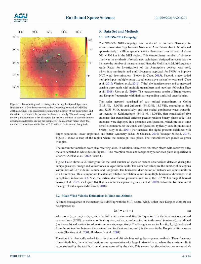
The radar network consisted of two pulsed transmitters in Collm (51.31°N, 13.00°E) and Juliusruh (54.63°N, 13.37°E), operating at 36.2 and 32.55  MHz, respectively; and one coded–continuous-wave transmit-ter located in Kühlungsborn (54.15°N, 11.76°E), that consisted of five antennas that transmitted different pseudo-random binary phase code. The antennas were deployed in a pentagon configuration, which presents some benefits compared to the Jones configuration, typically used in monostatic SMRs (Espy et al., 2004). For instance, the signal presents sidelobes with

larger separation, lower amplitude, and better symmetry (Chau & Clahsen,  2019; Younger & Reid,  2017). Figure  1 shows a map of the region where the campaign took place. The transmitters are placed as green triangles.

The transmitter locations were also receiving sites. In addition, there were six other places with receivers only, that are depicted as white dots in Figure 1. The reception mode and reception type for each place is specified in Charuvil Asokan et al. (2022, Table 1).

Figure 1 also shows a 2D histogram for the total number of specular meteor observations detected during the campaign as red, orange and yellow tones in logarithmic scale. The color bar values are the number of detections within bins of 0.1° wide in Latitude and Longitude. The horizontal distribution of meteors was almost uniform in all directions. This is important to calculate reliable correlation values in multiple horizontal directions, as it is explained in Section 3.3. Also, the vertical distribution presented maxima in the ∼87–96 km range (Charuvil Asokan et al., 2022, see Figure 1b), that lies in the mesopause region (Xu et al., 2007), below the Kármán line at the edge of outer space (McDowell, 2018).

3.2. Mean Wind Velocity Estimations in Time and Altitude

A direct consequence of the meteor trails drifting with the MLT neutral wind, is that their Doppler shifts (f) can be expressed as

2𝜋𝜋𝜋𝜋 = 𝐮𝐮 ⋅ 𝐤𝐤 + 𝜉𝜉 (8)

where u = (u1, u2, u3) = (u, v, w) is the full wind vector as defined in Equation 1 in the local meteor-centered east-north-up (ENU) cartesian coordinate system, with u, v, and w referring to the zonal (east-west), meridional (north-south) and vertical (up-down) components, respectively. The Bragg wave vector k = (ku, kv, kw) is obtained from the subtraction between the scattered and incident vectors, and ξ is the error in the Doppler shift measure-ments (Hocking et al., 2001; Holdsworth et al., 2004).

Equation  8 is classically solved for u in time and altitude bins using least-squares methods. Then, for every time-altitude bin, the wind estimations are representative of a large horizontal area, where the maximum limit is constrained by the total horizontal range covered by the data. This means that the solutions are mean winds

Figure 1. Transmitting and receiving sites during the Spread Spectrum Interferometric Multistatic meteor radar Observing Network (SIMONe) 2018 campaign. The green triangles mark the location of the transmitters and the white circles mark the location with receivers only. The red, orange and yellow tones represent a 2D histogram for the total number of specular meteor observations detected during the campaign. The color bar values show the number of detections within bins of 0.1° wide in Latitude and Longitude.

Earth and Space Science

POBLET ET AL.

10.1029/2021EA002201

5 of 16

U, and depending on the resolutions that are selected to calculate them, they represent average characteristics of different processes.

In the case of monostatic SMRs, the mean wind is frequently calculated in hourly values every 2–3 km of altitude (Hoffmann et al., 2010; Jacobi et al., 1999). For multistatic SMR networks, the resolutions can be considerably improved due to the larger amount of meteor detections. Time and vertical resolution values can be of ∼15 min and 1 km, respectively (Conte et al., 2021; Stober & Chau, 2015). In this case, as multistatic SMRs observe the same MLT volume from different viewing angles, horizontal gradients that contain vorticity information can be determined (Chau et al., 2017; Zhong et al., 2021).

Examples of mean winds estimated with different time and altitude resolutions can be seen in Conte et al. (2021, Figure 4) for measurements carried out in southern Patagonia, or in Chau et al. (2017, Figure 4) using SMRs located in Tromsø, Norway. The winds are estimated by the linear least-square method and show the typical behavior of winds at MLT altitudes that is, strong velocity changes from positive to negative throughout a day or a couple of days. Tidal modes can also be recognized.

For the SIMONe 2018 campaign, the mean winds are presented by Charuvil Asokan et al. (2022, Figure 2) and Vargas et al. (2021, Figure 2), estimated using 30 min and 1 km bins. The semidiurnal tide was dominant in both horizontal components and indications of higher-frequency fluctuations, in the order of hours can be recognized. These fluctuations are better observed if mean winds calculated with larger temporal and vertical resolutions are subtracted. The residuals winds that result from subtracting the 4 hr, 4 km resolution winds, presented coherent GW features in both horizontal components. In general, removing the 4 hr, 4 km mean winds works well to study fluctuating winds that include GWs activity (Conte et al., 2021).

3.3. Wind Field Correlation Function Inversion to Calculate 2D Horizontal Correlation Functions

The essence of the WCFI method is in considering products of Doppler shifts of meteor detections that occur in a different time and position to estimate correlation functions.

Consider two meteors n and m, detected at times tn and tm and positions rn and rm, respectively. The velocities at these coordinates will be u (n) = u(tn, rn) and u (m) = u(tm, rm). In addition, the Doppler shifts of meteors n and m will be given by f (n) = f(tn, rn) and f (m) = f(tm, rm), their Bragg wave vectors by k (n) = k(tn, rn) and k (m) = k(tm, rm), and their errors by ξ (n) = ξ(tn, rn) and ξ (m) = ξ(tm, rm). Multiplying Equation 8 for these two meteors we have

4𝜋𝜋2𝑓𝑓 (𝑛𝑛)𝑓𝑓 (𝑚𝑚) =(𝐮𝐮(𝑛𝑛)

⋅ 𝐤𝐤(𝑛𝑛)) (

𝐮𝐮(𝑚𝑚)

⋅ 𝐤𝐤(𝑚𝑚))+(𝐮𝐮(𝑛𝑛)

⋅ 𝐤𝐤(𝑛𝑛))𝜉𝜉(𝑚𝑚) +

(𝐮𝐮(𝑚𝑚)

⋅ 𝐤𝐤(𝑚𝑚))𝜉𝜉(𝑛𝑛) + 𝜉𝜉(𝑛𝑛)𝜉𝜉(𝑚𝑚). (9)

If the expected or mean value of Equation 9 is calculated, considering a sufficient amount of meteors n and m, only the first term on the right-hand side is different than zero. This is because the errors are assumed to be zero-mean, independent, and normally distributed random variables and the MLT winds can usually be modeled as a stationary and horizontally homogeneous stochastic process. The resulting expression has the form

⟨4𝜋𝜋2𝑓𝑓 (𝑛𝑛)𝑓𝑓 (𝑚𝑚)

⟩=⟨(

𝐮𝐮(𝑛𝑛)

⋅ 𝐤𝐤(𝑛𝑛)) (

𝐮𝐮(𝑚𝑚)

⋅ 𝐤𝐤(𝑚𝑚))⟩

. (10)

Vierinen et al. (2019) showed that if Equation 10 is expanded in terms of the vectors components, a linear system can be formed as

𝐲𝐲 = 𝐀𝐀�̃�𝐱 + 𝜼𝜼, (11)

in which y is an array of values containing the cross product between the Doppler shifts of different meteors, A is a matrix containing products and summations that involve the Bragg vector components of the different meteor detections, 𝐴𝐴 �̃�𝐱 is the least-square solution of the system that gives the correlation tensor components distributed in temporal and spatial lags, and η are the associated errors on solving the system. The reader can examine the detailed form of the matrix A in Vierinen et al. (2019, Equation 14).

More specifically, the solution 𝐴𝐴 �̃�𝐱 is given by the array

�̃�𝐱 = [𝑅𝑅𝑢𝑢𝑢𝑢(𝜏𝜏𝜏 𝐬𝐬)𝑅𝑅𝑣𝑣𝑣𝑣(𝜏𝜏𝜏 𝐬𝐬)𝑅𝑅𝑤𝑤𝑤𝑤(𝜏𝜏𝜏 𝐬𝐬)𝑅𝑅𝑢𝑢𝑣𝑣(𝜏𝜏𝜏 𝐬𝐬)𝑅𝑅𝑢𝑢𝑤𝑤(𝜏𝜏𝜏 𝐬𝐬)𝑅𝑅𝑣𝑣𝑤𝑤(𝜏𝜏𝜏 𝐬𝐬)]⊺

𝜏 (12)

Earth and Space Science

POBLET ET AL.

10.1029/2021EA002201

6 of 16

where 𝐴𝐴 𝐴𝐴𝑢𝑢𝑖𝑖𝑢𝑢𝑗𝑗 (𝜏𝜏𝜏 𝐬𝐬) =⟨𝑢𝑢(𝑛𝑛)

𝑖𝑖𝑢𝑢(𝑚𝑚)

𝑗𝑗

⟩= ⟨𝑢𝑢𝑖𝑖 (𝑡𝑡𝑛𝑛𝜏 𝐫𝐫𝑛𝑛) 𝑢𝑢𝑗𝑗 (𝑡𝑡𝑚𝑚𝜏 𝐫𝐫𝑚𝑚)⟩ are the six unique components that are retrieved by the

method. Note that, comparing with the definition in Equation 2, 𝐴𝐴 𝐴𝐴𝑢𝑢𝑖𝑖𝑢𝑢𝑗𝑗 = 𝐴𝐴𝑖𝑖𝑗𝑗 . In this case, the indices i, j = 1, 2, 3 refer here to u, v and w, respectively. We maintain the compact notation for Rij in the following.

Rij(τ, s) depend on temporal and spatial displacements (also called lags) τ = tm − tn and s = rm − rn. The criterion implemented to combine the meteors to solve the system gives the nature of the correlations, because it deter-mines the ranges of τ or s, resulting in temporal or spatial correlations.

The meteors are combined in pairs. For spatial, horizontal correlations distributed in two dimensions, that is, east-west (x) and north-south (y) directions, the meteor pairs are formed in the following manner. Since SMRs detect meteors almost continuously in time, approximately between 70 and 110 km of altitude, the first step is to confine these ranges. Then, the data in an interval of 6 or 2 km wide, and 1 day or 1 week are selected.

After that, the pairing scheme moves to particular detections. We select one meteor n and tune the vertical and temporal conditions, finding every meteor that is not separated from it by more than a given temporal and vertical resolution (Δτ and Δsz, respectively). Then, for each meteor fulfilling the temporal and vertical requirements, only those meteors that lie in the intervals s ± Δs/2 = (sx ± Δsx/2, sy ± Δsy/2) for particular values of s = (sx, sy) and fixed horizontal lag resolutions Δsx = Δsy, are selected. The meteor pairs are formed by combining the meteor n with each one of the resulting meteors.

The procedure continues by selecting another meteor to play the role of n in the previous step, and repeat the process. In the end, every pair has in common that their elements preserve the distance between each other (within the horizontal resolution ranges). Finally, the system in Equation 11 is solved for the correlation components Rij(sx, sy).

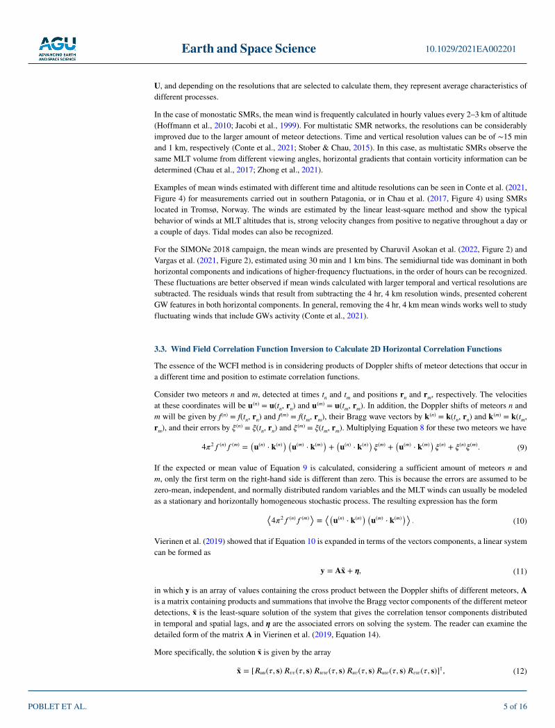
Figure  2 helps to schematically visualize the transition from the Latitude-Longitude domain, that is, where the measurements are taken, to the spatial horizontal lags domain, that is, where the correlation functions are calculated. The gray dots in the left-hand side panel represent the meteor positions mapped into a plane in Lati-tude and Longitude for the given altitude range. The colors represent different geometries, that manifest in the values of sx and sy, because the resolutions Δsx and Δsy are kept constant. The straight lines mark the distance between the starting point and the center of the searching area, of dimension ΔsxΔsy. If we look at the meteor n, the pairs are formed with the meteors that lie inside the green box, after the temporal and vertical filtering. For this particular geometry, the total amount of pairs is obtained when the process is extended to every meteor, considering the same sx and sy (every geometry in green for all the meteors). With every pair, the correlations are mapped to the corresponding s value, sketched also in green color on the right-hand side panel of the figure. In particular, note that for the sketches in red, that show opposite geometries, the relation Rij(s) = Rij(−s) is

Figure 2. Schematic representation of the meteors selection procedure to calculate 2D correlation functions. Left panel: plane view showing different geometries to form the meteor pairs. The gray dots represent meteor positions mapped into a plane in Latitude and Longitude for the given altitude range. The colors represent different geometries, given by the values of sx and sy. Right panel: Position in the lags domain where the correlations are calculated. The colors represent different values of sx and sy.

Earth and Space Science

POBLET ET AL.

10.1029/2021EA002201

7 of 16

valid, because almost the same measurements are used to form the pairs for both cases. Consequently, the method produces only two quadrants with independent correlations to analyze: (I) and (II), (I) and (IV), (II) and (III) or (III) and (IV).

3.3.1. Fluctuating Wind Correlations

In Section 3.3, the WCFI method was introduced for the more general case, that is when the correlations of the total wind Rij are needed. To estimate the two-dimensional correlations of the fluctuating wind 𝐴𝐴 𝐴𝐴′

𝑖𝑖𝑖𝑖 , two approaches

can be followed. The first one is to calculate the full correlation tensor in which correlations in short and long lags can be identified and also calculate another correlation tensor with lower resolutions over a large temporal and spatial extent. The difference between both gives the correlation functions of the fluctuating wind. In general, short lags show the contribution of the fluc-tuating winds while long lags capture the contributions of the mean winds.

The second method consists of filtering the Doppler shifts before applying the WCFI method. This is achieved by estimating U, using the procedure introduced in Section 3.2. In particu-lar, solving Equation  8 with low resolutions, for example, 4  hr, 4  km; so the filtered Doppler shifts f′ are f′ = f − U ⋅ k/2π with f′ the Doppler shift measurement of the high-pass-filtered wind. Then, the WCFI tech-nique is applied using f′ and k to get 2D correlation functions of the fluctuating wind. As stated by Vierinen et al. (2019), high-pass-filtered measurements have shorter temporal and spatial lengths, resulting in more inde-pendent samples of the wind field correlation function to be obtained per unit of time and space. The second approach was followed in this work. We subtracted mean winds calculated every 1 km and 30 min; with resolu-tions of 4 hr and 4 km.

3.4. Transformation From Zonal-Meridional (Ruu, Rvv) to Longitudinal-Transverse Components (RLL, RTT)

The WCFI method delivers 2D horizontal correlation functions in cartesian ENU components. These compo-nents are given by the solution array in Equation 12. In order to use the WCFI method solutions to solve Equa-tions 5 and 7 we must find a way to convert Ruu and Rvv to RLL and RTT. This can be done using a post-statistic approach under certain conditions. The conversion method is described in this section.

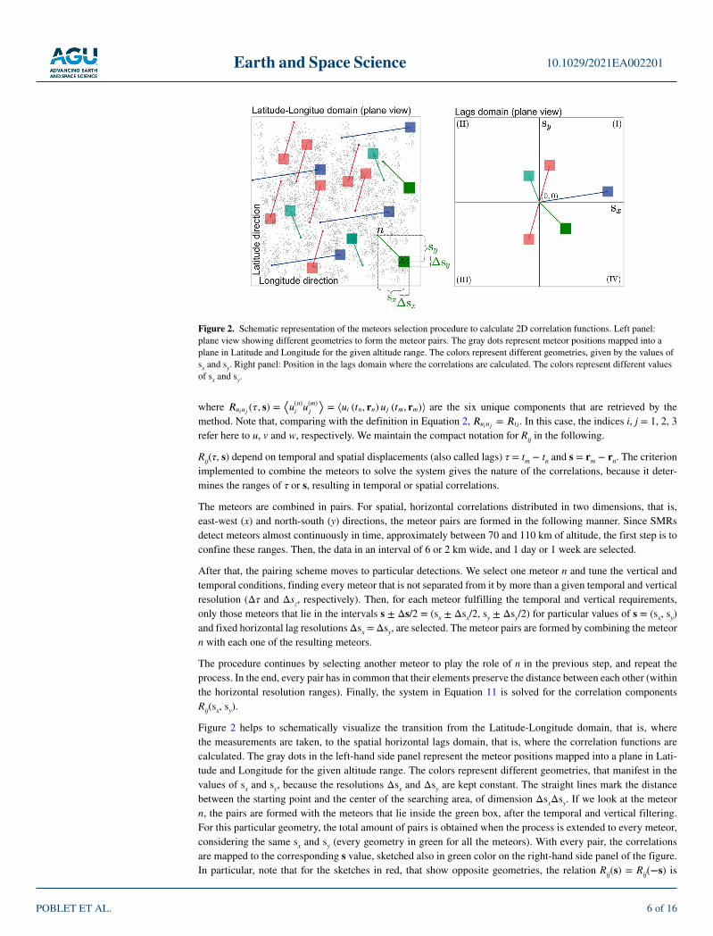
Similarly to Section 3.3, we consider the two points n and m that represent two meteor detections depicted in the diagram of Figure 3. At these two points, the neutral wind velocities are u (n) and u (m). These vectors can be decom-posed in longitudinal, transverse and vertical components 𝐴𝐴 𝐮𝐮

(𝑛𝑛) = 𝑢𝑢(𝑛𝑛)

𝐿𝐿�̂�𝒍 + 𝑢𝑢

(𝑛𝑛)

𝑇𝑇�̂�𝝓 +𝑤𝑤(𝑛𝑛)

�̂�𝒛 , 𝐴𝐴 𝐮𝐮(𝑚𝑚) = 𝑢𝑢

(𝑚𝑚)

𝐿𝐿�̂�𝒍 + 𝑢𝑢

(𝑚𝑚)

𝑇𝑇�̂�𝝓 +𝑤𝑤(𝑚𝑚)

�̂�𝒛 , where we have used the local, meteor-pair dependent basis 𝐴𝐴 �̂�𝒍 , 𝐴𝐴 �̂�𝝓 , 𝐴𝐴 �̂�𝒛 , with 𝐴𝐴 �̂�𝒛 in the vertical direction, 𝐴𝐴 �̂�𝒍 perpendicular to 𝐴𝐴 �̂�𝒛 along the line that connects both meteors and 𝐴𝐴 �̂�𝝓 perpendicular to 𝐴𝐴 �̂�𝒍 and 𝐴𝐴 �̂�𝒛 . The figure also shows the decompo-sition in the ENU system 𝐴𝐴 𝐮𝐮

(𝑛𝑛) = 𝑢𝑢(𝑛𝑛)�̂�𝒙 + 𝑣𝑣(𝑛𝑛)�̂�𝒚 +𝑤𝑤(𝑛𝑛)�̂�𝒛 , 𝐴𝐴 𝐮𝐮

(𝑚𝑚) = 𝑢𝑢(𝑚𝑚)�̂�𝒙 + 𝑣𝑣(𝑚𝑚)�̂�𝒚 +𝑤𝑤(𝑚𝑚)�̂�𝒛 , where the basis 𝐴𝐴 �̂�𝒙 , 𝐴𝐴 �̂�𝒚 , 𝐴𝐴 �̂�𝒛 are on

the east-west 𝐴𝐴 (�̂�𝒙) , north-south 𝐴𝐴 (�̂�𝒚) , and vertical 𝐴𝐴 (�̂�𝒛) directions. In the case of the vertical components, they are the same for both systems. On the other hand, the horizontal components in the two systems are related by a rotation of an angle (ϕ) around the vertical axis. The relation, for the point n for example, is

𝑢𝑢(𝑛𝑛)

𝐿𝐿= 𝑢𝑢(𝑛𝑛)cos𝜙𝜙 + 𝑣𝑣(𝑛𝑛)sin𝜙𝜙𝜙 (13)

𝑢𝑢(𝑛𝑛)

𝑇𝑇= −𝑢𝑢(𝑛𝑛)sin𝜙𝜙 + 𝑣𝑣(𝑛𝑛)cos𝜙𝜙𝜙 (14)

deduced considering the well-known conversion of a velocity vector from Cartesian to Cylindrical components, or by using geometrical arguments in Figure 5.

We can extend Equation 13 for point m, and build RLL as

Figure 3. Schematic diagram showing the wind velocity vectors for two different meteor detections n and m on a plane view. The vectors are decomposed in longitudinal, transverse and vertical components uL, uT, and w and in Cartesian ENU components u, v, and w. 𝐴𝐴 �̂�𝒍 , 𝐴𝐴 �̂�𝝓 , 𝐴𝐴 �̂�𝒛 and 𝐴𝐴 �̂�𝒙 , 𝐴𝐴 �̂�𝒚 , 𝐴𝐴 �̂�𝒛 are the unit vectors of the two systems.

Earth and Space Science

POBLET ET AL.

10.1029/2021EA002201

8 of 16

���(�) =⟨

�(�)� �(�)�

⟩

=⟨

�(�)�(�)cos2�⟩

+⟨

�(�)�(�)cos�sin�⟩

+⟨

�(�)�(�)sin�cos�⟩

+⟨

�(�)�(�)sin2�⟩

,

(15)

in which ideally, when the velocity vectors in ENU components are fully known, the expected values of the four terms are calculated combining the products of the sines, cosines and velocity components of every detection. In our case, this scenario is not feasible since we do not know the velocity vectors of every detection. However, once the correlation tensor components are calculated with the WCFI method, we can assume that for every detection within s ± Δs/2, ϕ is approximately constant. Then, the ϕ-dependent products of Equation 15 can be taken out the expected value operator to get the following expression

���(�) ≃ ���(�) cos2� + 2���(�) cos� sin� +���(�) sin2�, (16)

that considering horizontal isotropy (Ruv = Rvu = 0) becomes

���(�) ≃ ���(�) cos2� +���(�) sin2�. (17)

It is very important for Equations 16 and 17 to be valid that |Δs| < |s|, otherwise ϕ cannot be considered as a constant value for the given s. Therefore, if the resolution is fixed, Equations 16 and 17 are not valid for small lags.

Repeating the same procedure for RTT, similar expressions are obtained

��� (�) ≃ ���(�) sin2� − 2���(�) cos� sin� +���(�) cos2�, (18)

and

��� (�) ≃ ���(�) sin2� +���(�) cos2�, (19)

for the isotropic case.

4. Results4.1. 2D Horizontal Correlation Functions

The 2D correlation function components 𝐴𝐴 𝐴𝐴′

𝑢𝑢𝑢𝑢(𝐬𝐬) , 𝐴𝐴 𝐴𝐴′

𝑣𝑣𝑣𝑣(𝐬𝐬) and 𝐴𝐴 𝐴𝐴′

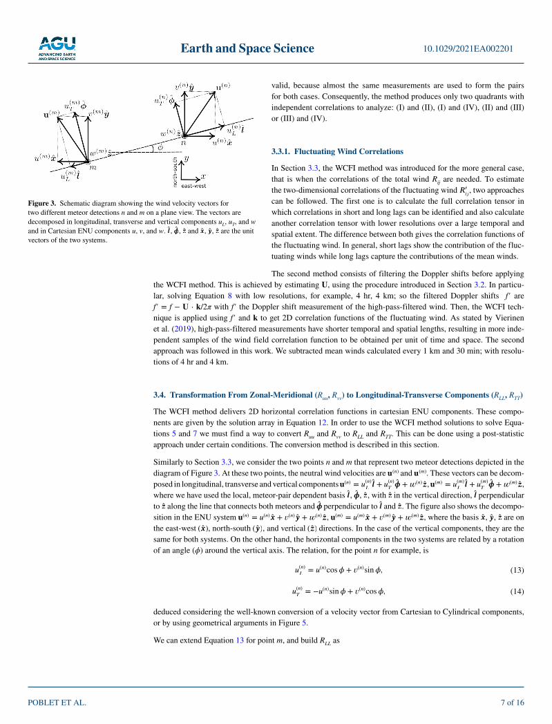
𝑢𝑢𝑢𝑢(𝐬𝐬) calculated for the SIMONe 2018 campaign can be seen in panels (a), (b) and (c) of Figure 4, respectively. The white lines are smoothed contours of the correla-tions, plotted to visualize the behavior for different directions. Also, the correlation errors are shown as light-blue contours in the three panels.

𝐴𝐴 𝐴𝐴′

𝑢𝑢𝑢𝑢(𝐬𝐬) , 𝐴𝐴 𝐴𝐴′

𝑣𝑣𝑣𝑣(𝐬𝐬) and 𝐴𝐴 𝐴𝐴′

𝑢𝑢𝑢𝑢(𝐬𝐬) were estimated using detections within the 87–93  km altitude range, and consider-ing time and altitude resolutions of Δτ = 30 min and Δsz = 1 km, respectively; and horizontal resolutions of Δsx = Δsy = 25 km. We calculated the correlations every 12.5 km in both directions, sx and sx, covering the displacements range given by sx = [−250, 250] km and sy = [0, 400] km; that is, only the quadrants I and II were considered to avoid working with repeated information (see the pairs selection procedure described in Section 3.3). The white areas for large |s| values mark correlations with errors larger than 25 m 2 s −2, that were excluded from the analysis.

𝐴𝐴 𝐴𝐴′

𝑢𝑢𝑢𝑢 and 𝐴𝐴 𝐴𝐴′

𝑣𝑣𝑣𝑣 show a gradual decorrelation as |s| increases, and 𝐴𝐴 𝐴𝐴′

𝑢𝑢𝑢𝑢 presents comparatively lower values of corre-lations in the entire domain. The decrease of 𝐴𝐴 𝐴𝐴′

𝑢𝑢𝑢𝑢 and 𝐴𝐴 𝐴𝐴′

𝑣𝑣𝑣𝑣 is not identical in every direction for certain separa-tion ranges. For example, a moderate alignment in the northwest/southeast direction can be identified for both

components. This behavior is more clear for mid-range lags, around horizontal lags 𝐴𝐴 𝐴𝐴ℎ =

√

s2

𝑥𝑥 + s2

𝑦𝑦 ≃ 150 km, and disappears for shorter values. For larger lags, the correlations increase their dispersion due to the increase in errors. The cross-correlation component 𝐴𝐴 𝐴𝐴′

𝑢𝑢𝑢𝑢 ≃ 0 , meaning that the background wind was correctly calculated and there was no preferential direction for the fluctuating wind during the campaign. As a result, u and v variations are approximately uncorrelated. The relatively high correlation values reached by 𝐴𝐴 𝐴𝐴′

𝑢𝑢𝑢𝑢 lie in the longest displacements region, where the errors are the largest as well.

Earth and Space Science

POBLET ET AL.

10.1029/2021EA002201

9 of 16

In general, the errors of the three components increase as the lags grow, partially because there are less number of pairs in longer lags to resolve the correlations with high precision. Figure 4d shows the gradual decrease in the number of pairs as lag values increase.

4.2. 1D Longitudinal and Transverse Correlation and Structure Functions

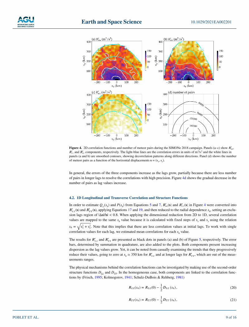
In order to estimate Qzz(sh) and P(sh) from Equations 5 and 7, 𝐴𝐴 𝐴𝐴′

𝑢𝑢𝑢𝑢(𝐬𝐬) and 𝐴𝐴 𝐴𝐴′

𝑣𝑣𝑣𝑣(𝐬𝐬) in Figure 4 were converted into 𝐴𝐴 𝐴𝐴′

𝐿𝐿𝐿𝐿(𝐬𝐬) and 𝐴𝐴 𝐴𝐴′

𝑇𝑇𝑇𝑇(𝐬𝐬) , applying Equations 17 and 19, and then reduced to the radial dependence sh, setting an exclu-

sion lags region of |Δs|/|s| < 0.8. When applying the dimensional reduction from 2D to 1D, several correlation values are mapped to the same sh value because it is calculated with fixed steps of sx and sy using the relation

𝐴𝐴 𝐴𝐴ℎ =

√

s2𝑥𝑥 + s2𝑦𝑦 . Note that this implies that there are less correlation values at initial lags. To work with single correlation values for each lag, we estimated mean correlations for each sh value.

The results for 𝐴𝐴 𝐴𝐴′

𝐿𝐿𝐿𝐿 and 𝐴𝐴 𝐴𝐴′

𝑇𝑇𝑇𝑇 are presented as black dots in panels (a) and (b) of Figure 5, respectively. The error

bars, determined by summation in quadrature, are also added to the plots. Both components present increasing dispersion as the lag values grow. Yet, it can be noted from casually examining the trends that they progressively reduce their values, going to zero at sh ≃ 350 km for 𝐴𝐴 𝐴𝐴′

𝐿𝐿𝐿𝐿 and at longer lags for 𝐴𝐴 𝐴𝐴′

𝑇𝑇𝑇𝑇 , which are out of the meas-

urements ranges.

The physical mechanisms behind the correlation functions can be investigated by making use of the second-order structure functions DLL and DTT. In the homogeneous case, both components are linked to the correlation func-tions by (Frisch, 1995; Kolmogorov, 1941; Schulz-DuBois & Rehberg, 1981)

���(�ℎ) = ���(0) −12��� (�ℎ) , (20)

��� (�ℎ) = ��� (0) −12��� (�ℎ) , (21)

Figure 4. 2D correlation functions and number of meteor pairs during the SIMONe 2018 campaign. Panels (a–c) show 𝐴𝐴 𝐴𝐴′

𝑢𝑢𝑢𝑢 , 𝐴𝐴 𝐴𝐴′

𝑣𝑣𝑣𝑣 and 𝐴𝐴 𝐴𝐴′

𝑢𝑢𝑢𝑢 components, respectively. The light-blue lines are the correlation errors in units of m 2/s 2 and the white lines in panels (a and b) are smoothed contours, showing decorrelation patterns along different directions. Panel (d) shows the number of meteor pairs as a function of the horizontal displacements s = (sx, sy).

Earth and Space Science

POBLET ET AL.

10.1029/2021EA002201

10 of 16

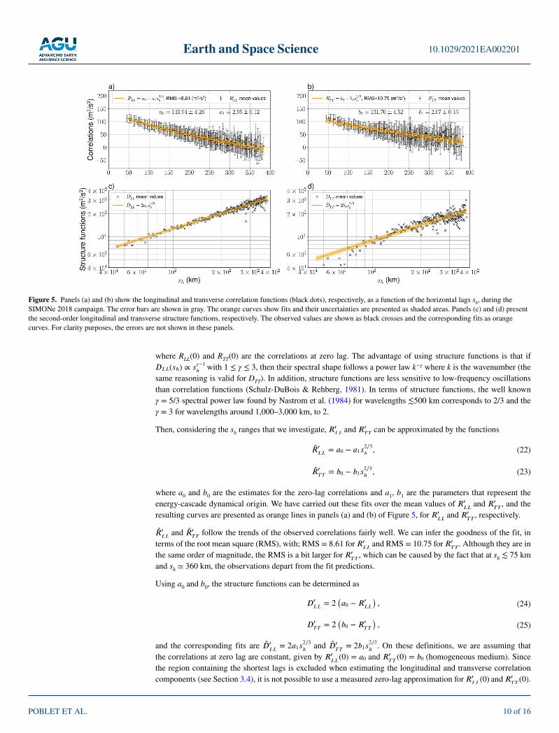
where RLL(0) and RTT(0) are the correlations at zero lag. The advantage of using structure functions is that if ���(�ℎ) ∝ ��−1ℎ with 1 ≤ γ ≤ 3, then their spectral shape follows a power law k −γ where k is the wavenumber (the same reasoning is valid for DTT). In addition, structure functions are less sensitive to low-frequency oscillations than correlation functions (Schulz-DuBois & Rehberg, 1981). In terms of structure functions, the well known γ = 5/3 spectral power law found by Nastrom et al. (1984) for wavelengths ≲500 km corresponds to 2/3 and the γ = 3 for wavelengths around 1,000–3,000 km, to 2.

Then, considering the sh ranges that we investigate, 𝐴𝐴 𝐴𝐴′

𝐿𝐿𝐿𝐿 and 𝐴𝐴 𝐴𝐴′

𝑇𝑇𝑇𝑇 can be approximated by the functions

�̂�𝑅′

𝐿𝐿𝐿𝐿= 𝑎𝑎0 − 𝑎𝑎1𝑠𝑠

2∕3

ℎ, (22)

�̂�𝑅′

𝑇𝑇𝑇𝑇= 𝑏𝑏0 − 𝑏𝑏1𝑠𝑠

2∕3

ℎ, (23)

where a0 and b0 are the estimates for the zero-lag correlations and a1, b1 are the parameters that represent the energy-cascade dynamical origin. We have carried out these fits over the mean values of 𝐴𝐴 𝐴𝐴′

𝐿𝐿𝐿𝐿 and 𝐴𝐴 𝐴𝐴′

𝑇𝑇𝑇𝑇 , and the

resulting curves are presented as orange lines in panels (a) and (b) of Figure 5, for 𝐴𝐴 𝐴𝐴′

𝐿𝐿𝐿𝐿 and 𝐴𝐴 𝐴𝐴′

𝑇𝑇𝑇𝑇 , respectively.

𝐴𝐴 �̂�𝑅′

𝐿𝐿𝐿𝐿 and 𝐴𝐴 �̂�𝑅′

𝑇𝑇𝑇𝑇 follow the trends of the observed correlations fairly well. We can infer the goodness of the fit, in

terms of the root mean square (RMS), with; RMS = 8.61 for 𝐴𝐴 𝐴𝐴′

𝐿𝐿𝐿𝐿 and RMS = 10.75 for 𝐴𝐴 𝐴𝐴′

𝑇𝑇𝑇𝑇 . Although they are in

the same order of magnitude, the RMS is a bit larger for 𝐴𝐴 𝐴𝐴′

𝑇𝑇𝑇𝑇 , which can be caused by the fact that at sh ≲ 75 km

and sh ≃ 360 km, the observations depart from the fit predictions.

Using a0 and b0, the structure functions can be determined as

𝐷𝐷′

𝐿𝐿𝐿𝐿= 2

(𝑎𝑎0 −𝑅𝑅′

𝐿𝐿𝐿𝐿

), (24)

𝐷𝐷′

𝑇𝑇𝑇𝑇= 2

(𝑏𝑏0 −𝑅𝑅′

𝑇𝑇𝑇𝑇

), (25)

and the corresponding fits are 𝐴𝐴 �̂�𝐷′

𝐿𝐿𝐿𝐿= 2𝑎𝑎1𝑠𝑠

2∕3

ℎ and 𝐴𝐴 �̂�𝐷′

𝑇𝑇𝑇𝑇= 2𝑏𝑏1𝑠𝑠

2∕3

ℎ . On these definitions, we are assuming that

the correlations at zero lag are constant, given by 𝐴𝐴 𝐴𝐴′

𝐿𝐿𝐿𝐿(0) = 𝑎𝑎0 and 𝐴𝐴 𝐴𝐴′

𝑇𝑇𝑇𝑇(0) = 𝑏𝑏0 (homogeneous medium). Since

the region containing the shortest lags is excluded when estimating the longitudinal and transverse correlation components (see Section 3.4), it is not possible to use a measured zero-lag approximation for 𝐴𝐴 𝐴𝐴′

𝐿𝐿𝐿𝐿(0) and 𝐴𝐴 𝐴𝐴′

𝑇𝑇𝑇𝑇(0) .

Figure 5. Panels (a) and (b) show the longitudinal and transverse correlation functions (black dots), respectively, as a function of the horizontal lags sh, during the SIMONe 2018 campaign. The error bars are shown in gray. The orange curves show fits and their uncertainties are presented as shaded areas. Panels (c) and (d) present the second-order longitudinal and transverse structure functions, respectively. The observed values are shown as black crosses and the corresponding fits as orange curves. For clarity purposes, the errors are not shown in these panels.

Earth and Space Science

POBLET ET AL.

10.1029/2021EA002201

11 of 16

𝐴𝐴 𝐴𝐴′

𝐿𝐿𝐿𝐿 and 𝐴𝐴 𝐴𝐴′

𝑇𝑇𝑇𝑇 are plotted as black crosses in panels (c) and (d) of Figure 5, respectively. The fitting functions are

also added to the plots as orange curves.

The agreement of 𝐴𝐴 𝐴𝐴′

𝐿𝐿𝐿𝐿 with a 2/3-power law of sh is remarkable. This is expected for horizontally distributed

second-order structure functions in these scales (Nastrom et al., 1984). Even though 𝐴𝐴 𝐴𝐴′

𝑇𝑇𝑇𝑇 values have a larger

dispersion, the 2/3-power approximation follows the general trends as well.

Other dynamical effects can be considered to fit the observations. Lindborg  (1999) proposed functional dependencies for second-order structure functions that incorporate not only an energy cascade mode but an enstrophy-cascade dynamical origin. For this, two terms are incorporated into the fitting models, to capture the variations for large scales, in the γ = 3 range (Lindborg, 1999, Equation 68 and 69). Since our measurements cover a more narrow range in the mesoscales, the enstrophy-cascade terms were not incorporated to fit the observations.

4.3. Vertical Vorticity and Horizontal Divergence Correlations and Spectra Estimation

Once the parameters of the models proposed to represent 𝐴𝐴 𝐴𝐴′

𝐿𝐿𝐿𝐿 and 𝐴𝐴 𝐴𝐴′

𝑇𝑇𝑇𝑇 are determined, we can make use of Equa-

tions 5 and 7 to calculate Qzz and P. Introducing Equations 22 and 23 into Equations 5 and 7 and calculating the derivatives it is found that

𝑄𝑄𝑧𝑧𝑧𝑧 = 𝑞𝑞1𝑠𝑠−4∕3

ℎ, 𝑃𝑃 = 𝑝𝑝1𝑠𝑠

−4∕3

ℎ, (26)

with 𝐴𝐴 𝐴𝐴1 =2

3

(5

3𝑏𝑏1 − 𝑎𝑎1

)= 0.34 × 10

−2 m 4/3 s −2 and 𝐴𝐴 𝐴𝐴1 =2

3

(5

3𝑎𝑎1 − 𝑏𝑏1

)= 1.90 × 10

−2 m 4/3 s −2. Both functions are plotted in the left-hand side panel of Figure 6 as blue and green lines for Qzz and P, respectively. The black dashed lines indicate the extrapolation to larger and shorter (not measured) displacements.

The characteristics of both functions can be inferred from the parameter values as well as from the plots. For example, it is clear that they quickly go to zero as sh grows. P reduces its values about a hundred times from the shortest displacement where P ≃ 0.01 s −2 to the largest displacement where P ≃ 0.0007 s −2. On the other hand, Qzz ≲ 0.002 s −2 for the entire sh range. Moreover, with the coefficients q1 and p1, we can estimate the ratio P/Qzz = p1/q1 = 5.6, meaning that P is more than five times larger than Qzz; that is, a clear predominance of P over Qzz.

The two-dimensional horizontal spectra of Qzz for wavenumbers k = 2π/sh can be calculated as

Φ(𝑘𝑘) = 2𝜋𝜋𝑘𝑘 [𝑄𝑄𝑧𝑧𝑧𝑧] , (27)

where the Fourier transform, expressed in polar cylindrical coordinates is

[���] =14�2 ∫

∞

0 ∫

2�

0��� (�ℎ) exp (−�� ⋅ �) �ℎ d�ℎ d�. (28)

Figure 6. Left panel: Qzz (blue) and P (green) as a function of the spatial lags sh. The shaded area shows Qzz and P calculated using the uncertainties of the fits in Equations 22 and 23. The dashed black lines show the continuation for larger and shorter (not measured) horizontal lags. Right panel: Qzz and P spectra (Φ and Ψ, respectively) as a function of the wavenumber k = 2π/sh. The same color coding as for Qzz and P is used.

Earth and Space Science

POBLET ET AL.

10.1029/2021EA002201

12 of 16

If k = (k, θ), the inner product in the exponential takes the form s ⋅ k = shk cos (ϕ − θ), but since ϕ goes from 0 to 2π, the integral on the angle does not depend of θ. Qzz is only a function of sh, so we can write Φ as

Φ(𝑘𝑘) = 𝑘𝑘∫

∞

0

𝑄𝑄𝑧𝑧𝑧𝑧 (𝑠𝑠ℎ) 𝐽𝐽0 (𝑠𝑠ℎ𝑘𝑘) 𝑠𝑠ℎ d𝑠𝑠ℎ, (29)

in which �0(�ℎ�) = 12�

∫ 2�0 exp (−�� �ℎ cos�) d� is the cylindrical Bessel function of zero order. Replacing Qzz in Equation 29, and changing the integration variable to η = shk, we get the expression

Φ(𝑘𝑘) = 𝑞𝑞1𝑘𝑘1∕3

∫

∞

0

𝜂𝜂−1∕3𝐽𝐽0 (𝜂𝜂) d𝜂𝜂𝜂 (30)

in which the integral can be taken from tabulated values to get

Φ(𝑘𝑘) ≃ 1.57𝑞𝑞1𝑘𝑘1∕3. (31)

An obvious problem to solve Equation 30 with this procedure is that Qzz is only known in a bounded sh interval, that in the wavenumber domain is k ∈ [2π/383.07, 2π/45.07] = [0.016, 0.139] km −1. The method is valid if we can assume that the contributions to the spectra outside these limits are small compared to a given k value inside the domain (Lindborg, 2007).

Repeating the exact same procedure for the spectrum of P, hereinafter referred to as Ψ, we get

Ψ(𝑘𝑘) ≃ 1.57𝑝𝑝1𝑘𝑘1∕3. (32)

Φ and Ψ are shown on the right-hand side panel of Figure 6 in the same color code as their corresponding func-tions in the space domain. The main feature of this plot is that Ψ > Φ in the entire mesoscales range studied, demonstrating the prevalence of P over Qzz in the wavenumbers domain. Also, Ψ/Φ = P/Qzz = 5.6 showing that the scaling between the two functions is maintained.

5. DiscussionLongitudinal and transverse horizontal correlation functions of wind fluctuations in the MLT have been deter-mined by making use of the WCFI technique. These functions were further analyzed to study the vorticity-tensor vertical component and horizontal divergence correlation functions. The detection range enabled the examination of horizontal displacements in the mesoscales, from about 40 to 400 km, in which the vorticity and divergence estimates account for different physical phenomena. On the one hand, Qzz may represent pancake-like structures with fine vertical resolutions in ∼300 m–1 km (Avsarkisov et al., 2022). Eddies in strongly stratified fluids can spread in horizontal planes, forming such structures with non-zero vertical vorticity. On the other hand, the diver-gent component given by P is composed of motions that are not hydrostatically and geostrophically balanced, such as GWs or stratified turbulence (Lindborg, 2014; Vallis, 2017), which are the probable physical processes behind P.

It is found that P spectrum was more than five times larger than the Qzz spectrum during the campaign. This result can be compared with the ones obtained by Lindborg (2007), in which the same orders of magnitude for both spectra were observed, with the vorticity spectrum a bit larger than the divergence spectrum. From this, the author argued that the mesoscale energy spectrum could not be generated by internal GWs, otherwise the divergence spectrum would have dominated over the vorticity spectrum. We can extend this reasoning to the results of our study to speculate that for MLT altitudes, internal GWs may be more important than vortical modes to explain the wind dynamics.

However, one must be cautious with the generalization of this assertion because we are using a much more limited data set than the one used by Lindborg (2007), and so the relative predominance of the divergent compo-nent might be representative of the campaign time conditions. In fact, according to the recent work by Vargas et al. (2021), the campaign presented a significant activity of small- and large-scale GWs interacting with the mean wind flow. In particular, Charuvil Asokan et al. (2022) found that during the campaign, GWs with periods smaller than 7 hours and greater than 2 hours were dominated by horizontal structures significantly larger than

Earth and Space Science

POBLET ET AL.

10.1029/2021EA002201

13 of 16

500 km. But, it should be noticed that the detailed examination of the waves' activity cannot be performed nor is it the objective of the method described in this work, since we obtain statistical estimates that represent a combi-nation of the divergence(vorticity) that particular structures have.

Extending the analysis to other data sets would also reduce the correlation errors, enabling to test of additional fitting models. For example, the exponent 2/3 can be generalized to an unknown fitting variable (so-called “Hurst parameter”). Preliminary tests applied to the SIMONe 2018 campaign data suggest that the correlations are still too noisy to obtain reliable fitted exponent values. This parameter has been shown to vary for different regions, seasons, and measurement instruments (King et al., 2015a). In the MLT for example, Roberts and Larsen (2014) were able to reconstruct the second-order structure functions exponent evolution for different stages of turbu-lence. They used trimethyl aluminum trails from sounding rockets as a tracer of the fluid motions, showing the asymptotic behavior of the parameter as time and horizontal scales increase. In addition, data sets from different SMR network geometries can be helpful to explore either shorter lags, improving zero-lag determinations, or larger lag dynamics, by means of the incorporation of additional terms in Equations 22 and 23 to represent an enstrophy cascade origin (Lindborg, 2007), or large-scales planetary waves (Frehlich & Sharman, 2010).

Another important outcome of this work is the estimation of 2D correlation functions of wind fluctuations in the MLT. These functions provide a direct way to characterize the horizontal correlation field from visual inspection and ultimately by statistical analyses. Important properties like the degree of horizontal axisymmetry can be evaluated. This has only been indirectly inferred in the past, for example, with the method by Cho and Lindborg (2001). The authors compared two types of one-dimensional transverse structure functions, one esti-mated from theoretical fits (just as we do for the correlations) and the other calculated following the 2D isotropic relation 𝐴𝐴 𝐴𝐴′

𝑇𝑇𝑇𝑇=

d

d𝑠𝑠ℎ

[𝑠𝑠ℎ𝐴𝐴

′

𝐿𝐿𝐿𝐿

] , where 𝐴𝐴 𝐴𝐴′

𝐿𝐿𝐿𝐿 is the measured longitudinal structure function. From the comparison,

they found considerable departures from isotropy in the stratospheric structure functions and lower departures from isotropy in the tropospheric structure functions.

For our case, the degree of horizontal axisymmetry can be inspected in more detail by separating the correlations 𝐴𝐴 𝐴𝐴′

𝑢𝑢𝑢𝑢 and 𝐴𝐴 𝐴𝐴′

𝑣𝑣𝑣𝑣 in different directions, and repeating the Qzz and P estimations for each direction. This method has been applied before by King et al. (2015a), using structure functions in the UTLS. For instance, by separating

𝐴𝐴 𝐴𝐴′

𝑢𝑢𝑢𝑢 and 𝐴𝐴 𝐴𝐴′

𝑣𝑣𝑣𝑣 in Figure 4 between quadrants I and II, it is found that the one-dimensional 𝐴𝐴 𝐴𝐴′

𝐿𝐿𝐿𝐿 component it is well

represented by the fitting model in both quadrants, while for the 𝐴𝐴 𝐴𝐴′

𝑇𝑇𝑇𝑇 component, the observations in quadrant II

are better represented by the fits than in quadrant I. For both cases Ψ > Φ.

6. Concluding RemarksIn this study, it has been demonstrated that the WCFI method has the potential to improve the understanding of the mesoscale dynamics in the MLT. This work analyzes only one of the applications of the method: the estimation of 2D correlation functions and the consequent estimation of longitudinal and transverse correlation func tions. As it was shown, this serves to account for the behavior and relative importance of vortical and divergent modes, showing the latter to be more significant in space and wavenumber domain, for the period and location in which the SIMONe 2018 campaign took place. Performing such a comparison in the MLT, using multistatic SMR observations has not been done before.

Exploiting the technique in longer multistatic data sets, measured at different locations such as those provided by SIMONe Argentina (Conte et al., 2021), and SIMONe Peru (Chau et al., 2021) will allow to more efficiently calculate the correlation functions of different spatial and temporal scales and to have a broad view of vortical and divergent modes behavior in the MLT.

Other products of the WCFI technique are temporal correlations, vertical correlations, and horizontal 1D corre-lation functions, which are currently being explored to characterize other aspects of the upper atmosphere corre-lation field.

Appendix A: Qzz and P in Cartesian ENU SystemThe derivation of Qzz and P can be performed in Cartesian ENU coordinates by expanding Equations 4 and 6 as a function of horizontal displacements sx and sy. This is achieved by summing over repeated indices, to get

Earth and Space Science

POBLET ET AL.

10.1029/2021EA002201

14 of 16

𝑄𝑄𝑧𝑧𝑧𝑧 = −𝜕𝜕2𝑅𝑅′

𝑢𝑢𝑢𝑢

𝜕𝜕s2𝑦𝑦−

𝜕𝜕2𝑅𝑅′

𝑣𝑣𝑣𝑣

𝜕𝜕s2𝑥𝑥+ 2

𝜕𝜕2𝑅𝑅′

𝑢𝑢𝑣𝑣

𝜕𝜕s𝑦𝑦𝜕𝜕s𝑥𝑥 (A1)

𝑃𝑃 = −𝜕𝜕2𝑅𝑅′

𝑢𝑢𝑢𝑢

𝜕𝜕s2𝑥𝑥−

𝜕𝜕2𝑅𝑅′

𝑣𝑣𝑣𝑣

𝜕𝜕s2𝑦𝑦− 2

𝜕𝜕2𝑅𝑅′

𝑢𝑢𝑣𝑣

𝜕𝜕s𝑦𝑦𝜕𝜕s𝑥𝑥. (A2)

It is interesting to note that, 𝐴𝐴 𝐴𝐴 +𝑄𝑄𝑧𝑧𝑧𝑧 = −∇2(𝑅𝑅′

𝑢𝑢𝑢𝑢 +𝑅𝑅′

𝑣𝑣𝑣𝑣) , which is also valid for 𝐴𝐴 𝐴𝐴′

𝐿𝐿𝐿𝐿 and 𝐴𝐴 𝐴𝐴′

𝑇𝑇𝑇𝑇 when summing

P and Qzz from Equations 5 and 7, as shown by Lindborg (2007, Equation 15). This means that by combining components of the velocity correlation tensor, one might get an idea of the total contribution of vortical and divergent correlation components. In theory, Equations A1 and A2 can be used to reproduce the analyses and results developed in this work.

Data Availability StatementThe data used to generate the figures presented in this paper can be found at: https://www.radar-service.eu/radar/en/dataset/jcRjcgeflfZOvfSL?token=domLcJVdNGTzAUqTDNNZ (https://doi.org/10.22000/536).

ReferencesAndrioli, V. F., Batista, P.  P., Clemesha, B. R., Schuch, N. J., & Buriti, R. A. (2015). Multi-year observations of gravity wave momentum

fluxes at low and middle latitudes inferred by all-sky meteor radar. Annales Geophysicae, 33(9), 1183–1193. https://doi.org/10.5194/angeo-33-1183-2015

Augier, P., & Lindborg, E. (2013). A new formulation of the spectral energy budget of the atmosphere, with application to two high-resolution general circulation models. Journal of the Atmospheric Sciences, 70(7), 2293–2308. https://doi.org/10.1175/jas-d-12-0281.1

Avsarkisov, V., Becker, E., & Renkwitz, T. (2022). Turbulent parameters in the middle atmosphere: Theoretical estimates deduced from a gravity wave–resolving general circulation model. Journal of the Atmospheric Sciences, 79(4), 933–952. https://doi.org/10.1175/JAS-D-21-0005.1

Batchelor, G. K. (1953). The theory of homogeneous turbulence. Cambridge university press.Billant, P., & Chomaz, J.-M. (2001). Self-similarity of strongly stratified inviscid flows. Physics of Fluids, 13(6), 1645–1651. https://doi.

org/10.1063/1.1369125Buell, C. E. (1960). The structure of two-point wind correlations in the atmosphere. Journal of Geophysical Research, 65(10), 3353–3366. https://

doi.org/10.1029/jz065i010p03353Callies, J., Bühler, O., & Ferrari, R. (2016). The dynamics of mesoscale winds in the upper troposphere and lower stratosphere. Journal of the

Atmospheric Sciences, 73(12), 4853–4872. https://doi.org/10.1175/JAS-D-16-0108.1Charuvil Asokan, H., Chau, J. L., Marino, R., Vierinen, J., Vargas, F., Urco, J. M., et al. (2022). Frequency spectra of horizontal winds in the

mesosphere and lower thermosphere region from multistatic specular meteor radar observations during the SIMONe 2018 campaign. Earth Planets and Space, 74(1), 69. https://doi.org/10.1186/s40623-022-01620-7

Chau, J. L., & Clahsen, M. (2019). Empirical phase calibration for multistatic specular meteor radars using a beamforming approach. Radio Science, 54(1), 60–71. https://doi.org/10.1029/2018RS006741

Chau, J. L., Stober, G., Hall, C. M., Tsutsumi, M., Laskar, F. I., & Hoffmann, P. (2017). Polar mesospheric horizontal divergence and relative vorticity measurements using multiple specular meteor radars. Radio Science, 52(7), 811–828. https://doi.org/10.1002/2016rs006225

Chau, J. L., Urco, J. M., Vierinen, J., Harding, B. J., Clahsen, M., Pfeffer, N., et al. (2021). Multistatic specular meteor radar network in Peru: System description and initial results. Earth and Space Science, 8(1). https://doi.org/10.1029/2020ea001293

Chau, J. L., Urco, J. M., Vierinen, J. P., Volz, R. A., Clahsen, M., Pfeffer, N., & Trautner, J. (2019). Novel specular meteor radar systems using coherent MIMO techniques to study the mesosphere and lower thermosphere. Atmospheric Measurement Techniques, 12(4), 2113–2127. https://doi.org/10.5194/amt-12-2113-2019

Cho, J. Y. N., & Lindborg, E. (2001). Horizontal velocity structure functions in the upper troposphere and lower stratosphere: 1. Observations. Journal of Geophysical Research, 106(D10), 10223–10232. https://doi.org/10.1029/2000jd900814

Conte, J. F., Chau, J. L., Liu, A., Qiao, Z., Fritts, D. C., Hormaechea, J. L., et  al. (2022). Comparison of MLT momentum fluxes over the Andes at four different latitudinal sectors using multistatic radar configurations. Journal of Geophysical Research: Atmospheres, 127(4), e2021JD035982. https://doi.org/10.1029/2021JD035982

Conte, J. F., Chau, J. L., Urco, J. M., Latteck, R., Vierinen, J., & Salvador, J. O. (2021). First studies of mesosphere and lower thermo-sphere dynamics using a multistatic specular meteor radar network over southern Patagonia. Earth and Space Science, 8(2). https://doi.org/10.1029/2020ea001356

Espy, P. J., Jones, G. O. L., Swenson, G. R., Tang, J., & Taylor, M. J. (2004). Seasonal variations of the gravity wave momentum flux in the antarctic mesosphere and lower thermosphere. Journal of Geophysical Research, 109(D23), 1–9. https://doi.org/10.1029/2003JD004446

Frehlich, R., & Sharman, R. (2010). Climatology of velocity and temperature turbulence statistics determined from rawinsonde and ACARS/AMDAR data. Journal of Applied Meteorology and Climatology, 49(6), 1149–1169. https://doi.org/10.1175/2010jamc2196.1

Frisch, U. (1995). Why a probabilistic description of turbulence? In Turbulence. The legacy of A. N. Kolmogorov (pp. 27–39). Cambridge Univer-sity Press. https://doi.org/10.1017/cbo9781139170666.004

Hamilton, K., Takahashi, Y. O., & Ohfuchi, W. (2008). Mesoscale spectrum of atmospheric motions investigated in a very fine resolution global general circulation model. Journal of Geophysical Research, 113(D18), D18110. https://doi.org/10.1029/2008jd009785

Hines, C. O. (1988). A modeling of atmospheric gravity waves and wave drag generated by isotropic and anisotropic terrain. Journal of the Atmospheric Sciences, 45(2), 309–322. https://doi.org/10.1175/1520-0469(1988)045<0309:amoagw>2.0.co;2

Hocking, W., Fuller, B., & Vandepeer, B. (2001). Real-time determination of meteor-related parameters utilizing modern digital technology. Journal of Atmospheric and Solar-Terrestrial Physics, 63(2–3), 155–169. https://doi.org/10.1016/s1364-6826(00)00138-3

AcknowledgmentsThis work has been supported by the Leibniz SAW project FORMOSA (Grant No. K227/2019). The work of J.F.C. is supported by the Bundesministerium für Bildung und Forschung via project WASCLIM-IAP, part of the ROMIC-II program. H. C. A. is supported by DFG under SPP 1788 Dynamic Earth CH1482/2, and by the French Ministry of Foreign and European Affairs for the Eiffel excellence scholarship (File N 945179K). The authors thank the Leibniz Institute of Atmospheric Physics person-nel T. Barth, N. Gudadze, R. Latteck, N. Pfeffer, M. Clahsen and J. Trautner for supporting the operations of the coded CW links.

Earth and Space Science

POBLET ET AL.

10.1029/2021EA002201

15 of 16

Hoffmann, P., Becker, E., Singer, W., & Placke, M. (2010). Seasonal variation of mesospheric waves at northern middle and high latitudes. Jour-nal of Atmospheric and Solar-Terrestrial Physics, 72(14–15), 1068–1079. https://doi.org/10.1016/j.jastp.2010.07.002

Holdsworth, D. A., Reid, I. M., & Cervera, M. A. (2004). Buckland park all-sky interferometric meteor radar. Radio Science, 39(5). https://doi.org/10.1029/2003rs003014

Jacobi, C., Portnyagin, Y., Solovjova, T., Hoffmann, P., Singer, W., Fahrutdinova, A., et al. (1999). Climatology of the semidiurnal tide at 52-56°N from ground-based radar wind measurements 1985–1995. Journal of Atmospheric and Solar-Terrestrial Physics, 61(13), 975–991. https://doi.org/10.1016/s1364-6826(99)00065-6

King, G. P., Vogelzang, J., & Stoffelen, A. (2015a). Second-order structure function analysis of scatterometer winds over the tropical Pacific. Journal of Geophysical Research: Oceans, 120(1), 362–383. https://doi.org/10.1002/2014jc009992

King, G. P., Vogelzang, J., & Stoffelen, A. (2015b). Upscale and downscale energy transfer over the tropical Pacific revealed by scatterometer winds. Journal of Geophysical Research: Oceans, 120(1), 346–361. https://doi.org/10.1002/2014jc009993

Kogure, M., Yue, J., Nakamura, T., Hoffmann, L., Vadas, S. L., Tomikawa, Y., et al. (2020). First direct observational evidence for second-ary gravity waves generated by mountain waves over the Andes. Geophysical Research Letters, 47(17), e2020GL088845. https://doi.org/10.1029/2020GL088845

Kolmogorov, A. N. (1941). The local structure of turbulence in incompressible viscous fluid for very large Reynolds numbers. Doklady Akademii Nauk SSSR, 30, 301–305.

Lindborg, E. (1999). Can the atmospheric kinetic energy spectrum be explained by two-dimensional turbulence? Journal of Fluid Mechanics, 388, 259–288. https://doi.org/10.1017/S0022112099004851

Lindborg, E. (2006). The energy cascade in a strongly stratified fluid. Journal of Fluid Mechanics, 550(1), 207. https://doi.org/10.1017/s0022112005008128

Lindborg, E. (2007). Horizontal wavenumber spectra of vertical vorticity and horizontal divergence in the upper troposphere and lower strato-sphere. Journal of the Atmospheric Sciences, 64(3), 1017–1025. https://doi.org/10.1175/jas3864.1

Lindborg, E. (2014). A Helmholtz decomposition of structure functions and spectra calculated from aircraft data. Journal of Fluid Mechanics, 762, R4. https://doi.org/10.1017/jfm.2014.685

Marenco, A., Thouret, V., Nédélec, P., Smit, H., Helten, M., Kley, D., et  al. (1998). Measurement of ozone and water vapor by airbus in-service aircraft: The mozaic airborne program, an overview. Journal of Geophysical Research, 103(D19), 25631–25642. https://doi.org/10.1029/98jd00977

McCormack, J. P., Coy, L., & Singer, W. (2014). Intraseasonal and interannual variability of the quasi 2 day wave in the northern hemisphere summer mesosphere. Journal of Geophysical Research: Atmospheres, 119(6), 2928–2946. https://doi.org/10.1002/2013jd020199

McDowell, J. C. (2018). The edge of space: Revisiting the Karman line. Acta Astronautica, 151, 668–677. https://doi.org/10.1016/j.actaastro.2018.07.003

Nastrom, G. D., Gage, K. S., & Jasperson, W. H. (1984). Kinetic energy spectrum of large-and mesoscale atmospheric processes. Nature, 310(5972), 36–38. https://doi.org/10.1038/310036a0

Placke, M., Hoffmann, P., Becker, E., Jacobi, C., Singer, W., & Rapp, M. (2011). Gravity wave momentum fluxes in the MLT—Part II: Meteor radar investigations at high and midlatitudes in comparison with modeling studies. Journal of Atmospheric and Solar-Terrestrial Physics, 73(9), 911–920. https://doi.org/10.1016/j.jastp.2010.05.007

Roberts, B., & Larsen, M. (2014). Structure function analysis of chemical tracer trails in the mesosphere-lower thermosphere region. Journal of Geophysical Research: Atmospheres, 119(11), 6368–6375. https://doi.org/10.1002/2013jd020796

Rossby, C.-G. (1939). Relation between variations in the intensity of the zonal circulation of the atmosphere and the displacements of the semi-permanent centers of action. Journal of Marine Research, 2(1), 38–55. https://doi.org/10.1357/002224039806649023

Schulz-DuBois, E. O., & Rehberg, I. (1981). Structure function in lieu of correlation function. Applied Physics A, 24(4), 323–329. https://doi.org/10.1007/bf00899730

Skamarock, W. C., Park, S.-H., Klemp, J. B., & Snyder, C. (2014). Atmospheric kinetic energy spectra from global high-resolution nonhydrostatic simulations. Journal of the Atmospheric Sciences, 71(11), 4369–4381. https://doi.org/10.1175/jas-d-14-0114.1

Stober, G., & Chau, J. L. (2015). A multistatic and multifrequency novel approach for specular meteor radars to improve wind measurements in the MLT region. Radio Science, 50(5), 431–442. https://doi.org/10.1002/2014rs005591

Urco, J. M., Chau, J. L., Milla, M. A., Vierinen, J. P., & Weber, T. (2018). Coherent MIMO to improve aperture synthesis radar imaging of field-aligned irregularities: First results at jicamarca. IEEE Transactions on Geoscience and Remote Sensing, 56(5), 2980–2990. https://doi.org/10.1109/tgrs.2017.2788425

Urco, J. M., Chau, J. L., Weber, T., & Latteck, R. (2019). Enhancing the spatiotemporal features of polar mesosphere summer echoes using coher-ent MIMO and radar imaging at MAARSY. Atmospheric Measurement Techniques, 12(2), 955–969. https://doi.org/10.5194/amt-12-955-2019

Vadas, S. L., & Fritts, D. C. (2002). The importance of spatial variability in the generation of secondary gravity waves from local body forces. Geophysical Research Letters, 29(20), 45-1–45-4. https://doi.org/10.1029/2002GL015574

Vadas, S. L., Fritts, D. C., & Alexander, M. J. (2003). Mechanism for the generation of secondary waves in wave breaking regions. Journal of the Atmospheric Sciences, 60(1), 194–214. https://doi.org/10.1175/1520-0469(2003)060<0194:mftgos>2.0.co;2

Vallis, G. K. (2017). Atmospheric and oceanic fluid dynamics. Cambridge University Press.Vargas, F., Chau, J. L., Asokan, H. C., & Gerding, M. (2021). Mesospheric gravity wave activity estimated via airglow imagery, multistatic meteor

radar, and SABER data taken during the SIMONe–2018 campaign. Atmospheric Chemistry and Physics, 21(17), 13631–13654. https://doi.org/10.5194/acp-21-13631-2021

Vierinen, J., Chau, J. L., Charuvil, H., Urco, J. M., Clahsen, M., Avsarkisov, V., et al. (2019). Observing mesospheric turbulence with specular meteor radars: A novel method for estimating second-order statistics of wind velocity. Earth and Space Science, 6(7), 1171–1195. https://doi.org/10.1029/2019ea000570

Vierinen, J., Chau, J. L., Pfeffer, N., Clahsen, M., & Stober, G. (2016). Coded continuous wave meteor radar. Atmospheric Measurement Tech-niques, 9(2), 829–839. https://doi.org/10.5194/amt-9-829-2016

Volz, R., Chau, J. L., Erickson, P. J., Vierinen, J. P., Urco, J. M., & Clahsen, M. (2021). Four-dimensional mesospheric and lower thermospheric wind fields using Gaussian process regression on multistatic specular meteor radar observations. Atmospheric Measurement Techniques, 14(11), 7199–7219. https://doi.org/10.5194/amt-2021-40

Xu, J., Liu, H.-L., Yuan, W., Smith, A. K., Roble, R. G., Mertens, C. J., et al. (2007). Mesopause structure from thermosphere, ionosphere, meso-sphere, energetics, and dynamics (TIMED)/sounding of the atmosphere using broadband emission radiometry (SABER) observations. Journal of Geophysical Research, 112(D9), D09102. https://doi.org/10.1029/2006jd007711

Younger, J. P., & Reid, I. M. (2017). Interferometer angle-of-arrival determination using precalculated phases. Radio Science, 52(9), 1058–1066. https://doi.org/10.1002/2017RS006284

Earth and Space Science

POBLET ET AL.

10.1029/2021EA002201

16 of 16

Zhong, W., Xue, X., Yi, W., Reid, I. M., Chen, T., & Dou, X. (2021). Error analyses of a multistatic meteor radar system to obtain a three-dimensional spatial-resolution distribution. Atmospheric Measurement Techniques, 14(5), 3973–3988. https://doi.org/10.5194/amt-14-3973-2021