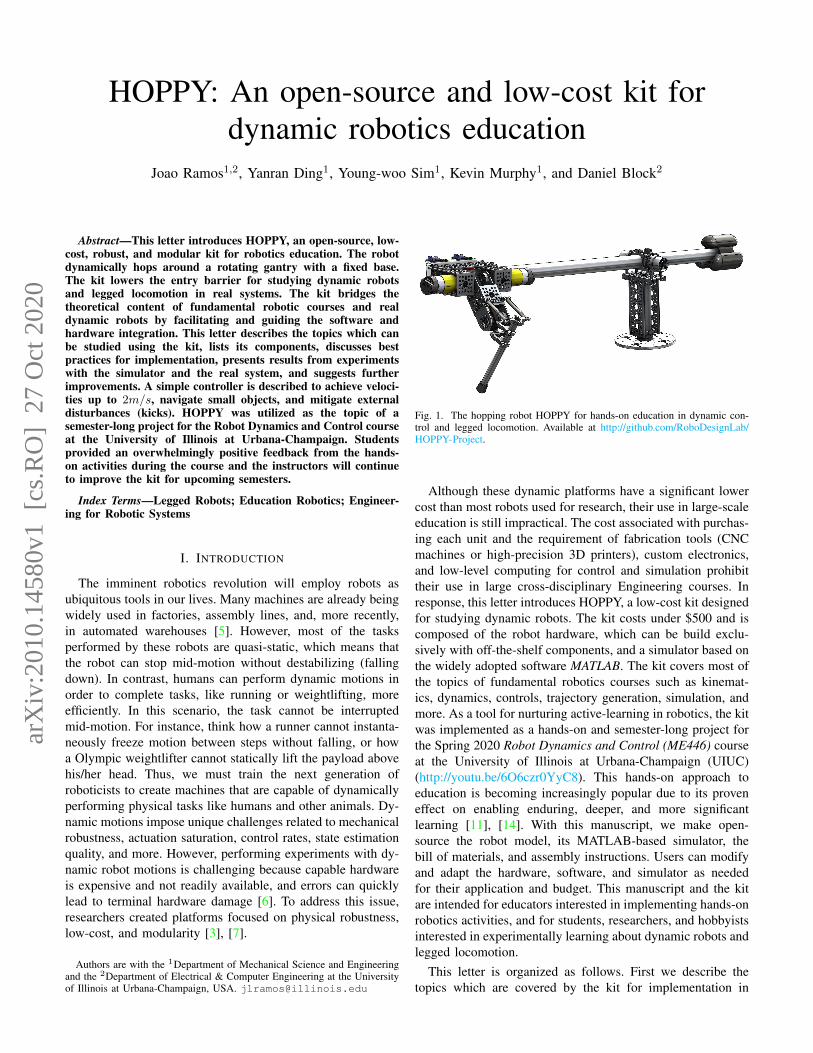
HOPPY: An open-source and low-cost kit for dynamic robotics education Joao Ramos 1,2 , Yanran Ding 1 , Young-woo Sim 1 , Kevin Murphy 1 , and Daniel Block 2 Abstract—This letter introduces HOPPY, an open-source, low- cost, robust, and modular kit for robotics education. The robot dynamically hops around a rotating gantry with a fixed base. The kit lowers the entry barrier for studying dynamic robots and legged locomotion in real systems. The kit bridges the theoretical content of fundamental robotic courses and real dynamic robots by facilitating and guiding the software and hardware integration. This letter describes the topics which can be studied using the kit, lists its components, discusses best practices for implementation, presents results from experiments with the simulator and the real system, and suggests further improvements. A simple controller is described to achieve veloci- ties up to 2m/s, navigate small objects, and mitigate external disturbances (kicks). HOPPY was utilized as the topic of a semester-long project for the Robot Dynamics and Control course at the University of Illinois at Urbana-Champaign. Students provided an overwhelmingly positive feedback from the hands- on activities during the course and the instructors will continue to improve the kit for upcoming semesters. Index Terms—Legged Robots; Education Robotics; Engineer- ing for Robotic Systems I. I NTRODUCTION The imminent robotics revolution will employ robots as ubiquitous tools in our lives. Many machines are already being widely used in factories, assembly lines, and, more recently, in automated warehouses [5]. However, most of the tasks performed by these robots are quasi-static, which means that the robot can stop mid-motion without destabilizing (falling down). In contrast, humans can perform dynamic motions in order to complete tasks, like running or weightlifting, more efficiently. In this scenario, the task cannot be interrupted mid-motion. For instance, think how a runner cannot instanta- neously freeze motion between steps without falling, or how a Olympic weightlifter cannot statically lift the payload above his/her head. Thus, we must train the next generation of roboticists to create machines that are capable of dynamically performing physical tasks like humans and other animals. Dy- namic motions impose unique challenges related to mechanical robustness, actuation saturation, control rates, state estimation quality, and more. However, performing experiments with dy- namic robot motions is challenging because capable hardware is expensive and not readily available, and errors can quickly lead to terminal hardware damage [6]. To address this issue, researchers created platforms focused on physical robustness, low-cost, and modularity [3], [7]. Authors are with the 1 Department of Mechanical Science and Engineering and the 2 Department of Electrical & Computer Engineering at the University of Illinois at Urbana-Champaign, USA. [email protected] Fig. 1. The hopping robot HOPPY for hands-on education in dynamic con- trol and legged locomotion. Available at http://github.com/RoboDesignLab/ HOPPY-Project. Although these dynamic platforms have a significant lower cost than most robots used for research, their use in large-scale education is still impractical. The cost associated with purchas- ing each unit and the requirement of fabrication tools (CNC machines or high-precision 3D printers), custom electronics, and low-level computing for control and simulation prohibit their use in large cross-disciplinary Engineering courses. In response, this letter introduces HOPPY, a low-cost kit designed for studying dynamic robots. The kit costs under $500 and is composed of the robot hardware, which can be build exclu- sively with off-the-shelf components, and a simulator based on the widely adopted software MATLAB. The kit covers most of the topics of fundamental robotics courses such as kinemat- ics, dynamics, controls, trajectory generation, simulation, and more. As a tool for nurturing active-learning in robotics, the kit was implemented as a hands-on and semester-long project for the Spring 2020 Robot Dynamics and Control (ME446) course at the University of Illinois at Urbana-Champaign (UIUC) (http://youtu.be/6O6czr0YyC8). This hands-on approach to education is becoming increasingly popular due to its proven effect on enabling enduring, deeper, and more significant learning [11], [14]. With this manuscript, we make open- source the robot model, its MATLAB-based simulator, the bill of materials, and assembly instructions. Users can modify and adapt the hardware, software, and simulator as needed for their application and budget. This manuscript and the kit are intended for educators interested in implementing hands-on robotics activities, and for students, researchers, and hobbyists interested in experimentally learning about dynamic robots and legged locomotion. This letter is organized as follows. First we describe the topics which are covered by the kit for implementation in arXiv:2010.14580v1 [cs.RO] 27 Oct 2020

Welcome message from author
This document is posted to help you gain knowledge. Please leave a comment to let me know what you think about it! Share it to your friends and learn new things together.
Transcript
HOPPY An open-source and low-cost kit fordynamic robotics education
Joao Ramos12 Yanran Ding1 Young-woo Sim1 Kevin Murphy1 and Daniel Block2
AbstractmdashThis letter introduces HOPPY an open-source low-cost robust and modular kit for robotics education The robotdynamically hops around a rotating gantry with a fixed baseThe kit lowers the entry barrier for studying dynamic robotsand legged locomotion in real systems The kit bridges thetheoretical content of fundamental robotic courses and realdynamic robots by facilitating and guiding the software andhardware integration This letter describes the topics which canbe studied using the kit lists its components discusses bestpractices for implementation presents results from experimentswith the simulator and the real system and suggests furtherimprovements A simple controller is described to achieve veloci-ties up to 2ms navigate small objects and mitigate externaldisturbances (kicks) HOPPY was utilized as the topic of asemester-long project for the Robot Dynamics and Control courseat the University of Illinois at Urbana-Champaign Studentsprovided an overwhelmingly positive feedback from the hands-on activities during the course and the instructors will continueto improve the kit for upcoming semesters
Index TermsmdashLegged Robots Education Robotics Engineer-ing for Robotic Systems
I INTRODUCTION
The imminent robotics revolution will employ robots asubiquitous tools in our lives Many machines are already beingwidely used in factories assembly lines and more recentlyin automated warehouses [5] However most of the tasksperformed by these robots are quasi-static which means thatthe robot can stop mid-motion without destabilizing (fallingdown) In contrast humans can perform dynamic motions inorder to complete tasks like running or weightlifting moreefficiently In this scenario the task cannot be interruptedmid-motion For instance think how a runner cannot instanta-neously freeze motion between steps without falling or howa Olympic weightlifter cannot statically lift the payload abovehisher head Thus we must train the next generation ofroboticists to create machines that are capable of dynamicallyperforming physical tasks like humans and other animals Dy-namic motions impose unique challenges related to mechanicalrobustness actuation saturation control rates state estimationquality and more However performing experiments with dy-namic robot motions is challenging because capable hardwareis expensive and not readily available and errors can quicklylead to terminal hardware damage [6] To address this issueresearchers created platforms focused on physical robustnesslow-cost and modularity [3] [7]
Authors are with the 1Department of Mechanical Science and Engineeringand the 2Department of Electrical amp Computer Engineering at the Universityof Illinois at Urbana-Champaign USA jlramosillinoisedu
Fig 1 The hopping robot HOPPY for hands-on education in dynamic con-trol and legged locomotion Available at httpgithubcomRoboDesignLabHOPPY-Project
Although these dynamic platforms have a significant lowercost than most robots used for research their use in large-scaleeducation is still impractical The cost associated with purchas-ing each unit and the requirement of fabrication tools (CNCmachines or high-precision 3D printers) custom electronicsand low-level computing for control and simulation prohibittheir use in large cross-disciplinary Engineering courses Inresponse this letter introduces HOPPY a low-cost kit designedfor studying dynamic robots The kit costs under $500 and iscomposed of the robot hardware which can be build exclu-sively with off-the-shelf components and a simulator based onthe widely adopted software MATLAB The kit covers most ofthe topics of fundamental robotics courses such as kinemat-ics dynamics controls trajectory generation simulation andmore As a tool for nurturing active-learning in robotics the kitwas implemented as a hands-on and semester-long project forthe Spring 2020 Robot Dynamics and Control (ME446) courseat the University of Illinois at Urbana-Champaign (UIUC)(httpyoutube6O6czr0YyC8) This hands-on approach toeducation is becoming increasingly popular due to its proveneffect on enabling enduring deeper and more significantlearning [11] [14] With this manuscript we make open-source the robot model its MATLAB-based simulator thebill of materials and assembly instructions Users can modifyand adapt the hardware software and simulator as neededfor their application and budget This manuscript and the kitare intended for educators interested in implementing hands-onrobotics activities and for students researchers and hobbyistsinterested in experimentally learning about dynamic robots andlegged locomotion
This letter is organized as follows First we describe thetopics which are covered by the kit for implementation in
arX
iv2
010
1458
0v1
[cs
RO
] 2
7 O
ct 2
020
Fig 2 Kinematic transformations and the five rigid-bodies which composeHOPPY The first two joints (θ1 and θ2) are passive while joints three andfour are driven by electric motors
fundamental robotics courses Next we list the open-sourcefiles and instructions made available with this manuscript Wethen suggest possible modifications or further improvementsto adapt the hardware to the needs of particular educators orresearchers Finally we discuss our experience implementingthe kit in the ME446 course at UIUC and address future work
II ROBOTICS TOPICS COVERED
This section describes the (non-exhaustive) list of topicscovered in the Robot Dynamics and Control course which areexplored using the HOPPY kit Although here we describehow the kit was modelled and implemented at UIUC eachtopic may be explored with more or less detail according tothe content of other courses
When HOPPY hops around the gantry it behaves as ahybrid system [19] This means that the dynamics have contin-uous evolution when the robot is on the ground (stance phase)or airborne (flight phase) but it is interrupted by discreteevents when the foot hits the ground (touchdown) or when ittakes-off In this section we describe the equations of motionduring stance and flight phases as well as the transitionsbetween the two
A Kinematics
The kinematic transformations of HOPPY are shown infig 2 The robot consists of a two degrees-of-freedom (DoF)active leg attached to a supporting gantry with two additionalDoFrsquos The origin coordinate frame X0Y0Z0 at the base ofthe rotating gantry is fixed to the ground Joints θ12 arepassive (no actuation) while joints θ34 are driven by electricmotors described in section II-C When hopping the robotcan translate horizontally around θ1 and vertically aroundθ2 If the gantry length LB is sufficiently long the robotmoves approximately in a 2D (Sagittal) plane [19] Thetransformation between coordinate frames is described bythe Homogeneous Transformation Matrices (HTM) given byT kk+1 which converts a vector pk+1 expressed in coordinate
frame k + 1 into a vector pk expressed in coordinate frame k[15]
pk = T kk+1pk+1 =
[Rkk+1 dk
01times3 1
]pk+1 (1)
Where the term 01times3 represents a 1 by 3 matrix of zeros TheHTM is composed of a rotation matrix Rkk+1 isin SO(3) anda Cartesian translation dk isin R3 represented in frame k Forinstance the HTM between frames X0Y0Z0 and XBYBZB isgiven by
T 0B =
cos(θ1) minussin(θ1) 0 0sin(θ1) cos(θ1) 0 0
0 0 1 HB
0 0 0 1
(2)
Where HB is the height of the gantry The position p0foot ofthe foot in respect to the base frame expressed in world-fixedcoordinates is[
p0foot1
]= T 0
F
[pFfoot1
]= T 0
BTBHT
HK T
KF
[03times1
1
] (3)
The complete kinematic transformations for HOPPY are de-scribed in the provided MATLAB-based simulator
B Rigid-body dynamics during flight phase
The robot state vector is given by the collection of jointangles q = [θ1 θ2 θ3 θ4]
T and their time rate of changeq When the foot is not contacting the ground and the robot isairborne the equation of motion (EoM) of the robot is givenby the well-known manipulator equation
M(q)q + C(q q)q +G(q) = τ (4)
which is derived from energy principles using the systemrsquosLagragian as described in [15] Where M(q) represents thesymmetric and positive definite inertia matrix as a functionof the configuration C(q q) is the Coriollis and centrifugalforces matrix G(q) is the vector of torques due to gravity andτ is the vector of input torques The system is underactuatedbecause the first two joints are passive (τ1 = τ2 = 0) andthus there are four overall DoF but only two inputs [16] Theinput vector is given by
τ = Beu+
000
τs(θ4)
=
0 00 01 00 1
[τHτK]+
000
τs(θ4)
(5)
where Be is a selection matrix which maps the input torques uto the full system dynamics and τs(θ4) represents the torqueexerted by the knee spring as a function of the knee angleθ4 The robot controller can only select torques for the hipτH and knee τK in order to hop around the gantry Thespring attached in parallel with the knee alleviates the jointrsquostorque requirements for hopping The expression for τs(θ4)and the rigid-body parameters for each link mass center ofmass (CoM) position and inertia tensor are provided in theinstructions
C Actuator dynamics model
Equation (5) assumes that the actuators are perfect torquesources which can generate arbitrary torque profiles Thisassumption may be reasonable for simulation but in realitythe actuator dynamics play a major role in the overall systembehavior and stability [10] Sophisticated drivers can rapidlyregulate the current i in the motor coils which is approx-imately linearly proportional to the output torque τ = kT iif the steel saturation is neglected (kT is the motor constant[7]) However such drivers are expensive (over $100) andhere we employ the $25 Pololu VNH5019 in our kit whichcan only control the voltage V across the motor terminalsIn this situation the back-electromotive force (back-EMF)significantly effects the actuator behavior On the other handthis limitation provides a valuable opportunity for studentsto explore how the actuator performance affects the overalldynamics The model for a brushed and brushless electricmotor assuming negligible coil inductance is given by [10]
V = Rwi+ kvNθ (6)
θN2Ir = kT i (7)
Where Rw is the coil resistance kv is the speed constant inV srad θ is the joint velocity (after the gear box) Ir is themotor rotor inertia and N is the gearbox speed reductionratio The hip and knee actuators in HOPPY utlize identicalelectric motors but with different gear ratios (NH = 269and NK = 288) Equation (4) is augmented to include theactuator dynamics using
(M(q) +Mr)q + (C(q q) +BEMF )q +G(q) = τ (8)
Where Mr is the inertial effect due to rotor inertia and BEMF
is the (damping) term due to the back-EMF
Mr = Ir
02times2 02times2
02times2
[N2H 00 N2
K
] (9)
BEMF =kvkTRw
02times2 02times2
02times2
[N2H 00 N2
K
] (10)
and the updated selection matrix and control inputs are givenby
Be =kTRw
02times2[NH 00 NK
] (11)
u =[VH VK
]T (12)
which illustrates that the input to the system is the voltageapplied to the motors not the torque they produce Actuatorswith large gearing ratios have high output inertia (due to theN2 term in (7)) and are usually non-backdrivable becauseof friction amplification Thus we select minimal reductionratio in HOPPY to mitigate the effect of shock loads in thesystem during touchdown [8] [18] Joint friction can havemajor (nonlinear) effects on the robot dynamics and modelsfor stiction dry coulomb friction viscous friction and moreare suggested in [10] and can be included in the model
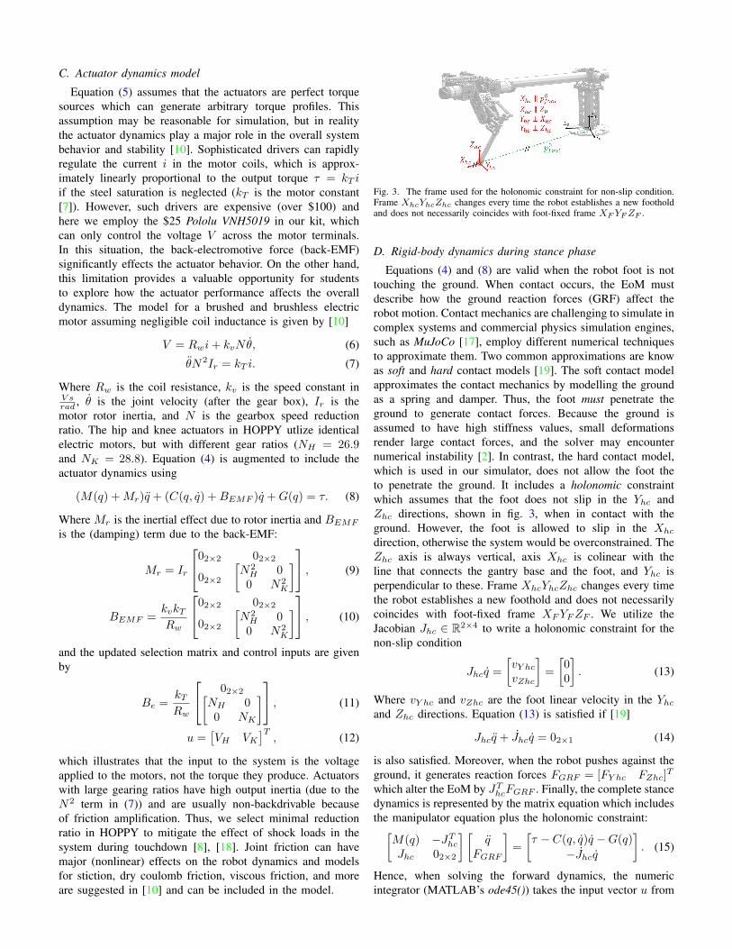
Fig 3 The frame used for the holonomic constraint for non-slip conditionFrame XhcYhcZhc changes every time the robot establishes a new footholdand does not necessarily coincides with foot-fixed frame XFYFZF
D Rigid-body dynamics during stance phase
Equations (4) and (8) are valid when the robot foot is nottouching the ground When contact occurs the EoM mustdescribe how the ground reaction forces (GRF) affect therobot motion Contact mechanics are challenging to simulate incomplex systems and commercial physics simulation enginessuch as MuJoCo [17] employ different numerical techniquesto approximate them Two common approximations are knowas soft and hard contact models [19] The soft contact modelapproximates the contact mechanics by modelling the groundas a spring and damper Thus the foot must penetrate theground to generate contact forces Because the ground isassumed to have high stiffness values small deformationsrender large contact forces and the solver may encounternumerical instability [2] In contrast the hard contact modelwhich is used in our simulator does not allow the foot theto penetrate the ground It includes a holonomic constraintwhich assumes that the foot does not slip in the Yhc andZhc directions shown in fig 3 when in contact with theground However the foot is allowed to slip in the Xhc
direction otherwise the system would be overconstrained TheZhc axis is always vertical axis Xhc is colinear with theline that connects the gantry base and the foot and Yhc isperpendicular to these Frame XhcYhcZhc changes every timethe robot establishes a new foothold and does not necessarilycoincides with foot-fixed frame XFYFZF We utilize theJacobian Jhc isin R2times4 to write a holonomic constraint for thenon-slip condition
Jhcq =
[vY hcvZhc
]=
[00
] (13)
Where vY hc and vZhc are the foot linear velocity in the Yhcand Zhc directions Equation (13) is satisfied if [19]
Jhcq + Jhcq = 02times1 (14)
is also satisfied Moreover when the robot pushes against theground it generates reaction forces FGRF = [FY hc FZhc]
T
which alter the EoM by JThcFGRF Finally the complete stancedynamics is represented by the matrix equation which includesthe manipulator equation plus the holonomic constraint[
M(q) minusJThcJhc 02times2
] [q
FGRF
]=
[τ minus C(q q)q minusG(q)
minusJhcq
] (15)
Hence when solving the forward dynamics the numericintegrator (MATLABrsquos ode45()) takes the input vector u from
the control law and calculates the joints acceleration q and theresultant contact forces FGRF at every iteration
E Foot impact model at touchdown
The impact dynamics are challenging to model realisticallyand they may cause numerical issues for the solver Oursimulator assumes a completely inelastic collision whichmeans that the foot comes to a complete stop after hittingthe ground And thus the robot looses energy every time thefoot impacts the ground [18] This assumption implies thatthe impulsive impact forces remove energy from the systemand the velocity instantaneously changes from qminus at timetminus before the impact to q+ immediately after the impact attime t+ However because this discontinuous changes occursinstantaneously the joint angles remain unchanged (qminus = q+)To compute the robot velocity after the impact we integrateboth sides of equation (15) between tminus and t+ Because thejoint angles and control inputs do not change during impactwe obtain [1] [19]
M(q+ minus qminus) = JThcFimp (16)
in addition to the constraint due to the inelastic collisionJhcq
+ = 0 We utilize these equations to write the impact mapwhich defines the transition between the aerial phase describedby the dynamic EOM (4) to the stance phase described byequation (15) [19][
q+
Fimp
]=
[M(q) minusJThcJhc 02times2
]minus1 [M(q)qminus
02times1
] (17)
Notice that the impact force Fimp is affected by the inverse ofthe inertia matrix which is amplified by the reflected inertiaof the rotors Hence actuators with high gear ratios willcreate large impact forces and thus HOPPY employs minimalgearing [18]
F Numerical simulation
A hybrid system is a dynamical system that exhibits bothcontinuous and discrete behavior HOPPY displays continuousdynamics during flight phase or stance phase but experiencesdiscontinuous transitions between the two To simulate hy-brid systems solvers like MATLABrsquos ode45() utilize guardfunctions to flag the transitions between continuum phasesFor instance the numerical simulation starts with the aerialphase dynamics and is interrupted when the touchdown guardfunction (foot height) cross a certain threshold (ground height)or p0Zfoot(t) = 0 Similarly the robot takes-off the groundwhen the vertical component of the ground reaction forcereaches a value equal to zero FZGRF (t) = 0 This sequenceis shown in fig 4 The simulator starts in the aerial phase andruns the integration for n hops which is defined by the numberof the transitions between the stance to aerial phase Thesimulator is described in detail in the provided instructions
Fig 4 Simulation loop of the hybrid dynamics of HOPPY for n hopsContinuous dynamics in flight (equation (4)) and stance (equation (15)) areinterrupted by discrete events touchdown and lift-off
G Hopping control framework
A challenging aspect of controlling hopping is that the footexperiences little resistance during aerial phase but infiniteresistance when touching the ground during stance phaseHence the controller must switch between different policiesfor the two scenarios During aerial phase the foot may followa predefined trajectory to reach a desired stepping location atimpact as shown in fig 4 left However during stance thefoot pushes against the ground to apply a desired impulse tothe CoM Thus it is a common practice to perform positioncontrol of the leg during swing and force control of the groundcontact force during stance We employ a simple strategy inwhich during flight the leg holds a desired configuration andwaits for touchdown while during stance the foot applies apredefined force profile against the ground An insightful andaccessible discussion on hopping control is provided in [9][12]
During flight phase HOPPY simply holds a predefined legconfiguration and waits for touchdown To achieve this weemploy a simple task-space Proportional plus Derivative (PD)control using
τaerial = JTc[Kp(p
Href minus pHfoot)minusKdp
Hfoot
] (18)
where Jc(q) isin R2times2 is the foot contact point Jacobian whichmaps the joint velocities to the linear velocity of the foot inrespect to the hip frame [yHfoot zHfoot]
T = Jc[θH θK ]T Inaddition Kpd are diagonal and positive semi-definite propor-tional and derivative gain matrices pHref is the desired positionof the foot in respect to the hip at touchdown and pHfoot is itscurrent value The desired torques τaerial are mapped usingthe motor dynamics to the required input voltages uaerial
uaerial =
[Rw
kTNH0
0 Rw
kTNK
]τaerial + kv
[NHθH
NKθK
] (19)
However notice the positive feedback sign before kv and thatθHK are the estimated joint velocities from an observer orfiltered derivative Thus overestimation of the speed constantkv or delay in the estimation of the joint velocities may causeoscillations or even instability For the presented experiments
Fig 5 Prescribed force profile for the horizontal (YH ) and vertical (ZH )components of FGRF during a projected stance of 015s The peak horizontaland vertical forces are modulated to control locomotion speed and hoppingheight respectively
we use a conservative approximation for the speed constantassuming kv asymp 0
During stance phase the robotrsquos foot applies a predefinedforce profile against the ground which results in an desired netimpulse on the robot The force profile can be generated usingsimple functions such as polynomials in order to be simple tocompute online Here we utilize Bezier polynomials to createa force profile for a projected 015s stance duration as shownin fig 5 [1] The force peak is modulated to control jumpingheight and forward velocity To apply the desired force againstthe ground we map FdGRF to the desired joint torques usingthe contact Jacobian similarly to equation (18)
τstance = JTc FdGRF (20)
Equation (20) assumes that the motion of the lightweightleg does not significantly affect the body dynamics [12]Otherwise the control law would need to include the torquerequired to accelerate the leg mechanism using for instanceComputed Torque Control [15] Torque is mapped to inputvoltage using equation (19)
Finally rapidly switching between the controllers for thestance and aerial phases can cause contact instability issueson the real robot To smoothly transition between the two wecommand the input
u = αustance + (1minus α)uaerial (21)
in which α smoothly changes from 0 to 1 after touchdownwithin a predefined time typically in the order of 10ms
This proposed control strategy is not affected by the legsingular configuration (straight knee) because it employs thetranspose of the contact Jacobian not its inverse In additionthe simple strategy also does not require solving the robotinverse kinematics
H Mechatronics
The control of HOPPY involves fundamental concepts re-lated to Mechatronics education Including
bull Embedded systems The robot controller runs in anonboard microcontroller (microC) which interfaces with theactuators sensors and the host computer
bull Discrete control The microC performs computations andinterfaces with peripherals at discrete time iterations Andthe deterministic execution of these events is fundamental
Fig 6 Achievable torque (τ ) and speed (θ) of the hip and knee jointsFunctions φ12(τ θ) are defined by the gearbox ratio N the torque constantkT and the maximum current the driver can supply Imax Functionsφ34(τ θ) are defined by the voltage supplied Vmax which limits the stalltorque τstall =
VmaxNRw
kT and no-load speed θNL asymp VmaxN
kv achievableby the joint The operating region is larger for negative work (τ and θ withopposite signals) due to the effect of the back-EMF
for the implementation of discrete control policies Toeffectively control dynamic motions we target a controlrate in the order of 1kHz (control loop of 1ms)
bull Communication protocols The microC regulates the motorvoltage via Pulse Width Modulation (PWM) receives ananalog signal which is proportional to the motor currenta binary signal for the foot contact switch sensor andemploys dedicated counters for the incremental encoders
bull Signal processing The encoder has a coarse resolutionof 28 counts per revolution (CPR) and the gearbox hasnoticeable backlash To avoid noise amplification weestimate the motor velocity using a filtered derivativeθ(s)θ(s) = λs
λ+s converted to discrete time with a period ofT = 1ms where s is the Laplace variable for frequencyand λ is a tunable constant (usually λ asymp 10) Fastsampling rates are essential to avoid delayed velocityestimation The analog signal from the motor currentestimation is also noisy and requires filtering if used forcontrols
bull Saturation The achievable joint torques and speeds arelimited by the available voltage supply (Vmax = 12V )and the maximum current that the driver can provide(Imax = 30A) [10] The operating region of the motorsis depicted in fig 6
III KIT DESIGN AND COMPONENTS
HOPPY is designed exclusively with off-the-shelf compo-nents to lower its cost and enable modularity customizationand facilitate maintenance In addition it is lightweight (to-tal weight about 38kg) portable and mechanically robustAll load-bearing components are made of metal parts fromhttpsgobildacom We intentionally avoid the use of plastic3D printed parts due to their short working life under impactloads Because of the kitrsquos durability only the initial cost forsetting up the course is required and the equipment can bereutilized in future semesters with minimal maintenance costsBoth motors are placed near the hip joint to reduce the movinginertia of the leg and enable fast swing motions The secondactuator is mounted coaxially with the hip joint and drives theknee joint through a timing belt The motors have minimalgearing ratio in order to be backdrivable To reduce the torque
Fig 7 Electrical components of the kit and communication diagram
requirements for hopping springs are added in parallel withthe knee and a counterweight is attached at the opposite endof the gantry as shown in fig 1 We employ cheap 23kg(5lb) weights typically utilized for gymnastics The additionof an excessively heavy counterweight reduces the achievablefrictional forces between the foot and the ground and the robotis more likely to slip
The diagram of electrical connections and communicationsprotocols is depicted in fig 7 The user computer communi-cates with the embedded microC (Texas Instruments LAUNCHXL-F28379D) via a usb port The microC commands the desiredvoltage to the motors (goBilda 5202-0002-0027 for the hip and0019 for the knee) via PWM to the drivers (Pololu VNH5019)and receives analog signals proportional to the motor currentand the pulse counts from the incremental encoders The motordrivers are powered by a 12V power supply (ALITOVE 12Volt10 Amp 120W) A linear potentiometer with spring return (TTElectronics 404R1KL10) attached in parallel with the footworks as a foot contact switch
The kit available at httpsgithubcomRoboDesignLabHOPPY-Project is composed of
1) the solid model in SolidWorks and STEP formats2) the video instructions for mechanical assembling3) the electrical wiring diagram4) the dynamic simulator code and instructions5) the complete list of components and quantities and6) the basic code for the microcontroller
IV MODIFICATIONS LIMITATIONS AND SAFETY
The kit is designed to facilitate the adjustment of physicalparameters and replacement of components For instancegearboxes with ratios of 37 1 to 188 1 can be used in eitherthe hip or knee The length of the lower leg is continuallytunable between 60mm and 260mm Additional springs canbe added (or removed) to the knee joint if necessary Thegantry length is continually adjustable between 01m and 11mand its height has multiple discrete options between 02m and11m The dynamic effect of the counterweight can be adjustedby shifting its position further away from the gantry joint oradding more mass
However the kit also presents performance limitations Forinstance voltage control of the motor is not ideal as it hindersthe precise regulation of ground reaction forces at high speedThe coarse resolution of the encoders and the backlash in
the gearbox also degrades position tracking performance Thehobby-grade brushed motors have limited torque density (peaktorque capability divided by unit mass) and thus the robotwill not be able to hop without the aid of the springs andthe counterweight In addition the simulator assumes simpledynamic models for impact and contact and neglects frictionstructural compliance vibrations and foot slip Due to theselimitations it is unlikely that the physical robot will behaveexactly like the simulator predicts However the simulator isa valuable tool to obtain insights about the behavior of thereal robot it can be used for preliminary tuning of controllersbefore implementation in the hardware and is a fundamentaltool for teaching
When experimenting with HOPPY (or any dynamic robot)some safety guidelines must be followed Students should wearsafety goggles and clear the robotrsquos path It is advised toconstantly check the temperature of the motorrsquos armature Ifthey are too hot to be touched the experiments should be in-terrupted until cool down Aggressive operations (high torqueand speeds) within negative work regimes should be donecarefully because electric motors regenerate part of the inputenergy back into the power supply when backdriven [13] Andthus utilizing a battery is more appropriated if considerablenegative work is expected For instance a conventional 12Vcar battery can be used both as power supply and a mechanicalcounterweight Finally it is advised to often check for loosecomponents due to the constant impacts and vibrations
If the budget allows some components of HOPPY canbe improved For instance (i) employing encoders with finerresolution around 12bits (4096 counts per revolution) would beideal This would improve position control and joint velocityestimation (ii) Implementation of motor drivers which canperform high-speed current control such as the Advanced Mo-tion Control AZBDC12A8 This feature would enable precisetorque control and considerably improve force tracking duringstance An even better solution would be (iii) the utilization ofbrushless motors similar to those employed in [3] [7] Thesehave much superior torque density and would enable hoppingwithout the aid of springs or counterweights (iv) Additionalsensors (encoders) could be added to the gantry joints (θ12) oran Inertial Measurement Unit (IMU) can be mounted on therobot for state estimation [4] (v) Data logging can be achievedusing external loggers such as the SparkFun OpenLog Andfinally (vi) to enable unrestricted rotations around the gantrya battery can be used to power the robot and a USB slip ringcan be included for communication between the microC and thehostrsquos computer
V RESULTS AND DISCUSSION
A snapshot of the output of the MATLAB-based simulatoris shown in fig 8 It displays an animation of the robotduring hopping (including a view of the robotrsquos Sagittal plane)with a trace of the hip joint and foot spatial trajectories Thevisualizer also shows the hopping velocity the joint statesrequired torques and the working regions of the actuatorsto check for saturation Areas shaded in red represent stancephases More information about the simulator is provided inthe accompanying instructions
Fig 8 Screenshot of the output screen of the simulator It shows the robot animation in isometric and Sagittal plane views along with the trajectories of thehip joint in blue and the foot in cyan Plot (B) shows the horizontal and vertical tangential velocities of the hip base around the gantry Areas shaded in redrepresent stance phases Hip and knee joint torques are shown in (D) and their angular velocities in (D) Plots (E) and (F) display the limiting polygon forthe hip and knee actuators along with the torque versus velocity trajectory Feasible trajectories must be always contained inside the polygon Finally plot(G) shows the hip an knee joint angles over time
For the experiments in companion video (httpsyoutube lbKIpiRWKI) we employed the controller described insection II-G using aerial phase gains of Kp = 500[12times2]and Ks = 50[12times2] the stance duration Ts = 015s andthe peak vertical force commanded of 80N Where 12times2
is a 2 times 2 identity matrix The peak horizontal force wasmodulated to control the locomotion speed Fig 9-(A) to (D)shows the data of robot accelerating from about 065msto around 12ms by increasing the horizontal force peakThe joint torques are estimated using the measured motorcurrent (τ = ikTN ) The saturation occurs when the requestedinput voltage is above the supplied 12V Fig 9-(D) showsthe stance duration measured from the contact switch whichdecreases according to the locomotion speed Notice thatat fast speeds the robot touches the ground for less that100ms Finally 9-(E) shows the achieved steady-state hoppingvelocities according to the commanded peak horizontal forceWe note that the locomotion speed is likely overestimatedbecause it was computed using the relative velocity betweenthe foot and the hip during stance assuming the the foot doesnot slip during contact
HOPPY was used in a semester-long project in the ME446Robot Dynamics and Control course at UIUC The courseis attended by senior undergraduate and first-year graduatestudents from the Departments of Mechanical Science and En-gineering Electrical and Computer Engineering and Industrialamp Enterprise Systems Engineering Ten cross-departmentalteams of four to five students each received their own leg(hip base of link 2 plus links 3 and 4) and all teams sharedsix gantries (fixed base plus links 1 and 2) During the firsthalf of the course students derived the kinematic and dynamic
model of the robot developed different controllers and cre-ated a simple version of the robot simulator in MATLABThey assembled their kits half-way through the semester andperformed experiments with the robot on the second halfAfter developing their own dynamic simulator students wereprovided with our code for comparison The results fromexperiments with the real robot from one of the teams areshown in the snapshots of fig 10 The team developed acustom foot contact sensor to detect stance phase The robotwas able to regulate hopping speed overcome small obstaclesand mitigate disturbances from gentle kicks
VI CONCLUSION AND FUTURE WORK
This letter introduced HOPPY an open-source low-costrobust and modular kit for robotics education The kit lowersthe barrier for studying dynamic robot behaviors and leggedlocomotion with real systems The control of dynamic mo-tions present unique challenges to the robot software andhardware and these are often overlooked in conventionalrobotics courses even those with hands-on activities Herewe describe the topics which can be explored using the kitlist its components discuss best practices for implementationand suggest further improvements HOPPY was utilized asthe topic of a semester-long project for an first year graduate-level course at UIUC Students provided an overwhelminglypositive feedback from the hands-on activities during thecourse The instructors will continue to improve the kit andcourse content for upcoming semesters To nurture activelearning future activities will include a friendly competitionbetween teams to elect the fastest robot and the most energy-efficient robot Speed is estimated by timing complete laps
Fig 9 Experimental data with HOPPY speeding up from around 065ms to 12ms Shaded magenta areas represent stance periods (A) Hip (θ3) jointangles in the left vertical axis and knee (θ4) angle in right axis (B) Hip joint commanded torque (black) and actual torque (red) estimated from the measuredcurrent (C) Knee joint torque (D) Stance phase duration (duration of following shaded areas) And (E) steady-state hopping speed as a function of thecommanded peak horizontal contact force FyGFP
Fig 10 Snapshots of the hopping experiment with HOPPY by one of the student teams (httpsyoutube6O6czr0YyC8)
around the gantry Energy efficiency is determined by the Costof Transport which is proportional to the ratio between thetotal electrical power consumed during one hopping cycle andthe average translation speed [13] Further improvements ofthe kit will be made open-source
REFERENCES
[1] Y Ding and H Park Design and experimental implementation ofa quasi-direct-drive leg for optimized jumping In 2017 IEEERSJInternational Conference on Intelligent Robots and Systems (IROS)pages 300ndash305 Sep 2017
[2] Roy Featherstone Rigid Body Dynamics Algorithms Springer-VerlagBerlin Heidelberg 2007
[3] F Grimminger A Meduri M Khadiv J Viereck M WuthrichM Naveau V Berenz S Heim F Widmaier T Flayols J FieneA Badri-Sprowitz and L Righetti An open torque-controlled modularrobot architecture for legged locomotion research IEEE Robotics andAutomation Letters 5(2)3650ndash3657 2020
[4] Ross Hartley Maani Ghaffari Jadidi Jessy W Grizzle and Ryan MEustice Contact-aided invariant extended kalman filtering for leggedrobot state estimation CoRR abs180510410 2018
[5] IEEE Spectrum Kiva systems Three engineers hundreds of robots onewarehouse 2008
[6] IEEE Spectrum Darpa robotics challenge A compilation of robotsfalling down 2015
[7] B Katz J D Carlo and S Kim Mini cheetah A platform forpushing the limits of dynamic quadruped control In 2019 InternationalConference on Robotics and Automation (ICRA) 2019
[8] G Kenneally A De and D E Koditschek Design principles for afamily of direct-drive legged robots IEEE Robotics and AutomationLetters 1(2)900ndash907 July 2016
[9] Jeff Koechling and H Marc How fast can a legged robot run InRobots and Biological Systems Towards a New Bionics Springer BerlinHeidelberg 1993
[10] Kevin Lynch and Frank Park Modern Robotics Mechanics Planningand Control Cambridge University Press USA 1st edition 2017
[11] M Orta Martinez C M Nunez T Liao T K Morimoto and A MOkamura Evolution and analysis of hapkit An open-source hapticdevice for educational applications IEEE Transactions on Haptics13(2)354ndash367 2020
[12] Marc H Raibert Legged Robots That Balance Massachusetts Instituteof Technology USA 1986
[13] S Seok A Wang Meng Yee Chuah D Otten J Lang and S KimDesign principles for highly efficient quadrupeds and implementationon the mit cheetah robot In 2013 IEEE International Conference onRobotics and Automation pages 3307ndash3312 May 2013
[14] S D Sheppard K Macatangay A Colby and W M Sullivan Ed-ucating Engineers Designing for the Future of the Field CarnegieFoundation for the Advancement of Teaching Jossey-Bass USA 2009
[15] Mark W Spong Robot Dynamics and Control John Wiley and SonsInc USA 1st edition 1989
[16] Russ Tedrake Underactuated robotics Algorithms for walking runningswimming flying and manipulation (course notes for mit 6832)downloaded on 09092020 from httpunderactuatedmitedu
[17] E Todorov Convex and analytically-invertible dynamics with contactsand constraints Theory and implementation in mujoco In 2014 IEEEInternational Conference on Robotics and Automation (ICRA) pages6054ndash6061 2014
[18] P M Wensing A Wang S Seok D Otten J Lang and S KimProprioceptive actuator design in the mit cheetah Impact mitigation andhigh-bandwidth physical interaction for dynamic legged robots IEEETransactions on Robotics 33(3)509ndash522 June 2017
[19] ER Westervelt JW Grizzle C Chevallereau JH Choi and B MorrisFeedback control of dynamic bipedal robot locomotion CRC press2007
- I Introduction
- II Robotics topics covered
-
- II-A Kinematics
- II-B Rigid-body dynamics during flight phase
- II-C Actuator dynamics model
- II-D Rigid-body dynamics during stance phase
- II-E Foot impact model at touchdown
- II-F Numerical simulation
- II-G Hopping control framework
- II-H Mechatronics
-
- III Kit design and components
- IV Modifications limitations and safety
- V Results and Discussion
- VI Conclusion and future work
- References
-
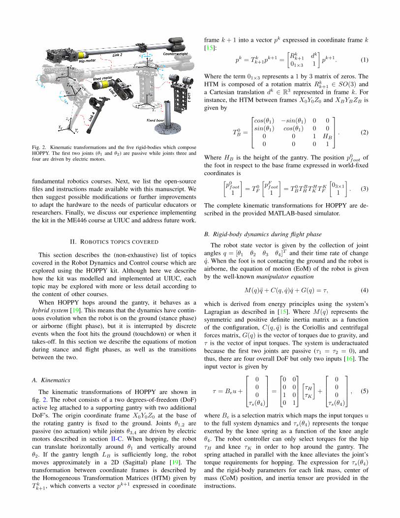
Fig 2 Kinematic transformations and the five rigid-bodies which composeHOPPY The first two joints (θ1 and θ2) are passive while joints three andfour are driven by electric motors
fundamental robotics courses Next we list the open-sourcefiles and instructions made available with this manuscript Wethen suggest possible modifications or further improvementsto adapt the hardware to the needs of particular educators orresearchers Finally we discuss our experience implementingthe kit in the ME446 course at UIUC and address future work
II ROBOTICS TOPICS COVERED
This section describes the (non-exhaustive) list of topicscovered in the Robot Dynamics and Control course which areexplored using the HOPPY kit Although here we describehow the kit was modelled and implemented at UIUC eachtopic may be explored with more or less detail according tothe content of other courses
When HOPPY hops around the gantry it behaves as ahybrid system [19] This means that the dynamics have contin-uous evolution when the robot is on the ground (stance phase)or airborne (flight phase) but it is interrupted by discreteevents when the foot hits the ground (touchdown) or when ittakes-off In this section we describe the equations of motionduring stance and flight phases as well as the transitionsbetween the two
A Kinematics
The kinematic transformations of HOPPY are shown infig 2 The robot consists of a two degrees-of-freedom (DoF)active leg attached to a supporting gantry with two additionalDoFrsquos The origin coordinate frame X0Y0Z0 at the base ofthe rotating gantry is fixed to the ground Joints θ12 arepassive (no actuation) while joints θ34 are driven by electricmotors described in section II-C When hopping the robotcan translate horizontally around θ1 and vertically aroundθ2 If the gantry length LB is sufficiently long the robotmoves approximately in a 2D (Sagittal) plane [19] Thetransformation between coordinate frames is described bythe Homogeneous Transformation Matrices (HTM) given byT kk+1 which converts a vector pk+1 expressed in coordinate
frame k + 1 into a vector pk expressed in coordinate frame k[15]
pk = T kk+1pk+1 =
[Rkk+1 dk
01times3 1
]pk+1 (1)
Where the term 01times3 represents a 1 by 3 matrix of zeros TheHTM is composed of a rotation matrix Rkk+1 isin SO(3) anda Cartesian translation dk isin R3 represented in frame k Forinstance the HTM between frames X0Y0Z0 and XBYBZB isgiven by
T 0B =
cos(θ1) minussin(θ1) 0 0sin(θ1) cos(θ1) 0 0
0 0 1 HB
0 0 0 1
(2)
Where HB is the height of the gantry The position p0foot ofthe foot in respect to the base frame expressed in world-fixedcoordinates is[
p0foot1
]= T 0
F
[pFfoot1
]= T 0
BTBHT
HK T
KF
[03times1
1
] (3)
The complete kinematic transformations for HOPPY are de-scribed in the provided MATLAB-based simulator
B Rigid-body dynamics during flight phase
The robot state vector is given by the collection of jointangles q = [θ1 θ2 θ3 θ4]
T and their time rate of changeq When the foot is not contacting the ground and the robot isairborne the equation of motion (EoM) of the robot is givenby the well-known manipulator equation
M(q)q + C(q q)q +G(q) = τ (4)
which is derived from energy principles using the systemrsquosLagragian as described in [15] Where M(q) represents thesymmetric and positive definite inertia matrix as a functionof the configuration C(q q) is the Coriollis and centrifugalforces matrix G(q) is the vector of torques due to gravity andτ is the vector of input torques The system is underactuatedbecause the first two joints are passive (τ1 = τ2 = 0) andthus there are four overall DoF but only two inputs [16] Theinput vector is given by
τ = Beu+
000
τs(θ4)
=
0 00 01 00 1
[τHτK]+
000
τs(θ4)
(5)
where Be is a selection matrix which maps the input torques uto the full system dynamics and τs(θ4) represents the torqueexerted by the knee spring as a function of the knee angleθ4 The robot controller can only select torques for the hipτH and knee τK in order to hop around the gantry Thespring attached in parallel with the knee alleviates the jointrsquostorque requirements for hopping The expression for τs(θ4)and the rigid-body parameters for each link mass center ofmass (CoM) position and inertia tensor are provided in theinstructions
C Actuator dynamics model
Equation (5) assumes that the actuators are perfect torquesources which can generate arbitrary torque profiles Thisassumption may be reasonable for simulation but in realitythe actuator dynamics play a major role in the overall systembehavior and stability [10] Sophisticated drivers can rapidlyregulate the current i in the motor coils which is approx-imately linearly proportional to the output torque τ = kT iif the steel saturation is neglected (kT is the motor constant[7]) However such drivers are expensive (over $100) andhere we employ the $25 Pololu VNH5019 in our kit whichcan only control the voltage V across the motor terminalsIn this situation the back-electromotive force (back-EMF)significantly effects the actuator behavior On the other handthis limitation provides a valuable opportunity for studentsto explore how the actuator performance affects the overalldynamics The model for a brushed and brushless electricmotor assuming negligible coil inductance is given by [10]
V = Rwi+ kvNθ (6)
θN2Ir = kT i (7)
Where Rw is the coil resistance kv is the speed constant inV srad θ is the joint velocity (after the gear box) Ir is themotor rotor inertia and N is the gearbox speed reductionratio The hip and knee actuators in HOPPY utlize identicalelectric motors but with different gear ratios (NH = 269and NK = 288) Equation (4) is augmented to include theactuator dynamics using
(M(q) +Mr)q + (C(q q) +BEMF )q +G(q) = τ (8)
Where Mr is the inertial effect due to rotor inertia and BEMF
is the (damping) term due to the back-EMF
Mr = Ir
02times2 02times2
02times2
[N2H 00 N2
K
] (9)
BEMF =kvkTRw
02times2 02times2
02times2
[N2H 00 N2
K
] (10)
and the updated selection matrix and control inputs are givenby
Be =kTRw
02times2[NH 00 NK
] (11)
u =[VH VK
]T (12)
which illustrates that the input to the system is the voltageapplied to the motors not the torque they produce Actuatorswith large gearing ratios have high output inertia (due to theN2 term in (7)) and are usually non-backdrivable becauseof friction amplification Thus we select minimal reductionratio in HOPPY to mitigate the effect of shock loads in thesystem during touchdown [8] [18] Joint friction can havemajor (nonlinear) effects on the robot dynamics and modelsfor stiction dry coulomb friction viscous friction and moreare suggested in [10] and can be included in the model
Fig 3 The frame used for the holonomic constraint for non-slip conditionFrame XhcYhcZhc changes every time the robot establishes a new footholdand does not necessarily coincides with foot-fixed frame XFYFZF
D Rigid-body dynamics during stance phase
Equations (4) and (8) are valid when the robot foot is nottouching the ground When contact occurs the EoM mustdescribe how the ground reaction forces (GRF) affect therobot motion Contact mechanics are challenging to simulate incomplex systems and commercial physics simulation enginessuch as MuJoCo [17] employ different numerical techniquesto approximate them Two common approximations are knowas soft and hard contact models [19] The soft contact modelapproximates the contact mechanics by modelling the groundas a spring and damper Thus the foot must penetrate theground to generate contact forces Because the ground isassumed to have high stiffness values small deformationsrender large contact forces and the solver may encounternumerical instability [2] In contrast the hard contact modelwhich is used in our simulator does not allow the foot theto penetrate the ground It includes a holonomic constraintwhich assumes that the foot does not slip in the Yhc andZhc directions shown in fig 3 when in contact with theground However the foot is allowed to slip in the Xhc
direction otherwise the system would be overconstrained TheZhc axis is always vertical axis Xhc is colinear with theline that connects the gantry base and the foot and Yhc isperpendicular to these Frame XhcYhcZhc changes every timethe robot establishes a new foothold and does not necessarilycoincides with foot-fixed frame XFYFZF We utilize theJacobian Jhc isin R2times4 to write a holonomic constraint for thenon-slip condition
Jhcq =
[vY hcvZhc
]=
[00
] (13)
Where vY hc and vZhc are the foot linear velocity in the Yhcand Zhc directions Equation (13) is satisfied if [19]
Jhcq + Jhcq = 02times1 (14)
is also satisfied Moreover when the robot pushes against theground it generates reaction forces FGRF = [FY hc FZhc]
T
which alter the EoM by JThcFGRF Finally the complete stancedynamics is represented by the matrix equation which includesthe manipulator equation plus the holonomic constraint[
M(q) minusJThcJhc 02times2
] [q
FGRF
]=
[τ minus C(q q)q minusG(q)
minusJhcq
] (15)
Hence when solving the forward dynamics the numericintegrator (MATLABrsquos ode45()) takes the input vector u from
the control law and calculates the joints acceleration q and theresultant contact forces FGRF at every iteration
E Foot impact model at touchdown
The impact dynamics are challenging to model realisticallyand they may cause numerical issues for the solver Oursimulator assumes a completely inelastic collision whichmeans that the foot comes to a complete stop after hittingthe ground And thus the robot looses energy every time thefoot impacts the ground [18] This assumption implies thatthe impulsive impact forces remove energy from the systemand the velocity instantaneously changes from qminus at timetminus before the impact to q+ immediately after the impact attime t+ However because this discontinuous changes occursinstantaneously the joint angles remain unchanged (qminus = q+)To compute the robot velocity after the impact we integrateboth sides of equation (15) between tminus and t+ Because thejoint angles and control inputs do not change during impactwe obtain [1] [19]
M(q+ minus qminus) = JThcFimp (16)
in addition to the constraint due to the inelastic collisionJhcq
+ = 0 We utilize these equations to write the impact mapwhich defines the transition between the aerial phase describedby the dynamic EOM (4) to the stance phase described byequation (15) [19][
q+
Fimp
]=
[M(q) minusJThcJhc 02times2
]minus1 [M(q)qminus
02times1
] (17)
Notice that the impact force Fimp is affected by the inverse ofthe inertia matrix which is amplified by the reflected inertiaof the rotors Hence actuators with high gear ratios willcreate large impact forces and thus HOPPY employs minimalgearing [18]
F Numerical simulation
A hybrid system is a dynamical system that exhibits bothcontinuous and discrete behavior HOPPY displays continuousdynamics during flight phase or stance phase but experiencesdiscontinuous transitions between the two To simulate hy-brid systems solvers like MATLABrsquos ode45() utilize guardfunctions to flag the transitions between continuum phasesFor instance the numerical simulation starts with the aerialphase dynamics and is interrupted when the touchdown guardfunction (foot height) cross a certain threshold (ground height)or p0Zfoot(t) = 0 Similarly the robot takes-off the groundwhen the vertical component of the ground reaction forcereaches a value equal to zero FZGRF (t) = 0 This sequenceis shown in fig 4 The simulator starts in the aerial phase andruns the integration for n hops which is defined by the numberof the transitions between the stance to aerial phase Thesimulator is described in detail in the provided instructions
Fig 4 Simulation loop of the hybrid dynamics of HOPPY for n hopsContinuous dynamics in flight (equation (4)) and stance (equation (15)) areinterrupted by discrete events touchdown and lift-off
G Hopping control framework
A challenging aspect of controlling hopping is that the footexperiences little resistance during aerial phase but infiniteresistance when touching the ground during stance phaseHence the controller must switch between different policiesfor the two scenarios During aerial phase the foot may followa predefined trajectory to reach a desired stepping location atimpact as shown in fig 4 left However during stance thefoot pushes against the ground to apply a desired impulse tothe CoM Thus it is a common practice to perform positioncontrol of the leg during swing and force control of the groundcontact force during stance We employ a simple strategy inwhich during flight the leg holds a desired configuration andwaits for touchdown while during stance the foot applies apredefined force profile against the ground An insightful andaccessible discussion on hopping control is provided in [9][12]
During flight phase HOPPY simply holds a predefined legconfiguration and waits for touchdown To achieve this weemploy a simple task-space Proportional plus Derivative (PD)control using
τaerial = JTc[Kp(p
Href minus pHfoot)minusKdp
Hfoot
] (18)
where Jc(q) isin R2times2 is the foot contact point Jacobian whichmaps the joint velocities to the linear velocity of the foot inrespect to the hip frame [yHfoot zHfoot]
T = Jc[θH θK ]T Inaddition Kpd are diagonal and positive semi-definite propor-tional and derivative gain matrices pHref is the desired positionof the foot in respect to the hip at touchdown and pHfoot is itscurrent value The desired torques τaerial are mapped usingthe motor dynamics to the required input voltages uaerial
uaerial =
[Rw
kTNH0
0 Rw
kTNK
]τaerial + kv
[NHθH
NKθK
] (19)
However notice the positive feedback sign before kv and thatθHK are the estimated joint velocities from an observer orfiltered derivative Thus overestimation of the speed constantkv or delay in the estimation of the joint velocities may causeoscillations or even instability For the presented experiments
Fig 5 Prescribed force profile for the horizontal (YH ) and vertical (ZH )components of FGRF during a projected stance of 015s The peak horizontaland vertical forces are modulated to control locomotion speed and hoppingheight respectively
we use a conservative approximation for the speed constantassuming kv asymp 0
During stance phase the robotrsquos foot applies a predefinedforce profile against the ground which results in an desired netimpulse on the robot The force profile can be generated usingsimple functions such as polynomials in order to be simple tocompute online Here we utilize Bezier polynomials to createa force profile for a projected 015s stance duration as shownin fig 5 [1] The force peak is modulated to control jumpingheight and forward velocity To apply the desired force againstthe ground we map FdGRF to the desired joint torques usingthe contact Jacobian similarly to equation (18)
τstance = JTc FdGRF (20)
Equation (20) assumes that the motion of the lightweightleg does not significantly affect the body dynamics [12]Otherwise the control law would need to include the torquerequired to accelerate the leg mechanism using for instanceComputed Torque Control [15] Torque is mapped to inputvoltage using equation (19)
Finally rapidly switching between the controllers for thestance and aerial phases can cause contact instability issueson the real robot To smoothly transition between the two wecommand the input
u = αustance + (1minus α)uaerial (21)
in which α smoothly changes from 0 to 1 after touchdownwithin a predefined time typically in the order of 10ms
This proposed control strategy is not affected by the legsingular configuration (straight knee) because it employs thetranspose of the contact Jacobian not its inverse In additionthe simple strategy also does not require solving the robotinverse kinematics
H Mechatronics
The control of HOPPY involves fundamental concepts re-lated to Mechatronics education Including
bull Embedded systems The robot controller runs in anonboard microcontroller (microC) which interfaces with theactuators sensors and the host computer
bull Discrete control The microC performs computations andinterfaces with peripherals at discrete time iterations Andthe deterministic execution of these events is fundamental
Fig 6 Achievable torque (τ ) and speed (θ) of the hip and knee jointsFunctions φ12(τ θ) are defined by the gearbox ratio N the torque constantkT and the maximum current the driver can supply Imax Functionsφ34(τ θ) are defined by the voltage supplied Vmax which limits the stalltorque τstall =
VmaxNRw
kT and no-load speed θNL asymp VmaxN
kv achievableby the joint The operating region is larger for negative work (τ and θ withopposite signals) due to the effect of the back-EMF
for the implementation of discrete control policies Toeffectively control dynamic motions we target a controlrate in the order of 1kHz (control loop of 1ms)
bull Communication protocols The microC regulates the motorvoltage via Pulse Width Modulation (PWM) receives ananalog signal which is proportional to the motor currenta binary signal for the foot contact switch sensor andemploys dedicated counters for the incremental encoders
bull Signal processing The encoder has a coarse resolutionof 28 counts per revolution (CPR) and the gearbox hasnoticeable backlash To avoid noise amplification weestimate the motor velocity using a filtered derivativeθ(s)θ(s) = λs
λ+s converted to discrete time with a period ofT = 1ms where s is the Laplace variable for frequencyand λ is a tunable constant (usually λ asymp 10) Fastsampling rates are essential to avoid delayed velocityestimation The analog signal from the motor currentestimation is also noisy and requires filtering if used forcontrols
bull Saturation The achievable joint torques and speeds arelimited by the available voltage supply (Vmax = 12V )and the maximum current that the driver can provide(Imax = 30A) [10] The operating region of the motorsis depicted in fig 6
III KIT DESIGN AND COMPONENTS
HOPPY is designed exclusively with off-the-shelf compo-nents to lower its cost and enable modularity customizationand facilitate maintenance In addition it is lightweight (to-tal weight about 38kg) portable and mechanically robustAll load-bearing components are made of metal parts fromhttpsgobildacom We intentionally avoid the use of plastic3D printed parts due to their short working life under impactloads Because of the kitrsquos durability only the initial cost forsetting up the course is required and the equipment can bereutilized in future semesters with minimal maintenance costsBoth motors are placed near the hip joint to reduce the movinginertia of the leg and enable fast swing motions The secondactuator is mounted coaxially with the hip joint and drives theknee joint through a timing belt The motors have minimalgearing ratio in order to be backdrivable To reduce the torque
Fig 7 Electrical components of the kit and communication diagram
requirements for hopping springs are added in parallel withthe knee and a counterweight is attached at the opposite endof the gantry as shown in fig 1 We employ cheap 23kg(5lb) weights typically utilized for gymnastics The additionof an excessively heavy counterweight reduces the achievablefrictional forces between the foot and the ground and the robotis more likely to slip
The diagram of electrical connections and communicationsprotocols is depicted in fig 7 The user computer communi-cates with the embedded microC (Texas Instruments LAUNCHXL-F28379D) via a usb port The microC commands the desiredvoltage to the motors (goBilda 5202-0002-0027 for the hip and0019 for the knee) via PWM to the drivers (Pololu VNH5019)and receives analog signals proportional to the motor currentand the pulse counts from the incremental encoders The motordrivers are powered by a 12V power supply (ALITOVE 12Volt10 Amp 120W) A linear potentiometer with spring return (TTElectronics 404R1KL10) attached in parallel with the footworks as a foot contact switch
The kit available at httpsgithubcomRoboDesignLabHOPPY-Project is composed of
1) the solid model in SolidWorks and STEP formats2) the video instructions for mechanical assembling3) the electrical wiring diagram4) the dynamic simulator code and instructions5) the complete list of components and quantities and6) the basic code for the microcontroller
IV MODIFICATIONS LIMITATIONS AND SAFETY
The kit is designed to facilitate the adjustment of physicalparameters and replacement of components For instancegearboxes with ratios of 37 1 to 188 1 can be used in eitherthe hip or knee The length of the lower leg is continuallytunable between 60mm and 260mm Additional springs canbe added (or removed) to the knee joint if necessary Thegantry length is continually adjustable between 01m and 11mand its height has multiple discrete options between 02m and11m The dynamic effect of the counterweight can be adjustedby shifting its position further away from the gantry joint oradding more mass
However the kit also presents performance limitations Forinstance voltage control of the motor is not ideal as it hindersthe precise regulation of ground reaction forces at high speedThe coarse resolution of the encoders and the backlash in
the gearbox also degrades position tracking performance Thehobby-grade brushed motors have limited torque density (peaktorque capability divided by unit mass) and thus the robotwill not be able to hop without the aid of the springs andthe counterweight In addition the simulator assumes simpledynamic models for impact and contact and neglects frictionstructural compliance vibrations and foot slip Due to theselimitations it is unlikely that the physical robot will behaveexactly like the simulator predicts However the simulator isa valuable tool to obtain insights about the behavior of thereal robot it can be used for preliminary tuning of controllersbefore implementation in the hardware and is a fundamentaltool for teaching
When experimenting with HOPPY (or any dynamic robot)some safety guidelines must be followed Students should wearsafety goggles and clear the robotrsquos path It is advised toconstantly check the temperature of the motorrsquos armature Ifthey are too hot to be touched the experiments should be in-terrupted until cool down Aggressive operations (high torqueand speeds) within negative work regimes should be donecarefully because electric motors regenerate part of the inputenergy back into the power supply when backdriven [13] Andthus utilizing a battery is more appropriated if considerablenegative work is expected For instance a conventional 12Vcar battery can be used both as power supply and a mechanicalcounterweight Finally it is advised to often check for loosecomponents due to the constant impacts and vibrations
If the budget allows some components of HOPPY canbe improved For instance (i) employing encoders with finerresolution around 12bits (4096 counts per revolution) would beideal This would improve position control and joint velocityestimation (ii) Implementation of motor drivers which canperform high-speed current control such as the Advanced Mo-tion Control AZBDC12A8 This feature would enable precisetorque control and considerably improve force tracking duringstance An even better solution would be (iii) the utilization ofbrushless motors similar to those employed in [3] [7] Thesehave much superior torque density and would enable hoppingwithout the aid of springs or counterweights (iv) Additionalsensors (encoders) could be added to the gantry joints (θ12) oran Inertial Measurement Unit (IMU) can be mounted on therobot for state estimation [4] (v) Data logging can be achievedusing external loggers such as the SparkFun OpenLog Andfinally (vi) to enable unrestricted rotations around the gantrya battery can be used to power the robot and a USB slip ringcan be included for communication between the microC and thehostrsquos computer
V RESULTS AND DISCUSSION
A snapshot of the output of the MATLAB-based simulatoris shown in fig 8 It displays an animation of the robotduring hopping (including a view of the robotrsquos Sagittal plane)with a trace of the hip joint and foot spatial trajectories Thevisualizer also shows the hopping velocity the joint statesrequired torques and the working regions of the actuatorsto check for saturation Areas shaded in red represent stancephases More information about the simulator is provided inthe accompanying instructions
Fig 8 Screenshot of the output screen of the simulator It shows the robot animation in isometric and Sagittal plane views along with the trajectories of thehip joint in blue and the foot in cyan Plot (B) shows the horizontal and vertical tangential velocities of the hip base around the gantry Areas shaded in redrepresent stance phases Hip and knee joint torques are shown in (D) and their angular velocities in (D) Plots (E) and (F) display the limiting polygon forthe hip and knee actuators along with the torque versus velocity trajectory Feasible trajectories must be always contained inside the polygon Finally plot(G) shows the hip an knee joint angles over time
For the experiments in companion video (httpsyoutube lbKIpiRWKI) we employed the controller described insection II-G using aerial phase gains of Kp = 500[12times2]and Ks = 50[12times2] the stance duration Ts = 015s andthe peak vertical force commanded of 80N Where 12times2
is a 2 times 2 identity matrix The peak horizontal force wasmodulated to control the locomotion speed Fig 9-(A) to (D)shows the data of robot accelerating from about 065msto around 12ms by increasing the horizontal force peakThe joint torques are estimated using the measured motorcurrent (τ = ikTN ) The saturation occurs when the requestedinput voltage is above the supplied 12V Fig 9-(D) showsthe stance duration measured from the contact switch whichdecreases according to the locomotion speed Notice thatat fast speeds the robot touches the ground for less that100ms Finally 9-(E) shows the achieved steady-state hoppingvelocities according to the commanded peak horizontal forceWe note that the locomotion speed is likely overestimatedbecause it was computed using the relative velocity betweenthe foot and the hip during stance assuming the the foot doesnot slip during contact
HOPPY was used in a semester-long project in the ME446Robot Dynamics and Control course at UIUC The courseis attended by senior undergraduate and first-year graduatestudents from the Departments of Mechanical Science and En-gineering Electrical and Computer Engineering and Industrialamp Enterprise Systems Engineering Ten cross-departmentalteams of four to five students each received their own leg(hip base of link 2 plus links 3 and 4) and all teams sharedsix gantries (fixed base plus links 1 and 2) During the firsthalf of the course students derived the kinematic and dynamic
model of the robot developed different controllers and cre-ated a simple version of the robot simulator in MATLABThey assembled their kits half-way through the semester andperformed experiments with the robot on the second halfAfter developing their own dynamic simulator students wereprovided with our code for comparison The results fromexperiments with the real robot from one of the teams areshown in the snapshots of fig 10 The team developed acustom foot contact sensor to detect stance phase The robotwas able to regulate hopping speed overcome small obstaclesand mitigate disturbances from gentle kicks
VI CONCLUSION AND FUTURE WORK
This letter introduced HOPPY an open-source low-costrobust and modular kit for robotics education The kit lowersthe barrier for studying dynamic robot behaviors and leggedlocomotion with real systems The control of dynamic mo-tions present unique challenges to the robot software andhardware and these are often overlooked in conventionalrobotics courses even those with hands-on activities Herewe describe the topics which can be explored using the kitlist its components discuss best practices for implementationand suggest further improvements HOPPY was utilized asthe topic of a semester-long project for an first year graduate-level course at UIUC Students provided an overwhelminglypositive feedback from the hands-on activities during thecourse The instructors will continue to improve the kit andcourse content for upcoming semesters To nurture activelearning future activities will include a friendly competitionbetween teams to elect the fastest robot and the most energy-efficient robot Speed is estimated by timing complete laps
Fig 9 Experimental data with HOPPY speeding up from around 065ms to 12ms Shaded magenta areas represent stance periods (A) Hip (θ3) jointangles in the left vertical axis and knee (θ4) angle in right axis (B) Hip joint commanded torque (black) and actual torque (red) estimated from the measuredcurrent (C) Knee joint torque (D) Stance phase duration (duration of following shaded areas) And (E) steady-state hopping speed as a function of thecommanded peak horizontal contact force FyGFP
Fig 10 Snapshots of the hopping experiment with HOPPY by one of the student teams (httpsyoutube6O6czr0YyC8)
around the gantry Energy efficiency is determined by the Costof Transport which is proportional to the ratio between thetotal electrical power consumed during one hopping cycle andthe average translation speed [13] Further improvements ofthe kit will be made open-source
REFERENCES
[1] Y Ding and H Park Design and experimental implementation ofa quasi-direct-drive leg for optimized jumping In 2017 IEEERSJInternational Conference on Intelligent Robots and Systems (IROS)pages 300ndash305 Sep 2017
[2] Roy Featherstone Rigid Body Dynamics Algorithms Springer-VerlagBerlin Heidelberg 2007
[3] F Grimminger A Meduri M Khadiv J Viereck M WuthrichM Naveau V Berenz S Heim F Widmaier T Flayols J FieneA Badri-Sprowitz and L Righetti An open torque-controlled modularrobot architecture for legged locomotion research IEEE Robotics andAutomation Letters 5(2)3650ndash3657 2020
[4] Ross Hartley Maani Ghaffari Jadidi Jessy W Grizzle and Ryan MEustice Contact-aided invariant extended kalman filtering for leggedrobot state estimation CoRR abs180510410 2018
[5] IEEE Spectrum Kiva systems Three engineers hundreds of robots onewarehouse 2008
[6] IEEE Spectrum Darpa robotics challenge A compilation of robotsfalling down 2015
[7] B Katz J D Carlo and S Kim Mini cheetah A platform forpushing the limits of dynamic quadruped control In 2019 InternationalConference on Robotics and Automation (ICRA) 2019
[8] G Kenneally A De and D E Koditschek Design principles for afamily of direct-drive legged robots IEEE Robotics and AutomationLetters 1(2)900ndash907 July 2016
[9] Jeff Koechling and H Marc How fast can a legged robot run InRobots and Biological Systems Towards a New Bionics Springer BerlinHeidelberg 1993
[10] Kevin Lynch and Frank Park Modern Robotics Mechanics Planningand Control Cambridge University Press USA 1st edition 2017
[11] M Orta Martinez C M Nunez T Liao T K Morimoto and A MOkamura Evolution and analysis of hapkit An open-source hapticdevice for educational applications IEEE Transactions on Haptics13(2)354ndash367 2020
[12] Marc H Raibert Legged Robots That Balance Massachusetts Instituteof Technology USA 1986
[13] S Seok A Wang Meng Yee Chuah D Otten J Lang and S KimDesign principles for highly efficient quadrupeds and implementationon the mit cheetah robot In 2013 IEEE International Conference onRobotics and Automation pages 3307ndash3312 May 2013
[14] S D Sheppard K Macatangay A Colby and W M Sullivan Ed-ucating Engineers Designing for the Future of the Field CarnegieFoundation for the Advancement of Teaching Jossey-Bass USA 2009
[15] Mark W Spong Robot Dynamics and Control John Wiley and SonsInc USA 1st edition 1989
[16] Russ Tedrake Underactuated robotics Algorithms for walking runningswimming flying and manipulation (course notes for mit 6832)downloaded on 09092020 from httpunderactuatedmitedu
[17] E Todorov Convex and analytically-invertible dynamics with contactsand constraints Theory and implementation in mujoco In 2014 IEEEInternational Conference on Robotics and Automation (ICRA) pages6054ndash6061 2014
[18] P M Wensing A Wang S Seok D Otten J Lang and S KimProprioceptive actuator design in the mit cheetah Impact mitigation andhigh-bandwidth physical interaction for dynamic legged robots IEEETransactions on Robotics 33(3)509ndash522 June 2017
[19] ER Westervelt JW Grizzle C Chevallereau JH Choi and B MorrisFeedback control of dynamic bipedal robot locomotion CRC press2007
- I Introduction
- II Robotics topics covered
-
- II-A Kinematics
- II-B Rigid-body dynamics during flight phase
- II-C Actuator dynamics model
- II-D Rigid-body dynamics during stance phase
- II-E Foot impact model at touchdown
- II-F Numerical simulation
- II-G Hopping control framework
- II-H Mechatronics
-
- III Kit design and components
- IV Modifications limitations and safety
- V Results and Discussion
- VI Conclusion and future work
- References
-
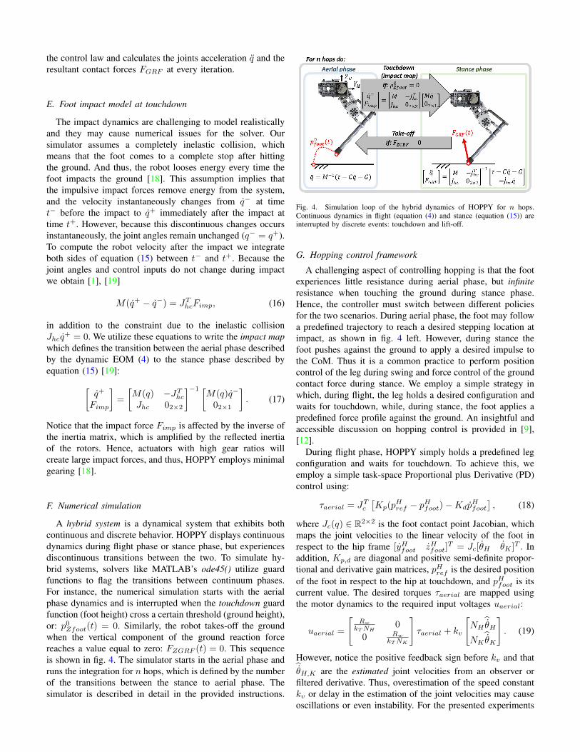
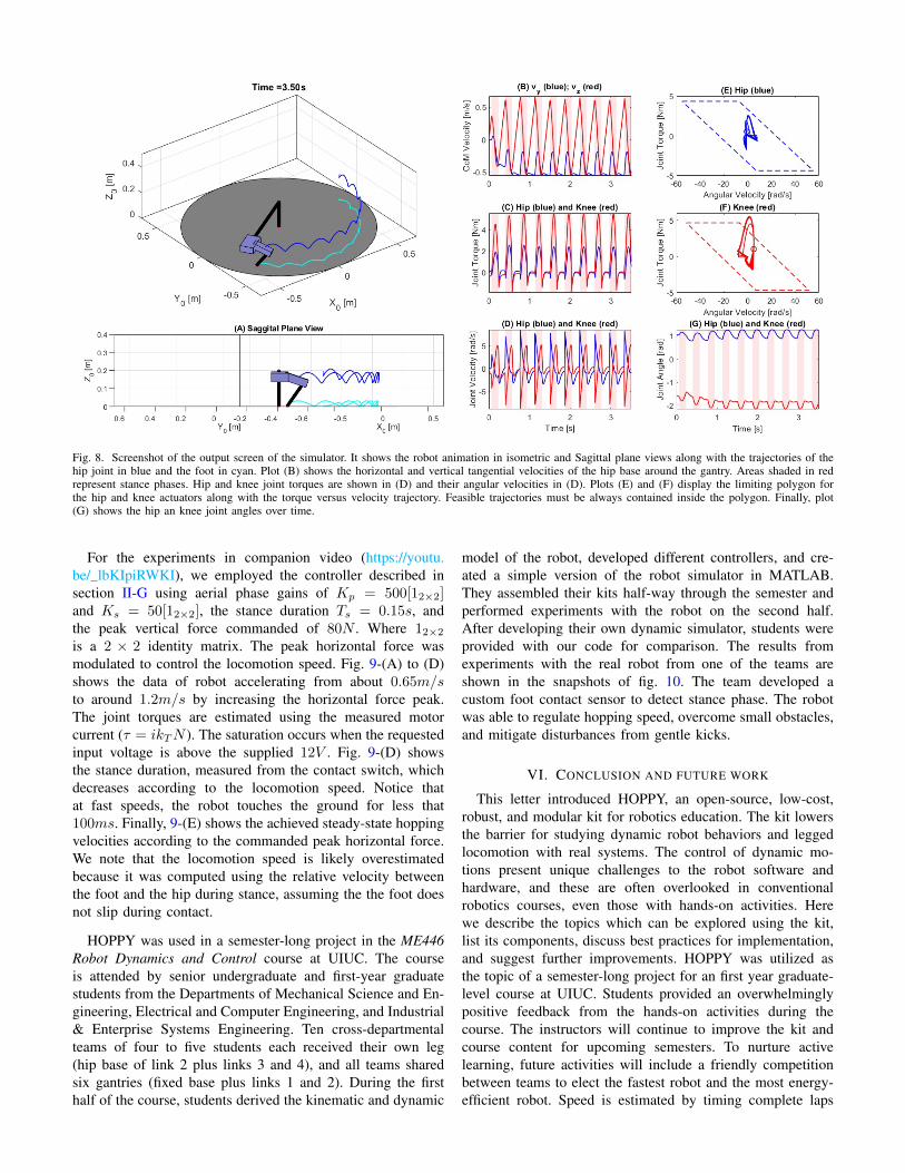
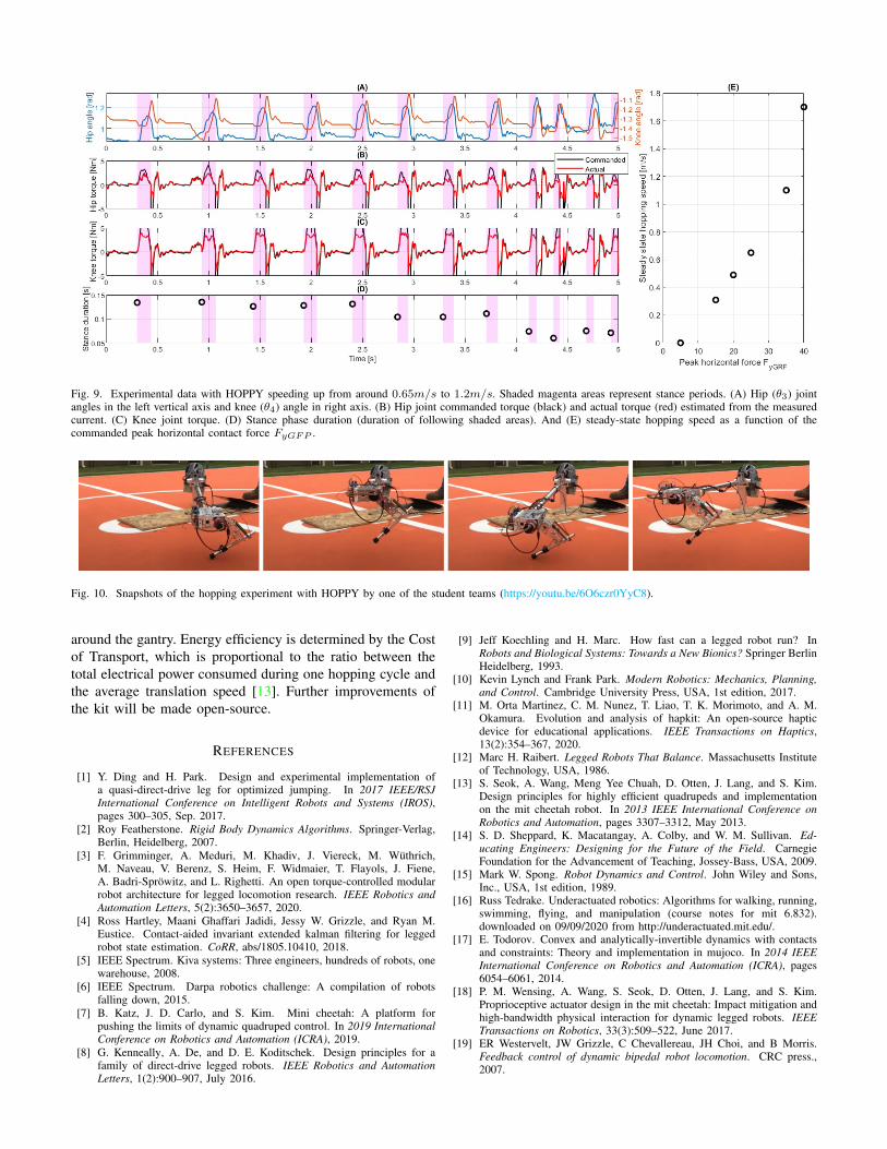
Related Documents