Preprint typeset in JHEP style - HYPER VERSION Holomorphic Linking, Loop Equations and Scattering Amplitudes in Twistor Space Mathew Bullimore Rudolf Peierls Institute for Theoretical Physics, 1 Keble Road, Oxford, OX1 3NP, United Kingdom David Skinner Perimeter Institute for Theoretical Physics, 31 Caroline St., Waterloo, ON, N2L 2Y5, Canada Abstract: We study a complex analogue of a Wilson Loop, defined over a complex curve, in non-Abelian holomorphic Chern-Simons theory. We obtain a version of the Makeenko-Migdal loop equation describing how the expectation value of these Wilson Loops varies as one moves around in a holomorphic family of curves. We use this to prove (at the level of the integrand) the duality between the twistor Wilson Loop and the all-loop planar S-matrix of N = 4 super Yang-Mills by showing that, for a particular family of curves corresponding to piecewise null polygons in space-time, the loop equation reduce to the all-loop extension of the BCFW recursion relations. The scattering amplitude may be interpreted in terms of holomorphic linking of the curve in twistor space, while the BCFW relations themselves are revealed as a holomorphic analogue of skein relations. arXiv:1101.1329v1 [hep-th] 6 Jan 2011

Welcome message from author
This document is posted to help you gain knowledge. Please leave a comment to let me know what you think about it! Share it to your friends and learn new things together.
Transcript

Preprint typeset in JHEP style - HYPER VERSION
Holomorphic Linking Loop Equations and
Scattering Amplitudes in Twistor Space
Mathew Bullimore
Rudolf Peierls Institute for Theoretical Physics
1 Keble Road Oxford OX1 3NP United Kingdom
David Skinner
Perimeter Institute for Theoretical Physics
31 Caroline St Waterloo ON N2L 2Y5 Canada
Abstract We study a complex analogue of a Wilson Loop defined over a complex
curve in non-Abelian holomorphic Chern-Simons theory We obtain a version of the
Makeenko-Migdal loop equation describing how the expectation value of these Wilson
Loops varies as one moves around in a holomorphic family of curves We use this
to prove (at the level of the integrand) the duality between the twistor Wilson Loop
and the all-loop planar S-matrix of N = 4 super Yang-Mills by showing that for a
particular family of curves corresponding to piecewise null polygons in space-time
the loop equation reduce to the all-loop extension of the BCFW recursion relations
The scattering amplitude may be interpreted in terms of holomorphic linking of
the curve in twistor space while the BCFW relations themselves are revealed as a
holomorphic analogue of skein relations
arX
iv1
101
1329
v1 [
hep-
th]
6 J
an 2
011
Contents
1 Introduction 1
2 Non-Abelian Holomorphic Wilson Loops 6
21 Holomorphic frames 6
22 The holonomy around a nodal curve 9
3 A Holomorphic Family of Curves 10
4 Holomorphic Loop Equations 13
41 Holomorphic linking 14
42 Loop equations for the twistor representation of N = 4 SYM 17
5 BCFW Recursion from the Loop Equations 20
1 Introduction
Scattering processes are usually defined for external states that each have some def-
inite momentum on the mass-shell Translational invariance implies that such an
amplitude is a distribution with support only when
nsum
i=1
pi = 0 (11)
In planar gauge theories the external states are cyclically ordered so we can solve
this constraint by introducing lsquoregionrsquo or lsquoaffinersquo momenta xi via
xi minus xi+1 = pi (12)
The mass-shell conditions p2i = 0 constrain adjacent xi s to be null separated In this
way the momenta and colour-ordering of the scattering amplitude are encoded in a
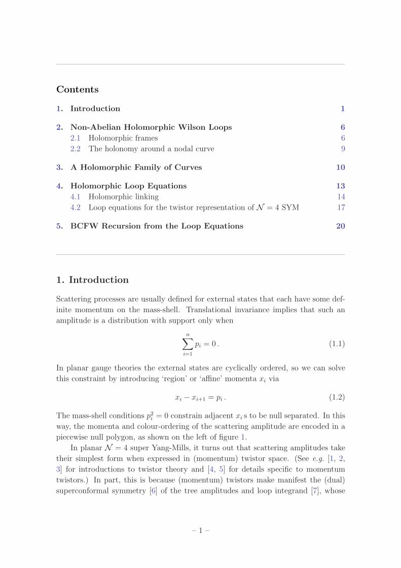
piecewise null polygon as shown on the left of figure 1
In planar N = 4 super Yang-Mills it turns out that scattering amplitudes take
their simplest form when expressed in (momentum) twistor space (See eg [1 2
3] for introductions to twistor theory and [4 5] for details specific to momentum
twistors) In part this is because (momentum) twistors make manifest the (dual)
superconformal symmetry [6] of the tree amplitudes and loop integrand [7] whose
ndash 1 ndash
incidence relations
xn
x1
x2
x3
x4
pn p1z1
zn
z2
z3
X1
X2Xn
Figure 1 A depiction of (a planar projection of) a nodal curve in twistor space corre-
sponding to a piecewise null polygon in space-time Via the incidence relations the vertex
xi corresponds to the line Xi = (ziminus1 zi) while the node zi corresponds to the null ray
through xi and xi+1
existence reflects the Yangian symmetry of the planar theory in the amplitude sector
(See also [8] for very interesting hints of the role of the Yangian in the loop amplitudes
themselves) However a perhaps deeper reason that these amplitudes belong in
twistor space is because their twistor data is unconstrained This is because points
in space-time correspond to complex lines (linearly embedded Riemann spheres) in
twistor space while two such points x1 and x2 are null separated if and only if their
corresponding twistor lines X1 and X2 intersect Thus to specify an n-sided piecewise
null polygon in space-time we can pick n arbitrary twistors and sequentially join them
up with (complex1) lines Adjacent lines intersect by construction so that as well as
momentum conservation the mass-shell condition is automatic Thus the scattering
data is encoded in a picture that is usually drawn as on the right of figure 1 where
the twistors zi are chosen freely
The key observation that motivates this paper is that although figure 1 always
provides an accurate representation of the twistor curve as an abstract Riemann
surface the holomorphic embedding of this Riemann surface in a complex three-fold
can be far more complicated than this picture indicates Depending on the choice of
vertices zi ie depending on the external kinematics the embedded twistor curve
can also appear as depicted in figure 2 that is it appears as a polygonal knot2
The new picture hints at an intriguing connection between scattering amplitudes
and a complexification of knot theory known as holomorphic linking To understand
this notion observe by a simple dimension count that while one can always use
smooth deformations to untangle real two-surfaces in a real six-manifold it is not
always possible to untangle complex curves in a complex three-fold if one is only
1As usual we draw real lines in three-space to depict complex lines in the complex three-
dimensional space2Planarity of the colour-ordered amplitude has nothing to do with the embedding of the curve
ndash 2 ndash
z1
z2
z3
z4
z5
z6
z7
z8
Figure 2 Depending on the location of the vertices the twistor lines may form a polygonal
knot The plane projection of the nodal curve can thus be far more involved than figure 1
suggests
allowed to vary the curve holomorphically (This restriction provides a second3 jus-
tification for the use of the half-dimensional representation in these figures) That
holomorphic linking in twistor space should encode interesting information about
gauge theories in space-time was originally envisaged by Atiyah [9] and Penrose [10]
Outside the twistor context holomorphic linking (and its relation to Abelian holo-
morphic Chern-Simons theory) has been studied by eg Khesin and Rosly [11] and
by Frenkel and Todorov [12]
It is the aim of this paper to elucidate and further investigate this link Consid-
erable evidence supporting the existence of such a relation comes from a conjecture
given by Mason and one of the present authors in [13] building on previous work by
Alday and Maldacena [14] using the AdSCFT correspondence and by Drummond
Korchemsky and Sokatchev [15] and by Brandhuber Heslop and Travaglini [16] in
space-time The conjecture states firstly that the complete classical S-matrix of
N = 4 super Yang-Mills is equivalent to the expectation value in the QFT defined
by the holomorphic Chern-Simons functional [17 18]
ShCS[A] =1
gs
int
CP3|4Ω and tr
(1
2A and partA+
1
3A andA andA
)(13)
of a certain operator defined over the complex curve C of figure 2 As we show in
section 2 this operator is a natural complexification of the standard Wilson Loop
operator given by the explicit formula
WR[C] = TrR P exp
(minusint
C
ω and A)
(14)
3The standard reason is that it gives a better picture of the structure of the nodes pictures of
2-surfaces incorrectly suggest that the component curves are tangent at the nodes
ndash 3 ndash
in terms of the connection (01)-form A where the precise definition of the meromor-
phic form ω and the meaning of the lsquopath-orderingrsquo symbol P is explained below The
expectation valuelangWR[C]
ranghCS
is thus a natural complexification of the expectation
valuelangWR[γ]
rang=
intDA eiSCS[A] TrR P exp
(minus∮
γ
A
)(15)
of a real Wilson loop in real Chern-Simons theory that famously computes knot
invariants [19] such as the HOMFLY polynomial (for gauge group U(N) and R the
fundamental representation)
Extrema of (13) correspond to holomorphic bundles on4 CP3|4 that (under mild
global conditions) in turn yield anti self-dual (or 12 BPS) solutions of the N =
4 super Yang-Mills equations on space-time via the Penrose-Ward correspondence
Thus holomorphic Chern-Simons theory corresponds only to the anti self-dual sector
of N = 4 SYM However it is possible to add a term to (41) so that the new action
corresponds to the complete (perturbative) N = 4 theory [20] The second part of
the conjecture of [13] is that when weighted by the exponential of this new actionlangW[C]
rangnow yields the complete planar S-matrix of N = 4 super Yang-Mills to all
orders in the rsquot Hooft coupling and for arbitrary external helicities
These conjectures were supported in [13] by perturbative calculations showing
that at least for small k and ` the axial gauge Feynman diagrams oflangW[C]
rangare
in one-to-one correspondence with MHV diagrams for the `-loop NkMHV scattering
amplitudes The momentum twistor formulation of the MHV diagram formalism
had previously been given in [21] and it has since been proved [22 23] that this
formalism correctly reproduces the all-loop recursion relation for the integrand of
planar N = 4 [7 24]
In this paper after reviewing the construction of the Wilson Loop operator
for a complex curve in section 2 we study a complex analogue of the Makeenko-
Migdal loop equations [25] for both the holomorphic Chern-Simons and N = 4 SYM
theories At least in principle these equations give a non-perturbative description of
the behaviour oflangW[C]
rangas C varies holomorphically
Now the loop equations for the expectation value (15) of a fundamental Wilson
Loop in real U(N) Chern-Simons theory were shown by Cotta-Ramusino Guadagnini
Martellini and Mintchev [26] to yield the skein relations for the HOMFLY polynomial
ndash in other words recursion relations allowing one to reconstruct the knot invariants
Quite remarkably in section 5 we find that (in the planar limit) the loop equations
forlangW[C]
rangmay be reduced to the BCFW relation [27] that recursively constructs
4The twistor superspace CP3|4 may be defined as the total space of (ΠOP3(1))oplus4
where OP3(1)
is the dual of the tautological line bundle on CP3 and Π reverses the Grassmann parity of the fibres
It is a Calabi-Yau supermanifold and we have written Ω for the canonical holomorphic section of
its Berezinian
ndash 4 ndash
the classical S-matrix The classical BCFW recursion relations thus emerge as a
holomorphic analogue of the skein relations for a knot polynomial Replacing the
pure Chern-Simons theory by the full N = 4 theory the loop equations involve a
new term and reduce instead to the recursion relation of Arkani-Hamed Bourjaily
Cachazo Caron-Huot and Trnka [7] for the all-loop integrand (See also [24] for
tentative extensions of this relation beyond N = 4 SYM) These results prove the
conjectures of [13] at least at the level of the integrand
Working in space-time Caron-Huot demonstrated in [28] that the expectation
value in N = 4 SYM of a certain extension of a regular Wilson Loop around the
null polygon on the left of figure 1 together with extra operator insertions at the
vertices also obeys the all-loop BCFW recursion relation This complete definition
of this Wilson Loop operator and the vertex insertions was not given in [28] but
it is expected to be fixed by supersymmetry Our proof that the twistor Wilson
Loop (with no extra insertions) obeys the same relation helps confirm that these two
approaches agree
There are at least two ways to view these results On the one hand accepting
the duality between scattering amplitudes and Wilson Loops one may see the loop
equations as providing an independent derivation of the all-loop BCFW recursion
relations However we prefer to interpret this work as a field theoretic explanation
for why the duality holds in the first place the behaviour of a scattering amplitude
near a factorisation channel is exactly equal to the behaviour of the twistor Wilson
Loop near a self-intersection Away from these singularities both the scattering
amplitudes and Wilson Loops are determined by analytic continuation of their data
For scattering amplitudes this is just the analyticity of the S-matrix as a function
of on-shell momenta encoding the familiar notions of crossing symmetry and space-
time causality while for Wilson Loops analyticity in the twistors zi expresses the
fact thatlangW[C]
ranggenerates analytic invariants associated to the holomorphic link
Finally although it is often said that BCFW recursion relations for scattering
amplitudes have little to do with Lagrangians path integrals or gauge symmetry our
work makes it clear that these standard tools of QFT are indeed intimately connected
to BCFW recursion from the point of view of Wilson Loops As always the Wilson
Loop is just the trace of the holonomy of a connection around a curve while the
loop equations themselves are derived from little more than the Schwinger-Dyson
equations of the appropriate path integral We view the connection to Lagrangians
and path integrals as a virtue because it suggests that BCFW-type techniques can be
applied to observables beyond scattering amplitudes Certainly the loop equations
we derive are valid for far more general curves than needed for scattering amplitudes
and for more general deformations than BCFW
ndash 5 ndash
z1
z2
z3
z4
z5
z6
z7
z8
Figure 3 Going beyond the application to scattering amplitudes we may allow the
component curves to have arbitrary degrees ge 1
2 Non-Abelian Holomorphic Wilson Loops
In this section we review the construction of [13] for a complex Wilson Loop defined
over a nodal curve C each of whose components is rational That is C = Z(Σ)
where Z is a holomorphic map to CP3|4 and the source curve
Σ = Σn cup middot middot middot cup Σ2 cup Σ1 (21)
with each component Σi rational and Σi+1capΣi = pt (i being counted mod n) For
scattering amplitudes we only need to consider the case that Z restricts to a linear
map on each irreducible component so that C generically appears as in figure 2
However it costs little to extend this to the case where each component is mapped
with arbitrary degree di ge 1 (shown in figure 3) and we allow this more general
possibility These curves may also be thought of as elliptic curves that have been
pinched n times around a given homology cycle They are certainly rather exotic
from the algebro-geometric point of view5 and it would clearly be interesting consider
the extension to non-degenerate elliptic curves
21 Holomorphic frames
Any Cinfin bundle E rarr CP3|4 is inevitably holomorphic on restriction to a arbitrary
complex curve C because D2|C = 0 trivially for dimensional reasons Suppose
first that C is a single irreducible rational curve Provided E|C is holomorphically
trivial6 we can find a gauge transformation h varying smoothly over C and such
5However it is curious that in the real category one often considers lsquotamersquo knots ndash ie knots
that are equivalent to an embedded polygon6By a theorem of Birkhoff and Grothendieck E|C =
oplusO(ai) withsumai = 0 if E|C is topolog-
ically trivial Triviality as a holomorphic bundle means that in addition ai = 0 for each i and
(perhaps surprisingly) is in fact generic
ndash 6 ndash
that
hminus1 (part +A)∣∣C h = part
∣∣C (22)
Under this gauge transformation covariantly holomorphic objects become simply
holomorphic on C so h is said to define a holomorphic frame for E|C It follows
from (22) that h itself obeys
(part +A)∣∣Ch = 0 (23)
and so is defined up to a gauge transform h rarr hhprime where hprime must be globally
holomorphic on C
For two points z0 z isin CP3|4 that lie on C we now define
U(z z0) equiv h(z)hminus1(z0) (24)
to be the particular solution of (23) obeying the initial condition that the gauge
transformation at z0 isin C is simply the identity The holomorphic frame U(z z0)
defines a map
U(z z0) E|z0 rarr E|z (25)
between the fibres of E at z0 and z isin CP3|4 that depends on the choice of curve
C (not unique if deg(C) gt 1) It is the natural complex analogue of the parallel
propagator U(x x0) between two points x and x0 along a real curve γ For example
it follows immediately from the definition (24) that
U(z zprime)U(zprime z0) = U(z z0) (26)
so that U(z z0) concatenates just as for the parallel propagator along a real curve
In particular U(z z0)U(z0 z) = U(z z) = 1R implying that
U(z0 z) = U(z z0)minus1 (27)
Likewise if we change our choice of connection (01)-form by a smooth gauge trans-
formation
A rarr Ag = g partgminus1 + gAgminus1 (28)
then since hminus1 (part +A)∣∣C h = (gh)minus1 (part +Ag)
∣∣C (gh) we find that
U(z z0)rarr g(z)U(z z0)gminus1(z0) (29)
again as for a parallel propagator in the real category
In the Abelian case with E a line bundle setting h = eminusφ for some smooth
function φ on C the holomorphic frame equation (23) becomes partφ = A|C This
equation always has a solution when C is rational given by
φ(z) =
int
C
ω and A (210)
ndash 7 ndash
where A is restricted to the curve and where ω is a meromorphic 1-form on C
whose only singularities are simple poles at z0 and z with residues plusmn1 respectively
Explicitly if C = Z(Σ) with Z(σ) = z isin CP3|4 and Z(σ0) = z0 then the pullback of
ω to Σ is
ω(σprime) =(σ minus σ0)
(σ minus σprime)(σprime minus σ0)
dσprime
2πi(211)
in terms of local coordinates σ isin Σ This is just the Greenrsquos function for the part-
operator acting on smooth functions on Σ The holomorphic frame equation fixes φ
only up to a globally holomorphic function which by Liouvillersquos theorem must be
constant The constant is fixed by the choice of reference point ω vanishes if z and
z0 coincide so (210) has φ(z0) = 0 Thus in the Abelian case we have the explicit
expression
U(z z0) = eφ = exp
(minusint
C
ω and A)
(212)
for our holomorphic frame
In the non-Abelian case acting on a representation R of the gauge group U(z z0)
may similarly be given by the (somewhat formal) expression7
U(z z0) = P exp
(minusint
C
ω and A) (213)
The meaning of the lsquopath orderingrsquo symbol P on our complex curve is that the ith
power of the meromorphic differential ω that appears from expanding the exponential
in (213) should be taken to have its simple poles located at the reference point z0 and
at either the insertion point of the (i+ 1)th power of the field A (counting according
to the colour-ordering) or else at the final evaluation point z Specifically
P exp
(minusint
C
ω and A)equiv 1R +
infinsum
m=1
(minus1)mint
(C)m
mand
i=1
(ω(zi) and A(zi)
)(214)
where ω(zi) is a meromorphic differential in zi with a simple pole at z0 and a simple
pole at zi+1 (or at z when i = m) Explicitly in terms of intrinsic coordinates
mand
i=1
ω(σi) =(σ minus σ0)
(σ minus σm) middot middot middot (σ2 minus σ1)(σ1 minus σ0)
dσm2πiand middot middot middot and dσ1
2πi (215)
7An equivalent formal expression given in [13] is U(z z0) =(
1 + partminus1A∣∣C
)minus1 where in the
series expansion of this expression the inverse part-operators are taken to act on everything to their
right
ndash 8 ndash
Equation (213) is thus analogous to the (equally formal) expression
P exp
(minusint x
x0
A
)
= 1R minusint x
x0
dymicroAmicro(y) +
int x
x0
dymicroAmicro(y)
int y
x0
dyprimeνAν(y
prime) minus middot middot middot
= 1R +infinsum
m=1
(minus1)mint
([01])m
dsm middot middot middot ds1 Amicro(sm)dxmicro
dsmθ(smminussmminus1) middot middot middot θ(s2 minus s1)Aν(s1)
dxν
ds1
(216)
for the parallel propagator of a connection d +A = dxmicro(partmicro +Amicro) along a real curve
γ where the step functions obey
part
partsθ(sminus sprime) = δ(sminus sprime) (217)
and are the Greenrsquos function for the exterior differential on the interval [0 1] We also
note that the iterated integrals appearing in (213) are somewhat similar to iterated
integrals that arise in studying parallel transport via the Knizhnik-Zamolodchikov
connection over the configuration space of n-points on a rational curve See [29] for
a recent discussion of this in a twistor context
22 The holonomy around a nodal curve
Having identified the holomorphic frame U(z z0) = h(z)hminus1(z0) as the natural ana-
logue of a parallel propagator for a complex curve we can define the holonomy of the
connection (01)-form around C based at some point z isin CP3|4 to be the ordered
product
Holz[C] equiv U(z zn) U(zn znminus1) middot middot middotU(z2 z1) U(z1 z) (218)
where zi is the image of the node Σi+1 cap Σi and where without any essential loss
of generality we have taken the base point to be on Z(Σ1) Reading from the right
of (218) this definition uses the holomorphic frame U(z1 z) on Z(Σ1) to map the
fibre E|z to the fibre E|z1 at the node z1 We can identify this fibre with a fibre of
E restricted to the next component line Z(Σ2) and then map to the following node
using the holomorphic frame U(z2 z1) on Z(Σ2) We continue transporting our fibre
around the nodal curve in this way until the final factor of U(z z1) returns us to the
starting point The result is thus an automorphism of the fibre E|z as required
The holomorphic Wilson Loop is now defined as in the real category as
WR[C] equiv TrR Holz[C] (219)
where to take the trace in a representation R we have used the fact that a holomorphic
frame for E|C induces a holomorphic frame for all tensor products of E|C and its
dual in other words for all choices of representation Cyclicity of the trace and the
ndash 9 ndash
concatenation property (26) immediately shows that the Wilson Loop is independent
of the base point
For an Abelian gauge group (E a line bundle) the holomorphic frame (212) gives
W[C] = exp
(minusint
C
ω and A)
(220)
where ω is a meromorphic form on C whose only singularities are simple poles at
each of the nodes with residues plusmn1 on each component Such a differential is nothing
but the holomorphic differential θ on a non-singular elliptic curve in the limit that
this curve degenerates to our nodal curve (see eg [30]) Thus in the Abelian case
we recover the prescription
W[C] = exp
(minusint
C
θ and A)
(221)
that was proposed by Thomas [31] by Khesin and Rosly [11] and by Frenkel and
Todorov [12] For a non-Abelian gauge group we can likewise use (213) to formally
write
WR[C] = TrR P exp
(minusint
C
ω and A)
(222)
as a natural complexification of the familiar expression
WR[γ] = TrR P exp
(minusint
γ
A
)(223)
for a Wilson Loop of a connection on a real curve γ In equation (222) as in (213)
the path ordering symbol means that for each component of C successive powers of
ω in the series expansion of (222) should have one simple pole at one of the nodes
and another at the subsequent (with respect to the colour-ordering) insertion point
of the field
3 A Holomorphic Family of Curves
We now investigate the behaviour of our complex Wilson Loop as the curve C varies
We shall prove that just as the change in the real Wilson Loop (223) under a smooth
deformation of a real curve γ is
δWR[γ] = minus∮
γ
dxmicro δxν TrR
(Fmicroν(x) Holx[γ]
) (31)
so too the complex Wilson Loop (219) obeys
δWR[C] = minusint
C
ω(z) and dzα and δzβ TrR
(Fαβ(z z) Holz[C]
)(32)
ndash 10 ndash
as the complex curve C moves over a holomorphic family In this equation δ is the part-
operator on the parameter space of the family and once again ω(z) is a meromorphic
differential on C whose only singularities are simple poles at the nodes with residues
plusmn1 Like its real analogue equation (32) expresses the change in the Wilson Loop
in terms of the curvature (02)-form F = partA+AandA through the complex 2-surface
swept out by the varying curve The key point here is that because the curve C varies
holomorphically only the (02)-form part of the curvature arises In particular if E
is a holomorphic bundle on twistor space then the Wilson Loop is also holomorphic
As before we prove (32) in more generality than we actually need for scattering
amplitudes allowing each irreducible component Ci = Z(Σi) to have degree di ge 1
Here is the proof8 For a fixed partial connection the holomorphic frame U(z1 z0)
depends on the choice of two points z0 z1 isin CP3|4 together with a choice of (ir-
reducible rational) curve C that joins them (Note that this curve is not unique
if its degree is greater than 1) Equivalently we can think of this data in terms of
an abstract Riemann sphere Σ together with two marked points σ0 σ1 isin Σ and
a degree d holomorphic map Z Σ rarr CP3|4 such that Z(Σ) = C and Z(σi) = zi
Now suppose we have a holomorphic family of such maps parametrized by a mod-
uli space B described say by local holomorphic coordinates ti Writing U(σ σ0 t)
for the pullback of U(z z0) to the abstract curve Σ for our family of curves the
holomorphic frame equation is
(part + ZlowastA)U(σ σ0 t) = dσ
(part
partσ+Aα
partzα
partσ(σ t)
)U(σ σ0 t) = 0 (33)
where we emphasise that both the holomorphic frame and the connection depend on
t ndash ie on the choice of curve
Consider the integral
int
Σ
ω10(σ) and U(σ1 σ t) (part + ZlowastA)U(σ σ0 t) (34)
over Σ where ω10(σ) is our familiar meromorphic differential (211) whose only
singularities are simple poles at σ0 and σ1 with residues +1 and minus1 respectively
and where part +A is as given in (33) In principle the integral depends on these two
points and on the map Z ndash that is it depends on the moduli space ndash but of course
it actually vanishes identically on B since U(σ σ0) obeys (33)
8It is also possible to show (32) by working directly with the formal expression (222) provided
(as in the real case) due care is taken of the lsquopath orderingrsquo
ndash 11 ndash
Letting δ be the part-operator on B we have
0 = δ
[int
Σ
ω10(σ) and U(σ1 σ t)(part + ZlowastA
)U(σ σ0 t)
]
=
int
Σ
ω10(σ) and U(σ1 σ t)(part + ZlowastA
)δU(σ σ0 t)
minusint
Σ
ω10(σ) U(σ1 σ t) and δ(ZlowastA) U(σ σ0 t)
= minusδU(σ1 σ0 t)minusint
Σ
ω10(σ) U(σ1 σ t) and δ (ZlowastA) U(σ σ0 t)
(35)
where the third line follows from integrating by parts in the first term then using the
poles of ω10 and the fact that partU(σ1 σ t) = U(σ1 σ t)ZlowastA to perform the integral9
In the final term of (35) we have
δ (ZlowastA) =
(partβAα
partzβ
parttıpartzα
partσ+Aα
part2zα
parttı partσ
)dtı and dσ (36)
The most important property here is that because the map Z varies holomorphically
only antiholomorphic derivatives of the connection arise Again integrating by parts
we find that
DBU(σ1 σ0 t) equiv δU(σ1 σ0 t) +A(z(σ1 t))U(σ1 σ0 t)minus U(σ1 σ0 t)A(z(σ0 t))
= minusint
Σ
ω10(σ) and dσ and dtı U(σ1 σ t)Fαβpartzα
partσ
partzβ
parttıU(σ σ0 t)
= minusint
C
ω10(z) and dzα and δzβ U(z1 z)Fαβ(z) U(z z0)
(37)
where DB is the natural covariant part-operator acting on sections of the sheaf E over
B induced by10 E
Equation (37) tells us how the holomorphic frame U(z1 z0) on an irreducible
curve varies as we move around in the moduli space For the Wilson Loop (219) on
9In fact the moduli space B may be identified with the Kontsevich moduli space M02(CP3|4 d)
of stable 2-pointed degree d maps Because it depends on three points σ0 σ1 σ isin Σ as well as
Z the integrand in (34) really lives on the universal curve C equiv M03(CP3|4 d) and the pullback
by the map Z is more properly written as the pullback by the evaluation map on the third marked
point (labelled σ) The integral itself is really the pushdown by the forgetful map π C rarr B and in
commuting δ past the integral sign in (35) we really mean the pullback πlowastδ = partCminuspartCB = partCminuspartΣ
Then (36) is just the statement that the evaluation map is holomorphic and so commutes with partC
with the partΣ term left over10More accurately E = πlowastevlowastσE
ndash 12 ndash
a nodal curve we now readily find
δWR[C(t)] =nsum
i=1
TrR
((DBU(zi+1 zi)
)U(zi ziminus1) middot middot middotU(zi+2 zi+1)
)
= minusint
C(t)
ω(z) and dzα and δzβ TrR
(Fαβ(z z) Holz[C(t)]
) (38)
where the integral is taken over the complete nodal curve C(t) = Z(Σ) and we
emphasise that this curve depends on the moduli of the map As usual ω(z) is a
meromorphic differential on C(t) with only simple poles at the nodes This completes
the proof
4 Holomorphic Loop Equations
In this section we derive an analogue of the loop equations of Makeenko and Migdal [25]
for our complex Wilson Loops To do this instead of considering the complexified
Wilson Loop itself we must study its averagelangWR[C]
rangover the space of gauge-
inequivalent connection (01)-forms on E weighted by the exponential of an appro-
priate action
In section 41 we choose the action to be the U(N) holomorphic Chern-Simons
functional
ShCS[A] =1
g2
int
CP3|4
D3|4z and tr
(1
2A and partA+
1
3A andA andA
) (41)
that may be interpreted as the open string field theory of the perturbative B-
model [17 18] In real Chern-Simons theory on a real 3-manifold M the correlation
function of a Wilson Loop gives a knot invariant Since these invariants depend
only on the (regular) isotopy class of the knot one expects that unlike WR[γ] itselflangWR[γ]
rangCS
should remain invariant as one smoothly deforms γ This is essentially
true except that there are important corrections when the deformation causes γ to
pass through a self-intersection so that the isotopy class of the knot jumps The
loop equations determine the behaviour oflangWR[γ]
rangCS
under such a jump and it was
shown in [26] that for Wilson Loops in the fundamental representation of U(N)
they amount to the skein relations
s12P+(r s)minus sminus 1
2Pminus(r s) = (r12 minus rminus 1
2 )P0(r s) (42)
from which the HOMFLY polynomial Pγ(r s) can be recursively constructed11
11The variables of the HOMFLY polynomial are related to N and the level k of the Chern-Simons
theory by and s = eλ and r = eλN where λ equiv 2πiN(k + N) may be interpreted as the rsquot Hooft
coupling In [26] the skein relations were obtained to lowest order in λ The skein relation only
determines the HOMFLY polynomial for Wilson Loops in the fundamental
ndash 13 ndash
We expect that correlation functions of our Wilson Loops in the holomorphic
Chern-Simons QFT are likewise associated with holomorphic linking invariants In-
deed [11 12] show that for two non-intersecting curves C1 C2 sub C3 of genera gi ge 1
the expectation valuelangW[C1] W[C2]
rangin Abelian holomorphic Chern-Simons theory
on C3 involves12 the holomorphic linking invariant
L(C1 θ1C2 θ2) =1
4π
int
C1timesC2
εık(z minus w)ı
|z minus w|6 dz and dwk and θ1 and θ2 (43)
that generalizes the Gauss linking number
L(γi γj) =1
4π
int
γitimesγj
εijk(xminus y)i
|xminus y|3 dxj and dyk (44)
in for real Abelian Wilson Loops in R3 Observe that (43) depends on a choice of
holomorphic 1-form θi on each curve For our nodal curve the corresponding form is
meromorphic and depends on the location of the nodes In section 41 we shall find
that δlangWR[C]
ranghCS
generically vanishes with important corrections when the type
of the curve jumps In the planar limit the loop equations may be reduced to the
BCFW relations [27] that recursively construct the classical S-matrix In this sense
the BCFW relations are simply the U(infin) skein relations for the holomorphic link
defined by C
As mentioned in the introduction holomorphic Chern-Simons theory on CP3|4
corresponds only to the anti self-dual sector of N = 4 super Yang-Mills theory on
space-time In section 42 we replace (41) by the action [20]
SN=4[A] = ShCS[A] +
int
Γ
d4|8x ln det(part +A)∣∣X
(45)
that as our notation indicates describes N = 4 super Yang-Mills theory on twistor
space We shall see that the new term is itself eminently compatible with the Wilson
Loop The loop equations in this theory involve a new term that leads to the all-loop
extension of the BCFW relations found by Arkani-Hamed et al in [7]
41 Holomorphic linking
In this section we choose the action to be the holomorphic Chern-Simons func-
tional (41) where D3|4z is the canonical holomorphic section of the Berezinian of
CP3|4 given explicitly by
D3|4z equiv 1
4εαβγδz
αdzβ and dzγ and dzδ1
4εabcddψ
a dψb dψc dψd (46)
12We will see later that at least for the N = 4 theory lsquoholomorphic self-linkingrsquo is well-defined
even without a choice of framing
ndash 14 ndash
in terms of homogeneous coordinates (zα ψa) isin C4|4 This action is defined on the
space A 01 of partial connections D on a Cinfin vector bundle E rarr CP3|4 given at least
locally by D = part+A in terms of a background partial connection part We take this to
obey part2 = 0 and so define a background complex structure on E Thus A(z z ψ)
is a superfield with component expansion
A(z z ψ) = a(z z) + ψaΓa(z) +1
2ψaψb Φab(z z) + middot middot middot+ 1
4εabcdψ
aψbψcψd g(z z)
(47)
where the coefficient of (ψ)r is a (01)-form on CP3 valued in smooth sections of
End(E)otimesOCP3(minusr)We choose the gauge group to be U(N) and consider only Wilson Loops in the
fundamental representation The Yang-Mills (or open string) coupling g2 is then
related to the Chern-Simons level k by g2 = 2π(k + N) In anticipation of taking
the planar limit we write g2 = λN in terms of the rsquot Hooft coupling λ and include
a factor of 1N in definition of the Wilson Loop so that W[C] = 1 if the holonomy
is trivial
Inserting (32) into the holomorphic Chern-Simons path integral one finds
δlangW[C(t)]
rang= minus 1
N
intDA
[int
C(t)
ω(z) and dzα and δzβ tr(Fαβ(z) Holz[C(t)]
)]eminusShCS[A]
=λ
N2
intDA
[int
C(t)
ω(z) and tr
(Holz[C(t)]
δ
δA(z)eminusShCS[A]
)]
(48)
since the variation of the holomorphic Chern-Simons functional is F02 times Nλ To
obtain an interesting equation for δlangW[C(t)]
rang as in [25] we integrate by parts in
the path integral bringing the variation of the connection to act on the holonomy
Essentially the same argument as in section 3 shows that under a variation of the
connection at some point zprime isin C (displaying colour indices)
0 =
[δ
δA(z)
i
j
(int
C
ω10(zprime) and U(z1 zprime)(part +A
)C
U(zprime z0)
)k
l
]
= minus[
δ
δA(z)
i
j
U(z1 z0)kl
]+
int
C
ω10(zprime) and U(z1 zprime)kj δ
3|4(z zprime) U(zprime z0)i l
(49)
where we have used the fact that for a U(N) gauge group
(δδA(z))i j A(zprime)mn = δ3|4(z zprime) δinδmj (410)
with δ3|4(z zprime) a Dirac current concentrated on the diagonal in CP3|4z times CP3|4
zprime ie
δ3|4(z zprime) is a distribution-valued (03)-form on CP3|4z times CP3|4
zprime such that for any α isinΩ0p(CP3|4) we have
int
CP3|4D3|4zprime and δ3|4(z zprime) and α(zprime) = α(z) (411)
ndash 15 ndash
z
z
C(t)
C(t)
Figure 4 The expectation valuelangW[C(t)]
rangin holomorphic Chern-Simons theory varies
holomorphically except where the curve develops a new node
Explicitly δ3|4(z zprime) may be represented by the integral [5 32]
δ3|4(z zprime) =
intdu
uand δ4|4(z minus uzprime) =
intdu
u
4and
α=1
part1
zα minus uzprimeα4prod
a=1
(ψa minus uψprimea) (412)
that forces zα prop zprimeα so that the two point must coincide projectively
We now apply equation (49) to the variation holonomy based say at a point
z isin C1 One finds
tr
(δ
δA(z)Holz[C(t)]
)=
δ
δA(z)
i
j
[U(z zn)jkU(zn znminus1)kl middot middot middotU(z1 z)
mi
]
=sum
i
int
Ci(t)
ωi+1i(zprime) and δ3|4(z zprime) tr
[U(z zn) middot middot middotU(zi+1 z
prime)]
tr[U(zprime zi) middot middot middotU(z1 z)
]
(413)
The factor of δ3|4(z zprime) ensures that this term has support only at points t in the
moduli space where the curve C(t) degenerates so that the component C1(t) ei-
ther self-intersects or else intersects some other component Similar contributions
arise from summing over the possible locations of the base-point z In other words
thinking of our original curve as an elliptic curve δlangW[C(t)]
rangvanishes everywhere
except on boundary components of the moduli space where the holomorphic map
degenerates so that two points on the source curve are mapped to the same image
Combining all the terms the holomorphic Chern-Simons loop equations (48)
become
δlangW[C(t)]
rang= minusλ
int
C(t)timesC(t)
ω(z) and ω(zprime) and δ3|4(z zprime)langW[C prime(t)] W[C primeprime(t)]
rang (414)
for normalised Wilson Loops in the fundamental of a U(N) gauge group where C prime(t)
and C primeprime(t) are the two curves obtained by ungluing C(t) at its new node z = zprime (see
figure 4) In the planar limit the correlation function of a product of Wilson Loops
factorizes into the product of correlation functions so (414) simplifies to
δlangW[C(t)]
rang= minusλ
int
C(t)timesC(t)
ω(z) and ω(zprime) and δ3|4(z zprime)langW[C prime(t)]
rang langW[C primeprime(t)]
rang(415)
ndash 16 ndash
where λ is the rsquot Hooft coupling Thus in the planar limit the behaviour at a self-
intersection is determined by the product of the expectation values of the Wilson
Loops around the two lower degree curves This may be viewed as an analogue
for holomorphic linking of the skein relations for real knot invariants In section 5
we shall see that the classical BCFW recursion relations are simply a special case
of (415)
42 Loop equations for the twistor representation of N = 4 SYM
We now consider the expectation value of the complex Wilson Loop in the twistor
action
SN=4[A] = ShCS[A] +
int
Γ
d4|8x log det(part +A)∣∣X (416)
where X is a line in twistor space and Γ is a middle-dimensional contour in the
space Gr2(C4) of these lines13 interpreted as a choice of real slice of complexified
conformally compactified space-time The proof that (416) is an action for N = 4
SYM on twistor space is given in [20] to which the reader is referred for further
details (Readers familiar with the MHV formalism may note that the new term
in (416) provides an infinite series of MHV vertices while the 3-point MHV vertex
in the Chern-Simons theory vanishes in an axial gauge From the point of view
of twistor string theory [18] the determinant may be understood as the partition
function of a chiral free fermion CFT on X coupled to the pullback of the twistor
space gauge field)
From the point of view of the present article it is possible to motivate this action
by observing that Wilson Loops on complex curves are again the natural observables
of the QFT based on (416) The reason this is so is because of the close connection
between determinants and holonomies More precisely just as
δ log detM = δ tr logM = tr(Mminus1δM) (417)
for a finite dimensional matrix M Quillen shows [33] that for an abstract curve Σ
under a variation of the connection the logarithm of a section of the determinant
line bundle Detrarr A 01Σ varies as14
δ log det(part +A)∣∣Σ
=
int
Σ
tr (JA and δA) (418)
where
JA(σ) equiv limσprimerarrσ
(GA(σprime σ)minusG0(σprime σ)
)(419)
13The fermionic integral is done algebraically as always14In writing this formula we assume that δ is a flat connection on Det in a trivialisation where
the local connection 1-form vanishes That Det should admit such a flat connection is necessary if
we wish to treat det(part +A)Σ as a (holomorphic) function on A 01Σ (the space of connection (01)-
forms on Σ) However [33] the construction of this flat connection requires a choice of background
connection
ndash 17 ndash
is the limit15 on the diagonal in Σ times Σ of difference between the Greenrsquos function
for part +A|Σ and the Greenrsquos function for background connection partΣ These Greenrsquos
functions are non-local operators on the Riemann surface the fact that we take their
limit on the diagonal can be understood as part of the trace For a single such Greenrsquos
function the limit on the diagonal is necessarily singular but the singularity cancels
in the difference (419) The dependence on a background connection reflects the fact
that to treat sections of the determinant line bundle as functions we must first pick
a trivialisation amounting to a choice of background connection (01)-form on the
bundle over Σ In our case we will of course choose this background part-operator to
be the one induced by our choice of base-point part isin A 01Σ in writing the holomorphic
Chern-Simons action
When Σ is a Riemann sphere the Greenrsquos functions are
GA(σprime σ) = h(σprime)G0(σprime σ)hminus1(σ) and G0(σprime σ) =1
2πi
dσ
σprime minus σ (420)
in terms of the holomorphic frame h on Σ Therefore Quillenrsquos prescription reduces
to
JA(σ) =dσ
2πilimσprimerarrσ
U(σprime σ)minus U(σ σ)
σprime minus σ =dσ
2πi
partU(σprime σ)
partσprime
∣∣∣∣σprime=σ
(421)
For our purposes the presence of the holomorphic derivative here is somewhat in-
convenient However it is easily seen from the formal series (214) that U(σprime σ)
depends only meromorphically on σprime and is regular at σprime = σ Thus we can use
Cauchyrsquos theorem to rewrite the derivative in (421) as an integral so
δ log det(part +A)∣∣Σ
=1
(2πi)2
int
Σ
dσ and tr
(∮dσprime
(σ minus σprime)2U(σprime σ) δA(σ)
)
=1
(2πi)3
int
ΣtimesS1timesS1
dσ and dσprime and dσprimeprime
(σ minus σprime)(σprime minus σprimeprime)(σprimeprime minus σ)tr (U(σprime σ) δA(σ))
(422)
where the integrals over σprimeprime and σprime are performed over contours encircling the poles at
σprimeprime = σprime and σprime = σ respectively (The reason for introducing the new point σprimeprime isin Σ
will become clear momentarily)
To apply this to the case that Σ = Zminus1(X) for X a line in twistor space suppose
Z(σprimeprime) = za Z(σprime) = zb and Z(σ) = z = za + σzb (423)
so that X = Span[za zb] Then
dσ and dσprime and dσprimeprime
(σ minus σprime)(σprime minus σprimeprime)(σprimeprime minus σ)= Zlowast
[ωab(z) and 〈a da〉 and 〈b db〉
〈a b〉2]
(424)
15Below this limit will be revealed as nothing but the forward limit of an amplitude
ndash 18 ndash
where ωab(z) is meromorphic with only simple poles only z = za and zb and where
〈a da〉〈b db〉〈a b〉2 is the fundamental bi-differential on X with a double pole along
the diagonal This bi-differential combines with the integral over the space of lines
X since
d4|8x and 〈a da〉 and 〈b db〉〈a b〉2 = D3|4za andD3|4zb (425)
giving a contour integral over CP3|4a timesCP3|4
b Therefore the variation of the new term
in the action is
δ
int
Γ
d4|8x log det(part +A)∣∣X
=
int
ΓtimesXtimesS1timesS1
D3|4za andD3|4zb(2πi)3
and ωab(z) tr(
U(zb z) δA(z))
(426)
where the S1 times S1 contour sets za rarr z and zb rarr z differentiating U(zb z) in the
process The integral over all z isin X is performed using the dependence on z in the
holomorphic frame and in the variation of the connection
Equation (426) expresses the variation of the logarithm of the determinant in
the twistor action (416) in terms of a holomorphic frame on the line X It dovetails
beautifully with the holonomy around the curve C providing a new contribution
minus λN
int
ΓtimesS1timesS1
D3|4za andD3|4zb
int
C(t)timesX
ω(z) and ωab(z) and δ3|4(z z) tr(
U(zb z) Holz[C(t)])
(427)
to the loop equations The δ-function δ3|4(z z) in this expression means that this
term only contributes at points in the moduli space where the curve C(t) 3 z inter-
sects the line X 3 z The integral over Γ then adds up these contributions for each
X isin Γ
To interpret the product U(zb z) Holz[C(t)] replace C(t) by a curve C(t) where
C(t) cap X = z zb isin CP3|4 (428)
and such that as zb rarr z C(t) rarr C(t) As a nodal curve C(t) has one more
component than C(t) with one component becoming double covered in the limit
(see figure 5) Now because the contour integral forces zb = z we can replace the
holonomy around C(t) based at z = z = C(t) cap X by a product of holomorphic
frames that transport us around C(t) from zb to z The remaining factor of U(zb z)
transports this frame back to zb along X The resulting trace can be interpreted as
Wilson Loop around C(t) cup X so that
1
Ntr(
U(zb z)Holz[C(t)])
= W[C(t) cup X] (429)
provided we are inside the contour integral over the location of zb sub X
ndash 19 ndash
=
X
z = zC
X
C zb
z
Figure 5 The new term in the loop equations for N = 4 SYM can be understood as a
holomorphic Wilson Loop around a new curve C cupX where C reduces to C when zb rarr z
along X Note that the nodal curve C has one more component than C In the scattering
amplitude context 〈W[C cup X]〉 may be interpreted as a forward limit of an n+ 2 particle
amplitude
Finally then we see that the holomorphic loop equations for the twistor repre-
sentation of planar N = 4 SYM are
δlangW[C(t)]
rang= minus λ
int
C(t)timesC(t)
ω(z) and ω(zprime) and δ3|4(z zprime)langW[C prime(t)]
rang langW[C primeprime(t)]
rang
minus λ
int
ΓtimesS1timesS1
D3|4za andD3|4zb
int
C(t)timesX
ω(z) and ωab(z) and δ3|4(z z)langW[C(t) cup X]
rang
(430)
and as in the original equations of Migdal amp Makeenko [25] are entirely expressed
in terms of expectation values of our (complexified) Wilson Loops In the following
section we show that for a particular one-parameter family of curves C(t) this holo-
morphic loop equation reduces to the all-loop BCFW recursion relation found in [7]
but we emphasise that (430) is valid for a far more general class of curves
5 BCFW Recursion from the Loop Equations
We now apply the holomorphic loop equation (430) to the case that each component
of C is a line as in figure 2 C can be completely specified by giving the location
of its n nodes and we shall often write C = (12) cup (23) cup middot middot middot cup (n1) for the curve
(where (i i+1) equiv Span[zi zi+1]) and W[1 2 n] for the corresponding Wilson Loop
(in the fundamental representation) We wish to show that the loop equations forlangW[1 2 n]
rangdirectly reduce to the all-loop BCFW recursion relations of Arkani-
Hamed et al [7] although it is important that our derivation of these relation is
completely independent of any notions of scattering theory
ndash 20 ndash
z1
z2
z3
z4
z5
z6
z7
z8
z8 t
Figure 6 The family of nodal curves C(t) corresponding to a BCFW deformation of a
planar amplitude in N = 4 SYM shown for n = 8 As we vary over the moduli space the
line (1 n(t)) sweeps out a pencil of lines in the plane (nminus1 n 1) with focus z1 This plane
necessarily intersects every other component of C(t)
Consider the holomorphic family of Wilson Loops determined by translating the
node zn along the line (nminus1 n) That is we define
zn(t) equiv zn + tznminus1 (51)
and consider the 1-parameter family of holomorphic curves
C(t) equiv (12) cup (23) cup middot middot middot cup (nminus1 n(t)) cup (n(t) 1) (52)
as shown in figure 6 Notice that although t can be thought of as a local holomorphic
coordinate on the line (nminus1n) it is really a coordinate on the moduli space of our
family of curves ie a coordinate on a CP1 sub B As t varies the line (n(t) 1) sweeps
out the plane (nminus1 n 1) with all other components of C(t) remaining fixed Lines
and planes necessarily intersect16 in CP3 so for every j = 3 nminus1 there exists a tjfor which (n(tj) 1) intersects the component Cj Let us call this intersection point
Ij and write nj for the point zn(tj) Clearly we have
Ij = (nminus1 n 1) cap (jminus1 j) and nj = (nminus1 n) cap (jminus1 j 1) (53)
essentially by definition (Note that we do not get any new intersections when j =
n 1 2)
16Lines and planes do not necessarily intersect in the superspace CP3|4 because they might lsquomissrsquo
in the fermionic directions The fermionic δ-functions in the δ3|4(z zprime) ensure that the right hand
side has support only when the curves do intersect in the superspace See also the discussion in [21]
ndash 21 ndash
We now study the loop equations for this family Considering first the case of
pure holomorphic Chern-Simons theory (415) becomes
minusint
CP1
dt
tand δlangW[C(t)]
rang=
λnminus1sum
j=3
int
CP1timesC1(t)timesCj
dt
tand ω(z) and ω(zprime) and δ3|4(z zprime)
langW[C prime(t)]
rang langW[C primeprime(t)]
rang (54)
whereC prime(t) = (12) cup (23) cup middot middot middot cup (jminus1 Ij)
C primeprime(t) = (Ij j) cup (j j+1) cup middot middot middot (nj 1)(55)
and where we have integrated (415) over our moduli space CP1 sub B using the
meromorphic differential dtt We can dispose of the left hand side immediately
integrating by parts gives
minusint
CP1
dt
tand δlangW[C(t)]
rang=langW[C(0)]
rangminuslangW[C(infin)]
rang
=langW[1 2 n]
rangminuslangW[1 2 nminus1]
rang
(56)
the difference of the Wilson Loops around the original curve and the curve with
zn = znminus1 Notice that the holomorphic frame U(zn znminus1)rarr 1 as zn rarr znminus1 so that
while the line (nminus1 n) does not simply lsquodisappearrsquo from the picture neither does it
contribute to the holonomy
The right hand side of (54) is almost as straightforward to compute because the
integrals over both the CP1 moduli space and the two copies of C(t) are completely
fixed by the δ-function δ3|4(z zprime) Since z isin (n(t) 1) and zprime isin (jminus1 j) we can
parametrize these integrals by setting
z = zn(t) + sz1 = zn + tznminus1 + sz1 and zprime = zjminus1 + rzj (57)
in terms of local coordinates r and s on C1(t) and Cj respectively With these
coodinates the meromorphic forms ω(z) and ω(zprime) become simply
ω(z) =ds
sand ω(zprime) =
dr
r(58)
which indeed have simple poles at the nodes of C1(t) and Cj as required Performing
the integral is then merely a matter of using the explicit form (412) of δ3|4(z zprime) and
computing a Jacobian In fact this integral is
[nminus1 n 1 jminus1 j] equivint
dr
r
ds
s
dt
t
du
uδ4|4(zn + tznminus1 + sz1 + uzjminus1 + rzj) (59)
ndash 22 ndash
which was shown in [5] to be just the basic dual superconformal invariant R1jn of [6]
Including the product of the two Wilson Loops on the smaller curves we find that
the loop equations in pure holomorphic Chern-Simons theory reduce to
langW[1 n]
rang=langW[1 nminus1]
rang
+ λnminus1sum
j=3
[nminus1 n 1 jminus1 j]langW[1 jminus1 Ij]
rang langW[Ij j nminus1 nj]
rang
(510)
where Ij and nj were given in (53) Re-interpreting the twistor space as momentum
twistor space this is just the tree-level BCFW recursion relation [27] in the momen-
tum twistor form given in [7] summed over all MHV degrees Expanding (510) in
powers of the Grassmann coordinates ψ at each vertex gives the BCFW relations for
specific NkMHV partial amplitudes
Turning now to the full N = 4 theory from (430) we have an additional contri-
bution
λ
int
ΓtimesS1timesS1
D3|4za andD3|4zb
int
CP1timesC(t)timesX
dt
tand ω(z) and ωab(z) and δ3|4(z z)
langW[C(t) cup X]
rang
(511)
where
C(t) cup X = (12) cup middot middot middot (nminus1 n(t)) cup (z b) cup (b 1) (512)
is our n + 2 component curve Once again the integrals inside the square brackets
are completely fixed by the δ3|4(z z) The intersection point z and the point n(t) are
fixed to be
z = (a b) cap (nminus1 n 1) and n(t) = (nminus1 n) cap (a b 1) (513)
and the Jacobian from the t z and z integrals gives the R-invariant [nminus1 n 1 a b]
The N = 4 loop equations thus reduce to
langW[1 n]
rang=langW[1 nminus1]
rang
+ λ
nminus1sum
j=3
[nminus1 n 1 jminus1 j]langW[1 jminus1 Ij]
rang langW[Ij j nminus1 nj]
rang
+ λ
int
ΓtimesS1timesS1
D3|4za andD3|4zb [nminus1 n 1 a b ]langW[1 nminus1 nab z zb]
rang
(514)
where we remind the reader that the S1timesS1 contour is taken to fix zab rarr z along X
(the R-invariant has a simple zero in this limit cancelling one of the factors of 〈za zb〉in the denominator of the measure) Re-interpreting the twistor space as momentum
ndash 23 ndash
twistor space this is the extension of the BCFW recursion for the all-loop integrand
found by Arkani-Hamed et al in [7]
Let us conclude with a few remarks Firstly the explicit power of the rsquot Hooft
coupling λ is present in (514) because our normalisation of the twistor action cor-
responds to the normalisation 14g2
inttr(F and lowastF ) = N
4λ
inttr(F and lowastF ) of the space-time
Yang-Mills action In this normalisation n-particle `-loop scattering amplitudes are
proportional to λ`minus1Nχ (with χ = 2 for planar diagrams) If one rescales the twistor
(or space-time) connection as A rarrradicλA the explicit λ disappears from (514) and
the `-loop planar scattering amplitude corresponds to the coefficient of λ(n+2`minus2)2
Secondly when computing real knot (rather than link) invariants it is necessary
to choose a lsquoframingrsquo ndash roughly a thickening of the knot into a band For Wilson
Loops in real Chern-Simons theory this may be understood perturbatively as a
point-splitting procedure that regularises potential divergences as the two ends of a
propagator approach each other along the knot γ This would seem to be particularly
important in the case that γ has cusps Above however we made no attempt to
choose a lsquoholomorphic framingrsquo of C In fact at least for the pure holomorphic
Chern-Simons theory this does not seem to be necessary Consider for example a
propagator stretched between two adjacent line components of C say (iminus1 i) and
(i i+1) We can regularise any potential divergence in this propagator by ungluing
the node replacing (i i+ 1) rarr (iε i+ 1) where ziε = zi + εzprime for some arbitrary
point zprime As shown in [13] the integral of an axial gauge holomorphic Chern-Simons
propagator along two non-intersecting lines gives an R-invariant and in this case we
obtain [lowast iminus1 i iε i+1] (where zlowast determines the axial gauge) It is then easy to
show that this is of order ε as εrarr 0 as a consequence of the N = 4 supersymmetry
In other words the short-distance singularity of the propagator is always integrable
provided one sums over the complete N = 4 supermultiplet
If the holomorphic Chern-Simons expectation value is finite (for generic zi)
the same cannot be said of the expectation value in the full theory The integral
over the space of lines X will diverges (at least if Γ is a contour corresponding
to a real slice of space-time) with the divergence coming from those X isin Γ that
intersect C at more than one place or if the intersection occurs at a node and
reflecting the divergence of the corresponding scattering amplitudes in the infra-
red Consequently without a regularisation (or else a choice of lsquoleading singularityrsquo
contour for Γ) the expression (514) is somewhat formal and provides a recursion
relation for the all-orders integrand rather than the all-orders Wilson Loop itself It
would be fascinating if it is possible to regularise these divergences using some form
of holomorphic framing of C(t) Curiously the Coulomb branch regulator of [34] ndash
interpreted in dual conformal space-time as bringing the vertices of the piece-wise
null polygon into the interior of AdS5 ndash corresponds in twistor space to replacing
the line X by a (complex) quadric See eg [35 36 37 38] for discussions of this
ndash 24 ndash
regulator in a twistor context
Further although we considered only the particular deformation zn rarr zn(t)
relevant for BCFW recursion it should be clear that the loop equations can equally
be applied to the more general deformation [39]
zi rarr zi minus tcizlowast i = 1 n (515)
of the scattering amplitude curve that translates each vertex towards some arbitrary
point zlowast isin CP3|4 (Here ci are arbitrary complex constants) This one-parameter
deformation includes both BCFW recursion and the MHV diagram formalism as
special cases and the validity of the corresponding recursion relation for the all-loop
N = 4 integrand has been shown recently in [22] It is also clear that many other
deformations of C are possible and it would be interesting to know if anything useful
can be learned from say non-linear or multi-parameter deformations
As a final remark many possible extensions to this work suggested by appealing
either to the analogy with real Chern-Simons and knot theory or else to the link
to scattering amplitudes in space-time We hope that this close relationship helps
to fertilise new progress both in understanding holomorphic linking and in N = 4
SYM
Acknowledgments
We thank Freddy Cachazo Jaume Gomis and Natalia Saulina for helpful comments
We would also particularly like to thank Lionel Mason for many useful discussions
The work of DS is supported by the Perimeter Institute for Theoretical Physics Re-
search at the Perimeter Institute is supported by the Government of Canada through
Industry Canada and by the Province of Ontario through the Ministry of Research
amp Innovation The work MB is supported by an STFC Postgraduate Studentship
References
[1] R Penrose and W Rindler Spinors and Space-Time vol 2 Cambridge University
Press 1986
[2] S Huggett and P Tod An Introduction to Twistor Theory Student Texts 4 London
Mathematical Society 1985
[3] R Ward and R Wells Twistor Geometry and Field Theory CUP 1990
[4] A Hodges Eliminating Spurious Poles from Gauge-Theoretic Amplitudes
arXiv09051473 [hep-th]
[5] L Mason and D Skinner Dual Superconformal Invariance Momentum Twistors
and Grassmannians JHEP 11 (2009) 045 [arXiv09090250]
ndash 25 ndash
[6] J M Drummond J Henn G P Korchemsky and E Sokatchev Dual
Superconformal Symmetry of Scattering Amplitudes in N = 4 Super-Yang-Mills
Theory Nucl Phys B828 (2010) 317ndash374 [arXiv08071095]
[7] N Arkani-Hamed J Bourjaily F Cachazo S Caron-Huot and J Trnka The
All-Loop Integrand for Scattering Amplitudes in Planar N = 4 SYM
arXiv10082958 [hep-th]
[8] J Drummond L Ferro and E Ragoucy Yangian Symmetry of Light-Like Wilson
Loops arXiv10114264
[9] M F Atiyah Greenrsquos Functions for Self-Dual Four Manifolds Adv Math Supp 7A
(1981) 129ndash158
[10] R Penrose Topological QFT and Twistors Holomorphic Linking Twistor
Newsletter 27 (1988) 1ndash4 [httppeoplemathsoxacuklmasonTn]
[11] B Khesin and A Rosly Polar Homology and Holomorphic Bundles
Phil Trans Roy Soc Lond A359 (2001) 1413ndash1428 [math0102152]
[12] I Frenkel and A Todorov Complex Counterpart of Chern-Simons-Witten Theory
and Holomorphic Linking Adv Theor Math Phys 11 (2007) no 4 531ndash590
[math0502169]
[13] L Mason and D Skinner The Complete Planar S-matrix of N = 4 Super Yang-Mills
from a Wilson Loop in Twistor Space JHEP 12 (2010) 018 [arXiv10092225]
[14] L F Alday and J Maldacena Gluon Scattering Amplitudes at Strong Coupling
JHEP 06 (2007) 064 [arxiv 07050303 [hep-th]]
[15] J Drummond G Korchemsky and E Sokatchev Conformal Properties of
Four-Gluon Planar Amplitudes and Wilson Loops Nucl Phys B795 (2007)
385ndash408 [arXiv07070243 [hep-th]]
[16] A Brandhuber P Heslop and G Travaglini MHV Amplitudes in N = 4 Super
Yang-Mills and Wilson Loops Nucl Phys B794 (2008) 231ndash243
[arXiv07071153]
[17] E Witten Chern-Simons Gauge Theory as a String Theory Prog Math 133 (1995)
637ndash678 [hep-th9207094]
[18] E Witten Perturbative Gauge Theory as a String Theory in Twistor Space
Commun Math Phys 252 (2004) 189ndash258 [hep-th0312171]
[19] E Witten Quantum Field Theory and the Jones Polynomial Commun Math Phys
121 (1989) 351
[20] R Boels L Mason and D Skinner Supersymmetric Gauge Theories in Twistor
Space JHEP 02 (2007) 014 [hep-th0604040]
ndash 26 ndash
[21] M Bullimore L Mason and D Skinner MHV Diagrams in Momentum Twistor
Space JHEP 12 (2010) 032 [arXiv10091854]
[22] M Bullimore MHV Diagrams from an All-Line Recursion Relation
arXiv10105921
[23] S He and T McLoughlin On All-Loop Integrands of Scattering Amplitudes in
Planar N = 4 SYM arXiv10106256
[24] R Boels On BCFW Shifts of Integrands and Integrals arXiv10083101 [hep-th]
[25] Y Makeenko and A Migdal Exact Equation for the Loop Average in Multicolor
QCD Phys Lett B88 (1979) 135ndash137
[26] P Cotta-Ramusino E Guadagnini M Martellini and M Mintchev Quantum Field
Theory and Link Invariants Nucl Phys B330 (1990) 557
[27] R Britto F Cachazo B Feng and E Witten Direct Proof Of Tree-Level Recursion
Relation In Yang-Mills Theory Phys Rev Lett 94 (2005) 181602
[hep-th0501052]
[28] S Caron-Huot Notes on the Scattering Amplitude Wilson Loop Duality
arXiv10101167
[29] Y Abe Holonomies of Gauge Fields in Twistor Space 1 Bialgebra Supersymmetry
and Gluon Amplitudes Nucl Phys B825 (2010) 242ndash267 [arXiv09062524]
[30] J Fay Theta Functions on Riemann Surfaces Lecture Notes in Mathematics
Springer 1973
[31] R P Thomas A Holomorphic Casson Invariant for Calabi-Yau 3-folds and Bundles
on K3 Fibrations J Diff Geom 54 (2000) no 2 367ndash438 [math9806111]
[32] L Mason and D Skinner Scattering Amplitudes and BCFW Recursion in Twistor
Space JHEP 01 (2010) 064 [arXiv09032083]
[33] D Quillen Determinants of Cauchy-Riemann Operators over Riemann Surfaces
Func Anal Appl 19 (1985) 37ndash41
[34] L F Alday J Henn J Plefka and T Schuster Scattering Into the Fifth Dimension
of N = 4 Super Yang-Mills JHEP 01 (2010) 077 [arXiv09080684 hep-th]
[35] A Hodges The Box Integrals in Momentum Twistor Geometry arXiv10043323
[36] L Mason and D Skinner Amplitudes at Weak Coupling as Polytopes in AdS5
Submitted to JPhys A (2010) [arXiv10043498]
[37] L F Alday Some Analytic Results for Two-Loop Scattering Amplitudes
arXiv10091110
ndash 27 ndash
[38] J Drummond J Henn and J Trnka New Differential Equations for On-Shell Loop
Integrals arXiv10103679
[39] H Elvang D Z Freedman and M Kiermaier Proof of the MHV Vertex Expansion
for All Tree Amplitudes in N = 4 SYM Theory JHEP 06 (2009) 068
[arXiv08113624]
ndash 28 ndash
Contents
1 Introduction 1
2 Non-Abelian Holomorphic Wilson Loops 6
21 Holomorphic frames 6
22 The holonomy around a nodal curve 9
3 A Holomorphic Family of Curves 10
4 Holomorphic Loop Equations 13
41 Holomorphic linking 14
42 Loop equations for the twistor representation of N = 4 SYM 17
5 BCFW Recursion from the Loop Equations 20
1 Introduction
Scattering processes are usually defined for external states that each have some def-
inite momentum on the mass-shell Translational invariance implies that such an
amplitude is a distribution with support only when
nsum
i=1
pi = 0 (11)
In planar gauge theories the external states are cyclically ordered so we can solve
this constraint by introducing lsquoregionrsquo or lsquoaffinersquo momenta xi via
xi minus xi+1 = pi (12)
The mass-shell conditions p2i = 0 constrain adjacent xi s to be null separated In this
way the momenta and colour-ordering of the scattering amplitude are encoded in a
piecewise null polygon as shown on the left of figure 1
In planar N = 4 super Yang-Mills it turns out that scattering amplitudes take
their simplest form when expressed in (momentum) twistor space (See eg [1 2
3] for introductions to twistor theory and [4 5] for details specific to momentum
twistors) In part this is because (momentum) twistors make manifest the (dual)
superconformal symmetry [6] of the tree amplitudes and loop integrand [7] whose
ndash 1 ndash
incidence relations
xn
x1
x2
x3
x4
pn p1z1
zn
z2
z3
X1
X2Xn
Figure 1 A depiction of (a planar projection of) a nodal curve in twistor space corre-
sponding to a piecewise null polygon in space-time Via the incidence relations the vertex
xi corresponds to the line Xi = (ziminus1 zi) while the node zi corresponds to the null ray
through xi and xi+1
existence reflects the Yangian symmetry of the planar theory in the amplitude sector
(See also [8] for very interesting hints of the role of the Yangian in the loop amplitudes
themselves) However a perhaps deeper reason that these amplitudes belong in
twistor space is because their twistor data is unconstrained This is because points
in space-time correspond to complex lines (linearly embedded Riemann spheres) in
twistor space while two such points x1 and x2 are null separated if and only if their
corresponding twistor lines X1 and X2 intersect Thus to specify an n-sided piecewise
null polygon in space-time we can pick n arbitrary twistors and sequentially join them
up with (complex1) lines Adjacent lines intersect by construction so that as well as
momentum conservation the mass-shell condition is automatic Thus the scattering
data is encoded in a picture that is usually drawn as on the right of figure 1 where
the twistors zi are chosen freely
The key observation that motivates this paper is that although figure 1 always
provides an accurate representation of the twistor curve as an abstract Riemann
surface the holomorphic embedding of this Riemann surface in a complex three-fold
can be far more complicated than this picture indicates Depending on the choice of
vertices zi ie depending on the external kinematics the embedded twistor curve
can also appear as depicted in figure 2 that is it appears as a polygonal knot2
The new picture hints at an intriguing connection between scattering amplitudes
and a complexification of knot theory known as holomorphic linking To understand
this notion observe by a simple dimension count that while one can always use
smooth deformations to untangle real two-surfaces in a real six-manifold it is not
always possible to untangle complex curves in a complex three-fold if one is only
1As usual we draw real lines in three-space to depict complex lines in the complex three-
dimensional space2Planarity of the colour-ordered amplitude has nothing to do with the embedding of the curve
ndash 2 ndash
z1
z2
z3
z4
z5
z6
z7
z8
Figure 2 Depending on the location of the vertices the twistor lines may form a polygonal
knot The plane projection of the nodal curve can thus be far more involved than figure 1
suggests
allowed to vary the curve holomorphically (This restriction provides a second3 jus-
tification for the use of the half-dimensional representation in these figures) That
holomorphic linking in twistor space should encode interesting information about
gauge theories in space-time was originally envisaged by Atiyah [9] and Penrose [10]
Outside the twistor context holomorphic linking (and its relation to Abelian holo-
morphic Chern-Simons theory) has been studied by eg Khesin and Rosly [11] and
by Frenkel and Todorov [12]
It is the aim of this paper to elucidate and further investigate this link Consid-
erable evidence supporting the existence of such a relation comes from a conjecture
given by Mason and one of the present authors in [13] building on previous work by
Alday and Maldacena [14] using the AdSCFT correspondence and by Drummond
Korchemsky and Sokatchev [15] and by Brandhuber Heslop and Travaglini [16] in
space-time The conjecture states firstly that the complete classical S-matrix of
N = 4 super Yang-Mills is equivalent to the expectation value in the QFT defined
by the holomorphic Chern-Simons functional [17 18]
ShCS[A] =1
gs
int
CP3|4Ω and tr
(1
2A and partA+
1
3A andA andA
)(13)
of a certain operator defined over the complex curve C of figure 2 As we show in
section 2 this operator is a natural complexification of the standard Wilson Loop
operator given by the explicit formula
WR[C] = TrR P exp
(minusint
C
ω and A)
(14)
3The standard reason is that it gives a better picture of the structure of the nodes pictures of
2-surfaces incorrectly suggest that the component curves are tangent at the nodes
ndash 3 ndash
in terms of the connection (01)-form A where the precise definition of the meromor-
phic form ω and the meaning of the lsquopath-orderingrsquo symbol P is explained below The
expectation valuelangWR[C]
ranghCS
is thus a natural complexification of the expectation
valuelangWR[γ]
rang=
intDA eiSCS[A] TrR P exp
(minus∮
γ
A
)(15)
of a real Wilson loop in real Chern-Simons theory that famously computes knot
invariants [19] such as the HOMFLY polynomial (for gauge group U(N) and R the
fundamental representation)
Extrema of (13) correspond to holomorphic bundles on4 CP3|4 that (under mild
global conditions) in turn yield anti self-dual (or 12 BPS) solutions of the N =
4 super Yang-Mills equations on space-time via the Penrose-Ward correspondence
Thus holomorphic Chern-Simons theory corresponds only to the anti self-dual sector
of N = 4 SYM However it is possible to add a term to (41) so that the new action
corresponds to the complete (perturbative) N = 4 theory [20] The second part of
the conjecture of [13] is that when weighted by the exponential of this new actionlangW[C]
rangnow yields the complete planar S-matrix of N = 4 super Yang-Mills to all
orders in the rsquot Hooft coupling and for arbitrary external helicities
These conjectures were supported in [13] by perturbative calculations showing
that at least for small k and ` the axial gauge Feynman diagrams oflangW[C]
rangare
in one-to-one correspondence with MHV diagrams for the `-loop NkMHV scattering
amplitudes The momentum twistor formulation of the MHV diagram formalism
had previously been given in [21] and it has since been proved [22 23] that this
formalism correctly reproduces the all-loop recursion relation for the integrand of
planar N = 4 [7 24]
In this paper after reviewing the construction of the Wilson Loop operator
for a complex curve in section 2 we study a complex analogue of the Makeenko-
Migdal loop equations [25] for both the holomorphic Chern-Simons and N = 4 SYM
theories At least in principle these equations give a non-perturbative description of
the behaviour oflangW[C]
rangas C varies holomorphically
Now the loop equations for the expectation value (15) of a fundamental Wilson
Loop in real U(N) Chern-Simons theory were shown by Cotta-Ramusino Guadagnini
Martellini and Mintchev [26] to yield the skein relations for the HOMFLY polynomial
ndash in other words recursion relations allowing one to reconstruct the knot invariants
Quite remarkably in section 5 we find that (in the planar limit) the loop equations
forlangW[C]
rangmay be reduced to the BCFW relation [27] that recursively constructs
4The twistor superspace CP3|4 may be defined as the total space of (ΠOP3(1))oplus4
where OP3(1)
is the dual of the tautological line bundle on CP3 and Π reverses the Grassmann parity of the fibres
It is a Calabi-Yau supermanifold and we have written Ω for the canonical holomorphic section of
its Berezinian
ndash 4 ndash
the classical S-matrix The classical BCFW recursion relations thus emerge as a
holomorphic analogue of the skein relations for a knot polynomial Replacing the
pure Chern-Simons theory by the full N = 4 theory the loop equations involve a
new term and reduce instead to the recursion relation of Arkani-Hamed Bourjaily
Cachazo Caron-Huot and Trnka [7] for the all-loop integrand (See also [24] for
tentative extensions of this relation beyond N = 4 SYM) These results prove the
conjectures of [13] at least at the level of the integrand
Working in space-time Caron-Huot demonstrated in [28] that the expectation
value in N = 4 SYM of a certain extension of a regular Wilson Loop around the
null polygon on the left of figure 1 together with extra operator insertions at the
vertices also obeys the all-loop BCFW recursion relation This complete definition
of this Wilson Loop operator and the vertex insertions was not given in [28] but
it is expected to be fixed by supersymmetry Our proof that the twistor Wilson
Loop (with no extra insertions) obeys the same relation helps confirm that these two
approaches agree
There are at least two ways to view these results On the one hand accepting
the duality between scattering amplitudes and Wilson Loops one may see the loop
equations as providing an independent derivation of the all-loop BCFW recursion
relations However we prefer to interpret this work as a field theoretic explanation
for why the duality holds in the first place the behaviour of a scattering amplitude
near a factorisation channel is exactly equal to the behaviour of the twistor Wilson
Loop near a self-intersection Away from these singularities both the scattering
amplitudes and Wilson Loops are determined by analytic continuation of their data
For scattering amplitudes this is just the analyticity of the S-matrix as a function
of on-shell momenta encoding the familiar notions of crossing symmetry and space-
time causality while for Wilson Loops analyticity in the twistors zi expresses the
fact thatlangW[C]
ranggenerates analytic invariants associated to the holomorphic link
Finally although it is often said that BCFW recursion relations for scattering
amplitudes have little to do with Lagrangians path integrals or gauge symmetry our
work makes it clear that these standard tools of QFT are indeed intimately connected
to BCFW recursion from the point of view of Wilson Loops As always the Wilson
Loop is just the trace of the holonomy of a connection around a curve while the
loop equations themselves are derived from little more than the Schwinger-Dyson
equations of the appropriate path integral We view the connection to Lagrangians
and path integrals as a virtue because it suggests that BCFW-type techniques can be
applied to observables beyond scattering amplitudes Certainly the loop equations
we derive are valid for far more general curves than needed for scattering amplitudes
and for more general deformations than BCFW
ndash 5 ndash
z1
z2
z3
z4
z5
z6
z7
z8
Figure 3 Going beyond the application to scattering amplitudes we may allow the
component curves to have arbitrary degrees ge 1
2 Non-Abelian Holomorphic Wilson Loops
In this section we review the construction of [13] for a complex Wilson Loop defined
over a nodal curve C each of whose components is rational That is C = Z(Σ)
where Z is a holomorphic map to CP3|4 and the source curve
Σ = Σn cup middot middot middot cup Σ2 cup Σ1 (21)
with each component Σi rational and Σi+1capΣi = pt (i being counted mod n) For
scattering amplitudes we only need to consider the case that Z restricts to a linear
map on each irreducible component so that C generically appears as in figure 2
However it costs little to extend this to the case where each component is mapped
with arbitrary degree di ge 1 (shown in figure 3) and we allow this more general
possibility These curves may also be thought of as elliptic curves that have been
pinched n times around a given homology cycle They are certainly rather exotic
from the algebro-geometric point of view5 and it would clearly be interesting consider
the extension to non-degenerate elliptic curves
21 Holomorphic frames
Any Cinfin bundle E rarr CP3|4 is inevitably holomorphic on restriction to a arbitrary
complex curve C because D2|C = 0 trivially for dimensional reasons Suppose
first that C is a single irreducible rational curve Provided E|C is holomorphically
trivial6 we can find a gauge transformation h varying smoothly over C and such
5However it is curious that in the real category one often considers lsquotamersquo knots ndash ie knots
that are equivalent to an embedded polygon6By a theorem of Birkhoff and Grothendieck E|C =
oplusO(ai) withsumai = 0 if E|C is topolog-
ically trivial Triviality as a holomorphic bundle means that in addition ai = 0 for each i and
(perhaps surprisingly) is in fact generic
ndash 6 ndash
that
hminus1 (part +A)∣∣C h = part
∣∣C (22)
Under this gauge transformation covariantly holomorphic objects become simply
holomorphic on C so h is said to define a holomorphic frame for E|C It follows
from (22) that h itself obeys
(part +A)∣∣Ch = 0 (23)
and so is defined up to a gauge transform h rarr hhprime where hprime must be globally
holomorphic on C
For two points z0 z isin CP3|4 that lie on C we now define
U(z z0) equiv h(z)hminus1(z0) (24)
to be the particular solution of (23) obeying the initial condition that the gauge
transformation at z0 isin C is simply the identity The holomorphic frame U(z z0)
defines a map
U(z z0) E|z0 rarr E|z (25)
between the fibres of E at z0 and z isin CP3|4 that depends on the choice of curve
C (not unique if deg(C) gt 1) It is the natural complex analogue of the parallel
propagator U(x x0) between two points x and x0 along a real curve γ For example
it follows immediately from the definition (24) that
U(z zprime)U(zprime z0) = U(z z0) (26)
so that U(z z0) concatenates just as for the parallel propagator along a real curve
In particular U(z z0)U(z0 z) = U(z z) = 1R implying that
U(z0 z) = U(z z0)minus1 (27)
Likewise if we change our choice of connection (01)-form by a smooth gauge trans-
formation
A rarr Ag = g partgminus1 + gAgminus1 (28)
then since hminus1 (part +A)∣∣C h = (gh)minus1 (part +Ag)
∣∣C (gh) we find that
U(z z0)rarr g(z)U(z z0)gminus1(z0) (29)
again as for a parallel propagator in the real category
In the Abelian case with E a line bundle setting h = eminusφ for some smooth
function φ on C the holomorphic frame equation (23) becomes partφ = A|C This
equation always has a solution when C is rational given by
φ(z) =
int
C
ω and A (210)
ndash 7 ndash
where A is restricted to the curve and where ω is a meromorphic 1-form on C
whose only singularities are simple poles at z0 and z with residues plusmn1 respectively
Explicitly if C = Z(Σ) with Z(σ) = z isin CP3|4 and Z(σ0) = z0 then the pullback of
ω to Σ is
ω(σprime) =(σ minus σ0)
(σ minus σprime)(σprime minus σ0)
dσprime
2πi(211)
in terms of local coordinates σ isin Σ This is just the Greenrsquos function for the part-
operator acting on smooth functions on Σ The holomorphic frame equation fixes φ
only up to a globally holomorphic function which by Liouvillersquos theorem must be
constant The constant is fixed by the choice of reference point ω vanishes if z and
z0 coincide so (210) has φ(z0) = 0 Thus in the Abelian case we have the explicit
expression
U(z z0) = eφ = exp
(minusint
C
ω and A)
(212)
for our holomorphic frame
In the non-Abelian case acting on a representation R of the gauge group U(z z0)
may similarly be given by the (somewhat formal) expression7
U(z z0) = P exp
(minusint
C
ω and A) (213)
The meaning of the lsquopath orderingrsquo symbol P on our complex curve is that the ith
power of the meromorphic differential ω that appears from expanding the exponential
in (213) should be taken to have its simple poles located at the reference point z0 and
at either the insertion point of the (i+ 1)th power of the field A (counting according
to the colour-ordering) or else at the final evaluation point z Specifically
P exp
(minusint
C
ω and A)equiv 1R +
infinsum
m=1
(minus1)mint
(C)m
mand
i=1
(ω(zi) and A(zi)
)(214)
where ω(zi) is a meromorphic differential in zi with a simple pole at z0 and a simple
pole at zi+1 (or at z when i = m) Explicitly in terms of intrinsic coordinates
mand
i=1
ω(σi) =(σ minus σ0)
(σ minus σm) middot middot middot (σ2 minus σ1)(σ1 minus σ0)
dσm2πiand middot middot middot and dσ1
2πi (215)
7An equivalent formal expression given in [13] is U(z z0) =(
1 + partminus1A∣∣C
)minus1 where in the
series expansion of this expression the inverse part-operators are taken to act on everything to their
right
ndash 8 ndash
Equation (213) is thus analogous to the (equally formal) expression
P exp
(minusint x
x0
A
)
= 1R minusint x
x0
dymicroAmicro(y) +
int x
x0
dymicroAmicro(y)
int y
x0
dyprimeνAν(y
prime) minus middot middot middot
= 1R +infinsum
m=1
(minus1)mint
([01])m
dsm middot middot middot ds1 Amicro(sm)dxmicro
dsmθ(smminussmminus1) middot middot middot θ(s2 minus s1)Aν(s1)
dxν
ds1
(216)
for the parallel propagator of a connection d +A = dxmicro(partmicro +Amicro) along a real curve
γ where the step functions obey
part
partsθ(sminus sprime) = δ(sminus sprime) (217)
and are the Greenrsquos function for the exterior differential on the interval [0 1] We also
note that the iterated integrals appearing in (213) are somewhat similar to iterated
integrals that arise in studying parallel transport via the Knizhnik-Zamolodchikov
connection over the configuration space of n-points on a rational curve See [29] for
a recent discussion of this in a twistor context
22 The holonomy around a nodal curve
Having identified the holomorphic frame U(z z0) = h(z)hminus1(z0) as the natural ana-
logue of a parallel propagator for a complex curve we can define the holonomy of the
connection (01)-form around C based at some point z isin CP3|4 to be the ordered
product
Holz[C] equiv U(z zn) U(zn znminus1) middot middot middotU(z2 z1) U(z1 z) (218)
where zi is the image of the node Σi+1 cap Σi and where without any essential loss
of generality we have taken the base point to be on Z(Σ1) Reading from the right
of (218) this definition uses the holomorphic frame U(z1 z) on Z(Σ1) to map the
fibre E|z to the fibre E|z1 at the node z1 We can identify this fibre with a fibre of
E restricted to the next component line Z(Σ2) and then map to the following node
using the holomorphic frame U(z2 z1) on Z(Σ2) We continue transporting our fibre
around the nodal curve in this way until the final factor of U(z z1) returns us to the
starting point The result is thus an automorphism of the fibre E|z as required
The holomorphic Wilson Loop is now defined as in the real category as
WR[C] equiv TrR Holz[C] (219)
where to take the trace in a representation R we have used the fact that a holomorphic
frame for E|C induces a holomorphic frame for all tensor products of E|C and its
dual in other words for all choices of representation Cyclicity of the trace and the
ndash 9 ndash
concatenation property (26) immediately shows that the Wilson Loop is independent
of the base point
For an Abelian gauge group (E a line bundle) the holomorphic frame (212) gives
W[C] = exp
(minusint
C
ω and A)
(220)
where ω is a meromorphic form on C whose only singularities are simple poles at
each of the nodes with residues plusmn1 on each component Such a differential is nothing
but the holomorphic differential θ on a non-singular elliptic curve in the limit that
this curve degenerates to our nodal curve (see eg [30]) Thus in the Abelian case
we recover the prescription
W[C] = exp
(minusint
C
θ and A)
(221)
that was proposed by Thomas [31] by Khesin and Rosly [11] and by Frenkel and
Todorov [12] For a non-Abelian gauge group we can likewise use (213) to formally
write
WR[C] = TrR P exp
(minusint
C
ω and A)
(222)
as a natural complexification of the familiar expression
WR[γ] = TrR P exp
(minusint
γ
A
)(223)
for a Wilson Loop of a connection on a real curve γ In equation (222) as in (213)
the path ordering symbol means that for each component of C successive powers of
ω in the series expansion of (222) should have one simple pole at one of the nodes
and another at the subsequent (with respect to the colour-ordering) insertion point
of the field
3 A Holomorphic Family of Curves
We now investigate the behaviour of our complex Wilson Loop as the curve C varies
We shall prove that just as the change in the real Wilson Loop (223) under a smooth
deformation of a real curve γ is
δWR[γ] = minus∮
γ
dxmicro δxν TrR
(Fmicroν(x) Holx[γ]
) (31)
so too the complex Wilson Loop (219) obeys
δWR[C] = minusint
C
ω(z) and dzα and δzβ TrR
(Fαβ(z z) Holz[C]
)(32)
ndash 10 ndash
as the complex curve C moves over a holomorphic family In this equation δ is the part-
operator on the parameter space of the family and once again ω(z) is a meromorphic
differential on C whose only singularities are simple poles at the nodes with residues
plusmn1 Like its real analogue equation (32) expresses the change in the Wilson Loop
in terms of the curvature (02)-form F = partA+AandA through the complex 2-surface
swept out by the varying curve The key point here is that because the curve C varies
holomorphically only the (02)-form part of the curvature arises In particular if E
is a holomorphic bundle on twistor space then the Wilson Loop is also holomorphic
As before we prove (32) in more generality than we actually need for scattering
amplitudes allowing each irreducible component Ci = Z(Σi) to have degree di ge 1
Here is the proof8 For a fixed partial connection the holomorphic frame U(z1 z0)
depends on the choice of two points z0 z1 isin CP3|4 together with a choice of (ir-
reducible rational) curve C that joins them (Note that this curve is not unique
if its degree is greater than 1) Equivalently we can think of this data in terms of
an abstract Riemann sphere Σ together with two marked points σ0 σ1 isin Σ and
a degree d holomorphic map Z Σ rarr CP3|4 such that Z(Σ) = C and Z(σi) = zi
Now suppose we have a holomorphic family of such maps parametrized by a mod-
uli space B described say by local holomorphic coordinates ti Writing U(σ σ0 t)
for the pullback of U(z z0) to the abstract curve Σ for our family of curves the
holomorphic frame equation is
(part + ZlowastA)U(σ σ0 t) = dσ
(part
partσ+Aα
partzα
partσ(σ t)
)U(σ σ0 t) = 0 (33)
where we emphasise that both the holomorphic frame and the connection depend on
t ndash ie on the choice of curve
Consider the integral
int
Σ
ω10(σ) and U(σ1 σ t) (part + ZlowastA)U(σ σ0 t) (34)
over Σ where ω10(σ) is our familiar meromorphic differential (211) whose only
singularities are simple poles at σ0 and σ1 with residues +1 and minus1 respectively
and where part +A is as given in (33) In principle the integral depends on these two
points and on the map Z ndash that is it depends on the moduli space ndash but of course
it actually vanishes identically on B since U(σ σ0) obeys (33)
8It is also possible to show (32) by working directly with the formal expression (222) provided
(as in the real case) due care is taken of the lsquopath orderingrsquo
ndash 11 ndash
Letting δ be the part-operator on B we have
0 = δ
[int
Σ
ω10(σ) and U(σ1 σ t)(part + ZlowastA
)U(σ σ0 t)
]
=
int
Σ
ω10(σ) and U(σ1 σ t)(part + ZlowastA
)δU(σ σ0 t)
minusint
Σ
ω10(σ) U(σ1 σ t) and δ(ZlowastA) U(σ σ0 t)
= minusδU(σ1 σ0 t)minusint
Σ
ω10(σ) U(σ1 σ t) and δ (ZlowastA) U(σ σ0 t)
(35)
where the third line follows from integrating by parts in the first term then using the
poles of ω10 and the fact that partU(σ1 σ t) = U(σ1 σ t)ZlowastA to perform the integral9
In the final term of (35) we have
δ (ZlowastA) =
(partβAα
partzβ
parttıpartzα
partσ+Aα
part2zα
parttı partσ
)dtı and dσ (36)
The most important property here is that because the map Z varies holomorphically
only antiholomorphic derivatives of the connection arise Again integrating by parts
we find that
DBU(σ1 σ0 t) equiv δU(σ1 σ0 t) +A(z(σ1 t))U(σ1 σ0 t)minus U(σ1 σ0 t)A(z(σ0 t))
= minusint
Σ
ω10(σ) and dσ and dtı U(σ1 σ t)Fαβpartzα
partσ
partzβ
parttıU(σ σ0 t)
= minusint
C
ω10(z) and dzα and δzβ U(z1 z)Fαβ(z) U(z z0)
(37)
where DB is the natural covariant part-operator acting on sections of the sheaf E over
B induced by10 E
Equation (37) tells us how the holomorphic frame U(z1 z0) on an irreducible
curve varies as we move around in the moduli space For the Wilson Loop (219) on
9In fact the moduli space B may be identified with the Kontsevich moduli space M02(CP3|4 d)
of stable 2-pointed degree d maps Because it depends on three points σ0 σ1 σ isin Σ as well as
Z the integrand in (34) really lives on the universal curve C equiv M03(CP3|4 d) and the pullback
by the map Z is more properly written as the pullback by the evaluation map on the third marked
point (labelled σ) The integral itself is really the pushdown by the forgetful map π C rarr B and in
commuting δ past the integral sign in (35) we really mean the pullback πlowastδ = partCminuspartCB = partCminuspartΣ
Then (36) is just the statement that the evaluation map is holomorphic and so commutes with partC
with the partΣ term left over10More accurately E = πlowastevlowastσE
ndash 12 ndash
a nodal curve we now readily find
δWR[C(t)] =nsum
i=1
TrR
((DBU(zi+1 zi)
)U(zi ziminus1) middot middot middotU(zi+2 zi+1)
)
= minusint
C(t)
ω(z) and dzα and δzβ TrR
(Fαβ(z z) Holz[C(t)]
) (38)
where the integral is taken over the complete nodal curve C(t) = Z(Σ) and we
emphasise that this curve depends on the moduli of the map As usual ω(z) is a
meromorphic differential on C(t) with only simple poles at the nodes This completes
the proof
4 Holomorphic Loop Equations
In this section we derive an analogue of the loop equations of Makeenko and Migdal [25]
for our complex Wilson Loops To do this instead of considering the complexified
Wilson Loop itself we must study its averagelangWR[C]
rangover the space of gauge-
inequivalent connection (01)-forms on E weighted by the exponential of an appro-
priate action
In section 41 we choose the action to be the U(N) holomorphic Chern-Simons
functional
ShCS[A] =1
g2
int
CP3|4
D3|4z and tr
(1
2A and partA+
1
3A andA andA
) (41)
that may be interpreted as the open string field theory of the perturbative B-
model [17 18] In real Chern-Simons theory on a real 3-manifold M the correlation
function of a Wilson Loop gives a knot invariant Since these invariants depend
only on the (regular) isotopy class of the knot one expects that unlike WR[γ] itselflangWR[γ]
rangCS
should remain invariant as one smoothly deforms γ This is essentially
true except that there are important corrections when the deformation causes γ to
pass through a self-intersection so that the isotopy class of the knot jumps The
loop equations determine the behaviour oflangWR[γ]
rangCS
under such a jump and it was
shown in [26] that for Wilson Loops in the fundamental representation of U(N)
they amount to the skein relations
s12P+(r s)minus sminus 1
2Pminus(r s) = (r12 minus rminus 1
2 )P0(r s) (42)
from which the HOMFLY polynomial Pγ(r s) can be recursively constructed11
11The variables of the HOMFLY polynomial are related to N and the level k of the Chern-Simons
theory by and s = eλ and r = eλN where λ equiv 2πiN(k + N) may be interpreted as the rsquot Hooft
coupling In [26] the skein relations were obtained to lowest order in λ The skein relation only
determines the HOMFLY polynomial for Wilson Loops in the fundamental
ndash 13 ndash
We expect that correlation functions of our Wilson Loops in the holomorphic
Chern-Simons QFT are likewise associated with holomorphic linking invariants In-
deed [11 12] show that for two non-intersecting curves C1 C2 sub C3 of genera gi ge 1
the expectation valuelangW[C1] W[C2]
rangin Abelian holomorphic Chern-Simons theory
on C3 involves12 the holomorphic linking invariant
L(C1 θ1C2 θ2) =1
4π
int
C1timesC2
εık(z minus w)ı
|z minus w|6 dz and dwk and θ1 and θ2 (43)
that generalizes the Gauss linking number
L(γi γj) =1
4π
int
γitimesγj
εijk(xminus y)i
|xminus y|3 dxj and dyk (44)
in for real Abelian Wilson Loops in R3 Observe that (43) depends on a choice of
holomorphic 1-form θi on each curve For our nodal curve the corresponding form is
meromorphic and depends on the location of the nodes In section 41 we shall find
that δlangWR[C]
ranghCS
generically vanishes with important corrections when the type
of the curve jumps In the planar limit the loop equations may be reduced to the
BCFW relations [27] that recursively construct the classical S-matrix In this sense
the BCFW relations are simply the U(infin) skein relations for the holomorphic link
defined by C
As mentioned in the introduction holomorphic Chern-Simons theory on CP3|4
corresponds only to the anti self-dual sector of N = 4 super Yang-Mills theory on
space-time In section 42 we replace (41) by the action [20]
SN=4[A] = ShCS[A] +
int
Γ
d4|8x ln det(part +A)∣∣X
(45)
that as our notation indicates describes N = 4 super Yang-Mills theory on twistor
space We shall see that the new term is itself eminently compatible with the Wilson
Loop The loop equations in this theory involve a new term that leads to the all-loop
extension of the BCFW relations found by Arkani-Hamed et al in [7]
41 Holomorphic linking
In this section we choose the action to be the holomorphic Chern-Simons func-
tional (41) where D3|4z is the canonical holomorphic section of the Berezinian of
CP3|4 given explicitly by
D3|4z equiv 1
4εαβγδz
αdzβ and dzγ and dzδ1
4εabcddψ
a dψb dψc dψd (46)
12We will see later that at least for the N = 4 theory lsquoholomorphic self-linkingrsquo is well-defined
even without a choice of framing
ndash 14 ndash
in terms of homogeneous coordinates (zα ψa) isin C4|4 This action is defined on the
space A 01 of partial connections D on a Cinfin vector bundle E rarr CP3|4 given at least
locally by D = part+A in terms of a background partial connection part We take this to
obey part2 = 0 and so define a background complex structure on E Thus A(z z ψ)
is a superfield with component expansion
A(z z ψ) = a(z z) + ψaΓa(z) +1
2ψaψb Φab(z z) + middot middot middot+ 1
4εabcdψ
aψbψcψd g(z z)
(47)
where the coefficient of (ψ)r is a (01)-form on CP3 valued in smooth sections of
End(E)otimesOCP3(minusr)We choose the gauge group to be U(N) and consider only Wilson Loops in the
fundamental representation The Yang-Mills (or open string) coupling g2 is then
related to the Chern-Simons level k by g2 = 2π(k + N) In anticipation of taking
the planar limit we write g2 = λN in terms of the rsquot Hooft coupling λ and include
a factor of 1N in definition of the Wilson Loop so that W[C] = 1 if the holonomy
is trivial
Inserting (32) into the holomorphic Chern-Simons path integral one finds
δlangW[C(t)]
rang= minus 1
N
intDA
[int
C(t)
ω(z) and dzα and δzβ tr(Fαβ(z) Holz[C(t)]
)]eminusShCS[A]
=λ
N2
intDA
[int
C(t)
ω(z) and tr
(Holz[C(t)]
δ
δA(z)eminusShCS[A]
)]
(48)
since the variation of the holomorphic Chern-Simons functional is F02 times Nλ To
obtain an interesting equation for δlangW[C(t)]
rang as in [25] we integrate by parts in
the path integral bringing the variation of the connection to act on the holonomy
Essentially the same argument as in section 3 shows that under a variation of the
connection at some point zprime isin C (displaying colour indices)
0 =
[δ
δA(z)
i
j
(int
C
ω10(zprime) and U(z1 zprime)(part +A
)C
U(zprime z0)
)k
l
]
= minus[
δ
δA(z)
i
j
U(z1 z0)kl
]+
int
C
ω10(zprime) and U(z1 zprime)kj δ
3|4(z zprime) U(zprime z0)i l
(49)
where we have used the fact that for a U(N) gauge group
(δδA(z))i j A(zprime)mn = δ3|4(z zprime) δinδmj (410)
with δ3|4(z zprime) a Dirac current concentrated on the diagonal in CP3|4z times CP3|4
zprime ie
δ3|4(z zprime) is a distribution-valued (03)-form on CP3|4z times CP3|4
zprime such that for any α isinΩ0p(CP3|4) we have
int
CP3|4D3|4zprime and δ3|4(z zprime) and α(zprime) = α(z) (411)
ndash 15 ndash
z
z
C(t)
C(t)
Figure 4 The expectation valuelangW[C(t)]
rangin holomorphic Chern-Simons theory varies
holomorphically except where the curve develops a new node
Explicitly δ3|4(z zprime) may be represented by the integral [5 32]
δ3|4(z zprime) =
intdu
uand δ4|4(z minus uzprime) =
intdu
u
4and
α=1
part1
zα minus uzprimeα4prod
a=1
(ψa minus uψprimea) (412)
that forces zα prop zprimeα so that the two point must coincide projectively
We now apply equation (49) to the variation holonomy based say at a point
z isin C1 One finds
tr
(δ
δA(z)Holz[C(t)]
)=
δ
δA(z)
i
j
[U(z zn)jkU(zn znminus1)kl middot middot middotU(z1 z)
mi
]
=sum
i
int
Ci(t)
ωi+1i(zprime) and δ3|4(z zprime) tr
[U(z zn) middot middot middotU(zi+1 z
prime)]
tr[U(zprime zi) middot middot middotU(z1 z)
]
(413)
The factor of δ3|4(z zprime) ensures that this term has support only at points t in the
moduli space where the curve C(t) degenerates so that the component C1(t) ei-
ther self-intersects or else intersects some other component Similar contributions
arise from summing over the possible locations of the base-point z In other words
thinking of our original curve as an elliptic curve δlangW[C(t)]
rangvanishes everywhere
except on boundary components of the moduli space where the holomorphic map
degenerates so that two points on the source curve are mapped to the same image
Combining all the terms the holomorphic Chern-Simons loop equations (48)
become
δlangW[C(t)]
rang= minusλ
int
C(t)timesC(t)
ω(z) and ω(zprime) and δ3|4(z zprime)langW[C prime(t)] W[C primeprime(t)]
rang (414)
for normalised Wilson Loops in the fundamental of a U(N) gauge group where C prime(t)
and C primeprime(t) are the two curves obtained by ungluing C(t) at its new node z = zprime (see
figure 4) In the planar limit the correlation function of a product of Wilson Loops
factorizes into the product of correlation functions so (414) simplifies to
δlangW[C(t)]
rang= minusλ
int
C(t)timesC(t)
ω(z) and ω(zprime) and δ3|4(z zprime)langW[C prime(t)]
rang langW[C primeprime(t)]
rang(415)
ndash 16 ndash
where λ is the rsquot Hooft coupling Thus in the planar limit the behaviour at a self-
intersection is determined by the product of the expectation values of the Wilson
Loops around the two lower degree curves This may be viewed as an analogue
for holomorphic linking of the skein relations for real knot invariants In section 5
we shall see that the classical BCFW recursion relations are simply a special case
of (415)
42 Loop equations for the twistor representation of N = 4 SYM
We now consider the expectation value of the complex Wilson Loop in the twistor
action
SN=4[A] = ShCS[A] +
int
Γ
d4|8x log det(part +A)∣∣X (416)
where X is a line in twistor space and Γ is a middle-dimensional contour in the
space Gr2(C4) of these lines13 interpreted as a choice of real slice of complexified
conformally compactified space-time The proof that (416) is an action for N = 4
SYM on twistor space is given in [20] to which the reader is referred for further
details (Readers familiar with the MHV formalism may note that the new term
in (416) provides an infinite series of MHV vertices while the 3-point MHV vertex
in the Chern-Simons theory vanishes in an axial gauge From the point of view
of twistor string theory [18] the determinant may be understood as the partition
function of a chiral free fermion CFT on X coupled to the pullback of the twistor
space gauge field)
From the point of view of the present article it is possible to motivate this action
by observing that Wilson Loops on complex curves are again the natural observables
of the QFT based on (416) The reason this is so is because of the close connection
between determinants and holonomies More precisely just as
δ log detM = δ tr logM = tr(Mminus1δM) (417)
for a finite dimensional matrix M Quillen shows [33] that for an abstract curve Σ
under a variation of the connection the logarithm of a section of the determinant
line bundle Detrarr A 01Σ varies as14
δ log det(part +A)∣∣Σ
=
int
Σ
tr (JA and δA) (418)
where
JA(σ) equiv limσprimerarrσ
(GA(σprime σ)minusG0(σprime σ)
)(419)
13The fermionic integral is done algebraically as always14In writing this formula we assume that δ is a flat connection on Det in a trivialisation where
the local connection 1-form vanishes That Det should admit such a flat connection is necessary if
we wish to treat det(part +A)Σ as a (holomorphic) function on A 01Σ (the space of connection (01)-
forms on Σ) However [33] the construction of this flat connection requires a choice of background
connection
ndash 17 ndash
is the limit15 on the diagonal in Σ times Σ of difference between the Greenrsquos function
for part +A|Σ and the Greenrsquos function for background connection partΣ These Greenrsquos
functions are non-local operators on the Riemann surface the fact that we take their
limit on the diagonal can be understood as part of the trace For a single such Greenrsquos
function the limit on the diagonal is necessarily singular but the singularity cancels
in the difference (419) The dependence on a background connection reflects the fact
that to treat sections of the determinant line bundle as functions we must first pick
a trivialisation amounting to a choice of background connection (01)-form on the
bundle over Σ In our case we will of course choose this background part-operator to
be the one induced by our choice of base-point part isin A 01Σ in writing the holomorphic
Chern-Simons action
When Σ is a Riemann sphere the Greenrsquos functions are
GA(σprime σ) = h(σprime)G0(σprime σ)hminus1(σ) and G0(σprime σ) =1
2πi
dσ
σprime minus σ (420)
in terms of the holomorphic frame h on Σ Therefore Quillenrsquos prescription reduces
to
JA(σ) =dσ
2πilimσprimerarrσ
U(σprime σ)minus U(σ σ)
σprime minus σ =dσ
2πi
partU(σprime σ)
partσprime
∣∣∣∣σprime=σ
(421)
For our purposes the presence of the holomorphic derivative here is somewhat in-
convenient However it is easily seen from the formal series (214) that U(σprime σ)
depends only meromorphically on σprime and is regular at σprime = σ Thus we can use
Cauchyrsquos theorem to rewrite the derivative in (421) as an integral so
δ log det(part +A)∣∣Σ
=1
(2πi)2
int
Σ
dσ and tr
(∮dσprime
(σ minus σprime)2U(σprime σ) δA(σ)
)
=1
(2πi)3
int
ΣtimesS1timesS1
dσ and dσprime and dσprimeprime
(σ minus σprime)(σprime minus σprimeprime)(σprimeprime minus σ)tr (U(σprime σ) δA(σ))
(422)
where the integrals over σprimeprime and σprime are performed over contours encircling the poles at
σprimeprime = σprime and σprime = σ respectively (The reason for introducing the new point σprimeprime isin Σ
will become clear momentarily)
To apply this to the case that Σ = Zminus1(X) for X a line in twistor space suppose
Z(σprimeprime) = za Z(σprime) = zb and Z(σ) = z = za + σzb (423)
so that X = Span[za zb] Then
dσ and dσprime and dσprimeprime
(σ minus σprime)(σprime minus σprimeprime)(σprimeprime minus σ)= Zlowast
[ωab(z) and 〈a da〉 and 〈b db〉
〈a b〉2]
(424)
15Below this limit will be revealed as nothing but the forward limit of an amplitude
ndash 18 ndash
where ωab(z) is meromorphic with only simple poles only z = za and zb and where
〈a da〉〈b db〉〈a b〉2 is the fundamental bi-differential on X with a double pole along
the diagonal This bi-differential combines with the integral over the space of lines
X since
d4|8x and 〈a da〉 and 〈b db〉〈a b〉2 = D3|4za andD3|4zb (425)
giving a contour integral over CP3|4a timesCP3|4
b Therefore the variation of the new term
in the action is
δ
int
Γ
d4|8x log det(part +A)∣∣X
=
int
ΓtimesXtimesS1timesS1
D3|4za andD3|4zb(2πi)3
and ωab(z) tr(
U(zb z) δA(z))
(426)
where the S1 times S1 contour sets za rarr z and zb rarr z differentiating U(zb z) in the
process The integral over all z isin X is performed using the dependence on z in the
holomorphic frame and in the variation of the connection
Equation (426) expresses the variation of the logarithm of the determinant in
the twistor action (416) in terms of a holomorphic frame on the line X It dovetails
beautifully with the holonomy around the curve C providing a new contribution
minus λN
int
ΓtimesS1timesS1
D3|4za andD3|4zb
int
C(t)timesX
ω(z) and ωab(z) and δ3|4(z z) tr(
U(zb z) Holz[C(t)])
(427)
to the loop equations The δ-function δ3|4(z z) in this expression means that this
term only contributes at points in the moduli space where the curve C(t) 3 z inter-
sects the line X 3 z The integral over Γ then adds up these contributions for each
X isin Γ
To interpret the product U(zb z) Holz[C(t)] replace C(t) by a curve C(t) where
C(t) cap X = z zb isin CP3|4 (428)
and such that as zb rarr z C(t) rarr C(t) As a nodal curve C(t) has one more
component than C(t) with one component becoming double covered in the limit
(see figure 5) Now because the contour integral forces zb = z we can replace the
holonomy around C(t) based at z = z = C(t) cap X by a product of holomorphic
frames that transport us around C(t) from zb to z The remaining factor of U(zb z)
transports this frame back to zb along X The resulting trace can be interpreted as
Wilson Loop around C(t) cup X so that
1
Ntr(
U(zb z)Holz[C(t)])
= W[C(t) cup X] (429)
provided we are inside the contour integral over the location of zb sub X
ndash 19 ndash
=
X
z = zC
X
C zb
z
Figure 5 The new term in the loop equations for N = 4 SYM can be understood as a
holomorphic Wilson Loop around a new curve C cupX where C reduces to C when zb rarr z
along X Note that the nodal curve C has one more component than C In the scattering
amplitude context 〈W[C cup X]〉 may be interpreted as a forward limit of an n+ 2 particle
amplitude
Finally then we see that the holomorphic loop equations for the twistor repre-
sentation of planar N = 4 SYM are
δlangW[C(t)]
rang= minus λ
int
C(t)timesC(t)
ω(z) and ω(zprime) and δ3|4(z zprime)langW[C prime(t)]
rang langW[C primeprime(t)]
rang
minus λ
int
ΓtimesS1timesS1
D3|4za andD3|4zb
int
C(t)timesX
ω(z) and ωab(z) and δ3|4(z z)langW[C(t) cup X]
rang
(430)
and as in the original equations of Migdal amp Makeenko [25] are entirely expressed
in terms of expectation values of our (complexified) Wilson Loops In the following
section we show that for a particular one-parameter family of curves C(t) this holo-
morphic loop equation reduces to the all-loop BCFW recursion relation found in [7]
but we emphasise that (430) is valid for a far more general class of curves
5 BCFW Recursion from the Loop Equations
We now apply the holomorphic loop equation (430) to the case that each component
of C is a line as in figure 2 C can be completely specified by giving the location
of its n nodes and we shall often write C = (12) cup (23) cup middot middot middot cup (n1) for the curve
(where (i i+1) equiv Span[zi zi+1]) and W[1 2 n] for the corresponding Wilson Loop
(in the fundamental representation) We wish to show that the loop equations forlangW[1 2 n]
rangdirectly reduce to the all-loop BCFW recursion relations of Arkani-
Hamed et al [7] although it is important that our derivation of these relation is
completely independent of any notions of scattering theory
ndash 20 ndash
z1
z2
z3
z4
z5
z6
z7
z8
z8 t
Figure 6 The family of nodal curves C(t) corresponding to a BCFW deformation of a
planar amplitude in N = 4 SYM shown for n = 8 As we vary over the moduli space the
line (1 n(t)) sweeps out a pencil of lines in the plane (nminus1 n 1) with focus z1 This plane
necessarily intersects every other component of C(t)
Consider the holomorphic family of Wilson Loops determined by translating the
node zn along the line (nminus1 n) That is we define
zn(t) equiv zn + tznminus1 (51)
and consider the 1-parameter family of holomorphic curves
C(t) equiv (12) cup (23) cup middot middot middot cup (nminus1 n(t)) cup (n(t) 1) (52)
as shown in figure 6 Notice that although t can be thought of as a local holomorphic
coordinate on the line (nminus1n) it is really a coordinate on the moduli space of our
family of curves ie a coordinate on a CP1 sub B As t varies the line (n(t) 1) sweeps
out the plane (nminus1 n 1) with all other components of C(t) remaining fixed Lines
and planes necessarily intersect16 in CP3 so for every j = 3 nminus1 there exists a tjfor which (n(tj) 1) intersects the component Cj Let us call this intersection point
Ij and write nj for the point zn(tj) Clearly we have
Ij = (nminus1 n 1) cap (jminus1 j) and nj = (nminus1 n) cap (jminus1 j 1) (53)
essentially by definition (Note that we do not get any new intersections when j =
n 1 2)
16Lines and planes do not necessarily intersect in the superspace CP3|4 because they might lsquomissrsquo
in the fermionic directions The fermionic δ-functions in the δ3|4(z zprime) ensure that the right hand
side has support only when the curves do intersect in the superspace See also the discussion in [21]
ndash 21 ndash
We now study the loop equations for this family Considering first the case of
pure holomorphic Chern-Simons theory (415) becomes
minusint
CP1
dt
tand δlangW[C(t)]
rang=
λnminus1sum
j=3
int
CP1timesC1(t)timesCj
dt
tand ω(z) and ω(zprime) and δ3|4(z zprime)
langW[C prime(t)]
rang langW[C primeprime(t)]
rang (54)
whereC prime(t) = (12) cup (23) cup middot middot middot cup (jminus1 Ij)
C primeprime(t) = (Ij j) cup (j j+1) cup middot middot middot (nj 1)(55)
and where we have integrated (415) over our moduli space CP1 sub B using the
meromorphic differential dtt We can dispose of the left hand side immediately
integrating by parts gives
minusint
CP1
dt
tand δlangW[C(t)]
rang=langW[C(0)]
rangminuslangW[C(infin)]
rang
=langW[1 2 n]
rangminuslangW[1 2 nminus1]
rang
(56)
the difference of the Wilson Loops around the original curve and the curve with
zn = znminus1 Notice that the holomorphic frame U(zn znminus1)rarr 1 as zn rarr znminus1 so that
while the line (nminus1 n) does not simply lsquodisappearrsquo from the picture neither does it
contribute to the holonomy
The right hand side of (54) is almost as straightforward to compute because the
integrals over both the CP1 moduli space and the two copies of C(t) are completely
fixed by the δ-function δ3|4(z zprime) Since z isin (n(t) 1) and zprime isin (jminus1 j) we can
parametrize these integrals by setting
z = zn(t) + sz1 = zn + tznminus1 + sz1 and zprime = zjminus1 + rzj (57)
in terms of local coordinates r and s on C1(t) and Cj respectively With these
coodinates the meromorphic forms ω(z) and ω(zprime) become simply
ω(z) =ds
sand ω(zprime) =
dr
r(58)
which indeed have simple poles at the nodes of C1(t) and Cj as required Performing
the integral is then merely a matter of using the explicit form (412) of δ3|4(z zprime) and
computing a Jacobian In fact this integral is
[nminus1 n 1 jminus1 j] equivint
dr
r
ds
s
dt
t
du
uδ4|4(zn + tznminus1 + sz1 + uzjminus1 + rzj) (59)
ndash 22 ndash
which was shown in [5] to be just the basic dual superconformal invariant R1jn of [6]
Including the product of the two Wilson Loops on the smaller curves we find that
the loop equations in pure holomorphic Chern-Simons theory reduce to
langW[1 n]
rang=langW[1 nminus1]
rang
+ λnminus1sum
j=3
[nminus1 n 1 jminus1 j]langW[1 jminus1 Ij]
rang langW[Ij j nminus1 nj]
rang
(510)
where Ij and nj were given in (53) Re-interpreting the twistor space as momentum
twistor space this is just the tree-level BCFW recursion relation [27] in the momen-
tum twistor form given in [7] summed over all MHV degrees Expanding (510) in
powers of the Grassmann coordinates ψ at each vertex gives the BCFW relations for
specific NkMHV partial amplitudes
Turning now to the full N = 4 theory from (430) we have an additional contri-
bution
λ
int
ΓtimesS1timesS1
D3|4za andD3|4zb
int
CP1timesC(t)timesX
dt
tand ω(z) and ωab(z) and δ3|4(z z)
langW[C(t) cup X]
rang
(511)
where
C(t) cup X = (12) cup middot middot middot (nminus1 n(t)) cup (z b) cup (b 1) (512)
is our n + 2 component curve Once again the integrals inside the square brackets
are completely fixed by the δ3|4(z z) The intersection point z and the point n(t) are
fixed to be
z = (a b) cap (nminus1 n 1) and n(t) = (nminus1 n) cap (a b 1) (513)
and the Jacobian from the t z and z integrals gives the R-invariant [nminus1 n 1 a b]
The N = 4 loop equations thus reduce to
langW[1 n]
rang=langW[1 nminus1]
rang
+ λ
nminus1sum
j=3
[nminus1 n 1 jminus1 j]langW[1 jminus1 Ij]
rang langW[Ij j nminus1 nj]
rang
+ λ
int
ΓtimesS1timesS1
D3|4za andD3|4zb [nminus1 n 1 a b ]langW[1 nminus1 nab z zb]
rang
(514)
where we remind the reader that the S1timesS1 contour is taken to fix zab rarr z along X
(the R-invariant has a simple zero in this limit cancelling one of the factors of 〈za zb〉in the denominator of the measure) Re-interpreting the twistor space as momentum
ndash 23 ndash
twistor space this is the extension of the BCFW recursion for the all-loop integrand
found by Arkani-Hamed et al in [7]
Let us conclude with a few remarks Firstly the explicit power of the rsquot Hooft
coupling λ is present in (514) because our normalisation of the twistor action cor-
responds to the normalisation 14g2
inttr(F and lowastF ) = N
4λ
inttr(F and lowastF ) of the space-time
Yang-Mills action In this normalisation n-particle `-loop scattering amplitudes are
proportional to λ`minus1Nχ (with χ = 2 for planar diagrams) If one rescales the twistor
(or space-time) connection as A rarrradicλA the explicit λ disappears from (514) and
the `-loop planar scattering amplitude corresponds to the coefficient of λ(n+2`minus2)2
Secondly when computing real knot (rather than link) invariants it is necessary
to choose a lsquoframingrsquo ndash roughly a thickening of the knot into a band For Wilson
Loops in real Chern-Simons theory this may be understood perturbatively as a
point-splitting procedure that regularises potential divergences as the two ends of a
propagator approach each other along the knot γ This would seem to be particularly
important in the case that γ has cusps Above however we made no attempt to
choose a lsquoholomorphic framingrsquo of C In fact at least for the pure holomorphic
Chern-Simons theory this does not seem to be necessary Consider for example a
propagator stretched between two adjacent line components of C say (iminus1 i) and
(i i+1) We can regularise any potential divergence in this propagator by ungluing
the node replacing (i i+ 1) rarr (iε i+ 1) where ziε = zi + εzprime for some arbitrary
point zprime As shown in [13] the integral of an axial gauge holomorphic Chern-Simons
propagator along two non-intersecting lines gives an R-invariant and in this case we
obtain [lowast iminus1 i iε i+1] (where zlowast determines the axial gauge) It is then easy to
show that this is of order ε as εrarr 0 as a consequence of the N = 4 supersymmetry
In other words the short-distance singularity of the propagator is always integrable
provided one sums over the complete N = 4 supermultiplet
If the holomorphic Chern-Simons expectation value is finite (for generic zi)
the same cannot be said of the expectation value in the full theory The integral
over the space of lines X will diverges (at least if Γ is a contour corresponding
to a real slice of space-time) with the divergence coming from those X isin Γ that
intersect C at more than one place or if the intersection occurs at a node and
reflecting the divergence of the corresponding scattering amplitudes in the infra-
red Consequently without a regularisation (or else a choice of lsquoleading singularityrsquo
contour for Γ) the expression (514) is somewhat formal and provides a recursion
relation for the all-orders integrand rather than the all-orders Wilson Loop itself It
would be fascinating if it is possible to regularise these divergences using some form
of holomorphic framing of C(t) Curiously the Coulomb branch regulator of [34] ndash
interpreted in dual conformal space-time as bringing the vertices of the piece-wise
null polygon into the interior of AdS5 ndash corresponds in twistor space to replacing
the line X by a (complex) quadric See eg [35 36 37 38] for discussions of this
ndash 24 ndash
regulator in a twistor context
Further although we considered only the particular deformation zn rarr zn(t)
relevant for BCFW recursion it should be clear that the loop equations can equally
be applied to the more general deformation [39]
zi rarr zi minus tcizlowast i = 1 n (515)
of the scattering amplitude curve that translates each vertex towards some arbitrary
point zlowast isin CP3|4 (Here ci are arbitrary complex constants) This one-parameter
deformation includes both BCFW recursion and the MHV diagram formalism as
special cases and the validity of the corresponding recursion relation for the all-loop
N = 4 integrand has been shown recently in [22] It is also clear that many other
deformations of C are possible and it would be interesting to know if anything useful
can be learned from say non-linear or multi-parameter deformations
As a final remark many possible extensions to this work suggested by appealing
either to the analogy with real Chern-Simons and knot theory or else to the link
to scattering amplitudes in space-time We hope that this close relationship helps
to fertilise new progress both in understanding holomorphic linking and in N = 4
SYM
Acknowledgments
We thank Freddy Cachazo Jaume Gomis and Natalia Saulina for helpful comments
We would also particularly like to thank Lionel Mason for many useful discussions
The work of DS is supported by the Perimeter Institute for Theoretical Physics Re-
search at the Perimeter Institute is supported by the Government of Canada through
Industry Canada and by the Province of Ontario through the Ministry of Research
amp Innovation The work MB is supported by an STFC Postgraduate Studentship
References
[1] R Penrose and W Rindler Spinors and Space-Time vol 2 Cambridge University
Press 1986
[2] S Huggett and P Tod An Introduction to Twistor Theory Student Texts 4 London
Mathematical Society 1985
[3] R Ward and R Wells Twistor Geometry and Field Theory CUP 1990
[4] A Hodges Eliminating Spurious Poles from Gauge-Theoretic Amplitudes
arXiv09051473 [hep-th]
[5] L Mason and D Skinner Dual Superconformal Invariance Momentum Twistors
and Grassmannians JHEP 11 (2009) 045 [arXiv09090250]
ndash 25 ndash
[6] J M Drummond J Henn G P Korchemsky and E Sokatchev Dual
Superconformal Symmetry of Scattering Amplitudes in N = 4 Super-Yang-Mills
Theory Nucl Phys B828 (2010) 317ndash374 [arXiv08071095]
[7] N Arkani-Hamed J Bourjaily F Cachazo S Caron-Huot and J Trnka The
All-Loop Integrand for Scattering Amplitudes in Planar N = 4 SYM
arXiv10082958 [hep-th]
[8] J Drummond L Ferro and E Ragoucy Yangian Symmetry of Light-Like Wilson
Loops arXiv10114264
[9] M F Atiyah Greenrsquos Functions for Self-Dual Four Manifolds Adv Math Supp 7A
(1981) 129ndash158
[10] R Penrose Topological QFT and Twistors Holomorphic Linking Twistor
Newsletter 27 (1988) 1ndash4 [httppeoplemathsoxacuklmasonTn]
[11] B Khesin and A Rosly Polar Homology and Holomorphic Bundles
Phil Trans Roy Soc Lond A359 (2001) 1413ndash1428 [math0102152]
[12] I Frenkel and A Todorov Complex Counterpart of Chern-Simons-Witten Theory
and Holomorphic Linking Adv Theor Math Phys 11 (2007) no 4 531ndash590
[math0502169]
[13] L Mason and D Skinner The Complete Planar S-matrix of N = 4 Super Yang-Mills
from a Wilson Loop in Twistor Space JHEP 12 (2010) 018 [arXiv10092225]
[14] L F Alday and J Maldacena Gluon Scattering Amplitudes at Strong Coupling
JHEP 06 (2007) 064 [arxiv 07050303 [hep-th]]
[15] J Drummond G Korchemsky and E Sokatchev Conformal Properties of
Four-Gluon Planar Amplitudes and Wilson Loops Nucl Phys B795 (2007)
385ndash408 [arXiv07070243 [hep-th]]
[16] A Brandhuber P Heslop and G Travaglini MHV Amplitudes in N = 4 Super
Yang-Mills and Wilson Loops Nucl Phys B794 (2008) 231ndash243
[arXiv07071153]
[17] E Witten Chern-Simons Gauge Theory as a String Theory Prog Math 133 (1995)
637ndash678 [hep-th9207094]
[18] E Witten Perturbative Gauge Theory as a String Theory in Twistor Space
Commun Math Phys 252 (2004) 189ndash258 [hep-th0312171]
[19] E Witten Quantum Field Theory and the Jones Polynomial Commun Math Phys
121 (1989) 351
[20] R Boels L Mason and D Skinner Supersymmetric Gauge Theories in Twistor
Space JHEP 02 (2007) 014 [hep-th0604040]
ndash 26 ndash
[21] M Bullimore L Mason and D Skinner MHV Diagrams in Momentum Twistor
Space JHEP 12 (2010) 032 [arXiv10091854]
[22] M Bullimore MHV Diagrams from an All-Line Recursion Relation
arXiv10105921
[23] S He and T McLoughlin On All-Loop Integrands of Scattering Amplitudes in
Planar N = 4 SYM arXiv10106256
[24] R Boels On BCFW Shifts of Integrands and Integrals arXiv10083101 [hep-th]
[25] Y Makeenko and A Migdal Exact Equation for the Loop Average in Multicolor
QCD Phys Lett B88 (1979) 135ndash137
[26] P Cotta-Ramusino E Guadagnini M Martellini and M Mintchev Quantum Field
Theory and Link Invariants Nucl Phys B330 (1990) 557
[27] R Britto F Cachazo B Feng and E Witten Direct Proof Of Tree-Level Recursion
Relation In Yang-Mills Theory Phys Rev Lett 94 (2005) 181602
[hep-th0501052]
[28] S Caron-Huot Notes on the Scattering Amplitude Wilson Loop Duality
arXiv10101167
[29] Y Abe Holonomies of Gauge Fields in Twistor Space 1 Bialgebra Supersymmetry
and Gluon Amplitudes Nucl Phys B825 (2010) 242ndash267 [arXiv09062524]
[30] J Fay Theta Functions on Riemann Surfaces Lecture Notes in Mathematics
Springer 1973
[31] R P Thomas A Holomorphic Casson Invariant for Calabi-Yau 3-folds and Bundles
on K3 Fibrations J Diff Geom 54 (2000) no 2 367ndash438 [math9806111]
[32] L Mason and D Skinner Scattering Amplitudes and BCFW Recursion in Twistor
Space JHEP 01 (2010) 064 [arXiv09032083]
[33] D Quillen Determinants of Cauchy-Riemann Operators over Riemann Surfaces
Func Anal Appl 19 (1985) 37ndash41
[34] L F Alday J Henn J Plefka and T Schuster Scattering Into the Fifth Dimension
of N = 4 Super Yang-Mills JHEP 01 (2010) 077 [arXiv09080684 hep-th]
[35] A Hodges The Box Integrals in Momentum Twistor Geometry arXiv10043323
[36] L Mason and D Skinner Amplitudes at Weak Coupling as Polytopes in AdS5
Submitted to JPhys A (2010) [arXiv10043498]
[37] L F Alday Some Analytic Results for Two-Loop Scattering Amplitudes
arXiv10091110
ndash 27 ndash
[38] J Drummond J Henn and J Trnka New Differential Equations for On-Shell Loop
Integrals arXiv10103679
[39] H Elvang D Z Freedman and M Kiermaier Proof of the MHV Vertex Expansion
for All Tree Amplitudes in N = 4 SYM Theory JHEP 06 (2009) 068
[arXiv08113624]
ndash 28 ndash
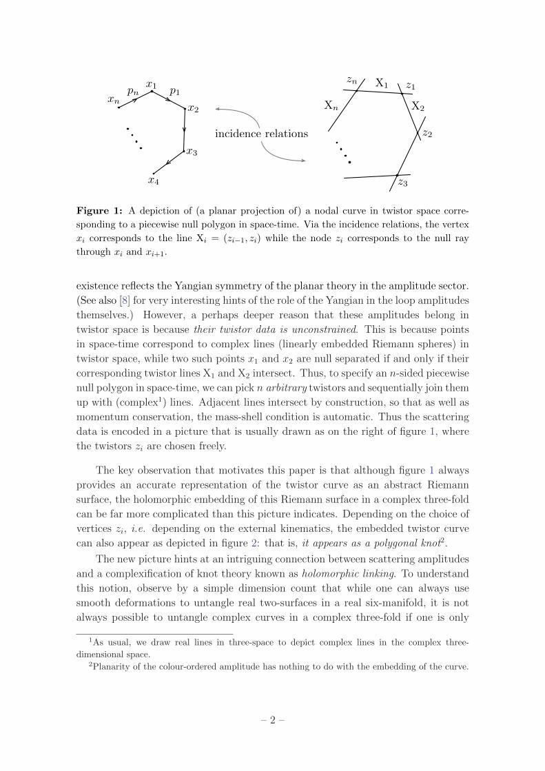

z1
z2
z3
z4
z5
z6
z7
z8
Figure 2 Depending on the location of the vertices the twistor lines may form a polygonal
knot The plane projection of the nodal curve can thus be far more involved than figure 1
suggests
allowed to vary the curve holomorphically (This restriction provides a second3 jus-
tification for the use of the half-dimensional representation in these figures) That
holomorphic linking in twistor space should encode interesting information about
gauge theories in space-time was originally envisaged by Atiyah [9] and Penrose [10]
Outside the twistor context holomorphic linking (and its relation to Abelian holo-
morphic Chern-Simons theory) has been studied by eg Khesin and Rosly [11] and
by Frenkel and Todorov [12]
It is the aim of this paper to elucidate and further investigate this link Consid-
erable evidence supporting the existence of such a relation comes from a conjecture
given by Mason and one of the present authors in [13] building on previous work by
Alday and Maldacena [14] using the AdSCFT correspondence and by Drummond
Korchemsky and Sokatchev [15] and by Brandhuber Heslop and Travaglini [16] in
space-time The conjecture states firstly that the complete classical S-matrix of
N = 4 super Yang-Mills is equivalent to the expectation value in the QFT defined
by the holomorphic Chern-Simons functional [17 18]
ShCS[A] =1
gs
int
CP3|4Ω and tr
(1
2A and partA+
1
3A andA andA
)(13)
of a certain operator defined over the complex curve C of figure 2 As we show in
section 2 this operator is a natural complexification of the standard Wilson Loop
operator given by the explicit formula
WR[C] = TrR P exp
(minusint
C
ω and A)
(14)
3The standard reason is that it gives a better picture of the structure of the nodes pictures of
2-surfaces incorrectly suggest that the component curves are tangent at the nodes
ndash 3 ndash
in terms of the connection (01)-form A where the precise definition of the meromor-
phic form ω and the meaning of the lsquopath-orderingrsquo symbol P is explained below The
expectation valuelangWR[C]
ranghCS
is thus a natural complexification of the expectation
valuelangWR[γ]
rang=
intDA eiSCS[A] TrR P exp
(minus∮
γ
A
)(15)
of a real Wilson loop in real Chern-Simons theory that famously computes knot
invariants [19] such as the HOMFLY polynomial (for gauge group U(N) and R the
fundamental representation)
Extrema of (13) correspond to holomorphic bundles on4 CP3|4 that (under mild
global conditions) in turn yield anti self-dual (or 12 BPS) solutions of the N =
4 super Yang-Mills equations on space-time via the Penrose-Ward correspondence
Thus holomorphic Chern-Simons theory corresponds only to the anti self-dual sector
of N = 4 SYM However it is possible to add a term to (41) so that the new action
corresponds to the complete (perturbative) N = 4 theory [20] The second part of
the conjecture of [13] is that when weighted by the exponential of this new actionlangW[C]
rangnow yields the complete planar S-matrix of N = 4 super Yang-Mills to all
orders in the rsquot Hooft coupling and for arbitrary external helicities
These conjectures were supported in [13] by perturbative calculations showing
that at least for small k and ` the axial gauge Feynman diagrams oflangW[C]
rangare
in one-to-one correspondence with MHV diagrams for the `-loop NkMHV scattering
amplitudes The momentum twistor formulation of the MHV diagram formalism
had previously been given in [21] and it has since been proved [22 23] that this
formalism correctly reproduces the all-loop recursion relation for the integrand of
planar N = 4 [7 24]
In this paper after reviewing the construction of the Wilson Loop operator
for a complex curve in section 2 we study a complex analogue of the Makeenko-
Migdal loop equations [25] for both the holomorphic Chern-Simons and N = 4 SYM
theories At least in principle these equations give a non-perturbative description of
the behaviour oflangW[C]
rangas C varies holomorphically
Now the loop equations for the expectation value (15) of a fundamental Wilson
Loop in real U(N) Chern-Simons theory were shown by Cotta-Ramusino Guadagnini
Martellini and Mintchev [26] to yield the skein relations for the HOMFLY polynomial
ndash in other words recursion relations allowing one to reconstruct the knot invariants
Quite remarkably in section 5 we find that (in the planar limit) the loop equations
forlangW[C]
rangmay be reduced to the BCFW relation [27] that recursively constructs
4The twistor superspace CP3|4 may be defined as the total space of (ΠOP3(1))oplus4
where OP3(1)
is the dual of the tautological line bundle on CP3 and Π reverses the Grassmann parity of the fibres
It is a Calabi-Yau supermanifold and we have written Ω for the canonical holomorphic section of
its Berezinian
ndash 4 ndash
the classical S-matrix The classical BCFW recursion relations thus emerge as a
holomorphic analogue of the skein relations for a knot polynomial Replacing the
pure Chern-Simons theory by the full N = 4 theory the loop equations involve a
new term and reduce instead to the recursion relation of Arkani-Hamed Bourjaily
Cachazo Caron-Huot and Trnka [7] for the all-loop integrand (See also [24] for
tentative extensions of this relation beyond N = 4 SYM) These results prove the
conjectures of [13] at least at the level of the integrand
Working in space-time Caron-Huot demonstrated in [28] that the expectation
value in N = 4 SYM of a certain extension of a regular Wilson Loop around the
null polygon on the left of figure 1 together with extra operator insertions at the
vertices also obeys the all-loop BCFW recursion relation This complete definition
of this Wilson Loop operator and the vertex insertions was not given in [28] but
it is expected to be fixed by supersymmetry Our proof that the twistor Wilson
Loop (with no extra insertions) obeys the same relation helps confirm that these two
approaches agree
There are at least two ways to view these results On the one hand accepting
the duality between scattering amplitudes and Wilson Loops one may see the loop
equations as providing an independent derivation of the all-loop BCFW recursion
relations However we prefer to interpret this work as a field theoretic explanation
for why the duality holds in the first place the behaviour of a scattering amplitude
near a factorisation channel is exactly equal to the behaviour of the twistor Wilson
Loop near a self-intersection Away from these singularities both the scattering
amplitudes and Wilson Loops are determined by analytic continuation of their data
For scattering amplitudes this is just the analyticity of the S-matrix as a function
of on-shell momenta encoding the familiar notions of crossing symmetry and space-
time causality while for Wilson Loops analyticity in the twistors zi expresses the
fact thatlangW[C]
ranggenerates analytic invariants associated to the holomorphic link
Finally although it is often said that BCFW recursion relations for scattering
amplitudes have little to do with Lagrangians path integrals or gauge symmetry our
work makes it clear that these standard tools of QFT are indeed intimately connected
to BCFW recursion from the point of view of Wilson Loops As always the Wilson
Loop is just the trace of the holonomy of a connection around a curve while the
loop equations themselves are derived from little more than the Schwinger-Dyson
equations of the appropriate path integral We view the connection to Lagrangians
and path integrals as a virtue because it suggests that BCFW-type techniques can be
applied to observables beyond scattering amplitudes Certainly the loop equations
we derive are valid for far more general curves than needed for scattering amplitudes
and for more general deformations than BCFW
ndash 5 ndash
z1
z2
z3
z4
z5
z6
z7
z8
Figure 3 Going beyond the application to scattering amplitudes we may allow the
component curves to have arbitrary degrees ge 1
2 Non-Abelian Holomorphic Wilson Loops
In this section we review the construction of [13] for a complex Wilson Loop defined
over a nodal curve C each of whose components is rational That is C = Z(Σ)
where Z is a holomorphic map to CP3|4 and the source curve
Σ = Σn cup middot middot middot cup Σ2 cup Σ1 (21)
with each component Σi rational and Σi+1capΣi = pt (i being counted mod n) For
scattering amplitudes we only need to consider the case that Z restricts to a linear
map on each irreducible component so that C generically appears as in figure 2
However it costs little to extend this to the case where each component is mapped
with arbitrary degree di ge 1 (shown in figure 3) and we allow this more general
possibility These curves may also be thought of as elliptic curves that have been
pinched n times around a given homology cycle They are certainly rather exotic
from the algebro-geometric point of view5 and it would clearly be interesting consider
the extension to non-degenerate elliptic curves
21 Holomorphic frames
Any Cinfin bundle E rarr CP3|4 is inevitably holomorphic on restriction to a arbitrary
complex curve C because D2|C = 0 trivially for dimensional reasons Suppose
first that C is a single irreducible rational curve Provided E|C is holomorphically
trivial6 we can find a gauge transformation h varying smoothly over C and such
5However it is curious that in the real category one often considers lsquotamersquo knots ndash ie knots
that are equivalent to an embedded polygon6By a theorem of Birkhoff and Grothendieck E|C =
oplusO(ai) withsumai = 0 if E|C is topolog-
ically trivial Triviality as a holomorphic bundle means that in addition ai = 0 for each i and
(perhaps surprisingly) is in fact generic
ndash 6 ndash
that
hminus1 (part +A)∣∣C h = part
∣∣C (22)
Under this gauge transformation covariantly holomorphic objects become simply
holomorphic on C so h is said to define a holomorphic frame for E|C It follows
from (22) that h itself obeys
(part +A)∣∣Ch = 0 (23)
and so is defined up to a gauge transform h rarr hhprime where hprime must be globally
holomorphic on C
For two points z0 z isin CP3|4 that lie on C we now define
U(z z0) equiv h(z)hminus1(z0) (24)
to be the particular solution of (23) obeying the initial condition that the gauge
transformation at z0 isin C is simply the identity The holomorphic frame U(z z0)
defines a map
U(z z0) E|z0 rarr E|z (25)
between the fibres of E at z0 and z isin CP3|4 that depends on the choice of curve
C (not unique if deg(C) gt 1) It is the natural complex analogue of the parallel
propagator U(x x0) between two points x and x0 along a real curve γ For example
it follows immediately from the definition (24) that
U(z zprime)U(zprime z0) = U(z z0) (26)
so that U(z z0) concatenates just as for the parallel propagator along a real curve
In particular U(z z0)U(z0 z) = U(z z) = 1R implying that
U(z0 z) = U(z z0)minus1 (27)
Likewise if we change our choice of connection (01)-form by a smooth gauge trans-
formation
A rarr Ag = g partgminus1 + gAgminus1 (28)
then since hminus1 (part +A)∣∣C h = (gh)minus1 (part +Ag)
∣∣C (gh) we find that
U(z z0)rarr g(z)U(z z0)gminus1(z0) (29)
again as for a parallel propagator in the real category
In the Abelian case with E a line bundle setting h = eminusφ for some smooth
function φ on C the holomorphic frame equation (23) becomes partφ = A|C This
equation always has a solution when C is rational given by
φ(z) =
int
C
ω and A (210)
ndash 7 ndash
where A is restricted to the curve and where ω is a meromorphic 1-form on C
whose only singularities are simple poles at z0 and z with residues plusmn1 respectively
Explicitly if C = Z(Σ) with Z(σ) = z isin CP3|4 and Z(σ0) = z0 then the pullback of
ω to Σ is
ω(σprime) =(σ minus σ0)
(σ minus σprime)(σprime minus σ0)
dσprime
2πi(211)
in terms of local coordinates σ isin Σ This is just the Greenrsquos function for the part-
operator acting on smooth functions on Σ The holomorphic frame equation fixes φ
only up to a globally holomorphic function which by Liouvillersquos theorem must be
constant The constant is fixed by the choice of reference point ω vanishes if z and
z0 coincide so (210) has φ(z0) = 0 Thus in the Abelian case we have the explicit
expression
U(z z0) = eφ = exp
(minusint
C
ω and A)
(212)
for our holomorphic frame
In the non-Abelian case acting on a representation R of the gauge group U(z z0)
may similarly be given by the (somewhat formal) expression7
U(z z0) = P exp
(minusint
C
ω and A) (213)
The meaning of the lsquopath orderingrsquo symbol P on our complex curve is that the ith
power of the meromorphic differential ω that appears from expanding the exponential
in (213) should be taken to have its simple poles located at the reference point z0 and
at either the insertion point of the (i+ 1)th power of the field A (counting according
to the colour-ordering) or else at the final evaluation point z Specifically
P exp
(minusint
C
ω and A)equiv 1R +
infinsum
m=1
(minus1)mint
(C)m
mand
i=1
(ω(zi) and A(zi)
)(214)
where ω(zi) is a meromorphic differential in zi with a simple pole at z0 and a simple
pole at zi+1 (or at z when i = m) Explicitly in terms of intrinsic coordinates
mand
i=1
ω(σi) =(σ minus σ0)
(σ minus σm) middot middot middot (σ2 minus σ1)(σ1 minus σ0)
dσm2πiand middot middot middot and dσ1
2πi (215)
7An equivalent formal expression given in [13] is U(z z0) =(
1 + partminus1A∣∣C
)minus1 where in the
series expansion of this expression the inverse part-operators are taken to act on everything to their
right
ndash 8 ndash
Equation (213) is thus analogous to the (equally formal) expression
P exp
(minusint x
x0
A
)
= 1R minusint x
x0
dymicroAmicro(y) +
int x
x0
dymicroAmicro(y)
int y
x0
dyprimeνAν(y
prime) minus middot middot middot
= 1R +infinsum
m=1
(minus1)mint
([01])m
dsm middot middot middot ds1 Amicro(sm)dxmicro
dsmθ(smminussmminus1) middot middot middot θ(s2 minus s1)Aν(s1)
dxν
ds1
(216)
for the parallel propagator of a connection d +A = dxmicro(partmicro +Amicro) along a real curve
γ where the step functions obey
part
partsθ(sminus sprime) = δ(sminus sprime) (217)
and are the Greenrsquos function for the exterior differential on the interval [0 1] We also
note that the iterated integrals appearing in (213) are somewhat similar to iterated
integrals that arise in studying parallel transport via the Knizhnik-Zamolodchikov
connection over the configuration space of n-points on a rational curve See [29] for
a recent discussion of this in a twistor context
22 The holonomy around a nodal curve
Having identified the holomorphic frame U(z z0) = h(z)hminus1(z0) as the natural ana-
logue of a parallel propagator for a complex curve we can define the holonomy of the
connection (01)-form around C based at some point z isin CP3|4 to be the ordered
product
Holz[C] equiv U(z zn) U(zn znminus1) middot middot middotU(z2 z1) U(z1 z) (218)
where zi is the image of the node Σi+1 cap Σi and where without any essential loss
of generality we have taken the base point to be on Z(Σ1) Reading from the right
of (218) this definition uses the holomorphic frame U(z1 z) on Z(Σ1) to map the
fibre E|z to the fibre E|z1 at the node z1 We can identify this fibre with a fibre of
E restricted to the next component line Z(Σ2) and then map to the following node
using the holomorphic frame U(z2 z1) on Z(Σ2) We continue transporting our fibre
around the nodal curve in this way until the final factor of U(z z1) returns us to the
starting point The result is thus an automorphism of the fibre E|z as required
The holomorphic Wilson Loop is now defined as in the real category as
WR[C] equiv TrR Holz[C] (219)
where to take the trace in a representation R we have used the fact that a holomorphic
frame for E|C induces a holomorphic frame for all tensor products of E|C and its
dual in other words for all choices of representation Cyclicity of the trace and the
ndash 9 ndash
concatenation property (26) immediately shows that the Wilson Loop is independent
of the base point
For an Abelian gauge group (E a line bundle) the holomorphic frame (212) gives
W[C] = exp
(minusint
C
ω and A)
(220)
where ω is a meromorphic form on C whose only singularities are simple poles at
each of the nodes with residues plusmn1 on each component Such a differential is nothing
but the holomorphic differential θ on a non-singular elliptic curve in the limit that
this curve degenerates to our nodal curve (see eg [30]) Thus in the Abelian case
we recover the prescription
W[C] = exp
(minusint
C
θ and A)
(221)
that was proposed by Thomas [31] by Khesin and Rosly [11] and by Frenkel and
Todorov [12] For a non-Abelian gauge group we can likewise use (213) to formally
write
WR[C] = TrR P exp
(minusint
C
ω and A)
(222)
as a natural complexification of the familiar expression
WR[γ] = TrR P exp
(minusint
γ
A
)(223)
for a Wilson Loop of a connection on a real curve γ In equation (222) as in (213)
the path ordering symbol means that for each component of C successive powers of
ω in the series expansion of (222) should have one simple pole at one of the nodes
and another at the subsequent (with respect to the colour-ordering) insertion point
of the field
3 A Holomorphic Family of Curves
We now investigate the behaviour of our complex Wilson Loop as the curve C varies
We shall prove that just as the change in the real Wilson Loop (223) under a smooth
deformation of a real curve γ is
δWR[γ] = minus∮
γ
dxmicro δxν TrR
(Fmicroν(x) Holx[γ]
) (31)
so too the complex Wilson Loop (219) obeys
δWR[C] = minusint
C
ω(z) and dzα and δzβ TrR
(Fαβ(z z) Holz[C]
)(32)
ndash 10 ndash
as the complex curve C moves over a holomorphic family In this equation δ is the part-
operator on the parameter space of the family and once again ω(z) is a meromorphic
differential on C whose only singularities are simple poles at the nodes with residues
plusmn1 Like its real analogue equation (32) expresses the change in the Wilson Loop
in terms of the curvature (02)-form F = partA+AandA through the complex 2-surface
swept out by the varying curve The key point here is that because the curve C varies
holomorphically only the (02)-form part of the curvature arises In particular if E
is a holomorphic bundle on twistor space then the Wilson Loop is also holomorphic
As before we prove (32) in more generality than we actually need for scattering
amplitudes allowing each irreducible component Ci = Z(Σi) to have degree di ge 1
Here is the proof8 For a fixed partial connection the holomorphic frame U(z1 z0)
depends on the choice of two points z0 z1 isin CP3|4 together with a choice of (ir-
reducible rational) curve C that joins them (Note that this curve is not unique
if its degree is greater than 1) Equivalently we can think of this data in terms of
an abstract Riemann sphere Σ together with two marked points σ0 σ1 isin Σ and
a degree d holomorphic map Z Σ rarr CP3|4 such that Z(Σ) = C and Z(σi) = zi
Now suppose we have a holomorphic family of such maps parametrized by a mod-
uli space B described say by local holomorphic coordinates ti Writing U(σ σ0 t)
for the pullback of U(z z0) to the abstract curve Σ for our family of curves the
holomorphic frame equation is
(part + ZlowastA)U(σ σ0 t) = dσ
(part
partσ+Aα
partzα
partσ(σ t)
)U(σ σ0 t) = 0 (33)
where we emphasise that both the holomorphic frame and the connection depend on
t ndash ie on the choice of curve
Consider the integral
int
Σ
ω10(σ) and U(σ1 σ t) (part + ZlowastA)U(σ σ0 t) (34)
over Σ where ω10(σ) is our familiar meromorphic differential (211) whose only
singularities are simple poles at σ0 and σ1 with residues +1 and minus1 respectively
and where part +A is as given in (33) In principle the integral depends on these two
points and on the map Z ndash that is it depends on the moduli space ndash but of course
it actually vanishes identically on B since U(σ σ0) obeys (33)
8It is also possible to show (32) by working directly with the formal expression (222) provided
(as in the real case) due care is taken of the lsquopath orderingrsquo
ndash 11 ndash
Letting δ be the part-operator on B we have
0 = δ
[int
Σ
ω10(σ) and U(σ1 σ t)(part + ZlowastA
)U(σ σ0 t)
]
=
int
Σ
ω10(σ) and U(σ1 σ t)(part + ZlowastA
)δU(σ σ0 t)
minusint
Σ
ω10(σ) U(σ1 σ t) and δ(ZlowastA) U(σ σ0 t)
= minusδU(σ1 σ0 t)minusint
Σ
ω10(σ) U(σ1 σ t) and δ (ZlowastA) U(σ σ0 t)
(35)
where the third line follows from integrating by parts in the first term then using the
poles of ω10 and the fact that partU(σ1 σ t) = U(σ1 σ t)ZlowastA to perform the integral9
In the final term of (35) we have
δ (ZlowastA) =
(partβAα
partzβ
parttıpartzα
partσ+Aα
part2zα
parttı partσ
)dtı and dσ (36)
The most important property here is that because the map Z varies holomorphically
only antiholomorphic derivatives of the connection arise Again integrating by parts
we find that
DBU(σ1 σ0 t) equiv δU(σ1 σ0 t) +A(z(σ1 t))U(σ1 σ0 t)minus U(σ1 σ0 t)A(z(σ0 t))
= minusint
Σ
ω10(σ) and dσ and dtı U(σ1 σ t)Fαβpartzα
partσ
partzβ
parttıU(σ σ0 t)
= minusint
C
ω10(z) and dzα and δzβ U(z1 z)Fαβ(z) U(z z0)
(37)
where DB is the natural covariant part-operator acting on sections of the sheaf E over
B induced by10 E
Equation (37) tells us how the holomorphic frame U(z1 z0) on an irreducible
curve varies as we move around in the moduli space For the Wilson Loop (219) on
9In fact the moduli space B may be identified with the Kontsevich moduli space M02(CP3|4 d)
of stable 2-pointed degree d maps Because it depends on three points σ0 σ1 σ isin Σ as well as
Z the integrand in (34) really lives on the universal curve C equiv M03(CP3|4 d) and the pullback
by the map Z is more properly written as the pullback by the evaluation map on the third marked
point (labelled σ) The integral itself is really the pushdown by the forgetful map π C rarr B and in
commuting δ past the integral sign in (35) we really mean the pullback πlowastδ = partCminuspartCB = partCminuspartΣ
Then (36) is just the statement that the evaluation map is holomorphic and so commutes with partC
with the partΣ term left over10More accurately E = πlowastevlowastσE
ndash 12 ndash
a nodal curve we now readily find
δWR[C(t)] =nsum
i=1
TrR
((DBU(zi+1 zi)
)U(zi ziminus1) middot middot middotU(zi+2 zi+1)
)
= minusint
C(t)
ω(z) and dzα and δzβ TrR
(Fαβ(z z) Holz[C(t)]
) (38)
where the integral is taken over the complete nodal curve C(t) = Z(Σ) and we
emphasise that this curve depends on the moduli of the map As usual ω(z) is a
meromorphic differential on C(t) with only simple poles at the nodes This completes
the proof
4 Holomorphic Loop Equations
In this section we derive an analogue of the loop equations of Makeenko and Migdal [25]
for our complex Wilson Loops To do this instead of considering the complexified
Wilson Loop itself we must study its averagelangWR[C]
rangover the space of gauge-
inequivalent connection (01)-forms on E weighted by the exponential of an appro-
priate action
In section 41 we choose the action to be the U(N) holomorphic Chern-Simons
functional
ShCS[A] =1
g2
int
CP3|4
D3|4z and tr
(1
2A and partA+
1
3A andA andA
) (41)
that may be interpreted as the open string field theory of the perturbative B-
model [17 18] In real Chern-Simons theory on a real 3-manifold M the correlation
function of a Wilson Loop gives a knot invariant Since these invariants depend
only on the (regular) isotopy class of the knot one expects that unlike WR[γ] itselflangWR[γ]
rangCS
should remain invariant as one smoothly deforms γ This is essentially
true except that there are important corrections when the deformation causes γ to
pass through a self-intersection so that the isotopy class of the knot jumps The
loop equations determine the behaviour oflangWR[γ]
rangCS
under such a jump and it was
shown in [26] that for Wilson Loops in the fundamental representation of U(N)
they amount to the skein relations
s12P+(r s)minus sminus 1
2Pminus(r s) = (r12 minus rminus 1
2 )P0(r s) (42)
from which the HOMFLY polynomial Pγ(r s) can be recursively constructed11
11The variables of the HOMFLY polynomial are related to N and the level k of the Chern-Simons
theory by and s = eλ and r = eλN where λ equiv 2πiN(k + N) may be interpreted as the rsquot Hooft
coupling In [26] the skein relations were obtained to lowest order in λ The skein relation only
determines the HOMFLY polynomial for Wilson Loops in the fundamental
ndash 13 ndash
We expect that correlation functions of our Wilson Loops in the holomorphic
Chern-Simons QFT are likewise associated with holomorphic linking invariants In-
deed [11 12] show that for two non-intersecting curves C1 C2 sub C3 of genera gi ge 1
the expectation valuelangW[C1] W[C2]
rangin Abelian holomorphic Chern-Simons theory
on C3 involves12 the holomorphic linking invariant
L(C1 θ1C2 θ2) =1
4π
int
C1timesC2
εık(z minus w)ı
|z minus w|6 dz and dwk and θ1 and θ2 (43)
that generalizes the Gauss linking number
L(γi γj) =1
4π
int
γitimesγj
εijk(xminus y)i
|xminus y|3 dxj and dyk (44)
in for real Abelian Wilson Loops in R3 Observe that (43) depends on a choice of
holomorphic 1-form θi on each curve For our nodal curve the corresponding form is
meromorphic and depends on the location of the nodes In section 41 we shall find
that δlangWR[C]
ranghCS
generically vanishes with important corrections when the type
of the curve jumps In the planar limit the loop equations may be reduced to the
BCFW relations [27] that recursively construct the classical S-matrix In this sense
the BCFW relations are simply the U(infin) skein relations for the holomorphic link
defined by C
As mentioned in the introduction holomorphic Chern-Simons theory on CP3|4
corresponds only to the anti self-dual sector of N = 4 super Yang-Mills theory on
space-time In section 42 we replace (41) by the action [20]
SN=4[A] = ShCS[A] +
int
Γ
d4|8x ln det(part +A)∣∣X
(45)
that as our notation indicates describes N = 4 super Yang-Mills theory on twistor
space We shall see that the new term is itself eminently compatible with the Wilson
Loop The loop equations in this theory involve a new term that leads to the all-loop
extension of the BCFW relations found by Arkani-Hamed et al in [7]
41 Holomorphic linking
In this section we choose the action to be the holomorphic Chern-Simons func-
tional (41) where D3|4z is the canonical holomorphic section of the Berezinian of
CP3|4 given explicitly by
D3|4z equiv 1
4εαβγδz
αdzβ and dzγ and dzδ1
4εabcddψ
a dψb dψc dψd (46)
12We will see later that at least for the N = 4 theory lsquoholomorphic self-linkingrsquo is well-defined
even without a choice of framing
ndash 14 ndash
in terms of homogeneous coordinates (zα ψa) isin C4|4 This action is defined on the
space A 01 of partial connections D on a Cinfin vector bundle E rarr CP3|4 given at least
locally by D = part+A in terms of a background partial connection part We take this to
obey part2 = 0 and so define a background complex structure on E Thus A(z z ψ)
is a superfield with component expansion
A(z z ψ) = a(z z) + ψaΓa(z) +1
2ψaψb Φab(z z) + middot middot middot+ 1
4εabcdψ
aψbψcψd g(z z)
(47)
where the coefficient of (ψ)r is a (01)-form on CP3 valued in smooth sections of
End(E)otimesOCP3(minusr)We choose the gauge group to be U(N) and consider only Wilson Loops in the
fundamental representation The Yang-Mills (or open string) coupling g2 is then
related to the Chern-Simons level k by g2 = 2π(k + N) In anticipation of taking
the planar limit we write g2 = λN in terms of the rsquot Hooft coupling λ and include
a factor of 1N in definition of the Wilson Loop so that W[C] = 1 if the holonomy
is trivial
Inserting (32) into the holomorphic Chern-Simons path integral one finds
δlangW[C(t)]
rang= minus 1
N
intDA
[int
C(t)
ω(z) and dzα and δzβ tr(Fαβ(z) Holz[C(t)]
)]eminusShCS[A]
=λ
N2
intDA
[int
C(t)
ω(z) and tr
(Holz[C(t)]
δ
δA(z)eminusShCS[A]
)]
(48)
since the variation of the holomorphic Chern-Simons functional is F02 times Nλ To
obtain an interesting equation for δlangW[C(t)]
rang as in [25] we integrate by parts in
the path integral bringing the variation of the connection to act on the holonomy
Essentially the same argument as in section 3 shows that under a variation of the
connection at some point zprime isin C (displaying colour indices)
0 =
[δ
δA(z)
i
j
(int
C
ω10(zprime) and U(z1 zprime)(part +A
)C
U(zprime z0)
)k
l
]
= minus[
δ
δA(z)
i
j
U(z1 z0)kl
]+
int
C
ω10(zprime) and U(z1 zprime)kj δ
3|4(z zprime) U(zprime z0)i l
(49)
where we have used the fact that for a U(N) gauge group
(δδA(z))i j A(zprime)mn = δ3|4(z zprime) δinδmj (410)
with δ3|4(z zprime) a Dirac current concentrated on the diagonal in CP3|4z times CP3|4
zprime ie
δ3|4(z zprime) is a distribution-valued (03)-form on CP3|4z times CP3|4
zprime such that for any α isinΩ0p(CP3|4) we have
int
CP3|4D3|4zprime and δ3|4(z zprime) and α(zprime) = α(z) (411)
ndash 15 ndash
z
z
C(t)
C(t)
Figure 4 The expectation valuelangW[C(t)]
rangin holomorphic Chern-Simons theory varies
holomorphically except where the curve develops a new node
Explicitly δ3|4(z zprime) may be represented by the integral [5 32]
δ3|4(z zprime) =
intdu
uand δ4|4(z minus uzprime) =
intdu
u
4and
α=1
part1
zα minus uzprimeα4prod
a=1
(ψa minus uψprimea) (412)
that forces zα prop zprimeα so that the two point must coincide projectively
We now apply equation (49) to the variation holonomy based say at a point
z isin C1 One finds
tr
(δ
δA(z)Holz[C(t)]
)=
δ
δA(z)
i
j
[U(z zn)jkU(zn znminus1)kl middot middot middotU(z1 z)
mi
]
=sum
i
int
Ci(t)
ωi+1i(zprime) and δ3|4(z zprime) tr
[U(z zn) middot middot middotU(zi+1 z
prime)]
tr[U(zprime zi) middot middot middotU(z1 z)
]
(413)
The factor of δ3|4(z zprime) ensures that this term has support only at points t in the
moduli space where the curve C(t) degenerates so that the component C1(t) ei-
ther self-intersects or else intersects some other component Similar contributions
arise from summing over the possible locations of the base-point z In other words
thinking of our original curve as an elliptic curve δlangW[C(t)]
rangvanishes everywhere
except on boundary components of the moduli space where the holomorphic map
degenerates so that two points on the source curve are mapped to the same image
Combining all the terms the holomorphic Chern-Simons loop equations (48)
become
δlangW[C(t)]
rang= minusλ
int
C(t)timesC(t)
ω(z) and ω(zprime) and δ3|4(z zprime)langW[C prime(t)] W[C primeprime(t)]
rang (414)
for normalised Wilson Loops in the fundamental of a U(N) gauge group where C prime(t)
and C primeprime(t) are the two curves obtained by ungluing C(t) at its new node z = zprime (see
figure 4) In the planar limit the correlation function of a product of Wilson Loops
factorizes into the product of correlation functions so (414) simplifies to
δlangW[C(t)]
rang= minusλ
int
C(t)timesC(t)
ω(z) and ω(zprime) and δ3|4(z zprime)langW[C prime(t)]
rang langW[C primeprime(t)]
rang(415)
ndash 16 ndash
where λ is the rsquot Hooft coupling Thus in the planar limit the behaviour at a self-
intersection is determined by the product of the expectation values of the Wilson
Loops around the two lower degree curves This may be viewed as an analogue
for holomorphic linking of the skein relations for real knot invariants In section 5
we shall see that the classical BCFW recursion relations are simply a special case
of (415)
42 Loop equations for the twistor representation of N = 4 SYM
We now consider the expectation value of the complex Wilson Loop in the twistor
action
SN=4[A] = ShCS[A] +
int
Γ
d4|8x log det(part +A)∣∣X (416)
where X is a line in twistor space and Γ is a middle-dimensional contour in the
space Gr2(C4) of these lines13 interpreted as a choice of real slice of complexified
conformally compactified space-time The proof that (416) is an action for N = 4
SYM on twistor space is given in [20] to which the reader is referred for further
details (Readers familiar with the MHV formalism may note that the new term
in (416) provides an infinite series of MHV vertices while the 3-point MHV vertex
in the Chern-Simons theory vanishes in an axial gauge From the point of view
of twistor string theory [18] the determinant may be understood as the partition
function of a chiral free fermion CFT on X coupled to the pullback of the twistor
space gauge field)
From the point of view of the present article it is possible to motivate this action
by observing that Wilson Loops on complex curves are again the natural observables
of the QFT based on (416) The reason this is so is because of the close connection
between determinants and holonomies More precisely just as
δ log detM = δ tr logM = tr(Mminus1δM) (417)
for a finite dimensional matrix M Quillen shows [33] that for an abstract curve Σ
under a variation of the connection the logarithm of a section of the determinant
line bundle Detrarr A 01Σ varies as14
δ log det(part +A)∣∣Σ
=
int
Σ
tr (JA and δA) (418)
where
JA(σ) equiv limσprimerarrσ
(GA(σprime σ)minusG0(σprime σ)
)(419)
13The fermionic integral is done algebraically as always14In writing this formula we assume that δ is a flat connection on Det in a trivialisation where
the local connection 1-form vanishes That Det should admit such a flat connection is necessary if
we wish to treat det(part +A)Σ as a (holomorphic) function on A 01Σ (the space of connection (01)-
forms on Σ) However [33] the construction of this flat connection requires a choice of background
connection
ndash 17 ndash
is the limit15 on the diagonal in Σ times Σ of difference between the Greenrsquos function
for part +A|Σ and the Greenrsquos function for background connection partΣ These Greenrsquos
functions are non-local operators on the Riemann surface the fact that we take their
limit on the diagonal can be understood as part of the trace For a single such Greenrsquos
function the limit on the diagonal is necessarily singular but the singularity cancels
in the difference (419) The dependence on a background connection reflects the fact
that to treat sections of the determinant line bundle as functions we must first pick
a trivialisation amounting to a choice of background connection (01)-form on the
bundle over Σ In our case we will of course choose this background part-operator to
be the one induced by our choice of base-point part isin A 01Σ in writing the holomorphic
Chern-Simons action
When Σ is a Riemann sphere the Greenrsquos functions are
GA(σprime σ) = h(σprime)G0(σprime σ)hminus1(σ) and G0(σprime σ) =1
2πi
dσ
σprime minus σ (420)
in terms of the holomorphic frame h on Σ Therefore Quillenrsquos prescription reduces
to
JA(σ) =dσ
2πilimσprimerarrσ
U(σprime σ)minus U(σ σ)
σprime minus σ =dσ
2πi
partU(σprime σ)
partσprime
∣∣∣∣σprime=σ
(421)
For our purposes the presence of the holomorphic derivative here is somewhat in-
convenient However it is easily seen from the formal series (214) that U(σprime σ)
depends only meromorphically on σprime and is regular at σprime = σ Thus we can use
Cauchyrsquos theorem to rewrite the derivative in (421) as an integral so
δ log det(part +A)∣∣Σ
=1
(2πi)2
int
Σ
dσ and tr
(∮dσprime
(σ minus σprime)2U(σprime σ) δA(σ)
)
=1
(2πi)3
int
ΣtimesS1timesS1
dσ and dσprime and dσprimeprime
(σ minus σprime)(σprime minus σprimeprime)(σprimeprime minus σ)tr (U(σprime σ) δA(σ))
(422)
where the integrals over σprimeprime and σprime are performed over contours encircling the poles at
σprimeprime = σprime and σprime = σ respectively (The reason for introducing the new point σprimeprime isin Σ
will become clear momentarily)
To apply this to the case that Σ = Zminus1(X) for X a line in twistor space suppose
Z(σprimeprime) = za Z(σprime) = zb and Z(σ) = z = za + σzb (423)
so that X = Span[za zb] Then
dσ and dσprime and dσprimeprime
(σ minus σprime)(σprime minus σprimeprime)(σprimeprime minus σ)= Zlowast
[ωab(z) and 〈a da〉 and 〈b db〉
〈a b〉2]
(424)
15Below this limit will be revealed as nothing but the forward limit of an amplitude
ndash 18 ndash
where ωab(z) is meromorphic with only simple poles only z = za and zb and where
〈a da〉〈b db〉〈a b〉2 is the fundamental bi-differential on X with a double pole along
the diagonal This bi-differential combines with the integral over the space of lines
X since
d4|8x and 〈a da〉 and 〈b db〉〈a b〉2 = D3|4za andD3|4zb (425)
giving a contour integral over CP3|4a timesCP3|4
b Therefore the variation of the new term
in the action is
δ
int
Γ
d4|8x log det(part +A)∣∣X
=
int
ΓtimesXtimesS1timesS1
D3|4za andD3|4zb(2πi)3
and ωab(z) tr(
U(zb z) δA(z))
(426)
where the S1 times S1 contour sets za rarr z and zb rarr z differentiating U(zb z) in the
process The integral over all z isin X is performed using the dependence on z in the
holomorphic frame and in the variation of the connection
Equation (426) expresses the variation of the logarithm of the determinant in
the twistor action (416) in terms of a holomorphic frame on the line X It dovetails
beautifully with the holonomy around the curve C providing a new contribution
minus λN
int
ΓtimesS1timesS1
D3|4za andD3|4zb
int
C(t)timesX
ω(z) and ωab(z) and δ3|4(z z) tr(
U(zb z) Holz[C(t)])
(427)
to the loop equations The δ-function δ3|4(z z) in this expression means that this
term only contributes at points in the moduli space where the curve C(t) 3 z inter-
sects the line X 3 z The integral over Γ then adds up these contributions for each
X isin Γ
To interpret the product U(zb z) Holz[C(t)] replace C(t) by a curve C(t) where
C(t) cap X = z zb isin CP3|4 (428)
and such that as zb rarr z C(t) rarr C(t) As a nodal curve C(t) has one more
component than C(t) with one component becoming double covered in the limit
(see figure 5) Now because the contour integral forces zb = z we can replace the
holonomy around C(t) based at z = z = C(t) cap X by a product of holomorphic
frames that transport us around C(t) from zb to z The remaining factor of U(zb z)
transports this frame back to zb along X The resulting trace can be interpreted as
Wilson Loop around C(t) cup X so that
1
Ntr(
U(zb z)Holz[C(t)])
= W[C(t) cup X] (429)
provided we are inside the contour integral over the location of zb sub X
ndash 19 ndash
=
X
z = zC
X
C zb
z
Figure 5 The new term in the loop equations for N = 4 SYM can be understood as a
holomorphic Wilson Loop around a new curve C cupX where C reduces to C when zb rarr z
along X Note that the nodal curve C has one more component than C In the scattering
amplitude context 〈W[C cup X]〉 may be interpreted as a forward limit of an n+ 2 particle
amplitude
Finally then we see that the holomorphic loop equations for the twistor repre-
sentation of planar N = 4 SYM are
δlangW[C(t)]
rang= minus λ
int
C(t)timesC(t)
ω(z) and ω(zprime) and δ3|4(z zprime)langW[C prime(t)]
rang langW[C primeprime(t)]
rang
minus λ
int
ΓtimesS1timesS1
D3|4za andD3|4zb
int
C(t)timesX
ω(z) and ωab(z) and δ3|4(z z)langW[C(t) cup X]
rang
(430)
and as in the original equations of Migdal amp Makeenko [25] are entirely expressed
in terms of expectation values of our (complexified) Wilson Loops In the following
section we show that for a particular one-parameter family of curves C(t) this holo-
morphic loop equation reduces to the all-loop BCFW recursion relation found in [7]
but we emphasise that (430) is valid for a far more general class of curves
5 BCFW Recursion from the Loop Equations
We now apply the holomorphic loop equation (430) to the case that each component
of C is a line as in figure 2 C can be completely specified by giving the location
of its n nodes and we shall often write C = (12) cup (23) cup middot middot middot cup (n1) for the curve
(where (i i+1) equiv Span[zi zi+1]) and W[1 2 n] for the corresponding Wilson Loop
(in the fundamental representation) We wish to show that the loop equations forlangW[1 2 n]
rangdirectly reduce to the all-loop BCFW recursion relations of Arkani-
Hamed et al [7] although it is important that our derivation of these relation is
completely independent of any notions of scattering theory
ndash 20 ndash
z1
z2
z3
z4
z5
z6
z7
z8
z8 t
Figure 6 The family of nodal curves C(t) corresponding to a BCFW deformation of a
planar amplitude in N = 4 SYM shown for n = 8 As we vary over the moduli space the
line (1 n(t)) sweeps out a pencil of lines in the plane (nminus1 n 1) with focus z1 This plane
necessarily intersects every other component of C(t)
Consider the holomorphic family of Wilson Loops determined by translating the
node zn along the line (nminus1 n) That is we define
zn(t) equiv zn + tznminus1 (51)
and consider the 1-parameter family of holomorphic curves
C(t) equiv (12) cup (23) cup middot middot middot cup (nminus1 n(t)) cup (n(t) 1) (52)
as shown in figure 6 Notice that although t can be thought of as a local holomorphic
coordinate on the line (nminus1n) it is really a coordinate on the moduli space of our
family of curves ie a coordinate on a CP1 sub B As t varies the line (n(t) 1) sweeps
out the plane (nminus1 n 1) with all other components of C(t) remaining fixed Lines
and planes necessarily intersect16 in CP3 so for every j = 3 nminus1 there exists a tjfor which (n(tj) 1) intersects the component Cj Let us call this intersection point
Ij and write nj for the point zn(tj) Clearly we have
Ij = (nminus1 n 1) cap (jminus1 j) and nj = (nminus1 n) cap (jminus1 j 1) (53)
essentially by definition (Note that we do not get any new intersections when j =
n 1 2)
16Lines and planes do not necessarily intersect in the superspace CP3|4 because they might lsquomissrsquo
in the fermionic directions The fermionic δ-functions in the δ3|4(z zprime) ensure that the right hand
side has support only when the curves do intersect in the superspace See also the discussion in [21]
ndash 21 ndash
We now study the loop equations for this family Considering first the case of
pure holomorphic Chern-Simons theory (415) becomes
minusint
CP1
dt
tand δlangW[C(t)]
rang=
λnminus1sum
j=3
int
CP1timesC1(t)timesCj
dt
tand ω(z) and ω(zprime) and δ3|4(z zprime)
langW[C prime(t)]
rang langW[C primeprime(t)]
rang (54)
whereC prime(t) = (12) cup (23) cup middot middot middot cup (jminus1 Ij)
C primeprime(t) = (Ij j) cup (j j+1) cup middot middot middot (nj 1)(55)
and where we have integrated (415) over our moduli space CP1 sub B using the
meromorphic differential dtt We can dispose of the left hand side immediately
integrating by parts gives
minusint
CP1
dt
tand δlangW[C(t)]
rang=langW[C(0)]
rangminuslangW[C(infin)]
rang
=langW[1 2 n]
rangminuslangW[1 2 nminus1]
rang
(56)
the difference of the Wilson Loops around the original curve and the curve with
zn = znminus1 Notice that the holomorphic frame U(zn znminus1)rarr 1 as zn rarr znminus1 so that
while the line (nminus1 n) does not simply lsquodisappearrsquo from the picture neither does it
contribute to the holonomy
The right hand side of (54) is almost as straightforward to compute because the
integrals over both the CP1 moduli space and the two copies of C(t) are completely
fixed by the δ-function δ3|4(z zprime) Since z isin (n(t) 1) and zprime isin (jminus1 j) we can
parametrize these integrals by setting
z = zn(t) + sz1 = zn + tznminus1 + sz1 and zprime = zjminus1 + rzj (57)
in terms of local coordinates r and s on C1(t) and Cj respectively With these
coodinates the meromorphic forms ω(z) and ω(zprime) become simply
ω(z) =ds
sand ω(zprime) =
dr
r(58)
which indeed have simple poles at the nodes of C1(t) and Cj as required Performing
the integral is then merely a matter of using the explicit form (412) of δ3|4(z zprime) and
computing a Jacobian In fact this integral is
[nminus1 n 1 jminus1 j] equivint
dr
r
ds
s
dt
t
du
uδ4|4(zn + tznminus1 + sz1 + uzjminus1 + rzj) (59)
ndash 22 ndash
which was shown in [5] to be just the basic dual superconformal invariant R1jn of [6]
Including the product of the two Wilson Loops on the smaller curves we find that
the loop equations in pure holomorphic Chern-Simons theory reduce to
langW[1 n]
rang=langW[1 nminus1]
rang
+ λnminus1sum
j=3
[nminus1 n 1 jminus1 j]langW[1 jminus1 Ij]
rang langW[Ij j nminus1 nj]
rang
(510)
where Ij and nj were given in (53) Re-interpreting the twistor space as momentum
twistor space this is just the tree-level BCFW recursion relation [27] in the momen-
tum twistor form given in [7] summed over all MHV degrees Expanding (510) in
powers of the Grassmann coordinates ψ at each vertex gives the BCFW relations for
specific NkMHV partial amplitudes
Turning now to the full N = 4 theory from (430) we have an additional contri-
bution
λ
int
ΓtimesS1timesS1
D3|4za andD3|4zb
int
CP1timesC(t)timesX
dt
tand ω(z) and ωab(z) and δ3|4(z z)
langW[C(t) cup X]
rang
(511)
where
C(t) cup X = (12) cup middot middot middot (nminus1 n(t)) cup (z b) cup (b 1) (512)
is our n + 2 component curve Once again the integrals inside the square brackets
are completely fixed by the δ3|4(z z) The intersection point z and the point n(t) are
fixed to be
z = (a b) cap (nminus1 n 1) and n(t) = (nminus1 n) cap (a b 1) (513)
and the Jacobian from the t z and z integrals gives the R-invariant [nminus1 n 1 a b]
The N = 4 loop equations thus reduce to
langW[1 n]
rang=langW[1 nminus1]
rang
+ λ
nminus1sum
j=3
[nminus1 n 1 jminus1 j]langW[1 jminus1 Ij]
rang langW[Ij j nminus1 nj]
rang
+ λ
int
ΓtimesS1timesS1
D3|4za andD3|4zb [nminus1 n 1 a b ]langW[1 nminus1 nab z zb]
rang
(514)
where we remind the reader that the S1timesS1 contour is taken to fix zab rarr z along X
(the R-invariant has a simple zero in this limit cancelling one of the factors of 〈za zb〉in the denominator of the measure) Re-interpreting the twistor space as momentum
ndash 23 ndash
twistor space this is the extension of the BCFW recursion for the all-loop integrand
found by Arkani-Hamed et al in [7]
Let us conclude with a few remarks Firstly the explicit power of the rsquot Hooft
coupling λ is present in (514) because our normalisation of the twistor action cor-
responds to the normalisation 14g2
inttr(F and lowastF ) = N
4λ
inttr(F and lowastF ) of the space-time
Yang-Mills action In this normalisation n-particle `-loop scattering amplitudes are
proportional to λ`minus1Nχ (with χ = 2 for planar diagrams) If one rescales the twistor
(or space-time) connection as A rarrradicλA the explicit λ disappears from (514) and
the `-loop planar scattering amplitude corresponds to the coefficient of λ(n+2`minus2)2
Secondly when computing real knot (rather than link) invariants it is necessary
to choose a lsquoframingrsquo ndash roughly a thickening of the knot into a band For Wilson
Loops in real Chern-Simons theory this may be understood perturbatively as a
point-splitting procedure that regularises potential divergences as the two ends of a
propagator approach each other along the knot γ This would seem to be particularly
important in the case that γ has cusps Above however we made no attempt to
choose a lsquoholomorphic framingrsquo of C In fact at least for the pure holomorphic
Chern-Simons theory this does not seem to be necessary Consider for example a
propagator stretched between two adjacent line components of C say (iminus1 i) and
(i i+1) We can regularise any potential divergence in this propagator by ungluing
the node replacing (i i+ 1) rarr (iε i+ 1) where ziε = zi + εzprime for some arbitrary
point zprime As shown in [13] the integral of an axial gauge holomorphic Chern-Simons
propagator along two non-intersecting lines gives an R-invariant and in this case we
obtain [lowast iminus1 i iε i+1] (where zlowast determines the axial gauge) It is then easy to
show that this is of order ε as εrarr 0 as a consequence of the N = 4 supersymmetry
In other words the short-distance singularity of the propagator is always integrable
provided one sums over the complete N = 4 supermultiplet
If the holomorphic Chern-Simons expectation value is finite (for generic zi)
the same cannot be said of the expectation value in the full theory The integral
over the space of lines X will diverges (at least if Γ is a contour corresponding
to a real slice of space-time) with the divergence coming from those X isin Γ that
intersect C at more than one place or if the intersection occurs at a node and
reflecting the divergence of the corresponding scattering amplitudes in the infra-
red Consequently without a regularisation (or else a choice of lsquoleading singularityrsquo
contour for Γ) the expression (514) is somewhat formal and provides a recursion
relation for the all-orders integrand rather than the all-orders Wilson Loop itself It
would be fascinating if it is possible to regularise these divergences using some form
of holomorphic framing of C(t) Curiously the Coulomb branch regulator of [34] ndash
interpreted in dual conformal space-time as bringing the vertices of the piece-wise
null polygon into the interior of AdS5 ndash corresponds in twistor space to replacing
the line X by a (complex) quadric See eg [35 36 37 38] for discussions of this
ndash 24 ndash
regulator in a twistor context
Further although we considered only the particular deformation zn rarr zn(t)
relevant for BCFW recursion it should be clear that the loop equations can equally
be applied to the more general deformation [39]
zi rarr zi minus tcizlowast i = 1 n (515)
of the scattering amplitude curve that translates each vertex towards some arbitrary
point zlowast isin CP3|4 (Here ci are arbitrary complex constants) This one-parameter
deformation includes both BCFW recursion and the MHV diagram formalism as
special cases and the validity of the corresponding recursion relation for the all-loop
N = 4 integrand has been shown recently in [22] It is also clear that many other
deformations of C are possible and it would be interesting to know if anything useful
can be learned from say non-linear or multi-parameter deformations
As a final remark many possible extensions to this work suggested by appealing
either to the analogy with real Chern-Simons and knot theory or else to the link
to scattering amplitudes in space-time We hope that this close relationship helps
to fertilise new progress both in understanding holomorphic linking and in N = 4
SYM
Acknowledgments
We thank Freddy Cachazo Jaume Gomis and Natalia Saulina for helpful comments
We would also particularly like to thank Lionel Mason for many useful discussions
The work of DS is supported by the Perimeter Institute for Theoretical Physics Re-
search at the Perimeter Institute is supported by the Government of Canada through
Industry Canada and by the Province of Ontario through the Ministry of Research
amp Innovation The work MB is supported by an STFC Postgraduate Studentship
References
[1] R Penrose and W Rindler Spinors and Space-Time vol 2 Cambridge University
Press 1986
[2] S Huggett and P Tod An Introduction to Twistor Theory Student Texts 4 London
Mathematical Society 1985
[3] R Ward and R Wells Twistor Geometry and Field Theory CUP 1990
[4] A Hodges Eliminating Spurious Poles from Gauge-Theoretic Amplitudes
arXiv09051473 [hep-th]
[5] L Mason and D Skinner Dual Superconformal Invariance Momentum Twistors
and Grassmannians JHEP 11 (2009) 045 [arXiv09090250]
ndash 25 ndash
[6] J M Drummond J Henn G P Korchemsky and E Sokatchev Dual
Superconformal Symmetry of Scattering Amplitudes in N = 4 Super-Yang-Mills
Theory Nucl Phys B828 (2010) 317ndash374 [arXiv08071095]
[7] N Arkani-Hamed J Bourjaily F Cachazo S Caron-Huot and J Trnka The
All-Loop Integrand for Scattering Amplitudes in Planar N = 4 SYM
arXiv10082958 [hep-th]
[8] J Drummond L Ferro and E Ragoucy Yangian Symmetry of Light-Like Wilson
Loops arXiv10114264
[9] M F Atiyah Greenrsquos Functions for Self-Dual Four Manifolds Adv Math Supp 7A
(1981) 129ndash158
[10] R Penrose Topological QFT and Twistors Holomorphic Linking Twistor
Newsletter 27 (1988) 1ndash4 [httppeoplemathsoxacuklmasonTn]
[11] B Khesin and A Rosly Polar Homology and Holomorphic Bundles
Phil Trans Roy Soc Lond A359 (2001) 1413ndash1428 [math0102152]
[12] I Frenkel and A Todorov Complex Counterpart of Chern-Simons-Witten Theory
and Holomorphic Linking Adv Theor Math Phys 11 (2007) no 4 531ndash590
[math0502169]
[13] L Mason and D Skinner The Complete Planar S-matrix of N = 4 Super Yang-Mills
from a Wilson Loop in Twistor Space JHEP 12 (2010) 018 [arXiv10092225]
[14] L F Alday and J Maldacena Gluon Scattering Amplitudes at Strong Coupling
JHEP 06 (2007) 064 [arxiv 07050303 [hep-th]]
[15] J Drummond G Korchemsky and E Sokatchev Conformal Properties of
Four-Gluon Planar Amplitudes and Wilson Loops Nucl Phys B795 (2007)
385ndash408 [arXiv07070243 [hep-th]]
[16] A Brandhuber P Heslop and G Travaglini MHV Amplitudes in N = 4 Super
Yang-Mills and Wilson Loops Nucl Phys B794 (2008) 231ndash243
[arXiv07071153]
[17] E Witten Chern-Simons Gauge Theory as a String Theory Prog Math 133 (1995)
637ndash678 [hep-th9207094]
[18] E Witten Perturbative Gauge Theory as a String Theory in Twistor Space
Commun Math Phys 252 (2004) 189ndash258 [hep-th0312171]
[19] E Witten Quantum Field Theory and the Jones Polynomial Commun Math Phys
121 (1989) 351
[20] R Boels L Mason and D Skinner Supersymmetric Gauge Theories in Twistor
Space JHEP 02 (2007) 014 [hep-th0604040]
ndash 26 ndash
[21] M Bullimore L Mason and D Skinner MHV Diagrams in Momentum Twistor
Space JHEP 12 (2010) 032 [arXiv10091854]
[22] M Bullimore MHV Diagrams from an All-Line Recursion Relation
arXiv10105921
[23] S He and T McLoughlin On All-Loop Integrands of Scattering Amplitudes in
Planar N = 4 SYM arXiv10106256
[24] R Boels On BCFW Shifts of Integrands and Integrals arXiv10083101 [hep-th]
[25] Y Makeenko and A Migdal Exact Equation for the Loop Average in Multicolor
QCD Phys Lett B88 (1979) 135ndash137
[26] P Cotta-Ramusino E Guadagnini M Martellini and M Mintchev Quantum Field
Theory and Link Invariants Nucl Phys B330 (1990) 557
[27] R Britto F Cachazo B Feng and E Witten Direct Proof Of Tree-Level Recursion
Relation In Yang-Mills Theory Phys Rev Lett 94 (2005) 181602
[hep-th0501052]
[28] S Caron-Huot Notes on the Scattering Amplitude Wilson Loop Duality
arXiv10101167
[29] Y Abe Holonomies of Gauge Fields in Twistor Space 1 Bialgebra Supersymmetry
and Gluon Amplitudes Nucl Phys B825 (2010) 242ndash267 [arXiv09062524]
[30] J Fay Theta Functions on Riemann Surfaces Lecture Notes in Mathematics
Springer 1973
[31] R P Thomas A Holomorphic Casson Invariant for Calabi-Yau 3-folds and Bundles
on K3 Fibrations J Diff Geom 54 (2000) no 2 367ndash438 [math9806111]
[32] L Mason and D Skinner Scattering Amplitudes and BCFW Recursion in Twistor
Space JHEP 01 (2010) 064 [arXiv09032083]
[33] D Quillen Determinants of Cauchy-Riemann Operators over Riemann Surfaces
Func Anal Appl 19 (1985) 37ndash41
[34] L F Alday J Henn J Plefka and T Schuster Scattering Into the Fifth Dimension
of N = 4 Super Yang-Mills JHEP 01 (2010) 077 [arXiv09080684 hep-th]
[35] A Hodges The Box Integrals in Momentum Twistor Geometry arXiv10043323
[36] L Mason and D Skinner Amplitudes at Weak Coupling as Polytopes in AdS5
Submitted to JPhys A (2010) [arXiv10043498]
[37] L F Alday Some Analytic Results for Two-Loop Scattering Amplitudes
arXiv10091110
ndash 27 ndash
[38] J Drummond J Henn and J Trnka New Differential Equations for On-Shell Loop
Integrals arXiv10103679
[39] H Elvang D Z Freedman and M Kiermaier Proof of the MHV Vertex Expansion
for All Tree Amplitudes in N = 4 SYM Theory JHEP 06 (2009) 068
[arXiv08113624]
ndash 28 ndash
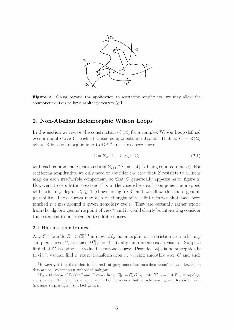
z1
z2
z3
z4
z5
z6
z7
z8
Figure 3 Going beyond the application to scattering amplitudes we may allow the
component curves to have arbitrary degrees ge 1
2 Non-Abelian Holomorphic Wilson Loops
In this section we review the construction of [13] for a complex Wilson Loop defined
over a nodal curve C each of whose components is rational That is C = Z(Σ)
where Z is a holomorphic map to CP3|4 and the source curve
Σ = Σn cup middot middot middot cup Σ2 cup Σ1 (21)
with each component Σi rational and Σi+1capΣi = pt (i being counted mod n) For
scattering amplitudes we only need to consider the case that Z restricts to a linear
map on each irreducible component so that C generically appears as in figure 2
However it costs little to extend this to the case where each component is mapped
with arbitrary degree di ge 1 (shown in figure 3) and we allow this more general
possibility These curves may also be thought of as elliptic curves that have been
pinched n times around a given homology cycle They are certainly rather exotic
from the algebro-geometric point of view5 and it would clearly be interesting consider
the extension to non-degenerate elliptic curves
21 Holomorphic frames
Any Cinfin bundle E rarr CP3|4 is inevitably holomorphic on restriction to a arbitrary
complex curve C because D2|C = 0 trivially for dimensional reasons Suppose
first that C is a single irreducible rational curve Provided E|C is holomorphically
trivial6 we can find a gauge transformation h varying smoothly over C and such
5However it is curious that in the real category one often considers lsquotamersquo knots ndash ie knots
that are equivalent to an embedded polygon6By a theorem of Birkhoff and Grothendieck E|C =
oplusO(ai) withsumai = 0 if E|C is topolog-
ically trivial Triviality as a holomorphic bundle means that in addition ai = 0 for each i and
(perhaps surprisingly) is in fact generic
ndash 6 ndash
that
hminus1 (part +A)∣∣C h = part
∣∣C (22)
Under this gauge transformation covariantly holomorphic objects become simply
holomorphic on C so h is said to define a holomorphic frame for E|C It follows
from (22) that h itself obeys
(part +A)∣∣Ch = 0 (23)
and so is defined up to a gauge transform h rarr hhprime where hprime must be globally
holomorphic on C
For two points z0 z isin CP3|4 that lie on C we now define
U(z z0) equiv h(z)hminus1(z0) (24)
to be the particular solution of (23) obeying the initial condition that the gauge
transformation at z0 isin C is simply the identity The holomorphic frame U(z z0)
defines a map
U(z z0) E|z0 rarr E|z (25)
between the fibres of E at z0 and z isin CP3|4 that depends on the choice of curve
C (not unique if deg(C) gt 1) It is the natural complex analogue of the parallel
propagator U(x x0) between two points x and x0 along a real curve γ For example
it follows immediately from the definition (24) that
U(z zprime)U(zprime z0) = U(z z0) (26)
so that U(z z0) concatenates just as for the parallel propagator along a real curve
In particular U(z z0)U(z0 z) = U(z z) = 1R implying that
U(z0 z) = U(z z0)minus1 (27)
Likewise if we change our choice of connection (01)-form by a smooth gauge trans-
formation
A rarr Ag = g partgminus1 + gAgminus1 (28)
then since hminus1 (part +A)∣∣C h = (gh)minus1 (part +Ag)
∣∣C (gh) we find that
U(z z0)rarr g(z)U(z z0)gminus1(z0) (29)
again as for a parallel propagator in the real category
In the Abelian case with E a line bundle setting h = eminusφ for some smooth
function φ on C the holomorphic frame equation (23) becomes partφ = A|C This
equation always has a solution when C is rational given by
φ(z) =
int
C
ω and A (210)
ndash 7 ndash
where A is restricted to the curve and where ω is a meromorphic 1-form on C
whose only singularities are simple poles at z0 and z with residues plusmn1 respectively
Explicitly if C = Z(Σ) with Z(σ) = z isin CP3|4 and Z(σ0) = z0 then the pullback of
ω to Σ is
ω(σprime) =(σ minus σ0)
(σ minus σprime)(σprime minus σ0)
dσprime
2πi(211)
in terms of local coordinates σ isin Σ This is just the Greenrsquos function for the part-
operator acting on smooth functions on Σ The holomorphic frame equation fixes φ
only up to a globally holomorphic function which by Liouvillersquos theorem must be
constant The constant is fixed by the choice of reference point ω vanishes if z and
z0 coincide so (210) has φ(z0) = 0 Thus in the Abelian case we have the explicit
expression
U(z z0) = eφ = exp
(minusint
C
ω and A)
(212)
for our holomorphic frame
In the non-Abelian case acting on a representation R of the gauge group U(z z0)
may similarly be given by the (somewhat formal) expression7
U(z z0) = P exp
(minusint
C
ω and A) (213)
The meaning of the lsquopath orderingrsquo symbol P on our complex curve is that the ith
power of the meromorphic differential ω that appears from expanding the exponential
in (213) should be taken to have its simple poles located at the reference point z0 and
at either the insertion point of the (i+ 1)th power of the field A (counting according
to the colour-ordering) or else at the final evaluation point z Specifically
P exp
(minusint
C
ω and A)equiv 1R +
infinsum
m=1
(minus1)mint
(C)m
mand
i=1
(ω(zi) and A(zi)
)(214)
where ω(zi) is a meromorphic differential in zi with a simple pole at z0 and a simple
pole at zi+1 (or at z when i = m) Explicitly in terms of intrinsic coordinates
mand
i=1
ω(σi) =(σ minus σ0)
(σ minus σm) middot middot middot (σ2 minus σ1)(σ1 minus σ0)
dσm2πiand middot middot middot and dσ1
2πi (215)
7An equivalent formal expression given in [13] is U(z z0) =(
1 + partminus1A∣∣C
)minus1 where in the
series expansion of this expression the inverse part-operators are taken to act on everything to their
right
ndash 8 ndash
Equation (213) is thus analogous to the (equally formal) expression
P exp
(minusint x
x0
A
)
= 1R minusint x
x0
dymicroAmicro(y) +
int x
x0
dymicroAmicro(y)
int y
x0
dyprimeνAν(y
prime) minus middot middot middot
= 1R +infinsum
m=1
(minus1)mint
([01])m
dsm middot middot middot ds1 Amicro(sm)dxmicro
dsmθ(smminussmminus1) middot middot middot θ(s2 minus s1)Aν(s1)
dxν
ds1
(216)
for the parallel propagator of a connection d +A = dxmicro(partmicro +Amicro) along a real curve
γ where the step functions obey
part
partsθ(sminus sprime) = δ(sminus sprime) (217)
and are the Greenrsquos function for the exterior differential on the interval [0 1] We also
note that the iterated integrals appearing in (213) are somewhat similar to iterated
integrals that arise in studying parallel transport via the Knizhnik-Zamolodchikov
connection over the configuration space of n-points on a rational curve See [29] for
a recent discussion of this in a twistor context
22 The holonomy around a nodal curve
Having identified the holomorphic frame U(z z0) = h(z)hminus1(z0) as the natural ana-
logue of a parallel propagator for a complex curve we can define the holonomy of the
connection (01)-form around C based at some point z isin CP3|4 to be the ordered
product
Holz[C] equiv U(z zn) U(zn znminus1) middot middot middotU(z2 z1) U(z1 z) (218)
where zi is the image of the node Σi+1 cap Σi and where without any essential loss
of generality we have taken the base point to be on Z(Σ1) Reading from the right
of (218) this definition uses the holomorphic frame U(z1 z) on Z(Σ1) to map the
fibre E|z to the fibre E|z1 at the node z1 We can identify this fibre with a fibre of
E restricted to the next component line Z(Σ2) and then map to the following node
using the holomorphic frame U(z2 z1) on Z(Σ2) We continue transporting our fibre
around the nodal curve in this way until the final factor of U(z z1) returns us to the
starting point The result is thus an automorphism of the fibre E|z as required
The holomorphic Wilson Loop is now defined as in the real category as
WR[C] equiv TrR Holz[C] (219)
where to take the trace in a representation R we have used the fact that a holomorphic
frame for E|C induces a holomorphic frame for all tensor products of E|C and its
dual in other words for all choices of representation Cyclicity of the trace and the
ndash 9 ndash
concatenation property (26) immediately shows that the Wilson Loop is independent
of the base point
For an Abelian gauge group (E a line bundle) the holomorphic frame (212) gives
W[C] = exp
(minusint
C
ω and A)
(220)
where ω is a meromorphic form on C whose only singularities are simple poles at
each of the nodes with residues plusmn1 on each component Such a differential is nothing
but the holomorphic differential θ on a non-singular elliptic curve in the limit that
this curve degenerates to our nodal curve (see eg [30]) Thus in the Abelian case
we recover the prescription
W[C] = exp
(minusint
C
θ and A)
(221)
that was proposed by Thomas [31] by Khesin and Rosly [11] and by Frenkel and
Todorov [12] For a non-Abelian gauge group we can likewise use (213) to formally
write
WR[C] = TrR P exp
(minusint
C
ω and A)
(222)
as a natural complexification of the familiar expression
WR[γ] = TrR P exp
(minusint
γ
A
)(223)
for a Wilson Loop of a connection on a real curve γ In equation (222) as in (213)
the path ordering symbol means that for each component of C successive powers of
ω in the series expansion of (222) should have one simple pole at one of the nodes
and another at the subsequent (with respect to the colour-ordering) insertion point
of the field
3 A Holomorphic Family of Curves
We now investigate the behaviour of our complex Wilson Loop as the curve C varies
We shall prove that just as the change in the real Wilson Loop (223) under a smooth
deformation of a real curve γ is
δWR[γ] = minus∮
γ
dxmicro δxν TrR
(Fmicroν(x) Holx[γ]
) (31)
so too the complex Wilson Loop (219) obeys
δWR[C] = minusint
C
ω(z) and dzα and δzβ TrR
(Fαβ(z z) Holz[C]
)(32)
ndash 10 ndash
as the complex curve C moves over a holomorphic family In this equation δ is the part-
operator on the parameter space of the family and once again ω(z) is a meromorphic
differential on C whose only singularities are simple poles at the nodes with residues
plusmn1 Like its real analogue equation (32) expresses the change in the Wilson Loop
in terms of the curvature (02)-form F = partA+AandA through the complex 2-surface
swept out by the varying curve The key point here is that because the curve C varies
holomorphically only the (02)-form part of the curvature arises In particular if E
is a holomorphic bundle on twistor space then the Wilson Loop is also holomorphic
As before we prove (32) in more generality than we actually need for scattering
amplitudes allowing each irreducible component Ci = Z(Σi) to have degree di ge 1
Here is the proof8 For a fixed partial connection the holomorphic frame U(z1 z0)
depends on the choice of two points z0 z1 isin CP3|4 together with a choice of (ir-
reducible rational) curve C that joins them (Note that this curve is not unique
if its degree is greater than 1) Equivalently we can think of this data in terms of
an abstract Riemann sphere Σ together with two marked points σ0 σ1 isin Σ and
a degree d holomorphic map Z Σ rarr CP3|4 such that Z(Σ) = C and Z(σi) = zi
Now suppose we have a holomorphic family of such maps parametrized by a mod-
uli space B described say by local holomorphic coordinates ti Writing U(σ σ0 t)
for the pullback of U(z z0) to the abstract curve Σ for our family of curves the
holomorphic frame equation is
(part + ZlowastA)U(σ σ0 t) = dσ
(part
partσ+Aα
partzα
partσ(σ t)
)U(σ σ0 t) = 0 (33)
where we emphasise that both the holomorphic frame and the connection depend on
t ndash ie on the choice of curve
Consider the integral
int
Σ
ω10(σ) and U(σ1 σ t) (part + ZlowastA)U(σ σ0 t) (34)
over Σ where ω10(σ) is our familiar meromorphic differential (211) whose only
singularities are simple poles at σ0 and σ1 with residues +1 and minus1 respectively
and where part +A is as given in (33) In principle the integral depends on these two
points and on the map Z ndash that is it depends on the moduli space ndash but of course
it actually vanishes identically on B since U(σ σ0) obeys (33)
8It is also possible to show (32) by working directly with the formal expression (222) provided
(as in the real case) due care is taken of the lsquopath orderingrsquo
ndash 11 ndash
Letting δ be the part-operator on B we have
0 = δ
[int
Σ
ω10(σ) and U(σ1 σ t)(part + ZlowastA
)U(σ σ0 t)
]
=
int
Σ
ω10(σ) and U(σ1 σ t)(part + ZlowastA
)δU(σ σ0 t)
minusint
Σ
ω10(σ) U(σ1 σ t) and δ(ZlowastA) U(σ σ0 t)
= minusδU(σ1 σ0 t)minusint
Σ
ω10(σ) U(σ1 σ t) and δ (ZlowastA) U(σ σ0 t)
(35)
where the third line follows from integrating by parts in the first term then using the
poles of ω10 and the fact that partU(σ1 σ t) = U(σ1 σ t)ZlowastA to perform the integral9
In the final term of (35) we have
δ (ZlowastA) =
(partβAα
partzβ
parttıpartzα
partσ+Aα
part2zα
parttı partσ
)dtı and dσ (36)
The most important property here is that because the map Z varies holomorphically
only antiholomorphic derivatives of the connection arise Again integrating by parts
we find that
DBU(σ1 σ0 t) equiv δU(σ1 σ0 t) +A(z(σ1 t))U(σ1 σ0 t)minus U(σ1 σ0 t)A(z(σ0 t))
= minusint
Σ
ω10(σ) and dσ and dtı U(σ1 σ t)Fαβpartzα
partσ
partzβ
parttıU(σ σ0 t)
= minusint
C
ω10(z) and dzα and δzβ U(z1 z)Fαβ(z) U(z z0)
(37)
where DB is the natural covariant part-operator acting on sections of the sheaf E over
B induced by10 E
Equation (37) tells us how the holomorphic frame U(z1 z0) on an irreducible
curve varies as we move around in the moduli space For the Wilson Loop (219) on
9In fact the moduli space B may be identified with the Kontsevich moduli space M02(CP3|4 d)
of stable 2-pointed degree d maps Because it depends on three points σ0 σ1 σ isin Σ as well as
Z the integrand in (34) really lives on the universal curve C equiv M03(CP3|4 d) and the pullback
by the map Z is more properly written as the pullback by the evaluation map on the third marked
point (labelled σ) The integral itself is really the pushdown by the forgetful map π C rarr B and in
commuting δ past the integral sign in (35) we really mean the pullback πlowastδ = partCminuspartCB = partCminuspartΣ
Then (36) is just the statement that the evaluation map is holomorphic and so commutes with partC
with the partΣ term left over10More accurately E = πlowastevlowastσE
ndash 12 ndash
a nodal curve we now readily find
δWR[C(t)] =nsum
i=1
TrR
((DBU(zi+1 zi)
)U(zi ziminus1) middot middot middotU(zi+2 zi+1)
)
= minusint
C(t)
ω(z) and dzα and δzβ TrR
(Fαβ(z z) Holz[C(t)]
) (38)
where the integral is taken over the complete nodal curve C(t) = Z(Σ) and we
emphasise that this curve depends on the moduli of the map As usual ω(z) is a
meromorphic differential on C(t) with only simple poles at the nodes This completes
the proof
4 Holomorphic Loop Equations
In this section we derive an analogue of the loop equations of Makeenko and Migdal [25]
for our complex Wilson Loops To do this instead of considering the complexified
Wilson Loop itself we must study its averagelangWR[C]
rangover the space of gauge-
inequivalent connection (01)-forms on E weighted by the exponential of an appro-
priate action
In section 41 we choose the action to be the U(N) holomorphic Chern-Simons
functional
ShCS[A] =1
g2
int
CP3|4
D3|4z and tr
(1
2A and partA+
1
3A andA andA
) (41)
that may be interpreted as the open string field theory of the perturbative B-
model [17 18] In real Chern-Simons theory on a real 3-manifold M the correlation
function of a Wilson Loop gives a knot invariant Since these invariants depend
only on the (regular) isotopy class of the knot one expects that unlike WR[γ] itselflangWR[γ]
rangCS
should remain invariant as one smoothly deforms γ This is essentially
true except that there are important corrections when the deformation causes γ to
pass through a self-intersection so that the isotopy class of the knot jumps The
loop equations determine the behaviour oflangWR[γ]
rangCS
under such a jump and it was
shown in [26] that for Wilson Loops in the fundamental representation of U(N)
they amount to the skein relations
s12P+(r s)minus sminus 1
2Pminus(r s) = (r12 minus rminus 1
2 )P0(r s) (42)
from which the HOMFLY polynomial Pγ(r s) can be recursively constructed11
11The variables of the HOMFLY polynomial are related to N and the level k of the Chern-Simons
theory by and s = eλ and r = eλN where λ equiv 2πiN(k + N) may be interpreted as the rsquot Hooft
coupling In [26] the skein relations were obtained to lowest order in λ The skein relation only
determines the HOMFLY polynomial for Wilson Loops in the fundamental
ndash 13 ndash
We expect that correlation functions of our Wilson Loops in the holomorphic
Chern-Simons QFT are likewise associated with holomorphic linking invariants In-
deed [11 12] show that for two non-intersecting curves C1 C2 sub C3 of genera gi ge 1
the expectation valuelangW[C1] W[C2]
rangin Abelian holomorphic Chern-Simons theory
on C3 involves12 the holomorphic linking invariant
L(C1 θ1C2 θ2) =1
4π
int
C1timesC2
εık(z minus w)ı
|z minus w|6 dz and dwk and θ1 and θ2 (43)
that generalizes the Gauss linking number
L(γi γj) =1
4π
int
γitimesγj
εijk(xminus y)i
|xminus y|3 dxj and dyk (44)
in for real Abelian Wilson Loops in R3 Observe that (43) depends on a choice of
holomorphic 1-form θi on each curve For our nodal curve the corresponding form is
meromorphic and depends on the location of the nodes In section 41 we shall find
that δlangWR[C]
ranghCS
generically vanishes with important corrections when the type
of the curve jumps In the planar limit the loop equations may be reduced to the
BCFW relations [27] that recursively construct the classical S-matrix In this sense
the BCFW relations are simply the U(infin) skein relations for the holomorphic link
defined by C
As mentioned in the introduction holomorphic Chern-Simons theory on CP3|4
corresponds only to the anti self-dual sector of N = 4 super Yang-Mills theory on
space-time In section 42 we replace (41) by the action [20]
SN=4[A] = ShCS[A] +
int
Γ
d4|8x ln det(part +A)∣∣X
(45)
that as our notation indicates describes N = 4 super Yang-Mills theory on twistor
space We shall see that the new term is itself eminently compatible with the Wilson
Loop The loop equations in this theory involve a new term that leads to the all-loop
extension of the BCFW relations found by Arkani-Hamed et al in [7]
41 Holomorphic linking
In this section we choose the action to be the holomorphic Chern-Simons func-
tional (41) where D3|4z is the canonical holomorphic section of the Berezinian of
CP3|4 given explicitly by
D3|4z equiv 1
4εαβγδz
αdzβ and dzγ and dzδ1
4εabcddψ
a dψb dψc dψd (46)
12We will see later that at least for the N = 4 theory lsquoholomorphic self-linkingrsquo is well-defined
even without a choice of framing
ndash 14 ndash
in terms of homogeneous coordinates (zα ψa) isin C4|4 This action is defined on the
space A 01 of partial connections D on a Cinfin vector bundle E rarr CP3|4 given at least
locally by D = part+A in terms of a background partial connection part We take this to
obey part2 = 0 and so define a background complex structure on E Thus A(z z ψ)
is a superfield with component expansion
A(z z ψ) = a(z z) + ψaΓa(z) +1
2ψaψb Φab(z z) + middot middot middot+ 1
4εabcdψ
aψbψcψd g(z z)
(47)
where the coefficient of (ψ)r is a (01)-form on CP3 valued in smooth sections of
End(E)otimesOCP3(minusr)We choose the gauge group to be U(N) and consider only Wilson Loops in the
fundamental representation The Yang-Mills (or open string) coupling g2 is then
related to the Chern-Simons level k by g2 = 2π(k + N) In anticipation of taking
the planar limit we write g2 = λN in terms of the rsquot Hooft coupling λ and include
a factor of 1N in definition of the Wilson Loop so that W[C] = 1 if the holonomy
is trivial
Inserting (32) into the holomorphic Chern-Simons path integral one finds
δlangW[C(t)]
rang= minus 1
N
intDA
[int
C(t)
ω(z) and dzα and δzβ tr(Fαβ(z) Holz[C(t)]
)]eminusShCS[A]
=λ
N2
intDA
[int
C(t)
ω(z) and tr
(Holz[C(t)]
δ
δA(z)eminusShCS[A]
)]
(48)
since the variation of the holomorphic Chern-Simons functional is F02 times Nλ To
obtain an interesting equation for δlangW[C(t)]
rang as in [25] we integrate by parts in
the path integral bringing the variation of the connection to act on the holonomy
Essentially the same argument as in section 3 shows that under a variation of the
connection at some point zprime isin C (displaying colour indices)
0 =
[δ
δA(z)
i
j
(int
C
ω10(zprime) and U(z1 zprime)(part +A
)C
U(zprime z0)
)k
l
]
= minus[
δ
δA(z)
i
j
U(z1 z0)kl
]+
int
C
ω10(zprime) and U(z1 zprime)kj δ
3|4(z zprime) U(zprime z0)i l
(49)
where we have used the fact that for a U(N) gauge group
(δδA(z))i j A(zprime)mn = δ3|4(z zprime) δinδmj (410)
with δ3|4(z zprime) a Dirac current concentrated on the diagonal in CP3|4z times CP3|4
zprime ie
δ3|4(z zprime) is a distribution-valued (03)-form on CP3|4z times CP3|4
zprime such that for any α isinΩ0p(CP3|4) we have
int
CP3|4D3|4zprime and δ3|4(z zprime) and α(zprime) = α(z) (411)
ndash 15 ndash
z
z
C(t)
C(t)
Figure 4 The expectation valuelangW[C(t)]
rangin holomorphic Chern-Simons theory varies
holomorphically except where the curve develops a new node
Explicitly δ3|4(z zprime) may be represented by the integral [5 32]
δ3|4(z zprime) =
intdu
uand δ4|4(z minus uzprime) =
intdu
u
4and
α=1
part1
zα minus uzprimeα4prod
a=1
(ψa minus uψprimea) (412)
that forces zα prop zprimeα so that the two point must coincide projectively
We now apply equation (49) to the variation holonomy based say at a point
z isin C1 One finds
tr
(δ
δA(z)Holz[C(t)]
)=
δ
δA(z)
i
j
[U(z zn)jkU(zn znminus1)kl middot middot middotU(z1 z)
mi
]
=sum
i
int
Ci(t)
ωi+1i(zprime) and δ3|4(z zprime) tr
[U(z zn) middot middot middotU(zi+1 z
prime)]
tr[U(zprime zi) middot middot middotU(z1 z)
]
(413)
The factor of δ3|4(z zprime) ensures that this term has support only at points t in the
moduli space where the curve C(t) degenerates so that the component C1(t) ei-
ther self-intersects or else intersects some other component Similar contributions
arise from summing over the possible locations of the base-point z In other words
thinking of our original curve as an elliptic curve δlangW[C(t)]
rangvanishes everywhere
except on boundary components of the moduli space where the holomorphic map
degenerates so that two points on the source curve are mapped to the same image
Combining all the terms the holomorphic Chern-Simons loop equations (48)
become
δlangW[C(t)]
rang= minusλ
int
C(t)timesC(t)
ω(z) and ω(zprime) and δ3|4(z zprime)langW[C prime(t)] W[C primeprime(t)]
rang (414)
for normalised Wilson Loops in the fundamental of a U(N) gauge group where C prime(t)
and C primeprime(t) are the two curves obtained by ungluing C(t) at its new node z = zprime (see
figure 4) In the planar limit the correlation function of a product of Wilson Loops
factorizes into the product of correlation functions so (414) simplifies to
δlangW[C(t)]
rang= minusλ
int
C(t)timesC(t)
ω(z) and ω(zprime) and δ3|4(z zprime)langW[C prime(t)]
rang langW[C primeprime(t)]
rang(415)
ndash 16 ndash
where λ is the rsquot Hooft coupling Thus in the planar limit the behaviour at a self-
intersection is determined by the product of the expectation values of the Wilson
Loops around the two lower degree curves This may be viewed as an analogue
for holomorphic linking of the skein relations for real knot invariants In section 5
we shall see that the classical BCFW recursion relations are simply a special case
of (415)
42 Loop equations for the twistor representation of N = 4 SYM
We now consider the expectation value of the complex Wilson Loop in the twistor
action
SN=4[A] = ShCS[A] +
int
Γ
d4|8x log det(part +A)∣∣X (416)
where X is a line in twistor space and Γ is a middle-dimensional contour in the
space Gr2(C4) of these lines13 interpreted as a choice of real slice of complexified
conformally compactified space-time The proof that (416) is an action for N = 4
SYM on twistor space is given in [20] to which the reader is referred for further
details (Readers familiar with the MHV formalism may note that the new term
in (416) provides an infinite series of MHV vertices while the 3-point MHV vertex
in the Chern-Simons theory vanishes in an axial gauge From the point of view
of twistor string theory [18] the determinant may be understood as the partition
function of a chiral free fermion CFT on X coupled to the pullback of the twistor
space gauge field)
From the point of view of the present article it is possible to motivate this action
by observing that Wilson Loops on complex curves are again the natural observables
of the QFT based on (416) The reason this is so is because of the close connection
between determinants and holonomies More precisely just as
δ log detM = δ tr logM = tr(Mminus1δM) (417)
for a finite dimensional matrix M Quillen shows [33] that for an abstract curve Σ
under a variation of the connection the logarithm of a section of the determinant
line bundle Detrarr A 01Σ varies as14
δ log det(part +A)∣∣Σ
=
int
Σ
tr (JA and δA) (418)
where
JA(σ) equiv limσprimerarrσ
(GA(σprime σ)minusG0(σprime σ)
)(419)
13The fermionic integral is done algebraically as always14In writing this formula we assume that δ is a flat connection on Det in a trivialisation where
the local connection 1-form vanishes That Det should admit such a flat connection is necessary if
we wish to treat det(part +A)Σ as a (holomorphic) function on A 01Σ (the space of connection (01)-
forms on Σ) However [33] the construction of this flat connection requires a choice of background
connection
ndash 17 ndash
is the limit15 on the diagonal in Σ times Σ of difference between the Greenrsquos function
for part +A|Σ and the Greenrsquos function for background connection partΣ These Greenrsquos
functions are non-local operators on the Riemann surface the fact that we take their
limit on the diagonal can be understood as part of the trace For a single such Greenrsquos
function the limit on the diagonal is necessarily singular but the singularity cancels
in the difference (419) The dependence on a background connection reflects the fact
that to treat sections of the determinant line bundle as functions we must first pick
a trivialisation amounting to a choice of background connection (01)-form on the
bundle over Σ In our case we will of course choose this background part-operator to
be the one induced by our choice of base-point part isin A 01Σ in writing the holomorphic
Chern-Simons action
When Σ is a Riemann sphere the Greenrsquos functions are
GA(σprime σ) = h(σprime)G0(σprime σ)hminus1(σ) and G0(σprime σ) =1
2πi
dσ
σprime minus σ (420)
in terms of the holomorphic frame h on Σ Therefore Quillenrsquos prescription reduces
to
JA(σ) =dσ
2πilimσprimerarrσ
U(σprime σ)minus U(σ σ)
σprime minus σ =dσ
2πi
partU(σprime σ)
partσprime
∣∣∣∣σprime=σ
(421)
For our purposes the presence of the holomorphic derivative here is somewhat in-
convenient However it is easily seen from the formal series (214) that U(σprime σ)
depends only meromorphically on σprime and is regular at σprime = σ Thus we can use
Cauchyrsquos theorem to rewrite the derivative in (421) as an integral so
δ log det(part +A)∣∣Σ
=1
(2πi)2
int
Σ
dσ and tr
(∮dσprime
(σ minus σprime)2U(σprime σ) δA(σ)
)
=1
(2πi)3
int
ΣtimesS1timesS1
dσ and dσprime and dσprimeprime
(σ minus σprime)(σprime minus σprimeprime)(σprimeprime minus σ)tr (U(σprime σ) δA(σ))
(422)
where the integrals over σprimeprime and σprime are performed over contours encircling the poles at
σprimeprime = σprime and σprime = σ respectively (The reason for introducing the new point σprimeprime isin Σ
will become clear momentarily)
To apply this to the case that Σ = Zminus1(X) for X a line in twistor space suppose
Z(σprimeprime) = za Z(σprime) = zb and Z(σ) = z = za + σzb (423)
so that X = Span[za zb] Then
dσ and dσprime and dσprimeprime
(σ minus σprime)(σprime minus σprimeprime)(σprimeprime minus σ)= Zlowast
[ωab(z) and 〈a da〉 and 〈b db〉
〈a b〉2]
(424)
15Below this limit will be revealed as nothing but the forward limit of an amplitude
ndash 18 ndash
where ωab(z) is meromorphic with only simple poles only z = za and zb and where
〈a da〉〈b db〉〈a b〉2 is the fundamental bi-differential on X with a double pole along
the diagonal This bi-differential combines with the integral over the space of lines
X since
d4|8x and 〈a da〉 and 〈b db〉〈a b〉2 = D3|4za andD3|4zb (425)
giving a contour integral over CP3|4a timesCP3|4
b Therefore the variation of the new term
in the action is
δ
int
Γ
d4|8x log det(part +A)∣∣X
=
int
ΓtimesXtimesS1timesS1
D3|4za andD3|4zb(2πi)3
and ωab(z) tr(
U(zb z) δA(z))
(426)
where the S1 times S1 contour sets za rarr z and zb rarr z differentiating U(zb z) in the
process The integral over all z isin X is performed using the dependence on z in the
holomorphic frame and in the variation of the connection
Equation (426) expresses the variation of the logarithm of the determinant in
the twistor action (416) in terms of a holomorphic frame on the line X It dovetails
beautifully with the holonomy around the curve C providing a new contribution
minus λN
int
ΓtimesS1timesS1
D3|4za andD3|4zb
int
C(t)timesX
ω(z) and ωab(z) and δ3|4(z z) tr(
U(zb z) Holz[C(t)])
(427)
to the loop equations The δ-function δ3|4(z z) in this expression means that this
term only contributes at points in the moduli space where the curve C(t) 3 z inter-
sects the line X 3 z The integral over Γ then adds up these contributions for each
X isin Γ
To interpret the product U(zb z) Holz[C(t)] replace C(t) by a curve C(t) where
C(t) cap X = z zb isin CP3|4 (428)
and such that as zb rarr z C(t) rarr C(t) As a nodal curve C(t) has one more
component than C(t) with one component becoming double covered in the limit
(see figure 5) Now because the contour integral forces zb = z we can replace the
holonomy around C(t) based at z = z = C(t) cap X by a product of holomorphic
frames that transport us around C(t) from zb to z The remaining factor of U(zb z)
transports this frame back to zb along X The resulting trace can be interpreted as
Wilson Loop around C(t) cup X so that
1
Ntr(
U(zb z)Holz[C(t)])
= W[C(t) cup X] (429)
provided we are inside the contour integral over the location of zb sub X
ndash 19 ndash
=
X
z = zC
X
C zb
z
Figure 5 The new term in the loop equations for N = 4 SYM can be understood as a
holomorphic Wilson Loop around a new curve C cupX where C reduces to C when zb rarr z
along X Note that the nodal curve C has one more component than C In the scattering
amplitude context 〈W[C cup X]〉 may be interpreted as a forward limit of an n+ 2 particle
amplitude
Finally then we see that the holomorphic loop equations for the twistor repre-
sentation of planar N = 4 SYM are
δlangW[C(t)]
rang= minus λ
int
C(t)timesC(t)
ω(z) and ω(zprime) and δ3|4(z zprime)langW[C prime(t)]
rang langW[C primeprime(t)]
rang
minus λ
int
ΓtimesS1timesS1
D3|4za andD3|4zb
int
C(t)timesX
ω(z) and ωab(z) and δ3|4(z z)langW[C(t) cup X]
rang
(430)
and as in the original equations of Migdal amp Makeenko [25] are entirely expressed
in terms of expectation values of our (complexified) Wilson Loops In the following
section we show that for a particular one-parameter family of curves C(t) this holo-
morphic loop equation reduces to the all-loop BCFW recursion relation found in [7]
but we emphasise that (430) is valid for a far more general class of curves
5 BCFW Recursion from the Loop Equations
We now apply the holomorphic loop equation (430) to the case that each component
of C is a line as in figure 2 C can be completely specified by giving the location
of its n nodes and we shall often write C = (12) cup (23) cup middot middot middot cup (n1) for the curve
(where (i i+1) equiv Span[zi zi+1]) and W[1 2 n] for the corresponding Wilson Loop
(in the fundamental representation) We wish to show that the loop equations forlangW[1 2 n]
rangdirectly reduce to the all-loop BCFW recursion relations of Arkani-
Hamed et al [7] although it is important that our derivation of these relation is
completely independent of any notions of scattering theory
ndash 20 ndash
z1
z2
z3
z4
z5
z6
z7
z8
z8 t
Figure 6 The family of nodal curves C(t) corresponding to a BCFW deformation of a
planar amplitude in N = 4 SYM shown for n = 8 As we vary over the moduli space the
line (1 n(t)) sweeps out a pencil of lines in the plane (nminus1 n 1) with focus z1 This plane
necessarily intersects every other component of C(t)
Consider the holomorphic family of Wilson Loops determined by translating the
node zn along the line (nminus1 n) That is we define
zn(t) equiv zn + tznminus1 (51)
and consider the 1-parameter family of holomorphic curves
C(t) equiv (12) cup (23) cup middot middot middot cup (nminus1 n(t)) cup (n(t) 1) (52)
as shown in figure 6 Notice that although t can be thought of as a local holomorphic
coordinate on the line (nminus1n) it is really a coordinate on the moduli space of our
family of curves ie a coordinate on a CP1 sub B As t varies the line (n(t) 1) sweeps
out the plane (nminus1 n 1) with all other components of C(t) remaining fixed Lines
and planes necessarily intersect16 in CP3 so for every j = 3 nminus1 there exists a tjfor which (n(tj) 1) intersects the component Cj Let us call this intersection point
Ij and write nj for the point zn(tj) Clearly we have
Ij = (nminus1 n 1) cap (jminus1 j) and nj = (nminus1 n) cap (jminus1 j 1) (53)
essentially by definition (Note that we do not get any new intersections when j =
n 1 2)
16Lines and planes do not necessarily intersect in the superspace CP3|4 because they might lsquomissrsquo
in the fermionic directions The fermionic δ-functions in the δ3|4(z zprime) ensure that the right hand
side has support only when the curves do intersect in the superspace See also the discussion in [21]
ndash 21 ndash
We now study the loop equations for this family Considering first the case of
pure holomorphic Chern-Simons theory (415) becomes
minusint
CP1
dt
tand δlangW[C(t)]
rang=
λnminus1sum
j=3
int
CP1timesC1(t)timesCj
dt
tand ω(z) and ω(zprime) and δ3|4(z zprime)
langW[C prime(t)]
rang langW[C primeprime(t)]
rang (54)
whereC prime(t) = (12) cup (23) cup middot middot middot cup (jminus1 Ij)
C primeprime(t) = (Ij j) cup (j j+1) cup middot middot middot (nj 1)(55)
and where we have integrated (415) over our moduli space CP1 sub B using the
meromorphic differential dtt We can dispose of the left hand side immediately
integrating by parts gives
minusint
CP1
dt
tand δlangW[C(t)]
rang=langW[C(0)]
rangminuslangW[C(infin)]
rang
=langW[1 2 n]
rangminuslangW[1 2 nminus1]
rang
(56)
the difference of the Wilson Loops around the original curve and the curve with
zn = znminus1 Notice that the holomorphic frame U(zn znminus1)rarr 1 as zn rarr znminus1 so that
while the line (nminus1 n) does not simply lsquodisappearrsquo from the picture neither does it
contribute to the holonomy
The right hand side of (54) is almost as straightforward to compute because the
integrals over both the CP1 moduli space and the two copies of C(t) are completely
fixed by the δ-function δ3|4(z zprime) Since z isin (n(t) 1) and zprime isin (jminus1 j) we can
parametrize these integrals by setting
z = zn(t) + sz1 = zn + tznminus1 + sz1 and zprime = zjminus1 + rzj (57)
in terms of local coordinates r and s on C1(t) and Cj respectively With these
coodinates the meromorphic forms ω(z) and ω(zprime) become simply
ω(z) =ds
sand ω(zprime) =
dr
r(58)
which indeed have simple poles at the nodes of C1(t) and Cj as required Performing
the integral is then merely a matter of using the explicit form (412) of δ3|4(z zprime) and
computing a Jacobian In fact this integral is
[nminus1 n 1 jminus1 j] equivint
dr
r
ds
s
dt
t
du
uδ4|4(zn + tznminus1 + sz1 + uzjminus1 + rzj) (59)
ndash 22 ndash
which was shown in [5] to be just the basic dual superconformal invariant R1jn of [6]
Including the product of the two Wilson Loops on the smaller curves we find that
the loop equations in pure holomorphic Chern-Simons theory reduce to
langW[1 n]
rang=langW[1 nminus1]
rang
+ λnminus1sum
j=3
[nminus1 n 1 jminus1 j]langW[1 jminus1 Ij]
rang langW[Ij j nminus1 nj]
rang
(510)
where Ij and nj were given in (53) Re-interpreting the twistor space as momentum
twistor space this is just the tree-level BCFW recursion relation [27] in the momen-
tum twistor form given in [7] summed over all MHV degrees Expanding (510) in
powers of the Grassmann coordinates ψ at each vertex gives the BCFW relations for
specific NkMHV partial amplitudes
Turning now to the full N = 4 theory from (430) we have an additional contri-
bution
λ
int
ΓtimesS1timesS1
D3|4za andD3|4zb
int
CP1timesC(t)timesX
dt
tand ω(z) and ωab(z) and δ3|4(z z)
langW[C(t) cup X]
rang
(511)
where
C(t) cup X = (12) cup middot middot middot (nminus1 n(t)) cup (z b) cup (b 1) (512)
is our n + 2 component curve Once again the integrals inside the square brackets
are completely fixed by the δ3|4(z z) The intersection point z and the point n(t) are
fixed to be
z = (a b) cap (nminus1 n 1) and n(t) = (nminus1 n) cap (a b 1) (513)
and the Jacobian from the t z and z integrals gives the R-invariant [nminus1 n 1 a b]
The N = 4 loop equations thus reduce to
langW[1 n]
rang=langW[1 nminus1]
rang
+ λ
nminus1sum
j=3
[nminus1 n 1 jminus1 j]langW[1 jminus1 Ij]
rang langW[Ij j nminus1 nj]
rang
+ λ
int
ΓtimesS1timesS1
D3|4za andD3|4zb [nminus1 n 1 a b ]langW[1 nminus1 nab z zb]
rang
(514)
where we remind the reader that the S1timesS1 contour is taken to fix zab rarr z along X
(the R-invariant has a simple zero in this limit cancelling one of the factors of 〈za zb〉in the denominator of the measure) Re-interpreting the twistor space as momentum
ndash 23 ndash
twistor space this is the extension of the BCFW recursion for the all-loop integrand
found by Arkani-Hamed et al in [7]
Let us conclude with a few remarks Firstly the explicit power of the rsquot Hooft
coupling λ is present in (514) because our normalisation of the twistor action cor-
responds to the normalisation 14g2
inttr(F and lowastF ) = N
4λ
inttr(F and lowastF ) of the space-time
Yang-Mills action In this normalisation n-particle `-loop scattering amplitudes are
proportional to λ`minus1Nχ (with χ = 2 for planar diagrams) If one rescales the twistor
(or space-time) connection as A rarrradicλA the explicit λ disappears from (514) and
the `-loop planar scattering amplitude corresponds to the coefficient of λ(n+2`minus2)2
Secondly when computing real knot (rather than link) invariants it is necessary
to choose a lsquoframingrsquo ndash roughly a thickening of the knot into a band For Wilson
Loops in real Chern-Simons theory this may be understood perturbatively as a
point-splitting procedure that regularises potential divergences as the two ends of a
propagator approach each other along the knot γ This would seem to be particularly
important in the case that γ has cusps Above however we made no attempt to
choose a lsquoholomorphic framingrsquo of C In fact at least for the pure holomorphic
Chern-Simons theory this does not seem to be necessary Consider for example a
propagator stretched between two adjacent line components of C say (iminus1 i) and
(i i+1) We can regularise any potential divergence in this propagator by ungluing
the node replacing (i i+ 1) rarr (iε i+ 1) where ziε = zi + εzprime for some arbitrary
point zprime As shown in [13] the integral of an axial gauge holomorphic Chern-Simons
propagator along two non-intersecting lines gives an R-invariant and in this case we
obtain [lowast iminus1 i iε i+1] (where zlowast determines the axial gauge) It is then easy to
show that this is of order ε as εrarr 0 as a consequence of the N = 4 supersymmetry
In other words the short-distance singularity of the propagator is always integrable
provided one sums over the complete N = 4 supermultiplet
If the holomorphic Chern-Simons expectation value is finite (for generic zi)
the same cannot be said of the expectation value in the full theory The integral
over the space of lines X will diverges (at least if Γ is a contour corresponding
to a real slice of space-time) with the divergence coming from those X isin Γ that
intersect C at more than one place or if the intersection occurs at a node and
reflecting the divergence of the corresponding scattering amplitudes in the infra-
red Consequently without a regularisation (or else a choice of lsquoleading singularityrsquo
contour for Γ) the expression (514) is somewhat formal and provides a recursion
relation for the all-orders integrand rather than the all-orders Wilson Loop itself It
would be fascinating if it is possible to regularise these divergences using some form
of holomorphic framing of C(t) Curiously the Coulomb branch regulator of [34] ndash
interpreted in dual conformal space-time as bringing the vertices of the piece-wise
null polygon into the interior of AdS5 ndash corresponds in twistor space to replacing
the line X by a (complex) quadric See eg [35 36 37 38] for discussions of this
ndash 24 ndash
regulator in a twistor context
Further although we considered only the particular deformation zn rarr zn(t)
relevant for BCFW recursion it should be clear that the loop equations can equally
be applied to the more general deformation [39]
zi rarr zi minus tcizlowast i = 1 n (515)
of the scattering amplitude curve that translates each vertex towards some arbitrary
point zlowast isin CP3|4 (Here ci are arbitrary complex constants) This one-parameter
deformation includes both BCFW recursion and the MHV diagram formalism as
special cases and the validity of the corresponding recursion relation for the all-loop
N = 4 integrand has been shown recently in [22] It is also clear that many other
deformations of C are possible and it would be interesting to know if anything useful
can be learned from say non-linear or multi-parameter deformations
As a final remark many possible extensions to this work suggested by appealing
either to the analogy with real Chern-Simons and knot theory or else to the link
to scattering amplitudes in space-time We hope that this close relationship helps
to fertilise new progress both in understanding holomorphic linking and in N = 4
SYM
Acknowledgments
We thank Freddy Cachazo Jaume Gomis and Natalia Saulina for helpful comments
We would also particularly like to thank Lionel Mason for many useful discussions
The work of DS is supported by the Perimeter Institute for Theoretical Physics Re-
search at the Perimeter Institute is supported by the Government of Canada through
Industry Canada and by the Province of Ontario through the Ministry of Research
amp Innovation The work MB is supported by an STFC Postgraduate Studentship
References
[1] R Penrose and W Rindler Spinors and Space-Time vol 2 Cambridge University
Press 1986
[2] S Huggett and P Tod An Introduction to Twistor Theory Student Texts 4 London
Mathematical Society 1985
[3] R Ward and R Wells Twistor Geometry and Field Theory CUP 1990
[4] A Hodges Eliminating Spurious Poles from Gauge-Theoretic Amplitudes
arXiv09051473 [hep-th]
[5] L Mason and D Skinner Dual Superconformal Invariance Momentum Twistors
and Grassmannians JHEP 11 (2009) 045 [arXiv09090250]
ndash 25 ndash
[6] J M Drummond J Henn G P Korchemsky and E Sokatchev Dual
Superconformal Symmetry of Scattering Amplitudes in N = 4 Super-Yang-Mills
Theory Nucl Phys B828 (2010) 317ndash374 [arXiv08071095]
[7] N Arkani-Hamed J Bourjaily F Cachazo S Caron-Huot and J Trnka The
All-Loop Integrand for Scattering Amplitudes in Planar N = 4 SYM
arXiv10082958 [hep-th]
[8] J Drummond L Ferro and E Ragoucy Yangian Symmetry of Light-Like Wilson
Loops arXiv10114264
[9] M F Atiyah Greenrsquos Functions for Self-Dual Four Manifolds Adv Math Supp 7A
(1981) 129ndash158
[10] R Penrose Topological QFT and Twistors Holomorphic Linking Twistor
Newsletter 27 (1988) 1ndash4 [httppeoplemathsoxacuklmasonTn]
[11] B Khesin and A Rosly Polar Homology and Holomorphic Bundles
Phil Trans Roy Soc Lond A359 (2001) 1413ndash1428 [math0102152]
[12] I Frenkel and A Todorov Complex Counterpart of Chern-Simons-Witten Theory
and Holomorphic Linking Adv Theor Math Phys 11 (2007) no 4 531ndash590
[math0502169]
[13] L Mason and D Skinner The Complete Planar S-matrix of N = 4 Super Yang-Mills
from a Wilson Loop in Twistor Space JHEP 12 (2010) 018 [arXiv10092225]
[14] L F Alday and J Maldacena Gluon Scattering Amplitudes at Strong Coupling
JHEP 06 (2007) 064 [arxiv 07050303 [hep-th]]
[15] J Drummond G Korchemsky and E Sokatchev Conformal Properties of
Four-Gluon Planar Amplitudes and Wilson Loops Nucl Phys B795 (2007)
385ndash408 [arXiv07070243 [hep-th]]
[16] A Brandhuber P Heslop and G Travaglini MHV Amplitudes in N = 4 Super
Yang-Mills and Wilson Loops Nucl Phys B794 (2008) 231ndash243
[arXiv07071153]
[17] E Witten Chern-Simons Gauge Theory as a String Theory Prog Math 133 (1995)
637ndash678 [hep-th9207094]
[18] E Witten Perturbative Gauge Theory as a String Theory in Twistor Space
Commun Math Phys 252 (2004) 189ndash258 [hep-th0312171]
[19] E Witten Quantum Field Theory and the Jones Polynomial Commun Math Phys
121 (1989) 351
[20] R Boels L Mason and D Skinner Supersymmetric Gauge Theories in Twistor
Space JHEP 02 (2007) 014 [hep-th0604040]
ndash 26 ndash
[21] M Bullimore L Mason and D Skinner MHV Diagrams in Momentum Twistor
Space JHEP 12 (2010) 032 [arXiv10091854]
[22] M Bullimore MHV Diagrams from an All-Line Recursion Relation
arXiv10105921
[23] S He and T McLoughlin On All-Loop Integrands of Scattering Amplitudes in
Planar N = 4 SYM arXiv10106256
[24] R Boels On BCFW Shifts of Integrands and Integrals arXiv10083101 [hep-th]
[25] Y Makeenko and A Migdal Exact Equation for the Loop Average in Multicolor
QCD Phys Lett B88 (1979) 135ndash137
[26] P Cotta-Ramusino E Guadagnini M Martellini and M Mintchev Quantum Field
Theory and Link Invariants Nucl Phys B330 (1990) 557
[27] R Britto F Cachazo B Feng and E Witten Direct Proof Of Tree-Level Recursion
Relation In Yang-Mills Theory Phys Rev Lett 94 (2005) 181602
[hep-th0501052]
[28] S Caron-Huot Notes on the Scattering Amplitude Wilson Loop Duality
arXiv10101167
[29] Y Abe Holonomies of Gauge Fields in Twistor Space 1 Bialgebra Supersymmetry
and Gluon Amplitudes Nucl Phys B825 (2010) 242ndash267 [arXiv09062524]
[30] J Fay Theta Functions on Riemann Surfaces Lecture Notes in Mathematics
Springer 1973
[31] R P Thomas A Holomorphic Casson Invariant for Calabi-Yau 3-folds and Bundles
on K3 Fibrations J Diff Geom 54 (2000) no 2 367ndash438 [math9806111]
[32] L Mason and D Skinner Scattering Amplitudes and BCFW Recursion in Twistor
Space JHEP 01 (2010) 064 [arXiv09032083]
[33] D Quillen Determinants of Cauchy-Riemann Operators over Riemann Surfaces
Func Anal Appl 19 (1985) 37ndash41
[34] L F Alday J Henn J Plefka and T Schuster Scattering Into the Fifth Dimension
of N = 4 Super Yang-Mills JHEP 01 (2010) 077 [arXiv09080684 hep-th]
[35] A Hodges The Box Integrals in Momentum Twistor Geometry arXiv10043323
[36] L Mason and D Skinner Amplitudes at Weak Coupling as Polytopes in AdS5
Submitted to JPhys A (2010) [arXiv10043498]
[37] L F Alday Some Analytic Results for Two-Loop Scattering Amplitudes
arXiv10091110
ndash 27 ndash
[38] J Drummond J Henn and J Trnka New Differential Equations for On-Shell Loop
Integrals arXiv10103679
[39] H Elvang D Z Freedman and M Kiermaier Proof of the MHV Vertex Expansion
for All Tree Amplitudes in N = 4 SYM Theory JHEP 06 (2009) 068
[arXiv08113624]
ndash 28 ndash
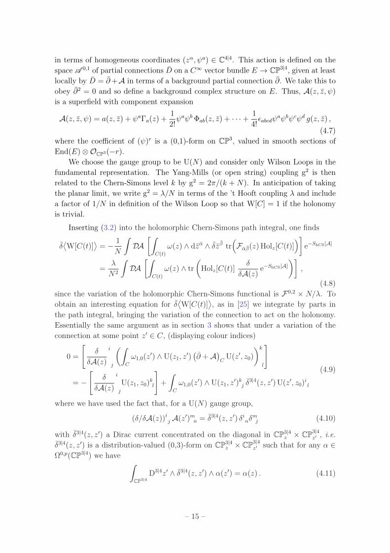

z
z
C(t)
C(t)
Figure 4 The expectation valuelangW[C(t)]
rangin holomorphic Chern-Simons theory varies
holomorphically except where the curve develops a new node
Explicitly δ3|4(z zprime) may be represented by the integral [5 32]
δ3|4(z zprime) =
intdu
uand δ4|4(z minus uzprime) =
intdu
u
4and
α=1
part1
zα minus uzprimeα4prod
a=1
(ψa minus uψprimea) (412)
that forces zα prop zprimeα so that the two point must coincide projectively
We now apply equation (49) to the variation holonomy based say at a point
z isin C1 One finds
tr
(δ
δA(z)Holz[C(t)]
)=
δ
δA(z)
i
j
[U(z zn)jkU(zn znminus1)kl middot middot middotU(z1 z)
mi
]
=sum
i
int
Ci(t)
ωi+1i(zprime) and δ3|4(z zprime) tr
[U(z zn) middot middot middotU(zi+1 z
prime)]
tr[U(zprime zi) middot middot middotU(z1 z)
]
(413)
The factor of δ3|4(z zprime) ensures that this term has support only at points t in the
moduli space where the curve C(t) degenerates so that the component C1(t) ei-
ther self-intersects or else intersects some other component Similar contributions
arise from summing over the possible locations of the base-point z In other words
thinking of our original curve as an elliptic curve δlangW[C(t)]
rangvanishes everywhere
except on boundary components of the moduli space where the holomorphic map
degenerates so that two points on the source curve are mapped to the same image
Combining all the terms the holomorphic Chern-Simons loop equations (48)
become
δlangW[C(t)]
rang= minusλ
int
C(t)timesC(t)
ω(z) and ω(zprime) and δ3|4(z zprime)langW[C prime(t)] W[C primeprime(t)]
rang (414)
for normalised Wilson Loops in the fundamental of a U(N) gauge group where C prime(t)
and C primeprime(t) are the two curves obtained by ungluing C(t) at its new node z = zprime (see
figure 4) In the planar limit the correlation function of a product of Wilson Loops
factorizes into the product of correlation functions so (414) simplifies to
δlangW[C(t)]
rang= minusλ
int
C(t)timesC(t)
ω(z) and ω(zprime) and δ3|4(z zprime)langW[C prime(t)]
rang langW[C primeprime(t)]
rang(415)
ndash 16 ndash
where λ is the rsquot Hooft coupling Thus in the planar limit the behaviour at a self-
intersection is determined by the product of the expectation values of the Wilson
Loops around the two lower degree curves This may be viewed as an analogue
for holomorphic linking of the skein relations for real knot invariants In section 5
we shall see that the classical BCFW recursion relations are simply a special case
of (415)
42 Loop equations for the twistor representation of N = 4 SYM
We now consider the expectation value of the complex Wilson Loop in the twistor
action
SN=4[A] = ShCS[A] +
int
Γ
d4|8x log det(part +A)∣∣X (416)
where X is a line in twistor space and Γ is a middle-dimensional contour in the
space Gr2(C4) of these lines13 interpreted as a choice of real slice of complexified
conformally compactified space-time The proof that (416) is an action for N = 4
SYM on twistor space is given in [20] to which the reader is referred for further
details (Readers familiar with the MHV formalism may note that the new term
in (416) provides an infinite series of MHV vertices while the 3-point MHV vertex
in the Chern-Simons theory vanishes in an axial gauge From the point of view
of twistor string theory [18] the determinant may be understood as the partition
function of a chiral free fermion CFT on X coupled to the pullback of the twistor
space gauge field)
From the point of view of the present article it is possible to motivate this action
by observing that Wilson Loops on complex curves are again the natural observables
of the QFT based on (416) The reason this is so is because of the close connection
between determinants and holonomies More precisely just as
δ log detM = δ tr logM = tr(Mminus1δM) (417)
for a finite dimensional matrix M Quillen shows [33] that for an abstract curve Σ
under a variation of the connection the logarithm of a section of the determinant
line bundle Detrarr A 01Σ varies as14
δ log det(part +A)∣∣Σ
=
int
Σ
tr (JA and δA) (418)
where
JA(σ) equiv limσprimerarrσ
(GA(σprime σ)minusG0(σprime σ)
)(419)
13The fermionic integral is done algebraically as always14In writing this formula we assume that δ is a flat connection on Det in a trivialisation where
the local connection 1-form vanishes That Det should admit such a flat connection is necessary if
we wish to treat det(part +A)Σ as a (holomorphic) function on A 01Σ (the space of connection (01)-
forms on Σ) However [33] the construction of this flat connection requires a choice of background
connection
ndash 17 ndash
is the limit15 on the diagonal in Σ times Σ of difference between the Greenrsquos function
for part +A|Σ and the Greenrsquos function for background connection partΣ These Greenrsquos
functions are non-local operators on the Riemann surface the fact that we take their
limit on the diagonal can be understood as part of the trace For a single such Greenrsquos
function the limit on the diagonal is necessarily singular but the singularity cancels
in the difference (419) The dependence on a background connection reflects the fact
that to treat sections of the determinant line bundle as functions we must first pick
a trivialisation amounting to a choice of background connection (01)-form on the
bundle over Σ In our case we will of course choose this background part-operator to
be the one induced by our choice of base-point part isin A 01Σ in writing the holomorphic
Chern-Simons action
When Σ is a Riemann sphere the Greenrsquos functions are
GA(σprime σ) = h(σprime)G0(σprime σ)hminus1(σ) and G0(σprime σ) =1
2πi
dσ
σprime minus σ (420)
in terms of the holomorphic frame h on Σ Therefore Quillenrsquos prescription reduces
to
JA(σ) =dσ
2πilimσprimerarrσ
U(σprime σ)minus U(σ σ)
σprime minus σ =dσ
2πi
partU(σprime σ)
partσprime
∣∣∣∣σprime=σ
(421)
For our purposes the presence of the holomorphic derivative here is somewhat in-
convenient However it is easily seen from the formal series (214) that U(σprime σ)
depends only meromorphically on σprime and is regular at σprime = σ Thus we can use
Cauchyrsquos theorem to rewrite the derivative in (421) as an integral so
δ log det(part +A)∣∣Σ
=1
(2πi)2
int
Σ
dσ and tr
(∮dσprime
(σ minus σprime)2U(σprime σ) δA(σ)
)
=1
(2πi)3
int
ΣtimesS1timesS1
dσ and dσprime and dσprimeprime
(σ minus σprime)(σprime minus σprimeprime)(σprimeprime minus σ)tr (U(σprime σ) δA(σ))
(422)
where the integrals over σprimeprime and σprime are performed over contours encircling the poles at
σprimeprime = σprime and σprime = σ respectively (The reason for introducing the new point σprimeprime isin Σ
will become clear momentarily)
To apply this to the case that Σ = Zminus1(X) for X a line in twistor space suppose
Z(σprimeprime) = za Z(σprime) = zb and Z(σ) = z = za + σzb (423)
so that X = Span[za zb] Then
dσ and dσprime and dσprimeprime
(σ minus σprime)(σprime minus σprimeprime)(σprimeprime minus σ)= Zlowast
[ωab(z) and 〈a da〉 and 〈b db〉
〈a b〉2]
(424)
15Below this limit will be revealed as nothing but the forward limit of an amplitude
ndash 18 ndash
where ωab(z) is meromorphic with only simple poles only z = za and zb and where
〈a da〉〈b db〉〈a b〉2 is the fundamental bi-differential on X with a double pole along
the diagonal This bi-differential combines with the integral over the space of lines
X since
d4|8x and 〈a da〉 and 〈b db〉〈a b〉2 = D3|4za andD3|4zb (425)
giving a contour integral over CP3|4a timesCP3|4
b Therefore the variation of the new term
in the action is
δ
int
Γ
d4|8x log det(part +A)∣∣X
=
int
ΓtimesXtimesS1timesS1
D3|4za andD3|4zb(2πi)3
and ωab(z) tr(
U(zb z) δA(z))
(426)
where the S1 times S1 contour sets za rarr z and zb rarr z differentiating U(zb z) in the
process The integral over all z isin X is performed using the dependence on z in the
holomorphic frame and in the variation of the connection
Equation (426) expresses the variation of the logarithm of the determinant in
the twistor action (416) in terms of a holomorphic frame on the line X It dovetails
beautifully with the holonomy around the curve C providing a new contribution
minus λN
int
ΓtimesS1timesS1
D3|4za andD3|4zb
int
C(t)timesX
ω(z) and ωab(z) and δ3|4(z z) tr(
U(zb z) Holz[C(t)])
(427)
to the loop equations The δ-function δ3|4(z z) in this expression means that this
term only contributes at points in the moduli space where the curve C(t) 3 z inter-
sects the line X 3 z The integral over Γ then adds up these contributions for each
X isin Γ
To interpret the product U(zb z) Holz[C(t)] replace C(t) by a curve C(t) where
C(t) cap X = z zb isin CP3|4 (428)
and such that as zb rarr z C(t) rarr C(t) As a nodal curve C(t) has one more
component than C(t) with one component becoming double covered in the limit
(see figure 5) Now because the contour integral forces zb = z we can replace the
holonomy around C(t) based at z = z = C(t) cap X by a product of holomorphic
frames that transport us around C(t) from zb to z The remaining factor of U(zb z)
transports this frame back to zb along X The resulting trace can be interpreted as
Wilson Loop around C(t) cup X so that
1
Ntr(
U(zb z)Holz[C(t)])
= W[C(t) cup X] (429)
provided we are inside the contour integral over the location of zb sub X
ndash 19 ndash
=
X
z = zC
X
C zb
z
Figure 5 The new term in the loop equations for N = 4 SYM can be understood as a
holomorphic Wilson Loop around a new curve C cupX where C reduces to C when zb rarr z
along X Note that the nodal curve C has one more component than C In the scattering
amplitude context 〈W[C cup X]〉 may be interpreted as a forward limit of an n+ 2 particle
amplitude
Finally then we see that the holomorphic loop equations for the twistor repre-
sentation of planar N = 4 SYM are
δlangW[C(t)]
rang= minus λ
int
C(t)timesC(t)
ω(z) and ω(zprime) and δ3|4(z zprime)langW[C prime(t)]
rang langW[C primeprime(t)]
rang
minus λ
int
ΓtimesS1timesS1
D3|4za andD3|4zb
int
C(t)timesX
ω(z) and ωab(z) and δ3|4(z z)langW[C(t) cup X]
rang
(430)
and as in the original equations of Migdal amp Makeenko [25] are entirely expressed
in terms of expectation values of our (complexified) Wilson Loops In the following
section we show that for a particular one-parameter family of curves C(t) this holo-
morphic loop equation reduces to the all-loop BCFW recursion relation found in [7]
but we emphasise that (430) is valid for a far more general class of curves
5 BCFW Recursion from the Loop Equations
We now apply the holomorphic loop equation (430) to the case that each component
of C is a line as in figure 2 C can be completely specified by giving the location
of its n nodes and we shall often write C = (12) cup (23) cup middot middot middot cup (n1) for the curve
(where (i i+1) equiv Span[zi zi+1]) and W[1 2 n] for the corresponding Wilson Loop
(in the fundamental representation) We wish to show that the loop equations forlangW[1 2 n]
rangdirectly reduce to the all-loop BCFW recursion relations of Arkani-
Hamed et al [7] although it is important that our derivation of these relation is
completely independent of any notions of scattering theory
ndash 20 ndash
z1
z2
z3
z4
z5
z6
z7
z8
z8 t
Figure 6 The family of nodal curves C(t) corresponding to a BCFW deformation of a
planar amplitude in N = 4 SYM shown for n = 8 As we vary over the moduli space the
line (1 n(t)) sweeps out a pencil of lines in the plane (nminus1 n 1) with focus z1 This plane
necessarily intersects every other component of C(t)
Consider the holomorphic family of Wilson Loops determined by translating the
node zn along the line (nminus1 n) That is we define
zn(t) equiv zn + tznminus1 (51)
and consider the 1-parameter family of holomorphic curves
C(t) equiv (12) cup (23) cup middot middot middot cup (nminus1 n(t)) cup (n(t) 1) (52)
as shown in figure 6 Notice that although t can be thought of as a local holomorphic
coordinate on the line (nminus1n) it is really a coordinate on the moduli space of our
family of curves ie a coordinate on a CP1 sub B As t varies the line (n(t) 1) sweeps
out the plane (nminus1 n 1) with all other components of C(t) remaining fixed Lines
and planes necessarily intersect16 in CP3 so for every j = 3 nminus1 there exists a tjfor which (n(tj) 1) intersects the component Cj Let us call this intersection point
Ij and write nj for the point zn(tj) Clearly we have
Ij = (nminus1 n 1) cap (jminus1 j) and nj = (nminus1 n) cap (jminus1 j 1) (53)
essentially by definition (Note that we do not get any new intersections when j =
n 1 2)
16Lines and planes do not necessarily intersect in the superspace CP3|4 because they might lsquomissrsquo
in the fermionic directions The fermionic δ-functions in the δ3|4(z zprime) ensure that the right hand
side has support only when the curves do intersect in the superspace See also the discussion in [21]
ndash 21 ndash
We now study the loop equations for this family Considering first the case of
pure holomorphic Chern-Simons theory (415) becomes
minusint
CP1
dt
tand δlangW[C(t)]
rang=
λnminus1sum
j=3
int
CP1timesC1(t)timesCj
dt
tand ω(z) and ω(zprime) and δ3|4(z zprime)
langW[C prime(t)]
rang langW[C primeprime(t)]
rang (54)
whereC prime(t) = (12) cup (23) cup middot middot middot cup (jminus1 Ij)
C primeprime(t) = (Ij j) cup (j j+1) cup middot middot middot (nj 1)(55)
and where we have integrated (415) over our moduli space CP1 sub B using the
meromorphic differential dtt We can dispose of the left hand side immediately
integrating by parts gives
minusint
CP1
dt
tand δlangW[C(t)]
rang=langW[C(0)]
rangminuslangW[C(infin)]
rang
=langW[1 2 n]
rangminuslangW[1 2 nminus1]
rang
(56)
the difference of the Wilson Loops around the original curve and the curve with
zn = znminus1 Notice that the holomorphic frame U(zn znminus1)rarr 1 as zn rarr znminus1 so that
while the line (nminus1 n) does not simply lsquodisappearrsquo from the picture neither does it
contribute to the holonomy
The right hand side of (54) is almost as straightforward to compute because the
integrals over both the CP1 moduli space and the two copies of C(t) are completely
fixed by the δ-function δ3|4(z zprime) Since z isin (n(t) 1) and zprime isin (jminus1 j) we can
parametrize these integrals by setting
z = zn(t) + sz1 = zn + tznminus1 + sz1 and zprime = zjminus1 + rzj (57)
in terms of local coordinates r and s on C1(t) and Cj respectively With these
coodinates the meromorphic forms ω(z) and ω(zprime) become simply
ω(z) =ds
sand ω(zprime) =
dr
r(58)
which indeed have simple poles at the nodes of C1(t) and Cj as required Performing
the integral is then merely a matter of using the explicit form (412) of δ3|4(z zprime) and
computing a Jacobian In fact this integral is
[nminus1 n 1 jminus1 j] equivint
dr
r
ds
s
dt
t
du
uδ4|4(zn + tznminus1 + sz1 + uzjminus1 + rzj) (59)
ndash 22 ndash
which was shown in [5] to be just the basic dual superconformal invariant R1jn of [6]
Including the product of the two Wilson Loops on the smaller curves we find that
the loop equations in pure holomorphic Chern-Simons theory reduce to
langW[1 n]
rang=langW[1 nminus1]
rang
+ λnminus1sum
j=3
[nminus1 n 1 jminus1 j]langW[1 jminus1 Ij]
rang langW[Ij j nminus1 nj]
rang
(510)
where Ij and nj were given in (53) Re-interpreting the twistor space as momentum
twistor space this is just the tree-level BCFW recursion relation [27] in the momen-
tum twistor form given in [7] summed over all MHV degrees Expanding (510) in
powers of the Grassmann coordinates ψ at each vertex gives the BCFW relations for
specific NkMHV partial amplitudes
Turning now to the full N = 4 theory from (430) we have an additional contri-
bution
λ
int
ΓtimesS1timesS1
D3|4za andD3|4zb
int
CP1timesC(t)timesX
dt
tand ω(z) and ωab(z) and δ3|4(z z)
langW[C(t) cup X]
rang
(511)
where
C(t) cup X = (12) cup middot middot middot (nminus1 n(t)) cup (z b) cup (b 1) (512)
is our n + 2 component curve Once again the integrals inside the square brackets
are completely fixed by the δ3|4(z z) The intersection point z and the point n(t) are
fixed to be
z = (a b) cap (nminus1 n 1) and n(t) = (nminus1 n) cap (a b 1) (513)
and the Jacobian from the t z and z integrals gives the R-invariant [nminus1 n 1 a b]
The N = 4 loop equations thus reduce to
langW[1 n]
rang=langW[1 nminus1]
rang
+ λ
nminus1sum
j=3
[nminus1 n 1 jminus1 j]langW[1 jminus1 Ij]
rang langW[Ij j nminus1 nj]
rang
+ λ
int
ΓtimesS1timesS1
D3|4za andD3|4zb [nminus1 n 1 a b ]langW[1 nminus1 nab z zb]
rang
(514)
where we remind the reader that the S1timesS1 contour is taken to fix zab rarr z along X
(the R-invariant has a simple zero in this limit cancelling one of the factors of 〈za zb〉in the denominator of the measure) Re-interpreting the twistor space as momentum
ndash 23 ndash
twistor space this is the extension of the BCFW recursion for the all-loop integrand
found by Arkani-Hamed et al in [7]
Let us conclude with a few remarks Firstly the explicit power of the rsquot Hooft
coupling λ is present in (514) because our normalisation of the twistor action cor-
responds to the normalisation 14g2
inttr(F and lowastF ) = N
4λ
inttr(F and lowastF ) of the space-time
Yang-Mills action In this normalisation n-particle `-loop scattering amplitudes are
proportional to λ`minus1Nχ (with χ = 2 for planar diagrams) If one rescales the twistor
(or space-time) connection as A rarrradicλA the explicit λ disappears from (514) and
the `-loop planar scattering amplitude corresponds to the coefficient of λ(n+2`minus2)2
Secondly when computing real knot (rather than link) invariants it is necessary
to choose a lsquoframingrsquo ndash roughly a thickening of the knot into a band For Wilson
Loops in real Chern-Simons theory this may be understood perturbatively as a
point-splitting procedure that regularises potential divergences as the two ends of a
propagator approach each other along the knot γ This would seem to be particularly
important in the case that γ has cusps Above however we made no attempt to
choose a lsquoholomorphic framingrsquo of C In fact at least for the pure holomorphic
Chern-Simons theory this does not seem to be necessary Consider for example a
propagator stretched between two adjacent line components of C say (iminus1 i) and
(i i+1) We can regularise any potential divergence in this propagator by ungluing
the node replacing (i i+ 1) rarr (iε i+ 1) where ziε = zi + εzprime for some arbitrary
point zprime As shown in [13] the integral of an axial gauge holomorphic Chern-Simons
propagator along two non-intersecting lines gives an R-invariant and in this case we
obtain [lowast iminus1 i iε i+1] (where zlowast determines the axial gauge) It is then easy to
show that this is of order ε as εrarr 0 as a consequence of the N = 4 supersymmetry
In other words the short-distance singularity of the propagator is always integrable
provided one sums over the complete N = 4 supermultiplet
If the holomorphic Chern-Simons expectation value is finite (for generic zi)
the same cannot be said of the expectation value in the full theory The integral
over the space of lines X will diverges (at least if Γ is a contour corresponding
to a real slice of space-time) with the divergence coming from those X isin Γ that
intersect C at more than one place or if the intersection occurs at a node and
reflecting the divergence of the corresponding scattering amplitudes in the infra-
red Consequently without a regularisation (or else a choice of lsquoleading singularityrsquo
contour for Γ) the expression (514) is somewhat formal and provides a recursion
relation for the all-orders integrand rather than the all-orders Wilson Loop itself It
would be fascinating if it is possible to regularise these divergences using some form
of holomorphic framing of C(t) Curiously the Coulomb branch regulator of [34] ndash
interpreted in dual conformal space-time as bringing the vertices of the piece-wise
null polygon into the interior of AdS5 ndash corresponds in twistor space to replacing
the line X by a (complex) quadric See eg [35 36 37 38] for discussions of this
ndash 24 ndash
regulator in a twistor context
Further although we considered only the particular deformation zn rarr zn(t)
relevant for BCFW recursion it should be clear that the loop equations can equally
be applied to the more general deformation [39]
zi rarr zi minus tcizlowast i = 1 n (515)
of the scattering amplitude curve that translates each vertex towards some arbitrary
point zlowast isin CP3|4 (Here ci are arbitrary complex constants) This one-parameter
deformation includes both BCFW recursion and the MHV diagram formalism as
special cases and the validity of the corresponding recursion relation for the all-loop
N = 4 integrand has been shown recently in [22] It is also clear that many other
deformations of C are possible and it would be interesting to know if anything useful
can be learned from say non-linear or multi-parameter deformations
As a final remark many possible extensions to this work suggested by appealing
either to the analogy with real Chern-Simons and knot theory or else to the link
to scattering amplitudes in space-time We hope that this close relationship helps
to fertilise new progress both in understanding holomorphic linking and in N = 4
SYM
Acknowledgments
We thank Freddy Cachazo Jaume Gomis and Natalia Saulina for helpful comments
We would also particularly like to thank Lionel Mason for many useful discussions
The work of DS is supported by the Perimeter Institute for Theoretical Physics Re-
search at the Perimeter Institute is supported by the Government of Canada through
Industry Canada and by the Province of Ontario through the Ministry of Research
amp Innovation The work MB is supported by an STFC Postgraduate Studentship
References
[1] R Penrose and W Rindler Spinors and Space-Time vol 2 Cambridge University
Press 1986
[2] S Huggett and P Tod An Introduction to Twistor Theory Student Texts 4 London
Mathematical Society 1985
[3] R Ward and R Wells Twistor Geometry and Field Theory CUP 1990
[4] A Hodges Eliminating Spurious Poles from Gauge-Theoretic Amplitudes
arXiv09051473 [hep-th]
[5] L Mason and D Skinner Dual Superconformal Invariance Momentum Twistors
and Grassmannians JHEP 11 (2009) 045 [arXiv09090250]
ndash 25 ndash
[6] J M Drummond J Henn G P Korchemsky and E Sokatchev Dual
Superconformal Symmetry of Scattering Amplitudes in N = 4 Super-Yang-Mills
Theory Nucl Phys B828 (2010) 317ndash374 [arXiv08071095]
[7] N Arkani-Hamed J Bourjaily F Cachazo S Caron-Huot and J Trnka The
All-Loop Integrand for Scattering Amplitudes in Planar N = 4 SYM
arXiv10082958 [hep-th]
[8] J Drummond L Ferro and E Ragoucy Yangian Symmetry of Light-Like Wilson
Loops arXiv10114264
[9] M F Atiyah Greenrsquos Functions for Self-Dual Four Manifolds Adv Math Supp 7A
(1981) 129ndash158
[10] R Penrose Topological QFT and Twistors Holomorphic Linking Twistor
Newsletter 27 (1988) 1ndash4 [httppeoplemathsoxacuklmasonTn]
[11] B Khesin and A Rosly Polar Homology and Holomorphic Bundles
Phil Trans Roy Soc Lond A359 (2001) 1413ndash1428 [math0102152]
[12] I Frenkel and A Todorov Complex Counterpart of Chern-Simons-Witten Theory
and Holomorphic Linking Adv Theor Math Phys 11 (2007) no 4 531ndash590
[math0502169]
[13] L Mason and D Skinner The Complete Planar S-matrix of N = 4 Super Yang-Mills
from a Wilson Loop in Twistor Space JHEP 12 (2010) 018 [arXiv10092225]
[14] L F Alday and J Maldacena Gluon Scattering Amplitudes at Strong Coupling
JHEP 06 (2007) 064 [arxiv 07050303 [hep-th]]
[15] J Drummond G Korchemsky and E Sokatchev Conformal Properties of
Four-Gluon Planar Amplitudes and Wilson Loops Nucl Phys B795 (2007)
385ndash408 [arXiv07070243 [hep-th]]
[16] A Brandhuber P Heslop and G Travaglini MHV Amplitudes in N = 4 Super
Yang-Mills and Wilson Loops Nucl Phys B794 (2008) 231ndash243
[arXiv07071153]
[17] E Witten Chern-Simons Gauge Theory as a String Theory Prog Math 133 (1995)
637ndash678 [hep-th9207094]
[18] E Witten Perturbative Gauge Theory as a String Theory in Twistor Space
Commun Math Phys 252 (2004) 189ndash258 [hep-th0312171]
[19] E Witten Quantum Field Theory and the Jones Polynomial Commun Math Phys
121 (1989) 351
[20] R Boels L Mason and D Skinner Supersymmetric Gauge Theories in Twistor
Space JHEP 02 (2007) 014 [hep-th0604040]
ndash 26 ndash
[21] M Bullimore L Mason and D Skinner MHV Diagrams in Momentum Twistor
Space JHEP 12 (2010) 032 [arXiv10091854]
[22] M Bullimore MHV Diagrams from an All-Line Recursion Relation
arXiv10105921
[23] S He and T McLoughlin On All-Loop Integrands of Scattering Amplitudes in
Planar N = 4 SYM arXiv10106256
[24] R Boels On BCFW Shifts of Integrands and Integrals arXiv10083101 [hep-th]
[25] Y Makeenko and A Migdal Exact Equation for the Loop Average in Multicolor
QCD Phys Lett B88 (1979) 135ndash137
[26] P Cotta-Ramusino E Guadagnini M Martellini and M Mintchev Quantum Field
Theory and Link Invariants Nucl Phys B330 (1990) 557
[27] R Britto F Cachazo B Feng and E Witten Direct Proof Of Tree-Level Recursion
Relation In Yang-Mills Theory Phys Rev Lett 94 (2005) 181602
[hep-th0501052]
[28] S Caron-Huot Notes on the Scattering Amplitude Wilson Loop Duality
arXiv10101167
[29] Y Abe Holonomies of Gauge Fields in Twistor Space 1 Bialgebra Supersymmetry
and Gluon Amplitudes Nucl Phys B825 (2010) 242ndash267 [arXiv09062524]
[30] J Fay Theta Functions on Riemann Surfaces Lecture Notes in Mathematics
Springer 1973
[31] R P Thomas A Holomorphic Casson Invariant for Calabi-Yau 3-folds and Bundles
on K3 Fibrations J Diff Geom 54 (2000) no 2 367ndash438 [math9806111]
[32] L Mason and D Skinner Scattering Amplitudes and BCFW Recursion in Twistor
Space JHEP 01 (2010) 064 [arXiv09032083]
[33] D Quillen Determinants of Cauchy-Riemann Operators over Riemann Surfaces
Func Anal Appl 19 (1985) 37ndash41
[34] L F Alday J Henn J Plefka and T Schuster Scattering Into the Fifth Dimension
of N = 4 Super Yang-Mills JHEP 01 (2010) 077 [arXiv09080684 hep-th]
[35] A Hodges The Box Integrals in Momentum Twistor Geometry arXiv10043323
[36] L Mason and D Skinner Amplitudes at Weak Coupling as Polytopes in AdS5
Submitted to JPhys A (2010) [arXiv10043498]
[37] L F Alday Some Analytic Results for Two-Loop Scattering Amplitudes
arXiv10091110
ndash 27 ndash
[38] J Drummond J Henn and J Trnka New Differential Equations for On-Shell Loop
Integrals arXiv10103679
[39] H Elvang D Z Freedman and M Kiermaier Proof of the MHV Vertex Expansion
for All Tree Amplitudes in N = 4 SYM Theory JHEP 06 (2009) 068
[arXiv08113624]
ndash 28 ndash
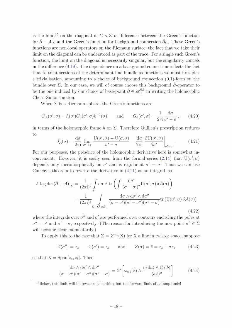
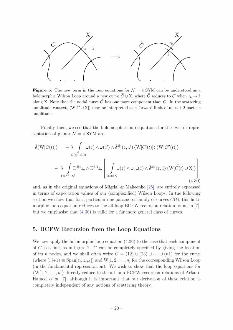
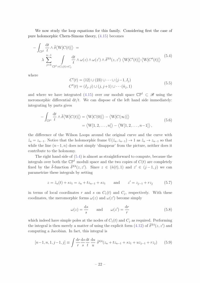
[38] J Drummond J Henn and J Trnka New Differential Equations for On-Shell Loop
Integrals arXiv10103679
[39] H Elvang D Z Freedman and M Kiermaier Proof of the MHV Vertex Expansion
for All Tree Amplitudes in N = 4 SYM Theory JHEP 06 (2009) 068
[arXiv08113624]
ndash 28 ndash
Related Documents