High Resolution Land Cover Integrating Copernicus Products

�����������������

Citation: De Fioravante, P.; Strollo,

A.; Assennato, F.; Marinosci, I.;

Congedo, L.; Munafò, M. High

Resolution Land Cover Integrating

Copernicus Products: A 2012–2020

Map of Italy. Land 2022, 11, 35.

https://doi.org/10.3390/

land11010035

Academic Editor: Adrianos Retalis

Received: 28 November 2021

Accepted: 20 December 2021

Published: 26 December 2021

Publisher’s Note: MDPI stays neutral

with regard to jurisdictional claims in

published maps and institutional affil-

iations.

Copyright: © 2021 by the authors.

Licensee MDPI, Basel, Switzerland.

This article is an open access article

distributed under the terms and

conditions of the Creative Commons

Attribution (CC BY) license (https://

creativecommons.org/licenses/by/

4.0/).

land

Article

High Resolution Land Cover Integrating Copernicus Products:A 2012–2020 Map of Italy

Paolo De Fioravante 1,2,* , Andrea Strollo 1 , Francesca Assennato 1, Ines Marinosci 1 , Luca Congedo 1

and Michele Munafò 1

1 Italian Institute for Environmental Protection and Research (ISPRA), Via Vitaliano Brancati 48,00144 Rome, Italy; [email protected] (A.S.); [email protected] (F.A.);[email protected] (I.M.); [email protected] (L.C.);[email protected] (M.M.)

2 Department of Innovation in Biology, Agri-Food and Forest Systems (DIBAF), University of Tuscia,Via San Camillo de Lellis SNC, 01100 Viterbo, Italy

* Correspondence: [email protected]

Abstract: The study involved an in-depth analysis of the main land cover and land use data availablenationwide for the Italian territory, in order to produce a reliable cartography for the evaluation ofecosystem services. In detail, data from the land monitoring service of the Copernicus Programmewere taken into consideration, while at national level the National Land Consumption Map and someregional land cover and land use maps were analysed. The classification systems were standardizedwith respect to the European specifications of the EAGLE Group and the data were integratedto produce a land cover map in raster format with a spatial resolution of 10 m. The map wasvalidated and compared with the CORINE Land Cover, showing a significant geometric and thematicimprovement, useful for a more detailed and reliable evaluation of ecosystem services. In detail, themap was used to estimate the variation in carbon storage capacity in Italy for the period 2012–2020,linked to the increase in land consumption

Keywords: land cover; Copernicus; land monitoring; ecosystem services; CORINE land cover; carbonstorage capacity; EAGLE matrix

1. Introduction

Territory is a source of resources such as food, biomass and raw materials and providesessential ecosystem services that support production functions, regulate natural cycles,provide cultural and spiritual benefits [1].

The European Environment Agency introduced the concept of “land system”, whichdefines the territory as a set of terrestrial components that includes all the processes andactivities related to its anthropic use [2,3]. This concept considers the territory as anintegrated system [4] that combines everything related to land use and land cover. Thestudy of land cover and land use is essential to understand the causes and effects of human-determined changes [5], seeing as now changes and transformations that occur within theland system lead to consequences for the well-being of humans and the environment at thelocal, regional and global levels.

1.1. Estimation and Monitoring of Ecosystem Services

The management of territory is fundamental, since its transformation alters the envi-ronmental processes and related ecosystem services [6], which are the benefits that humansobtain directly or indirectly from terrestrial ecosystems [7].

Since 2005, the concept of ecosystem services has been placed on the political agenda [8–10]thanks also to the Millennium Ecosystem Assessment (MEA). The MEA is an internationalresearch project launched in 2001 with the aim of evaluating the consequences of ecosystem

Land 2022, 11, 35. https://doi.org/10.3390/land11010035 https://www.mdpi.com/journal/land

Land 2022, 11, 35 2 of 30

changes on human well-being and establishing actions to improve the conservation andsustainable use of ecosystems and their contribution to health.

The Millennium Ecosystem Assessment [11] provides a classification of ecosystemservices which consist of four groups:

– Provisioning services, which provide products obtained from ecosystems, such as food,raw materials and water.

– Regulating services, i.e., the benefits provided through ecosystem processes, such ascarbon storage, erosion control.

– Cultural services, which represent the nonmaterial benefits that people obtain throughspiritual enrichment, cognitive development and aesthetic experience.

– Supporting services, which constitute a “transversal” category that supports the produc-tion of other services, providing living space for plants and animals or maintaininggenetic diversity. They differ from other categories since their impact on people isindirect or is visible after a very long period.

The Economics of Ecosystems and Biodiversity [12] provides a classification alignedwith MEA, while the Common International Classification of Ecosystem Services (CI-CES) excludes “support services” and renames the category of “regulation services” as“regulation and maintenance services”, including habitat maintenance [13,14].

In 1997, Costanza [7] published one of the first assessments of ecosystem services,which was then updated in 2014 [15]. Other application examples for more limited areasare readily available in the scientific literature: assessment on pollination can be found bothfrom a biophysical [16,17] and economic [18–20] point of view. The United Kingdom wasamong the first European country to draw up a complete official report in line with theMillennium Ecosystem Assessment [21]. Rabe et al. [22] developed a network of nationalindicators on ecosystem services in Germany using CORINE Land Cover data for theanalysis of nine ecosystem services divided into three classification categories (according toCICES). Spain published an official report in 2016 [23] related to twelve ecosystem services.Outside the European context, there are applications on a national scale in China [24], SouthAfrica [25] and South Korea [26].

Soil has fundamental functions for nature and humankind and is the source of manyecosystem services [27–29]:

– Fertility: the nutrient cycle ensures fertility in the soil and, at the same time, the releaseof nutrients necessary for plant growth;

– Filter and reserve: the soil can act as a filter against pollutants and can store largequantities of water, useful for plants and for the mitigation of floods;

– Structural: soils represent the support for plants, animals and infrastructures;– Climate regulation: the soil, in addition to being the largest carbon sink, regulates the

emission of important greenhouse gases (N2O and CH4);– Conservation of biodiversity: soils are an immense reservoir of biodiversity. They

represent the habitat for thousands of species capable of preventing the action ofparasites or facilitating waste disposal;

– Resource: soils can be an important source of supply of raw materials.

All soils perform their functions at the same time (food production, water purification,carbon sequestration, etc.) in a different way according to land use and pedogenetic charac-teristics. For example, the rate of carbon sequestration and water purification is higher in anatural area than in an agricultural one, which however has greater production capacity.

Carbon sequestration and storage is an important regulatory service linked to theattitude of ecosystems to fix greenhouse gases. This service contributes to climate regula-tion and is fundamental in defining adaptation strategies to climate change [30,31]. Thecapacity to store carbon depends, among other things, on land use and cover and on theclimate [32]. Land use, land use change and forestry (LULUCF) activities can act as sourcesof emissions or store carbon by acting as sinks. In particular, natural and seminaturalforest ecosystems have the highest carbon sequestration potential. Once natural land is

Land 2022, 11, 35 3 of 30

urbanized or degraded, it loses its ability to retain carbon which, as a result, is emittedinto the atmosphere [33]. Urban expansion, land consumption, deforestation and forestdegradation limit the ability of natural areas to store carbon and have contributed to theseemissions by releasing carbon stored in forests, vegetation and soil [6,34,35].

1.2. Land Monitoring

Land cover and land use are strongly related and for many applications both informa-tion categories are required [36]. To meet different monitoring needs, data with differentcharacteristics from a spatial, temporal and thematic point of view were introduced.

In this respect, different initiatives have been developed. The purpose of the Coperni-cus program is to collect information on the earth’s surface and organize it according tocriteria that allow to compare different data, to exchange data between EU countries andto increase the number of users. The Copernicus Land Monitoring Service (CLMS) allowsresearchers to obtain geographic information on soils and on numerous variables related tothem (such as the state of the vegetation or the water cycle), supporting applications in awide variety of sectors, such as territorial planning, management of water resources andforests, agriculture and food security. CORINE Land Cover is one of the main productsbelonging to CLMS. It has guaranteed information for the whole European territory since1990, with 44 land cover and land use classes and geometric detail of 25 hectares.

Recently, data with higher spatial and thematic details have been introduced in thecontext of the CLMS Local Component. It aims at providing detailed information on criticalareas from an environmental point of view, which require specific and detailed monitoring.Currently, this Copernicus component offers land cover and land use maps in vector format,with high spatial resolution and a 6-year update frequency for four categories of areas.Urban Atlas refers to the CLC classification system, describing with higher detail the landcover and land use characteristics of urban areas, while Riparian Zone and Natura 2000 usethe ecosystem types defined in the Mapping Assessment of Ecosystems and their Services(MAES) [37], which are based on the CLC classes too.

These aforementioned data adopt classification systems based on different combina-tions of land cover and land use classes that are difficult to compare and integrate withthose of other data. In order to coordinate data flows from a thematic point of view, theEAGLE group (EIONET Action Group on Land monitoring in Europe) was created. It aimsat defining a conceptual methodology to describe land cover and land use informationin a consistent data model. EAGLE is not a classification system but a tool to describeclasses of a given classification system by tracing them to the segments related to thethree categories. This allows to better understand the characteristics, the overlaps and thepossible conversions between different classification systems and provides a basis to definenew ones. The EAGLE model aims at separating the land cover and land use componentsthrough data modelling systems applicable at different scales and in different contexts,while maintaining compatibility with existing databases.

The EAGLE data model is based on the definition of three blocks, called “categories”:

• Land cover components (LCC), which refer to the definition of "land cover" provided bythe INSPIRE directive 2007/2/CE. The LCCs are mutually exclusive and exhaustiveand can be used as a modelling element to semantically describe a class definition orto map landscape;

• Land use attributes (LUA), that follow in principle the Hierarchical INSPIRE Land UseClassification System (HILUCS), with some changes to fit the purpose of the EAGLEconcept. The LUA are attached to the land cover unit;

• Landscape characteristics (CH), which describe further details of the land cover compo-nents. The first level distinguishes “land management”, “spatial pattern”, “crop type",“mining product type”, “ecosystem types”, “height zone”, “(bio-)physical character-istics”, “general parameters”, “status” and “temporal” parameters. This enhancesthe integration between national activities and European land monitoring initiativesencouraging a bottom-up approach in data production.

Land 2022, 11, 35 4 of 30

The problem of interoperability and non-homogeneity between data is also evidentat a national level. The National Land Consumption Map offers national coverage, withannual update and EAGLE compliant classification system, while most of the data availableat the regional level are inconsistent, not updated and difficult to relate to each other.

Despite the large amount and variety of land cover and land use data available atnational and European level, currently CLC is the only product capable of supporting anassessment of ecosystem services on a national scale [38], since it guarantees the mappingof the entire national territory and has a thematic detail suitable for the purpose. However,the low spatial resolution and the presence of mixed classes reduce the reliability of theassessments based on them.

In this sense, the first objective of this research concerns the development of a methodol-ogy that makes the main Copernicus and national land cover and land use data comparableand integrable, in order to obtain a product with national coverage that allows to overcomethe limits of the CLC in terms of classification system and geometric detail.

Furthermore, the activity refers to an EAGLE compliant classification system with athematic detail useful for conducting an assessment of ecosystem services, with particularreference to the variation of carbon stocks. This change was assessed with respect totheincrease in land consumption between 2012 and 2020.

2. Materials and Methods2.1. Overview

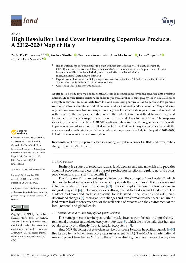
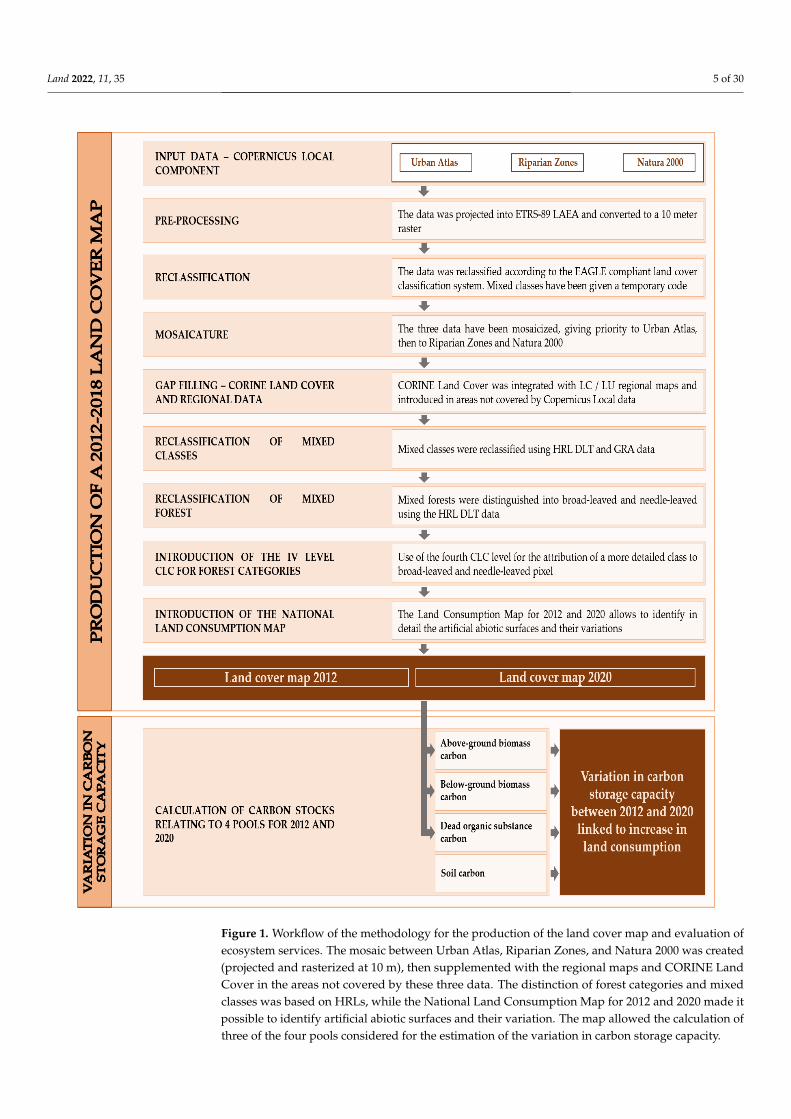
The methodology presented in this study integrates Copernicus and national datafor the production of a land cover map capable of supporting the ecosystem servicesassessment. Data were reclassified according to an EAGLE compliant classification systemand merged into a 10 m resolution land cover map of Italy. The map was used to assess theloss of carbon storage capacity for the period 2012–2020, associated with land consumption(Figure 1).

2.2. Study Area

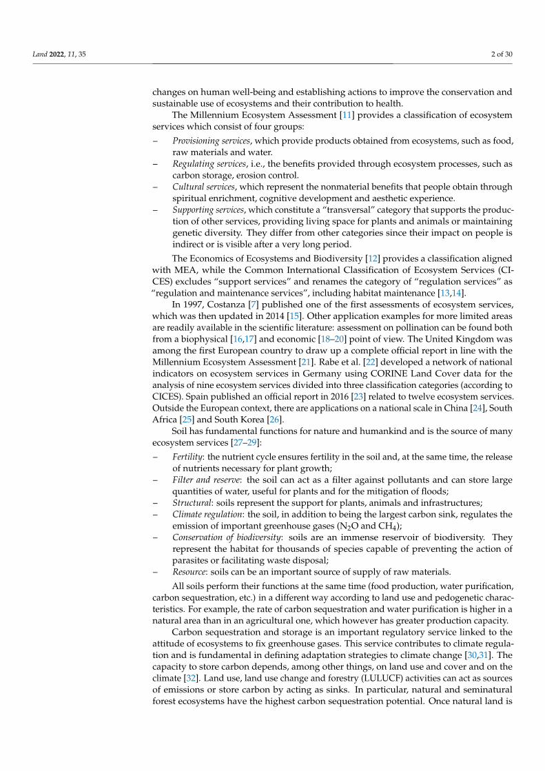
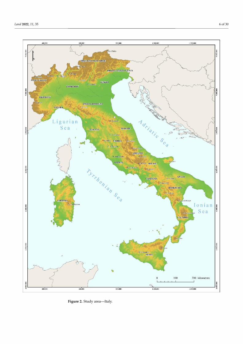
The analysis was carried out for the entire Italian territory (Figure 2), which covers301,338 km2. The country is composed mainly of hills (41.0%) and mountains (35.0%), whilethe remaining 23.0% of the territory is covered by plains. To the north is the mountain rangeof the Alps, which exceeds 4,000 m in altitude. In this area, the alpine climate prevails,with high rainfall with a maximum of 2,500–3,500 mm. In the peninsular area there is theApennine mountain range, reaching its highest peak in Abruzzo with Gran Sasso (2,912 m)and characterized by a continental climate. The coastal area has a Mediterranean climate,with average annual rainfall that reaches a minimum of 500 mm in Apulia and Molise.

Land cover is characterized by forest in mountain areas, with conifer concentrationin alpine areas. Crops and most of the urbanized areas are concentrated in the plains andalong the coast.

2.3. Land Cover Classification System

The activities described in this paper refers to a sixteen-class classification system. Theclasses are defined in accordance with the EAGLE group specifications [39–41] and areorganized into five levels (Table 1).

The classification system is based on previous activities of the working group [41] andimproved to maintain the thematic detail offered by the Copernicus and national inputdata. The first three classes coincide up to the third level of detail with Eagle concept landcover components. Wetland class and the fourth and fifth classification levels are based onEAGLE characteristics (LCH) definitions.

Land 2022, 11, 35 5 of 30Land 2022, 10, x FOR PEER REVIEW 5 of 31

Figure 1. Workflow of the methodology for the production of the land cover map and evaluation of

ecosystem services. The mosaic between Urban Atlas, Riparian Zones, and Natura 2000 was created

(projected and rasterized at 10 m), then supplemented with the regional maps and CORINE Land

Cover in the areas not covered by these three data. The distinction of forest categories and mixed

classes was based on HRLs, while the National Land Consumption Map for 2012 and 2020 made it

possible to identify artificial abiotic surfaces and their variation. The map allowed the calculation of

three of the four pools considered for the estimation of the variation in carbon storage capacity.

Figure 1. Workflow of the methodology for the production of the land cover map and evaluation ofecosystem services. The mosaic between Urban Atlas, Riparian Zones, and Natura 2000 was created(projected and rasterized at 10 m), then supplemented with the regional maps and CORINE LandCover in the areas not covered by these three data. The distinction of forest categories and mixedclasses was based on HRLs, while the National Land Consumption Map for 2012 and 2020 made itpossible to identify artificial abiotic surfaces and their variation. The map allowed the calculation ofthree of the four pools considered for the estimation of the variation in carbon storage capacity.

Land 2022, 11, 35 6 of 30Land 2022, 10, x FOR PEER REVIEW 6 of 31

Figure 2. Study area—Italy.

Figure 2. Study area—Italy.

Land 2022, 11, 35 7 of 30

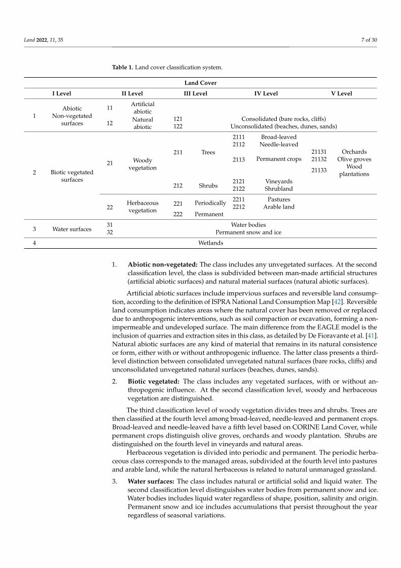
Table 1. Land cover classification system.

Land Cover

I Level II Level III Level IV Level V Level

1Abiotic

Non-vegetatedsurfaces

11 Artificialabiotic

12 Naturalabiotic

121 Consolidated (bare rocks, cliffs)122 Unconsolidated (beaches, dunes, sands)

2 Biotic vegetatedsurfaces

21 Woodyvegetation

211 Trees

2111 Broad-leaved2112 Needle-leaved

2113 Permanent crops21131 Orchards21132 Olive groves

21133 Woodplantations

212 Shrubs2121 Vineyards2122 Shrubland

22Herbaceousvegetation

221 Periodically 2211 Pastures2212 Arable land

222 Permanent

3 Water surfaces31 Water bodies32 Permanent snow and ice

4 Wetlands

1. Abiotic non-vegetated: The class includes any unvegetated surfaces. At the secondclassification level, the class is subdivided between man-made artificial structures(artificial abiotic surfaces) and natural material surfaces (natural abiotic surfaces).

Artificial abiotic surfaces include impervious surfaces and reversible land consump-tion, according to the definition of ISPRA National Land Consumption Map [42]. Reversibleland consumption indicates areas where the natural cover has been removed or replaceddue to anthropogenic interventions, such as soil compaction or excavation, forming a non-impermeable and undeveloped surface. The main difference from the EAGLE model is theinclusion of quarries and extraction sites in this class, as detailed by De Fioravante et al. [41].Natural abiotic surfaces are any kind of material that remains in its natural consistenceor form, either with or without anthropogenic influence. The latter class presents a third-level distinction between consolidated unvegetated natural surfaces (bare rocks, cliffs) andunconsolidated unvegetated natural surfaces (beaches, dunes, sands).

2. Biotic vegetated: The class includes any vegetated surfaces, with or without an-thropogenic influence. At the second classification level, woody and herbaceousvegetation are distinguished.

The third classification level of woody vegetation divides trees and shrubs. Trees arethen classified at the fourth level among broad-leaved, needle-leaved and permanent crops.Broad-leaved and needle-leaved have a fifth level based on CORINE Land Cover, whilepermanent crops distinguish olive groves, orchards and woody plantation. Shrubs aredistinguished on the fourth level in vineyards and natural areas.

Herbaceous vegetation is divided into periodic and permanent. The periodic herba-ceous class corresponds to the managed areas, subdivided at the fourth level into pasturesand arable land, while the natural herbaceous is related to natural unmanaged grassland.

3. Water surfaces: The class includes natural or artificial solid and liquid water. Thesecond classification level distinguishes water bodies from permanent snow and ice.Water bodies includes liquid water regardless of shape, position, salinity and origin.Permanent snow and ice includes accumulations that persist throughout the yearregardless of seasonal variations.

Land 2022, 11, 35 8 of 30

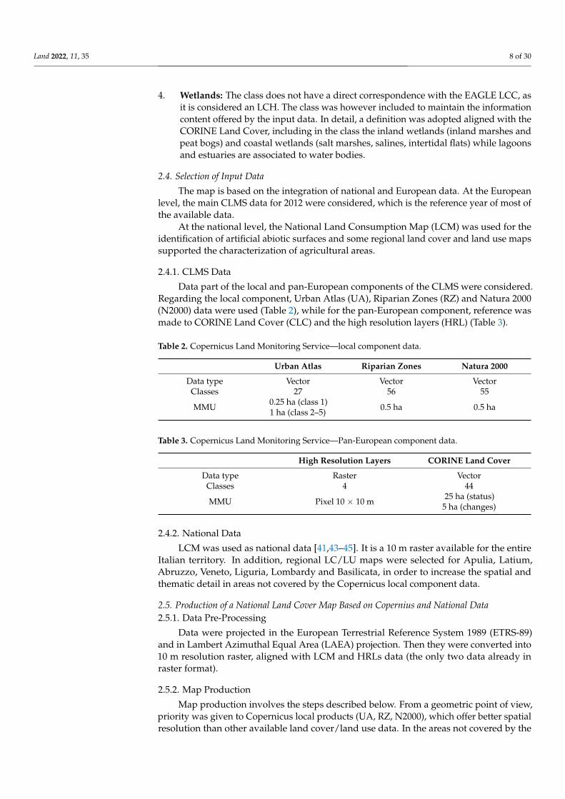
4. Wetlands: The class does not have a direct correspondence with the EAGLE LCC, asit is considered an LCH. The class was however included to maintain the informationcontent offered by the input data. In detail, a definition was adopted aligned with theCORINE Land Cover, including in the class the inland wetlands (inland marshes andpeat bogs) and coastal wetlands (salt marshes, salines, intertidal flats) while lagoonsand estuaries are associated to water bodies.

2.4. Selection of Input Data

The map is based on the integration of national and European data. At the Europeanlevel, the main CLMS data for 2012 were considered, which is the reference year of most ofthe available data.

At the national level, the National Land Consumption Map (LCM) was used for theidentification of artificial abiotic surfaces and some regional land cover and land use mapssupported the characterization of agricultural areas.

2.4.1. CLMS Data

Data part of the local and pan-European components of the CLMS were considered.Regarding the local component, Urban Atlas (UA), Riparian Zones (RZ) and Natura 2000(N2000) data were used (Table 2), while for the pan-European component, reference wasmade to CORINE Land Cover (CLC) and the high resolution layers (HRL) (Table 3).

Table 2. Copernicus Land Monitoring Service—local component data.

Urban Atlas Riparian Zones Natura 2000

Data type Vector Vector VectorClasses 27 56 55

MMU 0.25 ha (class 1)1 ha (class 2–5) 0.5 ha 0.5 ha

Table 3. Copernicus Land Monitoring Service—Pan-European component data.

High Resolution Layers CORINE Land Cover

Data type Raster VectorClasses 4 44

MMU Pixel 10 × 10 m 25 ha (status)5 ha (changes)

2.4.2. National Data

LCM was used as national data [41,43–45]. It is a 10 m raster available for the entireItalian territory. In addition, regional LC/LU maps were selected for Apulia, Latium,Abruzzo, Veneto, Liguria, Lombardy and Basilicata, in order to increase the spatial andthematic detail in areas not covered by the Copernicus local component data.

2.5. Production of a National Land Cover Map Based on Copernius and National Data2.5.1. Data Pre-Processing

Data were projected in the European Terrestrial Reference System 1989 (ETRS-89)and in Lambert Azimuthal Equal Area (LAEA) projection. Then they were converted into10 m resolution raster, aligned with LCM and HRLs data (the only two data already inraster format).

2.5.2. Map Production

Map production involves the steps described below. From a geometric point of view,priority was given to Copernicus local products (UA, RZ, N2000), which offer better spatialresolution than other available land cover/land use data. In the areas not covered by the

Land 2022, 11, 35 9 of 30

Local data, the CLC and the regional maps available for 2012 (derived from CLC) havebeen inserted.

From a thematic point of view, the input data were homogenized with respect to theclassification system of Table 1. For the mixed classes, Copernicus HRL data were used todistinguish the woody component from herbaceous vegetation, then reference was madeto the definitions of such mixed classes to distinguish natural areas from agricultural ones.The CLC data made it possible to attribute a detailed prevalent forest categories to areasclassified as broad-leaved and needle-leaved, while the LCM locates the consumed land.

Reclassification of Copernicus UA, RZ, N2000 Data and Creation of the Basic Mosaic

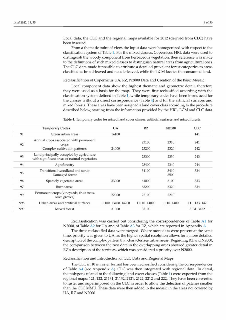
Local component data show the highest thematic and geometric detail, thereforethey were used as a basis for the map. They were first reclassified according with theclassification system defined in Table 1, while temporary codes have been introduced forthe classes without a direct correspondence (Table 4) and for the artificial surfaces andmixed forests. These areas have been assigned a land cover class according to the proceduredescribed below, starting from the information provided by the HRL, LCM and CLC data.

Table 4. Temporary codes for mixed land cover classes, artificial surfaces and mixed forests.

Temporary Codes UA RZ N2000 CLC

91 Green urban areas 14100 141

92Annual crops associated with permanent

crops 23100 2310 241

Complex cultivation patterns 24000 23200 2320 242

93 Land principally occupied by agriculturewith significant areas of natural vegetation 23300 2330 243

94 Agroforestry 23400 2340 244

95Transitional woodland and scrub 34100 3410 324

Damaged forest 3500

96 Sparsely vegetated areas 33000 61000 6100 333

97 Burnt areas 63200 6320 334

99 Permanent crops (vineyards, fruit trees,olive groves) 22000 22100 2210

998 Urban areas and artificial surfaces 11100–13400, 14200 11110–14000 1110–1400 111–133, 142

999 Mixed forest 31000 33100 3131–3132

Reclassification was carried out considering the correspondences of Table A1 forN2000, of Table A2 for UA and of Table A3 for RZ, which are reported in Appendix A.

The three reclassified data were merged. Where more data were present at the sametime, priority was given to UA, as the higher spatial resolution allows for a more detaileddescription of the complex pattern that characterizes urban areas. Regarding RZ and N2000,the comparison between the two data in the overlapping areas showed greater detail inRZ’s description of the territory, which was considered a priority over N2000.

Reclassification and Introduction of CLC Data and Regional Maps

The CLC in 10 m raster format has been reclassified considering the correspondencesof Table A4 (see Appendix A). CLC was then integrated with regional data. In detail,the polygons related to the following land cover classes (Table 1) were exported from theregional maps: 121, 122, 21131, 21132, 2121, 2122, 2212 and 222. They have been convertedto raster and superimposed on the CLC in order to allow the detection of patches smallerthan the CLC MMU. These data were then added to the mosaic in the areas not covered byUA, RZ and N2000.

Land 2022, 11, 35 10 of 30

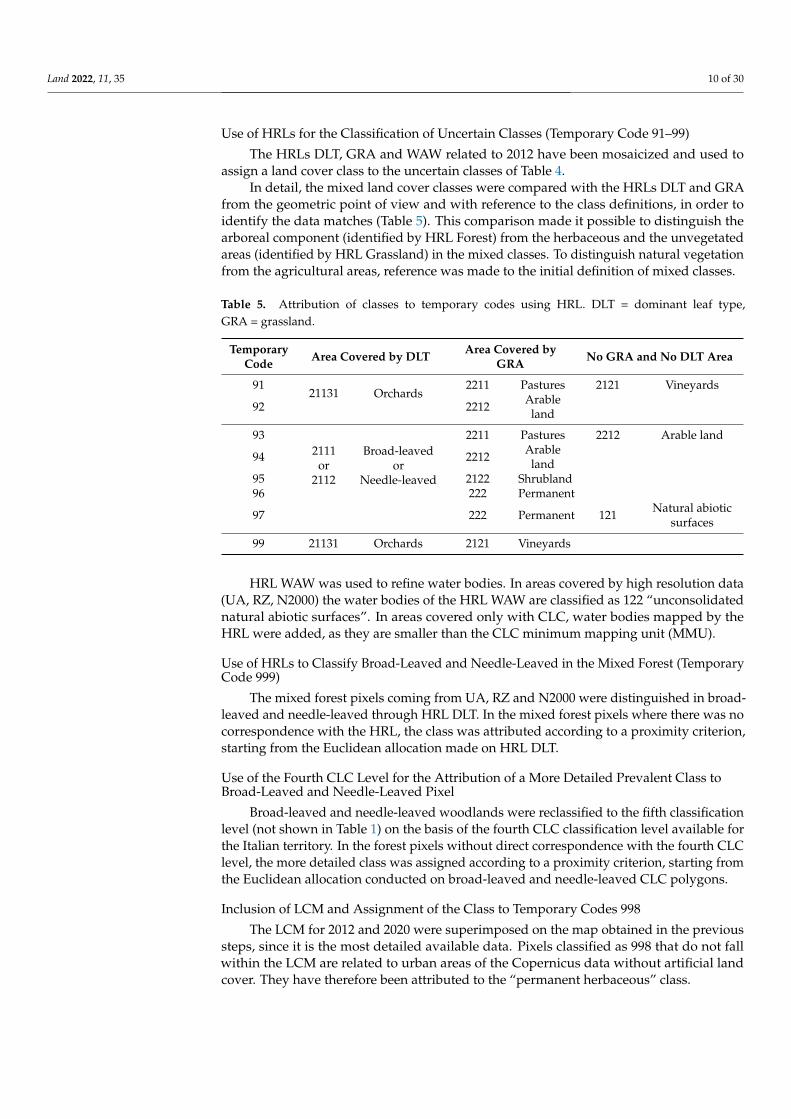
Use of HRLs for the Classification of Uncertain Classes (Temporary Code 91–99)

The HRLs DLT, GRA and WAW related to 2012 have been mosaicized and used toassign a land cover class to the uncertain classes of Table 4.

In detail, the mixed land cover classes were compared with the HRLs DLT and GRAfrom the geometric point of view and with reference to the class definitions, in order toidentify the data matches (Table 5). This comparison made it possible to distinguish thearboreal component (identified by HRL Forest) from the herbaceous and the unvegetatedareas (identified by HRL Grassland) in the mixed classes. To distinguish natural vegetationfrom the agricultural areas, reference was made to the initial definition of mixed classes.

Table 5. Attribution of classes to temporary codes using HRL. DLT = dominant leaf type,GRA = grassland.

TemporaryCode Area Covered by DLT Area Covered by

GRA No GRA and No DLT Area

9121131 Orchards

2211 Pastures 2121 Vineyards

92 2212 Arableland

932111

or2112

Broad-leavedor

Needle-leaved

2211 Pastures 2212 Arable land

94 2212 Arableland

95 2122 Shrubland96 222 Permanent

97 222 Permanent 121 Natural abioticsurfaces

99 21131 Orchards 2121 Vineyards

HRL WAW was used to refine water bodies. In areas covered by high resolution data(UA, RZ, N2000) the water bodies of the HRL WAW are classified as 122 “unconsolidatednatural abiotic surfaces”. In areas covered only with CLC, water bodies mapped by theHRL were added, as they are smaller than the CLC minimum mapping unit (MMU).

Use of HRLs to Classify Broad-Leaved and Needle-Leaved in the Mixed Forest (TemporaryCode 999)

The mixed forest pixels coming from UA, RZ and N2000 were distinguished in broad-leaved and needle-leaved through HRL DLT. In the mixed forest pixels where there was nocorrespondence with the HRL, the class was attributed according to a proximity criterion,starting from the Euclidean allocation made on HRL DLT.

Use of the Fourth CLC Level for the Attribution of a More Detailed Prevalent Class toBroad-Leaved and Needle-Leaved Pixel

Broad-leaved and needle-leaved woodlands were reclassified to the fifth classificationlevel (not shown in Table 1) on the basis of the fourth CLC classification level available forthe Italian territory. In the forest pixels without direct correspondence with the fourth CLClevel, the more detailed class was assigned according to a proximity criterion, starting fromthe Euclidean allocation conducted on broad-leaved and needle-leaved CLC polygons.

Inclusion of LCM and Assignment of the Class to Temporary Codes 998

The LCM for 2012 and 2020 were superimposed on the map obtained in the previoussteps, since it is the most detailed available data. Pixels classified as 998 that do not fallwithin the LCM are related to urban areas of the Copernicus data without artificial landcover. They have therefore been attributed to the “permanent herbaceous” class.

Land 2022, 11, 35 11 of 30

2.5.3. Accuracy Assessment

The 16-class map for 2012 was validated. Accuracy assessment consists of a first phaseof quality control conducted through a systematic visual search for macroscopic errors.A quantitative accuracy assessment was then performed through the photointerpretationof a sample of points, which were then compared with the values of the land cover mapat the same locations. The sample size was assessed using the methodology proposed byOlofsson [46], which is widely adopted in literature [47–49].

The sample size (n) is calculated starting from the areas of each class and from thedefinition of a first attempt user accuracy, using the following equation [47–50]:

(∑ WiSi)2

[S(O)]2

where:

Wi—is area proportion of each classes in the considered mapUi—user accuracy of class i. A conservative scenario was assumed, considering Ui = 0.6 forall classes.Si—standard deviation of stratum i, Si =

√(Ui(1 − Ui)) [50]. Considering Ui = 0.6, it turns

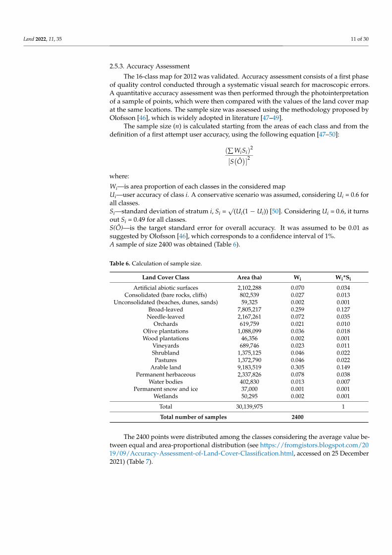
out Si = 0.49 for all classes.S(Ô)—is the target standard error for overall accuracy. It was assumed to be 0.01 assuggested by Olofsson [46], which corresponds to a confidence interval of 1%.A sample of size 2400 was obtained (Table 6).

Table 6. Calculation of sample size.

Land Cover Class Area (ha) Wi Wi*Si

Artificial abiotic surfaces 2,102,288 0.070 0.034Consolidated (bare rocks, cliffs) 802,539 0.027 0.013

Unconsolidated (beaches, dunes, sands) 59,325 0.002 0.001Broad-leaved 7,805,217 0.259 0.127

Needle-leaved 2,167,261 0.072 0.035Orchards 619,759 0.021 0.010

Olive plantations 1,088,099 0.036 0.018Wood plantations 46,356 0.002 0.001

Vineyards 689,746 0.023 0.011Shrubland 1,375,125 0.046 0.022Pastures 1,372,790 0.046 0.022

Arable land 9,183,519 0.305 0.149Permanent herbaceous 2,337,826 0.078 0.038

Water bodies 402,830 0.013 0.007Permanent snow and ice 37,000 0.001 0.001

Wetlands 50,295 0.002 0.001

Total 30,139,975 1

Total number of samples 2400

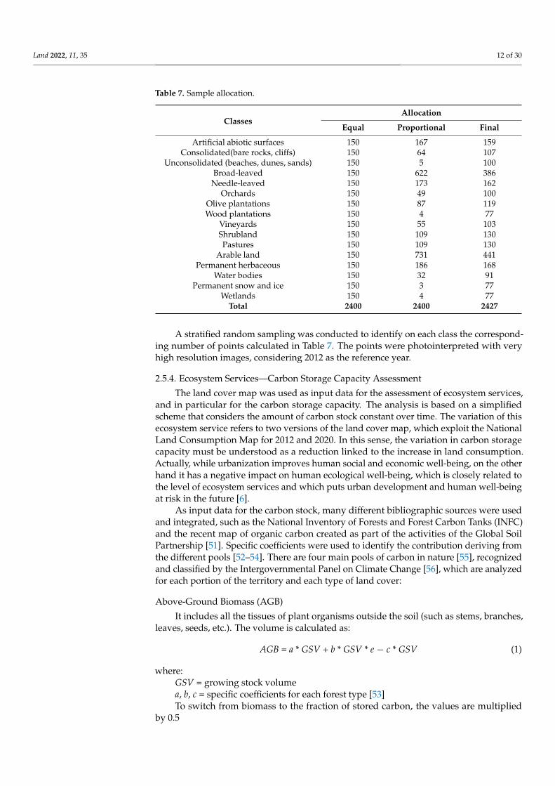
The 2400 points were distributed among the classes considering the average value be-tween equal and area-proportional distribution (see https://fromgistors.blogspot.com/2019/09/Accuracy-Assessment-of-Land-Cover-Classification.html, accessed on 25 December2021) (Table 7).

Land 2022, 11, 35 12 of 30

Table 7. Sample allocation.

ClassesAllocation

Equal Proportional Final

Artificial abiotic surfaces 150 167 159Consolidated(bare rocks, cliffs) 150 64 107

Unconsolidated (beaches, dunes, sands) 150 5 100Broad-leaved 150 622 386

Needle-leaved 150 173 162Orchards 150 49 100

Olive plantations 150 87 119Wood plantations 150 4 77

Vineyards 150 55 103Shrubland 150 109 130Pastures 150 109 130

Arable land 150 731 441Permanent herbaceous 150 186 168

Water bodies 150 32 91Permanent snow and ice 150 3 77

Wetlands 150 4 77Total 2400 2400 2427

A stratified random sampling was conducted to identify on each class the correspond-ing number of points calculated in Table 7. The points were photointerpreted with veryhigh resolution images, considering 2012 as the reference year.

2.5.4. Ecosystem Services—Carbon Storage Capacity Assessment

The land cover map was used as input data for the assessment of ecosystem services,and in particular for the carbon storage capacity. The analysis is based on a simplifiedscheme that considers the amount of carbon stock constant over time. The variation of thisecosystem service refers to two versions of the land cover map, which exploit the NationalLand Consumption Map for 2012 and 2020. In this sense, the variation in carbon storagecapacity must be understood as a reduction linked to the increase in land consumption.Actually, while urbanization improves human social and economic well-being, on the otherhand it has a negative impact on human ecological well-being, which is closely related tothe level of ecosystem services and which puts urban development and human well-beingat risk in the future [6].

As input data for the carbon stock, many different bibliographic sources were usedand integrated, such as the National Inventory of Forests and Forest Carbon Tanks (INFC)and the recent map of organic carbon created as part of the activities of the Global SoilPartnership [51]. Specific coefficients were used to identify the contribution deriving fromthe different pools [52–54]. There are four main pools of carbon in nature [55], recognizedand classified by the Intergovernmental Panel on Climate Change [56], which are analyzedfor each portion of the territory and each type of land cover:

Above-Ground Biomass (AGB)

It includes all the tissues of plant organisms outside the soil (such as stems, branches,leaves, seeds, etc.). The volume is calculated as:

AGB = a * GSV + b * GSV * e − c * GSV (1)

where:GSV = growing stock volumea, b, c = specific coefficients for each forest type [53]To switch from biomass to the fraction of stored carbon, the values are multiplied

by 0.5

Land 2022, 11, 35 13 of 30

Below-Ground Biomass (BGB)

It includes the root system of plants. The volume is calculated as [54]:

BGB = GSV * BEF * WBD * R (2)

where:

GSV = growing stock volumeBEF = biomass expansion factorWBD = wood basic densityR = crown/roots ratio, tabulated for the different species [52,54].

To switch from biomass to the fraction of stored carbon, the values are multipliedby 0.5

The Carbon Contained in the Dead Organic Substance (DOS)

The pool includes the necromass, the woody plant residues, the litter, the finer residuesnot yet decomposed. As regards the epigeal biomass, specific multiplicative coefficientsare considered to be applied to the values obtained from the calculation shown above, forexample 0.20 for evergreen plants and 0.14 for deciduous trees [56].

Specific formulas for each species present in the bibliography were used for thelitter [52,54].

Soil Carbon

The pool includes organic and mineral layers including up to a depth of 30 cm. Itis evaluated starting from the data produced by CREA-ABP, CNR-Ibimet, regions andsome universities as part of the Global Soil Partnership/FAO initiative [51] as an Italiancontribution to the Global Soil Organic Carbon map. The map offers the values of thecarbon contained in the soil in raster format with a resolution of 1 km.

In detail, for the forest cover areas, data from the National Inventory of Forests andForest Carbon Tanks (INFC) were used [57]. The inventory provides differentiated valuesboth by region and according to the different plant species, with reference to the classes ofthe CLC fourth classification level.

For the other land cover classes, estimates from the literature were used: the poolvalues for artificial areas were considered zero while for the other natural and agriculturalsurfaces the literature values reported in Table 8 were used [34].

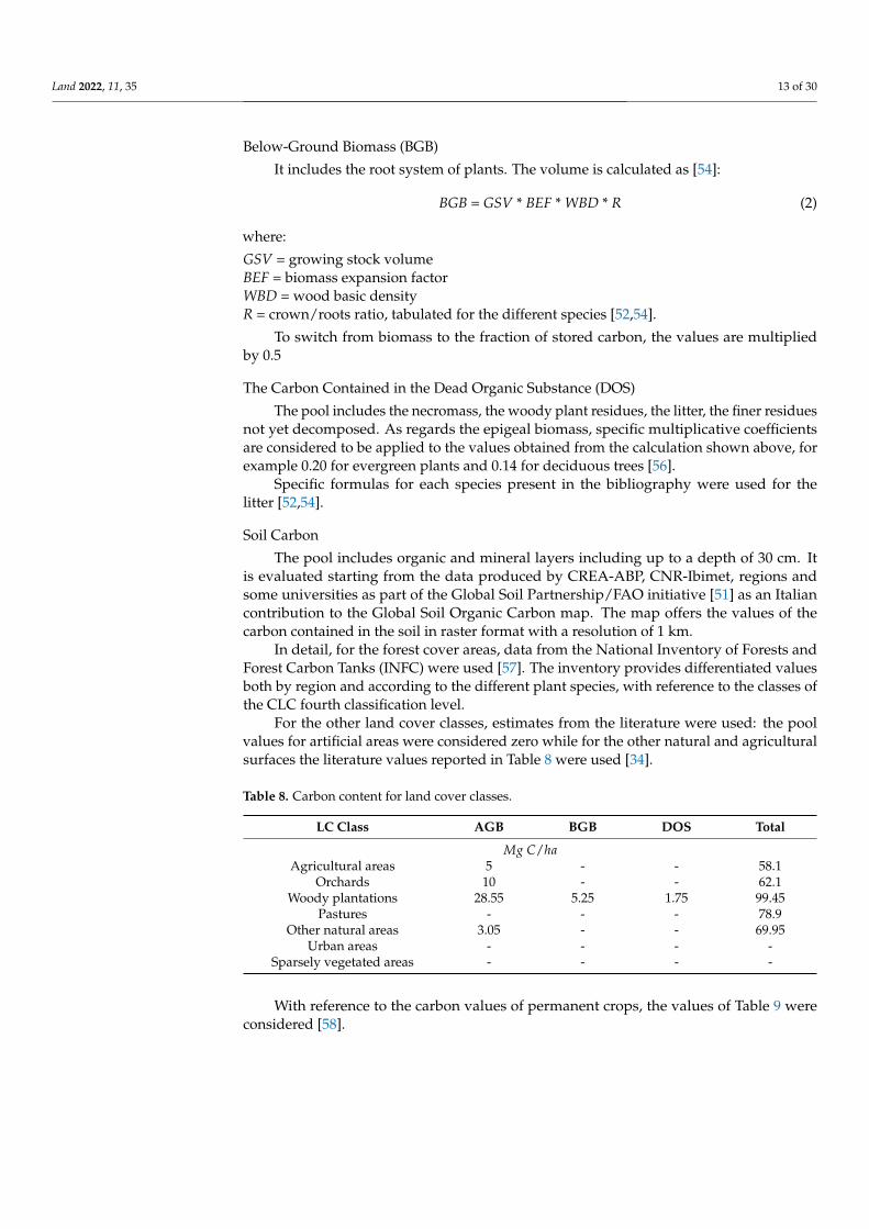
Table 8. Carbon content for land cover classes.

LC Class AGB BGB DOS Total

Mg C/haAgricultural areas 5 - - 58.1

Orchards 10 - - 62.1Woody plantations 28.55 5.25 1.75 99.45

Pastures - - - 78.9Other natural areas 3.05 - - 69.95

Urban areas - - - -Sparsely vegetated areas - - - -

With reference to the carbon values of permanent crops, the values of Table 9 wereconsidered [58].

Land 2022, 11, 35 14 of 30

Table 9. Carbon stock values for some agricultural classes.

LC Class AGB BGB

Mg C/haOlive trees 9.1 2.6Vineyards 5.5 4.4Fruit trees 8.3 5.6

3. Results3.1. Land Cover Map and Accuracy Assessment

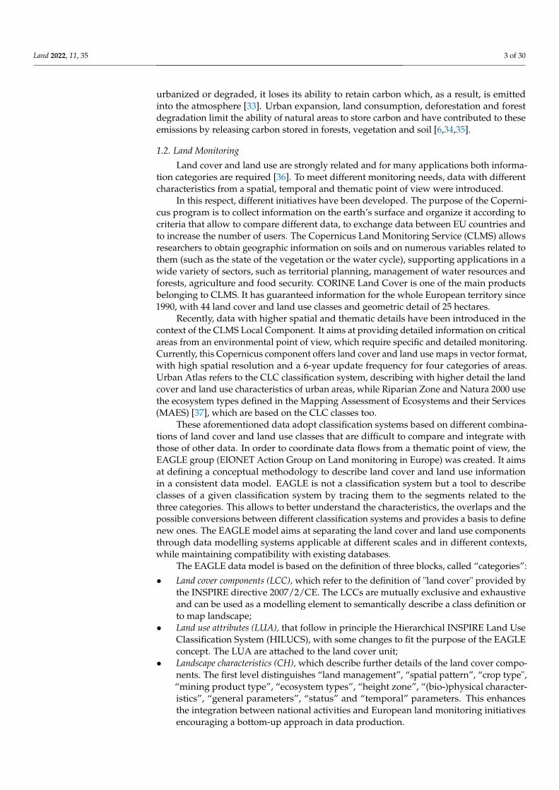
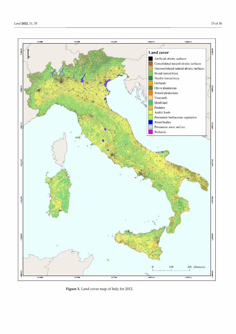
The map of Figure 3 was obtained by applying the procedure described in the previ-ous chapter.

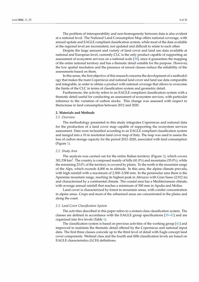
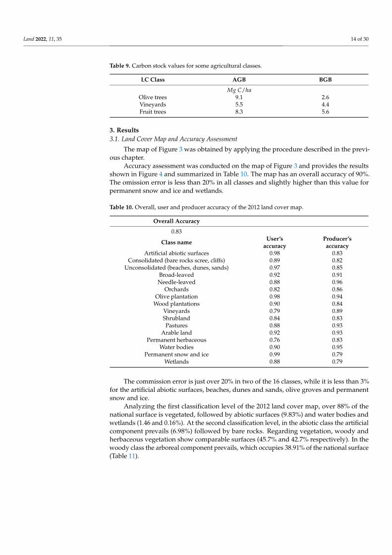
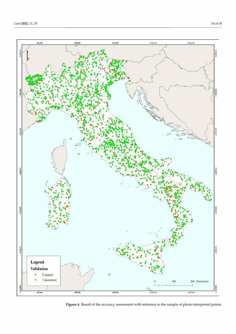
Accuracy assessment was conducted on the map of Figure 3 and provides the resultsshown in Figure 4 and summarized in Table 10. The map has an overall accuracy of 90%.The omission error is less than 20% in all classes and slightly higher than this value forpermanent snow and ice and wetlands.

Table 10. Overall, user and producer accuracy of the 2012 land cover map.

Overall Accuracy

0.83

Class name User’saccuracy

Producer’saccuracy

Artificial abiotic surfaces 0.98 0.83Consolidated (bare rocks scree, cliffs) 0.89 0.82

Unconsolidated (beaches, dunes, sands) 0.97 0.85Broad-leaved 0.92 0.91

Needle-leaved 0.88 0.96Orchards 0.82 0.86

Olive plantation 0.98 0.94Wood plantations 0.90 0.84

Vineyards 0.79 0.89Shrubland 0.84 0.83Pastures 0.88 0.93

Arable land 0.92 0.93Permanent herbaceous 0.76 0.83

Water bodies 0.90 0.95Permanent snow and ice 0.99 0.79

Wetlands 0.88 0.79

The commission error is just over 20% in two of the 16 classes, while it is less than 3%for the artificial abiotic surfaces, beaches, dunes and sands, olive groves and permanentsnow and ice.

Analyzing the first classification level of the 2012 land cover map, over 88% of thenational surface is vegetated, followed by abiotic surfaces (9.83%) and water bodies andwetlands (1.46 and 0.16%). At the second classification level, in the abiotic class the artificialcomponent prevails (6.98%) followed by bare rocks. Regarding vegetation, woody andherbaceous vegetation show comparable surfaces (45.7% and 42.7% respectively). In thewoody class the arboreal component prevails, which occupies 38.91% of the national surface(Table 11).

Land 2022, 11, 35 15 of 30Land 2022, 10, x FOR PEER REVIEW 15 of 31

Figure 3. Land cover map of Italy for 2012.

The commission error is just over 20% in two of the 16 classes, while it is less than 3%

for the artificial abiotic surfaces, beaches, dunes and sands, olive groves and permanent

snow and ice.

Figure 3. Land cover map of Italy for 2012.

Land 2022, 11, 35 16 of 30Land 2022, 10, x FOR PEER REVIEW 16 of 31

Figure 4. Result of the accuracy assessment with reference to the sample of photo-interpreted points.

Analyzing the first classification level of the 2012 land cover map, over 88% of the

national surface is vegetated, followed by abiotic surfaces (9.83%) and water bodies and

Figure 4. Result of the accuracy assessment with reference to the sample of photo-interpreted points.

Land 2022, 11, 35 17 of 30

Table 11. Land cover classes 2012 (first and second classification level).

ha % Total % Class

Abiotic Surfaces 2,964,151 9.83

Artificial abiotic surfaces 802,539 2.66 27.07Natural abiotic surfaces 59,325 0.20 2.00

Bioticvegetated 26,685,696 88.54

Woody vegetation 13,791,561 45.76 51.68Herbaceous vegetation 12,894,135 42.78 48.32

Water surfaces 439,830 1.46

Water bodies 402,830 1.34 91.59Permanent snow and ice 37,000 0.12 8.41

Wetlands 50,295 0.17

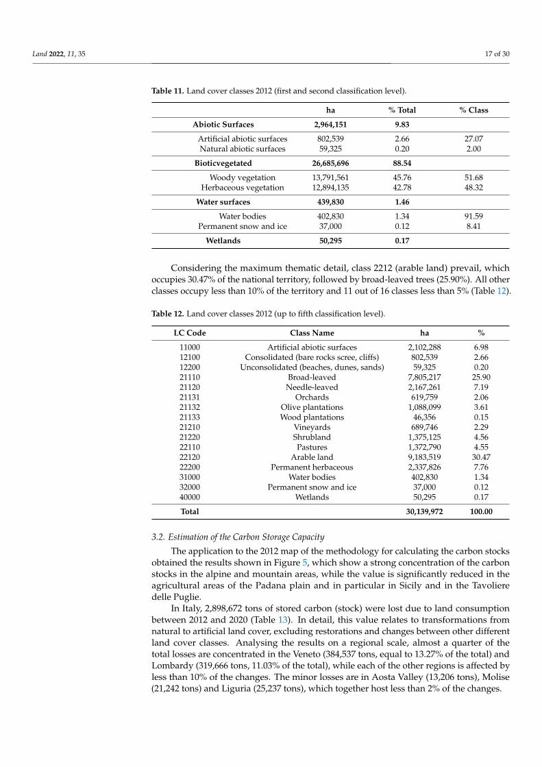
Considering the maximum thematic detail, class 2212 (arable land) prevail, whichoccupies 30.47% of the national territory, followed by broad-leaved trees (25.90%). All otherclasses occupy less than 10% of the territory and 11 out of 16 classes less than 5% (Table 12).

Table 12. Land cover classes 2012 (up to fifth classification level).

LC Code Class Name ha %

11000 Artificial abiotic surfaces 2,102,288 6.9812100 Consolidated (bare rocks scree, cliffs) 802,539 2.6612200 Unconsolidated (beaches, dunes, sands) 59,325 0.2021110 Broad-leaved 7,805,217 25.9021120 Needle-leaved 2,167,261 7.1921131 Orchards 619,759 2.0621132 Olive plantations 1,088,099 3.6121133 Wood plantations 46,356 0.1521210 Vineyards 689,746 2.2921220 Shrubland 1,375,125 4.5622110 Pastures 1,372,790 4.5522120 Arable land 9,183,519 30.4722200 Permanent herbaceous 2,337,826 7.7631000 Water bodies 402,830 1.3432000 Permanent snow and ice 37,000 0.1240000 Wetlands 50,295 0.17

Total 30,139,972 100.00

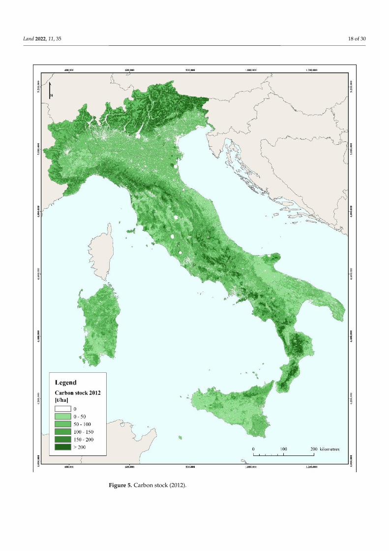
3.2. Estimation of the Carbon Storage Capacity

The application to the 2012 map of the methodology for calculating the carbon stocksobtained the results shown in Figure 5, which show a strong concentration of the carbonstocks in the alpine and mountain areas, while the value is significantly reduced in theagricultural areas of the Padana plain and in particular in Sicily and in the Tavolieredelle Puglie.

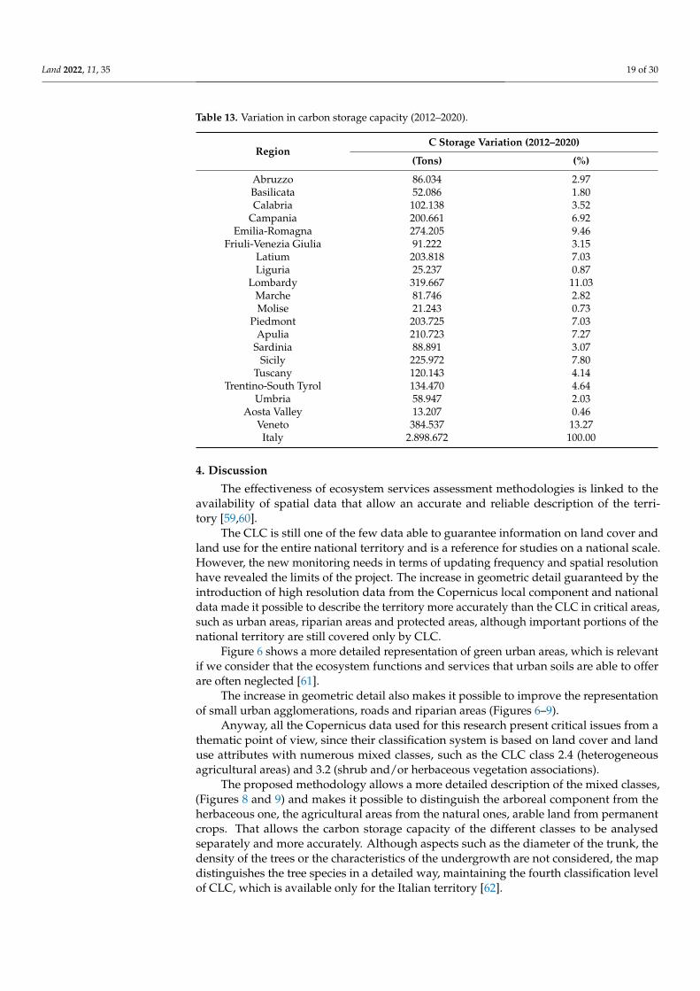
In Italy, 2,898,672 tons of stored carbon (stock) were lost due to land consumptionbetween 2012 and 2020 (Table 13). In detail, this value relates to transformations fromnatural to artificial land cover, excluding restorations and changes between other differentland cover classes. Analysing the results on a regional scale, almost a quarter of thetotal losses are concentrated in the Veneto (384,537 tons, equal to 13.27% of the total) andLombardy (319,666 tons, 11.03% of the total), while each of the other regions is affected byless than 10% of the changes. The minor losses are in Aosta Valley (13,206 tons), Molise(21,242 tons) and Liguria (25,237 tons), which together host less than 2% of the changes.

Land 2022, 11, 35 18 of 30Land 2022, 10, x FOR PEER REVIEW 18 of 31

Figure 5. Carbon stock (2012).

In Italy, 2,898,672 tons of stored carbon (stock) were lost due to land consumption

between 2012 and 2020 (Table 13). In detail, this value relates to transformations from

natural to artificial land cover, excluding restorations and changes between other different

land cover classes. Analysing the results on a regional scale, almost a quarter of the total

losses are concentrated in the Veneto (384,537 tons, equal to 13.27% of the total) and Lom-

bardy (319,666 tons, 11.03% of the total), while each of the other regions is affected by less

Figure 5. Carbon stock (2012).

Land 2022, 11, 35 19 of 30

Table 13. Variation in carbon storage capacity (2012–2020).

RegionC Storage Variation (2012–2020)

(Tons) (%)

Abruzzo 86.034 2.97Basilicata 52.086 1.80Calabria 102.138 3.52

Campania 200.661 6.92Emilia-Romagna 274.205 9.46

Friuli-Venezia Giulia 91.222 3.15Latium 203.818 7.03Liguria 25.237 0.87

Lombardy 319.667 11.03Marche 81.746 2.82Molise 21.243 0.73

Piedmont 203.725 7.03Apulia 210.723 7.27

Sardinia 88.891 3.07Sicily 225.972 7.80

Tuscany 120.143 4.14Trentino-South Tyrol 134.470 4.64

Umbria 58.947 2.03Aosta Valley 13.207 0.46

Veneto 384.537 13.27Italy 2.898.672 100.00

4. Discussion

The effectiveness of ecosystem services assessment methodologies is linked to theavailability of spatial data that allow an accurate and reliable description of the terri-tory [59,60].

The CLC is still one of the few data able to guarantee information on land cover andland use for the entire national territory and is a reference for studies on a national scale.However, the new monitoring needs in terms of updating frequency and spatial resolutionhave revealed the limits of the project. The increase in geometric detail guaranteed by theintroduction of high resolution data from the Copernicus local component and nationaldata made it possible to describe the territory more accurately than the CLC in critical areas,such as urban areas, riparian areas and protected areas, although important portions of thenational territory are still covered only by CLC.

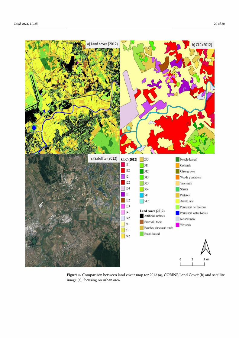
Figure 6 shows a more detailed representation of green urban areas, which is relevantif we consider that the ecosystem functions and services that urban soils are able to offerare often neglected [61].

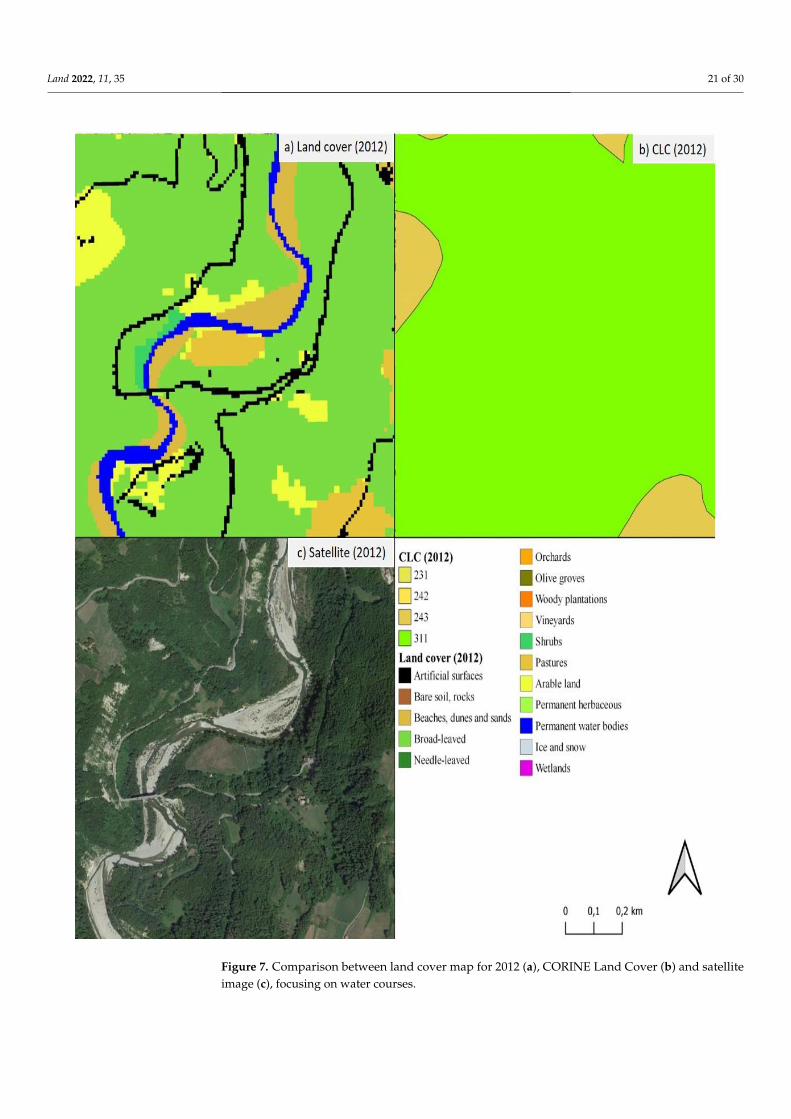
The increase in geometric detail also makes it possible to improve the representationof small urban agglomerations, roads and riparian areas (Figures 6–9).

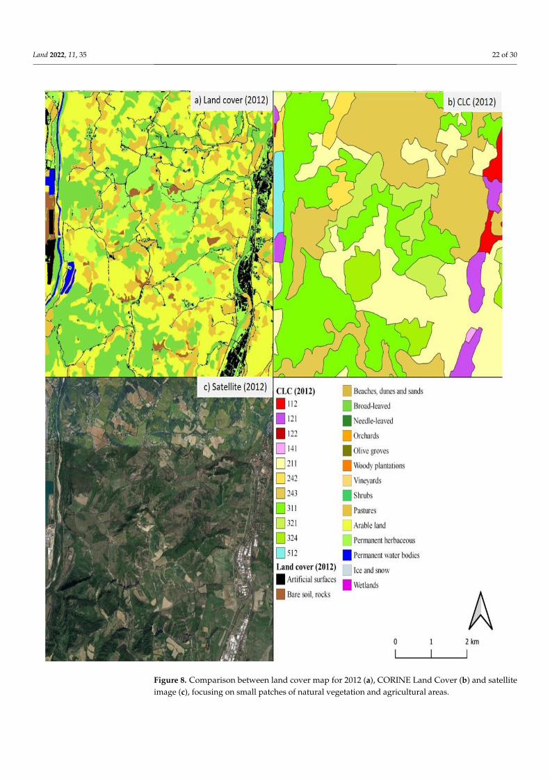
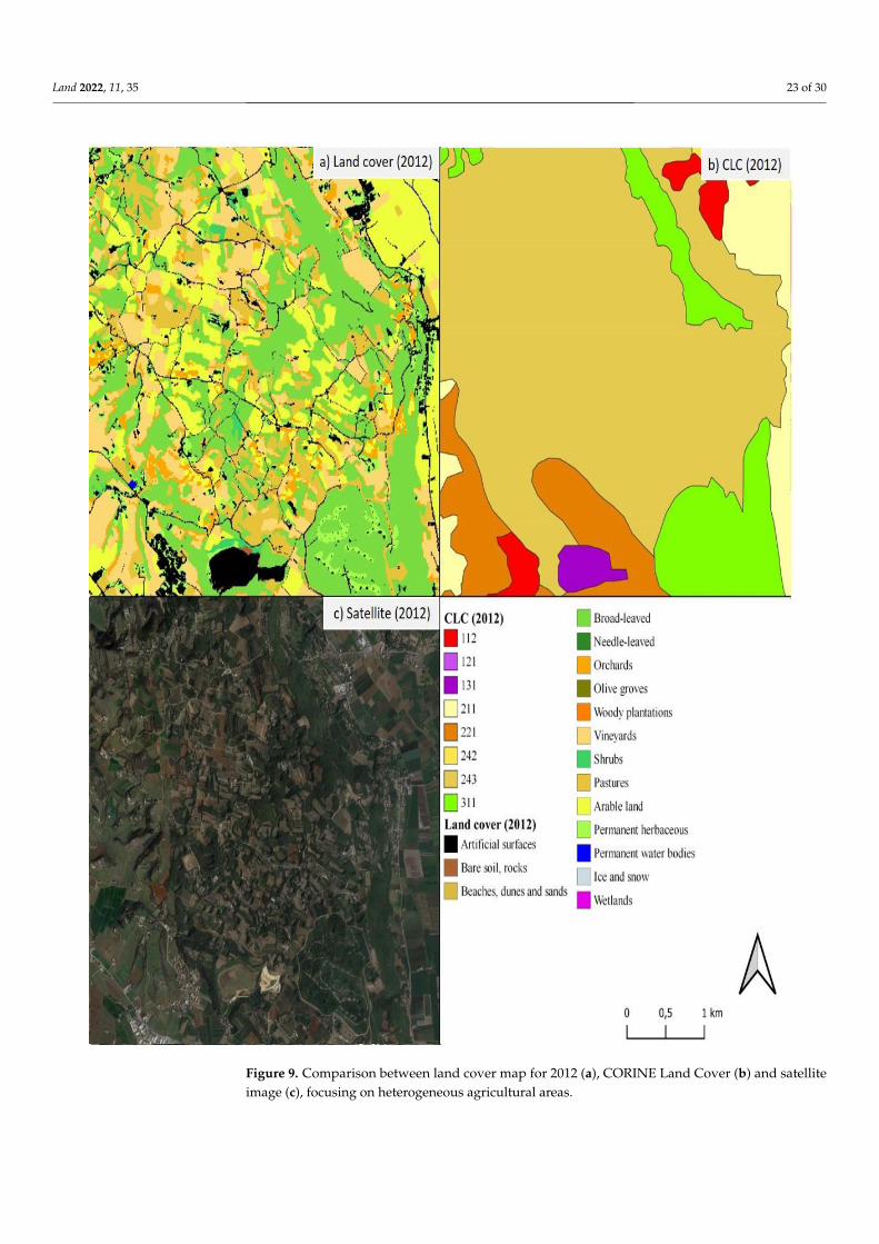
Anyway, all the Copernicus data used for this research present critical issues from athematic point of view, since their classification system is based on land cover and landuse attributes with numerous mixed classes, such as the CLC class 2.4 (heterogeneousagricultural areas) and 3.2 (shrub and/or herbaceous vegetation associations).

The proposed methodology allows a more detailed description of the mixed classes,(Figures 8 and 9) and makes it possible to distinguish the arboreal component from theherbaceous one, the agricultural areas from the natural ones, arable land from permanentcrops. That allows the carbon storage capacity of the different classes to be analysedseparately and more accurately. Although aspects such as the diameter of the trunk, thedensity of the trees or the characteristics of the undergrowth are not considered, the mapdistinguishes the tree species in a detailed way, maintaining the fourth classification levelof CLC, which is available only for the Italian territory [62].

Land 2022, 11, 35 20 of 30Land 2022, 10, x FOR PEER REVIEW 20 of 31

Figure 6. Comparison between land cover map for 2012 (a), CORINE Land Cover (b) and satellite

image (c), focusing on urban area.

The increase in geometric detail also makes it possible to improve the representation

of small urban agglomerations, roads and riparian areas (Figures 6–9).

Figure 6. Comparison between land cover map for 2012 (a), CORINE Land Cover (b) and satelliteimage (c), focusing on urban area.

Land 2022, 11, 35 21 of 30Land 2022, 10, x FOR PEER REVIEW 21 of 31

Figure 7. Comparison between land cover map for 2012 (a), CORINE Land Cover (b) and satellite

image (c), focusing on water courses. Figure 7. Comparison between land cover map for 2012 (a), CORINE Land Cover (b) and satelliteimage (c), focusing on water courses.

Land 2022, 11, 35 22 of 30Land 2022, 10, x FOR PEER REVIEW 22 of 31

Figure 8. Comparison between land cover map for 2012 (a), CORINE Land Cover (b) and satellite

image (c), focusing on small patches of natural vegetation and agricultural areas. Figure 8. Comparison between land cover map for 2012 (a), CORINE Land Cover (b) and satelliteimage (c), focusing on small patches of natural vegetation and agricultural areas.

Land 2022, 11, 35 23 of 30Land 2022, 10, x FOR PEER REVIEW 23 of 31

Figure 9. Comparison between land cover map for 2012 (a), CORINE Land Cover (b) and satellite

image (c), focusing on heterogeneous agricultural areas.

Anyway, all the Copernicus data used for this research present critical issues from a

thematic point of view, since their classification system is based on land cover and land

Figure 9. Comparison between land cover map for 2012 (a), CORINE Land Cover (b) and satelliteimage (c), focusing on heterogeneous agricultural areas.

Land 2022, 11, 35 24 of 30

An aspect that will require further development is the possibility of defining thecorrespondence between the classes of Copernicus data and a classification system orientedto the description of habitats, which would be more functional for conducting studies onecosystem services. In this sense it would be necessary to integrate ancillary data not easilyavailable on a national scale [63].

The data available at the time of the research limited the study on carbon stocks onlyto variations caused by increased land consumption. The availability of new Copernicusdata updated to 2018 will allow the production of land cover maps capable of evaluatingthe variations of ecosystem services associated with other land cover changes occurredbetween 2012 and 2018 [60]. However the update frequency remains too low for numerousmonitoring activities. Actually, the LCM is updated annually, while Copernicus data every6 years and the maps available at regional level in Italy are often based on CLC data andare updated in a few cases (Lombardy, updated to 2018, Tuscany 2016, Liguria 2018, Latium2016), while other maps are less up to date (2012 for Sicily and Apulia, 2013 for Abruzzoand Basilicata, 2006 for Calabria and 2009 for Campania).

Initiatives such as the next “CLC Plus” are expected to be decisive in the near future,guaranteeing the introduction of updated and interoperable products, more suitable forcarrying out the monitoring activities necessary to meet institutional needs. ISPRA isconducting other research activities in this direction [41,43–45,64], through the definition ofa land cover classification methodology for the production of maps with Sentinel resolution,annual update frequency and EAGLE compliant classification system, capable of providingupdated and reliable products for monitoring on a national scale, which can be integratedwith the activities of the “CLC Plus” and the National Strategic Plan for the Space Economy.

5. Conclusions

Since the 19th century, anthropogenic activities have led to a significant increase inthe level of carbon dioxide in the atmosphere [35] and negatively affected the regenerationcapacity and balance of ecosystems. Urban expansion, deforestation and forest degradationhave contributed to these emissions by releasing the carbon stored naturally in forests,vegetation and soil [34,35]. This type of carbon is added to greenhouse gas emissionsrelated to industries and energy production and to the products of impure combustion.Terrestrial ecosystems are able to sequester as much carbon as is currently in the atmospherebut over the course of the century terrestrial biosphere is likely to become a net source ofcarbon due to factors connected with climate change, pollution and the over-exploitationof resources that will alter the structure, reduce biodiversity and perturb functioning ofmost ecosystems, and compromise the services they currently provide.

The land cover and land use changes involve landscape fragmentation, reduction ofbiodiversity and loss of green areas important for carbon accumulation and more generallyfor the provision of ecosystem services. Current conservation practices are generally poorlyprepared to adapt to this level of change, and effective adaptation responses are likely to becostly to implement.

The monitoring of carbon stock accounting is an institutional duty enshrined in theKyoto protocol and the Paris agreements and an important driver in defining adaptationstrategies to climate change [33]. Effective monitoring strategies of land cover and landuse changes are essential for studying the phenomenon. In this sense, the methodologypresented in this paper represents a step forward for large-scale assessments of ecosys-tem services more relevant to reality, since compared to the CLC it provides productsfor the entire national territory with greater geometric detail and a better description ofmixed areas.

The methodology is easily applicable in other territorial areas, since it is based onCopernicus data available for many European countries, furthermore the use of an EAGLEcompliant classification system makes the methodology easily adaptable to the specificavailability of national data.

Land 2022, 11, 35 25 of 30

The main limitation of the methodology concerns the low update frequency of theinput data, which limited the monitoring of ecosystem services to variations related to landconsumption, which is the only data updated annually for the Italian territory.

A first future development concerns the updating of the map using the new CopernicusLocal and Pan-European products for 2018. This implementation will allow the evaluationof the variations in the carbon stocks associated not only with land consumption but alsowith other land cover changes.

The products of the application of the methodology are also in continuity with otheractivities carried out by the working group and can constitute a useful support tool for thedevelopment of land cover classification methodologies with high update frequency for thesatisfaction of the institutional needs envisaged by the new “Space Economy” Strategic Planand for the creation of “Istances” in the new CLC Plus Project. In this sense, an importantadded value of this research is linked to the suitability of products with respect to presentand future national and European initiatives and standards in the field of remote sensing.

Author Contributions: Conceptualization, P.D.F., A.S., L.C. and M.M.; methodology P.D.F. and A.S.;software, P.D.F., L.C. and A.S.; validation, A.S., L.C. and M.M.; formal analysis, P.D.F. and A.S.;investigation, P.D.F. and A.S.; resources, F.A. and M.M.; data curation, P.D.F. and A.S.; writing—original draft preparation P.D.F., A.S. and L.C.; writing—review and editing, P.D.F., A.S., F.A., M.M.I.M. and L.C.; visualization, P.D.F. and A.S.; supervision, F.A. and M.M.; project administration, F.A.and M.M.; funding acquisition, F.A. and M.M. All authors have read and agreed to the publishedversion of the manuscript.

Funding: This research was funded by the Italian Institute for Environmental Protection and Research(ISPRA) structural funds.

Institutional Review Board Statement: Not applicable.

Informed Consent Statement: Not applicable.

Data Availability Statement: Data presented in this study are available on request from the corre-sponding author. The data are not publicly available because they are part of ongoing research.

Conflicts of Interest: The authors declare no conflict of interest.

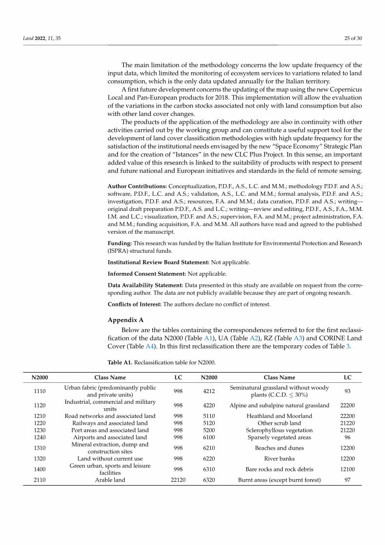
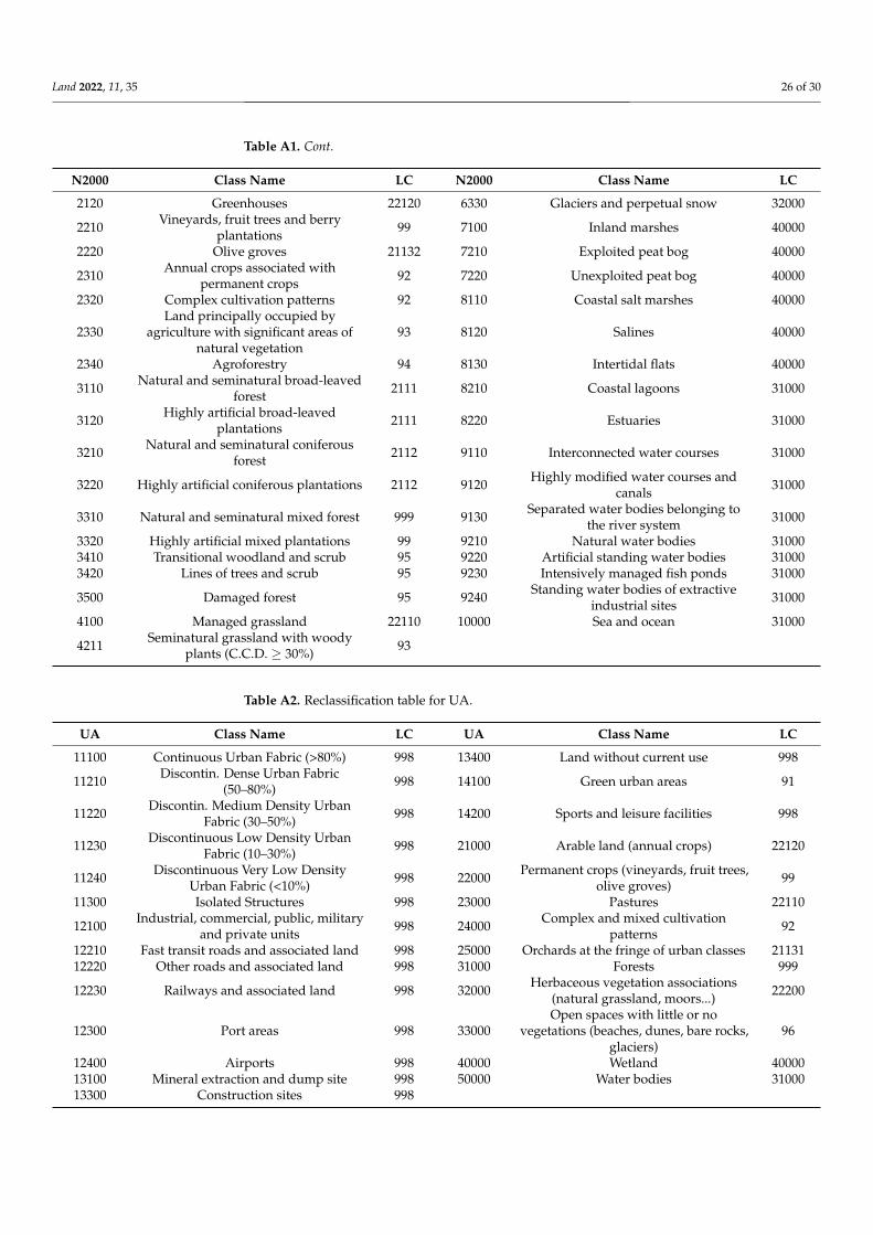
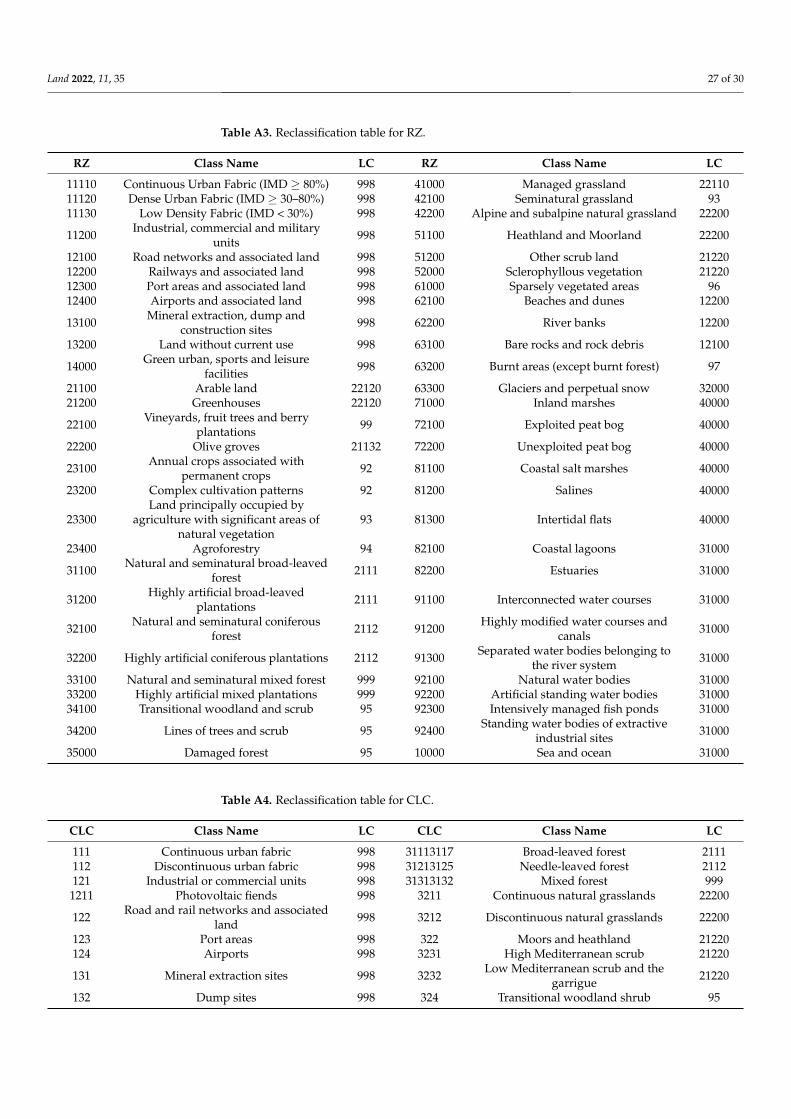
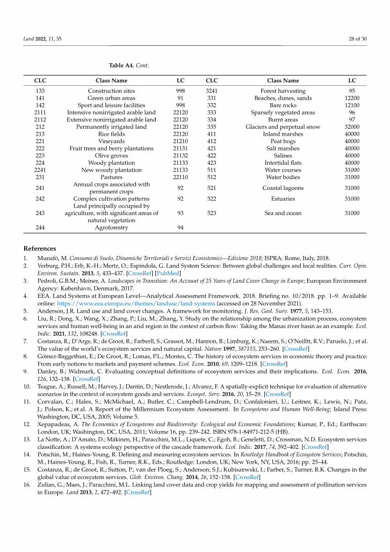
Appendix A

Below are the tables containing the correspondences referred to for the first reclassi-fication of the data N2000 (Table A1), UA (Table A2), RZ (Table A3) and CORINE LandCover (Table A4). In this first reclassification there are the temporary codes of Table 3.

Table A1. Reclassification table for N2000.

N2000 Class Name LC N2000 Class Name LC

1110 Urban fabric (predominantly publicand private units) 998 4212 Seminatural grassland without woody

plants (C.C.D. ≤ 30%) 93

1120 Industrial, commercial and militaryunits 998 4220 Alpine and subalpine natural grassland 22200

1210 Road networks and associated land 998 5110 Heathland and Moorland 222001220 Railways and associated land 998 5120 Other scrub land 212201230 Port areas and associated land 998 5200 Sclerophyllous vegetation 212201240 Airports and associated land 998 6100 Sparsely vegetated areas 96

1310 Mineral extraction, dump andconstruction sites 998 6210 Beaches and dunes 12200

1320 Land without current use 998 6220 River banks 12200

1400 Green urban, sports and leisurefacilities 998 6310 Bare rocks and rock debris 12100

2110 Arable land 22120 6320 Burnt areas (except burnt forest) 97

Land 2022, 11, 35 26 of 30

Table A1. Cont.

N2000 Class Name LC N2000 Class Name LC

2120 Greenhouses 22120 6330 Glaciers and perpetual snow 32000

2210 Vineyards, fruit trees and berryplantations 99 7100 Inland marshes 40000

2220 Olive groves 21132 7210 Exploited peat bog 40000

2310 Annual crops associated withpermanent crops 92 7220 Unexploited peat bog 40000

2320 Complex cultivation patterns 92 8110 Coastal salt marshes 40000

2330Land principally occupied by

agriculture with significant areas ofnatural vegetation

93 8120 Salines 40000

2340 Agroforestry 94 8130 Intertidal flats 40000

3110 Natural and seminatural broad-leavedforest 2111 8210 Coastal lagoons 31000

3120 Highly artificial broad-leavedplantations 2111 8220 Estuaries 31000

3210 Natural and seminatural coniferousforest 2112 9110 Interconnected water courses 31000

3220 Highly artificial coniferous plantations 2112 9120 Highly modified water courses andcanals 31000

3310 Natural and seminatural mixed forest 999 9130 Separated water bodies belonging tothe river system 31000

3320 Highly artificial mixed plantations 99 9210 Natural water bodies 310003410 Transitional woodland and scrub 95 9220 Artificial standing water bodies 310003420 Lines of trees and scrub 95 9230 Intensively managed fish ponds 31000

3500 Damaged forest 95 9240 Standing water bodies of extractiveindustrial sites 31000

4100 Managed grassland 22110 10000 Sea and ocean 31000

4211 Seminatural grassland with woodyplants (C.C.D. ≥ 30%) 93

Table A2. Reclassification table for UA.

UA Class Name LC UA Class Name LC

11100 Continuous Urban Fabric (>80%) 998 13400 Land without current use 998

11210 Discontin. Dense Urban Fabric(50–80%) 998 14100 Green urban areas 91

11220 Discontin. Medium Density UrbanFabric (30–50%) 998 14200 Sports and leisure facilities 998

11230 Discontinuous Low Density UrbanFabric (10–30%) 998 21000 Arable land (annual crops) 22120

11240 Discontinuous Very Low DensityUrban Fabric (<10%) 998 22000 Permanent crops (vineyards, fruit trees,

olive groves) 99

11300 Isolated Structures 998 23000 Pastures 22110

12100 Industrial, commercial, public, militaryand private units 998 24000 Complex and mixed cultivation

patterns 92

12210 Fast transit roads and associated land 998 25000 Orchards at the fringe of urban classes 2113112220 Other roads and associated land 998 31000 Forests 999

12230 Railways and associated land 998 32000 Herbaceous vegetation associations(natural grassland, moors...) 22200

12300 Port areas 998 33000Open spaces with little or no

vegetations (beaches, dunes, bare rocks,glaciers)

96

12400 Airports 998 40000 Wetland 4000013100 Mineral extraction and dump site 998 50000 Water bodies 3100013300 Construction sites 998

Land 2022, 11, 35 27 of 30

Table A3. Reclassification table for RZ.

RZ Class Name LC RZ Class Name LC

11110 Continuous Urban Fabric (IMD ≥ 80%) 998 41000 Managed grassland 2211011120 Dense Urban Fabric (IMD ≥ 30–80%) 998 42100 Seminatural grassland 9311130 Low Density Fabric (IMD < 30%) 998 42200 Alpine and subalpine natural grassland 22200

11200 Industrial, commercial and militaryunits 998 51100 Heathland and Moorland 22200

12100 Road networks and associated land 998 51200 Other scrub land 2122012200 Railways and associated land 998 52000 Sclerophyllous vegetation 2122012300 Port areas and associated land 998 61000 Sparsely vegetated areas 9612400 Airports and associated land 998 62100 Beaches and dunes 12200

13100 Mineral extraction, dump andconstruction sites 998 62200 River banks 12200

13200 Land without current use 998 63100 Bare rocks and rock debris 12100

14000 Green urban, sports and leisurefacilities 998 63200 Burnt areas (except burnt forest) 97

21100 Arable land 22120 63300 Glaciers and perpetual snow 3200021200 Greenhouses 22120 71000 Inland marshes 40000

22100 Vineyards, fruit trees and berryplantations 99 72100 Exploited peat bog 40000

22200 Olive groves 21132 72200 Unexploited peat bog 40000

23100 Annual crops associated withpermanent crops 92 81100 Coastal salt marshes 40000

23200 Complex cultivation patterns 92 81200 Salines 40000

23300Land principally occupied by

agriculture with significant areas ofnatural vegetation

93 81300 Intertidal flats 40000

23400 Agroforestry 94 82100 Coastal lagoons 31000

31100 Natural and seminatural broad-leavedforest 2111 82200 Estuaries 31000

31200 Highly artificial broad-leavedplantations 2111 91100 Interconnected water courses 31000

32100 Natural and seminatural coniferousforest 2112 91200 Highly modified water courses and

canals 31000

32200 Highly artificial coniferous plantations 2112 91300 Separated water bodies belonging tothe river system 31000

33100 Natural and seminatural mixed forest 999 92100 Natural water bodies 3100033200 Highly artificial mixed plantations 999 92200 Artificial standing water bodies 3100034100 Transitional woodland and scrub 95 92300 Intensively managed fish ponds 31000

34200 Lines of trees and scrub 95 92400 Standing water bodies of extractiveindustrial sites 31000

35000 Damaged forest 95 10000 Sea and ocean 31000

Table A4. Reclassification table for CLC.

CLC Class Name LC CLC Class Name LC

111 Continuous urban fabric 998 31113117 Broad-leaved forest 2111112 Discontinuous urban fabric 998 31213125 Needle-leaved forest 2112121 Industrial or commercial units 998 31313132 Mixed forest 999

1211 Photovoltaic fiends 998 3211 Continuous natural grasslands 22200

122 Road and rail networks and associatedland 998 3212 Discontinuous natural grasslands 22200

123 Port areas 998 322 Moors and heathland 21220124 Airports 998 3231 High Mediterranean scrub 21220

131 Mineral extraction sites 998 3232 Low Mediterranean scrub and thegarrigue 21220

132 Dump sites 998 324 Transitional woodland shrub 95

Land 2022, 11, 35 28 of 30

Table A4. Cont.

CLC Class Name LC CLC Class Name LC

133 Construction sites 998 3241 Forest harvesting 95141 Green urban areas 91 331 Beaches, dunes, sands 12200142 Sport and leisure facilities 998 332 Bare rocks 12100

2111 Intensive nonirrigated arable land 22120 333 Sparsely vegetated areas 962112 Extensive nonirrigated arable land 22120 334 Burnt areas 97212 Permanently irrigated land 22120 335 Glaciers and perpetual snow 32000213 Rice fields 22120 411 Inland marshes 40000221 Vineyards 21210 412 Peat bogs 40000222 Fruit trees and berry plantations 21131 421 Salt marshes 40000223 Olive groves 21132 422 Salines 40000224 Woody plantation 21133 423 Intertidal flats 40000

2241 New woody plantation 21133 511 Water courses 31000231 Pastures 22110 512 Water bodies 31000

241 Annual crops associated withpermanent crops 92 521 Coastal lagoons 31000

242 Complex cultivation patterns 92 522 Estuaries 31000

243Land principally occupied by

agriculture, with significant areas ofnatural vegetation

93 523 Sea and ocean 31000

244 Agroforestry 94

References1. Munafò, M. Consumo di Suolo, Dinamiche Territoriali e Servizi Ecosistemici—Edizione 2018; ISPRA: Rome, Italy, 2018.2. Verburg, P.H.; Erb, K.-H.; Mertz, O.; Espindola, G. Land System Science: Between global challenges and local realities. Curr. Opin.

Environ. Sustain. 2013, 5, 433–437. [CrossRef] [PubMed]3. Pedroli, G.B.M.; Meiner, A. Landscapes in Transition: An Account of 25 Years of Land Cover Change in Europe; European Environment

Agency: København, Denmark, 2017.4. EEA. Land Systems at European Level—Analytical Assessment Framework. 2018. Briefing no. 10/2018. pp. 1–9. Available

online: https://www.eea.europa.eu/themes/landuse/land-systems (accessed on 28 November 2021).5. Anderson, J.R. Land use and land cover changes. A framework for monitoring. J. Res. Geol. Surv. 1977, 5, 143–153.6. Liu, R.; Dong, X.; Wang, X.; Zhang, P.; Liu, M.; Zhang, Y. Study on the relationship among the urbanization process, ecosystem

services and human well-being in an arid region in the context of carbon flow: Taking the Manas river basin as an example. Ecol.Indic. 2021, 132, 108248. [CrossRef]

7. Costanza, R.; D’Arge, R.; de Groot, R.; Farberll, S.; Grassot, M.; Hannon, B.; Limburg, K.; Naeem, S.; O’Neilltt, R.V.; Paruelo, J.; et al.The value of the world’s ecosystem services and natural capital. Nature 1997, 387115, 253–260. [CrossRef]

8. Gómez-Baggethun, E.; De Groot, R.; Lomas, P.L.; Montes, C. The history of ecosystem services in economic theory and practice:From early notions to markets and payment schemes. Ecol. Econ. 2010, 69, 1209–1218. [CrossRef]

9. Danley, B.; Widmark, C. Evaluating conceptual definitions of ecosystem services and their implications. Ecol. Econ. 2016,126, 132–138. [CrossRef]

10. Teague, A.; Russell, M.; Harvey, J.; Dantin, D.; Nestlerode, J.; Alvarez, F. A spatially-explicit technique for evaluation of alternativescenarios in the context of ecosystem goods and services. Ecosyst. Serv. 2016, 20, 15–29. [CrossRef]

11. Corvalan, C.; Hales, S.; McMichael, A.; Butler, C.; Campbell-Lendrum, D.; Confalonieri, U.; Leitner, K.; Lewis, N.; Patz,J.; Polson, K.; et al. A Report of the Millennium Ecosystem Assessment. In Ecosystems and Human Well-Being; Island Press:Washington, DC, USA, 2005; Volume 5.

12. Xepapadeas, A. The Economics of Ecosystems and Biodiversity: Ecological and Economic Foundations; Kumar, P., Ed.; Earthscan:London, UK; Washington, DC, USA, 2011; Volume 16, pp. 239–242. ISBN 978-1-84971-212-5 (HB).

13. La Notte, A.; D’Amato, D.; Mäkinen, H.; Paracchini, M.L.; Liquete, C.; Egoh, B.; Geneletti, D.; Crossman, N.D. Ecosystem servicesclassification: A systems ecology perspective of the cascade framework. Ecol. Indic. 2017, 74, 392–402. [CrossRef]

14. Potschin, M.; Haines-Young, R. Defining and measuring ecosystem services. In Routledge Handbook of Ecosystem Services; Potschin,M., Haines-Young, R., Fish, R., Turner, R.K., Eds.; Routledge: London, UK; New York, NY, USA, 2016; pp. 25–44.

15. Costanza, R.; de Groot, R.; Sutton, P.; van der Ploeg, S.; Anderson, S.J.; Kubiszewski, I.; Farber, S.; Turner, R.K. Changes in theglobal value of ecosystem services. Glob. Environ. Chang. 2014, 26, 152–158. [CrossRef]

16. Zulian, G.; Maes, J.; Paracchini, M.L. Linking land cover data and crop yields for mapping and assessment of pollination servicesin Europe. Land 2013, 2, 472–492. [CrossRef]

Land 2022, 11, 35 29 of 30

17. Groff, S.C.; Loftin, C.S.; Drummond, F.; Bushmann, S.; McGill, B. Parameterization of the InVEST crop pollination model tospatially predict abundance of wild blueberry (Vaccinium angustifolium Aiton) native bee pollinators in Maine, USA. Environ.Model. Softw. 2016, 79, 1–9. [CrossRef]

18. Leonhardt, S.D.; Gallai, N.; Garibaldi, L.A.; Kuhlmann, M.; Klein, A.-M. Economic gain, stability of pollination and bee diversitydecrease from southern to northern Europe. Basic Appl. Ecol. 2013, 14, 461–471. [CrossRef]

19. Lautenbach, S.; Seppelt, R.; Liebscher, J.; Dormann, C.F. Spatial and temporal trends of global pollination benefit. PLoS ONE 2012,7, e35954. [CrossRef] [PubMed]

20. Hanley, N.; Breeze, T.D.; Ellis, C.; Goulson, D. Measuring the economic value of pollination services: Principles, evidence andknowledge gaps. Ecosyst. Serv. 2015, 14, 124–132. [CrossRef]

21. UK National Ecosystem Assessment. The UK National Ecosystem Assessment: Synthesis of the Key Findings; UNEP-WCMC:Cambridge, UK, 2011.

22. Rabe, S.-E.; Koellner, T.; Marzelli, S.; Schumacher, P.; Grêt-Regamey, A. National ecosystem services mapping at multiple scales.The German exemplar. Ecol. Indic. 2016, 70, 357–372. [CrossRef]

23. Santos-Martín, F.; García Llorente, M.; Quintas-Soriano, C.; Zorrilla-Miras, P.; Martín-Lopez, B.; Loureiro, M.; Benayas, J.; Montes,M. Spanish National Ecosystem Assessment: Socio-economic valuation of ecosystem services in Spain. Synthesis of the key findings;Biodiversity Foundation of the Spanish Ministry of Agriculture, Food and Environment: Madrid, Spain, 2016.

24. Xie, G.; Zhang, C.; Zhen, L.; Zhang, L. Dynamic changes in the value of China’s ecosystem services. Ecosyst. Serv. 2017,26, 146–154. [CrossRef]

25. Turpie, J.K.; Forsythe, K.J.; Knowles, A.; Blignaut, J.; Letley, G. Mapping and valuation of South Africa’s ecosystem services: Alocal perspective. Ecosyst. Serv. 2017, 27, 179–192. [CrossRef]

26. Choi, H.-A.; Song, C.; Lee, W.-K.; Jeon, S.; Gu, J.H. Integrated approaches for national ecosystem assessment in South Korea.KSCE J. Civ. Eng. 2018, 22, 1634–1641. [CrossRef]

27. Daily, G.C.; Matson, P.A.; Vitousek, P.M. Ecosystem services supplied by soil. In Nature’s Services: Societal Dependence on NaturalEcosystems; Daily, G.C., Ed.; Island Press: Washington, DC, USA, 1997; pp. 113–132.

28. Wall, D.H.; Bardgett, R.D.; Covich, A.P.; Snelgrove, P.V.R. The Need for Understanding How Biodiversity and Ecosystem FunctioningAffect Ecosystem Services in Soils and Sediments; Island Press: Washington, DC, USA, 2004.

29. Dominati, E.; Patterson, M.; Mackay, A. A framework for classifying and quantifying the natural capital and ecosystem servicesof soils. Ecol. Econ. 2010, 69, 1858–1868. [CrossRef]

30. Fryer, J.; Williams, I.D. Regional carbon stock assessment and the potential effects of land cover change. Sci. Total Environ. 2021,775, 145815. [CrossRef] [PubMed]

31. Mathew, I.; Shimelis, H.; Mutema, M.; Minasny, B.; Chaplot, V. Crops for increasing soil organic carbon stocks–A global metaanalysis. Geoderma 2020, 367, 114230. [CrossRef]

32. Clerici, N.; Cote-Navarro, F.; Escobedo, F.J.; Rubiano, K.; Villegas, J.C. Spatio-temporal and cumulative effects of land use-landcover and climate change on two ecosystem services in the Colombian Andes. Sci. Total Environ. 2019, 685, 1181–1192. [CrossRef]

33. Savaresi, A.; Perugini, L.; Chiriacò, M.V. Making sense of the LULUCF Regulation: Much ado about nothing? Rev. Eur. Comp. Int.Environ. Law 2020, 29, 212–220. [CrossRef]

34. Sallustio, L.; Quatrini, V.; Geneletti, D.; Corona, P.; Marchetti, M. Assessing land take by urban development and its impact oncarbon storage: Findings from two case studies in Italy. Environ. Impact Assess. Rev. 2015, 54, 80–90. [CrossRef]

35. Vashum, K.T.; Jayakumar, S. Methods to estimate above-ground biomass and carbon stock in natural forests-a review. J. Ecosyst.Ecography 2012, 2, 1–7. [CrossRef]

36. Sallustio, L.; Munafò, M.; Riitano, N.; Lasserre, B.; Fattorini, L.; Marchetti, M. Integration of land use and land cover inventoriesfor landscape management and planning in Italy. Environ. Monit. Assess. 2016, 188, 48. [CrossRef]

37. Maes, J.; Teller, A.; Erhard, M.; Liquete, C.; Braat, L.; Berry, P.; Egoh, B.; Puydarrieus, P.; Fiorina, C.; Santos, F.; et al. An AnalyticalFramework for Ecosystem Assessments under Action 5 of the EU Biodiversity Strategy to 2020; Publications Office of the EuropeanUnion: Luxembourg, 2013; ISBN 9789279293696.

38. Cabral, P.; Feger, C.; Levrel, H.; Chambolle, M.; Basque, D. Assessing the impact of land-cover changes on ecosystem services: Afirst step toward integrative planning in Bordeaux, France. Ecosyst. Serv. 2016, 22, 318–327. [CrossRef]

39. Arnold, S.; Kosztra, B.; Banko, G.; Smith, G.; Hazeu, G.; Bock, M. The EAGLE concept—A vision of a future EuropeanLand Monitoring Framework. In Proceedings of the 33th EARSeL Symposium towards Horizon 2020, Matera, Italy, 3–6 June2013; pp. 551–568.

40. Kleeschulte, S. Technical Specifications for Implementation of a New Land-Monitoring Concept Based on EAGLE. D3: Draft DesignConcept and CLC-Backbone, CLC-Core Technical Specifications, Including Requirements Review, 3rd ed.; European Environment Agency:Copenhagen, Denmark, 2019; p. 78.

41. De Fioravante, P.; Luti, T.; Cavalli, A.; Giuliani, C.; Dichicco, P.; Marchetti, M.; Chirici, G.; Congedo, L.; Munafò, M. MultispectralSentinel-2 and SAR Sentinel-1 Integration for Automatic Land Cover Classification. Land 2021, 10, 611. [CrossRef]

42. Munafò, M. Consumo di Suolo, Dinamiche Territoriali e Servizi Ecosistemici. Edizione 2020; ISPRA: Rome, Italy, 2020.43. Munafò, M. Consumo di Suolo, Dinamiche Territoriali e Servizi Ecosistemici Edizione 2021 Rapporto ISPRA SNPA; ISPRA: Rome, Italy,

2021; ISBN 9788844810597.

Land 2022, 11, 35 30 of 30

44. Luti, T.; De Fioravante, P.; Marinosci, I.; Strollo, A.; Riitano, N.; Falanga, V.; Mariani, L.; Congedo, L.; Munafò, M. LandConsumption Monitoring with SAR Data and Multispectral Indices. Remote Sens. 2021, 13, 1586. [CrossRef]

45. Strollo, A.; Smiraglia, D.; Bruno, R.; Assennato, F.; Congedo, L.; De Fioravante, P.; Giuliani, C.; Marinosci, I.; Riitano, N.; Munafò,M. Land consumption in Italy. J. Maps 2020, 16, 113–123. [CrossRef]

46. Olofsson, P.; Foody, G.M.; Herold, M.; Stehman, S.V.; Woodcock, C.E.; Wulder, M.A. Good practices for estimating area andassessing accuracy of land change. Remote Sens. Environ. 2014, 148, 42–57. [CrossRef]

47. FAO Map Accuracy Assessment and Area Estimation: A Practical Guide. National Forest Monitoring and Assessment Working Paper.2016. 46/E. p. 69. Available online: https://www.fao.org/publications/card/fr/c/e5ea45b8-3fd7-4692-ba29-fae7b140d07e/(accessed on 28 November 2021).

48. Stehman, S.V.; Czaplewski, R.L. Design and Analysis for Thematic Map Accuracy Assessment—An application of satelliteimagery. Remote Sens. Environ. 1998, 64, 331–344. [CrossRef]

49. Stehman, S.V.; Foody, G.M. Key issues in rigorous accuracy assessment of land cover products. Remote Sens. Environ. 2019,231, 111199. [CrossRef]

50. Cochran, W.G.; William, G. Sampling Techniques; John Wiley& Sons: New York, NY, USA, 1977.51. Lupia, F. MARSALa-A Model-Based Irrigation Water Consumption Estimation at Farm Level; INEA: Brussels, Belgium, 2013.52. Vitullo, M.; De Lauretis, R.; Federici, S. La Contabilità del Carbonio Contenuto Nelle Foreste Italiane; Agenzia per la Protezione

dell’ambiente e per i Servizi Tecnici: Rome, Italy, 2007.53. Di Cosmo, L.; Gasparini, P.; Tabacchi, G. A national-scale, stand-level model to predict total above-ground tree biomass from

growing stock volume. For. Ecol. Manag. 2016, 361, 269–276. [CrossRef]54. Romano, D.; Arcarese, C.; Bernetti, A.; Caputo, A.; Contaldi, M.; De Lauretis, R.; Di Cristofaro, E.; Gagna, A.; Gonella, B.;

Taurino, E.; et al. Italian Greenhouse Gas Inventory 1990–2015. National Inventory Report 2017. 2017. Available online: https://www.isprambiente.gov.it/en/publications/reports/italian-greenhouse-gas-inventory-1990-2015.-national-inventory-report-2017 (ac-cessed on 28 November 2021).

55. Li, S.; Liu, Y.; Yang, H.; Yu, X.; Zhang, Y.; Wang, C. Integrating ecosystem services modeling into effectiveness assessment ofnational protected areas in a typical arid region in China. J. Environ. Manag. 2021, 297, 113408. [CrossRef]

56. Penman, J.; Gytarsky, M.; Hiraishi, T.; Krug, T.; Kruger, D.; Pipatti, R.; Buendia, L.; Miwa, K.; Ngara, T.; Tanabe, K. Goodpractice guidance for land use, land-use change and forestry. Good Pract. Guid. L. Use Land-Use Chang. For. 2003. Availableonline: https://www.ipcc.ch/publication/good-practice-guidance-for-land-use-land-use-change-and-forestry/ (accessed on 28November 2021).

57. Marchetti, M.; Sallustio, L.; Ottaviano, M.; Barbati, A.; Corona, P.; Tognetti, R.; Zavattero, L.; Capotorti, G. Carbon sequestrationby forests in the National Parks of Italy. Plant Biosyst. Int. J. Deal. Asp. Plant Biol. 2012, 146, 1001–1011. [CrossRef]

58. Canaveira, P.; Manso, S.; Pellis, G.; Perugini, L.; De Angelis, P.; Neves, R.; Papale, D.; Paulino, J.; Pereira, T.; Pina, A. Biomass Dataon Cropland and Grassland in the Mediterranean Region. Final Report for Action A4 of Project MediNet. 2018. Available online:http://www.lifemedinet.com/ (accessed on 28 November 2021).

59. Burke, T.; Whyatt, J.D.; Rowland, C.; Blackburn, G.A.; Abbatt, J. The influence of land cover data on farm-scale valuations ofnatural capital. Ecosyst. Serv. 2020, 42, 101065. [CrossRef]

60. Tomlinson, S.J.; Dragosits, U.; Levy, P.E.; Thomson, A.M.; Moxley, J. Quantifying gross vs. net agricultural land use change inGreat Britain using the Integrated Administration and Control System. Sci. Total Environ. 2018, 628, 1234–1248. [PubMed]

61. Morel, J.L.; Chenu, C.; Lorenz, K. Ecosystem services provided by soils of urban, industrial, traffic, mining, and military areas(SUITMAs). J. Soils Sediments 2015, 15, 1659–1666. [CrossRef]

62. Sambucini, V.; Marinosci, I.; Bonora, N.; Chirci, G. La Realizzazione in Italia del Progetto CORINE Land Cover 2006; ISPRA: Rome,Italy, 2010; ISBN 9788844804770.

63. Tomaselli, V.; Dimopoulos, P.; Marangi, C.; Kallimanis, A.S.; Adamo, M.; Tarantino, C.; Panitsa, M.; Terzi, M.; Veronico, G.;Lovergine, F. Translating land cover/land use classifications to habitat taxonomies for landscape monitoring: A Mediterraneanassessment. Landsc. Ecol. 2013, 28, 905–930. [CrossRef]

64. Spadoni, G.L.; Cavalli, A.; Congedo, L.; Munafò, M. Analysis of Normalized Difference Vegetation Index (NDVI) multi-temporalseries for the production of forest cartography. Remote Sens. Appl. Soc. Environ. 2020, 20, 100419. [CrossRef]