High-Order Discontinuous Galerkin Methods using a Spectral Multigrid Approach

Journal of Computational Physics 213 (2006) 330–357

www.elsevier.com/locate/jcp

High-order discontinuous Galerkin methods usingan hp-multigrid approach

Cristian R. Nastase *, Dimitri J. Mavriplis

Department of Mechanical Engineering, University of Wyoming, 1000 E. University Avenue, Laramie, WY 82071-3295, United States

Received 13 April 2005; received in revised form 12 August 2005; accepted 15 August 2005Available online 7 October 2005

Abstract

The goal of this paper is to investigate and develop a fast and robust algorithm for the solution of high-order accuratediscontinuous Galerkin discretizations of non-linear systems of conservation laws on unstructured grids. Herein we presentthe development of a spectral hp-multigrid method, where the coarse ‘‘grid’’ levels are constructed by reducing the order (p)of approximation of the discretization using hierarchical basis functions (p-multigrid), together with the traditional (h-mul-tigrid) approach of constructing coarser grids with fewer elements. On each level we employ variants of the element-Jacobischeme, where the Jacobian entries associated with each element are treated implicitly (i.e., inverted directly) and all otherentries are treated explicitly. The methodology is developed for the two-dimensional non-linear Euler equations onunstructured grids, using both non-linear (FAS) and linear (CGC) multigrid schemes. Results are presented for the channelflow over a bump and a uniform flow over a four element airfoil. Current results demonstrate convergence rates which areindependent of both order of accuracy (p) of the discretization and level of mesh resolution (h).� 2005 Elsevier Inc. All rights reserved.

PACS: 47.11.+j; 83.85.Pt; 47.15.Ki

Keywords: Computational fluid dynamics; Discontinuous Galerkin finite element methods; High order methods; Numerical methods;Multigrid methods; Compressible flow; Gas dynamics

1. Introduction

While most currently employed CFD algorithms are asymptotically second-order accurate in time and inspace, the use of higher-order discretizations in both space and time offers a possible avenue for improving thepredictive simulation capability for many applications. This is due to the fact that higher-order methodsexhibit a faster asymptotic convergence rate in the discretization error than lower (second)-order methods.For example, with a fourth-order accurate spatial discretization, the error is reduced by a factor of 24 = 16

0021-9991/$ - see front matter � 2005 Elsevier Inc. All rights reserved.

doi:10.1016/j.jcp.2005.08.022

* Corresponding author. Tel.: +1 307 7665424; fax: +1 307 7662695.E-mail addresses: [email protected] (C.R. Nastase), [email protected] (D.J. Mavriplis).

mailto:[email protected]

mailto:[email protected]

C.R. Nastase, D.J. Mavriplis / Journal of Computational Physics 213 (2006) 330–357 331

each time the mesh resolution is doubled, while a second-order accurate method only achieves a 22 = 4 reduc-tion in error with each doubling of the mesh resolution. Since a doubling of mesh resolution in three dimen-sions entails an increase of overall work by a factor of 23 = 8, achieving an arbitrarily prescribed errortolerance with second-order accurate methods in three dimensions can quickly become unfeasible.

Thus, for increasingly high accuracy levels, higher-order methods ultimately become the method of choice.Therefore, the expectation is that an efficient higher-order discretization may provide an alternate path forachieving high accuracy in a flow with a wide disparity of length scales at reduced cost, by avoiding theuse of excessive grid resolution.

On the other hand, for levels of accuracy often associated with mean-flow engineering calculations, higher-order methods have proved to be excessively costly compared to simpler second-order accurate methods.Clearly, because of the different asymptotic nature of these methods, the cost comparison between methodsis a strong function of the required levels of accuracy. Nevertheless, for many engineering type calculations,higher-order methods have been found to be non-competitive compared to the simpler second-order accuratemethods.

While the formulation of discretization strategies for higher-order methods such as discontinuous Galerkin[1–7] and streamwise upwind Petrov–Galerkin [8] methods are now fairly well understood, the development oftechniques for efficiently solving the discrete equations arising from these methods has generally been lagging.This is partly due to the complex structure of the discrete equations originating from fairly sophisticateddiscretization strategies, as well as the current application of higher-order methods to problems where simpleexplicit time-stepping schemes are thought to be adequate solution mechanisms, due to the close matching ofspatial and temporal scales, such as acoustic phenomena.

The development of optimal, or near optimal solution strategies for higher-order discretizations, includingsteady-state solutions methodologies, and implicit time integration strategies, remains one of the key deter-mining factors in devising higher-order methods which are not just competitive but superior to lower-ordermethods in overall accuracy and efficiency.

Recent work by the second author has examined the use of spectral multigrid methods, where conver-gence acceleration is achieved through the use of coarse levels constructed by reducing the order (p) ofapproximation of the discretization (as opposed to coarsening the mesh) for discontinuous Galerkin dis-cretizations [9]. The idea of spectral multigrid was originally proposed by Ronquist and Patera [10], andhas been pursued for the Euler and Navier–Stokes equations by Fidkowski et al. [11–13] with encouragingresults. Implicit multi-level solution techniques for high-order discretizations have also been developed byLottes and Fisher [14].

In this work, we extend the original spectral multigrid approach described in [9] to the two-dimensionalsteady-state Euler equations, and couple the spectral p-multigrid approach with a more traditional agglomer-ation h-multigrid method for unstructured meshes. The investigation of efficient smoothers to be used at eachlevel of the multigrid algorithm is also pursued, and comparisons between linear and non-linear solver strat-egies are made as well. The overall goal is the development of a solution algorithm which delivers convergencerates which are independent of p (the order of accuracy of the discretization) and independent of h (the degreeof mesh resolution), while minimizing the cost of each iteration.

The key ingredient in the p-multigrid approach is to employ a hierarchical basis set together with a modalmethod. This renders the multigrid inter-level operators almost trivial to implement. This approach is ratherdifferent than the nodal method presented in [15], where a non-hierarchical basis (i.e., nodal basis based onLagrange polynomials) is employed and the multilevel process requires rather complicated grid transfer oper-ators. Moreover, in our methodology the coarse-grids are known a priori and the multilevel methodology isobtained by using known subsets of the original matrix. That is, the coarse grids correspond to a modal expan-sion in a lower space. This is also different than the algebraic multigrid (AMG) method [16] where a ‘‘matrix-free’’ operator is employed without prior knowledge of the coarse-grids and the multilevel process is obtainedfrom an algebraic standpoint.

Note that the ‘‘hp-’’ terminology is commonly used to denote adaptive spatial and polynomial resolutions.This is referred to as ‘‘h-’’ and ‘‘p-adaptivity’’. Although the current multigrid methodology is not appliedadaptively, it does make use of p-coarsened and h-coarsened levels leading to our terminology of either‘‘p-multigrid’’, ‘‘h-multigrid’’ or ‘‘hp-multigrid’’ for the combined algorithm.

332 C.R. Nastase, D.J. Mavriplis / Journal of Computational Physics 213 (2006) 330–357

2. Governing equations

The conservative form of the compressible Euler equations describing the conservation of mass, momentumand total energy is given in vectorial form

oUðx; tÞot

þr � FðUÞ ¼ 0 ð1Þ

subject to appropriate boundary and initial conditions within a two-dimensional domain X. Explicitly, thestate vector U of the conservative variables and the Cartesian components of the inviscid flux F = (Fx,Fy)are:

U ¼

q

qu

qv

Et

0BBB@

1CCCA; Fx ¼

qu

qu2 þ p

quv

ðEt þ pÞu

0BBB@

1CCCA; Fy ¼

qv

quv

qv2 þ p

ðEt þ pÞv

0BBB@

1CCCA; ð2Þ

where q is the fluid density, (u,v) are the fluid velocity Cartesian components, p is the pressure and Et is thetotal energy. For an ideal gas, the equation of state relates the pressure to total energy by:

p ¼ ðc� 1Þ Et �1

2qðu2 þ v2Þ

� �; ð3Þ

where c = 1.4 is the ratio of specific heats.

3. Spatial discretization

The computational domain X is partitioned into an ensemble of non-overlapping elements and within eachelement the solution is approximated by a truncated polynomial expansion

Uðx; tÞ � Upðx; tÞ ¼XMj¼1

ujðtÞ/jðxÞ; ð4Þ

where M is the number of modes defining the truncation level. The semi-discrete formulation (i.e., continuousin time) employs a local discontinuous Galerkin formulation [2,3,5,6] in spatial variables within each elementXk. The weak formulation for Eq. (1) is obtained by minimizing the residual with respect to the expansionfunction in an integral sense:

ZXk

/ioUpðx; tÞ

otþr � FðUpÞ

� �k

dXk ¼ 0. ð5Þ

After integrating by parts the weak statement of the problem becomes:

ZXk

/ioUp

otdXk �

ZXk

r/i � FðUpÞ dXk þZoXk

/iF�ðUpÞ � n dðoXkÞ ¼ 0. ð6Þ

The local discontinuous Galerkin approach makes use of element-based basis functions, which results in solu-tion approximations which are local, discontinuous, and doubled valued on each elemental interface. Mono-tone numerical fluxes are used to resolve the discontinuity, providing the means of communication betweenadjacent elements and specification of the boundary conditions. The numerical flux, F*(Up) Æ n, is obtainedas a solution of a local one-dimensional Riemann problem and depends on the internal interface state, U�

p ,the adjacent element interface state, Uþ

p , and the orientation as defined by the normal vector, n, of the inter-face. An approximate Riemann solver is used to compute the flux at inter-element boundaries and provides themeans of imposing boundary conditions. Current implementations include the flux difference splitting schemesof Rusanov [17], Roe [18], HLL [19] and HLLC [20–22].


The discrete form of the local discontinuous Galerkin formulation is defined by the particular choice of theset of basis functions, {/i,i = 1, . . .,M}. The basis set is defined on a standard triangle Xðn; gÞ spanning be-tween {0 < n,g < 1}. We seek a set of hierarchical basis functions in order to simplify our subsequent spectralmultigrid implementation. Defining the first order Lagrange polynomials:

L1 ¼ 1� n� g; L2 ¼ n; L3 ¼ g ð7Þ
the hierarchical basis set, {/i}, is fully described by vertex,
/v1 ¼ L1; /v

2 ¼ L2; /v3 ¼ L3 ð8Þ

edge,

/e1n ¼ L1L2wn�2ðL2 � L1Þ;



ð9Þ

and bubble,

/bn1;n2 ¼ L1L2L3wn1�1ðL2 � L1Þwn2�1ðL1 � L3Þ ð10Þ

shape functions, where 2 6 n 6 pe, n1 + n2 = pb � 1 and n1,n2 P 1. The kernel functions w(z) are given as:

wn�2ðzÞ ¼�2rn� 1

P 1;1n�2ðzÞ; ð11Þ

where P a;bn represents the Jacobi polynomial of order, n, with weights a and b. In our discretization the edge

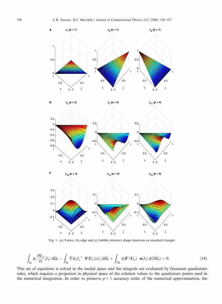
order, pe, and the bubble order, pb, are set to pe = pb = p, where p is the discretization order within the ele-ment. For p P 2 the basis functions within the standard triangle, {/i, i = 4 . . .M}, are normalized Lobatto(i.e., /nP2 ¼ r

R x�1 P

0;0n�1ðzÞ dz) functions [23], which take zero values at the end of their definition interval

(Fig. 1). The normalization factor, r, can be used to condition the mass or convection matrices.Although the choice of basis functions does not affect the accuracy of the method, this choice is dictated by

the intended application. In our application (Euler equations) which employs spatial derivatives, our choice ofbasis functions has a significant advantage over other types of bases described in [7,24,25]. Specifically, thebasis used in our implementation [23] is rotationally invariant within the standard triangle. The basis usedby Karniadakis and Sherwin [7] for triangular elements makes use of collapsed coordinate systems in orderto construct the basis as a tensor-product of Jacobi polynomials and does not preserve the rotational invari-ance. Although this basis has good orthogonality properties and the tensor-product brings advantages interms of number of operations required to compute the integral terms via quadrature rules, the lack of rota-tional invariance is somewhat inconvenient. It is known that in the case of a full orthogonal basis set, thetransformation operator from the polynomial space to physical space is identity and the mass matrix becomesdiagonal. However, in the steady state case considered here there is no need to employ the mass matrix. Fur-thermore, our choice of basis is not necessarily optimal but, under adequate scaling, the current basis presentsgood conditioning properties up to p = 10 (not shown), which is high enough for aerodynamic applications.Future work pertaining to time-dependent problems will revisit the issue of optimal choice of basis functions.

Since the basis set is defined in the standard triangle, a coordinate transformation, {x = x(n,g), y = y(n,g)},is required to compute the derivatives and the integrals in physical space Xk(x,y). For iso-parametric elements,the basis functions are expressed as functions of n and g, and the coordinate transformation, and its Jacobianwithin the standard element, Xkðn; gÞ, are given by:

xp ¼XMj¼1

xj/jðn; gÞ; Jkðn; gÞ ¼oðx; yÞoðn; gÞ . ð12Þ

In the simple case of straight-sided elements the mapping is linear and the determinant of the Jacobian, |Jk|,and metrics, nx = on/ox, ny = on/ oy, gx = og/ox, gy = og/oy, are constant within each element. For the generalcase, using Eq. (12), the solution expansion and the weak statement within each element, Xk, becomes:

Upðn; g; tÞ ¼XMj¼1

ujðtÞ/jðn; gÞ ð13Þ

0

0.5

1

0

0.5

10

0.5

1

ξ

φ1 (p = 1)

η 0

0.5

1

0

0.5

10

0.5

1

ξ

φ2 (p = 1)

η0

0.5

1

0

0.5

10

0.5

1

ξ

φ3 (p = 1)

η

0

0.5

1

0

0.5

1

0

0.2

ξ

φ4 (p = 2)

η 0

0.5

1

0

0.5

1

0

0.5

ξ

φ7 (p = 3)

η0

0.5

1

0

0.5

1

0

0.5

ξ

φ11

(p = 4)

η

0

0.5

1

0

0.5

1

0

0.1

0.2

0.3

ξ

φ10

(p = 3)

η 0

0.5

1

0

0.5

1

0

0.1

ξ

φ14

(p = 4)

η0

0.5

1

0

0.5

1

0

0.1

ξ

φ15

(p = 4)

η

a

b

c

Fig. 1. (a) Vertex, (b) edge and (c) bubble (interior) shape functions on standard triangle.


ZXk

/ioUp

otjJkj dXk �

ZXk

r/iJ�1k � FðUpÞjJkj dXk þ

ZoXk

/iF�ðUpÞ � njJkj dðoXkÞ ¼ 0. ð14Þ

This set of equations is solved in the modal space and the integrals are evaluated by Gaussian quadraturerules, which requires a projection in physical space of the solution values to the quadrature points used inthe numerical integration. In order to preserve p + 1 accuracy order of the numerical approximation, the


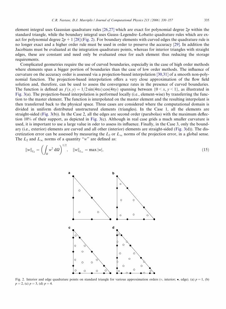
element integral uses Gaussian quadrature rules [26,27] which are exact for polynomial degree 2p within thestandard triangle, while the boundary integral uses Gauss–Legendre–Lobatto quadrature rules which are ex-act for polynomial degree 2p + 1 [28] (Fig. 2). For boundary elements with curved edges the quadrature rule isno longer exact and a higher order rule must be used in order to preserve the accuracy [29]. In addition theJacobians must be evaluated at the integration quadrature points, whereas for interior triangles with straightedges, these are constant and need only be evaluated once for each element thus reducing the storagerequirements.

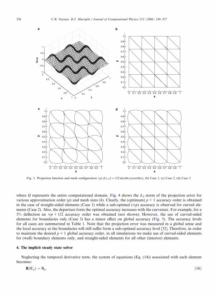
Complicated geometries require the use of curved boundaries, especially in the case of high order methodswhere elements span a bigger portion of boundaries than the case of low order methods. The influence ofcurvature on the accuracy order is assessed via a projection-based interpolation [30,31] of a smooth non-poly-nomial function. The projection-based interpolation offers a very close approximation of the flow fieldsolution and, therefore, can be used to assess the convergence rates in the presence of curved boundaries.The function is defined as f ðx; yÞ ¼ 1=2 sinð4pxÞ cosð4pyÞ spanning between {0 < x, y < 1}, as illustrated inFig. 3(a). The projection-based interpolation is performed locally (i.e., element-wise) by transferring the func-tion to the master element. The function is interpolated on the master element and the resulting interpolant isthen transferred back to the physical space. Three cases are considered where the computational domain isdivided in uniform distributed unstructured elements (triangles). In the Case 1, all the elements arestraight-sided (Fig. 3(b)). In the Case 2, all the edges are second order (parabolas) with the maximum deflec-tion 10% of their support, as depicted in Fig. 3(c). Although in real case grids a much smaller curvature isused, it is important to use a large value in oder to assess its influence. Finally, in the Case 3, only the bound-ary (i.e., exterior) elements are curved and all other (interior) elements are straight-sided (Fig. 3(d)). The dis-cretization error can be assessed by measuring the L2 or L1 norms of the projection error, in a global sense.The L2 and L1 norms of a quantity ‘‘w’’ are defined as:

Fig. 2.p = 2,

kwkL2 ¼ZXw2 dX

� �1=2

; kwkL1 ¼ max jwj; ð15Þ

a b

c d

Interior and edge quadrature points on standard triangle for various approximation orders (�, interior; �, edge). (a) p = 1, (b)(c) p = 3, (d) p = 4.

0

0.2

0.4

0.6

0.8

1 0

0.2

0.4

0.6

0.8

1

–1

–0.5

0

0.5

1

yx

f(x,

y)

x

y

0 0.1 0.2 0.3 0.4 0.5 0.6 0.7 0.8 0.9 1

0

0.1

0.2

0.3

0.4

0.5

0.6

0.7

0.8

0.9

1

x

y

0 0.1 0.2 0.3 0.4 0.5 0.6 0.7 0.8 0.9 1

0

0.1

0.2

0.3

0.4

0.5

0.6

0.7

0.8

0.9

1

x

y

0 0.1 0.2 0.3 0.4 0.5 0.6 0.7 0.8 0.9 1

0

0.1

0.2

0.3

0.4

0.5

0.6

0.7

0.8

0.9

1

a b

c d

Fig. 3. Projection function and mesh configuration: (a) f(x,y) = 1/2sin(4px) cos(4py), (b) Case 1, (c) Case 2, (d) Case 3.


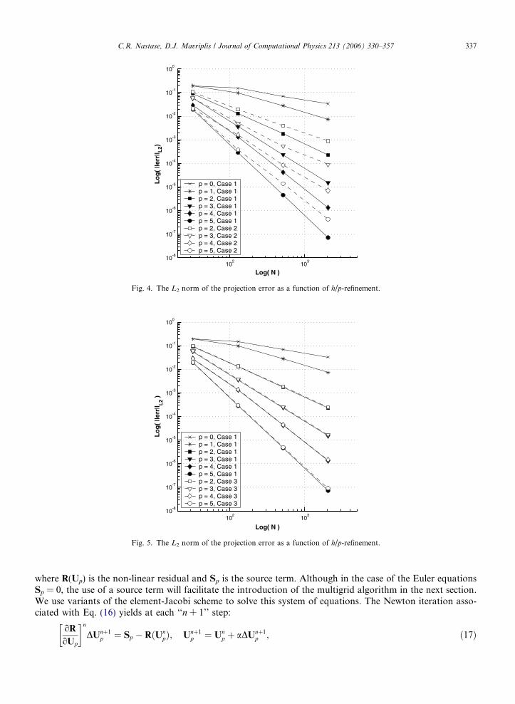
where X represents the entire computational domain. Fig. 4 shows the L2 norm of the projection error forvarious approximation order (p) and mesh sizes (h). Clearly, the (optimum) p + 1 accuracy order is obtainedin the case of straight-sided elements (Case 1) while a sub-optimal (�p) accuracy is observed for curved ele-ments (Case 2). Also, the departure form the optimal accuracy increases with the curvature. For example, for a5% deflection an �p + 1/2 accuracy order was obtained (not shown). However, the use of curved-sidedelements for boundaries only (Case 3) has a minor effect on global accuracy (Fig. 5). The accuracy levelsfor all cases are summarized in Table 1. Note that the projection error was measured in a global sense andthe local accuracy at the boundaries will still suffer form a sub-optimal accuracy level [32]. Therefore, in orderto maintain the desired p + 1 global accuracy order, in all simulations we make use of curved-sided elementsfor (wall) boundary elements only, and straight-sided elements for all other (interior) elements.

4. The implicit steady state solver

Neglecting the temporal derivative term, the system of equations (Eq. (14)) associated with each elementbecomes:

RðUpÞ ¼ Sp; ð16Þ

102

103

10-8

10-7

10-6

10-5

10-4

10-3

10-2

10-1

100

Log( N )

Lo

g(

||err

|| L2)

p = 0, Case 1p = 1, Case 1p = 2, Case 1p = 3, Case 1p = 4, Case 1p = 5, Case 1p = 2, Case 2p = 3, Case 2p = 4, Case 2p = 5, Case 2

Fig. 4. The L2 norm of the projection error as a function of h/p-refinement.

102

103

10-8

10-7

10-6

10-5

10-4

10-3

10-2

10-1

100

Log( N )

Lo

g(

||err

|| L2 )

p = 0, Case 1p = 1, Case 1p = 2, Case 1p = 3, Case 1p = 4, Case 1p = 5, Case 1p = 2, Case 3p = 3, Case 3p = 4, Case 3p = 5, Case 3

Fig. 5. The L2 norm of the projection error as a function of h/p-refinement.


where R(Up) is the non-linear residual and Sp is the source term. Although in the case of the Euler equationsSp = 0, the use of a source term will facilitate the introduction of the multigrid algorithm in the next section.We use variants of the element-Jacobi scheme to solve this system of equations. The Newton iteration asso-ciated with Eq. (16) yields at each ‘‘n + 1’’ step:

oR

oUp

� �nDUnþ1

p ¼ Sp � RðUnpÞ; Unþ1

p ¼ Unp þ aDUnþ1

p ; ð17Þ

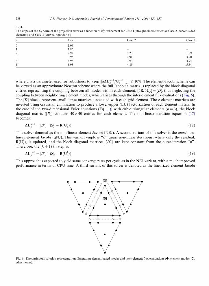
Table 1The slopes of the L2 norm of the projection error as a function of h/p-refinement for Case 1 (straight-sided elements), Case 2 (curved-sidedelements) and Case 3 (curved-boundaries)

p Case 1 Case 2 Case 3

0 1.09 – –1 1.86 – –2 2.92 2.23 1.893 3.95 2.91 3.904 4.98 3.93 4.945 5.98 4.89 5.84


where a is a parameter used for robustness to keep kaDUnþ1p =Unþ1

p kL1 6 10%. The element-Jacobi scheme canbe viewed as an approximate Newton scheme where the full Jacobian matrix is replaced by the block diagonalentries representing the coupling between all modes within each element, [oR/oUp] = [D], thus neglecting thecoupling between neighboring element modes, which arises through the inter-element flux evaluations (Fig. 6).The [D] blocks represent small dense matrices associated with each grid element. These element matrices areinverted using Gaussian elimination to produce a lower-upper (LU) factorization of each element matrix. Inthe case of the two-dimensional Euler equations (Eq. (1)) with cubic triangular elements (p = 3), the blockdiagonal matrix ([D]) contains 40 · 40 entries for each element. The non-linear iteration equation (17)becomes:

Fig. 6.edge m

DUnþ1p ¼ ½Dn��1ðSp � RðUn

pÞÞ. ð18Þ

This solver denoted as the non-linear element Jacobi (NEJ). A second variant of this solver it the quasi non-linear element Jacobi (qNJ). This variant employs ‘‘k’’ quasi non-linear iterations, where only the residual,RðUk

pÞ, is updated, and the block diagonal matrices, [Dn], are kept constant from the outer-iteration ‘‘n’’.Therefore, the (k + 1) th step is:

DUkþ1p ¼ ½Dn��1ðSp � RðUk

pÞÞ. ð19Þ

This approach is expected to yield same converge rates per cycle as in the NEJ variant, with a much improvedperformance in terms of CPU time. A third variant of this solver is denoted as the linearized element Jacobi

[D]

[O]

Discontinuous solution representation illustrating element based modes and inter-element flux evaluations (d, element modes;�,odes).


(LEJ) method. In this approach, the full Jacobian matrix is retained, but is decomposed into block diagonal[D] and off-diagonal [O] components:

oR

oUp

� �n¼ ½Dn� þ ½On�. ð20Þ

An iterative procedure can now be written by taking the [O] components, which contain terms arising from theinter-element flux evaluations, to the right-hand-side of Eq. (17). In matrix form the (k + 1)th step of the lin-earized element Jacobi step is written as:

DUkþ1p ¼ ½Dn��1

Sp � RðUnpÞ � ½On�DUk

p

� �. ð21Þ

Note that the linearized element Jacobi scheme involves a dual iteration strategy, where each nth outer non-linear iteration entails ‘‘k’’ inner linear iterations. The advantage of this formulation is that the non-linearresidual RðUn

pÞ and the Jacobian entries [Dn] and [On] are held constant during the linear iterations. Thiscan significantly reduce the required computational time per cycle for expensive non-linear residual construc-tions. Because this scheme represents an exact linearization of the element-Jacobi scheme (Eq. (18)), both ap-proaches can be expected to converge at the same rates per cycle (asymptotically) [33]. On the other hand, thelinearized element Jacobi scheme requires extra storage for the [O] Jacobian blocks, which may not be feasiblefor large three-dimensional problems.

The convergence of Eq. (21) can be further accelerated by using a Gauss–Seidel strategy where the off-diagonal matrices are split into lower, [L], and upper, [U], contributions (i.e., [O] = [L] + [U]). This last solvervariant (LGS) becomes:

DUkþ1p ¼ ½ðDþ LÞn��1

Sp � RðUnpÞ � ½Un�DUk

p

� �ð22Þ

which again involves a dual iteration strategy, but follows an ordered sweep across the elements using latestavailable neighboring information in the Gauss–Seidel sense. In this work, we employ a frontal sweep alongthe elements which begins near the inner boundary and proceeds toward the outer boundary, using the num-bering assigned to the grid elements from an advancing front mesh generation technique [34].

Note that a non-linear element Gauss–Seidel approach is also possible, based on the element-Jacobi solver,which does not require the storage of the off-diagonal [O] blocks. This approach is not considered in the cur-rent work. All the simulation results shown here are performed using the HLLC flux only.

The boundary conditions are imposed via the approximate Riemann solver at every iteration. In the case ofthe Newton solver, the boundary conditions are naturally included in the diagonal [D] term as a result of thefull linearization of the governing equations [22], and no additional treatment is required.

5. Single grid results

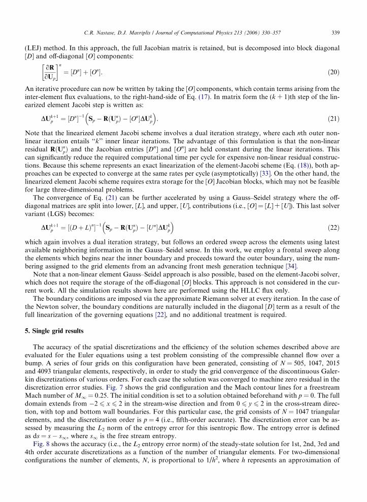
The accuracy of the spatial discretizations and the efficiency of the solution schemes described above areevaluated for the Euler equations using a test problem consisting of the compressible channel flow over abump. A series of four grids on this configuration have been generated, consisting of N = 505, 1047, 2015and 4093 triangular elements, respectively, in order to study the grid convergence of the discontinuous Galer-kin discretizations of various orders. For each case the solution was converged to machine zero residual in thediscretization error studies. Fig. 7 shows the grid configuration and the Mach contour lines for a freestreamMach number ofM1 = 0.25. The initial condition is set to a solution obtained beforehand with p = 0. The fulldomain extends from �2 6 x 6 2 in the stream-wise direction and from 0 6 y 6 2 in the cross-stream direc-tion, with top and bottom wall boundaries. For this particular case, the grid consists of N = 1047 triangularelements, and the discretization order is p = 4 (i.e., fifth-order accurate). The discretization error can be as-sessed by measuring the L2 norm of the entropy error for this isentropic flow. The entropy error is definedas ds = s � s1, where s1 is the free stream entropy.

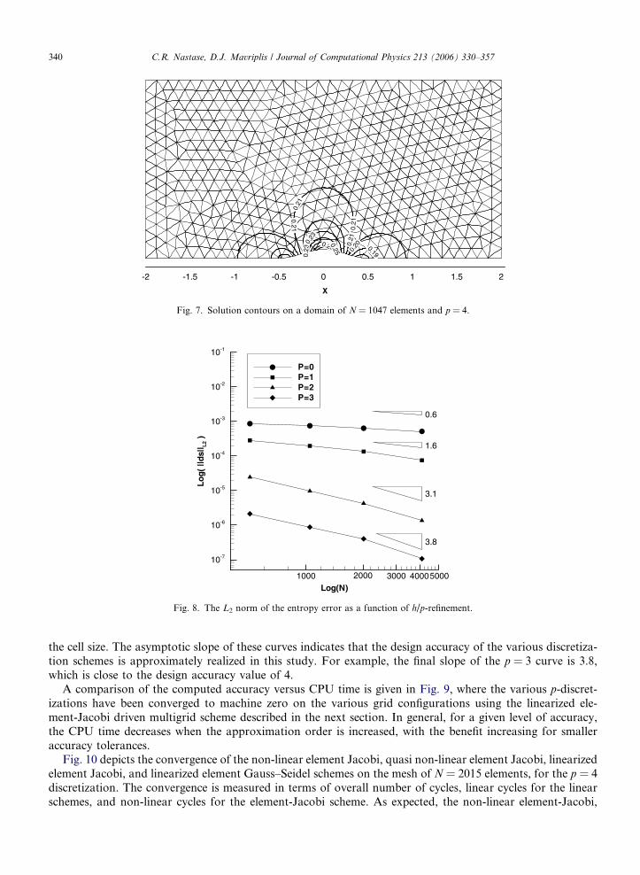
Fig. 8 shows the accuracy (i.e., the L2 entropy error norm) of the steady-state solution for 1st, 2nd, 3rd and4th order accurate discretizations as a function of the number of triangular elements. For two-dimensionalconfigurations the number of elements, N, is proportional to 1/h2, where h represents an approximation of

0.21

0.210.

200.21

0.23

0.26 0.19

0.21

0.250.

23

X

-2 -1.5 -1 -0.5 0 0.5 1 1.5 2

Fig. 7. Solution contours on a domain of N = 1047 elements and p = 4.

Log(N)

Log(

||ds|

| L2

)

1000 2000 3000 40005000

10-7

10-6

10-5

10-4

10-3

10-2

10-1

P=0P=1P=2P=3

0.6

1.6

3.1

3.8

Fig. 8. The L2 norm of the entropy error as a function of h/p-refinement.


the cell size. The asymptotic slope of these curves indicates that the design accuracy of the various discretiza-tion schemes is approximately realized in this study. For example, the final slope of the p = 3 curve is 3.8,which is close to the design accuracy value of 4.

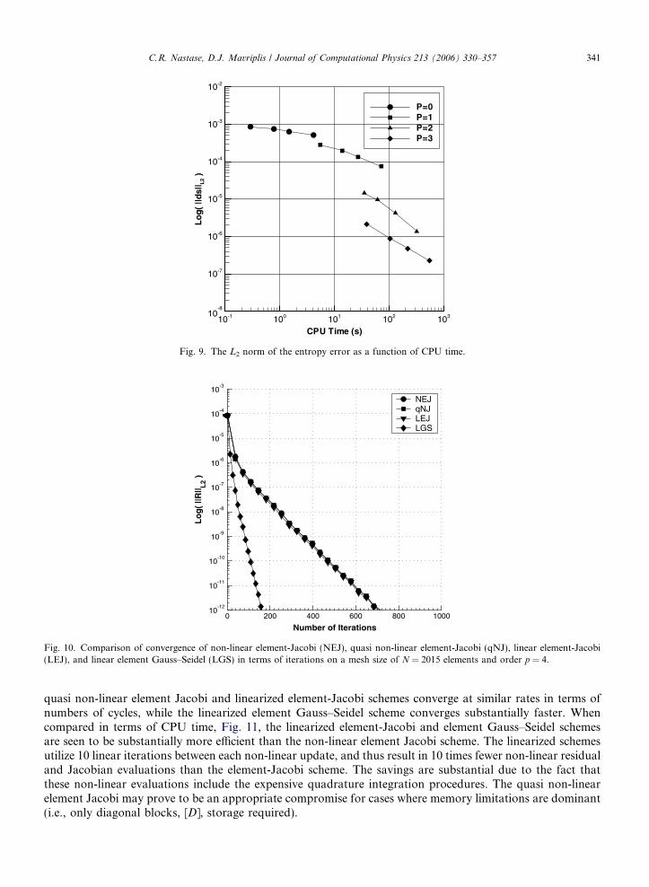
A comparison of the computed accuracy versus CPU time is given in Fig. 9, where the various p-discret-izations have been converged to machine zero on the various grid configurations using the linearized ele-ment-Jacobi driven multigrid scheme described in the next section. In general, for a given level of accuracy,the CPU time decreases when the approximation order is increased, with the benefit increasing for smalleraccuracy tolerances.

Fig. 10 depicts the convergence of the non-linear element Jacobi, quasi non-linear element Jacobi, linearizedelement Jacobi, and linearized element Gauss–Seidel schemes on the mesh of N = 2015 elements, for the p = 4discretization. The convergence is measured in terms of overall number of cycles, linear cycles for the linearschemes, and non-linear cycles for the element-Jacobi scheme. As expected, the non-linear element-Jacobi,

CPU T ime (s)

Log(

||ds|

| L2

)

10-1 100 101 102 10310-8

10-7

10-6

10-5

10-4

10-3

10-2

P=0P=1P=2P=3

Fig. 9. The L2 norm of the entropy error as a function of CPU time.

0 200 400 600 800 100010

-12

10-11

10-10

10-9

10-8

10-7

10-6

10-5

10-4

10-3

Number of Iterations

Lo

g(

||R|| L

2 )

NEJqNJLEJLGS

Fig. 10. Comparison of convergence of non-linear element-Jacobi (NEJ), quasi non-linear element-Jacobi (qNJ), linear element-Jacobi(LEJ), and linear element Gauss–Seidel (LGS) in terms of iterations on a mesh size of N = 2015 elements and order p = 4.


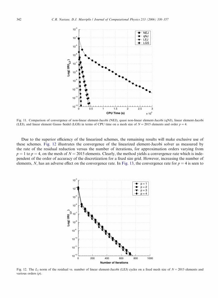
quasi non-linear element Jacobi and linearized element-Jacobi schemes converge at similar rates in terms ofnumbers of cycles, while the linearized element Gauss–Seidel scheme converges substantially faster. Whencompared in terms of CPU time, Fig. 11, the linearized element-Jacobi and element Gauss–Seidel schemesare seen to be substantially more efficient than the non-linear element Jacobi scheme. The linearized schemesutilize 10 linear iterations between each non-linear update, and thus result in 10 times fewer non-linear residualand Jacobian evaluations than the element-Jacobi scheme. The savings are substantial due to the fact thatthese non-linear evaluations include the expensive quadrature integration procedures. The quasi non-linearelement Jacobi may prove to be an appropriate compromise for cases where memory limitations are dominant(i.e., only diagonal blocks, [D], storage required).

0 0.5 1 1.5 2 2.5 3

x 104

10-12

10-11

10-10

10-9

10-8

10-7

10-6

10-5

10-4

10-3

CPU Time (s)

Lo

g(

||R|| L

2 )

NEJqNJLEJLGS

Fig. 11. Comparison of convergence of non-linear element-Jacobi (NEJ), quasi non-linear element-Jacobi (qNJ), linear element-Jacobi(LEJ), and linear element Gauss–Seidel (LGS) in terms of CPU time on a mesh size of N = 2015 elements and order p = 4.


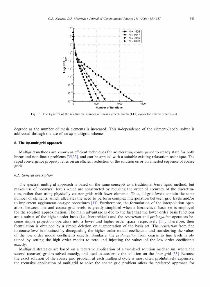
Due to the superior efficiency of the linearized schemes, the remaining results will make exclusive use ofthese schemes. Fig. 12 illustrates the convergence of the linearized element-Jacobi solver as measured bythe rate of the residual reduction versus the number of iterations, for approximation orders varying fromp = 1 to p = 4, on the mesh of N = 2015 elements. Clearly, the method yields a convergence rate which is inde-pendent of the order of accuracy of the discretization for a fixed size grid. However, increasing the number ofelements, N, has an adverse effect on the convergence rate. In Fig. 13, the convergence rate for p = 4 is seen to

0 200 400 600 800 100010

-12

10-11

10-10

10-9

10-8

10-7

10-6

10-5

10-4

10-3


Lo

g(

||R|| L

2 )

p = 1p = 2p = 3p = 4

Fig. 12. The L2 norm of the residual vs. number of linear element-Jacobi (LEJ) cycles on a fixed mesh size of N = 2015 elements andvarious orders (p).

0 500 1000 150010

-12

10-11

10-10

10-9

10-8

10-7

10-6

10-5

10-4

10-3


Lo

g(

||R|| L

2 )

N = 505N = 1047N = 2015N = 4093

Fig. 13. The L2 norm of the residual vs. number of linear element-Jacobi (LEJ) cycles for a fixed order p = 4.


degrade as the number of mesh elements is increased. This h-dependence of the element-Jacobi solver isaddressed through the use of an hp-multigrid scheme.

6. The hp-multigrid approach

Multigrid methods are known as efficient techniques for accelerating convergence to steady state for bothlinear and non-linear problems [35,33], and can be applied with a suitable existing relaxation technique. Therapid convergence property relies on an efficient reduction of the solution error on a nested sequence of coarsegrids.

6.1. General description

The spectral multigrid approach is based on the same concepts as a traditional h-multigrid method, butmakes use of ‘‘coarser’’ levels which are constructed by reducing the order of accuracy of the discretiza-tion, rather than using physically coarser grids with fewer elements. Thus, all grid levels contain the samenumber of elements, which alleviates the need to perform complex interpolation between grid levels and/orto implement agglomeration-type procedures [33]. Furthermore, the formulation of the interpolation oper-ators, between fine and coarse grid levels, is greatly simplified when a hierarchical basis set is employedfor the solution approximation. The main advantage is due to the fact that the lower order basis functionsare a subset of the higher order basis (i.e., hierarchical) and the restriction and prolongation operators be-come simple projection operators into a lower and higher order space, respectively [11]. Therefore, theirformulation is obtained by a simple deletion or augmentation of the basis set. The restriction from fineto coarse level is obtained by disregarding the higher order modal coefficients and transferring the valuesof the low order modal coefficients exactly. Similarly, the prolongation from coarse to fine levels is ob-tained by setting the high order modes to zero and injecting the values of the low order coefficientsexactly.

Multigrid strategies are based on a recursive application of a two-level solution mechanism, where thesecond (coarser) grid is solved exactly, and used to accelerate the solution on the finer grid [35]. Becausethe exact solution of the coarse grid problem at each multigrid cycle is most often prohibitively expensive,the recursive application of multigrid to solve the coarse grid problem offers the preferred approach for


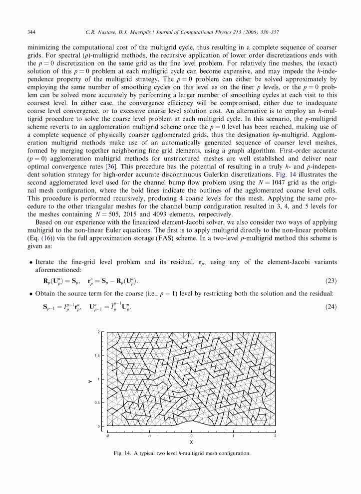
minimizing the computational cost of the multigrid cycle, thus resulting in a complete sequence of coarsergrids. For spectral (p)-multigrid methods, the recursive application of lower order discretizations ends withthe p = 0 discretization on the same grid as the fine level problem. For relatively fine meshes, the (exact)solution of this p = 0 problem at each multigrid cycle can become expensive, and may impede the h-inde-pendence property of the multigrid strategy. The p = 0 problem can either be solved approximately byemploying the same number of smoothing cycles on this level as on the finer p levels, or the p = 0 prob-lem can be solved more accurately by performing a larger number of smoothing cycles at each visit to thiscoarsest level. In either case, the convergence efficiency will be compromised, either due to inadequatecoarse level convergence, or to excessive coarse level solution cost. An alternative is to employ an h-mul-tigrid procedure to solve the coarse level problem at each multigrid cycle. In this scenario, the p-multigridscheme reverts to an agglomeration multigrid scheme once the p = 0 level has been reached, making use ofa complete sequence of physically coarser agglomerated grids, thus the designation hp-multigrid. Agglom-eration multigrid methods make use of an automatically generated sequence of coarser level meshes,formed by merging together neighboring fine grid elements, using a graph algorithm. First-order accurate(p = 0) agglomeration multigrid methods for unstructured meshes are well established and deliver nearoptimal convergence rates [36]. This procedure has the potential of resulting in a truly h- and p-indepen-dent solution strategy for high-order accurate discontinuous Galerkin discretizations. Fig. 14 illustrates thesecond agglomerated level used for the channel bump flow problem using the N = 1047 grid as the origi-nal mesh configuration, where the bold lines indicate the outlines of the agglomerated coarse level cells.This procedure is performed recursively, producing 4 coarse levels for this mesh. Applying the same pro-cedure to the other triangular meshes for the channel bump configuration resulted in 3, 4, and 5 levels forthe meshes containing N = 505, 2015 and 4093 elements, respectively.

Based on our experience with the linearized element-Jacobi solver, we also consider two ways of applyingmultigrid to the non-linear Euler equations. The first is to apply multigrid directly to the non-linear problem(Eq. (16)) via the full approximation storage (FAS) scheme. In a two-level p-multigrid method this scheme isgiven as:

� Iterate the fine-grid level problem and its residual, rp, using any of the element-Jacobi variantsaforementioned:

RpðUnpÞ ¼ Sp; rnp ¼ Sp � RpðUn

pÞ. ð23Þ

� Obtain the source term for the coarse (i.e., p � 1) level by restricting both the solution and the residual:

Sp�1 ¼ Ip�1p rnp; Un

p�1 ¼ ~Ip�1

p Unp. ð24Þ

X

Y

-2 -1 0 1 2

0

0.5

1

1.5

2

Fig. 14. A typical two level h-multigrid mesh configuration.


� Solve the coarse grid level problem

Rp�1ðUnp�1Þ ¼ Sp�1. ð25Þ

� Calculate the coarse grid error, enp�1:

enp�1 ¼ Unp�1 � ~I

p�1

p Unp. ð26Þ

� Prolongate the coarse grid error and correct the fine-grid level approximation:

Unþ1p ¼ Un

p þ Ipp�1enp�1. ð27Þ

In the case of p-multigrid, ~Ip�1

p and Ip�1p denote the state and residual restriction (i.e., from p to p � 1) oper-

ators, respectively. In the case of a hierarchical basis, Ip�1p is the identity matrix with zero columns appended.

Moreover, Ip�1p ¼ ~I

p�1

p for p-multigrid but note that this is not true in the case of h-multigrid. Similarly, theprolongation (i.e., from p � 1 to p) operator, Ipp�1, is obtained as the transpose of the restriction operator,Ipp�1 ¼ ðIp�1

p ÞT.

The second way of applying multigrid to the non-linear set of governing equations is to use the coarse gridcorrection (CGC) multigrid technique on the linearized problem obtained at each Newton iteration (Eq. (17)).This methodology, sometimes referred as ‘‘Newton-multigrid’’, is given (using the dual iteration strategy) asfollows:

� Outer non-linear (nth) iteration. Iterate the discrete linear problem using any of the linearized element-Jacobi variants (LEJ or LGS) aforementioned:

oRp

oUp

� �nDUnþ1

p ¼ Sp � RpðUnpÞ. ð28Þ

– Inner linear (kth) iteration. Solve for the fine-grid level correction wkp ¼ DUk

p with initial guess wk¼0p ¼ 0:

½Jkp�wk

p ¼ fkp; ð29Þ

where

½Jkp� ¼

oRp

oUp

� �n; fkp ¼ Sp � RpðUn

pÞ. ð30Þ

– Obtain the source term for the coarse level by restricting the linear residual rkp:

fkp�1 ¼ Ip�1p rkp; rkp ¼ fkp � ½Jp�wk

p. ð31Þ

– Solve the coarse grid correction problem with initial guess Dwkp�1 ¼ 0:

½Jkp�1�Dwk

p�1 ¼ fkp�1; ½Jkp�1� is a subset of ½Jk

p�. ð32Þ

– Prolongate the coarse grid correction and update the fine-grid correction:

DUkþ1p ¼ DUk

p þ Ipp�1Dwkp�1. ð33Þ

� Fine-grid non-linear update:

Unþ1p ¼ Un

p þ DUkþ1p . ð34Þ

In this implementation the basis set is hierarchical beginning at p = 1. Therefore, the Jacobian,½Jk

p�1� ¼ ½oRpðUpÞ=oUp�n, (and its inverse) represents a subset of ½JkpP2� and requires no additional operator

for its construction. Once the p = 1 level is reached the state variable, Up, and the residual, Rp(Up), arerestricted to p = 0, via two different operators defined as follows:


Uh ¼1

3

X3

i¼1

Uip¼1; RhðUhÞ ¼

X3

i¼1

RpðUip¼1Þ; ð35Þ

where {i = 1, . . ., 3} is the modal index corresponding to p = 1. Therefore, in the case of h-multigrid (i.e.,p = 0), the fine grid problem becomes Rh(Uh) = Sh, and both FAS and CGC algorithms are obtained in a sim-ilar fashion, with the exception of the ½Jk

h� ¼ ½Jkp¼0� term, in the case of CGC algorithm, which needs to be eval-

uated once at every non-linear nth step for all h-levels as ½Jkh� ¼ ½oRhðUhÞ=oUh�n, where the restriction of the

state variable and its residual to a coarse level, H, is obtained as:

UH ¼ 1

AH

XNh

k¼1

ðUhAhÞk; RHðUH Þ ¼XNh

k¼1

ðRhðUhÞÞk; ð36Þ

where Nh is the number of elements used in the agglomeration, Ah is the fine level elemental area, andAH ¼

PNhk¼1ðAhÞk is the coarse level area. This two-level multigrid can be easily extended to a multi-level

scheme.For robustness it is important to augment the resulting multi-level hp-multigrid with a full multigrid (FMG)

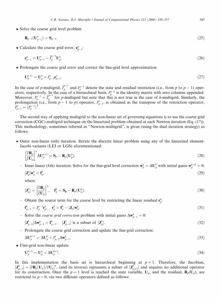
technique, in order to provide a good initial guess for the fine level problem. Moreover, the use of FMG iscritically important in the case of the CGC scheme for it is known that the Newton iteration will diverge ifthe initial guess is not close enough to the final solution. In our hp-multigrid approach, the solution processbegins at the coarsest grid level (p = 0), using all the h-levels available, and ends at the fine level where all thep- and h-levels are used to advance to solution to the desired accuracy, as depicted in Fig. 15. Alternatively, theFMG strategy can be initiated at the coarsest h-level, but no advantage over the latter approach was found, atleast for the inviscid grids/problem considered. This will be further investigated in a future work pertainingviscous flows.

Results are presented for both, FAS and CGC, multigrid methods in order to asses their performance. Un-less otherwise stated, all the simulated results are obtained via FMG using 5 V-cycles per level, starting atp = 0 level with uniform freestream initial conditions.

6.2. Channel flow over a bump

In the context of hp-multigrid methodology, the first case considered is of a compressible channel flow overa bump, with the flow and geometrical parameters as defined in Section 5.

6.2.1. Non-linear (FAS) hp-multigrid scheme

Fig. 16 illustrates the convergence rate of the residual as a function of the non-linear (FAS) hp-multigridcycles for various p-order discretizations for a fixed mesh resolution (N = 2015), using a multigrid V-cycle with10 linear element Jacobi smoothing passes on each grid level, including the agglomerated levels. While p-

S

S

S

S

S

S

p = 0

h = 1

h = 2

p = 2

p = 3

p = 1

Fig. 15. Full hp-multigrid (FMG) levels for p = 3 and h = 2 (–, restriction; - -, prolongation; d, smoothing; �, update).

0 10 20 30 40 50 60 70 8010

-12

10-10

10-8

10-6

10-4

10-2

Number of MGcycles

Lo

g(

||R|| L

2 )

p = 1p = 2p = 3p = 4

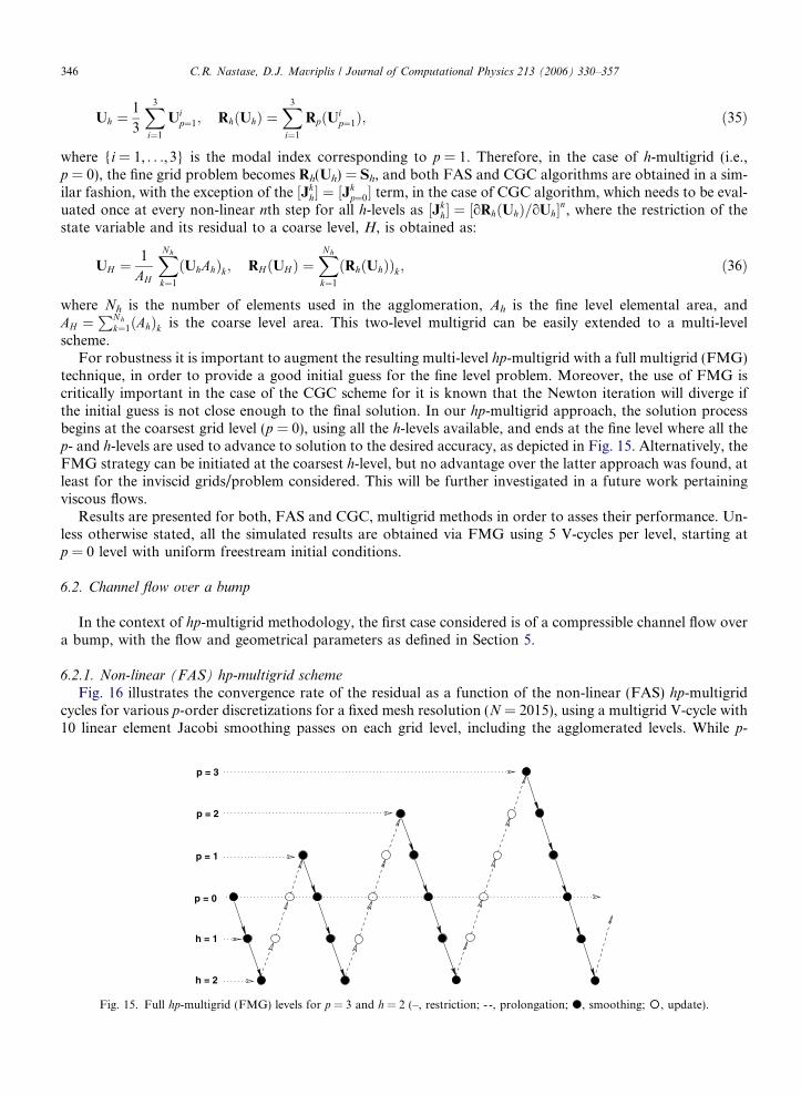
Fig. 16. The full hp-multigrid convergence vs. the number of multigrid (MG) cycles, on a mesh size of N = 4093 elements and variousorders (p), for the channel bump problem.


independent convergence rates are expected, since the Jacobi smoother was shown to be p-independent, con-vergence actually accelerates slightly with increasing p. Note that although the convergence rate increases, thecost of the higher p discretizations is substantially higher per cycle, due to the higher number of degrees offreedom and larger block matrices involved.

In Fig. 17, the convergence rates for a fixed discretization (p = 4) are compared on the various grids for thebump configuration. In all cases, convergence to machine accuracy is achieved in 50 multigrid cycles or less,and only a slight h-dependence is observed (i.e., the N = 505 case requires 39 cycles, while the N = 4093 case

0 10 20 30 40 50 6010

-12

10-10

10-8

10-6

10-4

10-2

Number of MGcycles

Log(

||R

|| L2 )

N = 505N = 1047N = 2015N = 4093

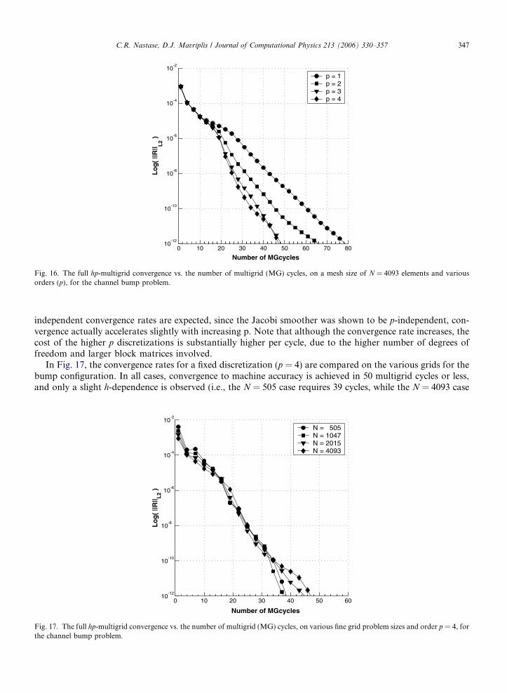
Fig. 17. The full hp-multigrid convergence vs. the number of multigrid (MG) cycles, on various fine grid problem sizes and order p = 4, forthe channel bump problem.


requires 47 cycles). Note that the largest case N = 4093 involves a total of 10 multigrid levels, 5 levels fromp = 4 to p = 0, and 5 h-agglomerated levels. The average convergence rates values are given in Table 2.

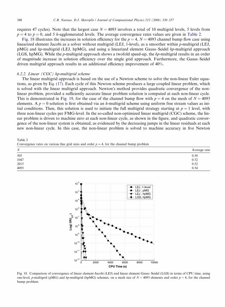
Fig. 18 illustrates the increases in solution efficiency for the p = 4, N = 4093 channel bump flow case usinglinearized element Jacobi as a solver without multigrid (LEJ, 1-level), as a smoother within p-multigrid (LEJ,pMG) and hp-multigrid (LEJ, hpMG), and using a linearized element Gauss–Seidel hp-multigrid approach(LGS, hpMG). While the p-multigrid approach shows a twofold speed-up, the hp-multigrid results in an orderof magnitude increase in solution efficiency over the single grid approach. Furthermore, the Gauss–Seideldriven multigrid approach results in an additional efficiency improvement of 40%.

6.2.2. Linear (CGC) hp-multigrid scheme

The linear multigrid approach is based on the use of a Newton scheme to solve the non-linear Euler equa-tions, as given by Eq. (17). Each cycle of this Newton scheme produces a large coupled linear problem, whichis solved with the linear multigrid approach. Newton�s method provides quadratic convergence of the non-linear problem, provided a sufficiently accurate linear problem solution is computed at each non-linear cycle.This is demonstrated in Fig. 19, for the case of the channel bump flow with p = 4 on the mesh of N = 4093elements. A p = 0 solution is first obtained via an h-multigrid scheme using uniform free stream values as ini-tial conditions. Then, this solution is used to initiate the full multigrid strategy starting at p = 1 level, withthree non-linear cycles per FMG-level. In the so-called non-optimized linear multigrid (CGC) scheme, the lin-ear problem is driven to machine zero at each non-linear cycle, as shown in the figure, and quadratic conver-gence of the non-linear system is obtained, as evidenced by the decreasing jumps in the linear residuals at eachnew non-linear cycle. In this case, the non-linear problem is solved to machine accuracy in five Newton

Table 2Convergence rates on various fine grid sizes and order p = 4, for the channel bump problem

N Average rate

505 0.501047 0.522015 0.524093 0.54

0 2000 4000 6000 8000 1000010

-12

10-11

10-10

10-9

10-8

10-7

10-6

10-5

10-4

10-3

CPU Time (s)

Lo

g(

||R|| L

2 )

LEJ ,1-levelLEJ , pMGLEJ , hpMGLGS, hpMG

Fig. 18. Comparison of convergence of linear element-Jacobi (LEJ) and linear element Gauss–Seidel (LGS) in terms of CPU time, usingone-level, p-multigrid (pMG) and hp-multigrid (hpMG) schemes, on a mesh size of N = 4093 elements and order p = 4, for the channelbump problem.

0 100 200 300 400 500 600 70010

-16

10-14

10-12

10-10

10-8

10-6

10-4

Number of Linear Iterations

Lo

g(

||rC

GC

|| L2 )

non-optimizedoptimized

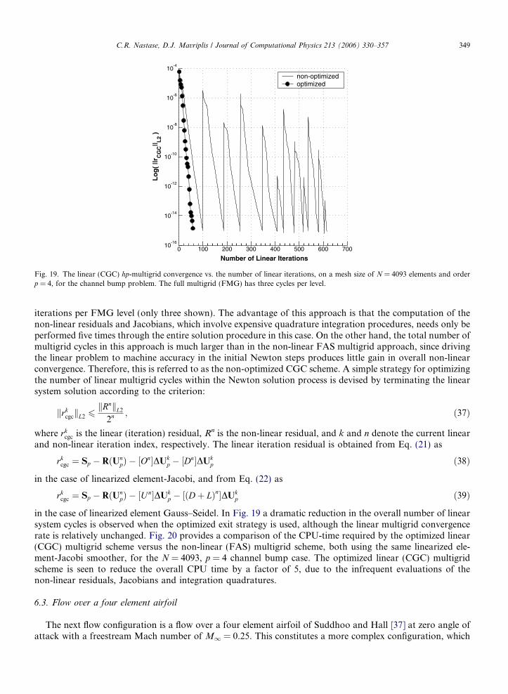
Fig. 19. The linear (CGC) hp-multigrid convergence vs. the number of linear iterations, on a mesh size of N = 4093 elements and orderp = 4, for the channel bump problem. The full multigrid (FMG) has three cycles per level.


iterations per FMG level (only three shown). The advantage of this approach is that the computation of thenon-linear residuals and Jacobians, which involve expensive quadrature integration procedures, needs only beperformed five times through the entire solution procedure in this case. On the other hand, the total number ofmultigrid cycles in this approach is much larger than in the non-linear FAS multigrid approach, since drivingthe linear problem to machine accuracy in the initial Newton steps produces little gain in overall non-linearconvergence. Therefore, this is referred to as the non-optimized CGC scheme. A simple strategy for optimizingthe number of linear multigrid cycles within the Newton solution process is devised by terminating the linearsystem solution according to the criterion:

krkcgckL2 6kRnkL22n

; ð37Þ

where rkcgc is the linear (iteration) residual, Rn is the non-linear residual, and k and n denote the current linear

and non-linear iteration index, respectively. The linear iteration residual is obtained from Eq. (21) as

rkcgc ¼ Sp � RðUnpÞ � ½On�DUk

p � ½Dn�DUkp ð38Þ

in the case of linearized element-Jacobi, and from Eq. (22) as

rkcgc ¼ Sp � RðUnpÞ � ½Un�DUk

p � ½ðDþ LÞn�DUkp ð39Þ

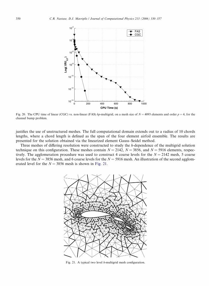
in the case of linearized element Gauss–Seidel. In Fig. 19 a dramatic reduction in the overall number of linearsystem cycles is observed when the optimized exit strategy is used, although the linear multigrid convergencerate is relatively unchanged. Fig. 20 provides a comparison of the CPU-time required by the optimized linear(CGC) multigrid scheme versus the non-linear (FAS) multigrid scheme, both using the same linearized ele-ment-Jacobi smoother, for the N = 4093, p = 4 channel bump case. The optimized linear (CGC) multigridscheme is seen to reduce the overall CPU time by a factor of 5, due to the infrequent evaluations of thenon-linear residuals, Jacobians and integration quadratures.

6.3. Flow over a four element airfoil

The next flow configuration is a flow over a four element airfoil of Suddhoo and Hall [37] at zero angle ofattack with a freestream Mach number of M1 = 0.25. This constitutes a more complex configuration, which

0 200 400 600 800 100010

-14

10-12

10-10

10-8

10-6

10-4

10-2

CPU Time (s)

Lo

g(

||R|| L

2 )

FASCGC

Fig. 20. The CPU time of linear (CGC) vs. non-linear (FAS) hp-multigrid, on a mesh size of N = 4093 elements and order p = 4, for thechannel bump problem.


justifies the use of unstructured meshes. The full computational domain extends out to a radius of 10 chordslengths, where a chord length is defined as the span of the four element airfoil ensemble. The results arepresented for the solution obtained via the linearized element Gauss–Seidel method.

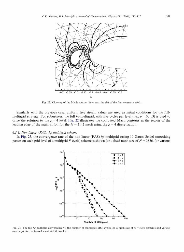
Three meshes of differing resolution were constructed to study the h-dependence of the multigrid solutiontechnique on this configuration. These meshes contain N = 2142, N = 3856, and N = 5916 elements, respec-tively. The agglomeration procedure was used to construct 4 coarse levels for the N = 2142 mesh, 5 coarselevels for the N = 3856 mesh, and 6 coarse levels for the N = 5916 mesh. An illustration of the second agglom-erated level for the N = 3856 mesh is shown in Fig. 21.

Fig. 21. A typical two level h-multigrid mesh configuration.

0.280.28

0.61

0.28

0.50

0.28

0.610.39 0.

500.39

0.50

0.61

0.17

0.17

0.61

0.170.17X

-0.7 -0.65 -0.6 -0.55 -0.5 -0.45 -0.4 -0.35 -0.3

Fig. 22. Close-up of the Mach contour lines near the slat of the four element airfoil.


Similarly with the previous case, uniform free stream values are used as initial conditions for the full-multigrid strategy. For robustness, the full hp-multigrid, with five cycles per level (i.e., p = 0 . . .3) is used todrive the solution to the p = 4 level. Fig. 22 illustrates the computed Mach contours in the region of theleading edge of the main airfoil for the N = 2142 mesh using the p = 4 discretization.

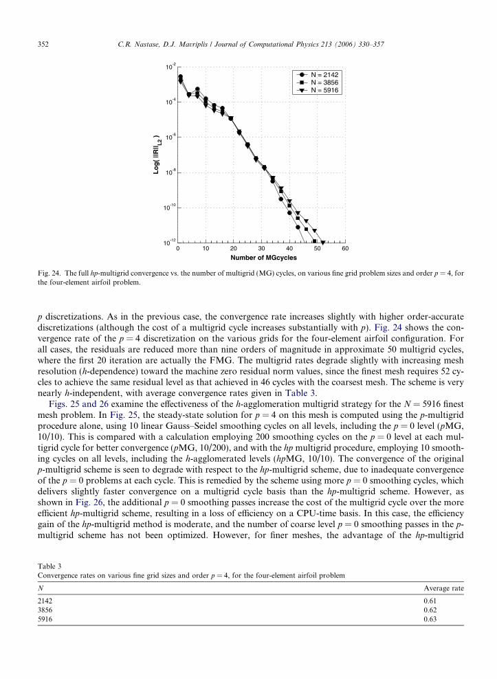
6.3.1. Non-linear (FAS) hp-multigrid scheme

In Fig. 23, the convergence rate of the non-linear (FAS) hp-multigrid (using 10 Gauss–Seidel smoothingpasses on each grid level of a multigrid V-cycle) scheme is shown for a fixed mesh size of N = 3856, for various

0 20 40 60 80 10010

-12

10-10

10-8

10-6

10-4

10-2

Number of MGcycles

Lo

g(

||R|| L

2 )

p = 1p = 2p = 3p = 4

Fig. 23. The full hp-multigrid convergence vs. the number of multigrid (MG) cycles, on a mesh size of N = 5916 elements and variousorders (p), for the four-element airfoil problem.

0 10 20 30 40 50 6010

-12

10-10

10-8

10-6

10-4

10-2

Number of MGcycles

Lo

g(

||R|| L

2 )

N = 2142N = 3856N = 5916

Fig. 24. The full hp-multigrid convergence vs. the number of multigrid (MG) cycles, on various fine grid problem sizes and order p = 4, forthe four-element airfoil problem.


p discretizations. As in the previous case, the convergence rate increases slightly with higher order-accuratediscretizations (although the cost of a multigrid cycle increases substantially with p). Fig. 24 shows the con-vergence rate of the p = 4 discretization on the various grids for the four-element airfoil configuration. Forall cases, the residuals are reduced more than nine orders of magnitude in approximate 50 multigrid cycles,where the first 20 iteration are actually the FMG. The multigrid rates degrade slightly with increasing meshresolution (h-dependence) toward the machine zero residual norm values, since the finest mesh requires 52 cy-cles to achieve the same residual level as that achieved in 46 cycles with the coarsest mesh. The scheme is verynearly h-independent, with average convergence rates given in Table 3.

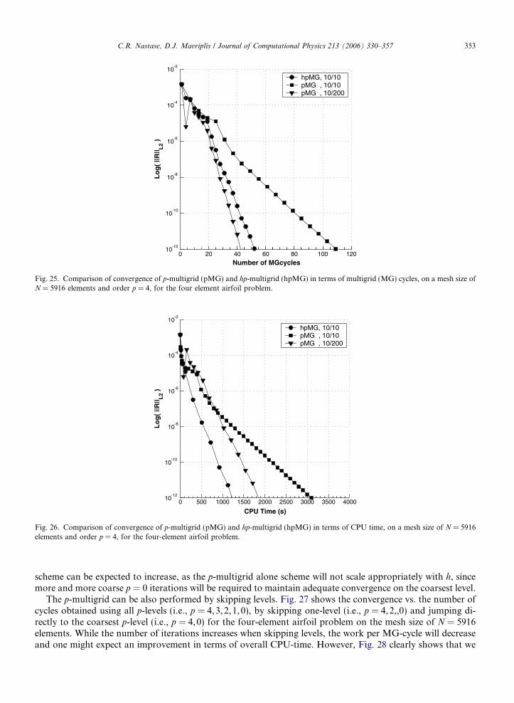
Figs. 25 and 26 examine the effectiveness of the h-agglomeration multigrid strategy for the N = 5916 finestmesh problem. In Fig. 25, the steady-state solution for p = 4 on this mesh is computed using the p-multigridprocedure alone, using 10 linear Gauss–Seidel smoothing cycles on all levels, including the p = 0 level (pMG,10/10). This is compared with a calculation employing 200 smoothing cycles on the p = 0 level at each mul-tigrid cycle for better convergence (pMG, 10/200), and with the hpmultigrid procedure, employing 10 smooth-ing cycles on all levels, including the h-agglomerated levels (hpMG, 10/10). The convergence of the originalp-multigrid scheme is seen to degrade with respect to the hp-multigrid scheme, due to inadequate convergenceof the p = 0 problems at each cycle. This is remedied by the scheme using more p = 0 smoothing cycles, whichdelivers slightly faster convergence on a multigrid cycle basis than the hp-multigrid scheme. However, asshown in Fig. 26, the additional p = 0 smoothing passes increase the cost of the multigrid cycle over the moreefficient hp-multigrid scheme, resulting in a loss of efficiency on a CPU-time basis. In this case, the efficiencygain of the hp-multigrid method is moderate, and the number of coarse level p = 0 smoothing passes in the p-multigrid scheme has not been optimized. However, for finer meshes, the advantage of the hp-multigrid

Table 3Convergence rates on various fine grid sizes and order p = 4, for the four-element airfoil problem

N Average rate

2142 0.613856 0.625916 0.63

0 20 40 60 80 100 12010

-12

10-10

10-8

10-6

10-4

10-2

Number of MGcycles

Lo

g(

||R|| L

2 )

hpMG, 10/10pMG , 10/10pMG , 10/200

Fig. 25. Comparison of convergence of p-multigrid (pMG) and hp-multigrid (hpMG) in terms of multigrid (MG) cycles, on a mesh size ofN = 5916 elements and order p = 4, for the four element airfoil problem.

0 500 1000 1500 2000 2500 3000 3500 400010

-12

10-10

10-8

10-6

10-4

10-2

CPU Time (s)

Lo

g(

||R|| L

2 )

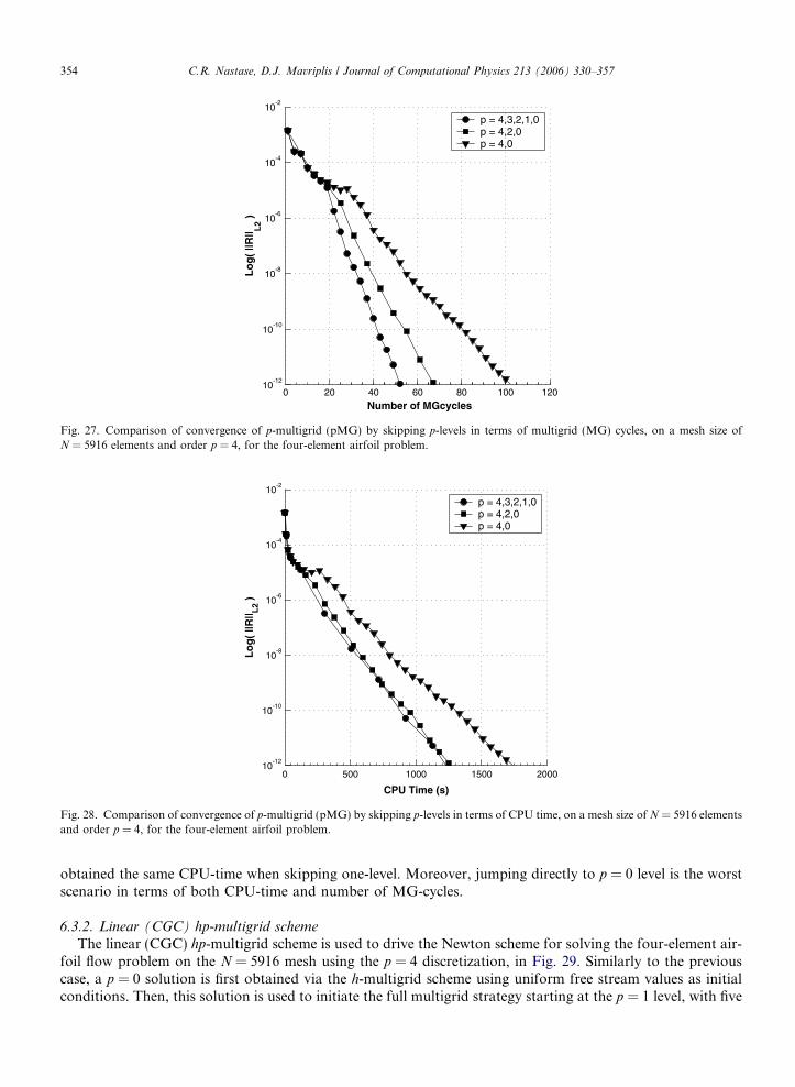
hpMG, 10/10pMG , 10/10pMG , 10/200

Fig. 26. Comparison of convergence of p-multigrid (pMG) and hp-multigrid (hpMG) in terms of CPU time, on a mesh size of N = 5916elements and order p = 4, for the four-element airfoil problem.


scheme can be expected to increase, as the p-multigrid alone scheme will not scale appropriately with h, sincemore and more coarse p = 0 iterations will be required to maintain adequate convergence on the coarsest level.

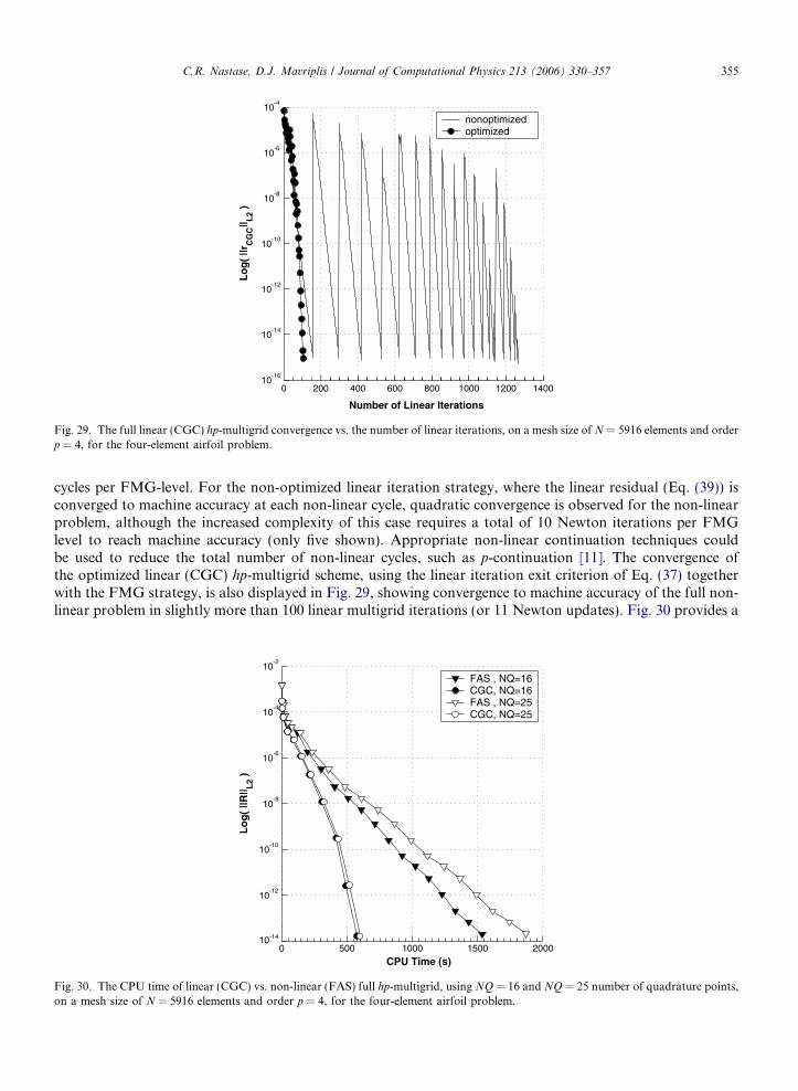
The p-multigrid can be also performed by skipping levels. Fig. 27 shows the convergence vs. the number ofcycles obtained using all p-levels (i.e., p = 4,3,2,1,0), by skipping one-level (i.e., p = 4,2,,0) and jumping di-rectly to the coarsest p-level (i.e., p = 4,0) for the four-element airfoil problem on the mesh size of N = 5916elements. While the number of iterations increases when skipping levels, the work per MG-cycle will decreaseand one might expect an improvement in terms of overall CPU-time. However, Fig. 28 clearly shows that we

0 20 40 60 80 100 12010

-12

10-10

10-8

10-6

10-4

10-2

Number of MGcycles

Lo

g(

||R|| L

2 )

p = 4,3,2,1,0p = 4,2,0p = 4,0

Fig. 27. Comparison of convergence of p-multigrid (pMG) by skipping p-levels in terms of multigrid (MG) cycles, on a mesh size ofN = 5916 elements and order p = 4, for the four-element airfoil problem.

0 500 1000 1500 200010

-12

10-10

10-8

10-6

10-4

10-2

CPU Time (s)

Lo

g(

||R|| L

2 )

p = 4,3,2,1,0p = 4,2,0p = 4,0

Fig. 28. Comparison of convergence of p-multigrid (pMG) by skipping p-levels in terms of CPU time, on a mesh size of N = 5916 elementsand order p = 4, for the four-element airfoil problem.


obtained the same CPU-time when skipping one-level. Moreover, jumping directly to p = 0 level is the worstscenario in terms of both CPU-time and number of MG-cycles.

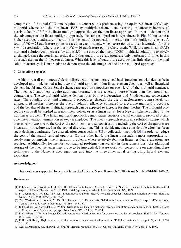
6.3.2. Linear (CGC) hp-multigrid schemeThe linear (CGC) hp-multigrid scheme is used to drive the Newton scheme for solving the four-element air-

foil flow problem on the N = 5916 mesh using the p = 4 discretization, in Fig. 29. Similarly to the previouscase, a p = 0 solution is first obtained via the h-multigrid scheme using uniform free stream values as initialconditions. Then, this solution is used to initiate the full multigrid strategy starting at the p = 1 level, with five

0 200 400 600 800 1000 1200 140010

-16

10-14

10-12

10-10

10-8

10-6

10-4

Number of Linear Iterations

Lo

g(

||rC

GC

|| L2 )

nonoptimizedoptimized

Fig. 29. The full linear (CGC) hp-multigrid convergence vs. the number of linear iterations, on a mesh size of N = 5916 elements and orderp = 4, for the four-element airfoil problem.


cycles per FMG-level. For the non-optimized linear iteration strategy, where the linear residual (Eq. (39)) isconverged to machine accuracy at each non-linear cycle, quadratic convergence is observed for the non-linearproblem, although the increased complexity of this case requires a total of 10 Newton iterations per FMGlevel to reach machine accuracy (only five shown). Appropriate non-linear continuation techniques couldbe used to reduce the total number of non-linear cycles, such as p-continuation [11]. The convergence ofthe optimized linear (CGC) hp-multigrid scheme, using the linear iteration exit criterion of Eq. (37) togetherwith the FMG strategy, is also displayed in Fig. 29, showing convergence to machine accuracy of the full non-linear problem in slightly more than 100 linear multigrid iterations (or 11 Newton updates). Fig. 30 provides a

0 500 1000 1500 200010-14

10-12

10-10

10-8

10-6

10-4

10-2

CPU Time (s)

Lo

g(

||R|| L

2 )

FAS , NQ=16CGC, NQ=16FAS , NQ=25CGC, NQ=25

Fig. 30. The CPU time of linear (CGC) vs. non-linear (FAS) full hp-multigrid, using NQ = 16 and NQ = 25 number of quadrature points,on a mesh size of N = 5916 elements and order p = 4, for the four-element airfoil problem.


comparison of the total CPU time required to converge this problem using the optimized linear (CGC) hp-multigrid scheme, and the non-linear (FAS) hp-multigrid scheme, demonstrating an efficiency increase ofnearly a factor of 3 for the linear multigrid approach over the non-linear approach. In order to demonstratethe advantage of the linear multigrid approach, the same comparison is reproduced in Fig. 30 but using ahigher accuracy quadrature integration in the spatial discretization operator for both multigrid schemes. Atotal of NQ = 25 quadrature points are used on each triangle, which corresponds to over-integration for thisp = 4 discretization (where previously NQ = 16 quadrature points where used). While the non-linear (FAS)multigrid solution cost increases by about 25%, the cost of the linear (CGC) multigrid solution is relativelyunchanged, since the non-linear residual and thus quadrature evaluations are only performed 11 times in thisapproach (i.e., at the 11 Newton updates). While this level of quadrature accuracy has little effect on the finalsolution accuracy, it is instructive to demonstrate the advantages of the linear multigrid approach.

7. Concluding remarks

A high-order discontinuous Galerkin discretization using hierarchical basis functions on triangles has beendeveloped and implemented using a hp-multigrid approach. Non-linear element-Jacobi, as well as linearizedelement-Jacobi and Gauss–Seidel schemes are used as smoothers on each level of the multigrid sequence.The linearized smoothers require additional storage, but are generally more efficient than their non-linearcounterparts. The hp-multigrid scheme demonstrates both p-independent and h-independent convergencerates. The coupling of p- and h-multigrid procedures, through the use of agglomerated coarse levels forunstructured meshes, increases the overall solution efficiency compared to a p-alone multigrid procedure,and the benefits of the hp-multigrid approach can be expected to increase for finer meshes. The multigrid pro-cedure can itself be applied as a non-linear solver, or as a linear solver for a Newton scheme applied to thenon-linear problem. The linear multigrid approach demonstrates superior overall efficiency, provided a suit-able linear iteration termination strategy is employed. The linear approach results in a solution strategy whichis relatively insensitive to the cost of the non-linear residual construction, including the cost of the quadratureintegration procedure used in the spatial discretization. This is significant, since considerable effort has beenspent devising quadrature-free discretization constructions [38] or collocation methods [39] in order to reducethe cost of the spatial residual operator. On the other-hand, the linear approach is most appropriate forsteady-state or implicit time-integration problems, where relatively few non-linear residual evaluations arerequired. Additionally, for memory constrained problems (particularly in three dimensions), the additionalstorage of the linear schemes may prove to be impractical. Future work will concentrate on extending thesetechniques to the Navier–Stokes equations and into the three-dimensional setting using hybrid elementtopologies.

Acknowledgment

This work was supported by a grant from the Office of Naval Research ONR Grant No. N00014-04-1-0602.

References

[1] P. Lesaint, P.A. Raviart, in: C. de Boor (Ed.), On a Finite Element Method to Solve the Neutron Transport Equation, MathematicalAspects of Finite Elements in Partial Differential Equations, Academic Press, New York, NY, 1974.

[2] B. Cockburn, C.-W. Shu, The local discontinuous Galerkin method for time-dependent convection–diffusion systems, SIAM J.Numer. Anal. 35 (6) (1998) 2440–2463.

[3] T.C. Warburton, I. Lomtev, Y. Du, S.J. Sherwin, G.E. Karniadakis, Galerkin and discontinuous Galerkin spectral/hp methods,Comput. Methods Appl. Mech. Eng. 175 (1999) 343–359.

[4] B. Cockburn, G. Karniadakis, C.-W. Shu, Discontinuous Galerkin methods: theory, computation and applications, in: Lecture Notesin Computational Science A, Springer, New York, NY, 1999, pp. 69–224.

[5] B. Cockburn, C.-W. Shu, Runge–Kutta discontinuous Galerkin methods for convection-dominated problems, SIAM J. Sci. Comput.16 (3) (2001) 173–261.

[6] F. Bassi, S. Rebay, High-order accurate discontinuous finite element solution of the 2D Euler equations, J. Comput. Phys. 138 (1997)251–285.

[7] G.E. Karniadakis, S.J. Sherwin, Spectral/hp Element Methods for CFD, Oxford University Press, New York, NY, 1999.


[8] T.J.R. Hughes, A. Brooks, Streamline upwind-Petrov–Galerkin formulations for convection dominated flows with particularemphasis on the incompressible Navier–Stokes equations, Comput. Meth. Appl. Mech. Eng. 32 (1982) 199–259.

[9] B. Helenbrook, D.J. Mavriplis, H. Atkins, Analysis of ‘‘p’’-multigrid for continuous and discontinuous finite element discretizations,in: Proceedings of the 16th AIAA Computational Fluid Dynamics Conference, 2003, AIAA Paper 2003-3989.

[10] E.M. Ronquist, A.T. Patera, Spectral element multigrid I: formulation and numerical results, SIAM J. Sci. Comput. 2 (4) (1987) 389–406.

[11] K.J. Fidkowski, D.L. Darmofal, Development of a higher-order solver for aerodynamic applications, in: Proceedings of the 42ndAerospace Sciences Meeting and Exihibit, Reno, NV, 2004, AIAA Paper 2004-0436.

[12] F. Bassi, S. Rebay, Numerical solution of Euler equations with a multiorder discontinuous finite element method, in: K.S.S. Armfield,P. Morgan (Eds.), Proceedings of the Second International Conference on Computational Fluid Dynamics, Sydney, Australia,Springer, Berlin, 2002, pp. 199–204.

[13] K.J. Fidkowski, T.A. Oliver, J. Lu, D.L. Darmofal, p-Multigrid solution of high-order discontinuous Galerkin discretizations of thecompressible Navier–Stokes equations, J. Comput. Phys. 207 (2005) 92–113.

[14] J.W. Lottes, P.F. Fischer, Hybrid multigrid/Schwarz algorithms for the spectral element method, SIAM J. Sci. Comput. 24 (2005).[15] P. Rasentarinera, M.Y. Hussaini, An efficient implicit discontinuous spectral Galerkin method, J. Comput. Phys. 172 (2001) 718–738.[16] J. Heys, T.A. Manteufell, S.F. McCormick, L.N. Olson, Algebraic multigrid for higher-order finite elements, J. Comput. Phys. 204

(2005) 520–532.[17] S.F. Davis, Simplified second-order Godunov-type methods, SIAM J. Sci. Statist. Comput. 9 (3) (1988) 445–473.[18] P.L. Roe, Approximate Riemann solvers, parameter vectors, and difference schemes, J. Comput. Phys. 43 (1981) 357–372.[19] A. Harten, P.D. Lax, B. Van Leer, On upstream differencing and Godunov-type schemes for hyperbolic conservation laws, SIAM

Rev. 25 (1) (1983) 35–61.[20] F.E. Toro, Riemann Solvers and Numerical Methods for Fluid Dynamics, Applied Mechanics, Springer, New York, NY, 1999.[21] P. Batten, N. Clarke, C. Lambert, D.M. Causon, On the choice of wavespeeds for the HLLC Riemann solver, SIAM J. Sci. Comput.

18 (2) (1997) 1553–1570.[22] P. Batten, M.A. Leschiner, U.C. Goldberg, Average-state jacobians and implicit methods for compressible viscous and turbulent

flows, J. Comput. Phys. 137 (1997) 38–78.[23] P. Solin, P. Segeth, I. Zel, High-Order Finite Element Methods, Studies in Advanced Mathematics, Chapman & Hall, London, 2003.[24] B. Szabo, I. Babuska, Finite Element Analysis, Wiley, New York, NY, 1991.[25] M. Dubiner, Spectral methods on triangles and other domains, SIAM J. Sci. Comput. 6 (1991) 345–390.[26] D.A. Dunavant, High degree efficient symmetrical gaussian guadrature rules for the triangle, Int. J. Numer. Meth. Eng. 21 (1985)

1129–1148.[27] D.A. Dunavant, Economical symmetrical quadrature rules for complete polynomials over a square domain, Int. J. Numer. Meth.

Eng. 21 (1985) 1777–1784.[28] B. Cockburn, S. Hou, C.-W. Shu, The Runge–Kutta local projection discontinuous Galerkin finite element method for conservation

laws IV: the multidimensional case, Math. Comput. 54 (545) (1990) 545–581.[29] B. Cockburn, C.-W. Shu, The Runge–Kutta discontinuous Galerkin method for conservation laws V: multidimensional systems, J.

Comput. Phys. 141 (1998) 199–224.[30] L. Demkowicz, Projection-based interpolation, ICES Report 04-03, The University of Texas at Austin, 2003.[31] L. Demkowicz, I. Babuska, Optimal p interpolation error estimates for edge finite elements of variable order in 2D, TICAM Report

01-11, The University of Texas at Austin, 2001.[32] J.J.W. van der Vegt, H. van der Ven, Slip flow boundary conditions in discontinuous Galerkin discretizations of the Euler equations

of gas dynamics, Technical Report, National Aerospace Laboratory NLR, 2002.[33] D.J. Mavriplis, An assessment of linear versus non-linear multigrid methods for unstructured mesh solvers, J. Comput. Phys. 175

(2002) 302–325.[34] D.J. Mavriplis, Unstructured mesh generation and adaptivity, in: VKI Lecture Series VKI-LS 1995-02, 1995.[35] U. Trottenberg, A. Schuller, C. Oosterlee, Multigrid, Academic Press, London, UK, 2000.[36] D.J. Mavriplis, V. Venkatakrishnan, Agglomeration multigrid for two dimensional viscous flows, Comput. Fluids 24 (5) (1995) 553–

570.[37] A. Suddhoo, I. Hall, Test cases for the plane potential flow past multi-element airfoils, Aeronaut. J. 89 (1985) 403–414.[38] H. Atkins, C.W. Shu, Quadrature-free implementation of discontinuous Galerkin method for hyperbolic equations, AIAA J. 36 (5)

(1998) 775–782.[39] J.S. Hesthaven, T. Warburton, Nodal high-order methods on unstructured grids I. Time-domain solution of Maxwell�s equations, J.

Comput. Phys. 181 (1) (2002) 186–221, ICASE Report No. 01-6.

High-Order Discontinuous Galerkin Methods using a Spectral Multigrid Approach

Documents