Hierarchical image segmentation based on similarity of NDVI ...

Hierarchical image segmentation based on similarity of NDVI time series

Stefaan Lhermitte a,!, Jan Verbesselt a, Inge Jonckheere a, Kris Nackaerts b,Jan A.N. van Aardt c, Willem W. Verstraeten a, Pol Coppin a

a M3-BIORES, Biosystems Department, Katholieke Universiteit Leuven, Celestijnenlaan 200E, Leuven, Belgiumb Mapping and Geospatial Solutions, Intergraph Belgium B.V., Riverside Business Park, Internationalelaan 55, Brussel, Belgium

c Ecosystems, Natural Resources and the Environment, CSIR, P.O. Box 395, Pretoria, South Africa

Received 15 January 2007; received in revised form 8 May 2007; accepted 10 May 2007

Abstract

Although a variety of hierarchical image segmentation procedures for remote sensing imagery have been published, none of them specificallyintegrates remote sensing time series in spatial or hierarchical segmentation concepts. However, this integration is important for the analysis ofecosystems which are hierarchical in nature, with different ecological processes occurring at different spatial and temporal scales. Therefore, theobjective of this paper is to introduce a multi-temporal hierarchical image segmentation (MTHIS) methodology to generate a hierarchical set ofsegments based on spatial similarity of remote sensing time series. MTHIS employs the similarity of the fast Fourier transform (FFT) componentsof multi-seasonal time series to group pixels with similar temporal behavior into hierarchical segments at different scales. Use of the FFT allowsthe distinction between noise and vegetation related signals and increases the computational efficiency. The MTHIS methodology is demonstratedon the area of South Africa in an MTHIS protocol for Normalized Difference Vegetation Index (NDVI) time series. Firstly, the FFT componentsthat express the major spatio-temporal variation in the NDVI time series, the average and annual term, are selected and the segmentation isperformed based on these components. Secondly, the results are visualized by means of a boundary stability image that confirms the accuracy ofthe algorithm to spatially group pixels at different scale levels. Finally, the segmentation optimum is determined based on discrepancy measureswhich illustrate the correspondence of the applied MTHIS output with landcover–landuse maps describing the actual vegetation. In futureresearch, MTHIS can be used to analyze the spatial and hierarchical structure of any type of remote sensing time series and their relation toecosystem processes.© 2007 Elsevier Inc. All rights reserved.

Keywords: Hierarchical image segmentation; Fast Fourier transform; NDVI time series; Vegetation mapping

1. Introduction

The development of effective methodologies to analyze timeseries of satellite imagery is one of themost important issues in theunderstanding of temporal dynamics of vegetation cover(Bruzzone et al., 2003). The temporal component, integratedwith the spectral and spatial dimensions, provides essentialinformation on ecological systems and vegetation dynamics.However, advanced analysis methods are crucial for the properexploration of that information; certainly with the ever increasingamount of time series data. Several methods and algorithms havealready been developed based on satellite-based biophysically

meaningful variables, e.g. the Normalized Difference VegetationIndex (NDVI) whose behavior follows annual cycles ofvegetation growth (Running et al., 1994). These applied methodsinclude Principal Component Analysis (PCA) (Anyamba &Eastman, 1996; Eastman & Fulk, 1993; Gurgel & Fereira, 2003),development of phenological metrics (Jönsson & Eklundh, 2004;Lee et al., 2002; Reed et al., 1994; Verbesselt et al., 2006), changedetection (Coppin et al., 2004), and harmonic or Fourier analysis(Andres et al., 1994).

The fast Fourier transform (FFT) has shown to be particularlyuseful for NDVI time series analysis to describe and quantifyfundamental temporal characteristics, since the noise-affectedNDVI time series are decomposed into simpler periodic signalsin the frequency domain. By performing analysis in thefrequency domain, a distinction can be made between frequency

Available online at www.sciencedirect.com

Remote Sensing of Environment 112 (2008) 506–521www.elsevier.com/locate/rse

! Corresponding author. Tel.: +32 16 329750; fax: +32 16 329760.E-mail address: [email protected] (S. Lhermitte).

0034-4257/$ - see front matter © 2007 Elsevier Inc. All rights reserved.doi:10.1016/j.rse.2007.05.018

http://dx.doi.org/10.1016/j.rse.2007.05.018

mailto:[email protected]

terms with daily frequencies, related to atmospheric and cloud-contamination effects, and specific frequency terms related tovegetation in dynamic ecosystems (Evans & Geerken, 2006;Jakubauskas et al., 2001, 2002; Juarez & Liu, 2001; Olsson &Eklundh, 2001). Azzali and Menenti (2000) and Moody andJohnson (2001) have used the inter- and intra-seasonal periodicsignals successfully in classification procedures to mapvegetation–soil–climate units. These studies revealed typicaltemporal characteristics of vegetation complexes, but they areper-pixel approaches based on clustering procedures oftemporal properties of individual pixels. Consequently, theydo not take into account the spatial or hierarchical context ofthe data. As such, they ignore the information in the spatialdomain and fail to aggregate the temporal information intohierarchical regions at different scales. These concepts areimportant since ecosystems are hierarchical in nature, withdifferent ecological processes occurring at different spatial andtemporal scales (Handcock & Csillag, 2004; Hay et al., 2003).For example, macro-ecological characteristics, e.g. climate,will have coarse spatial regional effects, while more localizedcharacteristics, e.g. weather, create patterns of variability atfiner spatial scales. In this context, ecological systems can beperceived as nested patch hierarchies, where patterns anddynamics at the focal scale are products of the potentialbehaviors of components at lower levels (smaller scales), andare bound within the environmental constraints imposed byhigher levels (larger scales) (Woodcock & Harward, 1992; Wu& Loucks, 1995).

Image segmentation methods provide a valuable alternativeto the conventional per-pixel classification methods, since theyconsider the spatial context. Segmentation methods partition astudy area into adjoining clusters of pixels, called segments orregions, based on similarity or dissimilarity of their single ormultiple-layer pixel values (Stuckens et al., 2000). Mathemat-ically, most of these methods operate on the principle ofminimizing the within-region variance, or other measures ofinternal homogeneity (Beaulieu & Goldberg, 1989). Differentapproaches are commonly used for this principle, ranging fromthreshold techniques, and boundary techniques, to region-basedtechniques and hybridized approaches (Fan et al., 2001). Theadvantages of the segmentation approach over classical per-pixel procedures are multiple. Firstly, they allow quantificationof spatial heterogeneity within the data at various scale levels.Such measures can indicate spatial complexity, variability, andfragmentation, which can have a significant influence on therate, character, and magnitude of ecosystem processes.Secondly, the delineation of homogeneous patches is possibleand involves a certain spatial generalization. This reduces theeffect of local spatial heterogeneity that often masks largerspatial patterns (Tilton & Lawrence, 2000). Thirdly, an explicithierarchal structure can be implemented between segments atdifferent spatial scales (Woodcock & Harward, 1992). Thehierarchical structure provides insight into the functionalecology of ecosystems, since it presents the study area as anested patch hierarchy. This means that the study area is dividedinto spatial sets corresponding to coarse regions. These coarsesets are subdivided into subsets corresponding to region

subparts at smaller scales. This hierarchy can be representedby a tree where the segments at the lower level are joined toform segments at higher levels.

Although a number of hierarchical image segmentationprocedures for remote sensing imagery have been published(e.g. Baatz & Schäpe, 2000; Tilton & Lawrence, 2000), none ofthem specifically incorporates similarity of temporal informa-tion in the algorithm. The objective of this paper is consequentlythe introduction of a multi-temporal hierarchical imagesegmentation (MTHIS) methodology that generates a hierar-chical structure of segments based on spatial similarity oftemporal profiles. MTHIS employs the similarity of FFTcomponents to assess that similarity of temporal profiles.Application of the MTHIS consequently allows hierarchicalclustering of image time series into spatio-temporal segments atnumerous scales based on specific periodic patterns. This willprovide insight in the hierarchical spatio-temporal structure ofecosystem processes, e.g. the relation of different landcoverproperties at various spatial scales, the relationship betweenclimate-weather and vegetation phenological variability.

In this paper, the MTHIS methodology is applied on NDVItime series of South Africa to demonstrate the concept. Section2 presents the study area and satellite data, while the MTHISmethodology is described based on its underlying theoreticalconcepts in Section 3. Since MTHIS is a general methodologythat can be applied to any image time series, a specific MTHISprotocol for multi-temporal NDVI image series is introduced inSection 4. This protocol serves to select the relevant temporalcharacteristics that describe the majority of spatio-temporalvariation in the original NDVI data (4.1), incorporateseffective application (4.2) and visualization (4.3), and allowsto extract the segmentation optima that relate to ecologicalprocesses occurring at different scales (4.4). Finally, the resultsof the MTHIS protocol are presented in Section 5 and theadvantages and drawbacks of the methodology are discussed inSection 6.

2. Data description

2.1. Study area

The proposed methodology was tested on the area of SouthAfrica, Swaziland and Lesotho, which approximately encom-passes the geographic region between latitudes 21°S and 35°Sand longitudes 33°Wand 16°E. The elevation ranges from sea-level to more than 3300 m, while the rainfall varies fromalmost zero to more than 3000 mm in mountainous areas.Rainfall regimes are defined as winter rainfall in the west tostrong summer rainfall regimes in the northeastern andnorthern parts of the study area. The vegetation in the studyarea is characterized by 68 different vegetation types (LR) asdescribed by Low and Rebelo's Vegetation Map of SouthAfrica, Lesotho and Swaziland (Low & Rebelo, 1996) and isillustrated in Fig. 1a. These broad vegetation types areprincipally identified by their vegetation structure, ecologicalprocesses and occurrence of important plant species. If thefactor of human influence is also considered, 31 landcover–

507S. Lhermitte et al. / Remote Sensing of Environment 112 (2008) 506–521

landuse types, ranging from natural vegetation to urban built-up land, can be distinguished as described by the NationalLand Cover Map of South Africa (LC) (Fig. 1b). This map was

developed by the Council for Scientific and Industrial Research(CSIR) and the Agricultural Research Council (ARC) (Thomp-son, 1999).

Fig. 1. a) The major vegetation types for South Africa, Lesotho and Swaziland exemplifying the spatial variation of vegetation structure, ecological processes andoccurrence of important plant species. For more detailed information on the legend see Low and Rebelo (1996); b) Landcover classification for South Africa, Lesothoand Swaziland as an in indication of the spatial variation in landcover–landuse types. For more detailed information on the legend see Thompson (1999).

508 S. Lhermitte et al. / Remote Sensing of Environment 112 (2008) 506–521

2.2. Satellite data

Ten-daily NDVI image composites (S10) were acquiredfrom the SPOT-VEGETATION (VGT) sensor. This low spatialresolution product (1 km) provides a very effective source forthe examination of intra- and inter-annual vegetative variations,given their temporal resolution. Preprocessing of the data wasperformed by the Vlaamse Instelling voor TechnologischOnderzoek (VITO, Mol, Belgium) in the framework of theGlobal Vegetation Monitoring (GLOVEG) preprocessing chain.It consisted of the Simplified Method for AtmosphericCorrection (SMAC) (Rahman & Dedieu, 1994) and compos-iting of daily images at ten-day intervals based on the MaximumValue Compositing (MVC) criterion (Holben, 1986). The finaldata set consisted of 180 ten-daily, 1 km resolution S10composites for the period July 1998 to July 2003.

3. MTHIS methodology

The presented MTHIS methodology consists of a hierarchi-cal segmentation approach to spatially cluster pixels based ontheir similar temporal behavior. Temporal similarity is thefundamental working principle of the MTHIS and is defined asthe similarity of the FFT components. The MTHIS, conse-quently, contains two main phases: i) decomposition of theoriginal image time series in FFT components, and ii)hierarchical segmentation based on the similarity of FFTcomponents.

3.1. Fast Fourier transform

In the first step, the original image time series are decomposedin periodic signals using the fast Fourier transform (FFT). TheFFT transforms a complex signal into a set of scaled sine andcosine waves that can be summed to reconstruct the originalsignal. The mixed radix FFT (Singleton, 1969) was used in thisstudy, since it is a computationally fast variant of the discreteFourier transform (DFT). This FFT can be used to transform anyequidistant discrete time series f(t) and is given by:

Fk !1N

XN"1

t!0

fte"2pikt=N #1$

where t is an index representing the sample number, ft is the timeseries value at moment t, k is the frequency of the FFTcomponentF, and N is the number of samples in the time series. Eq. (1)contains a real and imaginary part, but can be decomposed into aset of cosine (real part) and sine (imaginary part) waves inrectangular notation based on Euler's equation (James, 1994):

Fck !

1N

XN"1

t!0

#ftcos#2kkt=N$$ #2$

Fsk !

1N

XN"1

t!0

#ftsin#2kkt=N$$ #3$

where Fkc and Fk

s are the cosine and sine parts, respectively. Thefrequency k of the FFT components accordingly designates thenumber of cycles the sine and cosine waves complete over thetime series (e.g., the fifth term completes five cycles over fiveyears) and defines the periodicity or time between consecutivesine and cosine waves (period=1/k). An alternative polar notationexists wherein the time series f(t) is reconstructed using onlycosine waves with unique amplitudeAk and phase shift!k (Smith,1999):

f #t$ ! A0 %XN"1

k!1

Akcos#2kkt % /k$ #4$

with

Ak !!!!!!!!!!!!!!!!!!!!Fc2k % Fs2

k

q#5$

and

/k ! arctanFck

Fsk

" #: #6$

In the polar notation Ak and fk jointly describe the kthfrequency FFT component as one cosine wave in the frequencydomain, whereas the sum of the cosine waves represents theoriginal time series of each pixel. This representation as uniquecosine wave allows to discriminate between processes thatcontribute to the original time series signal with differentperiodic patterns. Additionally, the influence of these processeson the signal can be quantified.

Fig. 2. Illustration of the Fk-distance for the kth frequency FFT components oftwo segments, represented by their mean, p and q. Fk

c and Fks are amplitudes of

the cosine and sine waves in rectangular notation, while Ak and !k are theamplitude and phase in polar notation, respectively. Ak

p!q is the distance betweenpoints p and q used in the Fk-distance criterion.


3.2. Hierarchical segmentation based on FFT componentsimilarity

In the second step, the FFT components are imported in thehierarchical segmentation approach. The principle of MTHIS isanalogous to classical hierarchical image segmentation whichuses bottom-up region-merging techniques, e.g., eCognition

(Baatz & Schäpe, 2000) or Recursive Hierarchical Segmenta-tion (RHSEG) (Tilton & Lawrence, 2000). MTHIS starts withan initial partitioning of the image data into initial segments,which is an assignment of each image pixel to a separate region.Next, a segmentation run is launched in which each segment isselected once in a complete random sequence and comparedwith its spatially adjacent segments for similarity based on a

Fig. 3. Illustration of the difference vector: a) Four NDVI time series of neighboring one-pixel segments are shown. The time series with solid lines correspond to onereference unit (LC I), while the dot-dashed time series originate from a different reference unit (LC II); b) Schematic overview of relative location of one-pixelsegments in (a). The line types respond to the line types of (c) and (d). Solid lines are used for the difference between pixels of similar LC, while dot-dashes are usedwhen different LCs are compared; c) Difference vectors f p!q (t) for the time series of (a); d) Fk-distance as a function of the frequency. The Ak

p!q is the amplitudes ofthe FFT components of the difference vectors of (c).


dissimilarity criterion. This dissimilarity criterion provides ameasure S that indicates the dissimilarity of objects. The pairof compared segments that is most similar (i.e., the minimumS) is subsequently merged to form a larger region if theirdissimilarity S remains under a user-defined similaritythreshold value T. In this merge, the characteristics of theoriginal segments are replaced by the mean of their originalpixels. After this merge, the next segment is selected in therandom sequence. If the segment has no neighbors where SbT,the process is halted for that segment. When each segment ishandled once in the segmentation run, a new segmentation runis started for each segment. This process of segmentation runscontinues until all merging possibilities end (SNT for allsegments). The entire process is repeatedly iterated for a rangeof increasing similarity threshold values T, until it results in ahierarchical set of spatio-temporal segments of the same imagetime series at different levels of detail. The bottom-upapproach establishes hierarchy, since segments at coarse levelsof detail are produced from simple merges of segments at finerlevels of detail.

The classical hierarchical image segmentation approachwas modified in this paper by introducing the Fk-distancecriterion. This criterion employs the Euclidian distancebetween the FFT components of the same frequency asmeasure of similarity. The dashed line Ak

p!q in Fig. 2 illustratesthe Fk-distance for the kth frequency FFT component of twosegments, represented by their mean, p and q. The Fk-distanceincorporates both parameters that represent the FFT compo-nent, Ak and !k, respectively, into one dissimilarity measurethat depends on the amplitude and phase difference betweenthe FFT components. Consequently, it describes both differ-ences in amplitude and phase between the segments.Moreover, the Fk-distance differs from classical approachesthat quantify the difference in amplitude or phase separately,since FFT components are not additive in polar notation. TheFk-distance mathematically corresponds to subtracting theNDVI time series of neighboring segments, f p(t) and f q(t),respectively, for each observation in the temporal sequenceand using the amplitude of the resulting difference vector f p!q

(t):

Ap"qk !

!!!!!!!!!!!!!!!!!!!!!!!!!!!!!!!!!!!!!!!!!!!!!!!!!!!!!!!!!!!!!!!!!!!!!!!!!#Fc

k #p$ " Fck #q$$

2 % #Fsk#p$ " Fs

k#q$$2

q

!!!!!!!!!!!!!!!!!!!!!!!!!!!!!!!!!!!!!!!!!!!!!!!!!!!Fck #p" q$2 % Fs

k#p" q$2:q

#7$

Akp!q directly includes spatial context in the MTHIS

methodology as the NDVI times series of neighboring segmentsare subtracted before the amplitude of difference vector f p!q (t)is calculated. Insertion of the Fk-distance in the classicalhierarchical image segmentation approach results in the follow-ing dissimilarity criterion S:

S !XN"1

k!0

wkAp"qk #8$

where Akp!q is the Fk-distance between the mean FFT

components of the pixels of segments p and q respectively,

and wk is the weight of the kth frequency FFT component.Modification of the weights allows to enhance (high wk) ordiminish (low wk) the influence of each component on S and toaccentuate specific components in the segmentation.

The Fk-distance criterion is illustrated in Fig. 3. Fig. 3ashows the NDVI time series of four neighboring one-pixelsegments located in different landcover–landuse types (LC).The difference vectors of the time series are plotted in Fig. 3c,whereas Fig. 3d shows the amplitudes Ak

p!q of the differencevectors. The latter represents the Fk-distances between theFFT components of the segments used in the dissimilaritycriterion S. It clearly reveals three peaks for the Ak

p!q ofdissimilar LCs. The peak at the first frequency component,for example, corresponds to one amplitude cosine wave overthe studied time frame (five years). It can be interpreted as atrend term that reveals the tendency differences between thecompared time series. The peak at the 5th frequencycomponent relates to a sine wave that completes five wavesover the studied time frame. It reflects the annual differenceof the time series, i.e., the annual cycle for each of five yearsand is called the first harmonic. The third peak at the 10thfrequency component corresponds to the second harmonic.These harmonics originate from the FFT property thatperiodic signals of frequency k can be decomposed in cosinewaves of frequencies k, 2k, 3k, etc. However, the curves ofthe similar time series in Fig. 3d do not show these peaksclearly.

In other words, the difference between two similar NDVItime series is almost constant with a mean of zero. Thedifference of dissimilar time series (dot-dash lines) on the otherhand, presents a clear annual difference, which is evident inFig. 3c. The use of Ak

p!q as dissimilarity criterion now allowsdiscrimination between such similar and dissimilar time seriesand consequently enables the creation of a hierarchical structureof spatio-temporal segments.

4. MTHIS protocol

The MTHIS methodology can be applied to any imagetime series. Daily or monthly NDVI time series of landsurfaces contain however strong systematic periodic patternsrelated to vegetation features and nonsystematic highfrequent image noise caused by atmospheric and viewingangle effects and cloud contamination (Azzali & Menenti,2000). These characteristics specifically can be exploited inMTHIS application to remove noise factors and enhancevegetation specific information. As a result, a close agree-ment can be expected between segmentation output andecological processes related to vegetation at different scales.A specific MTHIS protocol for NDVI time series wastherefore applied on the VGT NDVI time series of SouthAfrica. The MTHIS protocol allows to select relevant FFTcomponents that describe the majority of spatio-temporalvariation in the original NDVI data, incorporates actualsegmentation and visualization, and assesses the optimalMTHIS parameters for describing the ecological processes atdifferent scales.


4.1. Selection of FFT components

For time series with strong periodic patterns, such as the usedNDVI time series, few principal FFT components will explainthe majority of the variation in the time series. This allows areduction of the FFT components and can be used to removenoise factors and enhance specific information. Consequentlymeaningful and stable characteristics of time series can be usedin the MTHIS procedure. Moreover, the elimination increasesthe computational efficiency of the segmentation approachbecause fewer components have to be compared in Eq. (8). Theselection and identification of these relevant spatio-temporalFFT components consisted of two steps. Firstly, the temporalinformational content of the FFT components was assessed bythe energy density spectrum (Ek) (Smith, 1999):

Ek !A2k

2k: #9$

The energy density spectrum describes how the energy (orvariance) of a time series is distributed according to frequency. Itallows the distinction of relevant periodic signals in the originaltime series. Secondly, the spatial variability of the FFTcomponents

was assessed by means of the Fk-distance as a function of thesegment lag distance. This measure is derived from the variogram(see Garrigues et al., 2006) and quantifies the spatial heterogeneityof the Fourier components using the amplitude of the resultingdifference vector Ak

p!q. The use of Akp!q allows to assess the spatial

variability that is directly included in the MTHIS methodology,namely the amplitude of the difference vector, and that differs fromthe classical spatial heterogeneity measures due to the non-additivity of Fourier components in polar notation. Consequently, itenables the distinction of FFT components with large spatialvariability for MTHIS application from components with uniformspatial distribution. For this purpose, theFk-distance was calculatedbetween all possible pairs of 500 random sample pixels in the studyarea and each pair was assigned a lag or distance interval class h:

gk#h$ !1

N#h$XN#h$

i!1

Ap"qk #10$

where "k (h) is the mean Fk-distance among sample pixelsseparated by lag h,N (h) is the number of paired pixels in lagh, andAkp!q is the Fk-distance between a pair of pixels p and q in lag h. "k

(h) consequently gives an indication of how similar the FFTcomponent is as a function of the lag distance.

Fig. 4. Logarithmic plot of the energy density spectrum describing how the energy (or variance) of time series is distributed over the frequency FFT components. The0th and 5th frequency term express 95% and 3% of the total energy of all terms.

Fig. 5. The mean Fk-distance among sample pixels separated by lag h=20 km for the kth frequency FFT components (k=0, 1,…, 10).


Fig. 6. a) Amplitude of the 0th frequency FFT component (average term; in color scale) and BSI overlay (in gray scale) for w0=1, w5=0 and T=0.005, 0.01,…, 0.14;b) Amplitude of the 5th frequency FFT component (annual term; in color scale) and BSI overlay (in gray scale) for w0=0, w5=1 and T=0.005, 0.01,…, 0.14. BSIvalues smaller than 0.2 are transparent. Zoom windows with a region subset are moreover provided.


4.2. MTHIS application

After the selection and identification of relevant vegeta-tion spatio-temporal FFT components, the actual MTHIS wasperformed. The iterative process was conducted in repeatedruns by assigning different weights (wk=0, 0.1,…, 1.0) to theFFT components in the dissimilarity criterion in Eq. (8) andby varying the segmentation threshold values (T=0.005,0.010,…, 0.14). The FFT components that represented limitedspatio-temporal variability in the original VGT time serieswere discarded in the whole process by assigning theirwk=0.

4.3. MTHIS visualization

The results of the MTHIS runs were visualized using aboundary stability image (BSI) (Lucieer & Stein, 2002). TheBSI shows the boundaries of different scale levels in oneimage and, consequently, allows a visual comparison andinterpretation of segmentation boundaries and the segmen-tation hierarchy. The BSI was established by calculating therelative presence of the boundary at different thresholdlevels. This was done by selecting the segment edge pixels ateach threshold level T. At step t these boundary pixels wereassigned the value 1 and non-boundary pixels the value 0

and were represented on a segment-boundary image It. Thisresulted in a BSI, defined as:

BSI ! 1Nt

XNt

t!0

It: #11$

The BSI contains values between 0 and 1, related to relativepresence of the boundary at different scale levels. Segmentboundaries with large BSI values are boundaries of coarse scalesegments that are detected at various threshold values T,whereas small BSI values represent boundaries occurring onlyat fine segmentation scales.

4.4. Assessment of segmentation optimum

The MTHIS methodology generates hierarchical segments ofhomogeneous temporal properties at various scales. Applicationof MTHIS on NDVI time series however allows additionalinterpretation, since NDVI time series relate closely to phenolog-ical characteristics of vegetation (Justice et al., 1985; Reed et al.,1994). A close agreement can therefore be expected betweenMTHIS segments of NDVI time series and ecological processesthat determine phenological characteristics. For example, agree-ment can be assumedbetween theMTHIS output and the referencemaps that describe the vegetation characteristics at different scales

Fig. 7. Phase of the 5th frequency FFT component (annual term; in color scale) and BSI overlay (in gray scale) for w0=0, w5=1 and T=0.005, 0.01,…, 0.14. BSIvalues smaller than 0.2 are transparent. A zoom window with a region subset is moreover provided.


(LR and LC see Section 2.1), because the interaction of soil,physical environment, climate, and landcover–landuse defines thephenological characteristics of vegetation. The agreement will bemaximal at a specific segmentation optimum where reference andsegmentation coincide at the pre-defined management scale of thereference layer. The goal of this step in the MTHIS protocol is theextraction of the different segmentation optima by discrepancymeasures that compare the segmented image with the referencemaps. This allows the assessment of the optimal threshold andweight values and also provides quantitative indicators that estimatethe agreement of the segmentationoptimumwith the referencemaps.

4.4.1. Thematic agreementA commonly used discrepancy metric to quantify the

agreement of thematic maps is Cohen's Kappa coefficient(Cohen, 1960). It requires thematic labeling of the MTHISoutput, which was done by assigning the zonal majority value ofthe reference layer (the value that appears most often) to theMTHIS output segments. Kappa coefficients (K̂) were calculatedsucceedingly to assess the disparity between MTHIS andreference segments:

K̂ !NXr

i!1

xii "Xr

i!1

#xi%d x%i$

N 2 "Pr

i!1#xi%d x%i$

#12$

where r is the number of labels in the reference layer, xii is thenumber of correctly assigned pixels, xi+ is the total number ofpixels classified as i, x+ i is the total number of pixels i in thereference layer, and N is the number of pixels in the image. K̂ranges from 0 to 1 indicating the percentage accuracy abovechance agreement. Because of the assignment of zonal majorityvalues of the reference layer, the Kappa coefficients overesti-mate the absolute thematic accuracy. Nevertheless, Kappacoefficients allow the relative comparison of geometriccorrespondence between segmentation output and referencelayer, since high K̂ values can be expected when the agreementbetween segmentation and reference is nearly perfect, whereasthe assignment errors in the zonal majority procedure signifi-cantly would reduce the Kappa coefficient in cases where theyshow imperfect agreement.

4.4.2. Boundary agreementThe Kappa coefficient, however, fails to correct for over-

segmentation that results in an over-estimation of thematiccorrespondence. Thus, another agreement measure was appliedbased on the accuracy of segmentation boundaries to correctfor this over-segmentation. The accuracy of the detectedboundaries was formulated by a boundary accuracy measure D(B) that expresses the average distance measured in pixelsbetween a segment and reference boundary pixel (Delves et al.,1992):

D#B$ !jB"M j%

XB

b!1

D#b$

B#13$

where b is a boundary pixel in the reference map, D(b) is theshortest Euclidian distance measured in pixels between b andany boundary pixel in the segmented image, and B and M arethe number of boundary pixels in the reference and segmentedimage, respectively. For a perfect fit, D(B) equals 0, whilehigher values indicate higher average distances measured inpixels between segment and reference boundaries, and thushigher discrepancies. The D(B) measure is corrected for over-segmented objects by penalizing segmentation outputs withhigh M values via |B!M|.

5. Results

The results of MTHIS protocol on the study area are dividedinto three sections, namely i) the selection and analysis of theFFT components that describe the majority of the spatio-temporal variability, ii) the visualization of the MTHIS resultsusing the BSI, and iii) assessment of the segmentation optima ofMTHIS based on the thematic and boundary agreement incomparison with the LR and LC reference layers.

5.1. Selection of FFT components

The energy density spectrum in Fig. 4 shows how thevariance of the original time series in the study area is distributedacross the FFT components. It reflects the importance of eachFFTcomponent to describe the original time series. The averageterm is the termwith zero frequency or the overall meanNDVI ofthe time series. The annual term is the term with frequency fiveover five years and it is related to the annual growing patterns ofthe time series. Both represent the largest part of the temporalvariability of the original time series. Together they describemore than 98% of the variation in the logarithmic plot.Contrarily, the FFT components with frequency above ten addlittle information to the original VGT time series.

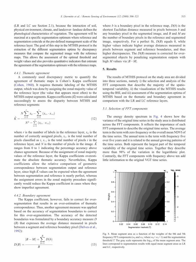
Fig. 8. Mean segment area as a function of the weights of the 0th and 5thfrequency FFTcomponents (w0 and w5; where w0+w5=1) and the segmentationthreshold T. The gray scale represents the log10 of the mean segment area. Thelines correspond to segmentation results with equal mean segment areas as LRand LC, respectively.


Fig. 5 presents the spatial variability ("k) of 0th to 10thfrequency FFT component that describe the largest part of thetemporal information in Fig. 4. It shows the spatial variability ofthe Fourier components by means of the mean Fk-distanceamong sample pixels separated by lag h and consequentlyreflects the spatial variability that is directly included in theMTHIS methodology, namely the amplitude of the differencevector. It confirms the relevance of the average and annual term,as the 0th and 5th frequency FFT components express thelargest part of the spatial variability for the MTHIS. These twoFFT components consequently were selected for further use inMTHIS, as they clearly correspond to relevant periodic signalsin the original NDVI time series. The other terms reflect asignificantly smaller amount of the NDVI time series spatio-temporal variability. Comparison of Figs. 4 and 5 also revealsthe distinction in spatio-temporal variability between theaverage and annual term. The level of spatial variability of the

annual term ("5) is approximately 60% of the level of spatialvariability of the average term ("0) (Fig. 5).

The peak of the annual term, on the other hand, explainsconsiderably less of the variance of the original time series(95% vs. 3%) in the logarithmic plot of the energy densityspectrum (Fig. 4). This means that the annual term containsmore spatial variation relative to the average term, since theannual term shows a variation over space that is 40% lower,whereas overall variation is considerably lower. This alsoindicates that higher spatial variation should be apparent, whichimplies more localized variability, less spatial correlation, andfiner spatial patterns, resulting in more speckled images.

The color scale in Fig. 6a–b displays the amplitude of theaverage (A0) and annual term (A5), respectively. Comparison ofboth figures reveals the characteristics of both FFT components.The average term shows high overall variability ranging from 0to 0.86 with coarse-smooth spatial patterns. Red colors indicate

Fig. 10. Boundary accuracy measure D(B) as a function of the weights of the 0thand 5th frequency FFT components (w0 and w5; where w0+w5=1) and thesegmentation threshold T. The lines correspond to segmentation results withequal mean segment areas as LR and LC, respectively: a) D(B) with LR asreference layer; b) D(B) with LC as reference layer and zoomed in on T"0.05.The X represents the segmentation optimum for each reference layer.

Fig. 9. Kappa coefficient as a function of the weights of the 0th and 5thfrequency FFT components (w0 and w5; where w0+w5=1) and the segmentationthreshold T. The gray scale represents Kappa coefficient of Eq. (12). The linescorrespond to segmentation results with equal mean segment areas as LR andLC, respectively: a) D(B) with LR as reference layer; b) D(B) with LC asreference layer.


high five year mean NDVI values related to a high vegetationcover, whereas the blue regions reflect low vegetation cover.The forested areas in the northeastern part and in the easterncoastal areas can clearly be delineated in this context, whereasthe dry Karoo areas in the northwest also can be detected. Theamplitude of annual term, on the other hand, presents only athird of the overall variability (from 0 to 0.33), but contains finerlocalized spatial patterns, resulting in a more speckled image.The red tones in Fig. 6b are related to a pronounced annualsignal in the original time series, whereas the blue areas do notshow this clear annual variation. This explains why agriculturaland grassland regions in the southwestern and central-easternparts contain red colors. These areas vary annually from dry soilor cured grass to high live vegetation content. Contrarily, theforested areas show little annual variation, as they representregions with a high mean NDVI and little annual variation.

5.2. MTHIS visualization

Fig. 6a–b contains also the BSI output of two MTHIS runsbased on only the average term (w0=1 and w5=0) and annualterm (w0=0 and w5=1), respectively. The BSI boundaries areplotted in gray scale on top of the colored amplitude maps andreflect the relative presence of the boundary at different scalelevels. The darker BSI values are boundaries of coarse scalesegments that are detected at various threshold values T andindicate the presence of the boundary at several hierarchical

scale levels, while lighter values are indicators of boundariesonly occurring at small threshold values; non-boundary pixelsand BSI values below 0.2 are transparent. The BSI boundarieseffectively indicate how the study area is partitioned atdifferent hierarchical scale levels, since the segments with lowBSI values are subsets of the coarse regions with high BSIvalues.

Additionally, the BSI gives an indication of the quality of theMTHIS methodology, since it allows visual comparison withthe input FFT component images. This visual comparisonillustrates that boundaries of clearly visible objects (e.g.,forested areas in the northeast of Fig. 6a or the agriculturalareas in the southwest of Fig. 6b) were identified at variousscale levels, while more subtle differences were only detected atfiner scales. This can be clearly seen in the zoom windows ofFig. 6a–b. Another example is the distinction between summerand winter rainfall regions that is detected at all scale levels inFig. 7. This figure illustrates the phase instead of the amplitudeof the annual term. The colors express the phase on the annualterm and describe the time of occurrence of the annual peak inthe original NDVI temporal profile, while the gray scale showsthe BSI. The BSI illustrates how the difference between summerand winter rainfall is detected at all scale levels, while smallphase differences are only recognized at finer scale levels.

A closer view of the BSI images also reveals the influence ofthreshold and weight values on the segment size. Small valuesof T lead to small segments, whereas large T values result in

Fig. 11. MTHIS segmentation optimum in comparison with the LC map after assigning the zonal majority value of the LC map. The colors represent the original LCmap, whereas the boundaries reflect the segmentation optimum after zonal majority assignment. The values for this MTHIS output are D(B)=1.10 and Kˆ=0.88 forw0=0.6, w5=0.4, and T=0.01.


large objects. The combination of weights and spatial variabilityof the FFT components likewise will influence the segment sizeas it will determine the intra-region similarity, S, before reachingthreshold T. This is confirmed in Fig. 8 where the mean segmentarea is plotted as a function of the weights wk and segmentationthreshold T. It shows that the higher overall spatial variability ofthe average term resulted in smaller segments for the same Tvalue. A logarithmic scale is used, since an exponential area sizecan be expected for increasing T values as each merge in theMTHIS approximately doubles the segment size.

5.3. Assessment of segmentation optimum

The agreement of the MTHIS output relative to the referencelayers is presented in Fig. 9 based on thematic accuracy valuesK̂. The Kappa coefficients decrease for increasing thresholdvalues T. Very high Kappa coefficients, however, are associatedwith severely over-segmented results as can be seen aftercomparison with Fig. 8. Very low values, on the other hand,correspond to under-segmentation. A correct interpretation of K̂or the extraction of optimal T and wk values is only reasonablewhen there is no over-or under-segmentation. This can beachieved when the segment size of segmentation output andreference has similar magnitudes as indicated by the lines inFig. 9. From these lines, it appears that only the thematiclabeling for LC resulted in K̂ values above 0.7, whereas lowerKappa coefficients were obtained for the LR labeling.

Fig. 10a–b presents the boundary accuracy measure D(B)from Eq. (13) that was corrected for over-segmentation. Alogarithmic scale is also used here, since D(B) values are alsorelated to exponential area size. All subplots display asegmentation optimum for each combination of weights, wherethe correspondence between segmentation output and referencereach a maximum in comparison with the T values. Analysis ofthe values of D(B) at these optima confirms the result of Fig. 9a,showing the best correspondence between segmentation opti-mum and LC. The MTHIS output resembled more accurately theLC map (D(B)=1.10 and K̂=0.88 for w0=0.6, w5=0.4, andT=0.01) than the LR map (D(B)=3.47 and K̂=0.52 for w0=0.9,w5=0.1, and T=0.03). This also illustrates the importance of thecombination of the average (w0=0.6) and annual (w5=0.4)temporal information for a correct landcover–landuse mapping,while the influence of the annual term is less (w5=0.1) foroptimal LR delineation. Fig. 11 shows the borders of the MTHISsegmentation optimum in comparison with the LC map afterassigning the zonal majority value of the LC map, whereas thecolor scale represents the original LC map. It can be seen that theoutput closely resembles the original LC map, where smallregions differences occur for the small regions of in the LC mapdue to the zonal majority procedure.

6. Discussion

6.1. MTHIS methodology

Although the MTHIS was developed for image time series, itprovides a hierarchical image segmentation methodology that

can be applied to any image series, e.g., image hyperspectralseries. The proposed MTHIS methodology differs however intwo points from the classic hierarchical segmentations. Firstly,the segmentation is not based on original data values, but on thedecomposition of these values in FFT components. Secondly,the incorporation of the Fk-distance criterion allows effectivelyto cluster based on the similarity of the FFTcomponents, since itcombines both parameters that represent the FFT component, Ak

and !k, respectively, into one dissimilarity measure. On thecontrary, classical hierarchical segmentations such as eCogni-tion (Baatz & Schäpe, 2000) or RHSEG (Tilton & Lawrence,2000) consider each input parameter separately. These classicmethodologies consequently do not allow to measure the simi-larity of the FFT components of the same frequency, since thedifference between FFT components cannot be calculated bysubtracting amplitude and phase separately (Smith, 1999).

The main advantage of the methodology is the use of FFTcomponents, which enables the distinction of signals with aspecific period. This is particularly amendable for detectingperiodic patterns in time series of satellite data, such as daily ormonthly NDVI time series of land surfaces that contain strongsystematic periodic patterns related to vegetation features andnonsystematic high frequent image noise. Hence, informationrelated to temporal vegetation characteristics can be separatedfrom noise originating from atmospheric and viewing angleeffects, cloud contamination, and other types of high frequencyfactors. A similar effect could be possibly achieved by applyingclassical hierarchical image segmentation techniques onPrincipal Component Analysis (PCA) components related tovegetation growth. PCA decomposition, however, does notallow the separation of different frequencies, since it iscompletely data dependent. It is therefore impossible to assertthat a given component will reflect identical temporal propertiesbetween geographical areas, whereas FFT components alwaysexpress the same specific periodicity. Additionally, thisadvantage of the FFT allows the accentuation of informationwith a specific periodicity, e.g. periods related to El Niño/Southern Oscillation (ENSO) processes like detected byBarbosa et al. (2006) and Young (2005). The periods relatedto these processes can be specifically selected by assigning highweights and may provide authors such as Nagai et al. (2007) ameans to better assess the influence of these processes onecosystems without noise components. Alternatively, one couldargue that this selection of some periodic patterns implies aninformation loss and that it obscures other temporal character-istics. This represents a valid concern and, as a consequence, thesegmentation results should be interpreted as segments withsimilar temporal properties related to the selected periodiccomponents.

One of the limitations of the FFT, on the other hand, is theassumption that time series show a certain periodicity (i.e., thatvariations in the time series are repeated at an uniform time-step) and have infinite duration. Consequently, the MTHISmethodology excludes the identification of stochastic dynamicsor the distinction between subsequences of time series, whichcan be very important for the interpretation of ecosystemprocesses. For example, consider a five year time series of a


grassland pixel that is burnt in the second year, but completelyrecovered after the third year. The MTHIS methodology will notdetect this change as it assumes that variations in conditionoccur at the same rate in all years. The MTHIS will also notdetect landcover–landuse changes between years, since it isbased on an assessment of the complete time series and does notallow distinction between subsequent years. However, thesechanges can be derived in other strategies, e.g. by applyingMTHIS to time series of individual years and considering thedifferences in MTHIS output between subsequent years. Thedevelopment of an alternative methodology based on similar-ities in wavelet transforms could also serve as a solution, sincethe wavelet transform can be used to scale conventionalFourier components. Accordingly, it decomposes a signal interms of both time and frequency simultaneously (Daubechies,1990).

MTHIS application however does not only depend on theselected FFT components. The result of MTHIS will moreoverbe influenced by the random selection sequence of segmentsand by threshold values T in the hierarchical segmentationprocess. Together they determine an arbitrary element in thesegmentation sequence that will be reflected by the MTHISoutput. This arbitrary element can nevertheless be minimized bycorrectly assigning threshold values T. If MTHIS is initializedwith T=x, 2x,…, #, where x is infinitely small, the arbitrarysequence is removed, since the hierarchical stepwise segmen-tation algorithm of Beaulieu and Goldberg (1989) is obtained.This algorithm produces a segmentation with minimal error byallowing only the smallest merge at each segmentation run andthus guaranteeing that each segment is merged with its nearestneighbor. The major limiting factor of this algorithm isunfortunately the computing speed due to one merge per run.Therefore a balance between objectivity and speed has to beassessed by allowing multiple merges per segmentation run anda minimal arbitrariness.

T values have to be selected accordingly, so they minimizethe computing time and level of arbitrariness. Additionalchanges to the segmentation sequence of MTHIS, such as themultiple merges per pass approach as proposed by Woodcockand Harward (1992) could reduce the stochastic element evenmore. Future changes of the methodology should consequentlyfocus on the implementation of these improvements.

Although the Fk-distance provides effectively a measure toassess the similarity between FFT components, which isimpossible with the classical hierarchical segmentation meth-odologies, the use of the Fk-distance has also certain limitations.These limitations correspond to the limitations of the minimumdistance to mean classifier (Lillesand & Kiefer, 2000). Both areinsensitive to different degrees of variance. The use ofalternative dissimilarity measures, such as the standarddeviation of FFT components, causes nevertheless otherdifficulties, since this approach would consider both parametersof the FFT component separately. On the other hand,introduction of other similarity measures that evaluate boththe variance and covariance of these parameters, such asGaussian maximum likelihood measures, would increasecomputing time tremendously, since for every possible merge

covariance measures need to be calculated between all pixels inneighboring segments. Given the size of the images we aredealing with in this study, this approach required far too muchcomputing time. We therefore believe that the methodologypresented here will prove useful until more sophisticatedapproaches for assessing the similarity between FFT compo-nents become available.

Moreover, the MTHIS methodology provides an genericmethodology that can be adapted towards user requirements, forexample, in remote sensing applications where the piecewisehomogeneous scene model is violated. In this model it isassumed that segments comprising the landscape have both lowinternal variance and a common level of internal variance(Woodcock & Harward, 1992). Unfortunately, this assumptionis often inadequate for images over different landcover–landusetypes. This means that for an average threshold value T,neighboring pixels of landcover–landuse types with lowinternal variance will be grouped in few segments, whereasneighboring pixels of landcover–landuse types with highinternal variance will not merge. Although the MTHISmethodology is partly adapted to this problem by allowingonly one merge per segment per segmentation run, it is veryunlikely that all the segments defined by the MTHIS outputcorrespond to patches of the same level of the landscapehierarchy. To solve this, additional size constraints or measuresof internal local variance can be incorporated by the user in theMTHIS methodology. Woodcock and Harward (1992) forexample proposed the use of an additional texture channel thatcould also be used as additional measure in S.

6.2. MTHIS protocol

Application of the MTHIS protocol on five year VGT NDVItime series of South Africa illustrated the potential of themethodology. The average and annual terms were selected,since they represented the major spatio-temporal variability inthe study area. The importance of these two terms for vegetationdescription corroborates the work of Azzali and Menenti (2000)and Moody and Johnson (2001). These authors discussed theaverage and annual term to demonstrate the usefulness of FFTcomponents to describe vegetation phenological characteristics.They exploited the information of these terms and the sixthmonth FFT term to classify the vegetation of South Africa usinga per-pixel iso-cluster procedure that is insensitive to nonsys-tematic data noise in the higher-order components.

Moreover, the selection and identification of the relevantspatio-temporal FFT components revealed the distinction inspatio-temporal variability between both the average and annualterm. This distinction is critical to an understanding ofvegetation dynamics, because both terms relate to differentbiophysical processes. The average term is mainly related toclimate effects and reflects the changing amounts of vegetationcover related to rainfall per-pixel (Azzali & Menenti, 2000).The overall variability of the vegetation cover is large, rangingfrom almost no rainfall in the western desert, to high rainfallareas like the forest plantations in the east (Fig. 6a). Moody andJohnson (2001), on the other hand, showed that the annual term


is linked to localized effects such as structural landcover–landuse (e.g. difference between evergreen, deciduous andannual habit) with a higher relative spatial variability.

The visualization by means of the BSI allowed aninterpretation of the segmentation boundaries at different scalelevels. Additionally, the BSI provided an indication of thequality of the MTHIS methodology when BSI boundaries werecompared with the input FFT component images. Hence, BSIboundaries are essential from a user's perspective as they allowa first analysis of the segmentation hierarchy. In this paper, thehierarchical structure of the segments was not specificallystudied in detail, but it was established inherently, and can beincorporated in future research to analyze how the segmentschange from one scale level to another.

Comparison of the MTHIS output with the LR and LCreference maps confirmed moreover the expected agreement ata specific scale level between segmentation result and factorsthat describe the vegetation characteristics at this scale level.The Kappa and boundary accuracy measures also showed thatthis agreement was much higher for the LC map than for the LRmap. This partly can be attributed to the definition and theoriginal purpose of the reference maps. The LR map describesthe biological resources from a perspective of potential naturalvegetation as a functional combination of soil, physicalenvironment, and climate, rather than actual landcover–landuseinfluenced by man-made transformations (Low & Rebelo,1996). The LR maps are by definition very heterogeneous andbased on vegetation structure, ecological processes andoccurrence of important plant species and do not necessarilyprovide direct information about the dynamics of vegetationgreen cover and its foliar phenology. Consequently, it fails todescribe the actual vegetation and is more related to potentialvegetation resulting from climatological and biophysicalcharacteristics which are often obscured by man-made altera-tions. The Kappa and boundary accuracy measures for thelandcover–landuse map, on the other hand, confirmed theresults of Moody and Johnson (2001), who showed that FFTcomponents provide a concise and repeatable input forsummarizing baseline inter-annual variability of landcoverdynamics over broad regions and can be used as criteria fordifferentiating landcover types on the basis of temporalproperties. The MTHIS methodology, however, groups thetemporal properties at more scale levels, for which applicablereference maps were not readily available. It is debateable whatthese other scale levels represent, besides uniformity intemporal behavior, for vegetation mapping purposes. Never-theless, certain scale levels already provide useful information,such as the difference in summer and winter rainfall regions.The description of these and all other scale levels is an importanttheme that should provide focus for future research on thistopic. Future work should therefore concentrate on theconstruction of truly objective and external reference datawith detailed hierarchical and spatio-temporal characteristicsthat effectively allow the validation of the MTHIS output at allscale levels. The use for example of artificial data sets, whosehierarchical and temporal properties can be completelycontrolled, could provide a great help in this context.

7. Conclusion

A MTHIS methodology was proposed to integrate remotesensing time series in a hierarchical image segmentationapproach. MTHIS clusters adjoining pixels with similar temporalproperties into hierarchical segments at various scales. Therefore,the similarity of temporal behavior was defined as similarity ofFFTcomponents and an Fk-distance criterion was introduced thatemploys the Euclidian distance between FFT components of thesame frequency as similarity measure. This choice was based onthe duality between the frequency domain of the FFTcomponents and time domain of the NDVI time series. Theycontain exactly the same information, but in a different form. Theuse of FFT components and Fk-distance, however, allowed theelimination of components that represented little more than noisecontained in the original time series, resulting in an increasedcomputational efficiency of the segmentation methodology.

Application of the methodology in a specific MTHISprotocol for VGT NDVI time series demonstrated the conceptof MTHIS. The actual MTHIS was performed on the averageand annual FFT term, since these components contained themajority of the spatio-temporal variability in the NDVI timeseries. The selection of these components was assessed bymeans of the energy density spectrum and Fk-distance as afunction of lag distance. The results of the MTHIS implemen-tation were visualized by means of BSI overlays. Theseoverlays provided an indication of the quality of the MTHIS.Additionally, they confirmed the usefulness of MTHIS topartition the study area at different hierarchical scale levels.

Finally, the correspondence between MTHIS results andreference layers of vegetation characteristics at different scaleswas assessed to determine the specific segmentation optimumwhere both coincide at the pre-defined management scale of thereference layer. The comparison of these optima revealed a closerelationship between segmentation output and landcover–landusereference map. This relationship was less clear for the vegetationtype reference maps due to the reference map purpose and defi-nition. On the other hand, the accuracymeasures for the landcover–landuse map strengthened the findings of earlier studies with FFTcomponents that also successfully mapped landcover types basedon these components. The MTHIS methodology, however, addsmuch more information as its provides results at several scalelevels. The description and evaluation of these other scale levelsbased on various data with a wide range of reference layers ishowever crucial for future research.

Acknowledgements

This workwas performed in the framework of a research projecton satellite remote sensing of terrestrial ecosystem dynamics,funded by the Belgian Science Policy Office (GLOVEG-VG/00/01). I. Jonckheere is 2006 Laureate of the Belgian StichtingRoeping, and is currently a Postdoctoral fellow of the FWOFlanders. The SPOT VGT S10 data set was generated by theVlaamse Instelling voor Technologisch Onderzoek (VITO),whereas the National Land Cover Map of South Africa wassupplied by the Agricultural Research Council (ARC). The authors


would like to thank T. Harding and D. Rizopoulos for feedback onprocessing and statistical questions. We are indebted to the editorand referees for their detailed reviews that led to an improvedversion of the manuscript.

References

Andres, L., Salas, W. A., & Skole, D. (1994). Fourier analysis of multitemporalAVHRR data applied to a landcover classification. International Journal ofRemote Sensing, 15(5), 1115!1121.

Anyamba, A., & Eastman, J. R. (1996). Interannual variability of NDVI overAfrica and its relations to El Niño/Southern Oscillation. InternationalJournal of Remote Sensing, 17(13), 2533!2548.

Azzali, S., & Menenti, M. (2000). Mapping vegetation–soil–climate complexesin southern Africa using temporal Fourier analysis of NOAA-AVHRRNDVI data. International Journal of Remote Sensing, 21(5), 973!996.

Baatz, M., & Schäpe, A. (2000). Multiresolution segmentation: Anoptimization approach for high quality multi-scale image segmentation.In J. Strobl, & T. Blaschke (Eds.), Angewandte geographische informa-tionsverarbeitung, vol. xii. (pp. 12!23)Heidelberg: Wichmann-Verlag.

Barbosa, H., Huete, A., & Baethgen, W. (2006). A 20-year study of NDVIvariability over the Northeast Region of Brazil. Journal of Arid Environ-ments, 67, 288!307.

Beaulieu, J. M., & Goldberg, M. (1989). Hierarchy in picture segmentation: Astepwise optimization approach. IEEE Transactions on Pattern Analysisand Machine Intelligence, 11, 150!163.

Bruzzone, L., Smits, P. C., & Tilton, J. C. (2003). Foreword special issue ananalysis of multitemporal remote sensing images. IEEE Transactions onGeoscience and Remote Sensing, 41(10), 2419!2420.

Cohen, J. (1960). A coefficient of agreement for nominal scales. Educationaland Psychological Measurement, 20, 37!46.

Coppin, P., Jonckheere, I., Lambin, E., Nackaerts, K., & Muys, B. (2004).Digital change detection methods in ecosystem monitoring: A review. In-ternational Journal of Remote Sensing, 25, 1565!1596.

Daubechies, I. (1990). The wavelet transform, time-frequency localization andsignal analysis. IEEE Transactions on Information Theory, 36(5), 961!1005.

Delves, L. M., Wilkinson, R., Oliver, C. J., & White, R. G. (1992). Comparingthe performance of SAR image segmentation algorithms. InternationalJournal of Remote Sensing, 13(11), 2121!2149.

Eastman, J. R., & Fulk, M. (1993). Long sequence time series evaluation usingstandardized principal components. Photogrammetric Engineering andRemote Sensing, 59(8), 1307!1312.

Evans, J. P., & Geerken, R. (2006). Classifying rangeland vegetation type andcoverage using a Fourier component based similarity measure. RemoteSensing of Environment, 105, 1!8.

Fan, J., Yau, D. K. Y., Elmagarmid, A. K., & Aref, W. G. (2001). Automaticimage segmentation by integrating color-edge extraction and seeded regiongrowing. IEEE Transactions on Image Processing, 10, 1454!1466.

Garrigues, S., Allard, D., Baret, F., & Weiss, M. (2006). Quantifying spatialheterogeneity at the landscape scale using variogram models. RemoteSensing of Environment, 103, 81!96.

Gurgel, H. C., & Fereira, N. J. (2003). Annual and interannual variability ofNDVI in Brazil and its connections with climate. International Journal ofRemote Sensing, 24(18), 3595!3609.

Handcock, R. N., & Csillag, F. (2004). Spatio-temporal analysis using amultiscale hierarchical ecoregionalization. Photogrammetric Engineeringand Remote Sensing, 70, 101!110.

Hay, G. J., Blaschke, T., Marceau, D. J., & Bouchard, A. (2003). A comparisonof three image-objects for the multiscale analysis of landscape structure.ISPRS Journal of Photogrammetry and Remote Sensing, 57, 327!345.

Holben, B. (1986). Characterization of maximum value composites from temporalAVHRR data. International Journal of Remote Sensing, 7, 1417!1434.

Jakubauskas, M. E., Legates, D. R., & Kastens, J. H. (2001). Harmonic analysisof time series AVHRR NDVI data. Photogrammetric Engineering andRemote Sensing, 67(4), 461!470.

Jakubauskas, M. E., Legates, D. R., & Kastens, J. H. (2002). Crop identificationusing harmonic analysis of time series AVHRR NDVI data. Computers andElectronics in Agriculture, 37, 127!139.

James, G. (1994). Advanced Modern Engineering Mathematics (pp. 288!291).Wokingham, England: Addison-Wesley.

Jönsson, P., & Eklundh, L. (2004). TIMESAT— A program for analyzing time-series of satellite sensor data. Computers & Geosciences, 30, 833!845.

Juarez, R. I. N., & Liu, W. T. (2001). FFT analysis on NDVI annual cycle andclimatic regionality in Northeast Brazil. International Journal of Climatol-ogy, 21, 1803!1820.

Justice, C. O., Townshend, J. R. G., Holben, B. N., & Tucker, C. J. (1985).Analysis of the phenology of global vegetation using meteorological satellitedata. International Journal of Remote Sensing, 6(8), 1271!1318.

Lee, R., Yu, F., Price, K. P., Ellis, J., & Shi, P. (2002). Evaluating vegetationphenological patterns in Inner-Mongolia using NDVI time-series analysis.International Journal of Remote Sensing, 23(12), 2505!2512.

Lillesand, T. M., & Kiefer, R.W. (2000).Remote sensing and image interpretation(pp. 538!539). New-York: John Wiley & Sons.

Low, A. B., & Rebelo, A. G. (1996). Vegetation of South Africa, Lesotho, andSwaziland. Pretoria: Dept. Environmental Affairs and Tourism.

Lucieer, A., & Stein, A. (2002). Existential uncertainty of spatial objectssegmented from satellite sensor imagery. IEEE Transactions on Geoscienceand Remote Sensing, 40(11), 2518!2521.

Moody,A.,& Johnson,D.M. (2001). Land-surface phenologies fromAVHRRusingthe discrete Fourier transform. Remote Sensing of Environment, 75, 305!323.

Nagai, S., Ichii, K., & Morimoto, H. (2007). Interannual variations in vegetationactivities and climate variability caused by ENSO in tropical rainforests.International Journal of Remote Sensing, 28(6), 1285!1297.

Olsson, L., & Eklundh, L. (2001). Fourier series for analysis of temporalsequences of satellite sensor imagery. International Journal of RemoteSensing, 15(18), 3735!3741.

Rahman, H., & Dedieu, G. (1994). SMAC: A simplified method for theatmospheric correction of satellite measurements in the solar spectrum. In-ternational Journal of Remote Sensing, 15, 123!143.

Reed, B. C., Brown, J. F., Vanderzee, D., Loveland, T. S., Merchant, J. W., &Ohlen, D. O. (1994). Measuring phenological variability from satelliteimagery. Journal of Vegetation Science, 5, 703!714.

Running, S. W., Loveland, T. R., & Pierce, L. L. (1994). A vegetationclassification logic based on remote sensing for use in global biogeochem-ical models. Ambio, 23, 77!81.

Singleton, R. C. (1969). Algorithm for computing the mixed radix fast Fouriertransform. I.E.E.E. Transactions on Acoustics, Speech, and SignalProcessing, 17, 93!103.

Smith, S. W. (1999). The scientist and engineer's guide to digital signalprocessing (pp. 161!165). San Diego, CA: California Technical Publishing.

Stuckens, J., Coppin, P. R., & Bauer, M. E. (2000). Intergrating contextualinformation with per-pixel classifications for improved land coverclassifications. Remote Sensing of Environment, 71, 282!296.

Thompson, M. W. (1999). South African national landcover database project,data users manual: Final report (phases 1, 2, and 3). Client report ENV/P/C98136 Pretoria: CSIR.

Tilton, J. C., & Lawrence, W. T. (2000). Interactive analysis of hierarchicalimage segmentation. Proceedings of the IGARSS, 733!735.

Verbesselt, J., Jönsson, P., Lhermitte, S., van Aardt, J., & Coppin, P. (2006).Evaluating indices derived from satellite and climate data as fire riskindicators in savanna ecosystems. IEEE Transactions on Geoscience andRemote Sensing, 44(6), 1622!1632.

Woodcock, C., & Harward, V. J. (1992). Nested-hierarchical scene models andimage segmentation. International Journal of Remote Sensing, 13, 3167!3187.

Wu, J., & Loucks, O. L. (1995). From balance-of-nature to hierarchical patchdynamics: A paradigm shift in ecology. Quarterly Review of Biology, 70,439!466.

Young, S. S., & H.R. (2005). Changing patterns of global-scale vegetationphotosynthesis, 1982–1999. International Journal of Remote Sensing, 20(20), 4537!4563.


Hierarchical image segmentation based on similarity of NDVI ...

Documents