Hierarchical data structures and algorithms for computer graphics…hjs/pubs/SameCGA88.pdf · · 2006-12-15Hierarchical Data Structures and Algorithms for Computer Graphics Part

Data Structures 59

Hierarchical Data Structures and Algorithms for Computer Graphics

Part 11: Applications n

Hanan Samet University of Maryland

Robert E. Webber Rutgers University

.............. .......... ........... ........... p .... .......... .I

This is the second part of a two-part overview of the use of hierarchical data structures and algorithms in computer graphics. The focus of Part I was on fundamentals. Part I1 focuses on advanced applications. Emphasis is on the octree, and the applications are primarily display methods. Topics include use of the quadtree as a basis for hidden-surface algorithms, parallel and perspective projection methods to display a collection of objects represented by an octree, and the use of octrees to facilitate such image-rendering techniques as ray tracing and radiosity.

H ierarchical data structures such as the quadtree and octree are frequently used in applications in computer graphics. In Part I,' we concentrated on fun- damentaI properties and operations. In Part I1 we describe some more advanced applications in which they find use. Emphasis is on the octree and on display methods. More references and details on hierarchical data structures are available el~ewhere. ' .~

Our presentation is organized as follows: The first section below describes the use of the quadtree as the basis of hidden-surface algorithms. The remaining sections focus on the octree. A review of the execution of a num-

July 1988 0272-1716/88/0700-0059$01.U0 1988 IEEE 59

A Figure 1. The viewing pyramid associated with the black pixel (shown shaded) in the viewplane.

ber of basic operations using an octree, including its construction, is followed by a section on how to apply the parallel and perspective projection methods to display the collection of objects that are represented by an octree. Implicit in this task is the solution of the hidden-surface problem to resolve the interaction between the objects in the scene modeled by an octree. Then we discuss how octrees-by use of ray tracing and radiosity-can facilitate image rendering (i.e., the problem of calculating what light falls on the viewplane). We conclude with some general comments and a brief discussion of the use of hierarchical methods in hardware.

Ray tracing models light as particles moving in the scene. The octree speeds up the determination of the objects that are intersected by rays emanating from the viewpoint. In contrast, radiosity models light as energy and seeks to determine a point at which its distribution is at equilibrium, a process requiring the derivation of a large set of linear equations. Octrees can simplify the calculation of the coefficients of these equations. This is especially true if rendering is to be done with respect to more than one viewpoint. The efficient solution of these equations is aided by heuristics, one of which is the adaptive recursive decomposition of the scene’s surface analogous to that used in the algorithms of Warnock and Catmull, described in the section on displaying curved surfaces.

Quadtree hiddensurface algorithms Probably one of the most basic graphics operations is

the conversion of an internal model of a 3D scene into a 2D scene that lies on the viewplane. The purpose is to generate an image of the scene as it would appear from a given viewpoint and to display it on a 2D screen. This is known as the hidden-surface operation (also discussed

as the visible-subset problem in the section on object- space hierarchies in Part 1’). Although many mappings are abstractly possible between a 3D space and a 2D space, we are interested in a mapping that closely models geometric optics. Such mappings are called projections (see the section below on parallel and perspective projections for more details).

Conceptually, understanding the image generation process is easiest when we examine how the color of a single pixel of the viewplane is calculated. In our presentation, each pixel of the viewplane determines a pyramid formed by the set of all rays originating at the viewpoint and intersecting the viewplane within the boundary of the pixel (see Figure 1). We clip away the objects or their parts that are outside the viewing pyramid to reduce the number of objects that need to be considered. A color is assigned to each pixel which, in the simplest case, is the color of the object closest to the viewpoint, while also lying within the pixel’s pyramid.

The hidden-surface task5 can be conceptualized as a two-stage sorting process. The first stage sorts the surfaces into the different viewing pyramids (this is also known as a bucket sort). The second stage sorts the surfaces within a given viewing pyramid to determine the one closest to the viewpoint.

Four approaches to this task are relevant to our discussion. First, the 3D scene can be viewed as a sequence of overlays of 2D scenes, each of which is represented by a quadtree. Second, quadtrees can be used to model the viewplane even when the 3D scene consists of polygons of arbitrary orientation and placement in the 3D space. This solution, first proposed by Warnock6a7 and known as Warnock’s algorithm, is an image-space method. War- nock was actually interested in two versions of the hidden-surface task: the basic hidden-surface task and the hidden-line task. The hidden-line task is an adaptation of the hidden-surface task to a wireframe representation of a solid. In the process of developing a solution to the hidden-surface task, Warnock also made contribu- tions to light modeling’ beyond the scope of this survey. For expository purposes, we shall first describe the hidden-line operation in our discussion of Warnock’s method and then its adaptation to the hidden-surface operation.

The third approach that we present is Weiler and Atherton’s object-space hidden-surface a l g ~ r i t h m , ~ which is analogous to Warnock’s image-space algorithm. Weiler and Atherton also point out how image-space heuristics can be used to speed up object-space methods.

The three approaches above assume a vector data representation’ of a 3D scene. In the fourth approach, a quadtree can be built for the representation of the surface of a 3D object in parametric space.

2.5-dimensional hidden-surface elimination The technique of 2.5-dimensional hidden-surface

elimination was devised to handle the display of 3D

60 IEEE Computer Graphics & Applications

scenes represented by a forest of quadtrees. It arises most commonly in applications in cel-based animation. A cel is a piece of transparent plastic on which a figure has been painted. A scene can be created by overlaying cels (see Figure 2). A given view of the scene can be constructed by first laying down the cel representing the background. On top of the background, cels are placed that represent objects in the foreground. When each cel is represented by a quadtree, scenes can be constructed easily. The nodes that correspond to the objects painted on the cel are marked as opaque and the remaining nodes are marked as transparent.

Cel-based scene construction is a simplification of the hidden-surface task and is described in greater detail below. It is simpler than the general 3D task because each object is restricted to be in just one cel. Thus, in our domain, occlusion is acyclic, whereas it need not be so in an unrestricted 3D domain (see Figure 3). As a result, xire need not be concerned with problems resulting from situations such as object A occluding object B, object B occluding object C, and object C occluding object A.

Equivalent to a sequence of set-union operations, 2.5-dimensional hidden-surface elimination can be implemented in a manner analogous to quadtree intersection as described in the section on aligned quadtrees in Part I. ' In particular, starting with the quadtree corresponding to the backmost cel, while moving toward the front cel, perform successive overlays of the quadtrees of the cels encountered along the path.'" Hunter and Steiglitz" '' have shown that the total cost of this process is proportional to the sum of the number of nodes in all the quadtrees of the cels.

While the algorithm given above is an optimal worst- case method, it can be modified to yield a better average- case performance as follows. Process the cels from "front-to-back" and mark the blocks in the intermediate quadtree as transparent, thereby indicating that up to now nothing in the sequence of quadtree nodes corresponding to that location has been opaque. Also mark the internal nodes as opaque if all of their subtrees are opaque, although their subtrees need not be the same color (i.e., they need not correspond to the same object). Thus, when traversing the intermediate quadtree and the next cel, say C, if the intermediate quadtree has an internal node that is marked opaque, then nothing in the corresponding subtree of cel C, say T, is visible. Hence T need not be traversed. Furthermore, when the root of the intermediate quadtree is marked opaque, then no more cels need be visited.

Such actions have a potential of reducing the execution time of the 2.5-dimensional hidden-surface elimination task because subtrees corresponding to invisible regions need not be traversed. Of course, in a more flexible animation system, it is often desirable to overlay unaligned cels (i.e., unaligned quadtrees). This can be handled by using the techniques described in Part I for computing set operations on unaligned quadtrees.'

Figure 3. A 3D image where occlusion is not transitive.

Warnock's algorithm The use of the quadtree for modeling the viewplane

during the hidden-surface operation was first described by Warnock.' A variant of the quadtree is used to represent the parts of the scene currently believed to be visible. Thus it is an image-space method. The hidden-line operation is a derivative task of the hidden-surface operation. They differ in how the result of the visibility calculation is displayed.

We will now describe the hidden-line operation in greater detail. The viewplane's quadtree consists of polygons formed by the visible edges of the objects in the 3D scene. At most one edge is associated with each pixel. The edge, if any, that is associated with a pixel corresponds to the one that passes through the pixel's region as part of the border of a polygon that is not occluded by another polygon closer to the viewpoint. We will use the term color to distinguish between pixels that correspond to edges of a polygon and those that do not. In other words, a pixel is output [i.e., colored) if a visible edge

July 1988 61

passes through it. The quadtree is used in the display process to rapidly

select the pixels that need to be colored (these are the pixels through which visible edges of the scene pass). The quadtree is not built explicitly. Instead, the viewplane is recursively decomposed (traversed as if it were a quadtree) using an appropriate decomposition rule to yield a collection of disjoint square regions (i.e., leaf nodes). At each such region, drawing (i.e., coloring) commands for driving a display are output.

The quadtree decomposition rule used is analogous to the one devised by Hunter and Steiglitz.””* There are two types of nodes: boundary and empty. A pixel is represented by a boundary node if an edge of a polygon passes through it; otherwise it is represented by an empty node. Empty nodes are merged to yield larger nodes, while boundary nodes are not merged. This rule enables us to formulate the actions taken by Warnock’s algorithm in terms of the following leaf node types and corresponding actions:

At an empty leaf node, draw nothing since no lines pass through this region.

At a leaf node corresponding to a pixel, draw a point representing the border of the polygon that occludes the upper left-hand corner of the pixel (if no such polygon exists, then draw nothing).

At a leaf node corresponding to a collection of polygons, draw nothing since the existence of such a node means that one of the polygons occludes all the other polygons over this region.

At this point we should briefly explain the relationship between the hidden-surface and hidden-line tasks. The hidden-line task is closely identified with the use of vector displays and plotters. This caused Warnock to inves- tigate edge quadtreelike decompositions.’ On the other hand, the hidden-surface task is closely identified with the use of raster devices. Although our treatment of the hidden-line task assumes vector data, it results in the output of line-drawing commands at a raster/pixel level. By doing a bit more calculation, we can often recognize that a line will be visible without having to subdivide all the way down to the pixel level.

The algorithm given above for the hidden-line task can be modified to handle the hidden-surface task as well. The only modification needed is that empty nodes representing regions completely spanned by a polygon must now be colored with the color of that polygon, instead of being ignored (as happens in the hidden-line display process). Of course, the boundary nodes must be assigned one of the colors of their shared polygons.

One problem with building quadtree decompositions of data presented as arbitrary collections of polygons in 3D space is how to determine when there is no need for further subdivision. For example, this situation arises

when a node contains a collection of polygons where one polygon completely occludes the other polygons. This requires a sort of all the polygons in the node. Since occlusion generally is not transitive, sorting does not always work (recall Figure 3). If sorting fails because of nontransitivity or because the nearest polygon does not occlude the entire region, then further subdivision is needed to determine what is visible in the region corresponding to the node.

Note that we have been assuming that the closest polygon’s color was the most appropriate color for a pixel. Clearly, however, a pixel could contain small features that this approach would represent falsely. This general problem is referred to as aliasingT3-attempts to resolve it are referred to as antialiasing. Warnock handled the situation of a pixel that contained complicated features by pretending that the viewing pyramid for the pixel was a single ray passing through the pixel’s upper left-hand corner. If this produces an approximation of the image that is too rough for a particular application, then classical antialiasing techniquesT3 (such as computing a weighted average of the visible intensities within a pixel) can be applied without altering the basic algorithm.

Weiler-Atherton’s algorithm Warnock’s algorithm is an image-space hidden-surface

algorithm. Weiler and Athertong developed an analogous object-space hidden-surface algorithm. The object space consists of a collection of polygons. Note that Weiler and Atherton use image-space heuristics to speed up their object-space algorithm. Their object-space algorithm has the following structure:

1.

2.

3.

4.

5.

6.

Order all the polygons by their smallest z value (where the viewer is located at a z value of minus infinity).

Find the closest polygon, say P, to the viewer.

Form two collections of polygons. The first collection contains those polygons whose projection overlaps (partially or totally) the projection of P on the viewplane (which we will call the inner set). The second collection contains those polygons whose projection is not entirely covered by the projection of P (which we will call the outer set). Where a polygon is in both the inner and outer sets, clipping that polygon against P and storing the resulting polygons in the appropriate sets is often convenient.

Remove all polygons from the inner set that do not occlude part of P.

If no polygons occlude P (i.e., the inner set is empty), then the hidden-surface task has now been solved for P. Proceed to solve the hidden-surface task for the outer set.

If there exist polygons that occlude P (i.e., the inner set is nonempty), then recursively go to step 2 and


choose a “nearest” polygon from the occluding polygons in the inner set of P. Upon return, process the outer set of P.

To reduce the number of polygons that have to be compared in step 4, Weiler and Atherton propose two preprocessing methods relevant to our study. The first method recursively subdivides the image space (in the x and y directions) until the number of polygons in a given region, say R, drops below a specified threshold. Within region R, the basic algorithm described above is used. Note that at step 4, only the polygons in region R need to be considered.

The second method is based on the observation that besides preprocessing by subdividing in the x and y directions, subdividing in the z direction might also be useful. In particular, after subdividing in the z direction, they propose to solve the hidden-surface task for the backmost volume elements first, and then to use this solution as part of the polygon list for the volume elements in the front. This “back-to-front” approach is also discussed above in the context of 2.5-dimensional hidden-surface elimination. The last heuristic could be viewed as an octree method (see the section on parallel and perspective projections for more details).

Displaying curved surfaces In this article, vector data is usually viewed as consist-

ing of straight line segments and polygons. However, the quadtree paradigm also has proved useful to researchers interested in the manipulation of curved features such as surfaces. Curved surfaces are often represented by a collection of parametric bicubic surface patches.I4 Curved surface representations are important in computer graphics applications, because they are often more compact than polygonal representations. They also enable the stipulation of continuity in the derivative of piecewise surface representations. This is important for ray-tracing calculations (see the section on ray tracing below).

One early approach to displaying such surfaces was developed by Catmull.” The idea is to decompose the patch into subpatches recursively until the subpatches that are generated are so small that they span only the center of one pixel (or can be shown to lie outside the display region). The test for how many pixel centers are spanned by the patch (or whether or not the patch lies outside the display area) is based on the approximation of the patch by a polygon connecting the patch’s corners. In our examples, patches are denoted by solid lines, and their approximating polygons are denoted by broken lines.

As an example of the recursive decomposition of patches, consider Figure 4. Figure 4a shows a single patch with corners A, B, C, and D on a grid of pixel centers. We observe that quadrilateral ABCD, which

. . . . . c . . . . . . . . c . . . a b . . . . . . . .

C

e

. c . . . . . . i

Figure 4. Example of the use of recursive decomposition into patches for the display of curved surfaces (in Figures 4a and 4b patches are denoted by solid lines; their approximating polygons, by broken lines): (a) a single patch, (b) decomposition of Figure 4a into four patches, (c) decomposition of Figure 4b into sixteen patches, (d) final decomposition such that each patch contains no more than one pixel center, (e) the raster image corresponding to the decomposition.

approximates the patch ABCD, contains more than one pixel center. Thus the patch must be decomposed. Fig- ure 4b shows the decomposition of patch ABCD into quadrilateral patches AFIE, BGIF, CHIG, and DEIH. Since the quadrilateral approximations of each of these patches again span more than one pixel center, they must each be subdivided further, as shown in Figure 4c. This time there is not enough detail in the figure to show the difference between the patch and its quadrilateral approximation. Note that in Figure 4c the quadrilateral approximation for patch JFKN contains only one pixel center and hence will not need to be subdivided further. Also, the quadrilateral approximation of patch MNLG contains no pixel centers, and thus it too will not need to be subdivided further. However, the quadrilateral

Ju ly 1988 63

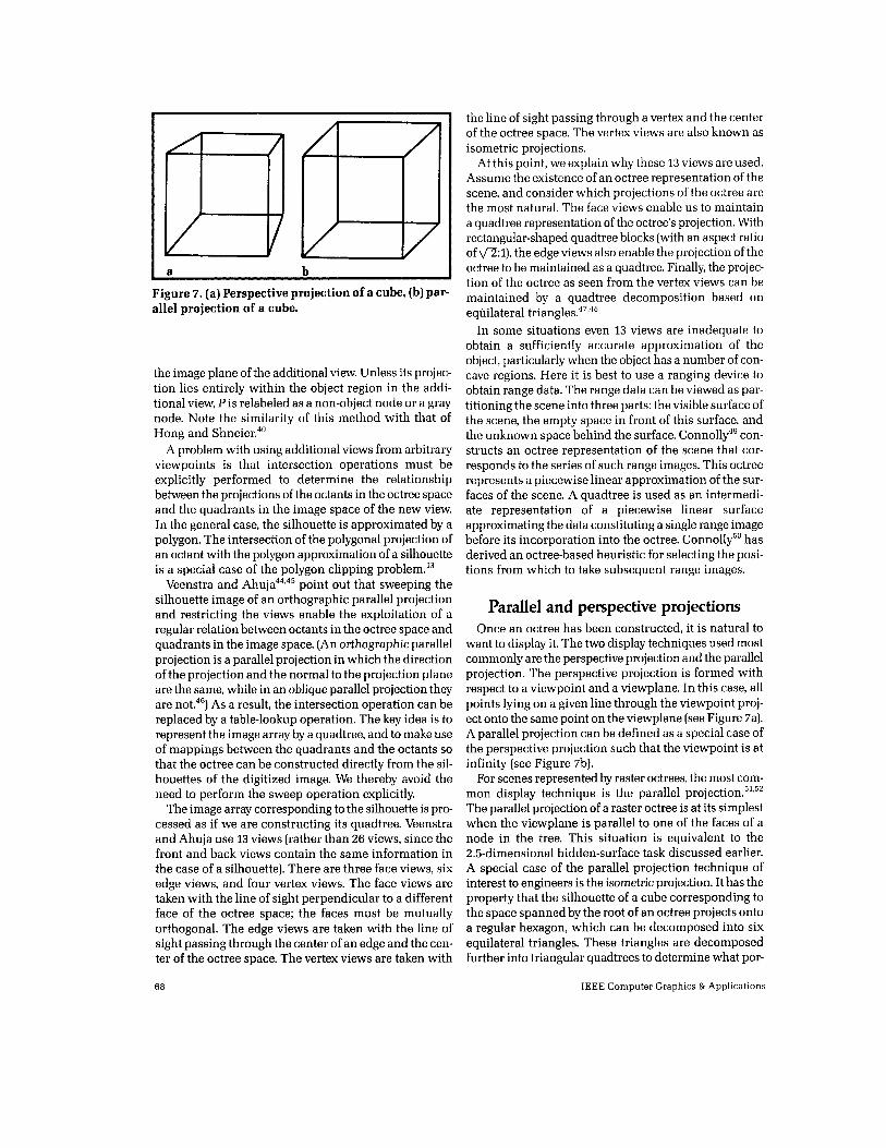
a b

C d

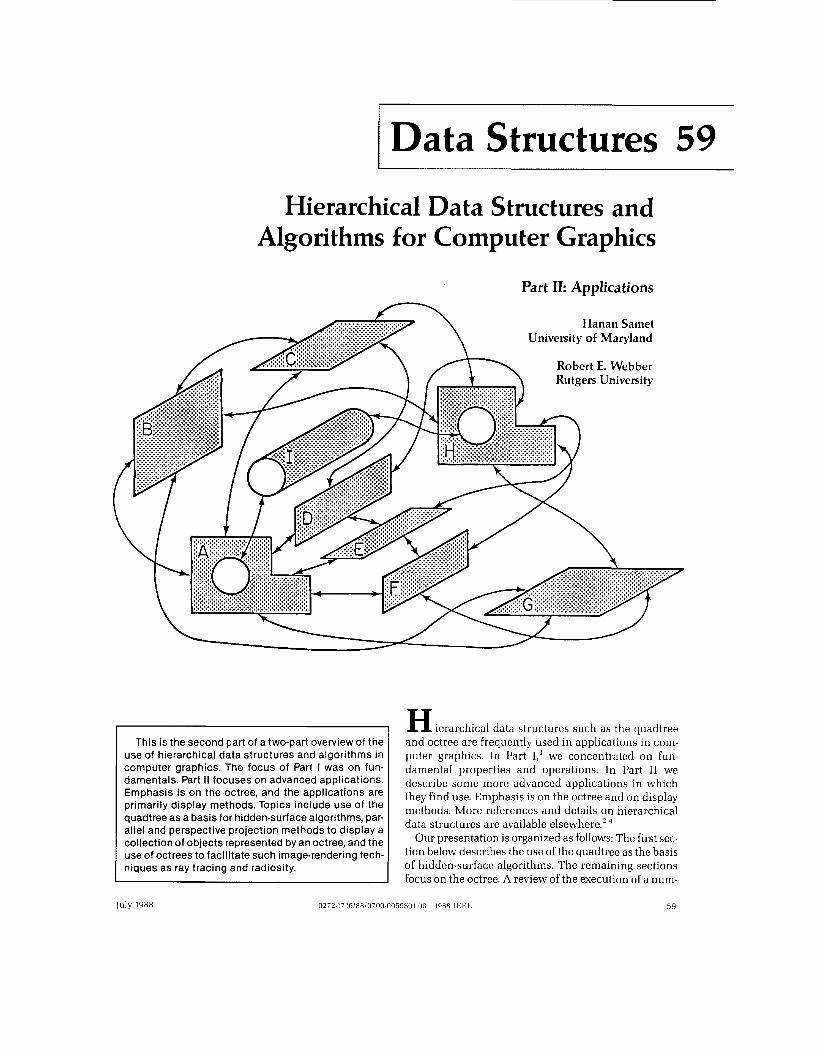
Figure 5. (a) The 3D view of the resulting subdivision of a surface using a quadtreelike decomposition rule in parameter space. Some of the cracks are shown shaded. (b) The quadtree of Figure 5a in parameter space. (c) The restricted quadtree corresponding to Figure 5b. (d) The triangulation of Figure 5c.

approximation of patch IJNM contains two pixel centers and therefore will need to be subdivided further. The final decomposition of the original patch is shown in Fig- ure 4d, and the raster image yielded by this decomposition is shown in Figure 4e.

As was observed by Catmull, the recursive decomposition approach to approximating the location of a patch can be generalized and thereby applied to other patch representations. Patch representations based on charac- teristic polyhedrons (e.g., Bezier and B-spline patches) allow these test decisions to be based on an approximation of each patch by the convex hull enclosing its control points (which is guaranteed to enclose the entire p a t ~ h ) . ' ~ This yields a more accurate result than Cat- mull's approximation, which is based only on four corners of a patch.

As with Warnock's algorithm, Catmull's algorithm is oriented toward the generation of display commands. Thus it does not explicitly generate the quadtree structure, although its processing follows the quadtree decomposition paradigm in the parametric space. Since the patches exist in 3D space, more than one patch can span the same pixel center. Thus the Catmull algorithm makes use of a z-buffer to keep track of the intensity/color of the

patch that has most recently been found to be closest to the viewpoint. Basically, a z-buffer is a 2D array that represents the displayed image. Each entry of the array contains a color and a depth. Initially, each pixel in the displayed image is black and at an infinite depth. When- ever a new color is to be assigned to a pixel, the depth of the location to which the pixel corresponds is checked. If it is greater than the current depth in the z-buffer, then the assignment is ignored; otherwise, the color and depth values in the z-buffer are updated. Although tra- ditionally the z-buffer has aliasing problems (i.e., it produces jagged borders between neighboring regions), these can be mitigated with the rgb-a-z approach.'6

Warnock's algorithm requires that the scene be completely specified at the time the algorithm is initiated. In contrast, the z-buffer enables elements of the scene to be processed in an arbitrary order. This permits elements to be added to the scene without having to reprocess elements of the scene that have been previously processed. In other words, at any time during its processing, the z- buffer represents what would be displayed if there were no further elements in the scene.

The z-buffer is represented explicitly as a 2D array. Such an array could be represented by a quadtree. This quadtree z-buffer representation might prove useful for generating line representations of the borders between surfaces, but not for generating shaded surfaces.17 Note that raster quadtrees are seldom efficient for representing scenes including shaded surfaces, since each pixel location on a shaded surface will have a slightly different color. However, if only the borders of the surfaces are represented, then the interior portions of the surfaces can be efficiently merged.

Catmull's display algorithm has been adapted to handle a constructive solid geometry" representation of objects (i.e., objects composed as Boolean combinations of primitive objects) for the case where the initial primitives are solids bordered by bicubic surface^.'^ Instead of subdividing down to the pixel level everywhere, the subdivision is performed only until it has generated subpatches that are mutually disjoint. Two subpatches can be viewed as disjoint when the interiors of the convex hulls of their respective control points are disjoint. While this approach helps to determine the actual intersection between two subpatches, it does not address the problem of choosing which patches should be compared to determine the possible existence of an intersection. A vector octree approach to this problem'' is mentioned in the section on vector octrees in Part I.'

While quadtrees are a natural way to organize the parametric representation of bicubic patches defined by four corner points plus auxiliary information (e.g., tangents and twist vectors in the case of B-~plines'~), the resulting set of quadrilaterals may be difficult to display. For example, it is difficult to ensure that the resulting four corners of the patches will actually be coplanar. Further- more, when one patch is subdivided further than its


neighbor, it is almost always the case that the patches will be misaligned (i.e., cracks will arise, as shown in Figure 5a).

The coplanarity problem can be resolved by triangulat- ing the quadrilaterals determined by the corner values of the leaf nodes. One way to regain alignment is to adjust the vertices of adjacent blocks of unequal size so that the vertex of the smaller block is on the edge between the vertices of its adjacent block of larger size. This method is used by Tamminen and Jansen." For example, the vertex at the NW corner of the SW son of the NE quadrant in Figure 5a would be replaced by the midpoint of the eastern boundary of the NW son. The adjacent block can be determined using quadtree neighbor-finding techniques as discussed in Part I. ' Tamminen and Jansen perform the adjustment process by traversing the quadtree of the patch, using an active border data structure."

The alignment problem can also be overcome by using a nonstandard decomposition rule. Von Herzen and Barrz3 propose a modification of the quadtree data structure, which they term a restricted quadtree. Given an arbitrary quadtree decomposition rule, to form a restricted quadtree, nodes that have a neighbor whose level in the tree is more than one level deeper are subdivided further until the condition holds. (This method of subdivision is also used in finite element analysis as part of a technique called h-refinementz4 to adaptively refine a mesh that has already been analyzed, as well as to achieve element compatibility.) In contrast to the more traditional representation shown in Figure 5b, the result is the quadtreelike decomposition shown in Figure 5c. Note that the SE quadrant of Figure 5b had to be decomposed once. A combined solution to these two problems triangulates the quadtree leaves of Figure 5c in the manner shown in Figure 5d. The rule is that every square is decomposed into no less than four and no more than eight triangles. Generally, for each block there are two triangles per side unless the side is shared by a larger block, in which case only one triangle is formed. Observe that there are no cracks.

Algorithms using octrees The algorithms for performing basic computer

graphics operations such as translation, rotation, scal- ing, and clipping on both raster and vector octrees are direct extensions of the algorithms presented in Part I for quadtrees.' The techniques used in performing some of these operations (e.g., preorder traversal, rec- tilinear unaligned traversal, general unaligned traversal, bottom-up neighbor finding, and top-down neighbor passing) can all be extended to deal with octrees once some additional bookkeeping information is maintained.

With the sheer amount of data that must be examined, constructing a raster octree from a 3D array representation of an image is quite costly. Because of the large

number of primitive elements that must be inspected, the conventional raster-scanning approach used to build quadtrees spends much time detecting the mergibility of nodes. The time and cost can be reduced, in part, by using the predictive techniques discussed in the section on constructing quadtrees in Part I.'~2".2h The method uses an auxiliary array whose storage requirements are as large as a cross section of the image, which may render the algorithm impractical. However, since this array is often quite sparse, the problem can be overcome by representing it with a linked list of blocks in a manner similar to one used for connected component labeling for images of arbitrary dimension." Alternatively, we can initially represent the data by using one of the more compact 3D representations, such as the boundary model or the CSG tree."

The boundary model represents a 3D object by its faces. The winged-edge representation mentioned in the beginning of Part when applied to polyhedrons, is one such representation. To create a boundary model, we must first decompose the surface of the object into a collection of faces. The result is a graph whose edges correspond to the interconnections between the faces of the object. For example, the object in Figure 6a can be decomposed into the set of faces and interconnections shown in Figure 6b.

Variations in the boundary model arise from the use of different methods for representing individual faces (which could be either polygons or curved surfaces), and different approaches to specifying the interconnection between adjacent faces. For example, we can view faces as meeting at either their borders or corners. Thus, instead of a graph where the vertices represent faces and the edges represent their interconnection, we also have boundary models where the vertices of the graph represent borders of a face or even the corners of a face. A method for building a raster octree from a boundary model by the use of connectivity labeling has been described elsewhere." Kunii, Satoh, and Yamaguchi address the opposite task of generating a valid boundary model from a raster octree.2g A related task is the output of a line drawing of an object represented by a raster octree."

Constructive solid geometry (CSG) methods represent rigid solids by decomposing them into primitive objects that are subsequently combined using variants of Boolean set operations such as union, intersection, and set-difference, and possibly geometric transformations (e.g., translation and rotation). These primitives are often in the form of such basic solids as cubes, parallelepipeds, cylinders, and spheres. A more fundamental primitive is a half-space whose border can be either linear or non- linear. For example, a linear half-space in three dimen- sions is given by the following inequality:

a . x + b . y + c . z r d

July 1988 65

a

U

/

C

Figure 6. (a) A 3D object, (b) its boundary model, and (c) its CSG tree.

CSG methods are usually implemented by a CSG tree-a binary tree in which internal nodes correspond to geometric transformations and Boolean set operations, while leaves correspond to the primitive objects

(e.g., half-spaces). For example, the object in Figure 6a can be decomposed into three primitive solids whose CSG tree is shown in Figure 6c. A bintree representation of a raster octree can be built from a CSG tree.31*32 These


techniques are useful for conversion as well as display.33,34

In some applications, a problem even more fundamental than building the octree is acquiring the initial boundary data to form the boundary of the object being represented. One approach is to use a 3D pointing device to create a collection of samples from the surface of the object. Once the point data are collected, a reasonable surface must be interpolated to join them.

Interpolation can be achieved by triangulation. A surface triangulation in 3D space is a connected set of disjoint triangles that forms a surface whose vertices are points in the original data set. There are many triangulation methods currently in use, both in 2D spaces35 and 3D spaces.36 They differ in how they determine which points are to be joined. For example, often we want to form compact triangles instead of long narrow ones. However, the problems of minimizing total edge length or maximizing the minimum angle pose difficult combinatorial problems. Posdamer" has suggested use of the ordering imposed by an octree on a set of points as the basis for determining which points should be connected to form the triangles.

Posdamer's algorithm uses an octree whose leaf criterion is that no leaf can contain more than three points. The initial set of triangles is formed by connecting the points in the leaves that contain exactly three points. Whenever a leaf node contains exactly two points, these points are connected to form a line segment associated with the leaf node. This is the starting point for a bottom-up triangulation of the points by merging disjoint triangulations to form larger triangulations. The isolated points (i.e., leaf nodes that contain just one point) and isolated line segments are viewed as degenerate triangulations. The triangulation associated with a gray node is the result of merging the triangulations associated with each of its sons. By merging or joining two triangulations, we mean that a sufficient number of line segments are drawn between vertices of the two triangulations so that we get a new triangulation containing the original two triangulations as subtriangulations.

When merging the triangulations of the eight sibling octants, we can use a number of heuristics to choose which triangulations are joined first. The order in which we choose the pair of triangulations to be joined is determined, in part, by the following factors. First and fore- most, merging triangulations in siblings whose corresponding octree blocks have a common face is pre- ferred. If this is impossible, then triangulations in nodes that have a common edge are merged. Again, if this is not feasible, then triangulations in nodes that have a common vertex are merged. For each preference, the triangulations that are closest according to some distance measure are merged first.

There are many other methods of building an octree for an object. The simplest is to take quadtrees of cross- sectional images of the object and merge them in

sequence. This technique is used in medical applications in which the cross sections are obtained by computed tomography methods. Yau and Srihari"' discuss this technique in its full generality by showing how to construct a k-dimensional octreelike representation from multiple (k-1)-dimensional cross-sectional images. Their algorithm processes the cross sections in sequence. Each pair of consecutive cross sections is merged into a single cross section. This pairwise merging process is applied recursively until there is one cross section left for the entire image.

For example, assuming a k-dimensional image of side length 2", once the initial 2" cross sections have been merged, the resulting 2" ~ cross sections are merged into 2"-* cross sections. In general, when merging 2"' cross sections into z"'-' cross sections, only nongray nodes at levels rn to n are tested for merging. Thus a cross section at level rn corresponds to a stack of 2" -I1' volume elements of side length 2"' and is represented by a (k ~ 1)-dimensional quadtree whose nodes are at levels rn through n.

In most applications the volume of the available data is much smaller and thus a small number of 2D images are used to reconstruct an octree representation of a 3D object or a scene of 3D objects. In this case, projection images (termed silhouettes) are taken from different viewpoints. These silhouettes are subsequently swept along the viewing direction, thereby creating a bounding volume, represented by an octree, that serves as an approximation of the object. The octrees of the bounding volumes, corresponding to views from different directions, are intersected to yield successively finer approximations of the object.

Martin and A g g a r ~ a l ~ ~ use this method with volume segments that are parallelepipeds stored in a structure that is not an octree. Chien and Aggarwal 39 show how to use this method to construct an octree from the quadtrees of the three orthogonal views. Hong and Shneier"" point out that the task of intersecting the octree and the bounding volume can be made more efficient by first projecting the octree onto the image plane of the silhouette and then performing the intersection in the image plane (see also an article by Potmesil"). In the rest of this section we assume that the silhouettes result from parallel views, although perspective views have also been

Generally, three orthogonal views often are insuffi- cient to obtain an accurate approximation of the object, and thus more views are needed. Chien and A g g a r ~ a l ~ ~ overcome this problem by constructing what they term a generalized octree from three arbitrary views whose only requirement is that they are not coplanar. The generalized octree differs from the conventional raster octree in that each node represents a parallelepiped whose faces are parallel to the viewing planes. The approximation is refined by intersecting the projection of each object node, say P, in the generalized octree with

Ju ly 1988 67

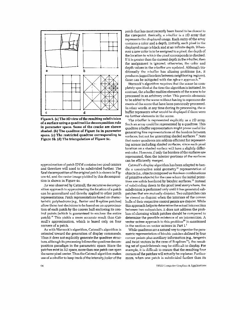
a b I Figure 7. (a) Perspective projection of a cube, (b) parallel projection of a cube.

the image plane of the additional view. Unless its projection lies entirely within the object region in the additional view, Pis relabeled as a non-object node or a gray node. Note the similarity of this method with that of Hong and S h n e i e ~ ~ '

A problem with using additional views from arbitrary viewpoints is that intersection operations must be explicitly performed to determine the relationship between the projections of the octants in the octree space and the quadrants in the image space of the new view. In the general case, the silhouette is approximated by a polygon. The intersection of the polygonal projection of an octant with the polygon approximation of a silhouette is a special case of the polygon clipping p r ~ b l e m . ' ~

point out that sweeping the silhouette image of an orthographic parallel projection and restricting the views enable the exploitation of a regular relation between octants in the octree space and quadrants in the image space. (An orthographic parallel projection is a parallel projection in which the direction of the projection and the normal to the projection plane are the same, while in an oblique parallel projection they are not.46) As a result, the intersection operation can be replaced by a table-lookup operation. The key idea is to represent the image array by a quadtree, and to make use of mappings between the quadrants and the octants so that the octree can be constructed directly from the silhouettes of the digitized image. We thereby avoid the need to perform the sweep operation explicitly.

The image array corresponding to the silhouette is processed as if we are constructing its quadtree. Veenstra and Ahuja use 13 views (rather than 26 views, since the front and back views contain the same information in the case of a silhouette). There are three face views, six edge views, and four vertex views. The face views are taken with the line of sight perpendicular to a different face of the octree space; the faces must be mutually orthogonal. The edge views are taken with the line of sight passing through the center of an edge and the center of the octree space. The vertex views are taken with

Veenstra and

the line of sight passing through a vertex and the center of the octree space. The vertex views are also known as isometric projections.

At this point, we explain why these 13 views are used. Assume the existence of an octree representation of the scene, and consider which projections of the octree are the most natural. The face views enable us to maintain a quadtree representation of the octree's projection. With rectangular-shaped quadtree blocks (with an aspect ratio of fl:l), the edge views also enable the projection of the octree to be maintained as a quadtree. Finally, the projection of the octree as seen from the vertex views can be maintained by a quadtree decomposition based on equilateral triangle^.^^'^'

In some situations even 13 views are inadequate to obtain a sufficiently accurate approximation of the object, particularly when the object has a number of con- cave regions. Here it is best to use a ranging device to obtain range data. The range data can be viewed as partitioning the scene into three parts: the visible surface of the scene, the empty space in front of this surface, and the unknown space behind the surface. Conn01ly~~ con- structs an octree representation of the scene that corresponds to the series of such range images. This octree represents a piecewise linear approximation of the surfaces of the scene. A quadtree is used as an intermediate representation of a piecewise linear surface approximating the data constituting a single range image before its incorporation into the octree. Connollyso has derived an octree-based heuristic for selecting the positions from which to take subsequent range images.

Parallel and perspective projections Once an octree has been constructed, it is natural to

want to display it. The two display techniques used most commonly are the perspective projection and the parallel projection. The perspective projection is formed with respect to a viewpoint and a viewplane. In this case, all points lying on a given line through the viewpoint proj- ect onto the same point on the viewplane (see Figure 7a). A parallel projection can be defined as a special case of the perspective projection such that the viewpoint is at infinity (see Figure 7b).

For scenes represented by raster octrees, the most common display technique is the parallel pr~jection.~'.~' The parallel projection of a raster octree is at its simplest when the viewplane is parallel to one of the faces of a node in the tree. This situation is equivalent to the 2.5-dimensional hidden-surface task discussed earlier. A special case of the parallel projection technique of interest to engineers is the isometric projection. It has the property that the silhouette of a cube corresponding to the space spanned by the root of an octree projects onto a regular hexagon, which can be decomposed into six equilateral triangles. These triangles are decomposed further into triangular quadtrees to determine what por-


tions of the leaf nodes are visible for display. A display algorithm based on this approach is reported by Yamaguchi et al.48

Implicit in the task of displaying an octree is the solution of the hidden-surface task for the interaction among the objects represented by the octree. Not surprisingly, since the octree imposes a spatial ordering on objects, the hidden-surface task for scenes represented by octrees can be solved more efficiently than the general hidden- surface task for arbitrary polygons.

Note that any opaque object in the four front octants of an octree will occlude any opaque object in the back four octants. This property holds recursively within each of the suboctants. Display of the scene is facilitated by constructing a display quadtree that corresponds to a partial 2D view of the scene. The display quadtree is updated as the nodes of the octree are traversed from back-to-front. Each opaque node, say P, encountered in this traversal “paints out” [i.e., overwrites) the previous view contained in a portion of the display quadtree that coincides with the projection of F! Of course, as indicated in the discussion of the 2.5-dimensional hidden-surface task, the nodes could also be processed from front-to- back, thereby allowing for the possibility of visiting fewer nodes.

Generalizations of the parallel projection to planes at arbitrary positions and orientations are described by M e a g h e ~ - ~ ~ and Y ~ u . ~ ~ Straightforward generalizations can also be made to compute perspective projections onto arbitrary planes. Another approach to the perspective projection task is first to transform the 3D scene into a new 3D scene whose parallel projection is the same as the corresponding perspective projection of the original scene. This approach has been used on CSG trees, which were then transformed into a bintree for display by one of the parallel projection methods discussed above.34

A drawback to displaying scenes represented by a raster octree is that there is little potential for using lighting models for the shading of the scene, since adjacent faces of octree nodes meet at 90” angles. One approach for overcoming this drawback is described by Doctor and Torborg.” They suggest that the amount for shading a face of a node can be calculated as a function of the number of the node’s transparent neighbors. Thus, since a node on the corner of an object surrounded by empty space has fewer transparent neighbors, it will be brighter than another node on the interior of a face of the object. An interesting highlighting effect results. In his octree machine,55 Meagher overcame this problem for octrees that are formed by conversion from other kinds of geometric models by storing surface normals in the voxels intersecting the surface of the object being viewed. This problem has been investigated more recently, too.56-58

Another solution to the problem of shading raster octree images is to use vector octrees to store the polygonal faces of the scene (from such faces, more accurate information about shading can be derived, as discussed

in the next section). An interesting alternative to the vector octree is the binary space-partitioning (BSP) tree,59 in which the planes that partition the scene are coplanar with some of the polygons in the scene. A hierarchical representation of the scene is formed by choosing a distinguished polygon from the scene. The scene is then decomposed into two half-spaces by the plane in which the distinguished polygon lies. Polygons intersected by this plane are split into two separate polygons. This partitioning process is recursively applied to these half- spaces. The choice of the partitioning polygons requires care. The BSP tree structure was originally proposed as a preprocessing step for a hidden-surface algorithm, but has since been applied to other computer graphics tasks. 5‘3-62

Ray tracing Although the parallel and perspective projection dis-

play techniques are suitable for computer-aided design, realistic modeling of lighting effects generally requires using some variant of ray t r a ~ i n g . ’ ~ Ray tracing is an approximate simulation of how the light propagated through a scene lands on the image plane. This simulation is based on classical optical notions of refraction and diffuse and specular r e f l e ~ t i o n . ~ ~ Although the geometry of the reflection and refraction of “beams” of light from surfaces is straightforward, the formulation of equations to model the intensity of the light as it leaves these surfaces is a recent development. The quality of the displayed image is a function of the appropriateness of the model represented by these equations and the pre- cision with which the scene is represented.

The amount of time required to display a scene is heav- ily influenced by the cost of tracing the path of the light rays as they move backward from the viewer’s eye, through the pixels of the image plane, and out through the scene. For example, Whitted63 reports that as much as 95 percent of the total picture-generation time may be required to calculate points of intersection between light rays and objects in a complex scene. Thus the motivation for using the octree in ray tracing is to enable the calculation of more rays with greater accuracy.

Since light-modeling equations rely on the availability of accurate information about the location of the normal to the surface at the point of its intersection with the ray, vector octrees are generally more appropriate than raster octrees. This is especially true for vector octrees that can represent curved rather than planar surfaces using either curved patches” or curved primitive^.^^

Octrees have been used to speed up intersection calculations for ray t r a ~ i n g . ~ ~ . ~ ’ The basic speedup can be seen by examining the 22-sided polygon in Figure 8a. We use a quadtree instead of an octree to simplify the presentation. A naive ray-tracing algorithm would have to test the ray emanating from the viewpoint against each of these sides, sort the resulting intersections, calculate

July 1988 69

"\ / /

a

b

Figure 8. (a) Example polygon and (b) its corresponding quadtree with a ray shown to emanate from the viewpoint and reflect from the object.

the reflected ray, and finally test the reflected ray to see if it intersects any other portion of the polygon. Figure 8b shows that an algorithm based on a quadtree or an octree would perform the same calculation by visiting only six leaf nodes (nodes 1, 2, 14, 6, 3, and 4).

Ray tracing in an octree is a two-step process. First, we must determine the identity of the neighboring node to be visited next. Several techniques can be used. G l a ~ s n e r ~ ~ uses a simplification of the Cyrus-Beck clipping a l g ~ r i t h m . ' ~ ' ~ ~ Fujimoto, Tanaka, and Iwata66 discuss how a fast 2D line-drawing algorithm can be adapted to perform 3D ray tracing in an octree. This results in an algorithm that can determine the direction of the neighbor relative to the node whose neighbor is being sought, using just a few integer addition, subtrac- tion, and shift operations.

Second, we must locate the neighboring node. A reasonable approach is to use the neighbor-finding techniques discussed in Part I.' Jansen6' discusses both top- down and bottom-up neighbor-finding for ray tracing in an octree. G l a ~ s n e r ~ ~ represents the octree as a linear octree but stores the octree nodes in a hash table rather than a list7' or a B-tree.71372 Instead of using standard neighbor-finding techniques (either top-down or bottom- up] to move between the nodes that lie sequentially along a given ray, the identity of the neighboring node is determined by calculating a point that would lie in the neighbor and then searching the octree for that point. This approach has also been applied to the pointer-based representation of o c t r e e ~ . ~ ~ * ~ ~ An analogous approach uses the bintree representation of ~ c t r e e s . ~ ~

The advantage of using the octree in ray tracing is a reduction in the number of ray-object intersection tests. The key is to choose an appropriate octree decomposi-

tion rule and to decide on the maximum level of decomposition. When the cells of the octree decomposition are large, the number of tests is reduced, but the tests become more complex. On the other hand, when the cells are small, there are many tests but their complexity is reduced. In particular, there are many empty cells. Fujimoto, Tanaka, and Iwata66 suggest that the space be subdivided into a regular grid and have found situations where this is preferable to the decomposition induced by an octree. Generally these are scenes where the number of distinct objects is large in comparison with the level of decomposition.

Snyder and Barr74 suggest an approach similar in spirit to that of Fujimoto, Tanaka, and Iwata. They propose a general structure that forms a hierarchy of 3D arrays (grids] and linked lists. A scene is decomposed into a list of bounding objects in a somewhat ad hoc manner. These bounding objects are in turn decomposed into a grid of cells. Each of these cells can contain a list of objects. In many ways, this method merges object-space and image-space techniques. The method has been used for scenes as large as 400 billion triangles.

A different approach to ray tracing has been proposed by Arvo and Kirk.75 They observe that neighboring rays tend to intersect the same objects. This property moti- vates them to represent the rays as points in a five- dimensional space (called a ray space]. A ray is defined by the x, y, and z coordinate values of its origin, and the 8 and 4 parameters of its direction as it leaves the origin. An object is inserted into this five-dimensional ray space by marking all the points representing rays that would intersect the object before any others. The mechanics of this insertion process are presented by Arvo and Kirk.75 The five-dimensional ray-tracing process is represented by a five-dimensional hyperoctree. Once a scene is built, ray tracing consists of performing point location operations in the five-dimensional space.

Nevertheless, the octree approach to ray tracing does seem promising. For example, G l a ~ s n e r ~ ~ reports that tracing 597,245 rays in a scene of 1,536 objects required 42 hours and 12 minutes using nonoctree ray-tracing techniques, while only 2 hours and 57 minutes were required using octrees. Another scene estimated to require 141 hours using nonoctree methods was analyzed in 5 hours and 5 minutes using octrees.

Radiosity While for many years ray tracing was the dominant

approach to the realistic rendering of images, newer and different techniques have recently emerged. One such method is the radiosity approach.76 Instead of modeling light as particles bouncing around in a scene (as is done in ray tracing], the radiosity approach models light as energy whose distribution tends toward a stable equilibrium. In other words, the radiosity approach treats light as if it were heat: Light sources behave as


sources of heat, and surfaces that reflect light behave as surfaces that reflect heat. Below we use the terms reflect, radiate, and emit interchangeably to denote the light leav- ing a patch where a patch is a portion of a surface of an object in the scene. Although energy in the form of light and heat is normally viewed as a continuous flow, the radiosity method uses a discrete simulation of the flow so that an approximate rendering can be computed. In this section we give only a brief general description of the method, and point out how and where hierarchical data structures can be used to improve its performance.

A scene is viewed as a collection of patches where the light emitted by the surface of a given patch, say Q, is either constant (e.g., for a light source) or is a linear com- bination of the light falling on Q from all the other patches. The simplifying assumption is made that the surfaces are Lambertian diffuse reflectors and light is reflected uniformly from the surface in all directions. This restriction can be lifted77 at the expense of greatly increasing the size of the problem. Of course, many patches do not contribute light to a particular patch, because they are occluded by closer patches. In essence, radiosity converts the image-rendering problem to one of solving a set of simultaneous linear equations. Each equation represents a portion of the discrete simulation of the light flow, that is, the portion of the light from the rest of the scene eventually reflected by the patch. Fur- thermore, the equation for patch Q depends on which patches are visible from Q.

The process of deriving the equations (i.e., determining the values of their coefficients) that describe the interactions among the patches was the computational bottleneck in the initial presentation of r a d i o ~ i t y . ~ ~ . ~ ' Deriving the equations is straightforward, although the exact m e c h a n i c ~ ~ ~ . ~ ' are beyond the scope of this survey. However, this process can be facilitated, in part, by observing that if two patches, say Q and R, are mutually invisible, then the coefficient of the term in the equation of Q (or R) associated with R (or Q) will be zero. The phys- ical interpretation of the concept of mutual invisibility is that light emitted by one of the patches cannot reach the other patch without first being reflected by yet a third patch. A geometric interpretation of this concept is that two patches, say Q and R, are mutually invisible only if there does not exist a pair of points pQ on Q and pR on R such that a straight line can be drawn between them without intersecting a third patch or passing through the interior of an object in the scene.

The determination of which terms in the equations have zero coefficients corresponds to a hidden-surface task among the patches. It must be solved separately for each patch. If we have M patches, then we must solve the hidden-surface interactions among each of the O(M2) combinations of patches. Worse, we need to solve these problems not just for a point on a patch, but for every point on the surface of the patch. Solving these problems could be made easier with a data structure such as the

octree to organize the elements of the scene, i.e., the 3D space occupied by the patches. This simplifies the determination of which patches are hidden with respect to the other patches, thereby yielding the zero coefficients.

Unfortunately, the application of radiosity to the rendering of more complicated scenes results in a marked increase in the number of equations necessary to model the scene. This has led to a shift of the computational bottleneck to the problem of solving the simultaneous equations. Nevertheless, recursive subdivision can still be used. Instead of recursively subdividing the 3D space occupied by the patches, Cohen et al.79 recursively subdivide the surfaces of the patches. This subdivision takes place in the parametric space of the patch in a manner similar to that in Catmull's algorithm (see the earlier section on displaying curved surfaces]. As with Catmull's algorithm, recursive subdivision of a patch (described below) does not actually require the construction of a quadtree. Instead, the data is simply aggregated in a manner equivalent to applying a particular leaf criterion to the organization of the surface of a scene.

Observe that to determine the rough flow of light through a scene, the number of patches needed to model the objects in the scene is considerably smaller than the number of patches needed to depict features of the scene caused by the actual flow of light through the scene (e.g., shadow boundaries). For example, suppose we are modeling a scene that corresponds to a room containing boxes. Here a rather coarse grid can be used to represent the surface of the room. However, the accurate representation of the shadows that the boxes cast on the walls will usually require a much finer grid. This is especially true for area light sources that cause varying shadow intensities (e.g., fluorescent tubes that cannot be modeled accurately as point light sources). Of course, the more patches used to represent a scene, the more expensive the solution required to solve the corresponding set of equations, since there are more equations with a con- comitant increase in terms. In particular, the number of equatioiis is proportional to the number of patches, which can potentially lead to a quadratic number of interpatch relations.

Note that we don't know how many patches will be needed to represent the results of the radiosity calculation until after it has been performed. Early work on radiosity simply guessed the maximum number. How- ever, with more complicated scenes, the guesses are overly pessimistic, thereby resulting in needlessly ineffi- cient algorithms. Recursive subdivision performed in an adaptive manner avoids the problem.

Cohen et al.79 propose a two-step algorithm to reduce the number of equations that must be solved simultane- ously. The basic approach is first to solve the set of simultaneous equations corresponding to the light flow among the patches used to model the surfaces of the scene. In the second step, patches whose intensity value computed by the first step differs greatly from that of their neigh-

July 1988 71

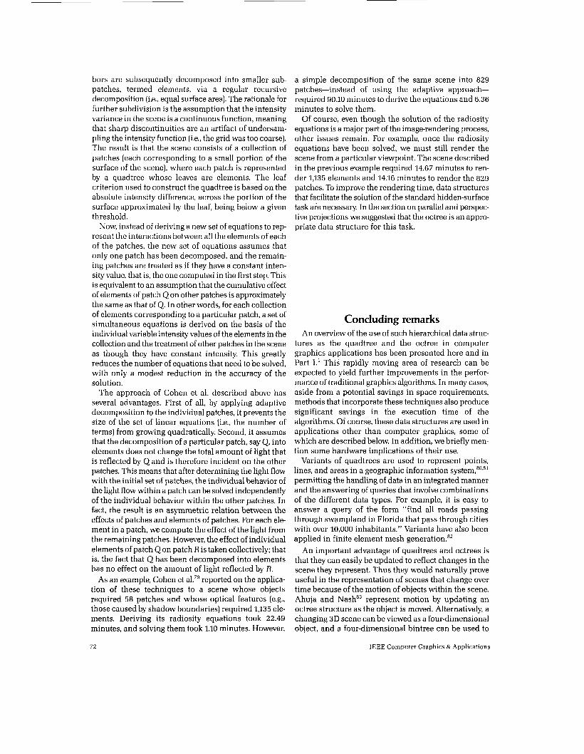
bors are subsequently decomposed into smaller subpatches, termed elements, via a regular recursive decomposition (i.e., equal surface area). The rationale for further subdivision is the assumption that the intensity variance in the scene is a continuous function, meaning that sharp discontinuities are an artifact of undersam- pling the intensity function (i.e., the grid was too coarse). The result is that the scene consists of a collection of patches [each corresponding to a small portion of the surface of the scene), where each patch is represented by a quadtree whose leaves are elements. The leaf criterion used to construct the quadtree is based on the absolute intensity difference, across the portion of the surface approximated by the leaf, being below a given threshold.

Now, instead of deriving a new set of equations to represent the interactions between all the elements of each of the patches, the new set of equations assumes that only one patch has been decomposed, and the remaining patches are treated as if they have a constant intensity value, that is, the one computed in the first step. This is equivalent to an assumption that the cumulative effect of elements of patch Q on other patches is approximately the same as that of Q. In other words, for each collection of elements corresponding to a particular patch, a set of simultaneous equations is derived on the basis of the individual variable intensity values of the elements in the collection and the treatment of other patches in the scene as though they have constant intensity. This greatly reduces the number of equations that need to be solved, with only a modest reduction in the accuracy of the solution.

The approach of Cohen et al. described above has several advantages. First of all, by applying adaptive decomposition to the individual patches, it prevents the size of the set of linear equations (i.e., the number of terms) from growing quadratically. Second, it assumes that the decomposition of a particular patch, say Q, into elements does not change the total amount of light that is reflected by Q and is therefore incident on the other patches. This means that after determining the light flow with the initial set of patches, the individual behavior of the light flow within a patch can be solved independently of the individual behavior within the other patches. In fact, the result is an asymmetric relation between the effects of patches and elements of patches. For each element in a patch, we compute the effect of the light from the remaining patches. However, the effect of individual elements of patch Q on patch R is taken collectively; that is, the fact that Q has been decomposed into elements has no effect on the amount of light reflected by R.

As an example, Cohen et al.79 reported on the application of these techniques to a scene whose objects required 58 patches and whose optical features (e.g., those caused by shadow boundaries) required 1,135 elements. Deriving its radiosity equations took 22.49 minutes, and solving them took 1.10 minutes. However,

a simple decomposition of the same scene into 829 patches-instead of using the adaptive approach- required 90.10 minutes to derive the equations and 6.36 minutes to solve them.

Of course, even though the solution of the radiosity equations is a major part of the image-rendering process, other issues remain. For example, once the radiosity equations have been solved, we must still render the scene from a particular viewpoint. The scene described in the previous example required 14.67 minutes to render 1,135 elements and 14.16 minutes to render the 829 patches. To improve the rendering time, data structures that facilitate the solution of the standard hidden-surface task are necessary. In the section on parallel and perspective projections we suggested that the octree is an appropriate data structure for this task.

Concluding remarks An overview of the use of such hierarchical data struc-

tures as the quadtree and the octree in computer graphics applications has been presented here and in Part I.’ This rapidly moving area of research can be expected to yield further improvements in the performance of traditional graphics algorithms. In many cases, aside from a potential savings in space requirements, methods that incorporate these techniques also produce significant savings in the execution time of the algorithms. Of course, these data structures are used in applications other than computer graphics, some of which are described below. In addition, we briefly men- tion some hardware implications of their use.

Variants of quadtrees are used to represent points, lines, and areas in a geographic information permitting the handling of data in an integrated manner and the answering of queries that involve combinations of the different data types. For example, it is easy to answer a query of the form “find all roads passing through swampland in Florida that pass through cities with over 10,000 inhabitants.” Variants have also been applied in finite element mesh generation.82

An important advantage of quadtrees and octrees is that they can easily be updated to reflect changes in the scene they represent. Thus they would naturally prove useful in the representation of scenes that change over time because of the motion of objects within the scene. Ahuja and N a ~ h ~ ~ represent motion by updating an octree structure as the object is moved. Alternatively, a changing 3D scene can be viewed as a four-dimensional object, and a four-dimensional bintree can be used to

72 lEEE Computer Graphics & Applications

represent the space-time object.31 Besides representing motion, octrees can also be used to plan motion. Kamb- hampati and Davise4 have developed a multiresolution path-planning heuristic for 2D motion using quadtrees that could easily be extended to 3D motion using octrees. A similar approach can be used to do path planning in the presence of moving obstacles.85

Many graphics displays accept filled rectangles as a display primitive,"' making the speed of displaying the quadtree proportional to the number of nodes in the displayed region. On the other hand, pure raster displays would require the user to decompose the rectangle into pixels. A central goal in designing graphics display primitives is to minimize the number of bits that need to be transferred while representing a given primitive. A general fill-rectangle primitive requires the specification of location, height, and width information in addition to color information. In contrast, a special-purpose quadtree processor that can handle a series of quadtree leaf nodes requires only the specification of the width and color of the leaf nodes; the location can be derived from the position of the leaf in the list. Such an approach has been taken with at least one MC68000-based graphics display." "' A more aggressive approach to quadtree hardware is to design a parallel computer where individual processors are connected like nodes in a quadtree." *' '' One such device that has proved useful in image processing is the pyramid machine." Meagher" describes an octree machine. Dew, Dods- worth, and Morrisg3 discuss mapping an octree approach to CSG evaluation onto a systolic array computer. Note that much of this work takes advantage of the interconnections within the hierarchy, but does not attempt to balance the workload efficiently among a restricted number of processors.

Open questions remain about recursive hierarchical data structures for tasks in computer graphics. For example, the use of quadtrees and octrees is often motivated by intuitive notions about the behavior of typical graphics data. However, this intuition still requires for- malization. Furthermore, although much attention has been devoted to the development of hierarchical data structures, there has been relatively little work done in comparing them. Comparisons based on more than a few "typical" examples would be a welcome contribu- tion to this domain.

Acknowledgments The support of the National Science Foundation

under grant DCR-86-05557 is gratefully acknowledged.

References 1. H. Samet and R.E. Webber, "Hierarchical Data Structures and

Algorithms for Computer Graphics, Part I: Fundamentals," CGe.4, May 1988, pp. 48-68.

2. H. Samet. "The Quadtree and Kelated Hierarc1iic:al Data Struc- tures," ACM Computing Surveys, June 1984, pp. 187-260.

3. H. Samet, "Bibliography on Quadtrees and Related Hierarchical Data Structures," in Data Structures for Raster Graphics, F.J. Peters. L.R.A. Kessener. and M.L.P. van Lierop, eds., Springer-Verlag. Ber- lin, 1986, pp. 181-201.

4. H. Samet. Spatial Doto Structures: Quadtrees, Octrces, and Other Hierarchicul Methods, to appear. 1989.

5. I.E. Sutherland, R.F. Sproull, and K.A. Schumacker, "A Characteri- zation of Ten Hidden-Surface Algorithms," ACM Computing Sur- veys: Mar. 1974, pp. 1-55.

6. J.E. Warnock, "A Hidden Line Algorithm for Halftone Picture Kep- resentation," Tech. Report TR 4-5, Computer Science Dept., Univ of Utah, Salt Lake City, 1968.

7. J.E. Warnock, "The Hidden Line Problem and the Use of Halftone Displays," in Pertinent Concepts in Computer Graphics-Proc. Sec- ond Univ. of Illinois Conf. Computer Graphics, M. Faiman and J . Nievergelt. eds., Univ. of Illinois Press, Urbana, I l l . , 1969, pp. 154-163.

8. J.E. Warnock, "A Hidden Surface Algorithm for Computer Gener- ated Half Tone Pictures," Tech. Report TR 4-15, Computer Science Dept., Univ. of Utah, Salt Lake City, 1969.

9. K. Weiler and P. Atherton, "Hidden Surface Removal Using Poly- gon Area Sorting," Computer Graphics (Proc. SIGGRAPH). July 1977, pp. 214-222.

10. A. Kaufman, D. Forgash, and Y, Ginsburg, "Hidden Surface Removal Using a Forest of Quadtrees," Proc. First IPA Conf. Image Processing, Computer Graphics, und Pattern Recognition, A. Kauf- man, ed., Information Processing Assoc. of Israel, Jerusalem, 1983. pp. 85-89.

11. G.M. Hunter, Efficient Computation and Data Structures for Graphics, doctoral dissertation, Princeton Univ., Princeton, N.J., 1978.

12. G.M. Hunter and K. Steiglitz, "Operationson Images Using Quad Trees," IEEE Trans. Pattern Analysis and Machine Intelligence, Apr. 1979, pp. 145-153.

13. D.R. Rogers, Procedural Elements for Computer Graphics, McCraw- Hill, New York, 1985.

14. M.E. Mortenson, Geometric Modeling, John Wiley and Sons, New York, 1985.

15. E. Catmull. "Computer Display of Curved Surfaces," Proc. Conf. Computer Graphics, Pattern Recognition, and Data Structure, CS Press, Los Alamitos, Calif., 1975, pp. 11-17.

16. T. Duff, "Compositing 3-D Rendered Images," Cornputer Graphics (Proc. SIGGRAPH), July 1985, pp. 41-44.

17. J.L. Posdarner, "Spatial Sorting for Sampled Surface Geometries." Proc:. SPIE-Uiostereometrics 82 361, San Diego, Calif., Aug. 1982.

18. A.A.G. Requicha, "Representations of Rigid Solids: Theory, Methods, and Systems," ACM Computing Surveys, Dec. 1980. pp. 437-464.

19. W.E. Carlson, "An Algorithm and Data Structure for 3D Object Synthesis Using Surface Patch Intersections," Computer Graphics (Proc. SIGGRAPH), July 1982, pp. 255-264.

20. I. Navazo. D. Ayala. and P. Brunet, A Geometric Modeller Rased on the Exact Octree Rcpresentation of Polyhedra, Escola Tecnica Superior d'Enginyers Industrials, Universitat Politechnica de Barcelona, Barcelona, Spain, 1986.

21. M. Tamminen and F.W. Jansen, "An Integrity Filter for Recursive Subdivision Meshes," Computers and Graphics, Vol. 9, No. 4,1985, pp. 351-363.

22. H. Samet and M. Tamminen, "Efficient Component Labeling of Images of Arbitrary Dimension," Tech. Report TR-1480, Computer

July 1988 73

Science Dept., Univ. of Maryland, College Park, Md., 1985. Also to be published in IEEE Trans. Pattern Analysis and Machine Intel- ligence.

23. B. Von Herzen and A.H. Barr, “Accurate Triangulations of Deformed, Intersecting Surfaces,” Computer Graphics (Proc. SIG-

24. A. Kela, R. Perucchio, and H. Voelcker, “Toward Automatic Finite Element Analysis,” Computers in Mechanical Engineering, July

25. C.A. Shaffer, Application of Alternative Quadtree Representations, doctoral dissertation and Tech. Report TR-1672, Computer Science Dept., Univ. of Maryland, College Park, Md., 1986.

26. C.A. Shaffer and H. Samet, “Optimal Quadtree Construction Algorithms,” Computer Vision, Graphics, and Image Processing, Mar. 1987, pp. 402-419.

27. B.G. Baumgart, “Winged-Edge Polyhedron Representation,” Tech. Report STAN-CS-320, Computer Science Dept., Stanford Univ., Stanford, Calif., 1972.

28. M. Tamminen and H. Samet, “Efficient Octree Conversion by Can- nectivity Labeling,” Computer Graphics (Proc. SIGGRAPH), July

29. T.L. Kunii. T. Satoh, and K. Yamaguchi, “Generation of Topologi- cal Boundary Representations from Octree Encoding,” CGGA, Mar. 1985, pp. 29-38.

30. J. Veenstra and N. Ahuja, “Line Drawings of Octree-Represented Objects,” ACM Trans. Graphics, Jan. 1988, pp. 61-75.

31. H. Samet and M. Tamminen, “Bintrees, CSG Trees, and Time,” Computer Graphics (Proc. SIGGRAPH), July 1985, pp. 121-130.

32. J.R. Woodwark and K.M. Quinlan, “Reducing the Effect of Com- plexity on Volume Model Evaluation,” Computer-Aided Design,

33. l? Koistinen, M. Tamminen, and H. Samet, “Viewing Solid Models by Bintree Conversion,” Proc. Eurographics 85 Conf.. C.E. Vandoni, ed., North-Holland, Amsterdam, 1985, pp. 147-157.

34. D.T. Morris and P. Quarendon, “An Algorithm for Direct Display of CSG Objects by Spatial Subdivision,” Fundamental Algorithms for Computer Graphics, R.A. Earnshaw, ed., Springer-Verlag, Berlin,

35. D.F. Watson and G.M. Philip, “Systematic Triangulations,” Com- puter Vision, Graphics, and Image Processing, May 1984, pp.

36. O.D. Faugeras, M. Hebert, l? Mussi, and J.D. Boissonnat, “Poly- hedral Approximation of 3-D Objects Without Holes,” Computer Vision, Graphics, and Image Processing, Feb. 1984, pp. 169-183.

37. M. Yau and S.N. Srihari, “A Hierarchical Data Structure for Mul- tidimensional Digital Images,” CACM, July 1983, pp. 504-515.

38. W.N. Martin and J.K. Aggarwal, “Volumetric Descriptions of Objects from Multiple Views,” IEEE Trans. Pattern Analysis and Machine Intelligence, Mar. 1983, pp. 150-158.

39. C.H. Chien and J.K. Aggarwal, ”Volume/Surface Octrees for the Representation of Three-Dimensional Objects,” Computer Vision, Graphics, and Image Processing, Oct. 1986, pp. 100-113.

40. T.H. Hong and M. Shneier, “Describing a Robot’s Workspace Using a Sequence of Views from a Moving Camera,” IEEE Trans. Pattern Analysis and Machine Intelligence, Nov. 1985, pp. 721-726.

41. M. Rotmesil, “Generating Octree Models of 3D Objects from Their Silhouettes in a Sequence of Images,” Computer Vision, Graphics, and Image Processing, Oct. 1987, pp. 1-29.

42. S.K. Srivastava and N. Ahuja, “An Algorithm for Generating Octrees from Object Silhouettes in Perspective Views,” Proc. IEEE Computer Soc. Workshop on Computer Vision, CS Press, Los Alamitos, Calif., 1987, pp. 363-365.

43. C.H. Chien and J.K. Aggarwal, “Identification of 3-D Objects from Multiple Silhouettes Using Quadtrees/Octrees,” Computer Vision, Graphics, and Image Processing, Nov./Dec. 1986, pp. 256-273.

44. J. Veenstra and N. Ahuja, “Octree Generation from Silhouette Views of an Object,’’ Proc. Int’l Conf. Robotics and Automation, CS Press, Los Alamitos, Calif., 1985, pp. 843-848.

GRAPH), July 1987, pp. 103-110.

1986, pp. 57-71.

1984, pp. 43-51.

Vol. 14, NO. 2, 1982, pp. 89-95.

1985, pp. 725-736.

217-223.

45. J. Veenstra and N. Ahuja, “Efficient Octree Generation from Sil- houettes,” Proc. Computer Vision and Pattern Recognition, CS Press, Los Alamitos, Calif., 1986, pp. 537-542.

46. J.D. Foley and A. van Dam, Fundamentals ofInteractive Computer Graphics, Addison-Wesley, Reading, Mass., 1982.

47. N. Ahuja, “On Approaches to Polygonal Decomposition for Hier- archical Image Representation,” Computer Vision, Graphics, and Image Processing, Nov. 1983, pp. 200-214.

48. K. Yamaguchi, T.L. Kunii, K. Fujimura, and H. Toriya, “Octree- Related Data Structures and Algorithms,” CGGA, Jan. 1984, pp. 53-59.

49. C.I. Connolly, “Cumulative Generation of Octree Models from Range Data,” Proc. Int’l Conf. Robotics, CS Press, Los Alamitos, Calif., 1984, pp. 25-32.

50. C.I. Connolly, “The Determination of Next Best Views,” Proc. Int’l Conf. Robotics and Automation, CS Press, Los Alamitos, Calif., 1985, pp. 432-435.

51. L.J. Doctor and J.G. Torborg, “Display Techniques for Octree- Encoded Objects,” CGGA, July 1981, pp. 29-38.

52. R. Gillespie and W.A. Davis, ‘“he Data Structures for Graphics and Image Processing,” Proc. Seventh Conf. Canadian Man- Computer Communications Soc., Canadian Information Process- ing Soc., Toronto, 1981, pp. 155-161.

53. D. Meagher, “Geometric Modeling Using Octree Encoding,” Com- puter Graphics and Image Processing, June 1982, pp. 129-147.

54. M. Yau, “Generating Quadtrees of Cross-Sections from Octrees,” Computer Vision, Graphics, and Image Processing, Aug. 1984, pp.

55. D. Meagher, “The Solids Engine: A Processor for Interactive Solid Modeling,” Proc. Nicograph 84 Conf., Tokyo, Nov. 1984.

56. D. Gordon and R.A. Reynolds, “Image Space Shading of Three- Dimensional Objects,” Computer Vision, Graphics, and Image Pro- cessing, Mar. 1985, pp. 361-376.

57. L.S. Chen, G.T. Herman, R.A. Reynolds, and J.K. Udupa, “Surface Shading in the Cuberille Environment,” CGGA, Dec. 1985, pp. 33-43.

58. S. Bright and S. Laflin, “Shading of Solid Voxel Models,” Computer Graphics Forum, Vol. 5, 1986, pp. 131-137.

59. H. Fuchs, Z.M. Kedem, and B.F. Naylor, “On Visible Surface Gener- ation by a Priori n e e Structures,” Computer Graphics (Proc. SIG-

60. H. Fuchs, G.D. Abram, and E.D. Grant, “Near Real-Time Shaded Display of Rigid Objects,” Computer Graphics (Proc. SIGGRAPH),

61. N. Dadoun, D.G. Kirkpatrick, and J.P. Walsh, “The Geometry of Beam ’kacing,” Proc. Symp. Computational Geometry, ACM, New York, 1985, pp. 55-61.

62. W.C. Thibault and B.F. Naylor, “Set Operations on Pblyhedra Using Binary Space Partitioning Trees,” Computer Graphics (Proc. SIG-

63. T. Whitted, “An Improved Illumination Model for Shaded Dis- play,” CACM, June 1980, pp. 343-349.

64. G. Wyvill and T.L. Kunii, “A Functional Model for Constructive Solid Geometry.” The Visual Computer, July 1985, pp. 3-14.

65. AS. Glassner, “Space Subdivision for Fast Ray Tracing,” CGGA,

66. A. Fujimoto, T. Tanaka, and K. Iwata, “ARTS: Accelerated Ray- ’kacing System,” CGGA, Apr. 1986, pp. 16-26.

67. M.R. Kaplan, “Space-Tracing: A Constant Time Ray-Tracer,” Uses ofspatial Coherence in Ray-Tracing, tutorial notes, SIGGRAPH 85, ACM, New York, 1985.

68. F.W. Jansen, “Data Structures for Ray ’Racing,” in Data Structures for Raster Graphics, F.J. Peters, L.R.A. Kessener, and M.L.P. van Lierop, eds., Springer-Verlag, Berlin, 1986, pp. 57-73.

69. M. Cyrus and J. Beck, “Generalized Two- and Three-Dimensional Clipping,” Computers and Graphics, Vol. 3, No. 1,1978, pp. 23-28.

211-238.

GRAPH), July 1980, pp. 124433.

July 1983, pp. 65-72.

GRAPH], July 1987, pp. 153-162.

Oct. 1984, pp. 15-22.


70. I . Gargantini, “Linear Octtrees for Fast Processing of Three- Dimensional Objects,” Computer Graphics and Image Processing, Dec:. 1982, pp. 365-374.

71. A. Rosenfeld, H. Samet, C. Shafter. and R.E. Webber, “Application of Hierarchical Data Structures to Geographical Information Sys- tems Phase 11,” Tech. Report TK-1327, Computer Science Dept., Univ. of Maryland, College Park, Md., 1983.

72. D.J. Abel, “A B ‘-Tree Structure for Large Quadtrees,” Computer Vision, Graphics, and Imcige Processing, luly 1984, pp. 19-31.

73. M. Kaplan. “The Use of Spatial Coherence in Ray Tracing,” in Techniques for Computer Graphics, D.F. Rogers and R.A. Earnshaw, eds.. Springer-Verlag, New York, 1987, pp. 173-193.

74. J.M. Snyder and A.H. Barr, “Ray Tracing Complex Models Con- taining Surface Tessellations.” Computer Graphics (Proc. SIG- GRAPH), July 1987, pp. 119.128.

i 5 . J . Arvo and D. Kirk, “Fast Ray Tracing by Ray Classification,” Com- puter Graphics (Proc. SIGGRAPH). July 1987, pp. 55-64.

76. C.M. Goral, K.E. Torrance, D.I? Greenberg, and B. Battaile, “Model- ing the Interaction of Light Between Diffuse Surfaces,” Computer Graphics (Proc. SIGGRAPH), July 1984, pp. 213-222.

77. D.S. Immel. M.F. Cohen, and D.P. Greenberg, “A Radiosity Method for Non-Diffuse Environments,” Computer Graphics (Proc. SIG-

78. M.F. Cohen and D.P. Greenberg, “The Hemi-Cube,” Computer Graphics (Proc. SIGGRAPH), July 1985, pp. 31-40.

79. M.F. Cohen, D.P. Greenberg, D.S. Immel, and P.J. Brock, “An Effi- cient Radiosity Approach for Realistic Image Synthesis,” CGGA, hlar. 1986, pp. 26-35.

80. H. Samet, A. Rosenfeld, C.A. Shaffer, and R.E. Webber, “A Geo- graphic Information System Using Quadtrees,” Pattern Recogni- tion, Nov./Dec. 1984, pp. 647-656.

81. C.A. Shaffer, H. Samet, and R.C. Nelson, “QUILT A Geographic Information System Based on Quadtrees,” Tech. Report TR-1885, Computer Science Dept.. Univ. of Maryland, College Park, Md., 1987.

GRAPH), Aug. 1986, pp. 133-142.

Hanan Samet is a professor of computer science at the Universitv of Maryland, where he serves as the director of the graduate program in computer science He I S also a member of the Com- puter Vision Laboratory of the Center for Automation Research and has a n appointment in the University of Maryland Institute for Advanced Computer Studies His research interests are data structures, computer graphics, geographic information systems, computer

vision, robotics, programming languages, artificial intelligence. and database management systems

Samet received his BS in engineering from UCLA and his MS in operations research and MS and PhD in computer science from Stan- ford University He is a senior member of IEEE and is a member of AC M

82. M.A. Yerry and M.S. Shepard, “A Modified Quadtree Approach to Finite Element Mesh Generation,” CGGA, Jan./Feb. 1983, pp. 39-46.

83. N. Ahuja and C. Nash, “Octree Representations of Moving Objects,” Computer Vision, Graphics, and Image Processing, May 1984, pp. 207-216.

84. S. Kambhampati and L.S. Davis, “Multiresolution Path Planning for Mobile Robots,” IEEE J. Robotics and Automation, Sept. 1986, pp. 135-145.

85. K. Fujimura and H. Samet, “Path Planning Among Moving Obsta- cles Using Spatial Indexing,” Proc. IEEE Int’l Conf. Robotics and Automation, CS Press, Los Alamitos, Calif., 1988, pp. 1662-1667.

86. D.S. Whelan, “A Rectangular Array Filling Display System Archi- tecture,” Computer Graphics (Proc. SIGGRAPH), July 1982, pp.

87. U.J. Milford and PC. Willis, “Quad Encoded Display,” IEE Proc., May 1984, pp. 70-75.

88. P. Willis and D. Milford, “Browsing High Definition Color Pic- tures,” Computer Graphics Forum, Vol. 4, 1985, pp. 203-208.

89. J . Linn, “General Methods for Parallel Searching,” Tech. Report 81, Digital Systems Lab, Stanford Univ., Stanford, Calif., 1973.

90. T. Kushner, A. Wu, and A. Rosenfeld, “Image Processing on ZMOB,” IEEE Trans. Computers, Oct. 1982, pp. 943-951.

91. M. Dippe and J . Swensen, “An Adaptive Subdivision Algorithm and Parallel Architecture for Realistic Image Synthesis,” Computer Graphics (Proc. SIGGRAPH), July 1984, pp, 149-158.

92. R. Miller and Q.F. Stout, “Pyramid Computer Algorithms for Deter- mining Geometric Properties of Images,” Proc. Symp. Computa- tional Geometry, ACM, New York, 1985, pp. 263-269.

93. P.M. Dew, J . Dodsworth, and D.T. Morris, “Systolic Array Architec- tures for High Performance CAD/CAM Workstations,” in Fun- damental Algorithms for Computer Graphics, R.A. Earnshaw, ed.. Springer-Verlag, Berlin, 1985, pp. 659-694.

14 7 -1 5 3,

Robert E. Webber is an assistant professor of computer science at Rutgers University His research interests are image synthesis, geographic information systems, analysis of algorithms, and discrete geometry

Webber received his BS, MS, and PhD in computer science from the University of Maryland H e is a member of ACM. IEEE, and NCGA

Samet can be reached at the Computer Science Department, Uni- Webber can be contacted at the Department of Computer Science, versity of Maryland, College Park, MD 20742. Rutgers University, Busch Campus, New Brunswick, NJ 08903.

J u l y 1988 75

Hierarchical data structures and algorithms for computer graphics…hjs/pubs/SameCGA88.pdf · · 2006-12-15Hierarchical Data Structures and Algorithms for Computer Graphics Part

Documents