ffi ~ | ~| ~ + ~ = ~ λ ·~ = ~ ~ λ ~ · ~ = | ~ |·| ~ |· α, α ~ ~.

Welcome message from author
This document is posted to help you gain knowledge. Please leave a comment to let me know what you think about it! Share it to your friends and learn new things together.
Transcript

14. Computer graphics
Computer Graphics algorithms create and render virtual worlds stored in the computer me-mory. The virtual world model may contain shapes (points, line segments, surfaces, solidobjects etc.), which are represented by digital numbers. Rendering computes the displayedimage of the virtual world from a given virtual camera. The image consists of small rec-tangles, called pixels. A pixel has a unique colour, thus it is sufficient to solve the renderingproblem for a single point in each pixel. This point is usually the centre of the pixel. Rende-ring nds that shape which is visible through this point and writes its visible colour into thepixel. In this chapter we discuss the creation of virtual worlds and the determination of thevisible shapes.
14.1. Fundamentals of analytic geometryThe base set of our examination is the Euclidean space. In computer algorithms the elementsof this space should be described by numbers. The branch of geometry describing the ele-ments of space by numbers is the analytic geometry. The basic tools of analytic geometryare the vector and the coordinate system.
Denition 14.1 A vector is an oriented line segment or a translation that is dened by itsdirection and length. A vector is denoted by ~v.
The length of the vector is also called its absolute value, and is denoted by |~v|. Vectors canbe added, resulting in a new vector that corresponds to subsequent translations. Addition isdenoted by ~v1 +~v2 = ~v. Vectors can be multiplied by scalar values, resulting also in a vector(λ ·~v1 = ~v), which translates at the same direction as ~v1, but the length of translation is scaledby λ.
The dot product of two vectors is a scalar that is equal to the product of the lengths ofthe two vectors and the cosine of their angle:
~v1 · ~v2 = |~v1| · |~v2| · cosα, where α is the angle between ~v1 and ~v2.
Two vectors are said to be orthogonal if their dot product is zero.On the other hand, the cross product of two vectors is a vector that is orthogonal to
the plane of the two vectors and its length is equal to the product of the lengths of the two
618 14. Computer graphics
vectors and the sine of their angle:
~v1 × ~v2 = ~v, where ~v is orthogonal to ~v1 and ~v2, and |~v| = |~v1| · |~v2| · sinα.
There are two possible orthogonal vectors, from which that alternative is selected where ourmiddle nger of the right hand would point if our thumb were pointing to the rst and ourforenger to the second vector (right hand rule). Two vectors are said to be parallel if theircross product is zero.
14.1.1. Cartesian coordinate systemAny vector ~v of a plane can be expressed as the linear combination of two, non-parallelvectors~i, ~j in this plane, that is
~v = x ·~i + y · ~j.
Similarly, any vector ~v in the three-dimensional space can be unambiguously dened by thelinear combination of three, not coplanar vectors:
~v = x ·~i + y · ~j + z · ~k.
Vectors~i, ~j,~k are called basis vectors, while scalars x, y, z are referred to as coordinates.We shall assume that the basis vectors have unit length and they are orthogonal to each other.Having dened the basis vectors any other vector can unambiguously be expressed by threescalars, i.e. by its coordinates.
A point can be dened by that vector which translates the reference point, called origin,to the given point. In this case the translating vector is the place vector of the given point.
The origin and the basis vectors constitute the Cartesian coordinate system, which isthe basic tool to describe the points of the Euclidean plane or space by numbers.
The Cartesian coordinate system is the algebraic basis of the Euclidean geometry, whichmeans that scalar triplets of Cartesian coordinates can be paired with the points of the space,and having made a correspondence between algebraic and geometric concepts, the axiomsand the theorems of the Euclidean geometry can be proven by algebraic means.
Exercises14.1-1 Prove that there is a one-to-one mapping between Cartesian coordinate triplets andpoints of the three-dimensional space.14.1-2 Prove that if the basis vectors have unit length and are orthogonal to each other, then(x1, y1, z1) · (x2, y2, z2) = x1x2 + y1y2 + z1z2.14.1-3 Prove that the dot product is distributive with respect to the vector addition.
14.2. Description of point sets with equationsCoordinate systems provide means to dene points by numbers. A set of conditions onthese numbers, on the other hand, may dene point sets. The set of conditions is usually anequation. The points dened by the solutions of these equations form the set.
14.2. Description of point sets with equations 619
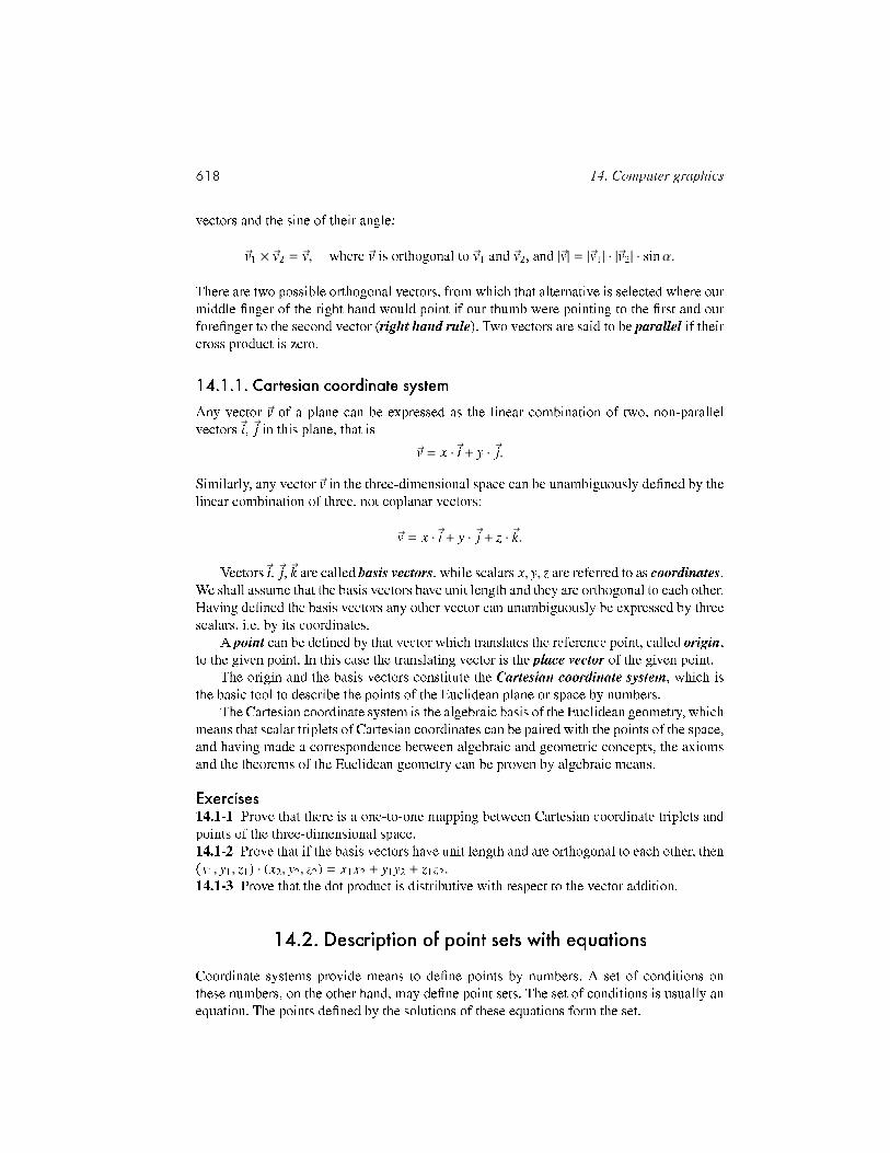
solid f (x, y, z) implicit functionsphere of radius R R2 − x2 − y2 − z2
block of size 2a, 2b, 2c mina − |x|, b − |y|, c − |z|torus of axis z, radii r (tube) and R (hole) r2 − z2 − (R −
√x2 + y2)2
Figure 14.1. Implicit functions dening the sphere, the block, and the torus.
14.2.1. SolidsA solid is a subset of the three-dimensional Euclidean space. To dene this subset, continu-ous function f is used which maps the coordinates of points onto the set of real numbers.We say that a point belongs to the solid if the coordinates of the point satisfy the followingimplicit inequality:
f (x, y, z) ≥ 0 .Points satisfying inequality f (x, y, z) > 0 are the internal points, while points dened byf (x, y, z) < 0 are the external points. Because of the continuity of function f , points sa-tisfying equality f (x, y, z) = 0 are between external and internal points and are called theboundary surface of the solid. Intuitively, function f describes the distance between a pointand the boundary surface.
We note that we usually do not consider any subset of the space as a solid, but alsorequire that the point set does not have lower dimensional degeneration (e.g. hanging linesor surfaces), i.e. that arbitrarily small neighbourhoods of each point of the boundary surfacecontain internal points.
Figure 14.1 denes the implicit functions of the sphere, the box and the torus.
14.2.2. SurfacesPoints having coordinates that satisfy equation f (x, y, z) = 0 are the boundary points of thesolid, which form a surface. Surfaces can thus be dened by this implicit equation. Sincepoints can also be given by the place vectors, the implicit equation can be formulated forthe place vectors as well:
f (~r) = 0 .A surface may have many different equations. For example, equations f (x, y, z) = 0,f 2(x, y, z) = 0, and 2 · f 3(x, y, z) = 0 are algebraically different, but they dene the same setof points.
A plane of normal ~n and place vector ~r0 contains those points for which vector ~r − ~r0is perpendicular to the normal, thus their dot product is zero. Based on this, the points of aplane are dened by the following vector and scalar equations:
(~r − ~r0) · ~n = 0, nx · x + ny · y + nz · z + d = 0 , (14.1)
where nx, ny, nz are the coordinates of the normal and d = −~r0 · ~n. If the normal vector hasunit length, then d expresses the signed distance between the plane and the origin of thecoordinate system. Two planes are said to be parallel if their normals are parallel.
Instead of using implicit equations, surfaces can also be dened by parametric forms.In this case, the Cartesian coordinates of surface points are functions of two independent

620 14. Computer graphics
solid x(u, v) y(u, v) z(u, v)sphere of radius R R · cos 2πu · sin πv R · sin 2πu · sin πv R · cos πv
cylinder of radius R, axis z, and of height h R · cos 2πu R · sin 2πu h · vcone of radius R, axis z, and of height h R · (1 − v) · cos 2πu R · (1 − v) · sin 2πu h · v
Figure 14.2. Parametric forms of the sphere, the cylinder, and the cone, where u, v ∈ [0, 1].
variables. Denoting these free parameters by u and v, the parametric equations of the surfaceare:
x = x(u, v), y = y(u, v), z = z(u, v), u ∈ [umin, umax], v ∈ [vmin, vmax] .
The implicit equation of a surface can be obtained from the parametric equations byeliminating free parameters u, v. Figure 14.2 includes the parametric forms of the sphere,the cylinder and the cone.
Parametric forms can also be dened directly for the place vectors:
~r = ~r(u, v) .
A triangle is the convex combination of points ~p1, ~p2, and ~p3, that is
~r(α, β, γ) = α · ~p1 + β · ~p2 + γ · ~p3, where α, β, γ ≥ 0 and α + β + γ = 1 .
From this denition we can obtain the usual two-variate parametric form substituting αby u, β by v, and γ by (1 − u − v):
~r(u, v) = u · ~p1 + v · ~p2 + (1 − u − v) · ~p3, where u, v ≥ 0 and u + v ≤ 1 .
14.2.3. CurvesBy intersecting two surfaces, we obtain a curve that may be dened formally by the implicitequations of the two intersecting surfaces
f1(x, y, z) = f2(x, y, z) = 0,
but this is needlessly complicated. Instead, let us consider the parametric forms of the twosurfaces, given as ~r1(u1, v1) and ~r2(u2, v2), respectively. The points of the intersection satisfyvector equation ~r1(u1, v1) = ~r2(u2, v2), which corresponds to three scalar equations, one foreach coordinate of the three-dimensional space. Thus we can eliminate three from the fourunknowns (u1, v1, u2, v2), and obtain a one-variate parametric equation for the coordinatesof the curve points:
x = x(t), y = y(t), z = z(t), t ∈ [tmin, tmax].
Similarly, we can use the vector form:
~r = ~r(t), t ∈ [tmin, tmax].
Figure 14.3 includes the parametric equations of the ellipse, the helix, and the line segment.Note that we can dene curves on a surface by xing one of free parameters u, v. For

14.2. Description of point sets with equations 621
test x(u, v) y(u, v) z(u, v)ellipse of main axes 2a, 2b on plane z = 0 a · cos 2πt b · sin 2πt 0helix of radius R, axis z, and elevation h R · cos 2πt R · sin 2πt h · t
line segment between points (x1, y1, z1) and (x2, y2, z2) x1(1 − t) + x2t y1(1 − t) + y2t z1(1 − t) + z2t
Figure 14.3. Parametric forms of the ellipse, the helix, and the line segment, where t ∈ [0, 1].
example, by xing v the parametric form of the resulting curve is ~rv(u) = ~r(u, v). Thesecurves are called iso-parametric curves.
Let us select a point of a line and call the place vector of this point the place vector ofthe line. Any other point of the line can be obtained by the translation of this point alongthe same direction vector. Denoting the place vector by ~r0 and the direction vector by ~v, theequation of the line is:
~r(t) = r0 + ~v · t, t ∈ (−∞,∞) . (14.2)
Two lines are said to be parallel if their direction vectors are parallel.Instead of the complete line, we can also specify the points of a line segment if para-
meter t is restricted to an interval. For example, the equation of the line segment betweenpoints ~r1,~r2 is:
~r(t) = ~r1 + (~r2 − ~r1) · t = ~r1 · (1 − t) + ~r2 · t, t ∈ [0, 1] . (14.3)
According to this denition, the points of a line segment are the convex-combinations ofthe endpoints.
14.2.4. Normal vectorsIn computer graphics we often need the normal vectors of the surfaces (i.e. the normalvector of the tangent plane of the surface). Let us take an example. A mirror reects lightin a way that the incident direction, the normal vector, and the reection direction are in thesame plane, and the angle between the normal and the incident direction equals to the anglebetween the normal and the reection direction. To carry out such and similar computations,we need methods to obtain the normal of the surface.
The equation of the tangent plane is obtained as the rst order Taylor approximation ofthe implicit equation around point (x0, y0, z0):
f (x, y, z) = f (x0 + (x − x0), y0 + (y − y0), z0 + (z − z0)) ≈
f (x0, y0, z0) +∂ f∂x · (x − x0) +
∂ f∂y · (y − y0) +
∂ f∂z · (z − z0) .
Points (x0, y0, z0) and (x, y, z) are on the surface, thus f (x0, y0, z0) = 0 and f (x, y, z) = 0,resulting in the following equation of the tangent plane:
∂ f∂x · (x − x0) +
∂ f∂y · (y − y0) +
∂ f∂z · (z − z0) = 0 .
Comparing this equation to equation (14.1), we can realize that the normal vector of the

622 14. Computer graphics
tangent plane is
~n =
(∂ f∂x ,
∂ f∂y ,
∂ f∂z
)= grad f . (14.4)
The normal vector of parametric surfaces can be obtained by examining the iso-parametric curves. The tangent of curve ~rv(u) dened by xing parameter v is obtainedby the rst-order Taylor approximation:
~rv(u) = ~rv(u0 + (u − u0)) ≈ ~rv(u0) +d~rvdu · (u − u0) = ~rv(u0) +
∂~r∂u · (u − u0) .
Comparing this approximation to equation (14.2) describing a line, we conclude that thedirection vector of the tangent line is ∂~r/∂u. The tangent lines of the curves running on asurface are in the tangent plane of the surface, making the normal vector perpendicular tothe direction vectors of these lines. In order to nd the normal vector, both the tangent lineof curve ~rv(u) and the tangent line of curve ~ru(v) are computed, and their cross product isevaluated since the result of the cross product is perpendicular to the multiplied vectors. Thenormal of surface ~r(u, v) is then
~n =∂~r∂u ×
∂~r∂v . (14.5)
14.2.5. Curve modellingParametric and implicit equations trace back the geometric design of the virtual world tothe solution of these equations. However, these equations are often not intuitive enough,thus they cannot be used directly during design. It would not be reasonable to expect thedesigner working on a human face or on a car to directly specify the equations of theseobjects. Clearly, indirect methods are needed which require intuitive data from the designerand dene these equations automatically. One category of these indirect approaches applycontrol points. Another category of methods work with elementary building blocks (box,sphere, cone, etc.) and with set operations.
Let us discuss rst how the method based on control points can dene curves. Supposethat the designer dened points ~r0,~r1, . . . ,~rm, and that parametric curve of equation ~r = ~r(t)should be found which follows these points. For the time being, the curve is not requiredto go through these control points.
We use the analogy of the centre of mass of mechanical systems to construct our curve.Assume that we have sand of unit mass, which is distributed at the control points. If a controlpoint has most of the sand, then the centre of mass is close to this point. Controlling thedistribution of the sand as a function of parameter t to give the main inuence to differentcontrol points one after the other, the centre of mass will travel through a curve runningclose to the control points.
Let us put weights B0(t), B1(t), . . . , Bm(t) at control points at parameter t. These weigh-ting functions are also called the basis functions of the curve. Since unit weight is distribu-ted, we require that for each t the following identity holds:
m∑
i=0Bi(t) = 1 .

14.2. Description of point sets with equations 623
0
0.2
0.4
0.6
0.8
1
0 0.2 0.4 0.6 0.8 1t
b0b1b2b3
Figure 14.4. A Bézier curve dened by four control points and the respective basis functions (m = 3).
For some t, the curve is the centre of mass of this mechanical system:
~r(t) =
∑mi=0 Bi(t) · ~ri∑m
i=0 Bi(t)=
m∑
i=0Bi(t) · ~ri .
Note that the reason of distributing sand of unit mass is that this decision makes the deno-minator of the fraction equal to 1. To make the analogy complete, the basis functions cannotbe negative since the mass is always non negative. The centre of mass of a point system isalways in the convex hull1 of the participating points, thus if the basis functions are nonnegative, then the curve remains in the convex hull of the control points.
The properties of the curves are determined by the basis functions. Let us now discusstwo popular basis function systems, namely the basis functions of the Bézier curves and theB-spline curves.
Bézier curvePierre Bézier, a designer working at Renault, proposed the Bernstein polynomials as basisfunctions. Bernstein polynomials can be obtained as the expansion of 1m = (t + (1 − t))m
according to binomial theorem:
(t + (1 − t))m =
m∑
i=0
(mi
)· ti · (1 − t)m−i .
The basis functions of Bézier curves are the terms of this sum (i = 0, 1, . . . ,m):
BBezieri,m (t) =
(mi
)· ti · (1 − t)m−i . (14.6)
According to the introduction of Bernstein polynomials, it is obvious that they reallymeet condition ∑m
i=0 Bi(t) = 1 and Bi(t) ≥ 0 in t ∈ [0, 1], which guarantees that Bézier curves
1The convex hull of a point system is by denition the minimal convex set containing the point system.

624 14. Computer graphics
lineáris bázisfüggvények
másodfokú bázisfüggvények
harmadfokú bázisfüggvények
lineáris simítás
lineáris simítás
bázisfüggvénylineáris simítás
B (t)i,2
B (t)i,3
B (t)i,4
4
1
1
B (t)i,11
konstans bázisfüggvények
lineáris simítást t t t3 5 6
t6
t3 t5
t7 t8
t7
t0 1t 2t
1t
2t
t5
t5
Figure 14.5. Construction of B-spline basis functions. A higher order basis function is obtained by blending twoconsecutive basis functions on the previous level using a linearly increasing and a linearly decreasing weighting,respectively. Here the number of control points is 5, i.e. m = 4. Arrows indicate useful interval [tk−1, tm+1] wherewe can nd m + 1 number of basis functions that add up to 1. The right side of the gure depicts control pointswith triangles and curve points corresponding to the knot values by circles.
are always in the convex hulls of their control points. The basis functions and the shape ofthe Bézier curve are shown in gure 14.4. At parameter value t = 0 the rst basis function is1, while the others are zero, therefore the curve starts at the rst control point. Similarly, atparameter value t = 1 the curve arrives at the last control point. At other parameter values,all basis functions are positive, thus they simultaneously affect the curve. Consequently, thecurve usually does not go through the other control points.
B-splineThe basis functions of the B-spline can be constructed applying a sequence of linear blen-ding. A B-spline weights the m + 1 number of control points by (k− 1)-degree polynomials.Value k is called the order of the curve, which expresses the smoothness of the curve. Letus take a non-decreasing series of m + k + 1 parameter values, called the knot vector:
t = [t0, t1, . . . , tm+k], t0 ≤ t1 ≤ · · · ≤ tm+k .
By denition, the ith rst order basis function is 1 in the ith interval, and zero elsewhere(gure 14.5):
BBSi,1 (t) =
1, if ti ≤ t < ti+1 ,0 otherwise .
Using this denition, m + k number of rst order basis functions are established, which

14.2. Description of point sets with equations 625
are non-negative zero-degree polynomials that sum up to 1 for all t ∈ [t0, tm+k) parameters.These basis functions have too low degree since the centre of mass is not even a curve, butjumps from control point to control point.
The order of basis functions, as well as the smoothness of the curve, can be increased byblending two consecutive basis functions with linear weighting (gure 14.5). The rst basisfunction is weighted by linearly increasing factor (t − ti)/(ti+1 − ti) in domain ti ≤ t < ti+1,where the basis function is non-zero. The next basis function, on the other hand, is scaledby linearly decreasing factor (ti+2 − t)/(ti+2 − ti+1) in its domain ti+1 ≤ t < ti+2 where it isnon zero. The two weighted basis functions are added to obtain the tent-like second orderbasis functions. Note that while a rst order basis function is non-zero in a single interval,the second order basis functions expand to two intervals. Since the construction makes anew basis function from every pair of consecutive lower order basis functions, the numberof new basis functions is one less than that of the original ones. We have just m + k − 1second order basis functions. Except for the rst and the last rst order basis functions, allof them are used once with linearly increasing and once with linearly decreasing weighting,thus with the exception of the rst and the last intervals, i.e. in [t1, tm+k−1], the new basisfunctions also sum up to 1.
The second order basis functions are rst degree polynomials. The degree of basis func-tions, i.e. the order of the curve, can be arbitrarily increased by the recursive application ofthe presented blending method. The dependence of the next order basis functions on theprevious order ones is as follows:
BBSi,k (t) =
(t − ti)BBSi,k−1(t)
ti+k−1 − ti+
(ti+k − t)BBSi+1,k−1(t)
ti+k − ti+1, if k > 1 .
Note that we always take two consecutive basis functions and weight them in their non-zero domain (i.e. in the interval where they are non-zero) with linearly increasing factor(t − ti)/(ti+k−1 − ti) and with linearly decreasing factor (ti+k − t)/(ti+k − ti+1), respectively.The two weighted functions are summed to obtain the higher order, and therefore smootherbasis function. Repeating this operation (k− 1) times, k-order basis functions are generated,which sum up to 1 in interval [tk−1, tm+1]. The knot vector may have elements that are thesame, thus the length of the intervals may be zero. Such intervals result in 0/0 like fractions,which must be replaced by value 1 in the implementation of the construction.
The value of the ith k-order basis function at parameter t can be computed with thefollowing Cox-deBoor algorithm:

626 14. Computer graphics
p0
p1
p2
c-1
c0
c1
c2
c3
cm
cm+1
pm
Figure 14.6. A B-spline interpolation. Based on points ~p0, . . . , ~pm to be interpolated, control points ~c−1, . . . ,~cm+1are computed to make the start and end points of the segments equal to the interpolated points.
B-S(i, k, t, t)1 if k = 1 B Trivial case.2 then if ti ≤ t < ti+13 then return 14 else return 05 if ti+k−1 − ti > 06 then b1 ← (t − ti)/(ti+k−1 − ti) B Previous with linearly increasing weight.7 else b1 ← 1 B Here: 0/0 = 1.8 if ti+k − ti+1 > 09 then b2 ← (ti+k − t)/(ti+k − ti+1) B Next with linearly decreasing weight.
10 else b2 ← 1 B Here: 0/0 = 1.11 B← b1 · B-(i, k − 1, t, t) + b2 · B-(i + 1, k − 1, t, t) B Recursion.12 return B
In practice, we usually use fourth-order basis functions (k = 4), which are third-degreepolynomials, and dene curves that can be continuously differentiated twice. The reason isthat bent rods and motion paths following the Newton laws also have this property.
While the number of control points is greater than the order of the curve, the basisfunctions are non-zero only in a part of the valid parameter set. This means that a controlpoint affects just a part of the curve. Moving this control point, the change of the curve islocal. Local control is a very important property since the designer can adjust the shape ofthe curve without destroying its general form.
A fourth-order B-spline usually does not go through its control points. If we wish touse it for interpolation, the control points should be calculated from the points to be interpo-lated. Suppose that we need a curve which visits points ~p0, ~p1, . . . , ~pm at parameter valuest0 = 0, t1 = 1, . . . , tm = m, respectively (gure 14.6). To nd such a curve, control points[~c−1,~c0,~c1, . . . ,~cm+1] should be found to meet the following interpolation criteria:
~r(t j) =
m+1∑
i=−1~ci · BBS
i,4 (t j) = ~p j, j = 0, 1, . . . ,m .
These criteria can be formalized as m + 1 linear equations with m + 3 unknowns, thus thesolution is ambiguous. To make the solution unambiguous, two additional conditions shouldbe imposed. For example, we can set the derivatives (for motion paths, the speed) at the startand end points.

14.2. Description of point sets with equations 627
B-spline curves can be further generalized by dening the inuence of the ith controlpoint as the product of B-spline basis function Bi(t) and additional weight wi of the controlpoint. The curve obtained this way is called the Non-Uniform Rational B-Spline, abbrevia-ted as NURBS, which is very popular in commercial geometric modelling systems.
Using the mechanical analogy again, the mass put at the ith control point is wiBi(t), thusthe centre of mass is:
~r(t) =
∑mi=0 wiBBS
i (t) · ~ri∑mj=0 w jBBS
j (t)=
m∑
i=0BNURBS
i (t) · ~ri .
The correspondence between B-spline and NURBS basis functions is as follows:
BNURBSi (t) =
wiBBSi (t)
∑mj=0 w jBBS
j (t).
Since B-spline basis functions are polynomials, NURBS basis functions are rationalfunctions. NURBS can describe quadratic curves (e.g. circle, ellipse, etc.) without any app-roximation error.
14.2.6. Surface modellingParametric surfaces are dened by two variate functions ~r(u, v). Instead of specifying thisfunction directly, we can take nite number of control points ~ri j which are weighted withthe basis functions to obtain the parametric function:
~r(u, v) =
n∑
i=0
m∑
j=0~ri j · Bi j(u, v) . (14.7)
Similarly to curves, basis functions are expected to sum up to 1, i.e. ∑ni=0
∑mj=0 Bi j(u, v) = 1
everywhere. If this requirement is met, we can imagine that the control points have massesBi j(u, v) depending on parameters u, v, and the centre of mass is the surface point corres-ponding to parameter pair u, v.
Basis functions Bi j(u, v) are similar to those of curves. Let us x parameter v. Chan-ging parameter u, curve ~rv(u) is obtained on the surface. This curve can be dened by thediscussed curve denition methods:
~rv(u) =
n∑
i=0Bi(u) · ~ri , (14.8)
where Bi(u) is the basis function of the selected curve type.Of course, xing v differently we obtain another curve of the surface. Since a curve of
a given type is unambiguously dened by the control points, control points ~ri must dependon the xed v value. As parameter v changes, control point ~ri = ~ri(v) also runs on a curve,which can be dened by control points ~ri,0,~ri,2, . . . ,~ri,m:
~ri(v) =
m∑
j=0B j(v) · ~ri j .
628 14. Computer graphics
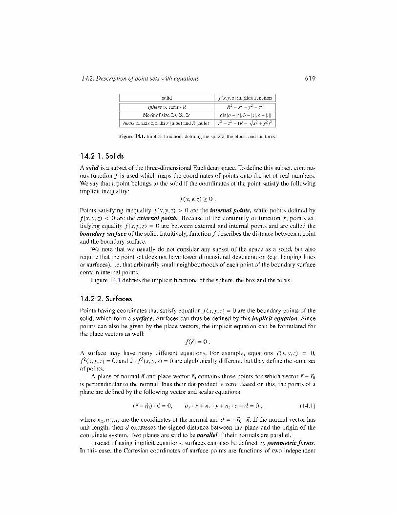
Figure 14.7. Iso-parametric curves of surface.
Substituting this into equation (14.8), the parametric equation of the surface is:
~r(u, v) = ~rv(u) =
n∑
i=0Bi(u)
m∑
j=0B j(v) · ~ri j
=
n∑
i=0
m∑
j=0Bi(u)B j(v) · ~ri j .
Unlike curves, the control points of a surface form a two-dimensional grid. The two-dimensional basis functions are obtained as the product of one-variate basis functions para-meterized by u and v, respectively.
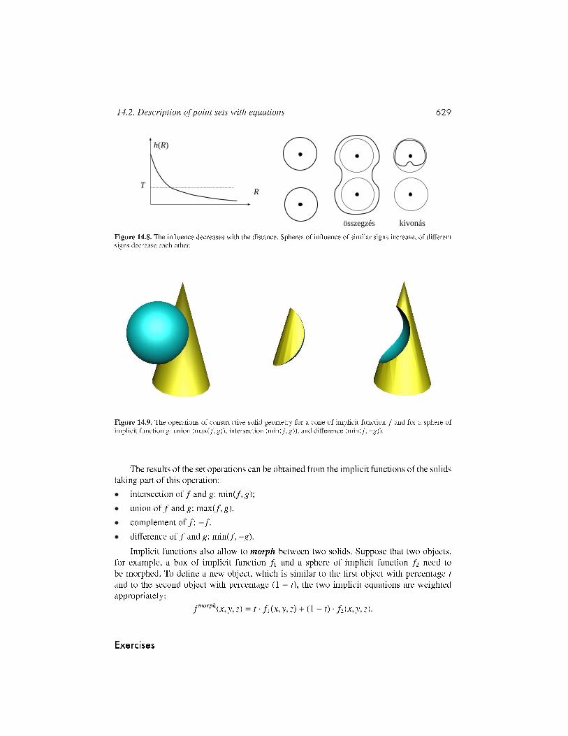
14.2.7. Solid modelling with blobsFree form solids similarly to parametric curves and surfaces can also be specied bynite number of control points. For each control point ~ri, let us assign inuence functionh(Ri), which expresses the inuence of this control point at distance Ri = |~r − ~ri|. By de-nition, the solid contains those points where the total inuence of the control points is notsmaller than threshold T (gure 14.8):
f (~r) =
m∑
i=0hi(Ri) − T ≥ 0, where Ri = |~r − ~ri| .
With a single control point a sphere can be modelled. Spheres of multiple control points arecombined together to result in an object having smooth surface (gure 14.8). The inuenceof a single point can be dened by an arbitrary decreasing function that converges to zero atinnity. For example, Blinn proposed the
hi(R) = ai · e−biR2
inuence functions for his blob method.
14.2.8. Constructive solid geometryAnother type of solid modelling is constructive solid geometry (CSG for short), whichbuilds complex solids from primitive solids applying set operations (union, intersection,difference) (gures 14.9 and 14.10). Primitives usually include the box, the sphere, the cone,the cylinder, the half-space, etc. whose implicit functions are known.
14.2. Description of point sets with equations 629
R
h(R)
T
összegzés kivonás
Figure 14.8. The inuence decreases with the distance. Spheres of inuence of similar signs increase, of differentsigns decrease each other.
Figure 14.9. The operations of constructive solid geometry for a cone of implicit function f and for a sphere ofimplicit function g: union (max( f , g)), intersection (min( f , g)), and difference (min( f ,−g)).
The results of the set operations can be obtained from the implicit functions of the solidstaking part of this operation:• intersection of f and g: min( f , g);• union of f and g: max( f , g).• complement of f : − f .• difference of f and g: min( f ,−g).
Implicit functions also allow to morph between two solids. Suppose that two objects,for example, a box of implicit function f1 and a sphere of implicit function f2 need tobe morphed. To dene a new object, which is similar to the rst object with percentage tand to the second object with percentage (1 − t), the two implicit equations are weightedappropriately:
f morph(x, y, z) = t · f1(x, y, z) + (1 − t) · f2(x, y, z).
Exercises

630 14. Computer graphics
Figure 14.10. Constructing a complex solid by set operations. The root and the leaf of the CSG tree represents thecomplex solid, and the primitives, respectively. Other nodes dene the set operations (U: union, \: difference).
14.2-1 Find the parametric equation of a torus.14.2-2 Prove that the fourth-order B-spline with knot-vector [0,0,0,0,1,1,1,1] is a Béziercurve.14.2-3 Give the equations for the surface points and the normals of the waving ag andwaving water disturbed in a single point.14.2-4 Prove that the tangents of a Bézier curve at the start and the end are the lines con-necting the rst two and the last two control points, respectively.14.2-5 Give the algebraic forms of the basis functions of the second, the third, and thefourth-order B-splines.14.2-6 Develop an algorithm computing the path length of a Bézier curve and a B-spline.Based on the path length computation move a point along the curve with uniform speed.
14.3. Geometry processing and tessellation algorithmsIn section 14.2 we met free-form surface and curve denition methods. During image synt-hesis, however, line segments and triangles play important roles. In this section we presentmethods that bridge the gap between these two types of representations. These methodsconvert geometric models to lines and triangles, or further process line and triangle models.Line segments connected to each other in a way that the end point of a line segment is thestart point of the next one are called polylines. Triangles connected at edges, on the otherhand, are called meshes. Vectorization methods approximate free-form curves by polylines.A polyline is dened by its vertices. Tessellation algorithms, on the other hand, approxi-mate free-form surfaces by meshes. For illumination computation, we often need the nor-mal vector of the original surface, which is usually stored with the vertices. Consequently, atriangle mesh contains a list of triangles, where each triangle is given by three vertices andthree normals. Methods processing triangle meshes use other topology information as well,

14.3. Geometry processing and tessellation algorithms 631
(a) (b) (c)
Figure 14.11. Types of polygons. (a) simple; (b) complex, single connected; (c) multiply connected.
for example, which triangles share an edge or a vertex.
14.3.1. Polygon and polyhedronDenition 14.2 A polygon is a bounded part of the plane, i.e. it does not contain a line,and is bordered by line segments. A polygon is dened by the vertices of the borderingpolylines.
Denition 14.3 A polygon is single connected if its border is a single closed polyline(gure 14.11).
Denition 14.4 A polygon is simple if it is single connected and the bordering polylinedoes not intersect itself (gure 14.11(a)).
For a point of the plane, we can detect whether or not this point is inside the polygonby starting a half-line from this point and counting the number of intersections with theboundary. If the number of intersections is an odd number, then the point is inside, otherwiseit is outside.
In the three-dimensional space we can form triangle meshes, where different trianglesare in different planes. In this case, two triangles are said to be neighbouring if they sharean edge.
Denition 14.5 A polyhedron is a bounded part of the space, which is bordered by poly-gons.
Similarly to polygons, a point can be tested for polyhedron inclusion by casting a halfline from this point and counting the number of intersections with the face polygons. Ifthe number of intersections is odd, then the point is inside the polyhedron, otherwise it isoutside.
14.3.2. Vectorization of parametric curvesParametric functions map interval [tmin, tmax] onto the points of the curve. During vectori-zation the parameter interval is discretized. The simplest discretization scheme generates Nevenly spaced parameter values ti = tmin + (tmax − tmin) · i/N (i = 0, 1, . . . ,N), and denes theapproximating polyline by the points obtained by substituting these parameter values intoparametric equation ~r(ti).
632 14. Computer graphics
r1
r3
r2
r0
r4
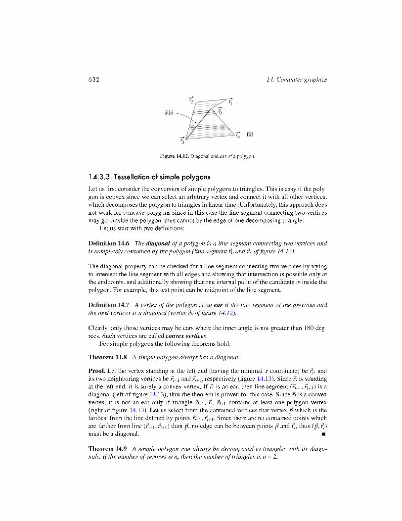
átló
fül
Figure 14.12. Diagonal and ear of a polygon.
14.3.3. Tessellation of simple polygonsLet us rst consider the conversion of simple polygons to triangles. This is easy if the poly-gon is convex since we can select an arbitrary vertex and connect it with all other vertices,which decomposes the polygon to triangles in linear time. Unfortunately, this approach doesnot work for concave polygons since in this case the line segment connecting two verticesmay go outside the polygon, thus cannot be the edge of one decomposing triangle.
Let us start with two denitions:
Denition 14.6 The diagonal of a polygon is a line segment connecting two vertices andis completely contained by the polygon (line segment ~r0 and ~r3 of gure 14.12).
The diagonal property can be checked for a line segment connecting two vertices by tryingto intersect the line segment with all edges and showing that intersection is possible only atthe endpoints, and additionally showing that one internal point of the candidate is inside thepolygon. For example, this test point can be midpoint of the line segment.
Denition 14.7 A vertex of the polygon is an ear if the line segment of the previous andthe next vertices is a diagonal (vertex ~r4 of gure 14.12).
Clearly, only those vertices may be ears where the inner angle is not greater than 180 deg-rees. Such vertices are called convex vertices.
For simple polygons the following theorems hold:
Theorem 14.8 A simple polygon always has a diagonal.
Proof. Let the vertex standing at the left end (having the minimal x coordinate) be ~ri, andits two neighboring vertices be ~ri−1 and ~ri+1, respectively (gure 14.13). Since ~ri is standingat the left end, it is surely a convex vertex. If ~ri is an ear, then line segment (~ri−1,~ri+1) is adiagonal (left of gure 14.13), thus the theorem is proven for this case. Since ~ri is a convexvertex, it is not an ear only if triangle ~ri−1, ~ri, ~ri+1 contains at least one polygon vertex(right of gure 14.13). Let us select from the contained vertices that vertex ~p which is thefarthest from the line dened by points ~ri−1,~ri+1. Since there are no contained points whichare farther from line (~ri−1,~ri+1) than ~p, no edge can be between points ~p and ~ri, thus (~p,~ri)must be a diagonal.
Theorem 14.9 A simple polygon can always be decomposed to triangles with its diago-nals. If the number of vertices is n, then the number of triangles is n − 2.

14.3. Geometry processing and tessellation algorithms 633
ri
ri+1
ri-1
átló
ri
ri+1
ri-1
átló
p
x
y
Figure 14.13. The proof of the existence of a diagonal for simple polygons.
Proof. This theorem is proven with induction. The theorem is obviously true when n =
3, i.e. when the polygon is a triangle. Let us assume that the statement is also true forpolygons having m (m = 3, . . . , n − 1) number of vertices, and consider a polygon with nvertices. According to theorem 14.8, this polygon of n vertices has a diagonal, thus we cansubdivide this polygon into a polygon of n1 vertices and a polygon of n2 vertices, wheren1, n2 < n, and n1 + n2 = n + 2 since the vertices at the end of the diagonal participatein both polygons. According to the assumption of the induction, these two polygons canbe separately decomposed to triangles. Joining the two sets of triangles, we can obtain thetriangle decomposition of the original polygon. The number of triangles is n1 − 2 + n2 − 2 =
n − 2.The discussed proof is constructive thus it inspires a subdivision algorithm: let us nd
a diagonal, subdivide the polygon along this diagonal, and continue the same operation forthe two new polygons.
Unfortunately the running time of such an algorithm is in Θ(n3) since the number ofdiagonal candidates is Θ(n2), and the time needed by checking whether or not a line segmentis a diagonal is in Θ(n).
We also present a better algorithm, which decomposes a convex or concave polygondened by vertices ~r0,~r1, . . . ,~rn. This algorithm is called ear cutting. The algorithm looksfor ear triangles and cuts them until the polygon gets simplied to a single triangle. Thealgorithm starts at vertex ~r2. When a vertex is processed, it is rst checked whether or notthe previous vertex is an ear. If it is not an ear, then the next vertex is chosen. If the previousvertex is an ear, then the current vertex together with the two previous ones form a trianglethat can be cut, and the previous vertex is deleted. If after deletion the new previous vertexhas index 0, then the next vertex is selected as the current vertex.
The presented algorithm keeps cutting triangles until no more ears are left. The termi-nation of the algorithm is guaranteed by the following two ears theorem:
Theorem 14.10 A simple polygon having at least four vertices always has at least two notneighboring ears that can be cut independently.
Proof. The proof presented here has been given by Joseph O'Rourke. According to theorem14.9, every simple polygon can be subdivided to triangles such that the edges of these tri-angles are either the edges or the diagonals of the polygon. Let us make a correspondencebetween the triangles and the nodes of a graph where two nodes are connected if and onlyif the two triangles corresponding to these nodes share an edge. The resulting graph is con-nected and cannot contain circles. Graphs of these properties are trees. The name of thistree graph is the dual tree. Since the polygon has at least four vertices, the number of nodes

634 14. Computer graphics
r (v)
v(u)
u
r
Figure 14.14. Tessellation of parametric surfaces.
in this tree is at least two. Any tree containing at least two nodes has at least two leaves2.Leaves of this tree, on the other hand, correspond to triangles having an ear vertex.
According to the two ears theorem, the presented algorithm nds an ear in O(n) steps.Cutting an ear the number of vertices is reduced by one, thus the algorithm terminates inO(n2) steps.
14.3.4. Tessellation of parametric surfacesParametric forms of surfaces map parameter rectangle [umin, umax] × [vmin, vmax] onto thepoints of the surface.
In order to tessellate the surface, rst the parameter rectangle is subdivided to triang-les. Then applying the parametric equations for the vertices of the parameter triangles, theapproximating triangle mesh can be obtained. The simplest subdivision of the parametricrectangle decomposes the domain of parameter u to N parts, and the domain of parameter vto M intervals, resulting in the following parameter pairs:
[ui, v j] =
[umin + (umax − umin) i
N , vmin + (vmax − vmin) jM
].
Taking these parameter pairs and substituting them into the parametric equations, pointtriplets ~r(ui, v j), ~r(ui+1, v j), ~r(ui, v j+1), and point triplets ~r(ui+1, v j), ~r(ui+1, v j+1), ~r(ui, v j+1)are used to dene triangles.
The tessellation process can be made adaptive as well, which uses small triangles onlywhere the high curvature of the surface justies them. Let us start with the parameter rec-tangle and subdivide it to two triangles. In order to check the accuracy of the resulting tri-angle mesh, surface points corresponding to the edge midpoints of the parameter trianglesare compared to the edge midpoints of the approximating triangles. Formally the followingdistance is computed (gure 14.15):
∣∣∣∣∣∣~r(u1 + u2
2 ,v1 + v2
2
)− ~r(u1, v1) + ~r(u2, v2)
2
∣∣∣∣∣∣ ,
where (u1, v1) and (u2, v2) are the parameters of the two endpoints of the edge.
2a leaf is a node connected by exactly one edge

14.3. Geometry processing and tessellation algorithms 635
hiba
Figure 14.15. Estimation of the tessellation error.
T csomópont
új T csomópont
rekurzív felosztás
felosztás
Figure 14.16. T vertices and their elimination with forced subdivision.
A large distance value indicates that the triangle mesh poorly approximates the para-metric surface, thus triangles must be subdivided further. This subdivision can be executedby cutting the triangle to two triangles by a line connecting the midpoint of the edge ofthe largest error and the opposing vertex. Alternatively, a triangle can be subdivided to fourtriangles with its halving lines. The adaptive tessellation is not necessarily robust since itcan happen that the distance at the midpoint is small, but at other points is still quite large.
When the adaptive tessellation is executed, it may happen that one triangle is subdividedwhile its neighbour is not, which results in a mesh where the previously shared edge istessellated in one of the triangles, thus has holes. Such problematic midpoints are called Tvertices (gure 14.16).
If the subdivision criterion is based only on edge properties, then T vertices cannot showup. However, if other properties are also taken into account, then T vertices may appear. Insuch cases, T vertices can be eliminated by recursively forcing the subdivision also for thoseneighbouring triangles that share subdivided edges.
14.3.5. Subdivision curves and meshesThis section presents algorithms that smooth polyline and mesh models. Smoothing meansthat a polyline and a mesh are replaced by other polylines and meshes having less facetedlook.
Let us consider a polyline of vertices ~r0, . . . ,~rm. A smoother polyline is generated bythe following vertex doubling approach (gure 14.17). Every line segment of the polylineis halved, and midpoints ~h0, . . . ,~hm−1 are added to the polyline as new vertices. Then the

636 14. Computer graphics
=1/2 Σ =1/2 Σ +1/4Σ
ri+1
ri-1
rihi
hi-1ri’
Figure 14.17. Construction of a subdivision curve: at each step midpoints are obtained, then the original verticesare moved to the weighted average of neighbouring midpoints and of the original vertex.
=1/4 Σ =1/4 Σ +1/4Σ =1/2 +1/16 Σ +1/16 Σ
Figure 14.18. One smoothing step of the Catmull-Clark subdivision. First the face points are obtained, then theedge midpoints are moved, and nally the original vertices are rened according to the weighted sum of its neigh-bouring edge and face points.
old vertices are moved taking into account their old position and the positions of the twoenclosing midpoints, applying the following weighting:
~r ′i =12~ri +
14~hi−1 +
14~hi =
34~ri +
18~ri−1 +
18~ri+1 .
The new polyline looks much smoother. If we should not be satised with the smoothnessyet, the same procedure can be repeated recursively. As can be shown, the result of therecursive process converges to the B-spline curve.
The polyline subdivision approach can also be extended for smoothing three-dimensional meshes. This method is called Catmull-Clark subdivision algorithm. Let usconsider a three-dimensional quadrilateral mesh (gure 14.18). In the rst step the midpo-ints of the edges are obtained, which are called edge points. Then face points are generatedas the average of the vertices of each face polygon. Connecting the edge points with the facepoints, we still have the original surface, but now dened by four times more quadrilaterals.The smoothing step modies rst the edge points setting them to the average of the verti-ces at the ends of the edge and of the face points of those quads that share this edge. Thenthe original vertices are moved to the weighted average of the face points of those facesthat share this vertex, and of edge points of those edges that are connected to this vertex.The weight of the original vertex is 1/2, the weights of edge and face are 1/16. Again, this
14.3. Geometry processing and tessellation algorithms 637
Figure 14.19. Original mesh and its subdivision applying the smoothing step once, twice and three times, respec-tively.
1/21/2
-1/16-w
-1/16-w-1/16-w
-1/16-w
1/8+2w
1/8+2w
Figure 14.20. Generation of the new edge point with buttery subdivision.
operation may be repeated until the surface looks smooth enough (gure 14.19).If we do not want to smooth the mesh at an edge or around a vertex, then the averaging
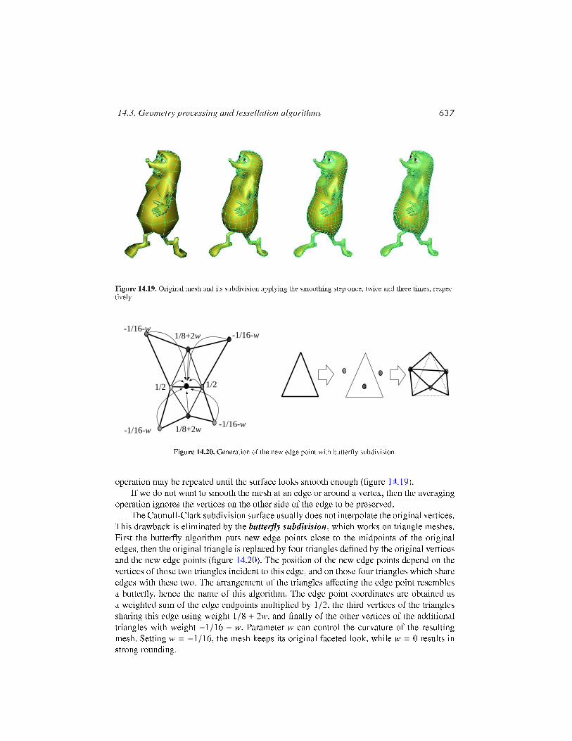
operation ignores the vertices on the other side of the edge to be preserved.The Catmull-Clark subdivision surface usually does not interpolate the original vertices.
This drawback is eliminated by the buttery subdivision, which works on triangle meshes.First the buttery algorithm puts new edge points close to the midpoints of the originaledges, then the original triangle is replaced by four triangles dened by the original verticesand the new edge points (gure 14.20). The position of the new edge points depend on thevertices of those two triangles incident to this edge, and on those four triangles which shareedges with these two. The arrangement of the triangles affecting the edge point resemblesa buttery, hence the name of this algorithm. The edge point coordinates are obtained asa weighted sum of the edge endpoints multiplied by 1/2, the third vertices of the trianglessharing this edge using weight 1/8 + 2w, and nally of the other vertices of the additionaltriangles with weight −1/16 − w. Parameter w can control the curvature of the resultingmesh. Setting w = −1/16, the mesh keeps its original faceted look, while w = 0 results instrong rounding.
638 14. Computer graphics
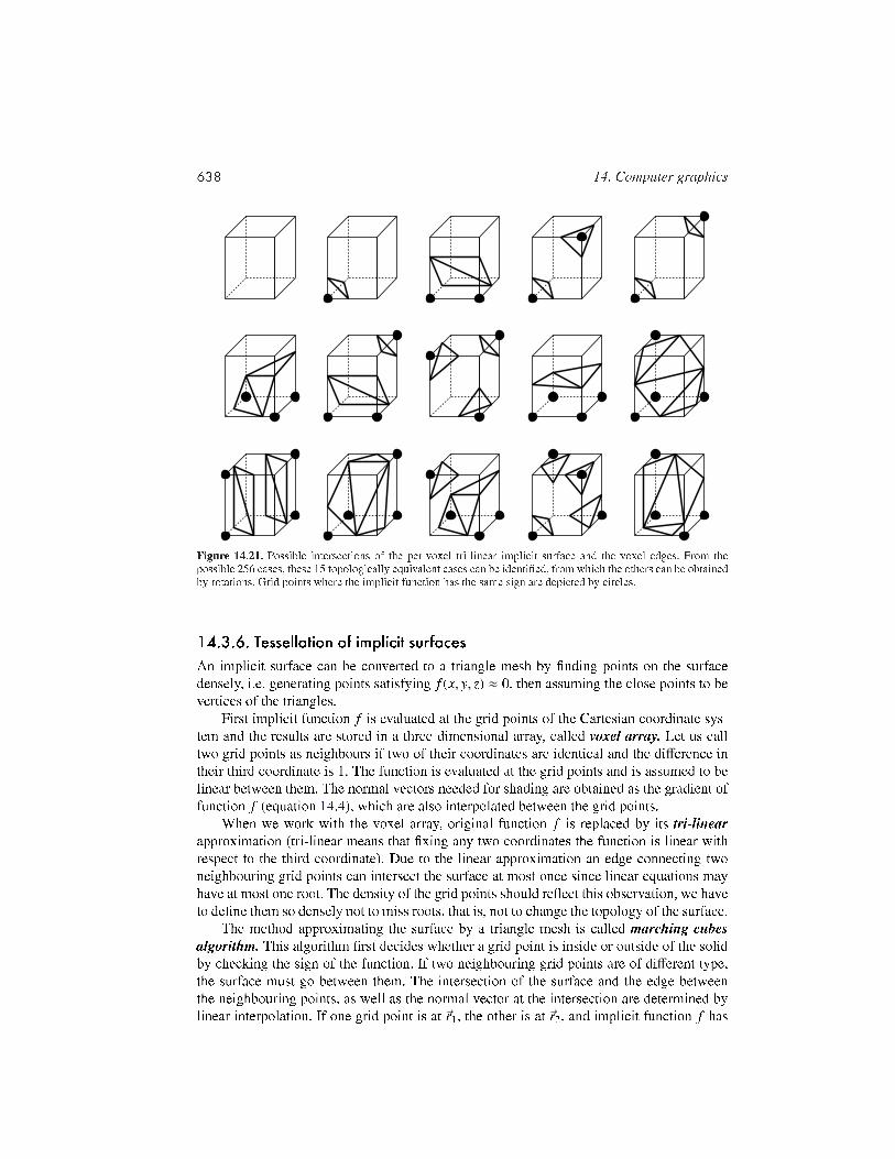
Figure 14.21. Possible intersections of the per-voxel tri-linear implicit surface and the voxel edges. From thepossible 256 cases, these 15 topologically equivalent cases can be identied, from which the others can be obtainedby rotations. Grid points where the implicit function has the same sign are depicted by circles.
14.3.6. Tessellation of implicit surfacesAn implicit surface can be converted to a triangle mesh by nding points on the surfacedensely, i.e. generating points satisfying f (x, y, z) ≈ 0, then assuming the close points to bevertices of the triangles.
First implicit function f is evaluated at the grid points of the Cartesian coordinate sys-tem and the results are stored in a three-dimensional array, called voxel array. Let us calltwo grid points as neighbours if two of their coordinates are identical and the difference intheir third coordinate is 1. The function is evaluated at the grid points and is assumed to belinear between them. The normal vectors needed for shading are obtained as the gradient offunction f (equation 14.4), which are also interpolated between the grid points.
When we work with the voxel array, original function f is replaced by its tri-linearapproximation (tri-linear means that xing any two coordinates the function is linear withrespect to the third coordinate). Due to the linear approximation an edge connecting twoneighbouring grid points can intersect the surface at most once since linear equations mayhave at most one root. The density of the grid points should reect this observation, we haveto dene them so densely not to miss roots, that is, not to change the topology of the surface.
The method approximating the surface by a triangle mesh is called marching cubesalgorithm. This algorithm rst decides whether a grid point is inside or outside of the solidby checking the sign of the function. If two neighbouring grid points are of different type,the surface must go between them. The intersection of the surface and the edge betweenthe neighbouring points, as well as the normal vector at the intersection are determined bylinear interpolation. If one grid point is at ~r1, the other is at ~r2, and implicit function f has

14.4. Containment algorithms 639
different signs at these points, then the intersection of the tri-linear surface and line segment(~r1,~r2) is:
~ri = ~r1 · f (~r2)f (~r2) − f (~r1) + ~r2 · f (~r1)
f (~r2) − f (~r1) ,
The normal vector here is:
~ni = grad f (~r1) · f (~r2)f (~r2) − f (~r1) + grad f (~r2) · f (~r1)
f (~r2) − f (~r1) .
Having found the intersection points, triangles are dened using these points as vertices,and the approximation surface becomes the resulting triangle mesh. When dening thesetriangles, we have to take into account that a tri-linear surface may intersect the voxel edgesat most once. Such intersection occurs if the implicit function has different sign at the twogrid points. The number of possible variations of positive/negative signs at the 8 vertices ofa cube is 256, from which 15 topologically equivalent cases can be identied (gure 14.21).
The algorithm inspects grid points one by one and assigns the sign of the function tothem encoding negative sign by 0 and non-negative sign by 1. The resulting 8 bit code is anumber in 0255 which identies the current case of intersection. If the code is 0, all voxelvertices are outside the solid, thus no voxel surface intersection is possible. Similarly, if thecode is 255, the solid is completely inside, making the intersections impossible. To handleother codes, a table can be built which describes where the intersections show up and howthey form triangles. Exercises
14.3-1 Prove the two ears theorem by induction.14.3-2 Develop an adaptive curve tessellation algorithm.14.3-3 Prove that the Catmull-Clark subdivision curve and surface converge to a B-splinecurve and surface, respectively.14.3-4 Build a table to control the marching cubes algorithm, which describes where theintersections show up and how they form triangles.14.3-5 Propose a marching cubes algorithm that does not require the gradients of the imp-licit function, but estimates these gradients from the values of the implicit function.
14.4. Containment algorithmsWhen geometric models are processed, we often have to determine whether or not oneobject contains points belonging to the other object. If only yes/no answer is needed, wehave a containment test problem. However, if the contained part also needs to be obtained,the applicable algorithm is called clipping.
Containment test is often called as discrete time collision detection since if one objectcontains points from the other, then the two objects must have been collided before. Ofcourse, checking collisions just at discrete time instances may miss certain collisions. Tohandle the collision problem robustly, continuous time collision detection is needed whichalso computes the time of the collision. Continuous time collision detection is based onray tracing (subsection 14.6). In this section we only deal with the discrete time collisiondetection and the clipping of simple objects.
640 14. Computer graphics
kívül
pont
belül
poliéder
kívülbelül
kívülbelül
poliéderkonvex
konkáv 1 2
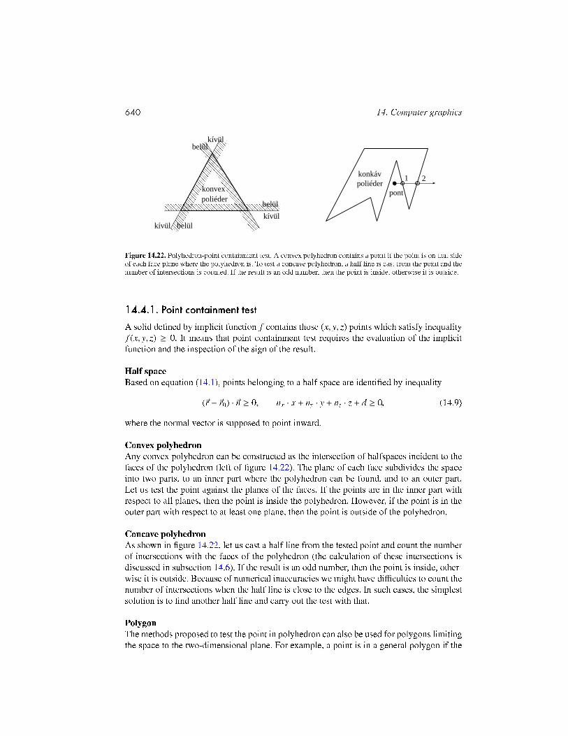
Figure 14.22. Polyhedron-point containment test. A convex polyhedron contains a point if the point is on that sideof each face plane where the polyhedron is. To test a concave polyhedron, a half line is cast from the point and thenumber of intersections is counted. If the result is an odd number, then the point is inside, otherwise it is outside.
14.4.1. Point containment testA solid dened by implicit function f contains those (x, y, z) points which satisfy inequalityf (x, y, z) ≥ 0. It means that point containment test requires the evaluation of the implicitfunction and the inspection of the sign of the result.
Half spaceBased on equation (14.1), points belonging to a half space are identied by inequality
(~r − ~r0) · ~n ≥ 0, nx · x + ny · y + nz · z + d ≥ 0, (14.9)
where the normal vector is supposed to point inward.
Convex polyhedronAny convex polyhedron can be constructed as the intersection of halfspaces incident to thefaces of the polyhedron (left of gure 14.22). The plane of each face subdivides the spaceinto two parts, to an inner part where the polyhedron can be found, and to an outer part.Let us test the point against the planes of the faces. If the points are in the inner part withrespect to all planes, then the point is inside the polyhedron. However, if the point is in theouter part with respect to at least one plane, then the point is outside of the polyhedron.
Concave polyhedronAs shown in gure 14.22, let us cast a half line from the tested point and count the numberof intersections with the faces of the polyhedron (the calculation of these intersections isdiscussed in subsection 14.6). If the result is an odd number, then the point is inside, other-wise it is outside. Because of numerical inaccuracies we might have difficulties to count thenumber of intersections when the half line is close to the edges. In such cases, the simplestsolution is to nd another half line and carry out the test with that.
PolygonThe methods proposed to test the point in polyhedron can also be used for polygons limitingthe space to the two-dimensional plane. For example, a point is in a general polygon if the
14.4. Containment algorithms 641
half line originating at this point and lying in the plane of the polygon intersects the edgesof the polygon odd times.
In addition to those methods, containment in convex polygons can be tested by addingthe angles subtended by the edges from the point. If the sum is 360 degrees, then the pointis inside, otherwise it is outside. For convex polygons, we can also test whether the point ison the same side of the edges as the polygon itself. This algorithm is examined in details fora particularly important special case, when the polygon is a triangle.
TriangleLet us consider a triangle of vertices ~a, ~b and ~c, and point ~p lying in the plane of the triangle.The point is inside the triangle if and only if it is on the same side of the boundary lines asthe third vertex. Note that cross product (~b − ~a) × (~p − ~a) has a different direction for point~p lying on the different sides of oriented line ~ab, thus the direction of this vector can beused to classify points (should point ~p be on line ~ab, the result of the cross product is zero).During classication the direction of (~b−~a)× (~p−~a) is compared to the direction of vector~n = (~b − ~a) × (~c − ~a) where tested point ~p is replaced by third vertex ~c. Note that vector ~nhappens to be the normal vector of the triangle plane (gure 14.23).
We can determine whether two vectors have the same direction (their angle is zero) orthey have opposite directions (their angle is 180 degrees) by computing their scalar productand looking at the sign of the result. The scalar product of vectors of similar directions ispositive. Thus if scalar product ((~b − ~a) × (~p − ~a)) · ~n is positive, then point ~p is on the sameside of oriented line ~ab as ~c. On the other hand, if this scalar product is negative, then ~p and~c are on the opposite sides. Finally, if the result is zero, then point ~p is on line ~ab. Point ~p isinside the triangle if and only if all the following three conditions are met:
((~b − ~a) × (~p − ~a)) · ~n ≥ 0 ,((~c − ~b) × (~p − ~b)) · ~n ≥ 0 ,((~a − ~c) × (~p − ~c)) · ~n ≥ 0 .
(14.10)
This test is robust since it gives correct result even if due to numerical precisionproblems point ~p is not exactly in the plane of the triangle as long as point ~p is in theprism obtained by perpendicularly extruding the triangle from the plane.
The evaluation of the test can be speeded up if we work in the two-dimensional projec-tions instead of the three-dimensional space. Let us project point ~p as well as the triangleonto one of the coordinate planes. In order to increase numerical precision, that coordinateplane should be selected on which the area of the projected triangle is maximal. Let us de-note the Cartesian coordinates of the normal vector by (nx, ny, nz). If nz has the maximumabsolute value, then the projection of the maximum area is on coordinate plane xy. If nx orny had the maximum absolute value, then planes yz, or xz would be the right choice. Hereonly the case of maximum nz is discussed.
First the order of vertices are changed in a way that when traveling from vertex ~a tovertex ~b, vertex ~c is on the left side. Let us examine the equation of line ~ab:
by − ay
bx − ax· (x − bx) + by = y .

642 14. Computer graphics
b
c
p
na-b a
-p a
-b a( ) )( -p a
-a c -p c( ) )(
-a c-p c
x
x
Figure 14.23. Point in triangle containment test. The gure shows that case when point ~p is on the left of orientedlines ~ab and ~bc, and on the right of line ~ca, that is, when it is not inside the triangle.
1.eset: ( b - a ) > 0
a
a
a
a
b
b
b
b
c c
c c
vagy
vagy
x x
2.eset: ( b - a ) < 0x x
Figure 14.24. Point in triangle containment test on coordinate plane xy. Third vertex ~c can be either on the leftor on the right side of oriented line ~ab, which can always be traced back to the case of being on the left side byexchanging the vertices.
According to gure 14.24 point ~c is on the left of the line if cy is above the line at x = cx:by − ay
bx − ax· (cx − bx) + by < cy .
Multiplying both sides by (bx − ax), we get:
(by − ay) · (cx − bx) < (cy − by) · (bx − ax) .
In the second case the denominator of the slope of the line is negative. Point ~c is on the leftof the line if cy is below the line at x = cx :
by − ay
bx − ax· (cx − bx) + by > cy .
When the inequality is multiplied with negative denominator (bx − ax), the relation is inver-ted:
(by − ay) · (cx − bx) < (cy − by) · (bx − ax) .

14.4. Containment algorithms 643
csúcs behatolás él behatolás
Figure 14.25. Polyhedron-polyhedron collision detection. Only a part of collision cases can be recognized bytesting the containment of the vertices of one object with respect to the other object. Collision can also occur whenonly edges meet, but vertices do not penetrate to the other object.
Note that in both cases we obtained the same condition. If this condition is not met, thenpoint ~c is not on the left of line ~ab, but is on the right. Exchanging vertices ~a and ~b in thiscase, we can guarantee that ~c will be on the left of the new line ~ab. It is also important tonote that consequently point ~a will be on the left of line ~bc and point ~b will be on the left ofline ~ca.
In the second step the algorithm tests whether point ~p is on the left with respect to allthree boundary lines since this is the necessary and sufficient condition of being inside thetriangle:
(by − ay) · (px − bx) ≤ (py − by) · (bx − ax) ,(cy − by) · (px − cx) ≤ (py − cy) · (cx − bx) ,(ay − cy) · (px − ax) ≤ (py − ay) · (ax − cx) .
(14.11)
14.4.2. Polyhedron-polyhedron collision detectionTwo polyhedra collide when a vertex of one of them meets a face of the other, and if they arenot bounced off, the vertex goes into the internal part of the other object (gure 14.25). Thiscase can be recognized with the discussed containment test. All vertices of one polyhedronis tested for containment against the other polyhedron. Then the roles of the two polyhedraare exchanged.
Apart from the collision between vertices and faces, two edges may also meet withoutvertex penetration (gure 14.25). In order to recognize this case, all edges of one polyhedronare tested against all faces of the other polyhedron. The test for an edge and a face is startedby checking whether or not the two endpoints of the edge are on opposite sides of theplane, using inequality (14.9). If they are, then the intersection of the edge and the plane iscalculated, and nally it is decided whether the face contains the intersection point.
Let us realize that the test of edge penetration and the containment of an arbitrary ver-tex also include the case of vertex penetration. However, edge penetration without vertexpenetration happens less frequently, and the vertex penetration is easier to check, thus it isstill worth applying the vertex penetration test rst.
Polyhedra collision detection tests each edge of one polyhedron against to each face ofthe other polyhedron, which results in an algorithm of quadratic time complexity with res-pect to the number of vertices of the polyhedra. Fortunately, the algorithm can be speededup applying bounding volumes (subsection 14.6.2). Let us assign a simple bounding object

644 14. Computer graphics
to each polyhedron. Popular choices are the spheres and the boxes. If the two boundingvolumes do not collide, then neither can the contained polyhedra collide. If the boundingvolumes penetrate each other, then one polyhedra is tested against the other bounding vo-lume. If this test is also positive, then nally the two polyhedra are tested. However, this lasttest is rarely required, and most of the collision cases can be solved by bounding volumes.
14.4.3. Clipping algorithmsClipping takes an object dening the clipping region and removes those points from anotherother object which are outside the clipping region. Clipping may alter the type of the object,which cannot be specied by a similar equation after clipping. To avoid this, we allow onlythose kinds of clipping regions and objects where the object type does not change. Let usthus assume that the clipping region is a half space or a polyhedron, while the object to beclipped is a point, a line segment or a polygon.
If the object to be clipped is a point, then containment can be tested with the algorithmsof the previous subsection. Based on the result of the containment test, the point is eitherremoved or preserved.
Clipping a line segment onto a half spaceLet us consider a line segment of endpoints ~r1 and ~r2, and of equation ~r(t) = ~r1 · (1− t)+~r2 · t,(t ∈ [0, 1]), and a half plane dened by the following equation derived from equation (14.1):
(~r − ~r0) · ~n ≥ 0, nx · x + ny · y + nz · z + d ≥ 0.
Three cases need to be distinguished:1. If both endpoints of the line segment are in the half space, then all points of the line
segment are inside, thus the whole segment is preserved.2. If both endpoints are out of the half space, then all points of the line segment are out,
thus the line segment should be completely removed.3. If one of the endpoints is out, while the other is in, then the endpoint being out should
be replaced by the intersection point of the line segment and the boundary plane of thehalf space. The intersection point can be calculated by substituting the equation of theline segment into the equation of the boundary plane and solving the resulting equationfor the unknown parameter:
(~r1 · (1 − ti) + ~r2 · ti − ~r0) · ~n = 0, =⇒ ti =(~r0 − ~r1) · ~n(~r2 − ~r1) · ~n .
Substituting parameter ti into the equation of the line segment, the coordinates of theintersection point can also be obtained.
Clipping a polygon onto a half spaceThis clipping algorithm tests rst whether a vertex is inside or not. If the vertex is in, thenit is also the vertex of the resulting polygon. However, if it is out, it can be ignored. On theother hand, the resulting polygon may have vertices other than the vertices of the originalpolygon. These new vertices are the intersections of the edges and the boundary plane of
14.4. Containment algorithms 645
p
p
p
p
pp
q
q
q
q
q
[1]
[4]
[3]
[5]
[4][0]
[0]
[3]
[1]
[2]
[2]vágósík
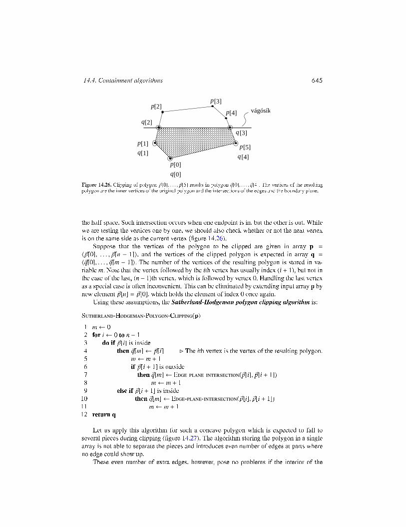
Figure 14.26. Clipping of polygon ~p[0], . . . , ~p[5] results in polygon ~q[0], . . . , ~q[4]. The vertices of the resultingpolygon are the inner vertices of the original polygon and the intersections of the edges and the boundary plane.
the half space. Such intersection occurs when one endpoint is in, but the other is out. Whilewe are testing the vertices one by one, we should also check whether or not the next vertexis on the same side as the current vertex (gure 14.26).
Suppose that the vertices of the polygon to be clipped are given in array p =
〈~p[0], . . . , ~p[n − 1]〉, and the vertices of the clipped polygon is expected in array q =
〈~q[0], . . . , ~q[m − 1]〉. The number of the vertices of the resulting polygon is stored in va-riable m. Note that the vertex followed by the ith vertex has usually index (i + 1), but not inthe case of the last, (n − 1)th vertex, which is followed by vertex 0. Handling the last vertexas a special case is often inconvenient. This can be eliminated by extending input array p bynew element ~p[n] = ~p[0], which holds the element of index 0 once again.
Using these assumptions, the Sutherland-Hodgeman polygon clipping algorithm is:
S-H-P-C(p)1 m← 02 for i← 0 to n − 13 do if ~p[i] is inside4 then ~q[m]← ~p[i] B The ith vertex is the vertex of the resulting polygon.5 m← m + 16 if ~p[i + 1] is outside7 then ~q[m]← E--(~p[i], ~p[i + 1])8 m← m + 19 else if ~p[i + 1] is inside
10 then ~q[m]← E--(~p[i], ~p[i + 1])11 m← m + 112 return q
Let us apply this algorithm for such a concave polygon which is expected to fall toseveral pieces during clipping (gure 14.27). The algorithm storing the polygon in a singlearray is not able to separate the pieces and introduces even number of edges at parts whereno edge could show up.
These even number of extra edges, however, pose no problems if the interior of the

646 14. Computer graphics
dupla határvonal
páros számúhatár
Figure 14.27. When concave polygons are clipped, the parts that should fall apart are connected by even numberof edges.
polygon is dened as follows: a point is inside the polygon if and only if starting a half linefrom here, the boundary polyline is intersected by odd number of times.
The presented algorithm is also suitable for clipping multiple connected polygons if thealgorithm is executed separately for each closed polyline of the boundary.
Clipping line segments and polygons on a convex polyhedronAs stated, a convex polyhedron can be obtained as the intersection of the half spaces denedby the planes of the polyhedron faces (left of gure 14.22). It means that the clipping on aconvex polyhedron can be traced back to a series of clipping steps on half spaces. The resultof one clipping step on a half plane is the input of clipping on the next half space. The nalresult is the output of the clipping on the last half space.
Clipping a line segment on an AABBAxis aligned bounding boxes, abbreviated as AABBs, play an important role in image synt-hesis.
Denition 14.11 A box aligned parallel to the coordinate axes is called AABB.An AABB is specied with the minimum and maximum Cartesian coordinates:[xmin, ymin, zmin, xmax, ymax, zmax].
Although when an object is clipped on an AABB, the general algorithms clipping ona convex polyhedron could also be used, the importance of AABBs is acknowledged bydeveloping algorithms specially tuned for this case.
When a line segment is clipped to a polyhedron, the algorithm would test the line seg-ment with the plane of each face, and calculated intersection points may turn out to be un-necessary later. We should thus nd an appropriate order of planes which makes the numberof unnecessary intersection calculations minimal. A simple method implementing this ideais the Cohen-Sutherland line clipping algorithm.
Let us assign code bit 1 to a point that is outside with respect to a clipping plane, andcode bit 0 if the point is inside with respect to this plane. Since an AABB has 6 sides,we get 6 bits forming a 6-bit code word (gure 14.28). The interpretation of code bitsC[0], . . . ,C[5] is the following:
C[0] =
1, x ≤ xmin,0 otherwise. C[1] =
1, x ≥ xmax,0 otherwise. C[2] =
1, y ≤ ymin ,0 otherwise .

14.4. Containment algorithms 647
000000
100010
101000101000
010100
000000
00000001
1001
0101 0100
0010
0110
10101000
Figure 14.28. The 4-bit codes of the points in a plane and the 6-bit codes of the points in space.
C[3] =
1, y ≥ ymax,0 otherwise. C[4] =
1, z ≤ zmin,0 otherwise. C[5] =
1, z ≥ zmax ,0 otherwise .
Points of code word 000000 are obviously inside, points of other code words are outside(gure 14.28). Let the code words of the two endpoints of the line segment be C1 and C2,respectively. If both of them are zero, then both endpoints are inside, thus the line segmentis completely inside (trivial accept). If the two code words contain bit 1 at the same location,then none of the endpoints are inside with respect to the plane associated with this code bit.This means that the complete line segment is outside with respect to this plane, and canbe rejected (trivial reject). This examination can be executed by applying the bitwise ANDoperation on code words C1 and C2 (with the notations of the C programming language C1& C2), and checking whether or not the result is zero. If it is not zero, there is a bit whereboth code words have value 1.
Finally, if none of the two trivial cases hold, then there must be a bit which is 0 in onecode word and 1 in the other. This means that one endpoint is inside and the other is outsidewith respect to the plane corresponding to this bit. The line segment should be clipped onthis plane. Then the same procedure should be repeated starting with the evaluation of thecode bits. The procedure is terminated when the conditions of either the trivial accept or thetrivial reject are met.
The Cohen-Sutherland line clipping algorithm returns the endpoints of the clipped lineby modifying the original vertices and indicates with true return value if the line is notcompletely rejected:
648 14. Computer graphics
C-S-L-C(~r1,~r2)1 C1 ← codeword of ~r1 B Code bits by checking the inequalities.2 C2 ← codeword of ~r23 while
4 do if C1 = 0 AND C2 = 05 then return B Trivial accept: inner line segment exists.6 if C1 & C2 , 07 then return B Trivial reject: no inner line segment exists.8 f ← index of the rst bit where C1 and C2 differ9 ~ri ← intersection of line segment (~r1, ~r2) and the plane of index f
10 Ci ← codeword of ~ri11 if C1[ f ] = 112 then ~r1 ← ~ri13 C1 ← Ci B ~r1 is outside w.r.t. plane f .14 else ~r2 ← ~ri15 C2 ← Ci B ~r2 is outside w.r.t. plane f .
Exercises14.4-1 Propose approaches to reduce the quadratic complexity of polyhedron-polyhedroncollision detection.14.4-2 Develop a containment test to check whether a point is in a CSG-tree .14.4-3 Develop an algorithm clipping one polygon onto a concave polygon.14.4-4 Find an algorithm computing the bounding sphere and the bounding AABB of apolyhedron.14.4-5 Develop an algorithm that tests the collision of two triangles in the plane.14.4-6 Generalize the Cohen-Sutherland line clipping algorithm to convex polyhedron clip-ping region.14.4-7 Propose a method for clipping a line segment on a sphere.
14.5. Translation, distortion, geometric transformationsObjects in the virtual world may move, get distorted, grow or shrink, that is, their equationsmay also depend on time. To describe dynamic geometry, we usually apply two functions.The rst function selects those points of space, which belong to the object in its referencestate. The second function maps these points onto points dening the object in an arbitrarytime instance. Functions mapping the space onto itself are called transformations. A trans-formation maps point ~r to point ~r ′ = T (~r). If the transformation is invertible, we can alsond the original for some transformed point ~r ′ using inverse transformation T −1(~r ′).
If the object is dened in its reference state by implicit equation f (~r) ≥ 0, then theequation of the transformed object is
~r ′ : f (T −1(~r ′)) ≥ 0 , (14.12)
since the originals belong to the set of points of the reference state.

14.5. Translation, distortion, geometric transformations 649
Parametric equations dene the Cartesian coordinates of the points directly. Thus thetransformation of parametric surface ~r = ~r(u, v) requires the transformations of its points
~r ′(u, v) = T (~r(u, v)) . (14.13)
Similarly, the transformation of curve ~r = ~r(t) is:
~r ′(t) = T (~r(t)) . (14.14)
Transformation T may change the type of object in the general case. It can happen,for example, that a simple triangle or a sphere becomes a complicated shape, which arehard to describe and handle. Thus it is worth limiting the set of allowed transformations.Transformations mapping planes onto planes, lines onto lines and points onto points areparticularly important. In the next subsection we consider the class of homogenous lineartransformations, which meet this requirement.
14.5.1. Projective geometry and homogeneous coordinatesSo far the construction of the virtual world has been discussed using the means of the Eucli-dean geometry, which gave us many important concepts such as distance, parallelism, angle,etc. However, when the transformations are discussed in details, many of these concepts areunimportant, and can cause confusion. For example, parallelism is a relationship of two lineswhich can lead to singularities when the intersection of two lines is considered. Therefore,transformations are discussed in the context of another framework, the projective geometry.
The axioms of projective geometry turn around the problem of parallel lines by igno-ring the concept of parallelism altogether, and state that two different lines always have anintersection. To cope with this requirement, every line is extended by a point in innitysuch that two lines have the same extra point if and only if the two lines are parallel. Theextra point is called the ideal point. The projective space contains the points of the Eucli-dean space (these are the so called affine points) and the ideal points. An ideal point gluesthe ends of an Euclidean line, making it topologically similar to a circle. Projective geo-metry preserves that axiom of the Euclidean geometry which states that two points dene aline. In order to make it valid for ideal points as well, the set of lines of the Euclidean spaceis extended by a new line containing the ideal points. This new line is called the ideal line.Since the ideal points of two lines are the same if and only if the two lines are parallel, theideal lines of two planes are the same if and only if the two planes are parallel. Ideal linesare on the ideal plane, which is added to the set of planes of the Euclidean space. Havingmade these extensions, no distinction is needed between the affine and ideal points. Theyare equal members of the projective space.
Introducing analytic geometry we noted that everything should be described by num-bers in computer graphics. Cartesian coordinates used so far are in one to one relationshipwith the points of Euclidean space, thus they are inappropriate to describe the points of theprojective space. For the projective plane and space, we need a different algebraic base.
Projective planeLet us consider rst the projective plane and nd a method to describe its points by numbers.To start, a Cartesian coordinate system x, y is set up in this plane. Simultaneously, another

650 14. Computer graphics
h=1
[x h,y h,h] egyenes
[X ,Y ,0] ponth h
. .
Xh
Yh
h
[x,y,1]
[X ,Y ,h] ponth h
Figure 14.29. The embedded model of the projective plane: the projective plane is embedded into a three-dimensional Euclidean space, and a correspondence is established between points of the projective plane andlines of the embedding three-dimensional Euclidean space by tting the line to the origin of the three-dimensionalspace and the given point.
Cartesian system Xh,Yh, h is established in the three-dimensional space embedding the planein a way that axes Xh,Yh are parallel to axes x, y, the plane is perpendicular to axis h, theorigin of the Cartesian system of the plane is in point (0, 0, 1) of the three-dimensional space,and the points of the plane satisfy equation h = 1. The projective plane is thus embeddedinto a three-dimensional Euclidean space where points are dened by Descartes-coordinates(gure 14.29). To describe a point of the projective plane by numbers, a correspondence isfound between the points of the projective plane and the points of the embedding Euclideanspace. An appropriate correspondence assigns that line of the Euclidean space to eitheraffine or ideal point P of the projective plane which is dened by the origin of the coordinatesystem of the space and point P.
Points of a line in the Euclidean space can be given by parametric equation [t · Xh, t ·Yh, t · h] where t is a free real parameter. If point P is an affine point of the projective plane,then the corresponding line is not parallel with plane h = 1 (i.e. h is not constant zero).Such line intersects the plane of equation h = 1 at point [Xh/h,Yh/h, 1], thus the Cartesiancoordinates of point P in planar coordinate system x, y are (Xh/h,Yh/h). On the other hand,if point P is ideal, then the corresponding line is parallel to the plane of equation h = 1 (i.e.h = 0). The direction of the ideal point is given by vector (Xh,Yh).
The presented approach assigns three dimensional lines and eventually [Xh,Yh, h] trip-lets to both the affine and the ideal points of the projective plane. These triplets are calledthe homogenous coordinates of a point in the projective plane. Homogeneous coordinatesare enclosed by brackets to distinguish them from Cartesian coordinates.
A three-dimensional line crossing the origin and describing a point of the projectiveplane can be dened by its arbitrary point except from the origin. Consequently, all threehomogeneous coordinates cannot be simultaneously zero, and homogeneous coordinatescan be freely multiplied by the same non-zero scalar without changing the described point.This property justies the name homogenous.
It is often convenient to select that triplet from the homogeneous coordinates of anaffine point, where the third homogeneous coordinate is 1 since in this case the rst twohomogeneous coordinates are identical to the Cartesian coordinates:
Xh = x, Yh = y, h = 1 . (14.15)
From another point of view, Cartesian coordinates of an affine point can be converted to

14.5. Translation, distortion, geometric transformations 651
homogenous coordinates by extending the pair by a third element of value 1.The embedded model also provides means to dene the equations of the lines and
line segments of the projective space. Let us select two different points on the projectiveplane and specify their homogeneous coordinates. The two points are different if homoge-neous coordinates [X1
h ,Y1h , h1] of the rst point cannot be obtained as a scalar multiple of
homogeneous coordinates [X2h ,Y2
h , h2] of the other point. In the embedding space, triplet[Xh,Yh, h] can be regarded as Cartesian coordinates, thus the equation of the line tted topoints [X1
h ,Y1h , h1] and [X2
h ,Y2h , h2] is:
Xh(t) = X1h · (1 − t) + X2
h · t ,Yh(t) = Y1
h · (1 − t) + Y2h · t , (14.16)
h(t) = h1 · (1 − t) + h2 · t .If h(t) , 0, then the affine points of the projective plane can be obtained by projectingthe three-dimensional space onto the plane of equation h = 1. Requiring the two points bedifferent, we excluded the case when the line would be projected to a single point. Henceprojection maps lines to lines. Thus the presented equation really identies the homogene-ous coordinates dening the points of the line. If h(t) = 0, then the equation expresses theideal point of the line.
If parameter t has an arbitrary real value, then the points of a line are dened. If para-meter t is restricted to interval [0, 1], then we obtain the line segment dened by the twoendpoints.
Projective spaceWe could apply the same method to introduce homogeneous coordinates of the projectivespace as we used to dene the homogeneous coordinates of the projective plane, but thisapproach would require the embedding of the three-dimensional projective space into afour-dimensional Euclidean space, which is not intuitive. We would rather discuss anotherconstruction, which works in arbitrary dimensions. In this construction, a point is describedas the centre of mass of a mechanical system. To identify a point, let us place weight Xhat reference point ~p1, weight Yh at reference point ~p2, weight Zh at reference point ~p3, andweight w at reference point ~p4. The centre of mass of this mechanical system is:
~r =Xh · ~p1 + Yh · ~p2 + Zh · ~p3 + w · ~p4
Xh + Yh + Zh + w .
Let us denote the total weight by h = Xh + Yh + Zh + w. By denition, elements of quadruple[Xh,Yh,Zh, h] are the homogeneous coordinates of the centre of mass.
To nd the correspondence between homogeneous and Cartesian coordinates, the rela-tionship of the two coordinate systems (the relationship of the basis vectors and the originof the Cartesian coordinate system and of the reference points of the homogeneous coordi-nate system) must be established. Let us assume, for example, that the reference points ofthe homogenous coordinate system are in points (1,0,0), (0,1,0), (0,0,1), and (0,0,0) of theCartesian coordinate system. The centre of mass (assuming that total weight h is not zero)is expressed in Cartesian coordinates as follows:
~r[Xh,Yh,Zh, h] =1h · (Xh · (1, 0, 0) + Yh · (0, 1, 0) + Zh · (0, 0, 1) + w · (0, 0, 0)) =
(Xhh ,
Yhh ,
Zhh
).

652 14. Computer graphics
Hence the correspondence between homogeneous coordinates [Xh,Yh,Zh, h] and Cartesiancoordinates (x, y, z) is (h , 0):
x =Xhh , y =
Yhh , z =
Zhh . (14.17)
The equations of lines in the projective space can be obtained either deriving themfrom the embedding four-dimensional Cartesian space, or using the centre of mass analogy:
Xh(t) = X1h · (1 − t) + X2
h · t ,Yh(t) = Y1
h · (1 − t) + Y2h · t ,
Zh(t) = Z1h · (1 − t) + Z2
h · t , (14.18)h(t) = h1 · (1 − t) + h2 · t .
If parameter t is restricted to interval [0, 1], then we obtain the equation of the projectiveline segment.
To nd the equation of the projective plane, the equation of the Euclidean plane isconsidered (equation 14.1). The Cartesian coordinates of the points on a plane satisfy thefollowing implicit equation
nx · x + ny · y + nz · z + d = 0 .
Using the correspondence between the Cartesian and homogenous coordinates (equation14.17) we still describe the points of the Euclidean plane but now with homogenous coor-dinates:
nx · Xhh + ny · Yh
h + nz · Zhh + d = 0 .
Let us multiply both sides of this equation by h, and add those points to the plane which haveh = 0 coordinate and satisfy this equation. With this step the set of points of the Euclideanplane is extended with the ideal points, that is, we obtained the set of points belonging tothe projective plane. Hence the equation of the projective plane is a homogenous linearequation:
nx · Xh + ny · Yh + nz · Zh + d · h = 0 , (14.19)or in matrix form:
[Xh,Yh,Zh, h] ·
nxnynzd
= 0 . (14.20)
Note that points and planes are described by row and column vectors, respectively. Both thequadruples of points and the quadruples of planes have the homogeneous property, that is,they can be multiplied by non-zero scalars without altering the solutions of the equation.
14.5.2. Homogenous linear transformationsTransformations dened as the multiplication of the homogenous coordinate vector of apoint by a constant 4 × 4 T matrix are called homogeneous linear transformations:
[X′h,Y ′h,Z′h, h′] = [Xh,Yh,Zh, h] · T . (14.21)

14.5. Translation, distortion, geometric transformations 653
Theorem 14.12 Homogeneous linear transformations map points to points.
Proof. A point can be dened by homogeneous coordinates in form λ · [Xh,Yh,Zh, h], whereλ is an arbitrary, non-zero constant. The transformation results in λ · [X′h,Y ′h,Z′h, h′] = λ ·[Xh,Yh,Zh, h] ·T when a point is transformed, which are the λ-multiples of the same vector,thus the result is a single point in homogeneous coordinates.
Note that due to the homogeneous property, homogeneous transformation matrix T isnot unambiguous, but can be freely multiplied by non-zero scalars without modifying therealized mapping.
Theorem 14.13 Invertible homogeneous linear transformations map lines to lines.
Proof. Let us consider the parametric equation of a line:
[Xh(t),Yh(t),Zh(t), h(t)] = [X1h ,Y1
h ,Z1h , h1] · (1 − t) + [X2
h ,Y2h ,Z2
h , h2] · t, t = (−∞,∞) ,
and transform the points of this line by multiplying the quadruples with the transformationmatrix:
[X′h(t),Y ′h(t),Z′h(t), h′(t)] = [Xh(t),Yh(t),Zh(t), h(t)] · T
= [X1h ,Y1
h ,Z1h , h1] · T · (1 − t) + [X2
h ,Y2h ,Z2
h , h2] · T · t
= [X1h′,Y1
h′,Z1
h′, h1′] · (1 − t) + [X2
h′,Y2
h′,Z2
h′, h2′] · t ,
where [X1h′,Y1
h′,Z1
h′, h1′] and [X2
h′,Y2
h′,Z2
h′, h2′] are the transformations of [X1
h ,Y1h ,Z1
h , h1]and [X2
h ,Y2h ,Z2
h , h2], respectively. Since the transformation is invertible, the two points aredifferent. The resulting equation is the equation of a line tted to the transformed points.
We note that if we had not required the invertibility of the the transformation, then itcould have happened that the transformation would have mapped the two points to the samepoint, thus the line would have degenerated to single point.
If parameter t is limited to interval [0, 1], then we obtain the equation of the projectiveline segment, thus we can also state that a homogeneous linear transformation maps a linesegment to a line segment. Even more generally, a homogeneous linear transformation mapsconvex combinations to convex combinations. For example, triangles of the projective planeare mapped to triangles.
However, we have to be careful when we try to apply this theorem in the Euclideanplane or space. Let us consider a line segment as an example. If coordinate h has differentsign at the two endpoints, then the line segment contains an ideal point. Such projectiveline segment can be intuitively imagined as two half lines and an ideal point sticking theendpoints of these half lines at innity, that is, such line segment is the complement of theline segment we are accustomed to. It may happen that before the transformation coordinatesh of the endpoints have similar sign, that is, the line segment meets our intuitive image aboutEuclidean line segments, but after the transformation, coordinates h of the endpoints willhave different sign. Thus the transformation wraps around our line segment.
Theorem 14.14 Invertible linear transformations map planes to planes.

654 14. Computer graphics
Proof. The originals of transformed points [X′h,Y ′h,Z′h, h′] dened by [Xh,Yh,Zh, h] =
[X′h,Y ′h,Z′h, h′] · T−1 are on a plane, thus satisfy the original equation of the plane:
[Xh,Yh,Zh, h] ·
nxnynzd
= [X′h,Y ′h,Z′h, h′] · T−1 ·
nxnynzd
= 0 .
Due to the associativity of matrix multiplication, the transformed points also satisfy equation
[X′h,Y ′h,Z′h, h′] ·
n′xn′yn′zd′
= 0 ,
which is also a plane equation, where
n′xn′yn′zd′
= T−1 ·
nxnynzd
.
This result can be used to obtain the normal vector of a transformed plane.An important subclass of homogeneous linear transformations is the set of affine trans-
formations, where the Cartesian coordinates of the transformed point are linear functionsof the original Cartesian coordinates:
[x′, y′, z′] = [x, y, z] · A + [px, py, pz] , (14.22)
where vector ~p describes translation, A is a matrix of size 3 × 3 and expresses rotation,scaling, mirroring, etc., and their arbitrary combination. For example, the rotation aroundaxis (tx, ty, tz), (|(tx, ty, tz)| = 1) by angle φ is given by the following matrix
A =
(1 − t2
x) cos φ + t2x txty(1 − cos φ) + tz sin φ txtz(1 − cos φ) − ty sin φ
tytx(1 − cos φ) − tz sin φ (1 − t2y ) cos φ + t2
y txtz(1 − cos φ) + tx sin φtztx(1 − cos φ) + ty sin φ tzty(1 − cos φ) − tx sin φ (1 − t2
z ) cos φ + t2z
.
This expression is known as the Rodrigues formula.Affine transformations map the Euclidean space onto itself, and transform parallel lines
to parallel lines. Affine transformations are also homogeneous linear transformations sinceequation (14.22) can also be given as a 4×4 matrix operation, having changed the Cartesiancoordinates to homogeneous coordinates by adding a fourth coordinate of value 1:
[x′, y′, z′, 1] = [x, y, z, 1] ·
A11 A12 A13 0A21 A22 A23 0A31 A32 A33 0px py pz 1
= [x, y, z, 1] · T . (14.23)
A further specialization of affine transformations is the set of congruence transforma-tions (isometries) which are distance and angle preserving.

14.6. Rendering with ray tracing 655
Theorem 14.15 In a congruence transformation the rows of matrix A have unit length andare orthogonal to each other.
Proof. Let us use the property that a congruence is distance and angle preserving for thecase when the origin and the basis vectors of the Cartesian system are transformed. Thetransformation assigns point (px, py, pz) to the origin and points (A11 + px, A12 + py, A13 +
pz), (A21 + px, A22 + py, A23 + pz), and (A31 + px, A32 + py, A33 + pz) to points (1, 0, 0),(0, 1, 0), and (0, 0, 1), respectively. Because the distance is preserved, the distances betweenthe new points and the new origin are still 1, thus |A11, A12, A13| = 1, |A21, A22, A23| = 1,and |A31, A32, A33| = 1. On the other hand, because the angle is also preserved, vectors(A11, A12, A13), (A21, A22, A23), and (A31, A32, A33) are also perpendicular to each other.
Exercises14.5-1 Using the Cartesian coordinate system as an algebraic basis, prove the axioms of theEuclidean geometry, for example, that two points dene a line, and that two different linesmay intersect each other at most at one point.14.5-2 Using the homogenous coordinates as an algebraic basis, prove an axiom of the pro-jective geometry stating that two different lines intersect each other in exactly one point.14.5-3 Prove that homogeneous linear transformations map line segments to line segmentsusing the centre of mass analogy.14.5-4 How does an affine transformation modify the volume of an object?14.5-5 Give the matrix of that homogeneous linear transformation which translates by vec-tor ~p.14.5-6 Prove the Rodrigues formula.14.5-7 A solid dened by equation f (~r) ≥ 0 in time t = 0 moves with uniform constantvelocity ~v. Let us nd the equation of the solid at an arbitrary time instance t.14.5-8 Prove that if the rows of matrix A are of unit length and are perpendicular to eachother, then the affine transformation is a congruence. Show that for such matrices A−1 = AT .
14.5-9 Give that homogeneous linear transformation which projects the space from point ~conto a plane of normal ~n and place vector ~r0.14.5-10 Show that ve point correspondences unambiguously identify a homogeneous li-near transformation if no four points are co-planar.
14.6. Rendering with ray tracingWhen a virtual world is rendered, we have to identify the surfaces visible in different direc-tions from the virtual eye. The set of possible directions is dened by a rectangle shapedwindow which is decomposed to a grid corresponding to the pixels of the screen (gure14.30). Since a pixel has a unique colour, it is enough to solve the visibility problem in asingle point of each pixel, for example, in the points corresponding to pixel centres.
The surface visible at a direction from the eye can be identied by casting a half line,called ray, from the eye at that direction and identifying its intersection closest to the eyeposition. This operation is called ray tracing.
Ray tracing has many applications. For example, shadow computation tests whether or

656 14. Computer graphics
Figure 14.30. Ray tracing
not a point is occluded from the light source, which requires a ray to be sent from the pointat the direction of the light source and the determination whether this ray intersects anysurface closer than the light source. Ray tracing is also used by collision detection since apoint moving with constant and uniform speed collides that surface which is rst intersectedby the ray describing the motion of the point.
A ray is dened by the following equation:
~ray(t) = ~s + ~v · t, (t > 0) , (14.24)
where ~s is the place vector of the ray origin, ~v is the direction of the ray, and ray parametert characterizes the distance from the origin. Let us suppose that direction vector ~v has unitlength. In this case parameter t is the real distance, otherwise it would only be proportional tothe distance3. If parameter t is negative, then the point is behind the eye and is obviously notvisible. The identication of the closest intersection with the ray means the determinationof the intersection point having the smallest, positive ray parameter. In order to nd theclosest intersection, the intersection calculation is tried with each surface, and the closest isretained. This algorithm is presented in the followings:
3In collision detection ~v is not a unit vector, but the velocity of the moving point since this makes ray parameter texpress the collision time.
14.6. Rendering with ray tracing 657
R-F-I(~s,~v)1 t ← tmax B initialization to the maximum size in the virtual world.2 for each object o3 do to ←R-S-I(~s,~v) B negative if no intersection exists.4 if 0 ≤ to < t B is the new intersection closer?5 then t ← to B ray parameter of the closest intersection so far.6 ovisible ← o B closest object so far.7 if t < tmax then B has been intersection at all?8 then ~x← ~s + ~v · t B intersection point using the ray equation.9 return t, ~x, ovisible
10 else return no intersection B no intersection.
This algorithm inputs the ray dened by origin ~s and direction ~v, and outputs the rayparameter of the intersection in variable t, the intersection point in ~x, and the visible objectin ovisible. The algorithm calls function R-- for each object, which de-termines the intersection of the ray and the given object, and indicates with a negative returnvalue if no intersection exists. Function R-- should be implementedseparately for each surface type.
14.6.1. Ray-surface intersection calculationThe identication of the intersection between a ray and a surface requires the solution of anequation. The intersection point is both on the ray and on the surface, thus it can be obtai-ned by inserting the ray equation into the equation of the surface and solving the resultingequation for the unknown ray parameter.
Intersection calculation for implicit surfacesFor implicit surfaces of equation f (~r) = 0, the intersection can be calculated by solving thefollowing scalar equation for t: f (~s + ~v · t) = 0 .
Let us take the example of quadrics that include the sphere, the ellipsoid, the cylinder,the cone, the paraboloid, etc. The implicit equation of a general quadric contains a quadraticform:
[x, y, z, 1] ·Q ·
xyz1
= 0 ,
where Q is a 4× 4 matrix. Substituting the ray equation into the equation of the surface, weobtain
[sx + vx · t, sy + vy · t, sz + vz · t, 1] ·Q ·
sx + vx · tsy + vy · tsz + vz · t
1
= 0 .
Rearranging the terms, we get a second order equation for unknown parameter t:
t2 · (v ·Q · vT ) + t · (s ·Q · vT + v ·Q · sT ) + (s ·Q · sT ) = 0 ,
658 14. Computer graphics
where v = [vx, vy, vz, 0] and s = [sx, sy, sz, 1].This equation can be solved using the solution formula of second order equations. Now
we are interested in only the real and positive roots. If two such roots exist, then the smallerone corresponds to the intersection closer to the origin of the ray.
Intersection calculation for parametric surfacesThe intersection of parametric surface ~r = ~r(u, v) and the ray is calculated by rst solvingthe following equation for unknown parameters u, v, t
~r(u, v) = ~s + t · ~v ,
then checking whether or not t is positive and parameters u, v are inside the allowed para-meter range of the surface.
Roots of non-linear equations are usually found by numeric methods. On the otherhand, the surface can also be approximated by a triangle mesh, which is intersected by theray. Having obtained the intersection on the coarse mesh, the mesh around this point isrened, and the intersection calculation is repeated with the rened mesh.
Intersection calculation for a triangleTo compute the ray intersection for a triangle of vertices ~a, ~b, and ~c, rst the ray intersectionwith the plane of the triangle is found. Then it is decided whether or not the intersectionpoint with the plane is inside the triangle. The normal and a place vector of the triangleplane are ~n = (~b − ~a) × (~c − ~a), and ~a, respectively, thus points ~r of the plane satisfy thefollowing equation:
~n · (~r − ~a) = 0 . (14.25)
The intersection of the ray and this plane is obtained by substituting the ray equation(equation (14.24)) into this plane equation, and solving it for unknown parameter t. If root t∗is positive, then it is inserted into the ray equation to get the intersection point with the plane.However, if the root is negative, then the intersection is behind the origin of the ray, thusis invalid. Having a valid intersection with the plane of the triangle, we check whether thispoint is inside the triangle. This is a containment problem, which is discussed in subsection14.4.1.
Intersection calculation for an AABBThe surface of an AABB, that is an axis aligned block, can be subdivided to 6 rectangularfaces, or alternatively to 12 triangles, thus its intersection can be solved by the algorithmsdiscussed in the previous subsections. However, realizing that in this special case the threecoordinates can be handled separately, we can develop more efficient approaches. In fact, anAABB is the intersection of an x-stratum dened by inequality xmin ≤ x ≤ xmax, a y-stratumdened by ymin ≤ y ≤ ymax and a z-stratum of inequality zmin ≤ z ≤ zmax. For example, theray parameter of the intersection with the x-stratum is:
t1x =
xmin − sxvx
, t2x =
xmax − sxvx
.
The smaller of the two parameter values corresponds to the entry at the stratum, while thegreater to the exit. Let us denote the ray parameter of the entry by tin, and the ray parameter

14.6. Rendering with ray tracing 659
of the exit by tout. The ray is inside the x-stratum while the ray parameter is in [tin, tout].Repeating the same calculation for the y and z-strata as well, three ray parameter intervalsare obtained. The intersection of these intervals determine when the ray is inside the AABB.If parameter tout obtained as the result of intersecting the strata is negative, then the AABBis behind the eye, thus no rayAABB intersection is possible. If only tin is negative, then theray starts at an internal point of the AABB, and the rst intersection is at tout. Finally, if tinis positive, then the ray enters the AABB from outside at parameter tin.
The computation of the unnecessary intersection points can be reduced by applying theCohen Sutherland line clipping algorithm (subsection 14.4.3). First, the ray is replaced bya line segment where one endpoint is the origin of the ray, and the other endpoint is anarbitrary point on the ray which is farther from the origin than any object of the virtualworld.
14.6.2. Speeding up the intersection calculationA naive ray tracing algorithm tests each object for a ray to nd the closest intersection.If there are N objects in the space, the running time of the algorithm is Θ(N) both in theaverage and in the worst case. The storage requirement is also linear in terms of the numberof objects.
The method would be speeded up if we could exclude certain objects from the intersec-tion test without testing them one by one. The reasons of such exclusion include that theseobjects are behind the ray or not in the direction of the ray. Additionally, the speedis also expected to improve if we can terminate the search having found an intersectionsupposing that even if other intersections exist, they are surely farther than the just foundintersection point. To make such decisions safely, we need to know the arrangement of ob-jects in the virtual world. This information is gathered during the pre-processing phase. Ofcourse, pre-processing has its own computational cost, which is worth spending if we haveto trace a lot of rays.
Bounding volumesOne of the simplest ray tracing acceleration technique uses bounding volumes. The boun-ding volume is a shape of simple geometry, typically a sphere or an AABB, which comp-letely contains a complex object. When a ray is traced, rst the bounding volume is triedto be intersected. If there is no intersection with the bounding volume, then neither can thecontained object be intersected, thus the computation time of the ray intersection with thecomplex object is saved. The bounding volume should be selected in a way that the rayintersection is computationally cheap, and it is a tight container of the complex object.
The application of bounding volumes does not alter the linear time complexity of thenaive ray tracing. However, it can increase the speed by a scalar factor.
On the other hand, bounding volumes can also be organized in a hierarchy puttingbounding volumes inside bigger bounding volumes recursively. In this case the ray tracingalgorithm traverses this hierarchy, which is possible in sub-linear time.
Space subdivision with uniform gridsLet us nd the AABB of the complete virtual world and subdivide it by an axis aligneduniform grid of cell sizes (cx, cy, cz) (gure 14.31).

660 14. Computer graphics
c
c
x
y
c /vx x c /vy y
v
(x ,y ,z )min min min
Figure 14.31. Partitioning the virtual world by a uniform grid. The intersections of the ray and the coordinateplanes of the grid are at regular distances cx/vx,cy/vy, and cz/vz, respectively.
In the preprocessing phase, for each cell we identify those objects that are at least par-tially contained by the cell. The test of an object against a cell can be performed using aclipping algorithm (subsection 14.4.3), or simply checking whether the cell and the AABBof the object overlap.
U-G-C()1 Compute the minimum corner of the AABB (xmin, ymin, zmin) and cell sizes (cx, cy, cz)2 for each cell c3 do object list of cell c← empty4 for each object o B register objects overlapping with this cell.5 do if cell c and the AABB of object o overlap6 then add object o to object list of cell c
During ray tracing, cells intersected by the ray are visited in the order of their distancefrom the ray origin. When a cell is processed, only those objects need to be tested forintersection which overlap with this cell, that is, which are registered in this cell. On theother hand, if an intersection is found in the cell, then intersections belonging to other cellscannot be closer to the ray origin than the found intersection. Thus the cell marching can beterminated. Note that when an object registered in a cell is intersected by the ray, we shouldalso check whether the intersection point is also in this cell.
We might meet an object again in other cells. The number of raysurface intersectioncan be reduced if the results of raysurface intersections are stored with the objects and arereused when needed again.
As long as no raysurface intersection is found, the algorithm traverses those cellswhich are intersected by the ray. Indices X,Y,Z of the rst cell are computed from rayorigin ~s, minimum corner (xmin, ymin, zmin) of the grid, and sizes (cx, cy, cz) of the cells:

14.6. Rendering with ray tracing 661
U-G-E-C(~s)1 X ← I((sx − xmin)/cx)2 Y ← I((sy − ymin)/cy)3 Z ← I((sz − zmin)/cz)4 return X,Y,Z
The presented algorithm assumes that the origin of the ray is inside the subspace cove-red by the grid. Should this condition not be met, then the intersection of the ray and thescene AABB is computed, and the ray origin is moved to this point.
The initial values of ray parameters tx, ty, tz are computed as the intersection of the rayand the coordinate planes by the U---- algorithm:
U-G-R-P-I(~s,~v, X,Y,Z)1 if vx > 02 then tx ← (xmin + (X + 1) · cx − sx)/vx3 else if vx < 04 then tx ← (xmin + X · cx − sx)/vx5 else tx ← tmax B The maximum distance.6 if vy > 07 then ty ← (ymin + (Y + 1) · cy − sy)/vy8 else if vy < 09 then ty ← (ymin + Y · cy − sy)/vy
10 else ty ← tmax11 if vz > 012 then tz ← (zmin + (Z + 1) · cz − sz)/vz13 else if vz < 014 then tz ← (zmin + Z · cz − sz)/vz15 else tz ← tmax16 return tx, ty, tz
The next cell of the sequence of the visited cells is determined by the 3D line drawingalgorithm (3DDDA algorithm). This algorithm exploits the fact that the ray parameters ofthe intersection points with planes perpendicular to axis x (and similarly to axes y and z) areregularly placed at distance cx/vx (cy/vy, and cz/vz, respectively), thus the ray parameter ofthe next intersection can be obtained with a single addition (gure 14.31). Ray parameters tx,ty, and tz are stored in global variables, and are incremented by constant values. The smallestfrom the three ray parameters of the coordinate planes identies the next intersection withthe cell.
The following algorithm computes indices X,Y,Z of the next intersected cell, and up-dates ray parameters tx, ty, tz:

662 14. Computer graphics
U-G-N-C(X,Y,Z, tx, ty, tz)1 if tx = min(tx, ty, tz) B Next intersection is on the plane perpendicular to axis x.2 then X ← X + sgn(vx) B function sgn(x) returns the sign.3 tx ← tx + cx/|vx|4 else if ty = min(tx, ty, tz) B Next intersection is on the plane perpendicular to axis y.5 then Y ← Y + sgn(vy)6 ty ← ty + cy/|vy|7 else if tz = min(tx, ty, tz) B Next intersection is on the plane perpendicular to axis z.8 then Z ← Z + sgn(vz)9 tz ← tz + cz/|vz|
To summarize, a complete ray tracing algorithm is presented, which exploits the uni-form grid generated during preprocessing and computes the raysurface intersection closestto the ray origin. The minimum of ray parameters assigned to the coordinate planes, vari-able tout, determines the distance as far as the ray is inside the cell. This parameter is usedto decide whether or not a ray-surface intersection is really inside the cell.
R-F-I--U-G(~s,~v)1 (X,Y,Z)← U-G-E-C(~s)2 (tx, ty, tz)← U-G-R-P-I(~s,~v, X,Y,Z)3 while X,Y,Z are inside the grid4 do tout ← min(tx, ty, tz) B Here is the exit from the cell.5 t ← tout B Initialization: no intersection yet.6 for each object o registered in cell (X,Y,Z)7 do to ←R--(~s,~v, o) B Negative: no intersection.8 if 0 ≤ to < t B Is the new intersection closer?9 then t ← to B The ray parameter of the closest intersection so far.
10 ovisible ← o B The rst intersected object.11 if t < tout BWas intersection in the cell?12 then ~x← ~s + ~v · t B The position of the intersection.13 return t, ~x, ovisible B Termination.14 U---(X,Y,Z, tx, ty, tz) B 3DDDA.15 return no intersection
Time and storage complexity of the uniform grid algorithmThe preprocessing phase of the uniform grid algorithm tests each object with each cell, thusruns in Θ(N · C) time where N and C are the numbers of objects and cells, respectively.In practice, the resolution of the grid is set to make C proportional to N since in this case,the average number of objects per cell becomes independent of the total number of objects.Such resolution makes the preprocessing time quadratic, that is Θ(N2). We note that sortingobjects before testing them against cells may reduce this complexity, but this optimizationis not crucial since not the preprocessing but the ray tracing time is critical. Since in theworst case all objects may overlap with each cell, the storage space is also in O(N2).

14.6. Rendering with ray tracing 663
The ray tracing time can be expressed by the following equation:
T = To + NI · TI + NS · TS , (14.26)
where To is the time needed to identify the cell containing the origin of the ray, NI is thenumber of raysurface intersection tests until the rst intersection is found, TI is the timerequired by a single raysurface intersection test, NS is the number of visited cells, and TSis the time needed to step onto the next cell.
To nd the rst cell, the coordinates of the ray origin should be divided by the cell sizes,and the cell indices are obtained by rounding the results. This step thus runs in constanttime. A single raysurface intersection test also requires constant time. The next cell isdetermined by the 3DDDA algorithm in constant time as well. Thus the complexity of thealgorithm depends only on the number of intersection tests and the number of the visitedcells.
Considering a worst case scenario, a cell may contain all objects, requiring O(N) in-tersection test with N objects. In the worst case the ray tracing has linear complexity. Thismeans that the uniform grid algorithm needs quadratic preprocessing time and storage, butsolves the ray tracing problem still in linear time as the naive algorithm, which is quitedisappointing. However, uniform grids are still worth using since worst case scenarios arevery unlikely. The fact is that classic complexity measures describing the worst case charac-teristics are not appropriate to compare the naive algorithm and the uniform grid based raytracing. For a reasonable comparison, the probabilistic analysis of the algorithms is needed.
Probabilistic model of the virtual worldTo carry out the average case analysis, the scene model, i.e. the probability distribution ofthe possible virtual world models must be known. In practical situations, this probabilitydistribution is not available, therefore it must be estimated. If the model of the virtual worldwere too complicated, we would not be able to analytically determine the average, i.e. theexpected running time of the ray tracing algorithm. A simple, but also justiable model isthe following: Objects are spheres of the same radius r, and sphere centres are uniformlydistributed in space.
Since we are interested in the asymptotic behavior when the number of objects is reallyhigh, uniform distribution in a nite space would not be feasible. On the other hand, theboundary of the space would pose problems. Thus, instead of dealing with a nite objectspace, the space should also be expanded as the number of objects grows to sustain constantaverage spatial object density. This is a classical method in probability theory, and its knownresult is the Poisson point process.
Denition 14.16 A Poisson point process N(A) counts the number of points in subset A ofspace in a way that• N(A) is a Poisson distribution of parameter ρV(A), where ρ is a positive constant called
intensity and V(A) is the volume of A, thus the probability that A contains exactly kpoints is
Pr N(A) = k =(ρV(A))k
k! · e−ρV(A) ,
and the expected number of points in volume V(A) is ρV(A);
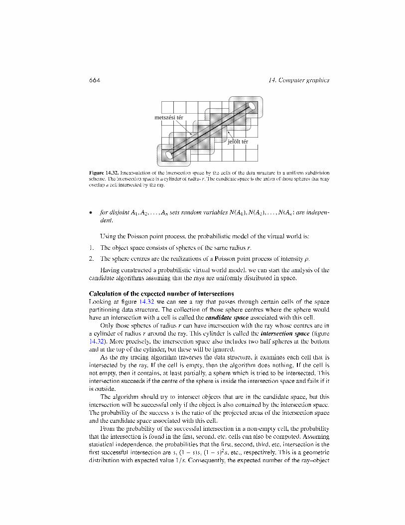
664 14. Computer graphics
jelölt tér
metszési tér
Figure 14.32. Encapsulation of the intersection space by the cells of the data structure in a uniform subdivisionscheme. The intersection space is a cylinder of radius r. The candidate space is the union of those spheres that mayoverlap a cell intersected by the ray.
• for disjoint A1, A2, . . . , An sets random variables N(A1),N(A2), . . . ,N(An) are indepen-dent.
Using the Poisson point process, the probabilistic model of the virtual world is:1. The object space consists of spheres of the same radius r.2. The sphere centres are the realizations of a Poisson point process of intensity ρ.
Having constructed a probabilistic virtual world model, we can start the analysis of thecandidate algorithms assuming that the rays are uniformly distributed in space.
Calculation of the expected number of intersectionsLooking at gure 14.32 we can see a ray that passes through certain cells of the spacepartitioning data structure. The collection of those sphere centres where the sphere wouldhave an intersection with a cell is called the candidate space associated with this cell.
Only those spheres of radius r can have intersection with the ray whose centres are ina cylinder of radius r around the ray. This cylinder is called the intersection space (gure14.32). More precisely, the intersection space also includes two half spheres at the bottomand at the top of the cylinder, but these will be ignored.
As the ray tracing algorithm traverses the data structure, it examines each cell that isintersected by the ray. If the cell is empty, then the algorithm does nothing. If the cell isnot empty, then it contains, at least partially, a sphere which is tried to be intersected. Thisintersection succeeds if the centre of the sphere is inside the intersection space and fails if itis outside.
The algorithm should try to intersect objects that are in the candidate space, but thisintersection will be successful only if the object is also contained by the intersection space.The probability of the success s is the ratio of the projected areas of the intersection spaceand the candidate space associated with this cell.
From the probability of the successful intersection in a non-empty cell, the probabilitythat the intersection is found in the rst, second, etc. cells can also be computed. Assumingstatistical independence, the probabilities that the rst, second, third, etc. intersection is therst successful intersection are s, (1 − s)s, (1 − s)2s, etc., respectively. This is a geometricdistribution with expected value 1/s. Consequently, the expected number of the rayobject

14.6. Rendering with ray tracing 665
intersection tests is:E[NI] =
1s . (14.27)
If the ray is parallel to one of the sides, then the projected size of the candidate space isc2 + 4cr + r2π where c is the edge size of a cell and r is the radius of the spheres. The otherextreme case happens when the ray is parallel to the diagonal of the cubic cell, where theprojection is a rounded hexagon having area
√3c2 + 6cr + r2π. The success probability is
then:r2π√
3c2 + 6cr + r2π≤ s ≤ r2π
c2 + 4cr + r2π.
According to equation (14.27), the average number of intersection calculations is the recip-rocal of this probability:
1π
(cr
)2+
4π
cr + 1 ≤ E [NI] ≤
√3π
(cr
)2+
6π
cr + 1 . (14.28)
Note that if the size of the cell is equal to the diameter of the sphere (c = 2r), then
3.54 < E [NI] < 7.03 .
This result has been obtained assuming that the number of objects converges to innity. Theexpected number of intersection tests, however, remains nite and relatively small.
Calculation of the expected number of cell stepsIn the following analysis the conditional expected value theorem will be used. An appropri-ate condition is the length of the ray segment between its origin and the closest intersection.Using its probability density pt∗(t) as a condition, the expected number of visited cells NScan be written in the following form:
E[NS ] =
∞∫
0
E[NS |t∗ = t] · pt∗(t) dt ,
where t∗ is the length of the ray and pt∗ is its probability density.Since the intersection space is a cylinder if we ignore the half spheres around the be-
ginning and the end, its total volume is r2πt. Thus the probability that intersection occursbefore t is:
Pr t∗ < t = 1 − e−ρr2πt .
Note that this function is the cumulative probability distribution function of t∗. The proba-bility density can be computed as its derivative, thus we obtain:
pt∗(t) = ρr2π · e−ρr2πt .
The expected length of the ray is then:
E[t∗] =
∞∫
0
t · ρr2π · e−ρr2πt dt =1
ρr2π. (14.29)

666 14. Computer graphics
In order to simplify the analysis, we shall assume that the ray is parallel to one of thecoordinate axes. Since all cells have the same edge size c, the number of cells intersectedby a ray of length t can be estimated as E[NS |t∗ = t] ≈ t/c + 1. This estimation is quiteaccurate. If the the ray is parallel to one of the coordinate axes, then the error is at most 1.In other cases the real value can be at most
√3 times the given estimation. The estimated
expected number of visited cells is then:
E [NS ] ≈∞∫
0
( tc + 1
)· ρr2π · e−ρr2πt dt =
1cρr2π
+ 1 . (14.30)
For example, if the cell size is similar to the object size (c = 2r), and the expected numberof sphere centres in a cell is 0.1, then E [NS ] ≈ 14. Note that the expected number of visitedcells is also constant even for innite number of objects.
Expected running time and storage spaceWe concluded that the expected numbers of required intersection tests and visited cells areasymptotically constant, thus the expected time complexity of the uniform grid based raytracing algorithm is constant after quadratic preprocessing time. The value of the runningtime can be controlled by cell size c according to equations (14.28) and (14.30). Smallercell sizes reduce the average number of intersection tests, but increase the number of visitedcells.
According to the probabilistic model, the average number of objects overlapping with acell is also constant, thus the storage is proportional to the number of cells. Since the numberof cells is set proportional to the number of objects, the expected storage complexity is alsolinear unlike the quadratic worst-case complexity.
The expected constant running time means that asymptotically the running time is inde-pendent of the number of objects, which explains the popularity of the uniform grid basedray tracing algorithm, and also the popularity of the algorithms presented in the next sub-sections.
OctreeUniform grids require many unnecessary cell steps. For example, the empty spaces are notworth partitioning into cells, and two cells are worth separating only if they contain differentobjects. Adaptive space partitioning schemes are based on these recognitions. The space canbe partitioned adaptively following a recursive approach. This results in a hierarchical datastructure, which is usually a tree. The type of this tree is the base of the classication ofsuch algorithms.
The adaptive scheme discussed in this subsection uses an octal tree (octree for short),where non-empty nodes have 8 children. An octree is constructed by the following algo-rithm:• For each object, an AABB is found, and object AABBs are enclosed by a scene AABB.
The scene AABB is the cell corresponding to the root of the octree.• If the number of objects overlapping with the current cell exceeds a predened thres-
hold, then the cell is subdivided to 8 cells of the same size by halving the original cellalong each coordinate axis. The 8 new cells are the children of the node correspondingto the original cell. The algorithm is recursively repeated for the child cells.

14.6. Rendering with ray tracing 667
12
3
1
1 2 2 1
3 1
I II
IIIIV
Figure 14.33. A quadtree partitioning the plane, whose three-dimensional version is the octree. The tree is const-ructed by halving the cells along all coordinate axes until a cell contains just a few objects, or the cell sizes getssmaller than a threshold. Objects are registered in the leaves of the tree.
• The recursive tree building procedure terminates if the depth of the tree becomes to big,or when the number of objects overlapping with a cell is smaller than the threshold.
The result of this construction is an octree (gure 14.33). Overlapping objects are re-gistered in the leaves of this tree.
When a ray is traced, those leaves of the tree should be traversed which are intersectedby the ray, and raysurface intersection test should be executed for objects registered inthese leaves:
R-F-I--O(~s,~v)1 ~q← intersection of the ray and the scene AABB2 while ~q is inside of the scene AABB B Traversal of the tree.3 cell← O-C-S(octree root, ~q)4 tout ← ray parameter of the intersection of the cell and the ray5 t ← tout B Initialization: no ray-surface intersection yet.6 for each object o registered in cell7 do to ←R-S-I(~s,~v) B Negative if no intersection exists.8 if 0 ≤ to < t B Is the new intersection closer?9 then t ← to B Ray parameter of the closest intersection so far.
10 ovisible ← o B First intersected object so far.11 if t < tout B Has been intersection at all ?12 then ~x← ~s + ~v · t B Position of the intersection.13 return t, ~x, ovisible14 ~q← ~s + ~v · (tout + ε) B A point in the next cell.15 return no intersection
The identication of the next cell intersected by the ray is more complicated for octreesthan for uniform grids. The O-C-S algorithm determines that leaf cell which

668 14. Computer graphics
contains a given point. At each level of the tree, the coordinates of the point are compared tothe coordinates of the centre of the cell. The results of these comparisons determine whichchild contains the point. Repeating this test recursively, we arrive at a leaf sooner or later.
In order to identify the next cell intersected by the ray, the intersection point of theray and the current cell is computed. Then, ray parameter tout of this intersection point isincreased a little (this little value is denoted by ε in algorithm R-F-I--O). The increased ray parameter is substituted into the ray equation, resulting inpoint ~q that is already in the next cell. The cell containing this point can be identied withO--.
Cells of the octree may be larger than the allowed minimal cell, therefore the octreealgorithm requires less number of cell steps than the uniform grid algorithm working onthe minimal cells. However, larger cells reduce the probability of the successful intersectiontests since in a large cell it is less likely that a random ray intersecting the cell also intersectsa contained object. Smaller successful intersection probability, on the other hand, results ingreater expected number of intersection tests, which affects the performance negatively. Italso means that non-empty octree cells are worth subdividing until the minimum cell sizeis reached even if the cell contains just a single object. Following this strategy, the size ofthe non-empty cells are similar, thus the results of the complexity analysis made for theuniform grid remain to be applicable to the octree as well. Since the probability of thesuccessful intersection depends on the size of the non-empty cells, the expected number ofneeded intersection tests is still given by inequality (14.28). It also means that when theminimal cell size of an octree equals to the cell size of a uniform grid, then the expectednumber of intersection tests is equal in the two algorithms.
The advantage of the ocree is the ability to skip empty spaces, which reduces the numberof cell steps. Its disadvantage is, however, that the time of the next cell identication is notconstant. This identication requires the traversal of the tree. If the tree construction isterminated when a cell contains small number of objects, then the number of leaf cells isproportional to the number of objects. The depth of the tree is in O(lg N), so is the timeneeded to step onto the next cell.
kd-treeAn octree adapts to the distribution of the objects. However, the partitioning strategy ofoctrees always halves the cells without taking into account where the objects are, thus theadaptation is not perfect. Let us consider a partitioning scheme which splits a cell into twocells to make the tree balanced. Such method builds a binary tree which is called binaryspace partitioning tree,, abbreviated as BSP-tree. If the separating plane is always perpen-dicular to one of the coordinate axes, then the tree is called kd-tree.
The separating plane of a kd-tree node can be placed in many different ways:• the spatial median method subdivides the cell into two similar cells.
• the object median method nds the separation plane to have the same number of objectsin the two child cells.
• the cost driven method estimates the average computation time needed when a cell isprocessed during ray tracing, and minimizes this value by placing the separation plane.An appropriate cost model suggests to separate the cell to make the probabilities of theraysurface intersection of the two cells similar.

14.6. Rendering with ray tracing 669
12
3
1
2 3
I
II
Figure 14.34. A kd-tree. A cell containing many objects are recursively subdivided to two cells with a plane thatis perpendicular to one of the coordinate axes.
The probability of the ray-surface intersection can be computed using a fundamentaltheorem of the integral geometry:
Theorem 14.17 If convex solid A contains another convex solid B, then the probability thata uniformly distributed line intersects solid B provided that the line intersected A equals tothe ratio of the surface areas of objects B and A.
According to this theorem the cost driven method nds the separation plane to equalizethe surface areas in the two children.
Let us now present a general kd-tree construction algorithm. Parameter cell identiesthe current cell, depth is the current depth of recursion, and coordinate stores the orienta-tion of the current separating plane. A cell is associated with its two children (cell.right andcell.left), and its left-lower-closer and right-upper-farther corners (cell.min and cell.max).Cells also store the list of those objects which overlap with the cell. The orientation of theseparation plane is determined by a round-robin scheme implemented by function R- providing a sequence like (x, y, z, x, y, z, x, . . .). When the following recursive algo-rithm is called rst, it gets the scene AABB in variable cell and the value of variable depthis zero:
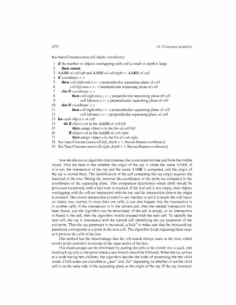
670 14. Computer graphics
K-T-C(cell, depth, coordinate)1 if the number of objects overlapping with cell is small or depth is large2 then return3 AABB of cell.left and AABB of cell.right← AABB of cell4 if coordinate = x5 then cell.right.min.x← x perpendicular separating plane of cell6 cell.left.max.x← x perpendicular separating plane of cell7 else if coordinate = y8 then cell.right.min.y← y perpendicular separating plane of cell9 cell.left.max.y← y perpendicular separating plane of cell
10 else if coordinate = z11 then cell.right.min.z← z perpendicular separating plane of cell12 cell.left.max.z← z perpendicular separating plane of cell13 for each object o of cell14 do if object o is in the AABB of cell.left15 then assign object o to the list of cell.left16 if object o is in the AABB of cell.right17 then assign object o to the list of cell.right18 K-T-C(cell.left, depth + 1,R-R(coordinate))19 K-T-C(cell.right, depth + 1,R-R(coordinate))
Now we discuss an algorithm that traverses the constructed kd-tree and nds the visibleobject. First we have to test whether the origin of the ray is inside the scene AABB. Ifit is not, the intersection of the ray and the scene AABB is computed, and the origin ofthe ray is moved there. The identication of the cell containing the ray origin requires thetraversal of the tree. During the traversal the coordinates of the point are compared to thecoordinates of the separating plane. This comparison determines which child should beprocessed recursively until a leaf node is reached. If the leaf cell is not empty, then objectsoverlapping with the cell are intersected with the ray, and the intersection closest the originis retained. The closest intersection is tested to see whether or not it is inside the cell (sincean object may overlap in more than one cells, it can also happen that the intersection isin another cell). If the intersection is in the current cell, then the needed intersection hasbeen found, and the algorithm can be terminated. If the cell is empty, or no intersectionis found in the cell, then the algorithm should proceed with the next cell. To identify thenext cell, the ray is intersected with the current cell identifying the ray parameter of theexit point. Then the ray parameter is increased a little to make sure that the increased rayparameter corresponds to a point in the next cell. The algorithm keeps repeating these stepsas it process the cells of the tree.
This method has the disadvantage that the cell search always starts at the root, whichresults in the repetitive traversals of the same nodes of the tree.
This disadvantage can be eliminated by putting the cells to be visited into a stack, andbacktracking only to the point where a new branch should be followed. When the ray arrivesat a node having two children, the algorithm decides the order of processing the two childnodes. Child nodes are classied as near and far depending on whether or not the childcell is on the same side of the separating plane as the origin of the ray. If the ray intersects

14.6. Rendering with ray tracing 671
only the near child, then the algorithm processes only that subtree which originates at thischild. If the ray intersects both children, then the algorithm pushes the far node onto thestack and starts processing the near node. If no intersection exists in the near node, thenthe stack is popped to obtain the next node to be processed.
The notations of the ray tracing algorithm based on kd-tree traversal are shown by gure14.35. The algorithm is the following:
R-F-I---T(root, ~s,~v)1 (tin, tout)← R-AABB-I(~s,~v, root) B Intersection with the scene AABB.2 if no intersection3 then return no intersection4 P(root, tin, tout)5 while the stack is not empty B Visit all nodes.6 do P(cell, tin, tout)7 while cell is not a leaf8 do coordinate← orientation of the separating plane of the cell9 d ← cell.right.min[coordinate] − ~s[coordinate]
10 t ← d/~v[coordinate] B Ray parameter of the separating plane.11 if d > 0 B Is ~s on the left side of the separating plane?12 then (near, far)← (cell.left, cell.right) B Left.13 else (near, far)← (cell.right, cell.left) B Right.14 if t > tout or t < 015 then cell← near B The ray intersects only the near cell.16 else if t < tin17 then cell← far B The ray intersects only the far cell.18 else P(far, t, tout) B The ray intersects both cells.19 cell← near B First near is intersected.20 tout ← t B The ray exists at t from the near cell.
B If the current cell is a leaf.21 t ← tout BMaximum ray parameter in this cell.22 for each object o of cell23 do to ←R-S-I(~s,~v) B Negative if no intersection exists.24 if tin ≤ to < t B Is the new intersection closer to the ray origin?25 then t ← to B The ray parameter of the closest intersection so far.26 ovisible ← o B The object intersected closest to the ray origin.27 if t < tout B Has been intersection at all in the cell?28 then ~x← ~s + ~v · t B The intersection point.29 return t, ~x, ovisible B Intersection has been found.30 return no intersection B No intersection.
Similarly to the octree algorithm, the likelihood of successful intersections can be inc-reased by continuing the tree building process until all empty spaces are cut (gure 14.36).
Our probabilistic world model contains spheres of same radius r, thus the non-emptycells are cubes of edge size c = 2r. Unlike in uniform grids or octrees, the separating planesof kd-trees are not independent of the objects. Kd-tree splitting planes are rather tangents

672 14. Computer graphics
bal jobb
t t
t
be
ki
d
jelölések
jobbd
bal jobbd
bal jobb
ttki
t > tki
d > 0 d < 0
bal jobb
t
t < 0
bal jobb
t
tbe
t < tbe
s
v
bals
s
s
s
s
Figure 14.35. Notations and cases of algorithm R-F-I---T. tin, tout, and t are the rayparameters of the entry, exit and the separation plane, respectively. d is the signed distance between the ray originand the separation plane.
Figure 14.36. Kd-tree based space partitioning with empty space cutting.
of the objects. This means that we do not have to be concerned with partially overlappingspheres since a sphere is completely contained by a cell in a kd-tree. The probability of thesuccessful intersection is obtained applying theorem 14.17. In the current case, the contai-ning convex solid is a cube of edge size 2r, the contained solid is a sphere of radius r, thusthe intersection probability is:
s =4r2π
6a2 =π
6 .
The expected number of intersection tests is then:
E [NI] =6π≈ 1.91 .
We can conclude that the kd-tree algorithm requires the smallest number of raysurfaceintersection tests according to the probabilistic model.
Exercises
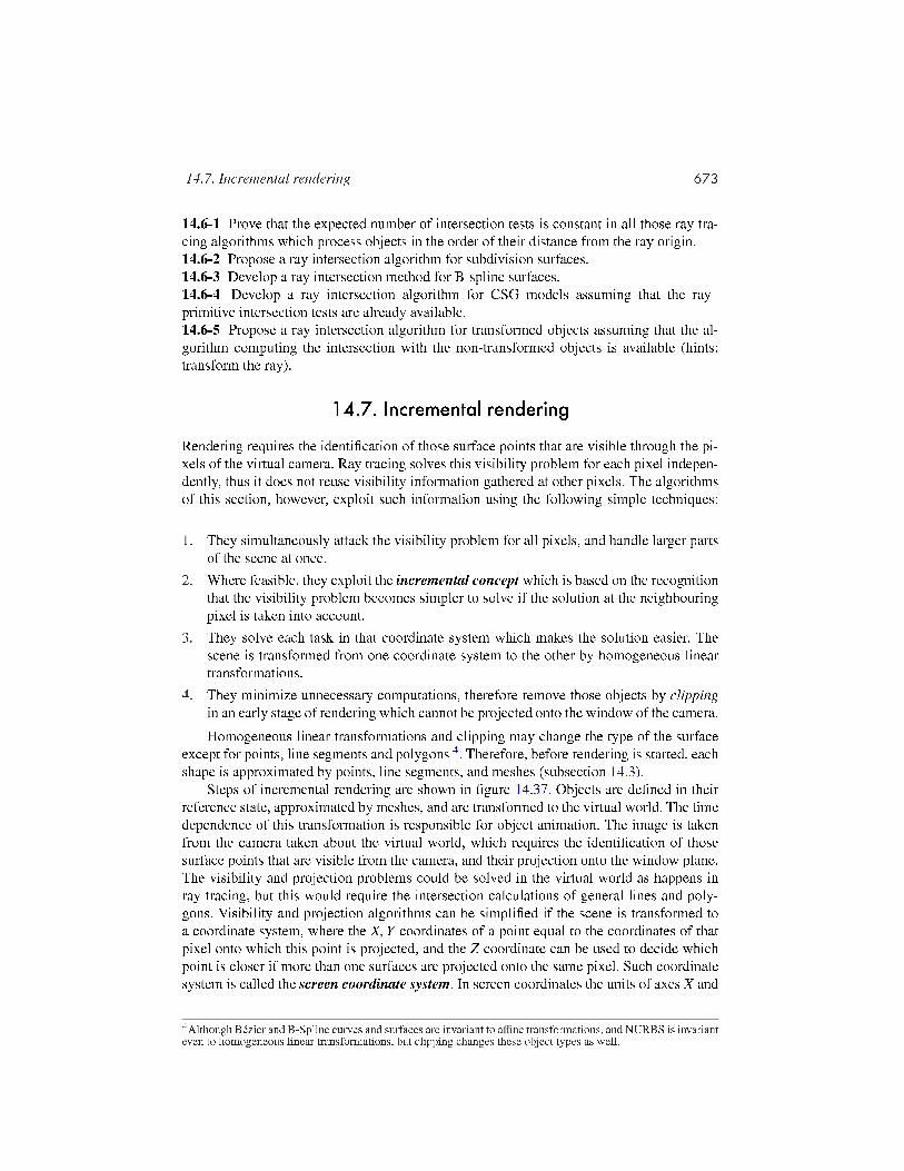
14.7. Incremental rendering 673
14.6-1 Prove that the expected number of intersection tests is constant in all those ray tra-cing algorithms which process objects in the order of their distance from the ray origin.14.6-2 Propose a ray intersection algorithm for subdivision surfaces.14.6-3 Develop a ray intersection method for B-spline surfaces.14.6-4 Develop a ray intersection algorithm for CSG models assuming that the rayprimitive intersection tests are already available.14.6-5 Propose a ray intersection algorithm for transformed objects assuming that the al-gorithm computing the intersection with the non-transformed objects is available (hints:transform the ray).
14.7. Incremental renderingRendering requires the identication of those surface points that are visible through the pi-xels of the virtual camera. Ray tracing solves this visibility problem for each pixel indepen-dently, thus it does not reuse visibility information gathered at other pixels. The algorithmsof this section, however, exploit such information using the following simple techniques:
1. They simultaneously attack the visibility problem for all pixels, and handle larger partsof the scene at once.
2. Where feasible, they exploit the incremental concept which is based on the recognitionthat the visibility problem becomes simpler to solve if the solution at the neighbouringpixel is taken into account.
3. They solve each task in that coordinate system which makes the solution easier. Thescene is transformed from one coordinate system to the other by homogeneous lineartransformations.
4. They minimize unnecessary computations, therefore remove those objects by clippingin an early stage of rendering which cannot be projected onto the window of the camera.Homogeneous linear transformations and clipping may change the type of the surface
except for points, line segments and polygons 4. Therefore, before rendering is started, eachshape is approximated by points, line segments, and meshes (subsection 14.3).
Steps of incremental rendering are shown in gure 14.37. Objects are dened in theirreference state, approximated by meshes, and are transformed to the virtual world. The timedependence of this transformation is responsible for object animation. The image is takenfrom the camera taken about the virtual world, which requires the identication of thosesurface points that are visible from the camera, and their projection onto the window plane.The visibility and projection problems could be solved in the virtual world as happens inray tracing, but this would require the intersection calculations of general lines and poly-gons. Visibility and projection algorithms can be simplied if the scene is transformed toa coordinate system, where the X,Y coordinates of a point equal to the coordinates of thatpixel onto which this point is projected, and the Z coordinate can be used to decide whichpoint is closer if more than one surfaces are projected onto the same pixel. Such coordinatesystem is called the screen coordinate system. In screen coordinates the units of axes X and
4Although Bézier and B-Spline curves and surfaces are invariant to affine transformations, and NURBS is invarianteven to homogeneous linear transformations, but clipping changes these object types as well.
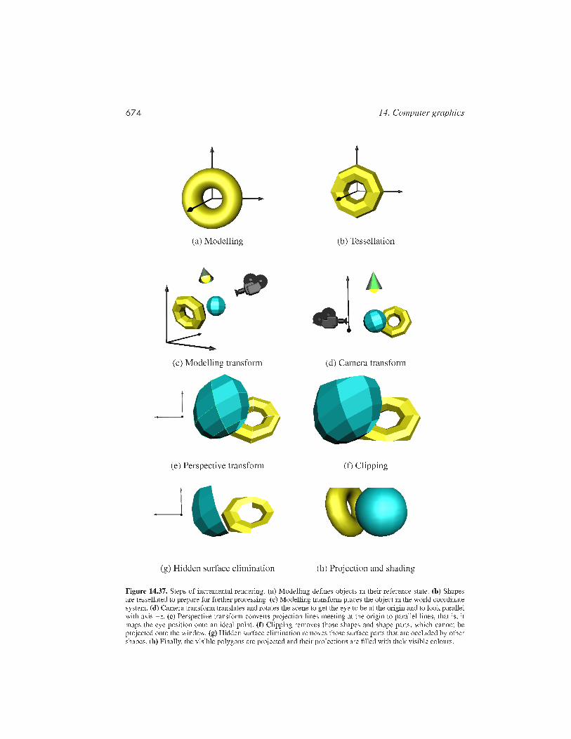
674 14. Computer graphics
(a) Modelling (b) Tessellation
(c) Modelling transform (d) Camera transform
(e) Perspective transform (f) Clipping
(g) Hidden surface elimination (h) Projection and shading
Figure 14.37. Steps of incremental rendering. (a) Modelling denes objects in their reference state. (b) Shapesare tessellated to prepare for further processing. (c) Modelling transform places the object in the world coordinatesystem. (d) Camera transform translates and rotates the scene to get the eye to be at the origin and to look parallelwith axis −z. (e) Perspective transform converts projection lines meeting at the origin to parallel lines, that is, itmaps the eye position onto an ideal point. (f) Clipping removes those shapes and shape parts, which cannot beprojected onto the window. (g) Hidden surface elimination removes those surface parts that are occluded by othershapes. (h) Finally, the visible polygons are projected and their projections are lled with their visible colours.
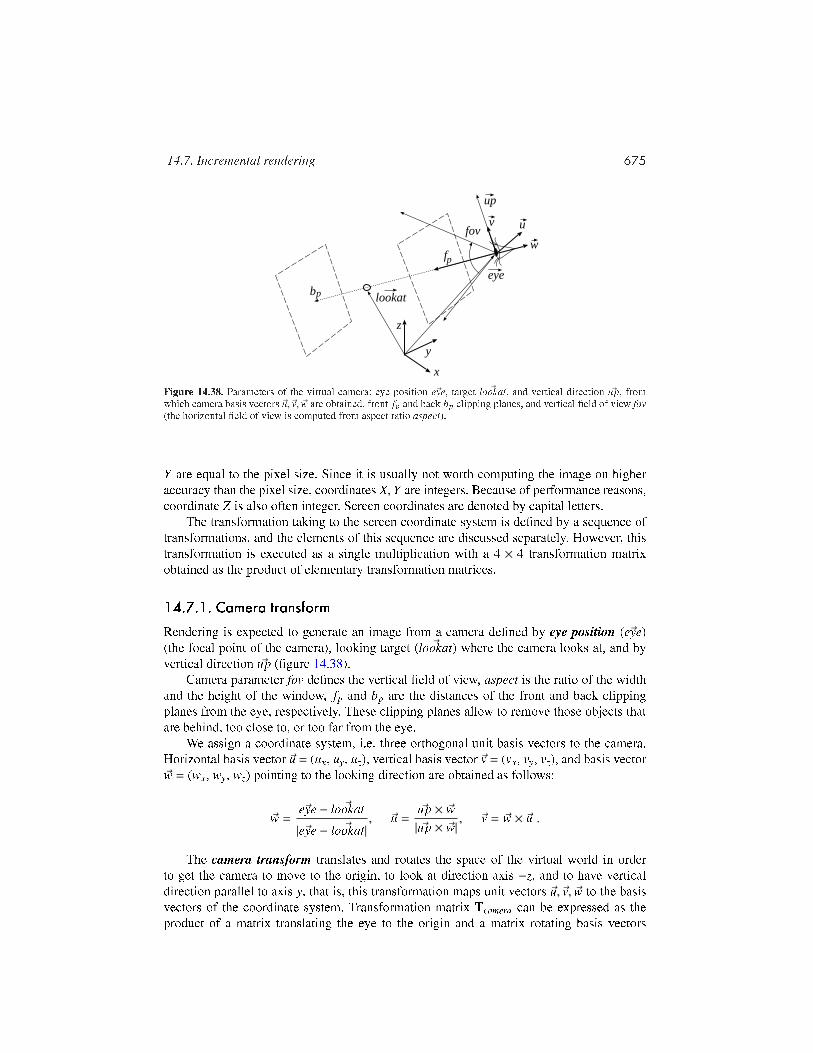
14.7. Incremental rendering 675
lookat
x
y
z
uv
w
b
f
eyep
p
up
fov
Figure 14.38. Parameters of the virtual camera: eye position ~eye, target ~lookat, and vertical direction ~up, fromwhich camera basis vectors ~u,~v, ~w are obtained, front fp and back bp clipping planes, and vertical eld of view fov(the horizontal eld of view is computed from aspect ratio aspect).
Y are equal to the pixel size. Since it is usually not worth computing the image on higheraccuracy than the pixel size, coordinates X,Y are integers. Because of performance reasons,coordinate Z is also often integer. Screen coordinates are denoted by capital letters.
The transformation taking to the screen coordinate system is dened by a sequence oftransformations, and the elements of this sequence are discussed separately. However, thistransformation is executed as a single multiplication with a 4 × 4 transformation matrixobtained as the product of elementary transformation matrices.
14.7.1. Camera transformRendering is expected to generate an image from a camera dened by eye position ( ~eye)(the focal point of the camera), looking target ( ~lookat) where the camera looks at, and byvertical direction ~up (gure 14.38).
Camera parameter fov denes the vertical eld of view, aspect is the ratio of the widthand the height of the window, fp and bp are the distances of the front and back clippingplanes from the eye, respectively. These clipping planes allow to remove those objects thatare behind, too close to, or too far from the eye.
We assign a coordinate system, i.e. three orthogonal unit basis vectors to the camera.Horizontal basis vector ~u = (ux, uy, uz), vertical basis vector ~v = (vx, vy, vz), and basis vector~w = (wx, wy, wz) pointing to the looking direction are obtained as follows:
~w =~eye − ~lookat| ~eye − ~lookat|
, ~u =~up × ~w| ~up × ~w| , ~v = ~w × ~u .
The camera transform translates and rotates the space of the virtual world in orderto get the camera to move to the origin, to look at direction axis −z, and to have verticaldirection parallel to axis y, that is, this transformation maps unit vectors ~u,~v, ~w to the basisvectors of the coordinate system. Transformation matrix Tcamera can be expressed as theproduct of a matrix translating the eye to the origin and a matrix rotating basis vectors
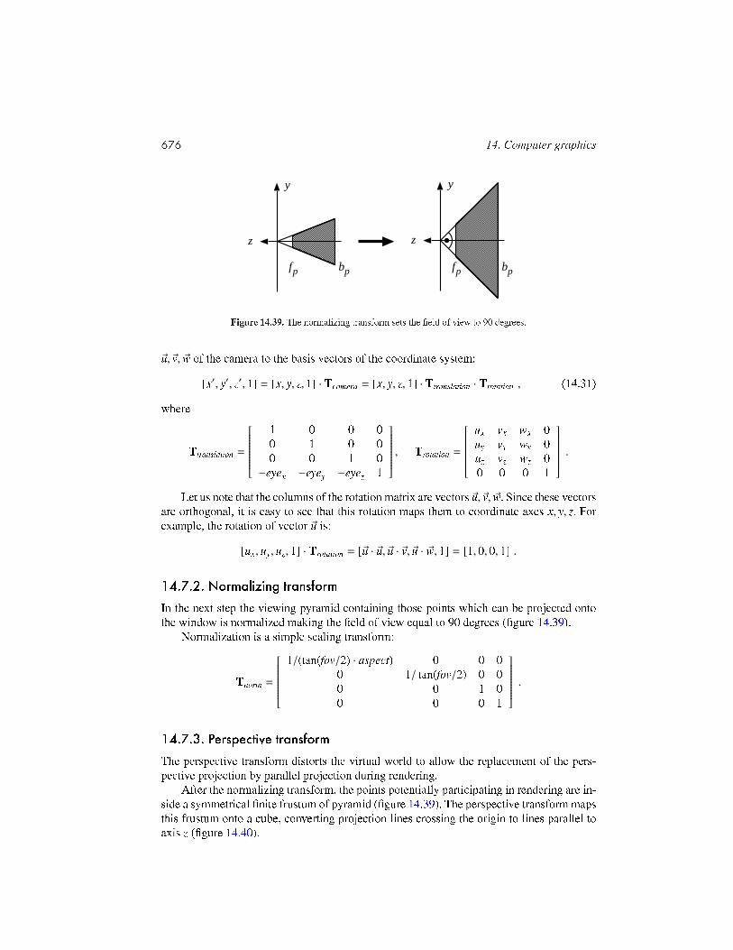
676 14. Computer graphics
y
z
y
z
fp bp fp bp
Figure 14.39. The normalizing transform sets the eld of view to 90 degrees.
~u,~v, ~w of the camera to the basis vectors of the coordinate system:
[x′, y′, z′, 1] = [x, y, z, 1] · Tcamera = [x, y, z, 1] · Ttranslation · Trotation , (14.31)
where
Ttranslation =
1 0 0 00 1 0 00 0 1 0−eyex −eyey −eyez 1
, Trotation =
ux vx wx 0uy vy wy 0uz vz wz 00 0 0 1
.
Let us note that the columns of the rotation matrix are vectors ~u,~v, ~w. Since these vectorsare orthogonal, it is easy to see that this rotation maps them to coordinate axes x, y, z. Forexample, the rotation of vector ~u is:
[ux, uy, uz, 1] · Trotation = [~u · ~u, ~u · ~v, ~u · ~w, 1] = [1, 0, 0, 1] .
14.7.2. Normalizing transformIn the next step the viewing pyramid containing those points which can be projected ontothe window is normalized making the eld of view equal to 90 degrees (gure 14.39).
Normalization is a simple scaling transform:
Tnorm =
1/(tan(fov/2) · aspect) 0 0 00 1/ tan(fov/2) 0 00 0 1 00 0 0 1
.
14.7.3. Perspective transformThe perspective transform distorts the virtual world to allow the replacement of the pers-pective projection by parallel projection during rendering.
After the normalizing transform, the points potentially participating in rendering are in-side a symmetrical nite frustum of pyramid (gure 14.39). The perspective transform mapsthis frustum onto a cube, converting projection lines crossing the origin to lines parallel toaxis z (gure 14.40).

14.7. Incremental rendering 677
y
z
y
z1
1
-1
-1fp bp
Figure 14.40. The perspective transform maps the nite frustum of pyramid dened by the front and back clippingplanes, and the edges of the window onto an axis aligned, origin centred cube of edge size 2.
Perspective transform is expected to map point to point, line to line, but to map theeye position to innity. It means that perspective transform cannot be a linear transform ofCartesian coordinates. Fortunately, homogenous linear transforms also map point to point,line to line, and are able to handle points at innity with nite coordinates. Let us thus tryto nd the perspective transform in the form of a homogeneous linear transform dened bya 4 × 4 matrix:
Tpersp =
t11 t12 t13 t14t21 t22 t23 t24t31 t32 t33 t34t41 t42 t43 t44
.
Figure 14.40 shows a line (projection ray) and its transform. Let mx and my be the x/zand the y/z slopes of the line, respectively. This line is dened by equation [−mx ·z,−my ·z, z]in the normalized camera space. The perspective transform maps this line to a horizontalline crossing point [mx,my, 0] and being parallel to axis z. Let us examine the intersectionpoints of this line with the front and back clipping planes, that is, let us substitute (− fp) and(−bp) into parameter z of the line equation. The transformation should map these points to[mx,my,−1] and [mx,my, 1], respectively.
The perspective transformation of the point on the rst clipping plane is:[mx · fp,my · fp,− fp, 1
]· Tpersp =
[mx,my,−1, 1
]· λ ,
where λ is an arbitrary, non-zero scalar since the point dened by homogeneous coordinatesdoes not change if the homogenous coordinates are simultaneously multiplied by a non-zeroscalar. Setting λ to fp, we get:
[mx · fp,my · fp,− fp, 1
]· Tpersp =
[mx · fp,my · fp,− fp, fp
]. (14.32)
Note that the rst coordinate of the transformed point equals to the rst coordinate ofthe original point on the clipping plane for arbitrary mx, my, and fp values. This is possibleonly if the rst column of matrix Tpersp is [1, 0, 0, 0]T . Using the same argument for thesecond coordinate, we can conclude that the second column of the matrix is [0, 1, 0, 0]T .Furthermore, in equation (14.32) the third and the fourth homogeneous coordinates of thetransformed point are not affected by the rst and the second coordinates of the originalpoint, requiring t13 = t14 = t23 = t24 = 0. The conditions on the third and the fourth
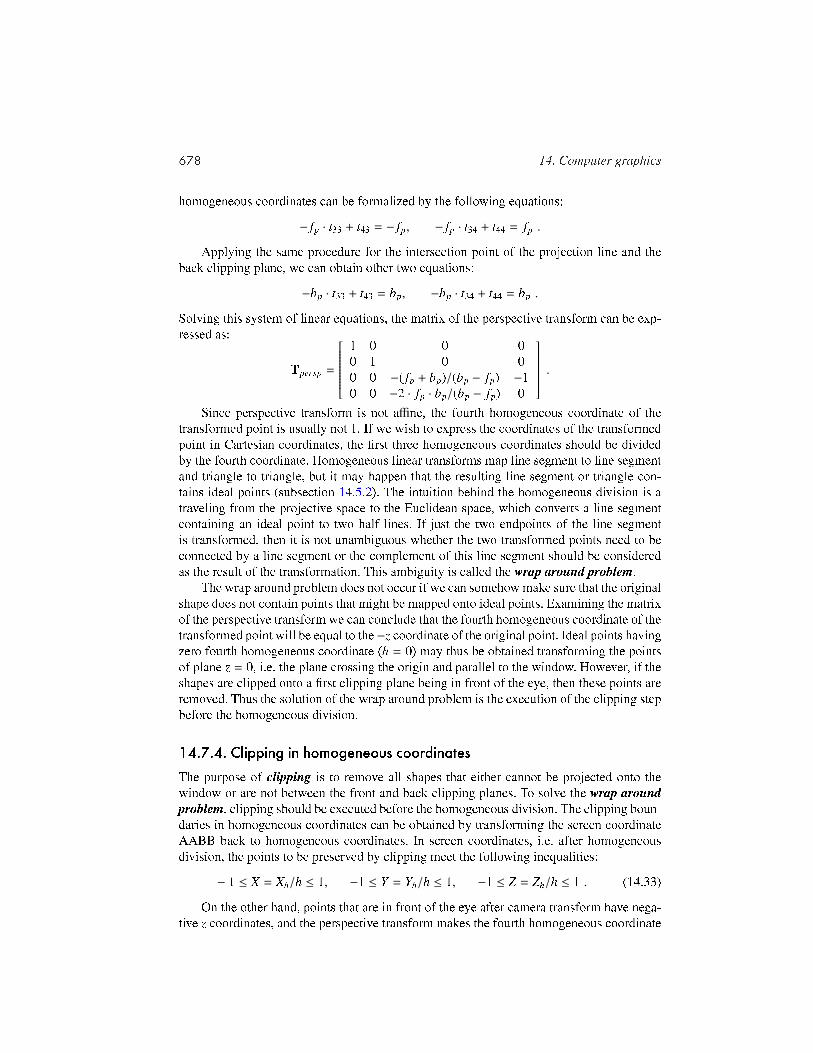
678 14. Computer graphics
homogeneous coordinates can be formalized by the following equations:
− fp · t33 + t43 = − fp, − fp · t34 + t44 = fp .
Applying the same procedure for the intersection point of the projection line and theback clipping plane, we can obtain other two equations:
−bp · t33 + t43 = bp, −bp · t34 + t44 = bp .
Solving this system of linear equations, the matrix of the perspective transform can be exp-ressed as:
Tpersp =
1 0 0 00 1 0 00 0 −( fp + bp)/(bp − fp) −10 0 −2 · fp · bp/(bp − fp) 0
.
Since perspective transform is not affine, the fourth homogeneous coordinate of thetransformed point is usually not 1. If we wish to express the coordinates of the transformedpoint in Cartesian coordinates, the rst three homogeneous coordinates should be dividedby the fourth coordinate. Homogeneous linear transforms map line segment to line segmentand triangle to triangle, but it may happen that the resulting line segment or triangle con-tains ideal points (subsection 14.5.2). The intuition behind the homogeneous division is atraveling from the projective space to the Euclidean space, which converts a line segmentcontaining an ideal point to two half lines. If just the two endpoints of the line segmentis transformed, then it is not unambiguous whether the two transformed points need to beconnected by a line segment or the complement of this line segment should be consideredas the result of the transformation. This ambiguity is called the wrap around problem.
The wrap around problem does not occur if we can somehow make sure that the originalshape does not contain points that might be mapped onto ideal points. Examining the matrixof the perspective transform we can conclude that the fourth homogeneous coordinate of thetransformed point will be equal to the −z coordinate of the original point. Ideal points havingzero fourth homogeneous coordinate (h = 0) may thus be obtained transforming the pointsof plane z = 0, i.e. the plane crossing the origin and parallel to the window. However, if theshapes are clipped onto a rst clipping plane being in front of the eye, then these points areremoved. Thus the solution of the wrap around problem is the execution of the clipping stepbefore the homogeneous division.
14.7.4. Clipping in homogeneous coordinatesThe purpose of clipping is to remove all shapes that either cannot be projected onto thewindow or are not between the front and back clipping planes. To solve the wrap aroundproblem, clipping should be executed before the homogeneous division. The clipping boun-daries in homogeneous coordinates can be obtained by transforming the screen coordinateAABB back to homogeneous coordinates. In screen coordinates, i.e. after homogeneousdivision, the points to be preserved by clipping meet the following inequalities:
− 1 ≤ X = Xh/h ≤ 1, −1 ≤ Y = Yh/h ≤ 1, −1 ≤ Z = Zh/h ≤ 1 . (14.33)
On the other hand, points that are in front of the eye after camera transform have nega-tive z coordinates, and the perspective transform makes the fourth homogeneous coordinate

14.7. Incremental rendering 679
h equal to −z in normalized camera space. Thus the fourth homogeneous coordinate ofpoints in front of the eye is always positive. Let us thus add condition h > 0 to the set ofconditions of inequalities (14.33). If h is positive, then inequalities (14.33) can be multipliedby h, resulting in the denition of the clipping region in homogeneous coordinates:
− h ≤ Xh ≤ h, −h ≤ Yh ≤ h, −h ≤ Zh ≤ h . (14.34)
Points can be clipped easily, since we should only test whether or not the conditionsof inequalities (14.34) are met. Clipping line segments and polygons, on the other hand,requires the computation of the intersection points with the faces of the clipping boundary,and only those parts should be preserved which meet inequalities (14.34).
Clipping algorithms using Cartesian coordinates were discussed in subsection 14.4.3.Those methods can also be applied in homogeneous coordinates with two exceptions.Firstly, for homogeneous coordinates, inequalities (14.34) dene whether a point is in orout. Secondly, intersections should be computed using the homogeneous coordinate equati-ons of the line segments and the planes.
Let us consider a line segment with endpoints [X1h ,Y1
h ,Z1h , h1] and [X2
h ,Y2h ,Z2
h , h2]. Thisline segment can be an independent shape or an edge of a polygon. Here we discuss theclipping on half space of equation Xh ≤ h (clipping methods on other half spaces are verysimilar). Three cases need to be distinguished:1. If both endpoints of the line segment are inside, that is X1
h ≤ h1 and X2h ≤ h2, then the
complete line segment is in, thus is preserved.2. If both endpoints are outside, that is X1
h > h1 and X2h > h2, then all points of the line
segment are out, thus it is completely eliminated by clipping.3. If one endpoint is outside, while the other is in, then the intersection of the line segment
and the clipping plane should be obtained. Then the endpoint being out is replaced bythe intersection point. Since the points of a line segment satisfy equation (14.19), whilethe points of the clipping plane satisfy equation Xh = h, parameter ti of the intersectionpoint is computed as:
Xh(ti) = h(ti) =⇒ X1h ·(1−ti)+X2
h ·ti = h1·(1−ti)+h2·ti =⇒ ti =X1
h − h1
X1h − X2
h + h2 − h1 .
Substituting parameter ti into the equation of the line segment, homogeneous coordina-tes [Xi
h,Y ih,Zi
h, hi] of the intersection point are obtained.Clipping may introduce new vertices. When the vertices have some additional features,
for example, the surface colour or normal vector at these vertices, then these additionalfeatures should be calculated for the new vertices as well. We can use linear interpolation.If the values of a feature at the two endpoints are I1 and I2, then the feature value at newvertex [Xh(ti),Yh(ti),Zh(ti), h(ti)] generated by clipping is I1 · (1 − ti) + I2 · ti.
14.7.5. Viewport transformHaving executed the perspective transform, the Cartesian coordinates of the visible pointsare in [−1, 1]. These normalized device coordinates should be further scaled and translatedaccording to the resolution of the screen and the position of the viewport where the image is
680 14. Computer graphics
expected. Denoting the left-bottom corner pixel of the screen viewport by (Xmin,Ymin), theright-top corner by (Xmax,Ymax), and Z coordinates expressing the distance from the eye areexpected in (Zmin,Zmax), the matrix of the viewport transform is:
Tviewport =
(Xmax − Xmin)/2 0 0 00 (Ymax − Ymin)/2 0 00 0 (Zmax − Zmin)/2 0
(Xmax + Xmin)/2 (Ymax + Ymin)/2 (Zmax + Zmin)/2 1
.
Coordinate systems after the perspective transform are left handed, unlike the coor-dinate systems of the virtual world and the camera, which are right handed. Left handedcoordinate systems seem to be unusual, but they meet our natural expectation that the sc-reen X coordinates grow from left to right, the Y coordinates from bottom to top and, the Zcoordinates grow with the distance from the virtual observer.
14.7.6. Rasterization algorithmsAfter clipping, homogeneous division, and viewport transform, shapes are in the screencoordinate system where a point of coordinates (X,Y,Z) can be assigned to a pixel by ext-racting the rst two Cartesian coordinates (X,Y).
Rasterization works in the screen coordinate system and identies those pixels whichhave to be coloured to approximate the projected shape. Since even simple shapes can covermany pixels, rasterization algorithms should be very fast, and should be appropriate forhardware implementation.
Line drawingLet the endpoints of a line segment be (X1,Y1) and (X2,Y2) in screen coordinates. Let usfurther assume that while we are going from the rst endpoint toward the second, bothcoordinates are growing, and X is the faster changing coordinate, that is,
∆X = X2 − X1 ≥ ∆Y = Y2 − Y1 ≥ 0 .
In this case the line segment is moderately ascending. We discuss only this case, other casescan be handled by exchanging the X,Y coordinates and replacing additions by substractions.
Line drawing algorithms are expected to nd pixels that approximate a line in a way thatthere are no holes and the approximation is not fatter than necessary. In case of moderatelyascending line segments this means that in each pixel column exactly one pixel should belled with the colour of the line. This coloured pixel is the one closest to the line in thiscolumn. Using the following equation of the line
y = m · X + b, where m =Y2 − Y1X2 − X1
, and b = Y1 − X1 · Y2 − Y1X2 − X1
, (14.35)
in pixel column of coordinate X the pixel closest to the line has Y coordinate that is equalto the rounding of m · x + b. Unfortunately, the determination of Y requires a oating pointmultiplication, addition, and a rounding operation, which are too slow.
In order to speed up line drawing, we apply a fundamental trick of computer graphics,the incremental concept. The incremental concept is based on the recognition that it is

14.7. Incremental rendering 681
usually simpler to evaluate a function y(X + 1) using value y(X) than computing it fromX. Since during line drawing the columns are visited one by one, when column (X + 1) isprocessed, value y(X) is already available. In case of a line segment we can write:
y(X + 1) = m · (X + 1) + b = m · X + b + m = y(X) + m .
Note that the evaluation of this formula requires just a single oating point addition (mis less than 1). This fact is exploited in digital differential analyzator algorithms (DDA-algorithms). The DDA line drawing algorithm is then:
DDA-L-D(X1,Y1, X2,Y2, colour)1 m← (Y2 − Y1)/(X2 − X1)2 y← Y13 for X ← X1 to X24 do Y ← R(y)5 P-W(X,Y, colour)6 y← y + m
Further speedups can be obtained using xed point number representation. This me-ans that the product of the number and 2T is stored in an integer variable, where T is thenumber of fractional bits. The number of fractional bits should be set to exclude cases whenthe rounding errors accumulate to an incorrect result during long iteration sequences. If thelongest line segment covers L columns, then the minimum number of fractional bits gua-ranteeing that the accumulated error is less than 1 is log2 L. Thanks to clipping only linestting to the screen are rasterized, thus L is equal to the maximum screen resolution.
The performance and simplicity of the DDA line drawing algorithm can still be imp-roved. On the one hand, the software implementation of the DDA algorithm requires shiftoperations to realize truncation and rounding operations. On the other handonce for everyline segmentthe computation of slope m involves a division which is computationally ex-pensive. Both problems are solved in the Bresenham line drawing algorithm.
Let us denote the vertical, signed distance of the line segment and the closest pixelcentre by s, and the vertical distance of the line segment and the pixel centre just above theclosest pixel by t (gure 14.41). As the algorithm steps onto the next pixel column, valuess and t change and should be recomputed. While the new s and t values satisfy inequalitys < t, that is, while the lower pixel is still closer to the line segment, the shaded pixel of thenext column is in the same row as in the previous column. Introducing error variable e = s−t,the row of the shaded pixel remains the same until this error variable is negative (e < 0). Asthe pixel column is incremented, variables s, t, e are updated using the incremental formulae(∆X = X2 − X1, ∆Y = Y2 − Y1):
s(X + 1) = s(X) +∆Y∆X , t(X + 1) = t(X) − ∆Y
∆X =⇒ e(X + 1) = e(X) + 2 ∆Y∆X .
These formulae are valid if the closest pixel in column (X + 1) is in the same row as incolumn X. If stepping to the next column, the upper pixel gets closer to the line segment(error variable e becomes positive), then variables s, t, e should be recomputed for the new

682 14. Computer graphics
t(X) t(X+1)
s(X) s(X+1)
t(X)
t(X+1)
s(X)
s(X+1)
X
Y
1
Figure 14.41. Notations of the Bresenham algorithm: s is the signed distance between the closest pixel centre andthe line segment along axis Y , which is positive if the line segment is above the pixel centre. t is the distance alongaxis Y between the pixel centre just above the closest pixel and the line segment.
closest row and for the pixel just above it. The formulae describing this case are as follows:
s(X + 1) = s(X) +∆Y∆X − 1, t(X + 1) = t(X) − ∆Y
∆X + 1 =⇒ e(X + 1) = e(X) + 2(∆Y∆X − 1
).
Note that s is a signed distance which is negative if the line segment is below the closestpixel centre, and positive otherwise. We can assume that the line starts at a pixel centre, thusthe initial values of the control variables are:
s(X1) = 0, t(X1) = 1 =⇒ e(X1) = s(X1) − t(X1) = −1 .
This algorithm keeps updating error variable e and steps onto the next pixel row whenthe error variable becomes positive. In this case, the error variable is decreased to have anegative value again. The update of the error variable requires a non-integer addition andthe computation of its increment involves a division, similarly to the DDA algorithm. Itseems that this approach is not better than the DDA.
Let us note, however, that the sign changes of the error variable can also be recognizedif we examine the product of the error variable and a positive number. Multiplying the errorvariable by ∆X we obtain decision variable E = e·∆X. In case of moderately ascending linesthe decision and error variables change their sign simultaneously. The incremental updateformulae of the decision variable can be obtained by multiplying the update formulae oferror variable by ∆X:
E(X + 1) =
E(X) + 2∆Y , if Y is not incremented ,
E(X) + 2(∆Y − ∆X), if Y needs to be incremented .
The initial value of the decision variable is E(X1) = e(X1) · ∆X = −∆X.The decision variable starts at an integer value and is incremented by integers in each
step, thus it remains to be an integer and does not require fractional numbers at all. The com-putation of the increments need only integer additions or subtractions and multiplications

14.7. Incremental rendering 683
X
Y
X X10
X
Y
q[0]
q[1]
q[2]
q[3]
X X10 X3 X2
q[0]
q[1]
q[2]
q[3]
Figure 14.42. Polygon ll. Pixels inside the polygon are identied scan line by scan line.
by 2.The complete Bresenham line drawing algorithm is:
B-L-D(X1,Y1, X2,Y2, colour)1 ∆X ← X2 − X12 ∆Y ← Y2 − Y13 (dE+, dE−)← (2(∆Y − ∆X), 2∆Y)4 E ← −∆X5 Y ← Y16 for X ← X1 to X27 do if E ≤ 08 then E ← E + dE− B The line stays in the current pixel row.9 else E ← E + dE+ B The line steps onto the next pixel row.
10 Y ← Y + 111 P-W(X,Y, colour)
The fundamental idea of the Bresenham algorithm was the replacement of the fractionalerror variable by an integer decision variable in a way that the conditions used by the algo-rithm remained equivalent. This approach is also called the method of invariants, which isuseful in many rasterization algorithms.
Polygon llThe input of an algorithm lling single connected polygons is the array of vertices~q[0], . . . , ~q[m − 1] (this array is usually the output of the polygon clipping algorithm). Edgee of the polygon connects vertices ~q[e] and ~q[e + 1]. The last vertex needs not be treatedin a special way if the rst vertex is put again after the last vertex in the array. Multiplyconnected polygons are dened by more than one closed polylines, thus are specied bymore than one vertex arrays.
The lling is executed by processing a horizontal pixel row called scan line at a time.For a single scan line, the pixels belonging to the interior of the polygon can be found by thefollowing steps. First the intersections of the polygon edges and the scan line are calculated.

684 14. Computer graphics
XY
X(Y) X(Y+1) X(Y+2)
∆X/∆Y ∆X/∆Y
Y+1
Y+2
Figure 14.43. Incremental computation of the intersections between the scan lines and the edges. Coordinate Xalways increases with the reciprocal of the slope of the line.
YAET ∆X/∆Ymax
X Y ∆X/∆Ymax
X
Figure 14.44. The structure of the active edge table.
Then the intersection points are sorted in the ascending order of their X coordinates. Finally,pixels between the rst and the second intersection points, and between the third and thefourth intersection points, or generally between the (2i + 1)th and the (2i + 2)th intersectionpoints are set to the colour of the polygon (gure 14.42). This algorithm lls those pixelswhich can be reached from innity by crossing the polygon boundary odd number of times.
The computation of the intersections between scan lines and polygon edges can bespeeded up using the following observations:1. An edge and a scan line can have intersection only if coordinate Y of the scan line is
between the minimum and maximum Y coordinates of the edge. Such edges are theactive edges. When implementing this idea, an active edge table (AET for short) isneeded which stores the currently active edges.
2. The computation of the intersection point of a line segment and the scan line requiresoating point multiplication, division, and addition, thus it is time consuming. Applyingthe incremental concept, however, we can also obtain the intersection point of the edgeand a scan line from the intersection point with the previous scan line using a single,xed-point addition (gure 14.43).When the incremental concept is exploited, we realize that coordinate X of the intersec-
tion with an edge always increases by the same amount when scan line Y is incremented.If the edge endpoint having the larger Y coordinate is (Xmax,Ymax) and the endpoint havingthe smaller Y coordinate is (Xmin,Ymin), then the increment of the X coordinate of the in-tersection is ∆X/∆Y , where ∆X = Xmax − Xmin and ∆Y = Ymax − Ymin. This increment isusually not an integer, hence increment ∆X/∆Y and intersection coordinate X should bestored in non-integer, preferably xed-point variables. An active edge is thus representedby a xed-point increment ∆X/∆Y , the xed-point coordinate value of intersection X, andthe maximum vertical coordinate of the edge (Ymax). The maximum vertical coordinate isneeded to recognize when the edge becomes inactive.
Scan lines are processed one after the other. First, the algorithm determines which edgesbecome active for this scan line, that is, which edges have minimum Y coordinate being
14.7. Incremental rendering 685
equal to the scan line coordinate. These edges are inserted into the active edge table. Theactive edge table is also traversed and those edges whose maximum Y coordinate equalsto the scan line coordinate are removed (note that this way the lower end of an edge issupposed to belong to the edge, but the upper edge is not). Then the active edge table issorted according to the X coordinates of the edges, and the pixels between each pair ofedges are lled. Finally, the X coordinates of the intersections in the edges of the activeedge table are prepared for the next scan line by incrementing them by the reciprocal of theslope ∆X/∆Y .
P-F(polygon, colour)1 for Y ← 0 to Ymax2 do for each edge of polygon B Put activated edges into the AET.3 do if edge.ymin = Y4 then P-AET(edge)5 for each edge of the AET B Remove deactivated edges from the AET.6 do if edge.ymax ≤ Y7 then D--AET(edge)8 S-AET B Sort according to X.9 for each pair of edges (edge1, edge2) of the AET
10 do for X ← R(edge1.x) to R(edge2.x)11 do P-W(X,Y, colour)11 for each edge in the AET B Incremental concept.12 do edge.x← edge.x + edge.∆X/∆Y
The algorithm works scan line by scan line and rst puts the activated edges(edge.ymin = Y) to the active edge table. The active edge table is maintained by threeoperations. Operation P-AET(edge) computes variables (Ymax,∆X/∆Y, X) of an edge andinserts this structure into the table. Operation D--AET removes an item from thetable when the edge is not active any more (edge.ymax ≤ Y). Operation S-AET sorts thetable in the ascending order of the X value of the items. Having sorted the lists, every twoconsecutive items form a pair, and the pixels between the endpoints of each of these pairsare lled. Finally, the X coordinates of the items are updated according to the incrementalconcept.
14.7.7. Incremental visibility algorithmsThe three-dimensional visibility problem is solved in the screen coordinate system. We canassume that the surfaces are given as triangle meshes.
Z-buffer algorithmThe z-buffer algorithm nds that surface for each pixel, where the Z coordinate of the visiblepoint is minimal. For each pixel we allocate a memory to store the minimum Z coordinateof those surfaces which have been processed so far. This memory is called the z-buffer orthe depth-buffer.
When a triangle of the surface is rendered, all those pixels are identied which fall into
686 14. Computer graphics
the interior of the projection of the triangle by a triangle lling algorithm. As the llingalgorithm process a pixel, the Z coordinate of the triangle point visible in this pixel is obtai-ned. If this Z value is larger than the value already stored in the z-buffer, then there exists analready processed triangle that is closer than the current triangle in this given pixel. Thus thecurrent triangle is occluded in this pixel and its colour should not be written into the rastermemory. However, if the new Z value is smaller than the value stored in the z-buffer, thenthe current triangle is the closest so far, and its colour and Z coordinate should be writteninto the pixel and the z-buffer, respectively.
The z-buffer algorithm is then:
Z-()1 for each pixel p B Clear screen.2 do P-W(p, background-colour)3 z-buffer[p]← maximum value after clipping4 for each triangle o B Rendering.5 do for each pixel p of triangle o6 do Z ← coordinate Z of that point o which projects onto pixel p7 if Z < z-buffer[p]8 then P-W(p, colour of triangle o in this point)9 z-buffer[p]← Z
When the triangle is lled, the general polygon lling algorithm of the previous sectioncould be used. However, it is worth exploiting the special features of the triangle. Let us sortthe triangle vertices according to their Y coordinates and assign index 1 to the vertex of thesmallest Y coordinate and index 3 to the vertex of the largest Y coordinate. The third vertexgets index 2. Then let us cut the triangle into two pieces with scan line Y2. After cutting weobtain a lower triangle and an upper triangle. Let us realize that in such triangles the rst(left) and the second (right) intersections of the scan lines are always on the same edges, thusthe administration of the polygon lling algorithm can be signicantly simplied. In fact,the active edge table management is not needed anymore, only the incremental intersectioncalculation should be implemented. The classication of left and right intersections dependon whether (X2,Y2) is on the right or on the left side of the oriented line segment from(X1,Y1) to (X3,Y3). If (X2,Y2) is on the left side, the projected triangle is called left oriented,and right oriented otherwise.
When the details of the algorithm is introduced, we assume that the already re-indexedtriangle vertices are
~r1 = [X1,Y1,Z1], ~r2 = [X2,Y2,Z2], ~r3 = [X3,Y3,Z3].
The rasterization algorithm is expected to ll the projection of this triangle and also tocompute the Z coordinate of the triangle in every pixel (gure 14.45).
The Z coordinate of the triangle point visible in pixel X,Y is computed using the equa-tion of the plane of the triangle (equation (14.1)):
nX ·X +nY ·Y +nZ ·Z +d = 0, where ~n = (~r2−~r1)× (~r3−~r1) and d = −~n ·~r1 . (14.36)
Whether the triangle is left oriented or right oriented depends on the sign of the Z coordinate

14.7. Incremental rendering 687
nr =(X , Y , Z )3 3 33
r =(X , Y , Z )2 2 2 2
r =(X , Y , Z )1 1 11
Z(X,Y)
X
Y
X,Y
Figure 14.45. A triangle in the screen coordinate system. Pixels inside the projection of the triangle on plane XYneed to be found. The Z coordinates of the triangle in these pixels are computed using the equation of the plane ofthe triangle.
(X ,Y ,Z )1 1 1
(X ,Y ,Z )
(X ,Y ,Z )2
3
22
3 3
X
Y
Z
Z = Z(X,Y)
YZsδ
YX eδ
X Zδ
YXsδ
Figure 14.46. Incremental Z coordinate computation for a left oriented triangle.
of the normal vector of the plane. If nZ is negative, then the triangle is left oriented. If it isnegative, then the triangle is right oriented. Finally, when nZ is zero, then the projectionsmaps the triangle onto a line segment, which can be ignored during lling.
Using the equation of the plane, function Z(X,Y) expressing the Z coordinate corres-ponding to pixel X,Y is:
Z(X,Y) = −nX · X + nY · Y + dnZ
. (14.37)
According to the incremental concept, the evaluation the Z coordinate can take advantageof the value of the previous pixel:
Z(X + 1,Y) = Z(X,Y) − nXnZ
= Z(X,Y) + δZX . (14.38)
Since increment δZX is constant for the whole triangle, it needs to be computed onlyonce. Thus the calculation of the Z coordinate in a scan line requires just a single additionper pixel. The Z coordinate values along the edges can also be obtained incrementally fromthe respective values at the previous scan line (gure 14.46). The complete incremental

688 14. Computer graphics
ablak ablak ablak ablak
poligonpoligon poligon
poligon
(a) (b) (c) (d)
Figure 14.47. Polygonwindow relations:: (a) distinct; (b) surrounding ; (c) intersecting; (d) contained.
algorithm which renders a lower left oriented triangle is (the other cases are very similar):
Z-B-L-T(X1,Y1,Z1, X2,Y2,Z2, X3,Y3,Z3, colour)1 ~n← ((X2,Y2,Z2) − (X1,Y1,Z1)) × ((X3,Y3,Z3) − (X1,Y1,Z1)) B Normal vector.2 δZX ← −nX/nZ B Z increment.3 (δXs
Y , δZ sY , δXe
Y )← ((X2 − X1)/(Y2 − Y1), (Z2 − Z1)/(Y2 − Y1), (X3 − X1)/(Y3 − Y1))4 (Xleft, Xright,Zleft)← (X1, X1,Z1)5 for Y ← Y1 to Y26 do Z ← Zleft7 for X ← R(Xleft) to R(Xright) B One scan line.8 if Z < z-buffer[X,Y] B Visibility test.9 then P-W(X,Y, colour)
10 z-buffer[X,Y]← Z11 Z ← Z + δZX12 (Xleft, Xright,Zleft)← (Xleft + δXs
Y , Xright + δXeY ,Zleft + δZ s
Y ) B next scan line.
This algorithm simultaneously identies the pixels to be lled and computes the Z co-ordinates with linear interpolation. Linear interpolation requires just a single addition whena pixel is processed. This idea can also be used for other features as well. For example, ifthe colour of the triangle vertices are available, the colour of the internal points can be set toprovide smooth transitions applying linear interpolation. Note also that the addition to com-pute the feature value can also be implemented by a special purpose hardware. Graphicscards have a great number of such interpolation units.
The z-buffer algorithm lls triangles one by one, thus requires Θ(N · P) time, where Nis the number of triangles and P is the number of pixels on screen. In practice, however, thealgorithm is since if there are more triangles in the virtual world due to higher tessellationlevels, then their projected sizes are smaller, making the running time Θ(P).
Warnock algorithmIf a pixel of the image corresponds to a given object, then its neighbours usually correspondto the same object, that is, visible parts of objects appear as connected territories on thescreen. This is a consequence of object coherence and is called image coherence.
If the situation is so fortunate from a labor saving point of view that a polygon in theobject scene obscures all the others and its projection onto the image plane covers the imagewindow completely, then we have to do no more than simply ll the image with the colour

14.7. Incremental rendering 689
of the polygon. If no polygon edge falls into the window, then either there is no visiblepolygon, or some polygon covers it completely. The window is lled with the backgroundcolour in the rst case, and with the colour of the closest polygon in the second case. If atleast one polygon edge falls into the window, then the solution is not so simple. In this case,using a divide-and-conquer approach, the window is subdivided into four quarters, and eachsubwindow is searched recursively for a simple solution.
The basic form of the algorithm called Warnock algorithm rendering a rectangularwindow with screen coordinates X1,Y1 (lower left corner) and X2,Y2 (upper right corner) isthis:
W(X1,Y1, X2,Y2)1 if X1 , X2 or Y1 , Y2 B Is the window larger than a pixel?2 then if at least one edge projects onto the window B Subdivision and recursion.3 then W(X1,Y1, (X1 + X2)/2, (Y1 + Y2)/2)4 W(X1, (Y1 + Y2)/2, (X1 + X2)/2,Y2)5 W((X1 + X2)/2,Y1, X2, (Y1 + Y2)/2)6 W((X1 + X2)/2, (Y1 + Y2)/2, X2,Y2)7 returnB Trivial case: window (X1,Y1, X2,Y2) is homogeneous.
8 polygon← the polygon visible in pixel ((X1 + X2)/2, (Y1 + Y2)/2)9 if no visible polygon
10 then ll rectangle (X1,Y1, X2,Y2) with the background colour11 else ll rectangle (X1,Y1, X2,Y2) with the colour of polygon
Note that the algorithm can handle non-intersecting polygons only. The algorithm canbe accelerated by ltering out those distinct polygons which can denitely not be seen ina given subwindow at a given step. Furthermore, if a surrounding polygon appears at agiven stage, then all the others behind it can be discarded, that is all those which fall ontothe opposite side of it from the eye. Finally, if there is only one contained or intersectingpolygon, then the window does not have to be subdivided further, but the polygon (or ratherthe clipped part of it) is simply drawn. The price of saving further recurrence is the use of ascan-conversion algorithm to ll the polygon.
Painter's algorithmIf we simply scan convert polygons into pixels and draw the pixels onto the screen withoutany examination of distances from the eye, then each pixel will contain the colour of thelast polygon falling onto that pixel. If the polygons were ordered by their distance from theeye, and we took the farthest one rst and the closest one last, then the nal picture wouldbe correct. Closer polygons would obscure farther ones just as if they were painted anopaque colour. This method, is really known as the painter's algorithm.
The only problem is that the order of the polygons necessary for performing the pain-ter's algorithm is not always simple to compute. We say that a polygon P does not obscureanother polygon Q if none of the points of Q is obscured by P. To have this relation, one ofthe following conditions should hold1. Polygons P and Q do not overlap in Z range, and the minimum Z coordinate of polygon
690 14. Computer graphics
P is greater than the maximum Z coordinate of polygon Q.
2. The bounding rectangle of P on the XY plane does not overlap with that of Q.
3. Each vertex of P is farther from the viewpoint than the plane containing Q.
4. Each vertex of Q is closer to the viewpoint than the plane containing P.
5. The projections of P and Q do not overlap on the XY plane.
All these conditions are sufficient. The difficulty of their test increases, thus it is worthtesting the conditions in the above order until one of them proves to be true. The rst step isthe calculation of an initial depth order. This is done by sorting the polygons according totheir maximal Z value into a list. Let us rst take the polygon P which is the last item on theresulting list. If the Z range of P does not overlap with any of the preceding polygons, then Pis correctly positioned, and the polygon preceding P can be taken instead of P for a similarexamination. Otherwise P overlaps a set Q1, . . . ,Qm of polygons. The next step is to tryto check whether P does not obscure any of the polygons in Q1, . . . ,Qm, that is, that P isat its right position despite the overlapping. If it turns out that P obscures Q for a polygonin the set Q1, . . . ,Qm, then Q has to be moved behind P in the list, and the algorithmcontinues stepping back to Q. Unfortunately, this algorithm can run into an innite loop incase of cyclic overlapping. Cycles can also be resolved by cutting. In order to accomplishthis, whenever a polygon is moved to another position in the list, we mark it. If a markedpolygon Q is about to be moved again, then assuming that Q is a part of a cycle Q iscut into two pieces Q1,Q2, so that Q1 does not obscure P and P does not obscure Q2, andonly Q1 is moved behind P.
BSP-treeBinary space partitioning divides rst the space into two halfspaces, the second plane di-vides the rst halfspace, the third plane divides the second halfspace, further planes splitthe resulting volumes, etc. The subdivision can well be represented by a binary tree, theso-called BSP-tree illustrated in gure 14.48. The kd-tree discussed in subsection 14.6.2 isalso a special version of BSP-trees where the splitting planes are parallel with the coordinateplanes. The BSP-tree of this subsection, however, uses general planes.
The rst splitting plane is associated with the root node of the BSP-tree, the second andthird planes are associated with the two children of the root, etc. For our application, notso much the planes, but rather the polygons dening them, will be assigned to the nodesof the tree, and the set of polygons contained by the volume is also necessarily associatedwith each node. Each leaf node will then contain either no polygon or one polygon in theassociated set.
The BSP-- algorithm for creating the BSP-tree for a set S of polygonsuses the following notations. A node of the binary tree is denoted by node, the polygon asso-ciated with the node by node.polygon, and the two child nodes by node.left and node.right,respectively. Let us consider a splitting plane of normal ~n and place vector ~r0. Point ~r be-longs to the positive (right) subspace of this plane if the sign of scalar product ~n · (~r − ~r0) ispositive, otherwise it is in the negative (left) subspace. The BSP construction algorithm is:

14.7. Incremental rendering 691
P1
P2
P4
P3 P1
P2 P3
P4 null
Figure 14.48. A BSP-tree. The space is subdivided by the planes of the contained polygons.
BSP-T-C(S )1 Create a new node2 if S is empty or contains just a single polygon3 then node.polygon← S4 node.left← null5 node.right← null6 else node.polygon← one polygon from list S7 Remove polygon node.polygon from list S8 S + ← polygons of S which overlap with the positive subspace of node.polygon9 S − ← polygons of S which overlap with the negative subspace of node.polygon
10 node.right← BSP-Tree-Construction(S +)11 node.left← BSP-Tree-Construction(S −)12 return node
The size of the BSP-tree, i.e. the number of polygons stored in it, is on the one handhighly dependent on the nature of the object scene, and on the other hand on the choicestrategy used when one polygon from list S is selected.
Having constructed the BSP-tree the visibility problem can be solved by traversing thetree in the order that if a polygon obscures another than it is processed later. During sucha traversal, we determine whether the eye is at the left or right subspace at each node, andcontinue the traversal in the child not containing the eye. Having processed the child notcontaining the eye, the polygon of the node is drawn and nally the child containing the eyeis traversed recursively.
Exercises14.7-1 Implement the complete Bresenham algorithm that can handle not only moderatelyascending but arbitrary line segments.14.7-2 The presented polygon lling algorithm tests each edges at a scan line whether itbecomes active here. Modify the algorithm in a way that such tests are not executed at eachscan line, but only once.14.7-3 Implement the complete z-buffer algorithm that renders left/righ oriented, up-per/lower triangles.14.7-4 Improve the presented Warnock algorithm and eliminate further recursions whenonly one edge is projected onto the subwindow.
692 14. Computer graphics
14.7-5 Apply the BSP-tree for discrete time collision detection.14.7-6 Apply the BSP-tree as a space partitioning structure for ray tracing.
Problems
14-1. Ray tracing rendererImplement a rendering system applying the ray tracing algorithm. Objects are dened bytriangle meshes and quadratic surfaces, and are associated with diffuse reectivities. Thevirtual world also contains point light sources. The visible colour of a point is proportionalto the diffuse reectivity, the intensity of the light source, the cosine of the angle between thesurface normal and the illumination direction (Lambert's law), and inversely proportionalwith the distance of the point and the light source. To detect whether or not a light source isnot occluded from a point, use the ray tracing algorithm as well.14-2. Continuous time collision detection with ray tracingUsing ray tracing develop a continuous time collision detection algorithm which computesthe time of collision between a moving and rotating polyhedron and a still half space. App-roximate the motion of a polygon vertex by a uniform, constant velocity motion in smallintervals dt.14-3. Incremental rendering systemImplement a three-dimensional renderer based on incremental rendering. The modelling andcamera transforms can be set by the user. The objects are given as triangle meshes, whereeach vertex has colour information as well. Having transformed and clipped the objects, thez-buffer algorithm should be used for hidden surface removal. The colour at the internalpoints is obtained by linear interpolation from the vertex colors.
Chapter notesThe elements of Euclidean, analytic and projective geometry are discussed in the booksof Maxwell [22, 23] and Coxeter [6]. The application of projective geometry in computergraphics is presented in Herman's dissertation [17] and Krammer's paper [20]. Curve andsurface modelling is the main focus of computer aided geometric design (CAD, CAGD),which is discussed by Gerald Farin [10], and Rogers and Adams [27]. Geometric modelscan also be obtained measuring real objects, as proposed by reverse engineering methods[38]. Implicit surfaces can be studied by reading Bloomenthal's work [2]. Solid modellingwith implicit equations is also booming thanks to the emergence of functional representa-tion methods (F-Rep), which are surveyed at http://cis.k.hosei.ac.jp/F-rep. Blobs have beenrst proposed by Blinn [1]. Later the exponential inuence function has been replaced bypolynomials [40], which are more appropriate when roots have to be found in ray tracing.
Geometric algorithms give solutions to geometric problems such as the creation of con-vex hulls, clipping, containment test, tessellation, point location, etc. This eld is discussedin the books of Preparata and Shamos [26] and of Marc de Berg [7, 8]. The triangulation ofgeneral polygons is still a difficult topic despite to a lot of research efforts. Practical triangu-lation algorithms run in O(n lg n) [8, 29, 41], but Chazelle [5] proposed an optimal algorithm

14. Megjegyzések a fejezethez 693
having linear time complexity. The presented proof of the two ears theorem has originallybeen given by Joseph O'Rourke [25]. Subdivision surfaces have been proposed and dis-cussed by Catmull and Clark [4], Warren and Heimer [39], and by Brian Sharp [31, 30].The buttery subdivision approach has been published by Dyn et al. [9]. The Sutherland-Hodgeman polygon clipping algorithm is taken from [32].
Collision detection is one of the most critical problems in computer games [35] since itprevents objects to y through walls and it is used to decide whether a bullet hits an enemyor not. Collision detection algorithms are reviewed by Jiménez, Thomas and Torras [18].
Glassner's book [15] presents many aspects of ray tracing algorithms. The 3D DDAalgorithm has been proposed by Fujimoto et al. [14]. Many papers examined the complexityof ray tracing algorithms. It has been proven that for N objects, ray tracing can be solvedin O(lg N) time [7, 36], but this is theoretical rather than practical result since it requiresΩ(N4) memory and preprocessing time, which is practically unacceptable. In practice, thediscussed heuristic schemes are preferred, which are better than the naive approach only inthe average case. Heuristic methods have been analyzed by probabilistic tools by Márton[36] , who also proposed the probabilistic scene model used in this chapter as well. We canread about heuristic algorithms, especially about the efficient implementation of the kd-treebased ray tracing in Havran's dissertation [16]. A particularly efficient solution is given inSzécsi's paper [34].
The probabilistic tools, such as the Poisson point process can be found in the books ofKarlin and Taylor [19] and Lamperti [21]. The cited fundamental law of integral geometrycan be found in the book of Santaló [28].
The geoinformatics application of quadtrees and octrees are also discussed in chapter16 of this book.
The algorithms of incremental image synthesis are discussed in many computer grap-hics textbooks [12]. Visibility algorithms have been compared in [33, 37]. The painter'salgorithm has been proposed by Newell et al. [24]. Fuchs examined the construction ofminimal depth BSP-trees [13]. The source of the Bresenham algorithm is [3].
Graphics cards implement the algorithms of incremental image synthesis, includingtransformations, clipping, z-buffer algorithm, which are accessible through graphics libra-ries (OpenGL, DirectX). Current graphics hardware includes two programmable processors,which enables the user to modify the basic rendering pipeline. Furthermore, this exibilityallows non graphics problems to be solved on the graphics hardware. The reason of usingthe graphics hardware for non graphics problems is that graphics cards have much highercomputational power than CPUs. We can read about such algorithms in the ShaderX or inthe GPU Gems [11] series or visiting the http://www.gpgpu.org web page.

Bibliography
[1] J. Blinn. A generalization of algebraic surface drawing. ACM Transactions on Graphics, 1(3):135256,1982. 692
[2] J. Bloomenthal. Introduction to Implicit Surfaces. Morgan Kaufmann Publishers, 1997. 692[3] J. E. Bresenham. Algorithm for computer control of a digital plotter. IBM Systems Journal, 4(1):2530,
1965. 693[4] E. Catmull, J. Clark. Recursively generated B-spline surfaces on arbitrary topological meshes. Computer-
Aided Design, 10:350355, 1978. 693[5] B. Chazelle. Triangulating a simple polygon in linear time. Discrete and Computational Geometry, 6(5):353
363, 1991. 692[6] H. S. M. Coxeter. Projective Geometry. University of Toronto Press, 1974 (2. edition). 692[7] M. de Berg. Efficient Algorithms for Ray Shooting and Hidden Surface Removal. PhD thesis, Rijksuniversi-
teit te Utrecht, 1992. 692, 693[8] M. de Berg, M. van Kreveld, M. Overmars, O. Schwarzkopf. Computational Geometry: Algorithms and
Applications. Springer-Verlag, 2000. 692[9] N. Dyn, J. Gregory, D. Levin. A buttery subdivision scheme for surface interpolation with tension control.
ACM Transactions on Graphics, 9:160169, 1990. 693[10] G. Farin. Curves and Surfaces for Computer Aided Geometric Design. Morgan Kaufmann Publishers, 1998.
692[11] R. Fernando. GPUGems: Programming Techniques, Tips, and Tricks for Real-Time Graphics. Addison-
Wesley, 2004. 693[12] J. D. Fooley, A., S. K. Feiner, J. F. Hughes. Computer Graphics: Principles and Practice. Addison-Wesley,
1990. 693[13] H. Fuchs, Z. M. Kedem, B. F. Naylor. On visible surface generation by a priory tree structures. In Computer
Graphics (SIGGRAPH '80 Proceedings), pp. 124133, 1980. 693[14] A. Fujimoto, T. Takayuki, I. Kansey. ARTS: accelerated ray-tracing system. IEEE Computer Graphics and
Applications, 6(4):1626, 1986. 693[15] A. Glassner. An Introduction to Ray Tracing. Academic Press, 1989. 693[16] V. Havran. Heuristic Ray Shooting Algorithms. PhD thesis, Czech Technical University, 2001. 693[17] I. Herman. The Use of Projective Geometry in Computer Graphics. Springer-Verlag, 1991. 692[18] P. Jiménez, F. Thomas, C. Torras. 3D collision detection: A survey. Computers and Graphics, 25(2):269
285, 2001. 693[19] S. Karlin, M. T. Taylor. A First Course in Stochastic Processes. Academic Press, 1975. 693[20] G. Krammer. Notes on the mathematics of the PHIGS output pipeline. Computer Graphics Forum, 8(8):219
226, 1989. 692[21] J. Lamperti. Stochastic Processes. Springer-Verlag, 1972. 693[22] E. A. Maxwell. Methods of Plane Projective Geometry Based on the Use of General Homogenous Coordi-
nates. Cambridge University Press, 1946. 692

Bibliography 695
[23] E. A. Maxwell. General Homogenous Coordinates in Space of Three Dimensions. Cambridge UniversityPress, 1951. 692
[24] M. E. Newell, R. G. Newell, T. L. Sancha. A new approach to the shaded picture problem. In Proceedingsof the ACM National Conference, pp. 443450, 1972. 693
[25] J. O'Rourke. Art Gallery Theorems and Algorithms. Oxford University Press, 1987. 693[26] F. P. Preparata, M. I. Shamos. Computational Geometry: An Introduction. Springer-Verlag, 1985. 692[27] D. F. Rogers, J. Adams. Mathematical Elements for Computer Graphics. McGraw-Hill Book Co., 1989. 692[28] L. A. Santaló. Integral Geometry and Geometric Probability. Addison-Wesley, 1976. 693[29] R. Seidel. A simple and fast incremental randomized algorithm for computing trapezoidal decompositions
and for triangulating polygons. Computational Geometry: Theory and Applications, 1(1):5164, 1991. 692[30] B. Sharp. Implementing subdivision theory. Game Developer, 7(2):4045, 2000. 693[31] B. Sharp. Subdivision Surface theory. Game Developer, 7(1):3442, 2000. 693[32] I. Sutherland, G. Hodgeman. Reentrant polygon clipping. Communications of the ACM, 17(1):3242, 1974.
693[33] I. E. Sutherland, R. Sproull, R. Schumacker. A characterization of ten hidden-surface algorithms. Computing
Surveys, 6(1):155, 1974. 693[34] L. Szécsi. An effective kd-tree implementation. in j. lauder (editor) Graphics Programming Methods, pp.
315326. Charles River Media, 2003. 693[35] L. Szirmay-Kalos, Gy. Antal, F. Csonka. Háromdimenziós graka, animáció és játékfejlesztés + CD (Three
Dimensional Graphics, Animation and Game Development). Computerbooks, 2003. 693[36] L. Szirmay-Kalos, G. Márton. Worst-case versus average-case complexity of ray-shooting. Computing,
61(2):103131, 1998. 693[37] L. Szirmay-Kalos (editor). Theory of Three Dimensional Computer Graphics. Akadémiai Kiadó, 1995. 693[38] T. Várady, R. R. Martin, J. Cox. Reverse engineering of geometric models - an introduction. Computer-Aided
Design, 29(4):255269, 1997. 692[39] J. Warren, H. Weimer. Subdivision Methods for Geometric Design: A Constructive Approach. Morgan Ka-
ufmann Publishers, 2001. 693[40] G. Wyvill, C. McPheeters, B. Wyvill. Data structure for soft objects. The Visual Computer, 4(2):227234,
1986. 692[41] B. Zalik, G. Clapworthy. A universal trapezoidation algorithms for planar polygons. Computers and
Graphics, 23(3):353363, 1999. 692

Subject Index
A, ÁAABB, 646active edge table, 684AET, 684affine point, 649affine transformation, 654analytic geometry, 617
Bbasis function, 622basis vector, 618Bernstein-polinom, 623Bézier curve, 623Bézier-görbe, 630gybinary space partitioning tree, 668blob method, 628block, 619boundary surface, 619bounding volume, 659
AABB, 659hierarchikus, 659sphere, 659
Bresenham algorithm, 681B-L-D, 683Bresenham line drawing algorithm, 683B-spline, 624, 626
order, 624BSP-tree, 668, 690BSP-T-C, 691buttery subdivision, 637
Ccamera transform, 675Cartesian coordinate system, 618Catmull-Clark subdivision, 636ábCatmull-Clark subdivision algorithm, 636clipping, 639, 644, 673, 678
line segments, 644C-S-L-C, 648Cohen-Sutherland line clipping algorithm, 646collision detection, 639, 656cone, 620constructive solid geometry, 628convex combination, 620convex-combination, 621convex hull, 623
convex vertex, 632coordinate, 618cost driven method, 668Cox-deBoor algorithm, 626cross product, 618curve, 620cylinder, 620
CSCSG, see constructive solid geometryCSG tree, 630
DDDA, see digital differential analyzator algorithmDDA-L-D, 681decision variable, 682depth-buffer, 685diagonal, 632digital differential analyzator algorithm, 681dot product, 617dual tree, 633
E, Éear, 632ear cutting, 633E--, 645edge point, 636ellipse, 621equation of the line, 651
in homogeneous coordinates, 652equation of the tangent plane, 621external point, 619eye position, 675
Fface point, 636xed point number representation, 681functional representation, 692
Hhelix, 621homogeneous coordinate, 651

Subject Index 697
homogeneous linear transformations, 652homogenous coordinates, 650homogenous linear transformation, 649
I, Íideal line, 649ideal plane, 649ideal point, 649image, 617implicit equation, 619incremental concept, 673, 680, 684integral geometry, 669, 693internal point, 619intersection calculation
plane, 658triangle, 658
iso-parametric curve, 621
Kkd-tree, 668K-T-C, 670knot vector, 624
Lleft handed, 680line, 621
direction vector, 621equation, 621place vector, 621
line segment, 621local control, 626
Mmarching cubes algorithm, 638mesh, 630method of invariants, 683morphing, 629
NNURBS, 627
O, Óobject median method, 668octree, 667origin, 618orthogonal, 617orthogonal: vector, 617
Ppainter's algorithm, 689, 693parallel, 618parallel: line, 621parallel: plane, 619parallel: vector, 618parametric equation, 620pixel, 617Poisson point process, 663polygon, 631P-F, 685polygon ll algorithm, 683polyhedron, 631
polyline, 630projective geometry, 649projective line, 652projective line segment, 652projective plane, 652projective space, 649
Qquadric, 657quadtree, 667gy
Rrasterization, 680ray, 655R-F-I, 657R-F-I---T, 671R-F-I--O, 667R-F-I--U-G, 662ray parameter, 656ray tracing, 655Rendering, 617reverse engineering, 692right handed, 680right hand rule, 618Rodrigues formula, 654, 655gy
Sscan line, 683screen coordinate system, 673shadow, 655shape, 617simple, 631simple polygon, 631single connected, 631solid, 619space, 617spatial median method, 668sphere, 619, 620surface, 619Sutherland-Hodgeman polygon clipping, 693S-H-P-C, 645Sutherland-Hodgeman polygon clipping algorithm,
645
Ttessellation, 630
adaptive, 6343D DDA algorithm, 6933D line drawing algorithm, 661torus, 619transformation, 648translation, 617triangle, 620
left oriented, 686right oriented, 686
tri-linear approximation, 638T vertex, 635two ears theorem, 633, 693
U, ÚU-G-C, 660U-G-E-C, 661U-G-N-N, 662
698 Subject Index
U-G-R-P-I, 661
Vvector, 617vector: absolute value, 617vector: addition, 617vector: cross product, 618vector: dot product, 617vector: multiplication with a scalar, 617vectorization, 630virtual world, 617visibility problem, 685
voxel, 638
WW, 689Warnockalgorithm, 689wrap around problem, 678
ZZ-, 685, 686z-buffer algorithm, 685Z-B-L-T, 688

Name index
A, ÁAdams, J. A., 695Antal, György, 695
BBernstein, Felix, 623Bézier, Pierre (19101999), 623, 630Blinn, Jim, 628, 692, 694Bloomenthal, J., 694Bresenham, Jack E., 681, 693, 694
CCatmull, Edwin, 636, 693, 694Chazelle, Bernhard, 692, 694Clapworthy, Gordon, 695Clark, James, 636, 693, 694Cox, J., 695Cox, M. G., 625Coxeter, Harold Scott MacDonald, 694
CSCsonka, Ferenc, 695
Dde Berg, Marc, 692, 694deBoor, Carl, 625Descartes, René (15961650), 618Dyn, Niva, 693, 694
FFarin, Gerald, 692, 694Feiner, Steven K., 694Fernando, Randoma, 694Foley, James D., 694Fuchs, Henri, 694Fujimoto, A., 693, 694
GGlassner, A. S., 694Gregory, J., 694
HHavran, Vlastimil, 693, 694Herman, Iván, 692, 694Hodgeman, G. W., 645, 693, 695Hughes, John F., 694
JJiménez, P., 694
KKansei, I., 694Karlin, Samuel, 693, 694Kedem, Z. M., 694Krammer, Gergely, 692, 694
LLambert, Johann Heinrich (17281777), 692Lamperti, J., 693, 694Levin, D., 694
MMartin, Ralph R., 695Márton, Gábor, 693, 695Maxwell, E. A., 694McPheeters, C., 695
NNaylor, B. F., 694Newell, M. E., 695Newell, R. G., 695
O, ÓO'Rourke, Joseph, 633, 693, 695Overmars, M., 694
PPoisson, Siméon-Denis (17811840), 663, 693
RRodrigues, Olinde, 654, 655
700 Name index
Rogers, D. F., 695
SSancha, T. L., 695Santaló, Luis A., 695Schumacker, R. A., 695Schwarzkopf, 694Seidel, R., 695Sharp, Brian, 693, 695Sproull, R. F., 695Sutherland, Ivan E., 645, 693, 695
SZSzécsi, László, 693, 695Szirmay-Kalos, László, 695
TTakayuki, T., 694Taylor, Brook, 621
Taylor, M. T., 693, 694Thomas, F., 694Torras, C., 694
Vvan Dam, Andries, 694van Kreveld, M., 694Várady, T., 695
WWarnock, John, 689Warren, Joe, 693, 695Weimer, Henrik, 693, 695Wyvill, Brian, 695Wyvill, Geaff, 695
ZZalik, Bornt, 695
Contents
14. Computer graphics algorithms (Szirmay-Kalos László) . . . . . . . . . . . . 61714.1. Fundamentals of analytic geometry . . . . . . . . . . . . . . . . . . . . . . 617
14.1.1. Cartesian coordinate system . . . . . . . . . . . . . . . . . . . . . 61814.2. Description of point sets with equations . . . . . . . . . . . . . . . . . . . 618
14.2.1. Solids . . . . . . . . . . . . . . . . . . . . . . . . . . . . . . . . . 61914.2.2. Surfaces . . . . . . . . . . . . . . . . . . . . . . . . . . . . . . . . 61914.2.3. Curves . . . . . . . . . . . . . . . . . . . . . . . . . . . . . . . . 62014.2.4. Normal vectors . . . . . . . . . . . . . . . . . . . . . . . . . . . . 62114.2.5. Curve modelling . . . . . . . . . . . . . . . . . . . . . . . . . . . 622
Bézier curve . . . . . . . . . . . . . . . . . . . . . . . . . . . . . 623B-spline . . . . . . . . . . . . . . . . . . . . . . . . . . . . . . . . 624
14.2.6. Surface modelling . . . . . . . . . . . . . . . . . . . . . . . . . . 62714.2.7. Solid modelling with blobs . . . . . . . . . . . . . . . . . . . . . . 62814.2.8. Constructive solid geometry . . . . . . . . . . . . . . . . . . . . . 628
14.3. Geometry processing and tessellation algorithms . . . . . . . . . . . . . . 63014.3.1. Polygon and polyhedron . . . . . . . . . . . . . . . . . . . . . . . 63114.3.2. Vectorization of parametric curves . . . . . . . . . . . . . . . . . . 63114.3.3. Tessellation of simple polygons . . . . . . . . . . . . . . . . . . . 63214.3.4. Tessellation of parametric surfaces . . . . . . . . . . . . . . . . . . 63414.3.5. Subdivision curves and meshes . . . . . . . . . . . . . . . . . . . . 63514.3.6. Tessellation of implicit surfaces . . . . . . . . . . . . . . . . . . . 638
14.4. Containment algorithms . . . . . . . . . . . . . . . . . . . . . . . . . . . . 63914.4.1. Point containment test . . . . . . . . . . . . . . . . . . . . . . . . 640
Half space . . . . . . . . . . . . . . . . . . . . . . . . . . . . . . . 640Convex polyhedron . . . . . . . . . . . . . . . . . . . . . . . . . . 640Concave polyhedron . . . . . . . . . . . . . . . . . . . . . . . . . 640Polygon . . . . . . . . . . . . . . . . . . . . . . . . . . . . . . . . 640Triangle . . . . . . . . . . . . . . . . . . . . . . . . . . . . . . . . 641
14.4.2. Polyhedron-polyhedron collision detection . . . . . . . . . . . . . 64314.4.3. Clipping algorithms . . . . . . . . . . . . . . . . . . . . . . . . . 644
Clipping a line segment onto a half space . . . . . . . . . . . . . . 644Clipping a polygon onto a half space . . . . . . . . . . . . . . . . . 644Clipping line segments and polygons on a convex polyhedron . . . 646

702 Contents
Clipping a line segment on an AABB . . . . . . . . . . . . . . . . 64614.5. Translation, distortion, geometric transformations . . . . . . . . . . . . . . 648
14.5.1. Projective geometry and homogeneous coordinates . . . . . . . . . 649Projective plane . . . . . . . . . . . . . . . . . . . . . . . . . . . . 649Projective space . . . . . . . . . . . . . . . . . . . . . . . . . . . . 651
14.5.2. Homogenous linear transformations . . . . . . . . . . . . . . . . . 65214.6. Rendering with ray tracing . . . . . . . . . . . . . . . . . . . . . . . . . . 655
14.6.1. Ray-surface intersection calculation . . . . . . . . . . . . . . . . . 657Intersection calculation for implicit surfaces . . . . . . . . . . . . . 657Intersection calculation for parametric surfaces . . . . . . . . . . . 658Intersection calculation for a triangle . . . . . . . . . . . . . . . . 658Intersection calculation for an AABB . . . . . . . . . . . . . . . . 658
14.6.2. Speeding up the intersection calculation . . . . . . . . . . . . . . . 659Bounding volumes . . . . . . . . . . . . . . . . . . . . . . . . . . 659Space subdivision with uniform grids . . . . . . . . . . . . . . . . 659Time and storage complexity of the uniform grid algorithm . . . . . 662Probabilistic model of the virtual world . . . . . . . . . . . . . . . 663Calculation of the expected number of intersections . . . . . . . . . 664Calculation of the expected number of cell steps . . . . . . . . . . 665Expected running time and storage space . . . . . . . . . . . . . . 666Octree . . . . . . . . . . . . . . . . . . . . . . . . . . . . . . . . . 666kd-tree . . . . . . . . . . . . . . . . . . . . . . . . . . . . . . . . 668
14.7. Incremental rendering . . . . . . . . . . . . . . . . . . . . . . . . . . . . . 67314.7.1. Camera transform . . . . . . . . . . . . . . . . . . . . . . . . . . . 67514.7.2. Normalizing transform . . . . . . . . . . . . . . . . . . . . . . . . 67614.7.3. Perspective transform . . . . . . . . . . . . . . . . . . . . . . . . . 67614.7.4. Clipping in homogeneous coordinates . . . . . . . . . . . . . . . . 67814.7.5. Viewport transform . . . . . . . . . . . . . . . . . . . . . . . . . . 67914.7.6. Rasterization algorithms . . . . . . . . . . . . . . . . . . . . . . . 680
Line drawing . . . . . . . . . . . . . . . . . . . . . . . . . . . . . 680Polygon ll . . . . . . . . . . . . . . . . . . . . . . . . . . . . . . 683
14.7.7. Incremental visibility algorithms . . . . . . . . . . . . . . . . . . . 685Z-buffer algorithm . . . . . . . . . . . . . . . . . . . . . . . . . . 685Warnock algorithm . . . . . . . . . . . . . . . . . . . . . . . . . . 688Painter's algorithm . . . . . . . . . . . . . . . . . . . . . . . . . . 689BSP-tree . . . . . . . . . . . . . . . . . . . . . . . . . . . . . . . 690
Bibliography . . . . . . . . . . . . . . . . . . . . . . . . . . . . . . . . . . . . . . 694Subject Index . . . . . . . . . . . . . . . . . . . . . . . . . . . . . . . . . . . . . . 696Name index . . . . . . . . . . . . . . . . . . . . . . . . . . . . . . . . . . . . . . . 699
Related Documents