Heavy Metals: Transboundary Pollution of the Environment

EMEP Status Report 2/2011 June 2011

Heavy Metals: Transboundary Pollution of the Environment

METEOROLOGICAL SYNTHESIZING CENTRE - EAST

I.Ilyin, O.Rozovskaya, O.Travnikov, M.Varygina

CHEMICAL CO-ORDINATING CENTRE

W.Aas, H.T.Uggerud

ccc Norwegian Institute for Air Research (NILU) P.O.Box 100 N-2027 Kjeller Norway Phone: +47 63 89 81 58 Fax: +47 63 89 81 58 E-mail: [email protected] Internet: www.nilu.no

msc-e Meteorological Synthesizing Centre - East Krasina pereulok, 16/1 123056 Moscow Russia Tel.: +7 495 981 15 67 Fax: +7 495 981 15 66 E-mail: [email protected] Internet: www.msceast.org

3

EXECUTIVE SUMMARY

Meteorological Synthesizing Centre – East (MSC-E) and Chemical Co-ordinating Centre (CCC) fulfilled assessment of modelled and measured levels of heavy metal pollution (Pb, Cd, Hg). The main directions of this activity were formulated in the EMEP Work-plan for 2011. Following the Work-plan, MSC-E and CCC prepared information on modelled and measured concentrations and deposition of the considered metals, their transboundary transport and atmospheric load to regional seas. Measurement information was obtained from the EMEP monitoring network. For the assessment of pollution levels in the EMEP countries a multi-scale (global/regional/local) approach was applied. An example of application of this approach on a local scale is the EMEP country-specific Case Study. Development of the global-scale modelling framework was continued, aiming at elaboration of a consistent approach for multi-scale simulations. This report is focused on the progress of CCC and MSC-E in the field of heavy metal modelling and monitoring in 2011.

Investigation of pollution levels on national/local scale (country-specific Case Study)

The main objective of the Case Study is to improve assessment of pollution levels in the EMEP domain on the base of the integrated analysis of factors affecting the assessment quality involving emission and measurement data as well as modelling with fine spatial resolution (e.g., 5x5 km, 10x10 km) in individual countries. Currently the Czech Republic, Croatia, the Netherlands and Spain are actively participating in the Case Study activities. This year MSC-E continued in-depth research of pollution levels in the Czech Republic, initiated the analysis in Croatia and performed pilot modelling for the Netherlands. Spain has started to provide national data for the Case Study.

In the course of the Case Study modelling results with different spatial resolutions were compared with each other and with measurement data. The analysis of the results demonstrates that transition from coarse (50x50 km) to finer (5x5 km, 10x10 km) spatial resolution leads to higher quality of pollution level assessment in terms of agreement with observations. Besides, spatial resolution of the emission data in neighbouring countries considerably affects the assessment results. Coarse spatial resolution of these emissions leads to significant uncertainties of heavy metal pollution assessment, especially near the state borders of the countries-participants of the Case Study. Therefore, emission data with fine spatial resolution from neighbouring countries are needed to improve the air pollution assessment.

Number of national monitoring stations involved in the country-specific analysis is significantly larger compared to that available from the EMEP monitoring network. For example, national information on heavy metal concentrations in air and/or in precipitation is available from 92 stations in the Czech Republic. For comparison, only two of those stations report heavy metal measurements to the EMEP database. The additional information derived from national monitoring stations allows performing more reliable analysis of country-scale pollution levels from viewpoint of spatial coverage and statistical significance.

It was demonstrated that wind re-suspension was an important contributor to heavy metal levels. In some individual short-term episodes its contribution to simulated concentrations of cadmium in air reaches 90%. High contribution of re-suspension in these episodes is confirmed by monitoring of dust levels at a number of stations. Besides, primary analysis of the model simulation results for Croatia and the Netherlands demonstrates that re-suspension could be one of the reasons responsible for the discrepancies between modelled and measured values.

4

Along with traditional measurements such as air concentrations and wet deposition observed at the EMEP monitoring stations, various supplementary data were involved into the integrated analysis for individual countries. In particular, data on concentrations of heavy metals in mosses is important supporting information for the analysis of country-scale pollution levels. Wide spatial coverage and high density of measurements in mosses allow to identify areas of relatively high or low levels of atmospheric deposition.

Next year MSC-E will continue cooperation with countries-participants of the Case Study. In particular, it is planned to finalize analysis of cadmium pollution levels for the Czech Republic. The research for Croatia and the Netherlands will be continued. Special attention will be paid to refinement of the wind re-suspension scheme. Pilot calculations for Spain will be carried out and analysis of pollution levels will be started. Model intercomparison studies involving Spanish national and EMEP models will be initiated.

Model developments on a global scale

MSC-E continues development of the Global EMEP Multi-media Modelling System (GLEMOS). This new modelling framework is aimed to provide effective means for multi-scale simulations of the environment pollution with various contaminants. Application of the framework on a global scale allows assessing intercontinental transport of long-lived pollutants and its contribution to pollution levels in Europe. The key feature of the modelling framework is the modular architecture providing a flexible approach to multi-pollutant and multi-media simulations. The latter are principal for study of long-term cycling and accumulation of such substances as mercury and POPs. This year the development was mainly focused on improvement of the global framework architecture, further elaboration of the multi-media approach and refining of the mercury chemical scheme.

Significant efforts have been undertaken to improve and further develop meteorological and oceanic pre-processors required for input data support of the model simulations. A new version of the WRF model has been adapted for use as a meteorological driver for the GLEMOS framework. An advantage of WRF is possibility of data support of multi-scale simulations (from global to local) on different projections and grids. MSC-E has also started development of the oceanological driver to supply the multi-media simulations with required data on sea currents, temperature, salinity, etc. based on the Parallel Ocean Program (POP) model. In addition, the oceanic transport module describing pollutants dispersion in the ocean has been re-designed and thoroughly tested.

Another important activity of the model development in 2011 was improvement of mercury chemical scheme in line with the new findings of the research community. In particular, the chemical mechanism of mercury oxidation by reactive halogens was considerably refined and applied for study of the Arctic mercury pollution. The updated mercury chemical scheme was evaluated against observations at an EMEP high latitude site and implemented for operational EMEP modelling. The simulations of mercury levels in the Arctic demonstrated significant effect of Atmospheric Mercury Depletion Events (AMDEs) on total mercury deposition, which, however, was largely compensated by prompt re-emission from snow.

Further steps aimed at development of the global modelling framework will include adaptation and testing of the nesting procedure for multi-scale simulations, improvement of the framework computational efficiency , incorporation of data on aerosols and atmospheric reactants for heavy metal and POP modelling, as well as comprehensive analysis of major physical and chemical processes governing mercury cycling in the atmosphere based on sensitivity study and evaluation against detailed measurements.

5

Assessment of heavy metal pollution within EMEP region

Assessment of heavy metal pollution levels in the EMEP region for 2009 region was performed on the base of an integrated approach involving information on emission inventories, measurement data and results of atmospheric transport modelling. The emission data officially reported by the EMEP countries were collected and processed by the EMEP Centre on Emission Inventories and Projections (CEIP). To fill gaps in the official emission data non-Party expert estimates were applied for modelling purposes. Gridded emission data were prepared by MSC-E and CEIP. Distribution of the emissions along the vertical and speciation of mercury emissions was prepared by MSC-E.

Spatial coverage of the EMEP region with monitoring data has been continued to improve in the last years in line with measurement obligations set by the EMEP monitoring strategy for 2009-2019 and the EU air quality directives. In 2009, there were 35 sites measuring heavy metals in both air and precipitation, and altogether there were 71 measurement sites. In addition to this, there were 26 sites measuring at least one form of mercury. However, there was still lack of measurements in the south-eastern and the eastern parts of Europe and in Central Asia.

The integrated measurement/modelling/emission approach was applied for evaluation of heavy metal pollution levels in the EMEP region. Spatial distribution of concentrations and deposition was evaluated via joint usage of modelling results and measurement data from the EMEP monitoring network. The highest regional-scale heavy metal pollution levels were obtained for Poland, north of Italy, the Benelux region, the Balkan region, and the central part of Russia. Scandinavia and the northern part of Russia were characterized by the lowest levels of heavy metal pollution. Significant role in pollution levels in the EMEP countries belonged to transboundary transport. Contribution of transboundary transport exceeded contribution of national sources to anthropogenic deposition of lead and cadmium in 36 countries, and that of mercury – in 26 countries.

Total emission data in the EMEP region used in modelling for 2009 were lower than the emissions in 2008. However, wind re-suspension in 2009 was higher compared to that in 2008 due to natural variability of meteorological parameters influencing this process (precipitation, wind velocity). Combined effect of these two counter-directing factors resulted in increase of deposition of lead by 9% and in decline of cadmium deposition by 2% in the EMEP countries. Estimates of mercury load to the EMEP countries in 2009 were 18% lower compared to 2008 due to reduction of emissions and changes associated with the model modifications. Decline of pollution levels of lead, cadmium and mercury was indicated in the eastern part of Europe (Russia, Ukraine, Romania, Poland). Marked increase of pollution levels of the heavy metals took place in Germany because of increase of the reported emissions.

Quality of heavy metal pollution assessment in the EMEP region was estimated considering uncertainties of emissions, measurement data and modelling results. Uncertainties of country’s total emissions values typically varied from 15 to 50%. The accuracy of analytical methods in all laboratories was better than ±26%, and in most of laboratories - better than ±10%. Overall uncertainty of measured wet deposition, estimated using results of field campaigns, was around 20% for lead and cadmium, and 40% for mercury. Modelled concentrations of lead, cadmium and mercury in air, and wet deposition of lead and mercury agreed with observed levels with satisfactory accuracy. For more than half of stations difference between modelled and measured values lay within a factor of 2, and mean relative bias ranged from -16% to 28%. Cadmium wet deposition were underestimated by 48%, mainly because of significant (several times) underestimation at some stations, located mainly in Scandinavia. If these stations were excluded from the statistical analysis, the underestimation was -30%. Further research is needed to establish the reasons of the underestimation.

6

Cooperation

This year MSC-E actively cooperated with the CLRTAP subsidiary bodies, EMEP task forces (WGE, TF HTAP), international organizations (HELCOM, European Commission, UNEP), and national experts. In the framework of cooperation with the ICP-Vegetation of WGE measurement data of concentrations in mosses were used in the evaluation of heavy metal pollution levels. MSC-E informed TF HTAP on the ongoing activities in the field of mercury pollution assessment on a global scale and presented an overview of relevant research initiatives. In the framework of co-operation with the European Commission MSC-E took part in EU FP7 project GMOS (Global Mercury Observation System) aimed at integrated research of mercury pollution on a global scale. Deposition of lead, cadmium and mercury to the Baltic Sea and their long-term trends were calculated for HELCOM. MSC-E supported development of local-scale modelling of heavy metal atmospheric pollution in Italy. Next year it is planned to continue cooperation with the CLRTAP subsidiary bodies, EMEP task forces, relevant international organizations as well as with national experts.

7

CONTENTS

EXECUTIVE SUMMARY 3 INTRODUCTION 8 1. INVESTIGATION OF POLLUTION LEVELS ON NATIONAL/LOCAL SCALE (COUNTRY-SPECIFIC CASE STUDY) 11

1.1. Objective and state of the art 11 1.2. The Czech Republic 12 1.3. Croatia 25 1.4. The Netherlands 29 1.5. Spain 31 1.6. Further activities 32

2. MODEL DEVELOPMENTS ON A GLOBAL SCALE 33 2.1. Further development of the global modelling framework GLEMOS 33 2.2. Mercury pollution of the Arctic 36

3. ASSESSMENT OF HEAVY METAL POLLUTION WITHIN EMEP REGION 43 3.1. Monitoring of heavy metals in EMEP 43 3.2. Emissions data for model assessment 46 3.3. Analysis of heavy metal pollution levels in 2009 48 3.4. Uncertainties of the pollution assessment 59 4. COOPERATION 64 4.1. Working Group on Effects (ICP-Vegetation) 64 4.2 Task Force on Hemispheric Transport of Air Pollution 64 4.3. European commission (EU FP7 project GMOS) 65 4.4. Marine Convention (HELCOM) 66 4.5 Contribution to development of local-scale modelling in Italy 68 5. FUTURE ACTIVITIES 70 CONCLUSIONS 72 REFERENCES 76 Annex A. COUNTRY-TO-COUNTRY DEPOSITION MATRICES FOR 2009 79

8

INTRODUCTION

Pollution of the environment by heavy metals and their compounds can cause harmful effects on human health and ecosystems. Health effects of heavy metals have been studied and documented for a long period of time. For example, cadmium is responsible for kidney and bone damage and cancer, lead and mercury are well known neurotoxins [WHO/CLRTAP, 2009]. Activities of various national and international organizations (e.g., EC, UNEP, AMAP) are aimed at reduction of heavy metal pollution. Atmosphere is one of the major pathways of heavy metal dispersion in the environment. Heavy metals emitted to the atmosphere contribute to pollution levels both nearby sources and can be transported by atmospheric flows over long distances (hundreds or thousands of kilometres) and deposited in remote regions. In order to take control over the atmospheric emissions of heavy metals 36 Parties to the Convention on Long-Range Transboundary Air Pollution (Convention) signed the Protocol on Heavy Metals (Protocol). Heavy metals targeted by the Protocol are lead (Pb), cadmium (Cd) and mercury (Hg).

According to the Protocol, the Cooperative Programme for Monitoring and Evaluation of Long-range Transmission of Air Pollutants in Europe (EMEP) provides the Executive Body for the Convention with information on deposition and transboundary transport of heavy metals within the geographical scope of EMEP. The Centre of Emission Inventories and Projections (CEIP) prepares emission data based on information reported by the EMEP countries. Measurements of heavy metal concentrations in air and precipitation are carried out at the EMEP monitoring network under the methodological guidance of the Chemical Coordinating Centre (CCC). Along with that the Meteorological Synthesizing Centre – East (MSC-E) performs the model assessment of deposition and air concentrations of heavy metals over the EMEP region as well as the transboundary fluxes between the EMEP countries. For the assessment of pollution levels in the EMEP countries a multi-scale (global/regional/local) approach is applied. This approach allows to establish links between atmospheric pollution levels at different scales. The aim of this report is to overview the main results of the activities of MSC-E and CCC in 2011 in the field of heavy metal pollution assessment. This work has been carried out according to the EMEP Work-plan [ECE/EB.AIR/2010/5].

An example of application of multi-scale approach on a local scale is the EMEP country-specific Case Study. This activity was initiated under EMEP in 2009. The main purpose of the Case Study is to improve assessment of pollution levels in the EMEP domain on the base of the integrated analysis of factors affecting quality of the assessment including emissions, measurements, and modelling with fine spatial resolution in individual countries.

Currently four countries-volunteers (the Czech Republic, Croatia, the Netherlands, Spain) are actively involved in the Case Study. These countries prepares national information on emissions, monitoring, meteorology, etc for the investigation of country-scale heavy metal pollution levels. MSC-E carries out modelling of the pollution levels with high spatial resolution (5x5 km or 10x10 km). Analysis and interpretation of the obtained results are performed jointly by MSC-E and representatives of the countries. The results are discussed at bi-lateral meetings, annual TFMM meetings and EMEP Steering Body sessions.

Individual programmes of the Case Study activities were prepared for each participating country keeping in mind availability of national information. Model simulations with 5x5 km spatial resolution and detailed analysis of the results were fulfilled for the Czech Republic. Modelled concentrations and deposition were compared with monitoring data. The influence of spatial resolution of emission and meteorological data were analysed, some factors governing pollution levels were revealed through investigation of short-term pollution episodes. Lead pollution levels with resolution 10x10 km were also simulated for Croatia. These results are currently analysed. Pilot modelling results with 5x5 km

9

resolution were produced for the Netherlands, and their analysis was initiated. Spain has started submission of various country-specific monitoring data, and the modelling activity is planned for the next year.

Another important field of MSC-E work in 2011 was further development of the modelling approaches to the assessment of heavy metal pollution on both regional and global scales. MSC-E continued development of the Global EMEP Multi-media Modelling System (GLEMOS). This new modelling framework is aimed to provide effective means for multi-scale simulations of the environment pollution with various contaminants. Application of the framework on a global scale allows assessing intercontinental transport of long-lived pollutants and its contribution to pollution levels in Europe. The key feature of GLEMOS is the modular architecture providing a flexible approach to multi-pollutant and multi-media simulations. The latter are principal for study of long-term cycling and accumulation of such substances as mercury and POPs. This year the development has been mainly focused on improvement of the global framework architecture, further elaboration of the multi-media approach and refining of the mercury chemical scheme.

In line with the Work-plan of EMEP, MSC-E carried out assessment of transboundary heavy metal pollution in the EMEP region for 2009 involving information on background measurements and applying appropriate modelling tools. Monitoring information on lead, cadmium and mercury concentrations in air and/or in precipitation is available from 71 stations. These stations are located mostly in the northern, the central and the western parts of Europe. Few stations are situated in the southern part. However, in the eastern and the south-eastern parts of Europe and in Central Asia coverage by monitoring stations is insufficient. It means that the assessment of pollution levels in these regions is based entirely on modelling. Model calculations of lead, cadmium and mercury concentrations, deposition and transboundary transport are made by means of the MSCE-HM regional-scale model. Results achieved by MSC-E and CCC in the field of heavy metal pollution under CLRTAP in 2011 are summarized in this report.

Chapter 1 describes the progress in the investigation of heavy metal pollution with fine resolution in individual countries. This chapter includes information about availability of national data submitted by the countries-participants of the EMEP Case Study. Modelling results with fine spatial resolution for the Czech Republic, Croatia and the Netherlands are described. Results of the analysis of cadmium pollution levels in the Czech Republic and lead levels in Croatia are presented. National monitoring information submitted by Spain is overviewed. Plans for further activities regarding the Case Study are formulated.

Chapter 2 includes description of new developments for pollution assessment on a global scale performed in MSC-E during the current year. Significant efforts were undertaken to further develop and improve the GLEMOS modelling framework. In particular, the framework modular architecture was updated to make possible flexible choice of the model configuration (model domain, spatial resolution, list of substances, environmental media, etc.) for particular research tasks; new meteorological and oceanological drivers were adapted and evaluated; the oceanic transport module was updated and tested; the mercury chemical scheme was refined and applied for study of the Arctic pollution.

Chapter 3 aims at the assessment of HM pollution levels in 2009 in the EMEP region. Emission data used in the modelling were overviewed. Measured concentrations in air and in precipitation at the EMEP background monitoring stations were described. Joint analysis of modelled and measured air concentrations and wet deposition fluxes, source-receptor matrices for the EMEP countries, and pollution of regional seas in 2009 were presented. Quality of the assessment was evaluated via comparison of model simulation results with observations taking into account uncertainties of measurement, emissions and the model.

10

Chapter 4 is focused on cooperation of MSC-E and CCC with the subsidiary bodies to the Convention, EMEP task forces, international organizations, and national experts. In particular, MSC-E continued to collaborate with the ICP-vegetation of Working Group on Effects in the field of joint analysis of measurements of heavy metals in mosses and their application for pollution assessment. The Task Force on Hemispheric Transport of Air Pollution was informed about EMEP current activities and plans for future work on mercury. Calculations of heavy metal deposition and its long-term trends to the Baltic Sea for the Helsinki Commission were carried out. In the framework of co-operation with the European Commission MSC-E started its work in the EU FP7 project GMOS aimed at integrated research of mercury pollution on a global scale. At the request of Italy the Centre also contributed to the development of national modeling system MINNI over the Italian domain.

In Chapter 5 MSC-E and CCC formulate plans of their future activities in the field of heavy metals. Main results of the EMEP Centres work in 2011 are summarized in section Conclusions. Detailed source-receptor matrices of lead, cadmium, and mercury for 2009 are presented in Annex A.

11

1. INVESTIGATION OF POLLUTION LEVELS ON NATIONAL/LOCAL SCALE (COUNTRY-SPECIFIC CASE STUDY)

This chapter is focused on the progress and current results of the investigation of heavy metal pollution on national/local scales in the framework of the EMEP country-specific Case Study on heavy metal pollution assessment. Availability of input information provided by national experts, results of the model simulations with fine spatial resolution and analysis of the pollution levels in individual countries are overviewed. Plans of future activities in this field are formulated.

1.1. Objective and state of the art

EMEP Case Study on heavy metal pollution assessment for individual countries started in 2009. The main objective of the Case Study is to improve assessment of pollution levels in the EMEP domain on the base of the integrated analysis of factors affecting quality of the assessment including emissions, measurements, and modelling with fine (e.g., 5x5 km, 10x10 km) spatial resolution in individual countries.

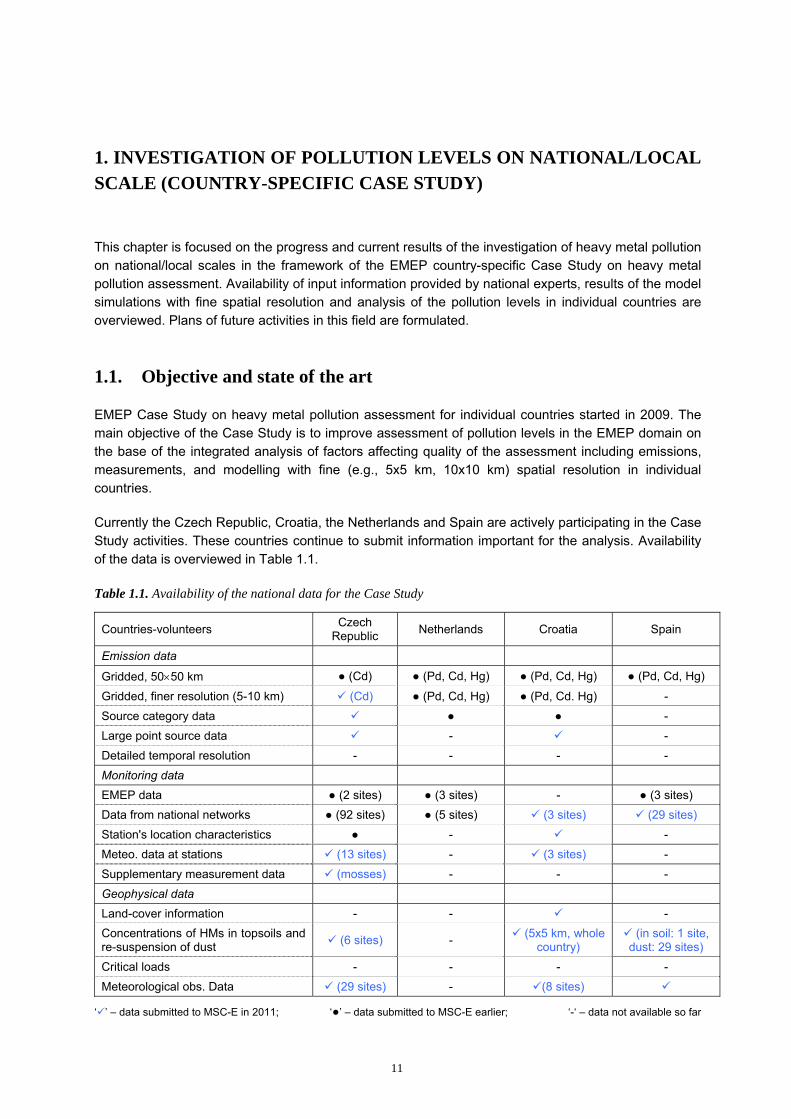
Currently the Czech Republic, Croatia, the Netherlands and Spain are actively participating in the Case Study activities. These countries continue to submit information important for the analysis. Availability of the data is overviewed in Table 1.1.

Table 1.1. Availability of the national data for the Case Study

Countries-volunteers Czech Republic Netherlands Croatia Spain

Emission data

Gridded, 50×50 km ● (Cd) ● (Pd, Cd, Hg) ● (Pd, Cd, Hg) ● (Pd, Cd, Hg)

Gridded, finer resolution (5-10 km) (Cd) ● (Pd, Cd, Hg) ● (Pd, Cd. Hg) - Source category data ● ● - Large point source data - - Detailed temporal resolution - - - - Monitoring data EMEP data ● (2 sites) ● (3 sites) - ● (3 sites) Data from national networks ● (92 sites) ● (5 sites) (3 sites) (29 sites) Station's location characteristics ● - - Meteo. data at stations (13 sites) - (3 sites) - Supplementary measurement data (mosses) - - - Geophysical data Land-cover information - - - Concentrations of HMs in topsoils and re-suspension of dust (6 sites) - (5x5 km, whole

country) (in soil: 1 site,

dust: 29 sites) Critical loads - - - - Meteorological obs. Data (29 sites) - (8 sites)

‘ ’ – data submitted to MSC-E in 2011; ‘●’ – data submitted to MSC-E earlier; ‘-‘ – data not available so far

12

Status of the current results differs from one participating country to another. Simulations of air concentrations and deposition of cadmium have been carried out for the Czech Republic. The obtained results are analyzed now in cooperation with the experts from this country. Analysis of modelled and measured levels of lead in Croatia has begun recently. For the Netherlands pilot calculations of lead pollution levels have been performed, and analysis is needed. Spain has provided MSC-E with national measurement data on heavy metals, observed meteorological parameters and dust suspension, and the model simulations will be carried out in future. In further sections of this chapter the results for each country are described in more detail.

Country-specific data, current results and future plans of the country-specific Case Studies were discussed at bi-lateral meetings: MSC-E and Croatia (Moscow, November, 2010), MSC-E and the Czech Republic (Moscow, April, 2011), MSC-E and the Netherlands, MSC-E and Spain (Zurich, May, 2011). The results of the collaborative work on heavy metal pollution assessment were presented at the annual TFMM meeting (Zurich, 2011, May).

1.2. The Czech Republic

Monitoring

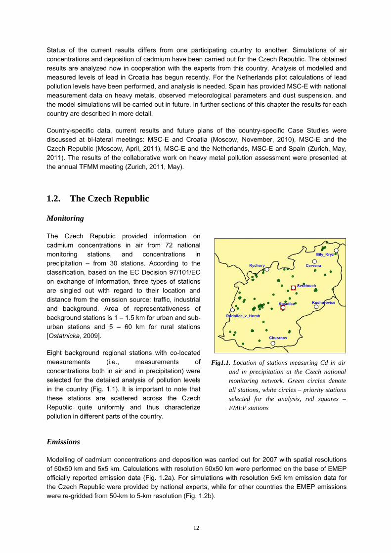
The Czech Republic provided information on cadmium concentrations in air from 72 national monitoring stations, and concentrations in precipitation – from 30 stations. According to the classification, based on the EC Decision 97/101/EC on exchange of information, three types of stations are singled out with regard to their location and distance from the emission source: traffic, industrial and background. Area of representativeness of background stations is 1 – 1.5 km for urban and sub-urban stations and 5 – 60 km for rural stations [Ostatnicka, 2009].

Eight background regional stations with co-located measurements (i.e., measurements of concentrations both in air and in precipitation) were selected for the detailed analysis of pollution levels in the country (Fig. 1.1). It is important to note that these stations are scattered across the Czech Republic quite uniformly and thus characterize pollution in different parts of the country.

Emissions

Modelling of cadmium concentrations and deposition was carried out for 2007 with spatial resolutions of 50x50 km and 5x5 km. Calculations with resolution 50x50 km were performed on the base of EMEP officially reported emission data (Fig. 1.2a). For simulations with resolution 5x5 km emission data for the Czech Republic were provided by national experts, while for other countries the EMEP emissions were re-gridded from 50-km to 5-km resolution (Fig. 1.2b).

Fig1.1. Location of stations measuring Cd in air and in precipitation at the Czech national monitoring network. Green circles denote all stations, white circles – priority stations selected for the analysis, red squares – EMEP stations

13

a b

Fig. 1.2. Spatial distribution of emission data with resolution 50x50 km (a) and 5x5 km (b). Location of priority stations is depicted by circles

Calculated Cd levels in the Czech Republic

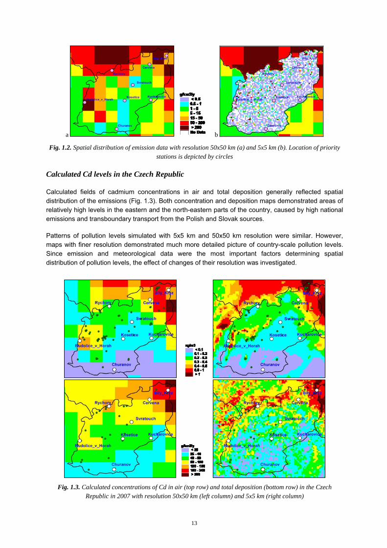
Calculated fields of cadmium concentrations in air and total deposition generally reflected spatial distribution of the emissions (Fig. 1.3). Both concentration and deposition maps demonstrated areas of relatively high levels in the eastern and the north-eastern parts of the country, caused by high national emissions and transboundary transport from the Polish and Slovak sources.

Patterns of pollution levels simulated with 5x5 km and 50x50 km resolution were similar. However, maps with finer resolution demonstrated much more detailed picture of country-scale pollution levels. Since emission and meteorological data were the most important factors determining spatial distribution of pollution levels, the effect of changes of their resolution was investigated.

Fig. 1.3. Calculated concentrations of Cd in air (top row) and total deposition (bottom row) in the Czech Republic in 2007 with resolution 50x50 km (left column) and 5x5 km (right column)

14

Influence of spatial resolution of meteorological and emission data

Influence of spatial resolution of emission and meteorological data was investigated in two steps. At the first step two model runs were performed. One model run was carried out with the usage of 50-km resolution of emissions and meteorological data and thus represented simulations which were performed operationally for the EMEP region. For the other run 50-km meteorological data were replaced by the data with 5-km resolution. Emission data were re-gridded from 50x50 km to 5x5 km resolution. Thus, each 50-km gridcell was split into one hundred 5-km grid cells, and real resolution of the emissions remained the same. The results of these two runs were compared with each other and with observed concentrations in air. Therefore, the first step allowed us to see the differences in modelling results caused by changes from coarser to finer resolution of meteorological data.

Resolution of meteorological data

Refinement of spatial resolution of meteorological data resulted to improvement of the model performance at most of stations (Fig. 1.4). Mean relative bias of annual average concentrations changed from 33% to 25% as resolution of meteorological data changed from 50 km to 5 km. More explicit changes in modelling results can be seen when time series are compared.

Example of time series of Cd air concentrations for one of stations (Cervena) is depicted in Fig. 1.5a. Changes between modelling results based on different resolutions are clearly seen for a number of short-term periods. For example, in the period from 3rd to 13th of February the model with 50-km resolution produced two high peaks of concentrations, and first of them was not confirmed by measurement data (Fig 1.5b). As resolution of meteorological data changed, model did not produce the peak. Another example is period from 6th to 30th of December. Changes of the resolution led to much closer agreement between modelled and measured values (Fig. 1.5c).

a

0

0.5

1

1.5

2

2.5

02.0

1_03

.01

12.0

1_13

.01

22.0

1_23

.01

01.0

2_02

.02

11.0

2_12

.02

21.0

2_22

.02

03.0

3_04

.03

13.0

3_14

.03

23.0

3_24

.03

02.0

4_03

.04

12.0

4_13

.04

22.0

4_23

.04

02.0

5_03

.05

12.0

5_13

.05

22.0

5_23

.05

01.0

6_02

.06

11.0

6_12

.06

21.0

6_22

.06

01.0

7_02

.07

11.0

7_12

.07

21.0

7_22

.07

31.0

7_01

.08

10.0

8_11

.08

20.0

8_21

.08

30.0

8_31

.08

09.0

9_10

.09

19.0

9_20

.09

29.0

9_30

.09

09.1

0_10

.10

19.1

0_20

.10

29.1

0_30

.10

08.1

1_09

.11

18.1

1_19

.11

28.1

1_29

.11

08.1

2_09

.12

18.1

2_19

.12

28.1

2_29

.12

Con

cent

ratio

ns in

air,

ng/

m3 Model (5km, meteo)Model (50km)Observed

February 3 - 13 December 6 - 30

0

0.1

0.2

0.3

0.4

0.5

0.6

Bily

_Kriz

Cer

vena

Chu

rano

v

Kos

etic

e

Krko

nose

-Ryc

hory

Kuch

arov

ice

Svra

touc

h

Rud

olic

e_v_

Hor

ach

Con

cent

ratio

ns in

air,

ng/

m3

Modelled (50km)Modelled (5km, meteo)Observed

Fig.1. 4. Mean annual modelled and observed concentrations of Cd in air in 2007

15

b

0

0.3

0.6

0.9

1.2

1.5

03.0

2_04

.02

05.0

2_06

.02

07.0

2_08

.02

09.0

2_10

.02

11.0

2_12

.02

13.0

2_14

.02

ObservedModel (50km)Model (5km, meteo)

c

0

0.3

0.6

0.9

1.2

1.5

06.1

2_07

.12

08.1

2_09

.12

10.1

2_11

.12

12.1

2_13

.12

14.1

2_15

.12

16.1

2_17

.12

18.1

2_19

.12

20.1

2_21

.12

22.1

2_23

.12

24.1

2_25

.12

26.1

2_27

.12

28.1

2_29

.12

30.1

2_31

.12

ObservedModel (50km)Model (5km, meteo)

Fig. 1.5. Time series of modelled and measured concentrations of Cd in air at station Cervena in 2007 (a) and extracts for periods 3rd -13th of February (b) and 6th - 30th of December (c).

Resolution of meteorological and emission data

At the second step additional model run based on emission and meteorology with 5-km resolution was performed. The results of this model run were compared with results obtained at the first step and with the observed levels. Therefore, the second step demonstrated the difference in calculated levels caused by changes of both emission and meteorological data resolution, compared to operational EMEP modelling with 50-km resolution.

Changes of resolution of emission data had most significant impact on the results for the stations Bily Kriz and Rudolice v Horah (Fig. 1.6), while for the other stations the changes on annual mean level were relatively small.

At station Rudolice v Horah the improvement was the most marked. When model simulations were made with 50 km resolution the observed concentrations were overestimated by 3.7 times. The refinement of resolution of emission and meteorological data led to much smaller difference (about 40%) between modelled and measured values. Station Rudolice v Horah was located in a grid cell where emission with 50-km resolution was relatively high (Fig. 1.2a). However, on the map with fine resolution of emission data it was seen that high emissions were located in few grid cells around the station. These changes of the emissions led to obvious improvement of the model performance throughout the whole year (Fig. 1.7).

0

0.1

0.2

0.3

0.4

0.5

0.6B

ily_K

riz

Cer

vena

Chu

rano

v

Kos

etic

e

Krko

nose

-Ryc

hory

Kuch

arov

ice

Svr

atou

ch

Rud

olic

e_v_

Hor

ach

Con

cent

ratio

ns in

air,

ng/

m3 Modelled (50km)

Modelled (5km, meteo)Modelled (5km, met & emis.)Observed

Fig. 1.6. Mean annual modelled and observed concentrations of Cd in air in 2007

16

0

0.5

1

1.5

2

02.0

1_03

.01

09.0

1_10

.01

17.0

1_18

.01

24.0

1_25

.01

02.0

2_03

.02

10.0

2_11

.02

17.0

2_18

.02

25.0

2_26

.02

04.0

3_05

.03

12.0

3_13

.03

19.0

3_20

.03

27.0

3_28

.03

03.0

4_04

.04

11.0

4_12

.04

20.0

4_21

.04

27.0

4_28

.04

05.0

5_06

.05

12.0

5_13

.05

20.0

5_21

.05

29.0

5_30

.05

05.0

6_06

.06

13.0

6_14

.06

20.0

6_21

.06

29.0

6_30

.06

07.0

7_08

.07

17.0

7_18

.07

28.0

7_29

.07

04.0

8_05

.08

13.0

8_14

.08

21.0

8_22

.08

28.0

8_29

.08

05.0

9_06

.09

12.0

9_13

.09

21.0

9_22

.09

29.0

9_30

.09

06.1

0_07

.10

14.1

0_15

.10

21.1

0_22

.10

29.1

0_30

.10

05.1

1_06

.11

13.1

1_14

.11

20.1

1_21

.11

28.1

1_29

.11

05.1

2_06

.12

13.1

2_14

.12

20.1

2_21

.12

28.1

2_29

.12

Con

cent

ratio

ns in

air,

ng/

m3 Model (50km)Model (5km, meteo & emission)Observed

b

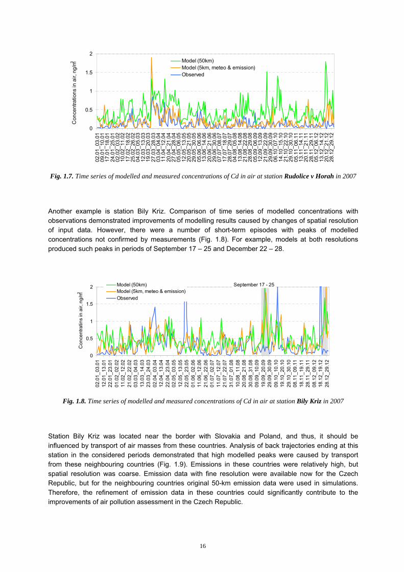
Fig. 1.7. Time series of modelled and measured concentrations of Cd in air at station Rudolice v Horah in 2007

Another example is station Bily Kriz. Comparison of time series of modelled concentrations with observations demonstrated improvements of modelling results caused by changes of spatial resolution of input data. However, there were a number of short-term episodes with peaks of modelled concentrations not confirmed by measurements (Fig. 1.8). For example, models at both resolutions produced such peaks in periods of September 17 – 25 and December 22 – 28.

0

0.5

1

1.5

2

02.0

1_03

.01

12.0

1_13

.01

22.0

1_23

.01

01.0

2_02

.02

11.0

2_12

.02

21.0

2_22

.02

03.0

3_04

.03

13.0

3_14

.03

23.0

3_24

.03

02.0

4_03

.04

12.0

4_13

.04

22.0

4_23

.04

02.0

5_03

.05

12.0

5_13

.05

22.0

5_23

.05

01.0

6_02

.06

11.0

6_12

.06

21.0

6_22

.06

01.0

7_02

.07

11.0

7_12

.07

21.0

7_22

.07

31.0

7_01

.08

10.0

8_11

.08

20.0

8_21

.08

30.0

8_31

.08

09.0

9_10

.09

19.0

9_20

.09

29.0

9_30

.09

09.1

0_10

.10

19.1

0_20

.10

29.1

0_30

.10

08.1

1_09

.11

18.1

1_19

.11

28.1

1_29

.11

08.1

2_09

.12

18.1

2_19

.12

28.1

2_29

.12

Con

cent

ratin

s in

air,

ng/

m3

Model (50km)Model (5km, meteo & emission)Observed

September 17 - 25

Fig. 1.8. Time series of modelled and measured concentrations of Cd in air at station Bily Kriz in 2007

Station Bily Kriz was located near the border with Slovakia and Poland, and thus, it should be influenced by transport of air masses from these countries. Analysis of back trajectories ending at this station in the considered periods demonstrated that high modelled peaks were caused by transport from these neighbouring countries (Fig. 1.9). Emissions in these countries were relatively high, but spatial resolution was coarse. Emission data with fine resolution were available now for the Czech Republic, but for the neighbouring countries original 50-km emission data were used in simulations. Therefore, the refinement of emission data in these countries could significantly contribute to the improvements of air pollution assessment in the Czech Republic.

17

Overall effect of spatial resolution changes on the model performance was expressed via statistical indexes. Mean relative bias characterized deviation of modelled value from the observed one on annual basis. When finer spatial resolution was used, the bias was much closer to zero for five stations compared to the results obtained with coarser resolution (Fig. 1.10).

Another parameter, characterizing deviation between modelled and observed values was normalized root mean square error (NRMSE). Unlike mean relative bias, NRMSE summarized effect of deviations of individual model-measurement pairs in time series. The smaller NRMSE meant that modelled results were closer to the observations. Transition from 50 km to 5 km resolution led to decrease of NRMSE at most of priority stations (Table 1.2).

Table 1.2. Root mean square error for modelling results with 50 km and 5 km resolution

Station 50 km 5 km Bily Kriz 1.5 1.2 Cervena 1.6 1.2 Churanov 0.9 0.8 Kosetice 0.7 0.7 Rychory 1.6 1.2 Kucharovice 0.6 0.8 Svratouch 0.8 0.7 Rudolice c Horah 3.8 1.4

Analysis of air pollution short-term episodes

Pollution levels in individual countries depend on a number of factors such as emissions, location of measurement station, trajectories of transport of air masses, fields of precipitation etc. The influence of these factors can change in time. Therefore, for detailed analysis of these factors short-term pollution episodes should be considered.

Episode in November

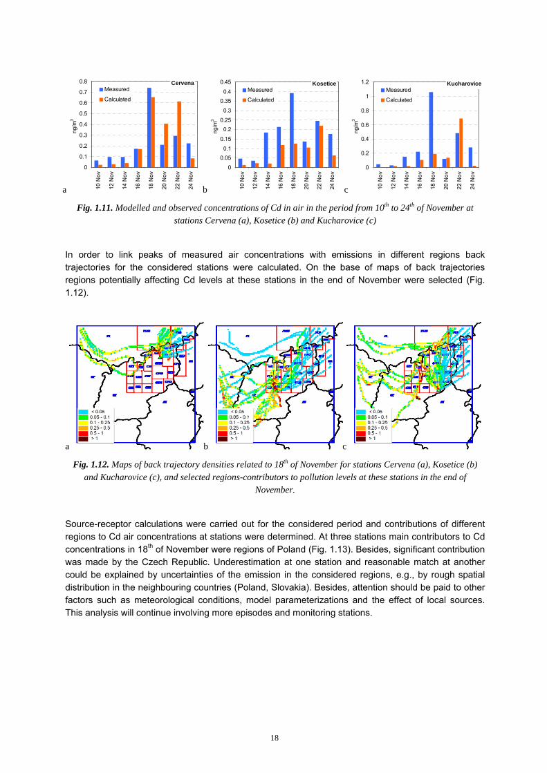
One of interesting episodes took place at the end of November, 2007. In this episode at three stations peak of concentrations in air was observed (Fig. 1.11). At stations Kosetice and Kucharovice the model significantly underestimated the observed concentrations, while at Cervena the peak was captured by the model.

Fig. 1.9. Density of back trajectories for station

Bily Kriz in the period from 17th to 25th of September

-100-80-60-40-20

020406080

100

Bily

_Kriz

Cer

vena

Krko

nose

-Ryc

hory

Kuc

haro

vice

Rud

olic

e_v_

Hor

ach

Kos

etic

e

Chu

rano

v

Svr

atou

ch

%

Modelled (50km)

Modelled (5km)

275

Fig.1.10. Mean relative bias for annual mean Cd air concentrations simulated with 50 km

and 5 km resolutions

18

a

Cervena

0

0.1

0.2

0.3

0.4

0.5

0.6

0.7

0.8

10 N

ov

12 N

ov

14 N

ov

16 N

ov

18 N

ov

20 N

ov

22 N

ov

24 N

ov

ng/m

3

Measured

Calculated

b

Kosetice

0

0.050.1

0.15

0.20.25

0.3

0.350.4

0.45

10 N

ov

12 N

ov

14 N

ov

16 N

ov

18 N

ov

20 N

ov

22 N

ov

24 N

ov

ng/m

3

Measured

Calculated

c

Kucharovice

0

0.2

0.4

0.6

0.8

1

1.2

10 N

ov

12 N

ov

14 N

ov

16 N

ov

18 N

ov

20 N

ov

22 N

ov

24 N

ov

ng/m

3

Measured

Calculated

Fig. 1.11. Modelled and observed concentrations of Cd in air in the period from 10th to 24th of November at stations Cervena (a), Kosetice (b) and Kucharovice (c)

In order to link peaks of measured air concentrations with emissions in different regions back trajectories for the considered stations were calculated. On the base of maps of back trajectories regions potentially affecting Cd levels at these stations in the end of November were selected (Fig. 1.12).

a b c

Fig. 1.12. Maps of back trajectory densities related to 18th of November for stations Cervena (a), Kosetice (b) and Kucharovice (c), and selected regions-contributors to pollution levels at these stations in the end of

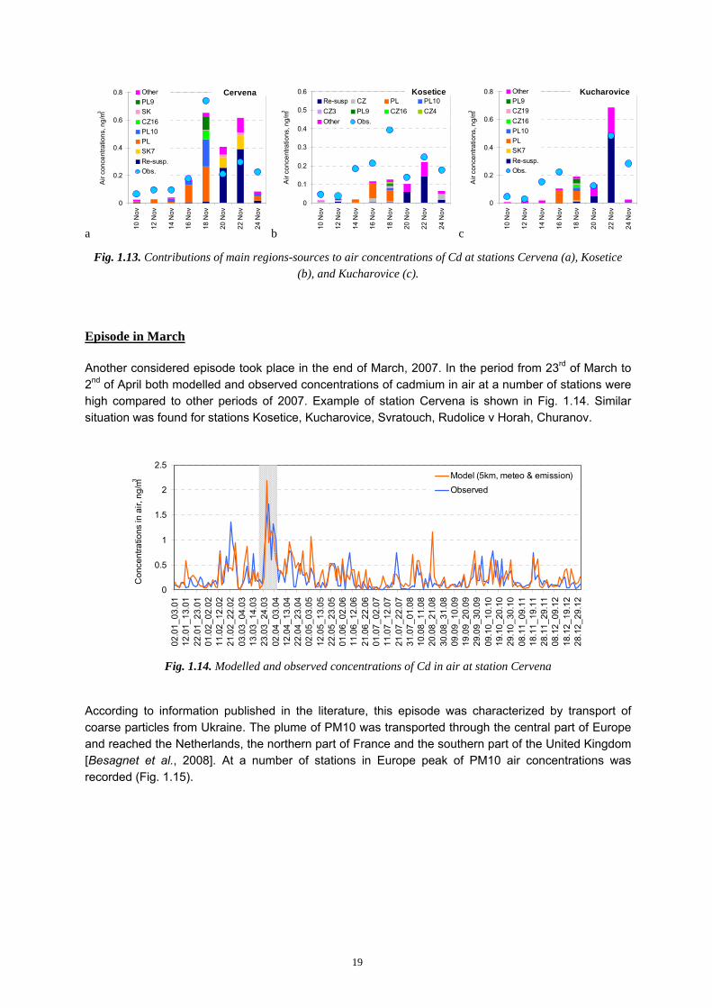
November.

Source-receptor calculations were carried out for the considered period and contributions of different regions to Cd air concentrations at stations were determined. At three stations main contributors to Cd concentrations in 18th of November were regions of Poland (Fig. 1.13). Besides, significant contribution was made by the Czech Republic. Underestimation at one station and reasonable match at another could be explained by uncertainties of the emission in the considered regions, e.g., by rough spatial distribution in the neighbouring countries (Poland, Slovakia). Besides, attention should be paid to other factors such as meteorological conditions, model parameterizations and the effect of local sources. This analysis will continue involving more episodes and monitoring stations.

19

a

0

0.2

0.4

0.6

0.8

10 N

ov

12 N

ov

14 N

ov

16 N

ov

18 N

ov

20 N

ov

22 N

ov

24 N

ov

Air

conc

entra

tions

, ng/

m3OtherPL9SKCZ16PL10PLSK7Re-susp.Obs.

Cervena

b

0

0.1

0.2

0.3

0.4

0.5

0.6

10 N

ov

12 N

ov

14 N

ov

16 N

ov

18 N

ov

20 N

ov

22 N

ov

24 N

ov

Air

conc

entra

tions

, ng/

m3

Re-susp CZ PL PL10CZ3 PL9 CZ16 CZ4Other Obs.

Kosetice

c

0

0.2

0.4

0.6

0.8

10 N

ov

12 N

ov

14 N

ov

16 N

ov

18 N

ov

20 N

ov

22 N

ov

24 N

ov

Air

conc

entra

tions

, ng/

m3

OtherPL9CZ19CZ16PL10PLSK7Re-susp.Obs.

Kucharovice

Fig. 1.13. Contributions of main regions-sources to air concentrations of Cd at stations Cervena (a), Kosetice (b), and Kucharovice (c).

Episode in March

Another considered episode took place in the end of March, 2007. In the period from 23rd of March to 2nd of April both modelled and observed concentrations of cadmium in air at a number of stations were high compared to other periods of 2007. Example of station Cervena is shown in Fig. 1.14. Similar situation was found for stations Kosetice, Kucharovice, Svratouch, Rudolice v Horah, Churanov.

0

0.5

1

1.5

2

2.5

02.0

1_03

.01

12.0

1_13

.01

22.0

1_23

.01

01.0

2_02

.02

11.0

2_12

.02

21.0

2_22

.02

03.0

3_04

.03

13.0

3_14

.03

23.0

3_24

.03

02.0

4_03

.04

12.0

4_13

.04

22.0

4_23

.04

02.0

5_03

.05

12.0

5_13

.05

22.0

5_23

.05

01.0

6_02

.06

11.0

6_12

.06

21.0

6_22

.06

01.0

7_02

.07

11.0

7_12

.07

21.0

7_22

.07

31.0

7_01

.08

10.0

8_11

.08

20.0

8_21

.08

30.0

8_31

.08

09.0

9_10

.09

19.0

9_20

.09

29.0

9_30

.09

09.1

0_10

.10

19.1

0_20

.10

29.1

0_30

.10

08.1

1_09

.11

18.1

1_19

.11

28.1

1_29

.11

08.1

2_09

.12

18.1

2_19

.12

28.1

2_29

.12

Con

cent

ratio

ns in

air,

ng/

m3 Model (5km, meteo & emission)Observed

Fig. 1.14. Modelled and observed concentrations of Cd in air at station Cervena

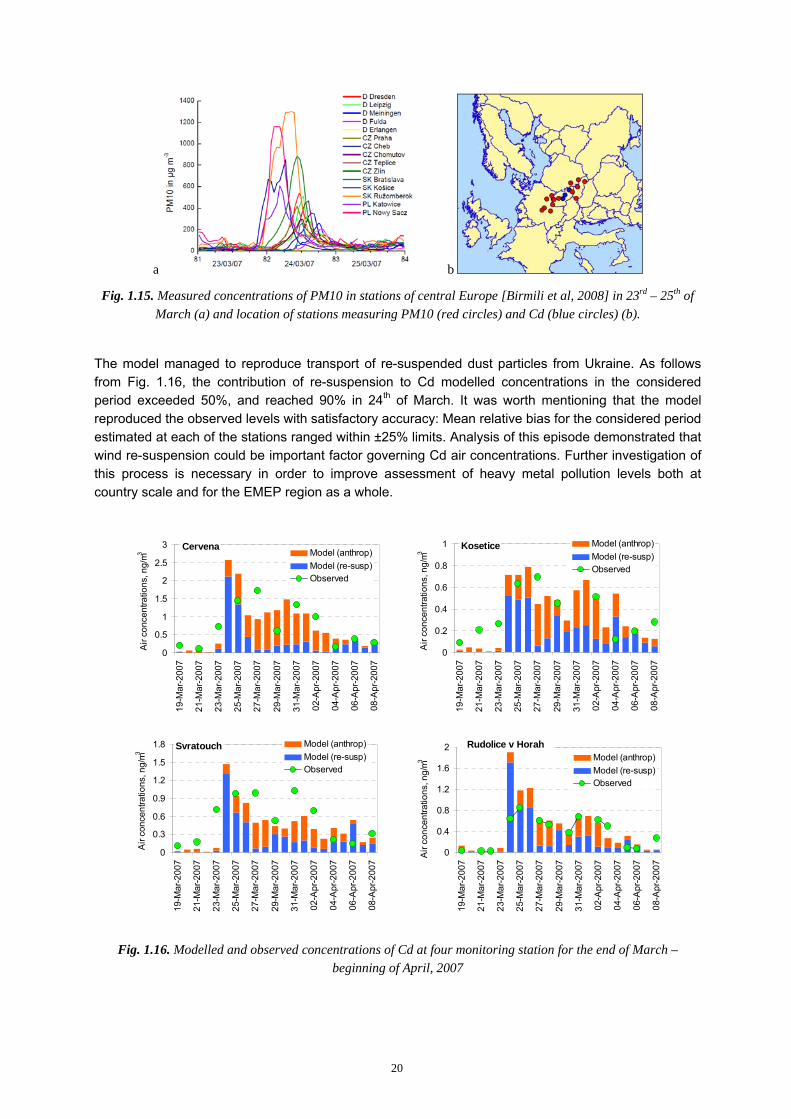
According to information published in the literature, this episode was characterized by transport of coarse particles from Ukraine. The plume of PM10 was transported through the central part of Europe and reached the Netherlands, the northern part of France and the southern part of the United Kingdom [Besagnet et al., 2008]. At a number of stations in Europe peak of PM10 air concentrations was recorded (Fig. 1.15).

20

a

b

Fig. 1.15. Measured concentrations of PM10 in stations of central Europe [Birmili et al, 2008] in 23rd – 25th of March (a) and location of stations measuring PM10 (red circles) and Cd (blue circles) (b).

The model managed to reproduce transport of re-suspended dust particles from Ukraine. As follows from Fig. 1.16, the contribution of re-suspension to Cd modelled concentrations in the considered period exceeded 50%, and reached 90% in 24th of March. It was worth mentioning that the model reproduced the observed levels with satisfactory accuracy: Mean relative bias for the considered period estimated at each of the stations ranged within ±25% limits. Analysis of this episode demonstrated that wind re-suspension could be important factor governing Cd air concentrations. Further investigation of this process is necessary in order to improve assessment of heavy metal pollution levels both at country scale and for the EMEP region as a whole.

Cervena

0

0.5

1

1.5

2

2.5

3

19-M

ar-2

007

21-M

ar-2

007

23-M

ar-2

007

25-M

ar-2

007

27-M

ar-2

007

29-M

ar-2

007

31-M

ar-2

007

02-A

pr-2

007

04-A

pr-2

007

06-A

pr-2

007

08-A

pr-2

007

Air

conc

entra

tions

, ng/

m3 Model (anthrop)Model (re-susp)Observed

Kosetice

0

0.2

0.4

0.6

0.8

1

19-M

ar-2

007

21-M

ar-2

007

23-M

ar-2

007

25-M

ar-2

007

27-M

ar-2

007

29-M

ar-2

007

31-M

ar-2

007

02-A

pr-2

007

04-A

pr-2

007

06-A

pr-2

007

08-A

pr-2

007

Air

conc

entra

tions

, ng/

m3

Model (anthrop)Model (re-susp)Observed

Svratouch

0

0.3

0.6

0.9

1.2

1.5

1.8

19-M

ar-2

007

21-M

ar-2

007

23-M

ar-2

007

25-M

ar-2

007

27-M

ar-2

007

29-M

ar-2

007

31-M

ar-2

007

02-A

pr-2

007

04-A

pr-2

007

06-A

pr-2

007

08-A

pr-2

007

Air

conc

entra

tions

, ng/

m3

Model (anthrop)Model (re-susp)Observed

0

0.4

0.8

1.2

1.6

2

19-M

ar-2

007

21-M

ar-2

007

23-M

ar-2

007

25-M

ar-2

007

27-M

ar-2

007

29-M

ar-2

007

31-M

ar-2

007

02-A

pr-2

007

04-A

pr-2

007

06-A

pr-2

007

08-A

pr-2

007

Air

conc

entra

tions

, ng/

m3 Model (anthrop)Model (re-susp)Observed

Rudolice v Horah

Fig. 1.16. Modelled and observed concentrations of Cd at four monitoring station for the end of March – beginning of April, 2007

21

Application of measurements in mosses for the analysis of pollution levels in the Czech Republic

Assessment of cadmium pollution levels in the Czech Republic was carried out involving variety of available information such as emissions, monitoring data and modelling results. Observed concentrations of heavy metals in terrestrial mosses are used as supplementary data for the assessment.

Concentrations in mosses for this country were used for the following purposes:

To investigate of relationships between observed wet deposition of Cd in the Czech Republic and measured concentrations in mosses

To evaluate total deposition over the Czech Republic, simulated with fine (5x5 km) and coarse (50x50 km) spatial resolution via comparison with measured concentrations in mosses

Various types of information were involved in the analysis for the Czech Republic. In particular, they included cadmium wet deposition measured at the Czech national monitoring network [Ostatnicka, 2009] for the period from 2004 to 2005 (Fig. 1.17a). Concentrations of cadmium measured in mosses were provided by the ICP-Vegetation and described in [Sucharova et al, 2008] (Fig. 1.17b). Emission data and modelled total deposition fluxes (Fig. 1.17c,d) over the Czech Republic with fine spatial resolution as well as operational modelling results obtained with resolution 50x50 km were involved in the analysis.

a b

c d Fig. 1.17. Observed wet deposition flux of Cd (mean for 2004-2005) (a), concentrations of Cd in mosses (b),

emission data used in modelling (c) and modelled total deposition of Cd in 2007 with fine spatial resolution (d) In this study observed wet deposition fluxes from almost 30 monitoring stations were compared with concentrations of Cd measured in mosses. Wet deposition and concentrations in mosses cannot be

22

compared directly. However, similarities in spatial distribution of these two variables can be evaluated by means of regression analysis. Similar approach was applied for comparison of heavy metal concentrations in mosses with measured deposition by other researches [Berg et al., 1995, Berg and Steinnes, 1997, Thöni et al., 2011].

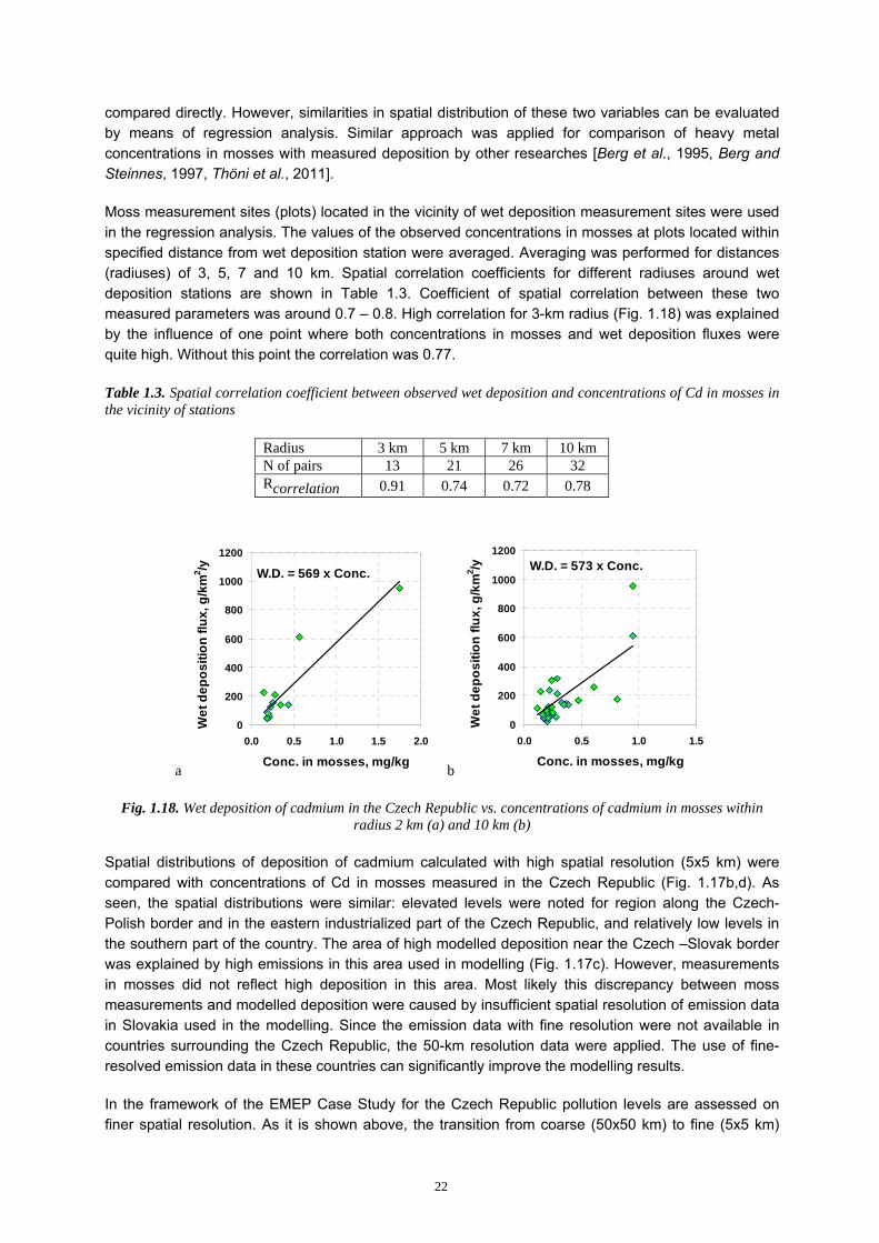
Moss measurement sites (plots) located in the vicinity of wet deposition measurement sites were used in the regression analysis. The values of the observed concentrations in mosses at plots located within specified distance from wet deposition station were averaged. Averaging was performed for distances (radiuses) of 3, 5, 7 and 10 km. Spatial correlation coefficients for different radiuses around wet deposition stations are shown in Table 1.3. Coefficient of spatial correlation between these two measured parameters was around 0.7 – 0.8. High correlation for 3-km radius (Fig. 1.18) was explained by the influence of one point where both concentrations in mosses and wet deposition fluxes were quite high. Without this point the correlation was 0.77.

Table 1.3. Spatial correlation coefficient between observed wet deposition and concentrations of Cd in mosses in the vicinity of stations

Radius 3 km 5 km 7 km 10 km N of pairs 13 21 26 32 Rcorrelation 0.91 0.74 0.72 0.78

a b

W.D. = 573 x Conc.

0

200

400

600

800

1000

1200

0.0 0.5 1.0 1.5

Conc. in mosses, mg/kg

Wet

dep

ositi

on fl

ux, g

/km

2 /y

Fig. 1.18. Wet deposition of cadmium in the Czech Republic vs. concentrations of cadmium in mosses within radius 2 km (a) and 10 km (b)

Spatial distributions of deposition of cadmium calculated with high spatial resolution (5x5 km) were compared with concentrations of Cd in mosses measured in the Czech Republic (Fig. 1.17b,d). As seen, the spatial distributions were similar: elevated levels were noted for region along the Czech-Polish border and in the eastern industrialized part of the Czech Republic, and relatively low levels in the southern part of the country. The area of high modelled deposition near the Czech –Slovak border was explained by high emissions in this area used in modelling (Fig. 1.17c). However, measurements in mosses did not reflect high deposition in this area. Most likely this discrepancy between moss measurements and modelled deposition were caused by insufficient spatial resolution of emission data in Slovakia used in the modelling. Since the emission data with fine resolution were not available in countries surrounding the Czech Republic, the 50-km resolution data were applied. The use of fine-resolved emission data in these countries can significantly improve the modelling results.

In the framework of the EMEP Case Study for the Czech Republic pollution levels are assessed on finer spatial resolution. As it is shown above, the transition from coarse (50x50 km) to fine (5x5 km)

W.D. = 569 x Conc.

0

200

400

600

800

1000

1200

0.0 0.5 1.0 1.5 2.0

Conc. in mosses, mg/kg

Wet

dep

ositi

on fl

ux, g

/km

2 /y

23

spatial resolution favours better agreement between modelled and observed concentrations at monitoring stations. Data on the observed concentrations of Cd in mosses were used as supplementary data to evaluate the differences of the model performance caused by changes of spatial resolution. For evaluation of similarities between modelled total deposition and concentrations in mosses spatial correlation coefficient between was used.

Modelled total deposition values represented separate gridcells, while concentrations in mosses were observed at individual points (plots). Each gridcell could include one or several plots. If a grid cell included two or more plots, the concentrations in mosses could be averaged and modelled total deposition value was compared with averaged concentration in mosses. Or the deposition could be compared with concentrations in moss sampled at each plot separately.

In the first case (with averaging of concentrations in mosses) the deposition simulated with fine spatial resolution were aggregated to coarser resolution for the purpose of comparability (Fig. 1.19). Correlation coefficients were almost equal: 0.85 for modelling with fine spatial resolution, and 0.84 - with coarse resolution. This correlation coefficient was rather high compared to correlation found between concentrations in mosses and observed deposition (Table 1.3).

Fig. 1.19. Total deposition of Cd simulated with spatial resolution 50x50 km (a) and 5x5 km, aggregated to 50x50 km (b) against observed concentrations of Cd in mosses in the Czech Republic. Concentrations of Cd in

mosses belonging to the same mode gridcell were averaged In the second case (without averaging of concentrations in mosses) the correlation coefficient between calculated 50-km total deposition and concentrations in mosses was 0.53 (Fig. 1.20). When deposition with finer resolution (5x5 km) was applied, the correlation was 0.59. Therefore, it is possible to make conclusion that the increase of spatial resolution improves quality of heavy metal pollution assessment, at least in the Czech Republic.

TD = 256 x Conc0

50

100

150

200

250

300

350

0.0 0.3 0.6 0.9 1.2 1.5

Conc. in mosses, mg/g

Tota

l dep

ositi

on, g

/km

2 /y

TD = 250 x Conc0

50

100

150

200

250

300

350

0.0 0.3 0.6 0.9 1.2 1.5

Conc. in mosses, mg/g

Tota

l dep

ositi

on, g

/km

2 /y

24

a b

TD = 249 x Conc0

50

100

150

200

250

300

350

0.0 0.3 0.6 0.9 1.2 1.5 1.8

Conc. in mosses, mg/g

Tota

l dep

ositi

on, g

/km

2 /y

Fig. 1.20. Total deposition of Cd simulated with spatial resolution 50x50 km (a) and 5x5 km (b) against observed

concentrations of Cd in mosses in the Czech Republic. Concentrations of Cd in mosses belonging to the same mode gridcell were not averaged

The analysis presented in this chapter demonstrates that data on concentrations in mosses can be used in the assessment of pollution levels as supplementary data. Because of wide spatial coverage and high density of measurements this type of information is helpful in identifying areas of relatively high or low levels of atmospheric deposition. Further cooperation with the effects community regarding usage of measurements of heavy metals in mosses is needed for better understanding of relationships between deposition and concentrations in mosses and for interpretation of the measurements.

Concluding remarks

On the base of the results of the analysis for the Czech Republic the following concluding remarks can be formulated:

- Transition to finer resolution of emission and meteorological data leads to higher quality of pollution level assessment

- Involvement of national measurement data increases a base for the analysis and validation of transboundary transport

- In order to investigate factors affecting pollution levels in the country analysis of short-term variability of heavy metal levels is highly important.

- Wind re-suspension is important contributor to HM levels and needs more detailed investigation

- Coarse spatial emission distribution in the neighbouring countries leads to additional uncertainties of pollution levels in the country

- Measurements of concentrations in mosses can be used as supplementary information for the analysis of country-scale pollution levels

TD = 190 x Conc

0

50

100

150

200

250

300

350

0.0 0.3 0.6 0.9 1.2 1.5 1.8

Conc. in mosses, mg/g

Tota

l dep

ositi

on, g

/km

2 /y

25

1.3. Croatia

Calculations of lead pollution levels for Croatia was carried out with resolution 50x50 km on the base of the official EMEP emission data and with resolution 10x10 km using emissions submitted by national experts (Fig. 1.21). To perform modelling with high resolution emissions from neighbouring countries were re-gridded from 50-km grid to 10-km gridcells.

a b

Fig. 1.21. Emissions of lead in Croatia in 2007 officially submitted with 50-km resolution (a) and prepared in the framework of the Case Study with 10-km resolution (b). Location of measurement stations is indicated by blue

stars (Croatia) and white triangles (EMEP)

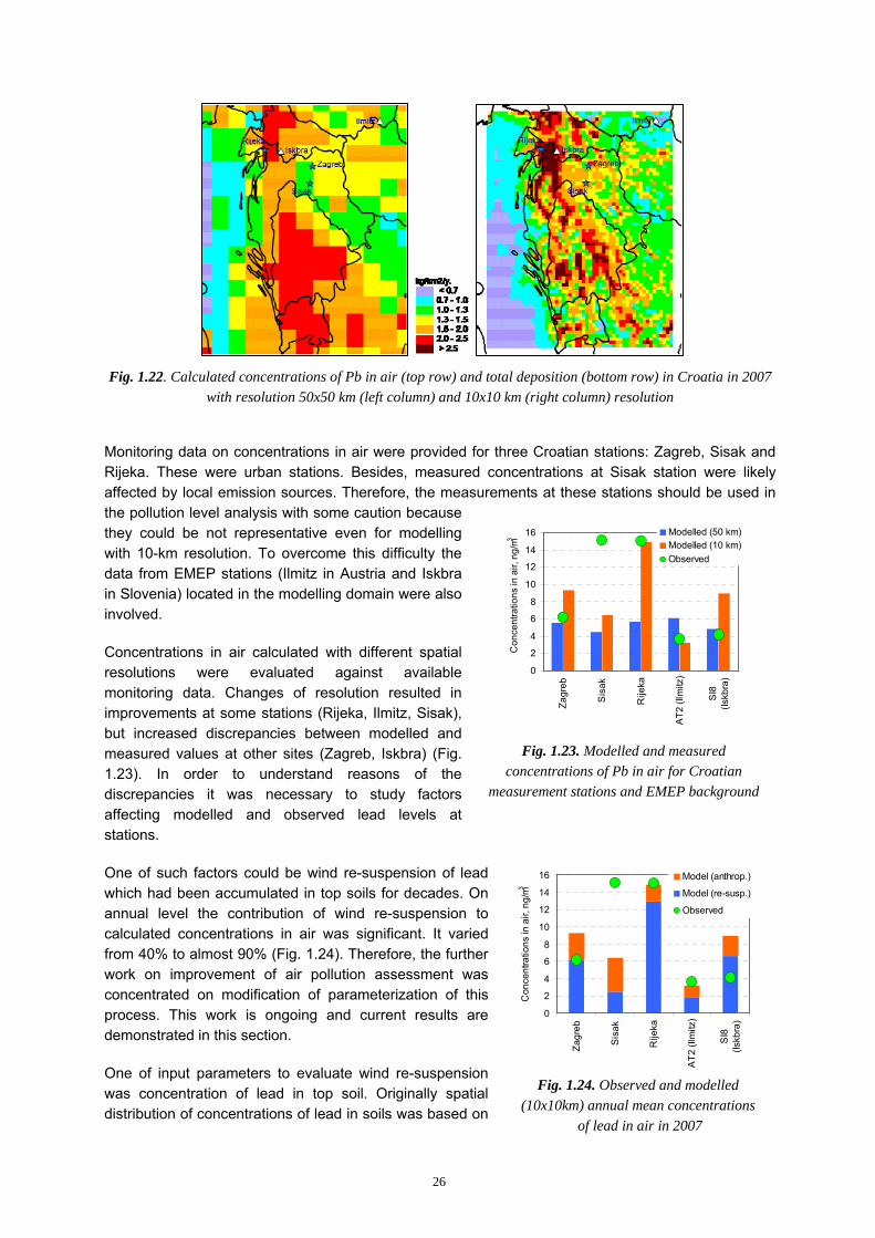
Spatial distributions of lead concentrations in air and total deposition simulated with different resolutions were similar (Fig. 1.22). However, the maps with 10-km resolution were more detailed compared to those with 50-km resolution. Besides, spatial gradients of pollution levels with coarser spatial resolution were less explicit due to smoothing effect of the larger grid cells.

26

Fig. 1.22. Calculated concentrations of Pb in air (top row) and total deposition (bottom row) in Croatia in 2007 with resolution 50x50 km (left column) and 10x10 km (right column) resolution

Monitoring data on concentrations in air were provided for three Croatian stations: Zagreb, Sisak and Rijeka. These were urban stations. Besides, measured concentrations at Sisak station were likely affected by local emission sources. Therefore, the measurements at these stations should be used in the pollution level analysis with some caution because they could be not representative even for modelling with 10-km resolution. To overcome this difficulty the data from EMEP stations (Ilmitz in Austria and Iskbra in Slovenia) located in the modelling domain were also involved.

Concentrations in air calculated with different spatial resolutions were evaluated against available monitoring data. Changes of resolution resulted in improvements at some stations (Rijeka, Ilmitz, Sisak), but increased discrepancies between modelled and measured values at other sites (Zagreb, Iskbra) (Fig. 1.23). In order to understand reasons of the discrepancies it was necessary to study factors affecting modelled and observed lead levels at stations.

One of such factors could be wind re-suspension of lead which had been accumulated in top soils for decades. On annual level the contribution of wind re-suspension to calculated concentrations in air was significant. It varied from 40% to almost 90% (Fig. 1.24). Therefore, the further work on improvement of air pollution assessment was concentrated on modification of parameterization of this process. This work is ongoing and current results are demonstrated in this section.

One of input parameters to evaluate wind re-suspension was concentration of lead in top soil. Originally spatial distribution of concentrations of lead in soils was based on

0

2

4

6

8

10

12

14

16

Zagr

eb

Sis

ak

Rije

ka

AT2

(Ilm

itz)

SI8

(Iskb

ra)

Con

cent

ratio

ns in

air,

ng/

m3

Modelled (50 km)Modelled (10 km)Observed

Fig. 1.23. Modelled and measured concentrations of Pb in air for Croatian

measurement stations and EMEP background

0

2

4

6

8

10

12

14

16

Zagr

eb

Sis

ak

Rije

ka

AT2

(Ilm

itz)

SI8

(Iskb

ra)

Con

cent

ratio

ns in

air,

ng/

m3

Model (anthrop.)

Model (re-susp.)

Observed

Fig. 1.24. Observed and modelled

(10x10km) annual mean concentrations of lead in air in 2007

27

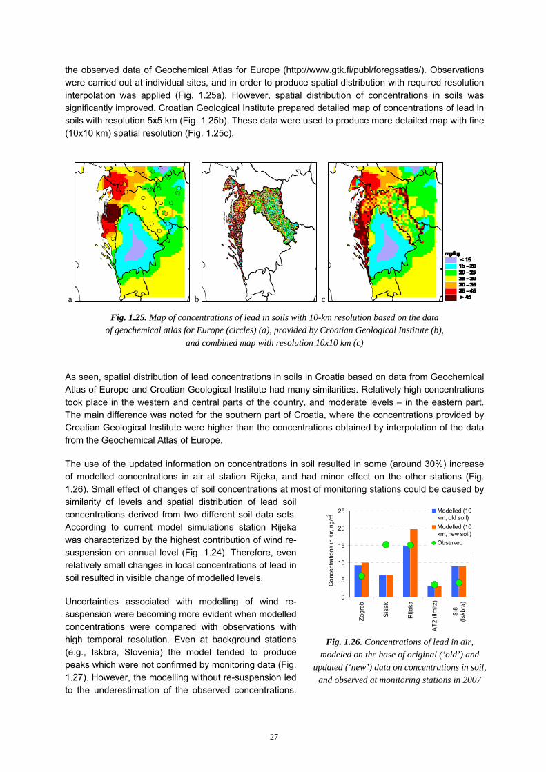
the observed data of Geochemical Atlas for Europe (http://www.gtk.fi/publ/foregsatlas/). Observations were carried out at individual sites, and in order to produce spatial distribution with required resolution interpolation was applied (Fig. 1.25a). However, spatial distribution of concentrations in soils was significantly improved. Croatian Geological Institute prepared detailed map of concentrations of lead in soils with resolution 5x5 km (Fig. 1.25b). These data were used to produce more detailed map with fine (10x10 km) spatial resolution (Fig. 1.25c).

a b c

Fig. 1.25. Map of concentrations of lead in soils with 10-km resolution based on the data of geochemical atlas for Europe (circles) (a), provided by Croatian Geological Institute (b),

and combined map with resolution 10x10 km (c)

As seen, spatial distribution of lead concentrations in soils in Croatia based on data from Geochemical Atlas of Europe and Croatian Geological Institute had many similarities. Relatively high concentrations took place in the western and central parts of the country, and moderate levels – in the eastern part. The main difference was noted for the southern part of Croatia, where the concentrations provided by Croatian Geological Institute were higher than the concentrations obtained by interpolation of the data from the Geochemical Atlas of Europe.

The use of the updated information on concentrations in soil resulted in some (around 30%) increase of modelled concentrations in air at station Rijeka, and had minor effect on the other stations (Fig. 1.26). Small effect of changes of soil concentrations at most of monitoring stations could be caused by similarity of levels and spatial distribution of lead soil concentrations derived from two different soil data sets. According to current model simulations station Rijeka was characterized by the highest contribution of wind re-suspension on annual level (Fig. 1.24). Therefore, even relatively small changes in local concentrations of lead in soil resulted in visible change of modelled levels.

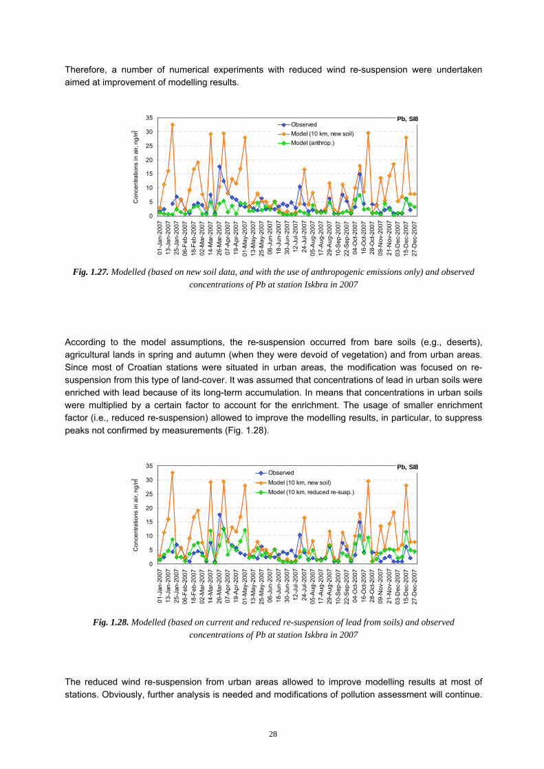
Uncertainties associated with modelling of wind re-suspension were becoming more evident when modelled concentrations were compared with observations with high temporal resolution. Even at background stations (e.g., Iskbra, Slovenia) the model tended to produce peaks which were not confirmed by monitoring data (Fig. 1.27). However, the modelling without re-suspension led to the underestimation of the observed concentrations.

0

5

10

15

20

25

Zagr

eb

Sis

ak

Rije

ka

AT2

(Ilm

itz)

SI8

(Iskb

ra)

Con

cent

ratio

ns in

air,

ng/

m3

Modelled (10km, old soil)Modelled (10km, new soil)Observed

Fig. 1.26. Concentrations of lead in air,

modeled on the base of original (‘old’) and updated (‘new’) data on concentrations in soil,

and observed at monitoring stations in 2007

28

Therefore, a number of numerical experiments with reduced wind re-suspension were undertaken aimed at improvement of modelling results.

Pb, SI8

0

5

10

15

20

25

30

35

01-

Jan-

2007

13-

Jan-

2007

25-

Jan-

2007

06-

Feb-

2007

18-

Feb-

2007

02-

Mar

-200

7 1

4-M

ar-2

007

26-

Mar

-200

7 0

7-A

pr-2

007

19-

Apr

-200

7 0

1-M

ay-2

007

13-

May

-200

7 2

5-M

ay-2

007

06-

Jun-

2007

18-

Jun-

2007

30-

Jun-

2007

12-

Jul-2

007

24-

Jul-2

007

05-

Aug

-200

7 1

7-A

ug-2

007

29-

Aug

-200

7 1

0-S

ep-2

007

22-

Sep

-200

7 0

4-O

ct-2

007

16-

Oct

-200

7 2

8-O

ct-2

007

09-

Nov

-200

7 2

1-N

ov-2

007

03-

Dec

-200

7 1

5-D

ec-2

007

27-

Dec

-200

7

Con

cent

ratio

ns in

air,

ng/

m3

ObservedModel (10 km, new soil)Model (anthrop.)

Fig. 1.27. Modelled (based on new soil data, and with the use of anthropogenic emissions only) and observed

concentrations of Pb at station Iskbra in 2007

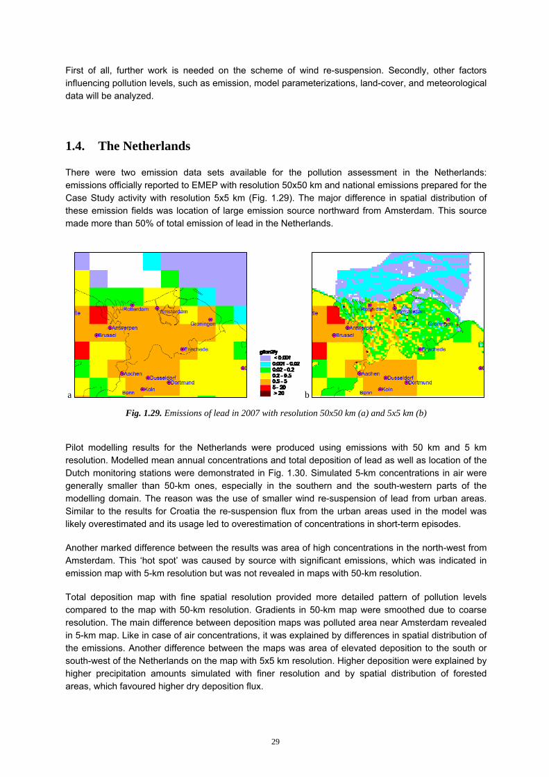
According to the model assumptions, the re-suspension occurred from bare soils (e.g., deserts), agricultural lands in spring and autumn (when they were devoid of vegetation) and from urban areas. Since most of Croatian stations were situated in urban areas, the modification was focused on re-suspension from this type of land-cover. It was assumed that concentrations of lead in urban soils were enriched with lead because of its long-term accumulation. In means that concentrations in urban soils were multiplied by a certain factor to account for the enrichment. The usage of smaller enrichment factor (i.e., reduced re-suspension) allowed to improve the modelling results, in particular, to suppress peaks not confirmed by measurements (Fig. 1.28).

Pb, SI8

0

5

10

15

20

25

30

35

01-

Jan-

2007

13-

Jan-

2007

25-

Jan-

2007

06-

Feb-

2007

18-

Feb-

2007

02-

Mar

-200

7 1

4-M

ar-2

007

26-

Mar

-200

7 0

7-A

pr-2

007

19-

Apr

-200

7 0

1-M

ay-2

007

13-

May

-200

7 2

5-M

ay-2

007

06-

Jun-

2007

18-

Jun-

2007

30-

Jun-

2007

12-

Jul-2

007

24-

Jul-2

007

05-

Aug

-200

7 1

7-A

ug-2

007

29-

Aug

-200

7 1

0-S

ep-2

007

22-

Sep

-200

7 0

4-O

ct-2

007

16-

Oct

-200

7 2

8-O

ct-2

007

09-

Nov

-200

7 2

1-N

ov-2

007

03-

Dec

-200

7 1

5-D

ec-2

007

27-

Dec

-200

7

Con

cent

ratio

ns in

air,

ng/

m3

ObservedModel (10 km, new soil)Model (10 km, reduced re-susp.)

Fig. 1.28. Modelled (based on current and reduced re-suspension of lead from soils) and observed

concentrations of Pb at station Iskbra in 2007

The reduced wind re-suspension from urban areas allowed to improve modelling results at most of stations. Obviously, further analysis is needed and modifications of pollution assessment will continue.

29

First of all, further work is needed on the scheme of wind re-suspension. Secondly, other factors influencing pollution levels, such as emission, model parameterizations, land-cover, and meteorological data will be analyzed.

1.4. The Netherlands

There were two emission data sets available for the pollution assessment in the Netherlands: emissions officially reported to EMEP with resolution 50x50 km and national emissions prepared for the Case Study activity with resolution 5x5 km (Fig. 1.29). The major difference in spatial distribution of these emission fields was location of large emission source northward from Amsterdam. This source made more than 50% of total emission of lead in the Netherlands.

a b

Fig. 1.29. Emissions of lead in 2007 with resolution 50x50 km (a) and 5x5 km (b)

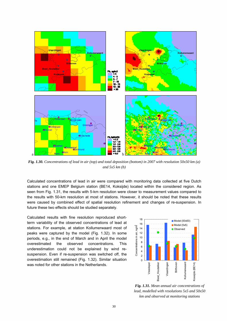
Pilot modelling results for the Netherlands were produced using emissions with 50 km and 5 km resolution. Modelled mean annual concentrations and total deposition of lead as well as location of the Dutch monitoring stations were demonstrated in Fig. 1.30. Simulated 5-km concentrations in air were generally smaller than 50-km ones, especially in the southern and the south-western parts of the modelling domain. The reason was the use of smaller wind re-suspension of lead from urban areas. Similar to the results for Croatia the re-suspension flux from the urban areas used in the model was likely overestimated and its usage led to overestimation of concentrations in short-term episodes.

Another marked difference between the results was area of high concentrations in the north-west from Amsterdam. This ‘hot spot’ was caused by source with significant emissions, which was indicated in emission map with 5-km resolution but was not revealed in maps with 50-km resolution.

Total deposition map with fine spatial resolution provided more detailed pattern of pollution levels compared to the map with 50-km resolution. Gradients in 50-km map were smoothed due to coarse resolution. The main difference between deposition maps was polluted area near Amsterdam revealed in 5-km map. Like in case of air concentrations, it was explained by differences in spatial distribution of the emissions. Another difference between the maps was area of elevated deposition to the south or south-west of the Netherlands on the map with 5x5 km resolution. Higher deposition were explained by higher precipitation amounts simulated with finer resolution and by spatial distribution of forested areas, which favoured higher dry deposition flux.

30

a b

a b

Fig. 1.30. Concentrations of lead in air (top) and total deposition (bottom) in 2007 with resolution 50x50 km (a) and 5x5 km (b)

Calculated concentrations of lead in air were compared with monitoring data collected at five Dutch stations and one EMEP Belgium station (BE14, Koksijde) located within the considered region. As seen from Fig. 1.31, the results with 5-km resolution were closer to measurement values compared to the results with 50-km resolution at most of stations. However, it should be noted that these results were caused by combined effect of spatial resolution refinement and changes of re-suspension. In future these two effects should be studied separately.

Calculated results with fine resolution reproduced short-term variability of the observed concentrations of lead at stations. For example, at station Kollumerwaard most of peaks were captured by the model (Fig. 1.32). In some periods, e.g., in the end of March and in April the model overestimated the observed concentrations. This underestimation could not be explained by wind re-suspension. Even if re-suspension was switched off, the overestimation still remained (Fig. 1.32). Similar situation was noted for other stations in the Netherlands.

0

2

4

6

8

10

12

14

16

18

Vre

edep

el

Bie

st_H

outa

kker

Vla

ardi

ngen

Bilt

hove

n

Kol

lum

erw

aard

Kos

sijd

e (B

E14

)

Con

cent

ratio

ns in

air,

ng/

m3

Model (50x50)Model (5x5)Observed

Fig. 1.31. Mean annual air concentrations of

lead, modelled with resolutions 5x5 and 50x50 km and observed at monitoring stations

31

Pb, Kollumerwaard

05

101520253035404550

03-J

an-2

007

13-J

an-2

007

23-J

an-2

007

18-F

eb-2

007

28-F

eb-2

007

10-M

ar-2

007

20-M

ar-2

007

30-M

ar-2

007

09-A

pr-2

007

19-A

pr-2

007

29-A

pr-2

007

09-M

ay-2

007

19-M

ay-2

007

29-M

ay-2

007

08-J

un-2

007

18-J

un-2

007

28-J

un-2

007

08-J

ul-2

007

18-J

ul-2

007

28-J

ul-2

007

07-A

ug-2

007

08-S

ep-2

007

18-S

ep-2

007

28-S

ep-2

007

08-O

ct-2

007

18-O

ct-2

007

28-O

ct-2

007

07-N

ov-2

007

17-N

ov-2

007

27-N

ov-2

007

07-D

ec-2

007

17-D

ec-2

007

27-D

ec-2

007

Con

cent

ratio

ns in

air,

ng/

m3

Observed

Model (5x5)

Model (5x5, anthrop)

Fig. 1.32. Modelled and observed concentrations of Pb at station Kollumerwaard in 2007

At present the modelling results obtained for the Netherlands are pilot and need detailed analysis in cooperation with national experts from this country. The analysis should be focused on the identification of reasons leading to the discrepancies between modelled and measured values at monitoring stations. In particular, the following activities should be undertaken:

- Refinement of spatial distribution of emissions in neighbouring countries

- Refinement of parameterization of wind re-suspension scheme

- Application of back trajectories in order to link peak concentrations with source regions

- Analysis of meteorological data applied in the assessment.

1.5. Spain

Active cooperation between MSC-E and Spain in the field of the country-specific Case Study has been started this year. Spain submitted to MSC-E large amount of national data including measurements of heavy metals (both targeted by the Protocol, and of second priority) in air at Spanish stations, meteorological observations, concentrations of metals in soils, monitoring data on chemical composition of particulate matter, especially mineral dust components highly important for evaluation of wind re-suspension scheme. Example of measured concentrations of lead at Spanish stations in 2007 is demonstrated in Fig. 1.33. It is important to note that Spain is located in the southern part of Europe, which is characterized by scarce monitoring network compared to the central, the northern and the western parts of Europe.

Future country-specific activity will include the following directions:

- Further collection and analysis of country-specific data (concentrations, deposition fluxes, meteorological information, emissions)

Fig. 1.33. Observed concentrations of lead at Spanish measurement stations in 2007

32

- Model simulations with 50-km and finer spatial resolution

- Joint analysis of the pollution levels on the base of available monitoring data, anthropogenic emissions, wind re-suspension and modelling results

- Initiation of model intercomparison studies between Spanish national and EMEP models for heavy metals

1.6. Further activities

MSC-E will continue to tightly cooperate with the countries participating in the country-specific Case Studies next year.

It is planned to finalize analysis of cadmium pollution levels for the Czech Republic using monitoring data, emissions and modelling results with fine spatial resolution. The updated assessment of pollution levels over the Czech Republic will be produced.

The analysis of heavy metal pollution levels in Croatia and the Netherlands will be continued. Special attention will be paid to refinement of wind re-suspension scheme. New country-specific data (emissions with fine resolution in neighbouring countries, land cover data, etc) will be involved in the analysis.

Pilot calculations for Spain will be carried out and analysis of pollution levels will be started. Model intercomparison studies involving Spanish national and EMEP models will be initiated.

33

2. MODEL DEVELOPMENTS ON A GLOBAL SCALE

In accordance with the Work-plan MSC-E continued development of the modelling approaches to the assessment of heavy metal pollution on both regional and global scales. In particular, significant efforts were undertaken to improve the global modelling framework GLEMOS and evaluate its performance against measurements. The recent improvements include further development of the framework architecture, implementation of the ocean transport module, update and evaluation of meteorological and oceanological drivers, and refinement of the mercury chemical scheme. The new developments in the mercury atmospheric chemistry were also implemented into the operational modelling and, in particular, were applied in the study of the Arctic mercury pollution. These and other aspects of heavy metal modelling activities are described in detail in the MSC-E Technical Report [Shatalov et al., 2011] and the Joint MSC-E and MSC-W Progress Report [Travnikov and Jonson, 2011].

2.1. Further development of the global modelling framework GLEMOS

The global modelling framework GLEMOS has being developed in MSC-E for last years to extend the scope of heavy metal and POP assessment to a global scale and to elaborate a consistent approach for multi-scale simulations in Europe. Progress of the framework development and evaluation was described in a number of recent technical reports [Tarrasón and Gusev, 2008; Travnikov et al., 2009; Jonson and Travnikov, 2010]. The formulated requirements to the modelling framework include a flexible choice of the model domain and grid resolution, multi-pollutant and multi-media approaches, a modular architecture and computational efficiency of the modelling. The modular architecture is one of the key features of the framework and it is aimed to provide flexibility for simulation of pollutants with diverse properties.

The general scheme of the framework reflecting the modular architecture is presented in Fig. 2.1. Each environmental medium is presented in the model by a set of procedures describing general processes in the medium which are combined into the program modules. Each module can be attached to or detached from the model at the compilation stage using command scripts. All pollutants are combined in groups of substances with similar properties (e.g. mercury, particulate heavy metals, POPs etc.). Each pollutant group is presented in the model by a number of modules defining the pollutant properties and its behaviour in each environmental media. Besides, each pollutant can be characterized by different physical forms or chemical compounds specific for each media. The pollutant groups can be attached to the model using the procedure similar to that for the environmental media.

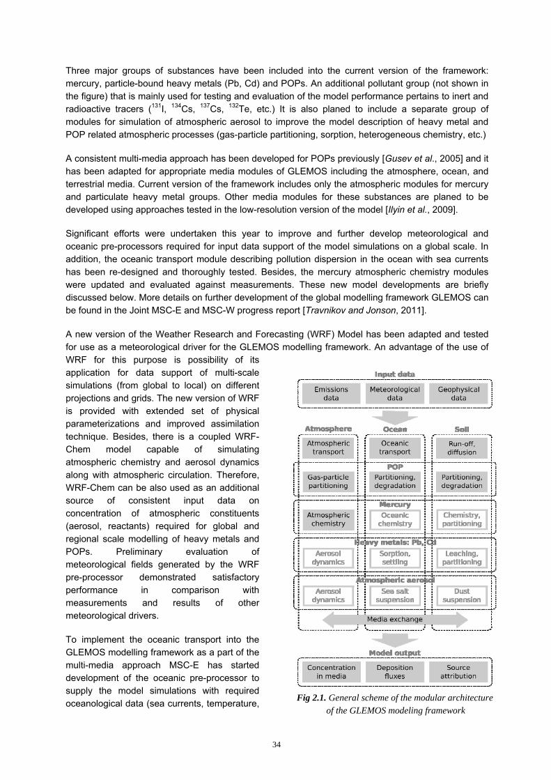
34

Three major groups of substances have been included into the current version of the framework: mercury, particle-bound heavy metals (Pb, Cd) and POPs. An additional pollutant group (not shown in the figure) that is mainly used for testing and evaluation of the model performance pertains to inert and radioactive tracers (131I, 134Cs, 137Cs, 132Te, etc.) It is also planed to include a separate group of modules for simulation of atmospheric aerosol to improve the model description of heavy metal and POP related atmospheric processes (gas-particle partitioning, sorption, heterogeneous chemistry, etc.)

A consistent multi-media approach has been developed for POPs previously [Gusev et al., 2005] and it has been adapted for appropriate media modules of GLEMOS including the atmosphere, ocean, and terrestrial media. Current version of the framework includes only the atmospheric modules for mercury and particulate heavy metal groups. Other media modules for these substances are planed to be developed using approaches tested in the low-resolution version of the model [Ilyin et al., 2009].

Significant efforts were undertaken this year to improve and further develop meteorological and oceanic pre-processors required for input data support of the model simulations on a global scale. In addition, the oceanic transport module describing pollution dispersion in the ocean with sea currents has been re-designed and thoroughly tested. Besides, the mercury atmospheric chemistry modules were updated and evaluated against measurements. These new model developments are briefly discussed below. More details on further development of the global modelling framework GLEMOS can be found in the Joint MSC-E and MSC-W progress report [Travnikov and Jonson, 2011].

A new version of the Weather Research and Forecasting (WRF) Model has been adapted and tested for use as a meteorological driver for the GLEMOS modelling framework. An advantage of the use of WRF for this purpose is possibility of its application for data support of multi-scale simulations (from global to local) on different projections and grids. The new version of WRF is provided with extended set of physical parameterizations and improved assimilation technique. Besides, there is a coupled WRF-Chem model capable of simulating atmospheric chemistry and aerosol dynamics along with atmospheric circulation. Therefore, WRF-Chem can be also used as an additional source of consistent input data on concentration of atmospheric constituents (aerosol, reactants) required for global and regional scale modelling of heavy metals and POPs. Preliminary evaluation of meteorological fields generated by the WRF pre-processor demonstrated satisfactory performance in comparison with measurements and results of other meteorological drivers.

To implement the oceanic transport into the GLEMOS modelling framework as a part of the multi-media approach MSC-E has started development of the oceanic pre-processor to supply the model simulations with required oceanological data (sea currents, temperature, Fig 2.1. General scheme of the modular architecture

of the GLEMOS modeling framework

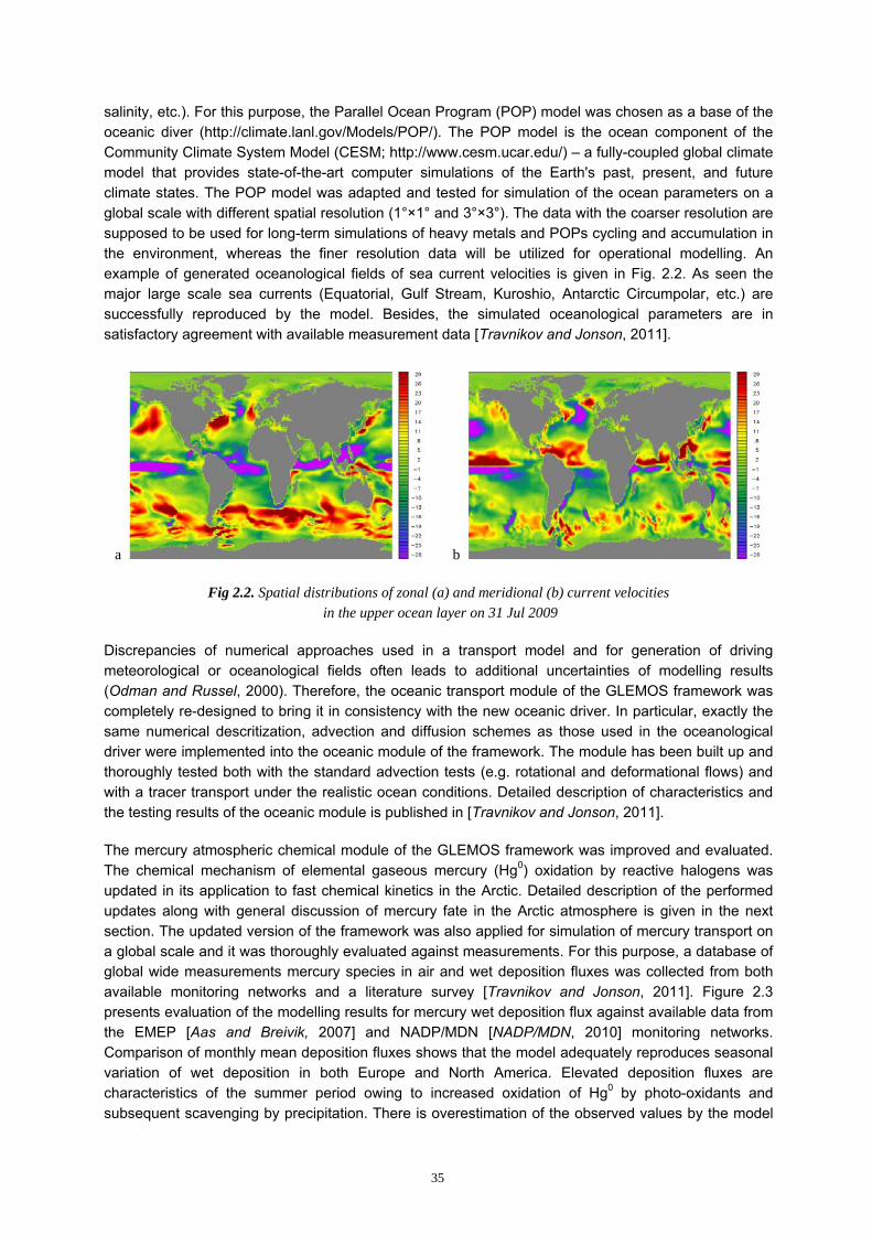
35

salinity, etc.). For this purpose, the Parallel Ocean Program (POP) model was chosen as a base of the oceanic diver (http://climate.lanl.gov/Models/POP/). The POP model is the ocean component of the Community Climate System Model (CESM; http://www.cesm.ucar.edu/) – a fully-coupled global climate model that provides state-of-the-art computer simulations of the Earth's past, present, and future climate states. The POP model was adapted and tested for simulation of the ocean parameters on a global scale with different spatial resolution (1°×1° and 3°×3°). The data with the coarser resolution are supposed to be used for long-term simulations of heavy metals and POPs cycling and accumulation in the environment, whereas the finer resolution data will be utilized for operational modelling. An example of generated oceanological fields of sea current velocities is given in Fig. 2.2. As seen the major large scale sea currents (Equatorial, Gulf Stream, Kuroshio, Antarctic Circumpolar, etc.) are successfully reproduced by the model. Besides, the simulated oceanological parameters are in satisfactory agreement with available measurement data [Travnikov and Jonson, 2011].

a b

Fig 2.2. Spatial distributions of zonal (a) and meridional (b) current velocities in the upper ocean layer on 31 Jul 2009

Discrepancies of numerical approaches used in a transport model and for generation of driving meteorological or oceanological fields often leads to additional uncertainties of modelling results (Odman and Russel, 2000). Therefore, the oceanic transport module of the GLEMOS framework was completely re-designed to bring it in consistency with the new oceanic driver. In particular, exactly the same numerical descritization, advection and diffusion schemes as those used in the oceanological driver were implemented into the oceanic module of the framework. The module has been built up and thoroughly tested both with the standard advection tests (e.g. rotational and deformational flows) and with a tracer transport under the realistic ocean conditions. Detailed description of characteristics and the testing results of the oceanic module is published in [Travnikov and Jonson, 2011].

The mercury atmospheric chemical module of the GLEMOS framework was improved and evaluated. The chemical mechanism of elemental gaseous mercury (Hg0) oxidation by reactive halogens was updated in its application to fast chemical kinetics in the Arctic. Detailed description of the performed updates along with general discussion of mercury fate in the Arctic atmosphere is given in the next section. The updated version of the framework was also applied for simulation of mercury transport on a global scale and it was thoroughly evaluated against measurements. For this purpose, a database of global wide measurements mercury species in air and wet deposition fluxes was collected from both available monitoring networks and a literature survey [Travnikov and Jonson, 2011]. Figure 2.3 presents evaluation of the modelling results for mercury wet deposition flux against available data from the EMEP [Aas and Breivik, 2007] and NADP/MDN [NADP/MDN, 2010] monitoring networks. Comparison of monthly mean deposition fluxes shows that the model adequately reproduces seasonal variation of wet deposition in both Europe and North America. Elevated deposition fluxes are characteristics of the summer period owing to increased oxidation of Hg0 by photo-oxidants and subsequent scavenging by precipitation. There is overestimation of the observed values by the model

36

in the second half of the year in Europe and in the first half in North America. In general the model somewhat underpredicts spatial variation of the observed wet deposition fluxes between different sites.

a

0.0

0.5

1.0

1.5

2.0

2.5Ja

n

Feb

Mar

Apr

May Ju

n

Jul

Aug

Sep Oct

Nov

Dec

Hg

wet

dep

ositi

on, g

/km2 /y

MeasurementsModel

Europe (9 sites)

b

0.0

0.5

1.0

1.5

2.0

2.5

Jan

Feb

Mar

Apr

May Ju

n

Jul

Aug

Sep Oct

Nov

Dec

Hg

wet

dep

ositi

on, g

/km2 /y

North America (90 sites)

Fig 2.3. Comparison of measured and simulated monthly mean mercury wet deposition flux in Europe (a) and North America (b) in 2005. Measurement data used in the comparison were retrieved from the EMEP and

NADP/MDN monitoring networks for Europe and North America, respectively. Dots depict average measured and modelled value, whereas whiskers show the standard deviation over all monitoring sites.

2.2. Mercury pollution of the Arctic

Mercury pollution attracts the growing attention within the environment protection community, particularly, in the run-up to negotiations of a global legally binding instrument on mercury being prepared under support of UNEP (www.unep.org). Mercury is widely recognised as a toxic chemical capable of long-range transport, bioaccumulation in the environment and significant negative effect on human health and the environment. The atmospheric fate of mercury from the moment of its release from an emission source up to deposition to the ground commonly includes a set of physical and chemical transformations (oxidation reactions, dissolution in could water, etc.) which largely define the pathways and character of mercury atmospheric dispersion as well as air-surface exchange.

Recent studies have demonstrated that chemical oxidation of Hg by reactive halogen species (primarily Br and BrO) may essentially affect or even determine the mercury cycle in the atmosphere, in particular, in the polar regions [Steffen et al., 2008; Ebinghaus et al., 2002]. As it was observed in the Arctic and Antarctica, during springtime Hg0 concentration episodically depleted to very low concentrations owing to fast transformation to short lived oxidized forms with subsequent deposition to the surface [Lindberg et al., 2002; Aria et al., 2004; Skov et al., 2004]. This phenomenon, termed as the Atmospheric Mercury Depletion Events (AMDE), leads to a considerable increase in total mercury deposition in the polar regions. However, a considerable proportion of deposited Hg is rapidly photoreduced in snowpack and re-emitted to the atmosphere [Kirk et al., 2006; Johnson et al., 2008; Ferrari et al., 2008].

Practical implementation of the bromine chemistry and the mechanism of AMDEs into a chemical transport model is associated with significant complications. Even taking into account the fact that the chemical kinetics of Hg oxidation by reactive bromine is relatively well understood [Hynes et al., 2009; Aria et al, 2009], available estimates of the reaction constants differ by an order of magnitude [Ariya et al., 2002; Goodsite et al., 2004, Donohoue et al., 2006]. However, even larger uncertainty is introduced by poor knowledge on the sources and ambient concentrations of bromine species in the troposphere. Sharp activation of the halogen photochemistry during springtime in the polar boundary layer leads to intensive production of reactive bromine species from sea salt but particular mechanisms triggering this process are poorly understood [Simpson et al., 2007]. In addition, chemical transformation

37

mechanisms of Hg in snow resulting in reduction and re-emission of deposited Hg(II) to the atmosphere are known only qualitatively.

The first attempt to implement the AMDEs mechanism into the mercury modelling within EMEP has been made last year for the global scale simulations with GLEMOS [Jonson and Travnikov, 2010]. In particular, the reactions of Hg0 oxidation by atomic Br and BrO in the Arctic and Antarctic environments were included into the model chemical scheme along with empirical parameterisation of the prompt re-emission from snow. This section includes description of further refinement of the model parameterisations with respect to mercury behaviour in the Arctic and its application to operation simulations within the EMEP region.

Figure 2.4 shows temporal variation of Hg0 concentration in air measured at the high latitude site Zeppelin (Norway) with typical depletion events during spring months. As seen from Fig. 2.4a relatively stable for the whole year concentration of Hg0 experiences significant alterations in the period from the end of March to the beginning of June. For short time the concentration is depleted to zero indicating complete oxidation of Hg0 in air mass (Fig. 2.4b). Afterwards, it is quickly recovered to the background level. AMDEs are strongly correlated with ozone depletion events (ODEs) implying similar mechanisms responsible for both destruction of ozone and oxidation of elemental mercury in the Arctic environment [Simpson et al., 2007]. It is possible to identify eight pronounced depletion events at this site in 2009 when Hg0 concentration dropped below 0.5 ng/m3 (Fig. 2.4b). Hereafter, they will be mentioned in the analysis according to their numbers.

a

0.0

0.5

1.0

1.5

2.0

2.5

3.0

01-Ja

n-09

21-Ja

n-09

10-Feb

-09

02-M

ar-09

22-M

ar-09

11-A

pr-09

01-M

ay-09

21-M

ay-09

10-Ju

n-09

30-Ju

n-09

20-Ju

l-09

09-A

ug-09

29-A

ug-09

18-S

ep-09

08-O

ct-09

28-O

ct-09

17-N

ov-09

07-D

ec-09

27-D

ec-09

Hg0 c

once

ntra

tion,

ng/

m3

b

0.0

0.5

1.0

1.5

2.0

2.5

3.0

11-M

ar-09

21-M

ar-09

31-M

ar-09

10-A

pr-09

20-A

pr-09

30-A

pr-09

10-M

ay-09

20-M

ay-09

30-M

ay-09

09-Ju

n-09

Hg0 c

once

ntra

tion,

ng/

m3

0

25

50

75

100

125

150

O3 c

once

ntra

tion,

ppb

vHg0 (obs)Ozone (obs)

1 2 3 4 5 6 7 8

Fig. 2.4. Time series of observed 6-hour mean Hg0 concentration at site Zeppelin, Norway (NO42): (a) – for the whole year 2009; (b) – for the AMDEs period from March 11 to June 11, 2009. Red rectangle shows the AMDEs

period. Identified AMDEs are shadowed in gray

AMDEs are commonly associated with air masses transported over young sea ice or, more specifically, over refreezing ice in open leads providing a source of reactive halogen in air. Therefore, it is important to analyze the pathways of air masses arriving at the monitoring site with depleted Hg0 concentrations. An example of the analysis of back trajectories corresponding to AMDEs at the Zeppelin site is illustrated in Fig. 2.5. More details are available in the technical report [Shatalov et al., 2011].

38

For all selected depletion events the air masses came from off-shore areas located in the north/northwest direction from the site. As it follows from the satellite observations, the site location is not characterized by high BrO concentration. However, in most the cases the air masses were transported during last 1-2 days over areas with high BrO vertical column density indicating availability of reactive bromine species. Therefore, it confirms the hypothesis that AMDEs at Zeppelin site are the most probably connected with oxidation of Hg0 over off-shore areas at some distance from the site. On the other hand, the transport of Hg0 depleted air masses hardly exceeds few days since afterwards the back trajectories leave the areas with high BrO density. Thus, for instance, the most deep depletion events (Events 2-5) are likely caused by intensive oxidation of Hg0 over distance between Spitsbergen and the coast of northern Greenland.

a b

Fig. 2.5. (a) Backtrajectories for the AMDE (13-17 April 2009) at Zeppelin site plotted with the HYSPLIT Trajectory Model [Draxler et al., 2011; Rolph, 2011] and (b) daily BrO density in the vertical atmospheric

column from GOME-2 satellite measurements [Theys et al., 2011; 0Uwww.temis.nlH]

Taking into account lack of reliable data on reactive bromine species concentration in the Arctic boundary layer and limited knowledge on processes triggering AMDEs we performed a study of ambient conditions accompanying AMDEs in the Arctic. Importance of meteorological conditions in addition to the halogen chemistry for AMDEs in polar regions was noted by Dastoor et al. [2008]. Therefore, we analysed correlation of Hg0 concentration measured at the Zeppelin site with a number of meteorological parameters including wind speed, friction velocity, air temperature, vertical eddy diffusion coefficient, boundary layer height, water vapour mixing ratio, precipitation amount and solar radiation. It should be noted that only few of these parameters (wind speed, air temperature, solar radiation, and precipitation) can be measured directly, whereas the others are purely model derived. Therefore, to keep consistency we used parameters simulated with MM5 meteorological driver keeping in mind limitation associated with uncertainties of the model. An example of the analysed time series of both Hg0 and some of the meteorological parameters for the period of AMDEs at Zeppelin site (from March 11 to June 11, 2009) is shown in Fig. 2.6. More detailed analysis is given in technical report [Shatalov et al., 2011].

The largest negative correlation was obtained between Hg0 concentration and the parameters of vertical mixing (eddy diffusion coefficient and boundary layer height, which are well correlated between each other). It means that intensive vertical mixing corresponds to lower Hg0 concentrations at the measurement site. It is in line with the assumption that the main part of oxidation reactions leading to Hg0 depletion takes place at a distance from the measurement site and then depleted air is transported to the site location within boundary layer. In this case increase of vertical mixing enhances descending of the depleted air to the ground.

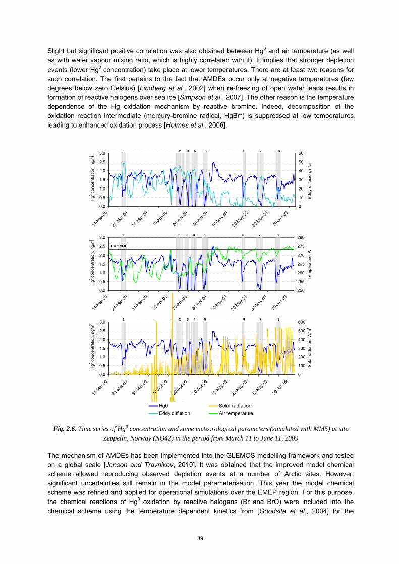
39

Slight but significant positive correlation was also obtained between Hg0 and air temperature (as well as with water vapour mixing ratio, which is highly correlated with it). It implies that stronger depletion events (lower Hg0 concentration) take place at lower temperatures. There are at least two reasons for such correlation. The first pertains to the fact that AMDEs occur only at negative temperatures (few degrees below zero Celsius) [Lindberg et al., 2002] when re-freezing of open water leads results in formation of reactive halogens over sea ice [Simpson et al., 2007]. The other reason is the temperature dependence of the Hg oxidation mechanism by reactive bromine. Indeed, decomposition of the oxidation reaction intermediate (mercury-bromine radical, HgBr*) is suppressed at low temperatures leading to enhanced oxidation process [Holmes et al., 2006].

0.0

0.5

1.0

1.5

2.0

2.5

3.0

11-M

ar-09

21-M

ar-09

31-M

ar-09

10-A

pr-09

20-A

pr-09

30-A

pr-09

10-M

ay-09

20-M

ay-09

30-M

ay-09

09-Ju

n-09

Hg0 c

once

ntra

tion,

ng/

m3

0

10

20

30

40

50

60

Edd

y di

ffusi

on, m

2 /s

1 2 3 4 5 6 7 8

0.0

0.5

1.0

1.5

2.0

2.5

3.0

11-M

ar-09

21-M

ar-09

31-M

ar-09

10-A

pr-09

20-A

pr-09

30-A

pr-09

10-M

ay-09

20-M

ay-09

30-M

ay-09

09-Ju

n-09

Hg0 c

once

ntra

tion,

ng/

m3

250

255

260

265

270

275

280

Tem

pera

ture

, K

1 2 3 4 5 6 7 8

T = 273 K

0.0

0.5

1.0

1.5

2.0

2.5

3.0

11-M

ar-09

21-M

ar-09

31-M

ar-09

10-A

pr-09

20-A

pr-09

30-A

pr-09

10-M

ay-09

20-M

ay-09

30-M

ay-09

09-Ju

n-09

Hg0 c

once

ntra

tion,

ng/

m3

0

100

200

300

400

500

600

Sol

ar ra

diat

ion,

W/m

2

1 2 3 4 5 6 7 8

Hg0 Solar radiationEddy diffusion Air temperature

Fig. 2.6. Time series of Hg0 concentration and some meteorological parameters (simulated with MM5) at site Zeppelin, Norway (NO42) in the period from March 11 to June 11, 2009

The mechanism of AMDEs has been implemented into the GLEMOS modelling framework and tested on a global scale [Jonson and Travnikov, 2010]. It was obtained that the improved model chemical scheme allowed reproducing observed depletion events at a number of Arctic sites. However, significant uncertainties still remain in the model parameterisation. This year the model chemical scheme was refined and applied for operational simulations over the EMEP region. For this purpose, the chemical reactions of Hg0 oxidation by reactive halogens (Br and BrO) were included into the chemical scheme using the temperature dependent kinetics from [Goodsite et al., 2004] for the

40

reaction with Br and the rate constant from [Raofie and Ariya, 2003] for the reaction with BrO, respectively.

Concentration of bromine compounds in the atmosphere is one of the most uncertain parts of the applied approach. Direct measurements of Br and its species in the lower troposphere are scarce and simulated concentration fields are quite uncertain. Therefore, concentration of BrO were derived from the GOME (Global Ozone Monitoring Experiment) satellite observations [Theys et al., 2011]. In particular, monthly mean global distributions of BrO density in total tropospheric column obtained by Theys et al. [2011] applying a combined retrieval/modelling approach were utilized in the model. Besides, following [Dastoor et al., 2008] we subtracted the global background BrO concentration from the tropospheric column to derive total BrO content in the atmospheric boundary layer. Mixing ratio of BrO was subsequently obtained assuming its uniform vertical distribution in the boundary layer. Keeping in mind that formation and destruction cycles of Br and BrO are linked closely, we assume similar spatial distributions of these two halogens and applied a constant Br/BrO ratio equal to 0.1 [Seigneur and Lohman, 2008].

Utilized monthly mean data on BrO concentration cannot reproduce fast kinetics of halogen photochemistry. It is assumed that lifetime of reactive halogens (such as Br and BrO) does not exceed a few hours in the absence of recycling on aerosol [Simpson et al., 2007]. Therefore, to account for these fast processes we modulate the monthly mean Br and BrO with a number of surrogate meteorological parameters aiming at better fit of the temporal variation of observed Hg0 concentration. For these purpose we performed a number of sensitivity runs with different combinations of meteorological parameters considered in the preceding analysis.

It is expected that one of the main processes leading to activation of halogen chemistry during AMDEs (and ODEs) is production of sea salt enriched aerosol. Formation of young sea ice over re-freezing open leads is accompanied by formation of specific ice crystals, known as frost flowers [Simpson et al., 2007]. Being enriched with sea salt brine, frost flowers can be suspended by wind and produce sea salt aerosol as a source of reactive halogens. It is known that ice begins to form in sea water at temperatures around -2°C. So one can hardly expect the activation of halogen chemistry at higher temperatures. Besides, it is well known that solar radiation is required for both halogen photochemistry and mercury oxidation reactions. In addition, wind blown aerosol production is a function of the wind stress. As it follows from contemporary dust suspension studies [e.g. Gomes et al., 2003] the flux of wind blown aerosol in proportional to the third power of friction velocity (U*). Thus, the optimal conditions used in the model to modulate temporal variation of halogen chemistry are the following – activation of reactive bromine occur at temperatures below -2°C, in the presence of solar radiation, and is proportional to the third power of friction velocity normalized by monthly mean values.

Another important process accompanying the enhanced mercury deposition during AMDEs is prompt re-emission of newly deposited mercury. Measurements in snowpack show that high mercury concentrations in the surface snow following AMDEs are substantially reduced during few days due to photoreduction of deposited mercury and re-emission to the atmosphere [Kirk et al., 2006; Johnson et al., 2008; Ferrari et al., 2008]. Thus, it considerably decreases mercury accumulation in snow and adverse effects of the Arctic vulnerable ecosystems. To account for this essential process we developed an empirical parameterization of the prompt re-emission based on the observational data [Jonson and Travnikov, 2010]. Assuming that re-emission occur only for newly deposited mercury in the presence of solar radiation we introduced two competing processes – photoreduction and ageing of deposited mercury with the characteristic times of 1 day and 10 days, respectively. It is assumed that all reduced mercury is immediately re-emitted back to the atmosphere. The aged fraction of mercury does not undergo reduction and is accumulated in snowpack. It should be noted that this accumulated

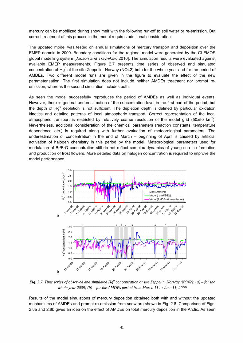
41

mercury can be mobilized during snow melt with the following run-off to soil water or re-emission. But correct treatment of this process in the model requires additional consideration.

The updated model was tested on annual simulations of mercury transport and deposition over the EMEP domain in 2009. Boundary conditions for the regional model were generated by the GLEMOS global modelling system [Jonson and Travnikov, 2010]. The simulation results were evaluated against available EMEP measurements. Figure 2.7 presents time series of observed and simulated concentration of Hg0 at the site Zeppelin, Norway (NO42) both for the whole year and for the period of AMDEs. Two different model runs are given in the figure to evaluate the effect of the new parameterisation. The first simulation does not include neither AMDEs treatment nor prompt re-emission, whereas the second simulation includes both.

As seen the model successfully reproduces the period of AMDEs as well as individual events. However, there is general underestimation of the concentration level in the first part of the period, but the depth of Hg0 depletion is not sufficient. The depletion depth is defined by particular oxidation kinetics and detailed patterns of local atmospheric transport. Correct representation of the local atmospheric transport is restricted by relatively coarse resolution of the model grid (50x50 km2). Nevertheless, additional consideration of the chemical parameters (reaction constants, temperature dependence etc.) is required along with further evaluation of meteorological parameters. The underestimation of concentration in the end of March – beginning of April is caused by artificial activation of halogen chemistry in this period by the model. Meteorological parameters used for modulation of Br/BrO concentration still do not reflect complex dynamics of young sea ice formation and production of frost flowers. More detailed data on halogen concentration is required to improve the model performance.

a

0.0

0.5

1.0

1.5

2.0

2.5

3.0

01-Ja

n-09

21-Ja

n-09

10-Feb

-09

02-M

ar-09

22-M

ar-09

11-A

pr-09

01-M

ay-09

21-M

ay-09

10-Ju

n-09

30-Ju

n-09

20-Ju

l-09

09-A

ug-09

29-A

ug-09

18-S

ep-09

08-O

ct-09

28-O

ct-09

17-N

ov-09

07-D

ec-09

27-D

ec-09

Hg0 c

once

ntra

tion,

ng/

m3

MeasurementsModel (no AMDEs)Model (AMDEs & re-emission)

b

0.0

0.5

1.0

1.5

2.0

2.5

3.0

11-M

ar-09

21-M

ar-09

31-M

ar-09

10-A

pr-09

20-A

pr-09

30-A

pr-09

10-M

ay-09

20-M

ay-09

30-M

ay-09

09-Ju

n-09

Hg0 c

once

ntra

tion,

ng/

m3

1 2 3 4 5 6 7 8

Fig. 2.7. Time series of observed and simulated Hg0 concentration at site Zeppelin, Norway (NO42): (a) – for the whole year 2009; (b) – for the AMDEs period from March 11 to June 11, 2009

Results of the model simulations of mercury deposition obtained both with and without the updated mechanisms of AMDEs and prompt re-emission from snow are shown in Fig. 2.8. Comparison of Figs. 2.8a and 2.8b gives an idea on the effect of AMDEs on total mercury deposition in the Arctic. As seen

42

this phenomenon leads to considerable increase of deposition fluxes over the Arctic Ocean and the coasts of Siberia and Greenland (Fig. 2.8b). There is practically no effect over the main part of Europe except for northern Scandinavia and northern Russia. Annual deposition levels over some parts of the Arctic are comparable with those in industrial areas of Europe. On the other hand, the major portion of mercury deposited to snow because of AMDEs is re-emitted back to the atmosphere in a short time (Fig. 2.8c). Some re-emission also takes place from snow covered areas in Europe – the Alps, the Balkans, Scandinavia and northern Russia. Therefore, net deposition flux of mercury, calculated as a difference between total deposition and re-emission, is considerably lower than total deposition over the Arctic (Fig. 2.8d). Taking into account that it is net deposition flux that accounts for resulting mercury input and contamination of the environment, this parameter will be preferably considered in the further analysis of mercury pollution.

a b

c d

Fig. 2.8. Spatial distribution of simulated mercury deposition and re-emission fluxes in 2009 over the EMEP domain: (a) - total deposition without AMDEs and re-emission; (b) - total deposition simulated using updated

AMDEs mechanism of and re-emission; (c) – prompt re-emission from snow; (d) – net deposition flux

Acknowledgments

The authors gratefully acknowledge the NOAA Air Resources Laboratory (ARL) for the provision of the HYSPLIT transport and dispersion model and/or READY website (http://www.arl.noaa.gov/ready.php) used in this publication.

43

3. ASSESSMENT OF HEAVY METAL POLLUTION WITHIN EMEP REGION

This chapter is focused on the integrated assessment of heavy metal (Pb, Cd, Hg) pollution levels in the EMEP region in 2009. Monitoring activity and emission data are considered. Besides, concentration and deposition, and transboundary transport issues are described. Finally, special attention is given to the uncertainties of the integrated assessment of pollution.

3.1. Monitoring of heavy metals in EMEP

Measurement network

Heavy metals were included in EMEP’s monitoring program in 1999. However, earlier data has been available and collected, and the EMEP database [ 1http://ebas.nilu.no] thus also includes older data, even back to 1987 for a few sites. A number of countries have been reporting heavy metals within the EMEP area in connection with different national and international programmers such as HELCOM, AMAP and OSPAR.

Detailed information about the sites and the measurement methods are found in EMEP/CCC’s data report on heavy metals and POPs [Aas and Breivik, 2011]. In 2009, there were 35 sites measuring heavy metals in both air and precipitation, and altogether there were 71 measurement sites, which were 1 more sites than in 2008. There were 26 sites measuring at least one form of mercury which is the same number of sites as previous year. 12 sites were measuring mercury in both air and precipitation, though several of these measures particulate mercury, 11 sites with measurements of gaseous mercury and of these, 8 also includes mercury in precipitation and fulfil the monitoring obligations. These 8 sites are all to be found in the Nordic countries, so obviously there is a need for better coverage of especially mercury in large part of Europe. That said however, the measurement obligations set by the EMEP monitoring strategy [UNECE, 2009] and the EU air quality directives [EU, 2004, 2008] have clearly improved the site coverage the last years.

Observed concentration level of Pb, Cd and Hg in 2009

Annual averages of Pb, Cd and Hg concentrations in precipitation and in air in 2009 are presented in Fig. 3.1-3.6. Note that Cyprus with measurements of heavy metals in air is outside the map domain so included as a dislocated point south of Turkey. The lowest concentrations for all elements in air as well as precipitation are generally found in northern Scandinavia. An increasing gradient can in general be seen southeast, but the concentration levels are not evenly distributed, there are some “hotspots” for some elements, i.e. in the BeNeLux countries for lead and cadmium in air. Further, an extremely high annual concentration of cadmium in precipitation (2.0 ng/l) is seen at IT01, which most likely must be due to local influence from sources in the Rome area. Portugal has also high level of cadmium, though this is due to high detection limit, and these data are therefore not shown in Fig 3.4. For the other more normal results the highest cadmium levels in precipitation is seen in Slovakia and the Czech Republic. For cadmium in air the highest levels are seen in the BeNeLux and in Slovakia. For lead in precipitation, the highest levels are observed in Italy and Hungary, while in air the highest level is in the

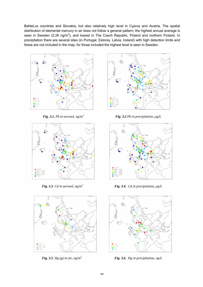
44

BeNeLux countries and Slovakia, but also relatively high level in Cyprus and Austria. The spatial distribution of elemental mercury in air does not follow a general pattern; the highest annual average is seen in Sweden (2.26 ng/m3), and lowest in The Czech Republic, Poland and northern Finland. In precipitation there are several sites (in Portugal, Estonia, Latvia, Ireland) with high detection limits and these are not included in the map, for those included the highest level is seen in Sweden.

Fig. 3.1. Pb in aerosol, ng/m3 Fig. 3.2 Pb in precipitation, μg/L

Fig. 3.3. Cd in aerosol, ng/m3 Fig. 3.4. Cd in precipitation, μg/L

Fig. 3.5. Hg (g) in air, ng/m3 Fig. 3.6. Hg in precipitation, ng/L

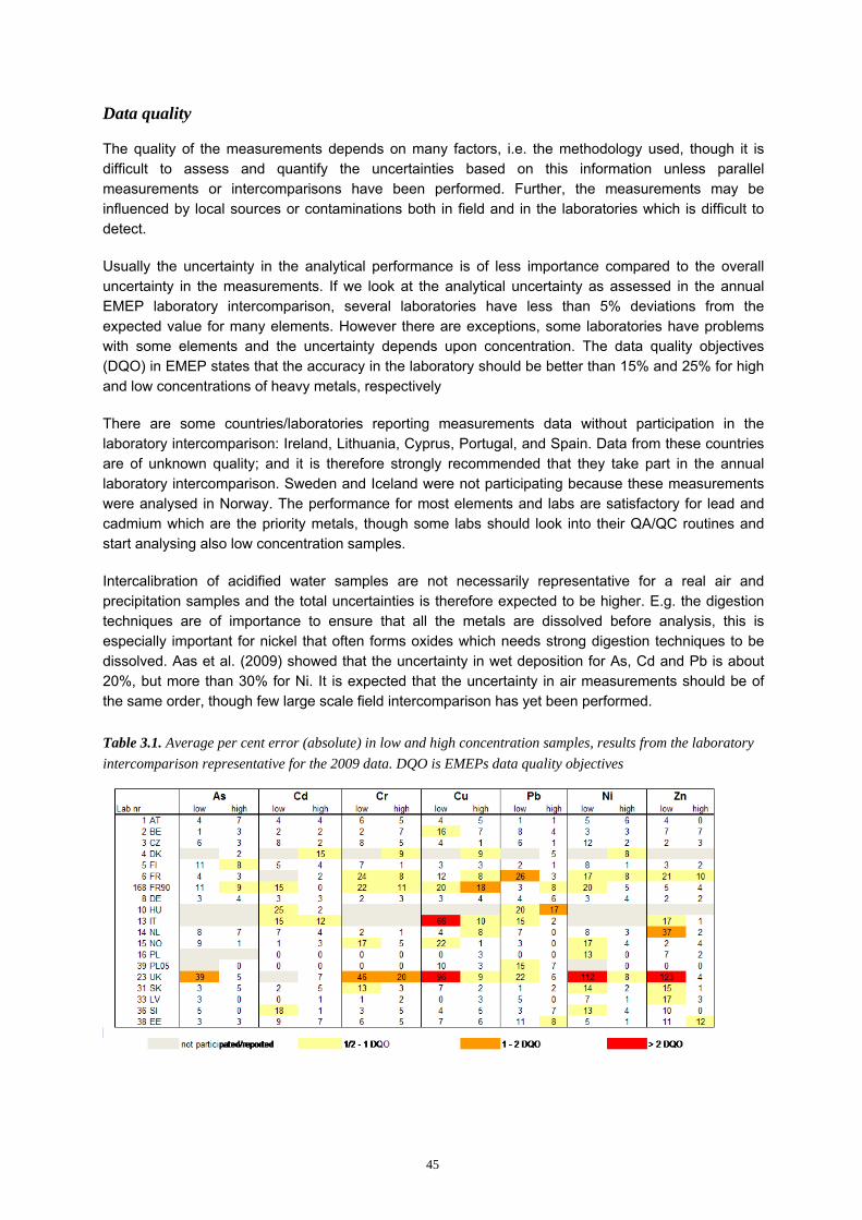
45

Data quality

The quality of the measurements depends on many factors, i.e. the methodology used, though it is difficult to assess and quantify the uncertainties based on this information unless parallel measurements or intercomparisons have been performed. Further, the measurements may be influenced by local sources or contaminations both in field and in the laboratories which is difficult to detect.

Usually the uncertainty in the analytical performance is of less importance compared to the overall uncertainty in the measurements. If we look at the analytical uncertainty as assessed in the annual EMEP laboratory intercomparison, several laboratories have less than 5% deviations from the expected value for many elements. However there are exceptions, some laboratories have problems with some elements and the uncertainty depends upon concentration. The data quality objectives (DQO) in EMEP states that the accuracy in the laboratory should be better than 15% and 25% for high and low concentrations of heavy metals, respectively

There are some countries/laboratories reporting measurements data without participation in the laboratory intercomparison: Ireland, Lithuania, Cyprus, Portugal, and Spain. Data from these countries are of unknown quality; and it is therefore strongly recommended that they take part in the annual laboratory intercomparison. Sweden and Iceland were not participating because these measurements were analysed in Norway. The performance for most elements and labs are satisfactory for lead and cadmium which are the priority metals, though some labs should look into their QA/QC routines and start analysing also low concentration samples.

Intercalibration of acidified water samples are not necessarily representative for a real air and precipitation samples and the total uncertainties is therefore expected to be higher. E.g. the digestion techniques are of importance to ensure that all the metals are dissolved before analysis, this is especially important for nickel that often forms oxides which needs strong digestion techniques to be dissolved. Aas et al. (2009) showed that the uncertainty in wet deposition for As, Cd and Pb is about 20%, but more than 30% for Ni. It is expected that the uncertainty in air measurements should be of the same order, though few large scale field intercomparison has yet been performed.

Table 3.1. Average per cent error (absolute) in low and high concentration samples, results from the laboratory intercomparison representative for the 2009 data. DQO is EMEPs data quality objectives

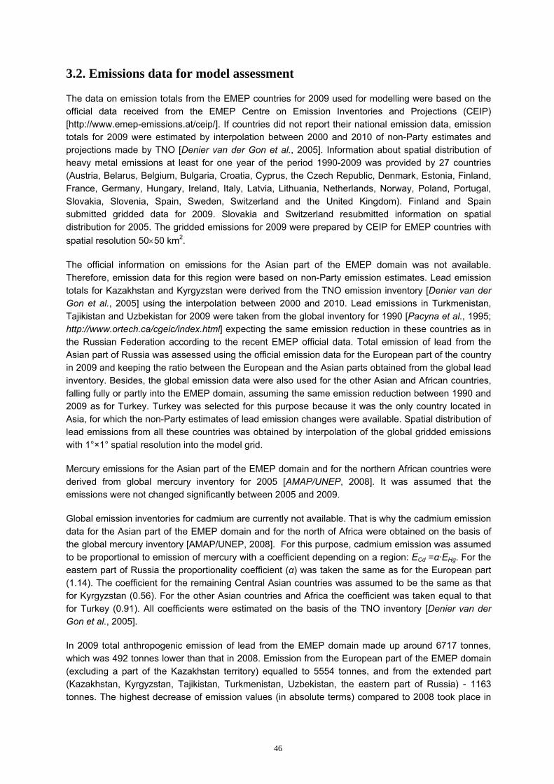
46

3.2. Emissions data for model assessment

The data on emission totals from the EMEP countries for 2009 used for modelling were based on the official data received from the EMEP Centre on Emission Inventories and Projections (CEIP) [http://www.emep-emissions.at/ceip/]. If countries did not report their national emission data, emission totals for 2009 were estimated by interpolation between 2000 and 2010 of non-Party estimates and projections made by TNO [Denier van der Gon et al., 2005]. Information about spatial distribution of heavy metal emissions at least for one year of the period 1990-2009 was provided by 27 countries (Austria, Belarus, Belgium, Bulgaria, Croatia, Cyprus, the Czech Republic, Denmark, Estonia, Finland, France, Germany, Hungary, Ireland, Italy, Latvia, Lithuania, Netherlands, Norway, Poland, Portugal, Slovakia, Slovenia, Spain, Sweden, Switzerland and the United Kingdom). Finland and Spain submitted gridded data for 2009. Slovakia and Switzerland resubmitted information on spatial distribution for 2005. The gridded emissions for 2009 were prepared by CEIP for EMEP countries with spatial resolution 50×50 km2.

The official information on emissions for the Asian part of the EMEP domain was not available. Therefore, emission data for this region were based on non-Party emission estimates. Lead emission totals for Kazakhstan and Kyrgyzstan were derived from the TNO emission inventory [Denier van der Gon et al., 2005] using the interpolation between 2000 and 2010. Lead emissions in Turkmenistan, Tajikistan and Uzbekistan for 2009 were taken from the global inventory for 1990 [Pacyna et al., 1995; http://www.ortech.ca/cgeic/index.html] expecting the same emission reduction in these countries as in the Russian Federation according to the recent EMEP official data. Total emission of lead from the Asian part of Russia was assessed using the official emission data for the European part of the country in 2009 and keeping the ratio between the European and the Asian parts obtained from the global lead inventory. Besides, the global emission data were also used for the other Asian and African countries, falling fully or partly into the EMEP domain, assuming the same emission reduction between 1990 and 2009 as for Turkey. Turkey was selected for this purpose because it was the only country located in Asia, for which the non-Party estimates of lead emission changes were available. Spatial distribution of lead emissions from all these countries was obtained by interpolation of the global gridded emissions with 1°×1° spatial resolution into the model grid.

Mercury emissions for the Asian part of the EMEP domain and for the northern African countries were derived from global mercury inventory for 2005 [AMAP/UNEP, 2008]. It was assumed that the emissions were not changed significantly between 2005 and 2009.

Global emission inventories for cadmium are currently not available. That is why the cadmium emission data for the Asian part of the EMEP domain and for the north of Africa were obtained on the basis of the global mercury inventory [AMAP/UNEP, 2008]. For this purpose, cadmium emission was assumed to be proportional to emission of mercury with a coefficient depending on a region: ECd =α·EHg. For the eastern part of Russia the proportionality coefficient (α) was taken the same as for the European part (1.14). The coefficient for the remaining Central Asian countries was assumed to be the same as that for Kyrgyzstan (0.56). For the other Asian countries and Africa the coefficient was taken equal to that for Turkey (0.91). All coefficients were estimated on the basis of the TNO inventory [Denier van der Gon et al., 2005].

In 2009 total anthropogenic emission of lead from the EMEP domain made up around 6717 tonnes, which was 492 tonnes lower than that in 2008. Emission from the European part of the EMEP domain (excluding a part of the Kazakhstan territory) equalled to 5554 tonnes, and from the extended part (Kazakhstan, Kyrgyzstan, Tajikistan, Turkmenistan, Uzbekistan, the eastern part of Russia) - 1163 tonnes. The highest decrease of emission values (in absolute terms) compared to 2008 took place in

47

the Russian Federation (228 tonnes), Poland (83 tonnes), Italy (63 tonnes), Ukraine (42 tonnes), Romania (36 tonnes), and Spain (33 tonnes).

Total emission of cadmium in Europe and Central Asia in 2009 (268 tonnes) was 50 tonnes lower than that for 2008. This value included 220 tonnes from emission sources located in the European countries and 48 tonnes – from the Central Asian region. Emission values for the Russian Federation, Slovakia, Ukraine and Poland used in modelling for 2009 were lower than those for 2008 by 25, 9.5, 4 and 3.5 tonnes, respectively.

Emission of mercury in the European and the Central Asian countries in 2009 amounted to 207 tonnes, which was 20 tonnes lower than that for 2008. European emissions were 145 tonnes, and the emissions from Central Asia and the Asian part of Russia – 62 tonnes. Most significant increase of emission values in individual countries took place in Germany and Lithuania (1.8 and 1.3 tonnes, respectively). The highest decrease was in Romania, the Russian Federation, Italy, Slovakia and Spain (7, 5.5, 3, 2.5 and 1.5 tonnes, respectively).

Vertical distribution of the pollutant concentration in the vicinity of emission sources as well as long-range atmospheric transport to some extend depend on height of the emission source. In order to estimate distribution of emissions with height MSC-E utilized sector-split emission information provided by the EMEP countries. Height distributions for different emission sectors were averaged taking into account a sector contribution to the total emission. It was assumed that heavy metal emission was distributed between three lowest model layers (0-70 m; 70-150 m and 150-300 m).

Lead and cadmium and their compounds are characterized by very low volatility. Therefore, it was assumed that they were emitted to the atmosphere in the composition of aerosol particles. In contrast to these metals, mercury was emitted both in gaseous and in particulate forms. Besides, gaseous species included elemental and oxidized forms. The speciation of mercury emissions was not included in the information submitted by the Parties to the Convention. Therefore, expert estimates of the mercury emission speciation were used in the MSCE-HM model [Axenfeld et al., 1991; Pacyna and Münch, 1991].

Detailed information on temporal and vertical distribution of the emission data and speciation of mercury emissions, employed in the MSCE-HM model, are described in [Travnikov and Ilyin, 2005]. Spatial distributions of heavy metal emissions used in the modelling are shown in Fig. 3.7.

a b c

Fig. 3.7. Spatial distribution of lead (a), cadmium (b) and mercury (c) emissions over the EMEP domain in 2009

48

3.3. Analysis of heavy metal pollution levels in 2009

This section is focused on the analysis of pollution levels of lead, cadmium and mercury based on modelling and monitoring information for 2009. Modelling results were obtained by the MSCE-HM model. Measurement data were submitted to CCC database by EMEP countries. Spatial distribution of heavy metal deposition and concentrations, description of the pollution level changes between 2008 and 2009, and source-receptor relationships in Europe and Central Asia were considered. Finally, evaluation of the atmospheric loads to the regional seas was presented.

LEAD

Atmospheric pollution levels of lead are formed by three groups of sources: anthropogenic sources, wind re-suspension of historical accumulated deposition and atmospheric transport from sources located outside the EMEP domain. The later includes transport through boundaries of modelled domain, transport from sources located in Africa and Asian countries which are situated within the modelling domain but do not belong to the Convention.

Levels of transboundary pollution of EMEP countries by lead were characterized by modelling results and measurement data. Annual mean concentrations of lead in air varied in 2009 from 0.5 to 10 ng/m3 over the most part of Europe (Fig. 3.8). In the central part of Russia, the Benelux region, north of Italy,

southern part of Poland, Bulgaria the concentrations exceed 10 ng/m3. It was explained by relatively high anthropogenic emissions in these areas. Over the northern part of Russia and Scandinavian countries the concentrations were below 0.5 ng/m3.

Spatial pattern of modelled concentrations was confirmed by the measurement information. With few exceptions, modelled and observed concentrations were similar. The gradient from the central to the northern part of Europe was also reproduced. However, over vast territories of the EMEP region, such as the southern, eastern and south-eastern parts of Europe, and Central Asia, measurement information was not available. Therefore, pollution levels in these areas were assessed only by means of modelling.

To estimate atmospheric pollution of ecosystems deposition data are typically used. Total atmospheric deposition consists of two components: wet and dry. Wet deposition is regularly measured at the EMEP monitoring network and is used for the assessment of lead pollution levels along with modelled wet deposition.

Over the most part of Europe annual wet deposition varied from 0.2 to 1.2 kg/km2/y (Fig. 3.9). Since periods of observations at stations often did not cover entire year, for comparability the modelled and observed wet deposition fluxes were scaled to annual sums. The central part of Russia, Balkans, northern Italy, the southern part of Poland and Benelux region were

Fig. 3.8. Calculated and measured surface concentrations of lead in air over Europe

and Central Asia in 2009

Fig.3.9. Calculated and measured annual sums

of wet deposition fluxes of lead over Europe and Central Asia in 2009

49

characterized by higher level of lead pollution, and wet deposition exceeded 1.2 kg/km2/y. It was explained mainly by location of significant emission sources in these regions (Fig. 3.7a). Observed levels of wet deposition were similar to modelled ones in the central part of Europe. In the northern part of Europe the observations demonstrated higher levels compared to the modelling results. Another factor governing wet deposition was precipitation amounts. Low wet deposition over the central part of Kazakhstan and northern Africa were explained by low precipitation.

Spatial distribution of total deposition of lead was similar to that of air concentrations and wet deposition (Fig. 3.10). Regions with relatively high deposition (2 – 3 kg/km2/y or even more) were associated with location of anthropogenic emission sources or wind re-suspension. Another important factors influencing deposition in the considered regions were meteorological processes (precipitation, wind patterns) and properties of the underlying surface.

Changes of anthropogenic emissions used in modelling and natural variability of meteorological parameters led to changes of annual deposition. Total deposition of lead to the countries of Europe and Central Asia from anthropogenic sources in 2009 was 5180 tonnes. Deposition to Europe was about 4100 tonnes, and to the Central Asian countries (Kazakhstan, Kyrgyzstan, Turkmenistan, Tajikistan and Uzbekistan) and Asian part of Russia – 1080 tonnes. Deposition from the anthropogenic sources in 2009 to the EMEP region as a whole declined by about 7% compared to 2008. The main reason was the decrease of anthropogenic emissions used in modelling. However, in some countries growth of the emissions was indicated. Besides, meteorological

factors also affected changes in pollution levels. Therefore, the differences between deposition in 2008 and 2009 varied among individual countries. Total deposition to the EMEP countries from all sources (anthropogenic, re-suspension, non-EMEP sources) in 2009 was around 12910 tonnes. It was higher than the corresponding value for 2008 by about 1000 tonnes (almost 9%). The increase of total deposition was caused by higher contribution of wind re-suspension to total deposition compared to 2008. Wind re-suspension is dependent on meteorological parameters (mainly wind and precipitation). Thus, natural variability of these parameters resulted to variability of wind re-suspension fluxes. However, it should be noted that wind re-suspension is highly uncertain factor, and work on improvements of its parameterization is ongoing.

In a number of countries emission values used in modelling significantly increased due to recalculations of their emissions, which resulted in the increase of deposition. For example, emissions in Germany increased almost 1.5 times, in Portugal –almost 3 times. Significant decline of the emission values, caused either by recalculations or economical changes, in Russia, Ukraine, Poland, Slovakia, Romania and the other eastern European countries led to reduction of deposition in these countries. Besides, the increase of deposition in western and south-western Europe was explained by the increased wind re-suspension.

Montenegro, the FYR of Macedonia, Bulgaria and Greece in 2009 were characterized by the highest country-averaged deposition flux of lead in 2009 exceeding 2 kg/km2/y (Fig. 3.11). The lowest deposition, lying within limits 0.25 – 0.30 kg/km2/y, was noted for the Nordic countries Iceland, Norway, and Finland. Contribution of wind re-suspension ranged from 20 to 80%. In 31 countries (of total 50) its contribution exceeded 50%. This high contribution means that this process should be further

Fig. 3.10. Total annual deposition of lead in

Europe and Central Asia in 2009

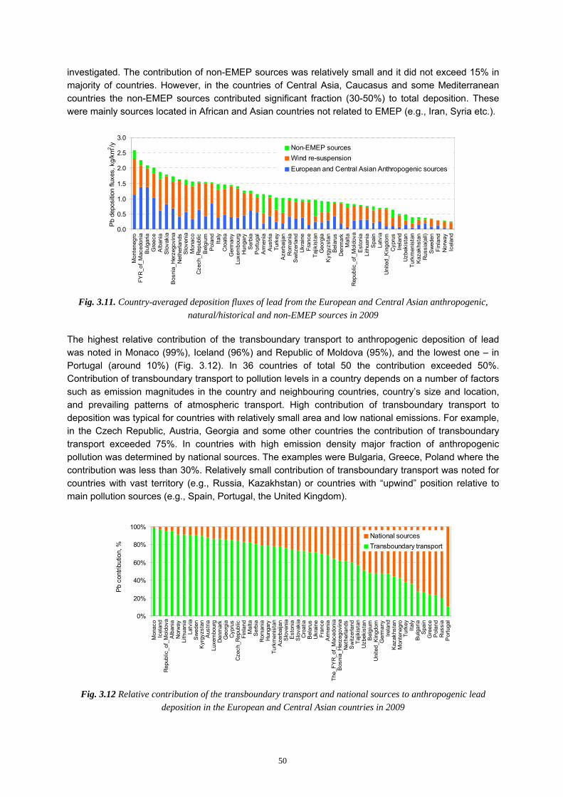
50

investigated. The contribution of non-EMEP sources was relatively small and it did not exceed 15% in majority of countries. However, in the countries of Central Asia, Caucasus and some Mediterranean countries the non-EMEP sources contributed significant fraction (30-50%) to total deposition. These were mainly sources located in African and Asian countries not related to EMEP (e.g., Iran, Syria etc.).

0.0

0.5

1.0

1.5

2.0

2.5

3.0M

onte

negr

oFY

R_o

f_M

aced

onia

Bul

garia

Gre

ece

Alb

ania

Slo

vaki

aB

osni

a_H

erze

govi

naN

ethe

rland

sS

love

nia

Mon

aco

Cze

ch_R

epub

licB

elgi

umP

olan

dIta

lyC

roat

iaG

erm

any

Luxe

mbo

urg

Hun

gary

Ser

bia

Por

tuga

lA

rmen

iaA

ustri

aTu

rkey

Aze

rbai

jan

Rom

ania

Sw

itzer

land

Ukr

aine

Fran

ceTa

jikis

tan

Geo

rgia

Kyr

gyzs

tan

Bel

arus

Den

mar

kM

alta

Rep

ublic

_of_

Mol

dova

Est

onia

Lith

uani

aS

pain

Latv

iaU

nite

d_K

ingd

omC

ypru

sIre

land

Uzb

ekis

tan

Turk

men

ista

nK

azak

hsta

nR

ussi

a(al

l)S

wed

enFi

nlan

dN

orw

ayIc

elan

d

Pb

depo

sitio

n flu

xes,

kg/

km2 /y Non-EMEP sources

Wind re-suspensionEuropean and Central Asian Anthropogenic sources

Fig. 3.11. Country-averaged deposition fluxes of lead from the European and Central Asian anthropogenic,

natural/historical and non-EMEP sources in 2009

The highest relative contribution of the transboundary transport to anthropogenic deposition of lead was noted in Monaco (99%), Iceland (96%) and Republic of Moldova (95%), and the lowest one – in Portugal (around 10%) (Fig. 3.12). In 36 countries of total 50 the contribution exceeded 50%. Contribution of transboundary transport to pollution levels in a country depends on a number of factors such as emission magnitudes in the country and neighbouring countries, country’s size and location, and prevailing patterns of atmospheric transport. High contribution of transboundary transport to deposition was typical for countries with relatively small area and low national emissions. For example, in the Czech Republic, Austria, Georgia and some other countries the contribution of transboundary transport exceeded 75%. In countries with high emission density major fraction of anthropogenic pollution was determined by national sources. The examples were Bulgaria, Greece, Poland where the contribution was less than 30%. Relatively small contribution of transboundary transport was noted for countries with vast territory (e.g., Russia, Kazakhstan) or countries with “upwind” position relative to main pollution sources (e.g., Spain, Portugal, the United Kingdom).

0%

20%

40%

60%

80%

100%

Mon

aco

Icel

and

Rep

ublic

_of_

Mol

dova

Alb

ania

Nor

way

Lith

uani

aLa

tvia

Sw

eden

Kyr

gyzs

tan

Aus

tria

Luxe

mbo

urg

Den

mar

kG

eorg

iaC

ypru

sC

zech

_Rep

ublic

Finl

and

Mal

taS

erbi

aR

oman

iaH

unga

ryTu

rkm

enis

tan

Aze

rbai

jan

Slo

veni

aE

ston

iaS

lova

kia

Cro

atia

Bel

arus

Ukr

aine

Fran

ceA

rmen

iaTh

e_FY

R_o

f_M

aced

onia

Bos

nia_

Her

zego

vina

Net

herla

nds

Sw

itzer

land

Tajik

ista

nU

zbek

ista

nB

elgi

umU

nite

d_K

ingd

omG

erm

any

Irela

ndK

azak

hsta

nM

onte

negr

oTu

rkey

Italy

Bul

garia

Spa

inG

reec

eP

olan

dR

ussi

aP

ortu

gal

Pb

cont

ribut

ion,

%

National sourcesTransboundary transport

Fig. 3.12 Relative contribution of the transboundary transport and national sources to anthropogenic lead

deposition in the European and Central Asian countries in 2009

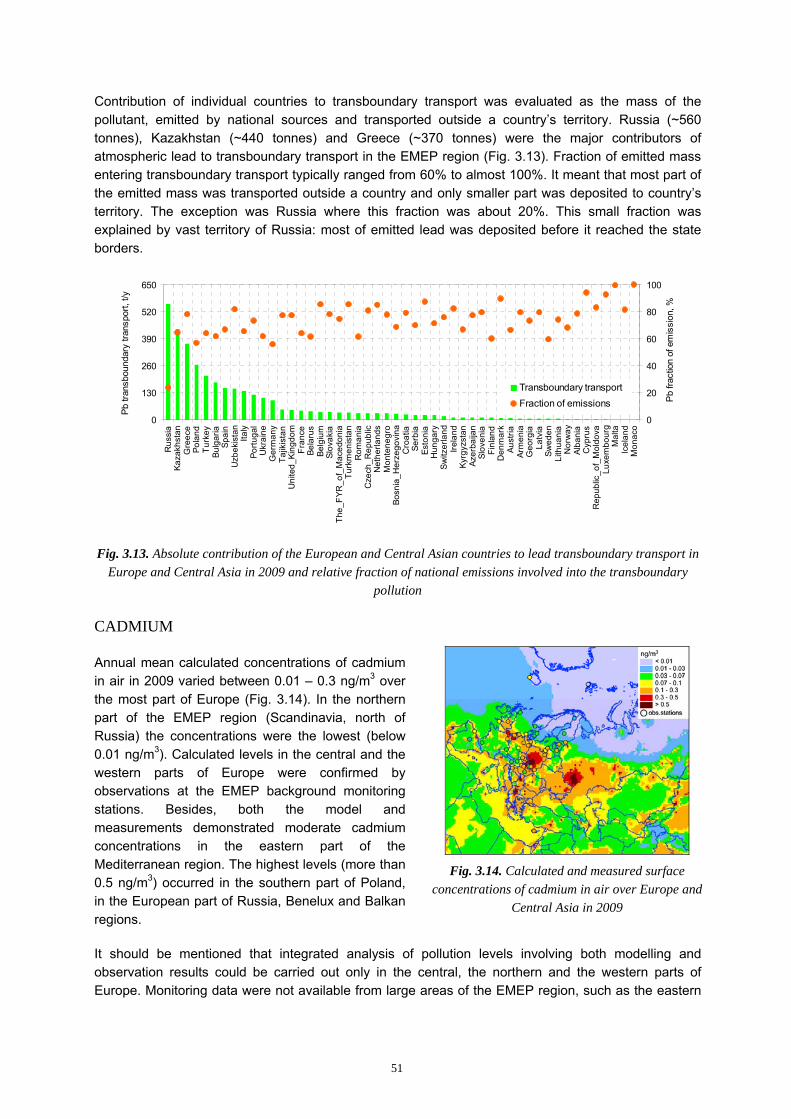
51

Contribution of individual countries to transboundary transport was evaluated as the mass of the pollutant, emitted by national sources and transported outside a country’s territory. Russia (~560 tonnes), Kazakhstan (~440 tonnes) and Greece (~370 tonnes) were the major contributors of atmospheric lead to transboundary transport in the EMEP region (Fig. 3.13). Fraction of emitted mass entering transboundary transport typically ranged from 60% to almost 100%. It meant that most part of the emitted mass was transported outside a country and only smaller part was deposited to country’s territory. The exception was Russia where this fraction was about 20%. This small fraction was explained by vast territory of Russia: most of emitted lead was deposited before it reached the state borders.

0

130

260

390

520

650

Rus

sia

Kaza

khst

anG

reec

ePo

land

Turk

eyBu

lgar

iaSp

ain

Uzb

ekis

tan

Italy

Portu

gal

Ukr

aine

Ger

man

yTa

jikis

tan

Uni

ted_

King

dom

Fran

ceBe

laru

sBe

lgiu

mSl

ovak

iaTh

e_FY

R_o

f_M

aced

onia

Turk

men

ista

nR

oman

iaC

zech

_Rep

ublic

Net

herla

nds

Mon

tene

gro

Bosn

ia_H

erze

govi

naC

roat

iaSe

rbia

Esto

nia

Hun

gary

Switz

erla

ndIre

land

Kyrg

yzst

anAz

erba

ijan

Slov

enia

Finl

and

Den

mar

kAu

stria

Arm

enia

Geo

rgia

Latv

iaSw

eden

Lith

uani

aN

orw

ayAl

bani

aC

ypru

sR

epub

lic_o

f_M

oldo

vaLu

xem

bour

gM

alta

Icel

and

Mon

aco

Pb tr

ansb

ound

ary

trans

port,

t/y

0

20

40

60

80

100

Pb

fract

ion

of e

mis

sion

, %

Transboundary transportFraction of emissions

Fig. 3.13. Absolute contribution of the European and Central Asian countries to lead transboundary transport in Europe and Central Asia in 2009 and relative fraction of national emissions involved into the transboundary

pollution

CADMIUM

Annual mean calculated concentrations of cadmium in air in 2009 varied between 0.01 – 0.3 ng/m3 over the most part of Europe (Fig. 3.14). In the northern part of the EMEP region (Scandinavia, north of Russia) the concentrations were the lowest (below 0.01 ng/m3). Calculated levels in the central and the western parts of Europe were confirmed by observations at the EMEP background monitoring stations. Besides, both the model and measurements demonstrated moderate cadmium concentrations in the eastern part of the Mediterranean region. The highest levels (more than 0.5 ng/m3) occurred in the southern part of Poland, in the European part of Russia, Benelux and Balkan regions.

It should be mentioned that integrated analysis of pollution levels involving both modelling and observation results could be carried out only in the central, the northern and the western parts of Europe. Monitoring data were not available from large areas of the EMEP region, such as the eastern

Fig. 3.14. Calculated and measured surface

concentrations of cadmium in air over Europe and Central Asia in 2009

52

and the south-eastern parts of Europe and Central Asia. Therefore, assessment of the pollution levels in these regions was based entirely on modelling information.

Spatial distribution of cadmium wet deposition flux was similar to that of concentrations in air: higher levels occurred in Poland, Russia and the Balkans, while the lowest – in the northern part of Russia and Scandinavia (Fig. 3.15). Besides, low levels of wet deposition took place over arid areas of Central Asia because of low precipitation amounts. Over the most part of the EMEP region modelled wet deposition fluxes ranged from 3 to 30 g/km2/y, and in relatively polluted areas the levels exceeded 30 g/km2/y. Observed wet deposition fluxes were higher than modelled ones in most areas where monitoring data were available.

Total deposition of cadmium ranged from 5 to 50 g/km2/y over the most part of the EMEP region (Fig. 3.16). Higher levels of deposition (50 – 100 g/km2/y) took place in Poland, Russia and south-eastern Europe (The FYR of Macedonia, Serbia, Bulgaria etc.). Low deposition levels in the northern areas of the EMEP domain were explained by remoteness from major emission sources, and in the Central Asian region – by low precipitation amounts.

In 2009 total deposition to the EMEP countries was around 410 tonnes. Deposition of cadmium to European countries was 300 tonnes, and to the eastern part of the EMEP region (Central Asia and the eastern part of Russia) – 110 tonnes. In comparison with 2008 deposition declined by about 2%. This decrease resulted from two contradictory changes. On one hand, anthropogenic emissions used in modelling for 2009 significantly (by 13.5%) reduced compared to previous year. On the other hand, wind re-suspension increased. It was interesting to note, that deposition caused by anthropogenic sources declined both in the European and the Asian parts of the EMEP domain. However, deposition caused by all sources declined in Europe but increased in the Asian part of the EMEP countries. The reason was the increase of re-suspension in 2009 compared to 2008 due to natural variability of meteorological parameters. The refinement of wind re-suspension scheme aimed at improvement of pollution level assessment is ongoing.

Similar to the EMEP region as a whole, changes of cadmium deposition in individual countries between 2008 and 2009 were determined by changes of emissions, re-suspension, and meteorological parameters. Like in the case of lead, increase of deposition took place in the western and the central parts of Europe: in France, Germany, Italy, etc. Increase of deposition in Germany, Belgium, Hungary was caused by increased values of anthropogenic emissions in these countries used in modelling. Besides, higher levels of re-suspension also contributed to overall growth of cadmium deposition. Decline of anthropogenic emissions in Poland, Ukraine, Russia, Slovakia and the Baltic countries was the dominant factor of the decrease of deposition in the eastern part of Europe.

Fig. 3.15. Calculated and measured annual sums of wet deposition fluxes of cadmium over Europe

and Central Asia in 2009

Fig. 3.16. Total annual deposition of cadmium in

Europe and Central Asia in 2009

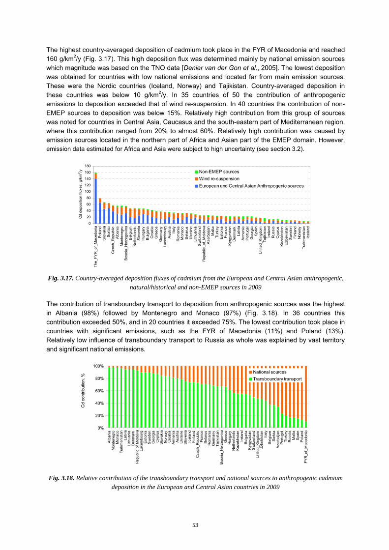
53

The highest country-averaged deposition of cadmium took place in the FYR of Macedonia and reached 160 g/km2/y (Fig. 3.17). This high deposition flux was determined mainly by national emission sources which magnitude was based on the TNO data [Denier van der Gon et al., 2005]. The lowest deposition was obtained for countries with low national emissions and located far from main emission sources. These were the Nordic countries (Iceland, Norway) and Tajikistan. Country-averaged deposition in these countries was below 10 g/km2/y. In 35 countries of 50 the contribution of anthropogenic emissions to deposition exceeded that of wind re-suspension. In 40 countries the contribution of non-EMEP sources to deposition was below 15%. Relatively high contribution from this group of sources was noted for countries in Central Asia, Caucasus and the south-eastern part of Mediterranean region, where this contribution ranged from 20% to almost 60%. Relatively high contribution was caused by emission sources located in the northern part of Africa and Asian part of the EMEP domain. However, emission data estimated for Africa and Asia were subject to high uncertainty (see section 3.2).

0

20

40

60

80

100

120

140

160

180

The_

FYR

_of_

Mac

edon

iaP

olan

dS

lova

kia

Ser

bia

Cze

ch_R

epub

licA

lban

iaM

onte

negr

oB

osni

a_H

erze

govi

naB

elgi

umN

ethe

rland

sS

love

nia

Hun

gary

Bul

garia

Cro

atia

Gre

ece

Ger

man

yLu

xem

bour

gA

ustri

aIta

lyR

oman

iaM

onac

oB

elar

usU

krai

neLi

thua

nia

Sw

itzer

land

Rep

ublic

_of_

Mol

dova

Aze

rbai

jan

Mal

taTu

rkey

Est

onia

Fran

ceK

yrgy

zsta

nD

enm

ark

Latv

iaA

rmen

iaP

ortu

gal

Geo

rgia

Spa

inU

nite

d_K

ingd

omTa

jikis

tan

Irela

ndR

ussi

aC

ypru

sK

azak

hsta

nU

zbek

ista

nS

wed

enFi

nlan

dN

orw

ayTu

rkm

enis

tan

Icel

and

Cd

depo

sitio

n flu

xes,

g/k

m2 /y Non-EMEP sources

Wind re-suspensionEuropean and Central Asian Anthropogenic sources

Fig. 3.17. Country-averaged deposition fluxes of cadmium from the European and Central Asian anthropogenic,

natural/historical and non-EMEP sources in 2009

The contribution of transboundary transport to deposition from anthropogenic sources was the highest in Albania (98%) followed by Montenegro and Monaco (97%) (Fig. 3.18). In 36 countries this contribution exceeded 50%, and in 20 countries it exceeded 75%. The lowest contribution took place in countries with significant emissions, such as the FYR of Macedonia (11%) and Poland (13%). Relatively low influence of transboundary transport to Russia as whole was explained by vast territory and significant national emissions.

0%

20%

40%

60%

80%

100%

Alb

ania

Mon

tene

gro

Mon

aco

Turk

men

ista

nLa

tvia

Lith

uani

aD

enm

ark

Rep

ublic

of M

oldo

vaLu

xem

bour

gE

ston

iaS

wed

enG

eorg

iaC

ypru

sS

lova

kia

Nor

way

Cro

atia

Arm

enia

Aus

tria

Ukr

aine

Slo

veni

aIc

elan

dFi

nlan

dC

zech

_Rep

ublic

Fran

ceB

elar

usR

oman

iaG

erm

any

Tajik

ista

nB

osni

a_H

erze

govi

naG

reec

eH

unga

ryN

ethe

rland

sK

azak

hsta

nIre

land

Bul

garia

Kyr

gyzs

tan

Sw

itzer

land

Uni

ted_

Kin

gdom

Uzb

ekis

tan

Italy

Bel

gium

Ser

bia

Aze

rbai

jan

Por

tuga

lTu

rkey

Rus

sia

Mal

taS

pain

Pol

and

FYR

_of_

Mac

edon

ia

Cd

cont

ribut

ion,

%

National sourcesTransboundary transport

Fig. 3.18. Relative contribution of the transboundary transport and national sources to anthropogenic cadmium

deposition in the European and Central Asian countries in 2009

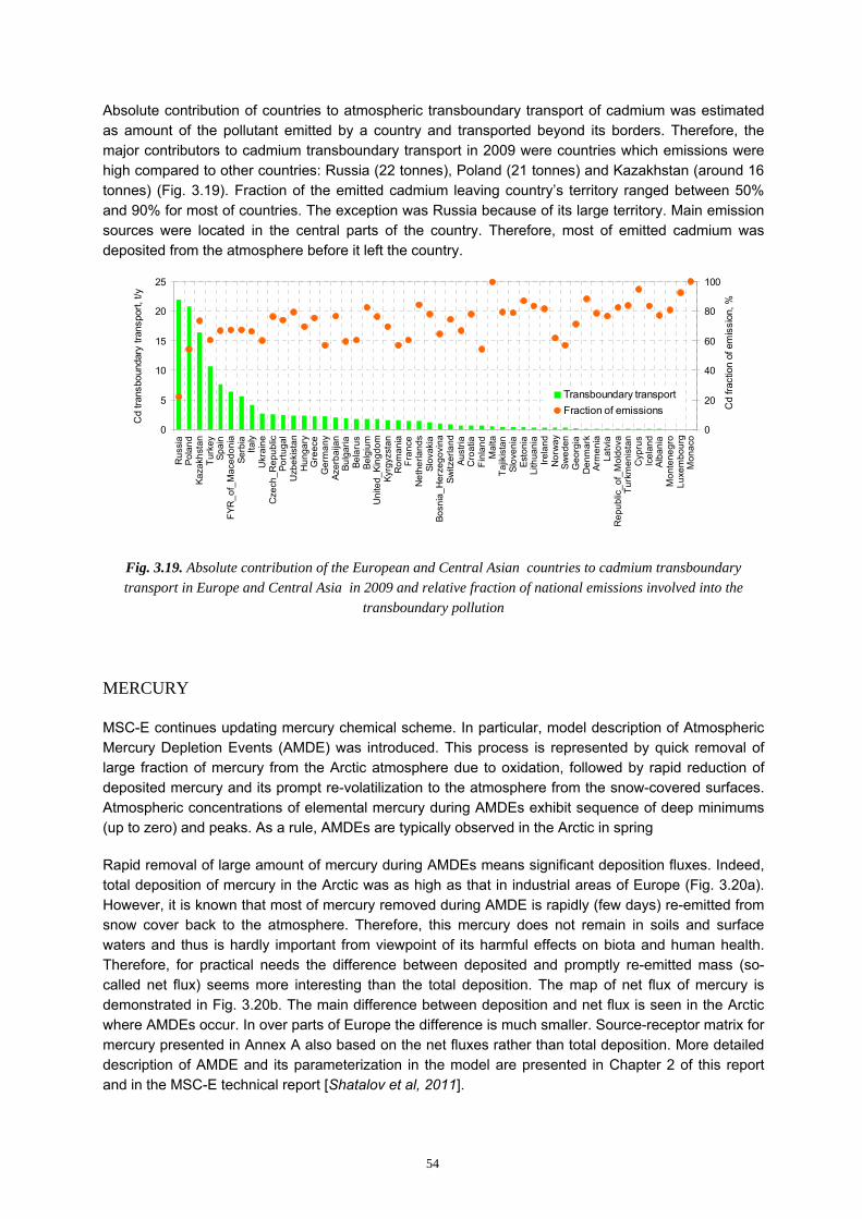
54

Absolute contribution of countries to atmospheric transboundary transport of cadmium was estimated as amount of the pollutant emitted by a country and transported beyond its borders. Therefore, the major contributors to cadmium transboundary transport in 2009 were countries which emissions were high compared to other countries: Russia (22 tonnes), Poland (21 tonnes) and Kazakhstan (around 16 tonnes) (Fig. 3.19). Fraction of the emitted cadmium leaving country’s territory ranged between 50% and 90% for most of countries. The exception was Russia because of its large territory. Main emission sources were located in the central parts of the country. Therefore, most of emitted cadmium was deposited from the atmosphere before it left the country.

0

5

10

15

20

25

Rus

sia

Pola

ndKa

zakh

stan

Turk

eySp

ain

FYR

_of_

Mac

edon

iaSe

rbia

Italy

Ukr

aine

Cze

ch_R

epub

licPo

rtuga

lU

zbek

ista

nH

unga

ryG

reec

eG

erm

any

Azer

baija

nBu

lgar

iaBe

laru

sBe

lgiu

mU

nite

d_Ki

ngdo

mKy

rgyz

stan

Rom

ania

Fran

ceN

ethe

rland

sSl

ovak

iaBo

snia

_Her

zego

vina

Switz

erla

ndAu

stria

Cro

atia

Finl

and

Mal

taTa

jikis

tan

Slov

enia

Esto

nia

Lith

uani

aIre

land

Nor

way

Swed

enG

eorg

iaD

enm

ark

Arm

enia

Latv

iaR

epub

lic_o

f_M

oldo

vaTu

rkm

enis

tan

Cyp

rus

Icel

and

Alba

nia

Mon

tene

gro

Luxe

mbo

urg

Mon

aco

Cd

trans

boun

dary

tran

spor

t, t/y

0

20

40

60

80

100

Cd

fract

ion

of e

mis

sion

, %

Transboundary transportFraction of emissions

Fig. 3.19. Absolute contribution of the European and Central Asian countries to cadmium transboundary transport in Europe and Central Asia in 2009 and relative fraction of national emissions involved into the

transboundary pollution

MERCURY

MSC-E continues updating mercury chemical scheme. In particular, model description of Atmospheric Mercury Depletion Events (AMDE) was introduced. This process is represented by quick removal of large fraction of mercury from the Arctic atmosphere due to oxidation, followed by rapid reduction of deposited mercury and its prompt re-volatilization to the atmosphere from the snow-covered surfaces. Atmospheric concentrations of elemental mercury during AMDEs exhibit sequence of deep minimums (up to zero) and peaks. As a rule, AMDEs are typically observed in the Arctic in spring

Rapid removal of large amount of mercury during AMDEs means significant deposition fluxes. Indeed, total deposition of mercury in the Arctic was as high as that in industrial areas of Europe (Fig. 3.20a). However, it is known that most of mercury removed during AMDE is rapidly (few days) re-emitted from snow cover back to the atmosphere. Therefore, this mercury does not remain in soils and surface waters and thus is hardly important from viewpoint of its harmful effects on biota and human health. Therefore, for practical needs the difference between deposited and promptly re-emitted mass (so-called net flux) seems more interesting than the total deposition. The map of net flux of mercury is demonstrated in Fig. 3.20b. The main difference between deposition and net flux is seen in the Arctic where AMDEs occur. In over parts of Europe the difference is much smaller. Source-receptor matrix for mercury presented in Annex A also based on the net fluxes rather than total deposition. More detailed description of AMDE and its parameterization in the model are presented in Chapter 2 of this report and in the MSC-E technical report [Shatalov et al, 2011].

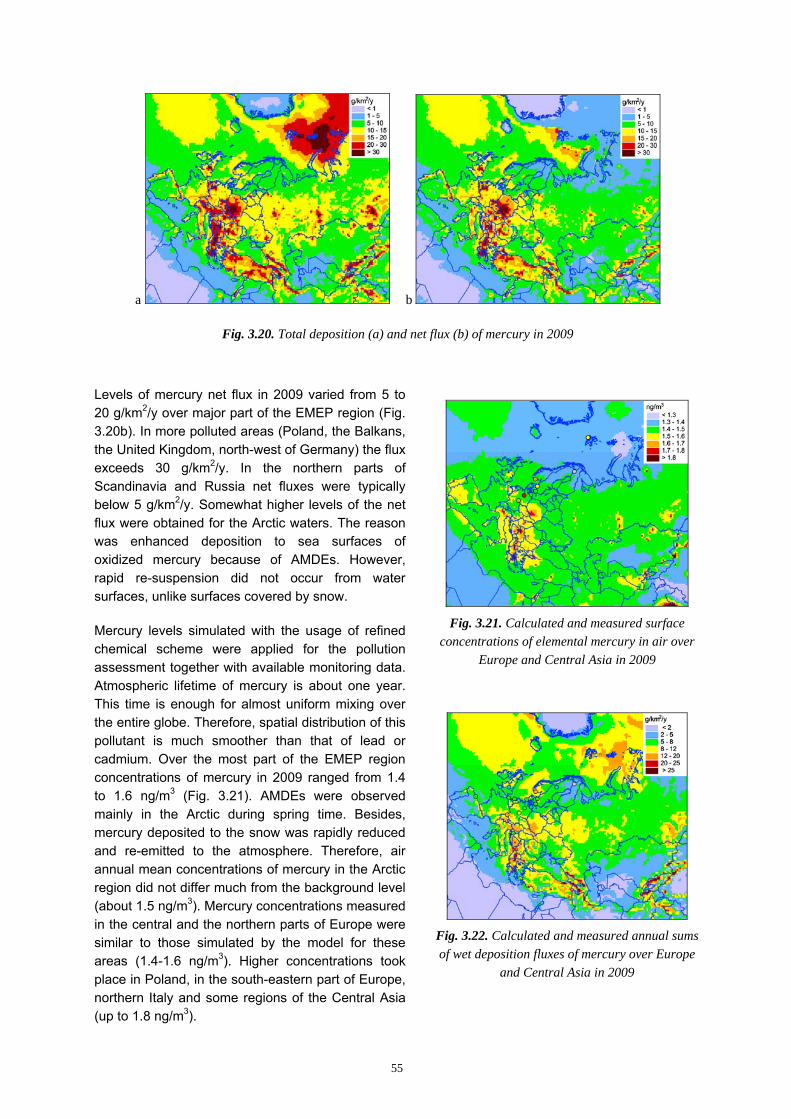
55

a b

Fig. 3.20. Total deposition (a) and net flux (b) of mercury in 2009

Levels of mercury net flux in 2009 varied from 5 to 20 g/km2/y over major part of the EMEP region (Fig. 3.20b). In more polluted areas (Poland, the Balkans, the United Kingdom, north-west of Germany) the flux exceeds 30 g/km2/y. In the northern parts of Scandinavia and Russia net fluxes were typically below 5 g/km2/y. Somewhat higher levels of the net flux were obtained for the Arctic waters. The reason was enhanced deposition to sea surfaces of oxidized mercury because of AMDEs. However, rapid re-suspension did not occur from water surfaces, unlike surfaces covered by snow.

Mercury levels simulated with the usage of refined chemical scheme were applied for the pollution assessment together with available monitoring data. Atmospheric lifetime of mercury is about one year. This time is enough for almost uniform mixing over the entire globe. Therefore, spatial distribution of this pollutant is much smoother than that of lead or cadmium. Over the most part of the EMEP region concentrations of mercury in 2009 ranged from 1.4 to 1.6 ng/m3 (Fig. 3.21). AMDEs were observed mainly in the Arctic during spring time. Besides, mercury deposited to the snow was rapidly reduced and re-emitted to the atmosphere. Therefore, air annual mean concentrations of mercury in the Arctic region did not differ much from the background level (about 1.5 ng/m3). Mercury concentrations measured in the central and the northern parts of Europe were similar to those simulated by the model for these areas (1.4-1.6 ng/m3). Higher concentrations took place in Poland, in the south-eastern part of Europe, northern Italy and some regions of the Central Asia (up to 1.8 ng/m3).

Fig. 3.21. Calculated and measured surface

concentrations of elemental mercury in air over Europe and Central Asia in 2009

Fig. 3.22. Calculated and measured annual sums of wet deposition fluxes of mercury over Europe

and Central Asia in 2009

56

Measurements on mercury wet deposition fluxes in 2009 were carried out in the central, the western and the northern parts of Europe. Modelled wet deposition in these regions ranged from 5 to 20 g/km2/y and generally corresponded to the observed levels (Fig. 3.22). Over the southern and the south-eastern part of Europe deposition ranged from 20 to 25 g/km2/y. Relatively high levels occurred over the Arctic. It was explained by removal of considerable mass of mercury oxidized during depletion. However, it should be noted that significant part of mercury deposited during AMDEs was re-volatilized from snow surfaces in short period of time, and thus, did not accumulate in soils or surface waters.

As shown above, total deposition of mercury was similar to its net flux except for the Arctic region. Therefore, in order to consider changes in mercury levels between 2009 and 2008 it makes sense to compare qualitatively deposition in 2008 with net flux in 2009, at least for most of the continental part of the EMEP region. Net flux of mercury to countries of the EMEP region in 2009 was 192 tonnes. Net flux to its European part was 132 tonnes, and to the Asian part (the Central Asian countries and Eastern part of Russia) – 60 tonnes. Net flux to the EMEP region in 2009 was lower by 42 tonnes (18%) than deposition in 2008. First of all, it was explained by decline of emissions used in modelling for 2009 by 20 tonnes compared to previous year. Besides, magnitudes of net flux and of total deposition over major part of the EMEP region were not equal, although the magnitudes were quite similar. Due to prompt re-emission the net flux should be lower than the deposition. Finally, transition from hemispheric model to global-scale model GLEMOS for calculations of boundary concentrations also resulted in somewhat smaller contribution of intercontinental transport to mercury pollution in the EMEP region in 2009 compared to 2008.

Country-averaged mercury net fluxes varied from 3 g/km2/y in Iceland to 26 g/km2/y in Greece (Fig. 3.23). Obviously, higher deposition fluxes were associated with countries with high density of national emissions, e.g., the FYR of Macedonia, Luxembourg, Poland. Unlike lead or cadmium, contribution of non-EMEP sources to mercury pollution was similar to the contribution of anthropogenic emissions. In 39 countries of 50 the contribution of non-EMEP sources to net mercury flux exceeded 50%. The contribution of natural emission from the EMEP region to mercury pollution of the EMEP countries was insignificant (1 – 3%) because of quick transport of naturally emitted mercury outside the EMEP region.

0

10

20

30

40

The_

FYR

_of_

Mac

edon

iaG

reec

eB

osni

a_H

erze

govi

naM

onte

negr

oC

zech

_Rep

ublic

Slo

vaki

aP

olan

dS

erbi

aLu

xem

bour

gS

love

nia

Bel

gium

Alb

ania

Arm

enia

Mon

aco

Aus

tria

Hun

gary

Sw

itzer

land

Turk

eyG

eorg

iaC

roat

iaK

yrgy

zsta

nA

zerb

aija

nR

oman

iaIta

lyB

ulga

riaN

ethe

rland

sG

erm

any

Uni

ted_

Kin

gdom

Lith

uani

aM

alta

Latv

iaB

elar

usU

krai

neTa

jikis

tan

Fran

ceN

orw

ayR

ussi

aE

ston

iaP

ortu

gal

Den

mar

kR

epub

lic_o

f_M

oldo

vaIre

land

Sw

eden

Kaz

akhs

tan

Icel

and

Spa

inC

ypru

sFi

nlan

dU

zbek

ista

nTu

rkm

enis

tan

Hg

depo

sitio

n flu

xes,

g/k

m2 /y Non-EMEP sources

Natural sources within EMEPEuropean and Central Asian Anthropogenic sources

Fig. 3.23. Country-averaged deposition fluxes of mercury from the European and Central Asian anthropogenic,

natural/historical and non-EMEP sources in 2009

Contribution of transboundary transport from EMEP anthropogenic sources to mercury net flux in 2009 ranged from about 6% in Malta to about 99% in Iceland (Fig.3.24). As a rule, the contribution was the highest in countries with low national emissions and surrounded by countries with significant emissions. Low contribution of transboundary transport, and hence, high contribution of national

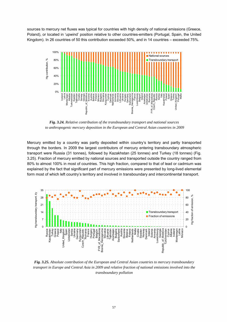
57

sources to mercury net fluxes was typical for countries with high density of national emissions (Greece, Poland), or located in ‘upwind’ position relative to other countries-emitters (Portugal, Spain, the United Kingdom). In 26 countries of 50 this contribution exceeded 50%, and in 14 countries – exceeded 75%.

0%

20%

40%

60%

80%

100%

Icel

and

Latv

iaM

onte

negr

oA

lban

iaTu

rkm

enis

tan

Sw

eden

Tajik

ista

nC

roat

iaN

orw

ayG

eorg

iaR

epub

lic_o

f_M

oldo

vaE

ston

iaA

ustri

aB

elar

usFi

nlan

dM

onac

oB

ulga

riaS

lova

kia

Kyr

gyzs

tan

Cyp

rus

Den

mar

kN

ethe

rland

sA

rmen

iaS

love

nia

Lith

uani

aU

krai

neH

unga

ryG

erm

any

Sw

itzer

land

Bos

nia_

Her

zego

vina

Fran

ceLu

xem

bour

gB

elgi

umIre

land

Aze

rbai

jan

Uzb

ekis

tan

Rom

ania

FYR

_of_

Mac

edon

iaC

zech

_Rep

ublic

Rus

sia

Ser

bia

Italy

Kaz

akhs

tan

Pol

and

Spa

inG

reec

eTu

rkey

Uni

ted_

Kin

gdom

Por

tuga

lM

alta

Hg

cont

ribut

ion,

%

National sourcesTransboundary transport

Fig. 3.24. Relative contribution of the transboundary transport and national sources

to anthropogenic mercury deposition in the European and Central Asian countries in 2009

Mercury emitted by a country was partly deposited within country’s territory and partly transported through the borders. In 2009 the largest contributors of mercury entering transboundary atmospheric transport were Russia (31 tonnes), followed by Kazakhstan (25 tonnes) and Turkey (18 tonnes) (Fig. 3.25). Fraction of mercury emitted by national sources and transported outside the country ranged from 80% to almost 100% in most of countries. This high fraction, compared to that of lead or cadmium was explained by the fact that significant part of mercury emissions were presented by long-lived elemental form most of which left country’s territory and involved in transboundary and intercontinental transport.

0

7

14

21

28

35

Rus

sia

Kaza

khst

anTu

rkey

Gre

ece

Pola

nd Italy

Uni

ted_

King

dom

Spai

nU

zbek

ista

nSe

rbia

Ukr

aine

Ger

man

yK

yrgy

zsta

nC

zech

_Rep

ublic

Rom

ania

Fran

ceH

unga

ryPo

rtuga

lB

elgi

umFY

R_o

f_M

aced

onia

Bosn

ia_H

erze

govi

naSl

ovak

iaLi

thua

nia

Tajik

ista

nAz

erba

ijan

Bul

garia

Switz

erla

ndAu

stria

Slo

veni

aB

elar

usFi

nlan

dN

ethe

rland

sM

alta

Cro

atia

Sw

eden

Nor

way

Den

mar

kIre

land

Esto

nia

Arm

enia

Luxe

mbo

urg

Geo

rgia

Rep

ublic

_of_

Mol

dova

Turk

men

ista

nC

ypru

sA

lban

iaIc

elan

dM

onte

negr

oLa

tvia

Mon

aco

Hg

trans

boun

dary

tran

spor

t, t/y

0

20

40

60

80

100H

g fra

ctio

n of

em

issi

on, %

Transboundary transportFraction of emissions

Fig. 3.25. Absolute contribution of the European and Central Asian countries to mercury transboundary transport in Europe and Central Asia in 2009 and relative fraction of national emissions involved into the

transboundary pollution

58

DEPOSITION TO REGIONAL SEAS

Atmospheric input to the North, the Mediterranean, the Black (with Azov), the Baltic and the Caspian Seas in 2009 was evaluated. The highest spatially average deposition fluxes of lead and cadmium took place in the Black Sea (Fig. 3.26). It was explained by the fact that this sea was surrounded by countries such as Russia, Ukraine, Turkey etc., with significant anthropogenic emissions of lead and cadmium. The lowest deposition of lead (0.51 kg/km2/y) and cadmium (12.5 g/km2/y) were found for the Caspian Sea. It is caused partly by smaller emissions in countries surrounding the sea, and partly by less annual precipitation in that region. The highest net mercury flux was calculated for the North Sea (9.6 g/km2/y), the lowest – over the Mediterranean and the Caspian Seas (6 and 6.2 g/km2/y).

Similar to countries, atmospheric input to the seas can be caused by various sources such as anthropogenic emissions in the EMEP countries, re-suspension or natural emission within EMEP, and non-EMEP sources. For example, about half of lead and cadmium atmospheric input to the Black Sea was caused by deposition of re-suspended dust particles (Fig. 3.27). Most part of mercury load to the Black Sea was caused by natural and anthropogenic sources located outside the EMEP region. Contribution of the EMEP anthropogenic sources of heavy metals made up about 1/3 of overall atmospheric input.

Contribution of individual EMEP countries to atmospheric input to the Black Sea is presented in Fig. 3.28. The main contributor to lead deposition in 2009 was Russia (28%), followed by Turkey (19%). Almost 20% of deposition was caused by anthropogenic sources of Asian and African countries. However, the emission in these regions was known with high uncertainty. Turkey contributed about one-third of cadmium deposition and more than a half of mercury net flux being the main anthropogenic source for the sea. The contribution of other countries was around 10% or less.

0

5

10

15

20

25

Nor

th

Med

iterr

anea

n

Bla

ck a

ndA

zov

Bal

tic

Cas

pian

Cd

and

Hg

depo

sitio

ns, g

/km

2/y

0.0

0.2

0.4

0.6

0.8

1.0

Pb d

epos

itions

, kg/

km2/

yCd Hg Pb

Fig. 3.26. Averaged deposition fluxes of lead, cadmium and net flux of mercury to regional

seas in 2009

0%

10%

20%

30%

40%

50%

60%

70%

80%

90%

100%

Lead Cadmium Mercury

Con

tribu

tion,

%

Outside EMEPRe-suspension/NaturalAsia and AfricaEMEP

Fig. 3.27. Contribution of different pollution sources

59

a

Asia14 t11%

Ukraine11 t8%

Africa10 t8%

Bulgaria10 t7%

Russia38 t28%

Turkey25 t19%

Other25 t19%

Pb

b

Bulgaria106 kg

3%

Ukraine310 kg

9%

Poland196 kg

5%Russia956 kg27%

Turkey1195 kg

34%

Other652 kg18%

Cd

The FYR of Macedonia

151 kg4%

c

Other159 kg13% Turkey

642 kg55%

Ukraine126 kg11%

Russia105 kg

9%

Greece77 kg6%

Romania51 kg4%

HgKazakhstan

29 kg2%

Fig. 3.28. Contribution of different countries to anthropogenic load of lead(a), cadmium(b) and mercury (c) to the Black Sea in 2009

3.4. Uncertainties of the pollution assessment

Assessment of air pollution includes information about three components: emission data, monitoring information and modelling results. Therefore, to understand quality of the assessment information about uncertainties of each component is highly important.

Emissions

Uncertainties of the emissions of the EMEP countries can be caused by missing emission sources, current understanding of emission factors, insufficient information about activities etc. Official information on uncertainties of country’s total emission of lead, cadmium and mercury for 2009 was available from five countries: Denmark, Finland, France, Sweden and the United Kingdom (Table 3.2). As follows from the table, uncertainty of emissions ranges from 15 to 50% for lead and cadmium, and from about 20 to 100% for mercury in most of countries reported this information. In Denmark the magnitude of emission uncertainties is much higher. It should be noted that emission data is one of the most important input parameters for modelling. Therefore, the uncertainty of the emission data affects modelling results.

In addition to total emission, correct spatial distribution of emission sources is highly important in the air pollution assessment. In Chapter 1 it was shown that the refinement of spatial distribution could significantly improve simulated concentrations in air.

Table. 3.2. Uncertainties of the heavy metal emission totals for 2009, %

Denmark [Nielsen et al., 2011]

Finland [SYKE, 2011]

France [CITEPA, 2011]

Sweden [SEPA, 2011]

United Kingdom [Passant et al.,

2011] Lead 625 ±25 51 15 -30 to +50 Cadmium 325 ±25 54 47 -20 to +50 Mercury 130 ±22 41 99 -30 to +40

60

Monitoring

Uncertainty of monitoring data is one of the sources of the uncertainties of heavy metal pollution assessment. This uncertainty depends on a number of factors such as sampling, storing, analysis of samples in laboratories, possible sample contamination etc. Estimation of the uncertainty caused by analytical methods is performed by regular intercomparisons of national laboratories involved in the analysis of lead and cadmium measurements sampled at the EMEP stations. The most recent intercomparison studies demonstrated that accuracy for majority of laboratories participated in the study is better than ±25% (See section 3.1)

Laboratory intercomparisons provide evaluation of the accuracy of analytical methods. Overall measurement accuracy can be estimated by field campaigns. Field comparison of measurements of total gaseous mercury concentrations held in May, 2005, demonstrated that the results of most of the laboratories, participated in the comparison, fall within ±30% range, and for concentrations in precipitation - within ±40% range [Aas, 2006]. Uncertainty of wet deposition of lead and cadmium, estimated on the base of the results of 2006-2007 field campaign, was around 20% [Aas et al., 2009]. However, these estimates do not take into account the effect of representativeness of station location.

Modelling

Uncertainty of air pollution assessment in the EMEP region can be evaluated by means of comparison of modelling results with data of background monitoring. For this purpose the most reliable monitoring data were selected from the data set for 2009, described in section 3.1. In particular, data of heavy metal concentrations in precipitation measured at Portuguese stations because most of measured values were below detection limit. The same reason was to exclude values of concentrations in precipitation from stations IE1(Pb, Cd, Hg), FR9, FR13, LV10, LV16, BE14, NL9, NL91 (Cd), EE9 (Cd, Hg). Due to low temporal coverage the data on Pb and Cd were also not used from stations IT1, ES1, ES7 and ES14. Mercury measurements in precipitation from Latvian stations LV10 and LV16 were ignored because of unrealistically low values (by two orders of magnitude) compared to measurements at other stations. Measured concentrations of mercury in air at stations PL5 and CZ3 exhibited strong temporal variability throughout the whole year, and at SE – in the middle of the year. This variability contradicts current understanding of mercury atmospheric behaviour. Therefore, the data form these stations were not used in the evaluation of modelling results.

Annual mean modelled and observed concentrations of lead, cadmium and mercury in air and wet deposition fluxes are demonstrated in scatter plots in Fig. 3.29. As seen, the model satisfactory well reproduced air concentrations of the three metals, and wet deposition fluxes of lead and mercury. However, wet deposition of cadmium was underestimated by the model. At a number of sites situated in Scandinavia (Sweden, Norway, Finland) and in the central and the eastern part of Europe (the Czech Republic, Slovakia, Latvia) the deposition fluxes were underestimated by 3 times or more.

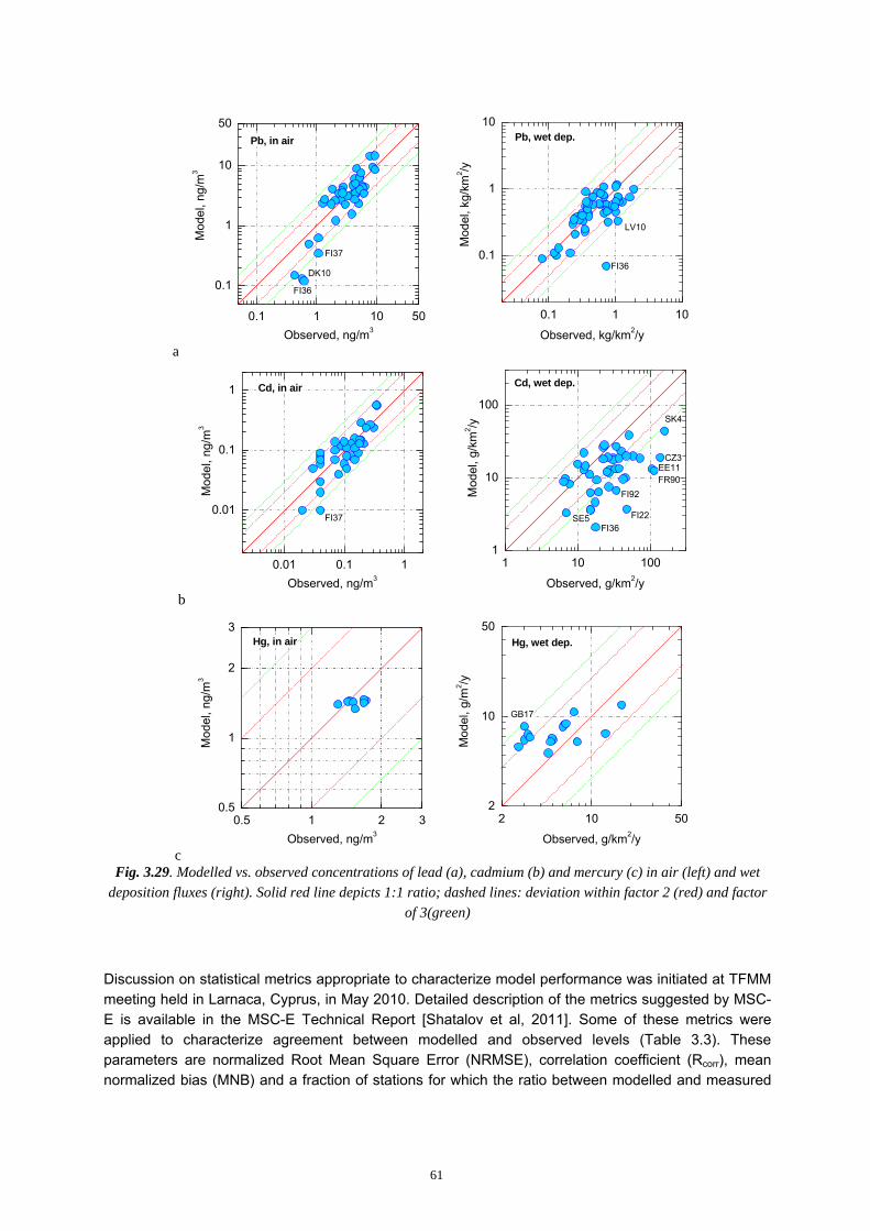
61

a

0.1 1 10 50

0.1

1

10

50Pb, in air

FI37

DK10

FI36

Mod

el, n

g/m

3

Observed, ng/m3

0.1 1 10

0.1

1

10Pb, wet dep.

FI36

LV10

Mod

el, k

g/km

2 /y

Observed, kg/km2/y

b

0.01 0.1 1

0.01

0.1

1 Cd, in air

FI37

Mod

el, n

g/m

3

Observed, ng/m3

1 10 1001

10

100

Cd, wet dep.

SE5

CZ3

SK4

EE11

FI92FR90

FI36FI22

Mod

el, g

/km

2 /y

Observed, g/km2/y

c

0.5 1 2 30.5

1

2

3Hg, in air

Mod

el, n

g/m

3

Observed, ng/m3

2 10 502

10

50Hg, wet dep.

GB17

Mod

el, g

/m2 /y

Observed, g/km2/y

Fig. 3.29. Modelled vs. observed concentrations of lead (a), cadmium (b) and mercury (c) in air (left) and wet deposition fluxes (right). Solid red line depicts 1:1 ratio; dashed lines: deviation within factor 2 (red) and factor

of 3(green)

Discussion on statistical metrics appropriate to characterize model performance was initiated at TFMM meeting held in Larnaca, Cyprus, in May 2010. Detailed description of the metrics suggested by MSC-E is available in the MSC-E Technical Report [Shatalov et al, 2011]. Some of these metrics were applied to characterize agreement between modelled and observed levels (Table 3.3). These parameters are normalized Root Mean Square Error (NRMSE), correlation coefficient (Rcorr), mean normalized bias (MNB) and a fraction of stations for which the ratio between modelled and measured

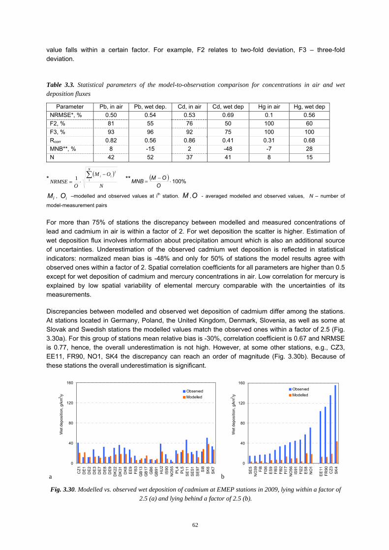
62

value falls within a certain factor. For example, F2 relates to two-fold deviation, F3 – three-fold deviation.

Table 3.3. Statistical parameters of the model-to-observation comparison for concentrations in air and wet deposition fluxes

Parameter Pb, in air Pb, wet dep. Cd, in air Cd, wet dep Hg in air Hg, wet dep NRMSE*, % 0.50 0.54 0.53 0.69 0.1 0.56 F2, % 81 55 76 50 100 60 F3, % 93 96 92 75 100 100 Rcorr 0.82 0.56 0.86 0.41 0.31 0.68 MNB**, % 8 -15 2 -48 -7 28 N 42 52 37 41 8 15

*( )

N

OM

ONRMSE

N

iii∑ −

⋅=

2

1 ** ( ) %100⋅−

=O

OMMNB

iM , iO –modelled and observed values at ith station. M ,O - averaged modelled and observed values, N – number of

model-measurement pairs

For more than 75% of stations the discrepancy between modelled and measured concentrations of lead and cadmium in air is within a factor of 2. For wet deposition the scatter is higher. Estimation of wet deposition flux involves information about precipitation amount which is also an additional source of uncertainties. Underestimation of the observed cadmium wet deposition is reflected in statistical indicators: normalized mean bias is -48% and only for 50% of stations the model results agree with observed ones within a factor of 2. Spatial correlation coefficients for all parameters are higher than 0.5 except for wet deposition of cadmium and mercury concentrations in air. Low correlation for mercury is explained by low spatial variability of elemental mercury comparable with the uncertainties of its measurements.

Discrepancies between modelled and observed wet deposition of cadmium differ among the stations. At stations located in Germany, Poland, the United Kingdom, Denmark, Slovenia, as well as some at Slovak and Swedish stations the modelled values match the observed ones within a factor of 2.5 (Fig. 3.30a). For this group of stations mean relative bias is -30%, correlation coefficient is 0.67 and NRMSE is 0.77, hence, the overall underestimation is not high. However, at some other stations, e.g., CZ3, EE11, FR90, NO1, SK4 the discrepancy can reach an order of magnitude (Fig. 3.30b). Because of these stations the overall underestimation is significant.

a

0

40

80

120

160

CZ1

DE

1D

E2

DE

3D

E7

DE

8D

E9

DK

22D

K31

DK

8E

E9

FI53

GB

13G

B17

GB

6G

B91

HU

2IS

90N

O55

PL4

PL5

SE

11S

E51

SE

97 SI8

SK

6S

K7

Wet

dep

ositi

on, g

/km

2 /y

ObservedModelled

b

0

40

80

120

160

SE

5N

O39 FI

8FI

36E

S9

FI93

FI92

FI17

NO

56IS

91FI

22E

S8

NO

1

EE

11FR

90C

Z3S

K4

Wet

dep

ositi

on, g

/km

2 /y

ObservedModelled

Fig. 3.30. Modelled vs. observed wet deposition of cadmium at EMEP stations in 2009, lying within a factor of 2.5 (a) and lying behind a factor of 2.5 (b).

63

Situation with stations where considerable overestimation is detected requires a special consideration. Firs of all, underestimation is noted for the Scandinavian stations, located mainly in Finland and Norway. These Nordic stations are located far from major emission sources, which is reflected by the modelling results: modelled deposition of Cd in this region are much lower than those in other parts of Europe. However, measured levels at these stations are similar or even higher to those observed in more industrialized regions of Europe, e.g., in Poland, Germany and Slovakia. It may imply that emissions in the Scandinavian region or in neighbouring countries can be underestimated, or local emission sources significantly contribute to deposition measured at these stations.

Deposition levels measured at stations SK5, EE11 and CZ3 seem extremely high compared to background observations measured at nearby stations. For example, wet deposition measured at Slovak station SK4 is 3 – 4.5 times higher than those measured at SK6 and SK7. The modelled deposition at SK6 and SK7 agree with measurements much better then at SK4. Therefore, high level of measured deposition at SK4, and possibly at EE11 and CZ3 may be caused by influence of local emission sources. Station FR90 is situated on the Brittany Peninsula and characterizes atmospheric masses transported from the Atlantic Ocean rather than anthropogenic pollution of the French territory. Measurements at this station can be affected by sea salt. Since the reasons of high Cd wet deposition fluxes measured at FR90, SK4, EE11 and CZ3, and hence, significant underestimation of the observed levels at these stations are unclear, the results for these stations were not included in statistical indexes in Table 3.3

Therefore, underestimated anthropogenic emissions and local emission sources can be the reasons of significant discrepancies at some stations measuring wet deposition of cadmium. Another possible reason could be uncertainties of measurements. Measured cadmium levels are much lower than those of lead, and thus cadmium measurements in precipitation are likely more complicated compared to lead. In particular, analysis of measurement data for 2009 indicated that observed values of cadmium concentrations in precipitation were below detection limit more often than those of lead. Finally, uncertainties of the model parameterizations can also contribute to the discrepancies. Currently these factors are analyzed in depth in the framework of the EMEP Case Study initiated by MSC-E and supported by TFMM of EMEP.

64

4. COOPERATION During this year the EMEP Centres were working in close co-operation with subsidiary bodies to the Convention, EMEP task forces, international organizations, and national experts. In particular, MSC-E continued to collaborate with the ICP-vegetation of Working Group on Effects in the field of joint analysis of measurements of heavy metals in mosses and their application for pollution assessment. The Task Force on Hemispheric Transport of Air Pollution was informed about EMEP current activities and plans for future work on mercury. Calculations of heavy metal deposition and its long-term trends to the Baltic Sea for the Helsinki Commission were carried out. Significant progress was achieved in the EU project “Global Mercury Observation System”. At the request of Italy MSC-E contributed to the development of national modelling system MINNI over the Italian domain.

4.1. Working Group on Effects (ICP-Vegetation) In 2011 MSC-E continued cooperation with the Working Group on Effects (WGE). In particular, joint analysis of heavy metal pollution levels involving measurements of concentrations in mosses was carried out. The concentrations were provided by the ICP-Vegetation. These data have already been used in the assessment of heavy metal pollution levels and their long-term trends both for Europe as a whole and for individual countries [Ilyin et al., 2009, 2010]. This year the main activity in this field was focused on the Czech Republic.

In the framework of this activity relationships between observed wet deposition of cadmium and measured concentrations in mosses in the Czech Republic were investigated. Besides, the concentrations were applied for evaluation of spatial distribution of total cadmium deposition simulated by the model with coarse (50x50 km) and fine (5x5 km) spatial resolution. The results of this work were presented and discussed at 24th ICP-Vegetation Task Force Meeting held in Zurich, Switzerland, 31 January - 2 February 2011. Technical details of the analysis are described in Chapter 1 of this report.

The analysis of pollution levels in the Czech Republic involving measurements of cadmium concentrations in mosses demonstrates that data on concentrations in mosses can be used as supplementary data to assess of pollution levels in the country. Because of wide spatial coverage and high density of measurements this type of information is helpful in identifying areas of relatively high or low levels atmospheric deposition. Further cooperation with the effects community in the field of application of measurements of heavy metals in mosses is highly appreciated. In particular, the cooperation is needed for better understanding of relationships between deposition and concentrations in mosses and for interpretation of measurements in mosses.

4.2. Task Force on Hemispheric Transport of Air Pollution

MSC-E continued co-operation with the Task Force on Hemispheric Transport of Air Pollution (TF HTAP). In particular it took part in development of new directions of HTAP activity and the Work-plan for next years conducted at the Task Force meeting in Arona, Italy in May 2011. The Centre presented

65

an overview of available data and ongoing EMEP activities aimed at development of new emission inventories, extension of monitoring networks and application of chemical transport models for assessment of the environment pollution by mercury and POPs on a global scale. It also noticed the importance of elaboration and application of the multi-media modelling approach to the assessment of cycling and accumulation in the environment of such long-lived pollutants as mercury and some POPs. The assessment could be the most effectively performed within the framework of integrated analysis involving combined use of emissions, monitoring and modelling aspects. The Task Force decided to continue its work on assessment of intercontinental pollution by a number of long-lived substances including mercury and selected POPs. It was also agreed that the Task Force would benefit from close cooperation with on-going activities within relevant projects and international programmes (GMOS and ArcRisc projects, UNEP, AMAP, Stockholm Convention etc.)

4.3. European commission (EU FP7 project GMOS)

In the framework of co-operation with the European Commission MSC-E takes part in the EU FP7 project GMOS (Global Mercury Observation System) (Fig. 4.1). The project was launched in the fall of 2010 and is aimed at:

• Establishment of a global monitoring system for mercury including land-based, over-water and aircraft observations;

• Improvement and validation of regional and global scale atmospheric mercury models; • Model application to evaluate source-receptor relationships, temporal trends and scenarios; • Development of interoperable system for dissemination of the project output data.

MSC-E as a leader of one of the project work packages (WP7) co-ordinates the modelling activities on a global scale as well as takes part in the regional scale model assessment. The model consortium of the project consists of five global/hemispheric models and three regional scale models from different scientific groups of Europe and North America. The program of model development and applications includes a variety of tasks:

• Update of modelling approaches and coupling global and regional-scale models;

• Utilizing measurement data for model evaluation and improvement;

• Model applications for the present-day conditions and reproduction of historical trends;

• Evaluation of mercury intercontinental transport patterns and contribution of global sources to mercury deposition in Europe;

• Forecasting mercury concentration and deposition patterns as well as source-receptor relationships for selected emission scenarios;

• Uncertainty analysis of the modelling results.

In the current year MSC-E has started preparatory work for the model simulations program within the project. In particular, it initiated preparation of an inventory of characteristics and parameterisations of the consortium models. The aim of the inventory is providing up-to-date information on the models participating in the project and support of the forthcoming analysis of modelling results. The information

Fig. 4.1. General structure of the GMOPS project

66

about the models formulation, grids used, input fields (meteorological fields, initial and boundary conditions, reactants concentration fields etc.) and the chemical mechanisms is included in the current version of the inventory.

Another part of this year activity related to development of the coupling procedure of the model assessment on global and regional scales. To ensure consistency of the model simulations on different scales initial and boundary conditions (IC/BC) for the regional models will be provided by the global models of the project consortium. Parameters, data exchange protocol, and data formats for the coupling procedure along with the target regions and the regional model grids were discussed and adopted by the project partners at the workshop in Hamburg, Germany, in March 2011. In addition, the modeling group has formulated demands to the over-water and aircraft field measurements planed within the project. They include a list of measured species, ancillary parameters, and measurement conditions required for evaluation and improvement of modelling approaches. The model requirements were presented and discussed with the measurement community at the project workshop in Piran, Slovenia in May 2011. The elaborated proposals have been adopted as priorities for the planned measurement campaigns.

4.4. Marine Convention (HELCOM)

In accordance with the Memorandum of Understanding between the Baltic Marine Environment Protection Commission (HELCOM) and the United Nations Economic Commission for Europe the EMEP Centres have prepared an annual joint report on the assessment of airborne pollution load to the Baltic Sea [Bartnicki et al., 2010]. MSC-E contributed to this report with the evaluation of atmospheric input of heavy metals (lead, cadmium, and mercury) to the Baltic Sea. The atmospheric transport and deposition were assessed on the base of the EMEP officially submitted emission data. Besides, this report provided detailed information on emissions of heavy metals in HELCOM countries, contributions of individual countries to the deposition over the Baltic Sea, and the comparison of modelling results against measurement data collected in the HELCOM region in 2008. The report was welcomed and endorsed by the Contracting Parties at the HELCOM MONAS 13 meeting in October 2010 and was recommended to be published on the EMEP and HELCOM websites.

Along with the contribution to the joint annual report, MSC-E prepared environmental indicator fact sheets with the updated information on variations of atmospheric emissions of heavy metals and levels of their deposition to the Baltic Sea for the period from 1990 to 2008. These indicator fact sheets are available in the Internet at the web site of the Helsinki Commission [www.helcom.fi].

According to the officially reported data, emissions in HELCOM countries declined from 1990 to 2008 by 47%, 52%, and 86% for cadmium, mercury, and lead, respectively (Fig. 4.2). The reduction of heavy metal emissions in this area is mostly caused by the extensive use of unleaded gasoline and application of cleaner production technologies in countries. Besides, it is partly connected with the economic re-structuring taken place in Poland, Estonia, Latvia, Lithuania, and Russia since early 1990s. The highest decrease of cadmium emissions can be seen in Lithuania (88%) and Estonia (86%). In case of lead emission, the most significant decrease took place in Sweden and Finland where the emissions in 2008 were about 40 and 16 times lower, respectively, than in 1990. Essential reduction of annual lead emission of HELCOM countries from 2003 to 2004 was mostly caused by the change of emission in Russia. Mercury emission most significantly decreased in Germany (81%) and Denmark (75%). Among the HELCOM countries the largest contributions to cadmium total emissions of HELCOM countries belong to Russia (56%) and Poland (39%), for mercury – to Poland (44%) and Russia (38%), and for lead – to Poland (49%) and Russia (32%).

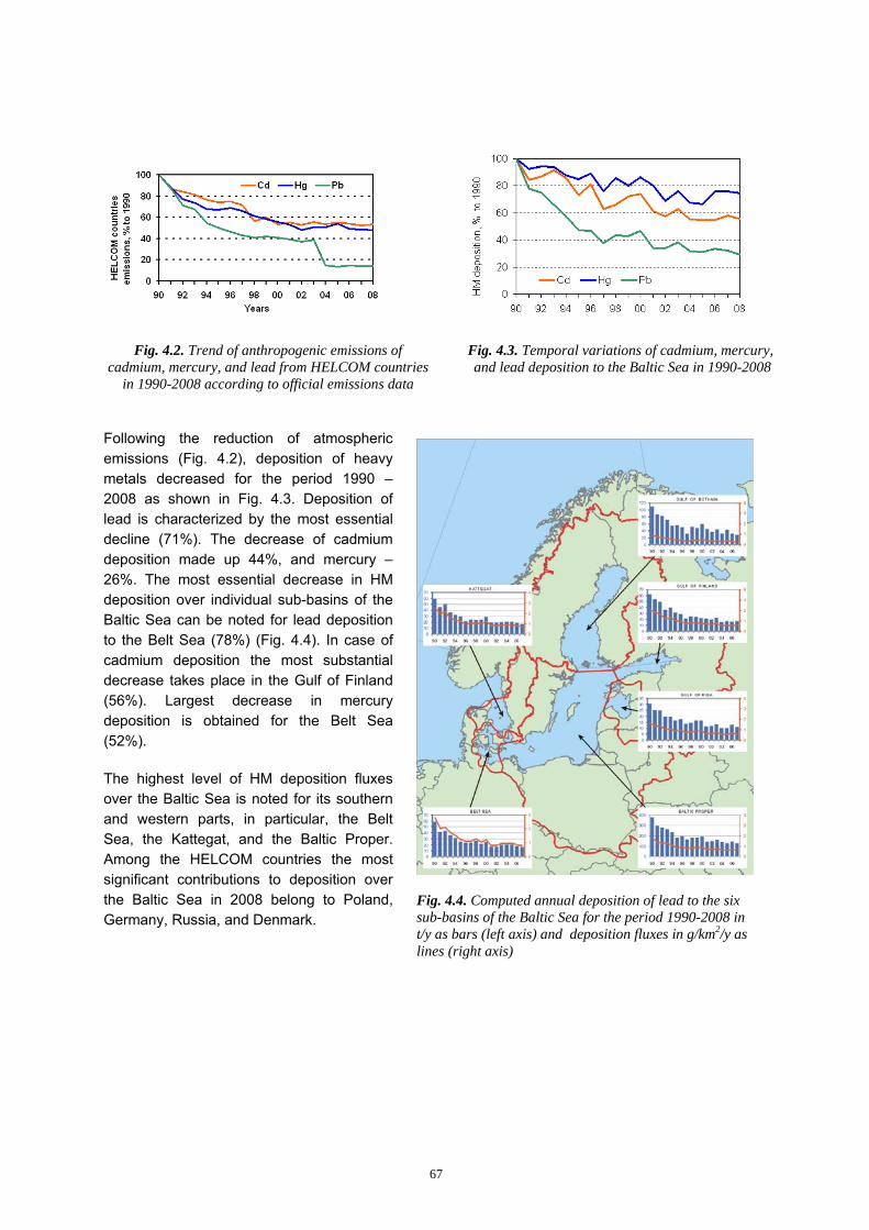
67

Fig. 4.2. Trend of anthropogenic emissions of cadmium, mercury, and lead from HELCOM countries

in 1990-2008 according to official emissions data

Fig. 4.3. Temporal variations of cadmium, mercury, and lead deposition to the Baltic Sea in 1990-2008

Following the reduction of atmospheric emissions (Fig. 4.2), deposition of heavy metals decreased for the period 1990 – 2008 as shown in Fig. 4.3. Deposition of lead is characterized by the most essential decline (71%). The decrease of cadmium deposition made up 44%, and mercury – 26%. The most essential decrease in HM deposition over individual sub-basins of the Baltic Sea can be noted for lead deposition to the Belt Sea (78%) (Fig. 4.4). In case of cadmium deposition the most substantial decrease takes place in the Gulf of Finland (56%). Largest decrease in mercury deposition is obtained for the Belt Sea (52%).

The highest level of HM deposition fluxes over the Baltic Sea is noted for its southern and western parts, in particular, the Belt Sea, the Kattegat, and the Baltic Proper. Among the HELCOM countries the most significant contributions to deposition over the Baltic Sea in 2008 belong to Poland, Germany, Russia, and Denmark.

Fig. 4.4. Computed annual deposition of lead to the six sub-basins of the Baltic Sea for the period 1990-2008 in t/y as bars (left axis) and deposition fluxes in g/km2/y as lines (right axis)

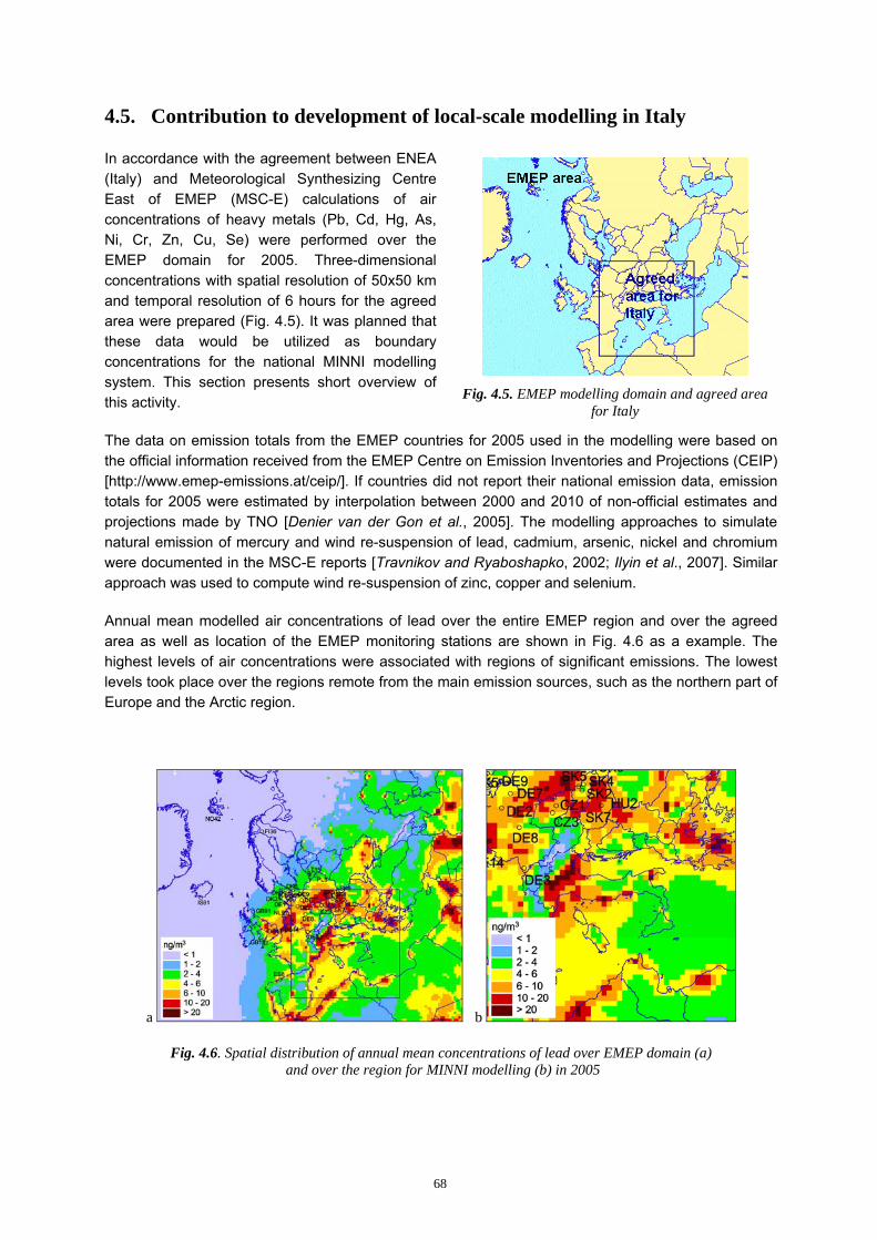
68

4.5. Contribution to development of local-scale modelling in Italy

In accordance with the agreement between ENEA (Italy) and Meteorological Synthesizing Centre East of EMEP (MSC-E) calculations of air concentrations of heavy metals (Pb, Cd, Hg, As, Ni, Cr, Zn, Cu, Se) were performed over the EMEP domain for 2005. Three-dimensional concentrations with spatial resolution of 50x50 km and temporal resolution of 6 hours for the agreed area were prepared (Fig. 4.5). It was planned that these data would be utilized as boundary concentrations for the national MINNI modelling system. This section presents short overview of this activity.

The data on emission totals from the EMEP countries for 2005 used in the modelling were based on the official information received from the EMEP Centre on Emission Inventories and Projections (CEIP) [http://www.emep-emissions.at/ceip/]. If countries did not report their national emission data, emission totals for 2005 were estimated by interpolation between 2000 and 2010 of non-official estimates and projections made by TNO [Denier van der Gon et al., 2005]. The modelling approaches to simulate natural emission of mercury and wind re-suspension of lead, cadmium, arsenic, nickel and chromium were documented in the MSC-E reports [Travnikov and Ryaboshapko, 2002; Ilyin et al., 2007]. Similar approach was used to compute wind re-suspension of zinc, copper and selenium.

Annual mean modelled air concentrations of lead over the entire EMEP region and over the agreed area as well as location of the EMEP monitoring stations are shown in Fig. 4.6 as a example. The highest levels of air concentrations were associated with regions of significant emissions. The lowest levels took place over the regions remote from the main emission sources, such as the northern part of Europe and the Arctic region.

a b

Fig. 4.6. Spatial distribution of annual mean concentrations of lead over EMEP domain (a) and over the region for MINNI modelling (b) in 2005

Fig. 4.5. EMEP modelling domain and agreed area

for Italy

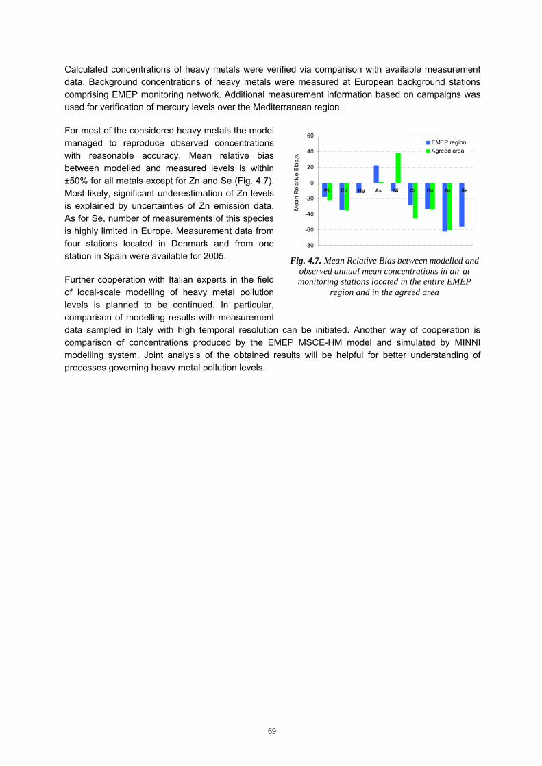
69

Calculated concentrations of heavy metals were verified via comparison with available measurement data. Background concentrations of heavy metals were measured at European background stations comprising EMEP monitoring network. Additional measurement information based on campaigns was used for verification of mercury levels over the Mediterranean region.

For most of the considered heavy metals the model managed to reproduce observed concentrations with reasonable accuracy. Mean relative bias between modelled and measured levels is within ±50% for all metals except for Zn and Se (Fig. 4.7). Most likely, significant underestimation of Zn levels is explained by uncertainties of Zn emission data. As for Se, number of measurements of this species is highly limited in Europe. Measurement data from four stations located in Denmark and from one station in Spain were available for 2005.

Further cooperation with Italian experts in the field of local-scale modelling of heavy metal pollution levels is planned to be continued. In particular, comparison of modelling results with measurement data sampled in Italy with high temporal resolution can be initiated. Another way of cooperation is comparison of concentrations produced by the EMEP MSCE-HM model and simulated by MINNI modelling system. Joint analysis of the obtained results will be helpful for better understanding of processes governing heavy metal pollution levels.

-80

-60

-40

-20

0

20

40

60

Pb Cd Hg As Ni Cr Cu Zn Se

Mea

n R

elat

ive

Bia

s, %

EMEP regionAgreed area

Fig. 4.7. Mean Relative Bias between modelled and

observed annual mean concentrations in air at monitoring stations located in the entire EMEP

region and in the agreed area

70

5. FUTURE ACTIVITIES

In order to further improve the quality of the pollution level assessment of lead, cadmium and mercury over the EMEP region, the following activities of MSC-E and CCC are proposed for 2012/2013:

On-going activities:

Review, store and make available monitoring data for the modelling centres and Parties

Publish the validated annual data and contribute to preparation, review and assessments of observation data presented in the series of EMEP reports

Arrange laboratory intercomparisons for heavy metals

Address global scale integration of quality assessment/quality control (QA/QC) activities of regional monitoring programmes, including standards for metadata provision and intercomparisons (in collaboration with the TFHTAP)

Maintain close interaction with relevant organizations and bodies in relation to integration of observations, including monitoring efforts under other Convention bodies (e.g., the ICPs and national monitoring obligations to European Commission Directives, as well as activities undertaken by EEA, WMO, OSPAR, HELCOM, UNEP, AMAP, GMES/GEOSS and others).

Evaluate air concentrations, deposition fluxes and transboundary atmospheric transport of heavy metals (Pb, Cd and Hg) for 2010 – 2011;

Calculate HM dispersion on a global scale with the help of global EMEP model (GLEMOS) for the evaluation of initial and boundary conditions and contributions of intercontinental transport to pollution levels in the EMEP domain and in remote regions (the Arctic) with spatial resolution 1°x 1°;

Perform model assessment of transboundary pollution within the EMEP region by HMs for 2010-2011 including contamination of marginal seas with spatial resolution 50 km x 50 km;

Perform detailed analysis of heavy metal pollution levels with finer spatial resolution (5km x 5km, 10km x 10km) for countries-participants of the Case Study (e.g. the Czech Republic, Croatia, the Netherlands and Spain);

Prepare input data required for global/regional/local modelling (emission, meteorological, and geophysical data);

Contribute to the effect community work with information on ecosystem-dependent deposition fluxes of HMs to different land use types to support evaluation of the pollutants adverse effect on human health and the environment;

Cooperate with the CLRTAP subsidiary bodies (WGSR, WGE), EMEP task forces (TFHTAP, TFMM), and relevant international organizations;

71

Support countries with information required for air quality management in and implementation of the CLRTAP Protocols on HMs with special emphasis to EECCA countries.

New (research and development) activities:

Cooperate with the EU FP7 project GMOS for further harmonization of measurements and data reporting of mercury in Europe

Global/regional/local modelling:

- Further develop and improve the modular architecture of the Global EMEP Multi-media Modelling System (GLEMOS) modelling framework;

- Incorporate data on aerosols and atmospheric reactants based on external datasets or simplified chemical modules for improving evaluation of HM pollution levels;

- Continue model development of wind re-suspension of heavy and investigation of its role in both on regional and country scales;

- Further develop and test the integrated monitoring/modelling/emission approach for HMs including the adjoint modelling;

- Perform comprehensive analysis of major physical and chemical processes governing mercury cycling in the atmosphere based on sensitivity study and evaluation against detailed measurements (in co-operation with EU GMOS project);

- Prepare the GLEMOS modelling framework for distribution and support as an open source software.

EMEP Case Study:

- Carry out integrated analysis of HM pollution levels in the Czech Republic, perform improved assessment of the country pollution including evaluation of contribution of major emission sources;

- Evaluate factors affecting pollution levels in Croatia, the Netherlands, and Spain on the base of emissions, measurements, and modelling results with fine spatial resolution, and involvement of country-specific input data provided by countries-participants.

72

CONCLUSIONS

Main activities of the EMEP Centres MSC-E and CCC in 2011 were focused on assessment of heavy metal pollution levels in the EMEP region, development of Global EMEP Multi-media Modelling System (GLEMOS) and investigation of pollution levels on national/local scales. The Centres paid significant attention to cooperation with the subsidiary bodies to the Convention, EMEP task forces, international organizations and programmes as well as with national experts. The main conclusions of the activities of MSC-E and CCC are formulated below.

Investigation of pollution levels on national/local scale (Country-specific Case Study)

Investigation of pollution levels on national/local scales in the framework of the EMEP country-specific Case Study on heavy metal pollution assessment continued in 2011. The Czech Republic, Croatia, the Netherlands and Spain are participants of the Case Study. In accordance with individual programmes model simulations with fine spatial resolution have already been performed for the Czech Republic (5x5 km), Croatia (10x10 km) and the Netherlands (5x5 km). National monitoring data from Spain are overviewed. Country-specific emissions, monitoring data and modelling results are analysed and discussed jointly with national experts from the participating countries. On the base of these analyses and discussions the main conclusions related to the Case Study activities have been agreed.

1. Transition from the coarse (50x50 km) to finer (5x5 km, 10x10 km) resolution lead to better quality of pollution level assessment. Coarse spatial resolution of the emissions in neighbouring countries leads to significant uncertainties of heavy metal pollution assessment, especially near the state borders of the countries-participants of the Case Study. Therefore, emission data with fine spatial resolution from neighbouring countries are needed to improve air pollution assessment.

2. Number of national monitoring stations involved in the country-specific analysis is significantly larger compared to that available from the EMEP monitoring network. National information on measurements of heavy metals in air and/or in precipitation is available from 92 stations in the Czech Republic (vs. 2 EMEP stations), 5 stations in the Netherlands (vs. 3 EMEP stations) and 3 stations in Croatia (no EMEP stations). The additional information derived from national monitoring stations allows to perform more reliable analysis of country-scale pollution levels from viewpoint of spatial coverage and statistical significance.

3. Wind re-suspension is an important contributor to heavy metal pollution levels. In some individual short-term episodes its contribution to simulated concentrations of cadmium in air reaches 90%. Primary analysis of the model simulation results for Croatia and the Netherlands demonstrates that re-suspension can be one of the reasons responsible for the discrepancies between modelled and measured values. Refinement of the wind re-suspension scheme is planned for the future work. Data on soil concentrations with fine spatial resolution can significantly contribute to the improvement of wind re-suspension parameterization.

4. Data on concentrations of heavy metals in mosses is an important supporting information for the analysis of country-scale pollution levels. In particular, it allows to evaluate spatial distribution of

73

atmospheric pollution because of wide spatial coverage and high density of measurements in mosses.

Model developments on a global scale

This year development activities were focused on further elaboration of the global modelling framework GLEMOS as well as on refining of the mercury chemical scheme for both global and regional scale applications.

1. The modular architecture is one of the key features of the GLEMOS modelling framework and it is aimed to provide flexibility for simulation of various pollutants with diverse properties. The architecture of the framework was considerably updated to make possible a flexible choice of the model configuration (model domain, spatial resolution, list of substances, environmental media, etc.) for particular research tasks.

2. A new version of the WRF model has been adapted for use as a meteorological driver for the GLEMOS framework. An advantage of WRF is possibility of data support of multi-scale simulations (from global to local) on different projections and grids. It can be also used as an additional source of consistent input data on concentration of atmospheric reactants required for heavy metal and POP modelling. Preliminary evaluation of WRF demonstrates satisfactory performance in comparison with measurements and results of other meteorological drivers.

3. MSC-E started development of the oceanological driver to supply the model simulations with required data on sea currents, temperature, salinity, etc. The Parallel Ocean Program model was adapted as the base of the driver. The simulated oceanological parameters were evaluated against available measurement data. In addition, the oceanic transport module of the GLEMOS framework was completely re-designed to bring it in consistency with the new driver and thoroughly tested.

4. The mercury chemical module was updated with the new findings of the research community. In particular, the chemical mechanism of mercury oxidation by reactive halogens was considerably refined and applied for study of the Arctic mercury pollution. The updated mercury chemical scheme was evaluated against observations at the EMEP high latitude site and implemented for operational EMEP modelling. The simulations of mercury levels in the Arctic demonstrated significant effect of Atmospheric Mercury Depletion Events (AMDEs) on total mercury deposition, which, however, was largely compensated by prompt re-emission from snow.

Assessment of heavy metal pollution levels

1. The measurement obligations set by the EMEP monitoring strategy for 2009-2019 and the EU air quality directives have clearly improved the site coverage of the EMEP region for the last years. In 2009, there were 35 sites measuring heavy metals in both air and precipitation, and altogether there were 71 measurement sites. There were 26 sites measuring at least one form of mercury. However, there was still a lack of measurements in the south-eastern and the eastern parts of Europe and in Central Asia.

74

2. Results of most of national laboratories participated in the intercomparison studies met the requirements of the current data quality objective. The accuracy of analytical methods in all laboratories was better than ±26%, and in most of laboratories - better than ±10%. However, there are some countries/laboratories reporting measurements data without participation in the laboratory intercomparison. Data from these countries are of unknown quality; and it is therefore strongly recommended that they take part in the annual laboratory intercomparison.

3. Spatial distribution of concentrations and deposition was evaluated via joint usage of modelling results and monitoring data. The highest regional-scale heavy metal pollution levels were obtained for Poland, north of Italy, the Benelux region, the Balkan region, and the central part of Russia. Scandinavia and the northern part of Russia were characterized by the lowest levels of heavy metal pollution.

4. Emissions of heavy metals used in modelling for 2009 in the EMEP region as a whole declined, but wind re-suspension of lead and cadmium grew compared to 2008. Combined effect of these two counter-directing factors resulted in increase of deposition of lead by 9% and in decline of cadmium deposition by 2% in the EMEP countries. Estimates of mercury load to the EMEP region for 2009 were 18% lower compared to those for 2008 due to reduction of emissions and changes associated with the model modifications. Decrease of pollution levels of lead, cadmium and mercury was indicated in the eastern part of Europe (Russia, Ukraine, Romania, Poland). Marked increase of estimated pollution levels of the heavy metals took place in Germany because of increase of the reported emissions.

5. Transboundary transport is one of the main factors determining pollution levels. Contribution of transboundary transport exceeded contribution of national sources to anthropogenic deposition of lead and cadmium in 36 countries, and that of mercury – in 26 countries. The fraction of national emissions of the EMEP countries transported outside their territories ranged from 60% to almost 100% for lead, from 50% to 90% for cadmium and from 80% to almost 100% for mercury.

6. Quality of heavy metal pollution assessment in the EMEP region was evaluated taking into account uncertainties of emissions, monitoring and modelling results. Uncertainties of country’s total emission values of lead, cadmium and mercury typically varied from 15 to 50%. Overall uncertainty of measured wet deposition, estimated using results of field campaigns, was around 20% for lead and cadmium, and 40% for mercury. However, these estimates did not include the effect of representativeness of stations location.

7. Modelled concentrations of lead, cadmium and mercury in air, and wet deposition of lead and mercury agreed with observed levels with satisfactory accuracy. For more than half of stations difference between modelled and measured values lay within a factor of 2, and mean relative bias ranged from -16% to 28%. Cadmium wet deposition were underestimated by 48%, mainly because of significant (several times) underestimation at some stations, located mainly in Scandinavia. If these stations are excluded from the statistical analysis, the underestimation is -30%. Further research is needed to establish the reasons of the underestimation.

Cooperation

1. MSC-E continued cooperation with the ICP-Vegetation of WGE in the field of application of measurements of concentrations in mosses for the analysis of pollution levels. Further

75

cooperation with the effects community regarding usage of measurements of heavy metals in mosses is needed for better understanding of relationships between deposition and concentrations in mosses and for interpretation of the measurements.

2. Co-operation of MSC-E with the Task Force on Hemispheric Transport of Air Pollution (TF HTAP) continued. The Centre informed TF HTAP on the ongoing EMEP activities in the field of mercury and POP pollution assessment on a global scale, presented an overview of available data and relevant research initiatives aimed at development of new emission inventories, extension of monitoring networks and application of chemical transport models, and took part in development of new directions of TF HTAP activity and the Work-plan for next years.

3. In the framework of co-operation with the European Commission MSC-E participates in EU FP7 project GMOS (Global Mercury Observation System) aimed at the integrated research of mercury pollution on a global scale. MSC-E as a leader of one of the project work packages co-ordinates the global scale modelling activities as well as takes part in the regional model assessment in Europe. In the current year MSC-E has initiated preparatory work for the model simulations program within the project and co-ordinated relations with external modelling groups.

4. MSC-E prepared contribution to the joint report of the EMEP Centres on the evaluation of airborne pollution loads to the Baltic Sea for the Helsinki Commission. Information on deposition of lead, cadmium and mercury to the Baltic Sea in 2008 and their trends for 1990 - 2008 period was provided. For this period the reduction of deposition was 71% (Pb), 44% (Cd) and 26% (Hg). The highest level of HM deposition fluxes over the Baltic Sea was noted for its southern and western parts.

5. In accordance with the agreement between ENEA (Italy) and MSC-E calculations of 3D air concentrations of heavy metals (Pb, Cd, Hg, As, Ni, Cr, Zn, Cu, Se) were performed over the EMEP domain for 2005. These concentrations were used for preparation of initial and boundary conditions for local-scale simulations over Italy by the MINNI modelling system. Modelled concentrations were evaluated via comparison with available monitoring data. Further cooperation with Italian experts could include intercomparison of modelling results obtained by MINNI and EMEP models for heavy metals.

6. Country-specific reports were prepared in Russian language to support EECCA countries.

76

REFERENCES

Aas W. [2006]. Data quality 2004, quality assurance and field comparisons. EMEP/CCC Report 4/2006.

Aas W., Alleman L.Y., Bieber E., Gladtke D., Houdret J.L., Karlsson V., Monies C. [2009]. Comparison of methods for measuring atmospheric deposition of arsenic, cadmium, nickel and lead. J. Environ. Monit., vol. 11, pp. 1276 - 1283 doi: 10.1039/B822330K.

Aas W. and K.Breivik [2007]. Heavy metals and POP measurements, 2005. EMEP/CCC-Report 6/2007.

Aas W. and K.Breivik [2011] Heavy metals and POP measurements 2008, Norwegian Institute for Air Research. EMEP/CCC-Report 3/2011.

AMAP/UNEP [2008] Technical Background Report to the Global Atmospheric Mercury Assessment. Arctic Monitoring and Assessment Programme / UNEP Chemicals Branch (2http://www.chem.unep.ch/mercury/Atmospheric_Emissions/Technical_background_report.pdf).

Ariya P., Dastoor A., Amyot M., Schroeder W., Barrie L., Anlauf K., Raofie F., Ryzhkov A., Davignon D., Lalonde J. and A.Steffen [2004] The Arctic: A sink for mercury. Tellus B, 56, 5, pp.397–403.

Ariya P.A., Khalizov A. and A.Gidas [2002] Reactions of gaseous mercury with atomic and molecular halogens: kinetics, product studies, and atmospheric implications. J. Phys. Chem., 106, pp.7310–7320.

Ariya P., Peterson K., Snider G. and M.Amyot [2009] Mercury chemical transformation in the gas, aqueous, and heterogenous phases: State of-the-art science and uncertainties in Mercury Fate and Transport in the Global Atmosphere: Emissions, Measurements, and Models, edited by N. Pirrone and R. Mason, pp.459-502, Springer, New York.

Axenfeld F., Münch J. and J.M.Pacyna [1991] Belastung von Nord- und Ostsee durch ökologisch gefährliche Stoffe am Beispiel atmosphärischer Quecksilberkomponenten. Teilprojekt: Europäische Test-Emissionensdatenbasis von Quecksilber-Komponenten für Modellrechnungen. Dornier, Report 104 02 726, p.99.

Bartnicki J., Gusev A., Aas W. and S.Valiyaveetil [2010] Atmospheric Supply of Nitrogen, Lead, Cadmium, Mercury and Dioxins/Furans to the Baltic Sea in 2008. MSC-W Technical Report 2/2010. (3Uhttp://emep.int/publ/helcom/2010/index.html H)

Berg T., Roset O. and E.Steinnes [1995] Moss (Hylocomium Splendens) used a biomonitor of atmospheric trace element deposition: estimation of uptake efficiencies. Atmospheric Environment, 29, pp.353-360.

Berg T. and E.Steinnes [1997] Use of mosses (Hylocomium Splendens and Pleurozium Schreberi) as biomonitors of heavy metal deposition: from relative to absolute deposition values. Environmental Pollution, 98, p.61-71.

Bessagnet B., Menut L., Aymoz G., Chepfer H. and R.Vautard [2008] Modeling dust emissions and transport within Europe: The Ukraine March 2007 event. J. Geophys. Research, 113, D15202, doi:10.1029/2007JD009541.

Birmili W., Schepanski K., Ansmann A., Spindler G., Tegen I., Wehner B., Nowak A., Reimer E., Mattis I., Müller K., Brüggemann E., Gnauk T., Herrmann H., Wiedensohler A., Althausen D., Schladitz A., Tuch T. and G. Löschau [2008] A case of extreme particulate matter concentrations over Central Europe caused by dust emitted over the southern Ukraine. Atmos. Chem. Phys., 8, pp.997–1016.

CITEPA [2011] Inventaire des emissions de polluants atmospheriques en France au titre de la convention sur la pollution atmospherique transfrontaliere a longue distance et de la directive Europeenne relative aux plafonds d’emissions nationaux (NEC). CEE–NU/NFR & NEC Mars 2011. p.225.

Dastoor A.P., Davignon D., Theys N., Roozendael M.V., Steffen A. and P.A.Ariya [2008] Modeling Dynamic Exchange of Gaseous Elemental Mercury at Polar Sunrise. Environmental Science and Technology, 42,14, pp.5183-5188.

Denier van der Gon D. H.A.C., van het Bolscher M., Visschedijk A.J.H. and Zandveld P.Y.J. [2005]. Study to the effectiveness of the UNECE Heavy Metals Protocol and costs of possible additional measures. Phase I: Estimation of emission reduction resulting from the implementation of the HM Protocol. TNO-report B&O-A R 2005/193.

Donohoue D.L., Bauer D., Cossairt B. and A.J.Hynes [2006] Temperature and Pressure Dependent Rate Coefficients for the Reaction of Hg with Br and the Reaction of Br with Br: A Pulsed Laser Photolysis-Pulsed Laser Induced Fluorescence Study. J. Phys. Chem. A, 110, pp.6623 – 6632, DOI: 10.1021/jp054688j.

Draxler R.R. and G.D.Rolph [2011] HYSPLIT (HYbrid Single-Particle Lagrangian Integrated Trajectory) Model access via NOAA ARL READY Website (http://ready.arl.noaa.gov/HYSPLIT.php). NOAA Air Resources Laboratory, Silver Spring, MD.

Ebinghaus R., Kock H.H., Temme C., Einax J.W., Lowe A.G., Richter A., Burrows J.P. and W.H.Schroeder [2002] Antarctic springtime depletion of atmospheric mercury. Environ. Sci. Technol., 36, pp.1238–1244.

EU [2004] Directive 2004/107/EC of the European Parliament and of the council of 15 Dec. 2004 relating to arsenic, cadmium, mercury, nickel and polycyclic aromatic hydrocarbons in ambient air. Off. J. Eur. Comm., L23, 26/01/2005, pp.3-16.

77

EU [2008] Directive 2008/50/EC of the European Parliament and of the Council of 21 May 2008 on ambient air quality and cleaner air for Europe. Off. J.Eur. Com., L 141, 11/06/2008, pp.1-44.

Ferrari C.P., Padova C., Faïn X., Gauchard P.-A., Dommergue A., Aspmo K., Berg T., Cairns W., Barbante C., Cescon P., Kaleschke L., Richter A., Wittrock F. and C.Boutron [2008] Atmospheric mercury depletion event study in Ny-Alesund (Svalbard) in spring 2005. Deposition and transformation of Hg in surface snow during springtime. Science of the Total Environment, 397, pp.167-177.

Goodsite M.E., Plane J.M. C. and H.Skov [2004] A Theoretical Study of the Oxidation of Hg0 to HgBr2 in the Troposphere. Environ. Sci. Technol., 38, pp.1772–1776.

Gomes L., Rajot J.L., Alfaro S.C. and A.Gaudichet [2003] Validation of a dust production model from measurements performed in semi-arid agricultural areas of Spain and Niger. Catena, vol. 52, pp.257–271.

Gusev A., Mantseva E., Shatalov V. and Strukov B. [2005]. Regional Multicompartment Model MSCE-POP. EMEP/MSC-E Technical Report 5/2005

Holmes C.D., Jacob D.J. and X.Yang [2006] Global lifetime of elemental mercury against oxidation by atomic bromine in the free troposphere. Geophys. Res. Lett., 33, L20808, doi:10.1029/2006GL027176.

Hynes A.J., Donohoue D.I., Goodsite M.E. and I.M.Hedgecock [2009] Our current understanding of the major chemical and physical processes affecting mercury dynamics in the atmosphere and at the air-water/terrestrial interfaces, in Mercury Fate and Transport in the Global Atmosphere: Emissions, Measurements, and Models, edited by N. Pirrone and R. P. Mason, pp.427-458, Springer, New York.

Ilyin I., Rozovskaya O., Sokovykh V., and Travnikov O. [2007] Atmospheric modelling of heavy metal pollution in Europe: Further development and evaluation of the MSCE-HM model. EMEP/MSC-E Technical Report 2/2007., 52 p.

Ilyin I., Rozovskaya O., Sokovykh V., Travnikov O., Varygina M., Aas W. and H.T.Uggerud [2010] Heavy Metals: Transboundary Pollution of the Environment. EMEP Status Report 2/2010, p.85.

Ilyin I., Rozovskaya O., Sokovykh V., Travnikov O. and W.Aas [2009] Heavy Metals: Transboundary Pollution of the Environment. EMEP Status Report 2/2009, p.55.

Johnson K.P., Blum J.D., Keeler G.J. and T.Douglas [2008] Investigation of the deposition and emission of mercury in arctic snow during an atmospheric mercury depletion event. Journal of Geophysical Research Atmospheres, 113(D17304).

Jonson J.E. and O.Travnikov (Eds.) [2010] Development of the EMEP global modeling framework: Progress report. Joint MSC-W/MSC-E Report. EMEP/MSC-W Technical Report 1/2010.

Kirk J.L., St.Louis V.L. and M.J.Sharp [2006] Rapid reduction and reemission of mercury deposited to snowpacks during atmospheric mercury depletion events at Churchill, Manitoba, Canada. Environmental Science and Technology, 40, pp.7590–7596.

Lindberg S.E., Brooks S., Lin C.-J., Scott K.J., Landis M.S., Stevens R.K., Goodsite M. and A.Richter [2002] Dynamic oxidation of gaseous mercury in the Arctic troposphere at Polar sunrise. Environmental Science and Technology, 36, pp.1245–1250.

Lindberg S.E., Brooks S.B., Lin C.J., Scott K., Meyers T., Chambers L., Landis M., R.K.Stevens [2001] Formation of reactive gaseous mercury in the Arctic: evidence of oxidation of Hg0 to gas-phase HgII compounds after arctic sunrise. Water Air Soil Pollut. 1, pp.295–302.

NADP/MDN [2010] National Atmospheric Deposition Program (NRSP-3). Mercury Deposition Network (MDN). NADP Program Office, Illinois State Water Survey, 2204 Griffith Dr., Champaign, IL 61820. 4Uhttp://nadp.sws.uiuc.edu/MDN/H.

Nielsen O.-K., Winther M., Mikkelsen M.H., Hoffmann L., Nielsen M., Gyldenkaerne S., Fauser P., Plejdrup M.S., Albrektsen R. and K.Hjelgaard [2011] Annual Danish Informative Inventory Report to UNECE. Emission inventories from the base year of the protocols to year 2009. NERI Technical Report no.821, p.34.

Odman M.T. and A.G.Russell [2000] Mass conservative coupling of non-hydrostatic meteorological models with air quality models. In: Gryning S.-E. and Batchvarova E. (Eds.) Air pollution modelling and its application XIII. Kluwer Academic/Plenum Publishers, New York, pp.651-660.

Ostatnicka J. (ed.) [2009] Air pollution in the Czech Republic in 2008. CHMI, p.247.

Pacyna J.M. and J. Münch [1991] Anthropogenic mercury emission in Europe. WASP, 56, pp.51-61.

Pacyna J.M., Scholtz M.T. and Y.-F.Li [1995] Global budget of trace metal sources. Environ. Rev., 3(2), pp.145–159.

Passant N.R., Wagner A., Murrells T.P., Li Y., Okamura S., Thistlethwaite G., Walker H.L.., Walker C., Whiting R., Sneddon S., Stewart R.A., Brophy N.C.J., MacCarthy J., Tsagatakis I. and T.Bush [2011] UK Informative Inventory Report (1980 to 2009). UK Emissions Inventory Team, AEA Group, p.51.

Raofie F. and P.A.Ariya [2003] Kinetics and products study of the reaction of BrO radicals with gaseous mercury, Journal de Physique IV, 107, pp.1119–1121.

78

Rolph G.D. [2011] Real-time Environmental Applications and Display sYstem (READY) Website (http://ready.arl.noaa.gov). NOAA Air Resources Laboratory, Silver Spring, MD.

Seigneur C. and K.Lohman [2008] Effect of bromine chemistry on the atmospheric mercury cycle. J. Geophys. Res. 113, D23309.

SEPA [2011] Informative Inventory Report 2011. Sweden. Annexes. Swedish Environmental Protection Agency, p.75.

Shatalov V., Ilyin I., Gusev A., Rozovskaya O., Sokovykh V., Travnikov O., Wiberg K. and Cousins I. [2011] Assessment of contamination by heavy metals and persistent organic pollutants: New developments. EMEP/MSC-E Technical Report 4/2011.

Simpson W.R., von Glasow R., Riedel K., Anderson P., Ariya P., Bottenheim J., Burrows J., Carpenter L.J., Frieß U., Goodsite M.E., Heard D., Hutterli M., Jacobi H.-W., Kaleschke L., Neff B., Plane J., Platt U., Richter A., Roscoe H., Sander R., Shepson P., Sodeau J., Steffen A., Wagner T., and E.Wolff [2007] Halogens and their role in polar boundary-layer ozone depletion. Atmos. Chem. Phys., 7, pp.4375-4418.

Skov H., Christensen J.H., Heidam N.Z., Jensen B., Wahlin P., and G.Geernaert [2004] Fate of elemental mercury in the Artcic during atmospheric depletion episodes and the load of atmospheric mercury to the Arctic, Environ. Sci. Technol., 38, pp.2373–2382.

Steffen A., Douglas T., Amyot M., Ariya P., Aspmo K., Berg T., Bottenheim J., Brooks S., Cobbett F., Dastoor A., Dommergue A., Ebinghaus R., Ferrari C., Gardfeldt K., Goodsite M.E., Lean D., Poulain A.J., Scherz C., Skov H., Sommar J., and C.Temme [2008] A synthesis of atmospheric mercury depletion event chemistry in the atmosphere and snow, Atmos. Chem. Phys., 8, pp.1445-1482.

Sucharova J., Suchara I. and M.Hola [2008] Contents of 37 elements in moss and their temporal and spatial trends in the Czech Republic during the last 15 years. Fourth Czech bio-monitoring survey pursued in the framework of the international programme UNECE ICP-Vegetation 2005/2006. Silva Tarouca Research Institute for Landscape and Ornamental Gardening, Publ. Res. Inst. P.96.

SYKE [2011] Air Pollutant Emissions in Finland 1980-2009. Informative Inventory Report. Finnish Environment Institute. Consumption and Production Centre, Environmental Performance Division Air Emissions Team, p.57.

Tarrasón L. and A. Gusev Ed. [2008] Towards the development of a common EMEP global modelling framework EMEP/MSC-W Technical Report 1/2008

Theys N., Van Roozendael M., Hendrick F., Yang X., De Smedt I., Richter A., Begoin M., Errera Q., Johnston P.V., Kreher K., and M.De Mazière [2011] Global observations of tropospheric BrO columns using GOME-2 satellite data, Atmos. Chem. Phys., 11, pp.1791-1811.

Thöni L., Yurukova L., Bergamini A., Ilyin I. and D.Matthae [2011] Temporal trends and spatial patterns of heavy metal concentrations in mosses in Bulgaria and Switzerland: 1990-2005. Atmospheric Environment, 45, pp.1899-1912.

Travnikov O. and I.Ilyin [2005] Regional Model MSCE-HM of Heavy Metal Transboundary Air Pollution in Europe. EMEP/MSC-E Technical Report 6/2005, p.59.

Travnikov O. and Jonson J.E. (Eds.) [2011] Global scale modelling within EMEP: Progress report. Joint MSC-W/MSC-E Report. EMEP/MSC-E Technical Report 1/2011.

Travnikov O. and A.Ryaboshapko [2002]. Modelling of mercury hemispheric transport and depositions. EMEP/MSC-E Technical Report 6/2002, Meteorological Synthesizing Centre - East, Moscow, Russia.

Travnikov O., J.E. Jonson, A.S Andersen, M. Gauss, A. Gusev, O. Rozovskaya, D. Simpson, V. Sokovykh, S. Valiyaveetil and P. Wind [2009] Development of the EMEP global modelling framework: Progress report. Joint MSC-E/MSC-W Report. EMEP/MSC-E Technical Report 7/2009.

Uggerud H. and A.G.Hjellbrekke [2011] Analytical intercomparison of heavy metals in precipitation 2008 and 2009- Norwegian Institute for Air Research EMEP/CCC-Report 5/2011.

UNECE [2009] Draft revised monitoring strategy. ECE/EB.AIR/GE.1/2009/15.

WHO/CLRTAP [2007] Heal risks of heavy metals from long-range transboundary air pollution. Joint WHO/Convention Task Force on the Health Aspects of Air Pollution, p.127.

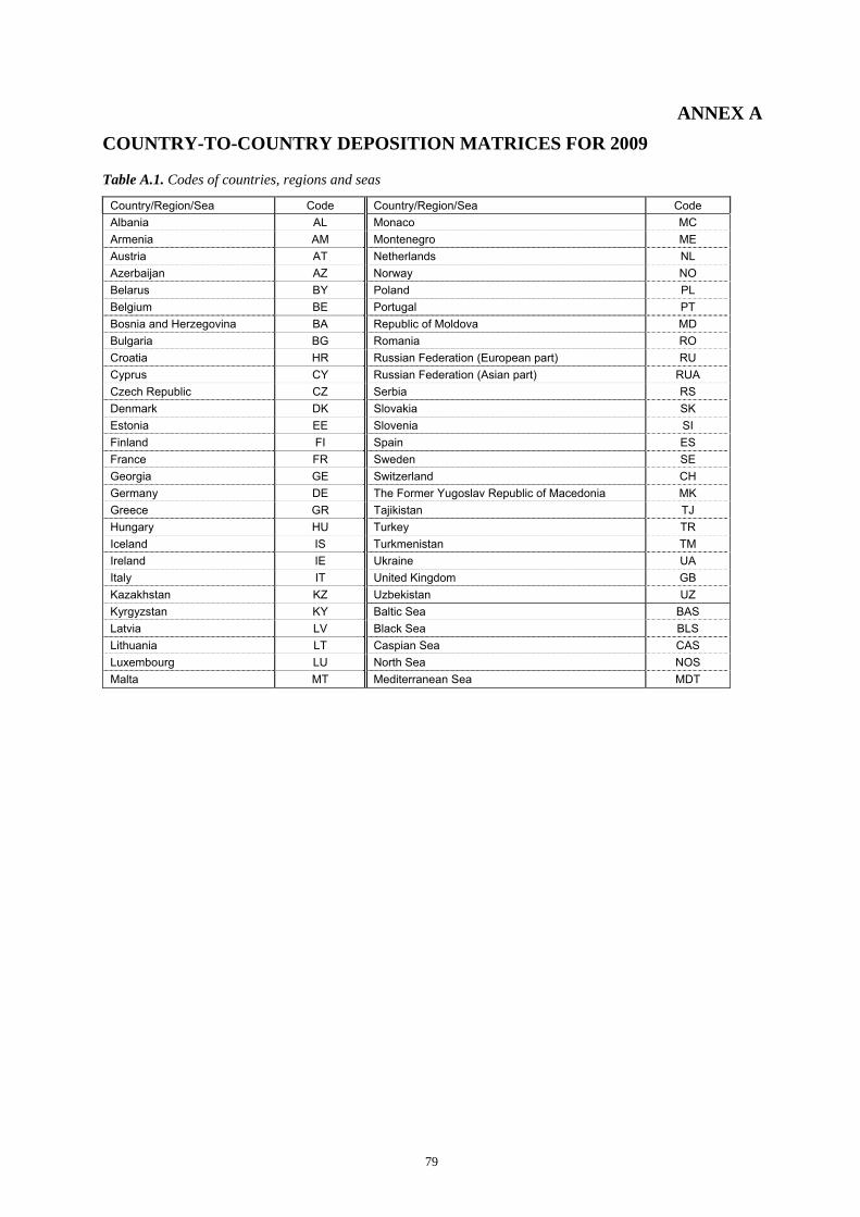
79

ANNEX A COUNTRY-TO-COUNTRY DEPOSITION MATRICES FOR 2009

Table A.1. Codes of countries, regions and seas

Country/Region/Sea Code Country/Region/Sea Code Albania AL Monaco MC Armenia AM Montenegro ME Austria AT Netherlands NL Azerbaijan AZ Norway NO Belarus BY Poland PL Belgium BE Portugal PT Bosnia and Herzegovina BA Republic of Moldova MD Bulgaria BG Romania RO Croatia HR Russian Federation (European part) RU Cyprus CY Russian Federation (Asian part) RUA Czech Republic CZ Serbia RS Denmark DK Slovakia SK Estonia EE Slovenia SI Finland FI Spain ES France FR Sweden SE Georgia GE Switzerland CH Germany DE The Former Yugoslav Republic of Macedonia MK Greece GR Tajikistan TJ Hungary HU Turkey TR Iceland IS Turkmenistan TM Ireland IE Ukraine UA Italy IT United Kingdom GB Kazakhstan KZ Uzbekistan UZ Kyrgyzstan KY Baltic Sea BAS Latvia LV Black Sea BLS Lithuania LT Caspian Sea CAS Luxembourg LU North Sea NOS Malta MT Mediterranean Sea MDT

80

Table A.2. Matrix of lead country-to-country deposition from anthropogenic sources in 2009, kg/y R e c e p t o r s E m i t t e r s

AL AM AT AZ BA BE BG BY CH CY CZ DE DK AL 853.6 0.6 16.5 1.1 256.5 12.3 2028 15.2 22.5 1.3 30.1 68.3 1.6 AL AM 0.7 1824 0.9 547.1 5.4 1.1 52.9 8.0 1.4 5.4 2.3 5.5 0.4 AM AT 11.6 2.2 4281 4.4 464.5 309.5 732.1 166.1 868.9 0.1 1405 4787 33.7 AT AZ 1.5 499.0 2.0 3356 11.7 2.5 111.5 28.7 3.2 8.7 6.0 13.8 1.0 AZ BA 100.8 1.1 143.3 2.6 13128 46.5 1925.6 56.5 72.0 0.6 292.4 386.8 10.3 BA BE 0.6 0.1 15.2 0.1 7.8 6689 28.7 10.9 77.6 0.003 34.2 1506 16.1 BE BG 88.8 9.1 48.5 17.0 412.5 32.0 110474 158.9 37.2 7.9 170.5 237.3 10.4 BG BY 14.3 18.3 134.7 26.5 279.1 205.5 2046 25412 139.8 3.0 868.6 1411 133.7 BY CH 3.3 0.2 74.2 0.4 72.4 219.3 148.1 14.9 5834 0.02 55.5 1236 7.2 CH CY 0.8 0.6 0.6 0.4 4.3 0.4 41.9 1.1 0.9 157.2 1.2 2.6 0.1 CY CZ 5.9 1.4 783.4 2.8 200.5 329.1 632.4 180.8 361.3 0.1 7661 4802 58.5 CZ DE 8.2 2.1 1139 4.0 164.2 6958 611.1 367.7 4388 0.1 2771 75008 516.5 DE DK 0.5 0.1 26.3 0.2 8.8 440.9 53.6 34.4 61.6 0.02 150.2 1926 1096 DK EE 1.1 1.7 9.9 3.0 24.8 102.6 54.9 469.5 18.2 0.3 65.2 363.1 53.3 EE ES 10.4 0.3 60.4 0.6 156.0 341.7 533.3 27.2 335.3 0.03 100.7 983.2 15.7 ES FI 2.0 4.5 38.2 8.3 58.5 292.9 150.2 847.4 55.1 0.3 199.6 1028 181.0 FI FR 17.6 0.9 255.9 2.0 310.3 4327 800.2 118.1 3100 0.1 443.7 7994 85.9 FR GB 1.5 0.2 39.2 0.4 18.8 1329 100.2 38.6 114.0 0.01 139.0 1811 125.7 GB GE 2.0 620.5 3.7 729.3 17.1 3.7 205.4 41.7 4.9 10.4 11.3 22.0 1.9 GE GR 209.1 6.2 39.0 9.0 385.1 28.7 13033 88.3 49.6 19.0 94.6 181.3 6.8 GR HR 45.6 0.9 232.9 2.0 2895 48.8 1229 62.2 92.4 0.4 333.7 407.1 7.4 HR HU 33.0 1.2 412.1 2.2 1530 80.1 3812 127.1 116.1 1.1 831.9 770.3 17.4 HU IE 0.4 0.0 7.9 0.0 4.2 124.7 24.0 6.0 21.2 0.002 24.2 267.0 24.9 IE IS 0.1 0.1 3.6 0.1 1.5 47.5 9.3 5.9 11.9 0.003 8.9 92.6 10.4 IS IT 134.4 3.4 532.6 8.0 2481 208.8 3491 172.9 1371 2.6 541.7 1665 18.4 IT KY 0.9 37.0 1.8 55.0 9.8 2.7 65.5 13.5 3.4 4.1 4.8 13.6 0.7 KY KZ 9.6 563.9 36.7 1048 116.0 71.9 1074 718.8 47.7 22.5 162.0 361.2 37.3 KZ LT 2.9 2.4 39.1 3.3 52.1 116.0 219.0 2004 53.7 0.3 277.6 766.7 108.7 LT LU 0.1 0.0 2.1 0.0 1.1 144.2 2.8 1.4 15.6 0.0 4.2 217.9 1.1 LU LV 2.5 2.4 22.5 3.7 44.0 130.3 158.7 1186 35.5 0.4 156.2 667.8 100.4 LV MC 0.002 0.0 0.02 0.001 0.05 0.02 0.1 0.01 0.1 0.0 0.02 0.1 0.001 MC MD 5.0 4.2 9.3 5.4 50.4 8.7 1131 123.4 7.9 1.0 43.4 64.3 4.9 MD ME 167.3 0.4 14.7 0.8 630.8 8.8 941.4 10.1 15.3 0.4 29.5 56.9 1.4 ME MK 181.9 1.0 13.4 2.1 149.0 9.1 7188 20.6 12.3 1.8 35.1 61.8 1.9 MK MT 0.0 0.0 0.1 0.0 0.5 0.1 1.1 0.0 0.3 0.004 0.1 0.3 0.01 MT NL 0.6 0.1 20.0 0.1 8.9 3466 36.8 16.1 66.4 0.004 60.8 2368 25.9 NL NO 2.6 1.3 45.7 2.4 40.7 643.4 292.6 124.7 95.2 0.2 232.6 1904 555.8 NO PL 17.1 7.0 647.3 12.0 515.8 881.7 1926 3727 565.6 1.6 9753 9056 552.4 PL PT 0.5 0.02 3.4 0.04 9.6 22.1 31.9 1.7 17.9 0.001 5.7 56.5 1.2 PT RO 101.0 11.6 189.7 19.5 1551 101.3 24928 589.1 126.3 10.6 627.7 813.0 35.8 RO RS 177.5 2.2 111.4 4.8 2179 52.7 13996 69.9 54.1 2.5 362.1 429.5 14.4 RS RU 64.1 1208 355.8 2787 1015 1033 9690 16488 457.3 58.7 1737 5010 594.6 RU RUA 10.0 242.5 51.9 368.0 163.3 157.4 1069 1113 74.0 11.9 216.8 669.1 72.0 RUA SE 2.4 3.9 88.5 6.5 57.6 992.1 307.5 687.1 168.0 0.6 556.4 3526 1392 SE SI 8.1 0.3 269.0 0.6 432.6 27.5 346.7 28.4 59.1 0.1 153.4 264.2 2.8 SI SK 12.3 0.9 279.4 1.6 506.9 65.9 1474 143.9 101.7 0.4 2911 689.9 20.2 SK TJ 0.4 22.9 0.8 36.5 4.1 1.2 30.5 5.3 1.5 2.5 2.0 5.8 0.3 TJ TR 64.6 1246 61.4 420.6 404.4 54.5 6981 384.8 80.7 344.4 159.6 324.4 16.6 TR TU 0.9 106.7 2.0 246.6 7.4 3.8 76.9 28.8 2.9 5.2 8.0 17.5 1.2 TU UA 70.4 135.3 284.3 232.5 1160 228.0 13300 4615 235.7 18.1 1416 1781 133.8 UA UZ 0.8 89.3 2.0 165.4 7.3 3.0 67.2 25.4 2.9 4.6 8.2 15.1 1.0 UZ BAS 3.8 5.3 167.0 8.5 114.5 1201 293.7 1782 269.5 1.0 1083 6440 1590 BAS BLS 41.0 170.1 62.6 183.9 315.0 48.2 9668 571.6 57.8 40.7 203.7 336.8 20.9 BLS CAS 1.5 368.2 6.0 1611 15.9 9.4 179.2 119.8 7.7 7.2 28.3 50.7 4.1 CAS MDT 804.5 32.3 593.1 38.2 5221 440.7 19370 339.6 1395 570.8 816.5 2406 49.2 MDT NOS 6.5 0.8 175.5 1.4 92.1 7022 572.3 216.6 516.0 0.2 771.8 12485 1552 NOS

AL AM AT AZ BA BE BG BY CH CY CZ DE DK

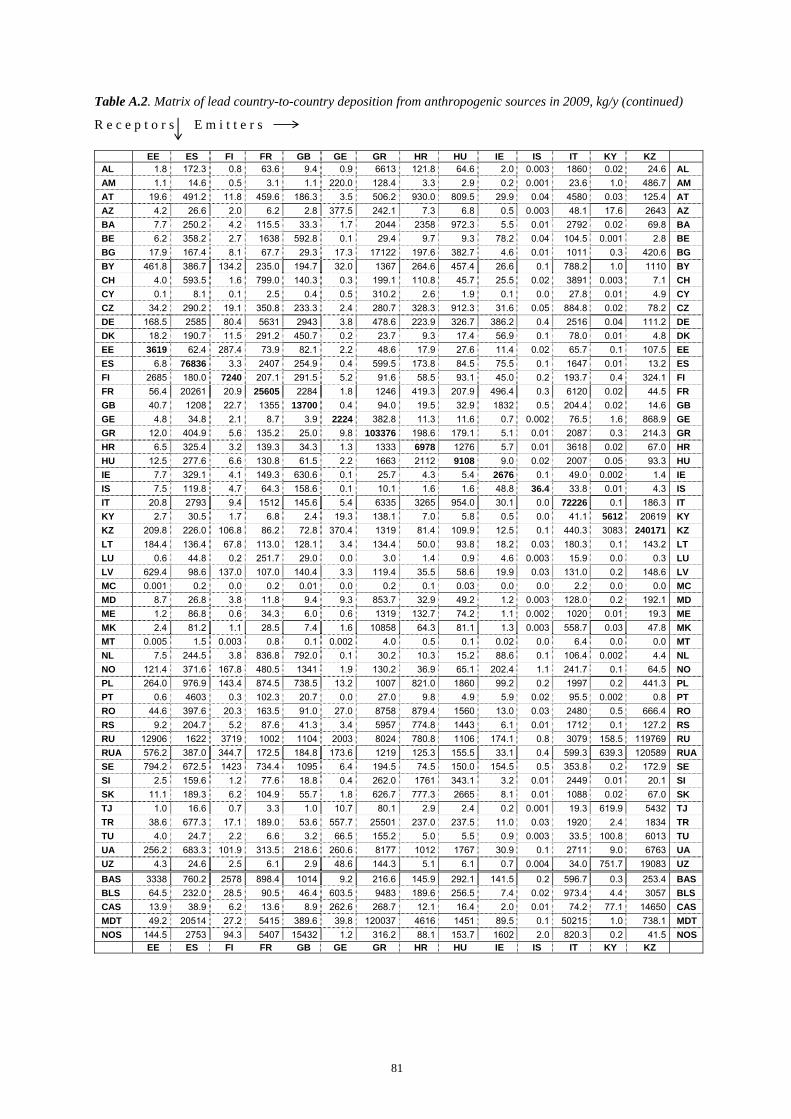
81

Table A.2. Matrix of lead country-to-country deposition from anthropogenic sources in 2009, kg/y (continued) R e c e p t o r s E m i t t e r s

EE ES FI FR GB GE GR HR HU IE IS IT KY KZ AL 1.8 172.3 0.8 63.6 9.4 0.9 6613 121.8 64.6 2.0 0.003 1860 0.02 24.6 AL AM 1.1 14.6 0.5 3.1 1.1 220.0 128.4 3.3 2.9 0.2 0.001 23.6 1.0 486.7 AM AT 19.6 491.2 11.8 459.6 186.3 3.5 506.2 930.0 809.5 29.9 0.04 4580 0.03 125.4 AT AZ 4.2 26.6 2.0 6.2 2.8 377.5 242.1 7.3 6.8 0.5 0.003 48.1 17.6 2643 AZ BA 7.7 250.2 4.2 115.5 33.3 1.7 2044 2358 972.3 5.5 0.01 2792 0.02 69.8 BA BE 6.2 358.2 2.7 1638 592.8 0.1 29.4 9.7 9.3 78.2 0.04 104.5 0.001 2.8 BE BG 17.9 167.4 8.1 67.7 29.3 17.3 17122 197.6 382.7 4.6 0.01 1011 0.3 420.6 BG BY 461.8 386.7 134.2 235.0 194.7 32.0 1367 264.6 457.4 26.6 0.1 788.2 1.0 1110 BY CH 4.0 593.5 1.6 799.0 140.3 0.3 199.1 110.8 45.7 25.5 0.02 3891 0.003 7.1 CH CY 0.1 8.1 0.1 2.5 0.4 0.5 310.2 2.6 1.9 0.1 0.0 27.8 0.01 4.9 CY CZ 34.2 290.2 19.1 350.8 233.3 2.4 280.7 328.3 912.3 31.6 0.05 884.8 0.02 78.2 CZ DE 168.5 2585 80.4 5631 2943 3.8 478.6 223.9 326.7 386.2 0.4 2516 0.04 111.2 DE DK 18.2 190.7 11.5 291.2 450.7 0.2 23.7 9.3 17.4 56.9 0.1 78.0 0.01 4.8 DK EE 3619 62.4 287.4 73.9 82.1 2.2 48.6 17.9 27.6 11.4 0.02 65.7 0.1 107.5 EE ES 6.8 76836 3.3 2407 254.9 0.4 599.5 173.8 84.5 75.5 0.1 1647 0.01 13.2 ES FI 2685 180.0 7240 207.1 291.5 5.2 91.6 58.5 93.1 45.0 0.2 193.7 0.4 324.1 FI FR 56.4 20261 20.9 25605 2284 1.8 1246 419.3 207.9 496.4 0.3 6120 0.02 44.5 FR GB 40.7 1208 22.7 1355 13700 0.4 94.0 19.5 32.9 1832 0.5 204.4 0.02 14.6 GB GE 4.8 34.8 2.1 8.7 3.9 2224 382.8 11.3 11.6 0.7 0.002 76.5 1.6 868.9 GE GR 12.0 404.9 5.6 135.2 25.0 9.8 103376 198.6 179.1 5.1 0.01 2087 0.3 214.3 GR HR 6.5 325.4 3.2 139.3 34.3 1.3 1333 6978 1276 5.7 0.01 3618 0.02 67.0 HR HU 12.5 277.6 6.6 130.8 61.5 2.2 1663 2112 9108 9.0 0.02 2007 0.05 93.3 HU IE 7.7 329.1 4.1 149.3 630.6 0.1 25.7 4.3 5.4 2676 0.1 49.0 0.002 1.4 IE IS 7.5 119.8 4.7 64.3 158.6 0.1 10.1 1.6 1.6 48.8 36.4 33.8 0.01 4.3 IS IT 20.8 2793 9.4 1512 145.6 5.4 6335 3265 954.0 30.1 0.0 72226 0.1 186.3 IT KY 2.7 30.5 1.7 6.8 2.4 19.3 138.1 7.0 5.8 0.5 0.0 41.1 5612 20619 KY KZ 209.8 226.0 106.8 86.2 72.8 370.4 1319 81.4 109.9 12.5 0.1 440.3 3083 240171 KZ LT 184.4 136.4 67.8 113.0 128.1 3.4 134.4 50.0 93.8 18.2 0.03 180.3 0.1 143.2 LT LU 0.6 44.8 0.2 251.7 29.0 0.0 3.0 1.4 0.9 4.6 0.003 15.9 0.0 0.3 LU LV 629.4 98.6 137.0 107.0 140.4 3.3 119.4 35.5 58.6 19.9 0.03 131.0 0.2 148.6 LV MC 0.001 0.2 0.0 0.2 0.01 0.0 0.2 0.1 0.03 0.0 0.0 2.2 0.0 0.0 MC MD 8.7 26.8 3.8 11.8 9.4 9.3 853.7 32.9 49.2 1.2 0.003 128.0 0.2 192.1 MD ME 1.2 86.8 0.6 34.3 6.0 0.6 1319 132.7 74.2 1.1 0.002 1020 0.01 19.3 ME MK 2.4 81.2 1.1 28.5 7.4 1.6 10858 64.3 81.1 1.3 0.003 558.7 0.03 47.8 MK MT 0.005 1.5 0.003 0.8 0.1 0.002 4.0 0.5 0.1 0.02 0.0 6.4 0.0 0.0 MT NL 7.5 244.5 3.8 836.8 792.0 0.1 30.2 10.3 15.2 88.6 0.1 106.4 0.002 4.4 NL NO 121.4 371.6 167.8 480.5 1341 1.9 130.2 36.9 65.1 202.4 1.1 241.7 0.1 64.5 NO PL 264.0 976.9 143.4 874.5 738.5 13.2 1007 821.0 1860 99.2 0.2 1997 0.2 441.3 PL PT 0.6 4603 0.3 102.3 20.7 0.0 27.0 9.8 4.9 5.9 0.02 95.5 0.002 0.8 PT RO 44.6 397.6 20.3 163.5 91.0 27.0 8758 879.4 1560 13.0 0.03 2480 0.5 666.4 RO RS 9.2 204.7 5.2 87.6 41.3 3.4 5957 774.8 1443 6.1 0.01 1712 0.1 127.2 RS RU 12906 1622 3719 1002 1104 2003 8024 780.8 1106 174.1 0.8 3079 158.5 119769 RU RUA 576.2 387.0 344.7 172.5 184.8 173.6 1219 125.3 155.5 33.1 0.4 599.3 639.3 120589 RUA SE 794.2 672.5 1423 734.4 1095 6.4 194.5 74.5 150.0 154.5 0.5 353.8 0.2 172.9 SE SI 2.5 159.6 1.2 77.6 18.8 0.4 262.0 1761 343.1 3.2 0.01 2449 0.01 20.1 SI SK 11.1 189.3 6.2 104.9 55.7 1.8 626.7 777.3 2665 8.1 0.01 1088 0.02 67.0 SK TJ 1.0 16.6 0.7 3.3 1.0 10.7 80.1 2.9 2.4 0.2 0.001 19.3 619.9 5432 TJ TR 38.6 677.3 17.1 189.0 53.6 557.7 25501 237.0 237.5 11.0 0.03 1920 2.4 1834 TR TU 4.0 24.7 2.2 6.6 3.2 66.5 155.2 5.0 5.5 0.9 0.003 33.5 100.8 6013 TU UA 256.2 683.3 101.9 313.5 218.6 260.6 8177 1012 1767 30.9 0.1 2711 9.0 6763 UA UZ 4.3 24.6 2.5 6.1 2.9 48.6 144.3 5.1 6.1 0.7 0.004 34.0 751.7 19083 UZ BAS 3338 760.2 2578 898.4 1014 9.2 216.6 145.9 292.1 141.5 0.2 596.7 0.3 253.4 BAS BLS 64.5 232.0 28.5 90.5 46.4 603.5 9483 189.6 256.5 7.4 0.02 973.4 4.4 3057 BLS CAS 13.9 38.9 6.2 13.6 8.9 262.6 268.7 12.1 16.4 2.0 0.01 74.2 77.1 14650 CAS MDT 49.2 20514 27.2 5415 389.6 39.8 120037 4616 1451 89.5 0.1 50215 1.0 738.1 MDT NOS 144.5 2753 94.3 5407 15432 1.2 316.2 88.1 153.7 1602 2.0 820.3 0.2 41.5 NOS

EE ES FI FR GB GE GR HR HU IE IS IT KY KZ

82

Table A.2. Matrix of lead country-to-country deposition from anthropogenic sources in 2009, kg/y (continued) R e c e p t o r s E m i t t e r s

LT LU LV MC MD ME MK MT NL NO PL PT AL 0.8 0.7 0.8 0.1 3.2 1207 2273 4.9 9.1 0.3 215.2 36.8 AL AM 0.5 0.0 0.4 0.003 0.6 6.8 9.6 0.2 0.9 0.1 27.8 5.6 AM AT 17.3 22.3 16.4 0.5 6.0 190.0 119.9 1.9 250.8 3.8 7333 118.9 AT AZ 1.7 0.1 1.4 0.01 1.6 14.6 20.1 0.3 2.4 0.4 71.7 10.1 AZ BA 3.9 2.4 4.5 0.2 6.7 3548 485.3 4.0 41.4 1.5 1889 56.3 BA BE 2.9 114.1 4.0 0.04 0.2 6.3 5.6 0.1 974.1 2.1 324.6 75.6 BE BG 8.1 1.4 7.5 0.1 71.1 653.1 3263 3.0 32.7 2.3 1547 45.8 BG BY 651.4 9.3 279.0 0.1 91.1 201.4 233.3 1.1 215.6 20.9 15075 108.8 BY CH 2.5 19.2 2.8 0.8 0.9 43.0 30.5 1.1 114.3 1.2 396.8 129.2 CH CY 0.1 0.0 0.1 0.003 0.2 5.8 9.6 0.2 0.4 0.0 8.7 1.8 CY CZ 28.4 18.5 30.4 0.2 4.8 99.4 86.3 0.6 339.8 6.2 26501 73.0 CZ DE 87.0 484.6 113.4 0.8 6.6 106.9 97.1 2.2 7717 43.5 21569 575.2 DE DK 10.9 10.7 14.7 0.02 0.6 6.8 7.1 0.1 539.6 15.0 2150 39.5 DK EE 112.1 2.6 279.3 0.01 2.1 20.3 11.7 0.1 99.6 13.8 1252 16.3 EE ES 3.7 22.4 4.7 0.6 1.7 124.5 112.4 2.7 192.9 2.3 750.5 18645 ES FI 176.9 7.5 276.6 0.04 4.5 35.6 23.3 0.3 283.7 109.6 3451 51.0 FI FR 20.8 388.3 26.6 9.9 4.7 214.2 168.8 6.5 1792 11.1 3287 3464 FR GB 12.4 23.2 18.3 0.1 1.0 18.5 16.3 0.1 1019 17.5 1526 550.6 GB GE 2.5 0.2 2.1 0.01 4.4 19.3 30.3 0.4 3.5 0.5 142.8 12.5 GE GR 4.6 1.4 4.2 0.2 25.6 645.3 3537 14.7 24.7 1.5 792.5 110.7 GR HR 4.3 2.7 4.0 0.3 5.6 735.5 254.1 3.7 41.1 1.2 2071 73.8 HR HU 9.5 4.3 8.6 0.2 15.8 688.2 531.9 1.8 75.6 2.5 5668 77.5 HU IE 1.8 3.0 2.7 0.01 0.2 4.5 3.9 0.0 111.6 2.6 251.4 183.5 IE IS 1.8 1.4 2.7 0.01 0.2 1.4 1.3 0.0 34.7 7.6 98.3 44.8 IS IT 12.3 14.7 11.4 7.1 16.0 1716 902.1 40.0 157.9 2.9 3628 610.4 IT KY 0.9 0.1 0.9 0.01 1.0 9.7 11.1 0.2 2.1 0.4 56.8 12.0 KY KZ 53.3 2.3 52.7 0.1 25.8 113.4 135.7 1.8 69.6 16.7 2342 83.7 KZ LT 1815 4.4 395.8 0.04 8.0 42.2 42.3 0.2 129.6 14.2 6204 39.7 LT LU 0.3 130.9 0.4 0.01 0.02 0.8 0.6 0.0 32.6 0.1 37.0 10.0 LU LV 674.7 4.2 1519 0.03 5.1 38.5 32.9 0.3 140.4 16.9 3212 28.0 LV MC 0.0 0.0 0.0 0.03 0.0 0.0 0.0 0.0 0.0 0.0 0.2 0.0 MC MD 5.0 0.3 3.8 0.02 444.6 53.9 97.3 0.5 9.5 1.0 605.4 8.0 MD ME 0.6 0.5 0.6 0.1 2.0 8990 497.6 2.3 6.8 0.2 205.8 17.6 ME MK 1.1 0.4 1.0 0.04 5.2 355.7 12510 1.5 8.1 0.4 269.0 19.5 MK MT 0.002 0.01 0.002 0.001 0.004 0.5 0.3 4.3 0.1 0.0 0.6 0.3 MT NL 4.3 20.4 5.2 0.04 0.3 6.8 6.4 0.1 5637 3.5 568.5 58.2 NL NO 47.2 14.9 81.1 0.04 3.8 36.2 37.6 0.2 619.2 1497 3651 91.1 NO PL 416.0 38.2 300.9 0.3 40.3 273.4 250.8 1.8 993.4 48.4 202546 262.8 PL PT 0.2 1.3 0.3 0.03 0.1 7.1 6.2 0.1 12.1 0.2 41.6 44142 PT RO 28.3 4.8 23.4 0.3 373.9 1405 1967 4.8 103.6 6.5 6299 109.3 RO RS 4.9 2.4 5.5 0.1 17.8 4531 3686 2.7 52.1 2.3 2509 49.5 RS RU 1113 34.9 1243 0.5 254.0 867.3 1050 7.6 1029 256.9 27123 499.2 RU RUA 98.8 5.2 109.0 0.1 23.3 136.7 139.0 1.8 147.2 51.3 3134 134.3 RUA SE 247.1 22.8 450.6 0.1 7.8 39.1 37.6 0.3 1053 526.8 10449 168.4 SE SI 2.5 1.8 1.9 0.2 1.8 128.7 60.4 1.5 21.0 0.4 951.1 37.9 SI SK 11.8 3.5 9.7 0.1 9.0 237.7 201.1 0.8 68.3 2.4 14006 51.4 SK TJ 0.3 0.1 0.3 0.003 0.4 4.3 5.3 0.1 0.9 0.2 22.9 6.5 TJ TR 21.4 2.4 16.8 0.2 75.2 520.5 1035 14.5 50.8 4.1 1718 221.7 TR TU 1.7 0.1 1.5 0.005 1.6 9.1 11.6 0.3 3.4 0.5 101.0 9.9 TU UA 181.2 9.9 121.6 0.3 655.7 885.8 1366 4.9 245.7 23.6 21813 215.8 UA UZ 1.4 0.1 1.2 0.01 1.5 8.3 10.5 0.2 2.7 0.5 97.5 9.4 UZ BAS 664.5 34.9 1501 0.2 10.7 67.9 44.7 0.7 1325 120.9 21500 207.0 BAS BLS 35.0 2.1 28.0 0.1 180.0 376.7 844.0 4.1 50.2 5.2 2488 70.5 BLS CAS 6.3 0.3 5.1 0.01 6.2 16.4 22.4 0.4 9.2 1.2 377.4 13.3 CAS MDT 22.0 30.5 22.8 6.9 70.5 5668 5241 338.0 298.1 9.3 5738 4159 MDT NOS 72.3 116.7 103.9 0.2 4.8 82.7 86.4 0.7 7103 377.9 9491 967.9 NOS

LT LU LV MC MD ME MK MT NL NO PL PT

83

Table A.2. Matrix of lead country-to-country deposition from anthropogenic sources in 2009, kg/y (continued) R e c e p t o r s E m i t t e r s

RO RS RU RUA SE SI SK TJ TR TU UA UZ Total, t/y

AL 111.6 617.9 292.0 1.9 0.6 23.4 61.7 0.0 344.5 1.2 122.2 1.5 17.6 AL AM 10.0 5.2 877.3 22.6 0.3 1.1 4.3 3.5 1244 104.3 60.9 78.2 5.8 AM AT 210.6 270.5 1136 8.6 11.6 2257 1755 0.1 113.8 5.2 407.2 5.3 35.5 AT AZ 21.7 11.2 4650 77.8 0.9 2.6 10.5 64.3 1597 546.2 207.8 593.5 15.3 AZ BA 468.9 1655 534.4 5.9 3.8 172.9 681.0 0.0 329.9 3.3 289.5 3.8 35.0 BA BE 4.6 5.0 101.3 0.2 3.3 6.4 19.3 0.0 6.9 0.1 13.6 0.1 12.9 BE BG 2762 1493 4255 30.2 5.5 51.9 413.8 0.7 4433 20.2 2027 27.7 152.3 BG BY 923.9 288.0 25230 54.0 72.4 114.1 1073 2.5 1267 26.4 6935 39.7 89.1 BY CH 24.7 36.3 145.2 0.5 1.9 62.2 58.4 0.0 30.6 0.4 48.1 0.4 14.6 CH CY 4.3 3.9 52.2 0.3 0.0 0.8 2.1 0.0 377.4 0.4 13.2 0.6 1.1 CY CZ 188.0 193.8 1210.3 4.4 19.1 218.7 2094 0.1 73.9 2.9 341.7 3.0 50.0 CZ DE 149.9 125.5 3222 7.5 105.8 172.2 765.4 0.1 129.7 4.2 500.7 4.4 143.4 DE DK 16.2 8.1 245.2 0.5 50.4 6.8 59.0 0.0 7.0 0.2 25.9 0.3 8.2 DK EE 33.9 20.0 6563 4.5 70.7 7.3 59.3 0.2 51.7 2.1 179.0 3.1 14.4 EE ES 63.5 89.4 242.6 1.0 4.9 78.7 104.9 0.0 66.0 0.9 78.6 1.1 105.3 ES FI 77.3 47.8 22602 23.4 753.6 27.1 176.3 1.0 93.9 7.2 358.9 10.7 42.9 FI FR 119.5 157.0 1182 2.9 22.7 232.8 335.2 0.1 206.7 2.4 261.7 2.5 86.1 FR GB 19.5 15.8 564.2 1.4 31.0 16.9 70.5 0.1 22.7 0.4 55.1 0.6 26.2 GB GE 52.2 18.0 5981 38.1 1.3 4.4 20.5 6.2 3250 151.7 443.4 122.0 15.6 GE GR 569.0 609.4 2620 14.9 3.3 50.2 189.6 0.6 5540 10.3 1053 14.0 136.6 GR HR 342.4 898.8 470.4 5.3 2.7 537.3 877.6 0.0 197.9 2.6 286.6 3.0 26.0 HR HU 1605 1824 1066 7.0 6.1 445.2 6313 0.1 310.5 2.4 852.8 2.9 42.7 HU IE 3.8 3.3 92.7 0.2 6.0 3.8 11.0 0.0 4.0 0.0 11.6 0.1 5.1 IE IS 2.6 1.1 137.8 1.7 4.4 1.7 4.8 0.0 3.9 0.2 9.3 0.2 1.0 IS IT 568.6 947.8 1628 15.1 7.1 1653 1044 0.1 1103 10.4 760.2 11.0 113.0 IT KY 16.4 8.6 1701 168.4 0.8 2.4 8.1 7511 440.1 566.4 79.5 19251 56.5 KY KZ 342.3 113.0 103625 13568 42.1 34.6 224.6 8423 4384 5314 3550 38036 431.1 KZ LT 117.1 51.8 5564 8.1 61.5 25.6 235.1 0.2 82.5 3.4 645.2 4.4 20.4 LT LU 0.5 0.6 12.7 0.0 0.2 0.8 1.9 0.0 0.8 0.0 1.7 0.0 1.0 LU LV 79.7 40.8 5720.9 7.4 81.9 16.3 132.9 0.3 88.1 3.4 409.2 5.1 16.4 LV MC 0.0 0.0 0.1 0.0 0.0 0.0 0.04 0.0 0.0 0.0 0.0 0.0 0.0 MC MD 879.1 71.5 2179.0 10.0 2.3 11.1 83.1 0.5 810.9 4.4 1700 6.5 9.8 MD ME 95.9 709.3 176.4 1.7 0.5 19.0 66.5 0.0 142.6 1.0 75.2 1.2 15.6 ME MK 172.7 705.7 513.6 3.9 0.8 13.9 79.0 0.1 626.3 2.4 203.9 3.0 34.9 MK MT 0.1 0.2 0.5 0.0 0.0 0.2 0.2 0.0 0.9 0.0 0.2 0.0 0.02 MT NL 6.7 6.8 115.0 0.4 5.3 7.2 32.2 0.0 8.3 0.1 16.9 0.2 14.7 NL NO 81.0 41.7 2874 25.7 391.4 21.1 129.2 0.3 53.0 2.4 189.9 3.2 17.1 NO PL 1052 483.8 9327 24.4 158.1 451.3 5512 0.4 481.2 12.9 3634 14.7 263.2 PL PT 4.0 5.2 19.0 0.1 0.4 4.0 5.8 0.0 2.9 0.0 5.3 0.1 49.3 PT RO 20729 2858 8111 42.8 14.9 245.9 1971 1.3 4361 20.9 5338 27.6 98.3 RO RS 1645 10634 1126 10.4 5.3 112.0 943.8 0.2 885.2 5.8 564.3 7.1 54.6 RS RU 3208 1015 1483850 10623 938.1 325.4 2213 488.8 19283 3082 38358 5422 1798.2 RU RUA 357.1 137.0 186667 133767 117.9 52.6 291.9 1483 2792 1236 2689 5860 468.8 RUA SE 136.1 51.4 6843 16.8 3720 46.6 371.7 0.7 144.5 6.1 519.5 7.9 38.5 SE SI 91.1 157.3 176.1 1.6 1.1 2754 378.5 0.0 38.7 0.8 98.6 0.8 11.6 SI SK 640.5 511.8 773.6 5.0 6.3 301.4 10576 0.1 131.2 1.6 635.1 1.9 40.0 SK TJ 6.8 3.7 678.2 57.4 0.3 1.0 3.3 14489 240.6 675.5 31.7 11007 33.5 TJ TR 1175 472.0 18365 102.3 10.0 79.8 308.3 7.2 118518 221.0 4546 192.5 189.5 TR TU 17.1 7.5 2889 154.3 1.0 1.9 10.6 1655 674.6 5813 198.7 8442 26.9 TU UA 6311 1386 70624 250.4 63.9 355.2 3476 25.5 9320 189.0 65534 308.0 229.3 UA UZ 17.9 7.0 2912 212.5 1.0 2.0 12.1 7631 602.3 2453 171.2 33322 68.0 UZ BAS 185.1 84.6 19216 13.8 1243 91.6 729.6 0.7 207.3 6.6 858.8 9.1 71.3 BAS BLS 2166 495.6 37981 136.9 15.4 72.3 403.3 9.9 24714 125.1 11210 170.6 108.3 BLS CAS 57.9 16.2 14258 225.6 3.1 5.7 38.2 376.8 1799 2282 937.2 3052 41.4 CAS MDT 1814 2538 7360 50.8 20.8 1330 1569 1.9 27486 44.3 3253 55.5 302.8 MDT NOS 132.9 88.6 1839 7.9 313.4 62.0 327.1 0.4 74.0 1.3 213.2 2.7 71.7 NOS

RO RS RU RUA SE SI SK TJ TR TU UA UZ Total, t/y

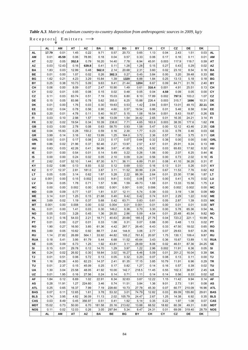
84

Table A.3. Matrix of cadmium country-to-country deposition from anthropogenic sources in 2009, kg/y R e c e p t o r s E m i t t e r s

AL AM AT AZ BA BE BG BY CH CY CZ DE DK AL 17.79 0.01 1.45 0.22 9.71 0.57 20.73 0.65 1.13 0.04 2.43 1.51 0.03 AL AM 0.01 45.59 0.06 78.95 0.18 0.04 0.57 0.33 0.06 0.17 0.16 0.11 0.01 AM AT 0.22 0.05 352.8 0.79 16.20 14.40 7.78 6.94 45.91 0.003 117.9 119.7 0.59 AT AZ 0.03 12.43 0.16 639.8 0.41 0.11 1.28 1.28 0.15 0.27 0.43 0.29 0.02 AZ BA 1.83 0.03 12.99 0.48 562.0 2.14 20.68 2.31 3.60 0.02 23.10 8.54 0.18 BA BE 0.01 0.00 1.07 0.02 0.26 382.3 0.27 0.45 3.84 0.00 3.20 39.48 0.33 BE BG 1.62 0.21 4.23 3.29 15.84 1.39 1320 6.88 1.84 0.25 13.13 5.18 0.18 BG BY 0.25 0.38 10.73 5.09 9.63 9.41 21.44 1204 6.67 0.09 64.71 31.78 2.40 BY CH 0.06 0.00 8.09 0.07 2.47 10.90 1.49 0.61 316.4 0.001 4.91 25.51 0.13 CH CY 0.02 0.01 0.05 0.08 0.15 0.02 0.48 0.05 0.04 4.59 0.09 0.05 0.00 CY CZ 0.11 0.03 63.74 0.51 7.19 15.03 6.80 8.10 17.89 0.002 797.5 103.2 1.07 CZ DE 0.15 0.05 83.98 0.78 5.62 355.0 6.25 15.88 226.4 0.003 315.7 1696 10.31 DE DK 0.01 0.00 1.76 0.03 0.30 19.63 0.53 1.42 2.84 0.001 13.01 48.15 22.11 DK EE 0.02 0.04 0.78 0.56 0.90 4.60 0.57 19.54 0.86 0.01 5.46 8.58 0.94 EE ES 0.20 0.01 4.78 0.11 5.40 16.57 5.15 1.08 16.54 0.001 8.43 19.87 0.26 ES FI 0.03 0.10 2.98 1.57 1.96 13.09 1.54 34.42 2.65 0.01 16.35 24.21 3.14 FI FR 0.32 0.02 19.54 0.34 10.39 238.8 7.71 4.65 163.9 0.003 38.35 177.6 1.62 FR GB 0.03 0.00 2.78 0.08 0.63 58.70 0.93 1.58 5.47 0.00 12.12 43.46 2.35 GB GE 0.04 15.93 0.28 150.2 0.59 0.16 2.30 1.77 0.23 0.33 0.78 0.46 0.03 GE GR 3.99 0.14 3.16 1.62 13.99 1.25 164.0 3.72 2.36 0.57 7.00 3.75 0.11 GR GRL 0.00 0.01 0.17 0.08 2.23 0.17 0.07 0.64 0.32 0.38 0.00 0.00 0.60 GRL HR 0.86 0.02 21.96 0.37 92.46 2.27 13.97 2.57 4.57 0.01 25.91 9.24 0.13 HR HU 0.63 0.03 42.26 0.41 56.96 3.67 41.85 5.55 5.92 0.03 65.83 17.92 0.32 HU IE 0.01 0.00 0.54 0.01 0.14 5.49 0.22 0.26 1.06 0.00 2.07 6.25 0.44 IE IS 0.00 0.00 0.24 0.02 0.05 2.10 0.09 0.24 0.56 0.00 0.73 2.02 0.18 IS IT 2.62 0.07 52.10 1.44 87.30 9.71 36.11 6.89 71.81 0.08 41.10 36.28 0.31 IT KY 0.02 0.86 0.13 8.93 0.32 0.12 0.69 0.53 0.16 0.13 0.31 0.26 0.01 KY KZ 0.17 12.37 2.81 181.0 3.87 3.11 11.52 30.99 2.24 0.67 11.53 7.76 0.62 KZ LT 0.05 0.05 3.14 0.62 1.87 5.28 2.22 88.39 2.64 0.01 23.30 17.96 1.87 LT LU 0.001 0.00 0.15 0.002 0.03 9.81 0.03 0.06 0.77 0.00 0.41 4.75 0.02 LU LV 0.04 0.05 1.78 0.71 1.57 5.96 1.59 49.73 1.68 0.01 13.33 15.58 1.75 LV MC 0.00 0.00 0.002 0.00 0.002 0.001 0.001 0.00 0.006 0.00 0.002 0.002 0.00 MC MD 0.09 0.09 0.77 1.07 1.81 0.37 12.11 5.74 0.39 0.03 3.19 1.38 0.09 MD ME 3.14 0.01 1.25 0.15 21.68 0.40 9.42 0.42 0.74 0.01 2.29 1.22 0.02 ME MK 3.69 0.02 1.19 0.37 5.68 0.42 63.71 0.83 0.61 0.05 2.87 1.39 0.03 MK MT 0.001 0.00 0.008 0.00 0.02 0.004 0.01 0.001 0.01 0.00 0.01 0.01 0.00 MT NL 0.01 0.00 1.41 0.03 0.30 149.2 0.36 0.70 3.30 0.00 5.78 65.36 0.54 NL NO 0.05 0.03 3.28 0.45 1.36 28.55 2.86 5.09 4.54 0.01 20.48 45.54 9.82 NO PL 0.31 0.16 54.03 2.21 18.71 40.63 20.68 185.0 27.76 0.04 723.2 221.1 10.99 PL PT 0.01 0.00 0.27 0.01 0.33 1.08 0.31 0.07 0.88 0.00 0.48 1.13 0.02 PT RO 1.90 0.27 16.50 3.85 61.36 4.42 267.7 26.45 6.43 0.33 47.50 18.02 0.65 RO RS 3.60 0.05 10.62 0.92 88.77 2.44 144.9 3.06 2.77 0.07 29.63 9.67 0.26 RS RU 1.14 27.82 26.89 564.1 33.92 44.82 105.2 761.8 20.97 1.75 130.1 109.4 9.87 RU RUA 0.18 5.41 3.95 61.79 5.44 6.68 11.52 45.64 3.43 0.36 15.67 13.89 1.15 RUA SE 0.05 0.09 6.73 1.25 1.92 43.81 3.11 28.69 8.06 0.02 46.51 87.36 24.25 SE SI 0.15 0.01 29.78 0.12 14.70 1.29 3.97 1.22 2.96 0.002 11.91 6.36 0.05 SI SK 0.24 0.02 26.92 0.30 18.84 3.02 16.27 6.46 5.09 0.01 201.2 16.04 0.39 SK TJ 0.01 0.51 0.06 5.72 0.13 0.05 0.32 0.20 0.07 0.08 0.13 0.11 0.00 TJ TR 1.16 29.26 4.93 62.23 14.37 2.41 81.35 17.15 3.85 10.79 11.91 6.96 0.29 TR TU 0.01 2.37 0.15 45.09 0.25 0.17 0.82 1.27 0.14 0.16 0.57 0.39 0.02 TU UA 1.30 3.04 23.58 48.05 41.92 10.00 142.7 218.5 11.45 0.55 102.3 38.87 2.45 UA UZ 0.01 1.95 0.16 27.56 0.24 0.14 0.71 1.11 0.14 0.14 0.56 0.33 0.02 UZ AF 1.84 0.12 6.69 1.02 22.91 6.34 32.63 3.67 12.22 1.15 11.42 9.94 0.14 AF AS 0.28 11.91 1.27 224.60 3.46 0.74 11.51 3.84 1.36 9.01 2.73 1.91 0.08 AS ATL 0.25 0.65 16.37 7.99 7.19 228.60 10.73 27.78 45.30 0.07 60.77 210.09 16.96 ATL BAS 0.07 0.11 12.65 1.61 3.78 53.32 3.01 74.79 12.82 0.03 89.09 155.80 29.61 BAS BLS 0.74 3.95 4.82 36.09 11.13 2.02 105.79 24.47 2.67 1.25 14.38 6.92 0.35 BLS CAS 0.03 8.49 0.45 356.97 0.51 0.41 1.92 5.14 0.35 0.22 1.97 1.08 0.07 CAS MDT 15.02 0.73 50.00 6.70 181.58 20.16 213.62 13.88 68.52 18.82 60.39 49.31 0.80 MDT NOS 0.11 0.02 12.03 0.26 3.05 297.84 5.34 8.47 24.31 0.01 69.09 319.40 28.79 NOS

AL AM AT AZ BA BE BG BY CH CY CZ DE DK

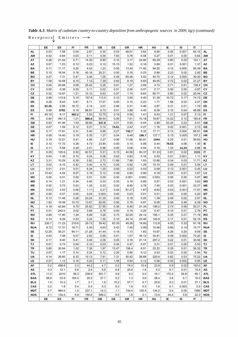
85

Table A.3. Matrix of cadmium country-to-country deposition from anthropogenic sources in 2009, kg/y (continued) R e c e p t o r s E m i t t e r s

EE ES FI FR GB GE GR HR HU IE IS IT AL 0.03 7.58 0.04 2.67 0.35 0.03 48.01 3.64 6.80 0.06 0.001 64.15 AL AM 0.02 0.64 0.03 0.11 0.04 7.83 0.76 0.08 0.27 0.01 0.00 0.64 AM AT 0.28 21.54 0.71 14.30 6.90 0.10 3.17 24.95 80.29 0.80 0.02 124.1 AT AZ 0.07 1.23 0.12 0.23 0.10 15.15 1.52 0.18 0.69 0.01 0.001 1.37 AZ BA 0.11 11.17 0.25 4.43 1.23 0.05 13.40 71.92 94.20 0.15 0.005 85.39 BA BE 0.10 16.54 0.18 45.18 25.21 0.00 0.18 0.23 0.86 2.23 0.02 2.92 BE BG 0.27 7.31 0.47 2.46 1.05 0.49 84.46 5.52 40.75 0.12 0.005 30.00 BG BY 7.58 16.58 8.15 7.12 7.29 0.83 8.19 6.65 49.05 0.72 0.02 21.27 BY CH 0.06 25.68 0.09 25.42 5.26 0.01 1.27 2.69 4.15 0.71 0.01 128.4 CH CY 0.00 0.38 0.00 0.11 0.02 0.01 2.00 0.07 0.17 0.00 0.00 0.87 CY CZ 0.52 12.67 1.21 10.12 8.63 0.07 1.74 8.63 85.77 0.85 0.02 25.04 CZ DE 2.69 113.8 5.10 157.8 113.9 0.12 3.00 5.45 31.39 10.72 0.17 74.73 DE DK 0.28 8.43 0.81 8.11 17.07 0.00 0.15 0.23 1.71 1.58 0.03 2.07 DK EE 62.26 2.89 16.72 2.14 3.07 0.06 0.31 0.46 2.87 0.31 0.01 1.79 EE ES 0.09 3792 0.19 88.91 9.73 0.01 3.88 4.40 8.09 2.10 0.04 48.89 ES FI 45.18 8.17 562.2 5.93 10.79 0.16 0.56 1.41 9.03 1.21 0.07 5.13 FI FR 0.84 947.3 1.21 986.6 96.54 0.05 7.61 10.18 18.87 14.22 0.12 183.8 FR GB 0.63 61.56 1.53 39.85 547.8 0.01 0.55 0.44 2.89 53.25 0.23 5.51 GB GE 0.07 1.59 0.12 0.31 0.14 74.61 2.42 0.27 1.16 0.02 0.001 2.13 GE GR 0.17 17.81 0.31 5.40 0.88 0.27 742.7 5.32 17.11 0.13 0.004 65.91 GR HR 0.09 14.40 0.19 5.35 1.27 0.04 8.48 196.7 127.7 0.15 0.005 107.2 HR HU 0.19 12.51 0.41 4.56 2.27 0.06 11.06 60.91 1044 0.25 0.01 56.83 HU IE 0.12 17.72 0.28 4.73 23.85 0.00 0.15 0.09 0.44 78.53 0.06 1.30 IE IS 0.11 5.58 0.28 2.01 5.98 0.00 0.06 0.04 0.16 1.33 14.24 0.88 IS IT 0.29 125.6 0.52 62.51 5.31 0.15 40.56 83.37 91.33 0.81 0.02 2131 IT KY 0.04 1.35 0.10 0.24 0.08 0.63 0.83 0.16 0.53 0.01 0.001 1.11 KY KZ 3.31 10.29 6.39 2.82 2.72 11.88 7.86 1.93 10.86 0.34 0.03 11.71 KZ LT 3.02 6.15 4.42 3.40 4.75 0.09 0.92 1.29 10.10 0.49 0.01 5.04 LT LU 0.01 2.01 0.01 6.34 1.20 0.00 0.02 0.03 0.09 0.13 0.001 0.45 LU LV 10.42 4.54 8.57 3.19 5.12 0.09 0.80 0.90 6.18 0.54 0.01 3.57 LV MC 0.00 0.01 0.00 0.01 0.00 0.00 0.001 0.002 0.003 0.00 0.00 0.07 MC MD 0.14 1.21 0.24 0.40 0.33 0.25 5.18 0.85 5.57 0.03 0.001 3.63 MD ME 0.02 3.73 0.03 1.35 0.22 0.02 8.80 3.78 7.40 0.03 0.001 33.27 ME MK 0.03 3.52 0.06 1.11 0.27 0.04 87.27 1.87 8.62 0.03 0.001 17.97 MK MT 0.00 0.07 0.00 0.04 0.003 0.00 0.03 0.01 0.01 0.00 0.00 0.20 MT NL 0.13 11.48 0.28 23.24 31.35 0.00 0.18 0.25 1.39 2.49 0.02 2.97 NL NO 1.83 16.59 10.70 13.67 50.95 0.06 0.78 0.87 6.08 5.56 0.46 6.39 NO PL 4.19 42.84 9.79 25.92 27.95 0.36 6.45 21.34 199.2 2.74 0.06 55.21 PL PT 0.01 242.0 0.02 3.69 0.76 0.00 0.18 0.25 0.47 0.15 0.01 2.79 PT RO 0.69 17.90 1.24 5.69 3.26 0.73 52.55 24.14 195.1 0.35 0.01 71.19 RO RS 0.14 9.29 0.33 3.24 1.55 0.10 44.14 23.46 145.8 0.17 0.01 52.15 RS RU 230.7 71.23 219.8 29.73 39.42 63.35 49.28 18.85 112.8 4.55 0.32 81.18 RU RUA 8.72 17.31 19.71 5.35 6.60 5.42 7.45 2.99 15.46 0.86 0.14 15.77 RUA SE 12.20 30.21 94.11 21.28 41.44 0.18 1.13 1.83 14.87 4.26 0.20 9.59 SE SI 0.04 7.08 0.07 2.93 0.69 0.01 1.67 45.12 34.81 0.09 0.002 73.20 SI SK 0.17 8.40 0.41 3.49 2.06 0.05 4.16 21.14 297.2 0.22 0.01 30.56 SK TJ 0.01 0.73 0.04 0.12 0.03 0.34 0.47 0.07 0.21 0.01 0.00 0.53 TJ TR 0.60 30.64 1.02 7.38 1.97 13.47 156.4 6.01 23.22 0.29 0.01 56.32 TR TU 0.07 1.17 0.14 0.24 0.12 2.26 0.90 0.12 0.53 0.02 0.00 0.94 TU UA 4.14 29.85 6.33 10.13 7.91 7.31 50.42 26.68 220.6 0.82 0.03 75.22 UA UZ 0.07 1.13 0.16 0.22 0.11 1.59 0.84 0.12 0.58 0.02 0.002 0.95 UZ AF 0.2 498.6 0.3 44.2 4.7 0.2 74.0 10.4 23.8 0.9 0.02 150.0 AF AS 0.3 12.1 0.6 2.4 0.6 6.8 25.6 1.6 5.3 0.1 0.01 15.4 AS ATL 11.0 2210 56.3 238.6 501.7 0.9 5.3 5.0 19.1 172.4 64.8 65.1 ATL BAS 56.9 33.9 163.4 25.5 37.7 0.2 1.3 3.6 28.4 3.8 0.1 16.0 BAS BLS 1.0 10.3 1.7 3.1 1.6 15.2 57.7 4.7 25.8 0.2 0.01 27.1 BLS CAS 0.2 1.8 0.4 0.4 0.3 9.3 1.6 0.3 1.6 0.1 0.003 2.0 CAS MDT 0.7 964.5 1.5 237.1 14.3 1.1 734.4 120.3 134.2 2.4 0.05 1590 MDT NOS 2.1 134.5 5.9 150.6 589.2 0.0 1.8 2.1 13.9 44.4 0.8 22.3 NOS

EE ES FI FR GB GE GR HR HU IE IS IT

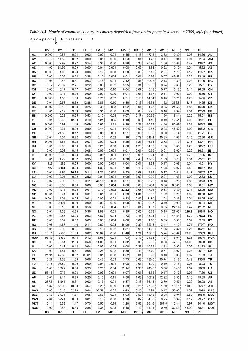
86

Table A.3. Matrix of cadmium country-to-country deposition from anthropogenic sources in 2009, kg/y (continued) R e c e p t o r s E m i t t e r s

KY KZ LT LU LV MC MD ME MK MT NL NO PL AL 0.002 0.55 0.04 0.02 0.02 0.01 0.15 1.15 477.5 3.62 0.39 0.03 14.36 AL AM 0.10 11.89 0.02 0.00 0.01 0.00 0.03 0.01 1.73 0.11 0.04 0.01 2.04 AM AT 0.003 2.99 0.97 0.54 0.38 0.06 0.26 0.33 20.26 1.36 10.84 0.42 439.7 AT AZ 1.92 64.99 0.09 0.00 0.04 0.001 0.08 0.02 3.83 0.22 0.10 0.04 5.72 AZ BA 0.003 1.63 0.23 0.06 0.10 0.03 0.29 6.89 87.43 2.91 1.79 0.17 115.7 BA BE 0.00 0.06 0.22 3.28 0.10 0.004 0.01 0.01 0.96 0.07 49.58 0.26 23.19 BE BG 0.04 9.43 0.41 0.03 0.18 0.01 3.42 0.87 398.3 2.13 1.39 0.24 111.0 BG BY 0.12 23.07 22.21 0.22 8.06 0.02 3.95 0.31 39.63 0.74 9.63 2.23 1501 BY CH 0.00 0.17 0.17 0.47 0.07 0.10 0.04 0.07 5.48 0.77 5.12 0.14 26.09 CH CY 0.00 0.11 0.00 0.00 0.00 0.00 0.01 0.01 1.77 0.17 0.02 0.00 0.56 CY CZ 0.003 1.83 1.88 0.43 0.75 0.02 0.21 0.18 14.04 0.43 15.21 0.70 1435 CZ DE 0.01 2.53 6.69 12.88 2.86 0.10 0.30 0.16 16.31 1.52 366.8 5.17 1475 DE DK 0.002 0.10 0.83 0.25 0.36 0.003 0.02 0.01 1.25 0.05 24.56 1.86 156.0 DK EE 0.01 2.17 9.53 0.06 8.31 0.00 0.09 0.03 2.25 0.10 4.39 1.54 125.9 EE ES 0.002 0.28 0.25 0.53 0.10 0.08 0.07 0.17 20.65 1.96 8.44 0.25 45.21 ES FI 0.04 6.38 12.80 0.19 7.21 0.005 0.19 0.05 4.13 0.19 12.51 9.90 329.1 FI FR 0.003 0.97 1.46 10.09 0.62 1.31 0.19 0.29 30.33 4.46 85.69 1.32 205.2 FR GB 0.002 0.31 0.99 0.59 0.44 0.01 0.04 0.02 2.55 0.08 46.52 1.99 105.2 GB GE 0.18 21.80 0.12 0.00 0.05 0.001 0.21 0.03 5.86 0.30 0.14 0.05 11.21 GE GR 0.04 4.54 0.22 0.03 0.10 0.02 1.18 0.79 618.1 10.83 1.02 0.15 52.20 GR HR 0.003 1.55 0.22 0.07 0.09 0.04 0.25 1.21 46.71 2.72 1.79 0.13 130.1 HR HU 0.01 2.09 0.53 0.10 0.21 0.03 0.68 1.29 94.83 1.33 3.35 0.28 385.7 HU IE 0.00 0.03 0.15 0.08 0.07 0.001 0.01 0.01 0.59 0.01 5.02 0.29 16.71 IE IS 0.001 0.09 0.13 0.03 0.06 0.001 0.01 0.00 0.21 0.01 1.51 0.79 7.36 IS IT 0.01 4.29 0.62 0.35 0.25 0.92 0.70 2.40 177.9 31.69 6.70 0.31 222.1 IT KY 717 282 0.05 0.00 0.02 0.001 0.04 0.01 1.91 0.17 0.08 0.04 4.01 KY KZ 427 5961 3.03 0.05 1.33 0.01 1.19 0.16 23.55 1.23 2.97 1.58 190.7 KZ LT 0.01 2.94 76.24 0.11 11.22 0.005 0.33 0.07 7.94 0.17 5.84 1.47 687.2 LT LU 0.00 0.01 0.02 3.53 0.01 0.001 0.00 0.00 0.09 0.01 1.63 0.02 2.53 LU LV 0.02 2.98 97.91 0.11 47.15 0.003 0.21 0.06 6.22 0.18 6.25 1.85 335.3 LV MC 0.00 0.00 0.00 0.00 0.00 0.004 0.00 0.00 0.004 0.00 0.001 0.00 0.01 MC MD 0.02 4.15 0.25 0.01 0.10 0.002 22.22 0.08 17.06 0.33 0.39 0.11 52.05 MD ME 0.001 0.44 0.03 0.01 0.01 0.01 0.09 11.32 95.57 1.62 0.29 0.02 13.08 ME MK 0.004 1.01 0.05 0.01 0.02 0.01 0.23 0.42 3180 1.08 0.36 0.04 18.25 MK MT 0.00 0.001 0.00 0.00 0.00 0.00 0.00 0.00 0.07 3.50 0.00 0.00 0.04 MT NL 0.00 0.10 0.33 0.56 0.14 0.004 0.01 0.01 1.07 0.05 276.9 0.42 42.02 NL NO 0.01 1.38 4.23 0.36 1.89 0.01 0.15 0.05 6.28 0.15 27.66 186.1 298.5 NO PL 0.03 9.86 23.03 0.93 7.87 0.04 1.73 0.47 45.01 1.27 44.54 5.72 17603 PL PT 0.00 0.02 0.02 0.03 0.01 0.004 0.00 0.01 1.16 0.09 0.53 0.02 2.55 PT RO 0.06 14.67 1.46 0.11 0.60 0.03 16.90 2.39 323.8 3.44 4.40 0.71 479.7 RO RS 0.01 2.98 0.31 0.06 0.13 0.02 0.81 8.96 613.2 1.96 2.32 0.26 162.1 RS RU 18.11 2585 61.03 0.82 33.07 0.06 11.48 1.24 187.3 5.24 43.67 23.20 2383 RU RUA 96.89 3539 5.48 0.12 2.66 0.01 1.03 0.19 24.53 1.24 6.04 4.28 253.4 RUA SE 0.03 3.51 22.56 0.56 11.03 0.01 0.32 0.06 6.50 0.23 47.13 53.05 994.3 SE SI 0.00 0.47 0.12 0.04 0.05 0.02 0.08 0.23 10.99 1.12 0.92 0.05 61.83 SI SK 0.00 1.51 0.67 0.08 0.25 0.02 0.39 0.44 36.79 0.54 3.07 0.28 961.7 SK TJ 21.91 42.63 0.02 0.001 0.01 0.00 0.02 0.01 0.90 0.10 0.03 0.02 1.53 TJ TR 0.27 41.38 1.05 0.06 0.42 0.03 3.73 0.68 186.5 10.74 2.18 0.42 135.9 TR TU 9.16 98.89 0.09 0.00 0.04 0.001 0.08 0.01 1.90 0.19 0.15 0.05 8.23 TU UA 1.06 150.9 8.30 0.23 3.25 0.04 32.14 1.38 245.6 3.50 10.45 2.57 2009 UA UZ 53.46 197.5 0.08 0.00 0.03 0.001 0.07 0.01 1.75 0.17 0.12 0.05 7.50 UZ AF 0.01 2.14 0.25 0.20 0.10 0.11 0.50 1.03 167.2 42.22 3.35 0.16 75.35 AF AS 267.6 649.1 0.31 0.02 0.13 0.01 0.37 0.16 36.41 2.79 0.57 0.20 29.08 AS ATL 1.82 86.08 10.93 3.67 5.23 0.09 0.59 0.25 27.88 1.60 166.1 110.8 658.7 ATL BAS 0.03 5.10 62.28 0.84 38.57 0.02 0.43 0.10 7.94 0.47 58.80 13.09 2099 BAS BLS 0.58 67.71 1.67 0.05 0.68 0.01 8.93 0.53 150.8 2.98 2.04 0.52 195.9 BLS CAS 7.84 375.4 0.30 0.01 0.13 0.00 0.28 0.02 4.00 0.25 0.39 0.12 29.27 CAS MDT 0.11 16.39 1.17 0.70 0.50 0.89 3.20 6.96 961.6 267.5 12.44 0.97 341.0 MDT NOS 0.02 0.83 5.43 2.88 2.38 0.03 0.18 0.12 14.04 0.50 324.3 45.99 682.1 NOS

KY KZ LT LU LV MC MD ME MK MT NL NO PL

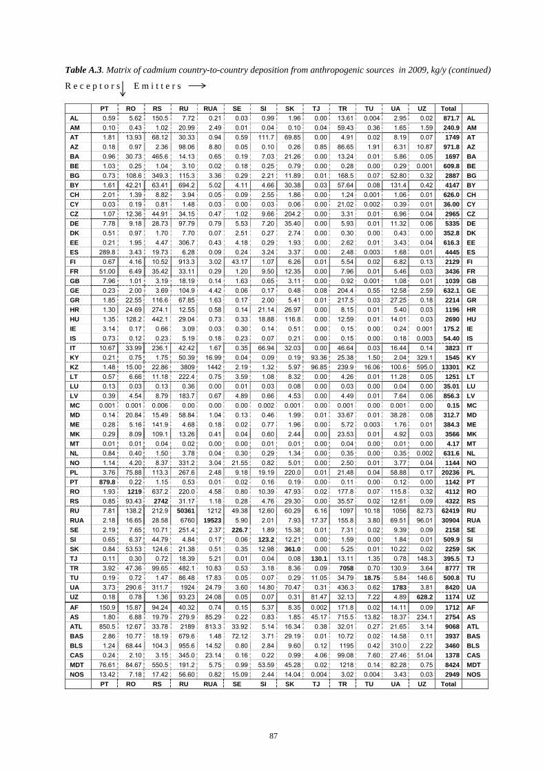
87

Table A.3. Matrix of cadmium country-to-country deposition from anthropogenic sources in 2009, kg/y (continued) R e c e p t o r s E m i t t e r s

PT RO RS RU RUA SE SI SK TJ TR TU UA UZ Total AL 0.59 5.62 150.5 7.72 0.21 0.03 0.99 1.96 0.00 13.61 0.004 2.95 0.02 871.7 AL AM 0.10 0.43 1.02 20.99 2.49 0.01 0.04 0.10 0.04 59.43 0.36 1.65 1.59 240.9 AM AT 1.81 13.93 68.12 30.33 0.94 0.59 111.7 69.85 0.00 4.91 0.02 8.19 0.07 1749 AT AZ 0.18 0.97 2.36 98.06 8.80 0.05 0.10 0.26 0.85 86.65 1.91 6.31 10.87 971.8 AZ BA 0.96 30.73 465.6 14.13 0.65 0.19 7.03 21.26 0.00 13.24 0.01 5.86 0.05 1697 BA BE 1.03 0.25 1.04 3.10 0.02 0.18 0.25 0.79 0.00 0.28 0.00 0.29 0.001 609.8 BE BG 0.73 108.6 349.3 115.3 3.36 0.29 2.21 11.89 0.01 168.5 0.07 52.80 0.32 2887 BG BY 1.61 42.21 63.41 694.2 5.02 4.11 4.66 30.38 0.03 57.64 0.08 131.4 0.42 4147 BY CH 2.01 1.39 8.82 3.94 0.05 0.09 2.55 1.86 0.00 1.24 0.001 1.06 0.01 626.0 CH CY 0.03 0.19 0.81 1.48 0.03 0.00 0.03 0.06 0.00 21.02 0.002 0.39 0.01 36.00 CY CZ 1.07 12.36 44.91 34.15 0.47 1.02 9.66 204.2 0.00 3.31 0.01 6.96 0.04 2965 CZ DE 7.78 9.18 28.73 97.79 0.79 5.53 7.20 35.40 0.00 5.93 0.01 11.32 0.06 5335 DE DK 0.51 0.97 1.70 7.70 0.07 2.51 0.27 2.74 0.00 0.30 0.00 0.43 0.00 352.8 DK EE 0.21 1.95 4.47 306.7 0.43 4.18 0.29 1.93 0.00 2.62 0.01 3.43 0.04 616.3 EE ES 289.8 3.43 19.73 6.28 0.09 0.24 3.24 3.37 0.00 2.48 0.003 1.68 0.01 4445 ES FI 0.67 4.16 10.52 913.3 3.02 43.17 1.07 6.26 0.01 5.54 0.02 6.82 0.13 2129 FI FR 51.00 6.49 35.42 33.11 0.29 1.20 9.50 12.35 0.00 7.96 0.01 5.46 0.03 3436 FR GB 7.96 1.01 3.19 18.19 0.14 1.63 0.65 3.11 0.00 0.92 0.001 1.08 0.01 1039 GB GE 0.23 2.00 3.69 104.9 4.42 0.06 0.17 0.48 0.08 204.4 0.55 12.58 2.59 632.1 GE GR 1.85 22.55 116.6 67.85 1.63 0.17 2.00 5.41 0.01 217.5 0.03 27.25 0.18 2214 GR HR 1.30 24.69 274.1 12.55 0.58 0.14 21.14 26.97 0.00 8.15 0.01 5.40 0.03 1196 HR HU 1.35 128.2 442.1 29.04 0.73 0.33 18.88 116.8 0.00 12.59 0.01 14.01 0.03 2690 HU IE 3.14 0.17 0.66 3.09 0.03 0.30 0.14 0.51 0.00 0.15 0.00 0.24 0.001 175.2 IE IS 0.73 0.12 0.23 5.19 0.18 0.23 0.07 0.21 0.00 0.15 0.00 0.18 0.003 54.40 IS IT 10.67 33.99 236.1 42.42 1.67 0.35 66.94 32.03 0.00 46.64 0.03 16.44 0.14 3823 IT KY 0.21 0.75 1.75 50.39 16.99 0.04 0.09 0.19 93.36 25.38 1.50 2.04 329.1 1545 KY KZ 1.48 15.00 22.86 3809 1442 2.19 1.32 5.97 96.85 239.9 16.06 100.6 595.0 13301 KZ LT 0.57 6.66 11.18 222.4 0.75 3.59 1.08 8.32 0.00 4.26 0.01 11.28 0.05 1251 LT LU 0.13 0.03 0.13 0.36 0.00 0.01 0.03 0.08 0.00 0.03 0.00 0.04 0.00 35.01 LU LV 0.39 4.54 8.79 183.7 0.67 4.89 0.66 4.53 0.00 4.49 0.01 7.64 0.06 856.3 LV MC 0.001 0.001 0.006 0.00 0.00 0.00 0.002 0.001 0.00 0.001 0.00 0.001 0.00 0.15 MC MD 0.14 20.84 15.49 58.84 1.04 0.13 0.46 1.99 0.01 33.67 0.01 38.28 0.08 312.7 MD ME 0.28 5.16 141.9 4.68 0.18 0.02 0.77 1.96 0.00 5.72 0.003 1.76 0.01 384.3 ME MK 0.29 8.09 109.1 13.26 0.41 0.04 0.60 2.44 0.00 23.53 0.01 4.92 0.03 3566 MK MT 0.01 0.01 0.04 0.02 0.00 0.00 0.01 0.01 0.00 0.04 0.00 0.01 0.00 4.17 MT NL 0.84 0.40 1.50 3.78 0.04 0.30 0.29 1.34 0.00 0.35 0.00 0.35 0.002 631.6 NL NO 1.14 4.20 8.37 331.2 3.04 21.55 0.82 5.01 0.00 2.50 0.01 3.77 0.04 1144 NO PL 3.76 75.88 113.3 267.6 2.48 9.18 19.19 220.0 0.01 21.48 0.04 58.88 0.17 20236 PL PT 879.8 0.22 1.15 0.53 0.01 0.02 0.16 0.19 0.00 0.11 0.00 0.12 0.00 1142 PT RO 1.93 1219 637.2 220.0 4.58 0.80 10.39 47.93 0.02 177.8 0.07 115.8 0.32 4112 RO RS 0.85 93.43 2742 31.17 1.18 0.28 4.76 29.30 0.00 35.57 0.02 12.61 0.09 4322 RS RU 7.81 138.2 212.9 50361 1212 49.38 12.60 60.29 6.16 1097 10.18 1056 82.73 62419 RU RUA 2.18 16.65 28.58 6760 19523 5.90 2.01 7.93 17.37 155.8 3.80 69.51 96.01 30904 RUA SE 2.19 7.65 10.71 251.4 2.37 226.7 1.89 15.38 0.01 7.31 0.02 9.39 0.09 2158 SE SI 0.65 6.37 44.79 4.84 0.17 0.06 123.2 12.21 0.00 1.59 0.00 1.84 0.01 509.9 SI SK 0.84 53.53 124.6 21.38 0.51 0.35 12.98 361.0 0.00 5.25 0.01 10.22 0.02 2259 SK TJ 0.11 0.30 0.72 18.39 5.21 0.01 0.04 0.08 130.1 13.11 1.35 0.78 148.3 395.5 TJ TR 3.92 47.36 99.65 482.1 10.83 0.53 3.18 8.36 0.09 7058 0.70 130.9 3.64 8777 TR TU 0.19 0.72 1.47 86.48 17.83 0.05 0.07 0.29 11.05 34.79 18.75 5.84 146.6 500.8 TU UA 3.73 290.6 311.7 1924 24.79 3.60 14.80 70.47 0.31 436.3 0.62 1783 3.81 8420 UA UZ 0.18 0.78 1.36 93.23 24.08 0.05 0.07 0.31 81.47 32.13 7.22 4.89 628.2 1174 UZ AF 150.9 15.87 94.24 40.32 0.74 0.15 5.37 8.35 0.002 171.8 0.02 14.11 0.09 1712 AF AS 1.80 6.88 19.79 279.9 85.29 0.22 0.83 1.85 45.17 715.5 13.82 18.37 234.1 2754 AS ATL 850.5 12.67 33.78 2189 813.3 33.92 5.14 16.34 0.38 32.01 0.27 21.65 3.14 9068 ATL BAS 2.86 10.77 18.19 679.6 1.48 72.12 3.71 29.19 0.01 10.72 0.02 14.58 0.11 3937 BAS BLS 1.24 68.44 104.3 955.6 14.52 0.80 2.84 9.60 0.12 1195 0.42 310.0 2.22 3460 BLS CAS 0.24 2.10 3.15 345.0 23.14 0.16 0.22 0.99 4.06 99.08 7.60 27.46 51.04 1378 CAS MDT 76.61 84.67 550.5 191.2 5.75 0.99 53.59 45.28 0.02 1218 0.14 82.28 0.75 8424 MDT NOS 13.42 7.18 17.42 56.60 0.82 15.09 2.44 14.04 0.004 3.02 0.004 3.43 0.03 2949 NOS

PT RO RS RU RUA SE SI SK TJ TR TU UA UZ Total

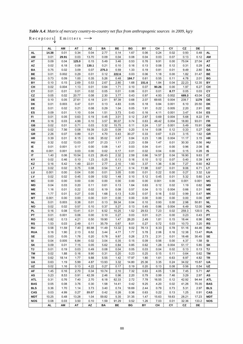
88

Table A.4. Matrix of mercury country-to-country net flux from anthropogenic sources in 2009, kg/y R e c e p t o r s E m i t t e r s

AL AM AT AZ BA BE BG BY CH CY CZ DE AL 14.38 0.01 0.34 0.04 2.77 0.14 1.67 0.06 0.24 0.02 0.93 0.48 AL AM 0.01 29.91 0.03 13.70 0.09 0.04 0.08 0.04 0.03 0.07 0.13 0.12 AM AT 0.09 0.04 125.0 0.15 5.49 3.46 0.53 0.76 9.91 0.00 75.04 27.04 AT AZ 0.02 6.18 0.08 130.1 0.21 0.10 0.16 0.13 0.08 0.12 0.31 0.29 AZ BA 0.75 0.02 3.09 0.07 275.3 0.59 1.33 0.19 0.81 0.01 9.49 2.80 BA BE 0.01 0.002 0.29 0.01 0.12 222.6 0.03 0.06 1.18 0.00 1.82 31.47 BE BG 0.73 0.09 1.00 0.35 5.26 0.48 184.7 0.61 0.55 0.11 4.78 2.01 BG BY 0.10 0.15 2.69 0.53 2.67 2.80 1.68 151.6 1.84 0.04 22.23 12.35 BY CH 0.02 0.004 1.13 0.01 0.64 1.71 0.10 0.07 90.26 0.00 1.97 6.27 CH CY 0.01 0.01 0.01 0.02 0.05 0.01 0.06 0.01 0.01 8.77 0.05 0.03 CY CZ 0.05 0.02 20.77 0.08 2.30 3.77 0.43 0.97 4.93 0.002 689.3 43.04 CZ DE 0.10 0.05 27.61 0.18 2.51 97.39 0.68 2.07 69.65 0.004 239.7 1179 DE DK 0.01 0.003 0.47 0.01 0.13 4.83 0.05 0.18 0.84 0.001 6.10 20.50 DK EE 0.01 0.02 0.21 0.08 0.29 1.04 0.05 1.91 0.22 0.005 2.20 2.91 EE ES 0.09 0.01 1.10 0.04 1.51 3.73 0.43 0.16 4.11 0.001 3.47 6.54 ES FI 0.01 0.05 0.63 0.19 0.45 3.01 0.12 2.87 0.69 0.004 5.68 8.22 FI FR 0.16 0.03 4.99 0.10 3.57 90.07 0.74 0.63 48.42 0.004 18.80 93.01 FR GB 0.02 0.01 0.71 0.03 0.32 15.75 0.11 0.24 1.57 0.001 5.49 15.91 GB GE 0.02 7.56 0.08 19.39 0.20 0.09 0.20 0.14 0.08 0.12 0.33 0.27 GE GR 2.26 0.07 0.89 0.21 4.70 0.43 30.27 0.33 0.67 0.23 3.15 1.62 GR HR 0.39 0.01 6.15 0.06 35.02 0.67 0.84 0.23 1.06 0.004 11.17 3.15 HR HU 0.32 0.02 13.03 0.07 21.23 1.11 2.23 0.59 1.47 0.01 30.30 6.56 HU IE 0.01 0.001 0.17 0.00 0.08 1.47 0.03 0.04 0.41 0.00 0.96 2.08 IE IS 0.001 0.001 0.03 0.00 0.02 0.17 0.01 0.02 0.04 0.00 0.15 0.28 IS IT 1.40 0.06 10.54 0.23 26.43 2.32 2.59 0.66 14.57 0.04 16.90 9.63 IT KY 0.02 0.46 0.10 1.23 0.25 0.13 0.16 0.10 0.12 0.07 0.40 0.39 KY KZ 0.16 5.42 1.49 22.01 2.77 2.10 1.93 3.37 1.36 0.36 7.27 6.60 KZ LT 0.02 0.02 0.75 0.08 0.54 1.41 0.14 11.98 0.67 0.01 9.06 6.71 LT LU 0.001 0.00 0.04 0.00 0.01 3.05 0.00 0.01 0.22 0.00 0.27 3.32 LU LV 0.02 0.02 0.45 0.09 0.52 1.48 0.10 5.12 0.45 0.01 5.32 5.60 LV MC 0.00 0.00 0.00 0.00 0.00 0.00 0.00 0.00 0.001 0.00 0.001 0.001 MC MD 0.04 0.03 0.20 0.11 0.61 0.13 1.64 0.63 0.12 0.02 1.19 0.62 MD ME 1.16 0.01 0.22 0.02 6.19 0.08 0.57 0.04 0.13 0.004 0.66 0.31 ME MK 1.77 0.01 0.27 0.05 1.68 0.13 5.20 0.07 0.16 0.02 0.99 0.47 MK MT 0.001 0.00 0.00 0.00 0.01 0.00 0.00 0.00 0.00 0.00 0.00 0.00 MT NL 0.01 0.003 0.38 0.01 0.13 59.34 0.04 0.10 0.93 0.00 2.98 50.81 NL NO 0.02 0.02 0.57 0.10 0.37 5.27 0.13 0.45 0.86 0.004 6.49 12.00 NO PL 0.16 0.08 13.41 0.31 6.52 10.25 1.52 29.53 7.23 0.02 259.3 120.5 PL PT 0.01 0.001 0.06 0.00 0.10 0.27 0.03 0.01 0.21 0.00 0.23 0.43 PT RO 0.82 0.13 4.21 0.50 19.90 1.47 26.20 2.49 1.81 0.15 18.44 6.96 RO RS 1.53 0.03 2.49 0.11 35.79 0.67 8.01 0.27 0.72 0.03 10.73 3.20 RS RU 0.58 11.59 7.40 65.98 11.49 13.32 9.02 76.13 6.33 0.78 51.16 44.46 RU RUA 0.16 1.90 2.13 6.52 3.44 4.77 1.77 5.78 2.06 0.16 12.38 13.47 RUA SE 0.03 0.05 1.78 0.20 0.78 9.87 0.26 2.73 2.31 0.01 18.48 30.45 SE SI 0.04 0.005 6.84 0.02 3.04 0.35 0.15 0.09 0.56 0.00 4.37 1.58 SI SK 0.09 0.01 7.15 0.05 5.62 0.84 0.85 0.62 1.28 0.004 51.17 5.85 SK TJ 0.01 0.19 0.03 0.49 0.08 0.04 0.05 0.03 0.04 0.02 0.13 0.13 TJ TM 0.02 1.88 0.16 9.90 0.31 0.20 0.23 0.25 0.15 0.11 0.64 0.62 TM TR 0.62 18.14 1.77 9.88 5.55 1.42 17.97 1.80 1.61 6.63 6.97 4.82 TR UA 0.63 1.19 5.99 4.87 13.93 3.32 14.80 25.36 3.35 0.24 34.02 15.87 UA UZ 0.02 1.16 0.13 4.22 0.27 0.17 0.19 0.20 0.13 0.08 0.56 0.54 UZ AF 1.45 0.16 2.70 0.34 10.74 2.10 7.32 0.63 4.05 1.38 7.45 5.71 AF AS 0.23 8.53 0.91 42.39 2.46 0.96 2.20 0.79 0.99 7.46 3.29 2.97 AS ATL 0.31 0.76 7.40 2.70 6.18 62.33 2.72 7.78 16.55 0.12 42.92 94.44 ATL BAS 0.05 0.08 3.76 0.30 1.58 14.41 0.42 9.25 4.20 0.02 41.26 70.35 BAS BLS 0.36 1.70 1.14 3.73 3.40 0.74 18.69 2.44 0.79 0.73 5.31 2.97 BLS CAS 0.03 4.99 0.27 89.87 0.42 0.26 0.36 0.63 0.22 0.13 1.25 0.91 CAS MDT 10.25 0.48 13.28 1.04 59.82 5.35 31.35 1.47 15.63 18.63 28.21 17.23 MDT NOS 0.08 0.03 3.50 0.10 1.59 91.29 0.52 1.26 7.03 0.01 32.36 133.2 NOS

AL AM AT AZ BA BE BG BY CH CY CZ DE

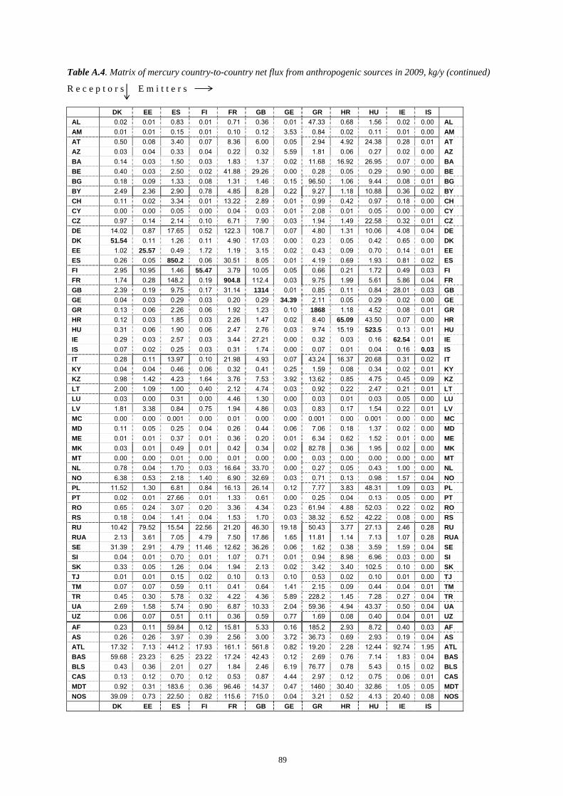
89

Table A.4. Matrix of mercury country-to-country net flux from anthropogenic sources in 2009, kg/y (continued) R e c e p t o r s E m i t t e r s

DK EE ES FI FR GB GE GR HR HU IE IS AL 0.02 0.01 0.83 0.01 0.71 0.36 0.01 47.33 0.68 1.56 0.02 0.00 AL AM 0.01 0.01 0.15 0.01 0.10 0.12 3.53 0.84 0.02 0.11 0.01 0.00 AM AT 0.50 0.08 3.40 0.07 8.36 6.00 0.05 2.94 4.92 24.38 0.28 0.01 AT AZ 0.03 0.04 0.33 0.04 0.22 0.32 5.59 1.81 0.06 0.27 0.02 0.00 AZ BA 0.14 0.03 1.50 0.03 1.83 1.37 0.02 11.68 16.92 26.95 0.07 0.00 BA BE 0.40 0.03 2.50 0.02 41.88 29.26 0.00 0.28 0.05 0.29 0.90 0.00 BE BG 0.18 0.09 1.33 0.08 1.31 1.46 0.15 96.50 1.06 9.44 0.08 0.01 BG BY 2.49 2.36 2.90 0.78 4.85 8.28 0.22 9.27 1.18 10.88 0.36 0.02 BY CH 0.11 0.02 3.34 0.01 13.22 2.89 0.01 0.99 0.42 0.97 0.18 0.00 CH CY 0.00 0.00 0.05 0.00 0.04 0.03 0.01 2.08 0.01 0.05 0.00 0.00 CY CZ 0.97 0.14 2.14 0.10 6.71 7.90 0.03 1.94 1.49 22.58 0.32 0.01 CZ DE 14.02 0.87 17.65 0.52 122.3 108.7 0.07 4.80 1.31 10.06 4.08 0.04 DE DK 51.54 0.11 1.26 0.11 4.90 17.03 0.00 0.23 0.05 0.42 0.65 0.00 DK EE 1.02 25.57 0.49 1.72 1.19 3.15 0.02 0.43 0.09 0.70 0.14 0.01 EE ES 0.26 0.05 850.2 0.06 30.51 8.05 0.01 4.19 0.69 1.93 0.81 0.02 ES FI 2.95 10.95 1.46 55.47 3.79 10.05 0.05 0.66 0.21 1.72 0.49 0.03 FI FR 1.74 0.28 148.2 0.19 904.8 112.4 0.03 9.75 1.99 5.61 5.86 0.04 FR GB 2.39 0.19 9.75 0.17 31.14 1314 0.01 0.85 0.11 0.84 28.01 0.03 GB GE 0.04 0.03 0.29 0.03 0.20 0.29 34.39 2.11 0.05 0.29 0.02 0.00 GE GR 0.13 0.06 2.26 0.06 1.92 1.23 0.10 1868 1.18 4.52 0.08 0.01 GR HR 0.12 0.03 1.85 0.03 2.26 1.47 0.02 8.40 65.09 43.50 0.07 0.00 HR HU 0.31 0.06 1.90 0.06 2.47 2.76 0.03 9.74 15.19 523.5 0.13 0.01 HU IE 0.29 0.03 2.57 0.03 3.44 27.21 0.00 0.32 0.03 0.16 62.54 0.01 IE IS 0.07 0.02 0.25 0.03 0.31 1.74 0.00 0.07 0.01 0.04 0.16 0.03 IS IT 0.28 0.11 13.97 0.10 21.98 4.93 0.07 43.24 16.37 20.68 0.31 0.02 IT KY 0.04 0.04 0.46 0.06 0.32 0.41 0.25 1.59 0.08 0.34 0.02 0.01 KY KZ 0.98 1.42 4.23 1.64 3.76 7.53 3.92 13.62 0.85 4.75 0.45 0.09 KZ LT 2.00 1.09 1.00 0.40 2.12 4.74 0.03 0.92 0.22 2.47 0.21 0.01 LT LU 0.03 0.00 0.31 0.00 4.46 1.30 0.00 0.03 0.01 0.03 0.05 0.00 LU LV 1.81 3.38 0.84 0.75 1.94 4.86 0.03 0.83 0.17 1.54 0.22 0.01 LV MC 0.00 0.00 0.001 0.00 0.01 0.00 0.00 0.001 0.00 0.001 0.00 0.00 MC MD 0.11 0.05 0.25 0.04 0.26 0.44 0.06 7.06 0.18 1.37 0.02 0.00 MD ME 0.01 0.01 0.37 0.01 0.36 0.20 0.01 6.34 0.62 1.52 0.01 0.00 ME MK 0.03 0.01 0.49 0.01 0.42 0.34 0.02 82.78 0.36 1.95 0.02 0.00 MK MT 0.00 0.00 0.01 0.00 0.01 0.00 0.00 0.03 0.00 0.00 0.00 0.00 MT NL 0.78 0.04 1.70 0.03 16.64 33.70 0.00 0.27 0.05 0.43 1.00 0.00 NL NO 6.38 0.53 2.18 1.40 6.90 32.69 0.03 0.71 0.13 0.98 1.57 0.04 NO PL 11.52 1.30 6.81 0.84 16.13 26.14 0.12 7.77 3.83 48.31 1.09 0.03 PL PT 0.02 0.01 27.66 0.01 1.33 0.61 0.00 0.25 0.04 0.13 0.05 0.00 PT RO 0.65 0.24 3.07 0.20 3.36 4.34 0.23 61.94 4.88 52.03 0.22 0.02 RO RS 0.18 0.04 1.41 0.04 1.53 1.70 0.03 38.32 6.52 42.22 0.08 0.00 RS RU 10.42 79.52 15.54 22.56 21.20 46.30 19.18 50.43 3.77 27.13 2.46 0.28 RU RUA 2.13 3.61 7.05 4.79 7.50 17.86 1.65 11.81 1.14 7.13 1.07 0.28 RUA SE 31.39 2.91 4.79 11.46 12.62 36.26 0.06 1.62 0.38 3.59 1.59 0.04 SE SI 0.04 0.01 0.70 0.01 1.07 0.71 0.01 0.94 8.98 6.96 0.03 0.00 SI SK 0.33 0.05 1.26 0.04 1.94 2.13 0.02 3.42 3.40 102.5 0.10 0.00 SK TJ 0.01 0.01 0.15 0.02 0.10 0.13 0.10 0.53 0.02 0.10 0.01 0.00 TJ TM 0.07 0.07 0.59 0.11 0.41 0.64 1.41 2.15 0.09 0.44 0.04 0.01 TM TR 0.45 0.30 5.78 0.32 4.22 4.36 5.89 228.2 1.45 7.28 0.27 0.04 TR UA 2.69 1.58 5.74 0.90 6.87 10.33 2.04 59.36 4.94 43.37 0.50 0.04 UA UZ 0.06 0.07 0.51 0.11 0.36 0.59 0.77 1.69 0.08 0.40 0.04 0.01 UZ AF 0.23 0.11 59.84 0.12 15.81 5.33 0.16 185.2 2.93 8.72 0.40 0.03 AF AS 0.26 0.26 3.97 0.39 2.56 3.00 3.72 36.73 0.69 2.93 0.19 0.04 AS ATL 17.32 7.13 441.2 17.93 161.1 561.8 0.82 19.20 2.28 12.44 92.74 1.95 ATL BAS 59.68 23.23 6.25 23.22 17.24 42.43 0.12 2.69 0.76 7.14 1.83 0.04 BAS BLS 0.43 0.36 2.01 0.27 1.84 2.46 6.19 76.77 0.78 5.43 0.15 0.02 BLS CAS 0.13 0.12 0.70 0.12 0.53 0.87 4.44 2.97 0.12 0.75 0.06 0.01 CAS MDT 0.92 0.31 183.6 0.36 96.46 14.37 0.47 1460 30.40 32.86 1.05 0.05 MDT NOS 39.09 0.73 22.50 0.82 115.6 715.0 0.04 3.21 0.52 4.13 20.40 0.08 NOS

DK EE ES FI FR GB GE GR HR HU IE IS

90

Table A.4. Matrix of mercury country-to-country net flux from anthropogenic sources in 2009, kg/y (continued) R e c e p t o r s E m i t t e r s

IT KY KZ LT LU LV MC MD ME MK MT NL NO AL 11.15 0.00 0.33 0.06 0.03 0.00 0.02 0.08 0.35 30.75 0.68 0.07 0.01 AL AM 0.28 0.03 5.82 0.04 0.01 0.00 0.002 0.02 0.00 0.11 0.02 0.02 0.01 AM AT 37.26 0.00 1.88 1.06 1.08 0.04 0.15 0.17 0.10 0.95 0.20 2.01 0.08 AT AZ 0.66 0.27 31.54 0.14 0.01 0.01 0.004 0.04 0.01 0.24 0.05 0.04 0.03 AZ BA 19.06 0.00 0.79 0.24 0.12 0.01 0.07 0.14 2.23 4.27 0.46 0.34 0.04 BA BE 0.97 0.00 0.09 0.25 10.69 0.01 0.01 0.01 0.00 0.07 0.01 44.84 0.06 BE BG 7.70 0.01 3.85 0.52 0.09 0.02 0.04 2.12 0.28 21.88 0.47 0.30 0.08 BG BY 6.61 0.03 10.07 30.26 0.52 1.13 0.04 1.80 0.08 1.72 0.24 2.03 0.54 BY CH 32.34 0.00 0.17 0.21 0.70 0.01 0.18 0.02 0.02 0.22 0.10 0.76 0.02 CH CY 0.18 0.00 0.09 0.01 0.00 0.00 0.001 0.01 0.00 0.09 0.02 0.00 0.00 CY CZ 8.14 0.00 1.15 2.00 0.96 0.07 0.05 0.13 0.05 0.69 0.10 2.96 0.14 CZ DE 25.98 0.01 2.53 8.08 32.64 0.27 0.25 0.22 0.07 1.24 0.30 99.84 1.17 DE DK 0.73 0.00 0.16 1.20 0.48 0.04 0.01 0.01 0.00 0.09 0.01 5.01 0.63 DK EE 0.57 0.00 1.27 12.41 0.11 1.27 0.005 0.04 0.01 0.10 0.03 0.78 0.35 EE ES 12.96 0.00 0.43 0.37 1.02 0.01 0.19 0.05 0.05 1.01 0.25 1.59 0.09 ES FI 1.56 0.02 3.68 11.63 0.37 0.66 0.01 0.10 0.01 0.19 0.03 2.12 1.90 FI FR 58.79 0.01 1.21 1.78 35.69 0.06 4.18 0.14 0.10 1.69 0.70 22.31 0.35 FR GB 1.84 0.01 0.48 1.20 1.19 0.04 0.02 0.03 0.01 0.19 0.02 10.22 0.46 GB GE 0.64 0.04 10.08 0.14 0.01 0.01 0.004 0.08 0.01 0.26 0.05 0.04 0.02 GE GR 15.71 0.01 2.12 0.31 0.08 0.01 0.06 0.65 0.28 57.72 2.15 0.23 0.06 GR HR 31.68 0.00 0.78 0.24 0.15 0.01 0.10 0.11 0.37 2.29 0.48 0.38 0.03 HR HU 19.30 0.00 1.16 0.57 0.24 0.02 0.07 0.33 0.46 4.87 0.27 0.79 0.07 HU IE 0.56 0.00 0.07 0.16 0.18 0.01 0.005 0.01 0.00 0.06 0.00 0.89 0.06 IE IS 0.11 0.00 0.14 0.07 0.02 0.00 0.001 0.00 0.00 0.01 0.00 0.09 0.07 IS IT 915.9 0.01 2.74 0.75 0.66 0.03 2.28 0.35 0.68 7.81 8.12 1.15 0.10 IT KY 0.84 109.7 114.6 0.13 0.02 0.01 0.01 0.04 0.01 0.23 0.05 0.05 0.04 KY KZ 8.70 104.5 4290 4.49 0.30 0.20 0.06 0.78 0.11 2.38 0.45 1.01 0.84 KZ LT 1.50 0.00 1.51 146.8 0.23 1.64 0.01 0.15 0.02 0.34 0.05 1.16 0.33 LT LU 0.14 0.00 0.01 0.02 17.61 0.00 0.002 0.00 0.00 0.01 0.00 0.85 0.00 LU LV 1.13 0.01 1.65 170.0 0.21 9.00 0.01 0.09 0.02 0.29 0.06 1.16 0.39 LV MC 0.02 0.00 0.00 0.00 0.00 0.00 0.02 0.00 0.00 0.00 0.00 0.00 0.00 MC MD 1.15 0.01 2.07 0.41 0.02 0.01 0.01 29.62 0.02 0.87 0.07 0.09 0.04 MD ME 4.26 0.00 0.23 0.03 0.02 0.00 0.01 0.04 3.97 3.57 0.18 0.04 0.01 ME MK 3.41 0.00 0.42 0.07 0.02 0.00 0.01 0.11 0.13 200.9 0.21 0.07 0.01 MK MT 0.09 0.00 0.00 0.00 0.00 0.00 0.00 0.00 0.00 0.00 2.97 0.00 0.00 MT NL 0.96 0.00 0.14 0.39 1.12 0.01 0.01 0.01 0.00 0.07 0.01 106.2 0.11 NL NO 1.49 0.02 2.17 2.99 0.58 0.11 0.01 0.05 0.01 0.23 0.03 3.94 37.12 NO PL 18.03 0.02 5.80 28.41 1.95 0.73 0.11 0.91 0.16 2.34 0.36 8.81 1.25 PL PT 0.71 0.00 0.05 0.03 0.06 0.00 0.01 0.00 0.00 0.07 0.01 0.11 0.01 PT RO 21.05 0.02 8.08 1.80 0.28 0.07 0.10 10.92 0.71 16.06 0.68 0.96 0.21 RO RS 12.97 0.00 1.31 0.29 0.13 0.01 0.05 0.38 3.37 36.80 0.37 0.43 0.06 RS RU 30.06 2.33 1205 71.10 2.02 4.04 0.21 5.60 0.42 9.20 1.36 8.49 5.81 RU RUA 10.59 7.84 1155 9.35 0.63 0.45 0.08 0.86 0.12 2.39 0.41 2.19 2.26 RUA SE 3.48 0.02 3.18 21.15 1.10 0.80 0.03 0.15 0.03 0.42 0.06 8.12 10.91 SE SI 19.69 0.00 0.27 0.10 0.09 0.00 0.04 0.03 0.04 0.28 0.10 0.18 0.01 SI SK 9.04 0.00 0.86 0.61 0.19 0.02 0.04 0.21 0.12 1.47 0.12 0.62 0.06 SK TJ 0.26 3.63 15.50 0.04 0.01 0.00 0.002 0.01 0.00 0.08 0.02 0.02 0.01 TJ TM 1.07 4.28 93.37 0.27 0.03 0.01 0.01 0.08 0.01 0.31 0.07 0.09 0.06 TM TR 18.28 0.14 25.73 1.74 0.23 0.07 0.11 2.48 0.25 11.36 2.09 0.67 0.26 TR UA 24.33 0.17 72.64 11.75 0.60 0.45 0.13 24.93 0.46 12.56 0.90 2.34 0.76 UA UZ 0.95 18.34 170.1 0.24 0.03 0.01 0.01 0.06 0.01 0.26 0.06 0.07 0.06 UZ AF 61.27 0.01 3.10 0.59 0.50 0.02 0.39 0.56 0.49 15.00 12.15 0.91 0.12 AF AS 8.56 37.96 274.4 0.98 0.16 0.04 0.06 0.40 0.10 3.26 0.67 0.37 0.25 AS ATL 36.58 1.28 120.0 20.24 8.41 0.94 0.36 0.95 0.22 4.30 0.73 32.30 32.18 ATL BAS 6.31 0.04 4.72 96.47 1.78 5.55 0.06 0.27 0.05 0.68 0.15 12.97 4.03 BAS BLS 7.61 0.10 29.26 2.26 0.12 0.09 0.05 7.44 0.17 7.56 0.68 0.45 0.20 BLS CAS 1.49 1.43 368.1 0.53 0.04 0.02 0.01 0.18 0.02 0.43 0.09 0.14 0.08 CAS MDT 587.4 0.06 9.14 1.80 1.36 0.07 2.77 1.79 2.26 51.34 97.59 2.63 0.38 MDT NOS 8.39 0.03 1.88 6.47 5.51 0.23 0.08 0.12 0.06 1.04 0.16 95.80 12.96 NOS

IT KY KZ LT LU LV MC MD ME MK MT NL NO

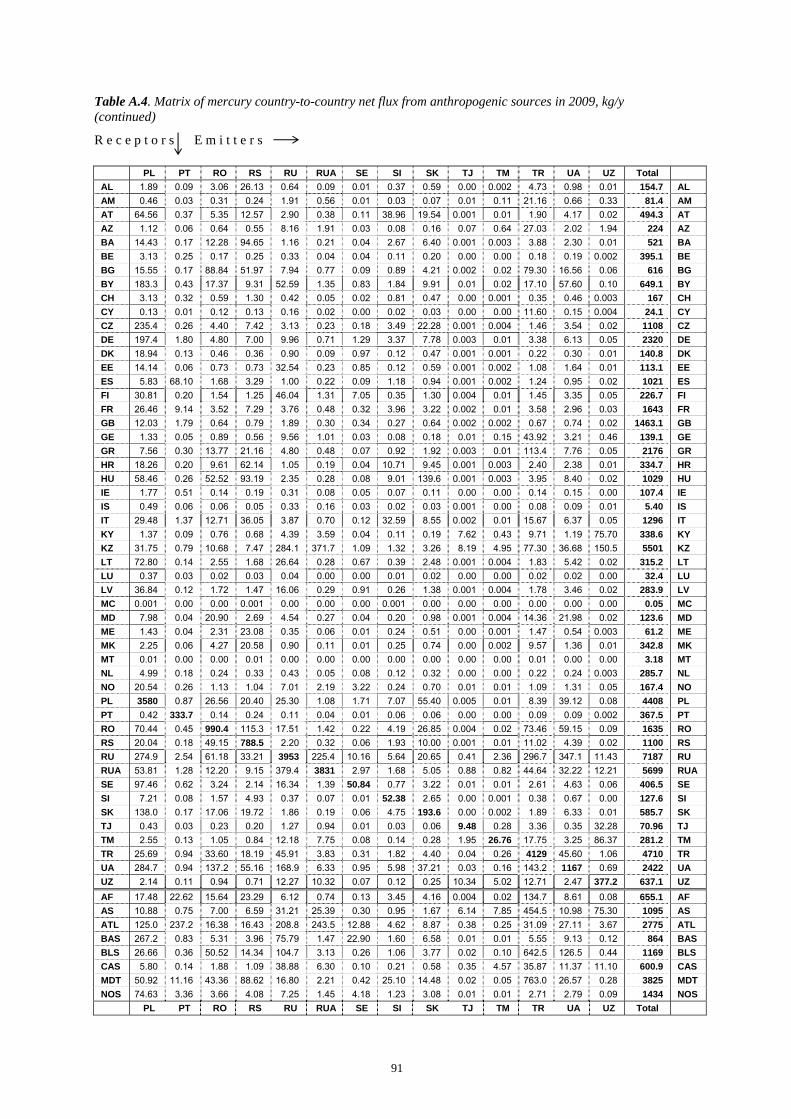
91

Table A.4. Matrix of mercury country-to-country net flux from anthropogenic sources in 2009, kg/y (continued) R e c e p t o r s E m i t t e r s

PL PT RO RS RU RUA SE SI SK TJ TM TR UA UZ Total AL 1.89 0.09 3.06 26.13 0.64 0.09 0.01 0.37 0.59 0.00 0.002 4.73 0.98 0.01 154.7 AL AM 0.46 0.03 0.31 0.24 1.91 0.56 0.01 0.03 0.07 0.01 0.11 21.16 0.66 0.33 81.4 AM AT 64.56 0.37 5.35 12.57 2.90 0.38 0.11 38.96 19.54 0.001 0.01 1.90 4.17 0.02 494.3 AT AZ 1.12 0.06 0.64 0.55 8.16 1.91 0.03 0.08 0.16 0.07 0.64 27.03 2.02 1.94 224 AZ BA 14.43 0.17 12.28 94.65 1.16 0.21 0.04 2.67 6.40 0.001 0.003 3.88 2.30 0.01 521 BA BE 3.13 0.25 0.17 0.25 0.33 0.04 0.04 0.11 0.20 0.00 0.00 0.18 0.19 0.002 395.1 BE BG 15.55 0.17 88.84 51.97 7.94 0.77 0.09 0.89 4.21 0.002 0.02 79.30 16.56 0.06 616 BG BY 183.3 0.43 17.37 9.31 52.59 1.35 0.83 1.84 9.91 0.01 0.02 17.10 57.60 0.10 649.1 BY CH 3.13 0.32 0.59 1.30 0.42 0.05 0.02 0.81 0.47 0.00 0.001 0.35 0.46 0.003 167 CH CY 0.13 0.01 0.12 0.13 0.16 0.02 0.00 0.02 0.03 0.00 0.00 11.60 0.15 0.004 24.1 CY CZ 235.4 0.26 4.40 7.42 3.13 0.23 0.18 3.49 22.28 0.001 0.004 1.46 3.54 0.02 1108 CZ DE 197.4 1.80 4.80 7.00 9.96 0.71 1.29 3.37 7.78 0.003 0.01 3.38 6.13 0.05 2320 DE DK 18.94 0.13 0.46 0.36 0.90 0.09 0.97 0.12 0.47 0.001 0.001 0.22 0.30 0.01 140.8 DK EE 14.14 0.06 0.73 0.73 32.54 0.23 0.85 0.12 0.59 0.001 0.002 1.08 1.64 0.01 113.1 EE ES 5.83 68.10 1.68 3.29 1.00 0.22 0.09 1.18 0.94 0.001 0.002 1.24 0.95 0.02 1021 ES FI 30.81 0.20 1.54 1.25 46.04 1.31 7.05 0.35 1.30 0.004 0.01 1.45 3.35 0.05 226.7 FI FR 26.46 9.14 3.52 7.29 3.76 0.48 0.32 3.96 3.22 0.002 0.01 3.58 2.96 0.03 1643 FR GB 12.03 1.79 0.64 0.79 1.89 0.30 0.34 0.27 0.64 0.002 0.002 0.67 0.74 0.02 1463.1 GB GE 1.33 0.05 0.89 0.56 9.56 1.01 0.03 0.08 0.18 0.01 0.15 43.92 3.21 0.46 139.1 GE GR 7.56 0.30 13.77 21.16 4.80 0.48 0.07 0.92 1.92 0.003 0.01 113.4 7.76 0.05 2176 GR HR 18.26 0.20 9.61 62.14 1.05 0.19 0.04 10.71 9.45 0.001 0.003 2.40 2.38 0.01 334.7 HR HU 58.46 0.26 52.52 93.19 2.35 0.28 0.08 9.01 139.6 0.001 0.003 3.95 8.40 0.02 1029 HU IE 1.77 0.51 0.14 0.19 0.31 0.08 0.05 0.07 0.11 0.00 0.00 0.14 0.15 0.00 107.4 IE IS 0.49 0.06 0.06 0.05 0.33 0.16 0.03 0.02 0.03 0.001 0.00 0.08 0.09 0.01 5.40 IS IT 29.48 1.37 12.71 36.05 3.87 0.70 0.12 32.59 8.55 0.002 0.01 15.67 6.37 0.05 1296 IT KY 1.37 0.09 0.76 0.68 4.39 3.59 0.04 0.11 0.19 7.62 0.43 9.71 1.19 75.70 338.6 KY KZ 31.75 0.79 10.68 7.47 284.1 371.7 1.09 1.32 3.26 8.19 4.95 77.30 36.68 150.5 5501 KZ LT 72.80 0.14 2.55 1.68 26.64 0.28 0.67 0.39 2.48 0.001 0.004 1.83 5.42 0.02 315.2 LT LU 0.37 0.03 0.02 0.03 0.04 0.00 0.00 0.01 0.02 0.00 0.00 0.02 0.02 0.00 32.4 LU LV 36.84 0.12 1.72 1.47 16.06 0.29 0.91 0.26 1.38 0.001 0.004 1.78 3.46 0.02 283.9 LV MC 0.001 0.00 0.00 0.001 0.00 0.00 0.00 0.001 0.00 0.00 0.00 0.00 0.00 0.00 0.05 MC MD 7.98 0.04 20.90 2.69 4.54 0.27 0.04 0.20 0.98 0.001 0.004 14.36 21.98 0.02 123.6 MD ME 1.43 0.04 2.31 23.08 0.35 0.06 0.01 0.24 0.51 0.00 0.001 1.47 0.54 0.003 61.2 ME MK 2.25 0.06 4.27 20.58 0.90 0.11 0.01 0.25 0.74 0.00 0.002 9.57 1.36 0.01 342.8 MK MT 0.01 0.00 0.00 0.01 0.00 0.00 0.00 0.00 0.00 0.00 0.00 0.01 0.00 0.00 3.18 MT NL 4.99 0.18 0.24 0.33 0.43 0.05 0.08 0.12 0.32 0.00 0.00 0.22 0.24 0.003 285.7 NL NO 20.54 0.26 1.13 1.04 7.01 2.19 3.22 0.24 0.70 0.01 0.01 1.09 1.31 0.05 167.4 NO PL 3580 0.87 26.56 20.40 25.30 1.08 1.71 7.07 55.40 0.005 0.01 8.39 39.12 0.08 4408 PL PT 0.42 333.7 0.14 0.24 0.11 0.04 0.01 0.06 0.06 0.00 0.00 0.09 0.09 0.002 367.5 PT RO 70.44 0.45 990.4 115.3 17.51 1.42 0.22 4.19 26.85 0.004 0.02 73.46 59.15 0.09 1635 RO RS 20.04 0.18 49.15 788.5 2.20 0.32 0.06 1.93 10.00 0.001 0.01 11.02 4.39 0.02 1100 RS RU 274.9 2.54 61.18 33.21 3953 225.4 10.16 5.64 20.65 0.41 2.36 296.7 347.1 11.43 7187 RU RUA 53.81 1.28 12.20 9.15 379.4 3831 2.97 1.68 5.05 0.88 0.82 44.64 32.22 12.21 5699 RUA SE 97.46 0.62 3.24 2.14 16.34 1.39 50.84 0.77 3.22 0.01 0.01 2.61 4.63 0.06 406.5 SE SI 7.21 0.08 1.57 4.93 0.37 0.07 0.01 52.38 2.65 0.00 0.001 0.38 0.67 0.00 127.6 SI SK 138.0 0.17 17.06 19.72 1.86 0.19 0.06 4.75 193.6 0.00 0.002 1.89 6.33 0.01 585.7 SK TJ 0.43 0.03 0.23 0.20 1.27 0.94 0.01 0.03 0.06 9.48 0.28 3.36 0.35 32.28 70.96 TJ TM 2.55 0.13 1.05 0.84 12.18 7.75 0.08 0.14 0.28 1.95 26.76 17.75 3.25 86.37 281.2 TM TR 25.69 0.94 33.60 18.19 45.91 3.83 0.31 1.82 4.40 0.04 0.26 4129 45.60 1.06 4710 TR UA 284.7 0.94 137.2 55.16 168.9 6.33 0.95 5.98 37.21 0.03 0.16 143.2 1167 0.69 2422 UA UZ 2.14 0.11 0.94 0.71 12.27 10.32 0.07 0.12 0.25 10.34 5.02 12.71 2.47 377.2 637.1 UZ AF 17.48 22.62 15.64 23.29 6.12 0.74 0.13 3.45 4.16 0.004 0.02 134.7 8.61 0.08 655.1 AF AS 10.88 0.75 7.00 6.59 31.21 25.39 0.30 0.95 1.67 6.14 7.85 454.5 10.98 75.30 1095 AS ATL 125.0 237.2 16.38 16.43 208.8 243.5 12.88 4.62 8.87 0.38 0.25 31.09 27.11 3.67 2775 ATL BAS 267.2 0.83 5.31 3.96 75.79 1.47 22.90 1.60 6.58 0.01 0.01 5.55 9.13 0.12 864 BAS BLS 26.66 0.36 50.52 14.34 104.7 3.13 0.26 1.06 3.77 0.02 0.10 642.5 126.5 0.44 1169 BLS CAS 5.80 0.14 1.88 1.09 38.88 6.30 0.10 0.21 0.58 0.35 4.57 35.87 11.37 11.10 600.9 CAS MDT 50.92 11.16 43.36 88.62 16.80 2.21 0.42 25.10 14.48 0.02 0.05 763.0 26.57 0.28 3825 MDT NOS 74.63 3.36 3.66 4.08 7.25 1.45 4.18 1.23 3.08 0.01 0.01 2.71 2.79 0.09 1434 NOS

PL PT RO RS RU RUA SE SI SK TJ TM TR UA UZ Total

92