Heat Based Descriptors For Multiple 3D View Object ...

Heat Based Descriptors For Multiple 3D View Object Recognition

Submitted in partial fulfillment of the requirements forthe degree of

Doctor of Philosophyin

Department of Electrical and Computer Engineering

Susana Dias Brandao

B.Sc. Physics Engineering,Instituto Superior Tecnico, University of Lisbon, Portugal

M.Sc. Electrical and Computer Engineering,Carnegie Mellon University

Carnegie Mellon UniversityPittsburgh, PA

August 2015

Copyright c© 2015 Susana Dias Brandao

For Guimas.

Abstract

This thesis contributes to the field of object recognition from observations collected by RGB-D

sensors by considering objects with very similar or very complex shapes.

We introduce new descriptors for object 3D partial views, corresponding to their visible surface

as observed by the RGB-D sensor. In particular we introduce the Partial View Heat Kernel (PVHK)

and the Partial View Stochastic Time (PVST). Both descriptors represent 3D partial views by the

distance between the partial view occlusion boundary and a reference point at the surface center.

Both descriptors represent distances, by simulating heat diffusing from a source in the reference

point to the whole surface. PVHK represents distances by the temperature at the boundary points

at a fixed time while PVST considers the time it takes for the boundary points to reach a fixed

temperature. We introduce descriptors that also represent the distribution of RGB values over

surfaces by associating a diffusion rate with the RGB values, e.g., by simulating a faster diffusion

in blue parts than in red ones.

We investigate the natural signature of loose connections in heat diffusion to introduce the

concept of complex objects, e.g., chairs. We explore the implications of these signatures in our

descriptors, and introduce new, part-aware metrics to compare PVHK descriptors. We also con-

sider very similar objects, that are not always distinguishable by single partial views, but that a

mobile robot can circle and collect multiple partial views. Assuming that the robot has a com-

plete representation of each object and that from its odometry can estimate expected changes on

observations, we provide an algorithm for the online update on the estimative on the object class.

Our algorithm uses a Monte Carlo Sampling-Importance Resampling Filter for combining multiple

observations, to which we introduced a similarity based resampling approach for the estimation of a

discrete, and constant variable, such as the object class. Our resampling strategy allows to reduce

the number of samples required for object classification. Finally, we focus on the importance of

the reference point position on the descriptors, and explore the large range of possible descriptors

for each partial view. We then introduce an algorithm that searches among all possible descriptors

from all partial views of the same object, those that are more closely bundled together and thus

improve recognition results in complex objects.

We present recognition results on different sets of objects, both rigid and non-rigid, with and

with out color and texture, focusing on same size, same class objects. We also introduce an

algorithm for the Joint Alignment and Stitching of Non-Overlapping Meshes (JASNOM), that

incidentally allows the construction of complete 3D meshes of objects in the datasets. Finally,

we show that the tools presented in this thesis naturally adapt to the representation of more ill-

defined shapes. In particular, in response to a challenge from the Veterinary College of The Lisbon

University, we applied our methodologies to the identification of very thin goats in an animal farms.

Keywords:RGB-D Sensors, Partial View Representation, Complex Objects, Multiple

View Object Recognition, 3D Mesh Construction

Acknowledgments

First and foremost, I would like to thank my advisors, Manuela Veloso and Joao Paulo Costeira.

The past six years have been a wonderful learning experience, and I would like to thank you for your

guidance in the incredible world of Robotics and Computer Vision. Also, between your pragmatism

and last minute optimism, what I have learned from both goes well beyond the scope of this thesis.

I would also like to thank my family, especially my parents, who always motivated me to

continue my education. Without them, I would not have embarked on this journey. I would not have

finished the journey without Luıs Gumarais. I cannot thank him enough for the companionship and

incredible awesomeness! I also thank my sister and my brother for their friendship and support.

Sabina Zejnilovic also deserves to be included in my family as she adopted me into her own in

Pittsburgh. Her friendship was (and still is) priceless and I am very thankful for her daily company

in the lab.

I would also like to thank Fernando de La Torre, Andrea Vedaldi, Manuel Marques and Rodrigo

Ventura, for serving on my thesis committee and for your useful comments. I would also like to thank

all the members of the CMU-Portugal structure, who provided me with the wonderful opportunity

to participate in a dual Ph.D between CMU and Instituto Superior Tecnico. In particular, I would

like to thank Prof. Jose Moura, and Prof. Joao Barros made the program possible. I would also

like to thank Ana Mateus, who, well beyond her job description, helped me with all the paperwork

I never saw, but whose existence I am aware of from other less fortunate Ph.D. students.

Ana Vieira was fundamental for this work, not only by her friendship and enthusiasm, but also

by opening the door to our collaboration on animal welfare, and allowing me to leave my lab and

visit cool goat farms, while working ! Telmo Monteiro, George Stiwell and Ines Ajuda, were also

important parts of this collaboration, and I am grateful to all.

This work would not have been possible without the help of Joao Carvalho, Pedro Santos, Tiago

Fonseca e Helder Miranda, who kindly served as human models in my work. I would also like to

thank Fernando Ribeiro for collaborating with me and investing time in learning and applying my

work on his Master thesis. I also want to express my appreciation for the work of Brain Coltin,

Joydeep Biswas, Junyun Tay and Somchaya Liemhetcharat whose own research provided me with

the infrastructure to use the Cobot and the Nao robots at Manuela’s Labs. I thank you for all your

help, and I am very pleased to count you among my friends.

Finally, there are all those remarkable people who, albeit not related to my research work, were

fundamental for my happiness on both sides of the Atlantic. Those include Sergio Pequito, Ricardo

Cabral, Maria Leite and Leid Zejnilovic with whom I had the pleasure of sharing the stress of the

first years of Ph.D. Your patience with me was/is remarkable. I would also like to express my

gratitude to my close friends Ana Neves, Ana Luısa Pedroso, Ana Luısa Pinho, David Batista,

Edgar Felizardo, Luıs Ferramacho, Nuno Feliciano, Pinar Ekim Oguz, Paulo Ferreira and Tatiana

Cantinho. Your friendship keeps me going! And at last but not the least, I was very happy to make

new friends along the way, both in Portugal and US and I would like to thank Beatriz Ferreira, Cetin

Mericli, Claudia Soares, Jeronimo Rodrigues, Joao Saude, Joao Mota, Jose Antunes, Juan Pablo

Mendoza, Ricardo Ferreira, Stephanie Rosenthal, Tekin Mericli, Mehdi Samadi, Vasco Ludovico,

and Zita Marinho.

I am deeply appreciative of the support of CMU-Portugal (ICTI) program and Fundacao Para a

Ciencia e Tecnologia (FCT) under the grants SFRH/BD/33780/2009, and FCT UID/EEA/50009/2013.

Contents

1 Introduction 1

1.1 Thesis Question and Approach . . . . . . . . . . . . . . . . . . . . . . . . . . . . . . 4

1.2 Thesis Contributions . . . . . . . . . . . . . . . . . . . . . . . . . . . . . . . . . . . . 6

1.3 Thesis Guide . . . . . . . . . . . . . . . . . . . . . . . . . . . . . . . . . . . . . . . . 7

2 Partial View Heat Kernel (PVHK) 11

2.1 Partial Views of RGB-D cameras . . . . . . . . . . . . . . . . . . . . . . . . . . . . . 11

2.2 Representations Based on Heat Diffusion . . . . . . . . . . . . . . . . . . . . . . . . . 14

2.3 Computing Partial View Descriptors . . . . . . . . . . . . . . . . . . . . . . . . . . . 17

2.4 Color and Texture in PVHK . . . . . . . . . . . . . . . . . . . . . . . . . . . . . . . . 19

2.5 Computational Effort . . . . . . . . . . . . . . . . . . . . . . . . . . . . . . . . . . . 21

2.6 PVHK Properties . . . . . . . . . . . . . . . . . . . . . . . . . . . . . . . . . . . . . . 22

2.7 Summary . . . . . . . . . . . . . . . . . . . . . . . . . . . . . . . . . . . . . . . . . . 27

3 Partial View Recognition 29

3.1 Recognizing Objects Using PVHK Descriptors . . . . . . . . . . . . . . . . . . . . . 29

3.2 Distance Between Partial Views . . . . . . . . . . . . . . . . . . . . . . . . . . . . . . 30

3.3 Identifying Real Objects . . . . . . . . . . . . . . . . . . . . . . . . . . . . . . . . . . 32

3.4 Disambiguation Through Color . . . . . . . . . . . . . . . . . . . . . . . . . . . . . . 33

3.5 Non Rigid Shapes . . . . . . . . . . . . . . . . . . . . . . . . . . . . . . . . . . . . . . 37

3.6 Comparing with Other Descriptors . . . . . . . . . . . . . . . . . . . . . . . . . . . . 40

3.7 Summary . . . . . . . . . . . . . . . . . . . . . . . . . . . . . . . . . . . . . . . . . . 43

4 Incremental Object Recognition 45

4.1 Ambiguous Objects . . . . . . . . . . . . . . . . . . . . . . . . . . . . . . . . . . . . . 45

4.2 Recognizing Objects from Multiple Views . . . . . . . . . . . . . . . . . . . . . . . . 47

4.3 Appearance Model . . . . . . . . . . . . . . . . . . . . . . . . . . . . . . . . . . . . . 50

4.4 Sequential Importance Resampling for Object Disambiguation . . . . . . . . . . . . . 50

4.5 Performance Evaluation . . . . . . . . . . . . . . . . . . . . . . . . . . . . . . . . . . 54

ix

4.6 Summary . . . . . . . . . . . . . . . . . . . . . . . . . . . . . . . . . . . . . . . . . . 57

5 Complex Objects and the Partial View Stochastic Time (PVST) 59

5.1 Regular Objects vs Complex Objects . . . . . . . . . . . . . . . . . . . . . . . . . . . 59

5.2 Time Scales in Complex Objects . . . . . . . . . . . . . . . . . . . . . . . . . . . . . 61

5.3 Parts in Complex objects . . . . . . . . . . . . . . . . . . . . . . . . . . . . . . . . . 66

5.4 PVHK for Complex Objects . . . . . . . . . . . . . . . . . . . . . . . . . . . . . . . . 68

5.5 Precision on Complex Objects . . . . . . . . . . . . . . . . . . . . . . . . . . . . . . . 75

5.6 Summary . . . . . . . . . . . . . . . . . . . . . . . . . . . . . . . . . . . . . . . . . . 78

6 Source Placement and Compact Libraries 81

6.1 Impact of Noise in the Heat Source Position . . . . . . . . . . . . . . . . . . . . . . . 81

6.2 Source Selection for Observed Partial Views . . . . . . . . . . . . . . . . . . . . . . . 83

6.3 Source Selection for Object Libraries . . . . . . . . . . . . . . . . . . . . . . . . . . . 85

6.4 Numerical Results . . . . . . . . . . . . . . . . . . . . . . . . . . . . . . . . . . . . . 90

6.5 Summary . . . . . . . . . . . . . . . . . . . . . . . . . . . . . . . . . . . . . . . . . . 91

7 Construction of 3D Models 93

7.1 Complete 3D Surface From 2 Complementary Meshes . . . . . . . . . . . . . . . . . 93

7.2 Mesh Alignment . . . . . . . . . . . . . . . . . . . . . . . . . . . . . . . . . . . . . . 95

7.3 Valid Assignments . . . . . . . . . . . . . . . . . . . . . . . . . . . . . . . . . . . . . 98

7.4 Final Stitching . . . . . . . . . . . . . . . . . . . . . . . . . . . . . . . . . . . . . . . 101

7.5 Proof of Concept . . . . . . . . . . . . . . . . . . . . . . . . . . . . . . . . . . . . . . 102

7.6 Summary . . . . . . . . . . . . . . . . . . . . . . . . . . . . . . . . . . . . . . . . . . 104

8 Application to Automated Classification of Animals’ Body Condition 105

8.1 Visual And Volumetric Cues for Assessing the Body Condition Score in Goats . . . . 105

8.2 Data Acquisition . . . . . . . . . . . . . . . . . . . . . . . . . . . . . . . . . . . . . . 108

8.3 Rump Description . . . . . . . . . . . . . . . . . . . . . . . . . . . . . . . . . . . . . 108

8.4 Results . . . . . . . . . . . . . . . . . . . . . . . . . . . . . . . . . . . . . . . . . . . . 111

8.5 Conclusion . . . . . . . . . . . . . . . . . . . . . . . . . . . . . . . . . . . . . . . . . 114

9 Related Work 115

9.1 Shape Representation . . . . . . . . . . . . . . . . . . . . . . . . . . . . . . . . . . . 115

9.2 Multiple View Multiple Hypotheses Object Identification . . . . . . . . . . . . . . . 119

9.3 Mesh Stitching . . . . . . . . . . . . . . . . . . . . . . . . . . . . . . . . . . . . . . . 121

10 Conclusions 123

10.1 Contributions . . . . . . . . . . . . . . . . . . . . . . . . . . . . . . . . . . . . . . . . 123

10.2 Future Work . . . . . . . . . . . . . . . . . . . . . . . . . . . . . . . . . . . . . . . . 125

10.3 Concluding Remarks . . . . . . . . . . . . . . . . . . . . . . . . . . . . . . . . . . . . 126

A Impact of sensor noise on the Laplace-Beltrami operator 127

B Impact of perturbations on the Laplace-Beltrami to the temperature 129

C Distance to equilibrium, upper and lower bounds 131

C.1 Proof of Eq. 5.4 . . . . . . . . . . . . . . . . . . . . . . . . . . . . . . . . . . . . . . . 131

C.2 Proof of Eq. 5.3 . . . . . . . . . . . . . . . . . . . . . . . . . . . . . . . . . . . . . . . 132

List of Figures

1.1 Data returned by an RGB-D sensor, comprising an RGB and Depth image. Using

both images, we obtain an object partial view, which we use as input to our work. . 2

1.2 Shapes of regulars and complex objects. The chair is complex, because its back is

loosely connected to the seat. . . . . . . . . . . . . . . . . . . . . . . . . . . . . . . . 3

1.3 Example of the acquisition setup and how goats are different types of surfaces that

we need to classify in order to identify extremes of very thin and very fat animals. . 4

1.4 Construction of the Partial View Heat Kernel by diffusing heat from a source and

evaluating the temperature at the boundary. . . . . . . . . . . . . . . . . . . . . . . 5

2.1 Partial view returned by an RGB-D sensor. . . . . . . . . . . . . . . . . . . . . . . . 11

2.2 Example of the information conveyed by the Partial View Heat Kernel (PVHK)

representation. . . . . . . . . . . . . . . . . . . . . . . . . . . . . . . . . . . . . . . . 13

2.3 Example of the main steps in the computation of the PVHK. . . . . . . . . . . . . . 13

2.4 Example of heat diffusion on similar surfaces. Color represents temperature and red

regions are warmer than blue. . . . . . . . . . . . . . . . . . . . . . . . . . . . . . . . 14

2.5 Example of the mesh structure, where the dots represent vertices and lines connecting

the dots correspond to edges. . . . . . . . . . . . . . . . . . . . . . . . . . . . . . . . 15

2.6 Example of the local coordinate system that we use to define the boundary origin

and orientation. . . . . . . . . . . . . . . . . . . . . . . . . . . . . . . . . . . . . . . . 18

2.7 Examples of descriptors in different objects that share similar shapes and sizes. The

red dot corresponds to the source position. . . . . . . . . . . . . . . . . . . . . . . . 20

2.8 Color impact on the descriptor. On the left, we present the mesh and colors. On

the right, we present the respective C-PVHK descriptors . . . . . . . . . . . . . . . 21

2.9 Time, in seconds, required to compute a PVHK descriptor as a function of the

number of vertices in the mesh. . . . . . . . . . . . . . . . . . . . . . . . . . . . . . . 22

2.10 Impact of noise on the descriptor for a circle at a 1m from the sensor. . . . . . . . . 24

2.11 2D Isomap projection applied to the set of objects in Figure 2.7. . . . . . . . . . . . 26

3.1 Objects in the library are represented by multiple partial views, each associated with

the sensor viewing angle in the object coordinate system. . . . . . . . . . . . . . . . 30

xiii

3.2 Two approached for comparing descriptors assuming different sources of error. . . . 31

3.3 Dataset of small objects grasped by a Kinect sensor. . . . . . . . . . . . . . . . . . . 32

3.4 Acquisition setup for Library-II. Objects are placed on a red cardboard, for back-

ground segmentation, together with QR-codes for orientation estimation with the

Aruco library. . . . . . . . . . . . . . . . . . . . . . . . . . . . . . . . . . . . . . . . . 33

3.5 Confusion matrix for PVHK testing . . . . . . . . . . . . . . . . . . . . . . . . . . . 34

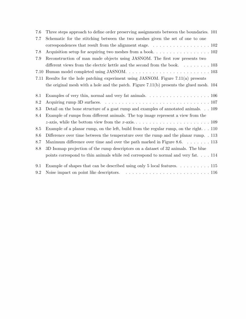
3.6 Objects in Library-II, composed of 32 objects divided in four classes. . . . . . . . . . 35

3.7 Global precision for different scalar functions. Dots correspond to results using

PVHK, lines correspond to results using C-PVHK. . . . . . . . . . . . . . . . . . . . 36

3.8 Precision per object using c3. Dots correspond to results using PVHK, and lines of

the same color correspond to results using PVHK-C. . . . . . . . . . . . . . . . . . . 37

3.9 Examples of partial from two objects in the instant noodles library. (a) is the object

with label 1 in Figure 3.6 and in Figure 3.7(d), and (b) is the object with label 6. . . 37

3.10 Sequences of humans moving freely in a room. . . . . . . . . . . . . . . . . . . . . . . 38

3.11 2D Isomap projection for a human moving. . . . . . . . . . . . . . . . . . . . . . . . 39

3.12 Confusion matrix between the humans in the frames with and without color. . . . . 39

3.13 2D Isomap projections of the descriptor from four partial view representations . . . 41

3.14 Comparison between ESF and PVHK on Library-II objects. . . . . . . . . . . . . . . 42

3.15 Impact of surface holes on ESF descriptors of planar surfaces. . . . . . . . . . . . . . 42

4.1 A mobile robot capturing a partial view of a mug from the viewing angle θ = (θ, φ). 46

4.2 Mug and cup library of partial views. . . . . . . . . . . . . . . . . . . . . . . . . . . . 46

4.3 Sequential Importance Resampling Filter for object estimation. . . . . . . . . . . . . 49

4.4 Example of the proposed bootstrap method. . . . . . . . . . . . . . . . . . . . . . . 49

4.5 Example the set of iterations of our Multiple Hypotheses for Multiple Views Object

Disambiguation algorithm. . . . . . . . . . . . . . . . . . . . . . . . . . . . . . . . . . 52

4.6 Dataset of partial views of a human in different orientations. The dataset corresponds

to two generic shapes: Human with no bag, at the top row and Human with a bag,

at the bottom row. . . . . . . . . . . . . . . . . . . . . . . . . . . . . . . . . . . . . 55

4.7 Dataset of similar chairs. . . . . . . . . . . . . . . . . . . . . . . . . . . . . . . . . . . 55

4.8 Evaluating efficiency and accuracy. . . . . . . . . . . . . . . . . . . . . . . . . . . . . 57

4.9 Confusion matrix between the testing dataset and the object library. . . . . . . . . . 58

4.10 Aggregate accuracy as a function of the number of particles per object. . . . . . . . 58

5.1 Shapes of regulars and complex objects. The chair is complex, because its back is

loosely connected to the seat. . . . . . . . . . . . . . . . . . . . . . . . . . . . . . . . 60

5.2 Temperature profiles over a kettle at different time instants. . . . . . . . . . . . . . . 60

5.3 Temperature profiles over a chair at different time instants. . . . . . . . . . . . . . . 61

5.4 Example of a complex object, composed by two squares connected by a bottleneck.

At the region of the bottleneck, we separate the surface in two fractions, S1 and S2,

by means of a boundary ∂S1. . . . . . . . . . . . . . . . . . . . . . . . . . . . . . . . 63

5.5 Impact of bottlenecks on the global time scale of heat propagation over an object. . 65

5.6 Impact of changes in the heat source position in objects with a very thin bottleneck. 66

5.7 Source position global derivative in three different chairs. . . . . . . . . . . . . . . . 67

5.8 Comparison between part identification approaches and the source position global

derivative. . . . . . . . . . . . . . . . . . . . . . . . . . . . . . . . . . . . . . . . . . . 68

5.9 Descriptors and weights for three objects: the kettle and the chair. . . . . . . . . . . 72

5.10 Time required for each vertex to reach a temperature of T=0.75. . . . . . . . . . . . 73

5.11 Comparison between PVHK and PVST for the three objects. . . . . . . . . . . . . 75

5.12 Complex objects, retrieved from 3D Google Warehouse, used in our experiments. . . 76

5.13 Aggregate precision using each of the three methods on the chairs dataset. . . . . . . 77

5.14 Confusion matrices using object libraries of different sizes. . . . . . . . . . . . . . . . 79

6.1 Impact on the PVHK by changes in the source position due to changes in the observer

position when we choose the source as the point closest to the observer. . . . . . . . 82

6.2 Impact on the PVHK by changes in the source position due to noise when we choose

the source as the point closest to the observer. . . . . . . . . . . . . . . . . . . . . . 82

6.3 Possible sources and descriptors for a chair partial view. . . . . . . . . . . . . . . . . 83

6.4 Example of a partial view, collected from view angle θ1, whose descriptor in the

dataset resulted from a source in a small part. . . . . . . . . . . . . . . . . . . . . . 86

6.5 Graph representing all possible combinations of descriptors for a single object. Nodes

correspond to possibles sources and edges the change in descriptors from consecutive

view angles. . . . . . . . . . . . . . . . . . . . . . . . . . . . . . . . . . . . . . . . . . 88

6.6 Datasets used for testing the accuracy on compact libraries using the PVST. . . . . 92

6.7 Aggregated precision for the chair and the guitar datasets using different approaches

for source selection. . . . . . . . . . . . . . . . . . . . . . . . . . . . . . . . . . . . . . 92

7.1 Example of a possible, and effortless, procedure for acquisition of two non-overlapping

meshes using a Kinect sensor. . . . . . . . . . . . . . . . . . . . . . . . . . . . . . . . 94

7.2 Construction of a mesh M from two other meshes, M1 and M2, by align both bound-

aries, B1 and B2 through a rotation R and a translation t. . . . . . . . . . . . . . . . 94

7.3 Example of two meshes connected by assigning edges from one boundary to the other. 97

7.4 Order constraints in the boundary: (a) shows how the orientability of surfaces in-

duces an ordering in the edges; (b) shows how the ordering reflects in the boundary. 99

7.5 Example of construction of an assignment between boundaries in the limit case where

the vertices in both boundaries coincide exactly. . . . . . . . . . . . . . . . . . . . . 100

7.6 Three steps approach to define order preserving assignments between the boundaries. 101

7.7 Schematic for the stitching between the two meshes given the set of one to one

correspondences that result from the alignment stage. . . . . . . . . . . . . . . . . . 102

7.8 Acquisition setup for acquiring two meshes from a book. . . . . . . . . . . . . . . . . 102

7.9 Reconstruction of man made objects using JASNOM. The first row presents two

different views from the electric kettle and the second from the book. . . . . . . . . 103

7.10 Human model completed using JASNOM. . . . . . . . . . . . . . . . . . . . . . . . . 103

7.11 Results for the hole patching experiment using JASNOM. Figure 7.11(a) presents

the original mesh with a hole and the patch. Figure 7.11(b) presents the glued mesh. 104

8.1 Examples of very thin, normal and very fat animals. . . . . . . . . . . . . . . . . . . 106

8.2 Acquiring rump 3D surfaces. . . . . . . . . . . . . . . . . . . . . . . . . . . . . . . . 107

8.3 Detail on the bone structure of a goat rump and examples of annotated animals. . . 109

8.4 Example of rumps from different animals. The top image represent a view from the

z-axis, while the bottom view from the x-axis. . . . . . . . . . . . . . . . . . . . . . . 109

8.5 Example of a planar rump, on the left, build from the regular rump, on the right. . . 110

8.6 Difference over time between the temperature over the rump and the planar rump. . 113

8.7 Maximum difference over time and over the path marked in Figure 8.6. . . . . . . . 113

8.8 3D Isomap projection of the rump descriptors on a dataset of 32 animals. The blue

points correspond to thin animals while red correspond to normal and very fat. . . . 114

9.1 Example of shapes that can be described using only 5 local features. . . . . . . . . . 115

9.2 Noise impact on point like descriptors. . . . . . . . . . . . . . . . . . . . . . . . . . 116

Chapter 1

Introduction

We envision robots capable of interacting and collaborating with humans in indoor environments.

To fulfill tasks in such environments, robots should be able to recognize and identify objects with

different appearance and regular shapes. Furthermore, in recent years, RGB-D sensors have become

ubiquitous, and both identification and object recognition from depth and RGB are hot topics in

computer vision. In this thesis, we contribute to the effort of having robots recognize objects as

perceived by RGB-D sensors. In particular, we introduce new forms of representing both: i) the

data retrieved by the sensor, and ii) the a-priori knowledge of the object shape.

The data provided by RGB-D sensors has three main characteristics: i) it corresponds to

an image whose pixels have information on the RGB color and depth of the object surface; ii)

it corresponds only to partial views of the object, i.e., to the visible surface of the object as

observed from a given viewing angle; and iii) it corresponds to a noisy version of the object surface.

Figure 1.1 exemplifies the two images provided by the sensor and the partial view of a human in

those images. We here address the problem of constructing object representations that allow any

future observation by an RGB-D sensor to be compared to previously observed and labeled partial

views of different objects, and thus recognized.

We use heat diffusion based descriptors to represent robustly individual partial views. Heat

diffusion is known to be resilient to the type of noise present in the RGB-D sensors. Such noise

takes the form of both perturbations to the 3D coordinates extracted from the depth information,

and to small holes in the object surface. Others have introduced different descriptors based on

heat diffusion and have used it to represent complete 3D object surfaces or points in complete

objects [13, 14, 18, 48, 56, 58]. Those descriptors depend both on local and global object geometry,

and thus do not handle properly large holes in the surface, e.g., the absence of half the object in

partial views would change any descriptor previously computed on the complete object. We here

contribute to the family of heat diffusion based descriptors with a new approach to representing

partial views.

Since a view from the sensor provides incomplete information on object surfaces, we represent

1

Figure 1.1: Data returned by an RGB-D sensor, comprising an RGB and Depth image. Using bothimages, we obtain an object partial view, which we use as input to our work.

complete objects as sets of partial views, each related to a different viewing angle. We thus organize

our a-priori knowledge of all objects of an environment as libraries, where we represent each object

as a collection of viewing angles and corresponding descriptors. We are concerned with the collection

size required to represent each object. When the collection is large, each new observation of that

object will likely be similar to a partial view in the collection, decreasing the probability of miss-

classifications. However, by increasing the library size, the effort required to recognize a single

partial view also increases.

This thesis focuses on human-made objects, often of the same class, e.g., mugs and kettles. These

objects have generic geometric features, such as planes and cylinders, and often share those features

with other objects. This lack of distinctive features leads to ambiguous shapes and to objects that

are only recognized when a small set of discriminative partial views is observed. Together with

libraries that represent only a sparse set of the possible set of partial views, ambiguous partial

views are one of the main sources of miss-classifications we faced in our experiments.

Miss-classifications can be detected and corrected when the agent estimating the object class

is a mobile robot capable of collecting multiple partial views from different viewing angles. By

combining past estimates on the object class while collecting new observations, the robot has

constant access to an increasingly accurate classification, and can stop the estimation when it finds

a distinctive feature that ensures high confidence. Others have previously introduced methods that

combine multiple 3D partial views, usually for the purpose of constructing a complete 3D model,

e.g., the kinectFusion algorithm [30]. Such methods could be used as a first step in a 3D object

recognition algorithm. However, the robot would first need to go around the complete object before

attempting to classify it. This thesis assumes a robot moving around an object, with access to its

odometry, and updating continuously the object class, by collecting and representing individual

partial views, combining past observations, making predictions on futures ones, and validating its

belief on classification. Such robot would not have to go around the complete object.

2

Heat diffusion based descriptors can seamlessly encode photometric information in the shape

descriptor. By indexing color and texture to the object shape, we can further disambiguate similar

shapes. Appearance provides discriminative information on the object, especially when we need to

identify same class, same geometry objects. Furthermore, indexing appearance to specific points on

the object surface allows to further discriminate between objects that share similar visual feature,

e.g., a human with a red shirt and blue jeans from another with blue shirt and read jeans.

We further realized that heat diffusion reflects strongly the existence of loosely connected parts,

and we introduced the concept of complex objects, e.g, the chair in Figure 1.2(a), as opposed to

those objects with compact surfaces, e.g., the kettle in Figure 1.2(b). We formalize the distinction

between regular objects and complex objects by exploring the impact of loosed parts on heat based

descriptors.

(a) Complex object (b) Regular objects

Figure 1.2: Shapes of regulars and complex objects. The chair is complex, because its back isloosely connected to the seat.

We also note that, as loosely connected parts often self occlude other parts, complex object

shapes change significantly between viewing positions, inducing changes in their representations.

To accommodated such variability and avoid miss-classification, complex objects require libraries

with a large number of partial views. Motivated by the difficulty in representing complex objects

by a collection of partial views, we address the construction of compact libraries, where descriptors

of the same object bundle together and are as far away as possible of other objects. We expect

that compact libraries obtain good recognition results even with a sparse set of partial views.

We address the problem of collecting partial views annotated by the respective sensor viewing

angle for inclusion in object libraries. In particular, the viewing angle is difficult to control and to

estimate. Thus, when we require precision in the viewing angle estimation, or partial views from

positions beyond the allowed by the experimental apparatus, we use existing 3D CAD models. Using

openGL libraries, we can generate partial views from these CAD models from all the positions and

sensor properties as we need. The CAD models can be retrieved from existing datasets, such as

3D Google Warehouse, or can be constructed by combining partial views into a single model. We

introduce an algorithm that allows the creation of 3D+RGB color models.

3

The tools we developed throughout this thesis are not constrained to the classification of objects,

and can be applied in different contexts. We had the opportunity to do so when members of the

Veterinary College of the Lisbon University asked us for help in estimating the Body Condition

Score (BCS) in goats in animal farms. The BCS conveys information on how fat or thin is an

animal, and is of relevance for milk production as both very fat and very thin animals have poor

production. Thus, we were invited to devise methods that would allow to automate the estimation

of the BCS while animals moved freely in a corridor, as showed in Figure 1.3. Such a premise

is in sharp contrast to current methods that require the physical constraint of each animal and a

specially trained veterinary. In an initial collaboration, [65], we showed that changes in the rump

volume are strongly correlated with BCS, as illustrated in the two rump examples in Figure 1.3

and that humans can be trained to consistently access BCS by visual inspection. In this thesis, we

show how our shape representation approach can assess changes in volume and identify very thin

animals.

Figure 1.3: Example of the acquisition setup and how goats are different types of surfaces that weneed to classify in order to identify extremes of very thin and very fat animals.

1.1 Thesis Question and Approach

This thesis seeks to answer the question:

How to represent 3D objects within a library, so that they can be identified from an

observation of an RGB-D sensor collected from at least one viewing angle, considering

that objects can have strong similarities or very complex shapes.

This thesis extends the heat diffusion based family of descriptors so that we can represent partial

views. In particular, we introduce the Partial View Heat Kernel (PVHK) that is resilient to noise,

is unique, depends on the viewing angle and can be extended to include photometric information.

PVHK represents the 3D surfaces corresponding to the visible part of an object in a holistic way,

i.e., so that a single descriptor contains information on the whole surface.

4

The information conveyed by PVHK represents the distance between points in the partial view

boundary and a reference point at the center of the surface. To be robust to noise, PVHK represents

distances using the solution to a heat diffusion process. Such process is inherently resilient to

small perturbations and holes on the surface and allows for the easy integration of photometric

information. As illustrated in Figure 1.4, we consider a heat source in the reference point and

simulate the heat diffusing through the surface. We then stop the simulation and evaluate the

temperature at the boundary. Points closer to the source will be warmer than points further away,

and thus temperature effectively represents distances.

Object t1 t2 t3 descriptor

Figure 1.4: Construction of the Partial View Heat Kernel by diffusing heat from a source andevaluating the temperature at the boundary.

The source position is fundamental to the descriptor, as the same partial view has different

descriptors if the source changes. We can choose the source position using different approaches

so that the resulting descriptor adapts to a specific need. For example, we can obtain descriptors

that depend on the observer position by choosing the source based on the relative position between

observer and object. Examples are: i) choosing the source as the point in the object surface that

is closest to the viewer, or ii) choosing the source as the point in the object surface that is closest

to the center of the segmented depth image. The above rules allow to consistently return the same

source position without prior knowledge of the object class and observer’s viewing angle.

The dependency of the descriptor on the viewing angle is essential when combining multiple

observations from different viewing angles to minimize miss-classification errors resulting from simi-

larity between object shapes and sparse libraries. We use a Bayesian setting to sequentially estimate

the probability of each object class, updating current estimates with each new observation. To im-

prove the estimate on the object class, the robot can use its odometry to predict new observations

and compare them with the actual ones, updating the belief on each classification.

The robot needs to keep estimates not only on the object class, but also in its relative position

with respect to the object. We use a Monte Carlo Sampling-Importance Resampling, for the

update, often used in tracking or localization algorithms. Common implementations use maps

from positions and objects to make predictions on observations and filter wrong hypotheses.

5

In our implementation of the particle filter, we follow [28] and use a map that relates observations

to objects and positions. The map seamlessly combines the notion of similarity between objects

and partial views into the filtering process, achieving better estimates of the object class with less

computational effort.

We further disambiguate similar shapes by seamlessly introducing color and texture information

into the heat diffusion process as a diffusion rate, e.g., we can say that heat diffuses faster in blue

than in red. The resulting descriptor represents the photometric information indexed to the 3D

shape, so that the descriptor is affected by both the RGB values and their geometric distribution

over the object surface.

To handle complex objects, we explored the impact of loose connections on the heat diffusion

to identify parts and define proper metrics for complex object’s descriptors. We also introduce

a second heat based partial view descriptor, the Partial View Stochastic Time (PVST), which

naturally handles the presence of parts. As the PVHK, the PVST represents partial views using a

robust representation of distances between boundary points and a reference point at the center of

the partial view. However, in PVST, distance is conveyed by the time required for the temperature

at each boundary point to reach a fixed temperature.

We further used the freedom to choose the source position to construct compact libraries for

complex objects, and thus reduce the number of partial views needed in the object library. We

take advantage of changes in the descriptor by the source position in the partial view to construct

object libraries that follow some desirable property. An example of such property is to have very

different descriptors for different objects.

We also introduce an algorithm for the construction of 3D+RGB models of regular objects. The

algorithm for the Joint Alignment and Stitching of Non-Overlapping Meshes (JASNOM), allows

the construction of an object 3D model by using only two, non-overlapping but complementary

partial views. Incidentally, such models can be used in the construction of object libraries as any

other CAD model.

We apply the above formalism for the classification of the Body Condition Score (BCS) of goats,

and in particular to identify very thin or very fat animals. To evaluate the BCS we assess the rump

volume by comparing the heat diffusion in the rump with the diffusion on a rump 2D projection.

The thinner the goat, the closest its rump is to a plane and the smallest the difference between

the heat diffusion in the two surfaces. The application is a promising example of other 3D images

understanding applications that we may tackle with the methodology we introduce in this thesis.

1.2 Thesis Contributions

The key contributions of this thesis are as follows:

• the Partial View Heat Kernel (PVHK) descriptor for the representation of noisy partial views

with photometric information;

6

• a multiple view multiple hypotheses algorithm for estimating objects from multiple observa-

tions;

• an analysis of the impact of the loose connections in complex objects to diffusion based

descriptors;

• a part-aware metric for the comparison of descriptors of complex objects;

• the Partial View Stochastic Time (PVST) for the representation of partial views of complex

objects;

• a source placement algorithm for the offline creation of robust object libraries;

• the Joint Alignment and Stitching of Non-Overlapping Meshes algorithm for the fast con-

struction of textured meshes of complete objects;

• an approach for the automatic identification of very thin goats in an animal farm using 3D

sensors.

1.3 Thesis Guide

The thesis is organized in 10 chapters where we present in detail the thesis contributions, and

results as we here we outline.

• Chapter 2 - Partial View Heat Kernel

We address the problem of representing the visible surface of an object, i.e., its partial view,

as collected by an RGB-D sensor. We review an existing class of 3D descriptors based on heat

diffusion, and introduce a partial view descriptor, the Partial View Heat Kernel (PVHK), for

the purpose of robustly representing partial views, and combining both the geometric and

photometric information into the same descriptor. We provide examples of descriptors in

rigid and non-rigid objects; analyze the impact of noise on the descriptor; and address the

conditions for which the descriptor is discriminative.

• Chapter 3 - Partial View Recognition

We address the problem of identifying a partial view by comparing its PVHK descriptor with

those stored in an object library. We introduce the distance metric we use for the comparison

of partial view descriptors, the modified Hausdorff distance. We then show the descriptor and

metric effectiveness on the recognition of different object sets. We use real everyday objects,

of similar size but distinct shape; same class objects both rigid and non-rigid, with almost

exact shape, but with different photometric information. We compare the performance of the

PVHK with other partial view descriptors.

7

• Chapter 4 - Incremental Object Recognition

We address the problem of combining information from multiple observations, captured by a

mobile robot that collects multiple partial views. We introduce our Multiple View Multiple

Hypotheses algorithm, and show that by using a map from observations to positions and

object classes, we can reduce the computational effort and improve recognition. We test

our algorithm in i) libraries of objects that are identical from some viewing angles, but have

distinctive features; and ii) libraries with a small number of partial views per object.

• Chapter 5 - Complex Objects and the Partial View Stochastic Time (PVST)

We address the problem of representing partial views of complex objects using heat diffusion.

We motivate the need to discriminate regular from complex objects, and show how the of

loosely connected parts of complex objects impacts heat diffusion. We then introduce a

new metric to compare partial view of complex objects, and a new descriptor, the Partial

View Stochastic Time, that seamlessly handles object parts. We empirically evaluate the

performance of the new approaches on libraries of partial views from 54 chair.

• Chapter 6 - Source Placement and Compact Libraries

We address the problem of defining a source position for a given partial view. We introduce

the notion of multiple descriptors for each partial view, by assuming that each point on

the surface is a possible heat source. We then choose among the multiple descriptors from

several partial views of the same object, those that lead to compact libraries, and to a better

recognition of each new partial view. We test our source placement in two libraries of same

class complex objects, one with guitars and the other with chairs.

• Chapter 7 - Construction of 3D Models

We address the problem of off-line creating object 3D models. We introduce an algorithm,

the Joint Alignment and Stitching of Non-Overlapping Meshes (JASNOM), that constructs

complete 3D models of object surfaces by aligning two non-overlapping meshes that cover

the complete object shape. By using directly the 3D information retrieved from the sensor,

JASNOM allows the creation of textured models. We empirically show that our algorithm

can generate complete models of common objects, such as kettles and books, as well as of

non-rigid shapes such as humans.

• Chapter 8 - Application to Automated Animal State Classification

We explore the possibility of using the developed approaches for shape representation and

understanding in applications beyond object recognition. In particular, we apply the heat

diffusion formalism to identify very thin animals in a dairy goat farm. We introduce our

approach to evaluating the rump volume by comparing heat diffusion in the rump with the

heat diffusion in a plane. We then show our representation results in an annotated set of 30

animals of different species, shapes, and sizes.

8

• Chapter 9 - Related Work

We provide an overview of the related work and how it relates to the work here presented.

In particular, we focus on the three fields to which this thesis contributes, namely: i)

3D+photometric representations; ii) multiple view object recognition; iii) mesh stitching.

• Chapter 10 - Conclusion

We conclude this dissertation with a summary of our contributions along with a discussion

of future work.

9

10

Chapter 2

Partial View Heat Kernel (PVHK)

In this chapter, we address the problem of representing the visible surface of an object, i.e., its

partial view, as retrieved by an RGB-D sensor. As we show in Section 2.1, these surfaces are rich

in information, as sensors provide both photometric and geometric information. However, the 3D

information provided by common RGB-D sensors is extremely noisy. We here introduce a noise

resilient partial view descriptor, the Partial View Heat Kernel (PVHK), [10], that represents both

the geometric and photometric information. While we leave to Chapter 3 a detailed analysis of

existing 3D partial views representations, in Section 2.2 we briefly overview existing representations

resilient to noise whose tools we share. We present PVHK in detail in Section 2.3, and in Section 2.4

we show how the PVHK can accommodate other sources of information, such as the photometric

information provided by the sensor. Finally, in Section 2.6 we highlight the main properties of the

PVHK.

2.1 Partial Views of RGB-D cameras

We address the representation of 3D partial views, i.e., the the surfaces formed by RGB-D sensors

as the object self occludes part of its complete 3D surface, as shown in Figure 2.1.

Figure 2.1: Partial view returned by an RGB-D sensor.

11

Furthermore, we assume a segmentation step, outside the scope of this work, that provides the

object partial view separated from the background. The focus of this work are rigid, human made

objects, but we empirically show that it can also handle non-rigid object such as those presented

in Figure 2.1.

We are interested in common depth sensors that provide partial views as an organized set of

vertices, such as the one highlighted in Figure 2.1. The vertices organization defines neighborhoods

between vertices and allows to represent partial views as triangular meshes, composed of non-

overlapping triangles that cover the visible surface of the object. Additionally, the sensor provides

the color of each vertex in the form of an RGB image.

Thus, the returned information from an RGB-D depth sensor is:

• an object mesh, M = {V,E, F}, composed of

– a set of vertices, V = {v1, ..., vNV };

– a set of edges, connecting neighboring vertices E = {e1 = (vl, vk), e2, ....eNE};

– a set of triangles, connecting edges F = {f1 = (el, ek, em), f2, ....fNF };

• the 3D coordinates of each vertex vi : xi ∈ R3, in the sensor coordinate system;

• the RGB values of each vertex, vi : ci ∈ R3.

However, the sensor is also noisy, inducing uncertainty in the 3D coordinates of surface points

and leading to surface holes, as exemplified in the human partial view in Figure 2.1.

To represent the partial views retrieved by such a sensor, we introduce the Partial View Heat

Kernel (PVHK) descriptor, which is:

1. Informative, i.e., a single descriptor robustly describes each partial view;

2. Stable, i.e., small perturbations on the surface yield small perturbations on the descriptor;

3. Inclusive, i.e., appearance properties, such as texture, can be seamlessly incorporated into

the geometry-based descriptor.

The combination of these three characteristics results in a representation especially suitable for

partial views captured from noisy RGB-D sensors during robot navigation or manipulation where

the object surfaces are visible with limited, if any, occlusion.

PVHK builds upon distances, over the object surface, between a reference vertex, vs, and

the boundary. The ordered set of all the distances represents surfaces in a unique way, apart from

symmetric and isometric transformations. In the example of Figure 2.2, we show the reference point

at the center of the partial view, and the different sets of shortest paths between the reference vertex

and each boundary point. We order all points in the boundary, {l0, la, ..., lc} as a line, and represent

12

Figure 2.2: Example of the information conveyed by the Partial View Heat Kernel (PVHK) repre-sentation.

each point by a function of the shortest distance to vs. The PVHK represents the complete surface

by the organized set of distance, represented in the plot on the right of Figure 2.2.

By representing the shape through its boundary, PVHK allows to easily compare two partial

views, without requiring any registration between the two. Furthermore, PVHK leverages on the

fact that the boundaries are well defined for each object and correspond to comparable sets of

points, i.e., we know that if two partial views were the same, we would have the same distances,

and if the distances are different, we can infer changes in partial views.

PVHK relies on diffusive geometry concepts to represent average distances ([42], [61]) to ensure

that the descriptor is stable with respect to noise and topological artifacts, e.g., holes or small

occlusions. Notably, we model the averaging process as the diffusion over the surface of heat

transferred to the surface at a single source point. Hence, PVHK represents a partial view as the

temperature at the boundary as a result of a heat pulse at the reference point v′s, as illustrated in

Figure 2.3.

Figure 2.3: Example of the main steps in the computation of the PVHK.

Finally, to ensure seamless integration of heterogeneous information, such as surface color,

PVHK treats different visual properties as different heat diffusion rates. As heterogeneous rates

lead to different temperature profiles on identical 3D shapes, PVHK uniquely represents objects

with the same geometry but different color or texture. By indexing color to the geometry, it

13

also differently represents objects with the same shape and similar appearance but with different

distributions.

2.2 Representations Based on Heat Diffusion

Diffusive distances [42] and diffusive geometry, provide a robust approach to representing shapes

subject to noise, and in particular to topological noise resulting from small holes in the surface.

Diffusive distances are related to shortest path distances, which are effective at representing a

surface topological information. However, are less sensitive to noise, as they are related to diffusive

processes occurring over a surface.

Diffusive processes can be interpreted as a sequence of local averaging steps applied to a function

representing some quantity, e.g., temperature. The averaging steps dilute local non-homogeneities

in the function and effectively transport the quantity from regions of higher values to regions of

lower values.

Figure 2.4 shows two examples of diffusive processes taking place on similar surfaces, different

only on account of a hole. In the first example, Figures 2.4(a) 2.4(c), the temperature evolves

from an initial source to the whole partial view following a concentric pattern, associated with the

shortest path between points. In the second example, Figure 2.4(d) to Figure 2.4(f), while the hole

affects the shortest path between points, it does not change the temperature significantly. The

averaging steps result in that the temperature at a point is defined first by the neighborhood and

only implicitly depends on the distance to the source.

(a) t1 (b) t2 > t1 (c) t3 > t2

(d) t1 (e) t2 (f) t3

Figure 2.4: Example of heat diffusion on similar surfaces. Color represents temperature and redregions are warmer than blue.

14

Diffusive processes can describe local features, such as the Heat Kernel Signature (HKS) [61]

and the Scale Invariant Heat Kernel Signature [14]. HKS is a highly robust local descriptor that

contains large-scale information. HKS represents a point with the temperature evolution after

placing a heat pulse on that point. The time evolution depends on how fast the temperature

diffuses to the neighborhood, which in turn depends on the object geometry.

While both descriptors, HKS and SI-HKS, perform well on complete 3D shapes, the same point

on an object surface may have different descriptors when parts of the shape are missing [14]. Thus,

as we address in Chapter 9, they are not suitable for the representation of partial views, where the

we have a large variability of shapes.

In the following, we review the formalism to simulate heat diffusing on surfaces represented by

meshes such as those returned by RGB-D sensors.

2.2.1 Heat Kernel

Formally, the temperature diffusion over a surface, as the one in Figure 2.5 defined by a set of

vertices V = {v1, v2, ..., vNV }, with coordinates {x1, x2, ..., xNV } together with a set of edges E =

{e1 = (vl, vk), e2, ..., eNE}, is described by Eq. 2.1:

Figure 2.5: Example of the mesh structure, where the dots represent vertices and lines connectingthe dots correspond to edges.

LT (t) = −∂tT (t), (2.1)

where L ∈ RN×N , is a discrete Laplace-Beltrami operator, and T (t) ∈ RN is a vector containing

the temperatures over all vertices in the surface at each instant t.

There are many approaches to representing the discrete Laplace-Beltrami operator [67]. We

choose a distance based one, which corresponds to a weighted graph Laplacian where the weight of

15

each edge is the inverse of its length:

LT (t) = (D −W ) T (t), (2.2)

[W ]vi,vj =

{1/‖xvi − xvj‖2, iff el = (vj , vi) ∈ E

0, otherwise, (2.3)

and where D is a diagonal matrix with entries Dii =∑N

j=1[W ]ij .

When we apply the Laplace-Beltrami to a vector T we obtain, for each vertex v, the averaged

difference between the value of [T ]v and its neighbors, i.e., if we represent the row v of L as Lv, we

can write:

LvT =∑i

([T ]v − [T ]i

)[W ]v,i (2.4)

Thus, the Laplace-Beltrami represents differences between the neighboring entries of a vector.

The heat diffusion equation in Eq. 2.1, relates the rate of change of temperature at a single

vertex with the difference between the temperature at that vertex and its neighbors. Furthermore,

with the Laplace-Beltrami operator defined in Eq. 2.2, closer neighbors have a closer influence in

the temperature. This means that sharp gradients in the temperature will be smoothed out very

fast. Furthermore, the heat diffusion naturally segments large edges, as they will have very small

weights.

The heat kernel, k(vj , vs, t) is the solution of Eq. 2.1 at time instant t and vertex vj when the

initial temperature T (0), is zero everywhere except at source vertex vs, i.e.,

T (0) : [T (0)]i =

{1, i = vs

0, otherwise. (2.5)

The above initial value problem has a closed form solution in terms of the eigenvectors, φi, and

eigenvalues, λi, of the Laplace-Beltrami operator, which is given by Eq. 2.6:

k(vj , vs, t) =N∑i=1

e−λit[φi]vj [φi]vs , (2.6)

where [φi]vj is the value of φi at the vertex vj .

Eq. 2.6 contains information on the complete surface through the eigenvalues and eigenvectors

of L, i.e., even when vj and vs are fixed points on the object surface, the descriptors changes if L

changes.

16

2.3 Computing Partial View Descriptors

We define PVHK as the surface boundary temperature measured by stopping the heat diffusion ts

seconds after placing the heat source on a vertex, vs.

To consistently obtain the same descriptor in independent observations, regardless of object

class or viewing angle, we need to define the stopping time, ts, the source vertex, vs, and the

boundary points where we compute the temperature.

2.3.1 Stopping time

The stopping time ts must be:

• large enough so that the temperature at the boundary, which is initially zero, raises above

some threshold;

• small enough so that the temperature does not become uniform over the whole surface.

In a graph, both events are governed by the diffusion time scale, which is proportional to λ−12 ,

the inverse of the first non-zero eigenvalue of the graph Laplace Matrix. For most regular objects,

composed of compact surfaces, the diffusion time scale ensures the two above conditions, and

guarantees that the temperature at the boundary vertices is representative of the distance to the

heat source. Thus, unless stated otherwise, we use ts = λ−12 . In Chapter 5, we will address in more

detail the impact of different values of ts in the descriptor.

2.3.2 Source Position

We choose vs using simple rules that do not require a-priori knowledge on the object class nor

orientation. For example, we use the point closest to the observer, or the point at the center of the

segmented depth image. Other approaches could be thought of, and implemented, but the most

important aspect is to use consistently the same approach.

The above suggestions have two main properties: i) are easy to find when the vertex coordinates,

xv ∈ X are in the sensor’s coordinate system; and ii) depend on the sensor position. When we

chose the source as the point closest to the observer, we find the source as:

vs = argminxv∈X

‖xv‖2 (2.7)

When we chose the source as the point in the center of the segmented depth image, we note that

the projection on the camera plane, corresponds to setting the z-coordinate in each xv to zero, so

we estimate the source position as:

vs = argminxv∈X

[xv]21 + [xv]

22 (2.8)

17

In Chapter 6, we address in detail the impact of different sources in the descriptor and propose

new approaches for the source placement.

2.3.3 Boundary Vertices

As the boundary is an oriented closed curve, to represent information on the boundary as a vector,

we to consistently define an origin to the curve. We here define such point by assuming that objects

have a privileged orientation, i.e., they have a top direction, which defines privileged points over

the boundary, e.g., the topmost. While other choices could be made, we define the boundary origin

based on a 2D coordinate system defined over the depth image, as illustrated in Figure 2.6. We

place the coordinate system origin at the center of the segmented depth image, and align its ey

axis with the depth image ev. We define the boundary origin as the intersection of the coordinate

system ex and the boundary, showed by the white spot in Figure 2.6.

Figure 2.6: Example of the local coordinate system that we use to define the boundary origin andorientation.

However, boundaries of different partial views have a different number of vertices. To have

comparable sets of temperatures, we cannot use the temperature over all the vertices. In a first

approach, we computed the temperature over the whole boundary, and then interpolate using

distances over the boundary. In a second approach, we used vertices over the boundary that, in

polar coordinates, were evenly spaced in the angle coordinate, as we show with the black dots in

Figure 2.6. The second option is more stable with respect to poor segmentation and noise in the

boundary coordinates, while the first is more stable with respect to deformable shapes.

2.3.4 Algorithm for Computing PVHK Descriptors

Given a segmented mesh, M , a set of coordinate vertices, X, expressed in the camera coordinate

system, and a set of ordered boundary vertices, B, we determine the source position, vs, then we

compute the Laplace-Beltrami operator, L, and estimate the eigenvectors and eigenvalues. From

the first non-zero eigenvalue, we compute the diffusion time scale ts = λ−12 . We finally compute

18

the temperature at the boundary as:

[z]j = k(vbj , vs, ts) ≈30∑i=1

e−λits [φi]vbj [φi]vs , (2.9)

which differs from 2.6 as we only use the lowest 30 eigenvalues, as e−λi/λ2 ∼ 0 for i > 30. Algo-

rithm 2.1 summarizes the steps required to estimate the PVHK descriptor.

Algorithm 2.1: Computing the PVHK descriptor

Input: Set of vertices X in the camera coordinate system, mesh M , Boundary verticesB = {vb1, vb2, ..., vbM}

Output: PVHK descriptor, z ∈ RM .Find source position:vs ← sourcePosition(X) (from Eq. 2.7 or 2.8)Compute Laplace-Beltrami operator:L← computeLaplaceBeltrami(M,X) (from Eq. 2.2)Estimate eigenvalues and eigenvectors:{φi, λi, i = 1, ..., 30} ← eigenvectors(L)Compute diffusion time scale:ts ← 1/λ2

Compute temperature at boundary:z : [z]i ← k(vbj , vs, ts) (from Eq. 2.9)

Figure 2.7, shows examples of descriptors of objects that share similar sizes and shapes: a

cylindrical box, a mug with a handle, a quadrangular box and a toy castle. We note for example

as the cylinder and the mug share an almost identical partial view, except that the cylindrical box

is taller than the mug. The difference in size is reflected in the descriptor, as the descriptor for the

mug has 4 hills while the descriptor for the cylinder has only 2. Also the mug handle is reflected

in the descriptor by a reduction in the temperature, resulting from the larger distance over the

boundary between the handle and the source.

2.4 Color and Texture in PVHK

We introduce color and texture information into PVHK representation by slightly modifying the

heat equation. The heat equation represents surfaces with the same diffusion rate on all points.

By using different rates at different points, we generate different descriptors for objects with the

same geometry and different descriptors for objects with the same color or texture but distributed

differently. Thus, to differentiate objects on both appearance and geometry, we relate appearance

with diffusion rate. We rewrite the heat equation in as:

C−1LT (t) = −∂tT (t) (2.10)

19

Figure 2.7: Examples of descriptors in different objects that share similar shapes and sizes. Thered dot corresponds to the source position.

where C is a diagonal matrix, whose element [C]v,v is any scalar associated with color, or texture,

at vertex v.

The solution to the non-homogeneous problem in Eq. 2.10 is identical to the solution to the

homogeneous problem in Eq. 2.4, but the eigenvalues, λci , and eigenvectors φci are now the solution

of the generalized eigenvalue problem Lφci = Cφciλci .

With the initial condition of Eq. 2.5, the heat kernel at t = ts then becomes:

kc(vj , vs, ts) =

30∑i=1

[φci ]vj exp(−λci ts)[φci ]vs [C]vs,vs . (2.11)

Our proposed approach differs from previous efforts to combine color and geometry, in particular

from [34]. Notably, we can extend [C]v,v to represent any scalar quantity and not just color.

Examples of useful scalars are the color hue value or cluster indices, e.g., after some clustering

preprocessing using any other appearance representation.

Hence, we introduce the C-PVHK, which is computed using Algorithm 2.1, only now we compute

the temperature at the boundary using Eq.2.11 instead of Eq. 2.9.

20

We illustrate the impact of adding appearance information to the descriptor by considering a

person in the same position, wearing the same clothes but with different colors, as in Figure 2.8.

We assume that [C]v,v corresponds to the color’ hue value when scaled to the interval [0.5,1] and

present the temperature along the boundary in the graphic on Figure 2.8. The four descriptors

present a common behavior associated with shape, e.g., the head, point l1, introduces the same

decrease in the temperature. However, the color modulates the temperature in a very significant

way. Notably, the color at the source, which in the example is placed in the blouse, leads to the

gap between Original+Different Skirt and Different Blouse + Different Dress.

Figure 2.8: Color impact on the descriptor. On the left, we present the mesh and colors. On theright, we present the respective C-PVHK descriptors

2.5 Computational Effort

Given a mesh with a boundary and a source position, the most time consuming step in the com-

putation of a PVHK descriptor is computing the first 30 eigenvectors and eigenvalues of a very

sparse matrix. Thus, the effort of computing the PVHK depends on the choice of algorithm to

estimate eigenvalues. We use Matlab eigs function as it is, to the best of our experience, the fastest

implemented algorithm to estimate the first n eigenvalues of sparse matrices.

The graphic in Figure 2.9 shows the time required for to compute the descriptor on a Intel(R)

Core(TM) i7-3770 Quad-Core @ 3.40GHz as a function of the number of the number of vertices in

the surface mesh.

The number of vertices in a partial view depends on the size of the object and of distance

between object and sensor. However, common everyday objects, observed from around 1m of

21

Figure 2.9: Time, in seconds, required to compute a PVHK descriptor as a function of the numberof vertices in the mesh.

distance have less than the 5000 vertices here presented, and the descriptor can be computed in

less then 0.2s. Larger meshes, e.g., as those from humans, will take a longer time, but still on the

order of the second per mesh.

2.6 PVHK Properties

We here address some of the PVHK properties, and the conditions for which the descriptor is

informative. Namely, we:

1. provide an estimative and examples of how much do we expect the descriptor of the same

partial view to change between observations due to sensor noise;

2. provide an estimative and examples of how much do we expect the descriptor of partial views

from similar viewing angles to change;

3. provide an estimative on the condition required for two partial views to have the same de-

scriptor.

2.6.1 Sensor Noise and Perturbations in the Descriptor

We here estimate how much change do we expect in the descriptors of two meshes of the same

partial view, M1 and M2, identical apart from changes in the coordinates, X1 and X2, due to

sensor noise.

22

Our analysis follows the propagation of noise from the sensor to the descriptor:

1. we analyze how the noise in coordinates changes the length of mesh edges and affects the

Laplace-Beltrami operator;

2. we use perturbation theory to estimate the relation between the magnitude of the noise in

the coordinates and the magnitude of change in the descriptor;

3. we provide the expected value of the descriptor in a noisy situation.

Our main result is that perturbations on the mesh have less and less impact on surface temper-

ature as t → +∞. Thus, by choosing large stopping times, we ensure that the descriptor is more

and more stable. We also estimate that a regular sensor, at 1m from an object, is associated with

changes in the temperature on the order of 10−3T , where T is the temperature over the boundary,

so we have larger perturbations in points where the temperature is higher, near the source, and

lower perturbations on the boundary, where we evaluate the temperature.

Impact of sensor noise to the Laplace-Beltrami operator

We assume that each z-coordinate returned by the camera is given by z = z0 + z20ε, where z0 is the

true distance between a point in the object surface and the camera, and ε ∼ N (0, τ2) is the camera

intrinsic random noise variation. This model is described for the Kinect camera in [33] with with

τ = 1.42× 10−3m−1.

In Appendix A, we show how noise propagates from coordinate z to the distance between

vertices and into to the Laplace-Beltrami operator. The main result is that the expected difference

between the operator of two meshes, Lδ = L1 − L2, is given by:⟨Lδ⟩

= 〈L1 − L2〉 ∝ ηL1, with

η ∼ O(z2τ2f2), where z is the distance to the object and f is the camera focal length. Using

typical values for the Kinect camera, with f ∼ 580 and z ∼ 1m we have η ∼ 5× 10−3.

Impact of perturbations to the Laplace-Beltrami operator in the temperature

Using first order perturbation theory, [16], we estimate the impact on temperature of perturbations

to the Laplace-Beltrami. In Appendix B we show how a small perturbation in the Laplace-Beltrami

operator impacts its eigenvectors and eigenvalues and how the perturbation passes on to the tem-

perature.

The main result is that the temperature perturbation, T δ(t) = T 1(t)− T 2(t), depends linearly

on: (i) Lδ; and on (ii) exp(−Λ1t). While the former leads to⟨T δ⟩∼ 5× 10−3T , the latter implies

that:

T δ(t) −−−−→t→+∞

0. (2.12)

23

Example

We compare our estimative with the real changes in the descriptor using a synthetic mesh, repre-

sented in Figure 2.10. Figure 2.10(a) shows how the descriptor changes with the increase in noise

level. The blue line corresponds to the mean distance to the noiseless descriptor, taken over 20

trials. The descriptors were computed at a fixed time instant, t = 1/λ2. The red lines correspond

to the mean distance ± the standard deviation and represent the range of change that we can

expect in the descriptors. Figure 2.10(b) and Figure 2.10(a) show how noise levels of 5× 10−3 and

10× 10−3 in the depth image reflect on the surface mesh and temperature profile at the boundary.

In particular, they show how the global shape of the descriptor does not change with noise.

(a) Effect of camera noiselevel.

(b) Noise level of 5 × 10−3 (c) Noise level of 10 × 10−3

Figure 2.10: Impact of noise on the descriptor for a circle at a 1m from the sensor.

2.6.2 Changes in the Viewing Angle

We here estimate how much changes do we expect in the descriptors of two meshes of the same

object, M1 and M2, obtained from similar viewing angles.

Changes in the viewing angle have a two fold impact on the descriptor:

1. the partial view changes, as occluded parts become visible;

2. the source position changes, as we consider sources that depend on the sensor.

We cannot model the first, as it depends only on the object surface, in the same way that we

do not know what happens to the source when the sensor moves. However, we do know that in

most regular objects, with compact surfaces, most changes in the viewing angle will result in small

changes in the source position over the surface. Furthermore, regular objects, such as a box or

a book, have similar partial views when we change the viewing angle, and only occasionally will

occluded parts become visible.

24

Our main result is that under the above conditions, perturbations on the viewing angle lead to

perturbations in the temperature at the boundary, which again go to zero when t→ +∞.

We exemplify the impact of changes in the temperature from changes in the source position using

the synthetic dataset of four objects from Figure 2.7, with partial views collected from multiple

viewing angles.

Changes in the temperature from changes in the source

When the source moves from a vertex vs to another vertex on its neighborhood, vl : (vs, vl) ∈ E,

the temperature at vertex vb1 ∈ B changes as: ∆Tvs = k(vb1, vs, ts)− k(vb1, vl, ts).

If we take the average over all vertices in the neighborhood to where the source can move, and

weight with respect to the distance to the neighbor, we arrive at:

∆Tvs =∑

vl:(vs,vl)∈E

(k(vb1, vs, ts)− k(vb1, vl, ts))/‖xs − xl‖2 (2.13)

=LsTvs = −∂tTvs (Eq. 2.4 and Eq. 2.1) (2.14)

=

Ns∑k=2

λ2[φi]vs [φi]vb1e−tsλi (2.15)

where Ls is the row of the Laplace-Beltrami operator L. Again, when time increases, as all λi are

positive, changes in the descriptor due to changes in the source position go to zero.

Example

We here provide an example of the set of partial view descriptor of the four objects in Figure 2.7.

We show in Figure 2.11 an Isomap projection of the descriptors from a smooth sequence of viewing

angles retrieved from the four objects.

We use the mug as an example of the impact of changes in the viewing angle in the descriptor.

At each figure, we show the partial view associated with the viewing angle, with the source1 marked

in black. We also present the descriptor of each partial view, and we mark its respective position

in the Isomap.

Finally, we note that nodes in the Isomap are connected to neighboring viewing angles, and

that there is a relation between similar viewing angles and similar partial view descriptors. This

is particularly clear when we look at the sequence of mug descriptors and their position in the

Isomap.

The set of descriptors associated with the cylinder does not display these properties, as its shape

does not change.

1In this experiment, we chose the source as the point closest to the observer.

25

(a) t1 (b) t2

(a) t3 (b) t4

Figure 2.11: 2D Isomap projection applied to the set of objects in Figure 2.7.

2.6.3 Uniqueness of the Boundary Temperature

Let M1 and M2 be two generic meshes. We want to know if M1 and M2 can be different, even

when their temperature profile obtained at a fixed time instant, ts, over a subset of vertices on the

mesh boundary, v ∈ B, is the same.

We know that if temperatures over all points, at all time instants, in M1 and M2 are the same,

then the two meshes are identical, [48]. However, we only have a subset of vertices at a fixed time

instant.

In general it is difficult to define conditions for which two identical temperatures would necessar-

ily imply the same surface. However, we here show sufficient conditions under which the descriptors

are the same, regardless of surface geometry. We then provide intuition on why these conditions

are unlikely to hold often.

Assuming that we have two different meshes, M1 and M2, each with its Laplace-Beltrami

operator, L1, L2, two surfaces will have the same descriptor if:

z1 = z2 ⇔ Φ2B c1(ts) = ΦB

2 c2(ts), (2.16)

where Φ1,2 = [1, φ1,22 , φ1,2

3 , ...] are two collections of orthogonal vectors, resulting from the eigende-

composition of symmetric matrices, the Laplace-Beltrami operators L1 and L2. Furthermore, by

26

how they were defined, both L1 and L2 share a common eigenvector 1, associated with the eigen-

value λ1 = 0. ΦB1,2 are subsets of rows of Φ1,2 corresponding to boundary vertices. The space of all

possible descriptors, i.e., considering all possible sources and stopping times, ts, for both M1 and

M2 are spanned by Φ1, Φ2 respectively. When we fix the source and ts, we define the coordinates

of each descriptor in the two spaces: c1,2(ts) = e−Λ1,2tsΦT1,2T (0).

The condition in Eq. 2.16 holds at least in two situations. The first is when the two spaces

spanned by Φ1 and Φ2 intersect at exactly c1(ts) and c2(ts).

The intersection is unlikely if the set of possible descriptors, generated by the above vectors

c1,2, is very sparse. So, first their l0-norm must be large, to ensure that they are spreaded around,

but the number of values that they can take has to be reduced.

Given the exponential e−Λ1,2ts , the norm of c1,2 clearly decreases with time, so ts must be the

smallest possible. Here we note that by fixing ts = 1/λ2, and provided that λ2 ∼ λ3, λ4, ..., λm

and that [φik]vs 6= 0∀k=1,...,m, c1,2 have a large enough dimension, reducing the probability of an

intersection.

We also ensure that the number of accessible values is reduced by considering that the initial

condition in Eq. 2.5 is zero everywhere and N for entry vs, we further constrain c1,2.

The second situation is when c1,2 becomes orthogonal to Φ1,2b , which happens, e.g., when ts = 0,

which we never consider throughout this work.

In Chapter 5, when analyzing the impact of stopping time in the descriptor, we will revisit

this problem in detail. Here we just point out that, while large values of ts lead to a noise robust

descriptor, they also yield a less discriminative one.

2.7 Summary

In this chapter, we introduced the Partial View Heat Kernel (PVHK) descriptor, for representing

the visible surface of an object as returned by a depth sensor, such a Kinect camera. While the

sensor provides rich information, the 3D information is often noisy. We here showed how to compute

the PVHK descriptor, and how to incorporate different information types onto the 3D description.

In particular, we showed how to incorporate the RGB information provided by the sensor with the

3D surface.

We have also showed how the descriptor provides a noise resilient descriptor of the partial views,

which makes it ideal to represent noisy surfaces.

27

28

Chapter 3

Partial View Recognition

In this chapter, we address the problem of identifying a partial view by comparing a PVHK descrip-

tor with those stored in an object library. We first define the distance metric we use to compare

partial views descriptors. In Section 3.3 we show the descriptor and metric effectiveness on the

recognition of real everyday objects, of similar sizes but distinct shapes. In Section 3.4 we show

how using color allows to disambiguate between same class objects, which share similar geome-

tries. In Section3.5 we show how we can use PVHK, and C-PVHK, in non rigid shapes such as

humans. Finally, in Section 3.6 we compare the performance of the PVHK with other partial view

descriptors.

3.1 Recognizing Objects Using PVHK Descriptors

To recognize the object class of a partial view, we compute the PVHK descriptor of that partial

view and then to compare it against previously labeled partial view descriptors, stored in an object

library O.

We represent objects in the library as sets of partial views, corresponding to the visible surface

of the object, as seen from multiple viewing angles, as represented in Figure 3.1. Its partial view is

labeled with respect to the sensor position in the object coordinate system.

It is through the object library that we map each object and viewing angle with descriptors.

Formally:

Definition 1. An object library, O = {(s1, zs1), (s2, zs2), ..., (ssM , zsNθ )}, is a set of tuples (S,RM )

that maps a descriptor z ∈ RM to a partial view label s ∈ S.

As partial views are defined by an object and a sensor viewing angle in the object coordinate

frame, we label each partial view as s = (o, θ).

In this chapter we use different libraries to highlight different aspects of the PVHK, namely:

• Library-I composed of Real Rigid Objects, provides empirical evidence on the accuracy of

our representation using sensor data;

29

Figure 3.1: Objects in the library are represented by multiple partial views, each associated withthe sensor viewing angle in the object coordinate system.

• Library-II composed of Real And Colorful Objects, retrieved from [35], illustrates the use

both color and 3D information and applicability of the descriptor on rigid objects;

• Library-III composed of Non rigid Objects, with and without the respective RGB informa-

tion, illustrates the applicability of the descriptor on non rigid objects;

• Library-IV composed of partial views rendered from CAD models, and previously presented

in Figure 2.7.

For all recognition tasks, we assume a nearest neighbor classifier. I.e., we search among all

partial views in the object library by the closest to the testing partial view and assume they belong

to the same object. We define the closest object based on a Modified Hausdorff distance, which

provides a relevant distance between descriptors.

3.2 Distance Between Partial Views

We define the distance between two partial views as the distance between their descriptors. How-

ever, due to noise, partial views of the same object, seen from the same viewing angle by a noisy

sensor, generate necessarily different descriptors.

The sensor noise affects not only the boundary temperature but also the boundary points where

we compute the temperature, i.e., the boundary parameterization. If we consider the descriptor as

the temperature at 1/M intervals of the boundary length, changes in the length caused by noise

lead to changes in the vertices where those intervals start and end.

30

Moreover, changes in boundary parameterization may lead to drastic changes in vector norms,

e.g., l1 or l2, as illustrated in Figure 3.2(a). In the example, while both descriptors share the same

shape, there is a small shift in the boundary. In regions of rapid change in the descriptor, the small

shift results in large differences in temperature and thus in large distances between descriptors.

(a) Error only on the temperature (b) Error on both temperature and boundary

Figure 3.2: Two approached for comparing descriptors assuming different sources of error.

Thus, we compare two descriptors using the modified Hausdorff distance, which provides a

measure of the difference between the two curves in the graphic. As illustrated in Figure 3.2(b),

when computing the Hausdorff distance we compare each point in one curve with its closest on the

second curve. Thus small shifts in boundary length will have a small impact on the distance.

To compute the distance between two descriptors, we first represent each as curves in 2D, i.e.,

the descriptor z ∈ RM becomes a set of points η = {[1/M, [z1]1], [2/M, [z2]2], ..., [1, [zM ]M ]}.

Then, we estimate the distance between two observations using Eq.3.1.

d(z, z′) = dMH(η, η′) = min

∑x∈η

infy∈η′‖x− y‖2,

∑y∈η′

infx∈η‖x− y‖2

(3.1)

We summarize the steps required for computing the distance between two partial view descrip-

tors z1, z2 in Algorithm 3.1.

Algorithm 3.1: Computing distances between PVHK descriptors.

Input: PVHK descriptors, z1 and z2

Output: d(z1, z2)Construct curve:η1,2 ← {[1/N, [z1,2]1], [2/N, [z1,2]2], ..., [N, [z1,2]N ]}:Compute Hausdorff distance:d(z, z′)← dMH(η1, η2) (from Eq. 3.1)

31

3.3 Identifying Real Objects

We demonstrate the effectiveness of PVHK on object recognition tasks from 3D partial views using

Library-I. The library is composed of 13 regular objects, with compact surfaces, of similar sizes but

with different and without RGB values.

3.3.1 Library-I

With a Kinect camera, we collected two sets of partial views, for training and testing respectively,

of 13 rigid and similar size objects, represented in Figure 3.3. Moreover, the partial views for each

object correspond to a known and dense sampling on the observer orientation, θ ∈ [0o, 360o].

Figure 3.3: Dataset of small objects grasped by a Kinect sensor.

Figure 3.4 represents the acquisition and labeling apparatus. We placed the objects individually

in a red cardboard, so that we could easily segment the background. Furthermore we used QR-codes

and the Aruco library[25] to define the orientation of the cardboard with respect to the observer.

32

Figure 3.4: Acquisition setup for Library-II. Objects are placed on a red cardboard, for backgroundsegmentation, together with QR-codes for orientation estimation with the Aruco library.

Object Training Testing Object Training Testing

Electric Kettle 434 306 Creamer 904 471

Mug with handle 777 374 Toy car 935 535

Mug without handle 1041 524 Cylinder 660 269

Cube 1039 448 Pencil holder 681 398

Book 514 292 Columns 675 302

Cookie box 778 401 Lego box 884 430

Stabler 970 459

3.3.2 Experimental Results

Figure 3.5 highlights the individual partial view results for PVHK using a confusion matrix that

relates the true viewing angle of each element on the testing dataset, on the x-axis, to the viewing

angle of the closest descriptor from the training dataset, on the y-axis. The confusion matrix shows

that a large percentage of miss classifications results from confusion between similar objects, e.g.,

the cream pitcher and the mug. Besides the miss-classification of object category, the matrix shows

also the inner category confusion that we expect in objects with strong symmetries, such as those

used in the dataset. The overall accuracy was 95% and the accuracy for each class is represented

in the column to the right of the matrix.

We note that the two objects with a larger confusion among them are the creamer and the

mug with a handle, which are very similar. Also, we note that in objects such as mug without

handle, there is a large confusion within the viewing angles, which is expected as the object is

symmetric with respect to changes in viewing angle. A similar effect can also be observed in the

Lego box, where we can see that there is a strong confusion between two sets of viewing angles,

which correspond to the box symmetry.

3.4 Disambiguation Through Color

When objects have very similar shapes, we can distinguish between them using color or texture. We

here show how the color extension of the partial view heat kernel allows to disambiguate different

33

Figure 3.5: Confusion matrix for PVHK testing

instances within four different classes of small real objects.

We recall that C-PVHK is computed as the solution of Eq. 2.10, that we here re-write:

C−1Lf(t) = −∂tf(t) (3.2)

and recall that C is a diagonal matrix, whose entry [C]v,v = c(v) provides a scalar representations

of color as different diffusion rates.

We evaluate the use of color by comparing the performance of C-PVHK with that of PVHK.

We thus experiment different maps from the RGB values, provided by the sensor, to the scalar

[C]v,v. This map can take many forms, and we could think of specially tailored maps for any

given library. Here we focus on simple experiments, which show how choices on [C]v,v impact the

descriptor performance. In particular, we are interested in understanding if smaller values of [C]v,v

would have any impact on recognition. We expect that the results will help modeling future maps.

Finally, we also consider the impact of using more or less partial views on the object library.

Our experiments show that, by indexing color to the geometry, we improve recognition results.

34

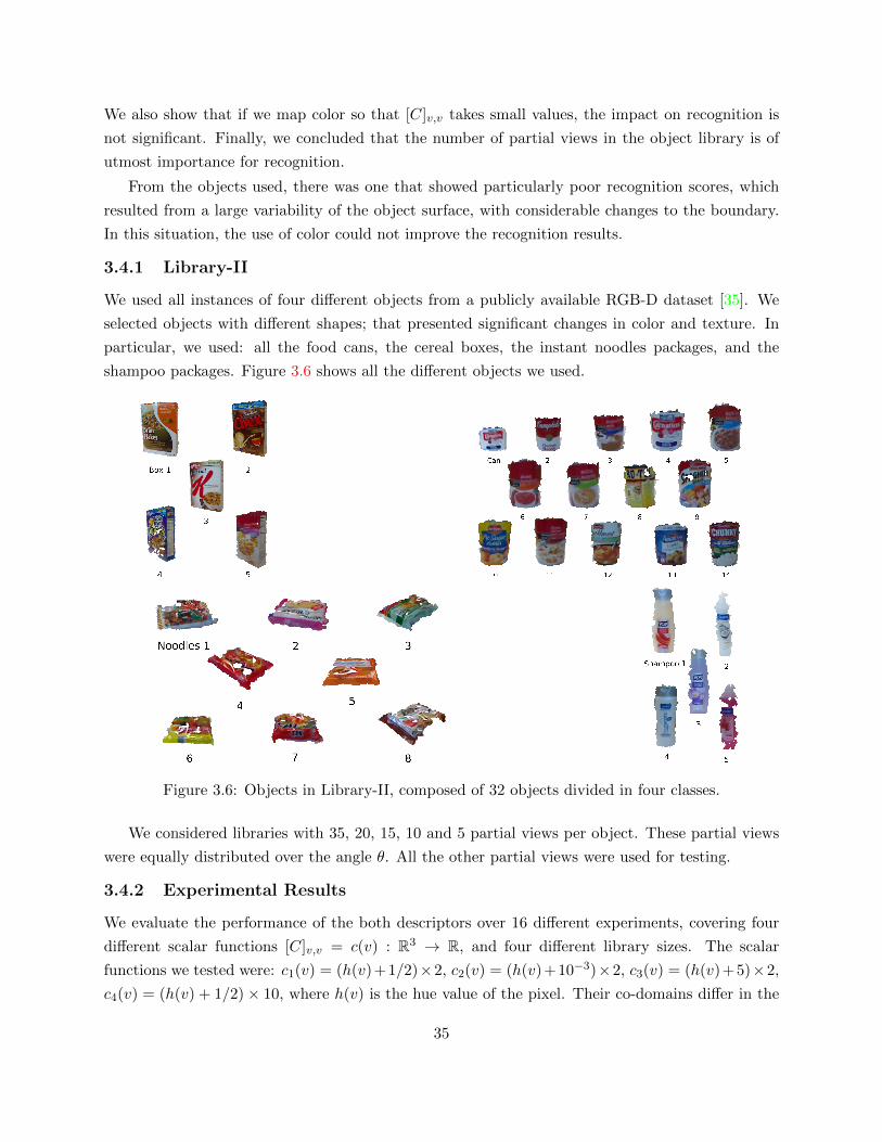
We also show that if we map color so that [C]v,v takes small values, the impact on recognition is

not significant. Finally, we concluded that the number of partial views in the object library is of

utmost importance for recognition.

From the objects used, there was one that showed particularly poor recognition scores, which

resulted from a large variability of the object surface, with considerable changes to the boundary.

In this situation, the use of color could not improve the recognition results.

3.4.1 Library-II

We used all instances of four different objects from a publicly available RGB-D dataset [35]. We

selected objects with different shapes; that presented significant changes in color and texture. In

particular, we used: all the food cans, the cereal boxes, the instant noodles packages, and the

shampoo packages. Figure 3.6 shows all the different objects we used.

Figure 3.6: Objects in Library-II, composed of 32 objects divided in four classes.

We considered libraries with 35, 20, 15, 10 and 5 partial views per object. These partial views

were equally distributed over the angle θ. All the other partial views were used for testing.

3.4.2 Experimental Results

We evaluate the performance of the both descriptors over 16 different experiments, covering four

different scalar functions [C]v,v = c(v) : R3 → R, and four different library sizes. The scalar

functions we tested were: c1(v) = (h(v)+1/2)×2, c2(v) = (h(v)+10−3)×2, c3(v) = (h(v)+5)×2,

c4(v) = (h(v) + 1/2)× 10, where h(v) is the hue value of the pixel. Their co-domains differ in the

35

lower and upper bounds, as well as range.

Figures 3.7 (a)-(d) present the results for each color combination as a function of the size of the

testing library. The results are aggregated by class, representing the precision over all the instances

of each class.

(a) (b)

(c) (d)

Figure 3.7: Global precision for different scalar functions. Dots correspond to results using PVHK,lines correspond to results using C-PVHK.

In all the experiments, the use of color clearly improved precision results. The results also

improved with library size, which is expected considering that we have a better coverage of all

possible descriptors associated with each object. Finally, results also hint to no direct relation

between the range of values that c(v) can take and precision. However, using small values of [C]v,v

clearly affects the results.

Figures 3.8(a)-(d) show precision results for each object in the library using the scalar function

[C]v,v = c3(v).

We see that not all objects are sensitive to the library size, e.g., instances of the shampoo class

present similar precisions regardless of library size. Also, some instances of the Instant Noodle class

clearly present a low precision, in particular, the object with the label 1. In Figure 3.9(a), we show

different partial views of this object, separating them between those that were correctly classified

and those that were incorrectly classified. What we notice is that the change in shape between

viewing angles is considerable. Thus, adding color to the representation just changes the descriptor

in a non expected way, yielding it more similar to other objects.

36

(a) (b)

(c) (d)

Figure 3.8: Precision per object using c3. Dots correspond to results using PVHK, and lines of thesame color correspond to results using PVHK-C.

(a) Instant Noodles 1 (b) Instant Noodles 6

Figure 3.9: Examples of partial from two objects in the instant noodles library. (a) is the objectwith label 1 in Figure 3.6 and in Figure 3.7(d), and (b) is the object with label 6.

3.5 Non Rigid Shapes

Deformations in both body and clothes shape raise important challenges for human tracking using

3D descriptors and affect the efficiency of representations aimed for rigid shapes. However, the heat

kernel is invariant to surfaces isometric changes, which means that PVHK will also be resilient to

37

most deformations.

We here show that the PVHK changes mostly when there are considerable changes in the body

shape, e.g., when arms move away from the body. These drastic changes in the shape lead to

important changes in the descriptor, and are more pronounced than those caused by moving the

arms around when they are already away from the body or those caused by walking with the arms

next to the body.

On the other hand, the body shape itself is too similar across individuals to allow recognition

using the PVHK. Thus, we again use C-PVHK and show that we can distinguish between them.

3.5.1 Library-III

For the purpose of showing how does the descriptor changes with deformations in body shape, and

how we can use color to distinguish between individuals, we introduce two sequences of humans

moving around. The first sequence represents a human moving around in a room, and purposefully

changing the body shape between the three main positions showed in Figure 3.10(a). The second

sequence consists of two humans moving side by side, as showed in Figure 3.10(b).

(a)

Frame 1 Frame 4 Frame 8 Frame 16Frame 13

(b)

Figure 3.10: Sequences of humans moving freely in a room.

38

3.5.2 Experimental Results

Results show that the first sequence generated two distinct groups of descriptors, depending on

whether arms were close or separated from the body. The groups are visible in Figure 3.11, where

we represent a 2D Isomap projection of the descriptors collection and their and respective labels.

This means that we can represent an articulated body by a reduced number of rigid shapes and

thus easily perform tracking and recognition tasks.

Figure 3.11: 2D Isomap projection for a human moving.

The results on the second sequence show that it is impossible to recognize between two indi-

viduals using just the PVHK. But again we distinguish between the two humans using PVHK-C

descriptor. Figure 3.12 shows the two distance matrices. Furthermore, by being insensitive to the

low level details of face features, PVHK allows for anonymously tracking humans in a contained

environment.

Figure 3.12: Confusion matrix between the humans in the frames with and without color.

39

3.6 Comparing with Other Descriptors

We evaluate the performance of our descriptor when compared with three existing descriptors:

1. the Scale Invariant Heat Kernel Signature (SI-HKS) [14];

2. the Viewpoint Feature Histogram (VFH) [54];

3. the Ensemble of Shape Features (ESF) [70].

We evaluate the performance of the three descriptors on Library-IV, composed of the four

objects presented in Figure 2.7. The results show that the ESF and PVHK represent the four

objects in such a way that there is little confusion between descriptors of different objects. We

then show that, while ESF performs well in the recognition of multiple objects, the PVHK is more

suitable for the representation of objects with large surfaces, such as the cereal boxes in Library-II.

3.6.1 Brief Description of other partial view descriptors

From the three descriptors, the VFH and ESF, are retrieved from the PCL library [55], and were

specifically introduced for the representation of partial views. We implemented the SI-HKS de-

scriptor following [14].

Viewpoint Feature Histogram

The VFH is a histogram of changes in surface normals orientation, with respect to a an averaged

normal, computed at a central point in the surface.

Ensemble of Shape Functions

The ESF is a set of histograms of shape functions: i) distances between randomly selected vertices;

ii) area of triangles formed by randomly selecting three vertices; iii) angles of those triangles,

Furthermore, to increase the discriminative power of the descriptor, each of these are separated

by whether the path between the two randomly selected vertices is over the surface, outside the

surface, or part over and part outside. So, for each of the above three shape functions, there are

three histograms, one for each type of path. A fourth function, and respective histogram, further

discriminate mixed paths by the ratio between the length outside and inside the object surface.

Scale Invariant Heat Kernel Signature

The Scale Invariant Heat Kernel Signature corresponds to the absolute value of the Heat Kernel

Signature time Fourier transform. The Fourier transform represents changes in the object scale as

a change in phase, which is then discarded by taking the absolute value. Geometric words are then

identified by clustering, using k-means [6], the SI-HKS features extracted from all surface points in

object surfaces. Each partial view is then represented by the distribution of visual features present.

We note that both the Heat Kernel Signature and the Scale Invariant Signature, depend on the

complete shape of the object, and thus the same geometric feature will depend on the partial view.

40

3.6.2 Results in Library-IV

In Figure 3.13, we represent an Isomap projection for the set of objects and descriptors. As in

Figure 2.11, dots correspond to partial views, and connected dots are contiguous view angles.

From the projections we see that ESF and PVHK are more effective at separating objects, since

partial views from different objects do not get mixed in a 2D projection. However, ESF does not

change as smoothly with the view angle as PVHK, notably in the cup and the castle example. In

fact, the ESF depends only on the surface shape, and not on sensor position. Thus, in regular

objects, such as boxes, where the shape does not change considerably with variations on the sensor

position, the ESF provides no insight on the viewing angle.

Figure 3.13: 2D Isomap projections of the descriptor from four partial view representations

As acknowledge in [14], the SI-HKS was thought for complete 3D objects, and is strongly

affected by missing object parts, as the heat kernel depends on the complete surface shape. So, its

performance in this library of partial views is expected.

The PVHK descriptor performs as well as the ESF in the above dataset, however the PVHK is

more suitable for representing objects composed of large planar surfaces, such as the Cereals Boxes

in Library-II. The results showed in Figure 3.14, show that when we want a higher accuracy, the

PVHK performs better than the ESF.

While ESF performs very well on many objects, it is sensitive to changes in the object topology.

The ESF separates each shape function in three histograms that depend on whether the path

between two points lays over the surface or not. Points collected over a plane will contribute only

41

Figure 3.14: Comparison between ESF and PVHK on Library-II objects.

for one of those histograms, as all the paths connecting them lay over the surface. As illustrated in

Figure 3.15, when we introduce a hole in the center of the plane, paths will leave the surface, and

the shape function for that path counts towards a different histogram. In the example, we note

that while the path V1− V2 and V1− V3 belong to the same plane, they will contribute to different

regions of the descriptor. We note that the impact is not felt so strongly on the other shapes, as

the histogram for the planes, is less relevant for the shape description.

Figure 3.15: Impact of surface holes on ESF descriptors of planar surfaces.

42

3.7 Summary

From classification results using datasets of real objects, we show the PVHK potential for (a)

discriminating everyday objects of regular sizes and similar shapes and (b) tracking humans.

PVHK is specially suitable in situations with no occlusion from other objects. We thus foresee

a large spectrum of applications for PVHK, ranging from robot manipulation, where in front of the

robot is only the target object, to robot controlled perception, where the robot can intentionally

move to avoid occlusions.

Furthermore, C-PVHK represents color distributions over geometry. This opens the door to

many other applications where we need to differentiate objects with the same geometry, from which

we highlight the possibility to identify boxes in a supermarket or anonymously tracking humans.

When compared with other descriptors, the PVHK provides a better accuracy than other heat

based descriptors, the SI-HKS, and than the VFH. It also performs better than the ESF on objects

composed mainly of planar surfaces, where the presence of holes impacts the ESF strongly.

43

44

Chapter 4

Incremental Object Recognition

In this chapter, we address the problem of recognition from multiple viewing angles. Often it is

not possible to recognize objects from a single partial view with a large certainty. In particular,

as showed in [12, 52], recognition from a single partial view is difficult when: i) objects are similar

and ambiguous from at least some viewing angles; ii) object libraries are sparse, in the sense that

the number and the quality of the partial views kept in the library is not representative of the

object. When the agent observing the objects is a mobile robot, it can collect multiple partial

views to disambiguate or validate initial guesses. The challenge is to efficiently combine the set

of observations into a single classification. We approach the problem with a multiple-hypotheses

filter that combines information from a sequence of observations given the robot movement. We

further innovate by off-line learning neighborhoods between possible hypotheses based on similarity

between observations. Such neighborhoods translate directly the ambiguity between objects and

allow to transfer the knowledge of one object to the other. In Section 4.2 we introduce the problem of

combining multiple observations, without knowing the viewing angle from where each was retrieved.

In Section 4.3 we introduce the appearance models required to estimate the class of each partial

views. Finally in Section 4.4 we introduce our Multiple View Multiple Hypotheses algorithm and

in 4.5 we evaluate its performance in different datasets.

4.1 Ambiguous Objects

We assume a mobile robot, equipped with an RGB-D sensor, that collects partial views of an object

as illustrated in Figure 4.1.

Furthermore, we start by assuming that the robot only expects to find two objects in his

environment: a mug with a handle and a mug with no handle. We show in Figure 4.2 the object

library for the two objects: the 3D shapes correspond to selected partial views and the colors

correspond to the temperature over the surface at t = ts. We recall that an object library, O =

{(s1, zs1), (s2, zs2), ..., (ssM , zsNθ )}, maps a descriptor z ∈ RM to a partial view label s = (o, θ) ∈ S.

The graphic associated with the 3D shapes corresponds to the PVHK descriptor, z. In the

45

Figure 4.1: A mobile robot capturing a partial view of a mug from the viewing angle θ = (θ, φ).

center, we represent the full set of descriptors, each associated with a viewing angle, and use color

to represent temperature, so that red corresponds to warmer regions and blue to colder ones.

Figure 4.2: Mug and cup library of partial views.

The descriptors on library 4.2 can be separated in four categories. The first corresponds to

shapes where the handle is on the left side. The second, associated with shapes where the handle is

facing the observer. The third, to shapes where the handle is on the right side. Finally, the fourth

represents shapes with no handle, corresponding to the cup and some viewing angles of the mug.

The partial view that the robot observes in Figure 4.1 does not have a handle, and thus the

robot cannot distinguish between the two possible objects. In this chapter, we propose to address

this problem by having the robot moving around the object while updating at each instance the

belief on the object class.

46

4.2 Recognizing Objects from Multiple Views

We here provide an algorithm to identify an object among similar ones by gathering contiguous

observations, assuming that the robot has no previous knowledge on:

• the number of observations;

• the initial viewing angle;

• the sequence of viewing angles.

We propose a probabilistic approach to handle the arbitrary sequence of observations. For-

mally, given a library of know objects, O, we estimate the object class, o, from n observations

Z1:t = {z1, ..., zt}, zi ∈ RM , of the same object as seen from a sequence of n viewing angles,

Θ1:t = {θ1, ..., θt}, θi ∈ [0, 2π]× [0, π], as the object o ∈ O maximizing the a-posteriori probability

p(o|Z1:t,Θ1:t).

We assume that the robot has access, through odometry measurements, to changes in the

viewing angle, ∆t. Thus, while the initial viewing angle θinit is not known, we compute the a-

posteriori probability by marginalizing with respect to the initial viewing angle and define our

estimator as:

o = arg maxo

∑θinit∈[0,2π]×[0,π]

p(o, θinit|∆1:t−1, Z1:t). (4.1)

Modeling the robot movement and observations as a Markov process, we can simplify the a-

posteriori probability in Eq.4.1 by using appearance models, p(z|o, θ), as building blocks. The

appearance models map each partial view defined by an object o and viewing angle θ to possible

observations z. By off-line learning these models, the robot can compute o during execution with

little cost.

Nevertheless, we would still need to perform a dense search over all the possible initial partial

views of all the objects. As there might be possibly infinite partial views, we sample hypothetical

initial robot orientations. To propagate these initial hypotheses, we propose a formulation based

on the Sequential Importance Resampling Filter, also known as a particle filter, in a Markovian

setting, [2]. These filters estimate the a-posteriori by defining a set of hypothesis, called particles.

Using the sampling of the search space we can approximate the a-posteriori probability in Eq. 4.1

at each time instant as:

p(o, θ1:t|∆1:t−1, Z1:t) ≈Np∑i=1

witδ(s− sit

)(4.2)

where each weight, wit, is associated with a particle sit = (oi, θit), here represented by the Dirac

delta distribution, δ, defined over s ∈ S, the space of all possible objects and viewing angles pairs.

47

Furthermore, the weights correspond to the ratio between the probability of p(o, θ1:t|Z1:t, ∆1:t−1)

evaluated at the particle center, and the density from which they were sampled, q(s|Z1:t, ∆1:t−1

):

wit ∝p(sit|Z1:t, ∆1:t−1

)q(sit|Z1:t, ∆1:t−1

) . (4.3)

In a Markovian setting, we can update the hypothesis probability iteratively by taking into

account the probability in the previous time step, a prediction of a new observation based on

changes in the robot position and the new observation itself. A general formulation of a particle

filter in object recognition would be:

Generate M random initial conditions :

Hypothesize M pairs of possible objects and initial orientations, si1 = (oi, θi)1, i = 1, ...,M ;

For each time step, j, until Convergence :

1. Estimate a new observation, zj ;

2. Propagate particles, sij = sij−1 + (0, ∆j−1) ;

3. Update the probability for each hypothesis;

4. Bootstrap by replacing low by high probability hypothesis;

5. Estimate the object identity;

6. Check convergence.

The inclusion of the object class in the state vector differentiates our problem from more common

uses of particle filters, such as, tracking and localization. In particular, the object class separates

the search space so that not all the partial views are reachable by a given particle. For example,

if a particle is associated with an object o′ and viewing angle θ′, the above algorithm updates θ′

according to the robot movement, but o′ will remain constant. As hypotheses can disappear in the

bootstrapping step, if, at some iteration, there is no hypothesis associated with a given object, it

disappears from the search space. When the removed object was the correct one, we cannot hope

to classify correctly the partial view without restarting the estimation.

In the case of very similar objects, this may happen quite often. Consider the example in

Figure 4.3, where the robot starts by observing the mug with a handle, but the handle is not

in view, i.e., the observation could belong to both objects. The robot draws an initial set of

hypotheses, marked with the green rectangles and compares them with the observation. As none

of the hypotheses included the mug with the hidden handle, the only hypotheses with considerable

weight are from the mug with no handle. In the bootstrapping stage, all hypotheses from the mug

with a handle have a small weight and are moved to the mug with no handle. From this step

forward, there is nothing in the Sequential Importance Resampling algorithm that would allow to

48

re-introduce the correct object into the search space and the robot would never be able to recognize

the object.

(a) Collect observation and drawset of hypotheses

(b) Compare hypotheses and re-sample

(c) Collect new observation anddiscard all hypotheses.

Figure 4.3: Sequential Importance Resampling Filter for object estimation.

To ensure that the whole search space is reachable at each stage of the algorithm, we take

advantage that our objects are actually similar to each other. We thus contribute a multiple

view object identification algorithm that, while leveraging on a Sequential Importance Resampling

framework, uses an off-line learned similarity between objects and viewing angles. The similarity

is used to find high probability hypothesis during the bootstrap and is based on observations only,

i.e., independent of objects and viewing angles.

Our proposed bootstrap method is illustrated in Figure 4.4 with an example with two very

similar objects: a cup with no handle and a mug. In the first step, Figure 4.4(a), we map the

current hypothesis into the observation space. In the second step, Figure 4.4(b), we search for

similar observations. Finally, in Figure 4.4(c), we inverse the map to find all viewing angles that

can be associated with those observations.

(a) (b) (c)

Figure 4.4: Example of the proposed bootstrap method.

49

4.3 Appearance Model

Each partial view is described using the PVHK, and the distances between partial views are esti-

mated using the Modified Hausdorff distance, as described in Algorithm 3.1, defined in the previous

chapter.

However, we here may have more than once observation from the same partial view related to

s = (o, θ), and when available, we use sets, Zs=(o,θ) = {z1, z2, ...}, to represent partial views. To

compare sets, we again use the Modified Hausdorff distance:

d(Z,Z ′) = min

∑x∈Z

infy∈Z′

d(x, y),∑y∈Z′

infx∈Z

d(x, y)

, (4.4)

where Z and Z ′ can have different cardinalities.

We establish the probability p(Z|s) that the set of observations Z corresponds to the partial view

s by computing the distance between Z and Zs. We define the probabilities based on distances using

an exponential distribution p(Z|s) = exp (−dH(Z,Zs)/αo,v) /αs. In this context αs represents the

average inner distance between a descriptor of a partial view associated with object o and viewing

angle θ, and the set of descriptors associated with the same partial view:

αs =∑z′∈Zs

dH({z′}, Zs\{z′})/|Zs| (4.5)

We define similarity, µ, between two partial views s = (o, θ) and s′ = (o′, θ′), based on the

probability that we would identify a set of descriptors from the former as being from as the latter:

µ(s, s′) = p(s|s′)) = p(Zs|Zs′) (4.6)

4.4 Sequential Importance Resampling for Object Disambigua-

tion

We motivate our Multiple Hypotheses for Multiple Views Object Disambiguation, presented in

Algorithm 4.1, by first applying it to the problem initially presented in Figure 4.3. We then

address each of the main stages of the filter.

In our example, we start with the robot facing the mug in the viewing angle where it looks like

the cup and collects the first observation, represented in Figure 4.5(a) with a star. In the first step,

the robot draws six random particles. Then given the first observation, we estimate the probability

of each particle, which is represented by the weights w in Figure 4.5(a). While most particles are

associated with the mug, they have a reduced probability and a small weight, w. But the particle

associated with the mug with no handle explains the observation. So, we collect a new set in the

vicinity of the high weight particle.

50

Figure 4.5(b) represents the new set of particles, and we note that all the new particles are now

associated with a descriptor identical to high weight particle, albeit they are associated with both

objects.

The robot then moves and propagates the particles accordingly, as illustrated in Figure 4.5(c),

where we highlight the guesses for the new observation. The weights are then updated by comparing

the guess with the observation retrieved, as illustrated in Figure 4.5(d).

In subsequent iterations, the particles coalesce around two main guesses, Figure 4.5(e), but when

the handle becomes visible, only one partial view explains the observation and all the remaining

partial views vanish, Figure 4.5(f).

The summary of the main steps sequence is provided in Algorithm 4.1. The algorithm receives

as input the appearance models that return the probability of each partial view s, and the a-priori

knowledge of the similarity between partial views. At each time step, the algorithm, also receives

as an input a new observation set Zt, and an odometry measurement. The output is an estimate

of the object class at each time instant.

Algorithm 4.1: Computing Multiple Hypotheses for Multiple View Object Disambiguation.

Input: (i) Appearance models; p(Z|s = (o, θ));(ii) Similarity µ(s|s′)Output: Object identity: oInitializationt← 0S0 ← sampleUniformlyAtRandom() (see Section 4.4.1)w0 ← uniformWeights()notConverged ← truewhile notConverged do

t← t+ 1Zt ← getNewObservation()∆t ← getDisplacement()for i← 0, i < N, i+ + doSt ← propagateParticles(St−1,∆t−1) (see Section 4.4.2)wt ← estimateAPriori(wt−1,St) (see Section 4.4.3)restart ← checkRestart(wt) (see Section 4.4.4)if restart thenSt ← sampleUniformlyAtRandom()

elsewt ← estimateAPosteriori(wt) (see Section 4.4.5)(notConverged , o)← checkConvergenceIdentify(St) (see Section 4.4.7)St ← bootstrap(wt, µ) (see Section 4.4.6 )

end

end

end

51

(a) (b)

(c) (d)

(e) (f)

Figure 4.5: Example the set of iterations of our Multiple Hypotheses for Multiple Views ObjectDisambiguation algorithm.

52

4.4.1 Initialize Particles

We start the particle filter by sampling uniformly at random N initial particles, S0 = {s10, ..., s

N0 },

from the set of possible objects and view angles, S. To each particle, we associate a weight wi0 = 1/N

for all i = 1, ..., N .

4.4.2 Propagate Particles

At each time step t, we propagate the particles by changing the viewing angle according to the

robot movement in the object coordinate system ∆t−1.

We thus define the function f : S × [0, 2π]× [0, π]→ S that updates each particle si = (oi, θi),

associated with the object oi and the viewing angle vi, given a robot movement ∆:

f(si, ∆) = (oi, θi + ∆) (4.7)

4.4.3 Estimate the a-Priori

From a new set of observations, Zt, we estimate the a-priori probability distribution by updating

each weight as wit = wit−1p(Zt|sit

).

4.4.4 Restarting the Filter

When none of the particles explains the current set of observations, i.e., all weights w are small,

we draw a new set of particles and stop the robot movement. We restart the filter until a set of

particles explains the current observation, i.e., when the sum of all the weights is higher than some

threshold Threstart.

4.4.5 Estimate the a-Posteriori

The a-posteriori is given by normalizing across all the a-priori weights, w.

wit = wit/

Np∑i=1

wit. (4.8)

4.4.6 Bootstrap

During bootstrap, we eliminate low weight particles and replace them with particles in the neigh-

borhood of those with high weight.

We say that a particle has a low weight by comparing it with the weight of the highest hypothesis,

wmaxh . The weight of an hypothesis, hj = (oj , vj), corresponds to summed weight of all the particles

si equal to hj .

Thus, given a threshold τboot ∈ [0, 1], we remove from St all the particles for which wi/wmaxh <

τboot.

We then re-populate St with the partial views more similar to the set of the remaining particles,

Sremaint .

53

We define the similarity µ(s,Sremaint ) between the partial view s = (oθ), and a set of particles,

St, as a weighted sum over the similarity between the partial views and each particle in Sremaint :

µ(s,Sremaint ) =

|Sremaint |∑i=1

wiµ(s|si). (4.9)

The new particles are then sampled using Stochastic Universal Sampling assuming a probability

distribution proportional to the similarity. However, only viewing angles that have a similarity

above some threshold σmin are considered.

4.4.7 Test Convergence and Identify Object

The algorithm converges when all the particles agree on the object class. By imposing such a strong

consensus, we prevent most false positives as, due to the bootstrap step, we ensure that as long as

the observations are consistent with two objects, we have particles from the two objects.

4.5 Performance Evaluation

We evaluate the algorithm performance with respect to both its accuracy at identifying objects, its

efficiency and its possible use in different problems.

As baseline for comparison, we use an alternative bootstrap step, where particles are included

based on a similarity between viewing angles, not appearance. The re-populate step in Section 4.4.6,

becomes just a random sampling over the neighborhood of the remaining particles. We also test for

the impact of changes in parameters, e.g., the initial number of particles or the maximum number

of particles we replace at each bootstrap step.

We introduce two datasets for testing of our algorithm. The first, similar to the mug example,

we use to show that we can disambiguate between real shapes and that there is an improvement

in terms of both computational effort and movement around the object. The second, composed of

8 chairs, that we use to show that the approach has more applications than the disambiguation

between odd objects.

4.5.1 Datasets

We further test the performance of our algorithm in a similar setup but on a dataset collected

with a Kinect sensor. Objects correspond now to human, spinning over himself with and without a

bag-pack, as illustrated in Fig. 4.6. In each case we have a total of 24 different orientations, equally

distributed around the z-axis. For each orientation, we collected two sets of 25 observations. One set

was used for learning the appearance models and the similarity between view angles, the other was

used for the algorithm evaluation. The human was segmented in the depth images by background

subtraction. This dataset is used to identify whether the human is carrying the bag or not.

Finally, we show the potential for generalization of our algorithm with an example of same-class

object identification. Our third dataset contains partial views of the eight chairs represented in

54

Figure 4.6: Dataset of partial views of a human in different orientations. The dataset correspondsto two generic shapes: Human with no bag, at the top row and Human with a bag, at the bottomrow.

Figure 4.7 and retrieved from 3D Google warehouse. While they are similar to each other the chairs

are not identical from any view angle. However, due to noise and sparse object libraries, it is not

always possible to correctly identify an object. The partial views were obtained from a manner

similar to that described for the mug and cup with no handle example. We collected three sets

of partial views, one for the construction of the library, one for learning similarities and the third

as the testing dataset. The testing dataset contains partial views gather from 127 different view

angles per chair, while the object library has only 13 per chair. In this dataset, we used a fixed

stopping time for all objects.

Figure 4.7: Dataset of similar chairs.

55

4.5.2 Accuracy

The accuracy accesses whether the algorithm reaches the correct identification at convergence

tconv. We consider two experiments to access the impact of the proposed bootstrap approach on

accuracy. In the first we compare with the baseline method of bootstrapping, where only the

similarity between viewing angles is accounted for. Second, we evaluate the accuracy as a function

of the number of particles replaced at each iteration.

Both experiments run on the human dataset, starting in the same initial state, with the human

carrying the bag facing the camera, i.e., in an ambiguous state. Furthermore, to account for the

stochastic nature of the algorithm, we repeat each experiment 30 times, and the results we here

present are the averages over the trials.

In the first experiment, we fix the convergence criteria and the conditions for restart and resam-

ple. The accuracy comparison between algorithms is presented in Figure 4.8(a). The results show

that we have a significant increase in accuracy when using the similarity between observations as

the criteria for sampling new particles. The impact is more noticeable when the number of particles

is kept small.

Furthermore, we note that reducing the number of particles replaced at each iteration has little

to no effect in terms of recognition, as we show in Figure 4.8(b). The number of replaced particles

is controlled by the threshold τboot, that defines the minimum ratio between a particle weight and

the highest hypothesis weight so that the particle is not discarded. By increasing the necessary

ratio, we are increasing the number of particles that are discarded and increasing the search of

alternative partial views to explain a sequence of observations.

4.5.3 Efficiency

We associate efficiency to the effort required to correctly differentiate between objects. The effort

can be either mechanical, evaluated in terms of the distance a robot would have to travel, and

computational, evaluated in terms of the total number of comparisons between partial views. Again

both were evaluated on the human dataset, using the same setup as the one used to access accuracy.

The distance the robot has to travel is associated with how much of the object surface it needs

to cover before identifying it. Our results represented in Figure 4.8(c), show that the robot would

have to cover on average 150o of the human, i.e., it did not had to see the complete object.

The number of comparisons between partial views corresponds to the number of particles used in

the experiment times the number of iterations used. Our results represented in Figure 4.8(d), show

that for smaller sets of particles the robot would require fewer comparisons using our algorithm

than applying exhaustive search. There are 48 known partial views in the dataset. Thus, exhaustive

search requires 48 comparisons. As the objects are ambiguous, we need at least two observations,

i.e., 96 comparisons, to identify the object. Our results show that we can use more observations

and from more viewing angles, and still be competitive in computational terms.

56

(a) (b) (c) (d)

Figure 4.8: Evaluating efficiency and accuracy.

4.5.4 Same-class Identification

Both by acquisition, storage and evaluation constraints, we cannot expect that each viewing an-

gle grasped by a robot was previously seen in the object library. In this case, and especially

when objects are from the same class, some partial views become misclassified, as we represent

in the confusion matrix in Figure 4.9. The figure represents the confusion matrix between the

testing dataset, composed of partial views collected from 127 different viewing angles per chair,

Θtest = {[45o, 0o], [45o, 2.8o], ..., [45o, 360]}, and the object libraries composed of partial views from

13 viewing angles per chair, Θlib = {[45o, 0o], [45o, 28.4o], ..., [45o, 360o]}Using Algorithm 4.1 with particles that could only populate the object library, i.e., that only

covered 13 viewing angles of the set of chairs, we were able to recognize all the eight chairs in the

viewing angles from the testing dataset. The results we present in Figure 4.10 correspond to the

aggregated accuracy over all the chairs and for 10 different initial viewing angles. Given the initial

viewing angle, the robot observed the whole object at intervals of 15o degrees. At each position,

the robot collected two observations and at the end of the path the robot identifies the chair. We

thus cover all the possible viewing angles in the testing dataset, Θtest.

The partial view observation models assumed an exponential distribution with α = 0.08. The

similarity µ was learned using an independent dataset.

The results show that, by collecting information from multiple partial views and using our

similarity metric, we were able to identify the objects correctly in all the cases. We were also able

to do so using a sampling even sparser than the 13 viewing angles per object in the object library,

as we obtained a perfect accuracy with only 7 partial views per object.

4.6 Summary

In this chapter, we presented an algorithm for the disambiguation of similar objects by collecting

and combining observations from a sequence of viewing angles. The algorithm leverages on a

similarity metric between observations to off-line learn neighborhoods between viewing angles. The

neighborhoods are used when bootstrapping hypothesis and ensuring that they reflect the objects

ambiguity.

57

Figure 4.9: Confusion matrix between the testing dataset and the object library.

Figure 4.10: Aggregate accuracy as a function of the number of particles per object.

The proposed approach has two main advantages: i) reduces the number of false positives as

ambiguous observations lead to an even distribution of particles among the objects; and ii) reduces

the number of particles required for estimation, as the particles can cover a much more diverse set

of partial views.

58

Chapter 5

Complex Objects and the Partial

View Stochastic Time (PVST)

In this chapter, we address the problem of representing partial views of complex objects using the

temperature at the boundary in a single time instant, [9]. In Section 5.1, we motivate the need

to discriminate regular objects from complex objects, i.e., objects composed of loosely connected

parts. In Section 5.2, we show as the loose connections alter the partial view heat kernel descriptor

in complex objects, and in particular hinder its discriminative capabilities. In Section 5.4, we

propose two new representations, also based on heat diffusion, but more suitable to handle loose

parts. The algorithms and their properties are presented in Section 5.4. We empirically evaluate

the performance of the new approaches on a dataset of complex objects in Section 5.5.

5.1 Regular Objects vs Complex Objects

In previous sections, we used PVHK descriptors to discriminate between several objects. However,

most objects were tightly connected and compact, e.g., the kettle in Figure 5.1(a). We call them

regular objects.

Additionally, there are less tightly connected objects, to which we call complex objects. For

example, the chair in Figure 5.1(b) is a complex object as it has a main and tightly connected part,

the seat, and smaller loosely connected parts, the back and the legs.

Complex objects require a re-thinking of the criteria we use to construct PVHK descriptors,

particularly on how long do we allow the heat to diffuse before measuring the temperature at

the boundary. To ensure descriptiveness, the temperature at the boundary should depend on the

distance between boundary and heat source. So, the time instant at which we stop diffusion, ts,

must represent the size or scale of the object.

As temperature at the boundary is initially zero, ts, must be large enough so that heat has

time to diffuse from the heat source to the boundary. The resulting temperature should then be

in higher temperatures closer to the source, where the heat reaches first. However, ts should also

59

(a) Regular objects Complex object

Figure 5.1: Shapes of regulars and complex objects. The chair is complex, because its back isloosely connected to the seat.

be small enough to avoid the equilibrium state, which is characterized by a constant temperature,

Teq, over the whole surface. Figure 5.2 illustrates the possible temperature profiles over the surface

of a regular object. The profile on the left corresponds to a small ts, where the temperature at

the boundary is very small. The profile on the right corresponds to the equilibrium state, and

the profile in the middle corresponds to our desired situation: the temperature at the boundary

changes based on the distance to the source.

Too small ts Good ts Too large ts

Figure 5.2: Temperature profiles over a kettle at different time instants.

In previous chapters, we used a stopping time, ts, associated with the time scale of heat diffusion

over the whole surface, i.e., a global time scale of the partial view. This global time scale, tglobal =

λ−12 , corresponds to the time required for the temperature on all the points in the object to be above

some temperature, Tth, defined as a fraction of the equilibrium temperature. Thus, evaluating the

temperature at ts = tglobal ensures that the temperature at the boundary is at least Tth.

The connected surfaces of regular objects reduce in-homogeneities in the surface temperature,

which ensures that a large fraction of the object cannot reach the equilibrium temperature, Teq,

while some parts are still at a temperature lower than Tth.

Thus, linking the time instant ts to tglobal also ensures that temperatures at the boundary of

regular objects are no longer zero, but different from Teq. In this case, tglobal depends on the length

60

of the path the heat has to travel to reach the boundary, and increases with the size of the object.

However, the loose connections of complex objects reduce the heat flux between parts, i.e., when

heat diffuses from one part to the other, it is constrained to pass on a small bridge or bottleneck.

Just like cars on the road, there is only so much heat that can pass at a given time instant on the

bottleneck. Thus, at tglobal, complex objects, such as the chair in Figure 5.3, will have most of its

surface with a temperature close to Teq, while the temperature is still very low within the smaller

parts.

to < tglobal to = tglobal

Figure 5.3: Temperature profiles over a chair at different time instants.

In summary, complex objects show:

1. an almost constant temperature at ts = tglobal,

2. strong in-homogeneities between different object parts.

As at t = tglobal most of the boundary is also at a temperature equal to Teq, the PVHK is

an almost constant descriptor. However, it will have sharp transitions near smaller, cooler parts,

leading to large distances between similar shapes.

In this chapter, we address both problems. The first by decreasing ts in complex objects. The

second by introducing a part-aware metric that allows to filter sharp transitions in the descriptor

without the need to remove small and loosely connected parts. We also propose an alternative

descriptor to the PVHK, the Partial View Stochastic Time, that associates distances to the time

it takes to reach a given temperature and thus is impervious to bottlenecks.

5.2 Time Scales in Complex Objects

We define diffusion time scales by establishing bounds on the temperature as a function of time.

We then show how the bounds, while globally relevant, do not describe what happens locally, at

each part. Finally, we show how loose connections lead to large global time scales and result in

poorly informative descriptors.

61

5.2.1 Global Diffusion Time Scale

As we saw in Chapter 2, heat diffusion is described by the equation:

∂tT (t) = −LT (t) (5.1)

where L is the Laplace-Beltrami operator. The equation has a closed form solution with respect to

the eigenvalues λi and eigenvectors φi of L expressed as:

T (t) =

NV∑i=1

φi exp{−λit}φTi T (0). (5.2)

If ts is too large, the temperature at the boundary would be constant everywhere. As by construc-

tion L is semi-positive definite, with λ1 = 0 and λi>1 > 0, when t→ +∞, exp{−λit} →6= 0 if and

only if i = 1. As φ1 = 1/√N , for large ts, Eq. 5.2 simplifies to T (t) = 1, independently of the

source position and object shape.

However, for ts = 1/λ2 as used in [10, 12, 52], there is a lower bound to how different T (t) is

from the equilibrium temperature:

maxs‖T s(t)− 1‖1 ≥

N

2exp{−λ2t}; (5.3)

where T s(t) is the temperature at t when we place the heat source at s. We present the proof of the

lower bound in Appendix B. The bound ensures that at t = 1/λ2, the maximum average distance

do the equilibrium temperature is greater than N/2 exp{−1}, and thus, the temperature is still not

constant everywhere.

If the stopping time ts is too small, the temperature at the boundary is zero everywhere, and

T (ts) does not contain enough information to describe objects. In fact, we can estimate the time

required for all vertices to be at a temperature above some threshold Tth from the bound in Eq. 5.4,

which proof we present in Appendix A.

‖T (t)− 1‖∞ ≤ N exp{−λ2t}, (5.4)

The above bound ensures that temperature at all points in the object surface, including those at the

boundary and regardless of source position, are above a temperature Tth for all t > 1λ2

log(N/(1−Tth)).

Both bounds are governed by λ2, and thus we used t0 = tglobal = 1/λ2 to compute the descriptor

on regular objects. However, in complex object, where parts are small and loosely connected, the

two bounds do not reflect what happens in the main part of the object. In particular, bottlenecks

introduced by the loose connections decrease λ2 considerably. In short, λ2 no longer represents the

time scale of diffusion over most of the object, but with the difficulty of heat passing through the

62

bottleneck.

5.2.2 Impact of Bottlenecks on λ2

A bottleneck separates the surface in two complementary parts, S1 and S2, with #S1 and #S2

vertices, connected by a boundary ∂S1, as illustrated in Figure 5.4.

Figure 5.4: Example of a complex object, composed by two squares connected by a bottleneck. Atthe region of the bottleneck, we separate the surface in two fractions, S1 and S2, by means of aboundary ∂S1.

We here show that the sum of all the weights of ∂S1, WS1 =∑

(i,j)∈∂S1wi,j imposes an upper

bound on λ2. To show this relation, we write WS1 as a function of the Laplace-Beltrami L and an

indicator vector, fS1 ∈ RN defined as:

[fS1 ]i =

{1/ #S1 , iff vi ∈ S1

−1/ #S2 , iff vi ∈ S2

(5.5)

As fS1 is constant everywhere, and only changes between neighboring vertices in ∂S1, we can

can writeWSi by recalling that the graph Laplace-Beltrami approximates a second order derivative:

[Lf ]i =∑j∈Ni

wi,j([fS1 ]i − [fS1 ]j) (5.6)

=

(1

#S1+

1#S2

){ ∑j∈Ni wi,j iff i : (i, j) ∈ ∂S1

0 otherwise(5.7)

where Ni is the set of all vertices connected to i by an edge.

Thus, WS1 is proportional to fT,S1LfS1

‖fS1‖2 = 2(1/ #S1 + 1/ #S2)∑

(i,j)∈∂S1wi,j , which leads to the

63

bound in Eq. 5.8

λ2 ≡ minf∈RN

fTLf

‖f‖2(5.8)

≤ minS1

2

(1

#S1+

1#S2

)WS1 (5.9)

where the latter inequality reflects that all indicator vectors fS1 are a subset of all possible f ∈RN : fT 1 = 0.

So, when we connected a partial view, S1, with time scale 1/λ12, to a second surface, S2,

by means of a bottleneck with a small total weight sum, W, we can expect the joint time scale

1/λtotal2 > 1/λ12 to increase in proportion to 1/W.

Numerical Example

Using the example from Figure 5.4, where we represent both the complete and the isolated subgraph

S1. We then estimate the minimum bound from Eq.5.8: (1/N1+1/N2)W for both shapes. Assuming

that the square S1, has a side L, and number of vertices Nl, the partition that minimizes W cuts

S1 surfaces in two equal rectangles, S1 :# V1 = 1/2N2l . In this case, the weight of all edges in the

cut is given by∑

k wk(ek) = Nl/l2 + (Nl − 1)/(2l), where l = L/(Nl − 1) and

√2l are the edges

lengths. Thus the upper bound to λ2 is given by λup = 1/(l2Nl) + 1/(lNl)− 1/(lN2l ).

For the second object, the cut passes over the bottleneck and S1 :# V1 = N2s + Nb, where Ns

is the number of vertices on each side of the small square and Nb is the number of vertices on the

bottleneck. The weights associated with this cut correspond to 3/l2 + 1/l. Thus the upper bound

is given by(1/l2 + 1/(4l)

)/(N2

s +Nb) ≤ λup.Computing for our example, we obtain λ1

2 = 9 × 10−3 for the square S1, and λ22 = 8.4 × 10−4

for the total shape. On the other hand, we have λup = 3.90 × 10−2. So, both λup and λ2 have

decreased by a factor of 10 with the introduction of the bottleneck.

5.2.3 Local Time Scales in Complex Objects

The main consequence of a bottleneck is that it introduces several time scales, destroying the

geometric correlation between object size and global time scale. However, in each part, heat

propagates as if the bottleneck was not present, and temperature reaches an equilibrium at their

original time scale.

Thus, while a regular object has a single time scale, when we attach to it a second object by

means of a bottleneck, we end up with three time scales:

1. the time scale associated with the size of the first object, 1/λ12;

2. the time scale associated with the size of the second object, 1/λ22;

3. the time scale associated with the time required by heat to cross the bottleneck tbottleneck.

64

The global time scale is necessarily larger than any of the three.

In the example of Figure 5.5, we simulate the heat diffusion process over the surface of four

similar objects, which differ on a bottleneck. The first object is the square S1 of Figure 5.4, where

we place a source at the center. The following three objects corresponds to the joint S1 and S2

surface, but with considerable changes to the bottleneck connecting the two squares.

t1 t2 t3 t4(a) Object with no bottleneck

t1 t2 t3 t4(b)Object with a very thin bottleneck.

t1 t2 t3 t4Object with a thin bottleneck

t1 t2 t3 t4Object with a large bottleneck

Figure 5.5: Impact of bottlenecks on the global time scale of heat propagation over an object.

The example highlights the impact of bottlenecks on time scales. For the first object, with

neither bottleneck nor small part, the time required to ensure that the temperature at all points

is above some threshold Tth, depends only on the distance between the point to the source. In

this case, the global time scale t1global = 1/λ12 is associated with the size and diameter of the mesh

graph, [38]. Thus, on the second time instant, the square a has a temperature almost constant over

65

the whole surface. The same happens with the other three objects, i.e., the temperature at a are

little affected by the second object. However, in all the remaining three objects, the temperature

on the smaller square depends on the bottleneck thickness. In particular, the time it takes for all

the parts in the object to be above some threshold temperature Tth decreases with the thickness,

decreasing the global time scale and increasing λ2.

5.3 Parts in Complex objects

The presence of bottlenecks also introduces large in-homogeneities in the temperature over the

partial view and in the descriptor. In particular, loosely connected parts, show a large contrast in

the temperature when compared with larger object parts.

In complex objects, as the global time scale is larger than the time scale of each part, when we use

ts = 1/λglobal2 , the temperature over the largest part is almost constant over time. Thus, regardless

of where we place the heat source within that part, there are little changes to its temperature.

However, the temperature in the smaller parts has not yet reached equilibrium and thus presents

larger changes in the temperature.

In Figure 5.6 we show changes in the temperature over the whole shape at ts = 1/λglobal2 , when

we move the source position in the largest part.

t1 t2 t3 t4

Figure 5.6: Impact of changes in the heat source position in objects with a very thin bottleneck.

We can thus use the impact in the temperature when we change the source position, for soft-

identification of small and loosely connected parts in the objects.

5.3.1 Soft Identification of Small and Loosely Connected Parts

As at t = 1/λ2 temperature over complex objects’ largest part does not change with variations to

source position, we identify small parts as those where the temperature does change. To quantify the

susceptibility of vertex i to changes in its temperature caused by variations in the source position,

we introduce the source position global derivative: ∆sTs(t). The global derivative measures how

much the temperature changes when the source moves from one vertex to another in the same edge,

and accounts for all vertices in the mesh:

∆s[Ts(t)]i =

N∑l=1

∑j∈N (l)

([T j ]i − [T l]i)2wl,j . (5.10)

We write ∆sTs(t) as a function of the eigenvalues and eigenvectors of L, recalling the relation

66

between the Laplace-Beltrami operator and the second order derivative. Namely, noting that the

temperature at vertex i when the source is placed at j is the same as the temperature at vertex j

when the heat source is at i, we have:

∆s[Ts(t)]i = T i(t)TLT i(t)/2 (5.11)

=

N∑k=2

λk[φk]2i exp{−2λkt}/2 (5.12)

We note that the solution is similar to the time derivative of the heat kernel, and thus we expect

a similar behavior. Namely, it will be low when the temperature is reaching equilibrium and high

when it is still changing. Thus, in complex objects at t = 1/λ2, we expect to find larger values of

∆sTs(t) only at small parts. By comparing changes in the global derivative in object surfaces, we

have a powerful tool for soft identification of object parts.

Figure 5.7 shows the source position global derivative in three chairs. The examples highlight

that small parts in complex objects have higher global derivatives.

Figure 5.7: Source position global derivative in three different chairs.

5.3.2 Comparison with other Part Identification Approaches

The Laplace-Beltrami operator has been often used in parts identification. Namely, its second

eigenvector has been used in spectral clustering[66] and persistence based clustering [51, 59].

Spectral clustering cuts a graph in two parts based on the sign of the second eigenvector in different

surface parts. The persistence based approach, uses the eigenvector minima and saddle points to

separate parts within a surface. Persistence based clustering was applied using the heat kernel

signature [59] at a fixed time instant t = 0.1.

We provide an example of a symmetric object in Figure 5.8, where we show how the second

eigenvector only identifies two of the four object parts. The heat kernel signature, also performs

very poorly as it is constant over most object. On the other hand the source position global

67

derivative,∆sTs(t), is sensitive to the four object parts and assumes higher values within each

parts.

Second eigenvector Heat Kernel Signature Source position global derivative

Figure 5.8: Comparison between part identification approaches and the source position globalderivative.

5.4 PVHK for Complex Objects

To represent partial views of complex objects, we introduce two new approaches that avoid the use

of a global time scale:

1. we fix a-priori the stopping time at which we estimate the temperature;

2. we use time as a surrogate for distance.

The first approach leads to the Fixed Time PVHK (FT-PVHK). FT-PVHK is equivalent to

PVHK in all the aspects but requires a-priori estimation of a convenient stopping time, lower than

the global time scale tglobal = 1/λ2. Using a stopping time lower than tglobal no longer ensures that

temperatures are significantly higher than zero throughout the whole boundary. Small and loosely

connected parts of the partial view that are part of the boundary will show discontinuities in the

descriptor, which will exacerbate distances between objects. We thus introduce a new part-aware

metric to handle seamlessly the discontinuities when comparing partial views.

The second approach leads to the Partial View Stochastic Time (PVST). This approach rep-

resents surfaces by the time it takes for the temperature in the boundary to reach a given value.

It does not require the estimation of a single time scale and thus is suitable for both regular and

complex objects.

5.4.1 Fixed Time PVHK

In our first approach, we impose a fixed stopping time, ts, for a given object. I.e., we offline

determine the time instant ts < tglobal, which provides descriptors representative of the distance

between most of the boundary and the source.

However, at this lower time scale, the descriptor will show strong discontinuities near loosely

connected parts, e.g., a leg of a chair. By themselves discontinuities are desirable as they expose

important object features. Withal, small parts are also highly susceptible to poor segmentation due

68

to sensor noise and, e.g., the chair leg may not appear connected to the main part of the object.

The leg may also disappear due to occlusion from other parts of the object. Both descriptors of

the chair, with and without the leg, will be very similar except for a strong discontinuity in the leg

region, which unreasonably increases the distance between descriptors.

When comparing descriptors, we must consider that some parts of the object are not so relevant.

To take the parts into account, we propose changes to our comparison metric, by introducing the

probability of a given point in the boundary to be inside a small or large part of the object. The

probability is estimated by soft classification of each point in the boundary.

In the following, we focus on the estimation of object time scales, then we introduce the prob-

ability of a vertex to be inside a small part of an object, and finally we introduce a new distance

metric to compare partial views using the fixed time PVHK.

Complex Object Time Scales

We first highlight that we do not need the exact time scale tmainlocal of the main part. As long as

ts ∼ tLlocal, temperatures at the boundary will represent the distance to the source. So, provided it

is consistently used to compute all the descriptors for a given object, we have some flexibility in

estimating a good ts.

There are several approaches that we can use to estimate a good value for ts, such as:(i) offline

test of different time scales in a validation dataset; (ii) offline segment the object, and estimate the

eigenvalues of the largest part.

Both approaches would provide the required timescale, but would be time consuming. We here

propose a natural segmentation of the object by considering the object as seen from multiple view

angles.

By self-occlusion, we expect that in at least from a single viewing angle only the main part of

the object is visible. We then choose the ts as the lowest global time scale associated with all the

partial views, as any local time scale will always be smaller that the global time scale, as we saw

in the previous section.

The main steps for estimating the global time scale of the main parts of complex objects are pre-

sented in Algorithm 5.1. The algorithm receives as input a set of Nθ meshes and the vertices coordi-

nates from the same object seen fromNθ different viewing angles: {M s1 = (V s1 , Es1 , F s1),M s2 , ...,M sNθ )}and the respective coordinates {Xs1 , ..., XsNθ }. For each partial view, the global time scale is com-

puted, and the algorithm returns the smallest of all time scales as an estimative of tmainlocal .

69

Algorithm 5.1: Estimating stopping time in complex objects.

Input: Meshes from the same object: {M s1 = (V s1 , Es1 , F s1),M s2 , ...,M sNθ }Vertex coordinates {Xs1 , ..., XsNθ }Output: Main part time scale, tMain

local

tmain ← +∞Estimate time scales of each mesh:

for j = 1toNθ doL← computeLaplaceBeltrami(M,X) λ2 ← computeEigenvalues(V,E)

tMainlocal ← min(tMain

local , 1/λsj2 )

end

Comparing Objects with Parts

So far we compare partial views using a modified Hausdorff distance between descriptors. Here,

we introduce a weighted modified Hausdorff distance that overlooks small and loosely connected

parts.

Weights used for computing this new distance should be low when the boundary is on a small

part, and close to 1 on the object main part. Different approaches could be used to map the global

temperature derivative in an interval close to [0, 1]. We here propose to map the global derivative

into this interval by introducing the probability that each boundary vertex is inside or outside a

small part. We model the the probability distribution as a Gaussian on the global derivative of

temperature with respect to source position.

Thus, to a descriptor z computed from the temperature profile k(vs, vb, ts) : vb ∈ B defined over

the boundary B, we associate a weight vector ρ, computed as:

ρ : [ρ]i = exp{−(∆vs TvsB (tglobal))

2α}. (5.13)

where α is a normalization constant. As ρ should be in the range of [0,1]1, we fix α as the average

of all the possible values of ∆sT , i.e., α = 1/mean((

∆sTvsB

)2).

As we introduced in Chapter 3, Eq. 3.1, we compute distances between two observations z and z′

defined over the boundary as: d(z, z′) = dMH(η, η′), where η = {[1/L, [z1]i], [2/L, [z]2], ..., [1, [z]L]}associates a temperature to a position in the boundary.

Thus, the distance between two partial views based on the fixed time PVHK descriptor, be-

1We note that we are using the term probability distribution as an analogy, as in truth we normalize [ρ]i so thatit has values close to 1, not to ensure that its integral with respect to the global derivative is 1.

70

comes:

dM (z, z′) = dWH (η, η′, w, w′)

= min

Nd∑i=1

ρi infj=1,...,Nd

‖ηi − η′j‖2,Nd∑j=1

ρ′j infi=1,...,Nd

‖ηi − η′j‖2 ; (5.14)

where Nd is the number of vertices in the boundary and we recall that η : ηi = ((i− 1)/Nd, [z]i) is

the curve version of the descriptor.

Algorithm 5.2 summarizes the steps essential for the comparison of partial view meshes using

the FT-PVHK.

Algorithm 5.2: Comparing FT-PVHK descriptors.

Input: Object Mesh: M1 = (V 1, E1, F 1), M2 = (V 2, E2, F 2)

Vertex coordinates: X1, X2

Boundary vertices: B1 ∈ V 1, B2 ∈ V 2

Stopping times: t1main, t2mainExpected value of ∆vs T

vs(tglobal): α1, α2

Output: Distance between partial views d(M1,M2)

Compute descriptors

η1,2 ← computeFixedTimePVHK(M1,2, x1,2, B1,2, t1,2main)

Compute derivatives using Eq. 5.11

∆1,2vs T

vsB (t1,2global)← softIdentificationOfPart(M1,2, x1,2, B1,2)

Compute weights using Eq. 5.13

ρ1,2 ← exp{−(∆1,2vs T

vsB (t1,2global))

2α1,2

Compute distance using Eq. 5.14

dk(M1,M2)←∑Nd

i=1wki infj=1,...,Nd ‖ηki − η

{1,2}\kj ‖2; d(M1,M2)← min

{d1, d2

}Figure 5.9 shows the relation between the descriptors and the weights. In particular, Fig-

ure 5.9(a) shows evidence of the discontinuities in the chair descriptors. For the chair, we represent

the descriptor both when the source is on the main or small part of the object. We notice that

both present strong discontinuities, especially when the source is placed on the small part. On the

other hand, Figure 5.9(b) shows how the weights in these discontinuity regions are much smaller

than the weights of the object main part. Thus when comparing two chair descriptors, we expect

that the discontinuity will have little to no impact in the distance we compute.

5.4.2 Partial View Stochastic Time

Instead of using the temperature at the boundary at a given time, we use the time it takes for

the boundary to reach a given temperature. This is possible, as all the points on the surface have

temperatures that, albeit not constrained to, have to pass through the same set of temperatures.

71

0 0.5 10

1

2

3

Boundary

Te

mp

era

ture

Main part

0 0.5 10

2

4

6

Boundary

Te

mp

era

ture

Main part

Small part

Kettle Chair(a) Fixed time Partial View Heat Kernel descriptors.

0 0.5 10.2

0.4

0.6

0.8

1

Boundary

∆s T

em

pe

ratu

re

0 0.5 10.2

0.4

0.6

0.8

1

Boundary

∆s T

em

pe

ratu

reKettle weights. Chair weights.

(b)Weights used while computing distances between descriptors.

Figure 5.9: Descriptors and weights for three objects: the kettle and the chair.

This fact is captured in the following Lemma:

Lemma 1. Let Ta be a temperature in the interval [0, 1[. Then, for each vertex vi in the partial

view boundary B there is a time instant t(vi) such that k(vi, vs, t(vi)) = Ta.

Proof. Proof of Lemma 1: We can show the Lemma by the Intermediate Value Theorem, as:

1. k(vi, vs, t) is a continuous function over time for all points in the object surface;

2. since the source is not placed at the boundary, k(vi, vs, 0) = 0 for all vi ∈ B.

3. as k(vi, vs, t) −−−−→t→+∞

1

Furthermore, we can also relate the resulting time t(vi) with the distance to the source vs:

points that are closer to the source increase temperature earlier, as seen in Figure 5.10. This figure

shows the time it takes for each point in the surface to reach a temperature of Ta = 0.75. The blue

regions, closer to the source, correspond to smaller time instants t(vi), while red regions, further

away from the source correspond to larger t(vi).

Computing PVST Descriptors

Algorithm 5.3 describes how to compute the partial view stochastic time (PVST). As with the

PVHK, we first need to extract the object mesh, M = (V,E, F ), determine the source position,

72

Figure 5.10: Time required for each vertex to reach a temperature of T=0.75.

vs ∈ V , and determine the boundary vertices, B ∈ V . Then, we choose the time interval [tinit,tfinal]

where we search for the correct time instant for each vertex.

Note that the temperature at time instant t is computed as T (t) =∑Ne

i=1 φi exp−λit φTi T (0),

thus to correctly describe the first time instances we require high order eigenvectors, i.e., we need

a large Ne. For example, if the initial temperature is zero everywhere except at a source vertex, vs,

to reconstruct the distribution, we need Ne = NV , where Vv is the number of vertices in mesh M .

This may prove to be impractical when we have a large number of vertices in the mesh. We thus

fix the number of eigenvectors, and then set the initial time based on the highest order eigenvalue.

Still, for objects with 30k vertices, we must compute around 1200 eigenvectors to ensure that the

temperature at t = 1/λ12 is realistic.

Then, for each boundary vertex we compute the time it takes to reach a temperature, Ta. As the

temperature at the boundary is not necessarily monotonous, we use an exhaustive search algorithm

to find the first time instant for which the temperature reaches a given threshold. The search is on

a logarithm scale, i.e., we fix a δt and then evaluate the temperature at instances ti = exp{iδt}.The interval δt is defined as δt← (log (tfinal)− log (tinit)) /Nt, were we choose tfinal = 10/λ2 as λ2

73

is associated with the time required by heat to propagate to the whole object.

Algorithm 5.3: Computing Partial View Stochastic Time.

Input: Object Mesh: M = (V,E, F )

Vertex coordinates: xviBoundary vertices: B ∈ VSource Position: vs

Number Time Instants: Nt

End temperature: Tend

Output: Partial View Stochastic Time, PVST: zt

Initialization:

zt ← 0

(Φ,Λ)← eigValuesVectors(M,x)

ΦB ← getSubset(Φ, B)

Φs ← getSubset(Φ, vs)

tinit ← 1/λ12

tfinal ← 10/lambda2

δt← (log (tfinal)− log (tinit)) /Nt

Compute temperature at each time instant:

for j ← 1toNB doi← 1

while [TB]j < 0.75 do

t← exp{iδt}[TB]j = ΦBj exp{−Λt}Φs

i← i+ 1end

[zt]j = t

end

In Figure 5.11, we compare the PVHK with the PVST for the same objects. While both de-

scriptors have shape signatures in the same regions of the boundary, there are two main differences.

1. Where PVHK decreases, PVST increases and vice-versa: the time it takes for a vertex to

reach a given temperature increases with its distance to the source.

2. Shape features leading to small changes in the PVHK are more noticeable in PVST.

The stochastic time partial view is an alternative to the partial view heat kernel: PVST also

represents the distance between a point in the source and the boundary points, using a surrogate

to shortest distances based on diffusive processes and that is less subjective to noise. However,

by requiring the computation of a larger number of eigenvalues, and by requiring the exhaustive

74

0 0.5 1

0.6

0.8

1

1.2

Boundary

Tem

pera

ture

at t=

1/λ

20 0.5 1

0.6

0.8

1

1.2

Boundary

Tem

pera

ture

at t=

1/λ

2

Descriptors using the partial view heat kernel.

0 0.5 10

0.005

0.01

Boundary

Tim

e to r

each T

=0.7

5

0 0.5 10

0.5

1

BoundaryT

ime to r

each T

=0.7

5

Kettle ChairDescriptors using the partial view stochastic time.

Figure 5.11: Comparison between PVHK and PVST for the three objects.

search for each boundary vertex for a specific temperature, this descriptor takes a considerably

longer time to compute.

In the following, we compare in terms of precision the three variants on the partial view heat

kernel, namely:

1. the original partial view heat kernel, computed at to = tglobal = 1/λ2;

2. the fixed time partial view heat kernel, computes at to ≤ tglobal;

3. the partial view stochastic time.

5.5 Precision on Complex Objects

To compare the three approaches we introduce a large set of complex objects: the set of chairs

represented in Figure 5.12.

We generated a test dataset with 120 partial views per object, by rendering them from different

view angles, but at the same distance and height. The rendering followed the Kinect noise model[33].

From this dataset, we chose subsets of 40, 12, 8, and 5 partial views per object and used them as

a training set. The selected partial views are rendered from equally spaced view angles.

By computing different descriptors, and weights, we compare each partial view in the testing

dataset with all those in the training dataset. The classification follows a nearest neighbor approach.

75

Figure 5.12: Complex objects, retrieved from 3D Google Warehouse, used in our experiments.

76

The aggregated precision results are presented in Figure 5.13, while Figure 5.14 shows the

confusion between chairs for the larger and the smaller object library. Results show that with the

Figure 5.13: Aggregate precision using each of the three methods on the chairs dataset.

proper handling of parts, we considerably improved the recognition of complex objects.

On the other hand, it also shows that we can obtain comparable results using both the PVST

descriptor and the FT-PVHK. However, PVST descriptor takes considerably more time to compute,

as it requires larger set of eigenvalues and eigenvectors.

The results show that the FT-PVHK improves significantly recognition when compared with the

PVHK. The confusion matrices are mostly diagonal for both the FT-PVHK and the PVHK, even

when there are only five partial views per object in the training dataset. The FT-PVHK classifies

with more accuracy than PVHK, showing the impact of our new weighted modified Hausdorff

distance in complex objects.

77

5.6 Summary

In this chapter, we described complex objects and showed that in those the PVHK is not so

informative as in regular objects. Moreover, we showed that complex objects have large diffusion

time scales and that these time scales, originally used compute the PVHK descriptor, are not

adequate to represent all objects.

Furthermore, we proposed two other approaches also based on the heat propagation. The

first represents the temperature at a time instant smaller than the global time scale. We also

introduce a new measure of similarity between objects, that reduces in weight of parts in the

distance between descriptors. The second approach relies on the time a vertex requires to reach

a predefined temperature at a time scale, but the time it takes a vertex to reach a predefined

temperature.

We showed numerical results on a complex object dataset, and concluded that the time based

descriptor performs better at representing partial views of complex objects than any of the other

proposed descriptors. However, it takes too long to compute. On the other hand, we achieved

a good precision using the modified distance to evaluate the fixed time partial view heat kernel.

While the overall precision was lower than the one achieved with the PVST, it still performed

better than the PVHK and was as fast to compute as the latter.

78

Size of object library

40 partial views/object 5 partial views/object

(a) PVHK

(b) PVST

(c) FT-PVHK

Figure 5.14: Confusion matrices using object libraries of different sizes.

79

80

Chapter 6

Source Placement and Compact

Libraries

In this chapter, we address the source placement in a partial view. In Chapters 2 to 5, we used an

a-priori set of rules to consistently define a source position for each partial view, ensuring that the

same partial view has the same descriptor both when constructing the library and when observed in

any other context. However, the source position obtained by those rules is sensitive to noise, and to

small changes in the sensor position. Complex objects, with their parts, are especially problematic

as, when the source moves between parts, the descriptor may change considerably significantly,

resulting in large estimated distances between partial views of similar shape. We here assume that

any new observed partial view should have a descriptor similar to those stored in the library. In

Section 6.2 we consider multiple possible sources for each new partial view and choose one that best

approximate those in the library. In Sections 6.3.1 and 6.3.2 we present our algorithm for selecting

sources and descriptors that create libraries that best represent the set of possible observations. We

empirically evaluate the performance of our new approaches on two datasets of complex objects in

Section 6.4.

6.1 Impact of Noise in the Heat Source Position

In previous chapters, we used simple rules that ensure that the source position is always the same

for the same object when we observe it from the same viewing angle in different and independent

observations, even when we have no prior knowledge on the object class and viewing angle. The

rules we used are: i) the selection of the closest point to the observer; and ii) the selection of the

vertex closest to the center of the segmented depth image.

In both cases, the heat source changes with the sensor position even when the partial view

shape remains unchanged. And while the PVHK and the PVST descriptors change smoothly with

small changes in the source position, the source itself may move considerably over the objects as

the observer moves or as noise changes the vertices position.

81

In Figure 6.1, we show how parts in complex objects can interfere with the source position. In

the example, we choose the source as the center of the segmented depth image and consider two

partial views obtained by slightly changing the viewing angle. While there was barely no change

in the observer position and the partial view shape, the source moved from the chair arm to the

chair seat, leading to drastic changes in the partial view descriptor.

Figure 6.1: Impact on the PVHK by changes in the source position due to changes in the observerposition when we choose the source as the point closest to the observer.

In Figure 6.2, we show how choosing the source based on the distance between the observer and

surface may still lead to changes in the source position, especially on planar surfaces. In planes

parallel to the sensor, only sensor noise impacts the distance to observer, affecting which vertices

are selected as heat sources.

Figure 6.2: Impact on the PVHK by changes in the source position due to noise when we choosethe source as the point closest to the observer.

In recognition tasks, where off-the-chart descriptors, resulting from unexpected source positions,

are not realistic. Next, we assume that sources should be chosen so that descriptors match the

object library and introduce different approaches for selecting the source both at recognition time

and at library construction.

82

6.2 Source Selection for Observed Partial Views

So far, to classify observed partial views, ν1, we first compute the descriptor that best represents it

by: i) estimating a source position; ii) simulating the heat diffusion over the surface; and iii) using

the temperature at the boundary as a descriptor. Then, to classify ν, we search over all descriptors

in the object library and search for the most similar to the descriptor of ν and assume that they

are both from the same object.

Here, we combine the representation and classification steps by: i) assuming that there are

more than one possible heat source, and hence descriptors, for ν; and ii) searching over all pairs

(zν1 , zO) of descriptors, the first from ν and the second from the object library O, we retrieve the

most similar descriptors zν1,∗, zO∗ . We represent ν by zν1,∗, and classify it based on the label of zO∗ .

6.2.1 Multiple Descriptors from Multiple Heat Sources

We consider as possible sources for an observed partial view, ν, a subset of its vertices, V sν ⊆

Vν . For each source in V sν we compute a descriptor, obtaining a set of possible descriptors,

Zν = {zν1 , ..., zνNp}. Figure 6.3 provides an example of possible sources, marked in red, and

possible descriptors for the partial view of a chair.

Figure 6.3: Possible sources and descriptors for a chair partial view.

The time required to compute several descriptors does not increase with the number, not change

as the most time consuming step is the computation of eigenvectors and eigenvalues, which is done

once per partial view. However, the computational effort while classifying a new partial view

depends on number of possible descriptors. Ideally, we would use all vertices as possible heat

sources, however when the number of resulting possible descriptors would be too large. Thus, we

use mesh simplification algorithms, e.g., [24], to extract a sub-sample of possible heat sources at

1Partial views in this chapter are represented by Greek letters as ν and µ and s represents the source vertex

83

positions that represent the partial view shape. We also represent a single partial view in the object

library by a single descriptor, to avoid the explosion of computational effort.

We thus introduce a combined approach where, as until now, in the library of known objects we

only keep a descriptor per partial view, zµsµ , computed using some source sµ. But, when we observe

a new partial view, ν, we use its complete set of possible descriptors, Zν , to find the one that best

matches any descriptor in O. We thus have two very different sets of descriptors: the first is the

set in the object library and the second is the set of possible descriptors from an observed partial

view.

6.2.2 Representation and Classification

In our combined approach, we classify a newly observed partial view, ν, by computing the distance,

Dobs,lib, between the set of possible descriptors, Zν , and the descriptor of each partial view µinO.

Thus, we define this distance as the minimum distance between elements of the set of possible

descriptors in ν, Zν , and the descriptor used to represent the partial view µ in the library, zµ.

Dobs,libν,µ (Zν , z

µ) = minz∈Zν

‖zµ − z‖ (6.1)

We again classify a newly observed partial view using a nearest neighbor approach, i.e., based

on the object class of its closest partial view in the library. Algorithm 6.1 summarizes the steps for

representing and classifying a new observation, assuming multiple descriptors.

Algorithm 6.1: Represent and classify a new partial view from a set of possible sources.

Input: Object library, O = {(µ1 = (o1, θ1), zµ1), (µ2, zµ2), ..., (µK , z

µK )}, Set of possibledescriptors Zν

Output: Object Class, o.Initializationdmin ← 1000o← 0forall (µ′ = (o′, θ′), zµ

′) ∈ O do

d← Dobs,libν,µ′ (Zν , z

µ′)

if d < dmin thendmin ← do← o′

end

end

Given this classification, we increase the probability of miss-classifications when the observed

partial view does not match exactly any partial view in the library. When we have many possible

descriptors for ν, but no exact match in the library for any of them, the miss-classification may

happen if a single descriptor of another object is closer.

However, as we dropped the rules for heat source placement when, we are no longer constrained

84

by them while creating the library. In the following, we address the problem of creating the library

of partial views, so that avoid miss-classifications.

6.3 Source Selection for Object Libraries

To avoid miss-classifications, a library should ensure that all possible descriptors Zνo1 of the possible

partial views νo1 of object o1, are closer to the descriptors of o1 in the library, zµo1 , than to the

descriptors of all possible objects, zωo2 6=o1 . This condition translates to:

∀νo1=(o1,θ1), ∀µo1=(o1,θ)∈O ∀ωo2=(o2 6=o1,θ2)∈O, Dobs,libνo1 ,µo1 (Zνo1 , z

µo1 ) < Dobs,libνo1 ,ωo2 (Zνo1 , z

ωo2 ).

(6.2)

The problem of jointly selecting a set of descriptors that ensure the condition in Eq.6.2 is ill

posed as there are possibly multiple sets of sources per partial view that we could select. On the

other hand, attempting to formulate the problem as an optimization problem, would yield a very

large binary problem, of the order of hundred of thousand variables.

In the following, we present two approaches to finding a set of sources that approximate the

above condition for a given dataset of objects and partial views. We consider that the set of possible

descriptors for all the partial views in the library is a good approximation to the set of all possible

descriptors from all possible partial views, even those that are not present in the library. We then

select source positions that not only ensure the above condition, as also generalize well to more

partial views.

In a first approach, we start by selecting sources from the set of possible descriptors in each

partial view in the library that favor large distances between objects. In the second approach, we

select sources that favor small distances within the same object.

6.3.1 Rewarding Distances to Other Objects

We want to ensure that possible descriptors of an observed partial view ν from object o are as far

as possible from the descriptors in the library of all other objects o′. So, we maximize the distance

of descriptors of o′ in the library, zµo′

, to all possible descriptors of ν, Z. For a library of known

objects, O, seen by a set of K view angles, we choose the source vertex sµ for each partial view

µ ∈ O based on the distance between the resulting descriptor zµsµ and all the possible descriptors

of the other objects:

sµ=(o,θ) = argmaxv∈Vµ

minν=(o′ 6=o,θ)∈O

Dobs,libν,µ (Zν z

µv ) (6.3)

= argmaxv∈Vµ

minz∈Zν

‖zµv − z‖. (6.4)

The solution of 6.3 favors sources that lead to descriptors very different from all the possible

descriptors of other objects, regardless of descriptors of the same object.

85

In complex objects, such sources usually end up in small and loosely connected parts. The

resulting descriptors are very different from any possible descriptor of other partial views of the

same object. Due to segmentation problems or small changes in the viewing angle, small parts may

not appear in observed partial view mesh. When the part of the object where we place the source

disappears, the descriptor becomes unattainable using the remaining partial view possible sources.

Thus, descriptors resulting from sources in the small parts are not usually reproducible, i.e., they

are outliers.

We illustrate the impact of outliers with the example in Figure 6.4, where we consider three

partial views of the same object, µ1 ∈ O, µ2 ∈ O and ν, obtained from close viewing angles, with

θµ1 < θν < θµ2 , but that only µ1 and µ3 are in the object library O. Furthermore, assume that

µ1 has a source in a small and loosely connected part, represented in Figure 6.4(a), while the third

partial view has a source in the object main part. The descriptors zµ1 and zµ3 are represented in

Figure 6.4(b).

(a) Partial view and source (b) Resulting descriptors (c) Distance to a partial view.

Figure 6.4: Example of a partial view, collected from view angle θ1, whose descriptor in the datasetresulted from a source in a small part.

We then assume that ν is an observed partial view, that we need to represent and classify. The

distances between its possible descriptors and the descriptors of zµ1 and zµ2 are represented in the

histogram of Figure 6.4(c). In the histogram, it is clear that there is a very large distance between

all the possible descriptors in ν and zµ1 . In fact, the shortest distance between the first partial

view is larger than the worst case distance to zµ2 . If zµ2 was not present in the library, most likely

we would not be able to identify ν based on zµ1 . Thus, zµ1 behaves as an outlier.

When the object library has a large number of partial views for each object, an outlier does is

not a problem. For each outlier there are other similar enough partial views, i.e., there are many

zµ2 for any zµ1 that we include. But when the library is composed of only a few examples, each

outlier introduced corresponds to one less example of a given object, and the overall accuracy of

recognition is affected.

86

6.3.2 Penalizing Local Variability

In a second approach, we avoid the inclusion of outliers by imposing that close view angles must

have similar descriptors.

The assumption is that if two partial views of the same object, ν1 and ν2, retrieved from viewing

angles, θ1 and θ2, have similar descriptors, zν1 and zν2 , then, in a new partial view ν3 with a view

angle θ3 ∈ [θν , θµ], there must be a possible descriptor z that is also very similar to both zν1 and

to zν2 . We aim at ensuring that our library generalizes well for new partial views.

We impose constraints on the variability of descriptors of any given object. We impose those

constraints by rewarding descriptors of partial views that are similar to descriptors of partial views

of close viewing angles, i.e., by penalizing local variability.

Let us consider an object library whose partial views νi are constrained to a fixed elevation,

φi = φ0, with azimuths evenly sampled around the object θi = i× 360/Nθ.

Definition 2. The descriptor local variation, ∆zνi = d(zνi , zνi+1), measures how much the descrip-

tors in the library change between two consecutive partial views.

Thus, the local variation is a function of the heat source positions on partial views νi and νi+1,

respectively sνi and sνi+1 .

To ensure that similar partial views have similar descriptors, we aim at decreasing ∆zνi over

the complete set of partial views, i.e., we solve the problem in Eq. 6.5, where vs is a vector whose

entry [vs]i is the source vertex on partial view νi.

vs = arg minv:[v]i∈V sνi

N∑i=1

∆zνi[v]i. (6.5)

This problem can be formulated as a linear optimization problem, provided a-priori knowledge of

the distances between the possible descriptors of consecutive view angles. In particular, we can

formulate it as shortest path problem, by representing sources in partial views as nodes in a graph.

The graph, which we depict in Figure 6.5, is a layered graph, created by connecting all the

possible sources in partial view νi to all the possible sources of the neighboring partial views: νi−1

and νi+1.

A node ni in the graph corresponds to a descriptor of object o, view angle θl and source

position vk. Edges connect nodes from different, but consecutive view angles. For example, the

edge eN1+1 connects the node n1, on the partial view with θ1, with the node nN1+1, on partial view

θ2. Furthermore, each edge ei, connecting the node nk to the node nl, has an associated cost [co]i,

which reflects the change in the descriptor from placing the source in nk and in nl, i.e.,

[co]i = d(zνik , zνi+1

l ) (6.6)

87

Figure 6.5: Graph representing all possible combinations of descriptors for a single object. Nodescorrespond to possibles sources and edges the change in descriptors from consecutive view angles.

The set of descriptors Zo ∈ O for object o, is generated by choosing for each partial view, a

source that globally minimizes changes in the descriptor from viewing angle to viewing angle. We

minimize cTo τ , where τ ∈ {0, 1}Nl is defined over the edges so that τi = 1 if and only if the edge ei

is selected.

Also, the set of edges has to form a closed path, in the sense that the arrival node of one edge

has to be the start point of another edge. This constraint can be represented by ensuring that, at

each node, the number of selected input edges is the same as the number of output edges, i.e., that

Aτ = b, where A ∈ {0,−1, 1}Nn×NE is the graph incidence matrix, i.e., [A]l,j = 1 if and only if ej

arrived to nl and [A]k,j = −1 if and only if it leaves nl. Furthermore, b ∈ {0, 1}Nn represents the

difference between input and output vertices and thus is equal to zero on all the nodes associated

with descriptors. However, to ensure that τ = 0 is not a solution to our problem, we add two extra

nodes in the graph, s and t, for which [b]s = 1 and [b]t = −1.

The problem in Eq.6.5 is then equivalent to:

τ∗ = argmin cTo τ (6.7)

s.t.Aτ = b (6.8)

[τ ]i ∈ {0, 1} (6.9)

This is a binary linear optimization problem, with an unimodular constraint matrix A. Thus,

Eq. 6.9 can be relaxed to the continuum, [τ ]i ∈ [0, 1] and solved with a generic linear programming

solver.

Finally, the sources vs that we must use to compute the object library descriptors, correspond

to the nodes in the edges for which τ∗ is equal to one.

Algorithm 6.2 describes the main steps required to select a set of descriptors that minimize the

88

variance between consecutive partial views. The algorithm receives as input an extended object

library, Oe = {(νo11 = (o1, θ1), Zνo11), (νo

1

2 = (o1, θ2), Zνo12), ..., (ν

oNoK = (oNo , θK), Z

νNoK)}, which

corresponds to the usual object library, but where each partial view is represented by the set of all

possible descriptors.

Algorithm 6.2: Select sources by penalizing changes in descriptors of the same object.

Input: Extended object library,Oe = {(νo11 = (o1, θ1), Zνo11

), (νo1

2 = (o1, θ2), Zνo12), (ν

oNoK = (oNo , θK), Z

νNoK)}

Number of possible sources per partial view Nνo11s , N

νo22s

Output: Sources vos , ∀o ∈ OeComputing edge weights c0

forall o ∈ Oe doj ← 0 forall νoi = (o, θi) ∈ Oe do

forall v ∈ Vνoi doComputing distances to consecutive partial viewsforall y ∈ Vνoi+1

doj ← j + 1

[co]j ← d(zνoiv , z

νoi+1y );

end

end

endConstructing the incidence matrix A and the continuity vector b[A, b]← computeAdjancyAndContinuity(N

νo1s , ..., N

νoKs )

Using a linear solver to find a set of edgesτ∗ ← solveLinearProblem(co, A, b)Converting edges to sources and computing descriptorsso ← sourcesInEdges(τ∗)

end

6.3.3 Combined Approach

We combine the two previous approaches to obtain descriptors that maximize the distance to

other objects and minimize the distance to the same object. Namely, we reduce the cost of edges

connected to sources that yield descriptors that are very different from descriptors of other objects.

For each edge ei, connecting the node nk to node nl, we assess how far are the node descriptors

to the set of possible descriptors of all the other objects, and penalize those that are close. The

penalty takes the form of a cost [wo]i, defined as:

[wo]i = − minz∈Zµ

‖zνik − z‖ − minz∈Zκ

‖zµv − z‖,∀µ,κ∈O (6.10)

89

The new cost [go]i for edge ei is then:

[go]i = α[co]i + (1− α)[wo]i, (6.11)

where [co]i is the penalty for large variations in the descriptor of consecutive viewing angles and

α ∈ [0, 1] is a mixing parameter, which allow us to decide whether we want to benefit more the first

or the second method.

The combined approach corresponds to solving:

τ∗ = argmin gTo τ (6.12)

s.t.Aτ = b (6.13)

[τ ]i ∈ [0, 1]. (6.14)

The Algorithm 6.3 provides the main steps for computing the set of sources, that lead to a

compact object library, i.e., a library where the descriptors of the same object are close together

and as far away as possible of the descriptors of the other objects.

6.4 Numerical Results

We empirically tested the algorithm on a set of three chairs, represented in Figure 6.6(a) and on

another set of 4 guitars represented in Figure 5.12(b). For each object class, we construct 4 object

libraries, with 40, 12, 8 and 5 partial views per object.

Using the representation and classification method in Algorithm 6.1, we tested the source se-

lection for the construction of object libraries in Algorithm 6.3, and compared four different values

for the mixing parameter α = {0, 0.25, 0.75, 1}. We also compared with the initial approach for

the construction of the object library. The line labeled as Initial in plots of Figures 6.7(a)-(b)

corresponds to a source placed at the center of the 2D segmented partial view. While creating the

object library, we simplified the mesh to 250 vertices. We considered each vertex as a potential

source.

The testing dataset corresponds to sets of 120 partial views from each object. We did not

perform any type of mesh simplification, and all the vertices in the meshes were used as possible

source positions.

Results in Figure 6.7(a)-(b) show that mixtures of the two approaches provide the most reliable

libraries. The impact is mostly noticeable when we use small sets of partial views in the object

library.

The results obtained in the two datasets are particularly exciting when compared to those

obtained using our initial source placement criteria for the objects in the dataset. The careful

tailoring of the object library allowed to improve results by almost 10% for the sparsest datasets.

90

Algorithm 6.3: Selecting sources for constructing a compact object library.

Input: Extended object library,Oe = {(νo11 = (o1, θ1), Zνo11

), (νo1

2 = (o1, θ2), Zνo12), (ν

oNoK = (oNo , θK), Z

νNoK)}

Number of possible sources per partial view, Nνo11s , N

νo22s

mixing parameter αOutput: Sources vos , ∀o = 1, ..., No

Computing minimum distances to all possible sources of the other objectsforall o ∈ Oe do

forall νoi = (o, θi) ∈ Oe do

forall v ∈ Vνoi do

ρνoiv ← minµ=(o′ 6=o,θ)∈Oe D

obs,libµ,νoi

(Zµ, zνoiv )

end

end

endComputing edge weights c0

forall o ∈ Oe doj ← 0 forall νoi = (o, θi) ∈ Oe do

forall v ∈ Vνoi doComputing distances to consecutive partial viewsforall y ∈ Vνoi+1

doj ← j + 1

[co]j ← d(zνoi+1v , z

νoi+1y ); Computing the cost of each edge

[wo]j ← −ρνoiv − ρ

νoi+1y

[go]j ← α[co]j + (1− α)[wo]jend

end

endConstructing the incidence matrix A and the continuity vector b[A, b]← computeAdjancyAndContinuity(N

νo1s , ..., N

νoKs )

Using a linear solver to find a set of edgesτ ← solveLinearProblem(go, A, b)Converting edges to sources and computing descriptorsso ← sourcesInEdges(τ)

end

6.5 Summary

In this chapter, we show how the source position can be affected by sensor noise and position. We

provided approaches for defining the source position, which depend on whether we are representing

a newly observed partial view or are creating new object libraries.

For the representation of new partial views, the selection of sources aims at reproducing any

descriptor in the object library. For the representation of partial views in the library, the source of

91

(a) Chairs.

(b) Guitars.

Figure 6.6: Datasets used for testing the accuracy on compact libraries using the PVST.

(a) Chairs (b) Guitars

Figure 6.7: Aggregated precision for the chair and the guitar datasets using different approachesfor source selection.

any partial view depends on the remaining objects in the library and should be chosen as to create

compact libraries, which improve the overall accuracy.

We empirically tested of our approach and showed that mixed approaches performed much

better than any other approach.

92

Chapter 7

Construction of 3D Models

In this chapter we present an algorithm, JASNOM, that allows the easy construction of extensive

datasets using Joint Alignment and Stitching of Non-Overlapping Meshes [11]. We empirically

show that our algorithm is able to create meshes of common objects, such as kettles and books as

well as humans. Incidentally this complete 3D meshes can be used for the construction of object

libraries, by offline rendering from new view angles.

7.1 Complete 3D Surface From 2 Complementary Meshes

We propose an algorithm, Joint Alignment and Stitching of Non-Overlapping Meshes (JASNOM),

that requires little preparation and technical knowledge to create a complete 3D model, which

can be used for offline rendering of partial views and dataset construction. JASNOM exploits the

underlying manifold structure of range sensors data to recreate the object surface from just two

range images.

Obtaining a pair of meshes that comply with these constraints can be easily achieved using

active 3D cameras such as the Kinect camera. Since mesh boundaries are typically in regions of

strong curvature, e.g., corners and edges, they do not change considerably under small perturbations

on the view point. Thus non-overlapping meshes can be obtained by simply flipping objects, as

illustrated in Figure 7.1, or roughly positioning two cameras in opposite directions of the object

for non-rigid objects.

By not requiring a-priori camera registration nor extra apparatus, JASNOM provides a sim-

plified process for object modeling. Furthermore, by using the boundary geometry for aligning

meshes, JASNOM does not depend on geometric nor texture feature matching. In this work we

illustrate the potential for fast object modeling using a non rigid object, a Human, and different

small and regular objects, with compact surfaces.

Another possible application of JASNOM is to fill holes in a mesh. In the case of interactive

object modeling, our algorithm allows a user to select parts from a mesh or library of meshes and

use them to fill holes in an incomplete 3D model. The possibility of filling holes from other mesh

93

Figure 7.1: Example of a possible, and effortless, procedure for acquisition of two non-overlappingmeshes using a Kinect sensor.

parts is of valuable use for modeling objects with self similar surfaces such as planes or cylinders,

which are the basic shapes of the man-made objects that populate indoor environments.

JASNOM addresses jointly both the problem of registration and merging of meshes by aligning

two meshes by their boundary. As depicted in Figure 7.2, JASNOM aligns two meshes, M1 and

M2, and glues them to create a single mesh, M . While JASNOM applications can be extended to

any problem that can be formulated by boundary alignment, e.g., puzzles, JASNOM was developed

with a primary focus on 3D object modeling.

Figure 7.2: Construction of a meshM from two other meshes, M1 andM2, by align both boundaries,B1 and B2 through a rotation R and a translation t.

JASNOM aligns meshes by assuming that their boundaries are the same geometric structure

but seen in different coordinate systems, i.e., that each point in one boundary has a corresponding

point in the other. Under this assumption, stitching edges should connect corresponding vertices

in the two boundaries and should have zero length. The stitching problem can be posed as that of

finding correspondences between boundaries and the aligning problem as that of finding the rigid

94

transformation that minimizes the total edge length.

However, in a realistic scenario, boundaries do not exactly match and there is no a-priori

knowledge on the correspondences between the boundaries. In this case, the previous solution

would have three main draw backs: i) if the boundaries are strongly irregular, simple minimization

of edge lengths may lead to intersections between meshes; ii) in general, finding correspondences

between vertices is a combinatorial problem; iii) there is no guarantee that the correspondences by

themselves will define a a triangular mesh that allows the completion of the mesh.

Our main contributions address these problems and allow the reconstruction of a triangular

mesh between the two boundaries. Namely JASNOM:

• introduces a cost function that penalizes both the edge lengths and the intersection between

meshes;

• introduces constraints that simplify the search for the assignments from a combinatorial

problem to a discrete linear programming problem, solvable in linear time;

• introduces a stitching algorithm that reconstructs the triangular mesh given a set of assign-

ments.

JASNOM penalizes the intersection between meshes by modeling the intersection as a set of

local conditions to be verified by each stitching edge.

To constrain the search space for the assignments, JASNOM uses the fact that the resulting

mesh should have the same properties as an object surface. E.g., object surfaces are 2D-manifolds

and thus object surface meshes cannot have edges crossing each other except at vertices.

To reconstruct the mesh structure, JASNOM makes use of the assignments from the alignment

stage and ensures that properties like mesh manifoldness are locally preserved.

7.2 Mesh Alignment

JASNOM addresses the problem of aligning and stitching two meshes M1 and M2 by focusing on

the boundaries of each mesh, B1 and B2 as shown in Figure 7.3. In particular, JASNOM creates

a complete mesh by assigning new edges from one boundary to the other and minimizing the total

length of these edges by means of a rigid transformation. Furthermore, while minimizing edge

length, it must prevent the meshes from intersecting each other. Formally, JASNOM solves an

optimization problem whose cost function, J , is composed of two independent terms J1 and J2.

The first term, J1, penalizes the total edge length, while J2 penalizes the intersection. The result

of the optimization is the mesh alignment and a initial set of assignments that will later be used

for stitching.

7.2.1 Minimizing Edge Lengths

To ensure that edges are as small as possible, JASNOM addresses the aligning of two meshes as a

registration problem, where edges represent assignments between vertices in the two meshes. These

95

assignments are represented by a binary matrix A, whose element Ai,j is equal to 1 if and only if

vertex vj in boundary B1 is connected to vertex v′i in boundary B2. Assuming there are K vertices

in B1 and N vertices in B2, A ∈ {0, 1}K×N and if no additional constraints are added, there are

2K×N different assignment matrices.

Matrix A defines a set of error vectors, ξi, each associated to a stitching edge. The error vector

represents the displacement between assigned vertices in the two borders:

ξi =

K∑j=1

Ai,j xj

− y′i, (7.1)

where xj and y′i are the coordinates of the vectors in B1 and B2 in the same coordinate system.

However we only have access to the coordinates in their original coordinate systems, which differ

by a rotation R and a translation t. Therefore, the cost function J1, responsible for minimizing the

length of the stitching edges, is given by Eq.7.2.

J1(A,R, t) =N∑i=1

‖ξi‖2 =N∑i=1

∥∥∥∥∥∥ K∑j=1

Ai,j xj

−Ryi + t

∥∥∥∥∥∥2

(7.2)

7.2.2 Preventing Intersection

To globally ensure that no intersection occurred, JASNOM would have to check for local intersec-

tions between each and all the vertices in one mesh versus each and all the faces of the other mesh.

JASNOM relaxes the problem by considering only intersections between a vertex v′i ∈ B2 and the

neighborhood of vj ∈ B1 to which it was assigned.

Local intersections can be modeled by keeping track of the position of mesh M1,2 with respect

to each vertex of the boundary B1,2. This relative position is represented for each boundary vertex

v by the normal to the boundary nv, as shown in the Figure 7.3. Keeping in mind that error vectors

ξ point from vertices v′ ∈ B2 to vertices v ∈ B1, if ξi points in the opposite direction of nv′ , the

vertex v′i ∈ B2 is on top of mesh M1.

Ideally, preventing intersections would then result on a set of constraints in the optimization

problem. However, since the estimation of the boundary normals is very sensible to noise and

irregularities on the boundary, the constraints may yield the problem unsolvable. We thus relax

these constraints by introducing them as a second term to the cost function, J2. The constraints

are modeled as a sum of logistic functions that receive as argument the projection of ξk on −nvkand nv′k as in Eq.7.3. The logistic function penalizes edges that cross the opposite boundary by

96

Figure 7.3: Example of two meshes connected by assigning edges from one boundary to the other.

penalizing the negative projections on nv′k and the positive projections on nvk.

J2(A,R, t, α) =N∑k=1

1/N

1 + exp{αξk · nvk′/‖ξk‖}

+

N∑k=1

1/N

1 + exp{−αξk · nvk/‖ξk‖}(7.3)

We introduce a slack variable α to control the steepness of the logistic function. High values

of α correspond to steepest transitions on the logistic function and enforce the constraints more

strictly. Lower values of lambda relax the constraints. The best value depends on the confidence

on the normal estimation.

7.2.3 Minimizing the Cost Function

Formally, JASNOM aligns and stitches the two meshes by finding the matrices A∗ and R∗, and the

vector t∗ that minimize the cost function in Eq. 7.4

A∗, R∗, t∗ = argmin J(A,R, t;α, β) = J1(A,R, t) + βJ2(A,R, t, α) (7.4)

s.t. A ∈ {0, 1}N×K , R ∈ O(3), t ∈ R3;

where β ∈ R+ weights the two cost functions and depends on the object or application. E.g., if the

task is hole filling and the patch we use is smaller than the hole there will be no intersection and

thus β can be set to zero.

Without further constraints, finding the matrix A is a combinatorial problem. However, we

note that if the assignments between meshes correspond to edges in the mesh of an object, not all

the assignments are valid. For example, no edge can cross the interior of the object. We explore

97

the physical constraints in the problem to reduce the number of possible assignments between

the two meshes. The constraints, which we address in Section 7.3, are independent of the rigid

transformation that aligns the two meshes.

JASNOM is then able to tackle separately the discrete problem of finding the assignment matrix

A from the problem of finding the rigid transformation, R and t. The separation and reduced

complexity allow the algorithm to address the discrete problem by enumeration, i.e., JASNOM

minimizes J(A,R, t;α, β) by finding the minimum over the set of all valid assignments, VA ∈{0, 1}N×K , using exhaustive search.

The problem in Eq. 7.4 can be re-written as:

A∗, R∗, t∗ = argminAτ ,R,t

J(R, t;Aτ , α, β) (7.5)

s.t. A ∈ VA (solved by enumerating all possible Aτ )

J(R, t;A,α, β) = minR,t

J(A,R, t) (7.6)

The optimization problem expressed in Eq. 7.6 is non-convex. To find a local solution, we use a

generic non-linear optimization algorithm, such as BFGS Quasi-Newton method [15]. To initialize

the optimization, JASNOM first solves the relaxed problem obtained from Eq. 7.4 by setting µ = 0,

which has a closed form solution [57].

7.3 Valid Assignments

Stitching assignments in JASNOM correspond to edges in an object surface and, as shown in

Figure 7.4(a.2), these edges have a specific geometric structure. In the following, we address the

geometric properties that can be used to constrain possible assignments and then present how

JASNOM uses the constraints to efficiently find the best stitching edges.

7.3.1 Assignment Constraints

The complete surface mesh of an object is an orientable 2-manifold mesh, while an isolated part

of the surface is an orientable 2-manifold mesh with a boundary. In Figure 7.4(a.2) we exemplify

the mesh structure corresponding to an object part. In particular, we note that there are only two

types of edges: those that belong to two triangles, and those that belong to only one, i.e., that

are in the mesh boundary. Formal definitions of all these concepts can be found in computational

geometry books, e.g., [44]. We briefly illustrate them here to allow a better comprehension of the

constraints.

Object surfaces are orientable because they have an inside and an outside. Using one of these

directions, it is possible to define consistently the normal directions for all points at the surface as

shown in Figure 7.4(a). For 2-manifold meshes, the definition of a normal to a triangle is associated

with a cyclic order of the triangle vertices. The normal to a triangle with vertices v1, v2 and v3 with

98

coordinates x1, x2, x3 ∈ R3 can be estimated by the outer product nF = (x2 − x1)× (x3 − x2). If

the order of the vertices changes, the direction of the normal vector will be the exact opposite. To

ensure consistency on the orientation of two adjacent faces, the two vertices of the common edge

must be in opposite order, as shown in Figure 7.4(a.3). Boundary edges have only one possible

orientation since they belong to a single triangle. This orientation defines the intrinsic direction of

the boundary cycle, as shown in Figure 7.4(b).

The whole surface mesh is orientable if all adjacent faces are consistent. To guarantee that the

union of two meshes is orientable, their boundaries cannot have a random orientation with respect

to each other. JASNOM stitches two meshes by assigning an edge from one boundary to the other.

This situation, illustrated in Figure 7.4(b.2), requires the orientation of the boundaries to oppose

each other. This is in consistency with the Gluing theorem.

Since the union of the two meshes is introduced by the assignment matrix A, the matrix must

reflect the ordering of the two boundaries. We thus introduce the constraint:

Ai,j = 1⇒ Ai+1,j+k = 0, ∀k ≥ 0. (7.7)

(a) (b)

Figure 7.4: Order constraints in the boundary: (a) shows how the orientability of surfaces inducesan ordering in the edges; (b) shows how the ordering reflects in the boundary.

7.3.2 Order Preserving Assignments

The space of matrices that satisfy the previous constraint is still very large. To further constrain

the valid assignments search space, VA, we introduce some geometric constraints. In particular, we

note that if the two meshes were the exact complementary of each other over the object surface,

the two boundaries would correspond to the same vertices and edges. In this case, given a mapping

ϕ : B2 → B1 between the two boundaries that returns the point vj ∈ B1 equivalent to the point

v′i ∈ B2, we can define the assignment between the two boundaries as Ai,j = 1 ⇔ vj = ϕ(v′i).

To construct this mapping, we define one origin in each boundary, and order the vertices ac-

99

cording to the boundary orientation. Assuming that the origins correspond to the same point, two

points that are at the same distance, i, from the origin, should be equivalent to each other. To

account for the opposite boundary orientations, the mapping needs to invert the vertex ordering,

e.g., as in ϕ(v′i) = vN−i. This is illustrated in Figure 7.5 where N refers to the total number of

vertices in the boundary and i to the order of the vertex v′i with respect to the boundary of B2.

Figure 7.5: Example of construction of an assignment between boundaries in the limit case wherethe vertices in both boundaries coincide exactly.

For vertices of the two boundaries to map to each other, the sampling in both surfaces has to

be exactly the same. Thus, in most cases, mapping the vertices order across boundaries does not

preserve the object geometry. It is then more reasonable to map distances over the boundaries.

In this work, we use the normalized curve length l ∈ [0, 1] to account for those cases when the

boundaries do not have the exact same length. In this case, the previous map can be rewritten as

ϕ(l′) = 1− l.After mapping a point between boundaries based on the normalized length, JASNOM still needs

to find the closest vertex to that point. This search can be efficiently implemented by introducing

an ordering function f(l) : [0, 1]→ [0, N ], which maps lengths over a specific boundary to a vertex

order. For example, if vertex vk is at a length lk, f(lk) = k. For values of l that do not correspond

to exact vertices length but to points on the boundary edges, f(l) returns the order of the closest

vertex.

Using the map ϕ(l′) and knowing the ordering function f(l) for B1, we can find the order j of

the vertex vj ∈ B1 to which assign v′i ∈ B2 by performing three steps. Namely:

i) computing the length l′i = l′(v′i) = l′i−1 + ‖yi − yi−1‖;

ii) mapping the length l′i to the length l of the equivalent point in B1: l = ϕ(l′(v′i));

iii) finding the vertices in B1 that have a distance to the boundary closest to l using the ordering

function over B1: j = f(ϕ(l′(v′i))).

The three steps are illustrated in Figure 7.6.

By repeating for all vi ∈ B2, JASNOM defines the assignment matrix A as

Ai,j = 1⇔ j = round(f(ϕ(l′(vi)))) (7.8)

100

Figure 7.6: Three steps approach to define order preserving assignments between the boundaries.

The previous definition for A depends only on the map ϕ and the ordering function f(l). However,

both functions depend on the vertex defined as an origin on either boundary. If any other vertex

v′τ ∈ B2 was assumed to be equivalent to the origin, v0 ∈ B1, the mapping could be recovered by

shifting l′ by lτ . This origin ambiguity is translated into N different valid maps between boundaries.

JASNOM addresses the ambiguity problem by considering all possible N different shifts τ of

the boundary B2 with respect to the boundary B1. Each shift gives rise to a new mapping ϕτ and

each mapping gives rise to a new assignment matrix Aτ . Thus, the combinatorial problem can be

reduced into N independent problems. We note that by changing the shift in B2 and not in B1,

the ordering function defined in B1 will be the same in all the shifts in Aτ .

7.4 Final Stitching

After aligning both meshes, JASNOM uses the best assignment to reconstruct the manifold Mc.

In particular, the assignment as defined in 7.8 ensures that each vertices in B2 already has an edge

connecting it to a vertex in B1. However, not all the vertices in B1 have an edge connecting to B2

and some vertices in B1 have more than one edge. Furthermore, just ensuring that there is an edge

for all the vertices, does not ensure that the end result is a triangular mesh.

To stitch the meshes together, we use two simple strategies. First, we create a triangular mesh

from the assignments already present. Then we assign the missing edges on B1 so that they do not

cross the edges already present.

For the first step, JASNOM adds a second edge to all the vertices v′i ∈ B2. As shown in

Figure 7.7(b), the target vertex, vt ∈ B1 of the second edge of v′i is the the first target of the next

vertex, v′i+1 ∈ B2.

In the second step JASNOM assigns the missing edges in B1 by running through all the vertices

vi ∈ B1 by their reverse order. As shown in Figure 7.7(c) each vertex with no edge is assigned the

same target vertex v′t ∈ B2 as the target of the previous vertex vj−1 ∈ B1.

This strategy locally ensures manifoldness since there are no crossings between neighboring

101

(a) (b) (c)

Figure 7.7: Schematic for the stitching between the two meshes given the set of one to one corre-spondences that result from the alignment stage.

edges. The constraints in the assignments ensure that the initial set of edges do not cross and the

new edges always preserve the ordering between boundaries.

In summary, JASNOM creates a complete 3D object surface model from non overlapping meshes

by enumerating all valid assignment matrices, Aτ ∈ VA and, for each matrix, finding the rigid trans-

formation that minimizes the cost function J(Aτ , R, t;α, β). JASNOM chooses the best assignment

as the one that minimizes the cost function over all the minima, and aligns the meshes accordingly.

This assignment serves also as initialization to the stitching algorithm, where the missing triangles

are added.

7.5 Proof of Concept

We test our stitching algorithm with three experiments. In the first we illustrate its potential

for fast 3D object scanning by modeling two smooth objects. In the second, we illustrate its

potential for reconstructing 3D models from articulated objects such as humans. Finally, in the

third experiment, we illustrate its potential for hole filling.

For the first experiment, we model two objects. The first is the electric kettle, Figure 7.1, and

the second a book, Figure 7.8. To collect both meshes for the example, we retrieve an image with

the object in its regular position and then flip it upside down to collect the second image. The

complete process is extremely fast from a user perspective and does not require previous registration

of multiple cameras. The resulting complete meshes are presented in Figure 7.9.

Figure 7.8: Acquisition setup for acquiring two meshes from a book.

102

For the purpose of accuracy while estimating centroids and other intermediate steps, JASNOM

interpolates boundaries to ensure an uniform and dense distribution of points. To deal with the

non-compactness of the object, JASNOM selected just the longest boundary. We note that the

reconstructed objects show a good match at the boundaries.

Figure 7.9: Reconstruction of man made objects using JASNOM. The first row presents two dif-ferent views from the electric kettle and the second from the book.

For the second experiment, two range images of the upper body of a human were retrieved

simultaneously by two unregistered Kinect cameras. The complete mesh obtained with JASNOM

algorithm is shown in Figure 7.10. We note that the two meshes do not cover the complete object

and there are several large missing parts across the boundary. However, by preventing intersection,

JASNOM was able to keep the overall human structure. In particular, the hole created by the cut at

the waist is large enough that by simply attempting to minimize the distance between points, would

lead to mesh intersections. Again we note that, with no previous camera registration, JASNOM

created a rough shape of a non-rigid object using two Kinect cameras.

For the last experiment, we use a simple range image of an object with a hole and a small

patch retrieved from another mesh, Figure 7.11(a). JASNOM covered and stitched the hole, Fig-

ure 7.11(b). Since the objective is to insert the patch on the hole in the other mesh, we did not

penalize intersections between meshes, i.e., µ = 0. We note that in this case the re-triangulation

method left a smooth surface after patching the hole.

Back Front Top

Figure 7.10: Human model completed using JASNOM.

When compared with existing stitching algorithms, JASNOM adds the capability to create

103

(a) (b)

Figure 7.11: Results for the hole patching experiment using JASNOM. Figure 7.11(a) presents theoriginal mesh with a hole and the patch. Figure 7.11(b) presents the glued mesh.

complete models without previous registration of individual meshes. The registration typically

requires overlap between the two meshes, which is not always available or convenient. JASNOM also

does not require the calibration of one camera position with respect to the other. The registration

and construction of models can be easily achieved with little effort and setup preparation. This

allows for the fast creation of extensive 3D (possibly 3D+RGB) models data sets.

JASNOM assumes that the two meshes are complementary over the object surface and, while

we showed it could reconstruct objects in more general cases, e.g., the human shape, other objects

might not be reconstructed so easily. In particular, we note that the boundaries of the human

shape meshes, had a preferential direction, i.e., the elongated shape means that small deviations

from the best assignment between boundaries lead to steep increases in the cost functions. More

symmetric objects do not benefit from the steepness in the cost function and the alignment is more

sensitive to gaps between boundaries. A possible approach, which we will explore in future work,

is to reintroduce the asymmetries by penalizing color discontinuities at the boundaries.

7.6 Summary

we have contributed an algorithm, JASNOM, that allows the easy construction of extensive datasets

using joint alignment and stitching of non-overlapping meshes. Furthermore, we provided evidence

of its potential for fast 3D object scanning through simple experiments with data obtained with a

Kinect camera.

From the experiments we here introduced, we conclude that JASNOM successfully constructs

3D models of different object types, including rigid and non rigid. The success of JASNOM is

due mostly to the cost function definition. By preventing the intersection between boundaries,

JASNOM preserves the object structure even with noisy boundaries. JASNOM is thus able to

reconstruct complex shapes with missing parts such as the human we presented.

104

Chapter 8

Application to Automated

Classification of Animals’ Body

Condition

In this chapter, we show how the tools we developed throughout this thesis are not constrained to

object representation and can be pplied in different contexts. The opportunity to explore different

uses for our representation arrived as an invitation from fellow colleagues from the Veterinary

College of the Lisbon University to help estimating the Body Condition Score (BCS) in dairy farm

goats. The BCS conveys information on whether an animal is fat or thin, and both very fat and

very thin animals have poor milk production. We were challenged to devise methods that would

allow to automate the estimation of the BCS while animals moved freely through a corridor. In an

initial collaboration,[65], we showed that changes in the rump volume are strongly correlated with

BCS. We here use 3D rump surfaces and a descriptor related to PVHK to classify very thin animals.

In Section 8.1 we introduce the body condition score in goats and its possible assessment by visual,

and volumetric, cues. In Section 8.2 we introduce all the steps from acquisition and pre-processing.

In Section 8.3, we introduce our descriptor, the Heat Based Rump Descriptor (HBRD), and the

algorithm to compute it. In Section 8.4 we show examples of the (HBRD), and how we were able

to distinguish very thin animals in a group of 32 animals.

8.1 Visual And Volumetric Cues for Assessing the Body Condi-

tion Score in Goats

The Body Condition Score (BCS) evaluates an animal fat deposits and is an important indicator

of the animal welfare, with implications in terms of milk production. In particular, very low or

very high BCS, as those represented in Figure 8.1(a) and (c), are correlated with a decrease in milk

production and are not in adherence with consumers expectations on animal’s rights.

105

(a) Very thin (b) Normal (c) Very Fat

Figure 8.1: Examples of very thin, normal and very fat animals.

Also, the European Union recognized farm animals’ right to freedom from hunger and thirst

and is currently moving towards the introduction of BCS as a key indicator on welfare assessment

protocols on goat farms. However, standard techniques for estimating the BCS in goats, e.g.,[27],

cannot be used in large scale assessments, as they require restraining and handling of each animal

individually by specially trained veterinaries.

During an initial collaboration, [65], we addressed the scalability problem by creating illustra-

tions, the Body Condition Score Pictorial Scale, to allow non-experts to assess the BCS by visual

inspection. For the construction of the Pictorial Scale, we identified several visual features in the

rump region that are strongly correlated with the animal’ BCS. Those features correspond to dis-

tances between bones and muscle folds, which are easy to identify visually. We used the features to

define a standard individual of each class, from which a professional illustrator generated drawings

for the scale. The Pictorial Scale can now be used in farms, but still requires trained evaluators.

The features we identified in the initial collaboration [65] worked well for the purpose of creating

visually accurate illustrations. However, to retrieve such features, we took photographs taking

careful control on conditions such as: i) animals stillness; and ii) rumps alignment with the camera.

Both conditions are difficult to ensure without animal handling. We here move towards a scenario

where no handling is required by using RGB-D cameras, as 3D information handles better changes

in the orientation between camera and animal. Such cameras can be fixed on top of the animals’

normal path, and can accurately collect data at roughly 2m from the animal.

RGB-D cameras provide both an RGB image and a depth image, from which we can recover

3D surfaces corresponding to the animal surface. From the whole animal, we extract the rump as

showed in Fig. 8.2.

As noted in [65], the main difference between the different BCS categories are the fat reserves

106

Figure 8.2: Acquiring rump 3D surfaces.

in the rump, which yield a bulkier appearance in fatter animals. To correctly access the animal

class we focus on descriptors that represent changes in volume between rumps of different animals.

Furthermore, the most noticeable changes in the rump volume concern its upper part, near the hip.

However, the direct comparison of volume between rumps 3D surfaces is very challenging, as:

(i) rump shapes vary considerably among animals, regardless of BCS, as showed in Fig.8.1; and (ii)

it is difficult to define consistently the rump region in a meaningful and consistent way.

So far, we used heat based descriptors to represent surfaces from 3D objects based on distances

between a reference point and the surface boundary. Assuming that boundaries of two surfaces

are equivalent, a larger distance means a larger volume and thus different surfaces. However, with

changes in rump shape that are not associated with the BCS and with the difficulty in accessing

the rump boundary, changes in distances between a reference point and the boundary are not

necessarily related to changes in volume.

While we cannot directly apply the PVHK nor the PVST we introduced so far, we are now

equipped with a robust set of tools to address this problem. Namely:

• In Chapter 2, we saw that for the differences in temperature across shapes to be significant,

we need to compare points equivalence points.

• In Chapter 5, we saw that locally similar shapes have a similar temperature evolution in time,

regardless of the surface shape in far parts of the surface regions.

107

We here show how we can use these tools to introduce a new descriptor to represent rumps

of thin animals. We compare the temperature between each rump and their planar projection,

as we can easily establish an equivalence relation between the two. Given the time evolution of

the temperature over the two, we can access how similar they are. Thin animal rumps, which

are similar to their planar projection, will have small differences. Furthermore, we can focus the

comparison on the upper part of the rump, without the need to further segment the rump.

8.2 Data Acquisition

While leaving the milking room, animals pass one by one on a narrow corridor. We placed a

calibrated RGB-D sensor on a fixed point on top of animals’ path. Exceptionally, an expert

manually evaluated the animals’ BCS to provide ground truth using the simplifies 3 points scale

defined in [65].

While we cannot identify the rump region accurately in the different animals, we follow [65]

and define the region based on the rump bone structure. In particular, we label in RGB images the

tuber sacrale (hip or hook bones) and the tuber ichia (pin bones), as illustrated in Fig. 8.3(a). As

seen in Fig. 8.3(b)-(d), those points correspond to features that are easily identifiable in animals of

all categories.

From the camera calibration, we can map the annotations in the RGB image, I, to the depth

image, D, to obtain the 3D coordinates of the left and right hip bones, bl,r, and pin bones pl,r.

When the goat is standing, bone tips approximately define a plane, as the hip and pin bones

are connected rigidly. By finding the orientation of the plane defined by the four bone tips with

respect to the floor, we rotate the whole surface, so the bone tips lay in the x− y plane. We define

the rump as all the points with a positive z. This segmentation is reproducible and consistent,

albeit it may lead to the inclusion of other parts of the animal in the rump, e.g., the tail.

To account for changes in the animal size, we normalize both x and y coordinates of all vertices,

so that the bone tips of all the animals are in the same position h′l,r p′l,r in the x − y plane. To

account for possible hip or tip bones miss-alignment, we use a projective transformation for the nor-

malization. The resulting normalized coordinates, Xnorm = [xnorm1 = [xnorm1 , ynorm1 , z1], ..., xnormN ],

maintain the same z-coordinate. The edges of the normalized surface connect the same vertices as

the edges in the original one.

After segmentation and normalization, we obtain a set of rumps similar to those represented in

Fig. 8.4.

8.3 Rump Description

8.3.1 Representing variable surfaces

Rumps in Figure 8.4 highlight that the most distinct feature of all surfaces is that thin goats are

almost flat. Figure 8.4 also illustrates the intra-class variation. In particular, it shows that goats

108

(a) Detail on the bone structure, showing that the hip and thepin bones are part of the same structure, and their distance isfixed.

(b) Very thin (c) Normal (d) Very fat

Figure 8.3: Detail on the bone structure of a goat rump and examples of annotated animals.

(a) Thin (b) Thin (c) Normal (d) Normal (e) Fat (f) Fat

Figure 8.4: Example of rumps from different animals. The top image represent a view from thez-axis, while the bottom view from the x-axis.

109

have different features that do not arise from the BCS. For example, rump boundaries change

considerably across animals, and in some animals the tail is included in our estimation of the rump

region.

Adding to the natural variation in the shape, we must also account for errors in the segmentation

process. Examples are: (i) uncertainty in the identification of hip and pin bones on the animal’s

rump; (ii) difficulty to ensure that the bone tips are on a plane; and (iii) errors errors in the map

between RGB and depth images resulting from poor camera calibration.

We compare the differences in volume by extracting shape information, e.g., distances between

points and areas, and compare it with the same information extracted from a planar projection,

as showed in Figure 8.5. The planar projection corresponds to the same mesh, but the with z-

coordinate set to zero, Xplane =[xplane1 = [xplanei , yplanei , 0], ..., xplaneN

].

Figure 8.5: Example of a planar rump, on the left, build from the regular rump, on the right.

The comparison between the two surfaces is possible because there is a natural bijection relating

the two surfaces, i.e., to each point in the rump corresponds a single point in the planar projection,

and for each point in the projection corresponds a single point in the rump. We thus compare the

two surfaces, by computing a geometry dependent function in each one. Again, the temperature

resulting from a heat diffusion process, as it provides a natural segmentation of the interest region

and is a distance proxy for surfaces retrieved by poor resolution sensors. We then access if the

geometry in the two surfaces is similar or not by comparing the temperature at equivalent points

in both surfaces.

8.3.2 Heat Based Rump Descriptors

We evaluate how much a rump differs from a plane by considering a heat diffusion process starting

at its center and the equivalent vertex on its planar projection. Thus, the initial condition for both

110

the temperature in the normalized surface, T (0), and in the plane, T ′(0), will be the same and

different from zero only at some vertex c in the center of the rump, i.e., [T ]c = 1 and [T ]i 6=c = 0.

The vertices at the center of both rumps, with coordinates xc, and xplane,c, are those closest to

the center of the quadrilateral defined by h′l,r, p′l,r in both Xnorm and Xplane respectively.

For each animal, given the set of edges E and the two sets of vertex coordinates Xnorm and

Xplane, we compute the Laplace-Beltrami operator, Lnorm and Lplane. From each operator we com-

pute the first 300 eigenvectors and eigenvalues and, given the initial condition, T (0), we propagate

the temperature at both surfaces using Eq. 5.2. As there is a bijection between the two surfaces,

we can compute the difference between the two temperatures, Tdiff (t) = Tnorm(t) − Tplane(t) at

each time instant.

We evaluate the time difference at exponentially large time intervals, as changes in temperature

occur faster at the first moments on propagation. In particular, we use time instants tk = 0.1ekδt,

spanning from 1/700 to 1/10.

We focus on the rump upper part by accessing ∆T (t) at a subset of vertices in the surfaces, S.

In particular, we consider those vertices that form the shortest path in the planar mesh between

xc and h′l.

Finally, we construct the descriptor, z by considering, for each time instant tk, the maximum

of ∆T (tk) over the subset of vertices S, i.e.,

z : [z]k = maxx∈S

[Tdiff (tk)]x (8.1)

The main steps for computing HBRD are highlighted in Algorithm 8.1. The algorithm requires

as input an RGB image, I, a Depth image, D, which we here assume that is already mapped into

the RGB image. The algorithm further requires as input the time instants at which we compute

the temperature, t, and the coordinates of the left and right hip and pin bones in the normalized

rump, h′l,r, p′l,r.

8.4 Results

We used the algorithm in Algorithm 8.1 to describe different animals.

Figure 8.6 shows that thinner animals converge faster to the temperature of a planar temper-

ature. The figure represents four rumps, two very thin and two normal. The colors represent the

absolute difference from the rump to the planar rump. The shortest path S, where we evaluate the

temperature, is marked in black.

Figure 8.7 shows the descriptors for the animals in Figure 8.6. There is a clear difference over

the maximum of the difference between normal and thin animals. Furthermore, we note that by

looking only into what happens on the top part of the rump, the animals tail has little impact on

the temperature on the top part of the rump.

Finally, we show that our rump descriptor can differentiate between a dataset of 32 animals, 9

111

Algorithm 8.1: Computing the Heat Based Rump Descriptor (HBRD).

Input: RGB image: I; Depth image: D; Time instants: t; bone tips in the normalizedrump: h′l,r, p

′l,r

Output: Rump descriptor, zr.Annotate Hip and Pin Bones in the RGB Image:[hl,r, pl,r]← annotate(I)Segment and Normalize depth image:[Xnorm, E]← segmentNormalize(D, hl,r, pl,r, h

′l,r, p

′l,r)

Xplane ← project(Xnorm)Find path between center and left hip bone:xc ← centroid(h′l, h

′r, p′l, p′r) S ← shortestPath(mesh,Xplane, h

′l, xc)

for i = 1; i < size(t); i+ + doEstimate both temperatures distributions, from Eq. 5.2:TSnorm ← propagateHeat(Xnorm, E,S, [t]i)TSplane ← propagateHeat(Xplane, E,S, [t]i)∆T ([t]i) = Tnorm − TplaneGet descriptor, from Eq. 8.1:[zr]i ← max(∆T ([t]i))

end

thin, 17 normal and 6 fat. Figure 8.8 shows the 3D-Isomap projection of the set of descriptors.

Results show that very thin animals are well clustered, i.e., that the Heat Based Rump De-

scriptor captures a very elusive characteristics. We further note that, by introducing a comparison

surface, i.e., the rump planar projection, we naturally remove most of the dependency from changes

in the rump that are not intrinsic to the class. Finally, as the result of heat diffusion is naturally

comparable between surfaces, we were able to compare one rump to its planar version, and to

compare differences in temperature across surfaces.

112

Figure 8.6: Difference over time between the temperature over the rump and the planar rump.

Figure 8.7: Maximum difference over time and over the path marked in Figure 8.6.

113

Figure 8.8: 3D Isomap projection of the rump descriptors on a dataset of 32 animals. The bluepoints correspond to thin animals while red correspond to normal and very fat.

8.5 Conclusion

We introduced the Heat Based Rump Descriptor (HBRD) for the identification of very thin goats

in dairy farms. The identification of such animals is of utmost relevance not only by the economic

implications of the decrease in the milk production associated with a low BCS, as it is in direct

violation of the animal’s rights.

The HBRD assesses the BCS by assessing the rump volume. To handle the large variability

of animals shapes and the difficulty of defining exactly which part of the rump is relevant, HBRD

uses heat diffusion to represent distances between points in two equivalent surfaces. The volume

is assessed by having the surfaces differ only on the characteristic that we want to measure, i.e.,

the volume. The use of heat diffusion allows to soft segment the region of interest. The difference

in temperature on both surfaces will be more significant in initial time instants, where only the

regions close to the source have a significant impact on the temperature.

Using a dataset of 32 animals, we showed that HBRD provides a good representation for the

problem, as all the very thin animals in the dataset were clustered together.

By the introduction of relevant descriptors, the work here presented is an important step towards

the automation of BCS assessment in dairy goats. Future work should then focus on the automatic

identification of the hip and pin bones in the RGB images.

In this chapter, we achieved two goals. The first was to show the potential of the methodologies

we used in this thesis to address different problems: the classification of goats based on their body

condition score. The second was to show that the intuitive interpretation of the temperature profile

allows to easily adapt the descriptor to other contexts, emphasizing different parts of shapes and

constructing descriptors suitable for each task.

114

Chapter 9

Related Work

In this chapter, we provide an overview of the related work pertaining to this thesis and how

it relates to our work. This thesis provides contributions in three fields that we can enumerate

by order of relevance: (i) 3D+photometric representation, which we address in Section 9.1; (ii)

multiple view object recognition, which we address in Section 9.2; (iii) mesh stitching, which we

address in Section 9.3.

9.1 Shape Representation

We view two ways to represent individual partial views, namely (i) as a set of local features and

(ii) as a single holistic feature. We present a brief overview of both alternatives, with emphasis on

the holistic features as they relate closely to PVHK.

9.1.1 Local Features

Local features are common to represent partial views since a small set of features can represent

complex objects. For example, Fig. 9.1 shows the five different features required to represent the

box and castle we saw in Chapter 2: three types of corners (P2, P4 and P5), an edge (P2), and a

plane (P1).

x

y

P2

P3

P1

z n

Figure 9.1: Example of shapes that can be described using only 5 local features.

Since local representations describe only a small portion of an object, recognition algorithms

either solve first a registration problem or combine features into bags of features, similar to bags of

115

words. Consequently, descriptors need to be invariant to changes in pose. Several representations

achieve invariance by describing the feature on a tangent space to the object surface at each point,

since this space is not only invariant to changes in a pose as is easy to reproduce. Examples of

such representations are the Fast Point Feature Histogram (FPFH) [53], Signatures of Histograms

of OrienTations(SHOT) [63], Local Surface Patches(LSP) [17], Spin Images (SI) [31], and Intrinsic

Shape Signatures (ISS) [71]

However, methods for estimating the tangent space are sensitive to noise because they rely on

normal estimation. As we illustrate in Figure 9.2, this negatively reflects on the descriptors. In the

figure, we show the variance of different representations as the distance, d, between object and sensor

increases, increasing the noise. We estimate the variance by computing the descriptor of the same

point over 40 point clouds generated for each value of d. As descriptors have high dimensionality,

we represent the variance as ratio between the maximum eigenvalue of the covariant matrix and

the mean descriptor. The point used for comparison is P1 from Figure 9.1 and the descriptors

correspond to SHOT, FPFH, and a holistic partial view representation, View Point Histogram,

that we include for comparison purposes.

0 0.5 1 1.5 210

-6

10-4

10-2

100

102

Distance Object-Sensor (m)

max σ

(cov(X

))/m

ean(X

)

X ← FPFH

X ← SHOT

X ← VFH

Figure 9.2: Noise impact on point like descriptors.

9.1.2 Holistic Partial View Features

By describing a larger surface, holistic partial view representations are more stable to noise, even

when defined on a tangent space. E.g., the Viewpoint Feature Histogram (VFH) [54] is an extension

of FPFH to the whole partial view, but has a lower variance, as shown in Figure 9.2.

To altogether avoid tangent space estimation, other representations build upon distances be-

tween points on the object surface. E.g., representations for complete objects can be build from the

distribution of Euclidean distances between points [47]. Extensions to account also for topological

information, e.g., [29], are constructed by classifying whether lines connecting pairs of points lay

inside the object surface or not. The later was also extended to partial views as Ensemble of Shape

Functions, (ESF) [70].

The discriminative power resulting from topological the information comes at the cost of in-

creased sensitivity to holes in the surface due to sensor noise. A more robust approach relies on

the use of diffusive distances [42] as a noise resilient surrogate to shortest path distances on object

116

surface.

Diffusive processes can describe local features, such as the Heat Kernel Signature (HKS) [61]

and the Scale Invariant Heat Kernel Signature (SI-HKS) [14]. HKS is a highly robust local descrip-

tor that contains large scale information. HKS represents a point with the temperature evolution

after placing a heat pulse source on that point. The evolution depends on how fast the tempera-

ture propagates to the neighborhood, which in turn depends on the object geometry. While both

descriptors, HKS and SI-HKS, perform well on complete 3D shapes, the same point on an ob-

ject surface may have different descriptors depending on the partial view. Accordingly, matching

features across partial views using HKS or SI-HKS is not feasible.

9.1.3 Shape and Appearance

To jointly combine the appearance and shape, some approaches, e.g., [7, 36], resort to extending

ad-hoc the descriptor dimension to include some color/texture descriptor on the extra dimensions.

However, the joint descriptors do not effectively associate appearance features with positions in the

object.

On the other hand, the photometric heat kernel [34], directly associates appearance to 3D

coordinates by changing the space where the object is defined. I.e., each point in the surface lays

in a 6D space with physical coordinates plus RGB values. The formalism used for diffusive process

extends naturally to this new space, however, it takes into account only color gradients. Color

gradients may improve segmentation as intended by authors, but hinders recognition as a white

wall becomes equivalent to a blue wall.

More recently, an approach that extends the photometric heat kernel to different types of texture

features were introduced (textMesh - our reference1), [68]. However, this approach does not rely on

diffusion, but on Local Binary Pattern, which is closely related to a binary version of the Laplace-

Beltrami operator. Also, a new method was proposed to introduce photometric information as

scalars over a mesh (w-HKS) [1]. In particular, the heat diffusion in a weighted manifold was also

used to represent non-rigid shapes, [1], however, it was used in the computation of local features

and ah-doc holistic of complete shapes on representations based on bag-of-features.

Finally, information of different sources can be fused by considering covariance matrices (cov-

RGBD - our reference)[62], over vectors describing different types of features, e.g., distances between

points, volumes, HI-HKS, or color values and other texture features.

9.1.4 Observer Position

The potential for 3D poses estimation through partial view descriptors as been the focus of different

representations, [54, 69]. The use of partial view descriptors as the advantage that it does not

require the registration of different point clouds. Besides the use of normal estimation in the

Viewpoint Feature Histogram[54], others have introduced and approach for Learning Descriptors

1Authors do not use a clear name for their algorithm. This name is our responsibility alone.

117

for Object Recognition and 3D Pose Estimation (learn3DPose - our reference)[69]. Learn3DPose

uses Convolutional Neural Networks that allow the embedding of descriptors on a manifold. The

position in the manifold encodes both information on both 3D pose and object class, so that

distances in the manifold are related to changes in the object pose.

9.1.5 Part Aware Representation

The identification of object parts, by their semantic value, is a well studied topic in computer

vision in both 2D and 3D. The field is extensive and very active throughout decades. A very

relevant contribution in terms of 2D images is the work developed by Felzenszwalb, P. F. et al., for

Object Detection with Discriminatively Trained Part-Based Models, [23], however, it is the result

of learning on large collections of 2D images, and not a geometry based representation in which we

focus next.

Most common approaches, e.g., [40, 50, 51, 59, 66], focus on the segmentation of shapes in

polygons or skeletons. Approaches can be separated in those that try to model the shape of the

object [40, 50], e.g., by finding regions of concavity in the shape, or those that resort to methods

similar to spectral clustering and also related to the eigenvectors and eigenvalues of the Laplace-

Beltrami operator, e.g., the Hierarchical Shape Segmentation and Registration via Topological

Features of Laplace-Beltrami Eigenfunctions [51]. In common, and as far as we are aware, all

the approaches focus on the segmentation/breaking of the object, and do not account for smooth

transitions between the parts.

The use of part-aware metrics, instead of object segmentation has also been proposed by Liu, R.

et al.[41] (PartAware - our reference), for the purpose of improving matching between points across

two objects represented as watertight CAD models. The definition of part for the construction of

such metric could not be extended to the context or partial views.

9.1.6 How our Work Fits

We represent partial views by a set of distances between boundaries and a reference point. Assuming

an equivalence between boundaries and the reference point across objects:

• distances uniquely define the partial view,

• changes in distances can be easily interpreted in terms of changes in the shape.

Furthermore, by using the boundary to represent partial views, we obtain a signature that can be

easily compared across shapes, without the need of registration.

We use a heat kernel approach to providing a noise resilient representation of distances that has

already proved to be easily expandable to include color. The heat diffusion over a graph is a well-

studied problem and thus allowed us to improve further our representation with the introduction

of new part aware metrics.

118

Finally, our proposed representation can be made either pose dependent or independent. The

view-dependent naturally lead to the distribution of descriptors over a manifold and allowed its use

in object identification and disambiguation from multiple views.

By representing complete partial views, we need a large number of partial views per object, and

thus there is the potential of our approach not to scale so well for vast datasets.

Handles Scales well to Extends to Is Robust to Depends onDescriptor partial Views large datasets texture noise posePVHK yes no yes yes yes

Local FeaturesFPFH yes yes no no noSHOT yes yes no no noSI no yes no no no

Holistic Partial View FeaturesHKS-SI no yes yes yes noESF yes no no yes noVFH yes no no no yescovRGBD yes no yes -2 nolearn3DPose yes no no - yes

9.2 Multiple View Multiple Hypotheses Object Identification

There are several approaches for merging information from multiple consecutive observations. We

here highlight those that also use 3D partial views as input data or that sequentially improve the

object class estimation using a Bayesian setting and a Bayesian setting.

The information from consecutive 3D partial views can be used to construct complete 3D

models, e.g., with the KinectFusion algorithm, [30] or with any method described in the following

section.

However, constructing a model does not solve the classification problem. Even a complete 3D

object surface would still need to be represented, e.g., as bag of HKS-SI features, and go through

a classifier. Furthermore, the use of KinectFusion would require an observer to see fully the object

before attempting to recognize it. Our algorithm can provide at each moment an estimative of the

object class.

Multiple-hypothesis approaches have also been extensively used for object tracking in 2D color

videos, e.g., in the Boosted Particle Filter algorithm (BPF) [46], or localization of real robots

actuating on the environment [19]. However, in both applications, hypotheses do not include the

object class and the localization or tracking algorithms assume that an independent algorithm

provides the object class.

Notwithstanding, some tracking algorithms and localization algorithms, such as Multiple Cue

3D object Recognition (MC3DOR) [45], Detection and Tracking (DT) [20] and Global Localization

by Soft Object Recognition from 3D Partial Views (GL)[52], also using the PVHK, have been

119

extended to include object classification. However, in none of above examples the similarity between

partial views of multiple objects are used.

The current work differs significantly from the previous examples in the sense that we use

an a-priori known map between the view angle and appearance to improve our recognition, in a

manner similar to what can be seen in Active Monte Carlo Recognition (AMCR) [28]. The latter

introduces an algorithm for object recognition based on multiple-hypothesis, as well as the notion

that when dealing with sequential class estimation there are two spaces: one associated with the

object appearance and another associated with the observer dynamics. The authors also propose

a mapping between the two, which reflects the notion of similarity between different state-vectors

based on the similarity between objects. However, AMCR uses the mapping to establish a relation

between two sets of particles, one that moves in the object appearance space, and the other that

moves on the observers space.

There is also a rich literature on hypotheses testing for active object recognition, e.g., [3] and

references therein. In the active context, object recognition is also formulated in a Bayesian frame-

work, where the belief on a set of hypotheses is propagated over a sequence of actions. However,

there is not a sampling approach as we here present. Instead there is an hypothesis associated with

each point in the search space. Our current work is complementary to these in the sense that it

provides a way to handle large search spaces.

9.2.1 How our Work fits

We use a Monte Carlo Sequential-Resampling Filter to estimate online an object class sequentially

collecting multiple partial views. The use of particle filters for improving an estimative from multiple

observations has been used in different scenarios, including object recognition. However, objects

and positions are usually estimated using dedicated sets of observations, while we here leverage on

the PVHK sensitivity to the observer viewing angle to determine the orientation between observer

and object through a sequence of movements.

To handle the coupling between position and object class we rely on the concept of two spaces

connected by an off-line mapping introduced in [28]. However, we only require a set of particles

on the observers space, as we use the mapping to infer distances from the appearance space.

Furthermore, we propose more complex appearance models and similarities than those used in [28].

Estimates Uses UsesApproach object class and pose similarity 3D partial views

PVS-Resampling yes yes yes

MC3DOR yes no yesDT yes no yesAMCR yes yes noBPF no no noMCOR no no noGL yes no yes

120

9.3 Mesh Stitching

The use of range images for 3D object modeling motivates the use of mesh stitching to construct

complete models. Due to their planar topology, range images induce an intrinsic mesh in point

clouds, but do not represent the whole object. Thus, to recover the complete object surface, several

meshes from range images can be stitched together, instead of using point cloud filtering approaches,

such as Poisson Reconstruction (PR) [32], Moving Least Squares (MLS) [37], Algebraic Point Sets

(APS) [26] or KinectFusion [30], or using approximations to the convex-hull, such as Alpha Shapes

(AS) [22] or ball pivoting (AB) [4].

In terms of applications, we note that using the original mesh and vertices instead of using pos-

processing approaches introduces several advantages, e.g., adding color to the models is immediate.

As such, we here focus on other works that preserve the original mesh.

In [64], authors present a three step algorithm for stitching range images that make use of the

overlap between images to both align and stitch them. The algorithm first step is to align meshes

by means of an Iterative Closest Point (ICP) algorithm, [5]. The second step removes overlapping

regions between two adjacent meshes, by deleting triangles. This step leaves only the triangles that

do not overlap or that overlap only partially. The final step stitches meshes by the points where the

partially overlapped triangles intersect. The stitching procedure adds vertices at the intersection

and new triangles are built on top of the original ones. When there is no overlap, meshes cannot

be aligned using ICP and the stitching cannot be built on top of existing triangles.

More recently, different authors, e.g. in [43] and [49], used the technique described in [64] for

mesh stitching with the purpose of filling holes in a model. In both algorithms an initial step

for mesh alignment was required. However, while [43] used parts of the same object from different

meshes to fill in the holes, [49] used parts of other objects. Because the objects are different, instead

of aligning the meshes with an ICP type of algorithm, [49] resorts to non-rigid deformations. Both

algorithms used the stitching algorithm proposed in [64] to combine different meshes.

The Progressive Gap Closing (PGC) [8] and Integration of Sets of Range Views (ISRV) [60]

focus on the stitching part, and assume that meshes are already registered. The former algorithm

stitches by introducing new edges and minimizes their length by creating and deleting vertices in

the boundaries. In our algorithm, JASNOM, we also focus on minimizing the edge length, but we

do it for the purpose of finding a rigid transformation that aligns the two meshes. The algorithm

in [60] uses a Delaunay triangulation on a re-projection of non-overlapping meshes. However, the

complete algorithm assumes that there is a very fine alignment between meshes, which JASNOM

does not require.

Finally, we call the attention to recent work that, as JASNOM, aims at simplifying the acquisi-

tion setup. Namely, the work of Dou, M. et al. for 3D Scanning Deformable Objects with a Single

RGBD Sensor (Scan1)[21]. Scan1 reconstructs deformable objects by combining multiple partial

views without rigidity constrains. Again by filtering across multiple partial views, they arrive at a

121

very good 3D model, but they have lost the RGB information of each point in the surface.

9.3.1 How our work fits

JASNOM adds to the capabilities of the previous algorithms, the possibility of aligning meshes with

no overlap and connecting meshes without resorting to existing triangles to ensure manifoldness.

Furthermore it does not require a-priori alignment and, as it preserves the original 3D mesh, allows

for the creation of color 3D meshes without the need to further register color into the mesh.

Independent of Preserves original Returns aApproach previous alignment RGB information manifold mesh

JASNOM yes yes yes

Poisson Reconstruction no no yesMLS no no yesAPS no no yesKinectFusion no no yesScan1 no no yesICP no yes no

122

Chapter 10

Conclusions

We review the major scientific contributions of this thesis before discussing promising directions

for future research.

10.1 Contributions

Heat diffusion for the representation of partial views

We introduce a heat diffusion approach for holistically represent surfaces, namely partial

views of objects. Using relevant characteristics of the heat diffusion, we developed an ap-

proach for partial view representation that relies on the distance between a reference point

, where we place a heat source, and the boundary points where we access the temperature.

By representing the partial view by the boundary points, we allow for a natural mapping

between partial views, not requiring any registration between shapes, while preserving ge-

ometric information on the descriptor. Furthermore, we introduce a method for encoding

geometric distributions of other relevant information by changing the diffusion rate point by

point. Currently, existing heat diffusion methods only represented points on a surface and,

as diffusion processes depend on the complete partial view, the descriptor of a single point

would change with changes in the partial view.

Partial views descriptors

We contribute to three novel approaches to representing partial views.

• The Partial View Heat Kernel (PVHK), which captures distance by the temperature at

the boundary at a time instant that depends on the partial view geometry.

• The Partial View Stochastic Time (PVST), which captures shape by the time it takes

the boundary points to reach a fixed temperature.

• The Color Partial View Heat Kernel (C-PVHK), which, by associating color and tex-

ture to the diffusion rate, captures both distance and photometric information by the

temperature at the boundary.

123

An analysis of regular vs. complex objects

We introduced the concept of complex objects as those with loosely connected parts. The

concept followed naturally on properties of heat diffusion, which we analyzed in detail. From

the analysis resulted:

• the introduction of a soft classification of points in the partial view as parts or not parts;

• the introduction of a novel metric for objects based on the soft classification of parts;

• the introduction of a new stopping time for the representation of complex objects with

the PVHK;

• the introduction of PVST.

Examples on how to adapt the proposed descriptors to different applications

We explored our liberty to choose the source position in each partial view to tailors the

descriptor to different applications. We created observer dependent descriptors by associating

the source to the relative position between the object and the observer. Such descriptors are

useful in applications where we want to combine multiple observations from multiple viewing

angles, e.g. for disambiguating similar objects or for localization tasks. We created observer

independent descriptors, by conveniently placing sources in the object library partial views

so that the descriptors in the library were more discriminative for a given set of objects and

partial views. We further showed how to extended the PVHK to a new and challenging

context: the assessment of very thin animals in a goat farm.

Multiple view multiple hypotheses object recognition algorithm

We introduced a multiple view multiple hypotheses object recognition algorithm, for the

purpose of disambiguating between similar objects and to validate recognition results. We

introduced a similarity based resampling approach to reducing the number of hypotheses

required to ensure a good coverage of the set of possible objects and viewing angles.

An algorithm for the creation of compact libraries

We introduced a source placement algorithm that takes into account the set of objects in the

library and their partial views, to create compact libraries. The sources are placed so that

the descriptors of different objects are as far away as possible from one another, and close to

descriptors of partial views of the same object, especially to those of similar view angles.

Analysis of the discriminative nature of introduced descriptors in different datasets and applications

We demonstrated the effectiveness of the introduced descriptors in several contexts.

• We classified an object library of small regular objects, with the PVHK and a using

nearest neighbors approach. The PVHK achieved an average recognition rate of 95%,

124

with most of the confusion occurring between objects that are clearly identical from

some view angles.

• We compared the PVHK with state of the art descriptors in a dataset of 4 objects. The

PVHK not only performed on par in terms of accuracy, but also had the advantage that

it changed smoothly with the viewing angle, allowing for observed position dependent

applications.

• We classified several regular and same class objects using C-PVHK and showed that

C-PVHK can effectively index color to geometry.

• We classified partial views of an object library of 54 chairs using both PVST and the

FT-PVHK with part-metrics. Both approaches can distinguish between all the 54 chairs

with an average accuracy of 85% using just eight partial views per object.

• We represented several non-rigid shapes using PVHK and showed that, as heat diffusion

is invariant the isometric deformations, PVHK does not change considerably between

changes in pose. We also showed that C-PVHK differentiates different humans, with

similar attire, while they walk and go through different changes in their shape.

• We showed that the we can disambiguate between similar shapes using multiple obser-

vations from different viewing angles, and that our multiple view multiple hypotheses

approaches, which relied on similarity to recognize objects can differentiate between

partial views of multiple objects.

JASNOM for the construction of complete 3D meshes

We contributed an algorithm for the Joint Alignment and Stitching of Non-Overlapping

Meshes (JASNOM), for the creation of complete 3D meshes representing object surfaces con-

structed from 2 non-overlapping but complementary meshes, with not previous alignment.

We showed how it could be used to reconstruct 3D meshes of a human from 2 meshes ac-

quired simultaneously from opposite sides of the human RGB-D sensors. We also showed how

to reconstruct regular objects using a 2-step approach.

10.2 Future Work

Color mapping

Currently, C-PVHK encodes photometric information by a means of a scalar function, the

diffusion rate, and we considered only very simple functions, such as the hue of each pixel.

How could we learn an optimal mapping that would improve recognition over a set of partial

views? Could such mapping receive as input other information, such as SIFT features? Are

we constrained by scalar function, or are there other approaches to introducing multivariate

functions?

125

Different graphs

Currently we use the PVHK and PVST to represent partial view meshes, which correspond to

a planar graph. It would be interesting to see how any of the above descriptors could handle

other sorts of graphs. For example, how could we describe a graph representing a building,

with nodes centered on doors, windows or other architectonic features of relevance?

Generating initial hypotheses

We introduced a resampling approach that handles similarity between objects for the purpose

of disambiguating between object. However, similar approaches could be used for the initial

hypotheses generation. How can we further reduce the number of particles by using good

criteria on the initial sampling approach?

Modeling sequences of observations

We introduced a Bayesian approach for combining multiple observations for the same object,

which was based on a map between annotated viewing angles and previously observed de-

scriptors. However, it would be interesting to model the set of possible descriptors, so that

we could have guesses to viewing angles not present in the object library. Could we use man-

ifold learning to model the set of possible observations? And could we use such manifolds to

recognize an object from multiple observations without the use of a Bayesian approach?

Recognizing very fat goats

We used the very thin goats as an example of the versatility of the methodologies we here

developed. Can we use similar approaches to recognizing very fat animals as well.

10.3 Concluding Remarks

This thesis contributes with a bottom-up approach to 3D partial views representation. We have

introduced a methodology to represent distances within partial views. We have showed its proper-

ties and explored its behavior in different types of objects. Equipped with the understanding on

the properties, we have introduced adaptations on the representation and showed how the repre-

sentation can be adapted to answer different types of problems.

126

Appendix A

Impact of sensor noise on the

Laplace-Beltrami operator

When estimating the impact of the sensor noise in the vertices position, we follow the noise model

introduced in [33]. We thus assume that the depth information retrieved by the sensor is perturbated

by Gaussian noise, i.e., zi = zi + εz2i , εi ∼ N (0, τ), with τ = 1.42× 10−3m−1.

This error on the depth impacts also the x and y coordinates, as those are computed from z the

focal length, f and the distance to the center of the image. Thus, the coordinates of vertex vi, whose

coordinates would be x0,i = (x0, y0, z0) in the absence of noise, become x ' (x0, y0, z0) (1 + z0ε).

The square of the distance between two vertices becomes d2i,j = ‖xj − xi‖ = ρ2

0,iz20(ei − ej).

2 +

d0,i,j(1 + z2e2j + 2zej) + 2ρ0,i,jz(ei − ej)(1 + zej), where ρ0,i = ‖x0,i‖ and ρ = xi · (xj − xi).

The Laplace-Beltrami depends on the inverse of the square of the distance, which in second

order expantion on e results in:

1

d2i,j

=1

d20,i,j

(1− 2ziej + 3z2

i e2j −

1

d20,i,j

[ρ2i z

2i (ei − ej)

2

−2ρzi(ei − ej)(1− 3ziej)]

+4

d40,i,j

ρ2z2i (ei − ej)

2

)(A.1)

On average, this means that⟨d −2i,j

⟩= d −2

0,i,j

(1 + 3z2

i τ2 − d −2

0,i,j

(ρ2i z

2i 2τ2 + 6ρzjτ

2)

+ 4d −40,i,j ρ2z2

i 2τ2)

(A.2)

' d −20,i,j

(1− d −2

0,i,j ρiz2j τ

2 + d −40,i,j ρ2z2

i 2τ2)

(A.3)

For typical values of the sensor distance, z = 1, and resolution, a focal length of 580 for a

460 × 680 image, the expected value is of ther order of :⟨d −2i,j

⟩= d −2

0,i,j

(1 + 5× 10−3

).

Thus the trace of the Laplace-Beltrami operator will be affected by something of the order of

127

5×10−3Tr(L0), where Tr(L0) is the trace of the Laplace-Beltrami operator in the absence of noise

and corresponds to the sum over all d−20,i,j in the object surface, i.e., is proportional to

⟨d−2

0,i,j

⟩.

128

Appendix B

Impact of perturbations on the

Laplace-Beltrami to the temperature

Given a Laplace-Beltrami operator L1 and a perturbation to that operator Lη, where ‖Lη‖ �‖L1‖ we can approximate the eigenvalues and eigenvectors of the operator L2 = L1 + Lη using

perturbation theory.

Provided that L1 does not have eigenvalues with geometric multiplicity greater than 1 and using

firts order expantion on the perturbations, we can write:

λ2i ≈ λ1

i + ληi , ληi = φ1,Ti Lηφ1

i (B.1)

φ2i ≈ φ1

i + φηi , φηi =∑j 6=i

φ1,Ti Lη(

√2τ)φ1

j

λ1i − λ1

j

φ1j . (B.2)

We note that φ1 = 0 as all the Laplace-Beltrami operators have λ1 = 0 and φ1 = 1.

The temperature associated with the operator L2 can be estimated as:

T 2(t2) = T 1 + T η(t2) ≈ (Φ1 + Φη) exp{−Λ1t − Ληt} (φ1s + φηs), where t2 = (λ1

2 + λη2)−1.

Retaining again only first order terms yields:

T η(t2) ≈Φη exp{−Λ1t2}Φ1,T T (0) + Φ1 exp{−Λ1t2}Φη,T T (0)−

Φ1 exp{−Λ1t2}(Ληt2)Φ1,T T (0). (B.3)

129

130

Appendix C

Distance to equilibrium, upper and

lower bounds

C.1 Proof of Eq. 5.4

Eq. 5.3 is a particular case of Theorem 20.6 from[39], and we here present its proof. We first

introduce a bound for the norm of the temperature vector T (t) for each time instant t and regardless

of the source position. And then, we show the bound for each vector entry [T (t)]i. A more general

proof for continuous diffusion processes in both directed and undirected graphs can be found in

[39].

Let T (0) be any initial temperature distribution over an undirected graph with a Laplacian L.

The temperature at each time instant is given by T (t) = exp{−Lt}T (0), and when t → +∞, the

temperature reaches equilibrium at Teq1 with Teq = ‖T (0)‖/N .

Let u(t) = ‖e−Lt(T (0)− Teq1)‖22 represent the norm of the difference between the temperature

at each time instant t and the equilibrium. The norm changes with time as:

u′(t) = −2(T (0)− 1Teq)T exp{−Lt}L exp{−Lt}(T (0)− 1Teq). (C.1)

Reminding the bound on λ2 for any function f with zero mean:

λ2 ≤fT exp{−Lt}L exp{−Lt}f

‖ exp{−Lt}f‖2, (C.2)

we introduce an upper bound for u′(t): u′(t) ≤ −2λ2u(t).

Given the initial condition u(0) = ‖T (0) − Teq‖22, we define an upper bound on u(t) based on

λ2: u(t) = ‖ exp{−Lt}f‖22 ≤ ‖f‖2e−2λ2t. Furthermore, as exp{−Lt}1 = 1, we bound the norm of

131

distances to equilibrium temperature by:

‖ exp{−Lt}T (0)− 1‖22 ≤ ‖T (0)− 1‖22 exp{−2λ2t} (C.3)

(C.4)

Assuming an initial temperature T (0) = δi defined as [δi]j = N for j = 1 and 0 otherwise, we

obtain the bound on the norm of the temperature distribution:

‖ exp{−Lt}δi − 1‖22 ≤ N2 exp{−2λ2t}. (C.5)

(C.6)

From the bound on the norm, we obtain a bound for the temperature at each vertex, when the

source is placed at vertex j, T (t) = e−Ltδj :

[T (t)]i = [exp{−Lt}δj ]i = δTi exp{−Lt}δj/N (C.7)∣∣[T (t)]i − 1∣∣ =

∣∣δTi exp{−Lt}δj/N − 1∣∣ (C.8)

=∣∣δTi e−Ltδj −N ∣∣ /N (C.9)

=∣∣(δi − 1)T exp{−L/2t} exp{−L/2t}(δj − 1)

∣∣ /N (C.10)

≤ ‖ exp{−Lt/2}{1− δi}‖/N (C.11)

≤ N exp{−λ2t} (C.12)

C.2 Proof of Eq. 5.3

We here present the proof for the lower bound from Eq. 5.4, which is a particular case of the

Lemma 20.11 from [39]. A more general proof for continuous diffusion processes in both directed

and undirected graphs can be found in [39].

Let L be the Laplacian of an undirected graph, with eigenvalues λi i = 1, N , and respective

eigenvectors φi, so that λ1 = 0 and φ1 = 1/N . Thus, exp{−Lt}φi =(exp{−Lt} − 11T /N

)φTi and

we have the identity:

δTj exp{−Lt}φi = exp{−tλi}δTj φi (C.13)∣∣[exp{−Lt}φi]j∣∣ =

∣∣φi∣∣j exp{−tλi} (C.14)

=∣∣[(exp{−Lt} − 11T /N)φTi ]j

∣∣ . (C.15)

132

It follows that

exp{−tλi}‖[φi]j‖ ≤ maxj

∣∣δTj (e−Lt − 11T /N)∣∣ /N ∣∣φTi ∣∣∞ (C.16)

≤ maxj

∣∣e−Ltδj − 1)∣∣ ∣∣φTi ∣∣∞ /N (C.17)

(C.18)

Choosing i = 2, as exp{−λ2t} ≥ exp{−λi>2t}, and j so that ‖ [barφi]j ‖ =∣∣φTi ∣∣∞, we arrive at

the bound in Eq. 5.4: exp{−tλi}N ≤ maxj∣∣e−Ltδj − 1)

∣∣

133

134

Bibliography

[1] M. Abdelrahman, A. Farag, D. Swanson, and M.T. El-Melegy. Heat diffusion over weighted

manifolds: A new descriptor for textured 3d non-rigid shapes. In The IEEE Conference on

Computer Vision and Pattern Recognition (CVPR), June 2015.

[2] M.S. Arulampalam, S. Gordon N. Maskell, and T. Clapp. A tutorial on particle filters for

online nonlinear/non-gaussian bayesian tracking. In IEEE Trans. on Sig. Processing, 2002.

[3] N. Atanasov, B. Sankaran, J. Le Ny, T. Koletschka, G. J. Pappas, and K. Daniilidis. Hypothesis

testing framework for active object detection. In ICRA, 2013.

[4] F. Bernardini, J. Mittleman, H. Rushmeier, C. Silva, and G. Taubin. The ball-pivoting algo-

rithm for surface reconstruction. IEEE Transactions on Visualization and Computer Graphics,

5(4):349–359, 1999.

[5] Paul J. Besl and Neil D. McKay. A method for registration of 3-d shapes. IEEE Trans. Pattern

Anal. Mach. Intell., 14(2):239–256, February 1992.

[6] C. M. Bishop. Pattern Recognition and Machine Learning (Information Science and Statistics).

Springer-Verlag New York, Inc., Secaucus, NJ, USA, 2006.

[7] M. Blum, J. T. Springenberg, J. Wulfing, and R. Riedmiller. A learned feature descriptor for

object recognition in rgb-d data. In ICRA, 2012.

[8] P. Borodin, M. Novotni, and R. Klein. Progressive gap closing for mesh repairing. In J. Vince

and R. Earnshaw, editors, Advances in Modelling, Animation and Rendering, pages 201–213.

Springer Verlag, July 2002.

[9] S. Brandao, J.P. Costeira, and Veloso M. Multi-part complex objects heat-based 3d partial

view descriptors. In Submitted Computer Vision and Image Understanding, 2015.

[10] S. Brandao, J.P. Costeira, and Veloso M.V. The partial view heat kernel descriptor for 3d

object representation. In 2014 IEEE International Conference on Robotics and Automation,

ICRA 2014, Hong Kong, China, May 31 - June 7, 2014, 2014.

135

[11] S. Brandao, J.P. Costeira, and M. Veloso. Effortless scanning of 3d object models by boundary

aligning and stitching. In Proceedings of the 9th International Conference on Computer Vision

Theory and Applications, 2014.

[12] S. Brandao, M. Veloso, and J.P. Costeira. Multiple hypotheses for object class disambiguation

from multiple observations. In 2nd International Conference on 3D Vision, 3DV 2014, Tokyo,

Japan, December 8-11, 2014, 2014.

[13] A. M. Bronstein, M. M. Bronstein, A. M. Bruckstein, and R. Kimmel. Partial similarity of

objects, or how to compare a centaur to a horse. Int. J. Comput. Vision, 84(2):163–183,

August 2009.

[14] M. M. Bronstein and I. Kokkinos. Scale-invariant heat kernel signatures for non-rigid shape

recognition. In CVPR, pages 1704–1711, 2010.

[15] C. G. Broyden. The convergence of a class of double-rank minimization algorithms. JIMA,

1970.

[16] F. W. Byron and R. W. Fuller. The Mathematics of Classical and Quantum Physics, chapter 9.

Dover, 1992.

[17] H. Chen and B. Bhanu. 3d free-form object recognition in range images using local surface

patches. Pattern Recognition Letters, 28(10):1252–1262, 2007.

[18] R. Coifman and S. Lafon. Diffusion maps. Applied and Computational Harmonic Analysis,

21(1):5–30, 2006.

[19] B. Coltin and M. Veloso. Multi-observation sensor resetting localization with ambiguous land-

marks. In AAAI, 2011.

[20] J. Czyz, B. Ristic, and B. Macq. A particle filter for joint detection and tracking of color

objects. IVC, 2007.

[21] M. Dou, J. Taylor, H. Fuchs, A. Fitzgibbon, and S. Izadi. 3d scanning deformable objects with

a single rgbd sensor. In The IEEE Conference on Computer Vision and Pattern Recognition

(CVPR), June 2015.

[22] H. Edelsbrunner and E.P. Mucke. Three-dimensional alpha shapes. Trans. Graph., 1994.

[23] P. F. Felzenszwalb, R.B. Girshick, D. McAllester, and D. Ramanan. Object detection with dis-

criminatively trained part-based models. IEEE Trans. Pattern Anal. Mach. Intell., 32(9):1627–

1645, September 2010.

[24] M. Garland and P. Heckbert. Surface simplification using quadric error metrics.

136

[25] S. Garrido-Jurado, R. Munoz Salinas, F. J. Madrid-Cuevas, and M. J. Marın-Jimenez. Au-

tomatic generation and detection of highly reliable fiducial markers under occlusion. Pattern

Recognition, 2014.

[26] G. Guennebaud and M. Gross. Algebraic point set surfaces. ACM Trans. Graph., 2007.

[27] J. Hervieu and P. Morand-Fehr. Comment noter l’etat corporel des chevres. pages 26—-32,

1999.

[28] F.V. Hundelshausen and M. Veloso. Active monte carlo recognition. In GCAI, 2007.

[29] C. Y. Ip, D. Lapadat, L. Sieger, and W. C. Regli. Using shape distributions to compare solid

models. In SMA, 2002.

[30] S. Izadi, D. Kim, O. Hilliges, D. Molyneaux, R. Newcombe, P. Kohli, J. Shotton, S. Hodges,

D. Freeman, A. Davison, and A. Fitzgibbon. Kinectfusion: real-time 3d reconstruction and

interaction using a moving depth camera. In UIST, 2011.

[31] A. E. Johnson and M. Hebert. Using spin images for efficient object recognition in cluttered

3d scenes. PAMI, 1999.

[32] M. Kazhdan, M. Bolitho, and H. Hoppe. Poisson surface reconstruction. In Eurographics,

2006.

[33] K. Khoshelham and S. O. Elberink. Accuracy and resolution of kinect depth data for indoor

mapping applications. Sensors, 2012.

[34] A. Kovnatsky, M. M. Bronstein, A. M. Bronstein, and R. Kimmel. Photometric heat kernel

signatures. In Proceedings of the Third international conference on Scale Space and Variational

Methods in Computer Vision, SSVM’11, pages 616–627, Berlin, Heidelberg, 2012. Springer-

Verlag.

[35] K. Lai, L. Bo, X. Ren, and D. Fox. A large-scale hierarchical multi-view rgb-d object dataset.

In In IEEE International Conference on Robotics and Automation (ICRA), May 2011.

[36] K Lai, L. Bo, X. Ren, and D. Fox. Sparse distance learning for object recognition combining

rgb and depth information. In ICRA, 2011.

[37] D. Levin. Mesh-independent surface interpolation. Geometric Modeling for Scientific Visual-

ization, 3, 2003.

[38] D. A. Levin, Y. Peres, and Wilmer E. L. Markov Chains and Mixing Times, chapter 13.

American Mathematical Society, 2006.

137

[39] D. A. Levin, Y. Peres, and Wilmer E. L. Markov Chains and Mixing Times, chapter 20.

American Mathematical Society, 2006.

[40] G. Liu, Z. Xi, and J. Lien. Dual-space decomposition of 2d complex shapes. In The IEEE

Conference on Computer Vision and Pattern Recognition (CVPR), June 2014.

[41] R. Liu, H. Zhang, A. Shamir, and D. Cohen-Or. A part-aware surface metric for shape analysis.

Computer Graphics Forum, 28(2):397–406, 2009.

[42] M. Mahmoudi and G. Sapiro. Three-dimensional point cloud recognition via distributions of

geometric distances. Graphical Models, 71(1):22 – 31, 2009.

[43] S. Marras, F. Ganovelli, P. Cignoni, R. Scateni, and R. Scopigno. Controlled and adaptive mesh

zippering. GRAPP International Conference on Computer Graphics Theory and Applications,

pages 104–109, 2010.

[44] J.R. Munkres. Elements of Algebraic Topology. Westview Press, 1984.

[45] K. Okada, M. Kojima, S. Tokutsu, T. Maki, Y. Mori, and M. Inaba. Multi-cue 3d object

recognition in knowledge-based vision-guided humanoid robot system. In IROS, 2007.

[46] K. Okuma, A. Taleghani, N. De Freitas, O. De Freitas, J. J. Little, and D. G. Lowe. A boosted

particle filter: Multitarget detection and tracking. In ECCV, 2004.

[47] R. Osada, T. Funkhouser, B. Chazelle, and D. Dobkin. Shape distributions. ACM Trans.

Graph., 2002.

[48] M. Ovsjanikov, Q. Merigot, F. Memoli, and L. J. Guibas. One point isometric matching with

the heat kernel. Comput. Graph. Forum, 29(5):1555–1564, 2010.

[49] M. Pauly, N. J. Mitra, J. Giesen, M. Gross, and L. Guibas. Example-based 3d scan completion.

In Symposium on Geometry Processing, pages 23–32, 2005.

[50] Z. Ren, J. Yuan, C. Li, and W. Liu. Minimum near-convex decomposition for robust shape

representation. In Computer Vision (ICCV), 2011 IEEE International Conference on, pages

303–310, Nov 2011.

[51] M. Reuter. Hierarchical Shape Segmentation and Registration via Topological Features of

Laplace-Beltrami Eigenfunctions. International Journal of Computer Vision, 89(2):287–308,

September 2010.

[52] Fernando Ribeiro, Susana Brandao, Joao P. Costeira, and Manuela Veloso. Global localization

by soft object recognition from 3d partial views. In IROS, 2015.

138

[53] R. B. Rusu, N. Blodow, and M. Beetz. Fast point feature histograms (fpfh) for 3d registration.

In ICRA, 2009.

[54] R. B. Rusu, G. Bradski, R. Thibaux, and J. Hsu. Fast 3D Recognition and Pose Using the

Viewpoint Feature Histogram. In IROS, October 18-22 2010.

[55] R. B. Rusu and D. Cousins. 3D is here: Point Cloud Library (PCL). In ICRA, May 9-13 2011.

[56] Y. Sahillioglu and Y. Yemez. 3d shape correspondence by isometry-driven greedy optimization.

In CVPR, pages 453–458. IEEE, 2010.

[57] P. Schonemann. A generalized solution of the orthogonal procrustes problem. Psychometrika,

March 1966.

[58] A. Sharma, R. Horaud, J. Cech, and E. Boyer. Topologically-robust 3d shape matching based

on diffusion geometry and seed growing. In CVPR, pages 2481–2488, 2011.

[59] P. Skraba, M. Ovsjanikov, F. Chazal, and L. Guibas. Persistence-based segmentation of de-

formable shapes. In Computer Vision and Pattern Recognition Workshops (CVPRW), 2010

IEEE Computer Society Conference on, page 2146, 2010.

[60] M. Soucy and D. Laurendeau. A general surface approach to the integration of a set of range

views. PAMI, 17(4):344–358, 1995.

[61] J. Sun, M. Ovsjanikov, and L. Guibas. A concise and provably informative multi-scale signature

based on heat diffusion. In SGP, 2009.

[62] H. Tabia, H. Laga, D. Picard, and P. Gosselin. Covariance descriptors for 3d shape matching

and retrieval. In The IEEE Conference on Computer Vision and Pattern Recognition (CVPR),

June 2014.

[63] F. Tombari, S. Salti, and L. Di Stefano. Unique signatures of histograms for local surface

description. ECCV’10, pages 356–369, 2010.

[64] G. Turk and M. Levoy. Zippered polygon meshes from range images. In Proceedings of the 21st

annual conference on Computer graphics and interactive techniques, SIGGRAPH ’94, pages

311–318, New York, NY, USA, 1994. ACM.

[65] A. Vieira, S. Brandao, A. Monteiro, I. Ajuda, and G. Stilwell. Development and validation of

a visual body condition scoring system for dairy goats. Journal of Dairy Science, 2015.

[66] U. von Luxburg. A tutorial on spectral clustering. Statistics and Computing, 17(4):395–416,

2007.

139

[67] M. Wardetzky, S. Mathur, F. Kalberer, and E. Grinspun. Discrete laplace operators: no

free lunch. In Proceedings of the fifth Eurographics symposium on Geometry processing, pages

33–37. Eurographics Association, 2007.

[68] N. Werghi, C. Tortorici, S. Berretti, and A. Del Bimbo. Representing 3d texture on mesh man-

ifolds for retrieval and recognition applications. In Computer Vision and Pattern Recognition

(CVPR), 2014 IEEE Conference on, June 2015.

[69] P. Wohlhart and V. Lepetit. Learning descriptors for object recognition and 3d pose estimation.

In The IEEE Conference on Computer Vision and Pattern Recognition (CVPR), June 2015.

[70] W. Wohlkinger and M. Vincze. Ensemble of shape functions for 3d object classification. In

ROBIO, 2011.

[71] Y. Zhong. Intrinsic shape signatures: A shape descriptor for 3D object recognition. In ICCV

Workshops, pages 689–696, September 2009.

140