HAL Id: hal-03253415 https://hal.inria.fr/hal-03253415 Submitted on 8 Jun 2021 HAL is a multi-disciplinary open access archive for the deposit and dissemination of sci- entific research documents, whether they are pub- lished or not. The documents may come from teaching and research institutions in France or abroad, or from public or private research centers. L’archive ouverte pluridisciplinaire HAL, est destinée au dépôt et à la diffusion de documents scientifiques de niveau recherche, publiés ou non, émanant des établissements d’enseignement et de recherche français ou étrangers, des laboratoires publics ou privés. HDG and HDG+ methods for harmonic wave problems with convection Hélène Barucq, Nathan Rouxelin, Sébastien Tordeux To cite this version: Hélène Barucq, Nathan Rouxelin, Sébastien Tordeux. HDG and HDG+ methods for harmonic wave problems with convection. [Research Report] RR-9410, Inria Bordeaux - Sud-Ouest; LMAP UMR CNRS 5142; Université de Pau et des Pays de l’Adour (UPPA), Pau, FRA. 2021. hal-03253415

Welcome message from author
This document is posted to help you gain knowledge. Please leave a comment to let me know what you think about it! Share it to your friends and learn new things together.
Transcript
HAL Id: hal-03253415https://hal.inria.fr/hal-03253415
Submitted on 8 Jun 2021
HAL is a multi-disciplinary open accessarchive for the deposit and dissemination of sci-entific research documents, whether they are pub-lished or not. The documents may come fromteaching and research institutions in France orabroad, or from public or private research centers.
L’archive ouverte pluridisciplinaire HAL, estdestinée au dépôt et à la diffusion de documentsscientifiques de niveau recherche, publiés ou non,émanant des établissements d’enseignement et derecherche français ou étrangers, des laboratoirespublics ou privés.
HDG and HDG+ methods for harmonic wave problemswith convection
Hélène Barucq, Nathan Rouxelin, Sébastien Tordeux
To cite this version:Hélène Barucq, Nathan Rouxelin, Sébastien Tordeux. HDG and HDG+ methods for harmonic waveproblems with convection. [Research Report] RR-9410, Inria Bordeaux - Sud-Ouest; LMAP UMRCNRS 5142; Université de Pau et des Pays de l’Adour (UPPA), Pau, FRA. 2021. �hal-03253415�
ISS
N02
49-6
399
ISR
NIN
RIA
/RR
--94
10--
FR+E
NG
RESEARCHREPORTN° 9410June 2021
Project-Team Makutu
HDG and HDG+ methodsfor harmonic waveproblems with convectionHélène Barucq, Nathan Rouxelin, Sébastien Tordeux


RESEARCH CENTREBORDEAUX – SUD-OUEST
200 avenue de la Vieille Tour
33405 Talence Cedex
HDG and HDG+ methods forharmonic wave problems with
convection
Hélène Barucq∗, Nathan Rouxelin∗, SébastienTordeux∗
Project-Team Makutu
Research Report n° 9410 — June 2021 — 88 pages
Abstract: In this report, we introduce three variants of the HDG method basedon two weak formulations of the convected Helmholtz equation. Two of them arestandard HDG methods with the same interpolation degree for all the unknownsand one of them uses a higher interpolation degree for the volumetric scalar un-known. For those three numerical methods, a detailed analysis including local andglobal well-posedness, as well as convergence estimates is carried out. We then pro-vide implementation details and numerical experiments to illustrate our theoreticalresults.Key-words: Hybridizable Discontinuous Galerkin Method (HDG), aeroacoustics,convected Helmholtz equation, harmonic regime
∗ Makutu, Inria, e2s-UPPA. Emails : {helene.barucq, nathan.rouxelin, sebastien.tordeux}@inria.fr
Méthodes HDG et HDG+ pour des problèmes d’ondesconvectées en régime harmonique
Résumé : Dans ce rapport, nous construisons trois variantes de la méthode HDG, basées surdeux formulations faibles de l’équation d’Helmholtz convectée. Deux de ces méthodes sont desméthodes HDG standard qui utilisent le même degré d’interpolation polynomiale pour toutes lesinconnues. La troisième méthode, quant à elle, utilise un degré d’interpolation plus élevé pourl’inconnue scalaire volumique, à l’instar des méthodes HDG+. Pour toutes ces méthodes, uneanalyse détaillée a été effectuée, elle inclut des résultats d’existence et unicité locale et globaleainsi qu’une étude de convergence. Pour finir, nous présentons les détails de l’implémentationde ces méthodes et des expériences numériques qui illustrent nos résultats théoriques.Mots-clés : Méthode de Galerkine discontinue hybridisable, aéroacoustique, équation d’Helmholtzconvectée, domaine fréquentiel
HDG and HDG+ methods for harmonic wave problems with convection 3
Contents
Introduction 4
1 Model problem 51.1 First-order formulations . . . . . . . . . . . . . . . . . . . . . . . . . . . . . . . 6
2 Notations 82.1 Approximation spaces . . . . . . . . . . . . . . . . . . . . . . . . . . . . . . . . 82.2 Hermitian products and norms . . . . . . . . . . . . . . . . . . . . . . . . . . . . 92.3 Faces, jumps and averages . . . . . . . . . . . . . . . . . . . . . . . . . . . . . . 10
3 HDG method for the total flux formulation 113.1 Constructing the formulation . . . . . . . . . . . . . . . . . . . . . . . . . . . . 113.2 Choice of penalization parameter . . . . . . . . . . . . . . . . . . . . . . . . . . 143.3 Local solvability . . . . . . . . . . . . . . . . . . . . . . . . . . . . . . . . . . . . 213.4 Error analysis . . . . . . . . . . . . . . . . . . . . . . . . . . . . . . . . . . . . . 243.5 Global solvability . . . . . . . . . . . . . . . . . . . . . . . . . . . . . . . . . . . 26
4 HDG(+) methods for the diffusive flux formulation 274.1 Construction of the method . . . . . . . . . . . . . . . . . . . . . . . . . . . . . 284.2 Local solvability . . . . . . . . . . . . . . . . . . . . . . . . . . . . . . . . . . . . 314.3 Error analysis of the HDG+ method . . . . . . . . . . . . . . . . . . . . . . . . 344.4 Error analysis of the HDG method with diffusive flux . . . . . . . . . . . . . . . 47
5 Implementation 485.1 Framework and notations . . . . . . . . . . . . . . . . . . . . . . . . . . . . . . 495.2 Implementation of the diffusive flux HDG method . . . . . . . . . . . . . . . . . 505.3 Implementation of the total flux HDG method . . . . . . . . . . . . . . . . . . . 535.4 Implementation of the HDG+ method . . . . . . . . . . . . . . . . . . . . . . . 545.5 Comparison of the cost of the HDG and HDG+ methods . . . . . . . . . . . . . 60
6 Numerical experiments 616.1 Convergence rate . . . . . . . . . . . . . . . . . . . . . . . . . . . . . . . . . . . 616.2 A posteriori error estimate . . . . . . . . . . . . . . . . . . . . . . . . . . . . . . 726.3 Is the upwinding mechanism necessary ? . . . . . . . . . . . . . . . . . . . . . . 766.4 Point-sources in a uniform flow . . . . . . . . . . . . . . . . . . . . . . . . . . . 786.5 Gaussian jet . . . . . . . . . . . . . . . . . . . . . . . . . . . . . . . . . . . . . . 81
Conclusion 82
A Intermediate results for the error analysis of the HDG method with diffusiveflux 83
References 88
RR n° 9410
4 Hélène Barucq, Nathan Rouxelin, Sébastien Tordeux
IntroductionNowadays the solar interior is studied by considering the propagation of aeroacoustic wavesin time-harmonic domain. Realistic models of solar oscillations require to approximate non-standard Hilbert settings leading to non-conforming methods, such as Discontinuous GalerkinMethods. As those methods have a very important numerical cost, we consider the so-calledHybridizable Discontinuous Galerkin Methods (HDG), which relies on a static condensationprocess to reduce the number of degrees of freedom.As a first step towards the use of HDG in helioseismology, we construct and study HDG forthe simplest aeroacoustic model : the convected Helmholtz equation.HDG have been used and validated by numerous authors for various problems such as ellipticequations in [CGL09, CDG+09, CC12, CC14], acoustic wave propagation in [GM11, GSV18,NPRC15], elastic wave propagation in [HPS17, BDMP21, CS13, FCS15, BCDL15], Maxwellequations in [CQSS17, CQS18, CLOS20]. These methods have also been used to implement theforward propagator in the context of quantitative inverse problems in [FS20] where a specificformulation of the adjoint method is developed. In this paper, we will consider the HDG+variant of HDG, introduced in [Leh10], where different polynomial degrees are used for thedifferent unknowns. This HDG+ has been considered for various applications in [CQSS17,Oik14, Oik16, Oik18, QSS16, QS16a, QS16b, Hun19] and to the best of our knowledge, thecase of the convected Helmholtz equation has not been addressed yet.Theory for HDGs is rather similar to the one for mixed finite elements and the actual con-nection was first established by Cockburn and his coworkers in [CGS10]. For a self-containedintroduction to the theory of HDG, we refer to [DS19]. For a historical perspective on HDG,we refer to [Coc14].For a comparison between HDG and Continuous Galerkin methods, we refer to [KSC12,YMKS16]. The relationship between HDG and HHO (Hybrid High-Order, another new gener-ation of high-order face-based finite element method) has been studied in [CDPE16].
Main results: We construct three variants of the HDG method for convected acoustics inthe frequency domain. Our main results include a detailed analysis of those methods wherethe most important properties of the method are proved including local and global solvabil-ity, convergence rate for regular solutions. The choice of the penalization parameter is alsodiscussed. Finally, those three methods were implemented in hawen (see [Fau21]) and we alsoprovide numerical experiments. Using those numerical experiments, we can conclude that theHDG+ and HDG-σh methods should be preferred to the HDG-qh method as they seem morerobust.
Organization of this paper: This work is organized as follows:• in Section 1: we present the convected Helmholtz equation and recall some results on
this equation, we also present two ways to reach a first-order in space formulation;• in Section 2: we introduce some notations and the approximation spaces needed to
construct HDGs developed in this paper;• in Section 3: we construct the HDG-σh method based on the total flux formulation
of the convected Helmholtz equation, we also provide theoretical results and discuss theoptimal choice of penalization parameter for this method;
• in Section 4: we construct the HDG-qh and HDG+ methods based on the diffusiveflux formulation of the convected Helmholtz equation, we also provide detailed analysisof those methods;
Inria

HDG and HDG+ methods for harmonic wave problems with convection 5
• in Section 5: we give details on how those methods can be implemented in a nodalsettings;
• in Section 6: we present numerical experiments to illustrate our theoretical results, aswell as some illustrative examples.
1 Model problemAs a model problem we consider the so-called convected Helmholtz equation
ρ0(−ω2p− 2iωv0 · ∇p+ v0 · ∇(v0 · ∇p)
)− div
(ρ0c
20∇p
)= s (1)
where ω is the angular frequency, ρ0 is the density of the fluid, v0 is the velocity of the fluid,c0 is the adiabatic sound speed, and s is the acoustic source.
Validity of this equation: Equation (1) is the simplest aeroacoustic models and thereforehas a limited validity. This equation can be used for
• a uniform background flow, in this case the unknown p can be interpreted as a pressureperturbation,
• a potential background flow, in this case the unknown p should be interpreted as an acousticpotential and the physical quantities can be retrieved using the following identities
Pressure perturbation: p′ = −ρ0c0(−iω + v0 · ∇)p,Velocity perturbation: v′ = −c0∇p,
see [Pie90, Sec. II.].
Combining the second-order differential operators: We will assume that the back-ground flow is incompressible which leads to the following local mass conservation equation
div (ρ0v0) = 0.
With this assumption, we have
ρ0v0 · ∇(v0 · ∇p) = div (ρ0(v0 · ∇p)v0)− (v0 · ∇p)������div (ρ0v0)= div (ρ0(v0 · ∇p)v0)= div
(ρ0v0v
T0∇p
)Leading to
ρ0(−ω2p− 2iωv0 · ∇p
)− div (K0∇p) = s (2)
where K0 = ρ0(c2
0Id− v0vT0
).
It is easy to prove that
Lemma 1.1:K0 is symmetric positive-definite and
Sp(K0) ={ρ0c
20, ρ0(c2
0 − |v0|2)}
Proof: K0v0 = ρ0(c2
0 − |v0|2)v0 and K0u = ρ0c
20u for all u ∈ v⊥0 .
RR n° 9410
6 Hélène Barucq, Nathan Rouxelin, Sébastien Tordeux
Fredholm type : If the background flow is subsonic, ie.
infO
(c2
0 − |v0|2)> 0, (3)
then (2) leads to a problem of Fredholm type. Indeed, by using Lemma 1.1 we can concludethat −div (K0∇p) is a coercive operator, and that the convected Helmholtz equation thereforehas a coercive + compact structure.
Boundary conditions: Let Γ be the boundary of the domain O and let n be the outward-facing normal vector.We will use the following boundary conditions
Neumann: (K0∇p) · n+ 2iω(ρ0v0 · n)p = gN on ΓN (4a)Dirichlet: p = gD on ΓD (4b)
Impedance: (K0∇p) · n+ Zp = gI on ΓI (4c)
andΓ = ΓN ∪ ΓD ΓD ∩ ΓN = ∅.
Remark 1.1: In this report, we will only consider Dirichlet (4b) and Neumann (4a) boundaryconditions. Impedance boundary condition (4c) is useful to consider local absorbing boundaryconditions which will be considered in a future work.
1.1 First-order formulationsAs it is usually done in the framework of HDG methods, we will rewrite (2) as a first-orderin space system. Notice that we have chosen to keep a second-order dependance in frequency.Adaptation of our method to a first-oder in frequency formulation is straightforward.We will compare two different ways to reach a first-order in space formulation.To lighten the notations in the remaining of this paper, we introduce the following vector field
b0 := ρ0v0,
that satisfies the following mass conservation equation
div (b0) = 0.
1.1.1 Diffusive flux formulation:
We begin by introducing the diffusive flux
q := −K0∇p
as a new unknown, leading to the following first-order in space system
W0q +∇p = 0 (5a)−ρ0ω
2p− 2iωb0 · ∇p+ div (q) = s (5b)
whereW0 := K0
−1 = 1ρ0c2
0
[Id + v0v
T0
c20 − |v0|2
]. (6)
Note that K0 is always invertible thanks to (3), indeed we have
detK0 = ρ0c20
(c2
0 − |v0|2)6= 0.
The second equality in (6) comes from the Sherman-Morrison formula, see [SM50] :
Inria
HDG and HDG+ methods for harmonic wave problems with convection 7
Lemma 1.2:If A ∈ GLn(R) and u,v ∈ Rn, then A+ uvT is invertible if and only if 1 + vTA−1u 6= 0 and
(A+ uvT
)−1= A−1 − A
−1uvTA−1
1 + vTA−1u.
With this formulation, the Neumann boundary condition (4a) becomes
q · n− 2iω(b0 · n)p = −gN .
Variational formulation: We can now write a variational formulation for (5a)–(5b) : Seek(q, p) ∈Hdiv(O)×H1(O) such that for all (r, w) ∈Hdiv(O)×H1(O)∫
OW0q · r∗dx−
∫Opdiv (r∗) dx+
∫∂Opr∗ · ndσ = 0(7a)
−ω2∫Oρ0pw
∗dx+ 2iω∫Opb0 · ∇w∗dx−
∫Oq · ∇w∗dx+
∫∂Ow∗q · n− 2iωpw∗b0 · ndσ =
∫Osw∗dx
(7b)
where the boundary integrals should formally be interpreted as the duality bracket 〈·, ·〉H−
12 (∂O),H
12 (∂O)
between H− 12 (∂O) and H 1
2 (∂O).
1.1.2 Total flux formulation:
As div (b0) = 0, we notice that
2iωb0 · ∇p = div (2iωpb0) ,
and we can therefore rewrite (2) as
−ρ0ω2p− div (K0∇p+ 2iωpb0) = s.
This leads to another possible first-order in space formulation. We introduce the total flux
σ := −K0∇p− 2iωpb0,
leading to the following system
W0σ +∇p+ 2iωpW0b0 = 0, (8a)−ρ0ω
2p+ div (σ) = s. (8b)
With this formulation, the Neumann boundary condition (4a) becomes
σ · n = −gN .
Variational formulation: We can now write a variational formulation for (8a)–(8b) : Seek(σ, p) ∈Hdiv(O)×H1(O) such that for all (r, w) ∈Hdiv(O)×H1(O)∫
OW0σ · r∗dx−
∫Opdiv (r∗) dx+ 2iω
∫OpW0b0 · r∗dx+
∫∂Opr∗ · ndσ = 0 (9a)
−ω2∫Oρ0pw
∗dx−∫Oσ · ∇w∗dx+
∫∂Ow∗σ · ndσ =
∫Osw∗dx (9b)
where the boundary integrals should formally be interpreted as the duality bracket 〈·, ·〉H−
12 (∂O),H
12 (∂O)
between H− 12 (∂O) and H 1
2 (∂O).
RR n° 9410
8 Hélène Barucq, Nathan Rouxelin, Sébastien Tordeux
2 NotationsIn this section, we introduce the notations and approximation spaces that will be used toconstruct the HDG methods considered in this paper.
2.1 Approximation spacesWe consider a mesh Th of the domain O of dimension n. For an element K ∈ Th, we denote byE(K) the set of its edges. We also consider
The set of boundary edges: Ebh := {e = ∂K ∩ Γ | K ∈ Th} ,The set of interior edges: E ih := {e = ∂K+ ∩ ∂K− | K+, K− ∈ Th} ,
The set of all edges: Eh := Ebh ∪ E ih.
To study the convergence of the methods, we will assume that the mesg has the usual shape-regularity property, see [EG04, Def. 1.107].For K ∈ Th, we denote by Pk(K) the space of polynomials of total degree at most k defined onK. We will also use the space of vectorial polynomials Pk(K) = Pk(K)n. Even if those spacescan be defined for k > 0, in this paper we will usually assume that k > 2 as HDG method oflower order have no interest from a computational point of view.On each element K ∈ Th, we introduce the following approximation spaces for the pressure andthe flux
Vh(K) :={q ∈ L2(O)
∣∣∣ q|K ∈ Pk(K)}
for the flux qh or σh,
Wh(K) :={p ∈ L2(O)
∣∣∣ p ∈ P`(K)}
for the pressure ph,
where ` can be equal to k or k + 1 depending on the formulation.To construct HDG formulations, we will need to add a surfacic unknown, called the numericaltrace and denoted by ph, to the problem. This unknown will be the main unknown of themethod as the static condensation process will allow to eliminate the volumetric unknowns toobtain a so-called global problem. To approximate this new unknown we introduce the followingspace for e ∈ E(K)
Mh(e) :={µ ∈ L2(Eh)
∣∣∣ µ|e ∈ Pk(e)} .As those approximation spaces are discontinuous, we can construct the global approximationspaces as the cartesian product of the local ones
Vh :=∏K∈Th
Vh(K) for the flux qh or σh,
Wh :=∏K∈Th
Wh(K) for the pressure ph,
Mh :=∏e∈Eh
Mh(e) for the trace ph.
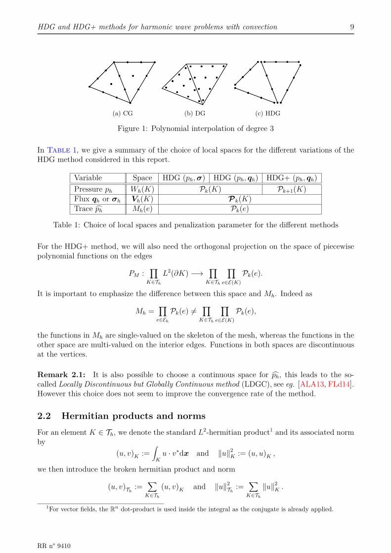
In Figure 1, we have depicted the differences in the degrees of freedom for the continuous (CG),discontinuous (DG) and hybridizable discontinuous (HDG) Galerkin methods. The degrees offreedom of the HDG methods are the ones associated with the numerical trace ph. As thenumerical cost of the method is directly linked to the number of degrees of freedom, we canclearly see that the HDG method is less expensive than the DG method.
Inria
HDG and HDG+ methods for harmonic wave problems with convection 9
(a) CG (b) DG (c) HDG
Figure 1: Polynomial interpolation of degree 3
In Table 1, we give a summary of the choice of local spaces for the different variations of theHDG method considered in this report.
Variable Space HDG (ph,σ) HDG (ph, qh) HDG+ (ph, qh)Pressure ph Wh(K) Pk(K) Pk+1(K)Flux qh or σh Vh(K) Pk(K)Trace ph Mh(e) Pk(e)
Table 1: Choice of local spaces and penalization parameter for the different methods
For the HDG+ method, we will also need the orthogonal projection on the space of piecewisepolynomial functions on the edges
PM :∏K∈Th
L2(∂K) −→∏K∈Th
∏e∈E(K)
Pk(e).
It is important to emphasize the difference between this space and Mh. Indeed as
Mh =∏e∈Eh
Pk(e) 6=∏K∈Th
∏e∈E(K)
Pk(e),
the functions in Mh are single-valued on the skeleton of the mesh, whereas the functions in theother space are multi-valued on the interior edges. Functions in both spaces are discontinuousat the vertices.
Remark 2.1: It is also possible to choose a continuous space for ph, this leads to the so-called Locally Discontinuous but Globally Continuous method (LDGC), see eg. [ALA13, FLd14].However this choice does not seem to improve the convergence rate of the method.
2.2 Hermitian products and normsFor an element K ∈ Th, we denote the standard L2-hermitian product1 and its associated normby
(u, v)K :=∫Ku · v∗dx and ‖u‖2
K := (u, u)K ,
we then introduce the broken hermitian product and norm
(u, v)Th:=
∑K∈Th
(u, v)K and ‖u‖2Th
:=∑K∈Th
‖u‖2K .
1For vector fields, the Rn dot-product is used inside the integral as the conjugate is already applied.
RR n° 9410

10 Hélène Barucq, Nathan Rouxelin, Sébastien Tordeux
On the boundary of an element K, we also denote the local hermitian product by
〈u, v〉∂K :=∑
e∈E(K)
∫eu · v∗dσ and ‖u‖2
∂K := 〈u, u〉∂K ,
and the broken hermitian product is denoted by
〈u, v〉∂Th:=
∑K∈Th
〈u, v〉∂K and ‖u‖2∂Th
:=∑K∈Th
‖u‖2∂K .
We have chosen to use angle brackets 〈·, ·〉 to denote the boundary integrals as they shouldformally be interpreted as the duality bracket between H− 1
2 (∂K) and H 12 (∂K).
We also define the following weighted norms
‖u‖2ρ0,K
:= (ρ0u, u)K which satisfies ‖u‖ρ0,K6 ‖ρ0‖
12L∞(K) ‖u‖K
‖q‖2W0,K
:= (W0q, q)K which satisfies ‖q‖W0,K6 CW0,K ‖q‖K
where
CW0,K =(
maxK
1ρ0 (c2
0 − |v0|2)
) 12
is the largest eigenvalue of W0 in K, see Lemma 1.1.
2.3 Faces, jumps and averagesIn this subsection, we will introduce notations for the faces quantities. As usual with methodsbelonging to the DG family, we will need to define jumps and averages which link the unknownsbetween two elements.
Faces and normals: For an interior face E ih 3 e = ∂K+∩∂K−, we denote by n+ (resp. n−)a unitary outgoing normal vector of ∂K+ (resp. ∂K−). We will always assume that the flowv0 goes from K− to K+, as depicted on Figure 2.
K−n−
K+
n+
v0 e = ∂K+ ∩ ∂K−
Figure 2: Normal vectors on an interior face
When the orientation of the face does not matter, we will denote by n any unitary normalvector to e.If e is a boundary edge, then n denotes the outward-pointing unitary normal vector.
Inria

HDG and HDG+ methods for harmonic wave problems with convection 11
Jumps and averages: We will often use the average operator defined by
On E ih 3 e = ∂K+ ∩ ∂K−, {{ϕ}}e := 12(ϕ+ + ϕ−
),
On Ebh 3 e = ∂K ∩ Γ, {{ϕ}}e := 12ϕ,
where ϕ can either be a scalar or vectorial quantity.We will also make frequent use of the jump operator defined by
On E ih 3 e = ∂K+ ∩ ∂K−, [[q]]e := q+ · n+ + q− · n−,On Ebh 3 e = ∂K ∩ Γ, [[q]]e := q · n,
for a vectorial quantity. Notice that with this definition, the jump operator only controls thenormal part of the vector. For a scalar quantity, the jump operator is defined by
On E ih 3 e = ∂K+ ∩ ∂K−, [[p]]e := p+ − p−,On Ebh 3 e = ∂K ∩ Γ, [[p]]e := p,
for a scalar quantity. A sketch of those quantities is given in Figure 3.
K− K+
n−
n+
[[ϕ]] {{ϕ}}
Figure 3: 1D-sketch of the jump and average on an interior node
3 HDG method for the total flux formulationIn this section, we will focus on the total flux formulation. We will first construct the HDGmethod and we will then discuss its most important properties.
3.1 Constructing the formulationOn an element K ∈ Th, we recall that the weak formulation (9a)–(9b) reads : seek (σ, p) ∈Hdiv(O)×H1(O) such that for all (r, w) ∈Hdiv(O)×H1(O)∫
KW0σ · r∗dx−
∫Kpdiv (r∗) dx+ 2iω
∫KpW0b0 · r∗dx+
∫∂Kpr∗ · ndσ = 0, (11a)
−ω2∫Kρ0pw
∗dx+∫K
div (σ)w∗dx =∫Ksw∗dx.(11b)
RR n° 9410

12 Hélène Barucq, Nathan Rouxelin, Sébastien Tordeux
Choice of approximation spaces: We denote by σh and ph the approximations of σ andp on K.For this method, we choose to use the following local approximation spaces
Vh(K) = Pk(K) for the flux σh,Wh(K) = Pk(K) for the pressurs ph,
where k > 3 is the degree of the method. We recall that if k 6 2, then there are no interiordegrees of freedom and the HDG method has no interest over the DG methods from a compu-tational point of view. Notice that we use the same interpolation degree for both unknowns,which may lead to unstable continuous Galerkin methods, see eg. [EG04, "Checkerboard-likeinstablitiy" p.188]. As we will discuss later, this is not a problem for HDG methods.
Introduction of the hybrid unknown: To reach a HDG formulation, we introduce a newunknown ph which is an approximation of p on Eh, the skeleton of the mesh Th. We will usuallyrefer to ph as the numerical trace. This unknown is the main unknown of the HDG method.Indeed, we will be able to use a static condensation process to eliminate the interior degrees offreedom and to obtain a so-called global problem for ph only. To introduce this unknown in theformulation, the boundary integral in (11a) is discretized as follows∫
∂Kpr∗ · ndσ becomes
∫∂Kphr
∗h · ndσ.
For this new unknown, we will use the following approximation space
Mh(e) = Pk(e), ∀e ∈ E(K).
Penalization parameter: The unknown ph is often called a Lagrange multiplier. Indeed,when going from a continuous Galerkin method to a HDG one, the continuity of the numericalsolution is not strongly enforced anymore and it is is added in the method as a constraint. Thequantity ph is therefore the Lagrange multiplier that enforces this weak continuity requirement.To enforce this constrain, we introduce a penalization parameter denoted by τ . and the followingboundary term
〈τ(ph − ph), wh〉∂Kwill be added to the local problem. This boundary term can be interpreted as a weak enforce-ment of the following Dirichlet boundary condition
ph = ph, on ∂K.
Practical choice of τ will be discussed later.
Local problem: We approximate the variational formulation (11a)–(11b) on an elementK ∈ Th leading to the local problem : seek (σh, ph) ∈ Vh(K)×Wh(K) such that
(W0σh, rh)K − (ph, div (rh))K + 2iω (phW0b0, rh)K + 〈ph, rh · n〉∂K = 0, (12a)−ω2 (ρ0ph, wh)K + (div (σh) , wh)K + iω 〈τ(ph − ph), wh〉∂K = (s, wh)K , (12b)
for all (rh, wh) ∈ Vh(K)×Wh(K).Notice that (12a)–(12b) is the variational formulation of the convected Helmholtz equation onK with weak Dirichlet boundary conditions on ∂K.
Inria
HDG and HDG+ methods for harmonic wave problems with convection 13
Transmission condition: Due to the discontinuous nature of the approximation spaces, weneed to link all the local problems together. To this end, we introduce the numerical flux forσh
σh · n := σh · n+ iωτ(ph − ph), (13)which satisfies the following transmission condition
〈σh, µh〉∂Th\ΓD+ 〈ph − gD, µh〉ΓD
= 〈gN , µh〉ΓN(14)
for all µh ∈Mh.Notice that (14) enforces the normal continuity of σh on the interior faces as well as theNeumann and Dirichlet boundary conditions on ΓN and ΓD.Indeed on the interior faces we have
〈σh, µh〉∂Th\ΓD=∑e∈Ei
h
〈[[σh]], µh〉e = 0,
as σh ∈ Vh, ph ∈ Wh and ph ∈Mh, we have [[σh]] ∈Mh and we therefore conclude that [[σh]] = 0,as [[σh]] is a polynomial of degree up to k orthogonal to all polynomials of degree up to k. Werecall that on an interior edge E ih 3 e = ∂K+ ∩ ∂K−, the jump operator is defined as
[[σh]] := σ+h · n+ + σ−h · n−.
Remark 3.1: The transmission condition (14) can be understood as a weak requirement ofHdiv(O)-conformity. Indeed it is shown in [PE12, Lemma 1.2.4] that σh ∈Hdiv(O) means
∀K ∈ Th, σKh ∈Hdiv(K) and ∀e ∈ E ih, [[σh]]e ≡ 0.
The former is a consequence of the polynomial nature of the approximation spaces, and we willnow focus and the latter. Owing to the transmission condition, we have
∀e ∈ E ih, 0 = [[σh]] = [[σh]] + iω[[τ(ph − ph)]].
As ph and ph are two approximations of the same unknown p, the quantity ph − ph is expectedto be small. We can therefore conclude that [[σh]] is small and that
[[σh]] −→hK→0
0.
For applications where a precise approximation of the flux is required, it is possible to post-process σh to obtain a new approximate σh with strong Hdiv-conformity, see [CGS10, Sec.5.1].
3.1.1 Compact formulation:
HDG methods are usually stated in a compact form that can be obtained by summing the localproblems (12a)–(12b) over the mesh elements and by adding the transmission condition (14).This formulation reads : seek (σh, ph, ph) ∈ Vh ×Wh ×Mh such that
(W0σh, rh)Th− (ph, div (rh))Th
+ 2iω (phW0b0, rh)Th+ 〈ph, rh · n〉∂Th
= 0, (15a)−ω2 (ρ0ph, wh)Th
+ (div (σh) , wh)Th+ iω 〈τ(ph − ph), wh〉∂Th
= (s, wh)Th, (15b)
〈σh · n+ iωτ(ph − ph), µh〉∂Th\ΓD+ 〈ph − gD, µh〉ΓD
= 〈gN , µh〉ΓN, (15c)
for all (rh, wh, µh) ∈ Vh ×Wh ×Mh. This formulation will be useful to perform the numericalanalysis of the method.
RR n° 9410

14 Hélène Barucq, Nathan Rouxelin, Sébastien Tordeux
Remark 3.2: At this point, to completely define the HDG method, it only remains to choosethe penalization parameter τ , this will be done in the next section.
3.1.2 Condensed variational formulation
The compact formulation (15a)–(15b)–(15c) cannot directly be used to efficiently implementthe HDG method. Indeed it is not clear how a formulation involving only ph can be reached.To emphasize how it can be done, we will now write a condensed variational formulation for phonly.We introduce the so-called local solvers
PK : (ph, s) 7−→ pKh ,
ΣK : (ph, s) 7−→ σKh ,
ΣK : (ph, s) 7−→ σhK ,
where (σKh , pKh ) is the solution of (12a)–(12b) and σhK is defined by (13).We can therefore rewrite the transmission condition (15c) as
ah(ph, µ) = `h(µ), (16)
where
ah(ph, µh) :=⟨
ΣK(ph, s) · n+ iωτ(PK(ph, s)− ph), µh⟩∂Th\ΓD
+ 〈ph, µh〉ΓD,
`h(µh) := 〈gN , µh〉ΓN+ 〈gD, µh〉ΓD
.
Equation (16) is the so-called global problem and is the main equation of the HDG method.From a computational point of view, we proceed as described in Algorithm 1.
Algorithm 1: Solving HDG-σh1 for K ∈ Th do2 Construct the local solvers PK , ΣK , ΣK
3 Add local contribution to the global problem (16)4 Solve (16) for ph // This is the main step5 for K ∈ Th do6 Reconstruct the local unknowns pKh = Pk(ph, s) and σKh = Σ(ph, s)
This algorithm is the blueprint of the practical implementation of the HDG method which willbe discussed in Section 5.
3.2 Choice of penalization parameterIn this section, we will show how the penalization parameter can be chosen to obtain anupwinding mechanism with physical meaning. To do that, we will first need to rewrite theHDG method as a DG one, we will then solve a Riemann problem to obtain the value ofτ .
3.2.1 DG formulation
In this section, we will rewrite the HDG method (15a)–(15b)–(15c) as a standard discontinuousGalerkin method.
Inria
HDG and HDG+ methods for harmonic wave problems with convection 15
We introduce the following bilinear form
Bh([σh, ph]; [rh, wh]) := (W0σh, rh)Th− (ph, div (rh))Th
+ 2iω (phW0b0, rh)Th
− ω2 (ρ0ph, wh)Th+ (div (σh) , wh)Th
+∑e∈Eh
(〈ph, [[rh]]〉e + 〈σh · n, [[wh]]〉e
), (17)
from which all the mixed DG methods can be generated by choosing ph and σh. Notice thatph was an unknown of the HDG method whereas it now should be chosen by the user of themethod.For example, the LDG method is obtained by choosing
ph = {{ph}}+ α[[ph]] and σh = {{σh}}+ β[[σh]]n+ γ[[ph]]n,
and the DG method with central flux is obtained by choosing
ph = {{ph}} and σh = {{σ}} − α[[ph]].
Proposition 3.1:The HDG method (15a)–(15b)–(15c) and the DG method associated to the bilinear form (17)are equivalent if and only if
ph = {{ph}}+ τ+ − τ−
2(τ+ + τ−) [[ph]] + 1iω(τ+ + τ−) [[σh]], (18a)
σh · n = {{σh}} · n+ iωτ+τ−
τ+ + τ−[[ph]]−
τ+ − τ−
2(τ+ + τ−) [[σh]], (18b)
for all interior edges Ebh 3 e = ∂K+ ∩ ∂K− and where τ± = τ |∂K± .
We recall the convention for the labelling ∂K± : v0 is directed from ∂K− toward ∂K+ and wedenote by n any normal vector to the face when the orientation does not matter.Proof: Writing down the transmission condition (15c) on an interior face e, we have
[[σh]] + 2iω({{τ}}{{ph}}+ 1
4[[τ ]][[ph]])− 2iω{{τ}}ph = 0,
which leads to
ph = {{ph}}+ [[τ ]]4{{τ}} [[ph]] + 1
2iω{{τ}} [[σh]],
and we obtain (18a) by developing the jumps and average terms.As the numerical flux σh is continuous across the interface, we have
σh · n = {{σh}} · n
= {{σh}} · n+ iω
2 [[τ ]] ({{ph}} − ph) + iω
2 {{τ}}[[ph]]
= {{σh}} · n−iω
2 [[τ ]](
[[τ ]]4{{τ}} [[ph]] + 1
2iω{{τ}} [[σh]])
+ iω
2 {{τ}}[[ph]]
and we obtain (18b) as
− [[τ ]]2
4{{τ}} + {{τ}} = −(τ+)2 − 2τ+τ− + (τ−)2
2(τ+ + τ−) + (τ+)2 + 2τ+τ− + (τ−)2
2(τ+ + τ−) = 2 τ+τ−
τ+ + τ−.
RR n° 9410
16 Hélène Barucq, Nathan Rouxelin, Sébastien Tordeux
We now have to show that this choice of numerical flux σh is compatible with the HDG method.Starting from (18b) we have
σh · n+ = σ+h · n+ − 1
2
(1 + τ+ − τ−
τ+ + τ−
)[[σh]] + iω
τ+τ−
τ+ + τ−[[ph]]
= σ+h · n+ − τ+
τ+ + τ−[[σh]] + iω
τ+τ−
τ+ + τ−[[ph]],
on the other hand, rewriting (18a) gives
− τ+
τ+ + τ−[[σh]] = iωτ+
[{{ph}} − ph + τ+ − τ−
2(τ+ + τ−) [[ph]]]
= iωτ+(p+h − ph) + iω
τ+
2
(τ+ − τ−
τ+ + τ−− 1
)[[ph]]
= iωτ+(p+h − ph)− iω
τ+τ−
τ+ + τ−[[ph]],
so we finally haveσh · n+ = σ+
h · n+ + iωτ+(p+h − ph).
Similar computations can be carried out on ∂K−.
Particular form of the HDG fluxes: We would like to point out that ph depends on [[σh]],this is a distinctive feature of HDG methods among the family of DG methods. To understandthis, let us consider DG method with the following fluxes
ph = {{ph}}+ α[[ph]] and σh = {{σh}}+ β[[σh]]n+ γ[[ph]]n, (19)
where α, β, γ are arbitrary constants. This construction is adapted from [HW08, Sec 7.2.2].Testing (17) with [rh, 0] leads to
(W0σh, rh)Th− (ph, div (rh))Th
+ 2iω (phW0b0, rh)Th+∑e∈Eh
〈ph, [[rh]]〉e = 0.
Integrating by parts leads to
(W0σh, rh)Th= − (∇ph, rh)Th
− 2iω (phW0b0, rh)Th+∑e∈Eh
[〈[[ph]]n, {{rh}}〉e − 〈ph, [[rh]]〉e]
+∑e∈Ei
h
〈{{ph}}, [[rh]]〉e , (20)
where we used the identity
〈ph, rh · n〉∂Th=∑e∈Eh
〈[[ph]]n, {{rh}}〉e +∑e∈Ei
h
〈{{ph}}, [[rh]]〉e ,
coming from [HW08, Lemma 7.9]. Using the definition of ph given in (19), the surfacic termsin (20) become
−∑e∈Ei
h
〈[[ph]], {{rh}} · n− α[[rh]]〉e −∑e∈Eb
h
〈ph, rh · n〉e .
We now introduce the lifting operator L defined by
(L(ph), rh)Th=∑e∈Ei
h
〈[[ph]], {{rh}} · n− α[[rh]]〉e +∑e∈Eb
h
〈ph, rh · n〉e , ∀rh ∈ Vh,
Inria

HDG and HDG+ methods for harmonic wave problems with convection 17
and (20) becomes
(W0σh, rh)Th= (−∇ph − 2iωphW0b0 − L(ph), rh)Th
.
We can see that σh is completely defined in terms of ph and it is therefore not possible to adda transmission condition, which is required to allow the static condensation process.On the other hand, if the HDG flux
ph = {{ph}}+ α[[ph]] + δ[[σh]]
is used, we will obtain an expression of σh in terms of ph and [[σh]]. We will therefore need toadd the transmission condition to close the discrete system and it will be possible to performthe static condensation.
3.2.2 Computing the penalization parameter
Proposition 3.2:On an interior face E ih 3 e = ∂K+ ∩ ∂K− the following choice of penalization parameter
τ± = ρ0(c0 + v0 · n±), (21)
where τ± = τ |∂K± , leads to an upwinding mechanism.
To prove this proposition, we will need to solve a Riemann problem and compare its solutionwith Proposition 3.1 to obtain a value for τ± with physical meaning. The first step to be ableto solve the Riemann problem is to rewrite the original equation as a time-domain hyperbolicsystem.
Hyperbolic system: We start from the convected acoustic wave equation
ρ0
(∂
∂t+ v0 · ∇
)2
p− div(ρ0c
20∇p
)= 0
and we write it as a hyperbolic system. First we have
ρ0∂2p
∂t2− div
(K0∇p− 2ρ0
∂p
∂tv0
)= 0,
we therefore introduce the total flux
∂σ
∂t= −K0∇p+ 2ρ0
∂p
∂tv0,
leading to the following first-order formulation
∂p
∂t= − 1
ρ0div (σ) , (22a)
∂σ
∂t= −K0∇p+ 2ρ0
∂p
∂tv0. (22b)
However this formulation does not have the form of a hyperbolic system.
RR n° 9410

18 Hélène Barucq, Nathan Rouxelin, Sébastien Tordeux
Using (22a) in (22b), we have
∂p
∂t= − 1
ρ0div (σ) , (23a)
∂σ
∂t= −K0∇p− 2div (σ)v0. (23b)
Notice that we need to work with a first-order in time formulation whereas our methods arewritten for second-order in time (or equivalently in frequency) formulations. However we havethe following relationship between σ and σ
σ = iωσ,
making it possible to go back to a second-order formulation.The system (23a)–(23b) can be written as
∂U∂t
= Ax∂U∂x
+ Ay∂U∂y
, (24)
where
U :=[pσ
]; Ax :=
0 − 1
ρ00
−M0,xx −2v0,x 0−M0,yx −2v0,y 0
; Ay :=
0 0 − 1
ρ0−M0,xy 0 −2v0,x−M0,yy 0 −2v0,y
.To check that (24) is a hyperbolic system, one needs to show that for all α, β ∈ R the matrix
Aα,β := αAx + βAy = −
0 α
ρ0
β
ρ0αM0,xx + βM0,xy 2αv0,x 2βv0,xαM0,yx + βM0,yy 2αv0,y 2βv0,y
is diagonalizable with real eigenvalues, see Figure 4.
Figure 4: Computation of the eigenvalues of Aα,β with WolframAlpha
Inria
HDG and HDG+ methods for harmonic wave problems with convection 19
Riemann solver: To compute the upwind penalization parameters, we consider a verticalinterface located at x = 0 and we assume that the background flow is uniform.We will solve the problem (24) with the following initial condition
U(x, y, 0) = U+, if x > 0,U(x, y, 0) = U−, if x < 0.
With this choice of initial condition, we obtain a well-posed problem which is invariant withrespect to y.Our goal is to compute U at x = 0.Due to the invariance with respect to y, we can rewrite (24) as
∂U∂t
= Ax∂U∂x
.
Furthermore, we can obtain the following system for [p, σx]T only
∂
∂t
[pσx
]=
0 − 1ρ0
−M0,xx −2v0,x
︸ ︷︷ ︸
=:A
∂
∂x
[pσx
],
as the DG method is only written in terms of σ · n = σx.To compute the eigenvalues of A, we need to solve∣∣∣∣∣∣∣
−λ − 1ρ0
−M0,xx −2v0,x − λ
∣∣∣∣∣∣∣ = 0 ⇐⇒ λ2 + 2v0,xλ−M0,xx
ρ0= 0.
Recalling thatM0,xx = ρ0c
20 − ρ0v
20,x,
we obtain the two following eigenvalues
λ1 = − (c0 + v0,x) ,λ2 = c0 − v0,x,
and the associated eigenvectors are
w1 :=[
1ρ0(c0 + v0,x)
]and w2 :=
[1
ρ0(v0,x − c0).
]
We can now defineW :=
[1 1
ρ0(c0 + v0,x) ρ0(v0,x − c0)
],
and thereforeW−1 = 1
2ρ0c0
[ρ0(c0 − v0,x) 1ρ0(c0 + v0,x) −1
]=[`1`2
].
We have[pσx
](0, t) = `1
[p+
σ+x
]w1 + `2
[p−
σ−x
]w2
= ρ0(c0 − v0,x)p+ + σ+x
2ρ0c0
[1
ρ0(c0 + v0,x)
]+ ρ0(c0 + v0,x)p− − σ−x
2ρ0c0
[1
ρ0(v0,x − c0)
],
RR n° 9410
20 Hélène Barucq, Nathan Rouxelin, Sébastien Tordeux
therefore
p = 12(p+ + p−
)− v0,x
2c0
(p+ − p−
)+ 1
2ρ0c0
(σ+x − σ−x
),
σx = 12(σ+x + σ−x
)+ v0,x
2c0
(σ+x − σ−x
)+ ρ0
c20 − v2
0,x
2c0
(p+ − p−
).
Finally, we can infer the form of the DG flux for a generic interface
p = {{p}} − v0 · n−
2c0[[p]] + 1
2ρ0c0[[σ]], (26a)
σ · n− = {{σ}} · n− + v0 · n−
2c0[[σ]] + ρ0
c20 − (v0 · n)2
2c0[[p]]. (26b)
Notice that we had to chose an orientation of the normal vector. Following our convention, wehave chosen to use n− as it has the same orientation as v0.Rewriting (26a)–(26b) in terms of σ instead of σ leads to
ph = {{p}} − v0 · n−
2c0[[p]] + 1
2iωρ0c0[[σ]] (27a)
σ · n− = {{σ}} · n− + v0 · n−
2c0[[σ]] + iωρ0
c20 − (v0 · n−)2
2c0[[p]]. (27b)
Comparing (27a)–(27b) with (18a)–(18b) , we see that
τ+ + τ− = 2ρ0c0, (28a)τ+τ−
τ+ + τ−= ρ0
c20 − (v0 · n−)2
2c0. (28b)
The system (28a)–(28b) leads to the following second-order equation
(τ+)2 − 2ρ0c0τ+ + ρ2
0
(c2
0 − (v0 · n−)2)
= 0,
and to the two following families for τ±
τ+1 = ρ0(c0 + v0 · n−), τ−1 = ρ0(c0 − v0 · n−),τ+
2 = ρ0(c0 − v0 · n−), τ−2 = ρ0(c0 + v0 · n−).
To discriminate between τ±1 and τ±2 we once again go back to (18a)–(18b) and we see that thesolution must satisfy
τ+ − τ−
2(τ+ + τ−) = −v0 · n−
2c0.
We can therefore conclude that the upwind fluxes are obtained by using the τ±2 solution. Wecan make this choice independent of the orientation convention by noticing that n+ = −n−,leading to
τ±2 = ρ0(c0 + v0 · n±).
Remark 3.3: To keep polynomial fluxes on the interfaces, the background quantities will beapproximated by their value at the center of the interface.
Remark 3.4: In the context of DG and HDG methods, τ is usually chosen to be of the «orderof unity» to ensure optimal convergence rate. In the error analysis of the method, we allow thedependency to the background coefficient to be hidden in the constants, so the choice (21) isactually possible.
Inria

HDG and HDG+ methods for harmonic wave problems with convection 21
3.3 Local solvabilityWe will now show the local solvability for the total flux formulation. Proving the well-posednessof the local problems is always very important when working with HDG methods. For thestrongly coercive problems, for which HDG methods were initially designed, this propertyusually comes directly from the continuous problem. However for harmonic wave equations,which are only weakly coercive, things are more complicated : indeed solving the local problemamounts to solving a wave problem with Dirichlet boundary conditions. We therefore need toensure that the local problem does not introduce resonance into the method, which is the casewhen the elements are small enough. In this section, we will prove that the static condensationprocess is well-defined when the mesh is fine enough.
Notice that in this case the proof relies on an absorption technique and is therefore verytechnical. Readers who are not familiar with HDG theory should probably begin with theproof for the diffusive flux formulation which is easier. It will be detailed in Subsection 4.2.
First, we need to show the
Lemma 3.1:For ph ∈ Pk(K) with k > 0, the following inverse inequality holds
‖∇ph · n‖∂K . ‖∇ph‖∂K . h− 1
2K ‖∇ph‖K .
Proof:First, we notice that if ph is constant the desired inequality reduces to 0 . 0. We thereforeonly consider non-constant ph.Let K be the reference unit element. We consider the map F : K −→ K. We use · to denotequantities on the reference element instead of the more standard notation · to avoid confusion,as we already used · to denote the numerical fluxes.Let γ1 : H2(K) −→ L2(∂K) be the normal derivative operator in the reference element. As γ1
is continuous, we have ∥∥∥γ1(ph)∥∥∥∂K
. ‖ph‖2,K . |ph|1,K
The second inequality holds as ph ∈ Pk(K) which is a finite-dimensional vector-space on whichall the norms are equivalent and ph is not constant.We now recall the following scaling inequalities, see [DS19, Eq (1.6), (1.7) & (1.8)]
|ph|1,K .| det Jac(F )|− 12 ‖Jac(F )‖ |ph|1,K . |ph|1,K ;
h12K ‖µh‖∂K . ‖µh‖∂K
Due to the regularity of the mesh, we have
h12K ‖∇ph · n‖∂K . ‖∇ph‖K .
RR n° 9410
22 Hélène Barucq, Nathan Rouxelin, Sébastien Tordeux
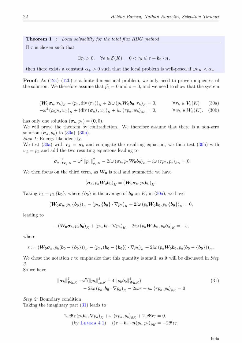
Theorem 1 : Local solvability for the total flux HDG methodIf τ is chosen such that
∃τ0 > 0, ∀e ∈ E(K), 0 < τ0 6 τ + b0 · n,
then there exists a constant α+ > 0 such that the local problem is well-posed if ωhK < α+.
Proof: As (12a)–(12b) is a finite-dimensional problem, we only need to prove uniqueness ofthe solution. We therefore assume that ph = 0 and s = 0, and we need to show that the system
(W0σh, rh)K − (ph, div (rh))K + 2iω (phW0b0, rh)K = 0, ∀rh ∈ Vh(K) (30a)−ω2 (ρ0ph, wh)K + (div (σh) , wh)K + iω 〈τph, wh〉∂K = 0, ∀wh ∈ Wh(K). (30b)
has only one solution (σh, ph) = (0, 0).We will prove the theorem by contradiction. We therefore assume that there is a non-zerosolution (σh, ph) to (30a)–(30b).Step 1: Energy-like identity.We test (30a) with rh = σh and conjugate the resulting equation, we then test (30b) withwh = ph and add the two resulting equations leading to
‖σh‖2W0,K
− ω2 ‖ph‖2ρ0,K− 2iω (σh, phW0b0)K + iω 〈τph, ph〉∂K = 0.
We then focus on the third term, as W0 is real and symmetric we have
(σh, phW0b0)K = (W0σh, phb0)K .
Taking rh = ph {b0}, where {b0} is the average of b0 on K, in (30a), we have
(W0σh, ph {b0})K − (ph, {b0} · ∇ph)K + 2iω (phW0b0, ph {b0})K = 0,
leading to
− (W0σh, phb0)K + (ph, b0 · ∇ph)K − 2iω (phW0b0, phb0)K = −ε,
where
ε := (W0σh, ph(b0 − {b0}))K − (ph, (b0 − {b0}) · ∇ph)K + 2iω (phW0b0, ph(b0 − {b0}))K .
We chose the notation ε to emphasize that this quantity is small, as it will be discussed in Step3.So we have
‖σh‖2W0,K
−ω2(‖ph‖2ρ0,K
+ 4 ‖phb0‖2W0,K
) (31)− 2iω (ph, b0 · ∇ph)K − 2iωε+ iω 〈τph, ph〉∂K = 0
Step 2: Boundary conditionTaking the imaginary part (31) leads to
2ωRe (phb0,∇ph)K + ω 〈τph, ph〉∂K + 2ωReε = 0,(by Lemma 4.1) 〈(τ + b0 · n)ph, ph〉∂K = −2Reε.
Inria
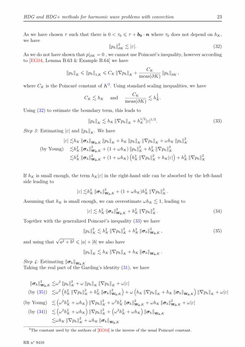
HDG and HDG+ methods for harmonic wave problems with convection 23
As we have chosen τ such that there is 0 < τ0 6 τ + b0 · n where τ0 does not depend on hK ,we have
‖ph‖2∂K . |ε|. (32)
As we do not have shown that p|∂K = 0 , we cannot use Poincaré’s inequality, however accordingto [EG04, Lemma B.63 & Example B.64] we have
‖ph‖K 6 ‖ph‖1,K 6 CK ‖∇ph‖K + CKmeas(∂K) ‖ph‖∂K ,
where CK is the Poincaré constant of K2. Using standard scaling inequalities, we have
CK . hK and CKmeas(∂K) . h
12K .
Using (32) to estimate the boundary term, this leads to
‖ph‖K . hK ‖∇ph‖K + h1/2K |ε|1/2. (33)
Step 3: Estimating |ε| and ‖ph‖K . We have
|ε| .hK ‖σh‖W0,K‖ph‖K + hK ‖ph‖K ‖∇ph‖K + ωhK ‖ph‖2
K
(by Young) .h2K ‖σh‖
2W0,K
+ (1 + ωhK) ‖ph‖2K + h2
K ‖∇ph‖2K
.h2K ‖σh‖
2W0,K
+ (1 + ωhK)(h2K ‖∇ph‖
2K + hK |ε|
)+ h2
K ‖∇ph‖2K
If hK is small enough, the term hK |ε| in the right-hand side can be absorbed by the left-handside leading to
|ε| .h2K ‖σh‖
2W0,K
+ (1 + ωhK)h2K ‖∇ph‖
2K .
Assuming that hK is small enough, we can overestimate ωhK . 1, leading to
|ε| . h2K ‖σh‖
2W0,K
+ h2K ‖∇ph‖
2K . (34)
Together with the generalized Poincaré’s inequality (33) we have
‖ph‖2K . h2
K ‖∇ph‖2K + h2
K ‖σh‖2W0,K
, (35)
and using that√a2 + b2 6 |a|+ |b| we also have
‖ph‖K . hK ‖∇ph‖K + hK ‖σh‖W0,K.
Step 4: Estimating ‖σh‖W0,K
Taking the real part of the Garding’s identity (31), we have
‖σh‖2W0,K
.ω2 ‖ph‖2K + ω ‖ph‖K ‖∇ph‖K + ω|ε|
(by (35)) .ω2(h2K ‖∇ph‖
2K + h2
K ‖σh‖2W0,K
)+ ω
(hK ‖∇ph‖K + hK ‖σh‖W0,K
)‖∇ph‖K + ω|ε|
(by Young) .(ω2h2
K + ωhK)‖∇ph‖2
K + ω2h2K ‖σh‖
2W0,K
+ ωhK ‖σh‖2W0,K
+ ω|ε|
(by (34)) .(ω2h2
K + ωhK)‖∇ph‖2
K +(ω2h2
K + ωhK)‖σh‖W0,K
.ωhK ‖∇ph‖2K + ωhK ‖σh‖W0,K
2The constant used by the authors of [EG04] is the inverse of the usual Poincaré constant.
RR n° 9410
24 Hélène Barucq, Nathan Rouxelin, Sébastien Tordeux
We obtained the last line by assuming that ω2h2K . ωhK which is true if hK is small enough.
If hK is small enough the term ωhK ‖σh‖2W0,K
in the right-hand side can be absorbed by theleft-hand side, leading to
‖σh‖2W0,K
. ωhK ‖∇ph‖2K . (36)
Step 5: Estimating ‖∇ph‖KTaking rh = ∇ph in (30a) and reverting the integration by parts, we have
‖∇ph‖2K = |(W0σh,∇ph)K + 2iω (phW0b0,∇ph)K + 〈ph,∇ph · n〉∂K |. ‖σh‖W0,K
‖∇ph‖K + ω ‖ph‖K ‖∇ph‖K + ‖ph‖∂K ‖∇ph‖∂K(by Lemma 3.1) . ‖σh‖W0,K
‖∇ph‖K + ω ‖ph‖K ‖∇ph‖K + h−1/2K ‖ph‖∂K ‖∇ph‖K
So we have
‖∇ph‖K . ‖σh‖W0,K+ ω ‖ph‖K + h
−1/2K ‖ph‖∂K
. ‖σh‖W0,K+ ω ‖ph‖K + (1 + ωhK)hK ‖∇ph‖K
. ‖σh‖W0,K+ ωhK ‖∇ph‖K + ωh
3/2K ‖σh‖W0,K
+ (1 + ωhK)hK ‖∇ph‖K
Finally we have‖∇ph‖K . ‖σh‖W0,K
. ‖σh‖K . (37)
Step 6: ContradictionCombining (36) and (37), we have
‖σh‖2K . ωhK ‖σh‖2
K
as we assumed that σh 6= 0, we can divide by ‖σh‖K , leading to
1 . ωhK ,
which does not hold if ωhK is small enough.This is the desired contradiction, and we can therefore conclude that (σh, ph) = (0, 0) is theonly solution of the system (30a)–(30b).
3.4 Error analysisThe error analysis can be carried out by following the projection analysis for the Helmholtzequation given in [DS19, Sec. 3.5.1 & 3.5.2] with some minor changes.This error analysis relies on the tailored HDG projection that fits the structure of the numericaltrace. This projection (Π,Π), with
(Π,Π) : Hdiv(O)×H1(O) −→ Vh ×Wh := Pk(Th)× Pk(Th)
is defined by the following equations
(Πσ, rh)K = (σ, rh)K , ∀rh ∈ Pk−1(K),(Πp, wh)K = (p, wh)K , ∀wh ∈ Pk−1(K),
〈Πσ · n+ iωτΠp, µh〉∂K = 〈σ · n+ iωτp, µh〉∂K , ∀µh ∈ Rk(∂K).
Notice that denoting the image of (σ, p) under (Π,Π) by (Πσ,Πp) is a slight abuse of notationas both components depend on σ and p. However it is very convenient and often found in theliterature.
Inria
HDG and HDG+ methods for harmonic wave problems with convection 25
We define the following error quantities
δσh := Πσ − σ ; δph := Πp− p ; δph := p− PMp
andεσh := Πσ − σh ∈ Vh ; εph := Πp− ph ∈ Wh ; εph := PMp− ph ∈Mh.
We will split the errors as
‖σh − σ‖W0,Th6 ‖εσh‖W0,Th
+ ‖δσh ‖W0,Th,
‖ph − p‖ρ0,Th6 ‖εph‖ρ0,Th
+ ‖δph‖ρ0,Th,
Notice that the following estimates hold
‖δph‖K . hk+1K
(|p|k+1,K + τ−1
max| divσ|k,K),
‖δσh ‖K . hk+1K (|σ|k+1,K + τ ?|p|k+1,K) ,
for some constants τmax and τ ?. So we only need to prove estimates for ‖εσh‖W0,Th, ‖εph‖ρ0,Th
.The error analysis can be summarized as follows
1. we derive an estimate for ‖εσh‖W0,Thusing the energy-like inequality,
2. we use a dual problem to estimate ‖εph‖ρ0,Thin terms of ‖εσh‖W0,Th
,3. those estimates are combined through a bootstrapping process.
This analysis is therefore strongly related to the Aubin-Nitsche method and only works forregular solutions.We will now give the main changes needed to adapt the error analysis from [DS19].The error equations (3.30) become
(W0εσh , rh)Th
− (εph, div (rh))Th+ 2iω (εphW0b0, rh)Th
+ 〈εph, rh · n〉∂Th= (W0δ
σh , rh)Th
+ 2iω (δphW0b0, rh)Th
−ω2 (ρ0εph, wh)Th
+ (div (εσh ) , wh)Th+ iω 〈τ(εph − ε
ph), wh〉∂Th
= −ω2 (ρ0δph, wh)Th
−〈εσh · n+ iωτ(εph − εph), µh〉∂Th
= 0.
The energy-like identity of Prop. 3.7 becomes
‖εσh‖2W0,Th
− ω2 ‖εph‖2ρ0,Th− 2iω (εσh , ε
phW0b0)Th
+ iω 〈τ(εph − εph), ε
ph − ε
ph〉∂Th
= (εσh ,W0δσh )Th
− 2iω (εσh , δphW0b0)Th
− ω2 (ρ0δph, ε
ph)Th
,
leading to the following estimate∣∣∣‖εσh‖2W0,Th
+ iω 〈τ(εph − εph), ε
ph − ε
ph〉∂Th
∣∣∣ .ω2 ‖εph‖2ρ0,Th
+ ω ‖εσh‖W0,Th‖δph‖ρ0,Th
+ ‖εσh‖W0,Th‖δσh ‖W0,Th
+ ω ‖εσh‖W0,Th‖δph‖ρ0,Th
+ ω2 ‖εph‖ρ0,Th‖δph‖ρ0,Th
.
The adjoint problem (3.31) becomes
W0ξ −∇θ − 2iωθW0b0 = 0−ρ0ω
2θ − div (ξ) = εph.
RR n° 9410
26 Hélène Barucq, Nathan Rouxelin, Sébastien Tordeux
We state the elliptic regularity assumption which is a key ingredient in the error analysis
‖θ‖2,O + ‖ξ‖1,O 6 Creg ‖εph‖O
The identity of Prop. 3.8 becomes
‖εph‖2ρ0,Th
=ω2 (ρ0(Πθ − θ), εph − δph)Th− ω2 (ρ0θ − {ρ0θ} , δph)Th
− (W0(Πξ − ξ), εσh − δσh )Th+ (W0ξ − {W0ξ} , δσh )Th
− 2iω (θb0,W0εσh )Th
+ 2iω (W0ξ, (εph − δph)b0)Th
+ 2iω (W0(Πξ − ξ), (εph − δph)b0)Th
,
leading to the following estimate
‖εph‖ρ0,Th.(ω3 + ω2 + ω
)h(‖εph‖ρ0,Th
+ ‖δph‖ρ0,Th
)+ (1 + ω)h
(‖εσh‖W0,Th
+ ‖δσh ‖W0,Th
)+ ‖εσh‖W0,K
+ ω ‖εph‖ρ0,K+ ω ‖δph‖ρ0,K
.
Notice that in contrast to the HDG method for the standard Helmholtz equation, both ph andσh have the same convergence rate.It is now straightforward to follow the bootstrapping argument of Sec. 3.5.2 to obtain the
Theorem 2 : Convergence of the HDG method with total fluxAssuming that ωh is small enough and under the elliptic regularity assumption, we have
‖ph − Πp‖Th= O(hk+1) ; ‖σh −Πσ‖Th
= O(hk+1).
Remark 3.5: Some HDG methods are known to achieve super-convergence, ie taking ph ∈ Pkleads to the following error estimate
‖Πp− ph‖Th= O(hk+2).
Superconvergence is an attractive property for a numerical scheme, indeed using a postprocess-ing scheme it is possible to use the solution (σh, ph) to construct a new approximation ph whichconverges with order O(hk+2), see [Ste91], [CGS10, Sec. 5] for more details.Here we were only able to prove optimal convergence and the use of post-processing schemes toimprove the convergence rate is therefore not possible.
3.5 Global solvabilityThe analysis that we have carried out in the previous subsection works for any solution(σh, ph, ph) of the discrete system (15a)–(15b)–(15c) provided that such solution exists. Wealready discussed the well-posedness of the local problems in Theorem 1, but we have not yetproved that the global problem (16) for ph was well-posed.To do that we can either directly show the well-posedness of the global problem (16). Or wecan choose take advantage of the error estimates of Theorem 2 as we will describe below3.
Resonant frequencies: We recall that the convected Helmholtz equation is a problem ofFredholm type. It is therefore uniquely solvable except on a set of resonant frequencies. Forthose frequencies, there exists non-zero solutions to the homogenous equation and unique solv-ability cannot be guaranteed.
3In [DS19] this idea is attributed to B. Cockburn.
Inria

HDG and HDG+ methods for harmonic wave problems with convection 27
Main result: We can now state and prove the main result of this section.
Theorem 3 : Global solvabilityUnder the assumptions of Theorem 1 and Theorem 2 and if ω is not a resonant frequency ofthe convected Helmholtz equation (1) then the global problem is well-posed, ie ph is uniquelydefined by (16).
Proof: First we recall that (15a)–(15b)–(15c), or equivalently (16), is a square system of linearequations, we therefore only need to show the uniqueness of the solution of the homogenoussystem (when gN = gD = s = 0).Assuming that ω is not a resonant frequency of (1), the exact solution is p = 0 and σ = 0, andtherefore
‖p‖s,O = 0 and ‖σ‖t,O = 0
andεph = −ph ; εσh = −σh ; εph = −ph.
The aim of the error analysis was to prove the following inequalities when h is small enough :
‖εph‖Th. ‖p‖s,O + ‖σh‖t,O = 0 (38a)
‖εσh‖Th. ‖p‖s,O + ‖σh‖t,O = 0 (38b)
Notice that we have hidden the powers of h in . as they do not play an important part here.Therefore using (38a) and (38b) we have shown that
ph ≡ 0 and σh ≡ 0
when h is small enough.For all K ∈ Th, we can now rewrite (12a) as
〈ph, rh · n〉∂K = 0, ∀rh ∈ Vh(K),
which leads toph ≡ 0.
4 HDG(+) methods for the diffusive flux formulationIn this section, we will construct HDG methods based on the diffusive flux formulation, whereq is used instead of σ. We will mostly describe the HDG+ method where different polynomialdegrees are used for the different unknowns, as it the most important novelty of this paper.Adaptation of the formulation construction and theoretical results to a more standard HDGmethod with the same polynomial interpolation for all the unknowns is straightforward. Themain differences between the HDG and HDG+ methods are stated but the details are left out.The global solvability will not be included in this section as the adaptation of the result fromthe previous section is immediate.
RR n° 9410
28 Hélène Barucq, Nathan Rouxelin, Sébastien Tordeux
4.1 Construction of the methodWe recall that on element K ∈ Th, the weak formulation (7a)–(7b) reads : Seek (q, p) ∈Hdiv(O)×H1(O) such that∫
KW0q · r∗dx−
∫Kpdiv (r∗) dx+
∫∂Kpr∗ · ndσ = 0, (39a)
−ω2∫Kρ0pw
∗dx− 2iω∫Kb0 · ∇pw∗dx+
∫K
div (q)w∗dx =∫Ksw∗dx, (39b)
for all (r, w) ∈Hdiv(O)×H1(O).
Choice of approximation spaces: For the HDG+ method, the choice of approximationspaces is different from the choice made for the previous HDG method. We consider thefollowing local approximation spaces
Vh(K) = Pk(K), for the flux qh,Wh(K) = Pk+1(K), for the pressure ph,
where k > 2 is the degree of the method. The use of a higher polynomial degree for ph is thedistinctive feature of the HDG+ method.
Introduction of the hybrid unknown: As we did before, we introduce the numerical traceph which approximates p on the skeleton Eh of the mesh. As before the boundary integral in(39a) will be discretized as∫
∂Kpr∗ · ndσ becomes
∫∂Kphr
∗h · ndσ.
For the HDG+ method, we use the following approximation space for phMh(e) = Pk(e), ∀e ∈ E(K).
With this choice, ph and ph do not have the same polynomial degree and we therefore havetwo approximations of p with different polynomial degrees on the skeleton of the mesh. Wetherefore need to change the penalization term to
τ(PMph − ph), (40)
where PM is the L2-orthogonal projection onto Mh. This is called the reduced stabilization andit was introduced in [Leh10]. It allows to get convergence rate of k + 2 for ph for the cost ofa method of degree k. A large penalization parameter τ ∼ hK
−1 is needed to obtain optimalconvergence as it will be detailed in Subsection 4.3.
Local problem: We approximate the weak formulation (39a)–(39b) on an element K ∈ Thleading to the so-called local problem : seek (qh, ph) ∈ Vh(K)×Wh(K) such that
(W0qh, rh)K − (ph, div (rh))K + 〈ph, rh · n〉∂K = 0, (41a)−ω2 (ρ0ph, wh)K − 2iω (b0 · ∇ph, wh)K + (div (qh) , wh)K
+2iω 〈τ(PMph − ph)− τupw(ph − ph), wh〉∂K = (s, wh)K , (41b)
for all (rh, wh) ∈ Vh(K)×Wh(K).Following [QS16a], we have introduced a second penalization parameter τupw defined by
τupw := max(b0 · n, 0).
To understand why this second parameter is required, we recall that in HDG methods thepenalization serves two purposes:
Inria
HDG and HDG+ methods for harmonic wave problems with convection 29
1. it enforces the Dirichlet boundary condition for the local problems,2. it controls the stability of the method.
Here as qh does not take the convection into account, the penalization term (40) with τ onlystabilizes the diffusion. We therefore need to add a second penalization to stabilize the convec-tion. We denoted it τupw as it leads to an upwinding behavior that will be detailed in the nextparagraph.
Transmission condition: Following the previous example, we introduce the following nu-merical flux
qh · n := qh · n+ 2iωτ (PMph − ph) , (42)
where τ = O(hK−1). As discussed before, we need to require the normal continuity of the totalflux on the interface between two elements, ands the quantity qh · n only takes the diffusioninto account. To deal with convection we add a second numerical flux
2iωphb0 · n := 2iω(b0 · n)ph + 2iωτupw(ph − ph). (43)
It is important to notice that this flux has an upwind behavior. Let e = ∂K+ ∩ ∂K− be aninterior edge with b0 · n− > 0 on ∂K−. We have
On ∂K−: τupw := max(b0 · n, 0) = b0 · n, so 2iωphb0 · n = 2iω(b0 · n)ph,(44a)On ∂K+: τupw := max(b0 · n, 0) = 0, so 2iωphb0 · n = 2iω(b0 · n)ph.(44b)
So on the outflow boundary we use the interior value ph, whereas on the inflow boundary weuse the trace value ph.Finally we write the transmission condition as⟨(
qh − 2iωphb0
)· n, µh
⟩∂Th\ΓD
+ 〈ph − gD, µh〉ΓD= 〈gN , µh〉ΓN
. (45)
This formulation enforces normal continuity of the total flux between the elements and theboundary conditions on ΓD and ΓN .
Remark 4.1: To ensure the well-posedness of the local problems, the second penalizationmust be
τupw(ph − ph),
and notτupw(PMph − ph),
see Theorem 4.
Remark 4.2: We would like to point out the main theoretical difficulty of this method :when the background flow is not constant, the second flux (43) leads to non-polynomial termson the skeleton. This is usually avoided as much as possible in HDG methods.
Adaptation to a standard HDG method: With this formulation, it is also possible toconsider a standard HDG method by using the same polynomial degree for ph and qh, ie. byusing the following local approximation spaces
Vh(K) = Pk(K), for the flux qh,Wh(K) = Pk(K), for the pressure ph.
RR n° 9410

30 Hélène Barucq, Nathan Rouxelin, Sébastien Tordeux
In this case, as Wh and Mh have the same polynomial degree, the projection term becomessimpler, indeed
PMph = ph.
For this formulation, we do not require a large penalization parameter anymore, and we onlyneed τ = O(1).
4.1.1 Compact formulation of the methods:
HDG methods are usually stated in a compact way that can be obtained by summing the localproblems (41a)–(41b) over the mesh elements and by adding the transmission condition (45).This formulation reads : seek (qh, ph, ph) ∈ Vh ×Wh ×Mh, such that
(W0qh, rh)Th− (ph, div (rh))Th
+ 〈ph, rh · n〉∂Th= 0, (46a)
−ω2 (ρ0ph, wh)Th− 2iω (b0 · ∇ph, wh)Th
+ (div (qh) , wh)Th(46b)
+2iω 〈τ(PMph − ph)− τupw(ph − ph), wh〉∂Th= (s, wh)Th⟨(
qh − 2iωphb0
)· n, µ
⟩∂Th\ΓD
+ 〈ph − gD, µh〉ΓD= 〈gN , µh〉ΓN
, (46c)
for all (rh, wh, µh) ∈ Vh ×Wh ×Mh.
4.1.2 Condensed variational formulation
The compact formulation (46a)–(46b)–(46c) cannot be used to efficiently implement the HDGmethod, indeed with this formulation it is not clear how the global problem for ph only can beobtained. To describe this process , we will now write a condensed variational formulation forph only.We introduce the so-called local solvers
PK : (ph, s) 7−→ pKh ,
QK : (ph, s) 7−→ qKh ,
QK : (ph, s) 7−→ qhK ,
where (qKh , pKh ) is the solution of (41a)–(41b) and qhK is defined by (42).We can therefore rewrite the transmission condition (46c) as
ah(ph, µ) = `h(µ), (47)
where
ah(ph, µh) :=⟨
QK(ph, s) · n+ 2iωτ(PMPK(ph, s)− ph) + 2iωτupw(PK(ph, s)− ph), µh⟩∂Th\ΓD
+ 〈ph, µh〉ΓD,
`h(µh) := 〈gN , µh〉ΓN+ 〈gD, µh〉ΓD
.
Equation (47) is the so-called global problem and is the main equation of the HDG method.From a computational point of view, we proceed as described in Algorithm 2.
Inria
HDG and HDG+ methods for harmonic wave problems with convection 31
Algorithm 2: Solving HDG+1 for K ∈ Th do2 Construct the local solvers PK , QK , QK
3 Add local contribution to the global problem (16)4 Solve (16) for ph // This is the main step5 for K ∈ Th do6 Reconstruct the local unknowns pKh = Pk(ph, s) and qKh = QK(ph, s)
4.2 Local solvabilityIt is worth remembering that HDG methods were originally developed for elliptic problemsand that harmonic wave equations are only coercive. It is well-known that solving those equa-tions with Dirichlet boundary conditions4 leads to numerical pollution due to the resonancephenomenon. In this section we will show that the static condensation process is well-definedwhen the mesh is fine enough, ie. the local problem does not produce resonance.Before actually showing the local solvability, we need to prove the following lemma.
Lemma 4.1:If p ∈ H1(K) and b0 ∈ L∞(K)∩C(O), where C(O) is the space of vector functions continuousin the domain O, then the following identity holds
Re (pb0,∇p)K = 12 〈(b0 · n)p, p〉∂K .
Proof: We use an integration by parts to obtain a relationship between (pb0,∇p)K and itscomplex conjugate :
2Re (pb0,∇p)K = (pb0,∇p)K + (pb0,∇p)∗K= (pb0,∇p)K + (∇p, pb0)K= − (div (pb0) , p)K + 〈(b0 · n)p, p〉∂K + (∇p, pb0)K
(div (b0) = 0) = − (∇p, pb0)K + 〈(b0 · n)p, p〉∂K + (∇p, pb0)K= 〈(b0 · n)p, p〉∂K .
We can now state and prove the main result of this section.
Theorem 4 : Local solvability for the HDG+ methodsIf
∀e ∈ E(K), τ |e < 0 (48)
and if
ωhK <−CW0,K ‖b0‖L∞(K) +
(C2W0,K
‖b0‖2L∞(K) + ‖ρ0‖L∞(K)
) 12
CW0,KC ‖ρ0‖L∞(K)(49)
where C > 0 is a constant that depends only on the shape regularity of K, then the local solver
(ph, s) 7−→ (ph, qh)
is well-posed.4Which is what the local solver does.
RR n° 9410
32 Hélène Barucq, Nathan Rouxelin, Sébastien Tordeux
Proof:As the local problems have a finite dimension, we only need to prove uniqueness of the solution.We therefore assume that ph = s = 0 and we need to prove that the system
(W0qh, rh)K − (ph, div (rh))K = 0, (50a)−ω2 (ρ0ph, wh)K − 2iω (b0 · ∇ph, wh)K
+ (div (qh) , wh)K + 2iω 〈τPMph − τupwph, wh〉∂K = 0, (50b)
has only one solution : (ph, qh) = (0,0).We will prove the theorem by contradiction. We therefore assume that the system (50a)–(50b)has a non-zero solution (ph, qh).Step 1: An energy-like systemWe begin by testing (50b) with wh = ph
−ω2 ‖ph‖2ρ0,K
+ 2iω (phb0,∇ph)K + (div (qh) , ph)K + 〈2iωτPMph − 2iωτupwph, ph〉∂K = 0 (51)
Then, (50a) is tested with rh = qh and conjugated :
‖qh‖2W0,K
− (div (qh) , ph)K = 0 (52)
We now add (51) and (52) leading to
‖qh‖2W0,K
− ω2 ‖ph‖2ρ0,K
+ 2iω (phb0,∇ph)K + 〈2iωτPMph − 2iωτupwph, ph〉∂K = 0 (53)
We now obtain the following system by taking the real and imaginary parts of (53)
Re : ‖qh‖2W0,K
− ω2 ‖ph‖2ρ0,K− 2ωIm (phb0,∇ph)K = 0 (54)
Im : Re (phb0,∇ph)K + 〈τPMph, ph〉∂K = 〈τupwph, ph〉∂K (55)
Indeed, as PMph ∈Mh and τ is constant on each edge, one has
〈τPMph, ph〉∂K = 〈τPMph, PMph〉∂K ∈ R
Step 2: We focus on (55) to express ph|∂K .By the Lemma 4.1 we have
Re (phb0,∇ph)K = 12 〈(b0 · n)ph, ph〉∂K
and (55) becomes
12 〈(b0 · n)ph, ph〉∂K + 〈τPMph, ph〉∂K = 〈τupwph, ph〉∂K
For the sake of simplicity, we assume that the sign of b0 ·n is constant on each edge. It amountsto assuming that hK is small enough. For a given edge e ∈ E(K), the three following cases areexhaustive:
• Case 1: b0 · n < 0: therefore τupw := max(b0 · n, 0) = 0 and
〈τPMph, PMph〉∂K︸ ︷︷ ︸60 by (48) as τ < 0
60︷ ︸︸ ︷−1
2 〈|b0 · n|ph, ph〉∂K = 0
Inria
HDG and HDG+ methods for harmonic wave problems with convection 33
• Case 2: b0 · n > 0: therefore τupw := max(b0 · n, 0) = b0 · n and
12 〈|b0 · n|ph, ph〉∂K + 〈τPMph, PMph〉∂K = 〈|b0 · n|ph, ph〉∂K
⇐⇒ 〈τPMph, PMph〉∂K︸ ︷︷ ︸60 by (48) as τ < 0
60︷ ︸︸ ︷−1
2 〈|b0 · n|ph, ph〉∂K = 0
• Case 3: b0 · n = 0: in this case we only have
〈τPMph, PMph〉∂K = 0.
In the first two cases we have ph|∂K = PMph = 0 and in the third one we only have PMph = 0.In particular, the following identity holds for all the three previous cases∫
∂Kphdσ = 0,
indeed as PMph is the L2-orthogonal projection of ph onto Mh, we have∫∂KPMphµ
∗hdσ =
∫∂Kphµ
∗hdσ, ∀µh ∈Mh :=
∏e∈E(K)
Pk(e),
and the previous identity is obtained by taking µh = 1.Step 3: ContradictionAs ph ∈ Pk+1(K), we have ph ∈ H1(K) and the following Poincaré-Friedrichs inequality holds5
‖ph‖K 6 ChK ‖∇ph‖K ,
see [EG04, Lemma B.66] with f(v) =∫∂Kvdσ. The constant C is the same one as in (49).
Going back to (50a), integrating by parts and testing it with rh = ∇ph we have
‖∇ph‖2K = |(W0qh,∇ph)K |6 CW0,K ‖qh‖W0,K
‖∇ph‖K‖∇ph‖K 6 CW0,K ‖qh‖W0,K
(56)
On the other hand, from (54) we see that
‖qh‖2W0,K
= ω2 ‖ph‖2ρ0,K
+ 2ωIm (phb0,∇ph)K6 ω2 ‖ρ0‖L∞(K) ‖ph‖
2K + 2ω ‖b0‖L∞(K) ‖ph‖K ‖∇ph‖K
‖qh‖2W0,K
6 C2 ‖ρ0‖L∞(K) ω2h2
K ‖∇ph‖2K + 2C ‖b0‖L∞(K) ωhK ‖∇ph‖
2K (57)
Combining (56) and (57) we have
‖∇ph‖2K 6 C2
W0,K
[C2 ‖ρ0‖L∞(K) ω
2h2K ‖∇ph‖
2K + 2C ‖b0‖L∞(K) ωhK ‖∇ph‖
2K
],
as we assumed (qh, ph) 6= (0, 0) we can divide by ‖∇ph‖K to obtain
1 6 C2W0,K
[C2 ‖ρ0‖L∞(K) ω
2h2K + 2C ‖b0‖L∞(K) ωhK
]. (58)
5When b0 · n 6= 0 we can use the standard Poincaré inequality instead.-
RR n° 9410

34 Hélène Barucq, Nathan Rouxelin, Sébastien Tordeux
We now define the function
f : α 7−→ C2W0,K
C2 ‖ρ0‖L∞(K) α2 + 2C2
W0,KC ‖b0‖L∞(K) α− 1
Rewriting (58) in terms of f givesf(ωhK) > 0.
We notice that f is a second-order polynomial whose roots are
α± =−CW0,K ‖b0‖L∞(K) ±
(C2W0,K
‖b0‖2L∞(K) + ‖ρ0‖L∞(K)
) 12
CW0,KC ‖ρ0‖L∞(K)
As the leading coefficient of f is positive, we know that
∀α ∈ (α−, α+), f(α) < 0
and it is obvious that α− < 0 and α+ > 0.Finally, we can see that the assumption on ωhK (49) is exactly
0 < ωhK < α+,
which meansf(ωhK) < 0.
This is the desired contradiction and concludes the proof, as we necessarily have ph ≡ 0 andqh ≡ 0.
Remark 4.3: For triangular elements, the constant C satisfies
C <1π.
Remark 4.4: when b0 = 0, the solvability assumption (48) becomes
ωhK <1
CCW0,K ‖ρ0‖12L∞(K)
which is similar to the ones given in [DS19, Prop. 3.9] and [Hun19, Prop. 3.4.2].
Remark 4.5: this proof is written for the HDG+method, for the more standard HDGmethodonly minor changes are needed : in Step 2, PMp should be replaced by p. Assumption (48) cantherefore be replaced with
∀e ∈ E(K), τ |e < 0 or τ |e > maxe
(12 |b0 · n|
).
4.3 Error analysis of the HDG+ methodIn this section we will carry out a detailed error analysis of the HDG+ method. The adaptationof this process to the HDG method is straightforward, see Subsection 4.4.We chose to use the orthogonal L2 projections instead of the tailored HDG(+) projectionsthat fit the numerical trace. As we study problems involving convection, the design of a newprojection would be required as using the standard HDG(+) projection would not lead to cleanererror system. The design of such a projection seems very difficult when b0 is not constant.
Inria
HDG and HDG+ methods for harmonic wave problems with convection 35
We denote by πV , πW and PM the L2-orthogonal projections onto Vh, Wh andMh respectively.We recall the following estimates due to standard approximation theory for polynomials andtrace inequalities which will be useful for our analysis, see eg. [EG04, Prop. 1.135] :
‖p− πWp‖O . hs ‖p‖s,O , 0 6 s 6 k + 2, (59a)‖q − πV q‖O . ht ‖q‖t,O , 0 6 t 6 k + 1, (59b)
‖p− PMp‖∂Th. hs−
12 ‖p‖s,O , 1 6 s 6 k + 1, (59c)
‖p− πWp‖∂K . hs−12‖p‖s,K , 1 6 s 6 k + 2, (59d)
‖q · n− πV q · n‖∂K . ht−12‖q‖t,K , 1 6 t 6 k + 1, (59e)
where a . b means that there exists a constant C > 0 independent of the mesh size andfrequency such that a 6 Cb.We will also frequently use the following inverse inequality
‖w‖∂K . h−12‖w‖K , ∀w ∈ Wh. (60)
4.3.1 Error equations
Let (p, q) be the solution of the original problem (7a)–(7b). We define the projection errors
δqh := πV q − q ; δph := πWp− p ; δph := p− PMp
andεqh := πV q − qh ∈ Vh ; εph := πWp− ph ∈ Wh ; εph := PMp− ph ∈Mh
RR n° 9410

36 Hélène Barucq, Nathan Rouxelin, Sébastien Tordeux
Lemma 4.2:The error quantities (εqh, ε
ph, ε
ph) satisfy the following error equations:
(W0εqh, rh)Th
− (εph, div (rh))Th+ 〈εph, rh · n〉∂Th
= (W0δqh, rh)Th
(61a)−ω2 (ρ0ε
ph, wh)Th
+ 2iω (εphb0,∇wh)Th− (εqh,∇wh)Th
+⟨Q · n− Qh · n, wh
⟩∂Th
=
−ω2 (ρ0δph, wh)Th
+ 2iω (δphb0, wh)Th(61b)⟨
Q · n− Qh · n, µh⟩∂Th
= 0 (61c)
whereQ · n = q · n− 2iω(b0 · n)p on ∂Th
and
Q · n− Qh · n = εqh · n− 2iω(b0 · n)εph + 2iωτ (PMεph − εph)− 2iωτupw (εph − ε
ph)
−δqh · n− 2iω(b0 · n)δph − 2iωτPMδph + 2iωτupw(δph − δ
ph
)(62)
Proof: Notice that (p, q) satisfy the equations (46a)–(46b)–(46c), introduce the projectionswherever possible and subtract the actual discrete equations.
A useful estimate: We will need to use the following estimate for ‖∇εph‖∂Thto carry out
our analysis
Lemma 4.3:The following estimate holds
‖∇εph‖Th6 CW0,Th
(‖εqh‖W0,Th
+ ‖δqh‖W0,Th
)+ C
∥∥∥|τ | 12 (PMεph − εph)∥∥∥∂Th
Proof: Going back to (61a), testing with rh = ∇εph and integrating by parts leads to
(W0εqh,∇ε
ph)Th
+ ‖∇εph‖2Th
+ 〈εph − εph,∇ε
ph · n〉∂Th
= (W0δqh,∇ε
ph)Th
As εph ∈ Wh, ∇εph · n ∈ Pk and we can use the following property of the projection PM :
〈PMεph,∇εph · n〉∂Th
= 〈εph,∇εph · n〉∂Th
Using the Cauchy-Schwartz inequality we get∣∣∣〈εph − εph,∇εph · n〉∂Th
∣∣∣ =∣∣∣〈εph − PMεph,∇εph · n〉∂Th
∣∣∣6 C ‖PMεph − ε
ph‖∂Th
‖∇εph‖∂Th
for some constant C > 0.Using the following trace inequality (60)
∀w ∈ Wh, ‖w‖∂K 6 Ch− 1
2K ‖w‖K
we have
‖∇εph‖2Th
6 CW0,K ‖εqh‖W0,K
‖∇εph‖Th+‖PMεph − ε
ph‖∂Th
Ch− 1
2K ‖∇ε
ph‖Th
+CW0,K ‖δqh‖W0,K
‖∇εph‖Th
which is the desired estimate as τ |K = O(h−1K ).
Inria
HDG and HDG+ methods for harmonic wave problems with convection 37
Using the Poincaré-Wirtinger inequality: We denote by {u} the L2-projection of u onP0, ie
∀K ∈ Th, {u} |K = 1|K|
∫Kudx
We will need to subtract {u} from the equations to apply the Poincaré-Wirtinger inequality :
‖u− {u}‖Th6 Ch ‖∇u‖Th
. (63)
We can do that thanks to the following property of the projections πW and πV , indeed we havefor ξ and q
(πV q, {W0ξ})Th= (q, {W0ξ})Th
as {W0ξ} ∈ P0 ⊂ Pk
therefore(δqh,W0ξ)Th
= (q − πV q,W0ξ)Th= (q − πV q,W0ξ − {W0ξ})Th
. (64)
Similar results can be obtained in the same way for the other quantities.
Best approximation property of PM : During the analysis, we will often need to comparequantities like ‖u− PMu‖∂K and ‖u− {u}‖∂K .
Lemma 4.4:For u ∈ Pk+1(Th), the following inequality holds
‖u− PMu‖∂K . ‖u− {u}‖∂K
Proof:We recall that Mh :=
∏e∈Eh
Pk(e) is a finite-dimensional vector subspace of L2(∂Th). We recalled
that functions in Mh are bi-valued piecewise polynomials of degree up to k on the skeleton ofthe mesh.On an internal edge e = ∂K− ∩ ∂K+, we define
{u}e :=
{u−}on K−{
u+}on K+
, where u± = u|K± .
With this definition {u}e is a bi-valued piecewise constant on the skeleton of the mesh, andtherefore {u}e ∈Mh.As PM is the orthogonal projection onto Mh, we can use the Hilbert projection theorem toobtain
‖u− PMu‖∂Th6 inf
v∈Mh
‖u− v‖∂Th.
We can therefore conclude that
‖u− PMu‖∂Th6 ‖u− {u}e‖∂Th
.
When no confusions are possible, we will denote {u}e by {u}.This property will often be referred to as the best approximation property of PM .
RR n° 9410

38 Hélène Barucq, Nathan Rouxelin, Sébastien Tordeux
Discrete energy-like equality: We will now establish a discrete energy-like equality whichwill be one of the key ingredients to study the convergence of our method.
Lemma 4.5:The following discrete energy-like equality holds
‖εqh‖2W0,Th
− ω2 ‖εph‖2ρ0,Th− 2iω
∥∥∥|τ | 12 (PMεph − εph)∥∥∥2
∂Th
− 2iω∥∥∥∥∥(1
2 |b0 · n|) 1
2(εph − ε
ph)∥∥∥∥∥
2
∂Th
−2ωIm (εphb0,∇εph)K= −ω2 (ρ0δ
ph, ε
ph)K + 2iω (δphb0,∇εph)K + (εqh,W0δ
qh)K
+⟨δqh · n+ 2iω(b0 · n)δph + 2iωτPMδph − 2iωτupw
(δph − δ
ph
), εph − ε
ph
⟩∂Th
(65)
Furthermore if p ∈ Hs(O) and q ∈ Ht(O) where s ∈ [1, k + 2] and t ∈ [1, k + 1] then thefollowing estimate holds∣∣∣∣∣∣‖εqh‖2
W0,Th− 2iω
∥∥∥|τ | 12 (PMεph − εph)∥∥∥2
∂Th
+∥∥∥∥∥(1
2 |b0 · n|) 1
2(εph − ε
ph)∥∥∥∥∥
2
∂Th
∣∣∣∣∣∣.ω2 ‖εph‖
2Th
+ ω ‖εph‖Th
(‖εqh‖W0,Th
+ ht ‖q‖t,O +∥∥∥|τ | 12 (PMεph − ε
ph)∥∥∥∂Th
+ ωhs−1 ‖p‖s,O)
+ ‖εqh‖W0,Th
(ht ‖q‖t,O + ωhs ‖p‖s,O
)+ h2t ‖q‖2
t,O + ωhs−1 ‖p‖s,O ht ‖q‖t,O
+∥∥∥|τ | 12 (PMεph − ε
ph)∥∥∥∂Th
(ωhs−1 ‖p‖s,O + ht ‖q‖t,O
)(66)
whereh := max
K∈Th
hK .
Proof: Test (61a)–(61b)–(61c) with (εqh, εph, ε
ph) and sum the resulting equations to obtain
‖εqh‖2W0,K
− ω2 ‖εph‖2ρ0,K
+ 2iω (εphb0,∇εph)K +⟨Q · n− Qh · n− εqh · n, ε
ph − ε
ph
⟩∂K
=−ω2 (ρ0δ
ph, ε
ph)K + 2iω (δphb0,∇εph)K + (εqh,W0δ
qh)K
We will now compute the boundary terms using (62).Boundary terms involving PM :Notice that, as PMεph − ε
ph ∈Mh(K) and τ ∈ R0 , we have
〈τ(PMεph − εph), PMε
ph〉∂K = 〈τ(PMεph − ε
ph), ε
ph〉∂K
and therefore
〈τ(PMεph − εph), ε
ph − ε
ph〉∂K = 〈τ(PMεph − ε
ph), PMε
ph − ε
ph〉∂K =
∥∥∥τ 12 (PMεph − ε
ph)∥∥∥2
∂K
.We also have the following estimate
2ω∣∣∣〈τPMδph, εph − εph〉∂Th
∣∣∣ 6 2ω∣∣∣〈|τ |PMδph, PMεph − εph〉∂Th
∣∣∣6 2ω
∣∣∣∣⟨|τ | 12 δph, |τ | 12 (PMεph − εph)⟩∂Th
∣∣∣∣. ω
∥∥∥|τ | 12 (PMεph − εph)∥∥∥∂Th
|τ |12 ‖δph‖∂Th
(τ = O(h−1) and by (59d)) . ωhs−1∥∥∥|τ | 12 (PMεph − ε
ph)∥∥∥∂Th
‖p‖s,O
Inria

HDG and HDG+ methods for harmonic wave problems with convection 39
Boundary terms involving convection:As in Step 2 of the proof of Theorem 4, we will separate the volumetric term involving b0
into its real and imaginary parts. By the Lemma 4.1 we have
Re (εphb0,∇εph)K = 12 〈(b0 · n)εph, ε
ph〉∂K
and we can now obtain the second boundary norm
〈(b0 · n)εph, εph − ε
ph〉∂Th
− 12 〈(b0 · n)εph, ε
ph〉∂Th
+ 〈τupw(εph − εph), ε
ph − ε
ph〉∂Th
=⟨−1
2(b0 · n)(εph − εph), ε
ph − ε
ph
⟩∂Th
− 12 〈(b0 · n)εph, ε
ph〉∂Th
+ 〈τupw(εph − εph), ε
ph − ε
ph〉∂Th
=⟨(τupw −
12(b0 · n)
)(εph − ε
ph), ε
ph − ε
ph
⟩∂Th
=∥∥∥∥∥(1
2 |b0 · n|) 1
2(εph − ε
ph)∥∥∥∥∥
2
∂Th
indeed as εph is single-valued across the skeleton of the mesh we have
〈(b0 · n)εph, εph〉∂Th
= 〈[[εphb0]], εph〉∂Th= 0
and we also use thatτupw −
12(b0 · n) = 1
2 |b0 · n| > 0 (67)
to use the square root.We will now eliminate the terms involving τupw from the right-hand side.∥∥∥∥∥
(12 |b0 · n|
) 12
(εph − εph)∥∥∥∥∥∂Th
. ‖εph − εph‖∂Th
. ‖εph − PMεph‖∂Th
+ ‖PMεph − εph‖∂Th
(by Lemma 4.4 and τ = O(h−1)) . ‖εph − {εph}‖∂Th
+ h12∥∥∥|τ | 12 (PMεph − ε
ph)∥∥∥∂Th
(by (60)) . h−12 ‖εph − {ε
ph}‖Th
+ h12∥∥∥|τ | 12 (PMεph − ε
ph)∥∥∥∂Th
(by (63)) . h12 ‖∇εph‖Th
+ h12∥∥∥|τ | 12 (PMεph − ε
ph)∥∥∥∂Th
(by Lemma 4.3) . h12
(‖εqh‖W0,Th
+ ‖δqh‖Th+∥∥∥|τ | 12 (PMεph − ε
ph)∥∥∥∂Th
)(by (59e)) . h
12
(‖εqh‖W0,Th
+ ht ‖q‖t,O +∥∥∥|τ | 12 (PMεph − ε
ph)∥∥∥∂Th
)(68)
Using the following inequalities that can be derived from (67)
τupw .12 |b0 · n|
b0 · n .12 |b0 · n|
RR n° 9410

40 Hélène Barucq, Nathan Rouxelin, Sébastien Tordeux
and using (59d) with s− 1 instead of s to keep s 6 k + 2, we deduce that
2ω⟨(b0 · n)δph, ε
ph − ε
ph
⟩∂Th
= 2ω⟨(b0 · n) 1
2 δph, (b0 · n) 12 (εph − ε
ph)⟩∂Th
. 2ω⟨
(b0 · n) 12 δph, (
12 |b0 · n|)
12 (εph − ε
ph)⟩∂Th
. ω∥∥∥δph∥∥∥∂Th
∥∥∥∥∥(1
2 |b0 · n|) 1
2(εph − ε
ph)∥∥∥∥∥∂Th
. ωhs−32
∥∥∥∥∥(1
2 |b0 · n|) 1
2(εph − ε
ph)∥∥∥∥∥∂Th
‖p‖s,O
. ωhs−1(‖εqh‖W0,Th
+ ht ‖q‖t,O +∥∥∥|τ | 12 (PMεph − ε
ph)∥∥∥∂Th
)‖p‖s,O
and
2ω⟨τupw(δph − δ
ph), ε
ph − ε
ph
⟩∂Th
. ω∥∥∥δph − δph∥∥∥∂Th
∥∥∥∥∥(τupw −
12b0 · n
) 12
(εph − εph)∥∥∥∥∥∂Th
. ωhs−32
∥∥∥∥∥(1
2 |b0 · n|) 1
2(εph − ε
ph)∥∥∥∥∥∂Th
‖p‖s,O
. ωhs−1(‖εqh‖W0,Th
+ ht ‖q‖t,O +∥∥∥|τ | 12 (PMεph − ε
ph)∥∥∥∂Th
)‖p‖s,O
Boundary term involving δqh:
〈δqh · n, εph − ε
ph〉∂Th
= 〈δqh · n, εph − PMε
ph + PMε
ph − ε
ph〉∂Th
= 〈δqh · n, εph − PMε
ph〉∂Th︸ ︷︷ ︸
=:T1
+ 〈δqh · n, PMεph − ε
ph〉∂Th︸ ︷︷ ︸
=:T2
Using a weighted Cauchy-Schwartz inequality and recalling that τ = O(h−1) we have
T2 .∥∥∥|τ | 12 (PMεph − ε
ph)∥∥∥∂Th
h12 ‖δqh‖∂Th
(by (59e)) . ht∥∥∥|τ | 12 (PMεph − ε
ph)∥∥∥∂Th
‖q‖t,O
T1 = 〈δqh · n, εph − PMε
ph〉∂Th
. ‖δqh‖∂Th‖εph − PMε
ph‖∂Th
(by Lemma 4.4) . ‖δqh‖∂Th‖εph − {ε
ph}‖∂Th
(by (59e) and (59d)) . ht−12 ‖q‖t,O h
− 12 ‖εph − {ε
ph}‖Th
(by (63)) . ht ‖q‖t,O ‖∇εph‖Th
(by Lemma 4.3) . ht ‖q‖t,O(‖εqh‖W0,Th
+ ‖δqh‖Th+∥∥∥|τ | 12 (PMεph − ε
ph)∥∥∥∂Th
)by (59b)) . ht ‖q‖t,O
(‖εqh‖W0,Th
+∥∥∥|τ | 12 (PMεph − ε
ph)∥∥∥∂Th
)+ h2t ‖q‖2
t,O
Therefore
〈δqh · n, εph − ε
ph〉∂Th
. ht ‖q‖t,O(‖εqh‖W0,Th
+∥∥∥|τ | 12 (PMεph − ε
ph)∥∥∥∂Th
)+ h2t ‖q‖2
t,O
Inria
HDG and HDG+ methods for harmonic wave problems with convection 41
Volumetric terms: By similar computations using the Cauchy-Schwartz inequality, the projec-tion estimates in (59) and Lemma 4.3 we can show that
ω2 (ρ0δph, ε
ph)Th
. ω2hs ‖p‖s,O ‖εph‖Th
2ω (δphb0,∇εph)Th. ωhs ‖p‖s,O
(‖εqh‖W0,Th
+ ht ‖q‖t,O +∥∥∥|τ | 12 (PMεph − ε
ph)∥∥∥∂Th
)(W0ε
qh, δ
qh)Th
. ht ‖εqh‖W0,Th‖q‖t,O
2ω (εphb0,∇εph)Th. ‖εph‖Th
(‖εqh‖W0,Th
+ ht ‖q‖t,O +∥∥∥|τ | 12 (PMεph − ε
ph)∥∥∥∂Th
)
We can rewrite estimate (66) in a more readable form :
Corollary 4.1:The following estimate holds∣∣∣∣∣∣‖εqh‖2
W0,Th− 2iω
∥∥∥|τ | 12 (PMεph − εph)∥∥∥2
∂Th
+∥∥∥∥∥(1
2 |b0 · n|) 1
2(εph − ε
ph)∥∥∥∥∥
2
∂Th
∣∣∣∣∣∣.ε
(‖εqh‖
2W0,Th
+∥∥∥|τ | 12 (PMεph − ε
ph)∥∥∥2
∂Th
)+ 1ε
(ω2 ‖εph‖
2Th
+ h2t ‖q‖2t,O + ω2h2s−2 ‖p‖2
s,O
)Proof: apply the weighted Young’s inequality to the right-hand side of (66). The value of εwill be discussed later.
4.3.2 Adjoint problem
As the identity (65) does not allow us to directly obtain any error estimate, we need to usea duality argument. For an introduction to the Aubin-Nitsche method we refer to [EG04,Sec. 2.3.4], similar processes for HDG(+) methods in the context of wave equations have beencarried out in [QSS16], [Hun19, Sec. 3.5] and [DS19, Sec. 3.5.2] and for coercive problems withconvection in [QS16a].The adjoint problem is
W0ξ −∇θ = 0 in O−ρ0ω
2θ − 2iωb0 · ∇θ − div (ξ) = εph in Oθ = 0 on ΓD
ξ · n− 2iω(b0 · n)θ = 0 on ΓN
and (ξ, θ) ∈H1(O)×H2(O) satisfy the following discrete problem for all (rh, wh, µh) ∈ Vh ×Wh ×Mh
(W0ξ, rh)Th+ (θ, div (rh))Th
+ 〈θ, rh · n〉∂Th= 0 (70a)
−ω2 (ρ0θ, wh)Th+ (2iωθb0 + ξ,∇wh)Th
+ 〈ξ · n− 2iω(b0 · n)θ, wh〉∂Th= (εph, wh)Th
(70b)〈ξ · n, µh〉∂Th\ΓD
= 0 (70c)
The last equation (70c) translates the continuity of ξ · n between the elements and should beinterpreted as a jump term. Indeed by the same argument as when we discussed weak continuityof qh · n in Subsection 4.1, we can show that∑
K∈Th
∫∂Kξ · nµ∗hdσ =
∑e∈Ei
h
∫e[[ξ]]µ∗hdσ −
∫ΓD
ξ · nµ∗hdσ. (71)
RR n° 9410

42 Hélène Barucq, Nathan Rouxelin, Sébastien Tordeux
Remark 4.6: The functional framework for (70c) is a bit complicated. Indeed the interiorintegrals should formally be interpreted as duality brackets between H−
12 and H
12 and the
restriction of those distributions to a segment is not defined. Notice however that the right-hand side of (71) is well-defined, therefore giving meaning to the left-hand side. Moreover, aswe assume additional regularity (ξ, θ) ∈H1(O)×H2(O) for the solution of the adjoint problemand as we will work with polynomial quantities at the discrete level, this is not problematic.In our analysis we will need to use the following elliptic regularity estimate for the dual problem
‖θ‖2,O + ‖ξ‖1,O 6 Creg ‖εph‖O . (72)
This estimate holds when ξ and θ are regular enough, which amounts to requiring enoughregularity on the background quantities ρ0, c0 and b0, and the convexity of the domain O.
Lemma 4.6:We have the following dual identity :
‖εph‖2Th
=− (W0εqh,πV ξ − ξ)Th
+ ω2 (ρ0εph, πW θ − θ)Th
+ 2iω (∇εph, (πW θ − θ)b0)Th
− 2iω 〈(b0 · n)εph, πW θ − θ〉∂Th
+ (W0δqh,πV ξ)Th
− ω2 (ρ0δph, πW θ)Th
+ 2iω (δphb0,∇(πW θ))Th
+ 2iω 〈(b0 · n)εph − τ (PMεph − εph) + τupw (εph − ε
ph) , πW θ − PMθ〉∂Th
− 2iω⟨(b0 · n)δph − τPMδ
ph + τupw
(δph − δ
ph
), πW θ − PMθ
⟩∂Th
+ 〈δqh · n, πW θ − PMθ〉∂Th
Proof: Introducing the projections in (70a)–(70b)–(70c) and testing with (εqh, εph, ε
ph)
(W0πV ξ, εqh)Th
+ (πW θ, div (εqh))Th− 〈PMθ, εqh · n〉∂Th
= (W0 (πV ξ − ξ) , εqh)Th(73a)
−ω2 (ρ0πW θ, εph)Th
+ 2iω ((πW θ)b0,∇εph)Th− (div (πV ξ) , εph)Th
− 2iω 〈(b0 · n)πW θ, εph〉∂Th=
(εph, εph)Th− ω2 (ρ0(πW θ − θ), εph)Th
+ 2iω ((πW θ − θ)b0,∇εph)Th− 2iω 〈(b0 · n)(πW θ − θ), εph〉∂Th
(73b)
〈πV ξ · n, εph〉∂Th= 0 (73c)
Now conjugate and sum those equations and compare with the sum of (61a)–(61b)–(61c) testedwith (πV ξ, πW θ, PMθ).
(W0εqh,πV ξ)Th
− (εph, div (πV ξ))Th+ 〈εph,πV ξ · n〉∂Th
= `1(πV ξ) (74a)−ω2 (ρ0ε
ph, πW θ)Th
− 2iω (∇εph, (πW θ)b0)Th(74b)
+ (div (εqh) , πW θ)Th+ 2iω 〈(b0 · n)εph, πW θ〉∂Th
= `2(πW θ)−〈εqh · n, PMθ〉∂Th
= `3(PMθ) (74c)
Inria
HDG and HDG+ methods for harmonic wave problems with convection 43
where
`1(πV ξ) := (W0δqh,πV ξ)Th
`2(πW θ) :=− ω2 (ρ0δph, πW θ)Th
+ 2iω (δphb0,∇πW θ)Th
+ 2iω 〈(b0 · n)εph − τ (PMεph − εph) + τupw (εph − ε
ph) , πW θ〉∂Th
+⟨δqh · n+ 2iω(b0 · n)δph + 2iωτPMδph − 2iωτupw(δph − δ
ph), πW θ
⟩∂Th
`3(PMθ) :=− 2iω 〈(b0 · n)εph − τ (PMεph − εph) + τupw (εph − ε
ph) , PMθ〉∂Th
−⟨δqh · n+ 2iω(b0 · n)δph + 2iωτPMδph − 2iωτupw
(δph − δ
ph
), PMθ
⟩∂Th
.
Notice that an integration by parts has been carried out in `2.As W0 is real and symmetric, we have
(W0πV ξ, εqh)Th
= (πV ξ,W0εqh)Th
and we can therefore notice that the left-hand sides of (73a)–(73b)–(73c) and (74a)–(74b)–(74c)(after being conjugated) are the same, leading to
(W0εqh,πV ξ − ξ)Th
+ (εph, εph)Th− ω2 (ρ0ε
ph, πW θ − θ)Th
−2iω (∇εph, (πW θ − θ)b0)Th+ 2iω 〈(b0 · n)εph, πW θ − θ〉∂Th
= `1(πV ξ) + `2(πW θ) + `3(PMθ)
And the identity is obtained by a reorganisation of the different terms.
Remark 4.7: conjugating gives the good sign for the convection term, indeed : [iz]∗ = −iz∗,therefore [
2iω ((πW θ)b0,∇εph)Th
]∗= −2iω (∇εph, (πW θ)b0)Th
Lemma 4.7:Assuming that the regularity assumption (72) holds and that ω2h2 ‖ρ0‖∞CregC (where C is theconstant of Theorem 4) is small enough, if p ∈ Hs(O) and q ∈ Ht(O) where s ∈ [1, k + 2]and t ∈ [1, k + 1] then
‖εph‖Th. ht+1(1+ω) ‖q‖t,O+hs(1+ω+ω2) ‖p‖s,O+ωh
∥∥∥τ 12 (PMεph − ε
ph)∥∥∥∂Th
+h(1+ω) ‖εqh‖W0,Th
whereh := max
K∈Th
hK
Proof: we are going to estimate the terms in the right hand side of the Lemma 4.6.Volumetric terms involving εqh :
(W0εqh, ξ − πV ξ)Th
. h ‖εqh‖W0,K‖ξ‖1,O . h ‖εqh‖W0,Th
‖εph‖Th(75a)
and ∣∣∣(W0δqh,πV ξ)Th
∣∣∣ =∣∣∣(W0δ
qh, ξ)Th
− (W0δqh, ξ − πV ξ)Th
∣∣∣(by (64)) =
∣∣∣(δqh,W0ξ − {W0ξ})Th− (W0δ
qh, ξ − πV ξ)Th
∣∣∣. ‖q − πV q‖Th
‖W0ξ − {W0ξ}‖Th+ ‖q − πV q‖Th
‖ξ − πV ξ‖Th
(by (63) and (59b)) . ht ‖q‖t,O h|ξ|1,O + ht ‖q‖t,O h ‖ξ‖1,O
(by regularity (72)) . ht+1 ‖q‖t,O ‖εph‖Th
(75b)
RR n° 9410
44 Hélène Barucq, Nathan Rouxelin, Sébastien Tordeux
Volumetric term involving εph :
ω2 (ρ0εph, πW θ − θ)Th
. ω2h2 ‖εph‖ρ0,K‖θ‖2,O . ω2h2 ‖εph‖O (75c)
and ∣∣∣ω2 (ρ0δph, πW θ)Th
∣∣∣ =∣∣∣(ρ0δ
ph, θ)Th
− (ρ0δph, θ − πW θ)Th
∣∣∣(by (64)) = ω2
∣∣∣(δph, ρ0θ − {ρ0θ})Th− (ρ0δ
ph, θ − πW θ)Th
∣∣∣. ω2 ‖p− πWp‖Th
‖ρ0θ − {ρ0θ}‖Th+ ω2 ‖p− πWp‖Th
‖θ − πW θ‖Th
(by (63) and (59a)) . ω2hs ‖p‖s,O h|θ|1,O + ω2hs ‖p‖s,O h ‖θ‖1,O
(by regularity (72)) . ω2hs+1 ‖p‖s,O ‖εph‖Th
(75d)
Volumetric convection term :
2ω (∇εph, (πW θ − θ)b0)Th. ω ‖∇εph‖Th
‖πW θ − θ‖Th
(by Lemma 4.3) . ω(‖εqh‖W0,Th
+ ‖δqh‖Th+∥∥∥τ 1
2 (PMεph − εph)∥∥∥∂Th
)‖πW θ − θ‖Th
(by (59b), (59a), (63) and (72)) . ω(‖εqh‖W0,Th
+ ht ‖q‖t,O +∥∥∥τ 1
2 (PMεph − εph)∥∥∥∂Th
)h ‖εph‖Th
. ω(h ‖εqh‖W0,Th
+ ht+1 ‖q‖t,O + h∥∥∥τ 1
2 (PMεph − εph)∥∥∥∂Th
)‖εph‖Th
(75e)
and
2ω∣∣∣(δphb0,∇(πW θ))Th
∣∣∣ = 2ω∣∣∣(δphb0,∇θ)Th
− (δphb0,∇(θ − πW θ))Th
∣∣∣(by (59a)) . ω ‖p− πWp‖Th
‖θ‖1,O
(by (59a) and (72)) . ωhs ‖p‖s,O ‖εph‖Th
(75f)
Boundary terms involving b0 · n : As we want to keep s 6 k + 2, we will use (59c) with s − 1instead of s.As
〈(b0 · n)εph, πW θ − PMθ〉∂Th= 〈(b0 · n)εph, πW θ − θ〉∂Th
we focus on
2ω 〈(b0 · n)(εph − εph), πW θ − θ〉∂Th
. ω ‖εph − εph‖∂Th
‖πW θ − θ‖∂Th
(by (68)) . ωh2 ‖εph‖Th
[‖εqh‖W0,Th
+ ht ‖q‖t,O +∥∥∥|τ | 12 (PMεph − ε
ph)∥∥∥∂Th
](75g)
and
2ω⟨(b0 · n)δph, πW θ − PMθ
⟩∂Th
. ω∥∥∥δph∥∥∥∂Th
‖πW θ − PMθ‖∂Th
(by (59d) and (59c)) . ωhs−12 ‖p‖s,O h
32 ‖θ‖2,O
(by (72)) . ωhs ‖p‖s,O ‖εph‖Th
(75h)
Boundary terms involving τ :
Inria
HDG and HDG+ methods for harmonic wave problems with convection 45
2ω 〈τ (PMεph − εph) , πW θ − PMθ〉∂Th
. ω ‖τ(PMεph − εph)‖∂Th
‖πW θ − PMθ‖∂Th
(τ = O(h−1)) . ωh−12∥∥∥τ 1
2 (PMεph − εph)∥∥∥∂Th
h32 ‖θ‖2,O
. ωh∥∥∥τ 1
2 (PMεph − εph)∥∥∥∂Th
‖εph‖Th(75i)
and
2ω 〈τPMδph, πW θ − PMθ〉∂Th= 2ω 〈τPMδph, PM(πW θ − θ)〉∂Th
. ω ‖τPMδph‖∂Th‖PM(θ − πW θ)‖∂Th
(τ = O(h−1)) . ωh−1 ‖p− πWp‖∂Th‖θ − πW θ‖∂Th
(by (59d)) . ωh−1hs−12 ‖p‖s,O h
2− 12 ‖θ‖2,O
. ωhs ‖p‖s,O ‖εph‖Th
(75j)
Boundary terms involving τupw: As we want to keep s 6 k + 2, we will use (59c) with s − 1instead of s.
2ω 〈τupw (εph − εph) , πW θ − PMθ〉∂Th
. ω ‖εph − εph‖∂Th
‖πW θ − PMθ‖∂Th
. ωhs−32 ‖p‖s,O h
32 ‖θ‖2,O
. ωhs ‖p‖s,O ‖εph‖Th
(75k)
and
2ω⟨τupw
(δph − δ
ph
), πW θ − PMθ
⟩∂Th
. ωhs ‖p‖s,O ‖θ‖2,O
. ωhs ‖p‖s,O ‖εph‖Th
(75l)
Boundary term involving δqh:
〈δqh · n, πW θ − PMθ〉∂Th. ht−
12 ‖q‖t,O h
32 ‖θ‖2,O (by (59e) and (59d))
. ht+1 ‖q‖t,O ‖εph‖Th
(75m)
The desired estimate can now be obtained by collecting the estimates (75a), (75b), (75c), (75d),(75e), (75f), (75g), (75h), (75i), (75j), (75k), (75l) and (75m), and using that h −→ 0.
4.3.3 Bootstraping process
We will now combine the results of Corollary 4.1 of Lemma 4.5 and Lemma 4.7 through abootstrapping process to obtain a convergence result.
RR n° 9410

46 Hélène Barucq, Nathan Rouxelin, Sébastien Tordeux
Theorem 5 : Convergence of the HDG+ method
Assuming that the regularity assumption (72) holds and that ω2h2 ‖ρ0‖∞CregC (where C is theconstant of Theorem 4) is small enough, if p ∈ Hs(O) and q ∈ Ht(O) where s ∈ [1, k + 2]and t ∈ [1, k + 1] then
‖εqh‖W0,Th+√
2ω∥∥∥|τ | 12 (PMεph − ε
ph)∥∥∥∂Th
+∥∥∥∥∥(1
2 |b0 · n|) 1
2(εph − ε
ph)∥∥∥∥∥∂Th
. ht ‖q‖t,O + hs−1 ‖p‖s,O
and‖εph‖Th
. (1 + ω)(ht+1 ‖q‖t,O + hs ‖p‖s,O
)Optimal error estimates are
‖πWp− ph‖Th= O(hk+2) and ‖πV q − qh‖Th
= O(hk+1),
and‖p− ph‖Th
= O(hk+2) and ‖q − qh‖Th= O(hk+1).
Proof: to make the computations easier we introduce the following notations
P := ω ‖εph‖Th; Q := ‖εqh‖W0,Th
; T :=∥∥∥τ 1
2 (PMεph − εph)∥∥∥∂Th
andPh := ωhs−1 ‖p‖s,O ; Qh := ht ‖q‖t,O
B :=∥∥∥|τ | 12 (PMεph − ε
ph)∥∥∥∂Th
+∥∥∥∥∥(1
2 |b0 · n|) 1
2(εph − ε
ph)∥∥∥∥∥∂Th
α := (ω + ω2)h ; β :=(1 + ω + ω2
)h ; γ := ω2h
With those shorthands the estimate of Lemma 4.7 can be rewritten as
P . (ω + ω2)hQh + (1 + ω + ω2)hPh + ω2hT +(ω + ω2
)hQ
. αQh + βPh + γB + αQ (76)
and the estimate of Corollary 4.1 can be rewritten as
Q2 + 2ωB2 .∣∣∣Q2 − 2iωB2
∣∣∣ . ε(Q2 + T 2
)+ 1ε
(P 2 +Q2
h + P 2h
). ε
(Q2 +B2
)+ 1ε
(P 2 +Q2
h + P 2h
)(77)
Taking the square of (76) and using Young’s inequality leads to
P 2 . α2Q2h + β2P 2
h + γ2B2 + α2Q2. (78)
Using (78) in (77) gives
Q2 + 2ωB2 .(
1 + 1ε
) [(1 + α2
)Q2h +
(1 + β2
)P 2h
]+(ε+ γ2
(1 + 1
ε
))B2 +
(ε+ α2
(1 + 1
ε
))Q2.
Inria
HDG and HDG+ methods for harmonic wave problems with convection 47
Let C1 denote the constant hidden in .. Choosing ε so that C1ε < 1 and assuming that h issmall enough the last two terms of the right hand side can be absorbed by the left hand side,leading to
Q2 + 2ωB2 .(
1 + 1ε
) [(1 + α2
)Q2h +
(1 + β2
)P 2h
].
As ε does not depend on ω and h, we can hide the first factor of the right-hand side into .leading to
Q2 + 2ωB2 .(1 + α2
)Q2h +
(1 + β2
)P 2h .
As α, β = O(h), we can overestimate α, β . 1 leading to
Q2 + 2ωB2 . Q2h + P 2
h .
And finally we have
Q+√
2ωB . Ph +Qh. (79)
Now by taking s = k + 2 and t = k + 1 in (59b) and (59d), we can see that
Q = O(hk+1) and B = O(hk+1) (80)
and finally by using (79) in (76), we have
P = O(hk+2). (81)
It is also possible to obtain a convergence result for the trace ph which is the main unknown ofthe method :
Corollary 4.2:Under the assumptions of Theorem 5, the following error estimates for ph hold
‖εph‖∂Th= O(hk+ 3
2 ) and ‖p− ph‖∂Th= O(hk+ 1
2 ).
Proof: We have
‖εph‖∂Th6 ‖PMεph‖∂Th
+ ‖PMεph − εph‖∂Th
(τ = O(h−1)) . ‖PMεph‖∂Th+ h
12∥∥∥|τ | 12 (PMεph − ε
ph)∥∥∥∂Th
(PM continuous) . ‖εph‖∂Th+ h
12∥∥∥|τ | 12 (PMεph − ε
ph)∥∥∥∂Th
(by (60)) . h−12 ‖εph‖Th
+ h12∥∥∥|τ | 12 (PMεph − ε
ph)∥∥∥∂Th
(by (80) and (81)) = O(h− 12hk+2 + h
12hk+1)
= O(hk+ 32 ),
which is the first estimate. The second one comes from (59c) with s = k + 1.
4.4 Error analysis of the HDG method with diffusive fluxAs the error analysis for the HDG method is very similar to the one for the HDG+ methodwe only state the main theorem. The intermediate results (error equations, Garding’s equality,dual estimate, . . . ) are stated without proof in Appendix A.
RR n° 9410
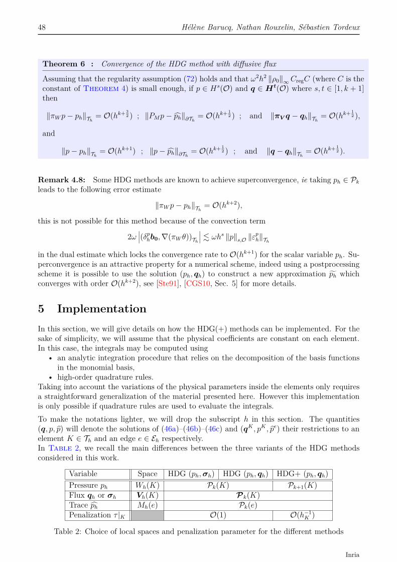
48 Hélène Barucq, Nathan Rouxelin, Sébastien Tordeux
Theorem 6 : Convergence of the HDG method with diffusive flux
Assuming that the regularity assumption (72) holds and that ω2h2 ‖ρ0‖∞CregC (where C is theconstant of Theorem 4) is small enough, if p ∈ Hs(O) and q ∈Ht(O) where s, t ∈ [1, k + 1]then
‖πWp− ph‖Th= O(hk+ 3
2 ) ; ‖PMp− ph‖∂Th= O(hk+ 1
2 ) ; and ‖πV q − qh‖Th= O(hk+ 1
2 ),
and
‖p− ph‖Th= O(hk+1) ; ‖p− ph‖∂Th
= O(hk+ 12 ) ; and ‖q − qh‖Th
= O(hk+ 12 ).
Remark 4.8: Some HDG methods are known to achieve superconvergence, ie taking ph ∈ Pkleads to the following error estimate
‖πWp− ph‖Th= O(hk+2),
this is not possible for this method because of the convection term
2ω∣∣∣(δphb0,∇(πW θ))Th
∣∣∣ . ωhs ‖p‖s,O ‖εph‖Th
in the dual estimate which locks the convergence rate to O(hk+1) for the scalar variable ph. Su-perconvergence is an attractive property for a numerical scheme, indeed using a postprocessingscheme it is possible to use the solution (ph, qh) to construct a new approximation ph whichconverges with order O(hk+2), see [Ste91], [CGS10, Sec. 5] for more details.
5 ImplementationIn this section, we will give details on how the HDG(+) methods can be implemented. For thesake of simplicity, we will assume that the physical coefficients are constant on each element.In this case, the integrals may be computed using
• an analytic integration procedure that relies on the decomposition of the basis functionsin the monomial basis,
• high-order quadrature rules.Taking into account the variations of the physical parameters inside the elements only requiresa straightforward generalization of the material presented here. However this implementationis only possible if quadrature rules are used to evaluate the integrals.To make the notations lighter, we will drop the subscript h in this section. The quantities(q, p, p) will denote the solutions of (46a)–(46b)–(46c) and (qK , pK , pe) their restrictions to anelement K ∈ Th and an edge e ∈ Eh respectively.In Table 2, we recall the main differences between the three variants of the HDG methodsconsidered in this work.
Variable Space HDG (ph,σh) HDG (ph, qh) HDG+ (ph, qh)Pressure ph Wh(K) Pk(K) Pk+1(K)Flux qh or σh Vh(K) Pk(K)Trace ph Mh(e) Pk(e)Penalization τ |K O(1) O(h−1
K )
Table 2: Choice of local spaces and penalization parameter for the different methods
Inria
HDG and HDG+ methods for harmonic wave problems with convection 49
5.1 Framework and notationsIn this section we present the notations used in [BCDL15, FS20] which are very close to theones used in hawen6. We will then give details on how the matrices are assembled.
Local problem: The discretization of the local problem (46a)–(46b) leads to the followingsystem
AKWK + CKΛK = SK , (82)
where
WK :=[pK qKx qKy qKz
]Tand ΛK :=
[pg(K,1) pg(K,2) pg(K,3) pg(K,4)
]T,
and pK denotes the vector of the coefficients of pKh in the basis of Wh(K).
Global problem: The discretization of the transmission condition (46c) leads to∑K∈Th
BKWK + LKΛK = 0 (83)
We denote by Λ the global trace approximation and for each element K ∈ Th we introduce theconnectivity map which is the operator AK such that7
AKΛ = ΛK .
Using (82), we can express WK in terms of Λ
WK =(AK
)−1SK −
(AK
)−1CKAKΛ
and we can finally construct the global problem using (83)
∑K∈Th
ATK[−BK
(AK
)−1CK + LK
]AKΛ = −
∑K∈Th
ATKBK(AK
)−1SK . (84)
For conciseness, we will denote
KK := −BK(AK
)−1CK + LK , K :=
∑K∈Th
ATKKKAK and S := −∑K∈Th
ATKBK(AK
)−1SK .
Remark 5.1: the invertibility of matrix AK was the object of Theorem 1 (HDG-σh) andTheorem 4 (HDG+ and HDG-qh) and the invertibility of the global matrix K was the objectof Theorem 3.
Remark 5.2: to efficiently implement the HDG(+) methods, we will need to compute theinverse of AK . As this matrix is not too large, it is possible to perform this operation usinglapack. However the discretization of the global problem will lead to a large sparse systemwhich will be solved using mumps.
6See https://ffaucher.gitlab.io/hawen-website/.7The aim of operator AK is to copy the global informations to the local solver, depending on the element it
may be a simple copy or also involve reordering.
RR n° 9410
50 Hélène Barucq, Nathan Rouxelin, Sébastien Tordeux
Solving HDG: In Algorithm 3, we describe how the HDG method can be efficientlyimplemented. Details on the construction of the local matrices AK , CK , BK and LK andon the implementation of boundary conditions will be given in the next sections.
Algorithm 3: Solving HDG/* Step 1: Construction of the local and global problems */
1 for K ∈ Th do2 Construct the local matrices AK , CK , BK and LK
3 Compute (AK)−1 using lapack
4 Compute KK = BK(AK
)−1CK + LK
5 Modify KK to enforce the boundary conditions6 Use the connectivity operator AK to add the local contribution to the global matrix K
/* Step 2: Construction of the source term */7 Localize the source8 for K ∈ Th where s 6= 0 do9 Construct the local source term SK
10 Compute −BK(AK)−1SK11 Use the connectivity operator AK to add the local contribution to the global source S
/* Step 3: Resolution of the global system */12 Solve KΛ = S with mumps
/* Step 4: Reconstruction of the solution */13 for K ∈ Th do14 Compute the local unknowns WK =
(AK
)−1SK −
(AK
)−1CKAKΛ
Convention for the indices: we will always use the following convention for the indices :• index of basis functions : i (test), j (trial), r (other)• component of a vector : u, v ∈ {x, y, z}• global number of an edge : m• local number of an edge : `• polynomial degree : k
The global number of the `-th face of element K will be denoted by g(K, `).
Dimension of polynomial spaces: We recall that the dimension of the space of polynomialsof n variables and of degree up to k is given by
dim (Pk(K)) =(k + nn
)=: dn(k), for K ⊂ Rn.
5.2 Implementation of the diffusive flux HDG methodIn this section, we focus on the implementation of the HDG-qh method.
5.2.1 Definition of the elementary matrices
We introduce the basis (ΦKj )dn(k)
j=1 of Pk(K) and (Ψej)dn−1(k)j=1 of Pk(e) and we decompose the
unknowns as
pK =dn(k)∑j=1
pKj ΦKj ; qKu =
dn(k)∑j=1
qKu,jΦKj ; pe(x) =
dn−1(k)∑j=1
pejΨej
Inria
HDG and HDG+ methods for harmonic wave problems with convection 51
for u ∈ {x, y, z}, K ∈ Th and e ∈ Eh.We introduce the following matrices
MKij =
∫K
ΦKi ΦK
j dx DKu,ij =
∫K
ΦKj ∂uΦK
i dx
EK`,ij =∫∂K`
ΦKi ΦK
j dσ FK`,ij =∫∂K`
Ψg(K,`)j ΦK
i dσ
Gmij =
∫em
Ψmi Ψm
j dσ
(85)
where g(K, `) is the global number of the `-th face of element K and m is also the globalnumber of the edge em.Notice that all those matrices except FK` (which has dimension dn(k) × dn−1(k)) are squarematrices and that all the elementary matrices are real.
5.2.2 Local problem
We introduce the following shorthand to make the algebra easier
α` = min∂K`
(b0 · n, 0) and tupw,` = max∂K`
(b0 · n, 0)
it corresponds to using the expression (44a)–(44b) of the numerical flux. From an implemen-tation point of view, this can be evaluated using array slicing or a ternary operator.Using the elementary matrices introduced in (85) we can write (46a) as∑
u
W0,vuMKqKu − DKv p
K +∑`
nK,`v FK` pg(K,`) = 0, ∀v ∈ {x, y, z} (86)
and (46b) as
−ω2ρ0MKpK + 2iω∑u
b0,uDKu p
K +∑u
(DKu )T qu
+2iω∑`
[−α`FK` pg(K,`) − tupw,`EK` pK + τ`(EK` pK − FK` pg(K,`))
]= SK (87)
Matrix form: To construct the global problem (84) we need to construct the matrices AK
and CK of the local problem (82) using (86) and (87).Matrix AK :AK pK qKx qKy qKz
−ρ0ω2MK + 2iω
∑u
b0,uDKu (DK
x )T (DKy )T (DK
z )T
pK +2iω∑`
(τ` − tupw,`)EK` −DKx +
∑`
nK,`x EK` −DKy +
∑`
nK,`y EK` −DKz +
∑`
nK,`y EK`
qKx −DKx WK
0,11MK WK0,12MK WK
0,13MK
qKy −DKy WK
0,21MK WK0,22MK WK
0,23MK
qKz −DKz WK
0,31MK WK0,32MK WK
0,33MK
The red terms can be used instead of the black ones, depending on wether or not an integrationby parts is performed.Matrix CK :
CK pg(K,1) pg(K,2) pg(K,3) pg(K,4)
pK −2iω(τ1 + α1)FK1 −2iω(τ2 + α2)FK2 −2iω(τ3 + α3)FK3 −2iω(τ4 + α4)FK4qKx nK,1x FK1 nK,2x FK2 nK,3x FK3 nK,4x FK4qKy nK,1y FK1 nK,2y FK2 nK,3y FK3 nK,4y FK4qKz nK,1z FK1 nK,2z FK2 nK,3z FK3 nK,4z FK4
RR n° 9410
52 Hélène Barucq, Nathan Rouxelin, Sébastien Tordeux
Remark 5.3: We chose to write the matrix form of the method with the equation for pK firstwhich is the opposite of the system (46a)–(46b)–(46c). This convention is interesting becausethe matrices for the method in dimension n are submatrices of the ones for dimension n+ 1.
5.2.3 Global problem
The transmission condition (46c) can be written as∑K,`
(∑u
nK,`u (FK` )T qKu + 2iω[−(α`Gg(K,`)pg(K,`) + tupw,`(FK` )TpK
)+ τ
((FK` )TpK −Gg(K,`)pg(K,`)
)])= 0
(88)
Matrix form: We will now use (88) to construct the matrices BK and LK of (83).Matrix BK :
BK pK qKx qKy qKz
e1 2iω(τ1 − tupw,1)(FK1 )T nK,1x (FK1 )T nK,1y (FK1 )T nK,1z (FK1 )Te2 2iω(τ2 − tupw,2)(FK2 )T nK,2x (FK2 )T nK,2y (FK2 )T nK,2z (FK2 )Te3 2iω(τ3 − tupw,3)(FK3 )T nK,3x (FK3 )T nK,3y (FK3 )T nK,3z (FK3 )Te4 2iω(τ4 − tupw,4)(FK4 )T nK,4x (FK4 )T nK,4y (FK4 )T nK,4z (FK4 )T
Matrix LK :
LK pg(K,1) pg(K,2) pg(K,3) pg(K,4)
e1 −2iω(τ1 + α1)Gg(K,1)
e2 −2iω(τ2 + α2)Gg(K,2)
e3 −2iω(τ3 + α3)Gg(K,3)
e4 −2iω(τ4 + α4)Gg(K,4
5.2.4 Boundary conditions:
The transmission condition (46c) was also used to weakly enforce the boundary conditions
q · n− 2iω(b0 · n)p = gN on ΓNp = gD on ΓD
Neumann boundary condition: If we want to enforce the Neumann boundary conditionon edge ` of element K we only need to add a right-hand side to (88) :
Gg(K,`)gN
where we assumed thatgN =
∑i
gN,iΨi.
Weak Dirichlet boundary conditions: However if we want to enforce the Dirichlet bound-ary condition on edge ` of element K we need to change the matrices BK and LK . This firstmethod of implementation corresponds to weakly enforcing the boundary conditions, ie usingthe expression
〈ph − gD, µ〉ΓD= 0.
This method is used for a modal implementation of the HDG method. It can be implementedas follows described in Algorithm 4.
Inria
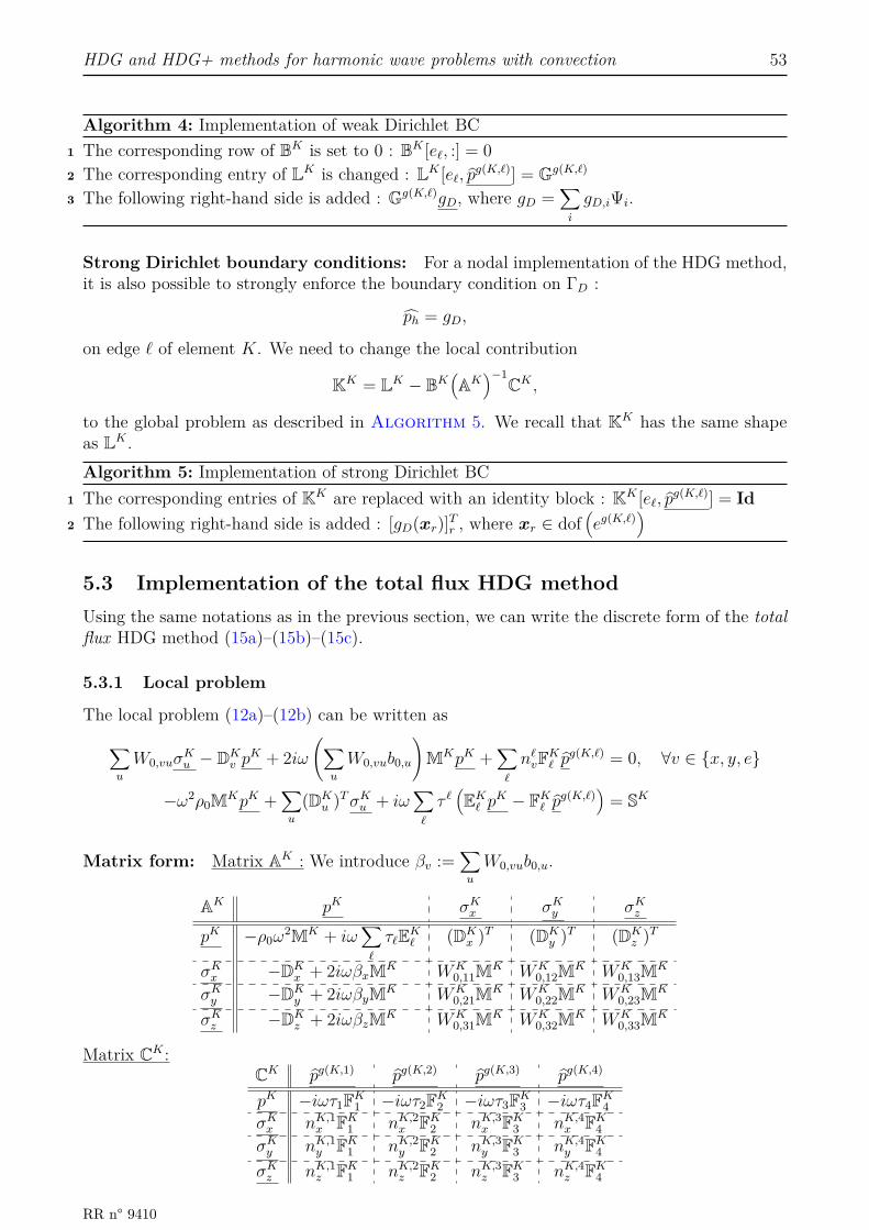
HDG and HDG+ methods for harmonic wave problems with convection 53
Algorithm 4: Implementation of weak Dirichlet BC1 The corresponding row of BK is set to 0 : BK [e`, :] = 02 The corresponding entry of LK is changed : LK [e`, pg(K,`)] = Gg(K,`)
3 The following right-hand side is added : Gg(K,`)gD, where gD =∑i
gD,iΨi.
Strong Dirichlet boundary conditions: For a nodal implementation of the HDG method,it is also possible to strongly enforce the boundary condition on ΓD :
ph = gD,
on edge ` of element K. We need to change the local contribution
KK = LK − BK(AK
)−1CK ,
to the global problem as described in Algorithm 5. We recall that KK has the same shapeas LK .Algorithm 5: Implementation of strong Dirichlet BC
1 The corresponding entries of KK are replaced with an identity block : KK [e`, pg(K,`)] = Id2 The following right-hand side is added : [gD(xr)]Tr , where xr ∈ dof
(eg(K,`)
)
5.3 Implementation of the total flux HDG methodUsing the same notations as in the previous section, we can write the discrete form of the totalflux HDG method (15a)–(15b)–(15c).
5.3.1 Local problem
The local problem (12a)–(12b) can be written as∑u
W0,vuσKu − DK
v pK + 2iω
(∑u
W0,vub0,u
)MKpK +
∑`
n`vFK` pg(K,`) = 0, ∀v ∈ {x, y, e}
−ω2ρ0MKpK +∑u
(DKu )TσKu + iω
∑`
τ `(EK` pK − FK` pg(K,`)
)= SK
Matrix form: Matrix AK : We introduce βv :=∑u
W0,vub0,u.
AK pK σKx σKy σKz
pK −ρ0ω2MK + iω
∑`
τ`EK` (DKx )T (DK
y )T (DKz )T
σKx −DKx + 2iωβxMK WK
0,11MK WK0,12MK WK
0,13MK
σKy −DKy + 2iωβyMK WK
0,21MK WK0,22MK WK
0,23MK
σKz −DKz + 2iωβzMK WK
0,31MK WK0,32MK WK
0,33MK
Matrix CK :CK pg(K,1) pg(K,2) pg(K,3) pg(K,4)
pK −iωτ1FK1 −iωτ2FK2 −iωτ3FK3 −iωτ4FK4σKx nK,1x FK1 nK,2x FK2 nK,3x FK3 nK,4x FK4σKy nK,1y FK1 nK,2y FK2 nK,3y FK3 nK,4y FK4σKz nK,1z FK1 nK,2z FK2 nK,3z FK3 nK,4z FK4
RR n° 9410

54 Hélène Barucq, Nathan Rouxelin, Sébastien Tordeux
5.3.2 Global problem
The discrete transmission condition (14) can be written∑K,`
[nK,`u (FK` )TσKu + iωτ `
((FK` )pK −Gg(K,`)pg(K,`)
)]= 0
Matrix form: Matrix BK :
BK pK σKx σKy σKz
e1 iωτ1(FK1 )T nK,1x (FK1 )T nK,1y (FK1 )T nK,1z (FK1 )Te2 iωτ2(FK2 )T nK,2x (FK2 )T nK,2y (FK2 )T nK,2z (FK2 )Te3 iωτ3(FK3 )T nK,3x (FK3 )T nK,3y (FK3 )T nK,3z (FK3 )Te4 iωτ4(FK4 )T nK,4x (FK4 )T nK,4y (FK4 )T nK,4z (FK4 )T
Matrix LK :
LK pg(K,1) pg(K,2) pg(K,3) pg(K,4)
e1 −iωτ1Gg(K,1)
e2 −iωτ2Gg(K,2)
e3 −iωτ3Gg(K,3)
e4 −iωτ4Gg(K,4
5.4 Implementation of the HDG+ method
As pK ∈ Pk+1(K), qK ∈ Pk(K) and pe ∈ Pk(e), one should be very careful while writing thematrix form of the system, indeed we have
pK ∈ Cdn(k+1) and qK ∈ Cn×dn(k) (⇐⇒ qKu ∈ Cdn(k), u ∈ {x, y, z})
so some of the elementary matrices will be rectangular.
5.4.1 Definition of the elementary matrices
Let (ΦK,kj )dn(k)
j=1 be the basis for Pk(K) and (Ψe,kj )dn−1(k)
j=1 be the basis for Pk(e).The unknowns are therefore decomposed in the following way
pK =dn(k+1)∑j=1
pKj ΦK,k+1j ; qKu =
dn(k)∑j=1
qKu,jΦK,kj ; pe =
dn−1(k)∑j=1
pejΨe,kj
for u ∈ {x, y, z}.We define the following elementary matrices :
MK,kij =
∫K
ΦK,ki ΦK,k
j dx
DK,ku,ij =
∫K
ΦK,kj ∂uΦK,k
i dx DK,k,k+1u,ij =
∫K
ΦK,k+1j ∂uΦK,k
i dx
FK,k`,ij =∫∂K`
ΦK,ki Ψg(K,`),k
j dσ FK,k+1,k`,ij =
∫∂K`
ΦK,k+1i Ψg(K,`),k
j dσ (89)
EK,k`,ij =∫∂K`
ΦK,ki ΦK,k
j dσ
Gmi,j =
∫em
Ψm,ki Ψm,k
j dσ
Inria
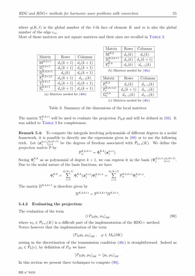
HDG and HDG+ methods for harmonic wave problems with convection 55
where g(K, `) is the global number of the `-th face of element K and m is also the globalnumber of the edge em.Most of those matrices are not square matrices and their sizes are recalled in Table 3.
Matrix Rows ColumnsMK,k+1 dn(k + 1) dn(k + 1)DK,k+1u dn(k + 1) dn(k + 1)
DK,k,k+1u dn(k) dn(k + 1)
FK,k+1,k` dn(k + 1) dn−1(k)
TK,k+1` dn(k + 1) dn(k + 1)
EK,k+1` dn(k + 1) dn(k + 1)(a) Matrices needed for (46b)
Matrix Rows ColumnsMK,k dn(k) dn(k)DK,k,k+1u dn(k) dn(k + 1)
FK,k` dn(k) dn−1(k)(b) Matrices needed for (46a)
Matrix Rows ColumnsFK,k` dn(k) dn−1(k)FK,k+1,k` dn(k + 1) dn−1(k)
Gm,k` dn−1(k) dn−1(k)(c) Matrices needed for (46c)
Table 3: Summary of the dimensions of the local matrices
The matrix TK,k+1` will be used to evaluate the projection PMp and will be defined in (93). It
was added to Table 3 for completeness.
Remark 5.4: To compute the integrals involving polynomials of different degrees in a nodalframework, it is possible to directly use the expressions given in (89) or to use the followingtrick. Let (xk+1
j )dn(k+1)j=1 be the degrees of freedom associated with Pk+1(K). We define the
projection matrix P byPK,k,k+1ij = ΦK,k
i (xk+1j ).
Seeing ΦK,ki as as polynomial of degree k + 1, we can express it in the basis (ΦK,k+1
j )dn(k+1)j=1 .
Due to the nodal nature of the basis functions, we have
ΦK,ki =
dn(k+1)∑r=1
ΦK,ki (xk+1
j )ΦK,k+1r =
dn(k+1)∑r=1
PK,k,k+1ir ΦK,k+1
r .
The matrix DK,k,k+1 is therefore given by
DK,k,k+1 = PK,k,k+1DK,k+1.
5.4.2 Evaluating the projection:
The evaluation of the term〈τPMph, wh〉∂K (90)
where wh ∈ Pk+1(K) is a difficult part of the implementation of the HDG+ method.Notice however that the implementation of the term
〈PMph, µh〉∂K , µ ∈Mh(∂K)
arising in the discretization of the transmission condition (46c) is straightforward. Indeed asµh ∈ Pk(e), by definition of PM we have
〈PMph, µh〉∂K = 〈ph, µh〉∂K .
In this section we present three techniques to compute (90).
RR n° 9410

56 Hélène Barucq, Nathan Rouxelin, Sébastien Tordeux
Efficient implementation using a hierarchical basis: The easiest way to compute (90)is to use a hierarchical and orthogonal basis for Pk+1(K). Let (ΦK
j )dn(k+1)j=1 be such a basis, then
(ΦKj )dn(k)
j=1 is a basis for Pk(K). Therefore if
pK =dn(k+1)∑j=1
pKj ΦKj
then
PMpK =
dn(k)∑j=1
pKj ΦKj .
A good choice for such a basis would probably be Dubiner’s one which is L2-orthogonal if thereference element is
• in 2D: the triangle with vertices
x1 = (−1,−1) ; x2 = (1,−1) ; x3 = (−1, 1),
• in 3D: the tetrahedron with vertices
x1 = (−1,−1,−1) ; x2 = (1,−1,−1) ; x3 = (−1, 1,−1) ; x4 = (−1,−1, 1).
See [Dub91, Kir04] for more details.As our solver is developed in the framework of nodal discontinuous Galerkin methods, we willnot use this method for our implementation.
Efficient implementation through Gauss-Legendre quadrature: As τ is constant oneach edge, we have
〈τPMph, u〉∂K = 〈τPMph, PMu〉∂K .
This integral can be efficiently computed in two dimensions by using a Gauss-Legendre quadra-ture. This trick is described in [Oik14, Sec. 3.4]. In two dimensions, the edges of a triangle isa one-dimensional interval I. For simplicity, we assume that I = [−1, 1].Denote by Gk the k points Gauss-Legendre quadrature rule. For a function f , it is given by
Gk[f ] =k∑i=1
wif(ai)
where (wi)i∈[[1,k]] are the quadrature weights and (ai)i∈[[1,k]] are the quadrature points. If thefunction f is regular enough, then Gk approximates the integral of f over I. In particular Gk+1is exact for polynomials of degree up to 2k+1. The usual stabilization term with p, u ∈ Pk+1(K),can be exactly computed with the k + 2 quadrature rule Gk+2 (which is exact for polynomialsof degree up to 2k + 3), ie.
Gk+2[τpu] = 〈τp, u〉∂K .
If the k + 1 points rule Gk+1 is used instead, the HDG+ stabilization term is obtained
Gk+1[τpu] = 〈τPMp, PMu〉∂K .
Lemma 5.1:
∀u, v ∈ Pk+1(I), Gk+1[uv] =∫IPMuPMvdx
Inria
HDG and HDG+ methods for harmonic wave problems with convection 57
Proof: Let ϕm be the Legendre polynomial of order m > 0. On I, we can write
u =k+1∑i=0
uiϕi and v =k+1∑i=0
viϕi.
Due to the hierarchical nature of the Legendre polynomials, we know that
PMu =k∑i=0
uiϕi and PMv =k∑i=0
viϕi.
We recall that Gk+1 is exact for polynomials of degree up to 2k + 1 and that ϕk+1 vanishes atthe quadrature points, ie.
∀i ∈ [[1, k + 1]], ϕk+1(ai) = 0.
Then we have
Gk+1[uv] =k+1∑i=1
[wi
k+1∑`=0
u`ϕ`(ai)k+1∑m=0
vmϕm(ai)]
=k+1∑i=1
[wi
k∑`=0
u`ϕ`(ai)k∑
m=0vmϕm(ai)
]
=k+1∑i=1
wi(PMu)(ai)(PMv)(ai)
= Gk+1[PMuPMv]
=∫IPMuPMvdx,
as deg(PMuPMv) = 2k.
Remark 5.5: the decomposition onto the Legendre basis is needed to prove the result, butanother basis (eg. Lagrange’s nodal basis) can be used in the implementation of the method.
Remark 5.6: unfortunately this result is not yet generalized for three-dimensional problems.
Generic implementation: We will now present a way to compute (90) that works for everychoice of polynomial basis in every space dimension. As this technique requires to precomputethe projections for all the basis functions of order k+ 1, the nodal HDG+ method may be lessattractive when p-adaptivity is needed.We assume that
pK =dn(k+1)∑j=1
pKj ΦK,k+1j and wh = ΦK,k+1
i
(90) therefore becomes
⟨PMp
Kh , wh
⟩∂K`
=dn(k+1)∑j=1
pKj⟨PMΦK,k+1
j ,ΦK,k+1i
⟩∂K`
. (91)
The next step is to decompose PMΦK,k+1j onto the basis of Mh(∂K)
PMΦK,k+1j =
dn−1(k)∑r=1
θK,`j,r Ψe,kr ,
RR n° 9410
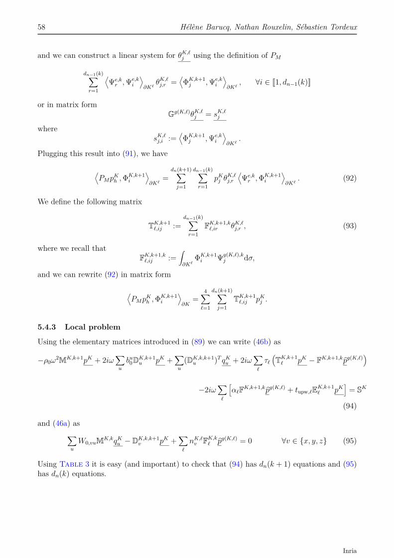
58 Hélène Barucq, Nathan Rouxelin, Sébastien Tordeux
and we can construct a linear system for θK,`j using the definition of PM
dn−1(k)∑r=1
⟨Ψe,kr ,Ψe,k
i
⟩∂K`
θK,`j,r =⟨ΦK,k+1j ,Ψe,k
i
⟩∂K`
, ∀i ∈ [[1, dn−1(k)]]
or in matrix formGg(K,`)θK,`j = sK,`j
wheresK,`j,i :=
⟨ΦK,k+1j ,Ψe,k
i
⟩∂K`
.
Plugging this result into (91), we have
⟨PMp
Kh ,Φ
K,k+1i
⟩∂K`
=dn(k+1)∑j=1
dn−1(k)∑r=1
pKj θK,`j,r
⟨Ψe,kr ,ΦK,k+1
i
⟩∂K`
. (92)
We define the following matrix
TK,k+1`,ij :=
dn−1(k)∑r=1
FK,k+1,k`,ir θK,`j,r , (93)
where we recall thatFK,k+1,k`,ij :=
∫∂K`
ΦK,k+1i Ψg(K,`),k
j dσ,
and we can rewrite (92) in matrix form
⟨PMp
Kh ,Φ
K,k+1i
⟩∂K
=4∑`=1
dn(k+1)∑j=1
TK,k+1`,ij pKj .
5.4.3 Local problem
Using the elementary matrices introduced in (89) we can write (46b) as
−ρ0ω2MK,k+1pK + 2iω
∑u
bu0DK,k+1u pK +
∑u
(DK,k,k+1u )T qKu + 2iω
∑`
τ`(TK,k+1` pK − FK,k+1,kpg(K,`)
)
−2iω∑`
[α`FK,k+1,kpg(K,`) + tupw,`EK,k+1
` pK]
= SK
(94)
and (46a) as∑u
W0,vuMK,kqKu − DK,k,k+1v pK +
∑`
nK,`v FK,k` pg(K,`) = 0 ∀v ∈ {x, y, z} (95)
Using Table 3 it is easy (and important) to check that (94) has dn(k + 1) equations and (95)has dn(k) equations.
Inria
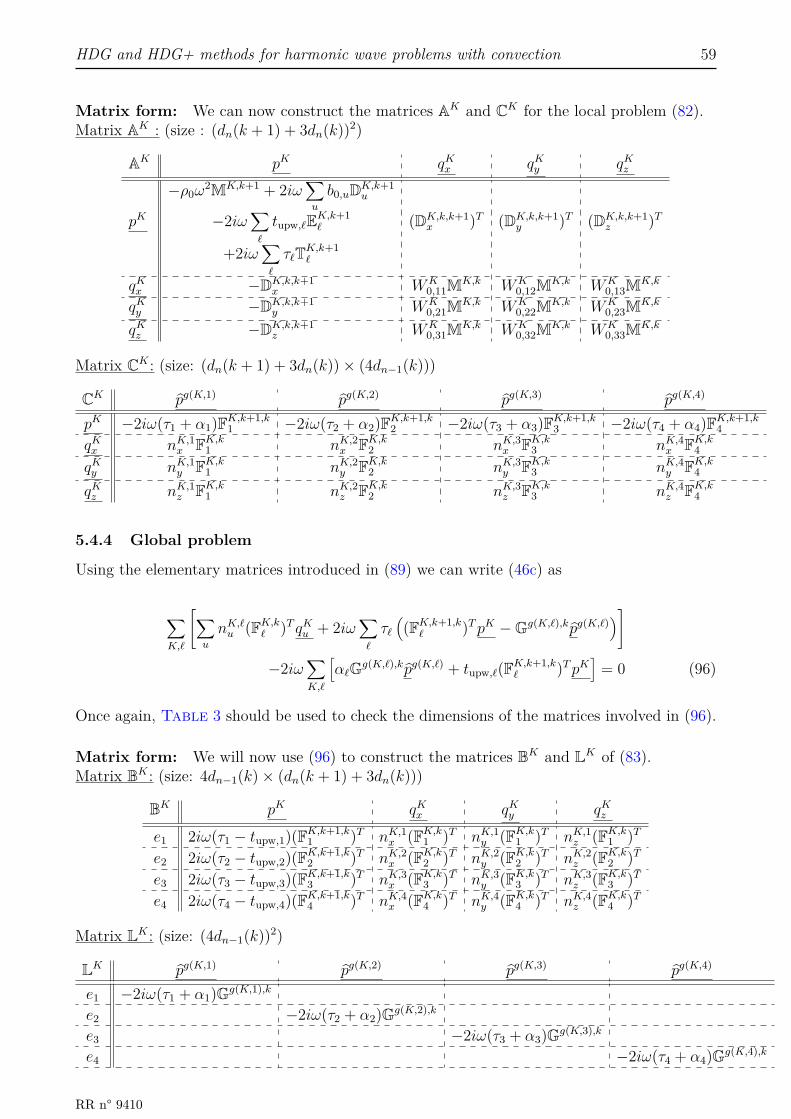
HDG and HDG+ methods for harmonic wave problems with convection 59
Matrix form: We can now construct the matrices AK and CK for the local problem (82).Matrix AK : (size : (dn(k + 1) + 3dn(k))2)
AK pK qKx qKy qKz
−ρ0ω2MK,k+1 + 2iω
∑u
b0,uDK,k+1u
pK −2iω∑`
tupw,`EK,k+1` (DK,k,k+1
x )T (DK,k,k+1y )T (DK,k,k+1
z )T
+2iω∑`
τ`TK,k+1`
qKx −DK,k,k+1x WK
0,11MK,k WK0,12MK,k WK
0,13MK,k
qKy −DK,k,k+1y WK
0,21MK,k WK0,22MK,k WK
0,23MK,k
qKz −DK,k,k+1z WK
0,31MK,k WK0,32MK,k WK
0,33MK,k
Matrix CK : (size: (dn(k + 1) + 3dn(k))× (4dn−1(k)))
CK pg(K,1) pg(K,2) pg(K,3) pg(K,4)
pK −2iω(τ1 + α1)FK,k+1,k1 −2iω(τ2 + α2)FK,k+1,k
2 −2iω(τ3 + α3)FK,k+1,k3 −2iω(τ4 + α4)FK,k+1,k
4qKx nK,1x FK,k1 nK,2x FK,k2 nK,3x FK,k3 nK,4x FK,k4
qKy nK,1y FK,k1 nK,2y FK,k2 nK,3y FK,k3 nK,4y FK,k4
qKz nK,1z FK,k1 nK,2z FK,k2 nK,3z FK,k3 nK,4z FK,k4
5.4.4 Global problem
Using the elementary matrices introduced in (89) we can write (46c) as
∑K,`
[∑u
nK,`u (FK,k` )T qKu + 2iω∑`
τ`((FK,k+1,k
` )TpK −Gg(K,`),kpg(K,`))]
−2iω∑K,`
[α`Gg(K,`),kpg(K,`) + tupw,`(FK,k+1,k
` )TpK]
= 0 (96)
Once again, Table 3 should be used to check the dimensions of the matrices involved in (96).
Matrix form: We will now use (96) to construct the matrices BK and LK of (83).Matrix BK : (size: 4dn−1(k)× (dn(k + 1) + 3dn(k)))
BK pK qKx qKy qKz
e1 2iω(τ1 − tupw,1)(FK,k+1,k1 )T nK,1x (FK,k1 )T nK,1y (FK,k1 )T nK,1z (FK,k1 )T
e2 2iω(τ2 − tupw,2)(FK,k+1,k2 )T nK,2x (FK,k2 )T nK,2y (FK,k2 )T nK,2z (FK,k2 )T
e3 2iω(τ3 − tupw,3)(FK,k+1,k3 )T nK,3x (FK,k3 )T nK,3y (FK,k3 )T nK,3z (FK,k3 )T
e4 2iω(τ4 − tupw,4)(FK,k+1,k4 )T nK,4x (FK,k4 )T nK,4y (FK,k4 )T nK,4z (FK,k4 )T
Matrix LK : (size: (4dn−1(k))2)
LK pg(K,1) pg(K,2) pg(K,3) pg(K,4)
e1 −2iω(τ1 + α1)Gg(K,1),k
e2 −2iω(τ2 + α2)Gg(K,2),k
e3 −2iω(τ3 + α3)Gg(K,3),k
e4 −2iω(τ4 + α4)Gg(K,4),k
RR n° 9410
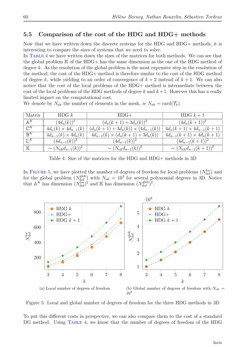
60 Hélène Barucq, Nathan Rouxelin, Sébastien Tordeux
5.5 Comparison of the cost of the HDG and HDG+ methodsNow that we have written down the discrete systems for the HDG and HDG+ methods, it isinteresting to compare the sizes of systems that we need to solve.In Table 4 we have written down the sizes of the matrices for both methods. We can see thatthe global problem K of the HDG+ has the same dimension as the one of the HDG method ofdegree k. As the resolution of the global problem is the most expensive step in the resolution ofthe method, the cost of the HDG+ method is therefore similar to the cost of the HDG methodof degree k, while yielding to an order of convergence of k + 2 instead of k + 1. We can alsonotice that the cost of the local problems of the HDG+ method is intermediate between thecost of the local problems of the HDG methods of degree k and k+1. However this has a reallylimited impact on the computational cost.We denote by Nelt the number of elements in the mesh, ie Nelt = card(Th).
Matrix HDG k HDG+ HDG k + 1AK (4dn(k))2 (dn(k + 1) + 3dn(k))2 (4dn(k + 1))2
CK 4dn(k)× 4dn−1(k) (dn(k + 1) + 3dn(k))× (4dn−1(k)) 4dn(k + 1)× 4dn−1(k + 1)BK 4dn−1(k)× 4dn(k) 4dn−1(k)× (dn(k + 1) + 3dn(k)) 4dn−1(k + 1)× 4dn(k + 1)LK (4dn−1(k))2 (4dn−1(k))2 (4dn−1(k + 1))2
K ∼ (Neltdn−1(k))2 ∼ (Neltdn−1(k))2 ∼ (Neltdn−1(k + 1))2
Table 4: Size of the matrices for the HDG and HDG+ methods in 3D
In Figure 5, we have plotted the number of degrees of freedom for local problems (N locdof) and
for the global problem (Nglobdof ) with Nelt = 103 for several polynomial degrees in 3D. Notice
that AK has dimension (N locdof)2 and K has dimension (Nglob
dof )2.
3 4 5 6 7 8
200
400
600
800
k
Nlo
cdo
f
HDG kHDG+HDG k + 1
(a) Local number of degrees of freedom
3 4 5 6 7 81
2
3
4
5
·104
k
Ngl
obdo
f
HDG kHDG+HDG k + 1
(b) Global number of degrees of freedom with Nelt =103
Figure 5: Local and global number of degrees of freedom for the three HDG methods in 3D
To put this different costs in perspective, we can also compare them to the cost of a standardDG method. Using Table 4, we know that the number of degrees of freedom of the HDG
Inria
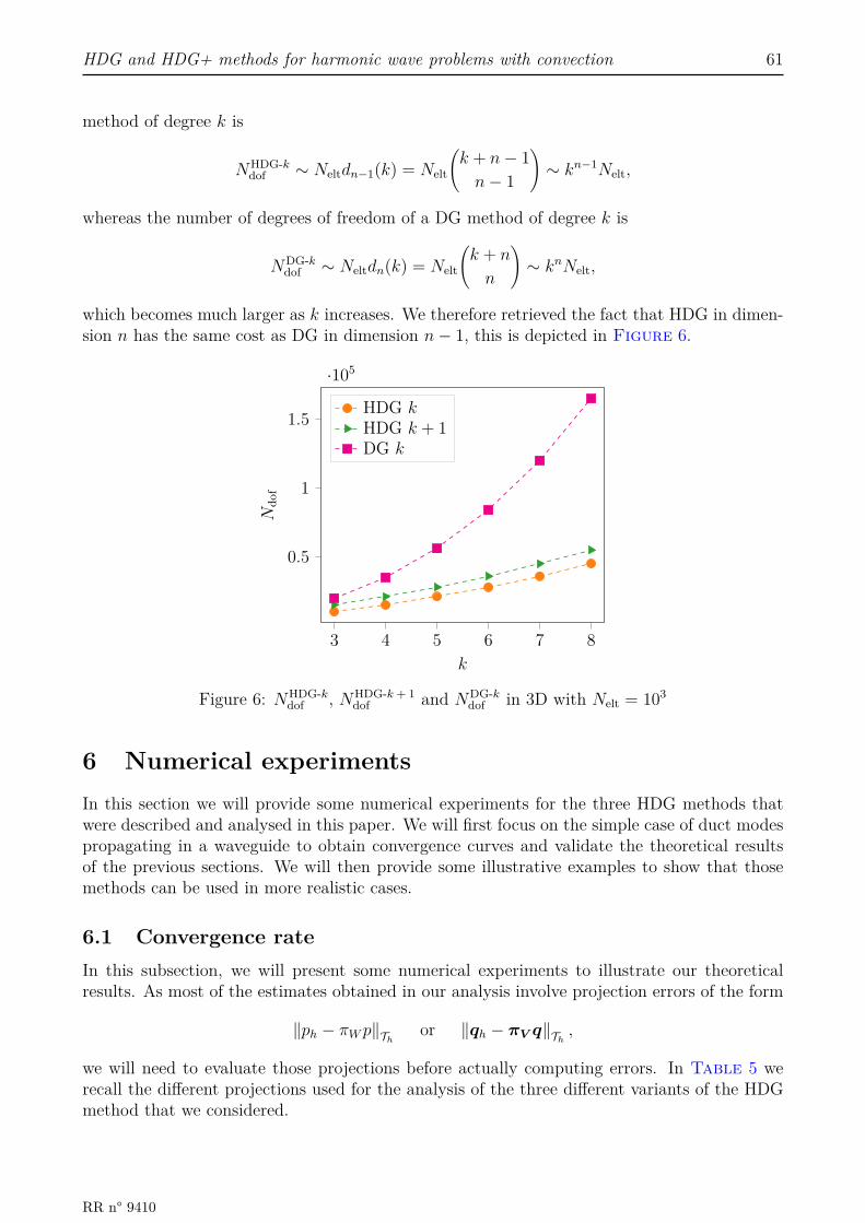
HDG and HDG+ methods for harmonic wave problems with convection 61
method of degree k is
NHDG-kdof ∼ Neltdn−1(k) = Nelt
(k + n− 1n− 1
)∼ kn−1Nelt,
whereas the number of degrees of freedom of a DG method of degree k is
NDG-kdof ∼ Neltdn(k) = Nelt
(k + n
n
)∼ knNelt,
which becomes much larger as k increases. We therefore retrieved the fact that HDG in dimen-sion n has the same cost as DG in dimension n− 1, this is depicted in Figure 6.
3 4 5 6 7 8
0.5
1
1.5
·105
k
Ndo
f
HDG kHDG k + 1DG k
Figure 6: NHDG-kdof , NHDG-k + 1
dof and NDG-kdof in 3D with Nelt = 103
6 Numerical experimentsIn this section we will provide some numerical experiments for the three HDG methods thatwere described and analysed in this paper. We will first focus on the simple case of duct modespropagating in a waveguide to obtain convergence curves and validate the theoretical resultsof the previous sections. We will then provide some illustrative examples to show that thosemethods can be used in more realistic cases.
6.1 Convergence rateIn this subsection, we will present some numerical experiments to illustrate our theoreticalresults. As most of the estimates obtained in our analysis involve projection errors of the form
‖ph − πWp‖Thor ‖qh − πV q‖Th
,
we will need to evaluate those projections before actually computing errors. In Table 5 werecall the different projections used for the analysis of the three different variants of the HDGmethod that we considered.
RR n° 9410
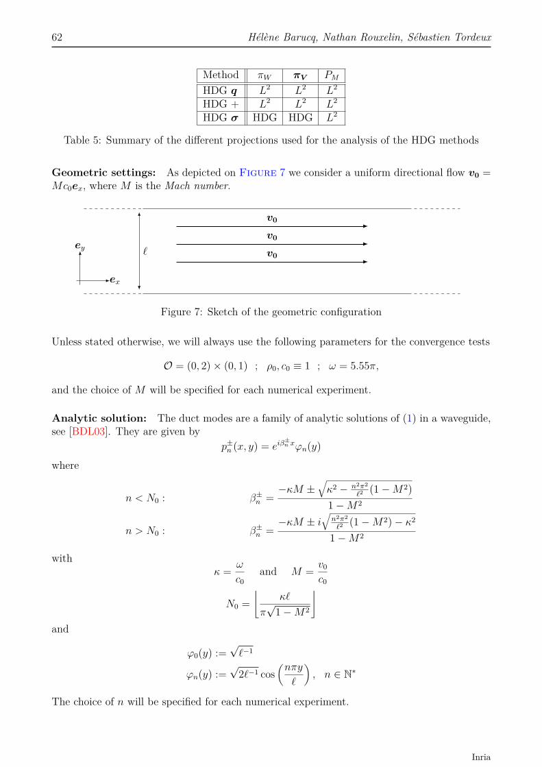
62 Hélène Barucq, Nathan Rouxelin, Sébastien Tordeux
Method πW πV PM
HDG q L2 L2 L2
HDG + L2 L2 L2
HDG σ HDG HDG L2
Table 5: Summary of the different projections used for the analysis of the HDG methods
Geometric settings: As depicted on Figure 7 we consider a uniform directional flow v0 =Mc0ex, where M is the Mach number.
`
ex
ey
v0
v0
v0
Figure 7: Sketch of the geometric configuration
Unless stated otherwise, we will always use the following parameters for the convergence tests
O = (0, 2)× (0, 1) ; ρ0, c0 ≡ 1 ; ω = 5.55π,
and the choice of M will be specified for each numerical experiment.
Analytic solution: The duct modes are a family of analytic solutions of (1) in a waveguide,see [BDL03]. They are given by
p±n (x, y) = eiβ±n xϕn(y)
where
n < N0 : β±n =−κM ±
√κ2 − n2π2
`2(1−M2)
1−M2
n > N0 : β±n =−κM ± i
√n2π2
`2(1−M2)− κ2
1−M2
withκ = ω
c0and M = v0
c0
N0 =⌊
κ`
π√
1−M2
⌋and
ϕ0(y) :=√`−1
ϕn(y) :=√
2`−1 cos(nπy
`
), n ∈ N∗
The choice of n will be specified for each numerical experiment.
Inria

HDG and HDG+ methods for harmonic wave problems with convection 63
Evaluating the projections: Here we give the details for evaluating the L2 projection ontoWh, the process is very similar for the other projections.We recall that the dimension of the polynomial spaces is given by
dimPk(K) =(n+ k
n
)=: dn(k), for K ⊂ Rn.
All the projections considered are local to an element K, so evaluating them amounts to solvinga linear system on each K. Indeed, the definition of the L2 projection onto Wh(K) = Pk(K)gives
∀i ∈ [[1, dn(k)]],(πWp,ΦK,k
i
)K
=(p,ΦK,k
i
)K.
As πWp ∈ Wh(K), we can write
πWp =dn(k)∑j=1
πjΦK,kj ,
where π = (πj)j is the vector of the coordinates of πWp in the basis (ΦKj )j of Pk(K). We
therefore obtain the following system
∀i ∈ [[1, dn(k)]],dn(k)∑j=1
πj(ΦK,kj ,ΦK,k
i
)K
=(p,ΦK,k
i
)K,
or in matrix formMK,kπ = s, where si =
(p,ΦK,k
i
)K.
The integral in the right-hand side is evaluated using a 91 points Gauss-Lobatto quadratureformula and the linear system can be solved using lapack.
Evaluating the L2-error: Now that the projections can be evaluated, it remains to computethe L2 norms. As the numerical solution and the projections are polynomial quantities, thiscan be done using the mass matrix. Indeed, for u ∈ Pk(K) we have
‖u‖2K =
dn(k)∑j=1
ujΦK,kj ,
dn(k)∑i=1
uiΦK,ki
K
=dn(k)∑i,j=1
uju∗i
(ΦK,kj ,ΦK,k
i
)K
=dn(k)∑i=1
u∗i
dn(k)∑j=1
MK,kij uj
= u∗MK,ku.
To obtain more meaningful results, we will use relative errors instead of the standard L2-error.This choice allows us to compare the errors computed on different meshes without any pollutioncoming from the different number of elements. The relative error for ph is given by
Ep :=‖ph − πWp‖Th
‖πWp‖Th
,
and similar expressions will be used for the other volumetric quantities.
RR n° 9410

64 Hélène Barucq, Nathan Rouxelin, Sébastien Tordeux
Some notation: To allow the comparison between the HDG+ method and the two HDGmethods, we would like to emphasize that k always denotes the polynomial degree used toapproximate the trace unknown ph. We have chosen to plot the relative errors against thequantity k
hwhich is proportional to the number of degrees of freedom per wavelength. We
would like to point out that all the plots in the next sections will use a log-log scale.
Hardware configuration: Those numerical experiments were carried out on a miriel nodeon the plafrim cluster8. This node is equipped with a 2 dodeca-core Haswell Intel XeonE5-2680 v3 with a clock rate of 2.5 GHz and 128 Go of memory.
6.1.1 Acoustic case without flow
A first important test to validate our implementation in the acoustic case without flow. In thiscase, the convected Helmholtz equation reduces to the standard Helmholtz equation and theHDG methods, either with the diffusive or total flux, are the same when there is no convection.We should therefore be able to reproduce the super-convergence of the HDG method for theHelmholtz equation , ie.
Ep = O(hk+2),
when an approximation of degree k is used for all the unknowns.Here we have chosen to use the following parameters
n = 0, and M = 0,
which correspond to a plane-wave.The resulting convergence curve is depicted on Figure 8 and we can clearly see that thesuper-convergence is obtained.
101.2 101.4 101.6 101.8 102
10−8
10−7
10−6
10−5
10−4
10−3
10−2
10−1
k
h
E p
P3P4P5
O(h5.0)O(h6.0)O(h7.0)
Figure 8: Convergence history for the HDG method without flow for the volumetric unknownph
8See http://www.plafrim.fr.
Inria
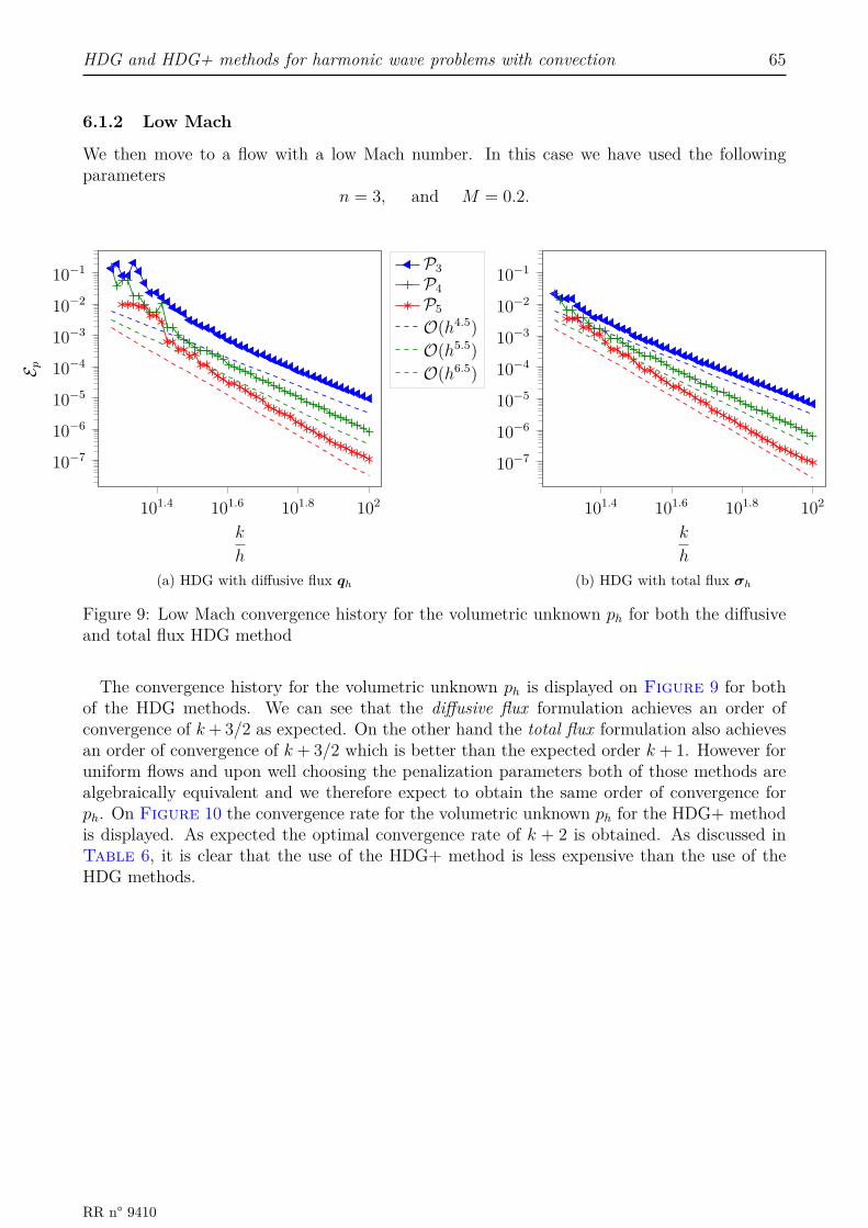
HDG and HDG+ methods for harmonic wave problems with convection 65
6.1.2 Low Mach
We then move to a flow with a low Mach number. In this case we have used the followingparameters
n = 3, and M = 0.2.
101.4 101.6 101.8 102
10−7
10−6
10−5
10−4
10−3
10−2
10−1
k
h
E p
P3P4P5
O(h4.5)O(h5.5)O(h6.5)
(a) HDG with diffusive flux qh
101.4 101.6 101.8 102
10−7
10−6
10−5
10−4
10−3
10−2
10−1
k
h
(b) HDG with total flux σh
Figure 9: Low Mach convergence history for the volumetric unknown ph for both the diffusiveand total flux HDG method
The convergence history for the volumetric unknown ph is displayed on Figure 9 for bothof the HDG methods. We can see that the diffusive flux formulation achieves an order ofconvergence of k+ 3/2 as expected. On the other hand the total flux formulation also achievesan order of convergence of k + 3/2 which is better than the expected order k + 1. However foruniform flows and upon well choosing the penalization parameters both of those methods arealgebraically equivalent and we therefore expect to obtain the same order of convergence forph. On Figure 10 the convergence rate for the volumetric unknown ph for the HDG+ methodis displayed. As expected the optimal convergence rate of k + 2 is obtained. As discussed inTable 6, it is clear that the use of the HDG+ method is less expensive than the use of theHDG methods.
RR n° 9410
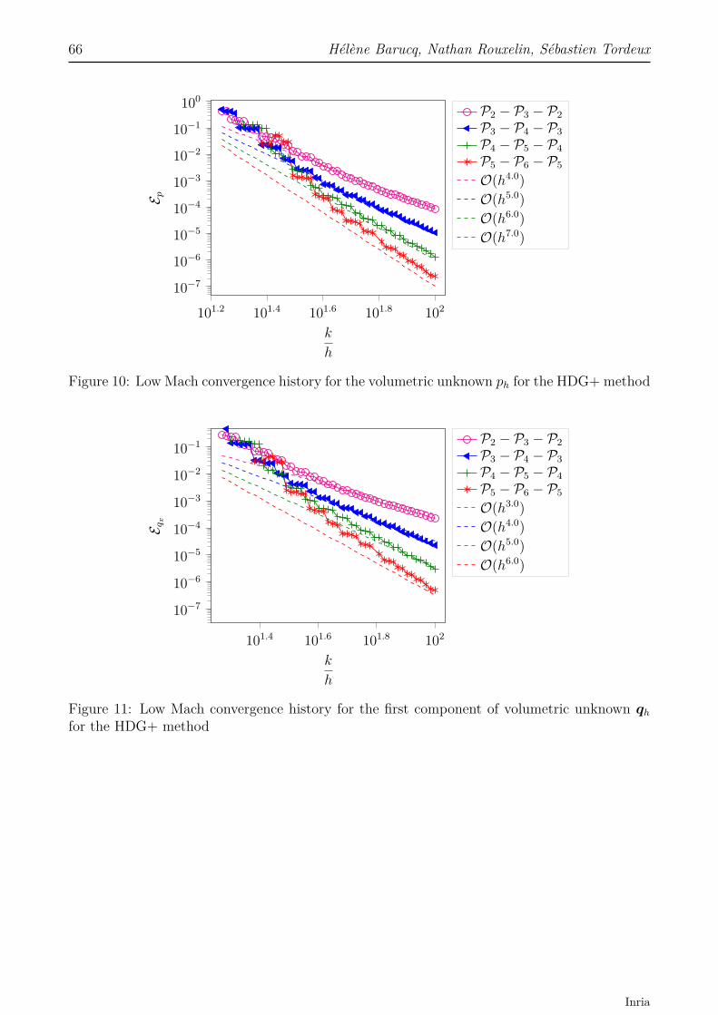
66 Hélène Barucq, Nathan Rouxelin, Sébastien Tordeux
101.2 101.4 101.6 101.8 102
10−7
10−6
10−5
10−4
10−3
10−2
10−1
100
k
h
E p
P2 − P3 − P2P3 − P4 − P3P4 − P5 − P4P5 − P6 − P5
O(h4.0)O(h5.0)O(h6.0)O(h7.0)
Figure 10: Low Mach convergence history for the volumetric unknown ph for the HDG+ method
101.4 101.6 101.8 102
10−7
10−6
10−5
10−4
10−3
10−2
10−1
k
h
E qx
P2 − P3 − P2P3 − P4 − P3P4 − P5 − P4P5 − P6 − P5
O(h3.0)O(h4.0)O(h5.0)O(h6.0)
Figure 11: Low Mach convergence history for the first component of volumetric unknown qhfor the HDG+ method
Inria

HDG and HDG+ methods for harmonic wave problems with convection 67
101.4 101.6 101.8 102
10−7
10−6
10−5
10−4
10−3
10−2
10−1
k
h
E qx
P3P4P5
O(h3.5)O(h4.5)O(h5.5)
(a) HDG with diffusive flux qh
101.4 101.6 101.8 102
10−7
10−6
10−5
10−4
10−3
10−2
10−1
k
h
E σx
P3P4P5
O(h4.5)O(h5.5)O(h6.5)
(b) HDG with total flux σh
Figure 12: Low Mach convergence history for the first component of the volumetric flux un-known
If we now move to the flux unknown, we can see on Figure 11 that qh converges with theoptimal order k + 1 as expected. For the HDG methods, the convergence histories for qh andσh are depicted on Figure 12. The diffusive flux formulation achieves a convergence order ofk+ 1/2 as expected, whereas the total flux formulation outperforms the theoretical results andachieves an order of k + 3/2. For this formulation it was however expected that both ph andσh converge with the same order, which is actually the case. Finally we would like to point outthat the choice between the formulations with qh or σh is application dependent.Finally information regarding the size of the global problems for a fixed number of degreesof freedom per wavelength are given in Table 6. We have included the HDG+ method with(k, k−1) and the HDG+ method with (k+1, k). When using the HDG+ method with (k, k−1),a smaller global problem is solved to obtain the same convergence rate as the HDG methods.When using the HDG+ method with (k+ 1, k), larger elements can be used to obtain the samenumber of degrees of freedom per wavelength because of the higher polynomial interpolationdegree. We can clearly see that the HDG+ methods are computationally less expensive than
RR n° 9410

68 Hélène Barucq, Nathan Rouxelin, Sébastien Tordeux
both of the HDG methods.
k h/k HDG-qh HDG-σh HDG+ HDG+(k, k − 1) (k + 1, k)
nnz 20 384 20 384 10 968 8 7203 10−1 nnz LU 36 872 36 872 15 216 9 800
MUMPS time 2.5 · 10−2 1.6 · 10−2 1.8 · 10−2 1.7 · 10−2
nnz 872 216 872 216 481 528 467 2803 10−2 nnz LU 3 572 752 3 572 752 1 835 148 1 673 560
MUMPS time 0.27 0.23 0.15 0.10nnz 17 130 17 130 8 720 4 980
4 10−1 nnz LU 24 125 24 125 9 800 4 644MUMPS time 1.9 · 10−2 2.0 · 10−2 1.7 · 10−2 9.5 · 10−3
nnz 752 330 752 330 467 280 423 6004 10−2 nnz LU 2 874 075 2 874 075 1 673 560 1 397 418
MUMPS time 0.19 0.17 0.10 8.6 · 10−2
nnz 12 552 12 552 4 980 4 3325 10−1 nnz LU 14 112 14 112 4 644 4 068
MUMPS time 1.7 · 10−2 2.7 · 10−2 9.5 · 10−3 9.9 · 10−3
nnz 672 840 672 840 432 600 414 4565 10−2 nnz LU 2 409 006 2 409 006 1 397 418 1 333 368
MUMPS time 0.12 0.11 8.6 · 10−2 6.8 · 10−2
Table 6: Size of the global systems and mumps elapsed time for different interpolation degree kfor the low Mach case with a fixed number of degrees of freedom per wavelength
Notice that the numerical experiments performed here lead to relatively small linear system. In-deed our goal was to validate the numerical method rather than showing the ability of hawen tohandle large numerical simulations.In Table 7, we review the size of the global system for various interpolation degrees k with afixed error threshold for ph. As we did before, we use the relative L2-error defined by
Ep :=‖ph − πWp‖Th
‖πWp‖Th
.
We can clearly see that, when the desired error is smaller than 10−2, increasing the interpolationdegree and thus the order of the method leads to solving a smaller linear system to obtain thesame error level. This less visible for an error threshold of 10−2, as this accuracy can be obtainedwith relatively large elements even with a low interpolation degree. For this error level, we canalso see that there is no real difference in the size of the linear systems of HDG and HDG+methods. This is expected as there is no real difference between the different interpolationdegrees for this error threshold. However for smaller error thresholds, we can see that theHDG-qh, HDG-σh and HDG+ with (k, k − 1) lead to linear systems with similar sizes, whichis expected as they share the same order. The HDG+ method with (k+ 1, k) also has a higherconvergence rate and therefore lead to significantly smaller linear system for the same errorlevel.
Inria
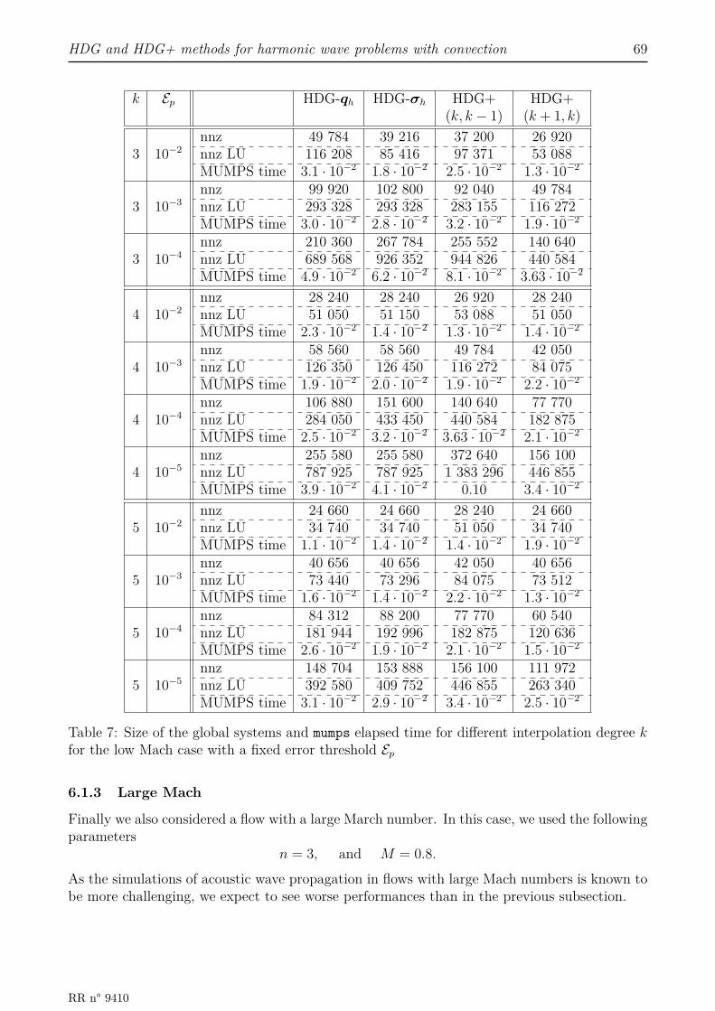
HDG and HDG+ methods for harmonic wave problems with convection 69
k Ep HDG-qh HDG-σh HDG+ HDG+(k, k − 1) (k + 1, k)
nnz 49 784 39 216 37 200 26 9203 10−2 nnz LU 116 208 85 416 97 371 53 088
MUMPS time 3.1 · 10−2 1.8 · 10−2 2.5 · 10−2 1.3 · 10−2
nnz 99 920 102 800 92 040 49 7843 10−3 nnz LU 293 328 293 328 283 155 116 272
MUMPS time 3.0 · 10−2 2.8 · 10−2 3.2 · 10−2 1.9 · 10−2
nnz 210 360 267 784 255 552 140 6403 10−4 nnz LU 689 568 926 352 944 826 440 584
MUMPS time 4.9 · 10−2 6.2 · 10−2 8.1 · 10−2 3.63 · 10−2
nnz 28 240 28 240 26 920 28 2404 10−2 nnz LU 51 050 51 150 53 088 51 050
MUMPS time 2.3 · 10−2 1.4 · 10−2 1.3 · 10−2 1.4 · 10−2
nnz 58 560 58 560 49 784 42 0504 10−3 nnz LU 126 350 126 450 116 272 84 075
MUMPS time 1.9 · 10−2 2.0 · 10−2 1.9 · 10−2 2.2 · 10−2
nnz 106 880 151 600 140 640 77 7704 10−4 nnz LU 284 050 433 450 440 584 182 875
MUMPS time 2.5 · 10−2 3.2 · 10−2 3.63 · 10−2 2.1 · 10−2
nnz 255 580 255 580 372 640 156 1004 10−5 nnz LU 787 925 787 925 1 383 296 446 855
MUMPS time 3.9 · 10−2 4.1 · 10−2 0.10 3.4 · 10−2
nnz 24 660 24 660 28 240 24 6605 10−2 nnz LU 34 740 34 740 51 050 34 740
MUMPS time 1.1 · 10−2 1.4 · 10−2 1.4 · 10−2 1.9 · 10−2
nnz 40 656 40 656 42 050 40 6565 10−3 nnz LU 73 440 73 296 84 075 73 512
MUMPS time 1.6 · 10−2 1.4 · 10−2 2.2 · 10−2 1.3 · 10−2
nnz 84 312 88 200 77 770 60 5405 10−4 nnz LU 181 944 192 996 182 875 120 636
MUMPS time 2.6 · 10−2 1.9 · 10−2 2.1 · 10−2 1.5 · 10−2
nnz 148 704 153 888 156 100 111 9725 10−5 nnz LU 392 580 409 752 446 855 263 340
MUMPS time 3.1 · 10−2 2.9 · 10−2 3.4 · 10−2 2.5 · 10−2
Table 7: Size of the global systems and mumps elapsed time for different interpolation degree kfor the low Mach case with a fixed error threshold Ep
6.1.3 Large Mach
Finally we also considered a flow with a large March number. In this case, we used the followingparameters
n = 3, and M = 0.8.
As the simulations of acoustic wave propagation in flows with large Mach numbers is known tobe more challenging, we expect to see worse performances than in the previous subsection.
RR n° 9410

70 Hélène Barucq, Nathan Rouxelin, Sébastien Tordeux
101.4 101.6 101.8 102
10−7
10−6
10−5
10−4
10−3
10−2
10−1
k
h
E p
P3P4P5
O(h4.5)O(h5.5)O(h6.5)
(a) HDG with diffusive flux q
101.4 101.6 101.8 102
10−7
10−6
10−5
10−4
10−3
10−2
10−1
k
h
(b) HDG with total flux σ
Figure 13: Large Mach convergence history for the volumetric unknown ph for both of the HDGmethods
101.2 101.4 101.6 101.8 102
10−7
10−6
10−5
10−4
10−3
10−2
10−1
k
h
E p
P2 − P3 − P2P3 − P4 − P3P4 − P5 − P4
O(h4.0)O(h5.0)O(h6.0)
Figure 14: Large Mach convergence history for the volumetric unknown ph for the HDG+method
The convergence history for the volumetric unknown is depicted in Figure 13 for both of theHDG methods. We can see that the total flux formulation still achieves the convergence orderof k+ 3/2 whereas the behaviour of the diffusive flux formulation seems less robust. The sameconvergence history for HDG+ method is displayed on Figure 14 and we can see that it stillachieves the optimal convergence rate of k + 2.
Inria
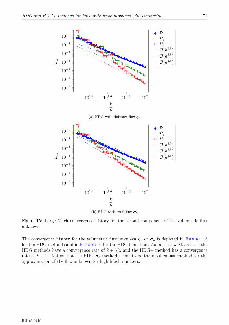
HDG and HDG+ methods for harmonic wave problems with convection 71
101.4 101.6 101.8 102
10−7
10−6
10−5
10−4
10−3
10−2
10−1
k
h
E qy
P3P4P5
O(h3.5)O(h4.5)O(h5.5)
(a) HDG with diffusive flux qh
101.4 101.6 101.8 102
10−7
10−6
10−5
10−4
10−3
10−2
10−1
k
h
E σy
P3P4P5
O(h4.5)O(h5.5)O(h6.5)
(b) HDG with total flux σh
Figure 15: Large Mach convergence history for the second component of the volumetric fluxunknown
The convergence history for the volumetric flux unknown qh or σh is depicted in Figure 15for the HDG methods and in Figure 16 for the HDG+ method. As in the low-Mach case, theHDG methods have a convergence rate of k + 3/2 and the HDG+ method has a convergencerate of k + 1. Notice that the HDG-σh method seems to be the most robust method for theapproximation of the flux unknown for high Mach numbers.
RR n° 9410
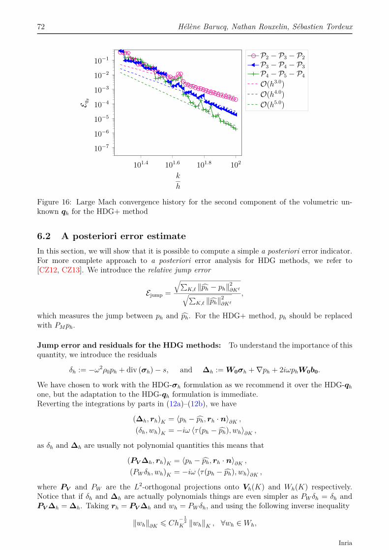
72 Hélène Barucq, Nathan Rouxelin, Sébastien Tordeux
101.4 101.6 101.8 102
10−7
10−6
10−5
10−4
10−3
10−2
10−1
k
h
E qy
P2 − P3 − P2P3 − P4 − P3P4 − P5 − P4
O(h3.0)O(h4.0)O(h5.0)
Figure 16: Large Mach convergence history for the second component of the volumetric un-known qh for the HDG+ method
6.2 A posteriori error estimateIn this section, we will show that it is possible to compute a simple a posteriori error indicator.For more complete approach to a posteriori error analysis for HDG methods, we refer to[CZ12, CZ13]. We introduce the relative jump error
Ejump =
√∑K,` ‖ph − ph‖
2∂K`√∑
K,` ‖ph‖2∂K`
,
which measures the jump between ph and ph. For the HDG+ method, ph should be replacedwith PMph.
Jump error and residuals for the HDG methods: To understand the importance of thisquantity, we introduce the residuals
δh := −ω2ρ0ph + div (σh)− s, and ∆h := W0σh +∇ph + 2iωphW0b0.
We have chosen to work with the HDG-σh formulation as we recommend it over the HDG-qhone, but the adaptation to the HDG-qh formulation is immediate.Reverting the integrations by parts in (12a)–(12b), we have
(∆h, rh)K = 〈ph − ph, rh · n〉∂K ,(δh, wh)K = −iω 〈τ(ph − ph), wh〉∂K ,
as δh and ∆h are usually not polynomial quantities this means that
(PV ∆h, rh)K = 〈ph − ph, rh · n〉∂K ,(PW δh, wh)K = −iω 〈τ(ph − ph), wh〉∂K ,
where PV and PW are the L2-orthogonal projections onto Vh(K) and Wh(K) respectively.Notice that if δh and ∆h are actually polynomials things are even simpler as PW δh = δh andPV ∆h = ∆h. Taking rh = PV ∆h and wh = PW δh, and using the following inverse inequality
‖wh‖∂K 6 Ch− 1
2K ‖wh‖K , ∀wh ∈ Wh,
Inria

HDG and HDG+ methods for harmonic wave problems with convection 73
leads to
‖PV ∆h‖K 6 C∆h− 1
2K ‖ph − ph‖∂K ,
‖PW δh‖K 6 Cδh− 1
2K ‖ph − ph‖∂K .
As‖δh‖K 6 ‖PW δh‖K + ‖(Id− PW )δh‖K , (97)
we can see that the size of the residuals and hence the quality of the approximation dependsonly on the size of the jump ph− ph (first term of the rhs) and the approximation properties ofWh(K) (second term of the rhs).When p ∈ Hs(K) with s ∈ [[0, k + 1]], we have
‖p− PWp‖K 6 ChsK ‖p‖s,K ,
so the penalization term τ(ph − ph) will ensure the stability of the method. Indeed (97) willtherefore lead to
‖δh‖K 6 Cδh− 1
2K ‖ph − ph‖∂K + ChsK ‖δh‖s,K ,
and assuming that hK is small enough, we have
‖δh‖K 6 Ch− 1
2K ‖ph − ph‖∂K ,
as the last term of the right-hand side can be absorbed by the left-hand side. A similar resultcan be obtained for ∆h.To illustrate this, we have depicted Ejump for the HDG methods for a low-Mach flow in Figure17 and for a large-Mach flow in Figure 18.
RR n° 9410
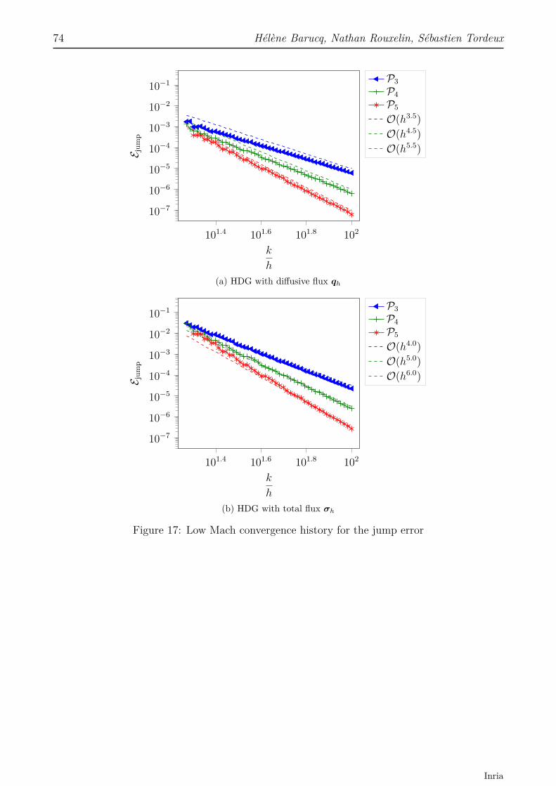
74 Hélène Barucq, Nathan Rouxelin, Sébastien Tordeux
101.4 101.6 101.8 102
10−7
10−6
10−5
10−4
10−3
10−2
10−1
k
h
E jum
p
P3P4P5
O(h3.5)O(h4.5)O(h5.5)
(a) HDG with diffusive flux qh
101.4 101.6 101.8 102
10−7
10−6
10−5
10−4
10−3
10−2
10−1
k
h
E jum
p
P3P4P5
O(h4.0)O(h5.0)O(h6.0)
(b) HDG with total flux σh
Figure 17: Low Mach convergence history for the jump error
Inria

HDG and HDG+ methods for harmonic wave problems with convection 75
101.4 101.6 101.8 102
10−7
10−6
10−5
10−4
10−3
10−2
10−1
k
h
E jum
p
P3P4P5
O(h4.5)O(h5.5)O(h6.5)
(a) HDG with diffusive flux qh
101.4 101.6 101.8 102
10−7
10−6
10−5
10−4
10−3
10−2
10−1
k
h
E jum
p
P3P4P5
O(h4.5)O(h5.5)O(h6.5)
(b) HDG with total flux σh
Figure 18: Large Mach convergence history for the jump error
Adaptation to the HDG+ method: For the HDG+ method, nothing changes for thevectorial residual ∆h but things are a little different for the scalar residual δh. Indeed this timewe have
‖PW δh‖K . h− 1
2K
(‖|τ |(PMph − ph)‖∂K + ‖|τupw|(ph − ph‖∂K
),
. h− 1
2K ‖|τ |(PMph − ph)‖∂K ,
(as τ = O(hK−1)) . h− 3
2K ‖PMph − ph‖∂K .
To illustrate this, we have depicted Ejump for the HDG+ method for a low-Mach flow in Figure19 and for a large-Mach flow in Figure 20. Once again, we can see that these quantities areclearly decreasing.
RR n° 9410

76 Hélène Barucq, Nathan Rouxelin, Sébastien Tordeux
101.4 101.6 101.8 102
10−7
10−6
10−5
10−4
10−3
10−2
10−1
k
h
E jum
p
P2 − P3 − P2P3 − P4 − P3P4 − P5 − P4P5 − P6 − P5
O(h4.0)O(h5.0)O(h6.0)O(h7.0)
Figure 19: Low Mach convergence history for the jump error for the HDG+ method
101.4 101.6 101.8 102
10−7
10−6
10−5
10−4
10−3
10−2
10−1
k
h
E jum
p
P2 − P3 − P2P3 − P4 − P3P4 − P5 − P4
O(h4.0)O(h5.0)O(h6.0)
Figure 20: Large Mach convergence history for the jump error for the HDG+ method
6.3 Is the upwinding mechanism necessary ?In this section we investigate the numerical impact of upwinding mechanisms. We have per-formed the same numerical simulations with the three methods with and without those mech-anisms. For the HDG-qh and the HDG+ methods, deactivating the upwinding mechanismcorresponds to taking τupw ≡ 0. For the HDG-σh it corresponds to taking τ = 1 instead of thevalue given by the Riemann solver.As it can be seen on Figure 21 the HDG-qh without upwinding leads to poor numerical results,whereas the two other methods seem to perform well.
Inria

HDG and HDG+ methods for harmonic wave problems with convection 77
Method With upwinding Without upwindingHDG-qh 4.3 · 10−7 0.53HDG-σh 4.9 · 10−7 5.8 · 10−7
HDG+ 6.3 · 10−8 5.77 · 10−7
Table 8: Jump error Ejump for the different method
We have also computed the jump error Ejump as quality indicator of the numerical solution. Thevalues are given in Table 8. Even if the error is higher without upwinding for the HDG+ andHDG-σh, it seems to remain at a reasonable level. For the HDG+ method, we can conclude thatthe τupw penalization seems optional. This can be understood as we need to choose τ = O(hK−1)which is large, so the method seems less sensitive to changes in the penalization. On the otherhand, this τupw penalization is mandatory to make the HDG-qh formulation work. Finally, forthe HDG-σh we still recommend to use the upwind penalization parameter τ as it leads to amethod with no arbitrary choice to make.
0 100 200 300 400 5000
100
200
−2
0
2
(a) HDG-qh with upwinding0 100 200 300 400 500
0
100
200
−5
0
5
(b) HDG-qh without upwinding
0 100 200 300 400 5000
100
200
−2
0
2
(c) HDG-σh with upwinding0 100 200 300 400 500
0
100
200
−2
0
2
(d) HDG-σh without upwinding
0 100 200 300 400 5000
100
200
−2
0
2
(e) HDG+ with upwinding0 100 200 300 400 500
0
100
200
−2
0
2
(f) HDG+ with upwinding
Figure 21: ph for the different HDG methods with and without upwind
RR n° 9410
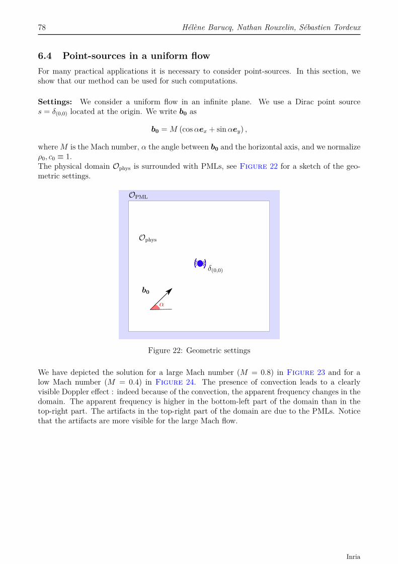
78 Hélène Barucq, Nathan Rouxelin, Sébastien Tordeux
6.4 Point-sources in a uniform flowFor many practical applications it is necessary to consider point-sources. In this section, weshow that our method can be used for such computations.
Settings: We consider a uniform flow in an infinite plane. We use a Dirac point sources = δ(0,0) located at the origin. We write b0 as
b0 = M (cosαex + sinαey) ,
whereM is the Mach number, α the angle between b0 and the horizontal axis, and we normalizeρ0, c0 ≡ 1.The physical domain Ophys is surrounded with PMLs, see Figure 22 for a sketch of the geo-metric settings.
b0
OPML
Ophys
δ(0,0)
α
Figure 22: Geometric settings
We have depicted the solution for a large Mach number (M = 0.8) in Figure 23 and for alow Mach number (M = 0.4) in Figure 24. The presence of convection leads to a clearlyvisible Doppler effect : indeed because of the convection, the apparent frequency changes in thedomain. The apparent frequency is higher in the bottom-left part of the domain than in thetop-right part. The artifacts in the top-right part of the domain are due to the PMLs. Noticethat the artifacts are more visible for the large Mach flow.
Inria
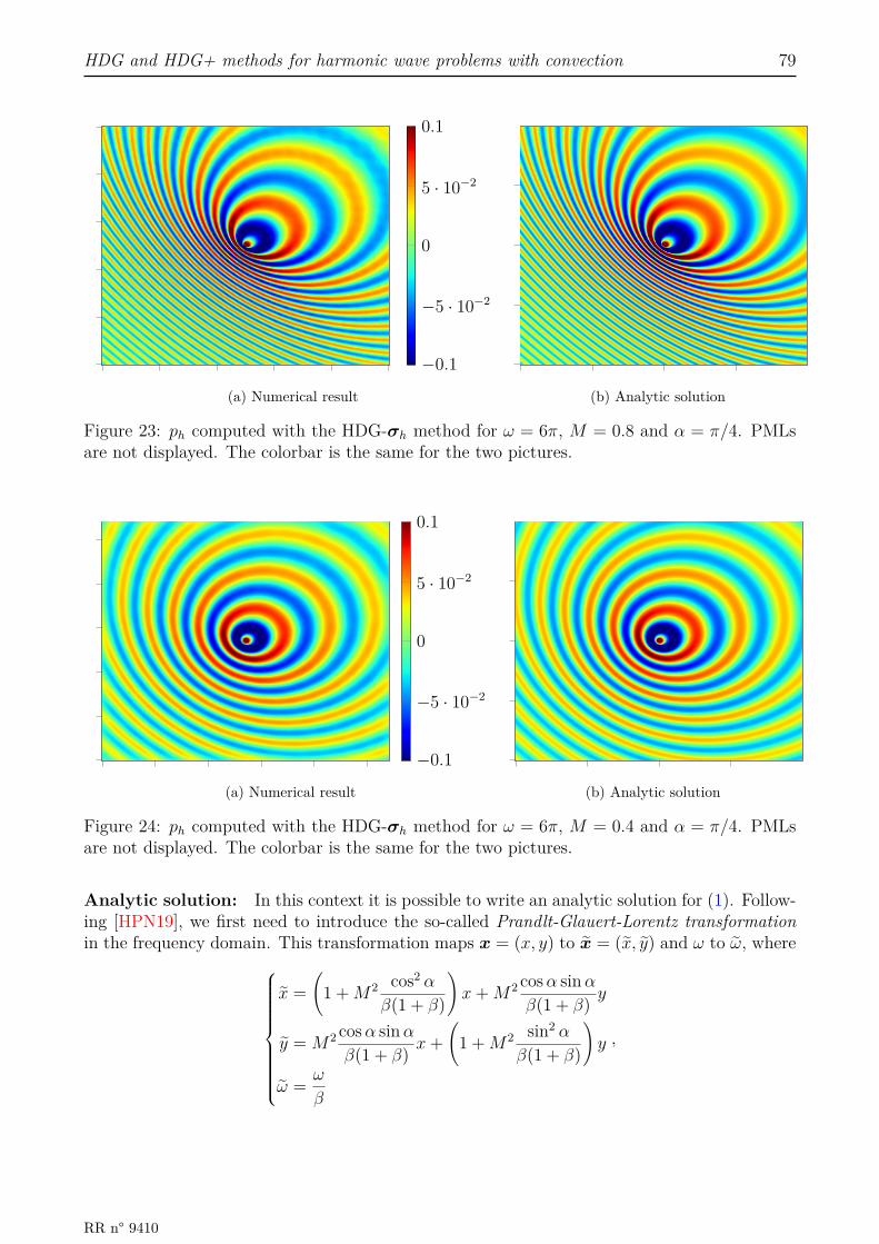
HDG and HDG+ methods for harmonic wave problems with convection 79
−0.1
−5 · 10−2
0
5 · 10−2
0.1
(a) Numerical result (b) Analytic solution
Figure 23: ph computed with the HDG-σh method for ω = 6π, M = 0.8 and α = π/4. PMLsare not displayed. The colorbar is the same for the two pictures.
−0.1
−5 · 10−2
0
5 · 10−2
0.1
(a) Numerical result (b) Analytic solution
Figure 24: ph computed with the HDG-σh method for ω = 6π, M = 0.4 and α = π/4. PMLsare not displayed. The colorbar is the same for the two pictures.
Analytic solution: In this context it is possible to write an analytic solution for (1). Follow-ing [HPN19], we first need to introduce the so-called Prandlt-Glauert-Lorentz transformationin the frequency domain. This transformation maps x = (x, y) to x = (x, y) and ω to ω, where
x =(
1 +M2 cos2 α
β(1 + β)
)x+M2 cosα sinα
β(1 + β) y
y = M2 cosα sinαβ(1 + β) x+
(1 +M2 sin2 α
β(1 + β)
)y
ω = ω
β
,
RR n° 9410
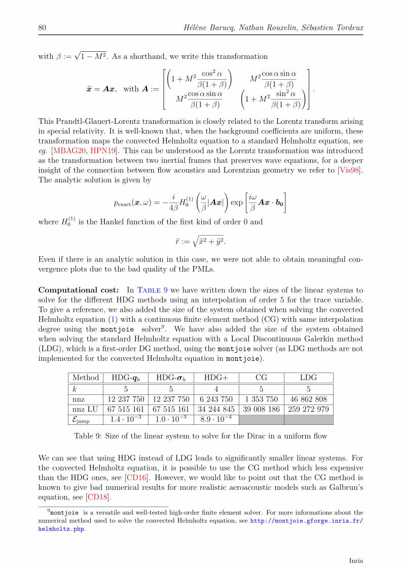
80 Hélène Barucq, Nathan Rouxelin, Sébastien Tordeux
with β :=√
1−M2. As a shorthand, we write this transformation
x = Ax, with A :=
(
1 +M2 cos2 α
β(1 + β)
)M2 cosα sinα
β(1 + β)
M2 cosα sinαβ(1 + β)
(1 +M2 sin2 α
β(1 + β)
) .
This Prandtl-Glauert-Lorentz transformation is closely related to the Lorentz transform arisingin special relativity. It is well-known that, when the background coefficients are uniform, thesetransformation maps the convected Helmholtz equation to a standard Helmholtz equation, seeeg. [MBAG20, HPN19]. This can be understood as the Lorentz transformation was introducedas the transformation between two inertial frames that preserves wave equations, for a deeperinsight of the connection between flow acoustics and Lorentzian geometry we refer to [Vis98].The analytic solution is given by
pexact(x, ω) = − i
4βH(1)0
(ω
β|Ax|
)exp
[iω
βAx · b0
]where H(1)
0 is the Hankel function of the first kind of order 0 and
r :=√x2 + y2.
Even if there is an analytic solution in this case, we were not able to obtain meaningful con-vergence plots due to the bad quality of the PMLs.
Computational cost: In Table 9 we have written down the sizes of the linear systems tosolve for the different HDG methods using an interpolation of order 5 for the trace variable.To give a reference, we also added the size of the system obtained when solving the convectedHelmholtz equation (1) with a continuous finite element method (CG) with same interpolationdegree using the montjoie solver9. We have also added the size of the system obtainedwhen solving the standard Helmholtz equation with a Local Discontinuous Galerkin method(LDG), which is a first-order DG method, using the montjoie solver (as LDG methods are notimplemented for the convected Helmholtz equation in montjoie).
Method HDG-qh HDG-σh HDG+ CG LDGk 5 5 4 5 5nnz 12 237 750 12 237 750 6 243 750 1 353 750 46 862 808nnz LU 67 515 161 67 515 161 34 244 845 39 008 186 259 272 979Ejump 1.4 · 10−3 1.0 · 10−3 8.9 · 10−4
Table 9: Size of the linear system to solve for the Dirac in a uniform flow
We can see that using HDG instead of LDG leads to significantly smaller linear systems. Forthe convected Helmholtz equation, it is possible to use the CG method which less expensivethan the HDG ones, see [CD16]. However, we would like to point out that the CG method isknown to give bad numerical results for more realistic aeroacoustic models such as Galbrun’sequation, see [CD18].
9montjoie is a versatile and well-tested high-order finite element solver. For more informations about thenumerical method used to solve the convected Helmholtz equation, see http://montjoie.gforge.inria.fr/helmholtz.php.
Inria

HDG and HDG+ methods for harmonic wave problems with convection 81
Local refinement: To handle the point-sources, a mesh with a local refinement around thesource should be used, otherwise artifacts could be present in the numerical solution. With theHDG method, those artifacts seem really limited when no local refinement is used, see Figure25.
−0.1
−5 · 10−2
0
5 · 10−2
0.1
Figure 25: Point-source without local refinement
Illustrative example: To show that our method can handle more complex simulations, weconsider the same test-case as before but with two point-sources located near the origin. OnFigure 26, we can still see the changes in the apparent frequency due to the Doppler effect,but also interference patterns due to the interactions between the two sources.
−0.1
−5 · 10−2
0
5 · 10−2
0.1
Figure 26: Interference between two point-sources
6.5 Gaussian jetIn this section we focus on a space-varying flow. We will use a gaussian jet, which is a commontest-case in the literature, see eg. [MMMP17, Sec. 3]. To work with parameters and unknownswithout dimension, we choose
ρ0 = c0 ≡ 1,
and we consider the following gaussian jet flow
v0 = M0(y)ex, where M0(y) := M∞ + µ exp(− y
2
R2
),
RR n° 9410
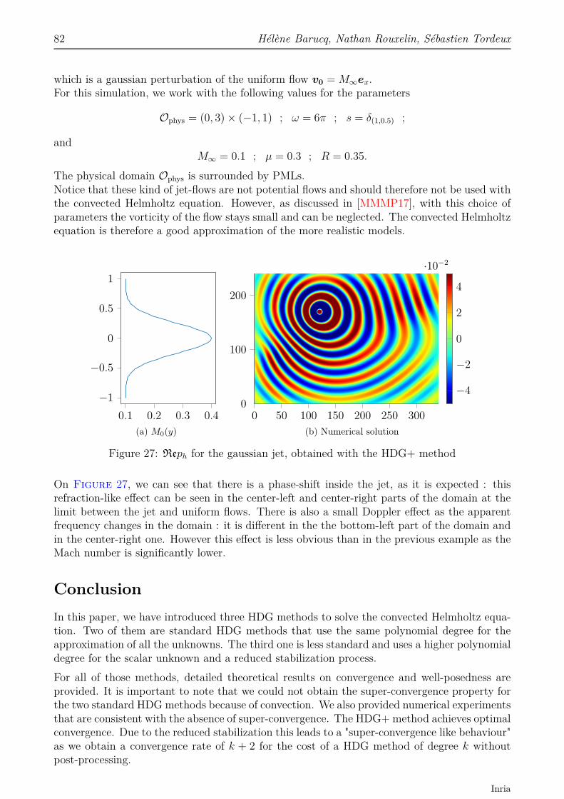
82 Hélène Barucq, Nathan Rouxelin, Sébastien Tordeux
which is a gaussian perturbation of the uniform flow v0 = M∞ex.For this simulation, we work with the following values for the parameters
Ophys = (0, 3)× (−1, 1) ; ω = 6π ; s = δ(1,0.5) ;
andM∞ = 0.1 ; µ = 0.3 ; R = 0.35.
The physical domain Ophys is surrounded by PMLs.Notice that these kind of jet-flows are not potential flows and should therefore not be used withthe convected Helmholtz equation. However, as discussed in [MMMP17], with this choice ofparameters the vorticity of the flow stays small and can be neglected. The convected Helmholtzequation is therefore a good approximation of the more realistic models.
0.1 0.2 0.3 0.4−1
−0.5
0
0.5
1
(a) M0(y)0 50 100 150 200 250 300
0
100
200
−4
−2
0
2
4
·10−2
(b) Numerical solution
Figure 27: Reph for the gaussian jet, obtained with the HDG+ method
On Figure 27, we can see that there is a phase-shift inside the jet, as it is expected : thisrefraction-like effect can be seen in the center-left and center-right parts of the domain at thelimit between the jet and uniform flows. There is also a small Doppler effect as the apparentfrequency changes in the domain : it is different in the the bottom-left part of the domain andin the center-right one. However this effect is less obvious than in the previous example as theMach number is significantly lower.
ConclusionIn this paper, we have introduced three HDG methods to solve the convected Helmholtz equa-tion. Two of them are standard HDG methods that use the same polynomial degree for theapproximation of all the unknowns. The third one is less standard and uses a higher polynomialdegree for the scalar unknown and a reduced stabilization process.For all of those methods, detailed theoretical results on convergence and well-posedness areprovided. It is important to note that we could not obtain the super-convergence property forthe two standard HDGmethods because of convection. We also provided numerical experimentsthat are consistent with the absence of super-convergence. The HDG+ method achieves optimalconvergence. Due to the reduced stabilization this leads to a "super-convergence like behaviour"as we obtain a convergence rate of k + 2 for the cost of a HDG method of degree k withoutpost-processing.
Inria

HDG and HDG+ methods for harmonic wave problems with convection 83
During the numerical experiments, it occurred to us that the HDG+ and HDG-σh methodsseemed more robust than the HDG-qh method. In particular, they are less sensitive to thechoice of penalization parameter.
Future work: Now that the use of HDG method has been validated for the convectedHelmholtz equation, we will generalize this work to more realistic aeroacoustic models suchas Galbrun’s equation or Goldstein’s equation.We also noticed that the use of PMLs may lead to bad numerical results, and we will there-fore address the construction of absorbing boundary conditions for the convected Helmholtzequation in a future paper.
Open-source implementation: An open-source implementation of those three methods inthe hawen solver will be released soon.
Acknowledgement: The authors would like to thank Florian Faucher for his help with thenumerical implementation.Experiments presented in this paper were carried out using the PlaFRIM experimental testbed,supported by Inria, CNRS (LABRI and IMB), Université de Bordeaux, Bordeaux INP andConseil Régional d’Aquitaine (see https://www.plafrim.fr).Nathan Rouxelin acknowledges financial support from e2s-UPPA (see https://e2s-uppa.eu).
A Intermediate results for the error analysis of the HDGmethod with diffusive flux
In this appendix we state the intermediate results allowing to adapt the analysis conducted inSubsection 4.3 to prove the convergence of the HDG method stated in Theorem 6. Theproofs are omitted but are very similar to the ones given in Subsection 4.3.The main differences to keep in mind are : s ∈ [1, k + 1] instead of s ∈ [1, k + 2] and τ = O(1)instead of τ = O(h−1).
Gradient estimate: this corresponds to Lemma 4.3
Lemma A.1:The following estimate holds
‖∇εph‖Th. ‖εqh‖W0,Th
+ ‖δqh‖Th+ h−
12 ‖εph − ε
ph‖∂Th
Energy-like equality: this corresponds to Lemma 4.5.
RR n° 9410
84 Hélène Barucq, Nathan Rouxelin, Sébastien Tordeux
Lemma A.2:The following energy-like equality holds
‖εqh‖2W0,Th
− ω2 ‖εph‖2ρ0,K− 2iω
‖εph − εph‖2∂Th
+∥∥∥∥∥(1
2 |b0 · n|) 1
2(εph − ε
ph)∥∥∥∥∥
2
∂Th
=− ω2 (ρ0δ
ph, ε
ph)Th
+ 2iω (δphb0,∇εph)Th+ (W0ε
qh, δ
qh)Th
+ 2ωIm (εphb0,∇εph)Th
+⟨δqh · n+ 2iω(b0 · n)δph − 2iωτ(δph − δ
ph) + 2iωτupw(δph − δ
ph), ε
ph − ε
ph
⟩∂Th
Furthermore if p ∈ Hs(O) and q ∈ Ht(O) where s, t ∈ [1, k + 1] then the following estimateholds ∣∣∣∣∣∣‖εqh‖2
W0,Th− 2iω
‖εph − εph‖2∂Th
+∥∥∥∥∥(1
2 |b0 · n|) 1
2(εph − ε
ph)∥∥∥∥∥
2
∂Th
∣∣∣∣∣∣.ω2 ‖εph‖
2Th
+ ω ‖εph‖Th
(‖εqh‖W0,Th
+ ht ‖q‖t,O + h−12 ‖εph − ε
ph‖∂Th
+ ωhs ‖p‖s,O)
+ ‖εqh‖W0,Th
(ht ‖q‖t,O + ωhs ‖p‖s,O
)+ h2t ‖q‖2
t,O
+ h−12 ‖εph − ε
ph‖∂Th
(ωhs ‖p‖s,O + ht ‖q‖t,O
)Dual identity: this corresponds to Lemma 4.6.
Lemma A.3:The following dual identity holds
‖εph‖2Th
=− (W0εqh,πV ξ − ξ)Th
+ ω2 (ρ0εph, πW θ − θ)Th
+ 2iω (∇εph, (πW θ − θ)b0)Th
− 2iω 〈(b0 · n)εph, πW θ − θ〉∂Th
+ (W0δqh,πV ξ)Th
− ω2 (ρ0δph, πW θ)Th
+ 2iω (δphb0,∇(πW θ))Th
+ 2iω 〈(b0 · n)εph − τ (εph − εph) + τupw (εph − ε
ph) , πW θ − PMθ〉∂Th
− 2iω⟨(b0 · n)δph − τ(δph − δ
ph) + τupw
(δph − δ
ph
), πW θ − PMθ
⟩∂Th
+ 〈δqh · n, πW θ − PMθ〉∂Th
Dual estimate: this corresponds to Lemma 4.7.
Lemma A.4:Assuming that the regularity assumption (72) holds and that ω2h2 ‖ρ0‖∞CregC (where C is theconstant of Theorem 4) is small enough, if p ∈ Hs(O) and q ∈Ht(O) where s, t ∈ [1, k + 1]then
‖εph‖Th. ht+1(1 + ω) ‖q‖t,O + hs(1 + ω + ω2) ‖p‖s,O + h(1 + ω) ‖εqh‖W0,Th
whereh := max
K∈Th
hK
References[ALA13] Natalia C. B. Arruda, Abimael F. D. Loula, and Regina C. Almeida. Locally dis-
continuous but globally continuous Galerkin methods for elliptic problems. Com-
Inria
HDG and HDG+ methods for harmonic wave problems with convection 85
puter Methods in Applied Mechanics and Engineering, 255:104–120, March 2013.Cited on page 9.
[BCDL15] Marie Bonnasse-Gahot, Henri Calandra, Julien Diaz, and Stéphane Lanteri. Hy-bridizable Discontinuous Galerkin method for the simulation of the propagationof the elastic wave equations in the frequency domain. Research Report RR-8990,INRIA Bordeaux ; INRIA Sophia Antipolis - Méditerranée, June 2015. Cited onpages 4 and 49.
[BDL03] Eliane Bécache, Anne-Sophie Bonnet-Ben Dhia, and Guillaume Legendre. Per-fectly matched layers for the convected Helmholtz equation. Technical report,2003. Cited on page 62.
[BDMP21] Hélène Barucq, Julien Diaz, Rose-Cloé Meyer, and Ha Pham. Implementation ofhybridizable discontinuous Galerkin method for time-harmonic anisotropic poroe-lasticity in two dimensions. International Journal for Numerical Methods in En-gineering, 122(12):3015–3043, 2021. Cited on page 4.
[CC12] Yanlai Chen and Bernardo Cockburn. Analysis of variable-degree HDG methodsfor convection–diffusion equations. Part I: General nonconforming meshes. IMAJournal of Numerical Analysis, 32(4):1267–1293, October 2012. Cited on page 4.
[CC14] Yanlai Chen and Bernardo Cockburn. Analysis of variable-degree HDG methodsfor convection-diffusion equations. Part II: Semimatching nonconforming meshes.Mathematics of Computation, 83(285):87–111, January 2014. Cited on page 4.
[CD16] Juliette Chabassier and Marc Duruflé. High Order Finite Element Method forsolving Convected Helmholtz equation in radial and axisymmetric domains. Appli-cation to Helioseismology. Research Report RR-8893, Inria Bordeaux Sud-Ouest,March 2016. Cited on page 80.
[CD18] Juliette Chabassier and Marc Duruflé. Solving time-harmonic Galbrun’s equationwith an arbitrary flow. Application to Helioseismology. Rapport de recherche Inria,2018. Cited on page 80.
[CDG+09] Bernardo Cockburn, Bo Dong, Johnny Guzmán, Marco Restelli, and Ric-cardo Sacco. A Hybridizable Discontinuous Galerkin Method for Steady-StateConvection-Diffusion-Reaction Problems. SIAM Journal on Scientific Computing,31(5):3827–3846, January 2009. Cited on page 4.
[CDPE16] Bernardo Cockburn, Daniele A. Di Pietro, and Alexandre Ern. Bridging the hybridhigh-order and hybridizable discontinuous Galerkin methods. ESAIM: Mathemat-ical Modelling and Numerical Analysis, 50(3):635–650, May 2016. Cited on page4.
[CGL09] Bernardo Cockburn, Jayadeep Gopalakrishnan, and Raytcho Lazarov. Unified Hy-bridization of Discontinuous Galerkin, Mixed, and Continuous Galerkin Methodsfor Second Order Elliptic Problems. SIAM J. Numer. Anal, 47:1319–1365, August2009. Cited on page 4.
[CGS10] Bernardo Cockburn, Jayadeep Gopalakrishnan, and Francisco-Javier Sayas. Aprojection-based error analysis of HDG methods. Mathematics of Computation,79(271):1351–1367, March 2010. Cited on pages 4, 13, 26, and 48.
RR n° 9410

86 Hélène Barucq, Nathan Rouxelin, Sébastien Tordeux
[CLOS20] Liliana Camargo, Bibiana López-Rodríguez, Mauricio Osorio, and Manuel Solano.An HDGmethod for Maxwell’s equations in heterogeneous media. Computer Meth-ods in Applied Mechanics and Engineering, 368:113178, August 2020. Cited onpage 4.
[Coc14] Bernardo Cockburn. Static Condensation, Hybridization, and the Devising of theHDG Methods. springerprofessional.de, 2014. Cited on page 4.
[CQS18] Huangxin Chen, Weifeng Qiu, and Ke Shi. A priori and computable a posteriorierror estimates for an HDG method for the coercive Maxwell equations. ComputerMethods in Applied Mechanics and Engineering, 333:287–310, May 2018. Citedon page 4.
[CQSS17] Huangxin Chen, Weifeng Qiu, Ke Shi, and Manuel Solano. A Superconver-gent HDG Method for the Maxwell Equations. Journal of Scientific Computing,70(3):1010–1029, March 2017. Cited on page 4.
[CS13] Bernardo Cockburn and Ke Shi. Superconvergent HDG methods for linear elastic-ity with weakly symmetric stresses | IMA Journal of Numerical Analysis | OxfordAcademic. IMA Journal of Numerical Analysis, 2013. Cited on page 4.
[CZ12] Bernardo Cockburn and Wujun Zhang. A Posteriori Error Estimates for HDGMethods. Journal of Scientific Computing, 51(3):582–607, June 2012. Cited onpage 72.
[CZ13] Bernardo Cockburn and Wujun Zhang. A Posteriori Error Analysis for Hybridiz-able Discontinuous Galerkin Methods for Second Order Elliptic Problems. SIAMJournal on Numerical Analysis, 51(1):676–693, January 2013. Cited on page 72.
[DS19] Shukai Du and Francisco-Javier Sayas. An Invitation to the Theory of the Hybridiz-able Discontinuous Galerkin Method: Projections, Estimates, Tools. SpringerBriefsin Mathematics. Springer International Publishing, Cham, 2019. Cited on pages4, 21, 24, 25, 26, 34, and 41.
[Dub91] Moshe Dubiner. Spectral methods on triangles and other domains. Journal ofScientific Computing, 6(4):345–390, December 1991. Cited on page 56.
[EG04] Alexandre Ern and Jean-Luc Guermond. Theory and Practice of Finite Elements.Applied Mathematical Sciences. Springer-Verlag, New York, 2004. Cited on pages8, 12, 23, 33, 35, and 41.
[Fau21] Florian Faucher. ‘hawen‘: Time-harmonic wave modeling and inversion using hy-bridizable discontinuous Galerkin discretization. Journal of Open Source Software,6(57):2699, January 2021. Cited on page 4.
[FCS15] G. Fu, B. Cockburn, and H. Stolarski. Analysis of an HDG method for linearelasticity. International Journal for Numerical Methods in Engineering, 102(3-4):551–575, 2015. Cited on page 4.
[FLd14] Cristiane O. Faria, Abimael F. D. Loula, and Antônio J. B. dos Santos. Primalstabilized hybrid and DG finite element methods for the linear elasticity problem.Computers & Mathematics with Applications, 68(4):486–507, August 2014. Citedon page 9.
Inria

HDG and HDG+ methods for harmonic wave problems with convection 87
[FS20] Florian Faucher and Otmar Scherzer. Adjoint-state method for Hybridizable Dis-continuous Galerkin discretization, application to the inverse acoustic wave prob-lem. Computer Methods in Applied Mechanics and Engineering, 372:113406, De-cember 2020. Cited on pages 4 and 49.
[GM11] Roland Griesmaier and Peter Monk. Error Analysis for a Hybridizable Discontinu-ous Galerkin Method for the Helmholtz Equation. Journal of Scientific Computing,49(3):291–310, December 2011. Cited on page 4.
[GSV18] Jay Gopalakrishnan, Manuel Solano, and Felipe Vargas. Dispersion Analysis ofHDG Methods. Journal of Scientific Computing, 77(3):1703–1735, December 2018.Cited on page 4.
[HPN19] Fang Q. Hu, Michelle E. Pizzo, and Douglas M. Nark. On the use of a Prandtl-Glauert-Lorentz transformation for acoustic scattering by rigid bodies with a uni-form flow. Journal of Sound and Vibration, 443:198–211, March 2019. Cited onpages 79 and 80.
[HPS17] Allan Hungria, Daniele Prada, and Francisco-Javier Sayas. HDG methods forelastodynamics. Computers & Mathematics with Applications, 74(11):2671–2690,December 2017. Cited on page 4.
[Hun19] Allan Hungria. Using HDG+ to Compute Solutions of the 3D Linear Elastic andPoroelastic Wave Equations. PhD thesis, University of Delaware, 2019. Cited onpages 4, 34, and 41.
[HW08] Jan S. Hesthaven and Tim Warburton. Nodal Discontinuous Galerkin Methods:Algorithms, Analysis, and Applications. Texts in Applied Mathematics. Springer-Verlag, New York, 2008. Cited on page 16.
[Kir04] Robert C. Kirby. Algorithm 839: FIAT, a new paradigm for computing finiteelement basis functions. ACM Transactions on Mathematical Software (TOMS),30(4):502–516, December 2004. Cited on page 56.
[KSC12] Robert M. Kirby, Spencer J. Sherwin, and Bernardo Cockburn. To CG or to HDG:A Comparative Study. Journal of Scientific Computing, 51(1):183–212, April 2012.Cited on page 4.
[Leh10] Christoph Lehrenfeld. Hybrid Discontinuous Galerkin Methods for Solving Incom-pressible Flow Problems. PhD thesis, RWTH Aachen, 2010. Cited on pages 4and 28.
[MBAG20] Philippe Marchner, Hadrien Beriot, Xavier Antoine, and Christophe Geuzaine.Stable Perfectly Matched Layers with Lorentz transformation for the convectedHelmholtz equation. Technical report, 2020. Cited on page 80.
[MMMP17] Jean-François Mercier, Colin Mietka, Florence Millot, and Vincent Pagneux.Acoustic propagation in a vortical homentropic flow. page 19, 2017. Cited onpages 81 and 82.
[NPRC15] N. C. Nguyen, J. Peraire, F. Reitich, and B. Cockburn. A phase-based hybridiz-able discontinuous Galerkin method for the numerical solution of the Helmholtzequation. Journal of Computational Physics, 290:318–335, June 2015. Cited onpage 4.
RR n° 9410
88 Hélène Barucq, Nathan Rouxelin, Sébastien Tordeux
[Oik14] Issei Oikawa. A hybridized discontinuous Galerkin method with reduced stabiliza-tion. arXiv:1405.2491 [math], November 2014. Cited on pages 4 and 56.
[Oik16] Issei Oikawa. Analysis of a Reduced-Order HDG Method for the Stokes Equations.Journal of Scientific Computing, 67(2):475–492, May 2016. Cited on page 4.
[Oik18] Issei Oikawa. An HDG Method with Orthogonal Projections in Facet Integrals.Journal of Scientific Computing, 76(2):1044–1054, August 2018. Cited on page 4.
[PE12] Daniele Antonio Di Pietro and Alexandre Ern. Mathematical Aspects of Discontin-uous Galerkin Methods. Mathématiques et Applications. Springer-Verlag, BerlinHeidelberg, 2012. Cited on page 13.
[Pie90] Allan D. Pierce. Wave equation for sound in fluids with unsteady inhomogeneousflow. The Journal of the Acoustical Society of America, 87(6):2292–2299, June1990. Cited on page 5.
[QS16a] Weifeng Qiu and Ke Shi. An HDG Method for Convection Diffusion Equation.Journal of Scientific Computing, 66(1):346–357, January 2016. Cited on pages 4,28, and 41.
[QS16b] Weifeng Qiu and Ke Shi. A superconvergent HDG method for the incompressibleNavier–Stokes equations on general polyhedral meshes. IMA Journal of NumericalAnalysis, 36(4):1943–1967, October 2016. Cited on page 4.
[QSS16] Weifeng Qiu, Jiguang Shen, and Ke Shi. An HDG method for linear elasticitywith strong symmetric stresses. arXiv:1312.1407 [math], February 2016. Cited onpages 4 and 41.
[SM50] Jack Sherman and Winifred J. Morrison. Adjustment of an Inverse Matrix Corre-sponding to a Change in One Element of a Given Matrix. Annals of MathematicalStatistics, 21(1):124–127, March 1950. Cited on page 6.
[Ste91] Rolf Stenberg. Postprocessing schemes for some mixed finite elements. ESAIM:Mathematical Modelling and Numerical Analysis, 25(1):151–167, 1991. Cited onpages 26 and 48.
[Vis98] Matt Visser. Acoustic black holes: Horizons, ergospheres, and Hawking radiation.Classical and Quantum Gravity, 15(6):1767–1791, June 1998. Cited on page 80.
[YMKS16] Sergey Yakovlev, David Moxey, Robert M. Kirby, and Spencer J. Sherwin. ToCG or to HDG: A Comparative Study in 3D. Journal of Scientific Computing,67(1):192–220, April 2016. Cited on page 4.
Inria

RESEARCH CENTREBORDEAUX – SUD-OUEST
200 avenue de la Vieille Tour
33405 Talence Cedex
PublisherInriaDomaine de Voluceau - RocquencourtBP 105 - 78153 Le Chesnay Cedexinria.fr
ISSN 0249-6399
Related Documents