handbook of acoustic noise control - DTIC

S- •~~~~'•r- i-i .. ••n • •U z.

WADC TECHNICAL REPORT 52-204

VOLUME I

SUPPLEMENT 1

HANDBOOK OF ACOUSTIC NOISE CONTROLVolume 1. Physical Acoustics

Supplement 1

EDITORS

STEPHEN 1. LUKASIK

A. WILSON NOLLE

BOLT BERANEK AND NEWMAN INC.

APRIL 1955

N.

Statement AApproved for Public Release

WRIGHT AIR DEVELOPMENT CENTER

. o4O6 //094#

*TECHNICAL LIBRARY'D0yton Since 1919

AF-WP-L-22 MAY 53 50M

When Government drawings, specifications, or other data areusedfor any purpose other than in connection with a definitely related Govern-ment procurement operation, the United States Government thereby in-curs no responsibility nor any obligation whatsoever; and the fact thatthe Government may have formulated, furnished, or in any way suppliedthe said drawings, specifications, or other data, is not to be regardedby implication or otherwise as in any manner licensing the holder orany other person or corporation, or conveying any rights or permissionto manufacture, use, or sell anypatented invention that may in any waybe related thereto.

Distributed by OTS in the Interest of IndustryWith the Cooperation of the

Originating AgencyThis report is a reproduction of an original document resulting from Government-sponsored research. It is made available by OTS through the cooperation of theoriginating agency. Quotations should credit the authors and the originatingagency. No responsibility is assumed for completeness or accuracy of this report.Where patent questions appear to be involved, the usual Preliminary search is

Z suggested. If copyrighted material appears, permission for use should be requestedof the copyright owners. Any security restrictions that may have

applied to this report have been removed.

U. S. DEPARTMENT OF COMMERCEOFFICE OF TECHNICAL SERVICES

WASHINGTON 25, D. C.

r-pa 16--71256-1

GP'A

WADC TECHNICAL REPORT 52-204

VOLUME I

SUPPLEMENT 1

HANDBOOK OF ACOUSTIC NOISE CONTROLVolume I. Physical Acoustics

Supplement 1

EDITORS

STEPHEN 1. LUKASIK

A. WILSON NOLLE

BOLT BERANEK AND NEWMAN INC.

APRIL 1955

AERO MEDICAL LABORATORYCONTRACT No. AF 33(600)-23901

RDO No. 695-63

WRIGHT AIR DEVELOPMENT CENTER

"AIR RESEARCH AND DEVELOPMENT COMMAND

UNITED STATES AIR FORCEI,

WRIGHT-PATTERSON AIR FORCE BASE, OHIO

Carpenter Litho & Prtg. Co., Springfield, 0.2000 - 29 June 1955

FOREWORD

This report was prepared by the firm of Bolt Beranekand Newman Inc. under Contract No. AF 33(600)-23901 andsupplemental agreement No. 1 for the Wright Air DevelopmentCenter. The work was supported by funds available underRDO 695-63 "Vibration, Sonic and Mechanical Action on AirForce Personnel". Technical supervision of the preparationof the report was the responsibility of Major Horace 0.Parrack, United States Air Force, Aero Medical Laboratory,Research Division, Wright Air Development Center, Wright-Patterson Air Force Base, Ohio.

WADC TR 52-204

ABSTRACT

The Handbook of Acoustic Noise Control is intended to providean overall view of the problem of the control of acoustic noise. Sincethe publication of the first two volumes, the need for their revisionhas become apparent. In sme cases, material has been added to enlargethe coverage of original sections. In others, sections have been complete-ly re-written to present the latest experimental or theoretical infor-mation available.

With ever-increasing interest and activity in acoustic noise con-trol, published procedures must, of necessity, lag behind the newestthinking in the field. There are few areas of the noise control problemwhere the present answers are the *best'. As the operational requirementsfor noise control devices change and as now or more powerful sound soinrcesappear in our advancing technology, better answers will have to be found.In presenting these revised sections, an attempt is being made to keoDup with our expanding knowledge.

This supplement contains additions and revisions to Volume I whichtreated the generation and control of various types of noise sources.Similarly, Volume II, which analyzed the interadtion between noise andmanis being supplemented. 2hese supplements, together with the un-ohanged sections of Volumes I and II, provide a unified view of noise

• control problems.

FUBLICATE•ON REVIEW

This report has been reviewed and is approved.

IM THE CON3WIDt,

JACK BOLLERUD

Colonel, USAF (MC)Chief, Aero Medical LaboratoryDirectorate of Research

WADC .R 52-204i

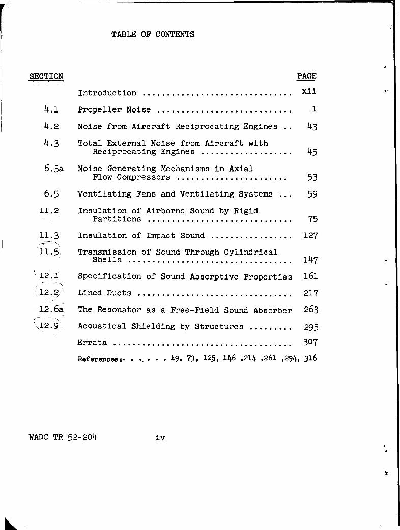
TABLE OF CONTENTS

SECTION PAGE

Introduction ............................... xii

4.1 Propeller Noise ............................ 1

4.2 Noise from Aircraft Reciprocating Engines 43

4.3 Total External Noise from Aircraft withReciprocating Engines ................... 45

6.3a Noise Generating Mechanisms in AxialFlow Compressors ....................... 53

6.5 Ventilating Fans and Ventilating Systems ... 59

11.2 Insulation of Airborne Sound by RigidPartitions .............................. 75

11.3 Insulation of Impact Sound ................. 127

ý11.5, Transmission of Sound Through CylindricalShells ................................... 147

12.1) Specification of Sound Absorptive Properties 161

12.2 Lined Ducts ................................. 217

12.6a The Resonator as a Free-Field Sound Absorber 263

2. 9 Acoustical Shielding by Structures ......... 295

Errata ..................................... 307

References:. . ... . 49, 73, 125, 146 .214 ,261 .294, 316

WADC TR 52-204 iv

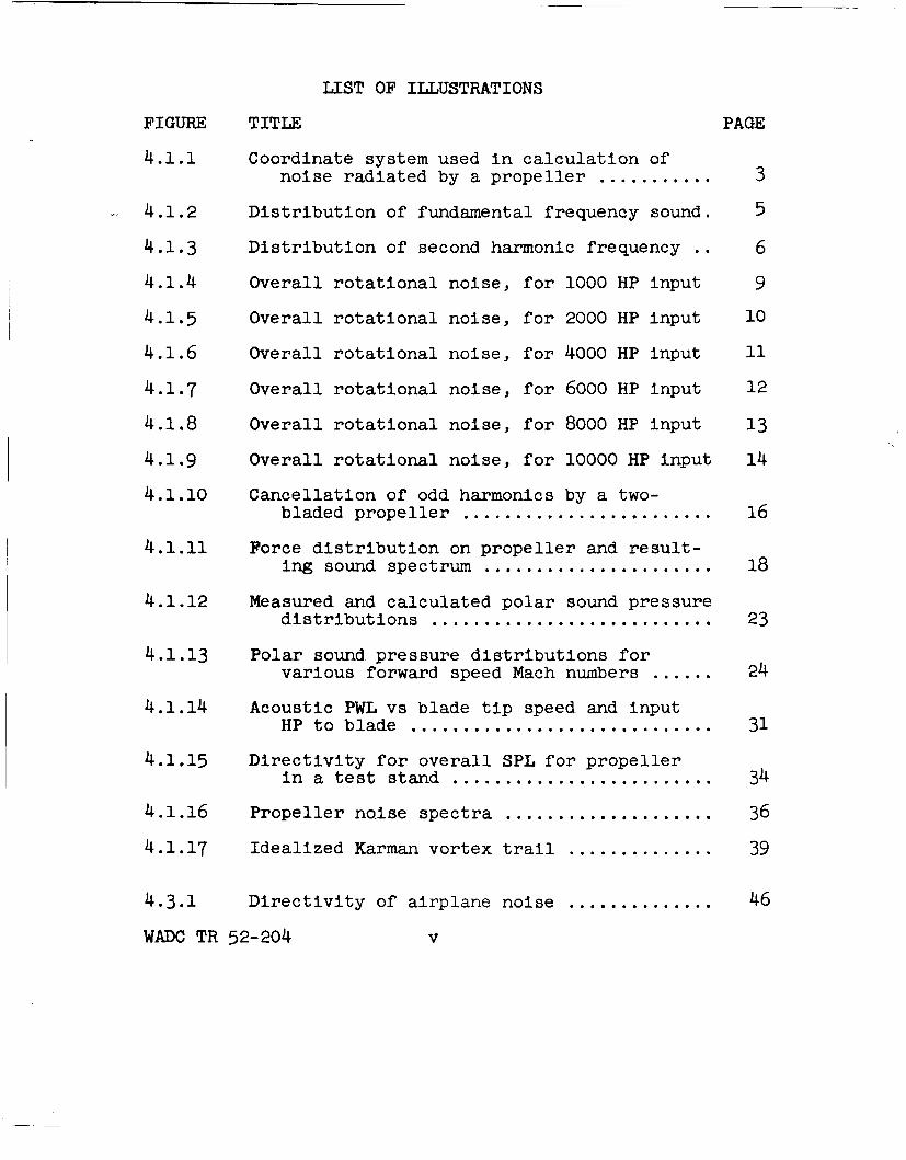
LIST OF ILLUSTRATIONS

FIGURE TITLE PAGE

4.1.1 Coordinate system used in calculation ofnoise radiated by a propeller ........... 3

4.1.2 Distribution of fundamental frequency sound. 5

4.1.3 Distribution of second harmonic frequency .. 6

4.1.4 Overall rotational noise, for 1000 HP input 9






4.1.10 Cancellation of odd harmonics by a two-bladed propeller ........................ 16

4.1.11 Force distribution on propeller and result-ing sound spectrum ...................... 18

4.1.12 Measured and calculated polar sound pressuredistributions ........................... 23

4.1.13 Polar sound pressure distributions forvarious forward speed Mach numbers ...... 24

4.1.14 Acoustic PWL vs blade tip speed and inputHP to blade ............................. 31

4.1.15 Directivity for overall SPL for propeller

in a test stand ......................... 34

4.1.16 Propeller noise spectra .................... 36

4.1.17 Idealized Karman vortex trail .............. 39

4.3.1 Directivity of airplane noise .............. 46

WADC TR 52-204 V

List of Illustrations

Figure Title Page

12.9.4 Correction of noise reduction for groundattenuation ............................... 302

12.9.5 Correction of noise reduction due toscattering by atmospheric turbulence ..... 304

12.9.6 Measured attenuation near the edge of afinite obstacle ......................... 3 05

WADC TR 52-204 xi

INTRODUCTION

This section briefly describes the changes that havebeen made to Volume I WADC TR 52-204, Handbook of AcousticNoise Control. The changes are essentially either of twobasic types. In some cases, new sections have been addedon subjects not covered in Volume I. More often, however,the new sections reflect changes in theory or practicewhich made a reorganization of the material desirable. Inone case, the new material was of a somewhat different na-ture and was simply appended to the existing section.These changes are detailed below to aid the reader in recog-nizing the relative status of the old and new section. Itwill be noted that the revision has proceded on a section-by-section basis. This has necessitated certain changes inthe figure and equation numbering conventions which are alsoindicated below.

All of Chapter 4 has been revised although the bulkof the changes are in Sec. 4.1 which makes up the main partof the chapter. The discussion of propeller noise has beenreorganized around the existing theory. Both rotationalnoise and vortex noise have been treated and N. A. C. A.charts constructed from the Gutin theory are given. Thedesign procedure based on the empirical PWL chart is essen-tially unchanged although its extension to other than threeblade propellers involves a somewhat greater uncertaintythan indicated in the original section. Chiefly, theempirical chart works in the transonic and supersonic tipspeeds where available theory is not as well developed.Also, the two spectrum charts have been replaced by a singlecurve which is similar to the transonic tip speed case ofthe original section.

Section 6.3a adds to the empirical information onaxial flow compressors presented in Sec. 6.3 The newsection discusses the physical principles involved in noisegeneration by an axial flow compressor. It contains ashort statement of the theoretical results to date andillustrates them with a calculation of the absolute soundpressure level for a compressor of given operating condi-tions. The previous empirical design procedure is stillapplicable. Nothing new is presented on centrifugalcompressors.

Section 6.5 on ventilating fans and noise fromventilating systems is new. There is no section in Volume Ito which it corresponds.

WADC TR 52-204 xii

The sections on wall construction and floating floorsin Volume I have been greatly expanded and reorganizedaround existing theory. However, the original sections arestill correct in what they say and they form a good intro-duction to the more detailed discussion of the revisedSecs. 11.2 and 11.3. In particular, Sec. 11.3 on the Insula-tion of Impact Sound corresponds only roughly to theoriginal Sec. 11.3 dealing with floating floors. Theoriginal section has more architectural details which may beuseful to the reader.

The new section on the transmission of sound throughcylindrical shells is intended to replace completely theoriginal section in Volume I. Research in this field iscontinuing, however, and. more experimental and theoreticalinformation may be expected in the future.

Section 12.1 on the specification of sound absorptiveproperties of materials is new. It replaces the very shortintroductory section in Vol. I which simply listed severaltopics to be discussed in connection with the control ofairborne sound.

The section on the attenuation of sound in lined ducts(Sec. 12.2) has been greatly expanded. Several differenttheoretical procedures for calculating the attenuation, eachof various degrees of accuracy and usefulness are presented,and all the available empirical information is summarized.A tabular summary of the various procedures is given. Thisrevised section is intended to replace the original sectionin Volume I completely.

Section 12.6a discusses the use of acoustic resonatorsin free space. Since the original section discussed resonatorsattached to ducts, the subject matter of the old and newsections are complementary rather than overlapping.

Finally, Section 12.9 presents a new design procedurefor the prediction of acoustic shielding by an obstacle.Although it is based on the same diffraction theory as theoriginal section, several modifications found necessary inactual practice have been introduced.

WADC TR 52-204 xiii

Because the total number of equations, figures, etc.in each revised section do not, in general, equal the cor-responding number in the section replaced, a new identifica-tion scheme has been used. Previously equations, figures,tables and references were numbered consecutively througha chapter and were identified by chapter and/or a serialnumber. Now all identification numbers refer to both chap-ter and section in addition to a serial number. Forexample, the fifth equation in Ch. 12, occurring say inSec. 2 is now numbered Eq. (12.2.5) while previously itwould be numbered simply Eq. (12.5). References, insteadof being a single number, such as Ref. (7) now contain asection identification also; the fourth reference is Sec.ll.5and is now numbered (5.4). Finally, a letter a followinga section designation indicates that the sectio-n does notreplace the previous section, but merely supplements it, e.g.,Sec. 12.6a. Figure, equation, table and reference numbersthen contain the letter also, e.g., Fig. 12.6a.5.

A list of errata to Volume I is given at the end ofthis volume.

WADC TR 5 2-2o4 xiv

CHAPTER 4

AIRCRAFT PROPELLERS AND RECIPROCATING ENGINES

4.1 Propeller Noise

Introduction. The propeller, rather than the engine,is the chief source of noise in the usual reciprocating-engine aircraft of 200 horsepower or more. For this reason,considerable work has been done toward explaining the actionof this important noise source. The problem has not as yetbeen treated rigorously from a theoretical standpoint, butthe approximate analysis which has been done has provedsatisfactory for engineering purposes in the case of pro-pellers operating at subsonic blade speeds and not too closeto obstacles. Also, the approximate analysis hows clearlythe role played by the various parameters which are importantin propeller noise generation, including particularly horse-power, thrust, tip speed, diameter, and number of blades.The results of this analysis are given here. Measurementsare cited and comparisons between theory and experiment areshown where possible. Equations and charts for engineeringcalculations are given. Their use is explained in a numericalexample at 'the end of the section.

Gutin's Theory of Rotational Propeller Noise. A rotat-ing propeller blade~at constant speed carries with it asteady pressure distribution. Hence, any non-axial point,fixed in space with reference to the aircraft, experiencesa periodic pressure variation, generally of complex waveform, always having the blade passage frequency as the funda-mental. This periodic pressure variation is an acousticdisturbance, and is known as the rotational noise. Forpoints lying in, or very nearly in, the volume swept out bythe propeller blades, and for cases where there is negligibleoverlap of the pressure distributions of adjacent blades,the pressure disturbance due to a multiple-blade propellercan be approximated simply as a repetition, at the appro-priate frequency, of the disturbance due to the passage ofan isolated blade. (In other words, for such near points,the pressure disturbance at a given time is due to thenearest blade, the influence of the more distant blades be-ing negligible.) To this approximation, the acousticdisturbance very near the propeller can be simply expressed,and the disturbance at more distant points can then becalculated by integrating the signal propagated from allregions near the propeller. To facilitate this calculation,the disturbance is considered to radiate from a zero-thick-ness disk in the region swept out by the propeller. This

WADC TR 52-2o4 1

is the basis for Gutin's analysis of the rotational pro-peller noise 1.1/. The Gutin analysis does not considernonperiodic disturbances (principally vortex noise), whichare produced by an actual propeller along with the periodicrotational noise. These will be considered later. Theanalysis assumes that the forward speed of the propeller issmall compared to the speed of sound.

Gutin's analysis proceeds by writing expressions forthe reaction on the air of the time-dependent thrust anddrag forces due to a single rotating propeller blade. Theseforces are then expressed as a Fourier series; the funda-mental frequency is the. blade passage frequency n 0Lwhere nis the number of blades in the propeller and XL is therotational frequency in radians/sec. The force exerted onthe air by a rotating blade also depends on the thrust dis-tribution along the blade. In the Fourier expansion, thesine function is approximated by its argument mn CLt where mis the harmonic number and t is the time. This is Justifiedprovided that the discussion is restricted to a suitablysmall value of the product of number of blades and of har-monic number, and provided that the portions of the bladenear the hub (which produce a relatively small part of theair forces) are ignored. Gutin also shows that hisexpressions, which are in no case valid for high harmonics,are correct when the air forces are not uniformly distributedover the width of the blade.

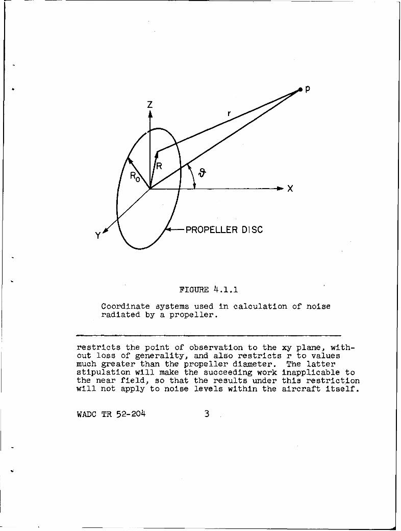
Expressions for the aerodynamic disturbance in thepropeller disk having now been established, the next stepis to compute the resultant acoustic effect at externalpoints. The coordinates shown in Fig. 4.1.1 are used.From hydrodynamics, we can immediately write the velocitypotential g for the resultant sound field from the knownforces acting on the air due to the rotating propellerblade 1.•/. The sound pressure is the time derivitive ofthe veTl-city potential. That is, for an air density p,the sound pressure p is pdg/dt. While this gives thedesired acoustic solution in principle, some simplifica-tions are desirable for ease in calculation. Gutin

WADC TR 52-204 2

pz

•X

y ,• ,PROPELLER DISC

FIGURE 4.1.1

Coordinate systems used in calculation of noiseradiated by a propeller.

restricts the point of observation to the xy plane, with-out loss of generality, and also restricts r to valuesmuch greater than the propeller diameter. The latterstipulation will make the succeeding work inapplicable tothe near field, so that the results under this restrictionwill not apply to noise levels within the aircraft itself.

WADC TR 52-204 3

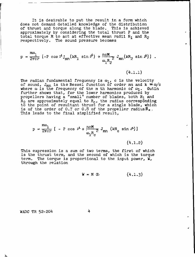
It is desirable to put the result in a form whichdoes not demand detailed knowledge of the distributionof thrust and torque along the blade. This is achievedapproximately by considering the total thrust P and thetotal torque M to act at effective mean radii R1 and R2respectively. The sound pressure becomes

2•c [-P cos Z'Jn(kR1 sin l) + ncM Jn(kR 2 sin A-)]

(4.1.1)

The radian fundamental frequency is wl, c is the velocityof sound, Jmn is the Bessel function of order mn and k = /cwhere w is the frequency of the m th harmonic of w1 . Gutinfurther shows that, for the lower harmonics produced bypropellers having a "small" number of blades, both R1 andR2 are approximately equal to Rc, the radius correspondingto the point of resultant thrust for a single blade, whichis of the order of 0.7 or 0.8 of the propeller radiusR0 .This leads to the final simplified result,

n W1 C s l ncMP =2- [ - P COS + 2 Jmn (kRc sin 2.)]

lc

(4.1.2)

This expression is a sum of two terms, the first of whichis the thrust term, and the second of which is the torqueterm. The torque is proportional to the input power, W,through the relation

W = M 0:, (4.1.3)

WADC TR 52-204 4

'9

900

1200

FROM GUTINTHEORY EQ.(4.1.2)RC=0.75 R0 KEMP'S MEASUREMENT

(FUNDAMENTAL)

150S~600

FROM GUTIN 300THEORY EQ.(4.1.Z)RC = 0.7 RO

1800 00DIRECTION OF

FLIGHT

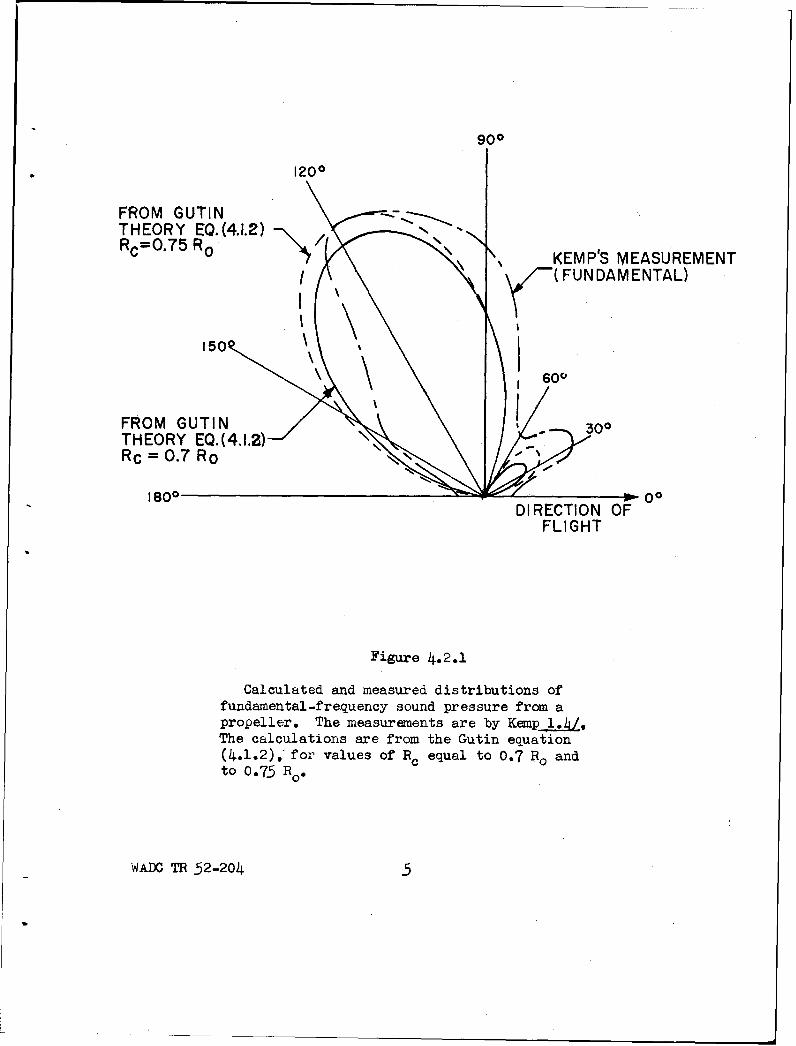
Figure 4.2.1

Calculated and measured distributions offundamental-frequency sound pressure from apropeller. The measurements are by Kemp l l..&.,The calculations are from the Gutin equation(4.1.2), for values of R. equal to 0.7 R. andto 0.75 Ro.

WADC TR 52-204 .5

900 FROM GUTIN

/200THEORY EQ.(4.1.2)

KEMP'S MEASUREMENTSSECOND HARMONIC

- -. 600//

1800DIRECTION OF

FLIGHT

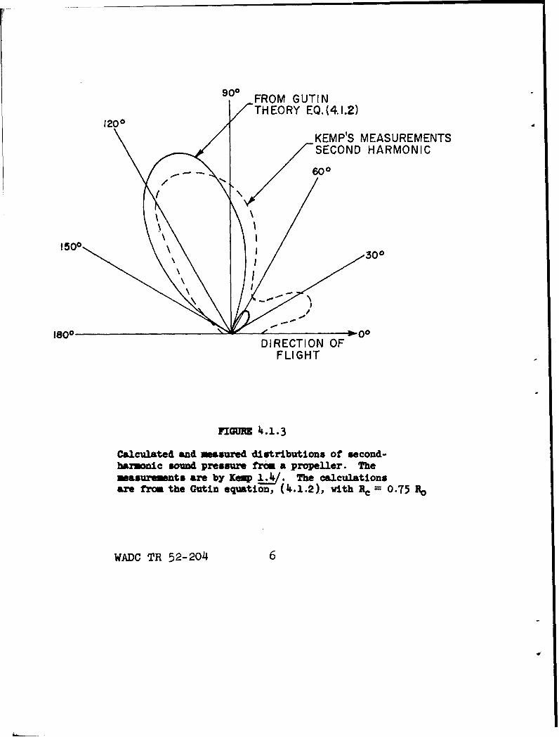
n=M 4.1.3

Calculated and measured distributions of second-harmonic sound pressure from a propeller. Themeasuuements are by Kemp L._ . The calculationsare from the Gutin equation, (..l.2), with RI = 0.75 1:,

WADC TR 52-204 6

The thrust P is related to the input power by anaerodynamic relation which Gutin gives in the form

P = (2pSW 2 Iq2 )1/3 (4.1.4)

where S is the area of the propeller disk and ý is anefficiency factor estimated to equal about 0.75.

Gutin calculated the expected polar distribution ofradiated sound for the first two harmonics, for the follow-ing situation: Two-blade propeller, radius 2.25 meters,1690 kg thrust, 515 kgm torque, 13.9 rev/sec. The results-were compared with experimental data for this situationas taken by Paris 1.3/ and by Kemp 1.4, with values ofboth 0.7 and 0.75 being tried for Rc/Ro. The comparisonwith the Kemp results is shown in Figs. 4.1.2 and 4.1-3.The agreement is fair for the fundamental, but appears to'deteriorate for higher harmonics. This would be expectedfrom the nature of the assumptions made in the derivation.Fortunately, the fundamental usually constitutes thegreatest single contribution to the sound output. Gutin'scalculations showed slightly better agreement with theParis data (fundamental only).

The general features of the polar patterns in Figs.4.1.2 and 4.1.3 are found in virtually all cases of noisegeneration by a propeller free of obstacles. The torqueterm results in an acoustic pressure pattern which is zeroon-the propeller axis and maximum in the propeller plane.The thrust term results in an acoustic pressure which issomewhat smaller than the maximum torque contribution (thisneed not always be true), and which is zero in the planeof the propeller as well as on the axis. The two contri-butions are out of phase for positions in front of thepropeller, but in phase for positions to the rear. Thecombined effect of the two terms is a radiation patternhaving symmetry of rotation, which is zero on the propelleraxis and which is maximum at a position some 150 behindthe propeller plane.

N.A.C.A. Propeller Noise Charts Based on Gutin's Equa-tion. No propeller noise analysis is available which doesno---include at least some of the approximations made byGutin. Fortunately, the simplified Gutin relation,

WADC TR 52-2o4 7

Eq. (4.1.2), seems to give the maximum overall soundpressure in the far field of a propeller to an accuracysufficient for the usual requirements of noise-controlengineering, at least for those propellers operating atsubsonic tip speeds which are currently in use.

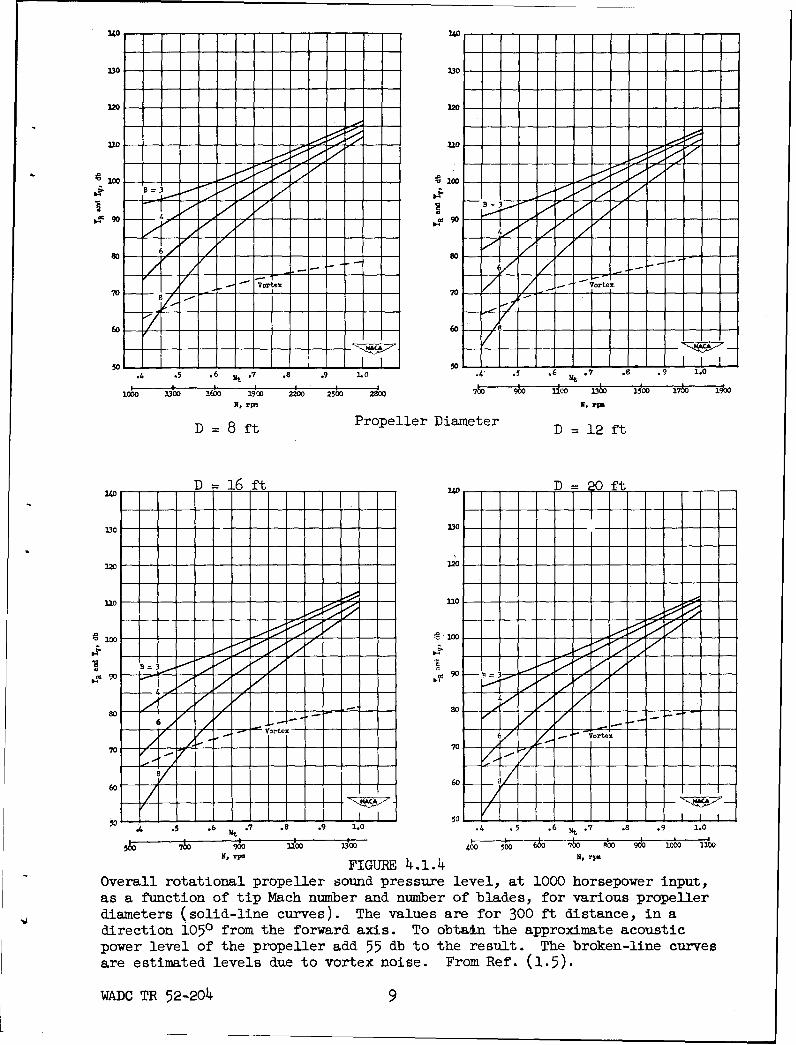
A convenient set of propeller-noise charts has beencomputed from the Gutin relation by Hubbard 1.,ý under theauspices of the N.A.C.A. These are reproduced in partin Figs. 4.1.4 through 4.1.9. The independent variablesare input horsepower, propeller diameter, number of blades,and rate of rotation or Mach number of the blade tip. Theresult is read from the charts as sound pressure level ata distance of 300 feet, at a position 1050 removed fromthe forward propeller axis (approximately the position ofmaximum sound pressure in ordinary cases). The soundpressure contributions from the first four harmonics havebeen added on an energy basis to give this result; hence,the values obtained are closely representative of overallsound pressure level, since ordinarily the contributionsof the higher harmonics drop off rapidly.

Analysis of a typical propeller radiation patternshows that the sound pressure level in the direction ofmaximum output is about five db above the space-averagevalue. Hence, 5 db should be subtracted from the chartvalues to obtain the space-average sound pressure levelat a distance of 300 ft. Adding 55 db to the N.A.C.A.chart values gives approximately the power level of thepropeller as a noise source.

The Gutin result is found in the N.A.C.A. publica-tions by Hubbard 1-5/ and others in the form and symbolsof Eq. (4.1.5). Mr-is is adapted to simple engineeringcomputation.

P = ... s M - T cos JmB(0.8mBMt sin

(4.1.5)

WADC TR 52-204 8

340 1W 0

230 0 -

IMI

SB=3no n

go09

s.- o 6- / s o 1 IX

I" o'Ze ..- Vortex

.4, .5 .6 ut .7 .8 .9 LO .,- .5 .6 Mt 7 .8 .9 1.0IO I I " _ _ _ _ _ _ _ _ _ __ _ _ _ _ _ _ _ _ _ _

1000 3.300 16O2 19 20 2500 2800 40 g300 1500 17t 9

N, rpm N, rpm

D 8 ft Propeller Diameter D = 12 ft

D _16 ft D 20ft

20- - - - - - - - - - - - 30- - - - - - - - -

no no

I-.I

~90 90 - - - - - - - - - - -

Vortex

I F -Vote

50 70 960 il00 3300 4:00 50'0 Z8o 0 RbO 900 ;e 10:00 1100

N, L,

S, FIGURE .4.1.14 N. , rpm

Overall rotational propeller sound pressure level, at 1000 horsepower input,as a function of tip Mach number and number of blades, for various propellerdiameters (solid-line curves). The values are for 300 ft distance, in adirection 1050 from the forward axis. To obtain the approximate acousticpower level of the propeller add 55 db to the result. The broken-line curvesare estimated levels due to vortex noise. From Ref. (1.5).

WADC TR 52-204 9

43

5 00 2300 1h0 191 220 20 1 2o 1SO 10 9J

D = 8 ft ~ Propeller DiameterD=12f

D = 16 ft UOD = 20 ft

130 130

90g- ~ --

50 0 00 10 30 i60 0 & 70 &O 90 100 20

3.1pN.zr

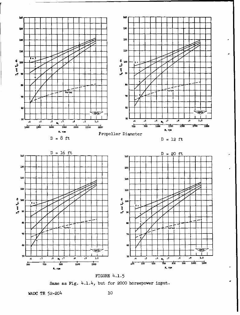
FIGURE 4.1.5

Same as Fig. 4.1.4, but for 2000 horsepower input.

WADC TR 52-204 10

1"0 - 230 --

Dno

UO UO

1t1 3'0 ht0 9JO ~ 0 2b0 2JO 00 90 10 100 150B70 13

Ar N i

= 8loPrpllrDamtr l 2f

66

Same VsogrI..1 u o 100 ospwrip t. x

70D - R /I 201 F1I- - 7

=3=

8~ -+

V ortek

60

W& 30 itO700 9 U'100 X,300 1500 1700 19003, r~c1, p

D 8 ft Propeller Diameter D = 12 ft

D 16 ft UD =20 ft

4100 00

or - so -otý - i- .~

60 60 -- ---

9W 65 . . 8 . . .4 .5 .6 Xt .7 .8 .9 1.0

900 140W30 ~ 500 600 700 RV 90 1 ~ 10

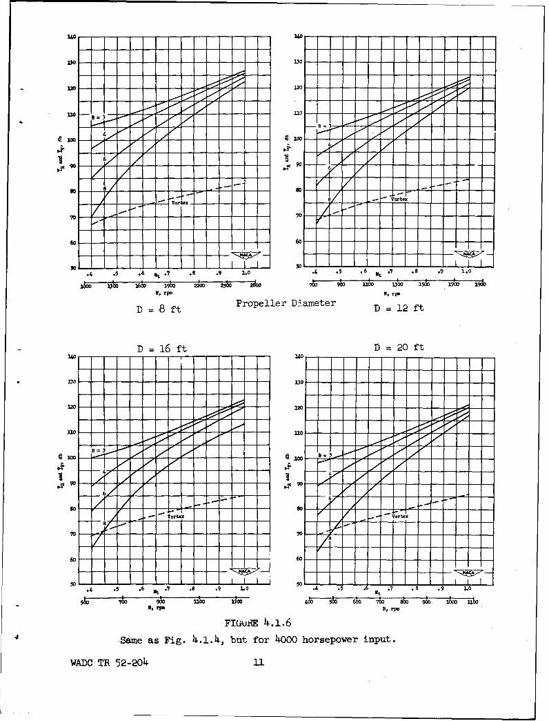
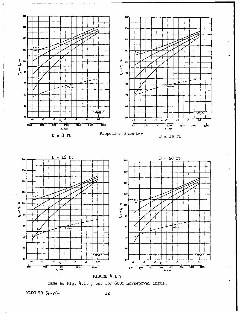
Same as Fig. 4i..1.4, but for 6000 horsepower input.

WADC TR 52-204e 12

3=no - I?

10--

I90.0 o .0 9

/.~~~~-" ... vortex •. re

"0-70

60 60

./, .5 .6 jet .7 .8 .9 1.0 .4 .5 .6 Ut 17 .8 .9 1.0I ' I I I~o • 5o io ~OOO 2300 2600 1900 007 900 0: it= 3 10

V, rr- N, rM

D= 8 ft Propeller Diameter D = 12 ft

D = 16 ft D = 20 ft

S1no

nno

90 90II

_.,.. -,.r;

S.- Yo~ex-- •8 Vorte

.4 .5 .6 llt .7 10 .9 1.0 .4 .5 .6 .• . .9 1-0

5;0 "tO0 900 11000 0 i0 40 50"O 800 900 .• M nooN, rim N, r;=

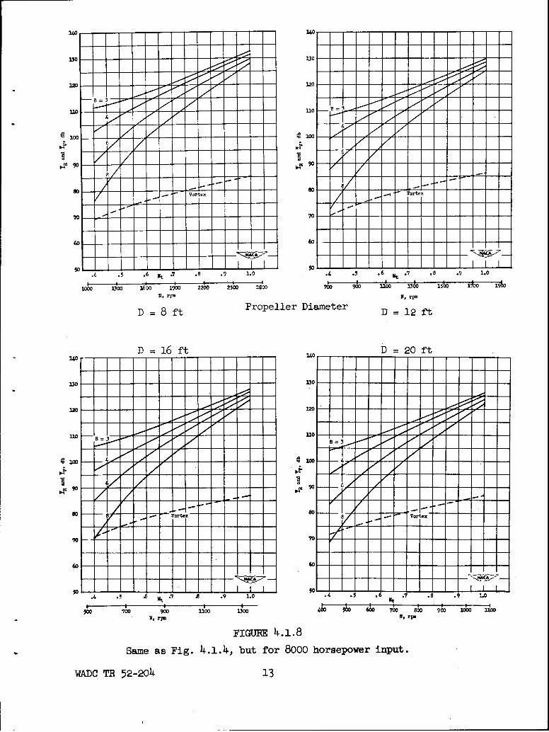
FIGURE i.i.8

Same as Fig. 4.1.4, but for 8000 horsepower input.

WADC TR 52-20o4 13

'UO

2WI

.. .5 .6 s .7 .8 S' .0 .1. .5 .6 .7 .8 .9 1.0

10i7 -2340-D 12900 2200 70' 0 W U10 30 1;'F 10

V. no. N, nn

D= 8 ft Propeller Diameter D = 1-2 ft

D = 16 ft D = 20 ft

'U

1z I I I

I-r ~ N 00 0

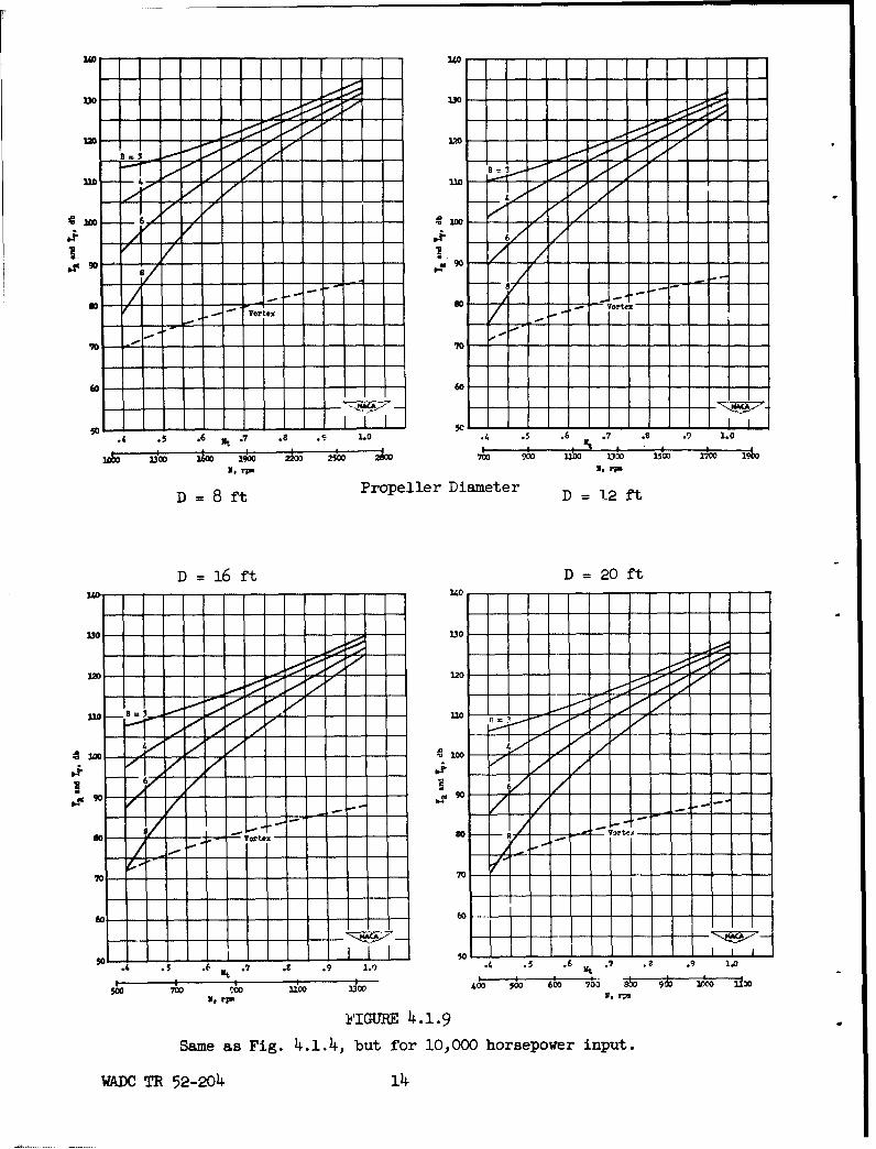
Ssm sr tig so.4 but for 1000hrepwript

WADO R 52-04 1

Here m is the harmonic number; B, number of blades;D, propeller diameter, ft; Mt, tip Mach number; s, dis-tance from propeller hub to observer, ft; A, propellerdisk area, sq ft; PH, input horsepower; T, thrust inpounds; P , angle between forward propeller axis and lineof observations. The effective radius has been taken as0.8 of the total.

In Hubbard's calculations, the thrust is derivedfrom the input horsepower by a relation equivalent to theone used by Gutin, Eq. (4.1.4), except that a revisedvalue of the constant gives thrust values which are 0.78of those computed by Gutin's procedure. The procedureused by Hubbard is said to be approximately correct forpropellers operating near the stall condition.

The sound pressure levels given in the N. A. C. A.charts include an estimated contribution from the non-periodic vortex noise, which ordinarily constitutes asmall portion of the total propeller noise power. Thebasis for calculation of the vortex noise will be discussedlater. The broken lines in the charts indicate the es-timated levels of vortex noise only.

Effect of Number and Shape of Blades on the RotationalNoise. Two of the most important parameters which can bealtered in the propeller with a certain amount of flexi-bility are the number and shape of the blades. It isreadily visualized that the number of the blades determinesthe frequency of the fundamental blade passage tone. Onthe other hand, it can be shown that the intensity of thesound will decrease as the number of blades is increased.

A qualitative explanation for the reduction of soundoutput by an increase of the number of blades can be givenon the basis of the phase cancellation of the several com-ponent forces. A simple example is given by the generation

WADC TR 52-204 15

ONE _ONE

REVOLUTION REVOLUTIONJJL...... JLPRESSURE IMPULSES FROM BLADE PRESSURE IMPULSES FROM BLADES

FUNDAMENTAL CANCELLATION OF FUNDAMENTAL

- \ /\ // #\ \ _ # \ \ _

SECOND HARMONIC SECOND HARMONIC (NEW FUNDAMENTAL)

THIRD HARMONIC CANCELLATION OF THIRD HARMONIC

(a) ONE-BLADE PROPELLER (b) TWO-BLADE PROPELLER

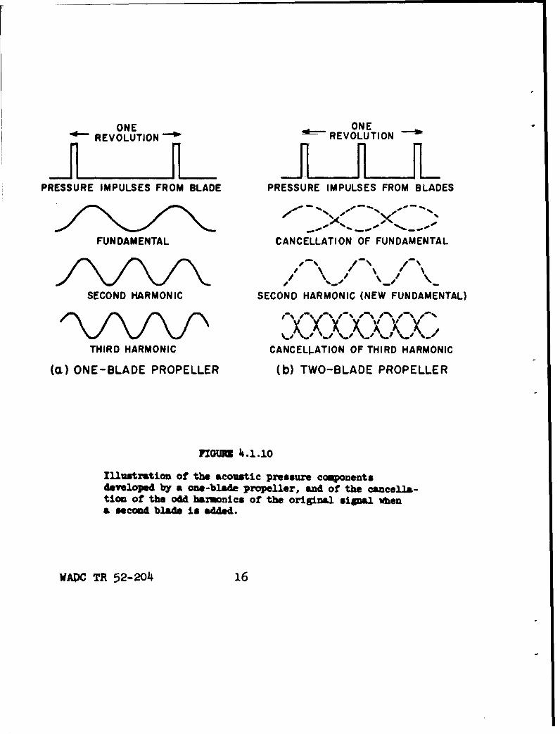
II£OmI 4.1.10

Illustration of the acoustic pressure componentsdeveloped by a one-blade propeller, and of the cancella-tio, of the odd harmonics of the original signal whena second blade is added.

WADC TR 52-204 16

of sound by a propeller consisting of one blade only. Thecorresponding aerodynamic force is shown in Fig. 4.1.10.In that figure the Fourier components have also been repre-sented (not to scale). In Figure 4.1.10 the case of a two-blade propeller is considered. The Fourier components ofthe force shown in this figure indicate that the odd harmonics(with reference to the original one-blade propeller) cancel,while the even harmonics are reinforced. A quantitativecalculation shows that the net effect, however, is an overalldecrease in the sound intensity. For the special case inwhich the tip speed, the thrust, and the input horsepowerare kept constant, while the blades are redesigned and in-creased in number, the acoustic effect can be seen directlyfrom Eq. (4.1.5). The quantity which varies is mB [JmB(0.8mBMt sin p )]. Examination of tables of Bessel functionsshows that, for typical values of the variables, this quan-tity decreases rapidly as mB increases.

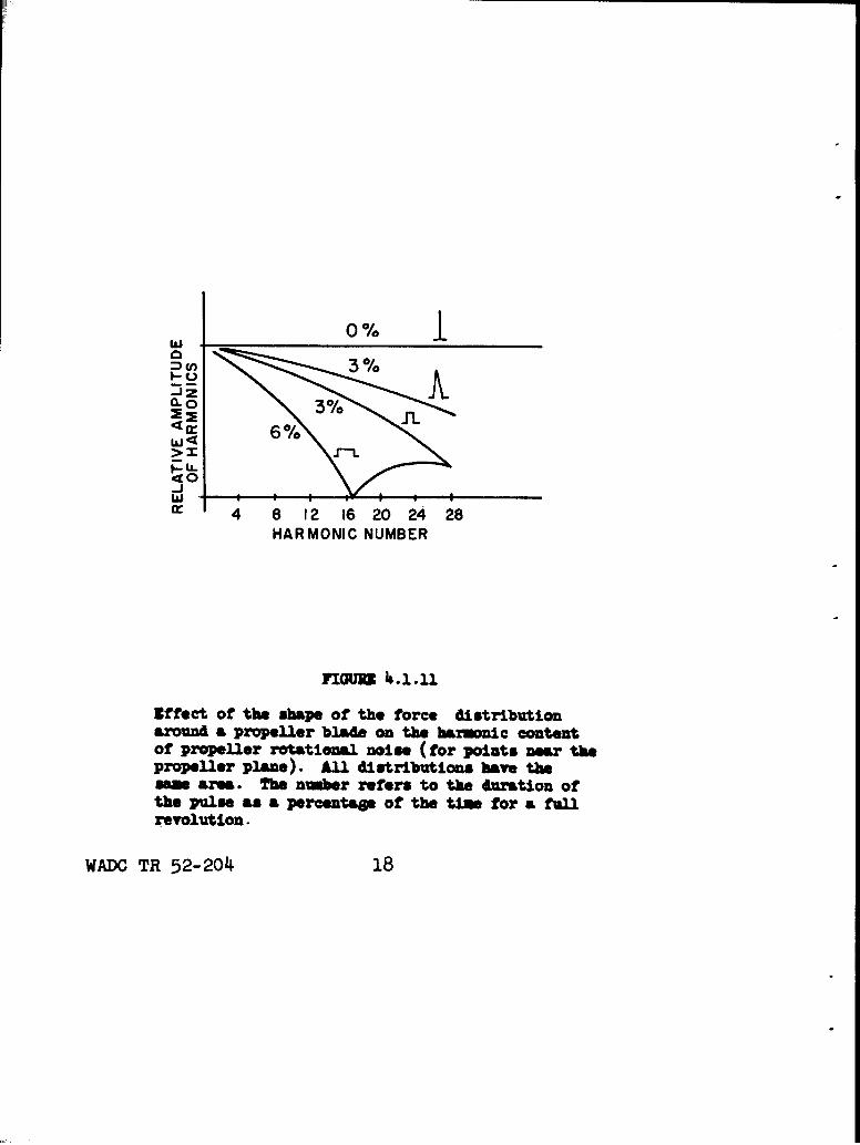
The effect of the blade width can be particularlyimportant for the higher harmonics. In the Gutin approxi-mation, the force produced in the propeller plane by thepassage of an individual blade is treated as an impulse.This is equivalent to assigning the propeller blade anegligible width. Regier 1._/ has evaluated the spectrumdistribution corresponding to several more nearly realisticforce-time characteristics, as shown in Fig. 4.1.11. All ofthese distributions have equal areas under the curves, andthus exert equal forces on the propeller. The horizontalline for the zero-width blade corresponds to the uniformFourier amplitudes in the Gutin approximation; the othercurves show the new distributions which replace this one inthe case of finite blade width. It is apparent that increas-ing the width of the blade, while the thrust is kept constant,decreases the intensity of the radiated sound through reduc-tions in the amplitudes of the higher harmonics.

The role played by the number and kind of bladesin the total noise radiated by a propeller is illustratedin a series of experiments by Beranek, Elwell, Roberts,and Taylor ._7/. The experiments consisted in measuringthe noise radiated in flight, by certain aircraft of lessthan 200 horsepower, for propellers of two, three, four,and six blades. The propellers exerted approximately

WADC TR 52-204 17

ao3%

3411-0

Z

o:34 8 12 16 20 24 28

HARMONIC NUMBER

FIIJOUI 1.1.11

Effect of the shape of the force distributionaround a propeller blade on the harmonic contentof propeller rotational neise (for points near thepropeller plane). All distributions have the

me area. The n~ber refers to the nrtion ofthe pulse as a peroentap of the time for a flrevolution.

WADC TR 52-2014 18

equal thrusts and were of nearly the same diameter. Theresults may be summarized approximately by the statementthat the intensity if lowered 6 db for each doubling ofthe number of blades in the propeller, the input powerand the speed of rotation remaining fixed.

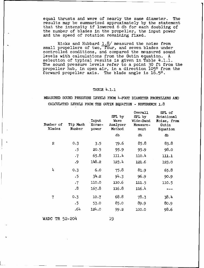
Hicks and Hubbard 1./ measured the noise fromsmall propellers of two, foT ur, and seven blades undercontrolled conditions, and compared the measured soundlevels with calculations from the Gutin equation. Aselection of typical results is given in Table 4.1.1.The sound pressure levels refer to a point 30 ft from thepropeller hub, in open air, in a direction 1050 from theforward propeller axis. The blade angle is 16.50.

TABLE 4.1.1

MEASURED SOUND PRESSURE LEVELS FROM 4-FO0T DIAMETER PROPELLERS AND

CALC0LATED LEVELS FROM THE GUTIN EQUATION - REFERENCE 1.8

Overall SPL ofSPL by SPL by Rotational

Input Wave Wide-Band Noise, fromNumber of Tip Mach 'Horse- Analyzer Measure- Gutin

Blades Number power Method ment Equation

db db db

2 0.3 3.5 79.6 85.8 83.8

.5 20.5 95.9 95.9 98.0

.7 65.8 111.4 110.4 111.1

.9 148.2 123.4 121.6 123.0

4 0.3 6.0 75.8 81.9 65.8

.5 34.2 94.3 96.9 90.9

.7 110.0 llO.6 111.5 110.5

.8 167.8 116.8 116.4

7 0.3 10.7 68.8 78.3 38.4

.5 53.0 85.0 89.9 80.9

.64 124.o 99.2 100.0 98.6

WADC TR 52-204 19

The results by the wave analyzer method refer to thesquare root of the sum of the squares of the amplitudesfor the first five harmonics of the blade passage fre-quency. This method therefore measures the level ofthe periodic rotational noise, provided that the effectof other noise components falling within the pass bandof the wave analyzer (25 cps) in negligible. Thecalculated values represent the square root of the sumof the squares of the individual calculated amplitudesfor the first five harmonics.

For each propeller, the SPL measured by the waveanalyzer method and that measured by the wide-bandmethod in the range of Mach numbers above about 0.6,are both closely equal to the value predicted by theGutin theory. This means that the noise at the higherMach numbers is almost entirely of the rotational type,and that its overall level under these conditions isadequately predicted by Gutin's equation. Thus, as faras operation at the higher Mach numbers Is concerned,theory and experiment agreeas to the amount of reductionin noise level which is obtained by increasing the num-ber of propeller blades and reducing the tip speed. Forexample, in Ref. 1.8 it is found that for a tip Machnumber of 0.7, 66 horsepower can be absorbed by the 2-blade propeller with a 16.50 attack angle, and 76 horse-power by the 7-blade propeller with a 100 attack angle.Although the horsepower is nearly the same, the secondconfiguration gives a wide-band sound pressure level of101 db, as compared to 110 db for the first. The calcu-lated values are 100 db and 111 db.

In the results for each propeller configuration inTable 4.1.1, the overall SPL at the lower Mach numbersis greater than the SPL by the wave analyzer method,which is in turn greater than the calculated value fromthe Gutin equation. These effects are explained atleast partially by the additional observation that thesound at the lower Mach numbers consists mostly of

WADC TR 52-204 20

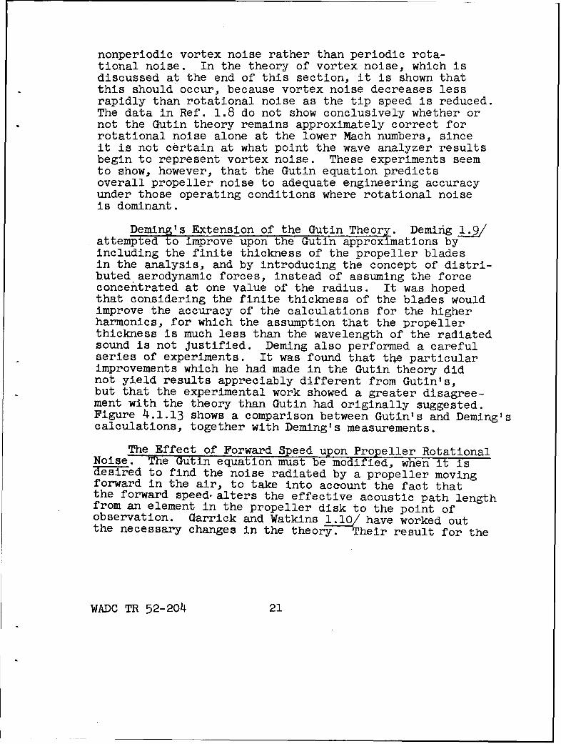
nonperiodic vortex noise rather than periodic rota-tional noise. In the theory of vortex noise, which isdiscussed at the end of this section, it is shown thatthis should occur, because vortex noise decreases lessrapidly than rotational noise as the tip speed is reduced.The data in Ref. 1.8 do not show conclusively whether ornot the Gutin theory remains approximately correct forrotational noise alone at the lower Mach numbers, sinceit is not certain at what point the wave analyzer resultsbegin to represent vortex noise. These experiments seemto show, however, that the Gutin equation predictsoverall propeller noise to adequate engineering accuracyunder those operating conditions where rotational noiseis dominant.

Deming's Extension of the Gutin Theory. Demirig L./attempted to improve upon the Gutin approximations byincluding the finite thickness of the propeller bladesin the analysis, and by introducing the concept of distri-buted aerodynamic forces, instead of assuming the forceconcentrated at one value of the radius. It was hopedthat considering the finite thickness of the blades wouldimprove the accuracy of the calculations for the higherharmonics, for which the assumption that the propellerthickness is much less than the wavelength of the radiatedsound is not Justified. Deming also performed a carefulseries of experiments. It was found that the particularimprovements which he had made in the Gutin theory didnot yield results appreciably different from Gutin's,but that the experimental work showed a greater disagree-ment with the theory than Gutin had originally suggested.Figure 4.1.13 shows a comparison between Gutin's and Deming'scalculations, together with Deming's measurements.

The Effect of Forward Speed upon Propeller RotationalNoise. The Gutin equation must be modified, when it isTaiTed to find the noise radiated by a propeller movingforward in the air, to take into account the fact thatthe forward speed- alters the effective acoustic path lengthfrom an element in the propeller disk to the point ofobservation. Garrick and Watkins 1.1y have worked outthe necessary changes in the theory. Their result for the

WADC TR 52-204 21

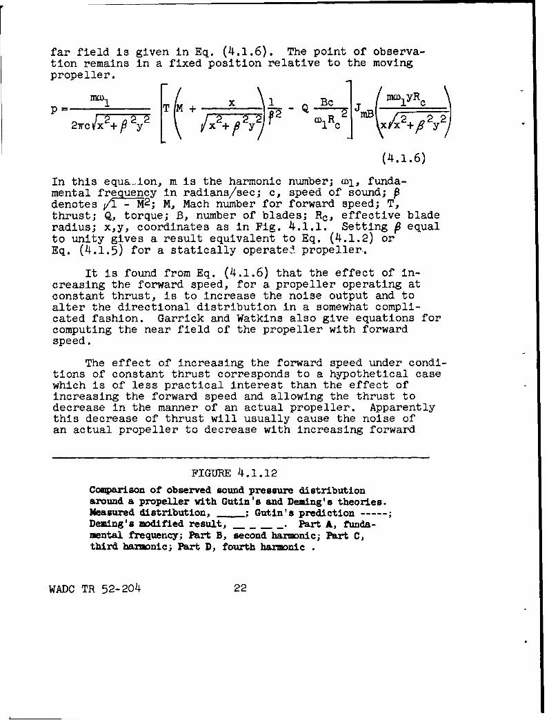
far field is given in Eq. (4.1.6). The point of observa-tion remains in a fixed position relative to the movingpropeller.

Fp (wTM + - '\ - Bec 1 (IUCDmw1yR0

(4.1.6)

In this equa.-lon, m is the harmonic number; wl, funda-mental frequency in radians/sec; c, speed of sound; pdenotes/1- M2; M, Mach number for forward speed; T,thrust; Q, torque; B, number of blades; Rc, effective bladeradius; x,y, coordinates as in Fig. 4.1.1. Setting P equalto unity gives a result equivalent to Eq. (4.1.2) orEq. (4.1.5) for a statically operatedt propeller..

It is found from Eq. (4.1.6) that the effect of in-creasing the forward speed, for a propeller operating atconstant thrust, is to increase the noise output and toalter the directional distribution in a somewhat compli-cated fashion. Garrick and Watkins also give equations forcomputing the near field of the propeller with forwardspeed.

The effect of increasing the forward speed under condi-tions of constant thrust corresponds to a hypothetical casewhich is of less practical interest than the effect ofincreasing the forward speed and allowing the thrust todecrease in the manner of an actual propeller. Apparentlythis decrease of thrust will usually cause the noise ofan actual propeller to decrease with increasing forward

FIGURE 4.1.12

Comparison of observed sound pressure distributionaround a propeller with Gutin's and Deming's theories.Measured distribution, _ ; Gutin's prediction -----Deming's modified result, _ _ _ _. Part A, funda-mental frequency; Part B, second harmonic; Part C,third harmonic; Part D, fourth harmonic

WADC TR 52-204 22

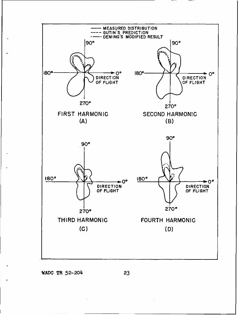
MEASURED DISTRIBUTION----. GUTIN 'S PREDICTION---- DEMING'S MODIFIED RESULT

900 900

Se.

B8Oa o 180 00DIRECTION DIRECTIONOF FLIGHT OF FLIGHT

2700 2700

FIRST HARMONIC SECOND HARMONIC(A) (B)

990

1800 00 'O 1800 _ moo

•.• DIRECTION DIRECTION

OF FLIGHT OF FLIGHT

2700 2700

THIRD HARMONIC FOURTH HARMONIC

(C) (D)

"WADC TR 52-204 23

L _________________________

90" 90T

3,0 0

,00,•-,,"', (a) M -0.8; T-1O850b. ,oo u,/cm, If) MM-0.6, T,201b.

20 ÷ " '

-Lgne y- 2 0 feet

... Circle s,.20 feet

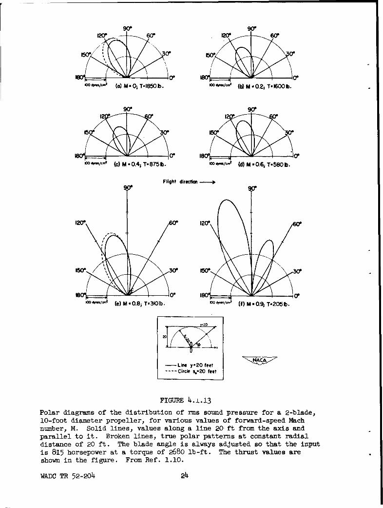
FIGURE 4. ±.13Polar diagrams of the distribution of rms sound pressure for a 2-blade,

10-foot diameter propeller, for various values of forward-speed Machnumber, M. Solid lines, values along a line 20 ft from the axis andparallel to it. Broken lines, true polar patterns at constant radialdistance of 20 ft. The blade angle is always adjusted so that the inputis 815 horsepower at a torque of 2680 lb-ft. The thrust values areshown in the figure. From Ref. 1.10.

WADC TR 52-20f4

speed up to Mach numbers of about 0.4. Garrick and Watkinshave calculated the noise output of a two-blade propellerfor various forward speeds, with the thrust values takenfrom actual aerodynamic measurements. The results areshown in Fig. 4.1.13. The initial drop of noise output asthe forward speed increases is confirmed in a measurementby Regier /, who found that the overall noise developedby a light trainer airplane in normal flight is 6 db lessthan that produced by the same airplane in static groundoperation.

As a practical matter, the distinction between theGutin relation and the modified equation for the case offorward flight, Eq. (4.1.6), may be neglected for forwardspeeds up to M = 0.3. At this. speed, the value of f hasdropped only to 0.95, from the value 1.00 corresponding tostatic operation. Therefore, within this range, the effectof forward speed may be represented adequately by makingthe appropriate changes in the thrust value used in theoriginal Gutin approximation.

Noise Levels Very Near a Propeller. Calculation ofthe noise levels near a propeller by Gutin's method requiresthat some of the convenient geometric approximations beomitted and that more complicated integrations be carriedout. These calculations have been done by Hubbard andRegier 1 for several cases. The work of Garrick andWatkins on the moving propeller, described above, also per-tains largely to the near field.

Hubbard aad Regier found that near-field calculatedsound pressures, for the first few harmonics, were in goodagreement with experiments performed with model propellersof diameters 48 to 85 inches, the range of propeller-tipMach numbers being 0.45 to 1.00. The observed pressureincreases very rapidly as the measuring point is broughtclose to the propeller tips; this behavior correspondsclosely to what would be observed if the propeller tipwere the effective noise source in the very near field.The distribution of sound pressure in the propeller planecan be expressed conveniently in terms of d/D, where d isdistance from the propeller tips, and D is the propellerdiameter, for a given propeller shape and given rotationalspeed. On this basis, good agreement was obtained betweenobservations taken near the full-sized propellers, andextrapolated results of the model studies.

WADC TR 52-204 25

The sound pressure ahead of the propeller plane isout of phase with that behind the propeller plane in mostcases where the near field was investigated. A plane wall(simulating a fuselage) placed Just behind the microphone,parallel to the propeller axis, and 0.083 of a propellerdiameter from the tips, doubles the pressure reading fora given location by reflection, but does not seem to reacton the acoustic behavior of the propeller. (This conclu-sion might not hold if the wall were brought much closerto the propeller tips.)

Input power and tip speed are of primary importancein determining the near field. At the lower tip-speedMach numbers, the sound pressure for given tip speed andinput power is reduced by using a propeller with a greaternumber of blades, but this difference virtually disappearsat Mach 1.0. At constant power, the pressure amplitudesof the lower harmonics tend to decrease, and of the higherharmonics to increase, as the tip speed is increased. Thedifference in sound pressure produced by square and roundedtips is found to be very slight, with the square tips pro-ducing about 1.0 db higher SPL than the round, in a veryrestricted region near the propeller plane. Also, bladewidth is found to have no important effect.

Further, Hubbard and Regier compared their moreaccurate near-field calculations with the results obtainedby using the Gutin equation for the near field, in theplane of the propeller. It is found that the Gutin equa-tion under-estimates the SPL in this situation. Apparentlythe discrepancy becomes less than 2 db when the distancefrom the propeller tips is greater than one propeller dia-meter, so that the Gutin equation is sufficiently accuratefor many purposes at distances greater than this.

Where it is desired to know the overall sound pres-sure level of propeller noise immediately within an air-plane cabin, at a location near the propeller tips, theexperimental findings of Rudmose and Beranek 1A3J1 may beused. They analyzed data taken within some 5=5ypes ofaircraft of the period 1941-1945; in seven types, asystematic study of the parameters which influence the low-frequency propeller noise was made.

WADC TR 52-204 26

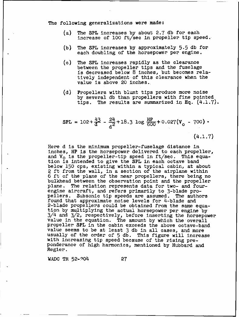
The following generalizations were made:

(a) The SPL increases by about 2.7 db for eachincrease of 100 ft/sec in propeller tip speed.

(b) The SPL increases by approximately 5.5 db foreach doubling of the horsepower per engine.

(c) The SPL increases rapidly as the clearancebetween the propeller tips and the fuselageIs decreased below 8 inches, but becomes rela-tively independent of this clearance when thevalue is above 20 inches.

(d) Propellers with blunt tips produce more noiseby several db than propellers with fine pointedtips. The results are summarized in Eq. (4.1.7).

SPL = 102+_ - 21+18.3 log HP0 +0.027(Vo - 700)

(14.1.7)

Here d is the minimum propeller-fuselage distance ininches, HP is the horsepower delivered to each propeller,and Vo is the propeller-tip speed in ft/sec. This equa-tion is intended to give the SPL in each octave bandbelow 150 cps, existing within a typical cabin, at about2 ft from the wall, in a section of the airplane within6 ft of the plane of the near propellers, there being nobulkhead between the observation point and the propellerplane. The relation represents data for two- and four-engine aircraft, and refers primarily to 3-blade pro-pellers. Subsonic tip speeds are assumed. The authorsfound that approximate noise levels for 4-blade and2-blade propellers could be obtained from the same equa-tion by multiplying the actual horsepower per engine by3/4 and 3/2, respectively, before inserting the horsepowervalue in the equation. The amount by which the overallpropeller SPL in the cabin exceeds the above octave-bandvalue seems to be at least 3 db in all cases, and moreusually of the order of 5 db. This figure will increasewith increasing tip speed because of the rising pre-ponderance of high harmonics, mentioned by Hubbard andRegier.

WADC TR 52-?04 27

The Rudmose-Beranek experimental results can bereconciled fairly effectively with the theoretical analy-sis. The increase of SPL by 5.5 db for each doubling ofinput power agrees closely with the predictions of thepropeller charts, Figs. 4.1.4 - 4.1.9, which show thatthis effect is generally 5 to 6 db per power doubling.The increase of SPL at the rate of 2.7 db per 100 ft/sec.increase of tip speed, as reported by Rudmose and Beranekfor the low frequencies, is somewhat less than that pre-dicted in Figs. 4.1.4 - 4.1.9, where the effect is about20 to 30 percent greater than this, for three-bladepropellers. This discrepancy is qualitatively reasonable,however, because the charts include the combined effect offour harmonics, and it is known that the effect of tipspeed goes up with increasing harmonic number. Thecritical effect of clearance between the propeller tip andthe fuselage is predicted in the analysis and measurementsby Hubbard and Regier 1. The final observation ofRudmose and Beranek, that propellers with fine pointed tipsproduce a lower cabin sound level, is superficially incontradiction to the findings of Hubbard and Regier, butcan probably be interpreted to mean that an extreme changeof blade shape, in this sense, causes the effective soundsource for fine tip blades to be located further in fromthe tip of the propeller. The absolute levels given byEq. (4.1.7) are considerably lower than those given byfree-space propeller theory, since Eq. (4.1.7) includesthe noise reduction afforded by a typical cabin.

Dual-Rotating Propellers. Hubbard 1.14/ has appliedGutin's analysis to dual-rotating propellers, and hasfound reasonably good agreement with the results of experi-ments on a model unit comprised of two, two-blade, 4-ftdiameter propellers. The sound field no longer hascircular symmetry about the propeller axis, but instead hasmaxima in the directions of blade overlap. These maximaof sound pressure correspond closely to the amplitudewhich would be produced by a single propeller having thesame number of blades as the total in the tandem unit.The intervening pressure minima have amplitudes correspond-ing closely to the output of one of the dual propellersonly. If the two propellers rotate at slightly differentspeeds, the pattern of maxima and minima then rotates,and the sound reaching the observer is consequentlyamplitude modulated. When the number of blades is notthe same in the front and rear units, this modulation is

WADC TR 52-204 28

found only for harmonics which are integral multiplesof both fundamental frequencies; forýexample, the lowestmodulated harmonic of a three-blade, two-blade dual-rotat-ing propeller is the sixth. The case of tandem propellersoperating side by side was also investigated, and similarphenomena were found. The results thus far mentioned arenot critically affected by the separation of the propellers.

An additional signal, the "mutual interference noise",is developed when the spacing of the dual-rotating elementsis made small. This noise component appears to be a maxi-mum on the forward axis of rotation, where the rotationalnoise is small, and has a fundamental frequency equal tothe blade passage frequency. The mutual interferencenoise is undetectable at positions near the propeller plane,where the rotational noise is strong, and apparentlyconsitutes only a small fraction of the total powerradiated by the propeller. The pressure amplitude of thisadditional noise component varies as the propeller powerand as the cube of the tip speed, according to measure-ments on the axis. The effect of spacing is critical; inHubbard's experiment, the mutual interference noise isthe predominant signal on the forward axis at a spacing of6 3/ff, but is not detectable with certainty at a spacingof 12".

The Effect of Struts on Propeller Noise. While notheoretical analysis has been made of the effect of astrut near the propeller plane, the experimental evidenceindicates that a much more serious disturbance is producedby a strut ahead of the propeller than by one behind.This question was examined in the work on dual-rotatingpropellers described above. No strut effect was reportedfor the tractor propeller, which was supported by a strutplaced behind. The pusher propeller (supported by a strutahead) was found to give 3 db higher overall SPL than thetractor when the pusher strut clearance was 11.75 inches,and about 7 db higher SPL than the tractor when thisclearance was 5.75 inches. The effect is nearly independentof tip speed.

An increase of noise resulting from a strut ahead ofthe propeller was also reported by Roberts and Beranek1.,/ in a series of experiments on quieting of a pusheramphibian. The total noise power radiated by this air-plane was greater than that from a tractor airplane operate-ing at greater power and tip speed. The sound level

WADC TR 5 2-2o4 29

measured from the pusher did not drop off sharply to therear as it does for a tractor airplane, and as the Gutintheory predicts. Whereas the noise output of a tractorairplane for specified power and tip speed can be de-creased by increasing the number of propeller blades,in at least qualitative agreement with the Gutin theory,the pusher airplane was found to become noisier as thenumber of blades was increased above four.

Supersonic Tip Speeds and Empirical Propeller NoiseChart.- The Gutin theory of rotational noise and itsvarfious modifications are all restricted to subsonic tipspeeds. At present, the knowledge of propeller noisegeneration for supersonic tip speeds is restricted toexperimental findings. In general, the experimental datashow that there is no discontinuous change in noise out-put as the propeller goes into the supersonic range. Ator near the beginning of the supersonic range, however,the noise power output becomes nearly independent of tipspeed, as shown in N. A. C. A. experiments L on amodel propeller, the sound output of which was in goodagreement with the Gutin theory in the subsonic range.A less extensive series of measurements by a commerciallaboratory (unpublished), on full-scale propellers, seemsto indicate that the noise output for supersonic tipspeeds also becomes relatively independent of input power.This statement is based upon observations of 10- and 16-ftdiameter propellers in the range 800 to 2000 horsepower.

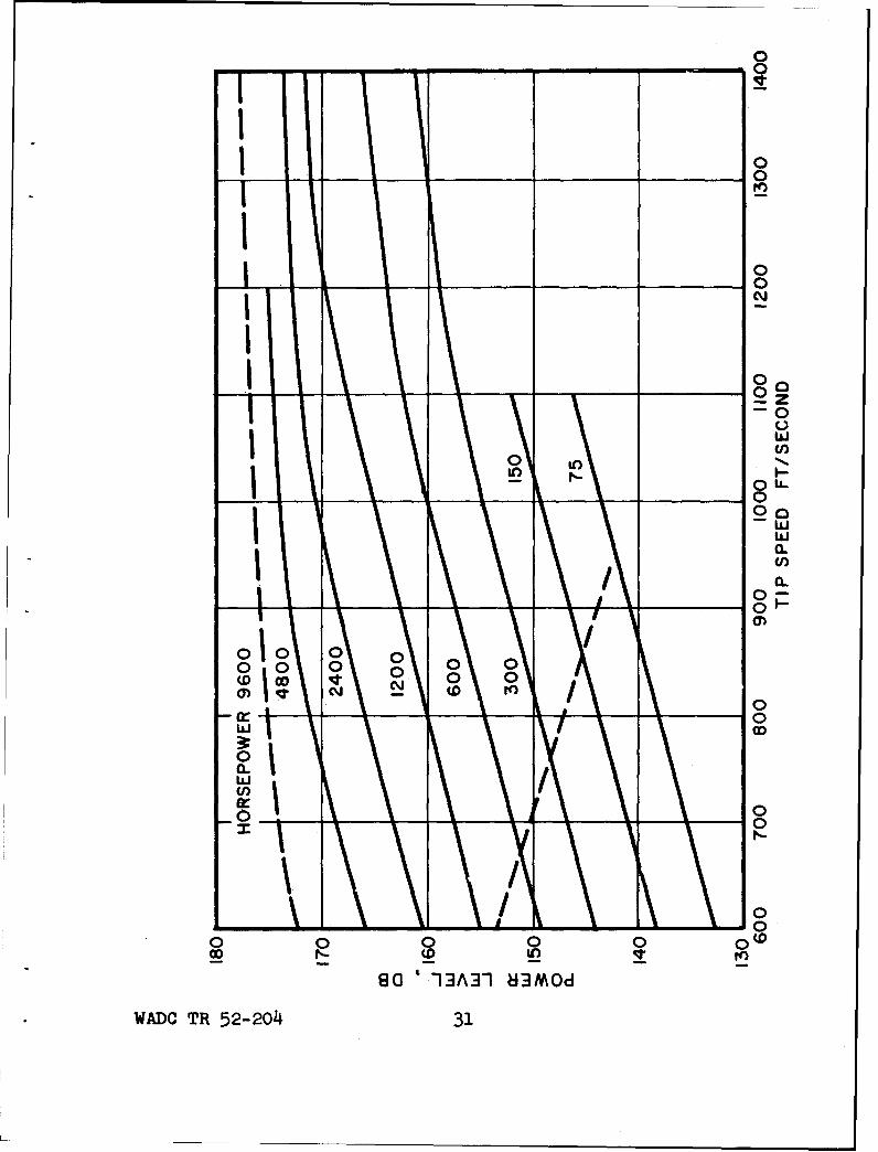
In the absence of a suitable theory of noise genera-tion in the range of supersonic tip speeds, the empiricalchart in Fig. 4.1.14 has been prepared as an approximate

FIGURE 4.1.14Propeller noise chart, constructed from experimental data,shoving the approximte acoustic power level for tip speedsinto the supersonic range. The chart applies to 3-bladepropellers, of diameter approximately 12 ft. Power levelsfor 2- and 1-blade propellers lie approximately 2 db aboveand below the chart values, respectively. For operatingconditions to the upper right of the broken line, propellernoise usually exceeds the exhaust noise from a reciprocatingengine, but for operating conditions to the lower left,exhaust noise my predominate (see Sec. 4.3).

WADC TR 52-204 30

I0

_ _ 00

0

I 000

-820w

I Ia.

00

0~ 0 0 /00 0 0 0

00 C~0Ok0

00

80 OD~1~3

WADCTR 2-24 3

0

summary of existing information. This chart gives theoverall power level of the propeller when the input horse-power and the tip speed are known. The information fortip speeds of 1000 ft/sec and greater was taken from thetwo sources mentioned above. The subsonic portion of thechart is arbitrarily drawn to have the dependence on tipspeed and input power which was reported by Rudmose andBeranek for low frequencies, as shown in Eq. (4.1.7); onthe basis of propeller noise theory, slightly greatereffect of tip speed might be argued. The absolutevalues indicated by the subsonic curves are determinedin part by the low-speed portions of the data on largepropellers mentioned above, and in part by several mea-surements of ground and flight operation of actual aircraftunder known conditions. Where measurements were taken witha microphone very near the ground and within 50 ft of thesource, pressure doubling at the microphones was assumed,and 6 db was subtracted from the SPL reading. Where themicrophone was 200 ft or more from the source, so thatground attenuation might be more important, this reflectioncorrection was arbitrarily reduced to 3 db. To get thepower level for an outdoor propeller from the SPL measuredin one direction, use was made of the typical propellerdirectivity curve shown in Fig. 4.1.15. The individual datapoints used to make the chart are generally consistentwith the final chart values within 4 db. The extensionof the curves into the supersonic range is determined byvery few measurements and is therefore tentative.

The chart in Fig. 4.1.14 does not show the effectof propeller diameter or of number of blades. The chartis an approximate average of data for propellers of two,three, and four blades, and is most nearly correct forthree blades. Very roughly, values for propellers of twoand four blades lie 2 db above and below the chart values,respectively. The chart is most nearly correct for pro-pellers of diameter 12 ft; for 3-blade, 12-ft propellers,the subsonic portions of this chart are generally in agree-ment with the charts based on Gutin's equation, Figs. 4.1.4through 4.1.9, within 3 db. For propellers of about thissize, the empirical chart in Fig. 4.1.14 may be used inlieu of the detailed charts for engineering predictions.Either this chart or the detailed charts, properly applied,should predict overall static propeller noise within ± 5 dbin most instances.

WADC TR 52-204 32

Parkins and Purvis l.L~j have measured maximumsound levels beneath a number of types of 2- and 4-engine aircraft immediately after takeoff, and havereduced their results to a standard distance. If it isassumed that the aircraft as a whole has approximately thesame directivity as a propeller*, so that the maximum SPLis approximately 5 db above the space-average value, andif it is assumed that the noise powers from the propellerson a given airplane are additive, these data can be reducedto give the power level of a single propeller under take-off conditions. It is found that the power levels obtainedin this way are typically 8 db lower than those predictedby the chart in Fig. 4.1.14. Therefore, 8 db should besubtracted from the chart values to obtain power levelsfor flight conditions following takeoff. This correctionis in the expected direction, inasmuch as the chart refersto static operation, for which noise generation is greatest.

The Spectrum of Propeller Noise. The theories ofpropeller noise do not give a generally successful treat-ment of the frequency distribution of the sound energy.The success of the theories in predicting overall soundpower is attributable partly to the fact that a large partof the energy radiated is found in the first few harmonicsof rotational noise. The theoretical calculations of rota-tional noise generally underestimate the amplitudes of thehigher harmonics. Moreover, a large part of the high-frequency energy often comes from vortex noise, the ampli-tude of which is not rigorously predictable at present.Theoretical considerations of both rotational and vortexnoise agree qualitatively, however, that the high-frequencyenergy increases relative to the low-frequency energy asthe propeller tip speed is increased (at least, in thesubsonic range).

* rSnme unpublished measurements of the polar sound distribu-tion for an airplane operating on the ground show that thisassumption is reasonable. The observed distribution issimilar to that in Fig. 4.1.13, which is for a propeller ona test stand, except that the sound levels behind the actualairplane do not fall off as rapidly for points toward thefront of the plane.

WADC TR 52-204 33

L

-T -O -- -T

0

w0~

0

C.)

00wa

I L 0

O w C 0 N w 0 NI 0 T I

S-13eli33G 30V83AV 33 Vd S 013AIlVI38 N01133810 N3AIS NI 13A31 3dflSS3d UNAOS -nV83AO

WADC TR 52-204 34

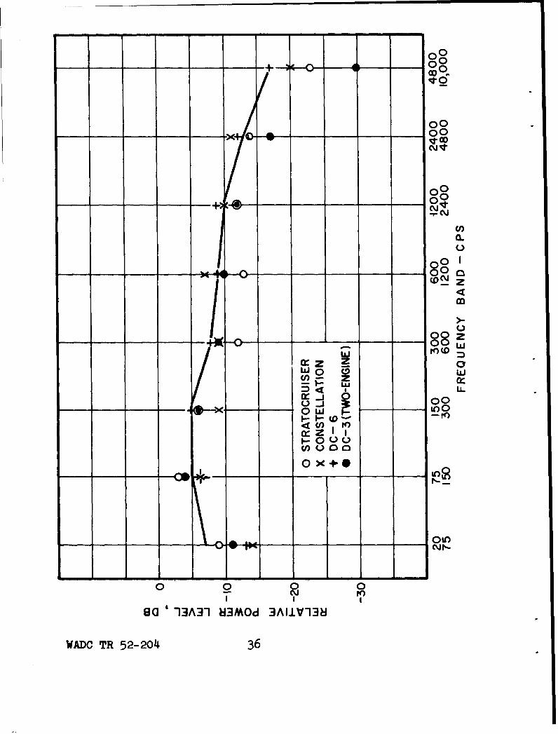
The octave-band spectra measured immediately beneathseveral types of transport airplanes shortly after takeoff,presumably under full-power operation, are shown inFig. 4.1.16. The information is from Ref. 1.17. There isa remarkable similarity in the results for the several air-planes, except that the two-engine airplane (of considerablylower horsepower than the others) gives relatively lessnoise in the two highest octave bands. The arbitrary curvedrawn in this figure is a suggested design curve forengineering prediction of the propeller noise spectrum undertakeoff conditions, for transport airplanes. It is assumedthat the observed noise from a propeller-driven aircraftat takeoff is due to the propellers. The results shownhere will be duplicated only in measurements taken fairlynear the aircraft and over a hard surface. Because atmos-pheric and terrain attenuation of sound rise with increasingfrequency, spectra measured over absorbing terrain, or at adistance of the order of thousands of feet, will haveappreciably lower relative levels in the highest bands thanthose shown. The relative high-frequency content of pro-peller sound also decreases upon change from takeoff tocruising operating conditions, but data are not availableto show precisely the extent of the effect.

Vortex Noise. It has been generally assumed thatthe nonperiodic part of the propeller noise (ordinarilyless than the periodic part) is associated with theshedding of vortices (eddies) in the wake of the moving

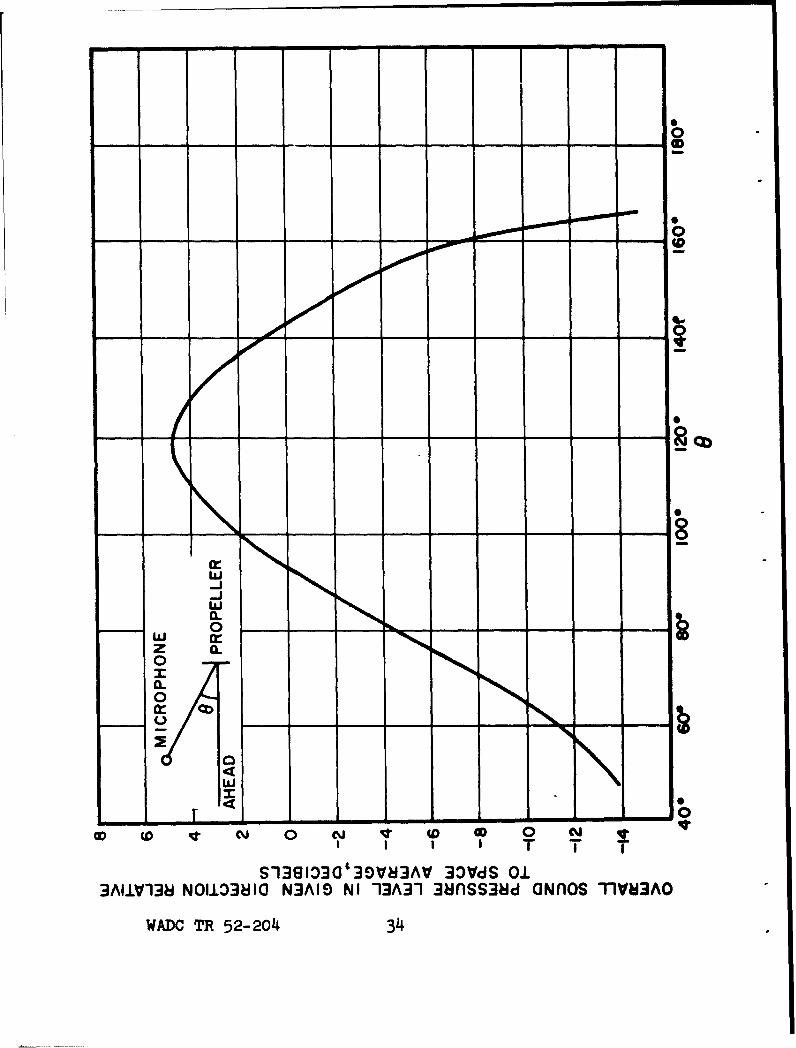
FIGuRE 4.1.15

Directivity pattern computed from overall SPL for apropeller on an outdoor test stand. The directivityis the difference in db between observed SPL in agiven direction and the SPL vhich vould be observedvith non-directional radiation of the same totalsound power. Computed from data in Ref. 1.16.

WADC TR 52-2o4 35

'00

-00

00

/ (DN00

00

I~CL

__ __00

1-000

00 0w row

g ~ ~ ~ ~~c z1A~ KJMd3IV

WADC~ 2R 52243

blade. These vortices are a normal consequency of theinstability of fluid flow past an object of more or lesscylindrical shape. Under idealized conditions, thevortices form and tear away from the obstacle in regularfashion, to form a Karman vortex trail 1 as shown inFig. 4.1.18. While pressure fluctuations are registeredby a detector placed in the trail, it can be proved thatthe vortices in the trail cannot radiate sound. theirpressure distributions fall off very rapidly with distance.The sound radiated by the vortex shedding process must arisefrom the immediate vicinity of the obstacle, as in theregion AO'O"B, and must be the result of the pressure im-pulses which occur whenever the flow system of a vortex issuddenly torn from the obstacle.

Some idea of the process is given by dimensionalanalysis. The intensity of an acoustic wave is given by

I = p2 /Pc (4.1.8)

where p is the fluid density, and c the speed of sound.Let the acoustic pressure p be measured in units of1/2 (pu 2 ), where u is the flow velocity past the obstacle,which can be expressed in terms of the Mach number,M = u/c. Then the intensity is

4I = OPU4 (4.1.9)c

where B is a coefficient which may be a function of theReynolds number, Re = put /p of the Mach number M, orn/r,where I is some dimension of the body and r the distanceto the point of observation, and also of Q,g, theazimuth and zenith angles of the point of observationwith respect to some reference axes. The symbol p denotesthe viscosity coefficient of air.

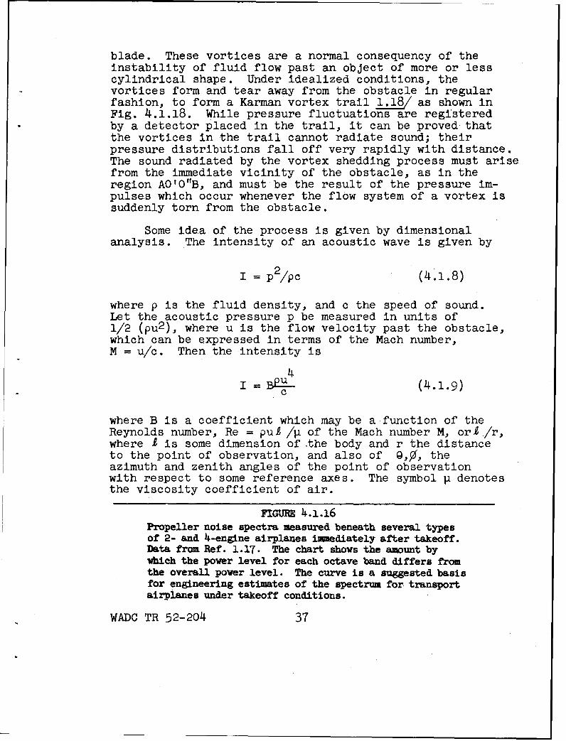
FIGURE 4.1.16Propeller noise spectra measured beneath several typesof 2- and 4-engine airplanes imnediately after takeoff.Data from Ref. 1.17. The chart shows the amount bywhich the power level for each octave band differs fromthe overall power level. The curve is a suggested basisfor engineering estimates of the spectrum for transportairplanes under takeoff conditions.

WADC TR 52-204 37

For large distances, the law of conservation ofenergy will require that the intensity fall off with thesquare of the distance, as expressed by the next rela-tion

13 ReZ. MY9. BI (Re, M, @, )

r(4.1.1o)

Furthermore, the Mach number effect must occur as amultiplier, since the sound intensity must vanish forincompressible fluids (c -00). Thus, the precedingequation may be rewritten as

B =-I Mn )B " (Re., 9, •

n

where the Mach number effect has been generalized as apower series in M. An approximate solution will besought by retaining one term of the series. It can beshown that the exponent n = 1 corresponds to a simplesource, and n = 2 to a dipole. The simple source may beruled out on the basis that the observed radiation isdirectional, or through a theoretical argument whichshows it to be inconsistent with the aerodynamic flowsituation. With the exponent n = ?, it is evident thatthe sound intensity will vary as uO. When the direc-tional function for a dipole is inserted, the finalexpression for the intensity is

I = L (e )Cos 2 Ap U6

r c

(4.1.12)

Here A, the projected area of the obstacle in the

WADC TR 52-204 38

direction of fluid flow, has been written instead of1..2. The coefficient CC (Re) cannot be determined fromdimensional analysis alone. In the case of a propellerblade, it is found that the dipole radiation pattern hasits maxima on the propeller axis.

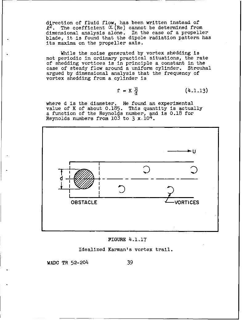
While the noise generated by vortex shedding isnot periodic in ordinary practical situations, the rateof shedding vortices is in principle a constant in thecase of steady flow around a uniform cylinder. Strouhalargued by dimensional analysis that the frequency ofvortex shedding from a cylinder is

f = K 11(4.1-13)

where d is the diameter. He found an experimentalvalue of K of about 0.185. This quantity is actuallya function of the Reynolds number, rnd is 0.18 forReynolds numbers from 103 to 3 x.10 .

_ ,I22

I I

OBSTACLE VORTICES

FIGUBE 4.1.17

Idealized Karman's vortex trail.

WADC TR 52-204 39

Evaluation of Vortex Noise Intensity. The knowledgeof vortex noise is not yet entirely satisfactory from aquantitative standpoint. Stowell and Deming 1../ experi-mented with a device in which circular rods, rather thanblades, projected from a rotating hub, and found the inten-sity of the radiated sound to be proportional to theprojected area A and to the sixth power of the velocity,as predicted by Eq. (4.1.12). In a later N.A.C.A. experi-ment 1 , the constant of proportionality was evaluatedfrom measurements on a helicopter blade. On this basis,Hubbard adopted the engineering equation below to give theoverall intensity level (essentially equal to SPL) of vor-tex noise at a distance of 300 ft from a propeller, presum-ably for those directions where the sound is strongest.

kA6IL = 10 log10 B (4.1.14)

10i lO

The value of k is given by 3.8 x 10-27. The symbol VO7denotes section velocity at 0.7 of. full radius, in ft/sec;AB denotes total plan area of blades, which is roughlyproportional to the area A of Eq. (4.1.12) if consistentoperating conditions somewhat below stall are assumed.The relation Eq. (4.1.19) is the basis for the broken-linecurves showing vortex noise in Figs. 4.1.4-4.1.9. Hubbardestimates these tentative results as being correct withint 10 db for conditions below stall, and points out thatthe vortex noise may increase by 10 db when the propelleris operated under stalled conditions.

The uncertainty in the present evaluation of vortexnoise may be explained in part by recalling that thecoefficient in Eq. (4.1.12) is a function of the Reynoldsnumber. Evaluations currently available were made atReynolds numbers much smaller than those found in pro-peller applications. Experiments at high Reynolds numbersnecessarily bring in rotational noise and are thereforemore difficult in that the rotational and vortex noisecontributions must be separated. Moreover, propellerblades may operate at Reynolds numbers greatly exceeding105, the value at which laminar flow in the boundarylayer is replaced by turbulent flow. Completely turbulentflow generates broad-band noise through mechanisms otherthan vortex shedding, and the vortex noise analysis doesnot apply rigorously.

WADC TR 52-204 40

The Spectrum of Vortex Noise. The rotating-rodexperiments of Stowell and Deming L_91/ and othersgive spectra in which most of the noise energy is lo-cated in the frequency range given by the Strouhal for-mula, Eq. (4.1.1 3 ). (The formula gives a range ofvalues rather than a single value in the case of arotating rod, since the section velocity varies con-tinuously from the hub to the tip.) Noise energy isobserved over the entire audible range, however, asillustrated by oscillograms given in Ref. 1.5. Thereis some evidence of peaks in the spectrum at harmonicsof the Strouhal frequencies. The spectral distributionof the noise needs further investigation.

Practical Importance of Vortex Noise. It appears,that vortex noise never constitutes a significant portionof the distant sound produced by heavily loaded propellers,operating at tip speeds of 900 ft/sec or more. Thus, itis not necessary to consider vortex noise in connectionwith takeoff operation of transport airplanes, and it isunlikely that vortex noise is important even in the soundproduced by transports under cruising conditions.

The intensity of rotational noise is much moresensitive to tip speed and to blade loading (angle ofattack) than that of vortex noise. Consequently, it isalways possible, by reducing the tip speed and possiblythe angle of attack, to reach a condition where thepropeller sound consists largely of vortex noise ratherthan rotational noise. Vortex noise thus becomes thelimiting factor when an attempt is made to reduce pro-peller noise by reducing the tip speed and increasing thenumber of blades. This point was discussed in an earlierparagraph.

An Example of Calculating Propeller Noise. Giventhe following propeller data, it is desired to estimate

(a) the SPL near the ground (hard surface)at 500 ft distance;

(b) the SPL at that point in the 600-1200 cpsband: Four propeller blades; tip speed 900 ft/sec(approximately Mach 0.9); 2000 horsepower input.

WADC TR 5 2-2o4 41

From Fig. 4.1.5, the power level is 112 + 55 =167 db. The direction-averaged SPL at 500 ft distance,in free space, would be the power level less 10 log[4r(500)2j, which gives 102 db. Near the hard ground,pressure doubling raises the SPL by 6 db to give 108 db,still on a direction-averaged basis. If the typicaldirectional distribution of Fig. 4.1.15 is assumed, theSPL in the propeller plane (900) is 1 db less than thedirection-average value, which yields 107 db. This isanswer (a).

The given conditions resemble takeoff operationfor a large airplane. Therefore the spectral distribu-tion in Fig. 4.1.16 should apply. According to thisfigure, the SPL in the 600-1200 cps band is approximately9 db below the overall SPL, which gives 99 db as answer(b).

Sometimes it is necessary to estimate sound pressurelevels external to a test cell, with the propeller operat-ing inside. For a cell which has no sound-absorbingtreatment, and which has openings looking out in a hori-zontal direction front and rear, a first approximationto low-frequency sound levels is obtained by making acalculation as given above, and using the space-averagedvalue, since the cell disturbs the normal directionalityof the propeller. For higher frequencies, the cellopenings must be assigned the directionality of a stackopening, and in general a proper allowance must beintroduced for sound-absorbing treatment. These topicsare reserved for later chapters.

The calculations above could also have been startedby reference to the empirical propeller-noise chart,Fig. 4.1.14, which is approximately correct for largepropellers of two to four blades. This chart gives apower level of 167.5 db, from which about 2 db should besubtracted to correct from three to four blades, givinga power level of approximately 166 db. All results wouldthen be less by one db than those obtained above.

WADC TR 52-204 42

4.2 Noise from Aircraft Reciprocating Engines

Reciprocating engine noise has been studied lessextensively than propeller noise, because the maximumnoise levels produced by propeller-driven aircraft, underfull-throttle conditions, are usually attributable tothe propeller. The tentative generalizations given be-low concerning engine noise are made on the basis of afew observations (Refs. 1.13 and 1.7); also a groundairplane test; and unpublished results of tests on an800 horsepower engine in a dynamometer test cell).

1. The noise developed by a reciprocating engineis produced almost exclusively by the exhaust,with possible exceptions in cases whereunusually effective mufflers are used.

2. The noise energy of the lowest-frequencyexhaust component of a reciprocating engineis approximately proportional to the totalpower developed. Quantitatively, the powerlevel of this exhaust component for an enginewithout exhaust mufflers is not less than

Power level of lowest frequency component =

122 + 10 loglO (horsepower).

(4.2.1)

On theoretical grounds, the horsepower valueused in Eq. (4.2.1) should include mechanicallosses in the engine. However, these areusually not known. In cases where the mechan-ical losses are large, they must be included.

3. The lowest-frequency exhaust component ofimportance usually has a frequency equal to thenumber of exhaust discharges per second (twodischarges occurring simultaneously are countedas one). This frequency is usually below 300 cps.

WADC TR 52-204 43

4. Usually the spectral distribution of noiseenergy is approximately as follows: The powerlevel in the octave band containing the lowest-frequency exhaust component lies about 3 dbbelow the overall power level. The levels inoctave bands above this one decrease at about3.db per octave of increasing frequency. Nosignificant noise is produced in octave bandsbelow the one containing the lowest-frequencyexhaust component. These conditions may betypical of engines operated at cruising condi-tions, and of small engines (150 horsepowerand less).

5. In the case of an engine of 800 horsepoweroperated at full throttle, a uniform octave-band spectrum has been observed (equal powerlevels in the octave band containing the lowest-frequency exhaust component and all higheroctave bands). This may be typical of largerengines under full-power conditions. In thiscase the overall power level is about 8 dblarger than that of the lowest frequencyexhaust component.

6. Directional effects are much smaller for enginenoise than for prgopeller noise. The totalvariation in SPL with direction is about 6 dbfor the lower-frequency components of enginenoise. This statement probably holds for highfrequencies also in the case of an isolatedengine, but no detailed measurements for highfrequencies are available. In the case of anengine mounted on an airplane, the high fre-quency directivity will be affected by shadow-ing produced by the airplane structure.

Simple relations for the overall power level of anengine without mufflers are obtained by combining state-ments 2, 4, and 5. For the case of small engines (150horsepower or less), or engines operated under cruisingconditions, the relation is

Overall power level - 125 + 10 lOg1 0 (horsepower).

(4.2.2)

WADC TR 52-204 44

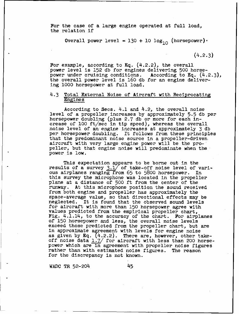
For the case of a large engine operated at full load,the relation if

Overall power level = 130 + 10 log1 0 (horsepower).

(4.2.3)

For example, according to Eq. (4.2.2), the overallpower level is 152 db for engines delivering 500 horse-power under cruising conditions. According to Eq. (4.2.3),the overall power level is 160 db for an engine deliver-ing 1000 horsepower at full load.

4.3 Total External Noise of Aircraft with ReciprocatingEngines

According to Secs. 4.1 and 4.2, the overall noiselevel of a propeller increases by approximately 5.5 db perhorsepower doubling (plus 2.7 db or more for each in-crease of 100 ft/sec in tip speed), whereas the overallnoise level of an engine increases at approximately 3 dbper horsepower doubling. It follows from these principlesthat the predominant noise source in a propeller-drivenaircraft with very large engine power will be the pro-peller, but that engine noise will predominate when thepower is low.

This expectation ap ears to be borne out in theresults of a survey 3._1 of take-off noise level of vari-ous airplanes ranging from 65 to 5800 horsepower. Inthis survey the microphone was located in the propellerplane at a distance of 500 ft from the center of therunway. At this microphone position the sound receivedfrom both engine and propeller has approximately thespace-average value, so that directional effects may beneglected. It is found that the observed sound levelsfor aircraft with more than 150 horsepower agree withvalues predicted from the empirical propeller chart,Fig. 4.1.14, to the accuracy of the chart. For airplanesof 150 horsepower and less, the overall noise levelsexceed those predicted from the propeller chart, but arein approximate agreement with levels for engine noiseas given by Eq. (4.2.2). There are, however, other take-off noise data 1.y7/ for aircraft with less than 200 horse-power which are in agreement with propeller noise figuresrather than with estimated noise figures. The reasonfor the discrepancy is not known.

WADC TR 52-204 45

0°0

300 300

600 600

Left Rightwing wing

120' 9020°0

150 5-"00

dbTail

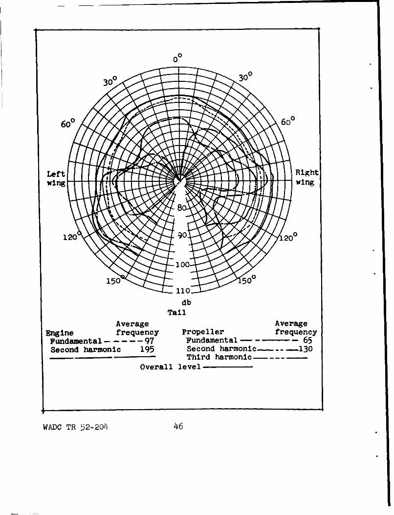
Average AverageEngine frequency Propeller frequencyFundamental ----- 97 Fundamental 65Second harmonic 195 Second harmonic- -- 130

- Third harmonic-Overall level

WADC TR 52-20'4 46

A convenient approximate expression for the over-all power level of various aircraft under take-off condi-tions has been deduced from the data of Ref. 3.1. Thisrelation is

verall power hTotal take-off(level take-off 121 + 12 logorsepower o

1 f) aircraft(4.3.1)

It happens that under the particular conditions found intake-off it is not necessary to consider propeller tipspeed explicitly. Since the tip speed is not consideredin Eq. (4.3.1), this relation cannot be applied to operat-ing conditions differing materially from takeoff.

The broken line drawn across the empirical propellernoise chart, Fig. 4.1.14, divides the chart approximatelyinto a region in which the propeller is the major noisesource for an entire aircraft (upper right-hand portion)and a region in which the engine is the major noise source(lower left-hand portion). This line is constructed bycomputing, for various values of total horsepower, the tipspeed at which the overall propeller noise power levelequals the overall engine noise power level given byEq. (4.2.2) is assumed. Operating data for small single-engine aircraft often fall in the region in which enginenoise is important (lower left). All data used in deriv-ing this dividing line represent average trends from whichresults for a particular aircraft may differ by as much as5 db as regards either engine noise or propeller noise.Therefore, the line as drawn on the chart will not indicateaccurately under what conditions propeller noise is dominantin a particular aircraft. Also, the results are averagesfor reciprocating engine aircraft as commercially producedup to 1952, and do not apply to specially constructed unitsin which noise control measures are incorporated. It hasbeen shown that overall aircraft noise can be reducedsignificantly by use of propellers with an increased numberof blades and by use of exhaust mufflers 1._6/.

FIGURE 4.3.1Directional distribution of SPL for certain discrete-frequency components of airplane noise. Measurements50 ft from hub; ground test at cruising power. Two-blade propeller; 1940 rpm; direct drive; 97 horsepower;blunt tips, speed 646 ft/sec. (From Fig. 27a of Ref.l.7).

WADC TR 52-204 47

The preceding remarks on total aircraft noiserefer to the space average of sound output. This con-cept is inherent in the definition of power level. Ingeneral, actual observation made in the propeller planewill agree approximately with space-average results.The directivity patterns of engine and propeller must beconsidered in predicting noise levels observed in otherdirections. A typical situation is illustrated inFig. 4.3.1, which shows the variation with azimuth angleof measured overall sound level and/or the levels ofselected propeller and engine noise components for aparticular small airplane. These results were obtainedby operating the airplane at cruising power on the groundand by placing the microphone in various locations 50 ftfrom the propeller hub, and approximately at the hublevel.

The tentative conclusions regarding external noiseor reciprocating-engine aircraft are summarized below.

1. For large aircraft, the overall PWL foreither cruising or take-off conditions isapproximately equal to the overall PWL forpropeller noise which may be estimated bythe methods given at the end of Sec. 4.1.

2. For aircraft of 150 horsepower or less, itappears that the overall PWL under cruisingor takeoff conditions is approximately thatgiven for the engine by Eq. (4.2.2).

3. The SPL in the propeller plane is approxi-mately that which would be produced by anon-directional source having the statedoverall PWL.

4. The overall PWL for various aircraftunder takeoff conditions is given approxi-mately by Eq. (4.3.1).

5. The observed noise for positions directlyahead of or directly behind, the aircraftis approximately the engine noise alonehaving a PWL given by Eq. (4.2.2) or (4.2.3).

WADC TR 52-204 48

6. The observed SPL for positions from 200 to300 behind the propeller plane has the greatestpreponderance of propeller components. Anapproximate indication of the overall SPL forthis region may be obtained, for either cruiseor takeoff conditions by adding 5 db to thevalue obtained by using the overall propellerPWL (Sec. 4.1) and proceeding as for a non-directional source.

References

(1.1) Gutin, L., "Uber das Schallfeld einerrotierenden Luftschraube," Phys. Zeits. derSowjetunion 9, 57-71 (1936). The followingis a translation into English: Gutin, L.,"On the Sound Field of a Rotating Propeller,"National Advisory Committee for Aeronautics,TM 1195 (1948).

(1.2) Lamb, H. Hydrodynamics, Dover Edition (New York),pp. 501 ff.

(1.3) Paris, E. T., "On the Sound Generated by aRotating Aircrew" Phil. Mag. 13 99-111 (1932).

(1.4) Kemp, S. F., "Some Properties of the SoundEmitted by Airscrews" Proc. Phys. Soc. (London)_44 151-165 (1932).

(1.5) Hubbard, H. H., "Pro~eller Noise Charts forTransport Airplanes, National Advisory Committeefor Aeronautics, TN 2968 (1953).

(1.6) Regier, A. A., and Hubbard, H. H., "Status ofResearch on Propeller Noise and Its Reduction,"J. Acout. Soc. Am. 25, 395-404 (1953).

WADC TR 52-204 49

References (cont.)

(1.7) Beranek, Elwell, Roberts, and Taylor,"Experiments in External Noise Reduction ofLight Airplanes," National Advisory Committeefor Aeronautics, TN 2079 (1950).

(1.8) Hicks, C. W., and Hubbard, H.H., "Comparisonof Souhd Emission from Two-Blade, Four-Blade,and Seven-Blade Propellers," National AdvisoryCommittee for Aeronautics, TN 1354 (1947).

(1.9) Deming, A. F., "Propeller Rotation Noise Dueto Torque and Thrust" J. Acoust.Soc. Am. 12,173-182 (194o).

(1.10) Garrick, I.E., and Watkins, C.E., "A TheoreticalStudy of the Effect of Forward Speed on the Free-Space Sound-Pressure Field Around Propellers,"National Advisory Committee for Aeronautics,TN 3018 (1953).

(1.11) Regier, A. A., "Effect of Distance on AirplaneNoise," National Advisory Committee for Aeronautics,TN 1353 (1947).

(1.12) Hubbard, H.H., and Regier, A.A., "Free-SpaceOscillating Pressures Near the Tips of RotatingPropellers," National Advisory Committee forAeronautics, Rept. 996 (1950).

(1.13) Rudmose, H.W., and Beranek, L.L., "Noise Reduc-tion in Aircraft", J. Aero. Sci. 14, 79-96(1947).

(1.14) Hubbard, H.H., "Sound from Dual-Rotating andMultiple Single-Rotating Propellers," NationalAdvisory Committee for Aeronautics, TN 1654 (1948).

(1.15) Roberts, J.P., and Beranek, L.L., "ExperimertBin External Noise Reduction of a Small Pusher-Type Amphibian Airplane,' 1 National AdvisoryCommittee for Aeronautics, TN 2727 (1952).

(1.16) Hubbard, H.H., and Lassiter, L.W., "Sound froma Two-Blade Propeller at Supersonic Tip Speeds,"National Advisory Committee for Aeronautics,Rept. 1079 (1952).

WADC TR 52-204 50

References (cont.)

(1.17) Parkin and Purvis. Article on take-offnoise of aircraft, supposed to be inAcustica in 1954.

(1.18) Lamb, H., Hydrodynamics, Dover Edition(New York), pp. 224 ff.

(1,19) Stowell, E. Z., and Deming, A. F., "VortexNoise from Rotating Cylindrical Rods,"National Advisory Committee for Aeronautics,TN 519 (1935).

(1.20) Hubbard, H. H., and Regier, A. A., "Pro-peller Loudness Charts for Light Airplanes,"National Advisory Committee for Aeronautics,TN 1358 (1947).

(3.1) Institute of Aeronautical Sciences, "ExternalSound Levels of Aircraft", Preprint No. 126.

WADC TR 52-204 51

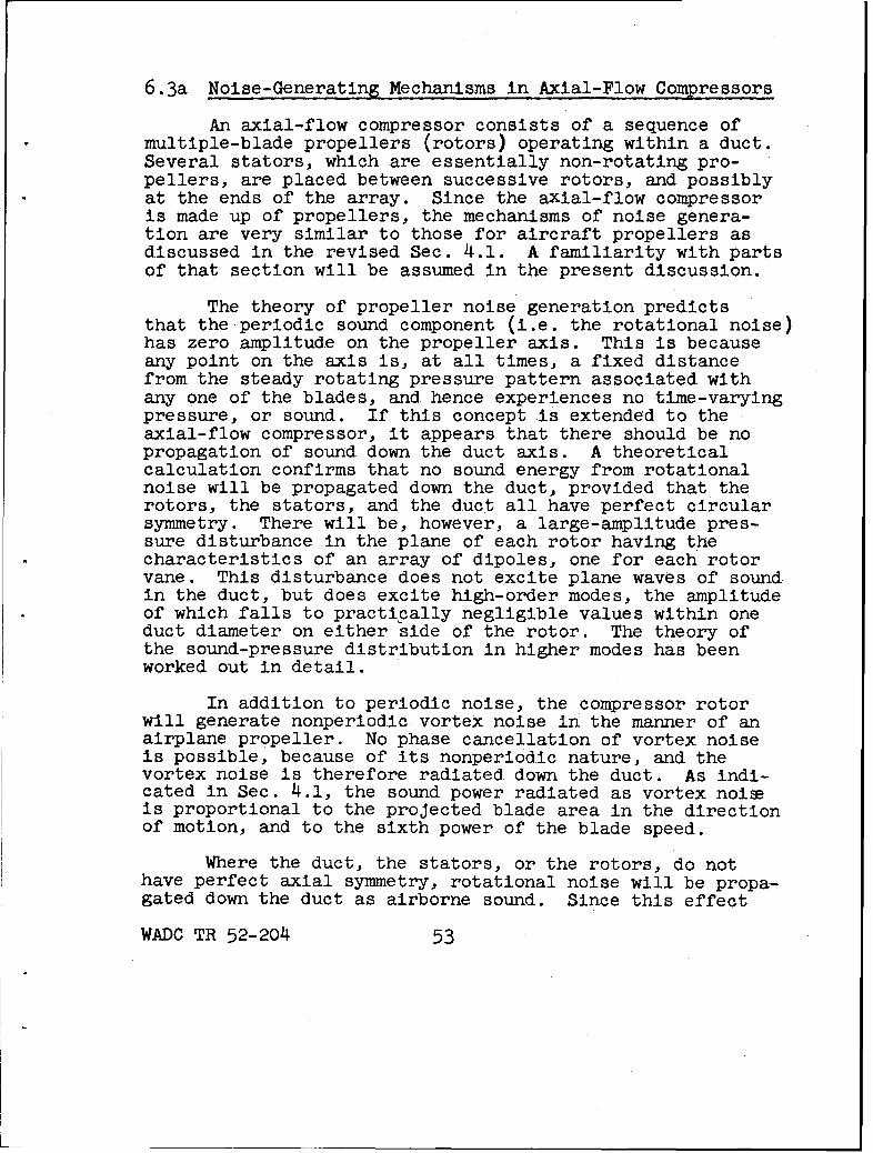
6.3a Noise-Generating Mechanisms in Axial-Flow Compressors

An axial-flow compressor consists of a sequence ofmultiple-blade propellers (rotors) operating within a duct.Several stators, which are essentially non-rotating pro-pellers, are placed between successive rotors, and possiblyat the ends of the array. Since the axial-flow compressoris made up of propellers, the mechanisms of noise genera-tion are very similar to those for aircraft propellers asdiscussed in the revised Sec. 4.1. A familiarity with partsof that section will be assumed in the present discussion.

The theory of propeller noise generation predictsthat the periodic sound component (i.e. the rotational noise)has zero amplitude on the propeller axis. This is becauseany point on the axis is, at all times, a fixed distancefrom the steady rotating pressure pattern associated withany one of the blades, and hence experiences no time-varyingpressure, or sound. If this concept is extended to theaxial-flow compressor, it appears that there should be nopropagation of sound down the duct axis. A theoreticalcalculation confirms that no sound energy from rotationalnoise will be propagated down the duct, provided that therotors, the stators, and the duct all have perfect circularsymmetry. There will be, however, a large-amplitude pres-sure disturbance in the plane of each rotor having thecharacteristics of an array of dipoles, one for each rotorvane. This disturbance does not excite plane waves of soundin the duct, but does excite high-order modes, the amplitudeof which falls to practically negligible values within oneduct diameter on either side of the rotor. The theory ofthe sound-pressure distribution in higher modes has beenworked out in detail.

In addition to periodic noise, the compressor rotorwill generate nonperiodic vortex noise in the manner of anairplane propeller. No phase cancellation of vortex noiseis possible, because of its nonperiodic nature, and thevortex noise is therefore radiated down the duct. As indi-cated in Sec. 4.1, the sound power radiated as vortex noiais proportional to the projected blade area in the directionof motion, and to the sixth power of the blade speed.

Where the duct, the stators, or the rotors, do nothave perfect axial symmetry, rotational noise will be propa-gated down the duct as airborne sound. Since this effect

WADC TR 52-204 53

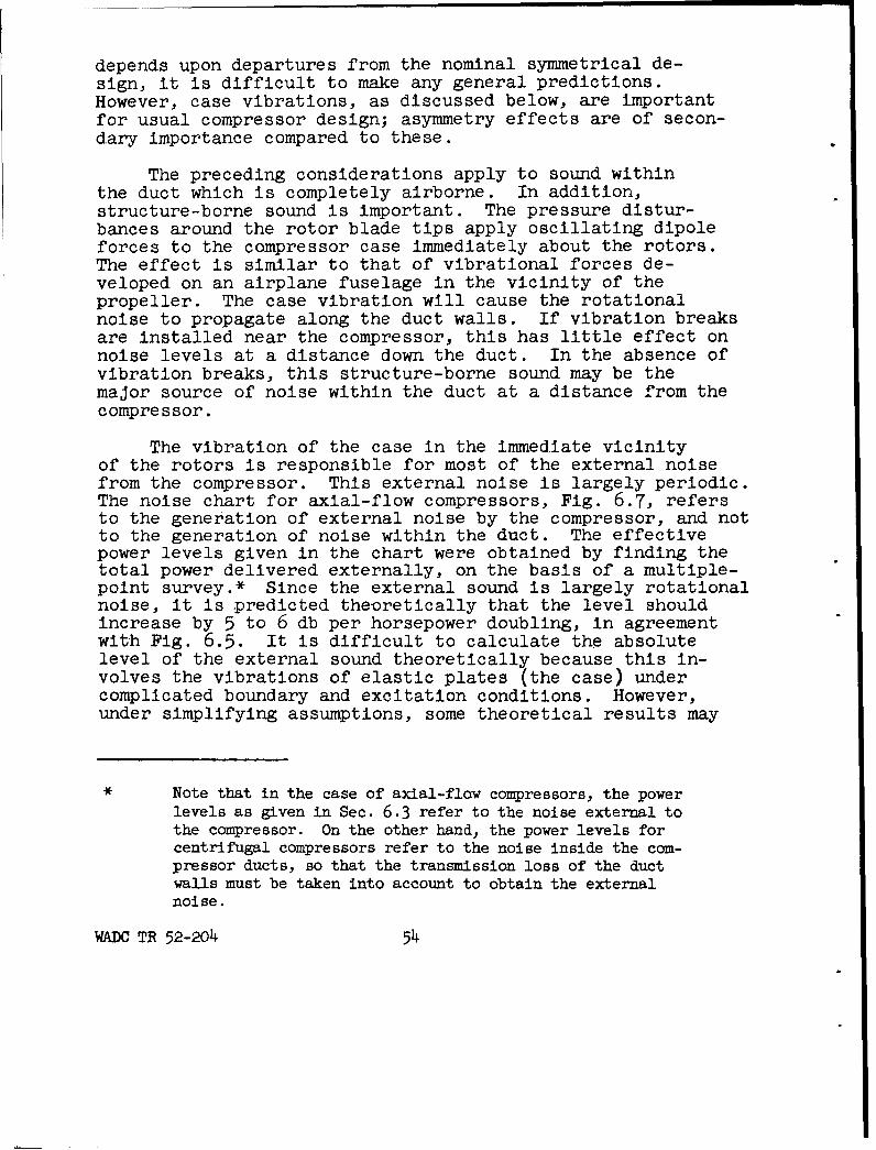
depends upon departures from the nominal symmetrical de-sign, it is difficult to make any general predictions.However, case vibrations, as discussed below, are importantfor usual compressor design; asymmetry effects are of secon-dary importance compared to these.

The preceding considerations apply to sound withinthe duct which is completely airborne. In addition,structure-borne sound is important. The pressure distur-bances around the rotor blade tips apply oscillating dipoleforces to the compressor case immediately about the rotors.The effect is similar to that of vibrational forces de-veloped on an airplane fuselage in the vicinity of thepropeller. The case vibration will cause the rotationalnoise to propagate along the duct walls. If vibration breaksare installed near the compressor, this has little effect onnoise levels at a distance down the duct. In the absence ofvibration breaks, this structure-borne sound may be themajor source of noise within the duct at a distance from thecompressor.

The vibration of the case in the immediate vicinityof the rotors is responsible for most of the external noisefrom the compressor. This external noise is largely periodic.The noise chart for axial-flow compressors, Fig. 6.7, refersto the generation of external noise by the compressor, and notto the generation of noise within the duct. The effectivepower levels given in the chart were obtained by finding thetotal power delivered externally, on the basis of a multiple-point survey.* Since the external sound is largely rotationalnoise, it is predicted theoretically that the level shouldincrease by 5 to 6 db per horsepower doubling, in agreementwith Fig. 6.5. It is difficult to calculate the absolutelevel of the external sound theoretically because this in-volves the vibrations of elastic plates (the case) undercomplicated boundary and excitation conditions. However,under simplifying assumptions, some theoretical results may

* Note that in the case of axial-flow compressors, the powerlevels as given in Sec. 6.3 refer to the noise external tothe compressor. On the other hand, the power levels forcentrifugal compressors refer to the noise inside the com-pressor ducts, so that the transmission loss of the ductwalls must be taken into account to obtain the externalnoise.

WAD• TR 52-204 54

be obtained. They are not intended to replace the empiricalresults of Sec. 6.3 but to give further quantitative insightinto the problem.

It is possible to identify three important mechanismsthat contribute to the intensity of the blade rotation noise:

(1) Blade rotation itself, as in the case of apropeller in free space.

(2) Aerodynamic interaction of the blades andstators.

(3) Fluid flow between the blade tips and thecompressor case.

Only the mechanism associated with (1) has been evaluatedtheoretically; preliminary calculations indicate that (2)and (3) are of secondary importance. In order to evaluate(1), it has been assumed that the distribution of thethrust force along the blades is independent of the dis-tance along the blades. Further, it has been assumed thatthe blade width and thickness is very small, so that thethrust force is concentrated on blade lines and so thatvolume change effects of the air as the blade passes maybe neglected. Then, the mean pressure in the plane ofrotation is found to be:

1/2P AP [5 + 1 In 5I (6.3a.1)

Pl =•-• "4 - 1

where p1 is the rms pressure for the fundamental frequency

AP is the pressure rise across the plane of rotation

5 is the ratio of the inside compressor radius R0,to the hub radius Rh.

The fundamental frequency is given by

f N RPM) , cps (6.3a.2)

WADC TR 52-204 55

where N is the number of blades. Harmonics of the funda-mental frequency are generated also. The pressure for theharmonics depends upon the assumed force versus timecharacter at each element of the blade disc; for theassumption used in Eq. (6.3a.l), equal magnitudes are pre-dicted for all the harmonics in the plane of rotation.(Note that this result does not agree with the empiricalinformation given in Sec. 6.3, in which the second harmonicis estimated to be the frequency of maximum radiation.)

The theoretical results above may be used to predictthe excitation of the compressor case, and thus the soundradiated from the case. As an example, consider thefollowing problem:

AP = 60" H2 0 per stage

Number of stages = 3

Distance between stages = 3"

Ro= 13"

Rh= 60

RPM = 7200

HP = 1350

Then, for each stage,

P1 = 1.2 x 104 dynes/cm2

or SPL = 155 db re .0002 dyne/cm2

at f, = 7200 cps

The transmission loss (TL) of the compressor case is ameasure of the radiation for a given pressure excitation.Assume the case is of cylindrical construction and about1/4" thick. Then the TL is about 30 db. The resultingpressure outside the case is thus about 125 db per stage.According to the assumed thrust distribution, this valueof SPL is valid for all the harmonicsas well as the funda-mental. All three stages, however, are operating indefinite phase relation. Thus conservative practice dic-tates that the combined sound pressure for the threestages Just outside the case is the sum of the soundpressures from each stage, giving SPL = 125 db + 20 log 3= 135 db.

WADC TR 52-204 56

It is instructive to compare the above estimate withthe values predicted by the empirical relations given inSec. 6.3. Figure 6.7 yields a PWL value of 135 db for thefrequency of maximum output (the second harmonic). Therelevant area for converting the PWL to SPL is not accuratelyknown, but may be assumed to vary between about 2 sq ft(corresponding to the cross-sectional area between the huband the case) and about 5 sq ft (corresponding to the surfacearea of the case in the vicinity of the blades). Thus theresulting SPL is between 128 db and 132 db, in reasoriableagreement with the value calculated above from Eq. (6.3a.1).

Section 6.3 also indicates a method. for estimatingthe spectrum below the fundamental frequency. Using the.information given in Sec. 4.1 on vortex noise*, the spec-trum below the fundamental may be calculated. The resultis also in reasonable agreement with the empirical resultfrom Sec. 6.3.

* In order to use the information, account has tobe taken of the different drag coefficients andReynolds' number for the present example and theexperiments quoted therein.

WADC TR 52-204 57

6.5 Noise from Ventilating Fans and Ventilation Systems

Experimentally Measured Power Levels and Spectra. Theacoustic power level of a ventilating fan in a duct may bedetermined from the average sound pressure across the ductpassage. The measurements must be made at locations atleast several fan diameters away from the fan and the soundpressure must be the result of acoustic energy travelingaway from the source, i.e., the reflection of the soundback from the more distant portions of the duct should benegligible. The power level for a fan in open air, or forthe back side of a fan which is connected to a duct on oneside only, can be determined from measurements of the soundpressure at several points on a surface in space whichsurrounds the source. This survey must be performed inthe absence of reflecting objects. The basic principlesof both of these methods are discussed. in Chapter 3.

The first method, which relates to a fan operating ina duct, may be applied successfully when the duct is verylong and has sufficient sound attenuation to prevent re-flections at all frequencies which are of importance, orwhen the duct is connected to a non-reflective terminationspecially designed for use in laboratory measurements offan noise. A laboratory system having a non-reflectivetermination, as described by Beranek, Reynolds and Wilson5.1/, is shown in Fig. 6.5.1. A recommended modificationofthis system, for future measurements is given in thereference.

Measurements performed with this laboratory systemon fans of both vaneaxial and centrifugal types, with in-put power up to six horsepower, have led to the followingconclusions 5.1, 5.2, 5.3/.

1. The spectrum for centrifugal fans falls offrapidly with increasing frequency. The de-crease of power level between successiveoctave bands is 5 db.

2. The spectrum for vaneaxial fans is nearlyuniform for octave bands 20-75 cps to 1200-2400 cps, inclusive, but decreases in thehigher bands.

WADC TR 52-204 59

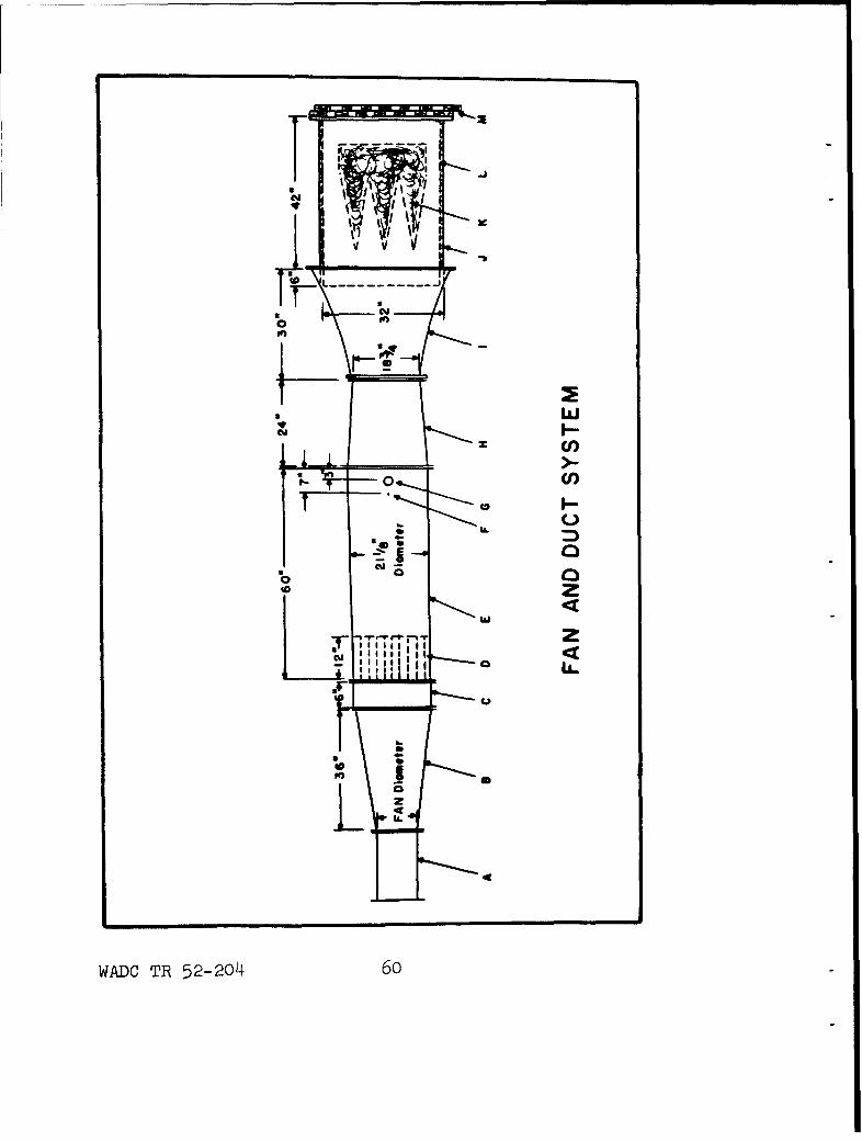
0

3 w

ClD

0 U)

CL)

o

tIL

WADC TR 52-204 60

3. The spectra on inlet and outlet sides of afan are similar, except that a narrow peakprotruding above the broad-band noise by6 db or less at the blade fundamental fre-quency, may be observed on the inlet side,but is scarcely observable in the exhaust.

4, The spectra and the power level are notsignificantly changed by varying the backpressure on the fan.

5. The exhaust spectrum is nearly independentof speed below the rated maximum.

6. The open inlet to the fan has very nearlythe same directional properties as a pistonof the same size.

7. Reversing a vaneaxial fan has no significanteffect on the sound output.

The summary spectra resulting from the study are shown inFig. 6.5.2 where the ordinate indicates octave band powerlevel relative to the overall power level. The shadedzones show the latitude within which variations may beexpected according to the individual fan design and operat-ing speed.

FIGURE 6.5.1Laboratory system for measuring noise deliveredto a duct by one side of a ventilating fan.

A - fanB - conical adapterC - canvas vibration-isolation couplingD - straightening vanesE - measuring sectionF - manometer locationG - microphone openingH - adapterI - exponential horn sectionJ - acoustic terminationK - three acoustic wedges, each 8" x 24"

base, 6 lb/ft3 FiberglasL - Fiberglas lining, 6 lb/ft 3 , 1" thickM - adjustable back-pressure panels 5.

WADC TR 52-2o4 61

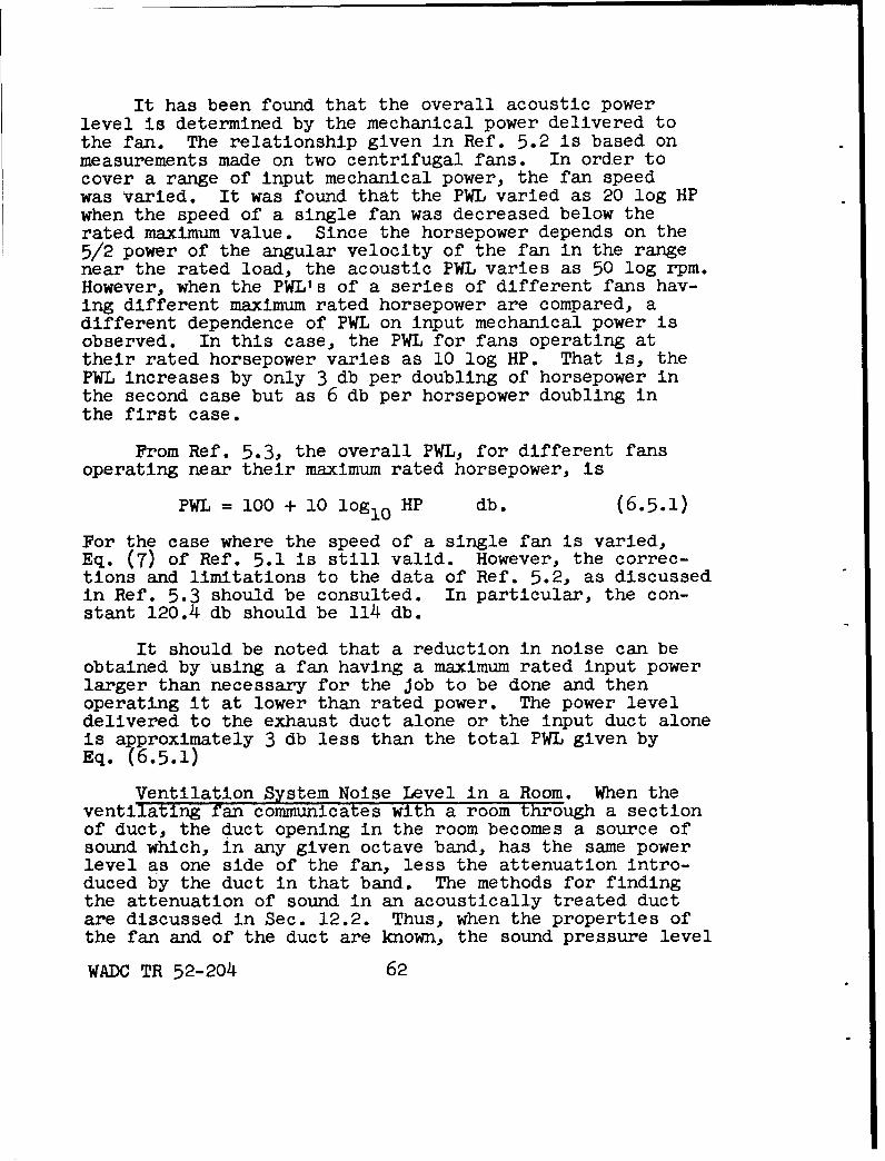
It has been found that the overall acoustic powerlevel is determined by the mechanical power delivered tothe fan. The relationship given in Ref. 5.2 is based onmeasurements made on two centrifugal fans. In order tocover a range of input mechanical power, the fan speedwas varied. It was found that the PWL varied as 20 log HPwhen the speed of a single fan was decreased below therated maximum value. Since the horsepower depends on the5/2 power of the angular velocity of the fan in the rangenear the rated load, the acoustic PWL varies as 50 log rpm.However, when the PWL's of a series of different fans hav-ing different maximum rated horsepower are compared, adifferent dependence of PWL on input mechanical power isobserved. In this case, the PWL for fans operating attheir rated horsepower varies as 10 log HP. That is, thePWL increases by only 3 db per doubling of horsepower inthe second case but as 6 db per horsepower doubling inthe first case.

From Ref. 5.3, the overall PWL, for different fans

operating near their maximum rated horsepower, is

PWL = 100 + 10 log1 o HP db. (6.5.1)

For the case where the speed of a single fan is varied,Eq. (7) of Ref. 5.1 is still valid. However, the correc-tions and limitations to the data of Ref. 5.2, as discussedin Ref. 5.3 should be consulted. In particular, the con-stant 120.4 db should be 114 db.

It should be noted that a reduction in noise can beobtained by using a fan having a maximum rated input powerlarger than necessary for the job to be done and thenoperating it at lower than rated power. The power leveldelivered to the exhaust duct alone or the input duct aloneis approximately 3 db less than the total PWL given byEq. (6.5.1)

Ventilation System Noise Level in a Room. When theventilating fan communicates with a room through a sectionof duct, the duct opening in the room becomes a source ofsound which, in any given octave band, has the same powerlevel as one side of the fan, less the attenuation intro-duced by the duct in that band. The methods for findingthe attenuation of sound in an acoustically treated ductare discussed in Sec. 12.2. Thus, when the properties ofthe fan and of the duct are known, the sound pressure level

WADC TR 52-204 62

in the room may be found by the methods which areemployed in any case where a sound source of known proper-ties is present. A method of calculating the level inthe room is discussed in Sec. 3.5. The quantities whichenter into the calculation are:

1. the power level of the source in the desiredfrequency band

2. the directivity factor, Q, of the source inthis frequency band, in the direction of theobserver

3. the distance, r (ft) between the observer in

the room and the source

4. the room constant, R in sq ft.

The room constant R is equal to S R/(l- U-) where Sis the area of the room boundaries in sq ft and 0C• is theaverage value of the absorption coefficient*. Ordinarily,the chamber absorption coefficient is used. (Sec. 12.1)

The accompanying charts facilitate evaluation ofsome of these quantities 5.__/. The effective directivityfactor for the source at low frequencies is affected bythe location at which the duct enters the room. Fourcases may be distinguished conveniently, as shown inFig. 6.5.3. A duct which opens in the center of the roomvolume (Case A) is assumed to radiate nondirectionally,as into open space, at low frequencies. This correspondsto a low-frequency value of 1.0 for Q. At the otherextreme, radiation from an opening in the corner (Case D)is restricted to one octant in space, with a minimum valueof 8 for Q. At sufficiently high frequencies the directi-vity in all cases approaches that of a piston of radius a,but in practice the directivity factot on the axis rarelyrises above 50. The axial directivity factor for eachof the four cases is plotted as a function of a dimension-less frequency parameter in Fig. 6.5.4. The quantity ais equal to the radius of a circular duct opening, or toL/ir•-for a square opening of width L. For a rectangular

* This quantity is called Orin Chapter 3.

WADC TR 52-204 63

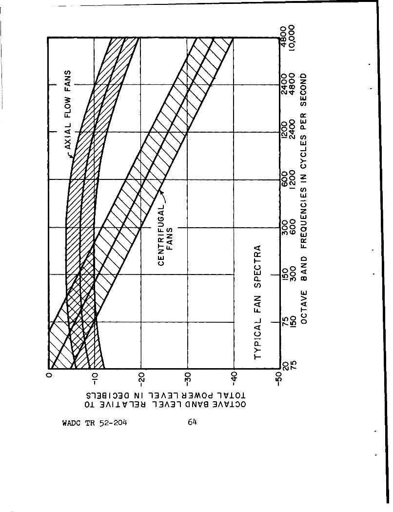
00__________ _00

0~

Cf, 00 1oz 00 z

8w8 C,)

w-i

wcnJw

zw

XOD 00

z w

w Cwz 0

LL o

0'r_ a__ _ -J _ l

U):

0

00 0 0 0 0

S-138103 0 N I -13A3-183M~d 1V1001 3AIIV-138i 13AT1 (ONVE 3A~iO0

WADO TR 52-204 64

opening of widths Lx, Ly, the value of Q lies between thevalues for the corresponding square openings. The largevalues of Q for high frequencies represent beaming of thesound in the axial direction, perpendicular to the planeof the opening. The off-axis values of Q are much smallerat high frequencies; for example, if the opening is in thecenter of a wall, the value of Q for the direction 450from the axis is approximately 2 at all frequencies.

In some cases an accurate calculation is not required,or information regarding the absorption coefficient of thewalls may be insufficient for accurate calculation. Inthese cases, an approximate value of the room constant, R,may be obtained by characterizing the room as "live"( 6L= 0.05) or "dead" ( a = 0.4) or by some intermediatedesignation, and by using the value of Orthus selectedwith the known wall area. If the room shape is specified.,the wall area is uniquely related to the volume; forexample, in a cubical enclosure the wall area is six timesthe two-thirds power of the volume. On this basis, thechart of Fig. 6.5.5 has been constructed to give valuesof the room constant as a function of room volume for fourvalues of the average absorption coefficient which coverthe range "dead" to "live". While the chart is derivedfor a cubical enclosure, it may be used for ordinary rooms,but is not applicable to extreme cases such as that ofa long corridor.

Grille Noise. In calculating the noise produced ina room by a ventilating system, it is necessary to considernot only noise generated directly by the fan, but air-flownoise produced at the grille opening into the room. Noextensive measurements of grille noise are available. Thefollowing tentative relations, which indicate how the PWLof noise from a grille is expected to vary with flowvelocity and with pressure drop across the grille, are givenin the Heating Ventilating Air Conditioning Guide L.4

FIGURE 6.5.2

Typical octave band spectra for vaneaxial andcentrifugal fans. Shaded areas show the expectedspread as a result of variations in details offan and blade design and speed 5.1, 5.3/.

WADC TR 52-204 65

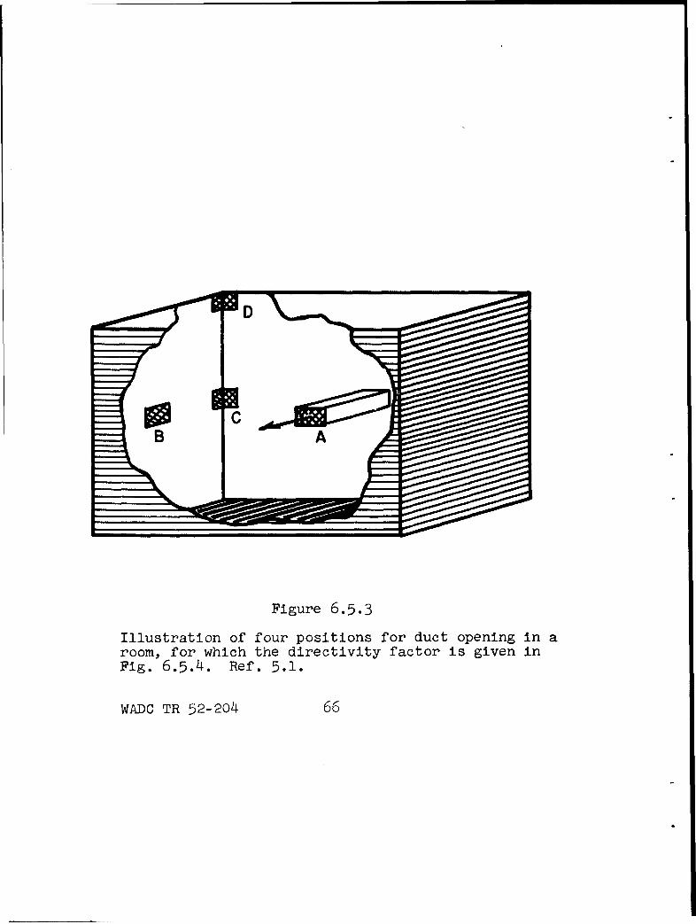
Figure 6.5.3

Illustration of four positions for duct opening in aroom, for which the directivity factor is given inFig. 6.5.4. Ref. 5.1.

WADC TR 52-204 66

PWL change in db = 50 logl 0 (V2/VI) (6.5.2)

V1 and V2 are flow velocities on the two sides of the grille

PWL change in db = 25 log10 (PjPI) (6.5.3)

P1 and P2 are the pressures on the two sides of the grille.Also, on the basis of very limited data, a typical value ofSPL at the grille is 48 db for a pressure drop of 0.1 in.water. If this figure is accepted for use with Eq. (6.5.3),the power level for one side of the grille is

PWL = 73 + 10 loglo A + loglo P (6.5.4)

where A is the grille area in sq ft and P is the pressuredrop in inches of water. In view of the limited evidenceon which this relation is based, it is preferable to workfrom experimental measurements on a grille of type similarto the one in question, rather than to use the above equa-tions, when this is possible.

Available data on grille noise give no detailedinformation on the spectrum of the noise. Until adequatedata are available, it is suggested that Curve D of Fig.6.11for noise due to air flow through a valve be used in estimat-ing the grille noise spectrum.

Example of Estimating Ventilation System Noise in aRoom. The application of these principles is now illlus-tr-ated by numerical example. Suppose that it is desiredto estimate the SPL in octave bands, for a location of10 ft in front of the grille opening, under the conditionswhich are listed below. Assuming it has been establishedthat the air flow noise at the grille will not exceedallowable limits, we now estimate noise due directly tothe fan.

Room Data: Volume 105 cu ft. Medium-live in thelower two octave bands, and medium-dead in the higher fre-quency bands. The corresponding values of the room con-stant, from Fig. 6.5.5, are 2300 sq ft for the lower twobands and 4400 sq ft for higher bands.

Connecting Duct: Length of duct, 40 ft. The totalattenuation of the duct, when split into several parallelsections each with individual acoustical lining, is assumedto be as shown in Table 6.5.1. The grille opening is nearthe center of a room wall, and is 4 ft square.

WADC TR 52-204 67

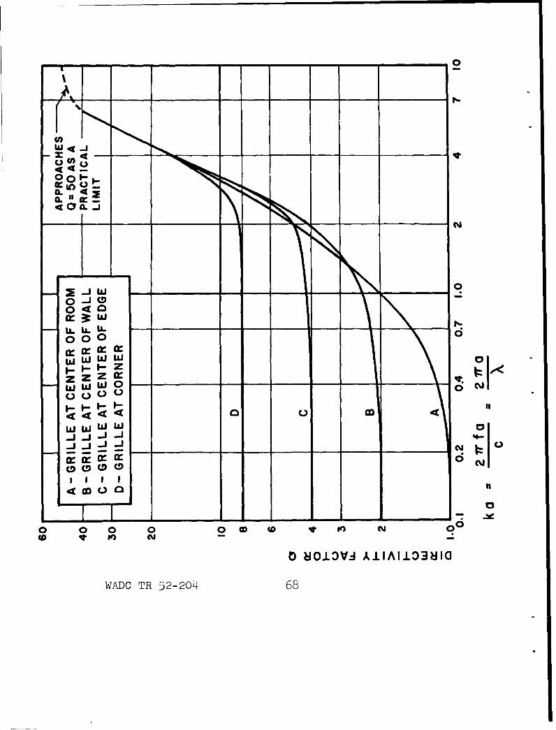
d9 - 7 -- T

Cl)q 2-

OoI-'

-i w

040

0000

LIWWW 0

0000

W W W W

04000 0 O D

ID NK)V ANII13 H

WADC TR 52-204 68

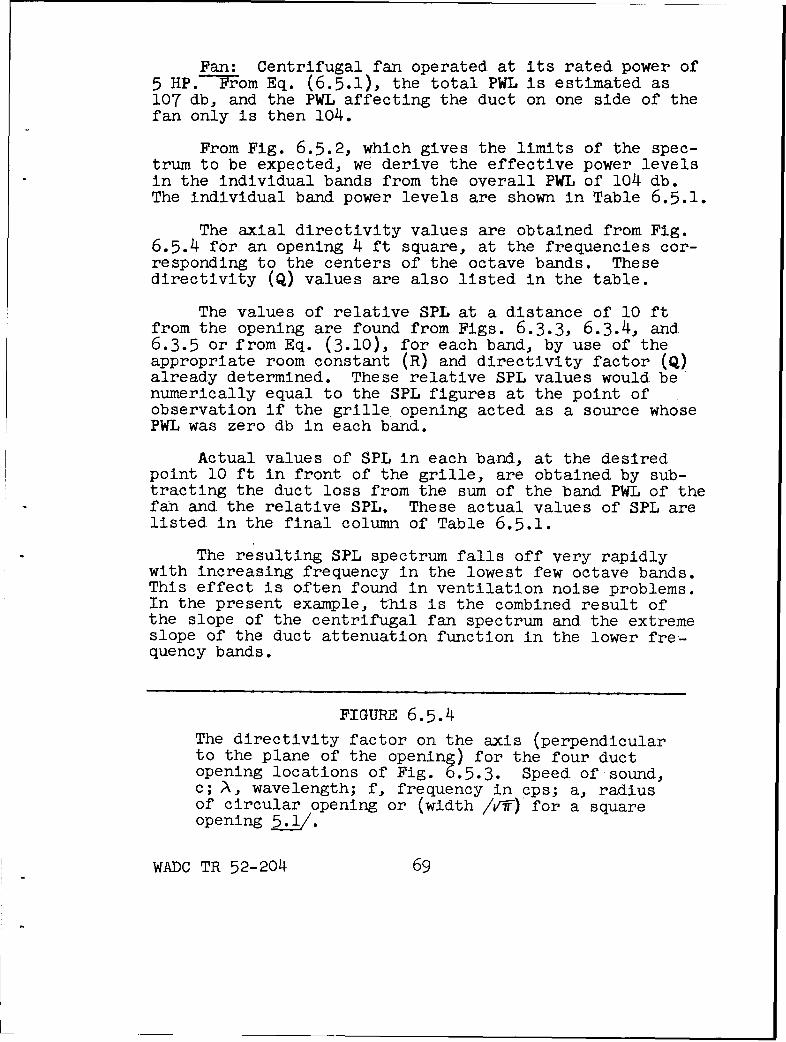
Fan: Centrifugal fan operated at its rated power of5 HP.P--rom Eq. (6.5.1), the total PWL is estimated as107 db, and the PWL affecting the duct on one side of thefan only is then 104.

From Fig. 6.5.2, which gives the limits of the spec-trum to be expected, we derive the effective power levelsin the individual bands from the overall PWL of 104 db.The individual band power levels are shown in Table 6.5.1.

The axial directivity values are obtained from Fig.6.5.4 for an opening 4 ft square, at the frequencies cor-responding to the centers of the octave bands. Thesedirectivity (Q) values are also listed in the table.

The values of relative SPL at a distance of 10 ftfrom the opening are found from Figs. 6.3.3, 6.3.4, and6.3.5 or from Eq. (3.10), for each band, by use of theappropriate room constant (R) and directivity factor (Q)already determined. These relative SPL values would benumerically equal to the SPL figures at the point ofobservation if the grille opening acted as a source whosePWL was zero db in each band.

Actual values of SPL in each band, at the desiredpoint 10 ft in front of the grille, are obtained by sub-tracting the duct loss from the sum of the band PWL of thefan and the relative SPL. These actual values of SPL arelisted in the final column of Table 6.5.1.

The resulting SPL spectrum falls off very rapidlywith increasing frequency in the lowest few octave bands.This effect is often found in ventilation noise problems.In the present example, this is the combined result ofthe slope of the centrifugal fan spectrum and the extremeslope of the duct attenuation function in the lower fre-quency bands.

FIGURE 6.5.4

The directivity factor on the axis (perpendicularto the plane of the opening) for the four ductopening locations of Fig. 6.5.3. Speed of sound,c; A, wavelength; f, frequency in cps; a, radiusof circular opening or (width /V-r-' for a squareopening 5=._

WADC TR 52-204 69

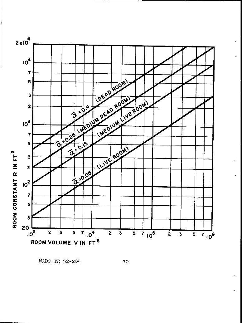
4

2xI

10 00

o 5l

10\0

50 10 Va100IC00 VO UM y N T

WADCT 22 .7

Usually, the designer is given the characteristicsof the fan and the allowable sound pressure levels in theroom, and the problem becomes one of finding the attenua-tion that must be provided in the duct system so that theallowable levels will not be exceeded. The methods forobtaining this attenuation are considered in Chap. 12.In many cases, an elaborate treatment must be used if thesound pressure level is to be substantially reduced in thelow-frequency bands.

Relation to Other Air Flow Devices as Noise Sources.The same basic phenomena are responsible for noise genera-tion in a wide variety of fluid flow devices. These pheno-mena include the mechanisms by which energy of flow isconverted into heat and into random acoustical energy inthe process of turbulence, and the mechanisms by which theair flow can be modulated to give an acoustic signal hav-ing a periodic waveform, as in a fan, propeller, turbine,or other device with rotating blades. An understandingof these phenomena enables the engineer to utilize prin-ciples of noise reduction in the basic design of ventila-tion equipment.

FIGURE 6.5.5

The room constant as a function of room volume,for average absorption coefficient categories"live" to "dead". This assumes that the rela-tion between wall area and volume is approximatelythat for a cubical room, but may be applied inusual cases where the room shape is not extreme.5%/

WADC TR 52-204 71

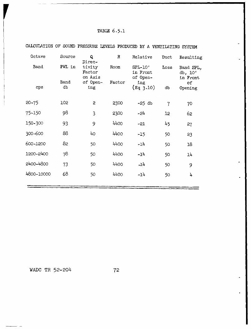
TABLE 6.5.1

CALCULATION OF SOUND PRESSURE LEVELS PRODUCED BY A VENTILATING SYSTEM

Octave Source Q R Relative Duct ResultingDirec-

Band PWL in tivity Room SPL-lO' Loss Band SPL,Factor in Front db, 1O'on Axis of Open- in Front

Band of Open- Factor ing ofcps db ing (Eq 3.10) db Opening

20-75 102 2 2300 -25 db 7 70

75-150 98 3 2300 -24 12 62

150-300 93 9 4400 -21 45 27

300-600 88 40 4400 -15 50 23

600-1200 82 50 4400 -14 50 18

1200-2400 78 50 4400 -14 50 14

2400-4800 73 50 4400 -14 50 9

4800-10000 68 50 4400 -14 50 4

WADC TR 52-204 72

References

(5.1) Beranek, L. L., Reynolds, J. L., and Wilson,K.E."Apparatus and Procedures for Predicting Ventila-tion System Noise", J. Acous. Soc. Am. 25,313-321 (1953).

(5.2) Peistrup, C. F., and Wesler, J. E., "Noise ofVentilating Fans", J. Acous. Soc. Am. 25,322-326 (1953).

(5.3) Beranek, L. L., Kamperman, G. W., Allen, C. H."Noise of Centrifugal Fans" (to be publishedin the J. Acoust. Soc. Am.)

(5.4) Heating Ventilating Air Conditioning Guide 1953(Vol. 31), (Am. Soc. Heating and VentilatingEngrs., New York, 1953), PP. 901-902; alsoearlier editions of this guide.

WADe TR 52-2o4 73

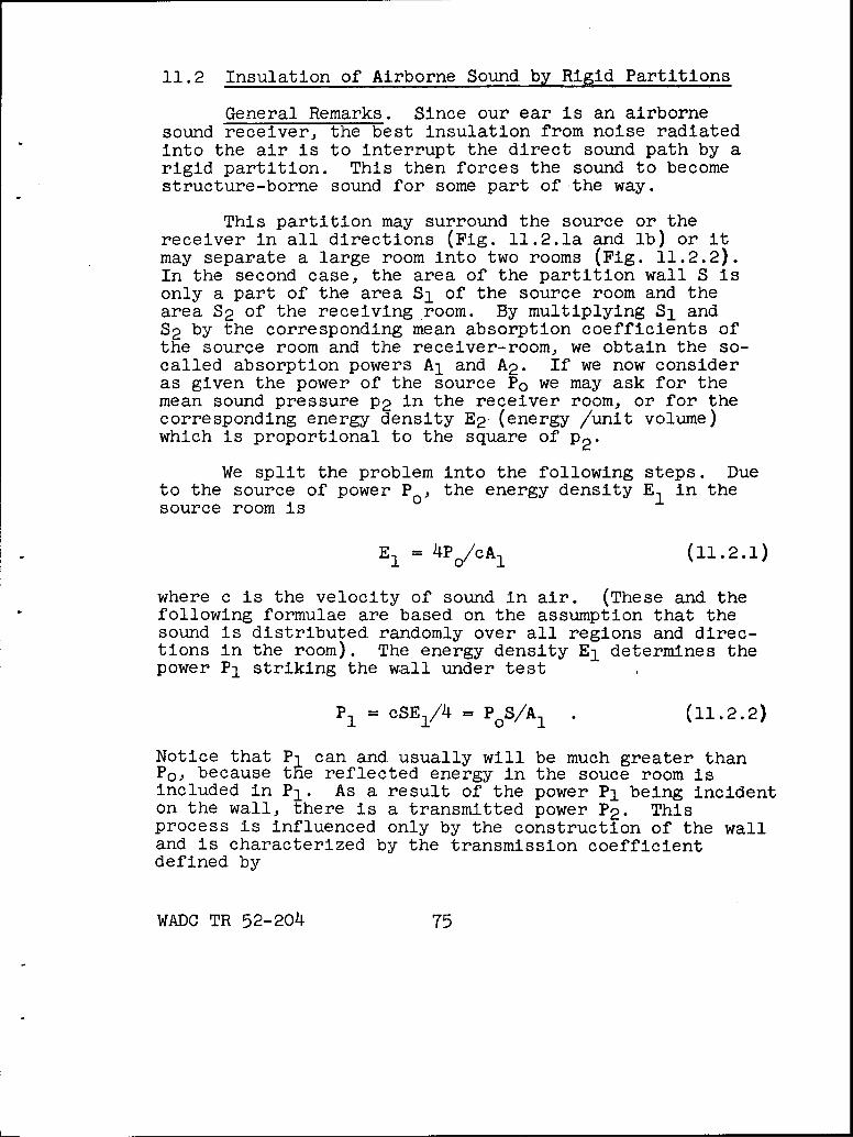
11.2 Insulation of Airborne Sound by Rigid Partitions

General Remarks. Since our ear is an airbornesound receiver, the best insulation from noise radiatedinto the air is to interrupt the direct sound path by arigid partition. This then forces the sound to becomestructure-borne sound for some part of the way.

This partition may surround the source or thereceiver in all directions (Fig. ll.2.1a and lb) or itmay separate a large room into two rooms (Fig. 11.2.2).In the second case, the area of the partition wall S isonly a part of the area S1 of the source room and thearea S2 of the receiving room. By multiplying Sl andS2 by the corresponding mean absorption coefficients ofthe source room and the receiver-room, we obtain the so-called absorption powers A1 and A2 . If we now consideras given the power of the source Po we may ask for themean sound pressure P2 in the receiver room, or for thecorresponding energy density E2 (energy /unit volume)which is proportional to the square of P2.

We split the problem into the following steps. Dueto the source of power Po, the energy density E1 in thesource room is

E 1 = 4P/cA1 (11.2.1)

where c is the velocity of sound in air. (These and thefollowing formulae are based on the assumption that thesound is distributed randomly over all regions and direc-tions in the room). The energy density E1 determines thepower P1 striking the wall under test

P1 = cSEI/4 = PoS/AI " (11.2.2)

Notice that P1 can and usually will be much greater thanPo, because the reflected energy in the souce room isincluded in Pl. As a result of the power P1 being incidenton the wall, there is a transmitted power P 2 . Thisprocess is influenced only by the construction of the walland is characterized by the transmission coefficientdefined by

WADC TR 52-204 75

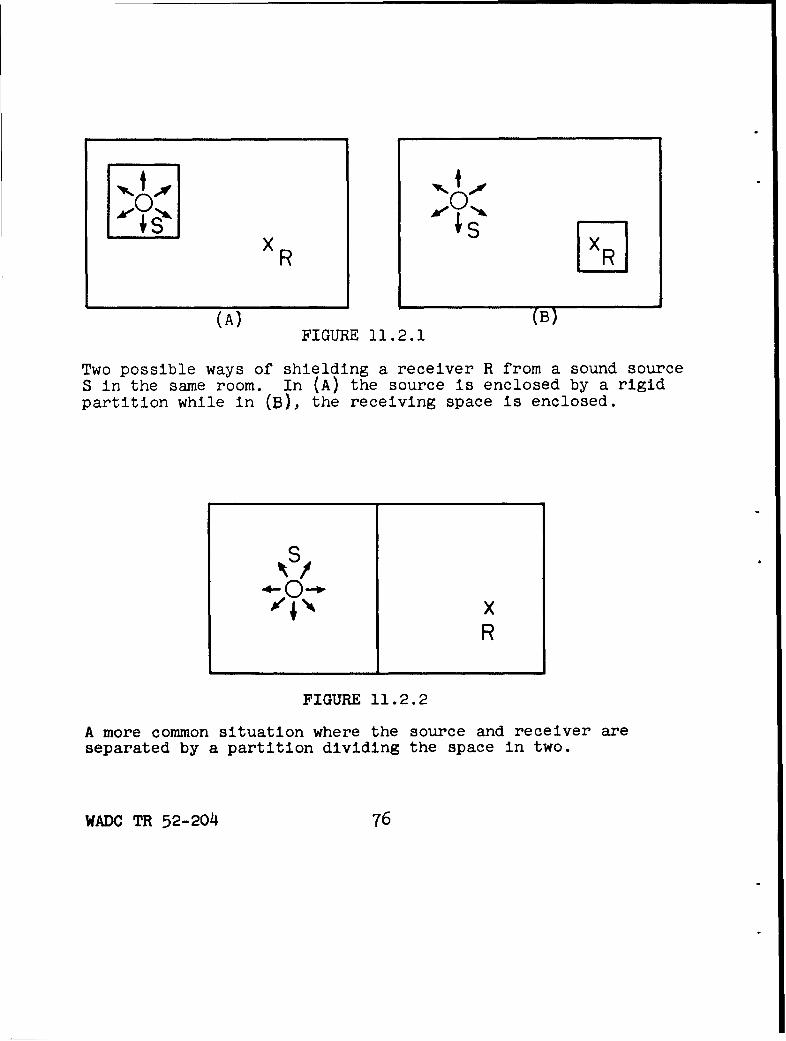
xR

(A) (B)FIGURE 11.2.1

Two possible ways of shielding a receiver R from a sound sourceS in the same room. In (A) the source is enclosed by a rigidpartition while in (B), the receiving space is enclosed.

xR

FIGURE 11.2.2

A more common situation where the source and receiver areseparated by a partition dividing the space in two.

WADC TR 52-204 76

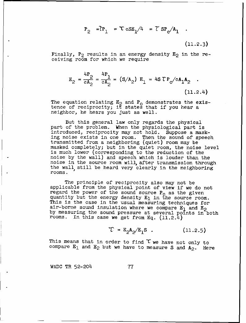
P 2 =TPI =t cSEl/4 = SPc/AI

(11.2.3)

Finally, P2 results in an energy density E2 in the re-ceiving room for which we require

E 4P2 4P2 == 2 A -2 = (S/A 2) E1 = 4SrP/cAIA2

(11.2.4)

The equation relating E and P0 demonstrates the exis-tence of reciprocity; i states that if you hear aneighbor, he hears you just as well.

But this general law only regards the physicalpart of the problem. When the physiological part isintroduced, reciprocity may not hold. Suppose a mask-ing noise exists in one room. Then the sound of speechtransmitted from a neighboring (quiet) room may bemasked completely; but in the quiet room, the noise levelis much lower (corresponding to the reduction of thenoise by the wall) and speech which is louder than thenoise in the source room will after transmission throughthe wall still be heard very clearly in the neighboringrooms.

The principle of reciprocity also may not beapplicable from the physical point of view if we do notregard the power of the sound source P0 as the givenquantity but the energy density E1 in the source room.This is the case in the usual measuring techniques forair-borne sound insulation where we compare E1 and E2by measuring the sound pressure at several points in bothrooms. In this case we get from Eq. (11.2.4)

E = E2 AIEIS . (11.2.5)

This means that in order to find C we have not only tocompare E1 and E2 but we have to measure S and A2 . Here

WADC TR 52-204 77

we get different ratios of energy density depending onwhich we choose to call the source and the receivingroom.

The absorption power A2 may be evaluated from themeasurement of the reverberation time T 2 in the receivingroom using Sabine's formula

A2 = 0.05 VIT 2 (11.2.6)

where A2 and V2 are the room absorption and room volumein units of sq ft and cu ft respectively.

Since we are usually trying to minimize the amountof sound energy transmitted to another room, we areinterested in values of T as small as possible. For char-acterizing the quality of sound insulation, it is moreuseful to define a reciprocal quantity and, since thisquantity varies between 10 and l10, we define a logar-ithmic measure called the Transmission Loss (TL) as

TL = 10 log i/r . (11.2.7)

Calculated in this way, the TL is expressed in decibels*.At first it was assumed that this logarithmic scale wouldalso correspond to our subjective valuation of soundintensity which we call loudness. Although this is notactually the case, we may say to a first approximation,that each increment of 9 db in TL is equivalent to halv-ing the loudness.

* This quantity is internationally used, but iscalled "transmission loss" in America only.For a European Code, the British proposed to callit reduction factor "R". In Germany the quantityis called "Schalldammzahl"and the letter K is used.Kosten (Netherlands) proposed the name "insulation"and the symbol i.

WADC TR 52-204 78

In the same way, the quantity

NR = 10 log E1 /E 2 db (11.2.8)

may be called the noise reduction (NR). With modernmeasurement equipment this quantity can be measureddirectly. Then Eq. (11.2.5) in the logarithmic form is

TL = NR + 10 log S/A 2 . (11.2.9)

The noise reduction to be expected with a given construc-tion is

NR = TL - 10 log S/A 2 . (11.2.9a)

Note that the noise reduction depends on the area of theseparating wall. The smaller this area is, the lower thetransmission loss which will be tolerated.

The last remark is of special importance if thepartition consists of two parallel parts, for instancea heavy wall and a door. It would be too expensive togive the door the same TL as the wall. Since the door,however, has only a small surface S2 compared to thesurface of the whole wall S1 + S2 the power entering thesecond room, consisting here of two parts,

P 2 = cE1 (CISI + C2S2 )/4

(11.2.10)

will not be increased very much if C2 is higher than 1The resulting loss of TL is given by

A (TL) = 10 log l(S1 +t$2S 2

(11.2.11)

WADC TR 52-204 79

If we chose a value for this quantity, we might calcu-late for the difference between both kinds of partitions

(TL) 2 -(TL) 1 =l0 log 'r/r= -10 log [106/1O(1+Sl/S 2 )-S 1/S 2 .

(11.2.12)

In Figure 11.2.3 this difference is plotted as a functionof the ratio S1/S2 for A = 1 and A = 3 db.

Now we may discuss the influence of the absorptionpower in the receiving room. For measurements, we preferrooms with small absorption power. In this case the mea-sured NR may be greater than the quantity we wish tomeasure, the TL. In the case of a closed box installedin a large, noisy room (Fig. ll.2.1b), all walls are trans-mitting. Then A2 /S is equal to the mean absorption coeffi-cient and therefore is always smaller than 1. In thiscase the NR is smaller than the TL. If, for example, itis possible to make OC2 = A2 /S = 0.5 (which is a ratherhigh value), we get from Eq. (ll.2.9a)

NR = TL - 3 db (11.2.13)

provided that these statistical formulae are valid forabsorption coefficients which are so high. If we have

0 2 = 0.25, we get

NR = TL - 6 db. (11.2.14)

We see that proper absorption in the receiving roomhas some advantage. In particular, very small amountsof absorption power must be avoided. If, in the limit,the absorption power in the receiving room is equal tothe transmissivity of the surface S only, i.e., by A2 ='(S,then we find from Eq. (11.2.5), E2 = El, or no transmis-sion loss at all. This result may easily be understoodfrom the standpoint of energy balance. If the receivingroom and the wall itself present no energy losses, thenthe wall may have an arbitrarily high TL; as steady-state is reached, the energy density at both sides ofthe common wall is the same. On the other hand, evenlarge amounts of absorbing material in the receiving roomcannot result in a high noise reduction. The most we canexpect is to get a free-field condition in which we have

WADC TR 52-204 80

near the wall, instead of Eq. (12.2.4)

E 2 = PjcS =

or

NR = TL + 6 db . (11.2.15)

At a greater distance from the wall, the sound levelwill fall off faster than the inverse square relation fora free field. But excluding this very unusual (and expen-sive)case, we may summarize the last results by saying:some amount of absorbing power in the receiving room isnecessary. An absorption power equal to half the surfaceof the separating wall may easily be reached, even in aclosed box, but further amounts of absorption never wouldbring more than a 9 db increase in energy density ratio.

Therefore, we see that we only get high sound leveldifferences with constructions of high TL.

Since the TL depends on frequency, it is not realisticto give only a mean value. Such a mean value can be atbest a very crude order of magnitude estimate of effective-ness. In order to define such a mean value, one must firstdecide on the limits of the frequency range, the quantitywe would like to average and the particular frequenciesat which one measures values to average. In the Europeancode of sound insulation measurements, the lowest frequencyis given by 100 cps and the highest by 3200 cps. Below100 cps measuring becomes very uncertain and, fortunately,the sensitivity of our ears is small. Above 3200 cpsinsulation is so good, generally, that we seldom havetrouble. The frequency scale is logarithmic. This cor-responds to the common use of octave steps or third-octave-steps and may be justified by the similar distribution ofresponse for different frequencies on the basilar membranein the inner ear. The most difficult question is to saywhat should be averaged. It is usual to average the trans-mission loss and therefore in the following [TL] meansthe TL averaged between 100 and 3200 cps over a logarithmicscale.

But we must realize that this kind of averaging isJustified only if the loudness or the rate of nervous im-pulses per unit of time is proportional to the sound level.

WADC TR 52-204 81

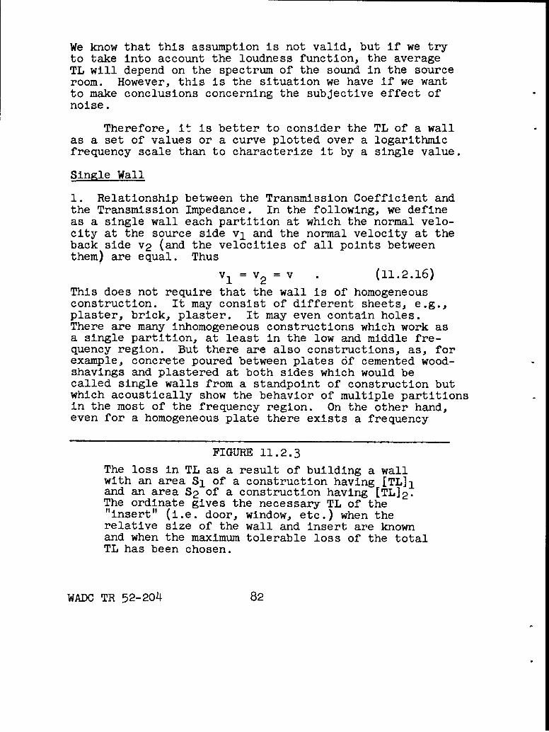
We know that this assumption is not valid, but if we tryto take into account the loudness function, the averageTL will depend on the spectrum of the sound in the sourceroom. However, this is the situation we have if we wantto make conclusions concerning the subjective effect ofnoise.

Therefore, it is better to consider the TL of a wallas a set of values or a curve plotted over a logarithmicfrequency scale than to characterize it by a single value.

Single Wall

1. Relationship between the Transmission Coefficient andthe Transmission Impedance. In the following, we defineas a single wall each partition at which the normal velo-city at the source side vI and the normal velocity at theback side v2 (and the velocities of all points betweenthem) are equal. Thus

v = v 2 = v . (11.2.16)

This does not require that the wall is of homogeneousconstruction. It may consist of different sheets, e.g.,plaster, brick, plaster. It may even contain holes.There are many inhomogeneous constructions which work asa single partition, at least in the low and middle fre-quency region. But there are also constructions, as, forexample, concrete poured between plates 6f cemented wood-shavings and plastered at both sides which would becalled single walls from a standpoint of construction butwhich acoustically show the behavior of multiple partitionsin the most of the frequency region. On the other hand,even for a homogeneous plate there exists a frequency

FIGURE 11.2.3

The loss in TL as a result of building a wallwith an area Sl of a construction having [TL] 1and an area S2 of a construction having [TL12 .The ordinate gives the necessary TL of the"insert" (i.e. door, window, etc.) when therelative size of the wall and insert are knownand when the maximum tolerable loss of the totalTL has been chosen.

WADC TR 52-204 82

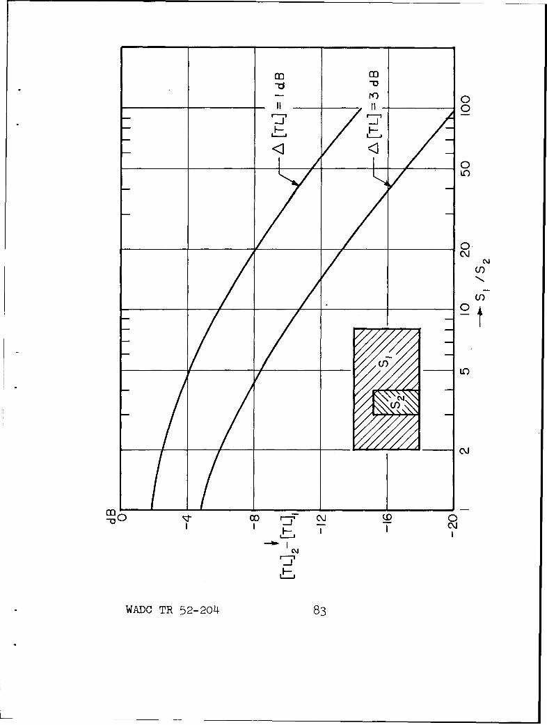
/I-0

-

.

-j~

(U))

F LO)

mN

-00 0- N1C~I I~

-~j

WADC TR 52-2o4I 83

limit, above which the assumption of Eq. (11.2.16)loses its validity. This limit is reached when the thick-ness becomes larger than a tenth of the wavelength forthe longitudinal wave in the wall. But in most cases ofpractical interest, this happens above the frequencyregion in which we are interested.

Assuming Eq. (11.2.16) is true, wenay characterizethe wall by its "transmission impedance" Z-r which we de-fine as the ratio of the pressure difference between innerand outer wall to the normal velocity

Z-r = (p1 - P 2 )/Vn . (11.217)

It is to be expected that this quantity is dependent onfrequency. This means that, in general, we have toconsider all the quantities in Eq. (11.2.17) as complex,involving not only amplitudes but also phases. Thetransmission impedance differs from the so-called wallimpedance

Zw = Pl/vn (11.2.18)

which characterizes the boundary condition for the sourceroom by the term p 2/vl. In the case of a wave radiatedat the angle Zi, which is the angle of incidence at thesource side, Zw is given by*

plvn = Pc/cos Zf. (11.2.19)

Practically, the difference between ZT andZw is much greater; in order to get the ab-sorption coefficient using Zw, we have totake into account also all losses which aregiven by heat conduction and friction,especially if the surface is porous. But forthe calculation of transmission, these effectshave no remarkable influence. Thus, if thewall is covered with a layer of fiberglas,we may split the whole problem into one ofabsorption and one of transmission.

WADC TR 52-204 84

The dimensionless transmission coefficient dependson the ratio of the impedances defined by Eqs. (11.2.17)and (11.2.19)

1/ 1 + Zt-cCos Zý/ r

(11.2.20)

It is clear that the transmission must become total (Or= 1)if the transmission impedance vanishes. This means thatthe pressures are equal at both sides of the wall. Thetransmission is zero if the transmission impedance tendsto infinity.

We see that, in general, 7depends on the angle ofincidence, even if Ztis independent of 29-. This meansthat the transmission loss we observe experimentally,where the sound is impinging the wall at different angles,depends on the particular angular distribution of thesound. Also one must realize that a given surface'Sonly subtends the area S cos gin the direction of theincident wave. (See Fig. 11.2.4). Therefore, whenaveraging 'C over different plane waves, we have to mul-tiply L with the weighting factor cos 9. Hence

n

=1 T k klk (11.2.21)nk=l

For a statistical sound distribution, as we may have inthe case of testing a wall between two reverberant rooms,we may assume that the sound is equally distributed overall directions. This requires the introduction of anotherweighting factor sin z-ýbecause the region between ZAand&R-+ ddcuts out a zone of a sphere 27r sin 2dZ d

Then we get for the average statistical transmission co-efficient

V/2 r/2

0= o ý tcos sin fdZ/Q 2

'ir2/2 2 t os 2sin dn 2' .

o cos sin Od 0- o

(11.2.22)

WADC TR 52-2o4 85

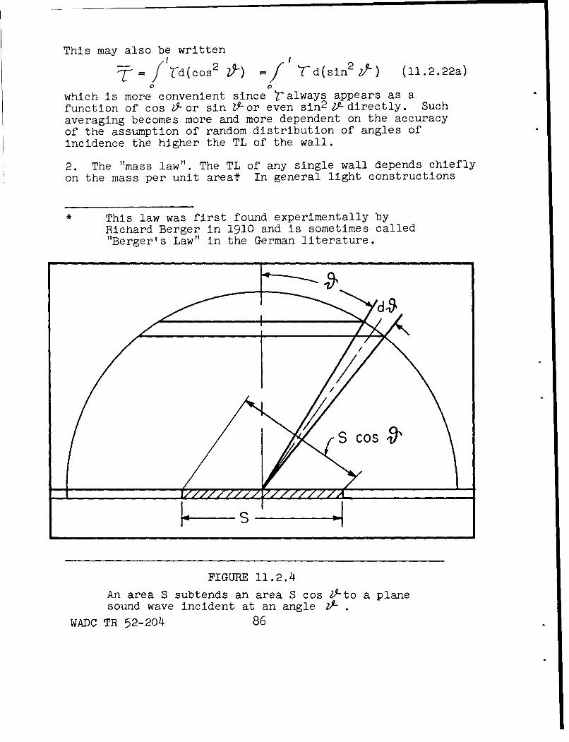
This may also be written[-d(cos 2 ?) d(sin2 (•1.2.22a)

0 a

which is more convenient since r always appears as afunction of cos O-or sin ZY-or even sin2 2Y-directly. Suchaveraging becomes more and more dependent on the accuracyof the assumption of random distribution of angles ofincidence the higher the TL of the wall.

2. The "mass law". The TL of any single wall depends chieflyon the mass per unit areat In general light constructions

* This law was first found experimentally by

Richard Berger in 1910 and is sometimes called"Berger's Law" in the German literature.

L -S

FIGURE 11.2.4

An area S subtends an area S cos ,'to a planesound wave incident at an angle 2'.

WADC TR 52-204 86

are more sound transmitting than heavy ones; and if itis necessary to save weight, it will always be difficultto have a high TL. However, there may be cases whereheavy constructions having special defects are worsethan other lighter constructions.

To a rough approximation, the mean TL may be

calculated from the formula

(TL)m = 14 log G + 24 (11.2.23)

where G is the surface weight in lb/sq ft. Tablelll.2.1shows the surface weights of some common building ma-terials.

A further empirical fact is that the TL generallyincreases with frequency f. This may be derived from themass law observation on the basis of similarity. If aheavier wall is better, then for a given material, thethicker wall is also better. But in a sound field, allthicknesses must be compared with the sound wavelength;therefore, we have to expect a dependence on the ratioh/ý or on the product hf if we replace i by c/f. Thisgeneral rule also holds when, as sometimes happens, anincrease of frequency results in a decrease of TL. Inthese cases, an increase in thickness also results in adecrease of TL.*

To explain these general dependences on weight andfrequency, the simplest assumption we can make is thatthe wall behaves like a mass. This means that we haveto consider the transmission impedance as a mass reactance

z = jan (11.2.24)

where m is the surface mass and w the angular frequency.Putting this into Eq. (11.2.20) we find

+(acos 2)I[ 1/l +2 c" (11.2.25)

* See Beranek, Leo L., Phys. Soc. Acoustics GroupSymposium p. 1-6 (1949).

WADC TR 52-204 87

Excluding grazing incidence, we may also derive thisresult from Rayleigh's more general solution for thetransmission through a sheet of non-rigid medium havinghigh specific mass and small compressibility . Thisshows that we do not have to discuss transmission through"a wall in terms of its movement of an inert mass and as"a result of longitudinal waves excited inside the wall.The first kind of motion is only a special limit of thesecond.

To compare Eq. (11.2.25) with experimental resultsfound for walls between reverberant rooms, we have toaverage t over cos 2 maccording to Eq. (11.2.22). Doingthis, we get

t= (2 c/mi)2 in [1 + (am/ 2 P c)2]

(11.2.26)

or*

[TL]random = [TLI - 10 log (0.23 [TL]o).

(11.2.27)

where [TL]o is the transmission loss for perpendicularincidence. This result sometimes fits the experimentalresults quite well because it gives values of TL lowerthan [TLIo and also a less rapid increase of TL withsurface mass and frequency.

However, this last equation can hardly be regardedas the real interpretation of what happens because plotting'" against cos 2 0-for high values of an/2 p c, we get avery sharp peak at grazing incidence where r becomes one.

* This dependence sometimes is called the random-incidence mass law.

WADC TR 52-204 88

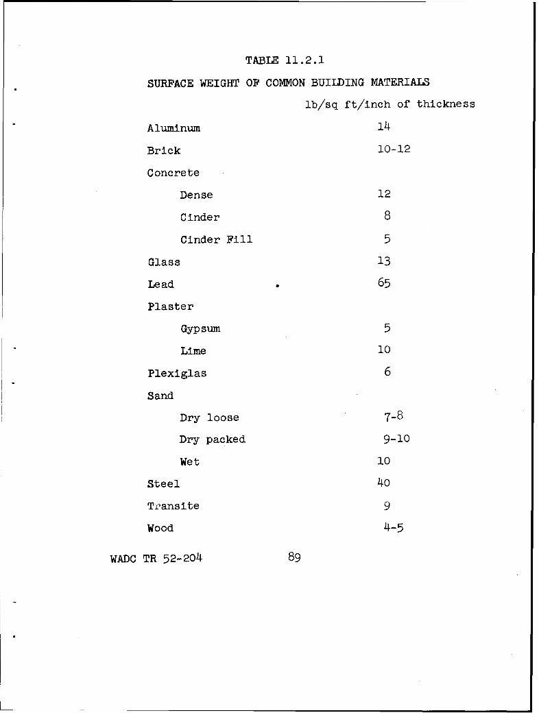
TABLE 11.2.1

SURFACE WEIGHT OF COMMON BUILDING MATERIALS

lb/sq ft/inch of thickness

Aluminum 14

Brick 10-12

Concrete

Dense 12

Cinder 8

Cinder Fill 5

Glass 13

Lead 65

Plaster

Gypsum 5

Lime 10

Plexiglas 6

Sand

Dry loose 7-8

Dry packed 9-10

Wet 10

Steel 40

Transite 9

Wood 4-5

WADC TR 52-204 89

This dependence always has to be expected when Zt isindependent of the angle of incidence or is nearly in-dependent in the region of grazing incidence. We maycall this the "component effect" because it has as itsbasis the fact that the normal velocity of a wall is onlya component of the resultant of the velocities of thesource side and the back side. We must realize, however,that the limit '-C = I for 2= 900 infers an infinite walland infinite plane waves and, therefore, cannot be realizedin practice. Furthermore, we know from wave acousticsthat in rooms, sound propagation exactly parallel to aboundary plane can never occur.

Therefore, it seems reasonable to exclude anglesfor which Eq. (11.2.28) does not hold

(Zr cos ZL9/2pc) 2 > ; 1. (11.2.28)

By integrating only to a limiting angle Z9', we find for

1

•-'=co / 2•, (2pc/awm cos a9) 2d(cos2 9ý)=(2pc/acn)lin ;/cos21z.,Cos 2

(11.2.29)

corresponding to

[TLI = [TL] 0 - 10 log in I/cos 2 1'

(11.2.30)

Now we have the difficulty that the result dependson the choice of the limit angle 29'. Taking lA' = 82.50as a value which guarantees that Eq. (11.2.28) is satisfiedfor [TL]o > 24 db, we get

[TL]o 8 25 = [TL] 0 - 6 db. (11.2.30a)

The same result is obtained if we calculate the TL for anangle ZA = 600 only, so we also may write

[TL] 6 0 0 = [TL]o - 6 db (11.2.30b)

WADC TR 52-204 90

We call this the "60° - mass law". It involves anessential simplification for it replaces the averagingover all angles of incidence by using a mean angle. Inthe present case where the Yis monotonically increasingwith z29-, the choice of zA= 600 is reasonable.

It would seem better to choose IA= 450 because thisangle is in the middle og the ZJ-range and has the highestweighting factor (cos 45 sin 450 = 1/2). In the presentcase we get

[TL] 4 5 0 = [TL]o -3 = 20 log G - 20 log f - 31 db

(11.2.31)

which also corresponds to the average 't value if werestrict the i-region from 0o to nearly 700. This "45°-mass law" fits the experimental results for light construc-tions quite well. By averaging over the frequency regionfrom 100 to 3200 cps (which means replacing f by thegeometric mean of 100 and 3200 cps),

[TL] 4 5 ,m = 20 log G - 24 db. (11.2.32)

where the second term agrees with that in the empiricallydetermined Eq. (11.2.23).

For higher values of G, all formulas which we havederived from the assumption of Eq. (11.2.24) gives TL'swhich are much too high. Therefore, we have to look forother reasons to explain this discrepancy.

3. The Influence of Stiffness. It seems likely thatstiffness may be of importance. If we try to move the wallvery slowly, we feel its stiffness only as the reaction tothe driving force. This stiffness is given by the support-ing or damping of the wall at the edges and also will be ofimportance if a very low frequency sound pressure is drivingthe wall. However, several authors have observed higher TL'sat low frequencies than those corresponding to mass law 2.2,2.3/.Although this problem has not been solved theoretically,it seems probable that such deviations may be accounted

WADC TR 52-204 91

for by stiffness. But cases where stiffness gives anincrease in the insulation power must be regarded as ex-ceptions for the present. Usually stiffness is a disadvantage because the reactive forces due to stiffnessand those due to mass are not added. However, becauseof their opposite phases they compensate for each other.

(a) Resonance. There are two kinds of effectswhere this happens. The first is well-known in acousticsas resonance, and means that the periodicity in time ofthe driving forces equals the periodicity in time of afree motion, i.e., a motion possible without externalforces. If we have a bar of the length I supported atboth ends, the resonance is given by the condition

/2 (11.2.33)

where AB is the wave length of the bending wave correspond-ing to the same frequency. Formally we have the samecondition for an organ pipe open at both ends or for atube closed at both ends

S= A 2 (11 .2. 34 )

where io is the wavelength in air. But therv is anessential difference between the two cases: in the caseof the propagation of the longitudinal waves in a tube,the wave length is inversely proportional to the frequency

10 = colf (11.2.35)

whereas in the case of a bending wave,.it is inverselyproportional to the square root of the wave length

14S= B ;:7j; (11.2.36)

or, the phase velocity of bending waves is proportionalto the square root of frequency

4

(11.2.37)

WADC TR 52-204 92

In these equations, B is the bending stiffness. For arectangular bar with Young's modulus E, height h and thebreadth b,

B = E b h 3 /12 • (11.2.38)

If we substitute m = p bh and introduce the velocity forlongitudinal waves

CL IE/p (11.2.39)

we can write instead of Eq. (11.2.36)

B= .8 Oh/f (11.2.40)

In the case of plates, Eqs. (11.2.38), (11.2.39) and(11.2.40) should be modified because of the hinderedlateral contraction in one direction. Taking this intoaccount, we have

BI = Ebh 3/12(l- P2) (11.2.38a)

cL' =/Ef(-2 (11.2.39a)

B /i.8 CLh/f (11.2.40a)

where p is Poissoxis ratio. Since this number is 0.3 inmost cases, the differences between these two groups ofequations, especially between Eqs. (11.2.40) and (ll.2.40a)become so small that we may neglect them and speak simplyof B, cL and A B only*. Furthermore, these values maydepend much more on the individual variation of samples

• In the available handbook tables of sound ve-locities, it is not even stated whether thelongitudinal velocity in a bar, a plate or aninfinite elastic medium is meant.

WADC TR 52-204 93

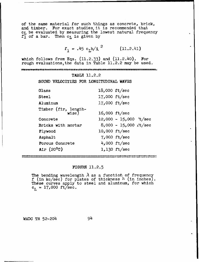
of the same material for such things as concrete, brick,and timber. For exact studies, it is recommended thatcL be evaluated by measuring the lowest natural frequencyfl of a bar. Then cL is given by

fl1 = .45 cLh/. 2 (11.2.41)

which follows from Eqs. (11.2.33) and (11.2.40). Forrough evaluations~the data in Table 11.2.2 may be used.

TABLE 11.2.2

SOUND VELOCITIES FOR LONGITUDINAL WAVES

Glass 18,000 ft/sec

Steel 17,000 ft/sec

Aluminum 17,000 ft/sec

Timber (fir, length-wise5 16,000 ft/sec

Concrete 12,000 - 15,000 't/sec

Bricks with mortar 8,000 - 15,000 Zt/sec

Plywood 10,000 ft/sec

Asphalt 7,000 ft/secPorous Concrete 4,000 ft/sec

Air (20 0 C) 1,130 ft/sec

FIGURE 11.2.5

The bending wavelength A as a functioh of frequencyf (in kc/sec) for plates of thickness h (in inches).These curves apply to steel and aluminum, for whichcL = 17,000 ft/sec.

WADC TR 52-204 94

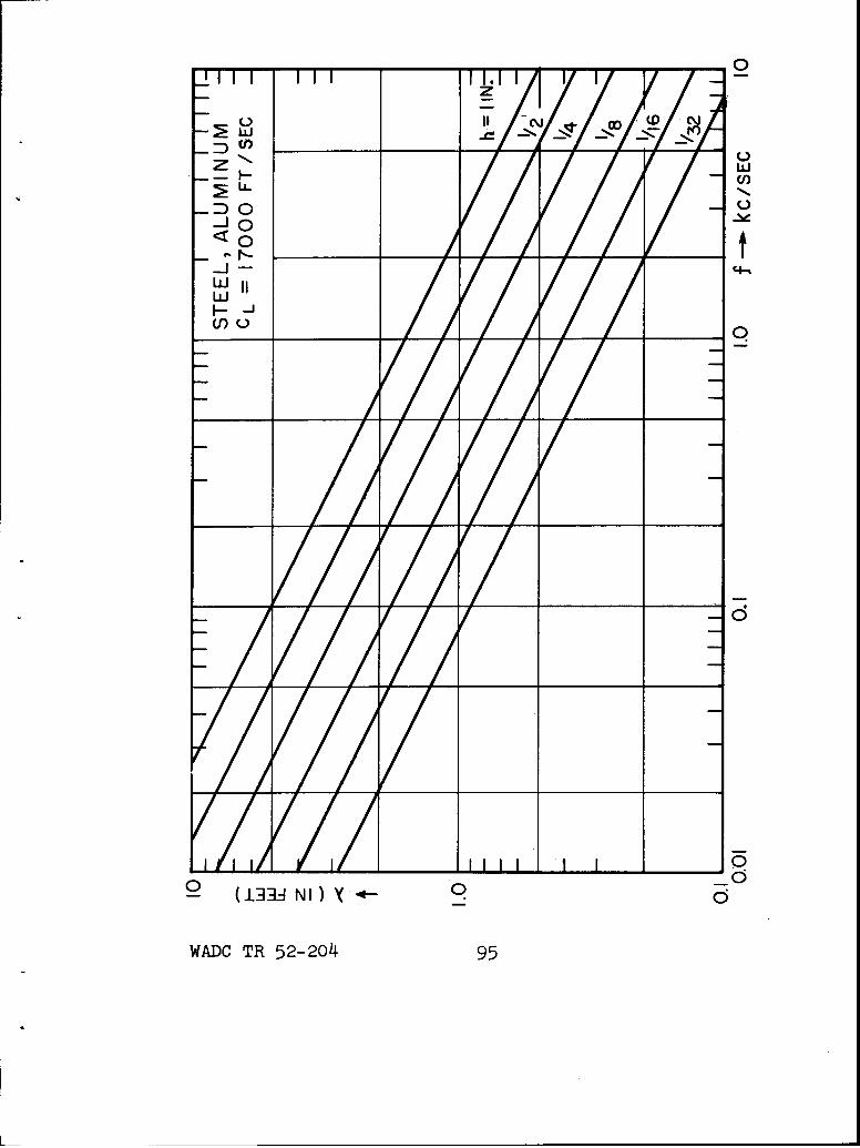
-n- -- IT YII111F 11 0z

CO,

Z) 0

Lii

I--0

0 (133A NI4 1 00

WADC TR 52-2o4 95

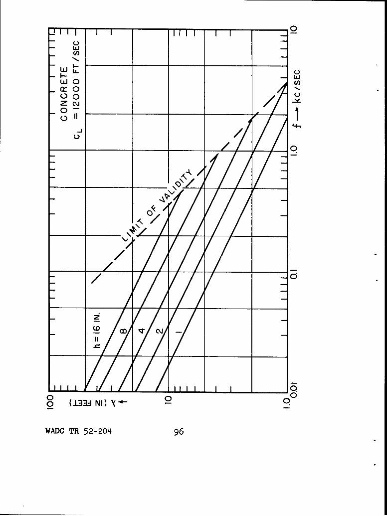
00wUl)

w 0

0--

0 /

a (133/NO---

WADO TR 52-204 96

Furthermore, Figs. 11.2.5-11.2.7 contain graphs for thedependence of length of a bending wave on frequency forplates of different thicknesses for steel and aluminum,concrete and plywood. From these graphs we also may findthe natural frequency of a rectangular bar supported atthe ends or a plate supported on an opposite pair of edgesif we remember that the wavelength is the double of thelength

For the case of plates of length •x and bzreadth vusually the four edges are supported. Then Eq. (11.2.335must be changed to read

AB =) 2/C/ 2 + Y)2

(11.2.42)From Fig. 11.2.8, the value ý B may be found for platesof lengths and breadths between- 0.2 and 20 feet. Thelowest natural frequency may be found either from this andthe graphs in Figs. 11.2.5-11.2.7 or by using directly theformula

f11 =0.45 cL h [(1/1 x) 2 + (1/ty)2 J*

(11.2.43)

FIGURE 11.2.6

The bending wavelength A as a function of frequencyf (in kc/sec) for plates of thickness h (in inches).These curves apply to concrete, for which cL=12,000 ft/sec.

WADC TR 52-204 97

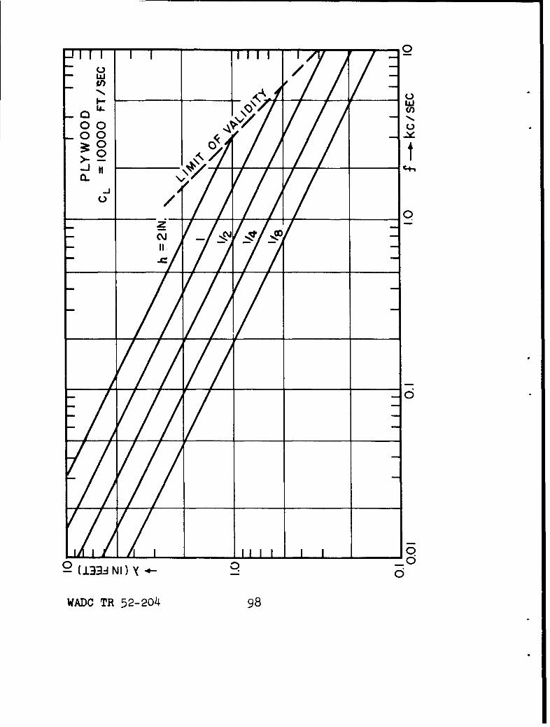
rF11 0

w0 0

- -N __ _

Ja

2 (133dNI) X 00

WADC TR 52-204 98

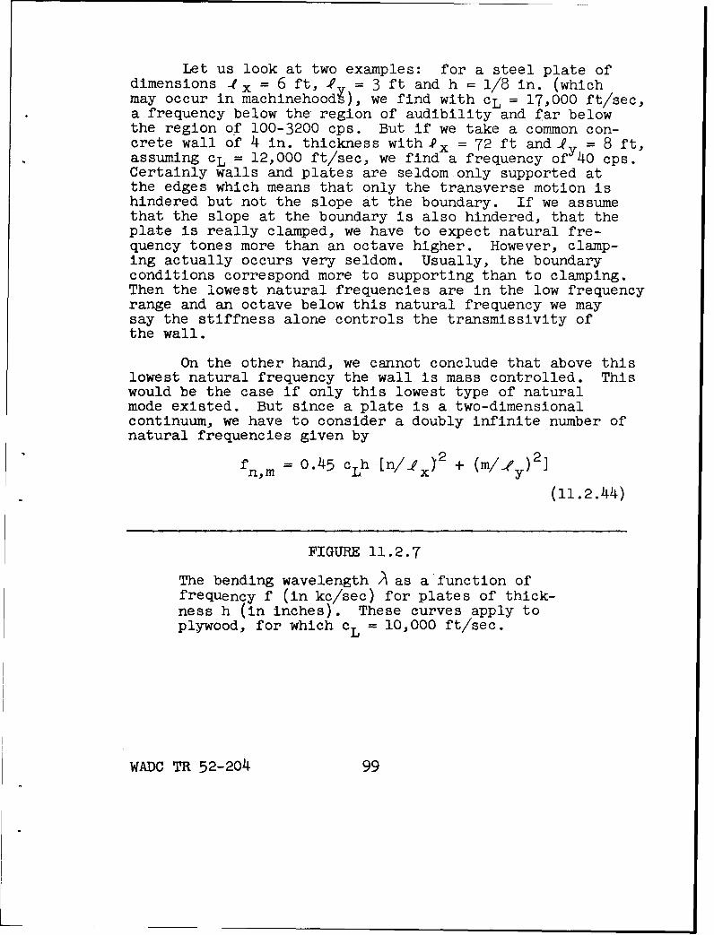
Let us look at two examples: for a steel plate ofdimensions -(x = 6 ft, .. = 3 ft and h = 1/8 In. (whichmay occur in machinehoodg), we find with cL = 17,000 ft/sec,a frequency below the region of audibility and far belowthe region of 100-3200 cps. But if we take a common con-crete wall of 4 in. thickness with Ox = 72 ft and I = 8 ft,assuming cL = 12,000 ft/sec, we find a frequency ofy40 cps.Certainly walls and plates are seldom-only supported atthe edges which means that only the transverse motion ishindered but not the slope at the boundary. If we assumethat the slope at the boundary is also hindered, that theplate is really clamped, we have to expect natural fre-quency tones more than an octave higher. However, clamp-ing actually occurs very seldom. Usually, the boundaryconditions correspond more to supporting than to clamping.Then the lowest natural frequencies are in the low frequencyrange and an octave below this natural frequency we maysay the stiffness alone controls the transmissivity ofthe wall.

On the other hand, we cannot conclude that above thislowest natural frequency the wall is mass controlled. Thiswould be the case if only this lowest type of naturalmode existed. But since a plate is a two-dimensionalcontinuum, we have to consider a doubly infinite number ofnatural frequencies given by

fn,m = 0.45 CLh [n/_ x) 2 + (m/y)21

(11.2.44)

FIGURE 11.2.7

The bending wavelength A as a function offrequency f (in kc/sec) for plates of thick-ness h (in inches). These curves apply toplywood, for which cL = 10,000 ft/sec.

WADC TR 52-204 99

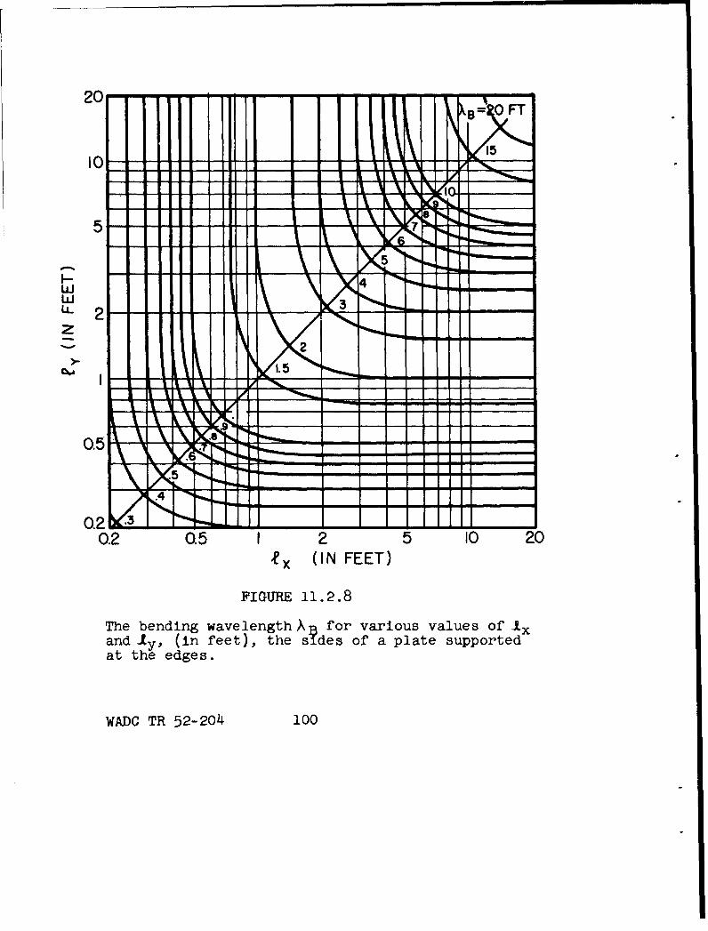
20 -q OFT ----

' O FT

5--S6

0.2

tx (IN FEET)

FIGURE 11. 2.8

The bending wavelength A for various values of JLxand ly, (in feet), the s~des of a plate supportedat the edges.

WADC TR 52-204l 100

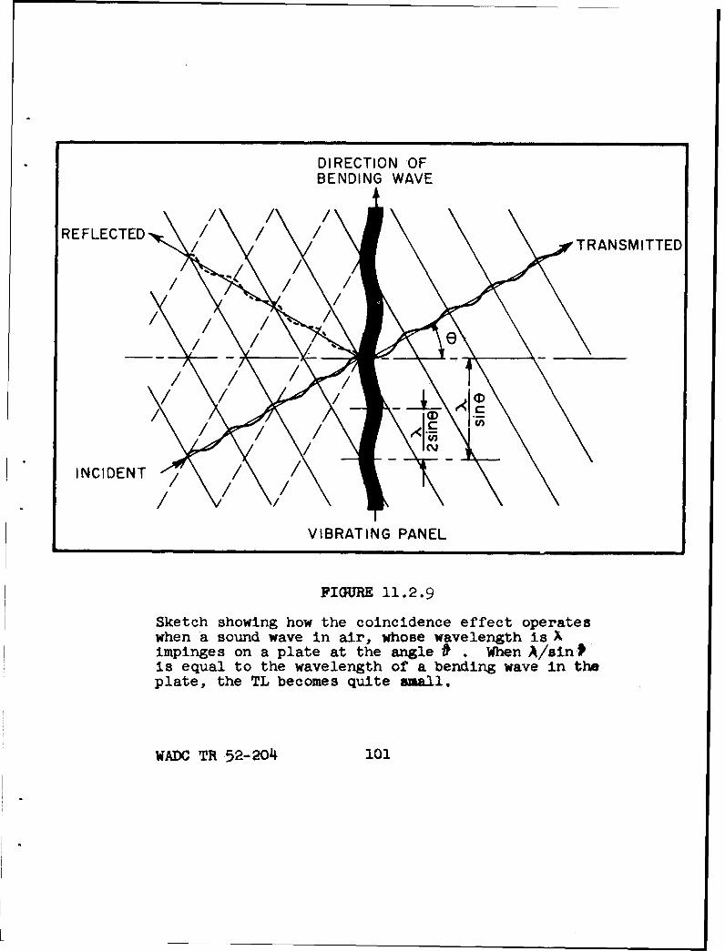
DIRECTION OFBENDING WAVE

REFECE-•,' / / /REFLECTED TRANSMITTED

//

/

INCIDENT ," / ..

VIBRATING PANEL

FIGURE 11.2.9

Sketch showing how the coincidence effect operateswhen a sound wave in air, whose wavelength is Ximpinges on a plate at the anglefr . When A/sintis equal to the wavelength of a bending wave in theplate, the TL becomes quite small.

WADC TR 52-204 101

and so we would have to expect the occurrence ofresonances in higher frequency regions too. Indeed, forvery undamped systems like a bell, this is the case.

However, if there are energy losses either in theplate or at the boundaries, we know by experience, or Onthe basis of an asymptotic law derived by Schoch 3.4/,that the higher natural modes have only a small inRfuence.Then a plate on which a sound wave impinges perpendicularlyacts like an inert mass the higher the frequency of soundis compared to the lowest natural frequency of the plate.

Summarizing, stiffness is desirable only if thelowest natural frequency is above the frequency region inwhich we are interested. This condition is usually diffi-cult to fulfill. Thus, we must make the natural frequenciesof walls as low aspossible. This means we should constructwalls of small stiffness but heavy mass.

(b) Trace Matching (Coincidence Effect). The samerule as above applies because of another effect, whereinertia and stiffness also work against one another andwhich seems to be of greater importance since it mayhappen in the middle of our frequency region. If a planesound wave impinges on a wall at oblique incidence thenthe pressure is working with opposite phases in the dis-tance of half the "trace-wavelength"A 0 /2 sin A. Sothe plate is forced to be deformed with the same periodi-city as shown in Fig. 11.2.9. For any observer movingwith the trace velocity co/sin2A along the plate, thedeformation appears the same as we get if the plate isperiodically supported at distances of Ac/2 sin 2A. Ifthis periodicity in space of the driving forces agreeswith what the plate would present without forces, i.e.,if

3o//)nB (11.2.45)

we have to expect total transmissivity Just as in the caseof resonance. Now by putting this into Eqs. (11.2.36) and(11.2.40), we find that this "coincidence or, as we maysay more precisely, this "trace matching", happens forspecial combinations of frequency and angles of incidencegiven by

f = (Co2 /2r sin2 ) B (11.2.46)

WADC TR 52-204 102

and f = 0.56 c0 2/cLh sin2 ?/ (11.2.46a)

Furthermore, since sin varies between zero and one,we may find these "trace matchings" only above a criticalfrequency given by

fc = (co 2/2v) (11.2.47)

or fc = 56 co 2 /cLh (ll.2.47a)

In Fig. 11.2.10 these frequencies are plotted as afunction of the thickness for different materials. Theregion where trace matching is possible is to the rightof these lines. We see that it is possible over the wholefrequency range for thick walls and that it is impossibleonly in thin plates.

The question arises as to how this statement can bein agreement with the general dependence on surface weightfound empirically. To discuss this problem more quantita-tively, we will again consider the transmission impedancewhich can be defined for a wall of infinite length on whichan infinite plane sound wave is incident. In this casewe get L

Z = Jam - jB sin 2 Z w 3/c 4 (11.2.48)

= J 2v fm (1-f 2 sin $/fc) (11.2.48a)

The first term gives the inertia reactance and is pre-dominant below the frequency of trace matching. Thesecond term gives the reactance of the bending stiffness;this term increases with the angle of incidence, beingzero at perpendicular incidence, and is proportional tothe third power of the frequency. From simple resonancephenomena we are accustomed to a stiffness reactanceinversely proportional to the frequency. But this isstill the case here. The f3 dependence is overcompen-sated by the fact that the stiffness of a beam supportedat its ends is inversely proportional to the fourthpower of the length of the beai and tois length is givenby co/2f sin zA; hence B I I/L+ Jl/fq.

WADC TR 52-204 103

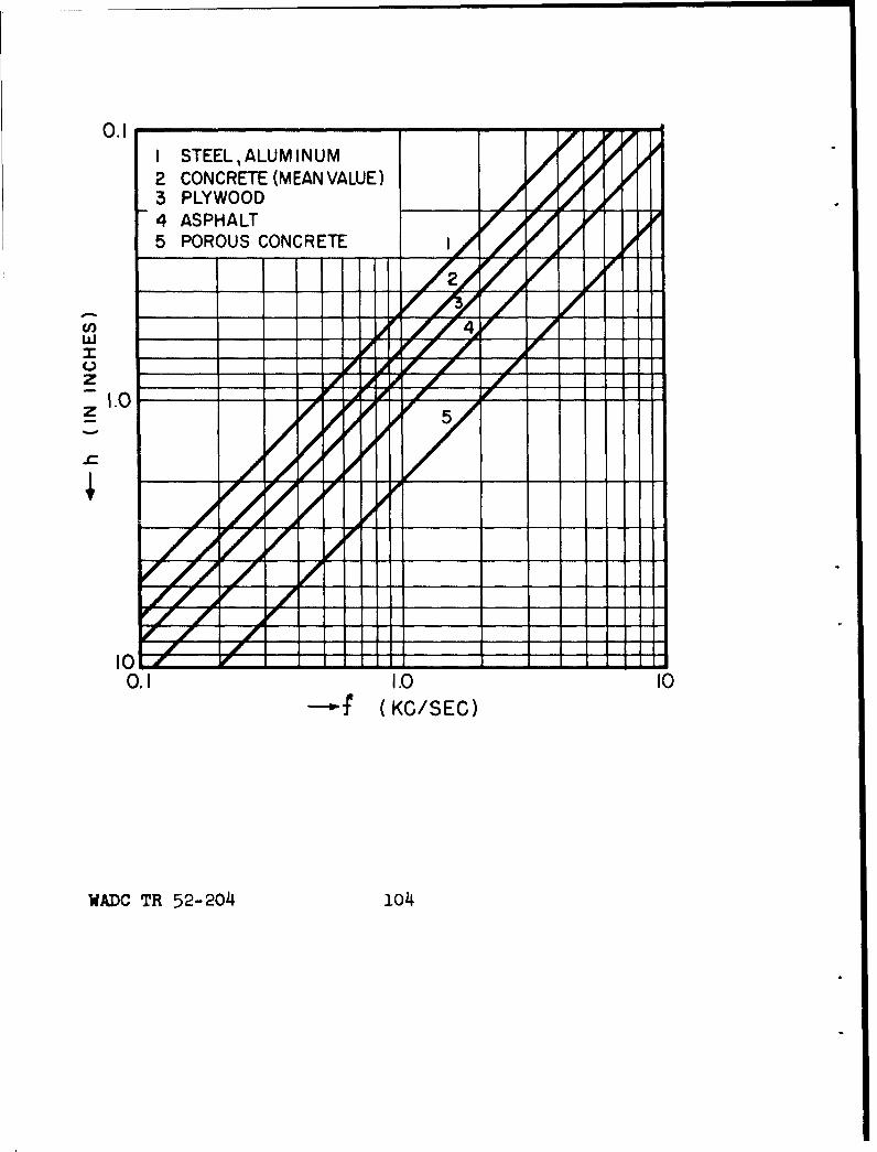
0.1 I ,00I STEEL ALUMINUM ýo •

2 CONCRETE (MEAN VALUE)3 PLYWOOD __,___

4 ASPHALT5 POROUS CONCRETE

I~l ' L Z/ /z __

I00

0.1 1.0 1-.1 (KO/SEC)

WADC TR 52-204 lo4

From Eq. (11.2.48a) we get for the TL

[TL] = 10 log [1 + (rfm cos 2/pco) 2 (1-f 2 sin2 Z/fc)2].

(11.2.49)

In Fig. 11.2.11, a map is given showing contoursof equal TL over a [log f - cOs 2 -9-] plane. Dark regionsindicate good sound insulation; light regions, poor soundinsulation. For 2A = 00 we have a monotonic increase ofTL corresponding to the 00 mass law. There is, in general,a decrease from bottom to top due to the component effect.The trace matching effect cuts a deep valley beginning atthe point (fc,0) and curving asymptotically to the (cos22A= 1)line. At the left of this valley the wall is mass controlledwhile at the right it is stiffness controlled.

Since for a given material and a homogeneous wall,stiffness also increases with thickness with the thirdpower, we see that the heavier wall insulates better alsoin the region where stiffness predominates. Since thespecific material constant, i.e., the longitudinal soundvelocity CL, only varies between 10,000 and 18,000 ft/secfor most materials in which we are interested, ithas been very difficult to decide if the empiricaldependence on weight means a dependence on mass only orif stiffness is a factor too. From Figs. 11.2.10 and11.2.11 we conclude that in most cases of walls in build-ings, stiffness must be predominant except at perpendicularor near perpendicular incidence. The special values for

FIGURE 11.2.10

The critical frequency f plotted as afunction of the plate thickness h (ininches) for which the coincidence effectis possible. At this frequency, the TLis quite small.

WADC TR 52-204 105

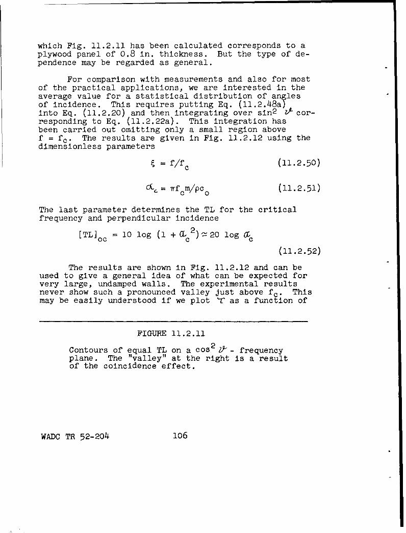
which Fig. 11.2.11 has been calculated corresponds to aplywood panel of 0.8 in. thickness. But the type of de-pendence may be regarded as general.

For comparison with measurements and also for mostof the practical applications, we are interested in theaverage value for a statistical distribution of anglesof incidence. This requires putting Eq. (II.2.48a)into Eq. (11.2.20) and then integrating over sin2 ZAcor-responding to Eq. (11.2.22a). This integration hasbeen carried out omitting only a small region abovef = fc. The results are given in Fig. 11.2.12 using thedimensionless parameters

=f/fc (11.2.50)

0% = cfcm/PCo (11.2.51)

The last parameter determines the TL for the criticalfrequency and perpendicular incidence

[TL]oc 10 log (l + a 2 ):20 log 6coc ~ c

(11.2.52)

The results are shown in Fig. 11.2.12 and can beused to give a general idea of what can be expected forvery large, undamped walls. The experimental resultsnever show such a pronounced valley Just above fc. Thismay be easily understood if we plot T as a function of

FIGURE 11.2.11

Contours of equal TL on a cos 2 g- frequencyplane. The "valley" at the right is a resultof the coincidence effect.

WADC TR 52-204 106

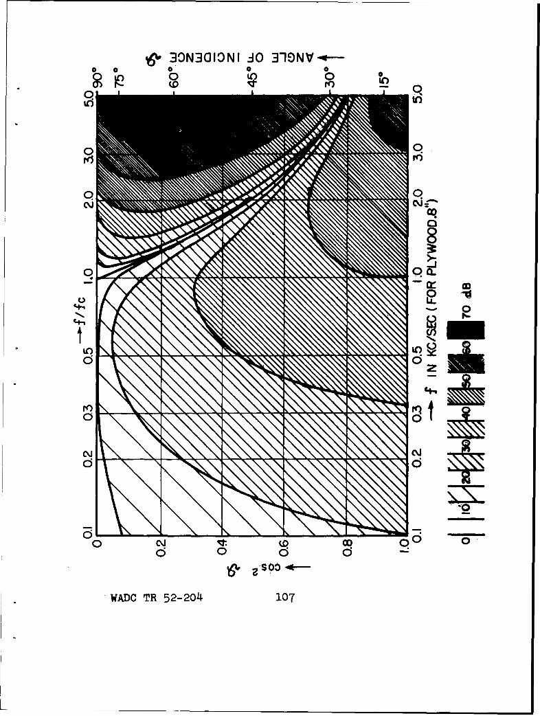
,6 30N30IONI JO 3719NV'w-0 0

cq

IC\\

0 a. •

'4--

C4-i

C.. 0L 0

0

o N o0 D -00 0 d0

WADC TR 52-204 107

50

40 00, _ _ _ - -

440

TL

FIUB 11..1

WA0 ad- 52- 0h

sin2 and see that this curve again has a sharp peak at

the angle of trace matching. We may write the expressionfor rC as

=1/Li + (61S) 2 (11.2.53)

where E is the relative variation of the abscissa with

sin 2 Z)- = 1/ý (11.2.54)

E = sin 2 ZY - 1/ý (11.2.55)

and 2 6 is the bandwidth, which in the present case is

6=l/[2 (T_ / (11.2.56)

It is not important that the dependence on 6 given byEq. (11.2.53) only holds for a small region because theintegration we have to execute gives

62

/ = &[tan -l/6 + tan-1 l/

(11.2.57)

or with sufficient accuracy

(11.2.57a)

as long as the limits E2 and 6 are greater than 3 SBut these restrictions are possible only for higher fre-quencies where trace matching no longer occurs atgrazing incidence. And in this region we would have toexpect

[TL] = 10 log (2 [1cL 2 ' 1 1/• /n) (11.2.58)

S(1/2) [TL] oc + 20 log (ffc - 2. (11.2.58a)

WADC TR 52-204 109

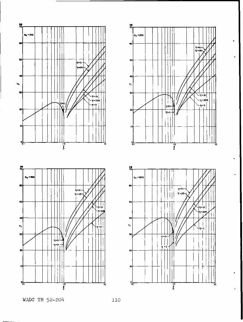
Os DO

0 200

7? -0.1I

-- 540 -

TL TL

30~ -600

0 - -06

WAD TRD 52-2040110

It seems plausible that such sudden changes of transmis-sivity with the angle of incidence will not really occurand the assumption that under the conditions of tracematching total transmissivity will be reached must beviolated; the conditions for trace matching must be alsoviolated if we take into account the finite length ofthe wall or any kind of losses either in the wall itselfor at its edges.

We can treat the inner losses by introducing acomplex Young's modulus instead of the usual real modulusE

E = E(l + ii) (11.2.59)

where V , the loss factor, characterizes the phase shiftbetween strain and stress and from experiment may beregarded as independent of frequency.

With this complex modulus the transmission impedance

becomes a complex quantity also, given by

Zt= ýBw3 sin 472'co4 + J[an - Bw3 sin4 ?-/co4].

(11.2.60)

Putting this into Eqs. (11.2.20) and (11.2.22a), we againmay find'm and finally TL. The results of this even moretroublesome calculation are given in Fig. 11.2.13 for thecase ofLc = 100, 200, 400 and 800 corresponding to [TLjoc= 40, 46, 52 and 58 db.

The behavior at high frequencies again may be under-stood by looking at the neighborhood of the peak only.Here first the peak itself is lowered to the value

m = i/[ + 1 - l/ ] 12. (11.2.61)

FIGURE 21.2.13TL vs. • for various values of OCc when innerlosses are introduced into the plate.

WADC TR 52-204 111

If we now write

(11.2.62)

and change 5 to

(1 + M /-42 l-1/e)

(11.2.63)

we get for high frequencies

T S r.-ir/[ 2 C~ j2 /1_1/4 + 2 )ýfl 2( 43_j2)]

(11.2.64)

or

[TL] =10 log [2 or 42 ,/¶i/ (1 + tl-1/o)/'r]

(11.2.65)

For th- , is identical to Eq. (11.2.58); fora z •v-1/e > 4, Eq. (11.2.65) becomes

[TL]=[TL]oc + 30 log(f/fc)-l0 log f/(f -f)-1o log (l/q2

(11.2.65a)

For a rough eva±uation, the third term may be neglected.Equation (11.2.65) also vanishes asymptotically but thefirst order theory of bending waves which have been usedis valid only as long as > B Ž6h. This will be the caseif 9 = 3.24 cL h/co AB <0 .5M C/Co; for concrete where cL=12,000 ft/sec, this means 9 < 5.2.

The most essential fact which may be seen fromFig. 11.2.13 is that the insulation power increases againin the region sufficiently far above fc* One of thephysical reasons for this behavior may easily be understoodby looking at the contours of Fig. 11.2.11. There the

WADC TR 52-20o4 112

"valley of trace matching" becomes smaller and smaller.This is connected with the fact that the "peaks" at bothsides become higher and higher but the latter alone wouldbe of less importance because the tops scarcely influencethe result. In the case of inner losses, the bottom ofthe valley increases in the region of higher frequencies.This general behavior is in agreement with experimentalresults, but the valley in the neighborhood of fc is notas deep and the slope above fc is not as large as wouldbe expected. Also the influence of damping, which shouldbe very high, has not yet been confirmed. It seems thatthe energy losses at the edges and the finite length ofthe wall are of more importance. This finite length hasto be compared with the wavelength of bending waves atthe critical frequency, which means the wavelength in airalso. This may be the reason why pronounced trace match-ing effects never have been found with thick, heavy walls,e.g. brick walls, where the critical frequency is below100 cps. Here the wavelength at 11 ft is of the sameorder of magnitude as the length and breadth of the wall.

Generally speaking, we may avoid the trace matchingeffects by either use of very thick and stiff walls or byuse of walls which have small stiffness, but not toosmall a mass. For homogeneous plates this is a questionof thickness. For example, we may say that walls ofporous concrete of thickness from 1 in. to 3 in. aredangerous since the critical frequency is in the middle audiorange. Also for wooden plates of common thicknesses thecritical frequencies are in the region of interest.Fig. 11.2.14 shows the measured TL for a plate of about5/8 in. thickness. By cutting grooves in the panel, thatis, by decreasing the stiffness without remarkably alter-ing the mass, it was possible to increase the criticalfrequency above the region of interest and so to improvethe insulation 2.

The decreasing of the stiffness not only increasesthe critical frequency, it also decreases the lowestnatural frequency, which is a further advantage. As maybe derived by comparing the formulas for the lowestnatural frequency for a bar or a plate only supportedat two opposite edges

f = (r/21 2 ) 7-M (11.2.66)

WADC TR 52-204 113

(following from Eqs. (11.2.33), (11.2.36), and (11.2.47),

fl fc = (c,/2 _)2 (11.2.67)

This is the square of the natural frequency of an openorgan pipe of the length I . Equation (11.2.62) may alsobe used to evaluate f experimentally by measuring f1 "

Another possibility for evaluating f. is by measur-ing the static sag 9 max due to its weight of a bar or plateof length I supported at the ends. This is proportionalto the surface mass and inversely proportional to thebending stiffness

ý max = 5 mg - 4/384B (11.2.68)

where g is the acceleration of gravity. Combining thiswith Eq. (11.2.47), we find

fc = 385 co2 (./lOr _Q2 g

(11.2.69)

or since c and g are given constants

= 90000 (11.2.70)

where C max is given in inches and I in feet. This equationis of special interest because it shows that a plate sup-ported at 6 ft intervals should have a sag of at least2.5 in. if the critical frequency shall be above 4000 cps.Certainly slich plates could never be loaded. But in allcases where plates which are not too heavy are to beinstalled for noise abatement only, this rule should beobserved as far as possible.

WADC TR 52-204 114

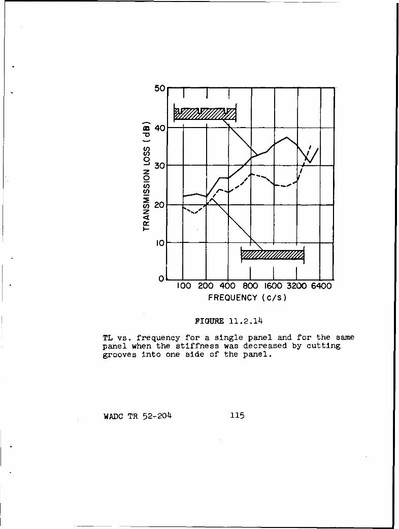
50-

m 40

30z0

U,

"D1

c o 20-

I.--Szo

0

100 200 400 800 1600 3200 6400FREQUENCY (c/s)

FIGURE l1.. 2.14

TL vs. frequency for a single panel and for the samepanel when the stiffness was decreased by cuttinggrooves into one side of the panel.

WADC TR 52-204 115

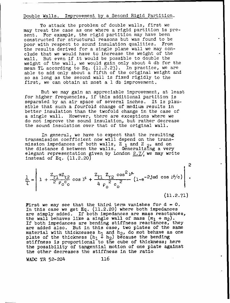
Double Walls. Improvement by a Second Rigid Partition.

To attack the problem of double walls, first wemay treat the case as one where a rigid partition is pre-sent. For example, the rigid partition may have beenconstructed for structural reasons but was found to bepoor with respect to sound insulation qualities. Fromthe results derived for a single plane wall we may con-clude that we would have to increase the weight of thewall. But even if it would be possible to double theweight of the wall, we would gain only about 4 db for themean TL according to Eq. (11.2.23). In practice, we areable to add only about a fifth of the original weight andso as long as the second wall is fixed rigidly to thefirst, we can obtain at most a 1 db improvement.

But we may gain an appreciable improvement, at leastfor higher frequencies, if this additional partition isseparated by an air space of several inches. It is plau-sible that such a fourfold change of medium results inbetter insulation than the twofold change in the case ofa single wall. However, there are exceptions where wedo not improve the sound insulation, but rather decreasethe sound insulation over that of the original wall.

In general, we have to expect that the resultingtransmission coefficient now will depend on the trans-mission impedances of both walls, Z 1 and Z 2 ,and onthe distance d between the walls. Generalizing a veryelegant representation given by London . we may write

instead of Eq. (11.2.20)

2

1 1+ S t 2 cs 2 + zInzC 2 C 2 go-e-22 p0c0 2 2 0 2

(11.2.71)

First we may see that the third term vanishes for d = 0.In this case we get Eq. (11.2.20) where both impedancesare simply added. If both impedances are mass reactances,the wall behaves like a single wall of mass (mi + m2 ).If both impedances are bending stiffness reactances, theyare added also. But in this case, two plates of the samematerial with thicknesses hl and h 2 , do not behave as oneplate of the thickness (hl + h 2 ) because the bendingstiffness is proportional to the cube of thickness; herethe possibility of tangential motion of one plate againstthe other decreases the stiffness in the ratio

WADC TR 52-204 116

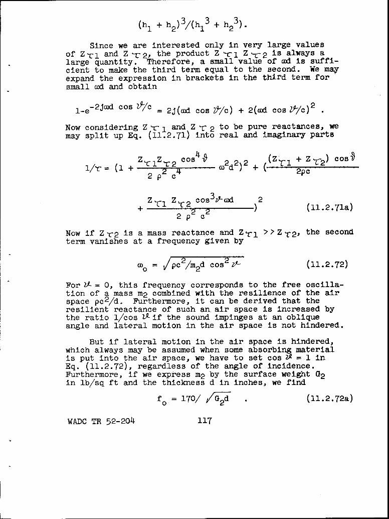
(h1 + h 2 )3/(h, 3 + h23).

Since we are interested only in very large valuesof Z -1 and Z -rc2, the product Z -Cl1 Z '-C2 is always alarge quantity. Therefore, a small value of cad is suffi-cient to make the third term equal to the second. We mayexpand the expression in brackets in the third term forsmall oa1 and obtain

l-e-2Jwd cos Z?/c = 2J(wd cos Z0/c) + 2(cid cos 2*/c) 2

Now considering Z 'c 1 and Z - 2 to be pure reactances, wemay split up Eq. (11.2.71) into real and imaginary parts

z 1z 2 cos 222 + ((Zrl + zV 2 ) cos2 p24 2..C2p c

Z+Ci Z coZ3-- d 2""2p2 ) (11.2.71a)

Now if Z r2 is a mass reactance and Z-C 1 >"Z - 2, the secondterm vanishes at a frequency given by

= /pcm 2d cos2 ZA- (11.2.72)

For 2- = 0, this frequency corresponds to the free oscilla-tion of a mass m2 combined with the resilience of the airspace pc 2/d. Furthermore, it can be derived that theresilient reactance of such an air space is increased bythe ratio 1/cos L2-if the sound impinges at an obliqueangle and lateral motion in the air space is not hindered.

But if lateral motion in the air space is hindered,which always may be assumed when some absorbing materialis put into the air space, we have to set cos a = 1 inEq. (11.2.72), regardless of the angle of incidence.Furthermore, if we express m2 by the surface weight G2in lb/sq ft and the thickness d in inches, we find

fo.= 170/ G2d . (11.2.72a)

WADC TR 52-204 117

If both reactances can be assumed to be pure massreactances and the surface weight of the first wall G,is not much greater than G2, we have to substitute forG2 the "resultant surface weight"

Gres = GG 2/(G + G2 ) . (11.2.72b)

In this case, both masses oscillate out of phase withthe ratio of the amplitudes of oscillation inverselyproportional to the ratio of the weights. At this 'zeromode" frequency of the double wall, the transmission lossis very small; for two equal mass reactances the TL maybe zero. In the neighborhood of this frequency, thedouble wall is worse than a single wall even of the weightof the heavier partition only. Thus the second partitionhas not improved the sound insulation.

The first step in calculating a double wall construc-tion is to make the product of G2 d or Gresd so large thatfo is below the region in which we are interested. Inmost practical cases, it will be sufficient to choosefo < 54 cps; this means that we have to make

G2 d > 10 lb in./sq ft . (11.2.73)

The only way to save weight is to enlarge the distance d,and even this holds only if d is not too large, as wewill see later.

One octave above fo, the second term in Eq. (ll.2.71a),is very much greater than the first. Comparing the cor-responding TL with that given by a wall of Z'1 l only, wefind that the improvement of transmission loss is

A [TLI = 20 log (w2 dm2 cos 2Y/pc 2 ) = 40 log (./c%)

(11.2.74)

If the lateral motion in the air space is hindered, wemay replace w0 by woo; the improvement of TL becomes then

A [TLI = 40 log (f/f 0 0 ) . (11.2.74a)

This very simple formula allows a rough evaluation of theslope of TL vs frequency in the region of f/f00 from one

WADC TR 52-204 118

to two and sometimes to even three octaves above foolBut then the slope of TL, which would be 18 db/octaveif both walls follow the mass law, decreases. One ofthe reasons may be se#e from Eq. (11.2.71). The expres-sion (1-e-2Jwd cos ?-/cJ only increases with frequency forsmall wxd, but it is never greater than 2. This highestvalue occurs at

f(2n + i),Z= (2ncos +)-

(11.2.75)

or when lateral motion in the air space is hindered, at

f(2n + 1),0 = (2n + 1) c/4d (11.2'.75a)

The corresponding highest values of the improvement inTL are given by

A [TL] = 20 log(wn 2/poc) cos 2A. (11.2.76)

This improvement is 6 db higher than the TL we wouldexpect from the second wall alone. The straight linesgiven by Eqs. (11.2.74a) and (11.2.76), the latter calcu-lated for ZR-= 450, may be used as upper limits for theimprovement by a second partition.

But we have to expect that between the frequenciesof maximum transmission loss, given by Eq. (11.2.75),there are always frequencies at which the transmissionloss is very small, or even zero for two identicalpartitions. For Z ' 1 >Z m i2' these frequencies are givenby

fn = nc(l + pd/v2n 2 m2 )/2d cos ZA (11.2.77)

or approximately

f = nc/2d cos -. (11.2.77a)

WADC TR 52-204 119

The difference between Eqs. (11.2.77) and (11.2.77a) isof interest only if the minimum transmission coefficientmust be calculated. Equation (11.2.77a) is true whenthe sound pressure in the air space at the opposite pointsof the walls is either in phase or 1800 out of phase.For Z• = 0, the condition becomes

fn = nc/2d (11.2.77b)

which is the well known formula for the eigenfrequenciesof one dimensional sound motion between parallel rigidwalls. Therefore we may call the fn the resonance fre-quencies of the air space and fo the resonance frequencyof the double wall.

With increasing separation of the two partitions,the lowest of these resonance frequencies decreases.This is the reason why increasing this distance may notalways be helpful. If, for example, we want to avoidthe case where f, becomes smaller than about 1000 cps,we should keep

d z_ 7 in. (11.2.78)

Again Eq. (11.2.77b) has to be used instead ofEq. (11.2.77a) if the lateral coupling in the air spaceis hindered. If this is done by a porous material, thedifference between minima and maxima of TL in thisfrequency region will decrease.

Influence of Absorbing Material in the Air Space.

As has been shown by London, in most cases we wouldnot expect any improvement in sound insulation by anadditional partition without introducing any absorptionThe reason is that for each frequency above fno, (n + I)angles of incidence exist for which total transmissionoccurs. By averaging over all angles, the sound trans-mission in the neighborhood of these angles predominatesand results in an average transmission coefficient thatis higher than that for the single wall. This may besubstantiated in a manner similar to that shown for theproblem of transmissivity in the case of trace matching.As in that case, it may be shown that the results forthe average transmission coefficient are influencedstrongly by any kind of energy losses.

WADC TR 52-204 120

To get agreement between the experimental dataobtained with reverberant rooms and theoretical calcu-lations, London introduced external friction terms inthe impedances of the partition walls which he assumedto be inversely proportional to cos 2.. There is nophysical evidence for such resistance terms and, there-fore, the physical properties of walls offer no data forthe evaluation of these resistances.

Another possible way to introduce energy lossesis by means of a complex Young's modulus, as was done inthe case of trace matching effects. But here also anadequate value of the loss factor can only be found byexperiment and must be assigned a much higher value thanthe loss factor corresponding to the material alone.

The only kind of energy losses which we are ableto calculate from measurable physical data are thosewhich occur when the space between double walls is filledwith porous material. The theory of those materials hasbeen developed to such a degree (see Sec. 12.1) thatsufficient agreement between theory and experiment hasbeen achieved. We are interested only in porous materialsthat do not make an elastic connection between the wallsby virtue of their skeleton. Under this assumption, weneed only two quantities to characterize the porous ma-terial. The first is the propagation coefficient forpropagation perpendicular to the walls inside the porousmaterial, which is assumed to be a complex quantity

kx = kx - J gx (11.2.79)

The second is the characteristic impedance of the porousmaterial, which is defined by the ratio of sound pressureto the component of the velocity perpendicular to the wallsfor a propagating wave

A

This also is a complex quantity. With these definitions,we find for the transmission coefficient

WADC TR 52-204 121

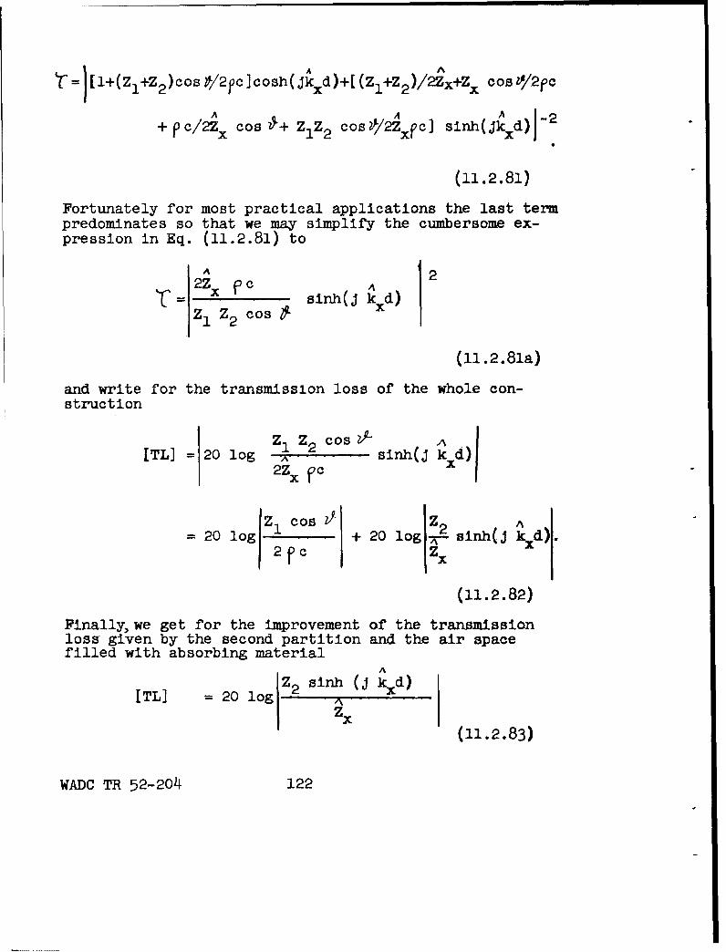
"C: =I[ '+(Zl+z2)°o COS • ]oh d)+[: (zl+Z2)/ ,+xco /oA A

+ Pc/2x cos §+ ZlZ2 cosA/Axfc] sinh(jkxd)1-2

(11.2.81)

Fortunately for most practical applications the last termpredominates so that we may simplify the cumbersome ex-pression in Eq. (11.2.81) to

A 22Zx P A-- 12 o sinh(j k xd)ZI z2 cos

(11.2.81a)

and write for the transmission loss of the whole con-struction

zI z 2 cos zf-[TL•] = 20 log 2 sinh(J k

2Zx vc

= 20 log z2 co.. + 20 log e-si(J kd).

(11.2.82)

Finally, we get for the improvement of the transmissionloss given by the second partition and the air spacefilled with absorbing material

A

z2 sinh (j kxd)[TL] = 20 log A

zx(11.2.83)

WADC TR 52-204 122

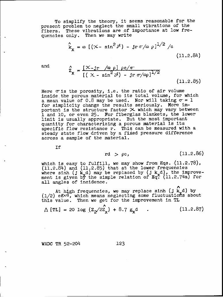
To simplify the theory, it seems reasonable for thepresent problem to neglect the small vibrations of thefibers. These vibrations are of importance at low fre-quencies only. Then we may write

A

k= [(c - sin 2') - Jrc/o p]1/2 /c

(11.2.84)

and A i-Jr /• p] pc/o-x X [ - sin2'9) - jr -/wpJii2

(11.2.85)

Here 0-is the porosity, i.e. the ratio of air volumeinside the porous material to its total volume, for whicha mean value of 0.8 may be used. Nor will taking a-= 1for simplicity change the results seriously. More im-portant is the structure factor X which may vary between1 and 10, or even 25. For fiberglas blankets, the lowerlimit is usually appropriate. But the most importantquantity for characterizing a porous material is itsspecific flow resistance r. This can be measured with asteady state flow driven by a fixed pressure differenceacross a sample of the material.

Ifrd > pc, (11.2.86)

which is easy to fulfill, we may show from Eqs. (11.2.78),(11.2.84) and (11.2.85) that at the lower frequencieswhere sinh (j k d) may be replaced by (j k d), the improve-ment is given bý the simple relation of Eq'. (11.2.74a) forall angles of incidence.

A

At high frequencies, we may replace sinh (j k d) by(1/2) egxd, which means neglecting some fluctuations aboutthis value. Then we get for the improvement in TL

A

A [TL] = 20 log (Z/2Zx) + 8.7 gxd • (11.2.87)

WADC TR 52-204 123

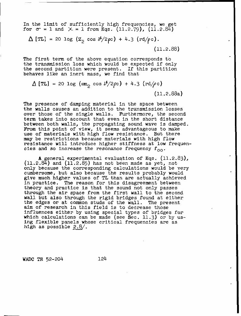
In the limit of sufficiently high frequencies, we get

for C- = 1 and -X = 1 from Eqs. (11.2.79), (11.2.84)

A [TL] = 20 log (Z 2 cos 2)/2ec) + 4.3 (rd/ec).

(11.2.88)

The first term of the above equation corresponds tothe transmission loss which would be expected if onlythe second partition were present. If this partitionbehaves like an inert mass, we find that

A [TL] = 20 log (an cos 2J/2pc) + 4.3 (rd/-c)

(ll.2.88a)

The presence of damping material in the space betweenthe walls causes an addition to the transmission lossesover those of the single walls. Furthermore, the secondterm takes into account that even in the short distancebetween both walls, the propagating sound wave is damped.From this point of view, it seems advantageous to makeuse of materials with high flow resistance. But theremay be restrictions because materials with high flowresistance will introduce higher stiffness at low frequen-cies and so increase the resonance frequency fool

A general experimental evaluation of Eqs. (11.2.83),(11.2.84) and (11.2.85) has not been made as yet, notonly because the corresponding calculations would be verycumbersome, but also because the results probably wouldgive much higher values of TL than are actually achievedin practice. The reason for this disagreement betweentheory and practice is that the sound not only passesthrough the air space from the first wall to the secondwall but also through the rigid bridges found at eitherthe edges or at common studs of the wAll. The presentaim of research in this field is to decrease thoseinfluences either by using special types of bridges forwhich calculations can be made (see Sec. 11.3) or by us-ing flexible panels whose critical frequencies are ashigh as possible 3.8/.

WADC TR 52-204 124

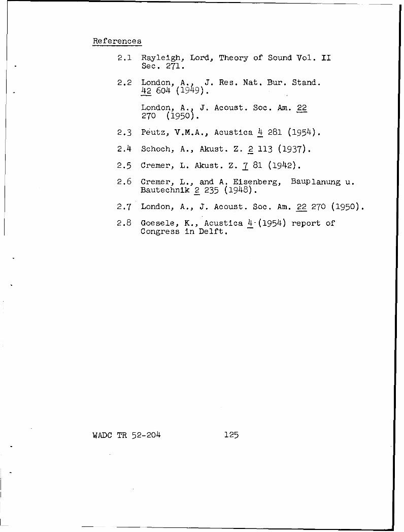
References

2.1 Rayleigh, Lord, Theory of Sound Vol. IISec. 271.

2.2 London, A. J. Res. Nat. Bur. Stand.42 6o4 (19)

London, A. J. Acoust. Soc. Am. 22270 (1950).

2.3 Peutz, V.M.A., Acustica 4 281 (1954).

2.4 Schoch, A., Akust. Z. 2 113 (1937).

2.5 Cremer, L. Akust. Z. 7 81 (1942).

2.6 Cremer, L., and A. Eisenberg, Bauplanung u.Bautechnik 2 235 (1948).

2.7 London, A., J. Acoust. Soc. Am. 22 270 (1950).

2.8 Goesele, K., Acustica 4-(1954) report ofCongress in Delft.

WADC TR 52-204 125

11.3 Insulation of Impact Sound

Excitation of Impact Sound. In the discussion ofthe insulation of airborne sound in the previous section,we had to deal with structure-borne sound problems be-cause every airborne sound will be transformed intostructure-borne sound if it impinges on a structural ele-ment. But structure-borne sound may also be exciteddirectly. This is the case, for example, if any vibratingapparatus is mounted on a wall. Also, a very common typeof direct excitation of structure-borne sound is the impactof rigid bodies against a rod or a plate.

The chief difference between the excitation by airsound pressures and by forces transferred by rigid bodiesis a difference in the extent of the area over which thedriving force is applied. In the last case, we may regardthis area as being concentrated at a point. Therefore,we are interested in knowing the reaction of the drivencontinuum to a "point source". In other words we areinterested in the mechanical point impedance, i.e., theratio of an alternating driving force to the resultantalternating velocity.

For a rod infinite in one direction and set inlongitudinal vibrations at the free end this mechanicalimpedance is

ZL = A Vr-E-= m cL . (11.3.1)

Here A is the area of the cross section, p the density,E Young's modulus of the material, m the mass per unitlength and cL the velocity of longitudinal waves in themedium composing the bar. In this case, the input imped-ance, which also is equal to the characteristic impedanceof a progressive longitudinal wave in the rod, is realand, therefore, independent of frequency.

But if the force is acting transversely at the freeend of the infinite rod, the impedance becomes complex,it being given by

ZB = m3 B Jw/2 = (1 + J) mcB/2 (11.3.2)

WADC TR 52-204 127

where B is the stiffness against bending and cB thephase velocity of bending waves; see Eqs. (11.2.37and (11.2.38). The input impedance is complexbecause in addition to a progressive ending wave aquasi-stationary motion which dies away exponentiallywith increasing distance from the source is excited.The general differential equation for bending waves ina rod

d4v 2B--=mUv (11.3.3)

is of the fourth order. This equation allows wavemotions,

V = exp (t 1 kBx) (11.3.4a)

as well as motion of the quasi-stationary type,

v = exp (+ kBx) (11.3.4b)

where

B=B=V (11.3.5)

(See Eq. (11.2.36)). Usually both types of motions areneeded to fulfill the boundary conditions for the force F,moment of bending M, transverse velocity v and angular ve-locity w. A further consequence of the complex characterof this impedance is its dependence on frequency, whichis included in the dependence of the phase velocity ofbending waves on frequency.

If the transverse force is acting at any point ona rod that is infinite in both directions, the impedancehas the same character but four times the magnitude. Inthis case

zB= 2(1 + j) m cB . (11.3.6)

The most important point impedance is that of aninfinite plate driven by a transverse force. Since herealso bending vibrations are excited, a complex impedance

WADC TR 52-204 128

as in Eqs. (11.3.5) and (11.3.6) would be expected.In addition, the problem is more complicated due to itstwo dimensional character. Fortunately both complica-tions compensate for each other in the case of the pointimpedance. In this case it is real and independent offrequency and is given by

z = 8 mB (11.3.7)2

where m is the surface mass density in, say, gm/cm2. Fora homogeneous plate of thickness h, this formula may bewritten

2Z = 2.3 cLp h (11.3.7a)

Fig. 11.3.1 gives the values of ZB as a function ofthe thickness for homogeneous plates of steel, aluminum,concrete, asphalt and plywood. For the last three kindsof material, the values are mean values. The straightlines are drawn between the limits of thicknesses whichare of practical interest. It may be remarked that thevalues for Z vary over the very large range from 102 to100 kg/sec.

For large, thin, damped plates, the values given byEq. (11.3.7) are in fairly good agreement with measurements3.12 3.2, 3.3/. For thicker "plates" such as walls andceilings, important deviations must be expected 3.2, 3.3/.For this reason the line for concrete walls in Fig. 11.3.1is dotted and shows only the order of magnitude. Forcomparison with measurements, the assumptions of theEqs. (11.3.7) and (11.3.7a) must be considered. First,the plate is assumed to be infinite or at least large com-pared to the bending wave length. This fixes the limitof validity for low frequencies where the eigenfrequenciesare well separated. Here we have to expect large devia-tions because of resonance phenomena. On the other hand,the simple theory of bending only holds as long as thebending wave length is at least six times greater thanthe thickness. This fixes the limit of validity for highfrequencies. These limits have been given in Fig. 11.2.5.For the present problem this limit may be lowered furtherbecause of the point-concentration of the force. Forthicker plates, one must always take into account the localelasticity which diminishes the motion of the plate fromthat of the driving point.

WADC TR 52-204 129

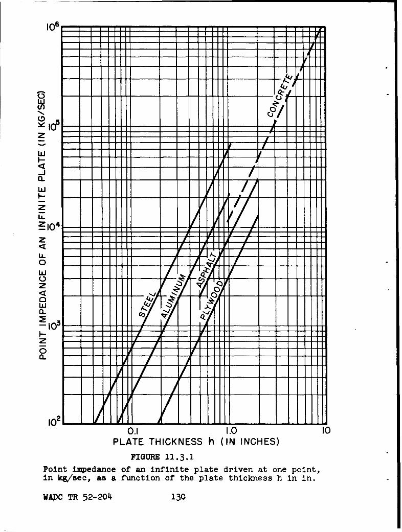
106

z

w

U-

z

a..

wz0

<,~awA.. -

a.'c--

102

0.1 1.0 10P LATE THICKNESS h (IN INCHES)

FIGURE 11 .3 .1Point impedance of an infinite plate driven at one point,in lcgjsec, as a function of the plate thickness h in in.

WADC TR 52-2o4 130

Finally, for all frequencies it is important thatthe plate be homogeneous. However, in many practicalcases this assumption is not valid. For example, some-times a plaster sheet is not in good contact with the wallto which it is attached. In such cases, especially if theconstruction is obviously inhomogeneous, it may be neces-sary to measure the impedance. Often it will be sufficientto know the absolute value of the impedance. This can bemeasured by exciting the plate with an electrodynamicsound source, with the moving coil fixed directly to thewall or ceiling. The magnet system should be connectedto the wall only by means of a resilient element. Thenthe same force (given by the magnetic field and the electriccurrent) acts on the mass reactance of the coil in serieswith the plate impedance and on the mass reactance of themagnet system. If now the same pick-up is used to measurefirst the velocity vl (or acceleration) of the plate andthen that of the magnet system v 2 we get

v2vl = (j ano + z)/jajn (11.3.8)

where M is the mass of the magnet system and mo the massof the moving coil.

From this we find for the absolute value of Z

Z = aonI v 2 /vI 1 1 (11.3.8a)

or if Z>anoZ = [()2 v /v 2 _ (o)12]I/2

(11.3.8b)

assuming that Z is real. In other cases, the phase anglebetween vI and v 2 must also be measured. One must besure that the magnet system behaves as a rigid body 3._/.If it does not, the force must be obtained from thecurrent in the coil and the absolute value of the velo-city must be measured L.21.

WADC TR 52-204 131

The Spectrum of Impact Sound. The knowledge of themechanical impedance has several advantages. For example,we may estimate whether or not a load will change thevibration of the body under test. We can calculate thevelocity which may be obtained using a sound source ofknown force and known internal impedance. Also, the caseof impact sound may be treated using the mechanical pointimpedance.

When a rigid body of the mass mo strikes a rod orplate with the velocity u 01 we get the same result as ifa force impulse (moUo) works on the mass reactance Janand the impedance of the rod or plate Z in series, pro-vided that the latter increases less rapidly with fre-quency than amno. In this case, the mass reactance Jmoinmay be regarded as the internal impedance of the source.Since the frequency components of the force impulse areall equal, namely mouo/i, we find for the correspondingcomponents of the velocity of the plate

u. =mou/r(Jaco + Z) (11.3.9)

if Z > Yano

uC mouIWZ (11.3.9a)

For thin, large and fairly well-damped plates, wemay take for Z the values given by Eq. (11.3.7) orFig. 11.3.1. In these cases, the mass reactance is greaterthan the wall impedance in the audio frequency region.The heavier the mass mO and, therefore, the lower the "cut-off" frequency given by the increasing mass reactance inseries with Z, the hollower the impact sounds. Also,this is in agreement with our experience that an impactsounds hollower, the thinner, lighter and more flexiblethe plate is.

For thick walls, Eq. (11.3.9) is no longer validbecause of the local elasticity around the point of impact.However, if we take into account a resilience K which forsimplicity is assumed to be linearly dependent on ampli-tude between the striking mass and the impedance of thewall calculated according to Eq. (11.3.7), the velocity

WADC TR 52-204 132

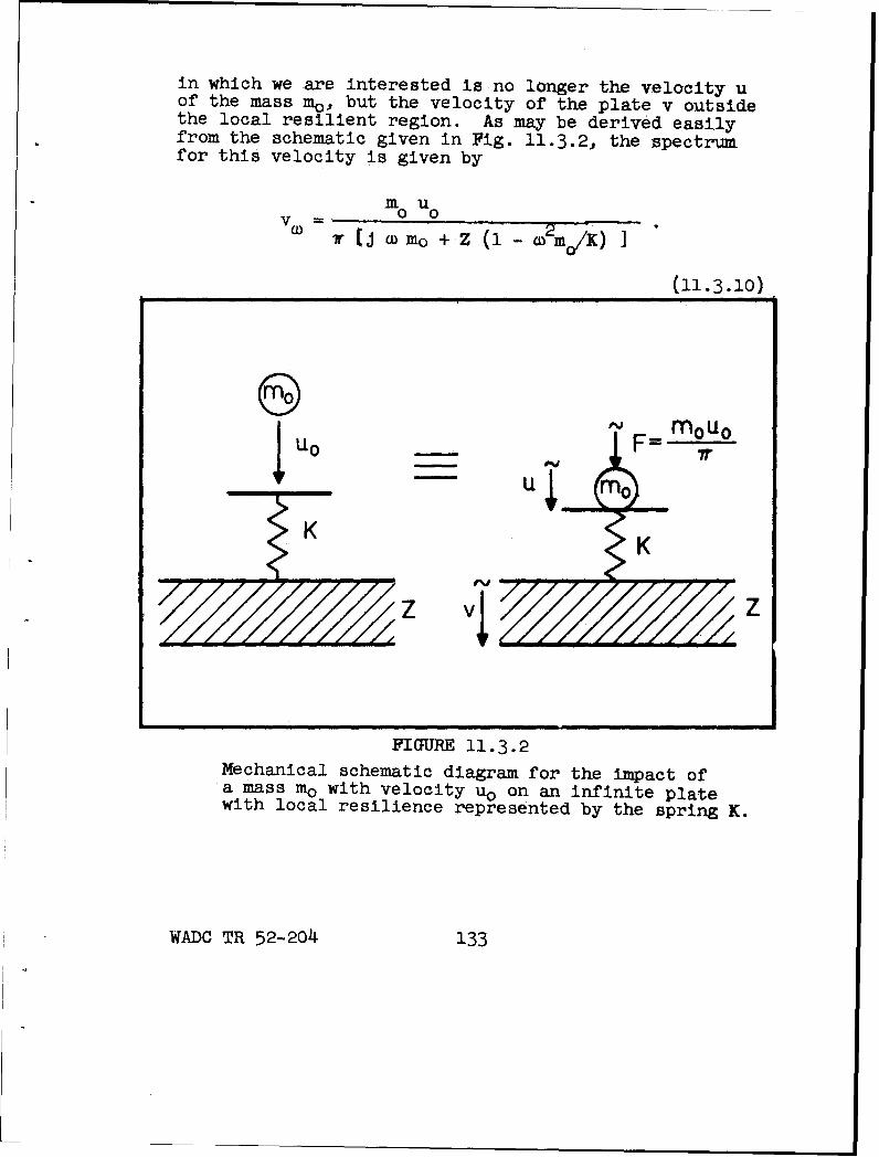
in which we are interested is no longer the velocity uof the mass to-, but the velocity of the plate v outsidethe local resilient region. As may be derived easilyfrom the schematic given in Fig. 11.3.2, the spectrumfor this velocity is given by

m uTF (J Wmo + Z (1 (0 mO/K)]

00I- F mu

K

FIGURE 11.3.2Mechanical schematic diagram for the impact ofa mass mo0 with velocity uo on an infinite platewith local resilience represented by the spring K.

WADC TR 52-204 133

In Fig. 11.3.3 the spectrum of v. is plotted for fixedvalues of mo and Z and different values of K. Sinceenergy losses are neglectedthe lack of high frequency com-ponents results in an emphasis of the lower frequencycomponents.

For comparison with measurements, it should be notedthat Eq. (11.3.10) assumes constant bandwidth. When usingoctave band filters or third-octave filters, the measuredresults must be reduced to equal bandwidth, i.e., themeasured amplitudes must be multiplied by w-1/2 .

In the routine technique of impact sound measurementsin buildings, instead of v the mean sound pressure in thereceiving room is measured. In this case the radiationpower of the wall or ceiling, which depends on the ratioof the frequency to the critical frequency (see Eq. 11.2.47)and the absorption power of the receiving room, enter intothe results.

Improvement With a Resilient Layer. In the lastsection we have introduced an unavoidable resilience Kbetween the striking mass m and the plate characterizedby Z. However, as we know from common experience withthick rugs, such an elastic layer is simple and effectiveas a remedy for impact noise.

The improvement of such a covering may be expressedby the difference of the sound pressure levels in thereceiving room measured with and without the covering.Since the absorption power and the radiating power of theceiling is not altered, the "improvement" may also beexpressed by the ratio of the corresponding velocitiesof the ceiling or wall at the place of impact

AL = 20 log (vl/v 2 ) . (11.3.11)

For not too high frequencies, we can use Eq. (I1.3.9a) that

V 1 = m0 Uo/WZ

WADC TR 52-204 134

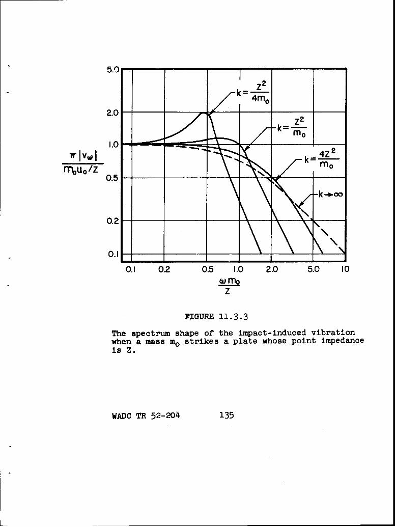
2.0-1

k= z2

2.0-4M

0.2-

0.1-- _

0.1 0.2 0.5 1.0 2.0 5.0 10

wMOz

FIGURE 11.3.3

The spectrum shape off the impact-induced vibrationwhen a mass mo strikes a plate whose point impedanceis Z.

WADC TR 52-204 135

and for not too low frequencies we get for the coveredceiling from Eq. (11.3.10)

v2 = Z Z

0

so that we find

A L = 40 log (w/c') = 40 log (f/f') (11.3.12)

where

f' (11.3.13)

is the eigenfrequency of the system consisting of thestriking mass mo and the stiffness K of the elastic layer.This stiffness is not only given by the properties of thelayer, but also depends on the compressed area, or in otherwords, the form of the striking body. Furthermore, inmost cases the area changes during the impact. Therefore,the linear resilience which has been assumed can beregarded only as a simple model. From this model we seethat the improvement depends not only on the kind ofcovering but also on the striking body, especially onits mass mo. As may be seen from Eqs. (11.3.12) and(11.3.13), the improvement increases with w.

The standardized European test technique for impactsound control uses a falling mass of 500 gm (1.15 lb).Compared to a person walking, this mass seems to be toosmall to represent step noise 3._/. However, step noiseis not the only kind of impact noise, In the case oflight switches, for example, the striking masses are muchsmaller, but the noise is still annoying.

It may be noticed that the improvement is independentof the impedance of the ceiling provided that it is suf-ficiently large and provided the local elasticity may beneglected. This is in agreement with measurements 3-/.

WADC TR 52-204 136

Improvement by a Floating Floor. Ideal Conditions.It is not always possible to cover a ceiling with onlya resilient layer. In addition, a durable finish isneeded. Covering the resilient layer with a rigid platenot only protects the layer, but it also has an acousticadvantage. We speak of a "floating floor" if the layeris highly resilient and the plate is stiff enough tobear the load of furniture and persons without too greata deformation.

In this case the improvement may be calculated.

The formula is similar to Eq. (11.3.12) 1./

An = 4o log (f/fl) . (11.3.14)

But now the reference frequency is the eigenfrequency ofthe system consisting of the surface mass unit area ofthe floating floor ml and the stiffness K1 per unit areaof the elastic layer. Thus,

f 1 (11.3.15)

Here the quantity K1 is well-defined. It consists of

two parts, K1' and KI" where

K1 = KI' + K1 " . (11.3.16)

K1' is the stiffness of the fibers of the layer whichholds the floor at the distance d from the ceiling

K1: = El/d (11.3.17)

and K " is the stiffness of the air enclosed between thefloating floor and the ceiling

K 1 = oc 2/crd. (11.3.18)

WADC TR 5 2-2o4 137

Here a-is the porosity of the fiber blanket and may beassumed to be nearly one. The elastic modulus E1 may beevaluated by measuring the eigenfrequency of a given masson a small portion of the blanket 11./. In this case theresilience of the air may be neglected since the air canescape laterally. But for an area of floating floorwhich is large compared to the wavelength of the soundfrequencies, the air under the floor must be compressed.Generally it is of no acoustic advantage to make theblanket more resilient than the air but it would be adisadvantage from the structural viewpoint.

If we assume K1 t_ K) = pPoc 2 /d, fl becomes equal tofo' defined by Eq. (ll.2.71a), i.e.

f1l = 170/ /Gld (11.3.19)

where GI is the surface weight density of the floatingfloor in lb/sq ft and d is the distance between the float-ing floor and the ceiling. This distance has to be mea-sured for the finished floor. It may be measured with apart of the blanket loaded by about 40 lb/sq ft, corres-ponding to the weight of floor and furniture.

It may be remarked that the improvement of the float-ing floor with respect to impact sound is the same as theimprovement with respect to airborne sound which was givenby Eq. (11.2.74). But it may be mentioned that the deri-vations of both formulae and the physical basis are quitedifferent. In one respect, however, we may make furtheruse of this analogy. For the airborne sound problems,we mentioned that for a wave at oblique incidence, lateralmotion in the air space is excited and results in ahigher stiffness. However, with a fiberglas blanket inthe air space, this motion is hindered and the stiffnessfor waves of perpendicular incidence is obtained for allangles of incidence. From this analogy, we can see thatin the case of impact sound also, the flow resistance ofthe blanket is effective in preventing lateral motion ofthe air. Hence an air space without a blanket has ahigher stiffness, thus gives a smoother improvement.

From Eq. (11.3.14), it is seen that the improvementof a floating floor is independent of the type of ceiling.This is also in agreement with measurements taken j/.

WADC TR 52-204 138

Furthermore, the improvement is independent of the strik-ing mass. However, this statement holds only as far asthe point impedance of the floating floor Z1 may be con-sidered as being large compared to the reactance of thefalling mass (wimo). For thin rigid coverings and highfrequencies, we have to add to Eq. (11.3.11) a second termto obtain for the improvement of the floating floor

L= 240 log (f/fl) + 10 log [1 + (2rfmIZl) 2 ]

(11.3.20)

As in the case of the improvement of airborne soundinsulation by a separated, second partition wall, Eqs.(ll.3.14)and (11.3.20) are valid only if they give values which arenot too high. However, the equations are useful for designbecause the frequency region where they are valid is the mostimportant region.

There are several reasons for the deviation ofexperimental results from Eq. (11.3.14). First, this for-mula is derived on the assumption of an infinite ceilingand a floating floor. Since the floating floor is care-fully separated from the side 3walls, there is total reflec-tion of bending waves at the sides. These reflecting waveswill also contribute to the mean sound pressure in thereceiving room. Furthermore, it seems that the tangentialmotion in the elastic layer cannot be prevented at higherfrequencies. But the most usual and dangerous deviationhappens if there are rigid connections between the float-ing floor and the ceiling, which may be called "sound-bridges."

Improvement by a Floating Floor. With Sound-Bridges.We now will consider the improvement of isolation by afloating floor and how it can be decreased if point "soundbridges are present 1./. Such more or less rigid bridgesmay not only occur as an error during the construction ofa floating floor, they may also be a result of the con-struction, as for example when the floor is laid oni'ubber mountings. In all these cases there are two ways.for the sound energy to pass from floor to ceiling. The

WADC TR 52-204 139

first is that over the air space inside the fiberglasblanket which is considered in Eq. (11.3.20). The secondis the path through the bridges. At high frequencies, theinternal impedance of the source (JOam) has to be con-sidered for both ways. Therefore, the second term ofEq. (11.3.20) remains unchanged.

Generally the expression for the improvement (actuallya deterioration by the bridges) may be written as

A L = - 10 l og (f l/ f ) + n LI k l A 12 2.

i-l

+ 10 log [1 + (2i fmo/Z9) 2 ]

(11.3.21)

Here ri is the distance between the place of impact andthe ith of the n bridges and k, is the propagation para-meter for a bending wave in the floating floor, which ingeneral is a complex quantity given by

kI = 2 (i - in/4)/h 1 (11.3.22)

Here A 1 is the length of the bending wave and n loss factorwhich has been introduced in Eq. (11.2.59) but which alsomay be defined by the measured attenuation per wave length.

The function 1T(klr) gives the ratio of the trans-verse velocity of the floor at a distance r which wouldbe present without the bridge to the velocity of the floorat the point of impact,

-f(klr) = v(r)/v(O) (11.3.23)

WADC TR 52-204 140

Therefore, in all cases we have

]-(O) = (11.3.23a)

For an infinite floating floor without damping,•-wouldincrease as k1r increases

-T (k1 r) = ý/2/r klr exp - J(klr - 'r/4)

or

I-TI2 = 2/ir k1r (11.3.23b)

But the assumption of an infinite size is not asvalid in the case of the floating floor as it is in the caseof the ceiling. The floating floor is carefully separatedfrom the wall so that the reflection of bending waves istotal. The energy losses only occur during the propagation.If these losses are high, as in asphalt floors, we mayneglect the reflections and set

M V 2 = (2/r k1 r) exp (-'YLklr/2) (11.3.23c)

If the loss factor is small, however, many reflectionsmust be taken into account. The resultant velocity willbe given by a statistical superposition of all the re-flected waves. In this case 11112 becomes

I iT1 = 4 ce1 hl/Sw Y (ll.3.23d)

where S is the surface area of the floating floor, cLC isthe velocity of propagation for longitudinal waves an h1the thickness of the floor.

The velocity at the distance rj, given by TMv(O), hasto be distinguished from the velocity vI which occurs ifa bridge is present, according to the formula

V, lv(O) - FI/Z1 (11.3.24)

WADC TR 52-204 141

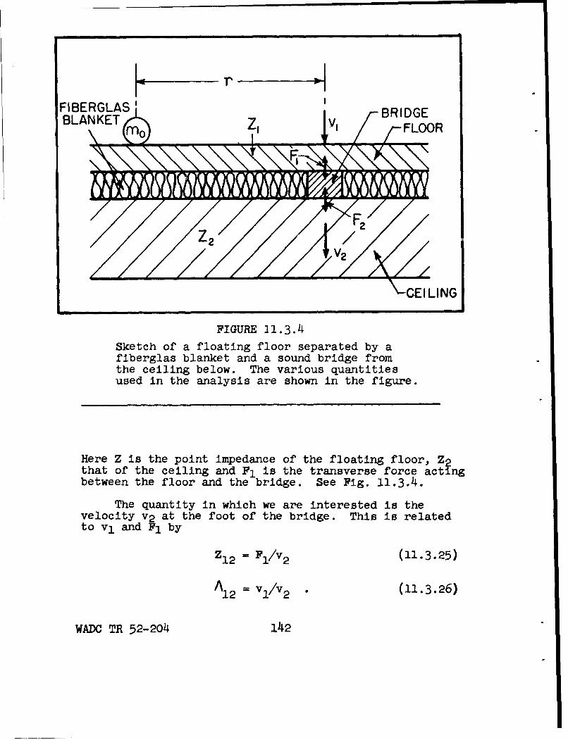
FIBERGLAS'BLANKET Z, T R FLOOR

,CEILING

FIGURE 31.3.4Sketch of a floating floor separated by afiberglas blanket and a sound bridge fromthe ceiling below. The various quantitiesused in the analysis are shown in the figure.

Here Z is the point impedance of the floating floor, Z2that of the ceiling and F1 is the transverse force actingbetween the floor and the bridge. See Fig. 11.3.4.

The quantity in which we are interested is thevelocity v 2 at the foot of the bridge. This is relatedto vy and Fl by

z12= Fl/v 2 (11.3.25)

A1 2 =V /V 2 (11.3.26)

WADO TR 52-204 142

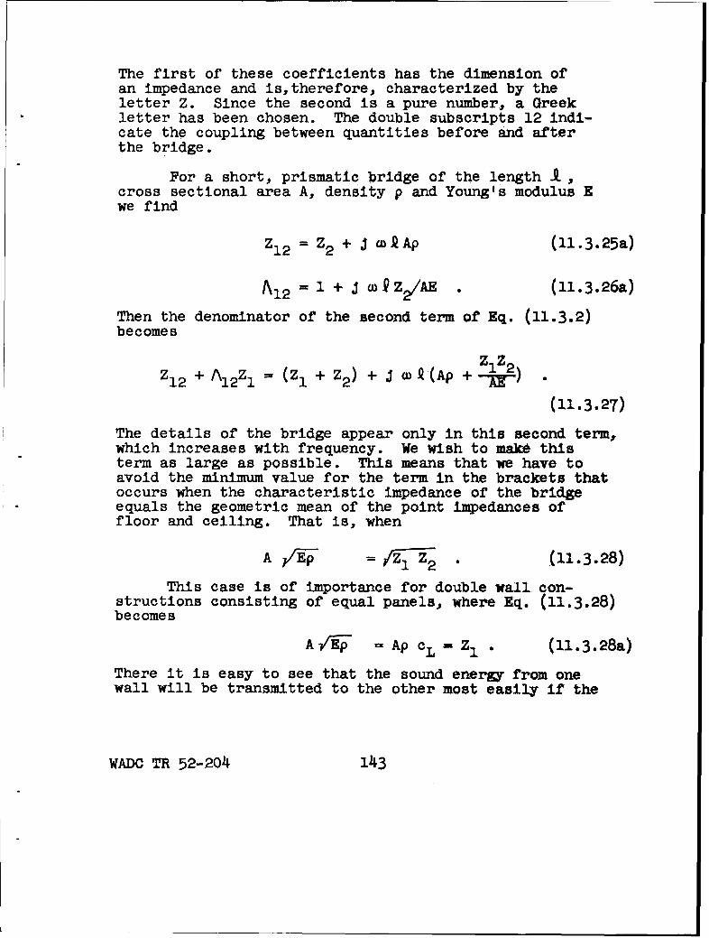
The first of these coefficients has the dimension ofan impedance and is,therefore, characterized by theletter Z. Since the second is a pure number, a Greekletter has been chosen. The double subscripts 12 indi-cate the coupling between quantities before and afterthe bridge.

For a short, prismatic bridge of the length i,cross sectional area A, density p and Young's modulus Ewe find

Z12 = 2 + J cc Ap (11.3.25a)

A12 - 1 + j D V Z2 /Al . (11.3.26a)

Then the denominator of the second term of Eq. (11.3.2)becomes

ZlZ2z1 2 +A12 Zl = (zI + z2 ) + j w•(Ap +-A-E-)

(11.3.27)

The details of the bridge appear only in this second term,which increases with frequency. We wish to make thisterm as large as possible. This means that we have toavoid the minimum value for the term in the brackets thatoccurs when the characteristic impedance of the bridgeequals the geometric mean of the point impedances offloor and ceiling. That is, when

A IR. . (11.3.28)

This case is of importance for double wall con-structions consisting of equal panels, where Eq. (11.3.28)becomes

A V = Ap cL = Z. (I1.3,28a)

There it is easy to see that the sound energy from onewall will be transmitted to the other most easily if the

WADC TR 52-204 143

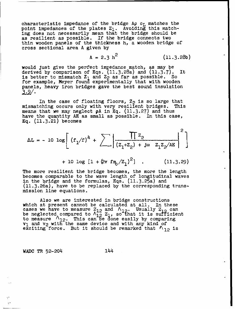
characteristic impedance of the bridge Ap cL matches thepoint impedances of the plates Z1 . Avoiding this match-ing does not necessarily mean that the bridge should beas resilient as possible. If the bridge connects twothin wooden panels of the thickness h, a wooden bridge ofcross sectional area A given by

A = 2.3 h 2 (11.3.28b)

would Just give the perfect impedance match, as may bederived by comparison of Eqs. (11.3.28a) and (11.3.7). Itis better to mismatch Z1 and Z2 as far as possible. Sofor example, Meyer found experimentally that with woodenpanels, heavy iron bridges gave the best sound insulation

In the case of floating floors, Z2 is so large thatmismatching occurs only with very resilient bridges. Thismeans that we may neglect pA in Eq. (11.3.27) and thushave the quantity AE as small as possible. In this case,Eq. (11.3.21) becomes

2.

AL - 10 log [ (f1 /f)14 +T 2 1 ( + Z2) J 2~,A

L I(Zl1+Z 2) + wZ lZ2 /AE

+ 10 log [I + (2r fmo/Zl) 2 ] (11.3.29)

The more resilient the bridge becomes, the more the lengthbecomes comparable to the wave length of longitudinal wavesin the bridge and the formulas, Eqs. (11.3.25a) and(11.3.26a), have to be replaced by the corresponding trans-mission line equations.

Also we are interested in bridge constructionswhich at present cannot be calculated at all. In thesecases we have to measure Z12 and A1 o. Usually Z canbe neglected compared to A1 2 Zl, so hat it is su.iicientto measure A1 2 . This can be done easily by comparingvI and v 2 with the same device and with any kind ofexciting force. But it should be remarked that A12 is

WADC TR 52-2o4 144

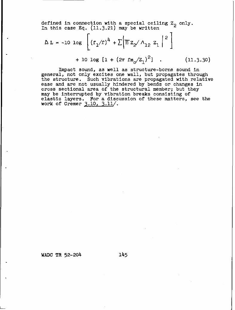
defined in connection with a special ceiling Z2 only.

In this case Eq. (11.3.21) may be written

L= -10 log [(fl/f) 4 + Z/Z /A 1 2 Z1 12

+ 10 log [l + (2r fm/Zl) 2 ] (11.3.30)

Impact sound, as well as structure-borne sound ingeneral, not only excites one wall, but propagates throughthe structure. Such vibrations are propagated with relativeease and are not usually hindered by bends or changes incross sectional area of the structural member; but theymay be interrupted by vibration breaks consisting ofelastic layers. For a discussion of these matters, see thework of Cremer 3.10,.3.11/.

WADC TR 52-20o 145

References

3.1 Cremer, L., Tekn. Tidskr. 80 393 (1950)

3.2 Elling, W., Acustica 4 396 (1954)

3.3 Heckl, M., Acustica 4 (1954) (to be published)

3.4 Gosele, K., Gesundheitsingenieur y 66 (1949)

3.5 Gosele, K., Gesundheitsingenieur 72, (1951)

3.6 Cremer, L., Acustica 2 762 (1952)

3.7 Gosele, K., and W. Bach (to be published)

3.8 Cremer, L., Acustica 4 273 (1954)

3.9 Meyer, E., Akust. Z. 2 74 (1932)

3.10 Cremer, L., Acustica 3 317-335 (1953)

3.11 Cremer, L., "Propagation of Structure-BorneSound" Sponsored Research in Germany,Report #1, Series B Dept. of Scientificand Industrial Research

WADC TR 52-204 146

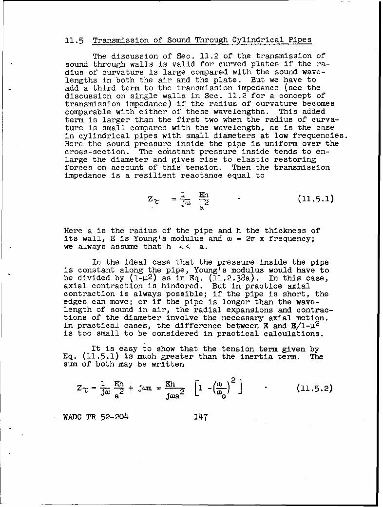
11.5 Transmission of Sound Through Cylindrical Pipes

The discussion of Sec. 11.2 of the transmission ofsound through walls is valid for curved plates if the ra-dius of curvature is large compared with the sound wave-lengths in both the air and the plate. But we have toadd a third term to the transmission impedance (see thediscussion on single walls in Sec. 11.2 for a concept oftransmission impedance) if the radius of curvature becomescomparable with either of these wavelengths. This addedterm is larger than the first two when the radius of curva-ture is small compared with the wavelength, as is the casein cylindrical pipes with small diameters at low frequencies.Here the sound pressure inside the pipe is uniform over thecross-section. The constant pressure inside tends to en-large the diameter and gives rise to elastic restoringforces on account of this tension. Then the transmissionimpedance is a resilient reactance equal to

z- Eh (11.5.1)a

Here a is the radius of the pipe and h the thickness ofits wall, E is Young's modulus and m = 2r x frequency;we always assume that h << a.

In the ideal case that the pressure inside the pipeis constant along the pipe, Young's modulus would have tobe divided by (1-p. 2 ) as in Eq. (11.2.38a). In this case,axial contraction is hindered. But in practice axialcontraction is always possible; if the pipe is short, theedges can move; or if the pipe is longer than the wave-length of sound in air, the radial expansions and contrac-tions of the diameter involve the necessary axial motion.In practical cases, the difference between E and E/1-p. 2

is too small to be considered in practical calculations.

It is easy to show that the tension term given byEq. (11.5.1) is much greater than the inertia term. Thesum of both may be written

_1 Eh Eh 1 () 2 ]Z- -- + jCM2 -N (11.5.2)

Mea jT-a L1

WA.DC TR 52-2o4 14

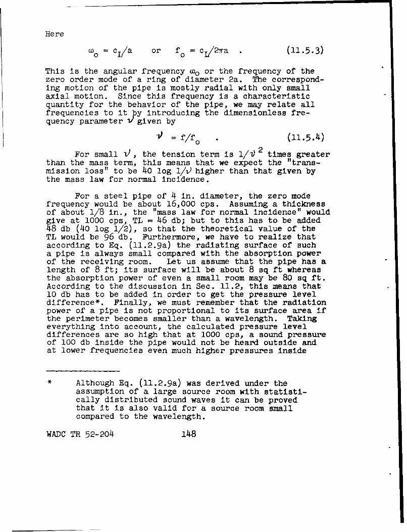
Here

Wo = ca or fo = cI2wa . (11.5.3)

This is the angular frequency coo or the frequency of thezero order mode of a ring of diameter 2a. The correspond-ing motion of the pipe is mostly radial with only smallaxial motion. Since this frequency is a characteristicquantity for the behavior of the pipe, we may relate allfrequencies to it Py introducing the dimensionless fre-quency parameter V given by

9 = f/f o (11.5.4)

For small 1), the tension term is 1/)2 times greaterthan the mass term, this means that we expect the "trans-mission loss" to be 40 log 1/7) higher than that given bythe mass law for normal incidence.

For a steel pipe of 4 in. diameter, the zero modefrequency would be about 16,000 cps. Assuming a thicknessof about 1/8 in., the "mass law for normal incidence" wouldive at 1000 cps, TL = 46 db; but to this has to be added8 db (40 log 1/2), so that the theoretical value of the

TL would be 96 db. Furthermore, we have to realize thataccording to Eq. (11.2.9a) the radiating surface of sucha pipe is always small compared with the absorption powerof the receiving room. Let us assume that the pipe has alength of 8 ft; its surface will be about 8 sq ft whereasthe absorption power of even a small room may be 80 sq ft.According to the discussion in Sec. 11.2, this means that10 db has to be added in order to get the pressure leveldifference*. Finally, we must remember that the radiationpower of a pipe is not proportional to its surface area ifthe perimeter becomes smaller than a wavelength. Takingeverything into account, the calculated pressure leveldifferences are so high that at 1000 cps, a sound pressureof 100 db inside the pipe would not be heard outside andat lower frequencies even much higher pressures inside

• Although Eq. (ll.2.9a) was derived under the

assumption of a large source room with statisti-cally distributed sound waves it can be provedthat it is also valid for a source room smallcompared to the wavelength.

WADC TR 52-204 148

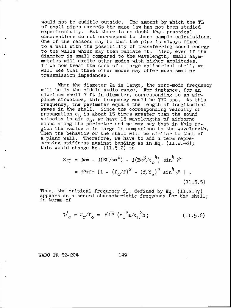
would not be audible outside. The amount by which the TLof small pipes exceeds the mass law has not been studiedexperimentally. But there is no doubt that practicalobservations do not correspond to these sample calculations.One of the reasons may be that the pipe is always fixedto a wall with the possibility of transferring sound energyto the walls which may then radiate it. Also, even if thediameter is small compared to the wavelength, small asym-metries will excite other modes with higher amplitudes.If we now treat the case of a large cylindrical shell, wewill see that these other modes may offer much smallertransmission impedances.

When the diameter 2a is large, the zero-mode frequencywill be in the middle audio range. For instance, for analuminum shell 7 ft in diameter, corresponding to an air-plane structure, this frequency would be 770 cps. At thisfrequency, the perimeter equals the length of longitudinalwaves in the shell. Since the corresponding velocity ofpropagation c1 is about 15 times greater than the soundvelocity in aIr co, we have 15 wavelengths of airbornesound along the perimeter and we may say that in this re-gion the radius a is large in comparison to the wavelength.Then the behavior of the shell will be similar to that ofa plane wall. Therefore, we have to add a term repre-senting stiffness against bending as in Eq. (11.2.48);this would change Eq. (11.5.2) to

Z-r = Jom - J(Eh/a 2) - J(B3/cCo 4 ) sin4

= J2wfm [1 _ (f/f)2 _ (ff c)2 sin24 ]

(11.5.5)

Thus, the critical frequency fc, defined by Eq. (11.2.47)appears as a second characteristic frequency for the shell;in terms of

Vc = fclfo = -2 (co 2a/CL 2h) (11.5.6)

WADC TR 52-204 149

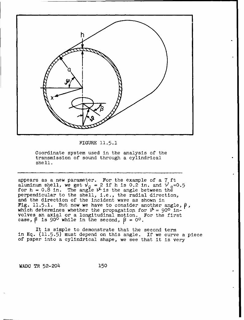
FIGURE 11.5.1

Coordinate system used in the analysis of thetransmission of sound through a cylindricalshell.

appears as a new parameter. For the example of a 7 ftaluminum shell, we get - = 2 if h is 0.2 in. and V c= 0 . 5

for h = 0.8 in. The angie 7-is the angle between theperpendicular to the shell, i.e., the radial direction,and the direction of the incident wave as shown inFig. 11.5.1. But now we have to consider another angle, P.,which determines whether the propagatiop for 2ý-= 900 in-volves an axial or a longitudinal motion. For the firstcase, P is 900 while in the second, P = 00.

It is simple to demonstrate that the second termin Eq. (11.5.5) must depend on this angle. If we curve a pieceof paper into a cylindrical shape, we see that it is very

WADC TR 52-204 150

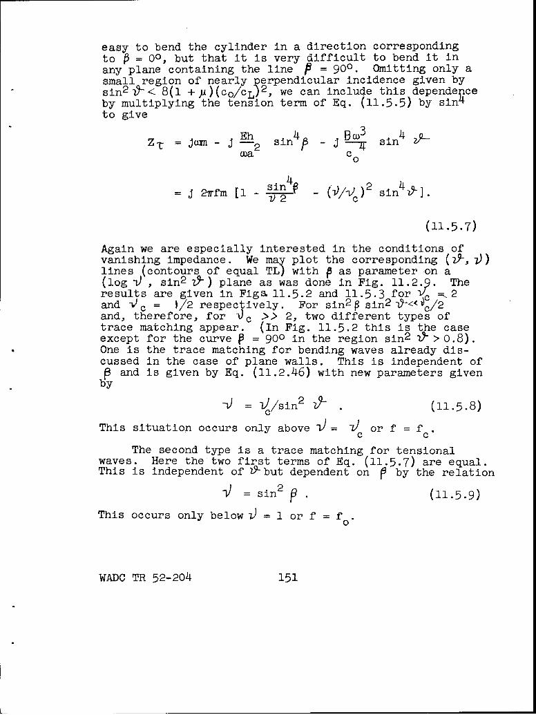
easy to bend the cylinder in a direction correspondingto A = 00, but that it is very difficult to bend it inany plane containing the line P = 900. Omitting only asmall region of nearly perpendicular incidence given bysin2 -z< 8(1 +yu)(co/CL) 2 , we can include this dependenceby multiplying the tension term of Eq. (11.5.5) by sin4

to give

Z j an- J Eh sin4• - s42 sin 4 -

cu c o0

j 2rfm [i s in24 sin) 4V 2 -(/nc sn4 ]

(11.5.7)

Again we are especially interested in the conditions ofvanishing impedance. We may plot the corresponding (W9 , 7))lines (contours of equal TL) with 0 as parameter on a(log 0 , sin2 Z7-) plane as was done in Fig. ll.2.%. Theresults are given in Figs 11.5.2 and 11.5.3 for *Vc =2and V c = 1/2 respectively. For sin2 sin2 -Lc/2and, therefore, for i)c > 2, two different types oftrace matching appear. (In Fig. 11.5.2 this is the caseexcept for the curve P = 900 in the region sin2 1Y>0.8).One is the trace matching for bending waves already dis-cussed in the case of plane walls. This is independent ofSand is given by Eq. (11.2.46) with new parameters given

by

S= 1c/sin 2 Z- . (11.5.8)

This situation occurs only above i)= }c or f = f

The second type is a trace matching for tensionalwaves. Here the' two first terms of Eq. (11.5.7) are equal.This is independent of 2-•but dependent on P by the relation

V = sin2 P . (11.5.9)

This occurs only below ) = 1 or f = fo0

WADC TR 52-204 151

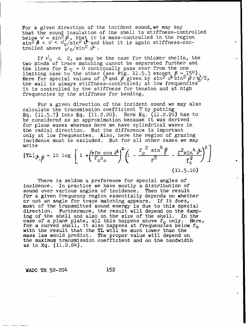
For a given direction of the incident soundwe may saythat the sound insulation of the shell is stiffness-controlledbelow V = sin2 P, that it is mass-controlled in the regionsin 2 A <-d < K)c/sin 2 2Yand that it is again stiffness-con-trolled above ic/sin 2 ,5-.

If •c < 2, as may be the case for thicker shells, thetwo kinds of trace matching cannot be separated further andthe lines for Zq- = 0 continually pass over from the onelimiting case to the other (see Fig. 11.5.3 except = = 150).Here for special values of O-and , given by sin2 Zý sin 2 871V/2,the wall is always stiffness-controlled; at low frequencies

it is controlled by the stiffness for tension and at highfrequencies by the stiffness for bending.

For a given direction of the incident sound we may alsocalculate the transmission coefficient T-by puttingEq. (11.5.7) into Eq. (11.2.20). Here Eq. (11.2.20) has tobe considered as an approximation because it was derivedfor plane waves whereas here we have cylindrical waves inthe radial direction. But the difference is importantonly at low frequencies. Also, here the region of grazingincidence must be excluded. But for all other cases we maywrite 11 f02sn4 f2si4a.\

[TL].,p 10 log 1 +fwfm cos 2 fo

(11.5.10)

There is seldom a preference for special angles ofincidence. In practice we have mostly a distribution ofsound over various angles of incidence. Then the resultfor a given frequency region essentially depends on whetheror not an angle for trace matching appears. If it does,most of the transmitted sound energy is due to this specialdirection. Furthermore, the result will depend on the damp-ing of the shell and also on the size of the shell. In thecase of a plane plate, all this happens above f only. Here,for a curved shell, it also happens at frequencies below fowith the result that the TL will be much lower than themass law would predict. The proper value will depend onthe maximum transmission coefficient and on the bandwidthas in Eq. (11.2.64).

WADC TR 52-204 152

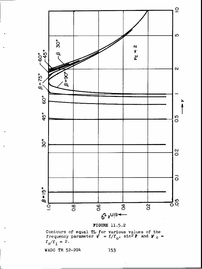
0

SoJ0

o0 00 H.J

0

LO 00L• 4O.

FIGURE 11.5.

0

Contours of equal TL for various values of thefrequency parameter -f/f op sin2 t and V cfclfl = 2.

WADC TR 52-2o4 153

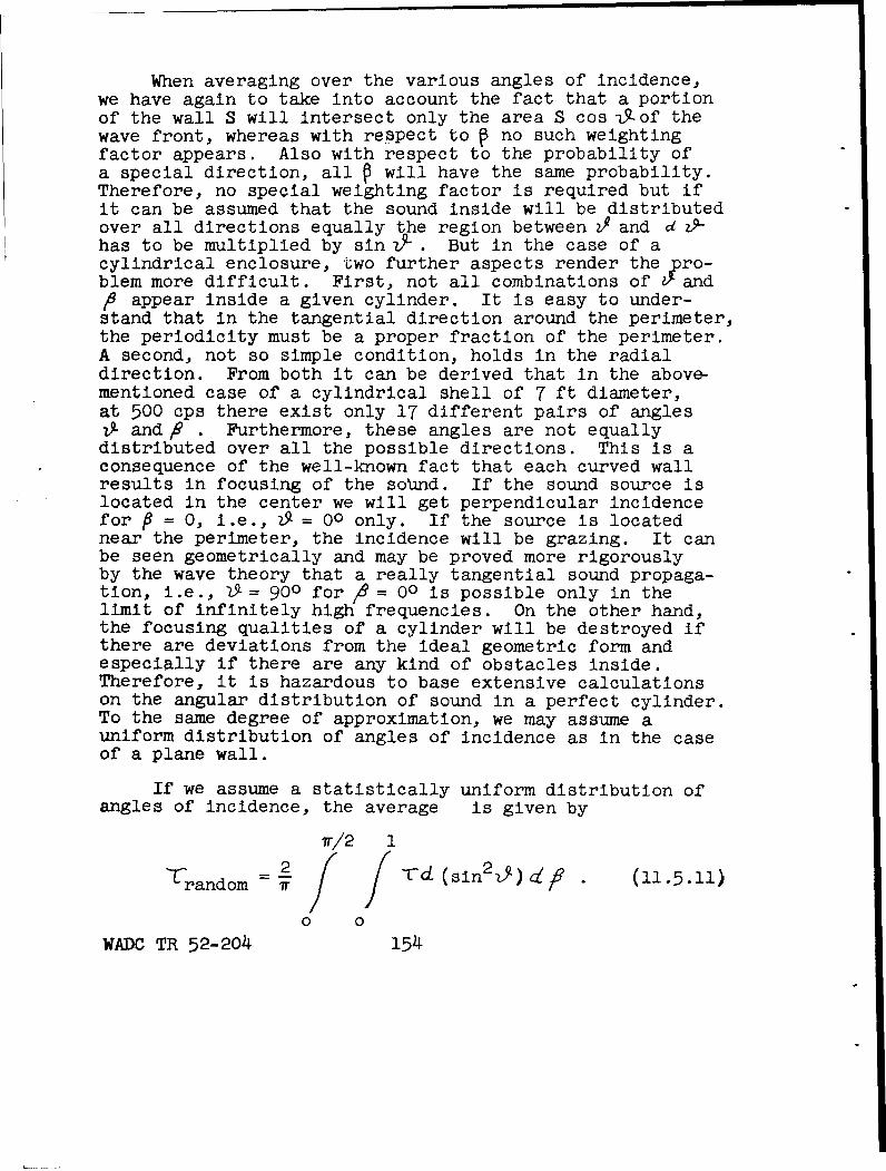
When averaging over the various angles of incidence,we have again to take into account the fact that a portionof the wall S will intersect only the area S cos 15-of thewave front, whereas with respect to ý no such weightingfactor appears. Also with respect to the probability ofa special direction, all P will have the same probability.Therefore, no special weighting factor is required but ifit can be assumed that the sound inside will be distributedover all directions equally the region between 2i and d z9-has to be multiplied by sin 72 . But in the case of acylindrical enclosure, two further aspects render thepro-blem more difficult. First, not all combinations of 0-and,6 appear inside a given cylinder. It is easy to under-stand that in the tangential direction around the perimeter,the periodicity must be a proper fraction of the perimeter.A second, not so simple condition, holds in the radialdirection. From both it can be derived that in the above-mentioned case of a cylindrical shell of 7 ft diameter,at 500 cps there exist only 17 different pairs of anglesi and,9 . Furthermore, these angles are not equallydistributed over all the possible directions. This is aconsequence of the well-known fact that each curved wallresults in focusing of the sobUnd. If the sound source islocated in the center we will get perpendicular incidencefor P = 0, i.e., 25- = 00 only. If the source is locatednear the perimeter, the incidence will be grazing. It canbe seen geometrically and may be proved more rigorouslyby the wave theory that a really tangential sound propaga-tion, i.e., 19= 900 for S = 00 is possible only in thelimit of infinitely high frequencies. On the other hand,the focusing qualities of a cylinder will be destroyed ifthere are deviations from the ideal geometric form andespecially if there are any kind of obstacles inside.Therefore, it is hazardous to base extensive calculationson the angular distribution of sound in a perfect cylinder.To the same degree of approximation, we may assume auniform distribution of angles of incidence as in the caseof a plane wall.

If we assume a statistically uniform distribution ofangles of incidence, the average is given by

r/2 12 -cd. (sin2 •) • (21.5.11)

"-random = r

0 0

WADC TR 52-204 154

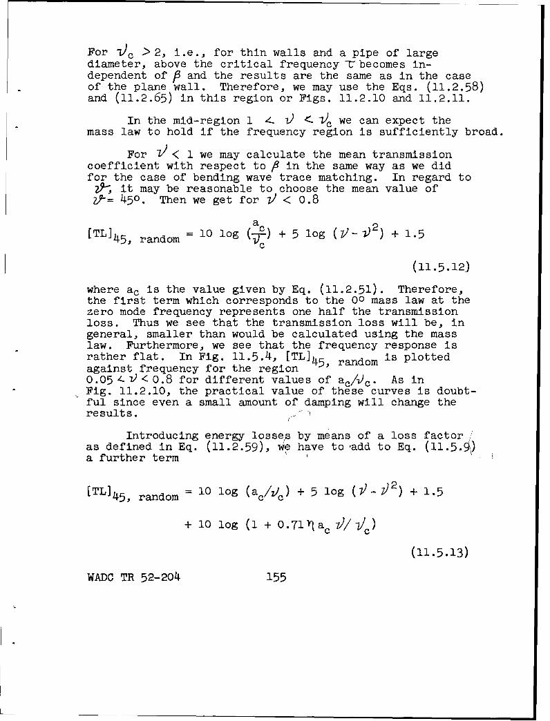
For 1c > 2, i.e., for thin walls and a pipe of largediameter, above the critical frequency qtbecomes in-dependent of P and the results are the same as in the caseof the plane wall. Therefore, we may use the Eqs. (11.2.58)and (11.2.65) in this region or Figs. 11.2.10 and 11.2.11.

In the mid-region 1 4- < -c we can expect themass law to hold if the frequency region is sufficiently broad.

For V'< 1 we may calculate the mean transmissioncoefficient with respect to P in the same way as we didfor the case of bending wave trace matching. In regard to29, it may be reasonable to choose the mean value ofzj-= 450. Then we get for i < 0.8

a

[TL] 4 5 , random (=c 10 log log (7- )2) + 1.5

(11.5.12)

where ac is the value given by Eq. (11.2.51). Therefore,the first term which corresponds to the 00 mass law at thezero mode frequency represents one half the transmissionloss. Thus we see that the transmission loss will be, ingeneral, smaller than would be calculated using the masslaw. Furthermore, we see that the frequency response israther flat. In Fig. 11.5.4, [TL] 4 5 , random is plottedagainst frequency for the region0.05 /--d< 0.8 for different values of ac/,4 c. As inFig. 11.2.10, the practical value of these curves is doubt-ful since even a small amount of damping will change theresults.

Introducing energy losse/s by means of a loss factoras defined in Eq. (11.2.59), we have to'add to Eq. (11.5.•)a further term

[TL] 4 5 , random = 10 log (ac/v)c) + 5 log (-)2) + 1.5

+ 10 log (1 + 0. 7 lylac /Vc)

(11.5.13)

WADC TR 52-204 155

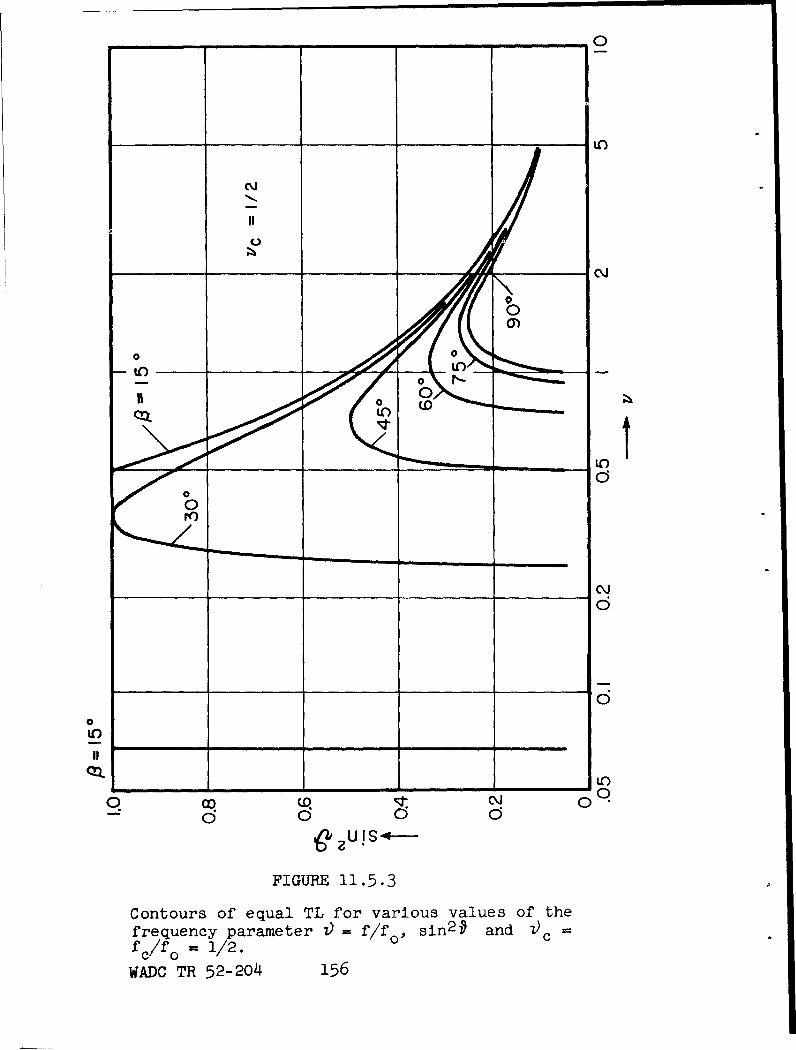
II0

0o

0

II IIIii

0d 0____ _ __ ___ ____ ___ __ O

00

9 N

FIGURE 11.5.3

Contours of equal TL for various values of thefrequency parameter z) = f/fo, sin2* and 2) =

fc/f =1/2.WADC TR 52-204 156

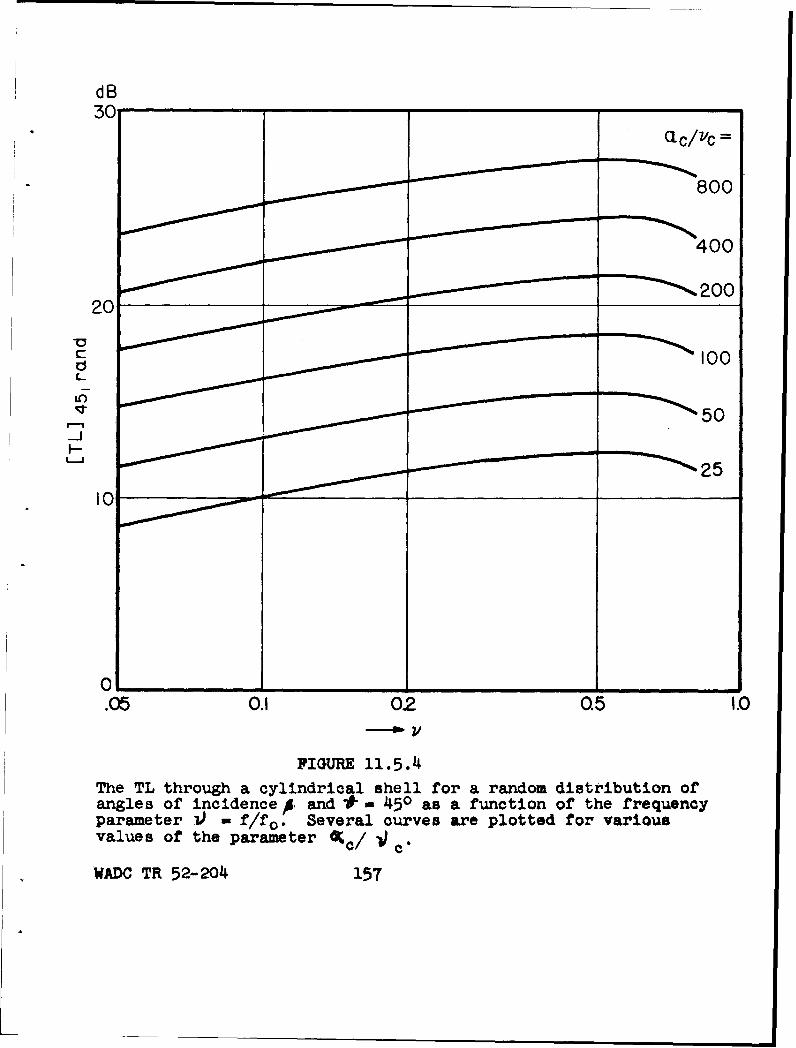
dB

LL/Z

B800

LO

.05 0.1 02 0.5 1.0

FIGURE 11.5.4The TL through a cylindrical Shell for a random distribution ofangles of incidence p and * - 450 as a function of the frequencyparameter i)-f/fo. Several curves are plotted for variousvalues or the parameter Qý/ -d

WADC TR 52-204 157

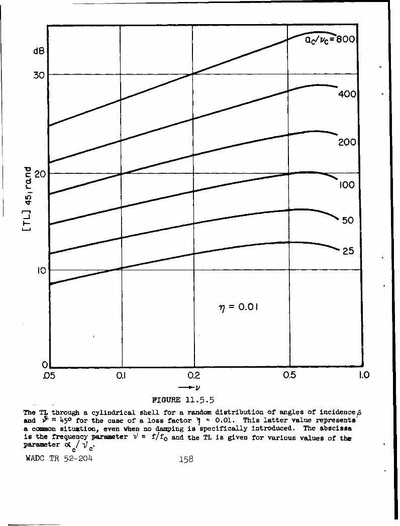
30

40

I--j 50L--j

25

77 =0.0 1

D5 0.1 0.2 0.5 1.0P.- I/

FIGURE 11.5.5The TL through a cylindrical shell for a random distribution of angles of incidenceand l -- 450i~ for the case of a loss factor I - 0.01. This latter value representsa common situation, even when no damping is specifically introduced. The abscissais the frequency parameter l2 = f/f 0 and the TL is given for various values of theparameter o C/ -djCWADC TR 52-204 158

In Fig. 11.5.5, the corresponding values of TL areplotted as a function of V for various values of ac/1)cas in Fig. 11.5.4 and for a loss factor of ý = 0.01(which may be assumed in most practical cases even ifthere is no special material used for dampingj. Forsmall ac/Vcthis amount of damping does not essentiallyalter the results shown in Fig. 11.5.4. For high valuesof ac/1)/c, generally if 0:71 acV/'c > 4 , we mayapproximate Eq. (11.5.13) by

a20 log (Cc) + 5 log (ý3_7) + 10 log[TL] 45,random 2c

(11.5.14)

Here we see that doubling the loss factor increases theTL by 3 db. Therefore, it would be advantageous to in-crease the loss factor of a shell for both high and lowfrequencies.

WADC TR 52-204 159

12.1 Specification of Sound Absorptive Properties

In connection with certain problems in the controlof airborne sound, and in the special problems of sound inrooms, the acoustical designer has to deal with the pro-perties of sound absorbing materials. It is necessary,therefore, to describe briefly the physical principles ofabsorbing materials, the manner in which the physicalproperties and the sound absorbing properties are measured,and in a general way, some of the applications of the datawhich describe the materials.

In this limited discussion, it is possible to describethe significance of several of the concepts only in a quali-tative way. The reader who desires a fuller knowledge of anyof the topics touched on in this section should consult moreextensive discussions which have been published 1.1, 1.2,1.1, 1.4/.

The Several "Coefficients" for an Acoustical Material.The energy-absorbing ability of an acoustical material at agiven frequency is most commonly specified by an "absorptioncoefficient". The widespread use of such a quantity suggeststhat this single measure is sufficient to indicate the per-formance of the material in all situations. However, thisis not true. Detailed acoustical theory shows that thespecific acoustic impedance has much wider applicability indescribing the material. This quantity, in general acomplex number, varies with frequency and may vary with theangle of incidence of the sound. Under special conditionssome real number (a "coefficient") may describe the behaviorof the material. Actually there are several differentcoefficients, each useful in special circumstances as ameasure of energy absorption. Each is derivable from thespecific acoustic impedance. Since the complex specificacoustic impedance contains two parts, it cannot, in general,be calculated from any single value of any of thecoefficients.

Before discussing the energy-absorption coefficients,it will be helpful to review the behavior of a simple oscil-lator. A "simple oscillator" may be a mechanical systemequivalent to a mass, a spring, and a damping element, ananalogous simple electrical circuit or a confined volume of

WADC TR 52-204 161

air in which one of the natural sinusoidal acoustical vibra-tions has been excited. In any case, elementary theory showsthat the energy of vibration of the simple oscillator decaysexponentially with time when the system is in free vibration(no external driving force). Thus, if the instantaneousenergy of vibration is W, and if the initial energy of vibra-tion is W0 , the energy at any time t follows the equation:

W =W e -2kt, (12.1.1)

where k is the damping constant. By differentiation ofthis relation, the definition of the damping constant is ob-tained in the form:

k = _1 dW/dt (12.1.2)2f W""

Ordinarily a sound source in an enclosure excitesmore than one mode of acoustical vibration. When a soundsource is turned off, each mode which has been excited actsas a simple oscillator at its natural frequency. In generaleach mode has a different decay rate, but it is found thatin a rectangular enclosure there exist three groups of modes,within each of which the damping is roughly the same for allmodes. The mode groups are designated as axial, tangential,and oblique. It will be seen later that these designationsrefer to the extent to which the wave motion of a particularmode involves tangential or oblique incidence on the variouswalls.

The.detailed wave theory shows that the damping ratesof the various modes can be related to quantities calledwall coefficients. The wall coefficients depend upon thesize and shape of the enclosure, the distribution of theabsorbing material, and the mode of vibration which is ex-cited, but in certain cases the special forms of the wallcoefficients can be regarded as intrinsic properties of theabsorbing material.

The normal wall coefficient of a surface, 0.p, isdefined as eight times the real part of the admittance ratio(impedance and admittance are discussed later in this section).This quantity measures, for a wall which is not highly absorb-ing, the damping of waves which meet the wall at normal oroblique incidence.

WADC TR 52-204 162

The grazing wall coefficient a t, is a measure of theamount by which a wall in a chamber of regular shape contri-butes to the damping of an acoustical vibration consistingof wave motion "parallel" to that wall. For a relativelynonabsorbent wall, however, there exists in place of thegrazing coefficient a supplementary wall coefficient, whichin the case of a rectangular enclosure, depends upon theproperties of the opposite wall. These coefficients can becomputed from the acoustic impedance. When both walls of apair are not highly absorbing, both the grazing coefficientand the supplementary coefficient are nearly equal to O'/2.(See Ref. 1.1 for a discussion of limits of validity of-these several coefficients.)

The wall coefficients above are related to the dampingof the energy of an acoustical mode of vibration in an en-closure. Another set of coefficients, which will now bedescribed, has to do with the fraction of incident powerwhich is absorbed when a free sound wave in space strikes anabsorbing surface. There is no general relation betweenthese absorption coefficients and the wall coefficients givenabove, but it will be shown that under special conditionsthe absorption coefficients are related to the rate at whichthe total energy of a group of modes of vibration in anenclosure decays with time. This leads to the very restrictedreverberation theory of elementary acoustics, and to theordinary procedure of characterizing an acoustical materialby an absorption coefficient as measured in a "reverberationchamber".

The basic quantity in the absorption of a single waveat a wall is the free-wave absorption coefficient, OL (@)This coefficient is simply the fraction of the power in thewave, incident at an angle 0, which is absorbed by the wall.The notation indicates that the free-wave absorption coeffi-cient is a function of the angle of incidence, 0. The con-cept of absorption as a function of angle of incidence (theangle between the normal to the absorbing surface and a lineperpendicular to the wavefront striking the surface) is validin practice for angles as great as 800. However, the conceptof a free-wave absorption coefficient breaks down for largerangles of incidence, because of distortion of the wave by theabsorbing boundary*.

The case of Q = 900 is meaningless in any case, because a wavecannot travel absolutely parallel to a surface having absorption;the wave fronts are curved by continuous flow of energy into thesurface. For this reason, quotation marks were used above instatements concerning waves traveling "parallel" to a wall.

WADC TR 52-204 163

The free-wave absorption coefficient can be obtained by adirect measurement of the amplitudes of incident and re-flected waves, or by techniques which depend upon the effectof an absorbing sample at the end of a tube in which "stand-ing waves" are set up.

The normal free-wave absorption coefficient, denotedby O , is the value of the free-wave absorption coefficientin the special case of normal incidence (9 - 0°). Therefore,

o is the fraction of incident power which is absorbedwhen a free plane wave is normally incident on the absorbingsurface.

Finally, when the power incident on the absorbingsurface is carried by an infinite number of plane waves uni-.formly distributed through all possible angles. The fractionof the power which is absorbed is defined as the statisticalabsorption coefficient otstat- For reasons which will begiven, this coefficient is sometimes called the Sabine absorp-tion coefficient, and at high frequencies this coefficientis closely equal to the chamber absorption coefficientordinarily reported by the manufacturers of acoustical absarb-Ing materials. The statistical absorption coefficient issimply a suitably averaged value of the free-wave absorptioncoefficient, which may be defined by the equation:

Q~stat = 2 f 0ý(0) cos 0 sin 0 dG. (12.1.3)

Relation of the Statistical Coefficient to Reverberation.W. C. Sabine, in the earliest systematic work on sound wavesin rooms, suggested on the basis of a series of experimentsthat the total sound energy decays exponentially in the "rever-beration" which occurs after the sound source is turned off L/The damping constant of the exponential decay is proportionalto the average "sound absorption coefficient" of the walls.A mathematical analysis shows that the sound absorptioncoefficient which is important in reverberation is identicalwith the statistical coefficient defined above, if certainvery special conditions are realized. These conditions are,

1. Only a small fraction of the total energy is lostin the time required for sound to travel the greatest dimen-sion of the enclosure.

WADC TR 52-2o4 164

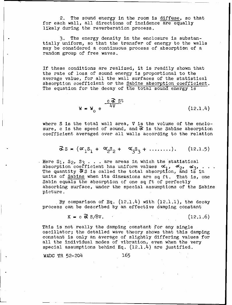
2. The sound energy in the room is diffuse, so thatfor each wall, all directions of incidence are equallylikely during the reverberation process.

3. The energy density in the enclosure is substan-tially uniform, so that the transfer of energy to the wallsmay be considered a continuous process of absorption of arandom group of free waves.

If these conditions are realized, it is readily shown thatthe rate of loss of sound energy is proportional to theaverage value, for all the wall surfaces of the statisticalabsorption coefficient or the Sabine absorption coefficient.The equation for the decay of the total sound energy is

c a St

W - W0 e W (12.1.4)

where S is the total wall area, V is the volume of the enclo-sure, c is the speed of sound, and 5 is the Sabine absorptioncoefficient averaged over all walls according to the relation

3s (c S1 + 2s2 + 3S3 + ........ ). (12.1.5)

Here Sl, S2 , S 3 . . . are areas in which the statisticalabsorption coefficient has uniform values Ol' 2, *3 • •The quantity a S is called the total absorption, and is inunits of Sabins when its dimensions are sq ft. That is, oneSabin equals the absorption of one sq ft of perfectlyabsorbing surface, under the special assumptions of the Sabinepicture.

By comparison of Eq. (12.1.4) with (12.A.1), the decayprocess can be described by an effective damping constant

K - c o S/8v. (12.1.6)

This is not really the damping constant for any singleoscillator; the detailed wave theory shows that this dampingconstant is only an average of slightly differing values forall the individual modes of vibration, even when the veryspecial assumptions behind Eq. (12.1.4) are justified.

WADC TR 52-204 165

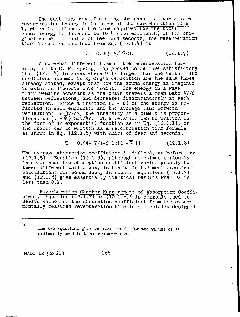
The customary way of stating the result of the simplereverberation theory is in terms of the reverberation timeT, which is defined as the time required for the total-soundenergy to decrease to 10-6 (one millionth) of its ori-ginal value. In units of feet and seconds, the reverberationtime formula as obtained from Eq. (12.1.4) is

T = 0.049 v/ Ms. (12.1.7)

A somewhat different form of the reverberation for-mula, due to C. F. Eyring, has proved to be more satisfactorythan (12.1.4) in cases where O is larger than one tenth. Theconditions assumed in Eyring's derivation are the same threealready stated, except that now the sound energy is imaginedto exist in discrete wave trains. The energy in a wavetrain remains constant as the train travels a mean path 4V/Sbetween reflections, and decreases discontinuously at eachreflection. Since a fraction (1 - U) of the energy is re-flected in each encounter and the average time betweenreflections is 4V/cS, the intensity at a time t is propor-tional to (1 - ý) Sct/4V. This relation can be written inthe form of an exponential function as in Eq. (12.1.1), orthe result can be written as a reverberation time formulaas shown in Eq. (12.1.8) with units of feet and seconds.

T = 0.049 V/[-S ln(l -&)] (12.1.8)

The average absorption coefficient is defined, as before, by(12.1.5). Equation (12.1.8), although sometimes seriouslyin error when the absorption coefficient varies greatly be-tween different wall areas, is the basis for most practicalcalculations for sound decay in rooms. Equations (12.1.7)and (12.1.8) give essentially identical results when 5- isless than 0.1.

Reverberation Chamber Measurement of Absorption Coeffi-cient. Equation (12.1.73 or (12.1.87)*i•-cmmonly used toderive values of the absorption coefficient from the experi-mentally measured reverberation time in a specially designed

.The two equations give the same result for the values ofordinarily used in these measurements.

WADC TR 52-204 166

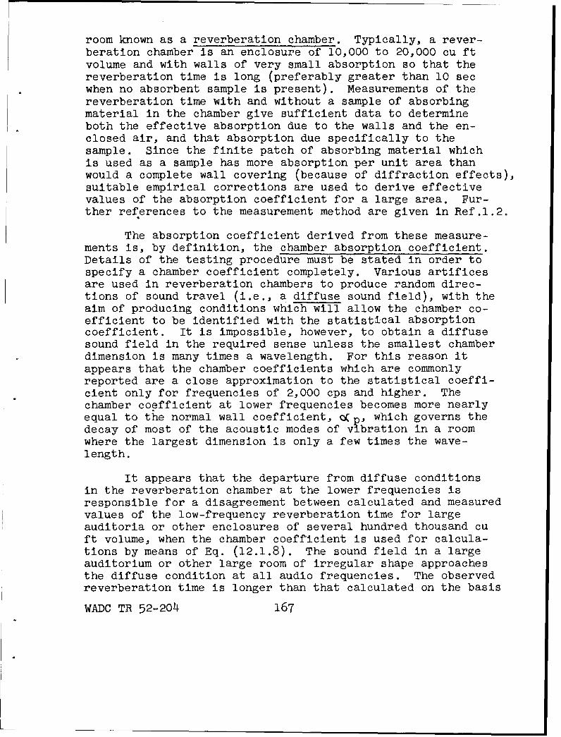
room known as a reverberation chamber. Typically, a rever-beration chamber is an enclosure of 10,000 to 20,000 cu ftvolume and with walls of very small absorption so that thereverberation time is long (preferably greater than 10 secwhen no absorbent sample is present). Measurements of thereverberation time with and without a sample of absorbingmaterial in the chamber give sufficient data to determineboth the effective absorption due to the walls and the en-closed air, and that absorption due specifically to thesample. Since the finite patch of absorbing material whichis used as a sample has more absorption per unit area thanwould a complete wall covering (because of diffraction effects),suitable empirical corrections are used to derive effectivevalues of the absorption coefficient for a large area. Fur-ther references to the measurement method are given in Ref.1.2.

The absorption coefficient derived from these measure-ments is, by definition, the chamber absorption coefficient.Details of the testing procedure must be stated in order tospecify a chamber coefficient completely. Various artificesare used in reverberation chambers to produce random direc-tions of sound travel (i.e., a diffuse sound field), with theaim of producing conditions which will allow the chamber co-efficient to be identified with the statistical absorptioncoefficient. It is impossible, however, to obtain a diffusesound field in the required sense unless the smallest chamberdimension is many times a wavelength. For this reason itappears that the chamber coefficients which are commonlyreported are a close approximation to the statistical coeffi-cient only for frequencies of 2,000 cps and higher. Thechamber coefficient at lower frequencies becomes more nearlyequal to the normal wall coefficient, Q , which governs thedecay of most of the acoustic modes of vibration in a roomwhere the largest dimension is only a few times the wave-length.

It appears that the departure from diffuse conditionsin the reverberation chamber at the lower frequencies isresponsible for a disagreement between calculated and measuredvalues of the low-frequency reverberation time for largeauditoria or other enclosures of several hundred thousand cuft volume, when the chamber coefficient is used for calcula-tions by means of Eq. (12.1.8). The sound field in a largeauditorium or other large room of irregular shape approachesthe diffuse condition at all audio frequencies. The observedreverberation time is longer than that calculated on the basis

WADC TR 52-204 167

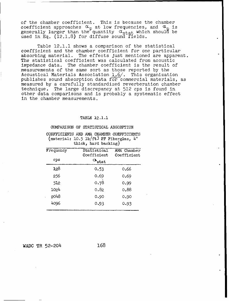
of the chamber coefficient. This is because the chambercoefficient approaches (Yp at low frequencies, and. a isgenerally larger than the quantity G•stat which shoulR beused in Eq. (12.1.8) for diffuse sound fields.

Table 12.1.1 shows a comparison of the statisticalcoefficient and the chamber coefficient for one particularabsorbing material. The effects Just mentioned are apparent.The statistical coefficient was calculated from acousticimpedance data. The chamber coefficient is the result ofmeasurements of the same sort as those reported by theAcoustical Materials Association 1.6 . This organizationpublishes sound absorption data for commercial materials, asmeasured by a carefully standardized reverberation chambertechnique. The large discrepancy at 512 cps is found inother data comparisons and is probably a systematic effectin the chamber measurements.

TABLE 12.1.1

COMPARISON OF STATISTICAL ABSORPTION

COEFFICIENTS AND AMA CHAMBER COEFFICIENTS(material: 10.5 lb/ft3 PF Fiberglas, 4"

thick, hard backing)

Frequency Statistical AMA ChamberCoefficient Coefficient

cps C•stat

128 0.53 0.66

256 0.69 0.69

512 0.78 0.99

1o24 0.82 0.88

2048 0.90 0.90

4096 0.93 0.93

WADC TR 52-204 168

Comparison of Statistical Coefficient and Wall Coeffi-cients. The statistical absorption coefficient applies toproblems of sound absorption only where a diffuse sound fieldexists. In this special case Eqs. (12.1.7) or (12.1.8) maybe used to compute the reverberation time. These equationsinfer that the absorption coefficient of the acousticalmaterial at a given frequency is independent of the shapeof the room, of the position of the material, and of thesound source in the room.

The detailed theory of wave acoustics, which has beenworked out for enclosures of simple shape, shows that ingeneral the acoustical damping produced by absorbing materialin a room depends upon the material, the shape of the room,the position of the material in the room, and which modes ofacoustical vibration in the enclosure are excited by thesound source. The Sabine assumptidns represent only a spe-cial limiting case, which can be approached when the enclo-sure (or the arrangement of absorbing patches within theenclosure) is irregular, and when the wavelength is verysmall compared to the shortest dimension of the enclosure.Also, the general wave theory indicates that, because thedamping constants differ for the various groups of vibrationalmodes, the decay of the total aooustical energy in the enclo-sure is not a single exponential function, and the reverbera-tion phenomenon cannot be described adequately by a singlereverberation time except under the special Sabine conditions.

The distinction between the two approaches may beillustrated for the case of a rectangular enclosure. Let thedimensions of the enclosure along the x, y, and z axes beLx, Ly, and Lz. According to wave theory, the frequenciesof free acoustical vibration of the enclosure are givenapproximately by

f(nxnynz) = (c/2) {(nx/Lx)2 (ny/L2 2(nzLz)2

(12.1.9)

where each n may be equal to any integer (including zero).The value of nx is equal to the number of pressure maximabetween the walls x - 0 and x = Lx in the wave pattern of thevibration; for nx = 0, the pressure is nearly uniform in thex direction. The other n's have corresponding interpretations.

WADC TR 52-204 169

Oblique waves correspond to the case of none of the n'sequal to zero. Tangential waves correspond to one n equalto zero; for example, for nx = 0, the wave motion is tan-gential (grazing) with respect to the x walls (the walls atx = 0, x = Lx). Axial wves correspond to two n's equal tozero; for example, for nx = 0, ny = 0, the wave motion isgrazing with respect to both x and y walls.

The damping of any one vibration in the rectangularenclosure, according to wave theory, is computed by usingin Eq. (12.1.6), in place of the Sabine absorption OCS, theroom absorption factor, aN, defined by Eq. (12.1.10). Itis assumed that each wall has uniform acoustical properties.

N = LyLz (O~l+ 0x 2 ) + LxLz(%l + Q+C2 ) + LxLy(O 1 + OX2)

(12.1.10)

The Oý-'s are the wall coefficients. Subscripts xl, x2 referto the walls at x = 0 and x = Lx respectively, and so forth.While considerable calculation may be required to find theCC's from acoustic impedance data for the walls, simple

approximations hold when the walls are "hard".* For a roomwith hard walls, each Cl-for a wall where the wave motion isobliquely incident is approximately equal to the normal wallcoefficient CE-, and each C for a wall subject to grazingincidence is equal to the grazing wall coefficient, whichin this case is approximately OC/2.

For a numerical example, consider an enclosure having di-mensions Lx,Ly,Lz equal respectively to 10,15, and 20 ft, witha freely decaying acoustical vibration in the mode nx = 0,n 1 1, nz 1 1. According to Eq.(12.1.9), the frequency ofthis vibration is approximately 46 cps (using c = 1100 ft/sec).

A "hard" wall is one for which the specific impedanceratio is greater than twice the length of the rpom inwavelengths, measured perpendicular to that wall; allordinary acoustical tiles on massive backings may beconsidered hard below 200 cps in rooms nQt larger than20' in any direction.

WADC TR 52-204 170

Let the normal absorption coefficient for each wall be 0.05at this frequency. The d's in Eq. (12.1.10) are then eachequal to 0.05 except that grazing incidence occurs on bothof the 10 x 15 ft walls, and the • value for each of theseis therefore 0.025. The room absorption factor aN fromEq. (12.1.10) is 50 ft 2 . This value can be used in place of

S in Eq. (12.1.6) to obtain the damping constant. Thevalue of the Sabine quantity of UtS is 65 ft 2 ; hence appre-ciably greater damping would be realized under the Sabineconditions than for the case considered here, in which the(0,1,1) mode Is excited. The discrepancy is more severe ifonly the 15 x 20 ft ceiling is absorBtive; then aN is 7.5 ft 2

and &S (the Sabine factor) is 15 ft . In the hard wallapproximation, there is no disagreement between the wavetheory and the diffuse-room reverberation formula for obliquemodes. Thus, in practice the oblique modes decay most rapidly,at roughly the rate given by the Sabine relation, and leavethe axial and tangential vibrations dying out at slower rates.This effect is especially pronounced when all the absorbingmaterial is on one surface.

When the hard-wall approximation is not introduced,the complete wave theory indicates further effects of theposition of the material and the nature of the excited modesupon the damping. For example, the effects of opposite wallsare not necessarily additive. The presence of a soft wallmay result in a concentration of the acoustical energy in theend of the room near that wall. This in turn increases theeffectiveness of the soft wall as a sound absorber, so thatthe normal wall coefficient for a soft wall may be greaterthan unity.

The Specific Acoustic Impedance and Related Quantities.A measure of the acoustical properties of a surface which hasmore general application than any of the' "coefficients" isthe normal specific acoustic .impedance. This quantity isdefined by the relation

z = r + Jx = p/v, (12.1.11)

where p is the acoustic pressure at the surface, and v isthe resulting velocity component normal to the surface of airparticles Just in front of the surface. Ordinarily p is indynes/cna2 and v in cm/sec. The resulting unit for z is calleda rMl. The acoustic pressure is the sum of the instantaneouspressure produced by an incident acoustic wave and of the

WADC TR 52-204 171

instantaneous pressure of any reflected wave whichmay be set up.

The normal specific acoustic impedance is independentof the angle of incidence of the sound if there is no effec-tive wave propagation behind the surface in a directionparallel to the surface. This requirement means that suchwave motion must be highly attenuated or have a velocitymuch smaller than the velocity of sound in air; this is thecondition of "local reaction" discussed in Sec. 12.2. Ithas also been shown experimentally that z is practicallyindependent of the incident angle for materials representa-tive of commercial acoustic tiles 1.-7/

The impedance is usually a complex number. The complexrepresentation, which has meaning only for sinusoidal signals,has the same significance as that used in alternating currenttheory. Thus, the real part of z is the ratio to v of thecomponent of p which is in phase with v, while the imaginarypart of z is the ratio to v of the portion of p which is 900out of phase with v. The real and imaginary parts of z, rand x, are respectively the normal specific acoustic resis-tance and the normal specific acoustic reactance. The adjec-tive "normal" will be omitted except where there is a possi-bility of confusion with some impedance not concerned withthe normal component of particle velocity.

The specific acoustic impedance for a perfect absorberof plane waves (or for an infinite body of air, which iseffectively a perfect absorber) is Pc, where p is the densityof air (Fig. 3.1) and c is the speed of sound. It is oftenconvenient to express z in units of 9c. The dimensionlessquantity obtained in this way is called the specific acousticimpedance ratio denoted by

zzý c 9 + J X•

The reciprocal of the specific acoustic impedance isthe specific acoustic admittance, y. The reciprocal of thespecific acoustic impedance ratio is the specific acousticadmittance ratio, ý m l/& - + jk. The quantityA( is thespecific acoustic conductance ratio, and k is the specificacoustic susceptance ratio.

WADC TR 52-204 172

Several methods for the measurement of the specificacoustic impedance are described in the literature 1.2/.All the methods have to do, in a general way, with measuringvarious aspects of the system of incident and reflected waveswhich is set up when an acoustic wave is incident on the testsurface, either in open space or in an enclosure. Ordinarilyacoustic impedance measurements are made on samples notlarger than one sq ft; usually the samples are much smaller,particularly if measurements in a standing-wave tube are tobe made to several thousand cps.

Because of the limitations on sample size, an averagingproblem arises in connection with materials having large-scale variations in structure. Also, with small samples itis difficult to reproduce any kind of backing other thanthat of an effectively rigid wall. In the techniques mostcommonly used, the sample is cut to fit snugly within theend of a containing tube. It has been shown that materialshaving a very light skeleton (not heavier than about 2 lb/ft3)must be treated with great caution in tube mountings, becausethe clamping effect of the walls hinders the ordinarilyappreciable motion of the skeleton in response to the soundwave and seriously changes the impedance. When the abovedifficulties are not important, impedance measurements canbe made with laboratory apparatus to within 3 per cent onacoustic tiles and blankets. The angle of incidence is 00in most impedance measurements.

Relation Between Impedance and Absorption Coefficients.For surfaces which can be characterized by a normal impedanceindependent of angle of incidence (this includes ordinaryacoustical tiles and blankets with hard backing), the relationbetween impedance and free-wave absorption coefficient issimple. This relation can be derived by setting up expressionsfor incident and reflected waves, and imposing the conditionthat the phase and amplitude relations between the waves shallbe such that the relation between total pressure at the surfaceand the normal particle velocity is just that correspondingto the specific acoustic impedance. It is then possible tocompute the difference of intensity of the incident and re-flected waves, and to obtain the absorption coefficient, whichis the fractional loss of intensity. In this way, it is foundthat the free-wave absorption coefficient, where the angle ofincidence as measured from the normal is Q,

WADC TR 52-204 173

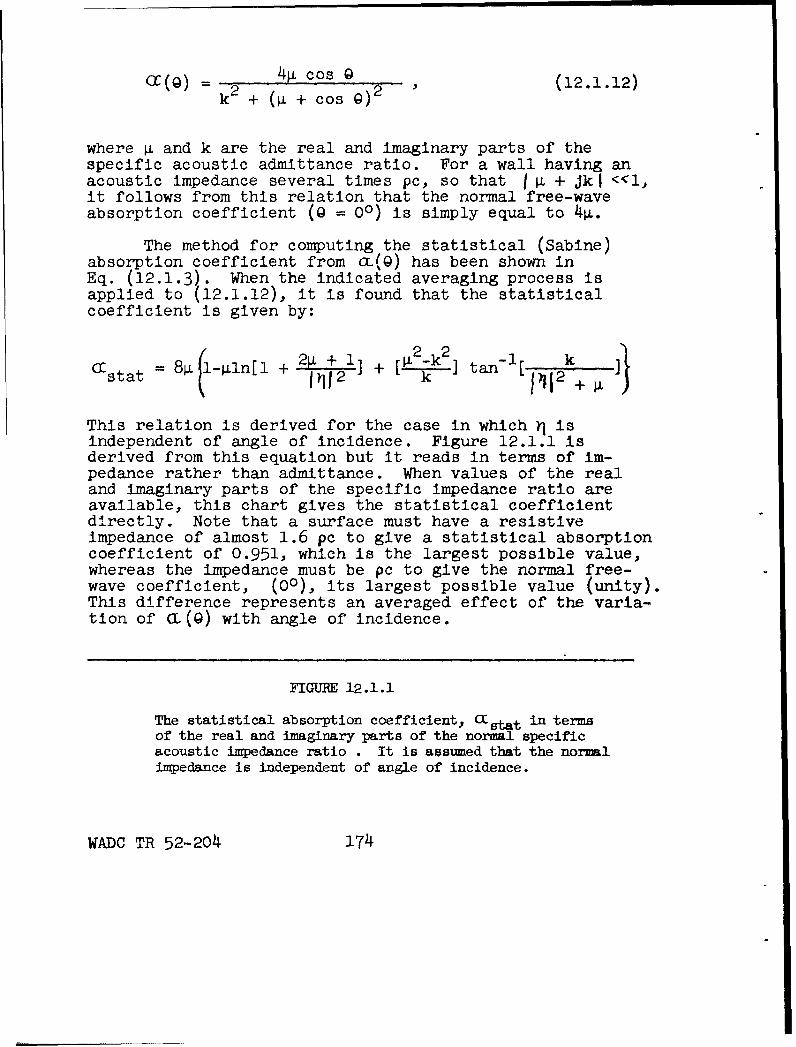
4•cosQ

( k + (.+ 1Cos " (12.1.12)

where 4 and k are the real and imaginary parts of thespecific acoustic admittance ratio. For a wall having anacoustic impedance several times pc, so that j 4 + Jkl <<1,it follows from this relation that the normal free-waveabsorption coefficient (9 = 00) is simply equal to 44.

The method for computing the statistical (Sabine)absorption coefficient from CL(Q) has been shown inEq. (12.1.3). When the indicated averaging process isapplied to (12.1.12), it is found that the statisticalcoefficient is given by:

ccstat = 8( -•In[l + 42t +] + 2__2 ] tan- •4k

This relation is derived for the case in which -q isindependent of angle of incidence. Figure 12.1.1 isderived from this equation but it reads in terms of im-pedance rather than admittance. When values of the realand imaginary parts of the specific impedance ratio areavailable, this chart gives the statistical coefficientdirectly. Note that a surface must have a resistiveimpedance of almost 1.6 pc to give a statistical absorptioncoefficient of 0.951, which is the largest possible value,whereas the impedance must be pc to give the normal free-wave coefficient, (00), its largest possible value (unity).This difference represents an averaged effect of the varia-tion of CL (Q) with angle of incidence.

FIGURE 12.1.1

The statistical absorption coefficient, " 1stat in termsof the real and imaginary parts of the normal specificacoustic impedance ratio . It is assumed that the normalimpedance is independent of angle of incidence.

WADC TR 52-204 174

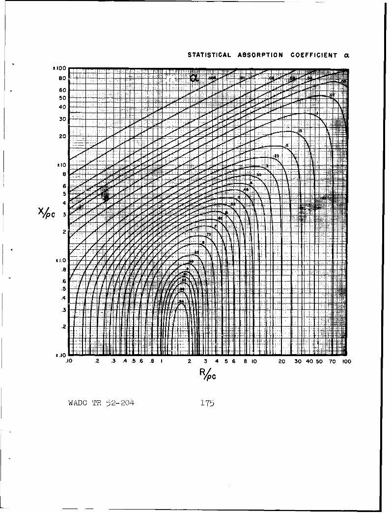
STATISTICAL ABSORPTION COEFFICIENT CL

t 100

30

ito7

60

50

40

J I0310.2 . .45 .82 34 6 0200000 0

"R/P

20 OTB5-04I~

Behavior of Acoustical Materials in Terms of TheirPhysical Structure. While the normal specific impedanceis a quantity of wider applicability than any of the coeffi-cients, the physical structure parameters of the materialsometimes have even wider applicability than the specificimpedance. For materials whose acoustic behavior is readilysubject to analysis, a knowledge of several structuralparameters permits the calculation of the impedance for anythickness of material, subject to a variety of backing condi-tions, and for any angle of incidence, even when theimpedance varies with angle. Since the structure parameterscan be measured simply, we can determine the acousticalbehavior of a material with a minimum of experimental effort.Moreover, working from the basic physical properties ofmaterial sometimes makes it possible to derive much moreuseful design equations or charts, showing the completefrequency behavior of a sound-reducing structure in termsof a few simple quantities. An example of this is found inSec. 12.2, in the discussion of a duct lined with a porousmaterial.

Considerable published material is available for thecalculation of acoustical properties from structural con-stants 1.1, 1.2, 1.3, 1.8_, 1.9_ The present discussion willbe restricted to the simple case of an isotropic porousmaterial with a rigid skeleton and mounted on a rigid backing.It will appear that the important parameters are the porosity(the fraction of the total volume which is occupied by air),the structure factor (related to the increased effectiveinertia of air which is accelerated in small passages), andthe flow resistance.

The porosity can be obtained from an experiment whichinvolves finding the apparent compressibility of the airin the sample. Because the solid is virtually imcompressible,the specimen acts like a volume of air in which the modulusof compression is 1/h times the true compressional modulusof air, where h is the porosity. For practical materials,h is at least 0.7 and is usually not less than 0.9. Theflow resistance of a sample is obtained by direct measure-ment of the pressure drop across the sample when air isforced at a known, steady rate through a slab of known areaand thickness. The result is usually reduced to the specificflow resistance (rf) (rayls per cm thickness). This isnumerically equal to the pressure drop associated with anair flow of one cm3/sec through a sample of area one sq cm

WADC TR 52-204 176

and thickness one cm (sometimes specific flow resistanceis reported in rayls per inch of thickness). The structurefactor, the exact definition of which can be obtained fromEq. (12.1.15), must be found from an experimental measure-ment of impedance or of propagation constant in the material.This does not discourage the use of this approach because(1) the structure factor ordinarily does not vary rapidlywith frequency, so that extensive measurements are unneces-1sary; (2) it is not necessary to know the structure factorin order to compute the impedance of a rigidly backed layerwhich is thin compared to a wavelength.

The theory of the absorbing layer gives the surfaceimpedance in terms of the propagation constant, the char-acteristic impedance for waves traveling in the layer, andthe thickness. The case of perpendicular incidence will beconsidered here, since it is an experimental fact that theresult is substantially independent of angle for most porouslayers. Suppose that a sinusoidal pressure variation at thesurface of the porous layer sets up plane waves in the layer,traveling normally to the surface. The pressure in the waveentering the material is proportional to exp (-Jk x), wheredistance is measured from the surface into the lay'er, andkI is the propagation constant which is to be found. Thelayer thickness is t. At the backing (x t) a reflectedwave is set up. The ratio of the pressure in the reflectedwave to that in the incident wave, at x = t, is defined as,exp (2 7r). Then the reflected wave must have pressure pro-portional to exp (2 Y + Jk x - J2klt). It is desired tofind the specific surface impedance, which is the ratio of.pressure to particle velocity at x - 0. The total pressureat x = 0 is proportional to 1 4 exp (2 V- j2klt). Theparticle velocity at the surface due to either wave Is equalto the pressure divided by Z1, which is the characteristicimpedance of the layer mater al (analogous to the quantitypc for open air). since the waves are oppositely directed,the particle velocities must be subtracted, and the totalsurface particle velocity is proportional to [1 - exp(23 - j2klt)]/ZI. Dividing the pressure by the particlevelocity gives for the surface specific impedance

z coth (Jklt ) (12.1.14)

WADC TR 52-204 177

The value of * depends upon the reflectivity of the backing.For a rigid backing, complete reflection occurs with nopressure phase shift, so that * is zero and the specificsurface impedance is

z = Z coth (Jk 1 t) . (12.1.14a)

(Rigidly backed layer)

If the layer is thin enough that k1 t <<1,z:- J(Z /klt) [1 - (klt) 2 ] . (12.1.14b)

(Rigidly backed layer thin comparedto wavelength)

The negative of the imaginary part of kI is the attenuationconstant 1/8.69) times the attenuation in db per unit dis-tance) for wave motion in the layer. For -Im(kl) > l/t, acondition which will be realized at high frequencies, thetotal attenuation is sufficiently large that the effect ofthe reflected wave may be neglected. Roughly speaking, thiscondition occurs when the thickness of a practical porousmaterial is greater than X/4. For this case, the surfaceimpedance is

z = ZI (12.1.14c)

(Thick layer, any backing)

The propagation constant and the characteristic imped-ance will now be related to the structure parameters of theporous layer. It is assumed that motion of the skeleton canbe neglected, which in practice seems to require porousmaterials having a density of 6 lb/ft 3 or more. A sinusoidalwave in the layer with pressure proportional to exp (Jwt-Jklx)is assumed. The volume velocity* per unit area, which at thesurface is equal to the ordinary particle velocity in theoutside air, is vl. The negative of the pressure gradientis Jklp. A portion of the pressure drop in a thin volumeelement, as described by this quantity, is associated with

.The volume velocity is the rate of volume flow(e.g., cm3 /sec).

WADC TR 52-204 178

the acceleration jc.vI of the volume flow in the element,and another portion with overcoming the frictional resistanceto air flow, as indicated in Eq. (12.1.15).

jklP - Jme PCv 1 + rfvI . (12.1.15)

Note that this equation effectively defines the structurefactor, m. The rate of change of volume is related to therate of pressure change by the effective modulus of compres-sion of the gas. The adiabatic modulus of free air is pc 2 ,but on account of the solid content present, the effectivemodulus is p c 2 /h in the adiabatic case, or ? c 2 /h in theevent that the compression is isothermal. Here Z is the ratioof the specific heat at constant pressure to the specificheat at constant volume, which for air is equal to.l.40.Thus:

JkIe c2 v 1 /h (-L,) = Jc4p (12.1.16)

(-J'to be omitted for the adiabatic case)

Combining Eqs. (12.1.15) and (12.1.16) gives for the propa-gation constant,

kI = k /h(m - j rf/P ) () (12.1.17)

(.-r to be omitted for the adiabatic case)

where k denotes the propagation constant for open air, equaltoc.,/c. To obtain the characteristic impedance, which isthe ratio of pressure to volume velocity in a plane wave,Eq. (12.1.16) may be used. This gives Z k c2/(=)h Wor:

Z 1 i c V(m - Jrf/w )/h (() (12.1.18)

(,'to be omitted for the adiabatic case)

The specific acoustic impedance of the rigidly backed layercan now be calculated by going back to Eqs. (121.11), andthe statistical absorption coefficient can be calculatedfrom the impedance. Where the layer is thin compared to thewavelength, so that Eq. (12.1.14b) applies, a particularlysimple result is obtained. The surface specific impedancethen is:

WADC TR 52-204 179

- t - 2 (12.1.19)

(r to be omitted for adiabatic case)

Thus, the thin layer behaves like a resistance added to thereactance of a stiffness element, the latter representingsimply the stiffness of air in the layer. The equationagrees reasonably with the experimental behavior of mineralwool or glass wool tiles under the isothermal assumption,whereas conditions are more nearly adiabatic, even at thelow frequencies, in materials having larger pores. Furtherapplications of the theory are made in Sec. 12.2 in the dis-cussion of lined ducts.

The theory is considerably more complicated when theskeleton cannot be considered rigid. Beranek 1.8/, however,has developed computation charts for a "soft bI•i--et" inwhich the skeleton rigidity can be neglected completely.Certain special cases where the skeleton has finite rigidityare described by Zwikker and Kosten .z•.

Perforated Facings for Acoustical Materials. By suit-able selection of a perforated facing for an absorbing material,the designer can either insure that the facing does not ma-terially alter the performance of the material, or bring abouta greatly increased sound absorption in a selected frequencyrange, sometimes at the expense of absorption at other fre-quencies. Two cases which have appeared in the literaturewill be reviewed. In the first case, the perforated facinglies directly against an acoustical material which is des-cribed only in terms of a normal impedance, independent ofangle 1.10/. In the second case, the perforated facing issepara tedfrom a rigid backing by an air layer, and the absorb-ing material, which is described only in terms of its flowresistance is either a thin cloth in contact with the facing,or a highly porous substance 1. It is necessary to con-sider separately the effect of an air space with cellularpartitioning and the effect of an unpartitioned space, sincethe latter arrangement makes the impedance dependent on angleof incidence.

For the first case, in which the facing lies directlyagainst a layer of given angle-independent impedance, thesymbols below are used:

WADC TR 52-204 180

RB + JXB normal specific acoustic impedance of

absorbing layer

n number of holes per sq ft

d diameter of hole in inches

t thickness of facing in inches

d" weight of perforated facing in lb/ft 2

f frequency in cps

Where the holes are non-circular with area S per hole, theresults will apply approximately if d is taken to be V'kS/ir.Application of the theory to slit perforations will also bedescribed. The analysis considers only the effects of addingto the impedance of the acoustical material the mass-likereactance of the facing. The mass-like facing reactance isa combined effect of the surface mass (which is counted-onlyif the facing is a flexible material) and the air mass in theholes. The air mass is computed by relations which are validonly if the wavelength of the incident sound is greater thanthe hole circumference, and also if the spacing of the holesis not less than two hole diameters. These considerationsrequire

d ( 4000/f

d < 6/kF F

Since the flow resistance of the holes is neglected, thefollowing condition must also be observed:

d < 0.01 t F- /nd 2

This condition insures that the hole resistance is less than0.2 Pc, so that its effect is negligible under ordinaryconditions.

The moving mass of air associated with a hole of radiusa in a plate of thickness b is 1.11/:

Mh (ra# b + 16 a3/3), (12.1.20)where e is the density of air. The specific reactance of one

hole is Mh w/wa2, and multiplying by the ratio of total

WADC TR 52-204 181

facing area to hole area gives the specific reactance forthe facing as a whole, which is Mh w/n(ra2 ) 2 . The addi-tional specific reactance Mw, where M is mass per unit areain the case of flexible facing material, is in parallelwith the previous reactance. Finally, in the engineeringunits originally defined, the specific impedance ratio ofthe facing is:

Xf

f = J - J(0"072)M f

kM= k

l +

K (l + 1.18 t/d)/nd

(12.1.21)

These equations are represented in the left upper, rightupper, and right center sections of the design chart inFig. 12.1.2 which is taken from Ref. (1.10). For a furtherdiscussion of the charts and equations, see Ref. (1.10).The lower two sections of the chart give the normal wallcoefficient Cp and the statistical absorption coefficientacstat for the structure as a whole, when the values RB and

XB for the absorbing layer are known. The chart for thenormal wall coefficient is obtained from the relation

Cp = 8d'= 8(R/pc/[(R/pc) 2 + (X/Pc)2],

while the chart for the statistical absorption coefficientis obtained from Eq. (12.1.13). The left center section

FIGURE 12.1.2

Design chart for perforated facings, to give trans-mission loss for isolated facing, or to give sta-tistical absorption coefficient when facing is usedwith an acoustical material of known impedance.Ref. (1.10).

WADC TR 52-204 182

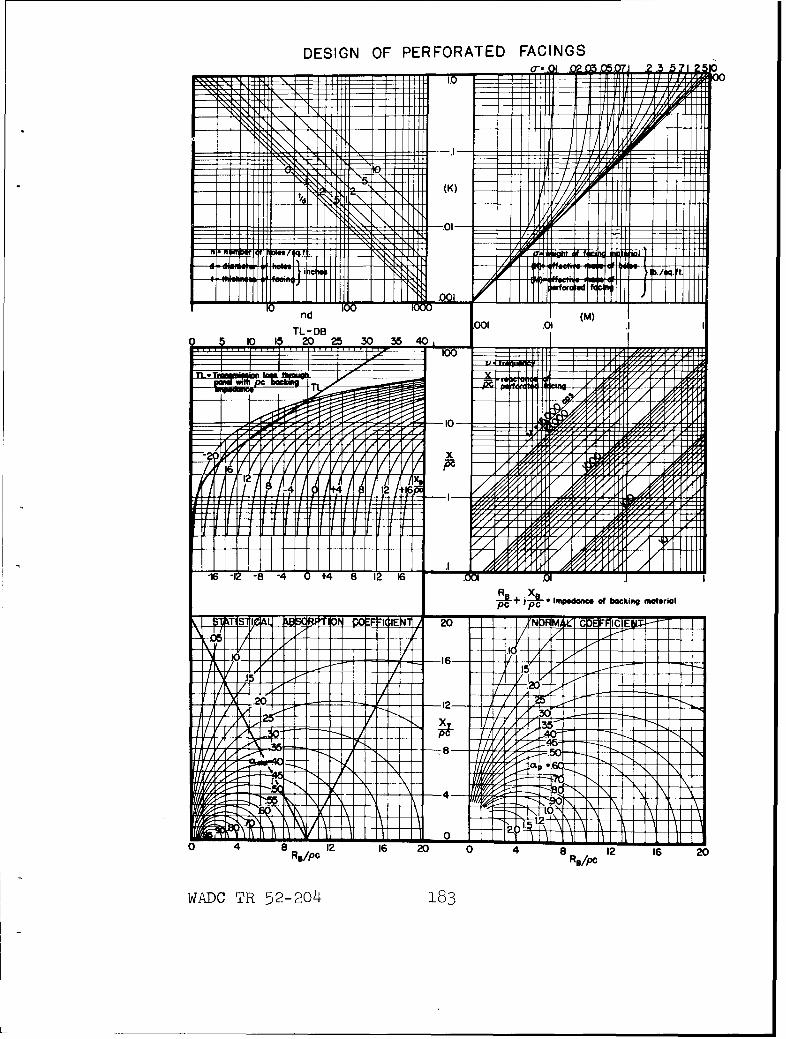
DESIGN OF PERFORATED FACINGS

1.0 :44P, fill] I ýýA I If

X"I IN, IM I

v(K)

I V///, 7 11 M

.01

I ]if I I "N"',-wo"lp r oil 101"114.7t. I Whu 3

t

nd )00 .001

TL- DB .001 .0 1 (M)

1 15 20 25 30 35 40,100tt7tt!

.n x IA -11- Z_

wm PCý'T

z

X- '_ýl 10-

A yv

XPC ItY/

4, k6.!?- /r

ýZz' Z AH4 A

z A/Z

-16 -12 -8 16

-!L+ j-XL 1woodonce of backing roaterial

$1AT1S11&L_4BSCftf7"_;ýF 111Eý 20 ___/(NPFjMilWj CDEFFICIEJ05 11 1 r I vi LV14 1 / I- I I I I/ __ Ic -N 1 11 +_ LL I /i A I

A 11 1J _L F-V E

A vi I Z-)51,

1112010- 12-

.2ý /',30F

v ýA IAoMA .45

-- 78- 5;%oir4C I

P..

\1 NA )L __j () ý_ 0 __

M1 I 1_12 _..

o 4 1111 1 LL

8 Re/po 12 16 20 0 4 8 RB/PC 12 16 20

WADC TR 52-204 183

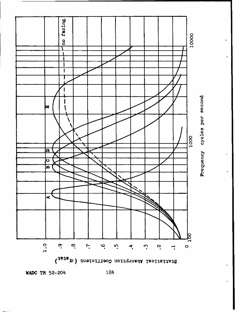
00

000

________ 0f-i

0C)�1)

0

0)0 H0 00 0

________ f-I

C)

0)

__ I.

0 '.0 tA 4 CU � 09

I-,

�ue�oTjJsoo U0T�dJoBqy !UOT�9T��

WADG TR 52-204 184

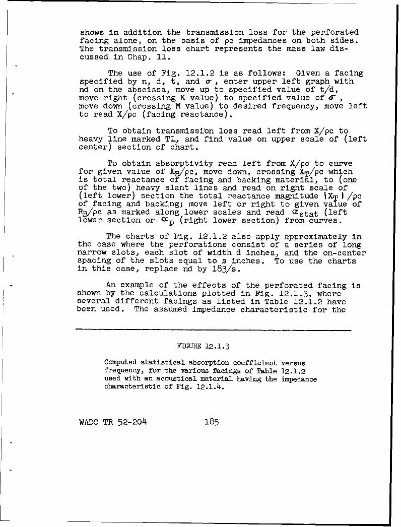
shows in addition the transmission loss for the perforatedfacing alone, on the basis of pc impedances on both sides.The transmission loss chart represents the mass law dis-cussed. in Chap. 11.

The use of Fig. 12.1.2 is as follows: Given a facingspecified by n, d, t, and a-, enter upper left graph withnd on the abscissa, move up to specified value of t/d,move right (crossing K value) to specified value of o-,move down (crossing M value) to desired frequency, move leftto read X/pc (facing reactance).

To obtain transmission loss read left from X/pc toheavy line marked TL, and find value on upper scale of (leftcenter) section of chart.

To obtain absorptivity read left from X/pc to curvefor given value of XB/pc, move down, crossing XT/pC whichis total reactance of facing and backing material, to (oneof the two) heavy slant lines and read on right scale of(left lower) section the total reactance magnitude IXTI /pcof facing and backing; move left or right to given value ofRB/pc as marked along lower scales and read •stat (leftlower section or O•p (right lower section) from curves.

The charts of Fig. 12.1.2 also apply approximately inthe case where the perforations consist of a series of longnarrow slots, each slot of width d inches, and the on-centerspacing of the slots equal to s inches. To use the chartsin this case, replace nd by 183/s.

An example of the effects of the perforated facing isshown by the calculations plotted in Fig. 12.1.3, whereseveral different facings as listed in Table 12.1.2 havebeen used. The assumed impedance characteristic for the

FIGURE 12.1.3

Computed statistical absorption coefficient versusfrequency, for the various facings of Table 12.1.2used with an acoustical material having the impedancecharacteristic of Fig. 12.1.4.

WADC TR 52-204 185

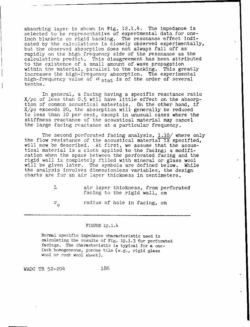
absorbing layer is shown in Fig. 12.1.4. The impedance isselected to be representative of experimental data for one-inch blankets on rigid backing. The resonance effect indi-cated by the calculations is closely observed experimentally,but the observed absorption does not always fall off asrapidly on the high frequency side of the resonance as thecalculations predict. This disagreement has been attributedto the existence of a small amount of wave propagationwithin the material, parallel to the backing. This greatlyincreases the high-frequency absorption. The experimentalhigh-frequency value of C stat is of the order of severaltenths.

In general, a facing having a specific reactance ratioX/pc of less than 0.5 will have little effect on the absorp-tion of common acoustical materials. On the other hand, ifX/pc exceeds 20, the absorption will generally be reducedto less than 10 per cent, except in unusual cases where thestiffness reactance of the acoustical material may cancelthe large facing reactance at a particular frequency.

The second perforated facing analysis, L.2/ where onlythe flow resistance of the acoustical material is specified,will now be described. At first, we assume that the acous-tical material is a cloth applied to the facing; a modifi-cation when the space between the perforated facing and therigid wall is completely filled with mineral or glass woolwill be given later. The symbols are defined below. Whilethe analysis involves dimensionless variables, the designcharts are for an air layer thickness in centimeters.

L air layer thickness, from perforatedfacing to the rigid wall, cm

ro 0radius of hole in facing, cm

FIGURE 12.1.4

Normal specific impedance characteristic used incalculating the results of Fig. 12.1.3 for perforatedfacings. The characteristic is typical for a one-inch homogeneous, porous tile (e.g., rigid glasswool or rock wool sheet).

WADC TR 52-204 186

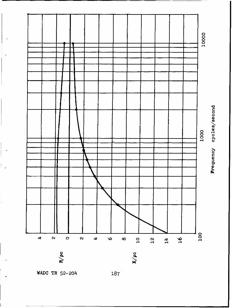
000-�0

'-I

000,@2

@2

ow0 H- - 0- - - - _____ r4 C)

- C)

0)

00

- - - - - ----

- --- ___ --- 04 c�j 0 ("J 4 '.0 �) 0 CU 4 � 0r1

r-4 -4 r"4

o C)0. 0."N

WADC TR 52-204 187

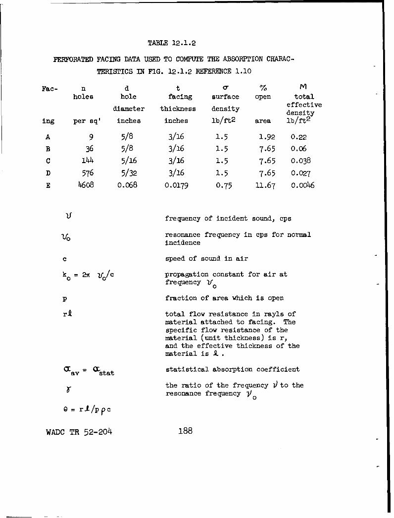
TABLE 12.1.2

PERFORATED FACING DATA USED TO COMPUTE THE ABSORPTION CHARAC-

TERISTICS IN FIG. 12.1.2 REFERENCE 1.10

Fac- n d t 70 Mholes hole facing surface open totaleffective

diameter thickness density density

ing per sq' inches inches lb/ft 2 area lb/ft 2

A 9 5/8 3/16 1.5 1.92 0.22

B 36 5/8 3/16 1.5 7.65 m.06

C 144 5/16 3/16 1.5 7.65 0.038

D 576 5/32 3/16 1.5 7.65 0.027

E 4608 O.068 0.0179 0.75 11.67 0.0046

if frequency of incident sound, cps

I/° resonance frequency in cps for normalincidence

c speed of sound in air

k 2:K 0/c propagation constant for air atfrequency Vof

p fraction of area which is open

ri total flow resistance in rayls ofmaterial attached to facing. Thespecific flow resistance of thematerial (unit thickness) is r,and the effective thickness of thematerial is k.

cav stat statistical absorption coefficient

the ratio of the frequency V to theresonance frequency Vo

0= r-/p pc

WADC TR 52-204 188

The analysis assumes that the facing is rigid. Thespecific impedance due to the perforations is obtained onthe basis of the effective air mass from Eq. (12.1.20).The added specific impedance due to the flow resistance ofthe cloth is r-/p*. The specific impedance due to the airlayer of depth L is -Jpc cot(koL), as may be shown fromEq. (12.1.14a), if the air layer is partitioned into cellsor if the incoming wave is at normal incidence. A morecomplicated relation is necessary for oblique incidence ona nonpartitioned layer. The total specific impedance ofthe layer is the sum of the three contributions (air massreactance, cloth flow resistance, air layer impedance).

Resonances occur at those frequencies where the re-actance of the air layer is Just sufficiently negative tocompensate for the hole reactance. Large absorption mayoccur at these resonances if the resistive component ofthe impedance is properly chosen. The statistical absorp-tion coefficient is computed by use of Eqs. (12.1.12) and(12.1.3). In the case of the unpartitioned air layer, therelations are sufficiently complicated to require numericalintegration.

The results of the analysis outlined above are givenas the statistical absorption coefficient vs a frequencyparameter, in Fig. 12.1.5, (for the partitioned air layer)and Fig. 12.1.6, (for the unpartitioned case). An auxiliarychart, Fig. 12.1.7, is required to compute the lowest normalincidence resonance frequency, corresponding to T = 1. Thisprovides numerical values for the dimensionless frequencyscale used on the preceeding absorption coefficient charts.

The open area factor p is used here because theair flow is confined to the parts of the clothwhich are behind perforations. For a cloth muchthicker than the hole diameter, the flow wouldspread out sufficiently that the factor p shouldbe omitted.

WADC TR 52-204 189

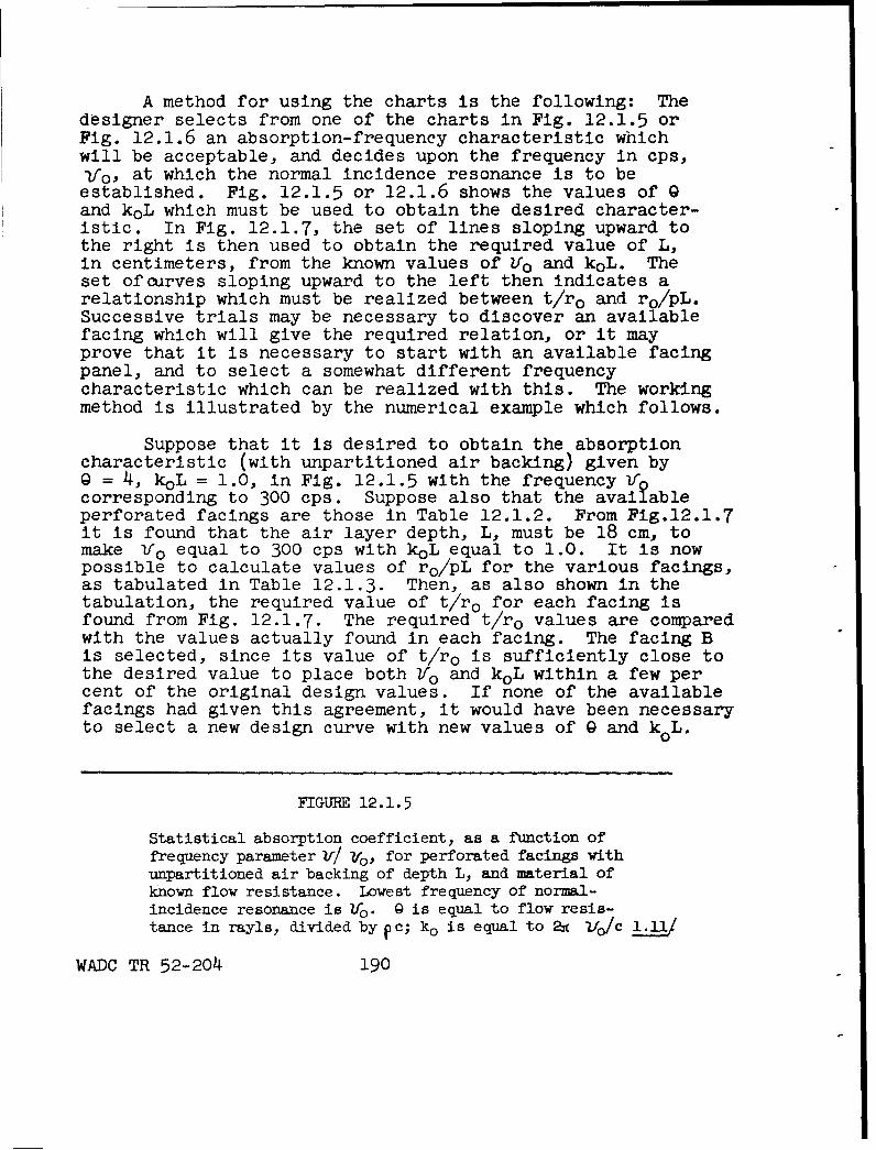
A method for using the charts is the following: Thedesigner selects from one of the charts in Fig. 12.1.5 orFig. 12.1.6 an absorption-frequency characteristic whichwill be acceptable, and decides upon the frequency in cps,Io, at which the normal incidence resonance is to beestablished. Fig. 12.1.5 or 12.1.6 shows the values of 9and koL which must be used to obtain the desired character-istic. In Fig. 12.1.7, the set of lines sloping upward tothe right is then used to obtain the required value of L,in centimeters, from the known values of Uo and koL. Theset of curves sloping upward to the left then indicates arelationship which must be realized between t/ro and ro/pL.Successive trials may be necessary to discover an availablefacing which will give the required relation, or it mayprove that it is necessary to start with an available facingpanel, and to select a somewhat different frequencycharacteristic which can be realized with this. The workingmethod is illustrated by the numerical example which follows.

Suppose that it is desired to obtain the absorptioncharacteristic (with unpartitioned air backing) given by0 = 4, koL = 1.0, in Fig. 12.1.5 with the frequency ifcorresponding to 300 cps. Suppose also that the availableperforated facings are those in Table 12.1.2. From Fig.12.1.7it is found that the air layer depth, L, must be 18 cm, tomake foo equal to 300 cps with koL equal to 1.0. It is nowpossible to calculate values of ro/pL for the various facings,as tabulated in Table 12.1.3. Then, as also shown in thetabulation, the required value of t/ro for each facing isfound from Fig. 12.1.7. The required t/ro values are comparedwith the values actually found in each facing. The facing Bis selected, since its value of t/ro is sufficiently close tothe desired value to place both Yo and koL within a few percent of the original design values. If none of the availablefacings had given this agreement, it would have been necessaryto select a new design curve with new values of 0 and k0 L.

FIGURE 12.1.5

Statistical absorption coefficient, as a function offrequency parameter v/ vo, for perforated facings withunpartitioned air backing of depth L, and material ofknown flow resistance. Lowest frequency of normal-incidence resonance is Yo. 0 is equal to flow resis-tance in rayls, divided by pc; ko is equal to 2x 1f0 /c 1.111

WADC TR 52-204 190

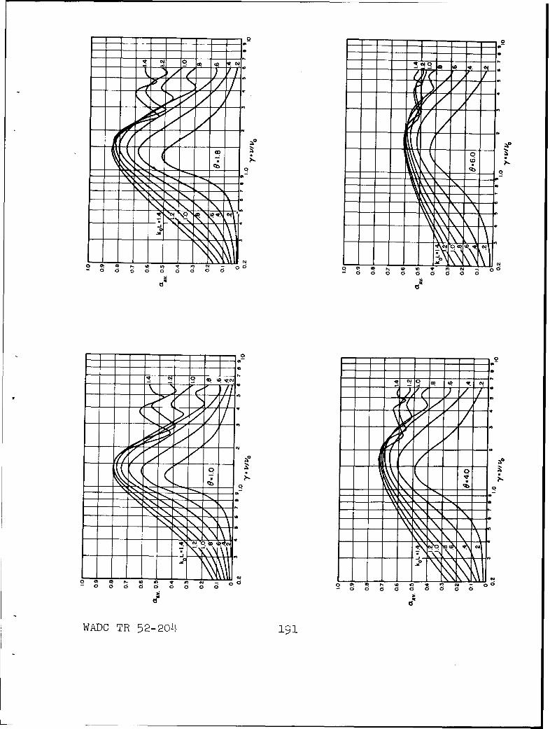
0

4 44

- - 0

00

00

-~~~C -t-4 -

-i - ,-

- 0 0 0 0 0 0 06 6 00- 0 0 0 c

4 Lo

WAC TR 5220 (9D

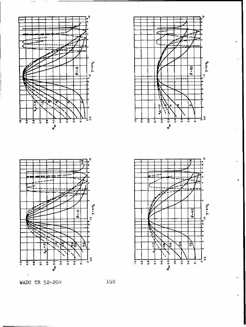
-~ - 0

-0 0 0 0 0 00 -6 W6 W66 6 0 0 0

-0 2 1 0

676

1 F

U of

WAX T 52-24 19

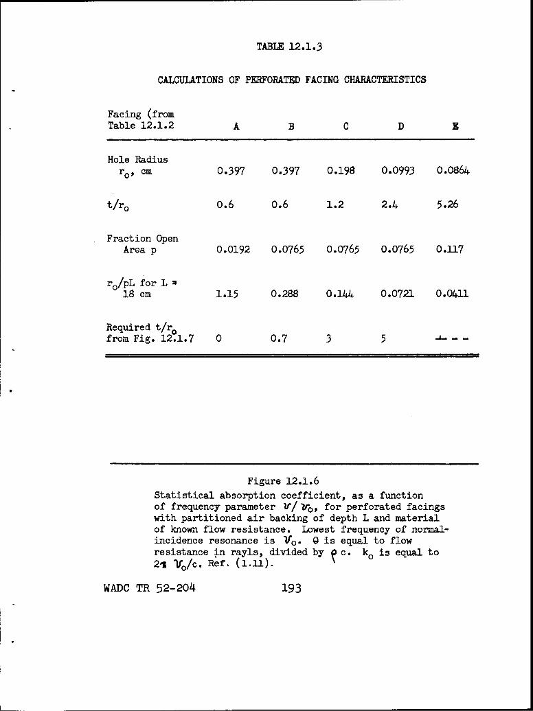
TABLE 12.1.3

CALCULATIONS OF PERFORATED FACING CHARACTERISTICS

Facing (fromTable 12.1.2 A B C D E

Hole Radiusto, cm 0.397 0.397 0.198 0.0993 0.0864

t/ro o.6 o.6 1.2 2.4 5.26

Fraction OpenArea p 0.0192 0.0765 0.0765 0.0765 0.117

r o /pL for L18 cm 1.15 0.288 0.144 0.0721 0.0411

Required t/rofrom Fig. 12.1.7 0 0.7 3 5.. _

Figure 12.1.6Statistical absorption coefficient, as a functionof frequency parameter v/ ?to, for perforated facingswith partitioned air backing of depth L and materialof known flow resistance. Lowest frequency of normal-incidence resonance is 1ro. Q is equal to flowresistance in rayls, divided by c. ko is equal to21 Vole. Ref. (1.11).

WADC TR 52-204 193

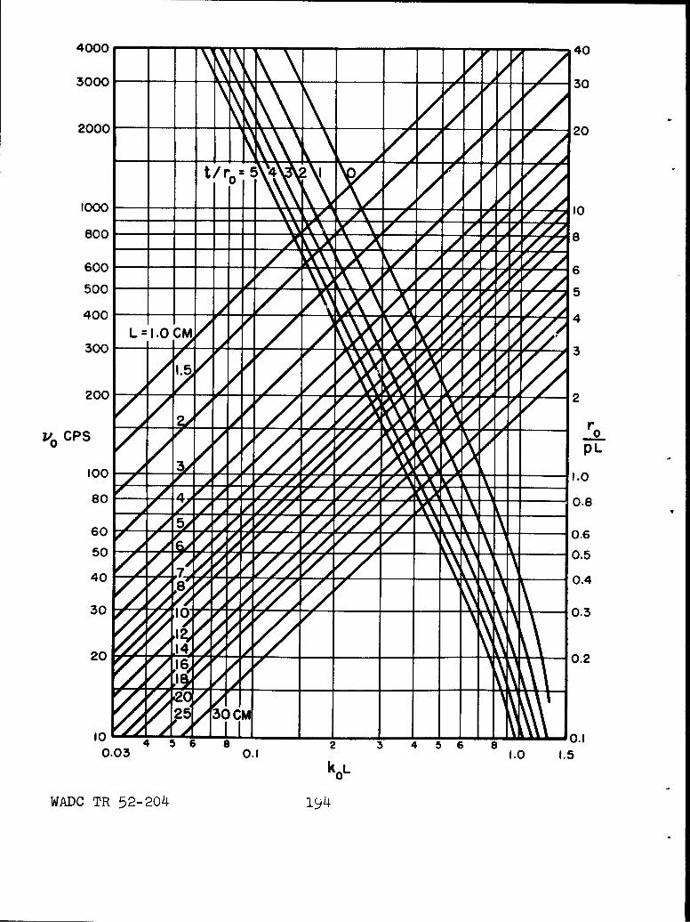
4000 40

3000-- 30

2000 -20 -- ___

01

800X x8

600500 O

400

300 L 1.1C

200O2

10.03 0.13/ 1. 1.0000,L

sA o TR0 52'0 1924 ,0.

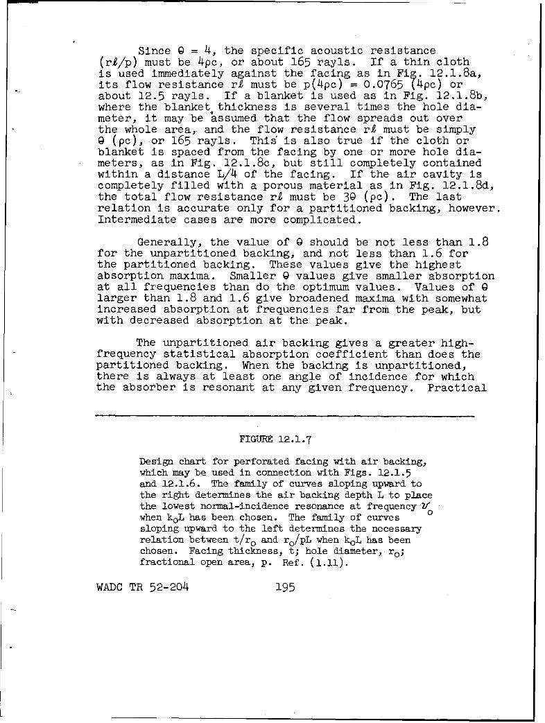
Since 0 = 4, the specific acoustic resistance(rl/p) must be 4pc, or about 165 rayls. If a thin clothis used immediately against the facing as in Fig. 12.1.8a,its flow resistance ri must be p(4pc) = 0.0765 (4pc) orabout 12.5 rayls. If a blanket is used as in Fig. 12.1.8b,where the blanket thickness is several times the hole dia-meter, it may be assumed that the flow spreads out overthe whole area, and the flow resistance ri must be simply@ (pc), or 165 rayls. This is also true if the cloth orblanket is spaced from the facing by one or more hole dia-meters, as in Fig. 12.1.8c, but still completely containedwithin a distance L/4 of the facing. If the air cavity iscompletely filled with a porous material as in Fig. 12.1.8d,the total flow resistance ri must be 30 (pc). The lastrelation is accurate only for a partitioned backing, however.Intermediate cases are more complicated..

Generally, the value of 9 should be not less than 1.8for the unpartitioned backing, and not less than 1.6 forthe partitioned backing. These values give the highestabsorption maxima. Smaller 0 values give smaller absorptionat all frequencies than do the optimum values. Values of 0larger than 1.8 and 1.6 give broadened maxima with somewhatincreased absorption at frequencies far from the peak, butwith decreased absorption at the peak.

The unpartitioned air backing gives a greater high-frequency statistical absorption coefficient than does thepartitioned backing. When the backing is unpartitioned,there is always at least one angle of incidence for whichthe absorber is resonant at any given frequency. Practical

FIGURE 12.1.7

Design chart for perforated facing with air backing,which may be used in connection with Figs. 12.1.5and 12.1.6. The family of curves sloping upward tothe right determines the air backing depth L to placethe lowest normal-incidence resonance at frequency Ywhen koL has been chosen. The family of curves 0

sloping upward to the left determines the necessaryrelation between t/ro and ro/pL when koL has beenchosen. Facing thickness, t; hole diameter, r o ;fractional open area, p. Ref. (1.11).

WADC TR 52-204 195

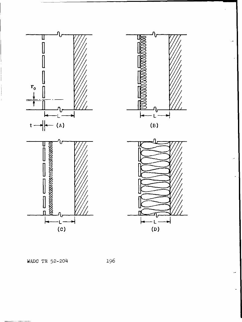
n n

(A) (B)

/~ - -44

(C) (D)

WADO TR 52-204 196

measurements with partitioned backing show performancewhich is intermediate between the partitioned. and. non-partitioned. predictions at very high frequencies; as thewavelength becomes smaller than the width of the cellsformed by partitioning, the performance approaches thatexpected for no partitions. At and below the frequency ofmaximum absorption, the absorption is increased by thepresence of partitions.

The method. of calculation applies with reasonableaccuracy if the facing is perforated by long narrow slotsrather than by circular holes. The calculations should. bebased on an equivalent hole radius equal to half the slotwidth.

Flow Resistance Data for Acoustical Materials.Figure 12.1.9 summarizes measured. values of specific flowresistance for severalp orous materials as a function ofvolume density in lb/ft . Individual samples may vary bysome 20 per cent from the nominal values.

It has been found 1.131 that the flow resistance ofloose sand can be expressed approximately by the equation

r = 19/d.13 (12.1.22)

FIGURE 12.1.8

Illustrations of special cases for which the effectiveflow resistance r' in the expression 9 = r'/pc is easilycomputed in the perforated facing analysis. Case A,cloth adjacent to facing, cloth thickness much less thanhole diameter, use r' equal to rA/p, where rY is flowresistance of cloth in rayls and p is fractional openarea of facing. Case D, blanket with thickness greaterthan hole diameter is adjacent to facing, but locatedentirely in left-hand quarter of backing space, user' = r k, flow resistance of blanket in rayls. Case C,cloth or blanket spaced from facing by at least one holediameter, but within left-hand quarter of backing space,use r' = rk , flow resistance in rayls. Case D, entirespace filled, use r' equal to one-third of blanket flowresistance in rayls.

WADC TR 52-204 197

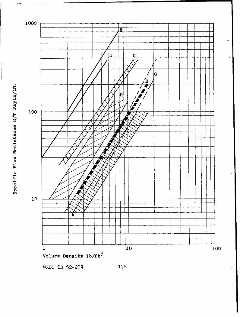
1000 -! II___1

/D CF//// A

/F/0,o

100

39

0

-r4

q.4

cn10

A ½

110 100

Volume Density lb/ft3

WAXC TR 52-204 198

where r is the specific flow resistance in rayls/cm andd is the average particle diameter in mm. This resultapplies where the particle size is reasonably uniform sothat an average diameter can be given. The flow resis-tance in rayls for a number of cloths and screens is givenin Table 12.1.4.

Porosity values for several materials are given inTable 12.1.5. The porosity of fibrous blankets of thematerials given, but having a different density may beestimated by means of the principle that (1 - porosity)is proportional to the density.

The structure factor m has been evaluated in a fewcases. A value of 2.7 for a structure consisting of manywire screens in close contact for the case of perpendicularincidence has been reported. However, considerable varia-tion with frequency was observed.1._/. The computedvalue of m is 3.0 for a structure which contains longnarrow passages oriented at random angles, l.3. The experi-mental value for loose sand is 4.3,1.3. lGenerally, mappears to be about 1.5 for blankets of porosity 0.95 ormore1.9

Propagation Constant. Illustrative propagation datafor two weights of Fiberglas, based on measurements 1.14in the range 50-1000 cps, are summarized in Table 12.1.6.The propagation constant is the quantity k1 correspondingto the expression exp (-Jklx) for the phase and amplitudebehavior of a plane wave. Expressions for the phasevelocity and the attenuation are given separately in thetable. Measurements of the propagation constant for a rockwool (J-M Stonefelt, Type M) .9 and for loose sandhave also been published.

FIGURE 12.1.9

Specific flow resistance (rayls/inch) for variousglass and mineral wools, as a function of volumedensity. A, PF (board) Fiberglas (the materialmeant by reference to "PF" Fiberglas unless a spe-cific style is stated); B, TWF white wool Fiberglas;C, PF 450 Fiberglas; D, Aerocor Fiberglas; E, J-MThermoflex; F, B-H rock wool, Style #1, with wirefacing; G, B-H rock wool, Style 2; H, J-M #305mineral wool.

WADC TR 52-204 199

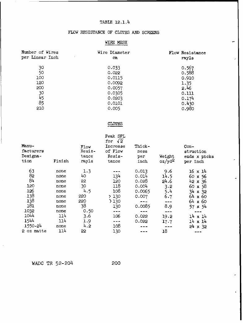
TABLE 12.1.4

FLOW RESISTANCE OF CLOTHS AND SCREENS

WIRE MESH

Number of Wires Wire Diameter Flow Resistanceper Linear Inch cm rayls

30 0.033 0.56750 0.022 0.588

100 0.0115 0.910120 0.0092 1.35200 0.0057 2.46

30 0.0305 0.11145 0.0203 0. 17485 0.0101 o.1430

210 0.005 o.98o

CLOTHS

Peak SPLfor 4-

Manu- Flow Increase Thick- Con-facturers Resis- of Flow ness structionDesigna- tance Resis- per Weight ends x pickstion Finish rayls tance inch oz/yd2 per inch

63 none 1.3 --- 0.013 9.6 16 x 1482 none 40 134 0.014 14.5 60 x 5684 none 22 120 0.028 24.6 42 x 36

120 none 30 118 0.004 3.2 60 x 58126 none 4.5 108 0.0065 5.4 34 x 32138 none 220 ) 130 0.007 6.7 64 x 60138 none 220 )130 --.--- 6 4 x 60181 none 38 130 0.0085 8.9 57 x 54

1032 none 0.50 ............1044 114 3.6 106 0.022 19.2 14 x 141544 114 1.9 --- 0.022 17.7 14 x 141550-24 none 4.2 108 --- 24 x 32

2 oz matte 114 22 130 18 ---

WADC TR 52-204 200

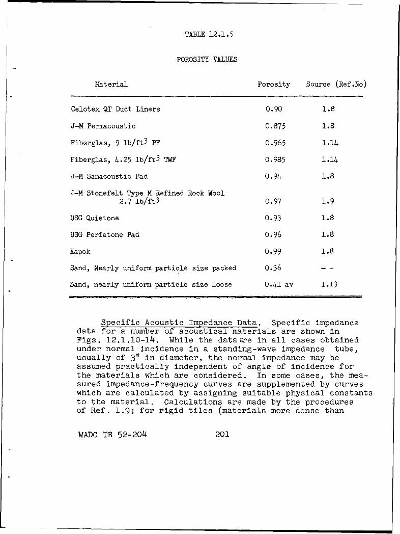
TABLE 12.1.5

POROSITY VALUES

Material Porosity Source (Ref.No)

Celotex QT Duct Liners 0.90 1.8

J-M Permacoustic 0.875 1.8

Fiberglas, 9 lb/ft 3 PF 0.965 1.14

Fiberglas, 4.25 lb/ft 3 TWF 0.985 1.14

J-M Sanacoustic Pad 0.94 1.8

J-M Stonefelt Type M Refined Rock Wool2.7 lb/ft3 0.97 1.9

USG Quietone 0.93 1.8

USG Perfatone Pad 0.96 1.8

Kapok 0.99 1.8

Sand, Nearly uniform particle size packed 0.36 - -

Sand, nearly uniform particle size loose 0.41 av 1.13

Specific Acoustic Impedance Data. Specific impedancedata for a number of acoustical materials are shown inFigs. 12.1.10-14. While the dataae in all cases obtainedunder normal incidence in a standing-wave impedance tube,usually of 3" in diameter, the normal impedance may beassumed practically independent of angle of incidence forthe materials which are considered. In some cases, the mea-sured impedance-frequency curves are supplemented by curveswhich are calculated by assigning suitable physical constantsto the material. Calculations are made by the proceduresof Ref. 1.9; for rigid tiles (materials more dense than

WADC TR 52-204 201

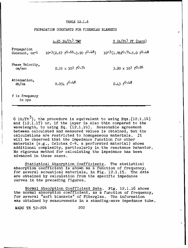
TABLE 12.1.6

PROPAGATION CONSTANTS FOR FIBERGLAS BLANKETS

4.25 lb/ft 3 TWF 9 lb/ft 3 PF (hard)

PropagationConstant, cm-I 10-3(2.67 f 0 "6 6 -3.90 fO-48) lo- 3 (l.96f0 .74 -5.0 fO.48

Phase Velocity,cm/sec 2.35 x 103 fO.34 3.20 x 103 fO.26

Attenuation,db/cm 0.034 f0 O48 0.43 f0 .4 8

f is frequencyin cps

6 lb/ft 3 ), the procedure is equivalent to using Eqs.(12.1.14)and (12.1.17) or, if the layer is also thin compared to thewavelength, to using Eq. (12.1.19). Reasonable agreementbetween calculated and measured values is obtained, but thecalculations are restricted to homogeneous materials. Itwill be observed that the impedance function for othermaterials (e.g., Celotex C-4, a perforated material) showsadditional complexity, particularly in the reactance behavior.No rigorous method for calculating the impedance has beenadvanced in these cases.

Statistical Absorption Coefficients. The statisticalabsorption coefficient is shown as a function of frequency,for several acoustical materials, in Fig. 12.1.15. The dataare obtained by calculation from the specific impedancecurves in the preceding figures.

Normal Absorption Coefficient Data. Fig. 12.1.16 showsthe normal absorption coefficient, as a function of frequency,for several "soft blankets" of Fiberglas. The informationwas obtained by measurements in a standing-wave impedance tube.

WADC TR 52-204 202

Chamber Absorption Coefficients. Figs. 12.1.17-19show the absorption coefficients as a function of frequencyfor perforated acoustical tiles of thickness 1, 1/2 and 1/4in. In each chart individual curves show the behavior ofmaterial of given thickness on standard mountings l, 2 and7 as defined by the Acoustical Materials Association. Thecharts are constructed from averages of the AMA chamberabsorption coefficients for perforated tiles of the variousmanufacturers. The data for the different tiles are suffi-ciently close together to Justify the use of these averagecharts for most engineering purposes. Detailed informationfor individual products is available in Ref. 1.6.

Average values of the noise reduction coefficient arealso shown for each mounting condition and for each tilethickness. The noise reduction coefficient is defined asthe average of the chamber absorption coefficients at 256,512, 1024 and 2048 cps, given to the nearest 5 per cent.(The average values given here are not rounded to the near-est 5 per cent).

The mounting conditions are defined as follows:

Mounting 1.

Sample cemented to plaster board.Considered equivalent to cementing toplaster or concrete ceiling.

Mounting 2.

Sample nailed to 1 in. x 3 in. woodfurring, ordinarily 12 in. on centers.

Mounting 7.

Sample mechanically mounted (spacedfrom ceiling).

WADC TR 52-204 203

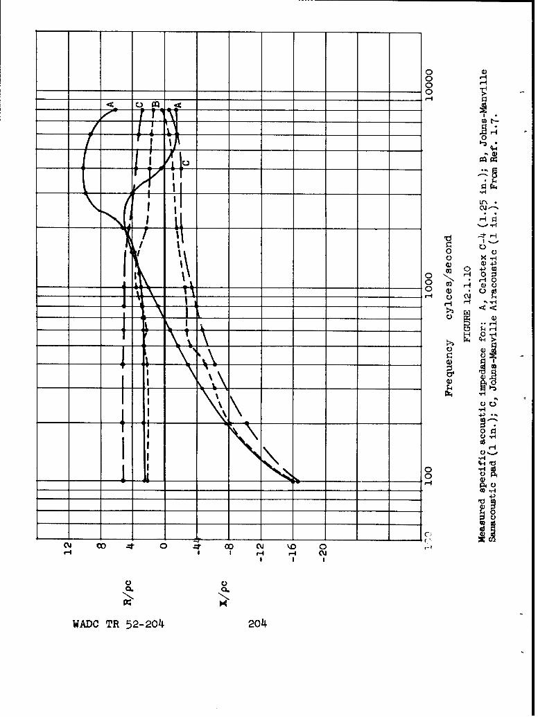
0010

0 8

-_ _ _ _ _"_-_

1 00

0 U NO ,i_ __IIE __ __-_

I 40. v_

I _ _ _ • -

I 0 )-

-U -HS-4- ,...

-4-Fa, ,

cmJ 4- 0 \ . 0

H 5

WADC TRt 52-204 204

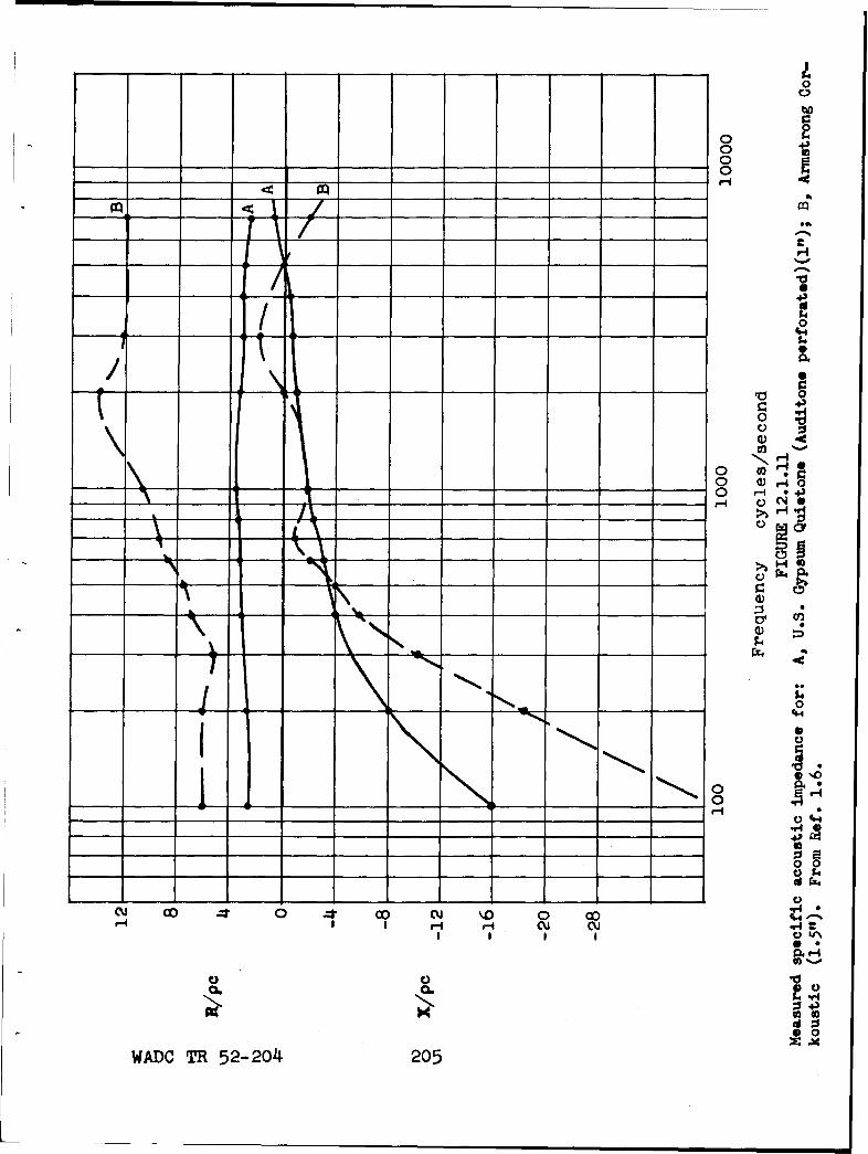
0

o0

o 43

43,

C~4 4

a .4

'd 0

all~

o r4 @4,

0)

WAD V 5-2o 0

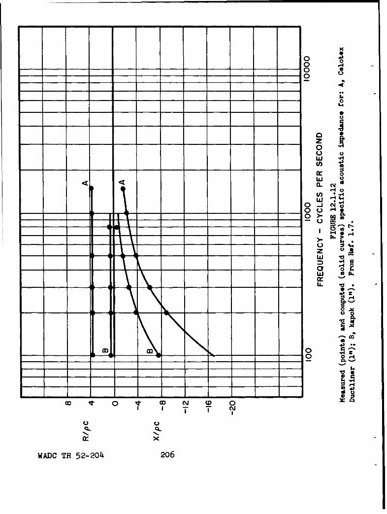
x0 +0)0

0

00

w

0U

00

w '

0.c

cr 4x

WADC R 52-o4 20

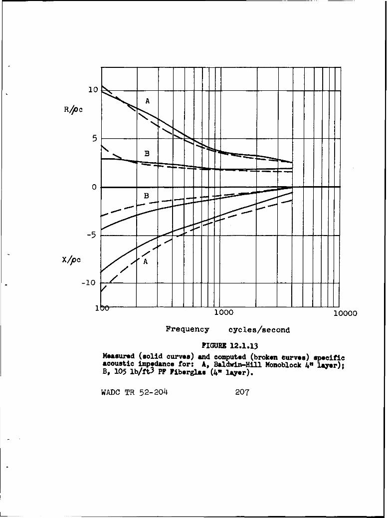
10 - - - - - - - -

R/pOc

5

0

-5

x/pc oo A

-10-- - -__

1000 10000

Frequency cycles/second

FIGURE 12.1.13Measured (solid curves) and computed (broken curves) specificacoustic impedance for: A. Baldwin-Hill Monoblock 4" layer);BO 105 lb/ft3 pP Fiberglas (40 layer).

WADC TR 52-2o14 207

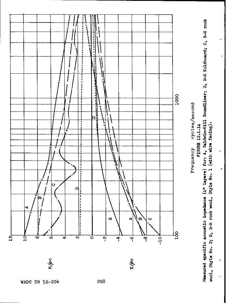
0

.0

as

~~4-1

____ 0__ ___t I- O__ 0

-a _

:4 0

WAD TR5-2420

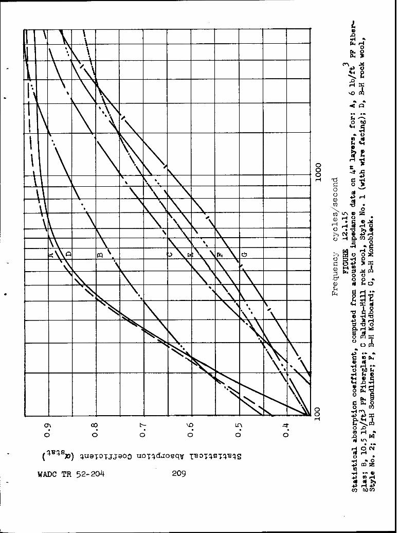
4

-rrz4 r-4

S . 0

0.

4- r-4~co 19

_ _ _ _ _ _ _ __ _ _ q.__ - - ~z

-(D HO'C.

_ _4 _ _ 4N3 _

___ _ _ ~N S .0

oo

I04

o0

0 C

.r4

0.0 m

WADO TR 5 2 -2 o~4 209 H5. .. w04> 0 #--143

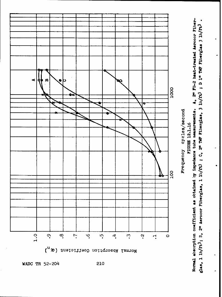
00__

__5

__IC__ __ _-4_ _ _

02%

q4 S

*0

'4

0

o C7 ~ ) ~ - ~ tC ~ -~ C H

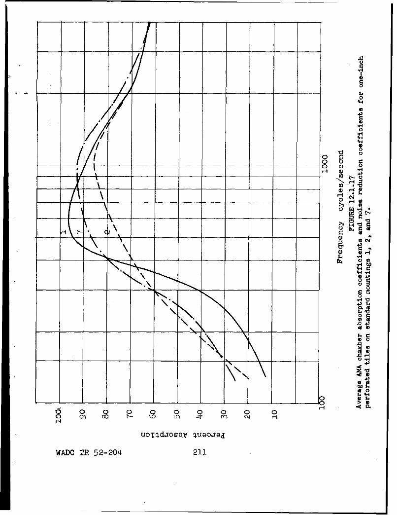
41000 0

kNI 0

.94

/0

0 ~ 0

0~~ ~ ~ ~ 0 0 0 0 0m 00 l- 110 n () U)

uo~qdosqV uaoaa

WADC R 52-04 21

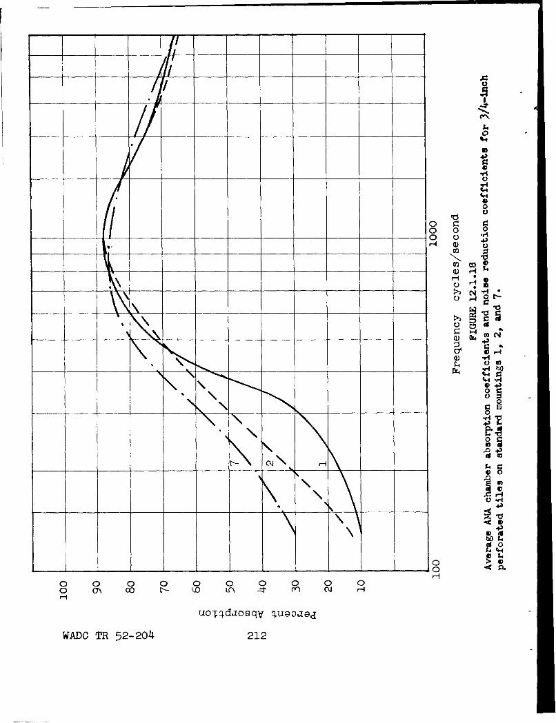
W4

54V

00

*r4 +

.9-4

0

o fno 0

4J

0 2~___ -. 0_ ) 5

0 0 0 00 0 0H0_ m_ 00 t_ _ 1_ _:t nl

uo~qdjosqo H aaa

WADC~~~ TR5224 1

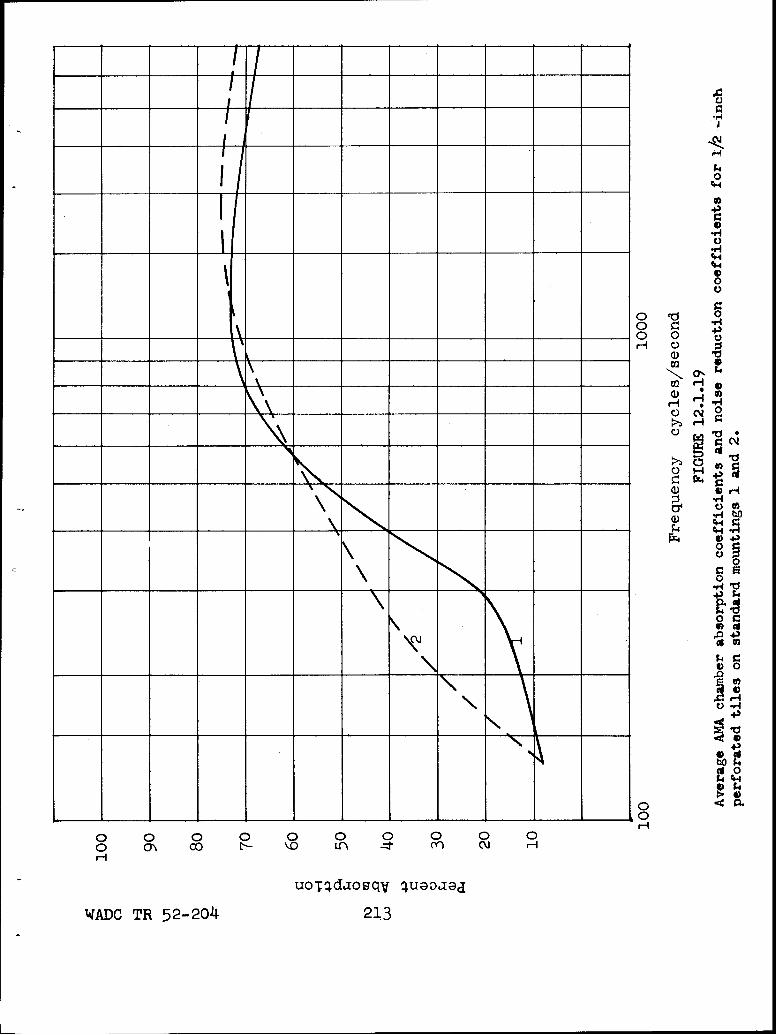
0

0 0

140 0 0

rI 0o C,4

o r40CQ

H 0

02 *

O 0

94

00r-0

0 0 0 0 0 0 00 m o t- ý10 Ln () N)

V .r

Uo~qdogqv uaoaa

WADC R 52-04 21

References:

(1.1) Morse, P.M., and Bolt, R. H., "Sound Waves inRooms," Rev. Mod. Phys. 16, 69-150 (1944).

(1.2) Beranek, L. L., Acoustic Measurements, J. Wileyand Sons (1949).

(1.3) Zwikker, C. and Kosten, C. W., Sound AbsorbingMaterials, Elsevier Publishing Co., Inc. (1949).

(1.4) Knudsen, V. 0. and Harris, C. M., AcousticalDesigning in Architecture, J. Wiley and Sons(1950) Chaps. 6-8 and App.l.

(1.5) Sabine, W. C. Collected Papers on AcousticsHarvard University Press (1927).

(1.6) Acoustical Materials Association, Bulletin XIII,Sound Absorption Coefficients of ArchitecturalAcoustical Materials, Acous. Mats. Assn., 59 E.55th St., New York (1951).

(1.7) Beranek, L. L., "Acoustic Impedance of CommercialMaterials and the Performance of Rectangular Roomswith One Treated Surface," J. Acous. Soc. Am 12,14-23 (1940).

(1.8) Beranek, L. L., "Acoustic Impedance of PorousMaterials," J. Acous. Soc. Am 13, 248-260 (1942).

(1.9) Beranek, L. L., "Acoustical Properties of Homo-geneous, Isotropic Rigid Tiles and Flexible Blankets,"J. Acous. Soc. Am 19, 556-568 (1947).

(1.10) Bolt, R. H., "On the Design of Perforated Facingsfor Acoustic Materials," J. Acous. Soc. Am., 19917-921 (1947).

(1.11) Ingard, U., and Bolt, R. H., "AbsorptionCharacteristics of Acoustic Material with PerforatedFacings," J. Acous. Soc. Am., 23, 533-540 (1951).

WADC TR 52-204 214

(1.12) Morse, P.M., Vibration and Sound, McGraw-HillBook Co., Inc. New York (1952), pp. 247-278.

(1.13) Ferrero, M. A. and Sacerdote, G. G., "Parametersof Sound Propagation in Granular AbsorbentMaterials," Acustica 1, 137-142 (1951).

(1.14) Esmail-Begui, Z. and Naylor, T. K., "Measurementof the Propagation of Sound in Fiberglas," J. Acous.Soc. Am. 25, 87-91 (1953).

WADC TR 52-204 215

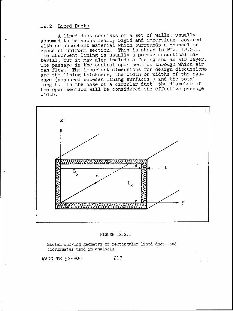
12.2 Lined Ducts

A lined duct consists of a set of walls, usuallyassumed to be acoustically rigid and impervious, covered

with an absorbent material which surrounds a channel orspace of uniform section. This is shown in Fig. 12.2.1.The absorbent lining is usually a porous acoustical ma-terial, but it may also include a facing and an air layer.The passage is the central open section through which aircan flow. The important dimensions for design discussionsare the lining thickness, the width or widths of the pas-sage (measured between lining surfaces,) and the totallength. In the case of a circular duct, the diameter ofthe open section will be considered the effective passagewidth.

x

Lt

y

Lx

FIGURE 12.2.1

Sketch showing geometry of rectangular lined duct, andcoordinates used in analysis.

WADC TR 52-204 217

A lined duct is usually designed to have an attenua-tion-frequency characteristic possessing a broad maximum.The frequency of the maximum is governed both by the passagedimensions and by the properties of the lining. In mostpractical cases, the condition of maximum attenuation isrealized when the wavelength of sound is of the order ofthe smaller passage width. The frequency of maximumattenuation can be lowered somewhat by increasing the lin-ing thickness. For this reason, the lining sometimesconsists of a layer of porous material (e.g., mineral woolor glass fiber blanket) which is separated by an air spacefrom the enclosure wall. This arrangement economicallyincreases the effective depth of the lining for a givenamount of acoustical material.

Qualitative Discussion of Attenuation in Ducts. Theacoustic attenuation of a lined duct is the result of con-version of acoustical energy into heat in the absorbinglayer. This energy absorption is most readily discussedfor the case in which the lining reacts locally with thesound wave. Local reaction means that there is noimportant transmission of waves within or behind the absorb.-ing material, in the direction parallel to the duct axis.Such wave transmission may materially reduce the attenuationof sound in the duct; therefore, in all applications to bediscussed, it is assumed that local reaction approximationis valid. In order to prevent longitudinal wave motion inan air space behind the lining, it is necessary to insertrigid partitions which are perpendicular to the duct axis.Successive partitions should be spaced by about one tenthof the wavelength at which maximum attendation is obtained.When the lining extends to the wall without an air space,lateral partitioning is usually unnecessary because of thelarge attenuation of sound in the lining material.

The duct lining may be characterized by its normalspecific acoustic impedance, which is the ratio of acousticpressure to particle velocity normal to the surface. Forthe case of local reaction, the normal specific acousticimpedance is independent of the angle of incidence and henceis the same for all directions which the incident wave inthe duct may have with respect to the lining.

The normal impedance of the lining usually contains

a resistive term, so that there is a component of the normal

WADC TR 52-2o4 218

particle velocity at the lining surface which is in phasewith the pressure. Thus, power is delivered to the liningat a rate proportional to the product of acoustic pressureand the in-phase particle velocity. Physically, thispower is transformed into heat due to both viscous frictionwithin the lining and compression by the acoustic wave ofthe gas contained within the lining.

The simplest analysis of duct action is obtained ifit is assumed that the acoustic pressure is uniform acrossthe open portion of the duct. It is then an easy matterto compute the effects of air flow into the lining, and tofind the attenuation of sound in the duct.

The uniform-pressure assumption is always reasonable(though not rigorous) for the special case in which thewavelength of sound is greater than the narrowest passagewidth, and at the same time the absorption coefficient ofthe lining is much less than unity. For this reason, simple,approximate attenuation formulas obtained from the uniformpressure treatment are almost always satisfactory in practice for frequencies well below the attenuation peak fora given duct. Moreover, if the lining has a relatively highimpedance, such simple formulas are valid for frequenciesclosely approaching the peak. Since it can be shown thatthe low-frequency formulas can be expressed in terms ofthe absorption coefficient of the lining, it is not neces-sary to know the specific acoustic impedance of the liningfor this approximate analysis.

Unfortunately, serious errors may be made by injudi-cious application of the approlmate results~obtained withthe uniform plane-wave assumption. If the frequency issufficiently high to allow the feorxation of cross-modes inthe duct, or if the lining has very large absorption, theacoustic pressure near the lining wfill be appreciably lessthan that at the axis of the duct; in this case the result-ing attenuation will be less than that computed on theplane wave assumption.

It is possible to solve the acoustic wave equationto determine the propagation of sound waves in a duct ofsimple shape for any frequency and for any boundary

WADC TR 52-204 219

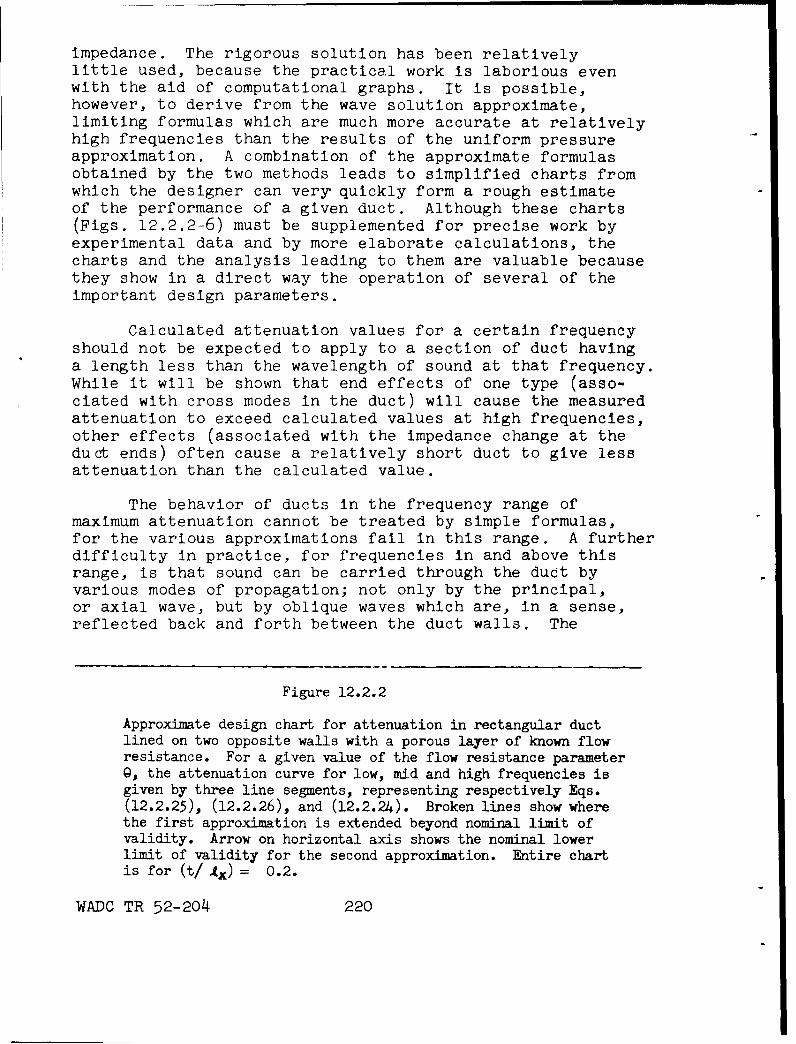
impedance. The rigorous solution has been relativelylittle used, because the practical work is laborious evenwith the aid of computational graphs. It is possible,however, to derive from the wave solution approximate,limiting formulas which are much more accurate at relativelyhigh frequencies than the results of the uniform pressureapproximation. A combination of the approximate formulasobtained by the two methods leads to simplified charts fromwhich the designer can very quickly form a rough estimateof the performance of a given duct. Although these charts(Figs. 12.2.2-6) must be supplemented for precise work byexperimental data and by more elaborate calculations, thecharts and the analysis leading to them are valuable becausethey show in a direct way the operation of several of theimportant design parameters.

Calculated attenuation values for a certain frequencyshould not be expected to apply to a section of duct havinga length less than the wavelength of sound at that frequency.While it will be shown that end effects of one type (asso-ciated with cross modes in the duct) will cause the measuredattenuation to exceed calculated values at high frequencies,other effects (associated with the impedance change at theduct ends) often cause a relatively short duct to give lessattenuation than the calculated value.

The behavior of ducts in the frequency range ofmaximum attenuation cannot be treated by simple formulas,for the various approximations fail in this range. A furtherdifficulty in practice, for frequencies in and above thisrange, is that sound can be carried through the duct byvarious modes of propagation; not only by the principal,or axial wave, but by oblique waves which are, in a sense,reflected back and forth between the duct walls. The

Figure 12.2.2

Approximate design chart for attenuation in rectangular ductlined on two opposite walls with a porous layer of known flowresistance. For a given value of the flow resistance parameterQ, the attenuation curve for low, mid and high frequencies isgiven by three line segments, representing respectively Eqs.(12.2.25), (12.2.26), and (12.2.24). Broken lines show wherethe first approximation is extended beyond nominal limit ofvalidity. Arrow on horizontal axis shows the nominal lowerlimit of validity for the second approximation. Entire chartis for (t/ .tx) = 0.2.

WADC TR 52-204 220

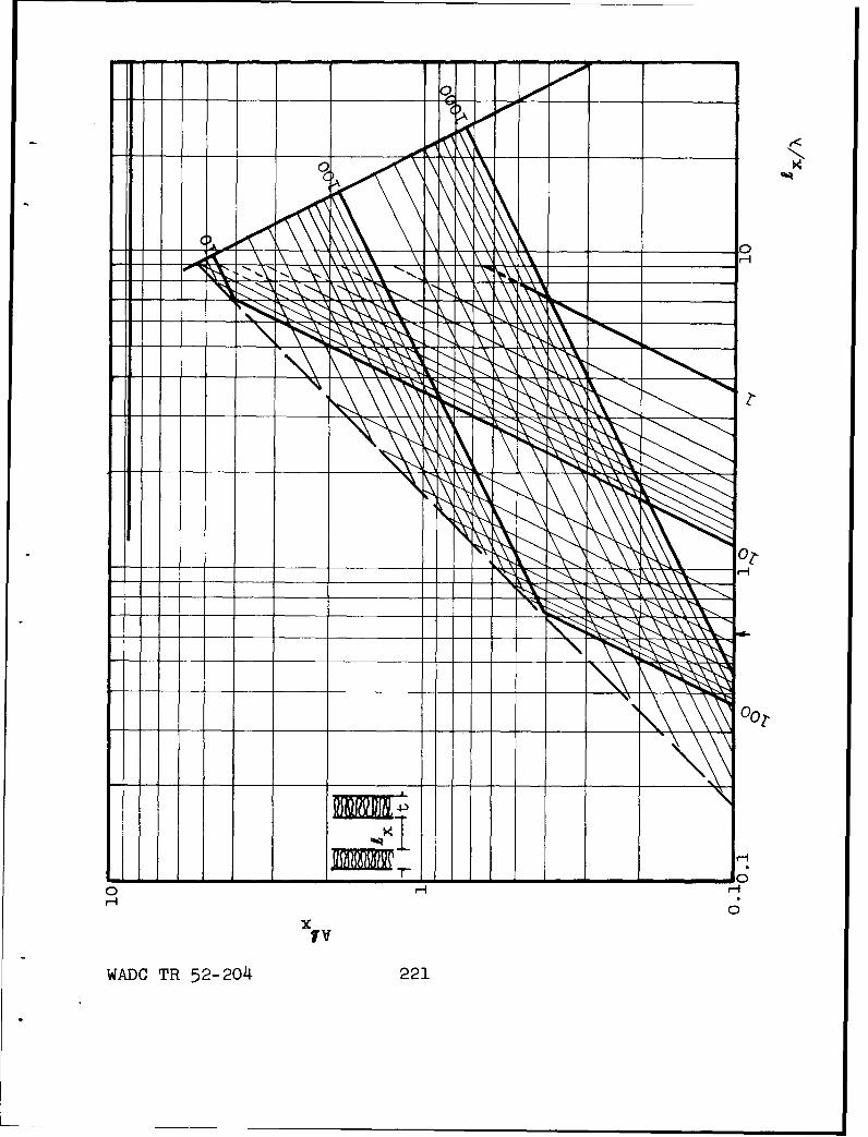
01 H00

H\ \ \N

WADC TR 52-204 221

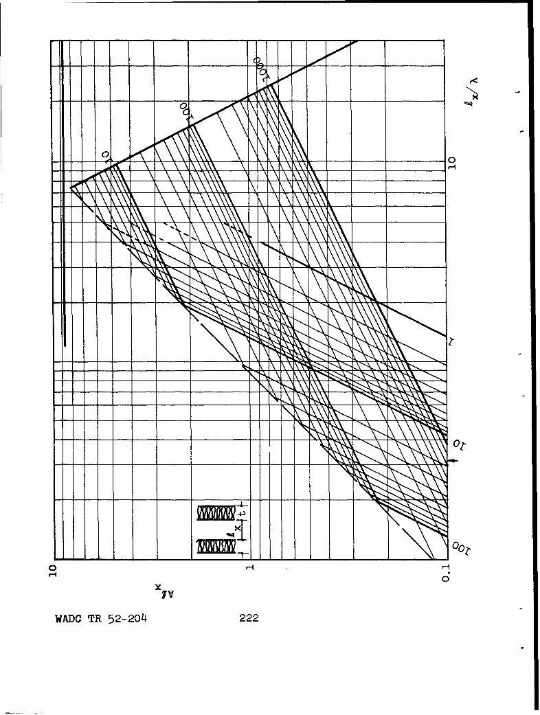
V N

WADC R 52-04 22

attenuation is greater for the higher modes (oblique waves)than for the principal waves. Thus if a large portion ofthe acoustical energy is carried in the higher modes, theattenuation will be greater than that predicted by calcula-tion, since calculations are ordinarily made for theprincipal wave.

In principle, acoustical theory would permitcalculation of the distribution of the energy among thevarious modes of travel, but in practice this calculationis almost never feasible. To make the calculation requiresmuch more detailed information about the acoustical fieldnear the sound source than is ordinarily available. Forthese reasons, considerable use is made of experimentaldata for frequencies in or above the range of the attenua-tion peak.

The remainder of this section contains briefderivations of the simplified attenuation formulas basedon both the uniform pressure approximation and the wave-theory treatment; design charts summarizing the resultsfrom these approximations and additional charts based ontypical experimental data are given.

Quantitative Treatment Under the Uniform PressureAssumption. The expression for a unidirectional plane wavetraveling in the positive x direction contains the spacefactor exp (-Jkz), where k is the propagation constant andx is the distance coordinate. For sound waves in a lossless

Figure 12.2.3

Approximate design chart for attenuation in rectangular ductlined on two opposite walls with a porous layer of knownflow resistance. For a given value of the flow resistanceparameter 9, the attenuation curve for low, mid and highfrequencies is given by three line segments, representingrespectively Eqs. (12.2.25), (12.2.26), and (12.2.24). Brokenlines show where the first approximation is extended beyondnominal limit of validity. Arrow on horizontal axis showsthe nominal lower limit of validity for the second approximation.Entire chart is for (t/1 x) = 0.4.

WADC TR 52-204 223

tube (or in open air) the propagation constant* is givenvery closely by:

SW 27 (K , (12.2.1)

where K is the compressibility of air, 9_ is the density,c is the speed of sound in air, and w is radian frequency.When the rigid boundary of the lossless tube is replacedby a non-rigid boundary, (the duct lining), the moving massis not changed as far as the wave motion is concerned, butthe effective compressibility is changed by the flow ofair into the lining. This effect is conveniently expressedin terms of the admittance index of the lining, Yr , whichis equal to the reciprocal of the impedance index. (SeeSec. 12.1). The effective compressibility is defined asK' = (l/p)(dV/V), where dV is the change of volume for aninitial volume V, under the excess pressure p.

The passage area of the duct will be denoted by A,and the total perimeter by P. If a sinusoidal excess pressure p is applied across a length dx of the duct, the volumeof air inflow is that due to the compressibility of thegas in the passage which is pKA dx, plus that due to theflow into the lining, which is pP \ dx/(- Jwe c). If the

* The term propagation constant is used in the literature in somecases to denote k and in some cases to denote the completecoefficient of x, which is -Jk.

Figure 12.2.4

Approximate design chart for attenuation in rectangular ductlined on two opposite walls with a porous layer of known flowresistance. For a given value of the flow resistance parameterQ, the attenuation curve for low, mid and high frequencies isiven by three line segments, representing respectively Eqs.12.2.25), (12.2.26), and (12.2.24). Broken lines show where

the first approximation is extended beyond nominal limit ofvalidity. Arrow on horizontal axis shows the nominal lowerlimit of validity for the second approximation. Entire chartis for t/A ) = 0.6.

x

WADC TR 52-204 224

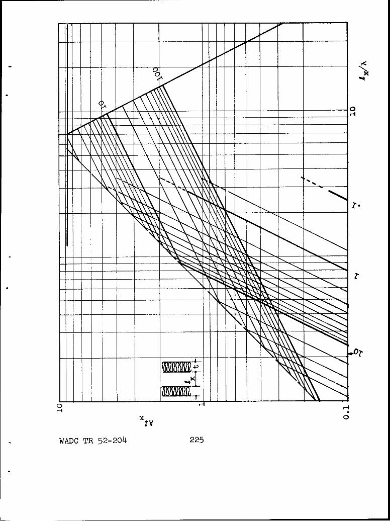
III

__ _

v___

IV

WADC TR 52-204 225

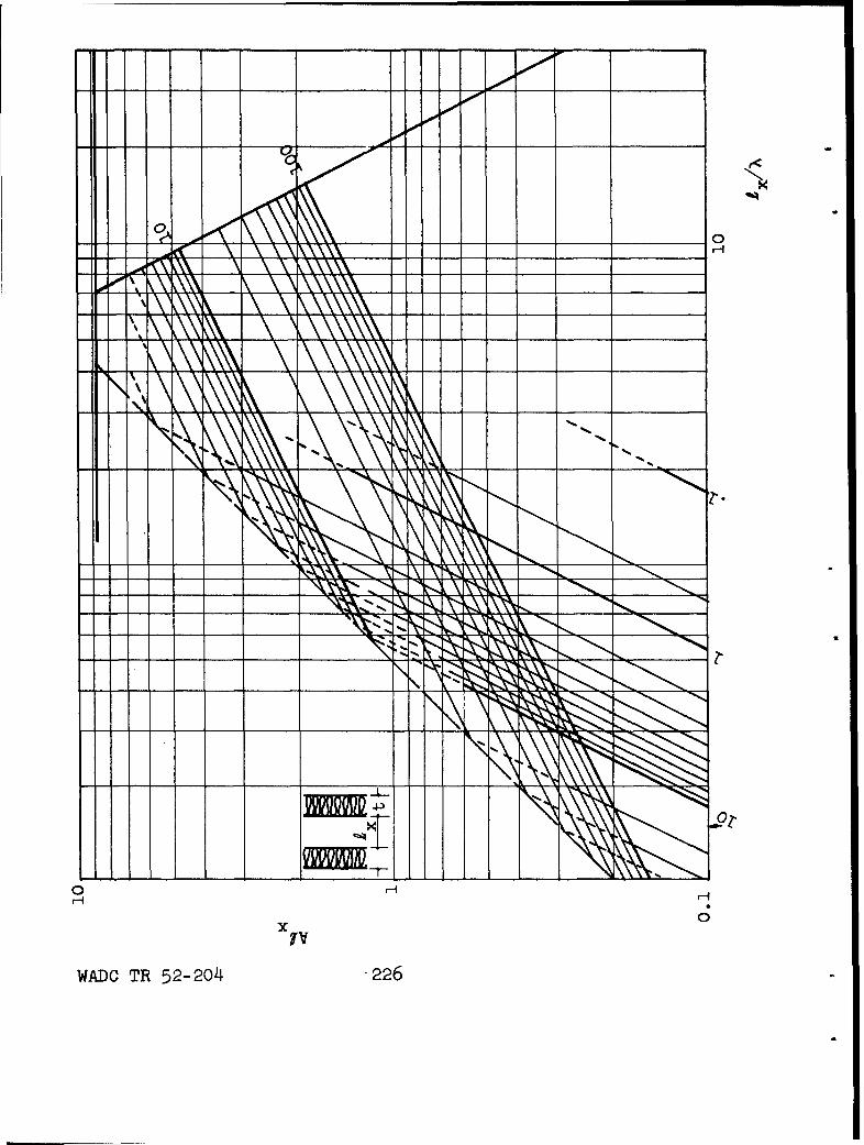
1111_ 1_ _ _ __1 0

I X

x

WADC TR 52-204 -226

definition of the compressibility is now applied, wherethe volume of gas in the section is V = Adx, it is foundthat the effective compressibility is:

K' = K + Py (12.2.2)-Jw pcA (

The propagation constant for the lined duct is then computedby substituting (12.2.2) into (12.2.1). By standard wavetheory, the attenuation constant is equal to the negativeof the imaginary part of the propagation constant and theattenuation o- in db per unit length is 8.69 times as great,so that

S=-8.69 Im(k[rlY- ' (12.2.3)

This is the desired attenuation formula. The quantity Lequals the ratio A/P and k is the propagation constant (c./c)for open air. In case the passage perimeter is not uniformlytreated with a single material, the admittance Yý is given by:

S= (n IPI +tý 2P2 + ...... Y n Pn )/P (12 .2 .4 )

where the length P of the perimeter has the admittance 1,the length P 2 has ihe admittance ýX 2' etc.

Figure 12.2.5

Approximate design chart for attenuation in rectangular ductlined on two opposite walls with a porous layer of known flowresistance. For a given value of the flow resistance parameter0, the attenuation curve for low, mid and high frequencies is given bythree line segments, representing respectively Eqs. (12.2.25),(12.2.26), and (12.2.24). Broken lines show where the first approxi-mation is extended beyond nominal limit of validity. Arrow onhorizontal axis shows the nominal lower limit of validity for thesecond approximation. Entire chart is for (t/ x) 0.8.

WADC TR 52-204 227

The formula (12.2.3) is a good approximation onlyfor JIvj << 1 ( a "hard" wall); otherwise the uniform pres-sure assumption may be unwarranted. In practice the liningusually has kie <' 1 for frequencies well below theattenuation maximum. Also, the relation will often beinaccurate for frequencies sufficiently high that the wave-length is less than the narrowest passage width of the duct,for again the pressure is not likely to be uniform.

A further simplification may be made if, in additionto the condition IiI ./ 1, the condition t ;,kL is realized*.Then the radical in (12.2.3) may be expanded to give the

It can be shown for ordinary tiles and blankets that this condi-

tion is substantially equivalent to requiring that the liningthickness be much less than L.

Figure 12.2.6

Approximate design chart for attenuation in rectangular ductlined on two opposite walls with a porous layer of known flowresistance. For a given value of the flow resistance parameter 9,the attenuation curve for low, mid and high frequencies is givenby three line segments, representing respectively Eqs. (12.2.25),(12.2.26), and (12.2.24). Broken lines show where the first approxima-tion is extended beyond nominal limit of validity. Arrow on hori-zontal axis shows the nominal lower limit of validity for the secondapproximation. Entire chart is for (t/.qx) = 1.0.

WADC TR 52-204 228

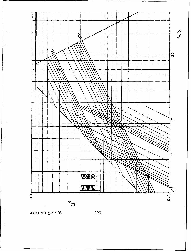
OC0

I I l - o ' M

ooo,

0NO H H

WADO TR 52-204 229

approximate result

T L -)-4.34 p. db (12.2.5)

which is a compact expression for the decibel loss in asection of length L. The quantity p., the conductance ratio,is the real part of Yt . Another way of writing (12.2.5)is

i- L -Y 1. 1 MO db (12.2.6)

where O is the normal free-wave absorption coefficientof the lining. The expression may be Justified by notingthat this absorption coefficient is approximately equalto 4P (Sec. 12.1) provided that 1•f <1i, which is a condi-tion already assumed.

The approximate expressions for duct attenuationwhich have been given in the literature are generally sim-ilar to (12.2.3), (12.2.5) or (12.2.6). These expressionsive useful results within their limitations. Equation12.2.6) is less accurate than the former two relations,

and always predicts smaller values of the attenuation thanare measured experimentally.

Special attention should be given to an empiricalexpression, comparable to Eq. (12.2.6), which was used bySabine 2.1/. In the present notation, it may be written*

0-L = 1.05 d 1.4 (12.2.6a)

where OL is the chamber absorption coefficient of thelining as ordinarily reported by acoustical materials manu-facturers. This relation applies to a duct uniformly linedon all sides. While no theoretical Justification for theexponent 1.4 is provided, it appears that this compensatesapproximately for both the differences between free-wavenormal absorption coefficients and chamber coefficients,

* The original form is (db/ft) 12.6 exl' 4 (p/A), whereP and A are expressed in inches and square inchesrespectively.

WADC TR 52-204 230

and for the errors of approximation inherent in a formulaof the nature of (12.2.6) as the absorption coefficientincreases with increasing frequency. Sabine showed that(12.2.6a) is approximately in agreement with experimentalattenuation measurements up to frequencies of 2000 cps forsix ducts whose open dimensions were combinations of 9, 12and 18 inches. These ducts were lined with rigid mineralwool one inch deep. According to Beranek's interpretation2.2/ of the Sabine experiments, the value of I'XI did notexceed 0.3; hence it may be considered that (12.2.6a) wasverified for 1V < <. 1. Beranek further showed that(12.2.6a) was in approximate agreement with rigorouscalculations from wave theory, under the stated conditions,and showed that the formula should not be applied if theduct shape is far removed from square. This approximaterelation has been widely used in attenuation calculationsfor ventilating ducts, and is to be recommended when usedwithin its limitations. Practically, it is advisable torestrict application to cases where the long passage-widthis not greater than twice the short passage-width.

Special Expressions for Boundary Consisting of aPorous Layer. The relations developed above convey noclear idea of the manner in which the attenuation willvary with frequency in a practical case. The frequency de-pendence comes about in part through the behavior of theadmittance index, Y% , and this can be stated only when thenature of the lining is specified. In many cases, however,the lining consists of a porous layer; i.e., a homogeneousacoustical blanket or tile. Consequently, it will behelpful to analyze this common case in detail by utilizingavailable theory for the porous layer (Sec. 12.1). Theresulting expressions will enable one to predict thefrequency dependence to be expected in certain special cases,even though complete experimental admittance or absorptionmeasurements for the lining are not available. The symbolswhich will be used in discussing the porous lining arelisted below:

m structure factor

t layer thickness

h porosity

e density of air

r specific flow resistance of the lining material

WADC TR 52-204 231

kI - k[h(m--jr/W )1/2 (Propagation constant inporous lining)

Z = c [(m -jr/c w )/h]l/2(Characteristic impedanceof lining material)

0 = rL/pc

c speed of sound in air

k propagation constant in air

L ratio of passage area to passage perimeter

By the theory of absorbing materials (Sec. 12.1), the

admittance of the layer is

= = (ec/Z1 ) tanh (Jk 1 t). (12.-2.7)

This expression may be replaced in certain regions offrequency by suitable approximations. First, a low-frequencyregion may be defined by Ik 1 t4l. For frequencies in thisregion, the hyperbolic tangent in Eq. (12.2.7) may be replacedto good accuracy by the first two terms in a series expansion.When this is done, and when the appropriate approximationsfor kI and Z are introduced, (12.2.7) becomes

1 h2 e(kL) 2 (L) 3 + jh[kt + i mh(kt)3 ] (12.2.8)

To obtain the speed of sound in the duct, c', and theattenuation in db per unit length, c, it is necessary touse the standard relations of wave theory, c' =co/Re(k'),and V= -8.69 Im(k'). With the restriction given belowin Eq. (12.2.14), Eqs. (12.2.1) and (12.2.2) can be expandedto give the simple relations

cl c/[l + Im(A) 1 /2 (12.2.9)kL

+Im-(A) ] 1 /241.2.0- 4.34 Re(Yl)/L[I + km~)L/

4.4R~v)Ll kL (12.2.10)

Combination of these relations with (12.2.8) gives thefollowing low-frequency equations for the phase velocityof sound, and for the db attenuation in a length L, in a

WADC TR 52-204 232

duct with a porous lining.

c- c/[1 + r]I/2 (12.2.11)

0FL c~1. 45 h2G L)()/[ + ht-l/ (12.2.12)

The restrictions imposed in deriving these approximaterelations are summarized in the two relations:

.2 @2(kL) 2< < L~~ 1 m2 (12.2.13)

2 2 (12.2.14)0 ht m

The first of these expresses the condition Ikltj e4 1, whilethe second expresses the condition Re(7)/kL(I + ht/L) z.< 1,which allowed the radical in (12.2.1) to be approximated.In Eq. (12.2.12), 0 is the flow resistance parameter rL/ pc,while kL is the frequency parameter.

Another range of approximation for the duct linedwith porous material, still under the uniform-pressure assump-tion, is obtained when the lining may be regarded as a "thicklayer." The "thick-layer" condition means that the porouslining is sufficiently thick that any wave motion, enteringthe lining perpendicularly, will be so highly attenuatedafter experiencing reflection at the duct wall and then com-pleting a round trip in the lining layer that the energyreturned to the surface is negligible. There is notnecessarily any frequency range in which the wavelength isshort enough for this assumption to be applicable and inwhich also the uniform pressure assumption is applicable,but in a number of cases of practical interest such a rangedoes exist. The "thick layer" condition, as described above,may be defined in terms of the attenuation constant for

WADC TR 52-204 233

wave motion in the porous material, which is -Im(k );a reasonable definition for the thick-layer condition ist > 1/-Im(kl). For porous materials likely to be chosenin practice, this is roughly equivalent to saying thatthe lining thickness must exceed one-eighth the wavelengthof sound in air.

The quantitative significance of the thick-layercondition is that the admittance of the thick layer isclosely equal to Zj 1-. The expression for Z1 has alreadybeen given; it is evident that this expression is a radicalwhich can be expanded in one form if the frequency para-meter kL is much less that 0/m, and in another form if thereverse holds. The low frequency condition (that is, kL 4<0/m) will be assumed. The admittance for this conditionis approximately

S-- (1 + J) (hkL/20)I/2. (12.2.15)

This value for the admittance is put into Eq. (12.2.3) togive the attenuation. It will be assumed that the frequencyand the flow resistance are sufficiently large that (2kLO/h)is much greater than unity. Then, approximately, theattenuation in db per length L is given by Eq. (12.2.16).

G L n3.l(hkL/) 1/2 (12.2.16)

The assumptions made in obtaining this relation are:

t i> 1k) , or roughly t

mkL/0 > - l

2kLO/h > 1

Uniform pressure across the duct opening.

Although these special conditions are not found over anyappreciable range of frequencies in a practical design,Eq. (12.2.16) gives useful information regarding the fre-quency dependence of the attenuation in a duct with porous

WADC TR 52-204 234

lining. This equation shows that the attenuation isproportional to the square root of the frequency, whilein the low frequency range, according to Eq. (12.2.12),the attenuation increases with the square of the frequency.

Finally, in the thick-layer approximation and atsufficiently high frequenies, it is found that Zl is approxi-mately equal to p c rm/h. The criterion for this range iskL >> 9/m. The attenuation per length L is approximately

9 L 4.34 / 7h/m db. (12.2.17)

This limiting formula will almost never apply in practicalcases because uniform pressure is not found ordinarily inthe frequency range for which it is valid. Its importanceis that it seems to represent an upper limit, not normallyattainable, for the attenuation in a duct with porous lining.

The uniform--pressure approximation has been discussedin the literature by Bosquet, Sivian, and Willms 2.3,2.4,2.5/.

Quantitative Treatment by Wave Theory. The rigoroustreatment of wave propagation in a duct is restricted toducts whose cross-section is of simple shape. A rectangularsection (Fig. 12.2.1) is assumed for the present discussion.The solution to the acoustic wave equation for the rectangularduct may be written, for a sinusoidal wave, as

p = X(x) Y(y) Z(z) ej"'t

where

X(x) = cosh (-Jkxx + x)

Y(y) = cosh ( Jk y + y

Z(z) = e-jkz z (12.2.18)

The propagation constants must obey the relation

2 2 2 2k + k + k = k . (12.2.19)x y z

To determine the attenuation, Im(kz) must be found.Basically, the solution is obtained by finding kx and ky,each of which is determined by the frequency and by theimpedances on one pair of walls, and then by computing kz

WADC TR 52-204 235

from (12.2.19). The relation giving kx, for example, is

k k

-Jk=x coth- 1 (kx )+ coth- 1 ( x (12.2.20)

where -x is the passage width in the x direction, Ylx is theadmittance of the wall at x = 0, and n2x is the admittanceof the wall at x = ýx" A similar relation holds for ky.

In general there is no simple calculation procedurefor solving Eq. (12.2.20). Morse has discussed a graphicalmethod of solution 2.8,2.9/. This method is recommendedfor accurate work, but it is time-consuming and is sufficientlycomplicated that it permits little insight into the relation-ships between the properties of the lining and the acousticalperformance of the duct. For low frequencies or for suffi-ciently high frequencies, approximate formulas may be derivedby expending (12.2.20) in series form, by procedures whichhave been given by Morse in connection with the problem ofsound waves in rooms 2.10/

The low-frequency series approximation for Eq. (12.2.20)gives

- (kx )2 Jk Sx(qlx + ý2x). (12.2.21)

This is a good approximation if both lk Ix qlxI and lk 2xare less than unity. The equation in the above formshows the additive effect, at low frequencies, of the treat-ments on opposite walls. Henceforth, for simplicity, it willbe assumed that all of the lining material has the sameadmittance, so that lix = ?2x =- . A similar approximateequation can be derived for the effect of the linings on thewalls y = 0 and y = -R If the attenuation is then foundfrom Eq. (12.2.19), the result for a square duct is, to theapproximations employed, the same as that already obtainedat low frequencies with the uniform pressure assumption.

Of more interest, however, is information regardingthe attenuation of oblique waves (higher order modes) whichcan be obtained from the wave theory but which cannot beobtained using the uniform-pressure approximation.

A case involving higher order modes is obtained byletting the dimension &y be considerably greater than Px, such

WADC TR 52-204 236

that m pressure nodes exist between the floor and ceilingof theduct (y = 0 and y =-y). For simplicity, the floorand ceiling are considered to be non-absorbing. Then they-axis wave constant is given by k y iy = mir. The attenua-tion constant, equal to -Im(kz), is computed from (12.2.19).The result is

= -Im[(k #x) 2 - (jx)2(m) 2-j2k x11/2. (12.2.22)

It is still assumed that I kx )I is less than unity. Theterm -4x/ y) 2 (mr) 2 makes a large contribution to theimaginary part of the expression, and therefore to theattenuation. Thus the attenuation for higher modes (m >O)is in general greater than that for the principal wave. Thecase treated here (long, narrow opening) is most nearly re-lated to the practical situation found in parallel baffles(Sec. 12.3), but qualitatively the behavior of oblique wavesis the same in all duct problems.

Experimentally, when a large part of the energy iscarried into the duct in the form of oblique waves, thesehigher modes have the effect of making the total attenuationexceed the calculated value, which ordinarily refers to theprincipal wave. There may be a region just inside the sourceend of the duct where the signal level drops more rapidlywith distance than is the case further along in the duct.This first region is the one in which the higher modes arerapidly reduced. It follows that if the duct is relativelyshort, so that this first region occupies a large fractionof the length, the reported attenuation per unit lengthmay be considerably greater than the principal-wave value.Since there is ordinarily no practical way to calculate howmuch of the acoustical energy will be carried by the highermodes this effect can only be estimated on the basis of pastexperience with particular structures and sound sources.The effect is usually significant only for frequencies abovethat where the attenuation peak for the principal wave occurs.

Other aspects of the low-frequency approximation arediscussed in the textbook by Morse L._9/•

From the wave theory viewpoint, the approximate solutionfor high frequencies is obtained by finding a series expan-sion for Eq. (12.2.20) which is valid when k.x 1. 2 1.

WADO TR 52-204 237

If, in addition, the frequency is sufficiently high thatkRx :'(n + 1)r, the resulting expression for the attenua-tion in a duct with two walls lined is

•x 17.4 (n + 1) 2 (12.2.23)Sx (k Jx) 2 1.2)

Here n is the mode number, equal in this case to the numberof pressure nodes between x = 0 and x = •x. Again, theattenuation for the higher modes exceeds that for the prin-cipal wave. Most important, the attenuation is inverselyproportional to the square of frequency in this high-frequencyrange. This is the result of an increasing concentration ofacoustical energy in the center of the duct at high frequencies,thus reducing the amount of energy absorbed by the lining.

If the duct is lined with a porous material, it isreasonable to expect that the high-frequency form of thethick-layer impedance approximation will apply in this highfrequency range. As was the case in (12.2.17), ý may beapproximated by /-{h/m, so that the principal-wave attenuationin distance -x for porous linings on two opposite walls is*

_ 17.-4r m (12.2.24)(kjx 2

The quantity7/i-7h is roughly equal to unity for most practicalporous linings; thus the attenuation at very high frequenciesis nearly independent of the material.

Other discussions of the duct from the standpoint ofwave theory have been given by Willms 2.5/, Cremer 2.11/ andScott 2.12/.

. Scott 2.12! has shown that the high-frequency limiting expression

for the attenuation is proportional to (kQx)&3/2 rather than to(k-x)2 in the case where the lining is not locally reacting butis instead a wave-propagating medium. It appears that many prac-tical blankets and tiles are not locally reacting at highfrequencies and that the Scott result may therefore apply in anumber of cases.

WADC TR 52-204 238

Theoretical Design Charts for Duct with Porous Lining.

Figures 12.2.2 through 12.2.6 are a series of design chartsto permit rapid calculation from the approximate formulaswhich have been developed for the principal-wave attenuationin a duct lined with porous material. These charts areconstructed for the case in which only a single pair ofopposite walls is lined, for this arrangement is often pre-ferred for economy and simplicity over four wall lining.The effect of lining four walls instead of two is, roughly,to double the attenuation if the lining thickness is keptconstant. The principal wave attenuation can be as readilyincreased by making the lining thicker on two walls as bycovering all four walls, however, so that there is no dis-tinct advantage in four-wall lining in many practical cases.

In order to use the charts, it is necessary to knowthe dimensions of duct and lining, and the specific flowresistance of the porous material i.e., the flow resistance,in rayls, for a sample one centimeter thick. The attenuationis given in terms of 6Qx, the attenuation in db in a dis-tance equal to the passage width •x between the lined walls.In each case, frequency is read from the horizontal scalein terms of the parameter Qx/A = f-Qx/c. Each chartrefers to a single value of the ratio t/ x (lining thick-ness t to passage width Rx). On each chart there are anumber of approximate attenuation-frequency curves; eachcurve is for a specified value of the flow resistance para-meter 91 (where 01 - rIx/lc).

An individual attenuation-frequency curve consists ofthree straight-line segments on the logarithmic chart.These segments represent the three frequency ranges alreadystudied. The low frequency segment of each curve representsthe relation

2.9h2 Q (k2•)(t/i )3X X (12.2.25)

X [1 + 2ht/ Q ]1/2

WADC TR 5 2-2o4 239

which is the form taken by Eq. (12.2.12) when two wallsare lined.* In plotting the curves, the porosity h hasbeen taken as unity.

The middle-frequency segment of each curve is givenby

C 6.2 (hk11/9 )1/2 (12.2.26

This is obtained from Eq. (12.2.16) for the case of twowalls lined. Again h has been taken as unity.

The high-frequency segment is identical for all chartsand is given by Eq. (12.2.24), with /Th7R taken as unity.

The use of broken lines indicates where one of thelower two approximations has been extended beyond the rangeof validity. The arrow on the horizontal axis of each chartindicates approximately the lower limit of validity of thethick-layer assumption, basic to the middle approximation.In some cases it is necessary to use this approximationbelow the limit indicated by the arrow.

The method of approximation used in these charts doesnot give a good quantitative description of the attenuationpeak, but the results at low frequencies (ox/A 4 0.2) andat high frequencies (-Rx/A > 1.5) are sufficiently accuratethat the attenuation-frequency function as a whole is fairlywell defined.

Experimental Design Curves for Ducts Lined with PorousMaterial. Experimental attenuation data, which have beenobtained for a series of ducts under certain conditions likelyto be encountered in practice, are summarized in the form ofa design chart in Fig. 12.2.7. The experimental chartcovers a more restricted range of conditions than do the pre-ceding charts. However, the experimentally determined curves

* The discussion up to this point has not been concerned with thedifference between lining only two opposite walls or all four walls.However, if only two walls are lined, L is defined as the passagearea to the lined perimeter. Therefore, for a square passage areaof length Vx, using this definition L = _x 2/2fx = Qx/2.

WADC TR 52-204 240

where applicable, will prove more detailed and accuratein the range of peak attenuation than those based on theapproximate formulas.

The variables plotted on the chart axes are the sameas those for the previous charts - db attenuation in alength .Qx as a function of Sx/A , where .x is the passagewidth between the treated pair of walls. Each curve isidentified by the proper value of t/Sx. The data forthese curves were obtained with structures having the 0 valueslisted below:

Value of t/ýQ X

3 1.5

1 3

0.5 4.5

0.25 6

0.1 7.5

These values correspond to a region in which the shapeand height of the attenuation peak are not highly sensitiveto changes in flow resistance. Therefore these designcurves can be applied over an appreciable range of 0 values.Further experimental data, obtained for the case (t,/x) = 0.25,indicate that the peak and high-frequency portions of thesecurves (Dx/A > 0.3) are not seriously affected by varying 0between half the nominal value and four times that value.At low frequencies the attenuation must be approximatelyproportional to 0, as indicated by Eq. (12.2.25) and by theprevious charts. A full allowance for this effect of vary-ing the flow resistance should be made for frequenciesbelow 9 x/A = 0.1.

The experimentally determined chart representsconservative values for the attenuation per lengthx in ductshaving lengths up to 15 Qx. When the duct is relativelyshort (length less than 4Sx) the observed attenuation perlength 9x in the region of the peak may be about 25 per centgreater than that shown by the chart. This discrepancy repre-sents end effects, including the attenuation of higher modes.

WADC TR 52-204 241

The designer who uses the complete theoreticalcomputation charts will discover that certain criticalcombinations of the parameters will give attenuation asgreat as 12 db in a length 1 x,2.8/. Unfortunately, thelarge attenuation given by these critical combinations isusually confined to a very narrow frequency band, and mayalso be difficult to obtain because of practical varia-tions in flow resistance of the lining and of dimensionsin actual construction. The empirical chart of Fig. 12.2.7shows broad-band attenuation which can be expected withoutcritical design. Because of the effects of higher modes,the effective attenuation in a practical installation, forfrequencies above the peak, may be well above the valuesindicated by this chart.

The results shown in Fig. 12.2.7 are attenuation perlength Qx for a duct having effectively infinite length.The experimental measurements show that the end effects ina finite length of duct are approximately explained if alength Ax is imagined to be added to each end of the duct.Therefore, the attenuation for a duct which has an actuallength of 3 1x for example, should be computed as thoughthe length were 5 x.

Under the non-critical conditions represented byFig. 12.2.7, the indicated attenuation can generally beobtained either with two opposite walls lined as indicated,or, in the case of a duct which is not too far from square(ratio of passage widths less than 2:1), with the same

Figure 12.2.7

Attenuation design chart, derived from a set of experimentalmeasurements, for ducts lined on two opposite walls with porouslayer of approximately-known flow resistance. Flow resistanceis not critical for the conditions shown and results aresubstantially unchanged when Q varies from half the indicatedvalues to four times indicated values. The curves may be appliedapproximately to ducts lined uniformly on all four sides if percent open area instead of (t/lx) is used to specify amount oflining. To allow for end effects, add 2 Rx to the actual lengthof a duct and compute total attenuation from this correctedlength.

WADC TR 52-204 242

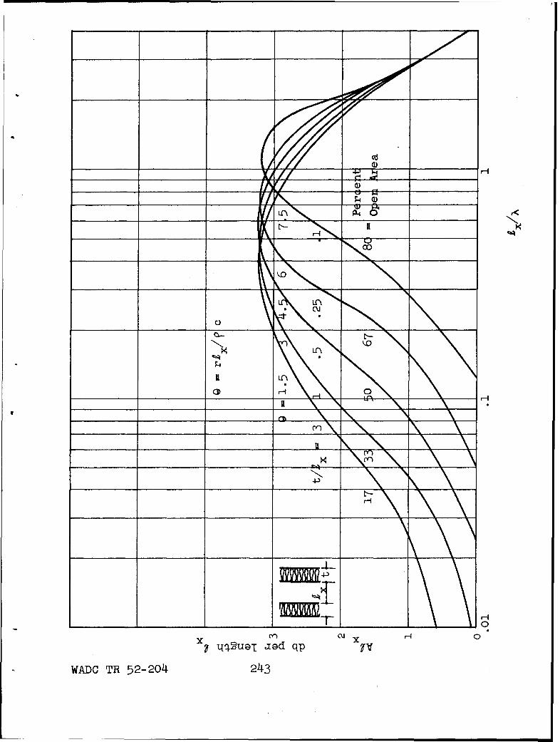
000,

3C

_ _ _ _ _ _ _ _ _ _ _ _ _ _ 13L

Ln

C~H

X 4Sa aad qp IV0

WADC TR 52-204 243

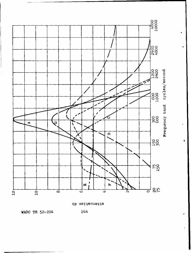
00___ __ _ _ _ _ __ ___ ___ 00

coo-=-t0

/ )00

00

4-00

0-0

00

'o'

-100

0400HL 0

qp uoTqvnuaqqv

WADC TR 52-204 244

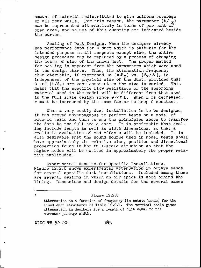
amount of material redistributed to give uniform coverageof all four walls. For this reason, the parameter (t/ x)can be represented alternatively in terms of per cent ofopen area, and values of this quantity are indicated besidethe curves.

Scaling of Duct Designs. When the designer alreadyhas performance data for a duct which is suitable for theintended purpose in all respects except size, the entiredesign procedure may be replaced by a process of changingthe scale of size of the known duct. The proper methodfor scaling is apparent from the parameters which were usedin the design charts. Thus, the attenuation-ftequencycharacteristic, if expressed as (Gx) vs. (.Rx/,A), isindependent of the physical size of the duct, provided thatE and (t/jx) are kept constant as the size is varied. Thismeans that the specific flow resistance of the absorbingmaterial used in the model will be different from that usedin the full scale design since G-'rL. When L is decreased,r must be increased by the same factor to keep 0 constant.

When a very costly duct installation is to be designed,it has proved advantageous to perform tests on a model ofreduced scale and then to use the principles above to transferthe data to the full-scale case. It is preferable that scal-ing include length as well as width dimensions, so that arealistic evaluation of end effects will be included. It isalso desirable that the sound source used in model tests shallhave approximately the relative size, position and directionalproperties found in the full-scale situation so that thehigher modes will be excited in approximately the proper rela-tive amplitudes.

Experimental Results for Specific Installations.Figure 12.2.8 shows experimental attenuation in octave bandsfor several specific duct installations. Included among theseare several designs in which an air space is used behind thelining. Dimensions and design details for the several cases

* Figure 12.2.8

Attenuation as a function of frequency (in octave bands) for thelined duct structures of Table 12.2.1. The vertical scale givesattenuation in decibels for a length of duct equal to thenarrower passage width.

WADC TR 52-204 245

are given in Table 12.2.1. The performance data for thesedesigns have proved useful as a basis for scaling.

The performance of structure F illustrates the natureof a disagreement which sometimes occurs between theory andpractice. This structure, according to the rigorous wavetheory, should have a maximum attenuation of approximately12 db per width unit of length. The observed attenuation peakhas half of this value, and is broader than the computedmaximum. This is a case where the theoretical design uses acritical set of values which are not realized because ofpractical tolerances.

Commercial Mufflers. Prefabricated circular ducts withabsorbent linings, usually constructed with heavy steel shells,are available commercially under the generic term "mufflers."Other structures commercially designated as mufflers includingresonators as well as absorbent linings, will not be discussedhere. The measured attenuation for several commercial mufflers(Maxim and Industrial Sound Control Products) is shown inFig. 12.2.9. Physical data and dimensions for these mufflersare shown in Table 12.2.2.

Duct with Resonant Lining. The attenuation for a selectedband of lower frequencies can be greatly increased by the useof a lining which resonates (has a purely resistive impedance)at the center of that band. This is considered in detail inSec. 12.7.

Attenuation in Smooth Pipes. Even if the absorbentlining were removed from a duct so that the structure couldbe considered a smooth pipe, some sound attenuation wouldremain. This attenuation results from viscous drag of the airat the walls, and from heat loss to the walls. Ordinarilythe attenuation resulting from these mechanisms is smaller byorders of magnitude than that in a lined duct and is thereforeneglected in duct calculations. Attenuation in smooth pipesis discussed briefly in Sec. 12.15.

Effects of Nonrigid Side Walls. The discussion in thissection has assumed that the duct enclosure is formed by

Figure 12.2.9

Attenuation as a function of frequency (in octave-bands) forthe commercial mufflers of Table 12.2.2.

WADC TR 52-204 246

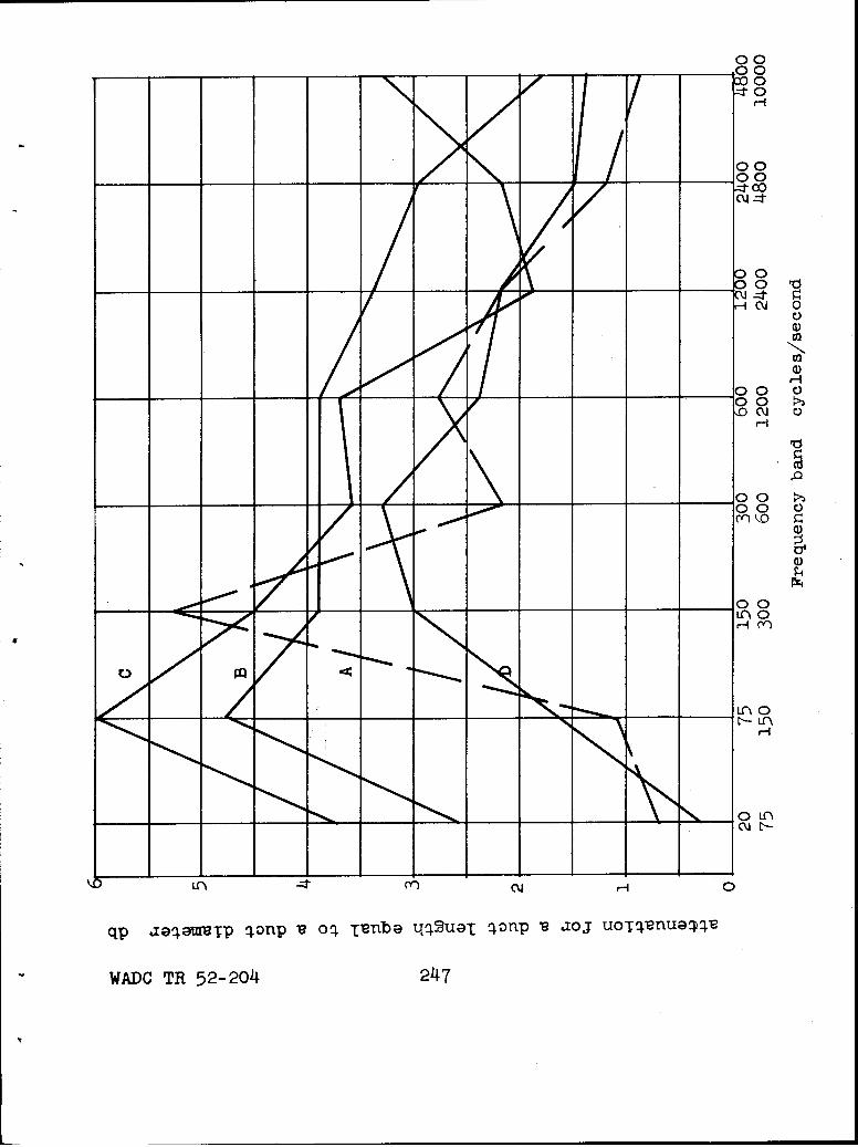
000040

00__ __ > \__ 00

0

0000

H

___ __ ___ _ _ ___00 C00

00 C

00

_ _ _ _ _ _ _ _ _ _ _ _ _ __000 0

Ln\

0 Cn

qp Jeaaqa=Tp 4onp v 04 Tvnba q~O 4Onp V aJo UoTqvnua44v

WADC TR 52-204 247

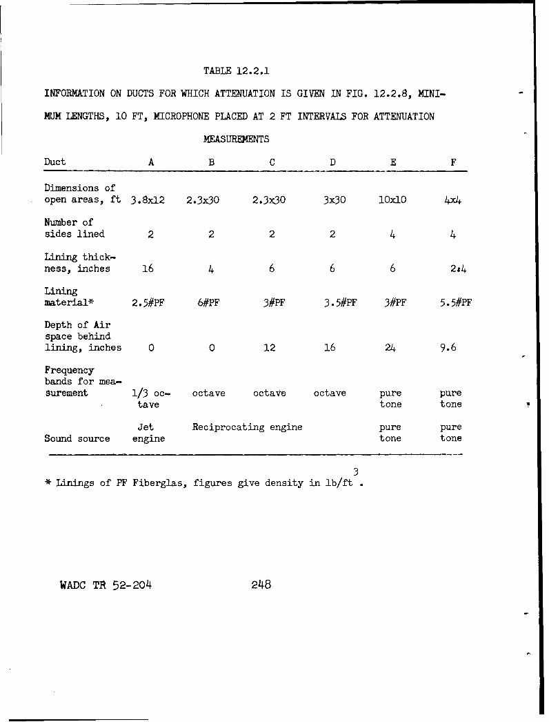
TABLE 12.2.1

INFORMATION ON DUCTS FOR WHICH ATTENUATION IS GIVEN IN FIG. 12.2.8, MINI-

MUM LENGTHS, 10 FT, MICROPHONE PLACED AT 2 FT INTERVALS FOR ATTENUATION

MEASUREMENTS

Duct A B C D E F

Dimensions ofopen areas, ft 3.8x12 2.3x30 2.3x30 3x30 lOxlO 4x4

Number ofsides lined 2 2 2 2 4 4

Lining thick-ness, inches 16 4 6 6 6 2.4

Liningmaterial* 2.5#PF 6#PF 3#PF 3.5#PF 3#PF 5.5#PF

Depth of Airspace behindlining, inches 0 0 12 16 24 9.6

Frequencybands for mea-surement 1/3 oc- octave octave octave pure pure

tave tone tone

Jet Reciprocating engine pure pureSound source engine tone tone

3* Linings of PF Fiberglas, figures give density in lb/ft

WADC TA 52-204 248

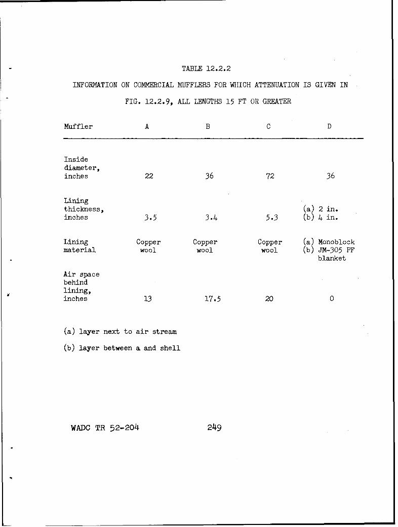
TABLE 12.2.2

INFORMATION ON COMMERCIAL MUFFLERS FOR WHICH ATTENUATION IS GIVEN IN

FIG. 12.2.9, ALL LENGTHS 15 FT OR GREATER

Muffler A B C D

Insidediameter,inches 22 36 72 36

Liningthickness, (a) 2 in.inches 3.5 3.4 5.3 (b) 4 in.

Lining Copper Copper Copper (a) Monoblockmaterial wool wool wool (b) JM-305 PF

blanket

Air spacebehindlining,inches 13 17.5 20 0

(a) layer next to air stream

(b) layer between a and shell

WADC TR 52-204 249

acoustically rigid, impervious walls. This assumption isreasonable for concrete or masonry ducts and usually formetal or wooden ducts with heavy walls. The assumption isnot valid for the lower frequencies (several hundred cyclesper second and lower), however, in the case of light sheetmetal ducts used in ventilation systems. Evidence of theeffects of nonrigid walls is found in Sabine's measurements2.1, 2.2/. Nonrigid walls cause the low-frequency attenua-tion to exceed calculated values. The amount of this effectcannot be estimated accurately except on the basis ofexperience with full-scale structures. Furthermore, nonrigidwalls radiate sound. In a case where large attenuation isrequired, side-wall radiation from a light structure mayconstitute an acoustic leak great enough to negate theattenuation in the duct. The amount of sound transmittedthrough the duct walls may be estimated using Secs. 11.2 and11.5.

Summary of Design Methods for Lined Ducts. The tabularsummary below shows the applicability of the various designequations and charts which have been presented in this sec-tion and will facilitate reference to them. The statementsas to restrictions on the uses of the various relations aregreatly simplified for compactness in this listing. Moreaccurate statements of the validity conditions have beengiven in the previous discussion of the individual relations.

The symbols listed and defined below are consistentwith the usage in the preceding parts of this section.

Swavelength of sound in o~pen air

acoustic admittance ratio of the lining

/A real part of

c( chamber absorption coefficient

qnormal free-wave absorption coefficient

t thickness of lining

L passage area divided by passage perimeter

k. narrowest passage width

WADC TR 52-204 250

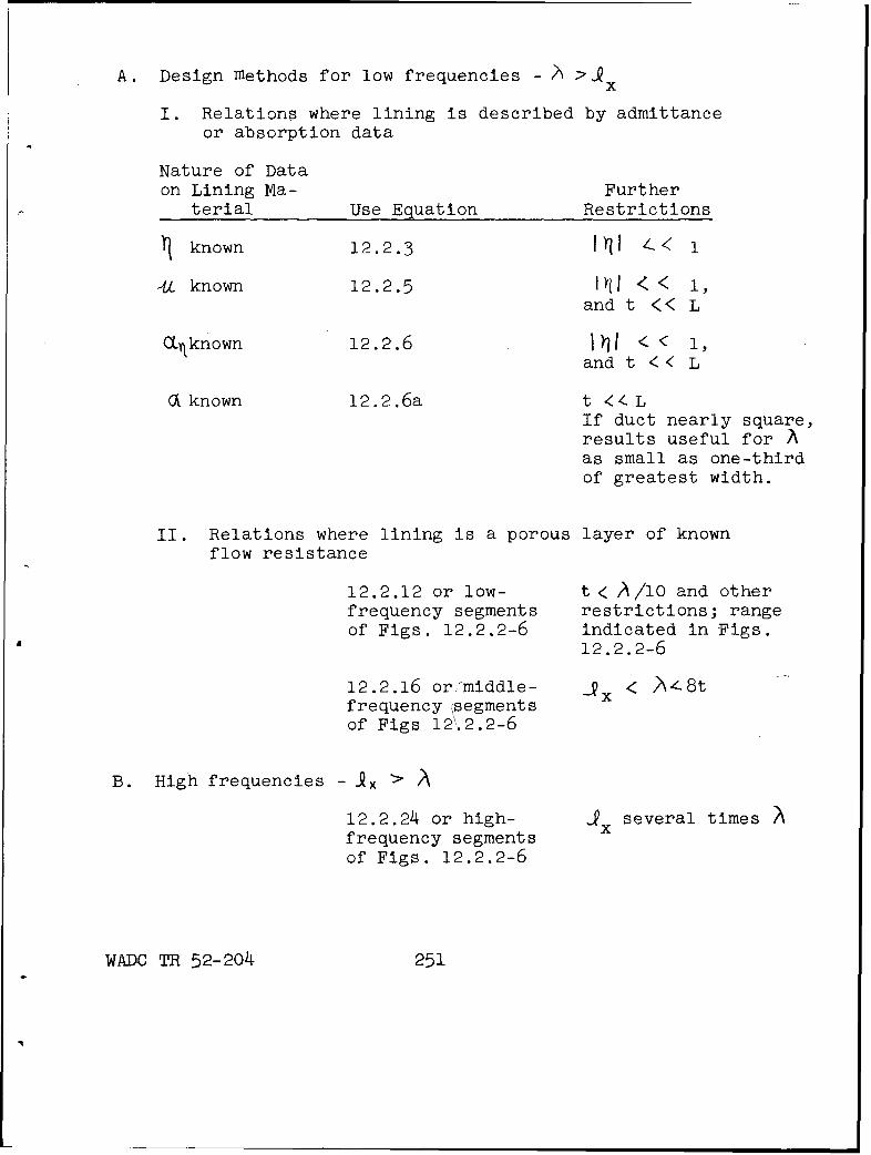
A. Design methods for low frequencies - \ 'x

I. Relations where lining is described by admittanceor absorption data

Nature of Dataon Lining Ma- Further

terial Use Equation Restrictions

known 12.2.3 I 4I -.< 1

AL known 12.2.5 <• (< 1,and t << L

Cc known 12.2.6 < < I,and t < < L

a known 12.2.6a t </, LIf duct nearly square,results useful for Aas small as one-thirdof greatest width.

II. Relations where lining is a porous layer of knownflow resistance

12.2.12 or low- t < //1O and otherfrequency segments restrictions; rangeof Figs. 12.2.2-6 indicated in Figs.

12.2.2-6

12.2.16 or/middle- -x < -•8tfrequency (segmentsof Figs 12'.2.2-6

B. High frequencies - > A

12.2.24 or high- x several timesfrequency segmentsof Figs. 12.2.2-6

WADC TR 52-204 251

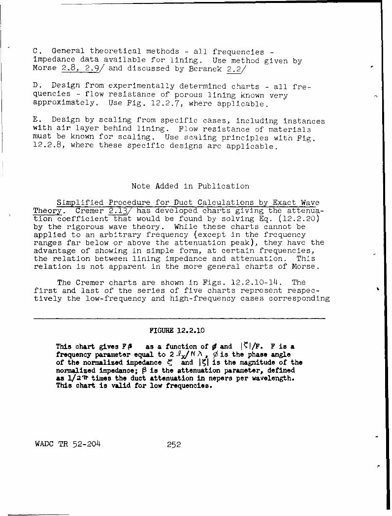
C. General theoretical methods - all frequencies -impedance data available for lining. Use method given byMorse 2.8, 2.9/ and discussed by Beranek 2.2/

D. Design from experimentally determined charts - all fre-quencies - flow resistance of porous lining known veryapproximately. Use Fig. 12.2.7, where applicable.

E. Design by scaling from specific cases, including instanceswith air layer behind lining. Flow resistance of materialsmust be known for scaling. Use scaling principles with Fig.12.2.8, where these specific designs are applicable.

Note Added in Publication

Simplified Procedure for Duct Calculations by Exact WaveTheory. Cremer 2.13/ has developed charts giving the attenua-tion coefficient that would be found by solving Eq. (12.2.20)by the rigorous wave theory. While these charts cannot beapplied to an arbitrary frequency (except in the frequencyranges far below or above the attenuation peak), they have theadvantage of showing in simple form, at certain frequencies,the relation between lining impedance and attenuation. Thisrelation is not apparent in the more general charts of Morse.

The Cremer charts are shown in Figs. 12.2.l0-14. Thefirst and last of the series of five charts represent respec-tively the low-frequency and high-frequency cases corresponding

FIGURE 12.2.10

This chart gives FP as a function of 9 and JIý/F. F is afrequency parameter equal to 2 -x/ N A, 0 is the phase angleof the normalized impedance 4r and II is the magnitude of thenormalized impedance; 0 is the attenuation parameter, definedas 1/a2t times the duct attenuation in nepers per wavelength.This chart is valid for low frequencies.

WADC TR 52-204 252

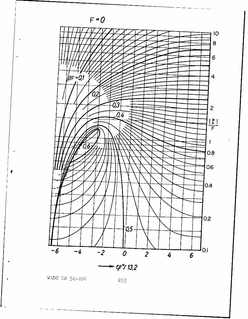
F=O

108

6

0.2

F

0.8

0.6

0.4

0.2

-6 -4 -2 0 204.1

"C? 0/"13.2W,.DC •DR 52-20! 253

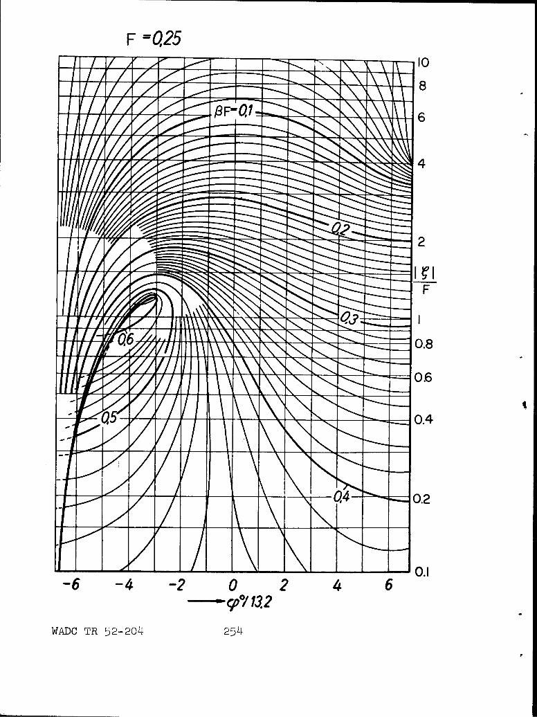
F =025h_ ___ 10

8

6

F

-6 -4 -2 0 2 46

WADC TR 52-204 254

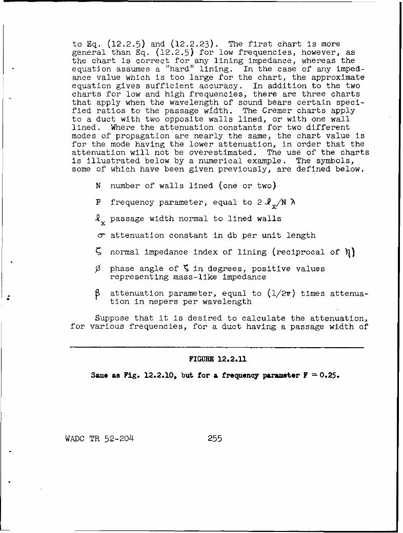
to Eq. (12.2.5) and (12.2.23). The first chart is moregeneral than Eq. (12.2.5) for low frequencies, however, asthe chart is correct for any lining impedance, whereas theequation assumes a "hard" lining. In the case of any imped-ance value which is too large for the chart, the approximateequation gives sufficient accuracy. In addition to the twocharts for low and high frequencies, there are three chartsthat apply when the wavelength of sound bears certain speci-fied ratios to the passage width. The Cremer charts applyto a duct with two opposite walls lined, or with one walllined. Where the attenuation constants for two differentmodes of propagation are nearly the same, the chart value isfor the mode having the lower attenuation, in order that theattenuation will not be overestimated. The use of the chartsis illustrated below by a numerical example. The symbols,some of which have been given previously, are defined below,

N number of walls lined (one or two)

F frequency parameter, equal to 2 xQ/N -A

Spassage width normal to lined wallsx

0- attenuation constant in db per unit length

r normal impedance index of lining (reciprocal of

0 phase angle of 1 in degrees, positive valuesrepresenting mass-like impedance

attenuation parameter, equal to (1/2r) times attenua-tion in nepers per wavelength

Suppose that it is desired to calculate the attenuation,for various frequencies, for a duct having a passage width of

FIGURE 12.2.31

Same as Fig. 12.2.10, but for a frequency parameter F = 0.25.

WADC TR 52-204 255

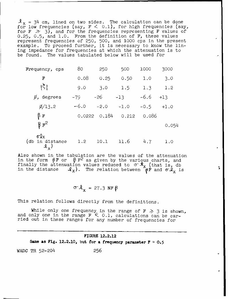
ýx = 34 cm, lined on two sides. The calculation can be donefor low frequencies (say, F K 0.I), for high frequencies (say,for F 2z- 3), and for the frequencies representing F values of0.25, 0.5, and 1.0. From the definition of F, these valuesrepresent frequencies of 250, 500, and 1000 cps in the presentexample. To proceed further, it is necessary to know the lin-ing impedance for frequencies at which the attenuation is tobe found. The values tabulated below will be used for

Frequency, cps 80 250 500 1000 3000

F 0.08 0.25 0.50 1.0 3.0

S9.0 3 .0 1 .5 1 .3 1 .2

•, degrees -79 -26 -13 -6.6 +13

9/13.2 -6.0 -2.0 -1.0 -0.5 +1.0

SF 0.0222 0.184 0.212 0.086

SF 2 0.054

(db in distance 1.2 10.1 11.6 4.7 1.0

Also shown in the tabulation are the values of the attenuationin the form PF or ý F 2 as given by the various charts, andfinally the attenuation values reduced to o-•x (that is, dbin the distance -Qx)" The relation between VF and 5-Qx is

Cr-• = 27.3 NFf

This relation follows directly from the definitions.

While only one frequency in the range of F > 3 is shown,and only one in the range F '• 0.1, calculations can be car-ried out in these ranges for any number of frequencies for

FIGURE 12.2.12Same as Fig. 12.2.10, but for a frequency parameter F = 0.5

WADC TR 52-204 256

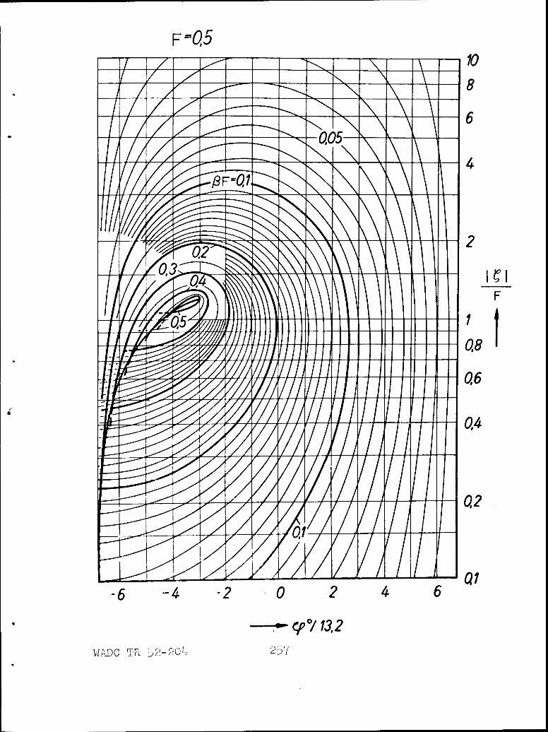
04

02 2

-6 4 2 240

WADC R 32-0,52

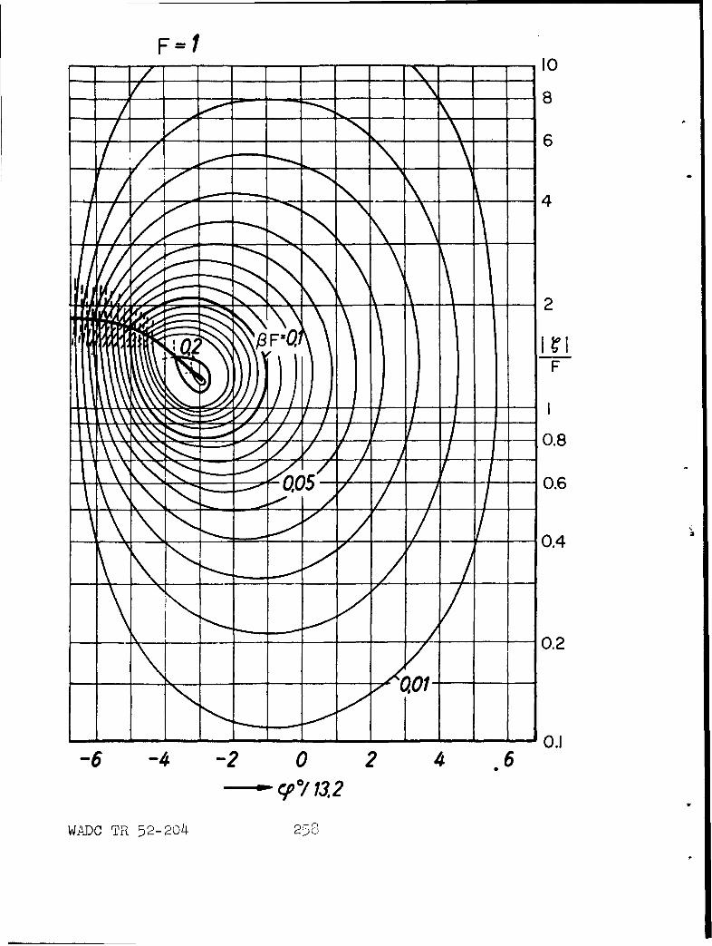
FF

-06

- 0~4

- - - ------ t- - -'- 0.8

-6 -4 -2 0 2 4 6;P 0713.2

WADC TR 52-204 2=3

which the lining impedance is known. The results for fre-quencies near the peak are restricted to the frequenciescorresponding to the three intermediate charts.

Use of these charts is to be recommended wheneverduct attenuation is to be calculated on the basis of a knownlining impedance. While the results do not show in detailthe sharp attenuation peak which is shown by careful use ofthe Morse charts, they do show the peak in sufficient detailfor design work dealing with wide-band noise, and in muchmore detail than the charts in Figs. 12.2.2-6. The lattercharts, on the other hand, are simpler to use than the Cremercharts in the special case for which they are intended, wherethe lining is a porous blanket.

Difficulty in obtaining normal impedance data for thelining will to some extent limit the use of the Cremer charts.Normal impedance data for a few materials are given inSec. 12.1. Normal impedance for porous blankets may be calcu-lated from Eq. (12.1.14) or, for long wavelengths, fromEq. (12.1.19).

In the Cremer charts, Figs. 12.2.10-14, the values oflining impedance which give greatest attenuation are evidencedby inspection. Cremer 2.13 gives the following simple for-mula for the optimum lining impedance index as a function offrequency:

optimum = 1.2 e-0"7i(2N Sx/l ) (12.2.27)

Fora duct having the lining impedance versus frequencycharacteristic given by this relation, the attenuation if onewall were lined would be 19 db per distance Rx up to F = 0.3;for higher frequencies the attenuation would be (3.5 h/Qx) db.These figures would be doubled if two sides were lined. Allactual ducts, in which this ideal impedance behavior cannotbe perfectly realized, will have an attenuation versus fre-quency characteristic which lies below the one given by thepreceding values.

FIGURE 12.2.13

Same as Fig. 12.2.10, but for a frequency parameter F 1

WADC TR 52-204 259

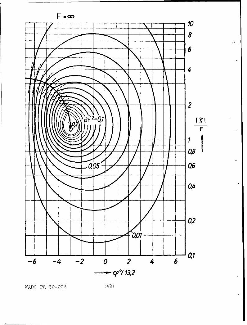
F woo

-6

- -- )9F2a00.

-6~~ ~ -4 -II f/ 1

WADC'2R52-24 200o

References, Section 12.2

(2.1) Sabine, Hale J., "The Absorption of Noise inVentilating Ducts." J. Acoust. Soc. Am. 12,53 (1940).

(2.2) Beranek, Leo L., "Sound Absorption in RectangularDucts." J. Acoust. Soc. Am., 12 228 (1940).

(2.3) Bosquet, I.P., Bull. Techn. Assoc. Ing. Bruxelles31, No. 12 (1935).

(2.4) Sivian, L. J., "Sound Propagation in Ducts Linedwith Absorbing Materials," J. Acoust. Soc. Am.9 135 (1937).

(2.5) Willms, W. Akustische Zeits. 6 150 (1941).

(2.6) Piening, W., Zeits. Ver. Dtsch. Ing. 31 776 (1937).

(2.7) Parkinson, J. A., Heating and Ventilating, pp 23-26 (March 1939). See also Heating VentilatingAir Conditioning Guide 1953 (Vol. 31) (Am. Soc.Heating and Ventilating Engrs., New York, 1953),pp. 898-899; also earlier editions of this guide.

(2.8) Morse, P. M., "Transmission of Sound Inside Pipes,"J. Acoust. Soc. Am. 11 205 (1939).

(2.9) Morse, P. M., Vibration and Sound, 2nd Ed.McGraw-Hill (1948) pp. 368-376.

(2.10) Morse, P. M., "Some Aspects of the Theory of RoomAcoustics," J. Acoust. Soc. Am., 12 56 (1939).

(2.11) Cremer, L., Akustiche Zeits 5 57 (1940).

(2.12) Scott, R. A., Proc. Phys. Soc. (London) 58 358(1946).

(2.13) Cremer, L., "Theory of Airborne Sound Dampingin Rectangular Ducts with Absorbing Walls andWhich Have a Very High Damping Constant".Acustica 3, 249-263 (1953).

FIGURE 12.2.1.4

Same as Fig. 12.2.10 but for "high" frequencies,

WADC TR 52-204 261

12.6a The Resonator as a Free-Field Sound Absorber

The use of the resonator to attenuate sound in aduct was considered in Sec. 12.6. Another use, that ofabsorbing sound in rooms, is considered in the present sec-tion. In this application, the behavior of a resonatoris best described by giving its sound absorption in sabins,rather than by giving a pressure reduction ratio.

The effect of a resonator in a room, for frequenciesnear the resonance, is similar to that of a patch of highlyefficient sound absorbing material. The reduction of smndpressure in the room is dependent upon the position of theabsorbing element, as pointed out in Sec. 12.1. Therefore,the sound absorption of a resonator can be stated only forspecified positions in the room. Two idealized cases willbe considered, namely, (a) the resonator in open air (freefield); (b) the resonator with its opening in a plane wallbounded by open air. The practical situations representedby a resonator near the center of a room, or by a resonatorin a room wall, are approximations to these idealized cases.

The properties of a resonator as a sound absorber aresummarized briefly in the next paragraph. Following thesummary, a brief derivation of the equations for the resonatorin free field is given. In the remainder of the section, theroles of the various parameters are considered in detail, anddesign procedures are developed.

Summary of Properties of the Resonator as a SoundAbsorber.

(1) The maximum absorption of a single resonator,in sabins, is approximately ?\2o /4) if the resonator is insubstantially free air, and is A20 /2r if the resonator open-ing is in a large wall, where ?o is the wavelength of sound,in feet, at the frequency of resonance.

(2) The minimum Q (corresponding to maximum bandwidth)which can be obtained in a practical resonator having maxi-mum absorption of the amount indicated above is about 25 fora resonator in free air, or about 13 for a resonator havingits opening in a wall.

(3) The width of the frequency band in which theabsorption is not less than half the value found at resonanceis equal to the frequency of resonance divided by Q.

WADC TR 52-204 263

(4) While the bandwidth of the absorption can bevaried over wide limits by adjusting the size of the resonatorand the resistance material placed in the aperture, the ab-sorption for all frequencies decreases greatly as the band-width is increased, so that it is usually not profitable toreduce the Q below the values given in (2) above.

A resonator is, therefore, useful primarily whenrelatively large sound absorption is required in a narrowfrequency band. The resonator has great practical valueparticularly for frequencies below about 200 cps, where itis often difficult to obtain large absorption by other me-thods. For example, a resonator (or a group of resonatorsnot too close to one another) can be used effectively toreduce the 120 cps "hum" in a transformer room. A group ofresonators tuned to successively larger frequencies is some-times used to give sound absorption in a wider frequencyband.

Tle Absorption Cross Section. A resonator placed ina progressive plane wave absorbs energy at a rate proportionalto the intensity of the wave. The power absorbed by the re-sonator can be expressed as the power which the undisturbedplane wave would deliver in some effective area, caaperpendicular to the direction of wave travel. The quantityaa is the absorption cross section of the resonator; if

expressed in square feet, the absorption cross section becomesthe absorption in sabins. The absorption cross section atresonance will be denoted by % 0 . (The subscript zero withany quantity will always refer to the resonance condition.)

For purposes of analysis, the resonator is assumedto have the spherical shape shown in Fig. 12.6a.1, where thesymbols for the dimensions are also shown. In all practicaldesigns, the resonator is small compared to the wavelengthof sound at resonance, 'A Therefore, diffraction effectsmay be neglected, to a fyrst approximation, and the rmsacoustic pressure at the opening is equal to P., the rmspressure in the incoming plane wave. If the resonator ismounted in a wall, the pressure at the opening becomes 2P ,

because of reflection at the wall. Both of these situati 8 nswill be covered by writing the driving pressure as < 2> E,.Throughout this section, a quantity enclosed in brokenbrackets is understood to apply only when tne resonator ismounted in a wall, and is to be replaced by unity if theresonator is in free air.

WADC TR 52-204 264

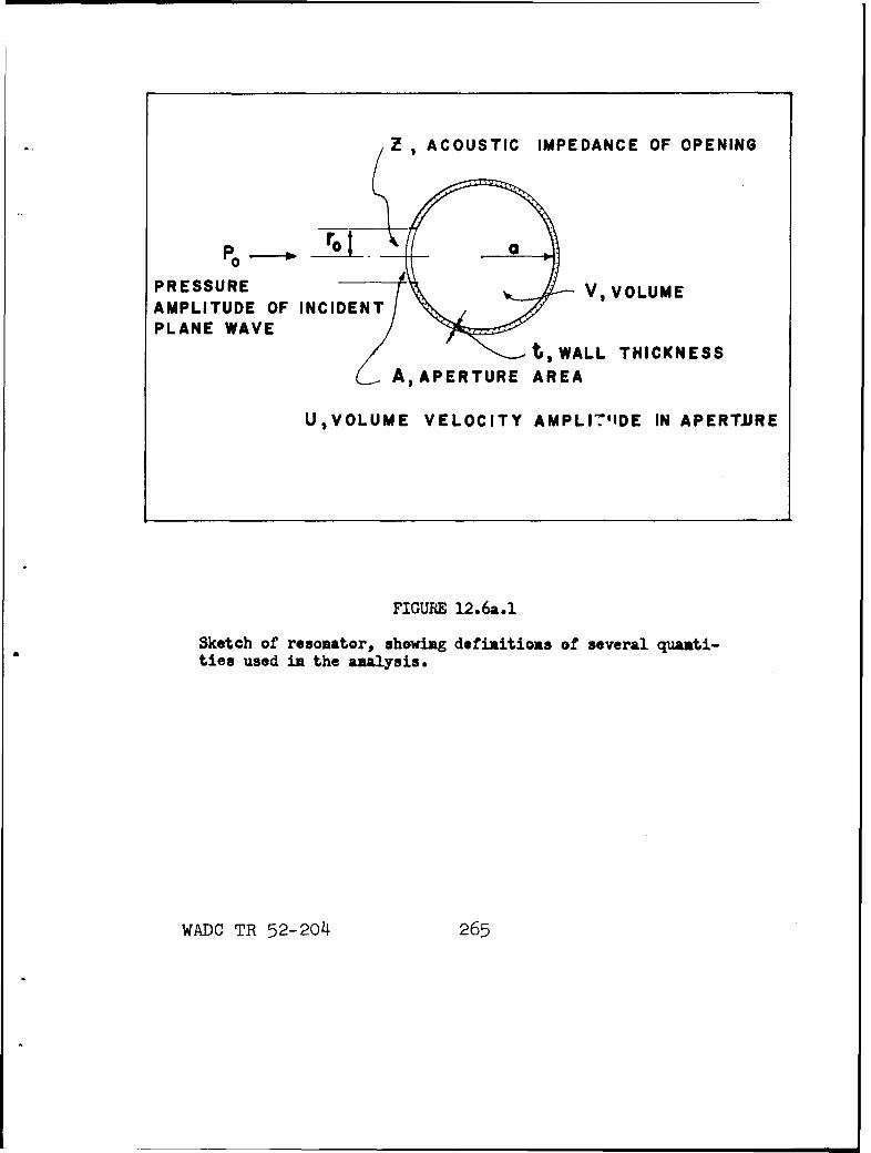
Z ,ACOUSTIC IMPEDANCE OF OPENING

PRESSURE V, VOLUMEAMPLITUDE OF INCIDENTPLANE WAVE

tWALL THICKNESS

A, APERTURE AREA

UVOLUME VELOCITY AMPLI71IDE IN APERTJURE

FIGURE 12.6a. 1

Sketch of resonator, showing definitions of several quanti-ties used in the analysis.

WADC TR 52-204 265

Let Z be the acoustic impedance at the resonator open-ing, and let R be the real part of Z. The aperture resis-tance R is the sum of two quantities, Ri, the resistancerepresenting losses within the resonator and at the opening,and Rr, the resistance associated with re-radiation of soundby the moving air in the aperture. The volume velocity inthe opening is < 2> Po/ IZI . The power dissipated in theresonator is Ri times the square of the volume velocity, or<40 Po 2 Ri/ IZ 2 1 . By definition of the absorption cross

section, the power absorbed is also equal to daPo 2 /pc, sinceP 2 /1pc is the intensity of the incident wave. Thus, theabsorption cross section is

ca = <4?pcRi/ Iz 2 (12.6a.1)

It will be shown how the absorption varies with frequency,with the physical properties of the resonator, and withsound pressure.

The maximum absorption of a given resonator occurs atthe resonance frequency fo, where the resonator impedance Zis simply equal to Ri + Rr. The resonance absorption crosssection is therefore

Sao <=4pcRiao (R i + R r)2

It is assumed that the circumference of the resonator aper-ture is appreciably less than the wavelength of sound. Thismakes it possible to approximate the radiation resistanceby R = <20 pcr/X2 , where X is the wavelength. Theresonance-frequency absorption cross section then becomes

<2> X02(Rid'r /0 -\w.r 2 (12.6a.2)

o (1 + Ri/Rr)

This function has a maximum value of (2) No2 /4Y when(Ri/R ) = I. A slight correction to this calculation willbe introduced later.

WADC TR 52-204 266

Variation of the Absorption Cross Section withFrequency. The acoustic impedance of the aperture can beexpressed as

Z = R[I + JQ(y - 1/7)] (12.6a.3)

where

' = f/fo

Q = 2rMfo/R

R=R. +Rr

M = acoustic mass of air in the resonatoropening; see Eq. (12.6a.5).

It follows that, if the relatively slow variation ofR with frequency is neglected, the variation of absorptionwith frequency can be expressed in the form

a ao = [1 + Q 2(7 - 1/T) 2 ]- 1 (12.6a.4)

The bandwidth, defined as the frequency range within whichSa is not less than one-half of Cao, is given by BW = fo/Q-

The acoustic mass of the air in the resonator opening isproportional to the "effective" length of the opening, equalto the wall thickness t plus anrf"end correction" 5. Thisend correction is proportional to the radius of the apertureand accounts for the fact that some air not directly in thýresonator opening moves as if it were in the opening. Fora small opening in a large flat'plate, the end correctionis b' = 1.70 ro = 0.96 ,/ where A is the area of theaperture. The value given for M in Sec. 12.6 is derived onthis basis. In many cases 6 is somewhat different from 6';typically, P = b/5' is about 0.9. The acoustic mass maybe written as

M = t + _ 1.70 pro tA = A ( + 0.59 (12.6a.5)

WADC TR 52-204 267

Methods for computing P in certain special cases are givenat the conclusion of this section. For present purposes, thevalue • 0.9 will be assumed.

The frequency of resonance, fo, can be computed by theprocedure of Sec. 12.6; it may be expressed as:

fo = 0.666 (c/2ra) r/a 1/2(12.6a.6)P + 0 .59 r--

Total Aperture Resistance at Resonance. The internalresistance of the resonator is the sum of the frictionalresistance due to air flow within the aperture, the resis-tance due to air flow over the surfaces at the ends of theaperture, and the acoustic resistance due to any cloth orscreen which may be placed in the aperture. The values ofthe first two contributions are approximately 6a.l

Frictional acousticresistance within aperture = 2tRs/Ar 0

Frictional acoustic

resistance of end surfaces = 4Rs/A

where Rs= [7,pf]l/2

Here )I and p are respectively the viscosity and density ofair, as in Sec. 12.6. The acoustic resistance due to thecloth or screen will be described by introducing the para-meter o

+ R'

where R' is the flow resistance in rayls* of the cloth orscreen.

* The flow resistance RI must not be confused with the other acousticresistances and impedances. By definition, acoustic impedance isimpedance in rayls, divided by aperture area.

WADC TR 52-204 268

The total internal acoustic resistance (that is, theresistance other than that due to radiation) is thenexpressible as

Ri = 4R s/A PE + 0.5 -] (12.6a.7)

Excep.t for the introduction of a resistance due to a screenor cloth, this is equivalent to Eq. (12.6a) in Sec. 12.6.

The acoustic resistance due to radiation will beexpressed by the approximate relation

Rr = <2) pcw/A 2

as already noted. In order to incorporate this resistancein a fashion which is convenient for the final design for-mulas, it is necessary to define two dimensionless parameters,;h and C, as follows:

( o + 0.59 rt )2

h + 0(12.6a.8)tE+o0.5r

CE. (k 0 a)-6 (RrRiR) (12.6a.9)

Here k denotes 2w/, , or 2w f O/. The latter parameteris given by

C - 0.316 <2? hpc/Rs , (12.6a.10)

as may be shown by combining Eqs. (12.6a,b) through (12.6a.9)Therefore the total resistance R = Ri + Rr can be expressedas

R = (4Rs/A)(C + 0.5 t-) [1 + (k a)6 C] (12. 6 a.11)0

WADC TR 52-2o4 269

It is useful to notice that if no cloth or screen is used,C is equal to unity, and if also (t/ro) <( 1, then alsoh is approximately equal to unity.

Resonator Formulas in Terms of Generalized Parameters.The basic resonator formulae, when expressed in terms ofthe dimensionless parameters (koa) = 2rfo/c, are suitable asa basis for orderly design work or for the construction ofgeneral design charts. The relations below, which give theabsorption cross section, the Q, and the reverberation timeof the resonator, are particularly useful.

The absorption cross section at resonance is

2 6< 2> Ao 04(k 0 a) CF

•ao = [I6 2 (12.6a.12)

where

F = 1 + 9 (k 0 a) 2 (Resonator in space)

F = 1 (Resonator in wall) I

The correction factor F, which is of the order of 1.2 in apractical resonator in space, is obtained by detailed wave-theory analysis of the spherical resonator.

The generalized expression for the Q is obtained bycombining the expressions for fo and M to give

2 rMfo0 = 0.240(2f 0 ) p/a(k0 a) 2

and by combining the expressions for R, fo , and C to give

R = <2> [0.0793 pc/a 2 (k 0 a) 4C][l + (koa) 6 C]

Thus, the Q, which is equal to 2rMfIR, is given by

WADC TR 52-204 270

_3 * 0 _3 (k 0 a) 3C (12.6a.14)(2) 1 + (k 0 a )6C

The reverberation time (the time for the power re-radiatedby the resonator to decrease by 60 db after the externalsignal ceases) is equal to 2.19 ýlf 0 Therefore, the re-verberation time is

T = 6.65 1 (k 0 a)3C 67:ýo 1 + (k 0 a) C

Optimum Design Values. When values are assigned totwo of the three quantities fo (frequency of resonance), h(hole parameter), and V (cavity volume), there then existsan optimum value for the remaining parameter such that theresonance absorption cross section U'aO will be as large aspossible. For the resonator in space, this maximum possiblevalue of 07 for any given set of conditions usually liesbetween XO/4 and 1.5 (-,\02/4r). These limits correspond tovalues of F between 1.0 and 1.5. The calculation of optimumvalues where fo and the hole parameter h have already beenchosen will be considered here. The value of h is dependentupon choices of t/ro and E , the latter quantity being anindex of the amount of flow resistance introduced by acloth or screen. The problem is then one of finding theoptimum value of the spherical cavity radius, al, for whichthe absorption cross section is maximum. The subscript 1will refer to an optimum value.) The required value of theaperture radius, ro is also easily found.

Since the frequency is given, the quantity C is aconstant. From Eq. (12.6a.12) it is found thatAe maximumabsorption cross section is obtained when (koal C = 1, or

k 0 a i = 1.08 1/b [47rjjpf 01 1/12 (12.6a.16)( <2) ech)

When numerical values for room temperature are inserted,the optimum sphere radius is

WADC TR 52-2o4 271

a1 = lO80 fo-11/12 h-1/ 6 cm (resonator in space)

a1 = 963 fo-11/12 h-1/ 6 cm (resonator in wall)

(12.6a.17)

For a cavity having the optimum radius a1 , the absorption,the Q, and the reverberation time are given by the relationsbelow where the numerical forms are for room temperature(700F).

0'al = (ho 2/4-)F (12.6a.18)

Q1 = 0.85(hpc)1/2/[ (7r4pfo)l/4 < V = 189 V-h/(fo 1/4< /Y-2 )

(12.6a.19)

T1 = 1.87(hpc)l/2/ (7rp)I/ 4 f o/ 40 ' 1=415 fi-h/(fo5/ 4<--2,>)

(12.6a.20)

Sometimes, when the optimum value of a has been obtained,it is desirable to be able to calculate directly the changein the above quantities which will result from changing to anon-optimum value for a. For this purpose, the equationscan be rewritten in the normalized forms

a-- =4(IB6)62 (12.6a.21)'5al (1l+ B)

T Q _ 2B3

T1 Q1 1 + BE (12.6a.22)

where B = a/a 1

WADC TR 52-204 272

Almost all calculations necessary to evaluate theoptimum resonator design, for given resonance frequencyand hole parameter, can be performed using the charts ofFigs. 12.6a.2-7. For those calculations which involve P ,

the value 1 = 0.9 has been used in constructing the charts.Room temperature values of the air constants have been used,and where the relations for resonator-in-space differ fromthose for resonator-in-wall, the charts apply to the in-spacecase. The use of the charts is explained below.

Procedure for Optimum Design Calculation. It is assumedthat the resonance frequency and the hole constants (theratio t/ro and the flow resistance of the cloth or screen inthe aperture) are known, and an optimum design is desired.Alternatively, if the value of the hole parameter h is known,the first step in the calculation is reversed, and possiblevalues of t/ro and of flow resistance are found which willpermit the desired h value to be realized. The calculationsmay be made in the order shown below.

1. Compute h, from known values of t/ro and of flowresistance R', from Eq. (12.6a.8) or from Fig. 12.6a.2.The chart assumes 0 = 0.9.

2. Compute the optimum cavity radius, a1 , fromEq. (12.6a.17) or from Fig. 12.6a.3. (For resonator-in-wall, multiply result from chart by 2-1/6 0.890.)

3. Compute koal = 2.fOal/c, or obtain this quantityfrom Fig. 12.6a.4.

4. Compute ro/a (and hence ro) from Eq. (12.6a.6) orobtain this value from Fig. 12.6a. 4 . The chartassumes P = 0.9.

5. Compute F from Eq. (12.6a.13).

6. Compute the maximum absorption cross section,

al 2 F 02/4.

7. Compute Ql from Eq. (12.6a.19), or fromFig. 12.6a.5. The bandwidth in which the absorptioncross section is at least (ral/2 is BW = fo/Ql.(If the resonator is in wall, multiply result fromchart by 1/ V7.).

WADC TR 52-204 273

1.0

0.5

0.010I 2 510 2 50 00 20 50

x 11'

WAD TR52-204274

8. If desired, obtain the reverberation time T, fromEq.(12.6a.20) or from Fig. 12.6a.6. (If resonatoris in wall, multiply result from chart by 1/ -/2.)

9. If it is desired finally to explore the effect ofchanging to a cavity radius a other than theoptimum value a , consult Eqs. (12.6a.21,22) orFig. 12.6a.7. lNot valid if resonator operationis in the nonlinear orifice resistance range, seeSec. 12.6 and the later discussion in this section;Eq. (12.6a.31) gives the non-linear resistance.)

Selection of Efficient Design. The calculation pro-cedure outlined above shows how to obtain an optimum setof related values, once the resonance frequency and thehole parameter are specified. Some further considerationmust be given to indicate on what basis the designer canmake the original choice of the hole parameter h, and toshow certain other practical aspects of the design problem.

1. The smaller values of h correspond to resonatorshaving relatively large volume, but relatively low Q andhence relatively large bandwidth. Conversely, the largervalues of h correspond to small-volume, high-Q, narrow-band resonators.

2. Small h is obtained by use of a short-neckaperature (t/ro << 1) in which a cloth or screen has beenintroduced to increase the resistance ( E > 1); largervalues of h are obtained with apertures having longer necks,with no'added resistance.

3. The basic equations are not applicable unless theradius of the aperture is appreciably less than the radiusof the cavity. In practice, it is considered that ro/ashould not exceed 0.3. At any given frequency, thisrequirement indirectly determines the smallest value of h,

FIGURE 12.6a.2The hole parameter, h, when the flow resistance parameter, E, andthe ratio t/ro of aperture thickness to radius, are known. Thechart represents Eq. (12.6a.8) for the case 0.9. FromIngard k&.lI.

WADC TR 52-204 275

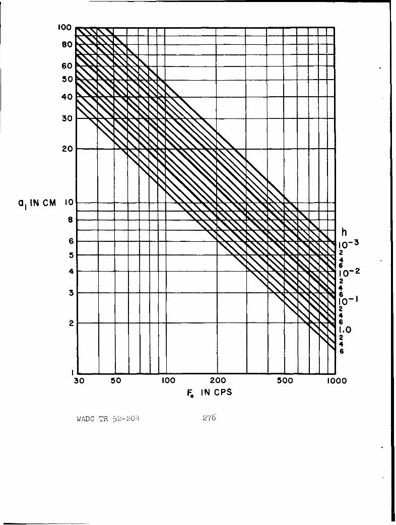
800

50

40

30

66 ioZ35 2

4 6

24

3 6I.024

2 6

30 50 100 200 500 1000

F, IN CPS

WADC ZR 52-20,1 276

and hence the smallest Q, which can be obtained. This isbecause ro/a increases with increasing resonator volume, andhence with decreasing h. (It will be shown that the Q, can-not be less than 25 for optimum-design resonators in space,or less than 13 for the wall location, if the restriction on(ro/a)is observed .

4. From the foregoing considerations, it follows thatefficient design (minimum volume used) for a resonator whichis to absorb sound of only one frequency is obtained whenthe aperture (neck) length t is made several times the aper-ture radius ro, and no additional resistance is added. Thisdesign results in small volume, large Q, and small bandwidth,but the absorption obtained at resonance, with an optimumcombination of values, is always ?o0

2/2r for the resonator ina wall or of the order of ?o 2/44ir for a resonator in space.

5. The greatest possible absorption in the greatestpossible bandwidth, for a single resonator, is obtained byputting (t/r << 1, and choosing the largest allowablevolume, which corresponds to (ro/a) = 0.3. Optimum designis then completed by finding the value of h for which theresulting cavity radius al is an optimum value, and selectinga cloth or screen of suitable flow resistance to give a valueof E which will result in this selected value of h.

6. The effect of using a cavity radius a other thanthe value which is optimum for a given f and h is to decreasethe absorption Crao at resonance and to increase the bandwidth,in such a way that the product c-ao(BW) 2 is constant.Specifically, the relation is

5ao (BW) 2 = >4? 2.8F vrf/h (12.6a.23)

FIGURE 12.6a.3

The optimum radius, al, for a spherical resonator cavity when thefrequency of resonance Fo, and the hole parameter h, are given.This is for air at room temperature only. For a resonator in spacethis chart is the same as Eq. (12.6a.17). Multiply result by 0.890if resonator opening is in or very near the wall. From Ingard ,k../

WADC TR 52-204 277

where 6ao is in ft 2 (sabins), and BW and f are in cps.This relation may be obtained by combining eqs. (12.6a.12),(12.6a.14), and (12.6a.10). For optimum design, '-ao isequal to C-al, or F )ýo2 /4r, and for other designs Y-ao isless than that value.

7. From Eq. (12.7a.23) or from the basic equations,it follows that the optimum design (the design which maxi-mizes absorption for a given h) represents the maximumpossible Q for a given h.

8. By further interpretation of Eq. (12.6a.23), itis found that a departure from the optimum design, for agiven h, reduces the absorption not only at resonance butat all frequencies, even though the Q is decreased. Forthis reason, it is preferable to use optimum combinationsof values except in unusual circumstances where a low Q isabsolutely necessary and greatly reduced absorption can beaccepted (or in cases where nonlinear effects necessitatea reduced Q, as will be shown later).

9. The cavity need not be spherical, but can have anyshape for which the volume is equal to 4ra 3/3, and whichpresents a sharp change of cross section at the aperture.Similarly, the aperture can be square rather than circular,if the same area is maintained.

10. The analysis does not consider interactions be-tween adjacent resonators tuned to the same frequency, andapplies only when the separation between individualresonators tuned to the same frequency is Xo/2 or more.

FIGURE 12.6a.4

Relation between the resonance frequency and the resonator dimen-sions, for air at room temperature. The broken lines give theresonance frequency Fo, in cps, as a function of k0a, for variousvalues of cavity radius a. The solid curves, which representEq. (12.6a.6) for the case P - 0.9, relate rda to koa for variousvalues of t/ro. Aperture thickness, t; aperture radius, ro;IC= 21rfdc; c is the speed of sound. From Ingard _

WADC TR 52-204 278

1.0

5a

rtO

0.

200Jj~ 12

220 7

800

60 nf

50 12

401.0

306

204202

ft ft_ 1 0 - i

6

5 2

10 -2

lftý 6

2 -

2

20 50 100 200 500 1000

Fo IN CPS

WADO TR 52-204- 280

The case of a large area continuously covered by resonatorstuned to the same frequency is treated in Sec. 12.1, underthe topic of perforated facings for acoustical materials.

11. Adjacent resonators can be considered non-interactingwhen the difference in the resonance frequencies is greaterthan either of the bandwidths. When this restriction is ob-served, the analysis applies to banks of adjacent resonatorswhich are "stagger-tuned" to cover a wide band of frequencies.

12. When short-neck resonators are used in an optimumdesign, as is necessary to secure large bandwidth, the band-width is proportional to the resonator volume. Therefore,the volume occupied by a "stagger-tuned" array for a givenfrequency band is a constant for optimum design, no matterwhether, say, n resonators are used with one set of Q values,of 2n resonators are used with individual Q's twice as large.

Simplified Design for Short-Neck Resonators. It isevident from the preceding list of design considerations thtresonators intended for large bandwidths represent a specialcase in which the neck is very short, or t/ro = O. Thedesign procedure can be greatly shortened for this condition.The simplified relations for the short-neck resonator aregiven below, with numerical coefficients given for the caseof room temperature air and P = 0.9. These relationsrepresent optimum-design combinations; that is, combinationswhich represent maximum possible resonance absorption andmaximum possible Q for a given resonator opening at a givenfrequency.

The optimum volume, in terms of the optimum Q and thefrequency of resonance, is

- 3.53 x 10 (12.6a.24)<2) Q1 fo3

FIGURE 12.6a.5

The Q value, Q1, obtained in an optimum resonator design when thefrequency of resonance in cps, F0 , and the hole parameter, h, aregiven. Represents Eq. (12.8a.19P for air at room temperature.From Ingard .

WADC TR 52-2o4 281

Here V1 is in ft 3 , and fo in cps. This relation is derivedby combining Eqs. (12.6a.17) and (12.6a.19). The requiredaperture radius is

ro = 1.90 x 10-4 f0 V1 (12.6a.25)

where ro is in inches, fo is in cps, and V1 is in ft 3 Thisrelation follows from Eq. (12.6a.6). Using Eq. (12.6a.24),the radius (in inches) can also be expressed as

ro = 6.70 x 103/fo0 , <2> (12.6a.26)

While the value of h, the hole parameter, is notrequired for the present calculations, it is helpful to beable to compute this quantity in order to refer back to themore extensive design charts. From Eq. (12.6a.19), thevalue of h for the present special conditions is

h= <2> 2.82 x 10- 5 vm 2f- 2

where f0 is in cps.

The required flow resistance of the screen of clothin the aperture is found by combining (12.6a.27) with(12.6a.8), and making use of the definition of E . Therequired added flow resistance in rayls is given by

Rt = 191 -(3.26 x 10-3) V7 (12.6a.28)<2) Q2 0

The maximum allowable volume for a resonator repre-senting an optimum combination of value is wt by the condi-tion (ro/al) "( 0.3. The value of this maximum allowablevolume is found by writing Eq. (12.6a.25) in the form of arelation between ro and a1 , imposing the required

FIGURE 12.6a.6

The reverberation time in seconds, T1 , obtained in an optimumresonator design when the frequency of resonance in cps, Fo, andthe hole parameter, h, are given. This represents Eq. (12.6a.20)for air at room temperature. From Ingard .

WADC TR 52-204 282

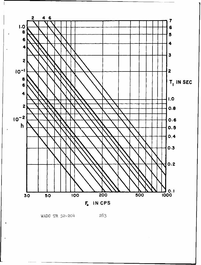
6.

2L

10- -- - - 28T IN SEC

61

4.

2

WA0C TR2-0 8

- - - - - - - -

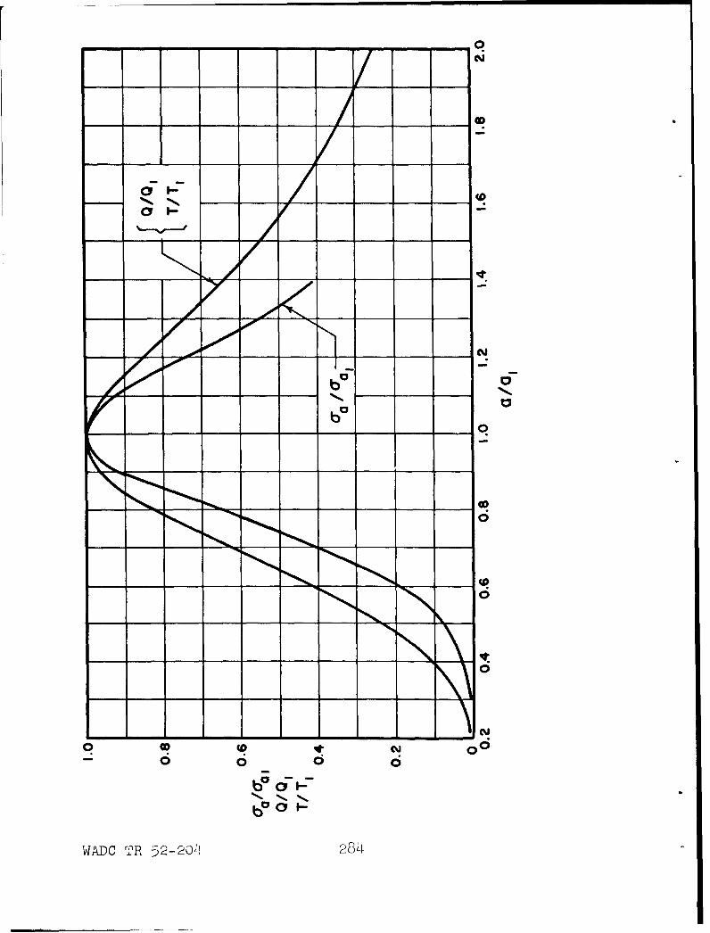
ozU

001r

04

-- 9i

OD_ __0 __ _ _ 06

6 6 c;

___C ___ 52200 2

conditions, and then finding the volume from the resultingvalue for a 1 . The resulting restriction on the volume is

V < 1.4 x lO6 ft 3 (12.6a.29)

0

The minimum Q which can be obtained with optimum designconditions is obtained in a resonator of maximum volume, andis found by combining (12.6a.29) and (12.6a.24). This mini-mum value of Ql is approximately 25/( 2>. Correspondingly,the minimum reverberation time in optimum designs is approxi-mately

Tm 55/ (2> fo sec. (12.6a.30)

Finally, the procedure for obtaining the optimum designof short-neck resonators can be summarized as follows:decide upon the desired resonance frequency. Then choose aresonator volume not exceeding the limit given by Eq.(12.6a.29),or choose a Q not less than 25/<2> . The remaining designquantities can then be found directly from the precedingequations if the resonator operates in air at room temperature.

The numerical coefficients, and the limiting values ofthe volume and the Q, will be different if other values ofthe density and the viscosity of the gas are used, and it willbe necessary in that event to go to the basic equations givenpreviously in this section.

FIGURE 12.6a.7

The relative effects upon the resonance absorption cross section,raoo, the reverberation time, T, and the Q, when a departure is

made from optimum resonator design. It is assumed that theresonance frequency fo and the hole parameter h retain the valuesfor which the optimum cavity radius al applies, but that the cavityradius has been changed arbitrarily from a1 to some value a, and acorresponding change made in the aperture radius. From Ingard k-.j/.

WADC TR 52-204 285

Effects of Non-linearity. The internal resistance ofthe resonator includes a non-linear contribution which be-comes important when the resonator is exposed to largeincident sound pressures, as was found in Sec. 12.6 inconnection with the design of a resonator attached to a duct.The effect of non-linearity may become significant when theSPL of the incident signal exceeds 80 to 90 db, but inlarge, low-frequency resonators this threshold may be muchhigher. The effect of the non-linear resistance is to de-crease the resonance absorption and the Q of the system.To include the non-linear resistance in the basic equationswould lead to results so cumbersome as not to be highlyuseful. Therefore, only special aspects of the problemwill be considered.

In the general case, the non-linear resistance dependsupon the orifice thickness, the particle velocity, and theparticle displacement. The effect of frequency isapparently not great, but this question has not been ex-plored extensively. Non-linear resistance data are experi-mental, because no general theory has been given yet. Forthe present purposes, an empirical relation 6a.l/expressedby Eq. (12.6a.31) will be used for the non-linear resistance.This relation is. more accurate over a wide range of condi-tions than the one used in Sec. 12.6, although both formulaslead to approximately the same value of sound pressure atwhich the response of the resonator is seriously affectedby non-linear resistance. Only the effect of particle velo-city is shown, since this is the variable of major importancein the non-linear resistance unless the particle displace-ment amplitude exceeds the orifice thickness. The non-linearacoustic resistance is

RNL = 1.36 x lO-5 u 1 .7 /A 2 "7 (12.6a.31)

where U is the rms yolume velocity in cm3/sec and A is theaperture area in cm .

The effects of the added resistance RTL upon the Q andthe peak absorption of a resonator designed to meet optimumconditions in the absence of the non-linear resistance areeasily expressed. The total resonator resistance is Ri + Rr;in the optimum design, this is simply 2 Rr. When non-linear

WADC TR 52-2o4 286

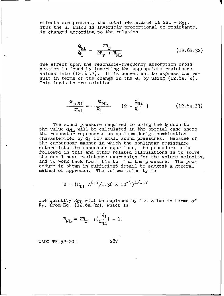
effects are present, the total resistance is 2Rr + RNL.Thus the Q, which is inversely proportional to resistance,is changed according to the relation

QNL 2R 2 (12.6a.32).Q- r R+ RNL

The effect upon the resonance-frequency absorption crosssection is found by inserting the appropriate resistancevalues into (12.6a.2). It is convenient to express the re-sult in terms of the change in the a,, by using (12.6a.32).This leads to the relation

aoN _ QN (2 - )(12.6a.33)Tal1

The sound pressure required to bring the q down tothe value QNL will be calculated in the special case wherethe resonator represents an optimum design combinationcharacterized by 'Ql for small sound pressures. Because ofthe cumbersome manner in which the nonlinear resistanceenters into the resonator equations, the procedure to befollowed in this and other related calculations is to solvethe non-linear resistance expression for the volume velocity,and to work back from this to find the pressure. The pro-cedure is shown in sufficient detail to suggest a generalmethod of approach. The volume velocity is

U _- (RNL A2 .7/1l.36 x 10-5)1/1.7

The quantity RN will be replaced by its value in terms ofRr, from Eq. (Yý.6a.32), which is

RNL = 2Rr NL) -11

WADC TR 52-204 287'

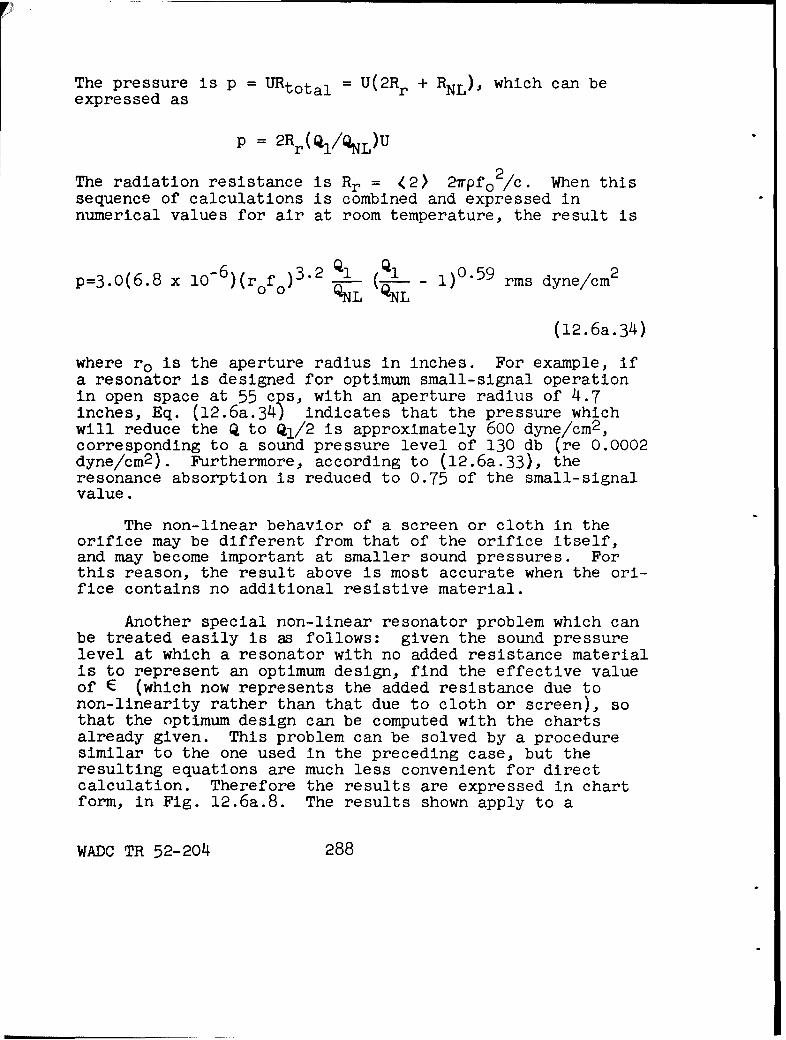
The pressure is p = URtotal = U(2Rr + RNL), which can be

expressed as

p = 2Rr(QI/QNL)U

The radiation resistance is Rr = (2) 2Tpfo 2 /c. When thissequence of calculations is combined and expressed innumerical values for air at room temperature, the result is

p=3.0( 6 .8 x 10- 6 )(r f )3.2 'IL (1NL 1)0.59 rms dyne/cm2

00 QNL QNL

(12.6a.34)

where ro is the aperture radius in inches. For example, ifa resonator is designed for optimum small-signal operationin open space at 55 cps, with an aperture radius of 4.7inches, Eq. (12.6a.34) indicates that the pressure whichwill reduce the Q to Qi/2 is approximately 600 dyne/cm2 ,corresponding to a sound pressure level of 130 db (re 0.0002dyne/cm2 ). Furthermore, according to (12.6a.33), theresonance absorption is reduced to 0.75 of the small-signalvalue.

The non-linear behavior of a screen or cloth in theorifice may be different from that of the orifice itself,and may become important at smaller sound pressures. Forthis reason, the result above is most accurate when the ori-fice contains no additional resistive material.

Another special non-linear resonator problem which canbe treated easily is as follows: given the sound pressurelevel at which a resonator with no added resistance materialis to represent an optimum design, find the effective valueof E (which now represents the added resistance due tonon-linearity rather than that due to cloth or screen), sothat the optimum design can be computed with the chartsalready given. This problem can be solved by a proceduresimilar to the one used in the preceding case, but theresulting equations are much less convenient for directcalculation. Therefore the results are expressed in chartform, in Fig. 12.6a.8. The results shown apply to a

WADC TR 52-204 288

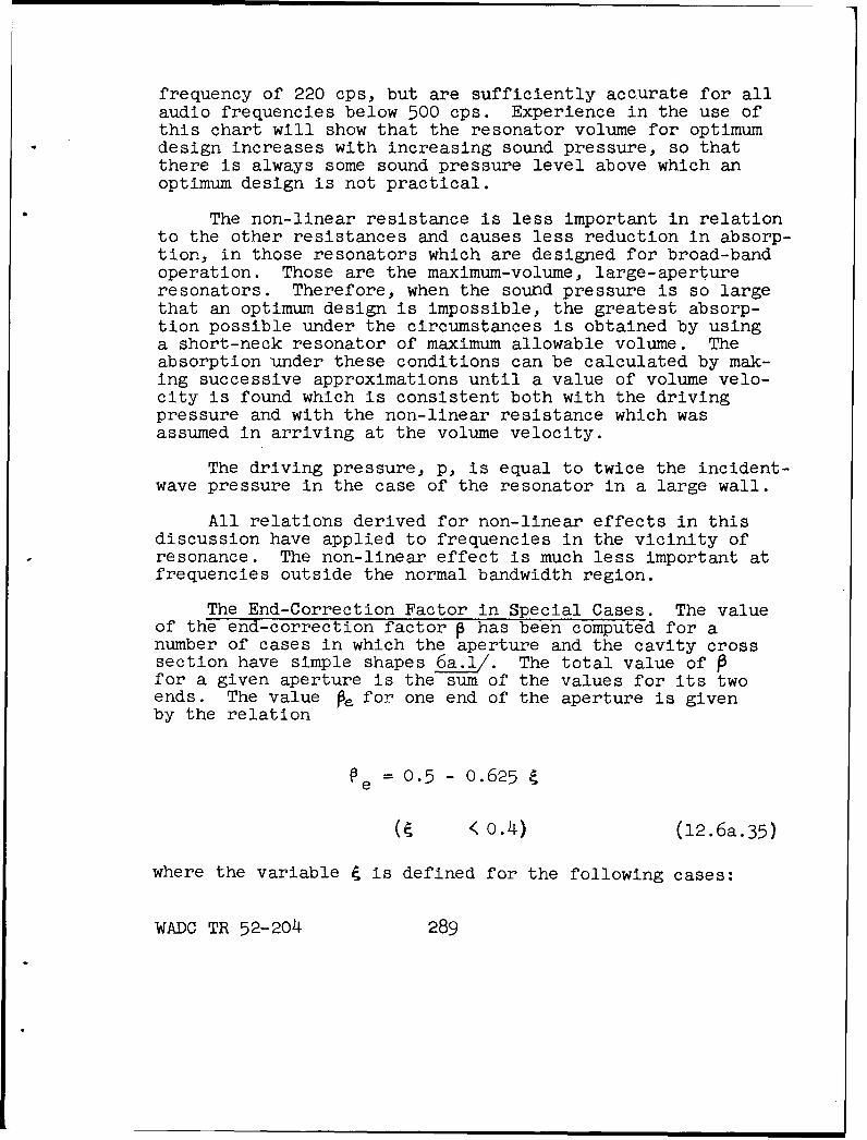
frequency of 220 cps, but are sufficiently accurate for allaudio frequencies below 500 cps. Experience in the use ofthis chart will show that the resonator volume for optimumdesign increases with increasing sound pressure, so thatthere is always some sound pressure level above which anoptimum design is not practical.

The non-linear resistance is less important in relationto the other resistances and causes less reduction in absorp-tion, in those resonators which are designed for broad-bandoperation. Those are the maximum-volume, large-apertureresonators. Therefore, when the sound pressure is so largethat an optimum design is impossible, the greatest absorp-tion possible under the circumstances is obtained by usinga short-neck resonator of maximum allowable volume. Theabsorption under these conditions can be calculated by mak-ing successive approximations until a value of volume velo-city is found which is consistent both with the drivingpressure and with the non-linear resistance which wasassumed in arriving at the volume velocity.

The driving pressure, p, is equal to twice the incident-wave pressure in the case of the resonator in a large wall.

All relations derived for non-linear effects in thisdiscussion have applied to frequencies in the vicinity ofresonance. The non-linear effect is much less important atfrequencies outside the normal bandwidth region.

The End-Correction Factor in Special Cases. The valueof the end-correction factor P has been computed for anumber of cases in which the aperture and the cavity crosssection have simple shapes a_.l/. The total value of 0for a given aperture is the sum of the values for its twoends. The value P. for one end of the aperture is givenby the relation

e =0.5 - o.625 4

< 0.4) (12.6a.35)

where the variable • is defined for the following cases:

WADC TR 52-204 289

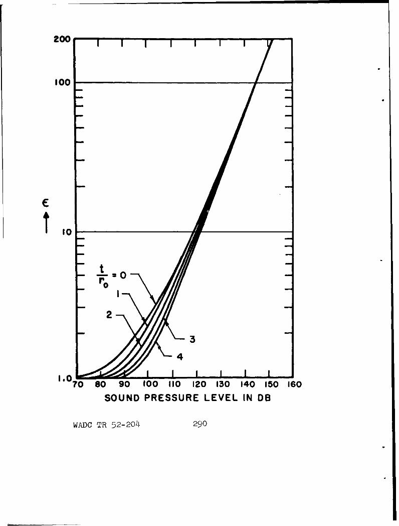
200 1

100

Ci

I0

•4

Io070 80 90 100 110 120 130 140 150 160

SOUND PRESSURE LEVEL IN DB

WADe TR 52-204 290

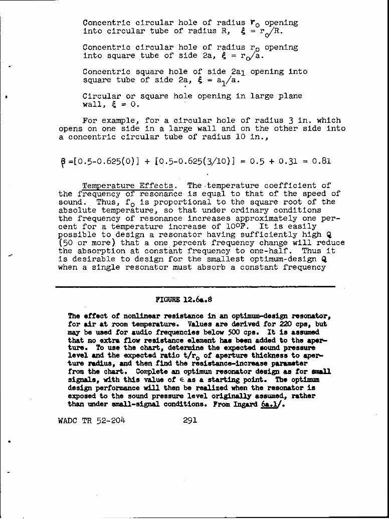
Concentric circular hole of radius ro openinginto circular tube of radius R, 4 = rIR.

Concentric circular hole of radius ro openinginto square tube of side 2a, e = ro/a.

Concentric square hole of side 2al opening intosquare tube of side 2a, 4=al/a.

Circular or square hole opening in large planewall, 4 = 0.

For example, for a circular hole of radius 3 in. whichopens on one side in a large wall and on the other side intoa concentric circular tube of radius 10 in.,

=[0.5-0.625(0)] + [0.5-0.625(3/10)] = 0.5 + 0.31 = 0.81

Temperature Effects. Thetemperature coefficient ofthe frequency of resonance is equal to that of the speed ofsound. Thus, fo is proportional to the square root of theabsolute temperature, so that under ordinary conditionsthe frequency of resonance increases approximately one per-cent for a temperature increase of lOOF. It is easilypossible to design a resonator having sufficiently high Q(50 or more) that a one percent frequency change will reducethe absorption at constant frequency to one-half. Thus itis desirable to design for the smallest optimum-design Qwhen a single resonator must absorb a constant frequency

FIGURE 12.6a.8

The effect of nonlinear resistance in an optimum-design resonator,for air at room temperature. Values are derived for 220 cps, butmay be used for audio frequencies below 500 cps. It is assumedthat no extra flow resistance element has been added to the aper-ture. To use the chart, determine the expected sound pressurelevel and the expected ratio t/ro of aperture thickness to aper-ture radius, and then find the resistance-increase parameterfrom the chart. Complete an optimum resonator design as for smallsignals, with this value of '- as a starting point. The optimumdesign performance will then be realized when the resonator isexposed to the sound pressure level originally assumed, ratherthan under small-signal conditions. From Ingard __. 1.

WADC TR 52-204 291

under conditions of fluctuating temperature. This diffi-culty is not pronounced in the case of a stagger-tunedarray of resonators, since all frequencies of resonanceare affected by the same factor when the temperature changes.

Practical Tuning of Resonators. The approximationsmade in calculating the frequency of resonance, or tolerancesin construction, may result in serious mistuning of a high-Q resonator which is intended to operate at a specificfrequency. The most reliable solution to the tuning pro-blem is to adjust the resonator to the proper frequency afterinstallation. The adjustment may be performed by varyingeither the volume or the area of the opening. An indicationof proper adjustment may be obtained by use of a sound levelmeter connected to a pressure microphone located outsidethe resonator next to the resonator opening. When theresonator is exposed to constant intensity sound of the fre-quency that one wishes to absorb, the resonatoristuned byadjusting the resonator variable for a minimum sound levelmeter reading compared to the initial sound pressure level.

Another source of tuning error is the non-linearcontribution to the acoustic mass, which becomes importantat high signal levels. This non-linear effect is generallyless important than the non-linear resistance and hence hasnot been considered in the analysis. Provision for tuningadjustment is particularly desirable to compensate for thiseffect where strong signals are expected.

Significance of Reverberation Time. When a resonator isused as a sound absorber in a room intended for listening tomusic or speech, the reverberation time of the resonatorshould be less than that of the room at the frequency ofresonance, in order to avoid a localized "hold over" follow-ing transient signals. This requirement on the reverbera-tion time is ordinarily not difficult to satisfy. Forexample, stagger-tuned resonator arrays have been successfullyused to provide low-frequency absorption in small radiostudios.

Numerical Examples of Resonator Design. As a firstexample, it will be supposed that an optimum-design, wall-mounted resonator is required to operate at 55 cps, with abandwidth of 2.2 cps.

WADC TR 52-204 292

Since the Q is relatively low (25), it will be desir-able to use the simplified design procedure for the short-neck resonator. The design is possible, since a Q as lowas 13 can be obtained with a wall-mounted resonator.

From Eq. (12.6a.24), the required volume is 4.24 ft 3 .

From Eq. (12.6a.25), the aperture radius is 2.44 in.

From Eq. (12.6a.28), the added flow resistance mustbe 0.15 rayls.

The reverberation time is 2.19 Ql/fo, or 1.0 sec.

From Eq. (12.6a.34), the driving sound pressure atwhich the Q. is halved is 110 dynes/cm2 , correspond-ing to a sound pressure of 55 dynes/cm2 in the waveincident on the wall, a sound pressure level of 109 db.This is also the incident sound pressure at which thecenter-frequency absorption is reduced to 75 percentof the small-signal value due to non-linear operationaccording to Eq. (12.6a.33).

The maximum small-signal absorption (?\o 2/2r) is 64sabins at a wavelength of 20 ft.

As a second example, suppose that it is desired todetermine the dimensions of a short-neck resonator, with noadded resistance in the aperture, which shall represent anoptimum design at 60 cps when used in space where the inci-dent SPL is 110 db. The initial step is to consultFig. 12.6a.8, according to which E = 4.9 under the givenconditions. The remaining steps are carried out accordingto the "Procedure for optimum design calculation", givenfollowing Eq. (12.6a.22).

From Fig. 12.6a.2, h = 0.18

From Fig. 12.6a.3, a1 = 34 cm.

From Fig. 12.6a.4, k0 a1 = 0.39

From Fig. 12.6a.4, rna = 0.29, so that r° = 9.9 cm.

From Eq. (12.6a.13), F = 1.34.

WADC TR 52-204 293

m m m I I I b

The maximum absorption cross sectionis 1.35 •o2/4• = 37 sabins.

From Fig. 12.6a.5, Q1 = 29•

References for Sec. 12.6a

6a•l Ingard, Uno, "On the Theory and Design ofAcoustic Resonators" J. Acous Soc Am25 1037 (1953)•

WADC TR 52-204 294

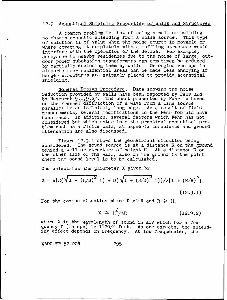
12.9 Acoustical Shielding Properties of Walls and Structures

A common problem is that of using a wall or buildingto obtain acoustic shielding from a noise source. This typeof solution is of value when the noise source is movable orwhere covering it completely with a muffling structure wouldinterfere with the operation of the device. For example,annoyance to nearby residences due to the noise of large, out-door power substation transformers can sometimes be reducedby partially enclosing them by walls. Or engine run-ups inairports near residential areas can be made less annoying ifhanger structures are suitably placed to provide acousticalshielding.

General Design Procedure. Data showing the noisereduction provided by walls have been reported by Fehr andby Hayhurst .2 The chart presented by Fehr is basedon the Fresnel diffraction of a wave from a line sourceparallel to an infinitely long edge. As a result of fieldmeasurements, several modifications to the Fehr formula havebeen made. In addition, several factors which Fehr has notconsidered but which enter into the practical acoustical pro-blem such as a finite wall, atmospheric turbulence and groundattenuation are also discussed.

Figure 12.9.1 shows the geometrical situation beingconsidered. The sound source is at a distance R on the groundbehind a wall or structure of height H. At a distance D onthe other side of the wall, also on the ground is the pointwhere the sound level is to be calculated.

One calculates the parameter X given by

X = 2[R(Vl + (H/R) -1) + D(Vl + (H/D-) I/M[ + (H/R)2].

(12.9.1)

For the common situation where D ?7 R and R > H,

X : H2 /XR (12.9.2)

where X is the wavelength of sound in air which for a fre-quency f (in cps) is 1120/f feet. As one expects, the shield-ing effect depends on frequency. At low frequencies, the

WADC TR 52-204 295

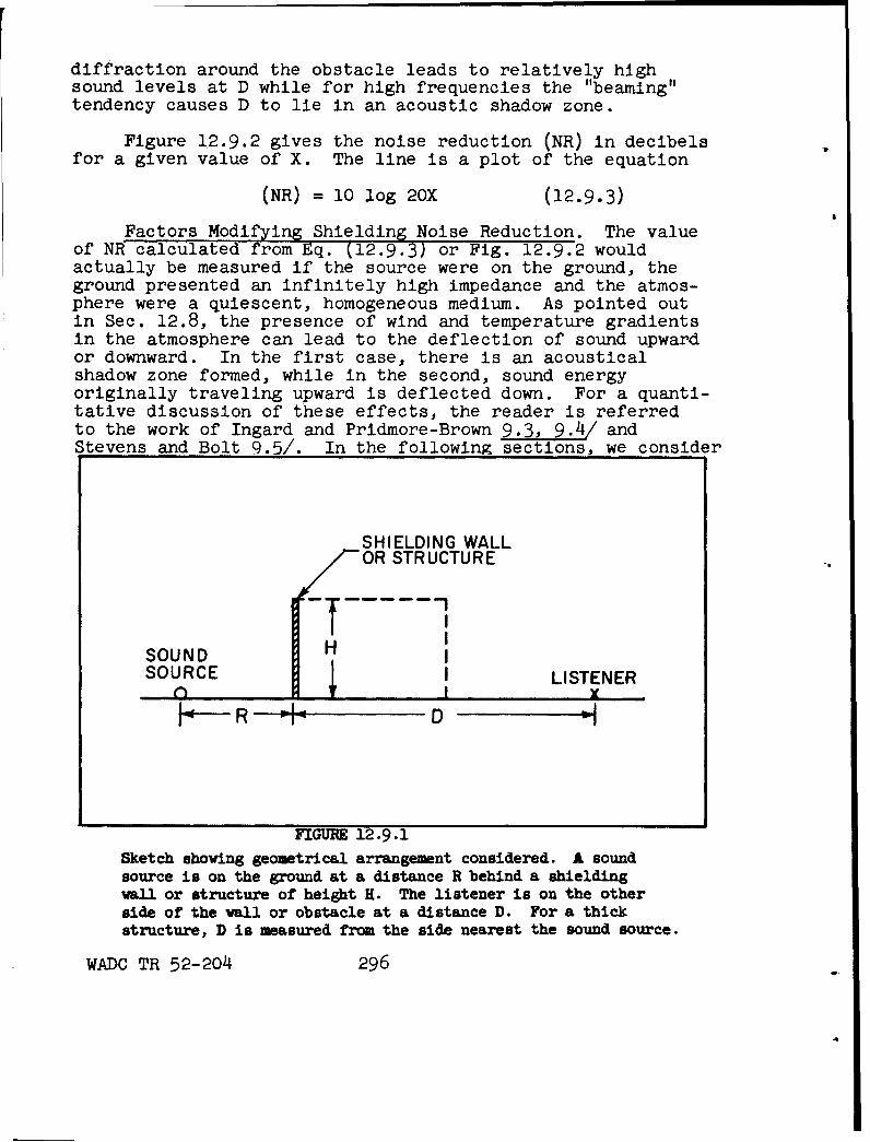
diffraction around the obstacle leads to relatively highsound levels at D while for high frequencies the "beaming"tendency causes D to lie in an acoustic shadow zone.

Figure 12.9.2 gives the noise reduction (NR) in decibelsfor a given value of X. The line is a plot of the equation

(NR) = 10 log 20X (12.9.3)

Factors Modifying Shielding Noise Reduction. The valueof NA calculated from Eq. (12.9.3) or Fig. 12.9.2 wouldactually be measured if the source were on the ground, theground presented an infinitely high impedance and the atmos-phere were a quiescent, homogeneous medium. As pointed outin Sec. 12.8, the presence of wind and temperature gradientsin the atmosphere can lead to the deflection of sound upwardor downward. In the first case, there is an acousticalshadow zone formed, while in the second, sound energyoriginally traveling upward is deflected down. For a quanti-tative discussion of these effects, the reader is referredto the work of Ingard and Pridmore-Brown 9.3, 9.4/ andStevens and Bolt 9.5/. In the following sections, we consider

SHIELDING WALLOR STRUCTURE

-T

SOUND HSOURCE I LISTENER

R " -- D -

FIGURE 12.9.1Sketch showing geometrical arrangement considered. A soundsource is on the ground at a distance R behind a shieldingwall or structure of height H. The listener is on the otherside of the wall or obstacle at a distance D. For a thickstructure, D is measured from the side nearest the sound source.

WADC TR 52-204 296

the modifications necessary to account for

1. the sound source not being on the ground

2. absorption by the ground

3. atmospheric turbulence

4. "flanking" around the side of a structure

1. Consider the situation shown in Fig. 12.9.3where a sound source is located some height h above theground and at a distance R from a shielding wall or struc-ture. Ray A shows the direct path from the source to theobstacle. For very high frequencies, this ray also marksthe edge of the shadow zone. Any sound energy found belowRay A on the receiving side of the shield must be therebecause of diffraction, by virtue of the wave nature ofsound. For a certain frequency Ql the distance SO alongpath B is longer than that along path A by X/2. The twowaves then destructively interfere, causing higher shield-ing than would otherwise be the case. For this to occur

C/2

[(H + h) 2 + R2]1/2 - [(H - h) 2 + R21]I/2

(12.9.4)

When the path length difference between the direct and re-flected ray is one wavelength, there will be pressure doubl-ing at point 0. Consequently the sound pressure will be 6 dbhigher and there will be a minimum in the shielding effect.This second case will occur at a frequency V2 given by12 = 2{l. When (H+h) and (H - h)<<R, we find for Vi

_1 = cR/4Hh (12.9.5)

WADC TR 52-204 297

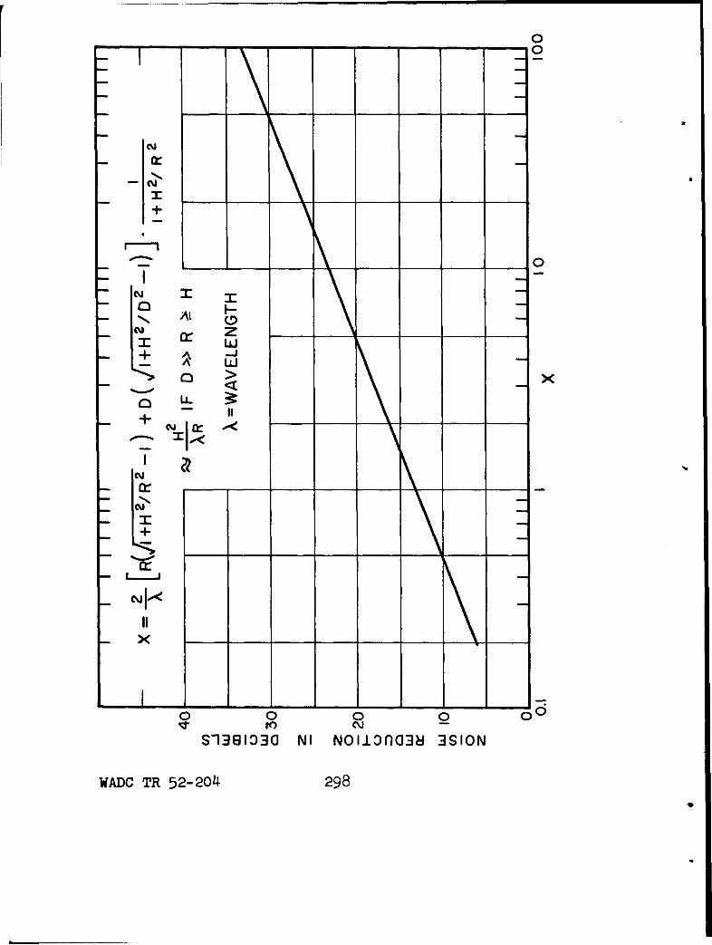
0

m

-I-cc

'A

>U--

+N-

II--

- I

IN

II

0 0 0 00

S1381030 NI NOIlOrG3J 3SION

WADC TR 5 2-204 298

2. Now consider the effect of the absorption of sounddue to the finite acoustic impedance of the ground. In theabsence of the shield, sound would travel from the source tothe receiver with an attenuation due to inverse square spread-

* ing (6 db per distance doubling) plus some additional groundattenuation. However, when an obstacle is present, thesound which reaches the receiver has traveled over the obstacleand so has suffered less ground attenuation. Therefore, ameasurement of the sound level with and without the obstacleshould show somewhat less shielding than diffraction theory(which assumes infinite ground impedance) would predict. Add-ing the obstacle has introduced shielding but has preventedthe terrain attenuation from being as great as when theground was fully exposed.

To correct this effect, one must know the groundattenuation for the type of terrain involved (concrete, bareearth, low or high grass, etc.). Then plot the attenuationexpected for the distance R + D as a function of frequency.On the basis of this, estimate the expected terrain attenua-tion considering the height of the structure and/or thefraction of the total path length R + D occupied by theshielding obstacle. Such a curve for the special case of highgrassy terrain is shown in Fig. 12.9.4. The estimate of thepercent of the terrain attenuation which should be takenwhen a shielding structure is in place is, of course, some-what arbitrary. However, it is important to make someestimate of the effect in the frequency region where it isimportant, even if the magnitude of the correction isdoubtful.

3. Next consider the effect of atmosphere turbulence.So far, it has been assumed that the air is still and that

FIGURE 12.9.2

Noise reduction (NR) in decibels due to a shielding structure.To find the shielding for a wavelength A for given values ofR, H and D, calculate x by Eq. (12.9.1) or (12.9.2) and readthe (NR)from this chart. This value of(NR)must be correctedfor the height of the source above the ground, terrain attenua-tion and turbulent scattering in the atmosphere, as discussedin the following sections.

WADC TR 52-204 299

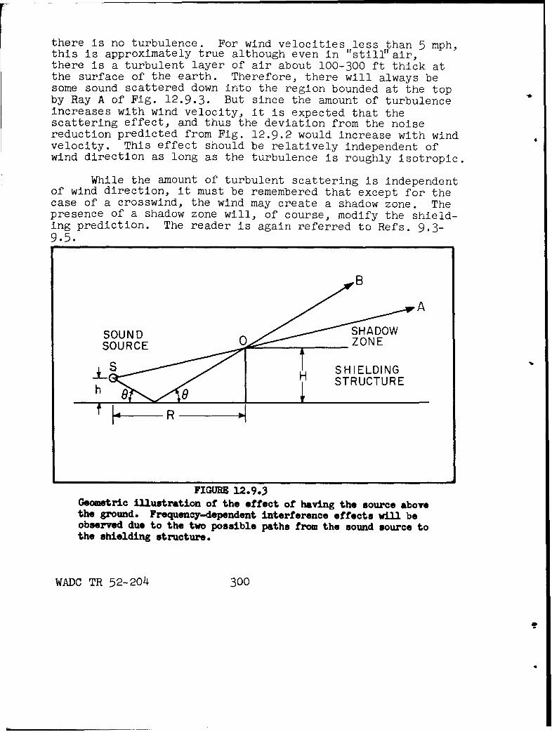
there is no turbulence. For wind velocities less than 5 mph,this is approximately true although even in "still"air,there is a turbulent layer of air about 100-300 ft thick atthe surface of the earth. Therefore, there will always besome sound scattered down into the region bounded at the topby Ray A of Fig. 12.9.3. But since the amount of turbulenceincreases with wind velocity, it is expected that thescattering effect, and thus the deviation from the noisereduction predicted from Fig. 12.9.2 would increase with windvelocity. This effect should be relatively independent ofwind direction as long as the turbulence is roughly isotropic.

While the amount of turbulent scattering is independentof wind direction, it must be remembered that except for thecase of a crosswind, the wind may create a shadow zone. Thepresence of a shadow zone will, of course, modify the shield-ing prediction. The reader is again referred to Refs. 9.3-9.5.

B

SOUND

SOURCE -ZONE

S SHIELDINGS H STRUCTURE

R

FIGURE 12.9.3Geometric illustration of the effect of having the source abovethe ground. Frequency-dependent interference effects will beobserved due to the two possible paths from the sound source tothe shielding structure.

WADC TR 52-204 300

Figure 12.9.5 shows approximate corrections to the expectednoise reduction which were found from a set of field measure-ments. The curves give the correction to be subtractedfrom the predicted noise reduction to account for turbulentscattering.

4. The last point, flanking around an obstacle dueto its finite length, can best be illustrated by a set ofmeasurements taken with a sound source located at a pointR = 50 ft and 50 ft from the.edge of a structure 40 ft highand 200 ft deep. Figure 12.9.6 shows measurements in fourfrequency regions. From these polar plots, it can be seenthat the maximum shielding effect is not obtained unless thereceiving point is on the 00 line, or directly opposite thesource. The 450 lines show the geometric "shadow". Nearthis line, the shielding is quite small compared to thecalculated (maximum) value. In general, a good idea is tohave the distance from the sound source to the edge of theshield at least twice the distance R. If the shield has"wings" such as to enclose the sound source on more thanone side, this precaution will, of course, be unnecessary.

Numerical Example. Consider the following case. Wewish to calculate the shielding at a distance of 400 ft ofa structure 40 ft high along the 00 line. There is a cross-wind whose speed is 10 mph, the ground is covered by longgrass (this is the type of ground for which Fig. 12.9.4 wasdrawn) and the sound source is 50 ft from the wall and wellback from the edge of the structure. Table 12.9.1 showsthe calculations for octave bands (carried out for thegeometric mean frequency of the band limits). Then R = 50,H = 40, D = 400 ft. Consider the sound source to be on theground.

From the approximate Eq. (12.9.2), one can see thatthe shielding increases with frequency and with the wallheight, but decreases as the sound source is moved backfrom the wall (R increasing). The shielding also decreasesas the listener moves back from the wall (D increasing).Atmospheric turbulence and the effect of ground absorptiondecrease the shielding from what diffraction theory wouldpredict.

WADC TR 52-204 301

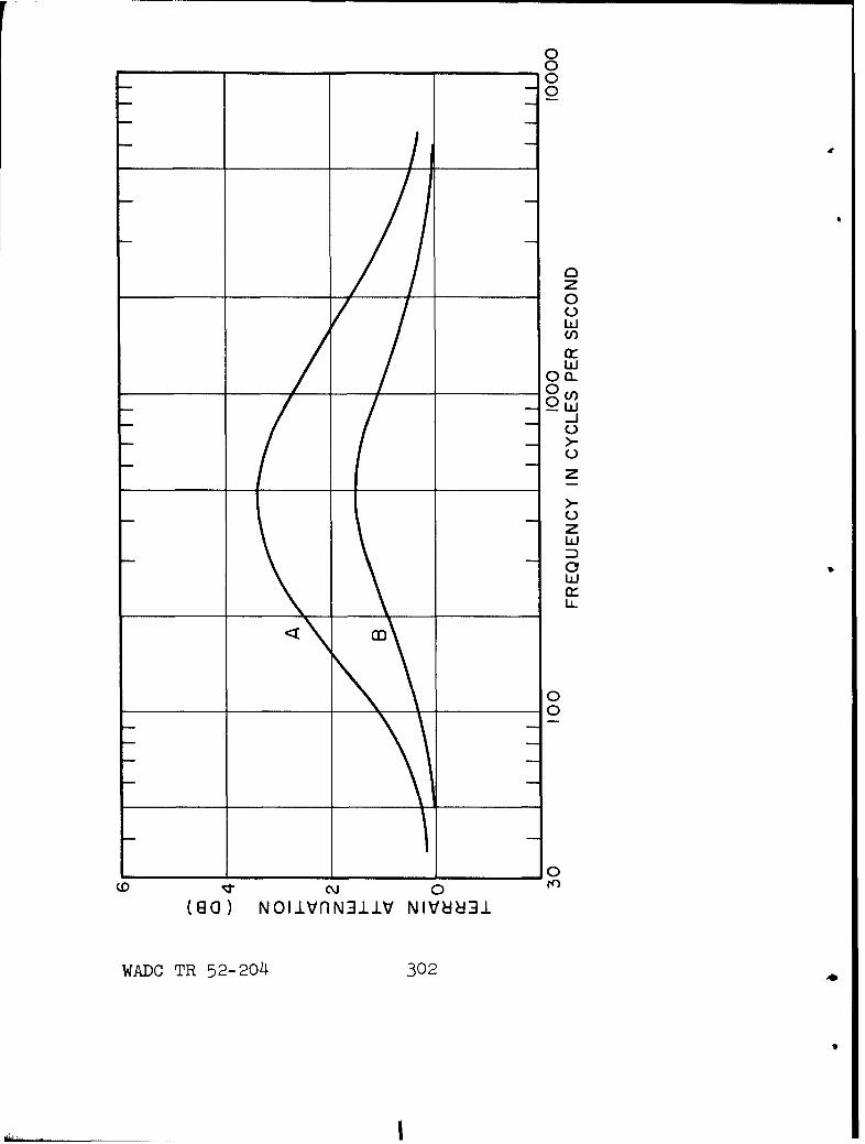
0___ ___ _ ___ __ ___ ___ _ ___ __ 0

0

0 a

0z

00a I&

w

0-0

L 100 rfz

(80 oiivN~iV NI88w

WADC R 52-o4 30

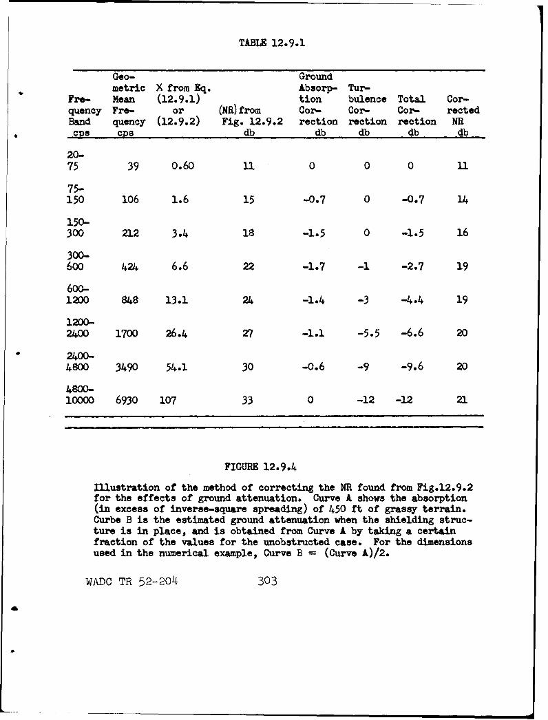
TABLE 12.9.1

Goo- Groundmetric X from Eq. Absorp- Tur-

Fre- Mean (12.9.1) tion bulence Total Cor-quency Fre- or (NR) from Cor- Cor- Cor- rectedBand quency (12.9.2) Fig. 12.9.2 rection rection rection NRcps CPS db db db db db

20-75 39 0.60 11 0 0 0 U1

75-150 106 1.6 15 -0.7 0 -0.7 14

150-300 212 3.4 18 -1.5 0 -1.5 16

300-600 424 6.6 22 -1.7 -1 -2.7 19

600-1200 848 13.1 24 -1.4 -3 -4.4 19

1200-2400 1700 26.4 27 -1.1 -5.5 -6.6 20

2400-4800 3490 54.1 30 -0.6 -9 -9.6 20

4800-10000 6930 107 33 0 -12 -12 21

FIGURE 12.9.4

Iflustration of the method of correcting the NR found from Fig.12.9.2for the effects of ground attenuation. Curve A shows the absorption(in excess of inverse-square spreading) of 450 ft of grassy terrain.Curbs B is the estimated ground attenuation when the shielding struc-ture is in place, and is obtained from Curve A by taking a certainfraction of the values for the unobstructed case. For the dimensionsused in the numerical example, Curve B = (Curve A)/2.

WADC TR 52-204 303

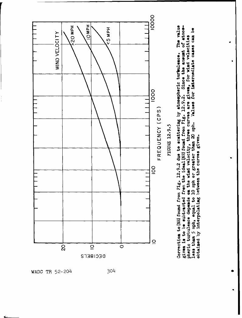
0I I 0

a-0

000wC 30

0_ _ _ 0 4 S.

2oCC-)

z- 4.(43

w2 0

0,9 434

0

0~ 00 b0 4k

_ _ _ _ _ _go _ _ _ _ _54 N O 0

CL .0

Z ~ CV 43 4-

ui C) *i-

O43~ 4-2 4

o t.o :3>

0. 0 (

La5*4 0 H

WADC~~4- TR5-043)

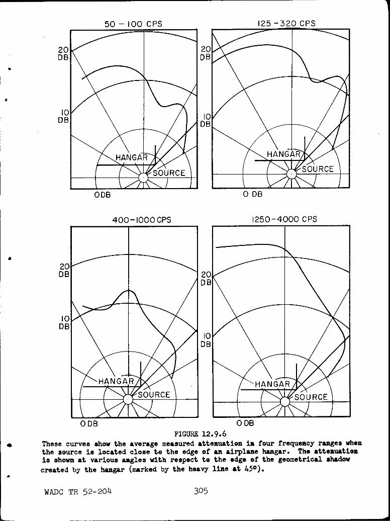
50 - 100 CPS 125 -320 CPS

20 20

ODB 0DB

400-10001CPS 1250-4000 CPS

DB D

SOUCESOU•' RCE

4

ODB 0 DBFIGURE 12.9.6

* These curves show the average measured attenuation in four frequency ranges whenethe source is located close to the edge of an airplane hangar. The attenuationis shown at various angles with respect to the edge of the geometrical shadowcreated by the hangar (marked by the heavy line at 450).

WADC TR 52-204 305

References

(9.1) Fehr, R. 0. "The Reduction of IndustrialMachine Noise" Proc. Second Annual NationalNoise Abatement Symposium, Technology Center,Chicago 16, Illinois 5 Oct. 1951

(9.2) Hayhurst, J. D. "Acoustic Screening by anExperimental Running-Up Pen" J. Roy. Aero. Soc.57 3-11 (1953)

(9.3) Ingard, U. "The Physics of Outdoor Sound"Proc. Fourth Annual National Noise AbatementSymposium, Technology Center, Chicago 16,Illinois 23-24 Oct. 1953

Ingard, U. "Review of the Influence ofMeteorological Conditions on Sound Pro agation"J. Acoust. Soc. Am., 25 405-11 (1953)

(9.4) Pridmore-Brown, D. and U. Ingard "SoundPropagation into the Shadow Zone in a Tempera-ture-Stratified Atmosphere Above a Plane Boundary"J. Acoust. Soc. Am. 27 36-42 (1955)

(9.5) Stevens, K.N. and R. H. Bolt "On the Shieldingof Noise Outdoors" paper presented at Forty-Seventh meeting of the Acoustical Society ofAmerica 23-26 June 1954

WADC TR 52-204 306

Errata to WADC TR 52-204, Volume I

Page

vii line (17) for wrapping read wrappings

viii line (6) for temperatures read temperature

viii add Sec. 15 "Attenuation of Sound. Within Piping"

xi title Fig.' 3.4 read Q >1

xi title Fig. 3.5 read Q.<I

xii title Fig. 6.4 for of read between

18 line (8) for sound pressure read sound. pressure level

20 line (5) for result read results

23 line (5) of text for median read medians

29 line (7) for .7% read 0.8%

46 the remark made in connection with Fig. 2.9 is trueonly in the limit of low frequencies

63 line (22) write toNational Noise Abatement Council9 Rockefeller PlazaNew York, N. Y.

64 add Noise Control57 East 55th StreetNew York 22, N. Y.

A bi-monthly journal published by theAcoustical Society of America, directed to thereader with practical noise problems. In addi-tion to technical information, this magazinepresents discussions of the legal aspects ofnoise control and pertinent news items concerningnoise problems.

98 line (35) read. Fig. 4.1

WADC TR 52-204 307

Page

123 read Eq. (5.2a)

W [5.70] S 3 (T - Ta) 3 AT 286

123 line (11) for T read T0 a

135 Caption Fig. 6.2 read 0L/U

149 line (29) for centrifugal read axial-flow

257 line (4) for k t read ko t

268 see Fig. 12.1.9 for a more complete figure,with all materials identified

279 lines (1) - (6) of text read:

The action of the bend may be explainedqualitatively by the statement thatincoming sound waves travel across the bendto strike the absorbent lining, where a largeportion of the energy may be absorbed. Asmaller portion of the energy, reflected backtoward the source, is partially absorbed uponagain traversing the incoming duct section.

342 ref. (22) for Reference (10) read Reference (8)

WADC TR 52-204 308

b

handbook of acoustic noise control - DTIC

Documents