HALL EFFECT

A3-1

HALL EFFECTLast Revision: August, 21 2007

QUESTION TO BE INVESTIGATED

How to individual charge carriers behave in an external

magnetic field that is perpendicular to their motion?

INTRODUCTION

The Hall effect is observed when a magnetic field is

applied at right angles to a rectangular sample of material

carrying an electric current. A voltage appears across the

sample that is due to an electric field that is at right

angles to both the current and the applied magnetic field.

The Hall effect can be easily understood by looking at the

Lorentz force on the current carrying electrons. The

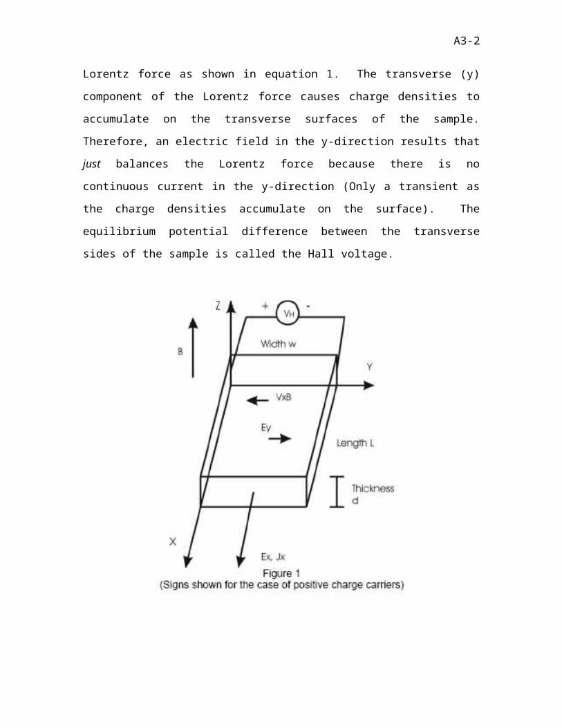
orientation of the fields and the sample are shown in Figure

1. An external voltage is applied to the crystal and

creates an internal electric field (Ex). The electric field

that causes the carriers to move through the conductive

sample is called the drift field and is in the x-direction

in Figure 1. The resultant drift current (Jx) flows in the

x-direction in response to the drift field. The carriers

move with an average velocity given by the balance between

the force accelerating the charge and the viscous friction

produced by the collisions (electrical resistance). The

drift velocity appears in the cross product term of the

A3-2

Lorentz force as shown in equation 1. The transverse (y)

component of the Lorentz force causes charge densities to

accumulate on the transverse surfaces of the sample.

Therefore, an electric field in the y-direction results that

just balances the Lorentz force because there is no

continuous current in the y-direction (Only a transient as

the charge densities accumulate on the surface). The

equilibrium potential difference between the transverse

sides of the sample is called the Hall voltage.

A3-3

A good measurement of the Hall voltage requires that

there be no current in the y-direction. This means that the

transverse voltage must be measured under a condition termed

“no load”. In the laboratory you can approximate the “no

load” condition by using a very high input resistance

voltmeter.

THEORY

The vector Lorentz force is given by:

(1)

where F is the force on the carriers of current, q is the

charge of the current carriers, E is the electric field

acting on the carriers, and B is the magnetic field inside

the sample. The charge may be positive or negative

depending on the material (conduction via electrons or

“holes”). The applied electric field E is chosen to be in

the x-direction. The motion of the carriers is specified by

the drift velocity v. The magnetic field is chosen to be in

the z-direction (Fig. 1).

The drift velocity is the result of the action of the

electric field in the x-direction. The total current is the

product of the current density and the sample’s transverse

area A (I = JxA; A = wt). The drift current Jx is given by;

A3-4

(2)

where n is the number density or concentration of carriers.

The carrier density n is typically only a small fraction of

the total density of electrons in the material. From your

measurement of the Hall effect, you will measure the carrier

density.

In the y-direction assuming a no load condition the free

charges will move under the influence of the magnetic field

to the boundaries creating an electric field in the y-

direction that is sufficient to balance the magnetic force.

(3)

The Hall voltage is the integral of the Hall field (Ey=EH)

across the sample width w.

(4)

In terms of the magnetic field and the current:

(5)

Here RH is called the Hall coefficient. Your first task

is to measure the Hall coefficient for your sample. This

equation is where you will begin. The measurements you will

take will be of VH as a function of drift current I and as a

function of magnetic field B. You will need to fix one

parameter in order to intelligibly observe VH. This

A3-5

experiment is setup to measure VH as a function of I, so you

will fix B for each trial you perform.

Other important and related parameters will also be

determined in your experiment. The mobility μ is the

magnitude of the carrier drift velocity per unit electric

field and is defined by the relation:

(6)

or,

(7)

This quantity can appear in the expression for the current

density and its practical form.

(8)

We have the relations:

(9)

Where σ is the conductivity and ρ is the resistivity. The

total sample resistance to the drift current is:

(10)

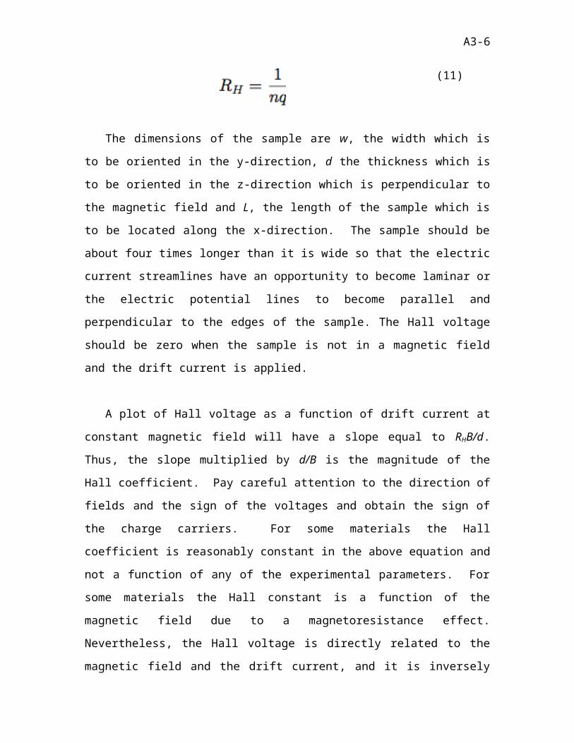
Not only does the Hall coefficient give the concentration of

carriers it gives the sign of their electric charge, by:

A3-6

(11)

The dimensions of the sample are w, the width which is

to be oriented in the y-direction, d the thickness which is

to be oriented in the z-direction which is perpendicular to

the magnetic field and L, the length of the sample which is

to be located along the x-direction. The sample should be

about four times longer than it is wide so that the electric

current streamlines have an opportunity to become laminar or

the electric potential lines to become parallel and

perpendicular to the edges of the sample. The Hall voltage

should be zero when the sample is not in a magnetic field

and the drift current is applied.

A plot of Hall voltage as a function of drift current at

constant magnetic field will have a slope equal to RHB/d.

Thus, the slope multiplied by d/B is the magnitude of the

Hall coefficient. Pay careful attention to the direction of

fields and the sign of the voltages and obtain the sign of

the charge carriers. For some materials the Hall

coefficient is reasonably constant in the above equation and

not a function of any of the experimental parameters. For

some materials the Hall constant is a function of the

magnetic field due to a magnetoresistance effect.

Nevertheless, the Hall voltage is directly related to the

magnetic field and the drift current, and it is inversely

A3-7

related to the thickness of the sample. The samples used

for the measurement are made as thin as possible to produce

the largest possible voltage for easy detection. The sample

has no strength to resist bending and the probe is to be

treated with great care. This applies to the probe of the

Gaussmeter as well. Do not attempt to measure the thickness

of the sample. The values for the dimensions of your sample

are:

w = 0.152 cm, width,

L = 0.381 cm, length,

d = 0.0152 cm, thickness.

The Hall effect probe is a thin slab of indium arsenide,

InAs, cemented to a piece of fiberglass. A four lead cable

is attached so that the necessary electrical circuit can be

used to detect the Hall voltage. The probe is equipped with

a bakelite handle that is used to hold the probe in place.

The white and green wires are used to measure the Hall

voltage and the red and black wires carry the drift current.

EXPERIMENT

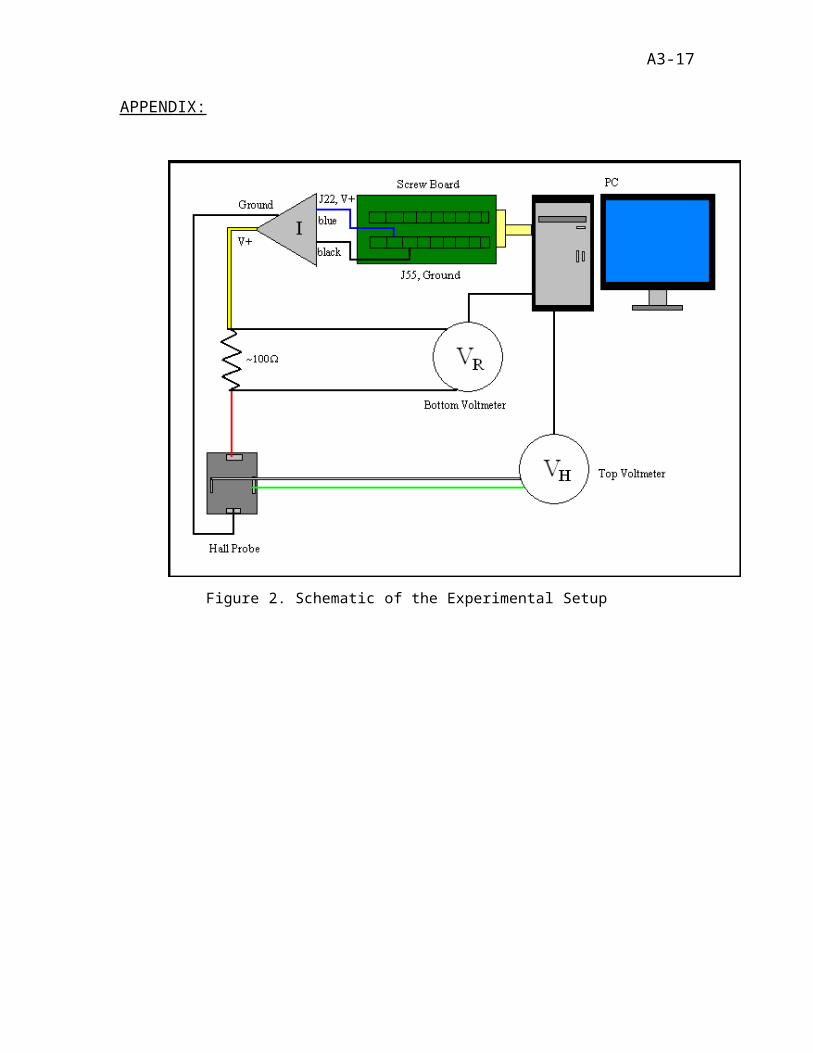
Before connecting the circuit, carefully measure the

resistance of the current limiting resistor with an ohm

meter (the resistance should be close to 100 ohms). Connect

the probe into the electrical circuit shown in Figure 2 (See

A3-8

Appendix). You are to measure the Hall voltage, the drift

current (determined from the voltage across the current

limiting resistor and the known voltage across the system),

and the drift voltage (this is the applied voltage minus

voltage across the current limiting resistor). You have to

keep track of directions and vectors.

Before you turn on the power, please make the following

checks:

- Check the circuit carefully to ensure it makes sense

to you.

- Put the meters on their correct scales. The voltage

across the current limiting resistor will be less

than 1 Volt. The Hall voltage will be even less.

As the drift current is stepped up by the computer, check

the following:

- The drift current must not exceed 10ma this

corresponds to 1.0 volt across the 100 ohm current

limiting resistor (This voltage is shown on one of

the voltmeters in Figure 2). Conduct all your scans

between 0V and 1V.

- The probe should remain cool to the touch. If it

warms at all something is drastically wrong! Turn

A3-9

off the power and disconnect the Hall probe

immediately.

Magnet Calibration:

The magnetic field B is produced by an electromagnet so

the field strength is proportional to the current through

its coil. There is a Gaussmeter (which also uses the Hall

effect) for you to directly measure the magnetic field

strength. Note that the probe for the Gaussmeter is

sensitive to the vector component of B that is normal to the

surface of the probe.

VH depends on the magnitude of the B field and the drift

current I. You will be varying I and will want to make B a

constant for each trial. Therefore, you will want to

understand how the magnet power supply current IM relates to

the magnitude of the B field. Use the Cenco Gaussmeter,

mentioned above, to construct a calibration curve for the

electromagnet (B vs. IM). Be certain that the Gaussmeter is

rotated to produce the maximum reading possible. Fit the

calibration curve to a function. Use the instrumental values

to determine the uncertainty in B at each current setting.

In the next section the calibration curve will be used to

determine B for each measured magnet current.

Determine R H:

A3-10

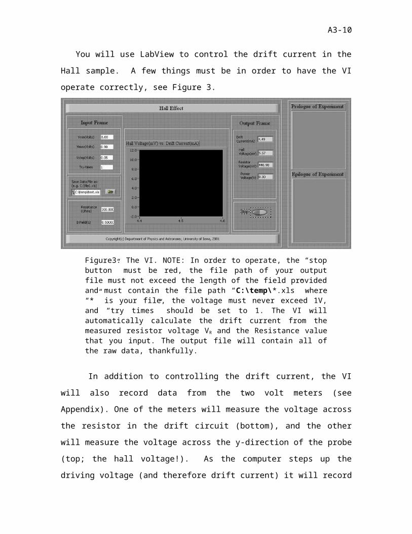
You will use LabView to control the drift current in the

Hall sample. A few things must be in order to have the VI

operate correctly, see Figure 3.

Figure3. The VI. NOTE: In order to operate, the “stopbutton” must be red, the file path of your outputfile must not exceed the length of the field providedand must contain the file path “C:\temp\*.xls” where“*” is your file, the voltage must never exceed 1V,and “try times” should be set to 1. The VI willautomatically calculate the drift current from themeasured resistor voltage VR and the Resistance valuethat you input. The output file will contain all ofthe raw data, thankfully.

In addition to controlling the drift current, the VI

will also record data from the two volt meters (see

Appendix). One of the meters will measure the voltage across

the resistor in the drift circuit (bottom), and the other

will measure the voltage across the y-direction of the probe

(top; the hall voltage!). As the computer steps up the

driving voltage (and therefore drift current) it will record

A3-11

the value from each of these meters, and then output them

when the program finishes. The probe is InAs, which has a

nearly constant Hall coefficient so, from Eq. (5), your data

should be very close to a straight line (VH vs. I) with a

slope that is related to the Hall constant RH.

Run the LabView program for 10 equally spaced values of

the magnet currents. You may wish to span the entire range

of IM, or choose the most linear portion of your calibration

to reside in. Save the data curves for each run and the

magnet currents for later analysis. This will allow you to

construct a family of curves that represent VH vs. I at

constant B. From the magnetic field and the fitted slope

you will be able to determine a Hall coefficient RH for each

curve. Should all of the slopes appear similar? How does

changing B affect the behavior of Eq. (5)? Histogram the

values for RH and determine a global RH and its uncertainty.

You should report the magnitude of the Hall coefficient

and the sign of the charge carriers. To do this you need to

know the direction of the magnetic field. This is most

easily found by using a compass. Using this evidence make a

claim about the behavior of moving charge carriers within a

transverse magnetic field.

A3-12

The slope of each of your curves is related to the Hall

coefficient. The intercept is related to the residual field

and your zero field Hall Voltage. Give the magnitude of the

intercept and offer an explanation of its origin. Can the

data be credibly fit to a one-parameter line (intercept

assumed equal to zero)?

Find (and report) the ratio of the number of carriers

per unit volume to the number of atoms of InAs per unit

volume.

Report your value of the mobility of the charge

carriers and the conductivity of the sample. Is the

mobility of the carriers a function of the magnetic field?

Support your claim with statistical evidence. Indium

Arsenide is used as a probe in Hall effect Gaussmeters

because the mobility and conductivity and hence these

coefficients are not strongly a function of the magnetic

field. Note, in the experiment you do not measure the

resistance of the sample directly. To get the resistance

you will need to determine the driving voltage (that drives

the drift current) and divide this by the drift current.

You have in your measurements the voltage applied by the

computer and the voltage across the 100 ohm resistor. Use

the measured value of the resistance of the resistor and use

A3-13

the actual value in your calculations of current and then in

the calculation of the sample resistance.

Plot the conductivity and the mobility as a function of

the magnetic field. You should find a very small effect, if

any, when you fit the mobility, conductivity or Hall

coefficient as a function of magnetic field. To show this

effect, calculate the difference between the measured values

and the average value. These values are called residuals.

Do the residuals vary as a function of magnetic field? Can

you quantify a systematic effect, given the errors?

B. Studying the Electromagnet

Using the global Hall coefficient for your newly

calibrated Hall probe, you can now use it as an instrument

to measure the spatial variation of the magnetic field of

your electromagnet.

Measure the Hall voltage as a function of distance from

the center of the pole pieces to about a meter away from the

center for a 5mA constant drift current and constant magnet

current. Move the probe away from the magnet in a direction

perpendicular to the magnetic field that is nearly constant

at the center and decreasing sharply at the edge of the pole

piece. Use small steps when you are close to the magnet and

A3-14

larger steps when outside. The field changes rapidly inside

the pole pieces and you will want greater resolution there.

A simple function will not fit the dependence in this region

because of the complexities of magnetic field fringing at

the edge. A short distance outside the edge of the pole

pieces and to a distant point, a functional fit to the data

should permit you to compare the actual field dependence on

distance to a model. What dependence would you expect to

see?

Now, double the separation between the magnet pole

pieces and repeat the measurements. Does the field at the

center change by roughly a factor of 2? Support this claim

with statistical evidence. Report your results by plotting

your data as a function of distance from the center of the

magnet. Finally, move the pole pieces to maximum separation

and measure the field from the center of the left pole piece

to the center of the right pole piece in about 10 equal

steps. Is the field constant? If not, why not? Present your

results as a plot.

Nominal Electrical Characteristics (From the manufacturer)

of InAs Hall Probe:

Internal Resistance (Ohms)

1

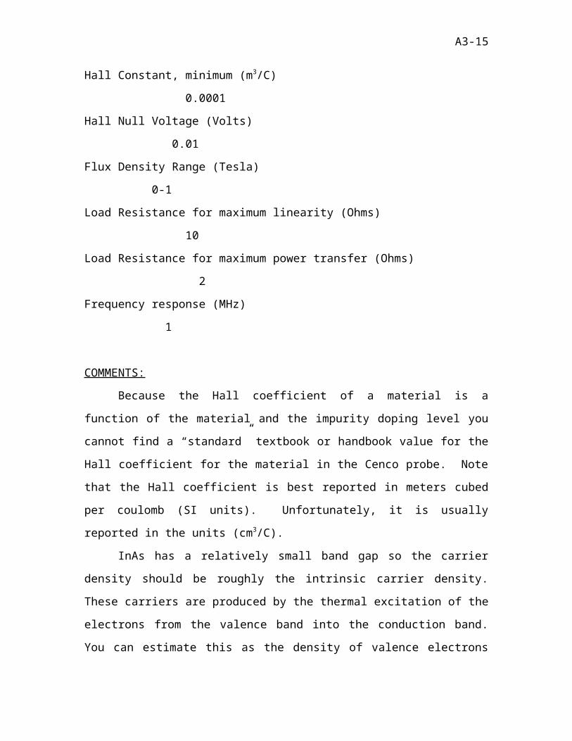
A3-15

Hall Constant, minimum (m3/C)

0.0001

Hall Null Voltage (Volts)

0.01

Flux Density Range (Tesla)

0-1

Load Resistance for maximum linearity (Ohms)

10

Load Resistance for maximum power transfer (Ohms)

2

Frequency response (MHz)

1

COMMENTS:

Because the Hall coefficient of a material is a

function of the material and the impurity doping level you

cannot find a “standard” textbook or handbook value for the

Hall coefficient for the material in the Cenco probe. Note

that the Hall coefficient is best reported in meters cubed

per coulomb (SI units). Unfortunately, it is usually

reported in the units (cm3/C).

InAs has a relatively small band gap so the carrier

density should be roughly the intrinsic carrier density.

These carriers are produced by the thermal excitation of the

electrons from the valence band into the conduction band.

You can estimate this as the density of valence electrons

A3-16

(~7x1028 m-3) multiplied by the Boltzmann factor, exp[-Eg/kT],

where Eg is about 0.35 eV for InAs and kT is room

temperature (which is about 1/40 eV). Does this agree with

your measurement? For additional information see Melissinos

§7.5 p 283.

A3-17

APPENDIX:

Figure 2. Schematic of the Experimental Setup