Louisiana State University LSU Digital Commons LSU Doctoral Dissertations Graduate School 2011 Guided modes and resonant transmission in periodic structures Hairui Tu Louisiana State University and Agricultural and Mechanical College, [email protected] Follow this and additional works at: hps://digitalcommons.lsu.edu/gradschool_dissertations Part of the Applied Mathematics Commons is Dissertation is brought to you for free and open access by the Graduate School at LSU Digital Commons. It has been accepted for inclusion in LSU Doctoral Dissertations by an authorized graduate school editor of LSU Digital Commons. For more information, please contact[email protected]. Recommended Citation Tu, Hairui, "Guided modes and resonant transmission in periodic structures" (2011). LSU Doctoral Dissertations. 1224. hps://digitalcommons.lsu.edu/gradschool_dissertations/1224

Welcome message from author
This document is posted to help you gain knowledge. Please leave a comment to let me know what you think about it! Share it to your friends and learn new things together.
Transcript

Louisiana State UniversityLSU Digital Commons
LSU Doctoral Dissertations Graduate School
2011
Guided modes and resonant transmission inperiodic structuresHairui TuLouisiana State University and Agricultural and Mechanical College, [email protected]
Follow this and additional works at: https://digitalcommons.lsu.edu/gradschool_dissertations
Part of the Applied Mathematics Commons
This Dissertation is brought to you for free and open access by the Graduate School at LSU Digital Commons. It has been accepted for inclusion inLSU Doctoral Dissertations by an authorized graduate school editor of LSU Digital Commons. For more information, please [email protected].
Recommended CitationTu, Hairui, "Guided modes and resonant transmission in periodic structures" (2011). LSU Doctoral Dissertations. 1224.https://digitalcommons.lsu.edu/gradschool_dissertations/1224

GUIDED MODES AND RESONANT TRANSMISSIONIN PERIODIC STRUCTURES
A Dissertation
Submitted to the Graduate Faculty of theLouisiana State University and
Agricultural and Mechanical Collegein partial fulfillment of the
requirements for the degree ofDoctor of Philosophy
in
The Department of Mathematics
byHairui Tu
B.S., University of Science and Technology of China, 2001M.S., Louisiana State University, 2006
August 2011

Acknowledgments
My dissertation would not be possible without the longtime support and mentoringfrom my advisor Prof. Stephen P. Shipman. Since my first semester at LSU, hehas taught me several semesters of classes, advised me in interdisciplinary researchprojects, encouraged and enlightened me in the dissertation research. His passion,diligence, thoughtfulness and insights have influenced me so much, and I considerit a great honor to have the opportunity to work and learn with him.
I would like to take this opportunity to thank my committee members, Dr.William Adkins, Dr. Fereydoun Aghazadeh, Dr. Jimmie Lawson, Dr. Robert Lip-ton, and Dr. Peter Wolenski for their valuable time and advice on this disserta-tion. Many thanks to other great professors that kindly taught and supported mein these years: Dr. Blaise Bourdin, Dr. Susanne Brenner, Dr. James Oxley, Dr.Leonard Richardson, Dr. Li-yeng Sung, and so on. Of course, my special thankshould go to the whole department of mathematics of LSU that provides me apleasant working environment. I will treasure for life the memories of friendshipwith friends such as Hong, Wei, Chao, Liqun, Yue, Zhe, Lingyan, Alvaro, Rick,Julius, Silvia, Maria, Jesse, and so on.
I deeply thank my family including my wife Ying Hu, my father Peichang Tu,my mother Mingzhen Yin, my brother Haifeng Tu and his wife and daughter, fortheir love and their sacrifice to support my study abroad at LSU. This dissertationis specially dedicated to my mother, for her deep love throughout many years andher support of my life despite her recent illness.
ii

Table of Contents
Acknowledgments . . . . . . . . . . . . . . . . . . . . . . . . . . . . . . . . . . . . . . . . . . . . . . . . ii
List of Figures . . . . . . . . . . . . . . . . . . . . . . . . . . . . . . . . . . . . . . . . . . . . . . . . . . . v
Abstract . . . . . . . . . . . . . . . . . . . . . . . . . . . . . . . . . . . . . . . . . . . . . . . . . . . . . . . . . viii
Chapter 1: Introduction . . . . . . . . . . . . . . . . . . . . . . . . . . . . . . . . . . . . . . . . . 11.1 Periodic Slabs . . . . . . . . . . . . . . . . . . . . . . . . . . . . . . 31.2 Periodic Pillars . . . . . . . . . . . . . . . . . . . . . . . . . . . . . 61.3 Summary of Dissertation . . . . . . . . . . . . . . . . . . . . . . . . 9
Chapter 2: Wave Scattering and Guided Modes inPeriodic Structures . . . . . . . . . . . . . . . . . . . . . . . . . . . . . . . . . . . . . . . . . . . . 112.1 The Wave Equation and Helmholtz Equation . . . . . . . . . . . . . 112.2 Periodic Structures and Pseudo-periodic Solutions . . . . . . . . . . 122.3 Plane-wave Scattering by Periodic Slabs . . . . . . . . . . . . . . . 14
2.3.1 Radiation Condition . . . . . . . . . . . . . . . . . . . . . . 142.3.2 Plane-wave Scattering Problems and Guided Modes . . . . . 152.3.3 Existence of Solutions of Scattering Problems . . . . . . . . 19
2.4 Guided Modes . . . . . . . . . . . . . . . . . . . . . . . . . . . . . . 222.5 Existence and Nonexistence of Guided Modes . . . . . . . . . . . . 25
2.5.1 Existence . . . . . . . . . . . . . . . . . . . . . . . . . . . . 252.5.2 Nonexistence . . . . . . . . . . . . . . . . . . . . . . . . . . 27
2.6 Transmission Anomalies . . . . . . . . . . . . . . . . . . . . . . . . 27
Chapter 3: Total Transmission Resonance in Periodic Slabs . . . . . . 303.1 Complex Extension . . . . . . . . . . . . . . . . . . . . . . . . . . . 303.2 Scattering and Guided Modes with Complex Extension . . . . . . . 333.3 Analyticity . . . . . . . . . . . . . . . . . . . . . . . . . . . . . . . 363.4 Main Theorem: Total Resonant Transmission and Reflection for
Symmetric Slabs . . . . . . . . . . . . . . . . . . . . . . . . . . . . 423.4.1 The Reduced Scattering Matrix . . . . . . . . . . . . . . . . 423.4.2 Resonant Transmission . . . . . . . . . . . . . . . . . . . . . 47
3.5 Nongeneric Resonant Transmission . . . . . . . . . . . . . . . . . . 513.5.1 Total Background Reflection and Transmission . . . . . . . . 513.5.2 Multiple Anomalies . . . . . . . . . . . . . . . . . . . . . . . 57
3.6 Transmission Graphs . . . . . . . . . . . . . . . . . . . . . . . . . . 65
Chapter 4: Guided Modes in Periodic Pillars . . . . . . . . . . . . . . . . . . . . . 714.1 Bessel Functions . . . . . . . . . . . . . . . . . . . . . . . . . . . . 714.2 Media Structure and Scattering Problem . . . . . . . . . . . . . . . 74
iii

4.2.1 Pillar Structure and Radiation Condition . . . . . . . . . . . 744.2.2 Scattering Problems . . . . . . . . . . . . . . . . . . . . . . 76
4.3 Guided Modes . . . . . . . . . . . . . . . . . . . . . . . . . . . . . . 794.4 Existence and Nonexistence of Guided Modes . . . . . . . . . . . . 81
4.4.1 Existence . . . . . . . . . . . . . . . . . . . . . . . . . . . . 814.4.2 Nonexistence . . . . . . . . . . . . . . . . . . . . . . . . . . 85
Chapter 5: Open Problems and Future Work . . . . . . . . . . . . . . . . . . . . . 92
References . . . . . . . . . . . . . . . . . . . . . . . . . . . . . . . . . . . . . . . . . . . . . . . . . . . . . . . 94
Vita . . . . . . . . . . . . . . . . . . . . . . . . . . . . . . . . . . . . . . . . . . . . . . . . . . . . . . . . . . . . . 97
iv

List of Figures
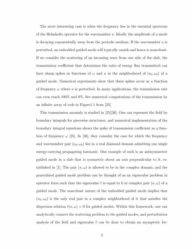
1.1 Numerical computation of the percentage of energy |T |2 transmittedacross a penetrable waveguide of period 2π as a function of thefrequency of the incident plane wave. Here, the wavenumber in thex-direction (Fig. 1.2) is κ = 0.02 and one period consists of a singlecircle of radius π/2 with ε = 10 and an ambient medium with ε = 1;µ = 1 throughout. The structure supports guided modes at (κ, ω) =(0, 0.5039...) and (κ, ω) = (0, 0.7452...), both contained within theregion D of one propagating diffractive order (Fig 3.1). Theorem26 guarantees that the transmission attains minimal and maximalvalues of 0% and 100% at each of the sharp anomalies near theguided-mode frequencies. This is Figure (6) in [23]. . . . . . . . . . 3
1.2 An example of a two-dimensional periodic slab. One period trun-cated to the rectangle [−π, π]× [−L,L] is denoted by Ω. . . . . . . 5
1.3 A pillar periodic in z and finite in x and y. . . . . . . . . . . . . . 7
2.1 Slab structure periodic in x and finite in z; uinc is transmitted toutrans and reflected to urefl. . . . . . . . . . . . . . . . . . . . . . . 13
3.1 The diamond D of one propagating diffractive order within the firstBrillouin zone. . . . . . . . . . . . . . . . . . . . . . . . . . . . . . . 31
3.2 |T |2 as a function of ω for κ = 0,±0.01,±0.02,±0.03. The genericconditions ∂`
∂ω, ∂a∂ω, ∂b∂ω6= 0 are satisfied at the bound-state pair (κ0, ω0).
In (3.15,3.16), `1 = 0 so that there is no linear detuning of theanomaly with κ. Left: 0 < t2 = 1 < r2 = 2 so that the peakis to the left of the dip and both are to the left of ω0. Right:r2 = −2 < 0 < t2 = 1. In both graphs, r0 = 0.6, t0 = 0.8. Thetransmission is symmetric in κ, and the curve without an anomalyis the transmission graph for κ = 0. . . . . . . . . . . . . . . . . . . 66
3.3 |T |2 as a function of ω for κ = 0,±0.003,±0.006,±0.009. Thegeneric conditions ∂`
∂ω, ∂a∂ω, ∂b∂ω6= 0 are satisfied at the bound-state
pair (κ0, ω0). In (3.15,3.16), `1 = 0.9 6= 0, so the anomaly is detunedfrom ω = ω0 (ω = 0) in a linear manner in κ. The coefficients r2 = 2and t2 = 1 of κ2 are distinct real numbers, and (r0, t0) = (0.6, 0.8). 67
v

3.4 |T |2 as a function of ω for κ = 0,±0.01,±0.02,±0.03. Left: Fullbackground transmission occurs when ∂`
∂ω6= 0, ∂a
∂ω= 0, and ∂b
∂ω6= 0
at (κ0, ω0). In (3.21), 0 < r(1)1 = 0.2 < t1 = `1 = 2 < r
(2)1 = 4,
(r(1)2 , r
(2)2 , t2) = (7, 7, 0.1), and r0 = 0.6. Right: ∂`
∂ω6= 0, ∂a
∂ω6= 0, and
∂b∂ω
= 0 at (κ0, ω0) and 0 < t(1)1 < r1 = `1 < t
(2)1 . . . . . . . . . . . . 67
3.5 |T |2 as a function of ω for κ = 0,±0.01,±0.02,±0.03. Full back-ground transmission occurs when ∂`
∂ω6= 0, ∂a
∂ω= 0, and ∂b
∂ω6= 0
at (κ0, ω0). In (3.21), 0 < r(1)1 = 0.6 < r
(2)1 = 1.2 < `1 = 3;
(r0, r(1)2 , r
(2)2 , t2) = (0.6, 1, 1, 0.2). . . . . . . . . . . . . . . . . . . . . 68
3.6 |T |2 as a function of ω for κ = 0,±0.01,±0.02,±0.03. Left: Fullbackground transmission occurs when ∂`
∂ω6= 0, ∂a
∂ω= 0, and ∂b
∂ω6= 0
at (κ0, ω0). In (3.21), r(1)1 = −0.04 < t1 = `1 = 0 < r
(2)1 = 0.06;
(r0, r(1)2 , r
(2)2 , t2) = (0.6,−1, 1, 1). Right: Magnification of the graphs
for κ = ±0.01, bringing into view the frequencies of total transmission. 68
3.7 |T |2 as a function of ω for κ = 0,±0.01,±0.02,±0.03. Full back-ground transmission occurs when ∂`
∂ω6= 0, ∂a
∂ω6= 0, and ∂b
∂ω= 0 at
(κ0, ω0) and 0 < t(1)1 < r1 = `1 < t
(2)1 . In (3.21), t
(1)1 = −0.04 < r1 =
`1 = 0 < t(2)1 = 0.06; (t0, t
(1)2 , t
(2)2 , t2) = (0.6,−1, 1, 1). . . . . . . . . 68
3.8 |T |2 as a function of ω for κ = 0,±0.01,±0.02,±0.03. Full back-ground transmission occurs when ∂`
∂ω6= 0, ∂a
∂ω= 0, and ∂b
∂ω6= 0
at (κ0, ω0). In (3.21), t1 = `1 = 0 < r(1)1 = 0.6 < r
(2)1 = 0.8;
(r0, r(1)2 , r
(2)2 , t2) = (0.6,−4, 5, 6). . . . . . . . . . . . . . . . . . . . . 69
3.9 |T |2 as a function of ω for κ = 0,±0.01,±0.02,±0.03. ∂`∂ω
∂a∂ω6=
0, ∂b∂ω
= 0 at (κ0, ω0). (r(1)1 , r
(2)1 , `1) = (2i,−2i, 0); (r0, r
(1)2 , r
(1)2 , t2) =
(0.6, 2i, 4i, 3). . . . . . . . . . . . . . . . . . . . . . . . . . . . . . . 69
3.10 |T |2 as a function of ω for κ = 0,±0.01,±0.02,±0.03. ∂`∂ω
∂a∂ω6=
0, ∂b∂ω
= 0 at (κ0, ω0). (r(1)1 , r
(2)1 , `1) = (0.5i,−0.5i, 2); (r0, r
(1)2 , r
(1)2 , t2) =
(0.6, i, i, 1). . . . . . . . . . . . . . . . . . . . . . . . . . . . . . . . 70
3.11 Left: |T |2 as a function of ω for κ = 0,±0.003,±0.006,±0.009. Thepartial derivatives of `, a, and b all vanish at (κ0, ω0), whereas their
second derivatives are nonzero. In (3.25), (`(1)1 , `
(2)1 ) = (0.7, 0.8),
(r0, t0) = (0.6, 0.8), r(1)2 = 2 < t
(1)2 = 8 and t
(2)2 = 4 < r
(2)2 = 5.
Right: κ = 0.003. . . . . . . . . . . . . . . . . . . . . . . . . . . . . 70
vi

3.12 Left: |T |2 as a function of ω for κ = 0,±0.003,±0.006,±0.009. Thepartial derivatives of `, a, and b all vanish at (κ0, ω0), whereas their
second derivatives are nonzero. In (3.25), (`(1)1 , `
(2)1 ) = (0.7, 0.8),
(r0, t0) = (0.6, 0.8), r(1)2 = 2 < t
(1)2 = 8 and r
(2)2 = 4 < t
(2)2 = 6.
Right: κ = 0.003. . . . . . . . . . . . . . . . . . . . . . . . . . . . . 70
vii

Abstract
We analyze resonant scattering phenomena of scalar fields in periodic slab and
pillar structures that are related to the interaction between guided modes of the
structure and plane waves emanating from the exterior. The mechanism for the
resonance is the nonrobust nature of the guided modes with respect to perturba-
tions of the wavenumber, which reflects the fact that the frequency of the mode
is embedded in the continuous spectrum of the pseudo-periodic Helmholtz equa-
tion. We extend previous complex perturbation analysis of transmission anomalies
to structures whose coefficients are only required to be measurable and bounded
from above and below, and we establish sufficient conditions involving structural
symmetry that guarantee that the transmission coefficient reach 0% and 100% at
nearby frequencies close to those of the guided modes. Our analysis demonstrates
a few more patterns of anomalies in nongeneric cases, including anomalies of two
peaks and one dip on the transmission graph with total background transmission,
anomalies of one peak and two dips with total background reflection, and multiple
anomalies, and we also prove sufficient conditions for these transmission coeffi-
cients to reach 0% and 100%. For pillar structures, we establish a fundamental
framework using Bessel functions for the analysis of guided modes, and prove the
existence and nonexistence in structures in analogy to results for slabs. We provide
a new existence result of nontrivial embedded guided modes, which are stable with
respect to the wavenumber and nonrobust under perturbations of the structural
geometry, in periodic pillars with smaller periodic cells.
viii

Chapter 1Introduction
Guided modes in periodic structures are very important in composite material
designs. They are electromagnetic or acoustic waves that are trapped within certain
periodic materials, and this special feature makes many applications possible such
as photonic crystal waveguides and light filters discussed in [11].
A related phenomenon is that of transmission anomalies. For a periodic slab
that is bounded in one direction, in some very special settings, the ratio of energy
transmitted through the slab can vary dramatically upon a small perturbation
of the structural geometry, the frequency ω, or the wavenumber κ. Transmission
anomalies are studied in various literature, and applications are suggested such as
polarization control, filtering, switching, surface plasmon resonance sensing, and
surface-enhanced scattering [8][7]. It is clear that the characterization and predic-
tion of transmission anomalies will continue to contribute to the manufacturing of
many devices based on periodic structures.
In this work, we try to understand guided modes and transmission anomalies
mathematically. The resonant transmission anomalies can be explained by the
dissolving of the frequency of a guided mode into the continuous spectrum, by
Fabry-Perot resonance, or by Wood’s anomalies near cutoff frequencies of the as-
sociated Bloch diffraction, and different models have been developed to describe
them [16, 3, 15, 17]. We are concerned with settings of transmission anomalies for
which material parameters and the frequency and wavenumber pair (κ, ω) are close
to those of guided modes. The transmission anomaly can be understood as caused
by the interaction between the incoming waves and the nonrobust embedded guided
1

mode. More particularly, we consider the resonant transmission appearing when
the wavenumber κ is perturbed from a nonrobust guided mode wavenumber κ0.
We consider slabs that are finite in one direction and periodic in one or two
other directions, as well as pillars period in one direction and finite in the other
directions perpendicular to them. In lossless isotropic structures, a time-harmonic
acoustic wave or electromagnetic wave satisfies the Helmholtz equation
∇ · 1
µ∇u+ εω2u = 0,
where µ, ε are material parameters. A periodic structure is given by the periodicity
of the parameters µ, ε. If the Helmholtz equation has a nontrivial solution without
source from the exterior of the periodic structure, the solution is a guided mode.
Suggested from the above discussions, there are two important problems that
bring our interest. One is to design periodic materials that support guided modes
robust or nonrobust with respect to perturbations, and to prove the existence
and nonexistence theoretically. Another one is to describe transmission anomalies
through periodic slabs.
In this dissertation, we answer the first problem for periodic pillars by establish-
ing a systematic framework for the analysis of guided modes using Bessel functions
and proving a few existence and nonexistence results similar to those for periodic
slabs in [1]. Guided mode analysis for periodic pillars has not yet been discussed ad-
equately, and this work sets up the foundation for future research. We also observe
that the embedded guided mode in section 5.2 of [1] is in fact a trivial one, and pro-
vide a new nontrivial design. To answer the problem of characterizing transmission
anomalies through slabs, we base our work on the framework of [25] and [26]. We
establish conditions under which the anomaly is optimized, that is, under which
the transmission rate reaches 100% and 0% at nearby frequencies close to that of
2

0.2 0.4 0.6 0.80
0.2
0.4
0.6
0.8
1
|T |2 vs. ω
FIGURE 1.1. Numerical computation of the percentage of energy |T |2 transmitted acrossa penetrable waveguide of period 2π as a function of the frequency of the incident planewave. Here, the wavenumber in the x-direction (Fig. 1.2) is κ = 0.02 and one periodconsists of a single circle of radius π/2 with ε = 10 and an ambient medium with ε = 1;µ = 1 throughout. The structure supports guided modes at (κ, ω) = (0, 0.5039...) and(κ, ω) = (0, 0.7452...), both contained within the region D of one propagating diffrac-tive order (Fig 3.1). Theorem 26 guarantees that the transmission attains minimal andmaximal values of 0% and 100% at each of the sharp anomalies near the guided-modefrequencies. This is Figure (6) in [23].
the guided mode. Our analysis shows more generic forms of anomalies besides a
single dip-peak graph, including total background transmission or reflection and
multiple anomalies.
1.1 Periodic Slabs
We consider slabs finite in z, periodic in x and invariant in y. (or more gener-
ally, periodic in both x and y.) The existence and nonexistence results of guided
modes have been studied theoretically in [1][27] and in many special geometries
numerically in a lot of literature. The frequencies of some guided modes are in the
point spectrum of the associated Helmholtz operator in one period of slab, and are
well understood. (See section 4.4 of [1] for some examples of guided modes of this
type.) The frequency and wavenumber (κ, ω) of these guided modes lie on a real
component of the dispersion relation. Under the perturbation of the wavenumber,
a guided mode with a nearby frequency persists, and thus is considered robust
under such perturbation.
3
The more interesting case is when the frequency lies in the essential spectrum
of the Helmholtz operator for the wavenumber κ. Ideally the amplitude of a mode
is decaying exponentially away from the periodic medium. If the wavenumber κ is
perturbed, an embedded guided mode will typically vanish and hence is nonrobust.
If we consider the scattering of an incoming wave from one side of the slab, the
transmission coefficient that determines the ratio of energy flux transmitted can
have sharp spikes as functions of ω and κ in the neighborhood of (κ0, ω0) of a
guided mode. Numerical experiments show that these spikes occur as a function
of frequency ω where κ is perturbed. In many applications, the transmission rate
can even reach 100% and 0%. See numerical computations of the transmission by
an infinite array of rods in Figure1.1 from [23].
This transmission anomaly is studied in [25][26]. One can represent the field by
boundary integrals for piecewise structures, and numerical implementation of the
boundary integral equations shows the spike of transmission coefficient as a func-
tion of frequency ω [25]. In [26], they consider the case for which the frequency
and wavenumber pair (κ0, ω0) lies in a real diamond domain admitting one single
energy-carrying propagating harmonic. One example of such is an antisymmetric
guided mode in a slab that is symmetric about an axis perpendicular to it, es-
tablished in [1]. The pair (κ, ω) is allowed to be in the complex domain, and the
generalized guided mode problem can be thought of as an eigenvalue problem in
operator form such that the eigenvalue ` is equal to 0 at complex pair (κ, ω) of a
guided mode. The nonrobust nature of the embedded guided mode implies that
(κ0, ω0) is the only real pair in a complex neighborhood of it that satisfies the
dispersion relation `(κ, ω) = 0 for guided modes. Within this framework, one can
analytically connect the scattering problem to the guided modes, and perturbation
analysis of the field and eigenvalue ` can be done to obtain an asymptotic for-
4

z = Lz = −L
z
x
Ω
︸︷︷
︸
π
FIGURE 1.2. An example of a two-dimensional periodic slab. One period truncated tothe rectangle [−π, π]× [−L,L] is denoted by Ω.
mula for the transmission coefficient in terms of perturbations for two-dimensional
structures [26, 21, 23]. More details on the proof and transmission graphs using
the formula are discussed in [26][23].
My work develops this idea and aims to find when the transmission can reach
100% and 0%, as shown in Figure 1.1. We consider a slab that is not only symmetric
in x, but also symmetric with respect to an axis parallel to the slab, as shown in
Figure 1.2. The unitary scattering matrix possesses special symmetric properties
due to the symmetry of the slab structure. Our main result in Chapter 3 is a proof
for slabs under generic assumptions that ensure the transmission magnitude of
100% and 0%. Specifically, if a two-dimensional lossless periodic slab is symmetric
about an axis parallel to the slab, and if the slab supports an embedded guided
mode nonrobust in κ at a real pair of frequency and wavenumber (κ0, ω0), then total
transmission and reflection is necessarily attained for pairs (κ, ω) close to those of
the guided mode. The frequencies that admit total transmission and reflection are
real-analytic functions of the wavenumber in the real (κ, ω) plane that intersect
tangentially at (κ0, ω0). In the proof of this result, the special symmetries of the
scattering matrix give more information on the transmission and reflection than
5

the analysis in [26][23], and is just what we need to show the real analyticity of
the total transmission and total reflection curves.
In our complex perturbation analysis of transmission anomalies, we extend to
structures whose coefficients are only required to be measurable and bounded from
below and above. In stead of using boundary integral representations for piecewise
constant slabs, we utilize only the analyticity of the solution of the eigenvalue
problem for which the operator has the form of the identity map plus an analytic
compact operator.
We also show that a more intricate patterns of transmission anomalies can be
excited by the perturbation of wavenumber if we relax our generic assumptions
to nongeneric cases. One type of anomaly possesses two peaks and one dip on
the transmission graph, which corresponds to total background transmission; sim-
ilarly one peak and two dips corresponds to total background reflection. We give
conditions for the total background transmission case for which the transmission
coefficient is nearly 100% and reaches 100% at two frequencies, but drops to 0%
at one frequency, and similarly for the total background reflection case. We also
analyze a case of multiple anomalies, for which the transmission coefficient reaches
100% and 0% twice in a narrow range of the frequency ω.
1.2 Periodic Pillars
In the remaining part of this dissertation, we consider a structure illustrated by
Figure 1.3, periodic in one direction and bounded in the other two directions. The
field is governed by the Helmholtz equation in which the material is homogeneous
in the exterior.
We have not found adequate foundational work on the scattering problem and
guided modes for periodic pillars in the literature, so we present here a system-
6

x
y
z
FIGURE 1.3. A pillar periodic in z and finite in x and y.
atic mathematical framework. My work uses standard variational techniques in
[4, 6, 12], and the analysis is similar the theory established in [1] for slabs. Bessel
functions are naturally introduced in cylindrical coordinates to characterize the
Fourier harmonics. The general solution of the Helmholtz equation in the exte-
rior domain with constant parameters is expanded as an infinite superposition of
Fourier harmonics:
u(r, θ, z) =∞∑
m,`=−∞
[A`H
1` (ηmr) +B`H
2` (ηmr)
]ei`θei(m+κ)z,
where η2m = ε0µ0ω
2 − (m + κ)2 and H1` = J` + iY` and H2
` = J` − iY` are Han-
kel functions. The Hankel functions’ monotonicity and phase change orientation
make it possible to separate between outgoing and incoming harmonics and impose
appropriate radiating boundary conditions through a Dirichlet-to-Neumann map.
Upon this, the solvability of the plane wave scattering problem, the characteriza-
tion of the guided-mode frequencies, and existence results analogous to those of
slabs can all be built.
There are a few nonexistence and existence results we establish in this disserta-
tion.
7

One is nonexistence. In [27], by introducing an augmented medium structure,
Shipman and Volkov give a proof of the nonexistence of guided modes in piecewise
inverse photonic slabs, i.e., piecewise structures that have higher wave speed in
the pillar than in the exterior. In their study, the proof of the nonexistence is
contingent on a restriction on the width of the slabs. Similar to their analysis, we
show here the nonexistence of guided modes in inverse pillars such as a periodic
array of bubbles in glass. Certain restrictions on the geometry of the structures
are needed in our proofs of the nonexistence, and whether the restrictions can be
removed remains an open problem.
There have been limited results on the existence of embedded guided modes, even
for periodic slabs. One example of an embedded guided mode is an antisymmetric
guided mode in periodic structures symmetric in the direction of waveguide, as
discussed earlier. This guided mode typically only exists at an isolated real pair
(κ0, ω0).
A non-isolated but artificially constructed example of embedded guided modes
is provided by Bonnet-Bendhia and Starling in section 5.2 of [1]. If a structure
of period p has smaller periodic cells, say of period q < p, then on the subspace
F consisting of all the functions with the smaller period q, the infimum of the
essential spectrum of the Helmholtz operator is strictly larger than that of the
space of functions with period p. One can find eigenfunctions with their frequencies
lying below the cutoff frequency for the restriction to F , which are non-embedded
and easy to find, but these are embedded in the essential spectrum on the full
period function space. However, these guided modes are simply non-embedded
guided modes for a smaller periodic structure. In other words, for a given periodic
structure, a larger period is artificially chosen so that the frequency of a non-
8

embedded guided mode is embedded in the artificial essential spectrum, and this
is therefore a trivial example. An essentially nontrivial example is strongly desired.
My main achievement in Chapter 4 is a proof of nontrivial embedded guided
modes in periodic pillars that are robust under perturbations of κ. In our con-
struction, the period of the mode is genuinely larger than that of the structure.
Our proof relies on choosing the material parameters so that the Helmholtz op-
erator is invariant on a subspace where the propagating harmonics automatically
vanish. This solution does not depend upon the exact choice of the wavenumber
and so is a guided mode robust in κ. On the other hand, the existence is based
on special properties of the structure, and is thus nonrobust with respect to the
perturbation of material geometries.
1.3 Summary of Dissertation
The structure of this dissertation is as follows.
In chapter 2, we give a brief introduction to the scattering problems and guided
modes, as well as the transmission anomaly phenomena. The focus is put on pe-
riodic slabs and we provide some standard tools used in the analysis of periodic
structures.
In chapter 3, for a slab that is symmetric with respect to an axis parallel to it,
we present the proof of the existence of total transmission and reflection associated
with a nonrobust guided mode. We also discuss the cases that the slab admits a
single anomaly and multiple anomalies. The diagrams of our results are shown the
last section of this chapter, based on the approximation formula given in [26, 23].
In chapter 4, we study the scattering problem and guided modes for pillar struc-
tures that are finite in two directions. Bessel functions are used to do the analysis
systematically. We provide a proof for the existence of embedded guided modes,
9

and nonexistence of guided modes for some special geometries in the last section
of this chapter.
In the chapter 5, we point out some restrictions of our work and pose chal-
lenges for future work. We also provide some new open problems on the nature of
transmission resonances.
10

Chapter 2Wave Scattering and Guided Modes inPeriodic Structures
In this chapter, we give a brief introduction to plane-wave scattering problems and
guided modes for time-harmonic wave equations, as well as previous analysis on
transmission anomalies.
We first introduce the wave equation and the Helmholtz equation, and explain
the periodic structures and the solutions in these structures. The plane wave scat-
tering problem is presented in section 2.3. We give existence and nonexistence
results for guided modes in periodic slabs. The proofs can be found in [1, 27].
The nonrobust guided modes shown in [27] typically vanish as the wavenmber κ
is perturbed from 0, and the transmission coefficients can reach a magnitude of
100% and 0%. The transmission anomaly for piecewise periodic slabs is studied in
[25, 26], and an asymptotic formula of the transmission coefficient as a function of
the perturbations of κ, ω is obtained.
In this chapter, except in the last section, we assume that the wave frequency and
wavenumber (κ, ω) are real. The wave frequency and wavenumber can be extended
to the complex domain, which we will use to prove our main result.
2.1 The Wave Equation and Helmholtz
Equation
We consider a physical structure that is three-dimensional but invariant in the y-
direction. In this structure, the Maxwell system of electromagnetics is y-independent
and has two polarizations that are simplified to the Helmholtz equation for the out-
of-plane components of the E field and the H field. We consider harmonic fields
with positive angular frequency ω. Given a frequency ω, plane waves and guided
11

modes are characterized by their propagation constant κ in the direction parallel
to the slab. We take the y component Ey of a harmonic E-polarized field with
propagation constant κ to be of the following pseudoperiodic form
Ey(x, z, t) = u(x, z)ei(κx−ωt),
u(x+ 2πn, z) = u(x, z) for n ∈ Z.
Ey satisfies the wave equation
ε∂2
∂t2Ey(x, y, z; t) = ∇ · 1
µ∇Ey(x, y, z; t) (2.1)
We are looking for time-harmonic waves Ey(x, y, z, t) = u(x, y, z)e−iωt. The spatial
factor of the wave satisfies the Helmholtz equation
∇ · 1
µ∇u+ εω2u = 0. (2.2)
2.2 Periodic Structures and Pseudo-periodic
Solutions
We consider periodic slab structures that are finite in the z-direction, periodic in
the x-direction and invariant in the y-direction.
The periodic slab is defined by the material parameters ε(x, z) and µ(x, z) for
x, z ∈ R. We take these parameters to be bounded from below and above by
positive numbers:
ε(x+ 2πn, z) = ε(x, z), µ(x+ 2πn, z) = µ(x, z), for n ∈ Z,
ε(x, z) = ε0, µ(x, z) = µ0, for |z| ≥ L,
0 < ε− < ε(x, z) < ε+, 0 < µ− < µ(x, z) < µ+.
(2.3)
The field u satisfies the pseudo-periodic, or quasi-periodic or κ-periodic condi-
tions:
u(x, z;κ) = eiκ·xu(x, z), (2.4)
12

z=Lz=−L
u inc
ureflu trans
x
z
FIGURE 2.1. Slab structure periodic in x and finite in z; uinc is transmitted to utrans
and reflected to urefl.
where u(x, z) is 2π-periodic in x. We call such solutions Bloch waves and the
number κ Bloch wavenumber. This can be understood as follows. The periodicity
of the slab implies that the values of the same incident field viewed at the point
(x + 2π, z) and at (x, z) have only a phase change. Thus, the field at (x + 2π, z)
can be seen as the field at (x, z) multiplied by the phase change factor e2πκi.
The field u has a Bloch factor eiκx, for which we have eiκ(x+2π) = eiκxe2πκi and
hence we can regard that the κ-peridicity is caused by the Bloch factor. It is
noticed that e2π(κ+m)i = e2πκi,∀m ∈ Z. This means the wave number κ and κ+m
have the same effect on the Bloch factor. Thus, we can reduce the wavenumber
κ by an integer and deal with the cases that κ lies in the first Brillouin zone
B = [−1/2, 1/2).
The periodic factor u satisfies the following modified Helmholtz equation
(∇+ iκ)µ−1(∇+ iκ)u(x, z) + εω2u(x, z) = 0, (2.5)
where κ = (κ, 0)T.
13

2.3 Plane-wave Scattering by Periodic Slabs2.3.1 Radiation Condition
The periodic solution of equation (2.5) has a Fourier series expansion
u(x, z) =∑
m
um(z)eimx, (2.6)
and the pseudo-periodic field is
u(x, z) = u(x, z)eiκx =∑
m
um(z)ei(m+κ)x (2.7)
If |z| > L, then um(z) = (u−m(z), u+m(z)), for z < −L or z > L, are solutions of the
ordinary differential equation
u′′m + η2mum = 0
where
η2m = ε0µ0ω
2 − (m+ κ)2. (2.8)
The solutions um(z) = c1mu
1(z)+c2mu
2(z), called spatial harmonics, where u1,2m (z)
are independent solutions of the linear ordinary differential equation, belong to the
following three classes:
um = c1me
iηmz + c2me−iηmz ∈ Zp (propagating), if η2
m > 0; we take ηm = |ηm|;
um = c1me
iηmz + c2me−iηmz ∈ Ze (evanescent), if η2
m < 0; we take ηm = |ηm|i;
um = c1m + c2
mz ∈ Zl (linear), if η2m = 0.
(2.9)
The classes Zp is finite, Zl is generically empty but has at most one harmonic, and
the class Ze is infinite. As long as η2m are nonzero for all integers m, the general
solution of this equation (2.5) admits a Fourier expansion on each side of the slab
u(x, z) =
∞∑
m=−∞
(A+me
iηmz +B+me−iηmz)eimx, for z > L,
∞∑
m=−∞
(A−meiηmz +B−me
−iηmz)eimx, for z < −L.(2.10)
14
The spatial harmonics eiηmz, e−iηmz for m ∈ Zp represent right-going or left-going
traveling waves, whose angles αm are
αm = arcsinκ+m
ω√ε0µ0
. (2.11)
The harmonics e±iηmz = e∓|ηm|z for m ∈ Ze represent exponentially decaying har-
monics for ±z > L, while e∓iηz = e±|ηm|z represent exponentially growing harmon-
ics for ±z > L. The linear orders ηm = 0 correspond to “grazing incidence”, and
will not play a role in the present study.
Dropping the exponentially growing harmonics, a function u is said to be radi-
ating or outgoing if in the form (2.10) the coefficients B+m = A−m = 0. We introduce
the following radiation condition:
Condition 1 (Radiation). A complex field u defined on R2 satisfies the radiadion
condition if there exist complex coefficients c±m such that
u(x, z) =∑
m∈Z
c±me±iηmzeimx for ± z > L.
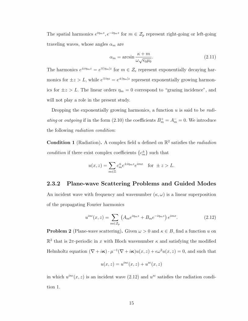
2.3.2 Plane-wave Scattering Problems and Guided Modes
An incident wave with frequency and wavenumber (κ, ω) is a linear superposition
of the propagating Fourier harmonics
uinc(x, z) =∑
m∈Zp
(Ame
iηmz +Bme−iηmz
)eimx. (2.12)
Problem 2 (Plane-wave scattering). Given ω > 0 and κ ∈ B, find a function u on
R2 that is 2π-periodic in x with Bloch wavenumber κ and satisfying the modified
Helmholtz equation (∇+ iκ) · µ−1(∇+ iκ)u(x, z) + εω2u(x, z) = 0, and such that
u(x, z) = uinc(x, z) + usc(x, z)
in which uinc(x, z) is an incident wave (2.12) and usc satisfies the radiation condi-
tion 1.
15

The scattering problem 2 can be formulated using standard variational tech-
niques in the truncated domain of one period
Ω = (x, z) ∈ R2 : −π < x < π, |z| < L. (2.13)
Let Γ± = (x, z) ∈ R2 : −π < x < π, z = ±L and Γ = Γ− ∪ Γ+. We make use
of the Dirichlet-to-Neumann map T = T (κ, ω) on the right and left boundaries
Γ± to characterize outgoing fields. It is a bounded linear operator from H12 (Γ) to
H– 12 (Γ) defined as follows. For any f ∈ H 1
2 (Γ), let fm = (f+m, f
−m) be the Fourier
coefficients of f , that is, f(±L, x) =∑
m f±me
imx. Then
T : H12 (Γ)→ H−
12 (Γ),
(Tf)m = −iηmfm.(2.14)
This operator has the property that
∂nu+ Tu = 0 on Γ ⇐⇒ u is outgoing.
The operator T has a nonnegative real part Tr and a nonpositive imaginary part
Ti:
T = Tr + iTi,
(Trf)m =
−iηmfm if m ∈ Ze,
0 otherwise.
(Tif)m =
−ηmfm if m ∈ Zp,
0 otherwise.
(2.15)
In the periodic Sobolev space
H1per(Ω) = u ∈ H1(Ω) : u(π, z) = u(−π, z) for all z ∈ (−L,L),
16

in which evaluation on the boundaries of Ω is in the sense of the trace map, we
also define the following forms in H1per(Ω):
p(v) = µ−10
∫
Γ
(∂nuinc + Tuinc)v,
a(u, v) = aκ,ω(u, v) =
∫
Ω
µ−1(∇+ iκ)u · (∇− iκ)v + µ−10
∫
Γ
(Tu)v,
ar(u, v) =
∫
Ω
µ−1(∇+ iκ)u · (∇− iκ)v + µ−10
∫
Γ
(Tru)v,
ai(u, v) = µ−10
∫
Γ
(Tiu)v,
b(u, v) =
∫
Ω
ε uv.
We have a = ar + iai.
Problem 3 (Scattering problem, variational form). Given a pair (κ, ω), find a
function u ∈ H1per(Ω) such that
a(u, v)− ω2b(u, v) = p(v), for all v ∈ H1per(Ω) (2.16)
Theorem 4. The problem 2 and the problem 3 are equivalent.
Proof. We observe that
[(∇+ iκ) · 1
µ(∇+ iκ)u
]v = ∇ ·
[(1
µ(∇+ iκ)u
)v
]− 1
µ(∇+ iκ)u · (∇− iκ)v.
Integrating it implies
∫
Ω
[(∇+ iκ) · 1
µ(∇+ iκ)u
]v =
∫
Γ
[(1
µ(∇+ iκ)u
)v
]·n−
∫
Ω
1
µ(∇+iκ)u·(∇−iκ)v.
We multiply the modified Helmholtz equation by v and integrate to obtain
∫
Γ
[(1
µ(∇+ iκ)u
)v
]· n−
∫
Ω
1
µ(∇+ iκ)u · (∇− iκ)v +
∫
Ω
εω2uv = 0,
or ∫
Γ
1
µ∂nuv −
∫
Ω
1
µ(∇+ iκ)u · (∇− iκ)v +
∫
Ω
εω2uv = 0.
17

By the radiation condition ∂n(u− uinc) = −T (u− uinc), we have
∫
Ω
1
µ(∇+ iκ)u · (∇− iκ)v +
∫
Γ
1
µ(Tu)v −
∫
Ω
εω2uv =
∫
Γ
1
µ0
v(∂nuinc + Tuinc)
This is the weak form (2.16).
Conversely, if a function u ∈ H1per(Ω) satisfies (2.16), we can take test functions
v ∈ C∞0 (Ω) to get (∇+ iκ) · 1µ(∇− iκ)u+ εµω2u = 0 in Ω. Then we can multiply
the modified Helmholtz equation by v ∈ H1per(Ω) to obtain
∫
Γ
1
µ∂nuv −
∫
Ω
1
µ(∇+ iκ)u · (∇− iκ)v +
∫
Ω
εω2uv = 0.
Comparing it with (2.16), we prove that ∂n(u− uinc) = −T (u− uinc), i.e. u solves
the problem 2.
A guided mode is a solution of the homogeneous problem where there is no
source:
a(u, v)− ω2b(u, v) = 0, for all v ∈ H1per(Ω). (2.17)
Note that in the proof of the above equivalence, it is not required that ω2 ∈ R.
But if the square frequency is real, we have the following result in particular for
the homogeneous problem.
Theorem 5. (Real eigenvalues) If ω2 ∈ R, then a function u ∈ H1per(Ω) satisfies
the homogeneous problem (2.17) if and only if it satisfies the equation
ar(u, v) + iai(u, v)− ω2b(u, v) = 0, for all v ∈ H1per(Ω), (2.18)
and if and only if it satisfies
ar(u, v)− ω2b(u, v) = 0, for all v ∈ H1per(Ω),
(u|Γ)m = 0,∀m ∈ Zp.(2.19)
18

Proof. We only need to show the equivalence of (2.18) and (2.19). If (u|Γ)m =
0,∀m ∈ Zp, then∫
Γ(Tiu)v = 0, so (2.19) implies (2.18). Conversely, we take
the imaginary part of ar(u, u) + iai(u, u) − ω2b(u, u) to obtain ai(u, u) = 0 for
all u ∈ H1per(Ω). This implies that (u|Γ)m = 0, ∀m ∈ Zp because ηm 6= 0 for
m ∈ Zp.
2.3.3 Existence of Solutions of Scattering Problems
The existence of the solution of the scattering problem can be analyzed by Fred-
holm alternative theory. To this end, we write the form a− ω2b as
a(u, v)− ω2b(u, v) = c1(u, v) + c2(u, v),
in which c1(u, v) = a(u, v) + b(u, v) and c2(u, v) = −(ω2 + 1)b(u, v).
Lemma 6. Both c1 and c2 are bounded in H1per(Ω).
Proof. The boundedness of c1 is shown by
|a(u, v) + b(u, v)| =∣∣∣∣∫
Ω
µ−1(∇+ iκ)u · (∇− iκ)v +
∫
Ω
ε uv
∣∣∣∣
≤ 1
µ−
∣∣∣∣∫
Ω
(∇+ iκ)u · (∇− iκ)v
∣∣∣∣+ ε+
∣∣∣∣∫
Ω
uv
∣∣∣∣
≤ 1
µ−‖(∇+ iκ)u‖L2‖(∇+ iκ)v‖L2 + ε+
∣∣∣∣∫
Ω
uv
∣∣∣∣
≤ 1
µ−(‖∇u‖L2 + |κ|‖u‖L2)(‖∇v‖L2 + |κ|‖v‖L2) + ε+‖u‖L2‖v‖L2
≤M‖u‖H1per(Ω) · ‖v‖H1
per(Ω) , for some M > 0,
and
∫
Γ
(Tu)v ≤∑
m∈Z
|η1/2m um| · |η1/2
m vm| ≤ ‖u‖H1/2(Γ)‖v‖H1/2(Γ) ≤ ‖u‖H1per(Ω)‖v‖H1
per(Ω)
The boundedness c2 is shown by
∫
Ω
εuv ≤ ε+
∫
Ω
uv ≤ ε+‖u‖L2(Ω)‖v‖L2(Ω) ≤ ε+‖u‖H1per(Ω)‖‖H1
per(Ω).
19

These forms are represented by bounded operators C1 and C2 in H1per(Ω) by
Riesz Representation:
(C1u, v)H1per(Ω) = c1(u, v),
(C2u, v)H1per(Ω) = c2(u, v).
Because of the coercivity of c1 and the compact embedding of L2(Ω) into H1per(Ω),
we have
Lemma 7. The operator C1 has a bounded inverse and C2 is compact.
Proof. The operator C1 has bounded inverse because the sesquilinear form c1(u, v)
is bounded and coercive:
Re(c1(u, u) + c2(u, u)) ≥ minµ−1+ , ε−‖u‖2
H1per(Ω).
The operator C2 can be written as C2 = I1I2, where I2 : H1per(Ω) → L2(Ω) is
the natural embedding, and I1 : L2(Ω) → H1per(Ω) is defined by 〈I1u, v〉H1
per(Ω) :=
−(ω2 + 1)∫
Ωuv. The operator I2 is compact because of the compactness of the
injection of H1per(Ω) into L2(Ω). The operator I1 is continuous because
‖I1u‖H1per(Ω) = sup
06=v∈H1per(Ω)
|∫
Ωuv|
‖v‖H1per(Ω)
≤ sup06=v∈H1
per(Ω)
|∫
Ωuv|
‖v‖L2(Ω)
≤ ‖u‖L2(Ω).
Their composition C2 is therefore compact.
If we denote by winc the unique element of H1per(Ω) such that (winc, v)H1
per(Ω) =
`(v), the scattering problem becomes (C1u, v) + (C2u, v) = (winc, v) for all v ∈
H1per(Ω), or
C1u+ C2u = winc. (2.20)
The term `(v) consists of the incident wave uinc and therefore winc represent the
source term in the equation (2.20). In the operator form, a guided mode is a
20

nontrivial solution of the homogeneous problem
C1u+ C2u = 0. (2.21)
By means of the Fredholm alternative one can demonstrate that, even if a slab
admits a guided mode for a given real pair (κ, ω), the problem of scattering of a
plane wave always has a solution. Proofs are given in [1, Thm. 3.1] and [23, Thm. 9];
the idea is essentially that plane waves contain only propagating harmonics whereas
guided modes contain only evanescent harmonics and are therefore orthogonal to
any plane-wave source field.
Theorem 8. For real ω > 0 and κ ∈ B, the scattering problem 3 with a plane-wave
source field has at least one solution and the set of solutions is a finite dimensional
affine space with the dimension equal to the dimension of the space of guided
modes.
Proof. By the Fredholm alternative, (2.20) has a solution if and only if 〈winc, v〉 = 0
for all v ∈ Null(C1 + C2)†, i.e. for all v satisfying
(w, (C1 + C2)†v) = 0,∀w ∈ H1per(Ω),
or for all v satisfying
ar(w, v) + iai(w, v)− ω2b(w, v) = 0,∀w ∈ H1per(Ω),
or just
ar(v, w)− iai(v, w)− ω2b(v, w) = 0,∀w ∈ H1per(Ω).
By Theorem 5, the propagating harmonics of v vanish on Γ, and so (winc, v) van-
ishes.
The space of solutions is finite-dimensional because C1 has a bounded inverse
and C2 is compact.
21

2.4 Guided Modes
A guided mode is a nonzero solution u(x, z) of the scattering problem without
the source originating from the exterior of the slab, that is, it satisfies (2.18) and
(2.19). It may also be understood as a nontrivial solution of the problem (2.20) in
operator form.
A functional analysis framework for spectral analysis is on one period in R2
S = (x, z) ∈ R2 : −π < x < π. (2.22)
We consider the Hilbert space L2(S, εdV ) of square-Lebesgue-integrable complex-
valued functions in S with inner product
b(u, v) =
∫
SεuvdV (2.23)
and the unbounded symmetric nonnegative quadratic form in L2(S, εdV ), with
form domain H1per(S), defined by
a(u, v) =
∫
Sµ−1(∇+ iκ)u · (∇− iκ)vdV, ∀u, v ∈ H1
per(S) (2.24)
This form defines a positive operator Sκ by
Sκu = −ε−1(∇+ iκ) · µ−1(∇+ iκ)u, u ∈ D(Sκ) ⊂ H1per(S) (2.25)
The spectrum of Sκ can be analyzed by min-max principle ([22], Chapter XIII).
The sequence defined by
λj(κ) = supV j−1<L2(S)
infu∈(V j−1)\0u∈H1
per(S)
a(u, u)
b(u, u)(2.26)
where the supremum is taken over all (j − 1)-dimensional subspaces, is nonde-
creasing, and converges to the infimum λ− of the essential spectrum of Sκ. Let
ε− = inf ε, ε+ = sup ε, µ− = inf µ, µ+ = inf µ. The following theorem is given by
Bonnet-Bendhia and Starling in [1].
22

Theorem 9. The spectrum of the operator Sκ has the following properties:
i). σ(Sκ) ⊂ [ κ2
ε+,µ+,+∞);
ii). the essential spectrum σess(Sκ) ⊂ [ κ2
ε−,µ−,+∞);
iii) there are finitely many eigenvalues λj strictly less than κ2
ε0µ0.
We have seen in Theorem 5 that a function u ∈ H1per(Ω) is a guided mode if and
only if it satisfies
ar(u, v)− ω2b(u, v) = 0, for all v ∈ H1per(Ω),
(u|Γ)m = 0,∀m ∈ Zp.(2.27)
The second condition requires that all the propagating harmonics vanish and so
there are only evanescent harmonics left. The first equation can be analyzed by the
min-max principle on the Rayleigh quotient ar(u,u)b(u,u)
because the sesquilinear form
ar is symmetric. We have the following theorem:
Theorem 10 (Guided-mode frequencies). Assume κ ∈ B and ηm 6= 0 as above.
The equation aωr (u, v) − ω2b(u, v) = 0 has a nontrivial solution u ∈ H1per(Ω) for
positive nondecreasing frequencies ωj∞j=1 that tends to ∞. The frequencies for
which the slab admits a guided mode with Bloch wavenumber κ is a subset of this
sequence that includes the ones that are less than |κ|√ε0µ0
.
Moreover, if parameters other than µ1 are fixed, the eigenvalues αj and eigenfre-
quencies ωj are strictly decreasing in ε1, and if parameters other than ε1 are fixed,
the eigenvalues and eigenfrequencies are strictly decreasing in µ1.
The proofs are given in [27][1]. The idea is as follows. We consider the problem
ar(u, v)−αb(u, v),∀v ∈ H1per(Ω) for any fixed ω > 0. It can be analyzed by the min-
max principle. In fact, from the proof in Lemma 6 we can see that a(u, v), b(u, v)
23

are bounded bilinear form. We can define operators Aωr , B on H1per(Ω) by
(Aωr u, v) = aωr (u, v) + b(u, v)
(Bu, v) = b(u, v)
The operator Aωr is bijective with bounded inverse and the operator B is compact.
Therefore the set of α that admit a nontrivial solution to [Aωr −(α2 +1)B]u = 0 is a
sequence converging to infinity. The values αj(ω) are constructed by the min-max
principle
λj(κ) = supV j−1<L2(S)
infu∈(V j−1)\0u∈H1
per(S)
a(u, u)
b(u, u).
These values are positive functions because aωr (u, u) ≥ 0 and in the second term
1µ0
∫(Tu)v of aαr , the multipliers −iηm =
√ε0µ0ω2 − (m+ κ)2 are nondecreasing
functions of ω, so the eigenvalues αj(ω) are also nondecreasing in ω. They can also
be proved continuous in ω (see [1]).
Therefore, the solution of αj(ωj) = ω2j for any j, are the values of frequencies
that admit nontrivial solutions to the equation ar(u, v)−ω2b(u, v) = 0, for all v ∈
H1per(Ω). The set of guided modes frequencies are subset of ωj∞j=1 for which the
second part of (2.19) are satisfied. If the eigenvalue ω is less than |κ|ε0µ0
, the second
part of (2.19) is automatically satisfied because the set Zp is empty. The corre-
sponding eigenfunction u is automatically a guided mode.
The special value |κ|√ε0µ0
is called the cutoff frequency. If the eigenfrequency ωj
is less than the cutoff frequency |κ|√ε0µ0
, the nontrivial solution u of ar(u, v) −
ω2j b(u, v) = 0, for all v ∈ H1
per(Ω) is naturally a guided mode. Moreover, these
ω2j coincide with the eigenvalues of the operator Sκ defined earlier in this section.
If the eigenfrequency ωj ≥ |κ|√ε0µ0
, the second part of (2.19) defines some extra
conditions that are in general not satisfied. If the extra conditions are satisfied
for some nonzero solution u of ar(u, v) − ω2j b(u, v) = 0, for all v ∈ H1
per(Ω), the
24

function u is a guided mode. We call it an embedded guided mode to indicate that
the associated ω2j is embedded in the continuous spectrum of the operator Sκ.
2.5 Existence and Nonexistence of Guided
Modes
We list a few existence results from [1, 27]. We will not give the proof for most
of them, but focus on the existence for slabs symmetric in x. This type of guided
modes are non-embedded guided modes.
2.5.1 Existence
The following two theorems on the existence are adapted from the proof in [1]. We
simply restate the theorems from [23] without providing the proofs. Let N (κ) be
the number of eigenvalues λj less than |κ|2ε0µ0
.
Theorem 11 (Non-embedded guided modes). i). If εµ > ε0µ0 on a set of positive
measure and∫
S
(ε
ε0− µ0
µ
)dV ≥ 0, (2.28)
then for all κ ∈ B \ 0, N (κ) ≥ 1, i.e. there exists a guided mode at a frequency
below |κ|√ε0µ0
.
ii). Let K be an open set in S, and βj∞j=1 be the spectrum of the Dirichlet
Lapalacian operator in K (i.e. −∇2 with Dirichlet boundary condition u = 0 on
∂K). If κ ∈ B \ 0 and ε > ε∗, µ > µ∗ on K, with ε∗µ∗ > βjε0µ0|k|2 , then N ≥ j,
and there are at least j independent guided modes with Bloch wavenumber κ and
frequency below |k|√ε0µ0
.
These guided modes are robust and hold continuous dispersion relations.
Theorem 12 (Dispersion relations). i). The eigenvalues λj(κ) are continuous func-
tions of κ ∈ B.
25

ii). If εµ ≥ ε0µ0, then for any κ ∈ R, the function λ(sκ) − s2
ε0µ0are nonincreasing
in s for sκ ∈ B, and therefore N (sκ) is nondecreasing.
We are more interested in the existence of embedded guided modes. One special
type is for a slab structure symmetric in x in each period.
Theorem 13 (Embedded guided modes). If κ = 0, then there exist functions
ε(x, z), µ(x, z) symmetric in x that admit a guided-mode frequency above the cutoff
frequency |κ|√ε0µ0
.
Proof. It ε, µ are symmetric with respect to x, then the symmetric part H1,symκ (Ω)
and the antisymmetric part H1,antκ (Ω) of the space H1
per(Ω) are orthogonal with
respect to aω and b. A function that is antisymmetric with respect to x and solves
aω(u, v)−b(u, v) = 0,∀v ∈ H1,antper (Ω) also solves aω(u, v)−b(u, v) = 0,∀v ∈ H1
per(Ω).
We can apply the min-max principle on H1,antper (Ω) to obtain frequencies ωantj ∞j=1
of antisymmetric modes that form a subset of the frequencies ωj∞j=1.
Since the eigenfrequencies are strictly decreasing to 0 in ε1 or µ1, there exist
ε+, µ+ large enough such that 0 < ε0µ0(ωantj )2 < 1. With these parameters, we
see that Zp = 0,Zl = ∅. In this regime of (κ, ω), the smallest eigenvalue ωant1
corresponds to an antisymmetric eigenfunction u. The extra condition (u|Γ)m = 0
is automatically satisfied because of the antisymmetry of u. Therefore, the function
u is an embedded guided mode.
The existence of this embedded guided mode requires the symmetry, and it is
typically nonrobust: as κ is perturbed from 0, the guided mode loses its antisym-
metry and vanishes. It is the interaction of the dissolution of the guided mode and
the scattering wave that causes the resonance.
26

2.5.2 Nonexistence
Certain nonexistence results can be proved for some materials. We introduce two
types of nonexistence. The first nonexistence result is from [27], and the second is
adapted from [1]. We simply restate the Theorem 13 in [23] in our notations:
Theorem 14. Let ω and κ be real, and one of the following conditions be satisfied:
i). In Ω, ε− < ε(x, z) ≤ ε0, and µ− < µ(x, z) ≤ µ0, and
L(ω2ε0µ0 − κ2)1/2 < π, if Zp 6= ∅;
ii) There is a real number z0 such that ε(x, z0+z), ε(x, z0−z), µ(x, z0+z), µ(x, z0−z)
are nondecreasing functions of z for all x ∈ R2.
Then there exists no such field u(x, z) for which the variational homogeneous prob-
lem (2.18) holds. The periodic slab does not admit guided modes with the pair
(κ, ω).
2.6 Transmission Anomalies
When a periodic slab admits an embedded true guided mode at a real pair (κ0, ω0),
the guided mode is typically nonrobust with respect to the perturbation of param-
eters. Transmission anomalies can be observed when the wavenumber is perturbed
slightly from κ0, such as numerically in [25], or when the geometry of the material
coefficients ε, µ is perturbed. In our study, we focus on real perturbations of κ0.
This perturbation can cause sharp downward and upward spikes in the graph of
the transmission coefficient as a function of frequency ω. The spikes emerge from
the frequency ω0 and become wider as κ deviates more from κ0.
In this section, we present some results from [25, 26, 23] for piecewise materials.
For the periodic slab discussed above, we assume in addition that in a domain
Ω1 ⊂ [−π, π]× [−L,L], ε = ε1, µ = µ1 and in the exterior domain Ω0 = S \ Ω1 of
27

Ω1, ε = ε0, µ = µ0. While we briefly list previous results from the literature, we will
prove them for more general structures for which the materials are not required to
be piecewise constant.
Consider the regime in which there is exactly one propagating harmonic. A left
incoming incident wave `(κ, ω)eiη0zeiκx is scattered into the reflected propagating
harmonic a(κ, ω)e−iη0zeiκx and a transmitted propagating harmonic b(κ, ω)eiη0zeiκx.
Using integral representations of u on the boundary Γ [25, 23], the coefficients of
the propagating spatial harmonics of the reflected and transmitted fields are seen
to be analytic functions of (κ, ω) at (κ0, ω0).
Let κ = κ− κ0, ω = ω − ω0. Assume ∂`∂ω, ∂a∂ω, ∂b∂ω6= 0 at (κ0, ω0). The Weierstraß
Preparation Theorem (Theorem 6.4.5 of [13]) can be applied to obtain the following
factorizations
a(κ, ω) = (ω + r1κ+ r2κ2 + · · · )(r0e
iγ + rκκ+ rωω +O(|κ|2 + |ω|2)),
b(κ, ω) = (ω + t1κ+ t2κ2 + · · · )(it0eiγ + tκκ+ tωω +O(|κ|2 + |ω|2)),
`(κ, ω) = (ω + `1κ+ `2κ2 + · · · )(1 + `κκ+ `ωω +O(|κ|2 + |ω|2)),
(2.29)
and
|`(κ, ω)| =[|ω + `1κ+ `2κ
2|+O(|κ|3)]×[1 + c1ω + c2κ+O(κ2 + ω2)
].
In lossless transient materials, the conservation of energy implies the relation |`|2 =
|a|2 + |b|2, for (κ, ω) ∈ R2.
In the special case of embedded guided mode shown in the previous section, the
slab symmetric in x admits an antisymmetric guided mode with the pair (κ0, ω0)
with κ0 = 0, lying in the regime for which Zp = 0. The relation `(κ, ω) = 0
represents a complex dispersion relation
ω = ω0 − `1(κ− κ0)− `2(κ− κ0)2 − · · · .
28

If we assume that Im(`2) 6= 0, then the pair (κ0, ω0) is the only real pair that
satisfies the equation `(κ, ω) = 0 and therefore admits the only true guided mode
in a neighborhood of (κ0, ω0).
The transmission rate
|T (κ, ω)|2 =
∣∣∣∣b(κ, ω)
`(κ, ω)
∣∣∣∣2
=|b|2
|a|2 + |b|2 (2.30)
characterizes the ratio of energy flux passing through the slab. If the coefficients
rn, tn are all real numbers, at the frequencies ω = ω0−r1(κ−κ0)−r2(κ−κ0)2−· · ·
and ω = ω0− t1(κ−κ0)− t2(κ−κ0)2−· · · , the transmission coefficient |T | reaches
the magnitude of 1 or 0, respectively.
The following approximation formula of the transmission rate holds:
T 2(κ, ω) =t20|ω + `1κ+ t2κ
2|2|ω + `1κ+ `2κ2|2 (1 + c1ω)2 +O(|κ|+ ω2). (2.31)
In Chapter 3, we prove the total transmission and reflection are in fact obtained
for structures symmetric in z at nearby frequencies near the pair (κ0, ω0).
29

Chapter 3Total Transmission Resonance inPeriodic Slabs
The wavenumber and frequency pair (κ, ω) can be extended to the complex domain
for the study of the scattering problem near the real pair (κ0, ω0) that admits a
nonrobust true guided mode, and certain asymptotic formula of the transmission
coefficient can be proved in [23, 25, 26]. We start from this idea and prove the
analyticity of the scattered field for a general periodic material with bounded
measurable parameters ε, µ. The main contribution of this chapter is that if the
frequency and wavenumber are close to those of the nonrobust guided modes, then
100% and 0% transmission is reached for structures with symmetry about a parallel
axis.
3.1 Complex Extension
Assume Z` is empty. We consider the modified Helmholtz equation
(∇+ iκ) · µ−1(∇+ iκ)u(x, z) + εω2u(x, z) = 0,
in which κ = (κ, 0), the number κ is restricted to lie in the Brillouin zone [−1/2 ,1/2 ),
and we have
u(x, z) =∞∑
m=−∞
(A±meiηmz +B±me
−iηmz)eimx for ± z > L. (3.1)
For real ω > 0 and κ, the square root is chosen with a branch on the negative
imaginary axis, and the sign is taken such that ηm = |ηm| if η2m > 0 and ηm = i|ηm|
if η2m < 0.
We will be concerned with the case of one propagating harmonic m = 0. This
regime corresponds to real pairs (κ, ω) that lie in the diamond
D =
(κ, ω) ∈ R2 : |κ| < 1/2 and |κ| < ω√ε0µ0 < 1− |κ|
.
30

!! "" !""#
$
$%#&!
'(#)#
$%#
'(#)#
ω
κ
ω√ε0µ0 = κ
ω√ε0µ0 = 1 − κ
(κ0,ω0)
1/2−1/2
FIGURE 3.1. The diamond D of one propagating diffractive order within the first Bril-louin zone.
The numbers ηm are analytic functions of (κ, ω) in a complex neighborhood D′ of
D; thus, R2 ⊃ D ⊂ D′ ⊂ C2.
We now assume that the frequency ω2 is perturbed from positive real line to the
complex plane. We first discuss the case that ω attains a small negative imaginary
part Im(ω) < 0. For m ∈ Zp,the number ηm =√ε0µ0ω2 − (m+ κ)2 still has a
positive real part, but it possesses a negative imaginary part. The propagating
harmonic eiηmzei(m+κ)xe−iωt of w in (2.1) can be calculated
eiηmzei(m+κ)xe−iωt = ei[Re(ηm)+iIm(ηm)]zei(m+κ)xe−iωt
= e−Im(ηm)zeiRe(ηm)zei(m+κ)xeIm(ω)te−iRe(ω)t.
This harmonic decays in time, is exponentially growing away from the slab, and is
still outgoing. These modes are associated with leaky modes (see [18, 28, 10]).
Form ∈ Ze, by our choice of square root, the number ηm = i√
(m+ κ)2 − ε0µ0ω2
will still have a positive imaginary part but has a negative real part. The evanescent
harmonic eiηmzei(m+κ)xe−iωt of w in (2.1) is e−Im(ηm)zeiRe(ηm)zei(m+κ)xeIm(ω)te−iRe(ω)t,
and decays in time and in space but is incoming.
In the other case for which Im(ω) > 0, for m ∈ Zp, ηm has a positive imaginary
part; the propagating harmonic eiηmzei(m+κ)xe−iωt grows exponentially in time, de-
31

cays exponentially in space parameter |z| and is outgoing. For m ∈ Ze, ηm has a
positive real part; the evanescent harmonic eiηmzei(m+κ)xe−iωt grows exponentially
in time, decays exponentially in |z| and is outgoing.
We do not deal with the cases when ω decreases through a value such that
ηm = 0, in which the transmission coefficient exhibits the Wood anomaly [28] [14].
Moreover, we do not discuss the perturbation of ω remaining real and κ being
extended to the complex domain which is treated in [19].
The radiation condition is extended to the following generalized outgoing condi-
tion.
Condition 15 (Outgoing Condition). A pseudo-periodic function u(x, z) = u(x, z)eiκx
is said to satisfy the outgoing condition for the complex pair (κ, ω), with Re(ω) > 0
if and complex coefficients c±m such that
u(x, z) =∑
m∈Z
c±me±iηmzeimx for ± z > L.
True guided modes are nontrivial solutions to the Helmholtz equation that de-
cays exponentially away from the slab. If the wavenumber κ is kept to be real and
ω is allowed to be complex, the imaginary part of ω for the guided mode must be
nonnegative. The following theorem is proved in [23][26].
Theorem 16 (Generalized Guided Modes). Suppose (κ, ω) is such that Z` = ∅
and u is a periodic equation with real wavevector κ and satisfies the modified
Helmholtz equation and the generalized outgoing condition. Then Im(ω) ≤ 0, and
u→ 0 as |z| → +∞ if and only if ω is real.
32

Proof. The Helmholtz equation gives
0 =
∫
Ω
((∇+ iκ) · µ−1(∇+ iκ)u+ ω2εu
)u
=
∫
Ω
(−µ−1|(∇+ iκ)u|2 + ω2ε|u|2
)+
∫
Γ
µ−10 (∂nu)u
=
∫
Ω
(−µ−1|(∇+ iκ)u|2 + ω2ε|u|2
)+
2π
µ0
∑
m∈Z
iηm(|c−m|2 + |c+m|2)e−2Im(ηm)L,
∀u ∈ H1per(Ω).
Taking the imaginary part of this identity, we have
−Im(ω2)
∫
Ω
ε|u|2 =2π
µ0
∑
m∈Z
Re(ηm)(|c−m|2 + |c+m|2)e−2Im(ηm)L (3.2)
Assume κ ∈ R, ω is purturbed from positive real line to the complex plain and ηm
are analytic in ω. If Im(ω) > 0, then Im(ω2) > 0 but Re(ηm) > 0. This gives a
contradiction on the signs of the two sides of the identity (3.2). Thus Im(ω) ≥ 0.
In particular, if Im(ω) = 0, the identity 3.2 implies that all the coefficients c−m, c+m
vanish for all m such that Re(ηm) > 0, i.e. m ∈ Zp and so u decays exponentially
as |z| → ∞. Conversely, since Im(ω) ≤ 0, all the harmonics m ∈ Zp exponentially
growing as |z| → ∞ should all vanish, i.e. c−m = c+m = 0,∀m ∈ Zp. In (3.2) we let
L→∞, then Im(ω2) = 0 and so Im(ω) = 0.
3.2 Scattering and Guided Modes with
Complex Extension
In the extended complex domain of the pair (κ, ω), the problem of scattering of
plane-waves by a periodic slab is the following:
Problem 17 (Scattering problem). Find a function u(x, z) such that
u(x, z) = eiκxu(x, z), u is 2π-periodic in x,
(∇+ iκ)·µ−1(∇+ iκ)u(x, z) + ε ω2 u(x, z) = 0, for (x, z) ∈ R2,
u(x, z) = uinc(x, z) + usc(x, z), usc satisfies the outgoing condition,
(3.3)
33

in which uinc(x, z) = A+0 e
iη0z +B−0 e−iη0z.
The variational, or weak, formulation of this problem is posed in the truncated
period Ω.
Problem 18 (Scattering problem, variational form). Given a pair (κ, ω), find a
function u ∈ H1per(Ω) such that
a(u, v)− ω2b(u, v) = p(v), for all v ∈ H1per(Ω), (3.4)
where the forms are defined in section 2.3.2.
A generalized guided mode is a nontrivial solution of Problem 18 with p set
to zero. The condition p = 0 means that there is no incident field and hence the
outgoing Condition 15 is satisfied. If (κ, ω) is a real pair, then the propagating
harmonics in the Fourier expansion (3.1) vanish altogether and the solution is a
true guided mode.
As we have introduced in Chapter 2, we write the form a− ω2b as
a(u, v)− ω2b(u, v) = c1(u, v) + c2(u, v),
in which c1(u, v) = a(u, v) + b(u, v) and c2(u, v) = −(ω2 + 1)b(u, v) are bounded
bilinear forms in H1per(Ω). If the pair (κ, ω) is in a sufficiently small neighborhood
D′ inside the diamond D, c1 can be shown to be coercive for all (κ, ω) in D′ by the
same argument in chapter 2. These forms are represented by bounded operators
C1 and C2 in H1per(Ω):
(C1u, v)H1per(Ω) = c1(u, v),
(C2u, v)H1per(Ω) = c2(u, v).
We denote by winc the unique element of H1per(Ω) such that (winc, v)H1
per(Ω) = p(v),
and the scattering problem becomes (C1u, v) + (C2u, v) = (winc, v) for all v ∈
34

H1per(Ω), or in the operator form
C1u+ C2u = winc. (3.5)
We have a similar lemma:
Lemma 19. The operator C1 has a bounded inverse and C2 is compact.
The following existence theorem of the scattered wave can be proved using the
Fredholm alternative. The reader can also refer [1, Thm. 3.1] and [23, Thm. 9].
Theorem 20. For any pair (κ, ω) ∈ D, the scattering Problem 18 with a plane-
wave source field has at least one solution and the set of solutions is a finite
dimensional affine space with the dimension equal to the dimension of the space
of guided modes. The far-field behavior of all solutions is identical.
Denote
A(κ, ω) = I + C1(κ, ω)−1C2(κ, ω),
ψ = u and φ = C−11 winc,
and the equation (3.5) can be written as
A(κ, ω)ψ(κ, ω) = φ(κ, ω), (Scattering problem in operator form) (3.6)
in which A is the identity plus a compact operator. A generalized guided mode in
operator form is a solution of the following homogeneous problem:
A(κ, ω)ψ(κ, ω) = 0. (Guided mode) (3.7)
As proved in chapter 2, if ε and µ are large enough and symmetric in the x
variable (i.e., about the z-axis normal to the slab), there exists an antisymmetric
embedded guided mode at some point (0, ω0) in the diamond D [27]. The operator
35

associated with the form ar(u, v) can be viewed as a Dirichlet operator in the
strip (x, z) : 0 < x < π, and the eigenvalue of the antisymmetric guided mode,
which is the smallest guided mode of this operator, is therefore simple. As the
wavenumber κ is perturbed from 0, the system loses its symmetry and consequently
the antisymmetric guided mode vanishes. Numerical computations have verified the
vanishing of this kind of guided mode in periodic cylinders, but we do not have a
rigorous proof of the nonrobustness for any embedded guided modes. In fact, there
do exist robust embedded guided modes and dispersion relations for structures
with smaller periodic cell structures in each period. We will give a proof of such
robust guided modes for pillars in the next Chapter.
3.3 Analyticity
In order to analyze the anomaly of the transmission coefficient, we establish the
analyticity of the solutions to the scattering problem in (κ, ω). In this section,
we prove the analyticity of the operator and the scattering problem. With the
result of analyticity, the solution to the scattering problem can be investigated by
analyzing the coefficients in the complex wave number and frequency (κ, ω) within
a neighborhood of (κ0, ω0).
Lemma 21. The operators C1, C2, and A are analytic with respect to ω and κ if
η2m 6= 0.
Proof. To prove C1 is analytic with respect to ω at (κ0, ω0), we let ω = ω0 + ∆ω
and show that
lim∆ω→0
∥∥∥∥C1(κ0, ω0 + ∆ω)− C1(κ0, ω0)
∆ω− C1ω
∥∥∥∥ = 0
in operator norm, where C1ω(κ0, ω0) : H1per(Ω)→ H1
per(Ω) is defined by
(C1ωu, v) =1
µ0
∑
m
−iε0µ0ω0√ε0µ0ω2
0 − (m+ κ0)2um ¯vm,∀u, v ∈ H1
per(Ω).
36

The partial derivatives of ηm with respect to ω are
ηmω(κ, ω) =ε0µ0ω√
ε0µ0ω2 − (m+ κ)2,
and the joint analyticity of ηm at (κ0, ω0) implies that
ηm(κ0, ω0 + ∆ω) = ηm(κ0, ω0) + ηmω(κ0, ω0)∆ω +R(2)m (∆ω)
= ηm(κ0, ω0) +ε0µ0ω0√
ε0µ0ω20 − (m+ κ0)2
∆ω +R(2)m (∆ω)
with the remainder term
R(2)m (∆ω) =
(∆ω)2
2πi
∫
C0
ηm(s)
(s− ω)(s− ω0)2ds
in which C0 is the circle in the complex plane centered at ω0 with radius r0 and
2|∆ω| < r0. For any s ∈ C0, |s−ω| ≥ |r0− |∆ω|| ≥ r0− |∆ω| ≥ r0/2. We estimate
that for all m 6= 0,
∣∣R(2)m (∆ω)
∣∣ ≤ |∆ω|2
2π· 2πr0 ·
sups∈C0|ηm(s)|(r0 − |∆ω|)r2
0
≤ sups∈C0|ηm(s)|(|∆ω|)2
r0/2 · r0
.
In the last expression, if m = 0, |ηm(s)| < C for some C > 0. If m 6= 0 and
ε0µ0ω20 − (m+ κ)2 ≤ 0, |ηm(s)| =
√(m+ κ)2 − ε0µ0ω2 ≤ (m+ κ) ≤ 2m < Cm for
some C; if m 6= 0 and ε0µ0ω20 − (m+ κ)2 ≥ 0, we have |ηm(s)| ≤
√ε0µ0ω2
0 ≤ C ≤
Cm. To summarize, |ηm(s)| ≤ C(m+ 1).
For some constants C ′, C ′′ > 0,
∣∣∣∣([
C1(κ0, ω0 + ∆ω)− C1(κ0, ω0)
∆ω− C1ω
]u, v
)∣∣∣∣
=
∣∣∣∣∣1
µ0
∑
m
(−i)[
(ηm(κ0, ω0 + ∆ω)− ηm(κ0, ω0))
∆ω− ε0µ0ω0√
ε0µ0ω20 − (m+ κ0)2
]um ¯vm
∣∣∣∣∣
=
∣∣∣∣∣1
µ0
∑
m
[R
(2)m (∆ω)
∆ω
]um ¯vm
∣∣∣∣∣ ≤C
µ0
|∆ω|∣∣∣∣∣∑
m
(m+ 1)um ¯vm
∣∣∣∣∣
≤ C ′|∆ω|‖u‖H1/2(Γ)‖v‖H1/2(Γ) ≤ C ′′|∆ω|‖u‖H1per(Ω)‖v‖H1
per(Ω)
37

and
lim∆ω→0
∥∥∥∥C1(κ0, ω0 + ∆ω)− C1(κ0, ω0)
∆ω− C1ω
∥∥∥∥
= lim∆ω→0
supu,v 6=0
∣∣∣([
C1(κ0,ω0+∆ω)−C1(κ0,ω0)∆ω
− C1ω
]u, v)∣∣∣
‖u‖H1per(Ω)‖v‖H1
per(Ω)
= 0.
and hence C1 is analytic with respect to ω.
Now we show that the operator C1 is analytic in κ. We prove the limit
lim∆κ→0
∥∥∥∥C1(κ0 + ∆κ, ω0)− C1(κ0, ω0)
∆κ− C1κ
∥∥∥∥ = 0
in operator norm, where C1κ is defined by
(C1κu, v) =
∫
Ω
1
µ[iuvx − iuxv + 2κ0uv] +
∑
m
1
µ0
i(m+ κ0)√ε0µ0ω2
0 − (m+ κ0)2um ¯vm.
The partial derivatives of ηm with respect to κ are
ηmκ(κ, ω) =−(m+ κ)√
ε0µ0ω2 − (m+ κ)2,
and
ηm(κ0 + ∆κ, ω0)− ηm(κ0, ω0) =−(m+ κ0)√
ε0µ0ω20 − (m+ κ0)2
∆κ+ T (2)m (∆κ),
with |T (2)m (∆κ)| ≤ D(m + 1)|∆κ|2 for some constant D > 0 and |∆κ| sufficiently
small. So
((C1(κ0 + ∆κ, ω0)u, v)− (C1(κ0, ω0)u, v))
=
∫
Ω
1
µ[∇+ i(κ0 + ∆κ)]u · [∇− i(κ0 + ∆κ)]v −
∫
Ω
1
µ(∇+ iκ0)u · (∇− iκ0)v
+∑
m
−iµ0
[ηm(κ0 + ∆κ, ω0)− ηm(κ0, ω0)] um ¯vm
=
∫
Ω
1
µ[∆κ(iuvx − iuxv + 2κ0uv) + (∆κ)2uv]
+∑
m
−iµ0
[−(m+ κ0)√
ε0µ0ω20 − (m+ κ0)2
∆κ+ T (2)m
]um ¯vm
38

and∣∣∣∣(
(C1(κ0 + ∆κ, ω0)u, v)− (C1(κ0, ω0)u, v)
∆κ
)− (C1κu, v)
∣∣∣∣
=
∣∣∣∣∣
∫
Ω
1
µuv∆κ+
∑
m
−iµ0
T(2)m
∆κum ¯vm
∣∣∣∣∣
≤ |∆κ|∣∣∣∣∫
Ω
1
µuv
∣∣∣∣+1
µ0|∆κ|
∣∣∣∣∣∑
m
T (2)m um ¯vm
∣∣∣∣∣
≤ D′|∆κ|(‖u‖H1
per(Ω)‖v‖H1per(Ω) + ‖u‖H1/2(Γ)‖v‖H1/2(Γ)
)
≤ D′′|∆κ|‖u‖H1per(Ω)‖v‖H1
per(Ω)
for some constant D′, D′′ > 0. Therefore
lim∆κ→0
∥∥∥∥C1(κ0 + ∆κ, ω0)− C1(κ0, ω0)
∆κ− C1κ
∥∥∥∥
= lim∆κ→0
supu,v∈H1
per(Ω),u,v 6=0
∣∣∣ (C1(κ0+∆κ,ω0)u,v)−(C1(κ0,ω0)u,v)∆κ
− (C1κu, v)∣∣∣
‖u‖H1per(Ω)‖v‖H1
per(Ω)
= 0
in the operator norm and so C1 is analytic with respect to κ.
To prove the analyticity of C2 with respect to ω at (κ0, ω0), we define an operator
C2ω(κ0, ω0) by
(C2ωu, v)H1per(Ω) = −2ω0
∫
Ω
εuu
and we have([
C2(κ0, ω0 + ∆ω)− C2(κ0, ω0)
∆ω− C2ω
]u, v
)
=
(−ω
20 + 2ω0∆ω + ∆ω2 − ω2
0
∆ω+ 2ω0
)∫
Ω
εuv = −∆ω
∫
Ω
εuv.
As ∆ω → 0, this tends to 0, and thus C2 is analytic with respect to ω.
The operator C2 does not depend upon κ. Because C1 is an analytic automor-
phism, it has an analytic inverse and, hence, A is analytic.
We can characterize a guided mode nonrobust to the perturbation of κ as follows.
We can assume that A(κ, ω) has a unique and simple eigenvalue ˜(κ, ω) for all (κ, ω)
39

in a complex neighborhood of (κ0, ω0) ∈ D ⊂ R, ˜(κ0, ω0) = 0, and that ˜(κ, ω) 6= 0
in any real neighborhood small enough in the real plane of (κ, ω). The solutions of
`(κ, ω) = 0 are considered the generalized guided modes, but only the pair (κ0, ω0)
is the real pair that admits a true (evanescent) guided mode. We let ` = c˜ for a
nonzero constant c.
For any analytic source field φ(κ, ω) at (κ0, ω0), we now consider the scattering
problem
A(κ, ω)ψ = `φ. (3.8)
The field ψ can be proved to be analytic and the values of `(κ, ω) connects gener-
alized guided modes on the complex dispersion relation `(κ, ω) = 0 with scattered
waves at `(κ, ω) 6= 0. The following proof is adapted from [23, §5.2].
Theorem 22. The simple eigenvalue ˜ is analytic at (κ0, ω0), and, for any source
field φ that is analytic at (κ0, ω0), the solution ψ(κ, ω) is analytic at (κ0, ω0).
Proof. To prove that for any source field, the solution to the scattering problem
exists and is analytic, we introduce the Riesz projection
P1(κ, ω) =1
2πi
∮
C
(λI − A(κ, ω))−1dλ, (3.9)
where C is a sufficiently small circle centered at 0 in the complex plain. The Riesz
projection is jointly analytic in (κ, ω) at (κ0, ω0), it commutes with A(κ, ω), and
its image is the one-dimensional eigenspace of the operator A(κ, ω) corresponding
to the eigenvalue ˜(κ, ω) if it is in the circle. The identity I can be decomposed to
P1 and its complement P2 = I − P1 both analytic at (κ0, ω0).
We define another operator A = P1 +AP2, for which A = P1 + (I +C−11 C2)P2 =
I +C−11 C2P2, where C−1
1 C2P2 is compact. In a neighborhood of (κ0, ω0) the eigen-
value of P1A is 1 and all eigenvalues of A are bounded away from zero uniformly.
40

Note that the analytic Fredholm Theorem (Theorem VI.14 of [22]) guarantees the
analyticity of the inverse of the operators of the form I + C(κ, ω) with C com-
pact, provided that there are no singular pairs (κ, ω) in the neighborhood such
that I + C(κ, ω) is non-invertible. The map A is hence analytically invertible in a
neighborhood of (κ0, ω0), and
AP2A−1P2 = P2.
Let ψ(κ0, ω0) be an eigenfunction of A(κ0, ω0) corresponding to the eigenvalue
˜(κ0, ω0), and ψ(κ, ω) = P1(κ, ω)ψ(κ0, ω0) be an analytic eigenfunction correspond-
ing to the eigenvalue ˜(κ, ω) of A. For any analytic source vector φ, we decompose
φ = P1φ+ P2φ and let
P1φ = αψ,
P2φ = φ2.
By the analyticity of P1 and P2, the fields αψ and φ2 are analytic. If we let
ψ = cαψ + `A−1φ2,
we can verify that
Aψ =
˜ 0
0 AP2
cαψ
`A−1φ2
=
`αψ
`φ2
= `φ
So ψ is the solution to the scattering problem, and all we need to show is the
analyticity of α and `.
To show that α and ` are analytic, let β(κ, ω) be such that
P1(κ0, ω0)ψ(κ, ω) = β(κ, ω)ψ(κ0, ω0)
The analyticity of ψ(κ, ω) implies that β is analytic, and β(κ0, ω0) = 1. Observing
that
P1(κ0, ω0)A(κ, ω)ψ(κ, ω) = ˜(κ, ω)β(κ, ω)ψ(κ0, ω0),
41

P1(κ0, ω0)α(κ, ω)ψ(κ, ω) = α(κ, ω)β(κ, ω)ψ(κ0, ω0),
we see the analyticity of ˜β and αβ. Since β is analytic and nonzero at (κ0, ω0),
the functions ˜(κ, ω) and α are analytic and so ` is, too.
3.4 Main Theorem: Total Resonant
Transmission and Reflection for Symmetric
Slabs
We assume that the structure is symmetric with respect to the x-axis, or equiv-
alently, ε(x,−z) = ε(x, z), µ(x,−z) = µ(x, z) for all x. As we have discussed
earlier in this chapter, we assume that `(κ, ω) is a simple eigenvalue in a complex
neighborhood D′ of the real point at (κ0, ω0) and that `(κ0, ω0) = 0.
3.4.1 The Reduced Scattering Matrix
Consider the scattering problem with the analytic incident field ei(κx+η0z) on the
left of the slab. From the existence Theorem 20 of the solution to the scattering
problem, the scattered field always exists up to a linear superposition of evanescent
harmonics, and if `(κ, ω) 6= 0, the solution is unique. The propagating components
of the periodic part u give rise to the following reflection and transmission coeffi-
cients R and T ,
u = eiη0z +Re−iη0z +∑
m6=0
c−mei(mx−ηmz) for z ≤ L,
u = Teiη0z +∑
m6=0
c+me
i(mx+ηmz) for z ≥ L.
Since the slab considered here is symmetric about the x-axis, an analytic incident
field ei(κx−η0z) from the right of the slab produces identical reflection and trans-
mission coefficients. Thus ,the reduced scattering matrix for the structure can be
42

written as
S(κ, ω) =
T (κ, ω) R(κ, ω)
R(κ, ω) T (κ, ω)
,
which gives the outward propagating components in terms of the inward propagat-
ing components in the expression (3.1) via S(A−0 , B+0 )T = (B−0 , A
+0 )T . To do the
analysis in this section, we take the incident field from the left to be `(κ, ω)ei(κx+η0z),
which renders a reflected far field a(κ, ω)ei(κx−η0z) for z → −∞ and a transmitted
far field b(κ, ω)ei(κx+η0z) for z →∞, with coefficients
a = `R, b = `T. (3.10)
The incident field `(κ, ω)ei(κx−η0z) from the right results in a reflected far field
a(κ, ω)ei(κx+η0z) for z →∞ and a transmitted far field b(κ, ω)ei(κx−η0z) for z → −∞,
with coefficients also given by (3.10).
Lemma 23. The coefficients a(κ, ω) and b(κ, ω) are analytic in κ and ω.
Proof. The analyticity of the incident field `(κ, ω)ei(κx+η0z) implies the analyticity
of the source field `(κ, ω)φ(κ, ω) in the equation A(κ, ω)ψ = `φ and hence, by
Theorem 22, also the analyticity of the solution field ψ(κ, ω) = u(x, z;κ, ω) in
H1per(Ω). The coefficients a(κ, ω) and b(κ, ω) of ψ are given by
a(κ, ω) =eiη0(κ,ω)L
2π
∫ 2π
0
u(x,−L;κ, ω)dx,
b(κ, ω) =e−iη0(κ,ω)L
2π
∫ 2π
0
u(x, L;κ, ω)dx,
and since η0(κ, ω) is analytic and u 7→∫ 2π
0u(x,±L)dx are bounded linear func-
tionals on H1per(Ω), both a and b are analytic.
43

If ` 6= 0, we can represent the scattering matrix by the ratios of functions a, b, `
analytic at (κ0, ω0) in D.
S(κ, ω) =1
`(κ, ω)
b(κ, ω) a(κ, ω)
a(κ, ω) b(κ, ω)
. (3.11)
For real wavenumber and frequency (κ, ω), the scattering matrix is well known in
scattering theory to be unitary
|`|2 = |a|2 + |b|2,
ab+ ab = 0.
(3.12)
At the point (κ0, ω0), this also implies that
`(κ0, ω0) = a(κ0, ω0) = b(κ0, ω0) = 0,
which corresponds to the guided modes at (κ0, ω0) with no propagating harmonics
at present.
In this section, we analyze the generic case
∂`
∂ω6= 0,
∂a
∂ω6= 0,
∂b
∂ω6= 0 at (κ0, ω0). (3.13)
Let κ = κ− κ0 and ω = ω− ω0. With the appropriate choice of c in ` = c˜, by the
Weierstraß Preparation Theorem, the coefficients have the following factorizations:
a(κ, ω) = (ω + r1κ+ r2κ2 + · · · )(r0e
iγ + rκκ+ rωω +O(|κ|2 + |ω|2)),
b(κ, ω) = (ω + t1κ+ t2κ2 + · · · )(it0eiγ + tκκ+ tωω +O(|κ|2 + |ω|2)),
`(κ, ω) = (ω + `1κ+ `2κ2 + · · · )(1 + `κκ+ `ωω +O(|κ|2 + |ω|2)),
(3.14)
in which 0 < r0 < 1 and either 0 < t0 < 1 or −1 < t0 < 0. Notice that in this
factorization, the same unitary number eiγ appears in the second factors of both
a and b. This rises from the second expression of the unitarity property (3.12).
There are some basic properties of the coefficients from [23, 26].
44

Lemma 24. The following relations hold among the coefficients in the form (3.14):
i) r20 + t20 = 1,
ii) `1 = r1 = t1 ∈ R,
iii) Im(`2) ≥ 0,
iv) `2 ∈ R ⇐⇒ r2 = t2 ∈ R ⇐⇒ `2 = r2 = t2 ∈ R.
We assume that Im(`2) > 0. This assumption is a sufficient condition for the
nonrobustness of the guided mode, because (κ0, ω0) is an isolated point of `(κ, ω) =
0 in the real region D.
Lemma 25. Under the assumptions (3.13) and Im(`2) > 0, one of the following
alternatives is satisfied:
i) r2 and t2 are distinct real numbers;
ii) r2 = t2 6∈ R and either `2 = r2 = t2 or `2 = r2 = t2.
Proof. We first compare the coefficients in |`|2−|a|2−|b|2 = 0 using the expansions
(3.14) and keeping in mind that `1 = r1 = t1. The coefficients of κ2, κ2ω, κω2 and
ω3 are
`1[(`2 + ¯2) + `1(`κ + `κ)− r2
0(r2 + r2)
−`1r0(rκe−iγ + rκe
iγ)− t20(t2 + t2) + i`1t0(tκe−iγ − tκeiγ)],
(`2+¯2) + 2`1(`κ + ¯
κ) + `21(`ω + ¯
ω)− r20(r2 + r2)− 2`1r0(rκe
−iγ + rκeiγ)− `2
1r0
× (rωe−iγ + rωe
iγ)− t20(t2 + t2)− 2i`1t0(tκe−iγ − tκeiγ) + i`2
1t0(tωe−iγ − tωeiγ),
(`κ + ¯κ) + 2`1(`ω + ¯
ω)−r0(rκe−iγ + rκe
iγ)− 2`1r0(rωe−iγ + rωe
iγ)
+ it0(tκe−iγ − tκeiγ) + 2i`1t0(tωe
−iγ − tωeiγ),
and
(`ω + ¯ω)− r0(rωe
−iγ + rωeiγ) + it0(tωe
−iγ − tωeiγ).
45

Define the real quantities A = rκe−iγ + rκe
iγ, B = i(tκe−iγ − tκeiγ), C = rωe
−iγ +
rωeiγ, D = i(tωe
−iγ − tωeiγ). Since Re(|`|2 − |a|2 − |b|2) = 0, the real parts of the
coefficients of κ3, κ2ω, κω2, and ω3 are all 0, that is,
`1[2Re(l2) + 2`1Re(`κ)− 2r20Re(r2)− `1r0A− 2t20Re(t2) + `1t0B] = 0,
2Re(`2) + 2`1Re(lκ) + 2`21Re(`ω)− 2r2
0Re(r2)− 2`1r0A+
− `21r0C − 2t20Re(t2) + 2`1t0B + `2
1t0D = 0,
2Re(`κ) + 4`1Re(`ω)− r0A− 2`1r0C + t0B + 2`1t0D = 0,
2Re(`ω)− r0C + t0D = 0.
This linear system can be reduced to
0 0 0 0
0 0 0 0
r0 t0 0 0
0 0 r0 t0
A
B
C
D
=
`1[2Re(`2)− 2r20Re(r2)− 2t20Re(t2)]
2Re(`2)− 2r20Re(r2)− 2t20Re(t2)
2Re(`κ)
2Re(`ω)
,
which implies Re(`2)− r20Re(r2)− t20Re(t2) = 0.
The coefficients of k3, k2ω, kω2, and ω3 in ab are
−i`1r0t0(r2 + t2) + `1
(r0tκe
iγ − it0rκe−iγ),
−ir0t0(r2 + t2) + 2`1
(r0tκe
iγ − it0rκe−iγ)
+ `21
(r0tωe
iγ − it0rωe−iγ),
(r0tκe
iγ − it0rκe−iγ)
+ 2`1
(r0tωe
iγ − it0rωe−iγ),
r0tωeiγ − it0rωe−iγ.
Since ab is purely imaginary, so are these coefficients, and from the second and
third, we obtain r2 + t2 ∈ R.
Along the curve (κ, ω) ∈ R2 : ω+`1κ = 0, the coefficients of κ4 in |`|2−|a|2−|b|2
and in ab are |`2|2−r20|r2|2−t20|t2|2 and −ir0r2t0t2. This yields |`2|2 = r2
0|r2|2+t20|t2|2
and r2t2 ∈ R.
46

The relations r2 + t2 ∈ R and r2t2 ∈ R imply that either r2, t2 ∈ R or r2 = t2.
Because, by Lemma 24, `2 ∈ R⇔ r2 = t2 ∈ R and because we assume Im(`2) > 0,
the numbers r2, t2 cannot be identical real numbers. In the second case with r2 =
t2 6∈ R, from Re(`2) = r20Re(r2) + t20Re(t2), |`2|2 = r2
0|r2|2 + t20|t2|2, and r20 + t20 = 1,
we find that Re(`2) = Re(r2) = Re(t2) and |Im(`2)| = |Im(r2)| = |Im(t2)|.
The second alternative of this Lemma seems like an unlikely case. We do not have
a proof to rule out this situation but have not observed any numerical examples
that support it.
3.4.2 Resonant Transmission
The main result given in the Theorem 26 in this section of this chapter is that, in
the first alternative of Lemma 25, all the coefficients rn and tn are real numbers.
Thus the coefficients a and b vanish along real-analytic curves in D given by
ω = ω0 − `1(κ− κ0)− r2(κ− κ0)2 − · · · , (a = 0) (3.15)
ω = ω0 − `1(κ− κ0)− t2(κ− κ0)2 − · · · . (b = 0) (3.16)
These curves are the loci of 100% and 0% transmission, respectively. In the fac-
torizations and the above real-analytic curves, the first order coefficient are both
`1 but r2 6= t2 ∈ R, and therefore the loci intersect with each other tangentially
at (κ0, ω0) but differ quadratically. In the graph of transmission coefficient vs. fre-
quency ω, these curves define the two frequencies that are quadratically close to
each other and produce the transmission spikes on the graph.
Theorem 26 (Total transmission and reflection). Given a two-dimensional loss-
less periodic slab that is symmetric about a line parallel to it, let (κ0, ω0) be a
wavenumber-frequency pair in the regime D of exactly one propagating harmonic
at which the slab admits a guided mode, that is `(κ0, ω0) = 0. Assume in addi-
47

tion the generic condition (3.13) and that Im(`2) > 0 in the expansion of ` in
(3.14). Then either the transmission coefficient is continuous at (κ0, ω0) or it at-
tains the magnitudes of 0 and 1 on two distinct real-analytic curves that intersect
quadratically at (κ0, ω0). Specifically,
i) If r2 6= t2, then rn and tn are real for all n. Moreover, a(κ0, ω)/`(κ0, ω) and
b(κ0, ω)/`(κ0, ω) can be extended to continuous functions of ω in a real neighbor-
hood of ω0 with values r0eiγ and it0e
iγ at ω0.
ii) If r2 6= t2, let c denote either a or b and let f denote the corresponding
function from the pair (3.15,3.16). Then f can be extended to a real analytic
function g(κ) on an interval (κ1, κ2) containing κ0 such that the graph of g is in D
and for each i = 1, 2, the limit g(κi) := limκ→κi g(κ) exists and either (κi, g(κi)) is
on the boundary of D or ∂c∂ω
(κi, g(κi)) = 0.
iii) If r2 = t2, then |a/`| and |b/`| can be extended to continuous functions in a
real neighborhood of (κ0, ω0) with values |r0| and |t0| at (κ0, ω0).
Proof. i) Assume r2 6= t2 ∈ R. Assuming r2, . . . , rn ∈ R for n ≥ 2, we will show that
rn+1 ∈ R. For (κ, ω) subject to the relation ω+ `1κ+ r2κ2 + r3κ
3 + . . .+ rnκn = 0,
a
b=
rn+1κn+1 + rn+2κ
n+2 + · · ·(t2 − r2)κ2 + (t3 − r3)κ3 + · · ·+ (tn − rn)κn + tn+1κn+1 + · · ·
[r0e
iγ +O(|κ|)it0eiγ +O(|κ|)
]
= κ(n−1) rn+1 + rn+2κ+ · · ·(t2 − r2)− (t3 − r3)κ+ · · ·
[r0e
iγ +O(|κ|)it0eiγ +O(|κ|)
].
Because ab+ ab = 0, a/b ∈ iR, so that
[rn+1 + rn+2κ+ · · ·
(t2 − r2) + (t3 − r3)κ+ · · ·
] [r0e
iγ +O(κ)
it0eiγ +O(κ)
]∈ iR.
Letting κ→ 0 yields
rn+1
t2 − r2
· r0
it0∈ iR,
which implies that rn+1 ∈ R. The proof that tn ∈ R for all n is analogous.
48

To prove the second statement, one sets κ = κ − κ0 = 0 and observes that the
ratios a/` and b/` have limiting values of r0eiγ and it0e
iγ, respectively, as ω → 0,
or ω → ω0.
ii) Define the set
G := g : (κ−, κ+)→R |κ0 ∈ (κ−, κ+), g is real analytic, a(κ, g(κ)) = 0, Γ(g) ∈ D,
in which Γ(g) is the graph of g. are the lower and upper sides of the diamond D,
and the numbers
κ1 := infκ− | g ∈ G,
κ2 := supκ+ | g ∈ G.
By virtue of the function (3.15), which belongs to G, κ1 < κ0 < κ2. Standard
arguments show that any two functions from G coincide on the intersection of their
domains, and one obtains thereby a maximal extension g ∈ G of (3.15) with domain
(κ1, κ2). We now show that limκκ2 g(κ) exists. Set ω− = lim infκκ2 g(κ) and
ω+ = lim supκκ2 g(κ). Because of the continuity of g, the segment (κ2, [ω−, ω+])
in D is in the closure of the graph of g, on which a vanishes. Thus a(κ2, ω) = 0 ∀ω ∈
[ω−, ω+]. Moreover, for each ω ∈ (ω−, ω+), there is a sequence of points (κj, ω) with
κj κ2 and a(κj, ω) = 0 from which we infer that ∂na/∂κn(κ2, ω) = 0∀n ∈ N
and hence that ∂m+na/∂ωm∂κn(κ2, ω) = 0∀m,n ∈ N ∀ω ∈ (ω−, ω+). If (ω−, ω+) is
nonempty, then a must vanish in D, which is untenable in view of the assumption
that ∂a/∂ω(κ0, ω0) 6= 0. This proves that ω− = ω+ so that ω2 := limκκ2 g(κ)
exists. If |κ|/√ε0µ0 < ω2 < (1 − |κ|)/√ε0µ0 and ∂a/∂ω(κ2, ω2) 6= 0, the implicit
function theorem provides an element of G with κ+ > κ2, which is not compatible
with the definition of κ2. Analogous arguments apply to the endpoint κ1 and to
the function b.
49

iii) If r2 = t2, then by Lemma 25, t2 = `2 or t2 = ¯2. Keeping in mind that
Im(`2) > 0 and `1 ∈ R and restricting to (κ, ω) ∈ R2,
limκ,ω→0
∣∣∣∣b
`
∣∣∣∣ = limκ,ω→0
∣∣∣∣ω + `1κ+ t2κ
2 + t3κ3 + · · ·
ω + `1κ+ `2κ2 + `3κ3 + · · ·
∣∣∣∣∣∣∣∣it0e
iγ +O(|ω|+ |κ|)1 +O(|ω|+ |κ|)
∣∣∣∣
= limκ,ω→0
|t0|∣∣∣∣ω + `1κ+ t2κ
2
ω + `1κ+ `2κ2
∣∣∣∣ .
Whether t2 is equal to `2 or ¯2, the second factor of the last expression is equal to
unity, and we obtain limκ,ω→0 |b/`| = |t0|. Similarly, one shows that limκ,ω→0 |a/`| =
|r0|.
The last part of this Theorem shows that the transmission coefficient is con-
tinuous at (κ0, ω0) and therefore has no spike on the graph for the alternative
r2 = t2 6∈ R of Lemma 25. However, no existing numerical examples lie in this al-
ternative and so it is hoped that this alternative can be ruled out. Here we just state
that if the transmission coefficient is discontinuous at the special value (κ0, ω0),
then it must attain the magnitude of 1 and 0, achieving full and zero transmission,
along the real-analytic curves (3.15,3.16).
In our example of antisymmetric nonrobust guided modes, the wavenumber κ =
0 and the slab is symmetric in the x direction. The guided mode is a standing
wave, and the symmetry of `(κ, ω) and the Helmholtz equation in κ implies that
`1 = 0. We have not seen any guided mode nonrobust to the perturbation of κ for
κ0 6= 0 or for structures nonsymmetric in x. But for discrete models in [20] and
[24], the existence of certain guided modes with `1 not necessarily zero have been
proved. These guided modes are all amenable to our analysis and the Theorem 26
in this chapter. In the transmission graph shown later in this chapter, we compare
the two cases in Fig. 3.2 and 3.3.
50

3.5 Nongeneric Resonant Transmission
In the generic case discussed in the previous section, we assume that the partial
derivatives ∂a∂ω, ∂b∂ω6= 0. Let κ = κ0 and ω → ω0, then the coefficients have limit
norms |r0| and |t0|, lying strictly between 0 and 1. The positive numbers |r0|2 and
|t0|2 are the ratios of the energy flux reflected or transmitted by the slab.
In more general cases, these “background” reflection and transmission values lie
between 0 and 1, possibly equal to 0 or 1. If we allow one of the derivatives ∂a∂ω
or
∂b∂ω
to be 0 at (κ0, ω0), then the form of the factorization by the Weierstraß Prepa-
ration Theorem is modified accordingly and these are precisely the conditions that
correspond to the limits r0 → 0 and t0 → 0. In the former case, the transmission
anomaly has a sharp dip down to 0 transmission, while in the second case, the
transmission anomaly is formed by one peak.
If we allow the partial derivative ∂`∂ω
= 0, but ∂2`∂ω2 6= 0 at (κ0, ω0), then the
perturbation of κ can excite two spikes from the guided mode frequency. This is
discussed in the last part of this section.
At (κ0, ω0), if we assume ∂`∂ω6= 0, there are three possibilities: i) ∂a
∂ω6= 0, ∂b
∂ω6= 0,
ii) ∂a∂ω6= 0, ∂b
∂ω= 0, iii) ∂a
∂ω= 0, ∂b
∂ω6= 0. The first generic case was analyzed in the
previous section. The second and the third cases are similar, and we analyze the
second case in this following subsection. We analyze the higher order case ∂`∂ω
in
the next subsection.
3.5.1 Total Background Reflection and Transmission
Here we assume that ∂`/∂ω 6= 0 at (κ0, ω0), then only one of the functions a and
b can be degenerate at (κ0, ω0).
Proposition 27. Suppose that at (κ0, ω0) ∈ D,
`(κ0, ω0) = 0, and∂`
∂ω(κ0, ω0) 6= 0.
51

Then
∂a
∂ω(κ0, ω0) 6= 0 or
∂b
∂ω(κ0, ω0) 6= 0.
Proof. By conservation of energy |`|2 = |a|2+|b|2 for (κ, ω) ∈ D, we have a(κ0, ω0) =
0 and b(κ0, ω0) = 0 and therefore the representations `(κ0, ω) = (ω − ω0)h1(ω),
a(0, ω) = (ω − ω0)mh2(ω), and b(0, ω) = (ω − ω0)nh3(ω), with hi analytic and
nonzero at ω0. This is consistent with |`|2 = |a|2 + |b|2 only if m = 1, that is
∂a/∂ω 6= 0, or n = 1, that is ∂b/∂ω 6= 0, at (κ0, ω0).
Without loss of generality, we only discuss the case of 100% background trans-
mission: ∂`/∂ω, ∂2a/∂ω2, ∂b/∂ω 6= 0 and ∂a/∂ω = 0 at (κ0, ω0). The Weierstraß
Preparation Theorem gives the following factorizations:
`(κ, ω) =(ω + `1κ+ `2κ
2 + · · ·)
(1 +O(|κ|+ |ω|)),
a(κ, ω) =(ω2 + ωα1(κ) + α0(κ)
)(r0e
iα +O(|κ|+ |ω|)),
b(κ, ω) =(ω + t1κ+ t2κ
2 + · · ·)
(t0eiβ +O(|κ|+ |ω|)),
where r0, t0 > 0. We also suppose that ω2 + ωα1(κ) + α0(κ) has distinct roots at
κ = 0, so that it can be factored analytically,
a =(ω + r
(1)1 κ+ r
(1)2 κ2 + · · ·
)(ω + r
(2)1 κ+ r
(2)2 κ2 + · · ·
) (r0e
iα +O(|κ|+ |ω|)).
Lemma 28. The coefficients of the expansions satisfy the following properties.
i) t0 = 1, t1 = `1 ∈ R, Im(`2) ≥ 0;
ii) eiβ = ±ieiα;
iii) r(1)1 + r
(2)1 , r
(1)1 r
(2)1 , and (r
(1)1 − `1)(r
(2)1 − `1) are real-valued. Therefore, either
r(1)1 , r
(2)1 are both real or they are conjugate complex numbers.
Proof. Since Im(ω) ≤ 0 whenever `(κ, ω) = 0 for real κ near κ0, the relation
`(κ, ω) = 0⇔ ω = ω0−`1(κ−κ0)−`2(κ−κ0)2−· · · implies that `1 ∈ R, Im(`2) ≥ 0.
52

The ω2 terms coefficients in |`|2−|a|2−|b|2 = 0 is ω2− t20ω2 = 0 so we know t0 = 1.
The κ2 terms coefficient in |`|2 − |a|2 − |b|2 is `21 − |t1|2t20 which implies |t1|2 = `2
1.
The ω3 coefficient in |`|2−|a|2−|b|2 is 2`1−Re(t1)t20 = 0 which implies Re(t1) = `1.
Combining these relations, we have t1 = `1 ∈ R. Part i) is proved.
To prove ii), we calculate that the coefficients of ω3 in ab is r0eiαt0e
−iβ ∈ iR,
and so eiα = ±ieiβ.
The ω2κ coefficient of ab is
r0t0eiαe−iβ
[t1 + r
(1)1 + r
(2)1
]∈ iR,
and since t1 = `1 ∈ R and eiαe−iβ ∈ iR, we have r(1)1 +r
(2)1 ∈ R. The ωκ2 coefficient
is
r0t0eiαe−iβ
[r
(2)1 t1 + r
(1)1 t1 + r
(1)1 r
(2)1 t1
]∈ iR.
Using r(1)1 + r
(2)1 ∈ R and t1 ∈ R, we know r
(1)1 r
(2)1 ∈ R. So (` − r(1)
1 )(` − r(2)1 ) =
`2 − (r(1)1 + r
(2)1 )`+ r
(1)1 r
(2)1 is also real and iii) is proved.
In order to analyze the transmission anomaly for this case, we need the following
lemma.
Lemma 29. One of the following alternatives holds.
i) If (r(1)1 − `1)(r
(2)1 − `1) 6= 0, then t2 = Re(`2) and |Im(`2)|2 = r2
0
∣∣∣r(1)1 − `1
∣∣∣2
·∣∣∣r(2)
1 − `1
∣∣∣2
6= 0,
ii) If (r(1)1 − `1)(r
(2)1 − `1) = 0, then Re(`2) = Re(t2) and |Im(`2)| = |Im(t2)|.
Proof. We let κ→ 0 along the set (κ, ω) : ω + `1κ = 0 ⊂ R2 and calculate that
the coefficient of κ4 in |`|2 − |a|2 − |b|2 = 0 is
|`2|2 − r20
∣∣∣(r(1)1 − `1)(r
(2)1 − `1)
∣∣∣2
− |t2|2 = 0,
so
|`2|2 = r20
∣∣∣r(1)1 − `1
∣∣∣2
·∣∣∣r(1)
1 − `1
∣∣∣2
+ |t2|2. (3.17)
53
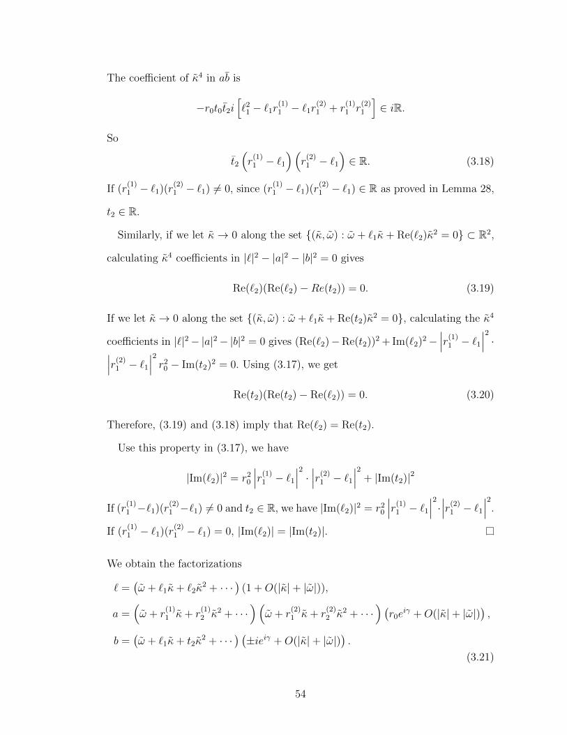
The coefficient of κ4 in ab is
−r0t0t2i[`2
1 − `1r(1)1 − `1r
(2)1 + r
(1)1 r
(2)1
]∈ iR.
So
t2
(r
(1)1 − `1
)(r
(2)1 − `1
)∈ R. (3.18)
If (r(1)1 − `1)(r
(2)1 − `1) 6= 0, since (r
(1)1 − `1)(r
(2)1 − `1) ∈ R as proved in Lemma 28,
t2 ∈ R.
Similarly, if we let κ→ 0 along the set (κ, ω) : ω + `1κ + Re(`2)κ2 = 0 ⊂ R2,
calculating κ4 coefficients in |`|2 − |a|2 − |b|2 = 0 gives
Re(`2)(Re(`2)−Re(t2)) = 0. (3.19)
If we let κ→ 0 along the set (κ, ω) : ω + `1κ+ Re(t2)κ2 = 0, calculating the κ4
coefficients in |`|2− |a|2− |b|2 = 0 gives (Re(`2)−Re(t2))2 + Im(`2)2−∣∣∣r(1)
1 − `1
∣∣∣2
·∣∣∣r(2)
1 − `1
∣∣∣2
r20 − Im(t2)2 = 0. Using (3.17), we get
Re(t2)(Re(t2)− Re(`2)) = 0. (3.20)
Therefore, (3.19) and (3.18) imply that Re(`2) = Re(t2).
Use this property in (3.17), we have
|Im(`2)|2 = r20
∣∣∣r(1)1 − `1
∣∣∣2
·∣∣∣r(2)
1 − `1
∣∣∣2
+ |Im(t2)|2
If (r(1)1 −`1)(r
(2)1 −`1) 6= 0 and t2 ∈ R, we have |Im(`2)|2 = r2
0
∣∣∣r(1)1 − `1
∣∣∣2
·∣∣∣r(2)
1 − `1
∣∣∣2
.
If (r(1)1 − `1)(r
(2)1 − `1) = 0, |Im(`2)| = |Im(t2)|.
We obtain the factorizations
` =(ω + `1κ+ `2κ
2 + · · ·)
(1 +O(|κ|+ |ω|)),
a =(ω + r
(1)1 κ+ r
(1)2 κ2 + · · ·
)(ω + r
(2)1 κ+ r
(2)2 κ2 + · · ·
) (r0e
iγ +O(|κ|+ |ω|)),
b =(ω + `1κ+ t2κ
2 + · · ·) (±ieiγ +O(|κ|+ |ω|)
).
(3.21)
54
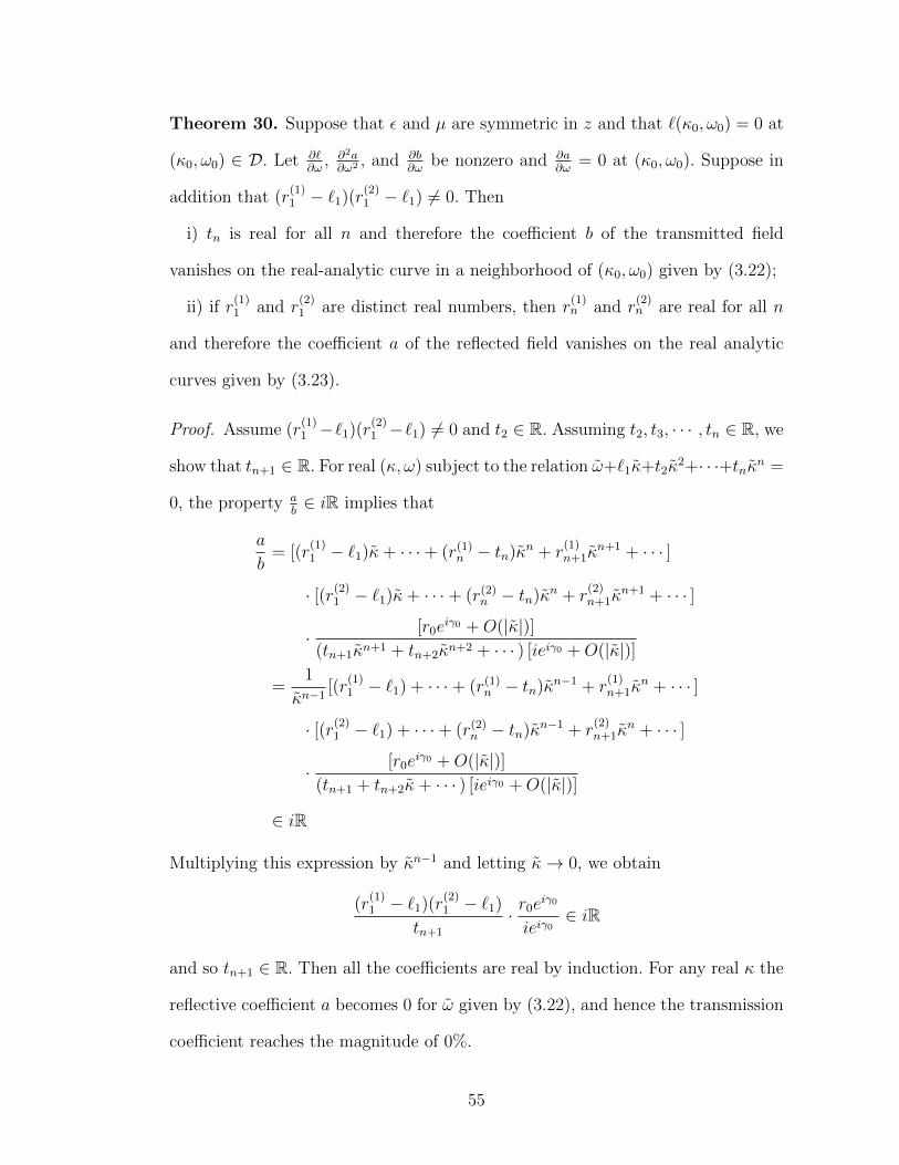
Theorem 30. Suppose that ε and µ are symmetric in z and that `(κ0, ω0) = 0 at
(κ0, ω0) ∈ D. Let ∂`∂ω
, ∂2a∂ω2 , and ∂b
∂ωbe nonzero and ∂a
∂ω= 0 at (κ0, ω0). Suppose in
addition that (r(1)1 − `1)(r
(2)1 − `1) 6= 0. Then
i) tn is real for all n and therefore the coefficient b of the transmitted field
vanishes on the real-analytic curve in a neighborhood of (κ0, ω0) given by (3.22);
ii) if r(1)1 and r
(2)1 are distinct real numbers, then r
(1)n and r
(2)n are real for all n
and therefore the coefficient a of the reflected field vanishes on the real analytic
curves given by (3.23).
Proof. Assume (r(1)1 −`1)(r
(2)1 −`1) 6= 0 and t2 ∈ R. Assuming t2, t3, · · · , tn ∈ R, we
show that tn+1 ∈ R. For real (κ, ω) subject to the relation ω+`1κ+t2κ2+· · ·+tnκn =
0, the property ab∈ iR implies that
a
b= [(r
(1)1 − `1)κ+ · · ·+ (r(1)
n − tn)κn + r(1)n+1κ
n+1 + · · · ]
· [(r(2)1 − `1)κ+ · · ·+ (r(2)
n − tn)κn + r(2)n+1κ
n+1 + · · · ]
· [r0eiγ0 +O(|κ|)]
(tn+1κn+1 + tn+2κn+2 + · · · ) [ieiγ0 +O(|κ|)]
=1
κn−1[(r
(1)1 − `1) + · · ·+ (r(1)
n − tn)κn−1 + r(1)n+1κ
n + · · · ]
· [(r(2)1 − `1) + · · ·+ (r(2)
n − tn)κn−1 + r(2)n+1κ
n + · · · ]
· [r0eiγ0 +O(|κ|)]
(tn+1 + tn+2κ+ · · · ) [ieiγ0 +O(|κ|)]
∈ iR
Multiplying this expression by κn−1 and letting κ→ 0, we obtain
(r(1)1 − `1)(r
(2)1 − `1)
tn+1
· r0eiγ0
ieiγ0∈ iR
and so tn+1 ∈ R. Then all the coefficients are real by induction. For any real κ the
reflective coefficient a becomes 0 for ω given by (3.22), and hence the transmission
coefficient reaches the magnitude of 0%.
55

If in addition r(1)1 , r
(2)1 are real and r
(1)1 6= r
(2)1 , we let κ → 0 along the curve
ω + r(1)1 κ = 0 to obtain
a
b=
[r(1)2 κ2 + · · · ][(r(2)
1 − r(2)1 )κ+ r
(2)2 κ2 + · · · ](r0e
iγ0 +O(|κ|))[(`1 − r(1)
1 )κ+ t2κ+ · · · ](ieiγ0 +O(|κ|))∈ iR
so
κ · [r(1)2 +O(|κ|)][(r(2)
1 − r(2)1 ) +O(|κ|)](r0e
iγ0 +O(|κ|))[(`1 − r(1)
1 ) +O(|κ|)](ieiγ0+O(|κ|))∈ iR
and r(1)2 (r
(2)1 −r(1)
1 ) ∈ R and so r(1)2 ∈ R. The induction arguments can be applied to
show r(1)3 , r
(1)4 , · · · ∈ R. Similarly, r
(2)2 , r
(2)3 , · · · ∈ R, and the transmission coefficient
obtains the magnitude of 100%.
In the first alternative of Lemma 29, Theorem 30 proves that tn are all real
numbers, and so the transmission vanishes along the real-analytic curve
ω = ω0 − `1(κ− κ0)− t2(κ− κ0)2 − · · · . (b = 0) (3.22)
If r(1)n and r
(2)n are real numbers as in the part ii) of this Theorem, then the trans-
mission achieves 100% along two real-analytic curves
ω = ω0 − r(i)1 (κ− κ0)− r(i)
2 (κ− κ0)2 − . . . , i = 1, 2. (a = 0) (3.23)
These frequencies of total transmission and total reflection move apart from ω0 as
κ is perturbed. The transmission rate at other frequencies are close to 1 and the
maximal transmission rate are difficult to detect, as in Fig. 3.4 and 3.6. We show
this by a magnified view on the right of Fig. 3.6. We also believe that t1 must lie
between r(1)1 and r
(2)1 but so far we do not have a proof.
56

3.5.2 Multiple Anomalies
If ∂`∂ω
= 0 at (κ0, ω0) ∈ D, then since |`|2 = |a|2 + |b|2 for real (κ, ω), we have
∂a∂ω
= ∂b∂ω
= 0. In this section, we consider the case in which
∂`
∂ω= 0,
∂a
∂ω= 0,
∂b
∂ω= 0 ;
∂2`
∂ω26= 0,
∂2a
∂ω26= 0,
∂2b
∂ω26= 0 .
(3.24)
The zero loci of the above a, b, ` are given locally by the roots of quadratic functions
in ω with coefficients analytic in κ and vanish at κ = 0. We have
`(κ, ω) =(ω2 + ωλ1(κ) + λ0(κ)
)(1 +O(|κ|+ |ω|)),
a(κ, ω) =(ω2 + ωα1(κ) + α0(κ)
)(r0e
iγ +O(|κ|+ |ω|)),
b(κ, ω) =(ω2 + ωβ1(κ) + β0(κ)
)(it0e
iγ +O(|κ|+ |ω|)),
where λi(0) = αi(0) = βi(0) = 0, 0 < r0 < 1, and t0 is real with 0 < |t0| < 1. The
common unitary factor eiγ comes from the second equation of 3.12, which is due
to the symmetry of the structure Similar to the total background transmission, we
assume again that the first factors of a, b, ` have distinct roots so that they can be
factored analytically. Then we have the following factorization
`(κ, ω) =(ω + `
(1)1 κ+ `
(1)2 κ2 + · · ·
)(ω + `
(2)1 κ+ `
(2)2 κ2 + · · ·
)(1 +O(|κ|+ |ω|)),
a(κ, ω) =(ω + r
(1)1 κ+ r
(1)2 κ2 + · · ·
)(ω + r
(2)1 κ+ r
(2)2 κ2 + · · ·
) (r0e
iγ + rκκ+ rωω + · · ·),
b(κ, ω) =(ω + t
(1)1 κ+ t
(1)2 κ2 + · · ·
)(ω + t
(2)1 κ+ t
(2)2 κ2 + · · ·
) (it0e
iγ + tκκ+ tωω + · · ·).
(3.25)
Lemma 31. Assume `(1)1 6= `
(2)1 . In these forms, the coefficients satisfy the following
properties:
i) `(1)1 , `
(2)1 ∈ R and Im(`
(1)2 ), Im(`
(2)2 ) ≥ 0;
ii) After possibly reindexing the coefficients r(i)1 and t
(i)1 , `
(1)1 = r
(1)1 = t
(1)1 , `
(2)1 =
57

r(2)1 = t
(2)1 ;
iii) |`(1)2 |2 = |r(1)
2 |2|r20 + |t(1)
2 |2t20, and |`(2)2 |2 = |r(2)
2 |2r20 + |t(2)
2 |2t20.
Proof. The relation `(κ, ω) = 0,∀(κ, ω) ∈ R2 gives ω = ω0− `(1)1 (κ− κ0) + `
(1)2 (κ−
κ0)2 + · · · or ω = ω0 − `(2)1 (κ − κ0) + `
(2)2 (κ − κ0)2 + · · · . The condition that
Im(ω) ≤ 0,∀κ ∈ R for generalized guided modes implies (i).
From the property |`|2 = |a|2 + |b|2 for all (κ, ω) ∈ R2, we take κ → 0 along
(κ, ω) : ω + `(1)1 κ = 0 ⊂ R2 to obtain
|`|2 =∣∣∣`(1)
2 κ2 + o(|κ|3)∣∣∣2 ∣∣∣(`(2)
1 − `(1)1 )κ+ `
(2)2 κ2 + · · ·
∣∣∣2
(1 +O(|κ|)),
|a|2 =∣∣∣(r(1)
1 − `(1)1 )κ+ r
(1)2 κ2 + · · · )
∣∣∣2 ∣∣∣(r(2)
1 − `(1)1 )κ+ r
(2)2 κ2 + · · ·
∣∣∣2
(r20 +O(|κ|)),
|b|2 =∣∣∣(t(1)
1 − `(1)1 )κ+ t
(1)2 κ2 + · · · )
∣∣∣2 ∣∣∣(t(2)
1 − `(1)1 )κ+ t
(2)2 κ2 + · · ·
∣∣∣2
(t20 +O(|κ|)).
Compare κ4 terms in |`|2 = |a|2 + |b|2, then we get
0 =∣∣∣r(1)
1 − `(1)1
∣∣∣2 ∣∣∣r(2)
1 − `(1)1
∣∣∣2
r20 +
∣∣∣t(1)1 − `(1)
1
∣∣∣2 ∣∣∣t(2)
1 − `(1)1
∣∣∣2
t20
=[(Re(r
(1)1 )− `(1)
1 )2 + Im(r(1)1 )2
] [(Re(r
(2)1 )− `(1)
1 )2 + Im(r(2)1 )2
]r2
0
+[(Re(t
(1)1 )− `(1)
1 )2 + Im(t(1)1 )2
] [(Re(t
(2)1 )− `(1)
1 )2 + Im(t(2)1 )2
]t20.
This implies that
`(1)1 = one of r
(1)1 , r
(2)1 , and
`(1)1 = one of t
(1)1 , t
(2)1
Similarly we can also prove
`(2)1 = one of r
(1)1 , r
(2)1 , and
`(2)1 = one of t
(1)1 , t
(2)1
Assuming `(1)1 6= `
(2)1 , without loss of generality, we have ii). Comparing the κ6
terms, we get
|`(1)2 |2
(`
(2)1 − `(1)
1
)2
= |r(1)2 |2|r(2)
1 − `(1)1 |2r2
0 + |t(1)2 |2|t(2)
1 − `(1)1 |2t20,
58

which simplifies to
|`(1)2 |2 = |r(1)
2 |2|r20 + |t(1)
2 |2t20.
Similarly, along (κ, ω) : ω + `(2)1 κ = 0, we have
|`(2)2 |2 = |r(2)
2 |2r20 + |t(2)
2 |2t20.
We can rewrite a, b as
a(κ, ω) =(ω + `
(1)1 κ+ r
(1)2 κ2 + · · ·
)(ω + `
(2)1 κ+ r
(2)2 κ2 + · · ·
) (r0e
iγ + rκκ+ rωω + · · ·),
b(κ, ω) =(ω + `
(1)1 κ+ t
(1)2 κ2 + · · ·
)(ω + `
(2)1 κ+ t
(2)2 κ2 + · · ·
) (it0e
iγ + tκκ+ tωω + · · ·).
Lemma 32. If we assume that Im(`(1)2 ), Im(`
(2)2 ) > 0, then for each i ∈ 1, 2,
either r(i)2 and t
(i)2 are distinct real numbers, or they are equal and not real.
Proof. By ab+ab = 0, ∀(κ, ω) ∈ R2, we compute that the κ5, κ4ω, κω4, κ2ω3, κ3ω2, ω5
coefficients of ab+ ab are
−r0t0i(r
(1)2 `
(2)1 + r
(2)2 `
(1)1 + `
(2)1 t
(1)2 + `
(1)1 t
(2)2
)+ `
(1)1 `
(2)1
(−rκt0e−iγi+ tκr0e
iγ),
−r0t0i[2`
(1)1 `
(2)2 (r
(2)2 + t
(2)2 + r
(1)2 + t
(1)2 )]
+ 2`(1)1 `
(2)1
[−irκt0e−iγ + r0tκe
iγ]
(`(1)1 + `
(2)1 )
− r0t0
[(`
(1)1 )2(t
(2)2 + r
(2)2 ) + (`
(2)1 )2(t
(1)2 + r
(1)2 )],
2(`(1)1 + `
(2)1 )[rωt0(−i)e−iγ + r0tω
]
+[rκt0(−i)e−iγ + tκr0e
iγ],
−ir0t0
[r
(1)2 + r
(2)2 + t
(1)2 + t
(2)2
]+ 2(`
(1)1 + `
(2)1 )[rκt0(−i)e−iγ + r0tκe
iγ]
+ ((`(1)1 )2 + (`
(2)1 )2)
[rωt0(−i)e−iγ + r0tωe
iγ]
+ 4`(1)1 `
(2)2
[rκt0(−i)e−iγ + r0tκe
iγ],
59

−ir0t0
[`
(1)1 r
(1)2 + 2`
(2)1 r
(1)2 + 2`
(1)1 r
(2)2 + `
(2)1 r
(2)2
]
+[(`
(1)1 )2 + (`
(2)1 )2
] [rκt0(−i)e−iγ + r0tκe
iγ]
+ 4`(1)1 `
(2)1
[rκt0(−i)e−iγ + r0tκe
iγ]
+ 2`(1)1 `
(2)1 (`
(1)1 + `
(2)1 )[rωt0(−i)e−iγ + r0tωe
iγ]
− ir0t0
[`
(1)1 t
(1)2 + 2`
(2)1 t
(1)2 + 2`
(1)1 t
(2)2 + `
(2)1 t
(2)2
],
rωt0(−i)e−iγ + r0tω.
In total, from the fact that ab ∈ iR,∀(κ, ω) ∈ R2 we have
(−r0t0i)A+ `(1)1 `
(2)1 B ∈ iR,
(−r0t0i)C + 2`(1)1 `
(2)1 B(`
(1)1 + `
(2)1 )− r0t0iD ∈ iR,
2(`(1)1 + `
(2)1 )E +B ∈ iR,
−ir0t0C
2`(1)1 `
(2)1
+ 2(`(1)1 + `
(2)1 )B + [(`
(1)1 )2 + (`
(2)1 )2]E + 4`
(1)1 `
(2)1 E ∈ iR,
−ir0t0G+ [(`(1)1 )2 + (`
(2)1 )2]B + 4`
(1)1 `
(2)1 B + 2`
(1)1 `
(2)1 (`
(1)1 + `
(2)1 )E − ir0t0H ∈ iR,
E ∈ iR,
where
A = r(1)2 `
(2)1 + r
(2)2 `
(1)1 + `
(2)1 t
(1)2 + `
(1)1 t
(2)2 ,
B = rκt0(−i)e−iγ + tκr0eiγ,
C = 2`(1)1 `
(2)1
(r
(2)2 + t
(2)2 + r
(1)2 + t
(1)2
),
D = (`(2)1 )2(t
(2)2 + r
(2)2 ) + (`
(2)1 )2(t
(1)2 + r
(1)2 ),
E = rωt0(−i)e−iγ + r0tω,
and
F =C
2`(1)1 `
(2)1
,
60

G = `(1)1 t
(1)2 + 2`
(2)1 t
(1)2 + `
(1)1 t
(2)2 + `
(2)1 t
(2)2 ,
= (`(1)1 + `
(2)1 )(r
(1)2 + r
(2)2 ) + `
(2)1 r(1)
r + `(1)1 r(2)
r ,
H = `(1)1 t
(1)2 + 2`
(2)1 t
(1)2 + 2`
(1)1 t
(2)2 + `
(2)1 t
(2)2
= (`(1)1 + `
(2)1 )(t
(1)2 + t
(2)2 ) + `
(2)1 t
(1)2 + `
(1)1 t
(2)2 ,
G+H = `(1)1 (r
(1)2 + t
(1)2 ) + 2`
(2)1 (r
(1)2 + t
(1)2 ) + 2`
(1)1 (r
(2)2 + t
(2)2 ) + `
(2)1 (r
(2)2 + t
(2)2 )
= (`(1)1 + `
(2)1 )
C
2`(1)1 `
(2)1
+ A.
These conditions can be written as a linear system
r0t0 `(1)1 `
(2)1 0 0 0
0 2`(1)1 `
(2)1 (`
(1)1 + `
(2)1 ) r0t0 r0t0 0
0 1 0 0 2(`(1)1 + `
(2)1 )
0 2(`(1)1 + `
(2)1 ) r0t0
2`(1)1 `
(2)1
0[(`
(1)1 )2 + (`
(2)1 )2 + 4`
(1)1 `
(2)1
]
r0t0
[(`
(1)1 )2 + (`
(2)1 )2 + 4`
(1)1 `
(2)1
]r0t0(`
(1)1 +`
(2)1 )
2`(1)1 `
(2)1
0 2`(1)1 `
(2)1 (`
(1)1 + `
(2)1 )
·
Im(A)
Re(B)
Im(C)
Im(D)
Re(E)
= 0.
The determinant of this matrix is
1
2`
(1)1 r3
0t30 +
(`(1)1 )3
2`(2)1
r30t
30 +
1
2`
(2)1 r3
0t30 +
1
2
(`(2)1 )2r3
0t30
`(1)1
=r3
0t30
2
[`
(1)1 + `
(2)1 +
(`(1)1 )2
`(2)1
+(`
(2)1 )2
`(1)1
]
=r3
0t30
2
(`
(1)1 + `
(2)1
)((`
(1)1 )2 + (`
(2)1 )2
)
`(1)1 `
(2)1
.
61

If `(1)1 + `
(2)1 6= 0, the determinant is nonzero and so
Im(A)
Re(B)
Im(C)
Im(D)
Re(E)
= 0.
Here Im(A) = 0 implies that r(1)2 `
(2)1 + r
(2)2 `
(1)1 + `
(2)1 t
(1)2 + `
(1)1 t
(2)2 = `
(1)1 (r
(2)2 + t
(2)2 ) +
`(2)1 (r
(1)2 +t
(1)2 ) ∈ R, Im(C) = 0 implies that r
(2)2 +t
(2)2 +r
(1)2 +t
(1)2 ∈ R, and Im(D) = 0
implies that (`(1)1 )2
(r
(2)2 + t
(2)2
)+(`
(2)1 )2(r
(1)2 + t
(1)2 ) ∈ R. Since we assume `
(1)1 6= `
(2)1 ,
it follows that
r(1)2 + t
(1)2 ∈ R,
r(2)2 + t
(2)2 ∈ R.
If `(1)1 + `
(2)1 = 0, then the system becomes
r0t0 −(`(1)1 )2 0 0 0
0 0 r0t0 r0t0 0
0 1 0 0 0
0 0 r0t0
−2(`(1)1 )2
0 0
r0t0 −2(`(1)1 )2 0 0 0
0 0 0 0 1
Im(A)
Re(B)
Im(C)
Im(D)
Re(E)
= 0.
This also implies that Im(A) = Re(B) = Im(C) = Im(D) = Re(E) = 0, and we
also have
r(1)2 + t
(1)2 ∈ R,
r(2)2 + t
(2)2 ∈ R.
62

To prove r(1)2 t
(1)2 ∈ R and r
(2)2 t
(2)2 ∈ R, we let κ → 0 along the set (κ, ω) :
ω + `(1)1 κ = 0 ⊂ R2. The condition ab ∈ iR implies that the coefficient of κ6 in ab
−ir0t0r(1)1 t
(1)2
[(`
(1)1 )2 − 2`
(1)1 `
(2)1 + (`
(2)1 )2
]∈ iR,
which implies r(1)2 t
(1)2 ∈ R because `
(1)1 6= `
(2)1 . Similarly, along (κ, ω) : ω + `
(2)1 κ =
0, we obtain r(2)2 t
(2)2 ∈ R.
In conclusion, r(1)2 , t
(1)2 are two roots of a real quadratic equation, which implies
the statement in this lemma.
The relation between r(i)2 and t
(i)2 can be categorized into three cases: i) all
r(1)2 , t
(1)2 , r
(2)2 , t
(2)2 are real; ii) only one pair of r
(i)2 , t
(i)2 is real, and the members of
the other pair are equal; iii) none of them are real numbers. Subject to structural
symmetry with respect to z, one can prove a theorem analogous to those for the
previous cases. It says in particular that, if the first alternative in the lemma holds
for i = 1 and i = 2, then two peak-dip anomalies emerge from ω0 as κ is perturbed
from κ0, each of which attains the values 0 and 1 along real-analytic curves passing
through (κ0, ω0).
Theorem 33. i) If
r(1)2 6= t
(1)2 ∈ R
r(2)2 6= t
(2)2 ∈ R,
then all the coefficients r(1)n ,r
(2)n , t
(1)n , and t
(2)n are real. For κ near κ0, there exist
two values of ω for which the transmission coefficient attains the magnitude of 1
along the real-analytic curves given by
ω = ω0 − r(1)1 (κ− κ0)− r(1)
2 (κ− κ0)2 − · · · ,
ω = ω0 − r(2)1 (κ− κ0)− r(2)
2 (κ− κ0)2 − · · · .
63

and the transmission coefficient attains the magnitude of 0 along the real-analytic
curve given by
ω = ω0 − t(1)1 (κ− κ0)− t(1)
2 (κ− κ0)2 − · · · ,
ω = ω0 − t(2)1 (κ− κ0)− t(2)
2 (κ− κ0)2 − · · · .
ii) If only one pair of them are real, for example, r(1)2 , t
(1)2 ∈ R, then there is only
one value of ω for which the transmission coefficient reaches the magnitude 100%
and one value for which the transmission is 0%.
iii) If r(i)2 = t
(i)2 for all i ∈ 1, 2, then a/` and b/` are continuous at (κ0, ω0). The
transmission coefficient is continuous with respect to κ and does not reach 100%
or 0%.
Proof. i) Letting κ→ 0 along the real curve (κ, ω) ∈ R2 : ω+ `(1)1 κ+ r
(1)2 κ2 = 0,
we have
a = (r(1)1 κ3 + · · · )
[(r
(2)2 − r(1)
2 )κ2 + · · ·]
(r0eiγ + · · · )
b =[(t
(1)2 − r(1)
2 )κ2 + · · ·] [
(t(2)2 − r(1)
2 )κ2 + · · ·]
(t0ieiγ + · · · )
Since ab∈ iR for real κ, the expression a
κbis also in R. So
(r(1)1 κ3 + · · · )
[(r
(2)2 − r(1)
2 )κ2 + · · ·]
(r0eiγ + · · · )
κ[(t
(1)2 − r(1)
2 )κ2 + · · ·] [
(t(2)2 − r(1)
2 )κ2 + · · ·]
(t0ieiγ + · · · )∈ iR.
Let κ→ 0, and we have r(1)3 ∈ R. Similarly, we can get t
(1)3 , r
(2)3 , t
(2)3 ∈ R.
Inductively, if r(2)2 6= r
(1)2 , and r
(1)2 , r
(2)2 , t
(1)2 , t
(2)2 are real, we can take κ→ 0 along
(κ, ω) ∈ R2 : ω + `(1)1 κ+ r
(1)2 κ2 + r
(1)3 κ3 + · · ·+ r(1)
n κn = 0
to prove that r(1)n+1 ∈ R, and therefore, r
(1)n ∈ R, ∀n ∈ N. Also it is similar to prove
t(1)n , r
(2)n , t
(2)n ∈ R,∀n ∈ N.
64

ii) Similarly, if r(2)2 6= t
(2)2 and are both in R, then one can use the same process
to prove r(2)n ∈ R,∀n ∈ N and so we have two real factors of a(κ, ω)
ω + `(2)1 κ+ r
(2)2 κ2 + r
(2)3 κ3 + · · ·
and
ω + `(2)1 κ+ t
(2)2 κ2 + t
(2)3 κ3 + · · · .
For any value of κ near 0, there is a value ω such that the transmission coefficient
vanishes and another value ω for which the reflective coefficient vanishes.
iii) If we assume r(1)2 = t
(1)2 and r
(2)2 = t
(2)2 but not real, then we can prove that
there is no spike. In fact,
ω + `(1)1 κ+ r
(1)2 κ2 6= 0,
|ω + `(1)1 κ+ r
(1)2 κ2| ≥ |Im(r
(1)2 )|κ2,
so
b
`=
[ω + t
(1)1 κ+ t
(1)2 κ2 + · · ·
] [ω + t
(2)1 κ+ t
(2)2 κ2 + · · ·
](it0e
iγ + tκκ+ tωω + · · · )[ω + `
(1)1 κ+ `
(1)2 κ2 + · · ·
] [ω + `
(2)1 κ+ `
(2)2 κ2 + · · ·
](1 +O(|κ|+ |ω|))
=(1 +
t(1)3 κ3
ω+`(1)1 κ+r2(1)κ2
+ · · · )(1 +t(2)3 κ3
ω+`(2)1 κ+r2(2)κ2
+ · · · )(it0eiγ + · · · )
(1 +`(1)3 κ3
ω+`(1)1 κ+r2(1)κ2
+ · · · )(1 +`(2)3 κ3
`(2)3 +`
(2)1 κ+r2(2)κ2
+ · · · )(1 + · · · )
Therefore,
b
`=
(1 +O(|κ|))(1 +O(|κ|)(it0eiγ +O(|ω|+ |κ|))(1 +O(|κ|)(1 +O(|κ|)(1 +O(|ω|+ |κ|))
is continuous with respect to κ, nonzero and finite. In this case, the transmission
coefficient does not attain the magnitude of 0 and 1.
3.6 Transmission Graphs
In this section, we demonstrate different forms of transmission anomalies by choos-
ing different values of the coefficients in the expansions (3.14,3.21, 3.25) of `, a,
65

-0.004 -0.002 0.000 0.002 0.0040.0
0.2
0.4
0.6
0.8
1.0
-0.004 -0.002 0.000 0.002 0.0040.0
0.2
0.4
0.6
0.8
1.0
FIGURE 3.2. |T |2 as a function of ω for κ = 0,±0.01,±0.02,±0.03. The generic condi-tions ∂`
∂ω ,∂a∂ω ,
∂b∂ω 6= 0 are satisfied at the bound-state pair (κ0, ω0). In (3.15,3.16), `1 = 0
so that there is no linear detuning of the anomaly with κ. Left: 0 < t2 = 1 < r2 = 2so that the peak is to the left of the dip and both are to the left of ω0. Right:r2 = −2 < 0 < t2 = 1. In both graphs, r0 = 0.6, t0 = 0.8. The transmission is symmetricin κ, and the curve without an anomaly is the transmission graph for κ = 0.
and b. More specifically, we graph the transmission coefficient
|T (κ, ω)|2 =
∣∣∣∣b(κ, ω)
`(κ, ω)
∣∣∣∣2
=|b|2
|a|2 + |b|2 , (3.26)
as a function of frequency ω = ω−ω0, keeping only terms up to quadratic order in
κ = κ − κ0 in the first factors and only the constant terms in the nonzero factor.
This approximation has the accuracy of O(|κ| + ω2) in the generic case (see [20,
Thm. 16]).
Figures 3.2, 3.3 show the generic case of Section 3.4.2, in which r2 and t2 are
distinct real numbers. For κ = κ0 (κ = 0) the anomaly is absent. As κ is perturbed,
i.e. κ 6= 0, the anomaly appears and widens with width |t2−r2|κ2, as shown in
Fig. 3.2 for `1 = 0. If `1 6= 0, as in Fig. 3.3, then the anomaly is detuned from ω0
at a rate of O(κ), whereas it widens with quadratic width |t2−r2|κ2.
Figures 3.4 show the degenerate case in which the anomaly pattern is one single
dip descending to 0 from a full background transmission or a single peak rising to
1 from a null background transmission (see Section 3.5.1). The peaks reside on two
sides of the dip. We show another possibility when the peaks are located on one
side of the dip in another Figure 3.5. In particular, if `1 = 0, we show the anomaly
66

-0.010 -0.005 0.000 0.005 0.0100.0
0.2
0.4
0.6
0.8
1.0
FIGURE 3.3. |T |2 as a function of ω for κ = 0,±0.003,±0.006,±0.009. The genericconditions ∂`
∂ω ,∂a∂ω ,
∂b∂ω 6= 0 are satisfied at the bound-state pair (κ0, ω0). In (3.15,3.16),
`1 = 0.9 6= 0, so the anomaly is detuned from ω = ω0 (ω = 0) in a linear manner in κ. Thecoefficients r2 = 2 and t2 = 1 of κ2 are distinct real numbers, and (r0, t0) = (0.6, 0.8).
-0.10 -0.05 0.00 0.05 0.100.0
0.2
0.4
0.6
0.8
1.0
-0.10 -0.05 0.00 0.05 0.100.0
0.2
0.4
0.6
0.8
1.0
FIGURE 3.4. |T |2 as a function of ω for κ = 0,±0.01,±0.02,±0.03. Left: Full back-ground transmission occurs when ∂`
∂ω 6= 0, ∂a∂ω = 0, and ∂b
∂ω 6= 0 at (κ0, ω0). In (3.21),
0 < r(1)1 = 0.2 < t1 = `1 = 2 < r
(2)1 = 4, (r
(1)2 , r
(2)2 , t2) = (7, 7, 0.1), and r0 = 0.6. Right:
∂`∂ω 6= 0, ∂a
∂ω 6= 0, and ∂b∂ω = 0 at (κ0, ω0) and 0 < t
(1)1 < r1 = `1 < t
(2)1 .
with single dip and two peaks, as well as two dips and single peak in Fig. 3.6,3.7,
and 3.8. In Fig. 3.6 and 3.7, the peaks are on two sides of the dip, or two dips lie
on two sides of the single peak, respectively, while in Fig. 3.8, two peaks reside on
the same side of the single dip. In the first case, we see that full transmission is
actually achieved at precisely two frequencies near ω = ω0 (ω = 0), as shown in
the magnified, right-hand image of Fig. 3.6.
Without the assumption r(1)1 , r
(2)1 ∈ R, one can still show that the single dip is
reached. We also give the figures for the case that r(1)1 , r
(2)1 are conjugate for `1 = 0
and `1 6= 0 in Fig. 3.10 and Fig. 3.9.
67

-0.10 -0.05 0.00 0.05 0.100.0
0.2
0.4
0.6
0.8
1.0
FIGURE 3.5. |T |2 as a function of ω for κ = 0,±0.01,±0.02,±0.03. Full backgroundtransmission occurs when ∂`
∂ω 6= 0, ∂a∂ω = 0, and ∂b
∂ω 6= 0 at (κ0, ω0). In (3.21),
0 < r(1)1 = 0.6 < r
(2)1 = 1.2 < `1 = 3; (r0, r
(1)2 , r
(2)2 , t2) = (0.6, 1, 1, 0.2).
-0.0020 -0.0015 -0.0010 -0.0005 0.0000 0.0005 0.00100.0
0.2
0.4
0.6
0.8
1.0
-0.010 -0.005 0.000 0.005 0.0100.99990
0.99992
0.99994
0.99996
0.99998
1.00000
FIGURE 3.6. |T |2 as a function of ω for κ = 0,±0.01,±0.02,±0.03. Left: Full back-ground transmission occurs when ∂`
∂ω 6= 0, ∂a∂ω = 0, and ∂b
∂ω 6= 0 at (κ0, ω0). In (3.21),
r(1)1 = −0.04 < t1 = `1 = 0 < r
(2)1 = 0.06; (r0, r
(1)2 , r
(2)2 , t2) = (0.6,−1, 1, 1). Right:
Magnification of the graphs for κ = ±0.01, bringing into view the frequencies of totaltransmission.
-0.0020 -0.0015 -0.0010 -0.0005 0.0000 0.0005 0.00100.0
0.2
0.4
0.6
0.8
1.0
FIGURE 3.7. |T |2 as a function of ω for κ = 0,±0.01,±0.02,±0.03. Full back-ground transmission occurs when ∂`
∂ω 6= 0, ∂a∂ω 6= 0, and ∂b
∂ω = 0 at (κ0, ω0) and
0 < t(1)1 < r1 = `1 < t
(2)1 . In (3.21), t
(1)1 = −0.04 < r1 = `1 = 0 < t
(2)1 = 0.06;
(t0, t(1)2 , t
(2)2 , t2) = (0.6,−1, 1, 1).
68

-0.010 -0.005 0.000 0.005 0.0100.0
0.2
0.4
0.6
0.8
1.0
FIGURE 3.8. |T |2 as a function of ω for κ = 0,±0.01,±0.02,±0.03. Full backgroundtransmission occurs when ∂`
∂ω 6= 0, ∂a∂ω = 0, and ∂b
∂ω 6= 0 at (κ0, ω0). In (3.21),
t1 = `1 = 0 < r(1)1 = 0.6 < r
(2)1 = 0.8; (r0, r
(1)2 , r
(2)2 , t2) = (0.6,−4, 5, 6).
-0.010 -0.005 0.000 0.005 0.0100.0
0.2
0.4
0.6
0.8
1.0
FIGURE 3.9. |T |2 as a function of ω for κ = 0,±0.01,±0.02,±0.03. ∂`∂ω
∂a∂ω 6= 0, ∂b∂ω = 0
at (κ0, ω0). (r(1)1 , r
(2)1 , `1) = (2i,−2i, 0); (r0, r
(1)2 , r
(1)2 , t2) = (0.6, 2i, 4i, 3).
If the first derivatives of `, a, b with respect to ω are zero at (κ0, ω0), under
the assumptions in Section 3.5.2, the anomaly has double spikes with peaks and
dips. This situation is shown in Figures 3.11 and 3.12 for two possible choices of
constants in the Weierstraß expansions. Either sets of the constant choices are
possible but we wish to find more properties to refine our results.
The vertical line in all graphs shows the location of ω = 0, or ω = ω0.
69

-0.05 0.00 0.050.0
0.2
0.4
0.6
0.8
1.0
-0.04 -0.02 0.00 0.02 0.040.990
0.992
0.994
0.996
0.998
1.000
FIGURE 3.10. |T |2 as a function of ω for κ = 0,±0.01,±0.02,±0.03. ∂`∂ω
∂a∂ω 6= 0, ∂b∂ω = 0
at (κ0, ω0). (r(1)1 , r
(2)1 , `1) = (0.5i,−0.5i, 2); (r0, r
(1)2 , r
(1)2 , t2) = (0.6, i, i, 1).
-0.005 0.000 0.0050.0
0.2
0.4
0.6
0.8
1.0
-0.0030 -0.0028 -0.0026 -0.0024 -0.0022 -0.0020 -0.00180.0
0.2
0.4
0.6
0.8
1.0
FIGURE 3.11. Left: |T |2 as a function of ω for κ = 0,±0.003,±0.006,±0.009. Thepartial derivatives of `, a, and b all vanish at (κ0, ω0), whereas their second derivatives
are nonzero. In (3.25), (`(1)1 , `
(2)1 ) = (0.7, 0.8), (r0, t0) = (0.6, 0.8), r
(1)2 = 2 < t
(1)2 = 8 and
t(2)2 = 4 < r
(2)2 = 5. Right: κ = 0.003.
-0.010 -0.005 0.000 0.005 0.0100.0
0.2
0.4
0.6
0.8
1.0
-0.0040 -0.0035 -0.0030 -0.0025 -0.0020 -0.0015 -0.00100.0
0.2
0.4
0.6
0.8
1.0
FIGURE 3.12. Left: |T |2 as a function of ω for κ = 0,±0.003,±0.006,±0.009. Thepartial derivatives of `, a, and b all vanish at (κ0, ω0), whereas their second derivatives
are nonzero. In (3.25), (`(1)1 , `
(2)1 ) = (0.7, 0.8), (r0, t0) = (0.6, 0.8), r
(1)2 = 2 < t
(1)2 = 8 and
r(2)2 = 4 < t
(2)2 = 6. Right: κ = 0.003.
70

Chapter 4Guided Modes in Periodic Pillars
This chapter deals with scattering problems and guided modes in periodic pillars.
We establish a systematic framework to study plane-wave scattering problems
and guided modes in periodic pillars. Existence and nonexistence results are es-
tablished, among which there is a main new theorem proving the existence of a
nontrivial embedded guided mode robust in the wavenumber κ.
4.1 Bessel Functions
We introduce some important properties of Bessel functions to be used in later
sections. More details for the properties of Bessel functions can be found in [29].
The Bessel equation
d2f
dz2+
1
z
df
dz+ (1− `2
z2)f = 0 (4.1)
admits two linearly independent solutions J`(z)and Y`(z). They are called the first
and second kind of Bessel functions. The third kind of Bessel functions are Hankel
functions defined by H1` (z) = J`(z) + iY`(z), H2
` (z) = J`(z)− iY`(z).
By a change of variables, one sees that a more general form of Bessel equation
d2f
dz2+
1
z
df
dz+ (λ2 − `2
z2)f = 0, λ ∈ R
has linear independent solutions J`(λz) and Y`(λz). The modified Bessel functions
of the first kind and the second kind are I`(z) and K`(z), which solve d2fdz2
+ 1zdfdz−
(1 + `2
z2)f = 0. Similar to the Bessel equation, the modified Bessel equation can be
generalized to
d2f
dz2+
1
z
df
dz− (λ2 +
`2
z2)f = 0, λ ∈ R
71

with independent solutions I`(λz) and K`(λz).
We will use H1` (z) = J`(z)+iY`(z) and H2
` (z) = J`(z)−iY`(z) as the two complex
valued independent solutions in the following. Observing that −λ2 = (iλ)2, we can
also use H1,2` (λx) as two independent solutions of the unifying equation
d2f
dz2+
1
z
df
dz+ (λ2 − `2
z2)f = 0, λ ∈ R or iR. (4.2)
The Bessel function J`(z) has a sequence of zeros j`,n → ∞ as z → ∞, and
j`,n > `. The modified function K` is strictly decreasing. If ` 6= 0, the function
I`(z) is nonzero except at 0, and I`(z) is strictly increasing. If ` = 0, I0(0) > 0 and
I0(z) increases to ∞ as z →∞.
For Hankel functions we have the asymptotic expansions for large arguments
H1` (z) ∼
√2
πzei(z−
`π2−π
4)(1 + o(z−1)), z > 0, (4.3)
H2` (z) ∼
√2
πze−i(z−
`π2−π
4)(1 + o(z−1)), z > 0. (4.4)
If 0 < z ∈ R, then H1` is outgoing and H2
` is incoming (given ω > 0). If z ∈ iR and
z = i|z|, then H1` is exponentially decaying as |z| → ∞, and H2
` is exponentially
growing as |z| → ∞.
The modified Bessel function K` has the following relation with H1` :
K`(z) =1
2πie
12`πiH1
` (iz).
The following results hold for the multiplier γm` used in the definition of the
Dirichlet-to-Neumann map in the next section.
Lemma 34. If ηm = i|ηm|, R > 0, then the multiplier γm` = −ηmH1′` (ηmR)
H1` (ηmR)
> 0. If
ηm > 0, R > 0, then the imaginary part of the multiplier Im
(−ηmH1′
` (ηmR)
H1′` (ηmR)
)6= 0.
72

Proof. Taking z = |ηm|R, if ηm = i|ηm|, we have
−ηmH1′
` (ηmR)
H1` (ηmR)
= −|ηm|i−iK ′l(|ηm|R)/(π
2ie`πi/2)
Kl(|ηm|R)/(π2ie`πi/2)
= −|ηm|K ′l(|ηm|R)
Kl(|ηm|R)
> 0.
If ηm = |ηm| > 0, R > 0, then
Im
(−ηm
H1′
` (ηmR)
H1` (ηmR)
)= Im
(−|ηm|
(J ′` + iY ′` )(J` − iY`)J2` + Y 2
`
)= −|ηm|
J ′`Y` − J`Y ′`J2` + Y 2
`
The numerator of the last fraction is the Wronskian determinant
∣∣∣∣∣∣∣
J` Y`
J ′` Y ′`
∣∣∣∣∣∣∣and is
therefore nonzero.
The Bessel function J`(Z) is the generating function of e12Z(t− 1
t):
e12Z(t− 1
t) =
∞∑
`=−∞
t`J`(Z). (4.5)
If we let t = ei(θ+θ0) to obtain eiZ sin(θ+θ0) = Σ`J`(Z)ei`(θ+θ0). then with sin θ0 =
κ1ηm, cos θ0 = κ2
ηm, and Z = ηmr. The incident wave can be written as a superposition
of Hankel functions:
ei(κ1x+κ2y+κ3z) =ei(ηmr cos θ sin θ0+ηmr sin θ cos θ0)eiκ3z
=eiηmr sin(θ+θ0)ei(m+κ)z
=∑
`∈Z
J`(ηmr)ei`(θ+θ0)ei(m+κ)z
=∑
`∈Z
1
2
[H1` (ηmr) +H2
` (ηmr)]ei`(θ+θ0)ei(m+κ)z.
(4.6)
As a result, the scattering problem of plane waves can be reduced to the linear
superposition of propagating Fourier harmonics with Hankel functions given in the
next section.
73

4.2 Media Structure and Scattering Problem4.2.1 Pillar Structure and Radiation Condition
We consider an infinitely long pillar that is periodic in the z-direction with period
2π and bounded in the x, y directions.
ε(x, y, z + 2π) = ε(x, y, z), µ(x, y, z + 2π) = µ(x, y, z), ∀x, y, z.
We use Ω = (x, y, z) : −π < z < π to denote one period. Suppose that
ε = ε0, µ = u0 for r > R and we denote the restricted domain ΩR = (x, y, z) :
−π < z < π, r =√x2 + y2 < R, which is a cylinder whose boundary consists of
ΓR = (x, y, z) ∈ Ω : −π < x, y < π, r = R plus the upper and lower horizontal
disks.
The spatial factor of a time-harmonic acoustic or electromagnetic wave is gov-
erned by the Helmholtz equation
∇ · 1
µ∇u(x, y, z) + εω2u(x, y, z) = 0. (4.7)
By the κ-pseudo-periodicity, u can be expanded as an infinite superposition u(x, y, z) =
∑∞m=−∞ um(x, y)ei(m+κ)z. where κ ∈ B = [−1/2, 1/2). Let (x, y) = (r cos θ, r sin θ).
If r =√x2 + y2 > R, then
∆um(x, y) + η2mum(x, y) = 0
where ηm = µ0ε0ω2 − (m+ κ)2. Using polar coordinates, we have
∂2um∂r2
+1
r
∂um∂r
+1
r2
∂2um∂θ2
+ η2mum = 0.
The function um can be written as an expansion of separable solutions
um =∞∑
`=−∞
Rm,`(r)ei`θ,
74

where Rm,`(r) satisfies
R′′m,` +1
rR′m,` −
`2
r2Rm,` + η2
mRm,` = 0.
This equation has solutions
Rm,`(r) =
am`H1` (ηmr) + bm`H
2` (ηmr), if ηm 6= 0,
cm1 + cm2 ln |r|, if ηm = 0, ` = 0,
cm`1|r|` + cm`2|r|−`, if ηm = 0, ` 6= 0.
(4.8)
Therefore, the spatial field u can be expanded as an infinite superposition of Fourier
harmonics in Ω \ ΩR:
u(x, y, z) =∞∑
m=−∞
∞∑
`=−∞
Rm,`(r)ei`θei(m+κ)z. (4.9)
In this expansion, the Hankel functions H1` (ηmr) are outgoing or exponentially
decaying, depending on whether ηm is imaginary or real, as r →∞, and the Hankel
functions H2` (ηmr) are incoming or exponentially growing.
The following radiation condition is required for the problem of scattering by a
periodic pillar.
Condition 35 (Radiation condition). A field u(r, θ, z) satisfies the radiation con-
dition if it admits the following Fourier-Bessel representation for r > R:
u(r, θ, z) =∑
m∈Zp∪Ze
∑
`∈Z
am`H1` (ηmr)e
i`θei(m+κ)z
+∑
m∈Z`
[∑
`>0
cml2 |r|−`ei`θ +∑
`<0
cm`1 |r|`ei`θ]ei(m+κ)z
(4.10)
where the sets Zp,a,e of Z depend on κ and are defined by
m ∈ Zp ⇔ η2m > 0, ηm > 0 (propagating harmonics)
m ∈ Za ⇔ η2m = 0, ηm = 0 (algebraic harmonics)
m ∈ Ze ⇔ η2m < 0,−iηm > 0 (evanescent harmonics) .
75

4.2.2 Scattering Problems
Before studying the guided modes, we first consider the scattering of a plane wave.
Problem 36 (Scattering problem, strong form). Given ε0, µ0 > 0, find u on Ω
such that
∇ · 1
µ∇u+ εω2u = 0 in Ω,
u is continuous on ∂Ω,
1
µ
∂u
∂nis continuous on ∂Ω,
uinc =∑
m∈Zp
uincm ei(κ1x+κ2y+(m+κ)z),
usc = u− uinc and its derivatives are κ-periodic in z,
usc = u− uinc satisfies the radiation condition .
(4.11)
On the truncated domain ΩR, define the pseudo-periodic field space H1κ(ΩR) =
u ∈ H1(ΩR) : u(x, y, π) = u(x, y,−π)e2πκi. On the vertical boundary ΓR, the
radiation condition is characterized by a Dirichlet-to-Neumann map T : H12κ (ΓR)→
H− 1
2κ (ΓR) (as in the Definition 5.19 of [2])
T :∑
m,`
um`ei`θei(m+κ)z 7→
∑
m,`
γm`um`ei`θei(m+κ)z, (4.12)
where
γm` =
−ηmH1′` (ηmR)
H1` (ηmR)
, if m 6∈ Za,
|`|R−1, if m ∈ Za and ` 6= 0,
0, if m ∈ Za and ` = 0
To satisfy the radiation condition, the harmonics in (4.9) with H2` (ηmr) for m ∈
Zp ∪ Ze, harmonics (cm1 + cm2 ln |r|)ei`θei(m+k)z for m ∈ Za, ` = 0, and harmonics
with |r|` for m ∈ Za, ` > 0 all vanish. The radiation condition is hence enforced by
∂nu+ Tu = 0 on ΓR. (4.13)
76

The operator T is split into two parts
T = Te + Tp, (4.14)
(Tef)m` =
−ηmH1′` (ηmR)
H1` (ηmR)
fm`, if m ∈ Ze,
|`|R−1fm`, if m ∈ Za and ` 6= 0,
0, otherwise
(4.15)
(Tpf)m` =
−ηmH1′` (ηmR)
H1` (ηmR)
fm`, if m ∈ Zp,
0, otherwise
(4.16)
Note that the multipliers γm` in Te are nonnegative. In Tp, the multipliers have
nonzero imaginary parts for any m ∈ Zp (see Lemma 34).
The variational form of the scattering problem in the truncated domain is
Problem 37 (Scattering problem, variational form).
u ∈ H1κ(ΩR)
a(u, v)− ω2b(u, v) = f(v),∀v ∈ H1κ(ΩR)
(4.17)
where
a(u, v) =
∫
ΩR
1
µ∇u · ∇v +
1
µ0
∫
ΓR
(Tu)v
b(u, v) =
∫
ΩR
εuv,
f(v) =1
µ0
∫
ΓR
[(∂nu
inc + Tuinc)v].
Similar to the analysis in Chapter 2, we can prove the existence of the scattered
wave by Fredholm alternative theory. The weak form PDE in problem 37 can be
written as
a(u, v)− ω2b(u, v) = c1(u, v) + c2(u, v)
77

with c1(u, v) =∫
ΩR( 1µ∇u · ∇v + εuv) + 1
µ0
∫ΓR
(Tu)v and c2(u, v) = −ε(ω2 +
1)∫
ΩRuv. Define operators C1 and C2 on H1
κ(ΩR) by (C1u, v)H1κ(ΩR) = c1(u, v)
and (C2u, v)H1κ(ΩR) = c2(u, v). Because of the coercivity of c1 and the compact
embedding of L2(Ω) into H1κ(ΩR), the operator C1 is an automorphism and C2 is
compact.
If we denote by f inc the unique element of H1κ(ΩR) such that (f inc, v)H1
κ(ΩR) =
f(v), the variational form of the scattering problem can be characterized by the
following operator form
C1u+ C2u = f inc.
The Fredholm alternative theory implies that the nonuniqueness of the solution
of this problem is equivalent to the singularity of the corresponding homogeneous
problem C1u+ C2u = 0, whose weak form is given by
a(u, v)− ω2b(u, v) = 0,∀v ∈ H1κ(ΩR) (4.18)
Theorem 38. The plane wave scattering problem has at least one solution, and
the set of solutions is at most finite dimensional.
Proof. From equation (4.6), we can express the incident plane wave as a superpo-
sition of harmonics∑
`
1
2
[H1` (ηmr) +H2
` (ηmr)]ei`(θ+θ0)ei(m+κ)z, with m ∈ Zp. By
the Fredholm alternative, the scattering problem has a solution if and only if
(f inc, w) = 0, for all w ∈ Null(C1 + C2)†,
i.e. for all w such that
a(v, w)− ω2b(v, w) = 0,∀v ∈ H1κ(ΩR)
This w satisfies
a(w, v)− ω2b(w, v) = 0,∀v ∈ H1κ(ΩR)
78

and by the decomposition of T , we know that for all m ∈ Zp, wm = 0. By the
definition of f inc, showing (f inc, w) = 0 is equivalent to showing that∫
ΓR(∂n +
T )uincw = 0. This is satisfied by the function w above.
The space of solutions is finite-dimensional because C1 is invertible and C2 is
compact.
4.3 Guided Modes
A guided mode is a solution to the Helmholtz equation in the periodic domain in
the absence of any source field. In the weak form, it is a solution to the homogeneous
equation (4.18).
The sesquilinear form
aω(u, v) =
∫
ΩR
1
µ∇u · ∇v +
1
µ0
∫
ΓR
(T ωu)v
can be split into evanescent and propagating parts,
aωe (u, v) =
∫
ΩR
1
µ∇u · ∇v +
1
µ0
∫
ΓR
(T ωe u)v,
aωp (u, v) =1
µ0
∫
ΓR
(T ωp u)v.
In this chapter we assume that the frequency and the wavenumber are real. Note
that in the decomposition (4.14), the multiplier γm` has a nonzero imaginary part
for m ∈ Zp, thus a(u, u) = 0 if and only if (u|ΓR)m = 0, for all m ∈ Zp.
Theorem 39. (Real eigenvalues) If the frequency ω is real, then u ∈ H1κ(ΩR)
solves the equation (4.18) if and only if
aωe (u, v)− aωp (u, v)− ω2b(u, v) = 0,∀v ∈ H1κ(ΩR), (4.19)
and if and only if
aωe (u, v)− ω2b(u, v) = 0,∀v ∈ H1κ(ΩR),
(u|ΓR)m = 0,∀m ∈ Zp.(4.20)
79

The eigenfrequencies can be obtained by applying the min-max principle to the
real form in (4.20). When ω <√
κ2
ε0µ0, the solutions u of aωr (u, v) − ω2b(u, v) =
0, ∀v ∈ H1κ(ΩR) are guided modes since this regime admits no propagating har-
monics and so the second conditions in (4.20) are automatically satisfied. When
ω ≥√
κ2
ε0µ0, to be guided modes, these solutions u must satisfy the extra conditions
(u|ΓR)m = 0,∀m ∈ Zp where Zp is nonempty. We will design some periodic struc-
tures that admit guided modes in the next section. We have the following theorem
on properties of the frequencies. The proof is similar to that for periodic slabs, for
which one may refer to [27] [1].
Theorem 40. (Eigenvalues and characteristic frequencies) The problem aωe (u, v)−
λb(u, v) = 0, ∀v ∈ H1κ(ΩR) has a nondecreasing sequence of eigenvalues λj∞j=1,
obtained through the min-max principle,
λj = supdimV=j−1,V⊂H1
κ(ΩR)
infu∈V ⊥\0
ae(u, u)
b(u, u), (4.21)
which tend to +∞ as j → ∞. Moreover, the homogeneous problem aωe (u, v) −
ω2b(u, v) = 0, ∀v ∈ H1κ(ΩR) has a nontrivial solution if and only if ω2 = λj(ω), in
which we denote it by ωj.
If the material is piecewise, i.e.,
ε = ε1, µ = µ1 in Ω1 ⊂ ΩR
ε = ε0, µ = µ0 in Ω \ Ω1
(4.22)
then each frequency ωj is a continuous function of ε1 that decreases from +∞ to
0, as ε1 increases from 0 to +∞ and µ1 is fixed. Similarly, the frequency ωj is a
continuous function of µ1 that decreases from +∞ to 0, as µ1 is increased from 0
to +∞ and ε1 is fixed.
80

The functional framework can be applied to determine the associated spectrum.
We can derive the weak form of the guided modes problem
aS(u, v) = ω2bS(u, v), ∀v ∈ H1κ(Ω) (4.23)
where
aS(u, v) =
∫
Ω
1
µ∇u · ∇v, (4.24)
bS(u, v) =
∫
Ω
εuv. (4.25)
The associated operator is the unbounded operator
Sκu = −1
ε∇ · 1
µ∇u. (4.26)
It is defined on the domain D(Sκ) = u ∈ H1κ(Ω) : ∃C such that |aS(u, v)| ≤
C√bS(v, v), ∀v ∈ H1
κ(Ω). This operator is positive self-adjoint and its eigenvec-
tors and eigenvalues are solutions of the guided modes problem. We denote the
spectrum of Sκ as σ, and its essential spectrum as σess. The following theorem is
an adaptation of Theorem 4.1 of [1] to periodic pillars.
Theorem 41. i) σ ⊂ [ κ2
µ+ε+,+∞), where µ+ = supΩ µ, ε+ = supΩ ε;
ii) σess = [ κ2
µ0ε0,+∞);
iii) there are finitely many eigenvalues λj(κ) below κ2
µ0ε0, and λj(κ) is an increasing
sequence that converges to κ2
µ0ε0.
4.4 Existence and Nonexistence of Guided
Modes4.4.1 Existence
The focus of this section is to find guided modes with frequency ω such that ω2 is
embedded in the continuous spectrum of Sκ. As discussed in the previous section,
certain extra conditions should be satisfied and hence bring the difficulty.
81

In [1], guided modes are proved to exist in a symmetric structure and a periodic
slab with a finer periodicity. The idea is to consider a closed subspace F on which
the operator Sκ has a cutoff frequency that is greater the cutoff frequency on
H1κ(ΩR), and prove the existence of guided modes corresponding to eigenfrequencies
lying between these two cutoff frequencies. These eigenfunctions are automatically
guided modes lying in F because their frequencies are below the cutoff frequency
for F , but the frequencies are embedded in the essential spectrum of Sκ on H1κ(ΩR).
In their proof, the embedded guide modes retain the original pseudo-periodicity,
but they are simply non-embedded guided modes with a smaller pseudo-period.
By artificially choosing a larger period, any guided modes with frequencies below
the cutoff frequency can be seen as embedded guided modes in the same structure
with the larger period. In this chapter, we present a proof of the existence of non-
artificial guided modes with frequencies embedded in the essential spectrum the
operator Sκ. We only need the parameters ε, µ to have smaller period, but the
guided modes do not have smaller pseudo-period.
Our newly designed pillar is a periodic structure with period 2πL
for L ≥ 2 in Z
that supports guided modes with pseudo-period strictly greater than 2πL
.
Theorem 42. For any κ in the first Brillouin zone of the structure of period
2π, there exists ε, µ with period 2πL
for L ≥ 2 that admits a guided mode with
frequencies ω lying above the cutoff frequency, and with smallest pseudo-period
strictly greater than 2πL
.
Proof. Write u ∈ H1κ(ΩR) as a Fourier expansion u(r, θ, z) =
∑
m
um(r, θ)ei(m+κ)z.
Given M,N ∈ N with 2M +N + 2 = L, define a nontrivial subspace of H1k(Ω):
V =u ∈ H1
k(Ω) : um(r, θ) ≡ 0, if |m− j(2M +N + 2)| ≤M for some j ∈ Z
(4.27)
82

Therefore, for −M + j(2M +N + 2) ≤ m ≤M + j(2M +N + 2), the coefficients
um(r, θ) are 0, and for M + 1 + j(2M +N + 2) ≤ m ≤M +N + 1 + j(2M +N + 2),
the coefficients um(r, θ) are possibly nonzero.
We claim that εV ⊆ V , µ−1V ⊆ V . In fact, let (ε)m(r, θ) be the Fourier coeffi-
cients of ε. The periodicity of the structure implies that (ε)m(r, θ) ≡ 0,∀r, θ, except
when m = j(2M+N+2) for some integer j. For any u ∈ V , if |m−j(2M+N+2)| ≤
M for some j ∈ Z, we calculate the mth Fourier coefficient of εu:
(εu)m =∑
`
(ε)`um−`
=∑
j
(ε)j(2M+N+2)um−j(2M+N+2)
= 0 , because um−j(2M+N+2) = 0 for the field u ∈ V.
Therefore, εu ∈ V . Similarly, µ−1V ⊆ V .
Therefore the subspace V is also invariant under the operator ∇· 1µ∇. Thanks to
the invariance properties, we can consider the Helmholtz equation in the subspace
V . The solution u ∈ V to the weak formulation aωr (u, v) − ω2b(u, v) = 0,∀v ∈ V
is also a solution to aωr (u, v) − ω2b(u, v) = 0,∀v ∈ H1κ(ΩR). In fact, for any field
u ∈ V and v ∈ V ⊥, ∇ · 1µ∇u+ω2εu ∈ V implies that ∇ · 1
µ∇uv+ω2εuv = 0 for all
v ∈ V ⊥. Integrating it we obtain∫
Ω
∇ · 1
µ∇uv +
∫ 2
Ω
εuv =1
µ0
∫
ΓR
∂nuv −∫
Ω
1
µ∇u · ∇v +
∫ 2
Ω
εuv
= −aωr (u, v) + b(u, v)
= 0.
We can obtain a pair (ω, u) by applying the min-max principle to the Rayleigh
quotient ar(u,u)b(u,u)
on the subspace V to obtain λj(ω) and solving the equation λj(ω) =
ω2. Since ω is continuous and decreasing from +∞ to 0 in ε1, µ1 separately, one can
choose the material parameters such that ε0µ0ω2 − (M + 1 + κ)2 < 0 < ε0µ0ω
2 −
83

(M+κ)2, i.e. for any pair (κ, ω) there are 2M+1 values −M,−M+1, . . . ,M−1,M
of m corresponding to propagating harmonics.
The field u obtained in the space V is automatically a guided mode, as the
propagating harmonics automatically vanish in the subspace V .
As an example, if we let M = N = 0, then 2M + N + 2 = 2, 2M + 1 = 1,
N + 1 = 1, The pillar has period π and ε2j+1 = 0 for all j, and we can allow one
propagating harmonic. We apply the min-max principle on the space V = u ∈
H1κ(ΩR) : u2j = 0,∀j and by choosing proper ε1 we can obtain an eigenfunction
of smallest period 2π that is automatically a guided mode.
If we take M = 1, N = 0, then 2M + N + 2 = 4, 2M + 1 = 3 and N + 1 = 1.
Let ε, µ have period π/2 and so εj = 0 for j 6∈ 4Z, or say ∀j, and we can allow to
have up to 2M + 1 = 3 propagating harmonics. One can minimize the Rayleigh
quotient on the space V = u ∈ H1κ(ΩR) : u4j−1 = u4j = u4j+1 = 0,∀j. If
we take M = N = 1, then 2M + N + 2 = 5, 2M + 1 = 3, and N + 1 = 2.
The parameters ε and µ have period 2π/5 and can be allowed to have up to
2M + 1 = 3 propagating harmonics. We apply the min-max principle on the space
V = u ∈ H1κ(ΩR) : u5j+1 = u5j+2 = u5j+3 = u5j+4 = 0,∀j. The pseudo-period of
the embedded guided mode is 2π.
In our design, the wave number κ can be nonzero and there exists a continuous
embedded dispersion relation ω(κ). The guided mode is robust with respect to
κ. It is also noticed that the modes are subject to the periodicity 2π2M+N+2
. If the
material is perturbed in a way that destroys the smaller periodicity while retaining
the period 2π, the guided mode typically vanishes.
84

This design can also be understood as an existence proof of a guided mode with
a larger pseudo-periodicity. If we assume the smallest period of the pillar is 2π,
embedded guided modes with period (2M +N + 2)2π can exist.
4.4.2 Nonexistence
Nonexistence results for slabs can be found in [27][1]. In [27], the nonexistence of
guided modes in inverse structures is discussed. Consider the piecewise constant
material as in Theorem 40. An inverse structure is a periodic structure with the
material parameters ε1, µ1 less than the corresponding parameters ε0, µ0 in the
exterior of the material. The proof in [27] requires that the slab satisfy a certain
restriction. The proof of the nonexistence includes introducing the subspace X in
which the propagating and linear harmonics vanish then estimating the minimum
of the Rayleigh quotient. With the restriction on the slab width, it is shown that
the Rayleigh quotient aω/b is strictly bounded below by ω2 in inverse structures,
and hence the weak problem has no solution in X. We use an analogous restriction
on the radius of the pillar in our proof, and whether this restriction is necessary
remains an open problem.
In [1], the assumption for the nonexistence proof is on the parameters only. It
is assumed that there exists one plane parallel to the slab such that the material
parameters ε, µ are nondecreasing in the direction perpendicular to the slab. In
Theorem 44, we present an analogous condition that the material parameters are
nondecreasing in the radial direction. The proof involves an appropriate Rayleigh
identity.
Theorem 43. Assume the material is a piecewise constant pillar defined in (4.22)
and ε1 < ε0 and µ1 < µ0. Let the frequency ω and the wave number κ be given in
85

the first Brillouin zone [−12, 1
2). Suppose that the radius R of the pillar satisfies
R ≤ 1√ε0µ0ω2 − κ2
(4.28)
Then the periodic pillar does not admit any guided modes at the given frequency
and wavenumber.
Proof. We restrict to the subspace X ⊂ H1κ(ΩR) with
X = u ∈ H1κ(ΩR) :
∫
ΓR
u(x, y, z)e−i`θe−i(m+κ)z = 0,
if either m ∈ Zp, or m ∈ Za and ` = 0
The form aω(·, ·) is conjugate symmetric in X, and the weak problem (4.19) is
equivalent to aω(u, v)− ω2b(u, v) = 0 on X, as well as aω(u, v)− ω2b(u, v) = 0 for
all v ∈ X⊥. This gives rise to a finite number of extra conditions (∂nu|ΓR)m` =
0,∀m ∈ Zp or m ∈ Za, ` = 0.
Consider the eigenvalue problem aω(u, v)−αω2b(u, v) = 0 onX. OnX, aω(u, v) =
aωr (u, v). The problem of guided modes is solved by minimizing the quotient a(u,u)b(u,u)
on X. Of course, the field u should satisfy the following radiation conditionPillar:
(∂nu|ΓR)m` + γm`(u|ΓR)m` = 0, ∀m ∈ Ze or m ∈ Za and ` 6= 0. (4.29)
We first let ε1 = ε0, µ1 = µ0. The eigenfunctions satisfy a strong form of the
Helmholtz equation
(∇+ iκ)2ψ + αε0µ0ω2ψ = 0 in ΩR
ψ ∈ X, Tψ + ∂nψ|Γ = 0
ψ satisfies pediodic boundary conditions in X.
(4.30)
86

In ΩR, the separable solutions are in the form of
Am`J`(|ζm|r)ei`θei(m+κ)z, if ζ2m > 0,
Am`I`(|ζm|r)ei`θei(m+κ)z, if ζ2m < 0,
[Cm1 + Cm2 ln |r|] ei`θei(m+κ)z, if ζ2m = 0, and ` = 0,
[Cm`1|r|` + Cm`2|r|−`
]ei`θei(m+κ)z, if ζ2
m = 0 and ` 6= 0,
(4.31)
where ζ2m = αε0µ0ω
2 − (m+ κ)2.
We treat the cases for m separately.
Case I: m ∈ Zp, i.e. η2m > 0. In this case, the propagating harmonics should
vanish, and (u|ΓR)m` = 0. If ζ2m > 0, and we assume ζm > 0, then
J`(|ζm|R) = 0,
so j` = ζmR =√αε0µ0 − (m+ k)2R, where j` is a zero of J`(x). The eigenvalues
are given by
α =
j2`R2 + (m+ k)2
ε0µ0ω2
The Bessel function Jl(z) has a sequence of zeros, and the corresponding α form a
sequence of eigenvalues αj∞j=1 with all possible jl and m ∈ Z. According to our
assumption of the radius of the pillar, the eigenvalues
αm` =1
ε0µ2ω
[j2`
R2+ (m+ κ)2
]
≥ 1
ε0µ0ω2
[j2`
R2+ κ2
]
≥ 1
ε0µ0ω2
[`2
R2+ κ2
]
≥ 1
ε0µ0ω2
[1
R2+ κ2
]
≥ 1.
If ζ2m = 0, the pillar does not support such harmonics for ` = 0. For ` 6= 0, the
separable solution Cm`1r` +Cm`2r
−` should satisfy Cm`1R` +Cm`2R
−` = 0 which is
87

not possible. If ζ2m < 0, we assume ζm = i|ζm| and
I`(|ζm|R) = 0.
It is not possible since the modified Bessel functions I` have no zeros except at 0.
Case II: m ∈ Ze, i.e. η2m < 0, and ηm = i|ηm|. In this case, the conditions in
(4.29) for m should be satisfied. If ζ2m > 0, and we assume ζm > 0, then
d
drJ`(ζmr)|r=R = −γmlJ`(ζmR),
where γm` = −ηmH1′` (ηmR)
H1` (ηmR)
. The value of R can be solved, and by comparing ζ2m and
η2m, one knows that α > 1. If ζ2
m = 0, we also have α > 1. If ζ2m < 0, we assume
ζm = i|ζm|. Then
|ζm|I ′`(|ζm|R) + γmlI`(|ζm|R) = 0.
However we know that I ′`(|ζm|R) > 0, γm` > 0 and I`(|ζm|R) > 0, and consequently
the left hand side cannot be 0.
Case III: η2m = 0 and ` 6= 0. The condition (∂nu|ΓR)m` + γm`(u|ΓR)m` = 0 should
be satisfied. If ζ2m ≥ 0, then α ≥ 1. If ζ2
m < 0, |ζm|I ′`(|ζm|R) + γmlI`(ζmR) = 0. It
is not possible.
Case IV: η2m = 0 and ` = 0. The guided modes satisfy (u|ΓR)m` = 0. If ζ2
m ≥ 0,
then α ≥ 1. If ζ2m < 0, I`(|ζ|mR) = 0. It is not possible because the Bessel function
I0 has no zero.
In general, when ε1 = ε0, any eigenvalue α ≥ 1.
We can now prove the nonexistence of guided modes for inverse structures when
µ1 = µ0 and ε1 < ε0. As we decrease the ε1 from ε0, the parameter α becomes
always > 1 by observing that the quotient ar(u,u)b(u,u)
is increasing with respect to ε1.
Under our assumption of the size of the pillar, the number α > 1. As a result,
there exists no guided mode because the number α > 1 does not correspond to a
guided mode.
88

Theorem 44. Assume there is a pair x0, y0 such that for all −π ≤ z ≤ π and any
vector r0 = (r0x, r0y, 0), the material parameters ε, µ are nondecreasing along the
direction of r0, that is, the weak directional derivatives ∇ε · r0, and ∇µ · r0 are
nonnegative. Then there exists no guided mode.
Proof. Using polar coordinates, we observe that
∇ · (r∂u∂rµ−1∇u) =∇(rur) · µ−1∇u+ rur(∇ · µ−1∇u)
=rur(∇ · µ−1∇u) + ur(∇r · µ−1∇u) + r∇ur · µ−1∇u.
We integrate this to obtain
∫
ΓR
rurµ−10
∂u
∂n=
∫
ΩR
rur(∇ · µ−1∇u) +
∫
ΩR
ur(∇r · µ−1∇u) +
∫
ΩR
r∇ur · µ−1∇u
= −ω2
∫
ΩR
rεuru+
∫
ΩR
ur(∇r · µ−1∇u) +
∫
ΩR
r∇ur · µ−1∇u.
Adding its complex conjugate, we have
2
∫
ΓR
µ−10 R|∂u
∂r|2 =− ω2
∫
ΩR
εr∂
∂r|u|2 +
∫
ΩR
ur(∇r · µ−1∇u)
+
∫
ΩR
ur(∇r · µ−1∇u) +
∫
ΩR
µ−1r∂
∂r|∇u|2.
Use integrate by parts in r for terms including r ∂∂r
,
∫
ΩR
εr∂|u|2∂r
=
∫ 2π
0
∫ π
−π
∫ R
0
εr∂|u|2∂r
rdrdzdθ
=
∫ 2π
0
∫ π
−π
∫ R
0
εr2∂|u|2∂r
drdzdθ
=
∫ 2π
0
∫ π
−πεr2|u|2|R0 dzdθ −
∫
ΩR
2εr|u|2drdzdθ −∫
ΩR
r2 ∂ε
∂r|u|2drdzdθ
=
∫ 2π
0
∫ π
−πεR2|u|2|R0 dzdθ −
∫
ΩR
2ε|u|2 −∫
ΩR
r∂ε
∂r|u|2,
and
∫
ΩR
µ−1r∂|u|2∂r
=
∫ 2π
0
∫ π
−πµ−1R2|u|2|R0 dzdθ −
∫
ΩR
2µ−1|u|2 −∫
ΩR
r∂µ−1
∂r|u|2.
89

The previous identity becomes
2
∫
ΓR
µ−10 R|∂u
∂r|2 =− ω2
[∫ 2π
0
∫ π
−πR2ε0|u(R)|2dzdθ −
∫
ΩR
2ε|∇u|2 −∫
ΩR
r∂ε
∂r|u|2]
+
∫
ΩR
ur(∇r · µ−1∇u) +
∫
ΩR
ur(∇r · µ−1∇u)
+
[∫ 2π
0
∫ π
−πR2µ−1
0 |u(R)|2dzdθ −∫
ΩR
2µ−1|∇u|2 −∫
ΩR
r∂µ−1
∂r|u|2].
Since the field satisfies the Helmholtz equation, we can replace −∫
ΩRµ−1|∇u|2 by
−ω2∫
ΩRε|u|2 + µ−1
0
∫ΓRuTru to obtain
2
∫
ΓR
µ−10 R|∂u
∂r|2 =
[−ω2
∫ 2π
0
∫ π
−πR2ε0|u(R)|2dzdθ + ω2
∫
ΩR
2ε|∇u|2 + ω2
∫
ΩR
r∂ε
∂r|u|2]
+
∫
ΩR
ur(∇r · µ−1∇u) +
∫
ΩR
ur(∇r · µ−1∇u)
+
[ ∫ 2π
0
∫ π
−πR2µ−1
0 |u(R)|2dzdθ − 2ω2
∫
ΩR
ε|u|2 + 2µ−10
∫
ΓR
uTru
−∫
ΩR
r∂µ−1
∂r|u|2],
and so
2
∫
ΓR
µ−10 R|∂u
∂r|2+ω2
∫ 2π
0
∫ π
−πR2ε0|u(R)|2dzdθ −
∫ 2π
0
∫ π
−πR2µ−1
0 |u(R)|2dzdθ
=ω2
∫
ΩR
r∂ε
∂r|u|2 +
∫
ΩR
ur(∇r · µ−1∇u) +
∫
ΩR
ur(∇r · µ−1∇u)
−∫
ΩR
r∂µ−1
∂r|u|2 + 2µ−1
0
∫
ΓR
uTru.
In this identity,
ur(∇r · µ−1∇u) = µ−1ur(r · ∇u) = (urr) · ∇uµ−1 =
∣∣∣∣∂u
∂rr
∣∣∣∣2
µ−1,
where ∇u = ∂u∂zz + ∂u
∂rr + 1
r∂u∂θθ, r = (cos θ, sin θ, 0),θ = (− sin θ, cos θ, 0), z =
(0, 0, 1), and |∇u|2 = |ur|2 + 1r2|uθ|2 + |uz|2. Simplify it to obtain
ω2
∫
ΩR
r∂ε
∂r|u|2 + 2
∫
ΩR
µ−1|∂u∂rr|2 −
∫
ΩR
r∂µ−1
∂r|∇u|2 + 2µ−1
0
∫
ΓR
uTru
=2
∫
ΓR
µ−10 R|∂u
∂r|2 + ω2
∫ 2π
0
∫ π
−πR2ε0|u(R)|2dzdθ
−∫ 2π
0
∫ π
−πR2µ−1
0 |∇u(R)|2dzdθ.
(4.32)
90

The left hand side of the identity (4.32) is nonnegative by our condition on the
material parameters, and it vanishes if and only if ‖u‖H1κ(ΩR) = 0. If we assume u
is a guided mode, and u has the expansion
u(r, θ, z) =∑
m∈Ze
∑
`
am`H1` (ηmr)e
i`θei(m+k)z +∑
m∈Za
∑
`6=0
cr−|`|ei`θei(m+k)z,
then the terms with m ∈ Za of the right hand side of (4.32) are a sum of multiples
of
ω2ε0R−2|`|+2 − µ−1
0 (m+ κ)2R−2|`|+2 = 0.
Since H1` (ηmR) and H1′
` (ηmR) are exponentially decaying as R → ∞, in this
limit, the limit of the right hand side is 0. On the other hand, the left hand side
does not converge to 0 if u 6= 0. Therefore u = 0.
91

Chapter 5Open Problems and Future Work
As discussed in the previous chapters, there are some assumptions made through-
out the discussion. We summarize some important ones and specify a few related
open problems. We also discuss some issues that are closely related to my current
work and can form future projects that involve broader interests.
Some generic assumptions are made in the proofs in Chapter 3. The first im-
portant one is that in the discussion of the Weierstraß factorization, we assume
Im(`2) > 0. This condition is sufficient to guarantee that the mentioned guided
mode is nonrobust with respect to the perturbation of the wavenumber κ. This
brings two open problems: prove the nonrobustness of the antisymmetric guided
modes in Theorem 13 rigorously, and show Im(`2) > 0 for that guided mode.
Another important assumption is in the proof of the total transmission and re-
flection, the second alternative in Lemma 25, as an extremal case, is hoped to be
ruled out. We also hope to gain more understanding of the behavior of anomalies
in nongeneric cases.
In the proof of the nonexistence theorem 43 in Chapter 4, we need a restriction
condition on the geometry and the parameters. We hope find a proof in a larger
regime without the restriction on the size of the pillar. Whether or not this kind of
restriction can be removed is one of the challenging open problems we are interested
in working on.
There are interesting open questions concerning the detailed nature of trans-
mission resonances. In passing from two-dimensional slabs (with one direction of
periodicity) to three-dimensional slabs (with two directions of periodicity), both
92

the additional dimension of the wavevector parallel to the slab as well as various
modes of polarization of the incident field that arise impart considerable complexity
to the guided-mode structure of the slab and its interaction with plane waves. The
role of structural perturbations is a mechanism for initiating coupling between
guided modes and radiation [5] [9, §4.4] that deserves a rigorous mathematical
treatment. A practical understanding of the correspondence between structural pa-
rameters and salient features of transmission anomalies, such as central frequency
and width, would be valuable in applications.
Other future work is to use numerical methods to track guided modes as func-
tions of both wavenumber and structural parameters. One may begin with an
antisymmetric embedded guided mode in a symmetric slab for wavenumber κ = 0.
If we consider the slab consisting of an array of circular cylinders, as the wavenum-
ber κ is perturbed from 0, the field loses its antisymmetry and the structure must
be perturbed from being symmetric to nonsymmetric to match the perturbation
of κ in order to retain the guided mode. One method to track the guided mode is
to perturb the position of one cylinder for every N cylinders in the direction par-
allel to the slab, and to determine the displacement of this cylinder that preserves
the guided mode at nonzero κ. The displacement analysis is useful in slabs with
periodic defects, when the displacement of one cylinder can be viewed as a defect
and the corresponding wavenumber and frequency represent those of a perturbed
guided mode in the defective structure.
93

References
[1] Anne-Sophie Bonnet-Bendhia and Felipe Starling. Guided waves by electro-magnetic gratings and nonuniqueness examples for the diffraction problem.Math. Methods Appl. Sci., 17(5):305–338, 1994.
[2] Fioralba Cakoni and David Colton. Qualitative Methods in Inverse ScatteringTheory. Springer-Verlag, 2006.
[3] T. W. Ebbesen, H. J. Lezec, H. F. Ghaemi, T. Thio, and P. A. Wolff. Ex-traordinary optical transmission through sub-wavelength hole arrays. lettersto Nature, 391:667–669, Feb. 1998.
[4] Lawrence C. Evans. Partial Differential Equations. Number 19 in GSM.AMS, 1998.
[5] Shanhui Fan and J. D. Joannopoulos. Analysis of guided resonances in pho-tonic crystal slabs. Phys. Rev. B, 65(23):235112, Jun 2002.
[6] David Gilbarg and Neil S. Trudinger. Elliptic Partial Differential Equationsof Second Order. Springer-Verlag, 1998.
[7] R. Gordon, A. G. Brolo, D. Sinton, and K. L. Kavanagh. Resonant opti-cal transmission through hole-arrays in metal films: physics and applications.Laser and Photonics Reviews, 4:311–335.
[8] Reuven Gordon, David Sinton, Karen L. Kavanagh, and Alexandre G. Brolo.A new generation of sensors based on extraordinary optical transmission. Ac-counts of Chemical Research, 41:1049–1057, 2008.
[9] Mansoor A. Haider, Stephen P. Shipman, and Stephanos Venakides.Boundary-integral calculations of two-dimensional electromagnetic scatteringin infinite photonic crystal slabs: channel defects and resonances. SIAM J.Appl. Math., 62(6):2129–2148 (electronic), 2002.
[10] Hermann A. Haus and David A. B. Miller. Attenuation of cutoff modes andleaky modes of dielectric slab structures. IEEE J. Quantum Elect., 22(2):310–318, 1986.
[11] J.D. Joannopoulos. Photonic crystals: molding the flow of light. PrincetonUniversity Press, 2008.
[12] Jurgen Jost. Partial Differential Equations. Number 214 in GTM. Springer-Verlag, 2002.
[13] Steven G. Krantz. Function Theory of Several Complex Variables. AMSChelsea Publishing, Providence, Rhode Island, 2 edition, 2000.
94

[14] C.M. Linton and I. Thompson. Resonant effects in scattering by periodicarrays. Wave Motion, 44:165–175, Jan 2007.
[15] Haitao Liu and Philippe Lalanne. Microscopic theory of the extraordinaryoptical transmission. Letters to Nature, 452:728–731, 2008.
[16] L. Martın-Moreno, F. J. Garcıa-Vidal, H. J. Lezec, K. M. Pellerin, T. Thio,J. B. Pendry, and T. W. Ebbesen. Theory of extraordinary optical transmis-sion through subwavelength hole arrays. Phys. Rev. Lett., 86(6):1114–1117,Feb 2001.
[17] Francisco Medina, Francisco Mesa, and Ricardo Marques. Extraordinarytransmission through arrays of electrically small holes from a circuit theoryperspective. IEEE Trans. Microw. Theory Tech., 56(12):3108–3120, 2008.
[18] P. Paddon and Jeff F. Young. Two-dimensional vector-coupled-mode theoryfor textured planar waveguides. Phys. Rev. B, 61(3):2090–2101, Jan 2000.
[19] S.T. Peng, T. Tamir, and H.L. Bertoni. Theory of periodic dielect waveguides.Microwave Theory and Techniques, IEEE Transactions on, 23(1):123–133, Jan1975.
[20] Natalia Ptitsyna and Stephen P. Shipman. A lattice model for resonance inopen periodic waveguides. Special ed. of Discret Contin Dyn S, in press.,2011.
[21] Natalia Ptitsyna, Stephen P. Shipman, and Stephanos Venakides. Fano reso-nance of waves in periodic slabs. pages 73–78. MMET, IEEE, 2008.
[22] Michael Reed and Barry Simon. Methods of Mathematical Physics: FunctionalAnalysis, volume I. Academic Press, 1980.
[23] Stephen P. Shipman. Resonant Scattering by Open Periodic Waveguides, vol-ume 1 of E-Book, Progress in Computational Physics. Bentham Science Pub-lishers, 2010.
[24] Stephen P. Shipman, Jennifer Ribbeck, Katherine H. Smith, and ClaytonWeeks. A discrete model for resonance near embedded bound states. IEEEPhotonics J., 2(6):911–923, 2010.
[25] Stephen P. Shipman and Stephanos Venakides. Resonance and bound statesin photonic crystal slabs. SIAM J. Appl. Math., 64(1):322–342 (electronic),2003.
[26] Stephen P. Shipman and Stephanos Venakides. Resonant transmission nearnon-robust periodic slab modes. Phys. Rev. E, 71(1):026611–1–10, 2005.
[27] Stephen P. Shipman and Darko Volkov. Guided modes in periodic slabs:existence and nonexistence. SIAM J. Appl. Math., 67(3):687–713, 2007.
95

[28] Sergei G. Tikhodeev, A. L. Yablonskii, E. A. Muljarov, N. A. Gippius, andTeruya Ishihara. Quasiguided modes and optical properties of photonic crystalslabs. Phys. Rev. B, 66:045102–1–17, 2002.
[29] G.N. Watson. A Treatise on the Theory of Bessel Functions. CambridgeUniversity Press, 1995.
96

Vita
Hairui Tu was born on November 4 1979, in Xiangfan City, China. He finished
his undergraduate studies at University of Science and Technology of China July,
2001. He earned a Master of Science degree in mathematics from Louisiana State
University in May 2006. He is currently a candidate for the degree of Doctor of
Philosophy in mathematics, which will be awarded in August 2011.
97
Related Documents


