Chapter 7 GROWTH THEORY THROUGH THE LENS OF DEVELOPMENT ECONOMICS ABHIJIT V. BANERJEE AND ESTHER DUFLO MIT, Department of Economics, 50 Memorial Drive, Cambridge, MA 02142, USA e-mails: [email protected]; [email protected] Contents Abstract 474 Keywords 474 1. Introduction: neo-classical growth theory 475 1.1. The aggregate production function 475 1.2. The logic of convergence 477 2. Rates of return and investment rates in poor countries 479 2.1. Are returns higher in poor countries? 479 2.1.1. Physical capital 479 2.1.2. Human capital 484 2.1.3. Taking stock: returns on capital 491 2.2. Investment rates in poor countries 493 2.2.1. Is investment higher in poor countries? 493 2.2.2. Does investment respond to rates of return? 495 2.2.3. Taking stock: investment rates 499 3. Understanding rates of return and investment rates in poor countries: aggrega- tive approaches 499 3.1. Access to technology and the productivity gap 499 3.2. Human capital externalities 501 3.3. Coordination failure 503 3.4. Taking stock 504 4. Understanding rates of return and investment rates in poor countries: non- aggregative approaches 505 4.1. Government failure 505 4.1.1. Excessive intervention 507 4.1.2. Lack of appropriate regulations: property rights and legal enforcement 508 4.2. The role of credit constraints 509 4.3. Problems in the insurance markets 512 4.4. Local externalities 515 Handbook of Economic Growth, Volume 1A. Edited by Philippe Aghion and Steven N. Durlauf © 2005 Elsevier B.V. All rights reserved DOI: 10.1016/S1574-0684(05)01007-5

Welcome message from author
This document is posted to help you gain knowledge. Please leave a comment to let me know what you think about it! Share it to your friends and learn new things together.
Transcript
Chapter 7
GROWTH THEORY THROUGH THE LENS OF DEVELOPMENTECONOMICS
ABHIJIT V. BANERJEE AND ESTHER DUFLO
MIT, Department of Economics, 50 Memorial Drive, Cambridge, MA 02142, USAe-mails: [email protected]; [email protected]
Contents
Abstract 474Keywords 4741. Introduction: neo-classical growth theory 475
1.1. The aggregate production function 4751.2. The logic of convergence 477
2. Rates of return and investment rates in poor countries 4792.1. Are returns higher in poor countries? 479
2.1.1. Physical capital 4792.1.2. Human capital 4842.1.3. Taking stock: returns on capital 491
2.2. Investment rates in poor countries 4932.2.1. Is investment higher in poor countries? 4932.2.2. Does investment respond to rates of return? 4952.2.3. Taking stock: investment rates 499
3. Understanding rates of return and investment rates in poor countries: aggrega-tive approaches 4993.1. Access to technology and the productivity gap 4993.2. Human capital externalities 5013.3. Coordination failure 5033.4. Taking stock 504
4. Understanding rates of return and investment rates in poor countries: non-aggregative approaches 5054.1. Government failure 505
4.1.1. Excessive intervention 5074.1.2. Lack of appropriate regulations: property rights and legal enforcement 508
4.2. The role of credit constraints 5094.3. Problems in the insurance markets 5124.4. Local externalities 515
Handbook of Economic Growth, Volume 1A. Edited by Philippe Aghion and Steven N. Durlauf© 2005 Elsevier B.V. All rights reservedDOI: 10.1016/S1574-0684(05)01007-5
474 A.V. Banerjee and E. Duflo
4.5. The family: incomplete contracts within and across generations 5184.6. Behavioral issues 520
5. Calibrating the impact of the misallocation of capital 5225.1. A model with diminishing returns 5235.2. A model with fixed costs 527
5.2.1. Taking stock 5346. Towards a non-aggregative growth theory 535
6.1. An illustration 5356.2. Can we take this model to the data? 538
6.2.1. What are the empirical implications of the above model? 5386.2.2. Empirical evidence 541
6.3. Where do we go from here? 542Acknowledgements 544References 544
Abstract
Growth theory has traditionally assumed the existence of an aggregate production func-tion, whose existence and properties are closely tied to the assumption of optimalresource allocation within each economy. We show extensive evidence, culled from themicro-development literature, demonstrating that the assumption of optimal resource al-location fails radically. The key fact is the enormous heterogeneity of rates of return tothe same factor within a single economy, a heterogeneity that dwarfs the cross-countryheterogeneity in the economy-wide average return. Prima facie, we argue, this evidenceposes problems for old and new growth theories alike. We then review the literature onvarious causes of this misallocation. We go on to calibrate a simple model which explic-itly introduces the possibility of misallocation into an otherwise standard growth model.We show that, in order to match the data, it is enough to have misallocated factors: therealso needs to be important fixed costs in production. We conclude by outlining the con-tour of a possible non-aggregate growth theory, and review the existing attempts to takesuch a model to the data.
Keywords
non-aggregative growth theory, aggregate production function, factor allocation,non-convexities
JEL classification: O0, O10, O11, O12, O14, O15, O16, O40

Ch. 7: Growth Theory through the Lens of Development Economics 475
1. Introduction: neo-classical growth theory
The premise of neo-classical growth theory is that it is possible to do a reasonable jobof explaining the broad patterns of economic change across countries, by looking at itthrough the lens of an aggregate production function. The aggregate production functionrelates the total output of an economy (a country, for example) to the aggregate amountsof labor, human capital and physical capital in the economy, and some simple measureof the level of technology in the economy as a whole. It is formally represented asF(A, KP , KH , L) where KP and KH are the total amounts of physical and humancapital invested, L is the total labor endowment of the economy and A is a technologyparameter.
The aggregate production function is not meant to be something that physically exists.Rather, it is a convenient construct. Growth theorists, like everyone else, have in mind aworld where production functions are associated with people. To see how they proceed,let us start with a model where everyone has the option of starting a firm, and when theydo, they have access to an individual production function
(1)Y = F(KP ,KH ,L, θ),
where KP and KH are the amounts of physical and human capital invested in the firmand L is the amount of labor. θ is a productivity parameter which may vary over time,but at any point of time is a characteristic of the firm’s owner. Assume that F is in-creasing in all its inputs. To make life simpler, assume that there is only one final goodin this economy and physical capital is made from it. Also assume that the populationof the economy is described by a distribution function Gt(W, θ), the joint distributionof W and θ , where W is the wealth of a particular individual and θ is his productivityparameter. Let G̃(θ), the corresponding partial distribution on θ , be atomless.
The lives of people, as is often the case in economic models, is rather dreary: In eachperiod, each person, given his wealth, his θ and the prices of the inputs, decides whetherto set up a firm, and if so how to invest in physical and human capital. At the end ofthe period, once he gets returns from the investment and possibly other incomes, heconsumes and the period ends. The consumption decision is based on maximizing thefollowing utility function:
(2)∞∑t=0
δtU(Ct , θ), 0 < δ < 1.
1.1. The aggregate production function
The key assumption behind the construction of the aggregate production function is thatall factor markets are perfect, in the sense that individuals can buy or sell as much as theywant at a given price. With perfect factor markets (and no risk) the market must allocatethe available supply of inputs to maximize total output. Assuming that the distributionof productivities does not vary across countries, we can therefore define F(KP ,KH , L)

476 A.V. Banerjee and E. Duflo
to be:
max{KP (θ),KH (θ),L(θ)}
{∫θ
F(KP (θ),KH (θ), L(θ), θ
)dG̃(θ)
}
subject to∫θ
KP (θ) dθ = KP ,
∫θ
KH (θ) dθ = KH , and∫
θ
L(θ) dθ = L.
This is the aggregate production function. It is notable that the distribution of wealthdoes not enter anywhere in this calculation. This reflects the fact that with perfect fac-tor markets, there is no necessary link between what someone owns and what getsused in the firm that he owns. The fact that G̃(θ) does not enter as an argument ofF(KP , KH , L) reflects our assumption that the distribution of productivities does notvary across countries.
It should be clear from the construction that there is no reason to expect a close rela-tion between the “shape” of the individual production function and the shape of the ag-gregate function. Indeed it is well known that aggregation tends to convexify the produc-tion set: In other words, the aggregate production function may be concave even if theindividual production functions are not. In this environment where there are a continuumof firms, the (weak) concavity of the aggregate production function is guaranteed as longas the average product of the inputs in the individual production functions is bounded inthe sense that there is a λ such that F(λKP , λKH , λL, θ) � λ‖(KP ,KH ,L, θ)‖ for allKP , KH , L and θ . It follows that the concavity of the individual functions is sufficientfor the concavity of the aggregate but by no means necessary: The aggregate productionfunction would also be concave if the individual production functions were S-shaped(convex to start out and then becoming concave). Alternately, the individual productionfunction being bounded is enough to guarantee concavity of the aggregate productionfunction. Moreover, the aggregate production function will typically be differentiablealmost everywhere.
It is a corollary of this result that the easiest way to generate an aggregate productionfunction with increasing returns is to base the increasing returns not on the shape ofthe individual production function, but rather on the possibility of externalities acrossfirms. If there are sufficiently strong positive externalities between investment in onefirm and investment in another, increasing the total capital stock in all of them togetherwill increase aggregate output by more (in proportional terms) than the same increasein a single firm would raise the firm’s output, which could easily make the aggregateproduction function convex. This is the reason why externalities have been intimatelyconnected, in the growth literature, with the possibility of increasing returns.
The assumption of perfect factor markets is therefore at the heart of neo-classicalgrowth theory. It buys us two key properties: The fact that the ownership of factors doesnot matter, i.e., that an aggregate production function exists; and that it is concave. Thenext sub-section shows how powerful these two assumptions can be.

Ch. 7: Growth Theory through the Lens of Development Economics 477
1.2. The logic of convergence
Assume for simplicity that production only requires physical capital and labor and thatthe aggregate production function, F(Kp, L) as defined above, exhibits constant returnsand is concave, increasing, almost everywhere differentiable and eventually strictly con-
cave, in the sense that F ′′ < ε < 0, for any Kp > K̃p. As noted above, this does notrequire the individual production functions to have this shape, though it does imposesome constraints on what the individual functions can be like. It does however requirethat the distribution of firm-level productivities is the same everywhere.
Under our assumption that capital markets are perfect, in the sense that people canborrow and lend as much as they want at the common going rate, rt , the marginal returnsto capital must be the same for everybody in the economy. This, combined with thepreferences as represented by (2), has the immediate consequence that for everybody inthe economy:
U ′(Ct , θ) = δrtU′′(Ct+1, θ).
It follows that everybody’s consumption in the economy must grow as long as δrt > 1and shrink if δrt < 1. And since consumption must increase with wealth, it follows thateveryone must be getting richer if and only if δrt > 1, and consequently the aggregatewealth of the economy must be growing as long as δrt > 1. In a closed economy, thetotal wealth must be equal to the total capital stock, and therefore the capital stock mustalso be increasing under the same conditions.
Credit market equilibrium, under perfect capital markets, implies that F ′(KP t , L) =rt . The fact that F is eventually strictly concave implies that as the aggregate capitalstock grows, its marginal product must eventually start falling, at a rate bounded awayfrom 0. This process can only stop when δF ′(KP t , L) = 1. As long as the productionfunction is the same everywhere, all countries must end up equally wealthy.
The logic of convergence starts with the fact that in poor countries capital is scarce,which combined with the concavity of the aggregate production function implies thatthe return on the capital stock should be high. Even with the same fraction of thesehigher returns being reinvested, the growth rate in the poorer countries would be higher.Moreover, the high returns should encourage a higher reinvestment rate, unless the in-come effect on consumption is strong enough to dominate. Together, they should makethe poorer countries grow faster and catch up with the rich ones.
Yet poorer countries do not grow faster. According to Mankiw, Romer and Weil(1992), the correlation between the growth rate and the initial level of Gross Domes-tic Product is small, and if anything, positive (the coefficient of the log of the GDP in1960 on growth rate between 1960 and 1992 is 0.0943). Somewhere along the way, thelogic seems to have broken down.
Understanding the failure of convergence has been one of the key endeavors of theeconomics of growth. What we try to do in this chapter is to argue that the failureof this approach is intimately tied to the failure of the assumptions that underlie the

478 A.V. Banerjee and E. Duflo
construction of the aggregate production function and to suggest an alternative approachto growth theory that abandons the aggregate production.
We start by discussing, in Section 2, the two implications of the neo-classical modelthat are at the root of the convergence result: Both rates of returns and investment ratesshould be higher in poor countries. We show that, in fact, neither rates of returns norinvestment are, on average, much higher in poor countries. Moreover, contrary to whatthe aggregate production approach implies, there are large variations in rate of returnswithin countries, and large variation in the extent to which profitable investment oppor-tunities are exploited.
In Section 3, we ask whether the puzzle (of no convergence) can be solved, whilemaintaining the aggregate production function, by theories that focus on reasons fortechnological backwardness in poor countries. We argue that this class of explanationsis not consistent with the empirical evidence which suggests that many firms in poorcountries do use the latest technologies, while others in the same country use obsoletemodes of production. In other words, what we need to explain is less the overall tech-nological backwardness and more why some firms do not adopt profitable technologiesthat are available to them (though perhaps not affordable).
In Section 4, we attempt to suggest some answers to the question of why firms andpeople in developing countries do not always avail themselves of the best opportu-nities afforded to them. We review various possible sources of the inefficient use ofresources: government failures, credit constraints, insurance failure, externalities, fam-ily dynamics, and behavioral issues. We argue that each of these market imperfectionscan explain why investment may not always take place where the rates of returns arethe highest, and therefore why resources may be misallocated within countries. Thismisallocation, in turn, drives down returns and this may lower the overall investmentrate. In Section 5, we calibrate plausible magnitudes for the aggregate static impact ofmisallocation of capital within countries. We show that, combined with individual pro-duction functions characterized by fixed costs, the misallocation of capital implied bythe variation of the returns to capital observed within countries can explain the mainaggregate puzzles: the low aggregate productivity of capital, and the low Total Fac-tor Productivity in developing countries, relative to rich countries. Non-aggregativegrowth models thus seem to have the potential to explain why poor countries remainpoor.
The last section provides an introduction to an alternative growth theory that does notrequire the existence of an aggregate production function, and therefore can accommo-date the misallocation of resources. We then review the attempts to empirically test thesemodels. We argue that the failure to take seriously the implications of non-aggregativemodels have led to results that are very hard to interpret. To end, we discuss an alterna-tive empirical approach illustrated by some recent calibration exercises based on growthmodels that take the misallocation of resources seriously.

Ch. 7: Growth Theory through the Lens of Development Economics 479
2. Rates of return and investment rates in poor countries
In this section, we examine whether the two main implications of the neo-classicalmodel are verified in the data: Are returns and investment rates higher in poor countries?
2.1. Are returns higher in poor countries?
2.1.1. Physical capital
• Indirect estimates
One way to look at this question is to look at the interest rates people are willing topay. Unless people have absolutely no assets that they can currently sell, the marginalproduct of whatever they are doing with the marginal unit of capital should be no lessthan the interest rate: If this were not true, they could simply divert the last unit of capitaltoward whatever they are borrowing the money for and be better off.
There is a long line of papers that describe the workings of credit markets in poorcountries [Banerjee (2003) summarizes this evidence]. The evidence suggests that asubstantial fraction of borrowing takes place at very high interest rates.
A first source of evidence is the “Summary Report on Informal Credit Markets inIndia” [Dasgupta (1989)], which reports results from a number of case studies that werecommissioned by the Asian Development Bank and carried out under the aegis of theNational Institute of Public Finance and Policy. For the rural sector, the data is based onsurveys of six villages in Kerala and Tamil Nadu, carried out by the Centre for Devel-opment Studies. The average annual interest rate charged by professional moneylenders(who provide 45.6% of the credit) in these surveys is about 52%. For the urban sec-tor, the data is based on various case surveys of specific classes of informal lenders,many of whom lend mostly to trade or industry. For finance corporations, they reportthat the minimum lending rate on loans of less than one year is 48%. For hire-purchasecompanies in Delhi, the lending rate was between 28% and 41%. For auto financiers inNamakkal, the lending rate was 40%. For handloom financiers in Bangalore and Karur,the lending rate varied between 44% and 68%.
Several other studies reach similar conclusions. A study by Timberg and Aiyar (1984)reports data on indigenous-style bankers in India, based on surveys they carried out:The rates for Shikarpuri financiers varied between 21% and 37% on loans to membersof local Shikarpuri associations and between 21% and 120% on loans to non-members(25% of the loans were to non-members). Aleem (1990) reports data from a study ofprofessional moneylenders that he carried out in a semi-urban setting in Pakistan in1980–1981. The average interest rate charged by these lenders is 78.5%. Ghate (1992)reports on a number of case studies from all over Asia: The case study from Thailandfound that interest rates were 5–7% per month in the north and northeast (5% per monthis 80% per year and 7% per month is 125%). Murshid (1992) studies Dhaner Upore(cash for kind) loans in Bangladesh (you get some amount in rice now and repay someamount in rice later) and reports that the interest rate is 40% for a 3–5 month loan

480 A.V. Banerjee and E. Duflo
period. The Fafchamps (2000) study of informal trade credit in Kenya and Zimbabwereports an average monthly interest rate of 2.5% (corresponding to an annualized rateof 34%) but also notes that this is the rate for the dominant trading group (Indians inKenya, whites in Zimbabwe), while the blacks pay 5% per month in both places.
The fact that interest rates are so high could reflect the high risk of default. However,this does not appear to be the case, since several of studies mentioned above give the de-fault rates that go with these high interest rates. The study by Dasgupta (1989) attemptsto decompose the observed interest rates into their various components,1 and finds thatthe default costs explain 7 per cent (not 7 percentage points!) of the total interest costsfor auto financiers in Namakkal and handloom financiers in Bangalore and Karur, 4%for finance companies and 3% for hire-purchase companies. The same study reports thatin four case studies of moneylenders in rural India they found default rates explainedabout 23% of the observed interest rate. Timberg and Aiyar (1984), whose study is alsomentioned above, report that average default losses for the informal lenders they stud-ied ranges between 0.5% and 1.5% of working funds. The study by Aleem (1990) givesdefault rates for each individual lender. The median default rate is between 1.5 and 2%,and the maximum is 10%.2
Finally, it does not seem to be the case that these high rates are only paid by thosewho have absolutely no assets left. The “Summary Report on Informal Credit Marketsin India” [Dasgupta (1989)] reports that several of the categories of lenders that havealready been mentioned, such as handloom financiers and finance corporations, focusalmost exclusively on financing trade and industry while Timberg and Aiyar (1984)report that for Shikarpuri bankers at least 75% of the money goes to finance trade and,to lesser extent, industry. In other words, they only lend to established firms. It is hard toimagine, though not impossible, that all the firms have literally no assets that they cansell. Ghate (1992) also concludes that the bulk of informal credit goes to finance tradeand production, and Murshid (1992), also mentioned above, argues that most loans inhis sample are production loans despite the fact that the interest rate is 40% for a 3–5month loan period.
Udry (2003) obtains similar indirect estimates by restricting himself to a sector whereloans are used for productive purpose, the market for spare taxi parts in Accra, Ghana.He collected 40 pairs of observations on price and expected life for a particular used carpart sold by a particular dealer (e.g., alternator, steering rack, drive shaft). Solving forthe discount rate which makes the expected discounted cost of two similar parts equalgives a lower bound to the returns to capital. He obtains an estimate of 77% for themedian discount rate.
1 In the tradition of Bottomley (1963).2 Here we make no attempt to answer the question of why the interest rates are so high. Banerjee (2003)
argues that it is not implausible that the enormous gap between borrowing and lending rates implied by thesenumbers simply reflects the cost of lending (monitoring and contracting costs of various kinds). Hoff andStiglitz (1998) suggest an important role for monopolistic competition, in the presence of a fixed cost oflending. There is also a view that the market for credit is monopolized by a small number of lenders who earnexcess profits, but Aleem (1990) finds no evidence of excess profits.

Ch. 7: Growth Theory through the Lens of Development Economics 481
Together, these studies thus suggest that people are willing to pay high interest ratesfor loans used for productive purpose, which suggests that the rates of return to capitalare indeed high in developing countries, at least for some people.
• Direct estimates
Some studies have tried to come up with more direct estimates of the rates of returnsto capital. The “standard” way to estimate returns to capital is to posit a production func-tion (translog and Cobb–Douglas, generally) and to estimate its parameters using OLSregression, or instrumenting capital with its price. Using this methodology, Bigsten et al.(2000) estimate returns to physical and human capital in five African countries. Theyestimate rates of returns ranging from 10% to 32%. McKenzie and Woodruff (2003)estimate parametric and non-parametric relationships between firm earnings and firmcapital. Their estimates suggest huge returns to capital for these small firms: For firmswith less than $200 invested, the rate of returns reaches 15% per month, well above theinformal interest rates available in pawn shops or through micro-credit programs (on theorder of 3% per month). Estimated rates of return decline with investment, but remainhigh (7% to 10% for firms with investment between $200 and $500, 5% for firms withinvestment between $500 and $1,000).
Such studies present serious methodological issues, however. First, the investmentlevels are likely to be correlated with omitted variables. For example, in a world withoutcredit constraints, investment will be positively correlated with the expected returns toinvestment, generating a positive “ability bias” [Olley and Pakes (1996)]. McKenzie andWoodruff attempt to control for managerial ability by including the firm owner’s wage inprevious employment, but this may go only part of the way if individuals choose to enterself-employment precisely because their expected productivity in self-employment ismuch larger than their productivity in an employed job. Conversely, there could be anegative ability bias, if capital is allocated to firms in order to avoid their failure.
Banerjee and Duflo (2004) take advantage of a change in the definition of the so-called “priority sector” in India to circumvent these difficulties. All banks in India arerequired to lend at least 40% of their net credit to the “priority sector”, which includessmall-scale industry, at an interest rate that is required to be no more than 4% abovetheir prime lending rate. In January, 1998, the limit on total investment in plants andmachinery for a firm to be eligible for inclusion in the small-scale industry categorywas raised from Rs. 6.5 million to Rs. 30 million. In 2000, the limit was lowered backto Rs. 10 million. Banerjee and Duflo (2004) first show that, after the reforms, newlyeligible firms (those with investment between 6.5 million and 30 million) received onaverage larger increments in their working capital limit than smaller firms. They thenshow that the sales and profits increased faster for these firms during the same period.The opposite happened when the priority sector was contracted again. Putting thesetwo facts together, they use the variation in the eligibility rule over time to constructinstrumental variable estimates of the impact of working capital on sales and profits.After computing a non-subsidized cost of capital, they estimate that the returns to capitalin these firms must be at least 74%.

482 A.V. Banerjee and E. Duflo
There is also direct evidence of very high rates of returns on productive investment inagriculture. Goldstein and Udry (1999) estimate the rates of returns to the production ofpineapple in Ghana. The rate of returns associated with switching from the traditionalmaize and Cassava intercrops to pineapple is estimated to be in excess of 1200%! Fewpeople grow pineapple, however, and this figure may hide some heterogeneity betweenthose who have switched to pineapple and those who have not.
Evidence from experimental farms also suggests that, in Africa, the rate of returns tousing chemical fertilizer (for maize) would also be high. However, this evidence maynot be realistic, if the ideal conditions of an experimental farm cannot be reproducedon actual farms. Foster and Rosenzweig (1995) show, for example, that the returns toswitching to high yielding varieties were actually low in the early years of the greenrevolution in India, and even negative for farmers without an education. This is despitethe fact that these varieties had precisely been selected for having high yields, in properconditions. But they required complementary inputs in the correct quantities and timing.If farmers were not able or did not know how to supply those, the rates of returns wereactually low.
To estimate the rates of returns to using fertilizer in actual farms in Kenya, Duflo,Kremer and Robinson (2003), in collaboration with a small NGO, set up small scale ran-domized trials on people’s farms: Each farmer in the trials designated two small plots.On one randomly selected plot, a field officer from the NGO helped the farmer applyfertilizer. Other than that, the farmers continued to farm as usual. They find that the ratesof returns from using a small amount of fertilizer varied from 169% to 500% dependingon the year, although of returns decline fast with the quantity used on a plot of a givensize. This is not inconsistent with the results in Foster and Rosenzweig (1995), since bythe time this study was conducted in Kenya, chemical fertilizer was a well establishedand well understood technology, which did not need many complementary inputs.
The direct estimates thus tend to confirm the indirect estimates: While there are somesettings where investment is not productive, there seems to be investment opportunitieswhich yield substantial rates of returns.
• How high is the marginal product on average?
The fact that the marginal product in some firms is 50% or 100% or even more doesnot imply that the average of the marginal products across all firms is nearly as high. Ofcourse, if capital always went to its best use, the notion of the average of the marginalproducts does not make sense. The presumption here is that there may be an equilibriumwhere the marginal products are not equalized across firms.
One way to get at the average of the marginal products is to look at the Incremen-tal Capital–Output Ratio (ICOR) for the country as a whole. The ICOR measures theincrease in output predicted by a one unit increase in capital stock. It is calculated byextrapolating from the past experience of the country and assumes that the next unit ofcapital will be used exactly as efficiently (or inefficiently) as the last one. The inverseof the ICOR therefore gives an upper bound for the average marginal product for theeconomy – it is an upper bound because the calculation of the ICOR does not control

Ch. 7: Growth Theory through the Lens of Development Economics 483
for the effect of the increases in the other factors of production which also contributes tothe increase in output.3 For the late 1990s, the IMF estimates that the ICOR is over 4.5for India and 3.7 for Uganda. The implied upper bound on the average marginal productis 22% for India and 27% in Uganda. This is also consistent with the work of Pessoa,Cavalcanti-Ferreira and Velloso (2004) who estimate a production function using cross-country data and calculate marginal products for developing countries which are in the10–20% range. It seems that the average returns are actually not much higher than 9%or so, which is the usual estimate for the average stock market return in the U.S.
• Variations in the marginal products across firms
To reconcile the high direct and indirect estimates of the marginal returns we just dis-cussed and an average marginal product of 22% in India, it would have to be that there issubstantial variation in the marginal product of capital within the country. Given that theinefficiency of the Indian public sector is legendary, this may just be explained by theinvestment in the public sector. However, since the ICOR is from the late 1990s, whenthere was little new investment (or even disinvestment) in the public sector, there mustalso be many firms in the private sector with marginal returns substantially below 22%.The micro evidence reported in Banerjee (2003), which shows that there is very sub-stantial variation in the interest rate within the same sub-economy, certainly goes in thisdirection. The Timberg and Aiyar (1984) study mentioned above, is one source of thisevidence: It reports that the Shikarpuri lenders charged rates that were as low as 21%and as high as 120%, and some established traders on the Calcutta and Bombay com-modity markets could raise funds for as little as 9%. The study by Aleem (1990), alsomentioned above, reports that the standard deviation of the interest rate was 38.14%.Given that the average lending rate was 78.5%, this tells us that an interest rate of 2%and an interest rate of 150% were both within two standard deviations of the mean.Unfortunately, we cannot quite assume from this that there are some borrowers whosemarginal product is 9% or less: The interest rate may not be the marginal product if theborrowers who have access to these rates are credit constrained. Nevertheless, given thatthese are typically very established traders, this is less likely than it would be otherwise.
Ideally we would settle this issue on the basis of direct evidence on the misallocationof capital, by providing direct evidence on variations in rates of return across groupsof firms. Unfortunately such evidence is not easy to come by, since it is difficult toconsistently measure the marginal product of capital. However, there is some rathersuggestive evidence from the knitted garment industry in the Southern Indian town ofTirupur [Banerjee and Munshi (2004), Banerjee, Duflo and Munshi (2003)]. Two groupsof people operate in Tirupur: the Gounders, who issue from a small, wealthy, agricul-tural community from the area around Tirupur, who have moved into the ready-madegarment industry because there was not much investment opportunity in agriculture.Outsiders from various regions and communities started joining the city in the 1990s.
3 The implicit assumption that the other factors of production are growing is probably reasonable for mostdeveloping countries, except perhaps in Africa.

484 A.V. Banerjee and E. Duflo
The Gounders have, unsurprisingly, much stronger ties in the local community, andthus better access to local finance, but may be expected to have less natural ability forgarment manufacturing than the outsiders, who came to Tirupur precisely because ofits reputation as a center for garment export. The Gounders own about twice as muchcapital as the outsiders on average. They maintain a higher capital–output ratio thanthe outsiders at all levels of experience, though the gap narrows over time. The dataalso suggest that they make less good use of their capital than the outsiders: While theoutsiders start with lower production and exports than the Gounders, their experienceprofile is much steeper, and they eventually overtake the Gounders at high levels ofexperience, even though they have lower capital stock throughout. This data thereforesuggests that capital does not flow where the rates of return are highest: The outsidersare clearly more able than the Gounders, but they nevertheless invest less.4
To summarize, the evidence on returns to physical capital in developing countriessuggests that there are instances with high rates of return, while the average of themarginal rates of return across firms does not appear to be that high. This suggests acoexistence of very high and very low rates of return in the same economy.
2.1.2. Human capital
• Education
The standard source of data on the rate of return to education is Psacharopoulos andPatrinos (1973, 1985, 1994, 2002) who compiles average Mincerian returns to education(the coefficient of years of schooling in a regression of log(wages) on years of school-ing) as well as what he call “full returns” to education by level of schooling. Comparedto Mincerian returns, full returns take into account the variation in the cost of schoolingaccording to year of schooling: The opportunity cost of attending primary school is low,because 6 to 12-year-old children do not earn the same wage as adults; and the directcosts of education increase with the level of schooling.
On the basis of this data, Psacharopoulos argues that returns to education are sub-stantial, and that they are larger in poor countries than in rich countries. We re-examinethe claim that returns to education are larger in poor countries, using data on traditionalMincerian returns, which have the advantage of being directly comparable. We startwith the latest compilation of rates of returns, available in Psacharopoulos and Patrinos(2002) and on the World Bank web site. We update it as much as possible, using studiesthat seem to have been overlooked by Psacharopoulos, or that have appeared since then(the updated data set and the references are presented in Table 1).5 We flag the observa-tions that Bennell (1996) rated as being of “poor” or “very poor” quality. We complete
4 This is not because capital and talent happen to be substitutes. In this data, as it is generally assumed,capital and ability appear to be complements.5 The bulk of the update is for African countries, where Bennell (1996) had systematically investigated the
Psacharoupoulos data, and found that many of the underlying studies were unreliable.

Ch.7:
Grow
thT
heorythrough
theL
ensofD
evelopmentE
conomics
485Table 1
Rate of returns to education and years of schooling
Country Continent Year Mincerianreturns
Years ofschooling(Psacharo-
poulos)
Years ofschooling
(WorldBank)
Source Datarating
(Bennel)
Additionsto
Psacharo-poulos data
Argentina South America 1989 10.3 9.1 8.83 Psacharopoulos (1994)Australia Australia 1989 8 10.92 Cohn and Addison (1998)Austria Europe 1993 7.2 8.35 Fersterer and Winter-Ebmer (1999)Bolivia South America 1993 10.7 5.58 Patrinos (1995)Botswana Africa 1979 19.1 3.3 6.28 Psacharopoulos (1994) PoorBrazil South America 1998 12.21 5.3 4.88 Verner (2001) AddedBurkina Faso Africa 1980 9.6 Psacharopoulos (1994) PoorCameroon Africa 1995 5.96 3.54 Appleton et al. (1999) AddedCanada North America 1989 8.9 11.62 Cohn (1997)Chile South America 1989 12 8.5 7.55 Psacharopoulos (1994)China Asia 1993 12.2 6.36 Hossain (1997)Colombia South America 1989 14 8.2 5.27 Psacharopoulos (1994)Costa Rica South America 1992 8.50 6.05 Funkhouser (1998) AddedCote d’lvoire Africa 1987 13.10 6.9 Schultz (1994) Poor AddedCyprus Europe 1994 5.2 9.15 Menon (1995)Denmark Europe 1990 4.5 9.66 Christensen and Westergard-Nielsen (1999)Dominican Rep. South America 1989 9.4 8.8 4.93 Psacharopoulos (1994)Ecuador South America 1987 11.8 9.6 6.41 Psacharopoulos (1994)Egypt Africa 1997 7.80 5.51 Wahba (2000)El Salvador South America 1992 7.6 5.15 Funkhouser (1996)Estonia Europe 1994 5.4 10.9 Kroncke (1999)Ethiopia Africa 1997 3.28 6 Krishnan, Selasie, Dercon (1989) Poor AddedFinland Europe 1993 8.2 9.99 Asplund (1999)France Europe 1977 10 6.2 7.86 Psacharopoulos (1994)Germany Europe 1988 7.7 10.2 Cohn and Addison (1998)Ghana Africa 1999 8.80 9.7 3.89 Frazer (1998) AddedGreece Europe 1993 7.6 8.67 Magoula and Psacharopoulos (1999)

486A
.V.Banerjee
andE
.Duflo
Table 1(Continued)
Country Continent Year Mincerianreturns
Years ofschooling(Psacharo-
poulos)
Years ofschooling
(WorldBank)
Source Datarating
(Bennel)
Additionsto
Psacharo-poulos data
Guatemala South America 1989 14.9 4.3 3.49 Psacharopoulos (1994)Honduras South America 1991 9.3 Funkhouser (1996)Hong Kong Asia 1981 6.1 9.1 4.8 Psacharopoulos (1994)Hungary Europe 1987 4.3 11.3 9.13 Psacharopoulos (1994)India Asia 1995 10.6 5.06 Kingdon (1998)Indonesia Asia 1995 7 8 4.99 Duflo (2000)Iran Asia 1975 11.6 5.31 Psacharopoulos (1994) PoorIsrael Asia 1979 6.4 11.2 9.6 Psacharopoulos (1994) PoorItaly Europe 1987 2.7 7.18 Brunello, Comi and Lucifora (1999)Jamaica South America 1989 28.8 7.2 5.26 Psacharopoulos (1994) PoorJapan Asia 1988 13.2 9.47 Cohn and Addison (1998)Kenya Africa 1995 11.39 8 4.2 Appleton et al. (1998) AddedKorea Asia 1986 13.5 8 10.84 Ryoo, Nam and Carnoy (1993)Kuwait Asia 1983 4.5 8.9 7.05 Psacharopoulos (1994) PoorMalaysia Asia 1979 9.4 15.8 6.8 Psacharopoulos (1994)Mexico South America 1997 35.31 7.23 Lopez-Acevedo (2001) AddedMorocco Africa 1970 15.8 2.9 Psacharopoulos (1994) PoorNepal Asia 1999 9.7 3.9 2.43 Parajuli (1999)Netherlands Europe 1994 6.4 9.36 Hartog, Odink and Smits (1999)Nicaragua South America 1996 12.1 4.58 Belli and Ayadi (1998)Norway Europe 1995 5.5 11.85 Earth and Roed (1999)Pakistan Asia 1991 15.4 3.88 Katsis, Mattson and Psacharopoulos (1998)Panama South America 1990 13.7 9.2 8.55 Psacharopoulos (1994)Paraguay South America 1990 11.5 9.1 6.18 Psacharopoulos (1994)Peru South America 1990 8.1 10.1 7.58 Psacharopoulos (1994)Philippines South America 1998 12.6 8.8 8.21 Schady (2000)

Ch.7:
Grow
thT
heorythrough
theL
ensofD
evelopmentE
conomics
487Table 1
(Continued)
Country Continent Year Mincerianreturns
Years ofschooling(Psacharo-
poulos)
Years ofschooling
(WorldBank)
Source Datarating
(Bennel)
Additionsto
Psacharo-poulos data
Poland Europe 1996 7 9.84 Nesterova and Sabirianova (1998)Portugal Europe 1991 8.6 5.87 Cohn and Addison (1998)Puerto Rico South America 1989 15.1 Griffin and Cox Edwards (1993)Russian Federation Europe 1996 7.2 11.7 Nesterova and Sabirianova (1998)Singapore Asia 1998 13.1 9.5 7.05 Sakellariou (2001)South Africa Africa 1993 10.27 7.1 6.14 Mwabu and Schultz (1995) AddedSpain Europe 1991 7.2 7.28 Mora (1999)Sri Lanka Asia 1981 7 4.5 6.87 Psacharopoulos (1994)Sudan Africa 1989 9.3 10.2 2.14 Cohen and House (1994)Sweden Europe 1991 5 11.41 Cohn and Addison (1998)Switzerland Europe 1991 7.5 10.48 Weber and Wolter (1999)Taiwan Asia 1998 19.01 9 Vere (2001) AddedTanzania Africa 1991 13.84 2.71 Mason and Kandker (1995) Poor AddedThailand Asia 1989 11.5 6.5 Patrinos (1995)Tunisia Africa 1980 8 4.8 5.02 Psacharopoulos (1994) PoorUganda Africa 1992 5.94 3.51 Appleton et al. (1996) AddedUnited Kingdom Europe 1987 6.8 11.8 9.42 Psacharopoulos (1994)United States North America 1995 10 12.05 Rouse (1999)Uruguay South America 1989 9.7 9 7.56 Psacharopoulos (1994)Venezuela South America 1992 9.4 6.64 Psacharopoulos and Mattson (1998)Vietnam Asia 1992 4.8 7.9 Moock, Patrinos and Venkataraman (1998)Yugoslavia Europe 1986 4.8 Bevc (1993)Zambia Africa 1995 10.65 5.46 Appleton et al. (1999) AddedZimbabwe Africa 1994 5.57 5.35 Appleton et al. (1999) Added
Notes: This table updates Psacharopoulos and Patrinos (2002). The last column indicates which rate of returns were added by us. The data rating quality is fromBennell (1996), and concerns only African Countries.

488 A.V. Banerjee and E. Duflo
this updated database by adding data on years of schooling for the year of the studywhen it was not reported by Psacharopoulos.
Using the preferred data, the Mincerian rates of returns seem to vary little acrosscountries: The mean rate of returns is 8.96, with a standard deviation of 2.2. The maxi-mum rate of returns to education (Pakistan) is 15.4%, and the minimum is 2.7% (Italy).Averaging within continents, the average returns are highest in Latin America (11%)and lowest in the Europe and the U.S. (7%), with Africa and Asia in the middle.
If we run an OLS regression of the rates of returns to education on the average ed-ucational attainment (number of years of education), using the preferred data (updateddatabase without the low quality data), the coefficient is −0.26, and is significant at10% level (Table 2, column (3)). The returns to education predicted from this regres-sion range from 6.9% for the country with the lowest education level to 10.1% for thecountry with the highest education level. This is a small range (smaller than the varia-tion in the estimates of the returns to education of a single country, or even in differentspecifications in a single paper!): There is therefore no prima facie evidence that returnsto education are much higher when education is lower, although the relationship is in-deed negative. Columns (1) and (2) in the same table show that the data constructionmatters: When the countries with “poor” quality are included, the coefficient of years ofeducation increases to −0.45. When only the 38 countries in the latest Psacharopoulosupdate are included (most countries are dropped because the database does not reportyears of education, even for countries where it is clearly available – Austria for exam-ple), the coefficient more than doubles, to −0.71. On the whole, this strong negativenumber does appear to be an artifact of data quality.
In column (4), we directly regress the Mincerian returns to education on GDP, andwe find a small and significant negative relationship. However, this is counteracted bythe fact that teacher salary grows less fast than GDP, and the cost of education is thusnot proportional to GDP: In column (5) we regress the log of the teacher salary onthe log of GDP per capita.6 The coefficient is significantly less than one, suggestingthat teachers are relatively more expensive in poor countries. This is to some extentattenuated by the fact that class sizes are larger in poor countries (which tends to makeeducation cheaper). We then compute the returns to educating a child for one year asthe ratio of the lifetime benefit of one year of education (assuming a life span of 30years, a discount rate of 5%, a share of wage in GDP of 60%, and no growth), to thedirect cost of education (assuming that teacher salary is 85% of the cost of education). Incolumn (6), we regress this ratio on GDP: There is no relationship between this measureof returns and GDP.7 If we factor in indirect costs (as a fraction of GDP) (in column (7)),the relationship becomes slightly more negative, but still insignificant. On balance, thereturns to one more year of education are therefore no higher in poor countries.
6 The teacher salary data is obtained from the “Occupational Wages Around the World” database [Freemanand Oostendorp (2001)].7 Note that by assuming that the lifespan is the same in poor and rich countries, we are biasing upwards the
returns in poor countries.

Ch.7:
Grow
thT
heorythrough
theL
ensofD
evelopmentE
conomics
489
Table 2Returns to education
VariableSample
Mincerian returns log(teacher salary) direct costs/benefits total costs/benefits
Psacharopoulos Psacharopoulosextended
Psacharopouloshigh quality
Psacharopouloshigh quality
(5) (6) (7)
(1) (2) (3) (4)
Constant 16.40 13.01 11.04 9.65 2.24 4.09 21.43(2.6) (1.35) (1.14) (0.46) (0.15) (0.21) (1.63)
Mean years ofschooling
−0.72 −0.47 −0.27(0.3) (0.16) (0.14)
GDP/capita −0.084 −0.034 −0.155(*1000) (0.039) (0.019) (0.147)lgdp 0.79
(0.02)n 37 70 62 62 532 61 61r2 0.139 0.106 0.062 0.072 0.7902 0.05 0.018
Source: The data on returns to education was compiled starting from Psacharopoulos and Patrinos (2002) and extended by surveying the literature. Table 1 liststhe data and the sources. The data on teacher salary is from Freeman and Oosterkberke. The data on pupil teacher ratio is from the UNESCO Institute for Statisticsdatabase, available at http://www.uis.unesco.org/.

490 A.V. Banerjee and E. Duflo
• Health
Education is not the only dimension of human capital. In developing countries, in-vestment in nutrition and health has been hypothesized to have potentially high returnsat moderate levels of investment. The report of the Commission for Macroeconomicsand Health [Commission on Macroeconomics and Health (2001)], for example, esti-mated returns to investing in health to be on the order of 500%, mostly on the basis ofcross-country growth regressions. Several excellent recent surveys [Strauss and Thomas(1995, 1998), Thomas (2001) and Thomas and Frankenberg (2002)] summarize the ex-isting literature on the impact of different measures of health on fitness and productivity,and lead to a much more nuanced conclusion.
There is substantial experimental evidence that supplementation in iron and vita-min A increases productivity at relatively low cost. Unfortunately, not all studies reportexplicit rates of returns calculations. The few numbers that are available suggest thatsome basic health intervention can have high rates of returns: Basta et al. (1979) studiesan iron supplementation experiment conducted among rubber tree tappers in Indone-sia. Baseline health measures indicated that 45% of the study population was anemic.The intervention combined an iron supplement and an incentive (given to both treatmentand control groups) to take the pill on time. Work productivity in the treatment group in-creased by 20% (or $132 per year), at a cost per worker-year of $0.50. Even taking intoaccount the cost of the incentive ($11 per year), the intervention suggests extremelyhigh rates of returns. Thomas et al. (2003) obtain lower, but still high, estimates in alarger experiment, also conducted in Indonesia: They found that iron supplementationexperiments in Indonesia reduced anemia, increased the probability of participating inthe labor market, and increased earnings of self-employed workers. They estimate that,for self-employed males, the benefits of iron supplementation amount to $40 per year,at a cost of $6 per year.8 The cost benefit analysis of a de-worming program [Migueland Kremer (2004)] in Kenya reports estimates of a similar order of magnitude: Takinginto account externalities (due to the contagious nature of worms), the program led to anaverage increase in school participation of 0.14 years. Using a reasonable figure for thereturns to a year of education, this additional schooling will lead to a benefit of $30 overthe life of the child, at a cost of $0.49 per child per year. Not all interventions have thesame rates of return however: A study of Chinese cotton mill workers [Li et al. (1994)]led to a significant increase in fitness, but no corresponding increase in productivity.Likewise, the intervention analyzed by Thomas et al. (2003) had no effect on earningsor labor force participation of women.
In summary, while there is not much debate on the impact of fighting anemia (throughiron supplementation or de-worming) on work capacity, there is more heterogeneityamongst estimates of economic rates of return of these interventions. The heterogene-ity is even larger when we consider other forms of health interventions, reviewed, for
8 This number takes into account the fact that only 20% of the Indonesian population is iron deficient: Theprivate returns of iron supplementation for someone who knew they were iron deficient – which they can findout using a simple finger prick test – would be $200.

Ch. 7: Growth Theory through the Lens of Development Economics 491
example, in Strauss and Thomas (1995), or when one compares various human capitalinterventions. As in the case of physical capital, there are instances of high returns, andsubstantial heterogeneity in returns.
2.1.3. Taking stock: returns on capital
The marginal product of physical and human capital in developing countries seemsvery high in some instances, but not necessarily uniformly. The average of the marginalproducts of physical capital in India may be as low as 22%, though even reasonablylarge firms often have marginal products of 60%, or even 100%.
As long as we remain in the world of aggregative growth theory, the average marginalproduct is of course equal to the marginal product, since marginal products are alwaysequated. Moreover even if there is some transitory variation in the marginal product, therelevant number from the point of view of any investor, should be the maximum and notthe average: Capital should flow to where the returns are highest. The investments withreturns of 60% or more should be the ones that guide investment, and not the 22%, andthis ought to favor convergence.
That being said, there is nothing in what we have said that tells us whether 22%is lower than what we would have predicted based on an aggregative growth modelthat predicts convergence, or is exactly right. Lucas (1990), in a well-known paper,suggests an approach to this question. He starts with the observation that according tothe Penn World Tables [Heston, Summers and Aten (2002)], in 1990, output-per-workerin India at Purchasing Power Parity was 1/11th of what it was in the U.S. To obtain aproductivity gap per effective use of labor, we need to adjust this ratio by the differencesin education between the two countries. Based on the work of Krueger (1967), Lucas(1990) argues that “one American worker is equal to five Indian workers” in terms ofhuman capital. In our case, since we are comparing productivity in 1990, and Krueger’sestimates of human capital are from the late 1960s, we presumably adjust the correctionfactor. Between 1965 and 1990, years of schooling among those 25 years or older wentfrom 1.90 years to 3.68 years in India and from 9.25 years to 12 years in the UnitedStates, i.e., from approximately 20% of the U.S. level, which fits with the 5 : 1 gap inproductivity that Krueger suggested, to about 30%.9
To show what this implies, Lucas starts with the assumption that net output is pro-duced using a production function Y = AL1−αKα , where K is investment and L is thenumber of workers.10
9 These numbers are based on Barro and Lee (2000). Another angle from which this can be looked at is thathealth improved also during the period: Over a slightly different period, (1970–1975 to 1995–2000), accordingto the Human Development Report [United Nations Development Program (2001)], life expectancy at birthwent from 50.3 to 62.3 years in India and from 71.5 years to 76.5 years in the U.S., reducing the gap betweenIndia and the U.S. by about 40%.10 Lucas actually computes the ratio of output per effective unit of labor, which, with our parameters, is equal
to 11 · 310 ≈ 3. Reassuringly, this is also the ratio that Lucas started with, albeit based on the average numbers
for the 1965–1990 period rather than the 1990 numbers.

492 A.V. Banerjee and E. Duflo
From this, it follows that output per worker is y = Akα , where k is investment perworker in equipment. Assuming that firms can borrow as much as they want at the rate r ,profit maximization requires that αAkα−1 = r , from which it follows that
(3)yU
yI
=(
rI
rU
) α1−α
(AU
AI
) 11−α
.
If we assume that the only difference between the TFP levels in the two countriesis due to the productivity per worker, the fact that Indian workers are only 30% asproductive as the U.S. workers and the share of capital is assumed to be 40% impliesthat:
(4)AU
AI
= (0.3)−0.6 ≈ 2.
With these parameters, the 11-fold difference between yU and yI would imply thatrI = (3.3)3/2rU ≈ 6rU . r is naturally thought of as the marginal product of capital. Inother words, if we take 9% for the marginal product of capital in the U.S., this wouldimply a 54% rate for India.
Lucas, at this point, did not even wait to look at the data: If the difference in thereturns were indeed so large, all the capital would flow from the U.S. to India. Hence,Lucas argued, the rate of returns cannot possibly be that high in India. As we know, thisis something of a leap of faith, since capital does not flow even when there are largedifferences in returns within the same country.
On the other hand, our estimates of the average marginal product is 22%. So Lucaswas right in insisting that the actual rates of returns are much lower than what we wouldexpect if the model were correct.
This is strictly only true if we estimate the marginal product from the data on outputper worker; however if we calculate it directly from the capital–labor ratio, the problemshows up elsewhere. To see this, recall from Equation (4) that assuming that workers areonly 30% as productive is equivalent to assuming that TFP in India should be approxi-mately 50% of what it is in the U.S. This, combined with the fact that, according to thePenn World Tables, the U.S. has 18 times more capital-per-worker than India impliesthat the marginal product of capital ought to be 1
2 (18)0.6 = 2.8 times higher in India,which tells us that the marginal product in India ought to be about 25%, which is prob-ably close to what it is. However if we now put in the numbers for capital-per-workerinto the production function, the ratio of output per worker in the two countries turnsout to be:
(5)yu
yI
= 2
(kU
kI
)0.4
= 2 · (18)0.4 = 6.35.
In the data this ratio is 11 : 1. In other words, the problem is still there: Earlier whenwe used the capital–labor ratio implied by the low level of worker productivity it toldus that the return on capital should be much higher than it is. On the other hand, whenwe use the actual capital–labor ratio, we see that the implied return on capital is quite

Ch. 7: Growth Theory through the Lens of Development Economics 493
reasonable, but the predicted worker productivity is much higher than it is in the data.Either way, it seems clear that we need to go beyond this model.
2.2. Investment rates in poor countries
2.2.1. Is investment higher in poor countries?
Prima facie, it does not seem to be the case that investment rates are higher in poorcountries. On the contrary, there is a robust positive correlation between investmentrates in physical capital and income per capita, when both are expressed in terms ofpurchasing power parity. In fact, Levine and Renelt (1992) and Sala-i-Martin (1997)identified investment per capita as the only robust correlate of income. For example,Hsieh and Klenow (2003) estimate that in 1985, the correlation between PPP invest-ment rate and PPP income per capita for the 115 countries present in the Penn WorldTables was 0.60. The coefficients they estimate suggest that an increase in one log pointin income per capita is associated with about a 5 percentage point higher PPP invest-ment rate (the mean investment rate is 14.5%). The same positive correlation obtainswith investment in plant and machinery. The relationship between investment rate andincome per capita is much less strong when both of them are expressed in nominal termsrather than in PPP terms [Eaton and Kortum (2001), Restuccia and Urrutia (2001) andHsieh and Klenow (2003)]. The coefficient drops by a third when all investments areconsidered, and becomes insignificant when the measure of investment includes onlyplant and machinery. According to Hsieh and Klenow (2003), the fact that poor coun-tries have a lower investment-to-GDP ratio, when expressed in PPP, is explained by thelow relative price of consumption, relative to investment: While there is no correlationbetween investment prices and GDP, there is a strong positive correlation between con-sumption prices and GDP. It is not clear, however, that knowing this helps us explainwhy there is not more investment in poor countries. First, because the high rates that wefound in some firms in developing countries and the lower, but still much higher thanU.S., rates that we found on average are there despite the high price of capital goods.This, by itself, should encourage investment, unless income effects are unusually strong.Moreover, even if we measure everything in nominal terms, there is no strong negativecorrelation between investment and GDP.
There are, of course, examples of poor countries with large investment-to-GDP ratios.Young (1995) shows that a substantial fraction of the rapid growth of the East-Asianeconomies in the post-WWII period can be accounted for by rapid factor accumulation(including increase in the size of the labor force, factor reallocation, and high invest-ment rates). In particular, according to the national accounts, between 1960 and 1985,the capital stock in Singapore, Korea, and Taiwan grew at more than 12% a year (inHong Kong, it grew only at 7.7% a year). Between 1966 and 1999, the capital–outputratio has increased at an average rate of 3.4% a year in Korea, and 2.8% in Singa-pore. In Singapore, for example, the constant investment-to-GDP ratio increased from10% in 1960 to 47% in 1984. In Singapore, Korea, and Taiwan, this increase in the

494 A.V. Banerjee and E. Duflo
stock of capital alone is responsible for about 1% out of the average yearly 3.4% to 4%of the “naive” Solow residual. Based on these results, Young (1995) concluded that theEast-Asian economies are perfect examples of transitional dynamics in the neo-classicalmodel. However, in subsequent research, Hsieh (1999) questioned the validity of the na-tional account data for investment for Singapore. He observes that if the capital-to-GDPratio had grown at that speed, one would have observed a commensurate reduction inthe rental price of capital. In practice, there was indeed a steady fall in the rental priceof capital (both the interest rates and the relative price of capital fell) in Korea, Taiwanand Hong Kong. The drop is particularly large in Korea, where the national accountstatistics also suggest a large increase in the capital stock. However, in Singapore, thereis no evidence that the rental rate declined over the period. If any thing, it seems to haveincreased.
As for investment in physical capital, there is no prima facie evidence that poor coun-tries invest more in education. The data is poor and extremely partial, since it is difficultto estimate private expenditure on education. What we can measure easily, governmentexpenditure on education as a fraction of GDP, however, is not higher in poor countries,though there is significant variation across countries. In 1996, according to the countrylevel data disseminated by the World Bank “edstat” department, government investmenton education was 4.8% in Africa, 4% in Asia, 4.1% in Latin America, 4.8% in NorthAmerica and 5.6% in Europe. The correlation between the log of government expendi-ture on education as a fraction of GDP and GDP-per-capita is strong (in current prices):The coefficient of the log of GDP was 0.18 in 1990, and 0.08 in 1996, larger than thecomparable estimate for rate of investment in physical capital.
As we noted earlier, the fact that teachers are relatively more expensive in developingcountries may imply that true returns to education may be much lower than the Min-cerian returns. Can this explain why there is not greater investment in education in poorcountries? Within the neo-classical model, the answer is no: Banerjee (2004) shows thatin the neo-classical world the same forces that raise the relative price of teachers in poorcountries (or in countries with low education levels) also raise the wages paid to edu-cated people, and on net the rate of return has to be higher rather than lower. And, in anycase, it is not true that public investment in education is higher when returns are higher:We found no correlation between government expenditure on education as a fraction ofGDP and rate of returns to education (the coefficient of the rates of return to educationon government expenditure in education in 1996 is −0.008, with a standard error of0.013).
In summary, while there are isolated cases of high investment rates in relatively poorcountries (Taiwan and Korea), this by no means seems to be a general phenomenon. Wehave already suggested one reason why this might be the case – it does not look likereturns are especially high. It may also be that investment is not particularly responsivewith respect to returns. This is the issue we turn to next.

Ch. 7: Growth Theory through the Lens of Development Economics 495
2.2.2. Does investment respond to rates of return?
There is little doubt that people do take up many investment opportunities with highpotential returns. Investment flowed into Bangalore when it became a hub for the soft-ware industry in India. When, in the 1990s, Tirupur, a smallish town in South India,became known in the U.S. as a good place to contract large orders of knitted garments,the industry in the city grew at more than 50% per year, due to substantial investmentsof both the local community (diversifying out of agriculture) and outsiders attracted toTirupur [Banerjee and Munshi (2004)]. Or, to take a last example from India, new hy-brid seeds and fertilizers spread rapidly during the “green revolution”, leading to veryrapid yield growth (yields were multiplied by 3 in Karnataka and 2.5 in Punjab [Fosterand Rosenzweig (1996)]).
However, there are many instances where investments options with very high rates ofreturns do not seem to be taken advantage of. For example, Goldstein and Udry (1999)find that, despite the high rates of returns to growing pineapple compared to other crops,only 18% of the land is used for pineapple farming. Similarly, Duflo et al. (2003) findthat only less than 15% of maize farmers in the area where they conducted field trials onthe profitability of fertilizer report having used fertilizer in the previous season, despiteestimated rates of return in excess of 100%.
From a more macro perspective, Bils and Klenow (2000) argue that the observedhigh correlation between educational attainment and subsequent growth observed incross-sectional data (one year of additional schooling attainment is associated with 0.30percent faster annual growth over the period 1960–1990) must be due, at least in part, tothe fact that higher expected growth rates increase the returns to schooling, and thereforethe demand for schooling. As we noted earlier, the correlation between education andsubsequent growth [found in many studies, e.g., Barro (1991), Benhabib and Spiegel(1994), and Barro and Sala-i-Martin (1995)] appears to be too high to be entirely ex-plained by the causal effect of transitional differences in human capital growth rates ongrowth rates. Bils and Klenow (2000) calibrate a simple neo-classical growth model,which requires that the impact of schooling on individual productivity has to be consis-tent with the average coefficient obtained from Mincerian regressions. Their calibrationsuggest that the high level of education in 1960 can only explain up to a third of thecorrelation between education and growth. Moreover, as we will discuss below, thiscorrelation cannot be explained by high human capital externalities. They therefore cal-ibrate an alternative model, where they construct the optimal schooling predicted bya country’s expected economic growth. The calibration, once again, requires that theimpact of education on human capital be consistent with the micro-estimates of theMincerian returns, so that there remains a large fraction of the correlation betweeneducation and growth to explain. Higher expected growth induces more schooling bylowering the effective discount rate. They assume that a country’s expected growth is aweighted average of its real ex post growth and the growth of the rest of the world. Theyestimate that, starting at 6.2 years of schooling, a 1 percent increase in growth induces1.4 to 2.5 more years of schooling, depending on the values chosen for the parameters

496 A.V. Banerjee and E. Duflo
that are imposed. A 1 percentage point higher Mincerian return to schooling increaseseducation by 1.1 to 1.9 years.
The aggregate data is thus consistent with a strong response of schooling to growth.However, it is also consistent with the presence of an omitted variable explaining botheducation and growth: In fact, Bils and Klenow acknowledge that their estimates suggestan elasticity of schooling demand to returns to schooling that is higher than what isimplied by existing micro-studies [reviewed by Freeman (1986)]. This problem cannotreally be adequately addressed in the macroeconomic data, since there it is difficult tofind a plausible instrument for growth, and the impact of expected growth on schoolingmust essentially be estimated as a residual impact (what remains to be explained fromthe correlation between growth and schooling after a plausible estimate for the impactof education on growth has been removed).
Foster and Rosenzweig, in a series of papers, use the green revolution in India asa source of partly exogenous increase in rate of returns to human capital to estimatethe impact of expected growth and increases in returns to education on schooling and,more generally, investment in human capital. Foster and Rosenzweig (1996) find that re-turns to education increased faster in regions where the green revolution induced fastertechnological change: Their estimates imply that in 1971, before the start of the greenrevolution, the profits in households where the head had completed primary educationwere 11% higher than the profits in households were he had not. By 1982, the profitswere 46% higher for districts where the growth rate was one standard deviation aboveaverage. They then turn to estimating whether educational choices were also sensitive tothe higher yield growth. After instrumenting for yield growth, they find that the impactof technological change on education is indeed substantial: In areas with recent growthin yields of one standard deviation above the mean, the enrollment rates of childrenfrom farm households are an additional 16 percentage points (53%) higher, comparedto average-growth areas. Foster and Rosenzweig (2000) find that technological growthalso affected the provision of schools, benefiting landless households. However, on bal-ance, technological growth seems to lead to lower educational investment by landlesshouseholds, perhaps because returns to education increase less for them (since they areengaged in more menial tasks) and because the fact that the withdrawal of childrenof landed households from the labor market increases children’s wages, and thus theopportunity cost of school attendance.
Foster and Rosenzweig (1999) consider another measure of investment in children’shuman capital, namely child survival. They argue that technological growth in the vil-lage increases the returns from investing in boys’ health, while technological growthoutside the village, but in the potential “marriage market”, increases the returns to in-vesting in girls (because better educated and healthier women will fetch a higher pricesin regions with higher technological progress). Their results indeed suggest that thegap in boys/girls mortality rates increases with technological change in the village, butdecreases with technological change in the labor market.
Other evidence that girls’ survival is affected by the expected returns to having girlsinclude Rosenzweig and Schultz (1982), who show that the boys/girls mortality gap is

Ch. 7: Growth Theory through the Lens of Development Economics 497
negatively correlated to women’s wages, and Qian (2003), who uses the liberalizationof tea prices in China as a natural experiment in female productivity. She shows that,in regions suitable to tea production, the ratio of boys to girls diminished considerablyafter tea production and tea prices were liberalized. Since tea is picked by women, thisis evidence that higher female productivity encourage parents to invest more in theirgirls. In contrast, in regions suitable for orchard production (for which males have anadvantage) the ratio of boys to girls increased during the period.
While these facts taken together do suggest that individuals respond to returns whenmaking human capital investment decisions, there are possible alternative explanationsfor these facts. The results from Rosenzweig and Schultz (1982) and Qian (2003) can-not easily be distinguished from a women’s bargaining power effect: If mothers tendto prefer girls, and their bargaining power increases as a result of the increase of theirproductivity, then the outcomes will improve for girls, even if households’ decisionsdo not respond to returns. The results in Foster and Rosenzweig (1996, 2000) couldin part be attributed to wealth effects (expected growth makes the households richer,and if education has any consumption value, one would expect growth to respond toit), although Foster and Rosenzweig (1996) estimate the wealth effect directly, andargue that it is not important. But it remains possible that the instrumented expectedincrease in yield captures real increases in expected wealth better than any other mea-sure (they show that land prices do adjust to the future expected yield increases, forexample). Moreover, there is also direct evidence that investment in human capital doesnot always respond to returns: Munshi and Rosenzweig (2004) show that the rapid in-crease in the returns to English education in India in the 1990s (the returns increasedfrom 15% to 24% in 10 years for boys, and 0% to 27% for girls) led to a convergencein the choice of English as a medium of instruction between the low and high castesamongst girls, but not amongst boys: Boys from the lower castes seem so far not tohave taken full advantage of the new opportunities offered by English medium educa-tion.
Another angle for approaching this question is the sensitivity of human capital invest-ment to the direct or indirect costs of these investments. Several recent studies suggestthat the elasticity of school participation with respect to user fees is high: Kremer,Moulin and Namunyu (2003) conducted a randomized trial in rural Kenya in which anNGO provided uniforms, textbooks, and classroom construction to seven schools ran-domly selected from a pool of 14 schools. Dropouts fell considerably in the schools thatreceived the program, relative to the other schools (after five years, pupils initially en-rolled in the treatment schools had completed 15% more schooling than those enrolledin the comparison schools). They argue that the financial benefits of the free uniformswere the main reason for this increase in participation. Several programs go beyondreducing the school fees to actually pay for attendance. The PROGRESA program inMexico provided grants to poor families, conditional on continued school participationand participation in health care. The program was initially launched as a randomizedexperiment, with 506 communities randomly assigned to either the treatment or controlgroup. Schultz (2004) finds a 3.4% increase in enrollment in all children. The largest in-

498 A.V. Banerjee and E. Duflo
crease was in the transition between primary and secondary school, especially for girls.Gertler and Boyce (2002) report a similar effect on health. In this case as well, it isdifficult to distinguish the pure price effect from the income effect.11 School meals,which is another way to pay children to attend school, have been shown to be as-sociated with increased school participation in several observational studies [Jacoby(2002), Long (1991), Powell, Grantham-McGregor and Elston (1983), Powell et al.(1998) and Dreze and Kingdon (2001)] and one experimental trial conducted amongpre-school children in Kenya [Vermeersch (2002)]. The available evidence, therefore,points toward a robust elasticity of schooling decisions with respect to the cost ofschooling.
While this could be indicative of households being extremely sensitive to net returns,the magnitude of these effects is hard to reconcile with this explanation. For example,using an estimate of 7% Mincerian returns per year of education, Miguel and Kremer(2004) estimate that the benefit of one year of primary schooling is in excess of $200over the lifetime of a child. Yet, the provision of a uniform valued at $6 induced anaverage increase of 0.5 years in the time a child spent in school (time spent in schoolsincreased from 4.8 years in the comparison schools on average, to 5.3 years in thetreatment schools). To be consistent with a model where the only reason where theprovision of uniforms increases school attendance is the increase in the rate of returnsthat it leads to, these numbers would mean that a large fraction of children (or theirparents) were exactly indifferent between attending school or not, before the uniform isprovided.
While this is certainly possible, other evidence suggests that human capital invest-ment does not always respond to rates of returns. For example, the take-up of thede-worming program studied by Miguel and Kremer (2004) was only 57%, despitethe fact that the program was free, and that the only investment required was to sign aninformed consent form (and some disutility for the child). Further, when a nominal feewas introduced in a randomly selected set of schools in the year after the initial exper-iment, the take-up fell by 80%, relative to free treatment [Kremer and Miguel (2003)].While this could be due to the fact that the private benefits are perceived to be low by theparents, it is worth noting that the hike in user fees happened after one year of free treat-ment, so that parents would have had time to observe the change in the child’s health andattendance at school. Moreover, Kremer and Miguel (2003) also observe that, as long asthe price was positive, there was no impact from the actual price on the take-up of thedrug. This strong non-linearity between a price of zero and any positive price (which isalso consistent with the evidence from school uniforms) appears to be inconsistent withan explanation of their findings in terms of rates of returns.
To sum up, the evidence suggests that, while investment seems to respond in part tothe cost and the benefits of these investments, it appears to do so in ways that suggestthat it does not only respond to returns as we are measuring them.
11 Moreover, there could be a bargaining power effect, since the grants were distributed through women.

Ch. 7: Growth Theory through the Lens of Development Economics 499
2.2.3. Taking stock: investment rates
Investment rates, both in physical and human capital, are typically no higher in poorercountries than in rich countries. If we are willing to accept that the average marginalproduct is the one that guides investment, this is perhaps not a surprise, especially giventhat the link between investment and rates of return is also not particularly strong.
3. Understanding rates of return and investment rates in poor countries:aggregative approaches
For Lucas, the inability to fit the cross-country differences into an aggregative growthmodel was direct evidence in favor of abandoning the assumption of equal TFP: Allow-ing the TFP level to be lower in India than in the U.S. will increase the difference inoutput per worker between the two countries, for any given difference in factor endow-ments. This is also the message of the more recent literature on development accounting[Klenow and Rodriguez-Clare (1997), Caselli (2005)], which demonstrates that it is im-possible to explain even half of the cross-country variation in output per worker basedon variation in the stocks of capital and human capital, even after making adjustmentsfor the quality of these inputs, and other possible sources of mismeasurement.
Allowing TFP differences across countries can also explain why the poor countriesdo not invest more and ultimately why there is no growth convergence: Once we assumefixed productivity differences, the steady states in different countries will be differentand there is no presumption that poorer countries should grow faster.
For rest of this section, we will therefore proceed under the assumption that it is possi-ble to resolve the “macro puzzles” by introducing cross-country differences in TFP. Wefocus on the so-called new growth approaches, which are theories within the aggregativegrowth framework that aim to explain persistent cross-country TFP differences, recog-nizing that these “new” growth theories, like “old” growth theories, make no attempt todeal with the obvious problems with the aggregate production function.
3.1. Access to technology and the productivity gap
The dominant answer, within growth theory, of why TFP should be lower in poorercountries comes down to technology. There is a now a large literature – due to Aghionand Howitt (1992), Grossman and Helpman (1991) and others – that emphasizes tech-nological differences as the source of this TFP gap. It is easy to think of reasons whythere may be a persistent technology gap between rich and poor countries. Essentially, itis too costly for the poor country to jump to the technological frontier because the fron-tier technologies belong to firms in the rich countries (who are the ones who have thebiggest stake in keeping the technological frontier moving) and they charge monopolis-

500 A.V. Banerjee and E. Duflo
tic prices for access to these technologies.12 Moreover, there is the issue of appropriatetechnology: The latest technology may not be suitable for use in a country with littlehuman capital13 or poor infrastructure.
By itself, this explanation focuses on investment in technology and cannot directlyaccount for the lack of investment in human capital in LDCs or why the returns thereoften seem so low. However, if there is strong complementarity between human capitalinvestment and investments in new technology,14 then the slow growth of TFP couldexplain the relative absence of investment in human capital in LDCs, assuming that weaccept the rather mixed evidence, reviewed above, on the responsiveness of investmentin human capital to the expected returns.
If the productivity gap between the U.S. and India has to be fully accounted for bytechnological differences in an aggregative model (i.e., if we rule out any differences inthe interest rates), then TFP in the U.S. would have to be about twice that of India. Howplausible is a TFP gap of 1 : 2 in a world of efficiently functioning markets? One way tolook at this is to observe that U.S. TFP growth rates seem to be on the order of 1–1.5%a year. Even at 1.5%, TFP takes about 45 years to go up by 200%.15 Therefore in 2000,Indians would have been using machines discarded by the U.S. in the 1950s.
This is also clearly very far from being true of the better Indian firms in most sectors.The McKinsey Global Institute’s [McKinsey Global Institute (2001)] recent report onIndia, reports on a set of studies of the main sources of inefficiency in a range of indus-tries in India in 1999, including apparel, dairy processing, automotive assembly, wheatmilling, banking, steel, retail, etc. In a number of these cases (dairy processing, steel,software) they explicitly say that the better firms were using more or less the global bestpractice technologies wherever they were economically viable. The latest (or if not thelatest, the relatively recent) technologies were thus both available in India and profitable(at least for some firms).
However, most firms do not make use of these technologies. And, according to thesame McKinsey report, it is not because these technologies are not economically viablein this sector: The report on the apparel industry tells us that in the apparel industry:
“Although machines such as the spreading machine provide major benefits tothe production process and are viable even at current labor costs, they are ex-tremely rare in domestic (i.e., non-exporting) factories” [McKinsey Global Insti-tute (2001)].
12 The dominance of rich countries in the latest technologies is reinforced by the fact that the rich countriesmay have an actual advantage in R&D, because of their larger market size or their superior human capitalendowments.13 For example, as in Acemoglu and Zilibotti (2001) or Howitt and Mayer (2002).14 As suggested, for example, in the work by Foster and Rosenzweig (1995) on the green revolution, whichwe discussed above.15 The effective rate of technological improvement will be larger, for example, if new technology needs tobe embodied in machines and machines are more expensive (or savings rates are lower) in the poorer country[see Jovanovic and Rob (1997)].

Ch. 7: Growth Theory through the Lens of Development Economics 501
Despite this, technological backwardness is not one of the main sources of ineffi-ciency that is highlighted in their report on the apparel industry. They focus, instead,on the fact that the scale of production is frequently too small, and in particular, on thefact that the median producer is a tailor who makes made-to-measure clothes at a verysmall scale, rather than a firm that mass produces clothes. TFP is low, not because thetailors are using the wrong technology given their size, but because tailoring firms aretoo small to benefit from the best technologies and therefore should not exist.
Reports from a number of other industries show a similar pattern. Certain specifictypes of technological backwardness are mentioned as a source of inefficiency in boththe dairy processing industry and the telecommunications industry, but in both cases itis argued that while all firms should find it profitable to upgrade along these dimensions[McKinsey Global Institute (2001)], only a few of them do.
In these two cases, however, there is also a reference to the gains (in terms of produc-tive efficiency) from what the report calls “non-viable automation”. This is automationthat would raise labor productivity but lower profits. One reason why automation may benon-viable in this sense is that the technology may be under patent and therefore expen-sive, along the lines suggested by Aghion and Howitt (1992), Grossman and Helpman(1991) and others, or it may demand skills that the country does not have. On the otherhand, it could also be something entirely neo-classical: Labor-saving devices are lessuseful in labor-abundant countries. Since we have no way of determining why the tech-nology is non-viable, we looked at the total labor productivity gain promised by thiscategory of innovations. In both the dairy processing industry and the telecom case, thisnumber is 15% or less, and in the automotive industry it is no larger [McKinsey GlobalInstitute (2001)]. This is clearly nowhere near being large enough to explain the entireTFP gap.
On other hand, it is clearly true that there are many firms that, for some reason, haveopted not to adopt the best practice despite the fact that others within the same economyfind it profitable to do so and, at least according to McKinsey, they too would benefitfrom moving in this direction. In other words, while there is a technology gap, it islargely a within-country phenomenon and not, as the models of technology productionand adoption imply, a problem at the level of the country.16
3.2. Human capital externalities
Another reason why there may be persistent TFP differences across countries is thatthere are aggregate increasing returns. As emphasized in the introduction, for this to betrue it is not enough to have firm-level increasing returns. We need externalities acrossfirms, or more generally across investors, which may arise, for example, because there
16 It is true that machines of different vintages, and therefore different productivities, can co-exist even whenmarkets work perfectly, as long as machines are long-lived [Bardhan (1969)]. However the technological gapbetween the tailor and the garment factory (or the milk-man and the fully-automatized dairy) seem too largeand too stable to be just a transitional problem.

502 A.V. Banerjee and E. Duflo
are human capital externalities: It has been argued that human capital is not just valuableto those who own and use it, but also to others.
Externalities in human capital would tend to limit the extent of diminishing returnswith respect to human capital in the production function, keeping as given the share ofhuman capital in total production. This would tend to raise productivity in rich countries(who have a lot of human capital) and slow down convergence.
Externalities could also explain a puzzle we did not discuss until now, pointed outby Acemoglu and Angrist (2001) and Bils and Klenow (2000): The high correlationbetween human capital and income that is observed in the cross-country data [e.g.,Mankiw et al. (1992)] is hard to reconcile with the micro evidence we have reviewedearlier, which suggested relatively low returns to education. To see this, note that thedifference in average schooling between the top and bottom deciles of the world edu-cation distribution in 1985 was less than 8 years. With a Mincerian returns to schoolingof about 10%, the top decile countries should thus produce about twice as much perworker as the countries in the bottom decile. In fact, the output-per-worker gap is about15. One possibility is that the Mincerian rate of return understates the true rate of re-turns to education, because it does not take into account positive externalities generatedby educated workers. More specifically, the human capital externalities on the order of20–25% (more than twice the private return) would be necessary to explain the cross-country relationship between education and income, which sounds implausible.
Early evidence [e.g., Rauch (1993)] suggested that externalities were positive, butnot of that order of magnitude. Using variation in education across U.S. cities, Rauch(1993) estimated that the human capital externalities may be on the order of 3% to 5%.Moreover, even this evidence is to be taken with caution, since cities where workers aremore educated vary in many other respects. Using variation in average education gener-ated by the passage of compulsory schooling laws, Acemoglu and Angrist (2001) findno evidence of average education on individual wages, after controlling for individualeducation.
In Indonesia, Duflo (2003) actually finds evidence that those who invest in their ed-ucation may inflict negative pecuniary externalities on others. She studies the impactof an education policy change that differentially affected different cohorts and differentregions of Indonesia. Between 1973 and 1979, oil proceeds were used to construct over61,000 primary schools throughout the country. Duflo (2004) shows that the programresulted in an increase of 0.3 years of education for the cohorts exposed to the program.Duflo (2003) takes advantage of the fact that individuals that were 12 or older when theprogram started did not benefit from the program, but worked in the same labor marketsas those who did. As the newly educated workers entered the labor force, starting in the1980s, the fraction of educated workers in the labor force increased. Since migrationflows in Indonesia remained relatively modest, the increase in the fraction of workerswith primary education between 1986 and 1999 was faster in regions which receivedmore INPRES schools. Using the interaction of year and region as instruments for thefraction of educated workers, she estimates that an increase of 10 percentage points inthe fraction of educated workers in the labor force resulted in a decrease in the wages

Ch. 7: Growth Theory through the Lens of Development Economics 503
of the older workers (both educated and uneducated) by 4% to 10%. This suggests that,on balance, there are strongly diminishing aggregate returns at the local level: Any pos-itive externality is more than compensated by these declining returns. The Mincerianreturns could then actually overestimate the aggregate returns of increasing education,because by comparing individuals within a labor market, they do not take into accountthe diminishing returns that affect everybody in the labor market.
To summarize, the available evidence does not suggest that there are strongly increas-ing returns to human capital. It appears that if human capital externalities are importantthey must take a very different form. One possibility is that they play a role in the inter-generational transmission of learning: For example, it is possible that parents or teachersdo not fully internalize the benefits that their investment in human capital confer on thenext generation of scholars. However as the figures above makes clear, in order to fit thedata the extent of this miscalculation has to be substantial.
3.3. Coordination failure
Another source of lower aggregate productivity is the possibility of coordination fail-ures, which reduces aggregate productivity through a demand effect. There is a long lineof work, starting with Rosenstein-Rodan (1943), that has emphasized the role of coor-dination failure in explaining why certain countries successfully industrialize, whileothers remain poor and non-industrialized. Murphy, Shleifer and Vishny (1989) exploremodels where industrialization in a sector creates demand for the products of anothersector (through higher wages for the workers), and which leads to multiple equilibria.A coordinated “big push”, where all industries start together, can place the country ona permanently higher level of investment and income. Developing countries may havelow investments and low returns to capital because such a “big push” has not happened.A large literature explores different forms of strategic complementarities. Since the ar-gument involves an entire economy’s coordination, it is difficult to use micro-evidenceto provide much direct evidence about these aggregate externalities.17 However, whilethese theories certainly have some relevance, the fact countries trade will tend to sub-stantially mitigate the effect of local demand. It is therefore not clear that aggregatedemand effects can be so powerful as to generate the necessary gap in TFP between,say, India and the U.S.
Another possible mechanism is suggested by Acemoglu and Zilibotti (1997). Theyargue that when one firm invests, others benefit, because each firm is subject to indepen-dent shocks and increasing the number of firms expands the ability of an individual firmto diversify its risk. When there are few firms around, risk diversification opportunitiesare limited and risk averse investors limit their investment.
The India–U.S. comparison is perhaps the worst example one could pick for apply-ing this theory, since between the 1920s and the 1940s the Indian stock market was
17 Below, we will review the evidence on more local externalities.

504 A.V. Banerjee and E. Duflo
comparable to that in many OECD countries in terms of number of listed firms and vol-ume of trade. However, lack of financial development is clearly a serious problem formany developing countries. However, within an aggregative model the lack of financialdevelopment can at best explain why all the firms underinvest. As emphasized earlier,the more important sources of inefficiency seem to come from the fact that some firmsunderinvest much more than others, and in particular that some firms adopt the latesttechnologies, while others do not.
3.4. Taking stock
While the evidence is somewhat impressionistic, it seems unlikely that the aggregativetheories discussed above can explain the entire TFP gap. Of course, if we were preparedto give up the idea that the entire problem comes from a lower aggregate productivity,for example by accepting that the marginal product is lower in India, the problem offitting the data would be easier. For example, if the TFP gap were 1.5 higher in theU.S. (on top of what is predicted by the difference in the productivity of labor), the factthat the U.S. has 18 times more capital-per-worker would imply that output-per-workerwould be (1.5)(2)(18)0.4 = 9.5 times higher in the U.S., and the marginal product
of capital would be (18)0.6
2(1.5)= 1.9 times higher in India. These are both clearly in the
ballpark, although the output gap between the U.S. and India predicted by this modelis still too low (the output gap is about 11 : 1 in the data) and the ratio of the marginalproduct of capital between India and the U.S., which was too high in a model withidentical TFP, is now too low (the ratio in the data is about 2.5).
It is worth noting that in order to get closer to 11 : 1 ratio in the data, the TFP ratiowould need to be higher than 1.5, which is perhaps already too big. Moreover, this wouldfurther reduce the predicted ratio between the marginal product of capital in India andin the U.S., which was already too low when the TFP gap was 1.5. In other words, weare facing a new problem: Given the existing capital stock, if a difference in TFP wasthe reason why the output per worker is so low in India, the marginal product of capitalshould be even lower in India than what it is. Indeed, there is no way to adjust the TFPratio to improve the fit along both dimensions – we can increase the gap in output-per-worker by raising the TFP ratio, but only at the cost of making the ratio of marginalproduct even smaller. The problem is quite basic: With a Cobb–Douglas productionfunction, the average product of capital is proportional to its marginal product. But thenoutput-per-worker must be proportional to the product of the marginal product of capitaland capital-per-worker. If the marginal product in India is 2.5 times that of the U.S., butcapital-per-worker is 18 times greater in the U.S., output-per-worker has to be 18
2.5 = 7.2times larger in the U.S. and not 11 times larger, irrespective of what we assume aboutthe ratio of TFP in the two countries. In other words, the only way we can hope to reallyfit what we see in the data is by abandoning the standard Cobb–Douglas formulation.This is useful to keep in mind when, in later sections, we discuss ways to improve thefit between the theory and the data.

Ch. 7: Growth Theory through the Lens of Development Economics 505
To sum up, Lucas’ question about why capital does not flow from the U.S. to Indiawas, in some sense, where it all started, but from the vantage point of what we knowtoday, this is in some ways the lesser problem. We know now that there are differences inthe marginal product of capital within the same economy that dwarf the gap that Lucascalculated from comparison of India and the U.S., and found so implausibly large thathe set out to rewrite all of growth theory. The harder question is why capital flows donot eliminate these differences.
Lucas’ resolution of the puzzle was to give up the key neo-classical postulate of equalTFP across countries. Based on the McKinsey report, this seems to be the obvious step,but the problem is less that people in developing countries do not find it profitable toadopt the latest (and best) technologies and more that many firms do not adopt tech-nologies that are available and would be profitable if adopted. The key question, onceagain, is why the market allows this to be the case.
The premise of the aggregative approach to growth was that markets function wellenough within countries that we can largely ignore the fact that there is inefficiencyand unequal access to resources within an economy when we are interested in dynam-ics at the country level. The evidence suggests that this is not true: The cross-countrydifferences in marginal products or technology that we want to explain are of the sameorder of magnitude as the differences we observe within each economy. A theory ofcross-country differences has to based on an understanding and an acknowledgment ofthe reasons why rates of returns vary so much within each country. This is what weturn to next: In Section 4, we first review the various reasons that have been proposed.In Section 5, we will then calibrate their impact to evaluate whether they can form thebasis of an explanation for the puzzles we observed.
4. Understanding rates of return and investment rates in poor countries:non-aggregative approaches
In this section, we review various possible reasons why individuals do not always makethe best possible use of resources available to them.
4.1. Government failure
One reason why firms may not choose the latest technologies or make the right invest-ments is because they do not have the proper incentives to do so. A line of work hasdeveloped the hypothesis that governments are largely responsible for this situation, ei-ther by not protecting investors well enough or by protecting some of them excessively.The firms that are ill-protected underinvest and have high marginal returns, while theover-protected firms overinvest and show low marginal returns. The net effect on in-vestment may be negative, because even those who are currently favored may fear afuture falling out and a corresponding loss of protection. Overall productivity may also
506 A.V. Banerjee and E. Duflo
go down, since the right people may not always end up in the right business, sinceconnections rather than skills will dominate the choice of professions.18
One approach to investigating this hypothesis has been to try to document variationsin the quality of institutions, and to try to evaluate their impact. La Porta et al. (1998)document important variations in the degree to which the law protects investors (credi-tors and shareholders) across countries, part of which seem to be explained by the originof these countries’ legal codes (the French civil law has much less legal protection forinvestors than Anglo-Saxon common law). Djankov et al. (2002) document wide vari-ation in the ability of someone to start a new firm in 85 countries. They argue that thecosts of entry are high in most countries (on average, they sum up to 47% of a country’sGDP per capita), and can be very high indeed: While it take 3 procedures and 3 days toobtain the permit to start company in New Zealand, it takes 19 procedures, 149 businessdays and 111.5 percent of GDP per capita in Mozambique. The procedure is shorter,and generally less expensive in terms of GDP per capita, in rich countries than in pooror middle-income countries. Djankov et al. (2003) document the time it takes in courtto evict a tenant or collect a bounced check, as well as the degree of formalism of thelegal procedures. They find, once again, wide variation: In particular, these procedurestake a much shorter time in countries with common law legal origins. Similarly, manystudies argue that, in cross-country regressions, there is a strong association betweenaggregate investment and measures of bad institutions or corruption [e.g., Knack andKeefer (1995), Mauro (1995), Svensson (1998)].
These papers also argue that low investor protections, legal barriers to entry, and longlegal procedures have implications for welfare and efficiency. There are indeed sugges-tive associations in the data (for example, ownership is more concentrated when investorprotection is worst), but there is always the possibility that the correlation between thequality of the institutions and the real outcomes they consider is due to a third factor.Acemoglu, Johnson and Robinson (2001) try to address this issue by finding exogenousvariations in the quality of institutions. They argue that there is a persistence of institu-tions, so that countries which accessed independence with extractive institutions (e.g.,Congo) have tended to keep these bad institutions. They then argue that colonial powerswere more likely to set up extractive institutions, with an unrestrained executive power,in places where they did not intend to settle. Finally, they were less likely to settle inplaces where the environment was hostile: In particular, the mortality of early settlerspredicted the number of people of European descent who settled in these countries, thequality of institutions at the turn of the 20th century, and the quality of institutions in1995 (measured as the risk of expropriation perceived by investors). In turn, it also isassociated with lower GDP in 1995. The authors then use early settler mortality as aninstrument for institutions in a regression of the impact of institutions on inequality, andfind a strong positive coefficient.
This evidence suggests that governments matter, and that bad governments will lowerreturns and discourage new investments. There is a literature that tries to investigate the
18 See Murphy, Shleifer and Vishny (1995).

Ch. 7: Growth Theory through the Lens of Development Economics 507
exact mechanisms through which the government affects the allocation of resources.One version of the story blames excessive intervention, while another talks about thelack of appropriate regulations. We now discuss these two explanations in turn, and tryto assess how far they can help us fit the evidence.
4.1.1. Excessive intervention
There is a line of work, following Parente and Prescott (1994, 2000), which argues thatthe productivity gap results from the way the heavy hand of the government operates.The government makes rules that discourage entry and innovation and protects the in-ept, and thereby slows the economy’s progress towards the ideal state where only themost productive firms survive. The regulation may lead the economy to have too fewfirms, leaving inefficient incumbents to run the firms [see Caselli and Gennaioli (2004)and other references in this study], or too many firms, when regulation discourages con-solidation by treating small firms and larger firms differently.
There is clearly something to this vision. Gelos and Werner (2002) show that financialde-regulation in Mexico (which started in 1988 and eliminated the interest rate ceiling,high reserve requirements which channeled 72% of commercial bank lending to thegovernment, and priority lending) increased the ability of small firms to access the creditmarket, and reduced the excess cash flow sensitivity of investment for small firms only.Until recently in India, a large number of sectors were reserved for firms below a certainsize (the small-scale sector) and/or firms in the cooperative sector. Small firms alsobenefited from tax exemptions and priority sector credits. This clearly limited the abilityto take advantage of economies of scale and restricted the market share of the mostefficient players.
Nonetheless, this is probably only a part of the story. As we noted in the contextof the discussion of Banerjee and Duflo (2004), even medium-sized firms that werewell above the cut-off for being included in the small-scale sector seem to be operatingwell below their optimal scale. In other words, notwithstanding the politically protectedpresence of the small-scale firms that is presumably driving down profits in the sector,these medium-sized firms were clearly still at the point where further investment wouldbe extremely profitable. There has to be something other than a policy-induced lack ofprofitability that was holding them back.
The same point is made in a different style in the paper by Banerjee and Munshi(2004), mentioned above. This paper studies investment and productivity differencesamong firms in the knitted-garment industry in Tirupur, India. The firms owned by theGounders tend to be much larger than the firms owned by all other participants in theindustry: The gap among firms that had just started is on the order of three to one.Yet these Gounder firms produce much less per unit of capital, and Gounder firms thathave been in business for more than five years actually produce less in absolute termsthan the smaller firms of the same vintage owned by non-Gounders. In other words, itis the bigger firms that are less productive, in an environment where the governmentdiscriminates, if at all, in favor of the smaller firms.

508 A.V. Banerjee and E. Duflo
To sum up, while there are certainly instances of excessive intervention, it seems thatthere are many inefficiencies that cannot be blamed on the government.
4.1.2. Lack of appropriate regulations: property rights and legal enforcement
Effective rates of return and investment rates can be low because the responsibilitiesand/or the benefits of the investments are shared, or the investors are worried about be-ing expropriated: The investor is therefore not capturing the full marginal returns of itsinvestment. Imperfect property rights will thus lead to low investments. Poorly enforcedproperty rights also make it difficult to provide collateral, which exacerbates the prob-lems of the credit market. For example, the study of the Mexican financial deregulationdiscussed above [Gelos and Werner (2002)] showed that after the deregulation, smallfirms’ access to credit became more linked to the value of the real estate assets theycould use as collateral: The role of the government does not end with not interfering, itmay also be to provide secure property rights.
In addition to the macro-economic evidence mentioned above, there is some micro-economic evidence that property rights matter for investment, although the findings aremore mixed. Goldstein and Udry (2002) show that, in Ghana, individuals are less likelyto leave their land fallow (which is an investment in long run land productivity) if theydo not hold a position of power within the family of the village hierarchy which ensuresthat their land is not taken away from them when it is fallow. However, Besley (1995)finds that, also in Ghana, investment (tree planting) is not significantly larger when indi-viduals have more secure rights to their land. Johnson, McMillan and Woodruff (2002)find that, in five post-Soviet countries, firms that are run by entrepreneurs who perceivethat their property rights are more secure invest more than those who do not. The effectis as strong for firms who rely mostly on internal finances as for those who have accessto external finance. Entrepreneurs who believe that they have strong property rights in-vest 56% of their profits in their firms (against 32% for those who do not). Do and Iyer(2003) find that a land reform which gave farmers the right to sell, transfer or inherittheir land usage rights also increased agricultural investment, in particular the plantingof multi-year crops (such as coffee).
Even when property rights themselves are legally well defined and protected, thereare institutions which reduce the private incentives to invest. Sharecropping is one en-vironment where both the landlord and the tenants have low incentive to invest in theinputs that they are responsible for providing [Eswaran and Kotwal (1985)]. Binswangerand Rosenzweig (1986) and Shaban (1987) both show that, controlling for farmer’sfixed effect (that is, comparing the productivity of owner-cultivated and farmed land forfarmers who cultivate both their own land and that of others) and for land characteristics,productivity is 30% lower in sharecropped plots. Shaban (1987) shows that all the inputsare lower on sharecropped land, including short-term investments (fertilizer and seeds).He also finds systematic differences in land quality (owner-cultivated has a higher priceper hectare), which could in part reflect long-term investment. Banerjee, Gertler andGhatak (2002) study a tenancy reform which increased the tenants’ bargaining power

Ch. 7: Growth Theory through the Lens of Development Economics 509
and security of tenure. They found that the land reform resulted in a substantial increasein the productivity of the land (62%). Since the reform took place at the same time asthe green revolution, this increase in productivity is probably in part due to an increasedwillingness to switch to the new seeds after the registration program.19
The example of sharecropping suggests that bad governments are not the only causefor the emergence of bad institutions. If sharecropping is inefficient, why does it arise?In particular, why do the landlord and the tenant not agree on a fixed rent, which willensure that the tenant is the full beneficiary of his effort at the margin? Explanationsof the persistence of sharecropping involve risk aversion [Stiglitz (1974)] or limitedliability [Banerjee et al. (2002)]. This suggests that while the proximate explanation forinefficient investment may well be based in a specific institution, the more basic causemay be lying elsewhere, in the way various asset markets function. This is what we turnto next.
4.2. The role of credit constraints
• Why would credit markets function poorly in poor countries?
The fact that the capital market does not function well in poor countries is a resultof a number of factors. First, information systems, including property records, are oftenunderdeveloped, making it hard to enforce contracts. This, in turn, partly reflects thefact that people may not know how to read or write and partly the fact that there hasnot been enough institutional investment.20 Second, the fact that potential borrowersare poor and under extreme economic pressure, might make them all too willing to tryto cheat the lender. Third, there are political pressures to protect borrowers from lendersin most LDCs.
• Consequence of poorly functioning credit market
Given the problems in enforcing the credit contract, what a lender will be preparedto offer a particular borrower will depend on the quality of the borrower’s collateral,his reputation in the market, the ease of keeping an eye on him and a host of othercharacteristics of the borrower. This has the obvious implication that two firms facingthe exact same technological options may end up choosing very different methods ofproduction. In particular, one person may start a large or more technologically advancedfirm because he has money and another may start a small and backward one because he
19 This interpretation is reinforced by the fact that their estimates are higher than Shaban’s and that of a studyby Laffont and Matoussi (1995) who use data from Tunisia to show that a shift from sharecropping to fixed-rent tenancy or owner cultivation raised output by 33 percent, and moving from a short-term tenancy contractto a longer-term contract increased output by 27.5 percent.20 For example, Djankov et al. (2002) document the time it takes the recover a bounced check across coun-tries. It takes longer in poorer countries.

510 A.V. Banerjee and E. Duflo
does not.21 As a result, neither interest rates, nor TFP, nor the marginal product need beequalized across borrowers.
This would also explain why investment responds so unpredictably to returns: Some-times the opportunities become available when there is large group of people who arelooking to invest and have the wherewithal to do it. At other times, the returns may bethere but most of those who have money may be heavily involved in promoting some-thing else.
A second set of implications of imperfect contracting in the credit market is that thesupply curve of capital to the individual borrower slopes up – a borrower who is moreleveraged will need more monitoring and the lender will charge him more to do theextra monitoring. And eventually, the extra monitoring may be too costly to be worth it,and the borrower will face an absolute limit on how much he can borrow.
An immediate consequence of an upward-sloping supply curve is that the marginalproduct of capital will be higher than what the borrower pays the lender. Indeed, thegap between the two may quite substantial, since the fact that borrowers are constrainedin borrowing also implies that the lenders are constrained in how much they can lendat rewarding rates. This drives the interests rates down, as lenders compete for the bestborrowers. Moreover, since the rates the lenders charge include the cost of the moni-toring that they have to do, the rates the lenders charge could be much higher than theopportunity cost of capital. In the case of a financial intermediary, such as a bank, thisimplies that the rates they charge their borrowers may be much higher than the ratesthey pay their depositors.
This implies, for example, that the American investor who gets 9% on his stock mar-ket investment could not just put the money in a bank in India and earn the 22% averagemarginal product. Indeed, he may not earn much more than 9% if he were to put it in anIndian bank. However, he could set up a business in India and earn those returns, andpresumably if enough people did that, the returns would be equalized; below we will tryto say something about why this does not happen.
It also implies that the incentive to save may be low in countries where the marginalproduct is high, except for those who are planning to invest directly. This might help toexplain the low equilibrium investment rate, though it is theoretically possible that thenegative effect on the savers would be swamped by the positive effect on investors if thefraction of investors is large enough.
• Evidence
We have already mentioned some evidence from South Asia showing that the interestrate varies enormously across borrowers within the same local capital market and thatthe extent of variation is too large to be explained by the observed differences in defaultrates. Banerjee (2003) lists a number of studies that make it clear that this is also true in
21 Aghion, Howitt and Mayer-Foulkes (2004) argue that credit constraints may also be important in explain-ing the cross-country differences in the adoption of new technologies.

Ch. 7: Growth Theory through the Lens of Development Economics 511
developing countries outside South Asia. This is suggestive, albeit indirect, evidence ofcredit constraints.
If the marginal product of capital in the firm is greater than the market interest rate,credit constraints naturally mean that a firm would want to borrow more than what isavailable. It is, however, not clear how one should go about estimating the marginalproduct of capital. The most obvious approach, which relies on using shocks to themarket supply curve of capital to estimate the demand curve, is only valid under theassumption that the supply is always equal to demand, i.e., if the firm is never creditconstrained.
The literature has therefore taken a less direct route: The idea is to study the effectsof access to what are taken to be close substitutes for credit – current cash flow, parentalwealth, community wealth – on investment. If there are no credit constraints, greateraccess to a substitute for credit would be irrelevant for the investment decision. Whilethis literature has typically found that these credit substitutes do affect investment,22
suggesting that firms are indeed credit constrained, the interpretation of this evidenceis not uncontroversial. The problem is that access to these other resources is unlikelyto be entirely uncorrelated with other characteristics of the firm (such as productivity)that may influence how much it wants to invest. To take an obvious example, a shock tocash-flow potentially contains information about the firm’s future performance.
The estimation of the effects of credit constraints on farmers is significantly morestraightforward since variation in the weather provides a powerful source of exogenousshort-term variation in cash flow. Rosenzweig and Wolpin (1993) use this strategy tostudy the effect of credit constraints on investment in bullocks in rural India.
The paper by Banerjee and Duflo (2004) that we discussed above makes use of anexogenous policy change that affected the flow of directed credit to an identifiable subsetof firms in India. Since the credit was subsidized, an increase in sales and investmentas a response to the increase in funds available needs to mean that firms are creditconstrained, since it may have decreased the marginal cost of capital faced by the firm.However, they argue that if a firm is not credit constrained, then an increase in the supplyof subsidized directed credit to the firm must lead it to substitute directed credit forcredit from the market. Second, while investment, and therefore total production, maygo up even if the firm is not credit constrained, it will only go up if the firm has alreadyfully substituted market credit with directed credit. They showed that bank lending andfirm revenues went up for the newly targeted firms in the years when the priority sectorwas expanded to include them, and declined in the years where they were excludedagain. They find no evidence that this was accompanied by substitution of bank creditfor borrowing from the market and no evidence that revenue growth was confined tofirms that had fully substituted bank credit for market borrowing. As already argued,
22 The literature on the effects of cash-flow on investment is enormous. Fazzari, Hubbard and Petersen (1988)provide a useful introduction to this literature. The effects of family wealth on investment have also beenextensively studied [see Blanchflower and Oswald (1998) for an interesting example]. There is also a growingliterature on the effects of community ties on investment [see, for example, Banerjee and Munshi (2004)].

512 A.V. Banerjee and E. Duflo
the last two observations are inconsistent with the firms being unconstrained in theirmarket borrowing.
The logic of credit constraints applies as much or more to human capital investments.Hart and Moore (1994), among others, have used human capital as the archetype of in-vestment that cannot be collateralized, and therefore is hard to borrow against. This ismade even more difficult by the fact that children would need to borrow for their educa-tion, or parents would need to borrow on their behalf. We return to this evidence below.The high responsiveness to user fees that we reviewed in Section 2, and the evidencethat investment in education are sensitive to parental income,23 are both consistent withcredit constraints. However, because human capital investments may involve direct util-ity or disutility (for example, a parent may like to see his child being educated), it ismore difficult to come up with evidence that systematically nails the role of credit con-straints for human capital investment. Edmonds (2004) is an interesting attempt to tryto isolate the effect of credit constraints using household’s response to an anticipatedincome shock. He studies the effect on child labor and education of a large old age pen-sion program, introduced in South Africa at the end of the Apartheid. Many childrenlive with older family members (often their grandparents). Women become eligible atage 60 and men become eligible at age 65. Since at the time he studies the program,the program was well in place and therefore fully anticipated, he argues that if morechildren start attending school as soon as their grandfather or grandmother crosses theage threshold and becomes eligible (rather than continuously, as they come closer toeligibility), this must be an indication of credit constraint. Indeed, he finds that childlabor declines, and school enrollment increases, discretely when a household memberbecomes eligible.
• Summary
Credit constraints seem to be pervasive in developing countries. Of course, we areinterested in whether the fact that access to capital varies across people helps us un-derstand the productivity gap. If people invest different amounts because of differentialaccess to capital, our intuitive presumption would be that capital is being misallocated,because there is no reason why richer people are always better at making use of the cap-ital. This misallocation could be a source of difference in productivity. We will returnto this question in Section 5.
4.3. Problems in the insurance markets
Even if credit markets function well, and there is no limited liability, individuals maybe reluctant to invest in any risky activity, for fear of losing their investment, if they arenot properly insured against fluctuations in their incomes. Risk aversion leads to inef-ficient investment, and efficiency would improve with insurance [this idea is explored
23 See Strauss and Thomas (1995) for several studies along these lines.

Ch. 7: Growth Theory through the Lens of Development Economics 513
theoretically in Stiglitz (1969), Kanbur (1979), Kihlstrom and Laffont (1979), Banerjeeand Newman (1991), Newman (1995) and Banerjee (2005)].
• Insurance in developing countries
A considerable literature has investigated the extent of insurance in rural areas indeveloping countries [see Bardhan and Udry (1999) for a survey]. Townsend (1994)used the ICRISAT data, a very detailed panel data set covering agricultural house-holds in four villages in rural India to test for perfect insurance. The main idea behindthis test is that with perfect insurance at the village level only aggregate (village-level) income fluctuation, and not idiosyncratic income fluctuations, should translateinto fluctuation in individual consumption. He was unable to reject the hypothesisthat the villagers insure each other to a considerable extent: Individual consumptionseems to appear to be much less volatile than individual income, and to be uncorre-lated with variations in income. This exercise had limits, however [see Ravallion andChaudhuri (1997) for a comment on the original paper], and subsequent analyses, no-tably by Townsend himself, have shown the picture to be considerably more nuanced.Deaton (1997) shows that there is no evidence of insurance in Cote d’Ivoire. Townsend(1995) finds the same results across different areas in Thailand. Fafchamps and Lund(2003) find that, in the Philippines, households are much better insured against someshocks than against others. In particular, they seem to be poorly insured against healthrisk, a finding corroborated by Gertler and Gruber (2002) in Indonesia. Most interest-ingly, Townsend (1995) describes in detail how insurance arrangements differ acrossvillages. While in one village there is a web of well-functioning risk-sharing institu-tions, the situations in other villages are different: In one village, the institutions existbut are dysfunctional; in another village, they are non-existent; finally, in a third vil-lage, close to the roads, there seems to be no risk-sharing whatsoever, even withinfamily.
This last fact is attributed to the proximity to the city, which makes the village aless close-knit community, where enforcement of informal insurance contracts is moredifficult. Coate and Ravallion (1993) was the first paper to build a theoretical modelof insurance with limited commitment, and to show that, when the only incentive tocontribute to the insurance scheme in good times is the fear of being cut away fromthe insurance in future periods, insurance will be limited. It will also be optimal tomake payment contingent on past history, which will lead to a blur between credit andinsurance [Ray (1998)]. Udry (1990) presents evidence from Nigeria that is consistentwith this model. The villages he studies are characterized by a dense network of loanexchange: Over the course of one year, 75% of the households had made loans, 65%had borrowed money, and 50% had been both borrowers and lenders. Ninety-sevenpercent of these loans took place between neighbors and relatives. Most importantly,the loans are “state-contingent”: Both the repayment schedule and the amount repaidare affected by the lender’s state and the borrower’s state. This is evidence that credit isto some extent used as an insurance device. The resulting system is a mix of credit andinsurance close to what the model of limited commitment would predict. However, and

514 A.V. Banerjee and E. Duflo
still consistent with this prediction, there is not enough of this “security” to fully insurehouseholds against income fluctuations: A shock to a particular borrower has a negativeimpact on the sum of the transfers received by his lender, which means that the lenderdid not fully diversify risk.
Despite this evidence, we do not fully understand the reasons for the lack of insuranceamong households. It is unlikely that either limited commitment or the more traditionalexplanations in terms of moral hazard or adverse selection can explain why the level ofinsurance seems to vary from one village to the next, or why there is no more insuranceagainst rainfall, for example.
• Consequences for investment
Irrespective of the ultimate reason for the lack of insurance, it may lead householdsto use productive assets as buffer stocks and consumption smoothing devices, whichwould be a cause for inefficient investment. Rosenzweig and Wolpin (1993) argue thatbullocks (which are an essential productive asset in agriculture) serve this purpose inrural India. Using the ICRISAT data, covering three villages in semi-arid areas in India,they show that bullocks, which constitute a large part of the households’ liquid wealth(50% for the poorest farmers), are bought and sold quite frequently (86% of householdshad either bought or sold a bullock in the previous year, and a third of the household-year observations are characterized by a purchase or sale), and that sales tend to takeplace when profit realizations are low, while purchases take place when profit realiza-tions are high. Since there is very little transaction in land, this suggests that bullocks areused for consumption smoothing. Because everybody needs bullocks around the sametime, and bullocks are hard to rent out, Rosenzweig and Wolpin estimate that, in order tomaximize production efficiency, each household should own exactly two bullocks at anygiven point in time. The data suggest that, for poor or mid-size farmers there is consider-able underinvestment in bullocks, presumably because of the borrowing constraints andthe inability to borrow and accumulate financial assets to smooth consumption: Almosthalf the households in any given year hold no bullock (most of the others own exactlytwo).24 Using the estimates derived from a structural model where household use bul-locks as a consumption smoothing device in an environment where bullocks cannot berented and there is no financial asset available to smooth consumption, they simulate apolicy in which the farmers are given a certain non-farm income of 500 rupees (whichrepresents 20% of the mean household food consumption) every period. This policywould raise the average bullock holding to 1.56, and considerably reduce its variability,due to two effects: The income is less variable, and by increasing the income, it makes“prudent” farmers (farmers with declining absolute risk aversion) more willing to bearthe agricultural risk.
24 The fact that there is under-investment on average, and not only a set of people with too many bullocksand a set of people with too few, is probably due to the fact that bullocks are a lumpy investment, and owningmore than two is very inefficient for production – there is no small adjustment possible at the margin.

Ch. 7: Growth Theory through the Lens of Development Economics 515
Moreover, we observe only insurance against the risks that people have chosen tobear; the inability to smooth consumption against variation in income may lead house-holds to choose technologies that are less efficient, but also less risky. Banerjee andNewman (1991) argue, for example, that the availability of insurance in one location(the village), while its unavailability in another (the city), may lead to inefficient migra-tion decisions, since some individuals with high potential in the city may prefer to stayin the village to remain insured.
There is empirical evidence that households’ investment is affected by the lack ofex post insurance. Rosenzweig and Binswanger (1993) estimate profit functions for theICRISAT villages, and look at how input choices are affected by variability in rainfall.They show that more variable rainfall affects input choices, and in particular, poor farm-ers make less efficient input choices in a risky environment. Specifically, a one standarddeviation increase in the coefficient of variation of rainfall leads to a 35% reductionin the profit of poor farmers, 15% reduction in the profit of median farmers, and noreduction in the profit of rich farmers. Morduch (1993) specifically investigates howthe anticipation of credit constraint affects the decision to invest in HYV seeds. Using amethodology inspired by Zeldes (1989), he splits the sample into two groups, one groupof landholders who are expected to have the ability to smooth their consumption, andone group that owns little land, whom we expect a priori to be constrained. He findsthat the more constrained group uses significantly less HYV seeds.
It is worth noting that the estimated impact of lack of insurance on investment is likelyto be a serious underestimate. It is not clear how one could evaluate how much the lackof insurance affects investment. While we might observe certain options consideredby the investor, there is no obvious way for knowing what other, even more lucrative,choices he chose not to even think about.
Another strategy for looking at the effects of underinsurance is to calculate the effectbased on the assumption of specific utility function. This, in effect, is what Krusseland Smith (1998) do. They argue that, for reasonable parameter values, the effect onaggregate investment tends to quite small: This is because most people can self-insurequite well against idiosyncratic shocks, and those who cannot, mainly the very poor,do very little of the investing in any case. However as pointed out by a more recentpaper by Angeletos and Calvet (2003), the Krusell and Smith result relies heavily onthe assumption that one cannot limit exposure to risk by investing less. If investingmore exposes you to more risk, even the non-poor will worry about risk, because theyare the ones who invest a lot and therefore are exposed to a lot risk.
4.4. Local externalities
As we discussed in Section 4, there is a line of work that focuses on coordination fail-ures at the level of the economy. However, Durlauf (1993) shows that externalities donot have to be aggregated for the economy to exhibit multiple equilibria: Local comple-mentarities (where adoption of a particular technology lowers production costs in a few

516 A.V. Banerjee and E. Duflo
“neighboring” sectors) can build up over time to affect aggregate behavior and generatelower aggregate growth.
An example of strategic complementarity of this kind arises when agents are learn-ing from each other. Banerjee (1992) shows how, when people try to infer the truthfrom other people’s actions, this leads them to under-utilize their own information,and leads to “herd behavior”. While this behavior is rational from the point of view ofthe individual, the resulting equilibrium is inefficient, and can lead to underinvestment,overinvestment, or investment in the wrong technology.25
The impact of learning on technology adoption in agriculture has been studied partic-ularly extensively. Besley and Case (1994) show that in India, adoption of HYV seeds byan individual is correlated with adoption among their neighbors. While this could be dueto social learning, it could also be the case that common unobservable variables affectadoption of both neighbors.26 To partially address this problem, Foster and Rosenzweig(1995) focus on profitability. As we mentioned previously, during the early years of thegreen revolution, returns to HYV were uncertain and dependent on adequate use of fer-tilizer. In this context, the paper shows that profitability of HYV seeds increased withpast experimentation, by either the farmers or others in the village. Farmers do not fullytake this externality into account, and there is therefore underinvestment. In this envi-ronment, the diffusion of a new technology will be slow if one neighbors’ outcomes arenot informative about an individual’s own conditions.27 Indeed, Munshi (2004) showsthat in India, HYV rice, which is characterized by much more varied conditions, dis-played much less social learning than HYV wheat.
All of these results could still be biased in the presence of spatially correlated prof-itability shocks. Using detailed information about social interactions Conley and Udry(2003) distinguish geographical neighbors from “information neighbors”, the set of in-dividuals from whom an individual neighbor may learn about agriculture. They showthat pineapple farmers in Ghana imitate the choices (of fertilizer quantity) of their in-formation neighbors when these neighbors have a good shock, and move further awayfrom these decisions when they have a bad shock. Conley and Udry try to rule out thatthis pattern is due to correlated shocks by observing that the choices made on an es-tablished crop (maize-cassava intercropping), for which there should be no learning, donot exhibit the same pattern.
The ideal experiment to identify social learning is to exogenously affect the choiceof technology of a group of farmers and to follow subsequent adoption by themselvesand their neighbors, or agricultural contacts. Duflo et al. (2003) performed such anexperiment in Western Kenya, where less than 15% of the farmers use fertilizer ontheir maize crop (the main staple) in any given year despite the official recommendation(based on results from trials in experimental farms), as well as the high returns (in excess
25 For a related model, see Bikhchandani, Hirshleifer and Welch (1992).26 See Manski (1993) for a discussion of the identification problem in social learning problems.27 Ellison and Fudenberg (1993) describe “rule of thumb” learning rules where individuals learn from othersonly if they are similar.

Ch. 7: Growth Theory through the Lens of Development Economics 517
of 100%) that they estimated. They randomly selected a group of farmers and providedfertilizer and hybrid seeds sufficient for small demonstration plots in these farmers’fields. Field officers from an NGO working in the area guided the farmers throughout thetrial, which was concluded by a debriefing session. In the next season, the adoption offertilizer by these farmers increased by 17%, compared to adoption by the comparisongroup. However, there is no evidence of any diffusion: People named by the treatmentfarmers as people they talk to about agriculture did not adopt fertilizer any more than thecontacts of the comparison group. The neighbors of the treatment group actually tendedto adopt fertilizer less often, relative to the neighbors of the comparison group. This isnot because only experimentation in one’s own field changes someone’s priors: Whenrandomly selected friends were invited to attend the harvest, the debriefing session, andother key periods of the trials, they were as likely to adopt fertilizer as the farmers whoparticipated in the experiment. Rather, it suggests that, spontaneously, information aboutagriculture is not shared. This points towards another type of externality and source ofmultiple steady states: When there is very little innovation in a sector, there is no news toexchange, and people do not discuss agriculture. As a result, innovation dies out beforespreading, and no innovation survives.
Depending on the priors of the individuals, social learning can either decrease orincrease investment. In Kenya, Miguel and Kremer (2003) show that random variation inthe number of friends of a child who was given the deworming medicine had a negativeimpact on the propensity of a child to take the medicine. They attribute this to the factthat parents may have initially over-estimated the benefits of the deworming drug.
In addition to social learning, there are many other sources of local interactions. First,people imitate each other even when they are not trying to learn, because of fashion orsocial pressure. Social norms may prevent the adoption of new technologies, becausecoordinating on a new equilibrium may require many people to change their practices atthe same time.28 Second, there are several sources of positive spillovers between indus-tries located close to each other. Silicon Valley-style geographic agglomerations occurin the developing world as well, such as the software industry in Bangalore. Ellison andGlaeser (1997) show that, in the U.S., most industries are indeed more concentratedthan they would be if firms decided to place their plants randomly. Only about half ofthis concentration is explained by the fact that some locations have natural advantagesfor specific industries [Ellison and Glaeser (1999)].
In addition to the traditional arguments for positive spillovers, such as transport costs(fast telecommunication lines that were installed for the software industry in Bangaloregreatly reduced the cost of setting up call centers, for example), intellectual spillovers orlabor market pooling, a powerful reason for geographical agglomeration in developingcountries is the role of a town’s reputation in the world market. For example, outsiderswho want to start working in garment manufacturing come to Tirupur, the small townstudied in Banerjee and Munshi (2004), despite their difficulty in finding credit there,
28 See Munshi and Myaux (2002) for an example on the spread of family planning in Bangladesh.

518 A.V. Banerjee and E. Duflo
because this is the place where large American stores come to place orders. There is asense in which the town has a good reputation, for quality and timeliness of delivery,and everybody who works there benefits from it. Tirole (1996) models “collective rep-utation”: If many people in a group are known to deliver good quality products, buyerswill have high expectations and be willing to trust the sellers to produce more elab-orate products, where quality matters. In turn, this will encourage sellers to producehigh quality products to avoid being outcast from the group, which will sustain a “highquality-high trust equilibrium”. But if buyers are expected to only ask for basic prod-ucts in the future, building a reputation for high quality is not useful, and opportunisticsellers will produce low quality in the first period. Knowing this, sellers indeed havethe incentive to ask for simple products, and the bad equilibrium persists. In this world,history matters. A collective reputation for low quality is very difficult to reverse, anda collective reputation for high quality is valuable. We should therefore expect groupsto try to set up institutions to develop a good collective reputation. There is certainlysome indication that this is happening. For example, the association of Indian softwarefirms (NASSCOM) tries to help the firms access quality certifications such as ISO 9001,SEI, or others. Much more work on whether collective reputation matters in practice is,however, clearly needed before we can assess the empirical relevance of these sourcesof externality.
To summarize, externalities can explain very large variations in productivity and in-vestment rates across otherwise similar environments.
4.5. The family: incomplete contracts within and across generations
Investment in human capital often pays in the long term, and in many crucial instancesmust be done by parents on behalf of the child. In this context, the way the decisionsare made in the family has a direct impact on investment decisions. In the benchmarkneo-classical model [Barro (1974), Becker (1981)], parents value the utility of their chil-dren, perhaps at some discounted rate. This world tends to be observationally equivalentto one where an individual maximizes his long run income, and has the same strongconvergence properties. However, if parents are not perfectly altruistic, the ability toconstrain the repayment of future generations influences investment decisions. Banerjee(2004) studies the short and long run implications of different ways to model the familydecision-making process. He shows that incomplete contracting between generationsgenerates potentially large deviations from the very strong convergence property of theBarro–Becker model. Deviations also occur if parents value human capital investmentfor its own sake (for example, because people like to see their children happy).29
29 Part of the reason why investment in human capital may appear like a preference factor is that individualswant their offspring to thrive and survive. In the U.S., Case and Paxson (2001) and Case, Lin and McLanahan(2000) find that investment in children is lower when they do not live with their birth mother. Using data fromseveral African countries, Case, Paxson and Ableidinger (2002) find that the gap between the probability ofbeing enrolled in school for orphans and non-orphans can be in part accounted for by the fact that they areless likely to live with at least one parent, and more likely to live with non-relatives.

Ch. 7: Growth Theory through the Lens of Development Economics 519
In particular, even with perfect credit markets, parental wealth will determine howmuch is invested in human capital. There can be more than one steady state, and therecan be inequality in equilibrium. In this world, increases in returns to human capitalmay not lead to an increase in human capital, if the production of human capital is skill-intensive (the increase in the price of teachers may dominate the added incentives toinvest in education).
Many studies have shown that human capital investment is correlated with familyincome [see Strauss and Thomas (1995) for references for developing countries]. Ingeneral, however, it is difficult to separate out the pure income effect from the effect ofan increase in the returns to investing in human capital, differences in the opportunitycost or the direct cost of schooling, and different discount rates. For example, in theBarro–Becker model, families with a lower discount rate will tend to be richer andmore likely to invest in education. To avoid this problem, a few studies have focusedon exogenous changes in government transfers. For example, Carvalho (2000) showsthat an increase in pension income in Brazil led to a decrease in child labor and anincrease in school enrollment. Duflo (2003) shows that, in South Africa, girls (thoughnot boys) have better nutritional status (they are taller and heavier) in households wherea grandmother is the recipient of a generous old age pension program.
This paper also touches on another set of issues. Different members of the familymay have different preferences. If education and health were pure investment, and ifthe members of the household bargained efficiently [as in Lundberg and Pollack (1994,1996) or the papers reviewed in Bourguignon and Chiappori (1992)], this would nothave any impact on education or health decisions. However, if either assumption isviolated, it means that not only the size of the income effects, but who gets the income,will affect investment decisions. In the case of the South African pensions, this wasclearly the case: Pensions received by men had no impact on the nutritional status ofchildren of either gender. This may come from the fact that women and men value childhealth differently, or from the fact that the household is not efficient, and a specificindividual is more likely to invest in children if the returns are more likely to directlyaccrue to her.
If the household does not bargain efficiently, the consequences extend beyond in-vestment in human capital to all investment decisions. In a Pareto efficient household,production and consumption decisions are separable: The household should choose in-puts and investment levels to maximize production, and then bargain over the divisionof the surplus. This property will be violated if individuals make investment decisionswith an eye toward maximizing the share of income that directly accrues to them. Udry(1996) shows that, in Burkina Faso, after controlling for various measures of the pro-ductivity of the field (soil quality, exposure, slope, etc.), crop, year, and household fixedeffects, yields on plots controlled by women are 20% smaller than yields on men’splots.30 This does not seem to be due to the fact that women and men have different
30 In Burkina Faso, as in many other African countries, agricultural production is carried out simultaneouslyon different plots controlled by different members of the household.

520 A.V. Banerjee and E. Duflo
production functions. Instead, this difference is largely attributed to differences in inputintensity: In particular, much less male labor and fertilizer is used on plots controlled bywomen than on plots controlled by males. The fertilizer result is particularly striking,since there is ample evidence that it has sharply decreasing returns to scale. Udry esti-mates that the households could increase production by 6% just by reallocating factorsof production within the household.
Udry explains underinvestment on women’s plots by their fear of being expropriatedby their husband if he provides too much labor and inputs. Another reason for inef-ficient investment may be the fear of being fully taxed by family members once theinvestment bears fruit. Again, an efficient household would first maximize production.However, the specific claims that a household member (or a neighbor, or a member ofthe extended family) can make on someone’s income stream may lead to inefficient in-vestment. Consider, for example, a situation where individuals have the right to makeemergency claims on the income or savings of others in their group (for example, ifsomeone is sick and has no money to pay for the doctors, others in his extended familyhave an obligation to pay the doctor). Consider a savings opportunity that will increaseincome by a large amount in the future (for example, saving money after harvest to beable to buy fertilizer at the time of planting). If everybody could commit not to exercisetheir claim during the period where the income needs to be saved, the money shouldbe saved, and the proceeds eventually distributed to those who have a claim on it, andeverybody would be better off. However, if no such commitment is possible, the in-dividual who earned the income knows that it is likely that, should he choose to saveenough for fertilizer, a claim will be exercised in the period during which the moneyneeds to be held. He is then better off spending the money right away: Even if individu-als are rational and have a low discount rate, as a group they will behave as “hyperbolicdiscounters”, who discount the immediate future relative to today more than future pe-riods relative to each other [Laibson (1991)]. The level of investment will be low in theabsence of savings opportunities offering some commitment to household members.
The fact that investments are often decided within a family, rather than by a single in-dividual, or that the proceeds of the investment will be shared among a set of people whohave not necessarily supported the cost of the investment therefore greatly complicatesthe incentive to invest. This may, once again, explain why some potential investmentswith high marginal product are not taken advantage of. It is worth noting that the lackof credit and insurance in poor countries makes these problems particularly acute there.For example, the lack of credit markets means that investment decisions are taken withinthe families – e.g., women cannot borrow to get the optimal amount of fertilizer on theirplot – and the lack of insurance plays an important role in justifying the norms on familysolidarity that seem to be hindering productive investment.
4.6. Behavioral issues
Individuals in the developing world appear not only to be credit constrained, but alsoto be savings constrained. Aportela (1998) shows that when the Mexican Savings In-

Ch. 7: Growth Theory through the Lens of Development Economics 521
stitution “Pahnal” (Patronoto del Ahorro Nacional) expanded its number of branchesthrough post offices in poor areas and introduced new savings instruments in the 1990s,household’s savings rates increased by 3% to 5% in areas where the expansion tookplace. The largest increase occurred for low income households.
When an individual (or his household) has time-inconsistent preferences, formal sav-ings instruments may increase savings rates even when they offer very low returns (evencompared to holding onto cash), because they offer a commitment mechanism. Micro-credit programs may also be understood as programs helping individuals to commit toregular reimbursements. This is particularly clear for programs, like the FINCA pro-gram in Latin America, which require that their clients maintain a positive savingsbalance even when they borrow.31
Duflo et al. (2003) provide direct evidence that there is an unmet demand for com-mitment savings opportunities among Kenyan farmers, and that investment in fertilizerincreases when households have access to this opportunity. In several successive sea-sons, they offered farmers the option to purchase a voucher for fertilizer right afterharvest (when farmers are relatively well off). The vouchers could be redeemed for fer-tilizer at the time when it is necessary to plant it. The take up of this program was quitehigh: 15% of the farmers took up the program the first time it was tried with farmerswho had never encountered the NGO before. Net adoption of fertilizer increased in thisgroup. The program was then offered to some of the farmers who had participated in thepilot program mentioned above (and thus had the opportunity to test the fertilizer forthemselves, and trusted the NGO), and in this group, the take up was 80%. There is alsodirect evidence of the difficulty for farmers to hold on to cash: In other experiments,when farmers were given a few days before they could purchase the voucher, the takeup fell by more than 50%. When they were offered the option of having the fertilizerdelivered at home at the time they actually needed it (and to pay for it then), none ofthe farmers who had initially signed up for the program had the money to pay for thefertilizer when it was delivered.
This area of research is quite recent, and wide open. Many questions need answer-ing, and the area of applicability is wide. For example, what is the best way to increaseparents’ willingness to invest in deworming drugs? Why don’t all parents sign the au-thorization form which will grant free access to deworming to their children [Migueland Kremer (2003)]? Is it a rational decision or is it procrastination? Why does the takeup of the deworming drug fall so rapidly when a small cost-sharing fee is introduced[Miguel and Kremer (2003)]? Understanding the psychological factors that constraininvestment decisions, and the role that social norms play in disciplining individuals, butalso potentially in limiting their options, is an important area for future research. Severalrandomized evaluations are trying to make progress in this area. They are addressing
31 Karlan (2003) argues that simultaneous borrowing and savings by many clients in these institutions canbe explained by the value to the small business owner of the fixed repayment schedule as a discipline device.Gugerty (2000) and Anderson and Baland (2002) interpret rotating credit and savings (ROSCAs) institutionsin this light.

522 A.V. Banerjee and E. Duflo
questions as diverse as: What is the role of marketing factors in the access of poor peo-ple to loans in South Africa [Bertrand et al. (2004)]? Do poor people take advantage ofsavings products with commitment options in the Philippines [Ashraf, Karlan and Yin(2004)]? What prevents people from doing a small action that would lead them to a highreturn [Duflo et al. (2003)]? What factors (deadline, framing, etc.) make it more likelythey will take an action [Bertrand et al. (2004)]?
A defining characteristic of these projects is that they do not involve laboratory ex-periments: Like the research on fertilizer in Kenya, they set up real programmes whichare likely to increase poor people’s investment and improve welfare if they indeed devi-ate from perfect rationality in the way the psychological literature suggests. In order tobe fruitful, this agenda will need to avoid simply transplanting to developing countriessome of the insights developed by observing behaviors in rich countries. Being pooralmost certainly affects the way people think and decide. Decisions, after all, are basednot on actual returns but on what people perceive the returns to be, and these percep-tions may very well be colored by their life experience. Also, when choices involvethe subsistence of one’s family, trade-offs are distorted in different ways than when thequestion is how much money one will enjoy at retirement. Pressure by extended fam-ily members or neighbors is also stronger when they are at risk of starvation. It is alsoplausible that decision-making is influenced by stress. What is needed is a theory ofhow poverty influences decision making, not only by affecting the constraints, but bychanging the decision making process itself.32 That theory can then guide a new roundof empirical research, both observational and experimental.
5. Calibrating the impact of the misallocation of capital
In this long list of potentially distorting factors there are some, like government failuresor credit market failures, that most people find a priori plausible, and others, such asintra-family inefficiencies or learning externalities, that are more contentious, and yetothers, like the behavioral factors, that have not yet been widely studied. However, evenwhere the prima facie evidence is the strongest, we cannot automatically conclude thatthe particular distortion has resulted in a significant loss in productivity.
To get a sense of the potential productivity loss, we return to the Indo-U.S. com-parison. Taking as given the stock of capital in India and the U.S. today, any of themultiple distortions listed above could have affected productivity in two different ways:First, there may be across-the-board inefficiency, because everyone could have chosenthe wrong technology or the wrong product mix. Second, capital may be misallocatedacross firms: There may be differences in productivity across firms, either because ofdifferences in scale, or because of differences in technology or because some entrepre-neurs are more skilled than others, and the distribution of capital across these firms maybe sub-optimal, in the sense that the most productive firms are too small.
32 See Ray (2003) for a very nice attempt to start in this direction.

Ch. 7: Growth Theory through the Lens of Development Economics 523
Here we have chosen to emphasize this latter source of inefficiency, motivated in partby the evidence, discussed above, that tells us that there are enormous differences inproductivity across firms. We take no stance on how such an inefficient allocation ofcapital came about, nor on why the firms do not make the right choices, either of scaleor technologies. Lack of access to credit is, of course, a potential explanation for both,but it could equally be explained by lack of insurance, the fear of confiscation by thegovernment, or the gap between real and perceived returns.
The goal of this section is to set-up and calibrate a simple model, to investigatewhether the misallocation of capital across firms within a country can explain the ag-gregate puzzles we started from: the low output-per-worker in developing countries,given the level of capital, and the low marginal product of capital, given the output-per-worker. We do not claim that we necessarily have the right explanation; there aresimply too many degrees of freedom in this kind of exercise. Nevertheless we feel thatthe exercise has some value, not least because it gives us some reason to believe that wehave not been entirely misguided in emphasizing the role of misallocation. Moreover,as we will see, it does rule on some kinds of misallocation stories in favor of others.
We begin with a model where the misallocation only affects the scale of production,because all the firms share the same technology. Scale obviously does not matter wherethere are constant returns to scale, so we need to turn to a model where there are dimin-ishing returns at the firm level.33 We will show that, with realistic assumptions aboutthe relative firm size in India and the U.S., this model cannot go very far in explainingthe aggregate facts. We then turn to a model where a better technology can be purchasedfor a fixed cost. We show that this model, coupled with the misallocation of capital, willhelp generate the aggregate facts, with realistic assumptions about the distribution offirm sizes.
5.1. A model with diminishing returns
• Model set-up
Consider a model where there is a single technology that exhibits diminishing returnsat the firm level, say, Y = ALγ Kα , with γ < 1−α. Also, we will assume that the econ-omy has a fixed number of firms: Without that assumption, everyone will set up multipleminuscule firms, thereby eliminating the diminishing returns effect. To justify this wemake the standard assumption that the economy has a fixed number of entrepreneursand each firm needs an entrepreneur.
Under these assumptions every firm would invest the same amount when marketsfunction perfectly, but when different firms are of different sizes, the marginal productwould vary across the firms and efficiency would suffer. The question is whether theseeffects are large enough to help us explain what we see in the data. Given that we are
33 The obvious alternative – increasing returns at the firm level – will clearly not fit the basic fact that thereis more than one firm in the U.S., or that the marginal product of capital is higher in India than in the U.S.

524 A.V. Banerjee and E. Duflo
still within the class of Cobb–Douglas models, we know from Section 3 that we cannotget both the right ratio for output-per-worker and the right value of the ratio of marginalproducts; we therefore focus on the output-per-worker.
We start with a population of firms indexed by i, and that firms face a limit on howmuch they can borrow, so that for firm i, K � K(i). The demand for labor from a
firm that invests K(i), is given by [AγK(i)α
w] 1
1−γ . We assume a perfect labor market, sothat given the level of capital, labor is efficiently allocated across firms. Labor marketclearing then requires that
w = Aγ
[∫ [K(i)α] 11−γ dG(i)
L
]1−γ
,
where G(i) represents the distribution of i and L is labor supply per firm. Since wagesare a fraction γ of output-per-worker, it follows that output-per-worker will be
A
[∫ [K(i)α] 11−γ dG(i)
L
]1−γ
.
Consider an economy where, for any of the reasons we have outlined above, somefirms have access to more capital than others. In particular, assume that in equilibriuma fraction λ of firms get to invest an amount K1 and the rest get to invest K2 > K1.34
This would clearly explain why the marginal product of capital varies within the sameeconomy. We would also expect that this inefficiency in the allocation of capital wouldlower productivity relative to the case where capital was optimally allocated. To get atthe magnitude of the efficiency loss, note that output-per-worker in this economy willbe:
A
[λ(K1)α/(1−γ ) + (1 − λ)(K2)α/(1−γ )
L
]1−γ
.
We compare this economy with another which has a TFP of A′, a labor force L′ anda capital stock K ′, which is, in contrast with the other economy, allocated optimallyacross firms. To say something about productivity we also need to say how many firmsthere are in this economy. Let us start by assuming that the number of firms is the same.Then the ratio of output-per-worker in our first economy to that in the second is:
(A/A′)(K
L
/K ′
L′
)α(L′/L
)1−α−γ
(6)× [λ(K1/K
)α/(1−γ ) + (1 − λ)(K2/K
)α/(1−γ )]1−γ.
34 Since all firms face the same technology and there are diminishing returns to scale, this would not happen
in the absence of these imperfections (all the firms should invest the same amount, λK1 + (1 − λ)K2 = K).

Ch. 7: Growth Theory through the Lens of Development Economics 525
We already noted that for the India–U.S. comparison, the ratio K
L
/K ′L′ is about 1 : 18.
The same source (the Penn World Tables) tells us that L/L′ is about 2.7. What arereasonable values of α and γ ? For 1 − α − γ , which is the share of pure profits inthe economy, we assume 20%, which is what Jovanovic and Rousseau (2003) find forthe U.S. This is presumably counted as capital income, so we keep γ = 0.6 and setα = 0.2.
First consider the case where λ = 1, so that capital is efficiently allocated in both
countries. Then the productivity ratio ought to be (A/A′)(K
L
/K ′L′ )
α(L′/L)1−α−γ : As-suming that 2A = A′, as before, because of the human capital differences across theseeconomies, the ratio works out to be 1
2 ( 118 )0.2( 1
2.7 )0.2 = 23%. Recall from Equation (5)that the model with constant returns predicted that output should be 6.35 higher in theU.S., or, equivalently that output per capita in India should be 15.7% the U.S. level.The 23% predicted by the current model is, of course, even further from the 9% we findin the data. The reason why this model does worse is because the production functionis more concave: The concavity penalizes the U.S., which has more capital relative toIndia.
• What if capital is misallocated?
To bring in the effects of misallocating capital, we need to determine the size of thegap between K2 and K1 that we can reasonably assume. One way to calibrate thesenumbers is to make use of the estimate of Banerjee and Duflo (2004) that in India,there are firms where the marginal product of capital seems to be close to 100%. On theother hand, some seem to have access to capital at 9% or so, and therefore may wellhave a marginal product reasonably close to 9% [Timberg and Aiyar (1984)]. From theproduction function, we know that if we assume that K1 corresponds to the firm with amarginal product of 100%, while K2 is the firm with the marginal product of 9%, then
(K2/K1)α
1−γ−1 = 9
100 or K2/K1 = ( 1009 )2 = 123. We can now evaluate the ratio of
output-per-worker in the two economies for any given value of λ, the fraction for firmswith capital stock K1. To pin down λ, we use the fact that the average of the marginalproduct in India seems to be somewhere in the range of 22%. In our model, under theassumption that the marginal dollar is allocated between small firms and large firms inthe same proportion as the average dollar, the average marginal product of capital isgiven by:
λ
λ + 123(1 − λ)100 + (1 − λ)123
λ + 123(1 − λ)9.
Since this is equal to 22% we have that λ = 0.95. We can now compute the extentof productivity loss due to the misallocation. From Equation (6), this is given by theexpression [λ(K1/K)α/(1−γ ) + (1−λ)(K2/K)α/(1−γ )]1−γ . Under the assumed values,it is approximately 0.8. In other words, the misallocation brings the productivity ratiowe expect to see between India and the U.S. down from 23% to about 18%.
Relative to the neo-classical model we started from (which generates an output perworker in India of 15.7% of the U.S. level), moving to this model therefore does not

526 A.V. Banerjee and E. Duflo
Table 3Distribution of firm size (Annual Survey of Industry, 2000)
95-5 ratio median-5 ratio mean-5 ratio 5th percentile
Manufacture of pasteurized milk 1007 95 216 61466Flour milling 786 150 285 29899Rice milling 1392 90 620 5681Cotton spinning 22300 440 5423 12870Cotton weaving 3093 31 1292 14159Textile garment manufacture 1581 104 410 22461Curing raw hides and skins 235 10 53 37075Manufacture of footwear 2639 122 683 21825Manufacture of car parts 1700 29 504 84103
help close the productivity gap between India and the U.S. The problem is, once again,that the additional productivity gap that the misallocation generates is more than com-pensated for by the effect of making the production function concave while keeping thenumber of firms fixed.
• Can we do better than this?
We could try to make the misallocation problem worse in India by making the bigfirms bigger and the small firms smaller. However the industry structure we started withwas already rather extreme. Table 3 lists, for nine of the largest industries in India (whereindustry is defined at 3 digit level) outside of agriculture, known for having a substantialpresence of small enterprises, some measures of variation in firm sizes (where size ismeasured by the net fixed capital in year 2000) from the Annual Survey of Industries(ASI). In the industry described by our model, the large firm in our model is 123 timesthe size of the small firm whereas in the ASI data, even the 95th percentile firm in themedian industry is no more than 72 times the 25th percentile firm. The firm that is 1
123times the 95th percentile firm in the median industry is around the 20th percentile in thesize distribution. More than 50% of the capital stock in the Indian economy is in firmsthat are bigger than the “small” firm and smaller than the “large” firms as we definedthem here. Realism therefore requires that we move weight away from the extremes, butthis will not help us fit the data, since it dampens the concavity effect that is at the heartof our argument.
Another problem with making the big firms bigger is that the big firms in our dataare already too big, relative to their American counterparts: Since K2 = 123K1, KI =[0.955 + 123(0.045)]K1 = 6.5K1 and K2 ≈ 19KI . Now since (K
L)I
/(K
L)U is about
1/18 and LI/LU is about 2.7, KI/KU = 0.15. Therefore K2/KU = 2.85. The biggestU.S. firms in our model are a third of the biggest Indian firms, whereas it is typicallyassumed that big U.S. firms are, if anything, bigger than big Indian firms.

Ch. 7: Growth Theory through the Lens of Development Economics 527
Finally note that in our model, the ratio of the 95th percentile firm to the 5th percentilefirm in the median industry is approximately 1600 : 1.35 Given the production function,we know that the marginal return on capital in the two firms should differ by a factor of16001/2 = 40 : 1. If the biggest firms pay about 9% for their capital, the smaller firmsmust have a marginal product that exceeds 360%, which seems implausible. Making thegap between small and large firms even larger would clearly exacerbate this problem.
Another possible way to augment the productivity gap is to give up the assumptionthat the two economies have same number of firms. Suppose the U.S. had λ > 1 timesas many firms as India: Then the labor productivity ratio computed above would haveto be divided by λ1−α−γ . If λ were equal to 32, the ratio of labor productivity in Indiato that in the U.S. would be 9%, which is what we find in the data.
Of course, increasing the number of the firms in the U.S. will tend to make the averagefirm in the U.S. smaller: Even with the same number of firms in the two countries, thefact that the biggest firms in India have about 18 times the average capital stock meansthat they are about 3 times the size of U.S. firms, which seems implausible. If there are32 times as many firms in the U.S., the average U.S. firm would be about a 1/100th ofthe biggest Indian firm, close to 25% in the Indian size distribution. This seems entirelycounterfactual.
• Taking stock
To sum up, moving to this more sophisticated model does not help us fit the macrofacts better. It obviously does suggest a simple theory of the cross-sectional variationin returns to capital, which is entirely absent from the model with constant returns, butends up throwing up a number of other problems that a theory of this type will need todeal with. In particular, a successful explanation has to be consistent with the fact thatthe firm size distribution in India has a large part of its weight near the mean/median;that even the biggest Indian firms are not larger than the bigger U.S. firms in the sameindustry; and that the marginal product of capital in the average small Indian firm, whilelarge (even 100%) is probably not 300% or more.
The next section introduces an alternative model where firms differ both in scaleand in technology, but still retains the assumption that there is no inherent differencebetween these alternative investors.
5.2. A model with fixed costs
• Model set up
Consider a world where setting up requires a fixed start-up cost in addition to anentrepreneur, but once these are in place, capital and labor get combined as in a stan-dard Cobb–Douglas with diminishing returns. This fixed cost could come from manysources: Machines come in certain discrete sizes and even the smallest machine may be
35 The median industry is the Textile Garment Manufacturing industry.

528 A.V. Banerjee and E. Duflo
expensive from someone’s point of view. Buildings, likewise, are somewhat indivisible,at least by the time we come down to a single room or less. Marketing and building areputation may also requires an indivisible up-front investment – Banerjee and Duflo(2000) describe the costs that a new firm in the customized software industry has to payin terms of harsh contractual terms, until it has a secured reputation. Turning to invest-ment in human capital, it also appears that the first five years or so of education mayhave much lower returns than the next few years, which in effect makes the first fewyears of education a fixed cost.36 Finally, as emphasized by Banerjee (2003) the fixedcost may be in the financial contracting that the firm has to go through – starting loansare often expensive because the lender cannot trust the borrower with a big loan andwhen the loan is small, the fixed costs of setting up the contract loom large.
Formally, we assume a production function y = A(K − K)αLγ . Since we continueto assume that the firm can buy as much labor as it wants, the production function canbe rewritten as:
(7)A1
1−γ
[γ
w
] γ1−γ [K − K] α
1−γ .
We continue to assume that γ + α < 1, so that there are diminishing returns. Theaverage cost function in this world has the classic Marshallian shape: Average costs godown first as the fixed costs get amortized over more and more output and then start torise again. The optimal scale of production is given by the equality of the marginal andaverage product of capital, which reduces to:
K = K1 − γ
1 − γ − α.
We allow firms the option of choosing between alternative technologies. Assume thatthere are three alternative technologies available, characterized by three different levelsof the fixed cost, K1, K2 and K3, three differing levels of labor and capital intensity,{(α1, γ1), (α2, γ2), (α3, γ3)} and three correspondingly different levels of productivity,A1, A2 and A3. We make the usual assumption that a higher cost buys a higher level ofTFP, i.e., that K1 � K2 � K3 and A1 � A2 � A3.
Compared to a Cobb–Douglas model with diminishing returns, this formulation hasa number of advantages. First, it allows firms to have large differences in size withoutnecessarily large differences in the marginal product of capital, since they could beusing different technologies. The fact that there are firms in the same industry operatingat very different scales posed a problem for the model with diminishing returns becausethe implied variation in the marginal product of capital seems implausibly large. Second,the fact that a lot of the capital stock in India is in firms that are close to the mean, was
36 All the estimates (14) we could find of Mincerian returns at different levels of education suggest that, indeveloping countries, the marginal benefit of a year of education increases with the level of education (in theU.S., it appears to be very flat). Schultz (2004) finds the same result in his study of six African countries.
Ch. 7: Growth Theory through the Lens of Development Economics 529
a problem when we had global diminishing returns, because with diminishing returns,firms close to the mean are at the optimal scale. In our present model, the right scalefor Indian firms is actually much bigger than the mean. A part of the inefficiency comesprecisely from the fact that there are many firms that are concentrated near the mean.Third, as noted above, this model generates a unique optimal scale of production, whichwould provide a reason why the biggest (and most productive) Indian and U.S. firmscould be more or less the same size. Fourth, because efficient firms tend to be quitelarge, it is easy to see why India, with its multitude of firms that are too small, will beinefficient relative to the U.S., where all firms are at the right scale. Fifth, the fact thatproduction requires a fixed cost helps explain why, despite the diminishing returns fromtechnology, we do not see people setting up a very large number of very small firms,thereby completely eliminating the diminishing returns effect. In this case, we can letthe number of firms be determined by what people are willing to invest, in combinationwith what we know about the fixed costs (actually as noted below, we cheat slightly onthis point, but only because it simplifies the calculations). Sixth, the fact that we allowthe number of firms to be determined endogenously means that there are less overalldiminishing returns. When we compare the U.S. and India, this helps explain why theproductivity gap is so large and why interest rates are not lower in the U.S. Finallymaking this assumption alters the nature of the link between the marginal product ofcapital and its average product. With a Cobb–Douglas, the ratio of the average product isalways proportional to the marginal product. Here, the average product starts lower thanthe marginal product but grows faster and eventually becomes larger than the marginalproduct. In other words, as firm size goes up the ratio of the marginal product of capitalto its average product goes down, at least initially. This would suggest that the ratio ofthe average products of capital in India and the U.S. should be less than the ratio of themarginal products, and indeed we find that while output-per-worker is 11 times largerin the U.S., capital-per-worker is 18 times as large, implying an average product ratio ofabout 1.6 : 1, as against the 2.5 : 1 ratio of marginal products delivered by the standardCobb–Douglas model. This is clearly an a priori advantage of this formulation, since, aswe noted in Section 3, the proportionality between the average product and the marginalproduct prevents any model based on a Cobb–Douglas production function to fit thesefacts.
Interestingly, this model brings together elements – market imperfections and someincreasing returns – that are also being invoked by recent work in new growth theory[Aghion et al. (2004), for example] for the same purpose, namely to explain the lackof convergence. However, the increasing returns and the credit constraints here are atthe level of the firm, whereas in the aggregative growth literature they are at the levelof the economy. Indeed, if there is no misallocation and no lack of people to start newfirms, the aggregate production function generated by our economy exhibits constantreturns in labor and capital: Indeed it has exactly the form that Lucas started with –Y = AKαL1−α .
In order to impose restrictions on the parameters of the model, we make use of theindustry data described in Table 3. We describe the representative Indian industry by

530 A.V. Banerjee and E. Duflo
a 3-point distribution of firms sizes, with fractions λ1, λ2, and λ3 at K1, K2 and K3.The first group of firms is made of the bottom 10% of the distribution of firms, and weassigned to them the size of the firm at the 5th percentile of the actual size distributionin the data. Likewise, we assume that the top 10% of all firms are in the group of“large firm”, and that their size is that of the firm at the 95th percentile of the firm sizedistribution.37 The rest we assign to the middle category, whose size we set at the meanfor the distribution. We assume that the largest firm is 1,600 times as big as the smallestfirm, which is roughly the median value of these ratios across these nine industries inour data.
These parameter values imply that the mean firm size in the industry will be 800 timesas large as the 5th percentile firm, which is higher than the mean in the median industryin our data (500 times), but well within the existing range in the data. Once again we areinterested in the within-economy variation in returns to capital. We therefore assume,as before, that the small firms have a marginal product of 100% while the medium sizedfirms have a marginal product of just 9%.
The more unorthodox assumption is that the large firms also have a marginal productof 100%. While clearly somewhat artificial, this is meant to capture the idea that thebest technology is expensive and only the biggest firms in India can afford to be at thecutting edge, an idea that is very much in the spirit of the McKinsey Global Institute’sstudy of a number of specific Indian industries. However, they are still relatively smalland therefore the marginal returns on an extra dollar of investment are very high. Therest of the firms use cheaper (i.e., lower K) but less effective technologies. In particular,the small firms are simply too small (which explains their high marginal product), andthe middle category consists of firms that have exhausted the potential of the mediocretechnology that they can afford but are too small to make use of the ideal technology.
How plausible is our assumption about industry structure? The average capital stockof the 95th percentile firms in the median industry was Rs. 36 million, which puts themat a size just above the category of firms that are the focus of Banerjee and Duflo (2004).The point of that paper was that a subset of these firms (the firms that attracted the extracredit after the policy change) had marginal returns on capital of close to 100%. There-fore it is not absurd to assume that the large firms in our model economy have very highreturns. Once we accept the idea that some large firms are very productive, given thatthe average marginal product is probably close to 22%, it is obviously very likely thatthere are many smaller firms that have a lower marginal product than the largest firms.Indeed, when we calculate the average marginal product based on our assumptions, un-der the premise that the marginal dollar is distributed across the three size categories inthe ratio of their share in the capital stock, the average marginal product turns out to beabout 27%.
Even with this long list of assumptions, we do not have enough information to com-pute output-per-worker in our model economy – there are several remaining degrees
37 We pick the 5th and the 95th percentile to make the difference in the returns to capital between the biggestand smallest firms as large as possible.

Ch. 7: Growth Theory through the Lens of Development Economics 531
of freedom. First, we need to choose units: Our assumption, which simplifies calcula-tions, is that capital is measured in multiples of the small firm. Finally, we assume thatK1 = 0, K2 = 100, and K3 = 800. The assumption that K3 = 800, implies that thebiggest Indian firms (which have 1,600 units of capital) are operating at the bottom ofthe average cost curve – given by K
1−γ1−γ−α
.38
• Results: Output-per-worker and average marginal product of capital
Under these assumptions, we can use the assumed marginal products to solve for A1,A2 and A3. According to these calculations, TFP in the medium firms is about 1.4 timesbigger than that in the small firms, and that in the large firms is about 2.7 times that inthe medium firms. Nevertheless, given the assumed limits on how much they can invest,each category of firms is optimizing by choosing its current technology. However, largegains in productivity are obviously possible if the economy can reallocate its capital sothat all the firms adopt the most productive technology.
To see how large this gain may be, we do another India–U.S. comparison. Once againwe assume that the U.S. takes full advantage of the available technology. In other words,every firm in the U.S. operates the best technology at the optimal scale, i.e., each of thesefirms operates technology 3 and has 1,600 units of capital. It is easily checked that theaggregate production function for the U.S. implied by these assumptions if of the formY = AK0.4L0.6. If India also operated at full efficiency (i.e., the production functionis the same as in the U.S.) we already know from our calculations based on the Lucasmodel that the ratio of output-per-worker in the two countries would be 6.35 : 1.
Our key assumption is that the distribution of firm sizes in India, by contrast with theU.S., includes a large fraction of firms that neither use the best technology nor operateat the optimal scale. The implicit premise is that in the U.S. there are enough peoplewho are able and willing to invest 1,600 units if there is any money to be made, but thisis not true in India because of borrowing constraints or other reasons.
A series of straightforward calculations gives the expression for the ratio of output-per-worker, which is also the ratio of wages in the two economies:(
yI
yU
) 11−γ =
(wI
wU
) 11−γ
= NI
NU
LU
LI
[λ1(AI )
11−γ (K1 − K1)
α1−γ + λ2(AIA2/A1)
11−γ (K2 − K2)
α1−γ
+ λ3(AIA3/A1)1
1−γ (K3 − K3)α
1−γ
]/[(AUA3/A1)
11−γ (K3 − K3)
α1−γ
],
where NI and NU are the numbers of firms in India and the U.S., and AI and AU
represent the base levels of TFP. The only reason that AI �= AU is, as before, that
38 This is where we cheat, since with decreasing returns to scale, there could again be an infinity of verysmall firms, so that all the firms should be in the small group. We can prevent that if we assume that thesmallest feasible firm size is actually ε greater than zero, and only a certain number of entrepreneurs are able(or willing) to invest at least ε.

532 A.V. Banerjee and E. Duflo
the human capital levels vary. We continue to assume that AU = 2AI . NI/NU can becomputed from the fact that the total demand for capital from these firms must exhaustthe supply of capital: i.e.,
KI
KU
= NI [λ1K1 + λ2K2 + λ3K3]NUK3
,
which, given the assumed parameter values, implies that NI/NU = 0.3, which can thenbe used to calculate yI /yU , which turns out to be almost exactly 1/10, not too far fromthe 1/11 that we found in the data.
We can also derive, as before, what this model tells us about the marginal product ofcapital in the U.S. Using the expression derived in the previous subsection, it is easilyshown that the ratio of the marginal product of capital in the U.S. to that in the biggest
and best Indian firms will be given by ( AI
AU )1
1−γ (wU/wI )γ
1−γ ,39 which turns out tobe 6.45. Given that the biggest Indian firms have a marginal product of 100%, the aver-age U.S. firms should have a marginal product of 100/6.45 = 15.5%. This is obviouslyhigher than the average stock market return but hardly beyond the reasonable range.
• Distribution of firm sizes
The most obvious advantage of the fixed cost approach is that we do not obtain theunreasonably large gap in the marginal products of capital between small and largefirms within the same economy that came out of the previous model. This underscoresthe importance of using evidence on cross-sectional differences within an economy toassess the validity of alternative models.
Finally, the success of this model in explaining the productivity gap depends, as inthe case of the previous model, heavily on the assumption that the U.S. has many morefirms than India. However, while in that model we needed the U.S. to have 32 times asmany firms as in India to fit the observed productivity gap, here we are doing very wellwith the U.S. having 3 1
3 times as many.How reasonable is the assumption that the U.S. has more firms than India? This is
not an easy question to answer, mainly because we have no clear sense of what shouldcount as a firm: Both economies have enormous numbers of tiny firms that reflect whatpeople do on the side. In India these “firms” are concentrated in a few sectors, suchas retailing or the collection of leaves, wood or waste products, which require little orno skills and can be done on part-time basis. In the U.S., the equivalent would be thenumerous ways in which you end up owning a small business for tax purposes, such aspart-time consulting, renting out part of your home, part-time telemarketing, etc. It isnot clear which of these should count as legitimate firms from the point of view of ourmodel and which of these should not.
A way to restate the same point is that by focusing on the median industry in theASI data, we have effectively ignored the industries (like the ones listed above) which
39 The fact that the biggest firms in India are the same size as any U.S. firm obviously simplifies the calcula-tion.

Ch. 7: Growth Theory through the Lens of Development Economics 533
attract all those in India who have nowhere better to go. While there are only a fewsuch industries, they are enormous, and quite unlike the rest of the industries: Amongthe industries listed in the table above, cotton spinning is probably most like what oneof these industries looks like, and it is apparent that it is quite different from the rest –there are many more tiny firms.
However this is not a problem for what we are doing here. Starting with the Indianfirm size distribution assumed in the above exercise, we could simply add many moreof the smallest firms to the Indian firms size distribution, until we get to the point whereIndia has the same number of firms as the U.S. Since we have increased the number offirms in India by 3 1
3 times while keeping the number of large firms (firms with 1,600units of capital) constant, the share of these firms goes down to 3% (from 10%). Thesetwo versions of the Indian economy are reasonably similar, because the smallest firmsdo not add up to a large amount of capital, but it is obvious that this economy will beless productive than the previous one (since inefficient small firms will have a largershare of total capital), and hence we will actually get somewhat closer to the 11 : 1productivity ratio that we were shooting for.
• Why doesn’t capital flow to India?
Finally we subject this model to an additional test: The fact that in our model there arefirms in India with returns in the neighborhood of 100% would suggest that there aremany unexploited opportunities. We have already argued that there are many reasonswhy a U.S. bank could not just lend to an Indian firm, and thereby benefit from theseopportunities. Nor is it easy for an American to borrow money in the U.S. and set up afirm in India: Once he is in India he may be beyond the reach of U.S. law and for thatreason alone, lenders will shy away from him. What is much more plausible, however,is that a U.S. entrepreneur moves to India to invest his money in these opportunities.The question is why this does not happen more often.
There are some obvious answers to this question: If the reason why these opportuni-ties have not already been taken is the lack of secure property rights in India, there is noreason why foreigners would be particularly keen to invest in India. On the other hand,if the problem is that Indians do not have the capital or that they fear the risk exposureor that they are simply unaware of the opportunity, to take some plausible alternatives,a well-diversified wealthy U.S. investor may well be attracted to move to India and starta firm.
How much money would such an investor make? To answer this we start by observ-ing from (7) that the production function in the largest Indian firms can be written as
C(K − 800)1/2, where C = A1
1−γ
3 [ γw
] γ1−γ . Of this, a fraction 3/5 goes to wages. Profits
are therefore given by 25C(K − 800)1/2. Since this firm has 1,600 units of capital, and
the marginal product of capital in this firm was assumed to be 100%, it follows that
1
5C(800)−1/2 = 1,
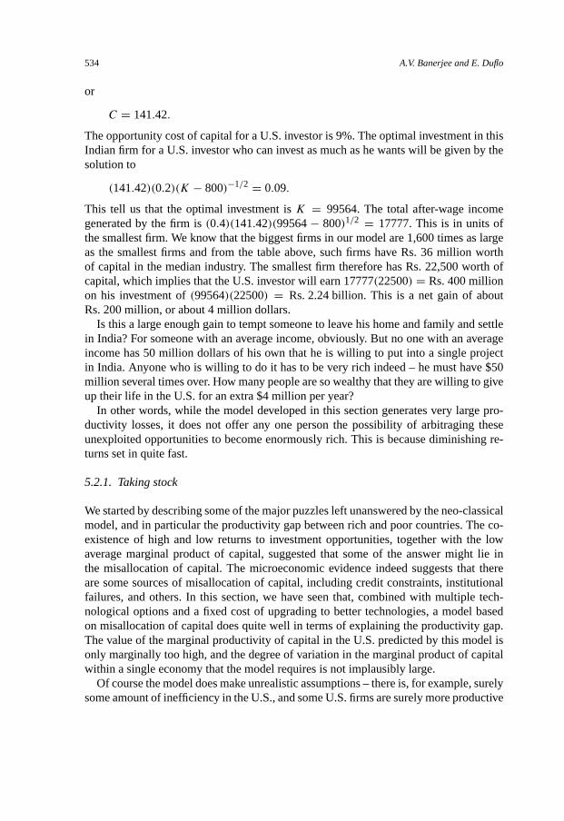
534 A.V. Banerjee and E. Duflo
or
C = 141.42.
The opportunity cost of capital for a U.S. investor is 9%. The optimal investment in thisIndian firm for a U.S. investor who can invest as much as he wants will be given by thesolution to
(141.42)(0.2)(K − 800)−1/2 = 0.09.
This tell us that the optimal investment is K = 99564. The total after-wage incomegenerated by the firm is (0.4)(141.42)(99564 − 800)1/2 = 17777. This is in units ofthe smallest firm. We know that the biggest firms in our model are 1,600 times as largeas the smallest firms and from the table above, such firms have Rs. 36 million worthof capital in the median industry. The smallest firm therefore has Rs. 22,500 worth ofcapital, which implies that the U.S. investor will earn 17777(22500) = Rs. 400 millionon his investment of (99564)(22500) = Rs. 2.24 billion. This is a net gain of aboutRs. 200 million, or about 4 million dollars.
Is this a large enough gain to tempt someone to leave his home and family and settlein India? For someone with an average income, obviously. But no one with an averageincome has 50 million dollars of his own that he is willing to put into a single projectin India. Anyone who is willing to do it has to be very rich indeed – he must have $50million several times over. How many people are so wealthy that they are willing to giveup their life in the U.S. for an extra $4 million per year?
In other words, while the model developed in this section generates very large pro-ductivity losses, it does not offer any one person the possibility of arbitraging theseunexploited opportunities to become enormously rich. This is because diminishing re-turns set in quite fast.
5.2.1. Taking stock
We started by describing some of the major puzzles left unanswered by the neo-classicalmodel, and in particular the productivity gap between rich and poor countries. The co-existence of high and low returns to investment opportunities, together with the lowaverage marginal product of capital, suggested that some of the answer might lie inthe misallocation of capital. The microeconomic evidence indeed suggests that thereare some sources of misallocation of capital, including credit constraints, institutionalfailures, and others. In this section, we have seen that, combined with multiple tech-nological options and a fixed cost of upgrading to better technologies, a model basedon misallocation of capital does quite well in terms of explaining the productivity gap.The value of the marginal productivity of capital in the U.S. predicted by this model isonly marginally too high, and the degree of variation in the marginal product of capitalwithin a single economy that the model requires is not implausibly large.
Of course the model does make unrealistic assumptions – there is, for example, surelysome amount of inefficiency in the U.S., and some U.S. firms are surely more productive

Ch. 7: Growth Theory through the Lens of Development Economics 535
than others. On the other hand, we have also ignored many reasons why Indian firmsmay be less efficient than they are in our model. For example, our current model assumesthat only 10% of the firms, who use less than 1% of the capital stock and produce lessthan 1% of the output, use the least efficient technology whereas the MGI report on theapparel sector tells us that almost 55% of the output of the sector is produced by tailorswho still use primitive technology. We also assumed that 10% of Indian firms are asproductive as the best U.S. firms. Clearly that fraction could be smaller.
We also assumed that everyone is equally competent. In the real world, imperfectcredit markets, for example, drive down the opportunity cost of capital and this en-courages incompetent producers to stay in business. In the model, we assume that alllarge firms earn high returns but in reality there are probably some large firms that havemuch lower productivity (anywhere down to 9% per year would be consistent with ourmodel). This too will drive down productivity. In a recent paper, Caselli and Gennaioli(2002) try to calibrate the impact of this factor in the context of a dynamic model withcredit constraints. They show that in steady state this can generate productivity losses of20% or so. We will argue in the next section that this severely understates the potentialproductivity gap starting from an arbitrary allocation of capital.
6. Towards a non-aggregative growth theory
6.1. An illustration
The presumption of neo-classical growth theory was that being a citizen of a poor coun-try gives one access to many exciting investment opportunities, which eventually leadon to convergence. The point of the previous section was to argue that most citizens ofpoor countries are not in a position to enjoy most of these opportunities, either becausemarkets do not do what they ought to or the government does what it ought not to, orbecause people find it psychologically difficult to do what is expected of them.
What can we say about the long-run evolution of an economy where there are re-warding opportunities that are not necessarily exploited? In this section we will explorethis question under the assumption that the only source of inefficiency in this econ-omy comes from limited access to credit. The goal is to illustrate what non-aggregativegrowth theory might look like, rather than to suggest an alternative canonical model.
The model we have in mind is as follows: There are individual production functionsassociated with every participant in this economy that are assumed to be identical anda function of capital alone (F (K)) but otherwise quite general. In particular, we doassume that they are concave. Individuals maximize an intertemporal utility function ofthe form:
∞∑t=0
δtU(Ct ), 0 < δ < 1,
U(Ct ) = c1−φ
1 − φ, φ > 0.

536 A.V. Banerjee and E. Duflo
People are forward-looking and at each point of time they choose consumption andsavings to maximize lifetime utility. However, the maximum amount they can borrowis linear and increasing in their wealth and decreasing in the current interest rate: Anindividual with wealth w can borrow up to λ(rt )w. Credit comes from other membersof the same economy and the interest rate clears the credit market. We do not assumethat everyone starts with the same wealth, but rather that at each point of time there is adistribution of wealth that evolves over time.
This model is a straightforward generalization of the standard growth model. Whatit tells us about the evolution of the income distribution and efficiency depends, notsurprisingly, on the shape of the production function.
The simplest case is that of constant returns in production. In this case, inequalityremains unchanged over time, and production and investment is always efficient.
With diminishing returns, greater inequality can lead to less investment and lessgrowth, because the production function is concave. However, inequality falls over timeand in the long run no one is credit constrained, although we do not necessarily getfull wealth convergence. The long run interest rate converges to its first best level, andhence investment is efficient. To see why this must be the case, note first that becauseof diminishing returns the poor always have more to gain from borrowing and investingthan the rich. In other words, the rich must be lending to the poor. As long as the poorare credit constrained, they will earn higher returns on the marginal dollar than theirlenders, i.e., the rich (that is what it means to be credit constrained). As a result, theywill accumulate wealth faster than the rich and we will see convergence. This processwill only stop when the poor are no longer credit constrained, i.e., they are rich enoughto be able to invest as much as they want.
With increasing returns, inequality increases over time; we converge to a Gini coeffi-cient of 1. Wealth becomes more and more concentrated with only the richest borrowingand investing. Because there are increasing returns, this is also the first best outcome.The logic of this result is very similar to the previous one: Now it is the rich who will beborrowing and the poor who will be lending, with the implication that the rich are theones who are credit constrained and the ones earning high marginal returns. Therefore,they will accumulate wealth faster and wealth becomes increasingly concentrated.
Finally we consider the case of “S-shaped” production functions, which are produc-tion functions that are initially convex and then concave. The Cobb–Douglas with aninitial set-up cost discussed at length in Section 5.2 is a special case of this kind oftechnology.
What happens in the long run in this model depends on the initial distribution of in-come. When the distribution is such that most people in the economy can afford to investin the concave part of the production function, the economy converges to a situation thatis isomorphic to the diminishing returns case, with the entire population “escaping” theconvex region of the production function.
The more unusual case is the one where some people start too poor to invest in theconcave region of the production function. The poorer among such people will earnvery low returns if they were to invest and therefore will prefer to be lenders. Now, as

Ch. 7: Growth Theory through the Lens of Development Economics 537
long as the interest rate on savings is less than 1/δ, they will decumulate capital (sincethe interest is less than the discount factor) and eventually their wealth will go to zero.On the other hand, anyone in this economy who started rich enough to want to borrowwill stay rich, even though they are also dissaving, in part because at the same time theybenefit from the low interest rates. The economy will converge to a steady state wherethe interest rate is 1/δ, those who started rich continue to be rich and those who startedpoor remain poor (in fact have zero wealth).
This is classic poverty trap: Moreover, since no one escapes from poverty, nor fallsinto it, there is a continuum of such poverty traps in this model. This kind of multiplicityis, however, fragile with respect to the introduction of random shocks that allow someof the poor to escape poverty and impoverish some of the rich.
Even in a world with such shocks there can be more than one steady state: The reasonis that the presence of lots of poor people drives down interest rates, and low interestrates make it harder for the poor to save up to escape poverty even with the help of apositive shock. As a result, in an economy that starts with lots of poor people, a greaterfraction of people may remain poor.
The key to this multiplicity is the endogeneity of the interest rate. It is the pecuniaryexternality that the poor inflict on other poor people that sustains it. This is why suchpoverty traps are sometimes called collective poverty traps, in contrast to the individualpoverty traps described above.
The investigation of the evolution of income distribution in models with creditconstraints and endogenous interest rates goes back to Aghion and Bolton (1997).Matsuyama (2000, 2003) and Piketty (1997) emphasize the potential for collectivepoverty traps in a variant of this model, without the forward-looking savings deci-sions.
This class of models is a part of a broader group of models which study the simulta-neous evolution of the occupational structure, factor prices and the wealth distributionin a model with credit constraints. Loury (1981) studied this class of models and showedthat in the long run the neo-classical predictions tend to hold as long as the productionfunction is concave. Dasgupta and Ray (1986) and Galor and Zeira (1993) provide ex-amples of individual poverty traps in the presence of credit constraints and S-shapedproduction functions. Banerjee and Newman (1993) show the possibility of a collectivepoverty trap in a model with a S-shaped production function which is driven by the en-dogeneity of the wage – essentially high wages allow workers to become entrepreneurseasily, which keeps the demand for labor, and hence wages, high. Recent work by Buera(2003) shows that the multiplicity results in Banerjee and Newman survive in an envi-ronment where savings is based on expectations of future returns.40 Ghatak, Morelliand Sjostrom (2001, 2002) and Mookherjee and Ray (2002, 2003) explore related butslightly different sources of individual and collective poverty traps.
40 On the possibility of collective poverty traps, see also Lloyd-Ellis and Bernhardt (2000), and Mookherjeeand Ray (2002, 2003).

538 A.V. Banerjee and E. Duflo
6.2. Can we take this model to the data?
Models like the one we just developed (as well as political economy models that we donot discuss here41) have been invoked as motivation for a large empirical literature onthe relationship between inequality and growth in cross-country data. In 1996, Benaboucited 16 studies on the question, and the number has been growing rapidly since then,in part due to the availability of more complete data sets, due to the effort of Deiningerand Squire [see Deininger and Squire (1996)], expanded by the World Institute for De-velopment Economics Research (WIDER). However, it is not clear that if we were totake this class of models seriously, they would justify estimating relationships like theones that are in the literature: First because the exact form of the predicted relationshipbetween inequality and growth depends on the shape of the production function. Im-posing the assumption that there are diminishing returns helps in this respect, but withthis assumption functional form issues loom large. Finally, it is not clear how, given themodel’s structure, we can avoid running into serious identification problems.
In this section, we evaluate whether, given these concerns, estimating the relationshipbetween inequality and growth in a cross-country data set remains useful. Having con-cluded that it has, at best, very limited use, we discuss an alternative approach based oncalibrating non-aggregative models using micro data.
6.2.1. What are the empirical implications of the above model?
Functional form issues With constant returns to scale, distribution is irrelevant forgrowth. With diminishing returns, an exogenous mean-preserving spread in the wealthdistribution in this economy will reduce future wealth and, by implication, the growthrate. However, the impact depends on the level of wealth in the economy: Once theeconomy is rich enough that everyone can afford the optimal level of investment, in-equality should not matter. The estimated relationship between inequality and growthshould therefore allow for an interaction term between inequality and mean income.Moreover, an economy closer to the steady state has both lower inequality and lowergrowth. This has two implications for the estimation of the inequality growth relation-ship. First, the fact that the economy becomes more equal as it grows tends to generatea spurious positive relation between growth and inequality, both in the cross-section aswell as in time-series. As a result, both the cross-sectional and the first differenced (orfixed effects) estimates of the effect of inequality on growth run the risk of being biasedupwards, compared to the true negative relation that we might have found if we hadcompared economies at the same mean wealth levels. Moreover, consider a variant ofthe model where there are occasional shocks that increase inequality. Since the natural
41 See Alesina and Rodrik (1994), Persson and Tabellini (1991) and Benhabib and Rustichini (1998). For acontrary point of view, arguing that the premise of the political economy model argument does not hold truein the data, see Benabou (1996).

Ch. 7: Growth Theory through the Lens of Development Economics 539
tendency of the economy is towards convergence, we should expect to see two types ofchanges in inequality: Exogenous shocks that increase inequality and therefore reducegrowth, and endogenous reductions in inequality that are also associated with a fall inthe growth rate. In other words, measured changes in inequality in either direction willbe associated with a fall in growth.
Controlling properly for the effect of mean wealth (or mean income), is therefore vitalfor getting meaningful results. The usual procedure is to control linearly (as in mostother growth regressions) for the mean income level at the beginning of the period. Itis, however, not clear that there is any good reason why the true effect should be linear.Moreover, it seems plausible that different economies will typically have different λs,and therefore will converge at different rates.
The model also tells us that while initial distribution matters for the growth rate, itonly matters in the short run. Over a long enough period, two economies starting at thesame mean wealth level will exhibit the same average growth rate. In other words, thelength of the time period over which growth is measured will affect the strength of therelationship between inequality and growth.
The preceding discussion assumed that the interest rates converged. As we noted,that does not need to be the case. If we do not assume it, variants of the simple concaveeconomy may no longer converge, even in the weaker sense of the long-run mean wealthbeing independent of the initial distribution of wealth. Intuitively, poor economies willtend to have high interest rates, and this in turn will make capital accumulation difficult(note that λ′ < 0) and tend to keep the economy poor.42 This effect reinforces the claimmade above that inequality matters most in the poorest economies.43 This economy canhave a number of distinct steady states that are each locally isolated. This means thatsmall changes in inequality can cause the economy to move towards a different andfurther away steady state, making it more likely that the relationship will be non-linear.
With increasing returns, growth rates increase with a mean preserving spread inincome. As the economy grows, it also becomes more unequal. Interpreting the relation-ship between inequality and growth is difficult even after controlling for convergence.
In the S-shaped returns case, the relationship between inequality and growth can benegative or positive depending on the initial distribution, and the size of the increase.For example, if everybody is very poor (on the left of the convex zone), a small increasein inequality will reduce growth, but increasing inequality enough may push more peo-ple to the point where they are able to take advantage of the more efficient technology,and increases in inequality will increase growth. The relation between inequality and
42 See Piketty (1997). For a more general discussion of the issue of convergence in this class of models, seeBanerjee and Newman (1993).43 There is, however, a counteracting effect: Poorer economies with high levels of inequality may actuallyhave low interest rates because a few people may own more wealth than they can invest in their own firms,and the rest may be too poor to borrow. For a model where this effect plays an important role, see Aghion andBolton (1997).

540 A.V. Banerjee and E. Duflo
growth delivered by this model is clearly non-monotonic. Moreover, the strong conver-gence property does not hold in general. In other words, the growth rate of wealth mayjump up once the economy is rich enough, with the obvious implication that economieswith higher mean wealth will not necessarily grow more slowly. In other words, theeffect of mean wealth, that is the so-called convergence effect, may not be monotonic inthis economy. Linearly controlling for mean wealth therefore does not guarantee that wewill get the correct estimate of the effect of inequality. It is worth noting that this econ-omy will have a connected continuum of steady states. This means that after a shockthe economy will not typically return to the same steady state. However, since it doesconverge to a nearby steady state, this is not an additional source of non-linearity.
Identification issues Even if we could agree on a specification that is worth estimating,it is not clear how we can use cross-country data to estimate it. Countries, like individ-uals, are different from each other. Even in a world of perfect capital markets, countriescan have very different distributions of wealth because, for example, they have differentdistributions of ability. There is no causal effect of inequality on growth in this case, butthey could be correlated for other reasons. For example, cultural structures (such as acaste system) may restrict occupational choices and therefore may not allow individu-als to make proper use of their talents, causing both higher inequality and lower growth.Conversely, if countries use technologies that are differently intensive in skilled labor,those countries using the more skill intensive technology can have both more inequalityand faster growth.
As we discussed in detail above, countries have different kinds of financial institu-tions, implying differences in the λ’s in our model. Our basic model would predict thatthe country with the better capital markets is likely both to be more equal and to growfaster (at least once we control for the mean level of income). The correlation betweeninequality and growth will therefore be a downwards-biased estimate of the causal pa-rameter, if the quality of financial institutions differs across countries.44
If these country specific effects were additive, one could control for them by includ-ing a country fixed-effect in the estimated relationship (or by estimating the model infirst difference). This strategy will be valid only under the assumption that changes ininequality are unrelated to unobservable country characteristics that are correlated withchanges in the growth rate. While this is a convenient assumption, it has no reason tohold in general. For example, skill-biased technological progress will lead both to achange in inequality and a change in growth rates, causing a spurious positive corre-lation between the two. To make matters worse, we have to recognize the fact that λ
itself (and therefore the effect of inequality on growth at a given point in time) may be
44 Allowing λ to vary also implies that the causal effects of inequality will vary with financial development(which is how Barro (2000) explains his results). The OLS coefficient is therefore a weighted average ofdifferent parameters, where the weights are the country-specific contributions to the overall variance in in-equality [Krueger and Lindahl (2001)]. It is not at all clear that we are particularly interested in this set ofweights.

Ch. 7: Growth Theory through the Lens of Development Economics 541
varying over time as a result of monetary policies or financial development, and mayitself be endogenous to the growth process.45
The more general point that comes out of the discussion above is that unless we as-sume capital markets are extremely efficient (which, in any case, removes one of theimportant sources of the effect of inequality), changes in inequality will be partly en-dogenous and related to country characteristics which are themselves related to changesin the growth rate. Identifying the effect of inequality by including a country fixed-effectwould not necessarily solve all the endogeneity problems. Moreover, as we discussedabove, the theory suggests that the specification should allow for non-linear functionalforms, and interaction effects, which will be difficult to accommodate with a fixed effectspecification.
6.2.2. Empirical evidence
The preceding discussion suggests that empirical exercises using aggregate, cross-country data to estimate the impact of inequality and growth will be extremely difficultto interpret. The results are also likely to be sensitive to the choice of specification.This may explain the variety of results present in the literature. A long literature [seeBenabou (1996) for a survey] estimated a long run equation, with growth between 1990and 1960 (say) regressed on income in 1960, a set of control variables, and inequality in1960. Estimating these equations tended to generate negative coefficients for inequality.As the discussion in the previous subsection suggests, there are many reasons to thinkthat this relationship may be biased upward or downwards. To address this problem,Li and Zou (1998) and Forbes (2000) used the Deininger and Squire data set to focuson the impact of inequality on short run (5 years) growth, and introduced a linear fixedeffect.46 The results change rather dramatically: The coefficient of inequality in thisspecification is positive, and significant. Finally, Barro (2000) used the same short fre-quency data (he is focusing on ten-year intervals), but does not introduce a fixed effect.He finds that inequality is negatively associated with growth in the poorer countries, andpositively in rich countries.
Banerjee and Duflo (2003) investigate whether there is any reason to worry about thenon-linearities that the theory suggests should be present. They find that when growth(or changes in growth) is regressed non-parametrically on changes in inequality, therelationship is an inverted U-shape. There is also a non-linear relationship between pastinequality and the magnitudes of changes in inequality. Finally, there seems to be anegative relationship between growth rates and inequality lagged one period. These factstaken together, and in particular the non-linearities in these relationships (rather than the
45 See Acemoglu and Zilibotti (1997), and Greenwood and Jovanovic (1999), for theories of growth withendogenous financial development.46 Forbes (2000) also corrects for the bias introduced by introducing a lagged variable in a fixed effect spec-ification by using the GMM estimator developed by Arellano and Bond (1991).

542 A.V. Banerjee and E. Duflo
variation in samples or control variables), account for the different results obtained bydifferent authors using different specifications.
Townsend and Ueda (2003) illustrate very clearly that this diversity of results is likelyto come from the functional form and identification problems we just discussed. Theysimulate the 30 year evolution for 1,000 economies based on a model similar to theones we describe in this section, with non-linear individual production function andcredit constraints. The economies start in 1976, with a distribution of wealth calibratedto match the Thai economy in the same year. They then introduce aggregate and indi-vidual level shocks, and run regressions similar to the regressions run in the literature.Using the 1985 year as the “base year”, they replicate the findings of the long run re-gressions. Using 1980 as the base year, they do not replicate those results. A regressionsimilar to that of Forbes (2000) finds either a positive or negative relationship, depend-ing on sampling decisions. This exercise clearly shows that aggregate cross-countryregressions are the wrong tool to evaluate the pertinence of this class of models.
6.3. Where do we go from here?
The discussion on functional form and identification, coupled with the empirical ev-idence of non-linearities even in very simple exercises, suggests that cross-countryregressions are unlikely to be able to shed any meaningful light on the empirical rel-evance of models that integrate credit constraints and other imperfections of the creditmarkets. This is made worse by the poor quality of the aggregate data, despite the con-siderable efforts to produce consistent and reliable data sets. This contrasts with theincreased availability of large, good quality, micro-economic data sets, which allow fortesting specific hypotheses and derive credible identifying restrictions from theory andexogenous sources of variation. Throughout this chapter, we quoted many studies usingmicro-economic data which tested the micro-foundations for the models we discussedin this section.
Even a series of convincing micro-empirical studies will not be enough to give us anoverall sense of how, together, they generate aggregate growth, the dynamics of incomedistribution, and the complex relationships between the two. The lessons of develop-ment economics will be lost to growth if they are not brought together in an aggregatecontext. In other words, it is not enough to use them to loosely motivate cross-sectionalgrowth regression exercises – the discussion in this section is but an example of themisleading conclusions to which this can lead.
An alternative that seems likely to be much more fruitful is to try to build macroeco-nomic models that incorporate the features we discussed, and to use the results fromthe microeconomic studies as parameters in calibration exercises. The exercise we per-formed in Section 5 of this chapter is an illustration of the kind of work that we canhope to do. There are a number of recent papers that in some ways go further in thisdirection than we have gone. In particular, Quadrini (1999) and Cagetti and De Nardi(2003), for the U.S., and Paulson and Townsend (2004), for Thailand, try to calibratea model with credit constraints to understand the correlation between wealth and the

Ch. 7: Growth Theory through the Lens of Development Economics 543
probability of becoming an entrepreneur. The paper by Buera (2003), mentioned above,emphasizes the fact that the long run correlation between wealth and entrepreneurshipis weaker than the short run correlation, because, as noted by Skiba (1978), Deaton(1992), Aiyagari (1994) and Carroll (1997), those who are credit constrained now butwant to invest in the future have a very strong incentive to save. This, Buera points out,reduces the ultimate efficiency cost of imperfect credit markets, though in spite of this,the person with the median ability level and the median starting wealth loses about 18%of lifetime welfare because of the credit constraints. Caselli and Gennaioli (2002) offera slightly different calibration: Like Buera, they are worried about the fact that withcredit constraints the biggest firms may not be run by the best entrepreneurs. This canbe a source of very large productivity losses in the short run. However, since the bestentrepreneurs will make the most money, in the long run their firms would necessarilybecome the largest, unless they died young. They show that even with this limiting fac-tor, reasonable death rates would imply a 20% loss of productivity when we comparean economy without credit constraints with one that has them.
The calibrations so far have not attempted to see if the path of wealth distributionthat results from calibrating this type of model matches the data. Our exercise above,for example, tries to match the distribution of firm sizes at a point of time, but saysnothing about the path, while Buera does not try to match the data. The one exceptionis the papers by Robert Townsend and his collaborators based on Thai data [Jeong andTownsend (2003), Townsend and Ueda (2003)].
These papers, as well as those mentioned in the previous paragraphs, start from theassumption that every firm has a single, usually strictly concave, production technol-ogy. The only fixed cost comes from the fact that the firm needs an entrepreneur. As wesaw above, this model does not do very well in terms of explaining the cross-sectionalvariation in the firm sector or the overall productivity gap, as compared to a model witha small number of alternative technologies and varying fixed costs. More generally, weneed both a better empirical understanding of where the most important sources of inef-ficiency lie and better integration of this understanding when we assess the predictionsof growth theory.
And perhaps above all, we need better growth theory: Our exercise at the beginningof this section was intended to advertise the possibility of a growth theory that does notassume aggregation. While we attempted to link the results to some relatively generalproperties of the production function, our analysis relies heavily on the fact that the in-efficiency we assumed was in the credit market and that this took the form of a creditlimit that was linear in wealth. One can easily imagine other ways for the credit marketto be imperfect and other results from such models. Moreover, while the class of pro-duction technologies covered by our model was broader than usual, it does not includethe (multiple-fixed-cost) technology that the previous section advocates.
There are, of course, other types of non-aggregative models: There are some exam-ples of non-aggregative growth models that build on the inefficiency that comes from

544 A.V. Banerjee and E. Duflo
poorly functioning insurance markets.47 There are also interesting attempts to buildgrowth models that emphasize the fact that some people are favored by the govern-ment while others are not, and especially the fact that this changes over time in somepredictable way (see Roland Benabou’s contribution to this volume). Some interestingrecent work has been done on the dynamic interplay between growth and political insti-tutions (see the chapter by Acemoglu, Johnson and Robinson in this volume) as well asbetween growth and social institutions [see Oded Galor’s contribution to this volume,as well as Cole, Mailath and Postlewaite (1992, 1998, 2001)]. However, even more thanin the case of the literature on credit markets and growth, it is not clear how much theinsights from these models rely on specific details of how the environment or the im-perfection was modeled and to what extent they can be seen as robust properties of thisentire class of models.
There are also areas where growth theory has not really reached: We have no modelsthat, for example, incorporate reputation-building or learning into growth theory. Thesame can be said about the entire class of behavioral models of underinvestment.
Finally, there is the open question of whether we gain anything by building grandmodels that incorporate all these different reasons for inefficiency in a single model. Toanswer this we would need to assess whether the fact that different forms of inefficiencyinteract with each other has empirically important consequences.
This is an exciting time to think about growth. We are beginning to see the contoursof a new vision, both more rooted in evidence and more ambitious in its theorizing.
Acknowledgements
The authors are grateful to Pranab Bardhan, Michael Kremer, Rohini Pande, ChrisUdry and Ivan Werning for helpful conversations and Philippe Aghion and Seema Jay-achandran for detailed comments. A part of this material was presented as the KuznetsMemorial Lecture, 2004, at Yale University. We are grateful for the many commentsthat we received from the audience.
References
Acemoglu, D., Angrist, J. (2001). “How large are human-capital externalities? Evidence from compulsoryschooling laws”. In: Bernanke, B., Rogoff, K. (Eds.), NBER Macroeconomics Annual 2000, vol. 15. MITPress, Cambridge and London, pp. 9–59.
Acemoglu, D., Johnson, S., Robinson, J. (2001). “The colonial origins of comparative development: An em-pirical investigation”. American Economic Review 91 (5), 1369–1401.
47 See Banerjee and Newman (1991) for a theoretical model of non-aggregative growth based on imperfectinsurance markets. Deaton and Paxson (1994) investigate some of empirical implications of this type of modelusing Taiwanese data. Krussel and Smith (1998) and Angeletos and Calvet (2003) are attempts to calibratethe impact of imperfect insurance on welfare and growth.

Ch. 7: Growth Theory through the Lens of Development Economics 545
Acemoglu, D., Zilibotti, F. (1997). “Was Prometheus unbound by chance? Risk, diversification, and growth”.Journal of Political Economy 105 (4), 709–751.
Acemoglu, D., Zilibotti, F. (2001). “Productivity differences”. Quarterly Journal of Economics 116 (2), 563–606.
Aghion, P., Bolton, P. (1997). “A trickle-down theory of growth and development with debt overhang”. Reviewof Economic Studies 64 (2), 151–172.
Aghion, P., Howitt, P. (1992). “A model of growth through creative destruction”. Econometrica 60 (2), 323–351.
Aghion, P., Howitt, P., Mayer-Foulkes, D. (2004). “The effect of financial development on convergence: The-ory and evidence”. Working Paper 10358, National Bureau of Economic Research.
Aiyagari, S.R. (1994). “Uninsured idiosyncratic risk and aggregate saving”. Quarterly Journal of Eco-nomics 109, 569–684.
Aleem, I. (1990). “Imperfect information, screening and the costs of informal lending: A study of a ruralcredit market in Pakistan”. World Bank Economic Review 3, 329–349.
Alesina, A., Rodrik, D. (1994). “Distributive politics and economic growth”. Quarterly Journal of Eco-nomics 109 (2), 465–490.
Anderson, S., Baland, J.-M. (2002). “The economics of ROSCAs and intrahousehold resource allocation”.Quarterly Journal of Economics 117 (3), 963–995.
Angeletos, G.-M., Calvet, L. (2003). “Idiosyncratic production risk, growth and the business cycle”. Mimeo,MIT.
Aportela, F. (1998). “The effects of financial access on savings by low-income people”. Mimeo, MIT.Arellano, M., Bond, S. (1991). “Some tests of specification for panel data: Monte Carlo evidence and an
application to employment equations”. Review of Economic Studies 58 (2), 277–297.Ashraf, N., Karlan, D.S., Yin, W. (2004). “Tying Odysseus to the mast: Evidence from a commitment savings
product in the Philippines”. Mimeo, Harvard University.Banerjee, A.V. (1992). “A simple model of herd behavior”. Quarterly Journal of Economics 117 (3), 797–817.Banerjee, A.V. (2003). “Contracting constraints, credit markets and economic development”. In: Hansen, L.,
Dewatripont, M., Turnovsky, S. (Eds.), Advances in Economics and Econometrics: Theory and Applica-tions, Eighth World Congress, vol. III. Cambridge University Press.
Banerjee, A.V. (2004). “Educational policy and the economics of the family”. Journal of Development Eco-nomics 74 (1), 3–32.
Banerjee, A.V. (2005). “The two poverties”. In: Dercan, S. (Ed.), Insurance Against Poverty. Oxford Univer-sity Press, pp. 59–75.
Banerjee, A.V., Duflo, E. (2000). “Reputation effects and the limits of contracting: A study of the Indiansoftware industry”. Quarterly Journal of Economics 115 (3), 989–1017.
Banerjee, A.V., Duflo, E. (2003). “Inequality and growth: What can the data say?”. Journal of EconomicGrowth 8, 267–299.
Banerjee, A.V., Duflo, E. (2004). “Do firms want to borrow more? Testing credit constraints using a directedlending program”. Mimeo, MIT. Also BREAD WP 2003-5, 2003.
Banerjee, A.V., Duflo, E., Munshi, K. (2003). “The (mis)allocation of capital”. Journal of the European Eco-nomic Association 1 (2–3), 484–494.
Banerjee, A.V., Gertler, P., Ghatak, M. (2002). “Empowerment and efficiency: Tenancy reform in West Ben-gal”. Journal of Political Economy 110 (2), 239–280.
Banerjee, A.V., Munshi, K. (2004). “How efficiently is capital allocated? Evidence from the knitted garmentindustry in Tirupur”. Review of Economic Studies 71 (1), 19–42.
Banerjee, A.V., Newman, A. (1991). “Risk bearing and the theory of income distribution”. Review of Eco-nomic Studies 58 (2), 211–235.
Banerjee, A.V., Newman, A. (1993). “Occupational choice and the process of development”. Journal of Po-litical Economy 101 (2), 274–298.
Bardhan, P. (1969). “Equilibrium growth in a model with economic obsolescence of machines”. QuarterlyJournal of Economics 83 (2), 312–323.

546 A.V. Banerjee and E. Duflo
Bardhan, P., Udry, C. (1999). Development Microeconomics. Oxford University Press, Oxford, New York.Barro, R.J. (1974). “Are government bonds net wealth?”. Journal of Political Economy 82 (6), 1095–1117.Barro, R.J. (1991). “Economic growth in a cross section of countries”. Quarterly Journal of Economics 106
(2), 407–443.Barro, R.J. (2000). “Inequality and growth in a panel of countries”. Journal of Economic Growth 5 (1), 5–32.Barro, R.J., Lee, J.-W. (2000). “International data on educational attainment updates and implications”. Work-
ing Paper 7911, National Bureau of Economic Research, September.Barro, R.J., Sala-i-Martin, X. (1995). Economic Growth. McGraw-Hill, New York.Basta, S.S., Soekirman, D.S., Karyadi, D., Scrimshaw, N.S. (1979). “Iron deficiency anemia and the produc-
tivity of adult males in Indonesia”. American Journal of Clinical Nutrition 32 (4), 916–925.Becker, G. (1981). A Treatise on the Family. Harvard University Press, Cambridge, MA.Benabou, R. (1996). “Inequality and growth”. In: Bernanke, B., Rotemberg, J.J. (Eds.), NBER Macroeco-
nomics Annual 1996. MIT Press, Cambridge and London, pp. 11–73.Benhabib, J., Rustichini, A. (1998). “Social conflict and growth”. Journal of Economic Growth 1 (1), 143–
158.Benhabib, J., Spiegel, M.M. (1994). “The role of human capital in economic development: Evidence from
aggregate cross-country data”. Journal of Monetary Economics 34 (2), 143–174.Bennell, P. (1996). “Rates of return to education: Does the conventional pattern prevail in sub-Saharan
Africa?”. World Development 24 (1), 183–199.Bertrand, M., Karlan, D., Mullainathan, S., Zinman, J. (2004). “Pricing psychology.” Mimeo, Harvard Uni-
versity.Besley, T. (1995). “Savings, credit and insurance”. In: Behrman, J., Srinivasan, T.N. (Eds.), Handbook of
Development Economics, vol. 3A. Elsevier Science, Amsterdam, pp. 2123–2207. Chapter 6.Besley, T., Case, A. (1994). “Diffusion as a learning process: Evidence from HYV cotton”. Discussion Paper
174, RPDS, Princeton University.Bigsten, A., Isaksson, A., Soderbom, M., Collier, P. (2000). “Rates of return on physical and human capital
in Africa’s manufacturing sector”. Economic Development and Cultural Change 48 (4), 801–827.Bikhchandani, S., Hirshleifer, D., Welch, I. (1992). “A theory of fads, fashion, custom, and cultural change as
informational cascades”. Journal of Political Economy 100 (5), 992–1026.Bils, M., Klenow, P. (2000). “Does schooling cause growth?”. American Economic Review 90 (5), 1160–
1183.Binswanger, H., Rosenzweig, M. (1986). “Behavioural and material determinants of production relations in
agriculture”. Journal of Development Studies 22 (3), 503–539.Blanchflower, D., Oswald, A. (1998). “What makes an entrepreneur?”. Journal of Labor Economics 16 (1),
26–60.Bottomley, A. (1963). “The cost of administering private loans in underdeveloped rural areas”. Oxford Eco-
nomic Papers 15 (2), 154–163.Bourguignon, F., Chiappori, P.-A. (1992). “Collective models of household behavior”. European Economic
Review 36, 355–364.Buera, F. (2003). “A dynamic model of entrepreneurship with borrowing constraints”. Mimeo, University of
Chicago.Cagetti, M., De Nardi, M. (2003). “Entrepreneurship, frictions and wealth”. Staff Report 324, Federal Reserve
Bank of Minneapolis.Carroll, C. (1997). “Buffer-stock saving and the life cycle/permanent income hypothesis”. Quarterly Journal
of Economics 112, 1–56.Carvalho, I. (2000). “Household income as a determinant of child labor and school enrollment in Brazil:
Evidence from a social security reform”. Mimeo, MIT.Case, A., Lin, I.-F., McLanahan, S. (2000). “How hungry is the selfish gene?”. Economic Journal 110 (466),
781–804.Case, A., Paxson, C. (2001). “Mothers and others: Who invests in children’s health?”. Journal of Health
Economics 20 (3), 301–328.

Ch. 7: Growth Theory through the Lens of Development Economics 547
Case, A., Paxson, C., Ableidinger, J. (2002). “Orphans in Africa”. Working Paper 9213, National Bureau ofEconomic Research.
Caselli, F. (2005). “Accounting for cross-country income differences”. In: Aghion, P., Durlauf, S. (Eds.),Handbook of Economic Growth. Elsevier, Amsterdam.
Caselli, F., Gennaioli, N. (2002). “Dynastic management”. Mimeo, Harvard University.Caselli, F., Gennaioli, N. (2004). “Dynastic management, legal reform and regulatory reform”. Mimeo, Lon-
don School of Economics.Coate, S., Ravallion, M. (1993). “Reciprocity without commitment: Characterization and performance of
informal insurance arrangements”. Journal of Development Economics 40, 1–24.Cole, H., Mailath, G., Postlewaite, A. (1992). “Social norms, savings behavior and growth”. Journal of Polit-
ical Economy 100 (6), 1092–1126.Cole, H., Mailath, G., Postlewaite, A. (1998). “Class systems and the enforcement of social norms”. Journal
of Public Economics 70 (1), 5–35.Cole, H., Mailath, G., Postlewaite, A. (2001). “Investment and concern for relative position”. Review of
Economic Design 6, 241–261.Commission on Macroeconomics, and Health (2001). Macroeconomics and Health: Investing in Health for
Economic Development: Report. World Health Organization, Geneva.Conley, T., Udry, C. (2003). “Learning about a new technology: Pineapple in Ghana”. Mimeo, Northwestern
University.Dasgupta, A. (1989). Reports on Informal Credit Markets in India: Summary. National Institute of Public
Finance and Policy, New Delhi.Dasgupta, P., Ray, D. (1986). “Inequality as a determinant of malnutrition and unemployment: Theory”. The
Economic Journal 96 (384), 1011–1034.Deaton, A. (1992). Understanding Consumption. Oxford University Press, Oxford.Deaton, A. (1997). The Analysis of Household Surveys. World Bank, International Bank for Reconstruction
and Development.Deaton, A., Paxson, C. (1994). “Intertemporal choice and inequality”. Journal of Political Economy 1–2 (3),
437–467.Deininger, K., Squire, L. (1996). “A new data set measuring income inequality”. World Bank Economic
Review 10, 565–591.Djankov, S., La Porta, R., Lopez de Silanes, F., Shleifer, A. (2002). “The regulation of entry”. Quarterly
Journal of Economics 117 (1), 1–37.Djankov, S., La Porta, R., Lopez de Silanes, F., Shleifer, A. (2003). “Courts”. Quarterly Journal of Eco-
nomics 118 (2), 453–518.Do, T., Iyer, L. (2003). “Land rights and economic development: Evidence from Vietnam”. Mimeo, Harvard
Business School.Dreze, J., Kingdon, G.G. (2001). “School participation in rural India”. Review of Development Economics 5
(1), 1–24.Duflo, E. (2004). “The medium run effects of educational expansion: Evidence from a large school construc-
tion program in Indonesia”. Journal of Development Economics 74 (1), 163–197.Duflo, E. (2003). “Poor but rational”. Mimeo, MIT.Duflo, E., Kremer, M., Robinson, J. (2003). “Understanding technology adoption: Fertilizer in Western Kenya,
preliminary results from field experiments”. Mimeo, MIT.Durlauf, S. (1993). “Nonergodic economic growth”. Review of Economic Studies 60 (2), 349–366.Eaton, J., Kortum, S. (2001). “Trade in capital goods”. European Economic Review 45 (7), 1195–1235.Edmonds, E. (2004). “Does illiquidity alter child labor and schooling decisions? Evidence from household
responses to anticipated cash transfers in South Africa”. Working Paper 10265, National Bureau of Eco-nomic Research.
Ellison, G., Fudenberg, D. (1993). “Rules of thumbs for social learning”. Journal of Political Economy 101(4), 93–126.
Ellison, G., Glaeser, E. (1997). “Geographic concentration in U.S. manufacturing industries: A dartboardapproach”. Journal of Political Economy 105 (5), 889–927.
548 A.V. Banerjee and E. Duflo
Ellison, G., Glaeser, E. (1999). “Geographic concentration of industry: Does natural advantage explain ag-glomeration?”. American Economic Review 89 (2), 311–316.
Eswaran, M., Kotwal, A. (1985). “A theory of contractual structure in agriculture”. American EconomicReview 75 (3), 352–367.
Fafchamps, M. (2000). “Ethnicity and credit in African manufacturing”. Journal of Development Eco-nomics 61, 205–235.
Fafchamps, M., Lund, S. (2003). “Risk-sharing networks in rural Philippines”. Review of Economic Stud-ies 71 (2), 261–287.
Fazzari, S., Hubbard, G., Petersen, B. (1988). “Financing constraints and corporate investment”. BrookingsPapers on Economic Activity 0 (1), 141–195.
Forbes, K.J. (2000). “A reassessment of the relationship between inequality and growth”. American EconomicReview 90 (4), 869–887.
Foster, A.D., Rosenzweig, M.R. (1995). “Learning by doing and learning from others: Human capital andtechnical change in agriculture”. Journal of Political Economy 103 (6), 1176–1209.
Foster, A.D., Rosenzweig, M.R. (1996). “Technical change and human-capital returns and investments: Evi-dence from the green revolution”. American Economic Review 86 (4), 931–953.
Foster, A.D., Rosenzweig, M.R. (1999). “Missing women, the marriage market and economic growth”.Mimeo, University of Pennsylvania.
Foster, A.D., Rosenzweig, M. (2000). “Technological change and the distribution of schooling: Evidencefrom green revolution in India”. Mimeo, Brown University.
Freeman, R. (1986). “Demand for education”. In: Ashenfelter, O., Layard, A. (Eds.), Handbook of LaborEconomics, vol. 1. Elsevier, Amsterdam. Chapter 6.
Freeman, R., Oostendorp, R. (2001). “The occupational wages around the world data file”. InternationalLabour Review 140 (4), 379–401.
Galor, O., Zeira, J. (1993). “Income distribution and macroeconomics”. Review of Economic Studies 60 (1),35–52.
Gelos, R.G., Werner, A. (2002). “Financial liberalization, credit constraints, and collateral: Investment in theMexican manufacturing sector”. Journal of Development Economics 67 (1), 1–27.
Gertler, P., Gruber, J. (2002). “Insuring consumption against illness”. American Economic Review 92 (1),51–76.
Gertler, P.J., Boyce, S. (2002). “An experiment in incentive-based welfare: The impact of PROGESA onhealth in Mexico”. Mimeo, University of California, Berkeley.
Ghatak, M., Morelli, M., Sjostrom, T. (2001). “Occupational choice and dynamic incentives”. Review ofEconomic Studies 68 (4), 781–810.
Ghatak, M., Morelli, M., Sjostrom, T. (2002). “Credit rationing, wealth inequality, and allocation of talent”.Mimeo, London School of Economics.
Ghate, P. (1992). Informal Finance: Some Findings from Asia. Oxford University Press for the Asian Devel-opment Bank, Oxford.
Goldstein, M., Udry, C. (1999). “Agricultural innovation and resource management in Ghana”. Mimeo, YaleUniversity. Final Report to IFPRI under MP17.
Goldstein, M., Udry, C. (2002). “Gender, land rights and agriculture in Ghana”. Mimeo, Yale University.Greenwood, J., Jovanovic, B. (1999). “The information technology revolution and the stock market”. Ameri-
can Economic Review 89 (2), 116–122.Grossman, G., Helpman, E. (1991). Innovation and Growth in the Global Economy. MIT Press, Cambridge,
MA.Gugerty, M.K. (2000). “You can’t save alone: Testing theories of rotating savings and credit associations”.
Mimeo, Harvard University.Hart, O., Moore, J. (1994). “A theory of debt based on inalienability of human capital”. Quarterly Journal of
Economics 109, 841–879.Heston, A., Summers, R., Aten, B. (2002). “Penn World Table version 6.1”. Technical Report, Center for
International Comparisons at the University of Pennsylvania.

Ch. 7: Growth Theory through the Lens of Development Economics 549
Hoff, K., Stiglitz, J. (1998). “Moneylenders and bankers: Price-increasing subsidies in a monopolisticallycompetitive market”. Journal of Development Economics 55 (2), 485–518.
Howitt, P., Mayer, D. (2002). “R&D, implementation and stagnation: A Schumpeterian theory of convergenceclubs.” Working Paper 9104, National Bureau of Economic Research.
Hsieh, C.-T. (1999). “Productivity growth and factor prices in East Asia”. American Economic Review 89(2), 133–138.
Hsieh, C.-T., Klenow, P.J. (2003). “Relative prices and relative prosperity”. Mimeo, University of California,Berkeley.
Jacoby, H. (2002). “Is there an intrahousehold flypaper effect? Evidence from a school feeding program”.Economic Journal 112 (476), 196–221.
Jeong H., Townsend R. (2003). “Growth and inequality: Model evaluation based on an estimation-calibrationstrategy”. Mimeo, University of Southern California.
Johnson, S., McMillan, J., Woodruff, C. (2002). “Property rights and finance”. American Economic Review 92(5), 1335–1356.
Jovanovic, B., Rob, R. (1997). “Solow vs. Solow: Machine prices and development”. Working Paper 5871,National Bureau of Economic Research.
Jovanovic, B., Rousseau, P. (2003). “Specific capital and the division of rents”. Mimeo, New York University.Kanbur, R. (1979). “Of risk taking and the personal distribution of income”. Journal of Political Economy 87,
769–797.Karlan, D. (2003). “Using experimental economics to measure social capital and predict financial decisions”.
Mimeo, Princeton University.Kihlstrom, R., Laffont, J. (1979). “A general equilibrium entrepreneurial theory of firm formation based on
risk aversion”. Journal of Political Economy 87, 719–748.Klenow, P.J., Rodriguez-Clare, A. (1997). “The neoclassical revival in growth economics: Has it gone too
far?”. In: Bernanke, B., Rotemberg, J.J. (Eds.), NBER Macroeconomics Annual 1997. MIT Press.Knack, S., Keefer, P. (1995). “Institutions and economic performance: Cross-country tests using alternative
institutional measures”. Economics and Politics 7 (3), 207–227.Kremer, M., Miguel, E. (2003). “The illusion of sustainability”. Mimeo, University of California, Berkeley.Kremer, M., Moulin, S., Namunyu, R. (2003). “Decentralization: A cautionary tale”. Mimeo, Harvard Uni-
versity.Krueger, A. (1967). “Factor endowments and per capital income differences among countries”. Economic
Journal 78, 641–659.Krueger, A., Lindahl, M. (2001). “Education for growth: Why and for whom?”. Journal of Economic Litera-
ture 39 (4), 1101–1136.Krussel, P., Smith, A. (1998). “Income and wealth heterogeneity in the macroeconomy”. Journal of Political
Economy 106 (5), 867–896.La Porta, R., Lopez de Silanes, F., Shleifer, A., Vishny, R. (1998). “Law and finance”. Journal of Political
Economy 106 (6), 1113–1155.Laffont, J.-J., Matoussi, M.S. (1995). “Moral hazard, financial constraints and sharecropping in El Oulja”.
Review of Economic Studies 62 (3), 381–399.Laibson, D. (1991). “Golden eggs and hyperbolic discounting”. Quarterly Journal of Economics 62, 443–477.Levine, R., Renelt, D. (1992). “A sensitivity analysis of cross-country growth regressions”. American Eco-
nomic Review 82 (4), 942–963.Li, H., Zou, H.-f. (1998). “Income inequality is not harmful for growth: Theory and evidence”. Review of
Development Economics 2 (3), 318–334.Li, R., Chen, X., Yan, H., Deurenberg, P., Garby, L., Hautvast, J.G. (1994). “Functional consequences of iron
supplementation in iron-deficient female cotton workers in Beijing China”. American Journal of ClinicalNutrition 59, 908–913.
Lloyd-Ellis, H., Bernhardt, D. (2000). “Enterprise, inequality and economic development”. Review of Eco-nomic Studies 67 (1), 147–169.
Long, S.K. (1991). “Do the school nutrition programs supplement household food expenditures?”. Journal ofHuman Resources 26, 654–678.

550 A.V. Banerjee and E. Duflo
Loury, G.C. (1981). “Intergenerational transfers and the distribution of earnings”. Econometrica 49 (4), 843–867.
Lucas, R. (1990). “Why doesn’t capital flow from rich to poor countries?”. American Economic Review 80(2), 92–96.
Lundberg, S., Pollak, R. (1994). “Noncooperative bargaining models of marriage”. American Economic Re-view 84 (2), 132–137.
Lundberg, S., Pollak, R. (1996). “Bargaining and distribution in marriage”. Journal of Economic Perspec-tives 10 (4), 139–158.
Mankiw, N.G., Romer, D., Weil, D.N. (1992). “A contribution to the empirics of economic growth”. QuarterlyJournal of Economics 107 (2), 407–437.
Manski, C. (1993). “Identification of exogenous social effects: The reflection problem”. Review of EconomicStudies 60, 531–542.
Matsuyama, K. (2000). “Endogenous inequality”. Review of Economic Studies 67 (4), 743–759.Matsuyama, K. (2003). “On the rise and fall of class societies”. Mimeo, Northwestern University.Mauro, P. (1995). “Corruption and growth”. Quarterly Journal of Economics 110 (3), 681–712.McKenzie, D., Woodruff, C. (2003). “Do entry costs provide an empirical basis for poverty traps? Evidence
from Mexican microenterprises”. Working Paper 2003-20, Bureau for Research in Economic Analysis ofDevelopment.
McKinsey Global Institute (2001). “India: The growth imperative”. Report, McKinsey Global Institute.Miguel, E., Kremer, M. (2003). “Networks, social learning, and technology adoption: The case of deworming
drugs in Kenya”. Working Paper 61.Miguel, E., Kremer, M. (2004). “Worms: Identifying impacts on education and health in the presence of
treatment externalities”. Econometrica 72 (1), 159–218.Mookherjee, D., Ray, D. (2002). “Contractual structure and wealth accumulation”. American Economic Re-
view 92 (4), 818–849.Mookherjee, D., Ray, D. (2003). “Persistent inequality”. Review of Economic Studies 70 (2), 369–393.Morduch, J. (1993). “Risk production and saving: Theory and evidence from Indian households”. Mimeo,
Harvard University.Munshi, K. (2004). “Social learning in a heterogeneous population: Technology diffusion in the Indian green
revolution”. Journal of Development Economics 73 (1), 185–213.Munshi, K., Myaux, J. (2002). “Development as a process of social change: An application to the fertility
transition”. Mimeo, Brown University.Munshi, K., Rosenzweig, M. (2004). “Traditional institutions meet the modern world: Caste, gender, and
schooling choice in a globalizing economy”. Mimeo, Brown University.Murphy, K., Shleifer, A., Vishny, R. (1989). “Industrialization and the big push”. Journal of Political Econ-
omy 97 (5), 1003–1026.Murphy, K., Shleifer, A., Vishny, R. (1995). “The allocation of talent: Implications for growth”. In: Tolli-
son, R., Congleton, R. (Eds.), The Economic Analysis of Rent Seeking. In: Elgar Reference Collection:International Library of Critical Writings in Economics, vol. 49. Ashgate, Elgar, pp. 301–328.
Murshid, K. (1992). “Informal credit markets in Bangladesh agriculture: Bane or boon?”. In: SustainableAgricultural Development: The Role of International Cooperation: Proceedings of the 21st InternationalConference of Agricultural Economists, Tokyo, Japan, 22–29 August 1991. Dartmouth/Ashgate, Alder-shot, UK/Brookfield, VT, pp. 657–668.
Newman, A. (1995). “Risk-bearing and ‘Knightian’ entrepreneurship”. Mimeo, Columbia University.Olley, G.S., Pakes, A. (1996). “The dynamics of productivity in the telecommunications equipment industry”.
Econometrica 64 (6), 1263–1297.Parente, S., Prescott, E. (1994). “Barriers to technology adoption and development”. Journal of Political
Economy 102 (2), 298–321.Parente, S., Prescott, E. (2000). Barriers to Riches: Walras–Pareto Lectures, vol. 3. MIT Press, Cambridge,
MA.Paulson, A., Townsend, R. (2004). “Entrepreneurship financial constraints in Thailand”. Journal of Corporate
Finance 10 (2), 229–262.
Ch. 7: Growth Theory through the Lens of Development Economics 551
Persson, T., Tabellini, G. (1991). “Is inequality harmful for growth? Theory and evidence”. American Eco-nomic Review 48, 600–621.
Pessoa, S., Cavalcanti-Ferreira, P., Velloso, F. (2004). “The evolution of international output differences(1960–2000): From factors to productivity”. Mimeo, EPGE-FGV Rio.
Piketty, T. (1997). “The dynamics of the wealth distribution and the interest rate with credit rationing”. TheReview of Economic Studies 64 (2), 173–189.
Powell, C., Grantham-McGregor, S., Elston, M. (1983). “An evaluation of giving the Jamaican governmentschool meal to a class of children”. Human Nutrition: Clinical Nutrition 37C, 381–388.
Powell, C., Walker, S., Chang, S., Grantham-McGregor, S. (1998). “Nutrition and education: A randomizedtrial of the effects of breakfast in rural primary school children”. American Journal of Clinical Nutri-tion 68, 873–879.
Psacharopoulos, G. (1973). Returns to Education: An International Comparison. Jossy Bass–Elsevier, SanFrancisco.
Psacharopoulos, G. (1985). “Returns to education: A further international update and implications”. Journalof Human Resources 20 (4), 583–604.
Psacharopoulos, G. (1994). “Returns to investments in education: A global update”. World Development 22(9), 1325–1343.
Psacharopoulos, G., Patrinos, H.A. (2002). “Returns to investment in education: A further update”. PolicyResearch Working Paper 2881, The World Bank.
Qian, N. (2003). “Missing women and the price of tea in China”. Mimeo, MIT.Quadrini, V. (1999). “The importance of entrepreneurship for wealth concentration and mobility”. Review of
Income and Wealth 45, 1–19.Rauch, J. (1993). “Productivity gains from geographic concentration of human capital: Evidence from the
cities”. Journal of Urban Economics 34 (3), 380–400.Ravallion, M., Chaudhuri, S. (1997). “Risk and insurance in village India: Comment”. Econometrica 65 (1),
171–184.Ray, D. (1998). Development Economics. Princeton University Press, Princeton, NJ.Ray, D. (2003). “Aspirations, poverty and economic change”. Mimeo, New York University.Restuccia, D., Urrutia, C. (2001). “Relative prices and investment rates”. Journal of Monetary Economics 47
(1), 93–121.Rosenstein-Rodan, P.N. (1943). “Problems of industrialization of Eastern and South-Eastern Europe”. Eco-
nomic Journal 53, 202–211.Rosenzweig, M.R., Binswanger, H. (1993). “Wealth, weather risk and the composition and profitability of
agricultural investments”. Economic Journal 103 (416), 56–78.Rosenzweig, M.R., Schultz, T.P. (1982). “Market opportunities, genetic endowments, and intrafamily resource
distribution: Child survival in rural India”. American Economic Review 72 (4), 803–815.Rosenzweig, M.R., Wolpin, K.I. (1993). “Credit market constraints, consumption smoothing, and the accu-
mulation of durable production assets in low-income countries: Investments in bullocks in India”. Journalof Political Economy 101 (21), 223–244.
Sala-i-Martin, X. (1997). “I just ran four million regressions”. Working Paper 6252, National Bureau ofEconomic Research.
Schultz, T.P. (2004). “School subsidies for the poor: Evaluating the Mexican PROGRESA poverty program”.Journal of Development Economics 74 (1), 199–250.
Shaban, R. (1987). “Testing between competing models of sharecropping”. Journal of Political Economy 95(5), 893–920.
Skiba, A.K. (1978). “Optimal growth with a convex-concave production function”. Econometrica 46, 527–539.
Stiglitz, J. (1969). “The effects of income, wealth, and capital gains taxation on risk-taking”. Quarterly Journalof Economics 83 (2), 263–283.
Stiglitz, J. (1974). “Incentives and risk sharing in sharecropping”. Review of Economic Studies 41 (2), 219–255.

552 A.V. Banerjee and E. Duflo
Strauss, J., Thomas, D. (1995). “Human resources: Empirical modeling of household and family decisions”.In: Behrman, J., Srinivasan, T.N. (Eds.), Handbook of Development Economics, vol. 3A. North-Holland,Amsterdam, pp. 1885–2023. Chapter 34.
Strauss, J., Thomas, D. (1998). “Health, nutrition, and economic development”. Journal of Economic Litera-ture 36 (2), 766–817.
Svensson, J. (1998). “Investment, property rights and political instability: Theory and evidence”. EuropeanEconomic Review 42 (7), 1317–1341.
Thomas, D. (2001). “Health, nutrition and economic prosperity: A microeconomic perspective”. WorkingPaper, Bulletin of the World Working Paper 7, Working Group 1, WHO Commission on Macroeconomicsand Health.
Thomas, D., Frankenberg, E. (2002). “Health, nutrition and prosperity: A microeconomic perspective”. Bul-letin of the World Health Organization 80 (2), 106–113.
Thomas, D., Frankenberg, E., Friedman, J., Habicht, J.-P. (2003). “Iron deficiency and the well being of olderadults: Early results from a randomized nutrition intervention”. Mimeo, UCLA.
Timberg, T., Aiyar, C.V. (1984). “Informal credit markets in India”. Economic Development and CulturalChange 33 (1), 43–59.
Tirole, J. (1996). “A theory of collective reputations (with applications to the persistence of corruption and tofirm quality)”. Review of Economic Studies 63 (1), 1–22.
Townsend, R. (1994). “Risk and insurance in village India”. Econometrica 62 (4), 539–591.Townsend, R. (1995). “Financial systems in Northern Thai villages”. Quarterly Journal of Economics 110 (4),
1011–1046.Townsend, R., Ueda, K. (2003). “Financial deepening, inequality, and growth: A model-based quantitative
evaluation”. Mimeo, University of Chicago.Udry, C. (1990). “Credit markets in Northern Nigeria: Credit as insurance in a rural economy”. World Bank
Economic Review 4 (3), 251–269.Udry, C. (1996). “Gender, agricultural production, and the theory of the household”. Journal of Political
Economy 101 (5), 1010–1045.Udry, C. (2003). “A note on the returns to capital in a developing country”. Mimeo, Yale University.United Nations Development Program (2001). Human Development Report 2001: Making New Technologies
Work for Human Development. Oxford University Press, Oxford and New York.Vermeersch, C. (2002). “School meals, educational achievement and school competition: Evidence from a
randomized evaluation”. Mimeo, Harvard University.Young, A. (1995). “The tyranny of numbers: Confronting the statistical realities of the East Asian growth
experience”. Quarterly Journal of Economics 110 (3), 641–680.Zeldes, S. (1989). “Consumption and liquidity constraints: An empirical investigation”. Journal of Political
Economy 97 (2), 305–346.
Related Documents