Growth and Poverty Reduction in Ethiopia: Evidence from Household Panel Surveys

Growth and Poverty Reduction in Ethiopia:Evidence from Household Panel Surveys1

by

Arne Bigsten2

Bereket Kebede3

Abebe Shimeles4

and Mekonnen Taddesse5

Working Papers in Economics no 65January 2002

Department of EconomicsGöteborg University

Abstract: The paper investigates the poverty impact of growth in Ethiopia by analysingpanel data covering the period 1994 to 1997, a period of economic recovery driven bygood weather, peace, and much improved macro economic management. Unlike mostdeveloping countries, urban and rural poverty in Ethiopia are not significantly differentfrom each other. The analysis of the structure of poverty shows asset ownership,education, type of crops planted, dependency ratios, and location to be importantdeterminants. Decomposition of changes in poverty into the growth and redistributioncomponents indicates that potential poverty-reduction due to the increase in real percapita income was to some extent counteracted by worsening income distribution. Theimplications of the results for a pro-poor policy are discussed.

Keywords: Growth, poverty, households, survey

JEL-classification: I3, O1

1 This article is based on research within the poverty project of the African Economic Research Consortium.

We are grateful for financial and other support from the AERC. We would also like to thank Rick Wicksfor very useful comments.

2 Department of Economics, Göteborg University.3 Department of Economics, Addis Ababa University, and St. Anthony’s College and Centre for the Study

of African Economies (CSAE), University of Oxford.4 Department of Economics, Göteborg University, and Economic and Social Policy Division, United

Nations Economic Commission for Africa, Addis Ababa.5 Department of Economics, Addis Ababa University; Mekonen Taddesse died unexpectedly in January

1999 in the middle of our project, and this work is dedicated to his memory.

1

1. Introduction

The most important goal for development efforts is to reduce poverty. A pro-poor

development strategy certainly must focus on economic growth, but it also needs to take

distributional impacts into account. The character of the relationship between growth and

inequality is therefore important from a poverty alleviation perspective.

The debate on the link between per capita incomes and inequality was initiated by

Simon Kuznets (1955), who found an inverted U-relationship between them in a cross-

section of countries; i.e. growth leads first to rising inequality and then to falling

inequality. He argued that this pattern was generated by structural change in a dual-

economy setting, in which labour was shifted from a poor and relatively undifferentiated

traditional sector to a more productive and more differentiated, modern sector. This

hypothesis has been exposed to many cross-country tests, which initially tended to give it

some support, but it was also obvious that inequality largely depended on other factors

(Anand and Kanbur, 1993). Deininger and Squire (1998) then used (reasonably

consistent) time-series data for individual countries over recent decades, but failed to find

any systematic link between per capita incomes and inequality.

Ravallion and Chen (1997) distributed country observations into four quadrants,

according to the direction of change in mean consumption and the poverty rate. Virtually

all observations fell either in the quadrant with rising poverty and falling mean

consumption or in the quadrant with rising mean consumption and falling poverty. Dollar

and Kraay (2000) found that the average income of the poor increased at the same rate as

average income overall, and that growth thus was good for the poor. There is thus, in

general, a strong correlation between per capita income-growth and reduction of poverty.

In a strategy to reduce poverty, economic policy aimed at rapid growth is thus

fundamental.6

Still, the strength of the poverty-reducing effect of growth will depend on the

characteristics of the growth process. Since poverty is most prevalent in Africa, and none of

the studies above focused especially on Africa, it is particularly important to investigate the

extent to which experiences there are consistent with those in other Third World regions,

6 For a review of the debate on links between growth, inequality and poverty, see Bigsten and Levin (2001).

2

and there is now a trickle of better quality data from Africa that starts to make it possible to

investigate relationships in greater detail than previously possible. With access to panel-data

sets, it is also possible to investigate income mobility, i.e. movements in or out of poverty.

Moser and Ichida (2001) showed that there was a significant link for African countries

between economic growth and improvements in non-monetary poverty indicators. Using

household survey-data for 16 African countries, Ali and Thorbecke (1998) found that rural

poverty tended to be more responsive to growth than urban poverty, while the latter tended

to be more responsive to changes in income distribution.

This paper aims to add to the discussion about the poverty-impact of growth in

Africa by analysing a panel data set for Ethiopia covering the period 1994 to 1997. Section

2 presents some facts about the socio-economic situation in Ethiopia, while Section 3 deals

with the choice of poverty-index, the data and measurement issues. Section 4 presents

poverty-estimates for Ethiopia, while Sections 5 and 6 examine the correlates of and

changes in poverty. Section 7 presents estimates of the relative contributions of growth and

income-distribution changes to poverty-reduction in Ethiopia. Section 8 summarizes and

draws conclusions.

2. Socio-Economic Conditions in Ethiopia

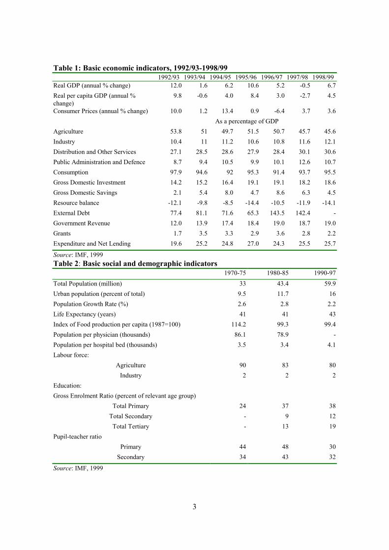
By all available indicators, Ethiopia is one of the poorest countries in the world. GDP per

capita is around USD 110, while life expectancy, educational enrolment, and other

indicators of well-being are all extremely low. Agriculture continues to dominate the

economy, contributing 45% of GDP (Table 1), but since it accounts for 80% of

employment, its level of productivity is obviously very low. The country suffers spells of

drought, with resulting famines, and such conditions have a strong influence on the

performance of the whole economy. Over the last thirty years, life expectancy has shown

little improvement, food production per capita has declined, and school enrolment has

changed little (Table 2).

3

Table 1: Basic economic indicators, 1992/93-1998/991992/93 1993/94 1994/95 1995/96 1996/97 1997/98 1998/99

Real GDP (annual % change) 12.0 1.6 6.2 10.6 5.2 -0.5 6.7Real per capita GDP (annual %change)

9.8 -0.6 4.0 8.4 3.0 -2.7 4.5

Consumer Prices (annual % change) 10.0 1.2 13.4 0.9 -6.4 3.7 3.6As a percentage of GDP

Agriculture 53.8 51 49.7 51.5 50.7 45.7 45.6Industry 10.4 11 11.2 10.6 10.8 11.6 12.1Distribution and Other Services 27.1 28.5 28.6 27.9 28.4 30.1 30.6Public Administration and Defence 8.7 9.4 10.5 9.9 10.1 12.6 10.7Consumption 97.9 94.6 92 95.3 91.4 93.7 95.5Gross Domestic Investment 14.2 15.2 16.4 19.1 19.1 18.2 18.6Gross Domestic Savings 2.1 5.4 8.0 4.7 8.6 6.3 4.5Resource balance -12.1 -9.8 -8.5 -14.4 -10.5 -11.9 -14.1External Debt 77.4 81.1 71.6 65.3 143.5 142.4 -Government Revenue 12.0 13.9 17.4 18.4 19.0 18.7 19.0Grants 1.7 3.5 3.3 2.9 3.6 2.8 2.2Expenditure and Net Lending 19.6 25.2 24.8 27.0 24.3 25.5 25.7

Source: IMF, 1999Table 2: Basic social and demographic indicators

1970-75 1980-85 1990-97Total Population (million) 33 43.4 59.9Urban population (percent of total) 9.5 11.7 16Population Growth Rate (%) 2.6 2.8 2.2Life Expectancy (years) 41 41 43Index of Food production per capita (1987=100) 114.2 99.3 99.4Population per physician (thousands) 86.1 78.9 -Population per hospital bed (thousands) 3.5 3.4 4.1Labour force:

Agriculture 90 83 80Industry 2 2 2

Education:Gross Enrolment Ratio (percent of relevant age group)

Total Primary 24 37 38Total Secondary - 9 12Total Tertiary - 13 19

Pupil-teacher ratioPrimary 44 48 30

Secondary 34 43 32

Source: IMF, 1999

4

During the 1990s there were significant changes in the political and economic

landscape of the country. The regime that had ruled for nearly two decades was ousted from

power in 1991 leading to the end of the civil war. In 1992/93 the government adopted an

Economic Reform Programme with the support of the international financial institutions. So

far, four Policy Framework Papers have been agreed between the Ethiopian government, the

International Monetary Fund, and the World Bank. A ten-year development strategy, known

as Agricultural Development-Led Industrialisation, was laid out. Major objectives are

promotion of economic growth and poverty reduction. Helped by the restoration of peace,

good weather, and changes in macroeconomic policies, the economy registered increased

rates of growth during 1992/93-1996/97. Nevertheless, domestic savings, a mere 5% of

GDP in 1998/99 (Table 1), are not sufficient to meet investment needs. The resource gap

(14% of GDP) led to a rise in external debt to 142% of GDP in 1998/99.

There are few studies of the effects in Ethiopia of policy measures on target

variables such as economic growth and poverty.7 This study aims to explore the link

between economic growth and poverty on the basis of household panel-data between 1994

and 1997. Without a full-fledged model of the economy, it is obviously hard to separate the

effects of policy changes from the impacts of weather and the restoration of peace. Still, we

will draw some tentative policy conclusions on the basis of our analysis.

3. The Measurement of Poverty

3.1. The Choice of Poverty Index

Standard measures of economic poverty, income- or consumption-based poverty-indices as

used herein are summary measures defined over mean income, the relevant poverty-line,

and parameters characterising the underlying income distribution. The general form is given

by

(1) P = P (z/µ, L)

7 Previous poverty studies in Ethiopia include Kebede and Taddesse (1996), Bevan and Joireman (1997),Dercon and Krishnan (1998), and the Welfare Monitoring Unit (1999).

5

where µ is the mean income of the population, z is the poverty line determined

exogenously, and L is a parameter characterising income distribution as measured by the

Lorenz function.

The specification of P as in (1) has practical advantages. It is possible to construct

tests of statistical significance of poverty estimates for a given poverty-line (Kakwani 1990),

and it is easy to decompose changes in poverty into those related to changes in mean

income and those related to changes in the underlying distribution (Datt and Ravallion,

1992). In addition, one can compute elasticities with respect to mean income and inequality

parameters. Furthermore, it can be shown that all flexible and ethically-sound poverty-

indices suggested in the literature can be expressed in terms of mean income and the income

distribution. For instance, given the parameters of the Lorenz function, the head count (H)

and income-gap (I) ratios can be readily calculated.8

An explicit and frequently used specification of P is an index originally suggested

by Foster, Greer, and Thorbecke (1984), the FGT-index. For a continuous income

distribution it is given by

(2) dyyfzyzPz

i i )}()/){(1� =

−= αα

where z again is the poverty line and y stands for income. For α = 0 and 1, the FGT-index

reduces to H and I, measuring, respectively, the prevalence and the intensity of poverty (see

Ravallion, 1992). For α=2 the FGT-index measures the severity of poverty. As the value

given to α increases, the FGT index gives more weight to the distribution of income at the

lower end. FGT indices for α ranging from 0 to 2, used throughout this paper, will be

represented by P0, P1 and P2.

8 Head-count and income-gap ratios are given, respectively, by q/n and {q/n((z-yp)/z)}, where q is the

number of poor people, n is total population, z is the poverty line, and yp is the mean expenditure of thepoor population. These two measures were the earliest, and are the most frequently used, measures ofpoverty.

6

3.2. Data

This study is based on panel data for 1994, 1995 and 1997. The data are from two separate

but closely related household surveys, one rural and the other urban, undertaken by the

Department of Economics of Addis Ababa University. The rural surveys were done in

collaboration with the Centre for the Study of African Economies of Oxford University and

the International Food Policy Research Institute (IFPRI), while the urban surveys were done

in collaboration with the Department of Economics of Göteborg University and Michigan

State University. The two surveys together covered about 3000 households, the sample size

of each being the same. The rural and urban samples were drawn independently of each

other, but the questionnaires were carefully standardised to enable the collection of

comparable data sets, allowing for the differences in the two settings.

The rural household survey was undertaken in 15 sites in four rounds: the first two

in 1994, the third in 1995, and the last in 1997. Though small, relative to the size and

diversity of the rural population, the sample tried to capture as many of the major socio-

economic groups, agro-ecological zones, and farming systems as possible, by spreading the

sites over the most important regions of the country. While the survey areas were purposely

selected to represent the diversity of the rural economy, households in each site were

selected randomly, the sample size in each region being proportional to the population in

the region (for details on the sampling procedure, see Kebede, 1994).

The urban surveys were conducted over a period of four successive weeks during a

month considered to represent average conditions. They covered seven major cities and

towns in Ethiopia – the capital Addis Ababa, Awassa, Bahir Dar, Dessie, Dire Dawa, Jima

and Mekele – selected to represent the major socio-economic characteristics of the urban

population in the country. A total sample size of 1500 households was allocated among the

urban centre in proportion to their population, then similarly to each wereda (district) in

each urban centre. Households were then selected randomly from half of the kebeles (the

lowest administration units) in each wereda, using the registration of residences available at

the urban administrative units. Such a sampling frame misses an important social group

from the point view of poverty measurement, the homeless, a group whose ranks are

swelling in most, particularly large, urban centres in Ethiopia.

7

The same initial sample size of 1500 households was maintained in all subsequent

rounds of both the rural and urban surveys by replacing households that dropped out. The

sampled communities were fairly stable during the survey period, as a result of which

attrition was low: about 3% from the rural and 7% from the urban samples. With a further

loss of data of about the same proportions due to mismatching of household identifications,

panel data on 1403 households from the rural surveys and 1249 households from the urban

surveys, was compiled. From these a “national” panel was constructed as follows: Since the

first and second rounds of the rural survey were undertaken in 1994 (the former covering

the first, and the latter the second, part of the year), they were merged to form the 1994 data.

The 1995 and 1997 rural data was obtained from the third and fourth rounds with

appropriate scaling (depending on the information from the first and second rounds) to take

account of possible seasonal variations. This rural data was then merged with proportional

sub-samples of the urban panel (about 15%, the urban weight in the country’s population) to

form the national panel, consisting of 1654 households used.

Both surveys collected data on the demographic characteristics of the households,

their educational and health status, ownership of assets, employment and income, credit,

and consumption and expenditure.

3.3 Estimation Procedures

Consumption expenditures may be a better indicator of household welfare than income, and

in our data-set expenditure estimates tend to be higher than income estimates, which could

mean that the use of the income variable would lead to an overestimation of the extent of

poverty. Consequently, consumption expenditure is used rather than income. However, the

use of consumption expenditures is not free of problems either. First, there is the issue of

how to handle consumption of own-produced goods, which is substantial among rural

households. In our case, a price survey was undertaken at the market nearest to each site and

the prices obtained from the surveys were used to express the monetary value of non-

marketed consumption. Second, in communities like Ethiopia, meal-sharing with non-

members is important and has to be adjusted for in the measurement of household welfare.

Our surveys collected data on this, which was used to make appropriate adjustments.

8

To construct poverty lines from the data described above, we proceeded in two

stages: We first estimated the food poverty-lines, and then made adjustments to account for

basic non-food consumption. The food poverty-lines were constructed following the cost-

of-basic-needs approach. We first derived the average quantities of food items that were

most frequently consumed by households falling in the lower half of the expenditure

distribution in 1994.9 These were then converted into calorie consumption and scaled up to

provide 2,100 kcal per person per day, the minimum energy requirement for a person to lead

a normal physical life under Ethiopian conditions as estimated by the Ethiopian Nutrition

Institute. To arrive at the food poverty lines, this bundle was held constant over the study

period and valued at market prices in each locality.

The non-food component of the poverty line was simply estimated using the

common practice of dividing the food poverty-line in each region by the average food share

in each region for households that had failed to attain a food-consumption level equal to the

food poverty-line. As in most methods of estimating the non-food component of the poverty

line, this procedure is anchored in the consumption behaviour of the poor, but it tends to

overestimate the total poverty line in richer regions, where the food share is likely to be

lower.10

A recurring problem in the use of either income or consumption expenditure to set

the poverty line is the issue of family size and composition, and scale economies in the

process of consuming goods and services. One can use more or less elaborate weighting-

schemes or equivalence scales (Deaton and Muellbauer, 1980, Lipton and Ravallion, 1995,

Coutler et al., 1992). In this paper, however, we have only adjusted for household size and

thus computed per capita estimates.

9 This can be interpreted as a starting guess at the level of poverty. We found that the food bundle and thefood poverty-line computed on its basis, are more or less invariant to using households falling below the40th or the 30th percentile.10 The application of alternative methods, in particular the one suggested by Ravallion and Bidani (1994),resulted in underestimation of the food-share in richer regions, thus leading to lower poverty lines due tovery low and insignificant coefficients of the regional dummies and demographic variables in the estimatedEngel functions.

9

4. Poverty Profile of Ethiopia (1994-97)

As indicated in the previous section, the consumption mix of the lower half of the sample,

which provides 2100 kcal/person/day was used as the ‘subsistence’ basket. Local prices at

each site in each round were used to value this ‘subsistence’ basket, giving us the poverty

lines. Those households with a lower nominal expenditure are here classified as poor and

the rest as non-poor. We use this information to compute household expenditures adjusted

not only for the regional variations in prices (including urban-rural) but also across time.

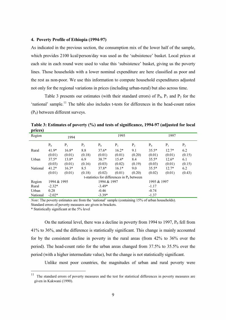
Table 3 presents our estimates (with their standard errors) of P0, P1 and P2 for the

‘national’ sample.11 The table also includes t-tests for differences in the head-count ratios

(P0) between different surveys.

Table 3: Estimates of poverty (%) and tests of significance, 1994-97 (adjusted for localprices)Region 1994 1995 1997

P0 P1 P2 P0 P1 P2 P0 P1 P2

Rural 41.9*(0.01)

16.8*(0.01)

8.8(0.18)

37.6*(0.01)

16.2*(0.01)

9.1(0.20)

35.5*(0.01)

12.7*(0.01)

6.2(0.15)

Urban 37.5*(0.03)

13.8*(0.01)

6.9(0.16)

38.7*(0.03)

15.4*(0.02)

8.4(0.19)

35.5*(0.03)

12.6*(0.01)

6.1(0.15)

National 41.2*(0.01)

16.3*(0.01)

8.5(0.18)

37.8*(0.02)

16.1*(0.01)

9.0(0.20)

35.5*(0.02)

12.7*(0.01)

6.2(0.43)

t-statistics for differences in P0 betweenRegion 1994 & 1995 1994 & 1997 1995 & 1997Rural -2.32* -3.49* -1.17Urban 0.28 -0.46 -0.74National -2.02* -3.39* -1.37Note: The poverty estimates are from the ‘national’ sample (containing 15% of urban households).Standard errors of poverty measures are given in brackets.* Statistically significant at the 5% level

On the national level, there was a decline in poverty from 1994 to 1997, P0 fell from

41% to 36%, and the difference is statistically significant. This change is mainly accounted

for by the consistent decline in poverty in the rural areas (from 42% to 36% over the

period). The head-count ratio for the urban areas changed from 37.5% to 35.5% over the

period (with a higher intermediate value), but the change is not statistically significant.

Unlike most poor countries, the magnitudes of urban and rural poverty were

11 The standard errors of poverty measures and the test for statistical differences in poverty measures are

given in Kakwani (1990).

10

similar.12 A possible reason for the relatively low levels of rural poverty is the land-tenure

system. With the land-reform programme of 1974, all rural land was nationalised and given

as usufruct to the farmers cultivating it, which increased the income of the poorer segments

of the rural population. The substantial decline in rural poverty from 1994 to 1997, and the

smaller decline in the urban areas suggest that the growth pattern resulting from policy and

other changes during the period also favoured rural rather than urban areas, thus further

reducing the remaining urban-rural gap.

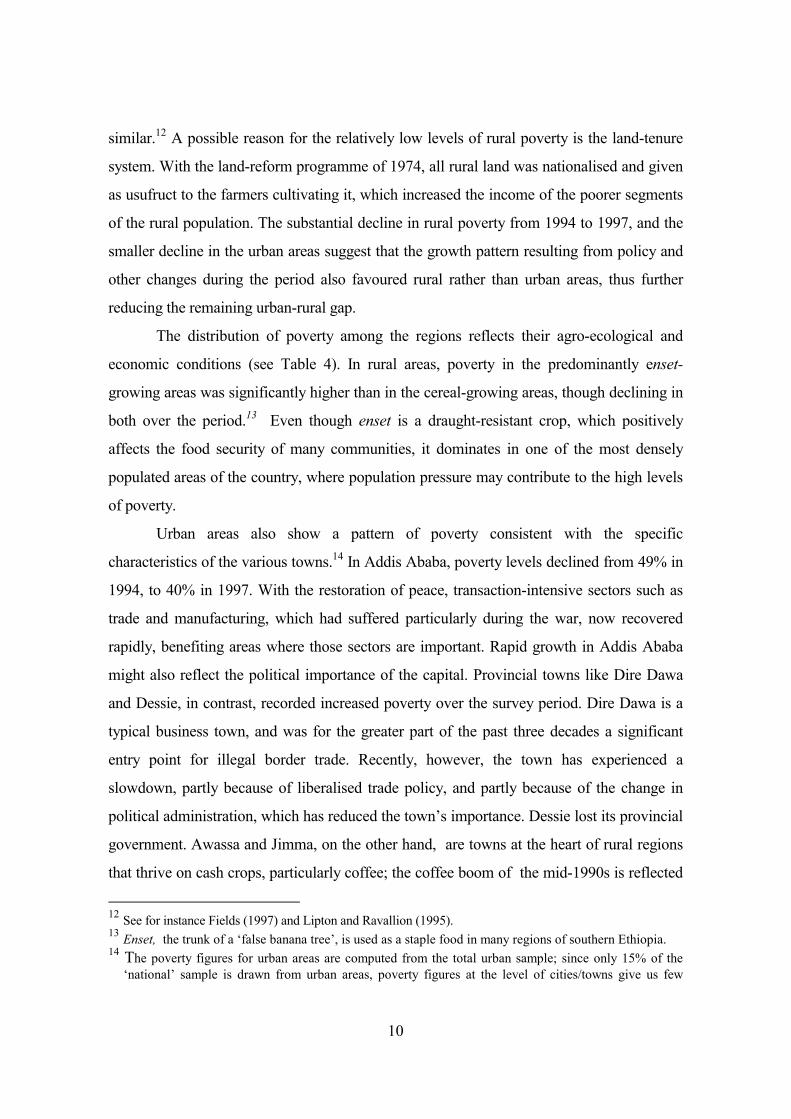
The distribution of poverty among the regions reflects their agro-ecological and

economic conditions (see Table 4). In rural areas, poverty in the predominantly enset-

growing areas was significantly higher than in the cereal-growing areas, though declining in

both over the period.13 Even though enset is a draught-resistant crop, which positively

affects the food security of many communities, it dominates in one of the most densely

populated areas of the country, where population pressure may contribute to the high levels

of poverty.

Urban areas also show a pattern of poverty consistent with the specific

characteristics of the various towns.14 In Addis Ababa, poverty levels declined from 49% in

1994, to 40% in 1997. With the restoration of peace, transaction-intensive sectors such as

trade and manufacturing, which had suffered particularly during the war, now recovered

rapidly, benefiting areas where those sectors are important. Rapid growth in Addis Ababa

might also reflect the political importance of the capital. Provincial towns like Dire Dawa

and Dessie, in contrast, recorded increased poverty over the survey period. Dire Dawa is a

typical business town, and was for the greater part of the past three decades a significant

entry point for illegal border trade. Recently, however, the town has experienced a

slowdown, partly because of liberalised trade policy, and partly because of the change in

political administration, which has reduced the town’s importance. Dessie lost its provincial

government. Awassa and Jimma, on the other hand, are towns at the heart of rural regions

that thrive on cash crops, particularly coffee; the coffee boom of the mid-1990s is reflected

12 See for instance Fields (1997) and Lipton and Ravallion (1995).13 Enset, the trunk of a ‘false banana tree’, is used as a staple food in many regions of southern Ethiopia.14 The poverty figures for urban areas are computed from the total urban sample; since only 15% of the

‘national’ sample is drawn from urban areas, poverty figures at the level of cities/towns give us few

11

in the decline in poverty there.

Table 4: Profile of poverty by region: 1994-97Region 1994 1995 1997

P0 P1 P2 P0 P1 P2 P0 P1 P2RuralEnset-growing 53.7 20.2 9.7 58.4 28.4 17.1 40.1 14.8 7.3Cereal-growing 36.9 15.3 8.3 28.7 11.0 5.7 33.5 11.9 5.8Urban*Addis Ababa 49.9 19.9 10.7 46.4 17.3 14.2 39.9 15.4 8.0Awassa 49.1 21.4 12.9 40.4 14.2 6.5 33.0 16.7 10.4Jimma 36.7 12.1 5.8 25.6 10.6 5.3 42.9 15.3 6.9Dessie 36.9 14.1 6.8 37.2 14.6 7.0 37.8 14.4 7.6Mekele 30.9 12.1 6.2 36.4 20.5 13.9 34.9 11.8 5.9Dire Dawa 18.2 5.8 2.2 28.6 8.6 3.6 36.6 12.3 5.8Bahir Dar 26.2 9.4 5.3 26.1 9.0 5.0 24.0 8.7 4.1*The urban poverty estimates are based on the full sample, while those reported in Table 3 are based on sub-samples combining urban and rural data into ‘national’ estimates.

5. Correlates of Poverty

To examine some correlates of poverty in rural and urban areas, we estimated probits for

the rural and urban data separately. In both estimates, the dependent variable is a zero/one

dummy variable identifying households that were poor in 1994. The independent

variables for rural areas are broadly classified into four groups: demographic and

educational, crop type, location and farm assets and off-farm activities. In the first group,

household size (hhsize), mean age of household members (and it square, meanage and

meanage2)15, a dummy for female-headed households (hhhfem), the age of the household

head (and its square, agehhh and agehhh2), dependency ratio (depndrat) and dummies for

household head and wives that completed primary education (hhhprime and wifeprim) are

included. The dependency ratio is defined as the percentage of household members

below the age of 15 and above 65 from total household size. Dummy variables for

households producing teff, coffee, chat and enset16 are the second group identifying types

of crops cultivated by households. To control for location two variables, ‘north’ and

‘market’, are included. While ‘north’ is a dummy variable identifying the sites located in

degrees of freedom.

15 The mean age of household members (and its square) were included to capture possible life cycle effects.16 Teff is an indigenous cereal used as a staple food by many Ethiopians, while chat is a mildly stimulating

plant chewed mainly in Middle Eastern countries.

12

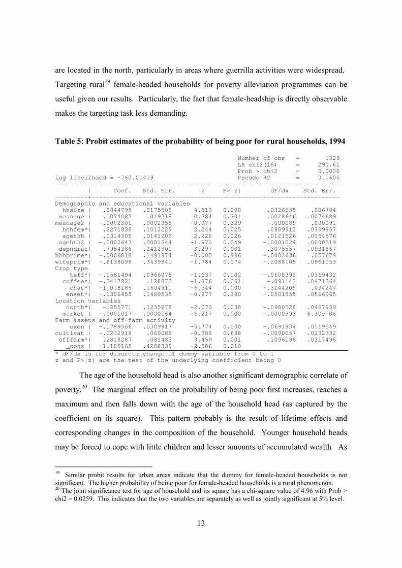
the northern part of the country, ‘market’ is an index-variable reflecting the proximity of

survey sites to big towns. This index was computed by dividing the population of the

nearest town by the distance from the survey site, with the expectation that the larger the

population of the urban area and the nearer to the survey site, the stronger would be its

influence, since urban centres affect the livelihood of rural areas by providing both

markets (for sales of agricultural products, and for purchase of manufactured goods and

labour) and infrastructure. The final set of variables are the number of oxen (oxen) and

cultivated land (cultivat) owned by the household and whether at least a member of the

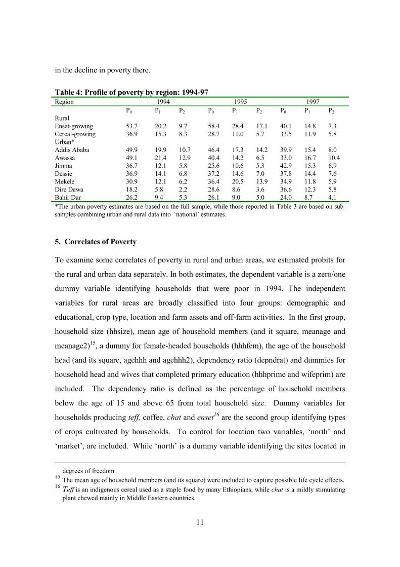
household participates in off-farm activities (offfarm). The probit results for rural areas

with the corresponding marginal effects of the variables at mean values are given in Table

5.

Except mean age and its square17 all the demographic and educational variables

are significant at 5% level. An additional household member increases the probability of

the household being poor by around 3.2% at mean values (and its effect is significant at

1% level). But this is to some extent due to the fact that we have used per capita

expenditure figures for defining poverty levels.

Compared to male-headed households, female-headed households face an 8.9%

higher probability of being poor in rural areas (significant at 5% level). In terms of the

magnitude of its effect, this variable seems to be one of the most important covariates of

poverty.18 Even though female-headship can be caused by different factors, civil war

seems to play an important role in Ethiopia. If we look at the percentage of female-

headed households by survey villages, the three with the highest percentages are found in

areas where the civil war was raging for long periods of time. Even though the average

percentage of female-headed households for the whole sample is 21%, the villages of

Haresaw, Geblen and Shumsheha have 47%, 39% and 30% respectively; all three villages

17 The joint test for the significance of mean age and its square has a chi-square value of 0.14 with Prob >chi2 = 0.7070. Hence, the two variables either separately or jointly are not statistically significant.18 From the demographic and educational variables, the only two variables with higher marginal effectsthan the dummy for female-headed households are dependency ratio and primary education of the wife. Since dependency ratio is a continuous variable and is a ratio (implying that to increase it by one unit thenumber of additional dependents required is large), we cannot directly compare it with that of female-headed households. In the case of the primary education of the wife, the coefficient is not significant at 5%level.

13

are located in the north, particularly in areas where guerrilla activities were widespread.

Targeting rural19 female-headed households for poverty alleviation programmes can be

useful given our results. Particularly, the fact that female-headship is directly observable

makes the targeting task less demanding.

Table 5: Probit estimates of the probability of being poor for rural households, 1994

Number of obs = 1329 LR chi2(18) = 290.61 Prob > chi2 = 0.0000Log likelihood = -760.01419 Pseudo R2 = 0.1605------------------------------------------------------------------------------ | Coef. Std. Err. z P>|z| dF/dx Std. Err.---------+--------------------------------------------------------------------Demographic and educational variables hhsize | .0844795 .0175509 4.813 0.000 .0326639 .006784 meanage | .0074087 .019318 0.384 0.701 .0028646 .0074689meanage2 | -.0002301 .0002355 -0.977 0.329 -.000089 .000091 hhhfem*| .2271838 .1012229 2.244 0.025 .0889912 .0399857 agehhh | .0314305 .0141203 2.226 0.026 .0121526 .0054576 agehhh2 | -.0002647 .0001344 -1.970 0.049 -.0001024 .0000519 depndrat| .7954386 .2412301 3.297 0.001 .3075557 .0931867hhhprime*| -.0006818 .1491974 -0.005 0.996 -.0002636 .057679wifeprim*| -.6138098 .3439941 -1.784 0.074 -.2088109 .0961053Crop type teff*| -.1581494 .0966075 -1.637 0.102 -.0608392 .0369432 coffee*| -.2417821 .128873 -1.876 0.061 -.091143 .0471264 chat*| -1.018185 .1604911 -6.344 0.000 -.3144205 .034247 enset*| -.1306455 .1489535 -0.877 0.380 -.0501555 .0566965Location variables north*| -.255771 .1235679 -2.070 0.038 -.0980528 .0467939 market | -.0001017 .0000164 -6.217 0.000 -.0000393 6.30e-06Farm assets and off-farm activity oxen | -.1789566 .0309917 -5.774 0.000 -.0691934 .0119549cultivat | -.0232918 .060088 -0.388 0.698 -.0090057 .0232332 offfarm*| .2818287 .081483 3.459 0.001 .1096196 .0317496 _cons | -1.109165 .4288339 -2.586 0.010 * dF/dx is for discrete change of dummy variable from 0 to 1z and P>|z| are the test of the underlying coefficient being 0

The age of the household head is also another significant demographic correlate of

poverty.20 The marginal effect on the probability of being poor first increases, reaches a

maximum and then falls down with the age of the household head (as captured by the

coefficient on its square). This pattern probably is the result of lifetime effects and

corresponding changes in the composition of the household. Younger household heads

may be forced to cope with little children and lesser amounts of accumulated wealth. As

19 Similar probit results for urban areas indicate that the dummy for female-headed households is notsignificant. The higher probability of being poor for female-headed households is a rural phenomenon.20 The joint significance test for age of household and its square has a chi-square value of 4.96 with Prob >chi2 = 0.0259. This indicates that the two variables are separately as well as jointly significant at 5% level.

14

the children grow (and sometimes leave home increasing per capita consumption) and

wealth is accumulated, the probability of being poor also falls.

Both in terms of its significance level (significant at 1%) as well as in terms of the

magnitude of its marginal effect, the dependency ratio seems to be extremely important in

affecting poverty status in rural areas. If the dependency ratio increases by one unit, a

household’s probability of falling into poverty increases by almost 31% at mean values.

Those households with proportionally more number of children under the age of 15 years

and older people above 65 seem particularly vulnerable to poverty. This underscores the

importance of adult labour in the welfare of rural households. The policy implication of

this result points towards the importance of decreasing fertility. Most of the high

dependency ratio is explained by a large number of children under the age of 15; due to

low life expectancy, the relative number of people over the age of 65 is small.

Even though the primary education of the household head is not statistically

significant, the primary education of the wife reduces the risk of poverty. If the wife in a

typical rural household has completed primary education, the probability of poverty falls

by around 21% (though the coefficient is significant only at 10% level). This result may

be due to endogeneity; for example, only well-off husbands may be sending their wives to

school or richer men may usually marry women with some level of education. The other

possibility is that wives with some degree of education in rural areas are actually more

efficient in contributing towards household income.

The crop types included in the regression are deliberately chosen to include a

staple food that is not much traded (enset), a staple food that is significantly traded in the

domestic market (teff), a traditional export crop (coffee) and a ‘new’ export crop (chat).

Teff is one of the main domestically marketed crops in Ethiopia. Generally, rural

households produce teff for the market and it is an important source of cash income.

Coffee and chat are also important export crops, the first being the most important export

item of the country and the importance of the second increased during the recent past.

While the cultivation of these crops by households has a tendency to decrease the

probability of poverty (all four coefficients are negative), the significant levels and the

15

marginal effects tell an interesting story. If we move from enset, to teff, to coffee and

then chat the variables become more and more statistically significant. While the

coefficient for enset is not significant at all, that for teff becomes significant around 10%,

for coffee around 6% and for chat at 1%. Similarly, the marginal effects successively

increase in absolute terms: -5.0%, -6.1%, -9.1% and -31.4% respectively. Households

cultivating chat have a 31.4% lower probability of being poor as compared to households

that do not; from all the variables included in our regression, the dummy variable has the

highest marginal effect and is highly significant. The expansion of exportable crops,

particularly non-traditional crops, seems to have a large impact on poverty reduction.

This tallies with the overall reform goal of encouraging the production of

tradables/exportables. The provision of infrastructure and giving the right incentives that

encourage the production of exportable agricultural outputs probably have the win-win

result of enhancing growth as well as reducing poverty.

Both location related variables, ‘north’ and ‘market’, are statistically significant at

5% level. Compared to their southern counterparts, households in the northern sites have

a 9.8% lower probability of being poor (significant at 5%). But much should not be read

from this result. First, the data from the surveys are not weighted and hence we cannot be

definite that our results accurately reflect the relative standing of the north and the south.

Second, variations within each part of the country are significant making generalisation

about north and south difficult. As expected the second location variable, ‘market’,

decreases the risk of being poor; if the variable increases by 10,000 (implying an increase

of 10,000 in the population of an urban area located 1 km away from the village), the

probability of poverty for the household decreases by 0.4% (significant at 1% level).

Rural areas nearer relatively big cities/towns have better access to markets and public

services and this reduces poverty. But the effect of urban areas on rural poverty is not

high; due to the low level of urbanization (only 15%), a population increase of 10,000 is

really big for most urban centres and the accompanying expected decline in the

probability of poverty is very low.

The last group of variables are related to farm assets and off-farm activities. The

amount of land cultivated by the household is not correlated to the probability of poverty.

16

This seemingly surprising result is probably due to the land tenure system in Ethiopia.

All agricultural land is owned by the state and it is given to households on a usufractuary

basis, the allocation of which is mostly determined by household size. This institutional

set-up has created, unlike most other countries, a situation where the accumulation of

land is no more an important avenue of increasing wealth. It seems that other farming

assets are the more important constraints due to this institutional arrangement. This

assertion is partly confirmed by the coefficient on the number of oxen. In the dominant

farming system of Ethiopia, oxen are the most important sources of traction power. The

marginal effects indicate that an additional ox decreases the probability of a household

being poor by 6.9% (significant at 1% level). Initiatives that improve the ox ownership of

households probably have a significant impact on poverty.

Households that are involved in off-farm activities are 11.0% more probable of

being poor than those that are not (significant at 1% level). In the case of rural Ethiopia,

off-farm activity seems to be a coping mechanism for poor people rather than a way of

accumulating more wealth and enjoying a relatively higher return to labour. Given the

weakness of the non-farm sectors, especially in rural areas, this draws a realistic picture

of conditions in Ethiopia.

A similar probit was run for urban households. While dropping variables not

relevant for urban areas, we included dummies identifying regional capitals (capitalc) and

the occupation of household heads. The occupation of household heads is classified into

private business employer (privbuss), own account worker (ownaccnt), civil servant

(civilser), public enterprise worker (publicen), private sector employee (privempl), casual

worker (casualwo), unemployed (unemploy), and others. The results are given in Table 6,

again including marginal effects.

17

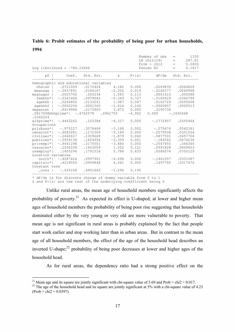
Table 6: Probit estimates of the probability of being poor for urban households,

1994 Number of obs = 1330 LR chi2(18) = 287.81 Prob > chi2 = 0.0000Log likelihood = -746.10646 Pseudo R2 = 0.1617------------------------------------------------------------------------------ p0 | Coef. Std. Err. z P>|z| dF/dx Std. Err. ---------+--------------------------------------------------------------------Demographic and educational variables hhsize | .0721009 .0172424 4.182 0.000 .0269839 .0064828 meanage | -.0437891 .0186167 -2.352 0.019 -.0166377 .0069968meanage2 | .0003705 .000234 1.583 0.113 .0001415 .000088 femhhh*| -.0341466 .0979042 -0.349 0.727 -.0169929 .0366794 agehhh | .0264806 .0133251 1.987 0.047 .0102729 .0050008 agehhh2 | -.0002204 .0001365 -1.614 0.106 -.0000857 .0000513depenrat | .8419948 .2173903 3.873 0.000 .3190736 .0817098hhhprime*| -.4762578 .0961755 -4.952 0.000 -.1692448 .0346324wifprime*| -.4463262 .103384 -4.317 0.000 -.1772457 .0355464Occupationsprivbuss*| -.975227 .3078486 -3.168 0.002 -.275676 .0542181ownaccnt*| -.6083281 .1172309 -5.189 0.000 -.2079938 .0351524civilser*| -.2460617 .1309669 -1.879 0.060 -.0877501 .0457704publicen*| -.5559138 .1654954 -3.359 0.001 -.184562 .0474236privempl*| -.8441298 .2175551 -3.880 0.000 -.2547855 .046365casualwo*| .2550208 .1643059 1.552 0.121 .0991828 .0649653unemploy*| .1405296 .1791516 0.784 0.433 .0586074 .0700129Location variables north*| -.4087424 .0997901 -4.096 0.000 -.1461057 .0331087capitalc*| .4218555 .0949848 4.441 0.000 .1497705 .0317476Constant term _cons | -.635158 .4901665 -1.296 0.195 ------------------------------------------------------------------------------* dF/dx is for discrete change of dummy variable from 0 to 1z and P>|z| are the test of the underlying coefficient being 0

Unlike rural areas, the mean age of household members significantly affects the

probability of poverty.21 As expected its effect is U-shaped; at lower and higher mean

ages of household members the probability of being poor rise suggesting that households

dominated either by the very young or very old are more vulnerable to poverty. That

mean age is not significant in rural areas is probably explained by the fact that people

start work earlier and stop working later than in urban areas. But in contrast to the mean

age of all household members, the effect of the age of the household head describes an

inverted U-shape;22 probability of being poor decreases at lower and higher ages of the

household head.

As for rural areas, the dependency ratio had a strong positive effect on the

21 Mean age and its square are jointly significant with chi-square value of 5.69 and Prob > chi2 = 0.017.22 The age of the household head and its square are jointly significant at 5% with a chi-square value of 4.23(Prob > chi2 = 0.0397).

18

probability of being poor. A unit increase was associated with a 32% higher probability of

being poor. The adverse effect of the dependency ratio at the household level in both rural

and urban areas provides a strong case for family planning. Further, like in most poor

countries, the Ethiopian government does not provide any support, direct or indirect, to

aging members of society. The burden of supporting the old mainly falls on the

household, or on the community. But the dependency ratio that we computed excluded

other sick, disabled, or weak members of the household, which generally would have

increased poverty. One of the striking results is the effect of the household head or wife

having at least primary education, which tends to decrease the probability of being poor.

In the rural areas, the coefficient of household head was smaller and highly insignificant,

but in the urban areas, both coefficients are highly significant at the 1% level, and both

are relatively large; primary education of the head or wife decreases the probability of

being poor by 17% and 18% respectively. Education thus seems to bring a higher rate of

return in urban than in rural areas. Perhaps the educational system develops skills that

increase productivity in urban occupations rather than in agriculture. The livelihood of

people in rural areas is mainly affected by their access to agricultural assets, like land and

oxen, which does not directly depend on their educational levels. Several studies have

shown that education can have an important positive effect on agricultural productivity in

situations where innovations are introduced, while it does not seem to have any

significant effect when only traditional methods are used. Ethiopia is certainly a case

where very little agricultural innovation has occurred. In any case, education may also

serve more as a screening device in urban than in rural areas, given the thinness or non-

existence of labour markets in the latter.

Unlike their counterparts in rural areas, female-headed households in urban areas

do not face a higher chance of being in poverty (the coefficient is not significant at all).

The fact that agriculture is probably the only viable occupation and farm activities are

traditionally male-dominated in rural areas and in contrast the availability of a variety of

occupations that females can participate in urban areas is probably the main explanation

for these results.

Most of the coefficients on the occupation variables are highly significant,

19

indicating that relative to “other”, the sector of work had a discernable impact on people’s

livelihoods. Except for casual workers and the unemployed, all occupations are associated

with a lower probability of being poor. The lowest probability of poverty was for private

business employers (28% less than “other”). Being a private sector employee reduced the

probability by 25%, while being an own account worker reduced it by 21%. Jobs in the

civil service were not very effective in reducing the probability of being poor.

Both location variables included in the probit are highly significant with relatively

large marginal effects. Contrary to expectation, households in urban areas in the north

(Bahr Dar, Dessie and Mekele) have a 15% lesser chance of being poor as compared to

households located in other towns. Also contrary to expectation, households in regional

capitals (Addis Ababa, Mekele, Bahr Dar and Awasa) have a 15% higher probability of

being poor.

In addition to looking at the correlates of poverty at a point in time, examining the

characteristics of households that have either fallen into or escaped from poverty is

important. This is done in the next section.

6. Changes in Poverty – 1994-97

Over time, as the status of households change, poor households may increase their

income, escaping poverty, while richer households may become poor. Examination of the

characteristics of households moving out of or falling into poverty can help to identify the

most vulnerable, as well as those with a better chance of escaping poverty. We estimated

probit equations to examine the attributes of households moving out of and falling into

poverty between 1994 and 1997. The same independent variables as in the previous

section were used. The estimates were again run separately for rural and urban

households.

The probits in this section examine conditional probabilities. For example, when

we look at the attributes of households that have moved out of poverty between 1994 and

1997, only those households poor in 1994 are included in the estimation. Hence, the

probabilities indicate the chance of moving out of poverty conditional on the household

being poor in 1994.

20

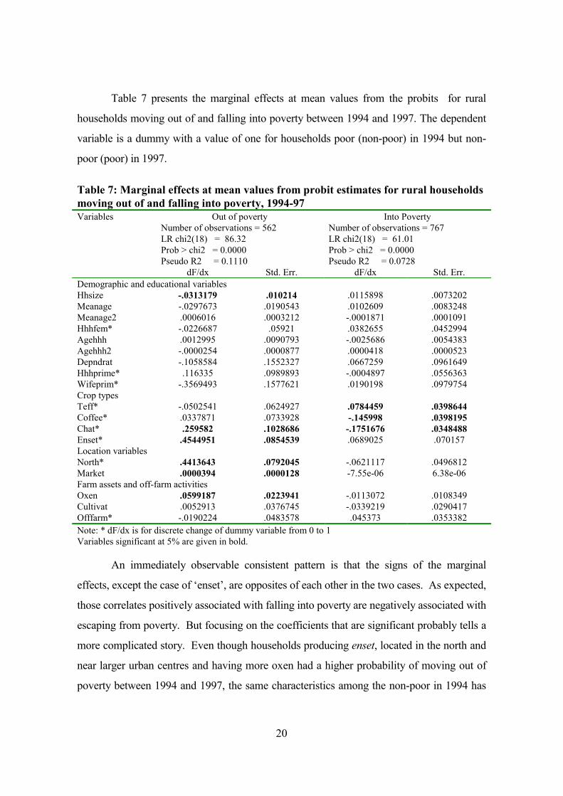
Table 7 presents the marginal effects at mean values from the probits for rural

households moving out of and falling into poverty between 1994 and 1997. The dependent

variable is a dummy with a value of one for households poor (non-poor) in 1994 but non-

poor (poor) in 1997.

Table 7: Marginal effects at mean values from probit estimates for rural householdsmoving out of and falling into poverty, 1994-97

Out of poverty Into PovertyNumber of observations = 562LR chi2(18) = 86.32Prob > chi2 = 0.0000Pseudo R2 = 0.1110

Number of observations = 767LR chi2(18) = 61.01Prob > chi2 = 0.0000Pseudo R2 = 0.0728

Variables

dF/dx Std. Err. dF/dx Std. Err.Demographic and educational variablesHhsize -.0313179 .010214 .0115898 .0073202Meanage -.0297673 .0190543 .0102609 .0083248Meanage2 .0006016 .0003212 -.0001871 .0001091Hhhfem* -.0226687 .05921 .0382655 .0452994Agehhh .0012995 .0090793 -.0025686 .0054383Agehhh2 -.0000254 .0000877 .0000418 .0000523Depndrat -.1058584 .1552327 .0667259 .0961649Hhhprime* .116335 .0989893 -.0004897 .0556363Wifeprim* -.3569493 .1577621 .0190198 .0979754Crop typesTeff* -.0502541 .0624927 .0784459 .0398644Coffee* .0337871 .0733928 -.145998 .0398195Chat* .259582 .1028686 -.1751676 .0348488Enset* .4544951 .0854539 .0689025 .070157Location variablesNorth* .4413643 .0792045 -.0621117 .0496812Market .0000394 .0000128 -7.55e-06 6.38e-06Farm assets and off-farm activitiesOxen .0599187 .0223941 -.0113072 .0108349Cultivat .0052913 .0376745 -.0339219 .0290417Offfarm* -.0190224 .0483578 .045373 .0353382Note: * dF/dx is for discrete change of dummy variable from 0 to 1Variables significant at 5% are given in bold.

An immediately observable consistent pattern is that the signs of the marginal

effects, except the case of ‘enset’, are opposites of each other in the two cases. As expected,

those correlates positively associated with falling into poverty are negatively associated with

escaping from poverty. But focusing on the coefficients that are significant probably tells a

more complicated story. Even though households producing enset, located in the north and

near larger urban centres and having more oxen had a higher probability of moving out of

poverty between 1994 and 1997, the same characteristics among the non-poor in 1994 has

21

not significantly helped them avoid falling into poverty in 1997. Similarly, even though

households producing teff (coffee) and were non-poor in 1994 had a higher (lower)

probability of falling into poverty by 1997 the same conditions have not played a significant

role for households that escaped out of poverty. The only variable that has opposite signs

and is significant is chat. Households poor in 1994 and cultivating chat had 26% better

chance of escaping poverty as compared to those not producing chat. On the other hand,

households that were not poor in 1994 and were producing chat had 18% smaller

probability of falling into poverty by 1997. As discussed in the previous section, chat-

producing households also had a higher chance of being non-poor to start with. Hence, this

cash crop seems to play an important role in improving the living standards of farmers,

which may explain the rapid expansion of chat production in many non-traditional areas.

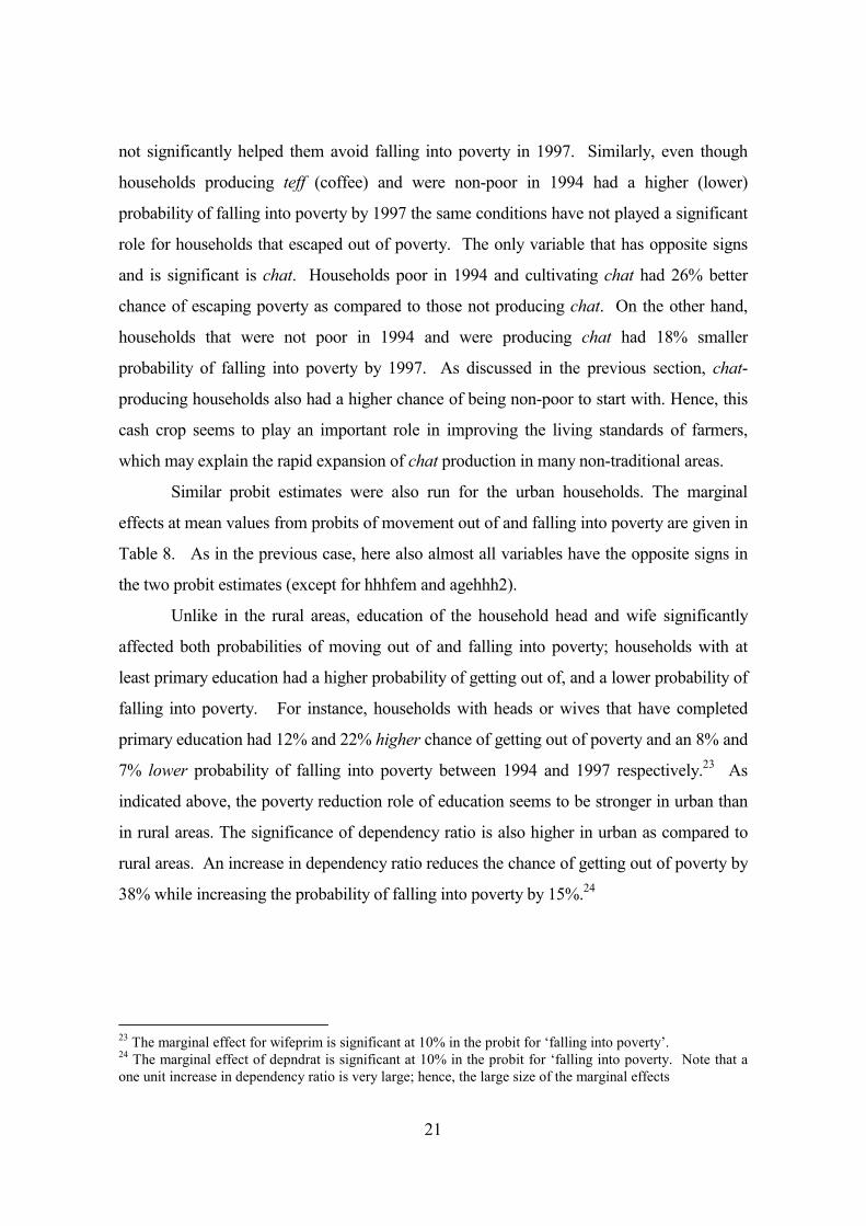
Similar probit estimates were also run for the urban households. The marginal

effects at mean values from probits of movement out of and falling into poverty are given in

Table 8. As in the previous case, here also almost all variables have the opposite signs in

the two probit estimates (except for hhhfem and agehhh2).

Unlike in the rural areas, education of the household head and wife significantly

affected both probabilities of moving out of and falling into poverty; households with at

least primary education had a higher probability of getting out of, and a lower probability of

falling into poverty. For instance, households with heads or wives that have completed

primary education had 12% and 22% higher chance of getting out of poverty and an 8% and

7% lower probability of falling into poverty between 1994 and 1997 respectively.23 As

indicated above, the poverty reduction role of education seems to be stronger in urban than

in rural areas. The significance of dependency ratio is also higher in urban as compared to

rural areas. An increase in dependency ratio reduces the chance of getting out of poverty by

38% while increasing the probability of falling into poverty by 15%.24

23 The marginal effect for wifeprim is significant at 10% in the probit for ‘falling into poverty’.24 The marginal effect of depndrat is significant at 10% in the probit for ‘falling into poverty. Note that aone unit increase in dependency ratio is very large; hence, the large size of the marginal effects

22

Table 8: Marginal effects at mean values from probit estimates for urban householdsmoving out of and falling into poverty, 1994-97

Out of poverty Into PovertyNumber of observations = 520LR chi2(18) = 55.60Prob > chi2 = 0.0000Pseudo R2 = 0.0782

Number of observations = 810LR chi2(18) = 82.31Prob > chi2 = 0.0000Pseudo R2 = 0.1041

Variables

dF/dx Std. Err. dF/dx Std. Err.Demographic and educational variablesHhsize -.0176835 .0101565 .0147649 .0060946Meanage .0095082 .0103268 -.0055338 .0070314Meanage2 -.0000579 .0001252 .0000641 .0000888Hhhfem* .0292815 .0577718 .0229715 .035951Agehhh -.0178748 .0083306 -.0026885 .0042611Agehhh2 .0001824 .0000824 .0000329 .0000468Depndrat -.3842491 .1267438 .1453629 .0815Hhhprime* .1173836 .0599716 -.0782867 .034732Wifeprim* .2163925 .0723332 -.0682705 .0330192Occupationsprivbuss* .2625518 .223046 -.1407597 .0340817Ownaccnt* .152197 .0735931 -.0773405 .0320255Civilser* .0882365 .0818675 -.1158046 .034252Publicen* -.0760733 .1134272 .0107097 .0523149Privempl* .0790109 .1610165 -.0335415 .0575256Casualwo* -.0172332 .0824905 .1123794 .0874063Unemploy* -.0370976 .1010645 .0984579 .0836389Location variablesNorth* .1099403 .0679645 -.0234932 .0314967Capitalc* .141027 .0618332 -.0554456 .0322175Note: * dF/dx is for discrete change of dummy variable from 0 to 1Variables significant at 5% are given in bold.

Of the seven occupational classifications, the only significant one in both equations

is that for own-account workers. Own-account workers had a 15% better chance of escaping

poverty and an 8% smaller chance of falling into poverty as compared to the “other”

occupation group. The creation of a better business environment after the introduction of

the economic reform program may partially explain this.

Households living in regional capitals had a statistically significant better chance of

improving their welfare; they had a 15% better chance of getting out of poverty and a 6%

smaller probability of falling into poverty between 1994 and 1997. This can be due to

recent decentralisation and accompanying expansion of the regional capitals.

Two important differences between the rural and urban areas relate to the effects of

education and dependency ratios. Education seems to play a smaller role in rural areas as a

means of escaping poverty, reflecting the fact that the employment structure in rural areas is

23

not education-intensive. The dependency ratio also seems to be more important in urban

than in rural areas, probably due to the fact that young children and elders are more

economically active in rural than in urban areas.

The changes in poverty levels between 1994 and 1997 can be the result of either

variation in mean income (due to growth or decline) or alterations in the distribution of

income. The next section examines the contribution of growth and redistribution to changes

in poverty.

7. Growth versus Redistribution in Poverty Reduction

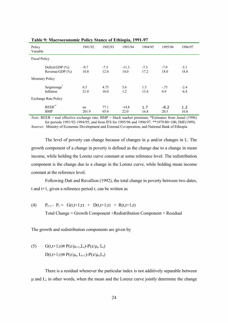
The period from 1993/94 to 1996/97 showed considerable improvement in the

macroeconomic policy stance of the country as illustrated by Table 9, and we have

already noted that growth was good during this period. It is hard to link growth and

poverty outcomes to the specific changes in policy variables or to changes in other

exogenous variables, although Demery and Squire (1996) report a positive association

between improved macroeconomic performance, economic growth and poverty reduction.

Over the period 1994-97 real GDP grew at an average rate of about 6% (see Table

1), which is unusual for an economy that had experienced a negative real growth rate for

more than a decade before that. The change in policy after the ouster of the previous

government in 1991 certainly contributed to growth, but we have not tried to specifically

measure this impact. Instead, we have concentrated on estimating the impact of growth on

poverty.

A method for decomposing changes in poverty into growth and redistribution

components is suggested by Kakwani (1990) and further explored by Datt and Ravallion

(1992). Given a poverty measure (Pt) fully characterised by the poverty line (z), mean

income (µ) and Lorenz curve (Lt) at period t,

(3) Pt = P (zt /µt, Lt)

24

Table 9: Macroeconomic Policy Stance of Ethiopia, 1991-97PolicyVariable

1991/92 1992/93 1993/94 1994/95 1995/96 1996/97

Fiscal Policy

Deficit/GDP (%)Revenue/GDP (%)

-9.710.8

-7.512.0

-11.314.0

-7.317.2

-7.918.0

-5.118.8

Monetary Policy

Seigniorage*

Inflation6.521.0

4.7510.0

5.61.2

1.513.4

-.750.9

-2.4-6.4

Exchange Rate Policy

REER**

BMPna201.9

77.165.0

-14.822.0

1.716.8

-8.220.5

1.210.0

Note: REER = real effective exchange rate; BMP = black market premium; *Estimates from Jemal (1996)for periods 1991/92-1994/95, and from IFS for 1995/96 and 1996/97. **1979/80=100, IMF(1999).

Sources: Ministry of Economic Development and External Co-operation, and National Bank of Ethiopia

The level of poverty can change because of changes in µ and/or changes in L. The

growth component of a change in poverty is defined as the change due to a change in mean

income, while holding the Lorenz curve constant at some reference level. The redistribution

component is the change due to a change in the Lorenz curve, while holding mean income

constant at the reference level.

Following Datt and Ravallion (1992), the total change in poverty between two dates,

t and t+1, given a reference period r, can be written as

(4) Pt+1 - Pt = G(t,t+1;r) + D(t,t+1;r) + R(t,t+1;r)

Total Change = Growth Component +Redistribution Component + Residual

The growth and redistribution components are given by

(5) G(t,t+1;r)≡ P(z/µt+1,Lr)-P(z/µt, Lr)

D(t,t+1;r)≡ P(z/µr, Lt+1)-P(z/µr,Lt)

There is a residual whenever the particular index is not additively separable between

µ and L; in other words, when the mean and the Lorenz curve jointly determine the change

25

in poverty, the residual will not vanish. Datt and Ravallion (1992) interpret the residual as

the difference between the growth components evaluated at the terminal and initial Lorenz

curves, and the redistribution component evaluated at the terminal and initial incomes.

We applied this method of decomposition for the period between 1994 and 1997 to

measure how growth of mean income and any change in inequality affected poverty. The

Lorenz functions fitted to the data are the Beta-specification suggested by Kakwani (1980)

and the Generalised Quadratic specification by Villasenoir and Arnold (1989). We used the

computer programme Povcal, developed by Chen, Datt and Ravallion, to generate the

relevant values for the decomposition analysis. The results are presented in Tables 10 and

11.

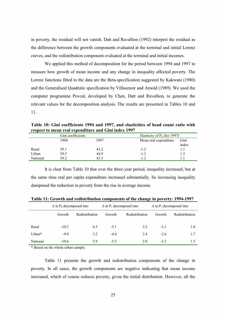
Table 10: Gini coefficients 1994 and 1997, and elasticities of head count ratio withrespect to mean real expenditure and Gini index 1997

Gini coefficients Elasticity of P0 (for 1997)1994 1997 Mean real expenditure Gini

indexRural 39.1 43.2 -1.2 1.1Urban 39.5 44.9 -1.3 1.2National 39.2 43.5 -1.2 1.1

It is clear from Table 10 that over the three-year period, inequality increased, but at

the same time real per capita expenditure increased substantially. So increasing inequality

dampened the reduction in poverty from the rise in average income.

Table 11: Growth and redistribution components of the change in poverty: 1994-1997∆ in P0 decomposed into ∆ in P1 decomposed into ∆ in P2 decomposed into

Growth Redistribution Growth Redistribution Growth Redistribution

Rural -10.2 6.5 -5.1 3.2 -3.1 1.8

Urban* -9.0 3.2 -4.4 2.4 -2.6 1.7

National -10.6 5.9 -5.3 2.8 -3.2 1.5* Based on the whole urban sample.

Table 11 presents the growth and redistribution components of the change in

poverty. In all cases, the growth components are negative indicating that mean income

increased, which of course reduces poverty, given the initial distribution. However, all the

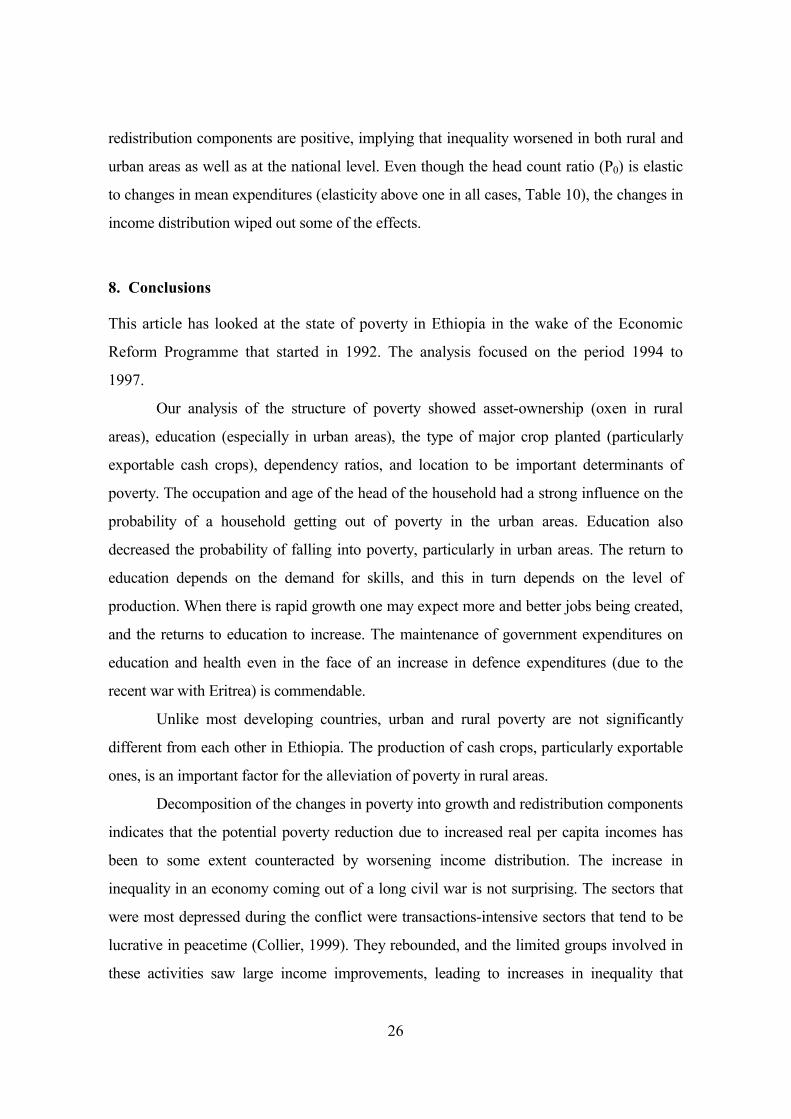
26

redistribution components are positive, implying that inequality worsened in both rural and

urban areas as well as at the national level. Even though the head count ratio (P0) is elastic

to changes in mean expenditures (elasticity above one in all cases, Table 10), the changes in

income distribution wiped out some of the effects.

8. Conclusions

This article has looked at the state of poverty in Ethiopia in the wake of the Economic

Reform Programme that started in 1992. The analysis focused on the period 1994 to

1997.

Our analysis of the structure of poverty showed asset-ownership (oxen in rural

areas), education (especially in urban areas), the type of major crop planted (particularly

exportable cash crops), dependency ratios, and location to be important determinants of

poverty. The occupation and age of the head of the household had a strong influence on the

probability of a household getting out of poverty in the urban areas. Education also

decreased the probability of falling into poverty, particularly in urban areas. The return to

education depends on the demand for skills, and this in turn depends on the level of

production. When there is rapid growth one may expect more and better jobs being created,

and the returns to education to increase. The maintenance of government expenditures on

education and health even in the face of an increase in defence expenditures (due to the

recent war with Eritrea) is commendable.

Unlike most developing countries, urban and rural poverty are not significantly

different from each other in Ethiopia. The production of cash crops, particularly exportable

ones, is an important factor for the alleviation of poverty in rural areas.

Decomposition of the changes in poverty into growth and redistribution components

indicates that the potential poverty reduction due to increased real per capita incomes has

been to some extent counteracted by worsening income distribution. The increase in

inequality in an economy coming out of a long civil war is not surprising. The sectors that

were most depressed during the conflict were transactions-intensive sectors that tend to be

lucrative in peacetime (Collier, 1999). They rebounded, and the limited groups involved in

these activities saw large income improvements, leading to increases in inequality that

27

would have been difficult and even inappropriate to counter through economic policy.

The bottom-line is still that even in Ethiopia, which is at the bottom of the

international income ladder and in spite of the peace dividend effects, growth reduced

poverty.

28

References

Ali, A.G.A, and E. Thorbecke, 1998, “The State and Path of Poverty in Africa”, paperpresented at the Bi-Annual Workshop of the African Economic Research Consortium,May, Nairobi

Anand, S. and R. Kanbur, 1993, “The Kuznets Process and the Inequality-DevelopmentRelationship”, Journal of Development Economics, vol. 40, pp. 25-52

Bevan, P. and S. Joireman, 1997, “The Perils of Measuring Poverty: Identifying the‘Poor’ in Rural Ethiopia”, Oxford Development Studies, vol. 25, no. 3, pp. 315-344.

Bigsten, A. and S. Kayizzi-Mugerwa, 1999, Crisis, Adjustment and Growth in Uganda:.A Study of Adaptation in an African Economy, Macmillan, London.

Bigsten, A. and J. Levin, 2001, “Growth, Income Distribution and Poverty: A Review”,paper for the WIDER conference on Growth and Poverty, 25-26 May, Helsinki.

Chen, S., G. Datt and M. Ravallion, 1994, “Is Poverty Increasing or Decreasing in theDeveloping World?”, Review of Income and Wealth, vol. 40, pp. 359-376

Collier, P. 1999, “On the Economic Consequences of Civil War”, Oxford EconomicPapers, vol. 51, pp. 168-183

Coulter, A.E., A.C. Cowell and S.P. Jenkins, 1992, “Equivalence Scale Relativities andthe Extent of Inequality and Poverty”, Economic Journal, vol. 102, pp. 1067-1082

Datt, G. and M. Ravallion, 1992, “Growth and Redistribution Components of Changes inPoverty Measures: A Decomposition with Applications to Brazil and India in the 1980s”,Journal of Development Economics, vol. 38, pp. 275-295

Deaton, A. and J. Muellbauer, 1980, Economics and Consumer Behaviour, CambridgeUniversity Press, Cambridge.

Deininger, K. and L. Squire, 1998, “New Ways of Looking at Old Issues: Asset Inequalityand Growth”, Journal of Development Economics, 57, pp. 259-287.

Demery, L. and L. Squire, 1996, “Macroeconomic Adjustment and Poverty in Africa: AnEmerging Trend”, World Bank Research Observer, vol. 2, no 1, pp. 24-39

Dercon, S. and P. Krishnan, 1998, “Changes in Poverty in Rural Ethiopia, 1989-1995:Measurement, Robustness Tests and Decomposition”, Working Paper Series 98.7, Centrefor the Study of African Economies (CSAE), Oxford University.

Dollar, D. and A. Kraay, 2000, “Growth Is Good for the Poor”, Policy Research Working

29

Paper No 2587, World Bank, Washington DC.

Fields, G., 1997, “Poverty, Inequality and Economic Well-being: African EconomicGrowth in Comparative Perspective”, paper prepared for AERC workshop, Kampala

Foster, J., J. Greer and E. Thorbecke, 1984, “Notes and Comments: A Class ofDecomposable Poverty Measures”, Econometrica, vol. 52, no 3, 761-766.

IMF, 1999, Ethiopia: Recent Economic Developments, Washington DC.

Kakwani, N., 1980, Income Inequality and Poverty: Methods of Estimation and PolicyApplications, Oxford University Press, Oxford.

Kakwani, N., 1990, “Poverty and Economic Growth with an Application to Coted’Ivoire”, LSMS Working Paper no 63, World Bank, Washington DC.

Kebede, B., 1994, “Report on Sample Selection”, mimeo, Department of Economics,Addis Ababa University.

Kebede, B. and M. Taddesse, eds., 1996, The Ethiopian Economy: Poverty and PovertyAlleviation, Proceeding of the Fifth Annual Conference on Ethiopian Economy,Department of Economics, Addis Ababa University and the Ethiopian EconomicAssociation (EEA), Addis Ababa.

Kuznets, S., 1955, “Economic Growth and Income Inequality”, American EconomicReview, vol. 45, pp. 1-28

Lipton, M., and M. Ravallion, 1995, “Poverty and Policy”, in J. Berhman and T.N.Srinivasan, eds., Handbook of Development Economics, vol. III, , Elsevier Science

Moser, G. and Ichida, T. 2001, “Economic Growth and Poverty Reduction in Sub-Saharan Africa”, IMF Working Paper WP/01/112, Washington DC.

Ravallion, M., 1992, “Poverty: A Guide to Concepts and Methods”, LSMS WorkingPaper 88, World Bank, Washington DC.

Ravallion, M. and Bidani, B. 1994, “How Robust is a Poverty Profile?”, World BankEconomic Review, vol. 8, no 1, pp. 357-382.

Ravallion, M. and S. Chen 1997, “What Can New Survey Data Tell Us about RecentChanges in Distribution and Poverty”, World Bank Economic Review, vol. 11, ´no 2, pp.

Welfare Monitoring Unit, 1999, Poverty Situation in Ethiopia, Ministry of EconomicDevelopment and Co-operation, Addis Ababa.