GROUP-CONTRIBUTION METHODS IN ESTIMATING A THESIS IN ...

GROUP-CONTRIBUTION METHODS IN ESTIMATING

LIQUID-LIQUID DISTRIBUTION COEFFICIENTS

by

CHE KEUNG LIU, B.A.

A THESIS

IN

CHEMICAL ENGINEERING

Submitted to the Graduate Faculty of Texas Tech University in

Partial Fulfillment of the Requirements for

the Degree of

MASTER OF SCIENCE

IN

CHEMICAL ENGINEERING

Approved

May, 1981

/ '

ACKNOWLEDGMENTS

To Dr. L. Davis Clements, chairman of my committee, I extend my

deepest appreciation for his helpful and expert advice, guidance, and

encouragement throughout this project. I would also like to thank the

rest of the committee. Dr. S. R. Beck and Dr. H. R. Heichelheim, for

their suggestions and criticisms.

Finally, my special thanks go to Ms. Sue Willis for her assistance

in preparing this thesis.

n

TABLE OF CONTENTS

PAGE

ACKNOWLEDGMENTS ii

LIST OF TABLES v

LIST OF FIGURES vi

CHAPTER I INTRODUCTION 1

CHAPTER II LITERATURE REVIEW 4

Uses of Distribution Coefficient 4

History 7

Thermodynamic Derivation of Distribution Law . . . 9

Activity Coefficient Models 11

Modifications of Wilson's Equation 12

NRTL (Non-random Two-liquid Equation) 13

UNIQUAC (Universal Quasi-Chemical) Equation. . . . 14

Group-Contribution Models 16

ASOG 18

UNIFAC Method (UNIQUAC Functional-Group

Activity Coefficients) 20

Empirical Correlation Methods 21

CHAPTER III DISTRIBUTION COEFFICIENTS OF HOMOLOGUES 23

Introduction 23

Relation of the Distribution Coefficients of Homologues to Molecular Structure 23 Derivation to Free-Energy Equations of Partitioning Process 32 Determination of Free Energy of Transfer of Methylene Group 40

. • •

PAGE

CHAPTER IV ESTIMATION OF LIQUID-LIQUID DISTRIBUTION COEFFICIENTS FROM GROUP CONTRIBUTIONS 43

Reasons for New Model Development 43

Data Collection 43

Group Contributions Model 44

Method 47

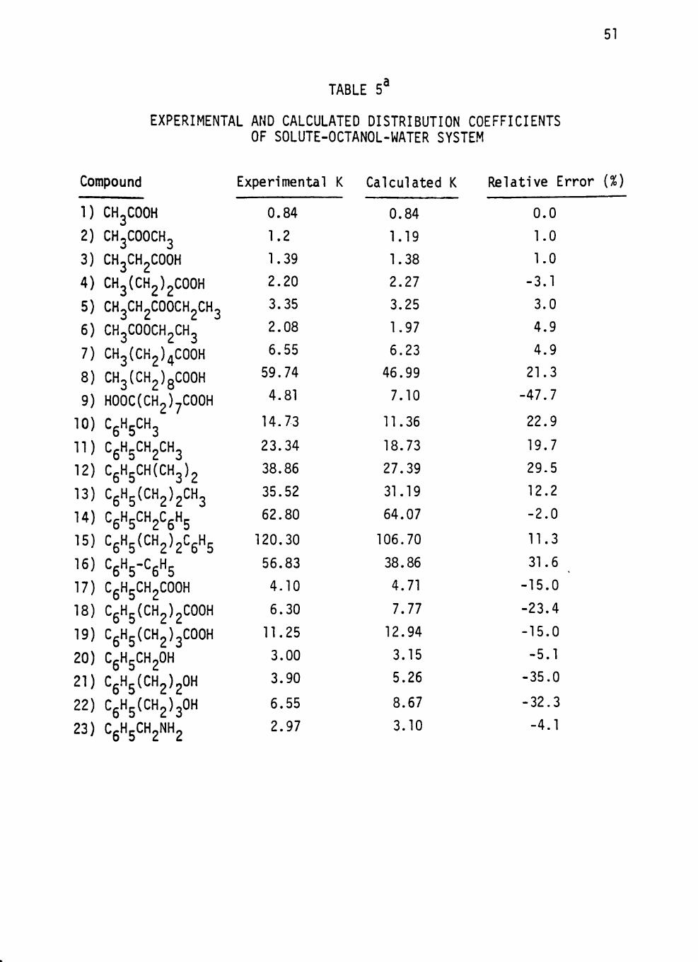
Predictivity of the Model 50

CHAPTER V EVALUATION OF FACTORS INFLUENCING LIQUID-LIQUID DISTRIBUTION COEFFICIENTS 61

Introduction 61

Effect of pH on Distribution Coefficient 61

Temperature Effect on Distribution Coefficient 68

Effect of Concentration on Distribution Coefficient 76

Discussion 79

CHAPTER VI CONCLUSIONS AND RECOMMENDATIONS FOR

FUTURE STUDIES 81

Summary of the Research 81

Conclusions 81

Recommendation for Future Studies 82

LIST OF REFERENCES 83 NOMENCLATURE 90

TV

LIST OF TABLES

PAGE

Table 1 RELATION OF DISTRIBUTION COEFFICIENTS TO THE NUMBER OF CARBON NUMBER AND METHYLENE NUMBER 25

Table 2 DISTRIBUTION COEFFICIENTS OF ACIDS OBTAINED FROM EXPERIMENTS AND CORRELATIONS 31

Table 3 FREE ENERGY CHANGES (AT 25°C) TO TRANSFER

A MOLE OF METHYLENE 42

Table 4 GROUP CONTRIBUTIONS FOR THE FOUR SYSTEMS 49

Table 5 EXPERIMENTAL AND CALCULATED DISTRIBUTION COEFFICIENTS OF SOLUTE-OCTANOL-WATER SYSTEM 51

Table 6 EXPERIMENTAL AND CALCULATED DISTRIBUTION COEFFICIENTS OF SOLUTE-DIETHYL ETHER-WATER SYSTEM 55

Table 7 EXPERIMENTAL AND CALCULATED DISTRIBUTION COEFFICIENTS OF SOLUTE-CHLOROFORM-WATER SYSTEM. . . . 57

Table 8 EXPERIMENTAL AND CALCULATED DISTRIBUTION

COEFFICIENTS OF SOLUTE-BENZENE-WATER SYSTEM 59

Table 9 SHIFT OF DISTRIBUTION COEFFICIENT WITH pH 62

Table 10 SHIFT OF DISTRIBUTION COEFFICIENTS WITH pH 65

Table 11 EFFECT OF TEMPERATURE UPON DISTRIBUTION

COEFFICIENT 70 Table 12 SHIFT OF DISTRIBUTION COEFFICIENTS OF

STRONG ACIDS WITH CONCENTRATION 77

LIST OF FIGURES

PAGE

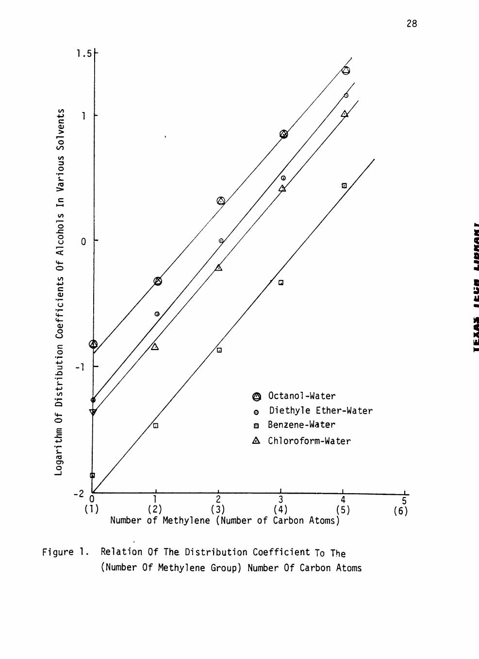
Figure 1. Relation Of The Distribution Coefficient To The (Number of Methylene Group) Number Of Carbon Atoms 28

Figure 2. Relation Of The Distribution Coefficient To The (Number of Methylene Group) Number Of Carbon Atoms 29

Figure 3. Relation Of The Distribution Coefficient To The (Number of Methylene Group) Number Of Carbon Atoms 30

Figure 4. Relation Of The Distribution Coefficient To The (Number Of Methylene Group) Number Of Carbon Atoms 33

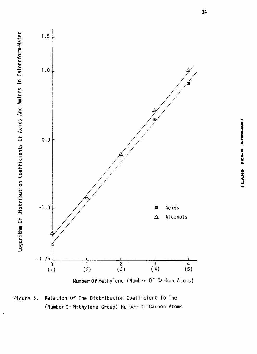
Figure 5. Relation Of The Distribution Coefficient To The (Number Of Methylene Group) Number Of Carbon Atoms 34

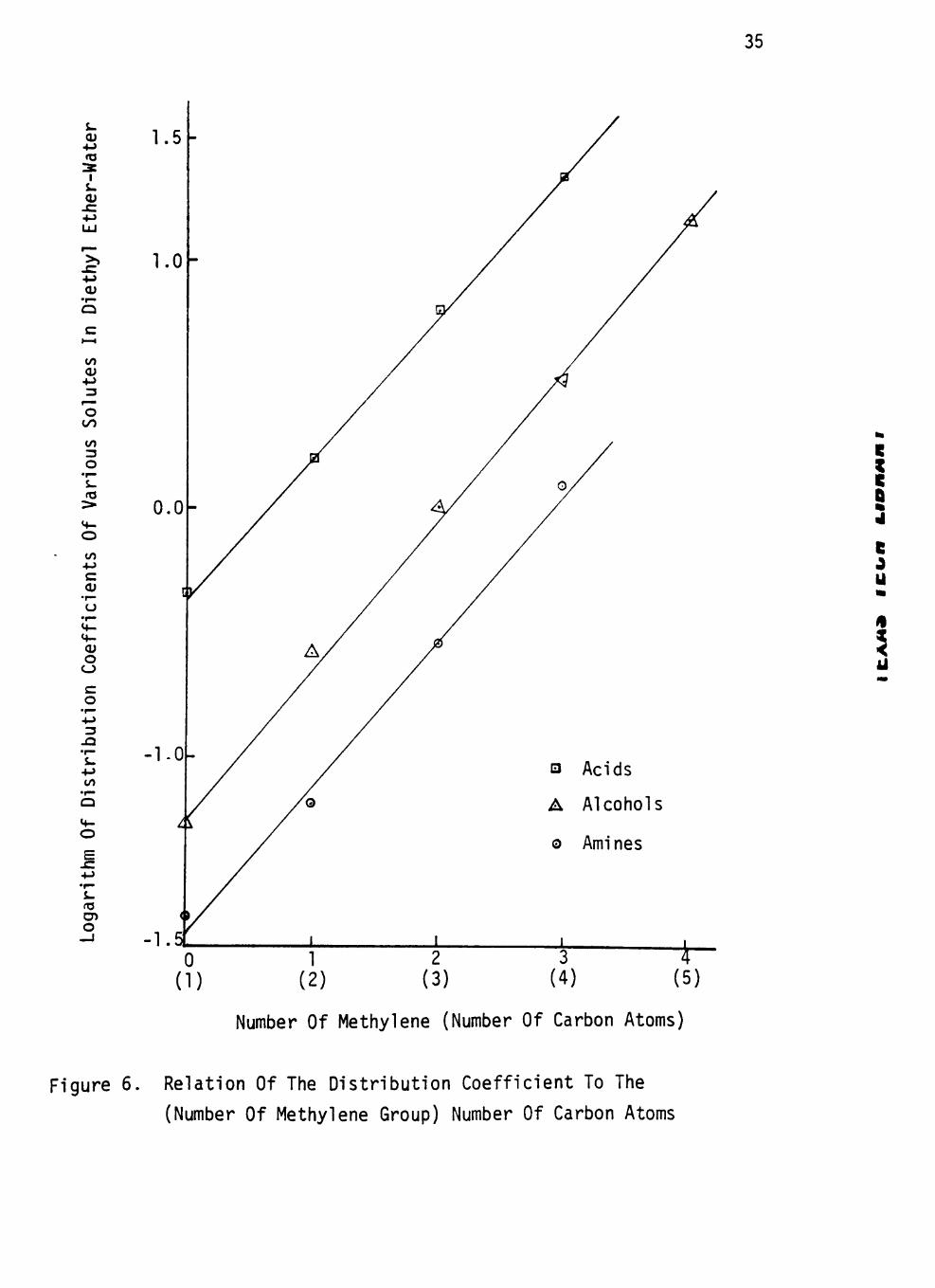
Figure 6. Relation Of The Distribution Coefficient To The (Number of Methylene Group) Number Of Carbon Atoms 35

Figure 7. Relation Of The Distribution Coefficient To The (Number of Methylene Group) Number Of Carbon Atoms 36

Figure 8. Relation Of The Distribution Coefficient To

The Number Of Carbon Atoms 37

Figure 9. Shift Of K With pH 63

Figure 10. Shift Of K With pH 66 Figure 11. Effect Of Temperature Upon Distribution

Coefficient 72

Figure 12. Effect Of Temperature Upon Distribution Coefficient 73

Figure 13. Effect Of Temperature Upon Distribution Coefficient 74

VI

PAGE

Figure 14. Effect Of Temperature Upon Distribution Coefficient 75

Figure 15. Shift Of Distribution Coefficient With Concentration 78

v n

CHAPTER I

INTRODUCTION

A large part of chemical engineering design is concerned with sepa­

ration processes such as distillation, absorption, and extraction. For

design of a liquid-liquid extraction system, one needs to know the rela­

tive distribution of the solutes between the two liquid phases. The key

to carrying out an effective extraction depends on the choice of a suit­

able solvent. The distribution coefficient is one of the important fac­

tors in the choice of solvents. According to Henley and Staffin (1),

the liquid-liquid distribution coefficient of a good solvent should be

at least 5, and perhaps as much as 50. At the early stages of process

development we can save money and time if we eliminate solvents which

appear least useful and work on those which are most promising. However,

the choice of solvent requires either a large base of experimental data,

or accurate prediction methods.

Since the number of different mixtures in chemical technology is

extremely large, satisfactory experimental equilibrium data are seldom

available for the conditions in a particular design problem. It is

therefore necessary to be able to predict liquid-liquid distribution co­

efficients from the available experimental data based on thermodynamics

and empirical models for the mixture. However, when suitable data are

lacking, we have to predict the coefficients from some generalized method,

For many years group-contribution methods have been used to predict

properties of pure substances with great success. For example, Souders

1

and Matthews (2) used group-contribution methods for the prediction of

heat capacity and heat contents of hydrocarbons in the ideal state.

During the last 15 years, group-contribution methods have also been

developed for the prediction of thermodynamic properties of liquid mix­

tures. These correlation methods are based on the premise that thermo­

dynamic functions within a molecule are additive. Thus, the values for

the liquid molecules can be built up from an assignment of contributions

to the various groups which make up the molecule under consideration.

The group-contribution method has two advantages. First, i t enables

systematic interpolation and extrapolation of liquid-liquid equilibrium

data for many chemically related mixtures. Secondly, i t provides a rea­

sonable method for predicting the properties of a wery large number of

mixtures in terms of a relatively small number of group parameters.

There is a need for more work on methods for the correlation and

prediction of liquid-liquid distribution coefficients. Today, the goal

of predicting the compositions of the two liquid phases in equilibrium

has remained elusive. Several attempts have been made to use the ASOG

(Analytical Solution of Groups) and UNIFAC (UNIQUAC Functional-group

Activity Coefficients) group-contribution methods to predict the liquid-

liquid equilibrium compositions. The agreement between experimental and

calculated equilibrium composition is not too convincing. Also, these

models are based on parameters estimated from experimental phase-

equilibrium data for the mixtures of interest and are not readily gen­

eralized to systems for which there are no data.

The purpose of this study was to investigate the properties of

liquid-liquid distribution coefficients in order to determine i f

development of a systematic group-contribution method to predict the

value of liquid-liquid distribution coefficients based on a knowledge

of the structural formula of the compound only is possible.

CHAPTER II

LITERATURE REVIEW

Uses of Distribution Coefficient

Solvent extraction is an important industrial separation method.

Industrial application of solvent extraction has increased rapidly over

the past two decades. The unique ability of solvent extraction to achieve

separation according to chemical type rather than according to physical

characteristics allows application to a great variety of processes. Ap­

plications range from nuclear-fuel enrichment and reprocessing to ferti­

lizer manufacture, and from petroleum refining to food processing.

The choice of solvents for extraction depends upon several factors,

including cost, availability, stability, selectivity for the desired

component and the distribution coefficient. In evaluating a solvent for

use in an extraction operation, it is of prime importance to know the

relative distribution of the material being extracted between the solvent

and raffinate phases. Both the quantity of solvent needed and the number

of extraction stages required to obtain the desired separation depend on

the value of distribution coefficient.

The distribution coefficient, K, is the ratio of the composition of

the solute in each liquid phase in equilibrium:

Y. <

'a K = -y^ at equilibrium (1) a A.

where Y = composition of solute a in the extract phase a

X^ = composition of solute a in the raffinate phas( a

The value of K is one of the main parameters used to establish the

minimum sol vent-feed ratio that can be used in an extraction process.

Consider the case that solvent S and carrier solvent R are immiscible.

The minimum solvent to feed ratio can be estimated from the liquid-liquid

distribution coefficient.

From the definition of the distribution coefficient, we have

B£/(S + B ) D = B /(R + Bj ) (2)

where Br = quantity of solute B in extract phase

Bn = quantity of solute B in raffinate phase

S = quantity of solvent

R = quantity of carrier solvent

If the concentration of solute B is low, then S is much bigger than B^

and R is much bigger than B, and the distribution coefficient can be

expressed as

Bp/S

S^VF ( )

where B = total quantity of B

F = quantity of feed (F = B+ R)

Rearranging the terms, the solvent to feed ratio, S/F, is

i=L.!i (4)

For 99% extraction, the values of b^ and B are 0.01 and 0.99, respec­

tively. Thus, i f the distribution coefficient is 4, 24.75 pounds of

solvent would be required to remove 99% of the solute from 1 pound of

feed.

The distribution coefficient also influences the selectivity. It

is desirable in any extraction process that the solvent used dissolve a

large portion of the solute, while at the same time the amount of non-

consolute component transferred be as low as possible. A measure of

this separation is the selectivity of the solvent.

The selectivity a^^ of solvents for solute C from a mixture of A

and C is

"ca K " \ ( Y j a a (5)

For separation to be possible, a should be larger than 1. The

larger a , the better the extraction process, since as a , increases, " ca

fewer stages- are required for a given separation and capital costs are

lower.

For extraction of solute C from a mixture of A and C, since

X^/Y^ > 1, then for solvent to have a high selectivity for the desired

component, the distribution coefficient, K , should have a favorable

value (K » 1). Thus the distribution coefficient is an important

property of the solvent in that it influences the selectivity.

Distribution coefficients have been used as an aid in identifica­

tion of extremely small amounts of organic compounds (3). From the

rate of migration of a substance in the countercurrent distribution ap­

paratus, its distribution coefficient may be calculated. It is thus pos

sible to characterize an unknown substance, never before isolated, in

terms of its distribution constants in mixtures of different solvents.

7

The distribution coefficient is one of the fundamental properties

of an emulsifier. Davies (4), who studied the kinetics of coalescence

in emulsion systems, has related the HLB (hydrophile-lipophile balance)

system to the distribution coefficient. Thus, the purely empirical HLB

system is related to the distribution coefficient, which is in turn based

firmly on thermodynamics. This relationship makes it possible to deter­

mine the molecule's ability to function as a wetting agent, detergent,

or defoamer.

Many equilibrium constants have been determined by distribution

measurements. Vandalen (5) measured the equilibrium constants for metal

ion complexing agents among water and organic phases. Other types of

equilibrium studied by distribution measurements are those which have

dimer dissociation and those which form Schiff bases (6, 7).

History

As early as 1870, Berthelot and Jungfleisch (8) investigated the

distribution of I^ and Br^ between CSp and water. They also studied the

partition of various organic acids between ethyl ether and water. They

showed that the ratio of the concentrations of solute distributed between

two immiscible solvents was a constant at constant temperature. From

these early investigations, they also observed that the liquid-liquid

distribution coefficient varies with temperature.

In 1891, Nernst (9) developed the distribution law. The distribu­

tion law stated that a solute will distribute between two essentially

immiscible solvents in such a manner that, at equilibrium, the ratio of

the concentrations of the solute in the two phases at a particular

8

temperature will be a constant, provided the solute has the same molecu­

lar weight in each phase. For a solute B distributing between solvents

1 and 2, we have

B^^B^

K = [ByCB]^ (6)

where K is the distribution coefficient, a constant independent of total

solute concentration, and [B]^ is the concentration of solute in solvent

phase 2, and [B]^ is the concentration of solute in solvent phase 1.

Although the distribution law is a useful approximation, it has two

shortcomings. First, the distribution law does not consider chemical re­

actions such as association and dissociation of solute in different

phases. Secondly, the distribution law is not thermodynamically rigor­

ous.

Chemical interactions of the distributing species with the other

components in different phases affect the concentrations of the distri­

buting species. If all the significant interactions of the distributing

species are known, we may evaluate a distribution ratio which describes

the stoichiometric ratio including all species of the same component in

the respective phases. We may express the distribution ratio, D, as

Pj _ Total concentration in organic phase , . Total concentration in aqueous phase ^''

Lacroix (10) illustrated the situation of ionization of solute in

the aqueous phase. He showed that the distribution ratio of 8-quinolinol

between chloroform and water with the problem of ionization of 8-quinolinol

could be related to distribution coefficient as

lM^+1 + ^ • 1 [H^]

where K, = first ionization constant

K2 = second ionization constant

K = distribution coefficient

Thermodynamic Derivation Of Distribution Law

The distribution law could be explained by classical thermodynamics

under the conditions that the solvent systems are almost completely im­

miscible and the solute concentration is wery low. Treybal (11) has pre­

sented a discussion of the thermodynamic derivation of distribution law.

The following discussion relies heavily on his summary.

At constant temperature and pressure, equilibrium is attained when

the chemical potentials, y, of the solute in each phase are equal. Thus

where 1 = solute phase 1

2 = solute phase 2

Consider the solution to be represented by an ideal molar solution,

and we have

y^^ + RT In m^ + RT In y^ = M^^ + RT In m^ + RT In y^ (10)

10

where m = solute concentration in molarity

Y = molar activity coefficient

y-j** = chemical potential of solute in a hypothetical ideal molar

solution.

From the above expression, the molar distribution coefficient, K,

can be expressed as

mp Yi '{\i^° - yi°)/RT

m Y2 . ^ '

If the presence of the solute does not significantly affect the

mutual solubilities of the two solvents, the y°'s become constant. Then

we have

mp Y^ K = ir = 7-C (12)

n ^2

where C is a constant for the system at constant temperature.

Thus, the distribution coefficient varies with the variations in the

activity coefficients in each of the phases. When solute concentration

is yery low, the distribution coefficient becomes constant as the acti­

vity coefficients approach unity. For example, Grahame and Seaborg (12)

found that the distribution coefficient of gallium chloride between

ethyl ether and 6 m hydrochloric acid remains essentially constant (with-

-12 -3 in 5%) over a concentration range from 10 to 2 x 10 m gallium

chloride.

n

Act iv i ty Coefficient Models

Unfortunately, the simplif ied approach of assuming that the rat io

of the ac t iv i t y coefficients of any component in the coexisting phases

approaches unity does not apply to the whole concentration range. For

calculation of distr ibut ion coefficients i t is necessary, in pr inc ip le,

to know the ac t iv i ty coefficients of solute in the equilibrium phases

over the concentration range of interest. Once a reasonable method for

predicting ac t iv i ty coefficients is available, one may use the ac t iv i ty

coeff icient of solute in each phase to calculate distr ibut ion coef f i c i ­

ents.

Tradi t ional ly, two dif ferent categories of models have been used in

correlating ac t iv i ty coeff icients. The f i r s t type of model uses empiri­

cal relations for interpolat ion. The second type of model is a direct

application of the thermodynamics of fluid-phase equi l ibr ia .

P ie ro t t i , Deal and Derr (13) have correlated in f in i te -d i lu t ion ac­

t i v i t y coefficients with the molecular structure of the components in ­

volved. In binary systems where the in f in i te -d i lu t ion act iv i ty coef f i ­

cients are quite large (larger than 25), so that the mutual so lub i l i t ies

are small, good estimates of the mutual so lubi l i t ies can be made on the

basis of the in f i n i te -d i l u t i on act iv i ty coeff icients. However, in sys­

tems with smaller immiscibi l i ty gaps and in multicomponent systems, the

l iqu id - l iqu id equilibrium compositions cannot be predicted with s u f f i ­

cient accuracy from in f in i te -d i l u t i on act iv i ty coefficients alone.

Hildebrand and Scott's regular solution theory (14) offers a pos­

s i b i l i t y of calculating ac t iv i ty coefficients without any use of mixture

experimental information. Al l one keeds to know is the "so lub i l i t y

12

parameter" for each pure component. However, regular solution theory

does not apply to even moderately polar substances. This is a serious

disadvantage, since water is present in most of the liquid-liquid systems

of interest. In situations where regular solution theory holds, i t may,

at most, be expected to yield predictions which are in qualitative agree­

ment with experiment.

The modifications of Wilson's equation, NRTL and UNIQUAC equations

are widely used today for calculating liquid phase activity coefficients.

These models were derived by various researchers by using Wilson's "local

composition" concept for representation of excess Gibbs energies of

liquid mixtures. The local composition concept provides a convenient

method for introducing nonrandomness into the liquid-mixture model. The

central idea of the local composition concept is that when viewed micro­

scopically, a liquid mixture is not homogeneous; the composition at one

point in the mixture is not necessarily the same as that at another point.

In engineering applications and in typical laboratory work only the

average, overall composition matters. However, for constructing liquid-

mixture models, i t appears that the local composition, rather than the

average composition is a more realistic primary variable.

Modifications of Wilson's Equation

Wilson's equation is not applicable to liquid mixtures which are

only partially miscible. The most used modification of Wilson's equa­

tion was introduced by Tsuboka and Katayama (15). They modified Wilson's

equation by introducing the parameter A.. which is defined as the

13

probability of finding a molecule of type j, next to a molecule of

type i.

The Wilson equation modified by Tsuboka and Katayama for the excess

Gibbs energy is:

G^ ^ , " J |y = - Z X. (In Z X. A.. + In E x. p. .) (13)

Pij = V./Vj. ; i, j = 1,2, . . .N (14)

The modified Wilson's equation uses two parameters per binary and

correlates binary and ternary data well. Prediction of ternary liquid-

liquid equilibrium from binary data is qualitatively satisfactory.

NRTL (Non-random Two-liquid Equation)

The NRTL is the most extensively used model for liquid-liquid equil­

ibrium to date. The equation was developed by Renon and Prausnitz (16).

To take into account nonrandomness in liquid mixtures, Renon modified

Wilson's equation by adding a term 3-]2» which is characteristic of the

nonrandomness of the mixture. Also, he introduced the two-liquid theory

of Scott (17), which assumes that there are two kinds of cells in a

binary mixture: one with molecule 1 at the center surrounded by 1 and 2

and the other, with molecule 2 at the center.

Renon defined the molar excess Gibbs energy for a binary solution

as the sum of two changes in residual Gibbs energy: f i rs t , that of

transferring n-. molecules from a cell of the pure liquid 1 into a cell 1

of the solution, and second, that of transferring n molecules from a

cell of the pure liquid 2 into a cell 2 of the solution.

14

In a multicomponent mixture, the NRTL equation for the excess Gibbs

energy and the activity coefficient are:

N

gE N .?, ji ji ^j fp= Z x.^ ; l,j,p = 1,2, ..., N (15)

^ ki \ k=l ^^ ^

N N Zr.. G..X. .1 „ r Z x F . G . .

'" i N ._, N ^Mj N ; Ub; ^ S. . X. "" Z G, . X, Z G, . X,

k=l ^ ^ k=l ^J ^ k=l 'J ^

There are three parameters per binary: r . . , r.. and 3^-. The para-

meters are calculated from experimental compositions of the two equili­

brated liquid phases. The NRTL equation appears to be applicable to a

wide variety of mixtures for calculating vapor-liquid and liquid-liquid

equilibria. The NRTL equation often correlates binary and ternary

liquid-liquid equilibria quantitatively correctly. Prediction of ternary

liquid-liquid equilibria from binary data is often qualitatively correct.

UNIQUAC (Universal Quasi-Chemical) Equation

The UNIQUAC equation was developed by Abrams and Prausnitz (18) in

1975 and modified by Anderson and Prausnitz in 1978 (19). The UNIQUAC

equation generalized the theory of Guggenheim to mixtures containing

molecules of different size and shape by utilizing the local composition

concept. The original Guggenheim quasi-chemical lattice model is re­

stricted to small molecules of essentially the same size. The effect of

molecular size and shape are introduced through structural parameters

15

obtained from pure-component data and through use of Staverman's combi­

natorial entropy as a boundary condition for athermal mixtures.

In a multicomponent mixture, the UNIQUAC equation for the activity

coefficient of component i is

In Y . = In Y.^ + In Y ^ (17)

combinatorial residual

The UNIQUAC model has only two adjustable parameters, r and r . ,

per binary. These parameters must be evaluated from experimental phase-

equilibrium data. No ternary parameters are required for systems con­

taining three or more components. Since i t often happens that binary-

parameter sets cannot be determined uniquely, ternary data should then

be used to fix the best binary sets from the ranges obtained from the

binary data.

For a few systems, Abrams and Prausnitz (18) show that UNIQUAC per­

forms reasonably well, both in predicting ternary diagrams from binary

information only and in correlating ternary diagrams. Anderson and Praus­

nitz (19) show that UNIQUAC predicts ternary diagrams very well from bi­

nary information when binary vapor-liquid and liquid-liquid equilibrium

data are correlated simultaneously with only a few ternary tie lines.

Comparing these models for correlating liquid-liquid equilibrium,

Fredenslund, et a l . (20) concluded that UNIQUAC is as good as or better

than NRTL and modifications of Wilson's equation by Tsuboka and Katayama.

However, these local composition models were developed for vapor-liquid

equilibrium and are not fully successful for liquid-liquid equilibrium.

I t is often not possible to represent the solute distribution coeffici­

ents with sufficient accuracy for extraction design purposes. Freden­

slund, et a l . (20) reported that the predicted value of distribution

16

coefficients by UNIQUAC using four parameters may be in error by more

than a factor of two.

Group-Contribution Models

The NRTL and UNIQUAC models are widely used for correlating liquid-

liquid equilibrium data. The parameters in these models are estimated

from experimental phase equilibrium data. For systems for which little

or no experimental information is available one needs prediction methods.

In recent years the group contribution approach has become a valuable

tool for such predictions. Notable in this development are the pioneer­

ing work by Pierotti, Deal and Derr (13), Wilson and Deal (21), and sub­

sequent contributions by Scheller (22), Rateliff and Chao (23), Derr and

Deal (24), and Fredenslund, Jones and Prausnitz (25).

In 1962, Wilson and Deal (21) presented the solution of groups con­

cept to calculate activity coefficients on the basis of solute and sol­

vent structures. The four assumptions they used became the basis for

most group-contribution methods used for the estimation of activity

coefficients.

The four assumptions are:

Assumption 1. The liquid solution can be treated as a solution of groups

which make up the components of the mixture. The "groups" are any con­

venient structural units such as -CH^, -OH, and -CH2OH.

Assumption 2. The partial molar excess free energy, or, simply, the

logarithm of the activity coefficient of a component is assumed to be

the sum of two contributions - one associated with differences in molecu­

lar size and shape and the other with energetic interactions between the

17

groups. For molecular solute i in any solution:

In Yi = In yS' + In Y - ^ (18)

C R where Y - is the combinatorial or size or entropy part and Y,- is the

residual or interaction or enthalpy part.

Assumption 3. The contribution from interactions of molecular "groups"

is assumed to be the sum of the individual contributions of each solute

"group" in the solution, less the sum of the individual contributions in

the conventional standard state environment. For molecular solute i,

containing groups K:

In y.^ = Z v^[ln r^ - In r^^^'^ (19)

K = 1, 2 ... N, where N is the number of different groups in the mixture,

r. is the residual activity coefficient of group K in a solution; r. ^

is the residual activity coefficient of group K in a reference solution

containing only molecules of type i; ^^ is the number of "interaction"

groups of kind K in molecule i. The standard state for the group resi­

dual activity coefficient need not be defined due to cancellation of

terms.

Assumption 4. The individual group contributions in any environment con­

taining groups of given kinds are assumed to be only a function of group

concentrations.

= F(x^, X2 . . .x^) (20)

18

(i) The same function is used to represent r. and T.^ \ The group fraction

F is defined by:

Fu = ^-:^ (21) Z Z v.^^^x.

i = 1, 2 . . .M (number of components)

j = 1, 2 . . .N (number of groups)

The assumption that individual group contributions are functions

only of group concentrations permits experimental data for one system to

be applied to a second system involving the same groups.

The pioneering work of Wilson and Deal lead to the development of

various group-contribution methods as stated previously. The difference

between the various group-contribution methods is essentially due to the

differences in the definition of functional groups and in the equations

used for calculating the combinatorial or size activity coefficient and

the group activity coefficient.

ASOG and UNIFAC models are based on the solution of groups concept.

These models may be used to compute the liquid phase activity coeffi­

cients by the properties of the groups. Hence, liquid-liquid distribu­

tion compositions at equilibrium may be predicted in the absence of ex­

perimental information for the mixture of interest.

ASOG

The "Analytical Solutions of Groups" (ASOG) method was developed

by Derr and Deal from previous work on group-contribution theory by

Wilson (21) and Pierotti, Deal and Derr (13). The Flory-Huggins relation

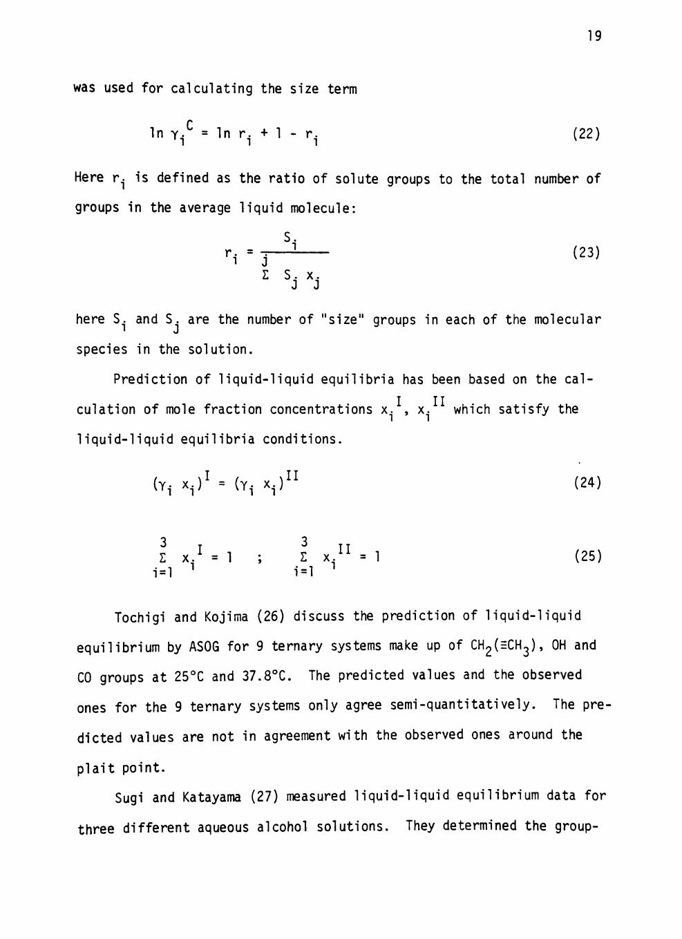
19

was used for calculating the size term

In Y - = In r. + 1 - r. (22)

Here r is defined as the ratio of solute groups to the total number of

groups in the average liquid molecule:

r, = j-^ (23)

Z S. X. J J

here S. and S. are the number of "s ize" groups in each of the molecular

species in the so lu t ion.

Predict ion of l i q u i d - l i q u i d equ i l i b r i a has been based on the ca l ­

culat ion of mole f rac t ion concentrations x. , x. which sat is fy the

l i q u i d - l i q u i d equ i l i b r i a condit ions.

(Yi x . )^ = {y. x . )^^ (24)

Z x.^ = 1 ; Z x,^^ = 1 (25) i= l ^ i= l ^

Tochigi and Kojima (26) discuss the predict ion of l i q u i d - l i q u i d

equi l ibr ium by ASOG for 9 ternary systems make up of CH2(=CH2), OH and

CO groups at 25°C and 37.8°C. The predicted values and the observed

ones fo r the 9 ternary systems only agree semi-quant i tat ively. The pre­

dicted values are not in agreement with the observed ones around the

p l a i t po in t .

Sugi and Katayama (27) measured l i q u i d - l i q u i d equi l ibr ium data for

three d i f f e ren t aqueous alcohol solut ions. They determined the group-

20

interaction parameters based on the data for the mutual solubility of

water and 1-butanol at 25**C. These parameters were then used for the

prediction of liquid-liquid equilibria for al l the other measured systems

Their results were in qualitative, but not quantitative, agreement with

experiment.

UNIFAC f^thod (UNIQUAC Functional-Group Activity Coefficients)

The UNIFAC method was originally developed by Fredenslund, et a l .

(25) in 1975 based on the UNIQUAC model for liquid mixtures. In the

UNIFAC method, the combinatorial term of the activity coefficient takes

into account not only the differences in molecular sizes as given by

group volumes but also the differences in molecular forms as presented

by group surface areas. The method was later revised and detailed des­

criptions of the method have been presented by Fredenslund, et a l . (28).

The UNIFAC equations for the calculation of activity coefficients

are:

In y- = In y.^ + In Y / (26)

combinatorial residual

In Y - = (In c^/x. + 1 - 4)^./x.) - 1/2 Z q.(ln (D./e. + 1 - <t)./9.) (27)

Is

The parameters needed for the use of UNIFAC are group volumes (R,^),

group surface areas (Qj ) and group interaction parameters (A^^ and A^^ ).

The group interaction parameters must be evaluated from phase equilibri urn

21

data. Extensive tables with parameters are given by Fredenslund, et

a l . (28).

Recently, Magnussen, e t a l . (29) decided to develop a new parameter

table e x p l i c i t l y for l i q u i d - l i q u i d equi l ibr ium at 25^C. These new para­

meter may well lead to s ign i f i can t improvements. However, the d i s t r i b u ­

t ion coef f ic ients cannot be expected to be predicted well since small

concentrations may be a f f l i c t e d with large re la t ive er rors .

Empirical Correlat ion Methods

Both the ASOG and UNIFAC approaches to estimating l i q u i d - l i q u i d

equi l ibr ium behavior have a common thermodynamic basis, and both depend

upon estimation of solute a c t i v i t y coef f ic ients to calculate a d i s t r i b u ­

t ion coe f f i c ien t . Soviet authors have taken a much more s imp l is t i c ap­

proach to corre la t ion of l i q u i d - l i q u i d d is t r ibu t ion coe f f i c ien ts .

Korenman, et a l . (30) found a l inear re la t ion between the number of

carbon atoms in the extractable molecule and the logarithm of the cor­

responding d i s t r i bu t i on coef f ic ients in n-alkanols, a l iphat ic amines,

and 2-alkoxyethanols homologues.

Abramzon, et a l . (31) observed that the re lat ion of the d i s t r i b u ­

t ion coe f f i c ien t values of amines in a homologous series to the number

of hydrogen atoms in the hydrocarbon chain is l inear and the graphs for

a homologous series of amines in d i f fe ren t solvents are p a r a l l e l . They

concluded that from the re la t ion of the d is t r ibu t ion coef f i c ien t to the

interphase tension and the size of the molecule undergoing p a r t i t i o n ,

i t i s possible to predict the d i s t r i bu t i on coef f ic ients of primary

amines in various l i q u i d - l i q u i d systems.

22

Nys and Rekker (32) estimated liquid-liquid distribution coeffi­

cients of solutes of different structures in octanol-water system.

Their calculations are based on the following equation:

n log K = Z a f (29)

where f is the group contribution, n is the structure type and a is the

number of times a given group occurs in the structure.

By means of regression analysis, Rekker, et al. obtained the group

values of 11 type of structure. The overall accuracy of the estimating

distribution coefficients is extremely good. The average absolute percent

error is 9.4%.

CHAPTER I I I

DISTRIBUTION COEFFICIENTS OF HOMOLOGUES

Introduction

The works of Korenman, et a l . (30) and Abramzon, et a l . (31) with

a limited number of homologous series of solute materials suggests an

interesting possibility. I f the linear relationship between distribu­

tion coefficient and carbon number in a homologous series is a general

relation, then one should be able to estimate the distribution coeffi­

cient of larger molecules in a series based solely upon values for the

smaller molecules of a series. Further, there exists the opportunity

of predicting, a priori, values for liquid-liquid distribution coeffi­

cients at infinite dilution based solely upon molecular structure, in

a manner similar to prediction of ASOG or UNIFAC parameters.

The work of this chapter has two purposes. First, the relation of

the distribution coefficients of several homologues to the number of

carbon atoms in the molecule is studied in order to verify the property

of log -linear distribution coefficients for homologues. Second, free-

energy equations are used to determine the free energy of the methylene

group, as a test to see i f other group-free-energy contributions may be

determined.

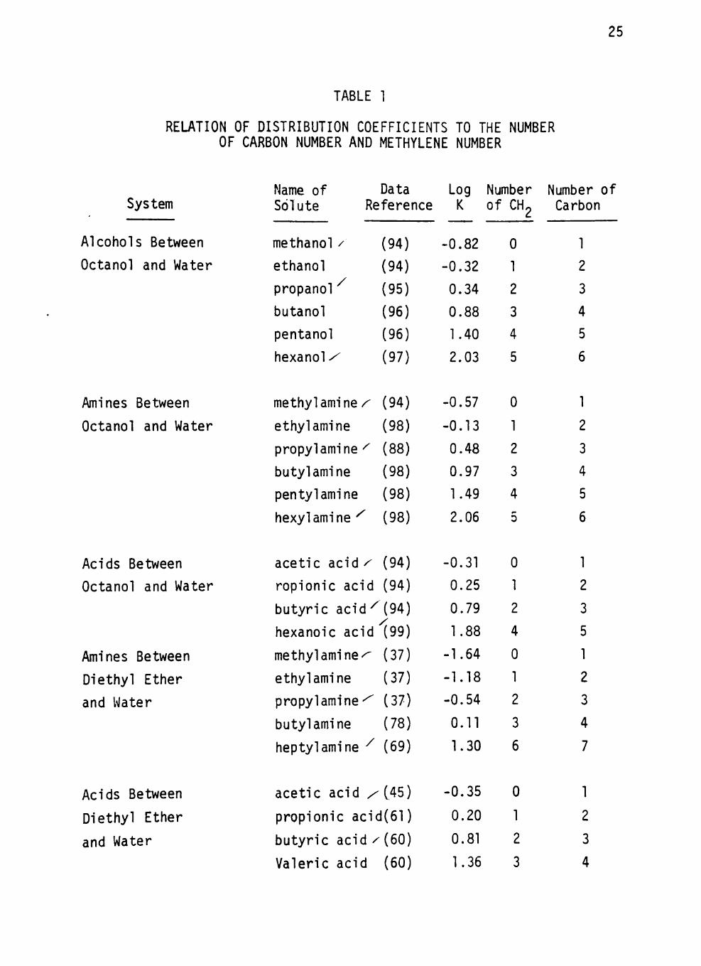
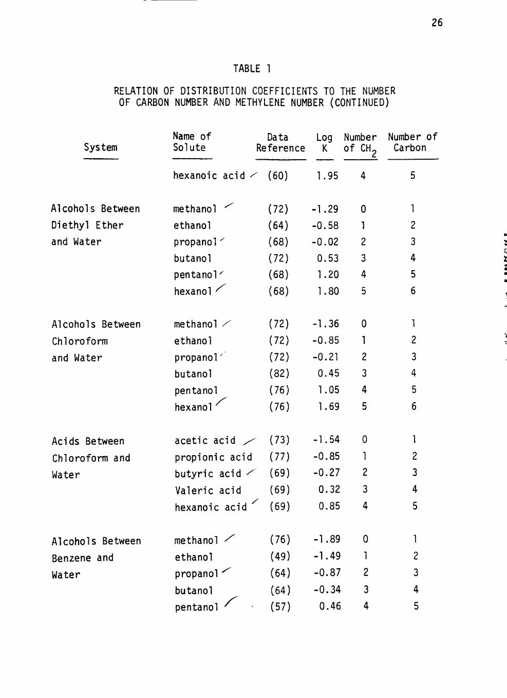
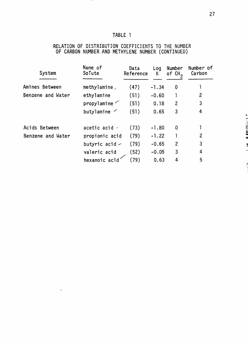
Relation of the Distribution Coefficients of Homologues to Molecular Structure

The liquid-liquid distribution coefficients of several homologues-

alkylamines, n-alkanols and carboxylic acids in octanol-water system.

23

24

diethyl ether-water system, chloroform-water system and benzene-water

system have been tabulated from the l i terature in Table 1. I t is obvious

that the distr ibut ion coefficients of these homologues increase with an

increase in the number of carbon atoms in the molecule.

The logarithms of distr ibut ion coefficients of the homologous series

of solutes in various systems are plotted against solute carbon number

in the hydrocarbon chain in Figures 1 to 3. In a l l cases a l inear rela­

t ion is observed between the number of carbon atoms in the hydrocarbon

chain of the solute and the logarithm of the corresponding distr ibut ion

coeff ic ients. The correlation coefficients of these relations are close

to unity.

The log-l inear behavior may be of practical value for predicting

the distr ibut ion coefficients of certain compounds. Table 2 gives an

example of the results obtained from correlation of acids in four d i f ­

ferent systems together with the experimental values. Good mutual agree­

ment is evident.

The homologous difference is given by the slope of the straight

l ines, and depends in general on the nature of the solvent (Figures 1 to

3). Comparing the distr ibut ion coefficients of the same solute in d i f ­

ferent solvents, i t appears that the distr ibut ion coefficients decrease

with an increase in solvent polar i ty. Acids in chloroform-water system

and in the benzene-water system give exactly the same slope by s t a t i s t i ­

cal analysis. Also, acids in octanol-water and in diethyl ether-water

system give approximately the same slope (0.57 vs. 0.55). This regular­

i t y can be explained by the properties of solvents. Chloroform and

benzene are classif ied as polar solvents and proton donors; while

25

TABLE 1

RELATION OF DISTRIBUTION COEFFICIENTS TO THE NUMBER OF CARBON NUMBER AND METHYLENE NUMBER

System

Alcohols Between

Octanol and Water

Amines Between

Octanol and Water

Acids Between

Octanol and Water

Amines Between

Diethyl Ether

and Water

Acids Between

Diethyl Ether

and Water

Name of Data Solute Reference

methanol / (

ethanol (

propanol (

butanol (

pentanol (

hexanol^ (

methyl amines (

ethyl amine i

propylamine'^ i

butyl amine i

pentylamine i

hexylamine ^ i

acetic acid ^ '

ropionic acid

butyric acid^

hexanoic acid

methyl amines (

ethyl amine

propylamine'^

butyl amine

heptylamine ^

acetic acid x

propionic acid

butyric acid ^

Valeric acid

94)

94)

95)

96)

96)

'97)

,94)

.98)

;88)

[98)

[98)

[98)

[94)

[94)

[94)

[99)

[37)

[37)

[37)

[78)

(69)

[45)

(61)

(60)

(60)

Log K

-0.82

-0.32

0.34

0.88

1.40

2.03

-0.57

-0.13

0.48

0.97

1.49

2.06

-0.31

0.25

0.79

1.88

-1.64

-1.18

-0.54

0.11

1.30

-0.35

0.20

0.81

1.36

Number of CH^

0

1

2

3

4

5

0

1

2

3

4

0

0

1

2

4

0

1

2

3

6

0

1

2

3

Number of Carbon

1

2

3

4

5

6

1

2

3

4

5

6

1

2

3

5

1

2

3

4

7

1

2

3

4

26

TABLE 1

RELATION OF DISTRIBUTION COEFFICIENTS TO THE NUMBER OF CARBON NUMBER AND METHYLENE NUMBER (CONTINUED)

System Name of Solute

Data Log Number Number of Reference K of CH,

hexanoic acid - (60) 1.95

Carbon

Alcohols Between

Diethyl Ether

and Water

Alcohols Between

Chloroform

and Water

Acids Between

Chloroform and

Water

Alcohols Between

Benzene and

Water

methanol ^

ethanol

propanol^

butanol

pentanoK

hexanol ^

methanol /

ethanol

propanol'

butanol

pentanol

hexanol

acetic acid ^

propionic acid

butyric acid ^

Valeric acid

hexanoic acid

methanol ^

ethanol

propanol ^

butanol

pentanol ^

(72)

(64)

(68)

(72)

(68)

(68)

(72)

(72)

(72)

(82)

(76)

(76)

(73)

(77)

(69)

(69)

(69)

(76)

(49)

(64)

(64)

(57)

-1.29

-0.58

-0.02

0.53

1.20

1.80

-1.36

-0.85

-0.21

0.45

1.05

1.69

-1.54

-0.85

-0.27

0.32

0.85

-1.89

-1.49

-0.87

-0.34

0.46

0

1

2

3

4

5

0

1

2

3

4

5

0

1

2

3

4

0

1

2

3

4

1

2

3

4

5

6

1

2

3

4

5

6

1

2

3

4

5

1

2

3

4

5

27

TABLE 1

RELATION OF DISTRIBUTION COEFFICIENTS TO THE NUMBER OF CARBON NUMBER AND METHYLENE NUMBER (CONTINUED)

System

Amines Between

Benzene and Water

Acids Between

Benzene and Water

Name of Data SoTute Reference

methyl amine.

ethyl amine

propylamine ^

butyl amine ^

acetic acid -

propionic acid

butyric acid ^

valeric acid

hexanoic acid

(47)

(51)

(51)

(51)

(73)

(79)

(79)

(52)

(79)

Log K

-1.34

-0.60

0.18

0.65

-1.80

-1.22

-0.65

-0.05

0.63

Number of CH^

0

1

2

3

0

1

2

3

4

Number of Carbon

1

2

3

4

1

2

3

4

5

28

4 0

>

o 0 0

CO 3 O

z. ns

to

'o o u

o 10

+J c

o

0)

o

3

4->

to

5 o E

o

«

s 8

41

1 2 3 4 (2) (3) (4) (5)

Number of Methylene (Number of Carbon Atoms)

Figure 1. Relation Of The Distribution Coefficient To The

(Number Of Methylene Group) Number Of Carbon Atoms

29

to 4 J C (U

>

o CO to 3

o z. n3

to

•r— u

<:

to +J c a>

•r— O

•r -

^-

o CJ c o 3

.o •r— +-> to

4 -O

CD O

Number Of Methylene (Number Of Carbon Atoms)

Figure 2. Relation Of The Distribution Coefficient To The

(Number Of Methylene Group) Number Of Carbon Atoms

30

to +J c a; >

o oo to 3 o

•r -& .

to

d

'i

to 4-> C <u

• I —

o

0) o CJ

• M to

•r—

a

o o Diethyl Ether-Water

a Octanol-Water

A Benzene-Water

-1.75 0 1 2 3 4 (1) (2) (3) (4) (5)

Number Of Methylene (Number Of Carbon Atoms)

Figure 3. Relation Of The Distribution Coefficient To The

(Number Of Methylene Group) Number Of Carbon Atoms

31

TABLE 2

DISTRIBUTION COEFFICIENTS OF ACIDS OBTAINED FROM EXPERIMENTS AND CORRELATIONS

System

Acids between

Octanol and Water

Name of Solute

Distribution Coefficients

From Experiments From Correlation

acetic acid 0.49 0.50

propoinic acid 1.78 1.74

butyric acid 6.17 6.17

hexanoic acid 75.86 75.86

Acids between

Diethyl-ether and

Water

Acids between

Chloroform and

Water

Acids between

Benzene and

Water

acetic acid

propoinic acid

butyric acid

valeric acid

acetic acid

propoinic acid

butyric acid

valeric acid

hexanoic acid

acetic acid

propoinic acid

butyric acid

valeric acid

hexanoic acid

0.45

1.58

6.46

22.91

0.03

0.14

0.54

2.09

7.08

0.02

0.06

0.22

0.89

4.27

0.44

1.66

6.17

23.44

0.03

0.13

0.50

2.00

7.76

0.02

0.06

0.24

0.95

3.89

c t t 0

u

5

32

octanol and diethyl ether are classified as non-polar solvents and pro­

ton acceptors (33).

In order to study the effect of the nature of solute on distribu­

tion coefficients for extraction by a given solvent, the logarithms of

distribution coefficients of alcohols, acids and amines in same liquid-

liquid systems are plotted against solute carbon number in the hydrocar­

bon chain in Figures 4 to 7. The slopes of amines, alcohols and acids

in same solvent systems are different except for that of the chloroform-

water system. It seems that the nature of the extractable compounds also

affects the size of the homologous difference for extraction by a given J

solvent.

c

0

e Figure 8 shows plots that form a series of parallel lines. The J

u

se lect iv i ty of a solvent for separating two components A and B is deter-

mined by the difference between the logarithms of the distr ibut ion coef- ^

f ic ients of A and B. Therefore, the vertical displacement between 2 par- "*

a l l e l l ines of the same solvent pair determines the select iv i ty of the

solvent pair. Also, the horizontal displacement between 2 parallel lines

of the same solvent pair can be taken as a measure of the ab i l i t y of the

solvent pair to separate broad-range mixtures. Therefore, the se lect i ­

v i ty and a b i l i t y of the solvent pair, chloroform-water in separating

broad-range mixtures can be determined by the vertical and horizontal

displacement between the two parallel l ines.

Derivation to Free-Energy Equations of Parti t ioning Process

Cratin (34) and Everett (35) have given an analysis of the thermo­

dynamics of the distr ibut ion process. The following mathematical develop­

ment is patterned after Cratin and Everett.

33

s.

+J

I

o c m

• M u o

to

o 00

to 3

o Z.

O

to

CU

4 -<U O

CJ

c o

•r— 4J 3

X i

&-• M to

•f— O

E x :

(a en o

C

e

e u

4

1 2 3 4 (2) (3) (4) (5)

Number Of Methylene (Number Of Carbon Atoms)

Figure 4. Relation Of The Distribution Coefficient To The

(Number Of Methylene Group) Number Of Carbon Atoms

34

•M

I

E O

H-O L. O

CJ

c

to

c

T3 C

< :

to

-o <

to

<u

CU o CJ

c o

3

.a •M to

O

C 0

e u

i i

-1.75

Number Of Methylene (Number Of Carbon Atoms)

Figure 5. Relation Of The Distribution Coefficient To The

(Number Of Methylene Group) Number Of Carbon Atoms

35

QJ 4->

<a

I <L)

(U

Q

C

to CD

O OO

to 3 O

s _ (T3

to

o CJ

o

4J to

o E

(T3 cn o

Z c 0

e u

Number Of Methylene (Number Of Carbon Atoms)

Figure 6. Relation Of The Distribution Coefficient To The

(Number Of Methylene Group) Number Of Carbon Atoms

36

4-> «T3

CU C Q) N C

<u CO

to (U

o oo to 3 o

4-O I/)

CU

( J • r -«4-4 -CU

o CJ e o

4-> 3

J 3

S-4 J to

•r -O

O

E 4 0

&.

o

Number Of Methylene (Number of Carbon Atoms)

Figure 7. Relation Of The Distribution Coefficient To The

(Number Of Methylene Group) Number Of Carbon Atoms

37

1.75 •

to C <u CJ

CU o C_J

3

.a •r -i-4-> to

O E sz

O

e t e

6

Acids In Chloroform-Water

Alcohols In Chloroform-Water

Alcohols In Diethyl Ether-Water

Acids In Benzene-Water

-1.9

Figure 8,

2 3 4 5 Number Of Carbon Atoms In The Hydrocarbon Chain

Relation Of The Distribution Coefficient To The

Number Of Carbon Atoms

38

An ideal solution is defined as one in which each component follows

the equation:

y.(T,P,X) = y.°(T,P) + RT In x. (30)

where y.** is the chemical potential of pure "i" in the solution at a

specified temperature and pressure, and x . is its mole fraction. y.° is

not the actual chemical potential of pure "i" but the value it would have

if the solution remained ideal up to x.=l.

The molar concentration of the ith component, C., is defined as

C i = ^ (31)

where N- is the number of moles of component i, and V is the volume of

solution.

If the solution is sufficiently dilute,

V = N3 \ ° (32)

o

in which N3 and V are the number of moles and molar volume, respec­

t ive ly , of solvent in the solution, Thus, N.

(33)

Furthermore,

L J - " 0 N V s s

N. 1

- i N. + N h h

(34)

since N^ » N^.

By substituting x^ for N./N^ in Equation 33 we obtain

C, = 0 (35)

39

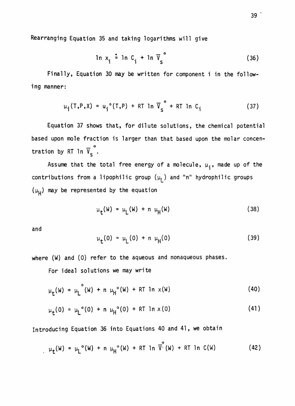
Rearranging Equation 35 and taking logarithms will give

In X. = In C. + In V ° (36)

l i s

Finally, Equation 30 may be written for component i in the follow­

ing manner:

y^-(T,P,X) = u.°(T,P) + RT In YJ + RT In C- (37)

Equation 37 shows that, for dilute solutions, the chemical potential

based upon mole fraction is larger than that based upon the molar concen-o

tration by RT In V .

Assume that the total free energy of a molecule, y., made up of the

contributions from a lipophilic group (y, ) and "n" hydrophilic groups

(yn) fnay be represented by the equation

y^(W) = M^W + n y^(W) (38)

and

y^(0) = M^{Q) + n y^(0) (39)

where (W) and (0) refer to the aqueous and nonaqueous phases.

For ideal solutions we may write

M^W = yJ(W) + n yj °(W) + RT In x(W) (40)

\i^(0) = yL°(0) + n y^°(0) + RT ]n x{0) (41)

Introducing Equation 36 into Equations 40 and 41, we obtain

y^(W) = yL°(W) + n y^°(W) + RT In V^W) + RT In C(W) (42)

40

and

y^(0) = y|_°(0) + n y^°(0) + RT In V°(0) + RT In C(0) (43)

When equilibrium is established between phases, y.(W) = y . (0) , we

may equate Equations 42 and 43 collect terms and replace C(0)/C(W) by

distribution coefficient, K, to obtain

l\°W ' yL°(0)] + RT ln[¥<'(W)/r(0)] + n[y^°(W) - y^°(0)] = RTlnK (44)

To simplify Equation 44, let us put

Ay° = y°(W) - y°(0) (45)

and, n Ay ^ Ay °

^°9 K = 273"^ " 273Tr •" Tog[V°(W)/V°(0)] (46)

According to Equation 46, a plot of log K vs. n will be linear with a

slope equal to AyL|°/2.3 RT, and with an intercept of Ay. °/2.3 RT + log

[V°(W)/V°(0)].

Determination of Free Energy of Transfer of Methylene Group

The validity of Equation 46 is tested by plotting methylene number

vs. log K for different solutes in different systems from data tabulated

in Table 1. The graphs are the. same as Figures 1 to 7. A good linear

relation was observed for all except amines in the diethyl ether-water

system.

The linear relationship between number of methylene of homologous

alkanols in chloroform-water system can be expressed as

41

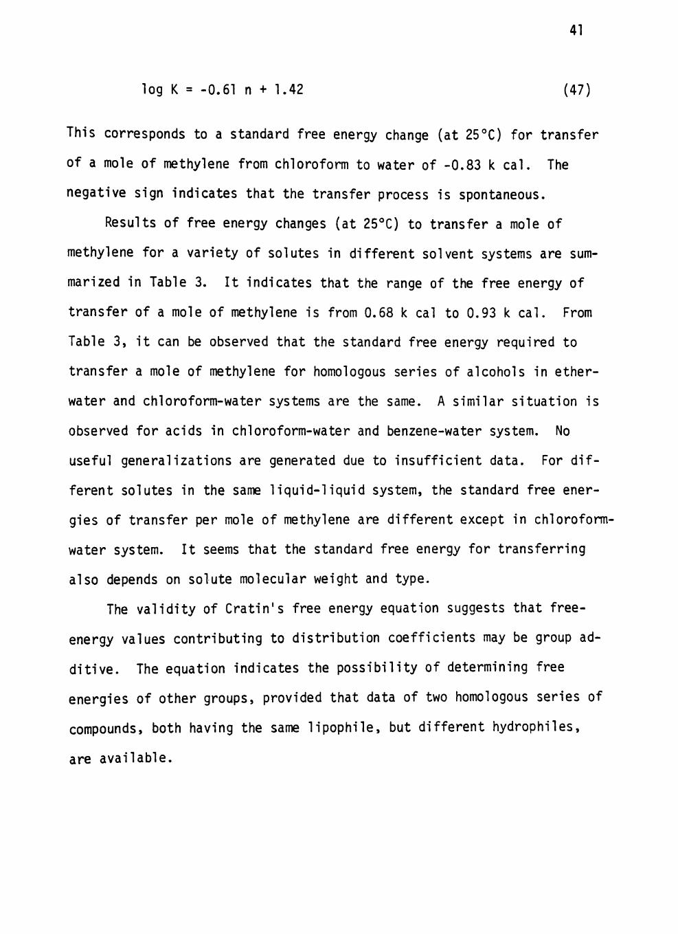
log K = -0.61 n + 1.42 (47)

This corresponds to a standard free energy change (at 25°C) for transfer

of a mole of methylene from chloroform to water of -0.83 k cal. The

negative sign indicates that the transfer process is spontaneous.

Results of free energy changes (at 25*'C) to transfer a mole of

methylene for a variety of solutes in different solvent systems are sum­

marized in Table 3. I t indicates that the range of the free energy of

transfer of a mole of methylene is from 0.68 k cal to 0.93 k cal. From

Table 3, i t can be observed that the standard free energy required to

transfer a mole of methylene for homologous series of alcohols in ether-

water and chloroform-water systems are the same. A similar situation is

observed for acids in chloroform-water and benzene-water system. No

useful generalizations are generated due to insufficient data. For dif­

ferent solutes in the same liquid-liquid system, the standard free ener­

gies of transfer per mole of methylene are different except in chloroform-

water system. I t seems that the standard free energy for transferring

also depends on solute molecular weight and type.

The validity of Cratin's free energy equation suggests that free-

energy values contributing to distribution coefficients may be group ad­

ditive. The equation indicates the possibility of determining free

energies of other groups, provided that data of two homologous series of

compounds, both having the same lipophile, but different hydrophiles,

are available.

42

TABLE 3

FREE ENERGY CHANGES (AT 25°C) TO TRANSFER A MOLE OF METHYLENE

AyCH^ of AcidS' AyCHp of Alcohols AyCHp of Amines

Solvents (kcal/mole) (kcal/mole) (kcal/mole)

Octanol and Water 0.75 0.78 0.72

Diethyl Ether .... 0.79 0.83 0.68 and Water

Chloroform and 0.83 0.83 Water

Benzene and Water 0.83 0.80 0.93

CHAPTER IV

ESTIMATION OF LIQUID-LIQUID DISTRIBUTION COEFFICIENTS FROM GROUP CONTRIBUTIONS

Reasons for New Model Development

The activity-coefficient models have not lived up to their early

expectation for predicting liquid-liquid distribution coefficients. I t

is often not possible to represent the solute distribution coefficients

with sufficient accuracy for extraction design purposes. There is a

strong need for more work on methods for the correlation and prediction

of liquid-liquid distribution coefficients.

In the meantime, we are in need of a practical procedure for esti­

mating liquid-liquid distribution coefficients. The model should be

fairly simple and easily applied. The results should have sufficient

accuracy to serve in preliminary design calculations and for screening

solvents.

The present work is intended as a demonstration of a simple group-

contribution technique. I t is intended to provide a way to estimate

liquid-liquid distribution coefficients for a wide variety of solutes

using the idea of structural group-contributions.

Data Collection

In spite of a large amount of work on liquid-liquid equilibrium, no

extensive l is t of liquid-liquid distribution coefficients has appeared

in the literature. Even the latest compilations are quite old. Some of

them are: Seidel, et a l . (36), Collandar (37), Von Metzsch (38), and

International Critical Tables (39).

43 .

44

From an intensive literature survey, liquid-liquid distribution co­

efficients for ternary mixtures have been collected. The kinds of sys­

tems considered are solutes with octanol-water, diethyl ether-water,

chloroform-water and benzene-water. The temperature range is roughly

15-35°C; and the pressure is atmospheric.

All available data were used for the model development except those

which are obviously erroneous such as the case that the summation of

mole fraction does not equal unity. No thermodynamic equation such as

Gibbs-Duhem equation was used for testing thermodynamic consistency.

Group Contributions Model

The group-contribution method is based on the premise that thermo­

dynamic functions for structural components of a molecule are additive.

Molecular structure groups have the same contribution to the thermodynamic

function no matter what molecule they appear in. Thus, the value of a

thermodynamic function can be built up from an assignment of specific

contributions to the various groups which make up the molecule.

Three assumptions were made in developing this group-contribution

method:

Assumption 1. The solute can be treated as mixtures of groups (CH^-,

-CHp- , -OH, etc.) which make up the molecular species present.

Assumption 2. The logarithm of the liquid-liquid distribution coeffici­

ent of a component is assumed to be the sum of two contributions. One

associated with the difference in free energy of the solute between the

two liquid phases and the other with the energy required to transfer

solute through the liquid-liquid interface.

45

For molecular solute j in any solution:

log K. = log K { + log K^ (48)

where K . is the part associated with the difference in free energy of the

solute between the two liquid phases and K. is the residue part associated

with the energy required to transfer solute through the liquid-liquid in-

terface.

The excess Gibbs energy G and the activity coefficient Y- are in­

terrelated by the following expressions:

G"" = RT Z X. In Y . (49)

and

"T 1" i = ^H^h,P,u, (50)

Since the activity coefficient is taken to be a function of tempera­

ture and liquid composition, the activity coefficient can be calculated

once G is expressed as a function of composition and temperature.

The excess Gibbs energy is related to the excess enthalpy and the

excess entropy by the following relationship:

G^ = H^ - TS^ (51)

The condition for equilibrium between two liquid phases I and II

is:

x / Y / = X.^^ y.^^ i = 1, 2 . . .M (52)

46

The liquid-liquid distribution coefficient K. for component i is

then defined as:

K.--ljj-.^ (53)

N i

Thus it is natural to assume the excess free energy, or, the liquid-

liquid distribution coefficient to be the sum of two contributions. The

model has a contribution to the distribution coefficient, associated with

the difference in free energy of the solute between the liquid phases and

a residual contribution, essentially associated with the extra energy re­

quired to transfer solute through the liquid-liquid interphase.

Assumption 3. The contribution associated with the difference in free

energy of the solute between the two liquid phases is assumed to be the

sum of the individual contributions of each solute group in the solution.

For molecular solute j containing group k:

log K^ = ^(f^kj^^^k^ ' ^

where: N. . = number of groups of type k in solute component j

r. = distribution coefficient of group k in the solution

environment

Substituting log KT by Equation 54, Equation 48 becomes

k , log K. = 2:(N^j)(r^) + log K^ (55)

The assumptions used for the new model are basically the same as

those used for the ASOG and the UNIFAC models. The new model uses the

term free energy difference to account for the contributions from the

47

enthalpy (interaction) part. A new term K. is added to the new model to

deal with the extra energy required for the transfer process due to the

nature of the liquid-liquid interface.

The main difference of the three models are the assumptions used

for calculating the entropy (size) part and the enthalpy (interaction)

part. The ASOG and UNIFAC models are theoretically based. The ASOG

model assumes that the combinatorial contribution of the excess Gibbs

energy of a mixture can be expressed by Flory-Huggins equation. The

UNIFAC model assumes that a semi-theoretical equation for the combina­

torial contribution of the excess Gibbs energy of a liquid mixture can

be obtained through generalization of Guggenheim quasi-chemical theory.

The new model uses an empirical approach to correlate the group distri­

bution coefficients and assumes the contribution from the difference in

free energy of the solute between the liquid phases depending upon the

numbers and kinds of structural groupings of the solute.

Method

The liquid-liquid distribution coefficients of any compound can be

determined by Equation 55, given appropriate structural parameters.

It is possible to obtain values of distribution coefficient from

published data on appropriate compounds, and to fit an equation of the

form denoted by Equation 55. The values of each of these groups can be

obtained by using multiple regression analysis to fit a set of equations

of the form denoted by Equation 55. The numbers of group k in solute

component i, N. ., are introduced as independent parameters and the logar­

ithm of the distribution of the compound, log K., as a dependent

48

parameter. The group-distribution coefficients, r. , can be obtained from

the regression coefficients and the extra energy part, log K. from the

intercept of the output.

Calculations were performed on NAS AS/6 computing system. The Sta-

tistical Analysis System (SAS) program, maximum R improvement technique

developed by James H. Goodnight was used to find r. and log K.. K J

It would be ideal to have a well balanced distribution of the groups

among data. Ten to eleven most populated structure types were selected

for group-contribution determination. Among them are: CH^-, -CH2-,

-CH-, NH2-, -NH-, -N-, CgHg-, H0-, -0-, HOOC-, and -CO-.

The calculated values for these groups are summarized in Table 4.

As an example, the liquid-liquid distribution coefficient of methoxyeth-

anol between octanol and water is calculated by the group-contribution

method adopted in this study: structure CH2-O-CH2-CH2-OH. The molecule

contains one CH^- group, two -CH2- groups, one -0- group and one -OH

group. From the group-contribution values and the log K. values pre-

sented in Table 4, the log K value for methanoxyethanol is calculated

as follows:

log K = (1 X r , ) + (1 X r.Q_) + (2 X r.cH2'

+ (1 X r_Qj^) + log K^

= (0.705) + (-1.142) + (2 X 0.505)

+ (-1.077) + (-0.213)

= -0.72

K = 0.19

The experimental value reported by Korenman, et a l . (40) is 0.17

and was not utilized for the establishment of group-contribution values

presented in Table 4. Yet the percent error was found to be 11.7%.

49

to

3 O %. CD

(U 3 to

i-rO OH O

TABLE 4

GROUP CONTRIBUTIONS FOR THE FOUR SYSTEMS

Systems

CH3-

-CH2-

-CH-1

^6^5-

-coo-

-COOH

- 0 -

-OH

NH2-

-NH-

-N-1

c=o

Octanol and Water

0.705

0.505

0.182

1.935

-1.027

-0.681

-1,142

-1.077

-1.094

-1.560

-1.734

—

Diethyl Ether and Water

0.823

0.246

-0,218

2.470

0.174

-0.094

-0.839

-1.057

-1.760

-2.228

-1.153

—

Chloroform and Water

1,517

0,545

-0,403

3.173

—

-1.244

-0,002

-0.800

-0.641

-1.637

—

-0.407

Benzene and Water

2,149

0.544

-1.328

4.020

-0,690

-0.656

-1,316

-0.809

-0.019

-2,095

-3,667

-0.430

Log K}- -0.213 -0.112 -1.767 -3.177

50

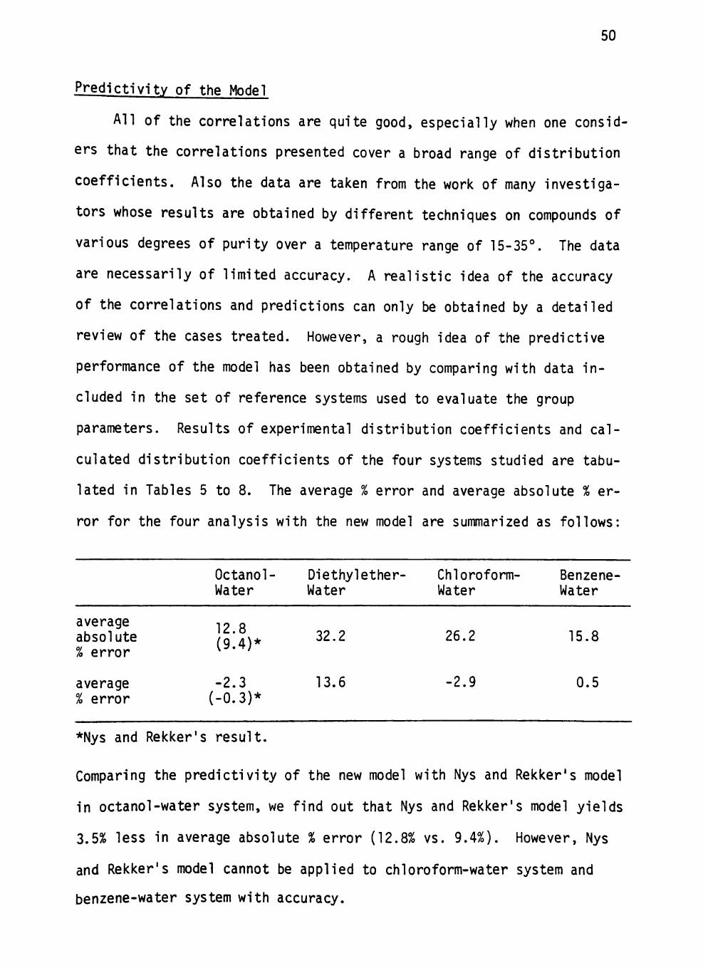
Predictivity of the Model

All of the correlations are quite good, especially when one consid­

ers that the correlations presented cover a broad range of distribution

coefficients. Also the data are taken from the work of many investiga­

tors whose results are obtained by different techniques on compounds of

various degrees of purity over a temperature range of 15-35°. The data

are necessarily of limited accuracy. A realistic idea of the accuracy

of the correlations and predictions can only be obtained by a detailed

review of the cases treated. However, a rough idea of the predictive

performance of the model has been obtained by comparing with data in­

cluded in the set of reference systems used to evaluate the group

parameters. Results of experimental distribution coefficients and cal­

culated distribution coefficients of the four systems studied are tabu­

lated in Tables 5 to 8. The average % error and average absolute % er­

ror for the four analysis with the new model are summarized as follows:

Octanol- Diethylether- Chloroform- Benzene-Water Water Water Water

average •,« p absolute Jn.x* 32.2 26.2 15.8 0/ % error

(9.4)

average -2.3 13.6 -2.9 0.5 % error (-0.3)*

*Nys and Rekker's result.

Comparing the predictivity of the new model with Nys and Rekker's model

in octanol-water system, we find out that Nys and Rekker's model yields

3.5% less in average absolute % error (12.8% vs. 9.4%). However, Nys

and Rekker's model cannot be applied to chloroform-water system and

benzene-water system with accuracy.

51

TABLE S"*

EXPERIMENTAL AND CALCULATED DISTRIBUTION COEFFICIENTS OF SOLUTE-OCTANOL-WATER SYSTEM

Cc

1)

2]

3]

4]

5]

6]

1]

8 ;

9;

10^

11

12'

13

14

15

16.

17'

18'

19'

20:

21.

22;

23;

impound

CH3COOH

CH3COOCH3

CH3CH2COOH

1 CH3(CH2)2C00H

1 CH3CH2COOCH2CH3

) CH3COOCH2CH3

) CH3(CH2)4C00H

1 CH3(CH2)3C00H

) H00C(CH2)7C00H

) CgH5CH3

) CgH5CH2CH3

) CgH5CH(CH3)2

1 CgH5(CH2)2CH3

* ^6"5^"2^6"5 ) CgH5(CH2)2C5H5

' ^e^s'^e'^s ) CgH5CH2C00H

) CgHg(CH2)2C00H

) CgHg(CH2)3C00H

) CgHgCH20H

) CgHg(CH2)20H

) CgHg(CH2)30H

1 CgH5CH2NH2

Experimental K

0.84

1.2

1.39

2.20

3.35

2.08

6.55

59.74

4.81

14.73

23.34

38.86

35.52

62.80

120.30

56.83

4.10

6.30

11.25

3.00

3.90

6.55

2.97

Calculated K

0.84

1.19

1.38

2.27

3.25

1.97

6.23

46.99

7.10

11.36

18.73

27.39

31.19

64.07

106.70

38.86

4.71

7.77

12.94

3.15

5.26

8.67

3.10

Relative Error (%)

0.0

1.0

1.0

-3.1

3.0

4.9

4.9

21.3

-47.7

22.9

19.7

29.5

12.2

-2.0

11.3

31.6

-15.0

-23.4

-15.0

-5.1

-35.0

-32.3

-4.1

52

TABLE 5^

EXPERIMENTAL AND CALCULATED DISTRIBUTION COEFFICIENTS OF SOLUTE-OCTANOL-WATER SYSTEM (CONTINUED)

Compound Experimental K Calculated K Relative Error (%)

24) CgHg(CH2)2NH2

25) CgHgCH2C00CH3

26) CH3C00CH2CgHg

27) CgHg(CH2)2C00CH3

28) CgHg(CH2)3C00CH3

29) CgH5(CH2)30CH3

30) CgHgCHOHCgHg

31) (CgHg)2CH.0.(CH2

32) pH2- ..^ CgHc-CH-C00-CH^CH« N-CH,

0 3 I I 2 3 CHoOH \ ruj

4.10

6.23

7.10

10.18

15.96

14.88

14.44

)2N(CH3)2

CH

26.

6.

31

23

5.16

6.75

6.75

11.13

18.54

16.44

15.80

29.37

6.37

-25.8

-8.3

4.9

-9.4

-16.2

-10.5

-9.4

-11.6

-2.0

i2un . CH 2

33;

34

35;

36;

37;

38]

39;

40;

41;

42;

43;

44;

CH2-

) CgH5CH2N(CH3)2

) CH3NH2

) CH3CH2NH2

) CH3(CH2)2NH2

) CH3(CH2)3NH2

1 CH3(CH2)4NH2

) CH3(CH2)5NH2

1 CH3(CH2)gNH2

I (CH3)2CHCH2NH2

> CH3CH2CHCH3NH2

1 CH3(CH2)4CH(CH2CF

1 CHo ~ CH« / Z / Z CH« CH - NH« Z s Z ^ CH2 - CH2

CH

6.75

0.57

0.88

1.62

2.41

4.44

7.24

13.07

2.41

2.10

l3)NH2 16.78

4.44

6.69

0.55

0.90

1.51

2.48

4.14

6.82

11.36

2.20

2.20

16.61

4.06

1.0

2.9

-2.3

6.7

-3.1

6.8

5.8

13.1

8.6

-4.8

1.0

8.6

53

TABLE 5^

EXPERIMENTAL AND CALCULATED DISTRIBUTION COEFFICIENTS OF SOLUTE-OCTAHOL-WATER SYSTEM (CONTINUED)

Compound Exp

45) (CH3)2CHNH2

46) CH3CH2NHCH3

47) (CH3CH2CH2)2NH

48) (CH3CH2CH2CH2)2NH

49) (CH3CHp)2NH

erimental K

1.30

1.16

5.31

14.59

1.79

50) CH3(CH2)2NH(CH2)3CH3 8.33

51) CH3(CH2)3NHCH3

52) ^CH2 - CH2

CH« NH

CH2 - CH2

53) CH3CH2NHCH(CH3)2

54) CH3CH2CHCH3NH(CH2)

3.78

2.25

2.53

2CH3 6.75

55) CH3(CH2)2NHCH2CH(CH3)2 7.92

56) (CH3)3N

57) (CH3)2N(CH2)3CH3

58) ^ C H 2 - C^2

CH, CH - OH

CHp •" CHp

59) CH3OH

60) CH3CH2OH

61) CH3(CH2)20H

62) CH3(CH2)30H

63) CH3(CH2)40H

64) CH3(CH2)50H

65) CH3(CH2)70H

66) CH3CH2OCH2CH3

1.31

5.47

3.42

0.52

0.73

1.40

2.41

4.06

7.61

23.34

2.16

Calculated K

1.34

1.15

5.26

14.44

1.93

8.67

3.19

2.12

2.80

7.69

7.69

1.46

5.37

4.14

0.56

0.92

1.54

2.53

4.22

6.96

19.11

2.92

Relative Error (%)

-3.0

1.0

1.0

1.0

-8.3

-4.1

15.6

5.8

-10.5

-13.9

3.0

-11.6

2.0

-20.9

-8.3

-27.0

-9.5

-5.1

-4.1

8.6

18.1

-35.0

67) CH3(CH2)20(CH2)2CH3 7.61 8.00 -5.1

54

TABLE 5^

EXPERIMENTAL AND CALCULATED DISTRIBUTION COEFFICIENTS OF SOLUTE-OCTANOL-WATER SYSTEM (CONTINUED)

Compound Experimental K Calculated K Relative Error (%)

68) CH3CH20(CH2)3CH3

69) (CH3)2CHCH20H

70) CH3CH2CH(CH3)0H

71) (CH3)2CH(CH2)20H

72) CH3CH(0H)CH(0H)CH3

73) CH3CH20(CH2)20H

74) (CgH5)2CHC00H

75) (CH3CH2)3N

76) HOCH2COOH

77) CH3CHOHCOOH

78) CgHgCHOHCOOH

79) CH3CH2OCH2OCH2CH3

80) H00C(CH2)2C00H

81) C.Hc CH-CH-NH-CH, ' 6 5 I \ 3 OH CH3

82) OHCHpCHpNHp ^ Cm Cm

83) CHp - CHp

0 0 1 1 CH2 - CH2

84) (H0CHCH2)2NH

CH3

^Reference (32)

7.61

1.92

1.84

3.19

0.40

0.58

21.12

4.22

0.33

0.54

1.75

2.32

0.55

2.53

0.27

0.66

. 0.44

8.00

2.25

2.25

3.71

0.55

0.81

23.57

5.37

0.29

0.34

1.16

1.54

0.57

2.36

0.25

0.62

0.32

-5.1

-21.2

-22.2

-16.2

-39.0

-39.3

-11.6

-27.1

13.0

36.7

33.7

33.6

-3.0

6.8

5.8

5.8

27.4

55

TABLE 6

EXPERIMENTAL AND CALCULATED DISTRIBUTION COEFFICIENTS OF SOLUTE-DIETHYL ETHER-WATER SYSTEM

1

2

3

4

5

6

7

8

9

10

11

C>0 CO

14;

is; 16;

17;

is; 19]

20]

21]

22]

23]

24]

25)

26]

Compound

) HOOCCHOHCH2COOH

) (CH0HC00H)2

) CH3(CH2)2C00H

) CH3(CH2)4C00H

) (CH2)7(C00H)2

) (CH2)3(C00H)2

) CH3NH2

) (CH3)2NH

) C2H5NH2

) CH3(CH2)2NH2

) (CH3CH2)2NH

Experimental K

0.16

0.088

2.24

6.55

3.32

5.81

0.19

0.30

0.31

0.58

0.76

) CgHg(CH2)3NH2 3.40

) CgHgCH2CH3(CH2)2NH 4.44

) CH3OH

) CH3CH2OH

) CH3(CH2)20H

1 CH0H(CH20H)2

) CH3(CH2)30H

1 CH3(CH2)2CH(0H)2

1 (CH3)2(CH0H)2

CH3(CH2)2CH(CH)2

CH3CH20(CH2)20H

CH3(CH2)40H

» CgHgOH

CH3(CH2)50H

C2H5OC2H5

0.43

0.61

1.32

0.52

2.34

0.25

0.21

0.25

0.50

3.32

4.86

6.05

2.72

Data Calculated Relative Reference K Error(%)

(58

(59

(60

(61

(62

(62

(37

(37

(37

(37

(37

(65

(65

(37

(37

(37

(66

(37

(67

(37

(67

(67

(68

(63

(68

f37

0.26

0.058

3.03

4.60

4.14

5.31

0.34

0.49

0.45

0.57

0.82

3.82

5.41

0.70

0.90

1.16

0.11

1.48

0.32

0.36

0.32

0.63

1.90

3.67

2.41

3.29

-67.0

34.1

-35.1

29.8

-24.6

8.6

-78.9

-63.3

-45.2

1.7

-7.9

-12.4

-21.9

-62.8

-47.5

12.2

78.8

36.8

-28.0

-69.6

-28.0

-26.0

42.8

24.4

60.1

-20.9

56

TABLE 6

EXPERIMENTAL AND CALCULATED DISTRIBUTION COEFFICIENTS OF SOLUTE-DIETHYL ETHER-WATER SYSTEM (CONTINUED)

27)

28)

29)

30)

31)

32)

33)

34)

35)

36)

37)

38)

39)

40)

41)

42)

43)

44)

45)

46)

47)

48)

Experimental Compound

CH30(CH2)2CH(0H)2

NH2COOCH3

NH2(CH2)20H

CH3CHOHCOOH

HOCH2CHOHCOOH

CH30(CH2)20H

CH3CHOHCH2COOH

CH2CHCH(CH20CH3)0H

HN(CH2CH20H)2

CH3(CH2)3C00H

CH(CH2)20(CH2)20CH3

CgH5NH2

(C00H)3(CH2)20H

HO(CH2)gOH

(CH2)5CH(0H)3

(H0CH2CH20CH2)2

N(CH2CH20H)3

CgHgCOOH

CH30CgHg

{(^zhh^^^h^^h CgHgCOOH

C^HcCHOHCHCH^^NHCH^

K

0.18

0.43

0.056

0.53

0.13

0.30

0.67

0.18

0.024

3.90

• 0.24

2.34

0.27

0.40

0.081

0.081

0.052

6.62

11.70

0.63

6.42

1.35

Data Reference

(37)

(37)

137)

(69)

(37)

(37)

(69)

(37)

(37)

(60)

(37)

(70)

(61)

(37)

(67)

(37)

(37)

(37)

(63)

(37)

(37)

(37)

Calculated K

0.14

0.42

0.087

0.52

0.10

0.50

0.66

0.14

0.031

3.86

0.35

1.82

0.38

0.47

0.103

0.088

0.090

9.58

10.40

0.58

9.58

1.32

Relative Error(%)

22.0

2.3

-55.4

1.9

23.1

-66.6

1.5

22.0

-29.2

1.0

-45.8

22.2

-40.9

-17.5

-27.2

-8.4

-73.1

-44.7

11.1

7.9

-49.2

2.0

57

TABLE 7

EXPERIMENTAL AND CALCULATED DISTRIBUTION COEFFICIENTS OF SOLUTE-CHLOROFORM-WATER SYSTEM

1)

2)

3)

4)

5)

6)

7]

8]

9]

10]

n; 12;

13;

14;

15;

16;

17'

18'

19

20'

21

22

23

24

25

26

27

Compound

CH3NH2

HONH2

CH3COOH

CgHgOH

CgHgNH2

CH3(CH2)4C00H

CH30CgH5

CgHgCH3CH2

CgH5CH2NH2

1 CH3(CH2)gOH

) CH3OCH2COOH

I CH3OH

) CH3CH2OH

) CH3(CH2)30H

) CH3(CH2)40H

) CH3(CH2)50H

) CH3CH2COOH

) CH3CHOHCOOH

) CH3(CH2)3NH2

) (CH3CH2)2NH

) CgHgCH3

) CgHgCHOHCOOH

) CH3CH20CgHg

) CH3CH(CgH5)NH2

) CH3CHCgHgC00H

) (CH2)7(C00H)2

) CgHg(CH2)3C00H

Experimental K

0.41

0.076

0.021

1.55

3.42

2.34

22.75

39.65

3.25

11.13

0.27

0.28

0.43

1.57

2.86

5.42

0.43

0.11

2.69

2.25

30.27

0.28

37.34

4.02

3.00

0.56

5.64

Data Reference

(71)

(72)

(73)

(74)

(75)

(69)

(68)

(68)

(69)

(76)

(77)

(76)

(76)

(76)

(76)

(76)

(77)

(77)

(78)

(78)

(68)

(79)

(68)

(80)

(69)

(81)

(82)

Calculated K

0.41

0.040

0.023

1.84

2.16

1.99

18.54

32.14

3.71

9.21

0.38

0.35

0.61

1.80

3.10

5.37

0.39

0.067

2.12

2.10

18.54

0.35

32.14

6.55

3.60

0.64

6.05

Relative Error(%)

0.0

46.6

-9.5

-18.6

36.9

14.8

18.1

18.9

-13.9

17.3

-42.3

•-25.0

-41.8

-14.7

-8.32

0.09

9.30

39.1

21.2

6.7

38.7

-25.0

13.9

-62.9

-19.8

-14.3

-7.3

58

TABLE 7

EXPERIMENTAL AND CALCULATED DISTRIBUTION COEFFICIENTS OF SOLUTE-CHLOROFORM-WATER SYSTEM (CONTINUED)

Compound

28) CH3COCOOH

29) CH3COCH3

30) CH3CH2CONH2

31) (CH3C0)2CH2

32) CH3C0(CH2)2C00H

33) CH3C0CgHg

34) CgHgNHC0CH3

35) CgHgC0CH2C0CH3 .

Experimental K

0.11

2.05

0.25

2.16

0.30

16.28

2.44

36.60

Data Reference

(77)

(74)

(83)

(84)

(77)

(68)

(85)

(86)

Calculated K

0.14

2.36

0.47

2.72

0.44

12.43

2.41

14.30

Relative Error(%)

-27.3

-15.1

-88.0

-25.9

-46.7

23.7

1.0

60.9

59

TABLE 8

EXPERIMENTAL AND CALCULATED DISTRIBUTION COEFFICIENTS OF SOLUTE-BENZENE-WATER SYSTEM

1)

2)

3)

4)

5)

6)

7]

8]

9]

lo ;

11-

12

13

14

15

16

17

18

19

20

21

22

23

24

25

26

27

28

Compound

CH3OH

CH3NH

CH3COOH

CH3CH2OH

(CH3)2NH

CH3CH2NH2

CH3CH2COOH

1 CH3(CH2)20H

> C2HgC00CH3

1 CH3(CH2)2C00H

) CH3(CH2)30H

) CH3CH20(CH2)20H

) CH3(CH2)3NH2

) (CH3C0)2CH2

) CH3(CH2)2C00CH3

) CH3(CH2)3C00H

) CH3(CH2)40H

) CgH5NH2

) CH3(CH2)4C00H

) (C3H7)2NH

) (C2H5)3N

) CgHgCOOH

) CgH5CH2NH2

) CH3(CH2)gOH

) CH3C0CgH5

) CgHgCHOHCOOH

) CcH.COCH,COCH, ' 6 D Z 3 ) (C.H,CO)pCHp

Experimental K

0.16

0.26

0.18

0.26

0.44

0.55

0.31

0.50

2.75

0.52

0.83

0.22

1.92

2.14

4.57

0.95

1.58

2.72

1.88

2.86

3.10

1.20

1.84

6.75

9.03

0.14

20.70

208.5

Data Reference

(46)

(47)

(48)

(46j

(50)

(51)

(52)

(76)

(53)

(52)

(54)

(55)

(51)

(56)

(53)

(52)

(57)

(87)

(79)

(47)

(88)

(89)

(90)

(76)

(83)

(91)

(92)

(93)

Calculated K

0.16

0.35

0.19

0.28

0.38

0.61

0.32

0.47

2.66

0.55

0.82

0.22

1.80

2.25

4.57

0.95

1.40

2.27

1.63

3.32

3.46

1.21

3.90

4.18

12.94

0.14

14.59

94.6

Relative Error(%)

0.0

-33.9

-6.0

-5.2

13.9

-10.5

-2.0

4.8

3.0

-5.2

1.0

0.0

6.0

-5.1

0.0

0.0

11.3

16.5

13.1

-16.2

-11.6

-1.0

-111.7

38.1

-43.3

0.0

29.5

54.6

60

It is difficult to compare the predictivity of the new model with

that of the UNIFAC and ASOG model. The ASOG and UNIFAC models are not

thoroughly tested in correlating liquid-liquid distribution coefficients

and not many results are available in the open literature. We think the

new model has better accuracy in correlating liquid-liquid distribution

coefficients than the ASOG and UNIFAC models at the present time. The

reason is based on the performance of the UNIFAC model carried out by

Fredenslund, et al. (28) for several ternary systems and the performance

of the ASOG model by Tochigi and Kojima (26) for 9 ternary systems. The

predicted liquid compositions at equilibrium are not quantitatively ac­

ceptable for the design purpose in either case. The advantage of ASOG

and UNIFAC models is that these models can be applied to e\/ery system

and are not specific to one system. However, the predicted liquid-liquid

distribution coefficients are usually of semi-quantitative values. The

new model is an empirical approach and correlates specific systems so

that quantitative results are obtained.

CHAPTER V

EVALUATION OF FACTORS INFLUENCING LIQUID-LIQUID DISTRIBUTION COEFFICIENTS

Introduction

Method of Chapter IV allows estimation of liquid-liquid distribu­

tion coefficients at single temperature, infinite dilution. It is de­

sirable to expand the application for other conditions. Several factors

which can affect the distribution of solute between two different phases

include pH of the aqueous phase, temperature, pressure, original concen­

tration of solute and structure of solute. For liquid mixtures at ordi­

nary pressure, the effect of pressure is negligible. In this chapter,

the evaluation of the effects of pH, temperature and concentration upon

liquid-liquid distribution coefficients is presented.

Effect of pH on Distribution Coefficient

For ionizable solutes, distribution coefficients will vary with pH.

Generally, dependence of distribution coefficients upon pH is not linear.

Data from Colaizzi and Klink (41) show the distribution behavior of metha-

cycline hydrochloride between n-octyl alcohol and water. Methacycline

hydrochloride is ionized at all pH values. The variation of distribu­

tion coefficient with pH is summarized in Table 9. The shift of log K

with change of pH is expressed graphically in Figure 9. The increase

in distribution coefficient observed with pH increases from 2.1 to

8.5 were nonuniform. The maximum distribution coefficient occurred at

pH equal to 5.6.

61

62

TABLE 9^

SHIFT OF DISTRIBUTION COEFFICIENT WITH pH

System pH

Mathacylcine Hydrochloride In

N-Octyl alcohol-Water

Reference (41)

2.1

3,0

3,9

5.6

6,6

7,5

8,5

0,69

0.72

0,82

0.91

0,82

0,43

0,16

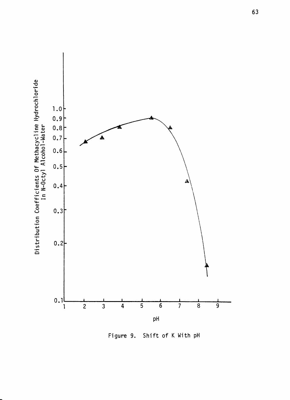
63

CU

•r— &-o

j r o o &--o

CU S -c <u

• I - + j >— ro O S >> I O f— ro O

. C JO. •M O CU O

O r ->>

in 4-> -> CJ C O (U I

•r- 2 1 U

•r- C

V « -cu O

o

3

s-• » - )

I/)

o

1.0 0,9 0,8 0,7

0.6

0.5

0.4

0.3

0,2

0.1 8

pH

Figure 9. S h i f t o f K With pH

64

A wide variety of phenolic compounds are potentially available in

huge amounts from coal-hydrogenation oils. Such mixtures are composed

largely of homologous and isomeric phenols, and separation by the usual

procedures of precise fractional distillation and fractional crystalliza­

tion is difficult. pH adjustment is used to increase the distribution

coefficients among groups of closely related phenols and thus separation

of isomeric phenols can be achieved.

Golumbic, et al. (42) studied the distribution of phenol between a

non-ionizing organic phase and an immiscible aqueous phase. Data for

distribution coefficient at different pH values are tabulated in Table

10. The results are shown in Figure 10. In Figure 10, the observed

distribution coefficient of 4 phenols, distributed in the system cyclo-

hexane - 0.5 m phosphate buffer, are plotted as a function of pH. A

straight line occurred in all cases. Three factors affect the distribu­

tion of a phenol between the organic and aqueous phase: pH of the aque­

ous phase, ionization constant of the phenol, and distribution coeffici­

ent of the unionized phenol.

Golumbic, et al., derived the relationship between distribution co­

efficient, pH and ionization constant of a weak acid, such as phenol be­

tween a non-ionizing organic phase and an immiscible aqueous phase.

When no association occurs in either phase, the observed distribution

coefficient, K', is given as the resultant of two equilibria: (a) the

distribution of the undissociated acid between the immiscible phases

and (b) the ionization of the acid in the aqueous phase.

[HA]o

65

TABLE 10^

SHIFT OF DISTRIBUTION COEFFICIENTS WITH pH

System pH Log K

P-Cyclohexylhenol In Cyclohexane-Phosphate 11.67 1.07

11.92 0.78

12.55 -0.04

0-Ethylphenol In Cyclohexane-Phosphate 11.11 0.17

11,43 -0,17

11,92 -0.63

12,55 -1,23

2,5 - Xylenol In Cyclohexane-Phosphate 11,12 -0,03

11.43 -0.32

11.92 -0.80

12.30 -1,13

M-Cresol In Cyclohexane-Phosphate 11.11 -1.03

11,43 -1,34

12.30 -1,99

^Reference (42)

66

1.1

0.8

0.4

CO +J c CU

o • I - O)

M- ro CU x : O CL

CJ to o

C J C O CL.

• I - I 40 OJ 3 C

.a ro • I - X S - CU

4 J x : CO O

•O CJ CU > c CU CO CO

.a 1 — o o M - CU o sz a. E

sz 4-+J o •r—

s -(O cn o

0.0

-0.4

-0.8

i 12.4 12,6

Figure 10. Shift of K With pH

67

The ionization constant of the acid, k, is defined as

^ _ [H^lwrA'lw ^ [HAJw in water (57)

The distribution coefficient, K, of the unnonized acid is given as

K = I . . . •

HA w (58)

From Equation 58 [HA]o = K[HA]w, and Equation 56 becomes

K' = K ' [HA]w

([HA]w + [ A ' ] w ) (59)

or

K' = K

(1 + A-HA < ^ )

(60)

w

From Equation 57, [A']w/[HA]w = k/[H ]w, so Equation 60 can be

written as

K' = K

(1 + - ^ ) (61)

When the aqueous phase contains a buffer of sufficient alkalinity

so that [H ] « k. Equation 61 can be approximated by

^ k (62)

or

log K' = log K - pH + pK (63)

According to Equation 63, a plot of log K' versus pH would be a

straight line with a slope of -1. Experimental results, represented

68

graphically in Figure 10, verified this relation. This observation also

indicates that there was no significant association in the organic phase.

Temperature Effect on Distribution Coefficient

The distribution coefficient of a solute between two solvent layers

is closely related to the solubility of the solute in either of the sol­

vents. In the condition in which the solute concentration is very low,

the distribution coefficient can be considered as a thermodynamic pro­

perty.

From thermodynamics, the standard free energy of transfer of solute

in the distribution process is given by

AG^^ = Ail = RT In K^ (64)

With the assumption that the molar heat of transfer of solute be­

tween two solvent layers is not temperature dependent over the range

studied, we get

d log K. = - ^ ^ dT (65)

^ 2.3 RT"

where AHs is the molar heat of transfer of solute between two solvents.

Equation 65 shows the expected manner for the distribution coeffi­

cient to vary with temperature. When Equation 65 is integrated, we have

When log K^ is plotted against 1/T, a straight line with (-AHs/2.3 R)

as slope is expected.

69

From the Clausius-Clapeyron equation, at the same temperature,

d log P' = ^' p dT (67) 2.3 RT

If Equation 65 is divided by the Clausius-Clapeyron equation, always at

the same temperature, we get

' ^^g 'D . AHs I,.. d log P' " H' ( ^

• Assuming AHs/AH' to remain constant and integrating the above equa­

tion, yields approximately

log Kj3 = -^ log P' + C (69)

where P' is vapor pressure of the reference liquid, H', the molar latent

heat of vaporization of the reference liquid, is assumed to remain nearly

constant.

It is obvious that the Othmer and Thaker plot (43), a plot of dis­

tribution coefficient versus the vapor pressures of the reference liquid

at the same temperature, will give a straight line on logarithm paper.

The slope of the line, AHs/H' represents the ratio of the molar heat of

transfer for the solute from one solvent layer to the other to the molar

latent heat of vaporization of the reference liquid. Examples of Othmer

and Thaker plots for several systems are given in Table 11 and plotted

in Figures 11 to 14.

The plot of distribution coefficient versus the vapor pressure of

the reference liquid has a more practical advantage. First, the lines

so obtained are more nearly straight on the logarithmic plot than on

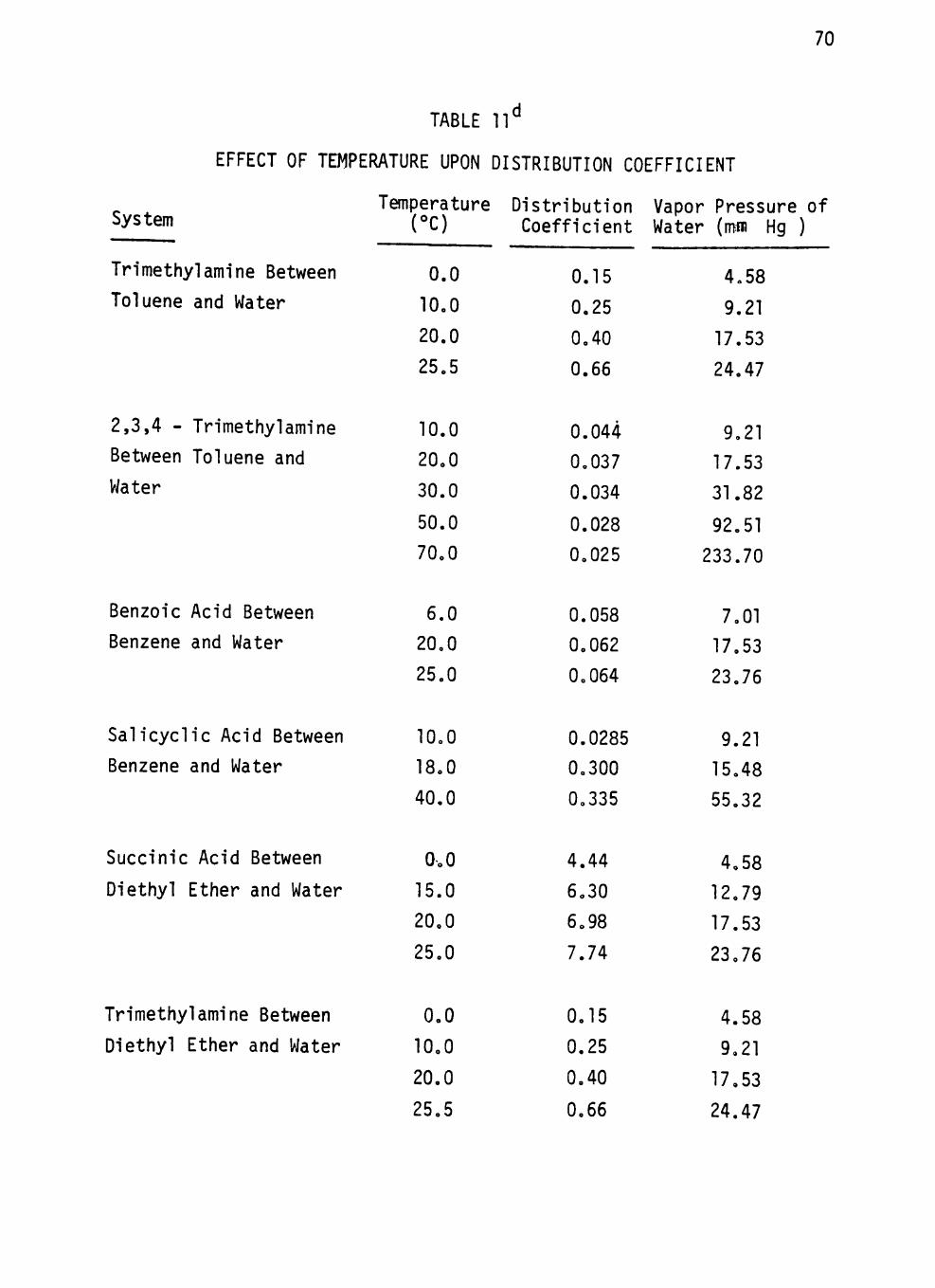
70

TABLE n ^

EFFECT OF TEMPERATURE UPON DISTRIBUTION COEFFICIENT

^ ^ Temperature Distribution Vapor Pressure of ^y^^^^ iX) Coefficient Water (mm Hg )

Trimethyl amine Between Toluene and Water

2,3,4 - Trimethylamine Between Toluene and Water

Benzoic Acid Between Benzene and Water

Salicyclic Acid Between Benzene and Water

Succinic Acid Between

Diethyl Ether and Water

Trimethylamine Between Diethyl Ether and Water

0.0

10,0

20.0

25,5

10.0

20,0

30.0

50.0

70,0

6.0 20,0

25,0

10,0

18.0

40.0

0.0

15.0

20,0

25,0

0.0

10.0

20.0

25,5

0.15

0.25

0.40

0.66

0.044 0.037

0.034

0.028 0,025

0.058 0,062

0,064

0.0285

0,300

0,335

4.44

6,30

6.98

7.74

0.15

0.25

0.40

0,66

4.58

9.21

17.53

24,47

9,21 17.53

31.82

92,51

233.70

7,01 17.53

23.76

9.21

15,48

55,32

4,58

12,79

17,53

23.76

4.58

9,21

17,53

24.47

71

TABLE 11^

EFFECT OF TEMPERATURE UPON DISTRIBUTION COEFFICIENT (CONTINUED)

Temperature Distribution Vapor Pressure of System •(°C) Coefficient Water (mm Hg.)

Oxalic Acid Between

Diethyl Ether and Water

Benzoic Acid Between

Chloroform and Water

Salicyclic Acid Between

Chloroform and Water

15.0 25,0

27.0

10,0

25,0

40.0

10.0

25.0

40,0

14,00

16.80 17,00

0.215

0,240

0.277

0,47

0,60

0.695

12.79 23,76 26,74

9,21 23,76

55,32

9,21

23,76

55.32

^Reference (39)

72

Temperature (°C)

20 30 40

CU +J ro

"T CU c CU

CO (U c

CO 4J £ (U

CJ

(U o CJ

3 j Q •r—

S . 4-> CO

0.1 • Trimethylamine

A 2,3,4 - trimethypyridine

0.01 100

Figure 11.

10 20 30 40 50 Vapor Pressure (mm Hg)

Effect Of Temperature Upon Distribution Coefficient

200 300 400

73

Temperature (°C)

10 18 20 25

0.4 -

s-CU

4-> ro 1

<U c CU N c CU

CO

c 1—1

T 3 •^ o

< vt-O

to +J

c (U • r -

o •r— H -<+-(U

o CJ

c: o

• r " 4-> 3

.a •r—

s.. + j CO

o

0,

0.

0.

0,

0.

0.

2

.1

08

.06

.04

02

0,01

•*r T—r

• Benzoic Acid

A Salicyclic Acid

± ± 10 20 30 40 50 60

Vapor Pressure Of Water (mm Hg)

Figure 12, Effect Of Temperature Upon Distribution Coefficient

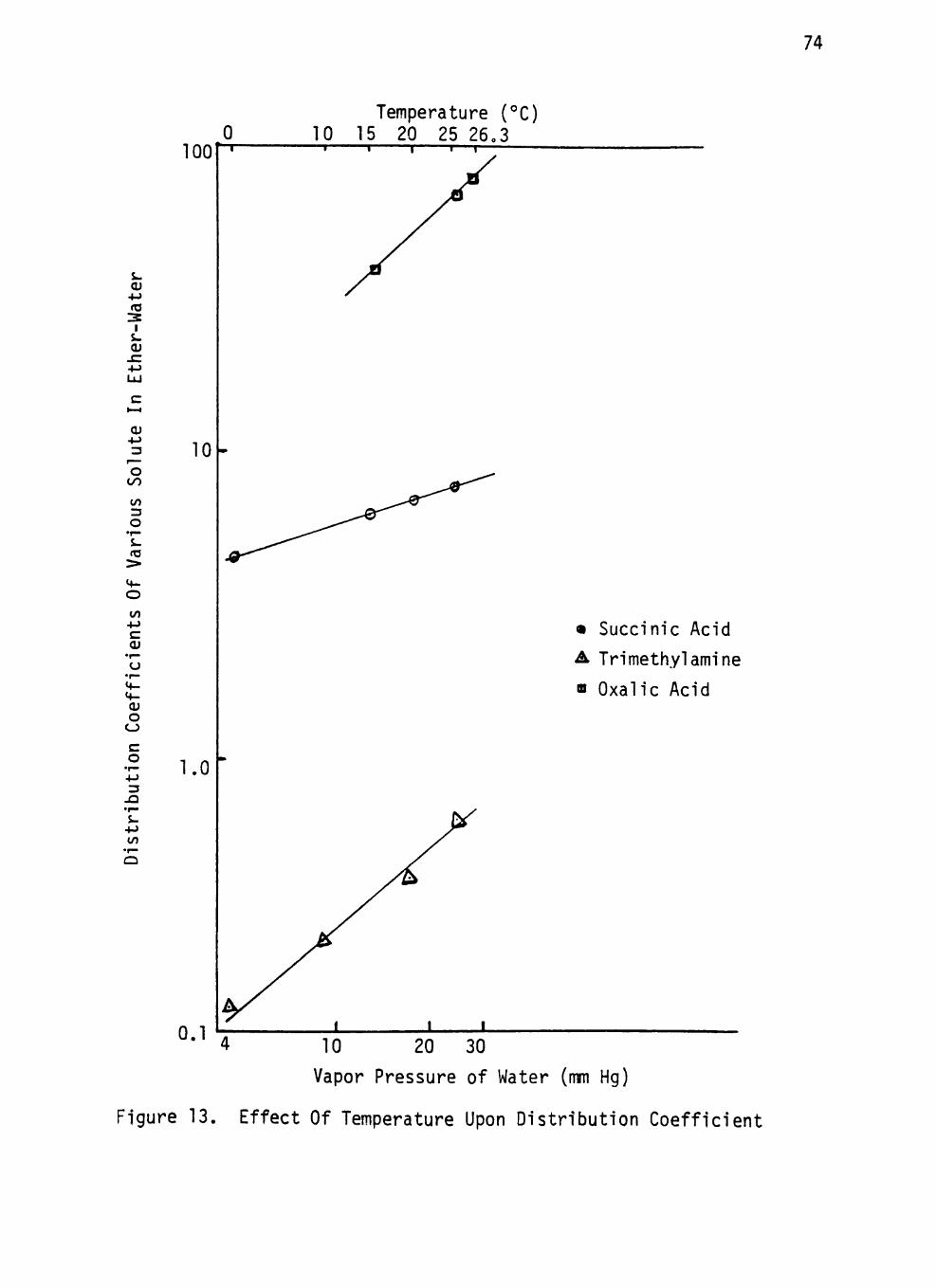
74

CU • M ro

CU

CU

3

'o

to 3 O

•r -&. ro

>

vv-O

to 4 J

CU • I —

CJ

CU o

CJ

c: o

3

•r-s -

4-) CO

o

100 0 10

10

1.0

0.1

Temperature (°C) 15 20 25 26,3

• Succinic Acid

A Trimethyl amine

n Oxalic Acid

10 20 30

Vapor Pressure of Water (mm Hg)

Figure 13. Effect Of Temperature Upon Distribution Coefficient

75

Temperature (°C)

CU 4-i ro

I

O M-O &. O

x: CJ

CO " O •r -CJ

<:

O

CO

CU

CJ

CU o

CJ

c o

3 .a s.

4-> CO

O

10

1.0

^ 25 40

—r

< Benzoic Acid

a Salicyclic Acid

5 10 30 50 70 90

Vapor Pressure Of Water (mm Hg)

Figure 14. Effect Of Temperature Upon Distribution Coefficient

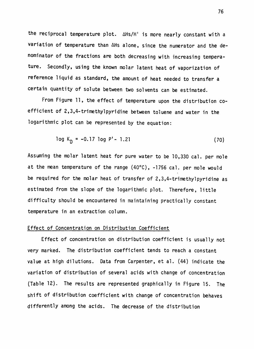
76

the reciprocal temperature plot. AHs/H' is more nearly constant with a

variation of temperature than AHs alone, since the numerator and the de­

nominator of the fractions are both decreasing with increasing tempera­

ture. Secondly, using the known molar latent heat of vaporization of

reference liquid as standard, the amount of heat needed to transfer a

certain quantity of solute between two solvents can be estimated.

From Figure 11, the effect of temperature upon the distribution co­

efficient of 2,3,4-trimethylpyridine between toluene and water in the

logarithmic plot can be represented by the equation:

log K^ = -0.17 log P'- 1.21 (70)

Assuming the molar latent heat for pure water to be 10,330 cal. per mole

at the mean temperature of the range (40°C), -1756 cal. per mole would

be required for the molar heat of transfer of 2,3,4-trimethylpyridine as

estimated from the slope of the logarithmic plot. Therefore, l i t t l e

difficulty should be encountered in maintaining practically constant

temperature in an extraction column.

Effect of Concentration on Distribution Coefficient

Effect of concentration on distribution coefficient is usually not

yery marked. The distribution coefficient tends to reach a constant

value at high dilutions. Data from Carpenter, et a l . (44) indicate the

variation of distribution of several acids with change of concentration

(Table 12). The results are represented graphically in Figure 15. The

shift of distribution coefficient with change of concentration behaves

differently among the acids. The decrease of the distribution

77

•a:

CJ

o CJ

CU CM

OQ ?a:

in Q t—(

CJ < CD

O CC I — C>0

o lyO

I — UJ l-H CJ

UJ

o CJ

o

o • r —

o

o o s..

o <:

o •r—

o in CM

vo cn CM

CO vo CO

cn

CM

CO 00 CM

00 00 CM

o o o m en o I— I CM CO ro CO

CO vo CO

u r*. CO

CO cn 00 r- CM CO "5J- «?r *;r

o cn '^

CO

vo * ; * •

O r>>. ^

in r-* «:3-

00 00 «;r

OQ 1—4

ai f-co

o

C>0

< :

o

o

>^

zc

(J <:

u &. o

CJ &-CU

a.

cn CM CO

00 CO CO

o cn CO

CO CO CO

O r>*. CO

CO r»« CO

00 CO

00 CO CO

vo CT» CO

o o

o cn in

o CM vo

o vo vo

o cn vo

o

r>. ,

o

o o cn r^

o vo cn O

ro f— S- ro •M E e s. CU o u z o CJ

o

o CM • o

CO

C3

*a-O

cn o

vo o

o

r •

o

CO

o cn •

o

o 0

^ «!»•

CJ S= CU

CU c*-CU

oc CU

78

CO • o •r -

U

cn c o s.

4 J LT) Vf-O CO

+ J c CU

•r-CJ

^

CU O

CJ

e o

•r— +J 3

JZX •r— S-

^ - > CO

o

1,0

0.9

0.8

0.7

0.6

0.5

0.4

0.3

0.2

0.1

0 Perchloric Acid

A Nitric Acid

Q Hydrobromic Acid

• Hydrochloric Acid

0.0 0.1 0.2 0.3 0.4 0.5 0,6 0.7 0.8 0.9 1.0

Concentration (Normality)

Figure 15. Shift Of Distribution Coefficient With Concentrati on

79

coefficients with dilution becomes increasingly greater from hydrobromic,

to nitric, to perchloric acids. The amount and rate of change appears

to be correlated with the size of the distribution coefficients of these

aci ds.

Discussion

Variation of liquid-liquid distribution coefficients with solute

concentration in dilute region is usually small and can be neglected.

In a system with a highly concentrated solution of polar compounds, the

composition of the solute in the equilibrium phases is a complex func­

tion of association, dissociation and other processes. Therefore, it

is not feasible to correlate liquid-liquid distribution coefficients at

high concentration.

For ionizable solutes, liquid-liquid distribution coefficients vary

with pH. Generally, the degree to which the liquid-liquid distribution

coefficients are shifted with pH is not linear. Also, the direction of

the change in distribution coefficients depends on the nature of the

solutes. Therefore, it is not possible to predict the effect of pH on

distribution coefficients except by experimental determinations.

Temperature has a marked effect on liquid-liquid distribution coef­

ficients. At infinite dilution, with the assumption that the standard

molar enthalpy change for the transfer process is not temperature de­

pendent in the range studied, it is possible to estimate the distribu­

tion coefficients at different temperature from

, " Dl _ -AH , 1 1 X ,^.^ Np2 K 2 'l

80

However, the predicted liquid-liquid distribution coefficients are

not precise because the solvent molar volume and the solvents miscibili-

ties vary with temperature. Also, the necessary enthalpies of transfer,

AH, are rarely available.

The present status of the new model is that it is not capable of

correlating liquid-liquid distribution coefficients at temperatures other

than 25°C. There are insufficient data to establish a general expression

to account for the temperature dependence of distribution coefficients.

Most of published liquid-liquid equilibrium data are within 10°C of room

temperature. In order to extrapolare liquid-liquid distribution coeffi­

cients with temperature, we need an improved model with temperature para­

meters and more liquid-liquid distribution coefficients outside this

temperature range.

CHAPTER VI

CONCLUSIONS AND RECOMMENDATIONS FOR FUTURE STUDIES

Summary of the Research

1. A group contribution method was used in estimating the liquid-

liquid distribution coefficients of solute-octanol-water, solute-

diethyl ether-water, solute-chloroform-water and solute-benzene-

water system.

2. The properties of liquid-liquid distribution coefficients of

homologues were related to the number of carbon atoms in the

hydrocarbon chain.

3. The effect of temperature, pH and solute concentration on liquid-

liquid distribution coefficients were studied.

Conclusions

From the results of study, the following conclusions can be drawn:

1. The group contribution method proposed by this study provides

a rapid means to estimate distribution coefficients which are

difficult to obtain experimentally and select proper solvents.

The advantage of this method is that no physical properties are

required and distribution coefficients can be calculated from

structure considerations alone.

2. The log K versus number of carbon atoms plots give very good

correlation coefficients and are useful for predicting the dis­

tribution coefficients of certain compounds.

3. Variation of distribution coefficients with solute concentration

is usually small. Distribution coefficients tend to reach a

81

82

constant value at high dilutions. In some cases, the shift of

distribution coefficients with solute concentration is related

to association in one or both of the phases.

4. Often, the effect of temperature is not large when consideration

is restricted to a moderate temperature range. The molar heat of

transfer of solute can be estimated from the slope of the plot of

distribution coefficient versus the vapor pressure of the refer­

ence liquid, provided that the molar latent heat of vaporization

of the reference liquid is known.

5. For ionizable solutes, distribution coefficients vary with pH.

Generally, the degree to which the distribution coefficients

are shifted with change in pH is not linear. pH adjustment is

useful in increasing the distribution coefficients among groups

of closed related compounds and thus separation of isomeric

compounds can be achieved.

Recommendation for Future Studies

For better prediction of distribution coefficient, it is recommended

that:

1. The liquid-liquid distribution coefficients of other systems and

outside the room temperature range need to be collected in order

to correlate the distribution coefficients to other solvent

systems and at other temperature.

2. More research should be done to understand the effect of inter-

molecular interaction of the liquid-liquid interphase on liquid-

liquid distribution coefficients.

LIST OF REFERENCES

1. Henley, E. J., and Staffin, K., Stagewise Process Design, John Wiley and Sons, New York, 53 (197^)7

2. Souders, M.. Jr., Matthews, C. S. and Hurd, C. 0., "Relationship of Thermodynamic Properties to Molecular Structure," Ind. Eng. Chem., 41' 1037-1047 (1949).

3. Craig, L. C., "Identification of Small Amounts of Organic Compounds by Distribution Studies," J. Biol. Chem., 155, 519-534 (1944).

4. Davies, J. T., Rideal, E. K., Interfacial Phenomena, Academic Press, New York, 343 (1961).

5. Bait, S., and Vandaler, E., "Extraction Dissociation Constants of the Carbazine Complexes," Anal. Chim. Acta., 30, 434-442 (1964).

6. Moelwyn-Hughes, S., Physical Chemistry, 2nd Edition, Pergamon Press, New York, 1077-1085 (1961).

7. Green, R., and Alexander, P., "Schiff Base Equilibria," Aust. J. Chem., 2^, 329-336 (1965).

8. Berthelot and Jungfleisch, "Sur Les Chlorures D'Acetylene Et Sur La Synthese du Chlorure de Jul in," Ann. Chim. Phys., 4 , 26-30 (1872).

9. Nernst, W., "Verteilung eines stoffes zweischen zwei ISsungsmitteln und Zwischen Lbsungsmittel und Dampftaum," Z. Physik. Chem., 8, 110-139 (1891).

10. Lacroix, S., "Separation Du Gallium Par Extraction Par Le Chloro-forme," Anal. Chim. Acta., 1, 260-267 (1947).

11. Treybal, R. E., Liquid Extraction, 2nd Edition, McGraw-Hill, New York, 64-76 (19281T

12. Grahame, D. C., and Seaborg, G. T., "The Distribution of Minute Amounts of Material Between Liquid Phases," J. Am. Chem. Soc, 60, 2524-2528 (1938).

13. Pierotti, G. J., Deal, C. H. and Derr, E. L., "Activity Coeffi­cients and Molecular Structure," Ind. Eng. Chem., 51, 95-102 (1959).

14. Hildebrand, J. H., and Scott, R. L., The Solubility of Nonelec-trolytes, Reinhold, New York (1950).

83

84

15. Tsuboka, T., and Katayame, T., "Correlations Based on Local Frac­tion Model between New Excess Gibbs Energy Equations," J. Chem. Eng. Japan, 8 , 404-418 (1975).

16. Renon, H., and Prausnitz, J. M., "Local Compositions in Thermo­dynamic Excess Functions for Liquid Mixtures," A.I.Ch.E. J., 14, 135-144 (1968). —

17. Scott, R. L., "Corresponding States Treatment of Nonelectrolyte Solutions," J. Chem. Phys., ^ , 193-205 (1956).

18. Abrams, D. S., and Prausnitz, J. M., "Statistical Thermodynamics of Liquid Mixtures: A New Expression for the Excess Gibbs Energy of Partly or Completely Miscible Systems," A.I.Ch.E. J., 21. 116-128 (1975). —

19. Anderson, T. F., and Prausnitz, J. M., "Application of the UNIQUAC Equation to Calculation of Multicomponent Phase Equilibria," Ind. Eng. Chem., 15, 561-567 (1978).

20. Sorensen, J. M., Magnussen, T., Rasmussen, P. and Fredenslund, Aa., "Liquid-Liquid Equilibrium Data: Their Retrieval, Correla­tion and Prediction. Part II: Correlation," Fluid Phase Equil­ibria, 1, 47-82 (1978).

21. Wilson, G. M., and Deal, C. H., "Activity Coefficients and Molecu­lar Structure," Ind. Eng. Chem. Fundamentals, 1, 20-33 (1962).

22. Scheller, W. A., "Group Contributions To Activity Coefficients," Ind. Eng. Chem. Fundamentals, 4 , 459-462 (1965).

23. Rateliff, G. A., and Chao, K. C , "Prediction of Thermodynamic Properties of Polar Mixtures by a Group Solution Model," Can. J. Chem. Eng., 47, 148-153 (1969).

24. Derr, E. L., and Deal, C. H., "Group Contributions in Mixtures," Ind. Eng. Chem., 60, 28-38 (1968).

25. Fredenslund, A., Jones, R. L., and Prausnitz, J. M., "Group-Contribution Estimation of Activity Coefficients in Nonideal Liquid Mixtures," A.I.Ch.E. J., 21, 1086-1975 (1975).

26. Tochigi, K., and Kojima, J., "Prediction of Liquid-Liquid Equili­bria by an Analytical Solutions of Groups," J. Chem. Eng. Japan, 10, 61-63 (1977).

27. Sugi, H., and Katayama, T., "Liquid-Liquid Equilibrium Data for Three Ternary Systems of Aqueous Alcohol Solutions and Applicabi­lity of the Analytical Solutions of Groups," J. Chem. Eng. Japan, 10, 400-402 (1977).

85

28. Fredenslund, Aa., Gmehling, J., and Rasmussen, P., Vapor-Liquid Equilibria Using UNIFAC, Elsevier, Amsterdam (1977).

29. Magnussen, T., Sorensen, J. M., Rasmussen, P., and Fredenslund, Aa., "Liquid-Liquid Equilibrium Data: Their Retrieval, Correla­tion and Prediction. Part III: Prediction," Fluid Phase Equili­bria,, 4, 151-163 (1979). ^

30. Korenman, I. M., and Others, "Extraction of Homologues," Zhur. Fiz. Khim.. IE, 177-178 (1974).

31. Abramzon, A. A., and Ovchatova, A. D., "Relation of the Partition Coefficients of Amines in Liquid-Liquid Systems to Molecular Struc­ture," Zhur. Obs. Khim., £, 1347-1350 (1974).

32. Nys, G. C , and Rekker, R. F., "Statistical Analysis of a Series of Partition Coefficients with Special Reference to the Predic­tability of Folding of Drug Molecules," Chim. Therap., 8, 521-535 (1973). -

33. Snyder, L. R., "Solutions to Solution Problems," Chem. Tech., 10, 191-194 (1980). •—

34. Cratin, P. D., "Partitioning at the Liquid-Liquid Interface," Ind. Eng. Chem., 60, 14-19 (1968).

35. Everett, D. M., Chemical Thermodynamics, Logmans, London, 54-90 (1959).

36. Seidell, A., Solubility of Organic Compounds, Vol. II, 3rd Edition, Van Nostrand, Princeton, New Jersey (1941).

37. Col lander, R., "Die Verteilung Organischer Verbindungen Zwischen Ather und Wasser," Acta Chem. Scand., 3, 717-747 (1949).

38. Metzsch, F. Von., "Wahl der Losungsmittel fur die Verteilung Zwischen Zwei Flussigen Phasen," Angew. Chem., 65 , 586-598 (1953).

39. Washburn, E. W., International Critical Tables of Numerical Data, Physics, Chemistry and Technology," Vol. Ill, McGraw-Hill, New York (1928).

40. Korenman, I. M., and Dobromyslova, T. M., "Distribution of Cello-solves between Organic Solvents and Water," Zh. Prikl. Khim., 48, 2711-2714 (1975).

41. Colaizzi, J., and Klink, P., "pH-Partition Behavior of Tetracyc­lines," J. Pharm. Sci., 58, 1184-1189 (1969).

86

42. Golumbic, C , Orchin, M., and Weller, S., "Relationship between Partition Coefficient and Ionization Constant," J. Amer. Soc., 71, 2624-2627 (1949).

43. Othmer, D. F., and Thaker, M. S., "Correlating Solubility and Distribution Coefficient Data," Ind. Eng. Chem., 44, 1654-1656 (1952).

44. Carpenter, F. H., McGregor, W. H., and Close, J. A., "A Relation­ship Between Charge and Distribution Constants of Compounds," J. Amer. Soc, 81, 849-855 (1959).

45. Archibald, R., "Distribution of Acids Between Water and Several Immiscible Solvents," J. Am. Chem. Soc, 54, 3178-3185 (1932).

46. Tanaka, M., and Kojima, I., "Synergic Extraction of Vandium 8-Quinolinolate in the Presence of Alcohol, as Explained by the Esterification," J. Inorg. Nucl. Chem., 2^, 1769-1797 (1967).

47. Herz, W., and Stanner, E., "Uber Verteilungskoeffizienten und ihre Beeinflussung durch Salzzusatze," Z. Physik. Chem., 128, 399-411 (1927).

48. Hantzsch, A., and Sebalt, F., "Veber den Zustand Wasseriger Ammoniak und Aminlbsungen," Z. Physik. Chem., 30, 258-299 (1899).

49. Hutchinson, E., "Diffusion Across Oil-Water Interfaces," J. Phys. Chem., 52, 897-907 (1948).

50. Greenfield, B., and Hardy, C , "Studies on Mono- and Di-n-butylphosphoric Acids," J. Inorg. Nucl. Chem., 21, 359-365 (1961).

51. Korenman, I., Gurevich, N. and Kulagina, T., "Extraction of Pri-marv Aliphatic Amines at Different Temperatures," Russ. J. Phys. Chem., 46, 1523EE (1972).

52. Brown, F., and Bury, C , "The Distribution of Normal Fatty Acids between Water and Benzene," J. Chem. Soc, 123, 2430-2434 (1923).

53. Traube, J., "Theorie der Osmose und Narkose," Archiv. Fur die Gesammte Physiologie, 105, 541-558 (1904).

54. Meeussen, E., and Huyskens, P., "'Etude De La Structure Du Butanol-n En Solution Par Les Coefficients De Partage," J. Chim. Phys., 62, 845-854 (1966).

55. Korenman, I. M., and Dobromyslova, T. M., "Distribution of Cello-solves between Organic Solvents and Water," Zh. Prikl. Khim., 48, 2711-2714 (1975).

87

56. Rydberg, J., Svensk, T., "The Distribution of Acetylacetone be­tween Benzene and Water," Kern. Tid., 62, 179-184 (1950).

57. Dyrssen, D., "Studies on the Extraction of Metal Complexes," Acta. Chem. Scand., U , 1771-1786 (1957).

58. Pinnow, J., "Verteilungs Koeffizient und Extraktionsgeschwin-digkeit einger Organischer SSuren," Z. Anal. Chem., 54, 321-345 (1915).

59. Dermer, 0., "Partition Ratios of Some Organic Acids between Water and Ethyl Ether," J. Am. Chem. Soc, 63_, 3524-3525 (1941).

60. Behrens, W., "Quantitative Analyse von Gemischen flUchtiger Fettsauren durch Verteilung Zwischen Athyeather und Wasser," Z. Anal. Chem., 69., 97-107 (1926).

61. Dermer, 0. and Dermer, V., "Identification of Organic Acids by Partition between Ethyl Ether and Hater," J. Am. Chem. Soc., 65, 1653-1656 (1943).

62. Chandler, E., "The Ionization Constants of the Second Hydrogen Ion of Dibasic Acids," J. Am. Chem. Soc., 30, 696-713 (1908).

63. Lindberg, J., "The Relation between the Distribution in Ether and Water and the Infrared Spectrum of Several Guaiacyl and Syringyl Compounds," Chem. Abs., 54, 14877 (1960).

64. Meyer, K., and Hemmi, H., "Beitrage zur Theorie der Narkose," Biochem. Z., 277, 39-76 (1935).

65. Thies, H., and Ermer, E., "Verteilungskoeffizienten und Konsti-tution bei Weckaminen und Verwandten Arylalky-laminderivaten," Naturwissen., 49, 37-40 (1962).

66. Ross, E., "The Transfer of Non-Electrolytes across the Blood-Aqueous Barrier," J. Physiol., 112, 299-237 (1951).

67. Collander, R., "The Permeability of Nitella Cells to Non-electrolytes," Phys. Plant., 7., 420-445 (1954).

68 Bowen, C , "Distribution of Anabasine between Certain Organic Solvents and Water," Ind. Eng. Chem., 41, 1295-1296 (1949).

69. Smith, H., "The Nature of Secondary Valence," J. Phys. Chem., 25 , 204-263 (1921).

70 Gier, T., and Hougen, J., "Concentration Gradients in Spray and Packed Extraction Column," Ind. Eng. Chem., 45, 1362-1370 (1953).

88

71. Moore, T., and Winmill, T., "The State of Amines in Aqueous Sol­ution," J. Chem. Soc, 101, 1635-1676 (1912).

72. Sandell, K., "Uber das Wasserstoffbindungsvermbgen von Sauren," Naturwissen., 51, 336-338 (1964).

73. Ivanov, B., and Makeikina, V., "Distribution Coefficients in the Systems Water-Phenol-Organic Solvent," Chem. Abs., 62, 15896 B (1965). ~

74. Herz, W., and Rathman, W., "Anwendungen des Verteilungssatzes," Z. Electrochem., 1^, 552-553 (1913).

75. Mayer, S., Maickel, R., and Brodie, B., "Kinetics of Penetration of Drugs and Other Foreign Compounds into Cerebrospinal Fluid and Brain," J. Pharm. and Expl. Ther., 127, 205-211 (1959).

76. Korenman, I., and Chernorukova, Z., "Distribution of Normal Alco­hols between Organic Solvents and Water," Zh. Prikl. Khim., 47, 2595-2597 (1974). "~

77. Sandell, K., "Uber das Wasserstoff-Bindungsvermbgen und die Struktur von Thioessigsaure und Thioacetamid," Naturwissen., 53, 330-331 (1966).

78. Sandell, K., "Verteilung Aliphatischer Amine Zwischen Wasser und Mischungen von Organischen Lbsungsmitteln," Naturwissen., 49, 12-14 (1962).

79. Smith, H., and White, T., "The Distribution Ratios of Some Organic Acids between Water and Organic Liquids," J. Phys. Chem., 33, 1953-1974 (1929).

80. Knuosen, L., and Grove, D., "A Graphic Method of Studying the Separation of Mixtures bv Immiscible Solvents," Ind. Eno. Chem. Anal. Ed., ]±, 556-557, "(1942).

81. Marvel, C , and Richards, J., "Separation of Polybasic Acids by Fractional Extraction," J. Anal. Chem., 21, 1480-1482 (1949).

82. Gordon, N., and Reid, E., "The Solubility of Liquids in Liquids," J. Phys. Chem., ^ , 773-789 (1922).

83. Carstensen, H., "Separation of Corticusteroids by Countercurrent Distribution," Acta Chem. Scand., £, 1026-1028 (1955).

84. Stevancevic, D., and Antonijevic, V., "Extraction of Copper and Uranium with 2-Methyl-2,4-heptane-dione and 2,4-hexane-dione," Chem. Ab., 63, 17215 (1965).

89

85. Marden, J . , "A Study of the Methods for Extractions by means of Immiscible Solvents from the Point of View of the Distribution Coefficients," Ind. Eng. Chem., i , 315-320 (1914).

86. Stary, I . , and Rudenko, N., "The Dissociation Constant of Benzo­yl acetone and its Distribution Coefficients between Some Organic Solvents and the Aqueous Phase," Chem. Ab., S3_, 5828 (1959).

87. Farmer, R., and Warth, F., "The Affinity Constants of Aniline and i ts Derivatives," J. Chem. Soc , 85, 1713-1715 (1904).

88. Greene, R. and Black, A., "The Preparation of Pure d-Riboflavin from Natural Sources," J. Am. Chem. Soc , 5^, 1820-1822 (1937).

89. Huq, A., and Lodhi, S. , "Distribution of Benzoic Acid between Benzene and Water and Dimerization of Benzoic Acid in Benzene," J. Phys. Chem., 70, 1354-1364 (1966).

90. Williams, G., and Soper, F., "The Ionization Constants of Some Chloro and Nitro-anilines by the Partition Method," J. Chem. Soc., 132, 2469-2474 (1930).

91. Schilow, N., and Lepin, L., "Studien liber die Verteilung von Stoffen Zwischen Zwei Lbsungsmitteln," Z. Physik. Chem., 101, 353-402 (1922).

92. Korenman, I . , and Graznova, M., "Distribution of 3-Diketones between Organic Solvents and Water," Zh. Anal. Khim., 29., 964-965 (1974).

93. Kuznetsova, E., "Theory of the Extraction of Organic Molecules with a High Dipole Moment into a Non-polar Solvent," Zh. Fizich. Khim., 49, 408 (1975).

94. Collander, R., "The Partition of Organic Compounds between Higher Alcohols and Water," Acta Chem. Scand., 5., 774-780 (1951).

95. Dillingham, E. 0 . , Mast, R. W., Bass, G. E., and Autian, J . , "Toxi­city of Methyl and Halogen-Substituted Alcohols in Tissue Culture Relative to Structure-Activity Models and Acute Toxicity in Mice," J. Pharm. Sc i . , 62., 22-30 (1973).

96. Rogers, K., and Cammarata, A., "Superdelocalizability and Charge Density," J. Med. Chem., U, 692-694 (1969).

97. Hansch, C , and Anderson, S. , "The Effect of Intramolecular Hydro­phobic Bonding on Partition Coefficients," J. Org. Chem., 32, 2583-2586 (1967).

98. Kurihara, N., and Fuji ta, T . , "Studies on BHC Isomers and Related ' mpounds," Pest. Biochem. and Physiol., 2, 383-390 (1973).

99. Korenman, Y., "Phenol Solvates in Organic Solvents," Russ. J. Phys. Chem., 46, 42-43 (1972).

NOMENCLATURE

a = number of occurrences

A = interaction parameter

B = total quantity of B

B^ = quantity of solute B in extract phase

Bf = quantity of solute B in raffinate phase

D = distribution ratio

F = quantity of feed

G = free energy

G = excess Gibbs energy

G.. = coefficient of NRTL equation

H = enthalpy

H' = molar latent of vaporization

H^ = molar heat of transfer

k = ionization constant

K' = observed liquid-liquid distribution coefficient

K = liquid-liquid distribution coefficient (molar basis)

Kp = liquid-liquid distribution coefficient (mass basis)

m = molarity

n = number

0 = non-aqueous phase

P' = vapor pressure

r = ratio of solute groups to the total number of groups

R = universal gas constant

R' = quantity of carrier solvent

90

91

S

T

V

W

x

X,Y

Greek

a

3

Y

U

r

9

0

V

A

=

=

=

s

=

=

quantity of solvent

absolute temperature

volume

aqueous phase

mole fraction

composition

Symbols

=

=

=

=

=

=

=

=

=

Subscripts

selectivity

non-randomness param

activity coefficient

chemical potential

group contribution

area fraction

volume fraction

number

difference

1,2,3, = components

a,c,i,j,k,l,n,m,p = components

E = extract phase

H

L

R

s

t

s

=

=

=

=

hydrophilic group

lipophilic group

raffinate phase

solvent

total

92

Superscripts

^»II = phases

^ = combinatorial

L = part associated with the energy required to transfer solute through liquid-liquid interface

^ = residue

T = part associated with the differences in free energy of the solute between the two liquid phases