Graphs Part 2. Shortest Paths C B A E D F 0 328 58 4 8 71 25 2 39.

GraphsPart 2

Shortest Paths

CB

A

E

D

F

0

328

5 8

48

7 1

2 5

2

3 9

Outline and Reading

• Weighted graphs (§13.5.1)– Shortest path problem– Shortest path properties

• Dijkstra’s algorithm (§13.5.2)– Algorithm– Edge relaxation

Shortest Path Problem• Given a weighted graph and two vertices u and v, we want to find a

path of minimum total weight between u and v.– Length of a path is the sum of the weights of its edges.

• Example:– Shortest path between Providence and Honolulu

• Applications– Internet packet routing – Flight reservations– Driving directions

ORDPVD

MIADFW

SFO

LAX

LGA

HNL

849

802

13871743

1843

10991120

1233337

2555

142

1205

Shortest Path Problem• If there is no path from v to u, we denote

the distance between them by d(v, u)=+• What if there is a negative-weight cycle in

the graph?

ORDPVD

MIADFW

SFO

LAX

LGA

HNL

849

-802

1387-17431099

1120-1233

2555

142

1205

1233

Shortest Path PropertiesProperty 1:

A subpath of a shortest path is itself a shortest pathProperty 2:

There is a tree of shortest paths from a start vertex to all the other vertices

Example:Tree of shortest paths from Providence

ORDPVD

MIADFW

SFO

LAX

LGA

HNL

849

802

13871743

1843

10991120

337

2555

142

1205

Dijkstra’s Algorithm• The distance of a vertex v

from a vertex s is the length of a shortest path between s and v

• Dijkstra’s algorithm computes the distances of all the vertices from a given start vertex s(single-source shortest paths)

• Assumptions:– the graph is connected– the edges are undirected– the edge weights are

nonnegative

• We grow a “cloud” of vertices, beginning with s and eventually covering all the vertices

• We store with each vertex v a label D[v] representing the distance of v from s in the subgraph consisting of the cloud and its adjacent vertices

• The label D[v] is initialized to positive infinity

• At each step– We add to the cloud the vertex u

outside the cloud with the smallest distance label, D[v]

– We update the labels of the vertices adjacent to u (i.e. edge relaxation)

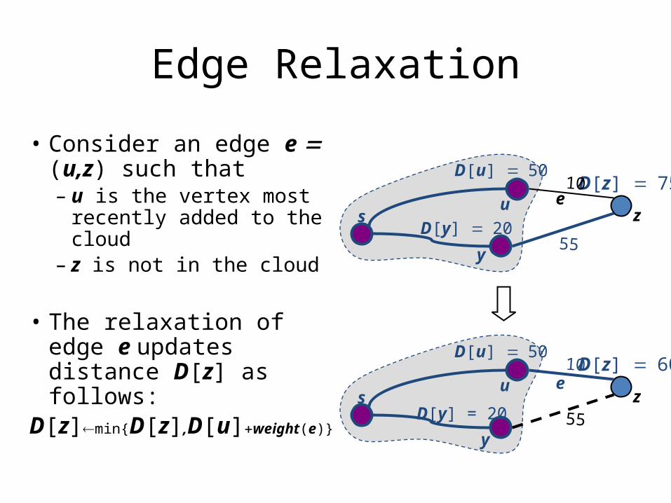
Edge Relaxation

• Consider an edge e = (u,z) such that– u is the vertex most

recently added to the cloud

– z is not in the cloud

• The relaxation of edge e updates distance D[z] as follows:

D[z]min{D[z],D[u]+weight(e)}

D[z] = 75

D[u] = 5010

zsu

D[z] = 60

D[u] = 5010

zsu

e

e

y

y

D[y] = 2055

D[y] = 20 55

Example

CB

A

E

D

F

0

428

48

7 1

2 5

2

3 9

CB

A

E

D

F

0

328

5 11

48

7 1

2 5

2

3 9

CB

A

E

D

F

0

328

5 8

48

7 1

2 5

2

3 9

CB

A

E

D

F

0

327

5 8

48

7 1

2 5

2

3 9

Example (cont.)

CB

A

E

D

F

0

327

5 8

48

7 1

2 5

2

3 9

CB

A

E

D

F

0

327

5 8

48

7 1

2 5

2

3 9

Exercise: Dijkstra’s alg

• Show how Dijkstra’s algorithm works on the following graph, assuming you start with SFO, I.e., s=SFO.• Show how the labels are updated in each iteration

(a separate figure for each iteration).

ORDPVD

MIADFW

SFO

LAX

LGA

HNL

849

802

13871743

1843

10991120

1233337

2555

142

1205

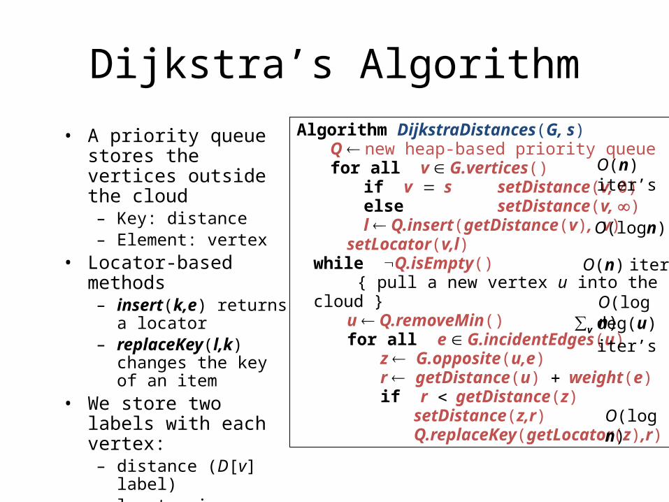
Dijkstra’s Algorithm

• A priority queue stores the vertices outside the cloud– Key: distance– Element: vertex

• Locator-based methods– insert(k,e) returns a

locator – replaceKey(l,k) changes

the key of an item• We store two labels with

each vertex:– distance (D[v] label)– locator in priority queue

Algorithm DijkstraDistances(G, s)Q new heap-based priority queuefor all v G.vertices()

if v = s setDistance(v, 0)

else setDistance(v, )

l Q.insert(getDistance(v), v)setLocator(v,l)

while Q.isEmpty() { pull a new vertex u into the cloud }u Q.removeMin() for all e G.incidentEdges(u)

z G.opposite(u,e)r getDistance(u) + weight(e)if r < getDistance(z)

setDistance(z,r) Q.replaceKey(getLocator(z),r)

O(n) iter’s

O(logn)

O(logn)∑v deg(u) iter’s

O(n) iter’s

O(logn)

Analysis• Graph operations

– Method incidentEdges is called once for each vertex• Label operations

– We set/get the distance and locator labels of vertex z O(deg(z)) times– Setting/getting a label takes O(1) time

• Priority queue operations– Each vertex is inserted once into and removed once from the priority

queue, where each insertion or removal takes O(log n) time– The key of a vertex in the priority queue is modified at most deg(w) times,

where each key change takes O(log n) time • Dijkstra’s algorithm runs in O((n + m) log n) time provided the graph is

represented by the adjacency list structure– Recall that Sv deg(v) = 2m

• The running time can also be expressed as O(m log n) since the graph is connected

• The running time can be expressed as a function of n, O(n2 log n)

Extension

• Using the template method pattern, we can extend Dijkstra’s algorithm to return a tree of shortest paths from the start vertex to all other vertices

• We store with each vertex a third label:– parent edge in the

shortest path tree• In the edge relaxation

step, we update the parent label

Algorithm DijkstraShortestPathsTree(G, s)

…

for all v G.vertices()…

setParent(v, )…

for all e G.incidentEdges(u){ relax edge e }z G.opposite(u,e)r getDistance(u) +

weight(e)if r < getDistance(z)

setDistance(z,r)

setParent(z,e)

Q.replaceKey(getLocator(z),r)

Why It Doesn’t Work for Negative-Weight Edges

Dijkstra’s algorithm is based on the greedy method. It adds vertices by increasing distance. If a node with a negative

incident edge were to be added late to the cloud, it could mess up distances for vertices already in the cloud.

C’s true distance is 1, but it is already in the cloud with D[C]=2!

CB

A

E

D

F

0

428

48

7 -3

2 5

2

3 9

CB

A

E

D

F

0

028

5 11

48

7 -3

2 5

2

3 9

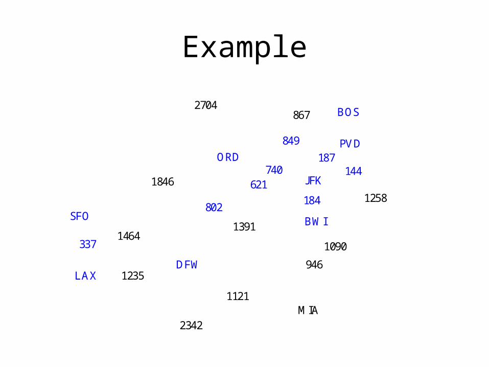
Minimum Spanning Trees

JFK

BOS

MIA

ORD

LAXDFW

SFO BWI

PVD

8672704

187

1258

849

144740

1391

184

946

1090

1121

2342

1846 621

802

1464

1235

337

Outline and Reading

• Minimum Spanning Trees (§13.6)• Definitions• A crucial fact

• The Prim-Jarnik Algorithm (§13.6.2)• Kruskal's Algorithm (§13.6.1)

Reminder: Weighted Graphs• In a weighted graph, each edge has an associated

numerical value, called the weight of the edge• Edge weights may represent, distances, costs, etc.• Example:

– In a flight route graph, the weight of an edge represents the distance in miles between the endpoint airports

ORDPVD

MIADFW

SFO

LAX

LGA

HNL

849

802

13871743

1843

10991120

1233337

2555

142

1205

Minimum Spanning Tree• Spanning subgraph

• Subgraph of a graph G containing all the vertices of G

• Spanning tree• Spanning subgraph that is itself a

(free) tree• Minimum spanning tree (MST)

• Spanning tree of a weighted graph with minimum total edge weight

• Applications• Communications networks• Transportation networks

ORD

PIT

ATL

STL

DEN

DFW

DCA

101

9

8

6

3

25

7

4

Exercise: MSTShow an MST of the following graph.

ORDPVD

MIADFW

SFO

LAX

LGA

HNL

849

802

13871743

1843

10991120

1233337

2555

142

1205

Cycle Property

Cycle Property:– Let T be a minimum

spanning tree of a weighted graph G

– Let e be an edge of G that is not in T and C let be the cycle formed by e with T

– For every edge f of C, weight(f) weight(e)

Proof:– By contradiction– If weight(f) > weight(e) we

can get a spanning tree of smaller weight by replacing e with f

84

2 36

7

7

9

8e

C

f

84

2 36

7

7

9

8

C

e

f

Replacing f with e yieldsa better spanning tree

Partition PropertyPartition Property:

– Consider a partition of the vertices of G into subsets U and V

– Let e be an edge of minimum weight across the partition

– There is a minimum spanning tree of G containing edge e

Proof:– Let T be an MST of G– If T does not contain e, consider the

cycle C formed by e with T and let f be an edge of C across the partition

– By the cycle property,weight(f)

weight(e) – Thus, weight(f) = weight(e)– We obtain another MST by replacing f

with e

U V

74

2 85

7

3

9

8 e

f

74

2 85

7

3

9

8 e

f

Replacing f with e yieldsanother MST

U V

Prim-Jarnik’s Algorithm• We pick an arbitrary vertex s and we grow the MST as a cloud

of vertices, starting from s• We store with each vertex v a label d(v) = the smallest weight

of an edge connecting v to a vertex in the cloud

• At each step:• We add to the cloud the

vertex u outside the cloud with the smallest distance label

• We update the labels of the vertices adjacent to u

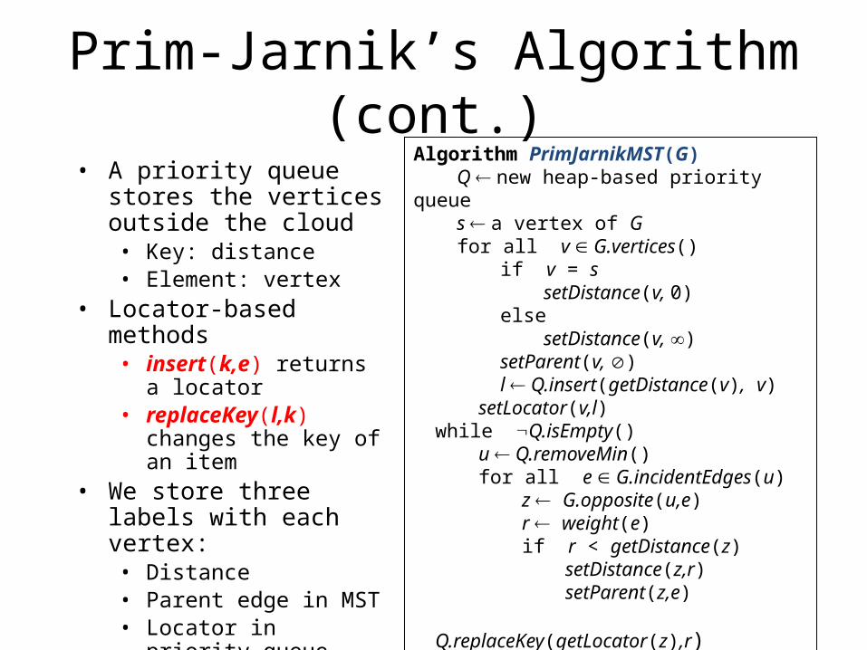
Prim-Jarnik’s Algorithm (cont.)• A priority queue stores the

vertices outside the cloud• Key: distance• Element: vertex

• Locator-based methods• insert(k,e) returns a

locator • replaceKey(l,k) changes

the key of an item• We store three labels with

each vertex:• Distance• Parent edge in MST• Locator in priority queue

Algorithm PrimJarnikMST(G)Q new heap-based priority queues a vertex of Gfor all v G.vertices()

if v = ssetDistance(v,

0)else

setDistance(v, )

setParent(v, )l

Q.insert(getDistance(v), v)setLocator(v,l)

while Q.isEmpty()u Q.removeMin() for all e G.incidentEdges(u)

z G.opposite(u,e)r weight(e)if r < getDistance(z)

setDistance(z,r)

setParent(z,e) Q.replaceKey(getLocator(z),r)

Example

BD

C

A

F

E

74

28

5

7

3

9

8

0 7

2

8

BD

C

A

F

E

74

28

5

7

3

9

8

0 7

2

5 4

7

BD

C

A

F

E

74

28

5

7

3

9

8

0 7

2

5

7

BD

C

A

F

E

74

28

5

7

3

9

8

0 7

2

5

7

Example (contd.)

BD

C

A

F

E

74

28

5

7

3

9

8

0 3

2

5 4

7

BD

C

A

F

E

74

28

5

7

3

9

8

0 3

2

5 4

7

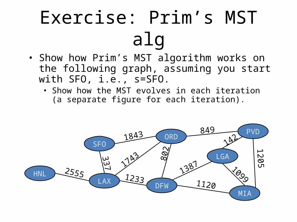
Exercise: Prim’s MST alg• Show how Prim’s MST algorithm works on the following

graph, assuming you start with SFO, i.e., s=SFO.• Show how the MST evolves in each iteration (a separate figure for

each iteration).

ORDPVD

MIADFW

SFO

LAX

LGA

HNL

849

802

13871743

1843

10991120

1233337

2555

142

1205

Analysis• Graph operations

• Method incidentEdges is called once for each vertex• Label operations

• We set/get the distance, parent and locator labels of vertex z O(deg(z)) times• Setting/getting a label takes O(1) time

• Priority queue operations• Each vertex is inserted once into and removed once from the priority queue,

where each insertion or removal takes O(log n) time• The key of a vertex w in the priority queue is modified at most deg(w) times,

where each key change takes O(log n) time • Prim-Jarnik’s algorithm runs in O((n + m) log n) time provided the graph

is represented by the adjacency list structure• Recall that Sv deg(v) = 2m

• The running time is O(m log n) since the graph is connected

29 Graphs

Kruskal’s Algorithm• A priority queue stores the

edges outside the cloud• Key: weight• Element: edge

• At the end of the algorithm• We are left with one cloud

that encompasses the MST• A tree T which is our MST

Algorithm KruskalMST(G)for each vertex V in G do

define a Cloud(v) of {v}

let Q be a priority queue.Insert all edges into Q using

their weights as the keyT

while T has fewer than n-1 edges edge e = T.removeMin()

Let u, v be the endpoints of e

if Cloud(v) Cloud(u) then

Add edge e to T

Merge Cloud(v) and Cloud(u)

return T

Data Structure for Kruskal Algortihm

• The algorithm maintains a forest of trees• An edge is accepted it if connects distinct trees• We need a data structure that maintains a partition,

i.e., a collection of disjoint sets, with the operations:• find(u): return the set storing u• union(u,v): replace the sets storing u and v with their

union

Representation of a Partition

• Each set is stored in a sequence• Each element has a reference back to the set

• operation find(u) takes O(1) time, and returns the set of which u is a member.

• in operation union(u,v), we move the elements of the smaller set to the sequence of the larger set and update their references

• the time for operation union(u,v) is min(nu,nv), where nu and nv are the sizes of the sets storing u and v

• Whenever an element is processed, it goes into a set of size at least double, hence each element is processed at most log n times

Algorithm Kruskal(G): Input: A weighted graph G. Output: An MST T for G.Let P be a partition of the vertices of G, where each vertex forms a separate set.Let Q be a priority queue storing the edges of G, sorted by their weightsLet T be an initially-empty treewhile Q is not empty do (u,v) Q.removeMinElement() if P.find(u) != P.find(v) then

Add (u,v) to TP.union(u,v)

return T

Partition-Based Implementation• A partition-based version of Kruskal’s

Algorithm performs cloud merges as unions and tests as finds.

Running time: O((n+m) log n)

Example

JFK

BOS

MIA

ORD

LAXDFW

SFO BWI

PVD

8672704

187

1258

849

144740

1391

184

946

1090

1121

2342

1846 621

802

1464

1235

337

Example

JFK

BOS

MIA

ORD

LAXDFW

SFO BWI

PVD

8672704

187

1258

849

144740

1391

184

946

1090

1121

2342

1846 621

802

1464

1235

337

JFK

BOS

MIA

ORD

LAXDFW

SFO BWI

PVD

8672704

187

1258

849

144740

1391

184

946

1090

1121

2342

1846 621

802

1464

1235

337

Example

JFK

BOS

MIA

ORD

LAXDFW

SFO BWI

PVD

8672704

187

1258

849

144740

1391

184

946

1090

1121

2342

1846 621

802

1464

1235

337

Example

Example

JFK

BOS

MIA

ORD

LAXDFW

SFO BWI

PVD

8672704

187

1258

849

144740

1391

184

946

1090

1121

2342

1846 621

802

1464

1235

337

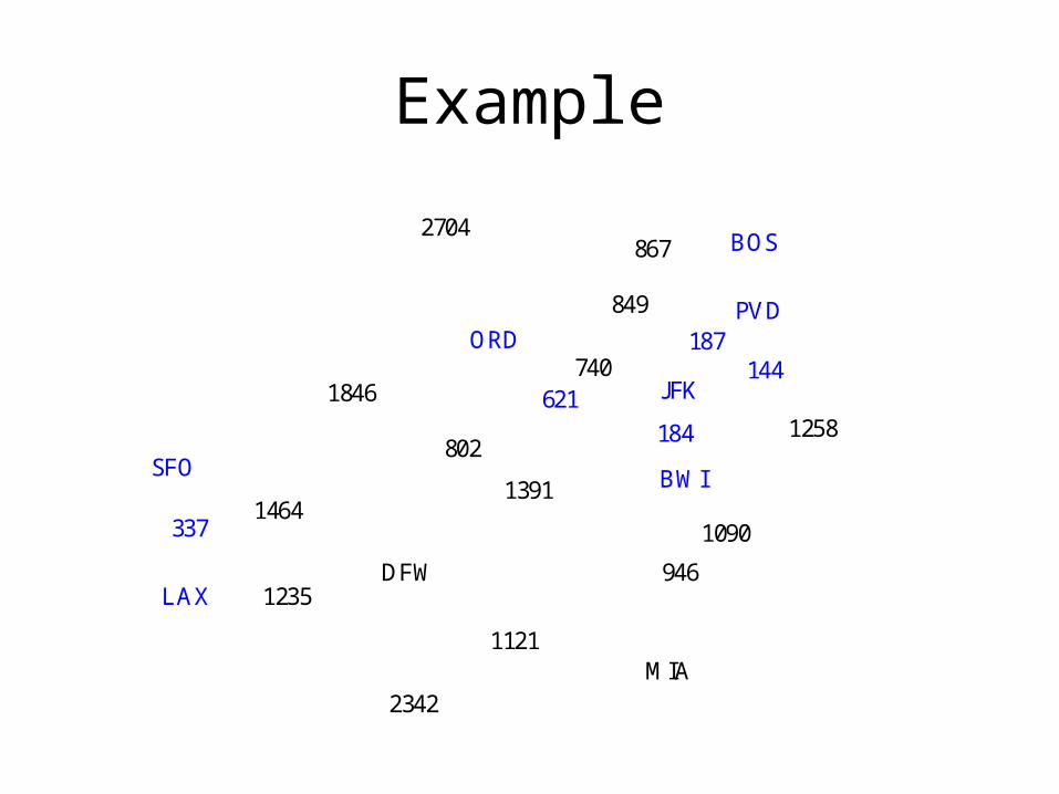
Example

JFK

BOS

MIA

ORD

LAXDFW

SFO BWI

PVD

8672704

187

1258

849

144740

1391

184

946

1090

1121

2342

1846 621

802

1464

1235

337

Example

JFK

BOS

MIA

ORD

LAXDFW

SFO BWI

PVD

8672704

187

1258

849

144740

1391

184

946

1090

1121

2342

1846 621

802

1464

1235

337

Example

JFK

BOS

MIA

ORD

LAXDFW

SFO BWI

PVD

8672704

187

1258

849

144740

1391

184

946

1090

1121

2342

1846 621

802

1464

1235

337

JFK

BOS

MIA

ORD

LAXDFW

SFO BWI

PVD

8672704

187

1258

849

144740

1391

184

946

1090

1121

2342

1846 621

802

1464

1235

337

Example

Example

JFK

BOS

MIA

ORD

LAXDFW

SFO BWI

PVD

8672704

187

1258

849

144740

1391

184

946

1090

1121

2342

1846 621

802

1464

1235

337

Example

JFK

BOS

MIA

ORD

LAXDFW

SFO BWI

PVD

8672704

187

1258

849

144740

1391

184

946

1090

1121

2342

1846 621

802

1464

1235

337

JFK

BOS

MIA

ORD

LAXDFW

SFO BWI

PVD

8672704

187

1258

849

144740

1391

184

946

1090

1121

2342

1846 621

802

1464

1235

337

Example

JFK

BOS

MIA

ORD

LAXDFW

SFO BWI

PVD

8672704

187

1258

849

144740

1391

184

946

1090

1121

2342

1846 621

802

1464

1235

337

Example

Example

JFK

BOS

MIA

ORD

LAXDFW

SFO BWI

PVD

8672704

187

1258

849

144740

1391

184

946

1090

1121

2342

1846 621

802

1464

1235

337

Exercise: Kruskal’s MST alg• Show how Kruskal’s MST algorithm works on the following

graph.• Show how the MST evolves in each iteration (a separate figure for

each iteration).

ORDPVD

MIADFW

SFO

LAX

LGA

HNL

849

802

13871743

1843

10991120

1233337

2555

142

1205

Bellman-Ford Algorithm

• Works even with negative-weight edges

• Must assume directed edges (for otherwise we would have negative-weight cycles)

• Iteration i finds all shortest paths that use i edges.

• Running time: O(nm).• Can be extended to detect a

negative-weight cycle if it exists – How?

Algorithm BellmanFord(G, s)for all v G.vertices()

if v = ssetDistance(v, 0)

else setDistance(v, )

for i 1 to n-1 dofor each e G.edges()

u G.origin(e)z G.opposite(u,e)r getDistance(u) +

weight(e)if r < getDistance(z)

setDistance(z,r)

Bellman-Ford Example

0

48

7 1

-2 5

-2

3 9

Nodes are labeled with their d(v) values

-2

0

48

7 1

-2 53 9

8 -2 4

First round

-2

-28

0

4

48

7 1

-2 53 9

-15

61

9

Second round

-25

0

1

-1

9

48

7 1

-2 5

-2

3 94

Third round

Exercise: Bellman-Ford’s alg

• Show how Bellman-Ford’s algorithm works on the following graph, assuming you start with the top node• Show how the labels are updated in each iteration

(a separate figure for each iteration).

0

48

7 1

-5 5

-2

3 9

DAG-based Algorithm

• Works even with negative-weight edges

• Uses topological order• Is much faster than

Dijkstra’s algorithm• Running time: O(n+m).

Algorithm DagDistances(G, s)for all v G.vertices()

if v = ssetDistance(v, 0)

else setDistance(v, )

Perform a topological sort of the vertices

for u 1 to n do {in topological order}

for each e G.outEdges(u){ relax edge e }z G.opposite(u,e)r getDistance(u) +

weight(e)if r < getDistance(z)

setDistance(z,r)

DAG Example

0

48

7 1

-5 5

-2

3 9

Nodes are labeled with their d(v) values1

2 43

6 5

-2

0

48

7 1

-5 53 9

-2 4

1

2 43

6 5

8

-2

-28

0

4

48

7 1

-5 53 9

-1

1 7

1

2 43

6 5

5-25

0

1

-1

7

48

7 1

-5 5

-2

3 94

1

2 43

6 5

0

(two steps)

Exercize: DAG-based Alg

• Show how DAG-based algorithm works on the following graph, assuming you start with the second rightmost node• Show how the labels are updated in each iteration

(a separate figure for each iteration).

∞ 0 ∞ ∞∞ ∞5 2 7 -1 -2

6 1

3 4

2

1

2

3

4

5

Summary of Shortest-Path Algs

• Breadth-First-Search• Dijkstra’s algorithm (§13.5.2)

– Algorithm– Edge relaxation

• The Bellman-Ford algorithm • Shortest paths in DAGs

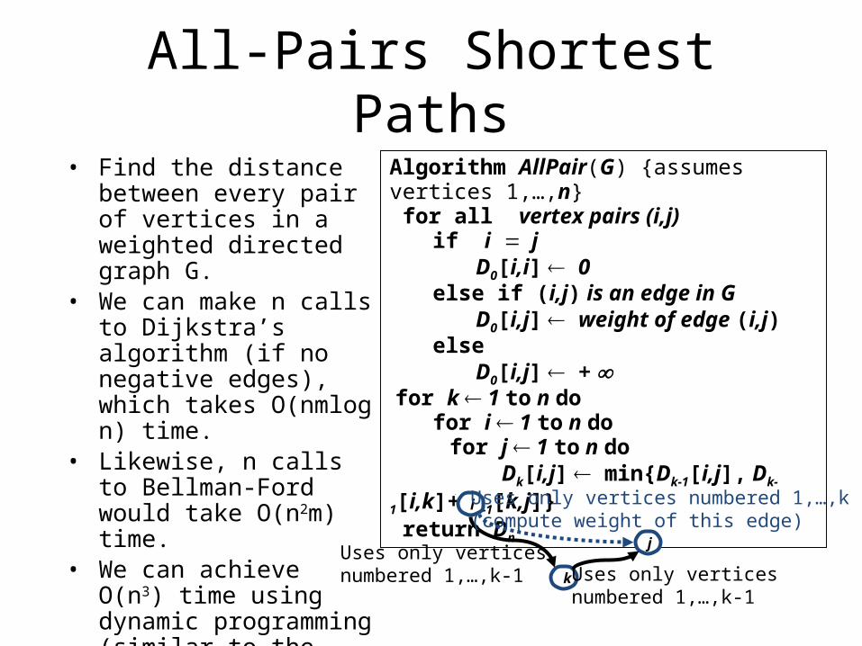
All-Pairs Shortest Paths• Find the distance between

every pair of vertices in a weighted directed graph G.

• We can make n calls to Dijkstra’s algorithm (if no negative edges), which takes O(nmlog n) time.

• Likewise, n calls to Bellman-Ford would take O(n2m) time.

• We can achieve O(n3) time using dynamic programming (similar to the Floyd-Warshall algorithm).

Algorithm AllPair(G) {assumes vertices 1,…,n} for all vertex pairs (i,j)

if i = jD0[i,i] 0

else if (i,j) is an edge in GD0[i,j] weight of edge (i,j)

elseD0[i,j] +

for k 1 to n do for i 1 to n do for j 1 to n do

Dk[i,j] min{Dk-1[i,j], Dk-

1[i,k]+Dk-1[k,j]} return Dn

k

j

i

Uses only verticesnumbered 1,…,k-1 Uses only vertices

numbered 1,…,k-1

Uses only vertices numbered 1,…,k(compute weight of this edge)

Why Dijkstra’s Algorithm Works• Dijkstra’s algorithm is based on the greedy

method. It adds vertices by increasing distance. Suppose it didn’t find all shortest

distances. Let F be the first wrong vertex the algorithm processed.

When the previous node, D, on the true shortest path was considered, its distance was correct.

But the edge (D,F) was relaxed at that time!

Thus, so long as D[F]>D[D], F’s distance cannot be wrong. That is, there is no wrong vertex.

CB

s

E

D

F

0

327

5 8

48

7 1

2 5

2

3 9