Goodness-of-Fit and Contingency Tables 11-1 Review and Preview 11-2 Goodness-of-Fit 11-3 Contingency Tables 11-4 McNemar’s Test for Matched Pairs 584 ISBN 0-558-58875-1 Elementary Statistics, Eleventh Edition, by Mario F. Triola. Published by Addison-Wesley. Copyright © 2010 by Pearson Education, Inc.

Welcome message from author
This document is posted to help you gain knowledge. Please leave a comment to let me know what you think about it! Share it to your friends and learn new things together.
Transcript

Goodness-of-Fit andContingency Tables
11-1 Review and Preview
11-2 Goodness-of-Fit
11-3 Contingency Tables
11-4 McNemar’s Test forMatched Pairs
584
ISB
N0-558-58875-1
Elementary Statistics, Eleventh Edition, by Mario F. Triola. Published by Addison-Wesley. Copyright © 2010 by Pearson Education, Inc.

Three alert nurses at the Veteran’s AffairsMedical Center in Northampton, Massachu-setts noticed an unusually high number ofdeaths at times when another nurse, KristenGilbert, was working. Those same nurses laternoticed missing supplies of the drug epineph-rine, which is a synthetic adrenaline that stim-ulates the heart. They reported their growing
C H A P T E R P R O B L E M
Is the nurse a serial killer?concerns, and an investigation followed. KristenGilbert was arrested and charged with fourcounts of murder and two counts of at-tempted murder. When seeking a grand juryindictment, prosecutors provided a key pieceof evidence consisting of a two-way tableshowing the numbers of shifts with deathswhen Gilbert was working. See Table 11-1.
Figure 11-1 Bar Graph of Death Rates withGilbert Working and Not Working
Table 11-1 Two-Way Table with Deaths When Gilbert Was Working
Shifts with a death Shifts without a death
Gilbert was working 40 217
Gilbert was not working 34 1350
George Cobb, a leading statistician andstatistics educator, became involved in theGilbert case at the request of an attorney forthe defense. Cobb wrote a report statingthat the data in Table 11-1 should have beenpresented to the grand jury (as it was) forpurposes of indictment, but that it shouldnot be presented at the actual trial. He notedthat the data in Table 11-1 are based on ob-servations and do not show that Gilbert ac-tually caused deaths. Also, Table 11-1 includesinformation about many other deaths thatwere not relevant to the trial. The judgeruled that the data in Table 11-1 could not beused at the trial. Kristen Gilbert was con-victed on other evidence and is now servinga sentence of life in prison, without the pos-sibility of parole.
This chapter will include methods for an-alyzing data in tables, such as Table 11-1. Wewill analyze Table 11-1 to see what conclusionscould be presented to the grand jury thatprovided the indictment.
The numbers in Table 11-1 might be betterunderstood with a graph, such as Figure 11-1,which shows the death rates during shiftswhen Gilbert was working and when she wasnot working. Figure 11-1 seems to make itclear that shifts when Gilbert was workinghad a much higher death rate than shiftswhen she was not working, but we need todetermine whether those results are statisti-cally significant.
ISB
N0-
558-
5887
5-1
Elementary Statistics, Eleventh Edition, by Mario F. Triola. Published by Addison-Wesley. Copyright © 2010 by Pearson Education, Inc.

586 Chapter 11 Goodness-of-Fit and Contingency Tables
Review and Preview
We began a study of inferential statistics in Chapter 7 when we presented methods forestimating a parameter for a single population and in Chapter 8 when we presentedmethods of testing claims about a single population. In Chapter 9 we extended thosemethods to situations involving two populations. In Chapter 10 we considered meth-ods of correlation and regression using paired sample data. In this chapter we use sta-tistical methods for analyzing categorical (or qualitative, or attribute) data that can beseparated into different cells. We consider hypothesis tests of a claim that the observedfrequency counts agree with some claimed distribution. We also consider contingencytables (or two-way frequency tables), which consist of frequency counts arranged in atable with at least two rows and two columns. We conclude this chapter by consider-ing two-way tables involving data consisting of matched pairs.
The methods of this chapter use the same (chi-square) distribution that wasfirst introduced in Section 7-5. See Section 7-5 for a quick review of properties of the
distribution.x2
x2
11-1
Goodness-of-Fit
Key Concept In this section we consider sample data consisting of observed fre-quency counts arranged in a single row or column (called a one-way frequency table).We will use a hypothesis test for the claim that the observed frequency counts agreewith some claimed distribution, so that there is a good fit of the observed data withthe claimed distribution.
Because we test for how well an observed frequency distribution fits some speci-fied theoretical distribution, the method of this section is called a goodness-of-fit test.
11-2
A goodness-of-fit test is used to test the hypothesis that an observed fre-quency distribution fits (or conforms to) some claimed distribution.
Objective
Conduct a goodness-of-fit test.
1. The data have been randomly selected.
Requirements
2. The sample data consist of frequency counts for eachof the different categories.
O represents the observed frequency of an out-come, found by tabulating the sample data.
E represents the expected frequency of an out-come, found by assuming that the distributionis as claimed.
Notation
k represents the number of different categories oroutcomes.
n represents the total number of trials (or observedsample values).
ISB
N0-558-58875-1
Elementary Statistics, Eleventh Edition, by Mario F. Triola. Published by Addison-Wesley. Copyright © 2010 by Pearson Education, Inc.

11-2 Goodness-of-Fit 587
Finding Expected FrequenciesConducting a goodness-of-fit test requires that we identify the observed frequencies,then determine the frequencies expected with the claimed distribution. Table 11-2 onthe next page includes observed frequencies with a sum of 80, so . If we as-sume that the 80 digits were obtained from a population in which all digits are equallylikely, then we expect that each digit should occur in of the 80 trials, so each ofthe 10 expected frequencies is given by . In general, if we are assuming that allof the expected frequencies are equal, each expected frequency is , where n isthe total number of observations and k is the number of categories. In other cases inwhich the expected frequencies are not all equal, we can often find the expected fre-quency for each category by multiplying the sum of all observed frequencies and theprobability p for the category, so . We summarize these two procedures here.
• Expected frequencies are equal: .
• Expected frequencies are not all equal: for each individual category.
As good as these two preceding formulas for E might be, it is better to use an in-formal approach. Just ask, “How can the observed frequencies be split up among thedifferent categories so that there is perfect agreement with the claimed distribution?”Also, note that the observed frequencies must all be whole numbers because they rep-resent actual counts, but the expected frequencies need not be whole numbers. For ex-ample, when rolling a single die 33 times, the expected frequency for each possibleoutcome is . The expected frequency for rolling a 3 is 5.5, even though itis impossible to have the outcome of 3 occur exactly 5.5 times.
We know that sample frequencies typically deviate somewhat from the values wetheoretically expect, so we now present the key question: Are the differences betweenthe actual observed values O and the theoretically expected values E statistically signifi-cant? We need a measure of the discrepancy between the O and E values, so we usethe test statistic given with the requirements and critical values. (Later, we will ex-plain how this test statistic was developed, but you can see that it has differences of
as a key component.)The test statistic is based on differences between the observed and expected
values. If the observed and expected values are close, the test statistic will be smalland the P-value will be large. If the observed and expected frequencies are not close,
x2x2
O - E
33>6 = 5.5
E � np
E � n/k
E = np
E = n>kE = 81>10
n = 80
3. For each category, the expected frequency is at least 5.(The expected frequency for a category is the fre-quency that would occur if the data actually have the
distribution that is being claimed. There is no require-ment that the observed frequency for each categorymust be at least 5.)
x2 = a(O - E )2
E
Test Statistic for Goodness-of-Fit Tests
1. Critical values are found in Table A-4 by using degrees of freedom, where k is the number of categories.
k - 1
Critical Values
2. Goodness-of-fit hypothesis tests are always right-tailed.
P-values are typically provided by computer software, or a range of P-values can be found from Table A-4.
P-Values
ISB
N0-
558-
5887
5-1
Elementary Statistics, Eleventh Edition, by Mario F. Triola. Published by Addison-Wesley. Copyright © 2010 by Pearson Education, Inc.

588 Chapter 11 Goodness-of-Fit and Contingency Tables
the test statistic will be large and the P-value will be small. Figure 11-2 summa-rizes this relationship. The hypothesis tests of this section are always right-tailed,because the critical value and critical region are located at the extreme right of the dis-tribution. If confused, just remember this:
“If the P is low, the null must go.”(If the P-value is small, reject the null hypothesis that the distribution isas claimed.)
Once we know how to find the value of the test statistic and the critical value, wecan test hypotheses by using the same general procedures introduced in Chapter 8.
x2
Fail to reject H0 Reject H0
Large X 2 value, small P-valueSmall X 2 value, large P-value
Compare the observed Ovalues to the correspondingexpected E values.
X 2 here X 2 here
Os and Esare close.
Os and Es arefar apart.
“If the P is low,the null must go.”
Not a good fitwith assumeddistribution
Good fitwith assumeddistribution
Figure 11-2
Relationships Among the2 Test Statistic, P-Value,
and Goodness-of-FitX
Last Digits of Weights Data Set 1 in Appendix B includesweights from 40 randomly selected adult males and 40 randomly selected adult fe-males. Those weights were obtained as part of the National Health ExaminationSurvey. When obtaining weights of subjects, it is extremely important to actuallyweigh individuals instead of asking them to report their weights. By analyzing thelast digits of weights, researchers can verify that weights were obtained through ac-tual measurements instead of being reported. When people report weights, theytypically round to a whole number, so reported weights tend to have many lastdigits consisting of 0. In contrast, if people are actually weighed with a scale havingprecision to the nearest 0.1 pound, the weights tend to have last digits that areuniformly distributed, with 0, 1, 2, , 9 all occurring with roughly the same fre-quencies. Table 11-2 shows the frequency distribution of the last digits from the
Á
1
Table 11-2 Last Digitsof Weights
Last Digit Frequency
0 7
1 14
2 6
3 10
4 8
5 4
6 5
7 6
8 12
9 8
ISB
N0-558-58875-1
Elementary Statistics, Eleventh Edition, by Mario F. Triola. Published by Addison-Wesley. Copyright © 2010 by Pearson Education, Inc.
11-2 Goodness-of-Fit 589
80 weights listed in Data Set 1 in Appendix B. (For example, the weight of 201.5 lbhas a last digit of 5, and this is one of the data values included in Table 11-2.)
Test the claim that the sample is from a population of weights in which thelast digits do not occur with the same frequency. Based on the results, what can weconclude about the procedure used to obtain the weights?
REQUIREMENT CHECK (1) The data come from randomlyselected subjects. (2) The data do consist of frequency counts, as shown in Table 11-2.(3) With 80 sample values and 10 categories that are claimed to be equally likely, eachexpected frequency is 8, so each expected frequency does satisfy the requirement ofbeing a value of at least 5. All of the requirements are satisfied.
The claim that the digits do not occur with the same frequency is equivalent tothe claim that the relative frequencies or probabilities of the 10 cells ( p0, p1, , p9) arenot all equal. We will use the traditional method for testing hypotheses (see Figure 8-9).
Step 1: The original claim is that the digits do not occur with the same frequency.That is, at least one of the probabilities p0, p1, , p9 is different from the others.
Step 2: If the original claim is false, then all of the probabilities are the same.That is,
Step 3: The null hypothesis must contain the condition of equality, so we have
H0:
H1: At least one of the probabilities is different from the others.
Step 4: No significance level was specified, so we select .
Step 5: Because we are testing a claim about the distribution of the last digits be-ing a uniform distribution, we use the goodness-of-fit test described in this sec-tion. The distribution is used with the test statistic given earlier.
Step 6: The observed frequencies O are listed in Table 11-2. Each correspondingexpected frequency E is equal to 8 (because the 80 digits would be uniformlydistributed among the 10 categories). Table 11-3 on the next page shows thecomputation of the test statistic. The test statistic is . The criticalvalue is (found in Table A-4 with in the right tail and degrees of freedom equal to ). The test statistic and critical value areshown in Figure 11-3 on the next page.
Step 7: Because the test statistic does not fall in the critical region, there is notsufficient evidence to reject the null hypothesis.
Step 8: There is not sufficient evidence to support the claim that the last digits donot occur with the same relative frequency.
This goodness-of-fit test suggests that the last digits providea reasonably good fit with the claimed distribution of equally likely frequencies. In-stead of asking the subjects how much they weigh, it appears that their weights wereactually measured as they should have been.
Example 1 involves a situation in which the claimed frequencies for the differentcategories are all equal. The methods of this section can also be used when the hy-pothesized probabilities (or frequencies) are different, as shown in Example 2.
k - 1 = 9a = 0.05x2 = 16.919
x2 = 11.250x2
x2
a = 0.05
p0 = p1 = p2 = p3 = p4 = p5 = p6 = p7 = p8 = p9
p0 = p1 = p2 = p3 = p4 = p5 = p6 = p7 = p8 = p9.
Á
Á
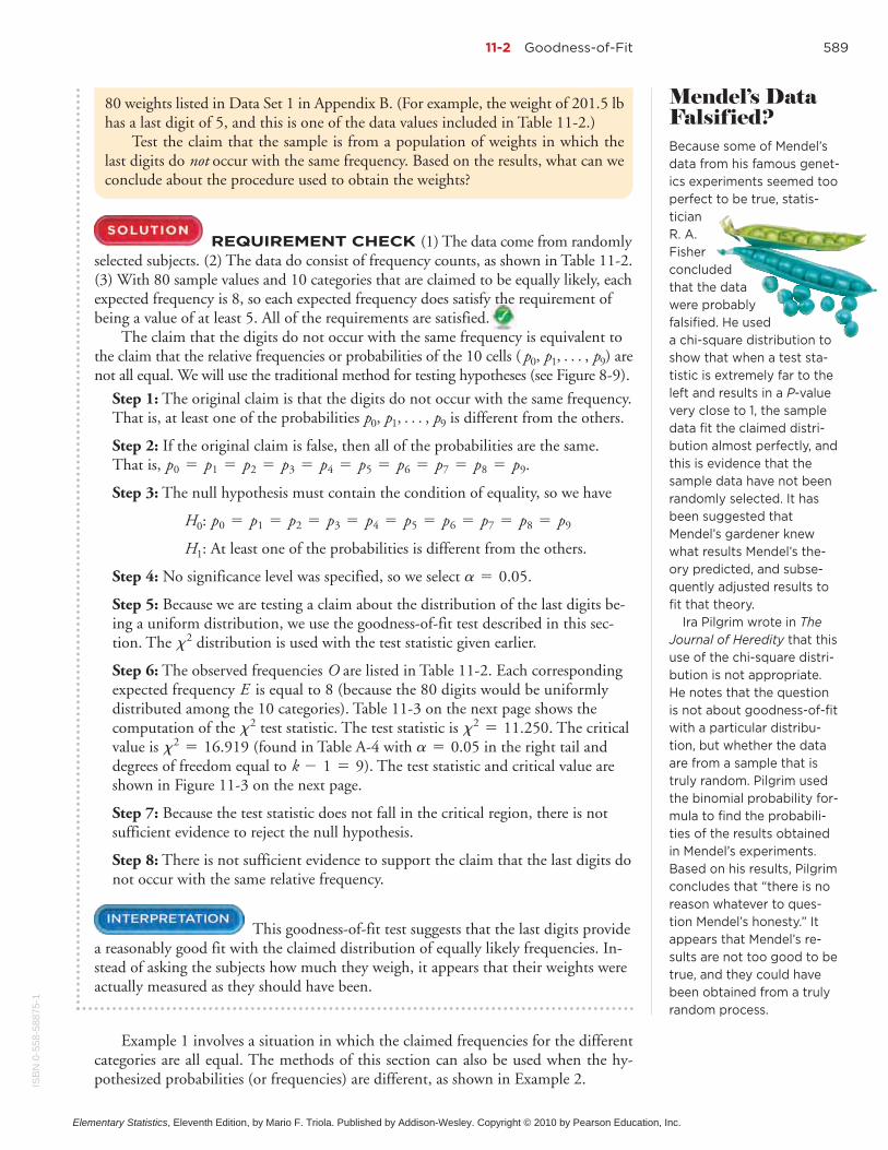
Mendel’s DataFalsified?Because some of Mendel’sdata from his famous genet-ics experiments seemed tooperfect to be true, statis-ticianR. A.Fisherconcludedthat the datawere probablyfalsified. He useda chi-square distribution toshow that when a test sta-tistic is extremely far to theleft and results in a P-valuevery close to 1, the sampledata fit the claimed distri-bution almost perfectly, andthis is evidence that thesample data have not beenrandomly selected. It hasbeen suggested thatMendel’s gardener knewwhat results Mendel’s the-ory predicted, and subse-quently adjusted results tofit that theory.
Ira Pilgrim wrote in TheJournal of Heredity that thisuse of the chi-square distri-bution is not appropriate.He notes that the questionis not about goodness-of-fitwith a particular distribu-tion, but whether the dataare from a sample that istruly random. Pilgrim usedthe binomial probability for-mula to find the probabili-ties of the results obtainedin Mendel’s experiments.Based on his results, Pilgrimconcludes that “there is noreason whatever to ques-tion Mendel’s honesty.” Itappears that Mendel’s re-sults are not too good to betrue, and they could havebeen obtained from a trulyrandom process.
ISB
N0-
558-
5887
5-1
Elementary Statistics, Eleventh Edition, by Mario F. Triola. Published by Addison-Wesley. Copyright © 2010 by Pearson Education, Inc.

590 Chapter 11 Goodness-of-Fit and Contingency Tables
X 2 � 16.9190
Fail to rejectp0 � p1 � . . . � p9
Rejectp0 � p1 � . . . � p9
Sample data: X 2 � 11. 250
Figure 11-3 Test of p7 � p8 � p9
p0 � p1 � p2 � p3 � p4 = p5 � p6 �
Table 11-3 Calculating the Test Statistic for the Last Digits of WeightsX2
Last DigitObserved
Frequency OExpected
Frequency E O E� (O E)2�(O � E )2
E
0 7 8 1- 1 0.125
1 14 8 6 36 4.500
2 6 8 2- 4 0.500
3 10 8 2 4 0.500
4 8 8 0 0 0.000
5 4 8 4- 16 2.000
6 5 8 3- 9 1.125
7 6 8 2- 4 0.500
8 12 8 4 16 2.000
9 8 8 0 0 0.000
x2 = a(O - E )2
E= 11.250
World Series Games Table 11-4 lists the numbers of gamesplayed in the baseball World Series, as of this writing. That table also includes theexpected proportions for the numbers of games in a World Series, assuming thatin each series, both teams have about the same chance of winning. Use a 0.05 sig-nificance level to test the claim that the actual numbers of games fit the distribu-tion indicated by the probabilities.
2
Which Car SeatsAre Safest?Many people believe thatthe back seat of a car is thesafest place to sit, but is it?
Univer-sity ofBuffalore-
searchersanalyzed more
than 60,000 fatal carcrashes and found that themiddle back seat is thesafest place to sit in a car.They found that sitting inthat seat makes a passen-ger 86% more likely to sur-vive than those who sit inthe front seats, and they are25% more likely to survivethan those sitting in eitherof the back seats nearestthe windows. An analysis ofseat belt use showed thatwhen not wearing a seatbelt in the back seat, pas-sengers are three timesmore likely to die in a crashthan those wearing seatbelts in that same seat. Pas-sengers concerned withsafety should sit in the mid-dle back seat wearing a seatbelt.
Table 11-4 Numbers of Games in World Series Contests
Games played 4 5 6 7
Actual World Series contests 19 21 22 37
Expected proportion 2 16> 4 16> 5 16> 5 16>
ISB
N0-558-58875-1
Elementary Statistics, Eleventh Edition, by Mario F. Triola. Published by Addison-Wesley. Copyright © 2010 by Pearson Education, Inc.

11-2 Goodness-of-Fit 591
REQUIREMENT CHECK (1) We begin by noting that theobserved numbers of games are not randomly selected from a larger population.However, we treat them as a random sample for the purpose of determining whetherthey are typical results that might be obtained from such a random sample. (2) Thedata do consist of frequency counts. (3) Each expected frequency is at least 5, as willbe shown later in this solution. All of the requirements are satisfied.
Step 1: The original claim is that the actual numbers of games fit the distributionindicated by the expected proportions. Using subscripts corresponding to thenumber of games, we can express this claim as and and
and .
Step 2: If the original claim is false, then at least one of the proportions does nothave the value as claimed.
Step 3: The null hypothesis must contain the condition of equality, so we have
H0: and and and .
H1: At least one of the proportions is not equal to the given claimed value.
Step 4: The significance level is .
Step 5: Because we are testing a claim that the distribution of numbers of gamesin World Series contests is as claimed, we use the goodness-of-fit test described inthis section. The distribution is used with the test statistic given earlier.
Step 6: Table 11-5 shows the calculations resulting in the test statistic of .The critical value is (found in Table A-4 with in the righttail and degrees of freedom equal to ). The Minitab display shows thevalue of the test statistic as well as the P-value of 0.048.
k - 1 = 3a = 0.05x2 = 7.815
x2 = 7.885
x2
a = 0.05
p7 = 5>16p6 = 5>16p5 = 4>16p4 = 2>16
p7 = 5>16p6 = 5>16p5 = 4>16p4 = 2>16
MINITAB
Which AirplaneSeats AreSafest?Because most crashesoccur during takeoff orlanding, passengers canimprove theirsafety by fly-ing non-stop.Also, largerplanes aresafer.
Manypeople be-lieve thatthe rearseats are safest in an air-plane crash. Todd Curtis isan aviation safety expertwho maintains a databaseof airline incidents, and hesays that it is not possibleto conclude that someseats are safer than others.He says that each crash isunique, and there are far toomany variables to consider.Also, Matt McCormick, asurvival expert for the Na-tional Transportation SafetyBoard, told Travel magazinethat “there is no one safeplace to sit.”
Goodness-of-fit tests canbe used with a null hypoth-esis that all sections of anairplane are equally safe.Crashed airplanes could bedivided into the front, mid-dle, and rear sections. Theobserved frequencies of fa-talities could then be com-pared to the frequenciesthat would be expectedwith a uniform distributionof fatalities. The 2 teststatistic reflects the size ofthe discrepancies betweenobserved and expected fre-quencies, and it would re-veal whether some sectionsare safer than others.
x
Table 11-5 Calculating the 2 Test Statistic for the Numbers of WorldSeries Games
X
Number ofGames
ObservedFrequency
O
ExpectedFrequencyE np� O E� (O E)2�
(O � E )2
E
4 1999 # 2
16= 12.3750
6.6250 43.8906 3.5467
5 2199 # 4
16= 24.7500
3.7500- 14.0625 0.5682
6 2299 # 5
16= 30.9375
8.9375- 79.8789 2.5819
7 3799 # 5
16= 30.9375
6.0625 36.7539 1.1880
x2 = a(O - E )2
E= 7.885
ISB
N0-
558-
5887
5-1
Elementary Statistics, Eleventh Edition, by Mario F. Triola. Published by Addison-Wesley. Copyright © 2010 by Pearson Education, Inc.

592 Chapter 11 Goodness-of-Fit and Contingency Tables
P-ValuesComputer software automatically provides P-values when conducting goodness-of-fittests. If computer software is unavailable, a range of P-values can be found fromTable A-4. Example 2 resulted in a test statistic of , and if we refer toTable A-4 with 3 degrees of freedom, we find that the test statistic of 7.885 lies be-tween the table values of 7.815 and 9.348. So, the P-value is between 0.025 and 0.05.In this case, we might state that “P-value 0.05.” The Minitab display shows thatthe P-value is 0.048. Because the P -value is less than the significance level of 0.05, wereject the null hypothesis. Remember, “if the P (value) is low, the null must go.”
Rationale for the Test Statistic: Examples 1 and 2 show that the test statisticis a measure of the discrepancy between observed and expected frequencies. Simplysumming the differences between observed and expected values does not result in an
x2
6
x2 = 7.885
4 5 6 7Number of Gamesin World Series
0.4
0.3
0.1
0.2
0
Pro
port
ion
Observed Proportions
ExpectedProportions
Figure 11-4
Observed and ExpectedProportions in theNumbers of WorldSeries Games
Step 7: The P-value of 0.048 is less than the significance level of 0.05, so there issufficient evidence to reject the null hypothesis. (Also, the test statistic of is in the critical region bounded by the critical value of 7.815, so there is suffi-cient evidence to reject the null hypothesis.)
Step 8: There is sufficient evidence to warrant rejection of the claim that actualnumbers of games in World Series contests fit the distribution indicated by theexpected proportions given in Table 11-4.
This goodness-of-fit test suggests that the numbers ofgames in World Series contests do not fit the distribution expected from probabilitycalculations. Different media reports have noted that seven-game series occur muchmore than expected. The results in Table 11-4 show that seven-game series occurred37% of the time, but they were expected to occur only 31% of the time. (A USAToday headline stated that “Seven-game series defy odds.”) So far, no reasonable ex-planations have been provided for the discrepancy.
x2 = 7.885
In Figure 11-4 we graph the expected proportions of 2 16, 4 16, 5 16, and 5 16along with the observed proportions of 19 99, 21 99, 22 99, and 37 99, so that wecan visualize the discrepancy between the distribution that was claimed and the fre-quencies that were observed. The points along the red line represent the expectedproportions, and the points along the green line represent the observed proportions.Figure 11-4 shows disagreement between the expected proportions (red line) and theobserved proportions (green line), and the hypothesis test in Example 2 shows thatthe discrepancy is statistically significant.
>>>> >>>>
ISB
N0-558-58875-1
Elementary Statistics, Eleventh Edition, by Mario F. Triola. Published by Addison-Wesley. Copyright © 2010 by Pearson Education, Inc.

11-2 Goodness-of-Fit 593
effective measure because that sum is always 0. Squaring the values provides abetter statistic. (The reasons for squaring the values are essentially the same asthe reasons for squaring the values in the formula for standard deviation.) Thevalue of measures only the magnitude of the differences, but we need tofind the magnitude of the differences relative to what was expected. This relative mag-nitude is found through division by the expected frequencies, as in the test statistic.
The theoretical distribution of is a discrete distribution becausethe number of possible values is finite. The distribution can be approximated by achi-square distribution, which is continuous. This approximation is generally consid-ered acceptable, provided that all expected values E are at least 5. (There are ways ofcircumventing the problem of an expected frequency that is less than 5, such as com-bining categories so that all expected frequencies are at least 5. Also, there are othermethods that can be used when not all expected frequencies are at least 5.)
The number of degrees of freedom reflects the fact that we can freely assign fre-quencies to categories before the frequency for every category is determined.(Although we say that we can “freely” assign frequencies to categories, we can-not have negative frequencies nor can we have frequencies so large that their sum ex-ceeds the total of the observed frequencies for all categories combined.)
k - 1k - 1
©(O - E )2>E
©(O - E )2x - x
O - EO - EU
SIN
G T
EC
HN
OL
OG
Y First enter the observed frequencies in the firstcolumn of the Data Window. If the expected frequencies are not allequal, enter a second column that includes either expected propor-tions or actual expected frequencies. Select Analysis from the mainmenu bar, then select the option Goodness-of-Fit. Choose between“equal expected frequencies” and “unequal expected frequencies” andenter the data in the dialog box, then click on Evaluate.
Enter observed frequencies in column C1. If theexpected frequencies are not all equal, enter them as proportions incolumn C2. Select Stat, Tables, and Chi-Square Goodness-of-FitTest. Make the entries in the window and click on OK.
First enter the category names in one column, enterthe observed frequencies in a second column, and use a third columnto enter the expected proportions in decimal form (such as 0.20, 0.25,0.25, and 0.30). If using Excel 2007, click on Add-Ins, then click onDDXL; if using Excel 2003, click on DDXL. Select the menu itemof Tables. In the menu labeled Function Type, select Goodness-of-Fit. Click on the pencil icon for Category Names and enter therange of cells containing the category names, such as A1:A5. Clickon the pencil icon for Observed Counts and enter the range of cells
EXCEL
MINITAB
STATDISK containing the observed frequencies, such as B1:B5. Click on thepencil icon for Test Distribution and enter the range of cells contain-ing the expected proportions in decimal form, such as C1:C5. ClickOK to get the chi-square test statistic and the P-value.
Enter the observed frequencies in listL1, then identify the expected frequencies and enter them in list L2.With a TI-84 Plus calculator, press K, select TESTS, select GOF-Test, then enter L1 and L2 and the number of degrees of free-dom when prompted. (The number of degrees of freedom is 1 lessthan the number of categories.) With a TI-83 Plus calculator, use the program X2GOF. Press N, select X2GOF, then enter L1 and L2 when prompted. Results will include the test statistic and P-value.
x2
T I -83/84 PLUS
Basic Skills and Concepts
Statistical Literacy and Critical Thinking1. Goodness-of-Fit A New York Times CBS News Poll typically involves the selection ofrandom digits to be used for telephone numbers. The New York Times states that “within each(telephone) exchange, random digits were added to form a complete telephone number, thuspermitting access to listed and unlisted numbers.” When such digits are randomly generated,what is the distribution of those digits? Given such randomly generated digits, what is a testfor “goodness-of-fit”?
>
11-2
ISB
N0-
558-
5887
5-1
Elementary Statistics, Eleventh Edition, by Mario F. Triola. Published by Addison-Wesley. Copyright © 2010 by Pearson Education, Inc.

594 Chapter 11 Goodness-of-Fit and Contingency Tables
2. Interpreting Values of When generating random digits as in Exercise 1, we can testthe generated digits for goodness-of-fit with the distribution in which all of the digits areequally likely. What does an exceptionally large value of the test statistic suggest about thegoodness-of-fit? What does an exceptionally small value of the test statistic (such as 0.002)suggest about the goodness-of-fit?
3. Observed Expected Frequencies A wedding caterer randomly selects clients from thepast few years and records the months in which the wedding receptions were held. The resultsare listed below (based on data from The Amazing Almanac). Assume that you want to test theclaim that weddings occur in different months with the same frequency. Briefly describe whatO and E represent, then find the values of O and E.
/
x2x2
X2
Month Jan. Feb. March April May June July Aug. Sept. Oct. Nov. Dec.
Number 5 8 7 9 13 17 11 10 10 12 8 10
4. P-Value When using the data from Exercise 3 to conduct a hypothesis test of the claimthat weddings occur in the 12 months with equal frequency, we obtain the P-value of 0.477.What does that P-value tell us about the sample data? What conclusion should be made?
In Exercises 5–20, conduct the hypothesis test and provide the test statistic, criti-cal value and or P-value, and state the conclusion.5. Testing a Slot Machine The author purchased a slot machine (Bally Model 809), andtested it by playing it 1197 times. There are 10 different categories of outcome, including nowin, win jackpot, win with three bells, and so on. When testing the claim that the observedoutcomes agree with the expected frequencies, the author obtained a test statistic of
. Use a 0.05 significance level to test the claim that the actual outcomes agreewith the expected frequencies. Does the slot machine appear to be functioning as expected?
6. Grade and Seating Location Do “A” students tend to sit in a particular part of theclassroom? The author recorded the locations of the students who received grades of A, withthese results: 17 sat in the front, 9 sat in the middle, and 5 sat in the back of the classroom.When testing the assumption that the “A” students are distributed evenly throughout theroom, the author obtained the test statistic of . If using a 0.05 significance level, isthere sufficient evidence to support the claim that the “A” students are not evenly distributedthroughout the classroom? If so, does that mean you can increase your likelihood of getting anA by sitting in the front of the room?
7. Pennies from Checks When considering effects from eliminating the penny as a unit ofcurrency in the United States, the author randomly selected 100 checks and recorded thecents portions of those checks. The table below lists those cents portions categorized accord-ing to the indicated values. Use a 0.05 significance level to test the claim that the four cate-gories are equally likely. The author expected that many checks for whole dollar amountswould result in a disproportionately high frequency for the first category, but do the resultssupport that expectation?
x2 = 7.226
x2 = 8.185
/
Cents portion of check 0–24 25–49 50–74 75–99
Number 61 17 10 12
8. Flat Tire and Missed Class A classic tale involves four carpooling students who missed atest and gave as an excuse a flat tire. On the makeup test, the instructor asked the students toidentify the particular tire that went flat. If they really didn’t have a flat tire, would they beable to identify the same tire? The author asked 41 other students to identify the tire theywould select. The results are listed in the following table (except for one student who selectedthe spare). Use a 0.05 significance level to test the author’s claim that the results fit a uniformdistribution. What does the result suggest about the ability of the four students to select thesame tire when they really didn’t have a flat?
Tire Left front Right front Left rear Right rear
Number selected 11 15 8 6
ISB
N0-558-58875-1
Elementary Statistics, Eleventh Edition, by Mario F. Triola. Published by Addison-Wesley. Copyright © 2010 by Pearson Education, Inc.

11-2 Goodness-of-Fit 595
9. Pennies from Credit Card Purchases When considering effects from eliminating thepenny as a unit of currency in the United States, the author randomly selected the amountsfrom 100 credit card purchases and recorded the cents portions of those amounts. The tablebelow lists those cents portions categorized according to the indicated values. Use a 0.05 sig-nificance level to test the claim that the four categories are equally likely. The author expectedthat many credit card purchases for whole dollar amounts would result in a disproportionatelyhigh frequency for the first category, but do the results support that expectation?
Cents portion 0–24 25–49 50–74 75–99
Number 33 16 23 28
Day Mon Tues Wed Thurs Fri
Number 23 23 21 21 19
Day Sun Mon Tues Wed Thurs Fri Sat
Number of births 77 110 124 122 120 123 97
10. Occupational Injuries Randomly selected nonfatal occupational injuries and illnessesare categorized according to the day of the week that they first occurred, and the results arelisted below (based on data from the Bureau of Labor Statistics). Use a 0.05 significance levelto test the claim that such injuries and illnesses occur with equal frequency on the differentdays of the week.
11. Loaded Die The author drilled a hole in a die and filled it with a lead weight, then pro-ceeded to roll it 200 times. Here are the observed frequencies for the outcomes of 1, 2, 3, 4, 5,and 6, respectively: 27, 31, 42, 40, 28, 32. Use a 0.05 significance level to test the claim thatthe outcomes are not equally likely. Does it appear that the loaded die behaves differently thana fair die?
12. Births Records of randomly selected births were obtained and categorized according tothe day of the week that they occurred (based on data from the National Center for HealthStatistics). Because babies are unfamiliar with our schedule of weekdays, a reasonable claim isthat births occur on the different days with equal frequency. Use a 0.01 significance level totest that claim. Can you provide an explanation for the result?
13. Kentucky Derby The table below lists the frequency of wins for different post positionsin the Kentucky Derby horse race. A post position of 1 is closest to the inside rail, so thathorse has the shortest distance to run. (Because the number of horses varies from year to year,only the first ten post positions are included.) Use a 0.05 significance level to test the claimthat the likelihood of winning is the same for the different post positions. Based on the result,should bettors consider the post position of a horse racing in the Kentucky Derby?
Post Position 1 2 3 4 5 6 7 8 9 10
Wins 19 14 11 14 14 7 8 11 5 11
14. Measuring Weights Example 1 in this section is based on the principle that when cer-tain quantities are measured, the last digits tend to be uniformly distributed, but if they are es-timated or reported, the last digits tend to have disproportionately more 0s or 5s. The last dig-its of the September weights in Data Set 3 in Appendix B are summarized in the table below.Use a 0.05 significance level to test the claim that the last digits of occur withthe same frequency. Based on the observed digits, what can be inferred about the procedureused to obtain the weights?
0, 1, 2, Á , 9
Last digit 0 1 2 3 4 5 6 7 8 9
Number 7 5 6 7 14 5 5 8 6 4
15. UFO Sightings Cases of UFO sightings are randomly selected and categorized accordingto month, with the results listed in the table below (based on data from Larry Hatch). Use a0.05 significance level to test the claim that UFO sightings occur in the different months with
ISB
N0-
558-
5887
5-1
Elementary Statistics, Eleventh Edition, by Mario F. Triola. Published by Addison-Wesley. Copyright © 2010 by Pearson Education, Inc.
596 Chapter 11 Goodness-of-Fit and Contingency Tables
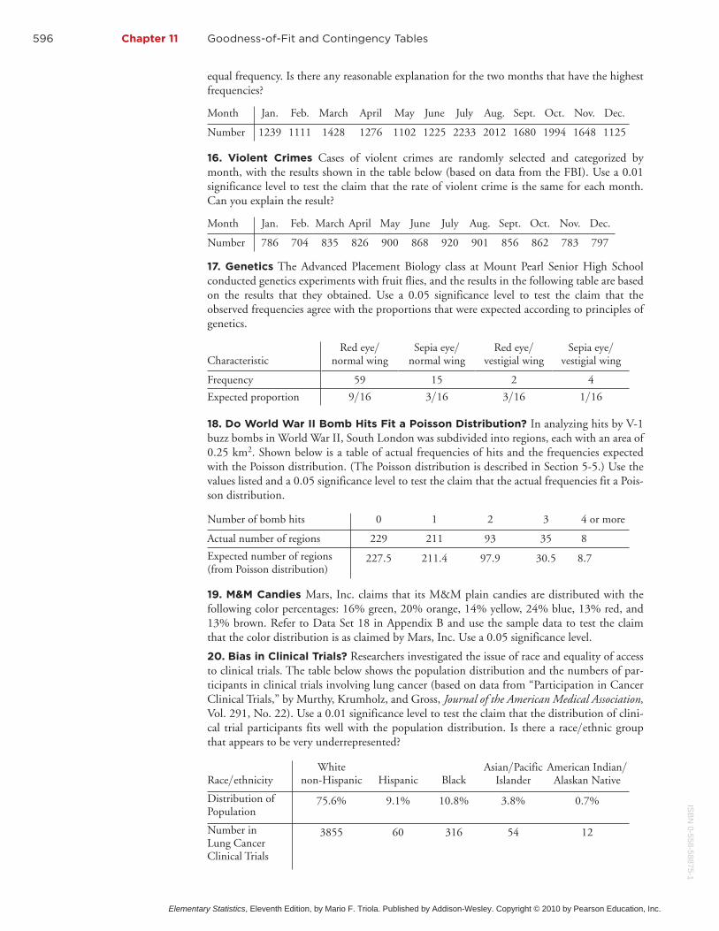
equal frequency. Is there any reasonable explanation for the two months that have the highestfrequencies?
Month Jan. Feb. March April May June July Aug. Sept. Oct. Nov. Dec.
Number 1239 1111 1428 1276 1102 1225 2233 2012 1680 1994 1648 1125
Month Jan. Feb. March April May June July Aug. Sept. Oct. Nov. Dec.
Number 786 704 835 826 900 868 920 901 856 862 783 797
CharacteristicRed eye
normal wing> Sepia eye
normal wing> Red eye
vestigial wing> Sepia eye
vestigial wing>
Frequency 59 15 2 4
Expected proportion 9 16> 3 16> 3 16> 1 16>
16. Violent Crimes Cases of violent crimes are randomly selected and categorized bymonth, with the results shown in the table below (based on data from the FBI). Use a 0.01significance level to test the claim that the rate of violent crime is the same for each month.Can you explain the result?
17. Genetics The Advanced Placement Biology class at Mount Pearl Senior High Schoolconducted genetics experiments with fruit flies, and the results in the following table are basedon the results that they obtained. Use a 0.05 significance level to test the claim that theobserved frequencies agree with the proportions that were expected according to principles ofgenetics.
18. Do World War II Bomb Hits Fit a Poisson Distribution? In analyzing hits by V-1buzz bombs in World War II, South London was subdivided into regions, each with an area of0.25 km2. Shown below is a table of actual frequencies of hits and the frequencies expectedwith the Poisson distribution. (The Poisson distribution is described in Section 5-5.) Use thevalues listed and a 0.05 significance level to test the claim that the actual frequencies fit a Pois-son distribution.
Number of bomb hits 0 1 2 3 4 or more
Actual number of regions 229 211 93 35 8
Expected number of regions(from Poisson distribution)
227.5 211.4 97.9 30.5 8.7
19. M&M Candies Mars, Inc. claims that its M&M plain candies are distributed with thefollowing color percentages: 16% green, 20% orange, 14% yellow, 24% blue, 13% red, and13% brown. Refer to Data Set 18 in Appendix B and use the sample data to test the claimthat the color distribution is as claimed by Mars, Inc. Use a 0.05 significance level.
20. Bias in Clinical Trials? Researchers investigated the issue of race and equality of accessto clinical trials. The table below shows the population distribution and the numbers of par-ticipants in clinical trials involving lung cancer (based on data from “Participation in CancerClinical Trials,” by Murthy, Krumholz, and Gross, Journal of the American Medical Association,Vol. 291, No. 22). Use a 0.01 significance level to test the claim that the distribution of clini-cal trial participants fits well with the population distribution. Is there a race ethnic groupthat appears to be very underrepresented?
>
Race ethnicity> Whitenon-Hispanic Hispanic Black
Asian PacificIslander> American Indian
Alaskan Native>
Distribution ofPopulation
75.6% 9.1% 10.8% 3.8% 0.7%
Number inLung CancerClinical Trials
3855 60 316 54 12
ISB
N0-558-58875-1
Elementary Statistics, Eleventh Edition, by Mario F. Triola. Published by Addison-Wesley. Copyright © 2010 by Pearson Education, Inc.

11-2 Goodness-of-Fit 597
Benford’s Law. According to Benford’s law, a variety of different data sets includenumbers with leading ( first) digits that follow the distribution shown in the tablebelow. In Exercises 21–24, test for goodness-of-fit with Benford’s law.
Leading Digit 1 2 3 4 5 6 7 8 9Benford’s law:distribution of leadingdigits
30.1% 17.6% 12.5% 9.7% 7.9% 6.7% 5.8% 5.1% 4.6%
21. Detecting Fraud When working for the Brooklyn District Attorney, investigator RobertBurton analyzed the leading digits of the amounts from 784 checks issued by seven suspectcompanies. The frequencies were found to be 0, 15, 0, 76, 479, 183, 8, 23, and 0, and thosedigits correspond to the leading digits of 1, 2, 3, 4, 5, 6, 7, 8, and 9, respectively. If the ob-served frequencies are substantially different from the frequencies expected with Benford’s law,the check amounts appear to result from fraud. Use a 0.01 significance level to test for goodness-of-fit with Benford’s law. Does it appear that the checks are the result of fraud?
22. Author’s Check Amounts Exercise 21 lists the observed frequencies of leading digitsfrom amounts on checks from seven suspect companies. Here are the observed frequencies ofthe leading digits from the amounts on checks written by the author: 68, 40, 18, 19, 8, 20, 6,9, 12. (Those observed frequencies correspond to the leading digits of 1, 2, 3, 4, 5, 6, 7, 8,and 9, respectively.) Using a 0.05 significance level, test the claim that these leading digits arefrom a population of leading digits that conform to Benford’s law. Do the author’s checkamounts appear to be legitimate?
23. Political Contributions Amounts of recent political contributions are randomly se-lected, and the leading digits are found to have frequencies of 52, 40, 23, 20, 21, 9, 8, 9, and30. (Those observed frequencies correspond to the leading digits of 1, 2, 3, 4, 5, 6, 7, 8, and9, respectively, and they are based on data from “Breaking the (Benford) Law: Statistical FraudDetection in Campaign Finance,” by Cho and Gaines, American Statistician, Vol. 61, No. 3.)Using a 0.01 significance level, test the observed frequencies for goodness-of-fit with Ben-ford’s law. Does it appear that the political campaign contributions are legitimate?
24. Check Amounts In the trial of State of Arizona vs. Wayne James Nelson, the defendantwas accused of issuing checks to a vendor that did not really exist. The amounts of the checksare listed below in order by row. When testing for goodness-of-fit with the proportions ex-pected with Benford’s law, it is necessary to combine categories because not all expected valuesare at least 5. Use one category with leading digits of 1, a second category with leading digitsof 2, 3, 4, 5, and a third category with leading digits of 6, 7, 8, 9. Using a 0.01 significancelevel, is there sufficient evidence to conclude that the leading digits on the checks do not con-form to Benford’s law?
$ 1,927.48 $27,902.31 $86,241.90 $72,117.46 $81,321.75 $97,473.96
$93,249.11 $89,658.16 $87,776.89 $92,105.83 $79,949.16 $87,602.93
$96,879.27 $91,806.47 $84,991.67 $90,831.83 $93,766.67 $88,336.72
$94,639.49 $83,709.26 $96,412.21 $88,432.86 $71,552.16
Beyond the Basics
25. Testing Effects of Outliers In conducting a test for the goodness-of-fit as described inthis section, does an outlier have much of an effect on the value of the test statistic? Test forthe effect of an outlier in Example 1 after changing the first frequency in Table 11-2 from 7 to 70.Describe the general effect of an outlier.
26. Testing Goodness-of-Fit with a Normal Distribution Refer to Data Set 21 inAppendix B for the axial loads (in pounds) of the aluminum cans that are 0.0109 in. thick.
x2
11-2
ISB
N0-
558-
5887
5-1
Elementary Statistics, Eleventh Edition, by Mario F. Triola. Published by Addison-Wesley. Copyright © 2010 by Pearson Education, Inc.

598 Chapter 11 Goodness-of-Fit and Contingency Tables
a. Enter the observed frequencies in the above table.
b. Assuming a normal distribution with mean and standard deviation given by the samplemean and standard deviation, use the methods of Chapter 6 to find the probability of a ran-domly selected axial load belonging to each class.
c. Using the probabilities found in part (b), find the expected frequency for each category.
d. Use a 0.01 significance level to test the claim that the axial loads were randomly selectedfrom a normally distributed population. Does the goodness-of-fit test suggest that the data arefrom a normally distributed population?
Axial load Less than239.5 239.5–259.5 259.5–279.5
More than279.5
Frequency
Contingency Tables
Key Concept In this section we consider contingency tables (or two-way frequencytables), which include frequency counts for categorical data arranged in a table with atleast two rows and at least two columns. In Part 1 of this section, we present amethod for conducting a hypothesis test of the null hypothesis that the row and col-umn variables are independent of each other. This test of independence is used in realapplications quite often. In Part 2, we will use the same method for a test of homo-geneity, whereby we test the claim that different populations have the same propor-tion of some characteristics.
Part 1: Basic Concepts of Testing for Independence
In this section we use standard statistical methods to analyze frequency counts in acontingency table (or two-way frequency table). We begin with the definition of acontingency table.
11-3
A contingency table (or two-way frequency table) is a table in which fre-quencies correspond to two variables. (One variable is used to categorizerows, and a second variable is used to categorize columns.)
Contingency Table from Echinacea Experiment Table 11-6is a contingency table with two rows and three columns. The cells of the table con-tain frequencies. The row variable identifies whether the subjects became infected,and the column variable identifies the treatment group (placebo, 20% extractgroup, or 60% extract group).
1
Table 11-6 Results from Experiment with Echinacea
Treatment Group
Placebo Echinacea: 20% extract Echinacea: 60% extract
Infected 88 48 42
Not infected 15 4 10
An Eight-YearFalse PositiveThe Associated Press re-cently released a reportabout Jim Malone, who hadreceived a positive test re-
sult for an HIVinfection. Foreight years,he attendedgroup sup-
port meetings,fought depression,
and lost weight while fear-ing a death from AIDS. Fi-nally, he was informed thatthe original test was wrong.He did not have an HIV in-fection. A follow-up testwas given after the firstpositive test result, and theconfirmation test showedthat he did not have an HIVinfection, but nobody toldMr. Malone about the newresult. Jim Malone agonizedfor eight years because of atest result that was actuallya false positive.
ISB
N0-558-58875-1
Elementary Statistics, Eleventh Edition, by Mario F. Triola. Published by Addison-Wesley. Copyright © 2010 by Pearson Education, Inc.

11-3 Contingency Tables 599
A test of independence tests the null hypothesis that in a contingency table,the row and column variables are independent.
Objective
Conduct a hypothesis test for independence between the row variable and column variable in a contingency table.
1. The sample data are randomly selected.
2. The sample data are represented as frequency countsin a two-way table.
3. For every cell in the contingency table, the expectedfrequency E is at least 5. (There is no requirement that
Requirements
every observed frequency must be at least 5. Also, thereis no requirement that the population must have anormal distribution or any other specific distribution.)
The null and alternative hypotheses are as follows:
H0: The row and column variables are independent.
H1: The row and column variables are dependent.
Test Statistic for a Test of Independence
where O is the observed frequency in a cell and E is the expected frequency found by evaluating
E =(row total) (column total)
(grand total)
x2 = a(O - E )2
E
Null and Alternative Hypotheses
1. The critical values are found in Table A-4 using
where r is the number of rows and c is the number ofcolumns.
degrees of freedom � (r � 1)(c � 1)
Critical Values
2. Tests of independence with a contingency table arealways right-tailed.
We will now consider a hypothesis test of independence between the row andcolumn variables in a contingency table. We first define a test of independence.
P-values are typically provided by computer software, or a range of P-values can be found from Table A-4.
P-Values
O represents the observed frequency in a cell of acontingency table.
E represents the expected frequency in a cell, foundby assuming that the row and column variablesare independent.
Notation
r represents the number of rows in a contin-gency table (not including labels).
c represents the number of columns in a contin-gency table (not including labels).
ISB
N0-
558-
5887
5-1
Elementary Statistics, Eleventh Edition, by Mario F. Triola. Published by Addison-Wesley. Copyright © 2010 by Pearson Education, Inc.
600 Chapter 11 Goodness-of-Fit and Contingency Tables
The test statistic allows us to measure the amount of disagreement between thefrequencies actually observed and those that we would theoretically expect when thetwo variables are independent. Large values of the test statistic are in the rightmostregion of the chi-square distribution, and they reflect significant differences betweenobserved and expected frequencies. The distribution of the test statistic can be ap-proximated by the chi-square distribution, provided that all expected frequencies areat least 5. The number of degrees of freedom reflects the fact that be-cause we know the total of all frequencies in a contingency table, we can freely assignfrequencies to only rows and columns before the frequency for every cellis determined. (However, we cannot have negative frequencies or frequencies so largethat any row (or column) sum exceeds the total of the observed frequencies for thatrow (or column).)
Finding Expected Values EThe test statistic is found by using the values of O (observed frequencies) and thevalues of E (expected frequencies). The expected frequency E can be found for a cellby simply multiplying the total of the row frequencies by the total of the column fre-quencies, then dividing by the grand total of all frequencies, as shown in Example 2.
x2
c - 1r - 1
(r - 1)(c - 1)
x2
x2
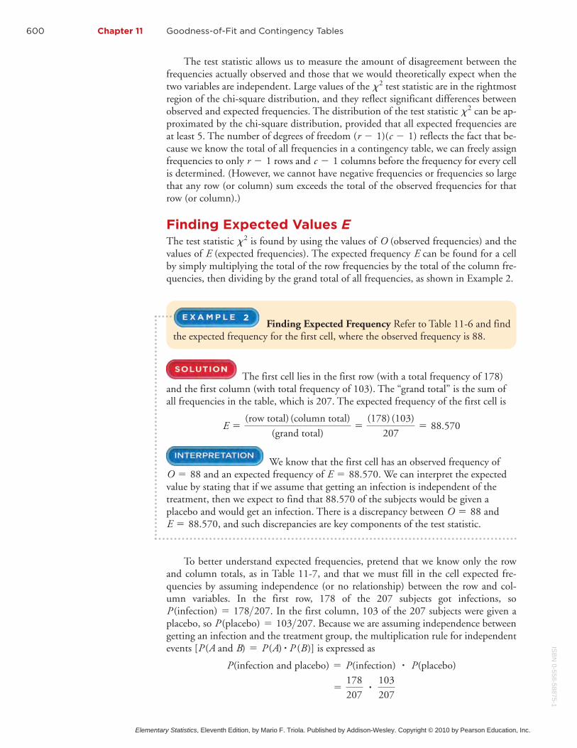
Finding Expected Frequency Refer to Table 11-6 and findthe expected frequency for the first cell, where the observed frequency is 88.
The first cell lies in the first row (with a total frequency of 178)and the first column (with total frequency of 103). The “grand total” is the sum ofall frequencies in the table, which is 207. The expected frequency of the first cell is
We know that the first cell has an observed frequency ofand an expected frequency of . We can interpret the expected
value by stating that if we assume that getting an infection is independent of thetreatment, then we expect to find that 88.570 of the subjects would be given aplacebo and would get an infection. There is a discrepancy between and
, and such discrepancies are key components of the test statistic.
To better understand expected frequencies, pretend that we know only the rowand column totals, as in Table 11-7, and that we must fill in the cell expected fre-quencies by assuming independence (or no relationship) between the row and col-umn variables. In the first row, 178 of the 207 subjects got infections, so
. In the first column, 103 of the 207 subjects were given aplacebo, so . Because we are assuming independence betweengetting an infection and the treatment group, the multiplication rule for independentevents is expressed as
P(infection and placebo) = P(infection) # P(placebo)
=178207
# 103
207
[P (A and B) = P (A) # P (B)]
P (placebo) = 103>207P (infection) = 178>207
E = 88.570O = 88
E = 88.570O = 88
E =(row total) (column total)
(grand total)=
(178) (103)
207= 88.570
2
ISB
N0-558-58875-1
Elementary Statistics, Eleventh Edition, by Mario F. Triola. Published by Addison-Wesley. Copyright © 2010 by Pearson Education, Inc.

11-3 Contingency Tables 601
We can now find the expected value for the first cell by multiplying the probability forthat cell by the total number of subjects, as shown here:
The form of this product suggests a general way to obtain the expected frequency of a cell:
This expression can be simplified to
We can now proceed to conduct a hypothesis test of independence, as in Example 3.
E =(row total) # (column total)
(grand total)
Expected frequency E = (grand total) # (row total)
(grand total)# (column total)
(grand total)
E = n # p = 207 c178207
# 103207d = 88.570
Table 11-7 Results from Experiment with Echinacea
Treatment Group Row totals:
Placebo Echinacea: 20%extract
Echinacea: 60%extract
Infected 178
Not infected 29
Column totals: 103 52 52 Grand total: 207
Does Echinacea Have an Effect on Colds? Commoncolds are typically caused by a rhinovirus. In a test of the effectiveness of echi-nacea, some test subjects were treated with echinacea extracted with 20%ethanol, some were treated with echinacea extracted with 60% ethanol, andothers were given a placebo. All of the test subjects were then exposed to rhi-novirus. Results are summarized in Table 11-6 (based on data from “AnEvaluation of Echinacea angustifolia in Experimental Rhinovirus Infections,” byTurner, et al., New England Journal of Medicine, Vol. 353, No. 4). Use a 0.05significance level to test the claim that getting an infection (cold) is inde-pendent of the treatment group. What does the result indicate about the effectiveness of echinacea as a treatment for colds?
REQUIREMENT CHECK (1) The subjects were recruitedand were randomly assigned to the different treatment groups. (2) The results are ex-pressed as frequency counts in Table 11-6. (3) The expected frequencies are all atleast 5. (The expected frequencies are 88.570, 44.715, 44.715, 14.430, 7.285, and7.285.) The requirements are satisfied.
The null hypothesis and alternative hypothesis are as follows:
H0: Getting an infection is independent of the treatment.
H1: Getting an infection and the treatment are dependent.
The significance level is .Because the data are in the form of a contingency table, we use the distribu-
tion with this test statistic:
x2 = a(O - E )2
E=
(88 - 88.570)2
88.570+ Á +
(10 - 7.285)2
7.285 = 2.925
x2a = 0.05
3
ISB
N0-
558-
5887
5-1
Elementary Statistics, Eleventh Edition, by Mario F. Triola. Published by Addison-Wesley. Copyright © 2010 by Pearson Education, Inc.

602 Chapter 11 Goodness-of-Fit and Contingency Tables
The critical value of is found from Table A-4 with in the right tail and the number of degrees of freedom given by
. The test statistic and critical value are shown in Figure 11-5.Because the test statistic does not fall within the critical region, we fail to reject thenull hypothesis of independence between getting an infection and treatment.
It appears that getting an infection is independent of thetreatment group. This suggests that echinacea is not an effective treatment for colds.
(2 - 1)(3 - 1) = 2(r - 1)(c - 1) =a = 0.05x2 = 5.991
Is the Nurse a Serial Killer? Table 11-1 provided with theChapter Problem consists of a contingency table with a row variable (whetherKristen Gilbert was on duty) and a column variable (whether the shift included adeath). Test the claim that whether Gilbert was on duty for a shift is independentof whether a patient died during the shift. Because this is such a serious analysis,use a significance level of 0.01. What does the result suggest about the charge thatGilbert killed patients?
REQUIREMENT CHECK (1) The data in Table 11-1 canbe treated as random data for the purpose of determining whether such random datacould easily occur by chance. (2) The sample data are represented as frequencycounts in a two-way table. (3) Each expected frequency is at least 5. (The expectedfrequencies are 11.589, 245.411, 62.411, and 1321.589.) The requirements aresatisfied.
4
P-ValuesThe preceding example used the traditional approach to hypothesis testing, but wecan easily use the P-value approach. STATDISK, Minitab, Excel, and the TI-83 84Plus calculator all provide P-values for tests of independence in contingency tables.(See Example 4.) If you don’t have a suitable calculator or statistical software, estimateP-values from Table A-4 by finding where the test statistic falls in the row corre-sponding to the appropriate number of degrees of freedom.
>
X 2 � 5.9910
Fail to rejectindependence
Rejectindependence
Sample data: X 2 � 2.925
Figure 11-5
Test of Independence forthe Echinacea Data
ISB
N0-558-58875-1
Elementary Statistics, Eleventh Edition, by Mario F. Triola. Published by Addison-Wesley. Copyright © 2010 by Pearson Education, Inc.

11-3 Contingency Tables 603
The null hypothesis and alternative hypothesis are as follows:
H0: Whether Gilbert was working is independent of whether there wasa death during the shift.
H1: Whether Gilbert was working and whether there was a death duringthe shift are dependent.
Minitab shows that the test statistic is and the P-value is 0.000.Because the P-value is less than the significance level of 0.01, we reject the null hypo-thesis of independence. There is sufficient evidence to warrant rejection of inde-pendence between the row and column variables.
x2 = 86.481
MINITAB
We reject independence between whether Gilbert wasworking and whether a patient died during a shift. It appears that there is an associa-tion between Gilbert working and patients dying. (Note that this does not show thatGilbert caused the deaths, so this is not evidence that could be used at her trial, but itwas evidence that led investigators to pursue other evidence that eventually led toher conviction for murder.)
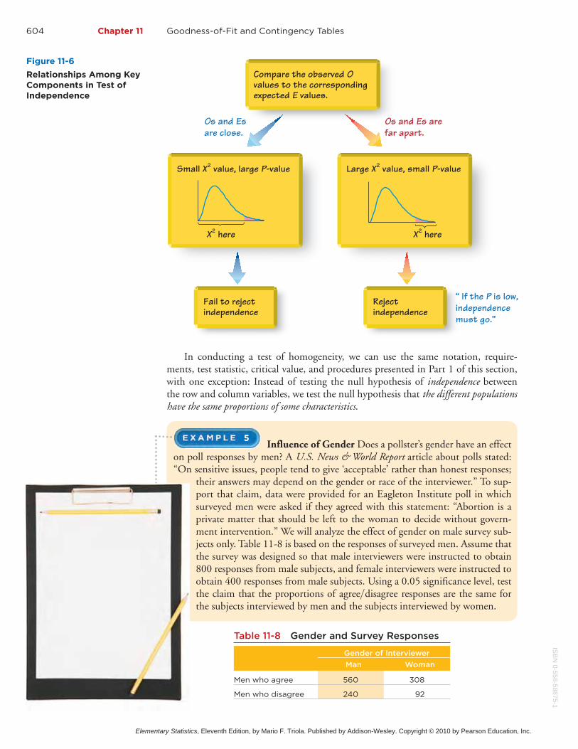
As in Section 11-2, if observed and expected frequencies are close, the test sta-tistic will be small and the P-value will be large. If observed and expected frequenciesare not close, the test statistic will be large and the P-value will be small. These re-lationships are summarized and illustrated in Figure 11-6 on the next page.
Part 2: Test of Homogeneity and the Fisher Exact Test
Test of HomogeneityIn Part 1 of this section, we focused on the test of independence between the row andcolumn variables in a contingency table. In Part 1, the sample data are from one pop-ulation, and individual sample results are categorized with the row and column vari-ables. However, we sometimes obtain samples drawn from different populations, andwe want to determine whether those populations have the same proportions of thecharacteristics being considered. The test of homogeneity can be used in such cases.(The word homogeneous means “having the same quality,” and in this context, we aretesting to determine whether the proportions are the same.)
x2
x2
In a test of homogeneity, we test the claim that different populations havethe same proportions of some characteristics.
ISB
N0-
558-
5887
5-1
Elementary Statistics, Eleventh Edition, by Mario F. Triola. Published by Addison-Wesley. Copyright © 2010 by Pearson Education, Inc.
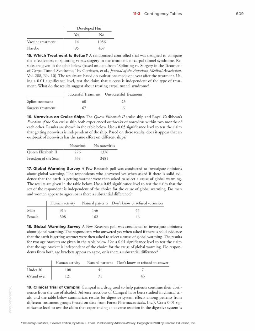
Influence of Gender Does a pollster’s gender have an effecton poll responses by men? A U.S. News & World Report article about polls stated:“On sensitive issues, people tend to give ‘acceptable’ rather than honest responses;
their answers may depend on the gender or race of the interviewer.” To sup-port that claim, data were provided for an Eagleton Institute poll in whichsurveyed men were asked if they agreed with this statement: “Abortion is aprivate matter that should be left to the woman to decide without govern-ment intervention.” We will analyze the effect of gender on male survey sub-jects only. Table 11-8 is based on the responses of surveyed men. Assume thatthe survey was designed so that male interviewers were instructed to obtain800 responses from male subjects, and female interviewers were instructed toobtain 400 responses from male subjects. Using a 0.05 significance level, testthe claim that the proportions of responses are the same forthe subjects interviewed by men and the subjects interviewed by women.
agree>disagree
5
604 Chapter 11 Goodness-of-Fit and Contingency Tables
In conducting a test of homogeneity, we can use the same notation, require-ments, test statistic, critical value, and procedures presented in Part 1 of this section,with one exception: Instead of testing the null hypothesis of independence betweenthe row and column variables, we test the null hypothesis that the different populationshave the same proportions of some characteristics.
“ If the P is low,independence must go.”
Fail to rejectindependence
Small X 2 value, large P-value
X 2 here
Rejectindependence
Large X 2 value, small P-value
X 2 here
Os and Esare close.
Os and Es arefar apart.
Compare the observed Ovalues to the correspondingexpected E values.
Figure 11-6
Relationships Among KeyComponents in Test ofIndependence
Table 11-8 Gender and Survey Responses
Gender of Interviewer
Man Woman
Men who agree 560 308
Men who disagree 240 92
ISB
N0-558-58875-1
Elementary Statistics, Eleventh Edition, by Mario F. Triola. Published by Addison-Wesley. Copyright © 2010 by Pearson Education, Inc.

11-3 Contingency Tables 605
REQUIREMENT CHECK (1) The data are random.(2) The sample data are represented as frequency counts in a two-way table. (3) Theexpected frequencies (shown in the accompanying Minitab display as 578.67, 289.33,221.33, and 110.67) are all at least 5. All of the requirements are satisfied.
Because this is a test of homogeneity, we test the claim that the proportions of agree disagree responses are the same for the subjects interviewed by males and thesubjects interviewed by females. We have two separate populations (subjects inter-viewed by men and subjects interviewed by women), and we test for homogeneitywith these hypotheses:
H0: The proportions of responses are the same for the subjectsinterviewed by men and the subjects interviewed by women.
H1: The proportions are different.
The significance level is . We use the same test statistic described earlier,and it is calculated using the same procedure. Instead of listing the details of that cal-culation, we provide the Minitab display for the data in Table 11-8.
x2a = 0.05
agree>disagree
>
MINITAB
The Minitab display shows the expected frequencies of 578.67, 289.33, 221.33,and 110.67. It also includes the test statistic of and the P-value of 0.011.Using the P-value approach to hypothesis testing, we reject the null hypothesis ofequal (homogeneous) proportions (because the P-value of 0.011 is less than 0.05).There is sufficient evidence to warrant rejection of the claim that the proportions arethe same.
It appears that response and the gender of the interviewerare dependent. Although this statistical analysis cannot be used to justify any state-ment about causality, it does appear that men are influenced by the gender of theinterviewer.
Fisher Exact TestThe procedures for testing hypotheses with contingency tables with two rows andtwo columns have the requirement that every cell must have an expected fre-quency of at least 5. This requirement is necessary for the distribution to be a suit-able approximation to the exact distribution of the test statistic. The Fisher exacttest is often used for a contingency table with one or more expected frequen-cies that are below 5. The Fisher exact test provides an exact P-value and does not re-quire an approximation technique. Because the calculations are quite complex, it’s agood idea to use computer software when using the Fisher exact test. STATDISK andMinitab both have the ability to perform the Fisher exact test.
2 * 2x2
x2(2 * 2)
x2 = 6.529
ISB
N0-
558-
5887
5-1
Elementary Statistics, Eleventh Edition, by Mario F. Triola. Published by Addison-Wesley. Copyright © 2010 by Pearson Education, Inc.

606 Chapter 11 Goodness-of-Fit and Contingency TablesU
SIN
G T
EC
HN
OL
OG
Y Enter the observed frequencies in the DataWindow as they appear in the contingency table. Select Analysisfrom the main menu, then select Contingency Tables. Enter a sig-nificance level and proceed to identify the columns containing thefrequencies. Click on Evaluate. The STATDISK results include thetest statistic, critical value, P-value, and conclusion, as shown in thedisplay resulting from Table 11-1.
STATDISK You must enter the observed frequencies, and youmust also determine and enter the expected frequencies. When fin-ished, click on the fx icon in the menu bar, select the function cate-gory Statistical, and then select the function name CHITEST. Youmust enter the range of values for the observed frequencies and therange of values for the expected frequencies. Only the P-value is pro-vided. (DDXL can also be used by selecting Tables, then Indep. Testfor Summ Data.)
First enter the contingency table as amatrix by pressing 2nd x 1 to get the MATRIX menu (or theMATRIX key on the TI-83). Select EDIT, and press ENTER. Enterthe dimensions of the matrix (rows by columns) and proceed to en-ter the individual frequencies. When finished, press STAT, selectTESTS, and then select the option 2-Test. Be sure that the ob-served matrix is the one you entered, such as matrix A. The expectedfrequencies will be automatically calculated and stored in the sepa-rate matrix identified as “Expected.” Scroll down to Calculate andpress ENTER to get the test statistic, P-value, and number ofdegrees of freedom.
X
�
T I -83/84 PLUS
EXCEL
Basic Skills and Concepts
Statistical Literacy and Critical Thinking1. Polio Vaccine Results of a test of the Salk vaccine against polio are summarized in thetable below. If we test the claim that getting paralytic polio is independent of whether thechild was treated with the Salk vaccine or was given a placebo, the TI-83 84 Plus calculatorprovides a P-value of 1.732517E 11, which is in scientific notation. Write the P-value in astandard form that is not in scientific notation. Based on the P-value, what conclusion shouldwe make? Does the vaccine appear to be effective?
->
11-3
Paralytic polio No paralytic polio
Salk vaccine 33 200,712
Placebo 115 201,114
2. Cause and Effect Based on the data in the table provided with Exercise 1, can we con-clude that the Salk vaccine causes a decrease in the rate of paralytic polio? Why or why not?
3. Interpreting P-Value Refer to the P-value given in Exercise 1. Interpret that P-value bycompleting this statement: The P-value is the probability of .
4. Right-Tailed Test Why are the hypothesis tests described in this section always right-tailed, as in Example 1?
In Exercises 5 and 6, test the given claim using the displayed software results.5. Home Field Advantage Winning team data were collected for teams in different sports,with the results given in the accompanying table (based on data from “Predicting Professional
First enter the observed frequencies in columns,then select Stat from the main menu bar. Next select the optionTables, then select Chi Square Test (Two-Way Table in Worksheet)and enter the names of the columns containing the observed fre-quencies, such as C1 C2 C3 C4. Minitab provides the test statisticand P-value, the expected frequencies, and the individual terms ofthe test statistic. See the Minitab displays that accompany Exam-ples 4 and 5.x2
MINITAB
STATDISK
ISB
N0-558-58875-1
Elementary Statistics, Eleventh Edition, by Mario F. Triola. Published by Addison-Wesley. Copyright © 2010 by Pearson Education, Inc.

11-3 Contingency Tables 607
Sports Game Outcomes from Intermediate Game Scores,” by Copper, DeNeve, andMosteller, Chance, Vol. 5, No. 3–4). The TI-83 84 Plus results are also displayed. Use a 0.05level of significance to test the claim that home visitor wins are independent of the sport.>>
Basketball Baseball Hockey Football
Home team wins 127 53 50 57
Visiting team wins 71 47 43 42
6. Crime and Strangers The Minitab display results from the table below, which lists dataobtained from randomly selected crime victims (based on data from the U.S. Department ofJustice). What can we conclude?
TI-83/84 PLUS
Homicide Robbery Assault
Criminal was a stranger 12 379 727
Criminal was acquaintance or relative 39 106 642
MINITAB
Chi-Sq 119.330, DF 2, P-Value 0.000
In Exercises 7–22, test the given claim.7. Instant Replay in Tennis The table below summarizes challenges made by tennis playersin the first U.S. Open that used the Hawk-Eye electronic instant replay system. Use a 0.05significance level to test the claim that success in challenges is independent of the gender ofthe player. Does either gender appear to be more successful?
===
Was the challenge to the call successful?
Yes No
Men 201 288
Women 126 224
8. Open Roof or Closed Roof? In a recent baseball World Series, the Houston Astroswanted to close the roof on their domed stadium so that fans could make noise and give theteam a better advantage at home. However, the Astros were ordered to keep the roof open, un-less weather conditions justified closing it. But does the closed roof really help the Astros? Thetable below shows the results from home games during the season leading up to the World Se-ries. Use a 0.05 significance level to test for independence between wins and whether the roofis open or closed. Does it appear that a closed roof really gives the Astros an advantage?
Win Loss
Closed roof 36 17
Open roof 15 11
9. Testing a Lie Detector The table below includes results from polygraph (lie detector)experiments conducted by researchers Charles R. Honts (Boise State University) and GordonH. Barland (Department of Defense Polygraph Institute). In each case, it was known if thesubject lied or did not lie, so the table indicates when the polygraph test was correct. Use a0.05 significance level to test the claim that whether a subject lies is independent of the poly-graph test indication. Do the results suggest that polygraphs are effective in distinguishing be-tween truths and lies?
Did the Subject Actually Lie?
No (Did Not Lie) Yes (Lied)
Polygraph test indicated that the subject lied. 15 42
Polygraph test indicated that the subject did not lie. 32 9
ISB
N0-
558-
5887
5-1
Elementary Statistics, Eleventh Edition, by Mario F. Triola. Published by Addison-Wesley. Copyright © 2010 by Pearson Education, Inc.

608 Chapter 11 Goodness-of-Fit and Contingency Tables
10. Clinical Trial of Chantix Chantix is a drug used as an aid for those who want to stopsmoking. The adverse reaction of nausea has been studied in clinical trials, and the table belowsummarizes results (based on data from Pfizer). Use a 0.01 significance level to test the claimthat nausea is independent of whether the subject took a placebo or Chantix. Does nausea ap-pear to be a concern for those using Chantix?
Placebo Chantix
Nausea 10 30
No nausea 795 791
Amalgam Composite
Adverse health condition reported 135 145
No adverse health condition reported 132 122
Amalgam Composite
Sensory disorder 36 28
No sensory disorder 231 239
Guilty Plea Not Guilty Plea
Sent to prison 392 58
Not sent to prison 564 14
11. Amalgam Tooth Fillings The table below shows results from a study in which some pa-tients were treated with amalgam restorations and others were treated with composite restora-tions that do not contain mercury (based on data from “Neuropsychological and Renal Effectsof Dental Amalgam in Children,” by Bellinger, et al., Journal of the American Medical Associa-tion, Vol. 295, No. 15). Use a 0.05 significance level to test for independence between thetype of restoration and the presence of any adverse health conditions. Do amalgam restora-tions appear to affect health conditions?
12. Amalgam Tooth Fillings In recent years, concerns have been expressed about adversehealth effects from amalgam dental restorations, which include mercury. The table belowshows results from a study in which some patients were treated with amalgam restorations andothers were treated with composite restorations that do not contain mercury (based on datafrom “Neuropsychological and Renal Effects of Dental Amalgam in Children,” by Bellinger,et al., Journal of the American Medical Association, Vol. 295, No. 15). Use a 0.05 significancelevel to test for independence between the type of restoration and sensory disorders. Do amal-gam restorations appear to affect sensory disorders?
13. Is Sentence Independent of Plea? Many people believe that criminals who pleadguilty tend to get lighter sentences than those who are convicted in trials. The accompanyingtable summarizes randomly selected sample data for San Francisco defendants in burglarycases (based on data from “Does It Pay to Plead Guilty? Differential Sentencing and the Func-tioning of the Criminal Courts,” by Brereton and Casper, Law and Society Review, Vol. 16,No. 1). All of the subjects had prior prison sentences. Use a 0.05 significance level to test theclaim that the sentence (sent to prison or not sent to prison) is independent of the plea. If youwere an attorney defending a guilty defendant, would these results suggest that you should en-courage a guilty plea?
14. Is the Vaccine Effective? In a USA Today article about an experimental vaccine for chil-dren, the following statement was presented: “In a trial involving 1602 children, only 14 (1%)of the 1070 who received the vaccine developed the flu, compared with 95 (18%) of the 532who got a placebo.” The data are shown in the table below. Use a 0.05 significance level to testfor independence between the variable of treatment (vaccine or placebo) and the variable repre-senting flu (developed flu, did not develop flu). Does the vaccine appear to be effective?
ISB
N0-558-58875-1
Elementary Statistics, Eleventh Edition, by Mario F. Triola. Published by Addison-Wesley. Copyright © 2010 by Pearson Education, Inc.
11-3 Contingency Tables 609
Developed Flu?
Yes No
Vaccine treatment 14 1056
Placebo 95 437
Successful Treatment Unsuccessful Treatment
Splint treatment 60 23
Surgery treatment 67 6
Norovirus No norovirus
Queen Elizabeth II 276 1376
Freedom of the Seas 338 3485
15. Which Treatment Is Better? A randomized controlled trial was designed to comparethe effectiveness of splinting versus surgery in the treatment of carpal tunnel syndrome. Re-sults are given in the table below (based on data from “Splinting vs. Surgery in the Treatmentof Carpal Tunnel Syndrome,” by Gerritsen, et al., Journal of the American Medical Association,Vol. 288, No. 10). The results are based on evaluations made one year after the treatment. Us-ing a 0.01 significance level, test the claim that success is independent of the type of treat-ment. What do the results suggest about treating carpal tunnel syndrome?
16. Norovirus on Cruise Ships The Queen Elizabeth II cruise ship and Royal Caribbean’sFreedom of the Seas cruise ship both experienced outbreaks of norovirus within two months ofeach other. Results are shown in the table below. Use a 0.05 significance level to test the claimthat getting norovirus is independent of the ship. Based on these results, does it appear that anoutbreak of norovirus has the same effect on different ships?
17. Global Warming Survey A Pew Research poll was conducted to investigate opinionsabout global warming. The respondents who answered yes when asked if there is solid evi-dence that the earth is getting warmer were then asked to select a cause of global warming.The results are given in the table below. Use a 0.05 significance level to test the claim that thesex of the respondent is independent of the choice for the cause of global warming. Do menand women appear to agree, or is there a substantial difference?
Human activity Natural patterns Don’t know or refused to answer
Male 314 146 44
Female 308 162 46
Human activity Natural patterns Don’t know or refused to answer
Under 30 108 41 7
65 and over 121 71 43
18. Global Warming Survey A Pew Research poll was conducted to investigate opinionsabout global warming. The respondents who answered yes when asked if there is solid evidencethat the earth is getting warmer were then asked to select a cause of global warming. The resultsfor two age brackets are given in the table below. Use a 0.01 significance level to test the claimthat the age bracket is independent of the choice for the cause of global warming. Do respon-dents from both age brackets appear to agree, or is there a substantial difference?
19. Clinical Trial of Campral Campral is a drug used to help patients continue their absti-nence from the use of alcohol. Adverse reactions of Campral have been studied in clinical tri-als, and the table below summarizes results for digestive system effects among patients fromdifferent treatment groups (based on data from Forest Pharmaceuticals, Inc.). Use a 0.01 sig-nificance level to test the claim that experiencing an adverse reaction in the digestive system is
ISB
N0-
558-
5887
5-1
Elementary Statistics, Eleventh Edition, by Mario F. Triola. Published by Addison-Wesley. Copyright © 2010 by Pearson Education, Inc.

610 Chapter 11 Goodness-of-Fit and Contingency Tables
independent of the treatment group. Does Campral treatment appear to have an effect on thedigestive system?
Placebo Campral 1332 mg Campral 1998 mg
Adverse effect on digestive system 344 89 8
No effect on digestive system 1362 774 71
20. Is Seat Belt Use Independent of Cigarette Smoking? A study of seat belt usersand nonusers yielded the randomly selected sample data summarized in the given table (basedon data from “What Kinds of People Do Not Use Seat Belts?” by Helsing and Comstock,American Journal of Public Health, Vol. 67, No. 11). Test the claim that the amount of smok-ing is independent of seat belt use. A plausible theory is that people who smoke more are lessconcerned about their health and safety and are therefore less inclined to wear seat belts. Isthis theory supported by the sample data?
Number of Cigarettes Smoked per Day
0 1–14 15–34 35 and over
Wear seat belts 175 20 42 6
Don’t wear seat belts 149 17 41 9
Placebo Atorvastatin 10 mg Atorvastatin 40 mg Atorvastatin 80 mg
Infection 27 89 8 7
No infection 243 774 71 87
21. Clinical Trial of Lipitor Lipitor is the trade name of the drug atorvastatin, which is usedto reduce cholesterol in patients. (This is the largest-selling drug in the world, with $13 billionin sales for a recent year.) Adverse reactions have been studied in clinical trials, and the tablebelow summarizes results for infections in patients from different treatment groups (basedon data from Parke-Davis). Use a 0.05 significance level to test the claim that getting an infec-tion is independent of the treatment. Does the atorvastatin treatment appear to have an effecton infections?
Beyond the Basics
23. Test of Homogeneity Table 11-8 summarizes data for male survey subjects, but thetable on the next page summarizes data for a sample of women (based on data from an EagletonInstitute poll). Using a 0.01 significance level, and assuming that the sample sizes of 800 menand 400 women are predetermined, test the claim that the proportions of re-sponses are the same for the subjects interviewed by men and the subjects interviewed bywomen. Does it appear that the gender of the interviewer affected the responses of women?
agree>disagree
11-3
Color of Helmet
Black White Yellow Orange> Red Blue
Controls (not injured) 491 377 31 170 55
Cases (injured or killed) 213 112 8 70 26
22. Injuries and Motorcycle Helmet Color A case-control (or retrospective) study wasconducted to investigate a relationship between the colors of helmets worn by motorcycledrivers and whether they are injured or killed in a crash. Results are given in the table below(based on data from “Motorcycle Rider Conspicuity and Crash Related Injury: Case-ControlStudy,” by Wells, et al., BMJ USA, Vol. 4). Test the claim that injuries are independent of hel-met color. Should motorcycle drivers choose helmets with a particular color? If so, whichcolor appears best?
ISB
N0-558-58875-1
Elementary Statistics, Eleventh Edition, by Mario F. Triola. Published by Addison-Wesley. Copyright © 2010 by Pearson Education, Inc.
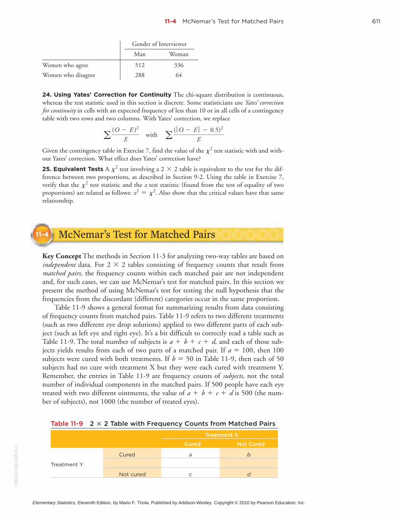
11-4 McNemar’s Test for Matched Pairs 611
24. Using Yates’ Correction for Continuity The chi-square distribution is continuous,whereas the test statistic used in this section is discrete. Some statisticians use Yates’ correctionfor continuity in cells with an expected frequency of less than 10 or in all cells of a contingencytable with two rows and two columns. With Yates’ correction, we replace
with
Given the contingency table in Exercise 7, find the value of the test statistic with and with-out Yates’ correction. What effect does Yates’ correction have?
25. Equivalent Tests A test involving a table is equivalent to the test for the dif-ference between two proportions, as described in Section 9-2. Using the table in Exercise 7,verify that the test statistic and the z test statistic (found from the test of equality of twoproportions) are related as follows: . Also show that the critical values have that samerelationship.
z2 = x2x2
2 * 2x2
x2
a( ƒO - E ƒ - 0.5)2
Ea(O - E )2
E
McNemar’s Test for Matched Pairs
Key Concept The methods in Section 11-3 for analyzing two-way tables are based onindependent data. For tables consisting of frequency counts that result frommatched pairs, the frequency counts within each matched pair are not independentand, for such cases, we can use McNemar’s test for matched pairs. In this section wepresent the method of using McNemar’s test for testing the null hypothesis that thefrequencies from the discordant (different) categories occur in the same proportion.
Table 11-9 shows a general format for summarizing results from data consistingof frequency counts from matched pairs. Table 11-9 refers to two different treatments(such as two different eye drop solutions) applied to two different parts of each sub-ject (such as left eye and right eye). It’s a bit difficult to correctly read a table such asTable 11-9. The total number of subjects is , and each of those sub-jects yields results from each of two parts of a matched pair. If , then 100subjects were cured with both treatments. If in Table 11-9, then each of 50subjects had no cure with treatment X but they were each cured with treatment Y.Remember, the entries in Table 11-9 are frequency counts of subjects, not the totalnumber of individual components in the matched pairs. If 500 people have each eyetreated with two different ointments, the value of is 500 (the num-ber of subjects), not 1000 (the number of treated eyes).
a + b + c + d
b = 50a = 100
a + b + c + d
2 * 2
11-4
Gender of Interviewer
Man Woman
Women who agree 512 336
Women who disagree 288 64
Table 11-9 2 2 Table with Frequency Counts from Matched Pairs:Treatment X
Cured Not Cured
Cured a b
Treatment Y
Not cured c d
ISB
N0-
558-
5887
5-1
Elementary Statistics, Eleventh Edition, by Mario F. Triola. Published by Addison-Wesley. Copyright © 2010 by Pearson Education, Inc.

612 Chapter 11 Goodness-of-Fit and Contingency Tables
Because the frequency counts in Table 11-9 result from matched pairs, the dataare not independent and we cannot use the methods from Section 11-3. Instead, weuse McNemar’s test.
McNemar’s test uses frequency counts from matched pairs of nominal datafrom two categories to test the null hypothesis that for a table such asTable 11-9, the frequencies b and c occur in the same proportion.
2 * 2
Objective
Test for a difference in proportions by using McNemar’s test for matched pairs.
Notation
a, b, c, and d represent the frequency counts from a table consisting of frequency counts from matched pairs.(The total number of subjects is )a + b + c + d.
2 * 2
1. The sample data have been randomly selected.
2. The sample data consist of matched pairs of frequencycounts.
3. The data are at the nominal level of measurement,and each observation can be classified two ways:
Requirements
(1) According to the category distinguishing valueswith each matched pair (such as left eye and righteye), and (2) according to another category with twopossible values (such as cured).
4. For tables such as Table 11-9, the frequencies are suchthat .b + c Ú 10
cured>not
Null and Alternative Hypotheses
H0: The proportions of the frequencies b and c (as in Table 11-9) are the same.
H1: The proportions of the frequencies b and c (as in Table 11-9) are different.
Test Statistic (for testing the null hypothesis that for tables such as Table 11-9, the frequencies b and c occur in thesame proportion):
where the frequencies of b and c are obtained from the table with a format similar to Table 11-9. (The frequen-cies b and c must come from “discordant” (or different) pairs, as described later in this section.)
Critical Values
1. The critical region is located in the right tail only.
2. The critical values are found in Table A-4 by using degrees of freedom 1.
P-Values
P-values are typically provided by computer software, or a range of P-values can be found from Table A-4.
�
2 * 2
x2 =( ƒ b - c ƒ - 1)2
b + c
ISB
N0-558-58875-1
Elementary Statistics, Eleventh Edition, by Mario F. Triola. Published by Addison-Wesley. Copyright © 2010 by Pearson Education, Inc.
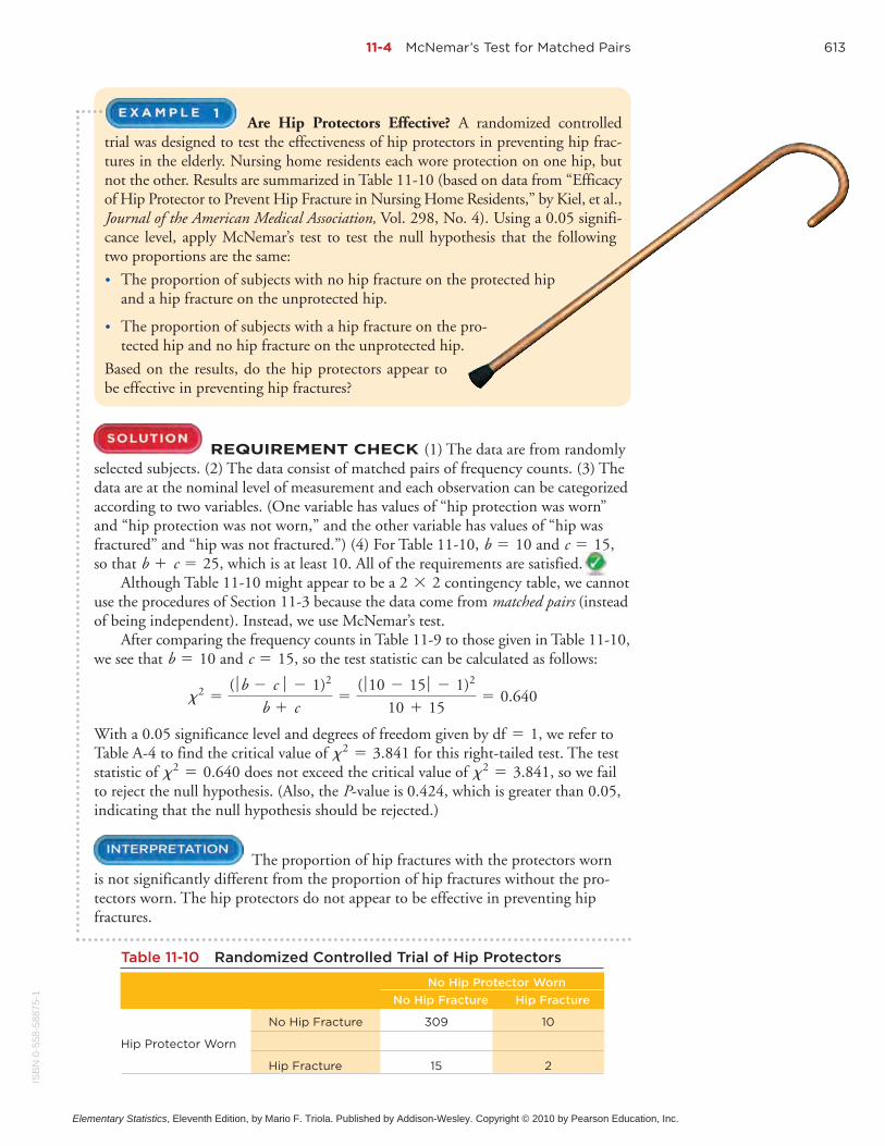
11-4 McNemar’s Test for Matched Pairs 613
Are Hip Protectors Effective? A randomized controlledtrial was designed to test the effectiveness of hip protectors in preventing hip frac-tures in the elderly. Nursing home residents each wore protection on one hip, butnot the other. Results are summarized in Table 11-10 (based on data from “Efficacyof Hip Protector to Prevent Hip Fracture in Nursing Home Residents,” by Kiel, et al.,Journal of the American Medical Association, Vol. 298, No. 4). Using a 0.05 signifi-cance level, apply McNemar’s test to test the null hypothesis that the followingtwo proportions are the same:
• The proportion of subjects with no hip fracture on the protected hipand a hip fracture on the unprotected hip.
• The proportion of subjects with a hip fracture on the pro-tected hip and no hip fracture on the unprotected hip.
Based on the results, do the hip protectors appear tobe effective in preventing hip fractures?
REQUIREMENT CHECK (1) The data are from randomlyselected subjects. (2) The data consist of matched pairs of frequency counts. (3) Thedata are at the nominal level of measurement and each observation can be categorizedaccording to two variables. (One variable has values of “hip protection was worn”and “hip protection was not worn,” and the other variable has values of “hip wasfractured” and “hip was not fractured.”) (4) For Table 11-10, and ,so that , which is at least 10. All of the requirements are satisfied.
Although Table 11-10 might appear to be a contingency table, we cannotuse the procedures of Section 11-3 because the data come from matched pairs (insteadof being independent). Instead, we use McNemar’s test.
After comparing the frequency counts in Table 11-9 to those given in Table 11-10,we see that and , so the test statistic can be calculated as follows:
With a 0.05 significance level and degrees of freedom given by df , we refer toTable A-4 to find the critical value of for this right-tailed test. The teststatistic of does not exceed the critical value of , so we failto reject the null hypothesis. (Also, the P-value is 0.424, which is greater than 0.05,indicating that the null hypothesis should be rejected.)
The proportion of hip fractures with the protectors worn is not significantly different from the proportion of hip fractures without the pro-tectors worn. The hip protectors do not appear to be effective in preventing hip fractures.
x2 = 3.841x2 = 0.640x2 = 3.841
= 1
x2 =( ƒ b - c ƒ - 1)2
b + c=
( ƒ10 - 15 ƒ - 1)2
10 + 15= 0.640
c = 15b = 10
2 * 2b + c = 25
c = 15b = 10
1
Table 11-10 Randomized Controlled Trial of Hip Protectors
No Hip Protector Worn
No Hip Fracture Hip Fracture
No Hip Fracture 309 10
Hip Protector Worn
Hip Fracture 15 2
ISB
N0-
558-
5887
5-1
Elementary Statistics, Eleventh Edition, by Mario F. Triola. Published by Addison-Wesley. Copyright © 2010 by Pearson Education, Inc.
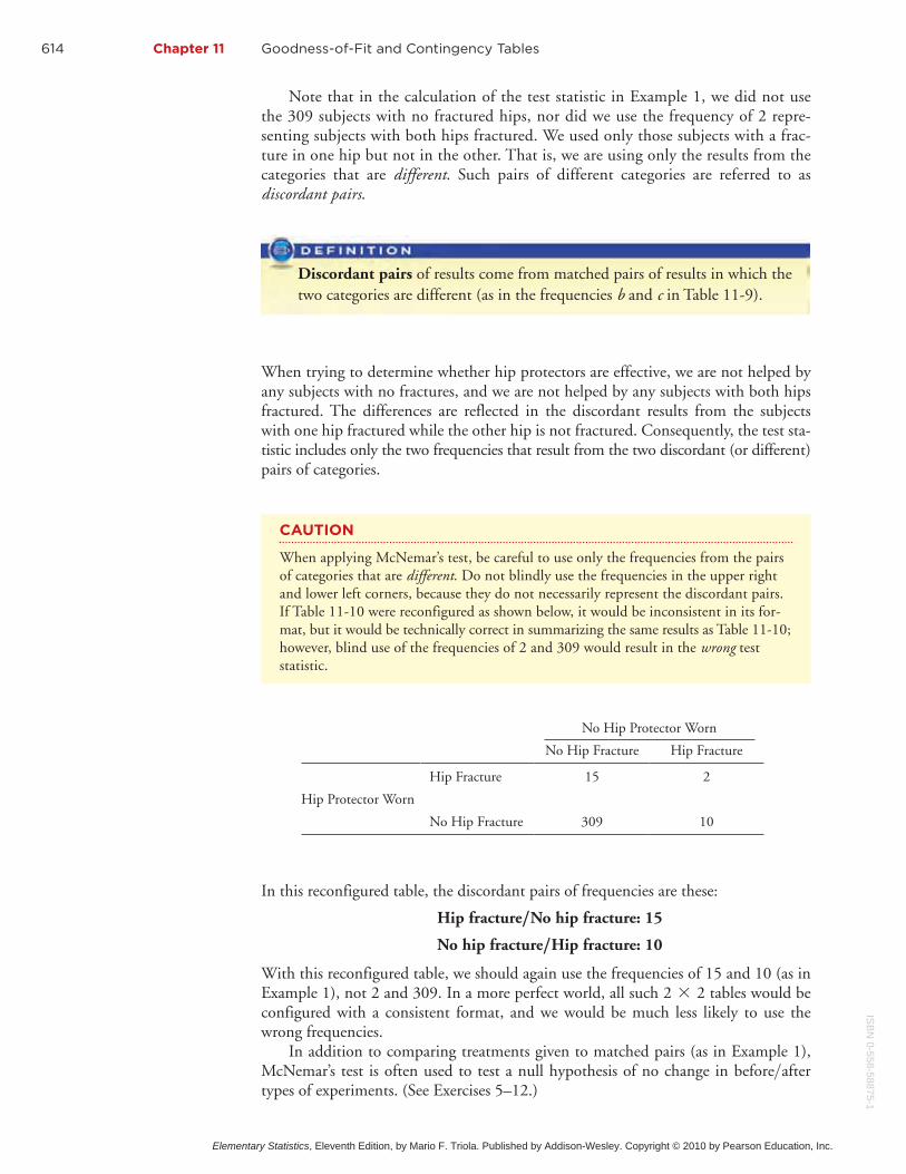
614 Chapter 11 Goodness-of-Fit and Contingency Tables
Note that in the calculation of the test statistic in Example 1, we did not usethe 309 subjects with no fractured hips, nor did we use the frequency of 2 repre-senting subjects with both hips fractured. We used only those subjects with a frac-ture in one hip but not in the other. That is, we are using only the results from thecategories that are different. Such pairs of different categories are referred to asdiscordant pairs.
When trying to determine whether hip protectors are effective, we are not helped byany subjects with no fractures, and we are not helped by any subjects with both hipsfractured. The differences are reflected in the discordant results from the subjectswith one hip fractured while the other hip is not fractured. Consequently, the test sta-tistic includes only the two frequencies that result from the two discordant (or different)pairs of categories.
In this reconfigured table, the discordant pairs of frequencies are these:
Hip fracture No hip fracture: 15
No hip fracture Hip fracture: 10
With this reconfigured table, we should again use the frequencies of 15 and 10 (as inExample 1), not 2 and 309. In a more perfect world, all such tables would beconfigured with a consistent format, and we would be much less likely to use thewrong frequencies.
In addition to comparing treatments given to matched pairs (as in Example 1),McNemar’s test is often used to test a null hypothesis of no change in types of experiments. (See Exercises 5–12.)
before>after
2 * 2
/
/
Discordant pairs of results come from matched pairs of results in which thetwo categories are different (as in the frequencies b and c in Table 11-9).
CAUTION
When applying McNemar’s test, be careful to use only the frequencies from the pairsof categories that are different. Do not blindly use the frequencies in the upper rightand lower left corners, because they do not necessarily represent the discordant pairs.If Table 11-10 were reconfigured as shown below, it would be inconsistent in its for-mat, but it would be technically correct in summarizing the same results as Table 11-10;however, blind use of the frequencies of 2 and 309 would result in the wrong teststatistic.
No Hip Protector Worn
No Hip Fracture Hip Fracture
Hip Fracture 15 2
Hip Protector Worn
No Hip Fracture 309 10
ISB
N0-558-58875-1
Elementary Statistics, Eleventh Edition, by Mario F. Triola. Published by Addison-Wesley. Copyright © 2010 by Pearson Education, Inc.

11-4 McNemar’s Test for Matched Pairs 615
US
ING
TE
CH
NO
LO
GY Select Analysis, then select McNemar’s Test.
Enter the frequencies in the table that appears, then enter the sig-nificance level, then click on Evaluate. The STATDISK results in-clude the test statistic, critical value, P-value, and conclusion.
MINITAB, EXCEL, and TI-83/84 Plus McNemar’s test is notavailable.
STATDISK
Basic Skills and Concepts
Statistical Literacy and Critical Thinking1. McNemar’s Test The table below summarizes results from a study in which 186 studentsin an introductory statistics course were each given algebra problems in two different formats:a symbolic format and a verbal format (based on data from “Changing Student’s Perspectivesof McNemar’s Test of Change,” by Levin and Serlin, Journal of Statistics Education, Vol. 8, No. 2).Assume that the data are randomly selected. Using only an examination of the table entries,does either format appear to be better? If so, which one? Why?
11-4
Verbal Format
Mastery Nonmastery
Mastery 74 31Symbolic Format
Nonmastery 33 48
2. Discordant Pairs Refer to the table in Exercise 1. Identify the discordant pairs of results.
3. Discordant Pairs Refer to the data in Exercise 1. Explain why McNemar’s test ignores thefrequencies of 74 and 48.
4. Requirement Check Refer to the data in Exercise 1. Identify which requirements are sat-isfied for McNemar’s test.
In Exercises 5–12, refer to the following table. The table summarizes results froman experiment in which subjects were first classified as smokers or nonsmokers,then they were given a treatment, then later they were again classified as smokersor nonsmokers (based on data from Pfizer Pharmaceuticals in clinical trials ofChantix).
Before Treatment
Smoke Don’t Smoke
Smoke 460 4After treatment
Don’t smoke 361 192
5. Sample Size How many subjects are included in the experiment?
6. Treatment Effectiveness How many subjects changed their smoking status after thetreatment?
ISB
N0-
558-
5887
5-1
Elementary Statistics, Eleventh Edition, by Mario F. Triola. Published by Addison-Wesley. Copyright © 2010 by Pearson Education, Inc.

616 Chapter 11 Goodness-of-Fit and Contingency Tables
7. Treatment Ineffectiveness How many subjects appear to be unaffected by the treat-ment one way or the other?
8. Why Not t Test? Section 9-4 presented procedures for data consisting of matched pairs.Why can’t we use the procedures of Section 9-4 for the analysis of the results summarized inthe table?
9. Discordant Pairs Which of the following pairs of before after results are discordant?
a.
b.
c.
d.
10. Test Statistic Using the appropriate frequencies, find the value of the test statistic.
11. Critical Value Using a 0.01 significance level, find the critical value.
12. Conclusion Based on the preceding results, what do you conclude? How does the con-clusion make sense in terms of the original sample results?
13. Testing Hip Protectors Example 1 in this section used results from subjects who usedhip protection at least 80% of the time. Results from a larger data set were obtained from thesame study, and the results are shown in the table below (based on data from “Efficacy of HipProtector to Prevent Hip Fracture in Nursing Home Residents,” by Kiel, et al., Journal of theAmerican Medical Association, Vol. 298, No. 4). Use a 0.05 significance level to test the effec-tiveness of the hip protectors.
don’t smoke>don’t smokedon’t smoke>smokesmoke>don’t smokesmoke>smoke
>
No Hip Protector Worn
No Hip Fracture Hip Fracture
No Hip Fracture 1004 17Hip Protector Worn
Hip Fracture 21 0
14. Predicting Measles Immunity Pregnant women were tested for immunity to therubella virus, and they were also tested for immunity to measles, with results given in the fol-lowing table (based on data from “Does Rubella Predict Measles Immunity? A Serosurvey ofPregnant Women,” by Kennedy, et al., Infectious Diseases in Obstetrics and Gynecology, Vol. 2006).Use a 0.05 significance level to apply McNemar’s test. What does the result tell us? If a womanis likely to become pregnant and she is found to have rubella immunity, should she also betested for measles immunity?
Measles
Immune Not Immune
Immune 780 62Rubella
Not Immune 10 7
15. Treating Athlete’s Foot Randomly selected subjects are inflicted with tinea pedis (ath-lete’s foot) on each of their feet. One foot is treated with a fungicide solution while the otherfoot is given a placebo. The results are given in the accompanying table. Using a 0.05 signifi-cance level, test the effectiveness of the treatment.
Fungicide Treatment
Cure No Cure
Cure 5 12Placebo
No cure 22 55
ISB
N0-558-58875-1
Elementary Statistics, Eleventh Edition, by Mario F. Triola. Published by Addison-Wesley. Copyright © 2010 by Pearson Education, Inc.

11-4 McNemar’s Test for Matched Pairs 617
16. Treating Athlete’s Foot Repeat Exercise 15 after changing the frequency of 22 to 66.
17. PET CT Compared to MRI In the article “Whole-Body Dual-Modality andWhole Body MRI for Tumor Staging in Oncology” (Antoch, et al., Journal of the AmericanMedical Association, Vol. 290, No. 24), the authors cite the importance of accurately identify-ing the stage of a tumor. Accurate staging is critical for determining appropriate therapy. Thearticle discusses a study involving the accuracy of positron emission tomography (PET) andcomputed tomography (CT) compared to magnetic resonance imaging (MRI). Using the datain the given table for 50 tumors analyzed with both technologies, does there appear to be adifference in accuracy? Does either technology appear to be better?
PET>CT/
PET/CT
Correct Incorrect
Correct 36 1MRI
Incorrect 11 2
18. Testing a Treatment In the article “Eradication of Small Intestinal Bacterial OvergrowthReduces Symptoms of Irritable Bowel Syndrome” (Pimentel, Chow, and Lin, American Journalof Gastroenterology, Vol. 95, No. 12), the authors include a discussion of whether antibiotictreatment of bacteria overgrowth reduces intestinal complaints. McNemar’s test was used to an-alyze results for those subjects with eradication of bacterial overgrowth. Using the data in thegiven table, does the treatment appear to be effective against abdominal pain?
Abdominal Pain Before Treatment?
Yes No
Yes 11 1Abdominal pain after treatment?
No 14 3
Beyond the Basics
19. Correction for Continuity The test statistic given in this section includes a correctionfor continuity. The test statistic given below does not include the correction for continuity,and it is sometimes used as the test statistic for McNemar’s test. Refer to Exercise 18 and findthe value of the test statistic using the expression given below, and compare the result to theone found in the exercise.
20. Using Common Sense Consider the table given in Exercise 17. The frequencies of 36and 2 are not included in the computations, but how are your conclusions modified if thosetwo frequencies are changed to 8000 and 7000 respectively?
21. Small Sample Case The requirements for McNemar’s test include the condition thatso that the distribution of the test statistic can be approximated by the chi-square
distribution. Refer to the table on the next page. McNemar’s test should not be used becausethe condition of is not satisfied since and . Instead, use the binomialdistribution to find the probability that among 8 equally likely outcomes, the results consist of6 items in one category and 2 in the other category, or the results are more extreme. That is, usea probability of 0.5 to find the probability that among trials, the number of successes xis 6 or 7 or 8. Double that probability to find the P-value for this test. Compare the result tothe P-value of 0.289 that results from using the chi-square approximation, even though thecondition of is violated. What do you conclude about the two treatments?b + c Ú 10
n = 8
c = 6b = 2b + c Ú 10
b + c Ú 10
x2 =(b - c)2
b + c
11-4
ISB
N0-
558-
5887
5-1
Elementary Statistics, Eleventh Edition, by Mario F. Triola. Published by Addison-Wesley. Copyright © 2010 by Pearson Education, Inc.

618 Chapter 11 Goodness-of-Fit and Contingency Tables
Treatment with Pedacream
Cured Not Cured
Cured 12 2Treatment with Fungacream
Not cured 6 20
Review
The three sections of this chapter all involve applications of the distribution to categoricaldata consisting of frequency counts. In Section 11-2 we described methods for using fre-quency counts from different categories for testing goodness-of-fit with some claimed distri-bution. The test statistic given below is used in a right-tailed test in which the distributionhas degrees of freedom, where k is the number of categories. This test requires that eachof the expected frequencies must be at least 5.
Test statistic is
In Section 11-3 we described methods for testing claims involving contingency tables (ortwo-way frequency tables), which have at least two rows and two columns. Contingency ta-bles incorporate two variables: One variable is used for determining the row that describes asample value, and the second variable is used for determining the column that describes asample value. We conduct a test of independence between the row and column variables byusing the test statistic given below. This test statistic is used in a right-tailed test in which the
distribution has the number of degrees of freedom given by , where r is thenumber of rows and c is the number of columns. This test requires that each of the expectedfrequencies must be at least 5.
Test statistic is
In Section 11-4 we introduced McNemar’s test for testing the null hypothesis that a sam-ple of matched pairs of data comes from a population in which the discordant (different) pairsoccur in the same proportion. The test statistic is given below. The frequencies of b and c mustcome from “discordant” pairs. This test statistic is used in a right-tailed test in which the distribution has 1 degree of freedom.
Test statistic is x2 =( ƒ b - c ƒ - 1)2
b + c
x2
x2 = a(O - E )2
E
(r - 1)(c - 1)x2
x2 = a(O - E )2
E
k - 1x2
x2
Statistical Literacy and Critical Thinking
1. Categorical Data In what sense are the data in the table below categorical data? (The dataare from Pfizer, Inc.)
Celebrex Ibuprofen Placebo
Nausea 145 23 78
No Nausea 4001 322 1786
2. Terminology Refer to the table given in Exercise 1. Why is that table referred to as a two-way table?
3. Cause/Effect Refer to the table given in Exercise 1. After analysis of the data in such a table,can we ever conclude that a treatment of Celebrex and or Ibuprofen causes nausea? Why orwhy not?
>
ISB
N0-558-58875-1
Elementary Statistics, Eleventh Edition, by Mario F. Triola. Published by Addison-Wesley. Copyright © 2010 by Pearson Education, Inc.

Review Exercises 619
4. Observed and Expected Frequencies Refer to the table given in Exercise 1. The cellwith the observed frequency of 145 has an expected frequency of 160.490. Describe what thatexpected frequency represents.
Chapter Quick Quiz
Questions 1–4 refer to the sample data in the following table (based on data fromthe Dutchess County STOP-DWI Program). The table summarizes results fromrandomly selected fatal car crashes in which the driver had a blood-alcohol levelgreater than 0.10.
Day Sun Mon Tues Wed Thurs Fri Sat
Number 40 24 25 28 29 32 38
1. What are the null and alternative hypotheses corresponding to a test of the claim that fatalDWI crashes occur equally on the different days of the week?
2. When testing the claim in Question 1, what are the observed and expected frequencies forSunday?
3. If using a 0.05 significance level for a test of the claim that the proportions of DWI fatali-ties are the same for the different days of the week, what is the critical value?
4. Given that the P-value for the hypothesis test is 0.2840, what do you conclude?
5. When testing the null hypothesis of independence between the row and column variablesin a contingency table, is the test two-tailed, left-tailed, or right-tailed?
6. What distribution is used for testing the null hypothesis that the row and column variablesin a contingency table are independent? (normal, t, F, chi-square, uniform)
Questions 7–10 refer to the sample data in the following table (based on datafrom a Gallup poll). The table summarizes results from a survey of workers andsenior-level bosses who were asked if it was seriously unethical to monitor em-ployee e-mail.
Yes No
Workers 192 244
Bosses 40 81
7. If using the given sample data for a hypothesis test, what are the appropriate null and alter-native hypotheses?
8. If testing the null hypothesis with a 0.05 significance level, find the critical value.
9. Given that the P-value for the hypothesis test is 0.0302, what do you conclude when usinga 0.05 significance level?
10. Given that the P-value for the hypothesis test is 0.0302, what do you conclude when us-ing a 0.01 significance level?
Review Exercises
1. Testing for Adverse Reactions The table on the next page summarizes results from aclinical trial (based on data from Pfizer, Inc). Use a 0.05 significance level to test the claimthat experiencing nausea is independent of whether a subject is treated with Celebrex, Ibupro-fen, or a placebo. Does the adverse reaction of nausea appear to be about the same for the dif-ferent treatments?
ISB
N0-
558-
5887
5-1
Elementary Statistics, Eleventh Edition, by Mario F. Triola. Published by Addison-Wesley. Copyright © 2010 by Pearson Education, Inc.
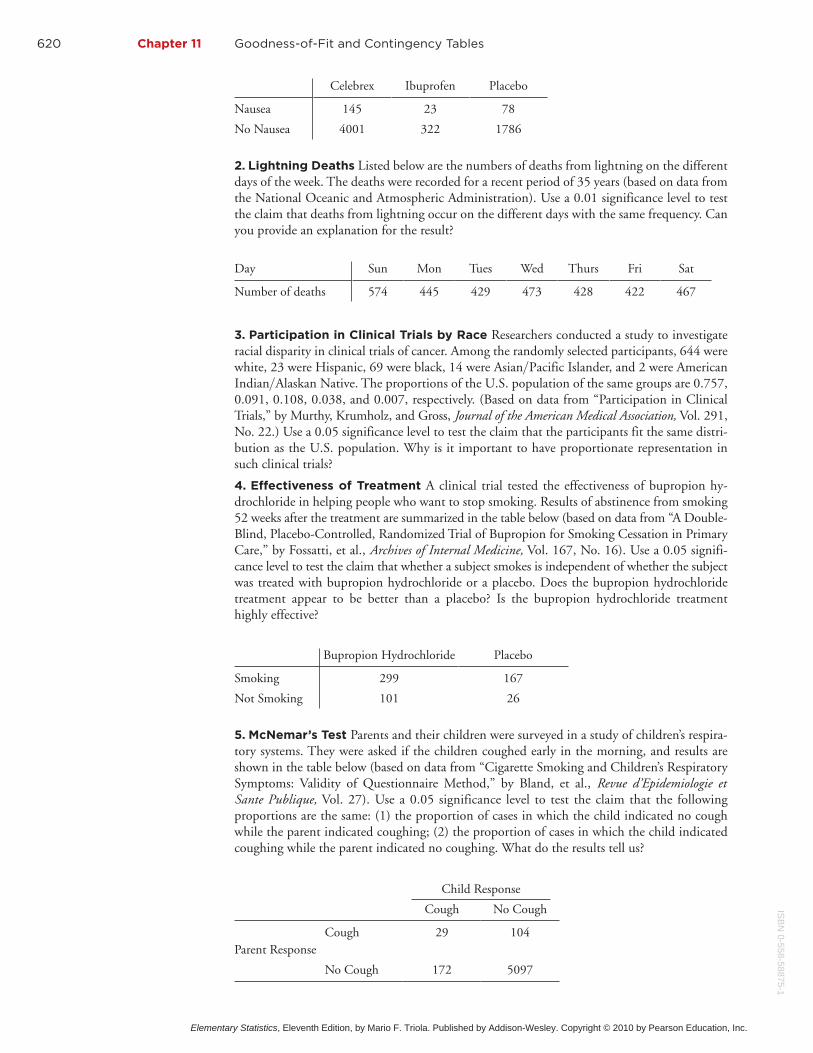
620 Chapter 11 Goodness-of-Fit and Contingency Tables
2. Lightning Deaths Listed below are the numbers of deaths from lightning on the differentdays of the week. The deaths were recorded for a recent period of 35 years (based on data fromthe National Oceanic and Atmospheric Administration). Use a 0.01 significance level to testthe claim that deaths from lightning occur on the different days with the same frequency. Canyou provide an explanation for the result?
Celebrex Ibuprofen Placebo
Nausea 145 23 78
No Nausea 4001 322 1786
Day Sun Mon Tues Wed Thurs Fri Sat
Number of deaths 574 445 429 473 428 422 467
3. Participation in Clinical Trials by Race Researchers conducted a study to investigateracial disparity in clinical trials of cancer. Among the randomly selected participants, 644 werewhite, 23 were Hispanic, 69 were black, 14 were Islander, and 2 were American
Native. The proportions of the U.S. population of the same groups are 0.757,0.091, 0.108, 0.038, and 0.007, respectively. (Based on data from “Participation in ClinicalTrials,” by Murthy, Krumholz, and Gross, Journal of the American Medical Association, Vol. 291,No. 22.) Use a 0.05 significance level to test the claim that the participants fit the same distri-bution as the U.S. population. Why is it important to have proportionate representation insuch clinical trials?
4. Effectiveness of Treatment A clinical trial tested the effectiveness of bupropion hy-drochloride in helping people who want to stop smoking. Results of abstinence from smoking52 weeks after the treatment are summarized in the table below (based on data from “A Double-Blind, Placebo-Controlled, Randomized Trial of Bupropion for Smoking Cessation in PrimaryCare,” by Fossatti, et al., Archives of Internal Medicine, Vol. 167, No. 16). Use a 0.05 signifi-cance level to test the claim that whether a subject smokes is independent of whether the subjectwas treated with bupropion hydrochloride or a placebo. Does the bupropion hydrochloridetreatment appear to be better than a placebo? Is the bupropion hydrochloride treatmenthighly effective?
Indian>AlaskanAsian>Pacific
Bupropion Hydrochloride Placebo
Smoking 299 167
Not Smoking 101 26
5. McNemar’s Test Parents and their children were surveyed in a study of children’s respira-tory systems. They were asked if the children coughed early in the morning, and results areshown in the table below (based on data from “Cigarette Smoking and Children’s RespiratorySymptoms: Validity of Questionnaire Method,” by Bland, et al., Revue d’Epidemiologie etSante Publique, Vol. 27). Use a 0.05 significance level to test the claim that the followingproportions are the same: (1) the proportion of cases in which the child indicated no coughwhile the parent indicated coughing; (2) the proportion of cases in which the child indicatedcoughing while the parent indicated no coughing. What do the results tell us?
Child Response
Cough No Cough
Cough 29 104Parent Response
No Cough 172 5097
ISB
N0-558-58875-1
Elementary Statistics, Eleventh Edition, by Mario F. Triola. Published by Addison-Wesley. Copyright © 2010 by Pearson Education, Inc.

Cumulative Review Exercises 621
Cumulative Review Exercises
1. Cleanliness The American Society for Microbiology and the Soap and Detergent Associa-tion released survey results indicating that among 3065 men observed in public restrooms,2023 of them washed their hands, and among 3011 women observed, 2650 washed theirhands (based on data from USA Today).
a. Is the study an experiment or an observational study?
b. Are the given numbers discrete or continuous?
c. Are the given numbers statistics or parameters?
d. Is there anything about the study that might make the results questionable?
2. Cleanliness Refer to the results given in Exercise 1 and use a 0.05 significance level to testthe claim that the proportion of men who wash their hands is equal to the proportion ofwomen who wash their hands. Is there a significant difference?
3. Cleanliness Refer to the results given in Exercise 1. Construct a two-way frequency tableand use a 0.05 significance level to test the claim that hand washing is independent of gender.
4. Golf Scores Listed below are first round and fourth round golf scores of randomlyselected golfers in a Professional Golf Association Championship (based on data from theNew York Times). Find the mean, median, range, and standard deviation for the first roundscores, then find those same statistics for the fourth round scores. Compare the results.
First round 71 68 75 72 74 67
Fourth round 69 69 69 72 70 73
5. Golf Scores Refer to the sample data given in Exercise 4. Use a 0.05 significance level totest for a linear correlation between the first round scores and the fourth round scores.
6. Golf Scores Using only the first round golf scores given in Exercise 4, construct a 95%confidence interval estimate of the mean first round golf score for all golfers. Interpret theresult.
7. Wise Action for Job Applicants In an Accountemps survey of 150 randomly selectedsenior executives, 88% said that sending a thank-you note after a job interview increases theapplicant’s chances of being hired (based on data from USA Today). Construct a 95% confi-dence interval estimate of the percentage of all senior executives who believe that a thank-younote is helpful. What very practical advice can be gained from these results?
8. Testing a Claim Refer to the sample results given in Exercise 7 and use a 0.01 significancelevel to test the claim that more than 75% of all senior executives believe that a thank-younote after a job interview increases the applicant’s chances of being hired.
9. Ergonomics When designing the cockpit of a single-engine aircraft, engineers must con-sider the upper leg lengths of men. Those lengths are normally distributed with a mean of42.6 cm and a standard deviation of 2.9 cm (based on Data Set 1 in Appendix B).
a. If one man is randomly selected, find the probability that his upper leg length is greaterthan 45 cm.
b. If 16 men are randomly selected, find the probability that their mean upper leg length isgreater than 45 cm.c. When designing the aircraft cockpit, which result is more meaningful: the result from part(a) or the result from part (b)? Why?
10. Tall Women The probability of randomly selecting a woman who is more than 5 feet tallis 0.925 (based on data from the National Health and Nutrition Examination Survey). Findthe probability of randomly selecting five women and finding that all of them are more than5 feet tall. Is it unusual to randomly select five women and find that all of them are more than5 feet tall? Why or why not?
ISB
N0-
558-
5887
5-1
Elementary Statistics, Eleventh Edition, by Mario F. Triola. Published by Addison-Wesley. Copyright © 2010 by Pearson Education, Inc.

622 Chapter 11 Goodness-of-Fit and Contingency Tables
Technology Project
Use STATDISK, Minitab, Excel, or a Plus calculator, or any other software packageor calculator capable of generating equally likely random digits between 0 and 9 inclusive.Generate 5000 digits and record the results in the accompanying table. Use a 0.05 signifi-cance level to test the claim that the sample digits come from a population with a uniform dis-tribution (so that all digits are equally likely). Does the random number generator appear tobe working as it should?
TI-83>84
Digit 0 1 2 3 4 5 6 7 8 9
Frequency
INT
ER
NE
T
PR
OJ
EC
T
Contingency Tables
Go to: http://www.aw.com/triola
An important characteristic of tests of indepen-
dence with contingency tables is that the data
collected need not be quantitative in nature. A
contingency table summarizes observations by
the categories or labels of the rows and columns.
As a result, characteristics such as gender, race,
and political party all become fair game for for-
mal hypothesis testing procedures. In the Internet
Project for this chapter you will find links to a va-
riety of demographic data. With these data sets,
you will conduct tests in areas as diverse as aca-
demics, politics, and the entertainment industry.
In each test, you will draw conclusions related to
the independence of interesting characteristics.
Open the Applets folder on the CD and double-clickon Start. Select the menu item of Random numbers.Randomly generate 100 whole numbers between 0and 9 inclusive. Construct a frequency distribution of
the results, then use the methods of this chapter totest the claim that the whole numbers between 0 and9 are equally likely.
ISB
N0-558-58875-1
Elementary Statistics, Eleventh Edition, by Mario F. Triola. Published by Addison-Wesley. Copyright © 2010 by Pearson Education, Inc.

Cooperative Group Activities 623
Cooperative Group Activities
1. Out-of-class activity Divide into groups of four or five students. The instructions forExercises 21–24 in Section 11-2 noted that according to Benford’s law, a variety of differentdata sets include numbers with leading (first) digits that follow the distribution shown in thetable below. Collect original data and use the methods of Section 11-2 to support or refute theclaim that the data conform reasonably well to Benford’s law. Here are some possibilities thatmight be considered: (1) amounts on the checks that you wrote; (2) prices of stocks; (3) pop-ulations of counties in the United States; (4) numbers on street addresses; (5) lengths of riversin the world.
Leading Digit 1 2 3 4 5 6 7 8 9
Benford’s law: 30.1% 17.6% 12.5% 9.7% 7.9% 6.7% 5.8% 5.1% 4.6%
FR
OM
DA
TA
TO
DE
CIS
ION
One of the most notable sea disasters oc-curred with the sinking of the Titanic onMonday, April 15, 1912. The table be-low summarizes the fate of the passengers
Analyzing the Results
If we examine the data, we see that19.6% of the men (332 out of 1692)survived, 75.4% of the women (318 outof 422) survived, 45.3% of the boys(29 out of 64) survived, and 60% of thegirls (27 out of 45) survived. There doappear to be differences, but are the dif-ferences really significant?
First construct a bar graph showingthe percentage of survivors in each ofthe four categories (men, women, boys,girls). What does the graph suggest?
Critical Thinking: Was the law of “womenand children first” followed in the sinkingof the Titanic?
Fate of Passengers and Crew on the Titanic
Men Women Boys Girls
Survived 332 318 29 27Died 1360 104 35 18
Next, treat the 2223 people aboardthe Titanic as a sample. We could takethe position that the Titanic data in theabove table constitute a population andtherefore should not be treated as a sam-ple, so that methods of inferential statis-tics do not apply. But let’s stipulate thatthe data in the table are sample datarandomly selected from the populationof all theoretical people who would findthemselves in the same conditions. Real-istically, no other people will actuallyfind themselves in the same conditions,
but we will make that assumption forthe purposes of this discussion andanalysis. We can then determinewhether the observed differences havestatistical significance. Use one or moreformal hypothesis tests to investigate theclaim that although some men survivedwhile some women and children died,the rule of “women and children first”was essentially followed. Identify the hy-pothesis test(s) used and interpret theresults by addressing the claim thatwhen the Titanic sank on its maidenvoyage, the rule of “women and chil-dren first” was essentially followed.
2. Out-of-class activity Divide into groups of four or five students and collect past resultsfrom a state lottery. Such results are often available on Web sites for individual state lotteries.Use the methods of Section 11-2 to test that the numbers are selected in such a way that allpossible outcomes are equally likely.
and crew. A common rule of the sea is thatwhen a ship is threatened with sinking,women and children are the first to besaved.
ISB
N0-
558-
5887
5-1
Elementary Statistics, Eleventh Edition, by Mario F. Triola. Published by Addison-Wesley. Copyright © 2010 by Pearson Education, Inc.

624 Chapter 11 Goodness-of-Fit and Contingency Tables
3. Out-of-class activity Divide into groups of four or five students. Each group membershould survey at least 15 male students and 15 female students at the same college by askingtwo questions: (1) Which political party does the subject favor most? (2) If the subject were tomake up an absence excuse of a flat tire, which tire would he or she say went flat if the instruc-tor asked? (See Exercise 8 in Section 11-2.) Ask the subject to write the two responses on an in-dex card, and also record the gender of the subject and whether the subject wrote with the rightor left hand. Use the methods of this chapter to analyze the data collected. Include these tests:
• The four possible choices for a flat tire are selected with equal frequency.
• The tire identified as being flat is independent of the gender of the subject.• Political party choice is independent of the gender of the subject.
• Political party choice is independent of whether the subject is right- or left-handed.
• The tire identified as being flat is independent of whether the subject is right- or left-handed.
• Gender is independent of whether the subject is right- or left-handed.• Political party choice is independent of the tire identified as being flat.
4. Out-of-class activity Divide into groups of four or five students. Each group membershould select about 15 other students and first ask them to “randomly” select four digits each.After the four digits have been recorded, ask each subject to write the last four digits of his orher social security number. Take the “random” sample results and mix them into one big sam-ple, then mix the social security digits into a second big sample. Using the “random” sampleset, test the claim that students select digits randomly. Then use the social security digits totest the claim that they come from a population of random digits. Compare the results. Doesit appear that students can randomly select digits? Are they likely to select any digits more of-ten than others? Are they likely to select any digits less often than others? Do the last digits ofsocial security numbers appear to be randomly selected?
5. In-class activity Divide into groups of three or four students. Each group should begiven a die along with the instruction that it should be tested for “fairness.” Is the die fair or isit biased? Describe the analysis and results.
6. Out-of-class activity Divide into groups of two or three students. The analysis of last dig-its of data can sometimes reveal whether values are the results of actual measurements orwhether they are reported estimates. Refer to an almanac and find the lengths of rivers in theworld, then analyze the last digits to determine whether those lengths appear to be actual mea-surements or whether they appear to be reported estimates. (Instead of lengths of rivers, youcould use heights of mountains, heights of the tallest buildings, lengths of bridges, and so on.)
ISB
N0-558-58875-1
Elementary Statistics, Eleventh Edition, by Mario F. Triola. Published by Addison-Wesley. Copyright © 2010 by Pearson Education, Inc.

625
STATIST ICS IN SPORTS
A previous edition of this bookincluded an interview withBill James, a recognized base-
ball expert who specializes in theanalysis of baseball statistics andidentifying the best game strategiesbased on past results. The BostonRed Sox hired Bill James as an advi-sor, and he is credited with some ofthe changes that led to the firstWorld Series victory by the Red Soxin 86 years. Another Bostonian whomakes extensive use of statistics in theworld of sports is Jackie Macmullan,who is Associate Editor and sportscolumnist for the Boston Globe.
Q: How do you use statistics whenwriting about sports?
A: Sports is all about statistics, really. Espe-cially baseball. Yesterday I wrote about whyC.C. Sabathia won the Cy Young awardover Josh Beckett. Beckett had more winsbut lost to Sabathia because of “deepernumbers,” which are the underlying statis-tics. The big one in this case was qualitystarts—a pretty good indicator of how pro-ficient you were on the mound (Sabathia’s25 vs. Beckett’s 20). In many of my storieson sports, and baseball in particular, the useof statistics gives readers a deeper understanding of the gameand its players.
Q: Please describe a specific example illustratingthe use of statistics.
A: For many years, as I covered the NBA as a beat writer for theBoston Celtics, I kept a binder full of information on every aspectof the game. After each game, I would record everything—points
per game, turnovers, assists, etc., for each player on the team.I would also keep track of the opposing team and what theydid—any player who scored 10 or more points, for example.I would break down all of the action by quarters, notingwhere the Celtics turned the game around. These meticulousrecords kept me on top of every player and their tendencies.I relied on that book for a tremendous amount of obscurelittle things, too, which I think are what makes a strongsportswriter.
Q: Is your use of probability and statistics increasing,decreasing, or remaining stable?
A: Now, everyone is so sophisticated in their use of statistics.Every college and professional team has their own statisticalteam that records all their data as they play. Every single teamin every single sport has its own scouting system that breaksevery statistic down. Here’s an example: There was a companyhired by the Chicago Bulls that would break down everythingMichael Jordan did. Things like, “when Jordan gets ball onleft block, shoots 36% of time, on right, 31% of time” soyou’d know where he’d prefer to shoot from and his rate ofsuccess in every location. Data told you players may like to doa certain thing more, but weren’t necessarily successful at it.This really influences other teams and strategies, because theyknow everything these players do and how good they are atdoing it.
Q: How critical do you find your knowledge ofstatistics for performing your responsibilities?
A: Using statistics really enhances mywriting — people don’t keep their ownstats now, but if you do keep them your-self it takes time, effort, and concentra-tion, and the data become more valuableto you. Collecting data like this providesinformation that you didn’t necessarilyknow you were looking for. For example,from my NBA binder, I would often findthat three quarters way through season, Ihad learned about player tendencies that Ididn’t see on my own, or even realize I wasrecording.
Q: In terms of statistics, what would you recommendfor prospective employees?
A: An introductory course would be fine. You really have toknow how to crunch numbers to do my job effectively. Some ofthe best articles are written by people who make these uniquestatistical observations.
NAME: Jackie Macmullan
JOB: Associate Editor, Sports
Columnist
COMPANY: Boston Globe
ISB
N0-
558-
5887
5-1
Elementary Statistics, Eleventh Edition, by Mario F. Triola. Published by Addison-Wesley. Copyright © 2010 by Pearson Education, Inc.
Related Documents