1 Power 14 Goodness of Fit & Contingency Tables. 2 Outline u I. Projects u II. Goodness of Fit & Chi Square u III.Contingency Tables.

11

Power 14Goodness of Fit

& Contingency Tables

22

Outline

I. ProjectsI. Projects II. Goodness of Fit & Chi SquareII. Goodness of Fit & Chi Square III.Contingency TablesIII.Contingency Tables

33

Part I: Projects

TeamsTeams AssignmentsAssignments PresentationsPresentations Data SourcesData Sources GradesGrades

44

Team One

Catherine Wohletz: Project choiceCatherine Wohletz: Project choice Joshua Friedberg: Data RetrievalJoshua Friedberg: Data Retrieval Julio Urenda: Statistical AnalysisJulio Urenda: Statistical Analysis Daniel Grund: PowerPoint PresentationDaniel Grund: PowerPoint Presentation Takuro Hatanaka: Executive SummaryTakuro Hatanaka: Executive Summary Sylvia Salinas: Technical AppendixSylvia Salinas: Technical Appendix

55

Assignments

1. Project choice1. Project choice 2. Data Retrieval2. Data Retrieval 3. Statistical Analysis3. Statistical Analysis 4. PowerPoint Presentation4. PowerPoint Presentation 5. Executive Summary5. Executive Summary 6. Technical Appendix6. Technical Appendix

66

PowerPoint Presentations: Member 4

1. Introduction: Members 1 ,2 , 31. Introduction: Members 1 ,2 , 3– WhatWhat– WhyWhy– HowHow

2. Executive Summary: Member 52. Executive Summary: Member 5 3. Exploratory Data Analysis: Member 33. Exploratory Data Analysis: Member 3 4. Descriptive Statistics: Member 34. Descriptive Statistics: Member 3 5. Statistical Analysis: Member 35. Statistical Analysis: Member 3 6. Conclusions: Members 3 & 56. Conclusions: Members 3 & 5 7. Technical Appendix: Table of Contents, 7. Technical Appendix: Table of Contents,

Member 6Member 6

77

Executive Summary and Technical Appendix

88

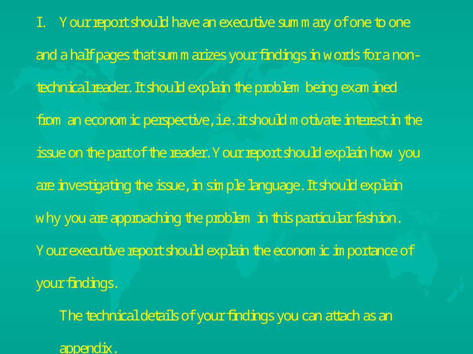
I. Your report should have an executive summary of one to one

and a half pages that summarizes your findings in words for a non-

technical reader. It should explain the problem being examined

from an economic perspective, i.e. it should motivate interest in the

issue on the part of the reader. Your report should explain how you

are investigating the issue, in simple language. It should explain

why you are approaching the problem in this particular fashion.

Your executive report should explain the economic importance of

your findings.

The technical details of your findings you can attach as an

appendix.

99

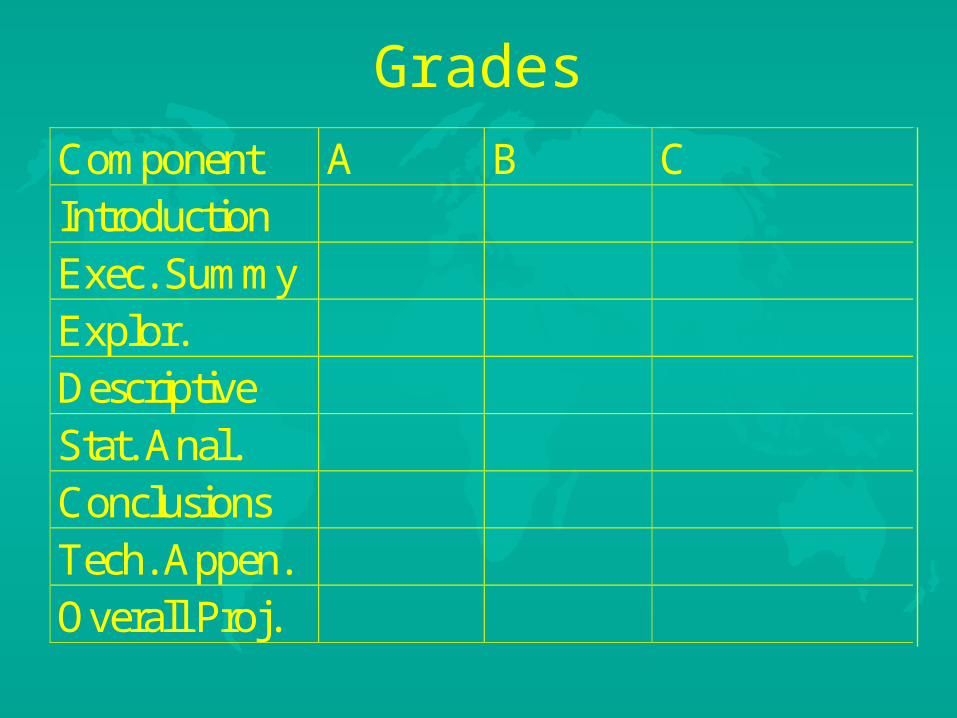
GradesComponent A B CIntroductionExec. SummyExplor.DescriptiveStat. Anal.ConclusionsTech. Appen.Overall Proj.

1010

Data Sources FRED: Federal Reserve Bank of St. Louis, FRED: Federal Reserve Bank of St. Louis,

http://research.http://research.stlouisfedstlouisfed.org/.org/fredfred//– Business/FiscalBusiness/Fiscal

Index of Consumer Sentiment, Monthly (1952:11)Index of Consumer Sentiment, Monthly (1952:11) Light Weight Vehicle Sales, Auto and Light Truck, Monthly Light Weight Vehicle Sales, Auto and Light Truck, Monthly

(1976.01)(1976.01)

Economagic, Economagic, http://www.http://www.economagiceconomagic.com/.com/ U S Dept. of Commerce, U S Dept. of Commerce, http://www.commerce.http://www.commerce.

govgov//– PopulationPopulation– Economic Analysis, http://www.bea.gov/Economic Analysis, http://www.bea.gov/

1111

Data Sources (Cont. ) Bureau of Labor Statistics, Bureau of Labor Statistics,

http://stats.bls.gov/http://stats.bls.gov/ California Dept of Finance, California Dept of Finance,

http://www.dof.ca.gov/ http://www.dof.ca.gov/

1212

II. Goodness of Fit & Chi Square

Rolling a Fair DieRolling a Fair Die The Multinomial DistributionThe Multinomial Distribution Experiment: 600 TossesExperiment: 600 Tosses

1313

Outcome Probability Expected Frequency1 1/6 1002 1/6 1003 1/6 1004 1/6 1005 1/6 1006 1/6 100

The Expected Frequencies The Expected Frequencies

1414

Outcome Expected Frequencies Expected Frequency1 100 1142 100 943 100 844 100 1015 100 1076 100 107

The Expected Frequencies & Empirical FrequenciesThe Expected Frequencies & Empirical Frequencies

Empirical FrequencyEmpirical Frequency

1515

Hypothesis Test

Null HNull H00: Distribution is Multinomial: Distribution is Multinomial

Statistic: (OStatistic: (Oii - E - Eii))22/E/Ei, i, : observed minus : observed minus

expected squared divided by expectedexpected squared divided by expected Set Type I Error @ 5% for exampleSet Type I Error @ 5% for example Distribution of Statistic is Chi SquareDistribution of Statistic is Chi Square

P(nP(n1 1 =1, n=1, n2 2 =0, nn3 3 =0, n =0, n4 4 =0, n=0, n5 5 =0, n=0, n6 6 =0) = n!/=0) = n!/

n

j

jnn

j

jpjn1

)(

1

)]([])(

P(nP(n1 1 =1, n=1, n2 2 =0, nn3 3 =0, n =0, n4 4 =0, n=0, n5 5 =0, n=0, n6 6 =0)= 1!/1!0!0!0!0!0!(1/6)=0)= 1!/1!0!0!0!0!0!(1/6)11(1/6)(1/6)00

(1/6)(1/6)0 0 (1/6)(1/6)0 0 (1/6)(1/6)0 0 (1/6)(1/6)00

One Throw, side one comes up: multinomial distributionOne Throw, side one comes up: multinomial distribution

1616

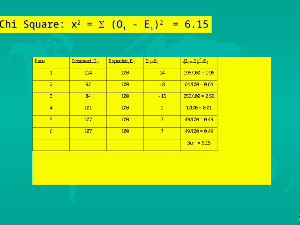
Face Observed, Oj Expected, Ej Oj - Ej (Oj – Ej)2 /Ej

1 114 100 14 196/100 = 1.96

2 92 100 - 8 64/100 = 0.64

3 84 100 - 16 256/100 = 2.56

4 101 100 1 1/100 = 0.01

5 107 100 7 49/100 = 0.49

6 107 100 7 49/100 = 0.49

Sum = 6.15

Chi Square: xChi Square: x22 = = (O (Oii - E - Eii))2 2 = 6.15 = 6.15

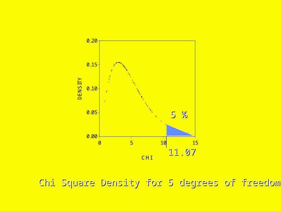
0.00

0.05

0.10

0.15

0.20

0 5 10 15

CHI

DE

NS

ITY

Chi Square Density for 5 degrees of freedomChi Square Density for 5 degrees of freedom

11.0711.07

5 %5 %

1818

Contingency Table Analysis

Tests for Association Vs. Independence For Tests for Association Vs. Independence For Qualitative VariablesQualitative Variables

1919

Purchase Consumer Inform Cons. Not Inform . TotalsFrost FreeNot Frost FreeTotals

Does Consumer Knowledge Affect Purchases?Does Consumer Knowledge Affect Purchases?

Frost Free Refrigerators Use More ElectricityFrost Free Refrigerators Use More Electricity

2020

Purchase Consumer Inform Cons. Not Inform . TotalsFrost Free 432Not Frost Free 288Totals 540 180 720

Marginal CountsMarginal Counts

2121

Purchase Consumer Inform Cons. Not Inform . TotalsFrost Free 0.6Not Frost Free 0.4Totals 0.75 0.25 1

Marginal Distributions, f(x) & f(y)Marginal Distributions, f(x) & f(y)

2222

Purchase Consumer Inform Cons. Not Inform . TotalsFrost Free 0.45 0.15 0.6Not Frost Free 0.3 0.1 0.4Totals 0.75 0.25 1

Joint Disribution Under IndependenceJoint Disribution Under Independencef(x,y) = f(x)*f(y)f(x,y) = f(x)*f(y)

2323

Purchase Consumer Inform Cons. Not Inform . TotalsFrost Free 324 108 432Not Frost Free 216 72 288Totals 540 180 720

Expected Cell Frequencies Under IndependenceExpected Cell Frequencies Under Independence

2424

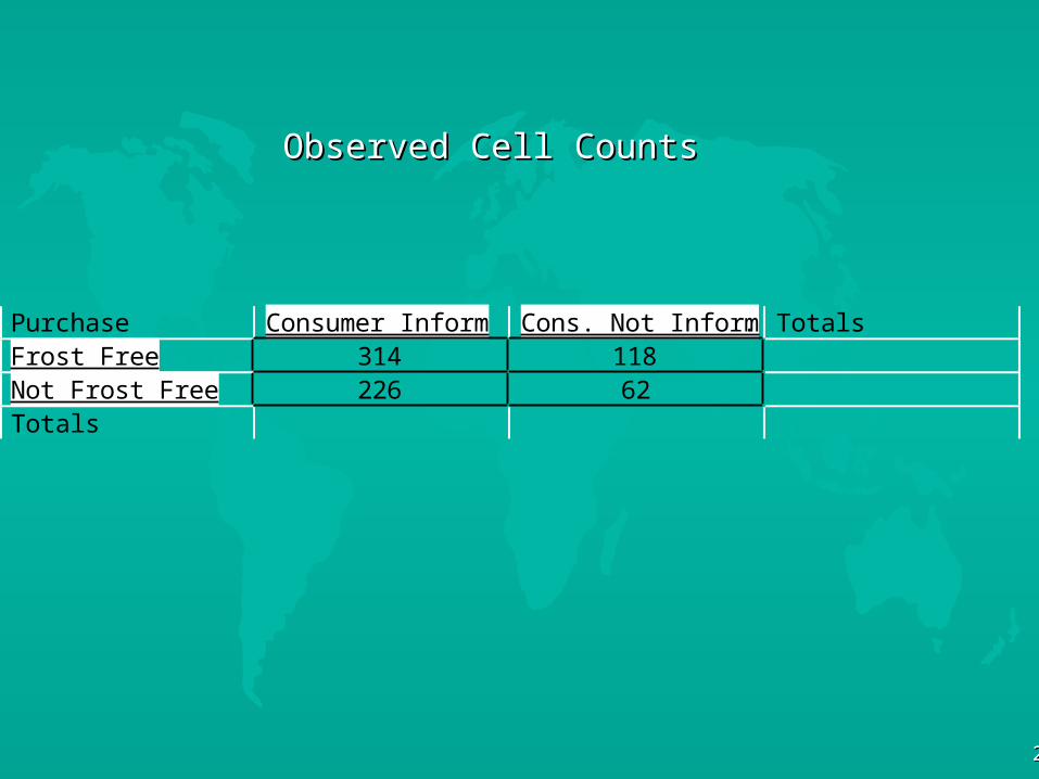
Purchase Consumer Inform Cons. Not Inform . TotalsFrost Free 314 118Not Frost Free 226 62Totals

Observed Cell CountsObserved Cell Counts

2525

Purchase Consumer Inform Cons. Not Inform . TotalsFrost Free 0.31 0.93Not Frost Free 0.46 1.39Totals

Contribution to Chi Square: (observed-Expected)Contribution to Chi Square: (observed-Expected)22/Expected/Expected

Chi Sqare = 0.31 + 0.93 + 0.46 +1.39 = 3.09Chi Sqare = 0.31 + 0.93 + 0.46 +1.39 = 3.09(m-1)*(n-1) = 1*1=1 degrees of freedom (m-1)*(n-1) = 1*1=1 degrees of freedom

Upper Left Cell: (314-324)Upper Left Cell: (314-324)22/324 = 100/324 =0.31/324 = 100/324 =0.31

0.0

0.2

0.4

0.6

0.8

1.0

0 2 4 6 8 10 12 14

Chi-Square Variable

Figure 4: Chi-Square Density, One Degree of Freedom

Density

5%5%

5.025.02

2727

Conclusion

No association between consumer No association between consumer knowledge about electricity use and knowledge about electricity use and consumer choice of a frost-free refrigeratorconsumer choice of a frost-free refrigerator

2828

Using Goodness of Fit to Choose Between Competing

Probability Models Men on base when a home run is hitMen on base when a home run is hit

2929

Men on base when a home run is hit

# 0 1 2 3 Sum

Observed 421 227 96 21 765

Fraction 0.550 0.298 0.125 0.027 1

3030

Conjecture

Distribution is binomialDistribution is binomial

3131

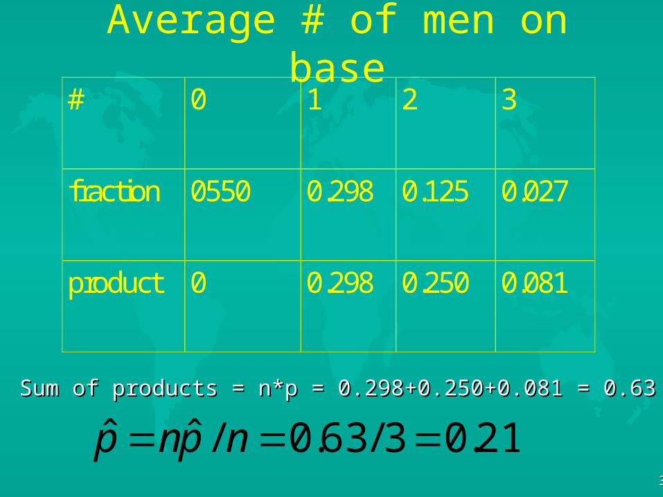
Average # of men on base# 0 1 2 3

fraction 0550 0.298 0.125 0.027

product 0 0.298 0.250 0.081

Sum of products = n*p = 0.298+0.250+0.081 = 0.63Sum of products = n*p = 0.298+0.250+0.081 = 0.63

21.03/63.0/ˆˆ npnp

3232

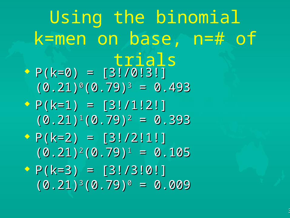
Using the binomialk=men on base, n=# of trials

P(k=0) = [3!/0!3!] (0.21)P(k=0) = [3!/0!3!] (0.21)00(0.79)(0.79)33 = 0.493 = 0.493 P(k=1) = [3!/1!2!] (0.21)P(k=1) = [3!/1!2!] (0.21)11(0.79)(0.79)22 = 0.393 = 0.393 P(k=2) = [3!/2!1!] (0.21)P(k=2) = [3!/2!1!] (0.21)22(0.79)(0.79)11 = 0.105 = 0.105 P(k=3) = [3!/3!0!] (0.21)P(k=3) = [3!/3!0!] (0.21)33(0.79)(0.79)00 = 0.009 = 0.009

3333

Assuming the binomial

The probability of zero men on base is The probability of zero men on base is 0.4930.493

the total number of observations is 765the total number of observations is 765 so the expected number of observations for so the expected number of observations for

zero men on base is 0.493*765=377.1zero men on base is 0.493*765=377.1

3434

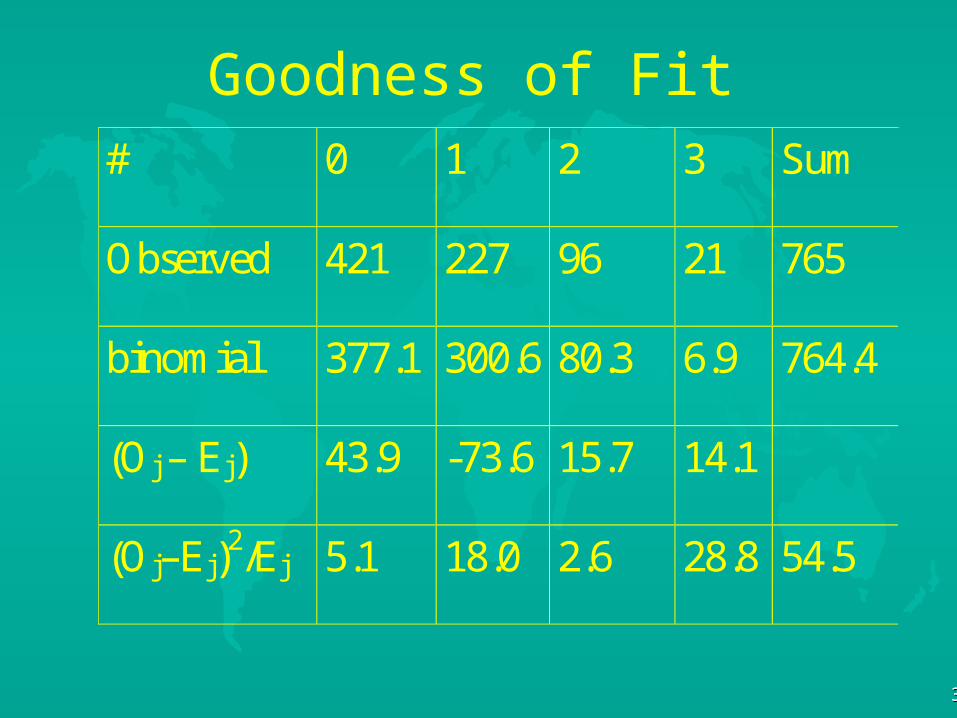
Goodness of Fit# 0 1 2 3 Sum

Observed 421 227 96 21 765

binomial 377.1 300.6 80.3 6.9 764.4

(Oj – Ej) 43.9 -73.6 15.7 14.1

(Oj–Ej)2/Ej 5.1 18.0 2.6 28.8 54.5

0.00

0.05

0.10

0.15

0.20

0.25

0 5 10 15 20

CHI

DE

NS

ITY

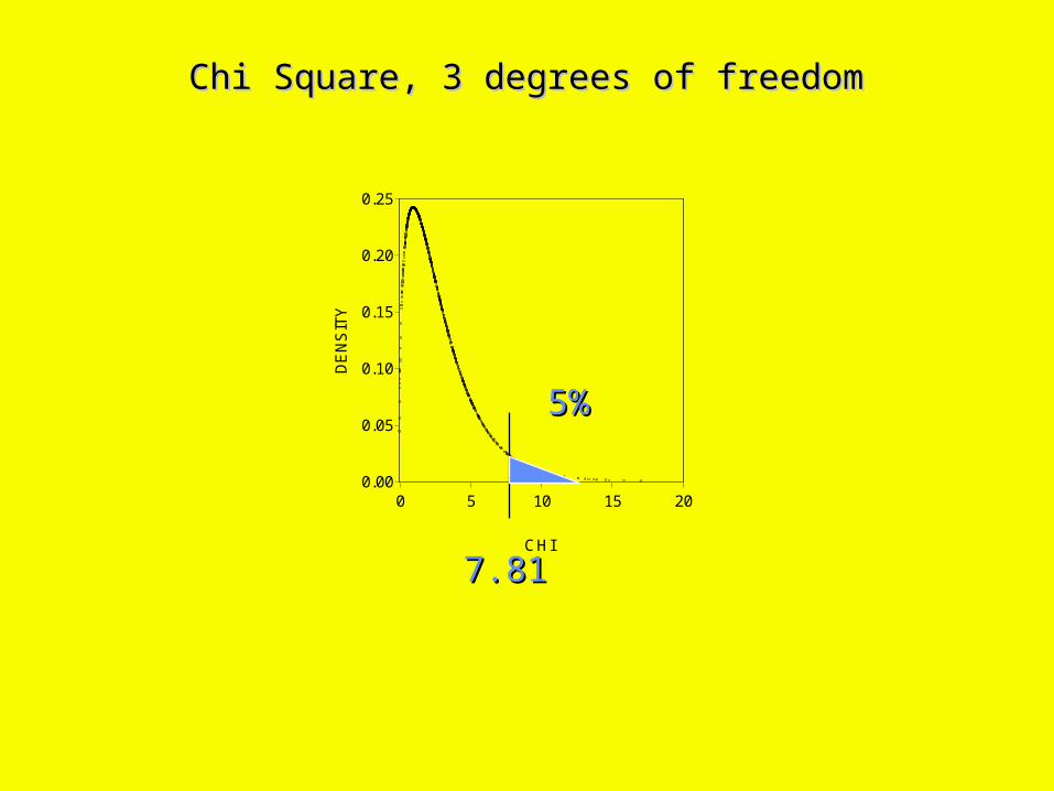
Chi Square, 3 degrees of freedomChi Square, 3 degrees of freedom

5%5%

7.817.81

3636

Conjecture: Poisson where np = 0.63

P(k=3) = 1- P(k=2)-P(k=1)-P(k=0)P(k=3) = 1- P(k=2)-P(k=1)-P(k=0) P(k=0) = eP(k=0) = e--k k /k! = e/k! = e-0.63 -0.63 (0.63)(0.63)00/0! = 0.5326/0! = 0.5326 P(k=1) = eP(k=1) = e--k k /k! = e/k! = e-0.63 -0.63 (0.63)(0.63)11/1! = 0.3355/1! = 0.3355 P(k=2) = eP(k=2) = e--k k /k! = e/k! = e-0.63 -0.63 (0.63)(0.63)22/2! = 0.1057/2! = 0.1057

3737

Average # of men on base# 0 1 2 3

fraction 0550 0.298 0.125 0.027

product 0 0.298 0.250 0.081

Sum of products = n*p = 0.298+0.250+0.081 = 0.63Sum of products = n*p = 0.298+0.250+0.081 = 0.63

21.03/63.0/ˆˆ npnp

3838

Conjecture: Poisson where np = 0.63

P(k=3) = 1- P(k=2)-P(k=1)-P(k=0)P(k=3) = 1- P(k=2)-P(k=1)-P(k=0) P(k=0) = eP(k=0) = e--k k /k! = e/k! = e-0.63 -0.63 (0.63)(0.63)00/0! = 0.5326/0! = 0.5326 P(k=1) = eP(k=1) = e--k k /k! = e/k! = e-0.63 -0.63 (0.63)(0.63)11/1! = 0.3355/1! = 0.3355 P(k=2) = eP(k=2) = e--k k /k! = e/k! = e-0.63 -0.63 (0.63)(0.63)22/2! = 0.1057/2! = 0.1057

3939

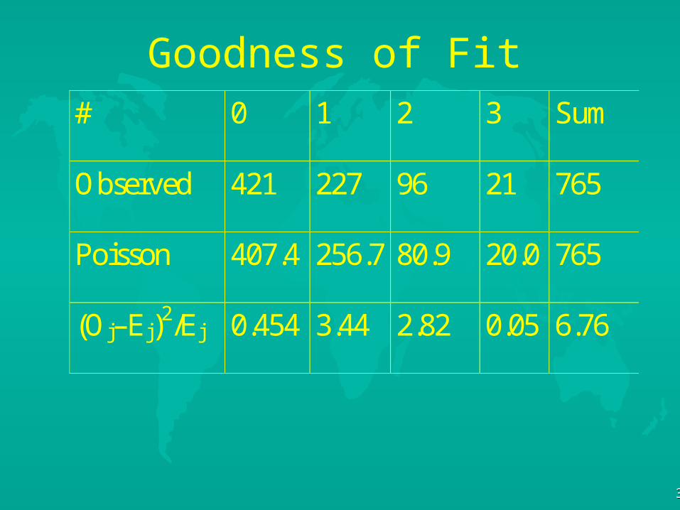
Goodness of Fit# 0 1 2 3 Sum

Observed 421 227 96 21 765

Poisson 407.4 256.7 80.9 20.0 765

(Oj–Ej)2/Ej 0.454 3.44 2.82 0.05 6.76

0.00

0.05

0.10

0.15

0.20

0.25

0 5 10 15 20

CHI

DE

NS

ITY

Chi Square, 3 degrees of freedomChi Square, 3 degrees of freedom

5%5%

7.817.81

4141

Likelihood Functions

Review OLS LikelihoodReview OLS Likelihood Proceed in a similar fashion for the probitProceed in a similar fashion for the probit

4242

Likelihood function The joint density of the estimated residuals The joint density of the estimated residuals

can be written as:can be written as:

If the sample of observations on the If the sample of observations on the dependent variable, y, and the independent dependent variable, y, and the independent variable, x, is random, then the observations variable, x, is random, then the observations are independent of one another. If the errors are independent of one another. If the errors are also identically distributed, f, i.e. i.i.d, are also identically distributed, f, i.e. i.i.d, thenthen

)ˆ.....ˆˆˆ( 1210 neeeeg

4343

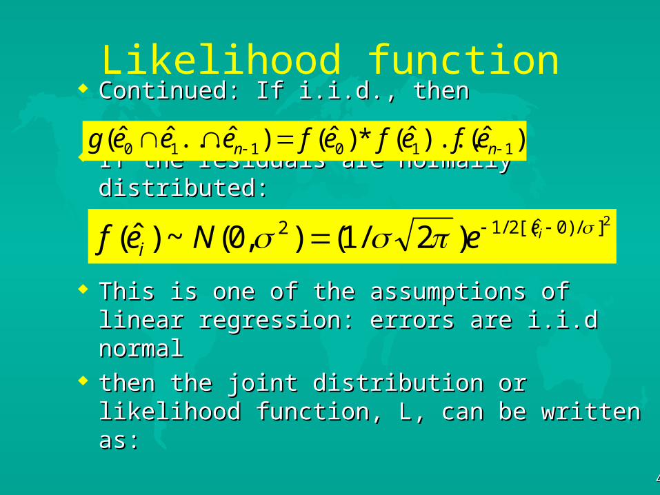
Likelihood function Continued: If i.i.d., thenContinued: If i.i.d., then

If the residuals are normally distributed:If the residuals are normally distributed:

This is one of the assumptions of linear This is one of the assumptions of linear regression: errors are i.i.d normalregression: errors are i.i.d normal

then the joint distribution or likelihood then the joint distribution or likelihood function, L, can be written as:function, L, can be written as:

)ˆ()...ˆ(*)ˆ()ˆ...ˆˆ( 110110 nn efefefeeeg

2]/)0ˆ[(2/12 )2/1(),0(~)ˆ( iei eNef

4444

Likelihood function

and taking natural logarithms of both sides, where and taking natural logarithms of both sides, where the logarithm is a monotonically increasing the logarithm is a monotonically increasing function so that if lnL is maximized, so is L:function so that if lnL is maximized, so is L:

1

0

22

2

]ˆ[)2/1(2/2/2

]/)0ˆ[(2/11

0110

*)2/1(*)/1(

)2/1()ˆ...ˆˆ(

n

ii

i

enn

en

in

eL

eeeegL

4545

Log-Likelihood

Taking the derivative of lnL with respect to Taking the derivative of lnL with respect to either a-hat or b-hat yields the same either a-hat or b-hat yields the same estimators for the parameters a and b as with estimators for the parameters a and b as with ordinary least squares, except now we know ordinary least squares, except now we know the errors are normally distributed.the errors are normally distributed.

21

0

22

1

0

222

]*ˆˆ[)2/1()2ln(*)2/(]ln[*)2/(ln

ˆ)2/1()2ln(*)2/(]ln[*)2/(ln

i

n

ii

n

ii

xbaynnL

ennL

4646

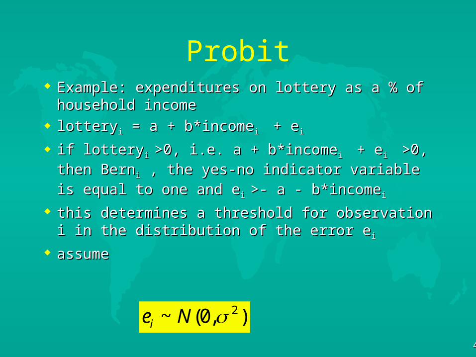
Probit Example: expenditures on lottery as a % of household Example: expenditures on lottery as a % of household

incomeincome lotterylotteryii = a + b*income = a + b*incomei i + e + eii

if lotteryif lotteryi i >0, i.e. a + b*income>0, i.e. a + b*incomei i + e + ei i >0, then Bern >0, then Bernii , ,

the yes-no indicator variable is equal to one and ethe yes-no indicator variable is equal to one and e i i >- a >- a

- b*income- b*incomeii

this determines a threshold for observation i in the this determines a threshold for observation i in the distribution of the error edistribution of the error eii

assume assume

),0(~ 2Nei

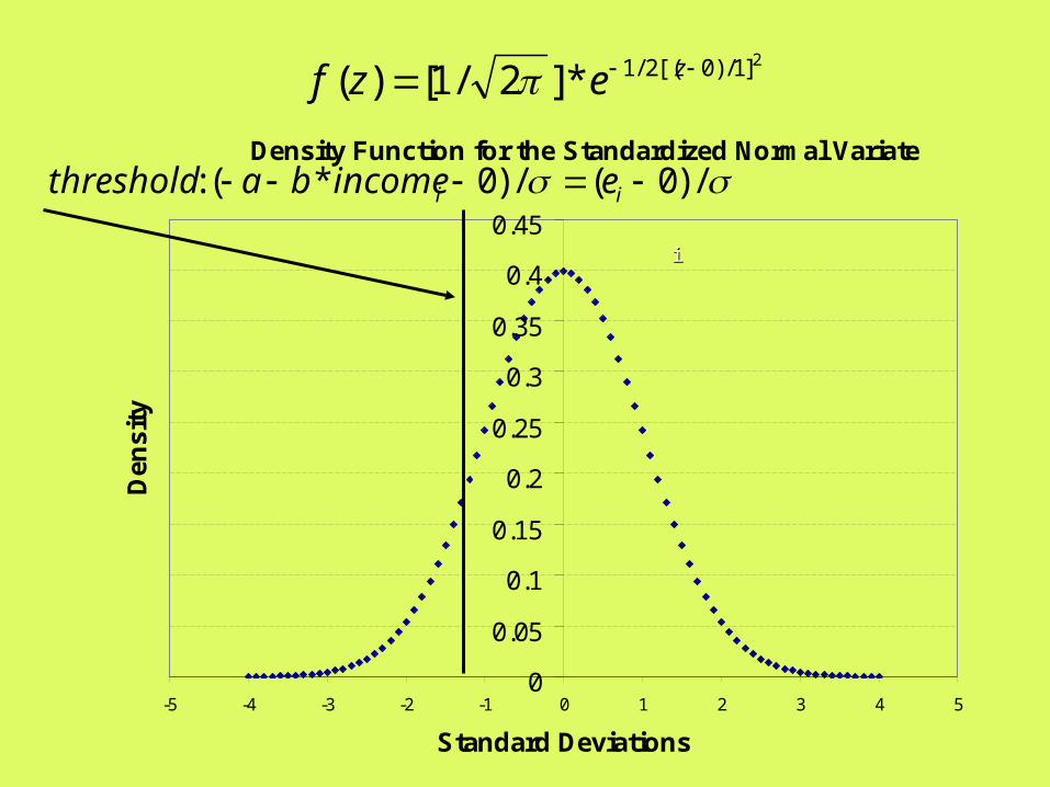
Density Function for the Standardized Normal Variate

0

0.05

0.1

0.15

0.2

0.25

0.3

0.35

0.4

0.45

-5 -4 -3 -2 -1 0 1 2 3 4 5

Standard Deviations

Den

sity

2]1/)0[(2/1*]2/1[)( zezf

ii

/)0(/)0*(: ii eincomebathreshold

Density Function for the Standardized Normal Variate

0

0.05

0.1

0.15

0.2

0.25

0.3

0.35

0.4

0.45

-5 -4 -3 -2 -1 0 1 2 3 4 5

Standard Deviations

Den

sity

2]1/)0[(2/1*]2/1[)( zezf

ii

/)0*(: iincomebathreshold

Area above the Area above the thresholdthresholdis the probability of is the probability of playing the lottery forplaying the lottery forobservation i, Pobservation i, Pyesyes

Density Function for the Standardized Normal Variate

0

0.05

0.1

0.15

0.2

0.25

0.3

0.35

0.4

0.45

-5 -4 -3 -2 -1 0 1 2 3 4 5

Standard Deviations

Den

sity

2]1/)0[(2/1*]2/1[)( zezf

ii

/)0*(: iincomebathreshold

Area above the Area above the thresholdthresholdis the probability of is the probability of playing the lottery forplaying the lottery forobservation i, Pobservation i, Pyesyes

PPno no for for

observation iobservation i

5050

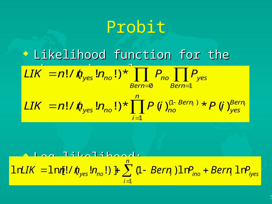
Probit

Likelihood function for the observed Likelihood function for the observed samplesample

Log likelihood:Log likelihood:

n

i

Bernyes

Bernnonoyes

Bern Bernyesnonoyes

ii iPiPnnnLIK

PPnnnLIK

1

)1(

0 1

)(*)(*)!!/(!

*)!!/(!

n

iiyesiinoinoyes PBernPBernnnnLIK

1

lnln)1()]!!/(!ln[ln

5151

incomeba

inoP*

2

2

)/]0)([2/1(

*

)/]0)([2/1(*

*]2/1[

*2/1

i

i

ii

e

incomebaiyes

eincomeba

ino

eP

eP

Density Function for the Standardized Normal Variate

0

0.05

0.1

0.15

0.2

0.25

0.3

0.35

0.4

0.45

-5 -4 -3 -2 -1 0 1 2 3 4 5

Standard Deviations

Den

sity

2]1/)0[(2/1*]2/1[)( zezf

ii

/)0*(: iincomebathreshold

Area above the Area above the thresholdthresholdis the probability of is the probability of playing the lottery forplaying the lottery forobservation i, Pobservation i, Pyesyes

PPno no for for

observation iobservation i

5353

Probit

Substituting these expressions for PSubstituting these expressions for Pno no and and

PPyes yes in the ln Likelihood function gives the in the ln Likelihood function gives the

complete expression.complete expression.

5454

Probit

Likelihood function for the observed Likelihood function for the observed samplesample

Log likelihood:Log likelihood:

n

i

Bernyes

Bernnonoyes

Bern Bernyesnonoyes

ii iPiPnnnLIK

PPnnnLIK

1

)1(

0 1

)(*)(*)!!/(!

*)!!/(!

n

iiyesiinoinoyes PBernPBernnnnLIK

1

lnln)1()]!!/(!ln[ln