Global Error versus Tolerance for ... - maths.ed.ac.uk

IMA Journal of Numerical Analysis (1991) 11, 457-480

Global Error versus Tolerance for Explicit Runge-Kutta Methods

DESMOND J. HIGHAM

Department of Computer Science, University of Toronto, Canada M5S1A4

Dedicated to Professor A. R. Mitchell on the occasion of his 70th birthday

[Received 3 August 1990 and in revised form 6 December 1990]

Initial value solvers typically input a problem specification and an error tolerance,and output an approximate solution. Faced with this situation many users assume,or hope for, a linear relationship between the global error and the tolerance. Inthis paper we examine the potential for such 'tolerance proportionality' in existingexplicit Runge-Kutta algorithms. We take account of recent developments in thederivation of high-order formulae, defect control strategies, and interpolants forcontinuous solution and first derivative approximations. Numerical examples areused to verify the theoretical predictions. The analysis draws on the work ofStetter, and the numerical testing makes use of the nonstiff DETEST package ofEnright and Pryce.

1. Introduction

WE are concerned with the numerical solution of the nonstiff initial valueproblem

y'(t)=f(t,y(t)), y(to) = yoeUN, to^t^tend. (1.1)

We assume that discrete numerical approximations are produced by a single'one-pass' integration with an s-stage explicit Runge-Kutta (RK) formula. Atypical step with such a formula advances the approximation vn_1«=y(fn_1) toyn~y{tn) according to

k1=f(tn_uyn_l),, 1 - 1 v

ki = /K- i + c,hn, yn-t + hn 2 OigkA, i = 2,...,s, (1.2)v /=i /

where hn := tn — tn_t is the local stepsize, and the fixed scalars {aip bit Cj}sij=1 are

the coefficients of the RK formula. In its simplest form, an 'implementation' ofthe RK formula is a method for choosing the stepsizes hn, and hence determiningthe mesh {tn}. This choice involves a trade-off between accuracy and computa-tional expense. Smaller stepsizes give greater accuracy, but larger stepsizes allowthe integration to be completed with fewer steps. For this reason, modern codes

Current address: Department of Mathematics and Computer Science, University of Dundee,Dundee DD14HN.

© Oxford University Press 1991

4 5 8 DESMOND J. HIGHAM

allow the user to supply a tolerance parameter, d, which gives an indication ofthe level of accuracy required. The codes then attempt to deliver a sufficientlyaccurate solution as efficiently as possible.

The fundamental measure of the error at each meshpoint tn is the global erroryn—y(tn). In general, it is not possible to keep the global error within aprescribed bound in a single integration. (Once we have strayed from the truesolution we begin to track a neighbouring, and possibly divergent solution curve.)Hence, codes normally control a locally based measure of the error, and socontrol the global error indirectly, in a problem-dependent manner. Perhaps thebest that we can ask in this situation is that if a fixed problem (1.1) is solvedrepeatedly over a 'reasonable' range of tolerance values, then the global errorshould decrease linearly with <5. Such behaviour is, of course, exactly what anoptimistic user would automatically expect. Following Stetter (1978, 1980) werefer to this characteristic as tolerance proportionality (TP). The aim of this workis to investigate the extent to which TP is likely to hold in modern RK codes. Wepay special attention to high-order formulas, defect control techniques, andcontinuous extensions (interpolants). In the remainder of this section we outlinethe error control techniques that are in current use.

On a particular step from tn_l to tn, the RK formula inherits the approximation}!„_, as a starting value. Hence the formula can be regarded as following the localsolution for the step zn(t), which is denned by

z'n{t)=f{t,zn{t)), zn(tH.1)=yH.1.

It is therefore useful to define the local error for the step,

We say that a formula has order p if p is the largest integer such that the localerror satisfies len = O{hp

n+X). Throughout this work we will suppose that the

numerical solution is advanced with a pth order formula. (We also assumewithout further comment that the problem (1.1) is sufficiently smooth.) A resultthat will be needed later is that the local error in a pth order formula has anexpansion of the form

len =/zr1V(%-i, rn-i) + W - 2 ) , (1-3)

where ip is a smooth function.Most of the error control techniques in existing codes attempt to ensure that

some measure of the local error is small on each step. If estn =£ S, where estn is ameasure of a local error estimate, then the step is accepted, otherwise the step isrepeated with a smaller stepsize hn. The error estimate can be obtained byadvancing from yn^ to yn with a subsidiary RK formula of a different order. Thequantity ||yn—>»n|| then gives an asymptotically correct approximation to thenorm of the local error in the lower-order formula. Some codes use estn =ll^n-yJI, while others use estn = \\yn -yn\\lhn. The former choice is callederror-per-step control, the latter error-per-unit-step. When the order of thesubsidiary formula is less than p, we are estimating the local error in yn whileadvancing with the higher-order approximation yn. This is normally referred to as

EXPLICIT RUNGE-KUTTA METHODS 459

local extrapolation. In the other case, when the subsidiary formula is of ordergreater than p, we are estimating the local error in the actual numerical solutionyn. There are thus four possible modes of local error control, which, followingShampine (1977), can be abbreviated to

EPS: No local extrapolation, error-per-step control.EPUS: No local extrapolation, error-per-unit-step control.XEPS: Local extrapolation, error-per-step control.XEPUS: Local extrapolation, error-per-unit-step control.

Each of the four modes has been used in practice. XEPS is arguably the mostpopular of the four, and is regarded as the most efficient (Shampine, 1977).

Usually the Euclidean or infinity norm is used in the computation of estn and,in general, the local error estimate will be premultiplied by a weighting matrixdiag {wf1} before the norm is taken. The extremes of w, = 1 and w, = id^n-ib +\yn\i) correspond to uniform absolute and uniform relative weights respectively.More general weighting schemes involve componentwise relative and absoluteweighting parameters RTOL, and ATOL,, which may be specified by the user.For example, the code DERKF (Shampine & Watts, 1979) uses

H>, = RTOLiKl^.jl, + \yn\i} + ATOL,.

A summary of the weighting types used in several popular codes is given inHigham & Hall (1989). It is clear that our concept of tolerance proportionalitymust include the assumption that the weighting parameters remain the same as <5varies.

In addition to the discrete numerical solution {yn}, it is frequently useful tohave available a continuous function q(t) which approximates y(t) over the range[fo,/end]. This can be done by augmenting the RK formula (1.2) with a'continuous extension' q(t) of the form

s

q{tn-l + xhn)=yn-l + xhn^Jbi(x)ki, r e (0 ,1], (1.4)

where each ft,(r) is a polynomial in x (see, for example, Dormand & Prince,1986; Enright etai, 1986; Higham, 1989ft; Shampine, 1985, 1986). (If s>s thenextra stages must be added to the basic RK formula.) The local approximationscan be joined together in a piecewise fashion to give a global approximation toy(t). Continuous extensions usually satisfy the conditions q{tn-\) = yn-\ andq{tn)=yn, and hence are referred to as interpolants. Modern interpolants alsomatch the derivative data at the meshpoints; that is,

q'(tn-i)=f(tn-l,yn-1) and q'(tn)=f(tn,yB),

in which case the corresponding global approximation is a C1 function. To assessthe accuracy of an interpolant, we say that q(t) has local order I if / is the largestinteger such that for any fixed x e [0 ,1]

q{tn^ + xhn) - zn{tn_x + xhn) = O(h'n).


The literature includes examples where l=p +1, so that the local errors in theformula and the extension have the same order, and others where / = p. We willuse the phrases 'higher order' and 'lower order' to distinguish between these twoclasses. For the latter class, since the global error in yn behaves like h^, wherehmax is the maximum stepsize, the global error in the discrete and continuousformulae should be compatible. Some consequences of the choice between/ =p + 1 and I =p will be discussed in later sections.

Given the availability of C1 approximations, Enright (1989a) suggested analternative to the local error control schemes described above (see also Enright,19896; Higham, 1989a, 19896, for further developments). The idea is to form aninterpolant and control a sample of the quantity

def (t)~q'(t)-f(t,q(t)),

which we call the defect in q(t). If we have an interpolant of local order /, andsample at a point tn_x + r*hn, for some fixed x* e (0 ,1), then the defect samplesatisfies

def (*„_! + T*hn) = hl-1*(yn-u f - i ) + O(h'n), (1.5)

where <P is a smooth function. For a general continuous extension, the shape ofthe defect depends upon the problem and hence max[0>1] ||def (tn_x + rhn)\\cannot be controlled by sampling at a single prechosen point. However,numerical tests (see, for example, Enright, 1989a) have shown that the maximumis very rarely more than ten times the sampled value, if the sample point iscarefully chosen. Special classes of interpolants were derived in Higham (1989a,19896) for which one sample gives an asymptotically correct estimate of themaximum defect. To obtain such a property, one must pay a rather high cost perstep in the formation of q(t).

In the next section we give some theoretical results relating the error controltechnique to the global errors in the discrete solution. The results are based onthose of Stetter (1978, 1980). Section 3 then summarizes some numerical testingof various error control strategies in conjunction with formula pairs of orders(3,4), (4,5), and (7,8). For these tests we make use of the nonstiff DETESTpackage (Enright & Pryce, 1987). In Section 4 we look at the way that the globalerrors in the continuous extensions vary with the tolerance. Predictions based onan asymptotic analysis are tested numerically. We consider the global errors inapproximations to the first derivative, both from the discrete data {f(tn, yn)} andthe continuous extensions, in Section 5. Again, we present numerical results totest the asymptotic theory. Finally, in Section 6 we summarize and discuss ourfindings.

2. Theoretical results

What local constraints on the stepsize are necessary/sufficient for the discretenumerical solution to exhibit tolerance proportionality? In this section wereorganize and slightly extend some results of Stetter (1978, 1980) that relate tothis question. To be specific, Theorem 2.1 below is contained in, and Theorems2.2 and 2.3 are extensions of, Theorem 1 of Stetter (1978). (We mention that the


0(6) term appearing in the statement of Theorem 1 of Stetter (1978) should be ano(hnd) term.) Corollaries 2.1 and 2.2 were outlined informally in Stetter (1980).Some related work on equivalent conditions for an approximate ODE solutioncan be found in Stewart (1970).

Before beginning an analysis, we must be clear about what we mean by TP fora discrete method. Since the location of the meshpoints {tn} will generally dependupon the tolerance, it does not make sense to ask for the 'global errors at themeshpoints' to decrease linearly with the tolerance. Instead, we should ask forthe existence of a continuous interpolant i](t) which passes through themeshpoint data {tn, yn} and satisfies i){t) — y(i)*=v{t)d, where v(t) is independ-ent of the tolerance 6. Note that r/(t) need not be computable, since we are onlyconcerned with the meshpoint approximation (in this section).

It is worth mentioning at this stage that the interpolant defined by

*?i(0==^(0 + ( f ~ / " " l ) l e . , f 6 (*„_,, 4,], (2.1)h

plays an important role in this work. Note that r]i(tn_1) = zn(tn_1)=yn_1 andViitn) = zn(tn) + len =yn> so we do indeed have a continuous interpolant throughthe mesh data. Following Stetter (1979) we will refer to f]\(f) as the idealinterpolant. (It is ideal in the sense that, asymptotically, its defect has the smallestpossible value on every step.) Note, however, that the first derivative of r\\{i) canbe discontinuous at each meshpoint.

In the following analysis we suppose that for any tolerance value b there existsa corresponding mesh {/„} for the RK solution. The proofs include the implicitassumption that the stepsizes tend to zero as 6—*0; that is, maxnhn = o(l) as6—»0. We restrict the phrase 'piecewise continuous' to mean continuous exceptpossibly at the meshpoints {tn}, and the phrase 'piecewise C1' to mean continuousover the whole range [t0, tend] with a first derivative which is continuous exceptpossibly at the meshpoints {tn}.

THEOREM 2.1 Given the initial value problem y'(t)-f(t,y(t)) = O, y(to)=y0,suppose r)(t) is piecewise C1 and satisfies r](to) = yo. Let e{t) := r){t)-y{t) denotethe global error in rj(t). Then the conditions A and B below are equivalent:

Condition A: e(t) = v(t)d +g(t), where v(t) is C1 and independent of d, andg(t) is piecewise C1 with zeroth and first derivatives of o(<5).

Condition B: r]'(t)—f(t,r)(t)) = Y(t)d+s(t), where y(t) is continuous andindependent of 6, and s(t) is piecewise continuous and o(6).

Proof. We introduce a third condition, C, and then prove thatand C=>A.

Condition C: e'(t)-fy(t, y(t))e(t) = y(t)S + u(t), where y{t) is the functionappearing in condition B, and u{t) is piecewise continuous and o(<5) + O{e(t)2).A=>B: We have

v'(t) -f(t, iKO) =/( ' ) + £'(0-fit, y(t) + e(0)

= v'(0 + e'(') - / (


where w(t) = O(e(t)2), and hence, from A, w(t) = o(6). Using A in this equationwe obtain

ri'(t) ~f(t, r,(t)) = 6[v'(t) -fy(t, y(t))v(t)] +g'(t) ~fy(t, y(t))g(t) + w(t),

which has the required form.B => C: Subtracting the original ODE, y\t) -f{t, y(t)) = 0, from B gives

*?'(') -y'C) - [/('. »?(<)) -fit, y{t))}

Using a Taylor expansion of f(t, r)(t)) =f(t, y(t) + e(r)) this becomes

eV) -fy(t, y(t))e(t) + w(t) = y(t)d+s(t),

where w(t) is piecewise continuous and O(e(t)2).C^> A: Let v(t) denote the unique solution to the linear initial value problem

v'(t) -fy(t, y(O)v(t) = y(0, v(t0) = o.

Then, from C, e(t) — 5v(t) satisfies

(e(0 - dv(tj)' -fy(t, y(t))(e(t) - Sv(t)) = u(t), e(t0) - 6v(t0) = 0.

Standard theory (see, for example, Ascher, Mattheij & Russell, 1988: p. 86)shows that this initial value problem has a solution of the form

- 6v(t) = Y(t) f Y-\n)u

where the fundamental solution matrix Y(t) is defined by

Y'(O=fy(t,y(t))Y{t), Y(to) = I.

Note that Y{t) is independent of <5. It follows that

e{t)-6v{t) = g{t),

where g(t) is o(<5) + O(e(t)2) and continuous, and g'(t) is o(8) + O(e(f)2) andpiecewise continuous, giving the desired result. •

Theorem 2.1 shows that TP as defined by A is equivalent to causing theinterpolant to solve a nearby system of differential equations. Asymptotically, thedifference between the original system and the nearby system must dependlinearly upon 6. Genuine TP also requires that the function v(t) in A should notbe everywhere zero. A glance at the proof of Theorem 2.1 shows that this will bethe case if y(f) # 0 in B. We should also note that A is quite a strong condition inthe sense that the first derivative of 77 (f) must also have a global error that varieslinearly with 6, and the limit function, v'{t), must be continuous. First derivativeglobal errors will be considered in Section 5.

We mentioned in the previous section that, ideally, the global error should varylinearly over the set of all 'reasonable' tolerances. Theorem 2.1 is an asymptoticresult (5 —» 0) and hence only comes into effect when 8 is sufficiently small (with'sufficiently small' being a problem-dependent concept). One purpose of thenumerical experiments described in the next section is to see the extent to which


useful practical conclusions can be drawn from this type of asymptotic analysis.The theorem also contains the implicit assumption that no rounding errors aremade in the computations—it is clear that with finite-precision arithmetic theglobal error cannot decrease indefinitely with 6.

THEOREM 2.2 If conditions A and B defined in Theorem 2.1 hold, then the localerror at each meshpoint satisfies

Proof. Let en(t) denote the local error in r]{t) over [tn-i,tn]; that is, en(t):=r)(t) — zn{t), where zn(t) is the local solution for the step. Condition B then saysthat

z'n(t) + e'n(t) -f(t, zn(t) + en(t)) = Y(t)6 + s(t), £„(*„_!) = 0.

Expanding the term/(f, zn{t) + en(t)), and noting that z'n{t) =f{t, zn(t)), we find

£'n(t) -fy(t, zn(t))en{t) = Y(t)6 + s(t), En(tn^) = 0,

where s(t) is piecewise continuous and o(<5) + O(en(t)2). We may replace zn(t)

with the true solution y(t) in the above expression to give

ett)-fy(t,y{t))eH(t) = Y(t)6 + s{t), eH(tn.l) = 0, (2.2)

where s(t) is o(8) + O(en(t)2). Our aim is to find an expression for en{tn) = len.

The solution of (2.2) at tn has the form (c.f. the proof of Theorem 2.1)

en(tn) = Y(O f Y-\t){y(t)d + s(t)} At,

where Y(t) is the fundamental solution matrix. Hence,

^ Y-\t)s(t)dt. (2.3)

A similar expression can be obtained for any t e (tn-\, tn), showing that en(t) isO(hn6) over [tn^, tn]. It follows that s(t) is o(d) and hence the second term onthe right-hand side of (2.3) is o(hn6). Since Y~1(t)y(t) is continuous, we have

Hence (2.3) becomes

as required D

We see from Theorem 2.2 that a consequence of TP (in the sense of A) is thateach component of the local-error-per-unit-step must depend linearly upon 5.Moreover, at each meshpoint the local-error-per-unit-step must be asymptoticallyequal to the same multiple of 6 as the defect.


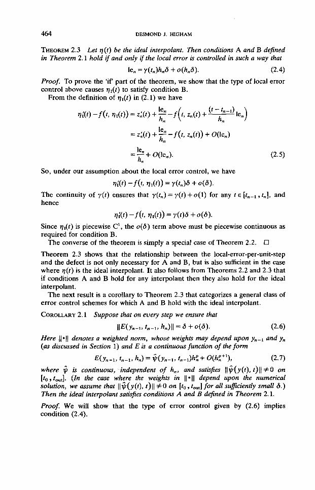
THEOREM 2.3 Let n(t) be the ideal interpolant. Then conditions A and B definedin Theorem 2.1 hold if and only if the local error is controlled in such a way that

lcn = y(tn)hnd+o(hnd). (2.4)

Proof. To prove the 'if part of the theorem, we show that the type of local errorcontrol above causes n^t) to satisfy condition B.

From the definition of rj^t) in (2.1) we have

rift) -f{t, !/,(/)) = z'n(t) + £=-/(*, zn{t) + ^ - ^ l e _ )hn \ hn I

= ^=+O(lea). (2.5)

So, under our assumption about the local error control, we have

The continuity of y(t) ensures that y{tn) = y(t) + o(l) for any t e [tn-i, tn], andhence

Since r\i(t) is piecewise C1, the o(5) term above must be piecewise continuous asrequired for condition B.

The converse of the theorem is simply a special case of Theorem 2.2. •

Theorem 2.3 shows that the relationship between the local-error-per-unit-stepand the defect is not only necessary for A and B, but is also sufficient in the casewhere r)(t) is the ideal interpolant. It also follows from Theorems 2.2 and 2.3 thatif conditions A and B hold for any interpolant then they also hold for the idealinterpolant.

The next result is a corollary to Theorem 2.3 that categorizes a general class oferror control schemes for which A and B hold with the ideal interpolant.

COROLLARY 2.1 Suppose that on every step we ensure that

\\E(yn-utn_l,hn)\\ = 6 + o(6). (2.6)

Here ||»|| denotes a weighted norm, whose weights may depend upon yn_x and yn

(as discussed in Section 1) and E is a continuous function of the form

E(yn-U *„_„ hn) = y(yn.u tH^)K + O(h"n+l), (2.7)

where %j> is continuous, independent of hn, and satisfies \\^>iy{t), t)\\ =£0 on[«0, /„„,]. (In the case where the weights in ||#|| depend upon the numericalsolution, we assume that ||V'(3'(0» Oil ̂ 0 o / l [lo»'ouj for all sufficiently small d.)Then the ideal interpolant satisfies conditions A and B defined in Theorem 2.1.

Proof. We will show that the type of error control given by (2.6) impliescondition (2.4).


From (2.7) we have

Now, as indicated in Section 1, the local error in the pth order Runge-Kuttaformula is known to satisfy

Using (2.8) this may be written

le -ib(v t

The local error control (2.6) then gives

We now have an expression for the local error that is almost of the form requiredby Theorem 2.3. A minor technicality is that the weighted norm ||»|| dependsupon the numerical solution and hence upon 6. However, if we define ||| • ||| tobe the corresponding weighted norm with true solution values ^(^- i) , y(tn),rather than yn-\,yn, appearing in the weights, then

III V(yn-i, tn-i) III = \\H>(yn-L tn.0\\ ( l + o(e('»-i)) + o(e(tn))),

where we recall that £(fn~i) = yn-i-y(tn-i) and e(tn) = yn-y{tn). Since thestepsizes tend to zero as 6 —* 0, it follows from standard theory (see, for example,Hairer, N0rsett, & Wanner, 1987: Thm 3.4, p. 160) that the global error alsotends to zero as <5 —* 0. So

lf *„_,) HI = \\j>(yn-lt tn^Hence, from (2.9),

III W\yn-l> ln-l) III

The continuity of V and y allows us to replace yn_! and fn_i by y(tn) and /„respectively in the right-hand side of (2.10). Now it is clear from (2.6) and (2.7)that an O(hp

n+2) term must also be O(h2

nd) and hence must be o{hn8). Thus (2.4)holds with Y(t) = rj>(y(t), t)l ||| %(y(f), t) |||. D

Roughly, the corollary tells us that we can achieve A by controlling a smoothlyvarying O(h%) quantity on every step. Considering local error control, the EPUSmode has estn := H^ —%\\lhn = O(h%), and if we are in the usual situation wherethe two formulae in the RK pair have orders that differ by one, then XEPS givesestn := ||yn —yn\[ = O(h%). In both cases it follows from (1.3) that the local errorestimate has an expansion of the form (2.7). Also, defect control based on ahigher order interpolant has estn = O(h'~l) = O(h1) and (1.5) gives the requiredexpansion.


The condition (2.6) is satisfied when the standard asymptotically based stepsizeselection formula is used. After a step from tn-x to tn_r + hn, the formula is

hnev/ — dhopt, hop,— I——I hn. (2.11)

Here hopt is the asymptotically optimal stepsize, and the constant safety factor6 6 (0,1) is introduced to reduce the chance of the step being rejected. Theformula can be used to compute a new stepsize after a successful step, or after arejected step. (In the latter case some authors favour a more crude strategy suchas halving the stepsize.) Strictly, (2.11) implies that estn = dp8 + o(6), so wemust interpret \\E(yn^u tn_lt hn)\\ in (2.6) as 6~p estn. We then have thefollowing corollary.

COROLLARY 2.2 Suppose that one of the following error control modes is used

(i) EPUS(ii) XEPS with a (/? — l)th and pth order pair of formulae

(iii) defect control with a higher-order interpolant

with stepsize selection based on the formula (2.11). Then, provided that xj> in (2.7)satisfies \\^{y(t),t)\\ ^ ^ on t'o»'out] for QH sufficiently small 8, and the initialstepsize is chosen so that (2.6) holds on the first step, the ideal interpolant satisfiesconditions A and B defined in Theorem 2.1.

Each of the three error control modes listed in Corollary 2.2 will be implementedin the numerical tests of the next section.

As a final point, we mention that some nonasymptotic theory that is relevantfor stiff and mildly stiff initial value problems was developed by Hall (1985, 1986)and by Hall & Higham (1988) and Higham & Hall (1989). This analysis givesalgebraic conditions involving the RK coefficients and the dominant eigenvalue(s)of the local Jacobian for determining whether or not a smooth stepsize sequencewill arise. The same conditions also determine whether or not TP will beobserved.

3. Discrete formulae

In this section we describe numerical tests on a variety of discrete RK formulaeand error control techniques. The following formula pairs were tested: a 3,4 pairof N0rsett that appears in Enright et al. (1986), the 4,5 pair RK5(4)7FM ofDormand & Prince (1980), and a 7,8 pair of Sharp & Smart (1989). Each pair wasimplemented in EPUS and XEPS mode. We also tested two defect controltechniques based on the 4,5 pair. The first one uses the locally O(h%)Dormand-Prince-Shampine (DPS) interpolant of Shampine (1986). This inter-polant is constructed in such a way that the defect is always zero at the midpointof a step, hence r* = \ should not be used as a sample point. It is also reasonableto ask for the sampled value to reflect the maximum size of the defect over thestep. Although, in general, the shape of the defect will depend on the differential


equations and will vary from step to step, in Higham (1990: Appendix B) we usean asymptotic expansion of the defect to justify the choice T* = 0-87832. Thesecond defect control scheme that we tested is based on the more expensivelocally O(h6

n) Hermite-Birkhoff (HB) interpolant from Higham (1989ft). In thiscase the sample point r* = 0-89994 is guaranteed to control the maximum defect,asymptotically.

For stepsize selection, we used the formula (2.11) with a safety factor of 0-9,subject to the restriction

old - = 5hM.

The final stepsize was further restricted so that the endpoint /end was reachedexactly.

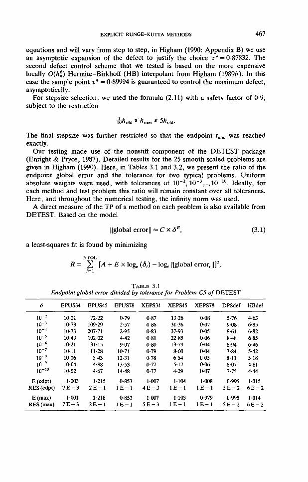
Our testing made use of the nonstiff component of the DETEST package(Enright & Pryce, 1987). Detailed results for the 25 smooth scaled problems aregiven in Higham (1990). Here, in Tables 3.1 and 3.2, we present the ratio of theendpoint global error and the tolerance for two typical problems. Uniformabsolute weights were used, with tolerances of 10~2,10~3,..., 1O"10. Ideally, foreach method and test problem this ratio will remain constant over all tolerances.Here, and throughout the numerical testing, the infinity norm was used.

A direct measure of the TP of a method on each problem is also available fromDETEST. Based on the model

Uglobal error|| «

a least-squares fit is found by minimizing

NTOL£xloge(<5,)-loge Uglobal error, |

(3.1)

TABLE 3.1Endpoint global error divided by tolerance for Problem C5 of DETEST

6

lO"2

10"3

lO"4

io-5

10"6

io-7

10~8

io-9

10-io

E (edpt)RES (edpt)

E(max)RES (max)

EPUS34

10-2110-7310-7310-4310-2110-11100610041002

1-0037E-3

10017E-3

EPUS45

72-22109-29207-71102-0231-1511-285-434-884-67

1-2152 E - 1

1-2182 E - 1

EPUS78

0-792-572-954-429-07

10-7112-3113-5314-48

0-8531 E - 1

0-8531 E - 1

XEPS34

0-870-860-830-810-800-790-780-770-77

10074E-3

1-0075E-3

XEPS45

13-2631-3637-9322-8513-798-606-545-174-29

1-1041 E - 1

11031 E - 1

XEPS78

0-080070050060040040-05006007

1-0081 E - 1

0-9791 E - 1

DPSdef

5-769088-618-488-947-848-118077-75

0-9955E-2

0-9955E-2

HBdef

4-636-856-826-856-465-425-184-814-44

10156E-2

10146E-2


TABLE 3.2Endpoint global error divided by tolerance for Problem E4 of DETEST

6

10"2

10"3

io-4

io-5

10~6

io-7

10"8

lO"9

10-io

E (edpt)RES (edpt)

E(max)RES (max)

EPUS34

3-152-012-732-722-953-243-263-313-32

0-9845E-2

0-9973E-2

EPUS45

0-200-432-271-782-522-352-522-712-88

0-8792 E - 1

0-9202 E - 1

EPUS78

3-404-270-650-821-901-611191-321-55

10352 E - 1

1-0351 E - 1

XEPS34

Oil0-090-110-120-130140140-14014

0-9783E-2

0-9934E-2

XEPS45

0010-04003007010014016018019

0-8551 E - 1

0-9102 E - 1

XEPS78

0-06001000001001002004008009

0-9143 E - 1

0-9942 E - 1

DPSdef

001

on1-230-310-820-410-500-520-52

0-8704 E - 1

0-9256 E - 1

HBdef

0010-830-151-640-780-800-730-810-76

0-8575 E - 1

0-9223 E - 1

where 5it i = 1,..., NTOL, is the range of tolerances used. The values of theproportionality constant C := exp (A), the exponent E, and the root mean squareresidual RES := (i?/NTOL)5 are returned. A method which comes close toexhibiting TP will have an exponent E = 1 and a small residual RES. Tables 3.1and 3.2 also include the exponent and residual values for both the endpoint globalerror (edpt) and the maximum global error over all meshpoints (max). Althoughit is clear that asking for linear proportionality of the norm of the endpoint ormaximum global errors is a weaker requirement than A in Theorem 2.1, theDETEST results will certainly give insights into the likelihood of a condition suchas A being satisfied.

Based on Tables 3.1 and 3.2, and the more detailed results in Higham (1990),we make the following observations on the ratio of the endpoint global error andthe tolerance:

(i) On all problems the ratio improves (varies less) as the tolerance decreases.Typically the behaviour is poor for 8 ^ 10~4, although the 5 for which theratio begins to settle down depends on the method and the problem.

(ii) For both the EPUS and XEPS modes the relative performance worsens asthe order increases—the lower-order methods exhibit better propor-tionality over a wider range of tolerances.

(iii) For each method and almost all problems, the ratio varies by less than afactor of 1-5 at the most stringent tolerances.

(iv) The performance of the defect control methods DPSdef and HBdef issimilar to that of the XEPS45 method. (Note that these methods advancewith the same RK formula while controlling different 0(/i;j) quantities.)

The first observation is not surprising, given the asymptotic nature of theanalysis in the previous section. With regard to the second observation, Stetter(1980) notes that if an O(h%) quantity is controlled by 8, then the stepsize hn will


decrease like O{5Vp). So, in the proofs that lead up to Corollary 2.2, discardingterms with an extra factor of hn is likely to be much less realistic than discardingterms with an extra factor of 6, and the theory becomes less meaningful as theorder p increases. In fact many of the DETEST problems are quite 'easy' in thesense that they are integrated with very few steps, even at quite stringenttolerances. For example, on problem E5 for 6 2= 10~6, all methods required lessthan 35 steps. (The range of integration is [0,20] for each DETEST problem.)As we would expect, the stepsizes used for a given problem and tolerance tend toincrease with the order of the error estimate estn. On B2 at 6 = 10~8, forexample, the XEPS34 method uses 267 steps while XEPS78 uses a mere 23.

An interesting side issue that is worth mentioning is the variation of the globalerror across different methods for a fixed problem and tolerance. Some insightcan be gained by examining the proofs of Theorems 2.1 and 2.2. If condition A ofTheorem 2.1 holds, then v(t) solves

v'(t)-f,(t,y(t))v(t) = Y(t), v(to) = 0. (3.2)

The right-hand side y{t) is closely related to the local-error-per-unit-step, \enlhn.Theorem 2.2 tells us that, at each meshpoint, y(t)d and \en/hn are asymptoticallyequal. However, it is important to note that y(t): U—*RN is a vector-valuedfunction of t in general. Hence, even if two different methods both keep the normof len/hn equal to 6 on each step, the individual components may have differentsigns and magnitudes, and hence the solutions v(t) of (3.2) will not necessarily beclose. On the other hand, it can be argued that, of the different error controltypes, EPUS should be the most 'method-insensitive' since with other strategies a/-dependent multiple of the local-error-per-unit-step is controlled, and hence y(t)has a much greater degree of freedom. This is borne out in the results; thevariation across the columns is generally less dramatic with EPUS than withXEPS.

4. Interpolants

We now turn our attention to the use of interpolants to provide continuousapproximations to y{t). The first question that we ask is whether any of thestandard interpolants can satisfy condition B (and hence condition A) of Theorem2.1. The answer is no for any of the C1 schemes that satisfy q'{tn) =f(tn, yn). Forsuch schemes the defect is forced to be zero at the meshpoints, and since thelocation of the meshpoints varies with 6, condition B cannot hold. Morespecifically, for t = tn_1 + xhn e {tn-i, tn] any continuous extension of the form(1.4) has a local error of the form

q(tn.t + xhn) - zn(tn-x + rhn) = h'n2 a^x)F,{tn.u yn_{) + O(h'+1), (4.1)

and a defect of the form

*'(*„_, + xhn) - /(<„_! + xhH, <?(/„-! + xhn)) = h1'1 2 aj(x)F,(tn_u >>„_,) + O(h').7 = 1

(4.2)


Here Fj(tn^, yn-t) is an elementary differential of /, and ay(r) is a scalarpolynomial that is independent of/. Because of the presence of the aj(r) factors,the value of the defect at the point t will depend on the relative location of t andthe meshpoints tn-i, tn. Again, since the mesh varies with 6, condition B cannotbe satisfied. Although this is discouraging, it is not the whole story, sinceTheorem 2.1 asks for proportionality of the global error in the interpolant and itsfirst derivative. As we show below, useful results about the global error can beobtained by comparing q(t) with Jj^f).

We suppose now that an error control of the type defined in Corollary 2.1 isused, so that the ideal interpolant satisfies

r / l(0-y(0 = "(0<5+g(0. (4-3)with v(t) and g(t) as in Theorem 2.1. For t e (fn_i, tn], it is helpful to split theglobal error in q{t) into three parts:

q(t)-y{t) = [q{t) - zn(t)] - [11,(0 - zn(t)} + [ij,(0 -y(t)]. (4.4)

We have #(0 - zn(t) = O(h'n) for the local error in q{t), where l=p + 1 or l=pdepending upon whether q(i) is chosen to be higher or lower order (see Section1). The local error in r/,(f) satisfies

ij,(0 - zn(t) = O(len) = O{K+x) = O(hn8) = o(6).

Hence (4.4) may be written

q(t) - y(t) = v(t)6 + o{6) + O(h'n). (4.5)

If <j(0 is higher order then the O(h'n) term is o(d), so that (4.5) becomes

q(t)-y(t) = v(t)6+o(6), (4.6)

showing that q(i) inherits the same proportionality as Jji(O- (Note that (4.6) isweaker than condition A, since A asks for g'(i) to be o{6).) A lower-orderinterpolant contributes an O{hp

n) = O(8) term in (4.5), and hence v(t)d will notnecessarily dominate. In this case the relative sizes of the [q(t) — zn(t)\ local errorterm and the \*li{t) — y(t)\ global error term in (4.4) will depend upon thedifferential equations. The expansion (4.1) shows that the local error term has ahighly mesh-dependent nature. Hence in general we cannot deduce a result of theform (4.6) for a lower-order interpolant.

To investigate the behaviour of interpolation schemes in practice, we per-formed numerical tests on four interpolants that have been derived for theDormand-Prince RK5(4)7FM pair. We used lower-order (locally O(h5

n)) inter-polants from Dormand & Prince (1986) and Shampine (1986), and higher-order(locally 0(/i*)) interpolants from Higham (19896) and Shampine (1986), denotedDF[O(h% DPS[0(/i5)], HB[O(h6)], and DPS[O(ft6)] respectively. The 4,5 pairwas implemented in XEPS mode and, by partitioning each basic RK step into 10equally spaced substeps, we used DETEST to compute

f mmax i max

EXPLICIT RUNGE-KUTTA METHODS 4 7 1

TABLE 4.1Maximum global error divided by tolerance for Problem C5 of

DETEST

8

10"2

lO"3

io-4

io-5

10"6

lO"7

1O"8

io-9

io-10

ERES

DP[0(/»5)]

17-9631-1224-4621-2713-118-836-635-414-59

1-1031-1E-1

DPS[O(/i5)]

17-9631-1224-4621-2713-118-836-595-374-55

11031-1E-1

DPS[O(/i6)]

17-96311224-4621-2713-118-126-375144-32

1-1071-1E-1

HB[0(/i6)]

17-96311224-4621-1713-118-126-385154-32

1-1071 - l E - l

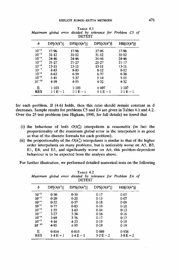
for each problem. If (4.6) holds, then this ratio should remain constant as 5decreases. Sample results for problems C5 and E4 are given in Tables 4.1 and 4.2.Over the 25 test problems (see Higham, 1990, for full details) we found that

(i) the behaviour of both O(hf,) interpolants is reasonable (in fact theproportionality of the maximum global error in the interpolant is as goodas that of the discrete formula for each problem);

(ii) the proportionality of the O{h5^) interpolants is similar to that of the higherorder interpolants on many problems, but is noticeably worse on A5, B3,El , E4, and E5, and significantly worse on A4; this problem-dependentbehaviour is to be expected from the analysis above.

For further illustration, we performed detailed numerical tests on the following

TABLE 4.2Maximum global error divided by tolerance for Problem E4 of

DETEST

sio-2

lO"3

io-4

io-5

10~6

io-7

io-8

lO"9

io-0

ERES

DP[O(h5)]

0-300-200-520-771-553-273-694-164-95

0-8141-4E-1

DPS[O(/i5)]

0-300-200-570-831-633-363-764-234-95

0-8151-4E-1

DPS[O(h6)]

0-170130180190140160-17019019

0-9895-2E-2

HB[O(h6)]

0070070090100130160-17019019

0-9383-8E-2


problems

(1) A problem of Fehlberg (see Hairer, N0rsett, & Wanner, 1987: p. 174):

y[ = 2tyx log [max (y2, KT3)], j>,(0) = 1,

y'2 = 2ty2 log [max (y1; 10"3)], y2(0) = e, 0 =£t« 5,

which has solution _y, = exp (sin t2), y2 = exp (cos t2).(2) Problem A4 (unsealed) from Enright & Pryce (1987):

for which

20y = 1 + 19 exp (-10

We present results for a uniform absolute weighting scheme; experiments withother weighting schemes gave similar qualitative results. As a point of reference,we plot the norm of the meshpoint global error, scaled by 8, for tolerances of10~\ 10~6, 10~8, and 10~10 in Figs 1 and 4. In both cases the global error ratioconverges to a discernible limit function.

The corresponding global errors in the higher- and lower-order interpolants ofShampine (1986) are plotted in Figs 2,3,5, and 6. These were generated byevaluating the global error at 100 equally spaced points in the interval ofintegration. For the higher-order interpolant, we see that on the Fehlbergproblem the global error ratios have almost exactly the same shape as for thediscrete solution. On problem A4, the curves are somewhat 'wobbly', but thebehaviour improves as the tolerance decreases. The proportionality of thelower-order interpolant is comparable with that of the discrete formula on theFehlberg problem, but is slightly erratic over the first part of the integration. Onproblem A4, however, the lower-order interpolant behaves very poorly; althoughthe global error ratios remain bounded, they are not smooth and do not appear toapproach a limit as 6 decreases.

The behaviour of the lower-order interpolant on these two problems can beexplained by looking at the actual size of the global errors. On the Fehlbergproblem, the global error in the lower-order interpolant is the same size as that ofthe meshpoint solution, which shows that of the two O(d) terms [r?i(f) — y(t)] and\q(t) — zn(t)] in (4.4), the first term is dominating in the plots. On problem A4 themeshpoint global error is never more than 1.56, and the [q(t) — zn(t)] term clearlytakes over in Fig. 6. We also mention that fairly large stepsizes are used onproblem A4—only 9, 19, 45, and 108 steps are needed at 6 = KT4, 10~6, NT8,and 1O~10 respectively. Thus, with the higher-order interpolant, we would expectthe O(hn6) term [q{t) — zn{t)\ in (4.4) to be significant, even at quite stringenttolerances—this is what appears to be happening in Fig. 5.

Although carried out for a different purpose, numerical testing of severallower- and higher-order interpolants was performed in Enright et al. (1986).There the authors used DETEST to compare the maximum global error in aninterpolant with the maximum global error in the underlying discrete RK method.

FIG. 1. Fehlberg problem: tolerances I E - 4 , I E - 6 , 1 E - 8 , I E -10 (lines become more solid as tolerance decreases).

tn

3

FIG. 2. Fehlberg problem, higher-order interpolant: tolerances 1 E - 4,I E - 6 , I E — 8, I E —10 (lines become more solid as tolerancedecreases).

1

FIG. 3. Fehlberg problem, lower-order interpolant: tolerances 1 E - 4,I E - 6 , I E - 8 , I E - 1 0 (lines become more solid as tolerancedecreases).

1.5-

1.75

global error/tolerance

I -

global error/lolerance

.5-

10t

15 20

FIG. 4. Problem A4: tolerances 1 E - 4, 1 E - 6, 1 E - 8, 1 E - 10(lines become more solid as tolerance decreases).


0

FIG. 5. Problem A4, higher-order interpolant: tolerances 1 E - 4,I E - 6 , 1 E - 8 , I E - 1 0 (lines become more solid as tolerancedecreases).

Dmin

IOX

5

0

FIG. 6. Problem A4, lower-order interpolant: tolerances 1 E — 4,1 E — 6, 1 E - 8, 1 E — 10 (lines become more solid as tolerancedecreases).


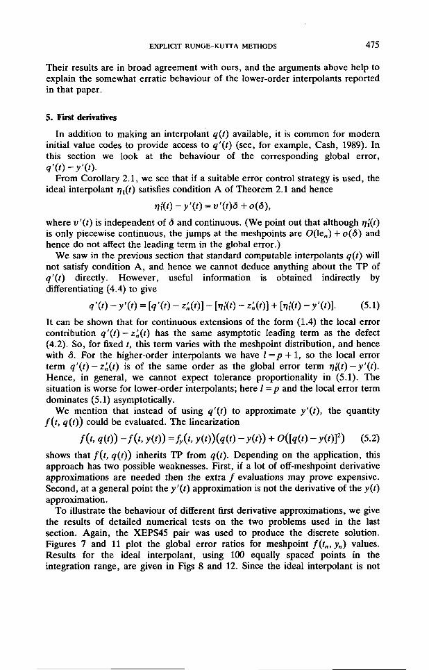
Their results are in broad agreement with ours, and the arguments above help toexplain the somewhat erratic behaviour of the lower-order interpolants reportedin that paper.

5. First derivatives

In addition to making an interpolant q(t) available, it is common for moderninitial value codes to provide access to q'{t) (see, for example, Cash, 1989). Inthis section we look at the behaviour of the corresponding global error,

From Corollary 2.1, we see that if a suitable error control strategy is used, theideal interpolant r\i(t) satisfies condition A of Theorem 2.1 and hence

where v'(t) is independent of 6 and continuous. (We point out that although rji(Ois only piecewise continuous, the jumps at the meshpoints are O(len) + o(<5) andhence do not affect the leading term in the global error.)

We saw in the previous section that standard computable interpolants q(i) willnot satisfy condition A, and hence we cannot deduce anything about the TP ofq'(t) directly. However, useful information is obtained indirectly bydifferentiating (4.4) to give

q'{t)-y'{t) = [q'{t) - z'n(t)] - [r,i(t) - z'n(t)] + fo,'(0 - / ( ' ) ] • (5-1)

It can be shown that for continuous extensions of the form (1.4) the local errorcontribution q'{t) — z'n(i) has the same asymptotic leading term as the defect(4.2). So, for fixed t, this term varies with the meshpoint distribution, and hencewith 6. For the higher-order interpolants we have l=p + 1, so the local errorterm q'(t)-z'n(t) is of the same order as the global error term r\[(t) — y'(t).Hence, in general, we cannot expect tolerance proportionality in (5.1). Thesituation is worse for lower-order interpolants; here I =p and the local error termdominates (5.1) asymptotically.

We mention that instead of using q'{t) to approximate y'(t), the quantityf(t, q(t)) could be evaluated. The linearization

/('> <?(')) - / ( ' , y(t)) =f,{t, y(t))(q(t) - y(0) + O([q(t) - y(0]2) (5.2)

shows that f(t, q(t)) inherits TP from q(t). Depending on the application, thisapproach has two possible weaknesses. First, if a lot of off-meshpoint derivativeapproximations are needed then the extra / evaluations may prove expensive.Second, at a general point the y'(t) approximation is not the derivative of the y(t)approximation.

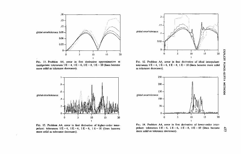
To illustrate the behaviour of different first derivative approximations, we givethe results of detailed numerical tests on the two problems used in the lastsection. Again, the XEPS45 pair was used to produce the discrete solution.Figures 7 and 11 plot the global error ratios for meshpoint f(tn, yn) values.Results for the ideal interpolant, using 100 equally spaced points in theintegration range, are given in Figs 8 and 12. Since the ideal interpolant is not


3 0 0 -

FIG. 7. Fehlberg problem, error in first derivative approximation atmeshpoints: tolerances I E — 4, I E — 6, I E — 8, IE— 10 (lines becomemore solid as tolerance decreases).


FIG. 9. Fehlberg problem, error in first derivative of higher-orderinterpolant: tolerances 1 E - 4, 1 E - 6, 1 E - 8, 1 E - 10 (lines becomemore solid as tolerance decreases).

2 0 0 -


100-

FIG. 8. Fehlberg problem, error in first derivative of ideal interpolant: E5t o l e r a n c e s I E - 4 , I E - 6 , I E - 8 , I E - 1 0 ( l i n e s b e c o m e m o r e s o l i d 1as tolerance decreases). Z

1500-

1000-


500

Xo>

FIG. 10. Fehlberg problem, error in first derivative of lower-orderinterpolant: tolerances 1 E - 4, 1 E - 6, 1 E - 8, 1 E - 10 (lines becomemore solid as tolerance decreases).

.18

.15 -

.12-

global error/tolerance 0.09 -

0.06-

0.03-

0

. 2 -

0

FIG. 11. Problem A4, error in first derivative approximation atmeshpoints: tolerances I E - 4 , I E - 6 , I E - 8 , I E - 1 0 (lines becomemore solid as tolerance decreases).

.15-

global error/lolerance.1 -

0.05

FIG. 12. Problem A4, error in first derivative of ideal interpolant:tolerances I E — 4, I E — 6, I E - 8 , IE— 10 (lines become more solidas tolerance decreases).

rn

jo

otn


0

FIG. 13. Problem A4, error in first derivative of higher-order inter-polant: tolerances I E - 4 , I E - 6 , I E - 8 , I E - 1 0 (lines becomemore solid as tolerance decreases).


0

FIG. 14. Problem A4, error in first derivative of lower-order inter-polant: tolerances I E - 4 , I E - 6 , I E - 8 , I E - 1 0 (lines becomemore solid as tolerance decreases).

1OO


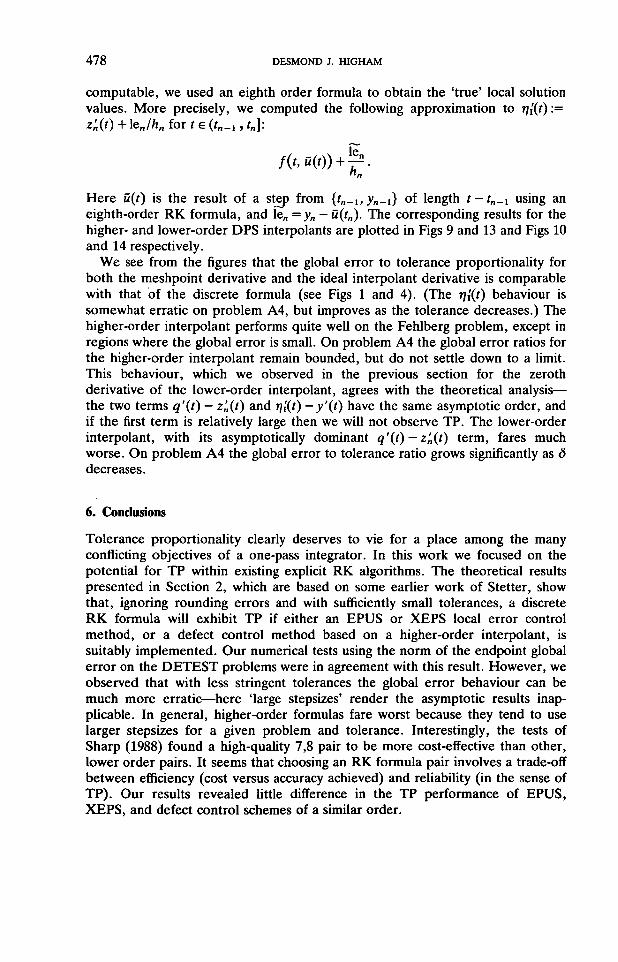
computable, we used an eighth order formula to obtain the 'true' local solutionvalues. More precisely, we computed the following approximation to ij/(f) :=

Here u{i) is the result of a step from {tn-i,yn-i} of length t — tn_1 using aneighth-order RK formula, and len = yn — u(tn). The corresponding results for thehigher- and lower-order DPS interpolants are plotted in Figs 9 and 13 and Figs 10and 14 respectively.

We see from the figures that the global error to tolerance proportionality forboth the meshpoint derivative and the ideal interpolant derivative is comparablewith that of the discrete formula (see Figs 1 and 4). (The r\{{t) behaviour issomewhat erratic on problem A4, but improves as the tolerance decreases.) Thehigher-order interpolant performs quite well on the Fehlberg problem, except inregions where the global error is small. On problem A4 the global error ratios forthe higher-order interpolant remain bounded, but do not settle down to a limit.This behaviour, which we observed in the previous section for the zerothderivative of the lower-order interpolant, agrees with the theoretical analysis—the two terms q'{t) — z'n{t) and r\[(t) — y'(t) have the same asymptotic order, andif the first term is relatively large then we will not observe TP. The lower-orderinterpolant, with its asymptotically dominant q'{i) — z'n(t) term, fares muchworse. On problem A4 the global error to tolerance ratio grows significantly as 5decreases.

6. Conclusions

Tolerance proportionality clearly deserves to vie for a place among the manyconflicting objectives of a one-pass integrator. In this work we focused on thepotential for TP within existing explicit RK algorithms. The theoretical resultspresented in Section 2, which are based on some earlier work of Stetter, showthat, ignoring rounding errors and with sufficiently small tolerances, a discreteRK formula will exhibit TP if either an EPUS or XEPS local error controlmethod, or a defect control method based on a higher-order interpolant, issuitably implemented. Our numerical tests using the norm of the endpoint globalerror on the DETEST problems were in agreement with this result. However, weobserved that with less stringent tolerances the global error behaviour can bemuch more erratic—here 'large stepsizes' render the asymptotic results inap-plicable. In general, higher-order formulas fare worst because they tend to uselarger stepsizes for a given problem and tolerance. Interestingly, the tests ofSharp (1988) found a high-quality 7,8 pair to be more cost-effective than other,lower order pairs. It seems that choosing an RK formula pair involves a trade-offbetween efficiency (cost versus accuracy achieved) and reliability (in the sense ofTP). Our results revealed little difference in the TP performance of EPUS,XEPS, and defect control schemes of a similar order.


New results for continuously extended RK formulae were also presented. Weshowed that the approximations generated by 'higher order' interpolants (whoselocal errors have the same asymptotic order as the RK formula) automaticallyinherit the asymptotic TP properties of the discrete method. The same cannot besaid for 'lower order' interpolants; here the local errors have an unpredictableproblem-dependent effect on the global error proportionality.

The situation is worse when first derivative approximations are required. In thiscase higher-order interpolants cannot be guaranteed to behave smoothly, andlower order interpolants will never achieve TP, asymptotically. A simple, butpotentially expensive fix is to evaluate / along the interpolant.

Acknowledgements

This paper benefited from the comments of Nick Higham, Ken Jackson andPhilip Sharp. The author was supported in this work by the InformationTechnology Research Centre of Ontario and the Natural Science and EngineeringResearch Council of Canada.

REFERENCES

ASCHER, U. M., MATTHEU, R. M. M., & RUSSELL, R. D. 1988 Numerical Solution ofBoundary Value Problems for Ordinary Differential Equations. New Jersey: Prentice-Hall.

CASH, J. R. 1989 A block 6(4) Runge-Kutta formula for nonstiff initial value problems.ACM Trans. Math. Soft. 15, 15-28.

DORMAND, J. R., & PRINCE, P. J. 1980 A family of embedded Runge-Kutta formulae. / .of Computational and Applied Maths. 6, 19-26.

DORMAND, J. R., & PRINCE, P. J. 1986 Runge-Kutta triples. Comp. and Maths, withAppls. 12, 1007-1017.

ENRIGHT, W. H. 1989a A new error-control for initial value solvers. Applied Maths, andComputation 31, 288-301.

ENRIGHT, W. H. 1989b Analysis of error control strategies for continuous Runge-Kuttamethods. SIAM J. Numer. Anal. 26, 588-599.

ENRIGHT, W. H., & PRYCE, J. D. 1987 Two FORTRAN packages for assessing initialvalue methods. ACM Trans. Math. Soft. 13, 1-27.

ENRIGHT, W. H., JACKSON, K. R., NORSETT, S. P., & THOMSEN, P. G. 1986 Interpolantsfor Runge-Kutta formulas. ACM Trans. Math. Soft. 12, 193-218.

HAIRER, E., NORSETT, S. P., & WANNER, G. 1987 Solving Ordinary DifferentialEquations I. Berlin: Springer-Verlag.

HALL, G. 1985 Equilibrium states of Runge-Kutta schemes. ACM Trans. Math. Soft. 11,289-301.

HALL, G. 1986 Equilibrium states of Runge-Kutta schemes: part II. ACM Trans. Math.Soft. 12, 183-192.

HALL, G., & HIGHAM, D. J. 1988 Analysis of stepsize selection schemes for Runge-Kuttacodes. IMA J. Numer. Anal. 8, 305-310.

HIGHAM, D. J. 1989a Robust defect control with Runge-Kutta schemes. SIAM J. Numer.Anal. 26, 1175-1183.

HIGHAM, D. J. 1989b Runge-Kutta defect control using Hermite-Birkhoff interpolation.Technical Report No. 221/89, Department of Computer Science, University ofToronto; to appear in SIAM J. Sci. Stat. Comput.


HIGHAM, D. J. 1990 Global error versus tolerance for explicit Runge-Kutta methods.Technical Report No. 233/90, Department of Computer Science, University ofToronto.

HIGHAM, D. J., & HALL, G. 1989 Runge-Kutta equilibrium theory for a mixed-relative/absoute error measure. Technical Report No. 218/89, Department ofComputer Science, University of Toronto; to appear in the Proceedings of the 1989IMA Conference on Computational ODEs (J. R. Cash and I. Gladwell, Eds).

SHAMPINE, L. F. 1977 Local error control in codes for ordinary differential equations.Applied Maths, and Computation 3, 189-210.

SHAMPINE, L. F. 1985 Interpolation for Runge-Kutta methods. SIAM J. Numer. Anal. 22,1014-1027.

SHAMPINE, L. F. 1986 Some practical Runge-Kutta formulas. Math. Comp. 46, 135-150.SHAMPINE, L. F., & WATTS, H. A. 1979 DEPAC—Design of a user oriented package of

ODE solvers. Report SAND79-2374, Sandia National Laboratories, Albuquerque,New Mexico.

SHARP, P. W. 1988 Numerical comparisons of explicit Runge-Kutta pairs of orders fourthrough eight. Technical Report 216/88, Department of Computer Science, Univers-ity of Toronto; to appear in ACM Trans. Math. Soft.

SHARP, P. W., & SMART, E. 1989 Private communication.STETTER, H. J. 1978 Considerations concerning a theory for ODE-solvers. In: Numerical

Treatment of Differential Equations: Proc. Oberwolfach, 1976 (R. Burlisch, R. D.Grigorieff, & J. Schroder, Eds). Lecture Notes in Mathematics 631. Berlin: Springer .pp. 188-200.

STETTER, H. J. 1979 Interpolation and error estimates in Adams PC-codes. SIAM J.Numer. Anal. 16, 311-323.

STETTER, H. J. 1980 Tolerance proportionality in ODE-codes. In: Proc. Second Conf. onNumerical Treatment of Ordinary Differential Equations (R. Marz, Ed.) Seminarb-erichte No. 32. Berlin: Humboldt University. Pp. 109-123. Also in Working Papersfor the 1979 SIGNUM Meeting on Numerical Ordinary Differential Equations, (R. D.Skeel, Ed.) Department of Computer Science, University of Illinois at Urbana-Champagne.

STEWART, N. F. 1970 Certain equivalent requirements of approximate solutions ofx' =f(t, x). SIAM J. Numer. Anal. 7, 256-270.

Global Error versus Tolerance for ... - maths.ed.ac.uk

Documents