GIS and Archaeological Survey Data: Four Case Studies in Landscape Archaeology from the Island of Kythera (Greece) Andrew Bevan and James Conolly Postprint of a 2004 paper in Journal of Field Archaeology 29: 123-138 (doi: 10.2307/3181488)

Welcome message from author
This document is posted to help you gain knowledge. Please leave a comment to let me know what you think about it! Share it to your friends and learn new things together.
Transcript

GIS and Archaeological Survey Data: Four
Case Studies in Landscape Archaeology from
the Island of Kythera (Greece)
Andrew Bevan and James Conolly
Postprint of a 2004 paper in Journal of Field Archaeology 29: 123-138
(doi: 10.2307/3181488)

Abstract
This paper uses GIS and quantitative analysis to explore a series of simple
but important issues in relation to GIS-led survey. We draw on informa-
tion collected during intensive archaeological field survey of the island of
Kythera, Greece, and consider: (i) the relationship between terracing and
enclosed field systems; (ii) the effect of vegetation on archaeological recov-
ery; (iii) site definition and characterization in multi-period and artifact-rich
landscapes, and; (iv) site location modelling, which considers some of the
decisions behind the placing of particular Bronze Age settlements. We have
chosen GIS and quantitative methods to extract patterns and structure in
our multi-scalar dataset, which demonstrates the value of GIS in helping to
understanding the archaeological record and past settlement dynamics. The
case studies can be viewed as examples of how GIS may contribute to four
stages in any empirically based landscape project insofar as they move from
the spatial structure of the modern landscape, to the visibility and patterning
of archaeological data, to the interpretation of settlement patterns.
Introduction
GIS is a well-established archaeological tool, but few analyses relating to field
survey have gone beyond discussing data-structures, field collection routines,
processing methods or visualization of static data patterns. Notable excep-
tions include Bintliff (2000) and Bell et al. (2002) which explore thematic
issues in human-landscape relationships using GIS. We continue this trend
and demonstrate the potential of GIS with four case-studies in Mediterranean
landscape archaeology: (i) an investigation of spatial structure of the modern
agricultural landscape; (ii) an assessment of the impact of ground visibility
on the recovery of archaeological remains; (iii) a study of site definition and
characterization; and (iv) an analysis of the human decision-making behind
ancient site location. The focus is not on the use of GIS per se, nor the me-
chanics of the analysis, but on the spatial organization of the contemporary
and ancient landscape. We suggest that the case studies can be viewed as
examples of stages in any empirically based landscape project insofar as they
move from an assessment of the modern landscape, to the visibility and pat-
terning of archaeological data, to the interpretation of settlement patterns.
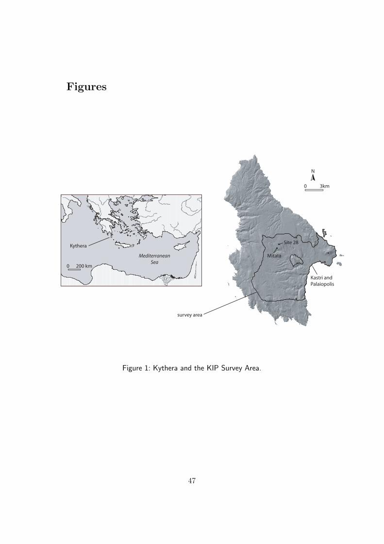
Our case studies come from the intensive field survey of the island of
Kythera, Greece (fig. 1). Lying 15 km off Cape Maleas on the southern tip
of the Peloponnese, this island is a stepping-stone between the culturally and
2

geographically distinctive areas of the Greek mainland to the north, and the
island of Crete to the SE. Some 280 sq km in area, it is a classic semi-arid
Mediterranean landscape. Yet as with many Mediterranean environments
(Horden and Purcell 2000), small-scale topographic and environmental vari-
ability is an important factor and has had an underlying effect on past and
present settlement dynamics and land-use. While Kythera might be treated
as a distinctive cultural entity in its own right, its integration within larger
networks of cultural interaction is a defining factor in the island’s long-term
history (Broodbank 1999).
Our work on the Kythera Island Project (KIP), directed by Cyprian
Broodbank, investigates many of these issues. It has several components,
the foremost of which is an intensive archaeological field survey of an area
comprising more than one third of the island (fig. 1). Complementary re-
search agendas target specific questions relating to geomorphology, biodiver-
sity, ethnography, and historical geography. The need to coordinate these
studies provides an ideal opportunity to deploy GIS as an integrative and
analytical tool. GIS has been an inextricable part of the project from the on-
set, a vehicle for the collection and treatment of data, and the primary tool
for exploring relationships between cultural and environmental dynamics.
3
Digital Data Integration and the Management
and Analysis of Multiscalar Datasets
A wide range of digital topographic, physiographic, geological, and vegeta-
tion data are part of the KIP dataset and was digitized and processed prior to
the start of the fieldwork to form the underlying digital environment within
which subsequent research was organized (table 1). Additional spatial data
were collected as part of the intensive archaeological survey and the map-
ping of several geo-archaeological study areas. Table 1 lists the broad range
of datasets and their spatial resolution and describes the main acquisition
and processing methods. Details of the survey methodology and preliminary
archaeological results are described by Broodbank (1999).
The spatial datasets describe the Kytheran landscape at a variety of
scales, ranging from 1:2000 local geoarchaeological maps, to remotely sensed
multi-spectral imagery with a 20 m resolution. Integrating this data is method-
ologically challenging, but heuristically valuable. Many proponents of GIS
claim that the technology facilitates the seamless movement between dif-
ferent spatial scales, but this is rarely the case. Site location choices, the
visibility of surface ceramics, and site identification and characterization are
three areas where the effect of scale is rarely acknowledged. Our base maps
are detailed enough that major variations in the physical landscape can read-
4

ily be identified and are sufficient for investigating widespread patterns, such
as regional site distribution and its relationship with the physical landscape
and environmental data. Such large scales are usually inappropriate for ex-
amining specific local conditions influencing the location, survival or modern
visibility of archaeological remains. For this reason, we used geomorphological
maps of selected sub-regions, and within these of the immediate environment
around sites, to identify the local characteristics of the landscape that may
have influenced site location and archaeological visibility.
Behind many of the recorded archaeological patterns are human decision-
making processes, which themselves occur at different temporal and spatial
scales. The challenge offered by a GIS approach is to move between the
analytic scales available, and to identify for any given pattern and process the
most relevant scale at which human choices were being made. The following
examples address specific survey questions, but have in common a concern
with exploring spatial scale in more detail.
5
Four Case Studies in Mediterranean Landscape
Archaeology
Extant Field Systems
This first study exploits the rich detail of the KIP dataset to look at an
challenge central to Mediterranean subsistence strategies: the effect of slope
on agricultural practices (Horden and Purcell 2000: 234-7, 585). The modern
Kytheran landscape has countless agricultural field systems, which can be
broken down into two main groups: enclosed fields and contour (hillslope)
terracing. Most of the physically visible examples appear to date to the last
three or four centuries, specifically the later Venetian and British occupations
(Leontsinis 1987: 214). These systems appear on aerial photos and have been
mapped by the Greek army. They have also been independently studied in
the field by survey teams and geoarchaeologists. This provides us with an
opportunity to compare these various sources of information and to consider
a wide range of questions relating to anthropogenic landscapes.
Field walls are dry-stone constructions, normally less than 2 m high and
1 m wide and used to enclose irregular units of land (hereafter ‘field enclo-
sures’ or ‘enclosed fields’). Terraces take a variety of forms and fulfil a variety
of functions (Rackham and Moody 1992; Frederick and Krahtopoulou 2000),
6
but those of interest here were built with dry-stone risers. Both enclosed fields
and terraces are now used for many purposes (e.g. cereals, vines, orchard
crops, garden vegetables and animal pens). In contrast to this recent diver-
sity of function, local Kytheran historical records (Leontsinis 1987) and com-
parative evidence from neighboring regions (Allen 1997: 263) suggests that
for the last few centuries, most of these were used primarily for cereal agri-
culture (even in marginal areas where the soil cover is now quite thin). The
traditional farming cycle on Kythera involved a biennial cultivated-fallow ro-
tation (with manuring by grazing flocks as part of the ‘off’-year practice) and
so, enclosed fields also controlled the movement of livestock, penning them
into fallow fields and keeping them out of cultivated ones. Concern with the
proper construction and maintenance of these boundaries is found in both
Venetian and British period sources (Leontsinis 1987: 82-3, 220-8).
Land enclosure patterns and terracing tend to follow quite regional pat-
terns in Greece, reflecting the impact of different local histories and envi-
ronments. The Kytheran system may be broadly similar to practices in the
Mani (Allen 1997: 264), but certainly differs from the pattern found on Kea
(Whitelaw 1991: 408-10). Studies of the Cretan terrace and field systems
also reveal a wide variety of different regional configurations, origins, and
functions (Rackham and Moody 1996: 140-53). The strong impression that
the Kytheran field systems are the specific products of the socio-economic
7

history of the island and not a pan-Aegean phenomenon should urge caution
in extrapolating results of any local Kytheran analysis to the wider Aegean
or Mediterranean sphere. However, the relatively strong spatial separation
of terraces and enclosed fields on Kythera does provide an opportunity to
explore the relationship between these constructions and the gradient of the
terrain on which they are found. This analysis should have relevance to the
relationship between agricultural strategies and slope observed in other re-
gions.
Terraces tend to be found mainly on steeper slopes and field enclosures on
flatter ground. Overlap occurs most frequently on patches of Quaternary al-
luvium within small drainage systems, where enclosed cross-channel terraces
are often found. The use of terracing in steeper areas reflects the negative
impact of slope, in the absence of such human intervention, on soil stability
and moisture retention. Analysis of prehistoric and historic period agriculture
has usually assumed that cultivation could only occur without terracing on
land of less than 10-15 degrees of slope (based on empirical observation in the
field: Wagstaff and Gamble 1982: 101; Whitelaw 1991: 405; Wagstaff 1992:
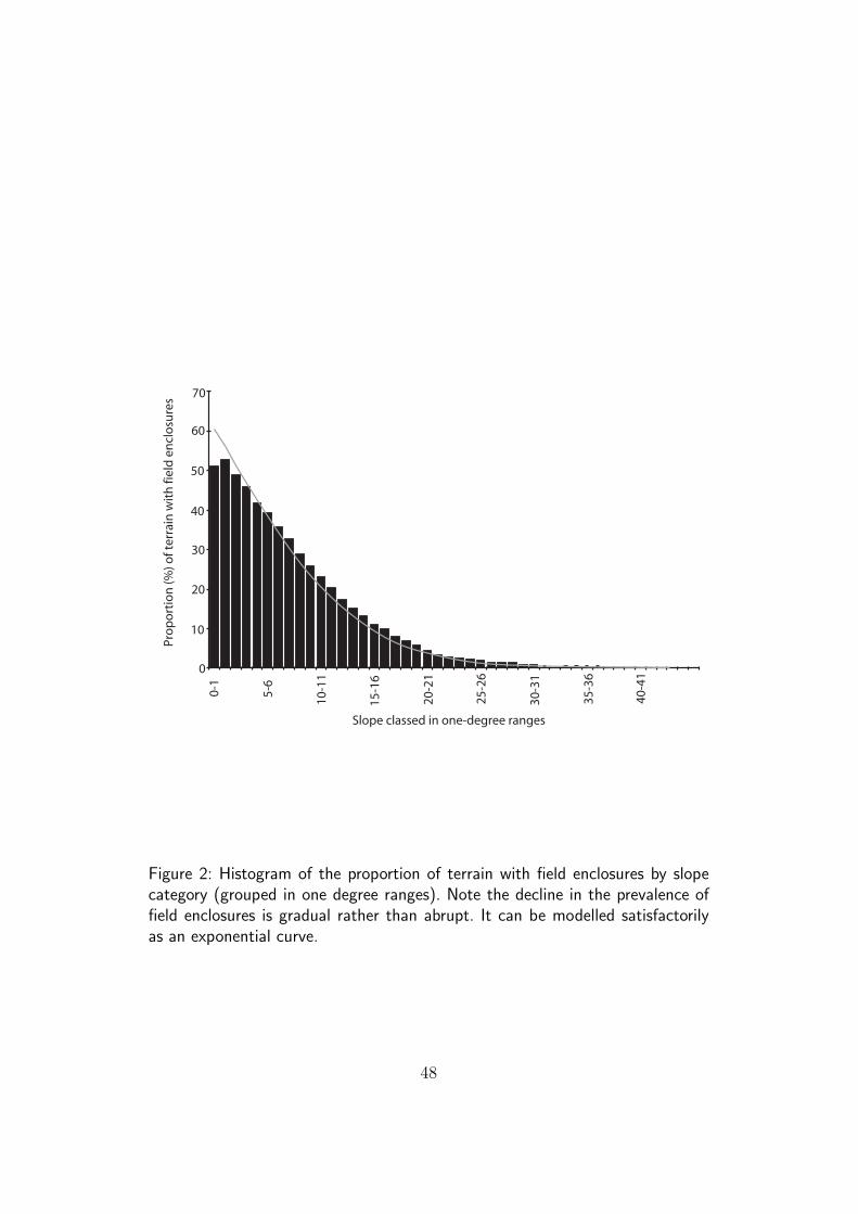
155). Using a GIS and taking advantage of fine resolution topographic data,1
we can test this assumption. The slope values of the terrain underlying all
field enclosures within the KIP survey area were extracted and grouped into
ranges of one degree. Within each slope range, we calculated the proportion
8

of terrain that is covered by such enclosed systems (fig. 2). For example,
of terrain in the survey area with a slope of 0-1 degree, about half seems to
be covered in field enclosures. This association can be further modelled with
log-linear regression analysis (using a method similar to Warren 1990), and
suggests a well-defined relationship between slope and the prevalence of field
enclosures.
Intensive field investigation by survey teams and geoarchaeologists has
shown that the enclosure systems mapped by the Greek Army in the 1960s
and used for this analysis are broadly accurate. In contrast, field observations
have also made it quite clear that the terraces shown on the same maps are a
very meagre and patchy sample of the actual terrace systems on the island.
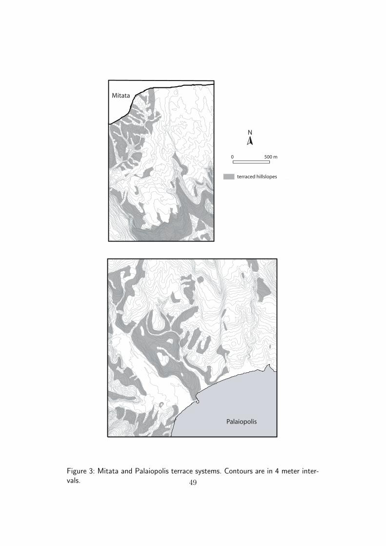
However, careful geoarchaeological investigation for two sub-regions of the
survey area (fig. 3) allows us to use a smaller analytical scale to get a much
more accurate impression of the relationship between terracing and slope.
Zones of terraced hillslope identified in the field can also be classed by slope
angle as was done for the fieldwalls.2
The chosen sample regions are known to have quite different agricultural
histories with more intense activity in the Medieval and post-Medieval peri-
ods around Mitata than around Palaiopolis. Mitata shows greater evidence
for terraces on all types of slope than Palaiopolis, but the proportion of total
land surface with terraces is quite similar in both locales (30% around Mitata
9
and 25% around Palaiopolis). This can be compared to much hillier terrain
on NW Keos where ca. 84% of the surveyed area showed signs of having
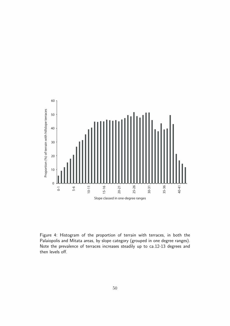
been terraced at some stage (Whitelaw 1991: 405). Viewed as separate plots,
or in combination (fig. 4), the evidence suggests that terraces increase in
prevalence up to ca. 12-13 degrees of slope and then reach a plateau.
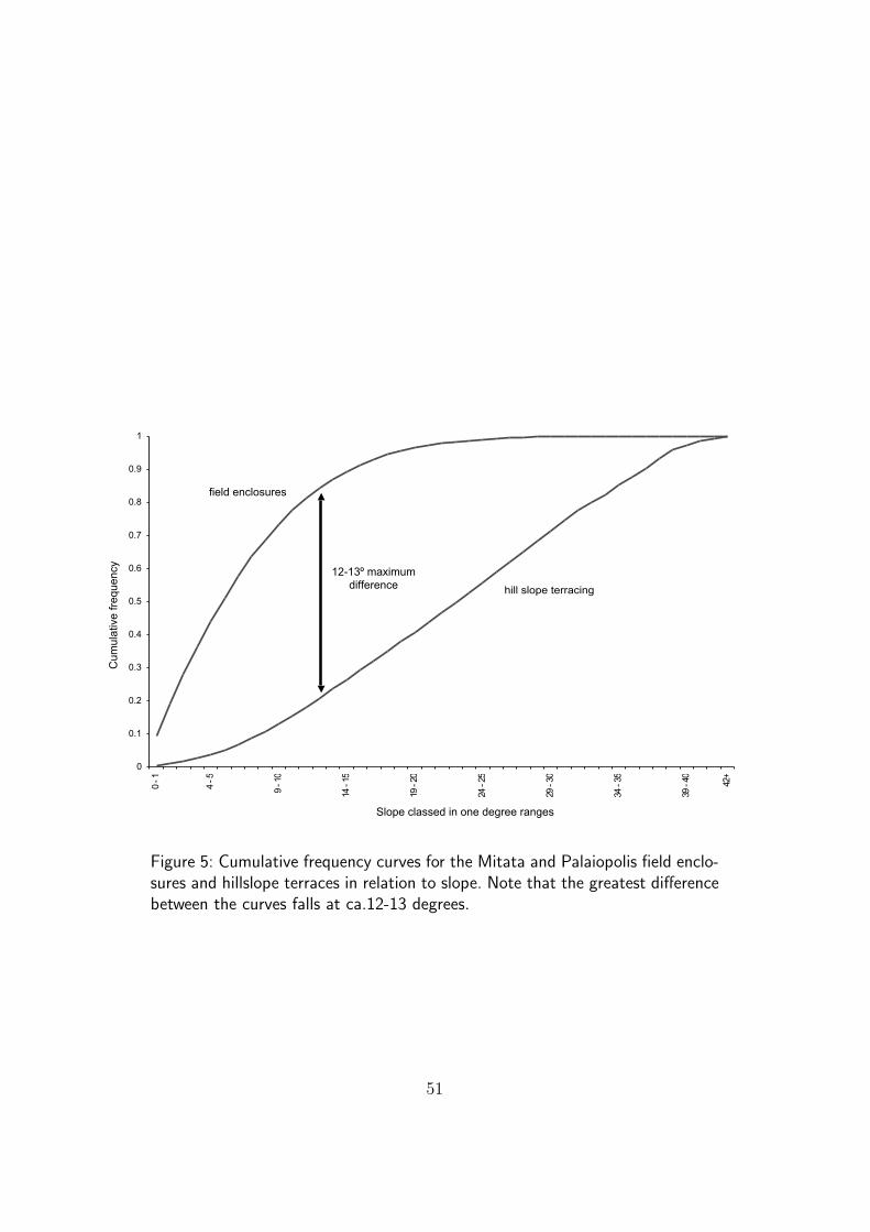
This contrasts with the pattern described for enclosed fields, which de-
crease steadily in relative frequency as slope angle increases. While there is no
unequivocal break between flat field agriculture and terracing, the Kytheran
evidence broadly supports the traditional assumptions that field management
strategies are likely to change within the 10-15 degrees range. A plot of the
cumulative frequencies of these data confirm that an appropriate threshold
would be at ca. 12-13 degrees (fig. 5).
The Effect of Surface Visibility on Artifact Recovery
and Site Discovery
Mediterranean survey projects have long acknowledged the effects of sur-
face visibility on the recovery of archaeological remains, and certain types of
agricultural activities have been shown to have a profound effect on visibility
(e.g. Ammerman 1995; Cherry 1983; Cherry et al. 1988; Verhoeven 1991). For
these reasons it is standard practice to record both current land-use and the
10
degree to which vegetation obscures the ground surface within each survey
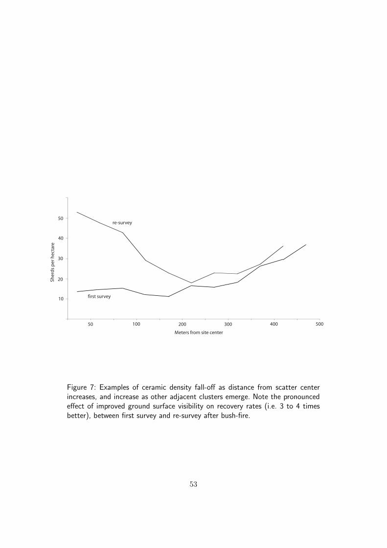
unit. Our own experience demonstrates the effect of vegetation on recovery
rates; a re-survey of a previously densely-vegetated area following a bush
fire produced a dramatic increase in artifact recovery. Our second case study
examines the relationship between surface visibility and artifact recovery, to
see whether or not the former can be usefully used to predict the latter.
Vegetation cover has traditionally been recorded by assigning a ‘visibility
class’ value to the survey unit under question, and we follow this practice.
This has at times been used to ‘weight’ the absolute number of artifacts re-
covered from a survey unit (e.g. Bintliff et al. 1999: 153-154; Gillings and
Sbonias 1999: 36), for example by the inverse of the proportion of visible
ground. In this way 10 artifacts from a unit where only 50% of the ground
is visible might be given a weighted artifact count of 20 sherds. As sensible
and logical as this seems, such an assumption has with few exceptions never
been properly tested (c.f. Schon 2000: 109) and we remain unconvinced that
measures of ground visibility can be used in this manner. While it may influ-
ence the recovery rate of archaeological data, it does not do so in any usefully
predictable manner.
Our test of the relationship between visibility categories and the quantity
of artifacts recovered from any unit shows no simple relationship at any
scale. Although mean tract densities do increase with ground visibility, there
11
is no linear correlation between individual tract artifact densities and tract
visibility (r2 = 0.06). In order to determine if this lack of correlation is a
product of the large size of survey tracts, the same test was performed using
5095 highly standardized 5 sq m units (collected in a timed 5-minute period)
for site recovery. The same lack of correlation (r2 = 0.04) emerged, suggesting
that it does not matter if collection units are large or small, visibility does
not have a predictable role in determining the amount of artifacts that will
be recovered at the level of the survey unit.
A related question of whether visibility influences the recovery of larger
and denser scatters of artifacts (e.g. ‘sites’) was also examined. Table 2 shows
the number of sites in each of the visibility categories, and the expected
number of sites for the proportion of land in each visibility class. Although
there is a suggestion that we are perhaps missing two sites in the 0-20%
visibility range, and site identification is slightly better than expected in
better visibility classes, these patterns are not statistically significant (χ2,
α = 0.69) and we can therefore state with some confidence that lack of
ground visibility has had no easily defined effect on site discovery.
While our observations suggest that dense vegetation does affect recovery
rates, we conclude that the relationship between surface visibility and recov-
ery rates is not predictable. The problem arises when a relationship between
artifact frequency (i.e. the actual number of surface artifacts in any given
12

area) and recovery rate is assumed (i.e. the chance of seeing them, which is a
product of several factors, of which surface visibility is but one). There is no
a priori relationship between the two, but using one (visibility) to estimate
the other (frequency) imposes a false relationship and introduces errors. We
suggest therefore that adjusting counts according to a measure of visibility, at
least without first exploring the relationship between these two variables, is
at best inaccurate, and at worst, can lead to erroneous distribution patterns.
Site Definition and Characterization
Aegean landscapes are strewn with cultural remains, in places quite densely,
which present a formidable challenge to the site-based approach on which
settlement system reconstruction usually depends. Mediterranean landscape
survey benefits from a long history of well-developed and well-tested methods
for site discovery and a lively debate concerning both human-landscape rela-
tionships, and the extent to which these can be reconstructed using archae-
ological survey data (Pettegrew 2001; Whitelaw 2000; Gillings and Sbonias
1999; Bintliff et al. 1999). One methodological issue concerns the differentia-
tion between ‘on-site’ and ‘off-site’ artifact scatters and their respective for-
mation processes (Bintliff 2000; Bintliff and Snodgrass 1988; Cherry 1983).
Recent reviews of surface archaeology in North America and Europe have
13
called for an abandonment of the site concept when dealing with survey
data because of the inherent difficulties in distinguishing ‘sites’ from ‘off-
site’ areas on the basis of artifact distribution patterns (e.g. Ebert 2001;
Kuna 2000a; Kvamme 1998). Aegean archaeological survey data are partic-
ularly well suited to investigate these issues given the prevalence of survey
projects that have documented by intensive survey methods, not only sites,
but also inter-site artifact distributions. Our third case study examines the
relationship between site and off-site artifact density patterns on Kythera and
suggests how the former can be distinguished from the latter in meaningful
ways.
We have retained the term ‘site’ as a convenient and shorthand term to
refer to clusters of artifacts that, on the basis of their composition and con-
textual association, are assumed to represent the visible material remains of
either short or long-term, and often multi-phased, places of human settle-
ment, although the choice, duration and scale of settlement is obviously of
major interest. At the same time, the identification of sites is clearly depen-
dent on a number of factors that range from the types of activities that were
performed, their duration and intensity, the taphonomic processes that have
transformed the original settlement and activity-place into the contemporary
archaeological record, and the surface visibility of the archaeological remains
(e.g. Pettegrew 2001; Cherry 1983; Allen 1991; Hayes 1991; Schofield 1991).
14

The site concept may be more problematic when studying the archae-
ological remains of highly mobile groups (Foley 1981), but notwithstanding
that some constituents of Neolithic and later communities are mobile and the
duration of occupation of ‘permanent’ occupations certainly varies, we have
not found any archaeological evidence of pre-Neolithic (i.e. hunter-gatherer)
activity on Kythera. Our retention of ‘site’ as both a conceptual and method-
ological tool does not lead to the exclusion of ‘off-site’ archaeology (or study
of past land-use), as this is of a major interest to us and is the focus of fur-
ther work. Defining specific locations as ‘sites’ can be used together with site
size and chronology to develop and test models of settlement systems and
long-term settlement dynamics in a manner similar to our work on Bronze
Age settlement choices (Bevan 2002).
GIS brings many advantages to the study of artifact distributions that
can help answer these questions. Methods of visualizing distribution patterns
(Lock et al. 1999), analytical methods to identify clustering and site definition
(Gillings and Sbonias 1999), and interpolation methods to help understand
off- and on-site distributions (Robinson and Zubrow 1999) have all received
attention in the past. Kythera presents its own specific problems and con-
texts in this regard, but we believe that our case study of site versus off-site
characterization is of relevance to other Mediterranean landscape projects.
We attempt to generalize about the nature and character of ‘sites’ using both
15

large and small-scale analysis of artifact distribution patterns (c.f. Gillings
2000).
Our survey strategy divided the landscape into irregular sub-hectare units
(‘tracts’), typically using field-walls, vegetation zones, or physiographic fea-
tures to define natural boundaries. Surveyors spaced at 15 m intervals walked
across the tract and counted the number of ceramic sherds, lithics and other
cultural remains. We surveyed nearly ca. 8700 tracts with a median area of
3825 sq m, which has given us a picture of artifact distribution over a very
extensive area. Large scale strategies such as this are suitable for the identi-
fication of clusters of artifacts, typically ceramic, of which some but not all
are designated as sites. For instance, figure 6 shows the distribution of multi-
period artifacts in an area roughly 2 sq km, collected in ca. 200 individual
tracts (individual tract boundaries are not shown for clarity, and an unsur-
veyed area is represented by the polygon in the lower right corner). Each dot
represents a single ceramic sherd, randomly placed within the tract in which
it was recorded. This ‘window’ contains several sites, most multi-period and
some overlapping, but is centered on a predominantly Neopalatial (ca. mid-
2nd millennium BC) artifact cluster defined as ‘site 28’. Artifact clustering
occurs here and elsewhere in this area (i.e. the distribution is neither random
nor regular), but at the same time this figure clearly shows the difficulty, if
not futility of attempting to define cluster boundaries for multi-period land-
16

scapes solely on the basis of artifact distribution patterns.
We conclude, as have others (e.g. Ebert 2001), that defining site bound-
aries at the tract-based level is difficult in landscapes of this kind. Small scale
(i.e. site-based) patterns can be investigated, however, with more intensive
artifact collection strategies, giving better indication of the size and shape of
a specific localized artifact distribution. Figure 8 shows a higher resolution
artifact distribution pattern for the cluster defined as ‘site 28’ than figure
6 above. These different methods point to a relationship between artifact
density and observation scale, but as they each involve different types of col-
lection strategy, they make direct comparison difficult. As we are interested
in the nature of the relationship between site scatters and off-site scatters,
the more extensive, but less intensive, dataset must be used because of the
consistency of the collection strategy across the wider landscape.
One useful method is to examine the internal variability of the survey
tracts. This is accomplished by calculating a coefficient of variation for each
tract, on the basis of the mean and standard deviation of numbers of arti-
facts recorded for each of the several transects that make up a survey tract.
Comparison of the aggregate coefficients of variation between those tracts
that contain sites and those without sites shows that the former have a slight
but significantly lower (at p < 0.05) coefficient of variation (tracts with sites
= 1.1, tracts without sites = 1.4). In other words, tracts with site scat-
17
ters are slightly more homogenous in terms of artifact variability, whereas
off-site tracts are more heterogeneous. Good examples of the types of phe-
nomena contributing to slightly greater off-site variability are the occasional
‘pot-smashes’ or tile dumps found in tracts with an otherwise low density of
artifacts. These result in a high coefficient of variation for that tract, com-
pared to a site which has a more even spread of material over a greater area
of the tract, resulting in a lower coefficent of variation.
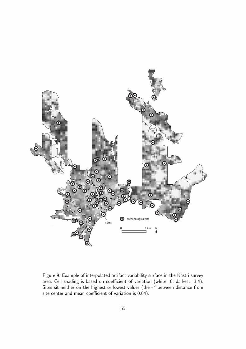
This analysis can be usefully extended by creating a ‘variability surface’
from an interpolation of the tracts’ coefficient of variation on a 50 m grid.
This surface can be examined for patterning in relation to the distribution
of sites (fig. 9). This image suggests that sites do not sit on areas of high
internal variability, nor on areas where variability is low to non-existent. This
is confirmed by a lack of linear correlation between the variability surface and
distance from site center. Put simply, the possibility of the landscape con-
taining dense but highly localized ‘blips’ when viewed against a background
of a generally low and even distribution of artifacts increases as one moves
away from sites. By examining the difference between site and off-site arti-
fact distribution patterns and the composition of these patterns we are in a
better position to understand what it is that makes a site distinctive from
the background ‘noise’ around it.
In conclusion, although it is actually quite difficult to define sites bound-
18
aries on the basis of ceramic fall-off patterns, the composition (rather than
simple density) of the artifact landscape is quantitatively different as one
moves away from the center of a site distribution. This suggests that we may
define ‘sites’ by their extensive, relatively dense, and relatively homogenous
sherd scatters, when compared to a less dense and more heterogeneous ar-
tifact pattern. Further work remains to be done, particularly once we have
better chronological control, and are better able to ascertain differences be-
tween the nature of site scatters of different time periods and can question the
sorts of cultural behavior responsible for the scatters themselves, as Pette-
grew (2001: 195-203) has done for Classical artifact scatters. For the present,
however, we regard our analysis as explaining and justifying our retention of
the site concept in Mediterranean landscape archaeology.
Terrain and Site Location
The advantages of using GIS to formalize the correlation of site location with
cultural and environmental variables has been recognized for over a decade.
Efforts at modelling have been inspired by the demands of Cultural Resource
Management (mainly in North America) and incorporated into the (usually
post-fieldwork) research designs of landscape survey projects (Warren 1990;
Dalla Bona 1994; Petrie et al. 1995; Kuna 2000b; Wescott and Brandon 2000).
19
Our final case study seeks neither to produce a full predictive model nor to
espouse a deterministic approach to understanding how humans decide where
to live, but considers how a range of insights about site location might be
gained by explicit study of these phenomena at different scales. The principal
focus is on the use of multi-scalar techniques to characterize terrain, and as a
useful counterpoint to this we also refer to the impact of local hydrology on
site location. In both parts of this case study, large numbers of Middle-Late
Bronze Age sites found by the KIP survey are used as the test case.3.
Various measures of the overall ruggedness of terrain (also known as its
texture or relief) have been proposed in archaeology (Warren and Asch 2000:
14), ecology (Forman 1995: 304-6), and geomorphology (Wood 1996: section
2.2.1) as a useful means of broadly characterizing landscapes. For example,
one frequently used index is the range of elevation values within a specific
neighbourhood around a given point in the landscape. Such a measure ex-
presses relief as a single value, which could just as well be calculated over
larger or smaller neighborhoods, and does not provide any idea of the shape
of the landscape.
Alternative measures of terrain ruggedness can be more sensitive (e.g.
fractal dimensions, Mandelbrot 1967; Burrough 1981; Mark and Aronson
1984; Clarke 1986, or positive wavelet analysis, Gallant and Hutchinson
1996). The approach offered here looks at terrain curvature as it varies over
20
different spatial neighborhoods. This is calculated by fitting a quadratic sur-
face to a given cell neighborhood4 and measuring the curvature of a two-
dimensional slice through this surface: in this case ‘cross-sectional’ curvature
measured directly across channels and ridges (Wood 1996: section 4.2.2).5
The simplest calculation uses the elevation values of the chosen cell and its
immediate neighbors (a 3 x 3 matrix), but the same operation can be per-
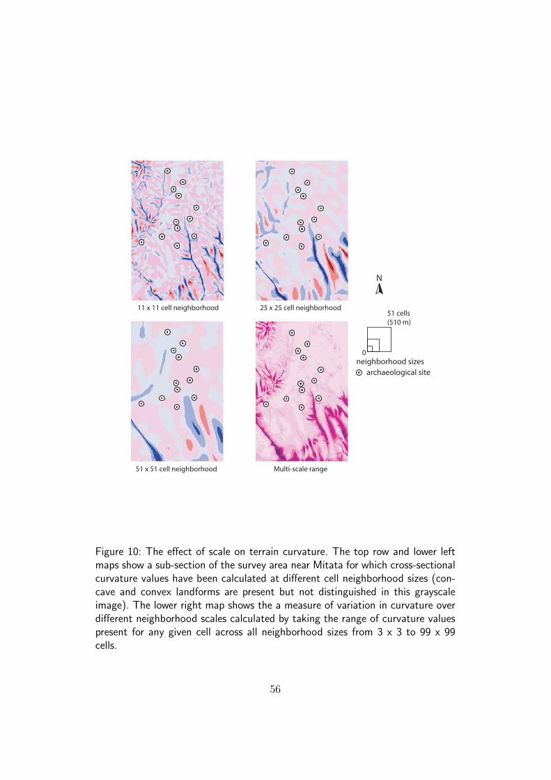
formed on any (odd) number of adjacent cells. Landforms that stand out
at one scale may not do so at others (fig. 10); shallow channels for exam-
ple may appear as an extreme negative curvature co-efficient at small-scales
(e.g. 3 x 3 cells or 0.1 ha), but appear relatively flat (close to zero) when
seen at larger scales (e.g. 51 x 51 cells, or more than 26 ha). The simplest
expression of this dispersion of curvature values across different scales is the
range6 and this was calculated for the Kythera survey area at all neighbor-
hoods from 3 x 3 cells to 99 x 99 cells (ca. 100 ha). There is a significant
pattern (p < 0.001) suggesting that Bronze Age (Neopalatial) sites are lo-
cated in areas of low-medium multi-scale dispersion of curvature which can
be satisfactorily modelled by linear regression (fig. 11).
This measure is useful for excluding certain types of terrain, namely
steeper slopes and the flatter sections of ridge and channel that lie between,
that did not have rural sites. While sensitive to variation over different neigh-
bourhood scales, it is better at defining broad types of terrain. It is also
21

worth examining other possible contextual scales at which environmentally-
based site location parameters might operate. Elevation data and stream
courses can be used in a GIS to model hydrology (e.g. Mark 1984; Jenson
and Domingue 1988; Garbrecht and Martz 1999). For example, stream net-
works can be extracted automatically from a digital elevation model (DEM)
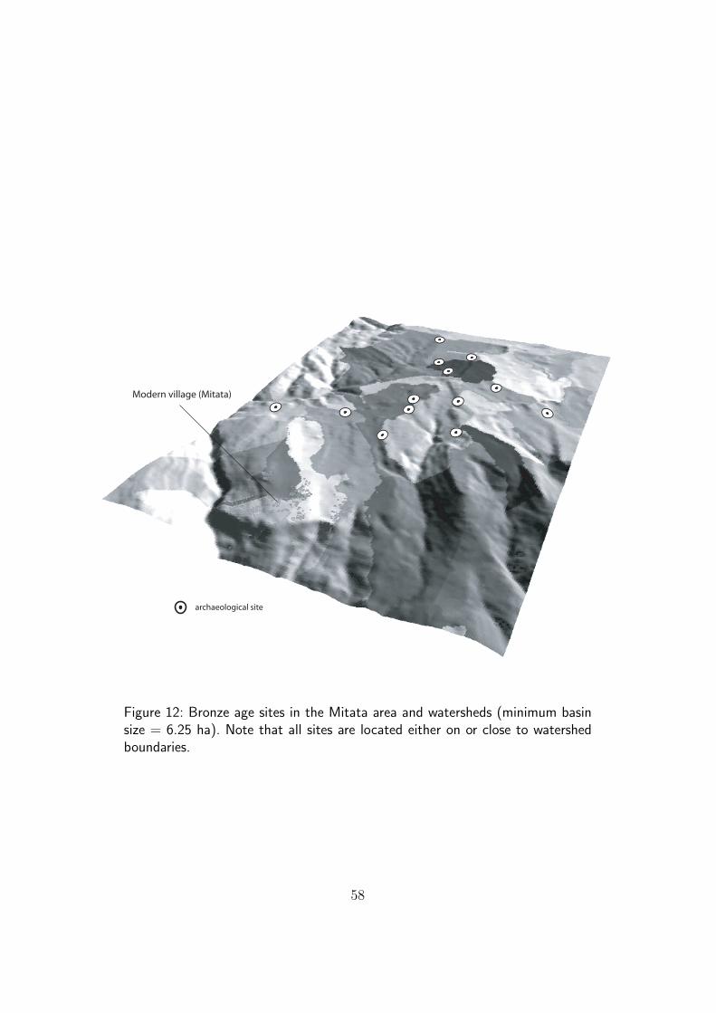
and used for a variety of purposes. Figure 12 shows the watersheds that can
be delineated for stream segments with less than 6.25 ha of surrounding land
flowing into them in the upland plateau region of Mitata. Watersheds define
those areas that drain to the same outlet point in the drainage network. They
can be explored at a number of different scales and represent natural basins,
often bounded by ridges and sharing the same erosion patterns and similar
soil moisture. At the scale shown in figure 12 (minimum basin size of 6.25
ha), it is significant (p < 0.001) that all of the known Neopalatial sites within
the Mitata region are within 50 m of a watershed boundary and regression
analysis indicates a strong linear relationship (r2 = 0.91).
There are a variety of reasons why this might be the case: (a) the areas
closer to watershed boundaries are likely to include the low to moderate relief
terrain we identified in figure 11 as being preferred; (b) watersheds represent
the structure of surface water flow, and site location within them may reflect
the land use priorities necessary for certain agricultural strategies; or (c)
watershed boundaries are sometimes physically prominent features such as
22

ridges, that might serve as landmarks or features against which to build.7
Multi-scalar approaches in a technical sense (e.g. exploring terrain rough-
ness across different spatial neighborhoods) are important, but our analysis
of terrain roughness and watersheds also show that this will not always be
enough. Human decisions are made at a variety of contextual scales from the
regional (e.g. this general landscape is or is not suitable to live in), to the
local (e.g. this patch of land is large enough to sustain a family, or this ridge
is a good place to build a house). If our modeling is sensitive to the context
of such behavior, it will not be deterministic and will also necessarily leave
room for an array of contingent human motivations.
Conclusions
This paper examines GIS data connected with the Kythera Island Project,
and raises a number of issues that have significance for all intensive archaeo-
logical survey projects. The case studies move from modern landscape struc-
ture to the visibility and definition of archaeological sites, to the interpreta-
tion of site distribution patterns.
The first case study use the different scales of data collection and field in-
vestigation (map-based, photographic, geoarchaeological) to test a traditional
assumption about flat-field vs. terraced agriculture in relation to slope. It was
23

possible to quantify the transition from one agricultural strategy to another
over terrain of varying steepness and show that this occurs gradually, but
that for practical analytical purposes a meaningful threshold value can be
distinguished of 12 to 13 degrees.
The second case study investiaged the relationship between survey unit
visibility and artifact recovery. We show that there was no simple correlation
between the two at any scale. We concluded that visibility is perhaps a useful
variable to assess, but cannot be used to modify (weight) density calculations
in any simplistic way.
The third case study considered site and off-site artifact patterns and
established that, at a large scale on a continuous surface of archaeological
material, fall-off patterns can be reliably and meaningfully defined for sites.
This has utility for understanding site-formation processes, and when inte-
grated into the fieldwork stage of the research, it can enable a more reflexive
approach to site-definition.
In the last case study, we used a specific multi-scale technique for looking
at terrain ruggedness and discussed how it could be deployed to shed light
on the locations of a particular group of Bronze Age sites on Kythera. When
combined with watershed scales, this study emphasized that human decisions
about site locations themselves reflect multi-scalar concerns.
In conclusion, we have identified some of the pattern underlying the con-
24

temporary and ancient Kytheran landscape and some of the factors influenc-
ing and governing site identification and definition in an artifact-rich envi-
ronment. In each case study we have chosen quantitative methods to extract
patterns and structure to demonstrate the value of GIS approaches, and while
further work is necessary using more detailed chronological and geomorpho-
logical data, we trust that our initial analyses demonstrate the way we can
combine multi-scalar datasets sucessfully in ways that lead to a better un-
derstanding of the archaeological record and of the dynamics of settlement
on Kythera.
25

Acknowledgments
This research draws on a dataset which is the product of collaborative ef-
forts by the many people involved in the Kythera Island Project. We would
particularly like to thank Cyprian Broodbank (KIP Director) for assistance
and encouragement at every stage. Our thanks also to Charles Frederick and
Nancy Krahtopoulou, as well as to Curtis Runnels and two anonymous re-
viewers for their helpful comments and suggestions. Any remaining errors are
our own. Bevan’s contribution was made possible by the tenure of a Lever-
hulme Trust Research Fellowship.
Authors’ Biography and Contact Details
Andrew Bevan ([email protected]) is a Leverhulme Research Fellow at
the Institute of Archaeology, University College London. His current
research interests include GIS and landscape archaeology, value theory
and trade in the Eastern Mediterranean Bronze Age.
James Conolly ([email protected]) is a Lecturer at the Institute of
Archaeology, University College London. His research interests include
GIS and landscape archaeology, lithic technology, and the Neolithic of
the Eastern Mediterranean.
26

Both authors can be contacted at: The Insitute of Archaeology, University
College London, 31-34 Gordon Sq., London WC1H 0PY, England.
27
References Cited
Allen, M.J.
1991. “Analysing the landscape: a geographical approach to archaeo-
logical problems,” in Schofield, A.J., ed., Interpreting Artifact Scatters:
Contributions to Ploughzone Archaeology. Oxford: Oxbow Books, 39-
57.
Allen, P.S.
1997. “Finding Meaning in Modifications of the Environment: The
Fields and Orchards of the Mani,” in Kardulias, P.N. and M.T. Shutes,
eds., Aegean Strategies: Studies of Culture and Environment on the
European Fringe. Lanham: Rowman and Littlefield, 259-269.
Ammerman, A.J.
1995. “The dynamics of modern land use and the Acconia Survey,”
Journal of Mediterranean Archaeology 8(1):77-92.
Bell, Tyler, Andrew Wilson, and Andrew Wickham
2002. “Tracking the Samnites: Landscape and Communications Routes
in the Sangro Valley, Italy,” American Journal of Archaeology 106(2):
169-186.
Bevan, A.
28
2002. “The Rural Landscape of Neopalatial Kythera: A GIS Perspec-
tive,” Journal of Mediterranean Archaeology 15(2): 217-256.
Bintliff, J.
2000. “Beyond dots on the map: future directions for surface artifact
survey in Greece,” in Bintliff, J., Kuna, M., and Venclova, N., eds.,
The Future of Surface artifact Survey in Europe. Sheffield: Sheffield
Academic Press, 3-20.
Bintliff, J., Howard, P., and Snodgrass, A.
1999. “The hidden landscape of prehistoric Greece,” Journal of Mediter-
ranean Archaeology 12(2): 139-168.
Bintliff, J. and Snodgrass, A.
1988. “Off-site pottery distributions: a regional and inter-regional per-
spective,” Current Anthropology 29: 506-513.
Broodbank, C.
1999. “Kythera Survey: Preliminary Report on the 1998 Season,” An-
nual of the British School at Athens 94: 191-214.
Burrough, P.A.
1981. “Fractal dimensions of landscapes and other environmental data,”
Nature 294: 241-242.
29
Cherry, J.F.
1983. “Frogs round the pond: perspectives on current archaeological
survey projects in the Mediterranean region,” in D.R. Keller and D.W.
Rupp, eds., Archaeological Survey in the Mediterranean Area. Oxford:
British Archaeological Reports, International Series 155, 375-416.
Cherry, J.F, Davis, J.L., Demitrack, A., Mantzourani, E., Strasser, T., and
Talalay, L.E.
1988. “Archaeological survey in an artifact-rich landscape: A Middle
Neolithic Example from Nemea, Greece,” American Journal of Archae-
ology 92: 159-176.
Clarke, K.C.
1986. “Computation of the fractal dimension of topographic surfaces
using the triangular prism surface area method,” Computers and Geo-
sciences 12: 713-722.
Ebert, James I.
2001. Distributional Archaeology. Salt Lake City: University of Utah
Press.
Foley, R.
1981. “A Model of Regional Archaeological Structure,” Proceedings of
30

the Prehistoric Society 47: 1-17.
Forman, R.T.T.
1995. “Land Mosaics. The Ecology of Landscapes and Regions”. Cam-
bridge: Cambridge University Press.
Frederick, C. D. and A. Krahtopoulou
2000. “Deconstructing Agricultural Terraces: Examining the Influence
of Construction Method on Stratigraphy, Dating and Archaeological
Visibility,” in Halstead, P. and C. Frederick, eds., Landscape and Land
Use in Postglacial Greece. Sheffield: Sheffield Academic Press, 79-94.
Gallant, J.C. and M.F. Hutchinson
1996. “Towards an understanding of landscape scale and structure. Pro-
ceedings of the Third International Conference on Integrating GIS and
Environmental Modelling,” accessed at 14.23, 14.9.01 at: http://www.
ncgia.ucsb.edu/conf/SANTA_FE_CD-ROM/sf_papers/gallant_john/
paper.html.
Garbrecht, J., and L.W. Martz
1999. “Digital elevation model issues in water resources modelling.
Proceedings of the 19th ESRI International User Conference, Envi-
ronmental Systems Research Institute, San Diego,” Internet Edition:
31
http://grl.ars.usda.gov/topaz/esri/paperH.htm
Gillings, M.
2000. “The utility of the GIS approach in the collection, management,
storage and analysis of surface survey data,” in Bintliff, J., Kuna, M.,
and Venclova, N., eds., The Future of Surface artifact Survey in Europe.
Sheffield: Sheffield Academic Press, 105-120.
Gillings, M. and Sbonias, K.
1999. “Regional survey and GIS: the Boeotia Project,” in Gillings, M.,
Mattingly, D. and van Dalen, J., eds., Geographical Information Sys-
tems and Landscape Archaeology. Oxford: Oxbow Books, 35-54.
Hayes, P.P.
1991. “Models for the distribution of pottery around former agricultural
settlements,” in Schofield, A.J., ed., Interpreting artifact Scatters: Con-
tributions to Ploughzone Archaeology. Oxford: Oxbow Books, 81-92.
Horden, P., and N. Purcell
2000. The Corrupting Sea. London: Blackwell.
Hutchinson, M.F.
1989. “A new method for gridding elevation and stream line data with
automatic removal of pits,” Journal of Hydrology 106: 211-232.
32

Hutchinson, M.F. and T.I. Dowling
1991. “A continental hydrological assessment of a new grid-based digital
elevation model of Australia,” Hydrological Processes 5: 45-58.
Jenson, S.K. and J.O. Domingue
1988. “Extracting Topographic Structure from Digital Elevation Data
for Geographic Information System Analysis,” Photogrammetric Engi-
neering and Remote Sensing 54(11): 1593-1600.
Kuna, M.
2000a. “Session 3 discussion: comments on archaeological prediction,”
in Lock, G., ed., Beyond the Map: Archaeology and Spatial Technolo-
gies. Amsterdam: IOS Press, 180-186.
Kuna, M.
2000b. “Surface artifact studies in the Czech Republic,” in Bintliff,
J., Kuna, M., and Venclova, N., eds., The Future of Surface Artifact
Survey in Europe. Sheffield: Sheffield Academic Press, 29-44.
Kvamme, K.
1990. “GIS algorithms and their effects on regional archaeological anal-
ysis,” in Allen, K.M.S., S.W. Green and E.B.W. Zubrow, eds., Inter-
preting Space: GIS and archaeology. London: Taylor and Francis, 112-
33

125.
Leontsinis, G.N.
1987. The Island of Kythera. A Social History (1700-1863). Athens: S.
Saripolos.
Lock, G., Bell, T., and Lloyd, J.
1999. “Towards a methodology for modelling surface survey data: the
Sangro Valley Project,” in Gillings, M., Mattingly, D. and van Dalen, J.,
eds., Geographical Information Systems and Landscape Archaeology.
Oxford: Oxbow Books, 55-64.
Mandelbrot, B.
1967. “How Long is the Coast of Britain? Statistical Self-Similarity and
Fractional Dimension,” Science 156: 636-638.
Mark, D.M.
1984. “Automatic detection of drainage networks from digital elevation
models,” Cartographica 21: 168-178.
Mark, D.M., and P.B. Aronson
1984. “Scale dependent fractal dimensions of topographic surfaces: an
empirical investigation with applications in geomorphology and com-
puter mapping,” Mathematical Geology 16(7): 671-683.
34
Olivera, F., S. Reed and D. Maidment
1998. “HEC-PrePro v. 2.0: An ArcView Pre-Processor for HEC’s Hy-
drologic Modelling System. ESRI User’s Conference,” accessed at 10.30am,
18.8.01 at: http://www.ce.utexas.edu/prof/olivera/esri98/p400.
htm
Pettegrew, David K. 2001.
2001. “Chasing the Classical Farmstead: Assessing the Formation and
Signature of Rural Settlement in Greek Landscape Archaeology,” Jour-
nal of Mediterranean Archaeology 14(2): 189-209.
Petrie, L., I. Johnston, B. Cullen and K. Kvamme
1995. GIS in archaeology: an annotated bibliography. Sydney: Univer-
sity of Sydney.
Rackham, O. and J.A. Moody
1992. “Terraces,” in Wells, B., ed., Agriculture in Ancient Greece.
Stockholm: Paul Astroms, 123-130.
Rackham, O. and J.A. Moody
1996. The Making of the Cretan Landscape. Manchester: Manchester
University Press.
Robinson, J.M and Zubrow, E.
35
1999. “Between spaces: interpolation in archaeology,” in Gillings, M.,
Mattingly, D. and van Dalen, J., eds., Geographical Information Sys-
tems and Landscape Archaeology. Oxford: Oxbow Books, 65-83.
Schofield, A.J.
1991. “Interpreting artifact scatters: an introduction,” in Schofield,
A.J., ed., Interpreting artifact Scatters: Contributions to Ploughzone
Archaeology. Oxford: Oxbow Books, 3-8.
Schon, R.
2000. “On a site and out of site: where have our data gone?,” Journal
of Mediterranean Archaeology 13(1): 107-111.
Shennan, S.
1997. Quantifying Archaeology. 2nd Edition. Edinburgh: Edinburgh
University Press.
Tarboton, D.G.
1997. “A New Method for the Determination of Flow Directions and
Upslope Areas in Grid Digital Elevation Models,” Water Resources
Research 33(2): 309-19.
Verhoeven, A.A.A.
1991. “Visibility factors affecting artifact recovery in the Agro Pontino
36

survey,” in Voorrips, A., S.H. Loving, and H. Kamermans, eds., The
Agro Pontino Survey Project. Amsterdam: Universiteit Van Amster-
dam, 87-96.
Wagstaff, M. and C. Gamble
1982. “Island Resources and their Limitations,” in Renfrew, C. and M.
Wagstaff, eds., An Island Polity: The Archaeology of Exploitation in
Melos. Cambridge: Cambridge University Press, 95-105.
Wagstaff, M.
1992. “Agricultural Terraces: The Vasilikos Valley, Cyprus,” in Bell, M.
and J. Boardman , eds., Past and Present Soil Erosion. Oxford: Oxbow,
155-61.
Warren, P. and V. Hankey
1989. Aegean Bronze Chronology. Bristol: Bristol Classical Press.
Warren, R.E.
1990. “Predictive modelling in archaeology: a primer,” in Allen, K.M.S.,
S.W. Green and E.B.W. Zubrow, eds., Interpreting Space: GIS and
archaeology. London: Taylor and Francis, 90-111.
Warren, R.E. and D.L. Asch
2000. “A Predictive Model of Archaeological Site Location in the East-
37

ern Prairie Peninsula,” in Wescott, K.L. and R.J. Brandon, eds., Prac-
tical Applications of GIS for Archaeologists: A Predictive Modelling
Kit. London: Taylor and Francis, 3-32.
Wescott, K.L. and R.J. Brandon, eds.,
2000. Practical Applications of GIS for Archaeologists: A Predictive
Modelling Kit. London: Taylor and Francis.
Whitelaw, T.
2000. “Settlement instability and landscape degradation in the southern
Aegean in the third millennium BC,” in Halstead, P. and Frederick, C.,
eds., Landscape and Landuse in Postglacial Greece. Sheffield Studies
in Aegean Archaeology 3. Sheffield: Sheffield Academic Press, 135-161.
Whitelaw, T.
1991. “The Ethnography of Recent Rural Settlement and Land Use in
North-West Keos,” in Cherry, J.F., J.L. Davis and E. Mantzourani,
eds., Landscape Archaeology as Long-Term History. Northern Keos in
the Cycladic Islands. Los Angeles: Institute of Archaeology, 403-454.
Wood, J.D.
1996. “The Geomorphological Characterisation of Digital Elevation
Models,” unpublished PhD dissertation, University of Leicester.
38

Notes
1The digital elevation model (DEM) of the survey area used in all of the
following analyses has a 10 m resolution and was produced using ArcInfo’s
TOPOGRID algorithm (Hutchinson 1989; Hutchinson and Dowling 1991)
from 2 m contours and spot heights (see table 1). A large number of different
interpolation algorithms were explored in the creation of the DEM, but given
the nature of the base data, TOPOGRID was found to produce the best
results. At this scale there are no signs of the inter-contour artificial terracing
sometimes associated with contour-based interpolations.
2The local bedrock geology in these two sub-regions is predominantly Neo-
gene marl, but there are also terraced areas on Cretaceous limestone, Neogene
regressive conglomerate, and Eocene flysch. Our thanks to Charles Frederick
and Nancy Krahtopoulou for permission to make use of this geoarchaeological
information and for discussions on this topic.
3These can be dated more precisely to the Cretan Neopalatial Period
or ca. 1700-1450 BC (Warren and Hankey 1989). Both terrain texture and
hydrology are part of a much fuller analysis of the Kytheran Neopalatial sites
to be published elsewhere (Bevan 2002)
4Significance levels in this section are those suggested by a Kolmogorov-
39

Smirnov one-sample test. ‘Sites’ (i.e. grid cells in locations for which sites
have been detected) were compared to a background population represented
by the cells making up the intensively tract-walked area. In this respect, the
method partly follows that employed by Warren and Asch (Warren 1990;
Warren and Asch 2000).
5More precisely it is calculated for the plane formed by the slope nor-
mal and perpendicular aspect. Channels have negative (concave) cell values
and ridges, positive (convex) curvature values. The following analysis was
conducted in Landserf: our thanks to Jo Wood for discussing aspects of his
program and the possible relevance of multi-scale analysis.
6Range measures are often prone to the effects of anomalous extreme
values. Alternative measures such as the inter-quartile range or, if the multi-
scale curvature values of any given cell were shown to be unimodal and
symmetric, a co-efficient of variation might be more robust or informative,
but the range is the most straightforward to calculate and easy to understand.
The problems of extreme values are likely to be less pronounced in this case
because the original values themselves are a product of the averaging process
involved in fitting the quadratic surface.
7The relationship between hydrology and these Neopalatial sites is ex-
40

plored in greater detail in Bevan (2002). The watersheds for figure 12 were
produced using CRWR-PrePro (Olivera et al. 1998). This uses a traditional
D8 flow distribution algorithm, but hydrological analysis was reassuringly
consistent with that carried out using an alternative D∞ method (Tar-
boton 1997). The TOPOGRID algorithm used to interpolate the Kythera
DEM is specifically designed to produce hydrologically correct interpolations
(Hutchinson 1989; Hutchinson and Dowling 1991).
41

Tables
Table 1: KIP Datasets
Data type Extent Format Entity Scale/ Resolution20 m contours Island Vector Arc 1:5000Spot heights Island Vector Point 1:50002-4 m contours Survey area Vector Arc 1:5000Cultural topography Island Vector Various 1:5000Bedrock geology Island Vector Area 1:50000Aerial photographs Island Raster Grid 1:15000Satellite imagery Island Raster Grid 20m resolutionDigital photos Local Raster n/a n/aElevation Local Vector Point n/aSite location Survey area Vector Point ca. 1:15000Site scatter Local/Survey area Vector Area ca. 1:15000Ceramic distribution (i) Local Vector Area 25-400 sq m collection unitsCeramic distribution (ii) Survey area Vector Area < 10000 sq mGeoarchaeology (i) Sub-survey area Vector All 1:5000Geoarchaeology (ii) Local Vector All 1:2000
Data type Acquisition and processing methods Notes20m contours Manual digitizing, automatic cleaning Photogrammetrically ex-
tracted from 1960s aerialsurvey
Spot heights As above As above2-4m contours As above As aboveCultural topography As above Roads, trackways, build-
ings, field-systems, terraces,toponyms
Bedrock geology As aboveAerial photographs Scanned and rectified (rms <5m) Taken in 1960sSatellite imagery Contrast stretch, histogram equaliza-
tionSPOT 4-band multi-spectral
Digital photos Digital image processing Site record photographs, usedfor QTVR development.
Elevation Total station surveySite location Intensive pedestrian field-survey Estimated center of artifact
distributionSite scatter As above Estimated on the basis of grid-
collections and local geomor-phology
Ceramic distribution (i) Intensive gridded collection Resolution dependent on localconditions
Ceramic distribution (ii) Intensive pedestrian field survey Resolution dependent on localconditions
Geoarchaeology (i) Geoarchaeological survey Includes three study areas: Mi-tata, Palaiopolis, Livadi
Geoarchaeology (ii) As above Mapped environment aroundsites
42

Table 2: Observed and predicted site discovery by ground visibility
visibility category 0-20 20-40 40-60 60-80 80-100Observed sites 35 44 34 25 32Proportion of survey area invisibility category (%)
22 26 22 12 18
Expected sites 37 44 37 20 31
43

List of Figures
Figure 1. Kythera and the KIP Survey Area.
Figure 2. Histogram of the proportion of terrain with field enclosures by
slope category (grouped in one degree ranges). Note the decline in the
prevalence of field enclosures is gradual rather than abrupt. It can be
modelled satisfactorily as an exponential curve.
Figure 3. Mitata and Palaiopolis terrace systems. Contours are in 4 meter
intervals.
Figure 4. Histogram of the proportion of terrain with terraces, in both the
Palaiopolis and Mitata areas, by slope category (grouped in one degree
ranges). Note the prevalence of terraces increases steadily up to ca.12-
13 degrees and then levels off.
Figure 5. Cumulative frequency curves for the Mitata and Palaiopolis field
enclosures and hillslope terraces in relation to slope. Note that the
greatest difference between the curves falls at ca.12-13 degrees.
Figure 6. Ceramic distribution around site 28. Each dot represents a single
sherd that for illustrative purposes has been randomly placed within
each tract (individual tract boundaries not shown). Other defined sites
are designated by a label adjacent to the cluster. The regional data
44

collection strategy that this map is based on is instrumental in under-
standing site versus off-site artifact distribution patterns.
Figure 7. Examples of ceramic density fall-off as distance from scatter center
increases, and increase as other adjacent clusters emerge. Note the pro-
nounced effect of improved ground surface visibility on recovery rates
(i.e. 3 to 4 times better), between first survey and re-survey after bush-
fire.
Figure 8. Dot-density map of sherd distribution for site 28 as observed
during intensive gridded collection. Each dot represents a single sherd,
that for illustration has been randomly placed in each 5 sq m collection
unit (not shown). Intensive site-based strategies provide an excellent
means for interpreting localized distribution patterns and site size, but
do not help us understand the relationship between on-site and off-site
distribution patterns.
Figure 9. Example of interpolated artifact variability surface in the Kastri
survey area. Cell shading is based on coefficient of variation (white=0,
darkest=3.4). Sites sit neither on the highest or lowest values (the r2
between distance from site center and mean coefficient of variation is
0.04).
45

Figure 10. The effect of scale on terrain curvature. The top row and lower
left maps show a sub-section of the survey area near Mitata for which
cross-sectional curvature values have been calculated at different cell
neighborhood sizes (concave and convex landforms are present but not
distinguished in this grayscale image). The lower right map shows the
a measure of variation in curvature over different neighborhood scales
calculated by taking the range of curvature values present for any given
cell across all neighborhood sizes from 3 x 3 to 99 x 99 cells.
Figure 11. Correlation of Bronze Age site location and terrain curvature
(linear regression: y = −0.17x+0.26, r2 = 0.96). Note that as curvature
increases and terrain becomes rougher, the prevalence of site scatters
steadily decreases.
Figure 12. Bronze age sites in the Mitata area and watersheds (minimum
basin size = 6.25 ha). Note that all sites are located either on or close
to watershed boundaries.
46
Figures
MediterraneanSea
survey area
Kythera
Kastri andPalaiopolis
Mitata
Site 28
0 3km
0 200 km
N
Figure 1: Kythera and the KIP Survey Area.
47
Pro
po
rtio
n (%
) of t
erra
in w
ith
fiel
d e
ncl
osu
res 70
0
60
50
40
30
20
10
0-1
5-6
10-1
1
Slope classed in one-degree ranges
15-1
6
20-2
1
25-2
6
30-3
1
35-3
6
40-4
1
Figure 2: Histogram of the proportion of terrain with field enclosures by slopecategory (grouped in one degree ranges). Note the decline in the prevalence offield enclosures is gradual rather than abrupt. It can be modelled satisfactorilyas an exponential curve.
48
Palaiopolis
Mitata
terraced hillslopes
0 500 m
N
Figure 3: Mitata and Palaiopolis terrace systems. Contours are in 4 meter inter-vals. 49
Pro
po
rtio
n (%
) of t
erra
in w
ith
hill
slo
pe
terr
aces
0
60
50
40
30
20
10
0-1
5-6
10-1
1
Slope classed in one-degree ranges
15-1
6
20-2
1
25-2
6
30-3
1
35-3
6
40-4
1
Figure 4: Histogram of the proportion of terrain with terraces, in both thePalaiopolis and Mitata areas, by slope category (grouped in one degree ranges).Note the prevalence of terraces increases steadily up to ca.12-13 degrees andthen levels off.
50
0
0.1
0.2
0.3
0.4
0.5
0.6
0.7
0.8
0.9
1
0 - 1
4 - 5
9 - 1
0
14 -
15
19 -
20
24 -
25
29 -
30
34 -
35
39 -
40 42+
12-13º maximum difference
field enclosures
hill slope terracing
Cum
ulat
ive
freq
uenc
y
Slope classed in one degree ranges
Figure 5: Cumulative frequency curves for the Mitata and Palaiopolis field enclo-sures and hillslope terraces in relation to slope. Note that the greatest differencebetween the curves falls at ca.12-13 degrees.
51

0 100m
site 28
site
sitesitesite
site
site
unsurveyed area
N
Figure 6: Ceramic distribution around site 28. Each dot represents a single sherdthat for illustrative purposes has been randomly placed within each tract (indi-vidual tract boundaries not shown). Other defined sites are designated by a labeladjacent to the cluster. The regional data collection strategy that this map isbased on is instrumental in understanding site versus off-site artifact distributionpatterns.
52
10
20
30
40
50
Sher
ds
per
hec
tare
50 100 200 300 400 500
Meters from site center
first survey
re-survey
Figure 7: Examples of ceramic density fall-off as distance from scatter centerincreases, and increase as other adjacent clusters emerge. Note the pronouncedeffect of improved ground surface visibility on recovery rates (i.e. 3 to 4 timesbetter), between first survey and re-survey after bush-fire.
53

N
0 25 meters
maquis
break in slope
fieldwalls
ceramic sherd
limit of data collection
Figure 8: Dot-density map of sherd distribution for site 28 as observed during in-tensive gridded collection. Each dot represents a single sherd, that for illustrationhas been randomly placed in each 5 sq m collection unit (not shown). Intensivesite-based strategies provide an excellent means for interpreting localized distri-bution patterns and site size, but do not help us understand the relationshipbetween on-site and off-site distribution patterns.
54
0 1 km
Kastri
archaeological site
N
Figure 9: Example of interpolated artifact variability surface in the Kastri surveyarea. Cell shading is based on coefficient of variation (white=0, darkest=3.4).Sites sit neither on the highest or lowest values (the r2 between distance fromsite center and mean coefficient of variation is 0.04).
55
0
51 cells (510 m)
11 x 11 cell neighborhood 25 x 25 cell neighborhood
51 x 51 cell neighborhood Multi-scale range
neighborhood sizes
N
archaeological site
Figure 10: The effect of scale on terrain curvature. The top row and lower leftmaps show a sub-section of the survey area near Mitata for which cross-sectionalcurvature values have been calculated at different cell neighborhood sizes (con-cave and convex landforms are present but not distinguished in this grayscaleimage). The lower right map shows the a measure of variation in curvature overdifferent neighborhood scales calculated by taking the range of curvature valuespresent for any given cell across all neighborhood sizes from 3 x 3 to 99 x 99cells.
56

0.3
Multi-scale range of curvature values
Pro
po
rtio
n (%
) of t
erra
in c
ove
red
by
site
sca
tter
s
2.500
Figure 11: Correlation of Bronze Age site location and terrain curvature (linearregression: y = −0.17x+0.26, r2 = 0.96). Note that as curvature increases andterrain becomes rougher, the prevalence of site scatters steadily decreases.
57
Modern village (Mitata)
archaeological site
Figure 12: Bronze age sites in the Mitata area and watersheds (minimum basinsize = 6.25 ha). Note that all sites are located either on or close to watershedboundaries.
58
Related Documents