Geotechnical Earthquake Engineering for Highways

Terms and Conditions of Use:

Visit our companion site

http://www.vulcanhammer.org

this document downloaded from

vulcanhammer.netSince 1997, your complete online resource for information geotecnical engineering and deep foundations:The Wave Equation Page for Piling

Online books on all aspects of soil mechanics, foundations and marine construction

Free general engineering and geotechnical software

And much more...

All of the information, data and computer software (“information”) presented on this web site is for general information only. While every effort will be made to insure its accuracy, this information should not be used or relied on for any specific application without independent, competent professional examination and verification of its accuracy, suitability and applicability by a licensed professional. Anyone making use of this information does so at his or her own risk and assumes any and all liability resulting from such use. The entire risk as to quality or usability of the information contained within is with the reader. In no event will this web page or webmaster be held liable, nor does this web page

or its webmaster provide insurance against liability, for any damages including lost profits, lost savings or any

other incidental or consequential damages arising from the use or inability to use the information contained

within.

This site is not an official site of Prentice-Hall, Pile Buck, the University of Tennessee at

Chattanooga, or Vulcan Foundation Equipment. All references to sources of

software, equipment, parts, service or repairs do not constitute an

endorsement.

Publication No. FHWA-SA-97-076

US. Deport of Tmnspa

Federal H Admlnistr, ..,. .

JGTON, 1

- -

a( . . . ..

LES

1 STRUCTURAL FOUNDATIONS SOIL h ROCK INSTABILITIES

I M~hanlcally Stabilized G r Earth Wall I

TECHNIQUES EARTH RETAINING

SYSTEMS

The FHWA Geotechnical Engineering Circulars are a series of comprehensive and practical manuals that provide state-of-the-practice methods and techniques to assist the highway engineer in the design and construction of highway facilities. No other agency or group has assembled such a complete set of manuals for geotechnical engineering. The manuals are modeled after the well-respected set of hydraulic engineering circulars and hydraulic design series, and they are expected to become a mainstay of geotechnical engineering practice worldwide.

The published circulars in this series are the following:

Geotechnical Engineering Circular No. 1 - Dynamic Compaction FHWA-SA-95-037 Geotechnical Engineering Circular No. 2 - Earth Retaining Systems FHWA-SA-96-038 Geotechnical Engineering Circular No. 3 - Design Guidance: Geotechnical Earthquake

Engineering for Highways, Volume I - Design Principles FHWA-SA-97-076 and Volume 11 - Design Examples FHWA-SA-97-077

Geotechnical Engineering Circulars are currently being developed in the following areas:

Ground Anchor Structures Soil and Rock Properties

- - - -

4. Title and Subtitle

Geotechnical Engineering Circular # 3 Design Guidance: Geotechnical Earthquake Engineering for Highways, Volume I - Design Principles 7. Author(s)

E. Kavazanjian, Jr., N. Matasovib, T. Hadj-Hamou, and P.J. Sabatini 9. Performing Organization Name and Address

GeoSyntec Consultants 2100 Main Street, Suite 150 Huntington Beach, CA 92648

12. Sponsoring Agency Name and Address Office of Technology Application Office of Engineeringhidge Division Federal Highway Administration 400 Seventh Street, S.W. Washington, D.C. 20590 15. Supplementary Notes

Contracting Officer's Technical Representative (COTR) FHWA Technical Consultant

Technical Report Documentation Page

4. Report Date

May 1997 6. Performing Organization Code:

1. Report No.

FHWA-SA-97-076

8. Performing Organization Report No.

10. Work Unit No.(TRAIS)

2. Government Accession No.

11. Contract or Grant No.

DTFH6 1 -94-C-00099 13 Type of Report and Period Covered

3. Recipient's Catalog No.

14. Sponsoring Agency Code

Chien-Tan Chang, HTA-22 Richard S . Cheney, HNG-3 1

16. Abstract

This document has been written to provide information on how to apply principles of geotechnical earthquake engineering to planning, design, and retrofit of highway facilities. Geotechnical earthquake engineering topics discussed in this document include:

deterministic and probablistic seismic hazard assessment; evaluation of design ground motions; seismic and site response analyses; evaluation of liquefaction and seismic settlements; seismic slope stability and deformation analyses; and

-

seismic design of foundations and retaining structures.

The document provides detailed information on basic principles and analyses, with reference to where detailed information on these analyses can be obtained. Design examples illustrating the principles and analyses described in this document are provided in a companion volume entitled, "Geotechnical Engineering Circular No. 3, Design Guidance: Geotechnical Earthquake Engineering for Highways, Volume 11: Design Examples."

I Service, Springfield, Virginia 22 16 1. 19. Security Classif. (of this report) I 20. Security Classif. (of this page) 1 21. NO. of pages 1 22. price %

17. Key Words Geotechnical earthquake engineering, soil dynamics, engineering seismology, engineering geology

Unclassified ( Unclassified I I ~ r m DOT F 1700.7 (8-72) Reproduction of completed page authorized

18. Distribution Statement

No restrictions. This document is available to the public from the National Technical Information

DISCLAIMER

The information in this document has been funded wholly or in part by the U.S. Department of

Transportation, Federal Highway Administration (FHWA) under Contract No. DTFH61-94-C-00099

to GeoSyntec Consultants. The document has been subjected to the Department's peer and

administrative review, and it has been approved for publication as a FHWA document. Mention

of trade names or commercial products does not constitute endorsement or recommendation for use

by either the authors or FHWA.

CONTENTS

. . . . . . . . . . . . . . . . . . . . . . . . . . . . . . . . . . . . . . . . . . 1 . INTRODUCTION 1

1.1 Introduction . . . . . . . . . . . . . . . . . . . . . . . . . . . . . . . . . . . . . . . . . . . 1 1.2 Sources of Damage in Earthquakes . . . . . . . . . . . . . . . . . . . . . . . . . . . . . 2

1.2.1 General . . . . . . . . . . . . . . . . . . . . . . . . . . . . . . . . . . . . . . . . 2 1.2.2 Direct Damage . . . . . . . . . . . . . . . . . . . . . . . . . . . . . . . . . . . . 2

1.2.2.1 Classification of Direct Damage . . . . . . . . . . . . . . . . . . . . 2 1.2.2.2 Primary Damage . . . . . . . . . . . . . . . . . . . . . . . . . . . . . 3 1.2.2.3 Secondary Damage . . . . . . . . . . . . . . . . . . . . . . . . . . . . 3

1.2.3 Indirect Damage . . . . . . . . . . . . . . . . . . . . . . . . . . . . . . . . . . . 5 1.3 Earthquake-Induced Damage to Highway Facilities . . . . . . . . . . . . . . . . . . . 6

1.3.1 Overview . . . . . . . . . . . . . . . . . . . . . . . . . . . . . . . . . . . . . . . 6 1.3.2 Historical Damage to Highway Facilities . . . . . . . . . . . . . . . . . . . . 7

1.4 Organization of the Document . . . . . . . . . . . . . . . . . . . . . . . . . . . . . . . 9

2 . EARTHQUAKE FUNDAMENTALS . . . . . . . . . . . . . . . . . . . . . . . . . . . . . . 10

2.1 Introduction . . . . . . . . . . . . . . . . . . . . . . . . . . . . . . . . . . . . . . . . . . . 10 2.2 Basic Concepts . . . . . . . . . . . . . . . . . . . . . . . . . . . . . . . . . . . . . . . . . 10

2.2.1 General . . . . . . . . . . . . . . . . . . . . . . . . . . . . . . . . . . . . . . . . 10 2.2.2 Plate Tectonics . . . . . . . . . . . . . . . . . . . . . . . . . . . . . . . . . . . . 10 2.2.3 Fault Movements . . . . . . . . . . . . . . . . . . . . . . . . . . . . . . . . . . . 13

2.3 Definitions . . . . . . . . . . . . . . . . . . . . . . . . . . . . . . . . . . . . . . . . . . . 15 2.3.1 Introduction . . . . . . . . . . . . . . . . . . . . . . . . . . . . . . . . . . . . . . 15 2.3.2 Type of Faults . . . . . . . . . . . . . . . . . . . . . . . . . . . . . . . . . . . . 15 2.3.3 Earthquake Magnitude . . . . . . . . . . . . . . . . . . . . . . . . . . . . . . . . 17 2.3.4 Hypocenter and Epicenter . . . . . . . . . . . . . . . . . . . . . . . . . . . . . 18 2.3.5 Zone of Energy Release . . . . . . . . . . . . . . . . . . . . . . . . . . . . . . . 18 2.3.6 Site-to-Source Distance . . . . . . . . . . . . . . . . . . . . . . . . . . . . . . . 18 2.3.7 Peak Ground Motions . . . . . . . . . . . . . . . . . . . . . . . . . . . . . . . . 19 2.3.8 Response Spectrum . . . . . . . . . . . . . . . . . . . . . . . . . . . . . . . . . 20 2.3.9 Attenuation Relationships . . . . . . . . . . . . . . . . . . . . . . . . . . . . . . 23

3 . SEISMIC HAZARD ANALYSIS . . . . . . . . . . . . . . . . . . . . . . . . . . . . . . . . 24

3.1 General . . . . . . . . . . . . . . . . . . . . . . . . . . . . . . . . . . . . . . . . . . . . . 24 3.2 Seismic Source Characterization . . . . . . . . . . . . . . . . . . . . . . . . . . . . . . 24

3.2.1 Overview . . . . . . . . . . . . . . . . . . . . . . . . . . . . . . . . . . . . . . . 24

iii

CONTENTS (continued)

Chapter

3.2.2 Methods for Seismic Source Characterization . . . . . . . . . . . . . . . . . . 25 . . . . . . . . . . . . . . . . . . . 3.2.3 Defining the Potential for Fault Movement 26

3.2.4 Seismic Source Characterization in the Eastern and . . . . . . . . . . . . . . . . . . . . . . . . . . . . . . . . Central United States 28

3.3 Determination of the Intensity of Design Ground Motions . . . . . . . . . . . . . . . 29 . . . . . . . . . . . . . . . . . . . . . . . . . . . . . . . . . . . . . . 3.3.1 Introduction 29

. . . . . . . . . . . . . . . . . . . . . . . . . . 3.3.2 Published Codes and Standards 29 3.3.3 The Deterministic Approach . . . . . . . . . . . . . . . . . . . . . . . . . . . . 35 3.3.4 The Probabilistic Approach . . . . . . . . . . . . . . . . . . . . . . . . . . . . . 37

4 . GROUND MOTION CHARACTERIZATION . . . . . . . . . . . . . . . . . . . . . . . . 41

. . . . . . . . . . . . . . . . . . . . . . . . . . . . 4.1 Basic Ground Motion Characteristics 41 4.2 Peak Values . . . . . . . . . . . . . . . . . . . . . . . . . . . . . . . . . . . . . . . . . . 42

4.2.1 Evaluation of Peak Parameters . . . . . . . . . . . . . . . . . . . . . . . . . . . 42 4.2.2 Attenuation of Peak Values . . . . . . . . . . . . . . . . . . . . . . . . . . . . . 42 4.2.3 Selection of Attenuation Relationships . . . . . . . . . . . . . . . . . . . . . . 47 4.2.4 Selection of Attenuation Relationship Input Parameters . . . . . . . . . . . . 48 4.2.5 Distribution of Output Ground Motion Parameter Values . . . . . . . . . . . 49

4.3 Frequency Content . . . . . . . . . . . . . . . . . . . . . . . . . . . . . . . . . . . . . . 49 4.4 Energy Content . . . . . . . . . . . . . . . . . . . . . . . . . . . . . . . . . . . . . . . . 51 4.5 Duration . . . . . . . . . . . . . . . . . . . . . . . . . . . . . . . . . . . . . . . . . . . . . 54 4.6 Influence of Local Site Conditions . . . . . . . . . . . . . . . . . . . . . . . . . . . . . 56 4.7 Selection of Representative Time Histories . . . . . . . . . . . . . . . . . . . . . . . . 60

5 . SITE CHARACTERIZATION . . . . . . . . . . . . . . . . . . . . . . . . . . . . . . . . . . 63

5.1 Introduction . . . . . . . . . . . . . . . . . . . . . . . . . . . . . . . . . . . . . . . . . . . 63 5.2 Subsurface Profile Development . . . . . . . . . . . . . . . . . . . . . . . . . . . . . . 63

5.2.1 General . . . . . . . . . . . . . . . . . . . . . . . . . . . . . . . . . . . . . . . . 63 5.2.2 Water Level . . . . . . . . . . . . . . . . . . . . . . . . . . . . . . . . . . . . . . 64 5.2.3 Soil Stratigraphy . . . . . . . . . . . . . . . . . . . . . . . . . . . . . . . . . . . 65 5.2.4 Depth to Bedrock . . . . . . . . . . . . . . . . . . . . . . . . . . . . . . . . . . 65

5.3 Required Soil Parameters . . . . . . . . . . . . . . . . . . . . . . . . . . . . . . . . . . . 66

CONTENTS (continued)

. . . . . . . . . . . . . . . . . . . . . . . . . . . . . . . . . . . . . . . . 5.3.1 General 66 . . . . . . . . . . . . . . . . . . . . . . . . . . . . . . . . . . . 5.3.2 Relative Density 66

. . . . . . . . . . . . . . . . . . . . . . . . . . . . . . . . 5.3.3 Shear Wave Velocity 67 . . . . . . . . . . . . . . . . . . . . . . . . . . . 5.3.4 Cyclic Stress-Strain Behavior 68

. . . . . . . . . . . . . . . . . . . . . . . . . 5.3.5 Peak and Residual Shear Strength 71 5.4 Evaluation of Soil Properties . . . . . . . . . . . . . . . . . . . . . . . . . . . . . . . . 72

. . . . . . . . . . . . . . . . . . . . . . . . . . . . . . . . . . . . . . . . 5.4.1 General 72 5.4.2 In Situ Testing for Soil Profiling . . . . . . . . . . . . . . . . . . . . . . . . . 72

5.4.2.1 Standard Penetration Testing (SPT) . . . . . . . . . . . . . . . . . . 72 . . . . . . . . . . . . . . . . . . . . 5.4.2.2 Cone Penetration Testing (CPT) 73

. . . . . . . . . . . . . . . . . . . . . . . . . . . . . . . . . . . . . . 5.4.3 Soil Density 75 5.4.4 Shear Wave Velocity . . . . . . . . . . . . . . . . . . . . . . . . . . . . . . . . 76

5.4.4.1 General . . . . . . . . . . . . . . . . . . . . . . . . . . . . . . . . . . . 76 5.4.4.2 Geophysical Surveys . . . . . . . . . . . . . . . . . . . . . . . . . . . 77 5.4.4.3 Compressional Wave Velocity . . . . . . . . . . . . . . . . . . . . . 80

5.4.5 Evaluation of Cyclic Stress-Strain Parameters . . . . . . . . . . . . . . . . . . 80 5.4.5.1 Laboratory Testing . . . . . . . . . . . . . . . . . . . . . . . . . . . . 80 5.4.5.2 Use of Empirical Correlations . . . . . . . . . . . . . . . . . . . . . . 82

5.4.6 Peak and Residual Shear Strength . . . . . . . . . . . . . . . . . . . . . . . . . 86

6 . SEISMIC SITE RESPONSE ANALYSIS . . . . . . . . . . . . . . . . . . . . . . . . . . . 90

6.1 General . . . . . . . . . . . . . . . . . . . . . . . . . . . . . . . . . . . . . . . . . . . . . 90 6.2 Site-Specific Site Response Analyses . . . . . . . . . . . . . . . . . . . . . . . . . . . . 90 6.3 Simplified Seismic Site Response Analyses . . . . . . . . . . . . . . . . . . . . . . . . 91 6.4 Equivalent-Linear One-Dimesional Site Response Analyses . . . . . . . . . . . . . . 95 6.5 Advanced One- and Two-Dimensional Site Response Analyses . . . . . . . . . . . 97

6.5.1 General . . . . . . . . . . . . . . . . . . . . . . . . . . . . . . . . . . . . . . . . 97 6.5.2 One-Dimensional Non-Linear Site Response Analyses . . . . . . . . . . . . . 97 6.5.3 Two-Dimensional Site Response Analyses . . . . . . . . . . . . . . . . . . . . 98

7 . SEISMIC SLOPE STABILITY . . . . . . . . . . . . . . . . . . . . . . . . . . . . . . . . 100

7.1 Background . . . . . . . . . . . . . . . . . . . . . . . . . . . . . . . . . . . . . . . . . 100

CONTENTS (continued)

Chapter Page

. . . . . . . . . . . . . . . . . . . . 7.2 Seismic Coefficient-Factor of Safety Analyses 102 . . . . . . . . . . . . . . . . . . . . . . . . . . . . . . . . . . . . . . . 7.2.1 General 102

. . . . . . . . . . . . . . . . . . . . . . . . . 7.2.2 Selection of Seismic Coefficient 103 . . . . . . . . . . . . . . . . . . . . . . . 7.3 Permanent Seismic Deformation Analyses 105

. . . . . . . . . . . . . . . . . . . . . . . . 7.3.1 Newmark Sliding Block Analysis 105 7.4 Unified Methodology for Seismic Stability and Deformation Analysis . . . . . . . 107

. . . . . . . . . . . . . . . . . . . . . . . . . . . . . . . . . 7.5 Additional Considerations 109

8 . LIQUEFACTION AND SEISMIC SETTLEMENT . . . . . . . . . . . . . . . . . . . . 110

. . . . . . . . . . . . . . . . . . . . . . . . . . . . . . . . . . . . . . . . . . 8.1 Introduction 110 8.2 Factors Affecting Liquefaction Susceptibility . . . . . . . . . . . . . . . . . . . . . . 110 8.3 Evaluation of Liquefaction Potential . . . . . . . . . . . . . . . . . . . . . . . . . . . 115 8.4 Post-Liquefaction Deformation and Stability . . . . . . . . . . . . . . . . . . . . . . 124 8.5 Seismic Settlement Evaluation . . . . . . . . . . . . . . . . . . . . . . . . . . . . . . 127

. . . . . . . . . . . . . . . . . . . . . . . . . . . . . . . . . . 8.6 Liquefaction Mitigation 130

9 . SEISMIC DESIGN OF FOUNDATIONS AND RETAINING WALLS . . . . . . . . 135

9.1 Introduction . . . . . . . . . . . . . . . . . . . . . . . . . . . . . . . . . . . . . . . . . . 135 9.2 Seismic Response of Foundation Systems . . . . . . . . . . . . . . . . . . . . . . . . 135

9.4.2 Pseudo-Static Analyses . . . . . . . . . . . . . . . . . . . . . . . . . . . . . . . 138 9.4.2.1 General . . . . . . . . . . . . . . . . . . . . . . . . . . . . . . . . . . 138 9.4.2.2 Load Evaluation for Pseudo-Static Bearing Capacity Analysis . . 139 9.4.2.3 The General Bearing Capacity Equation . . . . . . . . . . . . . . . 140 9.4.2.4 Bearing Capacity From Penetration Tests . . . . . . . . . . . . . . 144. 9.4..2.5 Sliding Resistance of Shallow Foundations . . . . . . . . . . . . . 146 9.4..3..6 Factors of Safety . . . . . . . . . . . . . . . . . . . . . . . . . . . . 146

4.4.3 Dynamic Response Analyses . . . . . . . . . . . . . . . . . . . . . . . . . . . 147 9.4.3.1 General . . . . . . . . . . . . . . . . . . . . . . . . . . . . . . . . . . 147 9.4.3.2 Stiffness Matrix of a Circular Surface Footing . . . . . . . . . . . 148

CONTENTS (continued)

Page

9.4.3.3 Damping . . . . . . . . . . . . . . . . . . . . . . . . . . . . . . . . . 149 9.4.3.4 Rectangular Footings . . . . . . . . . . . . . . . . . . . . . . . . . . 149 9.4.3.5 Embedment Effects . . . . . . . . . . . . . . . . . . . . . . . . . . . 151 9.4.3.6 Implementation of Dynamic Response Analyses . . . . . . . . . . 153

9.5 Design of Deep Foundations . . . . . . . . . . . . . . . . . . . . . . . . . . . . . . . . 153 9.5.1 General . . . . . . . . . . . . . . . . . . . . . . . . . . . . . . . . . . . . . . . 153 9.5.2 Method of Analysis . . . . . . . . . . . . . . . . . . . . . . . . . . . . . . . . 155

9.5.2.1 General . . . . . . . . . . . . . . . . . . . . . . . . . . . . . . . . . . 155 9.5.2.2 Pile-Head Stiffness Matrix . . . . . . . . . . . . . . . . . . . . . . . 156 9.5.2.3 Group Effects . . . . . . . . . . . . . . . . . . . . . . . . . . . . . . 156 9.5.2.4 Pile Uplift Capacity . . . . . . . . . . . . . . . . . . . . . . . . . . . 158 9.5.2.5 Liquefaction . . . . . . . . . . . . . . . . . . . . . . . . . . . . . . . 159

9.6 Retaining Structures . . . . . . . . . . . . . . . . . . . . . . . . . . . . . . . . . . . . . 159 9.6.1 General . . . . . . . . . . . . . . . . . . . . . . . . . . . . . . . . . . . . . . . 159 9.6.2 Seismic Evaluation of Retaining Structures . . . . . . . . . . . . . . . . . . 160

9.6.2.1 Pseudo-Static Theory . . . . . . . . . . . . . . . . . . . . . . . . . . 161 9.6.2.2 Displacement Approach . . . . . . . . . . . . . . . . . . . . . . . . 165 9.6.2.3 Stiffness Approach . . . . . . . . . . . . . . . . . . . . . . . . . . . 165 9.6.2.4 Mechanically-Stabilized Earth Walls . . . . . . . . . . . . . . . . . 166

vii

TABLES

Number P a ~ e

1 . Attenuation relationships for the western United States . . . . . . . . . . . . . . . . . . . . . 44

2 . Attenuation relationships for subduction zone earthquakes . . . . . . . . . . . . . . . . . . . 46

3 . NEHRP site classification (after Borcherdt. 1994) . . . . . . . . . . . . . . . . . . . . . . . . 60

. . . . . . . . . . . . . . . . . . 4 . Relative density of sandy soils (Terzaghi and Peck. 1948) 67

5 . Typical values of initial shear modulus . . . . . . . . . . . . . . . . . . . . . . . . . . . . . . 82

6 . Correlations to estimate initial shear modulus . . . . . . . . . . . . . . . . . . . . . . . . . . 84

7 . Susceptibility of sedimentary deposits to liquefaction during strong shaking (after Youd and Perkins. 1978) . . . . . . . . . . . . . . . . . . . . . . . . 112

8 . Recommended " standardized" SPT equipment (after Seed et al.. 1985 and Riggs. 1986) . . . . . . . . . . . . . . . . . . . . . . . . . . . . . . . 118

9 . Correction factors for non-standard SPT procedure and equipment (Richardson et al.. 1995) . . . . . . . . . . . . . . . . . . . . . . . . . . . . . . . . . . . . . 119

10 . Influence of earthquake magnitude on volumetric strain ratio for dry sands (after Tokimatsu and Seed. 1987) . . . . . . . . . . . . . . . . . . . . . . . . 130

1 1 . Improvement techniques for liquefiable soil foundation conditions (after NRC. 1985) . . . . . . . . . . . . . . . . . . . . . . . . . . . . . . . . . . . 131

12 . Inclination factors for bearing capacity of shallow foundations (after Meyerhof. 1956) . . . . . . . . . . . . . . . . . . . . . . . . . . . . . . . . . . . . . . . 145

13 . Equivalent damping ratios for rigid circular footings . (after Richart. et a1 1970) . . . . . . . . . . . . . . . . . . . . . . . . . . . . . . . . . . . . . 150

14 . Summary of centrifuge model tests in sand results (3 x 3 group. free and fixed head. plumb) (Pinto et al.. 1997) . . . . . . . . . . . . . . . . . . . . . . . . 157

viii

Number

FIGURES

Page

1 . Areas impacted by major historical earthquakes in the United States (after Nuttli. 1974. reprinted by permission of ASCE) . . . . . . . . . . . . . . . . . . . . . 1

2 . Tilting of buildings due to soil liquefaction during the Niigata (Japan) earthquake of 1964 . . . . . . . . . . . . . . . . . . . . . . . . . . . . . . . . . . . . . 4

. . . . 3 . Slumping of the Lower San Fernando Dam in the 1971 San Fernando earthquake 5

4 . Secondary earthquake damage caused by fire . . . . . . . . . . . . . . . . . . . . . . . . . . 6

5 . Collapse of Hanshin expressway during the 1995 Kobe (Hyogo-Ken Nabu. Japan) earthquake . . . . . . . . . . . . . . . . . . . . . . . . . . . . . . . 8

6 . Major tectonic plates and their approximate direction of movement (modified from Park. 1983. Foundations of Structural Geology. Chapman and Hall) . . . . . . . . . . . . . . . . . . . . . . . . . . . . . . . . . . . . 11

7 . Cross-section through tectonic plates in Southern Alaska (after Gere and Shah. 1984) . . . . . . . . . . . . . . . . . . . . . . . . . . . . . . . . . . . . . 12

8 . Types of fault movement . . . . . . . . . . . . . . . . . . . . . . . . . . . . . . . . . . . . . . 16

9 . Comparison of earthquake magnitude scales (Heaton et al.. 1986) . . . . . . . . . . . . . . 17

10 . Definition of basic fault geometry . . . . . . . . . . . . . . . . . . . . . . . . . . . . . . . . . 18

11 . Various distance measures used in earthquake engineering . . . . . . . . . . . . . . . . . . 19

12 . Acceleration. velocity. and displacement time histories . . . . . . . . . . . . . . . . . . . . 20

13 . Schematic representation of acceleration response spectra (reproduced from MatasoviC. 1993) . . . . . . . . . . . . . . . . . . . . . . . . . . . . . . . 21

14 . Tripartite representation of acceleration. velocity. and displacement response spectra . . . . . . . . . . . . . . . . . . . . . . . . . . . . . . . . . 22

Number

FIGURES (continued)

15. Effective peak acceleration levels (in decimal fractions of gravity) with a 1 in 10 chance of being exceeded during a 50-year period (ATC, 1978, reprinted by permission of ATC). . . . . . . . . . . . . . . . . . . . . . . . . , . . . . . . . . 30

16. Map and table for evaluation of UBC seismic zone factor, Z (Reproduced from the Uniform Building Code", copyrightB 1994, with the permission of the publisher, the International Conference of Building Officials). . . . . . . . . . . . 31

17. Peak horizontal ground acceleration in bedrock with a 10 percent probability of exceedance in 50 years (after Algerrnissen, et al., 1982; 1991). . . . . . . . . . . . . . 33

Seismic source zones in the central United States (Johnston and Nava, 1994, reprinted by permission of ATC). . . . . . . . . . . . . . . . . . . . . . . . . . . . . . . . . . 34

Seismic source zones in the central and eastern United States (EPRI, 1986 reprinted by permission of ATC). . . . . . . . . . . . . . . . . . . . . . . . . . . . . . . . . . 35

Cumulative frequency-magnitude plot of instrumental seismicity; San Andreas Fault South-Central Segment data (after Schwartz and Coppersmith, 1984). . . . . . . . 38

Magnitude-distance distribution for a specified peak ground acceleration (Moriwaki et al., 1994, reprinted by permission of ATC). . . . . . . . . . . . . . . . . . . 40

Comparison of attenuation relationships by various investigators. . . . . . . . . . . . . . . 45

Comparison of attenuation relationship for eastern and central United States to attenuation relationship for western United States. . . . . . . . . . . . . . . . . . 47

Comparison of smoothed acceleration response spectra for various earthquake magnitudes (Campbell, 1993 attenuation relationship). . . . . . . . . . . . . . . . . . . . . 50

Comparison of smoothed acceleration response spectra by various investigators. . . . . . 50

Attenuation of the root mean square acceleration (Kavazanjian et al., 1985a, reprinted by permission of ASCE). . . . . . . . . . . . . . . . , . . . . . . . . . . . . . . . . 52

27. Accelerograrn recorded during the 1989 Loma Prieta earthquake. . . . . . . . . . . . . . . 53

28. Bolt (1973) duration of strong shaking. . . . . . . . . . . . . . . . . . . . . . . . . . . . . . 54

FIGURES (continued)

Number

29. Trifunac and Brady (1975) duration of strong shaking. . . . . . . . . . . . . . . . . . . . . 55

30. Duration versus earthquake magnitude for the western United States (Dobry et al., 1978, reprinted by permission of SSA). . . . . . . . . . . . . . . . . . . . . 56

31. Soil conditions and characteristics of recorded ground motions, Daly City (San Francisco) M, 5.3 earthquake of 1957 (Seed, 1975, reprinted by permission of Chapman and Hall). . . . . . . . . . . . . . . . . . . . . . . . . . . . . . . . . 57

32. Comparison of soil and rock site acceleration response spectra for M, 8 event at 5 km (Campbell and Bozorgnia, 1994, reprinted by permission of EERI). . . . . . . . 58

33. Normalized uniform building code response spectra (UBC, 1994 reproduced from the Uniform Building Code", copyrighto 1994, with the permission of the publisher, the International Conference of Building Officials). . . . . . . . . . . . . . 59

34. Stresses induced in a soil element by vertically propagating shear wave. . . . . . . . . . 69

35. Hysteretic stress-strain response of soil subjected to cyclic loading. . . . . . . . . . . . . 70

36. Shear modulus reduction and equivalent viscous damping ratio curves. . . . . . . . . . . 71

37. SPT-relative density correlation (after Marcuson and Bieganousky , 1977, reprinted by permission of ASCE). . . . . . . . . . . . . . . . . . . . . . . . . . . . . . . . . 74

38. Soil classification system based on the CPT (Douglas and Olsen, 1981, reprinted by permission of ASCE). . . . . . . . . . . . . . . . . . . . . . . . . . . . . . . . . 75

39. CPT soil behavior - SPT correlation chart (Martin, 1992, reprinted by permission of ASCE). . . . . . . . . . . . . . . . . . . . . . . . . . . . . . . . . 76

40. Schematics of SASW testing (Kavazanjian et al., 1994). . . . . . . . . . . . . . . . . . . . 79

41. Shear modulus reduction curves for sands (Seed and Idriss, 1970, reprinted by permission of ASCE). . . . . . . . . . . . . . . . . . . . . . . . . . . . . . . . . 85

42. Shear modulus reduction curves for sands (Iwasaki et al., 1978, reprinted by permission of Japanese Society of Soil Mechanics and Foundation Engineering). . . . . 86

FIGURES (continued)

Number Page

43. Shear modulus reduction and damping ratio as a function of shear strain and soil plasticity index (Vucetic and Dobry, 1991, reprinted by permission of ASCE). . . . . . 87

44. Relationship between corrected "clean sand" blow count (N,),-,, and undrained residual strength (S,) from case studies (Seed and Harder, 1990). . . . . . . . . . . . . . . 89

45. Relationship between PHGA on rock and on other local site conditions (after Seed and Idriss, 1982, reprinted by permission of EERI). . . . . . . . . . . . . . . . . . . . . . 92

46. Relationship between PHGA on rock and on soft soil sites (Idriss, 1990). . . . . . . . .. 92

47. Comparison of peak base and crest accelerations recorded at earth dams (Harder, 1991). . . . . . . . . . . . . . . . . . . . . . . . . . . . . . . . . . . . . . . . . . . . . 93

48. Variation of peak average acceleration ratio with depth of sliding mass (Makdisi and Seed, 1978, reprinted by permission of ASCE). . . . . . . . . . . . . . . . . 95

49. Composite shear strength envelope. . . . . . . . . . . . . . . . . . . . . . . . . . . . . . . . 101

50. Pseudo-static limit equilibrium analysis for seismic loads. . . . . . . . . . . . . . . . . . 103

5 1. Permanent seismic deformation chart (Hynes and Franklin, 1984, reprinted by permission of U.S. Army Engineer Waterways Experiment Station). . . . . . . . . . . . 104

52. Basic elements of Newmark deformation analysis (MatasoviC et al., 1997). . . . . . . . 106

53. Permanent displacement versus normalized yield acceleration for embankments (after Makdisi and Seed, 1978, reprinted by permission of ASCE). . . . . . . . . . . . 109

54. Grain size distribution curves of potentially liquefiable soils (modified after Ishihara et al., 1989, reprinted with permission of A.A. Balkema, Old Post Road, Brookfield, VT 05036). . . . . . . . . . . . . . . . . . . . . . . . . . . . 113

55. Variation of qJN, ratio with mean grain size, D,, (Seed and De Alba, 1986, reprinted by permission of ASCE). . . . . . . . . . . . . . . . . . . . . . . . . . . . . . . . 114

56. Stress reduction factor, r, (modified after Seed and Idriss, 1982, reprinted by permission of EERI). . . . . . . . . . . . . . . . . . . . . . . . . . . . . . . . . . . . . . 117

xii

FIGURES (continued)

Number Page

57. Correction factor for the effective overburden pressure, C, (Seed et al., 1983, reprinted by permission of ASCE). . . . . . . . . . . . . . . . . . . . 120

58. Relationship between stress ratio causing liquefaction and (N,) , values for sands for M, 7.5 earthquakes (Seed et al., 1985, reprinted by permission of ASCE). . . . . . . . . . . . . . . . . . . .

59. Curve for estimation of magnitude correction factor, k, (after Seed et al., 1983). . . . . . . . . . . . . . . . . . . . . . . . . . . . . . . . . . . . . . 123

60. Curves for estimation of correction factor k, (Harder 1988, and Hynes 1988, as cited in Marcuson et al., 1990, reprinted by permission of EERI). . . . . . . . . . . 123

61. Curves for estimation of correction factor k, (Harder 1988, and Hynes 1988, as cited in Marcuson, et al., 1990, reprinted by permission of EERI). . . . . . . . . . . 124

62. Curves for estimation of post-liquefaction volumetric strain using SPT data and cyclic stress ratio for M, 7.5 earthquakes (Tokimatsu and Seed, 1987, reprinted by permission of ASCE). . . . . . . . . . . . . . . . . . . . . . . . 126

63. Plot for determination of earthquake-induced shear strain in sand deposits (Tokimatsu and Seed, 1987, reprinted by permission of ASCE). . . . . . . . . . . . . . 128

64. Relationship between volumetric strain, cyclic shear strain, and penetration resistance for unsaturated sands (Tokimatsu and Seed, 1987, reprinted by permission of ASCE). . . . . . . . . . . . . . . . . . . . . .

65. Principle of superposition of loads on footing. . . . . . . . . . . . . . . . . . . . . . . . . 136

66. Degrees of freedom of a footing and corresponding stiffness matrix. . . . . . . . . . . . 137

67. Evaluation of overturning moment. . . . . . . . . . . . . . . . . . . . . . . . . . . . . . . . 142

68. Calculation of equivalent radius of rectangular footing. . . . . . . . . . . . . . . . . . . . 151

69. Shape factor a for rectangular footings (Lam and Martin, 1986). . . . . . . . . . . . . . 151

70. Embedment factors for footings with D/R<0.5 (Lam and Martin, 1986). . . . . . . . 152

xiii

FIGURES (continued)

Number Page

71 . Embedment factors for footings with D/R> 0.5 (Lam and Martin. 1986) . . . . . . . . 152

72 . Three-dimensional soil pile interaction (after Bryant and Matlock. 1977) . . . . . . . . . 154

73 . Forces behind a gravity wall in the Mononobe-Okabe theory . . . . . . . . . . . . . . . . 161

74 . Effect of seismic coefficients and friction angle on seismic active pressure coefficient (Lam and Martin. 1986) . . . . . . . . . . . . . . . . . . . . . . . . . . 163

75 . Forces behind a gravity wall in the Richards and Elms theory . . . . . . . . . . . . . . . 164

xiv

amax a@> B B'. C

c, CN

normalizing constant for GmX calculation (equation 5-6) and/or maximum acceleration of earthquake record (equation 9-23) peak average acceleration, peak acceleration at the top of the embankment acceleration time history foundation width (footing width) and/or width of the abutment wall effective width of footing cohesion and/or viscous damping coefficient product of correction factors for use in calculating N, correction factor for use in calculating (N,), SPT correction factor for nonstandard hammer type SPT correction factor for nonstandard hammer weighttheight of fall SPT correction factor for nonstandard sample setup SPT correction factor for change in rod length SPT correction factor for nonstandard borehole diameter critical stress ratio induced by earthquake corrected critical stress ratio resisting liquefaction correction factors that depend on depth of the groundwater table displacement (equation 9-25) pile diameter and/or damping ratio in table 13 mean grain size bracketed duration of strong ground motion depth to the base of the footing from ground surface relative density significant duration of strong shaking depth of the groundwater level eccentricity of the resultant force and/or void ratio Young's modulus of a pile efficiency factor for stiffness of p-y curve due to group effects maximum void ratio small strain (initial) Young's modulus minimum void ratio in situ void ratio Young ' s modulus resonant frequency cone penetration test sleeve resistance factor of safety against liquefaction acceleration of gravity dynamic (secant) shear modulus small strain (initial) shear modulus

SYMBOLS (continued)

height of the wall and/or resultant horizontal seismic load and/or soil layer thickness (equation 4-5) slope of the surface of the backfill moment of inertia of a pile Arias intensity load inclination factors SDOF system spring constant (equation 2-1) and/or power factor for small strain shear modulus calculation (equation 5-6) stiffness matrix stiffness matrix of equivalent circular footing correction factor for the initial driving static shear stress stiffness coefficient relating force and displacement stiffness coefficient relating moment and rotation correction factor for stress levels larger than 96 kPa stiffness coefficient for horizontal rotation factor for G,,, calculation (equation 5-8) stiffness coefficient for vertical translation stiffness coefficient for rocking rotation stiffness coefficient for torsional rotation seismic active earth pressure coefficient seismic passive earth passive coefficient horizontal seismic coefficient coefficient of stiffness matrix correction factor for earth quake magnitudes other than M, 7.5 peak horizontal average acceleration coefficient of lateral earth pressure at rest seismic coefficient translational stiffness vertical seismic coefficient vertical ground acceleration pseudo-static inertia force yield acceleration foundation length mass (equation 2-1) (short period) body wave magnitude (long period) body wave magnitude Japan Meteorological Agency Magnitude Local (Richter) Magnitude Surface Wave Magnitude Moment Magnitude

xvi

SYMBOLS (continued)

N* Nm (N1)60

(N1)60-cs

Ncorr

Nc, N,, Nq OCR pae PPe PI

effective strain factor and/or correction factor (equation 9-6) uncorrected Standard Penetration Test (SPT) blow count and/or yield acceleration (equation 9-23) average blow count adjusted for submergence effects standardized SPT blow count normalized standard SPT blow count normalized standard "clean sand" SPT blow count correction factor for fines bearing capacity factors overconsolidation ratio seismic active earth force or thrust seismic passive earth force or thrust Plasticity Index Cone Penetration Test (CPT) point resistance normalized Cone Penetration Test (CPT) point resistance uniform surcharge load applied at ground surface ultimate bearing capacity (ultimate bearing pressure) equivalent radius for rectangular footing (Rx, &, R$, table 13) stress reduction factor epicentral distance hypocentral distance load inclination factor Joyner and Boore distance Rupture distance seismogenic distance center to center spacing of piles in a pile group andlor ground slope (in percent) spectral acceleration foundation shape factors spectral displacement residual shear strength steady-state shear strength spectral velocity duration of strong ground shaking fundamental period period maximum permanent displacement resultant vertical seismic load andlor peak velocity of the earthquake record (equation 9-23) compression wave velocity shear wave velocity

xvii

SYMBOLS (continued)

w s w w

z (7max)d (7max)r a

P Y Y c

Yeff (GeffJGmax) Y eff

Y max

Ymin .

Y 0

Yt 6

average shear wave velocity weight of the potential failure mass weight of the sliding wedge weight of the wall seismic zone factor, as used in UBC (1994) peak shear stress of a soil column peak shear stress of a rigid body inclination of resultant force and/or foundation shape correction factor slope of the back of the wall andlor foundation embedment factor unit weight cyclic shear strain hypothetical effective shear strain factor effective shear strain maximum unit weight; maximum shear strain minimum unit weight in situ unit weight total unit weight angle of friction of the walllbackfill interface or unit horizontal deflection of a pile head liquefaction-induced lateral displacement volumetric strain due to compaction post-liquefaction volumetric strain Poisson's ratio mass density mean normal total stress mean normal effective stress or confining pressure vertical total stress vertical effective stress vertical total stress vertical effective stress initial static shear stress on a horizontal plane maximum earthquake-induced shear stress at depth angle of internal friction angle of internal friction between the base of the wall and the foundation soil circular natural frequency equivalent viscous dumping ratio unit rotation of a pile head

xviii

ABBREVIATIONS AND ACRONYMS

AASHTO ASCE ASTM ATC BPT CALTRANS CSSASW CDMG CPT CSR CyDSS EERC EERI EPA EPRI FEMA FHWA FSAR GEC HBA IDOT JSSMFE MCE MFZ MHA MM MPE MSE NAPP NAVFAC NCEER NCHRP NEHRP NGDC NHI NISEE NRC NTIS NYSDOT

American Association of State Highway and Transportation Officials American Society of Civil Engineers American Society for Testing and Materials Applied Technology Council Becker Penetration Test California Department of Transportation Controlled Source Spectral Analysis of Surface Waves California Division of Mines and Geology Cone Penetration Test Critical Stress Ratio Cyclic Direct Simple Shear (Test) Earthquake Engineering Research Center Earthquake Engineering Research Institute Effective Peak Acceleration Electric Power Research Institute Federal Emergency Management Agency Federal Highway Administration Final Safety Analysis Report Geotechnical Engineering Circular Hypothetical Bedrock Outcrop Illinois Department of Transportation Japanese Society for Soil Mechanics and Foundation Engineering Maximum Credible Earthquake Mendocino Fracture Zone Maximum Horizontal Acceleration Modified Mercali (Intensity Scale) Maximum Probable Earthquake Mechanically Stabilized Earth National Aerial Photographic Program Naval Facilities Engineering Command National Center for Earthquake Engineering Research National Cooperative Highway Research Program National Earthquake Hazards Reduction Program National Geophysical Data Center National Highway Institute National Information Service for Earthquake Engineering National Research Council National Technical Information Service New York State Department of Transportation

PGA PGD PGV PHGA PHGD PHGV PSAR PVGA RMS RMSA SASW SDOF SPT SSA SSI UBC USEPA USGS

ABBREVIATIONS AND ACRONYMS (continued)

Peak Ground Acceleration Peak Ground Displacement Peak Ground Velocity Peak Horizontal Ground Acceleration Peak Horizontal Ground Displacement Peak Horizontal Ground Velocity Preliminary Safety Analysis Report Peak Vertical Ground Acceleration Root Mean Square Root Mean Square of Acceleration Spectral Analysis of Surface Waves Single Degree of Freedom (System) Standard Penetration Test Seismological Society of America Soil-Structure-Interaction Unified Building Code United States Environmental Protection Agency United States Geological Survey

ACKNOWLEDGEMENTS

The authors wish to express their appreciation to Dr. Rudolph Bonaparte of GeoSyntec Consultants

for his contribution in the writing and review of this document. The authors also thank Mr. Richard

S. Cheney , Mr. James C. Lyons, Mr. Chien-Tan Chang, and Mr. Barry D. Siel of Federal Highway

Administration (FHWA), Dr. Abbas Abghari of the California Department of Transportation

(CALTRANS), Mr. Victor Modeer of the Illinois Department of Transportation (IDOT), and

Mr. Teh Sung of the New York State Department of Transportation (NYSDOT) who reviewed the

manuscript and provided many valuable suggestions.

The authors also acknowledge the many individuals, too numerous to name here, who reviewed

parts of this document and who, over the years, have shared their experiences and recommendations

regarding seismic probability studies, liquefaction analysis, and dynamic stability evaluation.

xxi

PREFACE

Evaluation of the impact of earthquake loading is an important consideration in design and construction of highway facilities in the United States. Earthquake engineering for highway facilities is important not only in the states west of the Rocky Mountains, but also over broad areas of the eastern and central United States. Recent earthquakes in the United States and abroad have dramatically illustrated the potential for catastrophic loss due to even modest levels of earthquake loading when highway facilities are not designed or are under-designed to resist seismic loading. Furthermore, experience has shown that design and construction of civil facilities to resist earthquake loads improves the performance of these facilities when subject to other extreme loads (e . g . , wind, impact, blast) and under long-term service loads.

This document has been written to provide information on how to apply principles of geotechnical earthquake engineering to planning, design, and retrofit of highway facilities. Geotechnical earthquake engineering topics discussed in this document include:

a deterministic and probabilistic seismic hazard assessment; evaluation of design ground motions; seismic site response analyses;

evaluation of liquefaction potential and seismic settlements; seismic slope stability and deformation analyses; and

a seismic design of foundation and retaining structures.

This document provides detailed information on basic principles and analyses and their applicability to particular problems. The document also provides general information on advanced design analyses, with reference to where detailed information on these analyses can be obtained. Design examples illustrating the principles and analyses described in this document are provided in a companion volume titled, "Geotechnical Engineering Circular No. 3, Design Guidance: Geotechnical Earthquake Engineering for Highways, Volume 11: Design Examples. "

This document has been prepared using up-to-date information. However, earthquake engineering is a rapidly evolving field. Codes and standards are updated at regular intervals and analysis procedures are revised and improved frequently. Furthermore, almost every major earthquake leads to modification, qualification, extensions, and/or improvements of some of the methods and techniques presented herein. Therefore, the geotechnical professional using this document is encouraged to consult the technical literature for recent advantages in geotechnical earthquake engineering relevant to his project prior to completing his design.

xxii

CHAPTER 1

INTRODUCTION

1.1 INTRODUCTION

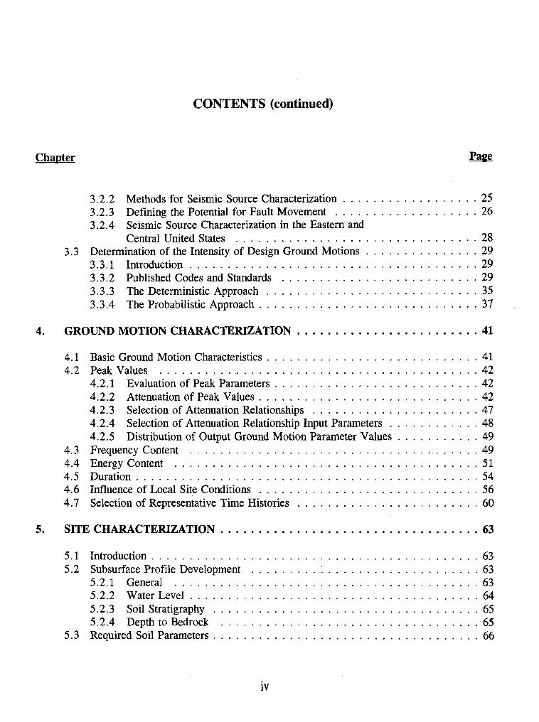
In the United States, design of constructed facilities to resist the effects of earthquakes is often considered a problem restricted to California or the western United States. However, historical records show that damaging earthquakes can, and do, also occur over broad areas of the eastern and central United States. Some of these historical eastern and central United States earthquakes have been truly major events, with intensities equal to or greater than that of the 1906 San Francisco earthquake, impacting areas far larger than the impact areas of major earthquakes that have occurred in the western United States in historical times (figure 1).

\\\\ SHAKING FELT, BUT LITTLE DAMAGE TO OBJECTS

MINOR TO MAJOR DAMAGE TO BUILDINGS AND THEIR CONTENTS

Figure 1. Areas impacted by major historical earthquakes in the United States (after Nuttli, 1974, reprinted by permission of ASCE).

The areas over which damaging earthquakes may reasonably be expected to occur cover more than 40 percent of the continental United States (e.g., see the seismic risk maps in chapter 3 of this document). Until recently, highway facilities in many of these areas have not been designed for seismic loading. Seismic design concepts are therefore relatively new to highway engineers in these regions. Furthermore, the state-of-practice in earthquake engineering has evolved rapidly in the past 25 years, as lessons learned from new earthquakes are incorporated into practice.

The objective of this document is to provide general guidance to geotechnical engineers on the seismic design of highway facilities. This document is intended to supplement existing FHWA guidance documents on seismic design of bridges and other highway facilities. Therefore, detailed information on geotechnical aspects of seismic design is provided herein while other aspects are addressed by reference and only briefly addressed herein. Furthermore, it is assumed that the geotechnical engineer using this document is familiar with the static design of highway facilities. Accordingly, this document only focuses on those aspects of geotechnical investigation, analysis, and design that relate to seismic design.

The practice of earthquake engineering continues to evolve rapidly. For instance, the coefficients for some of the acceleration attenuation relationships described in chapter 4 are updated on a yearly basis. A design engineer using this document should check the technical literature on geotechnical earthquake engineering for enhancements or modifications of the methods presented herein and for new developments in the field to be completely up to date.

1.2 SOURCES OF DAMAGE IN EARTHQUAKES

1.2.1 General

Damage resulting from earthquakes may be directly attributable to the effects of the earthquake or may be an indirect result of direct earthquake damage. Likewise, direct damage from earthquakes may result from both the primary impacts from the earthquake (i.e., ground shaking and fault displacement) or from secondary impacts, like landslides and soil liquefaction, generated by the primary impacts.

1.2.2 Direct Damage

1 .2.2.1 Classification of Direct Damage

Damage that is directly linked to the effects of the earthquake is referred to as direct damage. Direct damage can be separated into two broad classes: primary damage due to strong shaking and fault rupture and secondary damage due to the effects of strong shaking and fault rupture.

1.2.2.2 Primary Damage

Primary damage is damage that is a direct result of strong shaking or fault rupture. Primary damage attributable to strong shaking and fault rupture includes partial or total collapse of a structure. The magnitude of the damage due to strong shaking will depend on both the intensity of the motion and the frequency (or frequency content) of the motion. These factors, in turn, may depend upon the earthquake magnitude and source mechanism (e.g., strike-slip or thrust faulting), the location of the site with respect to the point of energy release of the earthquake (e.g., distance, azimuth), and the response characteristics of both the foundation for the impacted structure and the structure itself (e.g . , natural period). Damage due to fault rupture depends upon the amplitude, spatial distribution (e.g . , concentrated along a single strand or diffused across a zone), and direction (e. g . , vertical or lateral) of the fault displacement.

The relationship of the natural frequency of a structure (earthen or man-made) to the predominant frequency of the strong shaking generated at the site by the earthquake is an important factor influencing the damage potential of the ground motions. The predominant frequency of the strong shaking at the site is, in turn, influenced not only by the earthquake source mechanism, but also by travel path of the seismic waves from the source to the site and by the local geology and topography at the site. A notable example is the seismic response of the Mexico City sedimentary basin to distant earthquakes and associated structural damage to buildings. Both in the 1957 and 1985 earthquakes, only certain buildings in selected areas of the city were damaged whereas other areas remained unaffected.

Damage linked to vertical and horizontal fault displacement is most often associated with linear systems such as water lines, gas mains, roadways, and railways. Many of these linear systems provide essential services to the community and are therefore referred to as lifelines. Fault rupture will also impact structures that are constructed directly above the fault.

1.2.2.3 Secondary Damage

In addition to direct damage to constructed families and natural slopes caused by the inertial forces due to ground shaking and permanent ground displacement due to faulting, structures may also experience secondary damage as a consequence of direct damage induced by earthquake ground motions. For instance, the strong shaking may cause a landslide that damages a bridge or viaduct. In some soils (e.g., saturated sands), strong shaking may cause a loss of soil strength or stiffness in level ground that results in settlement or lateral spreading of foundations and failure of earthen structures. Secondary damage due to earthquake ground motions is an important consideration for highway systems. Examples of secondary damage to highway facilities include:

Damage due to landslides: There are numerous documented cases of landslides generated by earthquake ground motions. Ground movement associated with a landslide can cause structural damage to the superstructure or foundation of a highway facility, block roadways, and generate other types of secondary impacts (e. g . , seiches in reservoirs, rupture to pipelines).

Liquefaction: Strong ground shaking can cause a loss of strength in saturated cohesionless soils. This loss of strength is referred to as liquefaction. Liquefaction of saturated sands during earthquakes was first identified as a major source of secondary damage after the 1964 Niigata and Alaska earthquakes. Since that time, a considerable amount of research has been performed to understand and mitigate liquefaction problems. Soil liquefaction is discussed in detail in chapter 8 of this document. The consequences of liquefaction may include bearing capacity failure, lateral spreading, and slope instability.

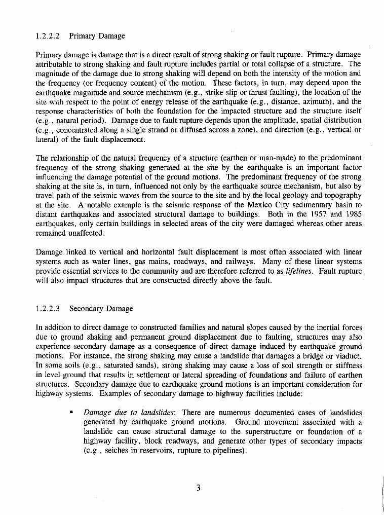
Bearing capacity failure: When the soil supporting a structure liquefies and loses strength, the bearing capacity of the soil drops to almost zero. As a consequence of this loss of bearing capacity, large foundation deformations can occur. Bearing capacity failure may result in the structure settling and rotating (tilting) as in Niigata in 1964 (see figure 2). Seismically-induced bearing capacity failure can also occur without liquefaction of the underlying soil.

Figure 2. Tilting of buildings due to soil liquefaction durlng the Niigata (Japan) earthquake of 1964.

Lateral spreading: Lateral spreading is the lateral displacement of large surficial blocks of soil as a result of liquefaction in a subsurface layer. Liquefaction of a layer or se:am of soil in even gently sloping ground can often result in lateral spreading. Movements may be triggered by the inertial forces generated by the earthquakes and continue in response to gravitational loads. Lateral spreading has been observed on slopes as gentle as 5 degrees.

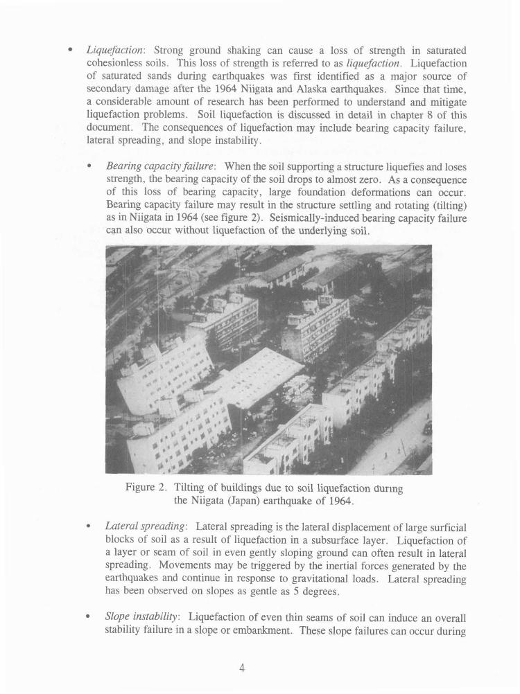
Slope instability: Liquefaction of even thin seams of soil can induce an overall stability failure in a slope or embankment. These slope failures can occur during

or after the earthquake. The slumping of the Los Angeles (Lower San Fernando) Dam in the 1971 San Fernando earthquake is perhaps the best known example of a I~quefaction-induced slope failure (see figure 3).

Figure 3. Slumping of the Lower San Fernando Dam in the 1971 San Fernando earthquake.

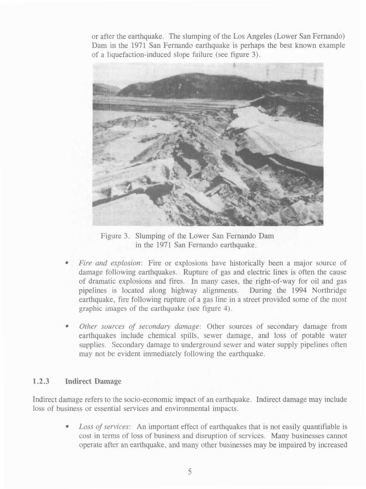
Fire and explosion: Fire or explosions have historically been a major source of damage following earthquakes. Rupture of gas and electric lines is often the cause of dramatic explosions and fires. In many cases, the right-of-way for oil and gas pipelines is located along highway alignments. During the 1994 Northridge earthquake, fire following rupture of a gas line in a street provided some of the most graphic images of the earthquake (see figure 4).

Other sources of secondaly damage: Other sources of secondary damage from earthquakes include chemical spills, sewer damage, and loss of potable water supplies. !;econdary damage to underground sewer and water supply pipelines often may not be evident immediately following the earthquake.

1.2.3 Indirect Damage

Indirect damage refers to the socio-economic impact of an earthquake. Indirect damage may include loss of business or essential services and environmental impacts.

Loss ofservices: An important effect of earthquakes that is not easily quantifiable is cost in temls of loss of business and disruption of services. Many businesses cannot operate after an earthquake, and many other businesses may be impaired by increased

travel and delivery times due to earthquake damage. The indirect impacts of earthquakes can last months and even years after the event. Loss of essential services such as transportation facilities and power and water systems are major contributors to indirect damage.

Environmental impact: The indirect environmental side effects of an earthquake can include increased consumption of fossil fuels, resulting in air pollution and health impacts due to disruption of waste disposal services. Increased travel time and traffic congestion can significantly increase air emissions following a seismic event. Closure of waste disposal facilities and disruption of waste collection both contribute to post- earthquake environmental impacts.

F ~ g u r c 4. Secondary cwrthqui~ke dzlrnase causetl by lire

1.3 EARTHQUAKE-INDUCED DAMAGE TO HIGHWAY FACILITIES

1.3.1 Overview

Recent earthquakes in the Uniced States and abroad have provided a vivid reminder of the potential for damage to highway facilities in earthquakes and the impact of that damage on the community. Damage in the 1989 Loma Prieta (Santa CNZ Mountains) and 1994 Northridge earthquakes in the United States and the 1995 Kobe (Hyogo-Ken Nabu) earthquake in Japan have illustrated the potential for not only direct damage, including loss of life and destruction of highway structures, but also indirect damage due to loss of service of portions of highway systems. Economic loss due to closure of the Bay Bridge following the Loma Prieta earthquake is a good example of the potential magnitude of indirect damage. Economic losses associated with closure of the bridge include the costs associated with increased travel time and air pollution due to necessary detours.

Furthermore, in many cases, business trips to San Francisco were simply deferred or canceled, resulting in loss of business. Travel and tourism also suffered. Estimates of the cost of these indirect losses exceed $10 billion. Thus, the estimated indirect costs are greater than the estimated $6.5 billion cost of repairing the direct damage from the earthquake. Disruption of highway systems also contributed to delays in emergency response and recovery activities, possibly increasing direct damage, including loss of life and fire-related damage.

1.3.2 Historical Damage to Highway Facilities

The historical record of damage to highway facilities in major earthquakes does not begin until the 1993 Long Beach earthquake since there were few major highway facilities prior to that time. However, the accounts of the impact of the 1906 San Francisco earthquake include reports of minor damage to railway tunnels from strong shaking (primarily at the tunnel portal) and numerous reports and pictures of damage to local thoroughfares induced by local ground failures that are now known to have been caused by liquefaction (see, e.g., Youd and Hoose, 1976). Furthermore, in earthquakes throughout history, there have been reports of landslides and mass soil movements blocking travel routes and disrupting commerce.

At the time of the 1933 Long Beach earthquake, the Los Angeles freeway network had yet to be developed. Furthermore, the earthquake struck south of Los Angeles in, at the time, relatively sparsely populated Orange County. However, damage accounts from the earthquake include reports of disruption to the Pacific Coast Highway, the main thoroughfare between Long Beach and the coastal areas of Orange County, due to lateral spreading of the ground. The lateral spreading is now recognized as attributable to liquefaction.

The first reports of major damage to structural elements of highway facilities due to earthquakes were from the 1964 Niigata and Alaska earthquakes. Numerous bridges were destroyed in both of these earthquakes by soil movements attributable to liquefaction (see, e.g., Ross et al., 1969). In fact, it was only after study of the damage induced by these earthquakes that liquefaction was recognized as an important phenomenon in earthquakes.

The 1971 San Fernando earthquake was the first event in which major damage to highway facilities were not attributed to liquefaction or landslides. Damage to highway facilities in the San Fernando event included toppling of highway overpasses and structural damage to bridge piers and retaining walls. Following the San Fernando event, the engineering profession undertook a comprehensive reassessment of procedures and practices for seismic design of highway facilities.

Significant damage to transportation systems was one of the major characteristics of the 1989 Loma Prieta earthquake. The collapse of a more than 1.5-krn long section of elevated roadway on Interstate 880 (the Cypress Street Viaduct) along with the loss of a 15-m long span of the upper deck of the Bay Bridge linking San Francisco to Oakland resulted in both loss of life and major disruption to the transportation system. At both locations, amplification of the ground motions from the relatively distant earthquake by local soil conditions (i.e., soft to medium-stiff clay soils) significantly affected the seismic loads on the structure, contributing to its collapse. Of the 1,500 highway bridges in the felt area of the Loma Prieta earthquake, 10 were closed due to structural

damage. 10 required shoring to remain in service, and 73 experienced lesser damage (EERI, 1989). In addition to this structural damage, a series of landslides disrupted State Route 17, the only direct high capacity roadway between the Santa Cruz and the San Jose areas.

It is estimated that approximately 10 percent of the 20,000 km of state highway in California experienced ground acceleration greater than 0.25 g during the 1994 Northridge earthquake (CDMG, 1995). The most significant damage to highway facilities occurred at the State Route 14-Interstate 5 interchange, constructed between 1971 to 1974. This interchange was under construction during the 1971 San Fernando earihquake and was designed to pre-San Fernando earthquake standards. In addition to bridge failure and damage, there was also extensive non-structural damage to highway systems in the Northridge event. Highway damage included excessive settlement of bridge approaches, soil settlement under pavement, and landslides.

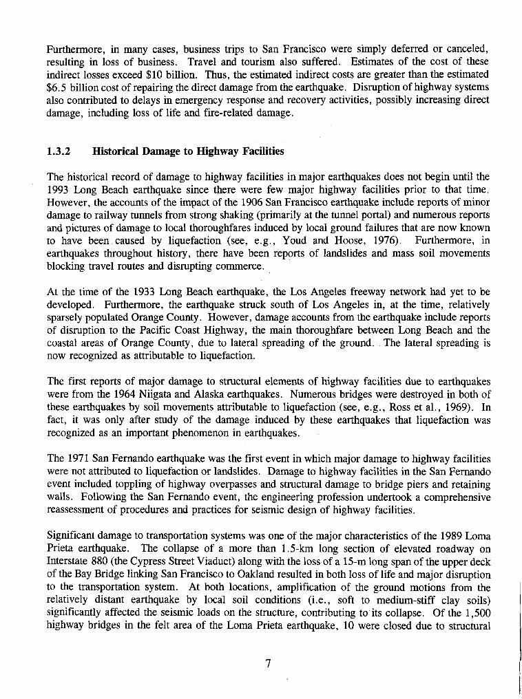
The collapse of the Hanshin expressway due to strong shaking during the 1995 Kobe earthquake in Japan provided another graphic example of damage to highway structures during earthquakes (see figure 5). 1 'r

I

\ I 5. clollapse of Hanshin expressway during the 1995 Kobe (Hyogo-Ken Nahu, Japan) earthquake.

This expressway was constructed before modern seismic details for columns were incorporated into practice (EERI, 1995). In this earthquake, some bridges in Kobe also experienced significant damage due to soil liquefaction.

Experience from the Loma Prieta, Northridge, and Kobe earthquakes indicates that bridges and other structural highway facilities designed in accordance with current codes will, in general, perform well when subjected to strong ground motions. However, damage from these earthquakes also illustrates the fragility of structures not designed in compliance with current codes. The damage to highway

facilities in these events emphasizes the continuing importance of consideration of effects of strong shaking, soil liquefaction, landslides, and local soil amplification.

1.4 ORGANIZATION OF THE DOCUMENT

General background information on the sources, types, and effects of earthquakes, including the definition of key terms used in earthquake engineering, is provided in Chapter 2. Chapter 3 of this document discusses seismic source characterization and provides information on readily available geological, seismological, and geophysical data. Chapter 4 describes the characterization of earthquake ground motions for use in engineering analysis. Details of geotechnical site characterization for seismic analyses are presented in Chapter 5. Seismic site response analyses are addressed in chapter 6 , and methods for evaluating the seismic stability of slopes and embankments based upon the results of a seismic site response analysis are presented in chapter 7. Techniques for evaluating the liquefaction and seismic settlement potential of a site are discussed in chapter 8. Basic elements of the seismic design of retaining walls, spread footings, and piles are presented in chapter 9. References cited in the document are listed in chapter 10.

Examples illustrating the application of the methods discussed in this document are presented in a companion volume titled, "Geotechnical Engineering Circular No. 3, Design Guidance: Geotechnical Earthquake Engineering for Highways, Volume I1 - Design Examples. "

CHAPTER 2

EARTHQUAKE FUNDAMENTALS

2.1 INTRODUCTION

Earthquakes are produced by abrupt relative movements on fractures or fracture zones in the earth's crust. These fractures or fracture zones are termed earthquake faults. The mechanism of fault movement is elastic rebound from the sudden release of built-up strain energy in the crust. The built-up strain energy accumulates in the earth's crust through the relative movement of large, essentially intact pieces of the earth's crust called tectonic plates. This relief of strain energy, commonly called fault rupture, takes place along the rupture zone. When fault rupture occurs, the strained rock rebounds elastically. This rebound produces vibrations that pass through the earth crust and along the earth's surface, generating the ground motions that are the source of most damage attributable to earthquakes. If the fault along which the rupture occurs propagates upward to the ground surface and the surface is uncovered by sediments, the relative movement may manifest itself as suvace rupture. Surface ruptures are also a source of earthquake damage to constructed facilities.

2.2 BASIC CONCEPTS

2.2.1 General

Faults are ubiquitous in the earth's crust. They exist both at the contacts of the tectonic plates and within the plates themselves. In some areas of the western United States, it is practically impossible to perform a site investigation and not encounter a fault. However, not all faults are seismogenic (i.e., not all faults produce earthquakes). Faults that are known to produce earthquakes are termed active faults. Faults that at one time produced earthquakes but no longer do are termed inactive faults. Faults for which the potential for producing earthquakes is uncertain are termed potentially active faults. When a fault is encountered in an area known or suspected to be a source of earthquakes, a careful analysis and understanding of the fault is needed to evaluate its potential for generating earthquakes.

2.2.2 Plate Tectonics

Plate tectonics theory has established that the earth's crust is a mosaic of tectonic plates. These plates may pull apart from each other, override one another, and slide past each other. The motions of the tectonic plates are driven by convection currents in the molten rock in the earth's upper mantle. These convection currents are generated by heat sources within the earth. Plates grow in size at spreading zones, where the convection currents send plumes of material from the upper

mantle to the earth's surface. Plates are consumed at subduction zones, where the relatively rigid plate is drawn downwards back into and consumed by the mantle.

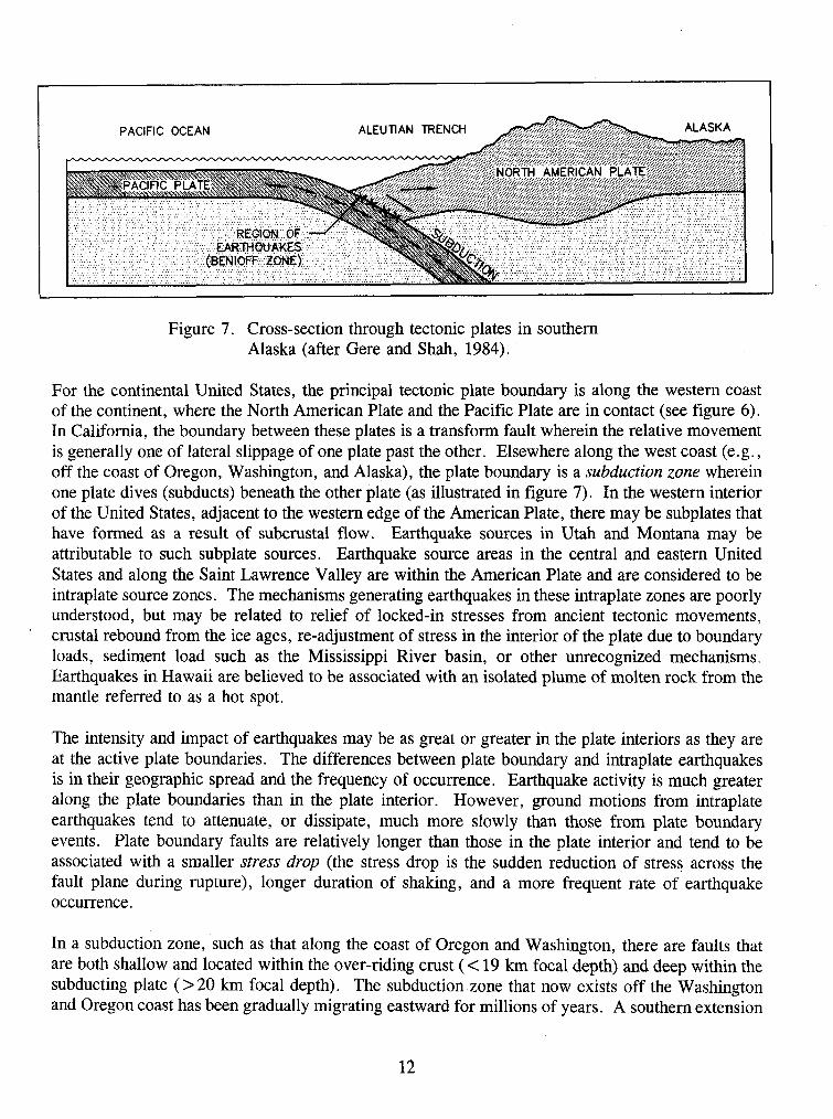
The major tectonic plates of the earth's crust are shown in figure 6 (modified from Park, 1983). There are also numerous smaller, minor plates not shown on this figure. The motions of these plates are related to the activation of faults, the generation of earthquakes, and the presence of volcanism. Most earthquakes occur on or near plate boundaries, in the so-called Benioff zone, the inclined contact zone between two tectonic plates that dips from near the surface to deep under the earth's crust, as illustrated in figure 7 (modified after Gere and Shah, 1984). Earthquakes also occur in the interior of the plates, although with a much lower frequency than at plate boundaries.

Figure 6. Major tectonic plates and their approximate direction of movement (modified from Park, 1983, Foundations of Structural Geology, Chapman and Hall).

PACIFIC OCEAN ALEUTIAN TRENCH

Figure 7. Cross-section through tectonic plates in southern Alaska (after Gere and Shah, 1984).

For the continental United States, the principal tectonic plate boundary is along the western coast of the continent, where the North American Plate and the Pacific Plate are in contact (see figure 6). In California, the boundary between these plates is a transform fault wherein the relative movement is generally one of lateral slippage of one plate past the other. Elsewhere along the west coast (e.g., off the coast of Oregon, Washington, and Alaska), the plate boundary is a subduction zone wherein one plate dives (subducts) beneath the other plate (as illustrated in figure 7). In the western interior of the United States, adjacent to the western edge of the American Plate, there may be subplates that have formed as a result of subcrustal flow. Earthquake sources in Utah and Montana may be attributable to such subplate sources. Earthquake source areas in the central and eastern United States and along the Saint Lawrence Valley are within the American Plate and are considered to be intraplate source zones. The mechanisms generating earthquakes in these intraplate zones are poorly understood, but may be related to relief of locked-in stresses from ancient tectonic movements, crustal rebound from the ice ages, re-adjustment of stress in the interior of the plate due to boundary loads, sediment load such as the Mississippi River basin, or other unrecognized mechanisms. Earthquakes in Hawaii are believed to be associated with an isolated plume of molten rock from the mantle referred to as a hot spot.

The intensity and impact of earthquakes may be as great or greater in the plate interiors as they are at the active plate boundaries. The differences between plate boundary and intraplate earthquakes is in their geographic spread and the frequency of occurrence. Earthquake activity is much greater along the plate boundaries than in the plate interior. However, ground motions from intraplate earthquakes tend to attenuate, or dissipate, much more slowly than those from plate boundary events. Plate boundary faults are relatively longer than those in the plate interior and tend to be associated with a smaller stress drop (the stress drop is the sudden reduction of stress across the fault plane during rupture), longer duration of shaking, and a more frequent rate of earthquake occurrence.

In a subduction zone, such as that along the coast of Oregon and Washington, there are faults that are both shallow and located within the over-riding crust (< 19 km focal depth) and deep within the subducting plate (> 20 krn focal depth). The subduction zone that now exists off the Washington and Oregon coast has been gradually migrating eastward for millions of years. A southern extension

of it was consumed beneath California during the collision of the North American and Pacific plates ten to twenty million years ago. In the plate interior, faults may vary from shallow to deep. In California, the plate boundary is generally of the transform type, wherein the plates slide laterally past each other, and faults are relatively shallow ( < 20 krn) .

2.2.3 Fault Movements

Faults are created when the stresses within geologic materials exceed the ability of those materials to withstand the stresses. Most faults that exist today are the result of tectonic activity that occurred in earlier geological times. These faults are usually inactive, but faults related to past tectonism can be reactivated by present-day tectonism.

Not all faults along which relative movement is occurring are a source of earthquakes. Some faults may be surfaces along which relative movement is occurring at a slow, relatively continuous rate, with an insufficient stress drop to cause an earthquake. Such movement is called fault creep. Fault creep may occur along a shallow fault, where the low overburden stress results in a relatively rapid dissipation of stresses. Alternatively, a creeping fault may be at depth in soft and/or ductile materials that deform plastically. Also, there may be a lack of frictional resistance or asperities (non-uniformities) along the fault plane, allowing steady creep and associated release of the strain energy along the fault. Fault creep may also prevail where phenomena such as magma intrusion or growing salt domes activate small shallow faults in soft sediments, where faults are generated by extraction of fluids (e.g., oil or water in southern California) which causes ground settlement and thus activates faults near the surface, where movements are associated with steady creep in response to adjustments of tectonically activated faults, and where faults are generated by gravity slides that take place in thick, unconsolidated sediments.

Active faults that extend into crystalline basement rocks are generally capable of building up the strain energy needed to produce, upon rupture, earthquakes strong enough to affect highway facilities. Fault ruptures may propagate from the crystalline basement rocks to the ground surface and produce ground rupture. However, in some instances, fault rupture may be confined to the subsurface with no breakage of the ground surface due to fault movement. Subsurface faulting without primary fault rupture at the ground surface is characteristic of almost all earthquakes in the central and eastern United States. In addition, several of the most recent significant earthquakes in the Pacific Coast plate boundary areas are due to rupture of thrust faults that do not break the ground surface, termed blind thrust faults. Strong shaking associated with fault rupture may also generate secondary ground breakage such as graben structures, ridge-top shattering, landslides, and liquefaction. While this secondary ground breakage may sometimes be interpreted as faulting, it is generally not considered to represent a surface manifestation of the fault.

Whether or not a fault has the potential to produce earthquakes is usually judged by the recency of previous fault movements. If a fault has propagated to the ground surface, evidence of faulting is usually found in geomorphic features associated with fault rupture (e.g., relative displacement of geologically young sediments). For faults that do not propagate to the ground surface, geomorphic evidence of previous earthquakes may be more subdued and more difficult to evaluate (e.g., near surface folding in sediments or evidence of liquefaction or slumping generated by the earthquakes).

If a fault has undergone relative displacement in relatively recent geologic time (within the time frame of the current tectonic setting), it is reasonable to assume that this fault has the potential to move again. If the fault moved in the distant geologic past, during the time of a different tectonic stress regime, and if the fault has not moved in recent (Holocene) time (generally the past 11,000 years), it may be considered inactive.

Geomorphic evidence of fault movement cannot always be dated. In practice, if a fault displaces the base of unconsolidated alluvium, glacial deposits, or surficial soils, then the fault is likely to be active. Also, if there is micro-seismic activity associated with the fault, the fault may be judged as active and capable of generating earthquakes. Microearthquakes occurring within basement rocks at depths of 7 to 20 km may be indicative of the potential for large earthquakes. Microearthquakes occurring at depths of 1 to 3 km are not necessarily indicative of the potential for large, damaging earthquake events. In the absence of geomorphic, tectonic, or historical evidence of large damaging earthquakes, shallow microtremors may simply indicate a potential for small or moderate seismic events. Shallow microearthquakes of magnitude 3 or less may also sometimes be associated with mining or other non-seismogenic mechanisms. If there is no geomorphic evidence of recent seismic activity and there is no microseismic activity in the area, then the fault may be inactive and not capable of generating earthquakes.

The maximum potential size of an earthquake on a capable (active or potentially active) fault is generally related to the size of the fault (i.e., a small fault produces small earthquakes and a large fault produces large earthquakes). Faults contain asperities (non-uniformities) and are subject to certain frictional and geometric restraints that allow them to move only when certain levels of accumulated stress are achieved. Thus, each fault tends to produce earthquakes within a range of magnitudes that are characteristic for that particular fault.

A long fault, like the San Andreas fault in California or the Wasatch fault in Utah, will generally not move along its entire length at any one time. Such faults typically move in portions, one segment at a time. An immobile (or "locked") segment, a segment which has remained stationary while the adjacent segments of the fault have moved, is a strong candidate for the next episode of movement. The lengths of fault segments may be interpreted from geomorphic evidence of prior movements or from fault geometry and kinematic constraints (e.g., abrupt changes in the orientation of the fault).

Short, disconnected faults aligned en-echelon in sediments at the ground surface may well be continuous at depth, with their surface expression modified by the near surface geologic structure. Thus, the observed length of a group of such faults is often shorter than their true length. However, these groups of faults may also move in distinct segments. The lengths of these groups of short fault segments may be identified by the continuity of the geomorphic evidence.

A variety of correlations between the size (magnitude) of an earthquake, the length or area of a fault plane, and the amount of displacement along the fault are available (Bonilla et al., 1984; de Polo and Slemmons, 1990; Hanks and Kanamori, 1979; Wesnousky, 1986; Woodward-Clyde Consultants, 1979; Wyss, 1979). However, evaluation of fault segmentation and magnitude potential is a complex task that is best left to qualified geologists and seismologists and should not be attempted by unqualified geotechnical engineers.

Finally, even in the best of circumstances, with a thorough understanding of local geology, geomorphology, and seismicity, one cannot assume that all active faults have been found. Engineering evaluations should be made in such a way that the potential for earthquakes from unknown faults is considered. For this purpose, floating or random earthquakes that can occur anywhere within a known earthquake zone are often used in engineering practice.

DEFINITIONS

2.3.1 Introduction

A variety of different terms are used to describe earthquakes and their influence on the ground and on engineering structures. A summary of terms commonly used in earthquake engineering and that will be frequently used in this document is provided below.

2.3.2 TypeofFaults

Faults may be broadly classified according to their mode, or style of relative movement. The principal modes of relative displacement are illustrated in figure 8 and are described subsequently.

Strike Slip Faults

Faults along which relative movement is essentially horizontal (i.e., the opposite sides of the fault slide past each other laterally), are called strike slip faults. Strike slip faults are often essentially linear (or planar) features. Strike slip faults that are not fairly linear may produce complex surface features. The San Andreas fault is a strike slip fault that is essentially a north-south linear feature over most of its length. Strike slip faults may sometimes be aligned in en-echelon fashion wherein individual sub-parallel segments are aligned along a linear trend. En-echelon strike slip faulting is sometimes accompanied by step over zones where fault displacement is transferred from adjacent strike slip faults. Ground rupture patterns within these zones may be particularly complex.

Dip Slip Faults

Faults in which the deformation is perpendicular to the fault plane may occur due to either normal (extensional) or reverse (compressional) motion. These faults are sometimes referred to as dip slip faults. Reverse faults are also referred to as thrust faults. Dip slip faults may produce multiple fractures within rather wide and irregular fault zones. Some dip slip fault zones may contain broad deformational features such as pressure ridges and sags rather than clearly defined fault scarps or shear zones (Hart, 1980).

RIGHT LATERAL (RL) LEFT LATERAL (LL)

m 8 U P

REVERSE (R) (THRUST)

\____1/

NORMAL (N)

REVERSE OBLIQUE (RO-LL) NORMAL OBLIQUE (NO-LL)

Figure 8. Types of fault movement.

Other Special Cases

Faults that show both strike slip and dip slip displacement may be referred to as oblique slip faults. In some cases, due to changes in fault alignment, the type of a given fault may be mixed. A good example of this is in the vicinity of the so-called "big-bend" in the alignment of the San Andreas fault in California, where the fault, generally north-south trending, bends into a generally east-west alignment. In the vicinity of the big-bend, the generally strike slip lateral movement along the plate boundary is transferred into thrusting and compression, generating deformation perpendicular to the east-west trending fault plane.

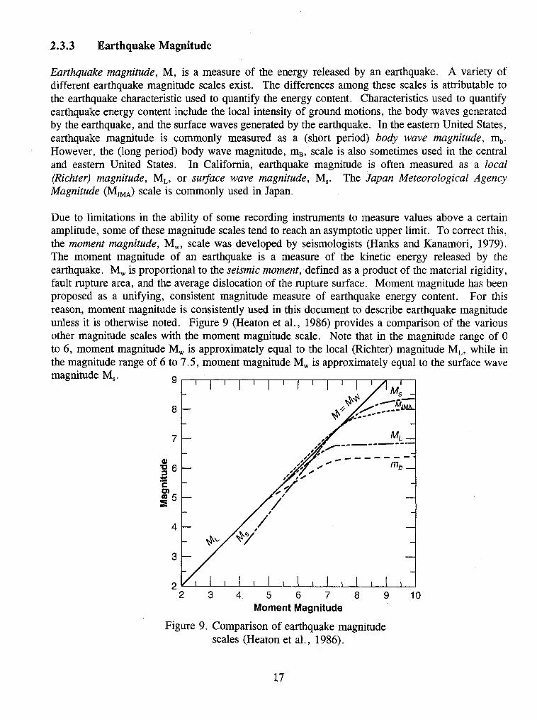
2.3.3 Earthquake Magnitude

Earthquake magnitude, M, is a measure of the energy released by an earthquake. A variety of different earthquake magnitude scales exist. The differences among these scales is attributable to the earthquake characteristic used to quantify the energy content. Characteristics used to quantify earthquake energy content include the local intensity of ground motions, the body waves generated by the earthquake, and the surface waves generated by the earthquake. In the eastern United States, earthquake magnitude is commonly measured as a (short period) body wave magnitude, m,. However, the (long period) body wave magnitude, m,, scale is also sometimes used in the central and eastern United States. In California, earthquake magnitude is often measured as a local (Richter) magnitude, ML, or suvace wave magnitude, Ms. The Japan Meteorological Agency Magnitude (MJMA) scale is commonly used in Japan.

Due to limitations in the ability of some recording instruments to measure values above a certain amplitude, some of these magnitude scales tend to reach an asymptotic upper limit. To correct this, the moment magnitude, M,, scale was developed by seismologists (Hanks and Kanamori, 1979). The moment magnitude of an earthquake is a measure of the kinetic energy released by the earthquake. M, is proportional to the seismic moment, defined as a product of the material rigidity, fault rupture area, and the average dislocation of the rupture surface. Moment magnitude has been proposed as a unifying, consistent magnitude measure of earthquake energy content. For this reason, moment magnitude is consistently used in this document to describe earthquake magnitude unless it is otherwise noted. Figure 9 (Heaton et al., 1986) provides a comparison of the various other magnitude scales with the moment magnitude scale. Note that in the magnitude range of 0 to 6, moment magnitude M, is approximately equal to the local (Richter) magnitude ML, while in the magnitude range of 6 to 7.5, moment magnitude M, is approximately equal to the surface wave magnitude Ms.

2 3 4 . 5 6 7 8 9 10 Moment Magnitude

Figure 9. Comparison of earthquake magnitude scales (Heaton et al., 1986).

2.3.4 Hypocenter and Epicenter

The hypocenter (focus) of an earthquake is the point from which the seismic waves first emanate. Conceptually, it may be considered as the point on a fault plane where the slip responsible for an earthquake was initiated. The epicenter is a point on the ground surface directly above the hypocenter. Figure 10 shows the relationship between the hypocenter, epicenter, fault plane, and rupture zone of an earthquake. Figure 10 also shows the definition of the strike and dip angles of the fault plane.

2.3.5 Zone of Energy Release

The zone of energy release, sometimes referred to as the zone of seismogenic rupture, is the area on the fault plane from which the seismic waves that generate strong ground motions emanate. The zone of energy release is generally the portion of the rupture zone that is within crystalline rock. Therefore, even if the fault plane ruptures to the ground surface, the zone of energy release may not extend to the ground surface.

Figure 10. Definition of basic fault geometry.

2.3.6 Site-to-Source Distance

Figure 11 provides definitions of various site-to-source distances commonly used to estimate earthquake-induced ground motions. In the eastern United States, epicentral distance, RE, is

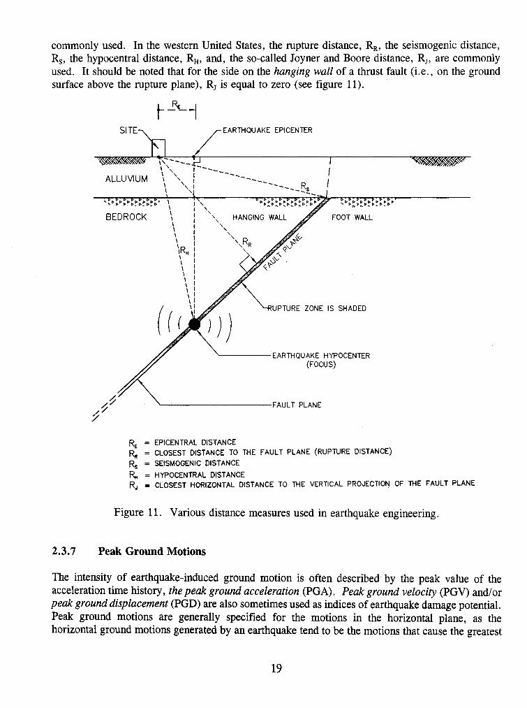
commonly used. In the western United States, the rupture distance, RR, the seismogenic distance, Rs, the hypocentral distance, RH, and, the so-called Joyner and Boore distance, Rj, are commonly used. It should be noted that for the side on the hanging wall of a thrust fault (i.e., on the ground surface above the rupture plane), Rj is equal to zero (see figure 1 1).

SITE\ ,-EARTHQUAKE EPICENTER

I , HANGING WALL // FOC BEDROCK '

~ U P T U R E ZONE IS SHADED

EARTHQUAKE HYPOCENTER (FOCUS)

/ \ FAULT PLANE

RE = EPICENTRAL DISTANCE R, = CLOSEST DISTANCE TO THE FAULT PLANE (RUPTURE DISTANCE) Rs = SElSMOGENlC DISTANCE

R H = HYPOCENTRAL DISTANCE Rj = CLOSEST HORIZONTAL DISTANCE TO M E VERTICAL PROJECTION OF THE FAULT PLANE

Figure 11. Various distance measures used in earthquake engineering.

2.3.7 Peak Ground Motions

The intensity of earthquake-induced ground motion is often described by the peak value of the acceleration time history, the peak ground acceleration (PGA) . Peak ground velocity (PGV) and/or peak ground displacement (PGD) are also sometimes used as indices of earthquake damage potential. Peak ground motions are generally specified for the motions in the horizontal plane, as the horizontal ground motions generated by an earthquake tend to be the motions that cause the greatest

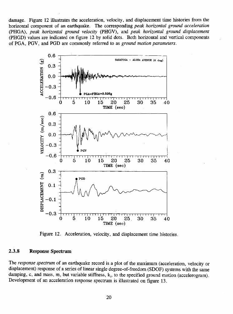
damage. Figure 12 illustrates the acceleration, velocity, and displacement time histories from the horizontal component of an earthquake. The corresponding peak horizontal ground acceleration (PHGA), peak horizontal ground velocity (PHGV), and peak horizontal ground displacement (PHGD) values are indicated on figure 12 by solid dots. Both horizontal and vertical components of PGA, PGV, and PGD are commonly referred to as ground motion parameters.

n 0.6 -

M SARATOGA - ALOHA AVENUE (0 deg) -

w

0.3 - 5 - 6 0.0

!3 - -

w -0.3 - U - U 4 - & PGA=PHGA=O.SZIg

-0.6 ~ ~ I I ~ ~ I ~ ~ ~ I ~ ~ ~ ~ ~ ~ ~ ~ ~ ~ ~ ~ ~ ~ ~ ~ ~ ~ ~ ~ ~ ~ ~ ~ ~ ~ ~ ~

0 5 10 15 20 25 30 35 40 TIME (sec)

TIME (sec)

PGD 1

- - - -

I I I I ~ I I I I ~ I l l I ~ ( I I I I I I i I I I I I I

0 5 10 15 20 25 3 TIME (sec)

Figure 12. Acceleration, velocity, and displacement time histories.

2.3.8 Response Spectrum

The response spectrum of an earthquake record is a plot of the maximum (acceleration, velocity or displacement) response of a series of linear single degree-of-freedom (SDOF) systems with the same damping, c, and mass, m, but variable stiffness, ki, to the specified ground motion (accelerogram). Development of an acceleration response spectrum is illustrated on figure 13.

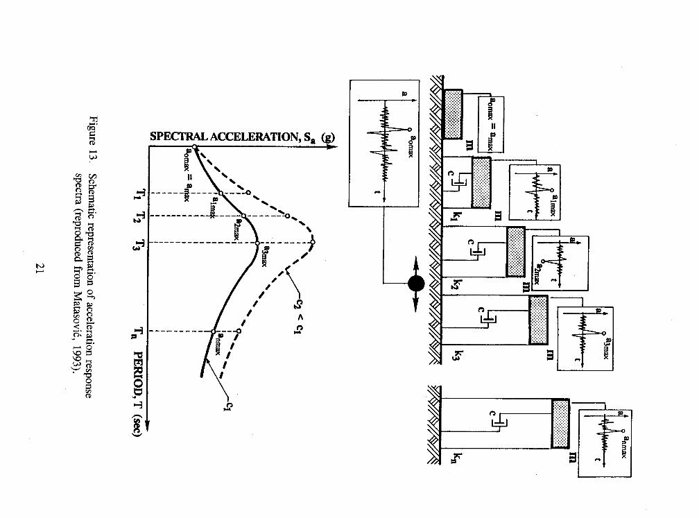
The undamped fundamental period, Ti, of each SDOF system used to develop the response spectrum is calculated as:

The damping of the SDOF system is represented by the viscous damping coeflcient, c, commonly referred to as the spectral damping. In geotechnical earthquake engineering, spectral damping is commonly assumed to be equal to 5 %.

Response spectra are commonly calculated by commercial computer programs (e.g., Nigam and Jennings, 1968; Idriss et al., 1992). The spectral accelerations, S,, spectral velocities, S,, and spectral displacements, S,, can be presented in several graphical forms. The most common presentation is a plot of the spectral values as a function of Ti, as illustrated on figure 13.

In structural and retaining wall design, where spectral velocities or displacements may govern the design, presentation of the response spectrum as a tripartite spectral plot is common. An example of such a tripartite plot is shown on figure 14. A tripartite plot simultaneously displays S,, S,, and S, values for the selected spectral damping. For a given fundamental period, To, (or fundamental frequency fo = l/To), S,, S,, and S, are read from appropriate ordinates. For example, as indicated on figure 14, for To = 0.7 sec (fo = 1.4 Hz), S, = 0.19 g, S, = 0.25 m/sec, and S, = 0.03 m.

FREQUENCY (Hz) /-f,=1.4 HZ

Figure 14. Tripartite representation of acceleration, velocity, and displacement response spectra.

2.3.9 Attenuation Relationships

An attenuation relationship describes the relationship between earthquake magnitude, site-to-source distance, and the peak or spectral value of a ground motion parameter (e. g . , PHGA, PHGV, PHGD, S,, S,, or S,). Acceleration attenuation relationships (for both peak and spectral values) are most common. Attenuation relationships are usually developed by statistical analysis of ground motion parameters observed in previous earthquakes. The variability in the ground motion parameters for a given magnitude and distance is generally characterized by the standard deviation of the statistical data. This variability is usually assumed to be log-normally distributed (i.e., the logarithm of the parameter value is normally distributed).

Numerous attenuation relationships can be found in the technical literature. Commonly used attenuation relationships are described in chapter 4. Figure 11 identifies the distance measures associated with the most common attenuation relationships used in engineering practice.

CHAPTER 3

SEISMIC HAZARD ANALYSIS

3.1 GENERAL

The process by which design ground motion parameters are established for a seismic analysis is termed the seismic hazard analysis. Seismic hazard analyses generally involve the following steps:

identification of the seismic sources capable of strong ground motions at the project site;

evaluation of the seismic potential for each capable source; and

evaluation of the intensity of the design ground motions at the project site.

Identification of seismic sources includes establishing the type of fault and its geographic location, depth, size, and orientation. Seismic source identification may also include specification of a random seismic source to accommodate earthquakes not associated with any known fault. Evaluation of the seismic potential of an identified source involves evaluation of the earthquake magnitude (or range of magnitudes, see section 3.3.3) that the source can generate and, often times, the expected rate of occurrence of events of these magnitudes.

Identification of capable seismic sources together with evaluation of the seismic potential of each capable source may be referred to as seismic source characterization. Once the seismic sources are characterized, the intensity of ground motions at the project site from these sources must be characterized. There are three general ways by which the intensity of ground motions at a project site are assessed in practice. They are, in order of complexity: (1) use of local building codes and standards; (2) deterministic seismic hazard evaluation; and (3) probabilistic seismic hazard evaluation. Which particular approach is adopted may depend on the importance and complexity of the project and may be dictated by regulatory agencies.

SEISMIC SOURCE CHARACTERIZATION

3.2.1 Overview

The importance of seismic source characterization cannot be overemphasized. Seismic source characterization forms the basis for the evaluation of potential ground motions for design analysis. Even if the intensity of the design ground motion is obtained from a building code or published map, seismic source characterization is still required for most geotechnical analyses to establish an earthquake magnitude for use in design.

Seismic source characterization is best done as part of a comprehensive geologic and seismologic evaluation that includes review of pertinent literature, aerial photograph interpretation, geologic field reconnaissance, geologic mapping, and micro-seismicity evaluations.

General information on regional seismic sources can usually be obtained from published information. Site specific studies may be required to characterize local seismic sources. Geophysical surveys, geologic mapping, and trenching are often useful for locating local faults and characterizing their seismic potential. However, such investigations may only identify those faults along which rupture has propagated to the ground surface. Buried faults without surface expression must also be considered in the characterization of seismic sources. A mirco-seismicity study (study of instrumentally-recorded earthquakes that are generally not felt and do not cause damage to structures) using data from local or regional seismic monitoring networks may be useful in evaluating the potential for buried faults in the project vicinity.

3.2.2 Methods for Seismic Source Characterization

Seismic sources are generally characterized on a fault-specific basis by geometry (location, length, dip angle, depth, and distance to the site), seismic potential (earthquake magnitude, activity, recurrence), and style of faulting (strike slip, dip slip, or oblique slip). In regions where the observed seismicity cannot be correlated with specific faults, broad area sources may be appropriate.

An investigation to identify the seismic sources that may impact a given site typically includes both a review of available data and field geologic reconnaissance. Available data may include pertinent technical publications, university theses and research reports, maps, aerial photographs, and interviews with experts familiar with the region under study. Pertinent technical publications include maps prepared by the California Division of Mines and Geology (CDMG) identifying young faults in the western dates (e,g., Jennings, 1994), publications of the Seismological Society of America (e. g . , SSA, 1988), and regional reports from seismological networks and state geological surveys. A detailed summary of available sources of engineering geologic information is presented by Trautmann and Kulhawy (1983).

Studies performed for siting of nuclear power plants and for high and low level radioactive waste disposal facilities can be a useful source of information on regional seismicity and geology. All applications for construction permits for nuclear generating stations are required to contain documentation on regional geology, including known faults and observed seismicity, within a 320 kilometer radius of the site. This information can be found in the Preliminary Safety Analysis Report (PSAR) and the Final Safety Analysis Report (FSAR) for the project. These reports are available through the National Technical Information Service (NTIS) for all existing and many proposed nuclear generating stations. However, as many of these reports are more than 20 years old, more recent sources of information on regional seismicity and tectonics should be consulted. More recent information may be available from siting studies performed for low level radioactive waste repositories, regional landfills, and other important or critical facilities.

Existing seismic networks often provide very detailed information about recent earthquakes within seismic impact regions. Such information typically includes the magnitude and epicentral location

of all detected events and is commonly available plotted in map form. A detailed evaluation of each detected event may also be available. The presence of micro-seismic activity can also be used to infer the location of a subsurface seismic source. Information from most of the established seismic networks in the United States can be obtained for a nominal cost from the National Geophysical Data Center which is located in Boulder City, Colorado.

Interpretation of aerial photographs can be particularly useful in identifying and locating potentially active faults. Sources of such photographs are discussed by Trautmann and Kulhawy (1983). Evidence of active faults may be indicated in aerial photographs by geomorphic features such as fault scarps, triangular facets, fault scarplets, fault rifts, fault slice ridges, shutter ridges, and fault saddles (Cluff et al., 1972). Additional evidence can be provided by ground features such as open fissures, offsets in such features as fence lines, landscape features, mole tracks, and furrows, rejuvenated streams, folding or warping of young deposits, groundwater barriers in recent alluvium, and fault paths on young surfaces. Usually a combination of such features is generated by recent fault movement at the ground surface. Note that many of the fault movement indicators require the presence of undisturbed surface soils at the site. Region that have limited surface soils due to geologic mechanisms or man's activities can provide a significant challenge in evaluating the recency of movement on existing faults.

Seismic source identification almost always includes preliminary field reconnaissance. Preliminary field reconnaissance should be performed in the project vicinity using the following steps (modified after USEPA, 1993):

Step 1: Walk the site and site vicinity to identify possible geomorphic or ground features that indicate faulting.

Step 2: Collect and interpret aerial photographs, such as low sun angle photographs, that use shadows to accentuate topographic differences, infrared photographs that indicate temperature differences containing surface moisture content, and color photographs to study slight color changes.

Step 3: Based on the above reconnaissance, draw a conclusion on the potential presence of active faults within the surveyed area.

Seismic source characterization can be a complex task, particularly in areas where the information available in the technical literature is incomplete or insufficient. Evaluation of micro-seismicity, interpretation of aerial photographs, and field reconnaissance studies should be performed by a geologist, seismologist, or geotechnical professional experienced in these areas and not by an unqualified geotechnical engineer.

3.2.3 Defining the Potential for Fault Movement

Movement within the Holocene Epoch (approximately the past 11,000 years), is generally regarded as the criterion for establishing that a fault is active (e.g., CDMG, 1986; USEPA, 1993). However, it is possible that the recurrence interval for major earthquakes may exceed 11,000 years on some

faults. Furthermore, since not all faults rupture the ground surface and geomorphic evidence of fault displacement ca'n be obliterated by natuml and man-made activities, it may not be possible to definitely establish whether or not a fault has moved in the past 11,000 years. Therefore, lack of evidence of Holocene movement may not in itself be sufficient grounds to dismiss a fault as inactive. Nevertheless, evidence that a fault has not moved in Holocene time is generally considered sufficient evidence to dismiss the potential for ground surface rupture.

Most Holocene fault activity in North America has been west of the Rocky Mountains. Only two instances of ground surface rupture in the east of the Rocky Mountains in Holocene time have been conclusively established (the Meers fault in Oklahoma and the Ungava fault in Quebec). However, there have been several major earthquakes that caused widespread damage (e.g., Cape Ann, Massachusetts, 1775; New Madrid, Missouri, 181 1 and 1812; and Charleston, South Carolina, 1886) and numerous smaller events causing local damage (e.g., Attica, New York, 1929; Massena, New York, 1944; Miramichi, New Hampshire, 1982) in the eastern and central United States in the past 250 years. Most of these damaging eastern and central United States events have had surface manifestations in the form of landslides, soil liquefaction, and ground cracking.

If the review of available geotechnical and seismological information and the preliminary site reconnaissance indicates the potential presence of active faults at the project site, then detailed geologic investigation may be required to establish the location of faults and the recency of fault movement in the vicinity of the site. A detailed geologic surface reconnaissance study may be sufficient to identify fault locations and assess the magnitude and direction of past fault movements. The detailed reconnaissance study may be supplemented, if necessary, by a subsurface field investigation. The field investigation may include the following:

use of geophysical methods such as resistivity, seismic refraction, seismic reflection, or magnetic survey methods to identify potential fault locations;

excavation of exploratory trenches across potential faults and through "marked" beds of geologic strata to allow the detailed examination of the trench walls for evidence of the presence or absence of earthquake-induced displacements and recovery of material for stratigraphic age dating; and

use of vertical and angled borings to locate fault zones and recover material for stratigraphic age dating.

The depth of the subgrade investigated by trenches and geophysical methods should be sufficient to encompass geologic activity within the Holocene Epoch. The depth of the boring may need to be significantly greater than the depth of Holocene strata if its purpose is to locate the fault trace. Radiocarbon dating of carbonaceous material encountered in the field investigation can be used to constrain the age of most recent fault offsets. A detailed description of soil-stratigraphic dating techniques is presented by Shlemon (1985). Sieh et al. (1989) describe the application of high- precision radiocarbon dating for chronological analysis of active faulting. Jibson (1985) describes field investigation of geomorphic evidence (e.g., landsliding, liquefaction) of earthquake activity in an area in the central United States where fault rupture did not propagate up to the ground surface. Establishing that recent displacement has or has not occurred is greatly complicated if a limited soil

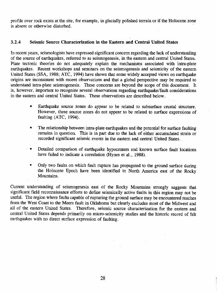
profile over rock exists at the site, for example, in glacially polished terrain or if the Holocene zone is absent or otherwise disturbed.

3.2.4 Seismic Source Characterization in the Eastern and Central United States

In recent years, seismologists have expressed significant concern regarding the lack of understanding of the source of earthquakes, referred to as seismogenesis, in the eastern and central United States. Plate tectonic theories do not adequately explain the mechanisms associated with intra-plate earthquakes. Recent workshops and seminars on the seismogenesis and seismicity of the eastern United States (SSA, 1988; ATC, 1994) have shown that some widely accepted views on earthquake origins are inconsistent with recent observations and that a global perspective may be required to understand intra-plate seismogenesis. These concerns are beyond the scope of this document. It is, however, important to recognize several observations regarding earthquakelfault considerations in the eastern and central United States. These observations are described below.

Earthquake source zones do appear to be related to subsurface crustal structure. However, these source zones do not appear to be related to surface expressions of faulting (ATC, 1994).

The relationship between intra-plate earthquakes and the potential for surface faulting remains in question. This is in part due to the lack of either accumulated strain or recorded significant seismic events in the eastern and central United States.

Detailed comparison of earthquake hypocenters and known surface fault locations have failed to indicate a correlation (Hynes et al., 1988).

Only two faults on which fault rupture has propagated to the ground surface during the Holocene Epoch have been identified in North America east of the Rocky Mountains.

Current understanding of seismogenesis east of the Rocky Mountains strongly suggests that significant field reconnaissance efforts to define seismically active faults in this region may not be useful. The region where faults capable of rupturing the ground surface may be encountered reaches from the West Coast to the Meers fault in Oklahoma but clearly excludes most of the Midwest and all of the eastern United States. Therefore, seismic source characterization for the eastern and central United States depends primarily on micro-seismicity studies and the historic record of felt earthquakes with no direct surface expression of faulting.

3.3 DETERMINATION OF THE INTENSITY OF DESIGN GROUND MOTIONS

3.3.1 Introduction

Once the seismic sources capable of generating strong ground motions at a project site have been identified and characterized, the intensity of the ground motions which may be generated at the site are evaluated for use in design. Design ground motions can be evaluated in three different ways:

from published codes and standards;

from a deterministic seismic hazard analysis; or

from a probabilistic seismic hazard analysis.

3.3.2 Published Codes and Standards

Inforrnation used for seismic source characterization can often be obtained from published codes and standards (e . g . , local building codes, publications of the United States Geological Survey (USGS) , or various state agencies). Published codes and standards are often used because they provide credibility for the designer and may give the engineer a feeling of security. However, due to the lag time between development and publication, published codes and standards may not incorporate recent developments on local or regional seismicity. Furthermore, published codes and standards are usually based upon rather broad, regional analyses and may not reflect local, site-specific conditions.

Building Codes often contain a seismic zone map that includes minimum required seismic design parameters. For example, the Applied Technology Council (ATC) map shown in figure 15 in a reduced size format divides the United States into five zones that reflect the expected intensity of shaking in each zone. Typically, seismic coefficients for use in structural analyses are associated with the seismic zones presented on the map. An example of such a map is shown in figure 16 (UBC, 1994). The seismic coefficients associated with these zones usually represent "effective" ground motions for structural analyses and are not suitable for use in geotechnical analyses. However, codes may occasionally provide minimum values of the seismic coefficient for use in slope stability analyses. In using building codes, it should be kept in mind that building codes are generally intended to mitigate collapse and loss of life and not necessarily prevent damage, and that a code presents a minimum standard of care for design.

Some published codes and standards provide information on the expected value of the peak earthquake ground motions. The California Department of Transportation (CALTRANS) has developed a statewide map showing the peak ground acceleration in bedrock from the Maximum Credible Earthquake (MCE) (Mualchin and Jones, 1992; updated by Mualchin, 1995). The MCE is the regulatory design-basis earthquake in California for major bridges (e.g., toll bridges) and other important facilities (e.g., hospitals, earth dams). The USGS map presented in figure 17 presents the estimated peak ground acceleration for a hypothetical bedrock outcrop at a project site

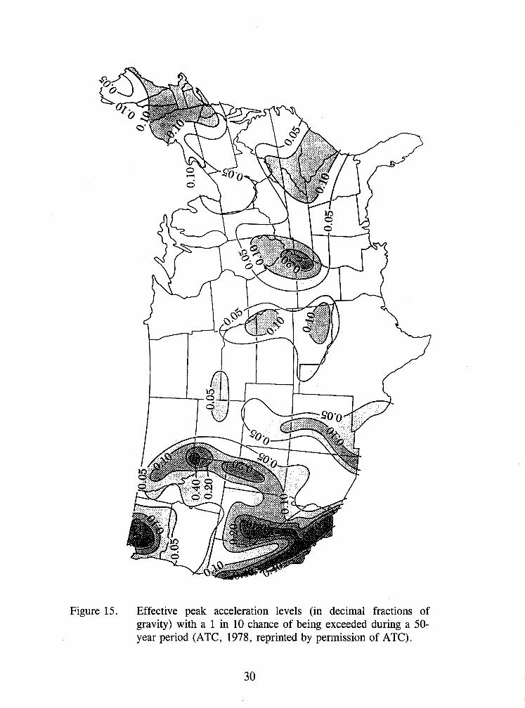
Figure 15. Effective peak acceleration levels (in decimal fractions of gravity) with a 1 in 10 chance of being exceeded during a 50- year period (ATC, 1978, reprinted by permission of ATC).

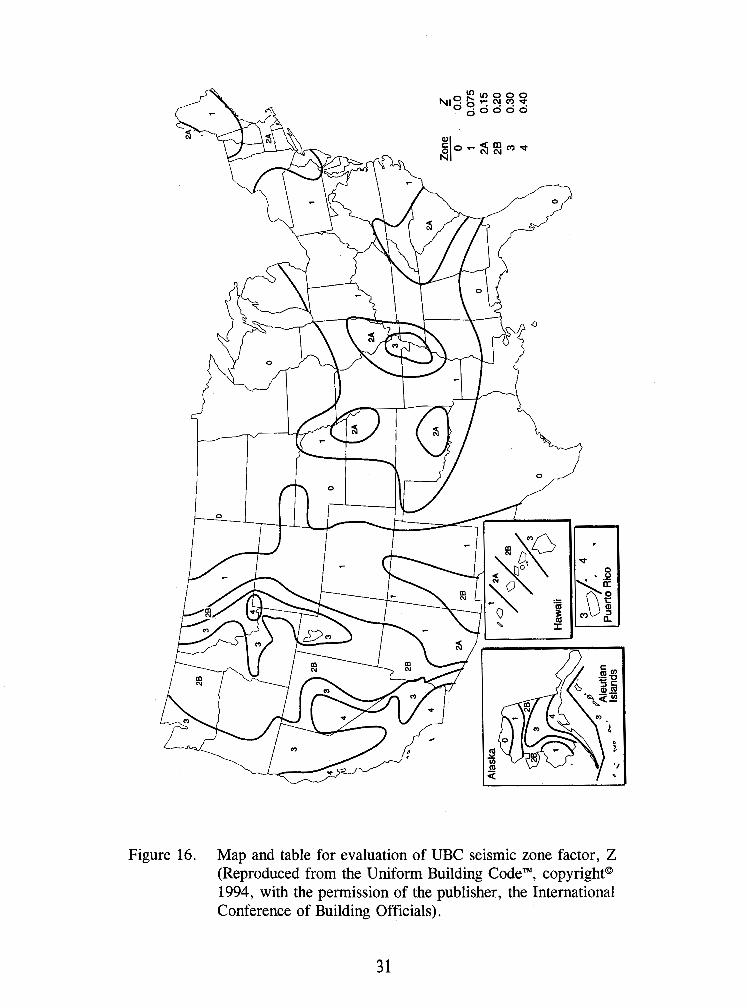
Figu re 16. Map and table for evaluation of UBC seismic zone factor, Z (Reproduced from the Uniform Building Code", copyrighta 1994, with the permission of the publisher, the International Conference of Building Officials).

3 1

with a 90 percent probability of not being exceeded in 50 years. USGS also provides maps for 10- and 50-year exposure periods and for the peak ground velocity (Algermissen et al., 1982, 1991). Maps that provide spectral acceleration values for specified spatial periods are currently being deployed by the USGS under the National Earthquake Hazard Reduction Program (NEHRP). If bedrock is not present at or near the ground surface, values from the CALTRANS or USGS maps may need to be modified to account for local site conditions.

The procedure for seismic hazard analysis using a published map is relatively simple:

Step 1: Read the design peak ground acceleration from the map.

Step 2: Assign a corresponding magnitude and distance to the peak design ground acceleration using information on regional seismic sources.

However, the CALTRANS , USGS , and other common seismic hazard maps typically do not provide information on the magnitude, distance, or duration of the earthquake associated with the map acceleration values. In fact, the acceleration values provided by the USGS maps are typically composed of contributions of earthquakes of many different magnitudes at many different distances. These maps provide a statistical estimate of the peak ground acceleration based on the estimated frequency of earthquakes of the various seismic sources considered in the analysis. For many geotechnical analyses, knowledge of earthquake magnitude and, in some cases, distance and/or duration, is required. Therefore, if the USGS or CALTRANS map acceleration is to be used in a geotechnical analysis, a means of assigning a representative magnitude to the design event may be needed.

Another problem associated with using a map acceleration in a geotechnical analysis is that the earthquake generating the maximum peak ground acceleration at a site may not necessarily be the most damaging earthquake. An earthquake of lesser peak intensity but greater duration may be more damaging than the event associated with the maximum peak ground acceleration. In such cases, it may prove necessary to perform a site-specific seismic risk analysis.

Despite these shortcomings, peak acceleration values derived from published maps can be, and often are, used in geotechnical practice. Information on the location and magnitudes of earthquake sources can be obtained from either background information published with the map or from other sources of information. For example, Mualchin and Jones (1992) include a listing of seismic sources and maximum magnitudes used to develop the CALTRANS map. Information on earthquake magnitudes associated with USGS map shown in figure 17 can be found in Algermissen et al. (1982). Figure 18 is a more recent map of seismic sources for the central United States. The map in figure 18 includes information on the maximum magnitude earthquake associated with each source zone, expressed in terms of body wave magnitude. Figure 19 is another example of a recent seismic source zone map. Thiq map, developed especially for the central and eastern united States, and accompanying detailed information on source and background zones and earthquake magnitudes, can be found in a comprehensive, ten-volume seismic hazard study by EPRI (1986).

Figure 17. Peak horizontal ground acceleration in bedrock with a 10 percent probability of exceedance in 50 years (after Algerrnisen et al., 1982; 1991).

3 3

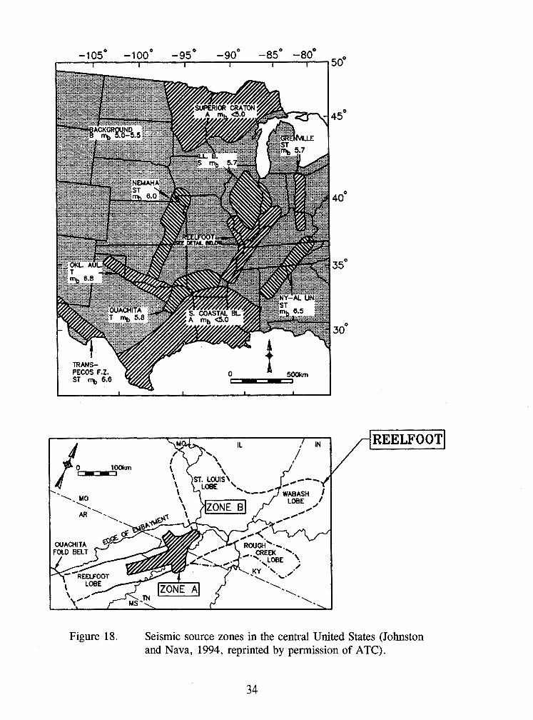
Figure 18. Seismic source zones in the central United States (Johnston and Nava, 1994, reprinted by permission of ATC).

Figure 19. Seismic source zones in the central and eastern United States (EPRI, 1986, reprinted by permission of ATC).

In using background zone and magnitude information to supplement PGA data from USGS, EERI, and other maps, the prudent engineer generally makes conservative assumptions to compensate for the uncertainty associated with published map data. For instance, the engineer may select the largest magnitude associated with the governing source zone for his project and locate it at the point within the zone closest to his site. If the governing source zone is uncertain, he may include multiple source zones in his analysis.

3.3.3 The Deterministic Approach

The objective of a deterministic seismic hazard analysis is to evaluate the magnitude of ground motion parameters (usually peak ground acceleration and acceleration response spectra) at a specific site from all the capable seismic sources with the potential for generating strong ground motions at the site. In some cases, particularly when soft soils capable of amplifying ground motions from

earthquakes are present at the site, the seismic hazard analysis may include sources located over 100 krn from the site.

In a deterministic seismic hazard analysis, the engineer or geologist performing the analysis first identifies the capable seismic sources and assigns a maximum magnitude to each source. Then, the intensity of shaking at the site from each capable source is calculated and the design earthquake is identified based on the source capable of causing the greatest damage. The steps in a deterministic seismic hazard analysis are as follows:

Step 1: Establish the location and characteristics (e.g., style of faulting) of all potential earthquake sources that might affect the site. For each source, assign a representative earthquake magnitude.

Step 2: Select an appropriate attenuation relationship and estimate the ground motion parameters at the site from each capable fault as a function of earthquake magnitude, fault mechanism, site-to-source distance, and site conditions.

Step 3: Screen the capable (active) faults on the basis of magnitude and the intensity of the ground motions at the site to determine the governing source.

Engineers or engineering geologists performing deterministic seismic hazard analyses should consider all reasonable interpretations, models, and values in characterizing the seismic source zones. While all capable sources are usually treated equally in a deterministic analysis regardless of their likelihood of occurrence, the likelihood of occurrence may enter into the determination of whether or not a fault is capable of generating earthquakes of specified magnitudes. For instance, some bridges in California have been designed for the Maximum Probable Earthquake (MPE) defined by the California Division of Mines and Geology (CDMG) as the maximum earthquake anticipated in the next 100 years (CDMG, 1975). Therefore, active faults with long recurrence intervals may not be considered in evaluating the MPE, and the MPE magnitude may not be the largest magnitude earthquake of which the fault is capable.

Screening for the most damaging event in a deterministic seismic hazard analysis is typically based upon magnitude, intensity, and distance wherein events of smaller magnitude and lower intensity than events closer to the source are eliminated from consideration. However, it may not be possible to establish a single event that is most damaging based on the results of a deterministic analysis, as this process can result in a family of design events of increasing magnitude and distance with decreasing intensity. As there is no general method for evaluating the relative damage potential of one event with a large magnitude and low intensity compared to a smaller magnitude event of higher intensity, it may be necessary to consider multiple events in subsequent engineering analysis (unless the intensity discrepancy is so great or the magnitudes are so close that the choice is obvious).

Screening capable seismic sources on the basis of magnitude and distance prior to evaluating the intensity of ground motions at the site is not recommended as it can lead to errors due to the dependence of the mode of faulting on the intensity of ground motions. It is generally assumed that thrust faults generate higher intensity ground motions than strike slip faults of the same magnitude

at the same distance. Therefore, if the family of capable (active) faults includes faults with different modes of behavior, faults should not be screened on the basis of magnitude and distance only.

The intensity of the earthquake ground motions at the site generated by a capable (active) fault (or seismic zone) is evaluated using an attenuation relationship. Attenuation relationships that discriminate between different styles of faulting and between rock and soil sites are available. However, attenuation relationships associated with soil sites typically have greater uncertainty assigned to them than rock site attenuation relationships due to the greater observed variability in ground motions at soil sites. Therefore, it is generally more desirable to use attenuation relationships developed for rock sites in a seismic hazard analysis for a geotechnical problem and then to perform a site-specific analysis of the impact of local soil conditions on the design ground motions rather than to use a soil site attenuation relationship. Attenuation relationships are described in more detail in chapter 4. Site-specific seismic response analyses are described in chapter 6.

3.3.4 The Probabilistic Approach

A probabilistic seismic hazard analysis incorporates the likelihood of a fault rupturing and the distribution of earthquake magnitudes associated with fault rupture into the assessment of the intensity of the design ground motion at a site. The objective of a probabilistic seismic hazard analysis is to compute, for a given exposure time, the probability of exceedance corresponding to various levels of a ground motion parameter (e.g., the probability of exceeding a peak ground acceleration of 0.2 g in a 100-year period). The ground motion parameter may be either a peak value (e. g . , peak ground acceleration) or a response spectra ordinate associated with the strong ground motion at the site. The probabilistic value of the design parameter incorporates both the uncertainty of the attenuation of strong ground motions and the randomness of earthquake occurrences. A probabilistic seismic hazard analysis usually includes the following steps:

Step 1: Identify the seismic sources capable of generating strong ground motion at the project site.

Step 2: Determine the minimum and maximum magnitude of an earthquake associated with each source. While the maximum magnitude is a physical parameter related to the fault dimensions, the minimum magnitude may be related to both the physical properties of the fault and the constraints of the numerical analysis. Use of a minimum magnitude less than 4.5 is not recommended, even if the seismic source is capable of generating smaller magnitude events, as inclusion of such small magnitude events can result in misleadingly high response values for extreme (low) probabilities of exceedance.

Step 3: For each source, assign a frequency distribution of earthquake occurrence to the established range of magnitudes.

Step 4: For each source, assign an attenuation relationship on the basis of the style of faulting. Uncertainty is usually assigned to the attenuation relationships based upon statistical analysis of attenuation in previous earthquakes.

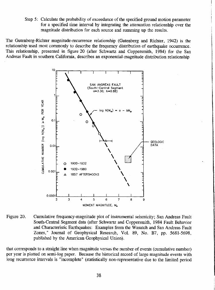
Step 5: Calculate the probability of exceedance of the specified ground motion parameter for a specified time interval by integrating the attenuation relationship over the magnitude distribution for each source and summing up the results.

The Gutenberg-Richter magnitude-recurrence relationship (Gutenberg and Richter, 1942) is the relationship used most commonly to describe the frequency distribution of earthquake occurrence. This relationship, presented in figure 20 (after Schwartz and Coppersmith, 1984) for the San Andreas Fault in southern California, describes an exponential-magnitude distribution relationship

10 - - - I I - - -

- - -

- - - -

SAN ANDREAS FAULT - -

(South-Central Segment - a=3.30; b=0.88)

1 - - - - - fY

- - $

- - - -

- - - fY - w log N(M,) = a - bM,

- a - - ., 0.1 - - - - - r? - - - - - zB

- - V

- Z - - 0 -

- - - - LY

- w 0.01- m - I

\ - -

3 - z - \ 9

- -

i= 4 -1

- 0 1900-1932 3 I 2 0.001 - 8 1932-1980 \

= A 1857AFTERSHOCKS \ - - - - -

- - \

- - - \

- -

- -

0.0001 I I I I I I 2

A

3 4 5 6 7 8 9

MOMENT MAGNITUDE, M,

GEOLOGIC DATA

Figure 20. Cumulative frequency-magnitude plot of instrumental seismicity; San Andreas Fault South-Central Segment data (after Schwartz and Coppersmith, 1984 Fault Behavior and Characteristic Earthquakes: Examples from the Wasatch and San Andreas Fault Zones," Journal of Geophysical Research, Vol. 89, No. 87, pp. 5681-5698, published by the American Geophysical Union).

that corresponds to a straight line when magnitude versus the number of events (cumulative number) per year is plotted on semi-log paper. Because the historical record of large magnitude events with long recurrence intervals is "incomplete" (statistically non-representative due to the limited period

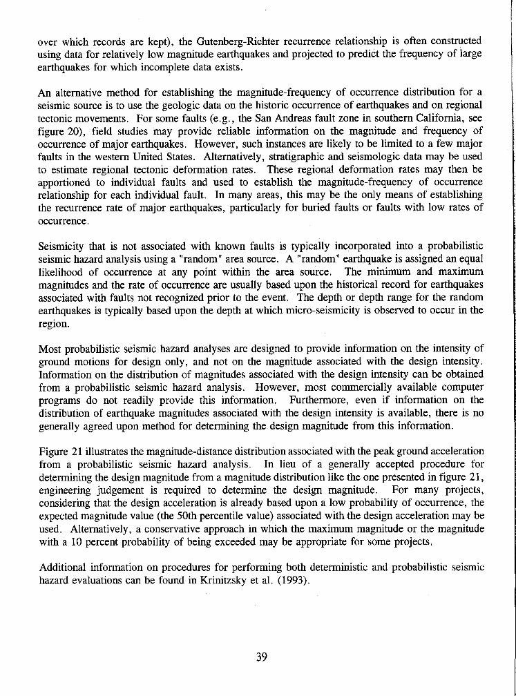
over which records are kept), the Gutenberg-Richter recurrence relationship is often constructed using data for relatively low magnitude earthquakes and projected to predict the frequency of large earthquakes for which incomplete data exists.

An alternative method for establishing the magnitude-frequency of occurrence distribution for a seismic source is to use the geologic data on the historic occurrence of earthquakes and on regional tectonic movements. For some faults (e.g . , the San Andreas fault zone in southern California, see figure 20), field studies may provide reliable information on the magnitude and frequency of occurrence of major earthquakes. However, such instances are likely to be limited to a few major faults in the western United States. Alternatively, stratigraphic and seismologic data may be used to estimate regional tectonic deformation rates. These regional deformation rates may then be apportioned to individual faults and used to establish the magnitude-frequency of occurrence relationship for each individual fault. In many areas, this may be the only means of establishing the recurrence rate of major earthquakes, particularly for buried faults or faults with low rates of occurrence.

Seismicity that is not associated with known faults is typically incorporated into a probabilistic seismic hazard analysis using a "random" area source. A "random" earthquake is assigned an equal likelihood of occurrence at any point within the area source. The minimum and maximum magnitudes and the rate of occurrence are usually based upon the historical record for earthquakes associated with faults not recognized prior to the event. The depth or depth range for the random earthquakes is typically based upon the depth at which micro-seismicity is observed to occur in the region.

Most probabilistic seismic hazard analyses are designed to provide information on the intensity of ground motions for design only, and not on the magnitude associated with the design intensity. Information on the distribution of magnitudes associated with the design intensity can be obtained from a probabilistic seismic hazard analysis. However, most commercially available computer programs do not readily provide this information. Furthermore, even if information on the distribution of earthquake magnitudes associated with the design intensity is available, there is no generally agreed upon method for determining the design magnitude from this information.

Figure 21 illustrates the magnitude-distance distribution associated with the peak ground acceleration from a probabilistic seismic hazard analysis. In lieu of a generally accepted procedure for determining the design magnitude from a magnitude distribution like the one presented in figure 21, engineering judgement is required to determine the design magnitude. For many projects, considering that the design acceleration is already based upon a low probability of occurrence, the expected magnitude value (the 50th percentile value) associated with the design acceleration may be used. Alternatively, a conservative approach in which the maximum magnitude or the magnitude with a 10 percent probability of being exceeded may be appropriate for some projects.

Additional information on procedures for performing both deterministic and probabilistic seismic hazard evaluations can be found in Krinitzsky et al. (1993).

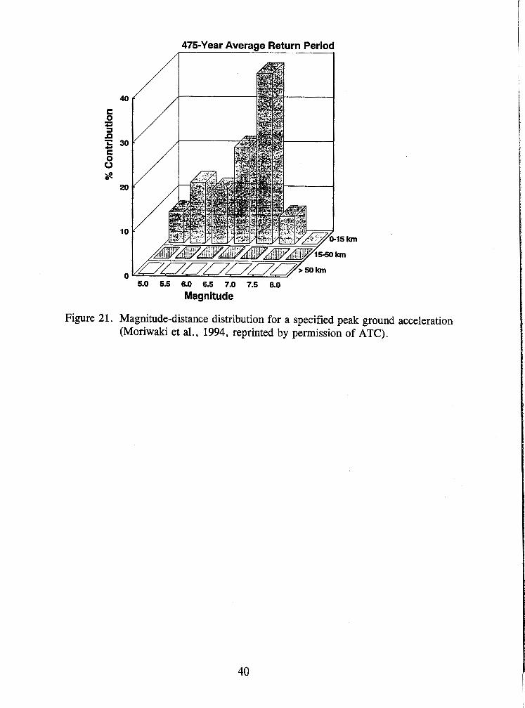
475-Year Average Return Period n I

5.0 5.5 6.0 6.5 7.0 7.5 8.0

Magnitude

Figure 21. Magnitude-distance distribution for a specified peak ground acceleration (Moriwaki et al.. 1994, reprinted by permission of ATC).

CHAPTER 4

GROUND MOTION CHARACTERIZATION

4.1 BASIC GROUND MOTION CHARACTERISTICS

Results of the seismic hazard analysis will establish the peak horizontal ground acceleration (PHGA) for use in design analysis. However, PHGA is only one of the characteristics of the earthquake ground motion at a site that influence the potential for damage. The damage potential of seismically-induced ground motions may also depend upon the duration of strong shaking, the frequency content of the motion, the energy content of the motion, peak vertical ground acceleration (PVGA), peak ground velocity and displacement, and the intensity of the motion at times other than when the peak acceleration occurs, as elaborated below.

The acceleration response spectrum is one commonly used index of the character of earthquake ground motions. An acceleration response spectrum provides quantitative information on both the intensity and frequency content of the acceleration time history. However, while widely used in structural engineering, response spectra are of limited use in geotechnical analysis. The primary application of response spectra to geotechnical practice is as an aid in selection of time histories for input to site response and deformation analyses, for comparison of accelerograms, and for illustration and evaluation of the influence of local soil conditions on ground motions.

Other parameters used less frequently than PHGA and the acceleration response spectrum to describe the character of earthquake ground motions include various measures of the duration and energy content of the acceleration time history. Duration is sometimes expressed directly as the length of time from the initiation of strong shaking to its cessation. Alternatively, indirect measures of duration, including the number of equivalent cycles and the number of positive zero crossings of the acceleration time history, are sometimes employed in earthquake engineering practice.

The energy content of the strong ground motion may be expressed in terms of the root-mean-square (RMS) and duration of the acceleration time history or in terms of the Arias intensity. The RMS, discussed in detail in section 4 -4, represents an "average" or representative value for the acceleration over the defined duration of the strong ground motion. The Arias intensity is the square of the acceleration integrated over the duration of the motion. The time history of the normalized Arias intensity, referred to as a Husid plot, is sometimes used to define the duration of strong shaking.

These various indices of the character of strong ground motions (ground motion parameters) commonly used in engineering practice are defined and described in this chapter. Following their definition and description, procedures for using these indices for selection of representative time histories to characterize earthquake ground motions at a site are presented.

4.2 PEAK VALUES

4.2.1 Evaluation of Peak Parameters

Peak horizontal ground acceleration (PHGA) is the most common index of the intensity of strong ground motion at a site. The PHGA is directly related to the peak inertial force imparted by strong shaking to a structure founded on the ground surface and to the peak shear stress induced within the ground itself. Peak vertical ground acceleration (PVGA), peak horizontal ground velocity (PHGV) , and peak horizontal ground displacement (PHGD) are also used in some engineering analyses to characterize the damage potential of ground motions. For instance, PHGV is a common index of structural damage and PHGD may be used in analyses of retaining walls, tunnels, and underground pipelines. PVGA is an important parameter in the design of base-isolated structures.

Peak values for design analyses are evaluated on the basis of the seismic hazard analysis. For major projects, a site or project specific seismic hazard analysis may be performed. Alternatively, results from published regional seismic hazard analyses or from seismic hazard analyses performed for previous projects in the same vicinity may be used. Most published seismic hazard maps tend to be probabilistic in nature. Both deterministic and probabilistic project-specific analyses are used in practice.

4.2.2 Attenuation of Peak Values

A key step in both deterministic and probabilistic seismic hazard analyses is calculation of the ground motion parameter of interest at a given site from an earthquake of a given magnitude and site-to-source distance. These ground motion parameter values are typically evaluated using an attenuation relationship, an equation that relates the parameter value to the key variables on which the ground motion parameter depends (e.g., earthquake magnitude, site-to-source distance, style of faulting). Attenuation relationships may be developed either from statistical analyses of values observed in previous earthquakes or from theoretical models of the propagation of strong ground motions. These observations and analyses indicate that the most important factors influencing peak values of earthquake strong ground motions at a site are the magnitude of the earthquake, the distance between the site and the earthquake source, the style of faulting, and local ground conditions (e. g., rock or soil site conditions).

There are many different attenuation relationships that have been proposed. Campbell (1985), Joyner and Boore (1988), and Atkinson and Boore (1990) provide excellent summaries of many of the available attenuation relationships.

A large number of attenuation relationships are available for the western united States. These attenuation relationships are based primarily on statistical analysis of recorded data. For the eastern and central United States, where little to no recorded strong motion data are available for statistical analysis, relatively few attenuation relationships are available. The few attenuation relationships that do exist for the eastern and central United States are based primarily upon theoretical models of ground motion propagation due to the lack of observational data.

Even when restricted to a relatively narrow geographic locale like the northwestern United States, there may still be a need to use different attenuation relationships for different tectonic conditions. For example, Youngs et al. (1988) found differences in attenuation of ground motions between earthquakes occurring along the interface between the subducting Juan de Fuca tectonic plate and the North American plate (interplate events) and earthquakes occurring within the subducting Juan de Fuca plate (intraplate events) in the Pacific northwest (see figure 6).

PHGA attenuation relationships for shallow earthquakes that occur at the interface between the Pacific and American tectonic plates in the western United States have been developed by many investigators, including Campbell and Duke (1974), Campbell (1993), Campbell and Bozorgnia (1994), Boore et al. (1993), Boore and Joyner (1994), Sadigh et al. (1993), Geomatrix (1995), Silva and Abrahamson (1993), Abrahamson and Silva (1996), and Idriss (1995). Table 1 presents a summary of commonly used PHGA attenuation relationships in the western United States. These relationships consider earthquake magnitude, site-to-source distance, and local ground conditions (soil or rock). These relationships may also discriminate on the basis of style of faulting, as statistical analysis shows that reverse (thrust) fault events generate peak ground accelerations approximately 20 to 30 percent greater than strike-slip events of the same magnitude at the same distance. Figure 22 compares mean value PHGA attenuation curves for magnitude 6.5 and 8.0 events on a strike-slip fault calculated by three commonly used attenuation relationships for western United States earthquakes.

Different attenuation relationships than those used for shallow crustal earthquakes are used for the subduction zone earthquakes that occur along the Pacific Coast in Alaska, Washington, Oregon, and the northwest corner of California. For subduction zone earthquakes, PHGA attenuation relationships by Cohee et al. (1991) and Youngs et al. (1988) are often used in earthquake engineering practice. Table 2 presents the relationships for attenuation of PHGA in subduction zone earthquakes developed by Cohee et al. (1991) and Youngs et al. (1988).

With respect to differences in ground motion attenuation between the western United States and the eastern and central United States, it is generally agreed that ground motions east of the Rocky Mountains attenuate more slowly than ground motions in the west. However, due to the much lower rates of seismicity and the absence of large magnitude earthquakes since the deployment of strong motion accelerographs in the eastern and central United States, there is insufficient data to characterize the attenuation of strong ground motions east of the Rocky Mountains using statistical methods. Therefore, attenuation relationships used for earthquakes occurring in eastern and central United States are based upon theoretical modeling of ground motion attenuation. Attenuation relationships for the eastern and central United States commonly used in engineering practice include relationships developed by Nuttli and Herrmann (1984), Boore and Atkinson (1987), McGuire et al. (1988), Boore and Joyner (1991), and Atkinson and Boore (1995).

Figure 23 compares typical PHGA attenuation relationship for the eastern and central United States to that used in the western United States (dashed lines).

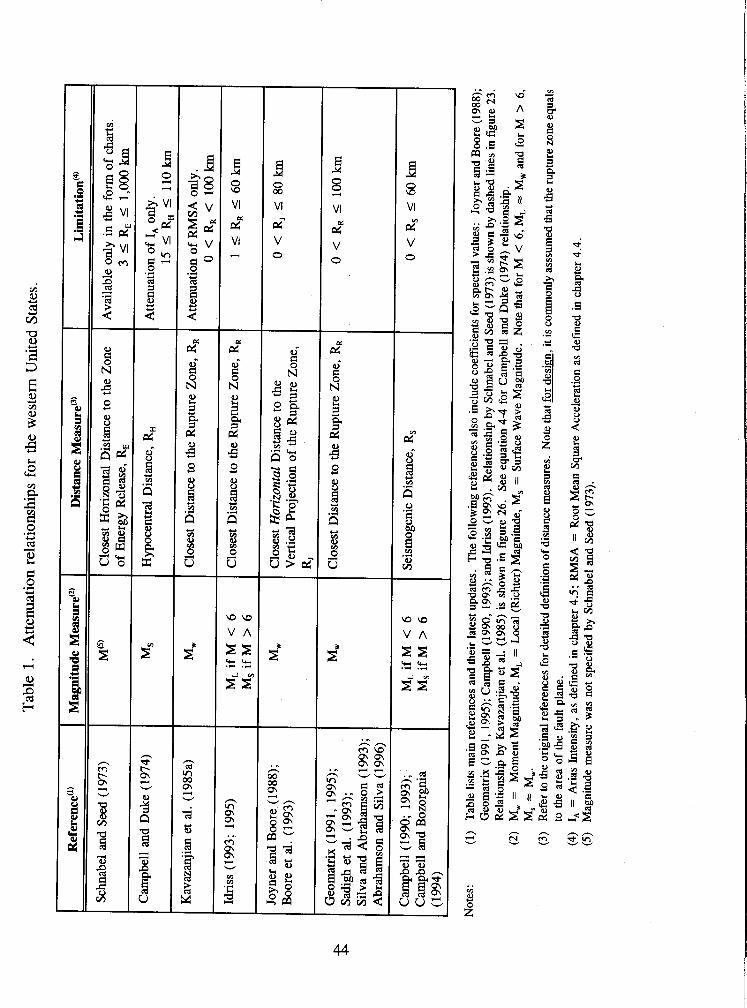
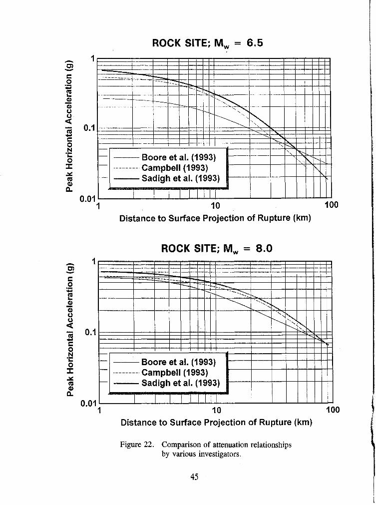
ROCK SITE; M, = 6.5

h I CD Y

s 0 .- C,

E a - a 0 a - 0.1 m .w c 3 .- I- 0 I Y m a, 9,

0.01 1 10 100

Distance to Surface Projection of Rupture (km)

ROCK SITE; M, = 8.0

Distance to Surface Projection of Rupture (km)

Figure 22. Comparison of attenuation relationships by various investigators.

Table 2. Attenuation relationship for subduction zone earthquakes.

Notes: M, = Moment magnitude. RH = Hypocentral distance. RR = Closest distance to the rupture zone (fault plane). Rs = Seismogenic distance (closest distance from the fault asperity). 2, = The tectonics term in Youngs et al. (1988). Equal to 0 for interplate events, and 1 for intraplate events. s = The site term in Cohee et al. (1991) relationship. Equal to 0 for rock sites and 1 for soil sites. (') = Refer to the original references for detailed description of distance measures and limitations.

Reference

Youngs et al. (1988)

Youngs et al. (1988)

Cohee et al. (1991)

Cohee et al. (1991)

Attenuation Relationship

ln(PGA) = 19.16 + 1 .045Mw - 4.738 In&, + 205.5exp(0.0968Mw)] + 0.542,

ln(PGA) = 19.16 + 1 .045Mw - 4.738 h[RH + 154.7exp(o. 1323M,)]

ln(PGA) = 1.5 - 3.33 ln(Rs + 128) + 0.79s

ln(PGA) = 2.8 - 1.26 ln(R& + 0.79s

Limitation'')

20 < RH r 40 lan M, r 8

20 < RH 5 40 km M, > 8

25 < Rs < 175 km M, 1 8

30 < RR < 100 km

M, > 8

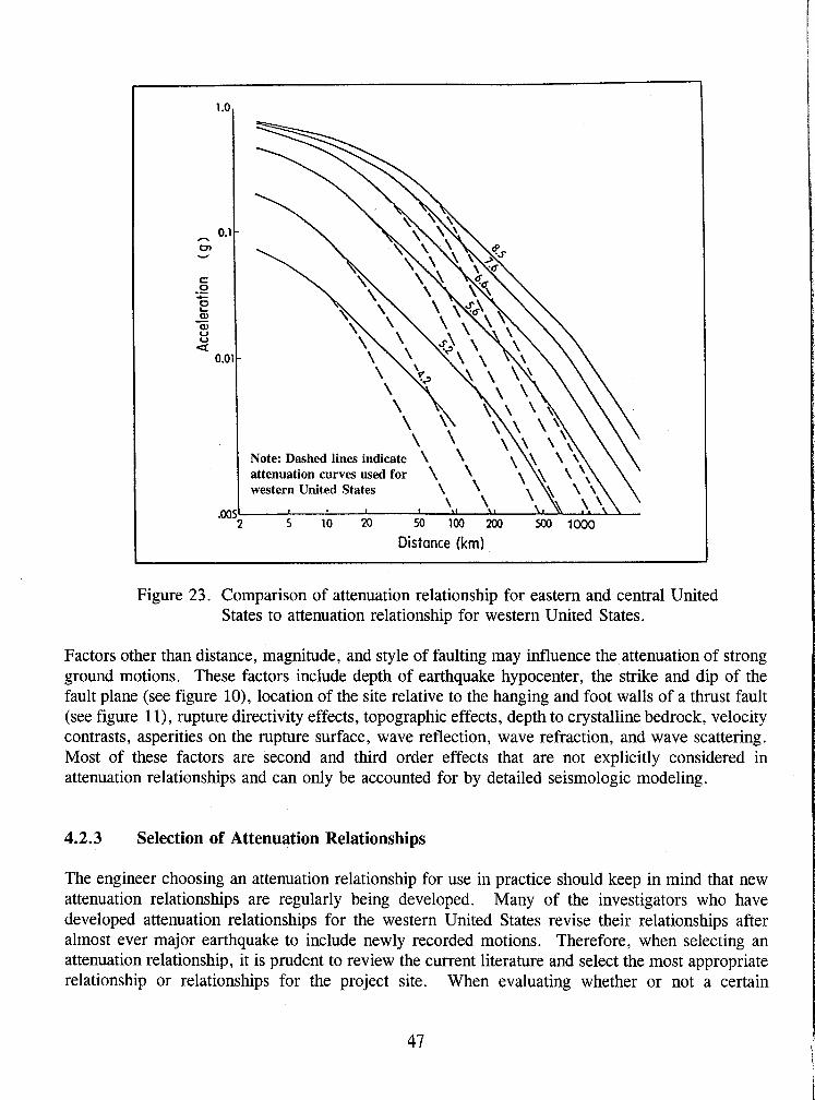
1 .o

0.1 - h

0, V

C 0 .- + e aJ - aJ U

2 0.01 -

Note: Dashed lines indicate \ \ attenuation curves used for \ \ western United States

MS 2 S 10 X) so 100 200 500 lo00

Distance (km)

Figure 23. Comparison of attenuation relationship for eastern and central United States to attenuation relationship for western United States.

Factors other than distance, magnitude, and style of faulting may influence the attenuation of strong ground motions. These factors include depth of earthquake hypocenter, the strike and dip of the fault plane (see figure lo), location of the site relative to the hanging and foot walls of a thrust fault (see figure 1 I), rupture directivity effects, topographic effects, depth to crystalline bedrock, velocity contrasts, asperities on the rupture surface, wave reflection, wave refraction, and wave scattering. Most of these factors are second and third order effects that are not explicitly considered in attenuation relationships and can only be accounted for by detailed seismologic modeling.

4.2.3 Selection of Attenuation Relationships

The engineer choosing an attenuation relationship for use in practice should keep in mind that new attenuation relationships are regularly being developed. Many of the investigators who have developed attenuation relationships for the western United States revise their relationships after almost ever major earthquake to include newly recorded motions. Therefore, when selecting an attenuation relationship, it is prudent to review the current literature and select the most appropriate relationship or relationships for the project site. When evaluating whether or not a certain

attenuation relationship is appropriate, the engineer should thoroughly review the published information regarding its development, especially the tectonic regime for which it was developed, the ranges of magnitude and distance to which it is restricted, and the local ground conditions to which it applies. Frequently, several different attenuation relationships may be found to be equally appropriate. In such a case, the geometric mean of the values calculated using all of the appropriate attenuation relationships is commonly employed in practice. By using the geometric mean of the values calculated by multiple relationships, bias inherent to individual relationships is minimized. However, when this approach is used, the multiple attenuation relationships should not include two generations of an attenuation relationship from the same investigator (e.g., Campbell, 1989 and Campbell and Bozorgnia, 1994).

Usually, attenuation relationships for both rock and soil sites will be available for use. Except for soil sites with less than 10 m of soil overlying bedrock and for soft soil sites where the average shear wave velocity over the top 30 m is less than 120 mls, soil-site attenuation relationships may be used directly to characterize ground motions at a soil site. However, due to the variability in conditions at soil sites and the resulting uncertainty in soil site response, engineers often prefer to use a rock site attenuation relationship to characterize the design earthquake motions at a hypothetical bedrock outcrop at the geometric center of the project site and then conduct a site response analysis to evaluate the influence of local soil conditions on the earthquake motions at the site. The hypothetical bedrock outcrop concept is congruent with both the free-field (i. e., not affected by structure and/or topography) criterion used to develop the attenuation relationships and with the concepts used to specify motions for input to computer programs for seismic site response analyses (rock outcrop and transmitting boundary models, see chapters 6.4 and 6.5).

4.2.4 Selection of Attenuation Relationship Input Parameters

When using an attenuation relationship, it is important to use the magnitude scale consistent with the scale used to develop the attenuation relationship. In the eastern and central United States, the magnitude measure generally used in practice is body wave magnitude, m,. In California, moment magnitude, M,, local (Richter) magnitude, ML, or surface wave magnitude, Ms, are used. The differences in these scales are due to the type of earthquake waves being measured, the type of instrument used to measure them, and local scaling factors. The relationship between these magnitude scales is shown on figure 9.

Consistency with the site-to-source distance measure used in developing the attenuation relationship is also important, especially for near-field earthquakes. In the early days of development of attenuation relationships, the epicentral distance was often used because it was generally the most reliable distance measure (seismographs were too sparsely located to adequately constrain the focal depth). As seismographs became more numerous and portable arrays were deployed to measure aftershock patterns that roughly delineate the rupture zone, the focal depth and extent of the rupture surface were able to be better located. Statistical analyses indicate that measures of distance from the recording site to the rupture surface provide a more robust measure of seismic wave attenuation than epicentral distance. Therefore, most current attenuation relationships for the western United States use some measure of the distance to the rupture zone. In the eastern and central United

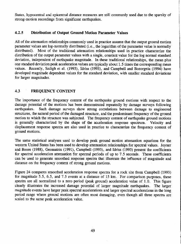
States, hypocentral and epicentral distance measures are still commonly used due to the sparsity of strong-motion recordings from significant earthquakes.

4.2.5 Distribution of Output Ground Motion Parameter Values

All of the attenuation relationships commonly used in practice assume that the output ground motion parameter values are log-normally distributed (i.e., the logarithm of the parameter value is normally distributed). Most of the traditional attenuation relationships used in practice characterize the distribution of the output parameter values with a single, constant value for the log normal standard deviation, independent of earthquake magnitude. In these traditional relationships, the mean plus one standard deviation peak acceleration values are typically about 1.5 times the corresponding mean values. Recently, Sadigh et al. (1993), Idriss (1993), and Campbell and Bozorgnia (1994) have developed magnitude dependent values for the standard deviation, with smaller standard deviations for larger magnitudes.

4.3 FREQUENCY CONTENT

The importance of the frequency content of the earthquake ground motions with respect to the damage potential of the motions has been demonstrated repeatedly by damage surveys following earthquakes. Such damage surveys show strong correlations between damage to engineered structures, the natural period of the damaged structure, and the predominant frequency of the ground motion to which the structure was subjected. The frequency content of earthquake ground motions is generally characterized by the shape of the acceleration response spectrum. Velocity and displacement response spectra are also used in practice to characterize the frequency content of ground motions.

The same statistical analyses used to develop peak ground motion attenuation equations for the western United States has been used to develop attenuation relationships for spectral values. Joyner and Boore (1988), Geomatrix (1991), Campbell (1993), and Idriss (1993) present the coefficients for spectral acceleration attenuation for spectral periods of up to 7.5 seconds. These coefficients can be used to generate smoothed response spectra that illustrate the influence of magnitude and distance on the frequency content of strong ground motions.

Figure 24 compares smoothed acceleration response spectra for a rock site from Campbell (1993) for magnitude 5.5, 6.5, and 7.5 events at a distance of 15 km. For comparison purposes, these spectra are all normalized to a zero period (peak ground) acceleration value of 1 .O. This figure clearly illustrates the increased damage potential of larger magnitude earthquakes. The larger magnitude events have larger peak spectral accelerations and larger spectral accelerations in the long period range where ground motions are often most damaging, even though all three spectra are scaled to the same peak acceleration value.

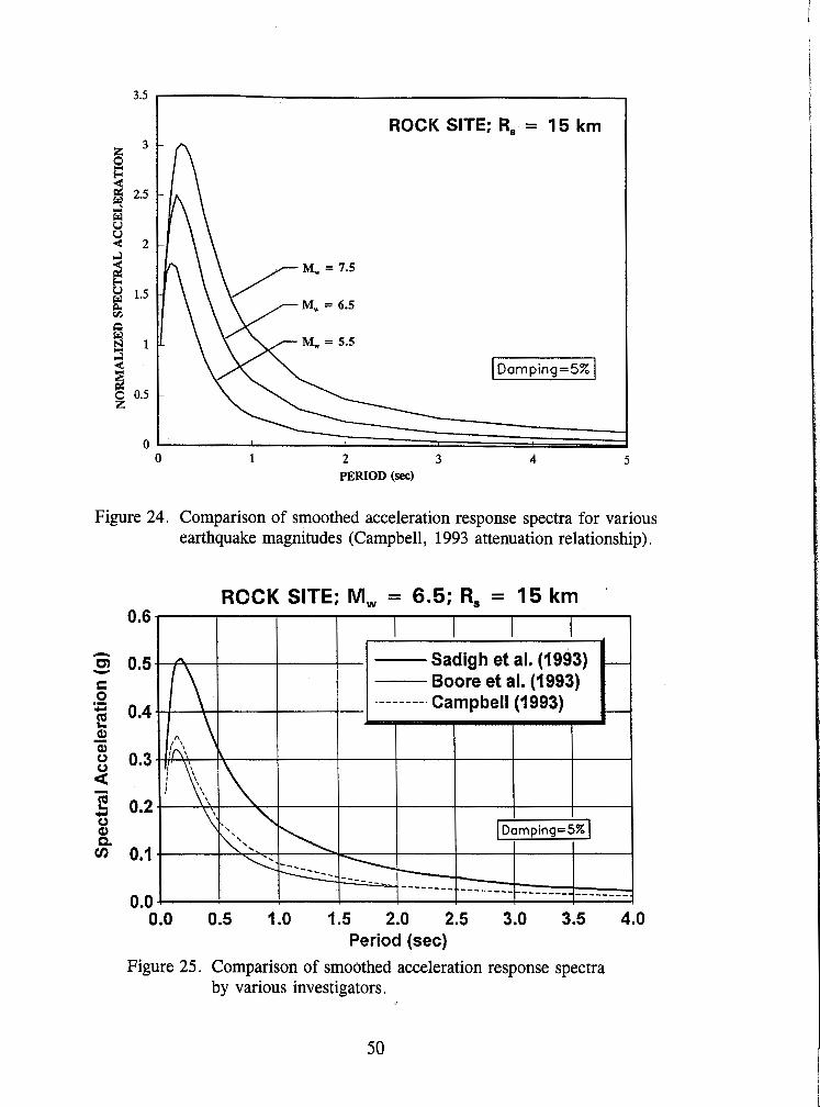
ROCK SITE; R, = 15 km

0 1 2 3 4 5 PERIOD (sec)

Figure 24. Comparison of smoothed acceleration response spectra for various earthquake magnitudes (Campbell, 1993 attenuation relationship).

ROCK SITE; M, = 6.5; R, = 15 km 0.6

0.0 0.5 1.0 1.5 2.0 2.5 3.0 3.5 4.0 Period (sec)

Figure 25. Comparison of smoothed acceleration response spectra by various investigators.

Figure 25 compares smoothed acceleration response spectra from three different investigators (Campbell, 1993; Sadigh et al., 1993; and Boore et al., 1993) for a rock site for a magnitude 6.5 event at a distance of 15 krn. This figure illustrates the differences among attenuation relationships developed by different investigators using essentially the same data base. These differences are primarily due to the weighting scheme used in statistical analysis and the screening criteria used by each investigator in culling records from the common data base of world-wide strong motion records available for the analysis.

The smoothed acceleration response spectra illustrated in figures 24 and 25 are important tools for selection of appropriate time histories for geotechnical analysis, as discussed subsequently.

4.4 ENERGY CONTENT

The energy content of the acceleration time history provides another means of characterizing strong ground motions. The energy content of the motion is proportional to the square of the acceleration. In engineering practice, the energy content of the motion is typically expressed in terms of either the root-mean-square (RMS) and duration of the acceleration time history or the Arias intensity, I,. The RMS of the acceleration time history is the square root of the square of the acceleration integrated over the duration of the motion and divided by the duration:

where RMSA is the RMS of the acceleration time history, a(t) is the acceleration time history, and tf is the duration of strong ground shaking. The RMSA represents an average acceleration for the time history over the duration of strong shaking. The square of the RMSA multiplied by the duration of the motion is directly proportional to the energy content of the motion.

The value of the RMSA depends upon the definition of the duration of the motion. For instance, if the duration of the motion is defined such that it extends into the quiet period beyond the end of strong shaking, the RMSA value will be "diluted" by the quiet period at the end of the record. However, as the energy content of the motion is unchanged, the product of the RMSA and duration will remain constant. As the RMSA is not used as frequently as peak ground acceleration in engineering practice, RMSA attenuation relationships are not developed or revised as frequently as peak acceleration attenuation relationships. Figure 26 presents an attenuation relationship for RMSA at rock sites in the western United States developed by Kavazanjian et al. (1985a) using the significant duration (Trifunac and Brady, 1975) defined in the next section of this chapter.

CLOSEST DISTANCE TO THE FAULT PLANE, % (km)

Figure 26. Attenuation of the root mean square acceleration (Kavazanjian et al., 1985a, reprinted by permission of ASCE).

The Arias intensity, I,, is proportional to the square of the acceleration integrated over the entire acceleration time history, a(t) :

where g is the acceleration of gravity and 9 is the duration of strong shaking. Arias (1969) showed that this integral is a measure of the total energy of the accelerogram. Arias intensity may be related to the RMSA as follows:

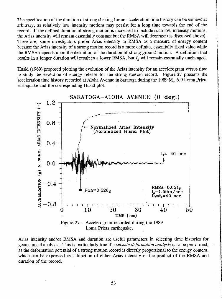
The specification of the duration of strong shaking for an acceleration time history can be somewhat arbitrary, as relatively low intensity motions may persist for a long time towards the end of the record. If the defined duration of strong motion is increased to include such low intensity motions, the Arias intensity will remain essentially constant but the RMSA will decrease (as discussed above). Therefore, some investigators prefer Arias intensity to RMSA as a measure of energy content because the Arias intensity of a strong motion record is a more definite, essentially fixed value while the RMSA depends upon the definition of the duration of strong ground motion. A definition that results in a longer duration will result in a lower RMSA, but I, will remain essentially unchanged.

Husid (1969) proposed plotting the evolution of the Arias intensity for an accelerogram versus time to study the evolution of energy release for the strong motion record. Figure 27 presents the acceleration time history recorded at Aloha Avenue in Saratoga during the 1989 M, 6.9 Loma Prieta earthquake and the corresponding Husid plot.

SARATOGA-ALOHA AVENUE (0 deg.)

Normalized Arias Intensity (Normalized Husid Plot)

ti= 40 sec

II .A A. ,.,.. . _. .. L

I I I I ~ l l l l ~ l l l l ~ l l l l ~ l l l l

0 10 20 30 40 50 TIME (sec)

Figure 27. Accelerogram recorded during the 1989 Loma Prieta earthquake.

Ariss intensity and/or RMSA and duration are useful parameters in selecting time histories for geotechnical analysis. This is particularly true if a seismic deformation analysis is to be performed, as the deformation potential of a strong motion record is directly proportional to the energy content, which can be expressed as a function of either Arias intensity or the product of the RMSA and duration of the record.

4.5 DURATION

The duration of shaking is important to the response of a soil deposit and/or overlying structures if the materials are susceptible to cyclic pore pressure generation, loss of strength or stiffness during cyclic loading, or other forms of cumulative damage (e.g., permanent seismic deformation). Duration is often neglected or treated indirectly in evaluating the dynamic response of structures, but is usually implicitly (based upon magnitude) or explicitly accounted for in liquefaction and seismic deformation analyses.

The bracketed duration of strong motion, D,, defined by Bolt (1973) as the elapsed time between the first and last acceleration excursion greater than a specified threshold level, is the definition most often found in strong motion catalogs. Figure 28 illustrates calculation of bracketed duration for Saratoga - Aloha Avenue accelerogram and a threshold acceleration of 0.05 g.

SARATOGA-ALOHA AVENUE (0 deg.) 0.6

- - - - - Bracket = +/-0.050g

0.4

h

hD w 0.2 Z h=40 sec

E 4 2 0.0 3 W U b=18.6 sec g -0.2

- 0 . 4 Bracketed Duration

PGA=PHGA=0.!526g Db=t2-tl=15.3 S ~ C

0 10 20 30 40 TIME (sec)

Figure 28. Bolt (1973) duration of strong shaking.

For problems dealing with cumulative damage during an earthquake, many engineers find the definition of significant duration, D,, proposed by Trifunac and Brady (1975) to be the most appropriate duration definition. Trifunac and Brady (1975) defined the significant duration as the time interval between 5 and 95 percent of the total Arias intensity on a Husid plot. The Trifunac and Brady definition of duration is illustrated on the Husid plot in figure 29.

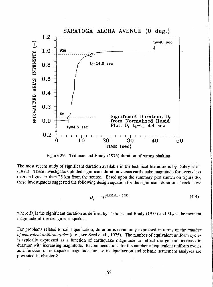
SARATOGA-ALOHA AVENUE ( 0 deg.) -

- n 1.2

I &=40 sec -

w - J

b=14.0 sec

m 0.6 -

8 - - -

Q 0.4 - -

W -

Significant Duration, D, from Normalized Husid

- tl=4.6 sec Plot: D,=t2-tl=9.4 sec

- 0 . 2 ~ I l l , I I I l , I I I I , I I I l , l l l r

0 10 20 30 40 TIME (sec)

Figure 29. Trifunac and Brady (1975) duration of strong shaking

The most recent study of significant duration available in the technical literature is by Dobry et al. (1978). These investigators plotted significant duration versus earthquake magnitude for events less than and greater than 25 km from the source. Based upon the summary plot shown on figure 30, these investigators suggested the following design equation for the significant duration at rock sites:

where D, is the significant duration as defined by Trifunac and Brady (1975) and Mw is the moment magnitude of the design earthquake.

For problems related to soil liquefaction, duration is commonly expressed in terms of the number of equivalent uniform cycles (e.g., see Seed et al., 1975). The number of equivalent uniform cycles is typically expressed as a function of earthquake magnitude to reflect the general increase in duration with increasing magnitude. Recommendations for the number of equivalent uniform cycles as a function of earthquake magnitude for use in liquefaction and seismic settlement analyses are presented in chapter 8.

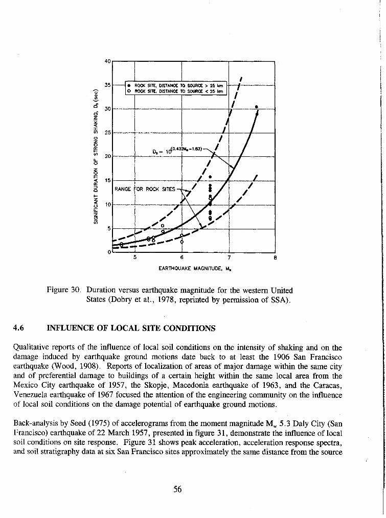
! I

35 ROCK SITE, DISTANCE TO SOUR= > 25 km . 0 ROCK SITE, MSTANCE TO SOURCE < 25 km I

I I 1

EARTHQUAKE MAGNITUDE, M,

Figure 30. Duration versus earthquake magnitude for the western United States (Dobry et al., 1978, reprinted by permission of SSA).

4.6 INFLUENCE OF LOCAL SITE CONDITIONS

Qualitative reports of the influence of local soil conditions on the intensity of shaking and on the damage induced by earthquake ground motions date back to at least the 1906 San Francisco earthquake (Wood, 1908). Reports of localization of areas of major damage within the same city and of preferential damage to buildings of a certain height within the same local area from the Mexico City earthquake of 1957, the Skopje, Macedonia earthquake of 1963, and the Caracas, Venezuela earthquake of 1967 focused the attention of the engineering community on the influence of local soil conditions on the damage potential of earthquake ground motions.

Back-analysis by Seed (1975) of accelerograms from the moment magnitude M, 5.3 Daly City (San Francisco) earthquake of 22 March 1957, presented in figure 3 1, demonstrate the influence of local soil conditions on site response. Figure 3 1 shows peak acceleration, acceleration response spectra, and soil stratigraphy data at six San Francisco sites approximately the same distance from the source

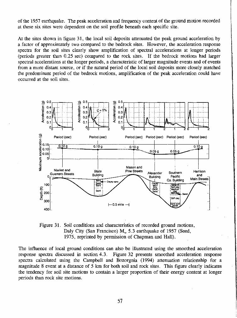
of the 1957 earthquake. The peak acceleration and frequency content of the ground motion recorded at these six sites were dependent on the soil profile beneath each specific site.

At the sites shown in figure 31, the local soil deposits attenuated the peak ground acceleration by a factor of approximately two compared to the bedrock sites. However, the acceleration response spectra for the soil sites clearly show amplification of spectral accelerations at longer periods (periods greater than 0.25 sec) compared to the rock sites. If the bedrock motions had larger spectral accelerations at the longer periods, a characteristic of larger magnitude events and of events from a more distant source, or if the natural period of the local soil deposits more closely matched the predominant period of the bedrock motions, amplification of the peak acceleration could have occurred at the soil sites.

Figure 31. Soil conditions and characteristics of recorded ground motions, Daly City (San Francisco) M, 5.3 earthquake of 1957 (Seed, 1975, reprinted by permission of Chapman and Hall).

m - t

Period (sec) Period (sec) Period (sec) Period (sec) Period (sec) Period (sec) 0 .- .- 2 0.15

The influence of local ground conditions can also be illustrated using the smoothed acceleration response spectra discussed in section 4.3. Figure 32 presents smoothed acceleration response spectra calculated using the Campbell and Bozorgnia (1994) attenuation relationship for a magnitude 8 event at a distance of 5 krn for both soil and rock sites. This figure clearly indicates the tendency for soil site motions to contain a larger proportion of their energy content at longer periods than rock site motions.

i 0.10- o 2 0.05.-

.!2 g ........... 0.10 g ......... 0.10 * g 0% O - ..... - '"..... 0.05 g 0.05 g/ - g " .- 2 5

Mason and Market and State

Pine Streets Alexander Southern Harrison

k 0 . 5 mile 4

PERIOD (sec)

Figure 32. Comparison of soil and rock site acceleration response spectra for M, 8 event at 5 km (Campbell and Bozorgnia, 1994, reprinted by permission of EERI).

The influence of local soil conditions on spectral shape may also be illustrated using design spectra developed for building codes. For example, the current version of the Uniform Building Code (UBC, 1994), defines three classes of site conditions when defining the shape of the normalized smoothed response spectra for structural design. These three classes of site conditions are rock (Type I), deep, cohesionless or stiff clay soil (Type 11), and soft to medium stiff clays and sands (Type 111). The smoothed normalized response spectra corresponding to these three site conditions, presented in figure 33, again illustrate the increase in spectral acceleration at long periods for soil site motions compared to rock site motions. Based upon observations of very large spectral amplification and severe damage to long period structures at deep, soft clay sites in earthquakes, a fourth soil type, deep, soft clay, with even more energy at long periods than the Type I11 site condition, has been proposed for soft clay sites for the UBC. The next (1997) version of the UBC may also incorporate near-field ground motion factors with the spectra shown in figure 33.

The Applied Technology Council (ATC) is developing a new generation of building codes as part of the National Earthquake Hazard Reduction Program (NEHFU?, 1991). The NEHRP (1991) code provides five classes of site conditions, from "Hard and Firm Rock" to "Special Study, " based upon the average shear wave velocity in the upper 30 m of the soil profile. This new classification system, summarized in table 3, retains the primary characteristic influence of local soil conditions in that the spectral acceleration at longer periods increases with decreasing stiffness of the ground. While building code response spectra are useful to illustrate the effect of local soil conditions on ground response, these spectra represent effective spectral accelerations for use in structural design

and are not intended to represent smoothed spectra from actual earthquakes. To represent an actual earthquake spectrum, the spectrum generated from an attenuation relationship, or the spectrum from seismic site response analysis (see chapter 6) should be used.

Local soil conditions can also affect duration. Durations on soil sites have greater scatter and tend to be longer than durations on rock sites. In fact, the range of durations for rock sites appears to be a lower bound for soil site durations.

Amplification of long period bedrock motions by local soil deposits is now accepted as an important phenomenon that can exert a significant influence on the damage potential of earthquake ground motions. Significant structural damage has been attributed to amplification of both peak acceleration and spectral acceleration by local soil conditions. Amplification of peak acceleration occurs when the resonant frequency of the soil deposits is close to the predominant frequencies of the bedrock earthquake motions (the frequencies associated with the peaks of the acceleration response spectra). The resonant frequency, f,, of a soil layer (deposit) of thickness H can be estimated as a function of the average shear wave velocity of the layer, (V,),,, using the following equation:

- SOIL PROFILE TYPE Ill - SOlL PROFILE TYPE II

SOlL PROFILE TYPE I

-

- -- ---- I I

PERIOD (sec)

Figure 33. Normalized uniform building code response spectra (UBC, 1994, reproduced from the Uniform Building Codem, copyrighto 1994, with the permission of the publisher, the International Conference of Building Officials).

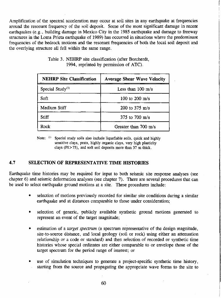
Amplification of the spectral acceleration may occur at soil sites in any earthquake at frequencies around the resonant frequency of the soil deposit. Some of the most significant damage in recent earthquakes (e.g., building damage in Mexico City in the 1985 earthquake and damage to freeway structures in the Loma Prieta earthquake of 1989) has occurred in situations where the predominant frequencies of the bedrock motions and the resonant frequencies of both the local soil deposit and the overlying structure all fell within the same range.

Table 3. NEHRP site classification (after Borcherdt, 1994, reprinted by permission of ATC).

Note: ( I ) Special study soils also include liquefiable soils, quick and highly sensitive clays, peats, highly organic clays, very high plasticity clays (PI > 7 3 , and soft soil deposits more than 37 m thick.

NEHRP Site Classification

Special Study")

Soft

Medium Stiff

Stiff

Rock

4.7 SELECTION OF REPRESENTATIVE TIME HISTORIES

Average Shear Wave Velocity

Less than 100 m/s

100 to 200 mls

200 to 375 m/s

375 to 700 m/s

Greater than 700 m/s

Earthquake time histories may be required for input to both seismic site response analyses (see chapter 6 ) and seismic deformation analyses (see chapter 7). There are several procedures that can be used to select earthquake ground motions at a site. These procedures include:

selection of motions previously recorded for similar site conditions during a similar earthquake and at distances comparable to those under consideration;

selection of generic, publicly available synthetic ground motions generated to represent an event of the target magnitude;

estimation of a target spectrum (a spectrum representative of the design magnitude, site-to-source distance, and local geology (soil or rock) using either an attenuation relationship or a code or standard) and then selection of recorded or synthetic time histories whose special ordinates are either comparable to or envelope those of the target spectrum for the period range of interest; or

use of simulation techniques to generate a project-specific synthetic time history, starting from the source and propagating the appropriate wave forms to the site to

generate a suite of time histories that can then be used to represent the earthquake ground motions at the site of interest.

In selecting a representative time history from the catalog of available records, an attempt should be made to match as many of the relevant characteristics of the design earthquake as possible. Important characteristics that should be considered in selecting a time history include:

earthquake magnitude; source mechanism (e.g., strike slip, dip slip, or oblique faulting); focal depth; site-to-source distance; site geology; peak ground acceleration; frequency content; duration; and energy content (RMSA or I,).

The relative importance of these factors varies from case to case. For instance, if a bedrock record is chosen for use in a site response analysis to model the influence of local soil conditions, site geology will not be particularly important in selection of the input bedrock time history. However, if a soil site record is to be scaled to a specified peak ground acceleration, site geology can be a critical factor in selection of an appropriate time history, as the record must already include any potential influence of local soil conditions on the motion. Scaling of the peak acceleration of a strong motion record by a factor of more than two is not recommended, as the frequency characteristics of ground motions can be directly and indirectly related to the amplitude of the motion. Leeds (1992) and Naeim and Anderson (1993) present comprehensive databases of available strong motion records and their characteristics. These strong motion records can be obtained in digital form (CD-ROM) from the National Geophysical Data Center (NGDC) in Boulder, Colorado. Also, Tao (1996) provides detailed information on several other sources from which accelerograms can be obtained directly via on-line systems or purchased in a variety of formats.

Due to uncertainties in the selection of a representative earthquake time history, response analyses are usually performed using a suite of time histories rather than a single time history. Engineers commonly use two to five time histories to represent each significant seismic source in a site response analysis. For earthquakes in the western United States, it should be possible to find three to five representative time histories that satisfy the above criteria. However, at the present time, there are only two bedrock strong motion records available from earthquakes of magnitude M, 5.0 or greater in the central and eastern United States:

the Les Eboutements record with a peak horizontal acceleration of 0.23 g from the 1988 Saguenay , Quebec earthquake of magnitude M, 6.0; and

the Loggie Lodge record with a peak horizontal acceleration of 0.4 g from the 1981 Mirimichi, New Brunswick earthquake of magnitude M, 5.0.

Therefore, for analysis of sites east of the Rocky Mountains, records from a western United States site, an international recording site, or synthetic accelerograms are required to compile a suite of at least three records for analysis. For the new Madrid seismic zone, where neither the Mirimichi nor Saguenay record is of appropriate magnitude, all three records must be from either the western united States, an international site, or synthetically generated.

Generic, synthetically generated ground motions are available only for a limited number of major faults (fault systems). For example, Jennings et al. (1968) developed the A1 synthetic accelerogram for soil site conditions for an earthquake on the southern segment of the San Andreas fault. Seed and Idriss (1969) developed a synthetic accelerogram for rock sites for an earthquake on the northern segment of the San Andreas fault. The Jennings et al. (1968) A1 accelerogram has an energy content which is larger than the energy content of any accelerogram recorded to date. For this reason, the A1 record is often used to simulate major earthquakes in the Cascadia and New Madrid seismic zones. Appropriate synthetic accelerograrns may also be available to the engineer from previous studies and may be used if they are shown to be appropriate for the site. Synthetic earthquake accelerograms for many regions of the country are currently being compiled by Dr. Klaus Jacob at the Lamont-Doherty Earth Observatory of Columbia University under the auspices of the National Center for Earthquake Engineering Research (NCEER). However, at the time of preparation of this guidance document, this compilation was not yet available.

The target spectrum may be estimated from available attenuation relationships (see section 4.3). These attenuation relationships, typically developed for a spectral damping of 5 percent, provide estimates of the median spectral ordinates and the log-normal standard deviation about the mean. Representative time histories are selected by trial-and-error on the basis of "reasonable" match with the target spectrum. A "reasonable" match does not necessarily mean that the response spectrum for the candidate record "hugs" the target spectrum. Particularly if a suite of time histories is used, a "reasonable" match only requires that the suite of response spectra averaged together approximates the mean target spectrum. Each individual spectrum may fluctuate within the plus and minus one standard deviation bounds over most of the period range of interest. Natural and/or generic synthetic time histories can be screened in this type of selection process.

An alternative approach to trial-and-error matching of the target spectrum is computerized generation of a synthetic time history or a suite of time histories whose spectral ordinates provide a reasonable envelope to those of the target spectrum. Existing time histories can also be modified to be spectrum compatible. Several computer programs are available for these tasks (e . g . , Gasparin and Vanrnarcke, 1976; Ruiz and Penzien, 1969; Silva and Lee, 1987). However, generation of realistic synthetic ground motions is not within the technical expertise of most geotechnical engineering consultants. The simulation programs should only be used by qualified engineering seismologists and earthquake engineers. For this reason, these simulation techniques are beyond the scope of this guidance document.

CHAPTER 5

SITE CHARACTERIZATION

5.1 INTRODUCTION

This chapter describes the site characterization information required to evaluate the geotechnical parameters used for the seismic design of highway facilities. It is assumed that the basic geological, geotechnical, and hydrological investigations required for the general design of the structure under consideration have been (or will be) conducted according to the state of practice. The goal of site characterization for seismic design is to develop the subsurface profile and soil property information necessary for seismic analyses. Soil parameters required for seismic analyses include the initial (small strain) dynamic shear modulus, equivalent viscous damping ratio, shear modulus reduction and equivalent viscous damping characteristics, cyclic shear strength parameters, and liquefaction resistance parameters.

Three broad categories of site investigation activities can be included in a seismic site exploration program. The first category is conventional geotechnical site exploration, including a drilling program followed by laboratory testing on undisturbed or remolded samples. The second category is in situ testing, wherein the parameters that describe dynamic soil properties are estimated in situ using penetrometers and other types of probes and in situ testing devices. The third category is geophysical exploration.

The remainder of this chapter will describe the relevant soil parameters for seismic site characterization, their importance for seismic analyses, and the available evaluation techniques.

SUBSURFACE PROFILE DEVELOPMENT

5.2.1 General

As for all geotechnical engineering analyses, seismic analysis requires knowledge of the subsurface profile, or stratigraphy, at the site under study. The required stratigraphic information includes information on the water level, the soil stratigraphic profile, and the underlying bedrock. Stratigraphy can be obtained using classical investigation techniques (drilling and sampling), in situ tests, or geophysical means.

As in any geotechnical analysis, identification and quantification of relatively thin, weak layers can be an important part of seismic site characterization. However, the "weak" layer in a seismic analysis may differ from the "weak" layer in a static analysis. For instance, a saturated sand layer considered a suitable foundation material with respect to static loads may be susceptible to liquefaction under earthquake loads and thus becomes a weak layer in a seismic analysis. In other

cases, such as soft material between beds of rock or stiff soil on a hillside, the same material that is a weak material for static analyses also represents a potential problem under earthquake loads.

5.2.2 Water Level

The groundwater level (or levels) should be established during a seismic site investigation. Groundwater may play an important role in seismic analysis, particularly if the soil deposits are liquefiable. Seasonal variability in the water level should be considered in developing the stratigraphic profile and performing liquefaction potential analyses.

Groundwater level information is often obtained by observation of the depth to which water accumulates in an open borehole. However, water level observations in boreholes may be unreliable due to a variety of factors, including:

insufficient time for equilibrium in borings in fine-grained soils; artesian pressures in confined aquifers; and perched water tables in coarser soils overlying fine-grained deposits.

Furthermore, borehole observations do not, in general, permit observations of seasonal fluctuations in water levels. Piezometers or observation wells installed in a borehole provide a much more reliable means of monitoring water levels in the subsurface. In deposits where layers of fine-grained soils are present and multiple water levels are suspected, multiple-point piezometers can be installed in a single borehole or multiple boreholes can be fit with single point piezometers.

A cone penetrometer (CPT) with pore pressure measuring capabilities, referred to as a piezocone, can also be used to estimate water level elevations. By holding the cone at a constant elevation arid waiting until the pore pressure drops to a constant value, the piezocone can be used to determine the steady state pore pressure at a specified elevation. The potential for perched water tables or confined aquifers can be assessed with the piezocone by combining steady-state pore pressure readings at several elevations with stratigraphic information developed from the tip and sleeve resistance of the cone.

Geophysical stratigraphic profiling methods are generally not used to evaluate the depth to groundwater. Geophysical methods used to evaluate soil stratigraphy are often based upon shear wave or Rayleigh wave velocity and thus are generally insensitive to the water level. Some resistivity methods (e.g., down hole resistivity surveys) can detect the presence of water in the soil pores but cannot measure the pressure in the water. Therefore, in a fine-grained soil, such methods can neither distinguish between soil above the water table saturated by capillarity and soil below the water table nor measure an artesian pressure in a confined aquifer.

5.2.3 Soil Stratigraphy

The subsurface investigation should provide a detailed description of the soil stratigraphy at the site, including the thickness and elevation of the different layers. Potentially liquefiable soils should be clearly identified and quantified by one of the methods described later in this chapter. Both conventional boring and sampling and in situ testing using the CPT offer the possibility of development of a continuous soil profile in which layers as small as 75 rnm can be identified. Thin continuous layers of weak or potentially liquefiable soil encountered between beds of more competent soil may prove to be the critical plane in seismic slope stability analyses. Borings offer the advantage of recovery of a sample for visual classification and, if desired, laboratory testing. In a boring in which continuous Standard Penetration Tests (SPT) sampling is performed, layers of soil can be visually identified from the sample recovered from the split spoon to develop a continuous stratigraphic profile. However, the SPT blow count, the primary measurement of cohesionless soil strength and consistency obtained using the SPT, generally applies only to the gross behavior of a relatively large 300 rnrn interval of the boring and thus cannot be used to characterize the liquefaction susceptibility of thin lenses of soil visually identified in the split-spoon sample. In the CPT, the resistance of the tip and sleeve of the cone to penetration can be used to develop continuous profiles of the shear strength of the soil that are applicable to layers as thin as 75 rnrn.

Geophysical methods will provide information on the stratigraphy of the soil with respect to the measured geophysical property. The measured geophysical property may be a physical property of direct interest in a seismic analysis (e.g., shear wave velocity) or may be correlated to a physical property of interest (e.g., electrical resistivity and water level). The ability of geophysical methods to resolve layering in the ground varies among the available methods and, in general, decreases with depth unless a down hole method is used (in which case a boring or in situ probe is required).

5.2.4 Depth to Bedrock

Ideally, the soil profile developed for a seismic analysis should extend to competent bedrock, where competent bedrock is defined as material with a shear wave velocity of at least 700 mls, and the physical properties of the soil over the entire interval between the ground surface and competent bedrock should be defined. However, if competent bedrock is not reachable at a reasonable depth, the depth over which the physical properties of the soil for seismic analyses are defined should be at least 30 m. Furthermore, the depth to which the soil profile is developed should be at least as deep as required for conventional geotechnical analyses.

5.3 REQUIRED SOIL PARAMETERS

5.3.1 General

At a minimum, a seismic analysis requires the same parameters used to describe soil properties for static analyses of earth structures and foundations. During the course of a typical geotechnical investigation, the following information is obtained:

soil classification and index parameters; unit weight of the soil; and compressibility and shear strength parameters of the soil.

For seismic design purposes, a series of other soil parameters and properties may need to be evaluated. For a seismic analysis, these may include:

a measure of the relative density of the soil; shear wave velocity; cyclic stress-strain behavior; and peak and residual shear strength.

5.3.2 Relative Density

Measures of both the absolute and relative density of the soil skeleton are required for seismic analysis. The absolute density is usually expressed in terms of unit weight. The unit weight of the soil is used to calculate the total and effective vertical stresses for liquefaction and slope stability analyses. Unit weight is also an important parameter in dynamic response and stability analyses, as the inertia force of an element of soil is equal to the acceleration times the total weight. Total unit weight may be assessed on the basis of measured values from undisturbed samples, or from the water content and specific gravity of saturated soil.

Relative density is an important parameter with respect to the potential for soil liquefaction and seismically-induced settlement of cohesionless soils. The relative density is a measure of the relative consistency of the soil.

Mathematically, relative density, D,, is related to the maximum density (y,,) or minimum void ratio e,,,, (the densest state to which the material can be compacted) and the minimum density (y,,) or maximum void ratio emax (the loosest state the material can attain) by:

where e, is the in situ void ratio of the material and yo is the in situ unit weight. Dry unit weights are used for yo, y,,, and ymax. The relative density is an important parameter with respect to

liquefaction and seismic settlement potential because it is related to the potential for a granular material to decrease in volume when subjected to disturbance.

Relative density is rarely measured directly. Generally, an index of the relative density is measured in situ. Commonly used indices of the relative density, or relative consistency, of soil in situ are the SPT blow count, N, and the normalized tip and sleeve resistance of the CPT probe, q,,, and f,, respectively. Table 4 presents the Terzaghi and Peck (1948) relationship between relative density and SPT blow count for sandy soils. Several of the indices used to evaluate relative density in situ have, in turn, been directly correlated to liquefaction and seismic settlement potential, often eliminating the need for direct evaluation of relative density in a seismic analyses.

Table 4. Relative density of sandy soils (after Terzaghi and Peck, 1948).

Note: See also figure 37 for an alternative N-D, correlation.

5.3.3 Shear Wave Velocity

Descriptive Term

Very Loose

Loose

Medium

Dense

Very Dense

Relative Density, D, (%)

0-15

15-35

35-65

65-85

85-100

The shear wave velocity of a soil is used to establish the stiffness of the soil at small strains. The small strain (initial) shear modulus of a soil, G,,,, is related to the shear wave velocity, V,, and the mass density, p , of the soil by the equation:

Penetration Resistance, N (blows/300mm)

0-4

5-10

11-30

31-50

> 50

Mass density of the soil is related to the total unit weight of the soil, y,, by the acceleration of gravity, g:

The mass density of most soils can be reasonably estimated from soil classification and location relative to the water table. Therefore, measurement of shear wave velocity can provide a reliable means for evaluating the small strain shear modulus of the soil if the stratigraphic profile is known.

Small strain (initial) Young's modulus, Em,, is related to small strain shear modulus as a function of Poisson's ratio, v, by the theory of elasticity:

For practical purposes, Poisson's ratio of soil can be assumed equal to 0.35 for sands and 0.45 for clays. Alternatively, if results of geophysical measurements are available, the following equation may be used to estimate v.

where V, and V, are shear and compressional wave velocities, respectively. Young's modulus can also be evaluated from the compressional wave velocity and mass density of the soil. Consequently an efficient and reliable means of obtaining the small-strain elasticity properties of the soil is through the measurement of shear and compressional wave velocities.

5.3.4 Cyclic Stress-Strain Behavior

During an earthquake, a soil deposit is subjected to a complex system of stresses and strains resulting from the ground motions induced by the earthquake. In general, these stresses and strains will be cyclical due to the vibrational nature of the earthquake loading. To evaluate the seismic response of the soil deposit, it is necessary to estimate how it responds to this cyclic loading.

The earthquake-induced stresses and strains that produce the most damage in soils are generally considered to be due to cyclic shearing of the soil. Shear waves propagate primarily upward near the ground surface. Therefore, most geotechnical earthquake engineering analyses assume that earthquake ground motions are generated by vertically-propagating shear waves.

The cyclic stresses induced on a soil element by a vertically-propagating shear wave are schematically presented in figure 34. The stress-strain response of soil to this type of cyclic loading is commonly characterized by a hysteresis loop. A typical hysteresis loop is shown on figure 35. Various constitutive models have been developed to characterize soil hysteresis loops. The most common model used to represent the hysteretic behavior of soil in seismic analysis is the equivalent- linear model (Seed and Idriss, 1970). Various non-linear constitutive models (Kondner and Zelasko, 1963; Martin, 1975; MatasoviC and Vucetic, 1993) have also been developed to represent hysteretic

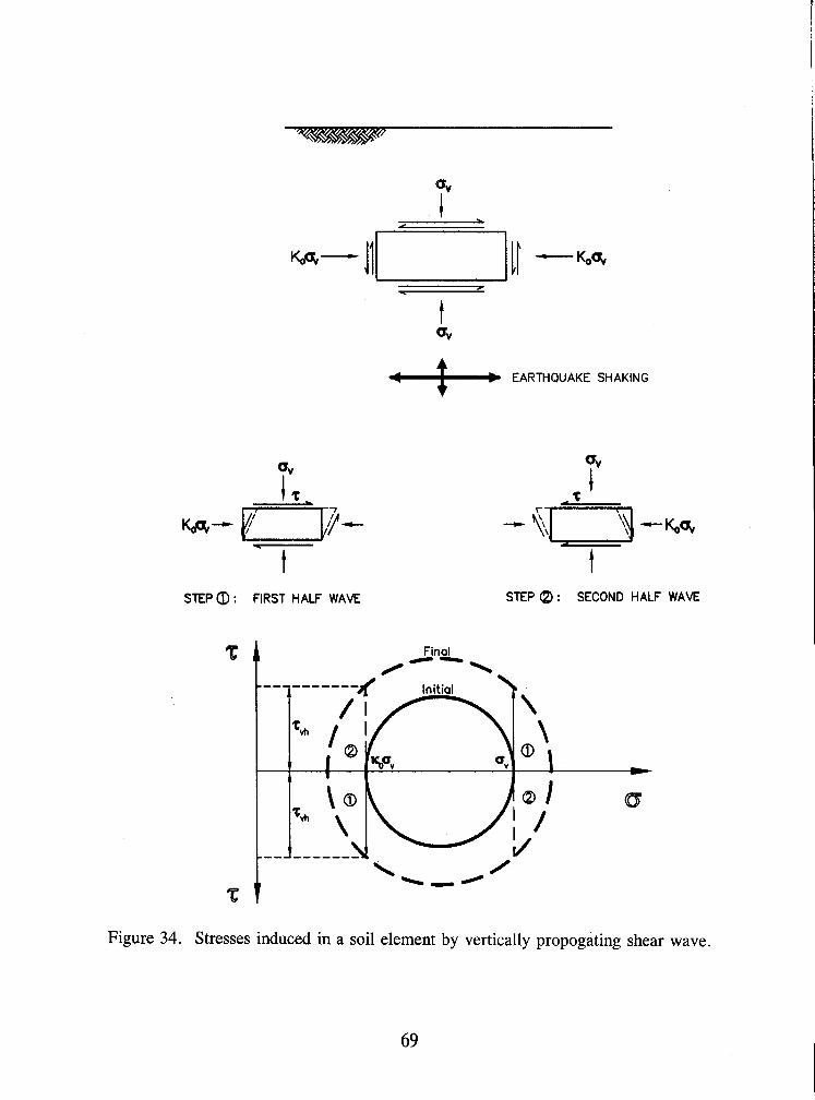
4 EARTHQUAKE SHAKING

0,

I,. K&- mp-

- I STEP a> : FIRST HALF WAVE STEP Q : SECOND HALF WAVE

Figure 34. Stresses induced in a soil element by vertically propogating shear wave.

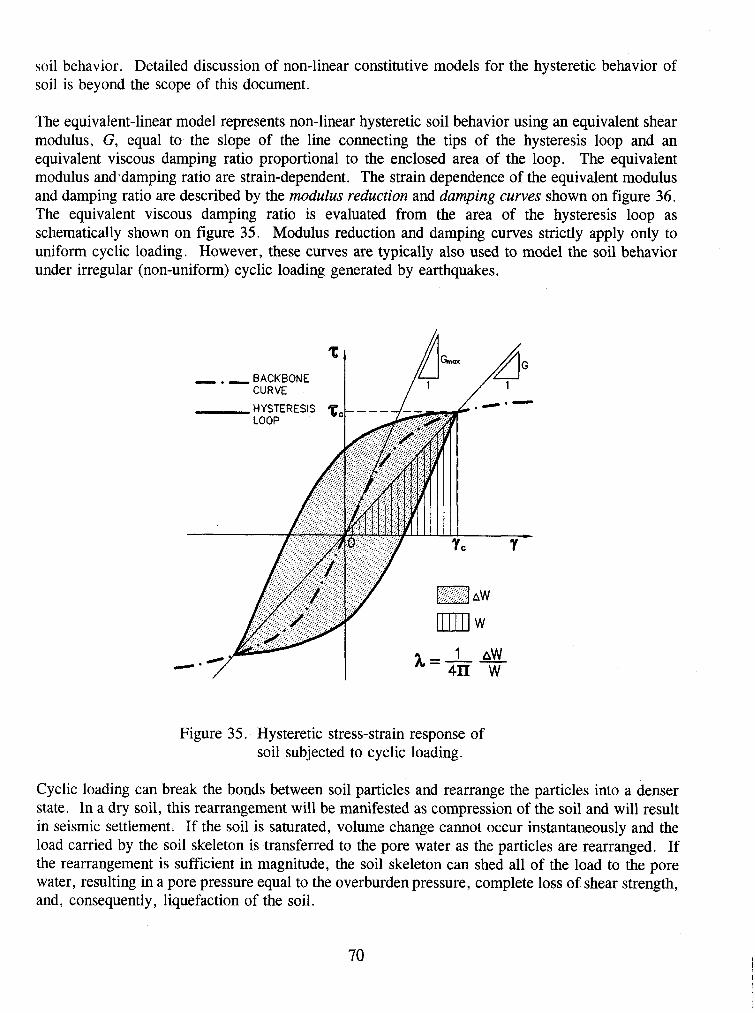
soil behavior. Detailed discussion of non-linear constitutive models for the hysteretic behavior of soil is beyond the scope of this document.

The equivalent-linear model represents non-linear hysteretic soil behavior using an equivalent shear modulus, G, equal to the slope of the line connecting the tips of the hysteresis loop and an equivalent viscous damping ratio proportional to the enclosed area of the loop. The equivalent modulus andadamping ratio are strain-dependent. The strain dependence of the equivalent modulus and damping ratio are described by the modulus reduction and damping curves shown on figure 36. The equivalent viscous damping ratio is evaluated from the area of the hysteresis loop as schematically shown on figure 35. Modulus reduction and damping curves strictly apply only to uniform cyclic loading. However, these curves are typically also used to model the soil behavior under irregular (non-uniform) cyclic loading generated by earthquakes.

Figure 35. Hysteretic stress-strain response of soil subjected to cyclic loading.

Cyclic loading can break the bonds between soil particles and rearrange the particles into a denser state. In a dry soil, this rearrangement will be manifested as compression of the soil and will result in seismic settlement. If the soil is saturated, volume change cannot occur instantaneously and the load carried by the soil skeleton is transferred to the pore water as the particles are rearranged. If the rearrangement is sufficient in magnitude, the soil skeleton can shed all of the load to the pore water, resulting in a pore pressure equal to the overburden pressure, complete loss of shear strength, and, consequently, liquefaction of the soil.

Figure 36. Shear modulus reduction and equivalent viscous damping ratio curves.

5.3.5 Peak and Residual Shear Strength

Peak and residual shear strengths are important elements in the evaluation of seismic stability. The peak shear strength refers to the maximum shearing resistance an element of soil can sustain during and after cyclic loading. The peak shear strength may be used to calculate the yield acceleration of a soil (the horizontal acceleration above which permanent seismic deformations begin to accumulate) if the buildup of seismically-induced pore pressures is not anticipated. Residual shear strength refers to shear strength of the soil after significant static and/or cyclic shearing has occurred. Residual shear strength is often used to evaluate stability and calculate the accumulation of permanent seismic deformation in a post-liquefaction stability and deformation analysis for a foundation or earth structure.

While there is some limited information to indicate that the shear strength of soil increases with increasing strain rate, the peak shear strength of soil subjected to cyclic loading is generally assumed to be less than or equal to the peak static strength. If the soil is dry, the drained shear strength may be used. If the soil is saturated, even if the soil is relatively free draining, the undrained shear strength should be used for seismic analyses because of the rapid nature of earthquake loading.

Residual shear strength is used to represent the post-peak strength of the soil subsequent to both monotonic and cyclic loading. Many soils and geosynthetic interfaces show a marked decrease in shearing resistance when subjected to relatively large monotonic shear strains. If the seismic design philosophy for a foundation or earth structure calls for allowing the peak strength to be exceeded as long as cumulative deformations remain within a range defined as acceptable, the residual shear strength after monotonic loading is typically used to assess the post-deformation stability. The yield

acceleration calculated using the residual shear strength can be used to assess cumulative seismic deformations on a conservative basis.

5.4 EVALUATION OF SOIL PROPERTIES

5.4.1 General

The key dynamic soil parameters required to perform a seismic response analysis are the shear wave velocity, modulus reduction and damping curves, peak and residual shear strength, and the parameters needed to evaluate soil liquefaction potential. A value for Poisson's ratio may also be required. These parameters can either be directly evaluated from laboratory test results or in situ test results or indirectly evaluated by correlation with index properties of soils. Laboratory tests generally provide the most direct means of evaluating soil parameters for seismic analyses. However, laboratory tests are subject to limitations on the recovery and testing of representative samples as well as on the testing itself. For some parameters (e.g., shear wave velocity), field testing provides a reliable and cost effective means of evaluation. However, in many cases, empirical correlation with index parameters and in situ test results is the most practical means of evaluating soil parameters for seismic analyses. Sometimes, for particular geographical areas and soils (e . g . , Piedmont region residual soils, Borden et a1 . , 1996) typical dynamic soil parameters have been established.

5.4.2 In Situ Testing for Soil Profiling

5.4 -2.1 Standard Penetration Testing (SPT)

Probably the most common in situ test used in geotechnical practice, the SPT, measures the resistance to penetration of a standard split-spoon sampler in a boring. The test method is rapid and yields useful data, although there are many factors that affect the results. The procedure used to perfom the SPT is codified under ASTM Standard D 1586. The SPT consists of driving a standard split barrel sampler with a 63.5 kg hammer dropping 762 mm in a free fall which theoretically delivers 60 percent of the energy to the drill rod. The (uncorrected) SPT blow count, N, is the result of the test.

Although widely recognized as an unsophisticated test, the SPT is performed routinely worldwide and, when performed properly, yields useful results. Extensive work has been conducted to understand the limitations of the test and develop reliable correction factors accounting for the influence of vertical stress, soil gradation, hammer efficiency, and other factors on test results. Correction factors to normalize and standardize the value of the SPT blow count, N, are discussed in chapter 8. Corrected SPT blow count values can be used to:

estimate the relative density of sand; estimate shear strength parameters of cohesionless soils; estimate bearing capacity; evaluate seismic settlement potential of sands;

evaluate liquefaction potential of saturated sands; and estimate the shear modulus at very low strain.

Hammer efficiency is a key factor in evaluating SPT blow count. Values of hammer efficiency, defined as the energy delivered to the sampler divided by the theoretical kinetic energy of the free- falling weight, measured in the field vary from 30 to 90 percent, with an average value of 60 percent, depending on the equipment, the operator, and other site-specific conditions. Field and analytical data indicate that the blow count is directly proportional to the energy delivered to the split spoon sampler (Seed et al., 1985). Measurement of efficiency made on the same day using the same equipment and operator has been known to vary by a factor of two. A two- to three-fold variation in efficiency will result in a two- to three-fold variation in blow count in a uniform soil. To mitigate this problem, i.e., to be able to relatively accurately standardize the blow count to correspond to the average efficiency of 60 percent, several companies have developed systems for measuring the energy delivered to the rods or split spoon sampler by the hammer. The services of these companies are available on a commercial basis and should seriously be considered for major projects or where liquefaction potential assessment is a critical issue.

Most soil mechanics text books contain correlations relating SPT blow counts to soil shear strength and foundation bearing capacity (e.g., Bowles, 1988). As discussed in chapter 5.3.2 and presented in table 4, SPT blow counts may also be used to estimate relative density of sand. Figure 37 presents a correlation between overburden pressure, relative density, and SPT blow count developed by Marcuson and Bieganousky (1977) for clean sand.

The use of SPT blow counts to evaluate soil liquefaction potential is described in detail in chapter 8.

5.4.2.2 Cone Penetration Testing (CPT)

The CPT test involves pushing a standard dimension conical probe into the ground at a constant rate and measuring the resistance of the tip of the cone and along the side of the cone to penetration. The cone tip resistance, q,, combined with the friction ratio, f, (the ratio between the side resistance and point resistance of the cone), has been shown to be strongly correlated to soil type and sail strength. In recent years, cone penetration testing probes have been fitted with pore pressure cells (piezocones) to measure pore pressure during penetrations and pore pressure dissipation after penetration, facilitating in situ measurement of consolidation properties and water table depth. The CPT can also be fitted with a geophone for use in "down hole" seismic profiling to determine shear wave velocity.

CPT testing is codified as ASTM Standard D 3441. Recommendations for CPT testing are also provided by FHWA (1992). The CPT is relatively easy to perform and provides a continuous profile of soil stratigraphy that can be invaluable in identifying the extent of liquefiable soils at a site.

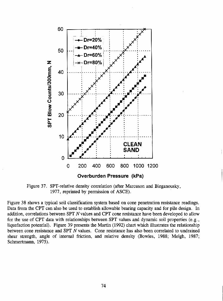
Overburden Pressure (kPa)

Figure 37. SPT-relative density correlation (after Marcuson and Bieganousky, 1977, reprinted by permission of ASCE).

Figure 38 shows a typical soil classification system based on cone penetration resistance readings. Data from the CPT can also be used to establish allowable bearing capacity and for pile design. In addition, correlations between SPT N values and CPT cone resistance have been developed to allow for the use of CPT data with relationships between SPT values and dynamic soil properties (e.g., liquefaction potential). Figure 39 presents the Martin (1992) chart which illustrates the relationship between cone resistance and SPT N values. Cone resistance has also been correlated to undrained shear strength, angle of internal friction, and relative density (Bowles, 1988; Meigh, 1987; Schrnertrnann, 1975).

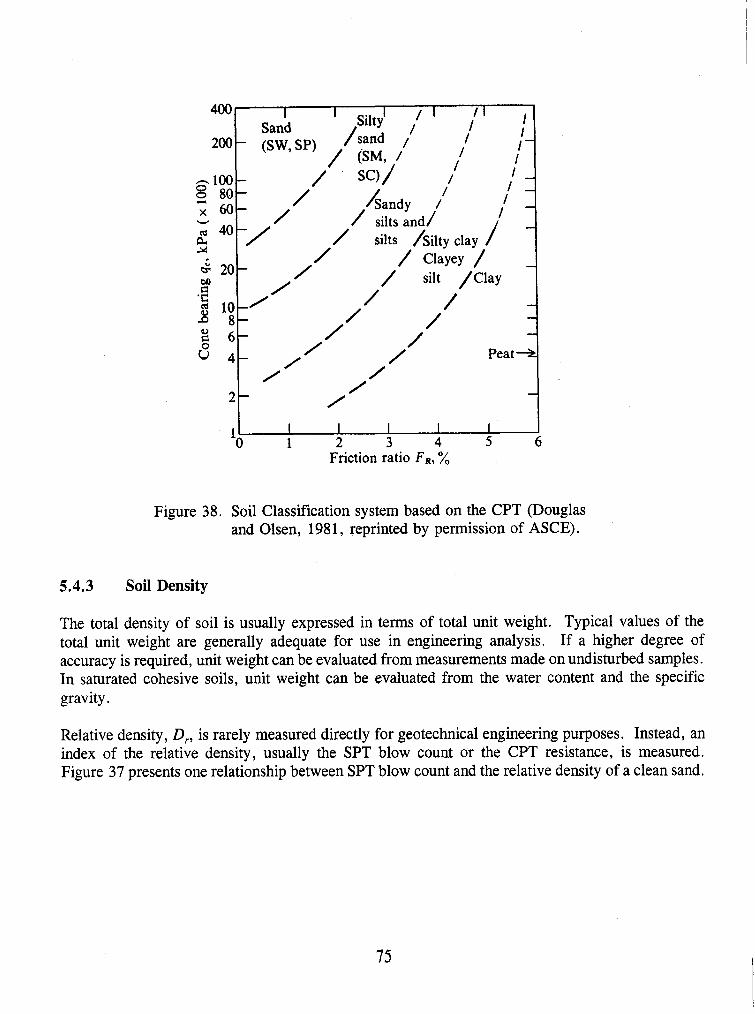
I I I I I I 1 2 3 4 5 6

Friction ratio FRY %

400. I I silty1 , / I 1 I

Sand I I /sand 1 I I

I I - / I

/ I - / / I -

d /Sandy / I

Figure 38. Soil Classification system based on the CPT (Douglas and Olsen, 1981, reprinted by permission of ASCE).

V x 6 0 -

9 G 20- DO

5.4.3 Soil Density

/ 40-/

/ silts and/ / silts /silty clay

/ / Clayey / - /

The total density of soil is usually expressed in terms of total unit weight. Typical values of the total unit weight are generally adequate for use in engineering analysis. If a higher degree of accuracy is required, unit weight can be evaluated from measurements made on undisturbed samples. In saturated cohesive soils, unit weight can be evaluated from the water content and the specific gravity.

Relative density, D,, is rarely measured directly for geotechnical engineering purposes. Instead, an index of the relative density, usually the SPT blow count or the CPT resistance, is measured. Figure 37 presents one relationship between SPT blow count and the relative density of a clean sand.

/ / silt /Clay

/ - /

/ - 0 c 6 - / /

6 4-

- / /

/ / Peat +t

0 / 2 - /

/ -

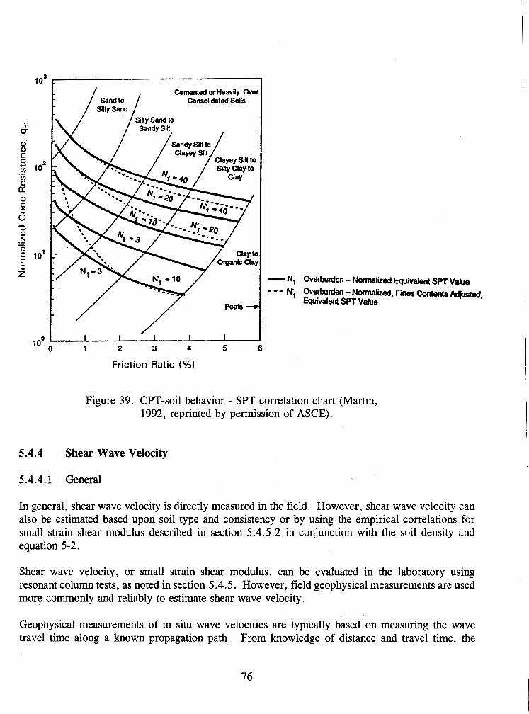
Cemenled w Heavily Over Consolidated Sols

I I I I I

1 2 3 4 5 6

Overburden - Normalied Walent SPT Value Overburden - Normalized, Fines Contents M j e d , Equivalen! SPT Value

Friction Ratio (%)

Figure 39. CPT-soil behavior - SPT correlation chart (Martin, 1992, reprinted by permission of ASCE).

5.4.4 Shear Wave Velocity

5.4.4.1 General

In general, shear wave velocity is directly measured in the field. However, shear wave velocity can also be estimated based upon soil type and consistency or by using the empirical correlations for small strain shear modulus described in section 5.4.5.2 in conjunction with the soil density and equation 5-2.

Shear wave velocity, or small strain shear modulus, can be evaluated in the laboratory using resonant column tests, as noted in section 5.4.5. However, field geophysical measurements are used more commonly and reliably to estimate shear wave velocity.

Geophysical measurements of in situ wave velocities are typically based on measuring the wave travel time along a known propagation path. From knowledge of distance and travel time, the

velocity is obtained. Wave velocity may be measured from intrusive methods such as boreholes and CPT soundings (seismic cone) or non-intrusively using seismic reflection, refraction, and surface wave profiling.

5.4.4.2 Geophysical Surveys

Geophysical techniques for subsurface exploration are described in detail by Woods (1994). Geophysical techniques commonly used in geotechnical practice are briefly summarized in the following paragraphs. Two general types of techniques. are available to measure shear wave velocities in the field:

intrusive techniques whereby measurements are made using probes and sensors that are lowered in boreholes or pushed into the ground; and

non-intrusive techniques whereby the measurements are made from the ground surface.

Borehole Surveys

In a borehole seismic survey, one or more boreholes are drilled into the soil to the desired depth of exploration. Wave sources andlor receivers are then lowered into the boreholes to perform the desired tests. There are three approaches to borehole seismic surveys:

Up Hole Surveys: Geophones are laid out on the surface in an array around the borehole. The energy source is set off within the borehole at successively decreasing depths starting at the bottom of the hole. The travel times from the source to the surface are analyzed to evaluate wave velocity versus depth. The energy source is usually either explosives or a mechanical pulse instrument composed of a stationary part and a hammer held against the side of the borehole by a pneumatic or hydraulic bladder.

Down Hole Surveys: In a down hole survey, the energy source is located on the surface and the detector, or geophone, is placed in the borehole. The travel time is measured with the geophone placed at progressively increasing depth to evaluate the wave velocity profile.

Cross Hole Survey: In a cross hole survey, the energy source is located in one boring and the detector (or detectors) is placed at the same depth as the energy source

' in one or more surrounding boreholes at a known spacing. Travel time between source and receiver is measured to determine the wave velocity.

The cross hole technique is generally the preferred technique for a borehole survey as it offers the highest resolution and greatest accuracy. However, cross hole measurements require a very precise evaluation of the distance between the energy source and the detector. An inclinometer reading is generally performed in the boreholes used in a cross hole survey to correct the results for deviation

of the boreholes from verticality. Cross hole geophysical testing is codified in ASTM Standard D 4428.

Seismic Refraction and Seismic Reflection Methods

Seismic refraction and reflection exploration surveys are conducted from the surface and do not require boreholes. The resolution of the methods is relatively poor and decreases with depth. These methods are most suitable as a means of identifying the depth to competent rock and the location of prominent soil horizons that have a large contrast in density and stiffness compared to the overlying soil.

Spectral Analysis of Su@ace Waves (SASW)

Spectral Analysis of Surface Waves (SASW) is a non-intrusive geophysical technique used primarily for evaluating subsurface shear wave velocity profiles. SASW testing evaluates shear wave velocity indirectly by direct measurement of Rayleigh, or surface wave, velocity. Rayleigh wave velocity is related to shear wave velocity by Poisson's ratio. The two velocities are usually within 5 percent of each other for most soils. SASW results are representative of the average properties of a relatively large mass of material, mitigating the potential for misleading results due to non- homogeneity. SASW can be a very cost-effective method of investigation. The ease and rapidity of field measurements and automated algorithms for data processing and inversion allow for evaluation of subsurface conditions at a relatively large number of points at a fraction of the cost of conventional intrusive exploration techniques.

A schematic representation of SASW testing is presented in figure 40. Excitation at the ground surface is used to generate the Rayleigh, or surface, waves at various frequencies. By spectral analysis of the ground surface response (velocity or acceleration) at two points a known distance apart, the Rayleigh wave velocity can be obtained at discrete frequencies. Usually, an inversion process (trial and error) is used to determine the velocity profile. At sites where wave velocity increases gradually with depth, the velocity profile may be determined directly from the field data. The depth over which reliable measurements can be made depends upon the energy and frequency content of the source excitation and the consistency of the subgrade material. Measurements are not affected by the depth to the water table.

The concept of measuring the velocity of Rayleigh waves of different frequencies to determine the profile of shear wave velocity with depth was first proposed by Jones (1962), in Great Britain, for pavement surveys and by Ballard (1964), at the Waterways Experiment Station in Vicksburg, Mississippi, for geotechnical analyses. These investigators used impact loading as the source excitation and developed an analysis based upon the assumption of a uniform, homogeneous layer. Stokoe and Nazarian (1985) at the University of Texas, Austin, extended the analysis to consider multi-layered media. These investigators also used a surface impact as the source excitation and thus reliable measurements were typically limited to maximum depths on the order of 10 meters by the relatively low energy content of the excitation at relatively long wave lengths.

Satoh and his co-workers (1991) in Japan developed an electro-magnetic controlled vibrator for use as the source excitation. Large (2000 kg) mass, Controlled Source Spectral Analysis of Surface

WAVE VELOCITY (m/s)

ELECTROMAGNETIC VIBRATOR (signal source)

Figure 40. Schematics of SASW testing (Kavazanjian et al., 1994).

79

Waves (CSSASW) equipment capable of penetrating over 100 meters below the ground surface has recently been developed. Comparisons between SASW and down hole velocity measurements have been made (Nazarian and Stokoe, 1984) and show good agreement between the two methods.

5.4.4.3 Compressional Wave Velocity

Compressional wave velocity may sometimes be required for seismic analyses. Compressional wave velocity can be directly measured in a bore hole survey or in a laboratory test. Alternatively, the compressional wave velocity can be calculated from the shear wave velocity and Poisson's ratio using equation 5-5.

5.4.5 Evaluation of Cyclic Stress-Strain Parameters

5.4.5.1 Laboratory Testing

Laboratory testing for evaluation of cyclic stress-strain parameters of soil .is appealing to many engineers because direct measurements are made of the hysteretic stress-strain behavior of soils. However, cyclic laboratory testing is subject to a variety of constraints, including:

difficulty in reproducing field stresses (or strains); difficulty in recovering and testing undisturbed cohesionless soil samples; and the time and expense associated with cyclic laboratory testing.

A summary of the different types of cyclic laboratory tests used in geotechnical practice and their advantages and limitations follows. More details on cyclic laboratory testing can be found in Kramer (1 996).

Qclic Direct Simple Shear Test

The cyclic direct simple shear (CyDSS) test may provide the most accurate representation of the stress state resulting from a vertically propagating shear wave in a horizontally layered soil deposit of any laboratory test. The simple shear device consists either of a rectangle box made of hinged plates or a cylindrical wire-reinforced membrane which surrounds the sample and restrains the sample from deforming laterally during the test. The apparatus includes either an arrangement for applying a constant vertical load or for maintaining a constant sample height while measuring the vertical load and a mechanism for applying a horizontal cyclic shear load. The sample is usually formed directly in the simple shear device. However, undisturbed samples of cohesive soil or frozen sand can be tested in the devices that use wire-reinforced membranes.

Cyclic Triaxial Test

The cyclic triaxial test was developed for geotechnical purposes by Seed and his co-workers at the University of California at Berkeley in the 1960s and has been used extensively to evaluate cyclic behavior of soils. The device consists of a regular triaxial cell and a cyclic, often sinusoidal loading machine attached to the loading piston. The sample is isotropically consolidated in the triaxial cell and then subjected to a cyclic axial load in extension and compression. The primary drawback of the cyclic triaxial tests is that it does not provide a good representation of the stress state induced in the ground by an earthquake (see figure 34). The main difference in cyclic triaxial test stress conditions compared to the field conditions are: (1) the laboratory soil sample is isotropically consolidated, whereas the soil is under a KO condition in the field; (2) in the field there is a continuous reorientation of the principal stresses whereas in the triaxial test, the reorientation angle is either 0 or 90 degrees; (3) the cyclic shear stress is applied on a horizontal plane in the field but on a 45 degree plane in the triaxial test; and (4) the mean normal stress in the field is constant while the mean normal stress in the laboratory varies cyclically.

Torsional Simple Shear Test

In order to overcome some of the limitations of the CyDSS and triaxial tests, Ishibashi and Sherif (1974) developed a torsional simple shear test. The sample is "doughnut-like" in shape with outer to inner radius and outer to inner height ratios of about two. This doughnut-like shape ensures a relatively uniform shear strain on the horizontal plane throughout the sample. The torsional simple shear test offers several advantages over CyDSS and cyclic triaxial tests:

simulates closely the field stress (strain) conditions like the CyDSS; it is possible to apply vertical and horizontal stresses independently; and permits the octahedral normal stress to remain unchanged during the test.

There are also some disadvantages associated with this test:

interpretation of the results is rather complicated and the definition of liquefaction (Ishibashi and Sherif, 1974) does not permit correlation of torsional simple shear results with those of other tests;

mobilization of enough interface shear between the sample and the top and bottom plates to prevent slippage may be difficult, however steel pins cast into porous stones will provide good contact between the sample and the plates; and

the shape of the sample makes the device impractical for use in conventional practice, particularly for undisturbed samples.

Resonant Column Test

The resonant column test for determining dynamic properties of soils is based on the theory of wave propagation in rods. Either compression or shear waves can be propagated through the soil specimen in resonant column testing. Solid or hollow specimens can be used in the apparatus.

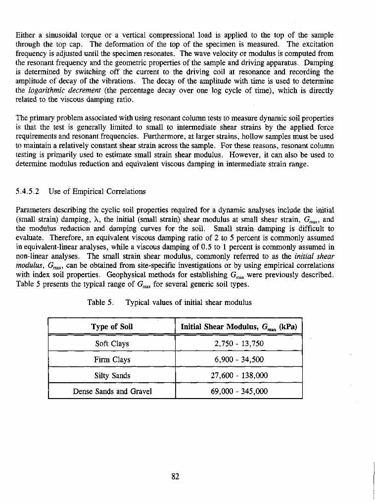
Either a sinusoidal torque or a vertical compressional load is applied to the top of the sample through the top cap. The deformation of the top of the specimen is measured. The excitation frequency is adjusted until the specimen resonates. The wave velocity or modulus is computed from the resonant frequency and the geometric properties of the sample and driving apparatus. Damping is determined by switching off the current to the driving coil at resonance and recording the amplitude of decay of the vibrations. The decay of the amplitude with time is used to determine the logarithmic decrement (the percentage decay over one log cycle of time), which is directly related to the viscous damping ratio.

The primary problem associated with using resonant column tests to measure dynamic soil properties is that the test is generally limited to small to intermediate shear strains by the applied force requirements and resonant frequencies. Furthermore, at larger strains, hollow samples must be used to maintain a relatively constant shear strain across the sample. For these reasons, resonant column testing is primarily used to estimate small strain shear modulus. However, it can also be used to determine modulus reduction and equivalent viscous damping in intermediate strain range.

5.4.5.2 Use of Empirical Correlations

Parameters describing the cyclic soil properties required for a dynamic analyses include the initial (small strain) damping, A, the initial (small strain) shear modulus at small shear strain, G,,, and the modulus reduction and damping curves for the soil. Small strain damping is difficult to evaluate. Therefore, an equivalent viscous damping ratio of 2 to 5 percent is commonly assumed in equivalent-linear analyses, while a viscous damping of 0.5 to 1 percent is commonly assumed in non-linear analyses. The small strain shear modulus, commonly referred to as the initial shear modulus, Gm,, can be obtained from site-specific investigations or by using empirical correlations with index soil properties. Geophysical methods for establishing G,,, were previously described. Table 5 presents the typical range of G,,, for several generic soil types.

Table 5. Typical values of initial shear modulus

Type of Soil

Soft Clays

Firm Clays

Silty Sands

Dense Sands and Gravel

Initial Shear Modulus, G,,, (kPa)

2,750 - 13,750

6,900 - 34,500

27,600 - 138,000

69,000 - 345,000

The parameter G,,,,, has been empirically related to both the SPT N value and CPT point resistance, q,. Correlations with SPT results by Seed et al. (1984) and Imai and Tonouchi (1982) and with CPT results by Mayne and Rix (1993) are presented in table 6.

Following the initial work of Hardin and Drnevich (1972), many researchers developed empirical relationships to estimate G,,, of the following general form:

where f(e) is some function of the void ratio, e, OCR is the overconsolidation ratio, A is a normalizing constant, k is the power factor, and a', is the mean normal effective stress obtained as:

where a', is the vertical effective stress and KO is the coefficient of lateral earth pressure at rest.

Seed and Idriss (1970) developed a series of curves relating G,,, to relative density and mean normal effective stress through a coefficient, (K,),,,:

Gmax = 1000 (K,),,, (a',,)" in psf (5-8)

where (K,),,,,, is a function of relative density and soil type (see table 6). This approach has been further extended to estimate stress-dependent modulus reduction curves for sandy soils using the strain dependent parameter K, instead of (K,),,,. An example of a curve relating K, to shear strain is shown in figure 41. Iwasaki et al. (1978) found that the mean normal effective stress is the predominant factor that governs the modulus reduction of cohesionless soils and developed stress dependent curves shown in figure 42. Note that the authors did not provide damping curves.

Vucetic and Dobry (1991) have shown that the relationships between modulus reduction and cyclic shear strain and between equivalent viscous damping and cyclic shear strain can, with a relatively high degree of confidence, be reduced to a set of curves that depend on the plasticity index, PI, of the soil. The Vucetic and Dobry modulus reduction and damping curves are presented in figure 43. Note that the curves for PI equal to zero apply to sands, gravels, and other cohesionless soil. The Vucetic and Dobry PI = 0 damping curve may be used in conjunction with the Iwasaki et al. (1978) stress-dependent modulus reduction curve to characterize the dynamic behavior of sandy soils.

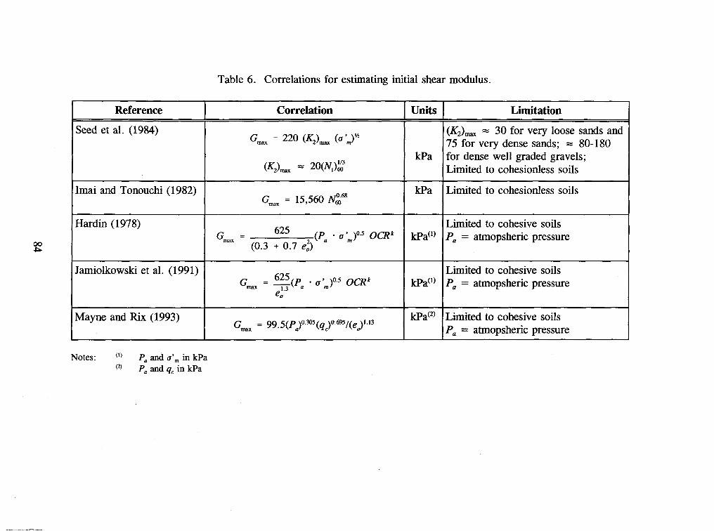
Table 6. Correlations for estimating initial shear modulus.

Notes: (') Pa and a', in kPa (*) Pa and q, in kPa

Reference

Seed et al. (1984)

Imai and Tonouchi (1982)

Hardin (1978)

Jarniolkowski et al. (1991)

Mayne and Rix (1993)

Correlation

GmX = 220 (6)- (@),)Ih

(k;)- = 2 0 ( ~ ~ ) :

G- = 15,560 flm6'

625 'max = (Pa u 'J" OCRk

(0.3 + 0.7 e:)

625 Gmax = -(Pa . u ',,,)O.' OCRk 1.3

e'7

G- = 99. 5(Pa)0 305(qc)0 695/(e0)1.13

Units

Wa

Wa

kPa(')

Pa(')

kPa"

Limitation

(K,),, = 30 for very loose sands and 75 for very dense sands; = 80-180 for dense well graded gravels; Limited to cohesionless soils

Limited to cohesionless soils

Limited to cohesive soils Pa = atmopsheric pressure

Limited to cohesive soils Pa = atmopsheric pressure

Limited to cohesive soils Pa = atmopsheric pressure

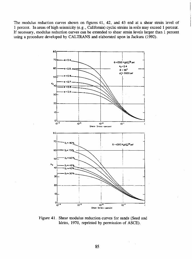
The modulus reduction curves shown on figures 41, 42, and 43 end at a shear strain level of 1 percent. In areas of high seismicity (e.g., California) cyclic strains in soils may exceed 1 percent. If necessary, modulus reduction curves can be extended to shear strain levels larger than 1 percent using a procedure developed by CALTRANS and elaborated upon in Jackura (1992).

Sheor Slroin -percent

Figure 41. Shear modulus reduction curves for sands (Seed and Idriss, 1970, reprinted by permission of ASCE).

0r0001 0.001 0.01 0.1

CYCLIC SHEAR STRAIN, yc (%)

Figure 42. Shear modulus reduction curves for sands (Iwasaki et al., 1978, reprlnted by permission of Japanese Society of Soil Mechanics and Foundation Engineering).

5.4.6 Peak and Residual Shear Strength

The peak shear strength of soil not subject to strength degradation under cyclic loading may be evaluated using conventional methods, including laboratory and in situ testing and correlations with soil index properties. A key difference in seismic problems compared to static problems is that undrained strength parameters are typically used for the strength of saturated soils subjected to cyclic loading, even for cohesionless soils (e.g., sands, gravels) because of the relatively rapid rate of earthquake loading.

The dynamic undrained shear strength of a soil may be influenced by the amplitude of the cyclic deviator stress, the number of applied loading cycles, and the plasticity of the soil. For saturated cohesionless soils, even relatively modest cyclic shear stresses can lead to pore pressure rise and a significant loss of undrained strength. However, Makdisi and Seed (1978) point out that substantial permanent strains may be produced by cyclic loading of clay soils to stresses near the yield stress, while essentially elastic behavior is observed for large numbers of (> 100) cycles of loading at cyclic shear stresses of up to 80 percent of the undrained strength. Therefore, these investigators recommend the use of 80 percent of the undrained strength as the "dynamic yield strength" for soils that exhibit small increases in pore pressure during cyclic loading, such as clayey materials, and partially saturated cohesionless soils.

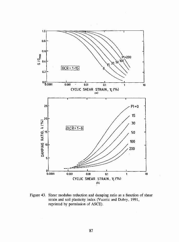
CYCLIC SHEAR STRAIN, (%I (4

CYCLIC SHEAR STRAIN , T, (%I fb)

Figure 43. Shear modulus reduction and damping ratio as a function of shear strain and soil plasticity index (Vucetic and Dobry, 1991, reprinted by permission of ASCE).

Evaluation of the potential for shear strength reduction in a saturated or almost saturated cohesionless soil (low plasticity silt, sand, or gravel) subjected to dynamic loading may require sophisticated cyclic laboratory testing. Alternatively, a residual strength may be assigned to the soil based upon either undrained laboratory tests or in situ test results.

The residual shear strength after cyclic loading is of critical importance in assessing the post- liquefaction stability of a foundation or earth structure. Saturated soils which liquefy typically possess some "residual" shear strength even when in the liquefied state. In initially loose soils, this residual strength may be very small and of little consequence. In initially dense soils, particularly in dense granular soils which tend to dilate, or expand in volume, when sheared, this residual strength can be significant and of great consequence in acting as a stabilizing force subsequent to liquefaction.

Evaluation of residual shear strength from laboratory tests is not typically recommended due to the difficulties associated with testing. Use of residual strengths derived from in situ testing is, in general, considered more reliable than use of laboratory test results. However, use of residual strengths in assessments of the pseudo-static factor of safety andlor yield acceleration can result in very conservative values (Marcuson et al., 1990), as discussed in chapter 7.

The steady-state shear strength, S,,, governs the behavior of liquefied soil. Poulos et al. (1985) proposed a methodology for evaluation of the in situ S,, based on obtaining high-quality soil samples with minimal disturbance. The high-quality samples were tested in the laboratory and the laboratory strengths were then adjusted for field conditions using specially developed techniques to correct the resulting laboratory S,, values for effects of void ratio changes due to sampling, handling, and test set-up. Due to the very high sensitivity of S,, to even small changes in void ratio, the laboratory techniques proposed by Poulos et al. presently do not appear to represent a reliable basis for engineering analyses unless very conservative assumptions and high factors of safety are employed to account for the considerable uncertainties involved.

Because of difficulties in measuring steady-state strength in laboratory, Seed (1987) proposed an alternate technique for evaluation of in situ undrained residual shear strength based on the results of SPT testing. He back analyzed a number of liquefaction-induced failures from which residual strength could be calculated for soil zones in which SPT data was available, and proposed a correlation between residual strength, S,, and (N,),,. (N,),-,, is a "corrected" normalized standardized SPT blow count, as discussed in chapter 5.4.2.1, with a correction, Ncorr, for fines content to generate an equivalent "clean sand" blow count as:

where Nco,, is a function of percent of fines. Recommendations for selecting N,, are given in the insert of figure 44. Since there is no guarantee that all the conditions for steady-state of deformation were satisfied in the case histories used to develop figure 44, the term residual strength is used instead of steady-strength strength. Note that the fines correction on figure 44 is the same "fines" correction as is used in the liquefaction susceptibility analyses (see, e.g., figure 58).

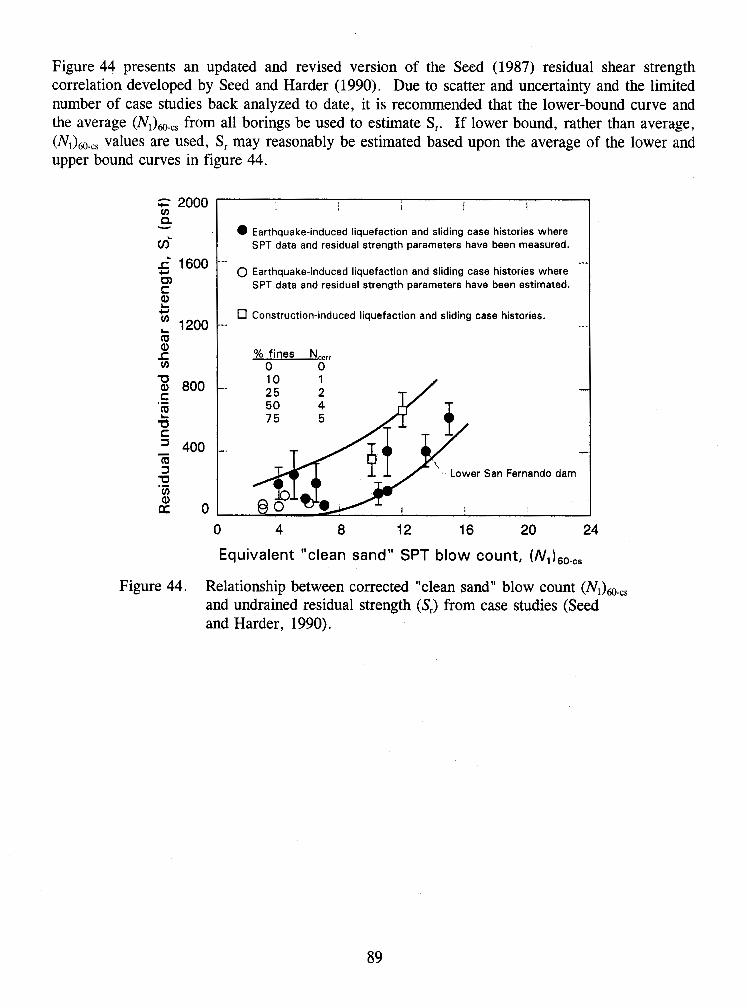
Figure 44 presents an updated and revised version of the Seed (1987) residual shear strength correlation developed by Seed and Harder (1990). Due to scatter and uncertainty and the limited number of case studies back analyzed to date, it is recommended that the lower-bound curve and the average (N,),,, from all borings be used to estimate S,. If lower bound, rather than average, (N,),,, values are used, S, may reasonably be estimated based upon the average of the lower and upper bound curves in figure 44.

I I i i

Earthquake-induced liquefaction and sliding case histories where SPT data and residual strength parameters have been measured.

. -. -.- 0 Earthquake-induced liquefaction and sliding case histories where

SPT data and residual strength parameters have been estimated.

-- . Construction-induced liquefaction and sliding case histories. ...

% fines N,,,, 0 0

-

.....

Lower San Fernando dam

0 4 8 12 16 20 24

Equivalent "clean sand" SPT blow count, (N,),,,,

Figure 44. Relationship between corrected "clean sand" blow count (N,),-,, and undrained residual strength (S,) from case studies (Seed and Harder, 1990).

CHAPTER 6

SEISMIC SITE RESPONSE ANALYSIS

6.1 GENERAL

The local soil profile at a project site can have a profound effect on earthquake ground motions. Local soil conditions can affect the intensity, frequency content, and duration of strong shaking. Amplification of peak bedrock acceleration by a factor of four or more and amplification of spectral accelerations by a factor of ten or more have been attributed to the response of the local soil profile to the bedrock ground motions.

The influence of local soil conditions on seismic ground motions can be assessed either in a gross empirical manner (using "soil-site" attenuation relationships, seismic hazard maps for soil sites, and/ or code-prescribed response spectra for soil sites) or by conducting a site-specific seismic site response analysis. The choice of the approach to employ is usually a discretionary decision of the design engineer and depends on a variety of factors, including local seismicity, local soil conditions, type of facility, and the importance of the project. For major projects and critical facilities, when an analysis more accurate than a gross empirical analysis is desired, and for deep deposits of soft clay and other Special Study soil sites (see UBC, 1994 and table 3), a site-specific site response analysis is usually warranted. A site-specific response analysis can be performed for foundation soils, for earthen embankments, or for the coupled response of foundation soil and an embankment, as discussed in the remainder of this chapter.

SITE-SPECIFIC SITE RESPONSE ANALYSES

Site-specific seismic site response analyses are generally based upon the assumption of a vertically propagating shear wave through uniform horizontal soil layers of infinite lateral extent. The influence of vertical motions, compression waves, laterally non-uniform soil conditions, incoherence and spatial variation of ground motions are typically not accounted for in conventional seismic site response analyses. Evaluation solely of the impact of vertically propagating shear waves in a site response analysis is consistent with common design and code practices. It is also consistent with geotechnical engineering analyses for liquefaction potential and seismic slope stability, which consider only the horizontal component of the seismic motions. Three different levels of site- specific seismic site response analysis are available to the geotechnical engineer.

simplified (empirical) analysis; equivalent-linear one-dimensional site response analyses; and advanced one- and two-dimensional site response analyses.

These three levels of site response analysis are discussed in detail in the remainder of this chapter.

6.3 SIMPLIFIED SEISMIC SITE RESPONSE ANALYSES

For screening purposes and preliminary analyses, the influence of local soil conditions on seismic site response can be assessed in a simplified manner using empirical relationships which correlate ground motions at rock sites to those at soil sites. These relationships, developed on the basis of both observations of ground motions in earthquakes and one-dimensional site response analysis, provide amplification factors that can be used to provide a rough estimate of the free-field (i.e., not affected by structure and/or topography) peak ground acceleration at soft and stiff soil sites from the free-field rock site peak ground acceleration determined in a seismic hazard analysis. Empirical relationships for the amplification of peak ground acceleration by earthen embankments have also been developed.

Whereas structural analyses typically require information on the spectral content of ground motions, and thus require a complete time history to characterize the design motion, geotechnical analyses frequently only require knowledge of either the peak ground acceleration or a combination of peak ground acceleration and earthquake magnitude. Earthquake magnitude and the peak acceleration at a hypothetical bedrock outcrop at the project site are generally evaluated as part of the seismic hazard analysis (see chapter 3). Several investigators have developed empirical relationships between the peak ground acceleration at a hypothetical bedrock outcrop at the project site to the peak ground acceleration at a specific site as a function of the local soil conditions. The plot on figure 45 shows a relationship developed by Seed and Idriss (1982) for soft soil and stiff soil site conditions. This plot was developed using SHAKE, a computer program for equivalent-linear one- dimensional site response analyses described in greater detail in section 6.4.

Experience from recent earthquakes has shown that the curves shown on figure 45 may significantly under-predict site amplification effects in many situations. Figure 46 shows an updated site amplification relationship for free-field soft soil sites developed by Idriss (1990). This updated plot yields peak acceleration values significantly greater than the soft soil site curve from the 1982 Seed and Idriss plot. The updated plot was developed by Idriss (1990) from both SHAKE analyses and field observations of soft soil site response in recent earthquakes.

Figure 47 presents a comparison of peak acceleration values recorded at the base (usually bedrock) of several earthen dams and the corresponding peak acceleration at the crest (Harder, 1991). Figure 47 indicates that larger amplification effects may be expected in earthen structures than at free-field soft soil sites due to two-dimensional effects.

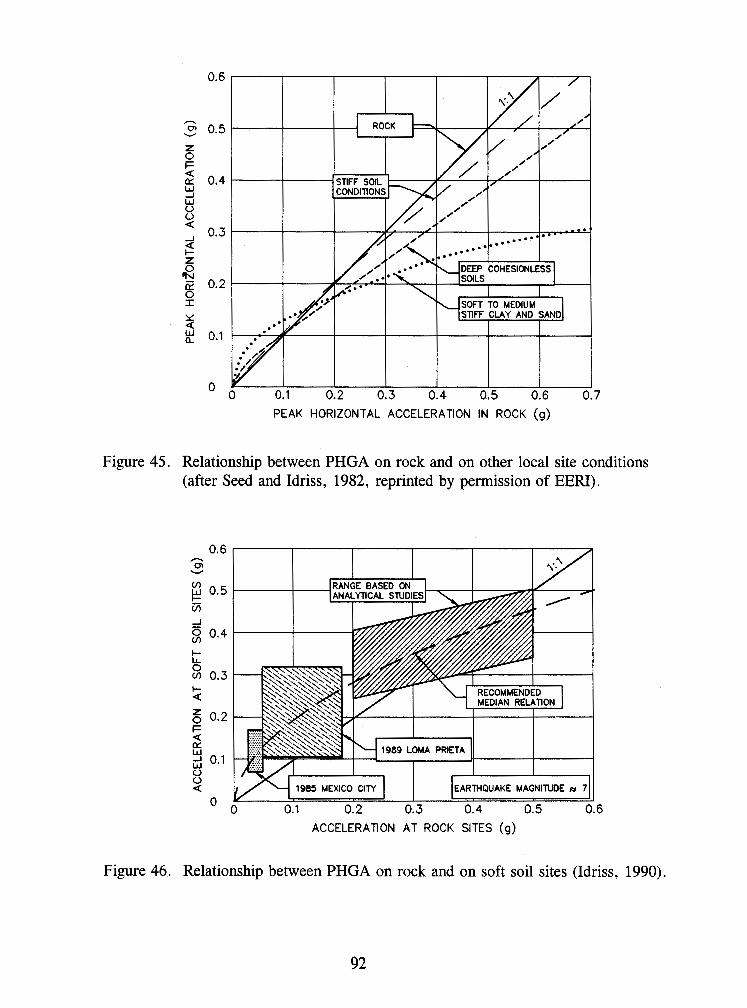
Figure 45.

PEAK HORIZONTAL ACCELERATION IN ROCK (g)

Relationship between PHGA on rock and on other local site conditions (after Seed and Idriss, 1982, reprinted by permission of EERI).

ACCELERATION AT ROCK SITES (g)

Figure 46. Relationship between PHGA on rock and on soft soil sites (Idriss, 1990).

PEAK TRANSVERSE BASE ACCELERATION ( Q)

Figure 47. Comparisons of peak base and crest accelerations recorded at earth dams (Harder, 1991).

The free-field soft soil site amplification curve presented in figure 46 and the embankment response observational data presented in figure 47 may be used in a simplified three- or four-step site response analysis procedure to account for the influence of local soil conditions and earthen embankments on the peak ground acceleration at a project site. The three- or four-step procedure is as follows:

Step 1: Classify the site. Using table 3 (Borcherdt; 1994), classify the site as a Special Study, soft, medium stiff, stiff, or rock on the basis of the average shear wave velocity for the top 30 meters of soil.

Step 2: Estimate the hypothetical free-field bedrock acceleration at the site. Using one of the methods discussed in chapter 3, estimate the free-field peak ground acceleration at a hypothetical bedrock outcrop at the project site.

Step 3: Estimate the free-field acceleration at the site. Estimate the potential amplification of the hypothetical bedrock peak ground motion by the local soil conditions based upon the soil profile classification. For soft soils, use the curve shown on figure 46 recommended by Idriss (1990). For medium stiff and stiff soil sites, for all acceleration levels, assume the free-field peak ground acceleration at the site is equal to the peak rock site acceleration. For Special Study soil sites, figures 45 and 46 should not be used. Instead, site specific seismic response analyses such as those described in the next section of this chapter should be conducted.

Step 4: Estimate the peak acceleration at the top of the embankment. Estimate the potential amplification of the peak acceleration at the top of the embankment, if an embankment is present, using the free-field peak soil acceleration derived in Step 3 and the earth dam amplification curve in figure 47.

Step 4 in the procedure presented above is based upon a simplified, "decoupled" assumption that the peak acceleration at the base of the embankment is the same as the free-field peak acceleration, thereby ignoring interaction between the embankment mass and the ground. Analyses of the coupled response of embankments and foundation soils indicates that this simplified, decoupled analysis usually yield a conservative upper bound estimate of the acceleration at the base of the embankment (Bray et al., 1995). However, in general, this simplified approach is intended only to give a rough estimate of amplification effects at a site and is not intended for use in final design of highway facilities. The design engineer should decide if this approach is appropriate for the intended purpose or, if it is necessary to perform a more sophisticated analysis.

The peak acceleration at the top of an embankment estimated in step 4 may also be used in preliminary analyses for various highway ancillary structures and for structures constructed on top of embankment fill. This acceleration is not, however, the appropriate peak acceleration for use in seismic stability and deformation potential calculations for an embankment mass or for bridge abutments. For these calculations, the average acceleration of the assumed failure mass, and not the acceleration at the top of the embankment, should be used. The average acceleration is directly proportional to the seismically-induced inertia forces and thus is the relevant response quantity. The peak average acceleration is always less than the peak ground acceleration due to spatial averaging.

For a given embankment height, h, and peak acceleration at the top of the embankment, a,,,, the peak average acceleration, k,,, may be estimated at any elevation y within an embankment from the Makdisi and Seed (1978) chart. This chart, developed on the basis of one- and two-dimensional equivalent-linear site response analyses of earth dams, is shown on figure 48.

PEAK AVERAGE ACCELERATION, box / PEAK CREST ACCELERATION. amo*

Figure 48. Variation of peak average acceleration ratio with depth of sliding mass (Makdisi and Seed, 1978, reprinted by permission of ASCE).

6.4 EQUIVALENT-LINEAR ONE-DIMENSIONAL SITE RESPONSE ANALYSES

When an analysis more accurate than the simplified analysis presented above is desired, a formal seismic site response analysis can be performed. Equivalent-linear one-dimensional analysis is by far the most common method used in engineering practice to analyze seismic site response. Even if a two-dimensional embankment or slope is to be analyzed, a one-dimensional response analysis can be used. Experience with response analyses of earth dams has shown that one-dimensional response analysis of vertical columns of soil within a two-dimensional earth structure provide a reasonable approximation of the two-dimensional response (Vrymoed and Calzascia, 1978).

In a one-dimensional equivalent-linear site response analysis, the soil profile is modeled as a horizontally layered, linear visco-elastic material characterized by an initial (small-strain) shear modulus and an equivalent viscous damping ratio. To account for the non-linear, strain-dependent behavior of soil, the equivalent-linear modulus and equivalent viscous damping ratio are evaluated from the modulus reduction and damping curves (see chapter 5). The equivalent-linear material

properties are evaluated in each iteration at the calculated effective shear strain level. The effective shear strain level is usually specified as:

where ye, is efective strain, y,,, is maximum absolute value of shear strain and n is the efective strain factor. Because ye, is not known prior to the start of the analysis, equivalent-linear response analyses are performed in an iterative manner, using the effective strain from one iteration of the analysis to evaluate the equivalent modulus and viscous damping ratio for the next iteration. Usually 5 to 10 iterations are needed for convergence.

The computer program SHAKE, originally developed by Schnabel et al. (1972) and updated by Idriss and Sun (1992) as SHAKE91, is perhaps the most commonly used computer program for one- dimensional equivalent-linear seismic site response analysis. SHAKE91 is available from the National Information Service for Earthquake Engineering (NISEE) at the University of California at Berkeley for a nominal cost. Basic input to SHAKE91 includes the soil profile, soil parameters, and the input acceleration time history. Soil parameters used in SHAKE91 include the shear wave velocity or initial (small strain) shear modulus and unit weight for each soil layer. Also, curves relating the shear modulus reduction and equivalent viscous damping ratio to shear strain for each soil type are used. Evaluation of representative values for these soil properties is discussed in chapter 5.

Once the soil profile and material properties have been specified, the only remaining input is the earthquake motion. Selection of representative acceleration time histories for the input motion is discussed in chapter 4. The acceleration-time history may be input as either the motion at a hypothetical bedrock outcrop (most commonly used option because it is congruent with assumptions embedded in attenuation relationships) or at the bedrock-soil interface at the base of the soil column. Results of the analysis provide shear stress-, shear strain-, and acceleration-time histories and peak values for the ground surface, hypothetical bedrock outcrop, and for each layer within the soil profile.

Historically, the value of the effective strain factor used in SHAKE analyses to determine the equivalent-linear modulus and damping has been n = 0.65. However, based upon back analysis of strong motion records obtained at soil sites in recent earthquakes, several investigators have proposed that n be related to the earthquake magnitude. Equation 6-2 presents the relationship between earthquake magnitude, M,, and n as proposed by Idriss and Sun (1992).

6.5 ADVANCED ONE- AND TWO-DIMENSIONAL SITE RESPONSE ANALYSES

6.5.1 General

An advanced seismic site response analysis may be necessary if one or more of the following project-specific conditions exists: (1) the project is considered important or critical; (2) irregular boundary conditions must be modeled; (3) the project includes an embankment founded on Special Study soils; and (4) an analysis more accurate than a one-dimensional equivalent-linear site response analysis is desired. Depending on the particular situation, either one-dimensional non-linear or two- dimensional equivalent-linear or non-linear site response analyses may be employed.

6.5.2 One-Dimensional Non-Linear Site Response Analyses

The primary difference between non-linear and equivalent-linear site response analyses is that non- linear analyses use a more realistic model to represent the behavior of soil subjected to cyclic loads. Essentially, a non-linear model traces the evolution of the hysteresis loops generated in a soil by cyclic loading in a sequential manner, whereas the equivalent-linear model only approximates the representative soil stiffness and damping over the entire sequence of cyclic loads. The more realistic representation of the non-linear behavior of cyclically-loaded soils gives non-linear analyses a significant advantage over equivalent-linear seismic response analyses at higher levels of seismic shaking where non-linear effects tend to dominate.

In general, equivalent-linear site response analyses are considered unreliable at ground shaking levels in excess of 0.4 g (see Ishihara, 1986) or if calculated peak shear strains exceed approximately 2 percent. However, non-linear site response analyses are also subject to limitations. The material models used in non-linear site response analyses often require parameters for which readily obtainable or published values do not exist. Furthermore, computer programs for non-linear site response analysis are not readily available to the general engineering community. Therefore, even though non-linear site response analyses typically provide a more accurate and more versatile representation of seismic behavior, equivalent-linear site response analyses and other approximate solutions still dominate highway engineering practice.

The computer program DESRA-2, originally developed by Lee and Finn (1978), and its descendants, are perhaps the most commonly used computer programs for performing total stress, one-dimensional non-linear seismic site response analysis. Basic input to DESRA-2 includes the soil profile, parameters of the Kondner and Zelasko (1963) constitutive model, and the input time history of ground motions. The Kondner-Zelasko constitutive model uses a hyperbola to describe the backbone curve of the hysteresis loop. The backbone curve of a soil element is drawn by connecting the tips of the hysteresis loops generated during uniform cyclic loading. Hysteresis loops are generated from the backbone curve based upon the assumption of Masing (1926) behavior during cyclic loading. Parameters required for the Kondner-Zelasko (1963) model are the shear modulus at small strains and the shear strength of the soil. However, as noted by several researchers (see e. g. , Ishihara, 1986), the relatively simple Kondner-Zelasko model can not accurately simulate the cyclic behavior of soil in the small shear strain range (i.e., for shear strain levels less than 0.1 percent).

Various derivative codes of DESRA-2 are also in use. In several of these codes, modifications have been made to improve the accuracy of the Kondner-Zelasko constitutive model at small strains. Chang et al., (1991) developed the computer program MARDES to study nonlinear ground response at a liquefied site in Taiwan. MARDES uses the three-parameter Martin-Davidenkov (Martin, 1975) constitutive model which enables a more accurate description of non-linear soil behavior than the Kondner-Zelasko model. MatasoviC (1993), while studying pore water pressure generation in saturated clay deposits, developed the computer program D-MOD. D-MOD employs a Modified Kondner and Zelasko (M-K-Z) constitutive model (MatasoviC and Vucetic, 1993) that also provides a better description of the actual soil behavior than the Kondner-Zelasko model. The M-K-Z parameters can be directly evaluated by curve-fitting of modulus reduction and damping curves. Li et a1 . (1992) developed a computer program, SUMDES , which enables calculation of the seismic response of soil deposits sub~ected to multi-directional shaking. Computer programs with non-linear soil models can also be used for evaluation of pore pressure generation and liquefaction potential and of the impact of pore pressure generation on site response in an effective stress analysis.

6.5.3 Two-Dimensional Site Response Analyses

A variety of finite element and finite difference computer programs are available for use in two- dimensional seismic site response analyses. The computer program QUAD4, originally developed by Idriss and his co-workers (Idriss et al., 1973) and recently updated as QUAD4M by Hudson et al. (1994), is among the most commonly used computer programs for two-dimensional site response analysis. QUAD4M uses an equivalent-liner soil model similar to the model used in SHAKE. Basic input to QUAD4M includes the two-dimensional soil profile, equivalent-linear soil properties, and the time history of horizontal ground motion. Time history of vertical ground motion may also be applied at the base of the soil profile. The base can be modeled as a rigid boundary, with design motions input directly at the base, or as a transmitting boundary which enables application of ground motions as hypothetical rock outcrop motions. With respect to the input soil properties, QUAD4M is very similar to SHAKE91. However, the ability to analyze two-dimensional geometry and the option for simultaneous base excitation with horizontal and vertical acceleration components make QUAD4M a more versatile analytical tool than SHAKE91.

A major difference between the QUAD4M and SHAKE91 equivalent-linear models is that the damping ratio in QUAD4M depends on the frequency of excitation or rate of loading. In QUAD4M, the equivalent-linear viscous damping ratio is used to fix the frequency dependent damping curve at the natural frequency of the soil deposit in order to optimize the gap between model damping and the damping ratio. A major drawback of QUAD4M is its limited pre- and post- processing capabilities. These limited capabilities make finite element mesh generation and processing and interpretation of the results difficult and time consuming. QUAD4M is available from the National Information Service for Earthquake Engineering (NISEE) at University of California at Berkeley for a nominal cost.

Other two-dimensional equivalent-linear seismic site response analysis computer programs that are available to the public include program TELDYN (Pyke, 1995) and FLUSH (Lysmer et al., 1975). TELDYN is an enhanced version of the original QUAD4 which can also be run in a nonlinear mode and is fully supported by its developer. FLUSH is a versatile frequency-domain program equipped

with transmitting boundaries which enable calculations with a mesh of smaller size and a "quasi" three-dimensional analysis option. Because of the quasi three-dimensional analysis capabilities, FLUSH is popular for use in soil-structure interaction problems and for analyses of major earth dams.

Computer programs are also available for truly non-linear two-dimensional seismic site response analyses (e.g., Prevost, 1981 ; Finn et al., 1986; Cundall and Board, 1988; Muraleetharan et al., 1991 ; Bardet, 1992). However, these programs are not particularly "user-friendly" and usually require involvement of the developers to establish the parameters of constitutive models and boundary conditions. Therefore, such programs are not commonly used in geotechnical engineering practice.

CHAPTER 7

SEISMIC SLOPE STABILITY

7.1 BACKGROUND

The ground accelerations associated with seismic events can induce significant inertia forces that may lead to instability and permanent deformations of natural and man-made slopes and embankments. There are, in general, two different but related methods used to evaluate the seismic stability of slopes and embankments in conventional geotechnical practice: (1) the seismic coefficient-factor of safety approach; and (2) the permanent seismic deformation approach. Both of these approaches to seismic stability assessment employ pseudo-static limit equilibrium analysis.

An essential element in both seismic coefficient-factor of safety analyses and permanent seismic deformation analyses to assess seismic slope stability is limit equilibrium slope stability analyses. In a pseudo-static limit equilibrium analysis, the earthquake inertia forces are represented by static loads applied at the center of gravity of each "slice" through the potential failure mass. Numerous limit equilibrium methods and procedures are currently available to evaluate static slope stability (Duncan, 1992). Most of these methods are, in some form, also suitable for pseudo-static seismic stability analysis. Pseudo-static limit equilibrium analyses required for both seismic coefficient and permanent seismic deformation analyses are generally carried out using the same model of the slope used in the static stability analysis. The cross sections are often reinterpreted using appropriate dynamic shear strength parameters. However, even if the cross section doesn't change, the search for the critical surface, i.e., the surface with the lowest factor of safety or yield acceleration, may have to be repeated because the critical surface from the static analysis is not necessarily the same as the critical surface for the dynamic analysis.

A wide variety of commercially available computer programs exist that can perform both static and pseudo-static limit equilibrium analyses. Most of these programs provide general solutions to slope stability problems with provisions for using the simplified Bishop, simplified Janbu, and/or Spencer's method of slices. Potential sliding surfaces, both circular or polygonal, can usually be pre-specified or randomly generated. Commonly used programs include PCSTABU (Carpenter, 1985) and PCSTABL5 (Achilleos, 1988) developed at Purdue University, UTEXAS3 (Wright, 1995) developed at the University of Texas at Austin, XSTABL (Sharma, 1994) developed at University of Idaho, Moscow, and SLOPEW distributed by Geo-Slope International.

In principle, pseudo-static limit equilibrium analysis can be performed using either a total or an effective stress analysis. Problems of estimating pore pressures induced by cyclic shearing are avoided by using a total stress analysis. The typical Corps of Engineers practice for pseudo-static stability analyses in sandy soils is to use a composite shear strength envelope based on consolidated drained (CD) test results at low confining pressures ("S" envelope) and on consolidated undrained (CU) test results at high confining pressures ("R" envelope), as shown on figure 49. This strength envelope, which conservatively takes into account any possible dissipation of shear-induced negative

pore pressures that might occur in the field in stiff clays and dense sands, is recommended for pervious soils. For soils of low permeability, in which undrained conditions are more likely to exist during an earthquake, a CU strength envelope is appropriate.

NORMAL STRESS, 6

Figure 49. Composite shear strength envelope.

In the seismic coefficient - factor of safety approach to pseudo-static limit equilibrium analysis, a seismic coefficient is used to represent the effect of the inertia forces imposed by the earthquake upon the potential failure mass. An allowable factor of safety is associated with the seismic coefficient in such a way that the behavior of the slope is within the range considered acceptable, i.e., the slope or embankment will experience acceptable deformation in the design earthquake. The seismic coefficient, k,, is a dimensionless constant. The main drawback of the seismic coefficient - factor of safety approach lies in the difficulty of directly relating the value of the seismic coefficient to the characteristics of the design earthquake. Therefore, a considerable amount of conservatism is usually built into seismic coefficient - factor of safety analyses. Use of either the peak ground acceleration PGA, or the peak average horizontal acceleration of the failure mass, k,,,,,, as the seismic coefficient (expressed as a function of gravity, i.e., k, = k,,,,,lg) in conjunction with a pseudo-static factor of safety of 1.0 has been shown to give excessively conservative assessments of slope performance in earthquakes. However, little guidance on selection of the seismic coefficient as a fraction of the peak acceleration is available to the engineer.

In contrast to the seismic coefficient-factor of safety approach, the permanent seismic deformation approach involves the explicit calculation of cumulative seismic deformation. In this approach, the potential failure mass is treated as a rigid body on a yielding base. The acceleration time history of the rigid body is assumed to correspond to the average acceleration time history of the failure mass. Deformation accumulates when the rigid body acceleration exceeds the yield acceleration of the failure mass, ky, where ky is defined as the horizontal acceleration that results in a factor of safety of 1.0 in a pseudo-static limit equilibrium analysis. The method, most commonly used for

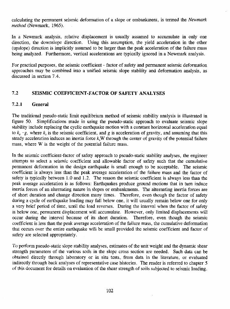
calculating the permanent seismic deformation of a slope or embankment, is termed the Newmark method (Newmark, 1965).

In a Newmark analysis, relative displacement is usually assumed to accumulate in only one direction, the downslope direction. Using this assumption, the yield acceleration in the other (upslope) direction is implicitly assumed to be larger than the peak acceleration of the failure mass being analyzed. Furthermore, vertical accelerations are typically ignored in a Newmark analysis.

For practical purposes, the seismic coefficient - factor of safety and permanent seismic deformation approaches may be combined into a unified seismic slope stability and deformation analysis, as discussed in section 7.4.

SEISMIC COEFFICIENT-FACTOR OF SAFETY ANALYSES

7.2.1 General

The traditional pseudo-static limit equilibrium method of seismic stability analysis is illustrated in figure 50. Simplifications made in using the pseudo-static approach to evaluate seismic slope stability include replacing the cyclic earthquake motion with a constant horizontal acceleration equal to k, -g, where k, is the seismic coefficient, and g is acceleration of gravity, and assuming that this steady acceleration induces an inertia force k,W through the center of gravity of the potential failure mass, where W is the weight of the potential failure mass.

In the seismic coefficient-factor of safety approach to pseudo-static stability analyses, the engineer attempts to select a seismic coefficient and allowable factor of safety such that the cumulative permanent deformation in the design earthquake is small enough to be acceptable. The seismic coefficient is always less than the peak average acceleration of the failure mass and the factor of safety is typically between 1.0 and 1.2. The reason the seismic coefficient is always less than the peak average acceleration is as follows: Earthquakes produce ground motions that in turn induce inertia forces of an alternating nature in slopes or embankments. The alternating inertia forces are of short duration and change direction many times. Therefore, even though the factor of safety during a cycle of earthquake loading may fall below one, it will usually remain below one for only a very brief period of time, until the load reverses. During the interval when the factor of safety is below one, permanent displacement will accumulate. However, only limited displacements will occur during the interval because of its short duration. Therefore, even though the seismic coefficient is less than the peak average acceleration of the failure mass, the cumulative deformation that occurs over the entire earthquake will be small provided the seismic coefficient and factor of safety are selected appropriately.

To perform pseudo-static slope stability analyses, estimates of the unit weight and the dynamic shear strength parameters of the various soils in the slope cross section are needed. Such data can be obtained directly through laboratory or in situ tests, from data in the literature, or evaluated indirectly through back analyses of representative case histories. The reader is referred to chapter 5 of this document for details on evaluation of the shear strength of soils subjected to seismic loading.

- -

TYPICAL SLICE

Figure 50. Pseudo-static limit equilibrium analysis for seismic loads.

7.2.2 Selection of the Seismic Coefficient

A major difficulty in the application of the seismic coefficient-factor of safety approach to seismic stability analysis arises from the fact that there are many different views on how to define the seismic coefficient (Seed and Martin, 1966; Seed, 1979; Marcuson, 1981; Hynes and Franklin, 1984). In many building codes, empirical values based on judgement and experience are used (k, = 0.1 to 0.25 is typical in the United States; k, = 0.15 to 0.25 is typical in Japan). Seed (1979) reports that clay slopes and embankments with a pseudo-static factor of safety of 1.15 using a seismic coefficient of 0.15 have experienced "acceptable" deformations in earthquakes of magnitude as great as 8.5 subjected to peak acceleration levels as great as 0.75 g. Seed's definition of acceptable deformation appears to include deformations of up to one meter in some cases. Seed (1979) also recommends that, for earthquakes of magnitude 6.5 or less, a seismic coefficient of 0.10 combined with a factor of safety of 1.15 should be used. Seed's definition recognizes the

importance of earthquake magnitude in determining the seismic coefficient. Unfortunately, this definition provides no guidance on selection of an appropriate value for k,, for earthquakes with peak acceleration levels less than 0.75 g.

Other investigators have attempted to relate the seismic coefficient to the peak horizontal ground acceleration without considering earthquake magnitude. Figure 51 shows the results of Newmark seismic deformation analyses performed by Hynes and Franklin (1984) using 348 strong motion records (all soil/rock conditions; 4.5 < M, < 7.4) and 6 synthetic records. Based upon this data and their experience with seismic response analyses of slopes and embankments, Hynes and Franklin (1984) concluded that slopes and embankments designed with a yield acceleration k, equal to half the peak ground acceleration a,, (i.e., a factor of safety of 1.0 for k, = 0.5 . a,,/g) would experience permanent seismic deformations, u, of less than one meter in any earthquake, even for embankments where amplification of peak accelerations by a factor of three occurs. In the absence of amplification, or if amplification is taken into account in determining the peak acceleration, the Hynes and Franklin "upper bound" curve presented in figure 51 suggests that deformations will be less than 0.3 m for yield accelerations greater than or equal to one-half the peak acceleration for all cases. Therefore, based upon the work of Hynes and Franklin, it appears that a value of k, equal to 0.5 . k,,,,,/g will limit permanent seismic deformations to less than 0.3 m, where k,,, is peak horizontal average acceleration of the potential failure mass. The value of k,, can be estimated using the methods presented in chapter 6 of this document.

Yield Acceleration, ky / Peak (Average) Acceleration, k,

Figure 5 1. Permanent seismic deformation chart (Hynes and Franklin, 1984, reprinted by permission of U.S. Army Engineer Waterways Experiment Station).

The Hynes and Franklin curves illustrate the influence of the magnitude of the allowable deformation on selection of the seismic coefficient. When using the upper bound curve on figure 51, the value of k,/k,,, is 0.17 for 1 m of permanent displacement. Thus, the Hynes and Franklin results indicate that deformations will be limited to less than 1 m if the yield acceleration is greater than 0.17 (approximately 116) of the peak average acceleration of the potential failure mass.

7.3 PERMANENT SEISMIC DEFORMATION ANALYSES

7.3.1 Newmark Sliding Block Analysis

Permanent seismic deformation analyses for slopes and embankment are generally conducted using the Newmark method (1965) in which the failure mass is modeled as a block on a plane. The shearing resistance between the potential sliding mass and the underlying soil, or between the block and the plane, is evaluated in terms of the yield acceleration, k,, the acceleration that will reduce the factor of safety obtained in a pseudo-static analysis to 1 .O. The lowest yield acceleration for all possible failure surfaces passing through the slope or embankment should be used in the Newmark analysis.

In contrast to the seismic coefficient - factor of safety approach, the Newmark permanent seismic deformation approach involves the explicit calculation of cumulative seismic deformations. In the Newmark approach, the potential failure mass is treated as a rigid body on a yielding base. The acceleration time history of the rigid body is assumed to correspond to the average acceleration time history of the failure mass. Deformations accumulate when the rigid body acceleration exceeds its yield acceleration.

The calculation of permanent seismic deformations using the Newmark approach is depicted in figure 52. Acceleration pulses in the time history that exceed the yield acceleration are double integrated to calculate cumulative relative displacement. In a Newmark analysis, relative displacement is often assumed to accumulate in only one direction, the downslope direction. With this assumption, the yield acceleration in the other (upslope) direction is implicitly assumed to be larger than the peak acceleration of the failure mass being analyzed. Analyses conducted by Yan et al. (1996) demonstrate that the influence of the vertical ground motion component in a Newmark analysis is generally relatively small for most situations encountered in practice.

The results of the permanent seismic deformation analysis must be compared to the criterion established for acceptable deformations to determine if seismic performance is satisfactory. The criterion for satisfactory performance may depend on both the system component analyzed and the geometry of the failure surface. Cut slopes may be able to sustain several meters of permanent seismic displacement without jeopardizing the structural components of the highway system. Highway embankments with approach slabs may be able to accommodate substantial deformation perpendicular to the alignment of the approach slab but may not be able to sustain significant deformation parallel to the slab alignment. Establishing how much deformation a system component can accommodate in a seismic event is usually determined by the design engineer.

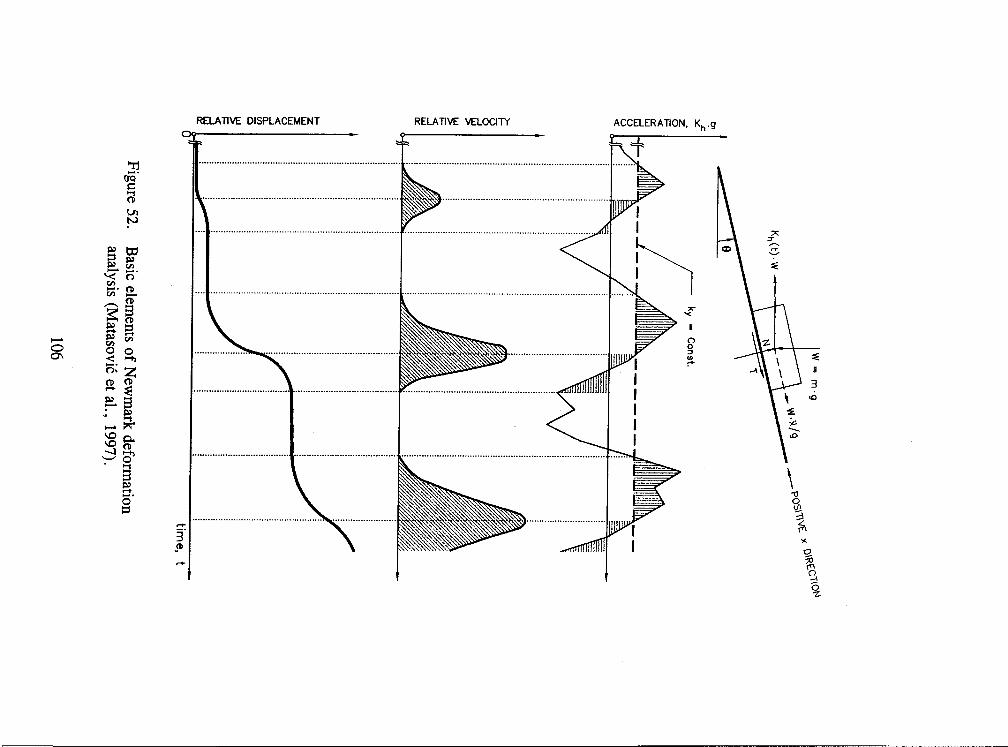
RELATIVE DISPLACEMENT RELATIVE VELOCITY ACCELERATION, Kh .g

...........................................................................

............................................................................. .................................................................

...........................................................................

............................................................................

....................................... .......................................

.......................................

.............................................................................

0 'a ....................................... ...............................

rr 3

3. (D

%

9 6- %

In using the acceleration time history from a one-dimensional site response analysis as the excitation in a Newmark sliding block analysis, the seismic response of a soil has been decoupled from its permanent seismic deformation. In other words, the influence of yielding and the accumulation of permanent seismic deformation has not been accounted for in the evaluation of the seismic response of the soil mass. Lin and Whitman (1986) have shown that this type of decoupled analysis overestimates seismic deformation by a minimum of 20 percent and by as much as a factor of 2 or 3 when the predominant period of the earthquake motion is close to the resonant period of the soil deposit. The predominant period of the earthquake motion can be determined from the acceleration response spectrum as the period at which the spectral acceleration is a maximum. Thefundamental period of the soil deposit, To, can be evaluated using equation 4-5 as To = I&.

While the residual shear strength is typically employed in practice to evaluate the yield acceleration, this common practice is another source of conservatism in permanent seismic deformation analyses. Deformations should not begin to accumulate until the seismic acceleration exceeds the yield acceleration corresponding to the peak shear strength. Furthermore, several centimeters of deformation may have to accumulate before the shear strength (and yield acceleration) fall from peak to residual values. Therefore, particularly for small calculated deformations, the use of residual shear strength to evaluate the yield acceleration for a Newmark deformation analysis can introduce considerable conservatism into the analysis.

7.4 UNIFIED METHODOLOGY FOR SEISMIC STABILITY AND DEFORMATION ANALYSIS

The seismic coefficient-factor of safety and permanent seismic deformation analysis methods for seismic slope stability may be combined into a single, unified method for evaluation of slopes and embankments. First, a seismic coefficient-factor of safety analysis is performed using a suitably conservative value for the seismic coefficient. Then, if the seismic coefficient-factor of safety analysis results in an unacceptable factor of safety, a permanent seismic deformation analysis is performed.

The "unified" seismic stability and deformation analysis is carried out using the same basic model(s) of slopes used in the static analysis. Note, however, that the critical surface with the lowest yield acceleration or pseudo-static factor of safety may be very different from the surface with the lowest static factor of safety. The following steps are carried out to perform the unified seismic slope stability and deformation analysis:

Step 1 : Reinterpret the cross-sections analyzed in the static stability analysis and assign appropriate dynamic residual strength parameters. In cases where it is not clear whether drained or undrained shear strength parameters are appropriate for the dynamic analysis, follow guidelines presented in Duncan (1992) or use a composite consolidated drained-consolidated undrained strength envelope proposed by the Corps of Engineers for pervious soils and the consolidated undrained strength envelope for silts and clays. For fully saturated or sensitive silts or clays, multiply the undrained peak shear strength by 0.8 for the analysis.

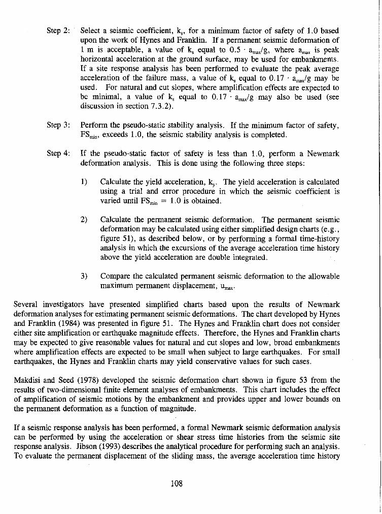
Step 2: Select a seismic coefficient, k,, for a minimum factor of safety of 1.0 based upon the work of Hynes and Franklin. If a permanent seismic deformation of 1 m is acceptable, a value of ks equal to 0.5 . a,,/g, where a,, is peak horizontal acceleration at the ground surface, may be used for embankments. If a site response analysis has been performed to evaluate the peak average acceleration of the failure mass, a value of ks equal to 0.17 . ama,/g may be used. For natural and cut slopes, where amplification effects are expected to be minimal, a value of ks equal to 0.17 . a,,/g may also be used (see discussion in section 7.3.2).

Step 3: Perform the pseudo-static stability analysis. If the minimum factor of safety, FS,,, exceeds 1 .O, the seismic stability analysis is completed.

Step 4: If the pseudo-static factor of safety is less than 1.0, perform a Newmark deformation analysis. This is done using the following three steps:

1) Calculate the yield acceleration, k,,. The yield acceleration is calculated using a trial and error procedure in which the seismic coefficient is varied until FS,, = 1.0 is obtained.

2) Calculate the permanent seismic deformation. The permanent seismic deformation may be calculated using either simplified design charts (e.g., figure 51), as described below, or by performing a formal time-history analysis in which the excursions of the average acceleration time history above the yield acceleration are double integrated.

3) Compare the calculated permanent seismic deformation to the allowable maximum permanent displacement, u,,.

Several investigators have presented simplified charts based upon the results of Newmark deformation analyses for estimating permanent seismic deformations. The chart developed by Hynes and Franklin (1984) was presented in figure 51. The Hynes and Franklin chart does not consider either site amplification or earthquake magnitude effects. Therefore, the Hynes and Franklin charts may be expected to give reasonable values for natural and cut slopes and low, broad embankments where amplification effects are expected to be small when subject to large earthquakes. For small earthquakes, the Hynes and Franklin charts may yield conservative values for such cases.

Makdisi and Seed (1978) developed the seismic deformation chart shown in figure 53 from the results of two-dimensional finite element analyses of embankments. This chart includes the effect of amplification of seismic motions by the embankment and provides upper and lower bounds on the permanent deformation as a function of magnitude.

If a seismic response analysis has been performed, a formal Newmark seismic deformation analysis can be performed by using the acceleration or shear stress time histories from the seismic site response analysis. Jibson (1993) describes the analytical procedure for performing such an analysis. To evaluate the permanent displacement of the sliding mass, the average acceleration time history

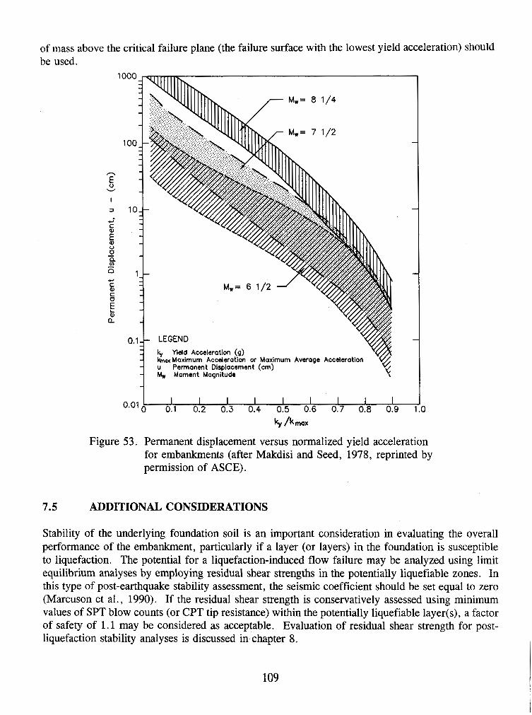
of mass above the critical failure plane (the failure surface with the lowest yield acceleration) should be used.

ky Yidd Acceleration (g) kmax Maximum Acceleration or Maximum Average Acceleration u Permanent Displacement (cm) M, Moment Magnitude

Figure 53. Permanent displacement versus normalized yield acceleration for embankments (after Makdisi and Seed, 1978, reprinted by permission of ASCE).

7.5 ADDITIONAL CONSIDERATIONS

Stability of the underlying foundation soil is an important consideration in evaluating the overall performance of the embankment, particularly if a layer (or layers) in the foundation is susceptible to liquefaction. The potential for a liquefaction-induced flow failure may be analyzed using limit equilibrium analyses by employing residual shear strengths in the potentially liquefiable zones. In this type of post-earthquake stability assessment, the seismic coefficient should be set equal to zero (Marcuson et al., 1990). If the residual shear strength is conservatively assessed using minimum values of SPT blow counts (or CPT tip resistance) within the potentially liquefiable layer(s), a factor of safety of 1.1 may be considered as acceptable. Evaluation of residual shear strength for post- liquefaction stability analyses is discussed in chapter 8.

CHAPTER 8

LIQUEFACTION AND SEISMIC SETTLEMENT

8.1 INTRODUCTION

During strong earthquake shaking, loose, saturated cohesionless soil deposits may experience a sudden loss of strength and stiffness, sometimes resulting in loss of bearing capacity, large permanent lateral displacements, and/or seismic settlement of the ground. This phenomenon is called soil liquefaction. In the absence of saturated or near-saturation conditions, strong earthquake shaking can induce compaction and settlement of the ground. This phenomenon is called seismic settlement.

Liquefaction and/or seismic settlement beneath and in the vicinity of highway facilities can have severe consequences with respect to facility integrity. Localized bearing capacity failures, lateral spreading, and excessive settlements resulting from liquefaction may damage bridges, embankments, and other highway structures. Liquefaction-associated lateral spreading and flow failures and seismically-induced settlement can also affect the overall stability of the roadway. Similarly, excessive total or differential settlement can impact the integrity and/or serviceability of highway facilities. Therefore, a liquefaction and seismic settlement potential assessment is a key element in the seismic design of highways.

This section outlines the current state-of-the-practice for evaluation of the potential for, and the consequences of (should it occur), soil liquefaction and seismic settlement as they apply to the seismic design of highways. Initial screening criteria to determine whether or not a liquefaction analysis is needed for a particular project are presented in section 8.2. The simplified procedure for liquefaction potential assessment commonly used in engineering practice is presented in section 8.3. Methods for performing a liquefaction impact assessment, i.e., to estimate post- liquefaction deformation and stability, are presented in section 8.4. The simplified procedures for seismic settlement of unsaturated sand evaluation commonly used in engineering practice are presented in section 8.5. Methods for mitigation of liquefaction and seismic settlement potential and of the consequences of liquefaction are discussed in section 8.6. Advanced methods for liquefaction potential assessments, including one- and two-dimensional fully-coupled effective stress site response analyses, are briefly discussed in section 8.3.

8.2 FACTORS AFFECTING LIQUEFACTION SUSCEPTIBILITY

The first step in any liquefaction evaluation is to assess whether the potential for liquefaction exists at the site. A variety of screening techniques exist to distinguish sites that are clearly safe with respect to liquefaction from those sites that require more detailed study (e.g., Dobry et al., 1980). The following five screening criteria are most commonly used to make this assessment:

Geologic age and origin. Liquefaction potential decreases with increasing age of a soil deposit. Pre-Holocene age soil deposits generally do not liquefy, though liquefaction has occasionally been observed in Pleistocene-age deposits. Table 7 presents the liquefaction susceptibility of soil deposits as a function of age and origin (Youd and Perkins, 1978).

Fines content and plasticity index. Liquefaction potential decreases with increasing fines content and increasing plasticity index, PI. Data presented in figure 54 (Ishihara et al., 1989) show grain size distribution curves of soils known to have liquefied in the past. This data serves as a rough guide for liquefaction potential assessment of cohesionless soils. Soils having greater than 15 percent (by weight) finer than 0.005 mm, a liquid limit greater than 35 percent, and an in-situ water content less than 0.9 times the liquid limit generally do not liquefy (Seed and Idriss, 1982).

Saturation. Although unsaturated soils have been reported to liquefy, at least 80 to 85 percent saturation is generally deemed to be a necessary condition for soil liquefaction. In many locations, the water table is subject to seasonal oscillation. In general, it is prudent that the highest anticipated seasonal water table elevation be considered for initial screening.

Depth below ground su@ace. While failures due to liquefaction of end-bearing piles resting on sand layers up to 30 m below the ground surface have been reported, shallow foundations are generally not affected if liquefaction occurs more than 15 m below the ground surface.

Soil penetration resistance. According to the data presented in Seed and Idriss (1982), liquefaction has not been observed in soil deposits having normalized Standard Penetration Test (SPT) blow counts, (N,) , larger than 22. Marcuson, et al. (1990) suggest a normalized SPT value of 30 as the threshold value above which liquefaction will not occur. However, Chinese experience, as quoted in Seed et al. (1983), suggests that in extreme conditions liquefaction is possible in soils having normalized SPT blow counts as high as 40. Shibata and Teparaska (1988), based on a large number of observations, conclude that no liquefaction is possible if normalized Cone Penetration Test (CPT) cone resistance, q,,, is larger than 15 MPa. This CPT resistance corresponds to normalized SPT blow counts between 30 and 60, depending on the grain size of the soil (see figure 55).

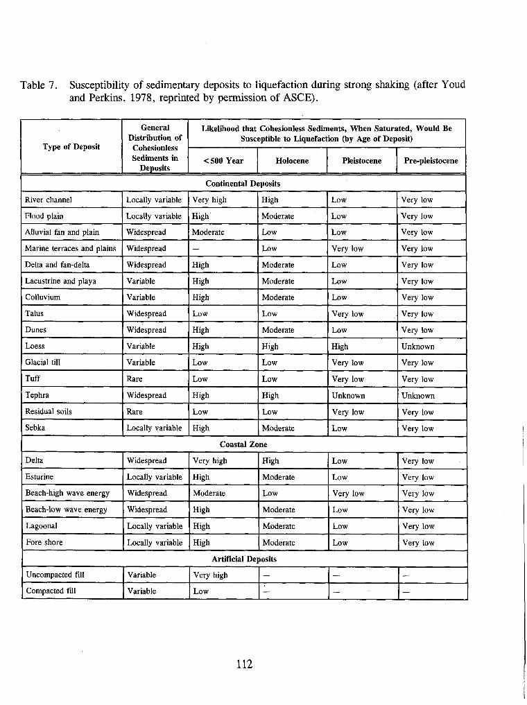
Table 7. Susceptibility of sedimentary deposits to liquefaction during strong shaking (after Youd and Perkins, 1978, reprinted by permission of ASCE) .

-

Type of Deposit

General Distribution of Cohesionless Sediments in

Deposits

Likelihood that Cohesionless Sediments, When Saturated, Would Be Susceptible to Liquefaction (by Age of Deposit)

River channel

Flood plain

Alluvial fan and plain

Marine terraces and plains

Delta and fan-delta

Lacustrine and playa

Colluvium

Talus

Dunes

Loess

Glacial till

Tuff

Tephra

Residual soils

Sebka

<500 Year

Locally variable

Locally variable

Widespread

Widespread

Widespread

Variable

Variable

Widespread

Widespread

Variable

Variable

Rare

Widespread

Rare

Locally variable

Continental

Very high

High

Moderate

-

High

High

High

Low

High

High

Low

Low

High

Low

High

Coastal

Delta

Esturine

Beach-high wave energy

Beach-low wave energy

Lagoonal

Fore shore

Holocene

Deposits

High

Moderate

Low

Low

Moderate

Moderate

Moderate

Low

Moderate

High

Low

Low

High

Low

Moderate

Zone

Low

Low

Low

Very low

Low

Low

Low

Very low

Low

High

Very low

Very low

Unknown

Very low

Low

Very low

Very low

Very low

Very low

Very low

Very low

Very low

Very low

Very low

Unknown

Very low

Very low

Unknown

Very low

Very low

Widespread

Locally variable

Widespread

Widespread

Locally variable

Locally variable

Pleistocene

Artificial Deposits

Pre-pleistocene

Very high

High

Moderate

High

High

High

Uncompacted fill

Compacted fill

High

Moderate

Low

Moderate

Moderate

Moderate

Variable

Variable

Very high

Low

Low

Low

Very low

Low

Low

Low

-

-

Very low

Very low

Very low

Very low

Very low

Very low

-

-

-

-

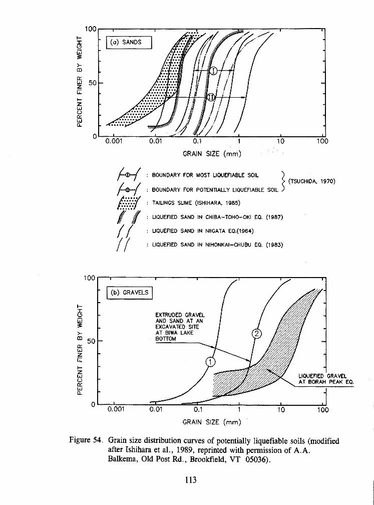
GRAIN SlZE (mm)

: BOUNDARY FOR MOST LIQUEFIABLE SOIL (TSUCHIDA, 1970)

: BOUNDARY FOR POTENTIALLY LIQUEFIABLE SOIL

f i : TAILINCs SLIME (ISHIHARA. 1985)

* : LIQUEFIED SAND IN CHIBA-TOHO-OK1 EQ. (1987)

l l : LIQUEFIED SAND IN NllGATA EQ.(1964)

/ / : LlQUEflED SAND IN NIHONKAI-CHUBU EQ. (1983)

1 00 I

- -

I- I - EXTRUDED GRAVEL 8 AND SAND AT AN - EXCAVATED SITE

AT Bl WA LAKE >- a 50- LT W z - iZ I- - Z W 0 - LIQUEFIED GRAVEL LT AT BORAH PEAK EQ. W a - -

O o.bo1 0.01 0.1 1 10 100

GRAIN SlZE (mm)

Figure 54. Grain size distribution curves of potentially liquefiable soils (modified after Ishihara et al., 1989, reprinted with permission of A.A. Balkema, Old Post Rd., Brookfield, VT 05036).

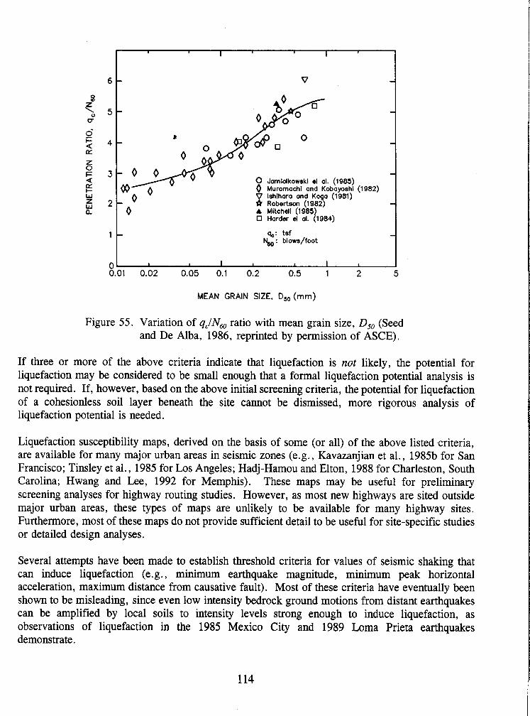
'I-

0

0 Jamldkowskl el al. (1985)

0 0 Muromachi and Kobayoshl lshlhara and KO a (1981) X Robertson (1984

A Mitchell (1985) Harder d al. (1984)

q,: tsf N,,,, : blows/foot

Figure 55. Variation of q,lN,, ratio with mean grain size, D,, (Seed and De Alba, 1986, reprinted by permission of ASCE).

If three or more of the above criteria indicate that liquefaction is not likely, the potential for liquefaction may be considered to be small enough that a formal liquefaction potential analysis is not required. If, however, based on the above initial screening criteria, the potential for liquefaction of a cohesionless soil layer beneath the site cannot be dismissed, more rigorous analysis of liquefaction potential is needed.

Liquefaction susceptibility maps, derived on the basis of some (or all) of the above listed criteria, are available for many major urban areas in seismic zones (e. g . , Kavazanjian et al., 1985b for San Francisco; Tinsley et al., 1985 for Los Angeles; Hadj-Hamou and Elton, 1988 for Charleston, South Carolina; Hwang and Lee, 1992 for Memphis). These maps may be useful for preliminary screening analyses for highway routing studies. However, as most new highways are sited outside major urban areas, these types of maps are unlikely to be available for many highway sites. Furthermore, most of these maps do not provide sufficient detail to be useful for site-specific studies or detailed design analyses.

Several attempts have been made to establish threshold criteria for values of seismic shaking that can induce liquefaction (e. g . , minimum earthquake magnitude, minimum peak horizontal acceleration, maximum distance from causative fault). Most of these criteria have eventually been shown to be misleading, since even low intensity bedrock ground motions from distant earthquakes can be amplified by local soils to intensity levels strong enough to induce liquefaction, as observations of liquefaction in the 1985 Mexico City and 1989 Lorna Prieta earthquakes demonstrate.

Most soil deposits known to have liquefied are sand deposits. However, as indicated on figure 54b, some deposits containing gravel particles (> 2 rnrn size) in a fine grained soil matrix may be susceptible to liquefaction. Discussion of the liquefaction potential of gravel deposits is beyond the scope of this document. The reader is referred to Ishihara (1985), Harder (1988), and Stark and Olson (1995) for a discussion of methods for evaluation of the liquefaction potential of gravels.

8.3 EVALUATION OF LIQUEFACTION POTENTIAL

Due to the difficulties in obtaining and testing undisturbed representative samples from most potentially liquefiable soil materials, in situ testing is the approach preferred by most engineers for evaluating the liquefaction potential of a soil deposit. Liquefaction potential assessment procedures involving both the SPT and CPT are widely used in practice (e.g., Seed and Idriss, 1982; Ishihara, 1985; Seed and De Alba, 1986; Shibata and Teparaska, 1988; Stark and Olson, 1995). For gravelly soils, the Becker Penetration Test (BPT) is commonly used to evaluate liquefac'tion potential (Harder and Seed, 1986). Geophysical techniques for measuring shear wave velocity, including non- intrusive spectral analysis of surface waves (SASW), have emerged as potential alternatives to the BPT for liquefaction potential assessment in gravels (Tokimatsu, et al., 1991), but still lack an adequate direct correlation with liquefaction potential.

The most common procedure used in engineering practice for the liquefaction potential assessment of sands and silts is the Simplified Procedure originally developed by Seed and Idriss (1982). Since its original development, the original Simplified Procedure as proposed by Seed and Idriss has been progressively revised, extended, and refined (Seed et al., 1983; Seed et al., 1985; Seed and De Alba, 1986; Liao and Whitman, 1986). The Simplified Procedure may be used with either SPT or CPT data. Recent summaries of the various revisions to the Simplified Procedure are provided by Marcuson et al., (1990) and Seed and Harder (1990). Based primarily on recommendations from these two studies, the Simplified Procedure for evaluating liquefaction potential at the site of highway facilities can be performed using the following steps:

Step 1: From borings and soundings, in situ testing and laboratory index tests, develop a detailed understanding of the project site subsurface conditions, including stratigraphy, layer geometry, material properties and their variability, and the areal extent of potential problem zones. Establish the zones to be analyzed and develop idealized, representative sections amenable to analysis. The subsurface data used to develop the representative sections should include the location of the water table, either SPT blow count, N, or tip resistance of a standard CPT cone, q,, mean grain size, D,,, unit weight, and the percentage of fines in the soil (percent by weight passing the U.S. Standard No. 200 sieve).

Step 2: Evaluate the total vertical stress, a,, and effective vertical stress, a,', for all potentially liquefiable layers within the deposit both at the time of exploration and for design. Vertical and shear stress design values should include the stresses resulting from facility construction. Exploration and design values for vertical total and effective stress may be the same or may differ due to seasonal fluctuations in the water table or changes in local hydrology resulting from

project development. Also evaluate the initial static shear stress on the horizontal plane, T,,, for design.

Step 3: If results of a site response analysis are not available, evaluate the stress reduction factor, rd as described below. The stress reduction factor is a soil flexibility factor defined as the ratio of the peak shear stress for the soil column, (T,,)~, to that of a rigid body, (T,,,),. There are several ways to obtain rd. For depths less than 12 m, the average value from figure 56 (Seed and Idriss, 1982) is commonly used. Alternatively, the following equation proposed by Iwasaki et al. (1978) can be used:

where z is the depth below the ground surface in meters.

If results of a site response analysis (see chapter 6) are available, evaluation of rd is not needed since the maximum earthquake-induced shear stress at depth z, T,,, is directly calculated in the analysis. However, it may still be convenient to calculate rd from the site response results for use in spreadsheet calculations using the following equation:

where a, is the total shear stress at depth z, a,,, is the peak ground surface acceleration, and g is the acceleration of gravity. The parameters a, and a,,, are also directly calculated by most site response computer programs described in chapter 6.

Use of T,, from site response analysis (or use of the results of a site response analysis to evaluate rd) is considered to be generally more reliable than any of the simplified approaches to estimate rd, and is strongly recommended for sites that are marginal with respect to liquefaction potential (i.e., sites where the factor of safety for liquefaction is close to 1.0).

Step 4: Calculate the critical stress ratio induced by the design earthquake, CSREp as:

If the results of a seismic site response analysis are available, CSREQ can be evaluated from r,,, as:

Note that the ratio r,,,lo,' corresponds to the peak average acceleration denoted by k,,,,, in chapter 6.

STRESS REDUCTlON FACTOR, r,

0

2

4

6

8

10

12

14

l6

l8

20

22

24

26

28

30 0

Figure 56. Stress reduction factor, r, (modified after Seed and Idriss, 1982, reprinted by permission of EERI).

I I - - - -

Seed and ldriss -

- -

- Seed and ldriss Range for Different

- Soil Profiles -

- - - - -

I I - 0.1 0.2 0.3 0.4 0.5 0.6 0.7 0.8 0.9 1.0

Step 5: Evaluate the standardized SPT blow count, N, which is the standard penetration test blow count for a hammer with an efficiency of 60 percent (60 percent of the nominal SPT energy is delivered to the drill rod). The "standardized" equipment corresponding to an efficiency of 60 percent is specified in table 8. If nonstandard equipment is used, N,, is obtained from the equation:

where C, is the product of various correction factors. Correction factors recommended by various investigators for some common non-standard SPT configurations are provided in table 9 (Richardson et al., 1995). Alternatively, if CPT data are used, N, can be obtained from the chart relating N, to q, and D,, presented in figure 55 (Seed and De Alba, 1986).

Table 8. Recommended "standardized" SPT equipment (after Seed et al., 1985 and Riggs, 1986, reprinted by permission of ASCE).

Notes: (') If the equipment meets the above specifications, N = N , and only a correction for overburden is needed.

(2) This specification is essentially the same to the ASTM D 1586 standard.

Element

Sampler

Drill Rods

Hammer

Rope

Borehole

Drill Bit

Blow Count Rate

Penetration Resistance Count

Standard Specification

Standard split-spoon sampler with: (a) Outside Diameter, O.D. = 51 mm, and (b) Inside Diameter, I.D. = 35 mm (constant - i.e., no room for liners in the barrel)

A or AW-type for depths less than 15.2 m; N- or NW-type for greater depths

Standard (safety) hammer with: (a) weight = 63.5 kg; (b) drop = 762 mrn (delivers 60% of theoretical free fall energy)

Two wraps of rope around the pulley

100- to 130-mm diameter rotary borehole with bentonite mud for borehole stability (hollow stem augers where SPT is taken through the stem)

Upward deflection of drilling mud (tricone or baffled drag bit)

30 to 40 blows per minute

Measured over range of 150 to 460 rnrn of penetration into the ground

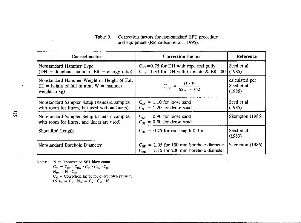
Table 9. Correction factors for nonstandard SPT procedure and equipment (Richardson et al., 1995).

= height of fall in mrn; W = hammer

Notes: N = Uncorrected SPT blow count. C, = C, .C, .css 'C,, .C,, N, = N . C , C, = Correction factor for overburden pressure. (N,), = C, . N, = C, - C, N

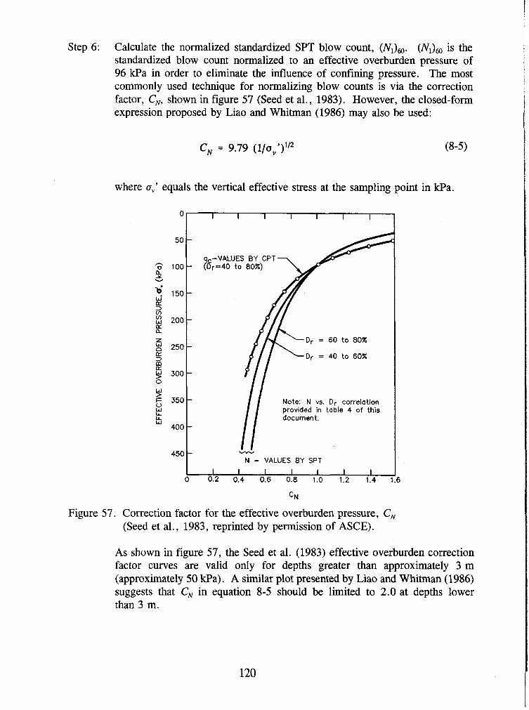
Step 6: Calculate the normalized standardized SPT blow count, (N,),. (N,), is the standardized blow count normalized to an effective overburden pressure of 96 kPa in order to eliminate the influence of confining pressure. The most commonly used technique for normalizing blow counts is via the correction factor, C,, shown in figure 57 (Seed et al., 1983). However, the closed-form expression proposed by Liao and Whitman (1986) may also be used:

where a,' equals the vertical effective stress at the sampling point in kPa.

Dr = 60 to 80%

Dr = 40 to 60%

Note: N vs. Dr correlation provided in table 4 of this

N - VALUES BY SPT I

Figure 57. Correction factor for the effective overburden pressure, CN (Seed et al., 1983, reprinted by permission of ASCE).

As shown in figure 57, the Seed et al. (1983) effective overburden correction factor curves are valid only for depths greater than approximately 3 m (approximately 50 kPa). A similar plot presented by Liao and Whitman (1986) suggests that CN in equation 8-5 should be limited to 2.0 at depths lower than 3 m.

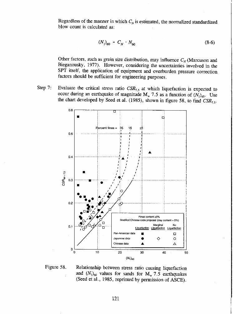
Regardless of the manner in which CN is estimated, the normalized standardized blow count is calculated as:

Other factors, such as grain size distribution, may influence CN (Marcuson and Bieganousky , 1977). However, considering the uncertainties involved in the SPT itself, the application of equipment and overburden pressure correction factors should be sufficient for engineering purposes.

Step 7: Evaluate the critical stress ratio CSR, , at which liquefaction is expected to occur during an earthquake of magnitude M, 7.5 as a function of (N,),. Use the chart developed by Seed et al. (1985), shown in figure 58, to find CSRT5.

Figure 58. Relationship between stress ratio causing liquefaction and (N,), values for sands for M, 7.5 earthquakes (Seed et al., 1985, reprinted by permission of ASCE).

50

........................... ........ ............................ i1.. I .............. ! ............................ ; I jl I i il I l j il I 1 ; $ 1 1; i 1 1 ; A I 1 1 ; li I ................................................................................. .........................................................

I ; A 1 I ; 1 ; I I j 1 ; I

1 : I ; I ;

1 ; / ........................................... ..... .......,....

........... ; -.- ....................................

( Nl 160

Fines content 25% Modified Chinese code proposal (clay content = 5%)

Marginal No Liquefaction Liquefaction Liquefaction

Pan-American data . Japanese data 0 0 Chinese data A A

'

0 10 20 30 40

Step 8: If needed, calculate the corrected critical stress ratio resisting liquefaction, CSRL. CSRL is calculated as:

where k, is the correction factor for earthquake magnitudes other than 7.5, k, is the correction factor for stress levels larger than 96 kPa, and k, is the correction factor for the initial driving static shear stress, T,,. The value k, can be obtained from chart presented on figure 59, developed by interpolation of tabular data presented by Seed et al. (1983). Recently, Arango (1996) presented an alternative chart for evaluation of k, which is based on energy principles. For a, larger than 96 kPa, k, can be determined from figure 60 (Harder, 1988; Hynes, 1988). The value of k, depends on both T,, and the relative density of the soil, Dr. On sloping ground, or below structures and embankments, T,, can be estimated using various closed-form elastic solutions (e.g., Poulos and Davis, 1974 see example 5 of volume 11) or using the results of finite element (static) analyses. Once T,, and a,,' are estimated, k, can be determined from figure 61, originally proposed by Seed (1983) and modified by Harder (1988) and Hynes (1988).

Step 9: Calculate the factor of safety against initial liquefaction, FSL, as:

There is no general agreement on the appropriate minimum factor of safety against liquefaction (NRC, 1985). There are cases where liquefaction-induced instability has occurred prior to complete liquefaction, i.e., with a factor of safety against initial liquefaction greater than 1.0. However, when the design ground motion is extreme or conservative, most engineers are satisfied with a factor of safety against initial liquefaction, FSL, greater than or equal to 1.0.

It should be noted that the Simplified Procedure is aimed primarily at moderately strong ground motions (0.2 g < a,,, < 0.5 g). If the peak horizontal acceleration is larger than 0.5 g, more sophisticated, truly non-linear effective stress-based analytical approaches may be advisable. Computer programs for evaluation of liquefaction potential as a part of a site response analysis include the one-dimensional response analysis computer program DESRA-2 (Lee and Finn, 1978) and its derivative codes MARDES (Chang et al., 1991), D-MOD (MatasoviC, 1993), and SUMDES (Li et al., 1992) as well as two-dimensional codes such as DYNAFLOW (Prevost, 1981), TARA-3 (Finn et al., 1986), LINOS (Bardet, 1992), DYSAC2 (Muraleetharan et al., 1991), and certain adaptations of FLAC (Cundall and Board, 1988) (e.g., Roth and Inel, 1993). These computer programs are briefly discussed in chapter 6.

An example of a liquefaction analysis performed using the Simplified Procedure is presented in volume I1 of this document.

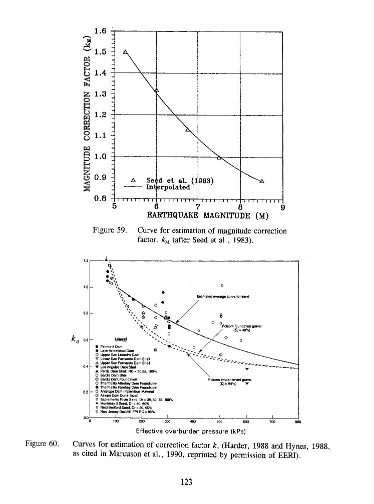
Figure 59. Curve for estimation of magnitude correction factor, k, (after Seed et al., 1983).

Figure 60. Curves for estimation of correction factor k, (Harder, 1988 and Hynes, 1988, as cited in Marcuson et al., 1990, reprinted by permission of EERI).

1.2

1.0

0.8

0.6

0.4

0.2

0.0 '

A, 9 ,,I

*d .%'I - I\ 0

-

Folsom loundation gravel

- Fainont Dam Lake Arrowhead Dam

0 Upper San Leandro Dam V Lower San Fernando Dam Shell A Upper San Fernando Dam Shell

- V Los Angeles Dam Shell A Perris Dam Shell. RC = 90.95. 100%

Sardis Dam Shell 0 Sardis Dam Foundation Folsom embankmenl gravel 0 Thanallto Aherbay Dam Foundalion (4- 64%) V

Thenalito Forebay Dam Foundation - El Antelope Dam Impewbus Material Aswan Dam hrne Sand

0 Sacramenlo River Sand. Dr - 38,60, 78. 100% Monterey 0 Sand. Dr = 40. wx

0 Reld Bedford Sand. Dr = 40. BO% 0 New Jersey Backfill, FPI RC - 95%

1 I I I I 100

I 200

I 300 400 500 600 700 800

Effective overburden pressure (kPa)

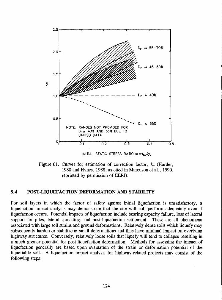
NOTE: RANGES NOT PROVIDED FOR D r w 40% AND 35% DUE TO LIMITED DATA

INITIAL STATIC STRESS RATIO, a

Figure 61. Curves for estimation of correction factor, k, (Harder, 1988 and Hynes, 1988, as cited in Marcuson et al., 1990, reprinted by permission of EERI).

8.4 POST-LIQUEFACTION DEFORMATION AND STABILITY

For soil layers in which the factor of safety against initial liquefaction is unsatisfactory, a liquefaction impact analysis may demonstrate that the site will still perform adequately even if liquefaction occurs. Potential impacts of liquefaction include bearing capacity failure, loss of lateral support for piles, lateral spreading, and post-liquefaction settlement. These are all phenomena associated with large soil strains and ground deformations. Relatively dense soils which liquefy may subsequently harden or stabilize at small deformations and thus have minimal impact on overlying highway structures. Conversely, relatively loose soils that liquefy will tend to collapse resulting in a much greater potential for post-liquefaction deformation. Methods for assessing the impact of liquefaction generally are based upon evaluation of the strain or deformation potential of the liquefiable soil. A liquefaction impact analysis for highway-related projects may consist of the following steps:

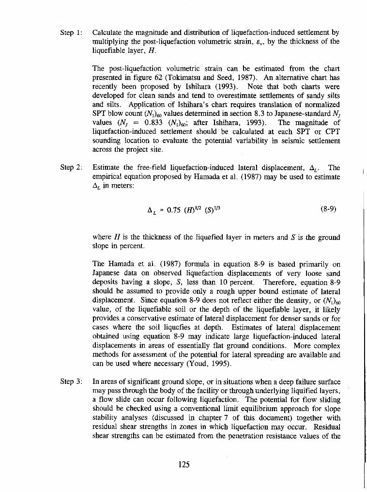
Step 1 : Calculate the magnitude and distribution of liquefaction-induced settlement by multiplying the post-liquefaction volumetric strain, E,, by the thickness of the liquefiable layer, H.

The post-liquefaction volumetric strain can be estimated from the chart presented in figure 62 (Tokimatsu and Seed, 1987). An alternative chart has recently been proposed by Ishihara (1993). Note that both charts were developed for clean sands and tend to overestimate settlements of sandy silts and silts. Application of Ishihara's chart requires translation of normalized SPT blow count (N,), values determined in section 8.3 to Japanese-standard Nj values (Nj = 0.833 (N,),; after Ishihara, 1993). The magnitude of liquefaction-induced settlement should be calculated at each SPT or CPT sounding location to evaluate the potential variability in seismic settlement across the project site.

Step 2: Estimate the free-field liquefaction-induced lateral displacement, A The empirical equation proposed by Hamada et al. (1987) may be used to estimate A, in meters:

where H is the thickness of the liquefied layer in meters and S is the ground slope in percent.

The Hamada et al. (1987) formula in equation 8-9 is based primarily on Japanese data on observed liquefaction displacements of very loose sand deposits having a slope, S, less than 10 percent. Therefore, equation 8-9 should be assumed to provide only a rough upper bound estimate of lateral displacement. Since equation 8-9 does not reflect either the density, or (N,), value, of the liquefiable soil or the depth of the liquefiable layer, it likely provides a conservative estimate of lateral displacement for denser sands or for cases where the soil liquefies at depth. Estimates of lateral displacement obtained using equation 8-9 may indicate large liquefaction-induced lateral displacements in areas of essentially flat ground conditions. More complex methods for assessment of the potential for lateral spreading are available and can be used where necessary (Youd, 1995).

Step 3: In areas of significant ground slope, or in situations when a deep failure surface may pass through the body of the facility or through underlying liquified layers, a flow slide can occur following liquefaction. The potential for flow sliding should be checked using a conventional limit equilibrium approach for slope stability analyses (discussed in chapter 7 of this document) together with residual shear strengths in zones in which liquefaction may occur. Residual shear strengths can be estimated from the penetration resistance values of the

soil using the chart proposed by Seed et al. (1988) presented in figure 44. Seed and Harder (1990) and Marcuson et al. (1990) present further guidance for performing a post-liquefaction stability assessment using residual shear strengths.

If liquefaction-induced vertical and/or lateral deformations are large, the integrity of the a highway facility may be compromised. The question the engineer must answer is "What magnitude of deformation is too large?" The magnitude of acceptable deformation should be established by the design engineer on a case-by-case basis. Calculated seismic deformations on the order of 0.15 to 0.30 m are generally deemed to be acceptable in current practice for highway embankments in California. For highway system components other than embankments, engineering judgement must be used in determining the allowable level of calculated seismic deformation. For example, components that are designed to be unyielding, such as bridge abutments restrained by batter piles, may have more restrictive deformation requirements than structures which can more easily accommodate foundation deformations. At the current time, determination of allowable deformations remains a subject requiring considerable engineering judgement.

Figure 62. Curves for estimation of post-liquefaction volumetric strain using SPT data and cyclic stress ratio for M, 7.5 earthquakes (Tokimatsu and Seed, 1987, reprinted by permission of ASCE).

1 I I i Volumetric strain (O/O)

1054 3 2 1 0.5

T I I -

-

:0.2 - . . .

- -

-

-

I

8.5 SEISMIC SETTLEMENT EVALUATION

Both unsaturated and saturated sands tend to settle and densify when subjected to earthquake shaking. If the sand is saturated and there is no possibility for drainage, so that constant volume conditions are maintained, the primary initial effect of the shaking is the generation of excess pore water pressures. Settlement then occurs as the excess pore pressures dissipate. In unsaturated sands, on the other hand, settlement may occur during the earthquake shaking under conditions of constant effective vertical stress (depending on the degree of saturation). In both cases (saturated and unsaturated soil), however, one result of strong ground shaking is settlement of the soil.

Liquefaction-induced settlement of saturated sand is addressed as part of a post-liquefaction deformation and stability assessment as described in section 8.4 of this chapter. A procedure for evaluating the seismic settlement of unsaturated sand, following the general procedure presented in Tokimatsu and Seed (1987), is outlined below.

Seismic settlement analysis of unsaturated sand can be performed using the following steps:

Step 1: From borings and soundings, in situ testing and laboratory index tests, develop a detailed understanding of the project site subsurface conditions, including stratigraphy, layer geometry, material properties and their variability, and the areal extent of potential problem zones. Establish the zones to be analyzed and develop idealized, representative sections amenable to analysis. The subsurface data used to develop the representative sections should include normalized standardized SPT blow counts, (N,), (or results of some other test, e.g., the CPT from which (N,), can be inferred) and the unit weight of the soil.

Step 2: Evaluate the total vertical stress, u,, and the mean normal total stress, u, = 0.65 a,, at several layers within the deposit at the time of exploration and for design. The design values should include stresses resulting from highway facility construction. Outside of the highway facility footprint, the exploration and design values are generally the same.

Step 3: Evaluate the stress reduction factor, rd, using one of the approaches presented in step 3 of section 8.3 of this chapter.

Step 4: Evaluate y, (G, IG,,,) using the Tokimatsu and Seed (1987) equation:

ref (G, Gmax) = (0.65 . a,,, . U, . rd)l(g . G,,,) (8- 10)

where y e , (Ge,Gm,) is a hypothetical egective shear stress factor, a,,, is the peak ground surface acceleration, g is the acceleration of gravity, and G,,,, is the shear modulus of the soil at small strain. Note that G,,, = p . Vs2, where Vs is the shear wave velocity and p is the mass density of the soil.

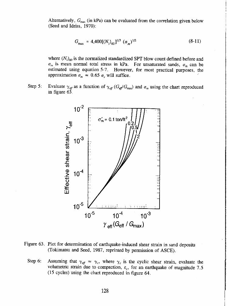
Alternatively, Gmax (in kPa) can be evaluated from the correlation given below (Seed and Idriss, 1970):

where (N,) , is the normalized standardized SPT blow count defined before and a,, is mean normal total stress in kPa. For unsaturated sands, a, can be estimated using equation 5-7. However, for most practical purposes, the approximation a, = 0.65 a,, will suffice. /

Step 5: Evaluate y,, as a function of yeff (GdG,,,) and a,, using the chart reproduced in figure 63.

1 o - ~ 1 o - ~ 1 o - ~ Y en (Get I Gmax

Figure 63. Plot for determination of earthquake-induced shear strain in sand deposits (Tokimatsu and Seed, 1987, reprinted by permission of ASCE).

Step 6: Assuming that y,, = y,, where y, is the cyclic shear strain, evaluate the volumetric strain due to compaction, E,, for an earthquake of magnitude 7.5 (15 cycles) using the chart reproduced in figure 64.

Step 7: Correct for earthquake (moment) magnitude other than M, 7.5 using the correction factors reproduced in table 10.

Step 8: Multiply the volumetric strain due to compaction for each layer by two to correct for the multidirectional shaking effect, as recommended by Tokimatsu and Seed (1987), to get the representative volumetric strain for each layer.

Step 9: Calculate seismic settlements of each layer by multiplying the layer thickness by the representative volumetric strain evaluated in step 8. Sum up the layer settlements to obtain the total seismic settlement for the analyzed profile.

h \o

Cyclic shear strain, y, (%)

Figure 64. Relationship between volumetric strain, cyclic shear strain, and penetration resistance for unsaturated sands (Tokimatsu and Seed, 1987, reprinted by permission of ASCE).

Considerable judgement is required when evaluating the performance of a highway facility based on an estimate of seismic settlement. The magnitude of calculated seismic settlement should be considered primarily as an indication of whether settlements are relatively small (several centimeters)

or relatively large (several meters). A more precise evaluation of seismic settlement is not within the capabilities of conventional engineering analyses using the simplified methods presented herein.

Table 10. Influence of earthquake magnitude on volumetric strain ratio for dry sands (after Tokimatsu and Seed, 1987, reprinted by permission of ASCE).

8.6 LIQUEFACTION MITIGATION

Earthquake Magnitude

8.5

7.5

6.75

6

5.25

If the seismic impact analyses presented in sections 8.4 and 8.5 yield unacceptable deformations, consideration may be given to performing a more sophisticated liquefaction potential assessment and to evaluation of liquefaction potential mitigation measures. Generally, the engineer has the following options: (1) proceed with a more advanced analysis technique; (2) design the facility to resist the anticipated deformations; (3) remediate the site to reduce the anticipated deformations to acceptable levels; or (4) choose an alternative site. If a more advanced analysis still indicates unacceptable impacts from liquefaction, the engineer must still consider options (2) through (4). These options may require additional subsurface investigation, advanced laboratory testing, more sophisticated numerical modeling, and, in rare cases, physical modeling. Discussion of these techniques is beyond the scope of this document.

Options that may be considered when desiging to resist anticipated deformation include the use of ductile pile foundations, reinforced earth, structural walls, or buttress fills keyed into non-liquefiable strata to resist the effects of lateral spreading. These techniques are described in detail elsewhere (e.g., Kramer and Holtz, 1991).

Number of Representative Cycles at 0.65 T,,,

26

15

10

5

2-3

A variety of techniques exist to remediate potentially liquefiable soils and mitigate the liquefaction hazard. Table 11 presents a summary of methods for improvement of liquefiable soil foundation conditions (NRC, 1985). The cost of foundation improvement can vary over an order of magnitude, depending on site conditions (e.g., adjacent sensitive structures) and the nature and geometry of the liquefiable soils. Remediation costs can vary from as low as several thousand dollars per acre for dynamic compaction of shallow layers of clean sands in open areas to upwards of $100,000 per acre for deep layers of silty soils adjacent to sensitive structures. Liquefaction remediation measures must be evaluated on a case-by-case basis to determine their economic viability.

Volumetric Strain Ratio &c,N/&c,N' 15

1.25

1 .O

0.85

0.6

0.4

Table 11: Improvement techniques for liquefiable soil foundation conditions (after NRC, 1985)

SP, SW, or SM soils which have average relative density equal to or greater than 85 percent and the minimum relative density not less than 80 percent are in general not susceptible to liquefaction (TM 5-818-1). D'Appolonia (1970) stated that for soil w i ~ m the zone of infhmce and umiinement of the structure faudation, the relative density should not be less rhan 70 percent. Therefore, a criterion may be used that relative density increase into the 70-90 percent range is in general considered to prevent liquefaction. These properdes of treated materials and applications occur only under ideal conditions of soil, moisture, and method application. The methods and properties achieved are not applicable a d will not occur in all soils.

Method

(I) Blasting

(2) Vibratory Probe (a) Terraprobe (b) Vibro-Rods (c) Vibro-Wig

(3) Vibr-Compaction (a) Vibroflot (b) VibreCnmpozer

System (c) Sod Vibratory stabilizing method

(4) Compactb Soils

" Applications and results of the improvement methods are dependent on: (a) soil profdes, types, and editions, (b) site conditions, (c) earthquake loading, (d) structure type and condition, and (e) material and equipment availability. Combitions of the memods will most likely provide the best and most stable solution.

Site conditinns have been classified into three cases; Case 1 is for beneath strucmres, Case 2 is for the not-under-water free field adjacent to a structure, and Case 3 is for the under-water free field adjacent to a structure

Rincipk

The costs (in 1985 dollars) will vary depending on: (a) site working conditions, location, and environment, (b) the location, area, depth, and volume of soil involved, (c) soil type and properties, (d) materials (sand, gravel, admixtures, etc.) equipment, and skills available, and (e) envirmental impact factors. The costs are average values based on: (a) verbal communication from companies providing the service, (b) current literature, and (c) literature reported costs updated for inflation.

' A means the method has potential use for Case 3 with special techniques required which would increase the cost

Most Snitable Soil

Types

Makimum Effective Treabmnt Depth

Shock waves and vibrations cause limited liquefaction, displacement, remolding and settlement to higher density.

Densii~tinn by vibration; liqaefactim-induced settlement and settlement in dry soil under overburden to produce a higher density.

Densifiiation by vibration and compactinn of backtidl material of sand or gravel.

Densiiicatim by displacement of pile vohune and by vibration during driving, increase in lateral effective earth pressure.

Saturated, clean sands; partly saturated sands and silts after flocding.

Saturated or dry clean sand; sand.

Cohesionless soils with less than 20% fmes.

Loose sandy soils; partly saturated clayey soils; loess

Economical Sue of Treated Area

>40 m Solymar (1984)

20 m routinely (ineffective above 3 4 m depth) > 30 m sometimes Mitchell (1981) Vibro-Wig-40 m Brans and Hansson (1984)

>30 m Solymar et al. (1984)

> 20 m Nataraja and Cnok (1983)

2 3

2 3

1 2

A$

1 2 3

Ideal Roperties of Treated Material'

Low ($2.00-$4.00 m3)

Moderate ($6.00-513.00 m3)

Low tomoderate ($6.00-$9.00 m')

Moderate to High

In-Situ Deep

Any Size

> 1,000 m'

> 1,000 m2

> 1,000 m2

Applications"

Compaction

Can obrain relative densities of 70.80%; may get variable density; time- dependent strength gain

Can obtain relative densities of 80% or more. Ineffective in some sands.

Can W m high relative densities (over 85%), good uniformity

Can obtain high densities, good uniformity. Relative densities of more than 80%

Relative Costs"

Induce liquefaction in controlled and limited stages and increase relative density to potentially non-liquefiable range.

Induce liquefaction in controlled and limited stages and increase relative density to potentially non-liquefiable range. Has been shown ineffective in preventing liquefaction.

Induce liquefaction in controlled and limited stages and increase relative densities to nonliquefiable condition. Is used extensively to prevent liquefaction. The dense column of bacWil provides (a) vertical support, (b) drains to relieve pore water pressure and (c) skar resistance in horizontal and inclined directions. Used to stabil'ie slopes and strengthen potential failure surfaces or slip circles.

Useful in mils with fmes. Increases relative densities to nonliquefiable range. Is used to prevent liquefaction. Provides shear resistance in horizontal and inclined directions. Useful to stabilize slopes and strengthen potential faihre surfaces or slip circles.

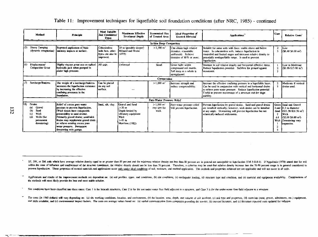
Table 11 : Improvement techniques for liquefiable soil foundation conditions (after NRC, 1985) - continued

SP, SW, or SM soils which have average relative density equal to or greater than 85 percent and the minimum relative density not less than 80 percent are in general not susceptible to liquefaction (TM 5-818-1). D'Appolonia (1970) stated that for soil within the zone of influence and confinement of the saucture faudation, the relative density should not be less than 70 percent. Therefore, a criterion may be used that relative density increase into the 70-90 percent range is in general considered to prevent l i fac t ion . These poperties of heated materials and applications occur only under ideal conditions of soil, moisture, and method application. The methods and properties achieved are not applicable and will not occur in all soils.

Metbod

"

Applications and results of the methods are dependent on: (a) soil profiles, types, and conditions, (b) site conditions, (c) earthquake loading, (d) structure type and condition, and (e) material and equipment availability. Combimtions of the methods will most likely provide the best and most stable solution.

Site conditions have been classified inm three cases: Case I is for beneath structures, Case 2 is for the not-under-water free field ad~acent to a structure, and Case 3 is for tbe under-water free field adjacent to a structure.

Principle

The Costs (in 1985 ddlars) will vary depedihg on: (a) site working cadirians, location, and environment, (b) the location, area, depth, a d volume of soil involved, (c) soil type and properties, (d) materials (sand, gravel, admixtures, etc.) equipment, and skills available, and (e) envimmental impact factors. The costs are average values based on: (a) verbal communication from companies providing the service. (b) current literature, and (c) literature reponed costs updated for inflation.

(5) Heavy Tamping (dynamic compaction)

(6) Displacement1 Canpacticm Gmut

(7) Surcharge/Bumess

(8) Drains (a) Gravel (b) saad (c) Wick (dl Wens (for

permanent dewatering)

Most Suitable Soil Conditioos/

Trpes

Repeated appbition of high- intensity impaws at surface.

Highly viscous grout acts as radical h y W i jack when pnoped in tinder high pressure.

The weight of a sun:hargdhmm increases the l i i fac t ico reristancz by increasmg the effective c o a f m i n g ~ e s i n t h e famdatioo.

Relief of excess pore-water prewre to prevent liifactioo. (Wid draim have canparable permeability to sand drains). Rhaarily gravel maim; sandlwick drains may +went gravel drain or r e l i e existing excess pore water? Pemulnent dewatering wth pnnps.

Maximum Effective Treatment Depth

Cohesiiess soils best, other types can also be improved.

AU soils.

Can be placed on any soil d a c e .

Sand, silt, clay.

Economical Size of Treated Area

30 m (possibly deeper) M h r d and Broise (1975)

Unlimited

..-

Gravel and Sand >30 m Depth limited by vibratory equipment Wick >45 m Morrison (1982)

Ideal Roperties of Treated a t e r i a l '

In-Situ Deep

> 3,300 m2

Small

Compression

> 1,000 m2

Pore-Water Pressure

> 1,500 m2 Any size for

wick.

ApplicatiomIISIIS

Compaction

Can obtain high relative densities, reasonable uniformity. Relative densities of 80% or more.

Grout bulbs within compressed soil matrix. Soil mass as a whole is strengthened.

Increase strength and reduce compressibility.

Relief

Pore-water pressure relief will prevent liquefaction.

Case' Relative Gmsi~

Suitable for some soils with fines; usable above and below water. In cohesionless soils, induces liquefaction in controlled and limited stages and increases relative density to potentially nonliquefiable range. Is used to prevent liefaction.

Increase in soil relative density and horizontal effective stress. Reduce liquefaction potential. Stabiiie the g r d against movement.

Increase the effective confining pressure in a liquefnble layer. Can be used in conjunction with vertical and horizontal drains to relieve pore water pressure. Reduce liquefaction potential. Useful to prevent movements of a structure and for slope stability.

Prevent liquefaction by gravel draii. Sand and gravel drains are installed vertically; however, wick draii can be installed at any angle. Dewatering will prevent liquefaction but wt seismically-induced settlements.

2 3

1 2 3

2 3

Grave l and Sand

2 A:

Wick 1 2 3

Low ($0.40-$6.00 m3)

Low to Moderate ($3.00-915.00 m3)

Moderate if vertical draii used.

Sand and Gravel 0.3 m diameter ($1 1.50-$21.50 m3) Wick ($2.W$4.00 m3) D e w a d g very expensive.

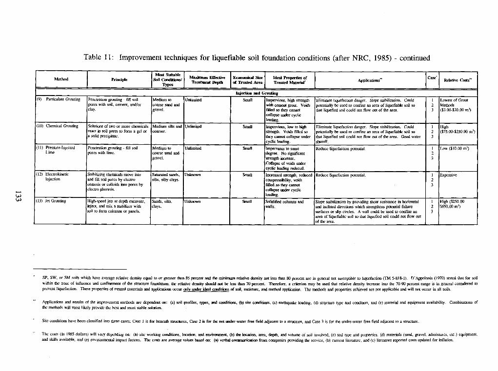
Table 11: Improvement techniques for liquefiable soil foundation conditions (after NRC, 1985) - continued

SP, SW, or SM soils which have average relative density equal to or greater than 85 percent and k minimum relative density mx less than 80 percent are in general not susceptible to liquefaction (TM 5-818-1). D'Appolonia (1970) stated that for soil within the zone of influence and confinement of the structure foundation, the relative density should nu be less t b a ~ ~ 70 percent. Therefore, a criterion may be used that relative density increase into the 70-90 percent range is in general considered to prevent liquefaction. These properties of treated materials and applications occur only under ideal caditioos of soil, moisture, and method application. The methods and properties achieved are not applicable and will not occur in all soils.

Method

"

Applications and results of the improvement methods are dependent on: (a) soil profiles, types, and d t i o m , (b) site umditicm, (c) eanhquake loading, (d) s*cture type and condition, and (e) material and equipment availability Combinations of the methods will most likely provide the best and most stable solution.

Site conditions have been classified into three cases; Case 1 is for beneath struclres, Case 2 is for the naunder-water free field adjacent to a structure, and Case 3 is for the under-water free field adjacent to a strucmre

Principle

The costs (in 1985 dollars) will vary depending on: (a) site working conditions, location. and environment- (b) the llocatim, area, depth, and volume of soil involved, (c) soil type and properties, (d) materials (sand, gravel, admixtures, etc.) equipment, and skills available. and (e) environmental impact factors. The costs are average values based on: (a) verbal carmnunication from companies providing the service, (b) current literature, and (c) literature reported costs updated for idation.

MaFt Suitable , ,- Types

(9) Particulate Grouting

(10) Chemical Grouting

(1 1) Pressure-Injected L i e

(12) Electrokinetic Injection

(13) Jet Grouting

h* ' EBStne Treatment Depth

Penetration grouting - fill soil pores with soil, cement, andlor clay.

Solutions of two or more chemicals react in soil pores to form a gel or a solid precipitate.

Penetration grouting - fill soil pores with lime.

Stabilizing chemicals move into and fill soil pores by electre osmosis or colloids into pores by electrephoresis.

High-speed jets at depth excavate, inject, and mix a stabilizer with soil to form columns or panels.

Unlimited

Unlimited

Unlimited

Unknown

Unknown

M e d i i to coarse sand and gravel.

M e d i i silts and coarser.

M e d i i to coarsesandand gravel.

Sahuated sands, silts, silty clays.

Sand., silts, clays.

Injeetioo and

Small

Small

Small

Small

Small

Eeommical SiLe of Treated Area

Lowest of Grout Methods ($3.00-$30.00 m3)

High ($75.00-$250.00 m3)

Low ($10.00 m3)

Expensive

High ($250.00- $650.00 m3)

Grouting Impervious, high strength with cement grout. Voids filled so they cannot collapse under cyclic laading. Impervious, low to high strenpul. Voids ffled so they cannct collapse under cyclic loading.

Impervious to some degree. No significant snength increase. Cdapse of voids under cyclic loadii reduced.

Increased suength, reduced compressibility, voids filled so they carmot collapse under cyclic loadimg.

Solidified cohrmns and walls.

Eliminate liquefaction danger. Slope stabilization. Could potentially be used to confine an area of liquefnble soil so that liquefied soil could not flow out of the area.

Eliminate liquefaction danger. Slope stabilization. Could potentially be used to confine an area of liquefnble soil so that liquefied soil could not flow out of the area. Good water shutoff.

Reduce liquefaction potential.

Reduce liquefaction potential.

Slope stabilization by providing shear resistance in horizontal and inclined directions which s t rewens potential failure surfaces or slip circles. A wall could be used to confine an area of liquefnble soil so that liquefied soil could not flow out of the area.

Relative CoststT Ideal Properties of Treated Material'

1 2 3

I 2 3

1 2 3

1 2 3

1 2 3

Applications" Case'

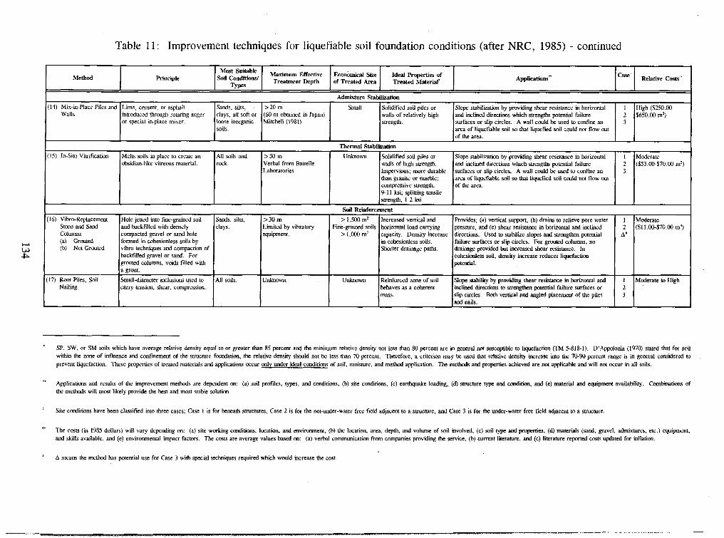
Table 11: Improvement techniques for liquefiable soil foundation conditions (after NRC, 1985) - continued

SP, SW, or SM soils which have average relative density equal to or greater than 85 percent and the minimum relative density not less rhan 80 percent are in general not susceptible to liquefaction (TM 5-818-1). D'Appolonia (1970) stated that for soil within the zone of influence and confmement of the structure foundation, the relative density should not be less than 70 percent. Therefore, a criterion may be used that relative density increase into the 70-90 percent range is in general considered to prevent liquefaction. These properties of treated materials and applications occur only under ideal conditions of soil, moisture, and method application. The methods and properties achieved are w t applicable and will not occur in all soils.

Method

(14) Mix-in-Place Piles and Walls

(15) In-SiU Vitrification

(16) Vibro-Replacement Stone and Sand Columns (a) Grouted (b) Not Grouted

(17) Root Pies, Soi Nailing

"

Applications and results of the improvement methods are dependent on: (a) soil profiles, types, and conditions, (b) site conditions, (c) earthquake loading, (d) structure type and condition, and (e) material and equipment availability. Combitions of the methods will most likely provide the best and most stable solution.

Site conditions have been classified into three cases; Case 1 is for beneath structures, Case 2 is for the not-under-water free field adjacent to a structure, and Case 3 is for the under-water free field adjacent to a structure.

Principle

" The costs (in 1985 dollars) will vary depending on: (a) site working conditions, location, and environment, (b) the location, area, depth, and volume of soil involved, (c) soil type and properties, (d) materials (sand, gravel, admixtures, etc.) equipment, and skills available, and (e) environmental impact factors. The costs are average values based on: (a) verbal communication from companies providing the service, (b) current literature, and (c) literature reported costs updated for inflation.

A means the method has potential use for Case 3 with special techniques required which would increase the cost.

Most Suitable Soil Conditions/

1s.pes

Madmum Effective Treatment Depth

L i e , cement, or asphalt introduced thrwgh rotating auger or special &place mixer.

Melts soils in place to create an obsidian-like vitrew material.

Hole jeaed into fme-grained soil and backfiilled with densely compacted gravel or sand hole formed in cohesianless soils by vibro techniques and compaction of backfilled gravel or sand. For grouted column., voids filled with a grout.

Smalldiameter inclusions used to carry tension, shear, compression.

Admixture S t a b h t i o n

High ($250.00- $650.00 m3)

Slope stabilization by providing shear resistance in horizontal and inched directions which strengths potential failure surfaces or slip circles. A wall could be used to contime an area of liquefmble soil so that liquefied soil could not flow out of the area.

Economical Size of Treated Area

Sands, silts, clays, all soft or loose inorganic soils.

1 2 3

Ideal Properties of Treated Material' Applications"

> 20 m (60 m obtained in Japan) Mitchell (1981)

All soils and rock.

Sands, sils, clays.

All soils.

CaseT Relative Costs"

Small

Moderate ($53.00-$70.00 m')

Moderate ($11.00-$70.00 m3)

Moderate to High

>30 m Verbal from Banelle Laboratories

>30 m Limited by vibratory equipment.

Unknown

S t a b k t i o n

Solidified soil piles or walls of high strength. Imperviws; more durable than granite or marble; compressive strength, 9-1 1 ksi; splitting tensile strength, 1-2 ksi

Increased vertical and horizontal load carrying capacity. Density increase in cohesionless soils. Shorter drainage paths.

Reinforced zone of soil behaves as a coherent mass.

Solidified soil piles or walls of relatively high strength.

Thermal

Unknown

Soil Reinforcement

> 1,500 m2 Fine-grained soils

> 1,000 m2

Unknown

Slope stabilization by providing shear resistance in horizontal and inclined directions which strengths potential failure surfaces or slip circles. A wall could be used to contime an area of liquefible soil so that liquefied soil could not flow out of the area.

Provides; (a) vertical support, (b) draii to relieve pore water pressure, and (c) shear resistance in horizontal and inclined directions. Used to stabilize slopes and strengthen potential failure surfaces or slip circles. For grouted columns, no drainage provided but increased shear resistance. In cohesionless soil, density increase reduces liquefaction potential.

Slope srability by providii shear resistance in horizontal and inclined directions to strengthen porential f a k e surfaces or dip circles. Both vertical and angled placement of the piles and nails.

1 2 3

1 2

A'

1 2 3

CHAPTER 9

SEISMIC DESIGN OF FOUNDATIONS AND RETAINING WALLS

9.1 INTRODUCTION

This chapter addresses geotechnical aspects of seismic design of foundations, retaining walls, and other structural components of highway systems. In addressing these issues, it is assumed that the ground motions at the site have been determined by the project geologist and/or geotechnical engineer and that the earthquake-induced forces from the superstructure have been provided by the structural engineer. Guidelines are available for the seismic design of highway bridges which cover some of the issues related to seismic design of foundations and retaining walls. Of particular note are the AASHTO standard specifications for highway bridges (AASHTO, 1994), the seismic design course notes prepared by ABAM Engineering (ABAM, 1994), FHWA guidelines for seismic design of highway bridge foundations (Lam and Martin, 1986), design and construction of wooden piles (Hannigan et a1 . , 1996), and laterally-loaded piles (Reese, 1984). Much of the information contained in these guidelines will not be covered in detail herein, but will be incorporated by reference.

The discussions herein are intended to cover routine situations encountered in highway engineering. Specialty topics such as seismic retrofit of long span bridges require special considerations and are beyond the scope of this document.

9.2 SEISMIC RESPONSE OF FOUNDATION SYSTEMS

In a manner similar to evaluation of the stability of a slope subject to earthquake ground motions (chapter 7), earthquake effects on foundations can,be modeled using either a pseudo-static approach, wherein the earthquake-induced loads are represented by static forces and/or moments to the foundation, or a dynamic approach, wherein the time history of transient cyclic earthquake forces is applied to the structure-foundation system.

In a pseudo-static analysis, the effects of the dynamic earthquake-induced loads on the foundation are represented using static forces and moments. The bearing capacity and lateral resistance of a foundation element is evaluated using static formulations and compared to the pseudo-static loads. However, the static shear strength may be either decreased or increased, depending on soil type and groundwater conditions, to account for dynamic loading conditions. Typically, the pseudo-static forces and moments are calculated by applying a horizontal force equal to the weight of the structure times a seismic coefficient through the center of gravity of the structure. The seismic coefficient is generally a fraction of the peak ground acceleration of the design earthquake and may also be dependent on the response characteristics of the structure, the behavior of the foundation soil, and the ability of the structure to accommodate permanent seismic displacement. Alternatively, peak

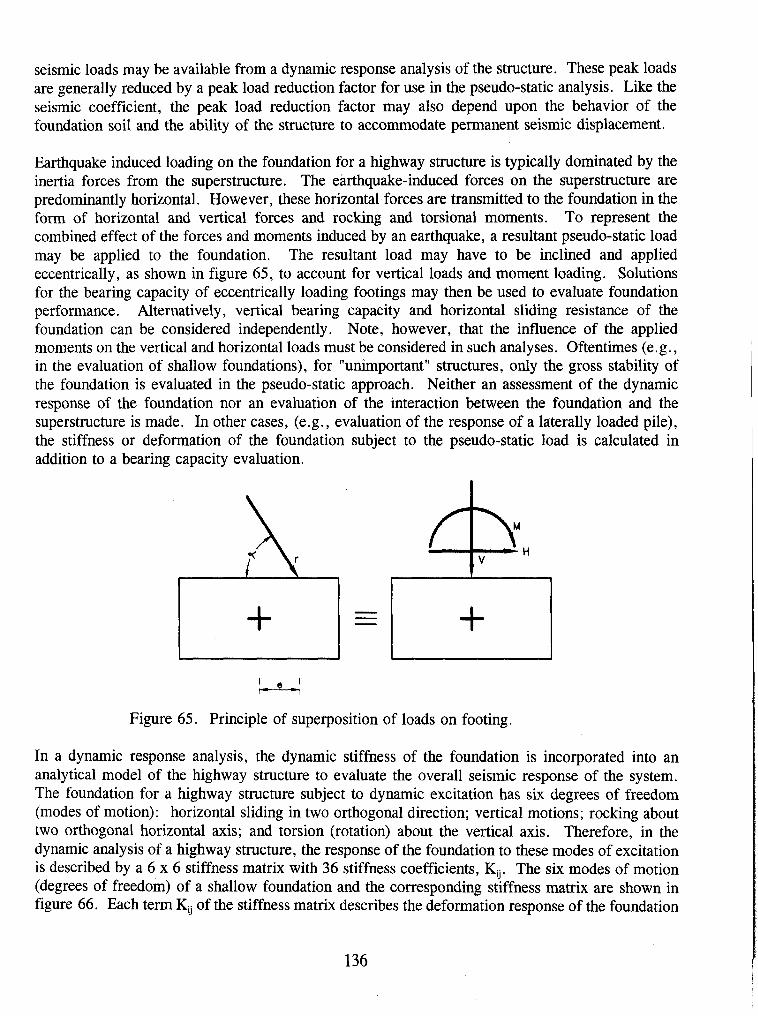
seismic loads may be available from a dynamic response analysis of the structure. These peak loads are generally reduced by a peak load reduction factor for use in the pseudo-static analysis. Like the seismic coefficient, the peak load reduction factor may also depend upon the behavior of the foundation soil and the ability of the structure to accommodate permanent seismic displacement.

Earthquake induced loading on the foundation for a highway structure is typically dominated by the inertia forces from the superstructure. The earthquake-induced forces on the superstructure are predominantly horizontal. However, these horizontal forces are transmitted to the foundation in the form of horizontal and vertical forces and rocking and torsional moments. To represent the combined effect of the forces and moments induced by an earthquake, a resultant pseudo-static load may be applied to the foundation. The resultant load may have to be inclined and applied eccentrically, as shown in figure 65, to account for vertical loads and moment loading. Solutions for the bearing capacity of eccentrically loading footings may then be used to evaluate foundation performance. Alternatively, vertical bearing capacity and horizontal sliding resistance of the foundation can be considered independently. Note, however, that the influence of the applied moments on the vertical and horizontal loads must be considered in such analyses. Oftentimes (e.g . , in the evaluation of shallow foundations), for "unimportant" structures, only the gross stability of the foundation is evaluated in the pseudo-static approach. Neither an assessment of the dynamic response of the foundation nor an evaluation of the interaction between the foundation and the superstructure is made. In other cases, (e.g., evaluation of the response of a laterally loaded pile), the stiffness or deformation of the foundation subject to the pseudo-static load is calculated in addition to a bearing capacity evaluation.

Figure 65. Principle of superposition of loads on footing.

In a dynamic response analysis, the dynamic stiffness of the foundation is incorporated into an analytical model of the highway structure to evaluate the overall seismic response of the system. The foundation for a highway structure subject to dynamic excitation has six degrees of freedom (modes of motion): horizontal sliding in two orthogonal direction; vertical motions; rocking about two orthogonal horizontal axis; and torsion (rotation) about the vertical axis. Therefore, in the dynamic analysis of a highway structure, the response of the foundation to these modes of excitation is described by a 6 x 6 stiffness matrix with 36 stiffness coefficients, KU. The six modes of motion (degrees of freedom) of a shallow foundation and the corresponding stiffness matrix are shown in figure 66. Each term KU of the stiffness matrix describes the deformation response of the foundation

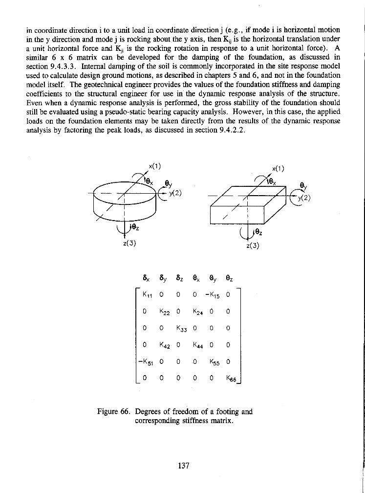
in coordinate direction i to a unit load in coordinate direction j (e.g., if mode i is horizontal motion in the y direction and mode j is rocking about the y axis, then Kij is the horizontal translation under a unit horizontal force and K,, is the rocking rotation in response to a unit horizontal force). A similar 6 x 6 matrix can be developed for the damping of the foundation, as discussed in section 9.4.3.3. Internal damping of the soil is commonly incorporated in the site response model used to calculate design ground motions, as described in chapters 5 and 6, and not in the foundation model itself. The geotechnical engineer provides the values of the foundation stiffness and damping coefficients to the structural engineer for use in the dynamic response analysis of the structure. Even when a dynamic response analysis is performed, the gross stability of the foundation should still be evaluated using a pseudo-static bearing capacity analysis. However, in this case, the applied loads on the foundation elements may be taken directly from the results of the dynamic response analysis by factoring the peak loads, as discussed in section 9.4.2.2.

Figure 66. Degrees of freedom of a footing and corresponding stiffness matrix.

9.3 SEISMIC PERFORMANCE OF RETAINING WALLS

The seismic performance of retaining walls is an important component of earthquake engineering for highway systems. Retaining walls are used extensively for bridge abutments, depressed segments of highway alignments, and elevated highways. Retaining walls are generally designed to resist sliding, overturning, and structural failure due to lateral pressures. Most retaining structures are designed to resist seismic loads using pseudo-static analyses. However, stiffness-based methods of analysis are also available for retaining wall design. Furthermore, for sliding of gravity walls, a deformation based design methodology is often used in practice.

9.4 DESIGN OF SHALLOW FOUNDATIONS

9.4.1 General

Shallow foundations are commonly used as foundations for bridge piers and abutment walls. Shallow foundations are suitable at rock sites or when firm soils are found at shallow depth provided the potential for landslide induced displacements is fairly low and the risk of liquefaction is very low or non-existent. In areas where deposits of compressible, expansive, or collapsible soils are found near the ground surface, shallow foundations may not be suitable. Where soil conditions are not suitable for the use of shallow foundations, deep foundations are used.

The seismic performance of shallow foundations may be evaluated using either pseudo-static limit equilibrium analysis or dynamic response analysis. The critical element in a pseudo-static analysis of a shallow foundation is the evaluation of the pseudo-static loads (forces and moments) for use in the analysis. The primary task of the geotechnical engineer in a dynamic response analysis of a structural system that employs shallow foundations is the evaluation of the coefficients of the stiffness matrix. If a dynamic response analysis of the structure is performed, the, gross stability of the shallow foundation should still be evaluated using pseudo-static limit equilibrium analysis.

In addition to evaluating the gross stability of the shallow foundation under dynamic loads, the risk of excessive seismic settlement and soil liquefaction should also be evaluated for foundations founded upon saturated cohesionless soils. Evaluation of liquefaction and settlement potential is described in chapter 8 of this document,

9.4.2 Pseudo-Static Analyses

9.4.2.1 General

Two alternative methods are commonly used in geotechnical practice to evaluate the ultimate bearing capacity of shallow foundations for highway structures:

the general bearing capacity equation using bearing capacity factors derived from soil shear strength parameters (c, 4) recommended by AASHTO (1994); and

the bearing capacity equation based on Standard Penetration Test blow counts recommended in NCHRP Report 343 (Barker et al., 199 1).

In theory, the two methods cited above should give similar results if the strength parameters used to represent the foundation soil are consistent with the SPT blow count. Some engineers prefer to use the blow count method for dynamic bearing capacity analysis because the SPT is a dynamic test and thus its use may take into account any tendency for the soil to lose strength when subjected to dynamic loading. However, the general bearing capacity equation method provides more flexibility in accounting for inclined and eccentric loading. Bearing capacity can also be evaluated using CPT results. However, the CPT resistance is typically either converted to an equivalent SPT blow count for use in the NCHRP Report 343 blow count-based method or used to estimate the soil shear strength parameters for use in the general bearing capacity equation.

Shallow foundations should also be designed to resist sliding under seismic loading. Sliding resistance is typically assessed using the interface friction and adhesion between the bottom of the foundation and the foundation soil to resist the applied seismic loads. Friction and adhesion on the sides of the foundation may also be included in evaluating the resistance of a foundation to sliding. Some engineers include the passive seismic soil resistance on the front of the footing when calculating sliding resistance. However, when passive resistance is employed in evaluating sliding resistance, the calculated passive seismic earth pressure is often divided by two to compensate for the relatively large lateral deformations required to mobilize the passive resistance of the soil. Furthermore, if the passive seismic resistance on the front of the footing is included in the analysis, the active seismic pressure on the back of the footing should also be considered. Evaluation of passive and active seismic earth pressures is discussed subsequently in section 9.6.

9.4.2.2 Load Evaluation for Pseudo-Static Bearing Capacity Analysis

The foundation loads for use in a pseudo-static bearing capacity analysis for a shallow foundation may be evaluated either by applying a pseudo-static load to the structure or from the results of a dynamic response analysis. In determining foundation loads by applying a pseudo-static force to the structure, both the horizontal and vertical inertial forces from the superstructure may be considered. These inertia forces are modelled by applying through the center of gravity of the superstructure, a load equal to the weight of the structure multiplied by a seismic coefficient. If applied centrically, the vertical load will generate only vertical forces on the foundation. However, if the vertical force is eccentrically applied to the foundation, it will generate a moment loading. The horizontal load typically generates both vertical forces and moments on the foundation. The peak vertical and horizontal dynamic loads are often considered separately, as it is highly unlikely that the peak vertical and horizontal forces will act simultaneously on the superstructure. In each case, the resultant forces and moments on the foundation elements are used in the pseudo-static bearing capacity analysis. Foundation performance should be evaluated for both compressive and tensile vertical seismic loads. Furthermore, the vertical and horizontal dead loads of the superstructure and foundation should be added to the seismic loads when analyzing the foundation system in either case.

There is no general agreement on establishing the seismic coefficient used in evaluation of the pseudo-static load for the seismic analysis of foundations. Based upon experience with the seismic stability of slopes (chapter 7), the seismic coefficient for foundation design should be a fraction of the peak ground acceleration (PGA) expressed as a fraction of gravity. For many cases, the effective peak acceleration from AASHTO maps may be appropriate for use as the seismic coefficient in pseudo-static analysis, as this value is typically already reduced from the expected maximum peak ground acceleration. Alternatively, based upon experience with seismic deformation analyses of slopes and embankments, including back analyses of the performance of slopes and embankments in earthquakes, a value equal to one-half the PGA (expressed as a fraction of gravity) would appear to be reasonable. However, for structures that cannot tolerate foundation deformations of up to several centimeters and for structures founded on soils subject to progressive failure and/or a post-peak strength decrease, a value equal to the PGA (expressed as a fraction of gravity) may be appropriate. Furthermore, the potential for amplification of the PGA by the structure itself should be considered. For slender, flexible structures, it may be prudent to multiply the above values by an amplification factor provided by the structural engineer.

If the loads used in the pseudo-static foundation analysis are determined from the results of a dynamic response analysis of the structure, then the potential for amplification of the ground motion by the structure is included in the peak loads from the response analysis. In this case, the peak loads provided by the structural engineer should be factored in the same manner described above to evaluate the seismic coefficient from the PGA; that is, a factor of one-half would appear to be reasonable in most situations, while a value of one may be used for structures that cannot tolerate significant deformations and for structures founded on soils subject to progressive failure and/or post-peak strength decrease. When using the loads from a dynamic response analysis to evaluate foundation performance, peak loads that occur at different times in the analysis should not be superimposed. Loads used in combination should be loads that act upon the foundation at the same time. For instance, the peak horizontal load should be used in combination with the vertical loads imposed on the foundation by the peak horizontal load and with other vertical loads acting on the foundation at the same time as the peak horizontal load, but not in combination with the peak rocking moment or peak vertical load.

9.4.2.3 The General Bearing Capacity Equation

Terzaghi presented the first comprehensive theory for the evaluation of the ultimate bearing capacity of rough, shallow foundations. Using limit equilibrium analysis, Terzaghi expressed the ultimate bearing capacity as a function of the geometry of the foundation, the geometry of the assumed failure surfaces, and the geotechnical properties of the foundation soil.

Terzaghi's early work was then expanded upon to provide formulations accounting for different foundation shapes, load inclination and load eccentricity, water table location, and other factors. These formulations are also based on the resolution of a limit equilibrium problem and the evaluation of the shear strength properties of the foundation soil.

Consequently, to account for eccentric loads, moments, inclined loads, and different foundation shapes, a series of correction factors were applied to the initial Terzaghi bearing capacity equation. Application of these correction factors results in a generalized bearing capacity equation of the form:

where q,,, is the ultimate bearing capacity, q, is a uniform surcharge load applied at the ground surface adjacent to the foundation, B is the foundation width, s,, s,, and s, are foundation shape factors, i,, i, and i, are load inclination factors, c and y are the cohesion and unit weight of the soil, and N,, N,, and N, are the bearing capacity factors. Note that the surcharge load q, is equal to yD for a foundation embedded at a depth D below the ground surface.

The bearing capacity factors, N,, N,, and N, are a function of the friction angle of the soil, 6. Charts of bearing capacity factors versus 6 are commonly available in geotechnical literature. For spread sheet calculations, the following equations may be used:

Nc = (N, - 1) cot (4)

Ny = (N, - 1) tan (1.44) (9-4)

Adjustments for Eccentric (Moment) Loading

The first step in a pseudo-static seismic bearing capacity analysis is to compute the pseudo-static loads. The pseudo-static and static loads are then combined into a single resultant force with an inclination a! and an eccentricity, e, as illustrated in figure 65.

Following computation of the resultant force, equivalent dimensions are computed for the footing to account for the eccentricity of the load on the footing. The load eccentricity is caused by the moment applied to the foundation. This applied moment creates a non-uniform pressure on the bottom of the footing and can lead to loss of contact pressure between the bottom of the footing and the ground. Therefore, the width of a footing subjected to an eccentric load is represented by a reduced, effective width, B'. The computation of equivalent dimensions to account for the load eccentricity is illustrated on figure 67.

Some widely used relationships for the effective contact area are B' = (B-2e), as recommended by Meyerhof (1953), and B' = (3Bl2-3e) corresponding to a linear soil pressure distribution. The

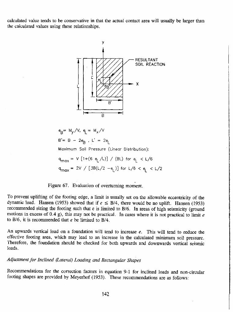
calculated value tends to be conservative in that the actual contact area will usually be larger than the calculated values using these relationships.

RESULTANT SOIL REACTION

eB= My/V, y= M,/V

B'= B - 2% , L' = 2e L

Maximum Soil Pressure (Linear Distribution):

qmax = V [ I+(6 e,-/~)] / (BL) for eL < L/6

qmax = 2V / [3B(L/2 -eL)] for L/6 < eL < L/2

Figure 67. Evaluation of overturning moment.

To prevent uplifting of the footing edge, a limit is usually set on the allowable eccentricity of the dynamic load. Hansen (1953) showed that if e 5 Bl4, there would be no uplift. Hansen (1953) recommended sizing the footing such that e is limited to B16. In areas of high seismicity (ground motions in excess of 0.4 g), this may not be practical. In cases where it is not practical to limit e to B16, it is recommended that e be limited to B14.

An upwards vertical load on a foundation will tend to increase e. This will tend to reduce the effective footing area, which may lead to an increase in the calculated minimum soil pressure. Therefore, the foundation should be checked for both upwards and downwards vertical seismic loads.

Adjustment for Inclined (Lateral) Loading and Rectangular Shapes

Recommendations for the correction factors in equation 9-1 for inclined loads and non-circular footing shapes are provided by Meyerhof (1953). These recommendations are as follows:

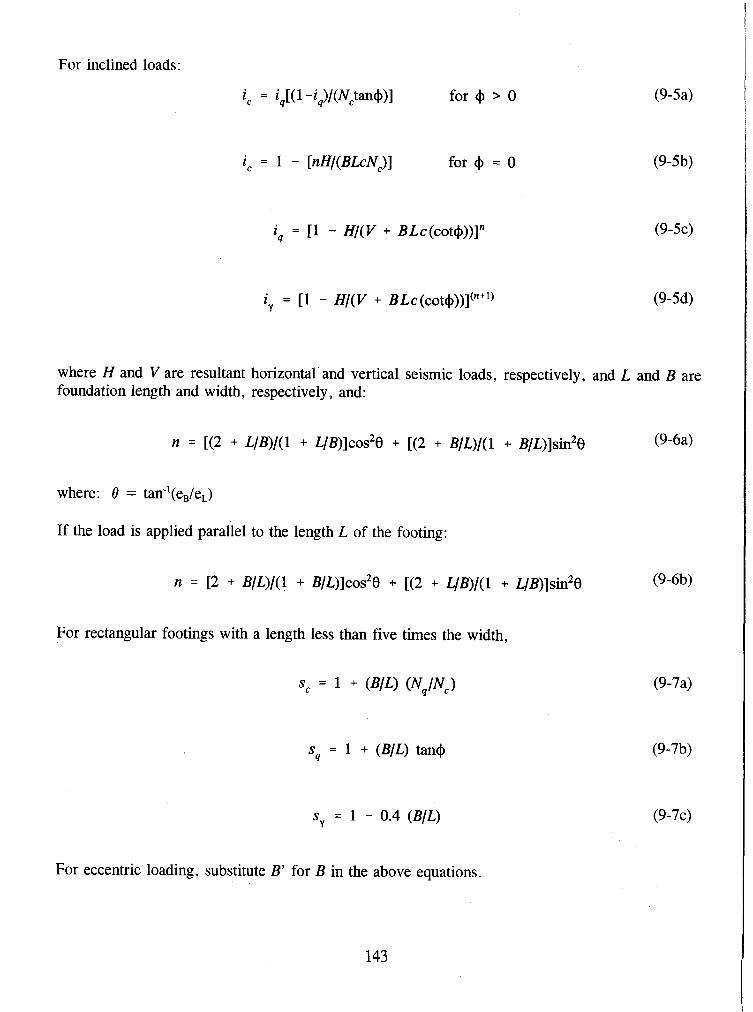
For inclined loads:

ic = iq[(l -iq)l(Nctan4)l for 4 > O

i, = 1 - [nH/(BLcN,)] for 4 = 0 (9-5b)

where H and V are resultant horizontal and vertical seismic loads, respectively, and L and B are foundation length and width, respectively, and:

where: 8 = tan-'(e,/e,)

If the load is applied parallel to the length L of the footing:

For rectangular footings with a length less than five times the width,

s, = 1 + (BIL) (NqINc)

S~ = 1 - 0.4 (BIL) (9-7~)

For eccentric loading, substitute B' for B in the above equations.

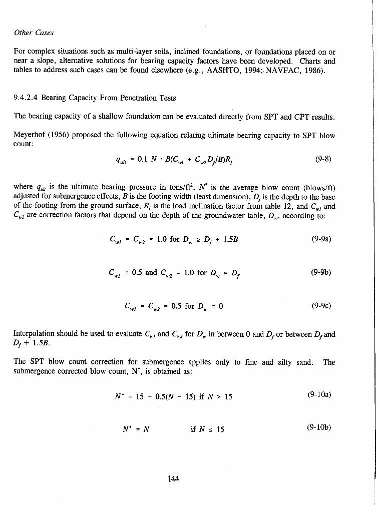
Other Cases

For complex situations such as multi-layer soils, inclined foundations, or foundations placed on or near a slope, alternative solutions for bearing capacity factors have been developed. Charts and tables to address such cases can be found elsewhere (e.g., AASHTO, 1994; NAVFAC, 1986).

9.4.2.4 Bearing Capacity From Penetration Tests

The bearing capacity of a shallow foundation can be evaluated directly from SPT and CPT results.

Meyerhof (1956) proposed the following equation relating ultimate bearing capacity to SPT blow count:

where q,, is the ultimate bearing pressure in tons/ft2, N* is the average blow count (blowslft) adjusted for submergence effects, B is the footing width (least dimension), Df is the depth to the base of the footing from the ground surface, R, is the load inclination factor from table 12, and C,, and C,, are correction factors that depend on the depth of the groundwater table, D,, according to:

Cwl = Cw2 = 1.0 for Dw 2 Df + 1.5B (9-9a)

Cwl = 0.5 and Cw2 = 1.0 for Dw = Df (9-9b)

Cwl = Cw2 = 0.5 for Dw = 0 (9-9c)

Interpolation should be used to evaluate Cwl and C, for D, in between 0 and Df or between Df and Df + 1.5B.

The SPT blow count correction for submergence applies only to fine and silty sand. The submergence corrected blow count, N*, is obtained as:

Table 12. Inclination factors for bearing capacity of shallow foundations (after Meyerhof, 1956).

HI V

0.10

0.15

0.20

0.25

0.30

0.35

0.40

0.45

0.50

0.55

0.60

Square Footings Load Inclination Factor, R,

HI V

0.10

0.15

0.20

0.25

0.30

0.35

0.40

0.45

0.50

0.55

0.60

Df IB=O

0.75

0.65

0.55

0.50

0.40

0.35

0.30

0.25

0.20

0.15

0.10

Load Inclination Factor, R,

Df IB=l

0.80

0.75

0.65

0.55

0.50

0.45

0.35

0.30

0.25

0.20

0.15

Df lB=5

0.85

0.80

0.70

0.65

0.55

0.50

0.45

0.40

0.30

0.25

0.20

Load Inclined in Width Direction

Df lB=O

0.70

0.60

0.50

0.40

0.35

0.30

0.25

0.20

0.15

0.10

0.05

Load Inclined in Length Direction

Df lB=O

0.80

0.70

0.65

0.55

0.50

0.40

0.35

0.30

0.25

0.20

0.15

Df lB=1

0.75

0.65

0.60

0.50

0.40

0.35

0.30

0.25

0.20

0.15

0.10

Df lB=5

0.80

0.70

0.65

0.55

0.50

0.40

0.35

0.30

0.25

0.20

0.15

Df lB=l

0.85

0.80

0.70

0.65

0.60

0.55

0.50

0.45

0.35

0.30

0.25

Df lB=5

0.90

0.85

0.75

0.70

0.65

0.60

0.55

0.50

0.45

0.40

0.35

where N is the measured blow count. The measured blow count value used in equation 9-10 is averaged within the range of depth from the bottom of the footing to 1.5B below the bottom of the footing.

Load eccentricity can be accommodated using equation 9-8 by substituting B' for B, where B' is evaluated in accordance with figure 67. No correction factors for non-circular footings were proposed by Meyerhof for use with these equations. However, the general bearing capacity equations presented in the previous section can be used to calculate a correction factor for the bearing capacity of a non-circular footing.

9.4.2.5 Sliding Resistance of Shallow Foundations

The sliding resistance of a shallow foundation should be calculated independently of the bearing capacity. In calculating sliding resistance, the unit adhesion andlor frictional resistance of the base of the foundation to sliding is multiplied by the area of the base to determine the sliding resistance. The adhesion and interface frictional resistance of the base depend upon both the type of soil and the foundation material. Typically, for a concrete foundation, the adhesion and interface friction coefficient will be reduced by 20 to 33 percent from the cohesion and friction coefficient of the underlying soil. Navy Design Manual DM 7.2 (NAVFAC, 1986) provides recommendations for interface friction and adhesion values for dissimilar construction materials (e.g., sandlconcrete, claylsteel). These values can be used for the design of both foundations and retaining walls against sliding. For eccentrically loaded foundations, the effective base area B' should be used in evaluating sliding resistance.

The vertical component of the seismic load on the footing should be included when evaluating the sliding resistance. Sliding resistance should be checked for both the maximum and minimum vertical loads (upwards and downwards seismic loading).

For embedded foundations, the passive seismic resistance in front of the foundation is often included in evaluation of the sliding resistance of a shallow footing. However, due to the relatively large deformations necessary for mobilization of the passive resistance, the passive earth pressure is typically reduced by a factor of two for use in sliding resistance analyses. Furthermore, the active seismic force on the front of the foundation should be either subtracted from the passive sliding resistance or added to the sliding driving force. The net result of factoring the passive seismic resistance and then subtracting the active seismic force may often be little to no change in the sliding resistance of the foundation.

9.4.2.6 Factors of Safety

Seismic loads represent an extreme loading condition, therefore relatively low factors of safety are generally considered acceptable in a pseudo-static analysis. Factors of safety on the order of 1.1 and 1.15 are typically used in practice for both bearing capacity and sliding resistance. The choice of the factor of safety and of the seismic coefficient (or peak load reduction factor) are intimately linked. For instance, if a seismic coefficient equal to the PGA (divided by the acceleration of

gravity) has been used in the pseudo-static analysis because the foundation cannot tolerate large movements, there may be no need to increase the factor of safety beyond 1 .O. Alternatively, if the seismic coefficient is one-half the PGA and the soil is susceptible to a post-peak strength decrease, it may be prudent use a factor of safety of 1.1 or 1.15.

9.4.3 Dynamic Response Analyses

9.4.3.1 General

Dynamic response analyses incorporate the foundation system into the general dynamic model 01 the structure. The combined analysis is commonly referred to as the soil-structure-interaction, SSI analysis. In SSI analyses, the foundation system can either be represented by a system of springs (classical approach), or by a foundation stiffness (and damping) matrix. The latter approach, commonly used for SSI analyses of highway facilities, is commonly referred to as the stzfSness matrix method approach.

The general form of the stiffness matrix for a rigid footing was presented in figure 66. The 6 x 6 stiffness matrix can be incorporated in most structural engineering programs for dynamic response analysis to account for the foundation stiffness in evaluating the dynamic response of the structural system. The diagonal terms of the stiffness matrix represent the direct response of a mode of motion to excitation in that mode while the off diagonal terms represent the coupled response. Many of the off-diagonal terms are zero or close to zero, signifying that the two corresponding modes are uncoupled (e.g . , torsion and vertical motion) and therefore may be neglected. In fact, for symmetric foundations loaded centrically, rocking and sliding (horizontal translation) are the only coupled modes of motion considered in a dynamic analysis.

Often, all of the off-diagonal (coupling) terms are neglected for two reasons: (1) the values of these off-diagonal terms are small, especially for shallow footings; and (2) they are difficult to compute. However, the coupling of the two components of horizontal translation to the two degrees of freedom of rocking (tilting) rotation may be significant in some cases. For instance, coupled rocking and sliding may be important for deeply embedded footings where the ratio of the depth of embedment to the equivalent footing diameter is greater than five. The reader is referred to Lam and Martin (1986) for more guidance on this issue.

The stiffness matrix, K, of an irregularly shaped and/or embedded footing can be expressed by the following general equation:

where K,,, is the stiffness matrix of an equivalent circular surface footing, described in chapter 9.4.3.2, a is the foundation shape correction factor, described in chapter 9.4.3.4, and 0 is the foundation embedment factor, described in chapter 9.4.3.5.

9.4.3.2 Stiffness Matrix of a Circular Surface Footing

The solution for a circular footing rigidly connected to the surface of an elastic half space provides the basic stiffness coefficients for the various modes of foundation displacement. For vertical translation, the stiffness coefficient K3, can be expressed as:

For horizontal translation, the stiffness coefficients K,, and K,, can be expressed as:

For torsional rotation, the stiffness coefficient K, can be expressed as:

For rocking rotation, the stiffness coefficients K4, and K,, can be expressed as:

In equation 9-12, G and v are the dynamic shear modulus and Poisson's ratio for the elastic half space (foundation soil) and R is the radius of the footing.

The dynamic shear modulus, G, used to evaluate the foundation stiffness should be based upon the representative, or average, shear strain of the foundation soil. However, there are no practical guidelines for evaluating a representative shear strain for a dynamically loaded shallow foundation. Frequently, the value of G,,,,,, the shear modulus at very low strain, is used to calculate foundation stiffness. However, this is an artifact of the original development of the above equations for foundation stiffness for the design of machine foundations. For earthquake loading, it is recommended that values of G be evaluated at shear strain levels calculated from a seismic site response analysis using the modulus reduction curves presented in chapter 5. If results of a site response analysis are not available, G may be evaluated using the modulus reduction curves presented in chapter 5 and an assumed shear strain level that depends upon the magnitude of the earthquake, intensity of ground motion, and soil type. For events of magnitude 6.0 or less, and for ground motion intensities of 0.4 g or less, a value of G corresponding to a strain level of 0.1 percent appears to be appropriate. For larger magnitudes and/or higher intensity earthquakes, a larger strain level may be used. For very large magnitude events (M > 7.5) with very high shaking intensity (PGA > 0.6 g), a value of G corresponding to a shear strain of 1 percent is recommended.

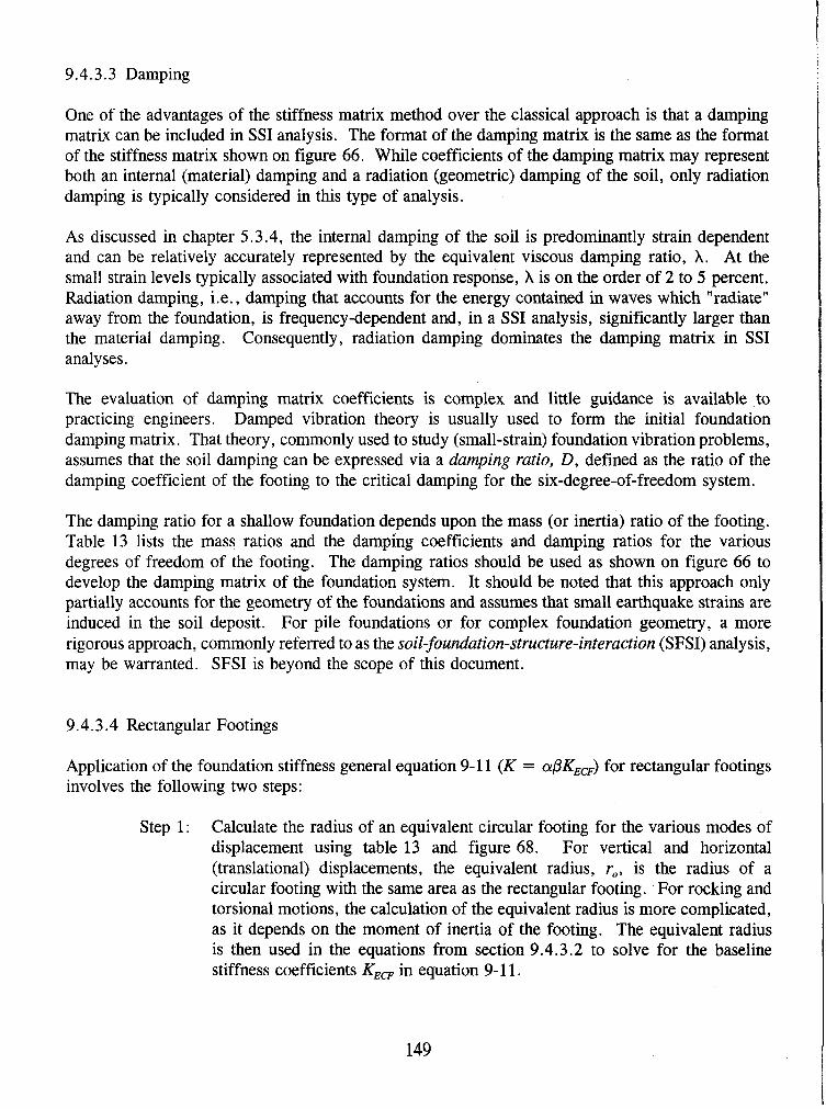
9.4.3.3 Damping

One of the advantages of the stiffness matrix method over the classical approach is that a damping matrix can be included in SSI analysis. The format of the damping matrix is the same as the format of the stiffness matrix shown on figure 66. While coefficients of the damping matrix may represent both an internal (material) damping and a radiation (geometric) damping of the soil, only radiation damping is typically considered in this type of analysis.

As discussed in chapter 5.3.4, the internal damping of the soil is predominantly strain dependent and can be relatively accurately represented by the equivalent viscous damping ratio, X. At the small strain levels typically associated with foundation response, X is on the order of 2 to 5 percent. Radiation damping, i. e . , damping that accounts for the energy contained in waves which "radiate" away from the foundation, is frequency-dependent and, in a SSI analysis, significantly larger than the material damping. Consequently, radiation damping dominates the damping matrix in SSI analyses.

The evaluation of damping matrix coefficients is complex and little guidance is available to practicing engineers. Damped vibration theory is usually used to form the initial foundation damping matrix. That theory, commonly used to study (small-strain) foundation vibration problems, assumes that the soil damping can be expressed via a damping ratio, D, defined as the ratio of the damping coefficient of the footing to the critical damping for the six-degree-of-freedom system.

The damping ratio for a shallow foundation depends upon the mass (or inertia) ratio of the footing. Table 13 lists the mass ratios and the damping coefficients and damping ratios for the various degrees of freedom of the footing. The damping ratios should be used as shown on figure 66 to develop the damping matrix of the foundation system. It should be noted that this approach only partially accounts for the geometry of the foundations and assumes that small earthquake strains are induced in the soil deposit. For pile foundations or for complex foundation geometry, a more rigorous approach, commonly referred to as the soil-foundation-structure-interaction (SFSI) analysis, may be warranted. SFSI is beyond the scope of this document.

9.4.3.4 Rectangular Footings

Application of the foundation stiffness general equation 9-1 1 (K = a@K,,,) for rectangular footings involves the following two steps:

Step 1 : Calculate the radius of an equivalent circular footing for the various modes of displacement using table 13 and figure 68. For vertical and horizontal (translational) displacements, the equivalent radius, r,, is the radius of a circular footing with the same area as the rectangular footing. For rocking and torsional motions, the calculation of the equivalent radius is more complicated, as it depends on the moment of inertia of the footing. The equivalent radius is then used in the equations from section 9.4.3.2 to solve for the baseline stiffness coefficients KEm in equation 9-1 1.

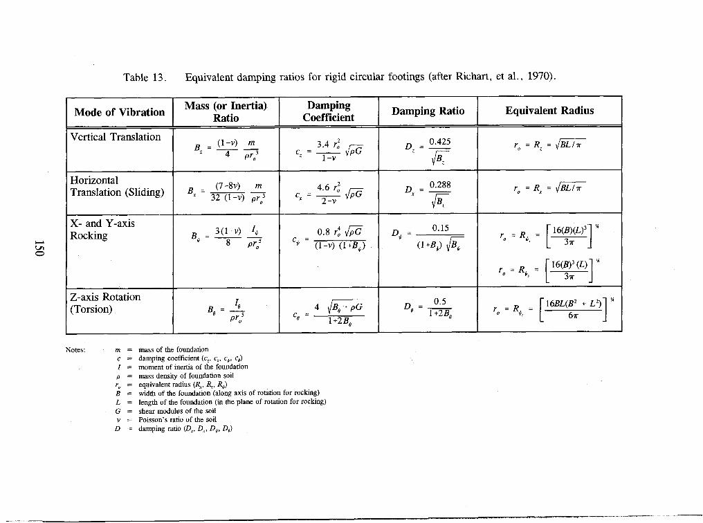
Table 13. Equivalent damping ratios for rigid circular footings (after Richart, et al., 1970).

Notes: m = C = I = P = r, = B = L = G = v = D =

mass of the foundation damping coefficient (c,, c,, c,, c,) moment of inertia of the foundation mass density of foundation soil equivalent radius (R,, R,, R,) width of the foundation (along axis of rotation for rocking) length of the foundation (in the plane of rotation for rocking) shear modulus of the soil Poisson's ratio of the soil damping ratio (D,, D,, D,, Do)

Equivalent Radius

ro = RZ = @izF

r, = R, = ,IBLI.lr

16(m3 (L) 'k

ro = R, = [ 3r ] ro = R, =

[16BL(;i + L~)] '

Damping Ratio

0.425 Dz = - K 0.288 0, = -

6 0.15

D, = (1 +B*) 6

0.5 Do = - 1 +2 Be

Damping Coefficient

3.4 r: @ C, = ----

1 -v

4.6 r: C, = -

2 -v

0.8 r: @ C, =

(1-v) (1 +B,)

4 {m c8 = 1 +2 Be

Mode of Vibration

Vertical Translation

Horizontal Translation (Sliding)

X- and Y-axis Rocking

Z-axis Rotation (Torsion)

Mass (or Inertia) Ratio

(1-V) m Bz=-- 4 P',3

(7-8v) m B, = 32 (1 -v)

3(1-V) I, B,=-- 8 P',5

IB B = - 8

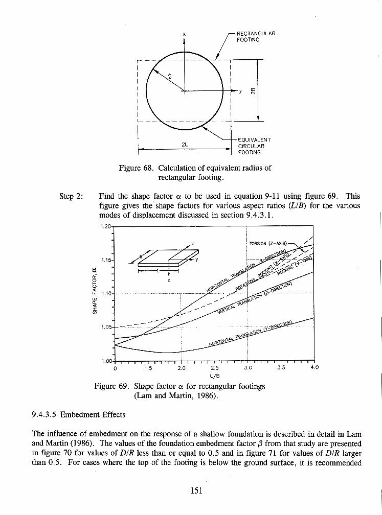
i RECTANGULAR FOOTING

2L -EQUIVALENT

4 - CIRCULAR FOOTING

Figure 68. Calculation of equivalent radius of rectangular footing.

Step 2: Find the shape factor CY to be used in equation 9-11 using figure 69. This figure gives the' shape factors for various aspect ratios (LIB) for the various modes of displacement discussed in section 9.4.3.1.

Figure 69. Shape factor CY for rectangular footings (Lam and Martin, 1986).

9.4.3.5 Embedment Effects

The influence of embedment on the response of a shallow foundation is described in detail in Lam and Martin (1986). The values of the foundation embedment factor f l from that study are presented in figure 70 for values of DIR less than or equal to 0.5 and in figure 71 for values of DIR larger than 0.5. For cases where the top of the footing is below the ground surface, it is recommended

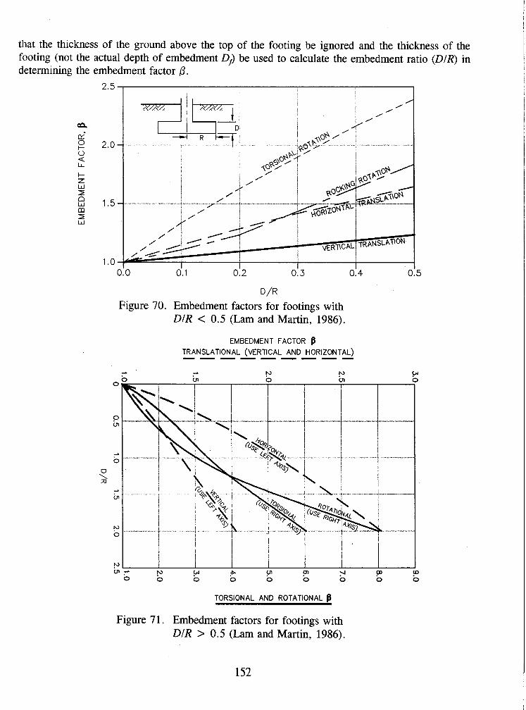
that the thickness of the ground above the top of the footing be ignored and the thickness of the footing (not the actual depth of embedment Df) be used to calculate the embedment ratio (DIR) in determining the embedment factor 0.

D/R Figure 70. Embedment factors for footings with

DIR < 0.5 (Lam and Martin, 1986).

EMBEDMENT FACTOR $ TRANSLATIONAL (VERTICAL AND HORIZONTAL) ---------

TORSIONAL AND ROTATIONAL fl

Figure 71. Embedment factors for footings with DIR > 0.5 (Lam and Martin, 1986).

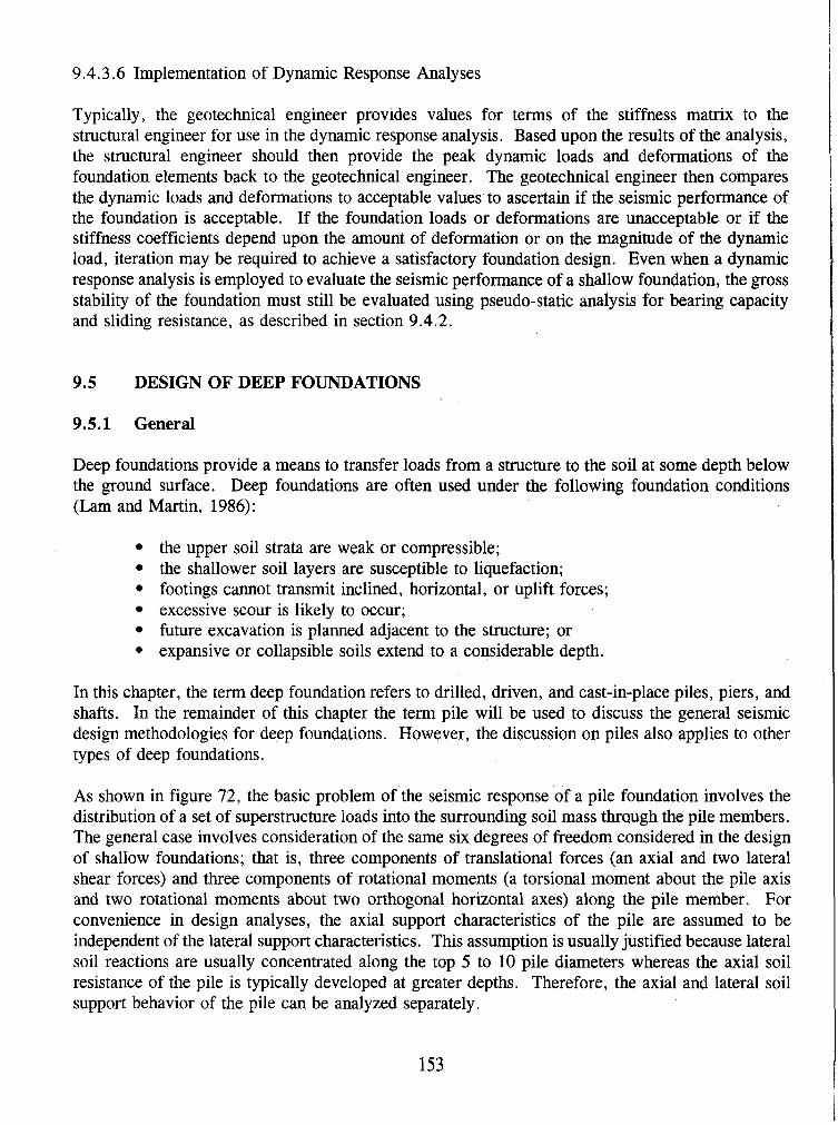
9.4.3.6 Implementation of Dynamic Response Analyses

Typically, the geotechnical engineer provides values for terms of the stiffness matrix to the structural engineer for use in the dynamic response analysis. Based upon the results of the analysis, the structural engineer should then provide the peak dynamic loads and deformations of the foundation elements back to the geotechnical engineer. The geotechnical engineer then compares the dynamic loads and deformations to acceptable values to ascertain if the seismic performance of the foundation is acceptable. If the foundation loads or deformations are unacceptable or if the stiffness coefficients depend upon the amount of deformation or on the magnitude of the dynamic load, iteration may be required to achieve a satisfactory foundation design. Even when a dynamic response analysis is employed to evaluate the seismic performance of a shallow foundation, the gross stability of the foundation must still be evaluated using pseudo-static analysis for bearing capacity and sliding resistance, as described in section 9.4.2.

9.5 DESIGN OF DEEP FOUNDATIONS

9.5.1 General

Deep foundations provide a means to transfer loads from a structure to the soil at some depth below the ground surface. Deep foundations are often used under the following foundation conditions (Lam and Martin, 1986):

the upper soil strata are weak or compressible; the shallower soil layers are susceptible to liquefaction; footings cannot transmit inclined, horizontal, or uplift forces; excessive scour is likely to occur; future excavation is planned adjacent to the structure; or expansive or collapsible soils extend to a considerable depth.

In this chapter, the term deep foundation refers to drilled, driven, and cast-in-place piles, piers, and shafts. In the remainder of this chapter the term pile will be used to discuss the general seismic design methodologies for deep foundations. However, the discussion on piles also applies to other types of deep foundations.

As shown in figure 72, the basic problem of the seismic response of a pile foundation involves the distribution of a set of superstructure loads into the surrounding soil mass thraugh the pile members. The general case involves consideration of the same six degrees of freedom considered in the design of shallow foundations; that is, three components of translational forces (an axial and two lateral shear forces) and three components of rotational moments (a torsional moment about the pile axis and two rotational moments about two orthogonal horizontal axes) along the pile member. For convenience in design analyses, the axial support characteristics of the pile are assumed to be independent of the lateral support characteristics. This assumption is usually justified because lateral soil reactions are usually concentrated along the top 5 to 10 pile diameters whereas the axial soil resistance of the pile is typically developed at greater depths. Therefore, the axial and lateral soil support behavior of the pile can be analyzed separately.

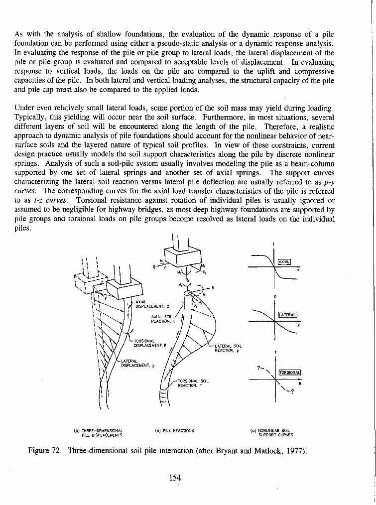
As with the analysis of shallow foundations, the evaluation of the dynamic response of a pile foundation can be performed using either a pseudo-static analysis or a dynamic response analysis. In evaluating the response of the pile or pile group to lateral loads, the lateral displacement of the pile or pile group is evaluated and compared to acceptable levels of displacement. In evaluating response to vertical loads, the loads on the pile are compared to the uplift and compressive capacities of the pile. In both lateral and vertical loading analyses, the structural capacity of the pile and pile cap must also be compared to the applied loads.

Under even relatively small lateral loads, some portion of the soil mass may yield during loading. Typically, this yielding will occur near the soil surface. Furthermore, in most situations, several different layers of soil will be encountered along the length of the pile. Therefore, a realistic approach to dynamic analysis of pile foundations should account for the nonlinear behavior of near- surface soils and the layered nature of typical soil profiles. In view of these constraints, current design practice usually models the soil support characteristics along the pile by discrete nonlinear springs. Analysis of such a soil-pile system usually involves modeling the pile as a beam-column supported by one set of lateral springs and another set of axial springs. The support curves characterizing the lateral soil reaction versus lateral pile deflection are usually referred to as p-y cuwes. The corresponding curves for the axial load transfer characteristics of the pile is referred to as t-z cuwes. Torsional resistance against rotation of individual piles is usually ignored or assumed to be negligible for highway bridges, as most deep highway foundations are supported by pile groups and torsional loads on pile groups become resolved as lateral loads on the individual piles.

(a) THREE-DWENSIONAL (b) PILE REACTIONS (c) NONLINEAR SOIL PILE DISPLACEMENTS SUPPORT CURES

Figure 72. Three-dimensional soil pile interaction (after Bryant and Matlock, 1977).

The constraint at the head of a pile can have a significant influence on lateral load response of the pile. Piles free to rotate at the head will generally undergo larger lateral displacements than fixed- head piles subject to the same load. Therefore, to achiever a stiffer lateral pile response, pile heads can be embedded deeper into the pile cap. A deeper embedment will increase the lateral stiffness and capacity of the pile footing. However, restraining the head of the pile against rotation may induce large moments at the head of the pile. Both the pile and pile cap must then be designed to accommodate this moment.

9.5.2 Method of Analysis

9.5.2.1 General

A comprehensive coverage on seismic analysis of pile foundations is provided in Lam and Martin (1986). Martin and Lam (1995) present additional, updated information on seismic design of pile foundations. The discussion provided herein will touch on only the key aspects of this problem. The readers are referred to Lam and Martin (1986), Martin and Lam (1995), and to the other references cited in this chapter for in-depth coverage of the subject.

Because of the inherently variable and nonlinear nature of soil, there is seldom any advantage in attempting to apply closed form mathematical solutions or in developing design charts for seismic design of pile foundations. Analysis of the response of piles to lateral loading is most conveniently accomplished using established computer programs. A variety of computer programs for the lateral and vertical load response of piles and pile groups are commercially available. Most of these programs use methods developed by Reese and his co-workers (e.g., Reese et al., 1984; Wang and Reese, 1991). Many of these programs have user-friendly input and output routines and thus can be easily used by most geotechnical engineers, even those with limited computer training. In limited cases, where the soil profile consists of a homogeneous layer, hand solutions based on the theory of a beam on an elastic foundation can be used (Lam and Martin, 1986). However, due to the limited applicability of such solutions, they will not be discussed herein.

The construction of a full set of p-y curves for the analysis of a laterally loaded pile involves calculating p-y curves at selected depths along the length of the pile. Calculations for p-y curves for laterally loaded piles are described in detail by Reese et al. (1984). These calculations are typically performed internally by the computer program based upon input soil types and shear strength parameters. Interpolations done internally in the computer program provide p-y characteristics at additional points between the points where p-y curves are input. The additional points generated by the computer should be spaced at about one-half the pile diameter to provide good resolution for the distributed soil support. Placement of p-y curves typically includes the top and bottom (or assumed bottom for a very long pile) of the pile. Since the lateral response of a pile is concentrated close to the soil surface, additional p-y curves are generally placed at closer spacings near the top of the pile. Usually, the pile response is relatively insensitive to p-y curves prescribed at greater depths. However, p-y curves should be placed at the top and bottom of all significant soil layers. In the analysis of a laterally loaded pile, the pile can usually be cut off at 30 to 40 diameters below the ground surface without affecting the lateral behavior of the upper part of the pile.

For evaluating the vertical response of piles subject to dynamic loading, t-z curves are generally calculated over the entire length of the pile. Rules for specifying t-z curves are similar to those cited above for specifying p-y curves. Procedures for evaluating t-z curves are provided by Lam and Martin (1986). Analysis of piles and pile groups subjected to dynamic vertical loads is also usually performed using commercially available computer programs.

9.5.2.2 Pile-Head Stiffness Matrix

The development of an equivalent linear pile-head stiffness matrix is a necessary step in structural seismic response evaluation of pile-supported structures. The pile-head stiffness relations may be expressed by the following equations from Martin and Lam (1995):

where 6 is unit horizontal deflection, 8 is unit rotation, and K, and K, are stiffness coefficients representing the force per unit horizontal deflection with zero rotation and the moment per unit rotation with zero deflection at the pile-head, respectively. The cross-coupling terms K,, and K,, represent the force necessary to maintain zero displacement for a unit rotation and the moment necessary to maintain zero rotation for a unit deflection, respectively. Martin and Lam (1995) present charts for these stiffness coefficients as a function of pile bending stiffness, EI, and soil subgrade reaction modulus for fixed-head pile.

9.5.2.3 Group Effects

One of the most difficult problems in evaluating the lateral response of pile foundations is the evaluation of group effects on pile stiffness. Historically, group effects have generally been addressed in two different manners. Either the stiffness of the p-y curves of the individual piles are decreased to account for group effects, or the pile group is analyzed as an equivalent single pile. As knowledge of the influence of group effects on the behavior of the individual piles has increased, use of equivalent single pile analyses has decreased. In practice today, equivalent single pile analyses should only be used for large groups of closely spaced piles where appropriate guidelines for the behavior of individual piles within the group are not available.

The behavior of individual piles within a 3 x 3 group of piles founded in sand has been discussed by Brown, et al. (1988), McVay, et al. (1995), and Pinto, et al. (1997). The findings of these investigations may be summarized as follows:

for center-to-center spacing, S, greater than 5D (5 pile diameters), group effects are negligible and may be ignored;

for center-to-center spacing of 5D or less, the behavior of individual piles within the group depends upon the relative density of the sand and position within the group;

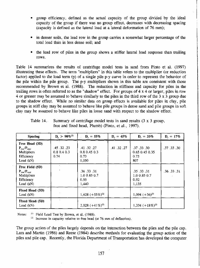
group efficiency, defined as the actual capacity of the group divided by the ideal capacity of the group if there was no group effect, decreases with decreasing spacing (capacity is defined as the lateral load at a lateral deformation of 76 rnrn);

in denser soils, the lead row in the group carries a somewhat larger percentage of the total load than in less dense soil; and

the lead row of piles in the group shows a stiffer lateral load response than trailing rows.

Table 14 summarizes the results of centrifuge model tests in sand from Pinto et al. (1997) illustrating these effects. The term "multipliers" in this table refers to the multiplier (or reduction factor) applied to the load term (p) of a single pile p-y curve in order to represent the behavior of the pile within the pile group. The p-y multipliers shown in this table are consistent with those recommended by Brown et al. (1988). The reduction in stiffness and capacity for piles in the trailing rows is often referred to as the "shadow" effect. For groups of 4 x 4 or larger, piles in row 4 or greater may be assumed to behave similarly to the piles in the third row of the 3 x 3 group due to the shadow effect. While no similar data on group effects is available for piles in clay, pile groups in stiff clay may be assumed to behave like pile groups in dense sand and pile groups in soft clay may be assumed to behave like piles in loose sand with respect to the shadow effect.

Table 14. Summary of centrifuge model tests in sand results (3 x 3 group, free and fixed head, Plumb) (Pinto, et al., 1997).

Notes: ( I ) Field Load Test by Brown, et al. (1988). "' Increase in capaoity relative to free head (at 76 mm of deflection).

The group action of the piles largely depends on the interaction between the piles and the pile cap. Lam and Martin (1986) and Reese (1984) describe methods for evaluating the group action of the piles and pile cap. Recently, the Florida Department of Transportation has developed the computer

Spacing

Free Head (3D) Prw/Pmta, Multipliers Efficiency Load (kN)

Free Field (5D) Prw/Ptota~ Multipliers Efficiency Load (kN)

Fixed Head (3D) Load (kN)

Fixed Head (SD) Load (kN)

D, > 90%")

.45 .32 .23 0.8 0.4 0.3 0.74

D, = 55%

-41 .32 .27 0.8 0.45 0.3 0.73 1,050

.36 .33 .31 1.0 0.85 0.7 0.95 1,440

1,628 (+55%)(')

2,028 (+41%)"'

D, = 17%

.37 .33 .30

2

.36 .33 .31

D, = 45%

.41 .32 .27

D, = 33%

.37 .33 .30 0.65 0.45 0.35 0.73 807

.35 .33 .31 1.0 0.85 0.7 0.92 1,135

1,094 (+36)(')

1,334 (+18%)("

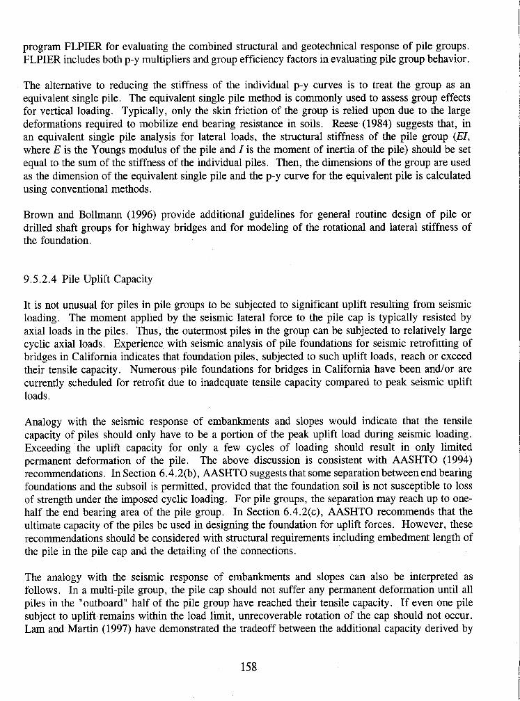
program FLPIER for evaluating the combined structural and geotechnical response of pile groups. FLPIER includes both p-y multipliers and group efficiency factors in evaluating pile group behavior.

The alternative to reducing the stiffness of the individual p-y curves is to treat the group as an equivalent single pile. The equivalent single pile method is commonly used to assess group effects for vertical loading. Typically, only the skin friction of the group is relied upon due to the large deformations required to mobilize end bearing resistance in soils. Reese (1984) suggests that, in an equivalent single pile analysis for lateral loads, the structural stiffness of the pile group (El, where E is the Youngs modulus of the pile and I is the moment of inertia of the pile) should be set equal to the sum of the stiffness of the individual piles. Then, the dimensions of the group are used as the dimension of the equivalent single pile and the p-y curve for the equivalent pile is calculated using conventional methods.

Brown and Bollmann (1996) provide additional guidelines for general routine design of pile or drilled shaft groups for highway bridges and for modeling of the rotational and lateral stiffness of the foundation.

9.5.2.4 Pile Uplift Capacity

It is not unusual for piles in pile groups to be subjected to significant uplift resulting from seismic loading. The moment applied by the seismic lateral force to the pile cap is typically resisted by axial loads in the piles. Thus, the outermost piles in the group can be subjected to relatively large cyclic axial loads. Experience with seismic analysis of pile foundations for seismic retrofitting of bridges in California indicates that foundation piles, subjected to such uplift loads, reach or exceed their tensile capacity. Numerous pile foundations for bridges in California have been andlor are currently scheduled for retrofit due to inadequate tensile capacity compared to peak seismic uplift loads.

Analogy with the seismic response of embankments and slopes would indicate that the tensile capacity of piles should only have to be a portion of the peak uplift load during seismic loading. Exceeding the uplift capacity for only a few cycles of loading should result in only limited permanent deformation of the pile. The above discussion is consistent with AASHTO (1994) recommendations. In Section 6.4.2(b), AASHTO suggests that some separation between end bearing foundations and the subsoil is permitted, provided that the foundation soil is not susceptible to loss of strength under the imposed cyclic loading. For pile groups, the separation may reach up to one- half the end bearing area of the pile group. In Section 6.4.2(c), AASHTO recommends that the ultimate capacity of the piles be used in designing the foundation for uplift forces. However, these recommendations should be considered with structural requirements including embedment length of the pile in the pile cap and the detailing of the connections.

The analogy with the seismic response of embankments and slopes can also be interpreted as follows. In a multi-pile group, the pile cap should not suffer any permanent deformation until all piles in the "outboard" half of the pile group have reached their tensile capacity. If even one pile subject to uplift remains within the load limit, unrecoverable rotation of the cap should not occur. Lam and Martin (1997) have demonstrated the tradeoff between the additional capacity derived by

allowing some of the piles in a group to yield in tension and the resulting permanent displacement of the pile caps. In general, permanent displacements are small provided at least one pile in the cap has not yielded.

The pile uplift capacity should be compared to uplift loads calculated using the peak seismic moment applied to the pile cap multiplied by a reduction factor. Based upon experience with seismic slope stability, a value of 0.5 may be reasonable for the reduction factor of the peak uplift load. Furthermore, in groups of four or more piles, at least two piles should reach their uplift capacity simultaneously before the foundation design is judged to be inadequate. However, current practice is to design the foundation so that none of the piles are subjected to a load in excess of their ultimate uplift capacity.

9.5.2.5 Liquefaction

Pile-supported structures have performed extremely well in areas subject to liquefaction in recent earthquakes. Notable examples include the performance of pile-supported container cranes at the Port of Oakland in the Loma Prieta earthquake of 1989 and the performance of pile-supported buildings on Port Island in the Kobe earthquake of 1995.

In many earthquakes where liquefaction occurs, the soil may not liquefy until the end of the earthquake. Therefore, piles in liquefied ground may still be able to rely on the vertical and lateral support of the soil in the potentially liquefied zone during the earthquake. However, due to uncertainties as to exactly when liquefaction will occur, it seems prudent to assign a reduced vertical and lateral resistance to potentially liquefiable soil surrounding a pile if the pile is expected to function as a load carrying member during and after an earthquake. Preliminary results by Dobry et al. (1996) suggests that the lateral resistance of a pile in liquefied ground is approximately 10 percent of the lateral resistance in non-liquefied ground. Therefore, if a pile foundation in potentially liquefiable soil is expected to carry lateral loads after the surrounding soil liquefies, batter piles may be required to provide adequate lateral support. If batter piles are used, the pile cap connections should be designed to sustain moment loads induced by lateral movements and the batter piles should be designed to sustain lateral loads due to soil settlement. Lateral spreading can also induce large loads on bridge abutments.

9.6 RETAINING STRUCTURES

9.6.1 General

Gravity earth retaining walls subjected to seismic loading have suffered large movements and extensive damage in earthquakes, even though the retaining structures had been designed with adequate factors of safety against static earth pressures. In some cases, this damage has been attributed to liquefaction. However, in some cases, the damage has been attributed to the increase in the magnitude of the lateral earth pressure during seismic events. Seed and Whitman (1970) have reported several cases of failure of gravity retaining walls in earthquakes by rotation about the wall- top as a result of the dynamic earth pressure. Descriptions of damage to gravity retaining structures

subjected to earthquakes are also given by Seed and Whitman (1970), Nazarian and Hadjian (1979), and others. Mechanically Stabilized Earth (MSE) walls, anchored walls, and soil-nailed walls have, in general, performed very well in earthquakes with no reports of significant damage.

Damage to retaining structures due to earthquakes can be classified using three main categories:

Damage to gravity retaining walls with saturated backfill: Damage of this type has been frequently reported for port and harbor structures such as quay walls. Seed and Whitman (1970) suggest that failure in quay walls from dynamic loads is primarily due to a combination of the increase in the lateral soil pressure behind the wall, a reduction in water pressure in front of the wall, and possibly liquefaction of the foundation soil. Liquefaction of retaining wall backfill created large lateral pressures that are believed to be responsible for outward movements of quay walls as great as 8 meters during recent earthquakes in Japan.

Damage to gravity retaining walls with unsaturated backfill: Fewer cases of failure of retaining walls with unsaturated backfill have been reported than for walls with saturated backfill. Jennings (1971) and Evans (1971) reported movements and failures in retaining walls and bridge abutments in the San Fernando earthquake. Ross et al. (1969) reported that as a result of the 1964 Alaskan earthquake, the flexible deck of a bridge structure buckled due to the movement of retaining walls in the abutments. Conventional gravity retaining walls supporting elevated portions of the Shinkansen ("bullet" train) track alignment failed in Kobe in the 1995 earthquake.

Damage to MSE walls, anchored walls, and soil-nailed walls: Tatsuoka, et al. (1995) report that mechanically stabilized earth walls (reinforced earth walls) along the same stretch of the alignment where conventional gravity walls failed performed very well in the 1995 Kobe earthquake. Mechanically stabilized earth walls also performed well in the 1989 Lorna Prieta earthquake. There have been no reports of serious damage to anchored walls in earthquakes. This includes several anchored walls in the epicentral region of the Northridge earthquake. Felio et al. (1990) report that eight soil-nailed walls in the San Francisco Bay area showed no signs of significant distress as a result of shaking during the Loma Prieta earthquake.

9.6.2 Seismic Evaluation of Retaining Structures

The seismic performance of earth retaining structures is most commonly evaluated using pseudo- static analysis, where the dynamic lateral earth force is estimated as a sum of the initial static earth force and the increment in activelpassive earth force due to the seismic loading. For some cases, alternative, displacement-based and stiffness-based approaches are also available. Generally, the displacement-based approach is used for gravity retaining walls and the stiffness method is used for restrained walls for bridge abutments.

Seismic design of gravity retaining walls is described in detail by Whitman (1990). The state of knowledge on seismic design of mechanically stabilized earth retaining walls is described by

Tatsuoka, et al. (1995) and Elias and Christopher (1996). The seismic design of soil-nailed walls is described in Byrne et al. (1997). In this section, only the basic elements of seismic design of retaining walls is presented. The readers are referred to the above mentioned references and other references cited herein for more detailed coverage on the topic.

9.6.2.1 Pseudo-Static Theory

The most commonly used method for seismic design of retaining structures is the pseudo-static method developed by Okabe (1926) and Mononobe (1929). The so-called Mononobe-Okabe method is based on Coulomb earth pressure theory. In developing their method, Mononobe and Okabe assumed the following:

the wall is free to move sufficiently to induce active earth pressure conditions;

the backfill is completely drained and cohesionless; and

the effect of earthquake motion is represented by a pseudo-static inertia force (k,Ws) and ( + kvW, or - kvWs), where W, is the weight of the sliding wedge, as shown in figure 73.

Figure 73. Forces behind a gravity wall in the Mononobe-Okabe theory.

Using Mononobe-Okabe theory, the dynamic earth pressure in the active and passive states is given by the following:

where: Y = H =

4 = 6 = i =

P = khg = kvg =

g =

D = [ l + [ sin ( 4 + 6 ) sin ( a - 0 - i ) cos (6 + p + 0) cos (i - p )

D J = [ l - [ sin ( 4 - 6 ) sin ( @ + i - 0 ' ) cos (6 - p + € I 1 ) cos ( i - j 3 )

0 ' = tan-' (kh/( l + k,))

unit weight of the backfill; height of the wall; angle of internal friction of the backfill; angle of friction of the wall/backfill interface; slope of the surface of the backfill; slope of the back of the wall; horizontal seismic coefficient; vertical seismic coefficient; and acceleration of gravity.

Figure 74, from Lam and Martin (1986), presents values for K, for values of 4 from 20 to 45 degrees for vertical walls with level backfill and a wall/backfill interface friction angle equal to @I, for horizontal seismic coefficients and vertical seismic coefficients (i.e., k,, and k,,) from 0 to 0.5 and from 0 to 0.2, respectively.

HORIZONTAL SEISMIC COEFFICIENT, kh

Figure 74. Effect of seismic coefficients and friction angle on seismic active pressure coefficient (Lam and Martin, 1986)

Besides determining the magnitude of the seismic earth pressure, the distribution of the seismic earth pressure or the location of the seismic earth pressure resultant is needed for analyses. Prakash and Basavanna (1969) show that, theoretically, the seismic component of the active earth pressure should act at one-third the height of the wall down from the top of the wall (i.e., two-thirds of the height above the base). Whitman (1990) states that observations of wall behavior and model test results indicate that the resultant of the seismic component of the active pressure acts at 0.6 times the height above the base. Lam and Martin (1986) suggests that, for practical purposes, it may be assumed that the total seismic active earth pressure is uniformly distributed over the height of the wall, meaning that the earth pressure resultant acts at the midheight of the wall. The Lam and Martin assumption appears appropriate for most highway problems.

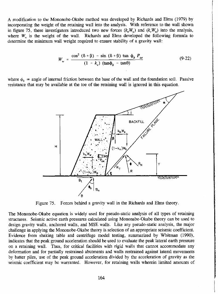
A modification to the Mononobe-Okabe method was developed by Richards and Elms (1979) by incorporating the weight of the retaining wall into the analysis. With reference to the wall shown in figure 75, these investigators introduced two new forces (k,W,,,) and (k,W,,,) into the analysis, where W, is the weight of the wall. Richards and Elms developed the following formula to determine the minimum wall weight required to ensure stability of a gravity wall:

c0s2 (8 + p) - sin (6 + p) tan @, P, ww = (1 - k") (tan@, - tan€))

where 4, = angle of internal friction between the base of the wall and the foundation soil. Passive resistance that may be available at the toe of the retaining wall is ignored in this equation.

'0

Figure 75. Forces behind a gravity wall in the Richards and Elms theory.

The Mononobe-Okabe equation is widely used for pseudo-static analysis of all types of retaining structures. Seismic active earth pressures calculated using Mononabe-Okabe theory can be used to design gravity walls, anchored walls, and MSE walls. Like any pseudo-static analysis, the major challenge in applying the Mononobe-Okabe theory is selection of an appropriate seismic coefficient. Evidence from shaking table and centrifuge model testing, summarized by Whitrnan (1990), indicates that the peak ground acceleration should be used to evaluate the peak lateral earth pressure on a retaining wall. Thus, for critical facilities with rigid walls that cannot accommodate any deformation and for partially restrained abutments and walls restrained against lateral movements by batter piles, use of the peak ground acceleration divided by the acceleration of gravity as the seismic coefficient may be warranted. However, for retaining walls wherein limited amounts of

seismic deformation are acceptable, as is the case for most highway systems, use of a seismic coefficient from between one-half to two-thirds of the peak horizontal ground acceleration divided by gravity would appear to provide a wall design that will limit deformations in the design earthquake to small values. Consistent with slope stability analyses, the vertical acceleration is usually ignored in practice in the design of retaining structures.

9.6.2.2 Displacement Approach

To circumvent the shortcomings associated with selection of an appropriate seismic coefficient, deformation-based analyses have been developed for design of gravity retaining walls. Several theories were developed to account for the displacement and rotation of walls during an earthquake. Richards and Elms (1979) extended the work of Franklin and Chang (1977) on seismic deformation of earth dams to gravity retaining walls. Richards and Elms proposed the following simplified formula for the displacement of a gravity wall.

where d is the displacement in inches, V is the peak velocity of the earthquake record in in./s, N is the peak seismic resistance coefficient sustainable by the wall before it slides (equal to the yield acceleration of the retaining wall divided by gravity), and A is the maximum acceleration of the earthquake record.

In the absence of information on the time history of velocity or displacement, the following values may be used:

V = 30 (A) (in./s) (9-24)

d = 0.3(A5/N4) (in.) (9-25)

When using the deformation approach, the retaining wall should also be checked for overturning using a pseudo-static analysis.

9.6.2.3 Stiffness Approach

Lam and Martin (1986) presents equations for incorporating the stiffness of abutment walls into a dynamic model of a bridge system. These investigators propose the following equations for the translational stiffness, K,, and the rotational stiffness, KO, of an integral abutment wall:

where H is the wall height, E, is the Young's modulus of the soil, and B is the width of the abutment wall. Equations 9-26 and 9-27 are used when the stiffness of the abutment wall is incorporated in the dynamic response analysis of the bridge structure.

The Young's modulus for the soil, E,, used in equations 9-26 and 9-27 can be evaluated using the equations in chapter 5. Use of strain-compatible Young's modulus values in equations 9-26 and 9-27 is recommended. The strain-compatible moduli values can be estimated from the shear strains calculated in site response analyses assuming that the reduction of Young's modulus follows the same modulus reduction curves as the shear modulus. If the results of a site response analysis are not available, strain-compatible Young's modulus may be evaluated using the same modulus reduction curves and assuming a shear strain level depending upon the magnitude of the earthquake, intensity of ground motion, and soil type. For events of magnitude 6.0 or less, and for ground motion intensities of 0.4 g or less, E, at a strain level of 0.1 percent may be used. For larger magnitudes and/or higher intensity earthquakes, a value of E, corresponding to a shear strain of 1 percent is recommended.

The location of the resultant force due to wall translation may be applied at 0.6 H from the base of the wall and the resultant force from wall rotation may be applied at 0.37 H from the base of the wall.

9.6.2.4 Mechanically-Stabilized Earth Walls and Soil-Nailed Walls

The seismic design of MSE and soil nailed walls is based on the Mononobe-Okabe method for evaluating external seismic stability. An internal seismic stability analysis is also performed as part of the design of these wall sysems. The internal stability analysis incorporates the effects of the inertial force generated by the reinforced soil volume on individual reinforcing elements during a seismic event as a pseudo-static horizontal load. The reinforcing elements must have sufficient length and cross-secional area to resist this additional horizontal load. These analyses are described in detail in Bathurst and Cai (1995), Elias and Christopher (1996), and Byrne, et al. (1997).

CHAPTER 10

REFERENCES

ABAM (1994), "Draft-Seismic Design Course," ABAM Engineers, Course Notes Prepared for the United States Department of Transportation, Federal Highway Administration, Central Federal Lands Highway Division, 28 December.

Abrahamson, N.A. and Silva. W. (1996), "Preliminary Attenuation Relations for Horizontal Response Spectra Including Data from the 1994 Northridge Earthquake," Draft Report to Brookhaven National Laboratory, New York.

Achilleos, E. (1988), "User Guide for PCSTABL 5M," Joint Informational Report JHRP-88/19, Indiana Department of Highways and Purdue University School of Civil Engineering, West Lafayette, Indiana, 132 p.

Algermissen, S.T., Perkins, D.M., Thenhaus, P.C., Hanson, S.L. and Bender, B.L. (1982), "Probabilistic Estimates of Maximum Acceleration and Velocity in Rock in the Contiguous United States, " United States Geological Survey, Open-File Report 82- 1033.

Algermissen, S.T., Perkins, D.M., Thenhaus, P.C., Hanson, S.L. and Bender, B.L. (1991), "Probabilistic Earthquake Acceleration and Velocity Maps for the United States and Puerto Rico," United States Geological Survey, Miscellaneous Field Studies Map MF-2120.

AASHTO (1994), "Standard Specifications for Highway Bridges, " 16th Edition, American Association of State Highway and Transportation Officials, Washington, D.C.

ASTM (1994), "Annual Book of ASTM Standards, Section 4, Construction," American Society for Testing and Materials, Philadelphia, Pennsylvania, 978 p.

Arango, I. (1996), "Magnitude Scaling Factors for Soil Liquefaction Evaluations," Journal of Geotechnical Engineering, ASCE, Vol. 122, No. 11, pp. 929-936.

Arias, A. (1969), "A Measure of Earthquake Intensity, " In: Seismic Design for Nuclear Power Plants, R. Hansen, Editor, Massachusetts Institute of Technology Press, Cambridge, Massachusetts.

ATC (1978), "Tentative Provisions for the Development of Seismic Regulations for Buildings," Report ATC 3-06, Applied Technology Council, San Francisco, California.

ATC (1 994), "Seminar on New Developments in Earthquake Ground Motion Estimation and Implications for Engineering Design Practice, " Applied Technology Council, ATC 35-1, Redwood City, California.

Atkinson, G. M. and Boore, D. M. (1990), "Recent Trends in Ground Motion and Spectral Response Relations for North America," Earthquake Spectra, Vol. 6, No. 1, pp. 15-35.

Atkinson, G. M. and Boore, D .M. (1995), "Ground-Motion Relations for Eastern North America, " Bulletin of the Seismological Society of America, Vol. 85, No. 1, pp. 17-30.

Ballard, R.F., Jr. (1964), "Determination of Soil Shear Moduli at Depth by In Situ Vibratory Techniques, " Miscellaneous Paper No. 4-691, U. S. Army Waterways Experiment Station, Vicksburg, MS, USA.

Bardet, J. P. (1992), "LINOS , a Nonlinear Finite Element Program for Geomechanics and Geotechnical Engineering, "User's Manual, Research Center for Computational Geomechanics, University of Southern California, Los Angeles, 145 p.

Barker, R.M., Duncan, J.M., Rojiani, K.B., Ooi, P.S.K., Tan, C.K. and Kim, S.G. (1991), "Manuals for the Design of Bridge Foundations," NCHRP Report No. 343, 308 p.

Bathurst, R.J. and Cai, Z. (1995), "Pseudo-Static Seismic Analysis of Geosynthetic-Reinforced Sequential Retaining Walls," Geosynthetics International, Vol. 2, No. 5, pp. 787-830.

Bolt, B.A. (1973), "Duration of Strong Ground Motion," Proc. 5th World Conference on Earthquake Engineering, Rome, Italy.

Bonilla, M.G., Mark, R.K., and Lienkaemper, J. J. (1984), "Statistical Relations Among Earthquake Magnitude, Surface Rupture Length and Surface Fault Displacement," Journal of Geophysical Research, Vol. 74, Vol. B6, pp. 2379-241 1.

Boore, D.M. and Atkinson, G.M. (1987), "Prediction of Ground Motion and Spectral Response Parameters at Hard-Rock Sites in Eastern North America," Bulletin of the Seismological Society of America, Vol. 77, No. 2, pp. 440-467.

Boore, D.M. and Joyner, W.B. (1991), "Estimation of Ground Motion at Deep-Soil Sites in Eastern North America, " Bulletin of the Seismological Society of America. Vol. 81, No. 6, pp. 2167-21 85.

Boore, D.M., Joyner, W .B. and Fumal, T.E. (1993), "Estimation of Response Spectra and Peak Accelerations From Western North America Earthquakes: An Interim Report," United States Geological Survey, Open File Report 93-509.

Boore, D.M. and Joyner, W .B. (1994), "Prediction of Ground Motion in North America, " Proc. Seminar on New Developments in Earthquake Ground Motion Estimation and Implication for Engineering Design Practice, Applied Technology Council Publication No. ATC 35- 1, Redwood City, California, pp. 6-1 - 6-41.

Borcherdt, R. D. (1994), "New Developments in Estimating Site Response Effects on Ground Motion," Proc. Seminar on New Developments in Earthquake Ground Motion Estimation and Implications for Engineering Design Practice, Applied Technology Council, ATC 35-1, Redwood City, California, pp. 10-1 - 10-44.

Borden, R.H., Shao. L., and Gupta, A. (1996), "Dynamic Properties of Piedmont Residual Soils, " Journal of Geotechnical Engineering, ASCE, Vol. 122, No. 10, pp. 813-821.

Bowles, J. E. (1988), "Foundation Analyses and Design, " 4th Edition, McGraw-Hill Book Company, New York, 1004 p.

Bray, J.D., Augello, A.J., Leonards, G.A., Repetto, P.C. and Byrne, R.J. (1995), "Seismic Stability Procedures for Solid-Waste Landfills," Journal of Geotechnical Engineering, ASCE, Vol. 121, No. 2, pp. 139-151.

Broms, B.B. and Hansson, 0 . (1984), "Deep Compaction with the Vibro-Wing Method, " Ground Engineering, Vol. 17, No. 5.

Brown, D.A., Morrison, C., and Reese, L.C. (1988), "Lateral Load Behavior of a Pile Group in Sand, " Journal of Geotechnical Engineering, ASCE, Vol. 114, No. 11, pp. 1261-1276.

Brown, D. and Bollmann, H.T. (1996), "Pile Group Design for Lateral Loading using COM624," Proc. The Design of Bridges for Extreme Events, Atlanta, Georgia, pp. 1-46.

Bryant, L.M. and Matlock, H. (1977), "Three Dimensional Analysis of Framed Structures with Nonlinear Pile Foundations," Proc. 9th Annual Offshore Technology Conference, Houston, Texas, Paper No. 2955.

Byrne, R.J., Cotton, D., Porterfield, J., Wolschlag, C., and Veblacker, G. (1997), "Manual for Design and Construction Monitoring of Soil Nail Walls, " Report No. FHWA-SA-96-069, U.S. Department of Transportation, Federal Highway Administration, Washington, District of Columbia, 468 p.

Campbell, K. W., and Duke, C.M. (1974), "Bedrock Intensity, Attenuation, and Site Factors from San Fernando Earthquake Records, " Bulletin of the Seismological Society of America, Vol. 64, NO. 1, pp. 173-185.

Campbell, K. W. (1985), "Strong Motion Attenuation Relations: a Ten-Year Perspective, " Earthquake Spectra, Vol. 1, No. 4, pp. 759-804.

Campbell, K.W. (1989), "Empirical Prediction of Near-Source Ground Motion for the Diablo Canyon Power Plant Site, San Luis Obispo County, California," United States Geological Survey, Open-File Report 89-484.

Campbell, K. W. (1990), "Empirical Prediction of Near-Source Soil and Soft-Rock Ground Motion for the Diablo Canyon Power Plant Site, San Luis Obispo County, California," Dames & Moore, Report Prepared for Lawrence Livermore National Laboratory, Evergreen, Colorado.

Campbell, K. W. (1 993), "Empirical Prediction of Near-Source Ground Motion From Large Earthquakes," Proc. International Workshop on Earthquake Hazard and Large Dams in the Himalaya, Sponsored by the Indian National Trust for Art and Cultural Heritage (INTACH), New Delhi, India, January 15- 16.

Campbell, K.W. and Bozorgnia, Y. (1994), "Near Source Attenuation of Peak Horizontal Acceleration From Worldwide Accelerographs Recorded From 1957 to 1993, " Proc. 5th U. S . National Conference on Earthquake Engineering, Chicago, Illinois, Vol. 3, pp. 283-292.

Carpenter, J.R. (1985), "PCSTABLA User Manual," Joint Highway Research Project No. JHRP-85-7, School of Civil Engineering, Purdue University, West Lafayette, Indiana.

CDMG (1986), "Guidelines for Evaluating the Hazard of Surface Fault Rupture," Technical Note 49, California Division of Mines and Geology, Sacramento, California, 2 p.

CDMG (1975), "Recommended Guidelines for Determining the Maximum Credible and the Maximum Probable Earthquakes, " Technical Note No. 43, California Division of Mines and Geology, Sacramento, California, 1 p.

CDMG (1995), "The Northridge, California Earthquake of 17 January 1994, " Mary C. Woods and W. Ray Seiple Editors, California Division of Mines and Geology Special Publication 116, Sacramento, California.

Chang, C.-Y., Mok, C.M., Power, M.S. and Tang, Y.K. (1991), "Analysis of Ground Response Data at Lotung Large Scale Soil-Structure Interaction Experiment Site," Report No. NP-7306-SL, Electric Power Research Institute, Palo Alto, California.

Cluff, L.S, Hansen, W.R., Taylor, C.L., Weaver, K.D., Brogan, G.E., Idriss, I.M., McClure, F.E. and Blayney, J.A. (1972), "Site Evaluation in Seismically Active Regions - An Interdisciplinary Team Approach," Proc. International Conference on Microzonation for Safety Construction, Research and Application, Seattle, Washington, Vol. 2, p. 9-57 - 9-87.

Cohee, B.P., Somerville, P.G. and Abrahamson, N .A. (1991), "Simulated Ground Motions for Hypothesized M, = 8 Subduction Earthquakes in Washington and Oregon," Bulletin of the Seismological Society of America, Vol. 8 1, No. 1, pp. 28-56.

Cundall, P. A. and Board, M. (1988), "A Microcomputer Program for Modelling Large-Strain Plasticity Problems, " In: Numerical Methods in Geomechanics, C. Swoboda, Ed., A. A. Balkema, Rotterdam, The Netherlands, pp. 2101-2108.

D'Appolonia, E. (1970), "Dynamic Loadings," Journal of the Soil Mechanics and Foundations Division, ASCE, Vol. 96, No. SM1.

dePolo . C . M . and Slernmons, D .B. (1990), "Estimation of Earthquake Size for Seismic Hazards, " Krinitzsky , E.L. and Slemrnons. D .B., Neotectonics in Earthquake Evaluation, Chapter 1, Geological Society of America, Vol. 8.

Dobry , R., Idriss, I.M. and Ng, E. (1978), "Duration Characteristics of Horizontal Components of Strong-Motion Earthquake Records," Bulletin of the Seismological Society of America, Vol. 68, No. 5, pp. 1487-1520.

Dobry, R., Powell, D. J., Yokel, F.Y. and Ladd, R.S. (1980), "Liquefaction Potential of Saturated Sand - The Stiffness Method, " Proc. 7th World Conference on Earthquake Engineering, Istanbul, Turkey, Vol. 3, pp. 25-32.

Dobry , R., Abdoun, T., and O'Rourke, T. D. (1996), "Evaluation of Pile Response to Liquefaction- Induced Lateral Spreading of the Ground," Proc. 4th CALTRANS Seismic Research Workshop, Sacramento, California, 10 p.

Douglas, B. J., and Olsen, R. S. (1981), "Soil Classification Using Electric Cone Penetrometer, " Symposium on Cone Penetration Testing and Experience, ASCE National Convention, St. Louis, Missouri, pp. 209-227.

Duncan, J. M. (1992), "State-of-the-Art: Static Stability and Deformation Analysis," Proc. Stability and Performance of Slopes and Embankments - 11, Vol. 1, pp. 222-266.

EERI (1989), "Loma Prieta Earthquake, October 17, 1989, " Preliminary Reconnaissance Report, Earthquake Engineering Research Institute, Oakland, California, 5 1 p.

EERI ( 1995), "The Hyogo-Ken Nanbu Earthquake, January 17, 1995, " Preliminary Reconnaissance Report, Earthquake Engineering Research Institute, Oakland, California, 116 p.

Elias, V. and Christopher, B. R. (1996), "Mechanically Stabilized Earth Walls and Reinforced Soil Slopes, Design and Construction Guidelines," Report No. FHWA-SA-96-071, U.S. Department of Transportation, Federal Highway Administration, Washington, D . C.

EPRI (1986), "Seismic Hazard Methodology for the Central and Eastern United States, " EPRI Report NP-4726, (10 Volumes), Electric Power Research Institute, Palo Alto, California.

Evans, G.L. (1971), "The Behavior of Bridges Under Earthquakes, " Proc. New Zealand Reading Symposium, Vol. 2.

Felio, G.Y., Vucetic, H., Hudson, M., Bara, P., and Chapman, R. (1990), "Performance of Soil Nailed Walls During the October 17, 1989 Loma Prieta Earthquake," Proc. of the 43rd Canadian Geotechnical Conference, Quebec, Canada, pp. 165- 173.

Finn, L. W .D., Yogendrakumar, M., Yoshida, N. and Yoshida, H. (1986), "TARA-3: A Program for Nonlinear Static and Dynamic Effective Stress Analysis," Department of Civil Engineering, University of British Columbia, Vancouver, British Columbia, Canada.

Franklin, A.G. and Chang, F.K. (1977), "Earthquake Resistance of Earth and Rock-Fill Dams, " Report 5: Permanent Displacement of Earth Embankments by Newmark Sliding Block Analysis, Misc. Paper 5-7 1-17, Soils and Pavements Laboratory, US Army Engineer Waterways Experiment Station, Vicksburg, Mississippi.

Gasparin, D.A. and Vanrnarcke, E.H. (1976), "SIMQKE - A Program for Artificial Motion Generation, " Department of Civil Engineering, Massachusetts Institute of Technology, Cambridge, Massachusetts.

Geomatrix (1991), "Seismic Ground Motion Study for West San Francisco Bay Bridge," Draft Report to CALTRANS, Division of Structures, Sacramento, California, March (note in February 1993: this report has been completed and was issued in final form in December, 1992).

Geomatrix (1995), "Adjustments to Rock Response Spectra for CALTRANS Toll Bridges in Northern California, " Report to CALTRANS, Division of Structures, Sacramento, California.

Gere, J.M., and Shah, H.C. (1984), "Terra Non Firma, " Stanford Alumni Association, Stanford, California.

Gutenberg, B . and Richter, C . F . (1 942), "Earthquake Magnitude, Intensity, Energy, and Acceleration, " Seismological Society of America Bulletin, Vol. 32, pp. 163-191.

Hadj-Hamou, T. and Elton, D.J. (1988), "A Liquefaction Potential Map for Charleston, South Carolina, " Report No. GT-88-1, Tulane University, New Orleans, Louisiana, 67 p.

Hamada, M. Towhata, I. , Yasuda S. and Isoyama, R. (1987), "Study on Permanent Ground Displacements Induced by Seismic Liquefaction," Computers and Geomechanics Vol. 4, pp. 197-220.

Hanks, T.C. and Kanamori, H. (1979), "A Moment Magnitude Scale, " Journal of Geophysical Research, Vol. 84, No. B8, pp. 2348-2350.

Hannigan, P.J., Goble, G.G., Thendean, G., Likins, G.E. and Raushe, F. (1996), "Design and Construction of Driven Pile Foundations, " Workshop Manual, NHI Course Nos. 13221 and 13222, U.S. Department of Transportation, Federal Highway Administration, Office of Technology Applications, Washington, District of Columbia.

Hansen, B . (1953), "Earth Pressure Calculations, " Teknisk Forlag, Copenhagen.

Harder, L.F. and Seed, H.B. (1986), "Determination of Penetration Resistance for Coarse-Grained Soils Using the Becker Hammer Drill," Report No. UCBIEERC-86/06, Earthquake Engineering Research Center, University of California at Berkeley, California.

Harder, L.F., Jr. (1988)*, "Use of Penetration Tests to Determine the Cyclic Loading Resistance of Gravelly Soils During Earthquake Shaking," Ph.D. Dissertation, University of California, Berkeley, California.

Harder, L. F., Jr . (199 I), "Performance of Earth Dams During the Loma Prieta Earthquake, " Proc. Second International Conference on Recent Advances in Geotechnical Earthquake Engineering and Soil Dynamics, University of Missouri, Rolla, pp. 1 1-15.

Hardin, B.O. and Drnevich, V. (1972), "Shear Modulus and Damping in Soils: Design Equations and Curves," Journal of the Soil Mechanics and Foundation Division, ASCE, Vol. 98, No. SM7, pp. 667-692.

Hardin, B. 0 . (1978), "The Nature of Stress-Strain Behavior of Soils, " Proc. Earthquake Engineering and Soil Dynamics, ASCE, Pasadena, California, Vol. 1, pp. 3-89.

Hart, E. W. (1980), "Fault-Rupture Hazard Zones in California, " Alquist-Priolo Special Studies Zones Act of 1972 with index to Special Studies Zones Maps. In: California Divison of Mines and Geology Special Publication 42 (Revised edition), 24 p .

Heaton, T.H., Tajima, F. and Mori, A. W. (1986), "Estimating Ground Motions Using Recorded Accelerograms, " Surveys in Geophysics, Vol. 8, pp. 23-83.

Hudson, M., Idriss, I. M. and Beikae, M. (1994)*, "QUAD4M - A Computer Program to Evaluate the Seismic Response of Soil Structures using Finite Element Procedures and Incorporating a Compliant Base," User's Manual, Center for Geotechnical Modeling, Department of Civil and Environmental Engineering, University of California, Davis, California, 27 p . (plus Appendices).

Husid, R.L. (1969), "Analisis de Terremotos: Analisis General," Revista del IDEM, No. 8, Santiago, Chile, pp. 2 1-42.

Hwang, H. and Lee, C.S. (1992), "Evaluation of Liquefaction Potential in Memphis Area, USA, " Proc. 10th World Conference on Earthquake Engineering, pp. 1457- 1460.

Hynes, M. E. and Franklin, A. G. (1984), "Rationalizing the Seismic Coefficient Method, " Miscellaneous Paper GL-84- 13, U. S. Army Engineer Waterways Experiment Station, Vicksburg, Mississippi, 34 p.

Hynes, M. E. (1 988)*, "Pore Pressure Generation Characteristics of Gravel Under Undrained Cyclic Loading, " Ph. D . Dissertation, University of California, Berkeley, California.

Idriss, I.M., Lysmer, J., Hwang, R. and Seed, H.B. (1973), "QUAD4 - A Computer Program for Evaluating the Seismic Response of Soil Structures by Variable Damping Finite Element Procedures, " Report No. EERC 73- 16, Earthquake Engineering Research Center, University of California, Berkeley, California, 67 p.

* Available through University Microfilms International, (800) 521-0600, Ext. 3879.

Idriss, I. M. (1990), "Response of Soft Soil Sites During Earthquakes, " Proc. Memorial Symposium to Honor Professor H . B . Seed, Berkeley, California.

Idriss, I.M. and Sun, J.I. (1992)*, "User's Manual for SHAKE91," Center for Geotechnical Modeling, Department of Civil and Environmental Engineering, University of California, Davis, California, 13 p. (plus Appendices).

Idriss, I. M. (1993), "Procedures for Selecting Earthquake Ground Motions at Rock Sites, " National Institute of Standards and Technology, NIST GCR 93-625, 7 p.

Idriss , I. M . (1995), "An Overview of Earthquake Ground Motions Pertinent to Seismic Zonation, " Proc. 5th International Conference on Seismic Zonation, Nice, France, Vol. 3, pp. 1-16.

Imai, T. and Tonouchi, K. (1982), "Correlation of N-Value with S-Wave Velocity and Shear Modulus, " Proc. 2nd European Symposium on Penetration Testing, Amsterdam, The Netherlands, pp. 67-72.

Ishibashi, I. and Sherif, M. A. (1974), "Soil Liquefaction by Torsional Simple Shear Device, " Journal of the Geotechnical Engineering Division, ASCE, Vol. 100, No. GT 8, pp. 871-888.

Ishihara, K. (1 985), "Stability on Natural Deposits During Earthquakes, " Proc. 1 1 th International Conference on Soil Mechanics and Foundation Engineering, San Francisco, California, Vol. 1, pp. 321-376 (Please order from A.A. Balkema, Old Post Road, Brookfield, Vermont 05036, Tel. (802) 276-3 162, fax (802) 276-3837, Price $995).

Ishihara, K. (1986), "Evaluation of Soil Properties for Use in Earthquake Response Analysis," In: Geomechanical Modelling in Engineering Practice, R. Dungar and J. A. Studer, Eds., A. A. Balkema, Rotterdam, the Netherlands, 241 - 275.

Ishihara, K., Kokusho, T. and Silver, M.L. (1989), "Recent Developments in Evaluating Liquefaction Characteristics of Local Soils," State-of-the-Art Report, Proc. 12th International Conference on Soil Mechanics and Foundation Engineering, Rio de Janeiro, Brazil, Vol. 4, pp. 2719-2734.

Ishihara (1 993), "Liquefaction and Flow Failure During Earthquakes, " GCotechnique, Vol. 43, No. 3., pp. 351-415.

Iwasaki, T., Tatsuoka, F. and Takagi, Y. (1978), "Shear Moduli of Sands Under Cyclic Torsional Shear Loadings, " Soils and Foundations, JSSMFE, Vol. 18, No. 1, pp. 39-56.

Jackura, K.A. (1992), "CALTRANS Procedures for Development of Site-Specific Acceleration Response Spectra," California Department of Transportation, Office of Geotechnical Engineering, Sacramento, California, 18 p.

* Available through NISEE / Computer Applications, (510) 642-51 13.

Jamiolkowski, M., Leroueil, S. and Lo Presti, D.C .F. (1991), "Theme Lecture: Design Parameters from Theory to Practice, " Proc. Geo-Coast '91, Yokohama, Japan, pp. 1-41.

Jennings, C . P . (1 97 I), "Engineering Features of San Fernando Earthquake, February 197 1, " Report of Earthquake Engineering Research Laboratory, California Institute of Technology, Pasadena, California.

Jennings, P. C . , Housner, R. W. and Tsai, N. C . (1968), "Simulated Earthquake Motions, " Research Report, Earthquake Engineering Research Laboratory, California Institute of Technology, Pasadena, California.

Jennings, C.W. (1994), "An Explanatory Text to Accompany the Fault Activity Map of California and Adjacent Areas," California Department of Conservation, Division of Mines and Geology, Sacramento, California, 92 p.

Jibson, R. W. (1985)*, "Landslides Caused by the 181 1-12 New Madrid Earthquakes, " Ph.D. Dissertation, Stanford, California, Stanford University, 234 p.

Jibson, R. W. (1993), "Predicting Earthquake-Induced Landslide Displacements Using Newmark's Sliding Block Analysis, " Transportation Research Record 141 1, Transportation Research Board, National Research Council, Washington, D.C., pp. 9-17.

Johnston, A.C. and Nava, S. J. (1994), "Seismic Hazard Assessment in the Central United States, " Proc. Seminar on New Developments in Earthquake Ground Motion Estimation and Implications for Engineering Design Practice, Applied Technology Council, AT C35-1, Redwood City, California, pp. 2-1 - 2-12.

Jones, R. (1962), "Surface Wave Technique for Measuring Elastic Properties and Thickness of Roads: Theoretical Development, " British Journal of Applied Physics, Vol. 13, pp. 21 -29.

Joyner, W .B. and Boore, D . M. (1988), "Measurement, Characterization, and Prediction of Strong Ground Motion. " In: Von Thun, J.L., Ed., Earthquake Engineering and Soil Dynamics 11, Recent Advances in Ground Motion Evaluation, ASCE Geotechnical Special Publication No. 20, pp. 43-102.

Kavazanjian, E., Jr., Echezuria, H. and McCann, M.W. (1985a), "RMS Acceleration Hazard for San Francisco, " Soil Dynamics and Earthquake Engineering, Vol. 4, No. 3, pp. 106-123.

Kavazanjian, E. Jr., Roth, R.A. and Echezuria, H. (1985b), "Liquefaction Potential Mapping for San Francisco, " Journal of Geotechnical Engineering, ASCE, Vol. 11 1, No. 1, pp. 54-76.

Kavazanjian, E., Jr., Snow, M.S., MatasoviC, N., Poran, C. and Satoh, T. (1994), "Non-Intrusive Rayleigh Wave Investigations at Solid Waste Landfills," Proc. 1st International Congress on Environmental Geotechnics, Edmonton, Alberta, pp. 707-7 12.

* Available through University Microfilms International, (800) 521-0600, Ext. 3879.

Kondner, R. L. and Zelasko, J. S. (1963), "A Hyperbolic Stress-Strain Formulation of Sands, " Proc. 2nd Pan American Conference on Soil Mechanics and Foundation Engineering, Sao Paulo, Brazil, pp. 289-324.

Kramer, S . L. (1996), "Geotechnical Earthquake Engineering, " Prentice-Hall, Inc., Upper Saddle River, New Jersey, 653 p.

Kramer , S . L. and Holtz, R. D . (1 99 I), "Soil Improvement and Foundation Remediation with Emphasis on Seismic Hazards," A Report of a Workshop Sponsored by the National Science Foundation, University of Washington, Seattle, Washington.

Krinitzsky , E. L. , Gould, J. P. and Edinger, P.H. (1993), "Fundamentals of Earthquake-Resistant Construction, " John Wiley & Sons, New York, New York.

Lam, I.P. and Martin, G.R. (1986), "Seismic Design of Highway Bridge Foundations - Vol. 11. Design Procedures and Guidelines, " Report No. FHWAIRD-86- 102, U. S. Department of Transportation, Federal Highway Administration, McLean, Virginia, 167 p.

Lam, I.P. and Martin, G.R. (1997), "Current Developments in Seismic Design of Bridge Foundations," Proc. Transportation Research Board 76th Annual Meeting, Session No. 236, Washington, District of Columbia, 21 p.

Lee, M.K. W. and Finn, W .D.L. (1978), "DESRA-2, Dynamic Effective Stress Response Analysis of Soil Deposits with Energy Transmitting Boundary Including Assessment of Liquefaction Potential," Soil Mechanics Series No. 36, Department of Civil Engineering, University of British Columbia, Vancouver, Canada, 60 p.

Leeds, D . L. (1 992), " State-of-the-Art for Assessing Earthquake Hazards in the United States: Report 28, Recommended Accelerograrns for Earthquake Ground Motions," Misc. Paper S-73- 1, Geotechnical Laboratory, U. S . Army Waterways Experiment Station, Vicksburg , Mississippi, 17 1 p. (plus Appendices).

Liao, S. S.C. and Whitman, R.V. (1986), "Overburden Correction Factors for SPT in Sand, " Journal of Geotechnical Engineering, ASCE, Vol. 112, No. 3, pp. 373-377.

Li, X.S., Wang, Z.L. and Shen, C.K. (1992), "SUMDES - A Nonlinear Procedure for Response Analysis of Horizontally-Layered Sites Subjected to Multi-Directional Earthquake Loading," Department of Civil Engineering, University of California, Davis, California.

Lin, S.J. and Whitman, R.V. (1986), "Earthquake Induced Displacements of Sliding Blocks," Journal of Geotechnical Engineering, ASCE, Vol. 112, No. 1, pp. 44-59.

Lysmer, J., Udaka, T. , Tsai, C . F. and Seed, H .B. (1 975), "FLUSH - A Computer Program for Approximate 3-D Analysis of Soil-Structure Interaction Problems," Report No. EERC-75/30, Earthquake Engineering Research Center, University of California, Berkeley.

Makdisi, F .I. and Seed, H. B. (1978), "Simplified Procedure for Estimating Dam and Embankment Earthquake-Induced Deformations," Journal of the Geotechnical Engineering Division, ASCE Vol. 104, No. GT7, pp. 849-867.

Marcuson, W. F., I11 and Bieganousky , W. A. (1977), "Laboratory Standard Penetration Tests on Fine Sands," Journal of the Geotechnical Engineering Division, ASCE, Vol. 103, No. GT6, pp. 565-588.

Marcuson, W.F., I11 (1981), "Earth Dams and Stability of Slopes Under Dynamic Loads," Moderators Report, Proc. 1st International Conference on Recent Advances in Geotechnical Earthquake Engineering and Soil Dynamics, St. Louis, Missouri, Vol. 3, pp. 1175.

Marcuson, W. F., 111, Hynes, M. E. and Franklin, A. G. (1990), "Evaluation and Use of Residual Strength in Seismic Safety Analysis of Embankments," Earthquake Spectra, Vol. 6, No. 3, pp. 529-572.

Martin, G.R. (1992), "Evaluation of Soil Properties for Seismic Stability Analysis of Slopes," In: Stability and Performance of Slopes and Enhancements 11, Geotechnical Special Publication No. 31, ASCE, Vol. 1, pp. 116-142.

Martin, G.R., and Lam, I.P. (1995), "Seismic Design of Pile Foundations: Structural and Geotechnical Issues," State of the Art (SOA4), Proc. 3rd International Conference on Recent Advances in Geotechnical Earthquake Engineering and Soil Dynamics, St. Louis, Missouri, Vol. 3, pp. 1491-1515.

Martin. P.P. (1975)*, " Non-Linear Methods for Dynamic Analysis of Ground Response, " Ph. D. Thesis, University of California, Berkeley.

Masing, G. (1 926), " Eigenspannungen und Verfestigung beim Messing, " Proc. 2nd International Congress on Applied Mechanics, Zurich, Switzerland, 332-335.

MatasoviC, N. and Vucetic, M. (1993), "Cyclic Characterization of Liquefiable Sands, " Journal of Geotechnical Engineering, ASCE, Vol. 1 19, No. 1 1, pp. 1805-1822.

MatasoviC, N. (1993)*, "Seismic Response of Composite Horizontally-Layered Soil Deposits, " Ph.D. Dissertation, Civil and Environmental Engineering Department, University of California, Los Angeles, 452 p.

MatasoviC, N., Kavazanjian, E. Jr., and Yan, L. (1997), "Newmark Deformation Anaylsis with Degrading Yield Acceleration, " Proc. Geosynthetic '97, Long Beach, California, Vol. 2, pp. 989-1000.

Mayne, P. W. and Rix, G. J. (1993), "G,,,-q, Relationships for Clays, " Geotechnical Testing Journal, ASTM, Vol. 16, No. 1, pp. 54-60.

* Available through University Microtilms International, (800) 521-0600, Ext. 3879.

McGuire, R.K., Toro, G.R. and Silva, W.J. (1988), "Engineering Model of Earthquake Ground Motion for Eastern North America, " Technical Report NP-6074, Electric Power Research Institute, Palo Alto, California.

McVay, M.C., Casper, R., and Shang, T. (1995), "Lateral Response of Three-Row Groups in Loose to Dense Sands at 3D and 5D Pile Spacing," Journal of Geotechnical Engineering, ASCE, Vol. 121, No. 5, pp. 436-441.

Meigh, A.C. (1987), "Cone Penetration Testing: Methods and Interpretation," CIRIA Ground Engineering Report: In Situ Testing, Butterworths, 141 p.

Mknard, L. and Broise, Y. (1975), "Theoretical and Practical Aspects of Dynamic Consolidation," Geotichnique, Vol. 15, No. 1.

Meyerhof, G. G. (1953), "The Bearing Capacity of Foundations under Eccentric Loads, " Proc. 3rd International Conference on Soil Mechanics and Foundation Engineering, Vol. 1, pp. 440-445.

Meyerhof, G. G. (1 956), "Penetration Tests and Bearing Capacity of Cohesionless Soils, " Journal of the Soil Mechanics and Foundations Division, ASCE, Vol. 82, SM1, pp. 1-19.

Mitchell, J. K. (198 I), "Soil Improvement: State of the Art, " Proc. 10th International Conference on Soil Mechanics and Foundation Engineering, Vol. 4, pp. 509-565.

Mononobe, N. (1929), "Earthquake-Proof Construction of Masonary Dams, " Proc. World Engineering Conference, Vol. 9, p. 275.

Moriwaki, Y., Tan, P. and Somerville, P. (1994), "Some Recent Site-Specific Ground Motion Evaluations - Southern California Examples and Selected Issues," Proc. Seminar on New Developments in Earthquake Ground Motion Estimation and Implication for Engineering Design Practice, Applied Technology Council ATC 35-1, Redwood City, California, pp. 14-1 - 14-25.

Morrison, A. (1982), "The Booming Business in Wick Drains," Civil Engineering, ASCE, Vol. 53, No. 3.

Mualchin, L. and Jones, A. L. (1992), "Peak Acceleration From Maximum Credible Earthquakes in California (Rock and Stiff Soil Sites)," California Department of Conservation, Division of Mines and Geology, Open-File Report 92- 1, Sacramento, California (updated in 1995 by L. Mualchin).

Muraleetharan, K.K., Mish, K. D . , Yogachandran, C. and Arulanandan, K. (199 I), "User's Manual for DYSAC2: Dynamic Soil Analysis Code for 2-Dimensional Problems," Research Report, Department of Civil Engineering, University of California, Davis, California.

Naeim, F. and Anderson, J. C. (1993), "Classification and Evaluation of Earthquake Records for Design," Report No. CE 93-08, Department of Civil Engineering, University of Southern California, Los Angeles, 288 p.

Nataraja, M.S. and Cook, B.E. (1983), "Increase in SPT N-Values Due to Displacement Piles, " Technical Note, Journal of the Geotechnical Engineering Division, ASCE, Vol. 109, No. 1, pp. 108-113.

NAVFAC (1986), "Foundations and Earth Structures, " Design Manual DM 7.02, Naval Facilities Engineering Command, Department of the Navy, Alexandria, Virginia.

Nazarian, H. N. and Hadjian, A.H. (1979), "Earthquake-Induced Lateral Soil Pressures on Structures," Journal of the Geotechnical Engineering Division, ASCE, Vol. 105, No. GT9, pp. 1049-1066.

Nazarian, S. and Stokoe, K.H. I1 (1984), "In Situ Shear Wave Velocities from Spectral Analysis of Surface Waves," Proc. 8th World Conference on Earthquake Engineering, San Francisco, California, Vol. 3, pp. 31-38.

NEHRP (1 99 I), " NEHRP Recommended Provisions for the Development of Seismic Regulations for New Buildings, " Part 1 : Provisions, Building Seismic Safety Council, Washington, District of Columbia, 199 p.

Newmark, N. M. (1965), "Effects of Earthquakes on Dams and Embankments, " Gebtechnique, Vol. 15, NO. 2, pp. 139-160.

Nigam, N .C. and Jennings, P.C. (1968)*, "SPECEQIUQ - Digital Calculation of Response Spectra from Strong-Motion Earthquake Records," CALTECH, Earthquake Engineering Research Laboratory, Pasadena, California, 65 p. (plus Appendix).

NRC (1985), "Liquefaction of Soils During Earthquakes," National Research Council, Committee on Earthquake Engineering, Washington, District of Columbia.

Nuttli, 0. W. (1974), "Seismic Hazard of the Rocky Mountains, " Preprint 2195, ASCE, National Structural Engineering Meeting, Cincinnati, Ohio.

Nuttli, 0 . W. and Herrmann, R.B. (1984), "Ground Motion of Mississippi Valley Earthquakes, " Journal of Technical Topics in Civil Engineering, ASCE, Vol. 1 10, No. 1, pp. 54-69.

Okabe, S. (1926), "General Theory of Earth Pressures, " Journal of the Japan Society of Civil Engineering, Vol. 12, No. 1.

Park, R. G. (1983), "Foundations of Structural Geology, " Blackle Publishing, Chapman and Hall, New York, New York.

Pinto, P. , McVay , M., Hoit, M. and Lai, P. (1997), "Centrifuge Testing of Plumb and Battered Pile Groups in Sand," Proc. Transportation Research Board, 17th Annual Meeting, Washington, District of Columbia, Paper No. 551, pp. 1-17.

* Available through NISEE / Computer Applications, (510) 642-51 13.

Poulos, S. J. , Castro, G. and France, W. (1985), "Liquefaction Evaluation Procedure, " Journal of Geotechnical Engineering Division, ASCE, Vol. 11 1, No. 6, pp. 772-792.

Poulos, H. G. and Davis, E.M. (1974), "Elastic Solutions for Soil and Rock Mechanics, " John Wiley and Sons, Inc., New York, 410 p. (reprinted in 1991 by Centre for Geotechnical Research, University of Sydney, Australia).

Prakash, S . and Basavanna, B . M . (1 969), "Earth Pressure Distribution Behind Retaining Walls During Earthquakes," Proc. 4th World Conference on Earthquake Engineering, Santiago, Chile.

Prevost, J. H. (198 I), "DYNAFLOW: A Nonlinear Transient Finite Element Analysis Program, " Department of Civil Engineering and Operational Research, Princeton University, (Last update January 1994).

Pyke, R. (1995), "TELDYN - User's Manual, " TAGA Engineering Systems & Software, Lafayette, California.

Reese, L.C. (1984), "Handbook on Design of Piles and Drilled Shafts Under Lateral Load," FHWA IP-84- 1 1, U. S . Department of Transportation, Federal Highway Administration, McLean, Virginia, 360 p.

Reese, L. C., Cooley , L. A. and Radhakrishman, N. (1984), "Laterally Loaded Piles and Computer Program COM 624G, " Technical Report K-84-2, U. S . Army Engineer, Lower Mississippi Valley.

Riaund, J. and Miran, J. (1992), "The Cone Penetrometer Test," FHWA-SA-91-043, USDOT FHWA, U.S. Department of Transportation, Federal Highway Administration, Washington, District of Columbia, 161 p.

Richards, R. Jr. and Elms, D.G. (1979), "Seismic Behavior of Gravity Walls, " Journal of the Geotechnical Engineering Division, ASCE, Vol. 105, No. GT4, pp. 449-464.

Richardson, G. N., Kavazanjian, E., Jr. and MatasoviC, N. (1995), "RCRA Subtitle D (258) Seismic Design Guidance for Municipal Solid Waste Landfill Facilities, " EPAl600lR-95/05 1, United States Environmental Protection Agency, Cincinnati, Ohio, 143 p.

Richart, F.E., Jr., Woods, R.D. and Hall, J.R., Jr. (1970), "Vibrations of Soils and Foundations, " Prentice-Hall, Inc., Englewood Cliffs, ~ e w Jersey, 414 p.

Richter, C . F . (1958), "Elementary Seismology, " W .H. Freeman and Company, San Francisco, California.

Riggs, C.O. (1986), "North American Standard Penetration Test Practice," In: Use of In Situ Tests in Geotechnical Engineering, ASCE Geotechnical Special Publication No. 6, pp. 949-965.

Ross, G.A., Seed, H.B. and Migliaccio, R.R. (1969), "Bridge Foundation Behavior in Alaska Earthquake," Journal of the Soil Mechanics and Foundations Division, ASCE, Vol. 95, No. SM4, pp. 1007-1036.

Roth, W .H. and Inel, S. (1993), "An Engineering Approach to the Analysis of VELACS Centrifuge Tests," Proc. International Conference on the Verifications of Numerical Procedures for the Analysis of Soil Liquefaction Problems, Davis, California, Vol. 1, pp. 1209- 1229.

Ruiz, J. and Penzien, J. (1 969), "PSEQGN - Artificial Generation of Earthquake Accelerograms, " Report No. EERC 69-3, Earthquake Engineering Research Center, University of California, Berkeley, California.

Sadigh, K., Chang, C.-Y., Abrahamson, N.A., Chiou, S. J. and Power, M.S. (1993), "Specification of Long-Period Ground Motions: Updated Attenuation Relationships for Rock Site Conditions and Adjustment Factors for Near-Fault Effects," Proc. Seminar on Seismic Isolation, Passive Energy Dissipation, and Active Control, Vol. 1, Applied Technology Council, ATC 17-1, pp. 59-70.

Satoh, T., Poran, C. J., Yamagata K. and Rodriguez, J.A. (1991), "Soil Profiling by Spectral Analysis of Surface Waves," Proc. 2nd International Conference on Recent Advances in Geotechnical Earthquake Engineering and Soil Dynamics, St. Louis, Missouri, Vol. 2, pp. 1429-1434.

Satoh, T. (1989), "On the Controlled Source Spectral Rayleigh Wave Excitation and Measurement System, " VIC Ltd., Tokyo, Japan.

Schmertmann, J.H. (1975), "The Measurement of In-Situ Shear Strength, " Proc. ASCE Specialty Conference In-Situ Measurement of Soil Properties, Vol. 2, pp. 57- 138.

Schnabel, P. B., Lysmer, J. and Seed, H. B. (1972), "SHAKE: A Computer Program for Earthquake Response Analysis of Horizontally Layered Sites," Report No. EERC 72-12, Earthquake Engineering Research Center, University of California, Berkeley, California.

Schnabel, P.B. and Seed, H.B. (1973), "Accelerations in Rock for Earthquakes in the Western United States, " Bulletin of the Seismological Society of America, Vol. 63, No. 1, pp. 501-5 16.

Schwartz, D.P. and Coppersmith, K. J. (1984), "Fault Behavior and Characteristic Earthquakes: Examples from the Wasatch and San Andreas Fault Zones," Journal of Geophysical Research, Vol. 89, No. B7, pp. 5681-5698.

Seed, H. B. (1 975), "Earthquake Effects on Soil-Foundation Systems, " In: Foundation Engineering Handbook, H.F. Winterkorn and H.Y. Fang (Eds.), Van Nostrand Reinhold, New York, pp. 700-732.

Seed, H. B. (1979), "Considerations in the Earthquake-Resistant Design of Earth and Rockfill Dams, " Geotechnique, Vol. 29, No. 3, pp. 215-263.

Seed, H.B. and Martin, G.R. (1966), "The Seismic Coefficient in Earth Dam Design, " Journal of Soil Mechanics and Foundations Division, ASCE, Vol. 92, No. SM3, pp. 25-58.

Seed, H .B. (1983), "Earthquake-Resistant Design of Earth Dams, " Proc., Symposium on Seismic Design of Embankments and Caverns, ASCE, Philadelphia, pp 6-10.

Seed, H . B . (1 987), "Design Problems in Soil Liquefaction, " Journal of Geotechnical Engineering Division, ASCE, Vol. 113, No. 8, pp. 827-845.

Seed, H.B. and Idriss, I.M. (1969), "Rock Motion Accelerograms for High Magnitude Earthquakes, " Report No. EERC 69-7, Earthquake Engineering Research Center, University of California, Berkeley, California, 8 p.

Seed, H. B. and Whitrnan, R. V. (1970), "Design of Earth Retaining Structures for Dynamic Loads, " Proc. Specialty Conference on: Lateral Stresses in Ground and Design of Earth Retaining Structures, Cornell University, Ithaca, New York.

Seed, H.B. and Idriss, I.M. (1970), "Soil Moduli and Damping Factors for Dynamic Response Analyses, " Report No. EERC 70- 10, Earthquake Engineering Research Center, University of California, Berkeley, California, 40 p.

Seed, H.B., Idriss, I.M., Makdisi, F. and Bannerje, N. (1975), "Representation of Irregular Stress Time Histories by Equivalent Uniform Stress Series in Liquefaction Analyses, " Report EERC 75-29, College of Engineering, University of California, Berkeley.

Seed, H. B. and Idriss, I. M. (1982), "Ground Motions and Soil Liquefaction During Earthquakes, " Monograph No. 5, Earthquake Engineering Research Institute, Berkeley, California, 134 p.

Seed, H . B., Idriss, I. M. and Arango, I. (1983), "Evaluation of Liquefaction Potential Using Field Performance Data, " Journal of Geotechnical Engineering, ASCE, Vol. 109, No. 3, pp. 458-482.

Seed. H.B., Wong, R.T., Idriss, I.M. and Tokimatsu, K. (1984), "Moduli and Damping Factors for Dynamic Analyses of Cohesionless Soils," Report No. UCBIEERC-84/14, Earthquake Engineering Research Center, University of California, Berkeley, California.

Seed, H.B., Tokimatsu, K., Harder, L.F. and Chung, R.M. (1985), "Influence of SPT Procedures in Soil Liquefaction Resistance Evaluations, " Journal of Geotechnical Engineering, ASCE, Vol. 11 1, No. 12, pp. 1425-1445.

Seed, H.B. and De Alba, P. (1986), "Use of SPT and CPT Tests for Evaluating the .Liquefaction Resistance of Sands." In: Use of In-Situ Tests in Geotechnical Engineering, ASCE Geotechnical Special Publication No. 6, pp. 281-302.

Seed, H.B., Seed, R.B., Harder, L.F., Jr. and Jong, H.-L. (1988), "Re-Evaluation of the Slide in the Lower San Francisco Dam in the Earthquake of February 9, 1971," Report No. UCBJEERC-88/04, Earthquake Engineering Research Center, University of California, Berkeley, California.

Seed, R. B. and Harder, L. F., Jr. (1990), " SPT-Based Analysis of Cyclic Pore Pressure Generation and Undrained Residual Strength, " In: H .B. Seed Memorial Symposium, J. M. Duncan, Editor, Tech Publishers Ltd., Vancouver, Canada, Vol. 2, pp. 351-376.

Sharma, S. (1988), "XSTABL - An Integrated Slope Stability Analysis Program for Personal Computers, " Reference Manual, Interactive Software Designs, Inc., Moscow, Idaho, 214 p.

Shibata, T. and Taparaska, W. (1988), "Evaluation of Liquefaction Potentials of Soils Using Cone Penetration Tests, " Soils and Foundations, JSSMFE, Vol. 28, No. 2, pp. 49-60.

Shlemon, R. J. (1 985), "Application of Soil-Stratigraphic Techniques to Engineering Geology, " Bulletin of the Association of Engineering Geologists, Vol. XXII, No. 2, pp. 129-142.

Sieh, K., Stuiver, M. and Brillinger, D. (1989), "A More Precise Chronology of Earthquakes Produced by the San Andreas Fault in Southern California," Journal of Geophysical Research, Vol. 94, No. B1, pp. 603-623.

Silva, W.J. and Abrahamson, N. A. (1993), "Attenuation of Long Period Strong Ground Motions," Proc. American Society of Military Engineers PVP Conference, Denver, Colorado.

Silva, W.D. and Lee, K. (1987), "State-of-the-Art for Assessing Earthquake Hazards in the United States: Report 24, WES RASCAL Code for Synthesizing Earthquake Ground Motions," Misc. Paper S-73- 1, Geotechnical Laboratory, U. S . Army Waterways Experiment Station, Vicksburg, Mississippi.

Skempton, A.W. (1986), "Standard Penetration Test Procedures and the Effects in Sands of Overburden Pressure, Relative Density, Particle Size, Ageing and Overconsolidation," GCotechnique, Vol. 36, No. 3, pp. 425-447.

Solymar, Z.V. (1984), "Compaction of Alluvial Sands by Deep Blasting, " Canadian Geotechnical Journal, Vol. 2 1.

SSA (1988), "National Workshop on Seismogenesis in the Eastern United States, " A.C. Johnston, A.C. et al., Eds. (presented in Seismological Research Letters, Vol. 59, No. 4, Seismological Society of America).

Stark, T.D. and Olson, S.M. (1995), "Liquefaction Resistance Using CPT and Field Case Histories, " Journal of Geotechnical Engineering, ASCE, Vol. 121, No. 12, pp. 856-869.

Stokoe, K.H., I1 and Nazarian, S. (1985), "Use of Rayleigh Waves in Liquefaction Studies, " Proc. Session on Measurement and Use of Shear Wave Velocity for Evaluating Soil Dynamic Properties, ASCE National Convention, Denver, Colorado, pp. 1-17.

Tao, D. (1996)*, "News from the Information Service - Increased Availability of Strong Motion Records, " NCEER Bulletin, Vol. 10, No. 3, pp. 15-17.

Tatsuoka, F., Koseki, J. and Tateyama, M. (1995), "Performance of Geogrid-Reinforced Soil Retaining Walls during the Great Honshin-Awaji Earthquake, January 17, 1995, " Proc. 1 st International Conference for Earthquake Geotechnical Engineering, Tokyo, Japan, Vol. 1, pp. 55-62.

Terzaghi, K. and R. B. Peck (1 967), "Soil Mechanics in Engineering Practice, " 2nd Edition, John Wiley and Sons, New York. The first edition was published in 1948.

Tinsley , J. C. , Youd, T. L. , Perkins, D .M. and Chen, A. T. F. (1985), "Evaluating Liquefaction Potential, " In: J.I. Ziony , Ed. , Evaluating Earthquake Hazards in the Los Angeles Region, an Earth Science Perspective, U. S . Geological Survey Professional Paper 1360, pp. 263-3 15.

Tokimatsu, K. and Seed, H.B. (1987), "Evaluation of Settlements in Sands due to Earthquake Shaking, " Journal of Geotechnical Engineering, ASCE, Vol. 113, No. 8, pp. 861-879.

Tokimatsu, K., Tamura, S. and Kuwayama, S. (199 l), "Liquefaction Potential Evaluation Based on Rayleigh Wave Investigation and its Companion with Field Behavior," Proc. 2nd International Conference on Recent Advances in Geotechnical Earthquake Engineering and Soil Dynamics, St. Louis, Missouri, Vol. 1, pp. 357-364.

Trautmann, C.H. and Kulhawy , F.H. (1983), "Data Sources for Engineering Geologic Studies, " Bulletin of the Association of Engineering Geologists, Vol. XX, No. 4, pp. 439-454.

Trifunac, M. D. and Brady , A.G. (1975), "A Study of the Duration of Strong Earthquake Ground Motion," Bulletin of the Seismological Society of America. Vol. 65, pp. 581-626.

UBC (1994), "Uniform Building Code, Volume 2 - Structural Engineering Design Provisions," International Conference of Building Officials, Whittier, California.

USEPA (1993), "Technical Manual: Solid Waste Disposal Facility Criteria" United States Environmental Protection Agency, EPA/530/R-931017, United States Environmental Protection Agency, Washington, District of Columbia.

Vrymoed, J. L. and Calzascia, E.R. (1978), "Simplified Determination of Dynamic Stresses in Earth Dams," Proc. Earthquake Engineering and Soil Dynamics, ASCE, Pasadena, California, pp. 991-1006.

* Available from NCEER, (716) 645-3391.

Vucetic M. and Dobry, R. (1991), "Effect of Soil Plasticity on Cyclic Response," Journal of Geotechnical Engineering, ASCE, Vol. 1 17, No. 1, pp. 89- 107.

Wang, S-T and Reese, L.C. (1991), "Analysis of Piles under Lateral Load - Computer Program COM624P for the Microcomputer, " FHWA-SA-91-002, U. S. Department of Transportation, Federal Highway Administration, 229 p.

Wesnousky , S. G. (1986), "Earthquakes, Quaternary Faults and Seismic Hazard in California, " Journal of Geophysical Research, Vol. 91, No. B12, pp. 12587-12631.

Whitman, R. V. (1 990), "Seismic Design of Gravity Retaining Walls, " Proc. Design and Performance of Earth Retaining Structures, ASCE Geotechnical Special Publication No. 25, pp. 817-842.

Winterkorn, H. F. and Fang, H. Y. (1 975), "Foundation Engineering Handbook, " Van Nostrand Reinhold, New York (2nd Edition published in 1991).

Wood, H. 0 . (1908), "Distribution of Apparent Intensity in San Francisco, " In: The California Earthquake of April 18, 1906, " Report of the State Earthquake Investigation Commission, Carnegie Institution of Washington, District of Columbia, pp. 220-245.

Woods, R. D. (1 994), "Geophysical Characterization of Sites, " Proc. 12th International Conference on Soil Mechanics and Foundation Engineering, Special Volume Prepared by TC 10, New Delhi, India.

Woodward-Clyde Consultants (1979), "Report of the Evaluation of Maximum Earthquake and Site Ground Motion Parameters Associated With the Offshore Zone of Faulting, San Onofre Nuclear Generating Station," Unpublished Report for Southern California Edison Company, 241 p.

Wright, S. (1995), "UTEXAS3 - A Computer Program for Slope Stability Calculations," User's Manual, Shinoak Software, Austin, Texas (originally coded in 1990).

Wyss, M. (1979), "Estimating Maximum Expectable Magnitude of Earthquakes from Fault Dimensions, " Geology, Vol. 7. pp. 336-340.

Yan, L., MatasoviC, N. and Kavazanjian, E., Jr. (1996), "Seismic Respqnse of Rigid Block on Inclined Plane to Vertical and Horizontal Ground Motions Acting Simultaneously," Proc. 11th ASCE Engineering Mechanics Conference, Fort Lauderdale, Florida, Vol. 2, pp. 1 1 10- 1 1 13.

Youd, T. L. (1995), " Liquefaction-Induced Lateral Ground Displacement, " Proc. 3rd International Conference on Recent Advances in Geotechnical Earthquake Engineering and Soil Dynamics, St. Louis, Missouri, Vol. 2, pp. 911-925.

Y oud, T . L., and Hose, S . N . (1 976), "Liquefaction during 1906 San Francisco Earthquake, " Journal of the Geotechnical Engineering Division, ASCE, Vol. 102, No. GT5, pp. 425-439.

Youd, T. L. and Perkins, D .M. (1978), "Mapping Liquefaction-Induced Ground Failure Potential, " Journal of Geotechnical Engineering, ASCE, Vol. 104, No. GT4, pp. 433-446.

Youngs, R.R, Day, S .M. and Stevens, J.L. (1988), "Near Field Ground Motions on Rock for Large Subduction Earthquakes," Earthquake Engineering and Soil Dynamics I1 - Recent Advances in Ground-Motion Evaluation, ASCE Geotechnical Special Publication No. 20, pp. 445-462.

4 U.S. GOVERNMENT PRINTING OFFICE: 1087 -428 - 816 180092

186