Geometric Variational Problems with Nonlocal Interactions Rustum Choksi McGill University Center for Nonlinear Analysis Colloquium Carnegie Mellon University March 30, 2017 Joint work with: S. Alama, L. Bronsard (McMaster) & I. Topaloglu (VCU), Preprint A. Burchard (Toronto) & I. Topaloglu (VCU), IUMJ ’17

Welcome message from author
This document is posted to help you gain knowledge. Please leave a comment to let me know what you think about it! Share it to your friends and learn new things together.
Transcript

Geometric Variational Problems with Nonlocal Interactions
Rustum ChoksiMcGill University
Center for Nonlinear Analysis ColloquiumCarnegie Mellon University
March 30, 2017
Joint work with:S. Alama, L. Bronsard (McMaster) & I. Topaloglu (VCU), Preprint
A. Burchard (Toronto) & I. Topaloglu (VCU), IUMJ ’17

Gamov’s Liquid Drop Model for the shape of atomic nuclei(1928)
Among all Ω ⊂ R3 with |Ω| = m,
minimize Per(Ω) +
∫
Ω
∫
Ω
1
|x − y | dx dy .
Wanted to predict:
the spherical shape of nuclei
the non-existence of nuclei when the atomic number (m) isgreater than some critical value.
existence of a nucleus with minimal binding energy per unitparticle.
Gamov’s variational problem is a marriage (or rather divorce) oftwo older geometric problems:
The Classical Isoperimetric Problem
A Problem of Poincare

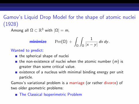
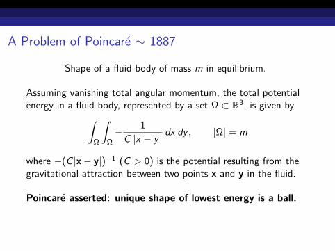
A Problem of Poincare ∼ 1887
Shape of a fluid body of mass m in equilibrium.
Assuming vanishing total angular momentum, the total potentialenergy in a fluid body, represented by a set Ω ⊂ R3, is given by
∫
Ω
∫
Ω− 1
C |x − y | dx dy , |Ω| = m
where −(C |x− y|)−1 (C > 0) is the potential resulting from thegravitational attraction between two points x and y in the fluid.
Poincare asserted: unique shape of lowest energy is a ball.
Rigorous proof: Lieb 1977 (Riesz Rearrangement Inequality).

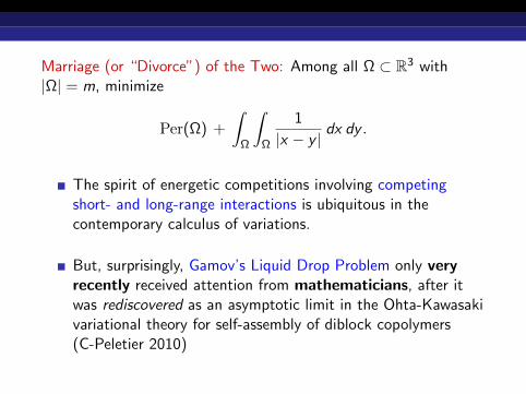
Marriage (or “Divorce”) of the Two: Among all Ω ⊂ R3 with|Ω| = m, minimize
Per(Ω) +
∫
Ω
∫
Ω
1
|x − y | dx dy .
The spirit of energetic competitions involving competingshort- and long-range interactions is ubiquitous in thecontemporary calculus of variations.
But, surprisingly, Gamov’s Liquid Drop Problem only veryrecently received attention from mathematicians, after itwas rediscovered as an asymptotic limit in the Ohta-Kawasakivariational theory for self-assembly of diblock copolymers(C-Peletier 2010)

The Ohta-Kawasaki Functional
Minimize
∫
T3
ε |∇u|2 +1
εu2(1− u2) dx + γ ‖u −M‖2
H−1
where u ∈ H1(T3), −∫
T3
u = M.
‖u −M‖2H−1 =
∫
T3
∫
T3
G (x , y)(u(x)−M) (u(y)−M) dx dy
G , Green’s function for −∆ on T3.
Gradient term: constant phasesDouble-well: phases of 0 or 1Nonlocal term: oscillations between phases 0 and 1 with mean M.
All three =⇒ periodic phase separation on an intrinsic scale.

Heuristic for Minimizers on Sufficiently Large Domain
periodic structures on an intrinsic scale (< domain size)
within a periodic cell, interfaces resemble a CMC surfaceGLOBAL MINIMIZERS WITH LONG-RANGE INTERACTIONS 521
Fig. 4. Zero level sets of the final state for some sample 3D simula-tions attempting to access the ground state; cf. [13].
by ϵ and σ. Herein lies the fidelity of (NLCH) to the diblock copolymer problem, with
the intrinsic scale being the consequence of the connectivity of the A and B subchains.
Note that this connectivity is now imposed as a soft constraint via minimization rather
than a hard constraint. The intrinsic length scale emulates the effective chain length of
a single diblock macromolecule.
It is convenient to compute the gradient flow of (NLCH) with respect to the Hilbert
space H−1. In doing so we obtain the following modified Cahn-Hilliard equation:
(MCH) ut = (−ϵ2u − u + u3
)− σ(u − m).
Since we compute the gradient flow in the H−1 norm, the presence of the nonlocal term
in the functional (NLCH) simply gives rise to a local zeroth order perturbation of the
well-known Cahn-Hilliard equation. However, as is illustrated in Figures 2 and 3, this
term favors u = m and significantly changes the dynamics and steady states. Figure 2
shows the solution at different times for the Cahn-Hilliard equation (i.e. σ = 0) with a
fixed value of m, random initial conditions, and periodic boundary conditions. Figure 3
gives the analogous picture for σ > 0 wherein an intrinsic length scale, independent of
the domain size, between the drops is eventually set. Note that for all simulations we
adopt periodic boundary conditions and deliberately take the domain size to be much
larger than this intrinsic length.
The precise geometry of the interfacial region will depend on m, and the range of
possibilities in 3D is significantly larger than in 2D. Numerical simulations suggest that
minimizers are periodic on some fixed scale independent of domain size and, within a
period cell, the structure appears to minimize surface area between the two phases. Thus
in 3D, the interface associated with minimizers resembles a triply periodic constant mean
curvature surface. Sample 3D simulations attempting to access the ground state are
shown in Figure 4.
Interfaces of low energy states for different Mcf. C.-Peletier-Williams SIAP 2009

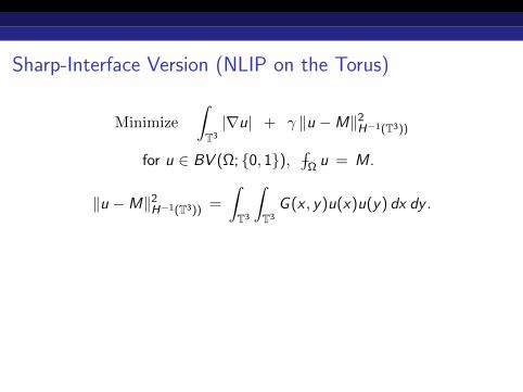
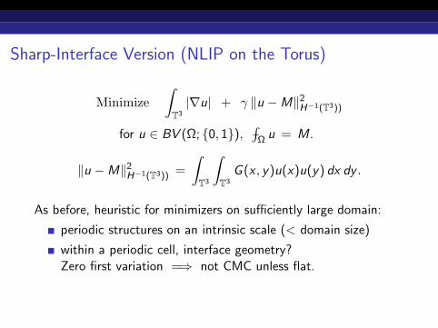
Sharp-Interface Version (NLIP on the Torus)
Minimize
∫
T3
|∇u| + γ ‖u −M‖2H−1(T3))
for u ∈ BV (Ω; 0, 1), −∫
Ω u = M.
‖u −M‖2H−1(T3)) =
∫
T3
∫
T3
G (x , y)u(x)u(y) dx dy .
As before, heuristic for minimizers on sufficiently large domain:
periodic structures on an intrinsic scale (< domain size)
within a periodic cell, interface geometry?Zero first variation =⇒ not CMC unless flat.
Idea: focus on droplet regime (spheres) and separate out theeffects of the nonlocal term on single vs interacting droplets.

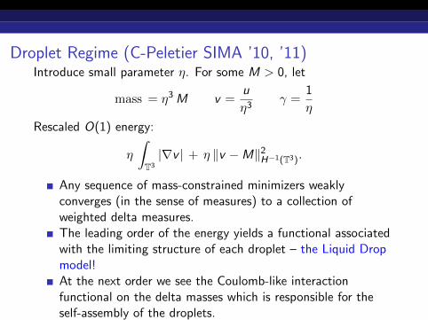
Droplet Regime (C-Peletier SIMA ’10, ’11)Introduce small parameter η. For some M > 0, let
mass = η3 M v =u
η3γ =
1
η
Rescaled O(1) energy:
η
∫
T3
|∇v | + η ‖v −M‖2H−1(T3).
Any sequence of mass-constrained minimizers weaklyconverges (in the sense of measures) to a collection ofweighted delta measures.The leading order of the energy yields a functional associatedwith the limiting structure of each droplet – the Liquid Dropmodel!At the next order we see the Coulomb-like interactionfunctional on the delta masses which is responsible for theself-assembly of the droplets.

Droplet Regime (C-Peletier SIMA ’10, ’11)Introduce small parameter η. For some M > 0, let
mass = η3 M v =u
η3γ =
1
η
Rescaled O(1) energy:
η
∫
T3
|∇v | + η ‖v −M‖2H−1(T3).
Any sequence of mass-constrained minimizers weaklyconverges (in the sense of measures) to a collection ofweighted delta measures.
The leading order of the energy yields a functional associatedwith the limiting structure of each droplet – the Liquid Dropmodel!At the next order we see the Coulomb-like interactionfunctional on the delta masses which is responsible for theself-assembly of the droplets.

Droplet Regime (C-Peletier SIMA ’10, ’11)Introduce small parameter η. For some M > 0, let
mass = η3 M v =u
η3γ =
1
η
Rescaled O(1) energy:
η
∫
T3
|∇v | + η ‖v −M‖2H−1(T3).
Any sequence of mass-constrained minimizers weaklyconverges (in the sense of measures) to a collection ofweighted delta measures.The leading order of the energy yields a functional associatedwith the limiting structure of each droplet – the Liquid Dropmodel!
At the next order we see the Coulomb-like interactionfunctional on the delta masses which is responsible for theself-assembly of the droplets.
Droplet Regime (C-Peletier SIMA ’10, ’11)Introduce small parameter η. For some M > 0, let
mass = η3 M v =u
η3γ =
1
η
Rescaled O(1) energy:
η
∫
T3
|∇v | + η ‖v −M‖2H−1(T3).
Any sequence of mass-constrained minimizers weaklyconverges (in the sense of measures) to a collection ofweighted delta measures.The leading order of the energy yields a functional associatedwith the limiting structure of each droplet – the Liquid Dropmodel!At the next order we see the Coulomb-like interactionfunctional on the delta masses which is responsible for theself-assembly of the droplets.

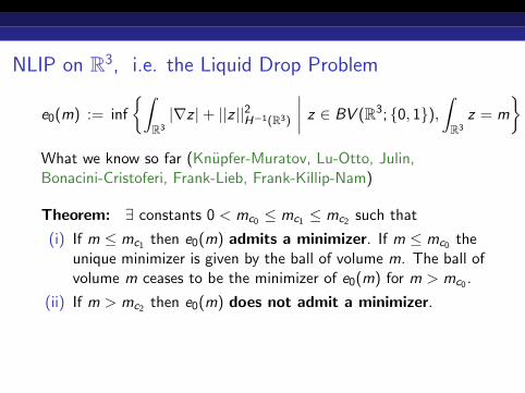
NLIP on R3, i.e. the Liquid Drop Problem
e0(m) := inf
∫
R3
|∇z |+ ||z ||2H−1(R3)
∣∣∣∣ z ∈ BV (R3; 0, 1),∫
R3
z = m
What we know so far (Knupfer-Muratov, Lu-Otto, Julin,Bonacini-Cristoferi, Frank-Lieb, Frank-Killip-Nam)
Theorem: ∃ constants 0 < mc0 ≤ mc1 ≤ mc2 such that
(i) If m ≤ mc1 then e0(m) admits a minimizer. If m ≤ mc0 theunique minimizer is given by the ball of volume m. The ball ofvolume m ceases to be the minimizer of e0(m) for m > mc0 .
(ii) If m > mc2 then e0(m) does not admit a minimizer.
Still open: prove or disprove whether any (or all) of the constantsmci , i = 0, 1, 2, above are pairwise equal.

NLIP on the Torus with Confinementwith Alama, Bronsard and Topaloglu (submitted preprint)
E(u) :=
∫
T3
|∇u|+ γ‖u −M‖2H−1(T3) + σ
∫
T3
(u − 1)2 dµ
for fixed µ = ρ(x) dx such that
(H1) ρ ∈ C (T3) with ρ ≥ 0 and∫T3 ρ dx = 1.
(H2) For T3 =[−1
2 ,12
]3, ρmax = ρ(0) > ρ(x).
(H3) ρ ∈ C 2(Br ) for some r > 0, and
ρ(x) = ρmax − q(x) + o(|x |2) as |x | → 0
q(x) :=3∑
i ,j=1
Hij αiαj x = (α1, α2, α3) ∈ T3
and Hij = − ∂2ρ∂αi∂αj
(0) with Hijαiαj ≥ δ|x |2, for δ > 0.

NLIP on the Torus with Confinementwith Alama, Bronsard and Topaloglu (submitted preprint)
E(u) :=
∫
T3
|∇u|+ γ‖u −M‖2H−1(T3) + σ
∫
T3
(u − 1)2 dµ
for fixed µ = ρ(x) dx
such that
(H1) ρ ∈ C (T3) with ρ ≥ 0 and∫T3 ρ dx = 1.
(H2) For T3 =[−1
2 ,12
]3, ρmax = ρ(0) > ρ(x).
(H3) ρ ∈ C 2(Br ) for some r > 0, and
ρ(x) = ρmax − q(x) + o(|x |2) as |x | → 0
q(x) :=3∑
i ,j=1
Hij αiαj x = (α1, α2, α3) ∈ T3
and Hij = − ∂2ρ∂αi∂αj
(0) with Hijαiαj ≥ δ|x |2, for δ > 0.

NLIP on the Torus with Confinementwith Alama, Bronsard and Topaloglu (submitted preprint)
E(u) :=
∫
T3
|∇u|+ γ‖u −M‖2H−1(T3) + σ
∫
T3
(u − 1)2 dµ
for fixed µ = ρ(x) dx such that
(H1) ρ ∈ C (T3) with ρ ≥ 0 and∫T3 ρ dx = 1.
(H2) For T3 =[−1
2 ,12
]3, ρmax = ρ(0) > ρ(x).
(H3) ρ ∈ C 2(Br ) for some r > 0, and
ρ(x) = ρmax − q(x) + o(|x |2) as |x | → 0
q(x) :=3∑
i ,j=1
Hij αiαj x = (α1, α2, α3) ∈ T3
and Hij = − ∂2ρ∂αi∂αj
(0) with Hijαiαj ≥ δ|x |2, for δ > 0.
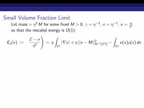
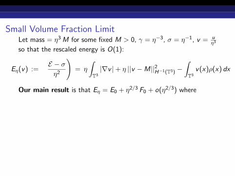
Small Volume Fraction LimitLet mass = η3 M for some fixed M > 0, γ = η−3, σ = η−1, v = u
η3
so that the rescaled energy is O(1):
Eη(v) :=
(E − ση2
)= η
∫
T3
|∇v |+ η ||v −M||2H−1(T3) −∫
T3
v(x)ρ(x) dx
Our main result is that Eη = E0 + η2/3 F0 + o(η2/3) where
E0(v) :=
∑∞i=1 e0(mi )−miρ(x i ) if v =
∑∞i=1 m
iδx i , mi ≥ 0
+∞ otherwise.
F0(v) :=
∑ni=1 m
i q(xi ) + 14π
∑ni,j=1i 6=j
mi mj
|xi−xj | if v =∑n
i=1 miδxi , mi ∈ M
+∞ otherwise.
M =mini=1
∣∣ ∑ni=1 m
i = M, e0(mi ) admits a minimizer.
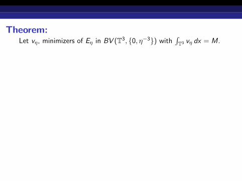
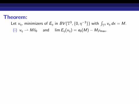
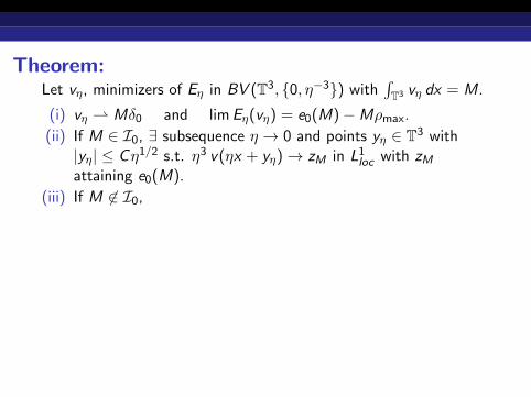
Theorem:Let vη, minimizers of Eη in BV (T3, 0, η−3) with
∫T3 vη dx = M.
(i) vη Mδ0 and limEη(vη) = e0(M)−Mρmax.
(ii) If M ∈ I0, ∃ subsequence η → 0 and points yη ∈ T3 with|yη| ≤ Cη1/2 s.t. η3 v(ηx + yη)→ zM in L1
loc with zMattaining e0(M).
(iii) If M 6∈ I0, ∃ subsequence of η → 0, n ∈ N, mini=1 ∈M,and distinct points x1, . . . , xn such that:
vη −n∑
i=1
miδη1/3xi 0 in the sense of Radon measures
Eη(vη) = e0(M)−Mρmax + η2/3
n∑
i=1
miq(xi ) +1
4π
n∑
i,j=1i 6=j
mi mj
|xi − xj |
+ o
(η2/3
).
Moreover, the expression in brackets is minimized by thechoice of points x1, . . . , xn given the values mini=1 ∈M.

Theorem:Let vη, minimizers of Eη in BV (T3, 0, η−3) with
∫T3 vη dx = M.
(i) vη Mδ0
and limEη(vη) = e0(M)−Mρmax.
(ii) If M ∈ I0, ∃ subsequence η → 0 and points yη ∈ T3 with|yη| ≤ Cη1/2 s.t. η3 v(ηx + yη)→ zM in L1
loc with zMattaining e0(M).
(iii) If M 6∈ I0, ∃ subsequence of η → 0, n ∈ N, mini=1 ∈M,and distinct points x1, . . . , xn such that:
vη −n∑
i=1
miδη1/3xi 0 in the sense of Radon measures
Eη(vη) = e0(M)−Mρmax + η2/3
n∑
i=1
miq(xi ) +1
4π
n∑
i,j=1i 6=j
mi mj
|xi − xj |
+ o
(η2/3
).
Moreover, the expression in brackets is minimized by thechoice of points x1, . . . , xn given the values mini=1 ∈M.
Theorem:Let vη, minimizers of Eη in BV (T3, 0, η−3) with
∫T3 vη dx = M.
(i) vη Mδ0 and limEη(vη) = e0(M)−Mρmax.
(ii) If M ∈ I0, ∃ subsequence η → 0 and points yη ∈ T3 with|yη| ≤ Cη1/2 s.t. η3 v(ηx + yη)→ zM in L1
loc with zMattaining e0(M).
(iii) If M 6∈ I0, ∃ subsequence of η → 0, n ∈ N, mini=1 ∈M,and distinct points x1, . . . , xn such that:
vη −n∑
i=1
miδη1/3xi 0 in the sense of Radon measures
Eη(vη) = e0(M)−Mρmax + η2/3
n∑
i=1
miq(xi ) +1
4π
n∑
i,j=1i 6=j
mi mj
|xi − xj |
+ o
(η2/3
).
Moreover, the expression in brackets is minimized by thechoice of points x1, . . . , xn given the values mini=1 ∈M.

Theorem:Let vη, minimizers of Eη in BV (T3, 0, η−3) with
∫T3 vη dx = M.
(i) vη Mδ0 and limEη(vη) = e0(M)−Mρmax.
(ii) If M ∈ I0,
∃ subsequence η → 0 and points yη ∈ T3 with|yη| ≤ Cη1/2 s.t. η3 v(ηx + yη)→ zM in L1
loc with zMattaining e0(M).
(iii) If M 6∈ I0, ∃ subsequence of η → 0, n ∈ N, mini=1 ∈M,and distinct points x1, . . . , xn such that:
vη −n∑
i=1
miδη1/3xi 0 in the sense of Radon measures
Eη(vη) = e0(M)−Mρmax + η2/3
n∑
i=1
miq(xi ) +1
4π
n∑
i,j=1i 6=j
mi mj
|xi − xj |
+ o
(η2/3
).
Moreover, the expression in brackets is minimized by thechoice of points x1, . . . , xn given the values mini=1 ∈M.

Theorem:Let vη, minimizers of Eη in BV (T3, 0, η−3) with
∫T3 vη dx = M.
(i) vη Mδ0 and limEη(vη) = e0(M)−Mρmax.
(ii) If M ∈ I0, ∃ subsequence η → 0 and points yη ∈ T3 with|yη| ≤ Cη1/2 s.t. η3 v(ηx + yη)→ zM in L1
loc with zMattaining e0(M).
(iii) If M 6∈ I0, ∃ subsequence of η → 0, n ∈ N, mini=1 ∈M,and distinct points x1, . . . , xn such that:
vη −n∑
i=1
miδη1/3xi 0 in the sense of Radon measures
Eη(vη) = e0(M)−Mρmax + η2/3
n∑
i=1
miq(xi ) +1
4π
n∑
i,j=1i 6=j
mi mj
|xi − xj |
+ o
(η2/3
).
Moreover, the expression in brackets is minimized by thechoice of points x1, . . . , xn given the values mini=1 ∈M.
Theorem:Let vη, minimizers of Eη in BV (T3, 0, η−3) with
∫T3 vη dx = M.
(i) vη Mδ0 and limEη(vη) = e0(M)−Mρmax.
(ii) If M ∈ I0, ∃ subsequence η → 0 and points yη ∈ T3 with|yη| ≤ Cη1/2 s.t. η3 v(ηx + yη)→ zM in L1
loc with zMattaining e0(M).
(iii) If M 6∈ I0,
∃ subsequence of η → 0, n ∈ N, mini=1 ∈M,and distinct points x1, . . . , xn such that:
vη −n∑
i=1
miδη1/3xi 0 in the sense of Radon measures
Eη(vη) = e0(M)−Mρmax + η2/3
n∑
i=1
miq(xi ) +1
4π
n∑
i,j=1i 6=j
mi mj
|xi − xj |
+ o
(η2/3
).
Moreover, the expression in brackets is minimized by thechoice of points x1, . . . , xn given the values mini=1 ∈M.

Theorem:Let vη, minimizers of Eη in BV (T3, 0, η−3) with
∫T3 vη dx = M.
(i) vη Mδ0 and limEη(vη) = e0(M)−Mρmax.
(ii) If M ∈ I0, ∃ subsequence η → 0 and points yη ∈ T3 with|yη| ≤ Cη1/2 s.t. η3 v(ηx + yη)→ zM in L1
loc with zMattaining e0(M).
(iii) If M 6∈ I0, ∃ subsequence of η → 0, n ∈ N, mini=1 ∈M,and distinct points x1, . . . , xn such that:
vη −n∑
i=1
miδη1/3xi 0 in the sense of Radon measures
Eη(vη) = e0(M)−Mρmax + η2/3
n∑
i=1
miq(xi ) +1
4π
n∑
i,j=1i 6=j
mi mj
|xi − xj |
+ o
(η2/3
).
Moreover, the expression in brackets is minimized by thechoice of points x1, . . . , xn given the values mini=1 ∈M.

So if the mass sufficiently large (i.e. M 6∈ I0), ∃ a newintermediate O(η1/3) scale.That is, still have collapse to the origin but by breaking up intoparticles (droplets) O(η1/3) apart.
T3
= 1/3
pn
p1 p2
p3
p4
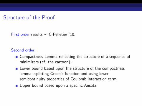
Structure of the Proof
First order results ∼ C-Pelletier ’10.
Second order:
Compactness Lemma reflecting the structure of a sequence ofminimizers (cf. the cartoon).
Lower bound based upon the structure of the compactnesslemma: splitting Green’s function and using lowersemicontinuity properties of Coulomb interaction term.
Upper bound based upon a specific Ansatz.

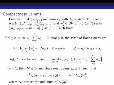
Compactness LemmaLemma: Let vηη>0 minimize Eη with
∫T3 vη dx = M. Then ∃
n ∈ N, mini=1, x iηni=1 ⊂ T3 and w iη ∈ BV (T3; 0, 1/η3) with
||w iη||L1(T3) = mi + o(1) as η → 0 such that:
If n ≥ 2, then vη−n∑
i=1
w iη 0 weakly in the sense of Radon measures,
∀ i , lim infη→0
(w iη −miδx iη) = 0 weakly, |x iη − x jη| η i 6= j ,
e0(mi ) is attained and lim infη→0
Eη(vη) ≥ lim infη→0
Eη
(n∑
i=1
w iη
).
If n = 1, then M ∈ I0 and there exist points yη ∈ T3 such that
n3 vη(ηx + yη)→ zM(x) in L1loc(R3)
where zM attains the minimum of e0(M).
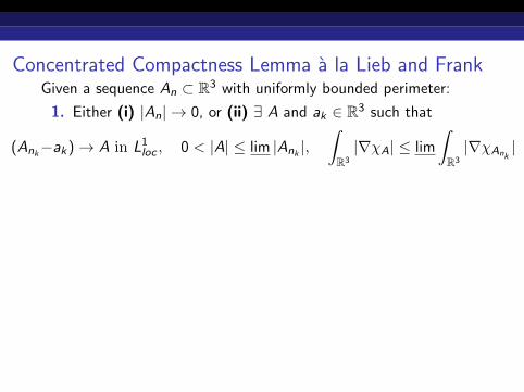
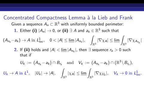
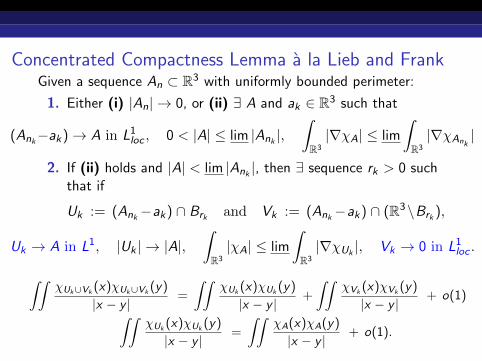
Concentrated Compactness Lemma a la Lieb and FrankGiven a sequence An ⊂ R3 with uniformly bounded perimeter:
1. Either (i) |An| → 0, or (ii) ∃ A and ak ∈ R3 such that
(Ank−ak)→ A in L1loc , 0 < |A| ≤ lim |Ank |,
∫
R3
|∇χA| ≤ lim
∫
R3
|∇χAnk|
2. If (ii) holds and |A| < lim |Ank |, then ∃ sequence rk > 0 suchthat if
Uk := (Ank−ak) ∩ Brk and Vk := (Ank−ak) ∩ (R3\Brk ),
Uk → A in L1, |Uk | → |A|,∫
R3
|χA| ≤ lim
∫
R3
|∇χUk|, Vk → 0 in L1
loc .
∫∫χUk∪Vk
(x)χUk∪Vk(y)
|x − y | =
∫∫χUk
(x)χUk(y)
|x − y | +
∫∫χVk
(x)χVk(y)
|x − y | + o(1)
∫∫χUk
(x)χUk(y)
|x − y | =
∫∫χA(x)χA(y)
|x − y | + o(1).

Concentrated Compactness Lemma a la Lieb and FrankGiven a sequence An ⊂ R3 with uniformly bounded perimeter:
1. Either (i) |An| → 0, or (ii) ∃ A and ak ∈ R3 such that
(Ank−ak)→ A in L1loc , 0 < |A| ≤ lim |Ank |,
∫
R3
|∇χA| ≤ lim
∫
R3
|∇χAnk|
2. If (ii) holds and |A| < lim |Ank |, then ∃ sequence rk > 0 suchthat if
Uk := (Ank−ak) ∩ Brk and Vk := (Ank−ak) ∩ (R3\Brk ),
Uk → A in L1, |Uk | → |A|,∫
R3
|χA| ≤ lim
∫
R3
|∇χUk|,
Vk → 0 in L1loc .
∫∫χUk∪Vk
(x)χUk∪Vk(y)
|x − y | =
∫∫χUk
(x)χUk(y)
|x − y | +
∫∫χVk
(x)χVk(y)
|x − y | + o(1)
∫∫χUk
(x)χUk(y)
|x − y | =
∫∫χA(x)χA(y)
|x − y | + o(1).
Concentrated Compactness Lemma a la Lieb and FrankGiven a sequence An ⊂ R3 with uniformly bounded perimeter:
1. Either (i) |An| → 0, or (ii) ∃ A and ak ∈ R3 such that
(Ank−ak)→ A in L1loc , 0 < |A| ≤ lim |Ank |,
∫
R3
|∇χA| ≤ lim
∫
R3
|∇χAnk|
2. If (ii) holds and |A| < lim |Ank |, then ∃ sequence rk > 0 suchthat if
Uk := (Ank−ak) ∩ Brk and Vk := (Ank−ak) ∩ (R3\Brk ),
Uk → A in L1, |Uk | → |A|,∫
R3
|χA| ≤ lim
∫
R3
|∇χUk|, Vk → 0 in L1
loc .
∫∫χUk∪Vk
(x)χUk∪Vk(y)
|x − y | =
∫∫χUk
(x)χUk(y)
|x − y | +
∫∫χVk
(x)χVk(y)
|x − y | + o(1)
∫∫χUk
(x)χUk(y)
|x − y | =
∫∫χA(x)χA(y)
|x − y | + o(1).

Application of the Frank-Lieb Lemma
Use FL Lemma to inductively find mi , x iη and Ωi with |Ωi | = mi
which minimize e0(mi ).
Let Ωη = rescaled O(1) support of vη. LF =⇒ ∃ y1η (x1
η atO(η) scale) s.t. Ωη translated by y1
η converges in L1loc to Ω1.
Let m1 = Ω1. If m1 = M we are done.
If m1 < M, use part 2 of LF to separate out the first dropletand the remainder. Note that at the rescaled O(1) scale, theremaining (droplets) go off to ∞.
Now repeat with the remainder.

Transition to a Different Nonlocal Geometric Problem onR3
Recall (NLIP)/Liquid Drop Model
Per(Ω) +
∫
Ω
∫
Ω
1
|x − y | dx dy .
attraction ∼ perimeter
Recall second-order-limit discrete energy for our confinementproblem over points xi and weights mi :
n∑
i=1
mi |xi |2 +1
4π
n∑
i ,j=1i 6=j
mi mj
|xi − xj |
first term ∼ algebraic attraction to the origin.
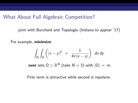
What About Full Algebraic Competition?
joint with Burchard and Topaloglu (Indiana to appear ’17)
For example, minimize
∫
Ω
∫
Ω
(|x − y |2 +
1
4π|x − y |
)dx dy
over sets Ω ⊂ RN (take N = 3) with |Ω| = m.
First term is attractive while second is repulsive.
Existence, nonexistence, role of m, optimal shapes (balls)?

(GP): Set Interactions with General Power Potentials
Geometric Problem (GP)Minimize
E(Ω) =
∫
Ω
∫
ΩK (x − y) dx dy over Ω ⊂ R3 with |Ω| = m,
where K (x) : =|x |qq︸︷︷︸
attractive
− |x |pp︸ ︷︷ ︸
repulsive
−N < p < q.
x¤
K@ x¤D
x¤
K@ x¤D
x¤
K@ x¤D
−N < p < 0 < q −N < p < q < 0 0 < p < q
Existence, nonexistence, role of m, p, q, optimal shapes (balls)?

Role of m in (GP)
For small m, minimizer of (GP) fails to exist.Heuristically: For m small, repulsion dominates. Enforcedbinary constraint =⇒ oscillations.
For large m attraction dominates =⇒ existence
Opposite of Liquid Drop (NLIP on R3)!

What Can One Prove
Burchard-C-Topaloglu: we focused on the case of q = 2,exploiting convexity structure).
For p = −1, we prove there exists mc such that (1)nonexistence for m < mc and (ii) ball unique minimizer form ≥ mc .
Key here is the relation to the relaxed problem.
Lieb and Frank recently extended our work for the case ofmore general q and p = −1 by exploiting certain properties ofsubharmonic functions.

Relaxed Problem (RP) Over Uniformly Bounded Densities
E [ρ] =
∫
RN
∫
RN
K (x − y)ρ(x)ρ(y) dxdy
over A =
ρ ∈ L1(RN)
∣∣∣∣ ‖ρ‖L1(R3) = m, 0 ≤ ρ(x) ≤ 1 a.e.
K (x) :=
(1
q|x |q
)−(
1
p|x |p
), −N < p < q.
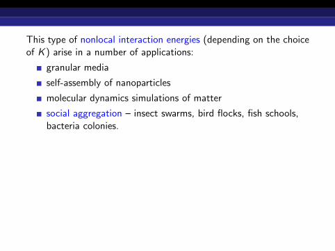
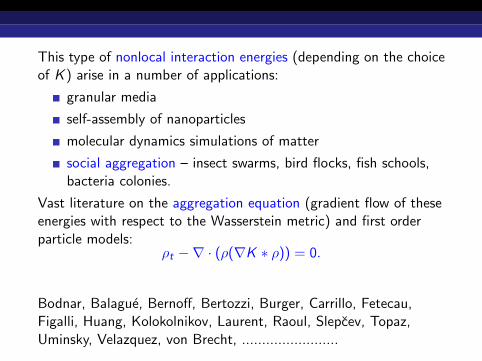
This type of nonlocal interaction energies (depending on the choiceof K ) arise in a number of applications:
granular media
self-assembly of nanoparticles
molecular dynamics simulations of matter
social aggregation – insect swarms, bird flocks, fish schools,bacteria colonies.
Vast literature on the aggregation equation (gradient flow of theseenergies with respect to the Wasserstein metric) and first orderparticle models:
ρt −∇ · (ρ(∇K ∗ ρ)) = 0.
Bodnar, Balague, Bernoff, Bertozzi, Burger, Carrillo, Fetecau,Figalli, Huang, Kolokolnikov, Laurent, Raoul, Slepcev, Topaz,Uminsky, Velazquez, von Brecht, ........................
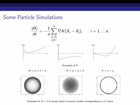
Some Particle Simulations
dXi
dt= −1
n
n∑
j=1j 6=i
∇K (Xi − Xj), i = 1 . . . n.
x¤
K@ x¤D
x¤
K@ x¤D
x¤
K@ x¤D
Examples of K
−N < p < 0 < q −N < p < q < 0 0 < p < q
−0.5 0 0.5
−0.5
0
0.5
x
y
−2 −1 0 1 2
−2
−1
0
1
2
x
y
−0.5 0 0.5
−0.5
0
0.5
xy
Examples for N = 2 of steady states of particle models corresponding to a K above

Global Existence over Densities
E [ρ] =∫R3
∫R3 K (x − y)ρ(x)ρ(y) dxdy
C-Fetecau-Topaloglu AIHP ’15: ∃ global minimizer in certainappropriate classes depending on p, q.Application of direct method in the calculus of variationsusing Lions’ Concentration Compactness.Only have weak convergence but convolution is smoothing.
More general ∃-results: Simione-Slepcev-Topaloglu JSP ’15and Canizo-Carrillo-Patacchini ARMA ’15. Later impliesminimizers of RP are compactly supported.
Other variational works: Balague-Carrillo-Laurent-Raoul,Carrillo-Di Francesco-Figalli-Laurent-Slepcev, Burger-DiFrancesco-Franek. Carrillo-Delgadino-Mellet . . .
Relaxed Problem (RP) has a minimizer for all m.

Relation to Geometric Problem (GP)GP has a minimizer iff relaxed problem RP has a characteristic
function as a minimizer
Nontrivial direction: ⇒Suppose any global min ρ of RP is not a characteristicfunction.
Can show ρ has compact support.
∃ characteristic functions χn s.t. χn ρ in L1.
Convolution structure implies E (χn)→ E (ρ).
Hence @ minimizer of GP.
Relation to Geometric Problem (GP)GP has a minimizer iff relaxed problem RP has a characteristic
function as a minimizer
Nontrivial direction: ⇒
Suppose any global min ρ of RP is not a characteristicfunction.
Can show ρ has compact support.
∃ characteristic functions χn s.t. χn ρ in L1.
Convolution structure implies E (χn)→ E (ρ).
Hence @ minimizer of GP.

Relation to Geometric Problem (GP)GP has a minimizer iff relaxed problem RP has a characteristic
function as a minimizer
Nontrivial direction: ⇒Suppose any global min ρ of RP is not a characteristicfunction.
Can show ρ has compact support.
∃ characteristic functions χn s.t. χn ρ in L1.
Convolution structure implies E (χn)→ E (ρ).
Hence @ minimizer of GP.

Summary
Gamov’s Liquid Drop Problem (Nonlocal IsoperimetricProblem on R3)
Rediscovered in droplet phase of the Ohta-Kawasaki functional
Still open questions regarding global minimizers. Alsostructure of local minimizers very interesting.
Discussed how the ∃ / @ of the LD problem appears in thebreak-up structure of small droplet minimizers for a nonlocalisoperimetric problem on T3 with confinement.
Discussed a different purely algebraic class of set interactionfunctionals in which the mass effects are reversed.
Related Documents