1 Genome Composition Plasticity in Marine Organisms A Thesis submitted to University of Naples “Federico II”, Naples, Italy for the degree of DOCTOR OF PHYLOSOPHY in “Applied Biology” XXVIII cycle by Andrea Tarallo March, 2016

Welcome message from author
This document is posted to help you gain knowledge. Please leave a comment to let me know what you think about it! Share it to your friends and learn new things together.
Transcript

1
Genome Composition Plasticity in
Marine Organisms
A Thesis submitted to
University of Naples “Federico II”, Naples, Italy for the degree of
DOCTOR OF PHYLOSOPHY
in
“Applied Biology”
XXVIII cycle
by
Andrea Tarallo March, 2016

2
University of Naples “Federico II”, Naples, Italy
Research Doctorate in Applied Biology
XXVIII cycle
The research activities described in this Thesis were performed at the Department of Biology and Evolution of Marine Organisms, Stazione Zoologica Anton Dohrn, Naples, Italy and at the Fishery Research Laboratory, Kyushu University, Fukuoka, Japan from April 2013 to March 2016.
Supervisor
Dr. Giuseppe D’Onofrio
Tutor Doctoral Coordinator
Prof. Claudio Agnisola Prof. Ezio Ricca
Candidate
Andrea Tarallo
Examination pannel
Prof. Maria Moreno, Università del Sannio Prof. Roberto De Philippis, Università di Firenze Prof. Mariorosario Masullo, Università degli Studi Parthenope

3
LIST OF PUBLICATIONS
1. On the genome base composition of teleosts: the effect of environment and
lifestyle
A Tarallo, C Angelini, R Sanges, M Yagi, C Agnisola, G D’Onofrio
BMC Genomics 17 (173) 2016
2. Length and GC Content Variability of Introns among Teleostean
Genomes in the Light of the Metabolic Rate Hypothesis
A Chaurasia, A Tarallo, L Bernà, M Yagi, C Agnisola, G D’Onofrio
PloS one 9 (8), e103889 2014
3. The shifting and the transition mode of vertebrate genome evolution in
the light of the metabolic rate hypothesis: a review
L Bernà, A Chaurasia, A Tarallo, C Agnisola, G D'Onofrio
Advances in Zoology Research 5, 65-93 2013
4. An evolutionary acquired functional domain confers neuronal fate
specification properties to the Dbx1 transcription factor
S Karaz, M Courgeon, H Lepetit, E Bruno, R Pannone, A Tarallo, F Thouzé, P
Kerner, M Vervoort, F Causeret, A Pierani and G D’Onofrio
EvoDevo, Submitted
5. Lifestyle and DNA base composition in annelid polychaetes
A Tarallo, MC Gambi, G D’Onofri
Physiological Genomics, Submitted

4
Abstract
The molar ratio of the nucleotides (GC%, i.e. the Guanine+Cytosine content)
is well known to evolve through the genomes of all the organisms. Several hypotheses
have been drawn out to explain the causes of the nucleotide composition variability
among orgnisms.
In the Thesis project major attention has been directed to the Metabolic Rate
hypothesis (MRh). The main goal was to test if the MRh, first proposed to explain the
nucleotide variability within mammalian genomes, could also explain the base
composition variability among lower vertebrates and invertebrates. To this aim an
extensive analysis of more than two hundred teleostean species has been carried out,
followed by a pioneering study of annelid polychaete and tunicate genomes.
Regarding teleosts, the results clearly highlighted that environment (i.e.
salinity) and lifestyle (i.e. migration) both affect simultaneously the physiology (the
metabolic rate), the morphology (the gill area) and the genome composition (GC%).
Thus supporting a link between the metabolic rate (MR) and the genome base
composition, as expected in the light of the MRh. Moreover, a comparative analysis of
completely sequenced teleostean genomes showed that the metabolic rate was
correlated not only with the GC content of the genome, but also with the intron
structures. Indeed, at increasing metabolic rates introns were shorter and GC-richer.
A preliminary analysis of annelids polychaetes showed that motile and sessile
species were characterized by different MR and GC%, being both higher in the former
than in the latter.
The investigation was extended to the well known solitary tunicates, C.
robusta and the congeneric C. savignyi. Our data revealed slight but significant
morpho-physiological differences between the two species, consistent not only with an
ecological niche differentiation, but also with their genomic GC content.
All the above results converge towards the same conclusion, thus giving
consistency to the MRh as major factor driving the genome base composition evolution
of all living organisms.

5
Index
List of Abbreviations ....................................................................................................... 8
List of Figures .................................................................................................................. 9
List of Tables.................................................................................................................. 10
Chapter I ........................................................................................................................ 11
INTRODUCTION ............................................................................................................. 11
1.1 BIASED GENE CONVERSION HYPOTHESIS ..................................................... 14
1.2 METABOLIC RATE HYPOTHESIS ..................................................................... 20
1.3 AIMS AND STRATEGIES ................................................................................. 23
Chapter II ....................................................................................................................... 25
INTRODUCTION ............................................................................................................. 25
2.1 GENOME COMPOSITION IN TELEOSTS .......................................................... 25
PART I ............................................................................................................................ 27
2.2 SALINITY AND MIGRATION ............................................................................ 27
RESULTS ......................................................................................................................... 29
2.3 EFFECT OF PHYLOGENY ................................................................................. 29
2.4 WHITHIN GENOME ANALYSIS ....................................................................... 32
2.5 THE EFFECT OF ENVIRONMENT AND LIFESTYLE ........................................... 34
DISCUSSION ................................................................................................................... 41
PART II ........................................................................................................................... 45
2.6 THE GENOME ARCHITECTURE OF TELEOSTS ................................................. 45
RESULTS ......................................................................................................................... 46
2.7 DISTRIBUTION OF THE INTRONIC GC CONTENT............................................ 46
2.8 PAIRWISE COMPARISON ............................................................................... 52
2.9 THE MR IN THE FIVE TELEOSTS ..................................................................... 57
DISCUSSION ................................................................................................................... 60

6
CONCLUSION ................................................................................................................. 62
Chapter III ...................................................................................................................... 64
INTRODUCTION ............................................................................................................. 64
3.1 GENOME COMPOSITION IN POLYCHAETES................................................... 64
3.2 DIFFERENCES IN LOCOMOTION .................................................................... 65
3.3 THE POLYCHAETA GENOME .......................................................................... 66
RESULTS ......................................................................................................................... 67
3.4 METABOLIC RATE IN POLYCHAETES .............................................................. 67
3.5 NUCLEOTIDE COMPOSITION ......................................................................... 67
DISCUSSION ................................................................................................................... 69
3.6 PHYLOGENETIC INDEPENDENCY OF GC% AND METABOLISM ...................... 69
3.7 BACTERIAL CONTAMINATION ....................................................................... 71
CONCLUSION ................................................................................................................. 72
Chapter IV ..................................................................................................................... 73
INTRODUCTION ............................................................................................................. 73
4.1 MORPHO-PHYSIOLOGICAL COMPARISON IN ASCIDIANS .............................. 73
4.2 DIFFERENCES BETWEEN C. robusta AND C. savignyi .................................... 74
4.3 DISTRIBUTION ............................................................................................... 76
4.4 OXYGEN CONSUMPTION IN Ciona spp ......................................................... 77
RESULTS ......................................................................................................................... 78
4.5 MORPHOMETRIC ANALYSES ......................................................................... 78
4.6 WATER RETENTION ....................................................................................... 82
4.7 OXYGEN CONSUMPTION ............................................................................... 84
DISCUSSION ................................................................................................................... 85
CONCLUSION ................................................................................................................. 89
Chapter V ...................................................................................................................... 91
GENERAL CONCLUSIONS ............................................................................................... 91
Appendix I ..................................................................................................................... 95
MATERIALS AND METHODS .......................................................................................... 95
I.1 TELEOSTS’ METABOLIC RATE, GILL AREA AND GC% ..................................... 95

7
I.2 GENE EXPRESSION DATA ............................................................................... 96
Statistical analyses ................................................................................................ 96
I.3 INTRON ANALYSES ........................................................................................ 97
I.4 TELEOSTS’ SPECIMENS ................................................................................ 100
I.5 RESPIROMETRY IN TELEOSTS ...................................................................... 100
I.6 POLYCHAETES TISSUE PREPARATION AND HPLC ANALYSES ....................... 102
I.7 METABOLIC RATE SURVEY FOR POLYCHAETES ........................................... 105
I.8 ASCIDIANS SPECIMENS................................................................................ 106
I.8 ASCIDIANS RESPIROMETRY ......................................................................... 109
Statistical analyses .............................................................................................. 111
Appendix II .................................................................................................................. 113
II.1 THE METABOLIC THEORY OF ECOLOGY EQUATION .................................... 113
Supplementary data .................................................................................................... 116
Acknowledgements ..................................................................................................... 149
Bibliography ................................................................................................................ 150

8
List of Abbreviations
A, T, G, C: respectively, Adenine, Timine, Guanine, Cytosine.
AT: Total amount of Adenine+Timine
GC: Total amount of Adenine+Timine
MRh: metabolic Rate hypothesis
BGCh: Biased gene Conversion hypothesis
NFP: Nucleosome Formation Potential
FW: Freshwater species
SW: Seawater species
MR: Metabolic Rate, mass- and temperature- corrected accprdng to the MTE
MTE: Metabolic Theory of Ecology
Gill: Specific Gilla Area
M: migratory teleostean species
NM: non-migratory teleostean species
FWNM: freshwater non-migratory teleostean species
FWM: freshwater migratory teleostean species
SWNM: seawater non-migratory teleostean species
SWM: seawatere migratory teleostean species
GCi: intronic amount of Guanine+Cytosine
GCg: genomic amount of Guanine+Cytosine
bpi: length of introns in bais pair
bp%: length of discarded repetitive elements in percentage of total amount of introns
SK: skewness
N/P: class of introns with negative bpi and positive GCi values
N/N: class of introns with both negative bpi and GCi values
P/N: class of introns with positive bpi and negative GCi values
P/P: class of introns with both positive bpi and GCi values
BL: Body Length, in cm
BW: Body Weight, in mg
TW: Tunic Weight, in mg
OW: Organ Weight, in mg
WW: Wet Weight, in mg
DW: Dry Weight, in mg

9
List of Figures
1.1 GC content distribution among living organisms pag. 12
1.2 Schematic representation of biased gene conversion pag. 16
1.3 Correlation between GC content and recombination rate among several
vertebrates and invertebrates pag. 19
1.4 Correlation between GC3 content and specific Metabolic Rate among
mammals pag. 23
2.1 Teleostean phylogenetic distribution of MR (panel A), specific gill area (panel
b) and GC-content (panel c) pag. 31
2.2 Genome organization of T. nigroviridis (panel a). Boxplot of the gene
expression level (panel b) pag. 33
2.3 Boxplot of routine metabolic rate (panel a), specific gill area (panel b), and
genomic GC content (panel c) for freshwater (FW) and seawater (SW) species. pag. 35
2.4 Boxplot of routine metabolic rate (panel a), specific gill area (panel b), and
genomic GC content (panel c) for non-migratory (NM) and migratory (M)
species. pag. 37
2.5 Boxplot of routine metabolic rate (panel a), specific gill area (panel b), and
genomic GC content (panel c) for freshwater non-migratory (FWNM),
freshwater migratory (FWM), seawater non-migratory (SWNM) and seawater
migratory (SWM) species pag. 40
2.6 Phylogenetic relationships among the five fish analyzed (according to Loh et al
(2008))(panel a); histograms of the GCi distribution in each genome (panel b) pag. 47
2.7 Histogram of orthologous intronic sequences increasing in length (Dbpi) and
GC content (DGCi) in each pairwise comparison. pag. 53
2.8 Histogram of the four classes N/P, N/N, P/N and P/P in each pairwise genome
comparisons pag. 55
2.9 Box plots of the MR measured in each teleostean fish. pag. 57
3.1 Boxplot of the average genomic GC-content (panel a) and MR of motile and
sessile polychaetes. pag. 68
3.2 Polychaeta phylogenetic distribution of GC-content (panel A) and MR (panel
B) pag. 70
4.1 Global distribution of C. robusta and C. savignyi pag. 76
4.2 Correlation between BL and BW for C. robusta and C. savignyi in comparison
with C. intestinalis (panel a); Boxplot showing the tunic/organ ratio (W/W) for
the specimens analyzed in this work (panel b) pag. 81
4.3 Correlation between BW and water retention in C. robusta and C. savignyi pag. 83
4.4 Allometric relationship between body weight (dry) and respiration rate in C.
robusta and C. savignyi pag. 84
S.1 Histogram showing the percentage of sequences eliminated in each pairwise
comparison pag. 99
S.2 HPLC run for Sabella spallanzanii as an example pag. 104
S.3 Allometric relationship between body weight (dry) and respiration rate in
polychaetes pag. 106
S.4 Particular from the siphons of C. robusta andC. savignyi pag. 108
S.5 Particular from the pigmentation of the terminal papillae of the vas deferens in
C. robusta pag. 109
S.6 Tunic/Organs weight correlation pag. 110

10
List of Tables
2.1 Medians for each group pag. 38
2.2 Average values of genome (GCg) and intron (GCi) base composition, intron lenght
(bpi) and metabolic rate Boltzmann corrected (MR) in fish genomes. pag. 46
2.3 Descriptive statistics of GCi% distribution in the five teleosts genomes pag. 49
2.4 Average bpi% and GCi% of repetitive elements removed by Repeat Masker pag. 50
2.5 Average GCi% in each set of orthologous genes before (bRM) and after (aRM)
Repeat Masker. pag.
2.6 Student-Newman-Keuls post hoc test. pag. 58
2.7 Correlation coefficients Rho (in italic) and p-values (in bold) of Spearman
correlation test. pag. 59
4.1 Comparison between C. robusta and C. savignyi equations obtained from wet and
dry body weight data. pag. 79-80
S.1 Basal metabolic rate bodymass- and temperature-corrected by Boltzman’s factor pag. 116-121
S.2 Gill area data for the teleostean species used in the analyses pag. 122-131
S.3 Genomic GC value (%), environmental and lifestyle data for the teleostean species
used in the analyses pag. 132-137
S.4 Mann-Whitney Bonferroni corrected for multiple comparisons among routine
metabolic rate of teleosts. pag. 138
S.5 Mann-Whitney Bonferroni corrected for multiple comparisons among Gill of
teleosts. pag. 139
S.6 Mann-Whitney Bonferroni corrected for multiple comparisons among GC% of
teleosts. pag. 140
S.7 Skewness of Gci% in each set of orthologous introns before RepeatMasker pag. 141
S.8 Binomial test pag. 142-143
S.9 List of the analyzed species pag. 144-145
S.10 MR data for the polychaetes species used in the analyses pag. 146-147
S.11 Mann-Whitney pairwise comparison (Bonferroni-corrected for multiple
comparisons) pag. 148
11
Chapter I
INTRODUCTION
The observation that DNA molecule contains equal amounts of the bases
adenine (A) and thymine (T), as well equal amounts of guanine (G) and
cytosine (C) date back in the fifties (Chargaff 1951). The quantitative
relationship among base pairs, nowadays known as the first Chargaff’s parity
rule, has been crucial in helping to elucidate the double-helix structure of the
DNA molecule. AT- and GC-pairs should be expected to occur with the same
frequency. However, at the genome level, the AT amount is rarely equal to the
GC amount. Before the genetic code was decoded (Nirenberg 1963), many
information on the nucleotide composition variability among prokaryotes were
already known. Indeed, Sueoka has been the first to systematically study the
nucleotide composition in bacteria (Sueoka 1959, 1962), and surprisingly at the
time, he showed that in prokaryotes the proportion of AT in a genome is not in
equilibrium with that of GC. Nowadays, according to recent assessments
(Agashe and Shankar 2014), the genome base composition (generally defined
as GC%, i.e. the molar ratio of guanine plus cytosine) is known to be highly
variable in all the Phyla (Fig. 1.1).
The report on the AT/GC ratio variability (Sueoka 1959, 1962) was the
starting point of the neutralist-selectionist debate on the nature of the forces
driving the base composition of a genome. Till now, several evolutionary
hypotheses have been proposed. Here, for sake of brevity, only the most
outstanding scientific thought will be discussed.
According to the Sueoka’s hypothesis, defined as the “directional
mutational pressure”, the major factor responsible of the increment/decrement

12
of the GC content (i.e. the shift from the expected theoretical value of 50% GC)
was a bias of the mutation rate toward the α pairs (A-T or T-A) or the γ pairs
(G-C or C-G).
Thanks to the massive genome sequencing, it has been definitively
shown, contrary to the Suekoa’s expectation, that the mutational bias of the
DNA polymerase favors only the GC->AT substitution in both prokaryotes
(Hershberg and Petrov 2010; Hildebrand et al. 2010; Rocha and Feil 2010) and
eukaryotes (Arbeithuber et al. 2015). Thus, the huge genomic GC-content
variation, especially among the bacterial genomes (Fig. 1.1) cannot be fully
explained on the basis of neutral mutations alone (Nishida 2012), suggesting
that selection has acted in opposition to the mutational bias (Maddamsetti et al.
2015).
Figure 1.1
GC content distribution in the kingdoms of living organisms (Animalia were split in Invertebrate and Vertebrate). Data downloaded from Kryukov et al. (2012)
13
According to the thermodynamic stability hypothesis, proposed to
explain the peculiar genome heterogeneity of “warm-blooded vertebrates”
absent in “cold-blooded vertebrates” (Bernardi et al. 1985), an increment of the
environmental or body temperature favors a GC increment (Bernardi 2004).
Bernardi’s hypothesis grounded on two main points: i) increasing the
occurrence of the GC pairs, or in other words increasing the DNA pairs
carrying triple hydrogen bond, increases the melting point, and thus the thermal
stability, of both DNA and RNA (Bernardi et al. 1985); and ii) the increment of
GC-rich codons, mainly encoding hydrophobic amino acids, increase the
average hydrophobicity, and hence stability, of the proteins (D’Onofrio et al.
1999).
Unfortunately, it has been shown that on a wider number of specimens
there is no correlation between temperature and average GC composition
among warm- (Berná et al. 2012) and cold-blood vertebrates (Uliano et al.
2010; Chaurasia et al. 2011). Nevertheless, the thermodynamic stability
hypothesis was recently recalled to explain the GC diversity found at the
transcriptomic level between two closely related fish species (Windisch et al.
2012). At the present the thermodynamic hypothesis was set aside, to leave
room to a more feasible role of the GC heterogeneity in the three-dimensional
reorganization of DNA during mitosis (Bernardi 2015).
At the present, two hypotheses are discussed in the literature to explain
the evolutionary change of GC among organisms, namely the Metabolic Rate
hypothesis, MRh (Vinogradov 2001, 2005) and the Biased Gene Conversion
hypothesis, BGCh (Duret and Galtier 2009 for a review). Both were first
proposed to explain the compositional compartmentalization of the mammalian
genome (Holmquist 1992; Eyre-Walker 1993; Vinogradov 2003, 2005). Later
on, the MRh has been extended to the ectotherms (Vinogradov and Anatskaya
2006; Chaurasia et al. 2011; Berná et al. 2012); while the BGCh has been
recently proposed to explain the GC variability among prokaryotes (Lassalle et
al. 2015) and vertebrates (Jannière et al. 2007; Figuet et al. 2015). To fully

14
understand every nuance of the two proposed explanation, below they will be
discussed in details. After a critical discussion about strong and weak points of
each hypothesis, a brief introduction will follow in order to expose the Thesis
project and how we tried to encompass some issues related to the study of the
evolution of genome architecture.
1.1 BIASED GENE CONVERSION HYPOTHESIS
The BGC is essentially based on the synergy between recombination
events and biased DNA repair (Wallberg et al. 2015 for a review). The BGCh
grounded on the work of Brown & Jiricny, who noted that G/T mismatches
taking place during the mitosis are frequently biased repaired towards GC
rather than AT (Brown and Jiricny 1988, 1989). Few years later, analyzing
human genome data, Holmquist (1992) and Eyre-Walker (1993) theorized the
presence of a biased mismatch repair also during the meiosis, on the base of the
following observations:
i. GC is positively correlated to chiasmata density;
ii. the non-recombining arm of the Y chromosome has one of the
lowest GC;
iii. the rate of recombination at several loci is linked to GC;
iv. human-mice chiasmata density comparison reflect the
differential variance in GC between the two species.
The BGC steps are summarized in Fig. 1.2. Mismatch repair occurs
during the prophase I, when the sister chromatids are still together within the
same nuclei (Fig. 1.2, panel a). Despite the fact that current knowledge of
meiotic recombination come mainly from studies on yeast, several steps have
been shown to be evolutionary conserved in mammals (Baudat et al. 2013).
Hence, it is possible to follow the meiotic cascade events in great details.
Meiotic recombination starts by the formation of a double-strand break One
single-stranded DNA complement the homologous sequence on the other

15
(uncut) chromosome (Fig. 1.2, panel b). This intermediate can be resolved via
different pathways that have two possible outcomes, according to how the
Holliday junctions are cut: crossovers and non-crossovers. In all cases, a DNA
heteroduplex is formed, involving the strand of one chromosome and that of the
sister chromosome. If this heteroduplex region includes a heterozygous site, i.e.
the two parental alleles are not identical, for example one strand carrying T and
the other G (Fig. 1.2, red and blue boxes), a mismatch will occur (Fig. 1.2,
panel c). This mismatch may be recognized and repaired, with the two possible
ways depending on the choice of the template strand used, leading to a gene
conversion (Fig. 1.2, panels e and e’) or a restoration (not shown). An unbiased
meiotic gene conversion process leads to a non-Mendelian segregation of
gametes derived from the germ cell where it occurs, with no consequences at
the population, i.e. both alleles have the 50% of conversion probability.
According to Duret and Galtier (2009), among the GC/AT heterozygote sites
involved in recombination events, the GC-allele is the donor in 50.62% of cases
in yeast. The reason for such a specific bias is unclear, as well as the underlying
mechanism. However, the hypothesis is that over an evolutionary timescale the
higher probability of transmission to the next generation of the favored GC
allele will led an overcome of the acceptor allele, producing a shift in the
genomic GC.

16
Figure 1.2
Schematic representation of a biased gene conversion event after a crossing over. Different alleles, respectively in red or blue, may be erroneously paired during recombination (c). The repair machinery, after cutting the Holliday’s junction, recognize and resolves the mismatch, with the substitution of one of the two original alleles, (d) and (d’). The event can produce four different outcomes: two of them resulting in a restoration of the originals alleles (not shown), while the other two can modify the molar ratio of Guanine and Cytosine of the resulting chromosomes (e) and (e’). (modified from Berná et al. 2013)

17
This model has been largely recognized in literature as the major
evolutionary force reshaping the genomic nucleotide composition, at least at the
recombination hot-spots sites. In fact, the correlation between recombination
rate and GC was reported to be widespread through the tree of life. Indeed, it
has been shown in mammals (Duret and Arndt 2008; Romiguier et al. 2010;
Auton et al. 2012; Clément and Arndt 2013; Arbeithuber et al. 2015), reptiles
(Figuet et al. 2015), birds (Mugal et al. 2013; Weber et al. 2014; Berglund et al.
2015; Singhal et al. 2015; Bolívar et al. 2016), fishes (Capra and Pollard 2011;
Roesti et al. 2013), insects (Capra and Pollard 2011; Kent et al. 2012; Wallberg
et al. 2015), annelids (Capra and Pollard 2011), plants (Serres-Giardi et al.
2012; Glémin et al. 2014), yeast (Mancera et al. 2008; Marsolier-Kergoat and
Yeramian 2009; Marsolier-Kergoat 2011; Lesecque et al. 2013), fungi (Lamb
1987; Marsolier-Kergoat 2013), and bacteria (Lassalle et al. 2015).
Unfortunately, several authors failed to find a solid correlation between
recombination rate and GC content among and within genomes., Among
genomes, for instance Kai and colleagues failed to find a robust correlation in
vertebrates (Fig. 1.3, modified from Kai et al. 2011), while, within genome,
unreliable correlation were reported for chicken (Capra and Pollard 2011) and
yeast genome (Noor 2008). In plants doubt has been cast upon the real effect of
biased gene conversion, since in Arabidopsis thaliana rate of crossover and GC
content are not correlated (Drouaud et al. 2006). Finally, the recombination rate
and the GC content of Ciona intestinalis and Ciona savignyi are negatively
correlated. Indeed, the recombination rates were reported to be 25-49 kb/cM in
the former (Kano et al. 2006) and 200 kb/cM in the latter (Hill et al. 2008),
while the average genomic GC% were reported to be 37.18 (Dehal et al. 2002)
and 38.67 (Vinson et al. 2005), respectively.
Further, two different studies argued that despite the presence of a GC
bias during the mismatch repair, the evolutionary significance of the biased
conversion is likely to have no effect on the evolution of the genomic GC%
(Mancera et al. 2008; Marsolier-Kergoat and Yeramian 2009). Assis and

18
Kondrashov computed the frequencies of AT/GC and GC/AT replacements
produced by non-allelic gene conversion for all gene conversion-consistent
replacements in Drosophila and primates (Assis and Kondrashov 2012). This
study revealed that gene conversion was not GC-biased in either lineage.
Rather, gene conversion was significantly AT-biased in primates. The authors
hypothesized that, in contrast to the non-allelic gene conversion, the allelic gene
conversion is GC-biased, resulting in two distinct nucleotide replacement
patterns. Later on, Robinson, analyzing the point mutation patterns in D.
melanogaster, confirmed that GC content genomic variation fails to provide
evidence that BGC contributes substantially to the polymorphic pattern
(Robinson et al. 2014).
The BCGh was also proposed to explain the isochore organization found
in all metazoan genomes so far analyzed (Thiery et al. 1976; Bernardi 2004,
2016; Costantini et al. 2016), more precisely the formation and maintenance of
the GC-richest isocores (Holmquist 1992; Eyre-Walker 1993; Eyre-Walker and
Hurst 2001). However, several points remain unsolved.
First, recombination hot-spots showed no phylogenetic preservation,
also in closely related species (Ptak et al. 2005; Winckler et al. 2005), whereas
the isochore pattern and the GC-architecture were found to be well conserved
among different mammalian lineages (Bernardi 2004; Berná et al. 2012).
Second, till now no evidence has been provided to explain how a very
small genome region of ~1kb (i.e. HARs and HACNSs) harboring hot-spot
recombination sites (Duret and Galtier 2009), can be transformed in a GC-rich
isochores having, for example in human, an average size of about 650 kb
(Cozzi et al. 2015). On the contrary, this riddle could explain some
contradictory results reached by different authors studying the same species. In
yeast, the strength of the correlation between recombination and GC% seems to
be linked to the length of analyzed sequences (Marsolier-Kergoat and Yeramian
2009). In human, as well, the crossover rate correlates with GC at the megabase
scale, but not at the 100-kb scale (Myers et al. 2005; Duret and Arndt 2008).

19
Third, as observed by Bernardi (2004), the magnitude of the BGC
events at the hot-spot sites are, most probably, just enough to compensate the
AT- mutational bias, found in all genomes so far analyzed.
Figure 1.3
Correlation between GC content and recombination rate among several vertebrates and invertebrates, r2=0.03 (modified from Kai et al. 2011)

20
1.2 METABOLIC RATE HYPOTHESIS
Bio-physic studies carried out on the DNA structure showed that to be
GC- or AT-rich is not without effect on the DNA molecule. Indeed, high GC
content confers to the molecule an increased flexibility, or bendability
(Gabrielian et al. 1996). Using a different approach, the result was recently
confirmed by Babbitt and Schulze (Babbitt and Schulze 2012). The effects of
the GC content on the DNA structure opened new perspectives regarding the
forces driving the nucleotide composition variability, leading Vinogradov to
first propose the metabolic rate hypothesis (MRh) to explain the evolution of
GC-rich isochores (Vinogradov 2001). This author showed a statistically
significant correlation between GC% and bendability, and that GC-richer DNA
sequences have lower propensity to the nucleosome formation potential (NFP)
than the AT-rich ones (Vinogradov 2003). Both findings were the pillars on
which the MRh was grounded. Indeed, DNA structure shows different degree
of flexibility at different base composition, being more bendable at higher GC
levels. This property is particularly crucial to better tolerate the torsion stress
produced, for example, during the transcriptional processes. Moreover, GC-rich
DNA, more prone to have an open configuration structure because low NFP,
would be easily accessible to the transcriptional complex (Vinogradov 2005).
Therefore, both properties bendability and nucleosome formation potential
converged towards the hypothesis that GC-poor and GC-rich regions should
have a specific chromatin structure. By in situ hybridization of GC-poor and
GC-rich probes, a “closed” and an “open” chromatin structure was respectively
found in GC-poor and GC-rich chromosomal regions (Saccone et al. 2002).
Duplication and transcription are the two main functional steps during which
the DNA molecule is under torsional stress because the opening of the double
helix. Noticeably, the duplication process cannot be invoked, since it is well
known that a great GC content variability have been observed not only among
organisms, but also within genomes. Thus, the transcriptional process should be
considered as the main factor of the torsion stress affecting the DNA structure

21
(Vinogradov 2001). Several studies, indeed, support the correlation between
GC content and the transcriptional levels. For instance, human GC-rich genes
showed transcriptional levels significantly higher than those of GC-poor ones
(Arhondakis et al. 2004). Moreover, according to the KOG classification of
genes (Tatusov et al. 2003), several mammalian genomes were analyzed
showing that genes involved in metabolic processes were, at the third codon
positions, GC-richer than those involved in information storage or in cellular
processes and signaling (Berná et al. 2012). The increment of the transcriptional
levels is the connection between the increase of the genomic GC% and the
metabolic rate of the organism. A higher metabolic rate, in fact, should imply
higher transcriptional levels. Testing this hypothesis on teleostean fishes, the
routine metabolic rate, temperature-corrected by Boltzmann’s factor (Gillooly
et al. 2001, see also Appendix II), turned out to be significantly correlated with
the genomic GC content, both decreasing from polar to tropical habitat (Uliano
et al. 2010). It is worth to stress that the decreasing of the GC content was not
dictated by a dissimilar rate of the methylation-deamination process of the CpG
doublets (Chaurasia et al. 2011). Interestingly, the data obtained by Romiguer
and colleagues (Romiguier et al. 2010), showing a correlation between the GC3
content and the recombination rates in mammals, could also be partially
explained by the MRh. In fact, a robust correlation holds between GC3 and
available specific metabolic rate for 16 mammals (adjusted R2=0.36, p-
value<1×10⁻²
; data from White and Seymour 2003) as showed in Fig.1.4. Also
in birds the GC content of coding sequences correlates with their expression
level (Rao et al. 2013). In prokaryotes the GC% is highly linked to both
lifestyle and environment (Foerstner et al. 2005; Rocha and Feil 2010; Dutta
and Paul 2012; Reichenberger et al. 2015). The most typical example is that one
of endosymbionts, characterized by AT-rich genomes (Rocha and Danchin
2002). According to the authors, the high AT content of not free-living bacteria
results from the differential cost of GTP and CTP, energetically more
‘expensive’ nucleotides than ATP and UTP. Interestingly, in the same frame,

22
was observed a depletion of GC in the genomes of bacteria living on the
oligotrophic ocean surface (Swan et al. 2013). Moreover, aerobic bacteria
usually have higher GC% than their anaerobic counterparts (McEwan et al.
1998; Naya et al. 2002; Foerstner et al. 2005). The not recent thought that high
metabolic rate cause an high nucleotide substitution (Martin and Palumbi 1993;
Gillooly et al. 2007; McGaughran and Holland 2010), has been recently re-
proposed as one of the reason for the high biodiversity in fish (April et al.
2013). One of the mechanisms invoked is the oxidative stress, producing a
mutagenic effect on the DNA. Peculiarly, guanine is the nucleotide most prone
to oxidation (Rocha and Feil 2010), a feature that seems contrasting
experimental observation, but in accord with the MRh expectation.
Few authors critically discussed the MRh. Bernardi observed that the
bendability values, calculated by Vinogradov (2001) on large DNA regions in
human, were indirect conclusions based on measurements performed just on di-
and tri-nucleotides (Bernardi 2004).
The finding that in prokaryotes genomic GC% is higher in free-living
species that in obligatory pathogens or symbionts (Naya et al. 2002; Rocha and
Danchin 2002) was counter pointed by Lassalle et al. (2015). Indeed, keeping in
mind that the BGC is strongly influenced by population size, the observation
that endosymbiotic bacteria are AT-rich is predicted by the BGCh, since for
those bacteria the long-term recombination rate is effectively null (Lassalle et
al. 2015).

23
Figure 1.4
Correlation between GC3 content and specific Metabolic Rate among mammals, r2=0.03 (r2=0.36, p-value<1×10⁻²; GC3 data were from Romiguier et al. (2010); MR data were from White and Seymour (2003)
1.3 AIMS AND STRATEGIES
With the aim to test the evolutionary hypotheses proposed to explain the
GC content variability among organisms, we focused on the analysis of aquatic
organisms. Indeed, differently from terrestrial ones, they live in an environment
where the available oxygen, dictated by the Henry’s law, is a limiting factor.
Hence, aquatic organisms are particularly suitable to test the metabolic rate
hypothesis.

24
Data about oxygen consumption rate, specific gill area and genome base
composition were collected for more than 300 bony fish species, in order to test
if a link holds between physiological, morphological and genomic factors
(Chapter II, Part I).
Further, the genomes of five completely sequenced fishes was analyzed,
namely Danio rerio, Oryzias latipes, Takifugu rubripes, Gasterosteus aculeatus
and Tetraodon nigroviridis, to shed light on current theories that, in the frame
of the metabolic rate hypothesis, predict a link between length of the intronic
sequences, genomic GC% and the metabolic rate (Chapter II, Part II).
We also investigated invertebrate marine organisms, namely Polychaeta
and Tunicates.
Regarding Polychaeta, the genomic GC% and the respiration rate were
analyzed for more than 60 species of segmented worms. A great variability of
their genomic GC content was detected. Interestingly, among several
considered parameters, GC% only correlates with the grade of motility of the
analyzed species (Chapter III).
Regarding Tunicates, physiological and morphological traits of two
closely related species, Ciona robusta and Ciona savignyi, were studied, since
both genomes are completely sequenced. The different oxygen consumption
and morphological traits turned out to be crucial in their differentiation on an
evolutionary timescale. At the present, the physiological and morphological
differences are the only possible explanation for their different GC content
(Chapter IV).

25
Chapter II
INTRODUCTION
2.1 GENOME COMPOSITION IN TELEOSTS
Teleosts represent the most inclusive group of actinopterygians not
including Amia and relatives (the Halecomorphi) and Lepisosteus and relatives
(the Ginglymodi) (Betancur-R et al. 2013).
Teleosts probably arose in the middle or late Triassic, about 220–
200Mya. They are the most species-rich and diversified group of all the
vertebrates, and the dominant group in rivers, lakes, and oceans, representing
~96% of all extant fish species, classified in 40 orders, 448 families, and 4’278
genera (Nelson 2006).
Recently, the comparative analysis of whole-genome sequences of
teleost fish provided compelling evidence for a specific teleost genome
duplication in addition to two round of whole genome duplication events in the
vertebrate lineage (Braasch and Postlethwait 2012). It is common thought that
whole-genome duplication event resulted in the widely variation in genome
size, morphology behavior, and adaptations typical of teleostean lineage (Ravi
and Venkatesh 2008). This huge variability makes them extremely attractive for
the study of many biological questions, particularly those related to genome
base composition evolution.
High genome plasticity has been observed in fishes. Indeed, compared
to other vertebrate genomes genetic changes, such as polyploidization, gene
duplications, gain of spliceosomal introns and speciation, are more frequent in
fishes (Venkatesh 2003). Traditionally fishes have been the subjects of
comparative studies. In the last decades, as model organisms in genomics and

26
molecular genetics, the interest towards teleosts increased. Indeed, the second
vertebrate genome to be completely sequenced, after that of human (Lander et
al. 2001), was that of Takifugu rubripes (Aparicio et al. 2002). The analyses of
fish sequences provided useful information for the understanding of structure,
function and evolution of vertebrate genes and genomes. Recently, teleost
received even further attention and a large amount of genomic sequence
information has become available (Bernardi et al. 2012).
The rationale of focusing our attention on teleosts was further grounded
on the fact that:
i. aquatic organisms, different from terrestrial ones, live in an
environment where the available oxygen, dictated by the Henry’s
law, is a limiting factor;
ii. occupying all kind of aquatic environments, they are particularly
suitable for comparative analyses about metabolic adaptation;
iii. large amount of available data can allow to carry on deeper
analyses on the fine structure of their genomes;
iv. in fishes increments of GC% from one species to another are
paralleled by a whole-genome shift (also known as the shifting
mode of evolution); in high vertebrates, on the contrary, increments
of the GC%, are paralleled by increments of the within genome base
composition variability, as for example from amphibians to
mammals (also known as the transition mode of evolution).
Two main approaches were used to test the metabolic rate hypothesis in
teleosts: i) the analyses of the energetic cost in different environment and
lifestyle, i.e. salinity and migration (Part I); and ii) the study of the genome
architecture, focusing on the link between introns length and genome base
composition (Part II).

27
PART I
2.2 SALINITY AND MIGRATION
Teleosts are equally distributed in the two main aquatic environments:
freshwater species (FW) populate all the inland waters, from river to lakes and
ponds, while seawater species (SW) populate oceans and seas. The osmotic
concentration is well known to be very different between the two environments
ranging, indeed, from 1 to 25 mOsmol·kg-1
in freshwater, and being ~1000
mOsmol·kg-1
in seawater (Bradley 2009). In spite of that, all teleosts share
almost the same internal fluid concentration, ranging from ~230 to ~300
mOsmol·kg-1
(Bradley 2009). Consequently, the osmotic deltas between
internal and external medium in FW and SW are different, being ~300 and
~700mOsmol·kg-1
, respectively (Bradley 2009).
The pioneering methods developed in order to quantify the amount of
energy required in the osmoregulatory process were grounded on the following
intuitive model: a lower osmotic delta (between internal and external fluids)
should have been less energetically demanding.
Along this line, acclimative studies were performed with the aim to
clarify if the hypo-osmoregulation of SW was more costly than the hyper-
osmoregulation of FW (Parry 1966). Unfortunately, no clear cut conclusions
were reached, and the following criticisms were raised against the acclimative
approach: i) only a small number of species are capable to adapt to large
salinity ranges (Edwards and Marshall 2012); and ii) the acclimation to
different salinity involves other energy-consuming processes not directly
coupled with the osmoregulation per se, such as the hormonal cascade produced
by the osmosensing and acclimation processes (Tseng and Hwang 2008).
A different approach to the problem of the energetic of the
osmoregulatory process was developed by Kirschner (Kirschner 1993, 1995).

28
Indeed, taking advantage from previous measurements of ions concentrations in
the organs individuated as the regulatory ones (i.e. gills and gut), knowing the
principal mechanism of passive and active ion movements, and calculating the
theoretical number of the ATP molecules spent to maintain the different
osmolarities between internal and external fluids, Kirschner reached the
conclusion that the hypo-osmoregulatory process was more energetically
demanding than the hyper-osmoregulatory one (Kirschner 1993, 1995).
However, also the Kirschner’s approach was not criticisms less, since the
energetic cost of the osmoregulatory process measured on isolated organs could
lead to different conclusions compared to the measurement performed using the
whole living animal (Boeuf and Payan 2001).
Independently from the above line of research, several studies on teleost
fishes highlighted that a very active lifestyle (such as that of migratory and/or
pelagic species) would affect the metabolic rate and some morphological traits,
such as the gill area.
Hughes in his pioneering studies, indeed, first provided evidence
showing that “more active” fishes tend to have larger gill surface and shorter
diffusion distances than less active species (Hughes 1966; Wegner and Graham
2010, for a review of Hughes’ works). The topic of gill feature was further
analyzed by De Jager and Dekkers (1974), showing that gill area and oxygen
uptake were positively correlated. Moreover the same authors observed that,
among marine fishes, the more active species also showed higher oxygen
uptake, a link barely discernible in FW (De Jager and Dekkers 1974). In
subsequent analyses carried out on few species, SW were reported to be
characterized by more extended gill area than FW (Palzenberger and Pohla
1992). Moreover, the same authors proposed that the more active species
among SW should have extended gill area and higher metabolic rate
(Palzenberger and Pohla 1992). Recently, Friedman and coworkers reported
that the adaptation of demersal fish species to the Oxygen Minimum Zone in

29
Monterey Canyon (California) is determined by increased gill surface area
rather than enzyme activity levels (Friedman et al. 2012).
On the other hand, osmoregulation poses a constraint on gill area, as an
increase of this area would increase diffusional ion uptake, for SW species, or
loss, for FW ones (Evans et al. 2005). This would carry a constraint on the
activity-metabolic rate relationship, which will be more dependent on
environmental salinity.
RESULTS
2.3 EFFECT OF PHYLOGENY
Does the phylogenetic relationship among species affects the three main
variables of the present study: metabolic rate, gill area and genomic GC
content?
The first to tackle the problem were Clarke and Johnston who observed
no effect of phylogeny on the routine metabolic rate of teleosts (Clarke and
Johnston 1999). However, their conclusion was biased by the absence of a
robust phylogenetic tree. Hence, we tackled the topic using a very recent tree
reconstruction of teleostean species (Betancur-R et al. 2013). According to
Clarke and Johnston (Clarke and Johnston 1999), in order to have a reliable
number of observations along the tree branches, species were grouped at order
level. Values of routine metabolic rate temperature and mass-corrected (MR),
gill area (Gill) and average genomic GC-content (GC%) were calculated for
each order present in our databases and showed as box plot (Fig. 5). Present
results confirmed the observation of Clarke and Johnston (1999), since no
phylogenetic signal was observed for the routine metabolic rate (Fig.2.1, panel
A; table S.4 for the Mann-Whitney pairwise comparison Bonferroni-corrected
for multiple tests). Indeed, the variation of MR within the order of Perciformes

30
was covering quite the entire range or variability shown by all teleostean
species. Considering Gill, although if a great variability was observed among
orders, no significant differences were found in pairwise comparisons according
to the Mann-Whitney test Bonferroni-corrected for multiple tests. Hence, also
in the case of Gill no phylogenetic signal was observed (Fig.5, panel B, table
S.5 for the Mann-Whitney pairwise comparison Bonferroni-corrected for
multiple tests). The same conclusion also applied for the GC% (Fig.5, panel C;
Table S6 for the Mann-Whitney pairwise comparison Bonferroni-corrected for
multiple tests), in very good agreement with previous reports by Bernardi and
Bernardi (1990).

31
Figure 2.1
Cladograms based on the phylogenetic tree reconstruction by (Betancur-R et al. 2013) showing the relations among the orders comprised in this study. The boxplot shown the distribution of the specific values within each order for the routine metabolic rate (panel a), specific gill area (panel b), and genomic GC content (panel c)

32
2.4 WHITHIN GENOME ANALYSIS
The study of a very broad parameter such as the genome average
nucleotide composition can raise question on the possibility that the state of the
complexity of an entire genome could be missed. To this regards, it is worth to
bring to mind that teleosts are characterized by a peculiar compositional
evolution mode. Indeed, differently from high vertebrates, where increments of
the GC%, as for example from amphibians to mammals (Bernardi et al. 1985;
Cruveiller et al. 2000), are paralleled by increments of the within genome base
composition variability (also known as the transition mode of evolution), in
fishes increments of GC% from one species to another are paralleled by a
whole-genome shift (also known as the shifting mode of evolution) (Bernardi
2004; Berná et al. 2013). In spite of a marked homogeneity of fish genomes,
characterized by the presence of two main isochores (Costantini et al. 2007),
bendability and nucleosome formation potential were both shown to
significantly correlates with the GC content of exons, introns and 10kb of DNA
stretches (Vinogradov 2001; Vinogradov and Anatskaya 2006). Here analyzing
data available for Tetraodon nigroviridis, we checked if also the gene
expression levels show, according to the metabolic rate hypothesis, a link with
the intra-genome base composition variability.
The results reported in Fig. 2.2, clearly showed a significant different
average gene expression level among the four isochores described in the green
spotted pufferfish genome (p-value<4.1x10⁻¹⁵
by the Kruskal-Wallis test).
Significant differences were also found restricting the analysis between the two
main isochores H1 and H2 (p-value<6.8x10⁻⁵
by the Mann-Whithey test).

33
Figure 2.2
Genome organization of Tetraodon nigroviridis (modified from Costantini et al. (2007)) (panel a). Boxplot of the gene expression level (p-value < 4.1 × 10⁻¹⁵ by Kruskal-Wallis test) (panel b). Dotted lines represent the limits used to split the expression level database.

34
2.5 THE EFFECT OF ENVIRONMENT AND LIFESTYLE
Classical multivariate statistics, such as the Principal Components
Analysis, could not be used for the study of the three variables: MR, Gill and
GC%. Indeed, the intersection of the three datasets accounted for only twelve
species. Therefore, on the basis on the environmental salinity, each independent
dataset was first split in two major groups: i) FW, grouping teleosts spending
the lifecycle mainly in streams or ponds (i.e. all the species whose range of
habitats is freshwater or freshwater-brackish, and the catadromous species); and
ii) SW, grouping teleosts spending the lifecycle mainly in oceans (i.e. marine,
marine-brackish plus the anadromous species). The specific routine metabolic
rate, temperature-corrected using the Boltzmann's factor (MR), the specific gill
area expressed in cm2xg
-1 of body mass (Gill), and the average genome base
composition, i.e. GC content (GC%), were computed and compared between
FW and SW by the Mann–Whitney test. All pairwise comparisons showed the
same trend. Indeed, MR, Gill and GC% were higher in SW species (Fig. 2.3).
The p-values of each FW vs SW comparison were <1.0x10⁻²
, <5.7x10⁻²
and
<1.8x10⁻⁴
, respectively.

35
Figure 2.3
Boxplot of routine metabolic rate (panel a), specific gill area (panel b), and genomic GC content (panel c) for freshwater (FW) and seawater (SW) species.

36
In order to assess if a different lifestyle could also affect MR, Gill and
GC%, the three independent datasets were split in two categories: migratory
species (M), grouping catadromous, potamodromous, amphidromous,
oceanodromous and anadromous, and non-migratory species (NM). The former
showed higher MR, Gill and the GC% then the latter (Fig. 2.4, panels A, B and
C). The corresponding p-values, according to the Mann–Whitney test, were
<7.9x10⁻²
, <3.8x10⁻²
and <6x10⁻³
, respectively. In literature a significant
positive correlation was reported to hold between the routine metabolic rate and
the maximum metabolic rate (Brett and Groves 1979; Priede 1985). In other
words, species with a larger capacity for highly costly activities, including
migration, would have not only a high routine metabolic rate (Brett and Groves
1979; Priede 1985), but also an extended gill area (De Jager and Dekkers 1974;
Palzenberger and Pohla 1992). On the basis of this expectation, the one-tail
Mann–Whitney test was applied in the comparison of migratory and non-
migratory species regarding both MR and Gill variables.

37
Figure 2.4
Boxplot of routine metabolic rate (panel a), specific gill area (panel b), and genomic GC content (panel c) for non-migratory (NM) and migratory (M) species

38
The combined role of salinity and migration on the three measured
variables, was assessed by partitioning each data set in four sub-groups: both
freshwater and seawater species were split in non-migratory and migratory
categories, namely FWNM, FWM, SWNM and SWM. The corresponding box
plots were reported in Fig. 9 (panels A, B and C, respectively). In each panel,
the medians of the four subgroups showed the same trend, specifically
increasing from FWNM to SWM (Fig. 2.5; see also Table 2.1). Unfortunately,
within each dataset the four categories were not equally represented, and a
normal distribution was not found (Shapiro-Wilk normality test p-value<5x10-
5). Thus, to assess the significance of the differences, if any, a two-way
ANOVA test with bootstrap was performed. The p-value was calculated as ∑I
(Resampling F-values > Real F-value)/1000, where I() denotes the indicator
function (script available at
https://www.researchgate.net/publication/299413295_Rmarkdown_Tarallo_etal
_2016_BMC_GENOMICS_171173-183).
Table. 2.1 Medians for each group
Gill, cm2xg-1 MR, ln GC, %
FWNM
1.41 30.58 41.22
FWM
3.24 30.63 41.62
SWNM
3.44 30.85 42.37
SWM
4.61 31.26 44.31
39
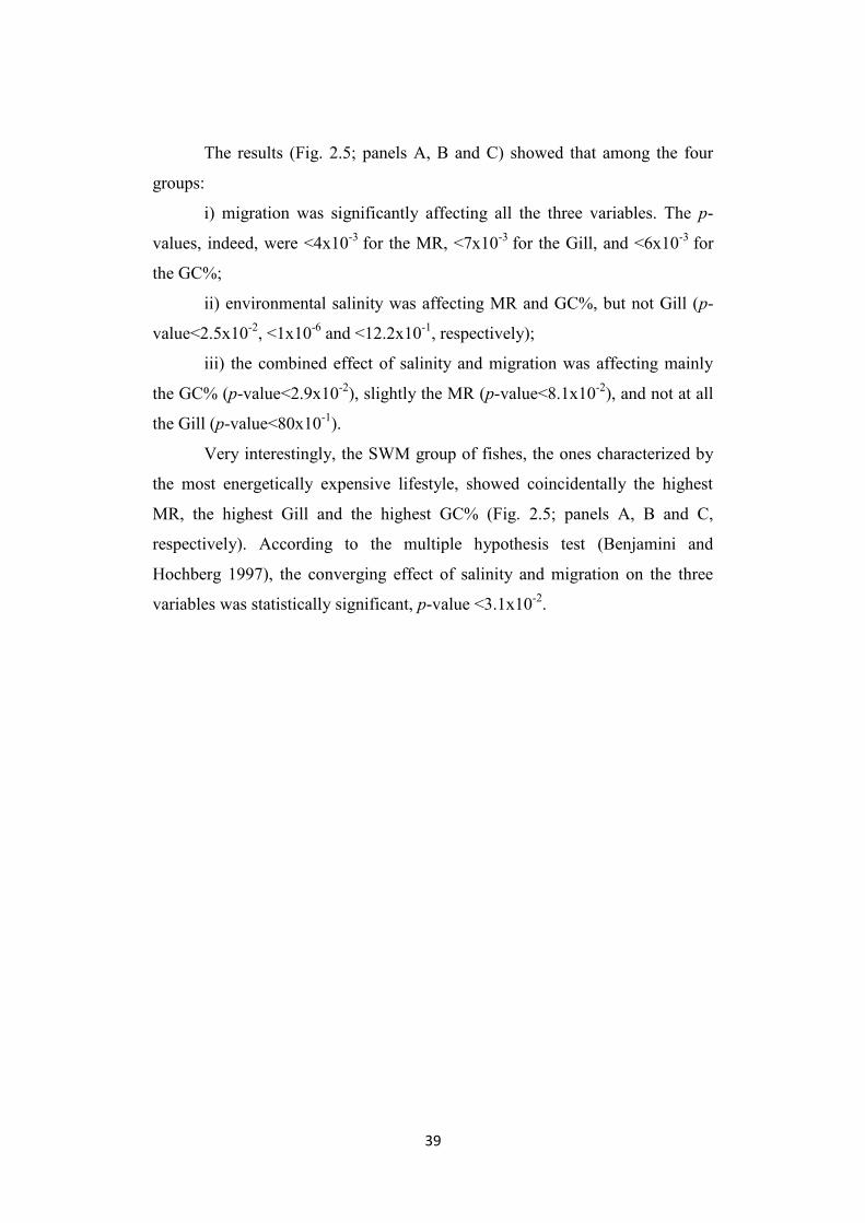
The results (Fig. 2.5; panels A, B and C) showed that among the four
groups:
i) migration was significantly affecting all the three variables. The p-
values, indeed, were <4x10⁻³
for the MR, <7x10⁻³
for the Gill, and <6x10⁻³
for
the GC%;
ii) environmental salinity was affecting MR and GC%, but not Gill (p-
value<2.5x10⁻²
, <1x10⁻⁶
and <12.2x10⁻¹
, respectively);
iii) the combined effect of salinity and migration was affecting mainly
the GC% (p-value<2.9x10⁻²
), slightly the MR (p-value<8.1x10⁻²
), and not at all
the Gill (p-value<80x10-1
).
Very interestingly, the SWM group of fishes, the ones characterized by
the most energetically expensive lifestyle, showed coincidentally the highest
MR, the highest Gill and the highest GC% (Fig. 2.5; panels A, B and C,
respectively). According to the multiple hypothesis test (Benjamini and
Hochberg 1997), the converging effect of salinity and migration on the three
variables was statistically significant, p-value <3.1x10⁻²
.

40
Figure 2.5
Boxplot of routine metabolic rate (panel a), specific gill area (panel b), and genomic GC content (panel c) for freshwater non-migratory (FWNM), freshwater migratory (FWM), seawater non-migratory (SWNM) and seawater migratory (SWM) species

41
DISCUSSION
Does the routine metabolic rate is higher in seawater than freshwater
fishes? This question, that has been matter of a long debate grounded on many
different experimental and theoretical approaches (Boeuf and Payan 2001 for a
review), find a positive answer in the present data. The consistency of this result
(p-value<1.0x10⁻²) rely on the analysis of ~200 species of teleosts (Table S1).
Such a huge comparison (based on species characterized by different body mass
and living in habitats with different environmental temperature) have been
possible due to the normalization of the data about the routine metabolic rate by
the Boltzmann’s factor, according to the equation MR=MR0eE/kT
(Gillooly et al.
2001). The result was further supported by the analysis of the phenotypic
character mainly linked to the metabolic rate, namely the specific gill area
(Hughes 1966). Indeed, analyzing an independent dataset of >100 teleosts
(Table S2), SW species turned out to have a specific gill area higher than those
of FW ones (p-value5.7x10-2). Hence, there was a very good accordance
between morphology and physiology in favor of the SW species. In the light of
the metabolic rate hypothesis (Vinogradov 2001, 2005), species showing a high
metabolic rate should also show a high GC content (in table S3 the Gc values
for teleosts were grouped). Thus the expectation would have been that the
average genomic GC content of SW species would be higher than FW ones. In
teleosts, the inter-genomic correlation between the two variables was found to
significantly hold (Uliano et al. 2010). The link between metabolic rate and GC
content obviously is not straightforward, but goes through a consideration about
the DNA structure. Indeed, to be GC- or AT-rich is not equivalent for the DNA
molecule (Vinogradov 2003). Structural analyses performed independently with
two different approaches reached, in fact, the same conclusion: a GC-richer
DNA is more suitable to cope the torsion stress (Gabrielian et al. 1996; Babbitt
42
and Schulze 2012). Duplication and transcription are the two main functional
steps during which the DNA molecule is under torsional stress because the
opening of the double helix. Noticeably, the duplication process cannot be
invoked, since it is well known that a great GC content variability have been
observed not only among organisms (Reichenberger et al. 2015 and references
therein), but also within genomes, well known to be a mosaic of genome
regions with different GC content, i.e. isochores (Bernardi et al. 1985; Bernardi
2004). Thus, the transcription process should be considered as the main factor
of the torsion stress affecting the DNA structure (Vinogradov 2001). Several
studies, indeed, support the correlation between GC content and the
transcription levels. In fact, the in situ hybridization of GC-rich and GC-poor
probes showed that human GC-rich regions, harboring GC-rich genes, were in
an open chromatin structure (Saccone et al. 2002). Besides, human GC-rich
genes showed transcriptional levels significantly higher than those of GC-poor
ones (Arhondakis et al. 2004). Moreover, according to the KOG classification
of genes (Tatusov et al. 2003), several mammalian genomes were analyzed
showing that genes involved in metabolic processes were, at the third codon
positions, GC-richer than those involved in information storage or in cellular
processes and signaling (Berná et al. 2012). Present results highlighted that also
within the genome of green spotted pufferfish GC-rich genes showed higher
transcriptional levels than GC-poor ones (Fig. 2.2).
In the line of the above considerations and results, and keeping in mind
that a significant correlation between MR and GC content was already observed
among teleosts (Uliano et al. 2010; Chaurasia et al. 2011), was not a mindless
expectation that the GC content of SW would have been significantly higher
than that of FW, and, indeed, the p-value was <1.8x10⁻⁴. Although the difference
seems to be in a very little order of magnitude, hence apparently negligible
from an evolutionary point of view, detailed analysis on five teleostean species,
zebrafish, medaka, stickleback, takifugu and pufferfish showed that small
differences of the average genome base composition hide great differences at

43
the genome organization level, and indeed, comparing the genome of
stickleback and pufferfish (average genomic GC content 44.5% and 45.6%,
respectively), the genome of the latter was characterized by the presence of a
very GC-rich regions (isochore) completely absent in the former (Costantini et
al. 2007). It worth to recall here that in teleosts the routine metabolic rate, not
only was found to correlate significantly with the genomic GC content, as
mentioned above (Uliano et al. 2010), but also to affect the genome features.
Indeed, analyzing five full sequenced fish genomes, increments of MR were
found to significantly correlate with the decrease of the intron length (Chaurasia
et al. 2014, Part II of this Chapter).
The comparison of migratory (i.e. catadromous, potamodromous,
amphidromous, oceanodromous and anadromous) and non-migratory species
showed that the specific gill area of migratory species was significantly higher
that than of non-migratory ones (p-value<3.8x10⁻²) and the GC% showed the
same statistically significant trend (p-value<6x10⁻³), being higher in the
migratory group. However, the difference of MR, also being higher in the
migratory group, was at the limit of the statistical significance (p-value <7.9x10-
2). Thus, in order to disentangle the effect of the environmental salinity from
that of the migratory attitude, the three datasets concerning MR, Gill and GC%
were split in four groups, namely freshwater non migratory (FWNM),
freshwater migratory (FWM), seawater non migratory (SWNM) and seawater
migratory (SWM). At first glance, among the four groups a good agreement
was observed regarding the three variables, showing, indeed, increasing average
values from FWNM to SWM (Fig. 2.5). However, the two-way ANOVA test
showed that the variation among the four groups was significantly affected by
both the environmental salinity and the migratory attitude only regarding MR
and GC content (Fig. 2.5; panels A and C), while Gill was significantly affected
only by migration and not by the environmental salinity (Fig. 2.5, panel B). The
combined effect of a costly osmoregulation and the need for a high scope for
aerobic metabolism would justify the higher MR in marine migratory fish

44
species. Moreover, the need of an adequate oxygen uptake in active species
(such as migratory species) is a major determinant of gill area. It is worth to
note that an increase in gill area is disadvantageous for osmoregulation,
particularly for freshwater species, as it increases the obligatory ion exchanges
and the energetic cost of compensating them (Gonzalez and McDonald 1992;
Evans et al. 2005). This would explain the observed discrepancy between MR
and Gill dependency from migratory habit and salinity. Nevertheless, the
multiple hypothesis test (Benjamini and Hochberg 1997) showed that the SWM
group was significantly the highest for all the three variables. Therefore, in the
teleost group, that is under the highest environmental demanding conditions due
to both salinity and migration, the three variables converged reaching the
highest values. On one hand, present results supported previous reports on both
metabolic rate and gill area (De Jager and Dekkers 1974; Palzenberger and
Pohla 1992), on the other opened to new genomic perspective since, as far as
we know, this is the first report that phenotypic, physiological and genomic
feature are linked under a common selective pressure. Interestingly, the
genomic feature, i.e. the average GC content, was a very “reactive” variable to
environmental changes. Indeed, according the two-way ANOVA test, the GC%
was the only variable being simultaneously affected, and by environmental
salinity and migration attitude, p-value<2.9x10⁻². Such “reactivity” was not
observed for both Gill and MR. Most probably this could be explained by other
morphological/functional and physiological constraints acting more on Gill area
and metabolic rate, than on the DNA base composition.

45
PART II
2.6 THE GENOME ARCHITECTURE OF TELEOSTS
A general agreement on the hypothesis that selection mainly shapes the
intron length through the expression level can be found in the current literature
(Castillo-Davis et al. 2002; Urrutia and Hurst 2003; Versteeg et al. 2003; Li et
al. 2007; Carmel and Koonin 2009; Rao et al. 2013). On the contrary, the link
between the forces shaping both the regional GC content and the intron length
remains a debated issue, since evidences have been produced both in favor or
against (Duret et al. 1995; Versteeg et al. 2003; Arhondakis et al. 2004;
Vinogradov 2004; Carmel and Koonin 2009). Taking advantage from the
sequence project of five teleosts fish, namely Danio rerio (zebrafish), Oryzias
latipes (medaka), Gasterosteus aculeatus (three-spine stickleback), Takifugu
rubripes (fugu) and Tetraodon nigrovirids (green-spotted puffer fish), the
teleostean genomic architecture was analyzed in the context of the metabolic
rate hypothesis predicting a link between: intron length, GC-content and
metabolic rate.

46
RESULTS
2.7 DISTRIBUTION OF THE INTRONIC GC CONTENT
The five species here analyzed, ordered according to the phylogenetic
tree reported in Fig. S1 according to Loh et al. (2008), showed an increasing
GC-content (Table 2). The genomic and the intronic base composition (GCg
and GCi, respectively) showed the same ranking order, i.e. D. rerio (zebrafish)
< O. latipes (medaka) < G. aculeatus (stickleback) < T. rubripes (fugu) < T.
nigroviridis (pufferfish). In each species, GCi was lower than the corresponding
GCg, with the exception of T. nigroviridis. As expected, the two variables were
significantly correlated (p-value<6.7x10⁻³
). On the contrary, bpi showed no
correlation with GCg, GCi (Table 2.2).
Table 2.2. Average values of genome (GCg) and intron
(GCi) base composition, intron lenght (bpi) and metabolic
rate Boltzmann corrected (MR) in fish genomes.
GCg(%) GCi (%) bpi MR(ln)
D. rerio 37.36 36.01 17992.57 31.21
O. latipes 40.1 39.9 3109.9 31.63
G. aculeatus 44.12 43.57 5056.68 32.00
T. rubripes 45.5 44.36 5366.9 32.05
T. nigroviridis 45.9 48.13 3011.24 31.72

47
In Fig. 2.6 (panel A), the histograms of the GCi distribution in each
genome were reported. Species were ordered according to the increasing
phylogenetic distance, as shown in Fig. 2.6 (panel B) according to Loh et al.
(2008).
Figure 2.6
Panel A: phylogenetic relationships among the five fish analyzed (according to Loh et al (2008)(drawings from http://egosumdaniel.blogspot.it/2011/09/some-notes-on-atlantic-cod-genome-and.html)
Panel B: histograms of the GCi distribution in each genome
48
Interestingly: i) the GCi% was higher in stickleback than zebrafish; and ii) the
values of the skewness (SK) were negatively correlated with the corresponding
GCi%. These results were in contradiction with the thermostability hypothesis,
since GC and genome heterogeneity (due to the formation of GC-rich
isochores) are expected to increase at increasing environmental temperature
(Bernardi 2004). The complete statistical analysis of GCi distribution in each
genome was reported in table 2.3. The lack of correlation between bpi and both
GCg and GCi (Table 2.2) deserved further consideration. Indeed, the number of
available full gene sequences (i.e. CDS+introns) was very different for each
species (see Materials and Methods). In order to avoid any bias due to the size
of the datasets, the comparative genome analysis was restricted to sets of
orthologous intronic sequences. Moreover, to highlight the possible effect of
transposable and/or repetitive elements, the software Repeat-Masker was used
to clean up all the intronic sequences. The average length (bp%) of the intronic
sequence masked by Repeat-Masker in each species, as well as the
corresponding GC%, were reported in Table 2.4.
.

49
S1. Descriptive Statistics of GCi% distribution in the five telosts genomes.
Mean Std. Dev. Std. Error Count Variance Skewness Kurtosis Median
D. rerio 36.011 4.363 0.028 24965 19,038 1.531 10.575 35.800
O. latipes 39.902 6.155 0.060 10680 37,884 1.143 3.111 38.900
G. aculeatus 43.578 5.045 0.033 23696 25,448 1.551 11.705 43.200
T. rubripes 44.364 5.396 0.046 13603 29,120 0.615 1.635 44.000
T. nigroviridis 48.126 8.372 0.061 18839 70,093 0.845 1.719 47.000
Table 2.3

50
Regarding length, the introns of zebrafish and stickleback showed the
highest and the lowest effect of the Repeat-Masker step. On the average
intronic sequences were shortened by a ~6% and ~2%, respectively (Table 3).
Regarding base composition, values were increasing from zebrafish (~14%) to
pufferfish (~42%). In spite of such a great variability, the average GCi% values
before and after Repeat-Masker changed slightly from set to set of orthologous
introns (Table 4), and were barely different from those of the whole set of
intronic sequences (Table 2).
Table 2.4. Average bpi% and GCi% of repetitive
elements
removed by Repeat Masker.
bpi % S.E. GCi % S.E.
D. rerio
5.710 0.086
14.200 0.023
O. latipes
2.224 0.133
23.459 0.005
G. aculeatus
2.040 0.032
35.517 0.003
T. rubripes
3.576 0.070
39.807 0.004
T. nigroviridis 3.059 0.058 42.685 0.004

51
Table 2.5. Average GCi% in each set of orthologous genes before (bRM) and after (aRM) Repeat Masker.
D. rerio O. latipes G. aculeatus T. rubripes T. nigroviridis
bRM aRM bRM aRM bRM aRM bRM aRM bRM aRM
D. rerio - 35.12 36.55 35.38 36.43 35.38 36.5 35.41 36.53
O. latipes 39.52 39.67 - 39.37 39.54 39.51 39.67 39.42 39.58
G. aculeatus 43.32 43.40 43.01 43.09 - 43.38 43.46 43.36 43.43
T. rubripes 43.98 43.96 43.62 43.61 43.91 43.87 - 44.13 44.11
T. nigroviridis 47.06 47.14 46.42 46.49 46.88 46.96 47.09 47.16 -

52
2.8 PAIRWISE COMPARISON
The SK values of each GCi distribution of orthologous intronic
sequences, before Repeat-Masker, were reported in Table S7. For each species
the average SK value was: 0.45 (zebrafish), 1.087 (medaka), 0.67 (stickleback),
0.50 (fugu) and 0.69 (pufferfish). The differences in length (bpi) and base
composition (GCi) of the intronic sequences, before and after Repeat-Masker,
were computed independently for each variable in each pairwise comparison of
orthologous intronic sequences. The pairwise comparisons were grouped in
three clusters. The first (A) grouping s of medaka, stickleback, fugu and
pufferfish vs zebrafish (i.e. medaka-zebrafish; stickleback- zebrafish; fugu-zebrafish and
pufferfish-zebrafish); the second (B) grouping those of stickleback, fugu and
pufferfish vs. medaka; and the third (C) comprising those of fugu and pufferfish
vs. stickleback (Fig. 2.7). Comparisons within each cluster were ordered
according to the increasing phylogenetic distance in Fig. 2.6 (panel A) (Loh et
al. 2008). In Fig. 2.7, the histogram bars referred to the percentage of sequences
longer (bpi%, blue bars) and GC-richer (GCi%, red bars) in the first of the
two species (for example medaka in the medaka-zebrafish). The percent of intronic
sequences longer and GC-richer in the second species (i.e. zebrafish in the
medaka-zebrafish) accounted for the complement to hundred (not shown). No
significant differences were observed before and after Repeat-Masker (Fig.
2.7), with the exception of data regarding cluster A, where GCi, after
removing transposable and repetitive elements, was reduced in each pairwise
comparison of a ~10%. In Fig. 2.7, bpi% and GCi% displayed an opposite
behavior within each pairwise comparison, indicating that the majority of the
intronic sequences were shorter and/or GCi-richer in the first of the two species
(for example medaka in the medaka-zebrafish). For example, in the cluster A, the
bpi values, even after Repeat-Masker, were very low ~11%, ~9%, ~5% and
~3%, whereas those of the corresponding GCi were very high ~70%, 90%,

53
~88% and ~92%. The above trend was observed also in clusters B and C, as
well as in the pairwise comparison fugu vs. pufferfish (Fig. 2.7).
Figure 2.7
The histogram shows the percents of orthologous intronic sequences increasing in length (Dbpi, blue bars) and GC content (DGCi, red bars) in each pairwise comparison. Data before (bRM) and after (aRM) RepeatMasker are reported. In cluster A: comparison of medaka, stickleback, fugu and pufferfish against zebrafish. In cluster B: comparison of stickleback, fugu and pufferfish against medaka. In cluster C: comparison of fugu and pufferfish against stickleback. Within each cluster pairwise comparisons were ordered according to the increasing phylogenetic distance.

54
Intron length (bpi) and GC content (GCi) were further analyzed,
testing the concomitant effect of both variables on the intronic sequences.
Orthologous sequences of each pairwise genome comparison were grouped into
four classes, according to the following criteria:
i. negative bpi and positive GCi values, named as N/P;
ii. both negative bpi and GCi values, named as N/N;
iii. positive bpi and negative GCi values, named as P/N;
iv. both positive bpi and GCi values, named as P/P.
The frequencies of each class in each pairwise comparison, before and
after Repeat-Masker, were reported in Fig. 2.8, clustered and ordered as in Fig.
2.6 (panel A).

55
Figure 2.8
The histogram shows the percent of the four classes N/P (negative Dbpi and positive DGCi values), N/N (negative Dbpi and negative DGCi values), P/N (positive Dbpi and negative DGCi values) and P/P (negative Dbpi and negative DGCi values) in each pairwise genome comparisons. Data before (bRM) and after (aRM) RepeatMasker are reported. Clusters A, B and C as in the legend of Fig. 2.7.
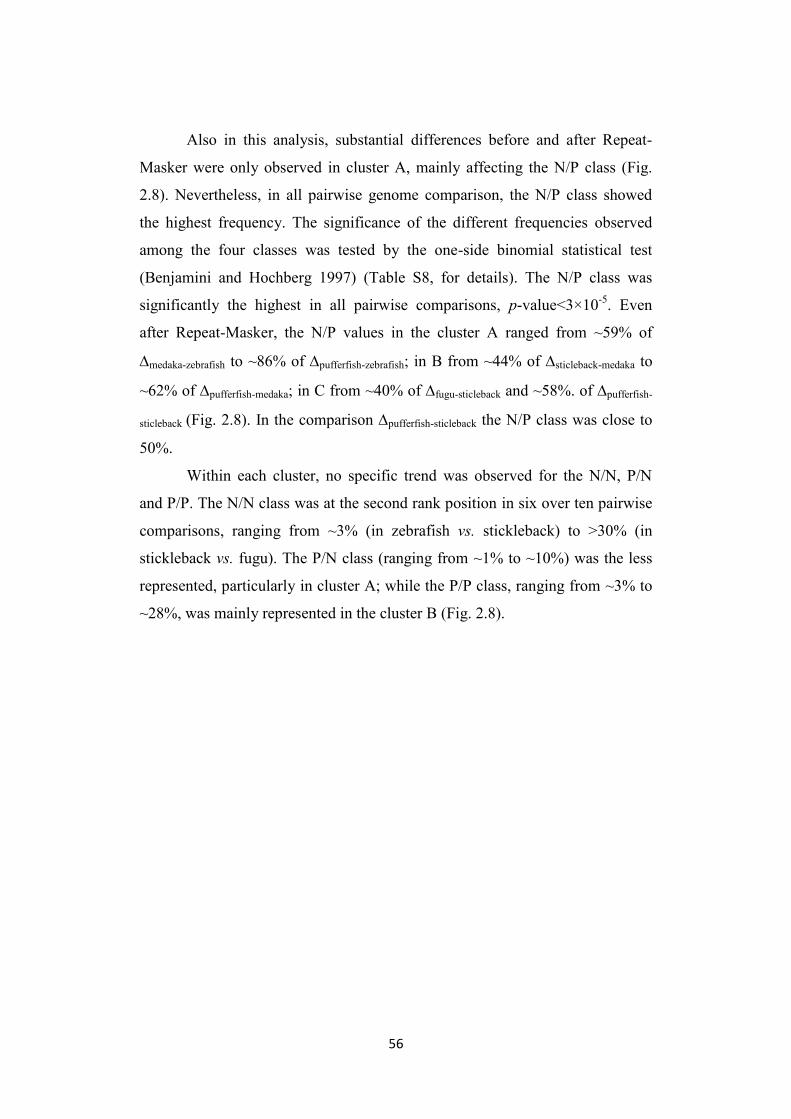
56
Also in this analysis, substantial differences before and after Repeat-
Masker were only observed in cluster A, mainly affecting the N/P class (Fig.
2.8). Nevertheless, in all pairwise genome comparison, the N/P class showed
the highest frequency. The significance of the different frequencies observed
among the four classes was tested by the one-side binomial statistical test
(Benjamini and Hochberg 1997) (Table S8, for details). The N/P class was
significantly the highest in all pairwise comparisons, p-value<3×10⁻⁵
. Even
after Repeat-Masker, the N/P values in the cluster A ranged from ~59% of
medaka-zebrafish to ~86% of pufferfish-zebrafish; in B from ~44% of sticleback-medaka to
~62% of pufferfish-medaka; in C from ~40% of fugu-sticleback and ~58%. of pufferfish-
sticleback (Fig. 2.8). In the comparison pufferfish-sticleback the N/P class was close to
50%.
Within each cluster, no specific trend was observed for the N/N, P/N
and P/P. The N/N class was at the second rank position in six over ten pairwise
comparisons, ranging from ~3% (in zebrafish vs. stickleback) to >30% (in
stickleback vs. fugu). The P/N class (ranging from ~1% to ~10%) was the less
represented, particularly in cluster A; while the P/P class, ranging from ~3% to
~28%, was mainly represented in the cluster B (Fig. 2.8).

57
2.9 THE MR IN THE FIVE TELEOSTS
The routine metabolic rate was measured for each species. The values
were temperature-corrected using the Boltzmann’s factor, and shortly denoted
as metabolic rate (MR). For each species, the distribution of log-normalized
MR values was reported as box plots (Fig. 2.9), while the average values were
reported in Table 2.2. The Student-Newman-Keuls post hoc test for multiple
comparisons was performed to assess the significance (threshold p<0.5×10⁻²
) of
the MR differences observed among species (Table 2.6).
Figure 2.9
Box plots of the routine metabolic rate temperature-corrected using the Boltzmann’s factor (MR) measured in each teleostean fish.

58
In short:
i. the MR of zebrafish was significantly the lowest;
ii. that of medaka was significantly lower than those of stickleback
and fugu, but not significantly different from that of pufferfish;
iii. the MR of stickleback and fugu were not significantly different;
iv. that of pufferfish was significantly different from those of
stickleback and fugu.
Table 2.6. Student-Newman-Keuls post hoc
test.
D. rerio O. latipes G. aculeatus T. rubripes
D. rerio -
O. latipes S -
G. aculeatus S S -
T. rubripes S S NS -
T. nigroviridis S NS S S
S = significant (threshold level p<5.0x10⁻²
) N.S. = not significant
The MR average values showed a correlation with GCg (p-
value<8.5×10⁻²
), and no correlation with GCi. It is worth to bring to mind that
in a larger dataset of 34 teleostean species the correlation between MR and GCg
was highly significant, p-value, 2.5×10⁻³
(Uliano et al. 2010). For each pair of
species, the MR values were computed and correlated with the corresponding
GCi and bpi average values obtained before running Repeat-Masker. The
Spearman rank correlation test was performed to assess the statistical
significance (Table 2.7).

59
Table 2.7. Correlation coefficients Rho (in italic) and
p-values (in bold) of Spearman correlation test.
bpi GCi MR
bpi - <3.3x10
-2 <5.1x10
-2
GCi -0.709 - <2.1x10⁻²
MR -0.648 0.770 -
GCi and bpi were significantly correlated (Rho -0.709, p-
value<3.3×10⁻²
), as well as GCi and MR (Rho 0.770, p-value<2.1×10⁻²
),
while the correlation between bpi and MR was at the limit of the statistical
significance (Rho -0.648, p-value<5.1×10⁻²
). Replacing MR with T, i.e. the
increments of the average, or the maximum, environmental temperature
experienced by each species, no significant correlation was observed with both
GCi (Rho -0.287, p-value<42.1×10⁻²
and Rho -0.126, p-value<72.8×10⁻²
,
respectively) bpi (Rho -0.037, p-value<92.1×10⁻²
and Rho -0.101, p-
value<78.1×10⁻²
, respectively).

60
DISCUSSION
In the present study, a linear correlation between intron length (bpi) and
the corresponding GC content (GCi) was not found, neither analyzing the whole
data set of intronic sequences available for each genome (Table 2.2) nor each
subset of orthologous intronic sequences. However, starting from orthologous
introns sets and computing independently bpi and GCi in each pairwise
genome comparison, a different picture came out. For example, in the pairwise
comparison medaka-zebrafish the largest part of the intronic sequences of medaka
showed a length shortening (both before and after cleaning sequences by
Repeat-Masker) and an increment of the GCi content (Fig. 2.7). The same
applied in all pairwise comparisons. Hence, bpi and GCi showed an opposite
trend. Differences between before and after Repeat-Masker were observed only
in the pairwise comparisons of the cluster A (Fig. 2.7). The effect should be
ascribed to the high occurrence of type II transposable elements, covering
~39% of the zebrafish genome, against the ~10% observed in medaka,
stickleback, fugu and pufferfish (Howe et al. 2013).
For each species, the routine metabolic rate was measured and
temperature-corrected using the Boltzmann's factor, according to Gillooly et al.
(2001). Differences of the average metabolic rate (MR) were calculated in
each pairwise comparison of the teleostean species. Interestingly, MR turned
out to be significantly correlated with both the average bpi and the average
GCi, both computed without masking transposable and repetitive elements. In
turn, bpi and GCi were significantly correlated (Table 2.7). The correlation
of MR vs. bpi was of particular interest because opened to the hypothesis
that the occurrence of transposable and repetitive elements would be under the
ultimate control of the metabolic rate of the organisms. A random insertion of

61
transposable elements or random increments of the repetitive elements in the
intronic regions, indeed, should alter the opposite trend between bpi and
GCi, also found to hold after cleaning up intronic sequences by Repeat-
Masker (Fig. 2.7).
The analyses of the four possible combinations of the differences in
intron length and GC content (the four classes in Fig. 2.8), further supported the
inverse relationship between the two variables. Indeed, the N/P class (grouping
intronic sequences showing negative bpi and positive GCi values
simultaneously) was significantly the highest in all pairwise comparisons,
p<3x10⁻⁵, also after Repeat-Masker (Fig. 2.8). Conversely, the P/N class
(grouping intronic sequences showing positive values for bpi and negative
ones for GCi simultaneously) was counter selected, accounting on the average
for ~5% the orthologous set of genes.
In short, the largest majority of intronic sequences (N/P class) were
under a converging constraint for a reduction of the length and an increment of
the GC content. For the other sequences grouped in the P/P, P/N and N/N
classes such a converging constraint was most probably not of use, because of
different or no constraints. Regarding the P/P and the P/N, the two classes of
grouping sequences opposed to the reduction of the intron length (barely
affected by Repeat-Masker and accounting for ~10% and ~5%, respectively), a
possible explanation would be that those classes are most probably harboring: i)
genes on which the process of co-transcriptional splicing is taking place, a
process coming out to be not such a rare event and mainly affecting genes
carrying long and GC-rich introns, i.e. the features of the genes whose introns
belong to the P/P class (Oesterreich et al. 2011); or i) genes showing alternative
splicing, a process that was reported to be favored in genes harboring long
introns, i.e. the features of the genes whose introns belong to the P/N class
(Kandul and Noor 2009).

62
A possible explanation for the discrepancy between the intra- and the
inter-genomes analysis most probably could be ascribed to the fact that the
former was a picture of a status quo, i.e. a snapshot of a genome, whereas the
latter was an analysis of an in fieri process, i.e. a work in progress. Indeed, it is
worth to recall that all pairwise comparisons between fishes were performed
according to the phylogenetic relationship of the five species (Loh et al. 2008;
see also figure 2.6, panel A).
CONCLUSION
Although the present analyses of teleostean fishes metabolic rate, gill
area and genomic GC-content could not be considered as a demonstration of the
cause-effect link between metabolism and DNA base composition, certainly
represent a further support to the metabolic rate hypothesis proposed by
Vinogradov (Vinogradov 2003, 2005) underlining that the torsion stress,
proposed to be the factor responsible of the GC increment, could be not such a
mysterious selective force.
Data on metabolic rate and genomic GC of fish showing different
lifestyles is supported by the analysis of the gill area. The results clearly
highlight that active species living in seawater show coincidentally the highest
routine metabolic rate, the highest specific gill area and the highest average
genomic GC content.
The different genome architecture observed among teleostean genomes
is not merely a difference` in their average genomic GC content. Here a large
dataset of orthologous introns has been analyzed, and the metabolic rate seems
to be the main selective factor driving the evolution of the genome architecture,
in particular that of length and base composition of intronic sequences. The
analysis of intron length and GCi content in the five teleosts genome

63
characterized by different genomic GC content and increasing metabolic rate,
were found to be in good hold with the results reported for all vertebrate
genomes so far analyzed (Duret et al. 1995; Versteeg et al. 2003; Arhondakis et
al. 2004; Zhu et al. 2009), giving further support to the current hypothesis
relating the intron length with the energetic cost of the transcriptional activity.
The present results not only further support previous observations about
genome evolution of vertebrates (Uliano et al. 2010; Chaurasia et al. 2011;
Berná et al. 2012, 2013), but also open a challenge for a comparative study of
the gene expression level among teleosts.

64
Chapter III
INTRODUCTION
3.1 GENOME COMPOSITION IN POLYCHAETES
Polychaetes, commonly known as bristle worms, emerged, according to
fossil records, in the early Cambrian Period (Rouse and Pleijel 2001). They
represent the most diverse clade within the Annelida (~90% of the known
species), mainly living in marine habitat (Jumars et al. 2015; WoRMS Editorial
Board 2016). A bilateral metameric organization, with distinct anterior and
posterior parts, characterizes their body plan (Rouse and Pleijel 2001). In spite
of this basic scheme, a tremendous diversity of body forms have been
originated, showing a wide array of adaptations related to theirs various
functional aspects, from feeding to reproduction, from behavior to locomotion
(Jumars et al. 2015). Regarding motility, two extreme lifestyles can be
highlighted: i) motile forms, i.e. showing different degree of movement, from
slow crawling or burrowing, to active swimming; and ii) sessile forms, i.e.
permanently and obligatory living inside the tubes they built, generally attached
to a hard substrate or inserted in a soft substrate (Rouse and Pleijel 2001).
Although lifestyle is well known to affect both the morphology and the
physiology of bristle worms, the “operational” sub-division in motile and
sessile is not supported by generally accepted phylogenetic inference (Rouse
and Pleijel 2001; Weigert et al. 2014). The lower number of sessile families (13
against ~85) and their more specialized morphology (Jumars et al. 2015) may
suggest an origin from simpler motile forms (Rouse and Pleijel 2001).
However, a phylogenomic analysis of several annelid families showed that the

65
basal branching taxa would include a huge variety of life styles, from
tubicolous to errant forms (Weigert et al. 2014).
3.2 DIFFERENCES IN LOCOMOTION
Regarding motility, two extreme lifestyles can be highlighted: sessile
forms, i.e. permanently and obligatory living inside the tubes they built and
generally attached to a hard substrate or inserted in a soft substrate, and motile
forms, i.e. showing different degree of movement, from slow crawling to active
swimming (Rouse and Pleijel 2001). It is worth to bring to mind that both
morphological and physiological adaptations are strongly related to motility.
Indeed, not only the locomotor apparatus, i.e. parapodia and chaetae, in sessile
species is reduced and usually modified (e.g. tori as parapodia; hooks or uncini
as chaetae) for hanging to the internal walls of the tube, but also the
morphology of the prostomium (head), the body differentiation (generally in
two regions, namely thorax and abdomen), and the organization of organs, such
as gills and brain (Rouse and Pleijel 2001). Actually, gills are strongly
regionalized in sessile species, showing plume-like structures, harbored in the
prostomium or along the body. The brain organization, on the contrary, shows
little differentiation in sessile forms, while is more complex in motile forms, as
in Eunicidae and Nereididae characterized by three brain regions (fore-, mid-
and hind-brain). The different brain organization between sessile and motile
forms was suggested to be presumably ascribed to the needs to integrate
complex signals coming from various sensorial appendages and organs
occurring in motile species (Rouse and Pleijel 2001).
At present there is not yet a unified view on the phylogenetic
relationships among annelid taxa, and consequently on the appearance of the
two main and contrasting life habits related to motility mainly characterizing
polychaetes. The traditional view describing the evolution of annelids from
simple motile forms to complex tube dwelling (Jumars et al. 2015), and

66
summarized by the comprehensive morphological-cladistic analyses of Rouse
and Pleijel (Rouse and Pleijel 2001), failed to be supported by the
phylogenomic reconstruction of the Annelida tree based on transcriptomic data
(Weigert et al. 2014).
3.3 THE POLYCHAETA GENOME
Although representing one of the most differentiate group of marine
invertebrates with a cosmopolitan distribution and wide ecological occurrence,
polychaetes have been quite neglected from the genomic point of view, and
little is known on their genome organization. An early work on genome size
showed that small interstitial species had lower C-values than the bigger
macrobenthic ones, raising the hypothesis that the short life span and the small
body size, characteristic of interstitial species, could affect the C-value (Gambi
et al. 1997). Only recently, the nuclear genetic variation in polychaetes was
tackled in Streblospio benedicti (Rockman 2012), and the draft genome of
Capitella teleta was available (Simakov et al. 2013).
Early physiological investigations between the two categories of
polychaetes with different degree of motility, i.e. Errantia and Sedentaria,
showed that the former were characterized by higher routine oxygen
consumption than the latter (Shumway 1979; Shumway et al. 1988). This
observation is particularly interesting in the frame of the evolutionary
hypothesis assigning to the metabolic rate the role of main force driving the
DNA base composition variability among organisms (Vinogradov and
Anatskaya 2006). According to the metabolic rate hypothesis, a number of
bristle worms species characterized by a motile or sessile lifestyle, were here
investigated with the aim to test the prediction that the former should show not
only a higher metabolic rate than the latter, but also a higher genomic GC-
content.

67
RESULTS
3.4 METABOLIC RATE IN POLYCHAETES
The respiration rate for 20 species was retrieved from literature (Table
S10). In order to perform a comparative analysis, all available data were
temperature-corrected by the Boltzmann’s factor, according to the equation
proposed by Gilloly et al. (Gillooly et al. 2001). In Fig. 3.1, panel A, the
boxplot of the specific respiration rate, i.e. the temperature-corrected respiration
rate on mg of dry tissue, for the motile and the sessile group was reported. The
differences were statistically significant, p-value <4.4x10⁻²
. Incidentally, the
observed difference cannot be ascribed to variations of body mass between the
specimens of the two groups, since no significant differences were found
according to the Mann-Whitney test. Moreover, the mass-oxygen consumption
graph built from the single species equations to avoid the mass-dependence
effect of the respiration rate (Fig. S.3), confirmed the previous observation of
Shumway (Shumway 1979). Indeed, motile polychaetes showed an higher
intercept of the mass-metabolic rate regression line than sessile species. The
statistically significance of the differences in elevation of the regression line
was assessed by ANCOVA test (p-value<4.6x10⁻²
).
3.5 NUCLEOTIDE COMPOSITION
In order to test if the metabolic rate hypothesis of genome evolution
could be extended to, and further supported by, invertebrate organisms, a
comparative analysis of bristle worms was performed. The average genomic
GC% was analyzed in the 37 available species, sixteen of which were classified
as “sessile forms”, covering 50% of the sessile families, while the remaining
species were classified as “motile forms”. Unfortunately, because it was

68
impossible to collect appropriate material, an exhaustive analysis of all sessile
families was not achieved (Table S9).
The GC-content of the motile group ranged from 30.5% to 48.3%,
average 40.2% (s.d.±4.4), while that of the sessile group ranged from 29.0% to
44.3%, average 35.2% (s.d.±3.8). The box plot of the two groups was reported
in Fig. 3.1, panel A. The different average GC-content between motile and
sessile species was statistically significant, p-value <7.0 x10⁻⁴
.
Figure 3.1
Boxplot of the average genomic GC-content (panel A) and metabolic rate, mass- and temperature-corrected by Boltzmann’s factor (panel B), of motile (red box) and sessile (blue box) species.

69
DISCUSSION
3.6 PHYLOGENETIC INDEPENDENCY OF GC% AND METABOLISM
It was clear from the study of the GC content distribution in the
polychaeta group that the energetic costs of motility shapes both the nucleotide
composition and the basal respiration rate, clearly showing that the motile
forms have evolved higher Guanine and Cytosine concentration in their
genomes, as well as an higher rate of aerobic respiration.
In the light of traditional phylogenetic hypothesis, the GC-content
showed a decreasing trend from higher, in the ancestral motile forms, to lower
values in the more specialized sessile ones. According to the recent molecular-
based tree by Weigert and colleagues (Weigert et al. 2014), which support an
independent evolution of the locomotion ability, the genomic GC% showed no
phylogenetic signals. The conclusion was supported by the pairwise Mann-
Whitney test (Bonferroni-corrected for multiple comparisons; Tab. S6,
Supplementary materials) among the analyzed families (Fig. 3.2, panel A, tree
reconstruction based on Weigert et al. 2014). The result was in good agreement
with previous inference on vertebrates (Bernardi and Bernardi 1990; Tarallo et
al. 2016).
In teleosts the problem of the interference of metabolic rate and genomic
GC content with phylogeny was already tackled. To address this issue in bristle
worms, the temperature-corrected mass-specific metabolic rate were compared
among families (Fig. 15 panel B; tree reconstruction based on Weigert et al.
2014). The Mann-Whitney pairwise comparison (Bonferroni-corrected for
multiple comparisons) didn’t support any phylogenetic inference (Table S11).
Accordingly, the morphological-cladistic analyses of Rouse and Pleijel (Rouse
and Pleijel 2001), supported the same clustering observed for the GC-content
also showed for the metabolic rate (Table S11).

70
Figure 3.2
Phylogenetic distribution of GC-content (panel A) and Metabolic rate (panel B), according to the phylogenetic inference of Weigert et al., (2014)

71
3.7 BACTERIAL CONTAMINATION
Does bacterial contamination could affect the above result? The caveat
deserves several considerations. Indeed, differently from the case of C. teleta,
whose whole genome sequencing was performed after growing organisms in
antibiotic milieu (Simakov et al. 2013), our samples were wild specimens
collected from natural habitats, harboring bacterial species on their exposed
surface as gills or epidermis. Hence, DNA contamination could not be totally
excluded. Nevertheless, comparing only the Mediterranean benthic species
collected in a limited geographic area, thus inhabited by similar bacterial
populations (Mapelli et al. 2013), the difference between motile and sessile
species still holds significantly, p-value <2.8x10⁻²
. In addition, it worth to stress
that the genomic GC-content of the motile species C. teleta (40.0%), measured
in specimens reared under antibiotic conditions, falls well within the range of
variability of the motile group (average 40.2%).
The effect of biogeographic distribution on the genomic GC-content was
also checked. Indeed, reports on teleosts showed that fish living in polar area
were GC-richer than those living in tropical one (Varriale and Bernardi 2006;
Uliano et al. 2010), a difference due to a routine metabolic rate also decreasing
from polar to tropical species (Uliano et al. 2010). Unluckily, in our dataset
motile and sessile species were not equally distributed according to the
biogeographic area. The polar group was mainly represented by sessile species
(three over four), while the tropical one was mainly represented by motile
species (six over seven). However, comparing just motile species living in
temperate and tropical area, the GC-content was not significantly different.
Little is known about the recombination frequencies in the genomes of
polychaetes, thus the observed differences in genome base composition
between motile and sessile could fit in the frame of the biased gene conversion
hypothesis (Duret and Galtier 2009). The hypothesis is essentially based on a
correlation between GC-content and recombination rate. In fish and mammalian

72
genomes, however, the inter-genome correlation failed to be found (Kai et al.
2011; Fig. 1.3).
CONCLUSION
Although present results could not be read as a demonstration of a
cause–effect link between metabolic rate and GC-content, certainly, as matter
of fact, they are part of the mosaic emerging from the study of a huge variety of
living organisms. Indeed, the analyses of fishes, mammals, birds, and now also
polychaetes, all supported a significant link between the two variables.
Unquestionably, this is of deep biological and evolutionary meaning.

73
Chapter IV
INTRODUCTION
4.1 MORPHO-PHYSIOLOGICAL COMPARISON IN ASCIDIANS
The subphylum Tunicata (Lamarck 1816), also called Urochordata
(Balfour 1881), is now universally recognized as the sister group of vertebrates
(Bourlat et al. 2006; Delsuc et al. 2006; Putnam et al. 2008). Although the
secondary loss of segmentation, coeloms and kidneys, they share with
vertebrates homologous development and structures, such as a dorsal proto-
neural crest, a notochord, the endostyle - pineal gland in vertebrates (Eales
1997) - a post-anal tail and pharyngeal gill slits, intercellular tight junctions,
striated heart muscles, protoplacode derivatives and voluminous blood plasma
with abundant circulating corpuscles (Holland et al. 2015). Behind that,
tunicates shown a very simple body plan. Thanks to their, sometimes invasive
(Lambert 2007), worldwide presence, they are relatively easy to collect and
maintain in laboratory conditions, and some representative species, such as
Ciona intestinalis, are widely used models for evo-devo studies.
In the last decades different groups of research have shown that the
species C. intestinalis was actually a complex of genetically differentiated types
(Suzuki et al. 2005; Caputi et al. 2007; Iannelli et al. 2007; Nydam and
Harrison 2010; Zhan et al. 2010). Very recently, those “types” were formerly
ascribed to two different species (Brunetti et al. 2015), namely C. robusta,
previously known as C. intestinalis type A, and C. intestinalis, previously
known C. intestinalis type B. This new classification, which is followed in the
present study, has been confirmed by Pennati et al. (2015) on the basis of
morphological differences at the larval stage.

74
We directed our attention on C. robusta and its congeneric C. savignyi,
often morphological mistaken for each other (Hoshino and Nishikawa 1985;
Lambert and Lambert 1998; Smith et al. 2010). The two species have
overlapping distribution area (Tokyo Bay, personal communication Yoshikuni
M.); San Diego bay, (Lambert 2003); New Zealand, (Smith et al. 2010), Korean
peninsula, (Taekjun and Sook 2014). Moreover the genomes of both the species
are completely sequenced (Dehal et al. 2002; Vinson et al. 2005). This scenario
prompt us to analyze the physiological constraints that could drive the genomic
base composition evolution in chordates, in particular the hypothesis that
metabolic rate can be a selective force for the shift of nucleotide composition in
organisms (Vinogradov 2003, 2005). A physiological comparative study can be
also useful to better understand the mechanisms of bio invasion. In recent
decades, ascidians have become increasingly ecologically problematic,
following their introduction into new regions (Lambert 2007), and have become
significant bio-fouling organisms for aquaculture and ports worldwide (Lambert
2007; Valentine et al. 2007). Along California coasts, C. savignyi replaces C.
robusta (Lambert and Lambert 1998), and recent news of C. savignyi and C.
robusta overlapping regions has been reported in New Zealand (Smith et al.
2010) and Korea (Taekjun and Sook 2014), where likely compete for space and
resources.
4.2 DIFFERENCES BETWEEN C. robusta AND C. savignyi
At the moment 13 different species are formally recognized within the
genus Ciona (Brunetti et al. 2015), but the identification at morphological level
can be sometimes tricky because of their typical inter-specific variability. In
particular the three species: C. intestinalis, C. savignyi and C. robusta, are very
similar in their morphology. Hoshino and Nishikawa provided the fully
description for the morphological identification of C. intestinalis, and were able
to recognize unambiguously C. savignyi thanks to the complete absence of the

75
endostylar appendage and the arrangement of the pharyngeo-epicardiac opening
(Hoshino and Nishikawa 1985). Interestingly, the morphological similarity of
the adult forms of C. intestinalis and C. savignyi is remarkable considering the
time of divergence estimated to be ~180My (Berná et al. 2009). Despite the
interest of scientists for C. intestinalis, few efforts were made to identify
morphological differences to unambiguously detect on field the two species.
After the recent discovery that C. savigny is also present in New Zealand
(Smith et al. 2010), the authors took advantage to re-discuss the external
morphology of C. savignyi in comparison with C. robusta sensu Brunetti et al.
(2015). They pointed out, like Lambert and Lambert (1998), that the presence
of pigmented flecks in the body wall and an orange pigmentation around the
siphon openings are unique to C. savignyi, while in C. robusta the pigmentation
around the siphon openings is yellow. They didn't mention at all the distal end
of vas deferens, while according to Hoshino and Nishikawa (1985) is a
peculiarity of C. savignyi to do not have an orange pigmentation at the end of
the sperm duct. The pigmentation of the vas deference is object of a recent
paper (Sato et al. 2012) in which the authors tried to identify the morphological
differences between C. robusta and C. intestinalis. Sato and colleagues
extensively documented an intense pigmentation of the terminal papillae of the
vas deference in C. robusta, but not any pigmentation of the gonoducts
themselves (however in small percentage found also in C. intestinalis);
moreover they pointed out the presence of tubercles, with no or yellowish
additional pigmentation around the siphons, also noted by Smith et al. (2010).
As already discussed above, very recently the Manni's group from
Padova University renames C. intestinalis type A and type B in C. robusta and
C. intestinalis, respectively (Brunetti et al. 2015). They described the
morphology of adults of C. robusta, referring to the same tubercular
prominescens, previosly noted by Hoshino and Nishikawa (1985) and Sato et
al. (2012), as unique feature of C. robusta (Brunetti et al. 2015). Genomic
comparison suggested divergence of types A and B at approximately 20My

76
(Suzuki et al. 2005) (See Materials and Methods section, par. I.8 for a detailed
analyses of the specimens used in this work).
4.3 DISTRIBUTION
Ciona spp. are widespread in all the oceans. C. robusta is found in the
Pacific Ocean on the west coast of North America, along Australia, New
Zealand, Korean and Japanese coasts, South Africa, Mediterranean sea and on
both French and English sides of the western English Channel (Caputi et al.
2007; Zhan et al. 2010) Fig. 4.1.
C. savignyi is very common in Japan, likely the area of origin (Hoshino
and Nishikawa 1985). It was early sampled in Alaska in 1913, but misidentified
as C. intestinalis, and today it had invaded the coast from San Diego to Santa
Barbara (Hoshino and Nishikawa 1985; Lambert and Lambert 1998; Lambert
2003). This species was also recently recorded in New Zealand (Smith et al.
2010), and in the south-east coasts of Korean peninsula (Taekjun and Sook
2014). Furthermore C. intestinalis also occupies the east coast of Asia (Zhan et
al. 2010; Taekjun and Sook 2014), previously considered a diffusion area of C.
robusta only (Caputi et al. 2007).
Figure 4.1
Global distribution of C. robusta (in blue) and C. savignyi (in red).

77
4.4 OXYGEN CONSUMPTION IN Ciona spp
At our knowledge the first published report of oxygen rate consumption
in adults of the ascidians C. intestinalis sensu Hoshino and Nishikawa (1985) is
from Jørgensen (1952). Previous measurements in the same species were
mostly focused in eggs and the fertilization event (D’Anna 1973) or embryos
(Holter and Zeuthen 1944). Jorgensen measurements were obtained with the
Winkler method, and the estimation is about 0.8 ml O2/hr. It is not clear from
the paper if the reported values were mass-corrected, but we should think so
because the measure is strong consistent with the other, more recent, report
using the same methodology by Markus and Lambert (1983): 0.82ml O2/g dry
weight/h. However Markus & Lambert stated that the Jorgensen measures
“were reported as relative values and not as weight-specific rates” (Markus
and Lambert 1983). Interestingly they reported also the organ dry weight
oxygen consumption (1.71±0.23mlO2/g/h) as the highest, in comparison with
other sea squirts from Styela genera. It should be noted that, while the measure
from Markus and Lambert were from animals sampled in California, almost
surely C. robusta, that one from Jorgensen were from Woods Hole Institute,
Massachusetts, so likely C. intestinalis sensu Brunetti et al. (2015).
Shumway was the first to report an oxygen consumption rate via oxygen
electrode methodology (Shumway 1978). He, studying the response to the
change in salinity in C. intestinalis sensu Hoshino and Nishikawa (1985),
measured an oxygen consumption rate of about 0.4mlO2/g dry weight/hr. Very
different results were then reached by Petersen and colleagues, which found a
specific respiration rate of 1.03 up to 1.08ml/g dry weight/hr for fed animals,
and a 0.28mlO2/g dry weight/hr for one week fasted animals (Petersen et al.
1995), so presumably in stress condition. Both those studies presumably
involved C. intestinalis sensu Brunetti et al. 2015. After that, few other study
addressed the question of variation in metabolic rate in sea squirt (Sigsgaard et
al. 2003; Minamoto et al. 2010), but it was not possible to extrapolate useful
data for the comparison with our or the other studies because of the differences

78
in the calculation procedures. Anyway, interestingly, Minamoto et al.
(2010)showed that relative oxygen consumption in C. robusta varies over daily
basis, reaching lower values during the day (lowest pic in the morning) and
higher values during the night.
To our knowledge no published report were available for C. savignyi.
RESULTS
4.5 MORPHOMETRIC ANALYSES
The wet body weight (BW) of C. robusta and C. savignyi specimens
ranged within 3.05-17.2g and 0.24-6.87g, respectively. The corresponding body
length (BL) ranged within 5.3-13.9cm and 2.2-8.9cm, respectively.
Unfortunately, in the present comparative study, it was impossible to sample
either bigger C. savignyi, or smaller C. robusta in order to increase the
overlapping range. According to Carver et al. (2006), who described the
relationship BW and BL in C. intestinalis as a power function, the equations for
the present data were BW=0.3068xBL1.541
(R2=0.76, p-value<10
-4) for C.
robusta, and BW=0.1432xBL1.779
(R2=0.74, p-value<10
-4) for C. savignyi (Fig.
17, panel A). In the same figure the equation obtained by Carver and colleagues
(2006) on C. intestinalis was also reported (Fig. 4.2, panel A; gray line).
Pairwise comparison showed that differences among the three equations were
all statistically significant (p-value<10-2
by F-test Bonferroni corrected). The
results were not affected if the wet body weight was replaced by the
corresponding dry values (Table 4.1).

79
Tab. 4.1 Comparison between C. robusta and C. savignyi equations obtained from
wet and dry body weight data.
Wet Weight
C. robusta C. savignyi robusta-savignyi comparison
Allometric eq. a 0,3068 0,1432
b 1,541 1,779
R2 0,7597 0,7414
Linear eq. Y = 1,508X – 4,363 Y = 0,9058X - 1,857
R2 0,7599 0,7324
Difference in slopes 0,00039
Extra sum of square 0,0003

80
Continued from previous page
Dry Weight
C. robusta C. savignyi
Allometric eq. a 0,01305 0,009373
b 1,605 1,646
R2 0,8006 0,7379
Linear eq. Y = 0,07805X - 0,2496 Y = 0,04428X - 0,08231
R2 0,8081 0,7368
Difference in slopes < 0.0001
Extra sum of square < 0.0001

81
The relationship between the weight of tunic and the organs has been
described to be linear in C. intestinalis (Carver et al. 2006). Analyzing the
relationship in C. robusta and C. savignyi. a significant linear correlation
between the two parameters was found, and the corresponding equations were:
TW = 0.011+0.76(OW) (r² = 0.75) and TW = 0.031 + 0.53 OW (r² = 0.57) for
C. robusta and C. savignyi, respectively (Fig. S.6).
The tunic/organ ratio (i.e. the dry weight of the tunic divided by the dry
weight of the organs) was calculated for each individual. Average values were
2.5 for C. robusta and 1.3 for C. savignyi. The differences were statistically
significant according to the Mann-Whitney test, p-value<10-4
(Fig. 4.2, panel
B).
Figure 4.2
Panel A: correlation between body length and wet body weight for C. robusta (in blue) and C. savignyi (in red) in comparison with C. intestinalis (Carver et al. 2006).
Panel B: Boxplot showing the tunic/organ ratio (W/W) for the specimens analyzed in this work.

82
4.6 WATER RETENTION
The whole body water retention of the two species was calculated as the
difference between the total WW and the total DW over the total WW. Average
values were 95.14% for C. robusta and 94.50% for C. savignyi. The differences
were statistically significant according to the Mann-Whitney test, p-value<10-10
.
The water retention vs. body weight correlation was assessed for both
species (Fig. 4.3). As already noticed, the ranges of body weight of the
specimens collected in Japan for both C. robusta and C. savignyi were only
partially overlapping (3.05-17.2g and 0.24-6.87g respectively). In order to
overcome the problem, the overlap was extended owing to the availability of C.
robusta at the SZN smaller than 5 grams (Naples, Italy). No models were
available for the correlation of water retention vs. body weight in this species,
thus a non-parametric model was applied, i.e. a locally weighted polynomial
regression curve. Differences or similarity could not be assessed with classical
statistics. Since the 95% confidence interval (shadow area in Fig.4.3) was
mostly overlapping, this implied a consistent degree of similarity.
The water retention was also calculated for tunic and organs
independently in each species. In C. robusta, the water retention for tunic and
organs were 95.8% and 93.4%, respectively. In C. savignyi they were 95.6%
and 93.3%, respectively. In both species: i) the differences between tunic and
organs were of the same order of magnitude (not significantly different); and ii)
the water retention was significantly higher in the tunic than in the organs (p-
value<10-17
and p-value<10-14
, respectively). Nevertheless, on average, the tunic
of C. robusta turned out to retain more water than that of C. savignyi (p-
value<10-7
).

83
Figure 4.3
Correlation between body wet weight and whole water retention in the two species: C. robusta (in blue) and C. savignyi (in red). The correlations were described by a locally weighted polynomial regression curve with 95% of the mean confidence interval area (in shadow).

84
4.7 OXYGEN CONSUMPTION
The oxygen consumption rate was measured by Dissolved Oxygen
probe as indirect quantification of metabolic rate. Average rates (18.93mg×kg-
1×h
-1 and 31.34mg×kg
-1×h
-1 for C. robusta and C. savignyi, respectively), were
significantly different, p-value<10-4
. One would expect smaller animals to have
a higher rate anyway, and the C. savignyi used in this study were smaller than
the C. robusta. This makes it very difficult to separate species differences from
size differences. To avoid the mass dependence of the oxygen consumption
rate, the linear log-log plot relationship between body mass and oxygen
consumption was analyzed (Fig. 4.4). C. savignyi was described by the equation
MR=0.36BW0.22
(R2=0.64), while C. robusta by the equation MR=0.92BW
0.59
(R2=0.76). The two logarithmic regressions were significantly different (p-value
1.2x10⁻²
, according to the F-test).
Figure 4.4
Allometric relationship between body weight (dry) and respiration rate in C. robusta (in blue) and C. savignyi (in red).
85
DISCUSSION
Ciona spp. is a widely studied genus in the eco-evo-devo field, but
relatively little is known about the comparative morpho-physiology of the
species belonging to this group. In spite of an historical role as model
organisms in life science (Satoh et al. 2003; Liu et al. 2006; Gallo and Tosti
2015), only recently peculiar morphological features have been identified,
leading to the inference of new species, such as the case of C. intestinalis and
C. robusta (Hoshino and Nishikawa 1985; Smith et al. 2010; Sato et al. 2012;
Brunetti et al. 2015; Pennati et al. 2015). (See Materials and Methods section,
par. I.8 for a detailed analyses of the specimens used in this work).
Body weight (BW) vs. body length (BL) scalings in C. robusta and C.
savignyi were described by two power correlation, with exponent equal to 1.54
and 1.78 for C. robusta, and C. savignyi, respectively (Fig. 4.2, panel A). The
results were also compared with those published by Carver and colleagues
(2006), first proposing a power dependence equation, i.e. BW= 0.000161
(BL)2.42
, most probably determined using C. intestinalis. According to the F-
test, the BW vs. BL distribution of the data among the three species could not
be described by a single equation. In other words the correlation turned out to
be species-specific. More precisely, C. robusta showed a steeper correlation
and a higher elevation than C. savignyi, thus confirming previous observation
that C. savignyi is “longer and more slender” than C. robusta (Lambert 2003).
Incidentally, C. intestinalis showed an intermediate trend between the two co-
generic species. Noticeably, the differences between C. robusta and C. savignyi
cannot be ascribed to a different whole-body water content, since replacing the
body-mass dry weight values by the corresponding wet weight was not
affecting the results (Table 4.1).

86
The ascidian body plan is very simple: a relatively stiff test surrounds
the outside of the animal, inside of which is the body wall which contains the
internal organs, including the branchial sac. Thus, organs and tunic can be
easily separated and weighed.
In C. intestinalis, the growth of the tunic over that of the internal organs
follows a linear relationship (Carver et al. 2006). The regression in C. robusta
(slope 0.76) was steeper than C. savignyi (slope 0.53) (Fig. S.6). Incidentally,
also in this case C. intestinalis (Carver et al. 2006) was in between the two co-
generic species (slope 0.59). Present data indicates that the tunic of C. robusta
grows faster than that of C. savignyi. The handling of the animals confirmed the
above observation. The tunic of C. savignyi appeared to be softer than that of C.
robusta, which is more chitinous and robust as described by (Hoshino and
Tokioka 1967). In particular, the average tunic/organ weight ratio in C. savignyi
was half of that found in C. robusta (Fig. 4.2, panel B). In other words this
means that in adult individuals with comparable body size the organ weight of
C. savignyi should be twice than that of C. robusta.
In ascidians, tissues are completely permeated with water, accounting
for ~95% of the whole body-weight for both C. savignyi and C. robusta. The
relationship between water-content vs. body mass has not been described, as far
as we know, in the current literature. Interestingly, the correlation was not
linear (Fig. 4.3). Present data were fitted with a non-parametric curve.
Combining the data of C. robusta from both Japan and Italy, an interval of body
weights from 0.04g up to 17g was covered, thus obtaining a range of weight
overlapping with that of C. savignyi. The two data sets showed a similar
correlation of water retention vs. the body mass. Only the first part (individuals
smaller than five grams in wet body-size) of the plot was represented by a
positive correlation (Fig. 4.3). For individuals more than five grams the water
retention seems not to be influenced by a further increment in body mass, since
the range of dispersion of the data was ±0.8%.

87
Interestingly, the amount of water retained by the tunic was significantly
higher than that retained by the organs as whole. The difference was not
species-specific; the gap in C. robusta (2.4%) was close to that of C. savignyi
(2.2%).
How can we explain the peculiar behavior of the tunic?
The tunic is a distinctive integumentary tissue, from which arose the
name of the subphylum, i.e. Tunicata. It is basically made of animal cellulose
(Carver et al. 2006), and has been considered to have solely a structural
function. It is known to have a very high water content: 95-98% of the wet
weight (Florkin and Scheer 1974; this study). Part of the water derives from
internal fluids, but most is “water of imbibition” (Florkin and Scheer 1974). We
could speculate that the polysaccharides, thanks to their physical-chemical
properties, confer to the tunic a higher water absorbing power than other
tissues. Being the primary barrier between seawater and internal organs, the
tunic can absorb more water during short-term seawater dilution, thus helping
to maintain a correct ionic balance within the vital organs, or, at least, to reduce
the osmotic shock. As a matter of fact tunicates, indeed, cannot actively
osmoregulate. In C. intestinalis has been shown that, in order to counteract
suddenly change in salinity, the animals try to avoid as much as possible the
osmotic stress closing the siphons (Shumway 1978), probably a response
common to all the ascidians (Ukena et al. 2008). Nonetheless, highly tolerant
species such as Ciona spp. survive a wide range of salinities (12-40%),
withstanding short periods of lower salinity (11o/oo) (Shenkar and Swalla 2011).
Thus the tunic, attracting more water than organs, would serve to allay
environmental salinity fluctuations, in addition to its known structural function.
The basal metabolic rate is considered the sum of all the biochemical
reactions that take place within an organism. Here the rate of oxygen
consumption has been measured as a proxy for metabolic rate in the adults of
the two species, C. robusta and C. savignyi. Regarding C. robusta, only the one
previous measurement from Markus and Lambert (1983) was referred to this

88
species. According to the authors, the mass-specific oxygen consumption for
dry weight of C. robusta sampled in San Diego, California (referred to
erroneously as C. intestinalis) was 377mg×kg-1
×h-1
, in accordance with the
average value here presented of 388mg×kg-1
×h-1
. In terms of specific oxygen
consumption, the measurements from C. savignyi here presented showed a
higher rate, with an average value of 576mg×kg-1
×h-1
. The differences here
observed could be, however, partially attributed to the different size range of
our specimens. The two samples, as discussed above, cover two different ranges
of size, although in the same stage of development, i.e. all the specimens from
both species were adults. The log-log allometric relationship between whole
metabolic rate and body weight should be linear throughout almost the full
range of sizes. In this respect, the allometric relationship between oxygen
consumption and body size was analyzed (Fig. 19). According to the F-test, C.
savignyi and C. robusta were described by two different equations. This allows
a reasonable extrapolation of the C. robusta metabolic rate for smaller body
weight. The 95% probability of mean fluctuation predicted area for C. robusta
and C. savignyi were plotted (Fig. 19, shadow area). Although only a few points
(seven) from C. savignyi fall inside the prediction area for C. robusta, the two
areas did not overlap in the range of smaller body size. Thus the theoretical
extrapolation suggested higher oxygen consumption for C. savignyi in the first
phase of growth. See my comment above, that smaller animals in general have
a higher metabolic rate than larger animals of the same species.
Although just a theoretical model, the hypothesis was supported by
measurement on mass-specific water flow-rate in ascidians. Indeed, the
pumping of seawater through the siphons is the major activity for sessile
ascidians, thus using the major portion of the total produced energy, as
suggested by Sherrard and LaBarbera (2005b). These authors tested the mass-
specific volumetric flow rates of seawater ingestion through the siphons at the
run of the adult phase in C. savignyi and C. intestinalis. Within a comparable
range of body mass (from 10 to 700mg of dry weight), the flow rate of C.

89
savignyi was significantly higher (p-value<5x10⁻⁴
), thus supporting our
inference that rate of oxygen consumption is higher in C. savignyi than C.
robusta, also in a comparable range of size.
CONCLUSION
The overall picture coming out from the morpho-physiological
measurements achieved on the two closely related species, carries interesting
implications for their ecology and interspecific interaction, opening a new
interesting functional role for the tunic, as well.
In short, we observed that in both species the tunic retains more water
than other tissues. This adaptation could be particularly useful for soft tunic
tunicates in order to efficiently counteract temporary changes in salinity.
Regarding interspecific differences, C. savignyi has a slender body form in
which the organ volume occupies a major portion. On the contrary, C. robusta
has a stiffer tunic twice in weight than that of C. savignyi. This difference could
result in different ecological strategies. C. robusta invests more in a stiffer and
voluminous tunic. As suggested by previous authors, this strategy lowers the
predation risk in ascidians (Sherrard and LaBarbera 2005a), though stiffer
tunics could hinder rapid expansion of the juvenile body (Sherrard and
LaBarbera 2005a). C. savignyi spends more on height gain. The major distance
from the ground improves both the quality and the concentration of the ingested
food, thus allowing a potentially faster growth. Moreover, height also affects
the position of the subject relative to other animals and macroalgae living in the
vicinity, which may compete for food or block the flow (Sherrard and
LaBarbera 2005a). This explains the higher oxygen consumption predicted in
C. savignyi and the higher seawater flow rate, an activity energy-costly,
especially in juveniles (Sherrard and LaBarbera 2005a). Interestingly, the few

90
data available for C. intestinalis show an intermediate situation between C.
robusta and C. savignyi.
Undeniably, the ecological interaction between C. savignyi and C.
intestinalis needs further investigation. Our comparative report, stressing that C.
savignyi could grow faster, primarily in the first portion of its life and thus
better exploiting food resources, provides a background hypothesis to explain
the observation that this species is replacing the indigenous C. robusta in new
co-occurrence areas (Lambert 2007).

91
Chapter V
GENERAL CONCLUSIONS
The variation of base composition among genomes is an open question
and still under debate in the neutralist/selectionist frame between “internal” and
“external” forces. The former are mainly based on stochastic events arising
during intracellular processes, such as DNA duplication, repair, and
recombination. The latter takes into account the role of adaptive processes
resulting from the interaction of the organism with the surrounding
environment. The mutational bias (Sueoka 1962) and the bias gene conversion
(BGC) (Eyre-Walker 1993; Galtier et al. 2001; Duret and Galtier 2009) belong
to the first group, while the thermal stability (Bernardi 2004 for a review) and
the metabolic rate (Vinogradov 2001, 2005) to the second group of hypotheses.
With the aim to assess which of the aforementioned forces mainly
influence the base compositional evolution, different approaches and strategies
were applied to analyze the compositional pattern of genomes belonging to: i)
teleosts, ii) polychaetes and iii) tunicates. The Thesis mainly tested the
metabolic rate hypothesis and the results were discussed in the light on the pros
and cons of all current evolutionary hypotheses.
First and foremost focus was on teleosts, a diverse group of fish
covering wide range of habitat. The rationale of the choice started from the
consideration that aquatic organisms, different from terrestrial ones, live in an
environment where the available oxygen is a limiting factor, dictated by the
Henry’s law. Hence, the aim was to disentangle the oxygen consumption from
the environmental temperature, and to check the role played by different factors
in shaping genome structure and organization.
92
Data about mass specific routine metabolic rate temperature-corrected
using the Boltzmann's factor (MR), gill area (Gill) and base composition of
genomes (GC%) were examined using a huge data set of ~300 teleosts fish. The
results significantly supported a link between the three variables. Indeed,
comparing and crossing group of fishes living in different environment
(salinity) and with different lifestyle (migration), we observed that seawater
migratory fishes (SWM) showed the highest metabolic rate, the highest gill area
and the highest GC content (Tarallo et al. 2016). In other words, physio-
morphological traits and DNA base composition are not only dependent from
each other, but also all together affected by “external” factors, thus supporting
the effect of adaptive forces acting on and shaping the whole organism traits
(Tarallo et al. 2016). In short, environmental factors through the metabolic rate,
the gene transcriptional levels and hence the “torsion stress” produced during
the transcriptional process, affects the DNA base composition of a genome.
Analyzing a single genome, i.e. that of T. nigroviridis, the gene expression
levels, indeed, increased at increasing GC content (Tarallo et al. 2016).
Interestingly, the conclusions reached by the above results were in good
agreement with those got by previous analysis of the major habitat: polar,
temperate, sub-tropical, tropical and deep-water. Indeed, fish of the polar
habitat showed the highest average MR and the highest average genomic GC%
(Uliano et al. 2010). Both variables were significantly correlated and decreasing
from polar to tropical habitat (Uliano et al. 2010). The results not only
emphasized the effect of the environment on both MR and GC, but also showed
that between the two adaptive hypotheses (i.e. the thermal stability and the
metabolic rate hypothesis) only the latter was clarifying data on teleosts.
We also observed that environmental factors also act on the whole
genome architecture. Indeed, pairwise genome comparisons, using orthologous
intron sequences of five teleost, showed that increments of the metabolic rate
were paralleled by: i) increments of the average GC content of introns; and (ii)
decrements of the average intron length (Chaurasia et al. 2014). Again, testing

93
the increments of environmental temperature, no correlation with both GC%
and length of intronic sequences was found (Chaurasia et al. 2014).
Lifestyle affects not only the vertebrate genomes, such as those of
teleostean fishes, but also the invertebrates ones, i.e. polychaetes and tunicates.
Regarding the former we focused our attention on the fact that bristle
worms can be divided in two distinct groups according to their motility: sessile
and motile. The expected result would have been a lower metabolic rate and a
lower GC level in sessile species. Indeed, the analyses confirmed the expected
results and were in very good agreement with the observation that species
showing energetically demanding lifestyles, like the teleostean migratory
seawater species (SWM), also show an elevated genomic GC content.
Regarding the latter a detailed morphometric and physiological analysis
of C. robusta and C. savignyi, revealed the different niche strategies put in
place by the two tunicates. The former showing a slower rate of growth and
slower metabolic rate, a cost counterbalanced by a minor risk to be preyed,
while the latter invests more on a faster growth, likely to the scope to improve
the quality and the concentration of the filtrated food, and sustaining a faster
metabolic rate and growth. Needless to say the genomic GC content of C.
savignyi is higher than that of C. robusta, stressing once more the tight link
between genome base composition and metabolic rate.
Certainly the present analyses carried out on teleosts, polychaetes and
tunicates could not be considered as a demonstration of the cause-effect link
between metabolism and DNA base composition. Nevertheless, all the analyses
till now performed from bacteria (Naya et al. 2002) to vertebrates (Arhondakis
et al. 2004; Vinogradov and Anatskaya 2006; Berná et al. 2012; Chaurasia et al.
2014; Tarallo et al. 2016), including present results on teleosts, polychaetes and
tunicates represents a convincing convergence. The fact that in all organisms so
far analyzed a statistically significant link holds between the two variables
encourage to go deeper in this topic, in order to shed light on the mechanisms
behind a little known biological phenomenon.

94
In conclusion, to give an answer to the starting question: which
hypothesis drives the base composition evolution among organisms, certainly
we can say that the metabolic rate hypothesis proposed by Vinogradov
(Vinogradov 2001, 2005) doubtless plays not a minor role in the genome
evolution of all living organisms.

95
Appendix I
MATERIALS AND METHODS
I.1 TELEOSTS’ METABOLIC RATE, GILL AREA AND GC%
Reports regarding the salinity of the habitat, the migratory performances
and the gill area of teleostean fishes were retrieved from www.fishbase.org
(Froese et al. n.d.). Species with conflicting information about salinity and/or
migration were discarded, namely: Aphanius dispar dispar, Aphanius fasciatus,
Ciprinodon variegatus, Fundulus heteroclitus, Lagodon rhomboides,
Leptococcus armatus, Takifugu rubripes, Bathygobius soporator and Perca
fluviatilis. Species with no indications about migration were considered non-
migratory.
Values of the routine metabolic rate were retrieved from literature
(Uliano et al. 2010), whereas those regarding Corydoras aeneus and Tetraodon
nigroviridis were determined according to the procedures described in section
“respirometry in teleosts”.
For each species the routine mass specific metabolic rate values,
expressed as milligrams of oxygen consumed per kilogram of wet weight per
hour (mgxkg−1
xh−1
), were temperature-corrected using the Boltzmann's factor
MR=MR0eE/kT
, where MR is the temperature-corrected mass specific
metabolism, MR0 is the metabolism at the temperature T expressed in °K; E is
the energy activation of metabolic processes ∼0.65 eV; k is the Boltzmann's
constant =8.62Å~10−5
eV K−1
(Gillooly et al. 2001). The MR values were ln-
normalized. The final dataset consisted in 196 species belonging to 75
teleostean families (Table S1).

96
Regarding the specific gill area (Gill), the value of each species was
expressed as cm2xg
-1, i.e. the ratio between the gill area and fresh body mass. If
more than one value was available for a given species the median was used.
The final dataset comprises 108 species, covering 56 families of teleostean
fishes (Table S2).
Regarding the GC content, data were retrieved from current literature
(Vinogradov 1998; Bucciarelli et al. 2002; Varriale and Bernardi 2006; Han and
Zhao 2008 see supplementary materials for detailed informations). The final
dataset consisted of 227 species covering 69 families of teleostean fishes (Table
S3).
I.2 GENE EXPRESSION DATA
Gene expression data of green spotted pufferfish Tetraodon nigroviridis
(Chan et al. 2009) were downloaded from ArrayExpress (Parkinson et al. 2007).
The corresponding gene coding sequences were retrieved from the Genoscope
site (http://www.genoscope.cns.fr). Length and base composition were
calculated for each sequence and merged with the log-transformed expression
data. Sequences containing unknown nucleotides or shorter than 100 bp were
removed. Moreover, considering the GC variability along genes (D’Onofrio and
Ghosh 2005), CDSs lacking of ATG start codon and/or the ending stop codons
were discarded. The final dataset accounted for 8317 unique CDSs. According
to the GC content of the CDSs, the dataset was split in four groups under the
implicit assumption that a correlation holds between the GC levels of isochores
(Costantini et al. 2007) and that of the CDSs.
Statistical analyses
Mann–Whitney and two-way ANOVA tests were used to assess the
statistical significance of the differences. Regarding the two-way ANOVA, the
significance of the main effects and the interaction effect was assessed non
97
parametrically by bootstrap (103 resampling), thus relaxing the assumption of
normality. The statistical analysis was implemented in R and it is provided as
supplementary material in the R-markdown form in the spirit of reproducible
research (Peng 2011). The significance of different expression levels observed
within the green spotted pufferfish genome was assessed by the Kruskal-Wallis
test.
I.3 INTRON ANALYSES
Coding sequences (CDS) of the genome assembly were retrieved from
the ENSEMBL (http://ftp.ensembl.org) for all five fishes namely:
D. rerio (Assembly: Zv7, Apr 2007, Ensembl Release: 48.7b); O. latipes
(Assembly: HdrR, Oct 2005, Ensembl Release 48.1d); G. aculeatus (Assembly:
BROAD S1, Feb 2006, Ensembl Release 48.1e); T. rubripes (Assembly: FUGU
4.0, Jun 2005, Ensembl Release 48.4h); T. nigroviridis (Assembly:
TETRAODON 7, Apr 2003, Ensembl Release 48.1j).
Intronic sequences were retrieved from UCSC Genome browser
(http://genome.ucsc.edu), for all five fishes namely: D. rerio (Assembly: Apr
2007, Zv7/danRer5); O. latipes (Assembly: Oct 2005, NIG/UT, MEDAKA 1/
oryLat2); G. aculeatus (Assembly: Feb 2006, BROAD/gas Acu1); T. rubripes
(Assembly: Oct 2004 (JGI 4.2/ fr2); T. nigroviridis (Assembly: Feb 2004,
Genoscope 7.0/tetNig1). In each genome the number of full length genes (i.e.
CDS + introns) was: D. rerio 17085, O. latipes 13247, G. aculeatus 16101, T.
rubripes 19123, T. nigroviridis 10898. Sequences containing ambiguity in the
identification of certain bases were discarded. Basic sequence information were
retrieved by using Infoseq, an application of EMBOSS package (EMBOSS,
Release 5.0; http://emboss.sourceforge.net/). The software CodonW (1.4.4) was
used to detect stop codons within the reading frame of CDSs (hence removed
from the dataset before inferring orthology) and to calculate the molar ratio of
guanine plus cytosine (GC).

98
Orthologous CDS were identified using a Perl script, which performs
reciprocal Blastp (Altschul et al. 1997) and selects the Best Reciprocal Hits.
The e-value threshold to filter the blast results was e-10
. Once pairs of
orthologous CDS were identified between two species, the orthology was
extended to the corresponding intronic sequences. More precisely, if the coding
sequence jith of species m (CDSjm) turned out to be the ortholog of the coding
sequences kith of species z (CDSkz), the intronic sequence (i.e. the sequence
obtained concatenating all internal introns) of CDSjm was considered ortholog to
the intronic sequence of CDSkz. Introns at 5’- and 3’-flanking regions were
disregarded. The differences in GC-content (GCi) and length (bpi) of
intronic sequences were computed for each pair of orthologs. Sequences
showing GCi<|0.1%| and/or bpi<|100| were disregarded from further
analysis. The histogram showing the percentage of sequences eliminated in
each pairwise comparison, before and after removing repetitive and
transposable elements, was reported in Fig. S.1. Incidentally, the amount of
sequences removed was well below the threshold of 10%, unless in the
comparison T. rubripes vs. T. nigroviridis (~20%), essentially due to the very
short phylogenetic distance between the two species (Loh et al. 2008).
The number of orthologous intronic sequences in each of the ten
possible pairwise combinations among the five fishes were the following: D.
rerio - O. latipes (2874); D. rerio - G. aculeatus (5703); D. rerio - T. rubripes
(5351); D. rerio - T. nigroviridis (4473); O. latipes - G. aculeatus (3206); O.
latipes - T. rubripes (2822); O. latipes - T. nigroviridis (2583); G. aculeatus -
T. rubripes (5966) G. aculeatus - T. nigroviridis (5077); T. rubripes - T.
nigroviridis (4401). The percent of positive GCi was calculated as follows:
[∑
∑
]

99
where: n is the number of orthologous genes between two species m and
z. The percent of positive bpi between species m and z was calculated
following the same rules. Needless to say, the percent of negative events was
the complement to hundred.
RepeatMasker (Version 3.1.9, http://repeatmasker.org) was used to
mask the interspersed repeats and low complexity DNA sequences.
Statistic was performed using the software StatView 5.0 and the
VassarStats website (http://www.vassarstats.net/index.html).
Figure S.1
Histogram showing the percentage of sequences eliminated in each pairwise comparison, before (in red) and after (in yellow) removing repetitive and transposable elements.

100
I.4 TELEOSTS’ SPECIMENS
Zebrafish, green spotted puffer fish and C. aeneus were obtained from a
local store (CARMAR, Italy), whereas three-spine stickleback (in the Thesis
shortly termed as stickleback) were collected in the Nature Reserve of Posta
Fibreno (FR, Italy), by the personnel of the Reserve and with the permission of
the Mayor of Posta Fibreno Town, which is the authority responsible of the
Posta Fibreno Nature Reserve. Animals were collected using fish traps. Medaka
were kindly provided by Dr. Conte (IGB, Naples – Italy).
Animals were maintained in the facilities of the Dept. of Biology of the
University of Naples Federico II, and were acclimated for a minimum of 14
days prior to experiments in glass tanks with dechlorinated, continuously
filtered and aerated water, with 10h:14h L:D photoperiod. Distinct
environmental parameters were set for each species, according to their habitat
conditions, respectively: Zebrafish: 27°C, freshwater, pH7.0; Medaka: 26°C,
freshwater, pH 6.5 (checked by CO2 controller); Stickelback: 20°C, freshwater,
pH 7.0; Pufferfish: 26°C, 10‰ salinity, pH 8.4. Zebrafish and medaka were fed
daily with commercial pellet (Tetramin, Tetra, Germany). Stickleback and
pufferfish were fed daily with Chironomus’ larvae (Eschematteo s.r.l., Italy).
All the species displayed a normal behaviour in the maintenance tanks.
Specimens were fasted for 48h before measuring oxygen consumption. The
above procedures were approved by the Animal Care Review Board of the
University Federico II of Naples. Regarding fugu, data are available in Yagi et
al. (2010) (see also next chapter for major details).
I.5 RESPIROMETRY IN TELEOSTS
Oxygen consumption was performed for each individual specimen in a
closed system, using a respirometer whose volume was different according to
the species used (ranging from 50 to 200ml). Water conditions in the

101
respirometer were identical to those of maintenance tanks for each species. An
oxygen microelectrode (YSI 5357 Micro Probe, USA) was set through the
respirometer cover to record the water oxygen content continuously. The
microelectrode was connected to an Oxygen Monitor System (YSI 5300 A),
whose output signal was acquired via an analogical-digital interface (Pico
Technology Ltd, UK) connected to a PC for automated data acquisition using
specific software (Picolog Pico Technology Ltd., UK). Water in the
respirometer was fully aerated and continuously stirred to maintain a uniform
oxygen concentration. Before to introduce the fish into the chamber, the oxygen
sensor was calibrated at 100% air saturated water. Animals were weighed,
transferred into the respirometer chamber and left undisturbed for 10-30 min to
adapt to the new ambience. After adaptation, aeration was set off, the chamber
was closed, and the fall in oxygen content was recorded. No more than 15-20%
of oxygen content fall was allowed. Atmospheric pressure during determination
was measured and used to calculate pO2 according to the equation:
pO2 = (AP − SVP) X 0.2096
where AP is the atmospheric pressure (kPa), SVP is the saturated vapor
pressure of water at the temperature of measurement, and 0.2096 the O2 fraction
in the air. From the pO2 value, the oxygen concentration, in mg l-1
, was
calculated as: [O2] = pO2 × , where (in mg-O2×l-1
×kPa-1
) is the oxygen
solubility in water at the temperature and salinity of measurement. Knowing the
chamber volume, the total amount of oxygen (in O2µg) in the chamber as a
function of time during the oxygen consumption measurement was determined.
The linear regression of the total oxygen vs. time relationship gives the amount
of oxygen consumed by the animal per unit time. Dividing this value by the
animal weight gives the specific oxygen consumption. Regarding fugu, Yagi et
102
al. (2010) followed a similar methodology, and published results were
supplemented with additional data.
Data regarding oxygen consumption were obtained in resting or routine
conditions, avoiding any possible source of stress. Fish mass specific metabolic
rate values, expressed as mgO2×kg-1
×h-1
, were temperature-corrected using the
Boltzmann's factor (MR=MR0eE/kT
, where MR is the temperature-corrected
mass specific metabolism, MR0 is the metabolic rate at the temperature T
expressed in K; E (energy activation of metabolic processes) 0.65 eV; k (the
Boltzmann's constant) = 8.62x10⁻⁵
eV K−1
) (Gillooly et al. 2001).
I.6 POLYCHAETES TISSUE PREPARATION AND HPLC ANALYSES
Polychaete specimens were selected as representatives of families with
opposite lifestyle (i.e. motile vs. sessile), and collected from different
biogeographic regions, i.e. tropical (Indonesia, Belize, Mexico), temperate
(Mediterranean Sea: Italy, Greece) and polar (Antarctica). Living animals were
ethanol fixed and identified whenever possible at species level. The analysis of
the average genomic GC-content was performed by HPLC following DNA
extraction (Varriale and Bernardi 2006), except for Streblospio benedicti and
Capitella teleta retrieved from the literature (Rockman 2012; Simakov et al.
2013). In particular, DNA extraction was carried following standard
methodologies with minor modifications. In order to avoid bacterial
contamination from gut, DNA was extracted, whenever possible, from gills,
prostomium or scales. In case of relatively small body size, specimens were
starved 48h in Petri’s dishes in filtered (45µ) seawater, to allow ejection of
intestine content, before tissue fixation and DNA extraction (see also Table S.9
for details).
The tissue was briefly re-hydrated than ground in liquid nitrogen and
transferred in 2ml Eppendorf containing 750l of digestion buffer (0.05M Tris-
Cl pH 8; 0.1M NaCl; 0.5% w/v SDS). 40µl of Proteinase K (10mg/ml) was

103
added and the sample was incubated at 56°C and continuously mixed overnight
in thermal shaker. After heat inactivation of Proteinase K, 5µl of RNaseA were
added in order to remove RNA. DNA was purified according to currently
running procedures (Sambrook and Russell 2006). To further remove traces of
RNA contamination, the re-suspended DNA was run in low melting agarose gel
0.7% and DNA extracted with GenElute kit (Sigma). DNA was re-suspended in
HPLC° water, than quantified by the absorbance at 260nm and its purity
checked by the ratios A260/A230 and A260/A280.
The procedure used to hydrolyze the DNA prior to HPLC experiments
was a modification of the method described by Varriale and Bernardi (2006).
Three to ten μg of DNA dissolved in 50μl of water were heated at 100°C for 2
min, then quenched in ice water. 1µl of Nuclease S1 (Roche 50.000U/µl) and
6µl of 10x buffer were added, and volume adjusted by HPLC° water. DNA
hydrolysis was carried out overnight at 37°C. 10μl of CIAP (Roche, 1U/μl) and
10μl of buffer were then added to samples in a final volume of 100µl than
incubated for additional 3-5h. The resulting 2′-deoxynucleosides were filtered
on Amicon Ultra centrifugal filters 3 kDa (Millipore) and injected in the HPLC
column. The samples were eluted with a gradient from 100% Buffer A to 100%
Buffer B in a 25 cm reversed-phase column (Sigma-Aldrich). Buffer A was a
50mM KH2PO4 sterilized autoclaved and filtered on Millipore GS-22 filter
0.22μm solution. Buffer B was a 95% (v/v) of HPLC° methanol (J.T. Baker).
At the end of the run, solvent B was pumped for 5 min to flush retained
material, followed by a linear gradient to 100% buffer A during 10min for re-
equilibration. The flow rate was 1.2ml/min and the column temperature was
35°C. Deoxyribonucleosides were detected at maximum λ using a diode array
system (Detector 168, Beckman-Coulter). For all samples the RP-HPLC
analysis was carried out at least twice. Each pic area was measured by the
software System Gould 32 Karat 5.0 (Beckman-Coultier), and then the molar
percentage of each deoxyribonucleoside determined (See Fig. S.2 for an
example of HPLC run in polychaetes).
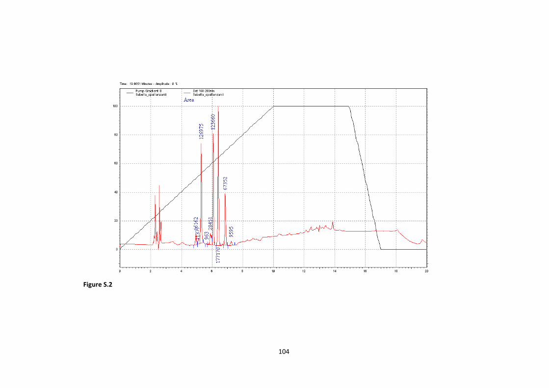
104
Figure S.2

105
I.7 METABOLIC RATE SURVEY FOR POLYCHAETES
Data regarding respiration rate for bristle worms were retrieved from
current literature (Borden 1931; Dales 1961a,b; Sander 1973; Shumway 1979;
Wells et al. 1980; Shumway et al. 1988; Mathilde Nithart et al. 1999;
Huusgaard et al. 2012; Kersey Sturdivant et al. 2015; see table S10 reported
below for details). Only data for which the temperature of the experiments was
reported, the weight range for the analyzed species and the mass/body weight
relation were used for the comparison. Data from Sturdivant et al. (2015)
regarding A. succinea were extracted from the graph using g3data (available at
http://www.frantz.fi/index.php?page=software). All the data were uniformed as
follow: body mass in total dry weight (for the data were only the wet body
weight were reported, 80% of retained water was calculated according to
Shumway (1979)); oxygen consumption as mg*h-1
. The respiration data were
temperature corrected according to Gillooly et al. (2001). Statistical analysis
was performed in PAST 3.10 (available at http://folk.uio.no/ohammer/past/).
The data were grouped in motile and sessile groups according to our
definition, i.e.:
1. Motile: showing different degree of movement, from
slow crawling or burrowing, to active swimming
2. Sessile: permanently and obligatory living inside the
tubes they built, and often attached to the substrate
The data were reported in Figure S.3
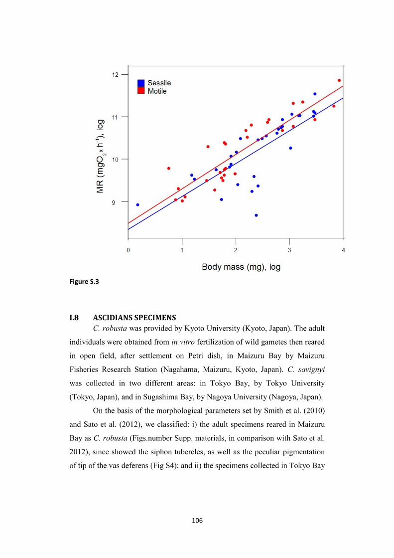
106
Figure S.3
I.8 ASCIDIANS SPECIMENS
C. robusta was provided by Kyoto University (Kyoto, Japan). The adult
individuals were obtained from in vitro fertilization of wild gametes then reared
in open field, after settlement on Petri dish, in Maizuru Bay by Maizuru
Fisheries Research Station (Nagahama, Maizuru, Kyoto, Japan). C. savignyi
was collected in two different areas: in Tokyo Bay, by Tokyo University
(Tokyo, Japan), and in Sugashima Bay, by Nagoya University (Nagoya, Japan).
On the basis of the morphological parameters set by Smith et al. (2010)
and Sato et al. (2012), we classified: i) the adult specimens reared in Maizuru
Bay as C. robusta (Figs.number Supp. materials, in comparison with Sato et al.
2012), since showed the siphon tubercles, as well as the peculiar pigmentation
of tip of the vas deferens (Fig S4); and ii) the specimens collected in Tokyo Bay

107
as C. savignyi, because of the lack of pigmentation on the vas deferens and the
presence of marked orange pigmentation of the inhalant siphon (Fig. S5).
The specimens shipped to Kyushu University Fishery Research
Laboratory (Fukutsu, Fukuoka, Japan) packaged to avoid as much as possible
termal shock during transportation, were transferred and maintained in 50 liter
aquaria with running filtered seawater and continuous aeration. Regarding
reared C. robusta, the animals were manually removed from the petri dishes.
Individuals grown joined to each other were separated and cleaned of any
animal hosted on the tunic surface by tweezers. Water temperature (ranging
from 16.5°C to 18.0°C) and salinity (on average 33.5ppt) were checked twice a
week. The animals were supplied once a day in the early morning with a 10ml
commercial mix of algae (Shellfish Diet 1800, Reed Mariculture Inc, USA) and
5ml of a 50x106cells/ml commercial solution of Chaetoceros calcitrans
(Higashimaru-marinetech PLC, Japan). During feeding the water flow was
stopped from 3 to 4 hours to allow the animals to filter enough algae. The tanks
are siphoned every two days and checked for dead individuals. After 6 days of
acclimation to the laboratory conditions, animals for the respirometry
experiments were selected for similarity in length, then moved into
experimental tank where temperature was fine controlled by a cooling and
heating system at 17°C, and fasted for 48h prior to experiments. The water in
the closed flow tanks was completely replaced weekly.
All experimental procedures were approved by a Kyushu University
committee and conducted in accordance with the Guideline for the Care and
Use of Laboratory Animals of Japan.

108
Figure S.4
Particular from the siphons of C. robusta (a from Sato et al. (2012), b and c from this
study) and C. savignyi (d and e, this study). In a and b the tubercles are visible, white
arrows. Black arrows in a indicates the red pigmentation at the end of the sperm
duct, visible through the tunic. c: the pigmentation in C. robusta specimens of this
study were visible when the animals were removed from the chamber. d: C.
savignyi removed from the water with partially closed siphons. e:C. savignyi in the
measuring chamber with completely extended siphons, the pigmentation is clearly
visible at the boards of the siphons.

109
Figure S.5
Particular from the pigmentation of the terminal papillae of the vas deferens in C. robusta: a and b this study; c from Sato et al. (2012)
I.8 ASCIDIANS RESPIROMETRY
Oxygen consumption rate in resting condition was measured via oxygen
electrode probes. Semi-closed method of Yagi and Oikawa (2014) was used to
determine the effective oxygen rate consumption, as a proxy for basal metabolic
rate, in both species. To eliminate background respiration, a bottle that received
water flowing out of the respiration chamber was used as the blank chamber.
This bottle was sealed at the beginning of the oxygen consumption
determination, and placed in the water-bath for the respiration chamber during
determination. The oxygen concentration in the bottle was determined at the
end of the measurement period (C0). By using this value as the initial oxygen
concentration in the respiration chamber, background respiration was cancelled.
Specimens were introduced into the respiration chambers (250ml each) and left
undisturbed to acclimate to the new condition for at least 1h after the siphons
opened and extended, under a constant air-saturated water flow. The chambers
were positioned in closed flow tanks with fine controlled temperature
(T=17°C). Closing time ranged from 45 minutes up to 3 hours, depending on
the size of the animals. At the opening time two volumes of 50ml were sampled

110
from the respiration chamber and the oxygen concentration was determined via
DO electrode (C1 and C2). The oxygen consumption was calculated as:
O2cons = [C0 – (C1 + C2)/2]×volume of the chamber.
i.e. the difference between the control value (C0) and the average of the
two oxygen concentration values obtained from the 50ml sampled water
(C1+C2)/2. Values of (C1 - C2) ≥0.1ppm were discarded.
The final set consisted of 58 data for C. robusta and 44 for C. savignyi.
After the respirometric experiments, the total body-length at the maximum
extension of the inhalant siphon was measured. The tunic and the organs were
dissected, rinsed in distilled water, drained with absorbant paper, and weighed
separately to determine the wet weight (WW). Then all tissues were dried in a
drying oven for at least 48h to determine the dry weight (DW).
The mass-specific rate of oxygen consumption was calculated as
follows:
Mass-specific Ocons = Ocons / WW (or DW), kg / Closing time, h
Figure S.6

111
Statistical analyses
To compare the interspecific morpho-physiological relationships
between C. robusta and C. savignyi, known allometric? equation models were
applied.
In particular, regarding the relationship body weight vs. body length, we
referred to the power equation Y=aXb according to Carver et al. (2006), where
Y = body weight (BW), X = body length (BL).
The relationship between body mass and routine metabolic rate also
followed the equation Y=aXb, where Y = respiration rate MR (mgO2×h
-1) and X
= BW (see Agutter and Wheatley 2004 for a review).
Both equations were log-log linearized and fitted with the least squares
method. The R2 and p-value were calculated (<5%). Each distribution was
checked for the normality of residuals (Shapiro-Wilk test, <1%). The F-test
was used to evaluate the best fit model: i) the model in which one curve fit all
data sets (p-value>5%), or ii) the model in which each species is fitted by a
different curve (p-value<5%). In multiple comparisons, the Bonferroni
correction for multiple tests was applied.
The tunic weight vs. organ weight correlation has been shown to be
linear (Carver et al. 2006), following the equation Y=a+Xb, where Y = weight
of the tunic (TW) and X = weight of the organs (OW). In this specific case the
data were not log-transformed, but the same procedure already described above
for the linearized model was applied, i.e. the r2 and p-value were calculated (
<5%). Each distribution was then checked for the normality of residuals and the
F-test was used to evaluate the best-fit model.
The correlation between water retention and body weight has not been
formerly studied. Since there was not a model to refer to, it was not possible to
compare the two species using a parametric model. A locally weighted
polynomial regression curve with 95% of the mean confidence interval area
was then calculated and reported in Fig. 4.3 (R packages ggplot2). The amount
of retained water in the tissues was calculated as a fraction of the total weight

112
(p). According to Bartlett (1947), for n number of observations near the higher
limit, i.e. p near to one, the values were transformed applying
Y √
.
Regarding the mass-specific MR (expressed as tissue×mgO2-1
×h-1
), the
tunic/organ ratio (expressed as grams of tunic divided by grams of organs), and
the retained-water comparison the statistical significance of the differences
were assessed by the Mann-Whitney Test.
All the statistical analyses were performed by Prism 6 (GraphPad).

113
Appendix II
II.1 THE METABOLIC THEORY OF ECOLOGY EQUATION
Metabolism is the bio-chemical process by which energy and material
are transformed within an organism and exchanged between the organism and
the environment (Brown et al. 2004). Organisms convert the acquired resources
from the environment to biologically usable forms and allocate them to the vital
processes of survival, growth, and reproduction, and eliminate the altered forms
back into the environment. On one hand metabolism determines the demands
that organisms place on their environment while on the other, environmental
factors constraints the allocated of resources to sustain life by influencing the
organismic performance, and hence their energetic demands.
The complex network of biochemical reactions (organized into
metabolic pathways) are catalyzed by enzymes regulating the rates of reactions.
The overall rate of the processes (rate at which energy and materials are taken
up, transform, and used up) is the metabolic rate is related to molecular
processes like DNA repair and mutation, because metabolism produces oxygen
radicals (highly reactive molecules with free electrons), which mediates the
oxidative damage to DNA. Naturally this damage is continuously repaired and
mutation may occur by incorrect repair. Hence species with higher metabolic
rates should have higher DNA substitution rates, due to the fact that DNA
damage and mutation rate are positively correlated (Martin and Palumbi 1993;
Gillooly et al. 2001, 2005).
Body mass and temperature are the two major factors affecting
metabolism (Gillooly et al. 2001), according to,

114
Where, B is the mass specific metabolic rate, B0 is the coefficient
independent of body size M, e–E/kT
is the Boltzmann factor with k as Boltzmann
constant, activation energy E and temperature T.
Mass specific metabolic rate varies with body size elevated to a factor
that approximates a quarter-power (Agutter and Wheatley 2004). At present it is
still questioned if this represents a universal scaling law. The debate is mainly
dealing with the meaning of the species-related variability in the normalizing
coefficient a and the scaling exponent b of the allometric equation, R = aMb,
where R is the resting metabolic rate and M is the body mass. Recently a
curvilinear rather than linear relationship between LogR and LogM has been
proposed (Kolokotrones et al. 2010). A metabolic level boundaries (MLB)
hypothesis stressing on the boundary constrains that limit the scaling of
metabolic rate has also been proposed and applied to teleost fish (Killen et al.
2010) suggesting that lifestyle, swimming mode and temperature affect the
intraspecific scaling of resting metabolic rate.
Regarding temperature dependence, is known that, within the range of
biologically relevant values (approximately 0-40°C), temperature affects
metabolism mainly via its effects on the rates of biochemical reactions, whose
kinetics varies according to the Boltzmann's factor (e−E/kT
), where E is the
activation energy, k is Boltzmann’s constant, and T is absolute temperature,
known as the universal temperature dependence (UTD) (Gillooly et al. 2001).
Thus, metabolic rate, the rate at which organisms transform energy and
materials is governed largely by two interacting processes: first the quarter-
power allometric relation, which describes how biological rate processes scale
with body size and second the Boltzmann factor, which describes the
temperature dependence of biochemical processes (UTD). The assumption of a
universal significance of both scaling and UTD forms the basis of the Metabolic
Theory of Ecology (MTE), proposed by Brown et al. (2004), that stresses the
ecological relevance of the mass and temperature dependence of metabolic rate.

115
Despite the fact that this hypothesis has been questioned (Glazier 2005),
UTD can be considered in any case a useful statistical tool to describe the
relationship between temperature and basal metabolic rate (Clarke and Johnston
1999; Price et al. 2012). In particular, the methodological approach of MTE
could be used to separate the effects of mass and temperature from those of
other sources of basal metabolic rate variability, including those related with
life history and specific environmental adaptations of a species or group of
species. In this view, mass and temperature correction of metabolism within a
group of phylogenetically related organisms may reveal a broad tendency to
adapt metabolism to different environments.

116
Supplementary data
Table S1. Basal metabolic rate bodymass- and temperature-corrected by
Boltzman’s factor
Order Family Species MR,
ln Env. LS
Anguilliformes Anguillidae Anguilla anguilla 30.20 FW M
Anguilla australis australis 29.22 FW M
Anguilla japonica 29.69 FW M
Anguilla rostrata 30.98 FW M
Congridae Conger conger 30.67 SW M
Aulopiformes Aulopiformes Benthalbella elongata 31.46 SW NM
Batrachoidiformes Batrachoididae Opsanus tau 31.62 SW NM
Beryciformes Anoplogastridae Anoplogaster cornuta 29.96 SW NM
Characiformes Characidae Colossoma macropomum 30.10 FW M
Erythrinidae Hoplerythrinus unitaeniatus 29.53 FW NM
Clupeiformes Clupeidae Brevoortia tyrannus 31.30 SW M
Gilchristella aestuaria 31.72 FW M
Engraulidae Engraulis japonicus 33.80 SW M
Cypriniformes Catostomidae Catostomus commersonii 30.32 FW M
Catostomus tahoensis 30.87 FW NM
Erimyzon oblongus 30.80 FW NM
Cobitidae Lepidocephalichthys guntea 31.65 FW M
Cyprinidae Abramis brama 32.01 FW M
Alburnus alburnus 31.25 FW M
Campostoma anomalum 31.05 FW NM
Carassius auratus 30.63 FW M
Carassius carassius 30.70 FW M
Cirrhinus cirrhosus 29.85 FW M
Ctenopharyngodon idella 30.47 FW M
Cyprinus carpio 30.06 FW M
Danio rerio 30.84 FW NM
Esomus danricus 32.45 FW M

117
Gobio gobio gobio 31.40 FW M
Labeo calbasu 31.47 FW M
Labeo rohita 31.50 FW M
Labeobarbus aeneus 30.40 FW M
Leucaspius delineatus 31.72 FW M
Leuciscus idus 30.87 FW M
Leuciscus leuciscus 31.83 FW M
Pimephales promelas 30.84 FW NM
Rhodeus amarus 31.26 FW NM
Rhodeus sericeus 31.43 FW M
Rutilus rutilus 31.03 FW M
Scardinius erythrophthalmus 31.01 FW M
Squalius cephalus 31.22 FW M
Tinca tinca 30.71 FW M
Cyprinodontidae Oryzya latipes 31.67 FW M
Lutjanidae Lutjanus campechanus 30.26 SW NM
Percidae Sander vitreus 29.90 FW M
Cyprinodontiformes Fundulidae Fundulus grandis 29.80 FW M
Fundulus parvipinnis 30.98 SW NM
Fundulus similis 29.21 SW NM
Poeciliidae Gambusia affinis 31.51 FW M
Gambusia holbrooki 31.31 FW M
Poecilia latipinna 30.52 FW NM
Xiphophorus hellerii 31.33 FW NM
Esociformes Esocidae Esox lucius 30.54 FW M
Esox masquinongy 31.32 FW NM
Gadiformes Gadidae Boreogadus saida 31.56 SW M
Pollachius pollachius 31.33 SW M
Theragra chalcogramma 31.26 SW NM
Lotidae Lota lota 30.72 FW M
Melanonidae Melanonus zugmayeri 30.23 SW M
Macrouridae Coryphaenoides armatus 28.60 SW NM
Gasterosteiformes Gasterosteidae Gasterosteus aculeatus 31.55 SW M
Spinachia spinachia 31.66 SW NM
Gonorynchiformes Chanidae Chanos chanos 31.95 FW M
Lophiiformes Oneirodidae Oneirodes acanthias 29.50 SW NM
Mugiliformes Mugilidae Liza dumerili 30.62 FW M
Liza macrolepis 30.44 FW M
Liza richardsonii 31.15 FW M
Mugil cephalus 30.52 FW M
Mugil curema 31.65 FW M
Continued from previous page

118
Myctophiformes Myctophidae Diaphus theta 32.14 SW NM
Electrona antarctica 31.58 SW M
Gymnoscopelus braueri 31.12 SW M
Gymnoscopelus opisthopterus 30.95 SW M
Nannobrachium regale 29.79 SW NM
Nannobrachium ritteri 31.04 SW NM
Parvilux ingens 29.91 SW NM
Stenobrachius leucopsarus 31.13 SW NM
Symbolophorus californiensis 31.47 SW NM
Tarletonbeania crenularis 31.75 SW NM
Triphoturus mexicanus 30.88 SW NM
Neoscopelidae Scopelengys tristis 29.58 SW M
Osmeriformes Bathylagidae Bathylagus antarcticus 26.12 SW NM
Bathylagus stilbius 30.57 SW NM
Bathylagus wesethi 31.45 SW NM
Lipolagus ochotensis 31.33 SW NM
Pseudobathylagus milleri 29.79 SW NM
Platytroctidae Sagamichthys abei 30.15 SW NM
Plecoglossidae Plecoglossus altivelis altivelis 32.41 FW M
Perciformes Alepocephalidae Bajacalifornia burragei 29.10 SW NM
Ambassidae Ambassis interrupta 29.96 FW M
Anabantidae Anabas testudineus 28.43 FW M
Bathydraconidae Gymnodraco acuticeps 31.45 SW NM
Callionymidae Callionymus lyra 31.00 SW NM
Carangidae Caranx hippos 31.52 SW M
Centrarchidae Lepomis cyanellus 30.31 FW NM
Lepomis gibbosus 30.37 FW M
Lepomis macrochirus 30.70 FW NM
Pomoxis annularis 30.37 FW NM
Channichthyidae Chaenocephalus aceratus 30.83 SW NM
Channichthys rhinoceratus 31.31 SW NM
Channidae Channa marulius 29.02 FW M
Channa orientalis 29.33 FW M
Channa punctata 30.42 FW M
Channa striata 29.28 FW M
Chiasmodontidae Chiasmodon niger 30.92 SW NM
Cichlidae Aequidens pulcher 30.01 FW NM
Cichlasoma bimaculatum 29.82 FW M
Hemichromis bimaculatus 30.47 FW M
Oreochromis aureus 29.49 FW M
Oreochromis mossambicus 31.54 FW M
Continued from previous page

119
Oreochromis niloticus 30.59 FW M
Pterophyllum scalare 30.47 FW NM
Sarotherodon galilaeus galilaeus 29.82 FW M
Thorichthys meeki 30.13 FW NM
Tilapia rendalli 30.36 FW NM
Tilapia zillii 31.15 FW M
Coryphaenidae Coryphaena equiselis 34.34 SW M
Coryphaena hippurus 32.32 SW M
Embiotocidae Embiotoca lateralis 30.75 SW NM
Gobiidae Gillichthys mirabilis 30.42 SW NM
Gobius paganellus 30.75 FW M
Oligolepis acutipennis 30.27 FW M
Haemulidae Pomadasys commersonnii 30.46 SW M
Kuhliidae Kuhlia sandvicensis 30.40 FW M
Kyphosidae Girella nigricans 30.60 SW NM
Labridae Labrus bergylta 31.31 SW NM
Tautogolabrus adspersus 30.64 SW NM
Nomeidae Cubiceps whiteleggii 32.69 SW NM
Nototheniidae Gobionotothen gibberifrons 30.62 SW NM
Notothenia coriiceps 31.41 SW NM
Notothenia cyanobrancha 31.76 SW NM
Notothenia rossii 31.61 SW M
Pagothenia borchgrevinki 31.49 SW NM
Trematomus bernacchii 31.51 SW NM
Trematomus centronotus 31.79 SW NM
Trematomus hansoni 31.39 SW NM
Osphronemidae Colisa fasciata 31.12 FW NM
Osphronemus goramy 29.44 FW NM
Trichogaster trichopterus 30.15 FW M
Percidae Etheostoma blennioides 31.20 FW NM
Gymnocephalus cernuus 30.97 FW M
Perca fluviatilis 30.63 SW M
Pomacentridae Chromis chromis 31.11 SW NM
Sciaenidae Leiostomus xanthurus 29.70 SW M
Scombridae Sarda chiliensis lineolata 32.91 SW M
Serranidae Centropristis melana 32.06 SW M
Epinephelus akaara 30.49 SW NM
Serranus scriba 31.10 SW NM
Sparidae Acanthopagrus schlegelii schlegelii 30.37 SW NM
Diplodus sargus sargus 31.60 SW M
Sparus aurata 31.08 SW NM
Continued from previous page

120
Trachinidae Echiichthys vipera 31.32 SW NM
Zoarcidae Lycodichthys dearborni 30.50 SW NM
Melanostigma pammelas 30.01 SW NM
Zoarces viviparus 31.54 SW NM
Pleuronectiformes Paralichthyidae Citharichthys stigmaeus 30.46 SW NM
Pleuronectidae Limanda limanda 31.12 SW M
Parophrys vetulus 30.68 SW M
Platichthys stellatus 30.68 FW M
Scophthalmidae Psetta maxima 30.81 SW M
Scophthalmus rhombus 30.75 SW M
Soleidae Solea solea 30.96 SW M
Salmoniformes Salmonidae Coregonus fera 32.10 FW NM
Coregonus autumnalis 32.62 SW M
Oncorhynchus kisutch 31.21 SW M
Oncorhynchus mykiss 31.76 SW M
Oncorhynchus nerka 30.69 SW M
Oncorhynchus tshawytscha 31.14 SW M
Salmo fario 31.41 SW M
Salmo salar 31.80 SW M
Salmo trutta trutta 31.57 SW M
Salvelinus fontinalis 30.93 SW M
Scorpaeniformes Cottidae Clinocottus analis 30.44 SW NM
Cottus gobio 31.68 FW M
Myoxocephalus octodecemspinosus 30.43 SW NM
Myoxocephalus scorpius 31.32 SW NM
Dactylopteridae Dactylopterus volitans 33.97 SW NM
Hexagrammidae Ophiodon elongatus 30.21 SW M
Scorpaenidae Scorpaena porcus 30.70 SW NM
Siluriformes Bagridae Mystus armatus 30.17 FW NM
Mystus gulio 30.09 SW M
Mystus vittatus 30.44 FW NM
Heteropneustidae Heteropneustes fossilis 29.57 FW NM
Ictaluridae Ameiurus melas 30.19 FW M
Ameiurus natalis 30.63 FW NM
Ameiurus nebulosus 29.95 FW NM
Stephanoberyciforme Melamphaidae Scopelogadus mizolepis mizolepis 30.01 SW NM
Melamphaes acanthomus 30.28 SW NM
Poromitra crassiceps 29.79 SW NM
Stomiiformes Gonostomatidae Cyclothone acclinidens 32.13 SW M
Cyclothone microdon 30.62 SW NM
Stomiidae Aristostomias lunifer 29.65 SW NM
Continued from previous page

121
Borostomias panamensis 30.33 SW NM
Stomias atriventer 30.60 SW NM
Stomias danae 31.00 SW NM
Synbranchiformes Synbranchidae Synbranchus marmoratus 29.19 FW M
Syngnathiformes Syngnathidae Hippocampus hippocampus 30.67 SW NM
Syngnathus acus 31.23 SW NM

122
Table S2. Gill area
Family Species Wght Gill
Area
Spec. Gill
A. Gill Env LS
(g) (cm2) (cm2/g)
Ictaluridae Ameiurus nebulosus 41.00 74.00 1.80 1.41 FW NM
50.00 80.00 1.60
59.00 110.00 1.86
179.00 219.00 1.22
239.00 275.00 1.15
356.00 363.00 1.02
Heteropneustidae Heteropneustes fossilis 6.96 9.25 1.33 1.01 FW NM
39.20 131.00 3.34
42.35 28.95 0.68
107.50 64.73 0.60
Erythrinidae Hoplerythrinus unitaeniatus 1015.00 572.31 0.56
FW NM
Erythrinidae Hoplias lacerdae 1000.00 1323.45 1.32
FW NM
Centrarchidae Micropterus dolomieu 0.30 3.00 10.00 3.45 FW NM
1.50 11.20 7.47
33.00 141.00 4.27
257.00 674.00 2.62
417.00 984.00 2.36
838.00 1705.00 2.03
Gobiidae Mistichthys luzonensis 0.01 0.15 13.24 9.55 FW NM
0.02 0.17 9.88
0.02 0.18 9.44
0.02 0.21 11.05
0.02 0.18 8.36
0.03 0.26 9.55
0.03 0.26 8.68
Bagridae Mystus vittatus 3.00 12.00 4.00 3.00 FW NM

123
13.00 39.00 3.00
23.00 61.00 2.65
Cyprinidae Blicca bjoerkna 47.00 768.00 16.34
FW M
Gobiidae Boleophthalmus boddarti 4.00 4.00 1.00 1.08 FW M
12.30 28.47 2.31
20.00 21.00 1.05
35.00 39.00 1.11
Cyprinidae Carassius auratus 0.55 2.20 4.00 2.00 FW M
10.00 20.00 2.00
183.00 209.00 1.14
Cyprinidae Catla catla 100.00 285.00 2.85
FW M
Catostomidae Catostomus commersonii 52.00 107.00 2.06 0.99 FW M
64.00 120.00 1.88
347.00 344.00 0.99
454.00 395.00 0.87
865.00 602.00 0.70
Channidae Channa punctata 1000.00 280.64 0.28
FW M
Channidae Channa striata 59.90 163.00 2.72
FW M
Cyprinidae Chondrostoma nasus 143.00 934.00 6.53
FW M
Cyprinidae Cirrhinus cirrhosus 5.00 44.00 8.80 3.37 FW M
913.00 3081.00 3.37
1821.00 5412.00 2.97
Clariidae Clarias batrachus 51.50 146.00 2.83
FW M
Cobitidae Cobitis taenia 0.10 1.00 10.00 3.17 FW M
1.00 6.00 6.00
3.00 9.00 3.00
3.00 10.00 3.33
6.00 12.00 2.00
8.00 13.00 1.63
Continued from previous page

124
Cottidae Cottus gobio 11.00 55.00 5.00 4.07 FW M
14.00 41.00 2.93
16.00 40.00 2.50
18.00 40.00 2.22
28.00 123.00 4.39
28.20 124.00 4.40
44.00 179.00 4.07
Cyprinidae Ctenopharyngodon idella 134.00 418.00 3.12 2.18 FW M
659.00 1434.00 2.18
1705.00 2995.00 1.76
Cyprinidae Cyprinus carpio 0.30 3.00 10.00 1.63 FW M
0.97 4.00 4.12
19.00 89.00 4.68
19.00 100.00 5.26
140.00 233.00 1.66
360.00 574.00 1.59
435.00 622.00 1.43
520.00 688.00 1.32
523.00 729.00 1.39
525.00 771.00 1.47
531.00 723.00 1.36
878.00 1010.00 1.15
1125.00 2177.00 1.94
2250.00 3764.00 1.67
Esocidae Esox lucius 238.00 3370.00 14.16 7.72 FW M
1016.00 1308.00 1.29
Percidae Gymnocephalus cernua 22.00 196.00 8.91
FW M
Cobitidae Misgurnus fossilis 36.00 183.00 5.08
FW M
Erythrinidae Hoplias malabaricus 1000.00 3313.61 3.31
FW M
Cyprinidae Labeo rohita 75.70 731.00 9.66 6.31 FW M
400.00 1187.00 2.97
Mugilidae Mugil cephalus 250.00 2525.00 10.10
FW M
Continued from previous page

125
Lotidae Lota lota 73.00 444.00 6.08 3.67 FW M
650.00 812.50 1.25
Bagridae Mystus cavasius 4.00 22.00 5.50 4.53 FW M
32.00 145.00 4.53
59.00 257.00 4.36
Cichlidae Oreochromis niloticus 1000.00 1024.84 1.02
FW M
Gobiidae
Periophthalmus
argentilineatus 7.60 5.73 0.75 1.00 FW M
9.80 12.30 1.26
Gobiidae Periophthalmus barbarus 7.30 6.47 0.89 2.01 FW M
10.70 21.50 2.01
10.70 21.55 2.01
Pleuronectidae Platichthys flesus 51.00 376.00 7.37 3.97 FW M
370.00 1470.00 3.97
490.00 924.95 1.89
Bagridae Rita rita 62.30 784.00 12.58
FW M
Cyprinidae Rutilus rutilus 1.30 2.58 1.98 4.00 FW M
2.00 8.00 4.00
3.50 14.00 4.00
20.00 120.00 6.00
24.00 116.00 4.83
30.00 65.00 2.17
36.00 172.00 4.78
78.00 320.00 4.10
105.00 456.00 4.34
161.00 284.00 1.76
184.00 758.00 4.12
222.00 348.00 1.57
230.00 810.00 3.52
267.00 421.00 1.58
320.00 506.00 1.58
Percidae Sander lucioperca 69.50 1061.00 15.27
FW M
Continued from previous page

126
Percidae Sander vitreus 410.00 710.00 1.73 1.91
M
888.00 1699.00 1.91
1365.00 2763.00 2.02
Gobiidae Scartelaos histophorus 6.80 6.62 0.97
FW M
Gobiidae Taenioides cirratus 22.00 36.50 1.66
FW M
Cyprinidae Tinca tinca 25.00 82.00 3.28 2.02 FW M
25.00 152.00 6.08
65.90 211.69 3.21
133.00 278.00 2.09
140.00 536.00 3.83
141.00 274.00 1.94
141.00 377.00 2.67
268.00 491.00 1.83
268.20 457.45 1.71
376.00 544.00 1.45
376.00 629.00 1.67
1274.00 2310.27 1.81
Trichiuridae Trichiurus lepturus 116.00 622.00 5.36
FW M
Gobiidae Trypauchen vagina 14.90 55.60 3.73
FW M
Gobiidae Acentrogobius caninus 10.00 48.60 4.86
FW M
Anabantidae Anabas testudineus 6.00 8.89 1.48 0.58 FW M
54.20 84.10 1.55
54.40 31.47 0.58
115.00 52.00 0.45
1000.30 389.11 0.39
Anguillidae Anguilla anguilla 69.50 688.00 9.90 6.57 FW M
800.00 2600.00 3.25
Anguillidae Anguilla rostrata 428.00 1293.00 3.02
FW M
Nemacheilidae Barbatula barbatula 1.00 2.00 2.00 2.00 FW M
3.00 6.00 2.00
4.00 18.00 4.50
Continued from previous page

127
5.00 9.00 1.80
15.00 41.00 2.73
36.00 72.00 2.00
Callionymidae Callionymus lyra 39.00 87.50 2.24
SW NM
Carangidae Caranx crysos 129.00 1267.00 9.82
SW NM
Channichthyidae Chaenocephalus aceratus 860.00 925.60 1.08 1.26 SW NM
1040.00 4368.00 4.20
1456.00 1840.00 1.26
Channichthyidae Champsocephalus esox 66.00 570.00 8.64
SW NM
Channichthyidae Channichthys rhinoceratus 450.00 605.50 1.35
SW NM
Diodontidae Chilomycterus schoepfii 316.00 1381.00 4.37
SW NM
Echeneidae Echeneis naucrates 393.00 2158.00 5.49
SW NM
Triglidae Eutrigla gurnardus 17.80 40.00 2.25
SW NM
Gobiidae Gobius auratus 5.40 9.50 1.76
SW NM
Gobiidae Gobius niger 9.70 27.54 2.84
SW NM
Centrolophidae Hyperoglyphe perciformis 199.00 1007.00 5.06
SW NM
Labridae Labrus merula 608.00 646.00 1.06
SW NM
Blenniidae Lipophrys pholis 0.24 2.41 10.04 5.43 SW NM
4.51 24.47 5.43
16.00 85.88 5.37
Lophiidae Lophius piscatorius 1550.00 2217.00 1.43 1.69 SW NM
6390.00 12500.00 1.96
Cottidae Myoxocephalus scorpius 60.00 90.00 1.50
SW NM
Batrachoididae Opsanus tau 15.00 48.00 3.20 1.68 SW NM
62.70 131.00 2.09
Continued from previous page

128
251.00 445.00 1.77
408.00 647.00 1.59
800.00 1102.00 1.38
1006.00 1317.00 1.31
Nototheniidae Patagonotothen tessellata 50.00 260.00 5.20
SW NM
Rajidae Raja clavata 418.30 514.09 1.23 1.22 SW NM
2930.60 3574.60 1.22
Tetraodontidae Sphoeroides maculatus 326.00 1366.00 4.19
SW NM
Centracanthidae Spicara maena 19.00 42.00 2.21
SW NM
Labridae Symphodus melops 65.00 218.00 3.35
SW NM
Cottidae Taurulus bubalis 46.00 162.00 3.52
SW NM
Labridae Tautoga onitis 466.00 2094.00 4.49
SW NM
Zoarcidae Zoarces viviparus 134.00 575.00 4.29
SW NM
Sparidae Archosargus probatocephalus 544.00 2548.00 4.68
SW NM
Balistidae Balistes capriscus 548.00 2340.00 4.27
SW NM
Clupeidae Brevoortia tyrannus 525.00 6913.00 13.17
SW M
Serranidae Centropristis striata 244.00 1118.00 4.58
SW M
Lotidae Ciliata mustela 50.00 131.00 2.62
SW M
Clupeidae Clupea harengus 11.00 70.00 6.36 6.38 SW M
85.00 544.00 6.40
Congridae Conger conger 2560.00 3455.00 1.35
SW M
Coryphaenidae Coryphaena hippurus 8634.00 33318.00 3.86
SW M
Sciaenidae Cynoscion regalis 705.00 1927.00 2.73
SW M
Continued from previous page
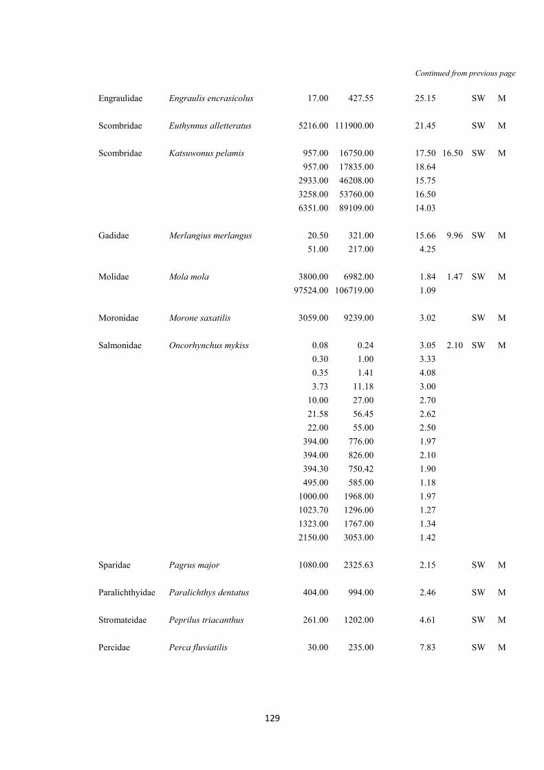
129
Engraulidae Engraulis encrasicolus 17.00 427.55 25.15
SW M
Scombridae Euthynnus alletteratus 5216.00 111900.00 21.45
SW M
Scombridae Katsuwonus pelamis 957.00 16750.00 17.50 16.50 SW M
957.00 17835.00 18.64
2933.00 46208.00 15.75
3258.00 53760.00 16.50
6351.00 89109.00 14.03
Gadidae Merlangius merlangus 20.50 321.00 15.66 9.96 SW M
51.00 217.00 4.25
Molidae Mola mola 3800.00 6982.00 1.84 1.47 SW M
97524.00 106719.00 1.09
Moronidae Morone saxatilis 3059.00 9239.00 3.02
SW M
Salmonidae Oncorhynchus mykiss 0.08 0.24 3.05 2.10 SW M
0.30 1.00 3.33
0.35 1.41 4.08
3.73 11.18 3.00
10.00 27.00 2.70
21.58 56.45 2.62
22.00 55.00 2.50
394.00 776.00 1.97
394.00 826.00 2.10
394.30 750.42 1.90
495.00 585.00 1.18
1000.00 1968.00 1.97
1023.70 1296.00 1.27
1323.00 1767.00 1.34
2150.00 3053.00 1.42
Sparidae Pagrus major 1080.00 2325.63 2.15
SW M
Paralichthyidae Paralichthys dentatus 404.00 994.00 2.46
SW M
Stromateidae Peprilus triacanthus 261.00 1202.00 4.61
SW M
Percidae Perca fluviatilis 30.00 235.00 7.83
SW M
Continued from previous page

130
Pleuronectidae Pleuronectes platessa 86.00 370.00 4.30 5.42 SW M
136.00 889.00 6.54
Gadidae Pollachius virens 1200.00 5050.00 4.21
SW M
Pomatomidae Pomatomus saltatrix 1035.00 6747.00 6.52
SW M
Pleuronectidae
Pseudopleuronectes
americanus 734.00 1468.00 2.00
SW M
Salmonidae Salmo trutta 175.00 593.00 3.39 3.00 SW M
400.00 1200.00 3.00
5000.00 15000.00 3.00
Scombridae Sarda sarda 2192.00 13040.00 5.95
SW M
Scombridae Scomber scombrus 226.00 2370.00 10.49 4.24 SW M
285.00 1208.00 4.24
383.00 1464.00 3.82
800.00 4720.00 5.90
1000.00 4153.04 4.15
Scombridae Scomberomorus maculatus 478.00 3676.00 7.69
SW M
Carangidae Seriola quinqueradiata 4.90 78.90 16.10 3.84 SW M
50.70 305.70 6.03
98.80 569.10 5.76
234.00 898.60 3.84
450.00 1161.00 2.58
555.00 1565.10 2.82
1117.00 4088.20 3.66
Sparidae Stenotomus chrysops 253.00 1240.00 4.90
SW M
Clupeidae Tenualosa ilisha 400.00 2663.00 6.66
SW M
Scombridae Thunnus albacares 3326.00 36680.00 11.03 10.13 SW M
4060.00 47930.00 11.81
14500.00 133900.00 9.23
50800.00 321600.00 6.33
Continued from previous page

131
Scombridae Thunnus thynnus 5670.00 60320.00 10.64 9.81 SW M
26600.00 239000.00 8.98
Carangidae Trachurus trachurus 26.00 209.00 8.04 8.19 SW M
26.00 213.00 8.19
130.00 1420.00 10.92
Zeidae Zeus faber 300.00 531.00 1.77
SW M
Alepisauridae Alepisaurus ferox 5000.00 2850.00 0.57
SW M
Clupeidae Alosa kessleri 40.00 1273.00 31.83
SW M
Continued from previous page

132
Table S3. Genomic GC value (%), environmental and lifestyle
data for the species used in the analyses
Species GC, % Ref. Environment Lifestyle
Cyprinus carpio 37.20 ** FW M
Labeo bicolor 37.20 ** FW NM
Danio rerio 37.49 AV FW NM
Copoeta (Barbus) semifasciolatus 37.54 * FW NM
Barbodes (Barbus) everetti 37.63 * FW NM
Puntius (Barbus) conchonius 37.85 * FW NM
Carassius carassius 37.94 * FW M
Austrofundulus limnaei 38.00 ** FW NM
Puntius (Barbus) ticto ticto 38.26 * FW M
Carassius auratus 38.39 AV FW M
Abramis brama 38.68 * FW M
Corydoras aeneus 38.80 ** FW NM
Xiphophorus variatus 38.86 * FW NM
Xiphophorus helleri 39.08 * FW NM
Puntius (Barbus) tetrazona 39.26 * FW NM
Rutilis rutilis 39.27 * FW M
Cobitis lutheri 39.44 * FW NM
Rivulus holmiae 39.50 ** FW NM
Hyphessobrycon pulchripinnis 39.51 * FW NM
Cobitis melanoleuca 39.70 * FW NM
Cyprinodon nevadensis 39.70 ** FW NM
Hemigrammus ocellifer 39.73 * FW NM
Hoplosternum thoracatum 39.88 * FW NM
Hyphessobrycon flammeus 39.97 * FW NM
Oryzias latipes 40.10 **** FW M
Hyphessobrycon callistus 40.11 * FW NM
Gymnocorymbus ternetzi 40.19 * FW NM
Cichlasoma meeki 40.20 ** FW NM
Poecilia sphenops 40.20 ** FW NM
Xiphophorus maculatus 40.39 AV FW NM
Cyprinodon macularius califor. 40.40 ** FW NM
Jordanella floridae 40.47 AV FW NM
Astyanax mexicanus 40.60 ** FW M

133
Cyprinodon salinus 40.80 ** FW NM
Tilapia buettikoferi 40.80 ** FW NM
Poecilia reticulata 41.13 * FW NM
Symphysodon discus 41.30 ** FW NM
Orechromis spilurus 41.40 ** FW NM
Aplocheilus dayi 41.60 ** FW NM
Oreochromis aureus 41.60 ** FW M
Percottus glehni 41.60 * FW NM
Stizostedion lucioperca 41.63 * FW M
Oreochromis niloticus 41.70 ** FW M
Oreochromis mossambicus 41.80 ** FW M
Aphyosemion punctatum 41.90 ** FW NM
Epiplatys chaperi 41.90 ** FW NM
Pterophyllum scalare 41.90 * FW NM
Trichogaster trichopterus 41.98 * FW M
Alcolapia alcalicus grahami 42.00 ** FW NM
Aphyosemion cameronense 42.00 ** FW NM
Aphyosemion herzogi 42.20 ** FW NM
Aphyosemion scheli 42.20 ** FW NM
Rivulus agilae 42.30 ** FW NM
Esox lucius 42.36 * FW M
Diapteron cyanostictum 42.40 ** FW NM
Diapteron cyanosticum georgiae 42.40 ** FW NM
Aphyosemion elegans 42.50 AV FW NM
Trichogaster leeri 42.69 * FW NM
Aphyosemion amieti 42.90 ** FW NM
Colisa chuna 42.92 * FW NM
Aphyosemion marmoratum 43.00 ** FW NM
Thymallus thymallus 43.23 * FW NM
Notopterus notopterus 43.93 AV FW M
Aphyosemion spoorenbergi 44.10 ** FW NM
Gnathonemus petersii 44.20 ** FW NM
Pantodon buchholzi 44.43 AV FW M
Tetraodon cutcutia 44.45 * FW M
Aphyolebias peruensis 45.70 *** FW NM
Tetraodon nigroviridis 45.90 **** FW NM
Aphyosemion striatum 46.70 ** FW NM
Pachypanchax playfairii 47.20 ** FW NM
Nothobranchius flammicomantis 47.26 *** FW NM
Aphyosemion australe 48.10 ** FW NM
Tetraodon fluviatilis 48.39 *** FW M
Continued from previous page
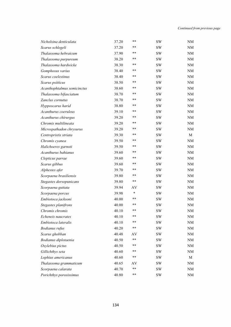
134
Nicholsina denticulata 37.20 ** SW NM
Scarus schlegeli 37.20 ** SW NM
Thalassoma hebraicum 37.90 ** SW NM
Thalassoma purpureum 38.20 ** SW NM
Thalassoma hardwicke 38.30 ** SW NM
Gomphosus varius 38.40 ** SW NM
Scarus coelestinus 38.40 ** SW NM
Scarus psitticus 38.50 ** SW NM
Acanthophtalmus semicinctus 38.60 ** SW NM
Thalassoma bifasciatum 38.70 ** SW NM
Zanclus cornutus 38.70 ** SW NM
Hypposcarus harid 38.80 ** SW NM
Acanthurus coeruleus 39.10 ** SW NM
Acanthurus chirurgus 39.20 ** SW NM
Chromis multilineata 39.20 ** SW NM
Microspathadon chrysurus 39.20 ** SW NM
Centropristis striata 39.30 ** SW M
Chromis cyanea 39.50 ** SW NM
Halichoeres garnoti 39.50 ** SW NM
Acanthurus bahianus 39.60 ** SW NM
Clepticus parrae 39.60 ** SW NM
Scarus gibbus 39.60 ** SW NM
Alphestes afer 39.70 ** SW NM
Scorpaena brasiliensis 39.80 ** SW NM
Stegastes dorsopunicans 39.80 ** SW NM
Scorpaena guttata 39.94 AV SW NM
Scorpaena porcus 39.98 * SW NM
Embiotoca jacksoni 40.00 ** SW NM
Stegastes planifrons 40.00 ** SW NM
Chromis chromis 40.10 ** SW NM
Echeneis naucrates 40.10 ** SW NM
Embiotoca lateralis 40.10 ** SW NM
Bodianus rufus 40.20 ** SW NM
Scarus ghobban 40.48 AV SW NM
Bodianus diplotaenia 40.50 ** SW NM
Oxylebius pictus 40.50 ** SW NM
Gillichthys seta 40.60 ** SW NM
Lophius americanus 40.60 ** SW M
Thalassoma grammaticum 40.65 AV SW NM
Scorpaena calarata 40.70 ** SW NM
Porichthys porosissimus 40.80 ** SW NM
Continued from previous page

135
Pseudodax moluccanus 40.80 ** SW NM
Lethrinus nebulosus 40.90 ** SW NM
Opsanus tau 40.90 ** SW NM
Xyrichthys novacula 40.90 ** SW NM
Gobiesox maendricus 41.00 ** SW NM
Limanda aspera 41.00 ** SW NM
Hemitripterus americanus 41.03 AV SW NM
Trematomus hansoni 41.10 ** SW NM
Clinocottus analis 41.20 ** SW NM
Pleurogrammus azonus 41.20 ** SW M
Epinephelus striatus 41.40 ** SW M
Psettichthys melanostictus 41.40 ** SW NM
Microspathodon dorsalis 41.43 AV SW NM
Acanthostracion quadricornis 41.60 ** SW NM
Hyperprosospon anale 41.80 ** SW NM
Pagothenia borchgrevinki 41.80 ** SW NM
Ophioblennius atlanticus 41.90 ** SW NM
Bovichtus diacanthus 41.95 *** SW NM
Diodon holocanthus 42.00 ** SW NM
Symphodus ocellatus 42.00 ** SW NM
Halichoeres poeyi 42.02 AV SW NM
Epinephelus guttatus 42.10 ** SW M
Paracirrhytices forsteri 42.30 ** SW NM
Symphodus mediterraneus 42.30 ** SW NM
Gymnodraco acuticeps 42.35 AV SW NM
Crenilabrus tinca 42.37 * SW NM
Symphodus cinereus 42.40 ** SW NM
Trematomus centronotus 42.50 ** SW NM
Trematomus nicolai 42.50 ** SW NM
Hermosilla azurea 42.58 AV SW NM
Anguilla rostrata 42.60 ** SW M
Sphyraena barracuda 42.60 ** SW NM
Gobionotothen gibberifrons 42.62 *** SW NM
Dissosticus mawsoni 42.80 AV SW NM
Limanda ferruginosa 42.90 ** SW NM
Prionotus carolinus 42.90 ** SW NM
Ophiodon elongatus 42.91 AV SW M
Lutjanus synagris 43.10 ** SW NM
Melichthys vidua 43.10 ** SW NM
Sardinella anchovia 43.10 ** SW M
Parachaenichthys charcoti 43.24 *** SW NM
Continued from previous page

136
Trematomus bernacchii 43.25 AV SW NM
Apogon imberbis 43.25 *** SW NM
Pleuronichthys californicus 43.25 AV SW M
Balistes capriscus 43.30 ** SW NM
Lepidonotothen kempi 43.31 *** SW NM
Alphestes immaculatus 43.40 *** SW NM
Brevoortia tyrannus 43.40 ** SW M
Siacium papillosum 43.40 ** SW NM
Lagocephalus laevigatus 43.50 ** SW NM
Dialommus fuscus 43.56 AV SW NM
Onchorhynchus mykiss 43.56 AV SW M
Trematomus newnesi 43.59 AV SW NM
Coris julis 43.60 AV SW NM
Ophidion holbrooki 43.60 ** SW NM
Sphyraena ensis 43.60 ** SW NM
Synodus intermedius 43.60 ** SW NM
Paralabrax maculatofasciatus 43.63 *** SW NM
Chionodraco rastrospinosus 43.65 *** SW NM
Cottoperca gobio 43.65 *** SW NM
Lepidonotothen nudifrons 43.74 *** SW NM
Lepidonotothen squamifrons 43.79 *** SW NM
Neopagetopsis ionah 43.80 *** SW NM
Synodus foetens 43.80 ** SW NM
Chionodraco hamatus 43.90 *** SW NM
Salmo trutta 43.93 * SW M
Anguilla anguilla 44.00 ** SW M
Eleginops maclovinus 44.04 *** SW NM
Patagonotothen guntheri 44.08 *** SW NM
Holacanthus passer 44.10 *** SW NM
Salmo salar 44.17 AV SW M
Chaenocephalus aceratus 44.27 *** SW NM
Gasterosteus aculeatus 44.31 AV SW M
Gobionotothen marionensis 44.32 *** SW NM
Serranus cabrilla 44.39 *** SW NM
Coregonus autunnalis 44.40 ** SW M
Notothenia coriiceps 44.40 *** SW NM
Onchorhynchus nerka 44.40 ** SW M
Arothron diadematus 44.50 ** SW NM
Onchorhynchus kisutch 44.50 ** SW M
Lepidonectes corrallicola 44.52 *** SW NM
Notothenia rossii 44.52 *** SW M
Continued from previous page

137
Trachurus mediterraneus 44.58 *** SW M
Boops boops 44.65 *** SW M
Aluterus schoepfi 44.80 ** SW NM
Salmo fario 44.80 ** SW M
Dactylopterus volitans 44.90 ** SW NM
Pseudochaenichthys georgianus 44.90 *** SW NM
Merluccius bilinearis 45.10 ** SW M
Stephanolepis hispidus 45.20 ** SW NM
Symphodus tinca 45.22 *** SW NM
Onchorhynchus keta 45.23 AV SW M
Osmerus eperlanus 45.39 * SW M
Trachinocephalus myops 45.40 ** SW NM
Monacanthus tuckeri 45.50 ** SW NM
Champsocephalus esox 45.53 *** SW NM
Rhinecanthus aculeatus 45.70 ** SW NM
Sphoeroides annulatus 46.20 ** SW NM
Liparis tunicatus 46.30 *** SW NM
Iluocoetes fibriatus 46.62 *** SW NM
Capros aper 46.69 *** SW NM
Arothron meleagris 46.70 ** SW NM
Sardina pilchardus 47.12 *** SW M
Urophycis chuss 47.20 ** SW M
Urophycis regius 47.80 ** SW NM
Arctogadus glacialis 48.13 *** SW NM
Boreogadus saida 48.40 *** SW M
Synchiropus splendidus 48.60 ** SW NM
Gadus morhua 48.61 *** SW M
Merluccius merluccius 48.69 *** SW NM
Mullus barbatus 48.86 *** SW NM
Legend
* Vinogradov 1998
**Bucciarelli et al. 2002 ***Varriale and Bernardi 2006
**** Han and Zhao 2008
Continued from previous page

138
Table S4. Mann-Whitney Bonferroni corrected for multiple comparisons among routine metabolic rate of teleosts.
Only orders comprising more than five species measured were take into account.
Anguillif. Cyprinif. Cyprinodontif. Gadif. Mugilif. Percif. Pleuronectif. Salmonif. Scorpaenif. Silurif.
Cypriniformes 0.7219
Cyprinodontiformes 1 1
Gadiformes 1 1 1
Mugiliformes 1 1 1 1
Perciformes 1 1 1 1 1
Pleuronectiformes 1 1 1 1 1 1
Salmoniformes 0.3221 1 1 1 1 0.1883 0.2962
Scorpaeniformes 1 1 1 1 1 1 1 1
Siluriformes 1 0.04013 1 1 1 1 0.1793 0.04182 0.9878
Stomiiformes 1 1 1 1 1 1 1 1 1 1

139
Table S5. Mann-Whitney Bonferroni corrected for multiple comparisons among Gill of teleosts.
Only orders comprising more than five species measured were take into account.
Clupeif. Cyprinif. Silurif. Scombrif. Carangif. Gobiif. Percif.
Cypriniformes 0.1324 Siluriformes 0.6294 1
Scombriformes 1 0.09509 0.6647 Carangiformes 1 1 1 1
Gobiiformes 0.164 1 1 0.03795 0.657 Perciformes 0.5105 1 1 0.6466 1 1
Tetraodontiformes 0.559 1 1 0.3052 1 1 1

140
Table S6. Mann-Whitney Bonferroni corrected for multiple comparisons among GC% of teleosts.
Only orders comprising more than five species measured were take into account.
Cyprinif. Characif. Salmonif. Gadif. Cyprinodontif. Percif. Pleuronectif. Scorpaenif.
Characiformes 0.3109 Salmoniformes 0.01092 0.06383
Gadiformes 0.009314 0.1226 0.05341 Cyprinodontiformes 0.001403 1 0.1572 0.009536
Perciformes 6.69E-05 1 0.0153 0.0008449 1 Pleuronectiformes 0.2192 0.2921 0.2734 0.2076 1 1
Scorpaeniformes 0.01792 1 0.5391 0.02881 1 1 1 Tetraodontiformes 0.0007727 0.01914 1 0.1105 0.04955 0.001007 0.5229 0.07899

141
Table S7.
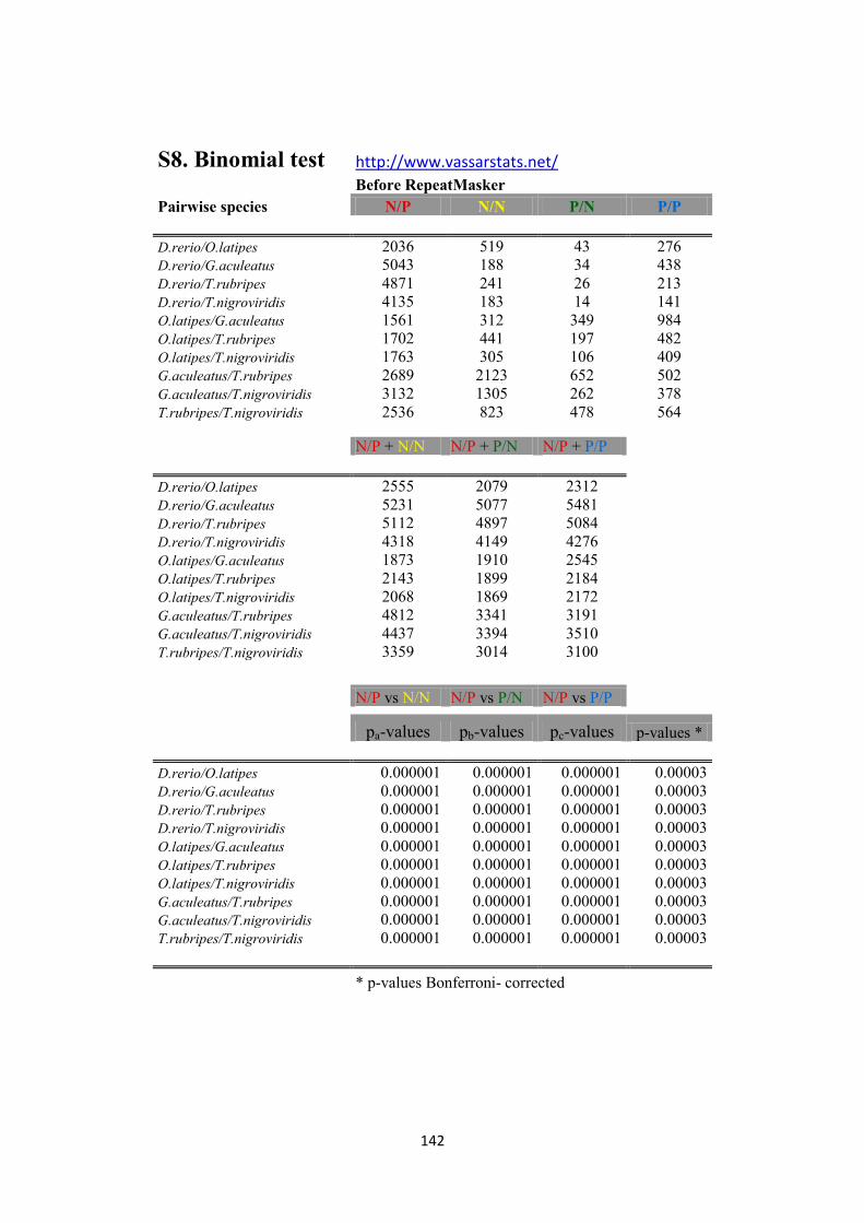
142
S8. Binomial test http://www.vassarstats.net/
Before RepeatMasker
Pairwise species N/P N/N P/N P/P
D.rerio/O.latipes 2036 519 43 276
D.rerio/G.aculeatus 5043 188 34 438
D.rerio/T.rubripes 4871 241 26 213
D.rerio/T.nigroviridis 4135 183 14 141
O.latipes/G.aculeatus 1561 312 349 984
O.latipes/T.rubripes 1702 441 197 482
O.latipes/T.nigroviridis 1763 305 106 409
G.aculeatus/T.rubripes 2689 2123 652 502
G.aculeatus/T.nigroviridis 3132 1305 262 378
T.rubripes/T.nigroviridis 2536 823 478 564
N/P + N/N N/P + P/N N/P + P/P
D.rerio/O.latipes 2555 2079 2312
D.rerio/G.aculeatus 5231 5077 5481
D.rerio/T.rubripes 5112 4897 5084
D.rerio/T.nigroviridis 4318 4149 4276
O.latipes/G.aculeatus 1873 1910 2545
O.latipes/T.rubripes 2143 1899 2184
O.latipes/T.nigroviridis 2068 1869 2172
G.aculeatus/T.rubripes 4812 3341 3191
G.aculeatus/T.nigroviridis 4437 3394 3510
T.rubripes/T.nigroviridis 3359 3014 3100
N/P vs N/N N/P vs P/N N/P vs P/P
pa-values pb-values pc-values p-values *
D.rerio/O.latipes 0.000001 0.000001 0.000001 0.00003
D.rerio/G.aculeatus 0.000001 0.000001 0.000001 0.00003
D.rerio/T.rubripes 0.000001 0.000001 0.000001 0.00003
D.rerio/T.nigroviridis 0.000001 0.000001 0.000001 0.00003
O.latipes/G.aculeatus 0.000001 0.000001 0.000001 0.00003
O.latipes/T.rubripes 0.000001 0.000001 0.000001 0.00003
O.latipes/T.nigroviridis 0.000001 0.000001 0.000001 0.00003
G.aculeatus/T.rubripes 0.000001 0.000001 0.000001 0.00003
G.aculeatus/T.nigroviridis 0.000001 0.000001 0.000001 0.00003
T.rubripes/T.nigroviridis 0.000001 0.000001 0.000001 0.00003
* p-values Bonferroni- corrected

143
After RepeatMasker
Pairwise species N/P N/N P/N P/P
D.rerio/O.latipes 1768 764 93 241
D.rerio/G.aculeatus 4692 487 53 453
D.rerio/T.rubripes 4505 579 38 209
D.rerio/T.nigroviridis 3928 371 18 135
O.latipes/G.aculeatus 1559 296 342 996
O.latipes/T.rubripes 1705 451 197 460
O.latipes/T.nigroviridis 1768 304 108 397
G.aculeatus/T.rubripes 2644 2218 625 463
G.aculeatus/T.nigroviridis 3168 1281 267 360
T.rubripes/T.nigroviridis 2569 758 474 538
N/P + N/N N/P + P/N N/P + P/P
D.rerio/O.latipes 2532 1861 2009
D.rerio/G.aculeatus 5179 4745 5145
D.rerio/T.rubripes 5084 4543 4714
D.rerio/T.nigroviridis 4299 3946 4063
O.latipes/G.aculeatus 1855 1901 2555
O.latipes/T.rubripes 2156 1902 2165
O.latipes/T.nigroviridis 2072 1876 2165
G.aculeatus/T.rubripes 4862 3269 3107
G.aculeatus/T.nigroviridis 4449 3435 3528
T.rubripes/T.nigroviridis 3327 3043 3107
N/P vs N/N N/P vs P/N N/P vs P/P
pa-values pb-values pc-values p-values *
D.rerio/O.latipes 0.000001 0.000001 0.000001 0.00003
D.rerio/G.aculeatus 0.000001 0.000001 0.000001 0.00003
D.rerio/T.rubripes 0.000001 0.000001 0.000001 0.00003
D.rerio/T.nigroviridis 0.000001 0.000001 0.000001 0.00003
O.latipes/G.aculeatus 0.000001 0.000001 0.000001 0.00003
O.latipes/T.rubripes 0.000001 0.000001 0.000001 0.00003
O.latipes/T.nigroviridis 0.000001 0.000001 0.000001 0.00003
G.aculeatus/T.rubripes 0.000001 0.000001 0.000001 0.00003
G.aculeatus/T.nigroviridis 0.000001 0.000001 0.000001 0.00003
T.rubripes/T.nigroviridis 0.000001 0.000001 0.000001 0.00003
* p-values Bonferroni- corrected
Continued from previous page

144
Tab. S9
List of the analyzed species
Order Family Species Sampling
Extraction
tissue Biogeography Lifestyle GC%
Eunicida Eunicidae Eunice sp. 1 Raja Ampat (Indonesia) Prostomium Tropical Motile 43.05
Eunice sp. 3 Raja Ampat (Indonesia) Prostomium Tropical Motile 39.69
Lysidice caribensis Carrie Bow Cay (Belize) Prostomium Tropical Motile 42.21
Lysidice sp. 1 Raja Ampat (Indonesia) Prostomium Tropical Motile 40.38
Lysidice thalassicola Puerto Morelos (Mexican Caribbean) Prostomium Tropical Motile 47.06
Lysidice unicornis Ischia (Italy) Prostomium Temperate Motile 46.58
Nicidion cariboea Carrie Bow Cay (Belize) Whole body Tropical Motile 30.51
Lumbrineridae Scoletoma impatiens Torre Annunziata (Italy) Prostomium Temperate Motile 38.03
Oenonidae Arabella iricolor Ischia (Italy) Prostomium Temperate Motile 42.13
Phyllodocida Aphroditidae Pontogenia chrysocoma Ischia (Italy) Body scales Temperate Motile 48.35
Hesionidae Kefersteinia cirrata Ischia (Italy) Prostomium Temperate Motile 38.59
Nereididae Nereis sp. Ischia (Italy) Prostomium Temperate Motile 40.40
Nereis zonata Ischia (Italy) Whole body Temperate Motile 33.49
Platynereis dumerilii Ischia (Italy) Prostomium Temperate Motile 33.47
Phyllodocidae Eulalia sp. Ischia (Italy) Prostomium Temperate Motile 44.16
Polynoidae Harmothoe fuligineum Weddell Sea (Antarctica) Body scales Polar Motile 41.48
Lepidonotus clava Ischia (Italy) Body scales Temperate Motile 37.58
Lepidonotus sp. Ischia (Italy) Body scales Temperate Motile 41.07

145
Syllidae Syllis prolifera Ischia (Italy) Whole body Temperate Motile 38.69
Scolecida Capitellidae Capitella teleta Lab population - Temperate Motile 40.00
Spionida Spionidae Streblospio benedicti Bayonne. New Jersey (US) - Temperate Motile 37.90
Chaetopterida Chetopteridae Phyllochaetopterus sp. Ischia (Italy) Prostomium Temperate Sessile 44.32
Owenida Oweniidae Owenia fusiformis Gulf of Pozzuoli (Italy) Prostomium Temperate Sessile 37.05
Sabellida Sabellidae Amphicorina eimeri Ischia (Italy) Prostomium Temperate Sessile 29.03
Branchiomma bairdi Ischia (Italy) Prostomium Tropical Sessile 32.76
Branchiomma bombyx Ischia (Italy) Gills Temperate Sessile 35.41
Euchoneira knoxi Weddell Sea (Antarctica) Prostomium+Gills Polar Sessile 30.58
Perkinsiana borsibrunoi Weddell Sea (Antarctica) Prostomium+Gills Polar Sessile 31.91
Perkinsiana littoralis Weddell Sea (Antarctica) Prostomium+Gills Polar Sessile 35.32
Sabella spallanzanii Ischia (Italy) Prostomium+Gills Temperate Sessile 35.34
Serpulidae Protula sp. Ustica (Italy) Prostomium Temperate Sessile 39.96
Serpula sp. Ustica (Italy) Gills Temperate Sessile 35.78
Serpula vermicularis Ustica (Italy) Prostomium+Gills Temperate Sessile 36.64
Vermiliopsis infundibulum Tessaloniki (Greece) Whole body Temperate Sessile 32.86
Vermiliopsis striaticeps Ustica (Italy) Prostomium+Gills Temperate Sessile 35.11
Siboglinidae Lamellibrachia anaximandri Cetaro (Italy) Prostomium Temperate Sessile 39.59
Terebellida Sabellariidae Sabellaria alveolata Santa Severa (Italy) Prostomium Temperate Sessile 32.61
Continued from previous page

146
Table S10
Order Family Authorship Specie
Dry
Weight Resp.Rate T MR
mg mgO2/h °C LN
Amphinomida Amphinomidae Sander 1973 H. carunculata 720,00 0,58 26 24,58
H. carunculata 3000,00 1,04 26 25,16
Phyllodocida Aphroditidae Shumway 1979 A. aculeata 1160,00 0,19 11 24,78
A. aculeata 6510,00 0,55 11 25,85
Glyceridae
G. americana 160,00 0,14 10 24,58
G. americana 1800,00 0,68 10 26,15
Nereididae Sturdivant 2015 A. succinea 7,59 0,01 25 20,87
A. succinea 8,82 0,02 25 21,44
A. succinea 10,39 0,01 25 20,78
A. succinea 11,17 0,01 25 20,99
A. succinea 27,63 0,03 25 21,80
A. succinea 42,47 0,02 25 21,36
A. succinea 58,20 0,04 25 21,86
A. succinea 54,18 0,04 25 22,00
A. succinea 49,90 0,06 25 22,33
A. succinea 60,53 0,06 25 22,40
A. succinea 65,76 0,07 25 22,49
A. succinea 60,85 0,05 25 22,11
A. succinea 93,58 0,05 25 22,19
Nithart 1999 N. diversicolor 5,50 0,01 5 22,57
N. diversicolor 160,00 0,06 5 24,24
Shumway 1979 N. diversicolor 65,00 0,07 10 23,81
N. diversicolor 380,00 0,22 10 25,03
N. virens 1180,00 0,58 10 26,00
N. virens 8520,00 2,24 10 27,34
P. nuntia 30,00 0,06 10 23,68
P. nuntia 200,00 0,18 10 24,83
Phyllodocidae
E. microphylla 60,00 0,07 10 23,90
E. microphylla 410,00 0,26 10 25,18
Sabellida Sabellidae
M.
infundibulum 100,00 0,04 10 23,36
M.
infundibulum 700,00 0,15 10 24,66
Sander 1973 S. magnifica 720,00 0,68 26 24,73
S. magnifica 3000,00 1,47 26 25,50
Dales 1961 S. insignis 80,00 0,02 12,5 22,61
S. insignis 1040,00 0,07 12,5 23,66
Husgaard 2012 O. mucofloris 54,00 0,00 6 20,88
O. mucofloris 110,00 0,01 6 21,67
O. mucofloris 17,00 0,01 6 21,95
O. mucofloris 44,00 0,01 6 22,44
O. mucofloris 81,00 0,02 6 22,77
Scolecida Arenicolidae Shumway 1979 A. assimilis 80,00 0,03 10 23,15
A. assimilis 580,00 0,12 10 24,42

147
Bordon 1931 A. marina 360,00 0,12 11 24,30
A. marina 1420,00 0,34 11 25,38
Shumway 1979 A. marina 310,00 0,09 10 24,14
A. marina 2720,00 0,40 10 25,62
Orbiniidae Nithart 1999 S. armiger 1,50 0,00 15 20,55
S. armiger 15,00 0,02 15 22,15
Terebellida Terebellidae Dales 1961 N. robusta 610,00 0,19 12,5 24,66
N. robusta 2810,00 0,37 12,5 25,32
Cirratulidae Dales 1980 C. tentaculata 264,60 0,01 10 21,60
C. tentaculata 198,80 0,01 10 21,29
C. tentaculata 238,20 0,00 10 19,95
C. tentaculata 215,20 0,01 10 22,09
Terebellidae Dales 1961 T. crispus 270,00 0,11 12,5 24,09
T. crispus 1560,00 0,40 12,5 25,38
Wells 1980 T. haplochaeta 144,00 0,63 20 25,17
T. haplochaeta 600,00 2,61 20 26,59
Dales 1961
E.
heterobranchia 120,00 0,11 12,5 24,12
E.
heterobranchia 1120,00 0,45 12,5 25,51
Continued from previous page

148
Tab S11 Mann-Whitney pairwise comparison (Bonferroni-corrected for multiple comparisons
GC Sabellidae Serpulidae Eunicida
Sabellidae
Serpulidae 0.4442
Eunicida 0.04883 0.273
Phyllodocida 0.03248 0.5895 1
MR Terebellidae Arenicolidae Sabellidae Cirratulidae/Siboglinidae
Terebellidae
Arenicolidae 1
Sabellidae 1 1
Cirratulidae/Siboglinidae 0.7487 1 1
Phyllodocida 1 1 0.4232 0.04378

149
Acknowledgements
First and foremost I want to thank my supervisor Dr Giuseppe D’Onofrio, for the
chance he gave me to make my Ph.D. at the SZN, and for all the stimulating discussions, ideas,
for all the everyday contributions which encouraged my research and allowed me to grow as a
research scientist, and for the unforgettable moments spent together in Japan.
I wish also to thank all the people involved in my thesis project, in alphabetic order:
Prof. Claudio Agnisola, for invaluable discussions and advices, and for helping me
dealing with the metabolic rate experiments.
Dr Claudia Angelini, for introduce me to statistical analyses and R programming, and
for all the time spent to solve my doubts.
Mr Salvatore Bocchetti, for helpful technical support, for HPLC analyses, and for his
constant presence in working and personal life.
Dr Claire Carver, for critical review of Chapter IV and for suggesting further readings
on ascidians morpho-physiology.
Dr Ankita Chaurasia, for retrieving the teleostean intronic sequences and preliminary
analyses of the data.
Dr Maria Cristina Gambi, for providing polychaetes tissues, taxonomy recognition of
the specimens, for critical reviews of Chapter III and for helpful discussions and advices.
Prof. Gretchen Lambert, for critical review of Chapter IV and helpful discussions on
ascidians.
Prof. Shin Oikawa, for having me at the Kyushu University Fishery Lab, for priceless
discussion, both scientific and cultural, and for all the memorable time spent together.
Dr Remo Sanges, for retrieve and process T. nigroviridis gene expression data.
Dr Mitsuharu Yagi, for sharing with me respirometer techniques and data on T.
rubripes, and for all the memorable time spent together.
The SZN Molecular Biology and Bioinformatics unit, for introducing me to the
molecular biology techniques and for helping me with the extraction and purification of nucleic
acids.
The SZN Marine Resource unit, for providing materials for oxygen consumption
experiments.

150
Bibliography
Agashe, D., and N. Shankar. 2014. The evolution of bacterial DNA base composition. … Dev.
Evol., doi: 10.1002/jez.b.22565.
Agutter, P. S., and D. N. Wheatley. 2004. Metabolic scaling: consensus or controversy? Theor.
Biol. Med. Model. 1–13.
Altschul, S. F., T. L. Madden, A. A. Schäffer, J. Zhang, Z. Zhang, W. Miller, and D. J. Lipman.
1997. Gapped BLAST and PSI-BLAST: A new generation of protein database search programs.
Aparicio, S., J. Chapman, E. Stupka, N. Putnam, J.-M. Chia, P. Dehal, A. Christoffels, S. Rash,
S. Hoon, A. Smit, M. D. S. Gelpke, J. Roach, T. Oh, I. Y. Ho, M. Wong, C. Detter, F. Verhoef,
P. Predki, A. Tay, S. Lucas, P. Richardson, S. F. Smith, M. S. Clark, Y. J. K. Edwards, N.
Doggett, A. Zharkikh, S. V Tavtigian, D. Pruss, M. Barnstead, C. Evans, H. Baden, J. Powell,
G. Glusman, L. Rowen, L. Hood, Y. H. Tan, G. Elgar, T. Hawkins, B. Venkatesh, D. Rokhsar,
and S. Brenner. 2002. Whole-genome shotgun assembly and analysis of the genome of Fugu
rubripes. Science 297:1301–10.
April, J., R. H. Hanner, R. L. Mayden, and L. Bernatchez. 2013. Metabolic Rate and Climatic
Fluctuations Shape Continental Wide Pattern of Genetic Divergence and Biodiversity in Fishes.
PLoS One 8:e70296.
Arbeithuber, B., A. J. Betancourt, T. Ebner, and I. Tiemann-Boege. 2015. Crossovers are
associated with mutation and biased gene conversion at recombination hotspots. Proc. Natl.
Acad. Sci. U. S. A. 112:2109–14.
Arhondakis, S., F. Auletta, G. Torelli, and G. D’Onofrio. 2004. Base composition and
expression level of human genes. Gene 325:165–169.
Assis, R., and A. S. Kondrashov. 2012. Nonallelic gene conversion Is Not GC-biased in
drosophila or primates. Mol. Biol. Evol. 29:1291–1295.
Auton, A., A. Fledel-Alon, S. Pfeifer, O. Venn, L. Segurel, T. Street, E. M. Leffler, R. Bowden,
I. Aneas, J. Broxholme, P. Humburg, Z. Iqbal, G. Lunter, J. Maller, R. D. Hernandez, C.
Melton, A. Venkat, M. A. Nobrega, R. Bontrop, S. Myers, P. Donnelly, M. Przeworski, and G.
McVean. 2012. A Fine-Scale Chimpanzee Genetic Map from Population Sequencing.
Babbitt, G. a, and K. V Schulze. 2012. Codons support the maintenance of intrinsic DNA

151
polymer flexibility over evolutionary timescales. Genome Biol. Evol. 4:954–65.
Balfour, F. M. 1881. A treatise on comparative embryology, VOL II. london Macmillan.
Bartlett, M. S. 1947. The Use of Transformations. Biometrics 3:39–52.
Baudat, F., Y. Imai, and B. de Massy. 2013. Meiotic recombination in mammals: localization
and regulation. Nat. Rev. Genet. 14:794–806.
Benjamini, Y., and Y. Hochberg. 1997. Multiple Hypotheses Testing with Weights. Scand. J.
Stat. 24:407–418.
Berglund, J., J. Quilez, P. F. Arndt, and M. T. Webster. 2015. Germline methylation patterns
determine the distribution of recombination events in the dog genome. Genome Biol. Evol.
7:522–30.
Berná, L., F. Alvarez-Valin, and G. D’Onofrio. 2009. How Fast Is the Sessile Ciona? Comp.
Funct. Genomics 2009:1–6.
Berná, L., A. Chaurasia, C. Angelini, C. Federico, S. Saccone, and G. D’Onofrio. 2012. The
footprint of metabolism in the organization of mammalian genomes. BMC Genomics 13:174.
BioMed Central Ltd.
Berná, L., A. Chaurasia, A. Tarallo, C. Agnisola, and G. D’Onofrio. 2013. The Shifting and the
Transition Mode of Vertebrate Genome Evolution in the Light of the Metabolic Rate
Hypothesis: a Review. Pp. 65–93 in Advances in Zoology Research.
Bernardi, G. 2015. Chromosome Architecture and Genome Organization. PLoS One
10:e0143739.
Bernardi, G. 2016. Genome Organization and Chromosome Architecture. Cold Spring Harb.
Symp. Quant. Biol., doi: 10.1101/sqb.2015.80.027318.
Bernardi, G. 2004. Structural and Evolutionary Genomics: Natural Selection in Genome
Evolution. Elsevier B.V.
Bernardi, G., and G. Bernardi. 1990. Compositional transitions in the nuclear genomes of cold-
blooded vertebrates. J. Mol. Evol. 31:282–293.
Bernardi, G., B. Olofsson, J. Filipski, and M. Zerial. 1985. The mosaic genome of warm-
blooded vertebrates. Science (80-. ). 228:953–8.
Bernardi, G., E. O. Wiley, H. Mansour, M. R. Miller, G. Orti, D. Haussler, S. J. O’Brien, O. A.
Ryder, and B. Venkatesh. 2012. The fishes of Genome 10K. Mar. Genomics 7:3–6.

152
Betancur-R, R., R. E. Broughton, E. O. Wiley, K. Carpenter, J. A. López, C. Li, N. I. Holcroft,
D. Arcila, M. Sanciangco, J. C. C. Ii, F. Zhang, M. A. Campbell, J. A. Ballesteros, A. Roa-
varon, S. Willis, W. C. Borden, D. J. Hough, and G. Lu. 2013. The Tree of Life and a New
Classification of Bony Fishes. PLOS Curr. Tree Life Apr 18:1–45.
Boeuf, G., and P. Payan. 2001. How should salinity influence fish growth? Comp. Biochem.
Physiol. C. Toxicol. Pharmacol. 130:411–23.
Bolívar, P., C. F. Mugal, A. Nater, and H. Ellegren. 2016. Recombination Rate Variation
Modulates Gene Sequence Evolution Mainly via GC-Biased Gene Conversion, Not Hill-
Robertson Interference, in an Avian System. Mol. Biol. Evol. 33:216–27.
Borden, M. A. 1931. A study of the respiration and of the function of haemoglobin in Planorbis
corneus and Arenicola marina. J. Mar. Biol. Assoc. United Kingdom (New Ser. 17:709–738.
Cambridge Univ Press.
Bourlat, S. J., T. Juliusdottir, C. J. Lowe, R. Freeman, J. Aronowicz, M. Kirschner, E. S.
Lander, M. Thorndyke, H. Nakano, A. B. Kohn, A. Heyland, L. L. Moroz, R. R. Copley, and
M. J. Telford. 2006. Deuterostome phylogeny reveals monophyletic chordates and the new
phylum Xenoturbellida. Nature 444:85–88.
Braasch, I., and J. H. Postlethwait. 2012. Polyploidy and Genome Evolution. Springer Berlin
Heidelberg, Berlin, Heidelberg.
Bradley, T. J. 2009. Animal Osmoregulation. Oxford University Press, Oxford; New York.
Brett, J. R., and T. D. D. Groves. 1979. 6 Physiological Energetics. Pp. 279–352 in D. J. R. and
J. R. B. B. T.-F. P. W.S. Hoar, ed. Bioenergetics and Growth. Academic Press.
Brown, J. H., J. F. Gillooly, A. P. Allen, V. M. Savage, and G. B. West. 2004. TOWARD A
METABOLIC THEORY OF ECOLOGY. Ecology 85:1771–1789.
Brown, T. C., and J. Jiricny. 1988. Different base/base mispairs are corrected with different
efficiencies and specificities in monkey kidney cells. Cell 54:705–11.
Brown, T. C., and J. Jiricny. 1989. Repair of base-base mismatches in simian and human cells.
Genome / Natl. Res. Counc. Canada = G nome / Cons. Natl. Rech. Canada 31:578–83.
Brunetti, R., C. Gissi, R. Pennati, F. Caicci, F. Gasparini, and L. Manni. 2015. Morphological
evidence that the molecularly determined Ciona intestinalis type A and type B are different
species: Ciona robusta and Ciona intestinalis. J. Zool. Syst. Evol. Res. 53:186–193.
Bucciarelli, G., G. Bernardi, and G. Bernardi. 2002. An ultracentrifugation analysis of two

153
hundred fish genomes. Gene 295:153–62.
Capra, J. a., and K. S. Pollard. 2011. Substitution patterns are GC-biased in divergent sequences
across the metazoans. Genome Biol. Evol. 3:516–527.
Caputi, L., N. Andreakis, F. Mastrototaro, P. Cirino, M. Vassillo, and P. Sordino. 2007. Cryptic
speciation in a model invertebrate chordate. Proc. Natl. Acad. Sci. U. S. A. 104:9364–9369.
Carmel, L., and E. V Koonin. 2009. A universal nonmonotonic relationship between gene
compactness and expression levels in multicellular eukaryotes. Genome Biol. Evol. 1:382–90.
Carver, C. E., a L. Mallet, and B. Vercaemer. 2006. Biological Synopsis of the Solitary
Tunicate Ciona intestinalis. Can. Manuscr. Rep. Fish. Aquat. Sci. No. 2746:55.
Castillo-Davis, C. I., S. L. Mekhedov, D. L. Hartl, E. V Koonin, and F. a Kondrashov. 2002.
Selection for short introns in highly expressed genes. Nat. Genet. 31:415–8.
Chan, E. T., G. T. Quon, G. Chua, T. Babak, M. Trochesset, R. a Zirngibl, J. Aubin, M. J. H.
Ratcliffe, A. Wilde, M. Brudno, Q. D. Morris, and T. R. Hughes. 2009. Conservation of core
gene expression in vertebrate tissues. J. Biol. 8:33.
Chargaff, E. 1951. Some recent studies on the composition and structure of nucleic acids. J.
Cell. Physiol. Suppl. 38:41–59.
Chaurasia, A., A. Tarallo, L. Bernà, M. Yagi, C. Agnisola, and G. D’Onofrio. 2014. Length and
GC Content Variability of Introns among Teleostean Genomes in the Light of the Metabolic
Rate Hypothesis. PLoS One 9:e103889. Public Library of Science, San Francisco, USA.
Chaurasia, A., E. Uliano, L. Berná, C. Agnisola, and G. D’Onofrio. 2011. Does Habitat Affect
the Genomic GC Content? A Lesson from Teleostean Fish: A Mini Review. Pp. 61–80 in Fish
Ecology.
Clarke, A., and N. M. Johnston. 1999. Scaling of metabolic rate with body mass and
temperature in teleost fish. J. Anim. Ecol. 68:893–905.
Clément, Y., and P. F. Arndt. 2013. Meiotic recombination strongly influences GC-content
evolution in short regions in the mouse genome. Mol. Biol. Evol. 30:2612–2618.
Costantini, M., F. Auletta, and G. Bernardi. 2007. Isochore patterns and gene distributions in
fish genomes. Genomics 90:364–371.
Costantini, M., G. Greif, F. Alvarez-Valin, and G. Bernardi. 2016. The Anolis Lizard Genome:
An Amniote Genome without Isochores? Genome Biol. Evol., doi: 10.1093/gbe/evw056.
Cozzi, P., L. Milanesi, and G. Bernardi. 2015. Segmenting the Human Genome into Isochores.

154
Evol. Bioinform. Online 11:253–61.
Cruveiller, S., G. D’Onofrio, and G. Bernardi. 2000. The compositional transition between the
genomes of cold-and warm-blooded vertebrates: codon frequencies in orthologous genes. Gene
261:71–83. Elsevier.
D’Anna, T. 1973. Respiratory rate and succinic dehydrogenase activity in the egg of Ciona
intestinalis (ascidian) upon fertilization. Acta Embryol. Exp. (Palermo). 2:165–77.
D’Onofrio, G., and T. C. Ghosh. 2005. The compositional transition of vertebrate genomes: An
analysis of the secondary structure of the proteins encoded by human genes. Gene 345:27–33.
D’Onofrio, G., K. Jabbari, H. Musto, and G. Bernardi. 1999. The correlation of protein
hydropathy with the base composition of coding sequences. Gene 238:3–14.
Dales, R. P. 1961a. Observation on the respiration of the sabellid polychaete Schizobranchia
insignis. Biol. Bull. 121:82–91.
Dales, R. P. 1961b. Oxygen uptake and irrigation of the burrow by three terebellid polychaetes:
Eupolymnia, Thelepus, and Neoamphitrite. Physiol. Zool. 34:306–311. JSTOR.
De Jager, S., and W. J. Dekkers. 1974. Relations Between Gill Structure and Activity in Fish.
Netherlands J. Zool. 25:276–308.
Dehal, P., Y. Satou, R. K. Campbell, J. Chapman, B. Degnan, A. De Tomaso, B. Davidson, A.
Di Gregorio, M. Gelpke, D. M. Goodstein, N. Harafuji, K. E. M. Hastings, I. Ho, K. Hotta, W.
Huang, T. Kawashima, P. Lemaire, D. Martinez, I. A. Meinertzhagen, S. Necula, M. Nonaka,
N. Putnam, S. Rash, H. Saiga, M. Satake, A. Terry, L. Yamada, H.-G. Wang, S. Awazu, K.
Azumi, J. Boore, M. Branno, S. Chin-Bow, R. DeSantis, S. Doyle, P. Francino, D. N. Keys, S.
Haga, H. Hayashi, K. Hino, K. S. Imai, K. Inaba, S. Kano, K. Kobayashi, M. Kobayashi, B.-I.
Lee, K. W. Makabe, C. Manohar, G. Matassi, M. Medina, Y. Mochizuki, S. Mount, T.
Morishita, S. Miura, A. Nakayama, S. Nishizaka, H. Nomoto, F. Ohta, K. Oishi, I. Rigoutsos,
M. Sano, A. Sasaki, Y. Sasakura, E. Shoguchi, T. Shin-i, A. Spagnuolo, D. Stainier, M. M.
Suzuki, O. Tassy, N. Takatori, M. Tokuoka, K. Yagi, F. Yoshizaki, S. Wada, C. Zhang, P. D.
Hyatt, F. Larimer, C. Detter, N. Doggett, T. Glavina, T. Hawkins, P. Richardson, S. Lucas, Y.
Kohara, M. Levine, N. Satoh, and D. S. Rokhsar. 2002. The Draft Genome of Ciona intestinalis:
Insights into Chordate and Vertebrate Origins. Science (80-. ). 298:2157–2167.
Delsuc, F., H. Brinkmann, D. Chourrout, and H. Philippe. 2006. Tunicates and not
cephalochordates are the closest living relatives of vertebrates. Nature 439:965–968.
Drouaud, J., C. Camilleri, P. Y. Bourguignon, A. Canaguier, A. Bérard, D. Vezon, S. Giancola,

155
D. Brunel, V. Colot, B. Prum, H. Quesneville, and C. Mézard. 2006. Variation in crossing-over
rates across chromosome 4 of Arabidopsis thaliana reveals the presence of meiotic
recombination “hot spots.” Genome Res. 16:106–114.
Duret, L., and P. F. Arndt. 2008. The impact of recombination on nucleotide substitutions in the
human genome. PLoS Genet. 4:e1000071.
Duret, L., and N. Galtier. 2009. Biased gene conversion and the evolution of mammalian
genomic landscapes. Annu. Rev. Genomics Hum. Genet. 10:285–311.
Duret, L., D. Mouchiroud, and C. Gautier. 1995. Statistical analysis of vertebrate sequences
reveals that long genes are scarce in GC-rich isochores. J. Mol. Evol. 40:308–17.
Dutta, C., and S. Paul. 2012. Microbial lifestyle and genome signatures. Curr. Genomics
13:153–62.
Eales, J. G. 1997. Iodine metabolism and thyroid-related functions in organisms lacking thyroid
follicles: are thyroid hormones also vitamins? Proc. Soc. Exp. Biol. Med. 214:302–317.
Edwards, S. L., and W. S. Marshall. 2012. 1 - Principles and Patterns of Osmoregulation and
Euryhalinity in Fishes. Pp. 1–44 in A. P. F. and C. J. B. Stephen D. McCormick, ed. Fish
Physiology. Academic Press.
Evans, D. H., P. M. Piermarini, and K. P. Choe. 2005. The Multifunctional Fish Gill : Dominant
Site of Gas Exchange , Osmoregulation , Acid-Base Regulation , and Excretion of Nitrogenous
Waste. 85:97–177.
Eyre-Walker, a. 1993. Recombination and mammalian genome evolution. Proc. Biol. Sci.
252:237–43.
Eyre-Walker, a, and L. D. Hurst. 2001. The evolution of isochores. Nat. Rev. Genet. 2:549–
555.
Figuet, E., M. Ballenghien, J. Romiguier, and N. Galtier. 2015. Biased gene conversion and
GC-content evolution in the coding sequences of reptiles and vertebrates. Genome Biol. Evol.
7:240–50.
Florkin, M., and B. Scheer. 1974. Chemical Zoology, vol VIII Deuterostomians, Cyclostomes,
and Fishes. Academic Press.
Foerstner, K. U., C. von Mering, S. D. Hooper, and P. Bork. 2005. Environments shape the
nucleotide composition of genomes. EMBO Rep. 6:1208–13.
Friedman, J. R., N. E. Condon, and J. C. Drazen. 2012. Gill surface area and metabolic enzyme
156
activities of demersal fishes associated with the oxygen minimum zone off California. Limnol.
Oceanogr. 57:1701–1710.
Froese, R., D. Pauly, and Editors. n.d. FishBase. World Wide Web Electron. Publ. version
(04/2012).
Gabrielian, a, a Simoncsits, and S. Pongor. 1996. Distribution of bending propensity in DNA
sequences. FEBS Lett. 393:124–30.
Gallo, A., and E. Tosti. 2015. The Ascidian Ciona Intestinalis as Model Organism for
Ecotoxicological Bioassays. J. Mar. Sci. Res. Dev. 05. OMICS International.
Galtier, N., G. Piganeau, D. Mouchiroud, and L. Duret. 2001. GC-Content Evolution in
Mammalian Genomes: The Biased Gene Conversion Hypothesis. Genet. 159 :907–911.
Gambi, M., L. Ramella, G. Sella, P. Protto, and E. Aldieri. 1997. Variation in genome size in
benthic polychaetes: systematic and ecological relationships. J. Mar. ….
Gillooly, J. F., A. P. Allen, G. B. West, and J. H. Brown. 2005. The rate of DNA evolution:
effects of body size and temperature on the molecular clock. Proc. Natl. Acad. Sci. U. S. A.
102:140–145.
Gillooly, J. F., J. H. Brown, G. B. West, V. M. Savage, and E. L. Charnov. 2001. Effects of size
and temperature on metabolic rate. Science 293:2248–2251.
Gillooly, J. F., M. W. McCoy, and A. P. Allen. 2007. Effects of metabolic rate on protein
evolution. Biol. Lett. 3:655–9.
Glazier, D. S. 2005. Beyond the “3/4-power law”: variation in the intra- and interspecific
scaling of metabolic rate in animals. Biol. Rev. Camb. Philos. Soc. 80:611–62.
Glémin, S., Y. Clément, J. David, and A. Ressayre. 2014. GC content evolution in coding
regions of angiosperm genomes: a unifying hypothesis. Trends Genet. 30:263–70.
Gonzalez, R. J., and D. G. McDonald. 1992. The relationship between oxygen consumption and
ion loss in a freshwater fish. J. Exp. Biol. 163:317–332.
Han, L., and Z. Zhao. 2008. Comparative analysis of CpG islands in four fish genomes. Comp.
Funct. Genomics 565631.
Hershberg, R., and D. a Petrov. 2010. Evidence that mutation is universally biased towards AT
in bacteria. PLoS Genet. 6:e1001115.
Hildebrand, F., A. Meyer, and A. Eyre-Walker. 2010. Evidence of selection upon genomic GC-
content in bacteria. PLoS Genet. 6:e1001107.

157
Hill, M. M., K. W. Broman, E. Stupka, W. C. Smith, D. Jiang, and A. Sidow. 2008. The C.
savignyi genetic map and its integration with the reference sequence facilitates insights into
chordate genome evolution. Genome Res. 18:1369–1379.
Holland, N. D., L. Z. Holland, and P. W. H. Holland. 2015. Scenarios for the making of
vertebrates. Nature 520:450–455.
Holmquist, G. P. 1992. Review Article: Chromosome Bands, their chromatin flavors and their
functional features. Am. J. Hum. Genet. 17–37.
Holter, H., and E. Zeuthen. 1944. The respiration of the egg and embryo of the Ascidian, Ciona,
intestinalis L. H. Hagerup, Copenhague.
Hoshino, Z., and T. Nishikawa. 1985. Taxonomic Studies of Ciona intestinalis ( L .) and Its
Allies. Publ. Seto Mar. Biol. Lab. 30:61/79.
Hoshino, Z., and T. Tokioka. 1967. An unusually robust Ciona from the northeastern coast of
Honsyu Island, Japan. 瀬戸臨海実験所.
Howe, K., M. D. Clark, C. F. Torroja, J. Torrance, C. Berthelot, M. Muffato, J. E. Collins, S.
Humphray, K. McLaren, L. Matthews, S. McLaren, I. Sealy, M. Caccamo, C. Churcher, C.
Scott, J. C. Barrett, R. Koch, G.-J. Rauch, S. White, W. Chow, B. Kilian, L. T. Quintais, J. a
Guerra-Assunção, Y. Zhou, Y. Gu, J. Yen, J.-H. Vogel, T. Eyre, S. Redmond, R. Banerjee, J.
Chi, B. Fu, E. Langley, S. F. Maguire, G. K. Laird, D. Lloyd, E. Kenyon, S. Donaldson, H.
Sehra, J. Almeida-King, J. Loveland, S. Trevanion, M. Jones, M. Quail, D. Willey, A. Hunt, J.
Burton, S. Sims, K. McLay, B. Plumb, J. Davis, C. Clee, K. Oliver, R. Clark, C. Riddle, D.
Elliot, D. Eliott, G. Threadgold, G. Harden, D. Ware, S. Begum, B. Mortimore, B. Mortimer, G.
Kerry, P. Heath, B. Phillimore, A. Tracey, N. Corby, M. Dunn, C. Johnson, J. Wood, S. Clark,
S. Pelan, G. Griffiths, M. Smith, R. Glithero, P. Howden, N. Barker, C. Lloyd, C. Stevens, J.
Harley, K. Holt, G. Panagiotidis, J. Lovell, H. Beasley, C. Henderson, D. Gordon, K. Auger, D.
Wright, J. Collins, C. Raisen, L. Dyer, K. Leung, L. Robertson, K. Ambridge, D.
Leongamornlert, S. McGuire, R. Gilderthorp, C. Griffiths, D. Manthravadi, S. Nichol, G.
Barker, S. Whitehead, M. Kay, J. Brown, C. Murnane, E. Gray, M. Humphries, N. Sycamore,
D. Barker, D. Saunders, J. Wallis, A. Babbage, S. Hammond, M. Mashreghi-Mohammadi, L.
Barr, S. Martin, P. Wray, A. Ellington, N. Matthews, M. Ellwood, R. Woodmansey, G. Clark, J.
D. Cooper, J. Cooper, A. Tromans, D. Grafham, C. Skuce, R. Pandian, R. Andrews, E.
Harrison, A. Kimberley, J. Garnett, N. Fosker, R. Hall, P. Garner, D. Kelly, C. Bird, S. Palmer,
I. Gehring, A. Berger, C. M. Dooley, Z. Ersan-Ürün, C. Eser, H. Geiger, M. Geisler, L. Karotki,
A. Kirn, J. Konantz, M. Konantz, M. Oberländer, S. Rudolph-Geiger, M. Teucke, C. Lanz, G.

158
Raddatz, K. Osoegawa, B. Zhu, A. Rapp, S. Widaa, C. Langford, F. Yang, S. C. Schuster, N. P.
Carter, J. Harrow, Z. Ning, J. Herrero, S. M. J. Searle, A. Enright, R. Geisler, R. H. a Plasterk,
C. Lee, M. Westerfield, P. J. de Jong, L. I. Zon, J. H. Postlethwait, C. Nüsslein-Volhard, T. J. P.
Hubbard, H. Roest Crollius, J. Rogers, and D. L. Stemple. 2013. The zebrafish reference
genome sequence and its relationship to the human genome. Nature 496:498–503.
Hughes, G. M. 1966. The dimensions of fish gills in relation to their function. J. Exp. Biol.
45:177–95.
Huusgaard, R. S., B. Vismann, M. Kühl, M. Macnaugton, V. Colmander, G. W. Rouse, A. G.
Glover, T. Dahlgren, and K. Worsaae. 2012. The potent respiratory system of Osedax
mucofloris (Siboglinidae, Annelida)--a prerequisite for the origin of bone-eating Osedax? PLoS
One 7:e35975.
Iannelli, F., G. Pesole, P. Sordino, and C. Gissi. 2007. Mitogenomics reveals two cryptic
species in Ciona intestinalis. Trends Genet. 23:419–422.
Jannière, L., D. Canceill, C. Suski, S. Kanga, B. Dalmais, R. Lestini, A.-F. Monnier, J. Chapuis,
A. Bolotin, M. Titok, E. Le Chatelier, and S. D. Ehrlich. 2007. Genetic evidence for a link
between glycolysis and DNA replication. PLoS One 2:e447.
Jørgensen, C. B. 1952. On the Relation between Water Transport and Food Requirements in
Some Marine Filter Feeding Invertebrates. Biol. Bull. 103:356–363 CR – Copyright ©
1952 Marine Biologi. Marine Biological Laboratory.
Jumars, P. A., K. M. Dorgan, and S. M. Lindsay. 2015. Diet of Worms Emended: An Update of
Polychaete Feeding Guilds. Ann. Rev. Mar. Sci. 7:497–520. Annual Reviews.
Kai, W., K. Kikuchi, S. Tohari, A. K. Chew, A. Tay, A. Fujiwara, S. Hosoya, H. Suetake, K.
Naruse, S. Brenner, Y. Suzuki, and B. Venkatesh. 2011. Integration of the genetic map and
genome assembly of fugu facilitates insights into distinct features of genome evolution in
teleosts and mammals. Genome Biol. Evol. 3:424–42.
Kandul, N. P., and M. A. F. Noor. 2009. Large introns in relation to alternative splicing and
gene evolution: a case study of Drosophila bruno-3. BMC Genet. 10:67.
Kano, S., N. Satoh, and P. Sordino. 2006. Primary genetic linkage maps of the ascidian, Ciona
intestinalis. Zoolog. Sci. 23:31–9.
Kent, C. F., S. Minaei, B. A. Harpur, and A. Zayed. 2012. Recombination is associated with the
evolution of genome structure and worker behavior in honey bees. Proc. Natl. Acad. Sci. U. S.
A. 109:18012–7.
159
Kersey Sturdivant, S., M. Perchik, R. W. Brill, and P. G. Bushnell. 2015. Metabolic responses
of the Nereid polychaete, Alitta succinea, to hypoxia at two different temperatures. J. Exp. Mar.
Bio. Ecol. 473:161–168.
Killen, S. S., D. Atkinson, and D. S. Glazier. 2010. The intraspecific scaling of metabolic rate
with body mass in fishes depends on lifestyle and temperature. Ecol. Lett. 13:184–93.
Kirschner, L. B. 1995. Energetics of osmoregulation in fresh water vertebrates. J. Exp. Zool.
271:243–252.
Kirschner, L. B. 1993. The energetics of osmotic regulation in ureotelic and hypoosmotic
fishes. J. Exp. Zool. 267:19–26.
Kolokotrones, T., Van Savage, E. J. Deeds, and W. Fontana. 2010. Curvature in metabolic
scaling. Nature 464:753–6.
Kryukov, K., K. Sumiyama, K. Ikeo, T. Gojobori, and N. Saitou. 2012. A new database (GCD)
on genome composition for eukaryote and prokaryote genome sequences and their initial
analyses. Pp. 501–512 in Genome Biology and Evolution.
Lamarck, J.-B. de. 1816. Histoire naturelle des animaux sans vertèbres.
Lamb, B. C. 1987. Tests of double-strand gap repair as a major source of meiotic gene
conversion in fungi. 59:63–71.
Lambert, C. C., and G. Lambert. 1998. Non-indigenous ascidians in southern California harbors
and marinas. Mar. Biol. 130:675–688.
Lambert, G. 2007. Invasive sea squirts: A growing global problem. J. Exp. Mar. Bio. Ecol.
342:3–4.
Lambert, G. 2003. New records of ascidians from the NE Pacific: a new species of
Trididemnum, range extension and redescription of Aplidiopsis pannosum (Ritter, 1899)
including its larva, and several non-indigenous species. Zoosystema 25:665–679.
Lander, E. S., L. M. Linton, B. Birren, C. Nusbaum, M. C. Zody, J. Baldwin, K. Devon, K.
Dewar, M. Doyle, W. FitzHugh, R. Funke, D. Gage, K. Harris, a Heaford, J. Howland, L.
Kann, J. Lehoczky, R. LeVine, P. McEwan, K. McKernan, J. Meldrim, J. P. Mesirov, C.
Miranda, W. Morris, J. Naylor, C. Raymond, M. Rosetti, R. Santos, a Sheridan, C. Sougnez, N.
Stange-Thomann, N. Stojanovic, a Subramanian, D. Wyman, J. Rogers, J. Sulston, R.
Ainscough, S. Beck, D. Bentley, J. Burton, C. Clee, N. Carter, a Coulson, R. Deadman, P.
Deloukas, a Dunham, I. Dunham, R. Durbin, L. French, D. Grafham, S. Gregory, T. Hubbard,
S. Humphray, a Hunt, M. Jones, C. Lloyd, a McMurray, L. Matthews, S. Mercer, S. Milne, J.
160
C. Mullikin, a Mungall, R. Plumb, M. Ross, R. Shownkeen, S. Sims, R. H. Waterston, R. K.
Wilson, L. W. Hillier, J. D. McPherson, M. a Marra, E. R. Mardis, L. a Fulton, a T. Chinwalla,
K. H. Pepin, W. R. Gish, S. L. Chissoe, M. C. Wendl, K. D. Delehaunty, T. L. Miner, a
Delehaunty, J. B. Kramer, L. L. Cook, R. S. Fulton, D. L. Johnson, P. J. Minx, S. W. Clifton, T.
Hawkins, E. Branscomb, P. Predki, P. Richardson, S. Wenning, T. Slezak, N. Doggett, J. F.
Cheng, a Olsen, S. Lucas, C. Elkin, E. Uberbacher, M. Frazier, R. a Gibbs, D. M. Muzny, S. E.
Scherer, J. B. Bouck, E. J. Sodergren, K. C. Worley, C. M. Rives, J. H. Gorrell, M. L. Metzker,
S. L. Naylor, R. S. Kucherlapati, D. L. Nelson, G. M. Weinstock, Y. Sakaki, a Fujiyama, M.
Hattori, T. Yada, a Toyoda, T. Itoh, C. Kawagoe, H. Watanabe, Y. Totoki, T. Taylor, J.
Weissenbach, R. Heilig, W. Saurin, F. Artiguenave, P. Brottier, T. Bruls, E. Pelletier, C. Robert,
P. Wincker, D. R. Smith, L. Doucette-Stamm, M. Rubenfield, K. Weinstock, H. M. Lee, J.
Dubois, a Rosenthal, M. Platzer, G. Nyakatura, S. Taudien, a Rump, H. Yang, J. Yu, J. Wang,
G. Huang, J. Gu, L. Hood, L. Rowen, a Madan, S. Qin, R. W. Davis, N. a Federspiel, a P.
Abola, M. J. Proctor, R. M. Myers, J. Schmutz, M. Dickson, J. Grimwood, D. R. Cox, M. V
Olson, R. Kaul, N. Shimizu, K. Kawasaki, S. Minoshima, G. a Evans, M. Athanasiou, R.
Schultz, B. a Roe, F. Chen, H. Pan, J. Ramser, H. Lehrach, R. Reinhardt, W. R. McCombie, M.
de la Bastide, N. Dedhia, H. Blöcker, K. Hornischer, G. Nordsiek, R. Agarwala, L. Aravind, J. a
Bailey, a Bateman, S. Batzoglou, E. Birney, P. Bork, D. G. Brown, C. B. Burge, L. Cerutti, H.
C. Chen, D. Church, M. Clamp, R. R. Copley, T. Doerks, S. R. Eddy, E. E. Eichler, T. S. Furey,
J. Galagan, J. G. Gilbert, C. Harmon, Y. Hayashizaki, D. Haussler, H. Hermjakob, K. Hokamp,
W. Jang, L. S. Johnson, T. a Jones, S. Kasif, a Kaspryzk, S. Kennedy, W. J. Kent, P. Kitts, E. V
Koonin, I. Korf, D. Kulp, D. Lancet, T. M. Lowe, a McLysaght, T. Mikkelsen, J. V Moran, N.
Mulder, V. J. Pollara, C. P. Ponting, G. Schuler, J. Schultz, G. Slater, a F. Smit, E. Stupka, J.
Szustakowski, D. Thierry-Mieg, J. Thierry-Mieg, L. Wagner, J. Wallis, R. Wheeler, a
Williams, Y. I. Wolf, K. H. Wolfe, S. P. Yang, R. F. Yeh, F. Collins, M. S. Guyer, J. Peterson,
a Felsenfeld, K. a Wetterstrand, a Patrinos, M. J. Morgan, P. de Jong, J. J. Catanese, K.
Osoegawa, H. Shizuya, S. Choi, Y. J. Chen, and J. Szustakowki. 2001. Initial sequencing and
analysis of the human genome. Nature 409:860–921.
Lassalle, F., S. Périan, T. Bataillon, X. Nesme, L. Duret, and V. Daubin. 2015. GC-Content
evolution in bacterial genomes: the biased gene conversion hypothesis expands. PLoS Genet.
11:e1004941.
Lesecque, Y., D. Mouchiroud, and L. Duret. 2013. GC-biased gene conversion in yeast is
specifically associated with crossovers: molecular mechanisms and evolutionary significance.
Mol. Biol. Evol. 30:1409–19.
161
Li, S.-W., L. Feng, and D.-K. Niu. 2007. Selection for the miniaturization of highly expressed
genes. Biochem. Biophys. Res. Commun. 360:586–92.
Liu, L., J. Xiang, B. Dong, P. Natarajan, K. Yu, and N. Cai. 2006. Ciona intestinalis as an
emerging model organism: its regeneration under controlled conditions and methodology for
egg dechorionation. J. Zhejiang Univ. Sci. B 7:467–74.
Loh, Y.-H., S. Brenner, and B. Venkatesh. 2008. Investigation of loss and gain of introns in the
compact genomes of pufferfishes (Fugu and Tetraodon). Mol. Biol. Evol. 25:526–35.
Maddamsetti, R., P. J. Hatcher, S. Cruveiller, C. Médigue, J. E. Barrick, and R. E. Lenski. 2015.
Synonymous Genetic Variation in Natural Isolates of Escherichia coli Does Not Predict Where
Synonymous Substitutions Occur in a Long-Term Experiment. Mol. Biol. Evol. 32:2897–2904.
Mancera, E., R. Bourgon, A. Brozzi, W. Huber, and L. M. Steinmetz. 2008. High-resolution
mapping of meiotic crossovers and non-crossovers in yeast. Nature 454:479–85.
Mapelli, F., M. M. Varela, M. Barbato, R. Alvariño, M. Fusi, M. Álvarez, G. Merlino, D.
Daffonchio, and S. Borin. 2013. Biogeography of planktonic bacterial communities across the
whole Mediterranean Sea. Ocean Sci. 9:585–595.
Markus, J. a., and C. C. Lambert. 1983. Urea and ammonia excretion by solitary ascidians. J.
Exp. Mar. Bio. Ecol. 66:1–10.
Marsolier-Kergoat, M. C., and E. Yeramian. 2009. GC content and recombination: Reassessing
the causal effects for the Saccharomyces cerevisiae genome. Genetics 183:31–38.
Marsolier-Kergoat, M.-C. 2011. A simple model for the influence of meiotic conversion tracts
on GC content. PLoS One 6:e16109.
Marsolier-Kergoat, M.-C. 2013. Models for the evolution of GC content in asexual fungi
Candida albicans and C. dubliniensis.
Martin, A. P., and S. R. Palumbi. 1993. Body size, metabolic rate, generation time, and the
molecular clock. Proc. Natl. Acad. Sci. 90:4087–4091.
Mathilde Nithart, Elisabeth Alliot, and Chantal Salen-Picard. 1999. Production, respiration and
ammonia excretion of two polychaete species in a north Norfolk saltmarsh. J. Mar. Biol. Assoc.
UK 79:1029–1037. Cambridge University Press.
McEwan, C. E., D. Gatherer, and N. R. McEwan. 1998. Nitrogen-fixing aerobic bacteria have
higher genomic GC content than non-fixing species within the same genus. Hereditas 128:173–
178.

162
McGaughran, A., and B. R. Holland. 2010. Testing the effect of metabolic rate on DNA
variability at the intra-specific level. PLoS One 5:e9686.
Minamoto, T., S. Hanai, K. Kadota, K. Oishi, H. Matsumae, M. Fujie, K. Azumi, N. Satoh, M.
Satake, and N. Ishida. 2010. Circadian clock in Ciona intestinalis revealed by microarray
analysis and oxygen consumption. J. Biochem. 147:175–84.
Mugal, C. F., P. F. Arndt, and H. Ellegren. 2013. Twisted signatures of GC-biased gene
conversion embedded in an evolutionary stable karyotype. Mol. Biol. Evol. 30:1700–12.
Myers, S., L. Bottolo, C. Freeman, G. McVean, and P. Donnelly. 2005. A fine-scale map of
recombination rates and hotspots across the human genome. Science 310:321–4.
Naya, H., H. Romero, A. Zavala, B. Alvarez, and H. Musto. 2002. Aerobiosis increases the
genomic guanine plus cytosine content (GC%) in prokaryotes. J. Mol. Evol. 55:260–264.
Nelson, J. 2006. Fishes of the World.
Nirenberg, M. W. 1963. The genetic code. II. Sci. Am. 208:80–94.
Nishida, H. 2012. Evolution of genome base composition and genome size in bacteria. Front.
Microbiol. 3:420.
Noor, M. a F. 2008. Mutagenesis from meiotic recombination is not a primary driver of
sequence divergence between Saccharomyces species. Mol. Biol. Evol. 25:2439–44.
Nydam, M. L., and R. G. Harrison. 2010. Polymorphism and divergence within the ascidian
genus Ciona. Mol. Phylogenet. Evol. 56:718–726.
Oesterreich, F. C., N. Bieberstein, and K. M. Neugebauer. 2011. Pause locally, splice globally.
Palzenberger, M., and H. Pohla. 1992. Gill surface area of water-breathing freshwater fish. Rev.
Fish Biol. Fish. 2:187–216.
Parkinson, H., M. Kapushesky, M. Shojatalab, N. Abeygunawardena, R. Coulson, a Farne, E.
Holloway, N. Kolesnykov, P. Lilja, M. Lukk, R. Mani, T. Rayner, a Sharma, E. William, U.
Sarkans, and a Brazma. 2007. ArrayExpress--a public database of microarray experiments and
gene expression profiles. Nucleic Acids Res. 35:D747–50.
Parry, G. 1966. Osmotic Adaptation in Fishes. Biol. Rev. 41:392–440.
Peng, R. D. 2011. Reproducible research in computational science. Science 334:1226–7.
Pennati, R., G. F. Ficetola, R. Brunetti, F. Caicci, F. Gasparini, F. Griggio, A. Sato, T. Stach, S.
Kaul-Strehlow, C. Gissi, and L. Manni. 2015. Morphological Differences between Larvae of the

163
Ciona intestinalis Species Complex: Hints for a Valid Taxonomic Definition of Distinct
Species. PLoS One 10:e0122879.
Petersen, J. K., O. Schou, and P. Thor. 1995. Growth and energetics in ascidian Ciona
intestinalis. Mar. Ecol. Prog. Ser. 120:175–184.
Price, C. a, J. S. Weitz, V. M. Savage, J. Stegen, A. Clarke, D. a Coomes, P. S. Dodds, R. S.
Etienne, A. J. Kerkhoff, K. McCulloh, K. J. Niklas, H. Olff, N. G. Swenson, and J. Chave.
2012. Testing the metabolic theory of ecology. Ecol. Lett. 15:1465–74.
Priede, I. 1985. Metabolic Scope in Fishes. Pp. 33–64 in P. Tytler and P. Calow, eds. Fish
Energetics SE - 2. Springer Netherlands.
Ptak, S. E., D. A. Hinds, K. Koehler, B. Nickel, N. Patil, D. G. Ballinger, M. Przeworski, K. A.
Frazer, and S. Pääbo. 2005. Fine-scale recombination patterns differ between chimpanzees and
humans. Nat. Genet. 37:429–34.
Putnam, N. H., T. Butts, D. E. K. Ferrier, R. F. Furlong, U. Hellsten, T. Kawashima, M.
Robinson-Rechavi, E. Shoguchi, A. Terry, J.-K. Yu, E. L. Benito-Gutiérrez, I. Dubchak, J.
Garcia-Fernàndez, J. J. Gibson-Brown, I. V Grigoriev, A. C. Horton, P. J. de Jong, J. Jurka, V.
V Kapitonov, Y. Kohara, Y. Kuroki, E. Lindquist, S. Lucas, K. Osoegawa, L. A. Pennacchio,
A. A. Salamov, Y. Satou, T. Sauka-Spengler, J. Schmutz, T. Shin-I, A. Toyoda, M. Bronner-
Fraser, A. Fujiyama, L. Z. Holland, P. W. H. Holland, N. Satoh, and D. S. Rokhsar. 2008. The
amphioxus genome and the evolution of the chordate karyotype. Nature 453:1064–1071.
Rao, Y. S., X. W. Chai, Z. F. Wang, Q. H. Nie, and X. Q. Zhang. 2013. Impact of GC content
on gene expression pattern in chicken. Genet. Sel. Evol. 45:9.
Ravi, V., and B. Venkatesh. 2008. Rapidly evolving fish genomes and teleost diversity.
Reichenberger, E. R., G. Rosen, U. Hershberg, and R. Hershberg. 2015. Prokaryotic nucleotide
composition is shaped by both phylogeny and the environment. Genome Biol. Evol. 7:1380–9.
Robinson, M. C., E. a. Stone, and N. D. Singh. 2014. Population genomic analysis reveals no
evidence for gc-biased gene conversion in drosophila melanogaster. Mol. Biol. Evol. 31:425–
433.
Rocha, E. P. C., and A. Danchin. 2002. Base composition bias might result from competition
for metabolic resources.
Rocha, E. P. C., and E. J. Feil. 2010. Mutational patterns cannot explain genome composition:
Are there any neutral sites in the genomes of bacteria? PLoS Genet. 6:e1001104.

164
Rockman, M. V. 2012. Patterns of nuclear genetic variation in the poecilogonous polychaete
Streblospio benedicti. Integr. Comp. Biol. 52:173–80.
Roesti, M., D. Moser, and D. Berner. 2013. Recombination in the threespine stickleback
genome--patterns and consequences. Mol. Ecol. 22:3014–27.
Romiguier, J., V. Ranwez, E. J. P. Douzery, and N. Galtier. 2010. Contrasting GC-content
dynamics across 33 mammalian genomes: Relationship with life-history traits and chromosome
sizes. Genome Res. 20:1001–1009.
Rouse, G. W., and F. Pleijel. 2001. Polychaetes. Oxford University Press, Oxford [etc.].
Saccone, S., C. Federico, and G. Bernardi. 2002. Localization of the gene-richest and the gene-
poorest isochores in the interphase nuclei of mammals and birds. Gene 300:169–178.
Sambrook, J., and D. W. Russell. 2006. Purification of nucleic acids by extraction with
phenol:chloroform. CSH Protoc. 2006:pdb.prot4455–.
Sander, F. 1973. A comparative study of respiration in two tropical marine polychaetes. Comp.
Biochem. Physiol. Part A Physiol. 46:311–323.
Sato, A., N. Satoh, and J. D. D. Bishop. 2012. Field identification of “types” A and B of the
ascidian Ciona intestinalis in a region of sympatry. Mar. Biol. 159:1611–1619.
Satoh, N., Y. Satou, B. Davidson, and M. Levine. 2003. Ciona intestinalis: An emerging model
for whole-genome analyses.
Serres-Giardi, L., K. Belkhir, J. David, and S. Glémin. 2012. Patterns and evolution of
nucleotide landscapes in seed plants. Plant Cell 24:1379–97.
Shenkar, N., and B. J. Swalla. 2011. Global Diversity of Ascidiacea. PLoS One 6:e20657.
Sherrard, K. M., and M. LaBarbera. 2005a. Form and function in juvenile ascidians. I.
Implications of early juvenile morphologies for performance. Mar. Ecol. Prog. Ser. 287:127–
138.
Sherrard, K. M., and M. LaBarbera. 2005b. Form and function in juvenile ascidians. II.
Ontogenetic scaling of volumetric flow rates. Mar. Ecol. Prog. Ser. 287:139–148.
Shumway, S. E. 1978. Respiration, pumping activity and heart rate in Ciona intestinalis exposed
to fluctuating salinities. Mar. Biol. 48:235–242.
Shumway, S. E. 1979. The effects of body size, oxygen tension and mode of life on the oxygen
uptake rates of polychaetes. Comp. Biochem. Physiol. -- Part A Physiol. 64:273–278.

165
Shumway, S. E., C. Bogdanowicz, and D. Dean. 1988. Oxygen consumption and feeding rates
of the sabellid polychaete, Myxicola infundibulum (Renier). Comp. Biochem. Physiol. -- Part A
Physiol. 90:425–428.
Sigsgaard, S. J., J. K. Petersen, and J. J. L. Iversen. 2003. Relationship between specific
dynamic action and food quality in the solitary ascidian Ciona intestinalis. Mar. Biol.
143:1143–1149.
Simakov, O., F. Marletaz, S.-J. Cho, E. Edsinger-Gonzales, P. Havlak, U. Hellsten, D.-H. Kuo,
T. Larsson, J. Lv, D. Arendt, R. Savage, K. Osoegawa, P. de Jong, J. Grimwood, J. a Chapman,
H. Shapiro, A. Aerts, R. P. Otillar, A. Y. Terry, J. L. Boore, I. V Grigoriev, D. R. Lindberg, E.
C. Seaver, D. a Weisblat, N. H. Putnam, and D. S. Rokhsar. 2013. Insights into bilaterian
evolution from three spiralian genomes. Nature 493:526–31. Nature Publishing Group.
Singhal, S., E. M. Leffler, K. Sannareddy, I. Turner, O. Venn, D. M. Hooper, A. I. Strand, Q.
Li, B. Raney, C. N. Balakrishnan, S. C. Griffith, G. McVean, and M. Przeworski. 2015. Stable
recombination hotspots in birds. Science (80-. ). 350:928–932.
Smith, K. F., P. L. Cahill, and A. E. Fidler. 2010. First record of the solitary ascidian Ciona
savignyi Herdman, 1882 in the Southern Hemisphere. Aquat. Invasions 5:363–368.
Sueoka, N. 1959. A statistical analysis of deoxyribonucleic acid distribution in density gradie
DISTRIBUTION IN DENSITY GRADIENT CENTRIFUGATION. Proc. Natl. Acad. Sci. U.
S. A. 45:1480–1490.
Sueoka, N. 1962. On the genetic basis of variation and heterogeneity of DNA base composition.
Proc. Natl. Acad. Sci. U. S. A. 48:582–92.
Suzuki, M. M., T. Nishikawa, and A. Bird. 2005. Genomic approaches reveal unexpected
genetic divergence within Ciona intestinalis. J. Mol. Evol. 61:627–635.
Swan, B. K., B. Tupper, A. Sczyrba, F. M. Lauro, M. Martinez-Garcia, J. M. González, H. Luo,
J. J. Wright, Z. C. Landry, N. W. Hanson, B. P. Thompson, N. J. Poulton, P. Schwientek, S. G.
Acinas, S. J. Giovannoni, M. A. Moran, S. J. Hallam, R. Cavicchioli, T. Woyke, and R.
Stepanauskas. 2013. Prevalent genome streamlining and latitudinal divergence of planktonic
bacteria in the surface ocean. Proc. Natl. Acad. Sci. U. S. A. 110:11463–8.
Taekjun, L., and S. Sook. 2014. Morphological and molecular identification of an introduced
alien sea squirt ( Tunicata : Ascidiacea ) in Korea. 127:284–297.
Tarallo, A., C. Angelini, R. Sanges, M. Yagi, C. Agnisola, and G. D’Onofrio. 2016. On the
genome base composition of teleosts: the effect of environment and lifestyle. BMC Genomics

166
17:173. BioMed Central.
Tatusov, R. L., N. D. Fedorova, J. D. Jackson, A. R. Jacobs, B. Kiryutin, E. V Koonin, D. M.
Krylov, R. Mazumder, S. L. Mekhedov, A. N. Nikolskaya, B. S. Rao, S. Smirnov, A. V
Sverdlov, S. Vasudevan, Y. I. Wolf, J. J. Yin, and D. a Natale. 2003. The COG database: an
updated version includes eukaryotes. BMC Bioinformatics 4:41.
Thiery, J., G. Macaya, and G. Bernardi. 1976. An analysis of eukaryotic genomes by density
gradient centrifugation. J. Mol. Biol.
Tseng, Y.-C., and P.-P. Hwang. 2008. Some insights into energy metabolism for
osmoregulation in fish. Comp. Biochem. Physiol. C. Toxicol. Pharmacol. 148:419–29. Elsevier
Inc.
Ukena, K., E. Iwakoshi-Ukena, and A. Hikosaka. 2008. Unique form and osmoregulatory
function of a neurohypophysial hormone in a urochordate. Endocrinology 149:5254–61.
Uliano, E., A. Chaurasia, L. Bernà, C. Agnisola, and G. D’Onofrio. 2010. Metabolic rate and
genomic GC: what we can learn from teleost fish. Mar. Genomics 3:29–34.
Urrutia, A. O., and L. D. Hurst. 2003. The signature of selection mediated by expression on
human genes. Genome Res. 13:2260–4.
Valentine, P. C., M. R. Carman, D. S. Blackwood, and E. J. Heffron. 2007. Ecological
observations on the colonial ascidian Didemnum sp. in a New England tide pool habitat. J. Exp.
Mar. Bio. Ecol. 342:109–121.
Varriale, A., and G. Bernardi. 2006. DNA methylation and body temperature in fishes. Gene
385:111–21.
Venkatesh, B. 2003. Evolution and diversity of fish genomes.
Versteeg, R., B. D. C. Van Schaik, M. F. Van Batenburg, M. Roos, R. Monajemi, H. Caron, H.
J. Bussemaker, and A. H. C. Van Kampen. 2003. The Human Transcriptome Map Reveals
Extremes in Gene Density , Intron Length , GC Content , and Repeat Pattern for Domains of
Highly and Weakly Expressed Genes. 1998–2004.
Vinogradov, a E. 2001. Bendable genes of warm-blooded vertebrates. Mol. Biol. Evol.
18:2195–2200.
Vinogradov, a E. 1998. Genome size and GC-percent in vertebrates as determined by flow
cytometry: the triangular relationship. Cytometry 31:100–9.
Vinogradov, A. E. 2004. Compactness of human housekeeping genes: selection for economy or

167
genomic design? Trends Genet. 20:248–53.
Vinogradov, A. E. 2003. DNA helix: the importance of being GC-rich. Nucleic Acids Res.
31:1838–44.
Vinogradov, A. E. 2005. Noncoding DNA, isochores and gene expression: Nucleosome
formation potential. Nucleic Acids Res. 33:559–563.
Vinogradov, A. E., and O. V Anatskaya. 2006. Genome size and metabolic intensity in
tetrapods: a tale of two lines. Proc. Biol. Sci. 273:27–32.
Vinson, J. P., D. B. Jaffe, K. O’Neill, E. K. Karlsson, N. Stange-Thomann, S. Anderson, J. P.
Mesirov, N. Satoh, Y. Satou, C. Nusbaum, B. Birren, J. E. Galagan, and E. S. Lander. 2005.
Assembly of polymorphic genomes: Algorithms and application to Ciona savignyi. Genome
Res. 15:1127–1135.
Wallberg, A., S. Glémin, and M. T. Webster. 2015. Extreme Recombination Frequencies Shape
Genome Variation and Evolution in the Honeybee, Apis mellifera. PLoS Genet. 11:e1005189.
Weber, C. C., B. Boussau, J. Romiguier, E. D. Jarvis, and H. Ellegren. 2014. Evidence for GC-
biased gene conversion as a driver of between-lineage differences in avian base composition.
Genome Biol. 15:1–16.
Wegner, N. C., and J. B. Graham. 2010. George Hughes and the history of fish ventilation: from
Du Verney to the present. Comp. Biochem. Physiol. A. Mol. Integr. Physiol. 157:1–6. Elsevier
Inc.
Weigert, A., C. Helm, M. Meyer, B. Nickel, D. Arendt, B. Hausdorf, S. R. Santos, K. M.
Halanych, G. Purschke, C. Bleidorn, and T. H. Struck. 2014. Illuminating the base of the
Annelid tree using transcriptomics. Mol. Biol. Evol. 31:1391–1401.
Wells, R. M. G., P. J. Jarvis, and S. E. Shumway. 1980. Oxygen uptake, the circulatory system,
and haemoglobin function in the intertidal polychaete Terebella haplochaeta (Ehlers). J. Exp.
Mar. Bio. Ecol. 46:255–277.
White, C. R., and R. S. Seymour. 2003. Mammalian basal metabolic rate is proportional to body
mass2/3. Proc. Natl. Acad. Sci. U. S. A. 100:4046–4049.
Winckler, W., S. R. Myers, D. J. Richter, R. C. Onofrio, G. J. McDonald, R. E. Bontrop, G. A.
T. McVean, S. B. Gabriel, D. Reich, P. Donnelly, and D. Altshuler. 2005. Comparison of fine-
scale recombination rates in humans and chimpanzees. Science 308:107–11.
Windisch, H. S., M. Lucassen, and S. Frickenhaus. 2012. Evolutionary force in confamiliar
168
marine vertebrates of different temperature realms: adaptive trends in zoarcid fish
transcriptomes. BMC Genomics 13:549.
WoRMS Editorial Board. 2016. World Register of Marine Species.
Yagi, M., T. Kanda, T. Takeda, A. Ishimatsu, and S. Oikawa. 2010. Ontogenetic phase shifts in
metabolism: links to development and anti-predator adaptation. Proc. Biol. Sci. 277:2793–801.
Yagi, M., and S. Oikawa. 2014. Ontogenetic phase shifts in metabolism in a flounder
Paralichthys olivaceus. Sci. Rep. 4:7135.
Zhan, A., H. J. MacIsaac, and M. E. Cristescu. 2010. Invasion genetics of the Ciona intestinalis
species complex: From regional endemism to global homogeneity. Mol. Ecol. 19:4678–4694.
Zhu, L., Y. Zhang, W. Zhang, S. Yang, J.-Q. Chen, and D. Tian. 2009. Patterns of exon-intron
architecture variation of genes in eukaryotic genomes. BMC Genomics 10:47.
Related Documents