Generalized planar curves and quaternionic geometry

arX

iv:m

ath/

0512

593v

1 [

mat

h.D

G]

27

Dec

200

5

GENERALIZED PLANAR CURVES AND

QUATERNIONIC GEOMETRY

JAROSLAV HRDINA AND JAN SLOVAK

Abstract. Motivated by the analogies between the projectiveand the almost quaternionic geometries, we first study the gen-eralized planar curves and mappings. We follow, recover, and ex-tend the classical approach, see e.g. [9, 10]. Then we exploit theimpact of the general results in the almost quaternionic geometry.In particular we show, that the natural class of H–planar curvescoincides with the class of all geodesics of the so called Weyl con-nections and preserving this class turns out to be the necessaryand sufficient condition on diffeomorphisms to become morphismsof almost quaternionic geometries.

Various concepts generalizing geodesics of affine connections havebeen studied for almost quaternionic and similar geometries. Let uspoint out the generalized geodesics defined via generalizations of nor-mal coordinates, cf. [2] and [3], or more recent [4, 11]. Another classof curves was studied in [10] for the hypercomplex structures with ad-ditional linear connections. The latter authors called a curve c quater-nionic planar if the parallel transport of each of its tangent vectorsc(t0) along c was quaternionic colinear with the tangent field c to thecurve. Yet another natural class of curves is given by the set of allunparameterized geodesics of the so called Weyl connections, i.e. theconnections compatible with the almost quaternionic structure withnormalized minimal torsion. The latter connections have remarkablysimilar properties for all parabolic geometries, cf. [3], and so their namehas been borrowed from the conformal case. In the setting of almostquaternionic structures, they were studied first in [7] and so they arealso called Oproiu connections, see [1].

The first author showed in [6] that actually the concept of quater-nionic planar curves was well defined for the almost quaternionic ge-ometries and their Weyl connections. Moreover, it did not depend onthe choice of a particular Weyl connection and it turned out that thequaternionic planar curves were just all unparameterized geodesics ofall Weyl connections.

The aim of this paper is to find further analogies of Mikes’s classicalresults in the realm of the almost quaternionic geometry. On the way we

1

2 JAROSLAV HRDINA AND JAN SLOVAK

simplify, recover, and extend results on generalized planar mappings,explain results from [6], and finally we show that morphisms of almostquaternionic geometries are just those diffeomorphisms which leave in-variant the class of all unparameterized geodesics of Weyl connections.Acknowledgments. The authors have been supported by GACR,grants Nr. 201/05/H005 and 201/05/2117, respectively. The secondauthor also gratefully acknowledges support from the Royal Society ofNew Zealand via Marsden Grant no. 02-UOA-108 during writing essen-tial part of this paper. The authors are also grateful to Josef Mikes fornumerous discussions and to Dmitri Alekseevsky for helpful comments.

1. Motivation and background on quaternionic geometry

There are many equivalent definitions of almost quaternionic geom-etry to be found in the literature. Let us start with the following one:

Definition 1.1. Let M be a smooth manifold of dimension 4n. Analmost hypercomplex structure on M is a triple (I, J, K) of smoothaffinors in Γ(T ∗M ⊗ TM) satisfying

I2 = J2 = −E, K = I J = −J I

where E = idTM .An almost quaternionic structure is a rank four subbundle Q ⊂

T ∗M ⊗ TM locally generated by the identity E and a hypercomplexstructure.

An almost complex geometry on a 2m–dimensional manifold M isgiven by the choice of the affinor J satisfying J2 = −E. Let us observe,that such a J is uniquely determined within the rank two subbundle〈E, J〉 ⊂ TM , up to its sign. Indeed, if J = aE+bJ , then the condition

J2 = −E implies a = 0 and b = ±1.Thus we may view the almost quaternionic geometry as a straight-

forward generalization of this case. Here, a similar simple computa-tion reveals that the rank three subbundle 〈I, J, K〉 is invariant of thechoice of the generators and this is the definition we may find in [1].

More explicitly, different choices will always satisfy I = aI + bJ + cKwith a2 + b2 + d2 = 1, and similarly for J and K. Let us also remarkthat the 4–dimensional almost quaternionic geometry coincides with4-dimensional conformal Riemannian geometries.

1.2. The frame bundles. Equivalently, we can define an almost quater-nionic structure Q on M as a reduction of the linear frame bundle P 1Mto an appropriate structure group, i.e. as a G–structure with the struc-ture group of all automorphisms preserving the subbundle Q. We may

GENERALIZED PLANAR CURVES AND QUATERNIONIC GEOMETRY 3

view such frames as linear mappings TxM → Hn which carry over

the multiplications by i, j, k ∈ H onto some of the possible choicesfor I, J, K. Thus, a further reduction to a fixed hypercomplex struc-ture leads to the structure group GL(n, H) of all quaternionic linearmappings on H

n. Additionally, we have to allow morphisms which donot leave the affinors I, J , K invariant but change them within thesubbundle Q. As well known, the resulting group is

(1) G0 = GL(n, H) ×Z2Sp(1)

where Sp(1) are the unit quaternions in GL(1, H), see e.g. [8].We shall write G0 ⊂ P 1M for this principal G0–bundle defining our

structure.The simplest example of such a structure is well understood as the

homogeneous spacePnH = G/P

where G0 ⊂ P are the subgroups in G = SL(n + 1, H)

G0 =

(

a 00 A

)

; A ∈ GL(n, H), Re(a det A) = 1

,(2)

P =

(

a Z0 A

)

;

(

a 00 A

)

∈ G0, Z ∈ (Hn)∗

.(3)

Since P is a parabolic subgroup in the semisimple Lie group G, thealmost quaternionic geometry is an instance of the so called parabolicgeometries. All these geometries enjoy a rich and quite uniform theorysimilar to the classical development of the conformal Riemannian andprojective geometries, but we shall not need much of this here. We referthe reader to [3] and the references therein.

1.3. Weyl connections. The classical prolongation procedure for G–structures starts with finding a minimal available torsion for a con-nection belonging to the structure on the given manifold M . Unlikethe projective and conformal Riemannian structures where torsion freeconnections always exist, the torsion has to be allowed for the almostquaternionic structures in general in dimensions bigger than four. Thestandard normalization comes from the general theory of parabolic ge-ometries and we shall not need this in the sequel. The details may befound for example in [5], [2], for another and more classical point ofview see [8]. The only essential point for us is that all connections com-patible with the given geometry sharing the unique normalized torsionare parameterized by smooth one–forms on M . In analogy to the con-formal Riemannian geometry we call them Weyl connections for thegiven almost quaternionic geometry on M .

4 JAROSLAV HRDINA AND JAN SLOVAK

The almost quaternionic geometries with Weyl connections withouttorsion are called quaternionic geometries.

From the point of view of prolongations of G–structures, the class ofall Weyl connections defines a reduction G of the semiholonomic secondorder frame bundle over the manifold M to a principal subbundle withthe structure group P , while the individual Weyl connections repre-sent further reductions of G to principal subbundles G0 ⊂ G with thestructure group G0 ⊂ P . Thus, the Weyl connections ∇ are in bijectivecorrespondence with G0–equivariant sections σ : G0 → G of the naturalprojection.

As mentioned above, the difference of two Weyl connections is aone–form and, also in full analogy to the conformal geometry, there areneat formulae for the change of the covariant derivatives of two suchconnections ∇ and ∇ in terms of their difference Υ = ∇−∇ ∈ Ω1(M).

1.4. Adjoint tractors. In order to understand the latter formulae, weintroduce the so called adjoint tractors. They are sections of the vectorbundle (called usually adjoint tractor bundle) over M

A = G0 ×G0g,

see (1) through (3) for the definition of the groups. The Lie algebrag = sl(n + 1, H) carries the G0–invariant grading

(4) g = g−1 ⊕ g0 ⊕ g1

where

g0 =

(

a 00 A

)

; A ∈ gl(n, H), a ∈ H Re(a + Tr A) = 0

,

g1 =

(

0 Z0 0

)

; Z ∈ (Hn)∗

, g−1 =

(

0 0X 0

)

; X ∈ Hn

.

Moreover, TM = G0 ×G0g−1, T ∗M = G0 ×G0

g1, and we obtain on thelevel of vector bundles

A = A−1 ⊕A0 ⊕A1 = TM ⊕A0 ⊕ T ∗M

where A0 = G0 × g0 is the adjoint bundle of the Lie algebra g0.The key feature of A is that all further G0–invariant objects on g are

carried over to the adjoint tractors, too. In particular, the Lie bracketon G induces an algebraic bracket , on A such that each fibre hasthe structure of the graded Lie algebra (4).

Now we may write down easily the transformation formula. Let ∇and ∇ be two Weyl connections, ∇ − ∇ = Υ ∈ Γ(A1). Then for all

GENERALIZED PLANAR CURVES AND QUATERNIONIC GEOMETRY 5

tangent vector fields X, Y ∈ Γ(A−1), i.e. sections of the g−1-componentof the adjoint tractor bundle,

(5) ∇XY = ∇XY + X, Υ, Y = ∇XY + Υ(X)Y,

where Υ(X) ∈ g0 = sp(1) + gl(n, H), see [3] or [2, 5] for the proof.Notice that the internal bracket results in an endomorphism on TM ,while the external bracket is just the evaluation of this endomorphismon Y (all this is read off the brackets in the Lie algebra easily).

2. Generalized planar curves and mappings

Various geometric structures on manifolds are defined as smoothdistributions in the vector bundle T ∗M ⊗TM of all endomorphisms ofthe tangent bundle. We have seen the two examples of almost complexand almost quaternionic structures above. Let us extract some formalproperties from these examples.

Definition 2.1. Let A be a smooth ℓ–dimensional vector subbundle inT ∗M ⊗TM , such that the identity affinor E = idTM restricted to TxMbelongs to AxM ⊂ T ∗

xM ⊗ TxM at each point x ∈ M . We say that Mis equipped by an A–structure.

For any tangent vector X ∈ TxM we shall write A(X) for the vectorsubspace

A(X) = F (X); F ∈ AxM ⊂ TxM

and we call A(X) the A–hull of the vector X. Similarly, the A–hull ofa vector field will be the subbundle in TM obtained pointwise. Noticethat the dimension of such a subbundle in TM may vary pointwise.For every smooth parameterized curve c : R → M we write c and A(c)for the tangent vector field and its A-hull along the curve c.

For any vector space V , we say that a vector subspace A ⊂ V ∗ ⊗ Vof automorphisms is of generic rank ℓ if the dimension of A is ℓ, andthe subset of vectors (X, Y ) ∈ V ×V , such that the A–hulls A(X) andA(Y ) generate a vector subspace A(X)⊕A(Y ) of dimension 2ℓ, is openand dense. An A–structure is said to be of generic rank ℓ if AxM hasthis property for each point x ∈ M .

Let us point out some examples:

• The 〈E〉–structure is of generic rank one on all manifolds ofdimensions at least 2.

• Any almost complex structure or almost product structure 〈E, J〉is of generic rank two on all manifolds of dimensions at least 4.

• Any almost quaternionic structure is of generic rank four on allmanifolds of dimensions at least 8.

6 JAROSLAV HRDINA AND JAN SLOVAK

Similar conclusions apply to paracomplex and parahermition struc-tures.

Definition 2.2. Let M be a smooth manifold with a given A–structureand a linear connection ∇. A smooth curve c : R → M is told to beA–planar if

∇cc ∈ A(c).

Clearly, A planarity means that the parallel transport of any tangentvector to c has to stay within the A–hull A(c) of the tangent vectorfield c along the curve. Moreover, this concept does not depend on theparametrization of the curve c.

Definition 2.3. Let M be a manifold with a linear connection ∇ andan A–structure, while N be another manifold with a linear connection∇ and a B–structure. A diffeomorphism f : M → N is called (A, B)–planar if each A–planar curve c on M is mapped onto the B–planarcurve F c on N .

Example 2.4. The 1–dimensional A = 〈E〉 structure must be givenjust as the linear hull of the identity affinor E, by the definition. Obvi-ously, the 〈E〉–planar curves on a manifold M with a linear connection∇ are exactly the unparameterized geodesics. Moreover, two connections∇ and ∇ without torsion are projectively equivalent (i.e. they share thesame unparameterized geodesics) if and only if their difference satisfies∇XY − ∇XY = α(X)Y + α(Y )X for some one–form α on M . Thelatter condition can be rewritten as

(6) ∇ − ∇ ∈ Γ(T ∗M ⊙ 〈E〉) ⊂ Γ(S2T ∗M ⊗ TM)

where the symbol ⊙ stays for the symmetrized tensor product.

The latter condition on projective structures may be also rephrasedin the terms of morphisms: A diffeomorphism f : M → M is calledgeodesical (or an automorphism of the projective structure) if f c isan unparameterized geodesic for each geodesic c and this happens ifand only if the symmetrization of the difference f ∗∇−∇ is a sectionof T ∗M ⊙ 〈E〉. We are going to generalize the above example in therest of this section.

In the case A = 〈E〉, the (〈E〉, B)–planar mappings are called simplyB–planar. They map each geodesic curve on (M,∇) onto a B–planar

curve on (N, ∇, B).Each ℓ dimensional A structure A ⊂ T ∗M ⊗ TM determines the

distribution A(1) in S2T ∗M ⊗ TM , given at any point x ∈ M by

A(1)x M = α1 ⊙ F1 + · · · + αℓ ⊙ Fℓ; αi ∈ T ∗

xM, Fi ∈ AxM.

GENERALIZED PLANAR CURVES AND QUATERNIONIC GEOMETRY 7

Theorem 2.5. Let M be a manifold with a linear connection ∇, let Nbe a manifold of the same dimension with a linear connection ∇ andan A–structure of generic rank ℓ, and suppose dim M ≥ 2ℓ. Then adiffeomorphism f : M → N is A–planar if and only if

(7) Sym(f ∗∇ − ∇) ∈ f ∗(A(1))

where Sym denotes the symmetrization of the difference of the two con-nections.

The proof is based on a purely algebraical lemma below. Let us firstobserve that the entire claim of the theorem is of local character. Thus,identifying the objects on N with their pullbacks on M , we may assumethat M = N and f = idM .

Next, let us observe that the A–planarity of f : M → N does notat all depend on the possible torsions of the connection. Indeed, wealways test expressions of the type ∇cc for a curve c and thus deform-ing ∇ into ∇′ = ∇ + T by adding some torsion will not effect theresults. Thus, without any loss of generality, we may assume that theconnections ∇ and ∇ share the same torsion, and then we may omitthe symmetrization from equation (7).

Finally, we may fix some (local) basis E = F0, Fi, i = 1, . . . ℓ − 1, ofA, i.e. A = 〈F0, . . . , Fℓ−1〉. Then the condition in equation (7) says

(8) ∇ = ∇ +ℓ−1∑

i=0

αi ⊙ Fi

for some suitable one–forms αi on M . Of course, the existence of suchforms does not depend on our choice of the basis of A.

The quite simplified statement we now have to prove is:

Proposition 2.6. Let M be a manifold of dimension at least 2ℓ, ∇and ∇ two connections on M with the same torsion, and consider anA–structure of generic rank ℓ on M . Then each geodesic curve withrespect to ∇ is A–planar with respect to ∇ if and only if there areone–forms αi satisfying equation (8).

Assume first we have such forms αi, and let c be a geodesic for∇. Then equation (8) implies ∇cc ∈ A(c) so that c is A–planar, bydefinition.

The other implication is the more difficult one. Assume each (unpa-rameterized) geodesic c is A–planar. This implies that the symmetric

difference tensor P = ∇ − ∇ ∈ Γ(S2T ∗M ⊗ TM) satisfies

P (c, c) = ∇cc ∈ 〈c, F1(c), . . . , Fℓ−1(c)〉.

8 JAROSLAV HRDINA AND JAN SLOVAK

In fact, the main argument of the entire proof boils down to a purelyalgebraic claim:

Lemma 2.7. Let A ⊂ V ∗ ⊗ V be a vector subspace of generic rankℓ, and assume that P (X, X) ∈ A(X) for some fixed symmetric tensorP ∈ V ∗ ⊗ V ∗ ⊗ V and each vector X ∈ V . Then the induced mappingP : V → V ∗ ⊗ V has values in A.

Proof. Let us fix a basis F0, F1, . . . , Fℓ−1 of A. Since A is of generic rankℓ, there is the open and dense subspace V ⊂ V of all vectors X ∈ Vfor which F0(X), F1(X), . . . , Fℓ−1(X) are linearly independent. Now,for each X ∈ V there are the unique coefficients αi(X) ∈ R such that

(9) P (X, X) =

ℓ−1∑

i=0

αi(X)Fi(X).

The essential technical step in the proof of our Lemma is to show thatall functions αi are in fact restrictions of one–forms on V . Let us notice,that P is a symmetric bilinear mapping and thus it is determined bythe restriction of P (X, X) to arbitrarily small open non–empty subsetof the arguments X in V .Claim 1. If a symmetric tensor P ∈ V ∗ ⊗ V ∗ ⊗ V is determinedover the above defined subspace V by (9), then the functions αi : V →R are smooth and their restrictions to the individual rays (half–lines)generated by vectors in V are linear.

Let us fix a local smooth basis ei ∈ V , the dual basis ei, and considerthe induced dual bases eI and eI on the multivectors and exterior forms.Let us consider the smooth mapping

χ : ΛℓV \ 0 → ΛℓV ∗, χ(∑

aIeI) =

∑ aI∑

a2I

eI .

Now, for all non–zero tensors Ξ =∑

aIeI , the evaluation 〈Ξ, χ(Ξ)〉 is

the constant function 1, while χ(k · Ξ) = k−1χ(Ξ).Next, we define for each X ∈ V

τ(X) = χ(

X ∧ F1(X) ∧ · · · ∧ Fℓ−1(X))

and we may compute the unique coefficients αi from (9):

α0(X) = 〈P (X, X) ∧ F1(X) ∧ F2(X) ∧ · · · ∧ Fℓ−1(X), τ(X)〉

α1(X) = 〈X ∧ P (X, X) ∧ F2(X) ∧ · · · ∧ Fℓ−1(X), τ(X)〉

...

αℓ−1(X) = 〈X ∧ F1(X) ∧ F2(X) ∧ · · · ∧ P (X, X), τ(X)〉.

In particular, this proves the first part our Claim 1.

GENERALIZED PLANAR CURVES AND QUATERNIONIC GEOMETRY 9

Let us now consider a fixed vector X ∈ V. The defining formula (9)for αi implies αi(kX) = kαi(X), for each real number k 6= 0. Passingto zero with positive k shows that α does have the limit 0 in the originand so we may extend the definition of αi’s (and validity of formula(9)) to the entire cone V ∪ 0 by setting αi(0) = 0 for all i.

Finally, along the ray tX; t > 0 ⊂ V, the derivative ddt

α(tX) hasthe constant value α(X). This proves the rest of Claim 1.

Now, in order to complete the proof of Lemma 2.7, we have to provethe following assertion.Claim 2. If a symmetric tensor P is determined over the above definedsubspace V ∪ 0 by (9), then the coefficients αi are linear one–formson V and the tensor P is given by

P (X, Y ) =1

2

ℓ−1∑

i=0

(

αi(Y )Fi(X) + αi(X)Fi(Y ))

.

The entire tensor P is obtained through polarization from its evalu-ations P (X, X), X ∈ TM ,

(10) P (X, Y ) = 12

(

P (X + Y, X + Y ) − P (X, X) − P (Y, Y ))

,

and again, the entire tensor is determined by its values on arbitrarilysmall non–empty open subset of X and Y in each fiber.

The summands on the right hand side have values in the followingsubspaces:

P (X + Y, X + Y ) ∈ 〈X + Y, F1(X + Y ), . . . , Fℓ−1(X + Y )〉 ⊂

〈X, F1(X), . . . Fℓ−1(X), Y, F1(Y ), . . . , Fℓ−1(Y )〉,

P (X, X) ∈ 〈X, F1(X), . . . Fℓ−1(X)〉,

P (Y, Y ) ∈ 〈Y, F1(Y ), . . . Fℓ−1(Y )〉.

Since we have assumed that A has generic rank ℓ, the subspace W ∈V ×M V of vectors (X, Y ) such that all the values

X, F1(X), . . . , Fℓ−1(X), Y, F1(Y ), . . . , Fℓ−1(Y )

are linearly independent is open and dense. Clearly W ⊂ V ×V. More-over, if (X, Y ) ∈ W than F0(X +Y ), . . . , Fℓ−1(X +Y ) are independent,i.e. X + Y ∈ V. Inserting (9) into (10), we obtain

P (X, Y ) =

ℓ−1∑

i=0

(

di(X, Y )Fi(X) + ei(X, Y )Fi(Y ))

.

10 JAROSLAV HRDINA AND JAN SLOVAK

For all (X, Y ) ∈ W, the coefficients di(X, Y ) = 12(αi(X + Y ) − αi(X))

at Fi(X), and ei(X, Y ) = 12(αi(X + Y ) − αi(Y )) at Fi(Y ) in the lat-

ter expression are uniquely determined. The symmetry of P impliesdi(X, Y ) = ei(Y, X). If (X, Y ) ∈ W then also (sX, tY ) ∈ W for allnon-zero reals s, t and the linearity of P in the individual argumentsyields for all real parameters s, t

stdi(X, Y ) = sdi(sX, tY ).

Thus the functions αi satisfy

αi(sX + tY ) − αi(sX) = t(αi(X + Y ) − αi(X)).

Since αi(tX) = tαi(X), in the limit s → 0 this means

αi(Y ) = αi(X + Y ) − αi(X).

Thus αi are additive over the open and dense set (X, Y ) ∈ W. Choosinga basis of V such that each couple of basis elements is in W, this showsthat αi are restrictions of linear forms, as required.

Now the completion of the proof of Theorem 2.5 is straightforward.Folowing the equivalent local claim in the Proposition 2.6 and thepointwise algebraic description of P achieved in Lemma 2.7, we justhave to apply the latter Lemma to individual fibers over the pointsx ∈ M and verify, that the linear forms αi may be chosen in a smoothway. But this is obvious from the explicit expression for the coefficientsαi in the proof of Claim 1 above.

Theorem 2.8. Let M be a manifold with a linear connection ∇ andan A–structure, N be a manifold of the same dimension with a linearconnection ∇ and a B–structure with generic rank ℓ. Then a diffeo-morphism f : M → N is (A, B)–planar if and only if f is B–planarand A(X) ⊂ (f ∗(B))(X) for all X ∈ TM .

Proof. As in the proof of Theorem 2.5, we may restrict ourselves tosome open submanifolds, fix generators Fi for B, assume that f = idM

and both connections ∇ and ∇ share the same torsion, and prove theequivalent local assertion to our theorem:Claim. Each A–planar curve c with respect to ∇ is B–planar withrespect to ∇, if and only if the symmetric difference tensor P = ∇−∇is of the form (9) with smooth one–forms αi, i = 0, . . . , ℓ − 1 andA(X) ⊂ B(X) for each X ∈ TM .

Obviously, the condition in this statement is sufficient. So let us dealwith its necessity.

GENERALIZED PLANAR CURVES AND QUATERNIONIC GEOMETRY 11

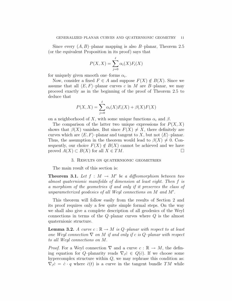
Since every (A, B)–planar mapping is also B–planar, Theorem 2.5(or the equivalent Proposition in its proof) says that

P (X, X) =

ℓ∑

j=0

αi(X)Fi(X)

for uniquely given smooth one–forms αi.Now, consider a fixed F ∈ A and suppose F (X) /∈ B(X). Since we

assume that all 〈E, F 〉–planar curves c in M are B–planar, we mayproceed exactly as in the beginning of the proof of Theorem 2.5 todeduce that

P (X, X) =ℓ

∑

j=0

αi(X)Fi(X) + β(X)F (X)

on a neighborhood of X, with some unique functions αi and β.The comparison of the latter two unique expressions for P (X, X)

shows that β(X) vanishes. But since F (X) 6= X, there definitely arecurves which are 〈E, F 〉–planar and tangent to X, but not 〈E〉–planar.Thus, the assumption in the theorem would lead to β(X) 6= 0. Con-sequently, our choice F (X) /∈ B(X) cannot be achieved and we haveproved A(X) ⊂ B(X) for all X ∈ TM .

3. Results on quaternionic geometries

The main result of this section is:

Theorem 3.1. Let f : M → M ′ be a diffeomorphism between twoalmost quaternionic manifolds of dimension at least eight. Then f isa morphism of the geometries if and only if it preserves the class ofunparameterized geodesics of all Weyl connections on M and M ′.

This theorem will follow easily from the results of Section 2 andits proof requires only a few quite simple formal steps. On the waywe shall also give a complete description of all geodesics of the Weylconnections in terms of the Q–planar curves where Q is the almostquaternionic structure.

Lemma 3.2. A curve c : R → M is Q–planar with respect to at leastone Weyl connection ∇ on M if and only if c is Q–planar with respectto all Weyl connections on M .

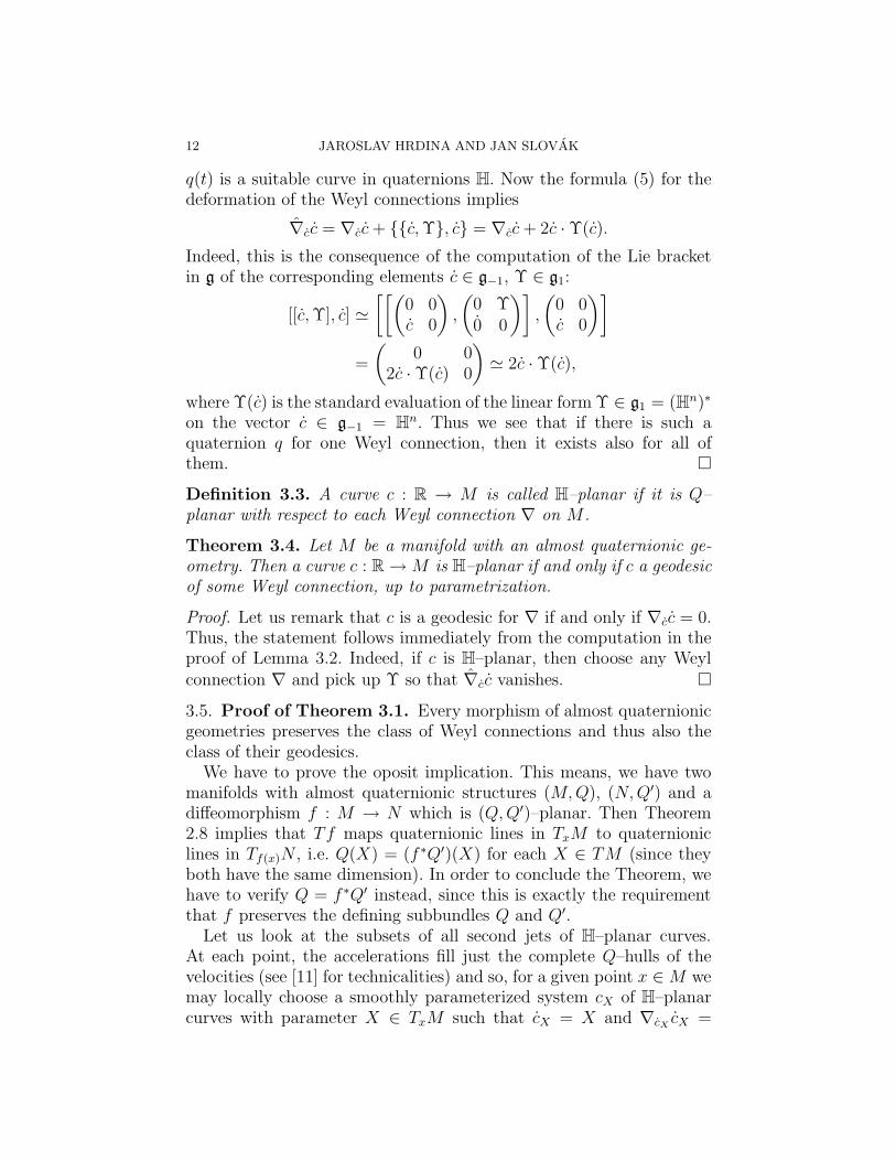
Proof. For a Weyl connection ∇ and a curve c : R → M , the defin-ing equation for Q–planarity reads ∇cc ∈ Q(c). If we choose somehypercomplex structure within Q, we may rephrase this condition as:∇cc = c · q where c(t) is a curve in the tangent bundle TM while

12 JAROSLAV HRDINA AND JAN SLOVAK

q(t) is a suitable curve in quaternions H. Now the formula (5) for thedeformation of the Weyl connections implies

∇cc = ∇cc + c, Υ, c = ∇cc + 2c · Υ(c).

Indeed, this is the consequence of the computation of the Lie bracketin g of the corresponding elements c ∈ g−1, Υ ∈ g1:

[[c, Υ], c] ≃

[[(

0 0c 0

)

,

(

0 Υ0 0

)]

,

(

0 0c 0

)]

=

(

0 02c · Υ(c) 0

)

≃ 2c · Υ(c),

where Υ(c) is the standard evaluation of the linear form Υ ∈ g1 = (Hn)∗

on the vector c ∈ g−1 = Hn. Thus we see that if there is such a

quaternion q for one Weyl connection, then it exists also for all ofthem.

Definition 3.3. A curve c : R → M is called H–planar if it is Q–planar with respect to each Weyl connection ∇ on M .

Theorem 3.4. Let M be a manifold with an almost quaternionic ge-ometry. Then a curve c : R → M is H–planar if and only if c a geodesicof some Weyl connection, up to parametrization.

Proof. Let us remark that c is a geodesic for ∇ if and only if ∇cc = 0.Thus, the statement follows immediately from the computation in theproof of Lemma 3.2. Indeed, if c is H–planar, then choose any Weylconnection ∇ and pick up Υ so that ∇cc vanishes.

3.5. Proof of Theorem 3.1. Every morphism of almost quaternionicgeometries preserves the class of Weyl connections and thus also theclass of their geodesics.

We have to prove the oposit implication. This means, we have twomanifolds with almost quaternionic structures (M, Q), (N, Q′) and adiffeomorphism f : M → N which is (Q, Q′)–planar. Then Theorem2.8 implies that Tf maps quaternionic lines in TxM to quaternioniclines in Tf(x)N , i.e. Q(X) = (f ∗Q′)(X) for each X ∈ TM (since theyboth have the same dimension). In order to conclude the Theorem, wehave to verify Q = f ∗Q′ instead, since this is exactly the requirementthat f preserves the defining subbundles Q and Q′.

Let us look at the subsets of all second jets of H–planar curves.At each point, the accelerations fill just the complete Q–hulls of thevelocities (see [11] for technicalities) and so, for a given point x ∈ M wemay locally choose a smoothly parameterized system cX of H–planarcurves with parameter X ∈ TxM such that cX = X and ∇cX

cX =

GENERALIZED PLANAR CURVES AND QUATERNIONIC GEOMETRY 13

β(X)F (X) where F is one of the generators of Q and β is a 1–form.Then

(∇cX− ∇cX

)cX = β(X)F (X) +∑

k

αk(X)Fk(X)

where Fk are the generators of Q′ and αk are smooth 1–forms, cf. theproof of Theorem 2.5. But this shows that, except of the zero set of β,F (X) =

∑

k γk(X)Fk(X) for some smooth γk. Since F is linear in X,γk have to be constants and we are done.

3.6. Final remarks. All curves in the four–dimensional quaternionicgeometries are H–planar by the definition. Thus this concept starts tobe interesting in higher dimensions only, and all of them are coveredby Theorem 3.1.

The class of the unparameterized geodesics of Weyl connections iswell defined for all parabolic geometries. Our result for the quaternionicgeometries suggests the question, whether a similar statement holds forother geometries as well.

References

[1] Alekseevsky, D.V.; Marchiafava, S.; Pontecorvo, M., Compatible complexstructures on almost quaternionic manifolds, Trans. Amer. Math. Soc 351(1999), no. 3, 997–1014.

[2] Bailey, T.N.; Eastwood, M.G., Complex paraconformal manifolds – their dif-ferential geometry and twistor theory, Forum Math., 3 (1991), 61-103.

[3] Cap, A.; Slovak, J., Weyl structures for parabolic geometries, Math. Scand.93 (2003), 53-90.

[4] Cap, A.; Slovak, J.; Zadnik, V.; On distinguished curves in parabolic geome-tries, Transform. Groups, Vol. 9, No. 2, (2004), 143–166.

[5] Gover, A.R.; Slovak, J., Invariant local twistor calculus for quaternionic struc-tures and related geometries, J. Geom. Physics, 32 (1999), no. 1, 14–56.

[6] Hrdina, J., H–planar curves, Proceedings Int. Conf. Differential Geometryand Applications, Prague, August 2004, Charles University Press, 2005.

[7] Oproiu, V., Integrability of almost quaternal structures, An. st. Univ. ”Al. I.Cuza” Iasi 30 (1984), 75-84.

[8] Salamon, S.M.; Differential geometry of quaternionic manifolds, Ann. Scient.ENS 19 (1987), 31–55.

[9] Mikes J., Sinyukov N.S. On quasiplanar mappings of spaces of affine connec-tion, Sov. Math. 27, No.1 (1983), 63–70.

[10] Mikes, J.; Nemcikova, J.; Pokorna, O., On the theory of the 4-quasiplanarmappings of almost quaternionic spaces, Rediconti del circolo matematico diPalermo, Serie II, Suppl. 54 (1998), 75–81.

[11] Zadnik, V., Generalized geodesics, Ph.D. thesis, Masaryk university in Brno,2003.

14 JAROSLAV HRDINA AND JAN SLOVAK

Department of Algebra and Geometry, Faculty of Science, Masaryk

University in Brno, Janackovo nam. 2a, 662 95 Brno, Czech Republic