Gene expression Terry Speed Lecture 4, December 18, 2001.

Gene expressionGene expression

Terry Speed

Lecture 4, December 18, 2001

Thesis:Thesis: the analysis of gene the analysis of gene expression data is going to be big expression data is going to be big

in 21st century statisticsin 21st century statistics

Many different technologies, including

High-density nylon membrane arrays

Serial analysis of gene expression (SAGE)

Short oligonucleotide arrays (Affymetrix)

Long oligo arrays (Agilent)

Fibre optic arrays (Illumina)

cDNA arrays (Brown/Botstein)*

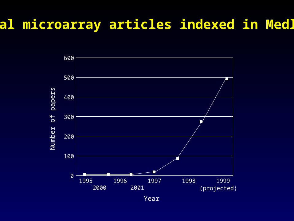
1995 1996 1997 1998 1999 2000 2001

0

100

200

300

400

500

600

(projected)

Year

Num

ber

of

papers

Total microarray articles indexed in Medline

Common themes themes

• Parallel approach to collection of very large amounts of data (by biological standards)

• Sophisticated instrumentation, requires some understanding

• Systematic features of the data are at least as important as the random ones

• Often more like industrial process than single investigator lab research

• Integration of many data types: clinical, genetic, molecular…..databases

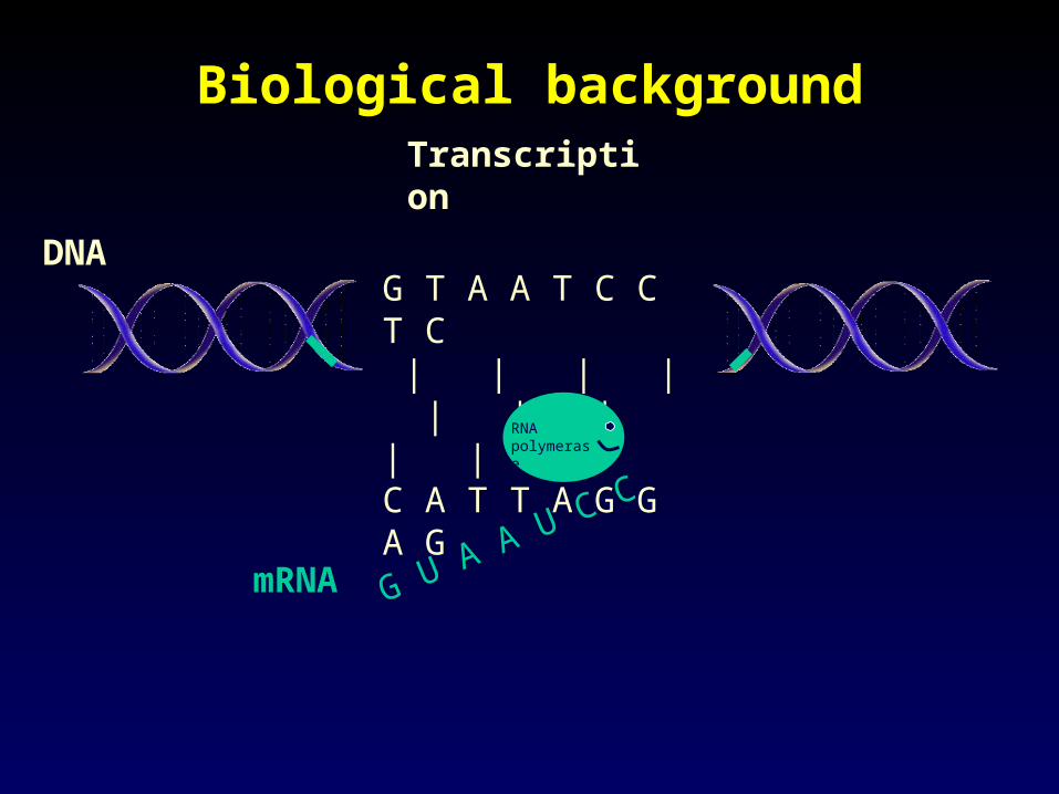
Biological backgroundBiological background

G T A A T C C T C | | | | | | | | | C A T T A G G A G

DNA

G U A A U C C

RNA polymerase

mRNA

Transcription

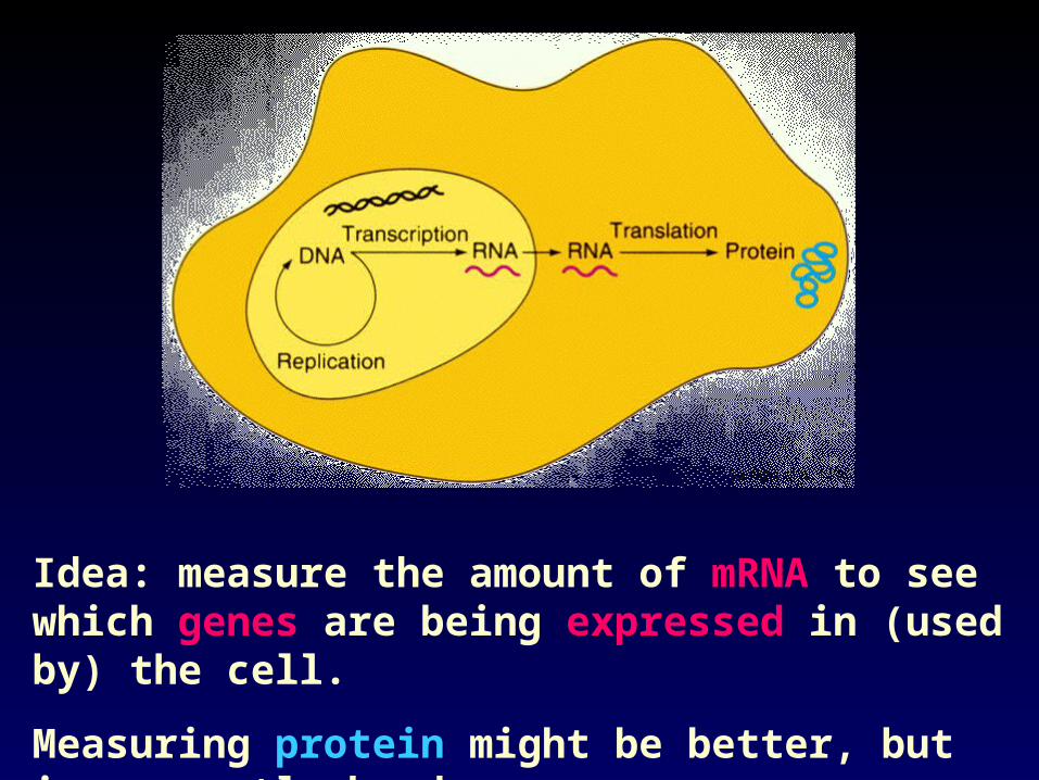
Idea: measure the amount of mRNA to see which genes are being expressed in (used by) the cell.

Measuring protein might be better, but is currently harder.

Reverse transcriptionReverse transcriptionClone cDNA strands, complementary to the mRNA

G U A A U C C U C

Reverse transcriptase

mRNA

cDNA

C A T T A G G A G C A T T A G G A G C A T T A G G A G C A T T A G G A G

T T A G G A G

C A T T A G G A G C A T T A G G A G C A T T A G G A G

C A T T A G G A G

C A T T A G G A G

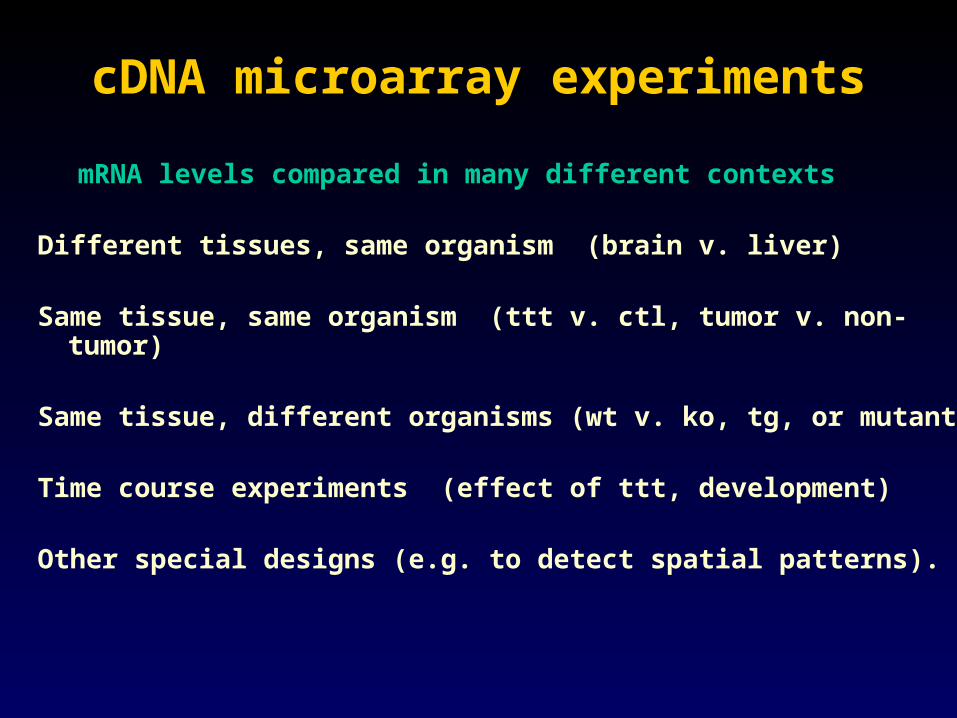
cDNA microarray experimentscDNA microarray experiments

mRNA levels compared in many different contexts

Different tissues, same organism (brain v. liver) Same tissue, same organism (ttt v. ctl, tumor v. non-tumor) Same tissue, different organisms (wt v. ko, tg, or mutant)

Time course experiments (effect of ttt, development)

Other special designs (e.g. to detect spatial patterns).

cDNA microarrayscDNA microarrays

cDNA clones

cDNA microarrayscDNA microarraysCompare the genetic expression in two samples of cells

PRINT

cDNA from one gene on each spot

SAMPLES

cDNA labelled red/green

e.g. treatment / control

normal / tumor tissue

HYBRIDIZE

Add equal amounts of labelled cDNA samples to microarray.

SCAN

Laser Detector

Biological questionDifferentially expressed genesSample class prediction etc.

Testing

Biological verification and interpretation

Microarray experiment

Estimation

Experimental design

Image analysis

Normalization

Clustering Discrimination

R, G

16-bit TIFF files

(Rfg, Rbg), (Gfg, Gbg)

Some statistical questionsSome statistical questions

Image analysis: addressing, segmenting, quantifying Normalisation: within and between slides

Quality: of images, of spots, of (log) ratios

Which genes are (relatively) up/down regulated?

Assigning p-values to tests/confidence to results.

Some statistical questions, ctdSome statistical questions, ctd

Planning of experiments: design, sample size

Discrimination and allocation of samples

Clustering, classification: of samples, of genes

Selection of genes relevant to any given analysis

Analysis of time course, factorial and other special experiments…..…...& much more.

Some bioinformatic questionsSome bioinformatic questions

Connecting spots to databases, e.g. to sequence, structure, and pathway databases

Discovering short sequences regulating sets of genes: direct and inverse methods

Relating expression profiles to structure and function, e.g. protein localisation

Identifying novel biochemical or signalling pathways, ………..and much more.

Part of the image of one channel false-coloured on a white (v. high) red (high) through yellow and green (medium) to blue (low) and black scale

Does one size fit all?

Segmentation: limitation of the Segmentation: limitation of the fixed circle methodfixed circle method

SRG Fixed Circle

Inside the boundary is spot (foreground), outside is not.

Some local backgroundsSome local backgrounds

We use something different again: a smaller, less variable value.

Single channelgrey scale

Quantification of expressionQuantification of expression

For each spot on the slide we calculate

Red intensity = Rfg - Rbg

fg = foreground, bg = background, and

Green intensity = Gfg - Gbg

and combine them in the log (base 2) ratio

Log2( Red intensity / Green intensity)

Gene Expression DataGene Expression Data On p genes for n slides: p is O(10,000), n is O(10-100), but growing,

Genes

Slides

Gene expression level of gene 5 in slide 4

= Log2( Red intensity / Green intensity)

slide 1 slide 2 slide 3 slide 4 slide 5 …

1 0.46 0.30 0.80 1.51 0.90 ...2 -0.10 0.49 0.24 0.06 0.46 ...3 0.15 0.74 0.04 0.10 0.20 ...4 -0.45 -1.03 -0.79 -0.56 -0.32 ...5 -0.06 1.06 1.35 1.09 -1.09 ...

These values are conventionally displayed on a red (>0) yellow (0) green (<0) scale.

The red/green ratios can be spatially biasedThe red/green ratios can be spatially biased

• .Top 2.5%of ratios red, bottom 2.5% of ratios green

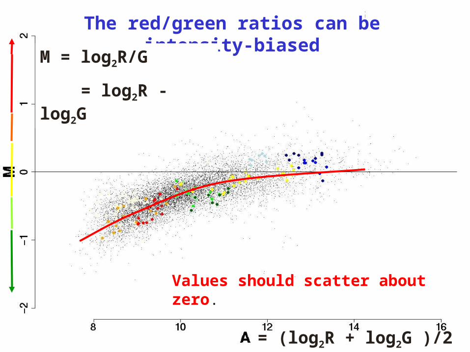
The red/green ratios can be intensity-biased

M = log2R/G

= log2R - log2G

= (log2R + log2G )/2

Values should scatter about zero.

Yellow: GAPDH, tubulin Light blue: MSP pool / titration

Orange: Schadt-Wong rank invariant set Red line: lowess smooth

Normalization: how we “fix” the previous problem

The curved line becomes the new zero line

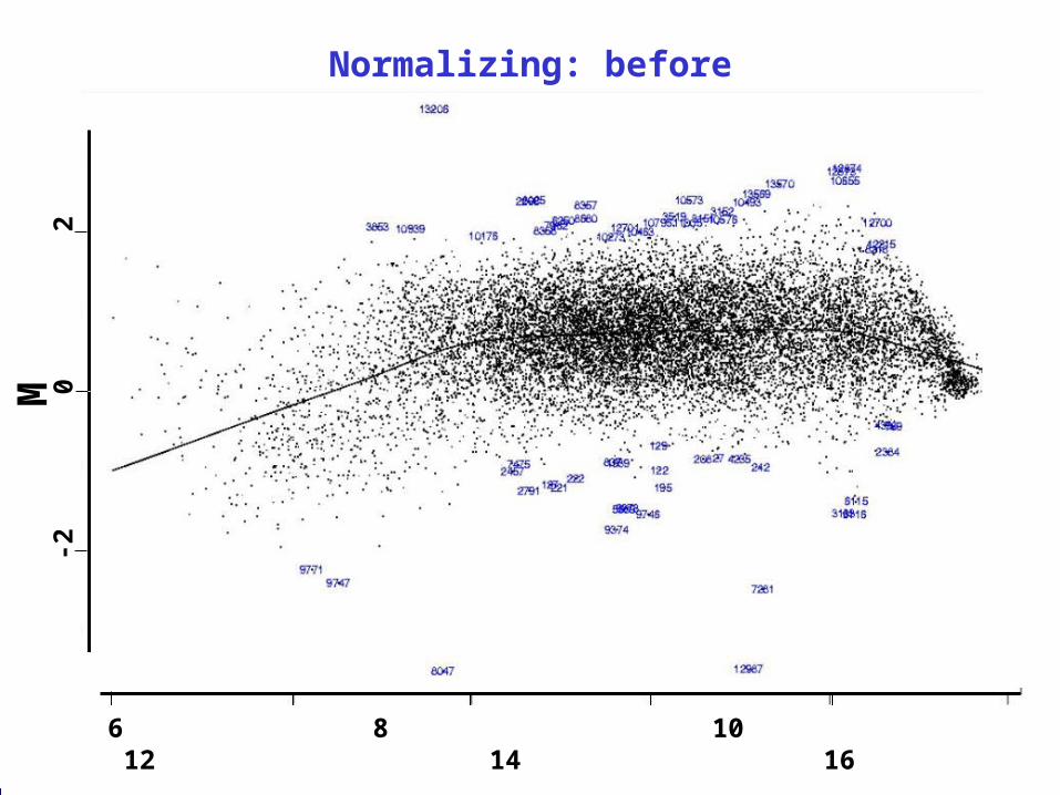
Normalizing: before2

0-2

-4

6 8 10 12 14 16

M

Normalizing: after2

0-2

-4

M n

orm

alis

ed

6 8 10 12 14 16

SCIENTIFIC: To determine which genes are differentially expressed between two sources of mRNA (trt, ctl).

STATISTICAL: To assign appropriately adjusted p-values to thousands of genes.

A basic problemA basic problem

• 8 treatment mice and 8 control mice

• 16 hybridizations: liver mRNA from each of the 16 mice (Ti , Ci ) is labelled with Cy5, while pooled liver mRNA from the control mice (C*) is labelled with Cy3.

• Probes: ~ 6,000 cDNAs (genes), including 200 related to lipid metabolism.

Goal. To identify genes with altered expression in the livers of Apo AI knock-out mice (T) compared to inbred C57Bl/6 control mice (C).

Apo AI experiment (Callow Apo AI experiment (Callow et alet al 2000, LBNL) 2000, LBNL)

Leukemia experiments (Golub Leukemia experiments (Golub et alet al 1999,WI) 1999,WI)

Goal. To identify genes which are differentially expressed in acute lymphoblastic leukemia (ALL) tumours in comparison with acute myeloid leukemia (AML) tumours.

• 38 tumour samples: 27 ALL, 11 AML.• Data from Affymetrix chips, some pre-processing.• Originally 6,817 genes; 3,051 after reduction.

Data therefore a 3,051 38 array of expression values.

Univariate hypothesis testingUnivariate hypothesis testing

Initially, focus on one gene only.

We wish to test the null hypothesis H that the gene is not differentially expressed.

In order to do so, we use a two sample t-statistic:

€

t=averofn1 trtx − averofn2ctlx

[1n1

(SDofn1trtx)2 +

1n1

(SDofn1ctlx)2]

Single-step adjustments of Single-step adjustments of pi

• Bonferroni: min (mpi, 1), m= #genes

•Sidák: 1 - (1 - pi)m

minP method of Westfall and Young:

Pr( min Pl ≤ pi | H)

1≤l≤m

• maxT method of Westfall and Young:

Pr( max |Tl | ≥ | ti | | H0C )

1≤l≤m

More powerful methods: More powerful methods: step-down adjustmentsstep-down adjustments

The idea: S Holm’s modification of Bonferroni.

Also applies to Sidák, maxT, and minP.

We illustrate this last adjustment.

Step-down adjustment of Step-down adjustment of minPminP

Initialization: Order the unadjusted p-values such that pr1 ≤ pr2 ≤ ≤ prm. The indices r1, r2, r3,.. are fixed for given data.

Step-down adjustment:

1. Compare min {Pr1, , Prm} with pr1 ;

2. Compare min {Pr2, , Prm} with pr2 ;

3 Compare min {Pr3 , Prm} with pri3 …….

m. Compare Prm with prm

Enforce the monotonicity on the adjusted pri

gene t unadj. p minP plower maxT

index statistic (104) adjust. adjust.

2139 -22 1.5 .53 8 10-5 2 10-4

4117 -13 1.5 .53 8 10-5 5 10-4

5330 -12 1.5 .53 8 10-5 5 10-4

1731 -11 1.5 .53 8 10-5 5 10-4

538 -11 1.5 .53 8 10-5 5 10-4

1489 -9.1 1.5 .53 8 10-5 1 10-3

2526 -8.3 1.5 .53 8 10-5 3 10-3

4916 -7.7 1.5 .53 8 10-5 8 10-3

941 -4.7 1.5 .53 8 10-5 0.65

2000 +3.1 1.5 .53 8 10-5 1.00

5867 -4.2 3.1 .76 0.54 0.90

4608 +4.8 6.2 .93 0.87 0.61

948 -4.7 7.8 .96 0.93 0.66

5577 -4.5 12 .99 0.93 0.74

Apo AI. Histogram & Q-Q plotApo AI. Histogram & Q-Q plot

ApoA1

Brief discussion

Not mentioned: strong vs weak control of Type 1 error.

The minP adjustment seems more conservative than the maxT adjustment, but is essentially model-free.

The adjusted minP values are very discrete; it seems that 12,870 permutations are not enough for 6,000 tests.

Extends to other statistics: Wilcoxon, paired t, F, blocked F..

Major question in practice: minP, maxT or something else?

Wanted are guidelines for use of minP in terms of sample sizes and number of genes.

Other approaches: False Discovery Rate (V/R), Bayes.

Olfactory Epithelium

VomeroNasal Organ

Main (Auxiliary)Olfactory Bulb

From Buck (2000)

From a study of the mouse olfactory system

Axonal connectivity between the nose and the mouse olfactory bulb

>2M, ~1,800 types

Two principles: “zone-to-zone projection”, and “glomerular convergence”

Neocortex

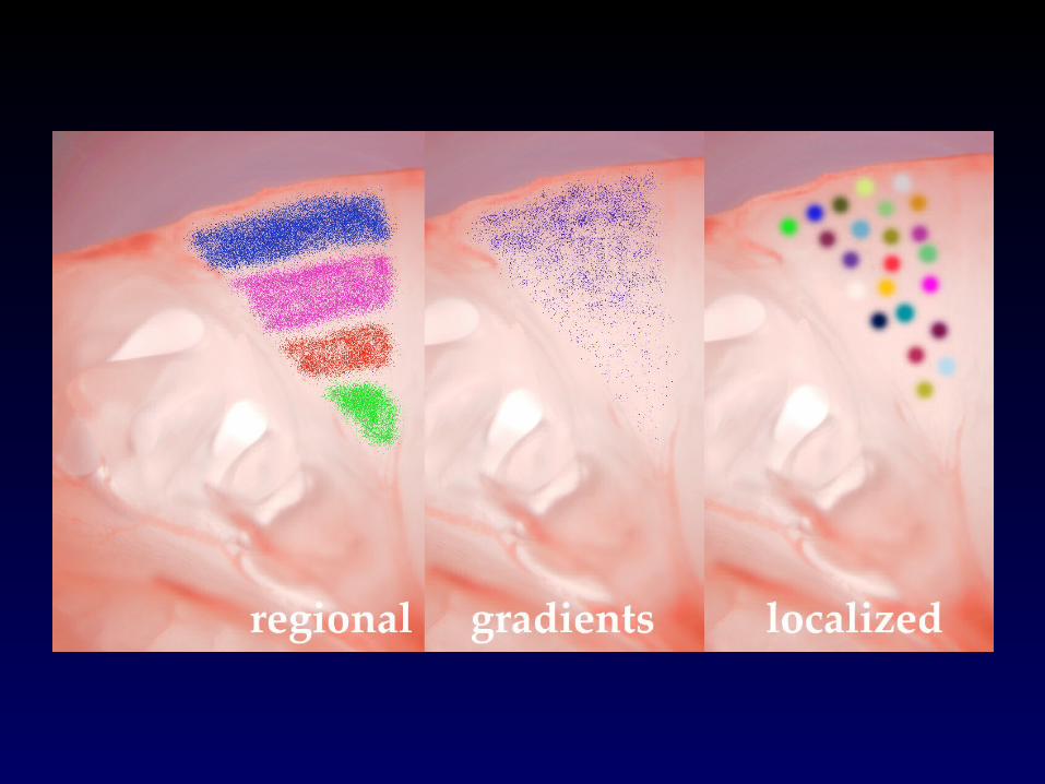
Of interest: the hardwiring of the Of interest: the hardwiring of the vertebrate olfactory systemvertebrate olfactory system

• Expression of a specific odorant receptor gene by an olfactory neuron.

• Targeting and convergence of like axons to specific glomeruli in the olfactory bulb.

The biological question in this caseThe biological question in this case

Are there genes with spatially restricted expression patterns within

the olfactory bulb?

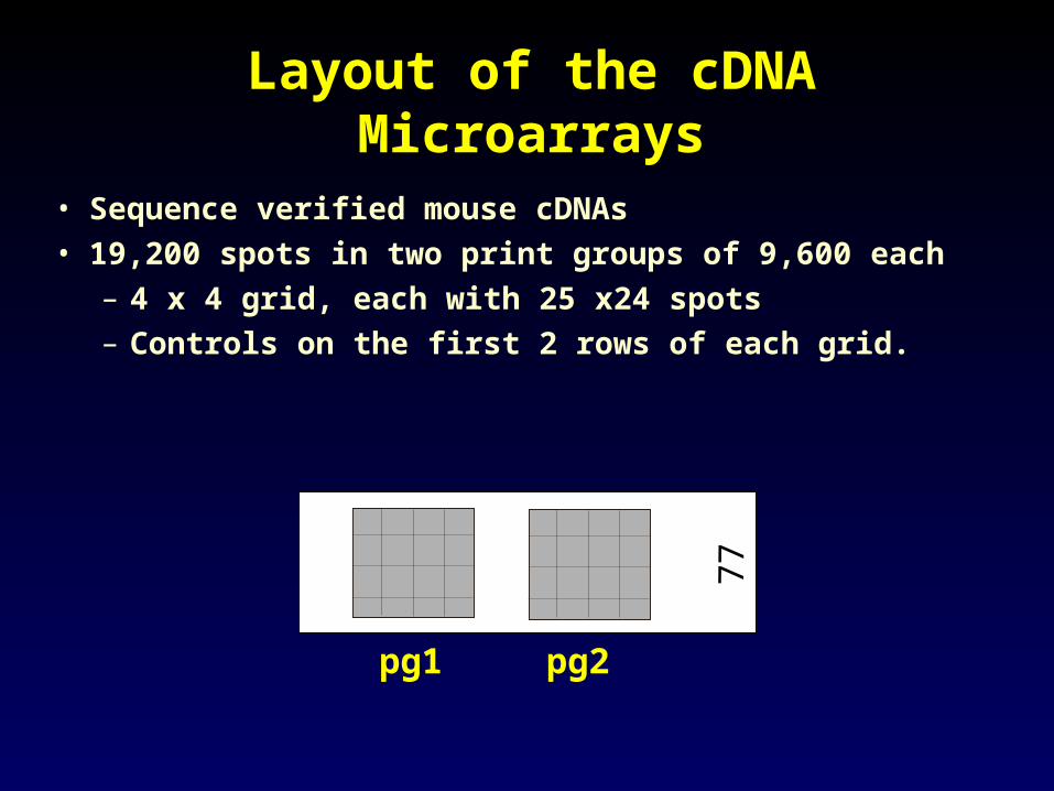
Layout of the cDNA MicroarraysLayout of the cDNA Microarrays

• Sequence verified mouse cDNAs• 19,200 spots in two print groups of 9,600 each

– 4 x 4 grid, each with 25 x24 spots– Controls on the first 2 rows of each grid.

77

pg1 pg2

Design: How We Sliced Up the BulbDesign: How We Sliced Up the Bulb

A

P D

V

M

L

Design: Two Ways to Do the Design: Two Ways to Do the ComparisonsComparisons

Goal: 3-D representation of gene expression

P

D

MA

V

L

R

Compare all samples to a common reference sample (e.g., whole bulb)

P

D

MA

V

L

Multiple direct comparisons between different samples (no common reference)

An Important Aspect of Our DesignAn Important Aspect of Our Design

Different ways of estimating the same contrast:

e.g. A compared to P

Direct = A-P

Indirect = A-M + (M-P) or

A-D + (D-P) or

-(L-A) - (P-L)

How do we combine these?

LL

PPVV

DD

MM

AA

Analysis using a linear model

Define a matrix X so that E(M)=X

Use least squares estimates for A-L, P-L, D-L, V-L, M-LIn practice, we use robust regression.

Estimates for other estimable contrasts follow in the usual way.

€

E

m1

m2

M

mn

⎛

⎝

⎜ ⎜ ⎜

⎞

⎠

⎟ ⎟ ⎟ =

0 0 0 −1 1

−1 0 0 0 0

M O M

−1 1 0 0 0

⎛

⎝

⎜ ⎜ ⎜

⎞

⎠

⎟ ⎟ ⎟ •

A−L

P −L

D−L

V −L

M−L

⎛

⎝

⎜ ⎜ ⎜ ⎜

⎞

⎠

⎟ ⎟ ⎟ ⎟

ˆ = X' X( )−1X'M

The Olfactory Bulb ExperimentsThe Olfactory Bulb Experiments completed so farcompleted so far

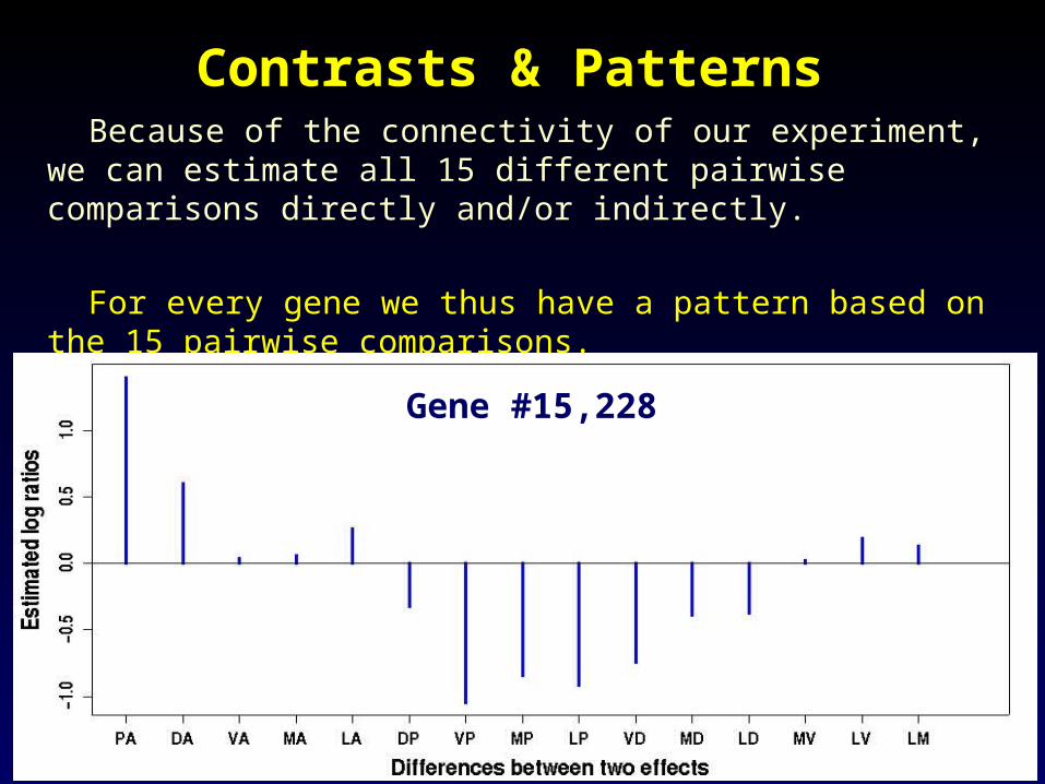
Contrasts & PatternsContrasts & Patterns Because of the connectivity of our experiment, we can estimate

all 15 different pairwise comparisons directly and/or indirectly.

For every gene we thus have a pattern based on the 15 pairwise comparisons.

Gene #15,228

Contrasts & patterns:another wayContrasts & patterns:another way Instead of estimating pairwise comparisons between each of the six

effects, we can come closer to estimating the effects themselves by doing so subject to the standard zero sum constraint (6 parameters, 5 d.f.).

What we estimate for A, say, subject to this constraint, is in reality an estimate of

A - 1/6(A + P + D + V + M + L).

This set of parameter estimates gives results similar to, but better than, the ones we would have obtained had we carried out the experiments with whole-bulb reference tissue.

In effect we have created the whole-bulb reference in silico.

Alternative pattern representationAlternative pattern representation

Gene #15,228 once again.

Reconstruction of the Bulb as a Cube:Reconstruction of the Bulb as a Cube:Expression of Gene # 15,228Expression of Gene # 15,228

ExpressionLevel

High

Low

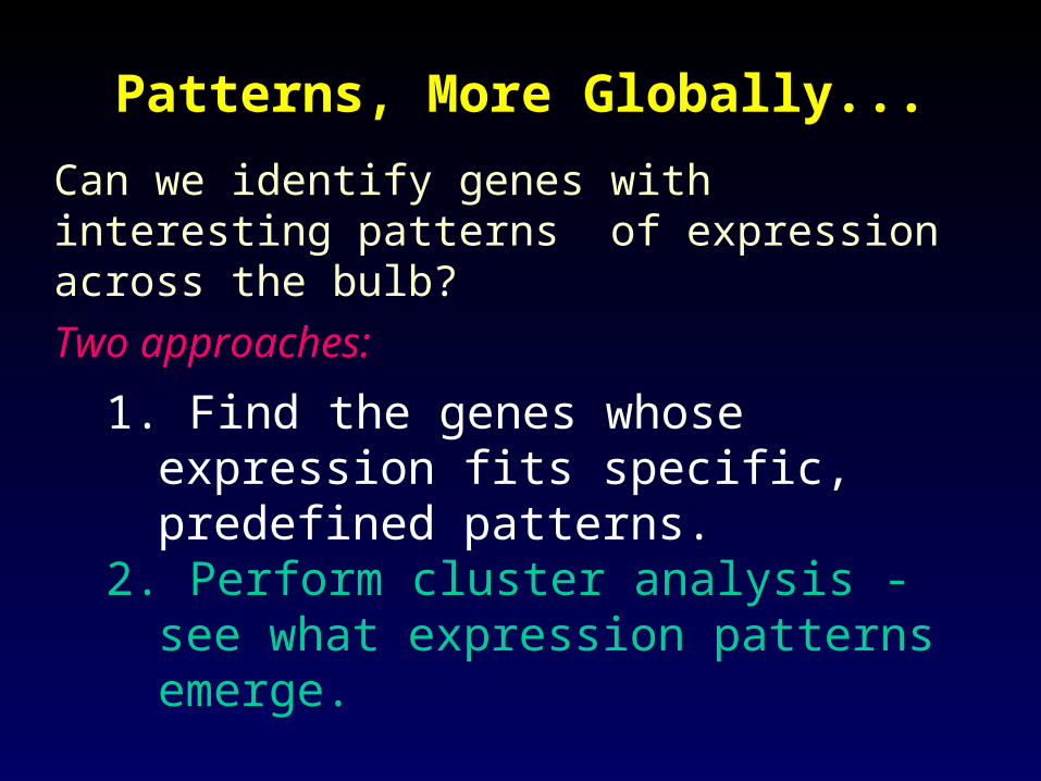
Patterns, More Globally...Patterns, More Globally...

1. Find the genes whose expression fits specific, predefined patterns.

2. Perform cluster analysis - see what expression patterns emerge.

Can we identify genes with interesting patterns of expression across the bulb?

Two approaches:

Clustering procedureClustering procedure

Start with a sets of genes exhibiting some minimal level of differential expression across the bulb; here ~650 were chosen from all 15 contrasts.

Carry out hierarchical clustering, building a dendrogram: Mahalanobis distance and Ward agglomeration (minimum variance) were used.

Now consider all clusters of 2 or more genes in the tree. Singles are added separately.

Measure the heterogeneity h of a cluster by calculating the 15 SDs

across the cluster of each of the pairwise effects, and taking the largest.

Choose a score s (see plots) and take all maximal disjoint clusters with

h < s. Here we used s = 0.46 and obtained 16 clusters.

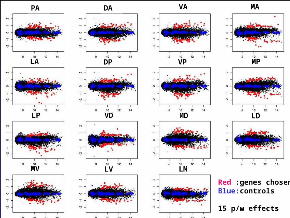
Red :genes chosenBlue:controls

15 p/w effects

PA DA VA

LA DP VPLA MP

MA

LP VD MD

LA LV LMMV

LD

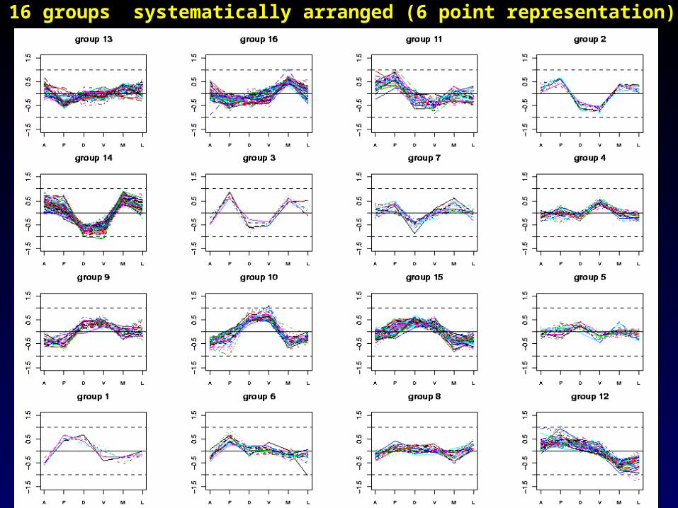
The 16 groups systematically arranged (6 point representation)

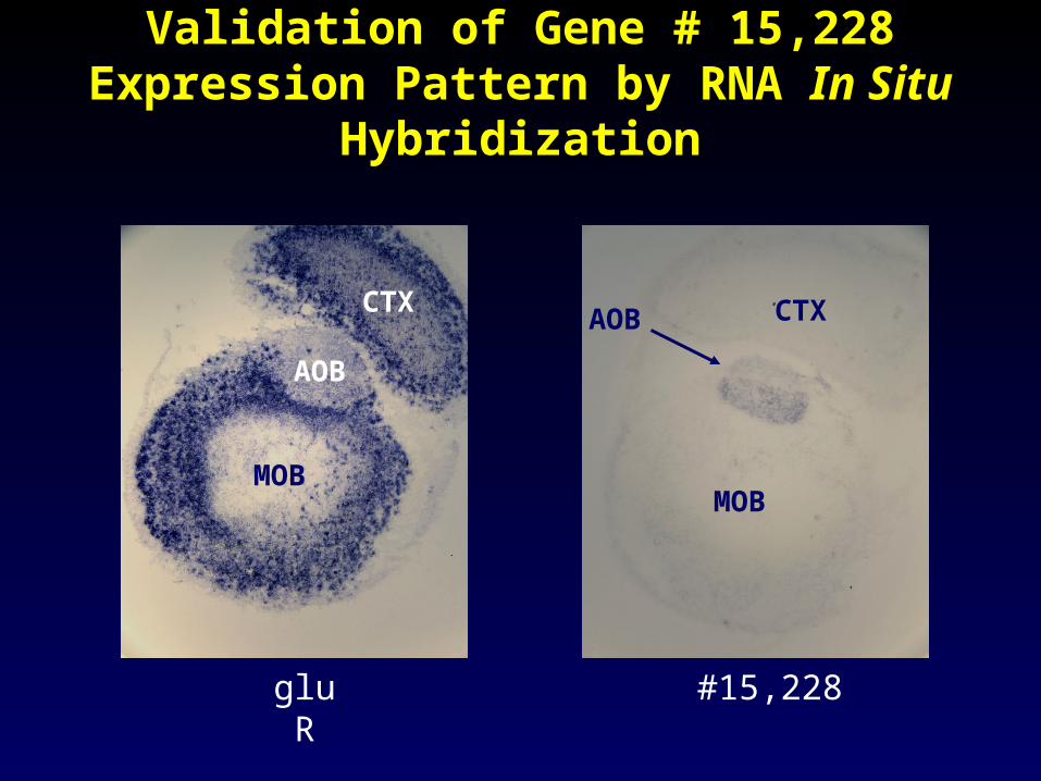
Validation of Gene # 15,228 Expression Validation of Gene # 15,228 Expression Pattern by RNA Pattern by RNA In SituIn Situ Hybridization Hybridization

gluR

CTX

MOB

AOB

#15,228

CTXAOB

MOB

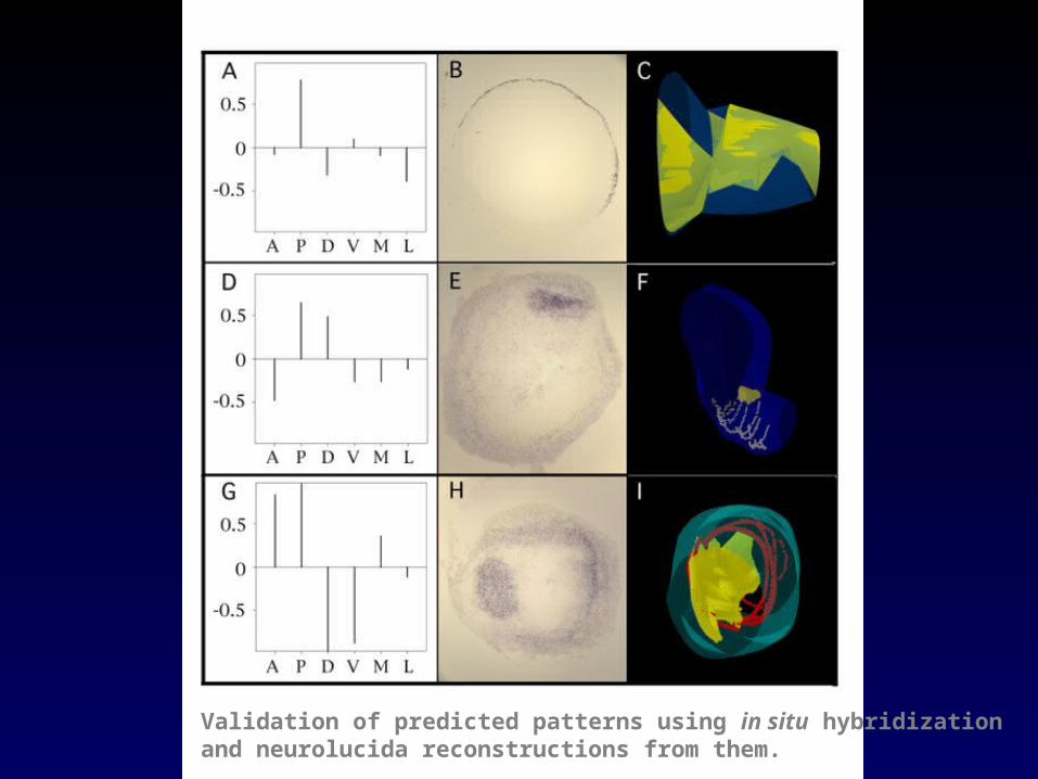
Validation of predicted patterns using in situ hybridizationand neurolucida reconstructions from them.

Some statistical research stimulated Some statistical research stimulated by microarray data analysisby microarray data analysis

Experimental design : Churchill & Kerr

Image analysis: Zuzan & West, ….

Data visualization: Carr et al

Estimation: Ideker et al, ….

Multiple testing: Westfall & Young , Storey, ….

Discriminant analysis: Golub et al,…

Clustering: Hastie & Tibshirani, Van der Laan, Fridlyand & Dudoit, ….

Empirical Bayes: Efron et al, Newton et al,…. Multiplicative models: Li &Wong

Multivariate analysis: Alter et al

Genetic networks: D’Haeseleer et al and more

AcknowledgmentsAcknowledgmentsStatistical collaboratorsStatistical collaboratorsYee Hwa Yang (Berkeley)Yee Hwa Yang (Berkeley)Sandrine Dudoit (Berkeley)Sandrine Dudoit (Berkeley)Ingrid Lönnstedt (Uppsala)Natalie Thorne (WEHI)Natalie Thorne (WEHI)Mauro Delorenzi (WEHI)

CSIRO Image Analysis GroupMichael BuckleyMichael BuckleyRyan Lagerstorm

WEHIGlenn BegleySuzie GrantRob Good

PMCIChuang Fong Kong

Ngai Lab (Berkeley)Cynthia DugganJonathan ScolnickDave Lin Vivian Peng Percy LuuElva DiazJohn Ngai

LBNLMatt Callow

RIKEN Genomic Sciences CenterRIKEN Genomic Sciences CenterYasushi OkazakiYoshihide Hayashizaki

Some web sites:

Technical reports, talks, software etc.

http://www.stat.berkeley.edu/users/terry/zarray/Html/

Statistical software R “GNU’s S” http://lib.stat.cmu.edu/R/CRAN/

Packages within R environment:

-- Spot http://www.cmis.csiro.au/iap/spot.htm

-- SMA (statistics for microarray analysis) http://www.stat.berkeley.edu/users/terry/zarray/Software /smacode.html