Gauged vortices in a background - arXiv

arX

iv:h

ep-t

h/05

0301

4v2

14

Sep

2005

Gauged vortices in a background

Nuno M. Romao ∗

School of Pure Mathematics, University of Adelaide

North Terrace, Adelaide SA 5005, Australia

October 17, 2018

Abstract

We discuss the statistical mechanics of a gas of gauged vortices in the canonical formal-ism. At critical self-coupling, and for low temperatures, it has been argued that theconfiguration space for vortex dynamics in each topological class of the abelian Higgsmodel approximately truncates to a finite-dimensional moduli space with a Kahlerstructure. For the case where the vortices live on a 2-sphere, we explain how local-isation formulas on the moduli spaces can be used to compute exactly the partitionfunction of the vortex gas interacting with a background potential. The coefficientsof this analytic function provide geometrical data about the Kahler structures, thesimplest of which being their symplectic volume (computed previously by Manton us-ing an alternative argument). We use the partition function to deduce simple resultson the thermodynamics of the vortex system; in particular, the average height on thesphere is computed and provides an interesting effective picture of the ground state.

MSC (2000): 53C80, 37K65; PACS (2003): 11.27.+d, 74.25.Bt

1 Introduction

One of the most challenging aspects in the study of topological solitons in gauge fieldtheories is to understand their interactions, even at the classical level. At critical self-coupling, where the solitons exert no net static forces among themselves, one can typicallydescribe the dynamical interactions at low speed in terms of geodesic flow for certainmetrics on the moduli spaces of stable field configurations [1]. Exact results about thesemetrics can be obtained in some instances, and they have provided detailed informationabout the classical dynamics of solitons in this regime [2]. There is now considerableevidence on the beautiful geometrical fact that these moduli spaces encode a whole rangeof physical information about the underlying field theories, which goes well beyond the

∗e-mail: [email protected]

1

problem of approximating the slow dynamics that brought them first into mathematicalphysics.

An example illustrating how physical information can be extracted from the geom-etry of the moduli spaces is provided by the study of the statistical mechanics of a gas ofvortices in the abelian Higgs model. Manton obtained the partition function in the crit-ically coupled (noninteracting) regime from the volumes of the moduli spaces [3]. Thesevolumes can be calculated once the Kahler classes of the moduli spaces are known. Atfirst, this calculation was performed for vortices on a sphere, but a similar argument canbe used to compute the partition function for vortices living on any compact Riemannsurface [4].

In this paper, the abelian Higgs model is modified by adding to the lagrangian (atcritical coupling) an external potential that will probe the interactions of the vorticesthemselves. For weak potentials, we expect the effect of this coupling to be well describedby the addition of a potential to the moduli space dynamics. In this setting, we calculateexactly the partition function for the vortex gas in a background field. Clearly, the problemthat we consider is still less ambitious than the more physically interesting (but also moredifficult) statistical mechanics of vortices with Ginzburg–Landau self-interaction, but itdoes provide a nontrivial extension of the study by Manton. The vortices will be allowedto live on a sphere with a particular axis singled out, and the potential we shall focus on isnatural given this geometry. To obtain the statistical mechanics of the system, we will bemaking use of a localisation formula for a circle action on the moduli space of N vortices.This turns out to be an alternative route to obtain Manton’s results (which we recover aswe switch off the interaction), in particular his formula for the volume of the moduli spaceof N vortices on a sphere [3].

2 Gauged vortices and their moduli spaces

Given a Riemann surface Σ, a gauged vortex is a pair (dA,Φ) consisting of a unitaryconnection on a hermitian line bundle L → Σ and a section of this bundle, satisfying theBogomol’nyı (or vortex) equations

∂AΦ = 0, (1)

BA = 12 ∗ (1− 〈Φ,Φ〉). (2)

Here, 〈·, ·〉 is the hermitian structure on L, and we have fixed a metric ds2Σ on Σ with Hodgestar ∗; ∂A is defined from dA = d − iA =: ∂A + ∂A as usual through the decompositionprovided by the complex structure of Σ, and BA = dA is the curvature of dA. Theseequations are invariant under gauge transformations

(dA,Φ) 7→ (dA+dΛ, eiΛΦ), Λ ∈ C∞(Σ;R) ∼= aut(L, 〈·, ·〉).

The choice of hermitian structure does not play an important role in our discussion, soonce we fix local trivialisations for L → Σ we use them to pull back the standard hermitianstructure of C.

2

To a configuration (dA,Φ) we associate the vortex number

N =1

2π

∫

ΣBA.

For the cases of interest, where Σ is compact or is effectively compactified by imposingsuitable boundary conditions, N ∈ Z and it corresponds to the degree of L, a topologicalinvariant. Since (1) states that Φ should be a holomorphic section, N is also the numberof zeroes of Φ, all having positive multiplicity. In fact, solutions of (1)–(2) are completelycharacterised by the zeroes of Φ, which can be any set of N points on Σ (counted withmultiplicity) (cf. [5]), provided that

4πN < Vol(Σ) (3)

holds [6, 7]. So the space of solutions to the vortex equations modulo gauge equivalencehas the structure

∐

N∈N

MN ,

where each moduli space of N -vortices MN is the Nth symmetric power of Σ, the smooth2N -manifold

MN = SymN (Σ) := ΣN/SN .

Complex coordinates on this (complex) manifold are usually referred to as moduli. If zis a local coordinate on an open set U ⊂ Σ, then the natural coordinates (z1, . . . , zN ) onthe cartesian product UN , denoting configurations with zeroes of Φ at each z = zr, forman appropriate set of moduli on SymN (U)−∆, where ∆ ⊂ MN is the locus on which atleast two zeroes become coincident (and thus the SN -action fails to be free). The zr areinterpreted as positions of N individual vortex cores.

The Bogomol’nyı equations above appeared for the first time in the study of theabelian Higgs model, a field theory for vortex dynamics defined by the functional

AHλ2(DA,Φ) = −1

4‖FA‖2L2 +

1

2‖DAΦ‖2L2 −

λ2

8‖〈Φ,Φ〉 − 1‖2L2 (4)

depending on a self-coupling λ2 ∈ R+. The fields A and Φ here depend on a time parameter

t ∈ R, and the L2 norms are taken with respect to the metric dt2 − ds2Σ on R×Σ and thehermitian structure on pr∗ΣL; notice DA = ( ∂

∂t − iAt)dt+dA(t) here has a time component,and we denote its curvature by FA = d(Atdt + A) =: EA ∧ dt + BA. It was observed [8]that static configurations at critical self-coupling λ2 = 1 are minima of the energy definedby AH1 if and only if they satisfy the first-order equations (1)–(2). The (potential)energy of a gauged vortex with vortex number N is then πN . Since these equations areeasier to study than the second-order Euler–Lagrange equations of (4), one might hopeto understand the dynamics of the abelian Higgs model from a study of gauged vortices,at least in the setting where the velocities are small, so that the field configurations arewell approximated at any instant by solutions of the Bogomol’nyı equations [1]. One wayto describe this so-called adiabatic approximation is as follows: construct from (4) an

3

action on each TMN by taking the fields to be solutions (dA(z),Φ(z)) of (1)–(2) withtime-dependent moduli (z1(t), . . . , zN (t)), and integrate over Σ in the L2 norms. It hasbeen proven that the resulting mechanical system does give a good description of thetrue (infinite-dimensional) vortex dynamics, even when we shift slightly from critical self-coulpling [9]. Upon this process of adiabatic reduction, a potential term in the field theorybecomes a potential function for the dynamics on MN .

The approximated abelian Higgs dynamics on the moduli space was discussed bySamols [10] following work by Strachan [11]. It consists of geodesic motion with inertialmass π (the static energy of one vortex) for a metric grs on MN . This metric is Kahlerwith respect to the complex structure on MN induced by the one on Σ. We call it theL2 metric on MN , since it is obtained from the natural L2 norms (4) on the space of(covariant) derivatives of pairs (DA,Φ). It is described by the closed (1, 1)-form

ω =i

2

N∑

r,s=1

grsdzr ∧ dzs =i

2

N∑

r,s=1

(

Ω2(zr)δrs + 2∂bs∂zr

)

dzr ∧ dzs. (5)

Here, zr are the moduli associated to a complex coordinate z for which ds2Σ = Ω2(z)|dz|2.The quantities br(z1, . . . , zN ) are defined as follows. One can combine (1)–(2) into a singleequation for the gauge-invariant quantity h := log〈Φ,Φ〉,

4∂2h

∂z∂z+Ω2(z)(1 − eh) = 4π

N∑

r=1

δ(z − zr), (6)

where δ is the Dirac delta-function. A solution h(z; z1, . . . , zN ) to (6) has an expansion

h(z) = log |z − zr|2 + ar +1

2br(z − zr) + +

1

2br(z − zr) +

Ω2(zr)

4|z − zr|2 + · · · (7)

about a simple zero zr of Φ. It is a remarkable fact that only the linear coefficients br inthis expansion appear in (5). It is clear that (7) only makes sense in a neighbourhood ofthe vortex zr which does not contain any other vortex positions. In fact, (6) implies thatwe can write [10] for each r = 1, . . . , N

br(z1, . . . , zN ) =N∑

s=1

s6=r

2

zr − zs+ br(z1, . . . , zN ), (8)

where br are smooth on the coincidence locus ∆. In an expansion about the positionof a vortex with multiplicity n ≤ N , the logarithmic term in (7) has a prefactor n.The local moduli zr cannot be used to describe a neighbourhood in MN of such a vortexconfiguration, and so the coefficients in an expansion equivalent to (7) cannot be expressedas functions of the zr.

Samols’s formula (5) still does not give the Kahler form explicitly, since the nontrivialquantities br are specified in terms of unknown solutions to (6). Extracting concreteinformation about the moduli space metrics is still a nontrivial challenge. One may feel

4

that work in this direction must inevitably rely on a numerical study of equation (6);however, analytical results have been derived in particular cases using approximations ofsome sort [12, 13], integrability [11], or even a remarkable argument involving T-duality instring theory [14]. In the following, we shall obtain further analytical information aboutthe moduli space metrics when Σ is a 2-sphere.

3 Vortex dynamics in a background potential

In this paper, we would like to extend the abelian Higgs model to include a couplingwith a background potential, which we define to be any smooth function f : Σ → R.To introduce the coupling term, we first define a vorticity 2-form v(DA,Φ) on Σ by theequation (cf. [15])

(d j + FA) ∧ dt =: v ∧ dt,

where j is the gauge-invariant supercurrent 1-form on R× Σ

j := Im 〈φ,DAφ〉.

The coupling to the potential f we propose is given by adding to the potential energyterm of the action functional (4) the interaction term

µ2

∫

Σf v (9)

where µ2 is a coupling constant.The Euler–Lagrange equations for the modified action

AHλ2(DA,Φ)− µ2

∫

f v(DA,Φ) ∧ dt (10)

are as follows. We obtain the same Gauß’s law as for the abelian Higgs model (4),

d ∗EA = 2 ∗ Im 〈Φ,DtΦ dt〉 (11)

(where Dt := ∂∂t − iAt), which is to be regarded as a constraint on the space of fields

determining At. The dynamical equations are

d ∗BA − ∗∂EA

∂t= − ∗ Im 〈Φ, dAΦ〉 − µ2(〈Φ,Φ〉+ 1) df, (12)

Φ =λ2

2(〈Φ,Φ〉 − 1)Φ + 2iµ2 ∗ (df ∧ dAΦ), (13)

where := (Dt)2 − ∗ dA ∗ dA is the covariant d’Alembertian on pr∗ΣL → R × Σ. As

expected, there are new terms (proportional to µ2) adding to the current in Ampere’s law(12), and also to the potential in the nonlinear Klein–Gordon equation (13).

From our discussion in section 2, we know that solutions to the vortex equations (1)–(2) solve the equations of motion (11)–(13) above in the static case (and setting At = 0),

5

provided λ2 = 1 and µ2 = 0. When the couplings are perturbed slightly away from thesecritical values, we expect a slow-moving solution to have a best vortex approximation, andthat we can follow its evolution under the dynamics defined above. A detailed analysisof the case λ2 ≃ 1, µ2 = 0 has been carried out by Stuart in [9], where distances to bestvortex approximations were estimated (in terms of λ2 − 1 and initial errors) after finite-time evolution, and shown to be controlled for evolution times of order O

(

|λ2 − 1|−1/2)

.In this paper, we make the natural assumption that an analogous result holds for λ2 = 1and µ2 ≃ 0. This assumption can be regarded as a motivation to the study of the dynamicson the moduli space of gauged vortices with a certain (and rather natural) backgroundpotential.

The coupling (9) satisfies a number of desirable properties. One of them is that, ifwe take f to be a constant, it reduces to a constant potential on the moduli space. To seethis, we use (1) and (2) to rewrite [15]

v = −i〈dAΦ, dAΦ〉+ (1− 〈Φ,Φ〉)BA

= −i〈∂AΦ, ∂AΦ〉+ 2(∗BA)BA,

which is precisely twice the energy density for solutions of the Bogomol’nyı equations atcritical self-coupling. Thus

∫

Σv|MN

= 2πN.

Notice that df = 0 in this situation, so the terms proportional to µ2 in the field equations(12) and (13) vanish. This is a rather degenerate case of our model (10), but the fact thatthe adiabatic approximation leads to sensible results at this level is already reassuring.

For the rest of the paper, we shall restrict ourselves to vortices living on a 2-sphereof radius R, Σ = S2

R. In this context, we shall illustrate another natural property of theinteraction term (9) in section 4.1.

4 Localisation and the partition function

The exact results we want to derive refer to the case Σ = S2R, on which z shall denote a

stereographic coordinate. The metric on S2R has Kahler (volume) form

ωS2

R=

2iR2

(1 + |z|2)2dz ∧ dz (14)

and the constraint (3) readsR2 > N.

The moduli spaces in this case are

MN = SymN (S2R)

∼= CPN , (15)

equipped with the Kahler structures

ω = iN∑

r,s=1

(

R2δrs(1 + |zr|2)2

+∂bs∂zr

)

dzr ∧ dzs. (16)

6

One way to understand (15) is as follows. Let Vj ⊂ MN be the locus where preciselyj vortices are at z = ∞. Then Vj is parametrised by the (unordered) positions of theremaining N − j vortices on C, which are unambiguously specified by the coefficients of amonic polynomial of degree N − j having these positions as roots. Hence Vj

∼= CN−j. The

way in which these 2(N − j)-cells are glued together in MN is determined by attachingmaps corresponding to letting one vortex go to z = ∞ at a time. This yields precisely thedescription of CPN as a CW-complex.

4.1 Rotational symmetry

For most of our discussion, we shall restrict our attention to the potential

f = R2 1− |z|21 + |z|2 . (17)

This potential is very natural if we assume that there is a special axis on the sphere. Infact, (17) is the simplest nontrivial circularly symmetric function on S2

R, in the sense thatother potentials with circular symmetry can be expanded as power series in f .

It is easy to check that (17) is a hamiltonian for the circle action of rotations aroundthe axis of S2

R associated to the stereographic coordinate z,

ιi(z ∂∂z

−z ∂∂z )

ωS2

R= −df.

There is an induced circle action on MN = SymN (S2R) with generator

ξ = iN∑

r=1

(

zr∂

∂zr− zr

∂

∂zr

)

(18)

which extends to a smooth vector field on MN . Rotational symmetry on S2R implies [16]

N∑

r=1

(

zrbr − zr br)

= 0, (19)

and one can use this equality to show that the Kahler structure (16) is preserved by theone-parameter group generated by (18). Since ω is closed, it follows from

0 = £ξω = ιξ(dω) + d(ιξω) = d(ιξω)

and H1(CPN ) = 0 that there is also a hamiltonian for the circle action on MN , which canbe computed to be

J = 2π

N∑

r=1

(

R2 1− |zr|21 + |zr|2

− (zrbr + 1)

)

. (20)

Notice that this formula assumes that all the vortices are separated, but it does extend toa smooth function on the whole of MN .

7

Hamiltonians of circle actions are defined up to a constant. However, this constant isfixed if the circle involved is a one-parameter subgroup of a Lie group with discrete centreand hamiltonian action on the symplectic manifold, and we demand that the hamiltonianshould be a component of the corresponding moment map. In our case, the circle actionextends to a hamiltonian action of Iso(S2

R) = SO(3) on MN . The choice of constants in(20) can be checked [16] to be consistent with the moment map MN → so(3)∗. The samecan be said of f in (17) in relation to the symplectic structure ωS2

Rin (14).

A natural question to ask at this point is whether our coupling behaves well withrespect to moment maps. We can regard the adiabatic reduction of couplings of the form(9) as defining a linear map between Lie algebras

R : C∞(S2R, ωS2

R) −→ C∞(MN , ω)

f 7−→∫

S2

Rf v

(21)

for each N (where the Lie bracket on each side is the Poisson bracket defined by thesymplectic structure). One may hope that this map preserves the Lie algebra structures,and that it relates corresponding components of the SO(3)-moment maps on each of S2

R

and MN . The following proposition shows that this is indeed the case.

Proposition 4.1. For each N < R2, there is a commutative diagram of Lie algebras

C∞(S2R)

րso(3)

y Rց

C∞(MN )

where the diagonal arrows denote the dual maps to the moment maps S2R → so(3)∗ and

MN → so(3)∗, respectively.

Proof. The existence of the moment maps is guaranteed by the vanishing of the Lie algebracohomology group H2(so(3);R), a consequence of simplicity [17].

Given the linearity of R in (21), the proposition will follow if we check the commu-tativity of the diagram on the generators of so(3).

We start by sketching how to obtain

J = R(f), (22)

where f is given by (17). This calculation is paradigmatic of the process of reduction tothe moduli space. Suppose that the vortices are all separated, and work first on the subset

Cǫ :=

z ∈ C : |z| < 1

ǫ

−N⋃

r=1

Bǫ(zr) ⊂ S2R,

where ǫ is taken small enough. Then (6) can be used to write on Cǫ

v =i

2R2d

(

(1 + |z|2)2 ∂2h

∂z∂z(∂ − ∂)h

)

8

and

fv =i

2R2d

(

∂

∂z(1− |z|4) ∂

∂z

(

∂h

∂z

)2

+∂

∂z(1 + |z|2)2

(

∂h

∂z

)2)

∧ dz.

Using Stokes’ theorem and the estimates

∂2h

∂z∂z= − R2

(1 + |zr|2)2+ o(ǫ),

∂h

∂z=

1

ǫei arg(z−zr) +

br2

+ o(1) as ǫ → 0

for z ∈ ∂Bǫ(zr), which follow from (7), we do obtain (22) after taking ǫ → 0.To proceed, we can either repeat the calculation for the other generators (as in [16]),

keeping track of the constants to preserve the so(3) algebra, or change integration variablesand apply the appropriate rotations to the two sides of (22). The second procedurebecomes straightforward once we observe that the br transform as [4]

(T ∗br)(z1, . . . zN ) =1

T ′(zr)br(z1, . . . , zN )− T ′′(zr)

T ′(zr)2

under any holomorphic T ∈ Iso(Σ). This equation is readily obtained from the expansion(7).

It should be noted that R does not preserve the structures of C∞(S2R, ωS2

R) and

C∞(MN , ω) as Poisson algebras.Since the moduli spaces are compact in our case, the circle actions we are interested

in must have fixed points (the zeroes of ξ). It is easy to see that these are exactly theN + 1 points pj ∈ MN (with j = 0, 1, . . . , N) describing configurations of j vortices atz = 0 and N − j vortices at z = ∞, which will be fixed by a rotation of all the vorticesaround the axis through 0 and ∞. We remark that J is a Morse function on MN , withcritical set

Crit(J) = p0, p1, . . . , pN.In the next section, it will be useful to understand the circle action in the neigh-

bourhood of the fixed points. On each tangent space TpjMN∼= C

N , the action linearisesto a complex N -dimensional representation of the circle group; this in turn decomposesinto N 1-dimensional representations of U(1), and each of them is uniquely specified byits weight k ∈ Z:

e2πit : ζ 7→ e2πiktζ, t ∈ R, ζ ∈ C.

Thus to each of the fixed points pj we can associate N weights kj,ℓ, 1 ≤ ℓ ≤ N , welldefined up to order. The product of the weights at each fixed point

e(pj) :=

N∏

ℓ=1

kj,ℓ (23)

is a local invariant of the circle action: it does not depend on the choice of coordinates onthe moduli space. We shall make use of the following result:

9

Lemma 4.2. For the circle action generated by (20) on (MN , ω),

e(pj) = (−1)j+Nj!(N − j)!, 0 ≤ j ≤ N.

Proof. In terms of the moduli zr, the circle action is simply given by

e2πit : zr 7→ e2πitzr, t ∈ R. (24)

However, all the pj except p0 lie in ∆, where the coordinate system defined by the zrbecomes singular, and so we must introduce other coordinates to compute the weights.We fix j and arrange the vortex labels such that vortices 1, . . . , j are at z = 0, and vorticesj + 1, . . . , N are at z = ∞. (We are allowed to do this since the vortices in each clusterare to be thought of as interchangeable, but vortices belonging to different clusters haveseparate identities.) Now we introduce

uj,r := s[j]r (z1, . . . , zj), 1 ≤ r ≤ j,

vj,r := s[N−j]r (z−1

j+1, . . . , z−1N ), 1 ≤ r ≤ N − j,

where s[j]r denotes the rth elementary symmetric polynomial in j variables,

s[j]r (t1, . . . , tj) :=∑

i1<···<ir

ti1 · · · tir .

Clearly, uj,1, . . . , uj,j, vj,1, . . . , vj,N−j is a centred local coordinate system at pj ∈ MN ,and we can also use it as a coordinate system on TpjMN . From (24), we find that thelinearisation of the circle action is described by

uj,r 7→ e2πirtuj,r

vj,r 7→ e2πi(−r)tvj,r

and therefore we obtain in (4.2)

e(pj) =

(

j∏

k=1

k

)(

N−j∏

ℓ=1

(−ℓ)

)

= (−1)j+Nj!(N − j)!.

4.2 The partition function

The dynamics on the moduli space of N vortices is defined by the lagrangian

L =π

2

N∑

r,s=1

grs(z1, . . . , zN )zr ˙zs − µ2J(z1, . . . , zN ),

10

where grs are the coefficients of the metric on MN and π is the mass of a single vortex.In the canonical picture, we describe the dynamics as a hamiltonian system on the 4N -dimensional manifold T ∗MN equipped with its canonical symplectic structure

ωcan =1

2

N∑

r=1

(dzr ∧ dwr + dzr ∧ dwr).

Here, the wr are complex coordinates for the fibres of T ∗MN → MN , conjugate to themoduli zr:

wr =∂L

∂zr= π

N∑

s=1

grs ˙zs.

The dynamics is generated by the hamiltonian

H =1

2π

N∑

r,s=1

grs(z1, . . . , zN )wrws + µ2J(z1, . . . , zN ),

where grs denote the entries of the inverse to the matrix of coefficients of the metric.According to the canonical formalism for classical statistical mechanics, the partition

function of the vortex moduli space dynamics is given by the Gibbs formula

Z =1

(2π~)2N

∫

T ∗MN

e−H(z1,...,zN ,w1,...,wN )/T ω2Ncan

(2N)!. (25)

The prefactor to the integral is Planck’s constant 2π~ raised to the power 12 dimR T ∗MN =

2N , and T is the temperature. We are normalising Boltzmann’s constant to unity.In parallel with the calculation in [3], we find that the integral (25) factorises as a

product of a gaussian integral along the fibres, which can be readily calculated, and anintegral over the moduli space with the Liouville measure associated to (16):

Z =

(

T

2~2

)N ∫

MN

e−µ2J(z1,...,zN )/T ωN

N !. (26)

The integral remaining still looks very complicated, but we shall show that it can also becomputed exactly, using localisation in symplectic geometry. The main tool we will use isthe following version of a famous result by Duistermaat and Heckman [18]:

Theorem 4.3 (Duistermaat–Heckman formula). Let (M,ω) be a (2n)-dimensionalcompact symplectic manifold with a hamiltonian circle action generated by a Morse func-tion K : M → R. Then

∫

MeτK

ωn

n!=

∑

p∈Crit(K)

eτK(p)

τne(p), (27)

where e(p) denotes the product of the weights of the linearised action at the critical pointp, and τ is a formal parameter.

11

A streamlined proof of this theorem can be found in section 5.6 of reference [19].In our context, taking M = MN , K = J and τ = −µ2/T , and making use of

Lemma 4.2, the equality (27) takes the form

∫

MN

e−µ2J/T ωN

N !=

N∑

j=0

(−1)jTNe−µ2J(pj)/T

µ2Nj!(N − j)!. (28)

Hence, to compute the integral in (26), we only need to evaluate the potential J at thecritical points pj ∈ MN .

We shall make use of the spherical symmetry of the problem to determine the con-tribution of the br terms in the formula (20) to J(pj). Suppose that the Higgs field Φ hasa zero at z = y of order j and a zero at z = − 1

y of order N − j, a vortex configurationcorresponding to a point of MN that we shall denote by pj(y). Then h = log〈Φ,Φ〉 mustsatisfy

∂2h

∂z∂z− R2(eh − 1)

(1 + |z|2)2 = jπδ(z − y) + (N − j)πδ

(

z − 1

y

)

. (29)

This equation leads to the following expansions for h:

h(z, y) = j log |z − y|2 + a+(y) +1

2b+(y)(z − y) +

1

2b+(y)(z − y) + · · ·

around z = y, and

h(z, y) = (N − j) log

∣

∣

∣

∣

z +1

y

∣

∣

∣

∣

2

+ a−(y) +1

2b−(y)

(

z +1

y

)

+1

2b−(y)

(

z +1

y

)

+ · · ·

around z = − 1y . We need to calculate b±(y). Extending an argument in [3], we explore the

fact that h(z, y) must be a function of the spherical (and thus also of the chordal) distancebetween the points of coordinates z and y on S2

R. The square of the chordal distance isgiven by

4R2|z − y|2(1 + |z|2)(1 + |y|2) ,

and so h can be expanded as

h(z, y) = j log|z − y|2

(1 + |z|2)(1 + |y|2) + c+ + d+|z − y|2

(1 + |z|2)(1 + |y|2) + · · · . (30)

For y = 0, this yields

h(z, 0) = j log |z|2 + c+ + (d+ − j)|z|2 + · · · ;

substituting this into (29) with y = 0 and small z, and looking at the zeroth order termin |z|2, we conclude that

d+ = j −R2.

12

Now taking y arbitrary, we rearrange (30) as

h(z, y) = j log |z − y|2 + c+ − 2j log(1 + |y|2)− jy

1 + |y|2 (z − y)− jy

1 + |y|2 (z − y)

+jy2

(1 + |y|2)2 (z − y)2 +jy2

(1 + |y|2)2 (z − y)2 − R2

(1 + |y|2)2 |z − y|2 + · · ·

to read off

b+(y) = − 2jy

1 + |y|2 . (31)

We proceed similarly for b−(y): writing

h(z, y) = (N − j) log

∣

∣

∣z + 1

y

∣

∣

∣

2

(1 + |z|2)(

1 + 1|y|2

)2 + c− + d−

∣

∣

∣z + 1

y

∣

∣

∣

2

(1 + |z|2)(

1 + 1|y|2

)2 + · · · (32)

we can calculatec− = N − j −R2

by taking y = ∞, substituting in (29) and looking at the zeroth term in the large |z|2expansion; then rearrange (32) as

h(z, y) = (N − j) log

∣

∣

∣

∣

z +1

y

∣

∣

∣

∣

2

− 2(N − j) log1 + |y|2

|y| + c−

+(N − j)y

1 + |y|2(

z +1

y

)

+(N − j)y

1 + |y|2(

z +1

y

)

+(N − j)y2

(1 + |y|2)2(

z +1

y

)2

+(N − j)y2

(1 + |y|2)2(

z +1

y

)2

− R2|y|2(1 + |y|2)2

∣

∣

∣

∣

z +1

y

∣

∣

∣

∣

2

+ · · ·

and read off

b−(y) =2(N − j)y

1 + |y|2 . (33)

To proceed, we must interpret the formula (20) carefully to deal with vortex clusterssuch as the configurations pj(y) ∈ MN . When any number of vortices become coincident,the smooth part br of their individual br coefficients tends to the linear coefficient in thecluster expansion of h about the position of the cluster, but the singularities in (8) mustbe treated with some care. Although these singular parts diverge separately, they alwaysyield a finite contribution in aSN -invariant linear combination over the individual vortices— for example, they cancel mutually in a term like

∑Nr=1 br. In (20), these singular parts

are multiplied by the vortex positions, and so in the clustering (z1, . . . , zN ) → pj(y) they

13

give a contribution

−2π

N∑

r=1

zr∑

s6=rsame cluster

2

zr − zs= −4π

j∑

r=1

∑

s 6=r

zrzr − zs

− 4π

N∑

r=j+1

∑

s 6=r

zrzr − zs

= −4π

j∑

r=1

∑

s<r

+

N∑

r=j+1

∑

s<r

(

zrzr − zs

+zs

zs − zr

)

= −4π

j∑

r=1

∑

s<r

+N∑

r=j+1

∑

s<r

1

= −4π

(

j(j − 1)

2+

(N − j)(N − j − 1)

2

)

= −2π((N − j)2 + j2 −N) (34)

to J(pj(y)). The remaining part of J(pj(y)) is

2πN∑

r=1

(

R2 1− |zr|21 + |zr|2

− (zr br + 1)

)

= 2πR2

(

j1− |y|21 + |y|2 + (N − j)

1 − 1|y|2

1 + 1|y|2

)

−2π

(

j(y b+(y) + 1) + (N − j)

((

−1

y

)

b−(y) + 1

))

= 2π(2j −N)(R2 −N)1− |y|21 + |y|2

+2π((N − j)2 + j2 −N), (35)

where we used (31) and (33). Adding (34) and (35), we obtain

J(pj(y)) = 2π(R2 −N)(2j −N)1− |y|21 + |y|2

and henceJ(pj) = J(pj(0)) = 2π(R2 −N)(2j −N), 0 ≤ j ≤ N. (36)

Inserting (36) in (28), we find

∫

MN

e−µ2J/T ωN

N !=

N∑

j=0

(−1)jTNe−2πµ2(R2−N)(2j−N)/T

µ2N j!(N − j)!. (37)

This equation can be interpreted as an equality in the formal power series ring R[[µ2

T ]],which is equivalent to an infinite number of identities over the reals. The first N nontrivialidentities are

N∑

j=0

(−1)j

j!(N − j)!(2j −N)k = 0, 0 ≤ k ≤ N − 1, (38)

and they must be true for consistency. But they are implied by the following technicallemma.

14

Lemma 4.4. For all N ∈ N,

N∑

j=0

(−1)j

N !

(

N

j

)(

N

2− j

)k

=

0 if 0 ≤ k ≤ N − 1,1 if k = N.

Proof. We start from the equality

(

xd

dx

)ℓ

(1− x)N =N∑

j=0

(−1)j(

N

j

)

jℓxj , ℓ ∈ N ∪ 0,

obtained by successively acting on the binomial expansion with the Euler operator x ddx .

Setting x = 1 yields

N∑

j=0

(−1)j(

N

j

)

jℓ =

(

xd

dx

)ℓ

(1− x)N

∣

∣

∣

∣

∣

x=1

.

We use this to writeN∑

j=0

(−1)j(

N

j

)(

N

2− j

)k

=N∑

j=0

k∑

ℓ=0

(−1)j+ℓ

(

N

j

)(

k

ℓ

)(

N

2

)k−ℓ

jℓ

=

N∑

ℓ=0

(−1)ℓ(

k

ℓ

)(

N

2

)k−ℓ N∑

j=0

(−1)j(

N

j

)

jℓ

=

N∑

ℓ=0

(−1)ℓ(

k

ℓ

)(

N

2

)k−ℓ (

xd

dx

)ℓ

(1− x)N

∣

∣

∣

∣

∣

x=1

=

(

N

2− x

d

dx

)k

(1− x)N

∣

∣

∣

∣

∣

x=1

. (39)

It is clear that (39) is zero whenever 0 ≤ k < N , since the differential operator (N2 −x ddx)

k

will not annihilate enough (1− x) factors before x → 1. However, if k = N one obtains(

N

2− x

d

dx

)N

(1− x)N

∣

∣

∣

∣

∣

x=1

= (−1)N(

xd

dx

)N

(1− x)N

∣

∣

∣

∣

∣

x=1

= (−1)NxN(

d

dx

)N

(1− x)N

∣

∣

∣

∣

∣

x=1

= N !

making use of [ ddx , x] = 1.

Notice that Lemma 4.4 yields yet another identity from (37):

Vol(MN ) :=

∫

MN

ωN

N !=

(4π)N (R2 −N)N

N !

N∑

j=0

(−1)j

j!(N − j)!

(

N

2− j

)N

=(4π)N (R2 −N)N

N !. (40)

15

This is precisely the formula found by Manton for the volume of the vortex moduli spacein [3], using a more direct argument involving the cohomology of CPN . Equation (40)provides a nontrivial check of our calculations.

Beyond the identities (38) and the formula (40) for Vol(MN ), our localisation argu-ment yields an infinite number of integrals over the moduli space: for m ∈ N

∫

MN

J(z1, . . . , zN )mωN

N !=

N∑

j=0

(−1)N−jm!

j!(N − j)!(N +m)!

(

2π(R2 −N)(2j −N))N+m

. (41)

Notice that both sides of this equation vanish when m is odd: The left-hand side fromreflection symmetry on S2

R and Proposition 4.1, and the right-hand side from

N∑

j=0

(−1)j

j!(N − j)!

(

N

2− j

)N+2n−1

= 0, ∀n ∈ N,

which follows from substituting j by N − j in the sum. For m even, (41) yields newquantitative information about the metric on MN . We note in passing that even thevanishing integrals (m odd) have interesting content. For example, using the result form = 1, we find from (20) that

∫

MN

N∑

r=1

zrbr(z1, . . . , zN )ωN

N != −Vol(MN );

a similar argument for rotations around z = 1 and z = i yields

∫

MN

N∑

r=1

br(z1, . . . , zN )ωN

N != 0,

which in turn also leads to

∫

MN

N∑

r=1

z2rbr(z1, . . . , zN )ωN

N != 0

by a property of the functions br analogous to (19) [16]:

N∑

r=1

(2zr + z2r br + br) = 0.

Using the result (41), together with (40), we can obtain the integral over MN ofany power series in J . Such power series, when convergent, give analytic functions on MN

which are invariant under the circle action generated by (18).

16

Finally, we can use (37) to compute the partition function (26) of the vortex gas inthe backgound field (17) to be

Z =

(

T 2

2~2µ2

)N

e2πµ2N(R2−N)/T

N∑

j=0

(−1)j

j!(N − j)!e−4πµ2(R2−N)j/T

=1

N !

(

T 2

2~2µ2

)N

e2πµ2N(R2−N)/T

(

1− e−4πµ2(R2−N)/T)N

=1

N !

(

T

~µ

)2N

sinhN(

2πµ2(R2 −N)

T

)

. (42)

5 Thermodynamics of the vortex gas

The Helmholtz free energy of the vortex system can be computed from (42) as

F = −T logZ ≃ −NT

(

log sinhµ2(A− 4πN)

2T− logN + 2 log

√eT

~µ

)

,

where we made use of Stirling’s approximation lnN ! ≃ N lnN − N , and we introducedthe area of S2

R, A = 4πR2. The entropy is given by

S = −∂F

∂T= N

(

log sinhµ2(A− 4πN)

2T+ log

e3T 2

~2µ2N− µ2(A− 4πN)

2Tcoth

µ2(A− 4πN)

2T

)

.

Both these quantities turn out to be nonextensive, due to a nonlinear effect produced bythe interaction with the external potential.

The interaction is controlled by the coupling µ2; at small coupling, keeping A andN finite, we can approximate the hyperbolic functions to first order as sinhχ ≃ χ andcothχ ≃ 1

χ , leading to the same results found by Manton in the absence of interaction [3].In this noninteracting setting, both F and S become extensive in the thermodynamicallimit of A → ∞, N → ∞ and constant density n = N

A . The pressure P = −∂F∂A of the

system in this regime can be readily computed and yields the equation of state [3]

P (A− 4πN) = NT. (43)

This is a particular limit of the van der Waals equation, known as a Clausius equationof state. It holds more generally on any compact Riemann surface [4]. The fact that thefactor A−4πN appears in (43) can be interpreted as an interaction among the vortices [3]:each vortex effectively occupies an area of 4π (consistently with (3)), hence N coexistingvortices have an area available for their motion which is a reduction of the area A of thesphere by N × 4π. The virial coefficients associated to (43) are found to be all constantand equal to powers of 4π:

PA = NT

∞∑

ℓ=0

(4π)ℓnℓ; (44)

17

this virial expansion is reminiscent of the one for a gas of hard particles of finite size in aone-dimensional box [2]. Thus one might be tempted to think of the vortices in effectiveterms as rigid discs of area 4π moving on the surface. But this picture already fails atfirst order in the expansion (44): the gas of hard disks would have first virial coefficient8π [20], which is twice the coefficient of n in the power series in (44). In fact, a crucialdifference between the gas of vortices and a gas of hard discs is that the shapes of theregions where the vortex density is concentrated become very different in the two caseswhenever two or more particles come close together, and we expect the equation of stateto be extremely sensitive to this.

Now we shall consider the statistical mechanics of the interacting regime (µ2 6= 0).From our partition function (42), we can compute the thermodynamic average value ofthe observable J ∈ C∞(MN ) given by (20):

〈J〉 =1

Z

∫

T ∗MN

J e−H/T ω2Ncan

(2N)!

= −T∂

∂µ2logZ

= −NT

(

A− 4πN

2Tcoth

µ2(A− 4πN)

2T− 1

µ2

)

. (45)

Recall that J is related to the height function on the sphere x3 := R 1−|z|2

1+|z|2∈ C∞(S2

R)

by J = R(Rx3) (cf. (22)). Thus we propose to interpret the quantity J/(2πNR) as anobservable giving the height on S2

R of configurations of N vortices, and we shall denote itby x3. We find

〈x3〉 =〈J〉

2πNR= −

(

1− N

R2

)

R

(

cothχ− 1

χ

)

, (46)

where

χ :=µ2(A− 4πN)

2T. (47)

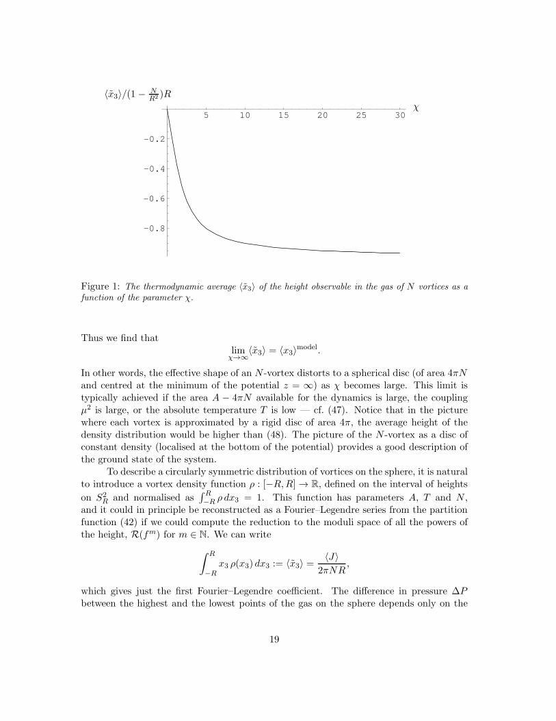
The dependence of the average height on the parameter χ is plotted in Figure 1.To interpret the meaning of (46), consider a simple model where the vortex density

is supported and homogeneously distributed on a spherical disc of area 4πN and centred atthe minimum z = ∞ of the potential (17). The height xmax

3 of the points at the boundaryof this disc is computed as

2πR

∫ xmax

3

−Rdx3 = 4πN =⇒ xmax

3 = −R+2N

R,

where we made use of Archimedes’ hat-box theorem. In this model, the average height forthe vortex density is then given by

〈x3〉model :=

∫ xmax

3

−R x3 dx3∫ xmax

3

−R dx3= −

(

1− N

R2

)

R. (48)

18

5 10 15 20 25 30

-0.8

-0.6

-0.4

-0.2

〈x3〉/(1 − NR2 )R

χ

Figure 1: The thermodynamic average 〈x3〉 of the height observable in the gas of N vortices as a

function of the parameter χ.

Thus we find thatlimχ→∞

〈x3〉 = 〈x3〉model.

In other words, the effective shape of an N -vortex distorts to a spherical disc (of area 4πNand centred at the minimum of the potential z = ∞) as χ becomes large. This limit istypically achieved if the area A − 4πN available for the dynamics is large, the couplingµ2 is large, or the absolute temperature T is low — cf. (47). Notice that in the picturewhere each vortex is approximated by a rigid disc of area 4π, the average height of thedensity distribution would be higher than (48). The picture of the N -vortex as a disc ofconstant density (localised at the bottom of the potential) provides a good description ofthe ground state of the system.

To describe a circularly symmetric distribution of vortices on the sphere, it is naturalto introduce a vortex density function ρ : [−R,R] → R, defined on the interval of heights

on S2R and normalised as

∫ R−R ρ dx3 = 1. This function has parameters A, T and N ,

and it could in principle be reconstructed as a Fourier–Legendre series from the partitionfunction (42) if we could compute the reduction to the moduli space of all the powers ofthe height, R(fm) for m ∈ N. We can write

∫ R

−Rx3 ρ(x3) dx3 := 〈x3〉 =

〈J〉2πNR

,

which gives just the first Fourier–Legendre coefficient. The difference in pressure ∆Pbetween the highest and the lowest points of the gas on the sphere depends only on the

19

trivial zeroth order coefficient: using the relation

∇P +Nρ∇f = 0

for the pressure of a fluid of N particles subject to a potential f at equilibrium (this isanalogous to the problem of fluid motion in a constant gravitational field, cf. [21] §25), wefind

∆P =

∫ R

−R∇P dx3 = −

∫ R

−RNρ(x3)

∂

∂x3(µ2Rx3) dx3 = −µ2NR < 0.

6 Discussion

We have been able to calculate the partition function of a gas of critically coupled abelianHiggs vortices interacting with an axially symmetric background potential on a sphere.When we switch off the interaction, we recover Manton’s partition function that givesphysical insight on the Liouville volume of vortex moduli spaces MN . Our study yields, inaddition to Manton’s formula (40) for Vol(MN ), an infinite number of nontrivial integrals(41) over MN . These are additional data about the geometry of the moduli spaces, andthey are all encapsulated by our partition function. As an application, we computedthe thermodynamic average height of the gas of N vortices, and the result we found isconsistent with the effective picture of the ground state as an N -vortex localised at thebottom of the potential as a spherical disc of constant density and area 4πN .

Our analysis was essentially an application of the Duistermaat–Heckman localisationformula for a natural circle action on (MN , ω), in which the symplectic structure of themoduli space is a crucial ingredient. There is an alternative model [22] for dynamics ofGinzburg–Landau vortices with a Schrodinger–Chern–Simons kinetic term, for which MN

(not T ∗MN ) plays the role of phase space in the adiabatic approximation; in this context,the Kahler form ω appears naturally as a symplectic structure [16]. Our work illustratesthat the symplectic point of view can also be fruitful in the study of the abelian Higgsmodel.

We have already noted that our formula (41) can be applied to calculate integralsof general circularly symmetric functions on the moduli space. One may therefore hope tostudy the interaction of the vortices with any symmetric potential f on S2

R — or perhapseven an SO(3)-invariant intervortex interaction modelling the Ginzburg–Landau potentialat λ2 6= 1 to some degree of approximation, which would be an obviously interestingextension of our work [23]. Analytical results about the Ginzburg–Landau potential (forarbitraryN) are already available [24, 25], but they refer to the situation where the vorticesare well separated on the plane. A treatment of the interaction to include the interestingeffects near clustering configurations on the moduli spaces will almost certainly need touse some numerical input [26]. It is believed that abelian Higgs vortices even slightly awayfrom critical coupling should satisfy a realistic equation of state such as the van der Waalsequation, which accounts for phase transitions. Progress in this direction would shed lighton the phenomenology of thin superconductors.

20

Acknowledgements

The author is thankful to Nick Buchdahl, Nick Manton and Michael Murray for usefulcomments. This work was supported by the Australian Research Council.

References

[1] N.S. Manton: A remark on the scattering of BPS monopoles. Phys. Lett. B 110 (1982)54–56.

[2] N.S. Manton and P.M. Sutcliffe: Topological Solitons. Cambridge University Press,2004.

[3] N.S. Manton: Statistical mechanics of vortices. Nucl. Phys. B 400 [FS] (1993) 624–632.

[4] N.S. Manton and S.M. Nasir: Volume of vortex moduli spaces. Commun. Math. Phys.

199 (1999) 591–604, hep-th/9807017.

[5] A. Jaffe and C. Taubes: Vortices and Monopoles. Birkhauser, 1980.

[6] M. Noguchi: Yang–Mills–Higgs theory on a compact Riemann surface. J. Math. Phys. 28(1987) 2343–2346.

[7] S. Bradlow: Vortices in holomorphic line bundles over closed Kahler manifolds. Commun.

Math. Phys. 135 (1990) 1–17.

[8] E.B. Bogomol’nyı: The stability of classical solutions. Sov. J. Nucl. Phys. 24 (1976)449–454.

[9] D. Stuart: Dynamics of Abelian Higgs vortices in the near Bogomolny regime. Commun.

Math. Phys. 159 (1994) 51–91.

[10] T.M. Samols: Vortex scattering. Commun. Math. Phys. 145 (1992) 149–180.

[11] I.A.B. Strachan: Low-velocity scattering of vortices in a modified Abelian Higgs model.J. Math. Phys. 33 (1992) 102–110.

[12] N.S. Manton and J.M. Speight: Asymptotic interactions of critically coupled vortices.Commun. Math. Phys. 236 (2003) 535–555, hep-th/0205307.

[13] J.M. Baptista and N.S. Manton: The dynamics of vortices on S2 near the Bradlow limit.J. Math. Phys. 44 (2003) 3495–3508, hep-th/0208001.

[14] D. Tong: NS5-branes, T-duality and worldsheet instantons. JHEP 07 (2002) 013–036,hep-th/0204186.

[15] N.S. Manton and S.M. Nasir: Conservation laws in a first-order dynamical system ofvortices. Nonlinearity 12 (1999) 851–865, hep-th/9809071.

[16] N.M. Romao: Quantum Chern–Simons vortices on a sphere. J. Math. Phys. 42 (2001)3445–3469, hep-th/0010277.

[17] V. Guillemin and S. Sternberg: Symplectic Techniques in Physics. Cambridge UniversityPress, 1984.

21

[18] J.J. Duistermaat and G.J. Heckman: On the variation in the cohomology of the sym-plectic form of the reduced phase space. Invent. Math. 69 (1982) 259–268.

[19] D. McDuff and D. Salamon: Introduction to Symplectic Topology, 2nd edition. OxfordUniversity Press, 1998.

[20] F.H. Ree and W.G. Hoover: Fifth and sixth virial coefficients for hard spheres and harddisks. J. Chem. Phys. 40 (1964) 939–950.

[21] E.M. Lifshitz and L.P. Pitaevskii: Statistical Physics (Part 1), Landau and LifshitzCourse of Theoretical Physics, Vol. 5. Pergamon Press, 3rd edition, 1980.

[22] N.S. Manton: First-order vortex dynamics. Ann. Phys. 256 (1997) 114–131,hep-th/9701027.

[23] M.G. Eastwood and N.M. Romao: A combinatorial formula for homogeneous momentsmath.SG/0508402.

[24] J.M. Speight: Static intervortex forces. Phys. Rev. D55 (1997) 3830–3835,hep-th/9603155.

[25] N.M. Romao and J.M. Speight: Slow Schrodinger dynamics of gauged vortices. Nonlin-earity 17 (2004) 1337–1355, hep-th/0403215.

[26] P.A. Shah: Scattering of vortices at near-critical coupling. Nucl. Phys. B 249 (1994)259–276, hep-th/9402075.

22