Nernst branes in gauged supergravity

arX

iv:1

108.

0296

v2 [

hep-

th]

17

Aug

201

1

LMU-ASC 29/11

MPP-2011-91

Nernst branes in gauged supergravity

Susanne Barisch∗,×, Gabriel Lopes Cardoso+, Michael Haack∗,

Suresh Nampuri∗, Niels A. Obers†

∗ Arnold Sommerfeld Center for Theoretical Physics

Ludwig-Maximilians-Universitat Munchen

Theresienstrasse 37, 80333 Munchen, Germany

× Max-Planck-Institut fur Physik

Fohringer Ring 6, 80805 Munchen, Germany

+ CAMGSD, Departamento de Matematica

Instituto Superior Tecnico, Universidade Tecnica de Lisboa

Av. Rovisco Pais, 1049-001 Lisboa, Portugal

† The Niels Bohr Institute

Blegdamsvej 17, 2100 Copenhagen Ø, Denmark

ABSTRACT

We study static black brane solutions in the context of N = 2 U(1) gauged supergravity

in four dimensions. Using the formalism of first-order flow equations, we construct novel ex-

tremal black brane solutions including examples of Nernst branes, i.e. extremal black brane

solutions with vanishing entropy density. We also discuss a class of non-extremal generaliza-

tions which is captured by the first-order formalism.

Contents

1 Introduction 1

2 First-order flow equations for extremal black branes 6

2.1 Flow equations in big moduli space . . . . . . . . . . . . . . . . . . . . . . . . 6

2.2 Generalizations of the first-order rewriting . . . . . . . . . . . . . . . . . . . 13

2.2.1 Charge transformations . . . . . . . . . . . . . . . . . . . . . . . . . . 13

2.2.2 Flux transformations . . . . . . . . . . . . . . . . . . . . . . . . . . . . 14

2.2.3 Non-supersymmetric examples . . . . . . . . . . . . . . . . . . . . . . 15

2.3 AdS2 × R2 backgrounds . . . . . . . . . . . . . . . . . . . . . . . . . . . . . . 16

3 Exact solutions 18

3.1 Solutions with constant γ . . . . . . . . . . . . . . . . . . . . . . . . . . . . . 18

3.1.1 The F (X) = −iX0X1 model . . . . . . . . . . . . . . . . . . . . . . . 18

3.1.2 The F = − (X1)3/X0 model: Interpolating solution between AdS4

and AdS2 × R2 . . . . . . . . . . . . . . . . . . . . . . . . . . . . . . . 23

3.2 Solutions with non-constant γ . . . . . . . . . . . . . . . . . . . . . . . . . . . 26

3.2.1 The F = − iX0X1 model . . . . . . . . . . . . . . . . . . . . . . . . 26

3.2.2 The STU model . . . . . . . . . . . . . . . . . . . . . . . . . . . . . . 28

4 Nernst brane solutions in the STU model 30

5 Non-extremal deformation 33

A Special geometry 37

B First-order rewriting in minimal gauged supergravity 40

References 41

1 Introduction

Black holes play an important role as testing grounds for theories of quantum gravity. They

originally arise as solutions of the equations of classical gravitation which encapsulate regions

of space-time where the curvature becomes of the order of Planck length and classical grav-

itation breaks down. Thus, a quantum theory of gravity must be able to make statements

about these systems. Further, in classical gravitation, there is a correspondence between

physical observables that characterize the horizon of the black hole, such as its surface area

and the surface gravity, and thermodynamic quantities such as entropy and temperature,

and once this correspondence is made, the laws of black hole mechanics can be rewritten

as the laws of thermodynamics of black holes. Therefore, an essential requirement for any

quantum theory of gravity is that it has to be able to derive this correspondence from first

1

principles and more generally, derive the thermodynamics of black holes from a microscopic

statistical physical viewpoint. Hence, black hole thermodynamics and in particular questions

of microstate counting of black hole entropy have been an active area of research in string

theory.

Amongst these intriguing systems exists a subclass of black holes which pose extremely

interesting problems that have been the target of concentrated research in string theory.

These are a subset of charged black holes called extremal black holes. Charged black holes

arise as solutions of gravity coupled to gauge fields and in general can carry electric and

magnetic charge quantum numbers w.r.t. these gauge fields. Extremal black holes are charged

black holes that carry the minimum mass possible in the theory for a given set of charge

quantum numbers, and their mass is uniquely fixed in a given theory in terms of the charges

and the asymptotic values of the scalar fields. These are zero temperature black holes which

radically violate the third law of thermodynamics – the so called Nernst Law,1 which states

that the entropy of a thermodynamic system vanishes at zero temperature. Because these

black holes gravitationally attract matter, they reduce the entropy of the region of space-

time outside the horizon, and hence for consistency with the second law of thermodynamics,

they must have a corresponding increase in entropy. Hence these black holes have a very

high non-zero entropy at zero temperature. Some of the major successes in the study of the

statistical mechanics of black holes in string theory has been for this class of black holes. In

particular, their entropy can be given a statistical interpretation [2, 3] and exact formulae

for the microscopic degeneracies of extremal black holes are known for certain classes of

supersymmetric extremal black holes. These include black holes in N = 4 , D = 4 string

theory or N = 4 , D = 5 string theory (see [4, 5, 6, 7, 8]), and in N = 8 , D = 4 string

theory (see [9]).

Simultaneously, there is another critical way in which black holes play an essential role in

string theory. String theory naturally generates a beautiful and extremely powerful correspon-

dence between the dynamics of fields in gravitational backgrounds that are asymptotically

AdS and conformal field theories on the boundary of this AdS space. The AdS/CFT corre-

spondence implies the equality of the Hilbert spaces of the bulk theory and the field theory

at the boundary, whose operator content is defined by the boundary values of the bulk fields.

Hence every state in the bulk has a corresponding state in the field theory. Black holes

which are states in the bulk are represented as thermal ensembles in the dual field theory

at the same temperature as the black hole. The dynamics of bulk fields in the black hole

background therefore provides information on the interaction of the corresponding operators

in the thermal ensemble of the dual field theory. Since the AdS/CFT correspondence is a

strong-weak coupling duality, non-perturbative aspects of the boundary field theory can, in

principle, be understood in terms of perturbative calculations in gravity and vice versa.2

1The original Nernst heat theorem states that entropy changes go to zero at zero temperature. The strong

form of the law which states that entropy goes to zero at zero temperature was formulated by Max Planck,

for pure crystalline homogenous materials [1].2Incidentally, the AdS/CFT correspondence also lies at the heart of the entropy computation for extremal

2

A lot of effort has been put in applying this paradigm to extract information about field

theory systems from a gravitational perspective, recently specifically about those field theo-

ries that could underlie condensed matter physics, (for a comprehensive introduction to the

various aspects of this field see the reviews [13, 14, 15, 16, 17, 18]). One of the most interest-

ing and rich problems in such systems is the problem of understanding phase transitions. In

some important cases these are inaccessible to perturbative calculations on the field theory

side and as such offer a ready application ground to applying the principles of AdS/CFT

or, more generally, in applying knowledge of gravitational physics to the corresponding field

theory dual using gauge-gravity duality. Black holes play a vital role in this new application.

Amongst the most challenging classes of phase transitions are quantum critical phase

transitions which are phase transitions that occur in condensed matter systems at zero tem-

perature and which are driven by quantum fluctuations. In order to analyze these transitions

gravitationally, one must necessarily focus on the gravitational duals of zero temperature

thermal ensembles in field theory – the extremal black holes. Further, if one expects to find

results applicable to real condensed matter systems, these black holes must obey the usual

thermodynamic properties of condensed matter systems. All extremal black holes obey the

first two laws of thermodynamics and we therefore need to explore extremal black holes that

do not violate the third law. Hence finding these ’Nernst black holes’ is a relevant problem

with potentially rich implications. Smooth Nernst configurations in AdS have already been

found in [19, 20, 21].

Once we find a class of Nernst black holes, we need to have a systematic way of classifying

these objects. Phase transitions in field theory are classified by their universality classes and

distinguishing between various kinds of Nernst black holes could help in identifying those

relevant for a particular field theory. One way that suggests itself as a useful approach in

classification is in terms of a behavior that is uniquely exhibited by extremal configurations –

namely the attractor mechanism. This mechanism was discovered when studying uncharged

scalar fields in an extremal black hole background.3 In the absence of fluxes, the attractor

mechanism forces the values of the fields on the horizon to be independent of their asymptotic

values and fixes them solely in terms of the charges of the black hole. Hence the extremal

black hole horizon serves as a fixed point in moduli space (see [22, 23, 24, 25, 26, 27]).4

Therefore, classifying extremal black holes can be restated as classifying these fixed points in

moduli space and identifying any non-universality in the fixed point flow behavior.

The purpose of this paper is therefore to make a step towards addressing the analogous

problem in the presence of fluxes by studying static (black) brane solutions in the context

black holes in string theory: The leading order entropy of extremal black holes with a local AdS3 factor in

the near horizon geometry (arising from combining the usual AdS2 factor with an internal circle direction)

can be obtained by relating their Bekenstein-Hawking entropy to the Cardy-Hardy-Ramanujan formula for

the leading term in the entropy of a 2D CFT (see [10, 11, 12]).3The dynamics of these fields is encoded in a low-energy effective action arising from string theory.4In general there can also be flat directions in moduli space. However, the entropy of an extremal black

hole does not depend on the values of the moduli associated with these flat directions, so that it still makes

sense to view the extremal black hole horizon as a fixed point in moduli space.

3

of N = 2 U(1) gauged supergravity in four dimensions with only vector multiplets. Related

work on extending the attractor mechanism to the case with gaugings can be found in [28,

29, 30, 31, 32, 33, 34]. Our study starts with obtaining first-order flow equations for extremal

black branes, building on and extending recent work done in [30, 32, 33]. Using this, we

first study a number of new exact (non-Nernst) solutions both in the single scalar and STU

model. These include, in particular, generalizations of the (extremal limit) of a solution

recently discussed in the context of AdS/CMT in [35], as well as a solution that interpolates

between AdS4 and AdS2 × R2. We then show how our formalism can be used in the STU

model to find explicit examples of extremal black brane solutions in four dimensions with

vanishing entropy, which we denote as Nernst branes. We also show how the first-order

formalism can be extended to non-extremal solutions and we give examples thereof.

The paper is organized as follows. In section 2, we first study the equations of motion

governing the flow of the fields towards a fixed point, in the presence of fluxes. The presence

of a fixed point in moduli space basically halves the degrees of freedom and hence the flow

equations for the fields can be formulated as first-order ODEs. In four-dimensional ungauged

supergravity these equations were first constructed and solved for black holes in [26, 36]. In

the case of black holes in ungauged supergravity, the curvature of the horizon is positive and

inversely proportional to the square of the spherical radius of the horizon. A vanishing entropy

simply corresponds to a vanishing horizon size and a curvature larger than Planck scale

curvature, which clearly pushes these objects outside the regime of analysis of supergravity.

In general, for systems with a non-vanishing horizon curvature, classical supergravity analysis

applies when the radius of curvature is macroscopic w.r.t. both the Planck as well as the string

scales. In four dimensions, both these scales are related by the string coupling constant as

lp = gs ls. At the horizon, if the string coupling is fixed and the horizon does not encode

information about the quantum numbers of the internal states of the system, that is if it

has vanishing entropy, the string coupling value at the fixed point is a universal number

independent of charges and independent of its asymptotic value. For ’small’ black holes with

vanishing entropy, the string coupling constant is generally zero or infinite [37] and in either

case, for non-vanishing value of the dimensionfull curvature, the dimensionless curvature will

blow up in either string or Planck units. Hence, we should naturally turn towards black

objects with Ricci-flat horizons. These are black branes in string theory. In the absence

of fluxes, in an asymptotically flat space, black objects in D = 4 can have only a spherical

topology. Hence, we need to turn on fluxes to generate black branes in non-flat backgrounds.

In the presence of fluxes, extremal supersymmetric configurations in four dimensions were

first discovered by [30] and subsequently discussed in [32, 33]. The first-order formalism in

the presence of fluxes was first presented in [32]. There are significant differences in this

formalism vis-a-vis the ungauged case. The two most crucial ones being that there is a

symplectic constraint that restricts the choices of charges given the fluxes and secondly, the

phase of the effective ‘central’ charge (which we denote by γ) is no longer constant as in

the ungauged case, but is a dynamical quantity with an equation of its own. The first-order

formalism simply depends on the existence of fixed points in moduli space, and is independent

4

of whether the solutions being considered are supersymmetric or non-supersymmetric. Hence,

after re-deriving the supersymmetric first-order equations of [32], as a generalization, we

indicate how to develop a first-order equation for moduli flows in a non-supersymmetric

black brane background, and we give examples thereof. We demonstrate how the invariance

of the action under certain transformation operations on the fluxes can lead to alternative

first-order rewritings of the differential equations of flow. We finish this formalism section by

identifying the necessary conditions for the near-horizon geometry to be AdS2 × R2.

In section 3, we begin to explore the solution space of the first-order flow equations.

We first choose the simplest prepotential encoding one complex vector multiplet scalar field,

given by F = − iX0X1, and obtain a class of general fixed point solutions representing

non-Nernst black branes. These turn out to be generalizations of the solution discussed in

[35]. This serves as a consolidating check on the formalism. This solution, like an ungauged

solution, has a constant phase γ. As another example of a solution with constant γ, we show

a full numerical solution that interpolates between a near-horizon AdS2 × R2 geometry and

an asymptotic AdS4 geometry (for the prepotential F = − (X1)3/X0). We then proceed to

explore the possibility to have non-constant γ. So far we have only found local geometries

whose curvature and string coupling become large at some point. It might be possible,

though, that they describe the asymptotic region of a global solution once higher derivative

corrections are taken into account. It would be interesting to further investigate the existence

of well behaved solutions with non-constant γ, given that such solutions would be radically

different from the constant phase sector and have no counterpart in the ungauged case.

In section 4, we finally pursue the question of finding Nernst brane solutions. For this

purpose, we explore axion-free solutions of the fixed point flow equations in the STU model,

and write down a solution with constant γ and a fixed point at the zero of the radial coordi-

nate. At this point, the scalar that parametrizes the dilaton in the heterotic frame flows to

zero. Moreover, at this point, the metric has a coordinate singularity and the area density in

the constant time and constant radial coordinate hyperplane vanishes. The geometry near

this fixed point has an infinitely long radial throat which suppresses fluctuations in the scalar

fields such that their solutions become independent of their asymptotic values. We will take

this infinite throat property to mean that the solution is extremal, and the vanishing of the

area density to mean that the solution has zero entropy density. However, these solutions

asymptote to geometries that are not AdS4 and, thus, it is not clear which role they might

play in the gauge/gravity correspondence. Nevertheless, they are well behaved in that the

curvature invariants are finite. We end this section with a few comments on this Nernst brane

solution.

In section 5, we present a generalization of the first-order formalism to non-extremal black

branes and show how in certain cases, the moduli flow in these backgrounds can be encoded

in first-order equations.

5

2 First-order flow equations for extremal black branes

In the following, we will be interested in extremal black brane solutions of N = 2 U(1)

gauged supergravity in four dimensions with vector multiplets. First-order flow equations for

supersymmetric black holes and black branes were recently obtained in [32] by a rewriting of

the action, where they were given in terms of physical scalar fields zi = Y i/Y 0 (i = 1, . . . , n).

Here, we will re-derive them by working in big moduli space, so that the resulting first-order

flow equations will now be expressed in terms of the Y I . Also, we will not restrict ourselves

to supersymmetric solutions only. The formulation in big moduli space becomes particularly

useful when discussing the coupling to higher-derivative curvature terms [40].

2.1 Flow equations in big moduli space

Following [30, 32, 33] we make the ansatz for the black brane line element,

ds2 = −e2U dt2 + e−2U(

dr2 + e2ψ(dx2 + dy2))

, (2.1)

where U = U(r) , ψ = ψ(r). The black brane will be supported by scalar fields that only

depend on r.

The Lagrangian we will consider is given in (A.25). It is written in terms of fields XI of

big moduli space. The rewriting of this Lagrangian as a sum of squares of first-order flow

equations will, however, not be in terms of the XI , but rather in terms of rescaled variables

Y I defined by

Y I = eA XI = eA ϕXI . (2.2)

Here A = A(r) denotes a real factor that will be determined to be given by

A = ψ − U , (2.3)

while ϕ denotes a phase with a U(1)-weight that is opposite to the one of XI . Thus, XI =

ϕXI denotes a U(1) invariant variable so that

NIJ DrXI DrX

J = NIJ X′I ¯X ′J , (2.4)

where X ′I = ∂rXI . Observe that in view of (A.3),

e2A = −NIJ YI Y J , (2.5)

and that

e2AA′ = −12 NIJ

(

Y ′I Y J + Y I Y ′J)

, (2.6)

where we used the second homogeneity equation of (A.1).

We will first discuss electrically charged extremal black branes in the presence of electric

fluxes hI only, so that for the time being the flux potential (A.30) reads

V (X, ¯X) =(

N IJ − 2 XI ¯XJ)

hI hJ . (2.7)

6

Subsequently, we will extend the first-order rewriting to the case of dyonic charges as well as

dyonic fluxes.

We take F Itr = EI(r) as well as XI = XI(r). Inserting the line element (2.1) into the

action (A.25) yields the one-dimensional Lagrangian

L1d =√−g L−QI E

I , (2.8)

where L is given in (A.25) and the QI denote the electric charges. Extremizing with respect

to EI yields

− e2ψ−2U ImNIJ EJ = QI , (2.9)

and hence

EI = −e2U−2ψ[

(ImN )−1]IJ

QJ . (2.10)

The associated one-dimensional action reads,

− S1d =

∫

dr e2ψ{

U ′2 − ψ′2 +NIJ X′I ¯X ′J − 1

2 e2U−4ψ QI

[

(ImN )−1]IJ

QJ

+g2 e−2UV (X, ¯X)}

+

∫

drd

dr

[

e2ψ(

2ψ′ − U ′)

]

, (2.11)

in accordance with [32] for the case of black branes. Next, we rewrite (2.11) in terms of the

rescaled variables Y I . We also find it convenient to introduce the combination

qI = eU−2ψ+iγ(

QI − i g e2(ψ−U)hI

)

, (2.12)

where γ denotes a phase which can depend on r. Using

X ′I = e−A(

Y ′I −A′ Y I)

, (2.13)

as well as (2.6), we obtain the intermediate result

− S1d =

∫

dr e2ψ{

U ′2 − ψ′2

+e−2ANIJ

(

Y ′I − eAN IK qK) (

Y ′J − eANJL qL)

+(

A′ +Re[

XI qI

])2

−12 e

2U−4ψ QI

[

(ImN )−1]IJ

QJ − qI NIJ qJ −

(

Re[

XI qI

])2+ g2 e−2UV (X, ¯X)

}

+2

∫

dr e2ψ Re[

X ′I qI

]

+

∫

drd

dr

[

e2ψ(

2ψ′ − U ′)

]

. (2.14)

Next, using the identity,

− 12

[

(ImN )−1]

IJ = N IJ + XI ¯XJ + XJ ¯XI , (2.15)

7

as well as the explicit form of the potential (2.7), we obtain

− S1d =

∫

dr e2ψ{

U ′2 − ψ′2

+e−2ANIJ

(

Y ′I − eAN IK qK) (

Y ′J − eANJL qL)

+(

A′ +Re[

XI qI

])2

+2e2U−4ψ QIXI QJ

¯XJ −(

Re[

XI qI

])2− 2 g2 e−2U hI X

I hJ¯XJ}

+2

∫

dr e2ψ Re[

X ′I qI

]

+

∫

drd

dr

[

e2ψ(

2ψ′ − U ′)

]

. (2.16)

Inserting the expression (2.12) into the fourth line of (2.16) yields

2

∫

dr e2ψ Re[

X ′I qI

]

= 2

∫

drd

dr

[

eU Re(

eiγ XI QI

)

+ g e2ψ−U Im(

eiγ XI hI

)]

−2

∫

dr eU U ′ Re[

eiγ XI QI

]

−2 g

∫

dr e2ψ−U(

2ψ′ − U ′)

Im[

eiγ XI hI

]

(2.17)

+2

∫

dr γ′[

eU Im(

eiγ XI QI

)

− g e2ψ−U Re(

eiγ XI hI

)]

.

Combining the terms proportional to ψ′2 and to ψ′ into a perfect square, and the terms

proportional to U ′2 and to U ′ into a perfect square, yields

− S1d = SBPS + STD , (2.18)

where

SBPS =

∫

dr e2ψ{

[

U ′ − eU−2ψ Re(

eiγ XI QI

)

+ g e−U Im(

eiγ XI hI

) ]2

−(

ψ′ + 2 g e−U Im[

eiγ XI hI

])2(2.19)

+e−2ANIJ

(

Y ′I − eAN IK qK) (

Y ′J − eANJL qL)

+(

A′ +Re[

XI qI

])2+∆

}

,

and

∆ = 2[

eU−2ψ Im(

eiγ XI QI

)

− g e−U Re(

eiγ XI hI

)]

[

γ′ + eU−2ψ Im(

eiγ XI QI

)

+ g e−U Re(

eiγ XI hI

)]

. (2.20)

Finally,

STD =

∫

drd

dr

[

e2ψ(

2ψ′ − U ′)

+ 2eU Re(

eiγ XI QI

)

+ 2 g e2ψ−U Im(

eiγ XI hI

)]

.

(2.21)

Setting the squares in SBPS to zero gives

U ′ = eU−2ψ Re(

eiγ XI QI

)

− g e−U Im(

eiγ XI hI

)

,

ψ′ = −2 g e−U Im[

eiγ XI hI

]

,

A′ = −Re[

XI qI

]

,

Y ′I = eAN IK qK , (2.22)

8

while demanding the variation of ∆ to be zero yields

eU−2ψ Im(

eiγ XI QI

)

− g e−U Re(

eiγ XI hI

)

= 0 (2.23)

as well as

γ′ = −eU−2ψ Im(

eiγ XI QI

)

− g e−U Re(

eiγ XI hI

)

. (2.24)

Note that the first-order flow equations for the Y I and for A are consistent with one another:

the latter is a consequence of the former by virtue of (2.6).

Comparing the flow equations (2.22) with the ones obtained in the supersymmetric context

in [32] shows that the flow equations derived above are the ones for supersymmetric black

branes, and that the phase γ is to be identified with the phase α of [32] via γ′ = − (α′ +Ar),

with Ar given in (A.20).

Next, we study the dyonic case, with charges (QI , PI) and fluxes (hI , h

I) turned on. The

above results can be easily extended by first writing the term Q(ImN )−1Q in the action

(2.11) as

VBH = −12 QI

[

(ImN )−1]IJ

QJ

=(

N IJ + 2 XI ¯XJ)

QI QJ

= gij DiZ DjZ + |Z|2 , (2.25)

where we used (A.29) to write VBH in terms of Z = −QI XI . Turning on magnetic charges

amounts to extending Z to [24]

Z = P I FI −QI XI =

(

P I FIJ −QJ)

XJ = −QI XI , (2.26)

where

QI = QI − FIJ PJ . (2.27)

Similarly, the flux potential with dyonic fluxes can be obtained from the one with purely

electric fluxes by the replacement of hI by

hI = hI − FIJ hJ , (2.28)

cf. (A.30).

Thus, formally the action looks identical to before, and we can adapt the computation

given above to the case of dyonic charges and fluxes by replacing QI and hI with QI and hI .

Performing these replacements in (2.12) as well yields

qI = eU−2ψ+iγ(

QI − i g e2(ψ−U)hI

)

. (2.29)

The above procedure results in

− S1d = SBPS + STD + Ssympl , (2.30)

9

where SBPS and STD are given as in (2.19) and (2.21), respectively, with QI and hI replaced

by QI and hI , and with qI now given by (2.29). The third contribution, Ssympl, is given by

Ssympl = g

∫

dr(

QI hI − P I hI

)

. (2.31)

Observe that this term is constant, independent of the fields, and hence it does not contribute

to the variation of the fields. Imposing the constraint S1d = 0 (which is the Hamiltonian

constraint, to be discussed below) on a solution yields the condition

QI hI − P I hI = 0 , (2.32)

in agreement with [32] for the case of black branes. The condition (2.32) can also be written

as

Im(

QI NIJ ¯hJ

)

= 0 . (2.33)

The flow equations are now given by

U ′ = eU−2ψ Re[

eiγ XI QI

]

− g e−U Im[

eiγ XI hI

]

,

ψ′ = −2 g e−U Im[

eiγ XI hI

]

,

A′ = −Re[

XI qI

]

,

Y ′I = eAN IJ qJ ,

γ′ = eU−2ψIm(

eiγ Z)

+ g e−URe(

eiγ W)

, (2.34)

where Z and W denote Z and W with X replaced by X, as in (A.31). Inspection of the flow

equations (2.34) yields

A′ = (ψ − U)′ , (2.35)

and hence we obtain (2.3) (without loss of generality).

Observe that, as before, the flow equations for A and Y I are consistent with one another.

The latter can be recast into(

(Y I − Y I)′

(FI − FI)′

)

= −2i e−ψ Im

(

eiγ N IK QK

eiγ FIK NKJ QJ

)

+ 2i g eψ−2U Re

(

eiγ N IK hK

eiγ FIK NKJ hJ

)

,(2.36)

where here FI = ∂F (Y )/∂Y I . Each of the vectors appearing in this expression transforms as

a symplectic vector under Sp(2(n + 1))transformations, i.e. as

(

Y I

FI

)

→(

U IJ ZIJ

WIJ VIJ

)(

Y J

FJ

)

, (2.37)

where UT V −W T Z = I. For instance, under symplectic transformations,

N IJ ¯hJ → SIK NKL ¯hL , FIJ →(

VIL FLK +WIK

)

[S−1]KJ , (2.38)

where SIJ = U IJ +ZIK FKJ [38]. Using this, it can be easily checked that the last vector in

(2.36) transforms as in (2.37).

10

The constraint (2.23) becomes

eU−2ψ Im(

eiγ Z(Y ))

− g e−U Re(

eiγW (Y ))

= 0 , (2.39)

where

Z(Y ) = P I FI(Y )−QI YI ,

W (Y ) = hI FI(Y )− hI YI . (2.40)

Using the flow equations (2.34), we find that the constraint (2.39) is equivalent to the condi-

tion

qI YI = qI Y

I . (2.41)

The phase γ is not an independent degree of freedom. It can be expressed in terms of

Z(Y ) and W (Y ) as [32]

e−2iγ =Z(Y )− ig e2(ψ−U)W (Y )

Z(Y ) + ig e2(ψ−U) W (Y ). (2.42)

When γ = kπ (k ∈ Z), equation (2.42) implies

Z(Y ) = Z(Y ) , W (Y ) = −W (Y ) . (2.43)

Differentiating (2.39) with respect to r yields a flow equation for γ′ that has to be consis-

tent with the last flow equation in (2.34). We proceed to check consistency of these two flow

equations. Multiplying (2.39) with exp (2ψ − U) and differentiating the resulting expression

with respect to r yields

Im[

i qI YI(

γ′ − 2g e−ψ eiγW (Y )) ]

= 0 , (2.44)

where we used the flow equations for Y I and for (ψ − U). Using (2.41), this results in

γ′ = 2g e−ψ Re[

eiγW (Y )]

, (2.45)

which, upon using (2.39), equals the flow equation for γ given in (2.34). Thus, we con-

clude that upon imposing the constraint (2.39), the flow equation for γ′ given in (2.34) is

automatically satisfied.

Summarizing, we obtain the following independent flow equations. Since e2A is expressed

in terms of Y I , it is not an independent quantity, cf. (2.5). Since U = ψ − A on a solution,

U is also not an independent quantity. The independent flow equations are thus

ψ′ = 2 g e−ψ Im[

eiγW (Y )]

,

Y ′I = eψ−U N IK qK , (2.46)

with qK given in (2.29) and with γ given in (2.42) (observe that the latter is, in general, r-

dependent). In addition, a solution to these flow equations has to satisfy the reality condition

(2.41) as well as the symplectic constraint (2.32). The flow equations for the scalar fields Y I

can equivalently be written in the form (2.36). Observe that in view of (2.5) and (2.41), the

11

number of independent variables in the set (U,ψ, Y I) is the same as in the set (U,ψ, zi =

Y i/Y 0), which was used in [32]. Indeed, the flow equations (2.46) are equivalent to the ones

presented there and, thus, they describe supersymmetric brane solutions.

Observe that the right hand side of the flow equations (2.46) may be expressed in terms

of the Y I only by redefining the radial variable into ∂/∂τ = eψ ∂/∂r, in which case they

become

∂ψ

∂τ= 2 g Im

[

eiγW (Y )]

,

∂Y I

∂τ= e−iγ N IK

(

¯QK + i g e2A

¯hK

)

, (2.47)

with A expressed in terms of the Y I according to (2.5).

Let us now discuss the Hamiltonian constraint mentioned above. For a Lagrangian density√−g ( 1

2R + LM ) it is given by the variation of the action w.r.t. g00 as

12R00 +

δLMδg00

− 12 g00

(

12R + LM

)

= 0 . (2.48)

Using the matter Lagrangian (A.25) as well as the metric ansatz (2.1), and replacing the

gauge fields by their charges, as in (2.10), gives

e2ψ{

U ′2 − ψ′2 + NIJ XI′ ¯XJ ′ + g2 e−2U Vtot(X,

¯X)}

+[

e2ψ (2ψ′ − 2U ′ )]′

= 0 , (2.49)

where Vtot denotes the combined potential

Vtot(X,¯X) = g2 V (X, ¯X) + e−4A VBH(X,

¯X)

= g2[

N IJ ∂IW∂J¯W − 2|W |2

]

+ e−4A[

N IJ ∂I Z∂J¯Z + 2|Z|2

]

. (2.50)

The Hamiltonian constraint (2.49) can now be rewritten (up to a total derivative term) as

LBPS + Lsympl = 0 , (2.51)

where LBPS and Lsympl denote the integrands of (2.19) (with the charges and fluxes replaced

by their hatted counterparts) and (2.31), respectively. Since LBPS = 0 on a solution to the

flow equations, it follows that the Hamiltonian constraint reduces to the symplectic constraint

(2.32). The total derivative term vanishes by virtue of the flow equation for A = ψ − U .

In the following, we briefly check that (2.36) reproduces the standard flow equations for

supersymmetric domain wall solutions in AdS4. Setting QI = P I = 0, and choosing the

phase γ = π/2, we obtain ψ = 2U , A = U as well as(

(Y I − Y I)′

(FI − FI)′

)

= i g

(

hI

hI

)

, (2.52)

which describes the supersymmetric domain wall solution of [39]. Observe that the choice

γ = 0 leads to a solution of the type (2.52) with the imaginary part of (Y I , FI)′ replaced by

the real part. The flow equations (2.52) can be easily integrated and yield(

Y I − Y I

FI − FI

)

= i g

(

HI

HI

)

= i g

(

αI + hI r

βI + hI r

)

, (2.53)

12

where (αI , βI) denote integration constants. This solution satisfies W (Y ) = W (Y ), which is

precisely the condition (2.39). In addition, using (2.5), we obtain e2U = g(

HI FI(Y )−HI YI)

.

2.2 Generalizations of the first-order rewriting

In the preceding section the first order rewriting was done for a general prepotential. In mi-

nimal gauged supergravity other first order rewritings are possible. For a detailed discussion

see appendix B. Moreover, in the first-order rewriting performed above, what was used

operationally was the fact that i) for an arbitrary charge and flux configuration the 1-D bulk

Lagrangian can be written as a sum of squares and ii) imposing the symplectic constraint

(2.32), the vanishing of the squares gives a vanishing bulk Lagrangian, which in turn is equal

to the Hamiltonian density. This ensures that both the equations of motion as well as the

Hamiltonian constraint are satisfied. Given this procedure, we may identify invariances of

the action under transformations of the charges and/or fluxes, since any such transformation

will automatically produce a new, possibly physically distinct, rewriting of the action.

In the ungauged case in four dimensions this has been already explored in terms of an

S-matrix that operates on the charges, while keeping the action invariant [41].5 In the gauged

case, the presence of both charges and fluxes allows for a wider class of transformations, in

which both sets of quantum numbers are transformed. Thus finding transformations on both

charges and fluxes that leave the action invariant allows for more general rewritings. Here we

illustrate this with two possible types of transformations, one based on charge transformations

and the other on fluxes. It is in principle also possible to find combinations thereof, but we

do not attempt to do so explicitly.

2.2.1 Charge transformations

The combined potential (2.50) arising in the 1-D action consists of a sum of two positive

definite terms, one associated with charges and the other one with fluxes. The part arising

from charges can be written as

VBH = −12QTMQ , (2.54)

where Q = (P I , QI) and the symplectic matrix M takes the form (following the notation of

[41])

M = IM , M =

(

D C

B A

)

, I =

(

0 −I

I 0

)

(2.55)

with

A = −DT = ReN (ImN )−1 , C = (ImN )−1 , B = − ImN − ReN (ImN )−1 ReN .

(2.56)

Note that M2 = −I. Given a matrix S that transforms the charge vector Q to Q′ = SQ and

obeying STMS = M the charge potential remains invariant. Moreover, if in addition we

5See also [42] for related transformations in five dimensions.

13

choose a set of fluxes H = (hI , hI) such that their symplectic product (2.32) with the charges

remains invariant,

HTIQ = HTISQ , (2.57)

then the 1-D action (2.51) remains invariant. Consequently, the same action can have two

different rewritings, one being the usual supersymmetric rewriting in terms of the original

charges and fluxes and the other being a rewriting in terms of the new ’S-transformed’ charges

and old fluxes. Since the latter rewriting is distinct from the original supersymmetric one, it

would necessarily be non-supersymmetric.

In further detail, if one furthermore assumes that S is symplectic, it was shown in [41]

that the invariance of (2.54) implies that it needs to satisfy

[S,M ] = 0 (2.58)

with M defined in (2.55). In the present case with gauging, one needs to require in addition

(2.57). A sufficient condition for this is that H = S H so that S leaves the flux vector

unchanged [41]. This shows that one can generically satisfy this condition by choosing a

matrix S that only mixes non-zero charges (in the original configuration) and by only turning

on fluxes that are dual to those charges that are set to zero.

Examples of the S-matrix and charge and flux configurations satisfying the conditions

stated above will be given in section 2.2.3 below. Explicit rewritings for a constant S-matrix

in the ungauged case were given in [41] for the 4-D case and in [42] for 5-D. In particular, in

the 4-D case a constant S-matrix implies that one can define a new “fake superpotential” that

gives rise to the same black hole potential as Z. It must be noted that though in principle

one can construct non-constant S-matrices that are field dependent and which satisfy these

criteria, for the purpose of first-order rewriting, it is non-trivial to employ these matrices

since their derivatives then appear in the action so that the squaring technique in the action

becomes highly involved. We will only give explicit examples of the equations in the case of

a constant S-matrix.

2.2.2 Flux transformations

There are two distinct types of flux transformations that leave the action invariant and can

hence be used to generate new solutions.

The first one is in spirit analogous to the charge transformation discussed above. One

may write the flux potential (A.30) as

Vg = HT LH (2.59)

with H = (hI , hI) and the matrix L given by

L =

(

FT F −FT−T F T

)

(2.60)

14

in terms of FIJ and the matrix

T IJ = N IJ − 2XIXJ . (2.61)

Note that we thus have (FT )IJ = FIKT

KJ , (T F )IJ = T IKFKJ , (FT F )IJ = FIKTKLFLJ .

We now look for transformations on the fluxes H → H′ = RH that leave the flux potential

invariant, i.e. RTLR = L as well as the symplectic constraint HTIQ = HTRTIQ. This

is a new feature of the gauged case, examples of which will be given in section 2.2.3. Note

that if one finds an S-matrix transforming the charges and an R-matrix transforming the

fluxes, that simultaneously keep the symplectic constraint fixed, it is possible to perform a

non-supersymmetric rewriting with both transformed charges and fluxes.

A second possibility, which is more model-dependent, occurs if there is a flux configuration

h∗ that contributes vanishingly to the flux potential Vg = hI (NIJ − 2XI XJ )

¯hJ , cf. [43].

6

If, in addition, the charges that are symplectically dual to the fluxes in h∗ are not turned on,

then this flux vector becomes a flat direction in flux space. This means that for a given 1-D

action one can introduce these starred fluxes by adding a null term to the action as well as

the Hamiltonian, while not affecting the symplectic constraint. Then a new rewriting of the

action can be implemented with the old charges but the fluxes changed by the addition of

the corresponding h∗. An example of this arises in the STU model where a candidate h∗ is

simply the flux configuration with only h0 turned on. One can then easily show that

(h+ h∗)I TIJ (h+ h∗)J = hI T

IJhJ . (2.62)

Hence the replacement h→ h+ h∗ can be made in the action, provided the charge P 0 is not

turned on, and a new rewriting can be achieved. Note that this type of rewriting satisfies the

supersymmetry equations and is hence also supersymmetric. Note also that higher derivative

corrections will almost certainly lift this apparent degeneracy in solution space. Finally, this

new rewriting technique could be combined with the two previous ones for appropriate charge

and flux configurations to achieve further rewritings.

2.2.3 Non-supersymmetric examples

As an illustration of the transformations discussed above, we now give several examples in

the two particular models for which we later in sections 3 and 4 obtain new extremal black

brane solutions. The transformations below (along with other examples one might wish to

construct) can thus be used to generate non-supersymmetric extremal black brane solutions

from these.

We start with the F (X) = −iX0X1 model. In this case one can compute a constant

(symplectic) S-matrix satisfying (2.58) (see eq. (4.8) of [41]),

S =

(

− cos θσ3 −i sin θσ2i sin θσ2 − cos θσ3

)

, (2.63)

6We thank Stefanos Katmadas for pointing this out to us.

15

with σa the standard Pauli matrices. One may then for example choose θ = 0 (or θ = π).

The matrix S then becomes block-diagonal and we can ensureH = S H (and, thus, (2.57)) by

taking non-zero Q0, Q1 and h1 (or h0), or non-zero P0, P 1 and h1 (or h0). Then the solution

with Q → Q′ = S Q is non-supersymmetric.

It is also possible to find R-matrices mixing the fluxes. Here we content ourselves with

giving a field dependent example of a matrix R fulfilling RTLR = L. For this one needs Lin (2.60) which, together with (A.2), can be computed using that the matrices T and F are

given by

T = −1

2

[

1Re z 1 + z

Re z

1 + zRe z

|z|2

Re z

]

, F =

0 −i

−i 0

, (2.64)

with z = X1/X0. As an example, we take R to be block diagonal in electric/magnetic fluxes.

We find the solution

R =

(

A 0

0 A

)

, A =i√3

(

−1− zRe z − 1

Re z|z|2

Re z 1 + zRe z

)

, AIJ = |ǫIKǫJL|AKL , (2.65)

where ǫIK is the 2-dimensional Levi-Civita-symbol. For this type of R-matrix we can then

satisfy the symplectic constraint invariance by either taking the electric charges QI non-zero

accompanied by non-zero fluxes hI or magnetic charges P I together with fluxes hI . There

are many further possible R-matrices that can be constructed, mixing electric and magnetic

charges, even containing arbitrary parameters.

We also comment on possible S- and R-matrices in the STU-model. A constant (sym-

plectic) S-matrix satisfying (2.58) was constructed in [41],

S = diag(ǫ0, ǫ1, ǫ2, ǫ3, ǫ0, ǫ1, ǫ2, ǫ3) , ǫI = ±1 (2.66)

Without any details of the computation, we also note that it is possible to find corresponding

R-matrices mixing the fluxes. A simple example in the case of purely imaginary S = X1/X0,

T = X2/X0 and U = X3/X0 is

R =

(

A 0

0 AT

)

, A =

(

I2 0

0 B

)

, B =

(

0 T2U2

U2T2

0

)

, (2.67)

where T2 = ImT and U2 = ImU . It is not difficult to find charge/flux configurations that

have the property that R acts non-trivially on the fluxes, while at the same time leaving the

symplectic constraint invariant.

2.3 AdS2 × R2 backgrounds

In the following, we will consider space-times of the type AdS2 × R2, i.e. line elements (2.1)

with constant A. In view of the relation (2.5), we thus demand that the Y I are constant

in this geometry. Observe that the latter differs from the case of black holes in ungauged

supergravity. There, the appropriate Y I variable is not given in terms of (2.3), but rather

16

in terms of A = −U , and the associated flow equations are solved in terms of Y I = Y I(r)

rather than in terms of constant Y I .

For constant Y I , their flow equation yields qI = 0, which implies QI = i g e2A hI . Inserting

this into the flow equation for U gives

eA(eU )′ = −2g Im[

eiγ Y I hI

]

, (2.68)

which equals (eψ)′. Hence we obtain ψ′ = U ′, which is consistent with A = ψ−U = constant.

Combining the flow equations (2.45) and (2.68) gives

eA(

eU−iγ)′= 2 i g Y I hI = constant , (2.69)

which yields

eA eU−iγ = 2 i g Y I hI r + c , c ∈ C . (2.70)

It follows that

eA eU = Re[

2 i g eiγ Y I hI r + c eiγ]

= −2 g Im[

eiγ Y I hI

]

r +Re[

c eiγ]

. (2.71)

Now recall that γ is given by (2.42), which takes a constant value, since the Y I are constant.

Hence Re[

c eiγ]

is constant, and it can be removed by a redefinition of r, resulting in

eA+U = −2 g Im[

eiγ Y I hI

]

r . (2.72)

Observe that Im[

eiγ Y I hI

]

6= 0 to ensure that the space-time geometry contains an AdS2

factor.

Contracting QI = i g e2A hI with Y I yields the value for e2A as

e2A = −i YI QI

g Y J hJ= −i Z(Y )

gW (Y )= i

Z(Y )

g W (Y ), (2.73)

and hence

QI =Z(Y )

W (Y )hI . (2.74)

The values of the Y I are, in principle, obtained by solving (2.74), or equivalently,

QI − 12(FIJ + FIJ)P

J = 12g e

2ANIJhJ ,

−12NIJ P

J = g e2A(

hI − 12(FIJ + FIJ)h

J)

. (2.75)

There may, however, be flat directions in which case some of the Y I remain unspecified, and

an example thereof is given in section 3. The reality of e2A forces the phases of Z(Y ) and of

W (Y ) to differ by π/2 [32].

This relation (2.74) has an immediate consequence, similar to the one for black holes

derived in [32]. Namely, using (2.74) and (2.73) in (2.33) leads to

0 = Im

(

Z(Y )

W (Y )hIN

IJ ¯hJ

)

= Im(

i g e2A hINIJ ¯hJ

)

= g e2A hINIJ ¯hJ . (2.76)

17

Given that g e2A 6= 0, we infer that for any AdS2 × R2 geometry

hINIJ ¯hJ = 0 . (2.77)

We will use this fact below in section 3.1.2.

3 Exact solutions

In the following, we consider exact (dyonic) solutions of the flow equations in specific models.

In general, solutions fall into two classes, namely solutions with constant γ and solutions with

non-constant γ along the flow.

3.1 Solutions with constant γ

Let us discuss dyonic solutions in the presence of fluxes. For concreteness, we choose γ = 0

in the following. The flow equations (2.34) for U,ψ and A read,

(eU )′ = e−3A Re[

Y I QI

]

− g e−A Im[

Y I hI

]

,

(eψ)′ = −2 g Im[

Y I hI

]

,

(eA)′ = −Re[

Y I qI]

, (3.1)

while the flow equations for the Y I are(

(Y I − Y I)′

(FI − FI)′

)

= 2i e−ψ

[

− Im

(

N IK QK

FIK NKJ QJ

)

+ g e2A Re

(

N IK hK

FIK NKJ hJ

)]

. (3.2)

In the presence of both fluxes and charges, the flow equations (3.2) cannot be easily integrated.

A simplification occurs whenever ReFIJ = 0. This is, for instance, the case in the model

F = −iX0X1, to which we now turn.

3.1.1 The F (X) = −iX0X1 model

For this choice of prepotential, we have F (X) = (X0)2 F(z), where F(z) = −iz with z =

X1/X0 = Y 1/Y 0. The associated Kahler potential reads K = − ln(z + z), and z is related

to the dilaton through Re z = e−2φ. We also have

NIJ = −2

(

0 1

1 0

)

, N IJ = −12

(

0 1

1 0

)

, (3.3)

as well as

N00 = −iz , N11 = −i/z , N01 = 0 . (3.4)

The flow equations (3.2) become

(Y 0 − Y 0)′

(Y 1 − Y 1)′

−i(Y 1 + Y 1)′

−i(Y 0 + Y 0)′

= i e−ψ Im

Q1

Q0

i Q0

i Q1

− i g e−ψ+2A Re

h1

h0

i h0

i h1

. (3.5)

18

This yields

(Y 0 − Y 0)′

(Y 1 − Y 1)′

−i(Y 1 + Y 1)′

−i(Y 0 + Y 0)′

= i e−ψ Re

P 0 − g e2A h1

P 1 − g e2A h0

Q0 + g e2A h1

Q1 + g e2A h0

. (3.6)

In order to gain some intuition for finding a solution with all charges and fluxes turned

on, let us first consider a simpler example. We retain only one of the four charge/flux

combinations appearing in (3.6), namely the one with Q1 6= 0, h0 6= 0. Observe that any

of these four combinations satisfies the symplectic constraint (2.32). The associated flow

equations (3.6) are

(Y 0 − Y 0)′

(Y 1 − Y 1)′

−i(Y 1 + Y 1)′

−i(Y 0 + Y 0)′

= i e−ψ

0

0

0

Q1 + g e2A h0

, (3.7)

which yields Y 1 = constant and

(Y 0)′ = −12 e

−ψ(

Q1 + g e2A h0)

. (3.8)

The flow equations for ψ and A read,

(eψ)′ = −2g Re(

Y 1)

h0 ,(

e2A)′

= −2e−ψ Re(

Y 1) (

Q1 + g e2A h0)

. (3.9)

For the equation for A we used q0 = 0 and q1 = e−A−ψ(

Q1 + g e2A h0)

. The flow equation

for ψ can be readily integrated and yields

eψ = −2g Re(

Y 1)

h0 (r + c) , (3.10)

where c denotes an integration constant. Inserting this into the flow equation for A gives

(

e2A)′=Q1 + g e2A h0

g h0 (r + c), (3.11)

which can be integrated to

e2A =eβ(r + c)−Q1

g h0, (3.12)

where β denotes another integration constant. Plugging this into the flow equation for Y 0,

we can easily integrate the latter,

Y 0 =eβ

4gh0 (ReY 1)(r + δ) , (3.13)

where δ denotes a third integration constant. Using (2.5), we infer

δ = c− e−βQ1 . (3.14)

19

Moreover, for U we obtain

e2U = e2ψ−2A =4g3 (h0)3

(

Re Y 1)2

(r + c)2

eβ(r + c)−Q1. (3.15)

We take the horizon to be at r + c = 0, i.e. we set c = 0 in the following. Summarizing,

we thus obtain

Y 1 = constant ,

Y 0 =eβ r −Q1

4 gh0 (ReY 1),

Re z =4 g h0 (ReY 1)2

eβ r −Q1,

e2A =eβ r −Q1

g h0=

4 (ReY 1)2

Re z,

e2U =4g3 (h0)3

(

Re Y 1)2r2

eβ r −Q1,

e2ψ = 4g2(

Re Y 1)2

(h0)2 r2 . (3.16)

We require h0 > 0 and Q1 < 0 to ensure positivity of Re z, e2A and e2U . This choice is also

necessary in order to avoid a singularity of Re z and e2U at r = e−βQ1. The resulting brane

solution has non-vanishing entropy density, i.e. e2A(r=0) 6= 0. The imaginary part of z is

left unspecified by the flow equations. However, demanding the constraint (2.41) imposes

Y 1 to be real, so that Im z = 0. Note that Re Y 1 corresponds to a flat direction. The

above describes the extremal limit of the solution discussed in sec. 7 of [35] in the context of

AdS/CMT (see also [44, 45, 46]).7

We now want to solve the equations (3.6) when all charges and fluxes are non-zero. Since

the equations are quite difficult to solve directly, we will make an ansatz for eψ and e2A and

then solve for the Y I . In the example above we saw that eψ and e2A were linear functions of

r, so we choose the following ansatz for these functions,

eψ(r) = a r ,

e2A(r) = b r + c . (3.17)

When plugging this ansatz into the flow equations (3.6) we get

(Y 0(r))′ = − 1

2ar

(

¯Q1 + igc

¯h1

)

− gb

2ai¯h1 ,

(Y 1(r))′ = − 1

2ar

(

¯Q0 + igc

¯h0

)

− gb

2ai¯h0 . (3.18)

These equations can easily be integrated to give

Y 0(r) = − 1

2a

(

¯Q1 + igc

¯h1

)

ln r − gb

2ai¯h1r + C0 ,

Y 1(r) = − 1

2a

(

¯Q0 + igc

¯h0

)

ln r − gb

2ai¯h0r + C1 . (3.19)

7In order to compare the solutions, one would have to set γ = δ = 1 in (7.1) of [35], take their solution to

the extremal limit m2 = q2

8and relate the radial coordinates according to r(us) = 1

2l(r(them))2 − 1

2q√8.

20

In order for (3.17) and (3.19) to constitute a solution, several conditions on the parameters

a, b, c, the charges and the fluxes have to be fulfilled. On the one hand, one has to impose

the constraints

Im(

QIYI)

= 0 , Re(

hIYI)

= 0 , (3.20)

following from (2.34) and (2.39) for γ = 0. On the other hand, further constraints on the

parameters arise from (2.5), (2.33) and the equation for ψ in (3.1). Note that the equation

for U does not give additional information, as U is determined, once the Y I and ψ are given.

First, the constraints (3.20) imply

Re(

QINIJ ¯hJ

)

= 0 ,

Im(

QICI)

= 0 ,

Re(

hICI)

= 0 . (3.21)

Next, let us have a look at the equation for ψ. Using our ansatz for eψ, it reads

a = −2 g Im(

Y I hI

)

. (3.22)

With the form of the Y I given in (3.19) and demanding that the right hand side of (3.22) is

a constant, we obtain the constraint

Re(

¯h1h0

)

= 0 . (3.23)

This directly leads to a vanishing of the term linear in r. Together with the symplectic

constraint (2.33) it also implies that the logarithmic term vanishes. Moreover, we read off

a = −2g Im(

CI hI

)

. (3.24)

Next, we analyze the constraints coming from e2A = −NIJYI Y J . With our ansatz (3.17)

and the form of NIJ given in (3.3), one obtains

b r + c = 4Re(

Y 0Y 1)

. (3.25)

This fixes the constant c to be

c = 4Re(C0C1) . (3.26)

Using (3.24) the term linear in r on the right hand side of (3.25) is just identically b r,

i.e. there is no constraint on b (except that it has to be positive in order to guarantee the

positivity of e2A for all r). All other terms on the right hand side vanish if one demands

QINIJ ¯QJ = 0 , (3.27)

Re[(

QI − igchI

)

CI]

= 0 , (3.28)

in addition to (3.23) and the symplectic constraint (2.33).

We now show that (3.28) is fulfilled because the even stronger constraint

QI − igchI = 0 (3.29)

21

holds. To do so, we note that (3.28) together with (3.21) and (3.24) imply

Q0C0 + Q1C

1 = −ac2,

h0C0 + h1C

1 = −i a2g. (3.30)

To get a solution for C0 and C1 one of the two following conditions has to be valid:

i) If and only if Q0h1 − h0Q1 = ρ 6= 0 there is a unique solution for C0 and C1.

ii) If the two lines in (3.30) are multiples of each other then there exists a whole family of

solutions.

We will now show that case i) can be ruled out. To do so we combine the determinant

condition of case i) with the first constraint in (3.21), i.e. we look at the system of linear

equations for Q0 and Q1

Q0h1 − Q1h0 = ρ ,

Q0¯h1 + Q1

¯h0 = 0 . (3.31)

Obviously, the two lines cannot be multiples of each other for ρ 6= 0. Thus, in order to find

a solution at all, the determinant h1¯h0 +

¯h1h0 has to be non-vanishing. This is, however, in

conflict with (3.23). Thus, the two lines in (3.30) have to be multiples of each other, implying

(3.29). Note that this implies the absence of the logarithmic terms in the solutions for Y I .

To summarize we have found the following solution:

Y 0(r) = − gb2ai¯h1r + C0 ,

Y 1(r) = − gb2ai¯h0r + C1 ,

eψ(r) = ar ,

e2A(r) = br + c . (3.32)

In addition, the parameters have to fulfill the conditions

Re(h0¯h1) = 0 , QI = igchI , hIC

I = −i a2g, Re(C0C1) =

c

4, (3.33)

while the parameter b can be any non-negative number. For b = 0 this solution falls into the

class discussed in section 2.3.

Let us finally also mention that one can show that the F (X) = −iX0X1 model does

not allow for Nernst brane solutions (i.e. solutions with vanishing entropy) of the first-order

equations. Making an ansatz eU ∼ rα, eψ ∼ rβ and eA ∼ rβ−α for the near-horizon geometry,

one can show that the only solutions with both non-vanishing charges and fluxes have α =

β = 1 and are captured by the solution discussed in this section after setting b = 0.

22

3.1.2 The F = − (X1)3/X0 model: Interpolating solution between AdS4 and

AdS2 × R2

Next, we would like to construct a (supersymmetric) solution that interpolates between an

AdS4 vacuum at spatial infinity, and an AdS2 × R2 background with constant Y I at r = 0.

Thus, asymptotically, we require the solution to be of the domain wall type (see (2.52)) with

γ = π/2. Hence the Y I satisfy (2.53) with αI = βI = 0, so that we may write Y I = yI∞ r with

yI∞ = g N IJ ¯hJ = constant. The latter can be established as follows. Using (Y − Y )I = ig hI r

and FI − FI = ig hI r, we obtain

iNIJ YJ = FI − FIJ Y

J = ig¯hI r , (3.34)

so that12(Y + Y )I = g

(

N IJ ¯hJ − 12 i h

I)

r . (3.35)

It follows that asymptotically,

Y I = g N IJ ¯hJ r , (3.36)

and hence, in an AdS4 background,

e2A = e2U = −g2 hI N IJ ¯hJ r2 . (3.37)

Since this expression only depends on the Y I through the combinations NIJ and FIJ , which

are homogeneous of degree zero, the r-dependence scales out of these quantities, and thus

hI NIJ ¯hJ is a constant. For e2A to be positive, we need to require a2 ≡ −hI N IJ ¯hJ > 0.

At r = 0, on the other hand, we demand γ = γ0 as well as YI = constant, with A given by

(2.73). Thus, we want to construct a solution with a varying γ(r) that interpolates between

the values π/2 and γ0. From (2.77) we know that hI NIJ ¯hJ = 0 at the horizon. The Y I

appearing in this expression are evaluated at the horizon. In general, their values will differ

from the asymptotic values, so that the flow will interpolate between an asymptotic AdS4

background satisfying hI NIJ ¯hJ < 0 and an AdS2×R

2 background satisfying hI NIJ ¯hJ = 0.

This, however, will not be possible whenever FIJ is independent of the Y I , such as in the

F = −iX0X1 model, as already observed in [32]. Thus, in the example below, we will

consider the F = − (X1)3/X0 model instead.

The interpolating solution has to have the following properties. At spatial infinity, where

ImW (Y ) = 0, γ is driven away from its value π/2 by the term ReZ(Y ) in the flow equation

of γ,

γ′ =[

e2U−3ψ ReZ(Y )]

∞=[

e−4U ReZ(Y )]

∞=

ReZ(y∞)

a4 r3, (3.38)

and hence

γ(r) ≈ π

2− ReZ(y∞)

2a4 r2. (3.39)

Our example below has ReZ(y∞) = 0 though and, thus, the phase γ will turn out to be

constant. Near r = 0, on the other hand, the deviation from the horizon values can be

determined as follows. Denoting the deviation by δY I = βI rp, we obtain δ(e2A) = c rp with

c = −NIJ(βI Y J + Y I βJ) , (3.40)

23

where in this expression the Y I and NIJ are calculated at the horizon. Using this, we compute

the deviation of qI from its horizon value qI = 0,

δqI = e−A−ψ−iγ0(

−FI JL(pJ + ighJ )βL + ig¯hI c

)

rp , (3.41)

where all the quantities that do not involve βI are evaluated on the horizon. The flow

equations for the Y I then yield

pNIK βK =

e−iγ0

∆

(

−FI J L(pJ + ighJ )βL + ig¯hI c

)

, (3.42)

where

∆ = −2g Im(

eiγ0 hI YI)

. (3.43)

Contracting (3.42) with Y I yields p = 1. Inserting this value into (3.42) yields a set of

equations that determines the values of the βI .

Next, using the flow equation for γ, we compute the deviation from the horizon value γ0,

which we denote by δγ = Σ r. We obtain

Σ = − g

∆Re(

eiγ0 βI hI

)

. (3.44)

The example below will have a vanishing Σ, consistent with a constant γ. Finally, using the

flow equation for ψ we compute the change of ψ,

δψ = − g

∆Im(

eiγ0 βI hI

)

r . (3.45)

We now turn to a concrete example of an interpolating solution. As already mentioned,

this will be done in the context of the F (X) = − (X1)3

X0 model. To obtain an interpolating

solution we first need to specify the form of the solution at both ends.

Let us first have a look at the near horizon AdS2×R2 region. According to our discussion

in sec. 2.3, we have to solve (2.77) and QI = ige2AhI under the assumption that the Y I

are constant. It turns out that these constraints can be solved, for instance, by choosing

Q0, P1, h1, h

0 6= 0 and all other parameters vanishing. Of course, due to the symplectic

constraint (2.32), the four non-vanishing parameters are not all independent, but have to

fulfill

P 1 =Q0h

0

h1. (3.46)

For F (Y ) = − (Y 1)3

Y 0 , and introducing z = z1 + iz2 = Y 1

Y 0 , we have

NIJ =

(

−4 Im(

z3)

6 Im(

z2)

6 Im(

z2)

−12 Im (z)

)

. (3.47)

Using

e2A = 8|Y 0|2z32 , (3.48)

24

which follows from (2.5), shows that one can fulfill QI = ige2AhI and (2.77) by fixing

z1 = 0 ,

z2 =

√

(3 + 2√3)h1

3h0,

|Y 0| =3

14√Q0

2√2z22

√h1. (3.49)

Interestingly we find that the axion has to vanish and all parameters Q0, P1, h1, h

0 have to

have the same sign.

In order to describe the asymptotic AdS4 region, we note that asymptotically the charges

Q0 and P 1 can be neglected and we can read off the asymptotic form of the solution from

(2.53) with vanishing integration constants αI and βI . More precisely, we have to allow that

the asymptotic form of the interpolating solution differs from (2.53) by an overall factor. This

is because, apriori, we only know that asymptotically (ψ − 2U)′ = 0, cf. (2.34) for vanishing

charges. Without the need to match the asymptotic region to a near horizon AdS2 × R2

region, we could just absorb the constant ψ − 2U in a rescaling of the coordinates x and y.

However, when we start from the hear horizon solution and integrate out to infinity, we can

not expect to end up with this choice of convention. Allowing for a non-vanishing constant

ψ − 2U = C 6= 0, the flow equations (2.52) for Y I and, thus, also the solutions (2.53), would

obtain an overall factor eC . Concretely, we obtain

Y 0AdS4

(r) = ieCg

2h0r ,

Y 1AdS4

(r) = −eCg√h0h1

2√3

r , (3.50)

with a constant eC to be determined by numerics below. Note, however, that the dilaton

e−2φ = z2 =√

h13h0

is independent of this factor and it comes out to be real if h1 and h0 have

the same sign, consistently with what we found from the near horizon region.

We would now like to discuss the interpolating solution, which we obtain by specifying

boundary conditions at the horizon and then integrating numerically from the horizon to

infinity using Mathematica’s NDSolve. Given that in the AdS4 region Y0 is purely imaginary

and Y 1 is purely real, we choose the same reality properties at the horizon, i.e. we fulfill

(3.49) by

Y 0h = i

354h0

√Q0

2√2(3 + 2

√3)h

321

,

Y 1h = iY 0

h z2 = − 334

√

h0Q0

2√

2(3 + 2√3)h1

. (3.51)

The subscript h means that these values pertain to the horizon. Now we can determine the

phase γ0 at the horizon using (2.42). We get e−2iγ0 = −1 independently of h1, h0, Q0 and

25

P 1. We choose γ0 = π/2 as in the asymptotic AdS4 region and we will see that this leads to

a constant value for γ throughout.

Next we have to determine how the solution deviates near the horizon from AdS2 × R2.

We do this following our discussion at the beginning of this section, cf. (3.40) - (3.45). Given

the reality properties of Y I in both limiting regions, we choose β0 purely imaginary and β1

purely real. Solving (3.42) for the β’s results in

Imβ0 = Re β1h0(

(√3− 2)

√

3 + 2√3h1

√

h1h0

+ (5√3− 9)Q0)

)

h21. (3.52)

Given this, the deviation of all the fields close to the horizon can be determined (resulting

in initial conditions at, say ri = 10−6) and a numerical solution for the flow equations (2.34)

can be found, integrating from the horizon outwards. To do the numerics we chose

g = 1 , Re β1 = 0.01 , Q0 = 1 , h1 = 1 , h0 = 10 . (3.53)

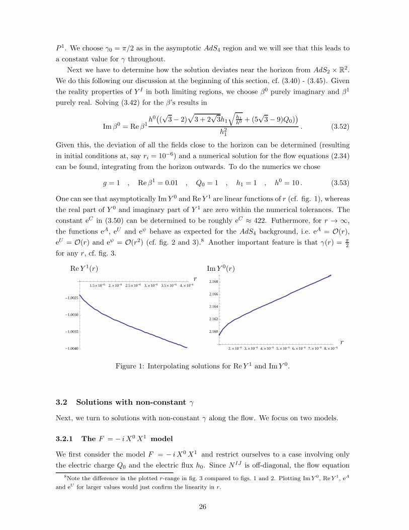
One can see that asymptotically ImY 0 and ReY 1 are linear functions of r (cf. fig. 1), whereas

the real part of Y 0 and imaginary part of Y 1 are zero within the numerical tolerances. The

constant eC in (3.50) can be determined to be roughly eC ≈ 422. Futhermore, for r → ∞,

the functions eA, eU and eψ behave as expected for the AdS4 background, i.e. eA = O(r),

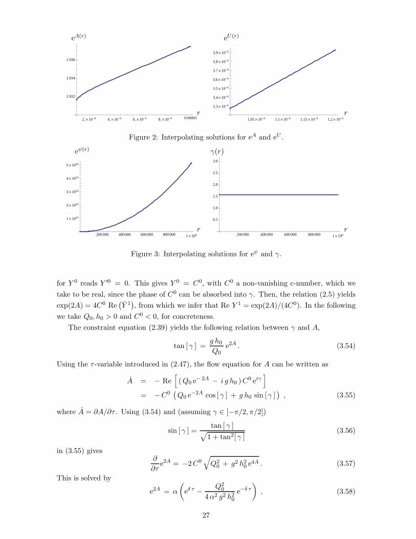
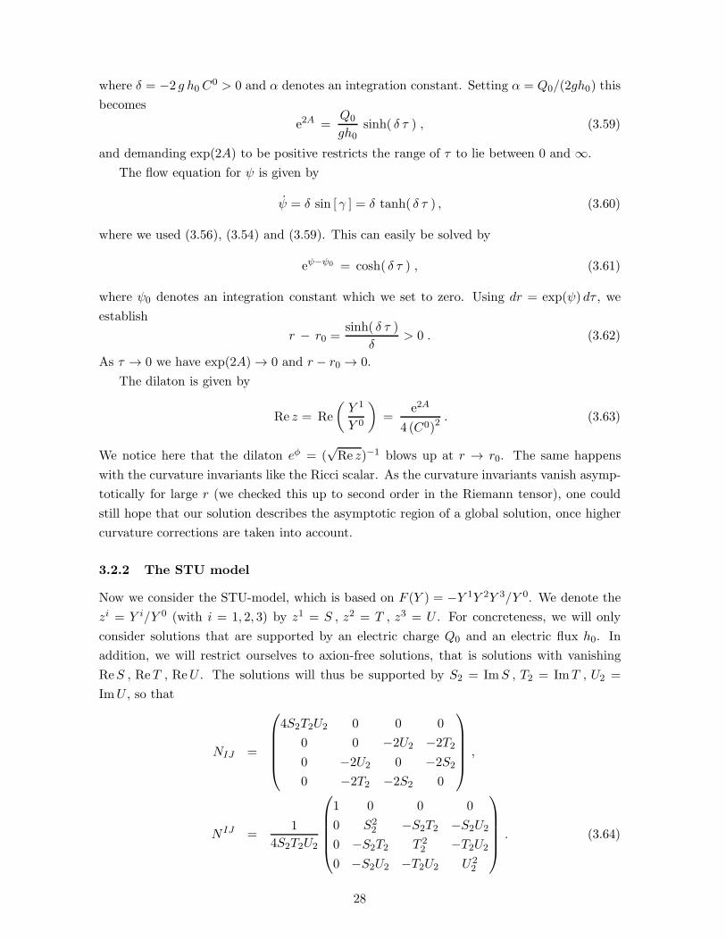
eU = O(r) and eψ = O(r2) (cf. fig. 2 and 3).8 Another important feature is that γ(r) = π2

for any r, cf. fig. 3.

1.5´10-6 2.´10-6 2.5´10-6 3.´10-6 3.5´10-6 4.´10-6

-1.0040

-1.0035

-1.0030

-1.0025

2.´10-6 3.´10-6 4.´10-6 5.´10-6 6.´10-6 7.´10-6 8.´10-6

2.160

2.162

2.164

2.166

2.168

ReY 1(r)

r

ImY 0(r)

r

Figure 1: Interpolating solutions for ReY 1 and ImY 0.

3.2 Solutions with non-constant γ

Next, we turn to solutions with non-constant γ along the flow. We focus on two models.

3.2.1 The F = − iX0X1 model

We first consider the model F = − iX0X1 and restrict ourselves to a case involving only

the electric charge Q0 and the electric flux h0. Since N IJ is off-diagonal, the flow equation

8Note the difference in the plotted r-range in fig. 3 compared to figs. 1 and 2. Plotting ImY 0, ReY 1, eA

and eU for larger values would just confirm the linearity in r.

26

2.´10-6 4.´10-6 6.´10-6 8.´10-6 0.00001

1.932

1.934

1.936

1.05´10-6 1.1´10-6 1.15´10-6 1.2´10-6

3.3´10-6

3.4´10-6

3.5´10-6

3.6´10-6

3.7´10-6

3.8´10-6

3.9´10-6

eA(r)

r

eU(r)

r

Figure 2: Interpolating solutions for eA and eU .

200 000 400 000 600 000 800 000 1´106

1´1014

2´1014

3´1014

4´1014

5´1014

200 000 400 000 600 000 800 000 1´106

0.5

1.0

1.5

2.0

2.5

3.0

eψ(r)

r

γ(r)

r

Figure 3: Interpolating solutions for eψ and γ.

for Y 0 reads Y ′0 = 0. This gives Y 0 = C0, with C0 a non-vanishing c-number, which we

take to be real, since the phase of C0 can be absorbed into γ. Then, the relation (2.5) yields

exp(2A) = 4C0 Re(

Y 1)

, from which we infer that Re Y 1 = exp(2A)/(4C0). In the following

we take Q0, h0 > 0 and C0 < 0, for concreteness.

The constraint equation (2.39) yields the following relation between γ and A,

tan [ γ ] =g h0Q0

e2A . (3.54)

Using the τ -variable introduced in (2.47), the flow equation for A can be written as

A = − Re[

(Q0 e− 2A − i g h0 )C

0 eiγ]

= −C0(

Q0 e−2A cos [ γ ] + g h0 sin [ γ ]

)

, (3.55)

where A = ∂A/∂τ . Using (3.54) and (assuming γ ∈ [−π/2, π/2])

sin [ γ ] =tan [ γ ]

√

1 + tan2[ γ ](3.56)

in (3.55) gives∂

∂τe2A = −2C0

√

Q20 + g2 h20 e

4A . (3.57)

This is solved by

e2A = α

(

eδ τ − Q20

4α2 g2 h20e−δ τ

)

, (3.58)

27

where δ = −2 g h0 C0 > 0 and α denotes an integration constant. Setting α = Q0/(2gh0) this

becomes

e2A =Q0

gh0sinh( δ τ ) , (3.59)

and demanding exp(2A) to be positive restricts the range of τ to lie between 0 and ∞.

The flow equation for ψ is given by

ψ = δ sin [ γ ] = δ tanh( δ τ ) , (3.60)

where we used (3.56), (3.54) and (3.59). This can easily be solved by

eψ−ψ0 = cosh( δ τ ) , (3.61)

where ψ0 denotes an integration constant which we set to zero. Using dr = exp(ψ) dτ , we

establish

r − r0 =sinh( δ τ )

δ> 0 . (3.62)

As τ → 0 we have exp(2A) → 0 and r − r0 → 0.

The dilaton is given by

Re z = Re

(

Y 1

Y 0

)

=e2A

4 (C0)2. (3.63)

We notice here that the dilaton eφ = (√Re z)−1 blows up at r → r0. The same happens

with the curvature invariants like the Ricci scalar. As the curvature invariants vanish asymp-

totically for large r (we checked this up to second order in the Riemann tensor), one could

still hope that our solution describes the asymptotic region of a global solution, once higher

curvature corrections are taken into account.

3.2.2 The STU model

Now we consider the STU-model, which is based on F (Y ) = −Y 1Y 2Y 3/Y 0. We denote the

zi = Y i/Y 0 (with i = 1, 2, 3) by z1 = S , z2 = T , z3 = U . For concreteness, we will only

consider solutions that are supported by an electric charge Q0 and an electric flux h0. In

addition, we will restrict ourselves to axion-free solutions, that is solutions with vanishing

ReS , ReT , ReU . The solutions will thus be supported by S2 = ImS , T2 = ImT , U2 =

ImU , so that

NIJ =

4S2T2U2 0 0 0

0 0 −2U2 −2T2

0 −2U2 0 −2S2

0 −2T2 −2S2 0

,

N IJ =1

4S2T2U2

1 0 0 0

0 S22 −S2T2 −S2U2

0 −S2T2 T 22 −T2U2

0 −S2U2 −T2U2 U22

. (3.64)

28

The flow equations for the Y i imply that they are constant. To ensure that S, T and U

are axion-free, we take the constant Y i to be purely imaginary, i.e. Y i = i Ci, where the Ci

denote real constants. Using (2.5) in the form

e2A = 8 |Y 0|2 S2 T2 U2 , (3.65)

the flow equation (2.47) for Y 0 gives

Y 0 = 2 |Y 0|2 (Q0 e− 2A + i g h0 ) e

− i γ . (3.66)

Using the constraint equation (2.39) in the form

Im[

(Q0 e− 2A + i g h0 ) e

− iγ Y 0]

= 0 (3.67)

as well as the flow equation for A,

A = − Re[

(

Q0 e− 2A + i g h0

)

e− iγ Y 0]

, (3.68)

we can rewrite (3.66) as

Y 0 = − 2Y 0 A . (3.69)

This immediately gives

Y 0 = C0 e− 2A , (3.70)

where C0 denotes an integration constant which we take to be real, for simplicity. Then, it

follows from (3.65) that

8C1C2C3

C0= 1 . (3.71)

For concreteness we take CI < 0 (I = 0, . . . , 3) in the following (ensuring the positivity of

S2, T2 and U2), as well as h0, Q0 > 0.

The constraint equation (3.67) yields the following relation between γ and A,

tan [ γ ] =g h0Q0

e2A . (3.72)

The flow equation (3.68) can be written as

12

∂

∂τe2A = −C0

(

Q0 e−2A cos [ γ ] + g h0 sin [ γ ]

)

(3.73)

which, using (3.72), leads to

14

∂

∂τe4A = −C0

√

Q20 + g2 h20 e

4A . (3.74)

This can be solved to give

e4A =4 g4 h40

(

C0)2

(τ + c )2 − Q20

g2 h20, (3.75)

29

where c denotes a further integration constant. Hence, the prefactor of the planar part of the

metric is

e2A =

√

4 g4 h40 (C0)2 (τ + c )2 − Q20

g h0. (3.76)

This is well behaved provided that (τ + c)2 ≥ Q20/(4g

4 h40 (C0)2).

The flow equation for ψ,

ψ = −2 g h0 C0 e− 2A sin [ γ ] (3.77)

is solved by (using (3.56), (3.72) and (3.75))

eψ =1

τ + c. (3.78)

The radial coordinate is then related to the τ variable by

r [ τ ] = log [ τ + c ] , (3.79)

where we set an additional integration constant to zero.

The physical scalars are given by

S2 =C1

C0e2A , T2 =

C2

C0e2A , U2 =

C3

C0e2A . (3.80)

They are positive as long as e2A is. However, as in the previous example, they vanish at

the lower end of the radial coordinate (indicating that string loop and α′ corrections should

become important). Again also the curvature blows up there and one can at best consider this

solution as an asymptotic approximation to a full solution which might exist after including

higher derivative terms. As we said in the introduction, it would be worthwhile to further

pursue the search for everywhere well behaved solutions with non-constant γ as they might

be radically different from the ungauged case.

4 Nernst brane solutions in the STU model

In the following we construct Nernst brane solutions (i.e. solutions with vanishing entropy

density) in a particular model, namely the STU-model already discussed in sec. 3.2.2. As

there, we denote the zi = Y i/Y 0 (with i = 1, 2, 3) by z1 = S , z2 = T , z3 = U . For

concreteness, we will only consider solutions that are supported by the electric charge Q0 and

the electric fluxes h1, h2, h3. In addition, we will restrict ourselves to axion-free solutions,

that is solutions with vanishing ReS , ReT , ReU . The solutions will thus be supported by

S2 = ImS , T2 = ImT , U2 = ImU , and the corresponding matrices NIJ and N IJ are given

in eq. (3.64). We thus have that e2A is determined by (3.65). In the following, we take Y 0 to

be real, so that the Y i will be purely imaginary.

Let us consider the flow equation (2.47) for the Y I . We set γ = 0. Instead of working

with a τ coordinate defined by dτ = e−ψ dr, we find it convenient to work with dτ = −e−ψ dr.

30

We obtain

Y 0 = − Q0

4S2T2U2,

Y i = 2 i g Y i[

2Y i hi − Y j hj

]

, (4.1)

where i, j = 1, 2, 3 and Y I = ∂Y I/∂τ . Here, i is not being summed over, while j is. The flow

equations for Y i are solved by

Y i = − i

2 g hi τ. (4.2)

Next, using that for an axion-free solution S2 = − i Y 1/Y 0, T2 = − i Y 2/Y 0 and U2 =

− i Y 3/Y 0, and inserting (4.2) into the flow equation for Y 0, we obtain

Y 0 = 2g3Q0 h1h2h3(

Y 0)3τ3 . (4.3)

This equation can be easily solved to give

Y 0 = − 1√

−g3Q0 h1 h2 h3 ( τ4 + C0 ), (4.4)

where C0 denotes an integration constant. We also take Q0 < 0 and h1, h2, h3 > 0. This

ensures that the physical scalars

S2 =1

2 g h1 τ

√

−g3 Q0 h1 h2 h3 ( τ4 + C0) ,

T2 =1

2 g h2 τ

√

−g3Q0 h1 h2 h3 ( τ4 + C0) ,

U2 =1

2 g h3 τ

√

−g3Q0 h1 h2 h3 ( τ4 + C0) (4.5)

take positive values.

Next, we consider the flow equation for ψ following from (2.34). Using (4.2), we obtain

ψ = 2 g Im[

Y i hi

]

= −3

τ, (4.6)

which upon integration yields

eψ−ψ0 =1

τ3, (4.7)

where ψ0 denotes an integration constant, which we set to ψ0 = 0. We can thus take τ to

range between 0 and ∞. The relation dτ = −e−ψ dr then results in

r [ τ ] =1

2 τ2+ Cr , (4.8)

where Cr denotes a real constant, which we take to be zero in the following. This sets the

range of r to vary from ∞ to 0 as τ varies from 0 to ∞.

Using (3.65), we obtain

e2A =

√−Q0√

g3 h1 h2 h3

√τ4 + C0

τ3, (4.9)

31

and hence

e−2U =

√−Q0√

g3 h1 h2 h3

√

τ4 + C0 τ3 . (4.10)

We take C0 to be non-vanishing and positive to ensure that the curvature scalar remains

finite througout and that the above describes a smooth solution of Einstein’s equations.

Asymptotically (τ → 0) we obtain

e2Ar→∞−→ α

(

1 +1

8C0 r2

)

(2 r)3/2 ,

e−2U r→∞−→ α

(

1 +1

8C0 r2

)(

1

2 r

)3/2

,

e2Ur→∞−→ α−1

(

1− 1

8C0 r2

)

(2 r)3/2 , (4.11)

where α =√

−Q0C0/(g3 h1 h2 h3). Observe that both exp(2A) and exp(2U) have an asymp-

totic r3/2 fall-off, which is rather unusual. Finally, observe that the scalar fields S2, T2 and

U2 grow as(

C0 r)1/2

asymptotically.

The near-horizon solution (which corresponds to τ → ∞) can be obtained by setting

C0 = 0 in the above. This yields

e2Ar→0−→

√−Q0√

g3 h1 h2 h3(2 r)1/2 ,

e−2U r→0−→√−Q0

√

g3 h1 h2 h3

1

(2 r)5/2, (4.12)

while S2, T2 and U2 approach the horizon as r−1/2. The near-horizon geometry has an in-

finitely long radial throat as well as a vanishing area density, which indicates that the solution

describes an extremal black brane with vanishing entropy density. It describes a supersym-

metric Nernst brane solution that is valid in supergravity, and hence in the supergravity

approximation to string theory when switching off string theoretic α′-corrections. When em-

bedding this solution into type IIA string theory, where S, T and U correspond to Kahler

moduli, the fact that asymptotically and at the horizon S2 , T2 and U2 blow up indicates that

this solution should be viewed as a good solution only in ten dimensions. In the heterotic de-

scription, where S2 is related to the inverse of the heterotic string coupling gs, the behaviour

S2 = ∞ (which holds asymptotically and at the horizon) is consistent with working in the

classical limit gs → 0.

We observe that the Nernst brane solution constructed above differs substantially from

the one constructed in [29]. This is related to the fact that here we deal with a flux potential

in gauged supergravity, and not with a cosmological constant as in [29].

The solution given above is supported by electric charges and fluxes, only. Additional

supersymmetric Nernst solutions can be generated through the technique of symplectic trans-

formations. On the other hand, a non-supersymmetric Nernst solution can be obtained from

the above one by replacing the charge vector Q by S Q in the flow equations, as described in

section 2.2.

32

5 Non-extremal deformation

In this section we construct a class of non-extremal black brane solutions that are based on

first-order flow equations. We do this by turning on a deformation parameter in the line

element describing extremal black branes. In the context of N = 2 U(1) gauged supergravity

in five dimensions, it was shown in [47] that there exists a class of non-extremal charged

black hole solutions that are based on first-order flow equations, even though their extremal

limit is singular. There, the non-extremal parameter is not only encoded in the line element,

but also in the definition of the physical charges. Here, we will only study the case where

the deformation parameter enters in the line element. A different procedure for constructing

non-extremal black hole solutions has recently been given in [48] in the context of ungauged

supergravity in four dimensions.

We begin by deforming the line element (2.1) into

ds2 = −(e2U − µ e2R)dt2 + (e2U − µ e2R)−1dr2 + e2(ψ−U)(

dx2 + dy2)

, (5.1)

where R = R(r) and µ is the non-extremal deformation parameter. Using

− 1

2

√−gR = e2ψ[

(

U ′ − ψ′)2

+ 2ψ′2 + 2ψ′′ − U ′′]

+µ e2(ψ−U+R)[

6U ′ ψ′ − 3U ′2 − 3ψ′2 + 2U ′′ − 2ψ′′

−2R′2 − 4R′ (ψ′ − U ′)−R′′]

, (5.2)

the one-dimensional action (2.30) gets deformed into

− S1d = −S1d(µ = 0) + µ

∫

dr e2(ψ−U+R)[

(ψ′ − U ′)2 + 2R′ (ψ′ − U ′)]

−µ∫

dr e2(R+ψ−U−A) NIJ

(

Y ′I −A′ Y I) (

Y ′J −A′ Y J)

+µ

∫

drd

dr

[

e2(ψ−U+R)(

2U ′ − 2ψ′ −R′)

]

, (5.3)

where S1d(µ = 0) denotes the action given in (2.30). Using (2.5) and (2.6), the second line

of this action can be written as

−µ∫

dr e2(R+ψ−U−A)[

NIJ Y′I Y ′J + (A′)2 e2A

]

= −µ∫

dr e2(R+ψ−U−A)[

NIJ

(

Y ′I − eAN IK qK) (

Y ′J − eANJL qL)

(5.4)

+eA[

qI(

Y ′I − 12eAN IK qK

)

+ qI(

Y ′I − 12eAN IL qL

)]

+ (A′)2 e2A]

.

33

Using this, we rewrite the action (up to a total derivative) as

− S1d = −S1d(µ = 0)

+µ

∫

dr e2R

(

[

(

eψ−U)′

−(

eA)′]2

+ 2(

eA)′[

(

eψ−U)′

−(

eA)′]

)

+µ

∫

dr 12

(

e2R)′(

e2(ψ−U))′

−µ∫

dr e2(R+ψ−U−A)[

NIJ

(

Y ′I − eAN IK qK) (

Y ′J − eANJL qL)

+eA[

qI(

Y ′I − 12eAN IK qK

)

+ qI(

Y ′I − 12eAN IL qL

)]

]

+µ

∫

dr e2R[

(

eA)′]2 (

1− e2(ψ−U−A))

. (5.5)

Now consider varying the action (5.5) and imposing the first-order flow equations (2.34) on

the fields. We begin by considering the variation

δ[

qI(

Y ′I − 12eAN IK qK

)]

+ δ[

qI(

Y ′I − 12eAN IL qL

)]

, (5.6)

which on a solution to the first-order flow equations equals

qI δ(Y′I) + qI δ(Y

′I)− qI NIJ qJ δ

(

eA)

− qI δ(N IJ) qJ eA , (5.7)

showing that there is no need to explicitly compute the variation of qI . Note, in particular,

that the variation of γ drops out of the problem. The independent variations are

δψ[

qI(

Y ′I − 12eAN IK qK

)]

+ δψ[

qI(

Y ′I − 12eAN IL qL

)]

= 0 ,

δU[

qI(

Y ′I − 12eAN IK qK

)]

+ δU[

qI(

Y ′I − 12eAN IL qL

)]

= 0 ,

δY[

qI(

Y ′I − 12eAN IK qK

)]

+ δY[

qI(

Y ′I − 12eAN IL qL

)]

= qI δ(Y′I)

−qI N IJ qJ δY(

eA)

− i qI N IP FPQLNQJ qJ e

A δY L . (5.8)

Then, varying the action (5.5) with respect to ψ gives

(

e2R)′′

e2A +(

e2R)′ (

e2A)′+(

e2R) (

e2A)′′

+ 2e2R+2A qI NIJ qJ = 0 . (5.9)

Now we use that on a solution to the first-order flow equations,

(

e2A)′′

= −2 e2A qI NIJ qJ . (5.10)

This relation will be established below. Then, using (5.10) in (5.9) gives

(

e2R)′′

e2A +(

e2R)′ (

e2A)′

=[

(

e2R)′e2A]′

= 0 , (5.11)

which implies(

e2R)′

= C e−2A , (5.12)

where C denotes an integration constant.

34

The variation of the action (5.5) with respect to U also gives the equation (5.11), while

varying the action with respect to R yields (5.10), which is satisfied on a solution to the

first-order flow equations.

Finally, varying the action (5.5) with respect to Y I and using its flow equation in the

form

NIJ Y′′J =

(

eA qI)′+ i e2A qLN

LP FPJI NJK qK , (5.13)

yields (upon integration by parts)

(

e2R)′ (

Y ′J −A′ Y J)

+ e2R Y ′′J = 0 (5.14)

which, using (5.12), can also be written as

(

e2R)′′Y J + 2

(

e2R)′Y ′J + 2e2R Y ′′J = 0 . (5.15)

Now, let us demonstrate the validity of (5.10). This relation can be established by noticing

that it equals(

e2A)′′

+ 2NIJ Y′I Y ′J = 0 (5.16)

on a solution to the first-order flow equations. Using (2.6), this in turn becomes

NIJ

(

Y ′′I Y J + Y I Y ′′J)

= i(

FIJK Y′I Y ′J Y K − FI JK Y

′I Y ′J Y K)

= 0 . (5.17)

The second equality in (5.17) follows from

FIJK Y′I Y ′J = (FIJK Y

I Y ′J)′ − FIJK YI Y ′′J = 0 , (5.18)

where (A.1) was used in the last step. We now proceed to show the vanishing of the left hand

side of (5.17), which will then imply (5.16).

Using (5.18) and the first-order flow equation for Y I , we compute

Y ′′I = N IK(

eA qK)′ − iN IK FKP Q Y

′P Y ′Q . (5.19)

Inserting this into (5.17) gives

(

eA qI)′Y I +

(

eA qI)′Y I = 0 . (5.20)

Next, using (2.29) we obtain

(

eA qI)′Y I = (i γ − ψ)′ eA qI Y

I − 2i g A′ e2A−ψ+i γ hI YI . (5.21)

Using

A′ = −e−AqI YI , (5.22)

which holds due to (2.41), (5.21) becomes

(

eA qI)′Y I =

[

(i γ − ψ)′ − 2i g e−ψ+i γW (Y )]

eA qI YI . (5.23)

35

Inserting the flow equations for γ′ and ψ′ into this, and using the constraint (2.39) yields

(

eA qI)′Y I = 0 . (5.24)

Thus we conclude that (5.20) vanishes on a solution to the first-order flow equations, and

hence also the left hand side of (5.17).

This concludes the discussion of equations resulting from the variation of the one-dimensional

action (5.5). Next, we have to impose the Hamilton constraint (2.48). Inserting the deformed

line element (5.1), we find that the changes induced in (2.51) are proportional to derivatives of

R. Thus, demanding R = constant, we obtain that both the Hamilton constraint and (5.12)

are satisfied, provided we set C = 0 in the latter equation. Finally, inserting R = constant in

(5.15) yields Y ′′J = 0. Thus, we conclude that the class of non-extremal black brane solutions

described by the deformed line element (5.1) with constant R has a description in terms of

the first-order flow equations (2.34) provided that the Y I are either constant or exhibit a

growth that is linear in r.

Examples of non-extremal black brane solutions that fall into this class are 1) the non-

extremal version of the solution presented in (3.32), which includes the solution discussed in

[35], 2) the non-extremal deformation of the extremal domain wall solution (2.53) and 3) the

non-extremal version of the interpolating solution near AdS4 and near AdS2 × R2 discussed

in section 3.1.2.

Acknowledgments

We would like to thank Gianguido Dall’Agata, Stefanos Katmadas and Stefan Vandoren

for valuable discussions. SB, MH, SN and NO thank CAMGSD for hospitality. GLC thanks

the Niels Bohr Institute and ASC-LMU for hospitality. This work is supported in part by

the Excellence Cluster “The Origin and the Structure of the Universe” in Munich. The work

of GLC is supported by the Fundacao para a Ciencia e a Tecnologia (FCT/Portugal). The

work of MH and SN is supported by the German Research Foundation (DFG) within the

Emmy-Noether-Program (grant number: HA 3448/3-1). The work of NO is supported in part

by the Danish National Research Foundation project “Black holes and their role in quantum

gravity”. The work of SB, GLC, MH and SN is supported in part by the transnational

cooperation FCT/DAAD grant “Black Holes, duality and string theory”.

36

A Special geometry

As is well known, the Lagrangian describing the couplings of N = 2 vector multiplets to

N = 2 supergravity is encoded in a holomorphic function F (X), called the prepotential, that

depends on n + 1 complex scalar fields XI (I = 0, . . . , n). Here, n counts the number of

physical scalar fields. The coupling to supergravity requires F (X) to be homogeneous of

degree two, i.e. F (λX) = λ2F (X), from which one derives the homogeneity properties

FI = FIJ XJ ,

FIJK XK = 0 , (A.1)

where FI = ∂F (X)/∂XI , FIJ = ∂2F/∂XI∂XJ , etc. The XI are coordinates on the big

moduli space, while the physical scalar fields zi = Xi/X0 (i = 1, . . . , n) parametrize an

n-dimensional complex hypersurface, which is defined by the condition that the symplectic

vector (XI , FI(X)) satisfies the constraint

i(

XI FI − FI XI)

= 1 . (A.2)

This can be written as

−NIJ XI XJ = 1 , (A.3)

where

NIJ = −i(

FIJ − FIJ)

. (A.4)

The constraint (A.3) is solved by setting

XI = eK(z,z)/2XI(z) , (A.5)

where K(z, z) is the Kahler potential,

e−K(z,z) = |X0(z)|2 [−NIJ ZI ZJ ] (A.6)

with ZI(z) = (Z0, Zi) = (1, zi). Writing

F (X) =(

X0)2 F(z) , (A.7)

which is possible in view of the homogeneity of F (X), we obtain

F0 = X0(

2F(z) − zi Fi)

, (A.8)

where Fi = ∂F/∂zi. In addition, we compute

F00 = 2F − 2zi Fi + zi zj Fij ,F0j = Fj − ziFij ,Fij = Fij , (A.9)

to obtain

−NIJ ZI ZJ = i

[

2(

F − F)

−(

zi − zi) (

Fi + Fi)]

, (A.10)

37

and hence

e−K(z,z) = i |X0(z)|2[

2(

F − F)

−(

zi − zi) (

Fi + Fi)]

. (A.11)

The XI(z) are defined projectively, i.e. modulo multiplication by an arbitrary holomorphic

function,

XI(z) → e−f(z)XI(z) . (A.12)

This transformation induces the Kahler transformation

K → K + f + f (A.13)

on the Kahler potential, while on the symplectic vector (XI , FI(X)) it acts as a phase trans-

formation, i.e.

(XI , FI(X)) → e−12 (f−f) (XI , FI(X)) . (A.14)

The resulting geometry for the space of physical scalar fields zi is a special Kahler geometry,

with Kahler metric

gi =∂2K(z, z)

∂zi ∂zj(A.15)

based on a Kahler potential of the special form (A.11).

Let us relate the Kahler metric (A.15) to the metric (A.4) on the big moduli space.

Differentiating e−K yields

∂ke−K = −∂kK e−K = i |X0(z)|2

[

Fk − Fk − (zi − zi)Fik]

+ ∂k lnX0(z) e−K ,

∂k∂le−K = [−∂k∂lK + ∂kK ∂lK] e−K = [−gkl + ∂kK ∂lK] e−K

= i |X0(z)|2(

Fkl − Fkl)

−[

∂k lnX0(z) ∂l ln X

0(z)

−∂k lnX0(z) ∂lK − ∂kK ∂l ln X0(z)

]

e−K . (A.16)

Using (A.9) we have

Nij = −i(

Fij − Fij)

, (A.17)

and hence we infer from (A.16) that

gi = Nij |X0|2 + 1

|X0(z)|2DiX0(z)D X

0(z) , (A.18)

where

DiX0(z) = ∂iX

0(z) + ∂iKX0(z) (A.19)

denotes the covariant derivative ofX0(z) under the transformation (A.12), i.e. Di

(

e−fX0(z))

=

e−f DiX0(z).

Next, let us consider the combination NIJ DµXI DµXJ , where the space-time covariant

derivative Dµ reads

DµXI = ∂µX

I + iAµXI = ∂µX

I +1

2

(

∂iK ∂µzi − ∂ıK∂µz

i)

XI , (A.20)

38

which is a covariant derivative for U(1) transformations (A.14). The combination NIJ DµXI DµXJ

is thus invariant under U(1)-transformations. Observe that

DµX0 = eK/2DiX

(0)(z) ∂µzi . (A.21)

Using (A.3) we obtain

NIJ DµXI DµXJ = |X0|2Nij ∂µz

i ∂µzj − 1

|X0|2 DµX0 DµX0

+X0

X0NiJX

J ∂µziDµX0 +

X0

X0NIjX

I ∂µzj DµX0 . (A.22)

Next, using

X0 XJ NkJ =1

X0(z)DkX

0(z) , (A.23)

as well as (A.18) and (A.21) we establish

NIJ DµXI DµXJ = gi ∂µz

i ∂µzj , (A.24)

which relates the kinetic term for the physical fields zi to the kinetic term for the fields

XI on the big moduli space. Observe that both sides of (A.24) are invariant under Kahler

transformations (A.13).

Using the relation (A.24), we express the bosonic Lagrangian (describing the coupling

of n vector multiplets to N = 2 U(1) gauged supergravity) in terms of the fields XI of big

moduli space,

L = 12R−NIJ DµX

I DµXJ + 14ImNIJ F

Iµν F

µνJ − 14ReNIJ F

Iµν F

µνJ − g2V (X, X) , (A.25)

where

NIJ = FIJ + iNIK X

K NJLXL

XM NMN XN, (A.26)

which satisfies the relation

NIJ XJ = FI . (A.27)

The flux potential reads

V = giDiW DW − 3|W |2 , W = hI FI − hI XI , (A.28)

where DiXI = ∂iX

I + 12∂iKXI . Here, (hI , hI) denote the magnetic/electric fluxes. AdS4

with cosmological constant Λ = −3g2 corresponds to a constant W with |W | = 1. Switching

off the flux potential corresponds to setting g = 0.

Using the identity (see (23) of [40])

N IJ = giDiXI DX

J −XI XJ , (A.29)

the flux potential can be expressed as

V (X, X) =[

giDiXI DX

J − 3XIXJ] (

hK FKI − hI) (

hK FKJ − hJ)

=[

N IJ − 2XIXJ] (

hK FKI − hI) (

hK FKJ − hJ)

= N IJ ∂IW∂J¯W − 2 |W |2 , (A.30)

39

where in the last line W is expressed in terms of U(1)-invariant fields XI ,

W = hI FI(X)− hI XI =

(

hI FIJ − hJ)

XJ . (A.31)

B First-order rewriting in minimal gauged supergravity

The N = 2 Lagrangian in minimal gauged supergravity is given in terms of the prepotential

F = − i (X0)2. Only a single scalar field, X0 is turned on, whose absolute value is set to

a constant, |X0|2 = 14 by the constraint (A.3), and the consequent bulk 1-D Lagrangian

density for the metric ansatz (2.1) is given by

− L1D = e2A+2U [−A′2 − 2A′ U ′ +1

4e−2U − 4A ( |Q0|2 − 3 g2 |h0|2e4A ) ] . (B.1)

Here A = ψ − U . We now perform a first-order rewriting for this Lagrangian inspired by

the corresponding rewriting for black holes in minimal gauged supergravity, as done in [49].

Denoting φ1 = A , φ2 = U , W = eU√

( |Q0|2 + g2 |h0|2 e4A + γ eA ) ,9 and the matrix,

m =

(

1 1

1 0

)

, we can write the above Lagrangian density as

L1D = e2A+2U [φa′mab φb′ +

1

4e−4U − 4AmabWaWb ] . (B.2)

Here, W1 = WA is the derivative of W w.r.t A and W2 = WU is the derivative of W w.r.t

U , given explicitly as

WA =e2U

2W( 4 g2 |h0|2 e4A + γ eA ) ,

WU = W . (B.3)

The first-order rewriting is then simply,

L1D = e2A+2U [mab (φa′ − 1

2e− 2U − 2AmacWc ) (φ

b ′ − 1

2e− 2U − 2AmbdWd ) ] + φa′Wa .

(B.4)

Using the chain-rule of derivatives on W = W (φa ) , the last term in the above equation

becomes φa′Wa = W ′ . Hence the first-order rewritten Lagrangian can finally be written as

L1D = e2A+2U [mab (φa′ − 1

2e− 2U − 2AmacWc ) (φ

b ′ − 1

2e− 2U − 2AmbdWd ) ] + W ′ .

(B.5)

The first-order equations for the metric functions can be written as

A′ =1

2e−2U − 2AWU , (B.6)

U ′ =1

2e−2U − 2A (WA − WU ) . (B.7)

9Here γ is an arbitrary real number.

40

The Hamiltonian density can be written as H = L1D − [ e2 (A+U ) ( 2A′ ) ]′ . On-shell, using

the first-order equations, this can be written as H = L1D − [(W ′ ) ] . Substituting for L1D

from (B.6), we see that the on-shell Hamiltonian density becomes

H = e2A+2U [mab (φa′ − 1

2e− 2U − 2AmacWc ) (φ

b′ − 1

2e− 2U − 2AmbdWd ) ] . (B.8)

This is trivially zero on-shell as the perfect squares vanish due to the first order equations.

Hence the Hamiltonian constraint from General Relativity is satisfied for field configura-

tions obeying these first-order equations. This completes the first-order rewriting for the

Lagrangian in minimal gauged supergravity. All smooth black brane solutions to these first-

order first order equations are necessarily non-supersymmetric. Smooth non-supersymmetric

black brane solutions in minimal gauged supergravity which solve the above first-order equa-

tions have been written down in [50] where it was also shown that the supersymmetric

solutions are singular.

For the metric ansatz,

ds2 = (−r2

vdt2 + v

dr2

r2) + e2A ( dx2 + dy2 ) , (B.9)

there is a different rewriting of this Lagrangian given by,

L1D = − [ ( ( eA )′)2 e2U + 2eA+U ( ( eA )

′) ( ( eU )

′ − 1√v)

+ 2 ( ( eA )′) eA+U 1√

v− 1

4e− 2A ( |Q0|2 − 3 g2 |h0|2e4A ) ] . (B.10)

The first-order equations following from the rewriting above are

( eA )′

= 0 , (B.11)

( eU )′

=1√v, (B.12)

with v = 2 e4A

|Q0|2. The Hamiltonian density vanishes on-shell provided e4A = |Q0|2

3 g2 |h0|2. The

AdS2 × R2 background with AdS2 radius,

√v , which is a near-horizon black brane geometry

in the presence of fluxes, is a solution to these first order equations.

References

[1] M. Planck, The Theory of Heat Radiation (1915), Springer (reprint).

[2] A. Strominger and C. Vafa, Microscopic origin of the Bekenstein-Hawking entropy,

Phys. Lett. B379 (1996) 99–104 [arXiv:hep-th/9601029].

[3] J. M. Maldacena, A. Strominger, and E. Witten, Black hole entropy in M-theory,

JHEP 12 (1997) 002 [arXiv:hep-th/9711053].

[4] R. Dijkgraaf, E. P. Verlinde, and H. L. Verlinde, Counting dyons in N = 4 string

theory, Nucl. Phys. B484 (1997) 543–561 [arXiv:hep-th/9607026].

41

[5] R. Dijkgraaf, G. W. Moore, E. P. Verlinde and H. L. Verlinde, Elliptic genera of

symmetric products and second quantized strings, Commun. Math. Phys. 185 (1997)

197-209 [arXiv:hep-th/9608096].

[6] D. Shih, A. Strominger, and X. Yin, Recounting dyons in N = 4 string theory, JHEP

10 (2006) 087 [arXiv:hep-th/0505094].

[7] D. P. Jatkar and A. Sen, Dyon spectrum in CHL models, JHEP 04 (2006) 018

[arXiv:hep-th/0510147].

[8] A. Dabholkar, J. Gomes and S. Murthy, Counting all dyons in N =4 string theory,

JHEP 1105 (2011) 059 [arXiv:0803.2692 [hep-th]].

[9] A. Sen, N=8 Dyon Partition Function and Walls of Marginal Stability, JHEP 0807

(2008) 118 [arXiv:0803.1014 [hep-th]].

[10] A. Strominger, Black hole entropy from near horizon microstates, JHEP 9802 (1998)

009 [arXiv:hep-th/9712251].

[11] V. Balasubramanian and F. Larsen, Near horizon geometry and black holes in

four-dimensions, Nucl. Phys. B 528 (1998) 229 [arXiv:hep-th/9802198].

[12] A. Dabholkar, A. Sen, and S. P. Trivedi, Black hole microstates and attractor without

supersymmetry, JHEP 01 (2007) 096 [arXiv:hep-th/0611143].

[13] S. A. Hartnoll, Lectures on holographic methods for condensed matter physics, Class.

Quant. Grav. 26 (2009) 224002 [arXiv:0903.3246 [hep-th]].

[14] C. P. Herzog, Lectures on Holographic Superfluidity and Superconductivity, J. Phys. A

42, 343001 (2009) [arXiv:0904.1975 [hep-th]].

[15] J. McGreevy, Holographic duality with a view toward many-body physics, Adv. High

Energy Phys. 2010 (2010) 723105 [arXiv:0909.0518 [hep-th]].

[16] S. A. Hartnoll, Quantum Critical Dynamics from Black Holes, arXiv:0909.3553

[cond-mat.str-el].

[17] G. T. Horowitz, Introduction to Holographic Superconductors, arXiv:1002.1722 [hep-th].

[18] S. Sachdev, Condensed matter and AdS/CFT, arXiv:1002.2947 [hep-th].

[19] J. P. Gauntlett, J. Sonner and T. Wiseman, Holographic superconductivity in

M-Theory, Phys. Rev. Lett. 103 (2009) 151601 [arXiv:0907.3796 [hep-th]].

[20] G. T. Horowitz and M. M. Roberts, Zero Temperature Limit of Holographic

Superconductors, JHEP 0911 (2009) 015 [arXiv:0908.3677 [hep-th]].

[21] E. D’Hoker and P. Kraus, Charged Magnetic Brane Solutions in AdS (5) and the fate

of the third law of thermodynamics, JHEP 1003, 095 (2010) [arXiv:0911.4518 [hep-th]].

42

[22] S. Ferrara, R. Kallosh, and A. Strominger, N=2 extremal black holes, Phys. Rev. D52

(1995) 5412–5416 [arXiv:hep-th/9508072].

[23] A. Strominger, Macroscopic entropy of N = 2 extremal black holes, Phys. Lett. B383

(1996) 39–43 [arXiv:hep-th/9602111].

[24] S. Ferrara and R. Kallosh, Supersymmetry and attractors, Phys. Rev. D54 (1996)

1514–1524 [arXiv:hep-th/9602136].

[25] S. Ferrara and R. Kallosh, Universality of supersymmetric attractors, Phys. Rev. D54

(1996) 1525–1534 [arXiv:hep-th/9603090].

[26] S. Ferrara, G. W. Gibbons and R. Kallosh, Black holes and critical points in moduli

space, Nucl. Phys. B 500 (1997) 75 [arXiv:hep-th/9702103].

[27] K. Goldstein, N. Iizuka, R. P. Jena, and S. P. Trivedi, Non-supersymmetric attractors,

Phys. Rev. D72 (2005) 124021 [arXiv:hep-th/0507096].

[28] S. Bellucci, S. Ferrara, A. Marrani and A. Yeranyan, d=4 Black Hole Attractors in

N=2 Supergravity with Fayet-Iliopoulos Terms, Phys. Rev. D 77 (2008) 085027

[arXiv:0802.0141 [hep-th]].

[29] K. Goldstein, S. Kachru, S. Prakash and S. Trivedi, Holography of Charged Dilaton

Black Holes, JHEP 08 (2010) 078 [arXiv:0911.3586 [hep-th]].

[30] S. L. Cacciatori and D. Klemm, Supersymmetric AdS4 black holes and attractors,

JHEP 1001 (2010) 085 [arXiv:0911.4926 [hep-th]].

[31] K. Goldstein, N. Iizuka, S. Kachru, S. Prakash, S. Trivedi and A. Westphal, Holography

of Dyonic Dilaton Black Branes, JHEP 10 (2010) 027 [arXiv:1007.2490 [hep-th]].

[32] G. Dall’Agata and A. Gnecchi, Flow equations and attractors for black holes in

N = 2 U(1) gauged supergravity, JHEP 1103 (2011) 037 [arXiv:1012.3756 [hep-th]].

[33] K. Hristov and S. Vandoren, Static supersymmetric black holes in AdS4 with spherical

symmetry, JHEP 1104 (2011) 047 [arXiv:1012.4314 [hep-th]].

[34] S. Kachru, R. Kallosh and M. Shmakova, Generalized Attractor Points in Gauged

Supergravity, arXiv:1104.2884 [hep-th].

[35] C. Charmousis, B. Gouteraux, B. S. Kim, E. Kiritsis and R. Meyer, Effective

Holographic Theories for low-temperature condensed matter systems, JHEP 1011

(2011) 151 [arXiv:1005.4690 [hep-th]].

[36] F. Denef, Supergravity flows and D-brane stability, JHEP 0008 (2000) 050

[arXiv:hep-th/0005049].

43

[37] A. Sen, Extremal black holes and elementary string states, Mod. Phys. Lett. A 10

(1995) 2081 [arXiv:hep-th/9504147].

[38] B. de Wit, N = 2 electric-magnetic duality in a chiral background, Nucl. Phys. Proc.

Suppl. 49 (1996) 191 [arXiv:hep-th/9602060].

[39] K. Behrndt, G. L. Cardoso and D. Lust, Curved BPS domain wall solutions in

four-dimensional N = 2 supergravity, Nucl. Phys. B607 (2001) 391

[arXiv:hep-th/0102128].

[40] B. de Wit, N=2 symplectic reparametrizations in a chiral background, Fortsch. Phys.

44 (1996) 529 [arXiv:hep-th/9603191].

[41] A. Ceresole and G. Dall’Agata, Flow Equations for Non-BPS Extremal Black Holes,

JHEP 0703 (2007) 110 [arXiv:hep-th/0702088].

[42] G. L. Cardoso, A. Ceresole, G. Dall’Agata, J. M. Oberreuter and J. Perz, First-order

flow equations for extremal black holes in very special geometry, JHEP 0710 (2007)

063 [arXiv:0706.3373 [hep-th]].

[43] P. Galli, K. Goldstein, S. Katmadas and J. Perz, First-order flows and stabilisation

equations for non-BPS extremal black holes, JHEP 06 (2011) 070 [arXiv:1012.4020

[hep-th]].

[44] M. Taylor, Non-relativistic holography, arXiv:0812.0530 [hep-th].

[45] C. Charmousis, B. Gouteraux and J. Soda, Einstein-Maxwell-Dilaton theories with a

Liouville potential, Phys. Rev. D 80, 024028 (2009) [arXiv:0905.3337 [gr-qc]].

[46] B. Gouteraux and E. Kiritsis, Generalized holographic quantum criticality at finite

density, arXiv:1107.2116 [hep-th].

[47] G. L. Cardoso and V. Grass, On five-dimensional non-extremal charged black holes and

FRW cosmology, Nucl. Phys. B803 (2008) 209 [arXiv:0803.2819 [hep-th]].

[48] P. Galli, T. Ortin, J. Perz and C. S. Shahbazi, Non-extremal black holes of N=2, d=4

supergravity, JHEP 07 (2011) 041 [arXiv:1105.3311 [hep-th]].

[49] H. Lu, C. N. Pope, J. F. Vazquez-Poritz, From AdS black holes to supersymmetric flux

branes, Nucl. Phys. B709 (2005) 47-68. [hep-th/0307001].

[50] A. Chamblin, R. Emparan, C. V. Johnson and R. C. Myers, Charged AdS black holes

and catastrophic holography, Phys. Rev. D 60, 064018 (1999) [arXiv:hep-th/9902170].

44