Gauge coupling unification and phenomenology of selected orbifold 5D N=1 SUSY models

arX

iv:h

ep-p

h/02

0408

0v3

4 N

ov 2

002

Gauge Coupling Unification and Phenomenology

of Selected Orbifold 5D N = 1 SUSY Models

Filipe Paccetti Correiaa, Michael G. Schmidta, Zurab Tavartkiladzea,b

aInstitut fur Theoretische Physik, Universitat Heidelberg, Philosophenweg 16,D-69120 Heidelberg, Germany

b Institute of Physics, Georgian Academy of Sciences, Tbilisi 380077, Georgia

Abstract

We study gauge coupling unification and various phenomenological issues, suchas baryon number conservation, the µ problem and neutrino anomalies, within SUSY5D orbifold models. The 5D MSSM on an S(1)/Z2 orbifold with ’minimal’ field con-tent does not lead to low scale unification, while some of its extensions can giveunification near the multi TeV scale. Within the orbifold SU(5) GUT, low scaleunification can not be realized due to full SU(5) multiplets participating in therenormalization above the compactification scale. As alternative examples, we con-struct 5D N = 1 SUSY Pati-Salam SU(4)c × SU(2)L ×SU(2)R ≡ G422 and flippedSU(5)×U(1) ≡ G51 GUTs [both maximal subgroups of SO(10)] on an S(1)/Z2×Z ′

2

orbifold. New examples of low scale unifications within G422 are presented. For G51

the unification scale is shown to be necessarily close to ∼ 1016 GeV. The possibleinfluence of brane couplings on the gauge coupling unification is also outlined. Forthe resolution of the various phenomenological problems extensions with a discreteZ symmetry turn out to be very effective.

1 Introduction: Old and new features of GUTs

The standard model of elementary particle physics (SM) gives an excellent explanationof all existing experimental data. However, there are quite strong theoretical motivationsto believe that the SM is an effective theory of a more fundamental theory and thatthe gauge couplings of SU(3)c × SU(2)L × U(1)Y ≡ G321 have a common origin. Theconstruction of grand unified theories (GUTs) [1], which unify G321 gauge interactionsin a single non Abelian group [SU(5), SO(10), E6 etc], give an elegant explanation ofcharge quantization and also unify quark-lepton families. The idea of GUT got a greatsupport from the fact that the three gauge couplings measured at that early times wereindeed unifying at energies near MG ∼ 1015 GeV [2]. Progress in measuring the stronggauge coupling and also the weak mixing angle sin2 θW with higher accuracy has ruled outthe minimal SU(5) GUT [and also minimal SO(10) without intermediate scale] from theviewpoint of coupling unification [3], [8]. However, the minimal supersymmetric extensionof the standard model (MSSM) and also the minimal SUSY SU(5) GUT [4](which exceptfor GUT threshold corrections both have the same pattern of running of couplings belowMG) were giving values for the α3(MZ) coupling [5]-[8] well within the experimental limitsat that time. Indeed since SUSY theories stabilize hierarchies, for realistic model buildingsupersymmetry might be the best way to proceed. It is assumed, that the SUSY breakingscale m lies in a range 500 GeV - few TeV and below this characteristic scale the theoryis just the SM with minimal particle content except the Higgs sector, while above the mscale the theory is supersymmetric. Despite these nice features of SUSY theories, thereare various puzzles and problems, which are connected with SUSY GUTs and we will listsome of them here.

(i) Baryon number violation is a particular feature of GUTs such as SU(5), SO(10).Since for SUSY GUTs the unification scale MG ≃ 2 · 1016 GeV is larger than for nonSUSY GUTs, the gauge mediated d = 6 nucleon decay is compatible with the latestSuperKamiokande (SK) limit τN

>∼ 1033 yrs [9]. However, with SUSY there is a newsource for nucleon decay through d = 5 operators, which makes the minimal SU(5) andSO(10) scenarios incompatible [10] with SK data.

(ii) The unified multiplets of minimal SU(5) lead to the wrong asymptotic mass

relations m(0)d = m(0)

e . In the minimal SO(10) the situation is even worse, since m(0)u =

m(0)d = m(0)

e and VCKM = 1 is predicted.(iii) The problem of doublet-triplet (DT) splitting in the Higgs supermultiplet still

needs to be resolved. In GUTs, the MSSM Higgs doublets are usually accompanied bycolored triplets. In order to maintain coupling unification and reasonably stable nucleons[triplets could induce nucleon decay through d = 5 operators, see (i)], triplet componentsmust be superheavy. So, one should provide a natural explanation of the fact that some-times states (Higgs doublets and colored triplets) coming from the same GUT multiplet

1

are split with a huge mass gap MT /MD ≥ 1013.(iv) The spontaneous breaking of the GUT symmetry requires scalars in a high repre-

sentation of the gauge group considered; thus the superpotential, responsible for symmetrybreaking, contains many unknown parameters and usually looks rather complicated.

(v) The so-called µ problem exists even within the MSSM. 4D superpotential couplingsallow a Mhuhd term, where hu, hd are the MSSM Higgs doublets and M is some massclose to the cutoff scale of the theory. So, somehow large values for µ(∼ M) must beavoided. In order to have the desired electroweak symmetry breaking and a reasonablephenomenology, a µ term of the magnitude ∼ 500 GeV - few TeV has to be generatedin a good model (also within GUTs after solution of the DT splitting problem (iii) andhaving succeeded to obtain µ = 0 ).

(vi) Recent atmospheric [11] and solar [12] neutrino SK data have confirmed neu-trino oscillations. The explanation of the atmospheric anomaly (by a characteristic masssquared scale m2

atm ∼ 10−3 eV2) already forces us to step beyond the MSSM and theminimal SUSY SU(5) (a neutrino mass ∼ 10−5 eV can be generated through Planck scaled = 5 operators and can explain the solar anomaly through large angle vacuum oscilla-tions. However, this solution is disfavored by the SK data). In order to have neutrinoswith masses 0.1 − 1 eV, the lepton number must be violated by a proper amount. Thisrequires considering extensions of the MSSM and the minimal SUSY SU(5). It wouldbe most welcome if the considered model would contain a source for the needed leptonnumber violation.

(vii) Very accurate measurements of α3(MZ) [9] already allow to judge whether a givenGUT scenario is viable or not. Two loop renormalization studies of the MSSM (withall SUSY particles near the MZ scale) predict α3(MZ) = 0.126 [13], which contradictsthe experimental αexp

3 (MZ) = 0.119 ± 0.002 [9]. This situation can be improved eitherby pushing all SUSY particle masses up to the ∼ 3 TeV mass scale [13], or by someGUT threshold corrections. With the latter the minimal SUSY SU(5) does not giveany promising results [14]. Comparing GUT scenarios, those would be considered moreattractive which, without constraining the SUSY particle mass spectra, give acceptablevalues for the strong coupling.

On the theoretical side quite a few new possibilities have been found since the earlydays of GUTs and also the introduction of SUSY.

α) String theory is primarily a theory of (super)gravity but it also contains in a lessunique manner matter and gauge fields. It had an enormous effect on the taste of modelbuilders although concrete phenomenological results are still not obvious. We particularlymention symmetry breaking mechanisms not requiring very high Higgs representations ofthe GUT gauge groups and a natural assignment of fundamental representation to matter.Also the possibility to calculate (in principle!) Yukawa couplings is very impressive. Butunfortunately there is a huge and even increasing number of string vacua with (presently)

2

no possibility to make a choice of one or the other except for phenomenological reasons.Still until recently [23] it was notoriously difficult to find a string model realization im-plementing the SM with three generations.

β) Extra dimensions: The Kaluza-Klein use of extra dimensions to be curled upone way or the other had several renaissances. Of course it is very tempting to obtainextra model informations from some extra dimensions - there is plenty of space in thisdreamland, which can contain geometry/topology. In string theory extra dimensions aremandatory for consistency. A drawback then seems to be that such extra dimensionswould show up only at the string scale which is normally identified with the Planck scaleof our gravity. One then is led to talk about physics which presumably never will betested in the laboratory. Recently it became a point of common interest whether thestring scale might be as low as the TeV scale [24] still allowing for our gravity scale. Inthis case higher dimensions should show up soon in experiments [25].

γ) It was exciting news that dualities connect the various types of string theories [26].The open string picture allows for D-branes which contain our 3-dimensional space butalso allow for some extra dimensions which may be curled up or projected out in thecase of intersecting branes. This version of string theory may be particularly appropriatealso in the case of singular points of divided out symmetries for an approximation by adescription in local quantum field theory language since there are no winding states.

In resolving problems (i)-(iv) of SUSY GUT scenarios the orbifold constructionsseem to be very promising [15]-[22]. In the original paper of ref. [15], a five dimensional(5D) N = 1 SUSY SU(5) GUT on an S(1)/Z2 × Z ′

2 orbifold was considered. Due to thisconstruction, it turns out that the problems (i)-(iv) can be resolved in a very natural wayfor a wide class of unified models [15]-[22], while (v)-(vii) still depend on peculiaritiesof the scenario considered and will be discussed in more detail below. Due to specificboundary conditions, it is possible to mod out selected sub-states from a given GUTrepresentation. Through this self consistent procedure, it is possible to obtain the desiredGUT symmetry breaking, nucleon stability and natural DT splitting.

In the last years, theories with extra dimensions have attracted great attention. Orig-inally the main phenomenological motivation was the possibility to resolve the gaugehierarchy problem without supersymmetry. It was observed [27], that due to sufficientlylarge extra dimensions, it is possible to lower the fundamental scale Mf even down toa few TeV (indeed, this can be an excellent starting point for understanding the elec-troweak scale), while the 4D Planck mass still has the required value ∼ 1019 GeV. Due tothe large extra dimensions, Newton’s law could be modified at short distances where thebehavior of gravity is still unknown and is studied in ongoing experiments [28]. Similarlyand perhaps with a richer phenomenology [25], one can study the spectrum for scenarioswith a string scale of a few TeV [24]. It turned out, that the presence of extra dimensionscan play a crucial role also for obtaining low scale unification of gauge couplings [29]-

3

[32] through power law running [33]. The construction of realistic GUT scenarios withlow scale unification raises the hope that phenomenological implications can be detected.However, the orbifold GUT scenarios considered up to now do not allow for low scaleunification [20], [21] because in these settings the GUT symmetry is restored at energieshigher than the compactification scale. Thus full GUT multiplets [either of SU(5) orSO(10)] will participate in the running and power law unification does not take place.Relatively low scales ∼ 1013−14 GeV are also preferable for lepton number violation. Oneway for obtaining unification on a scale much below ∼ 1016 GeV is to consider eitherGUT models with product groups or with (intermediate) stages of symmetry breaking -step by step compactification of more than one extra dimension. On the GUT scale MG

a first step compactification (1/R′ ∼ MG) takes place and the unified group G reducesto its subgroup H . In the second step compactification, whose scale µ0 = 1/R is belowMG, the subgroup H is broken. If H is different from SU(5) and if the states are noncomplete multiplets of SU(5), then due to their contribution to the running between µ0

and MG there can appear power law unification on intermediate or low scales.In this paper we consider 5D N = 1 SUSY models with orbifold compactifications. We

start our discussion with the standard model G321 gauge group and an S(1)/Z2 orbifold.In order to have a model without the phenomenological problems (i)-(vi) [in this case ex-cept the (ii)-(iv) of course], we introduce a discrete Z symmetry which elegantly resolvesproblems (i), (v) and replacing matter R parity allows for some lepton number violatingcouplings which can generate neutrino masses. Thus, (vi) also can be resolved. We con-firm that, with the MSSM states plus appropriate Kaluza-Klein (KK) excitations, success-ful unification holds only for 1/R ≃ MG ∼ 1016 GeV. Low scale unification requires eithersome extensions [30], [31] or the existence of specific threshold corrections [32]. Similarlywe can discuss 5D N = 1 SUSY SU(5) GUT on an S(1)/Z2 × Z ′

2 orbifold. In this settingthe problems (ii)-(iv) are resolved naturally, while (i), (v) will again be resolved by intro-ducing a discrete symmetry Z. As far as the gauge coupling unification is concerned, allstates including matter supermultiplets and their copies form full SU(5) multiplets abovethe compactification scale. Because of this, low and intermediate scale unification can nottake place. Then we address the question whether power law unification is possible or not(at low or intermediate scale) within the orbifold GUT construction. We emphasize thepossibility of a so-called step by step compactification with an intermediate gauge group,different from the SU(5) in structure and field content. This potentially allows for powerlaw unification. Besides the latter a quite different and peculiar phenomenology can arise.To demonstrate this we consider Pati-Salam SU(4)c × SU(2)L × SU(2)R ≡ G422 [34] andflipped SU(5) × U(1) ≡ G51 GUTs. Both these gauge groups are maximal subgroupsof SO(10) [35], [36] and thus one could imagine that they are produced in a first stepbreaking of SO(10) in six dimensions by the compactification of one dimension. Within5D N = 1 SUSY G422 and G51 models an extension with a discrete Z symmetry is needed

4

for a simultaneous solution of the problems (i)-(vi). These models involve SM singletright handed states which are necessary for the breaking of the rank and obtaining theG321 gauge group. In combination with the Z symmetry, these singlet states also play acrucial role in understanding of problems (i), (v), (vi). They are also tied with leptonnumber violation and the generation of an intermediate symmetry breaking scale. TheG422 model allows to lower the unification scale not only down to intermediate scales, buteven down to the multi TeV region. Differently, within G51 the unification scale is closeto ∼ 1016 GeV. The models considered have some peculiar phenomenological implicationstestable in the future.

The paper is organized as follows. In section 2 we present the main construction princi-ples of the models considered. In section 3 we write the needed one loop renormalization-group equations (RGE). Using them we study gauge coupling unification within variousmodels, in the presence of KK states. Sections 4 and 5 are devoted to the 5D orbifoldN = 1 SUSY G321 and the SU(5) models resp. In section 6 we discuss the issue of powerlaw unification, within orbifold GUT scenarios, and outline the ways of its realization. Insections 7 and 8 Pati-Salam G422 and flipped SU(5) × U(1) GUTs resp. are studied onan S(1)/Z2 × Z ′

2 orbifold. Finally discussions and conclusions are presented in section 9.The paper contains an Appendix A, in which the influence of some brane couplings onthe gauge coupling running is estimated.

2 Construction principles of 5D SUSY

orbifold theories

In this section we present our construction principles of 5D SUSY theories. As we willsee they are divided into two categories: principles which are related to the higher dimen-sionality and others which deal with problems existing on the 4D level, after dimensionalreduction.

10. 5D SUSY actionWe start the construction with a 5D N = 1 SUSY theory. From the viewpoint of 4D

(with coordinates x), with the fifth coordinate x5 ≡ y as a parameter, it is equivalent toN = 2 SUSY. N = 2 supermultiplets can be expressed in terms of the usual 4D N = 1supermultiplets [38]: a gauge supermultiplet VN=2 = (V, Σ) contains the 4D N = 1vector superfield V and the chiral superfield Σ, both in the adjoint representation of thegauge group G and depending on the fifth coordinate. The 5D matter superfield, in 4Dlanguage, is the N = 2 chiral supermultiplet ΦN=2 = (Φ, Φ), where Φ is the N = 1 chiralsuperfield and Φ is it’s conjugate -the so-called mirror (through out the paper the mirrorswill be denoted by an overline). So, if Φ is in some irreducible representation r of G, thenΦ will be in an antirepresentation r of G.

5

Under gauge transformations one has

eV → eΛeV eΛ+

, Σ → eΛ(Σ −√

2∂5)e−Λ ,

Φ → eΛΦ , Φ → Φe−Λ , (2.1)

where Λ is a chiral superfield. The transformation of Σ in (2.1) reflects the 5D gaugeinvariance, since Σ contains the fifth component of the five dimensional gauge field [37],[38]. The 5D action can be written in terms of 4D N = 1 superfields [38] and has theform

S(5) =∫

d5x(L(5)V + L(5)

Φ ), (2.2)

where

L(5)V =

1

4g2

∫

d2θW αWα + h.c.+

1

g2

∫

d4θ(

(√

2∂5V + Σ+)e−V (−√

2∂5V + Σ)eV + ∂5e−V ∂5e

V)

, (2.3)

L(5)Φ =

∫

d4θ(

Φ+e−V Φ + ΦeV Φ+)

+∫

d2θΦ

(

MΦ + ∂5 −1√2Σ

)

Φ + h.c.. (2.4)

Here Wα is the field strength supermultiplet, also in the adjoint representation of G andbuilt from V ( Wα = −1

4DDDαV ). The last term in (2.4) contains the F -term of Φ∂5Φ,

which is crucial for 5D Lorentz invariance: for a bosonic component Φs of the Φ superfieldit produces the term |∂5Φs|2 which together with |∂µΦs|2 [coming from the first couplingin (2.4)] is 5D Lorentz invariant. The same happens for the fermionic components. The∂5 − 1√

2Σ combination is crucial for the 5D gauge invariance under (2.1).

There are two supersymmetries in L(5), the obvious 4D N = 1 SUSY and one relatedby a global SU(2)R symmetry to the former one [37]. Thus the SUSY transformationparameters as well as the scalar components of (Φ, Φ) and the two spinors (λ, λ′) in Wα

and Σ form doublets under this SU(2)R. The fermionic components of (Φ, Φ) and thebosonic components of Wα and Σ are SU(2)R singlets. The N = 1 SUSY theory in 5D hasthe advantage that there is no free superpotential. The action is completely fixed exceptfor the MΦ term in (2.4) which in some cases might be forbidden by orbifold parities (seebelow). The MΦ only connects fields with their mirrors.

20. Compactification and orbifold symmetriesSince we have one extra dimension, it is important somehow to reduce the theory to

the 4D one. One can start from a M(4) ⊗S(1) theory, where M(4) is the four dimensionalMinkowski space-time and S(1) a compact circle. Equivalently, one can consider the fifthdimension as an infinite R(1) line and impose some periodicity y ∼ y+2πR, where R is theradius of the circle corresponding to the characteristic compactification scale µ0 ≃ 1/R.So, the theory in the fifth dimension is defined on a interval L′ = [0, 2πR] or equivalently

6

on L = [−πR, πR]. On the interval L one can introduce discrete symmetries, and Z2 isthe simplest one

Z2 : y → −y , (2.5)

which folds the circle. The theory is then built on an S(1)/Z2 orbifold. Under (2.5)all introduced fields φ should have definite parity transformation properties φ(x, y) →Pφ(x, y), such that the 5D Lagrangian (2.3), (2.4) is invariant (φ designates all gauge andmatter supermultiplets we have). P = ±1 and the mode expansions of states φ+ and φ−with positive and negative parities resp. have the form

φ+(x, y) =∞∑

n=0

φ(n)+ (x) cos

ny

R, φ−(x, y) =

∞∑

n=1

φ(n)− (x) sin

ny

R, (2.6)

φ(n)+ and φ

(n)− are Kaluza-Klein (KK) states. As we see, φ−(x, y) does not contain a zero

mode. Massive KK modes have masses mKKn = n/R = nµ0. We have two fixed points

y = 0 and y = πR. With the help of the Z2 orbifold parity it is possible to project out somestates (assigning them negative parities) and to achieve the breaking of supersymmetriesand gauge symmetries. If we wish to break the gauge group G down to its subgroup H ,gauge fields V (G/H) should have negative parities, while the parities of fragments V (H)are positive. From (2.3), it is clear that in this case P [Σ(H)] = −1 and P [Σ(G/H)] = +1(because y changes sign under Z2). Also, it follows from (2.4) that mirrors must haveopposite parities. Because of all this, together with the gauge symmetry, half of the SUSYis broken and at the fixed points we have a 4D N = 1 SUSY theory with a reduced gaugegroup. But we are also left with the additional zero mode states of Σ(G/H). In order toavoid them, the orbifold symmetry can be extended to Z2 ×Z ′

2 [15]: by additional foldingof the half circle

Z2 : y → −y , Z ′2 : y′ → −y′ , (2.7)

where y′ = y + πR2

, one can ascribe negative Z ′2 parity to Σ(G/H) and ’Z ′

2 charge’ forV (G/H). Now the theory is defined on an S(1)/Z2 × Z ′

2 orbifold and at the y = 0 fixedpoint (identified with our 4D world 3-brane) we have a 4D N = 1 SUSY theory withgauge group H . No additional fragments of Σ with zero mode wave functions emerge.Of course, also in this case mirrors should have opposite Z ′

2 parities. In the next sectionswe will demonstrate transparently with concrete examples how this procedure is realized.Each state has a definite Z2 × Z ′

2 parity (P, P ′) parity ∼ (±, ±). Therefore, under thetransformations (2.7):

φ → Pφ , φ → P ′φ . (2.8)

Depending on the (P, P ′) parity, there are four possible mode expansions φ±±

φ++(x, y) =∞∑

n=0

φ(2n)++ (x) cos

2ny

R,

7

φ+−(x, y) =∞∑

n=0

φ(2n+1)+− (x) cos

(2n + 1)y

R,

φ−+(x, y) =∞∑

n=0

φ(2n+1)−+ (x) sin

(2n + 1)y

R,

φ−−(x, y) =∞∑

n=0

φ(2n+2)−− (x) sin

(2n + 2)y

R. (2.9)

Consequently, the masses of the appropriate Kaluza-Klein (KK) modes of φ(2n)++ , φ

(2n+1)+− ,

φ(2n+1)−+ (x) and φ

(2n+2)−− will be 2n

R, 2n+1

R, 2n+1

R, and 2n+2

R, resp. Only the φ++ states contain

massless zero modes. States with other parities are massive. We emphasize again that, ifwe introduce states in the bulk and ascribe to them some parity (p, p′), the mirror mustcarry (−p,−p′) parity. In this way we have 5D Lorentz invariance. This is quite differentwhen a state is fully restricted to the brane and does not have KK excitations (as possiblychiral matter in some cases which we will consider below) 1. If we want a state (introducedin the bulk) to have a zero mode component, we should assign to it (+, +) parity. For allother parity choices, the states have only massive KK excitations.

30. Construction of the 4D theory on a brane,additional discrete symmetries and extensionsAs we have already mentioned, 5D SUSY does not allow to have a superpotential

which leads to Yukawa couplings. This enforces brane couplings in order to build arealistic phenomenology. Couplings at the y = 0 fixed point2

L′ =∫

dyδ(y)W (4)(x, y) , (2.10)

possess 4D N = 1 supersymmetry and involve fields with zero mode wave functions. W (4)

includes Yukawa couplings which are responsible for the generation of fermion masses. Thecouplings in (2.10) do not violate the higher supersymmetries and gauge symmetries ofthe 5D bulk. The reason for this is that the wave functions of generators which transformzero mode states to states with negative orbifold parities vanish in the 4D fixed point. Inthis way the whole theory is self consistent.

As we have already mentioned in the introduction, the orbifold constructions have bigadvantages in resolving various puzzles connected with GUTs. However, the problems(i), (v)-(vii) (mentioned in the introduction) still remain at the 4D level, and need to betackled. Amongst them the most urgent ones are baryon number conservation and the µproblem. Furthermore, problems emerging from matter parity violating operators should

1The latter scenario has not much to do with the orbifold symmetries which we consider here. It canbe realized if states are confined on intersecting branes [23].

2We are selecting the fixed point which is more suitable for realistic model building as our 4D world.

8

be avoided and the neutrino deficits must be explained. We consider these problems to besevere enough to motivate us to think about some reasonable extension of the consideredscenario. Starting with the µ problem, for its solution we introduce an additional discretesymmetry Z and prescribe transformation properties to hu, hd in such a way as to forbid adirect µ term. We also introduce singlets S, S which have VEVs ≪ M (the cutoff scale).

Through(

SSM2

)nhuhu type couplings with a proper choice of n we obtain a µ term of the

desired magnitude [43]. In section 4, we explicitly demonstrate how the generation of S,S VEVs and the µ term suppression are realized. The MSSM and the minimal SUSYSU(5) require S, S singlets, while the models SU(4)c × SU(2)L × SU(2)R and flippedSU(5) × U(1) automatically involve scalars being singlets of the MSSM (see sections 7,8).

In the MSSM and SUSY GUTs, usually a Z2 R-parity is assumed, which distinguishesmatter and scalar superfields and avoids baryon number and large lepton number viola-tion. In our approach, for the same purpose we use the Z symmetry, which avoids allbaryon number violating couplings which also violate R parity. With help of the intro-duced Z symmetry we also avoid d = 5 and d = 6 baryon number violating Planck scaleoperators, which are otherwise allowed on the 4D level, causing unacceptably rapid nu-cleon decay (d = 6 operators become dangerous if we are dealing with low or intermediatescale theories). So, from this point of view, the extension with a discrete Z symmetryturns out to be very efficient [39] 3.

As far as the lepton number violating couplings are concerned it is well known thatthe MSSM and the minimal SUSY SU(5) do not give sufficiently large neutrino massesand that, for accommodation of atmospheric and solar neutrino data, some extensions areneeded. In our constructions we admit some lepton number violating couplings (whichusually are absent due to R parity) and due to proper suppression (with the help of theZ symmetry) they give desirable value(s) for the neutrino masses. We will discuss thisissue in more detail through the sections 4, 5 and 8.

Concluding this section we point out that, when using Z symmetry, one should makethe corresponding charge assignments to the matter and scalar supermultiplets in such away that the terms in (2.4), allowed by orbifold symmetries, are invariant also under Z 4.This means that mirrors must have opposite ’Z charges’ and if the considered scenario isa GUT, the states coming from one unified multiplet should have the same transformationproperties under the Z symmetry.

3For the same purposes discrete, continuous R [40] and anomalous gauge U(1) [41] symmetries havebeen used. In [42] models with gauged baryon number were suggested.

4This requirement does not apply for matter states which do not live in the bulk, but are introducedonly at a fixed point brane.

9

3 Renormalization-group equations

In this section we will present general expressions for the solutions of the one looprenormalization-group equations (RGE) in the presence of KK excitations correspondingto one extra space like dimension, which will be needed to estimate gauge coupling unifi-cation in different scenarios. At energy scales below the compactification scale µ0 = 1/Rthe one loop running of the gauge couplings αi has logarithmic form [6]

α−1i (µρ+1) = α−1

i (µρ) −bρi

2πln

µρ+1

µρ. (3.1)

For the standard model the gauge groups labeled by i = 1, 2, 3 correspond to U(1)Y ,SU(2)L, SU(3)c resp. Without intermediate scales and additional states, the bρ

i ≡ bi

factors will be just those corresponding to the states of the SM or the MSSM (dependingon whether the theory we are studying is supersymmetric or not). Assume that up to acertain mass scale MI we have the SU(3)c × SU(2)L × U(1)Y ≡ G321 gauge group withthe minimal content of SM/MSSM. Then the couplings at MI are

α−1a (MI) = α−1

a (MZ) − ba

2πln

MI

MZ

. (3.2)

Labeling couplings in (3.2) by a we emphasize that we are dealing with G321 gauge cou-plings. Above the scale MI the gauge group can be different and consequently runningsshould be studied according to the existing gauge group and the corresponding states.Couplings at different mass scale regions must be matched at the intermediate scale(s)MI . So, we will run couplings up to the unification scale MG, which we treat as the cutoffscale of a theory. Since we are considering theories with one compact dimension, abovethe scale µ0 we should include the effects of KK modes. In the concrete models consideredbelow, at an intermediate scale MI , two gauge groups [either two U(1)s or SU(2) andU(1)] are reduced to the U(1)Y . We have the boundary/matching condition

α−11 (MI) = sin2 θ · α−1

G1(MI) + cos2 θ · α−1

G2(MI) , (3.3)

where tan θ is a group-theoretical factor determined from the pattern of U(1)Y gaugegroup embedding in a product group G1 × G2. αG1

, αG2are the couplings of the gauge

groups G1, G2 and above MI we will have equations of the (3.1) type for them. However,we can also write RGE for the combinations (3.3) in (3.1) form, where the role of b1 isnow to be played by a superposition of bG1

and bG2, similar to (3.3)

bMI

1 = sin2 θ · bG1+ cos2 θ · bG2

. (3.4)

10

Taking all this into account, we will have

α−1a (MG) = α−1

a (MZ) − ba

2πln

MI

MZ

+ ∆a , (3.5)

with∆a = ∆0

a + ∆KKa , (3.6)

where

∆0a = −(bMI

a )α

2πln

MG

(MI)α(3.7)

includes contributions from all existing zero mode states α with mass (MI)α. ∆KKa comes

from the contributions of KK states. In the case that their masses are nµ0, we have

∆KKa = − ba

2πS , S =

N0∑

n=1

lnMG

nµ0, (3.8)

where ba is a common factor of the given KK states and N0 stands for the maximal numberof KK states which lie below MG.

For models with Z2 × Z ′2 orbifold parities, ∆KK

a will have the form

∆KKa = − γa

2πS1 −

δa

2πS2 , (3.9)

where S1 and S2 include contributions from KK states with masses (2n + 2)µ0 and (2n +1)µ0 resp.:

S1 =N∑

n=0

lnMG

(2n + 2)µ0, S2 =

N ′

∑

n=0

lnMG

(2n + 1)µ0. (3.10)

In (3.10), N and N ′ are the maximal numbers of appropriate KK states which lie belowMG, i.e.

(2N + 2)µ0<∼ MG , (2N ′ + 1)µ0

<∼ MG . (3.11)

KK states with masses larger than MG are irrelevant. For a given MG/µ0 the N and N ′

can be calculated from (3.11). Let us note, that (bMI

1 )α, γ1 and δ1 will be expressed bysimilar superpositions as bMI

1 in (3.4),

γ1 = sin2 θ · γG1+ cos2 θ · γG2

, δ1 = sin2 θ · δG1+ cos2 θ · δG2

. (3.12)

If at a scale MG we impose the condition of gauge coupling unification

α1(MG) = α2(MG) = α3(MG) ≡ αG , (3.13)

11

then from (3.5), eliminating αG and ln MI/MZ , we find for the strong coupling at the MZ

scale

α−13 =

b1 − b3

b1 − b2α−1

2 − b2 − b3

b1 − b2α−1

1 +b1 − b3

b1 − b2∆2 −

b2 − b3

b1 − b2∆1 − ∆3 , (3.14)

where αa in (3.14) stands for αa(MZ). Also, from (3.5) one can obtain

lnMI

MZ=

2π

b1 − b2(α−1

1 − α−12 ) +

2π

b1 − b2(∆1 − ∆2) , (3.15)

and finally the value of the unified gauge coupling

α−1G = α−1

2 − b2

2πln

MI

MZ+ ∆2 . (3.16)

For a given model, the values of ∆a can be fixed [according to (3.6), (3.7), (3.8) or(3.9)] and from (3.14) one can calculate α3. The contribution from the ∆as should notbe too large, such that the experimental value [9] α3(MZ) = 0.119± 0.002 is obtained. Ifthe contributions from ∆a in (3.15) are negative and large, one can obtain a (relatively)low MI scale and consequently small µ0, MG. When constructing models, we should keepin the mind that the gauge couplings must remain in the perturbative regime until theyreach the unification point. For this it is enough to require a perturbative value for αG,calculated from (3.16).

In the following, equations (3.14)-(3.16) will be used to estimate the status of gaugecoupling unification in various scenarios. Of course, taking into account various thresholdcorrections (from weak and GUT scales or from some brane localized operators), theseequations will have additional entries. The relevance of such contributions will be com-mented below.

4 5D SUSY SU(3)c×SU(2)L×U(1)Y on S(1)/Z2 orbifold

Consider a 5D N = 1 SUSY SU(3)c × SU(2)L × U(1)Y ≡ G321 theory. Since we do nothave to break the gauge group it is enough to introduce only one Z2 orbifold parity, i.e.the theory is defined on an S(1)/Z2 orbifold. According to the discussions of section 2,in this way we can break half of the supersymmetries. The field content, their orbifoldparities and Y hypercharges are given in Table 1. We use the SU(5) normalization

Y =1√60

(2, 2, 2, − 3, − 3) . (4.1)

At the y = 0 fixed point we are left with the SUSY G321 gauge theory with zero modestates q, l, uc, dc, ec, hu, hd, which is just the content of the MSSM.

12

Fixed y = 0 point brane couplingsand some phenomenologyIn order to build a realistic theory we write brane couplings of the (2.10) type. The

4D Yukawa superpotential, responsible for the generation of up-down quark and chargedlepton masses, has the form (neglecting coupling constants)

WY = quchu + qdchd + lechd . (4.2)

According to part 30 of section 2, to resolve various problems, it is useful to introducea Z discrete symmetry. With the symmetry transformation

huhd → ei 2π

n huhd , (4.3)

the Mhuhd coupling is forbidden. Introducing singlet states S, S 5 with the transformation

SS → ei 2π

n SS , (4.4)

we get that the relevant coupling will be

Wµ = M

(

SSM2

)n−1

huhd . (4.5)

Due to the transformations of huhd and SS, Z acts as a Zn symmetry. If S, S developVEVs such that 〈S〉, 〈S〉 ≪ M , by an adequate choice of n one can obtain a properlysuppressed µ term. The lowest superpotential coupling for S, S is

WS = λM3

(

SSM2

)n

, (4.6)

and in the unbroken SUSY limit the conditions FS = FS = 0 give 〈S〉 = 〈S〉 = 0. AfterSUSY breaking, soft SUSY breaking terms should be involved. The relevant soft termsconcerning S, S are

Vsoft(S) = m21|S|2 + m2

2|S|2 + m3A(WS + W ∗S) , (4.7)

where m1, m2, m3 are all of order of the SUSY scale m and A is a dimensionless constant.With (4.6), (4.7) one can write the total potential for S as

V (S) = |FS |2 + |FS |2 + Vsoft(S) . (4.8)

5S, S states can be introduced in the bulk. In this case, on the 5D level they are accompanied by theappropriate mirrors with opposite orbifold parities. For us the 4D superpotential couplings are importantin which only the zero modes of S, S participate.

13

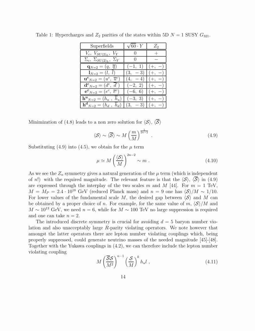
Table 1: Hypercharges and Z2 parities of the states within 5D N = 1 SUSY G321.

Superfields√

60 · Y Z2

Vc, VSU(2)L, VY 0 +

Σc, ΣSU(2)L, ΣY 0 −

qN=2 = (q, q) (−1, 1) (+, −)

lN=2 = (l, l) (3, − 3) (+, −)uc

N=2 = (uc, uc) (4, − 4) (+, −)

dcN=2 = (dc, d

c) (−2, 2) (+, −)

ecN=2 = (ec, ec) (−6, 6) (+, −)

huN=2 = (hu , hu) (−3, 3) (+, −)

hdN=2 = (hd , hd) (3, − 3) (+, −)

Minimization of (4.8) leads to a non zero solution for 〈S〉, 〈S〉

〈S〉 ∼ 〈S〉 ∼ M(

m

M

) 1

2n−2

. (4.9)

Substituting (4.9) into (4.5), we obtain for the µ term

µ ≃ M

(

〈S〉M

)2n−2

∼ m . (4.10)

As we see the Zn symmetry gives a natural generation of the µ term (which is independentof n!) with the required magnitude. The relevant feature is that the 〈S〉, 〈S〉 in (4.9)are expressed through the interplay of the two scales m and M [44]. For m = 1 TeV,M = MP = 2.4 · 1018 GeV (reduced Planck mass) and n = 9 one has 〈S〉/M ∼ 1/10.For lower values of the fundamental scale M , the desired gap between 〈S〉 and M canbe obtained by a proper choice of n. For example, for the same value of m, 〈S〉/M andM ∼ 1013 GeV, we need n = 6, while for M ∼ 100 TeV no large suppression is requiredand one can take n = 2.

The introduced discrete symmetry is crucial for avoiding d = 5 baryon number vio-lation and also unacceptably large R-parity violating operators. We note however thatamongst the latter operators there are lepton number violating couplings which, beingproperly suppressed, could generate neutrino masses of the needed magnitude [45]-[48].Together with the Yukawa couplings in (4.2), we can therefore include the lepton numberviolating coupling

M

(

SSM2

)n−1 ( SM

)k

hul , (4.11)

14

which after substituting the appropriate VEVs [see (4.9), (4.10)] leads to the bi-linearoperator

µlhul , µl ∼(

〈S〉M

)k

µ . (4.12)

Due to this operator the sneutrino field can gain a VEV of the order 〈ν〉 ∼ µl

µO(100 GeV) ≡

sin ξO(100 GeV). The latter produces a neutrino-neutralino mixing which leads to a neu-trino mass through the see-saw type mechanism [46]

mν ∼ O(100 GeV) sin2 ξ , (4.13)

where sin ξ ∼ µl/µ (assuming that there is no alignment between the superpotential andthe soft SUSY breaking couplings). To have a neutrino mass <∼ 1 eV, in (4.13) we needsin ξ <∼ 3 · 10−6. With a µ-term ∼ m and k = 6, 5, 〈S/M〉 ∼ 1/10 - 1/15, from (4.12) wehave sin ξ ∼ 10−6 which gives mντ

∼ 0.1 eV, indeed the order of magnitude needed forexplaining the atmospheric neutrino anomaly.

The phases of hu, hd, S, S were not fixed by the couplings (4.5) , (4.6). The couplingsgiven above determine the transformation properties of the different states under the Zsymmetry φi → eiα(φi)φi [α(φi) is the phase of state φi, and its mirror φi has oppositephase). Due to the couplings in (4.2), (4.5), (4.6), (4.11) we have

α(S) = α − α(S) , α(hd) = α − α(hu) ,

α(dc) = −α(q) + α(hu) − α , α(l) = −α(hu) − kα(S) + α ,

α(uc) = −α(q) − α(hu) , α(ec) = 2α(hu) + kα(S) − 2α , α =2π

n, (4.14)

where α(q), α(hu), α(S) are undetermined. Other allowed R parity breaking operatorsalso violating the lepton number are

( SM

)k

qdcl ,( S

M

)k

ecll . (4.15)

After substituting VEV of S they lead to the couplings

λqdcl , λ′ecll , λ ∼ λ′ ∼(

〈S〉M

)k

. (4.16)

These couplings induce neutrino masses at one loop, with the dominant contribution givenby the bc state inside the loop,

mν′ ∝ λ2

8π2

m2bm

m2b

, (4.17)

15

which for k = 4 − 6, 〈S〉/M ∼ 1/10, m = 1 TeV, mb = 300 GeV is evaluated asm′

ν ∼ (10−2 − 3 · 10−6) eV, to explain the solar neutrino puzzle either through MSW (bylarge or small angle, depending on which mixing scenario is realized for the fermion sector)or large angle vacuum oscillations (LAVO). This way of neutrino mass generation throughproperly suppressed R parity violating operators [45]-[48] looks attractive since it doesnot require the introduction of right handed neutrinos. However, additional symmetries(in this case Z) are crucial [47], [48] for obtaining properly suppressed neutrino masses.

With the assignments (4.14) and taking α(q) = α/2, α(hu) = α, α(S) = α/3 thediscrete symmetry introduced would be Z6n. With the phases presented, the S3n and otherhigher order terms are allowed, but along the (4.9) solution they are strongly suppressedin comparison to terms in (4.6), (4.7). Therefore, the analyzes above stay valid. One canalso verify that for any integer k the baryon number violating d = 4 operator ucdcdc isforbidden. Also, the baryon number violating d = 5 operators

1

Mqqql ,

1

Mucucdcec ,

1

Mqqqhd (4.18)

are not allowed. There are also d = 6 baryon number violating D-term operators

1

M2

[

qquc+ec+]

D,

1

M2

[

qluc+dc+]

D,

1

M2

[

qhduc+dc+

]

D, (4.19)

which for low values of M can become important and induce nucleon decay. It is easy tocheck that they are also forbidden by the Z = Z6n symmetry.

Unstable LSPWith the presence of R parity violating couplings, the LSP - the lightest neutralino χ

- is an unstable particle. In the scenario considered, the LSP three body decays mostlyproceed due to the bi-linear (4.12) coupling, and the LSP lifetime is

τ−1χ = µ2

l Z2χH

(

1

4+ sin2 θW +

4

3sin4 θW

) G2F m3

χ

192π3. (4.20)

For the value µl ∼ 10−6µ ∼ 10−3 GeV (dictated from the atmospheric neutrino scale)we have τχ ∼ 10−20 sec. Therefore the LSP would be cosmologically irrelevant and someother candidate for cold dark matter should be found.

4.1 Gauge coupling unification in 5D SUSY G321

Below the compactification scale µ0 the field content is just that of the MSSM and thecorresponding b factors are

(b1, b2, b3) =(

33

5, 1, − 3

)

. (4.21)

16

Above the µ0 scale the KK states enter into the renormalization. Having KK excitationsfor all gauge and scalar superfields and also for η families of bulk matter, the b factors,corresponding to the power law running (3.8), are

(b1, b2, b3) =(

6

5,−2,−6

)

+ 4η (1, 1, 1) . (4.22)

From (3.14)-(3.16), taking into account (3.8), (4.21), (4.22), we obtain

α−13 =

12

7α−1

2 − 5

7α−1

1 − 6

7πS, (4.23)

lnMG

MZ

=5π

14(α−1

1 − α−12 ) − 4

7S, (4.24)

α−1G = α−1

2 − 1

2πln

MG

MZ

+1 − 2η

πS, (4.25)

where MI = MG was taken since there is no intermediate scale . α−11 , α−1

2 are known withhigh precision and α−1

3 with some precision and thus, eq.(4.23) sets a constraint to thevalues of S. With α−1

1 = 59, α−12 = 29.6 and 0.117 ≤ α3 ≤ 0.121 we get

0.19 ≤ S ≤ 1.23 . (4.26)

From eq.(4.24) we see that the unification scale is also constrained:

MG ≃ (1 − 2) · 1016 GeV. (4.27)

From the definition (3.8) of S and (4.26), (4.27) a constraint to the values of N0, thenumber of KK levels, arises. It is not difficult to see that N0 = 1, 2 are the only valuesof N0 allowed for 0.19 ≤ S ≤ 1.23. Two examples of unification for these values of N0 are(

N0,MG

µ0

,MG

GeV, α3

)

=(

1, 1.3, 1.7 · 1016, 0.117)

,(

2, 2, 1.3 · 1016, 0.119)

. (4.28)

The question may arise whether taking into account some threshold corrections willchange the results or not. In fact, the SUSY threshold corrections would introduce ad-ditional terms in (4.23)-(4.25), which can be important for the predictions of α3. Thesethreshold corrections can be characterized by one ’threshold scale’ MSUSY and change

the strong coupling as [13] α′3−1 = α−1

3 + 1928π

ln MSUSY

MZ, where α−1

3 is given in (4.23). For

100 GeV < MSUSY < 1 TeV inequality (4.26) is modified to 0.26 ≤ S ≤ 3.13, whichwould change MG not more than by factor of 3. As we see, there is no qualitative change,but scales can be modified slightly. Because of this, throughout the paper we will nottake into account this type of threshold corrections. Apart from this, on the 4D fixed

17

points N = 1 SUSY invariant kinetic terms are allowed, which in general could alterthe unification picture [49]. However, if the size of extra dimension(s) is relatively large1/R = µ0 ≪ M(=fundamental scale), then contributions from localized kinetic termswill be negligible [20]. The condition µo ≪ M holds for the low scale unification scenar-ios considered below and is also crucial for avoiding unwanted effects from other braneoperators (see Appendix A).

Low scale unificationBy a look at the equations (4.23), (4.24) we recognize that to have low scale unification

it is important that the last term in eq.(4.24) is a large negative number, while the KKcontributions in (4.23) must be small or vanish. Thus, to have low scale unification weneed some extension as to cancel the last term in (4.23) and to keep the negative lastterm in (4.24). Among a few possible extensions [29]-[31], the simplest one seems to be

the model of ref. [30], where states E(i)N=2 = (E, E)(i) (i = 1, 2) were introduced. The

E(i), E(i)

states are singlets of SU(3)c, SU(2)L and carry hypercharges 6, −6, resp., inthe 1/

√60 units (4.1). With the Z2 parities

(E(1), E(2)

) ∼ + , (E(2), E(1)

) ∼ − , (4.29)

only the E(1), E(2)

states will have zero modes. The contribution of the E(1,2)N=2 states to

the b factors is then

∆E(b1, b2, b3) =(

12

5, 0, 0

)

, (4.30)

while the b factors corresponding to the logarithmic runnings get the additions

∆E(b1, b2, b3) =(

6

5, 0, 0

)

. (4.31)

Taking these into account we have

α−13 =

12

7α−1

2 − 5

7α−1

1 +3

7πln

MG

ME

, (4.32)

lnMG

MZ

=5π

14(α−1

1 − α−12 ) − 3

14ln

MG

ME

− S, (4.33)

and

α−1G = α−1

2 − 1

2πln

MG

MZ+

1 − 2η

πS , (4.34)

where ME is the 4D mass of E(1), E(2)

written as a brane coupling. In this setting theKK modes do not contribute in (4.32). To have a reasonable value for α3 one has totake ME ≃ MG. The GUT scale MG can be as low as we like. With MG/µ0 ≃ 30,

18

N0 = 29 we have S = 27.38 and from (4.33) we obtain MG ≃ 25 TeV. For η = 0 in (4.34)the αG remains in the perturbative regime. Although the value of ME is much higher

than µ0, the form of the power law function S of (3.8) is not affected by the MEE(1)E(2)

brane coupling. In appendix A we study the possible brane operator effects on RGE andshow that for µ0 ≪ MG they do not affect the expressions of (3.8), (3.10). Therefore theanalysis carried out through eqs. (4.32)-(4.34) remains valid.

5 5D SUSY SU(5) GUT on S(1)/Z2 × Z ′2 orbifold

We start our study of GUT orbifold models with the 5D N = 1 SUSY SU(5) theory. Thefifth dimension is compact and is considered to be an S(1)/Z2 × Z ′

2 orbifold. Two Z2’sare necessary to avoid extra zero mode states. In the notation of sect. 2, the 4D N = 1gauge supermultiplet V (24) in G321 terms splits up as

V (24) = Vc(8, 1)0 + VSU(2)L(1, 3)0 + Vs(1, 1)0 + VX(3, 2)5 + VY (3, 2)−5 , (5.1)

where subscripts are the hypercharge Y in the 1/√

60 units of (4.1). The decompositionof Σ(24) will be similar to (5.1).

We ascribe to the fragments of V (24) and Σ(24) the following Z2 × Z ′2 parities

(

Vc, VSU(2)L, Vs

)

∼ (+, +) , (VX , VY ) ∼ (−, +) ,

(

Σc, ΣSU(2)L, Σs

)

∼ (−, −) , (ΣX , ΣY ) ∼ (+, −) . (5.2)

With this assortment all the couplings in (2.3) remain invariant. From the N = 2 SUSYSU(5) gauge supermultiplet only the N = 1 gauge superfields of G321 have zero modes.Therefore, at the y = 0 fixed point (brane) we have a N = 1 SUSY G321 gauge theory.The other states, including the X, Y gauge bosons which would induce d = 6 nucleondecay, are projected out.

To have two MSSM Higgs doublets, one should introduce two N = 2 supermultipletsHN=2 = (H, H), H′

N=2 = (H ′, H′) where H , H ′ are 5-plets of SU(5). In terms of G321

H(5) = hu(1, 2)−3 + T (3, 1)2 , H(5) = hd(1, 2)3 + T (3, 1)−2 , (5.3)

and similarly for H ′, H′. H and H

′are mirrors of H and H ′ resp. With the following

assignment of orbifold parities

(hu, hd′) ∼ (+, +) , (hd, hu

′) ∼ (−, −) , (T, T′) ∼ (−, +) , (T , T ′) ∼ (+, −) , (5.4)

the states hu, hd′ have zero modes, which we identify with one pair of MSSM Higgs

doublets. As we can see, all colored triplet states are projected out and therefore will not

19

participate in the d = 5 nucleon decays. All couplings in (2.4) are invariant under theZ2 × Z ′

2 symmetry except the MΦΦΦ type couplings, which thus are not allowed. Thismeans that on the 5D level the huhd

′ coupling is absent due to N = 2 SUSY, while huhd

and hu′hd

′ are not allowed by the orbifold parities.Concerning the matter sector in SU(5) we have anomaly free 10, 5 multiplets, one

per generation. If at the level of the 5D SUSY theory we wish to introduce them as bulkfields, we should embed them into the N = 2 matter supermultiplets. Per generation wethen have XN=2 = (10, 10) and VN=2 = (5, 5), where 10 and 5 are mirrors of 10 and 5resp. In terms of G321 this reads

10 = ec(1, 1)−6 + q(3, 2)−1 + uc(3, 1)4 , 5 = l(1, 2)3 + dc(1, 3)−2 . (5.5)

Attempting to assign appropriate orbifold parities to the mirrors and to project them out,one can easily realize that due to the parities (5.2) of the gauge fields, some of the statesin (5.5) will not have zero modes. To overcome this difficulty one can introduce copies([20] and first refs. in [21]) X ′

N=2, V ′N=2 where exactly those states are allowed to have

zero modes which correspond to the MSSM states which come from XN=2 and VN=2 andare projected out. With orbifold parity prescriptions

(

q, l, uc′, dc′, ec′)

∼ (+, +) , (q′, l′, uc, dc, ec) ∼ (−, +) , (5.6)

and opposite ones for the corresponding mirrors, it is easy to verify that now the scenariois compatible with the bulk construction since all terms (except the mass term) of (2.4)are invariant.

An alternative possibility would be to introduce fermionic states only on the y = 0fixed point brane. This case can appear in string models with intersecting branes [23].Thus, in general one can have 3−η of generations living at the brane only and η generationsliving also in the bulk. For the latter case we have to introduce η copies. This applies notonly for the SU(5) model, but also for the other scenarios considered below.

Fixed point brane couplings at y = 0and some phenomenologyAt the y = 0 fixed point we are left with a SUSY G321 gauge theory with states q,

l, uc′, dc′, ec′, hu, hd′, which is just the field content of the MSSM. Since the 5D action

does not provide any Yukawa couplings, we should write appropriate couplings on thebrane. The 4D Yukawa superpotential, responsible for the generation of up-down quarkand lepton masses, has the form

WY = quc′hu + qdc′hd′ + lec′hd

′ . (5.7)

Since states with primes and without primes come from different unified multiplets, in thiscase we do not have any asymptotic relations between fermion masses. This avoids the

20

problem (ii) of fermion masses which exists in the minimal SU(5) GUT. Also, since thecolored triplets are projected out, the DT splitting problem (iii) as well as the problem(i) caused by d = 5 colored triplet exchange nucleon decay do not exist any more.

However, the problem due to general d = 5 baryon number violating operators and theµ problem are still unresolved on the 4D level (as in the case of the MSSM) unless someadditional mechanism is applied. One way for resolving these problems is to impose acontinuous R symmetry [20], [18], which in orbifold constructions emerges on the 4D levelafter compactification as an U(1)R symmetry [20]. The latter can guarantee baryon num-ber conservation, a suppressed µ term and automatic matter parity. Here and throughoutthe paper, alternatively, we impose a discrete Z symmetry which allows some matterparity/lepton number violating operators responsible for the generation of appropriatelysuppressed neutrino masses. In the spirit of sect. 4, we also introduce S, S singlets. Withthe transformations (4.4) for SS and for doublets (4.3) (here in all couplings hd must bereplaced by hd

′) the relevant couplings will be precisely the same as in (4.5) and (4.6).Through the couplings in (4.8) the VEV in (4.9) is obtained and consequently a µ termof the (4.10) right magnitude is generated.

Since the minimal SUSY SU(5) does not involve right handed neutrino states theneutrinos are massless. To give them mass, we also include, together with the Yukawacouplings (5.7), the lepton number violating bi-linear coupling (4.11), which (as discussedin sect. 4) induces the neutrino mass (4.13). For k = 2, 〈S/M〉 ∼ 10−3 according to(4.12) we obtain mντ

∼ 0.1 eV, a desirable value to explain the atmospheric anomaly.With the couplings in (5.7), (4.5), (4.6), (4.11) and taking into account the unified

SU(5) multiplets on 5D level we have

α(S) = α − α(S) , α(hd′) = α − α(hu) ,

α(uc′) = α(ec′) = kα(S) + 2α(hu) − 2α , α(dc′) = kα(S) + 4α(hu) − 3α ,

α(l) = −kα(S) − α(hu) + α , α(q) = −kα(S) − 3α(hu) + 2α , α =2π

n, (5.8)

where α(hu), α(S) are undetermined. This still allows the lepton number violating cou-plings (4.15) , giving for k = 2, 〈S〉/M ∼ 10−3 a radiative neutrino mass m′

ν ∼ 3 ·10−6 eV[see eq. (4.17), (4.16)]. This is the relevant scale for explaining the solar neutrino puzzlethrough the large angle vacuum oscillations of the νe state into the νµ,τ .

As we will see in the next subsection, the scale of unification is close to 1016 GeV.Assuming that the cutoff scale M has the same magnitude for S/M ∼ 10−3 in (4.9) weneed n = 3. If in the eqs. (5.8) one takes k = 2, n = 3, α(hu) = α/4, α(S) = α/3 thediscrete symmetry would be Z12n and one can verify that baryon number violating d = 5operators qqql, uc′uc′dc′ec′ are forbidden. Also, all other R-parity and baryon numberviolating couplings are absent in this scenario.

21

5.1 Gauge coupling unification in 5D SUSY SU(5)

Below the compactification scale µ0, we have precisely the MSSM field content with theb factors given in (4.21), while above µ0, due to the Z2 × Z ′

2 parities of the states givenin (5.2), (5.4) and for η generations of (5.6) in the bulk, we have

(γ1, γ2, γ3) =(

6

5, − 2, − 6

)

+ 4η(1, 1, 1) ,

(δ1, δ2, δ3) =(

−46

5, − 6, − 2

)

+ 4η(1, 1, 1) . (5.9)

From this and (3.14)-(3.16), and taking into account (3.9), we get

α−13 =

12

7α−1

2 − 5

7α−1

1 − 6

7π(S1 − S2) , (5.10)

lnMG

MZ

=5π

14(α−1

1 − α−12 ) − 4

7(S1 − S2) , (5.11)

α−1G = α−1

2 − 1

2πln

MG

MZ+

1 − 2η

πS1 +

3 − 2η

πS2 . (5.12)

(Here we do not have an intermediate scale and we take MI = MG.) We see that con-tributions to (5.10), (5.11) from the power law functions S1, S2 [defined in (3.10)] arecanceled out in the limit S1 = S2. This is understandable, since in this limit the SU(5)symmetry is restored above the µ0 scale and there are only contributions from completeSU(5) multiplets [according to (5.9) γa + δa =const.]. To have a reasonable value for α3

one needs S1 − S2 ≃ 0, which means MG/µ0 ≃ 1 leading to S1 ≃ S2 ≃ 0. Because of this,from (5.11) we get MG ≃ 2 · 1016 GeV. The value of αG in (5.12) remains perturbativefor η = 0− 3. Thus in contrast to the 5D SUSY G321 scenario, it is impossible to get lowscale unification within the orbifold SU(5) scenario.

6 Step by step compactification and

power law unification

In the previous section we have seen that within orbifold SU(5) GUT a power law unifi-cation does not take place. Although above the µ0 = 1/R scale each coupling of G321 haspower law running, the renormalization of their relative slope (e.g. running of α−1

i −α−1j )

is still logarithmic because above µ0 the full SU(5) multiplets participate in renormaliza-tion. Because of this, one does not get low scale unification. This result would be the samefor any higher dimensional orbifold GUT scenario with semisimple gauge group [such asSO(10), SU(5 + N), E6, E8, · · · ] if the compactification of all extra dimensions occurs

22

at a single mass scale. Then representations of all gauge groups listed above again canbe decomposed to complete SU(5) multiplets. Low scale unification within GUT modelswith orbifold extra dimensions is however possible if we allow for compactifications ofvarious extra dimensions at different mass scales. Suppose, we have a GUT model withgauge group G and with two extra spacial dimensions, and assume compactification intwo steps with scales 1

R′≫ 1

Rwith a symmetry breaking chain

G1/R′

−→ H 1/R−→ H1 . (6.1)

For having power law unification it is crucial that H must be different from SU(5) andalso must not contain it as a subgroup. Then the field content of H, relevant between1R′

and 1R, will not constitute full SU(5) multiplets. This would give us the possibility

of low scale unification. The bottom-up picture of such a scenario looks as follows: atan energy scale µ0 = 1

Rthe gauge group H1 is ’restored’ to H and above µ0 KK states

in incomplete multiplets give power law differential running (of α−1i − α−1

j ). The gap1R′

≫ 1R

must be big enough to reduce the ’intermediate’ scale µ0 [see eq. (3.15), whichgives a low intermediate scale MI in case of large S (or S1, S2) and a negative coefficient;a similar expression can be derived for scale µ0 in case of several compactification massscales]. Scale 1

R′is close to MG: note, that the case with 1

R′≪ MG will not work because

above 1R′

the unification group G is restored and its full multiplets would be ’alive’.In order to realize this idea, the gauge group G a) must be higher (in rank) than

SU(5); b) should have subgroups different from SU(5) and c) its subgroups must give arealistic phenomenology, e.g. they should contain the G321 gauge group and MSSM states.One of the groups, which has these properties, is SO(10). Its maximal subgroups areSU(4)c×SU(2)L ×SU(2)R ≡ G422 and flipped SU(5)×U(1) ≡ G51. It is straightforwardto study compactification breaking of these groups and to see what is going on abovethe scale µ0 = 1

R. Since for power law unification the region between 1

Rand 1

R′≃ MG is

relevant, we can consider five dimensional G422 and G51 orbifold models. As we will see inthe following sections this type of bottom-up approach turns out to be quite transparentand convenient for studying various phenomenological issues together with gauge couplingunification.

7 5D SU(4)c × SU(2)L × SU(2)R N = 1 SUSY model

on S(1)/Z2 × Z ′2 orbifold

In the following we consider a supersymmetric SU(4)c ×SU(2)L ×SU(2)R ≡ G422 modelin five dimensions (5D). V (15c) the adjoint of SU(4)c, in SU(3)c × U(1)′ terms reads

V (15c) = Vs(1)0 + Vc(8)0 + Vt(3)4 + Vt(3)−4 , (7.1)

23

where subscripts denote U(1)′ charges in 1/√

24 units (SU(4)c normalization):

YU(1)′ =1√24

Diag(1 , 1 , 1 , − 3) . (7.2)

The decomposition of Σ(15c) is identical.The decomposition of the SU(2)R’s adjoints through the SU(2)R → U(1)R channel

has the formV (3R) = VR(1)0 + Vp(1)2 + Vp(1)−2 , (7.3)

and the same for Σ(3R). Here subscripts denote U(1)R charges in 1/2 units:

YU(1)R=

1

2Diag(1 , − 1) . (7.4)

Matter sector. We introduce η generations of N = 2 chiral supermultiplets

FN=2 = (F , F ) , FcN=2 = (F c , F

c) , (7.5)

where under G422

F ∼ (4 , 2 , 1) , F c ∼ (4 , 1 , 2) , (7.6)

F = (q , l) , F c = (uc , dc , νc , ec), (7.7)

and also η generations of ’copies’

F′N=2 = (F ′ , F

′) , F′c

N=2 = (F ′c , F′c) . (7.8)

with precisely the same content and transformation properties as FN=2 and FcN=2 resp.

The remaining 3 − η generations at the fixed point have the same massless field contentas the η bulk generations. Note that the introduction of copies is crucial if one wants aZ2 × Z ′

2 orbifold invariant 5D action, with matter both in the bulk and on a fixed point,which reduces at low energies to the chiral content of the MSSM, extended only by righthanded neutrino states.

Scalar sector. We need two sets of scalars. First we introduce hypermultiplets, whichwill contain the two Higgs doublet superfields of the MSSM.

ΦN=2 = (Φ , Φ) , Φ′N=2 = (Φ′ , Φ

′) , (7.9)

where under G422

Φ ∼ (1 , 2 , 2) , Φ ∼ (1 , 2 , 2) . (7.10)

24

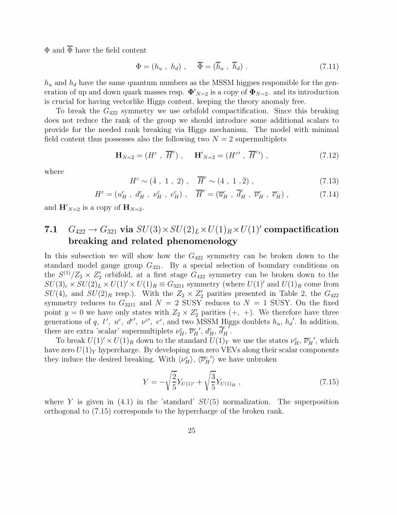
Φ and Φ have the field content

Φ = (hu , hd) , Φ = (hu , hd) . (7.11)

hu and hd have the same quantum numbers as the MSSM higgses responsible for the gen-eration of up and down quark masses resp. Φ′

N=2 is a copy of ΦN=2. and its introductionis crucial for having vectorlike Higgs content, keeping the theory anomaly free.

To break the G422 symmetry we use orbifold compactification. Since this breakingdoes not reduce the rank of the group we should introduce some additional scalars toprovide for the needed rank breaking via Higgs mechanism. The model with minimalfield content thus possesses also the following two N = 2 supermultiplets

HN=2 = (Hc , Hc) , H′

N=2 = (Hc ′ , Hc ′) , (7.12)

whereHc ∼ (4 , 1 , 2) , H

c ∼ (4 , 1 , 2) , (7.13)

Hc = (ucH , dc

H , νcH , ec

H) , Hc= (uc

H , dc

H , νcH , ec

H) , (7.14)

and H′N=2 is a copy of HN=2.

7.1 G422 → G321 via SU(3)×SU(2)L×U(1)R×U(1)′ compactification

breaking and related phenomenology

In this subsection we will show how the G422 symmetry can be broken down to thestandard model gauge group G321. By a special selection of boundary conditions onthe S(1)/Z2 × Z ′

2 orbifold, at a first stage G422 symmetry can be broken down to theSU(3)c × SU(2)L ×U(1)′ ×U(1)R ≡ G3211 symmetry (where U(1)′ and U(1)R come fromSU(4)c and SU(2)R resp.). With the Z2 × Z ′

2 parities presented in Table 2, the G422

symmetry reduces to G3211 and N = 2 SUSY reduces to N = 1 SUSY. On the fixedpoint y = 0 we have only states with Z2 × Z ′

2 parities (+, +). We therefore have threegenerations of q, l ′, uc, dc′, νc′, ec, and two MSSM Higgs doublets hu, hd

′. In addition,there are extra ’scalar’ supermultiplets νc

H , νcH

′, dcH , d

c

H

′.

To break U(1)′ ×U(1)R down to the standard U(1)Y we use the states νcH , νc

H′, which

have zero U(1)Y hypercharge. By developing non zero VEVs along their scalar componentsthey induce the desired breaking. With 〈νc

H〉, 〈νcH

′〉 we have unbroken

Y = −√

2

5YU(1)′ +

√

3

5YU(1)R

, (7.15)

where Y is given in (4.1) in the ’standard’ SU(5) normalization. The superpositionorthogonal to (7.15) corresponds to the hypercharge of the broken rank.

25

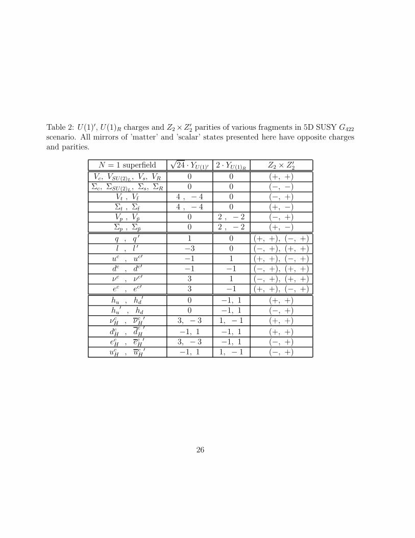
Table 2: U(1)′, U(1)R charges and Z2×Z ′2 parities of various fragments in 5D SUSY G422

scenario. All mirrors of ’matter’ and ’scalar’ states presented here have opposite chargesand parities.

N = 1 superfield√

24 · YU(1)′ 2 · YU(1)RZ2 × Z ′

2

Vc, VSU(2)L, Vs, VR 0 0 (+, +)

Σc, ΣSU(2)L, Σs, ΣR 0 0 (−, −)

Vt , Vt 4 , − 4 0 (−, +)Σt , Σt 4 , − 4 0 (+, −)Vp , Vp 0 2 , − 2 (−, +)Σp , Σp 0 2 , − 2 (+, −)

q , q ′ 1 0 (+, +), (−, +)l , l ′ −3 0 (−, +), (+, +)

uc , uc′ −1 1 (+, +), (−, +)dc , dc′ −1 −1 (−, +), (+, +)νc , νc′ 3 1 (−, +), (+, +)ec , ec′ 3 −1 (+, +), (−, +)

hu , hd′ 0 −1, 1 (+, +)

hu′ , hd 0 −1, 1 (−, +)

νcH , νc

H′ 3, − 3 1, − 1 (+, +)

dcH , d

c

H

′ −1, 1 −1, 1 (+, +)ec

H , ecH

′ 3, − 3 −1, 1 (−, +)uc

H , ucH

′ −1, 1 1, − 1 (−, +)

26

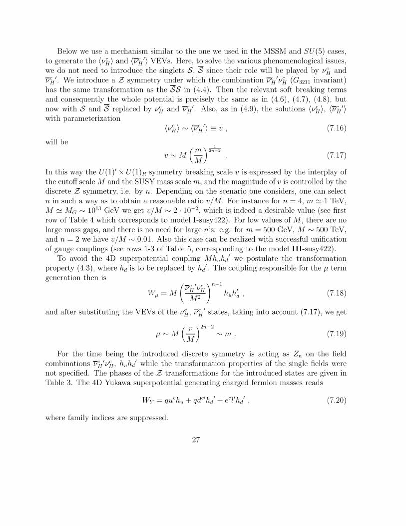
Below we use a mechanism similar to the one we used in the MSSM and SU(5) cases,to generate the 〈νc

H〉 and 〈νcH

′〉 VEVs. Here, to solve the various phenomenological issues,we do not need to introduce the singlets S, S since their role will be played by νc

H andνc

H′. We introduce a Z symmetry under which the combination νc

H′νc

H (G3211 invariant)has the same transformation as the SS in (4.4). Then the relevant soft breaking termsand consequently the whole potential is precisely the same as in (4.6), (4.7), (4.8), butnow with S and S replaced by νc

H and νcH

′. Also, as in (4.9), the solutions 〈νcH〉, 〈νc

H′〉

with parameterization〈νc

H〉 ∼ 〈νcH

′〉 ≡ v , (7.16)

will be

v ∼ M(

m

M

) 1

2n−2

. (7.17)

In this way the U(1)′ ×U(1)R symmetry breaking scale v is expressed by the interplay ofthe cutoff scale M and the SUSY mass scale m, and the magnitude of v is controlled by thediscrete Z symmetry, i.e. by n. Depending on the scenario one considers, one can selectn in such a way as to obtain a reasonable ratio v/M . For instance for n = 4, m ≃ 1 TeV,M ≃ MG ∼ 1013 GeV we get v/M ∼ 2 · 10−2, which is indeed a desirable value (see firstrow of Table 4 which corresponds to model I-susy422). For low values of M , there are nolarge mass gaps, and there is no need for large n’s: e.g. for m = 500 GeV, M ∼ 500 TeV,and n = 2 we have v/M ∼ 0.01. Also this case can be realized with successful unificationof gauge couplings (see rows 1-3 of Table 5, corresponding to the model III-susy422).

To avoid the 4D superpotential coupling Mhuhd′ we postulate the transformation

property (4.3), where hd is to be replaced by hd′. The coupling responsible for the µ term

generation then is

Wµ = M

(

νcH

′νcH

M2

)n−1

huh′d , (7.18)

and after substituting the VEVs of the νcH , νc

H′ states, taking into account (7.17), we get

µ ∼ M(

v

M

)2n−2

∼ m . (7.19)

For the time being the introduced discrete symmetry is acting as Zn on the fieldcombinations νc

H′νc

H , huhd′ while the transformation properties of the single fields were

not specified. The phases of the Z transformations for the introduced states are given inTable 3. The 4D Yukawa superpotential generating charged fermion masses reads

WY = quchu + qdc′hd′ + ecl′hd

′ , (7.20)

where family indices are suppressed.

27

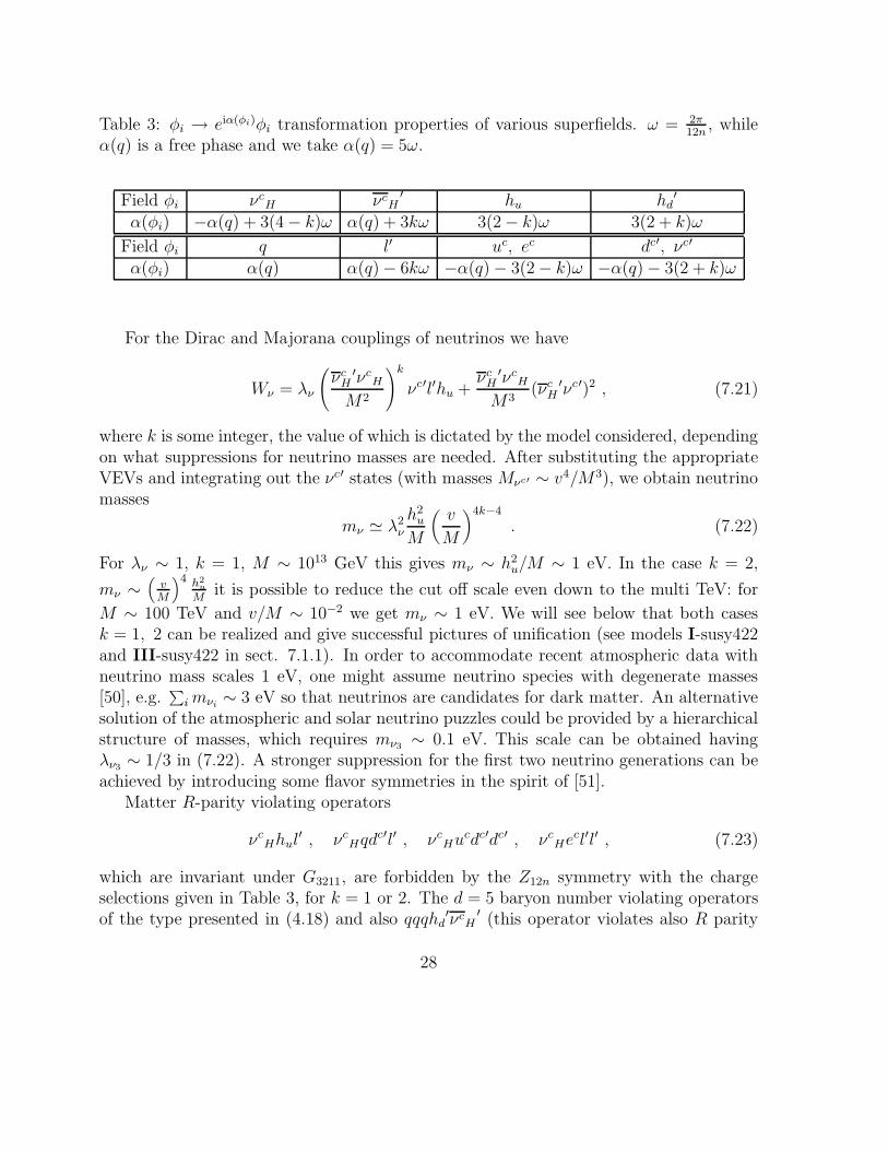
Table 3: φi → eiα(φi)φi transformation properties of various superfields. ω = 2π12n

, whileα(q) is a free phase and we take α(q) = 5ω.

Field φi νcH νc

H′ hu hd

′

α(φi) −α(q) + 3(4 − k)ω α(q) + 3kω 3(2 − k)ω 3(2 + k)ω

Field φi q l′ uc, ec dc′, νc′

α(φi) α(q) α(q) − 6kω −α(q) − 3(2 − k)ω −α(q) − 3(2 + k)ω

For the Dirac and Majorana couplings of neutrinos we have

Wν = λν

(

νcH

′νcH

M2

)k

νc′l′hu +νc

H′νc

H

M3(νc

H′νc′)2 , (7.21)

where k is some integer, the value of which is dictated by the model considered, dependingon what suppressions for neutrino masses are needed. After substituting the appropriateVEVs and integrating out the νc′ states (with masses Mνc′ ∼ v4/M3), we obtain neutrinomasses

mν ≃ λ2ν

h2u

M

(

v

M

)4k−4

. (7.22)

For λν ∼ 1, k = 1, M ∼ 1013 GeV this gives mν ∼ h2u/M ∼ 1 eV. In the case k = 2,

mν ∼(

vM

)4 h2u

Mit is possible to reduce the cut off scale even down to the multi TeV: for

M ∼ 100 TeV and v/M ∼ 10−2 we get mν ∼ 1 eV. We will see below that both casesk = 1, 2 can be realized and give successful pictures of unification (see models I-susy422and III-susy422 in sect. 7.1.1). In order to accommodate recent atmospheric data withneutrino mass scales 1 eV, one might assume neutrino species with degenerate masses[50], e.g.

∑

i mνi∼ 3 eV so that neutrinos are candidates for dark matter. An alternative

solution of the atmospheric and solar neutrino puzzles could be provided by a hierarchicalstructure of masses, which requires mν3

∼ 0.1 eV. This scale can be obtained havingλν3

∼ 1/3 in (7.22). A stronger suppression for the first two neutrino generations can beachieved by introducing some flavor symmetries in the spirit of [51].

Matter R-parity violating operators

νcHhul

′ , νcHqdc′l′ , νc

Hucdc′dc′ , νcHecl′l′ , (7.23)

which are invariant under G3211, are forbidden by the Z12n symmetry with the chargeselections given in Table 3, for k = 1 or 2. The d = 5 baryon number violating operatorsof the type presented in (4.18) and also qqqhd

′νcH

′ (this operator violates also R parity

28

and leads to a d = 5 baryon number violating coupling after the substitution of VEV〈νc

H′〉) are forbidden in this scenario for both choices k = 1 and k = 2. There are also

d = 6 (4.19) type operators allowed by G3211 symmetry and in addition the (qqdc′ +νc′ +)D

coupling. It is easy to check that these are absent due to the Z12n symmetry.In order that the 5D Lagrangian terms of (2.3), (2.4), allowed by the Z2 ×Z ′

2 orbifoldparities, are invariant under the introduced Z12n discrete symmetry, we must assure thatthe other fields transform properly. This is the case if α(F ) = α(q), α(F ′) = α(l′),

α(F c) = α(uc), α(F c′) = α(dc′), α(Φ) = α(hu), α(Φ′) = α(hd′), α(Hc) = α(νc

H), α(Hc′) =

α(νcH

′) (and all mirrors with opposite phases).

Since the states dcH and d

c

H

′transform as νc

H and νcH resp., their mass term is generated

through an operator (νcH

′νcH/M2)n−1Md

c

H

′dc

H and one gets Mdc

H∼ m. First of all we must

make sure that these triplet states do not cause nucleon decay. The allowed couplings ofdc

H , dc

H

′with matter are (νc

H′νc

H)n−1νcHql′dc

H and νcH

′ecucdc

H

′for k = 1, while for k = 2

the operators νcHql′dc

H and (νcH

′νcH)n−1νc

H′ecucd

c

H

′are permitted. However, the couplings

νcHucdc′dc

H and νcH

′qqdc

H

′are forbidden (see Table 3) and the baryon number violating

d = 5 operators qqql, ucucdc′ec do not emerge. The issue of gauge coupling unification inthis model , which we call I-susy422, will be studied below. As it turns out, successfulunification can be obtained for various scales as presented in Table 4. For the case shownin the first row we obtain v/M ∼ 2 · 10−2 (obtained for n = 4 according to (7.17)).This mass gap is crucial for µ-term generation with the correct magnitude. For thiscase we have Mdc

H≃ 10 TeV. The existence of colored triplet states with this mass can

have interesting phenomenological implications [52]. There might be a leptoquark likesignature [53], similar to what is expected within some R-parity violating models.

A different scenario, with heavy dcH , d

c

H

′states, can be constructed introducing addi-

tional two N = 2 supermultiplets 6(i)N=2 = (6, 6)(i) (i = 1, 2) of SU(4)c, where

6(i) = T (i)(3−2) + T(i)

(32) , 6(i) = T (i)(3−2) + T (i)(32) . (7.24)

With the Z2 × Z ′2 parity assignment

(T (1), T(2)

) ∼ (+, +), (T (2), T(1)

) ∼ (−, +) ,

(T (1), T (2)) ∼ (+, −) , (T (2), T (1)

) ∼ (−, −) , (7.25)

the triplet-antitriplet pair T (1), T(2)

will have zero modes and can therefore couple with

the dcH , d

c

H

′giving them large masses. With Z12n phases α(T (1)) = −2α(νc

H), α(T(2)

) =−2α(νc

H′) the relevant 4D superpotential couplings will thus be

WT = νcHdc

HT (1) + νcH

′dc

H

′T

(2). (7.26)

29

After substituting the VEVs of νcH , νc

H′, the triplet states acquire masses MT ∼ v. The al-

lowed couplings of the T (1), T(2)

states with matter, are (νcH

′νcH)kql′T

(2), (νc

H′νc

H)3−kecucT (1).

However, the couplings qqT (1), ucdc′T(2)

are forbidden by Z12n symmetry and baryon num-ber is still conserved. We refer to this model as II-susy422. Also in this case successfulunification of gauge couplings occurs if MI ≃ µ0 ≃ MG (see sect. 7.1.1). However, as wewill see, with a specific extension it is possible to get unification near the multi TeV region(see Table 5 for the model III-susy422, which presents mass scales for which unificationholds). For this case, since triplets get masses ∼ MI through the couplings (7.26), theirmasses are a few TeV, making this scenario testable in future collider experiments.

We conclude this section by noting that, together with a natural U(1)′×U(1)R break-ing pattern and µ-term generation, the Z12n symmetry provides automatic R-parity andbaryon number conservation within the 5D SUSY orbifold G422 model.

7.1.1 Gauge coupling unification in 5D SUSY with G422 → G3211

intermediate breaking

Here we will study the issue of gauge coupling unification for SUSY G422 model withcompactification breaking to G3211. Throughout this analysis we will use the expressionsobtained in section 3.

Model I-susy422The field content of this scenario is as follows. We have the scalar superfields of (7.9),

(7.12), which are necessary to obtain the pair of MSSM Higgs doublets and to realize thewanted G3211 breaking to G321. We also have η generations of F , F c presented in (7.5),and η copies, if η generations of matter have KK excitations. We then identify the scale ofU(1)R × U(1)′ symmetry breaking 〈νc

H〉 = 〈νcH

′〉 with the intermediate scale MI in (3.2),(3.3). Below MI , the gauge group is G321 and the field content is that of the MSSM with

the b-factors (4.21), plus the states dcH , d

c

H

′with a mass Mdc

Hin the range 100 GeV-1 TeV,

which have b-factors

bdc

H

i =(

2

5, 0 , 1

)

. (7.27)

Above the scale MI we have

(

bU(1)R, bU(1)′ , b2, b3

)MI

= (9, 7, 1, − 2) . (7.28)

With the Z2 × Z ′2 parities shown in Table 2, the corresponding γ and δ-factors of (3.9),

will be(

γU(1)R, γU(1)′ , γ2, γ3

)

= (6, 2, − 2, − 4) + 4η (1, 1, 1, 1) ,(

δU(1)R, δU(1)′ , δ2, δ3

)

= (2, − 6, 2, 0) + 4η (1, 1, 1, 1) . (7.29)

30

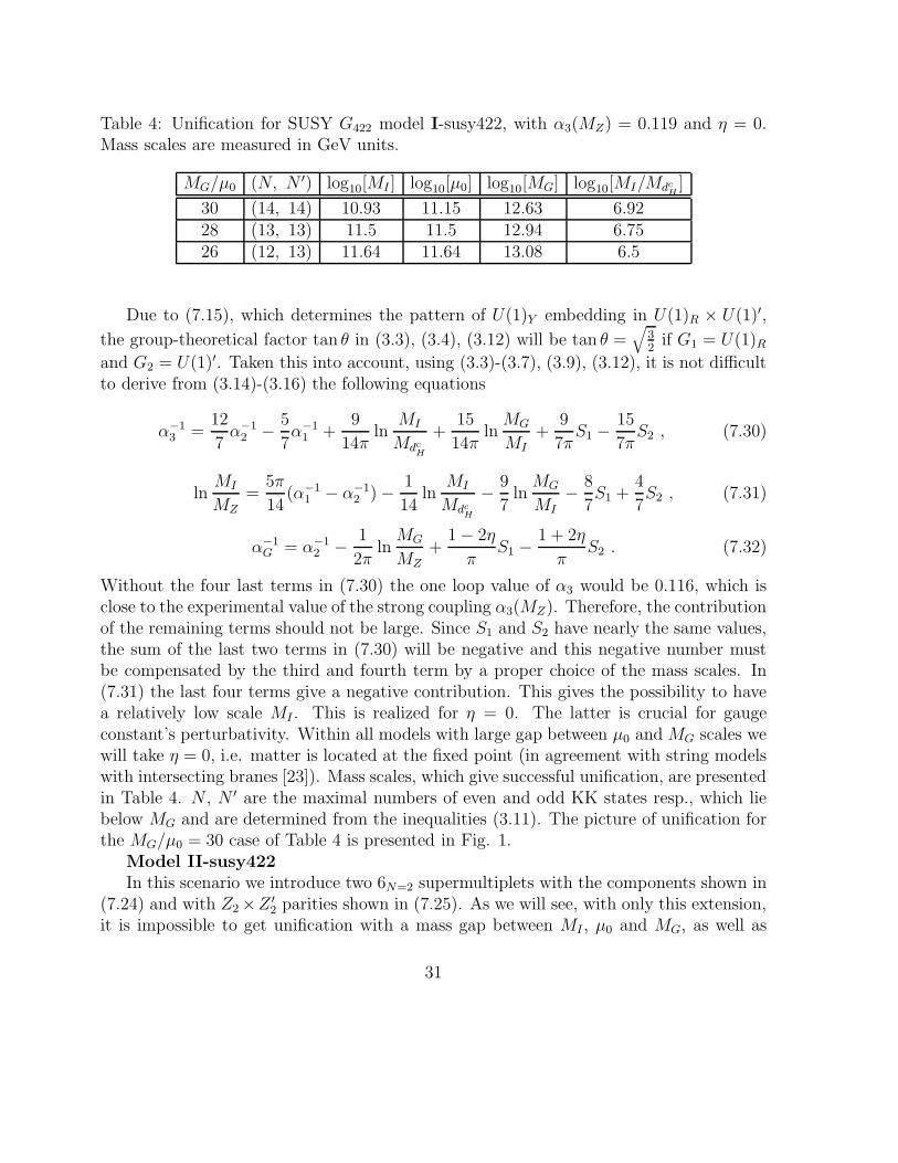
Table 4: Unification for SUSY G422 model I-susy422, with α3(MZ) = 0.119 and η = 0.Mass scales are measured in GeV units.

MG/µ0 (N, N ′) log10[MI ] log10[µ0] log10[MG] log10[MI/Mdc

H]

30 (14, 14) 10.93 11.15 12.63 6.9228 (13, 13) 11.5 11.5 12.94 6.7526 (12, 13) 11.64 11.64 13.08 6.5

Due to (7.15), which determines the pattern of U(1)Y embedding in U(1)R × U(1)′,

the group-theoretical factor tan θ in (3.3), (3.4), (3.12) will be tan θ =√

32

if G1 = U(1)R

and G2 = U(1)′. Taken this into account, using (3.3)-(3.7), (3.9), (3.12), it is not difficultto derive from (3.14)-(3.16) the following equations

α−13 =

12

7α−1

2 − 5

7α−1

1 +9

14πln

MI

Mdc

H

+15

14πln

MG

MI+

9

7πS1 −

15

7πS2 , (7.30)

lnMI

MZ=

5π

14(α−1

1 − α−12 ) − 1

14ln

MI

Mdc

H

− 9

7ln

MG

MI− 8

7S1 +

4

7S2 , (7.31)

α−1G = α−1

2 − 1

2πln

MG

MZ+

1 − 2η

πS1 −

1 + 2η

πS2 . (7.32)

Without the four last terms in (7.30) the one loop value of α3 would be 0.116, which isclose to the experimental value of the strong coupling α3(MZ). Therefore, the contributionof the remaining terms should not be large. Since S1 and S2 have nearly the same values,the sum of the last two terms in (7.30) will be negative and this negative number mustbe compensated by the third and fourth term by a proper choice of the mass scales. In(7.31) the last four terms give a negative contribution. This gives the possibility to havea relatively low scale MI . This is realized for η = 0. The latter is crucial for gaugeconstant’s perturbativity. Within all models with large gap between µ0 and MG scales wewill take η = 0, i.e. matter is located at the fixed point (in agreement with string modelswith intersecting branes [23]). Mass scales, which give successful unification, are presentedin Table 4. N , N ′ are the maximal numbers of even and odd KK states resp., which liebelow MG and are determined from the inequalities (3.11). The picture of unification forthe MG/µ0 = 30 case of Table 4 is presented in Fig. 1.

Model II-susy422In this scenario we introduce two 6N=2 supermultiplets with the components shown in

(7.24) and with Z2 ×Z ′2 parities shown in (7.25). As we will see, with only this extension,

it is impossible to get unification with a mass gap between MI , µ0 and MG, as well as

31

relatively low MG. But this can be achieved with a simple additional extension (modelIII-susy422).

Due to the couplings (7.26), all triplet zero mode states decouple on the MI = v scaleand consequently, below MI , the gauge coupling runnings will be precisely the same as in

the MSSM, with b-factors (4.21). Due to the presence of the T (1), T(2)

states, the b-factorswill be modified above MI and (7.28) will be changed by

∆6

(

bU(1)R, bU(1)′ , b2, b3

)MI

= (0, 1, 0, 1) . (7.33)

The γ and δ factors in (7.29) are modified by

∆6

(

γU(1)R, γU(1)′ , γ2, γ3

)

= ∆6

(

δU(1)R, δU(1)′ , δ2, δ3

)

= (0, 2, 0, 2) . (7.34)

(The subscript ’6’ in ∆6 indicates that the changes are due to states coming from the two6N=2 supermultiplets.) Taking all this into account, we have

α−13 =

12

7α−1

2 − 5

7α−1

1 +12

7πln

MG

MI

+18

7πS1 −

6

7πS2 , (7.35)

lnMI

MZ=

5π

14(α−1

1 − α−12 ) − 19

14ln

MG

MI− 9

7S1 +

3

7S2 . (7.36)

In (7.35) we see that the contribution of the last three terms is always positive and forreasonable α3 the only possibility is to have MI ≃ µ0 ≃ MG. Due to this fact, from (7.36)one can see that MI ≃ 2 · 1016 GeV.

Model III-susy422: low scale unificationHere we present an extension which gives low scale unification. In addition to the field

content of model II-susy422 we introduce two 2(j)N=2 = (D, D)(j) (j = 1, 2), which are

supermultiplets of SU(2)L. With Z2 × Z ′2 parities

(D(1), D(2)

) ∼ (+, +) , (D(2), D(1)

) ∼ (−, −) , (7.37)

only the states D(1), D(2)

have zero modes. The contributions to the bMI , γ, and δ-factors,due to 2

(j)N=2 supermultiplets, are

∆2

(

bU(1)R, bU(1)′ , b2, b3

)MI

= (0, 0, 1, 0) ,

∆2

(

γU(1)R, γU(1)′ , γ2, γ3

)

= (0, 0, 2, 0) , ∆2δi = 0 , (7.38)

and consequently we obtain

α−13 =

12

7α−1

2 − 5

7α−1

1 +12

7πln

MG

MI− 6

7πln

MG

MD+

6

7π(S1 − S2) , (7.39)

32

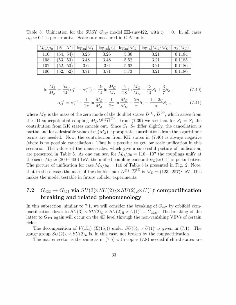
Table 5: Unification for the SUSY G422 model III-susy422, with η = 0. In all casesαG ≃ 0.1 is perturbative. Scales are measured in GeV units.

MG/µ0 (N, N ′) log10[MI ] log10[µ0] log10[MG] log10[MG/MD] α3(MZ)

110 (54, 54) 3.26 3.26 5.30 3.21 0.1184108 (53, 53) 3.48 3.48 5.52 3.21 0.1185107 (52, 53) 3.6 3.6 5.62 3.21 0.1186106 (52, 52) 3.71 3.71 5.73 3.21 0.1186

lnMI

MZ=

5π

14(α−1

1 − α−12 ) − 19

14ln

MG

MI+

5

28ln

MG

MD− 13

14S1 +

3

7S2 , (7.40)

α−1G = α−1

2 − 1

2πln

MG

MZ− 1

2πln

MG

MD− 2η

πS1 −

1 + 2η

πS2 , (7.41)

where MD is the mass of the zero mode of the doublet states D(1), D(2)

, which arises from

the 4D superpotential coupling MDD(1)D(2)

. From (7.39) we see that for S1 = S2 thecontribution from KK states cancels out. Since S1, S2 differ slightly, the cancellation ispartial and for a desirable value of α3(MZ), appropriate contributions from the logarithmicterms are needed. Now, the contribution from KK states in (7.40) is always negative(there is no possible cancellation). Thus it is possible to get low scale unification in thisscenario. The values of the mass scales, which give a successful picture of unification,are presented in Table 5. As one can see, for MG/µ0 = 110−107 the couplings unify atthe scale MG ≃ (200−400) TeV; the unified coupling constant αG(≃ 0.1) is perturbative.The picture of unification for case MG/µ0 = 110 of Table 5 is presented in Fig. 2. Note,

that in these cases the mass of the doublet pair D(1), D(2)

is MD ≃ (123−257) GeV. Thismakes the model testable in future collider experiments.

7.2 G422 → G321 via SU(3)×SU(2)L×SU(2)R×U(1)′ compactification

breaking and related phenomenology

In this subsection, similar to 7.1, we will consider the breaking of G422 by orbifold com-pactification down to SU(3) × SU(2)L × SU(2)R × U(1)′ ≡ G3221. The breaking of thelatter to G321 again will occur on the 4D level through the non-vanishing VEVs of certainfields.

The decomposition of V (15c) (Σ(15c)) under SU(3)c × U(1)′ is given in (7.1). Thegauge group SU(2)L × SU(2)R is, in this case, not broken by the compactification.

The matter sector is the same as in (7.5) with copies (7.8) needed if chiral states are

33

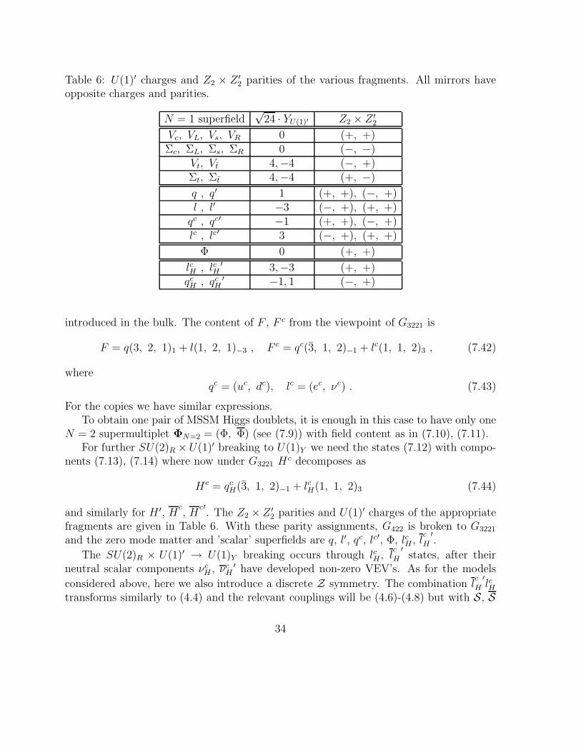
Table 6: U(1)′ charges and Z2 × Z ′2 parities of the various fragments. All mirrors have

opposite charges and parities.

N = 1 superfield√

24 · YU(1)′ Z2 × Z ′2

Vc, VL, Vs, VR 0 (+, +)Σc, ΣL, Σs, ΣR 0 (−, −)

Vt, Vt 4,−4 (−, +)Σt, Σt 4,−4 (+, −)

q , q′ 1 (+, +), (−, +)l , l′ −3 (−, +), (+, +)

qc , qc′ −1 (+, +), (−, +)lc , lc′ 3 (−, +), (+, +)

Φ 0 (+, +)

lcH , lcH′ 3,−3 (+, +)

qcH , qc

H′ −1, 1 (−, +)

introduced in the bulk. The content of F , F c from the viewpoint of G3221 is

F = q(3, 2, 1)1 + l(1, 2, 1)−3 , F c = qc(3, 1, 2)−1 + lc(1, 1, 2)3 , (7.42)

whereqc = (uc, dc), lc = (ec, νc) . (7.43)

For the copies we have similar expressions.To obtain one pair of MSSM Higgs doublets, it is enough in this case to have only one

N = 2 supermultiplet ΦN=2 = (Φ, Φ) (see (7.9)) with field content as in (7.10), (7.11).For further SU(2)R ×U(1)′ breaking to U(1)Y we need the states (7.12) with compo-

nents (7.13), (7.14) where now under G3221 Hc decomposes as

Hc = qcH(3, 1, 2)−1 + lcH(1, 1, 2)3 (7.44)

and similarly for H ′, Hc, H

c′. The Z2 × Z ′

2 parities and U(1)′ charges of the appropriatefragments are given in Table 6. With these parity assignments, G422 is broken to G3221

and the zero mode matter and ’scalar’ superfields are q, l′, qc, lc′, Φ, lcH , lc

H

′.

The SU(2)R × U(1)′ → U(1)Y breaking occurs through lcH , lc

H

′states, after their

neutral scalar components νcH , νc

H′ have developed non-zero VEV’s. As for the models

considered above, here we also introduce a discrete Z symmetry. The combination lc

H

′lcH

transforms similarly to (4.4) and the relevant couplings will be (4.6)-(4.8) but with S, S

34

replaced by lcH , lc

H

′. Thus, νc

H and νcH

′ which are components of lcH and lc

H

′resp. will

have non-vanishing VEV’s (7.16), (7.17). This provides the symmetry breaking down toG321 at an intermediate mass scale between the SUSY scale m and the unification scaleM . As a first example suppose that M ∼ 1016GeV in which case v ∼ 101610−7/(n−1)GeV.With n = 7 we get v <∼ M , the value needed to have successful high scale unification inthe I’-susy422 model (see below). On the other hand if the unification scale is as smallas M ∼ 106GeV, with n = 2 we obtain v ∼ 104GeV as needed in low scale unificationscenarios.

With Φ transforming under Z as

Φ → ei π

n Φ , (7.45)

the coupling responsible for the µ-term generation is

Wµ = M

lc

H

′lcH

M2

n−1

Φ2, (7.46)

and we obtain the same µ term as in (7.19). The 4D Yukawa superpotential, responsiblefor generation of up-down quark and charged lepton masses, is

WY = qqcΦ + l′lc′Φ . (7.47)

From this coupling the Dirac type coupling for the neutrinos is also generated and mDν ∼

me. There is therefore no additional suppression of the Dirac neutrino masses. For alow fundamental scale this turns out to be a problem. To overcome this difficulty we canintroduce an additional singlet state N . The relevant couplings are

1

M

(

lcH′lcH

M2

)k

N lcHΦl′ + lcH′lc′N . (7.48)

Due to the last term in (7.48) the state νc′ decouples at the scale 〈νcH〉 ≡ MI and the

first term, which violates lepton number, is suppressed by appropriate powers of MI/M .This can lead to a neutrino mass generation of the needed magnitude. It is not difficultto verify that together with the νc′ν ′hu coupling, the operators in (7.48) give

mν ∼(

MI

M

)2k 〈h0u〉2

M. (7.49)

Note that we consider MI ≪ M and therefore for k > 0 one can obtain the neededsuppression. For instance, with k = 1, 2, MI/M ∼ 3·10−4−10−2 and M = (106−109) GeV,one can have mν ∼ 1 eV.

35

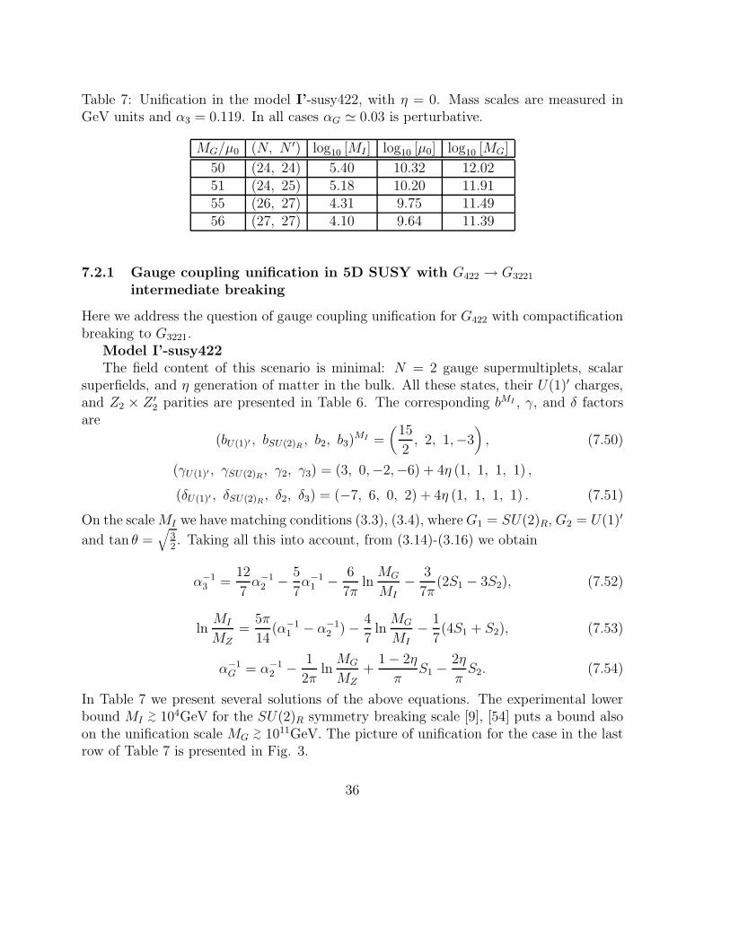
Table 7: Unification in the model I’-susy422, with η = 0. Mass scales are measured inGeV units and α3 = 0.119. In all cases αG ≃ 0.03 is perturbative.

MG/µ0 (N, N ′) log10 [MI ] log10 [µ0] log10 [MG]

50 (24, 24) 5.40 10.32 12.0251 (24, 25) 5.18 10.20 11.9155 (26, 27) 4.31 9.75 11.4956 (27, 27) 4.10 9.64 11.39

7.2.1 Gauge coupling unification in 5D SUSY with G422 → G3221

intermediate breaking

Here we address the question of gauge coupling unification for G422 with compactificationbreaking to G3221.

Model I’-susy422The field content of this scenario is minimal: N = 2 gauge supermultiplets, scalar

superfields, and η generation of matter in the bulk. All these states, their U(1)′ charges,and Z2 × Z ′

2 parities are presented in Table 6. The corresponding bMI , γ, and δ factorsare

(bU(1)′ , bSU(2)R, b2, b3)

MI =(

15

2, 2, 1,−3

)

, (7.50)

(γU(1)′ , γSU(2)R, γ2, γ3) = (3, 0,−2,−6) + 4η (1, 1, 1, 1) ,

(δU(1)′ , δSU(2)R, δ2, δ3) = (−7, 6, 0, 2) + 4η (1, 1, 1, 1) . (7.51)

On the scale MI we have matching conditions (3.3), (3.4), where G1 = SU(2)R, G2 = U(1)′

and tan θ =√

32. Taking all this into account, from (3.14)-(3.16) we obtain

α−13 =

12

7α−1

2 − 5

7α−1

1 − 6

7πln

MG

MI

− 3

7π(2S1 − 3S2), (7.52)

lnMI

MZ=

5π

14(α−1

1 − α−12 ) − 4

7ln

MG

MI− 1

7(4S1 + S2), (7.53)

α−1G = α−1

2 − 1

2πln

MG

MZ+

1 − 2η

πS1 −

2η

πS2. (7.54)

In Table 7 we present several solutions of the above equations. The experimental lowerbound MI

>∼ 104GeV for the SU(2)R symmetry breaking scale [9], [54] puts a bound alsoon the unification scale MG

>∼ 1011GeV. The picture of unification for the case in the lastrow of Table 7 is presented in Fig. 3.

36

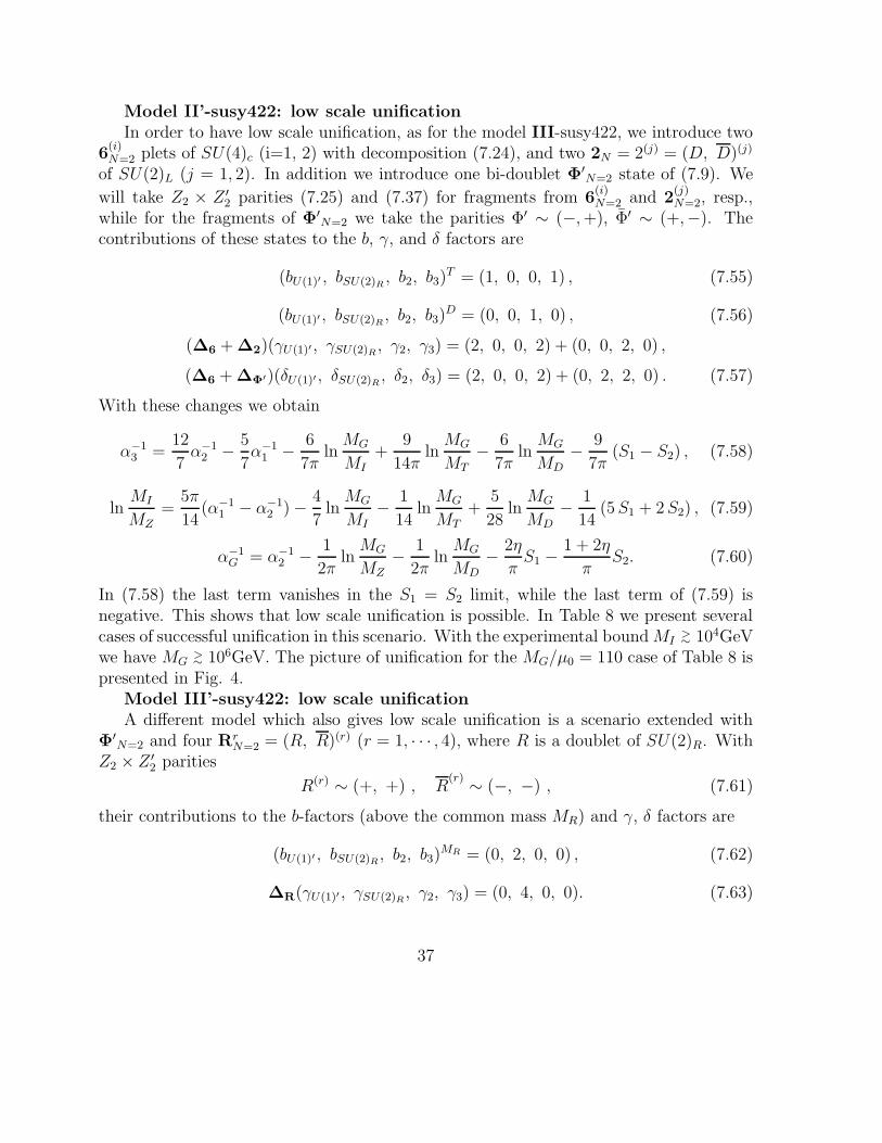
Model II’-susy422: low scale unificationIn order to have low scale unification, as for the model III-susy422, we introduce two

6(i)N=2 plets of SU(4)c (i=1, 2) with decomposition (7.24), and two 2N = 2(j) = (D, D)(j)

of SU(2)L (j = 1, 2). In addition we introduce one bi-doublet Φ′N=2 state of (7.9). We

will take Z2 × Z ′2 parities (7.25) and (7.37) for fragments from 6

(i)N=2 and 2

(j)N=2, resp.,

while for the fragments of Φ′N=2 we take the parities Φ′ ∼ (−, +), Φ′ ∼ (+,−). The

contributions of these states to the b, γ, and δ factors are

(bU(1)′ , bSU(2)R, b2, b3)

T = (1, 0, 0, 1) , (7.55)

(bU(1)′ , bSU(2)R, b2, b3)

D = (0, 0, 1, 0) , (7.56)

(∆6 + ∆2)(γU(1)′ , γSU(2)R, γ2, γ3) = (2, 0, 0, 2) + (0, 0, 2, 0) ,

(∆6 + ∆Φ′)(δU(1)′ , δSU(2)R, δ2, δ3) = (2, 0, 0, 2) + (0, 2, 2, 0) . (7.57)

With these changes we obtain

α−13 =

12

7α−1

2 − 5

7α−1

1 − 6

7πln

MG

MI

+9

14πln

MG

MT

− 6

7πln

MG

MD

− 9

7π(S1 − S2) , (7.58)

lnMI

MZ=

5π

14(α−1

1 − α−12 ) − 4

7ln

MG

MI− 1

14ln

MG

MT+

5

28ln

MG

MD− 1

14(5 S1 + 2 S2) , (7.59)

α−1G = α−1

2 − 1

2πln

MG

MZ− 1

2πln

MG

MD− 2η

πS1 −

1 + 2η

πS2. (7.60)

In (7.58) the last term vanishes in the S1 = S2 limit, while the last term of (7.59) isnegative. This shows that low scale unification is possible. In Table 8 we present severalcases of successful unification in this scenario. With the experimental bound MI

>∼ 104GeVwe have MG

>∼ 106GeV. The picture of unification for the MG/µ0 = 110 case of Table 8 ispresented in Fig. 4.

Model III’-susy422: low scale unificationA different model which also gives low scale unification is a scenario extended with

Φ′N=2 and four Rr

N=2 = (R, R)(r) (r = 1, · · · , 4), where R is a doublet of SU(2)R. WithZ2 × Z ′

2 parities

R(r) ∼ (+, +) , R(r) ∼ (−, −) , (7.61)

their contributions to the b-factors (above the common mass MR) and γ, δ factors are

(bU(1)′ , bSU(2)R, b2, b3)

MR = (0, 2, 0, 0) , (7.62)

∆R(γU(1)′ , γSU(2)R, γ2, γ3) = (0, 4, 0, 0). (7.63)

37

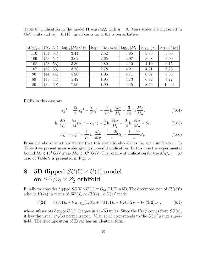
Table 8: Unification in the model II’-susy422, with η = 0. Mass scales are measured inGeV units and α3 = 0.119. In all cases αG ≃ 0.1 is perturbative.

MG/µ0 (N, N ′) log10 [MG/MT ] log10 [MG/MD] log10 [MI ] log10 [µ0] log10 [MG]

110 (54, 54) 3.44 2.52 3.85 3.86 5.90109 (53, 54) 3.62 2.65 3.97 3.98 6.00108 (53, 53) 3.80 2.80 4.10 4.10 6.15107 (52, 53) 3.78 2.78 4.21 4.21 6.2390 (44, 44) 5.26 1.96 4.71 6.67 8.6389 (43, 44) 5.42 1.95 4.73 6.82 8.7780 (39, 39) 7.90 1.90 4.45 8.46 10.36

RGEs in this case are

α−13 =

12

7α−1

2 − 5

7α−1

1 − 6

7πln

MG

MI+

3

7πln

MG

MR, (7.64)

lnMI

MZ=

5π

14(α−1

1 − α−12 ) − 4

7ln

MG

MI− 3

14ln

MG

MR− S1, (7.65)

α−1G = α−1

2 − 1

2πln

MG

MZ+

1 − 2η

πS1 −

1 + 2η

πS2. (7.66)

From the above equations we see that this scenario also allows low scale unification. InTable 9 we present mass scales giving successful unification. In this case the experimentalbound MI

>∼ 104 GeV gives MG>∼ 105.8GeV. The picture of unification for the MG/µ0 = 57

case of Table 9 is presented in Fig. 5.

8 5D flipped SU(5) × U(1) model

on S(1)/Z2 × Z ′2 orbifold

Finally we consider flipped SU(5)×U(1) ≡ G51 GUT in 5D. The decomposition of SU(5)’sadjoint V (24) in terms of SU(3)c × SU(2)L × U(1)′ reads

V (24) = Vc(8, 1)0 + VSU(2)L(1, 3)0 + Vs(1, 1)0 + VX(3, 2)5 + VY (3, 2)−5 , (8.1)

where subscripts denote U(1)′ charges in 1/√

60 units. Since the U(1)′ comes from SU(5),it has the usual 1/

√60 normalization. Vs in (8.1) corresponds to the U(1)′ gauge super-

field. The decomposition of Σ(24) has an identical form.

38

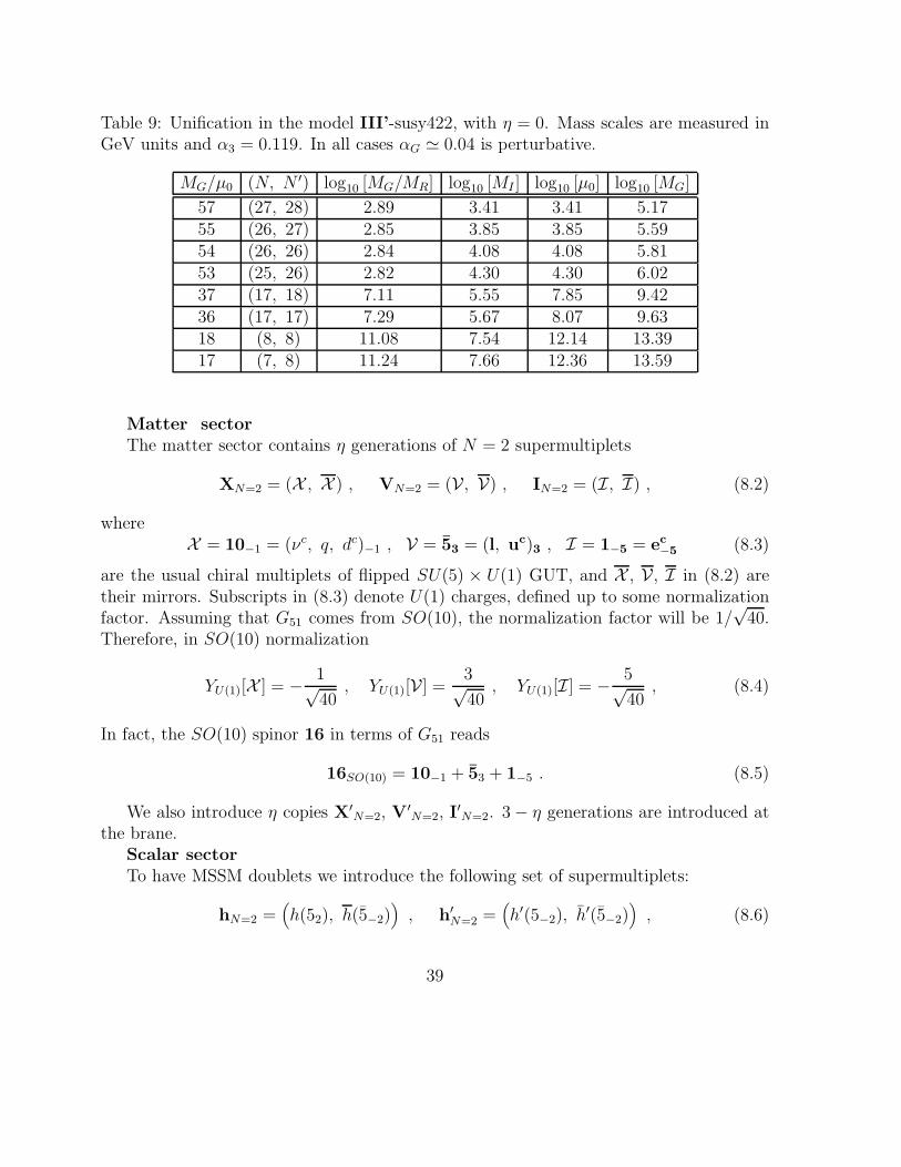
Table 9: Unification in the model III’-susy422, with η = 0. Mass scales are measured inGeV units and α3 = 0.119. In all cases αG ≃ 0.04 is perturbative.

MG/µ0 (N, N ′) log10 [MG/MR] log10 [MI ] log10 [µ0] log10 [MG]

57 (27, 28) 2.89 3.41 3.41 5.1755 (26, 27) 2.85 3.85 3.85 5.5954 (26, 26) 2.84 4.08 4.08 5.8153 (25, 26) 2.82 4.30 4.30 6.0237 (17, 18) 7.11 5.55 7.85 9.4236 (17, 17) 7.29 5.67 8.07 9.6318 (8, 8) 11.08 7.54 12.14 13.3917 (7, 8) 11.24 7.66 12.36 13.59

Matter sectorThe matter sector contains η generations of N = 2 supermultiplets

XN=2 = (X , X ) , VN=2 = (V, V) , IN=2 = (I, I) , (8.2)

whereX = 10−1 = (νc, q, dc)−1 , V = 53 = (l, uc)3 , I = 1−5 = ec

−5(8.3)

are the usual chiral multiplets of flipped SU(5) × U(1) GUT, and X , V, I in (8.2) aretheir mirrors. Subscripts in (8.3) denote U(1) charges, defined up to some normalizationfactor. Assuming that G51 comes from SO(10), the normalization factor will be 1/

√40.

Therefore, in SO(10) normalization

YU(1)[X ] = − 1√40

, YU(1)[V] =3√40

, YU(1)[I] = − 5√40

, (8.4)

In fact, the SO(10) spinor 16 in terms of G51 reads

16SO(10) = 10−1 + 53 + 1−5 . (8.5)

We also introduce η copies X′N=2, V′

N=2, I′N=2. 3 − η generations are introduced atthe brane.

Scalar sectorTo have MSSM doublets we introduce the following set of supermultiplets:

hN=2 =(

h(52), h(5−2))

, h′N=2 =

(

h′(5−2), h′(5−2))

, (8.6)

39

where subscripts denote U(1) charges in 1/√

40 units. In (8.6) one has

h(52) = (hd, dc

h)2 , h(5−2) = (hu, dch)−2 , (8.7)

and the same for states with primes.For reducing the rank of the group via Higgs breaking we need additional states. Thus

we introduceHN=2 =

(

H, H)

, H′N=2 =

(

H ′, H ′)

, (8.8)

whereH = 10H

−1 = (νcH , dc

H , qH)−1 , H = 10H1 =

(

νcH , d

c

H , qH

)

1, (8.9)

and similarly for H ′ and H ′.

8.1 G51 → G321 breaking and related phenomenological questions

The first stage of breakdown of the G51 gauge group again occurs through orbifolding:prescribing to various fragments of G51 multiplets certain Z2 × Z ′

2 parities some statesare projected out, and at a fixed point we remain with a reduced gauge group. Thetransformation properties of the fragments of 5D SUSY G51 are given in Table 10. One caneasily see that at the y = 0 fixed point we have a SU(3)c×SU(2)L×U(1)×U(1)′ ≡ G′

3211

gauge group. At this fixed point together with three generations of quark-lepton and righthanded neutrino superfields q, uc′, dc′, l, ec, νc′ and an MSSM pair of Higgs doublets hu,hd

′, we also have the states dcH , d

c

H

′, νc

H , νcH

′. The latter two states are responsible for anU(1) × U(1)′ breaking down to U(1)Y . If they develop VEVs on the scale MI the secondstage of symmetry breaking occurs and we have the unbroken U(1)Y generator

Y =2√

6

5YU(1) −

1

5YU(1)′ , (8.10)

where YU(1)′ and YU(1) charges of the states are given in Table 10. [For YU(1) again wehave used SO(10) normalization (8.4), since flipped SU(5) × U(1) is one of its maximalsubgroups [35], [36]].

The generation of 〈νcH〉, 〈νc

H′〉 VEVs can happen in the same way as for the SU(4)c ×

SU(2)L×SU(2)R scenario presented in sect. 7.1. Introducing a discrete Z symmetry anda transformation for νc

H′νc

H as in (4.4), the relevant superpotential, soft SUSY breaking,and all the potential couplings will have the form of (4.6), (4.7), (4.8) resp. if the statesS, S are replaced by νc

H , νcH

′. From all this one can ensure non zero VEV solutions (7.16),(7.17). By a proper choice of n one can obtain a gap between the mass scales v ≡ MI

and M . Also µ term generation can happen similarly. With transformation (4.3) for thehuhd

′ combination and coupling (7.18) the µ term (7.19) is derived.

40

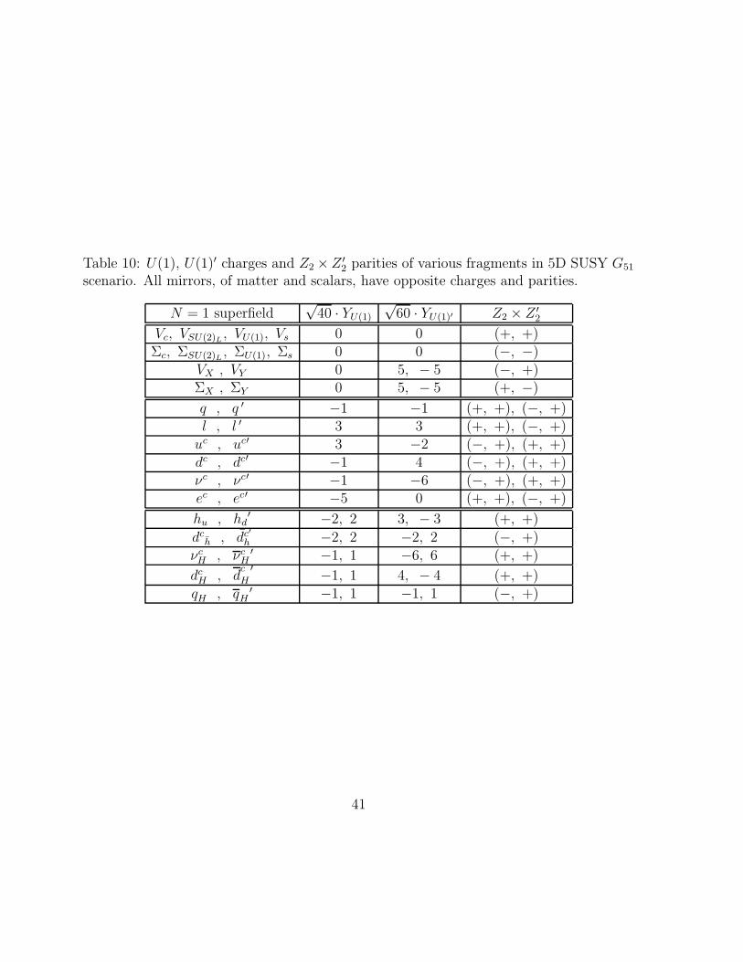
Table 10: U(1), U(1)′ charges and Z2 ×Z ′2 parities of various fragments in 5D SUSY G51

scenario. All mirrors, of matter and scalars, have opposite charges and parities.

N = 1 superfield√

40 · YU(1)

√60 · YU(1)′ Z2 × Z ′

2

Vc, VSU(2)L, VU(1), Vs 0 0 (+, +)

Σc, ΣSU(2)L, ΣU(1), Σs 0 0 (−, −)

VX , VY 0 5, − 5 (−, +)ΣX , ΣY 0 5, − 5 (+, −)

q , q ′ −1 −1 (+, +), (−, +)l , l ′ 3 3 (+, +), (−, +)

uc , uc′ 3 −2 (−, +), (+, +)dc , dc′ −1 4 (−, +), (+, +)νc , νc′ −1 −6 (−, +), (+, +)ec , ec′ −5 0 (+, +), (−, +)

hu , hd′ −2, 2 3, − 3 (+, +)

dch , dc′

h −2, 2 −2, 2 (−, +)νc

H , νcH

′ −1, 1 −6, 6 (+, +)

dcH , d

c

H

′ −1, 1 4, − 4 (+, +)qH , qH

′ −1, 1 −1, 1 (−, +)

41

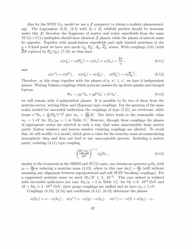
Also for the SUSY G51 model we use a Z symmetry to obtain a realistic phenomenol-ogy. The Lagrangian (2.3), (2.4) with Z2 × Z ′

2 orbifold parities should be invariantunder this Z; therefore the fragments of matter and scalar superfields from the sameSU(5)×U(1) multiplets should have identical Z phases, while the phases of mirrors mustbe opposite. Together with quark-lepton superfields and right handed neutrinos at they = 0 fixed point we have zero mode νc

H , νcH

′, dcH , d

c

H

′states. With couplings (4.6) (with

SS replaced by νcH

′νcH), (7.18) we thus have

α(νcH) + α(νc

H′) = α(hd

′) + α(hu) =2π

n, (8.11)

andα(νc′) = α(dc′) , α(νc

H) = α(dcH) , α(νc

H′) = α(d

c

H

′) . (8.12)

Therefore, at this stage together with the phases of q, uc, l, ec, we have 8 independentphases. Writing Yukawa couplings which generate masses for up-down quarks and chargedleptons

WY = quc′hu + qdc′hd′ + lechd

′ , (8.13)

we will remain with 4 independent phases. It is possible to fix two of them from theneutrino sector, writing Dirac and Majorana type couplings. For the question of the massscales needed for successful unification the couplings of type (7.21) are irrelevant, while

terms νc′lhu + 1M

(νcH

′νc′)2 give mν ∼ h2u

M2I

M . The latter leads to the reasonable value

mν ∼ 1 eV for MG/µ0 = 1 in Table 11. However, through these couplings the phasesof appropriate states are selected in such a way, that some unacceptably large matterparity (lepton number) and baryon number violating couplings are allowed. To avoidthis, we will modify to a model, which gives a value for the neutrino mass accommodatingatmospheric data and does not lead to any unacceptable process. Including a matterparity violating (4.11) type coupling

(

νcH

′νcH

M2

)n−1

νcH lhu , (8.14)

similar to the treatment in the MSSM and SU(5) cases, one obtains an operator µllhu withµl ∼ MI

Mm inducing a neutrino mass (4.13), where in this case sin ξ ∼ MI

M(still without

assuming any alignment between superpotential and soft SUSY breaking couplings). Fora suppressed neutrino mass we need MI/M ≤ 3 · 10−6. This case indeed is realizedwith successful unification [see case MG/µ = 5 in Table 11]: for MI ≃ 6 · 1010 GeV andM = MG ≃ 2 · 1016 GeV, three gauge couplings are unified and we have mν

<∼ 1 eV.Couplings (8.13), (8.14) and conditions (8.11), (8.12) determine the phases

α(hd′) = α − α(hu) , α(uc′) = −α(q) − α(hu) , α(ec) = −α(l) + α(hu) − α ,

42

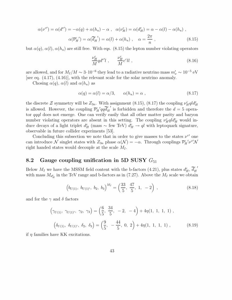
α(νc′) = α(dc′) = −α(q) + α(hu) − α , α(νcH) = α(dc

H) = α − α(l) − α(hu) ,

α(νcH

′) = α(dc

H

′) = α(l) + α(hu) , α =

2π

n, (8.15)

but α(q), α(l), α(hu) are still free. With eqs. (8.15) the lepton number violating operators

νcH

Mqdc′l ,

νcH

Mecll , (8.16)

are allowed, and for MI/M ∼ 3·10−6 they lead to a radiative neutrino mass m′ν ∼ 10−5 eV

[see eq. (4.17), (4.16)], with the relevant scale for the solar neutrino anomaly.Chosing α(q), α(l) and α(hu) as

α(q) = α(l) = α/3, α(hu) = α , (8.17)

the discrete Z symmetry will be Z3n. With assignment (8.15), (8.17) the coupling νcHqldc

H

is allowed. However, the coupling νcH

′qqdc

H

′is forbidden and therefore the d = 5 opera-

tor qqql does not emerge. One can verify easily that all other matter parity and baryonnumber violating operators are absent in this setting. The coupling νc

HqldcH would in-

duce decays of a light triplet dcH (mass ∼ few TeV) dc

H → ql with leptoquark signature,observable in future collider experiments [53].

Concluding this subsection we note that in order to give masses to the states νc′ onecan introduce N singlet states with Z3n phase α(N ) = −α. Through couplings νc

H′νc′N

right handed states would decouple at the scale MI .

8.2 Gauge coupling unification in 5D SUSY G51

Below MI we have the MSSM field content with the b-factors (4.21), plus states dcH , d

c

H

′

with mass Mdc

Hin the TeV range and b-factors as in (7.27). Above the MI scale we obtain

(

bU(1), bU(1)′ , b2, b3

)MI

=(

33

5,

47

5, 1, − 2

)

, (8.18)

and for the γ and δ factors

(

γU(1), γU(1)′ , γ2, γ3

)

=(

6

5,

34

5, − 2, − 4

)

+ 4η(1, 1, 1, 1) ,

(

δU(1), δU(1)′ , δ2, δ3

)

=(

9

5, − 44

5, 0, 2

)

+ 4η(1, 1, 1, 1) , (8.19)

if η families have KK excitations.

43

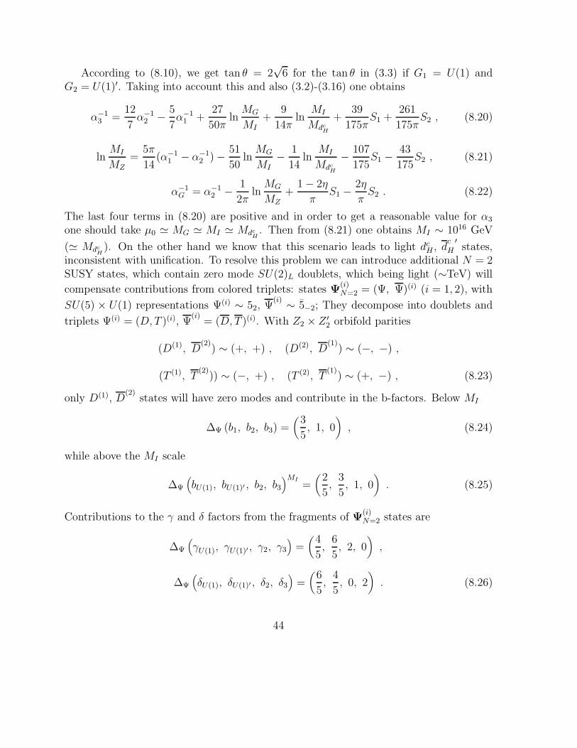
According to (8.10), we get tan θ = 2√

6 for the tan θ in (3.3) if G1 = U(1) andG2 = U(1)′. Taking into account this and also (3.2)-(3.16) one obtains

α−13 =

12

7α−1

2 − 5

7α−1

1 +27

50πln

MG

MI

+9

14πln

MI

Mdc

H

+39

175πS1 +

261

175πS2 , (8.20)

lnMI

MZ

=5π

14(α−1

1 − α−12 ) − 51

50ln

MG

MI

− 1

14ln

MI

Mdc

H

− 107

175S1 −

43

175S2 , (8.21)

α−1G = α−1

2 − 1

2πln

MG

MZ+

1 − 2η

πS1 −

2η

πS2 . (8.22)

The last four terms in (8.20) are positive and in order to get a reasonable value for α3

one should take µ0 ≃ MG ≃ MI ≃ Mdc

H. Then from (8.21) one obtains MI ∼ 1016 GeV

(≃ Mdc

H). On the other hand we know that this scenario leads to light dc

H , dc

H

′states,

inconsistent with unification. To resolve this problem we can introduce additional N = 2SUSY states, which contain zero mode SU(2)L doublets, which being light (∼TeV) will

compensate contributions from colored triplets: states Ψ(i)N=2 = (Ψ, Ψ)(i) (i = 1, 2), with

SU(5) × U(1) representations Ψ(i) ∼ 52, Ψ(i) ∼ 5−2; They decompose into doublets and

triplets Ψ(i) = (D, T )(i), Ψ(i)

= (D, T )(i). With Z2 × Z ′2 orbifold parities

(D(1), D(2)

) ∼ (+, +) , (D(2), D(1)

) ∼ (−, −) ,

(T (1), T(2)

)) ∼ (−, +) , (T (2), T(1)

) ∼ (+, −) , (8.23)

only D(1), D(2)

states will have zero modes and contribute in the b-factors. Below MI

∆Ψ (b1, b2, b3) =(

3

5, 1, 0

)

, (8.24)

while above the MI scale

∆Ψ

(

bU(1), bU(1)′ , b2, b3

)MI

=(

2

5,

3

5, 1, 0

)

. (8.25)

Contributions to the γ and δ factors from the fragments of Ψ(i)N=2 states are

∆Ψ

(

γU(1), γU(1)′ , γ2, γ3

)

=(

4

5,

6

5, 2, 0

)

,

∆Ψ

(

δU(1), δU(1)′ , δ2, δ3

)

=(

6

5,

4

5, 0, 2

)

. (8.26)

44

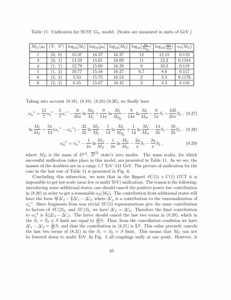
Table 11: Unification for SUSY G51 model. (Scales are measured in units of GeV.)

MG/µ0 (N, N ′) log10[MI ] log10[µ0] log10[MG] log10[MI

Mdc

H

] log10[MI

MD] α3(MZ)

1 (0, 0) 15.37 16.37 16.37 12 12.15 0.1193 (0, 1) 14.59 15.61 16.09 11 12.2 0.11844 (1, 1) 12.79 15.69 16.29 8 10.2 0.1195 (1, 2) 10.77 15.58 16.27 6.7 8.6 0.1176 (2, 2) 5.53 15.75 16.53 2 3.3 0.11766 (2, 2) 6.45 15.67 16.45 3 4.3 0.116

Taking into account (8.18), (8.19), (8.24)-(8.26), we finally have

α−13 =

12

7α−1

2 − 5

7α−1

1 − 6

35πln

MG

MI+

9

14πln

MI

Mdc

H

− 9

14πln

MI

MD− 6

5πS1 +

102

35πS2 , (8.27)

lnMI

MZ=

5π

14(α−1

1 − α−12 ) − 32

35ln

MG

MI− 1

14ln

MI

Mdc

H

+1

14ln

MI

MD− 14

35S1 −

16

35S2 , (8.28)

α−1G = α−1

2 − 1

2πln

MG

MZ

− 1

2πln

MG

MD

− 2η

πS1 −

2η

πS2 , (8.29)

where MD is the mass of D(1), D(2)

state’s zero modes. The mass scales, for whichsuccessful unification takes place in this model, are presented in Table 11. As we see, themasses of the doublets are in a range 1.7 TeV–141 GeV. The picture of unification for thecase in the last row of Table 11 is presented in Fig. 6.

Concluding this subsection, we note that in the flipped SU(5) × U(1) GUT it isimpossible to get low scale (near few or multi TeV) unification. The reason is the following:introducing some additional states, one should cancel the positive power law contributionin (8.20) in order to get a reasonable α3(MZ). The contribution from additional states willhave the form 12

7∆′

2 − 57∆′

1 − ∆′3, where ∆′

a is a contribution to the renormalization ofα−1

a . Since fragments from non trivial SU(5) representations give the same contributionto factors of SU(2)L and SU(3)c we have ∆′

3 = ∆′2. Therefore the final contribution

to α−13 is 5

7(∆′

2 − ∆′1). The latter should cancel the last two terms in (8.20), which in

the S1 = S2 ≡ S limit are equal to 127π

S. Thus, from the cancellation condition we have∆′

1 − ∆′2 = 12

5πS; and thus the contribution in (8.21) is 6

7S. This value precisely cancels

the last two terms of (8.21) in the S1 = S2 = S limit. This means that MG can notbe lowered down to multi TeV. In Fig. 5 all couplings unify at one point. However, it

45

would be quite natural in spirit of a two step unification that at a first step only thethree couplings of SU(5) unify and the U(1) coupling joins at a higher scale. This can beachieved either by a change of the intermediate scale or by a different choice of the extrastate’s masses.

9 Conclusions and outlook

We have considered 5D orbifold SUSY models and within them we have addressed nu-merous phenomenological issues. Orbifold constructions give an attractive resolution ofseveral outstanding problems of GUTs, but some extensions are still needed to have fullcontrol of difficulties which even appear outside GUTs. In fact, problems such as baryonnumber violation, µ problem and neutrino oscillations (tied with lepton number violation)are not cured by extra dimensions, and some care is needed to deal with them. In our ap-proach we have considered extensions with a discrete Z symmetry, which gives a naturaland simultaneous understanding of these problems. In the essential part of the paper wehave addressed the question of gauge coupling unification, which in the presence of KKstates gets new facets. Since the orbifold approach to the celebrated SU(5) GUT doesnot allow for low or intermediate scale unification, we studied extended (in rank) GUTs.As we have seen this opens up new and interesting possibilities from the viewpoints ofunification and phenomenological implications. For extended GUTs, symmetry breakingcan occur by a step by step compactification and if the intermediate gauge group differsfrom semisimple SU(5), power law unification can take place. As an example we haveconsidered the two maximal subgroups of SO(10) - the Pati-Salam G422 and flipped G51

GUTs. Within G422, low scale unification can take place, while G51 only allows for uni-fication at scales ∼ 1016 GeV. The latter scales are also possible for G422. Within bothscenarios extensions with a discrete Z symmetry were pursued; thus key phenomenologi-cal problems were resolved in an elegant way. The G51 model and also in some cases theG422 one predict colored triplet states in the few TeV range. G422 models with low scaleunification lead to additional relatively light states. Because of these the models have aninteresting phenomenology, in particular if KK states appear near the TeV scale. Futurehigh energy collider experiments will test the relevance of such models.

In our studies we have used one loop RGE analysis. Two loop power law contributionsto the β-function would contribute significantly. This would make estimates unstable.However, due to higher dimensional supersymmetries, in higher loops full sets of N = 2supermultiplets can contribute [29], [30] and in this case effects of higher loops will belogarithmic. The latter contributions would not change the unification picture and mightonly imply a slight modification of mass scales. The same argument could be applied forthreshold corrections coming from different sources.

46

Our studies of the G422 and G51 groups were performed in a bottom-up approachand therefore the ’low energy’ sector was more relevant for our considerations. Havingin mind that both G422 and G51 are maximal subgroups of SO(10), it would be inter-esting to construct a higher (at least two extra) dimensional SO(10) model where extradimensions do not compactify at a single mass scale (in contrast to the models of [22])but with intermediate groups G422 or G51 at a scale between 1

R′≫ 1

R. Only this kind

of step by step compactification breaking of an initial semisimple gauge group can givepower law unification near the TeV scale. It would be also interesting to consider otherextended gauge groups in higher dimensions and to study the breaking pattern and thephenomenological implications. We wish to study these and other relevant issues in ourfuture publications.

AcknowledgementF.P.C. is supported by Fundacao de Ciencia e Tecnologia (grant SFRH/BD/4973/2001).

Appendix A: Influence of brane couplings

on gauge coupling unification

In this appendix we investigate the influence of some brane operators on gauge couplingrenormalization. We will show that the 4D mass term of bulk vectorlike states does notchange the expressions for the power law functions S and S1, S2 of (3.8) and (3.10) resp..Also, it turns out that some brane bi-linear derivative couplings, involving states withnegative parities, do not change this picture for µ0 ≪ M ∼ MG. The latter conditionis usually satisfied in models with power law unification 6. Our discussion will be modelindependent. We will consider here the case of S(1)/Z2 orbifold, but generalization toS(1)/Z2 × Z ′

2 scenarios is straightforward.Consider two N = 2 supermultiplets EN=2 = (E, E) and E′

N=2 = (E ′, E′) transform-

ing non trivially under a certain gauge group G. If E, E ′ belong to some representationr of G, then E, E

′transform as r. Let us assign the orbifold parities as

(E, E′) ∼ + , (E ′, E) ∼ − . (A.1)

Thus, only E, E′states have zero modes. Writing the brane coupling

∫

d5xd2θδ(y)(

λE EE′+ h.c.

)

, (A.2)

6Also in the models with additional bulk vectorlike states, which we have studied, µ0 ≪ MG issatisfied.

47

we obtain, after performing the integration over y, the 4D superpotential mass terms

WE = 2ME

∑

m,n

E(m)E(n)′

η(m)η(n) , (A.3)

where ME = λEµ0/π = λE/(πR) and η(0) = 1/√

2, η(n)|n 6=0 = 1. On the other hand, thelast term in the 5D bulk Lagrangian (2.4) gives direct mass terms for the KK states

W KKE = µ0

∞∑

n=1

n(

E(n)E(n)

+ E(n)′E(n)′)

. (A.4)

For our calculations only a certain number of KK states is relevant, which contribute tothe gauge coupling runnings. So, we truncate the tower of KK states on the level N0.Taking this into account and combining (A.3), (A.4), the mass terms can be written incompact form as

WE + W KKE = EME , (A.5)

where

E =(

E ′(N) . . . E ′(0) E(1) . . . E(N))

, ET =(

E ′(N) . . . E ′(1) E(0) . . . E(N))

, (A.6)

M ≡[

M0 ME

0 M0

]

, ME = ME

√2 2 . . . 2...

. . ....√

2 2 . . . 2

1√

2 . . .√

2

, (A.7)

and

M0 = µ0

N0 0 . . . 00 N0 − 1 0...

. . ....

0 0 . . . 10 0 . . . 0

, M0 = µ0

0 1 . . . 0 0...

. . ....

0 0 N0 − 1 00 0 . . . 0 N0

. (A.8)

To estimate the KK and zero mode contributions to the running, one should diagonalizethe matrix M and find the eigenvalues M0, M1, · · ·, M2N0

. If all these masses lie belowMG, then their contribution to the renormalization of α−1

i up to the GUT scale will be

∆Ei = − bE

i

2π

2N0∑

n=0

lnMG

Mn= − bE

i

2πln

M2N0+1G

detM . (A.9)

48

From (A.7), (A.8) it is easy to see that

detM = ME

N0∏

n=1

Mn

2

= ME

N0∏

n=1

nµ0

2

. (A.10)

Using (A.10) in (A.9) we obtain

∆Ei = − bE

i

2πln

MG

ME−− bE

i

2π

N0∑

n=1

lnMG

nµ0, (A.11)

(where we have set bEi = 2bE

i ). As one can see, the first term in (A.11) is just the naivelogarithmic running of ’zero mode’ states, while the second term has precisely the formof the ’unaffected’ KK power law running (3.8). From this we conclude that due to thebrane coupling (A.2), the RGEs will in addition include a logarithmic term corresponding

to the zero modes E(0), E(0)′

above the scale ME , while the effect of the KK states mustbe estimated by the power law function S. These conclusions are valid for any value ofME

<∼ MG.Higher order brane couplings, preserving orbifold symmetries, imply ∂5 derivatives and

must be cut off at the fundamental scale M ∼ MG. For example, the couplings

∫

d5xd2θδ(y)(

1

ME∂5E +

1

ME

′∂5E

′)

, (A.12)

after integration along the fifth dimension, change the masses by the amount ∼ µ20/M .

The latter is negligible for µ0 ≪ M and (A.11) is still valid.

References

[1] H. Georgi, S.L. Glashow, Phys.Rev.Lett. 32 (1974) 438; H. Fritzsch, P. Minkowski,Ann. Phys. 93 (1975) 193.

[2] H. Georgi, H. Quinn, S. Weinberg, Phys. Rev. Lett. 33 (1974) 451; W. Marciano, A.Sirlin, Phys. Rev. Lett. 46 (1981) 163.

[3] J. Ellis, S. Kelley, D. Nanopoulos, Phys. Lett. B 260 (1991) 131;

[4] S. Dimopoulos, H. Georgi, Nucl. Phys. B 193 (1981) 150; N. Sakai, Z. Phys. C 11(1982) 153.

[5] S. Dimopoulos, S. Raby, F. Wilczek, Phys. Rev. D 24 (1981) 1681; W. Marciano, G.Senjanovic, Phys. Rev. D 25 (1982) 3092.

49

[6] D.R.T. Jones, Phys.Rev. D 25 (1982) 581.

[7] C. Giunti, C. Kim, U. Lee, Mod. Phys. Lett. A 6 (1991) 1745; P. Langacker, M. Luo,Phys. Rev. D 44 (1991) 817.

[8] U. Amaldi, W. de Boer, H. Furstenau, Phys. Lett. B 260 (1991) 447.

[9] Particle Data Group, Eur. Phys. J. C 15 (2000) 1.

[10] R. Arnowitt, P. Nath, Phys. Lett. B 287 (1992) 89; Phys. Rev. Lett. 70 (1993) 3696;J. Hisano, H. Murayama, T. Yanagida, Nucl. Phys. B 402 (1993) 46; K.S. Babu, S.M.Barr, Phys. Lett. B 381 (1996) 137; Z. Berezhiani, Z. Tavartkiladze, M. Vysotsky,hep-ph/9809301; R. Dermisek, A. Mafi, S. Rabi, Phys. Rev. D 63 (2001) 035001; H.Murayama, A. Pierce, hep-ph/0108104.

[11] S. Fukuda et al. [Super-Kamiokande Collaboration], Phys. Rev. Lett. 88 (2000) 3999;N. Fornengo et al., Nucl. Phys. B 580 (2000) 58.

[12] S. Fukuda et al. [Super-Kamiokande Collaboration], Phys. Rev. Lett. 86 (2001) 5651;J. Bahcall, P. Krastev, A. Smirnov, hep-ph/0006078; M.C. Gonzalez-Garcia et al.,Nucl. Phys. B 573 (2000) 3.

[13] I. Antoniadis, J. Ellis, S. Kelley, D. Nanopoulos, Phys.Lett. B 272 (1991) 31. P.Lamgacker, N. Polonsky, Phys. Rev. D 47 (1993) 4028; Phys. Rev. D 52 (1995) 52;N. Polonsky, hep-ph/0108236; see also references terein.

[14] M. Shifman, Mod. Phys. Lett. A 10 (1995) 605; J. Bagger, K. Matchev, D. Pierce,Phys. Lett. B 348 (1995) 443.

[15] Y. Kawamura, Prog. Theor. Phys. 105 (2001) 999; ibid. 105 (2001) 691.

[16] G. Altarelli, F. Feruglio, hep-ph/0102301; A. Kobakhidze, hep-ph/0102323; M. Kak-izaki, M. Yamaguchi, hep-ph/0104103; N. Maru, hep-ph/0108002.

[17] Y. Nomura, D. Smith, N. Weiner, hep-ph/0104041; T. Kawamoto, Y. Kawamura,hep-ph/0106163; R. Barbieri, L. Hall, Y. Nomura, hep-th/0107004; A. Hebecker, J.March-Russell, hep-ph/0107039; C. Csaki, G. Kribs, J. Terning, hep-ph/0107266.

[18] Q. Shafi, Z. Tavartkiladze, hep-ph/0108247.

[19] T. Li, hep-ph/0108120; hep-th/0110065; M. Chaichian, J. Chkareuli, A. Kobakhidze,hep-ph/0108131; C.S. Huang, J. Jiang, T. Li, hep-th/0112046; K.S. Babu, S.M. Barr,B. Kyae, hep-ph/0202178.

50

[20] L. Hall, Y. Nomura, hep-ph/0103125; hep-ph/0205067.

[21] A. Hebecker, J. March-Russell, hep-ph/0106166; H. Cheng, K. Matchev, J. Wang,hep-ph/0107268; L. Hall, J. March-Russell, T. Okui, D. Smith, hep-ph/0108161; Y.Nomura, hep-ph/0108170.

[22] T. Asaka, W. Buchmuller, L. Covi, hep-ph/0108021; L. Hall, Y. Nomura, T. Okui, D.Smith, hep-ph/0108071; R. Dermisek, A. Mafi, hep-ph/0108139; N. Haba, T. Kondo,Y. Shimizu, hep-ph/0112132, hep-ph/0202191.

[23] R. Blumenhagen, L. Goerlich, B. Kors, D. Lust, hep-th/0010198; G. Aldazabal, S.Franco, L. Ibanez, R. Rabadan, A. Uranga, hep-th/0011073; hep-ph/0011132; L.E.Ibanez, F. Marchesano, R. Rabadan, hep-th/0105155; R. Blumenhagen, B. Kors, D.Lust, T. Ott, hep-th/0107138.

[24] I. Antoniadis, Phys. Lett. B 246 (1990) 377; I. Antoniadis, C. Munoz, M. Quiros,Nucl. Phys. B 397 (1993) 515; J. Lykken, Phys. Rev. D 54 (1996) 3693; I. Antoniadis,S. Dimopoulos, A. Giveon, hep-th/0103033.

[25] I. Antoniadis, K. Benakli, M. Quiros, Phys. Lett. B 331 (1994) 313; hep-ph/9905311;I. Antoniadis, K. Benakli, hep-ph/0007226; and references therein.

[26] For recent reviews see J. Polchinski, hep-th/9611050; C. Vafa, hep-th/9702201; A.Sen, hep-th/9802051; I. Antoniadis, G. Ovarlez, hep-th/9906108; I. Antoniadis, hep-th/0102202.

[27] N. Arkani-Hamed, S. Dimopoulos, G. Dvali, Phys. Lett. B 429 (1998) 263; Phys.Rev. D 59 (1999) 086004; I. Antoniadis, N. Arkani-Hamed, S. Dimopoulos, G. Dvali,Phys. Lett. B 436 (1998) 257.

[28] J. Price, proc. Int. Symp. on Experimental Gravitational Physics, ed. P. Michelson,Guangzhou, China (World Sci., Singapore 1988); J. Price et al., NSF proposal 1996;A. Kapitulnik, T. Kenny, NSF proposal, 1997; J. Long et al., hep-ph/9805217.

[29] K. Dines, E. Dudas, T. Gherghetta, Phys. Lett. B 436 (1998) 55; Nucl. Phys. B 537(1999) 47.

[30] Z. Kakushadze, Nucl. Phys. B 548 (1999) 205; ibid. B 552 (1999) 3.

[31] C. Carone, hep-ph/9902407; A. Delgado, M. Quiros, hep-ph/9903400; P. Frampton,A. Rasin, hep-ph/9903479; A. Perez-Lorenzana, R.N. Mohapatra, hep-ph/9904504;Z. Tavartkiladze, hep-ph/0105281.

51

[32] T. Kobayashi, J. Kubo, M. Mondragon, G. Zoupanos, Nucl. Phys. B 550 (1999) 99;K. Huitu, T. Kobayashi, Phys. Lett. B 470 (1999) 90.

[33] T. Taylor, G. Veneziano, Phys. Lett. B 212 (1988) 147.

[34] J. Pati, A. Salam, Phys. Rev. D 10 (1974) 275.

[35] S. Barr, Phys. Lett. B 112 (1982) 219.

[36] R. Slansky, Phys. Rept. 79 (1981) 1.

[37] M. Sohnius, Phys. Rep. 128 (1985) 39; A. Salam, E. Sezgin, V. 1, 2, World Scientific,1989; E. Mirabelli, M. Peskin, hep-th/9712214.

[38] N. Arkani-Hamed, T. Gregoire, J. Wacker, hep-th/0101233; D. Marti, A. Pomarol,hep-th/0106256; A. Hebecker, hep-ph/0112230.

[39] L. Ibanez, G. Ross, Nucl. Phys. B 368 (1992) 3.

[40] I. Antoniadis, J. Hagelin, D. Nanopoulos, Phys. Lett. B 194 (1987) 231; G. Lazarides,C. Panagiotakopoulos, Q. Shafi, Phys. Lett. B 315 (1993) 325; G. Dvali, Q. Shafi,Phys. Lett. B 403 (1997) 65; Q. Shafi, Z. Tavartkiladze, hep-ph/9811282; hep-ph/9807502.

[41] I. Antoniadis, hep-th/0102202.

[42] C. Carone, H. Murayama, Phys. Rev. D 52 (1995) 484; D. Bailey, S. Davidson,hep-ph/9411355.

[43] G. Dvali, Q. Shafi, Phys. Lett. B 326 (1994) 258; B 339 (1994) 241. J.E. Kim, H.P.Nilles, Mod. Phys. Lett. A 38 (1994) 3575. K. Choi, E.J. Chun, H. Kim, Phys. Rev.D 55 (1997) 7010.

[44] G. Dvali, Q. Shafi, Phys.Lett. B 339 (1994) 241; Z. Berezhiani, C. Csaki, L. Randall,hep-ph/9501336; see also Q. Shafi, Z. Tavartkiladze, in ref. [40].

[45] G. Bhattacharyya, Nucl. Phys. Proc. Suppl. A 52 (1997) 83; J.C. Romao, hep-ph/9811454.

[46] T. Banks, Y. Grossman, E. Nardi, Y. Nir, Phys. Rev. D 52 (1995) 5319.

52

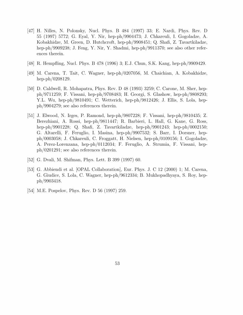
[47] H. Nilles, N. Polonsky, Nucl. Phys. B 484 (1997) 33; E. Nardi, Phys. Rev. D55 (1997) 5772; G. Eyal, Y. Nir, hep-ph/9904473; J. Chkareuli, I. Gogoladze, A.Kobakhidze, M. Green, D. Hutchcroft, hep-ph/9908451; Q. Shafi, Z. Tavartkiladze,hep-ph/9909238; J. Feng, Y. Nir, Y. Shadmi, hep-ph/9911370; see also other refer-ences therein.

[48] R. Hempfling, Nucl. Phys. B 478 (1996) 3; E.J. Chun, S.K. Kang, hep-ph/9909429.

[49] M. Carena, T. Tait, C. Wagner, hep-ph/0207056, M. Chaichian, A. Kobakhidze,hep-ph/0208129.

[50] D. Caldwell, R. Mohapatra, Phys. Rev. D 48 (1993) 3259; C. Carone, M. Sher, hep-ph/9711259; F. Vissani, hep-ph/9708483; H. Georgi, S. Glashow, hep-ph/9808293;Y.L. Wu, hep-ph/9810491; C. Wetterich, hep-ph/9812426; J. Ellis, S. Lola, hep-ph/9904279; see also references therein.

[51] J. Elwood, N. Irges, P. Ramond, hep-ph/9807228; F. Vissani, hep-ph/9810435; Z.Berezhiani, A. Rossi, hep-ph/9811447; R. Barbieri, L. Hall, G. Kane, G. Ross,hep-ph/9901228; Q. Shafi, Z. Tavartkiladze, hep-ph/9901243; hep-ph/0002150;G. Altarelli, F. Feruglio, I. Masina, hep-ph/9907532; S. Barr, I. Dorsner, hep-ph/0003058; J. Chkareuli, C. Froggatt, H. Nielsen, hep-ph/0109156; I. Gogoladze,A. Perez-Lorenzana, hep-ph/0112034; F. Feruglio, A. Strumia, F. Vissani, hep-ph/0201291; see also references therein.

[52] G. Dvali, M. Shifman, Phys. Lett. B 399 (1997) 60.

[53] G. Abbiendi et al. [OPAL Collaboration], Eur. Phys. J. C 12 (2000) 1; M. Carena,G. Giudice, S. Lola, C. Wagner, hep-ph/9612334; B. Mukhopadhyaya, S. Roy, hep-ph/9903418.

[54] M.E. Pospelov, Phys. Rev. D 56 (1997) 259.

53

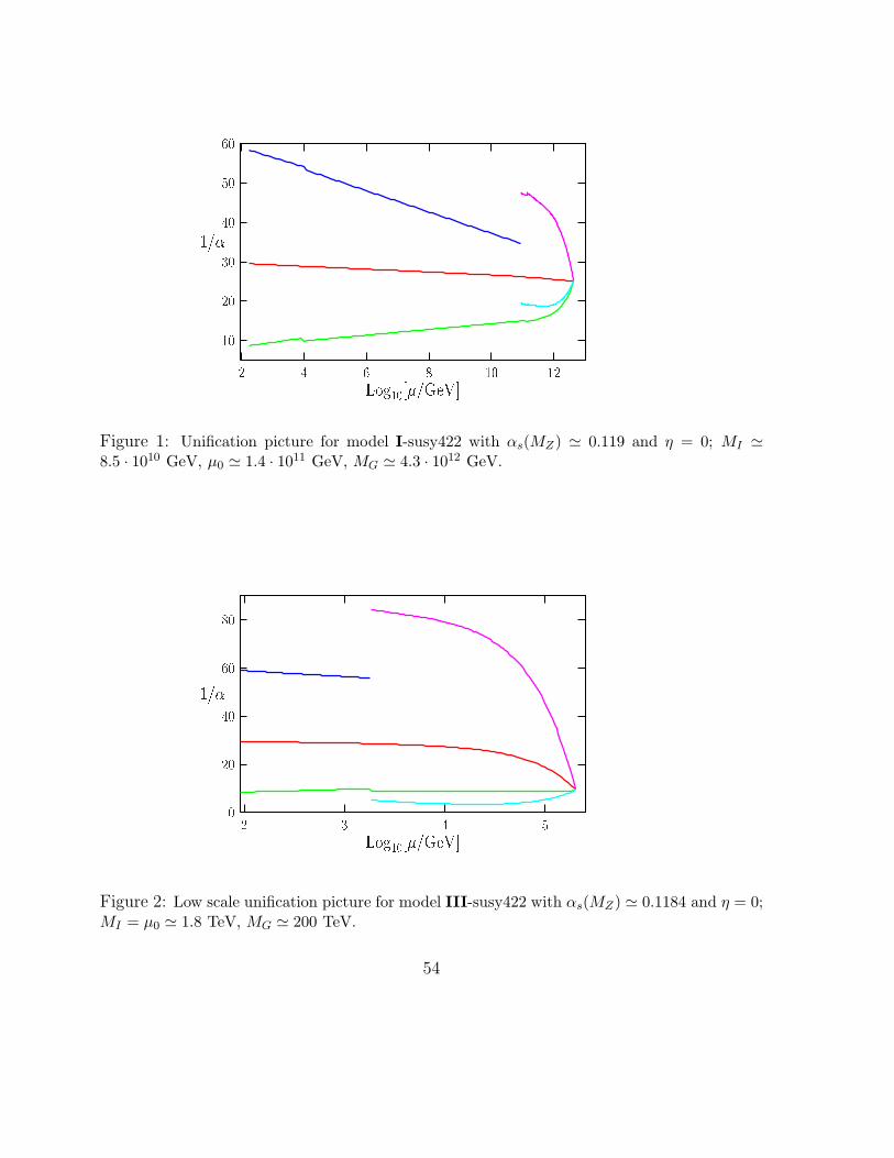
Log10[�=GeV℄1=�

12108642

605040302010Figure 1: Unification picture for model I-susy422 with αs(MZ) ≃ 0.119 and η = 0; MI ≃8.5 · 1010 GeV, µ0 ≃ 1.4 · 1011 GeV, MG ≃ 4.3 · 1012 GeV.

Log10[�=GeV℄1=�

5432

806040200Figure 2: Low scale unification picture for model III-susy422 with αs(MZ) ≃ 0.1184 and η = 0;MI = µ0 ≃ 1.8 TeV, MG ≃ 200 TeV.

54

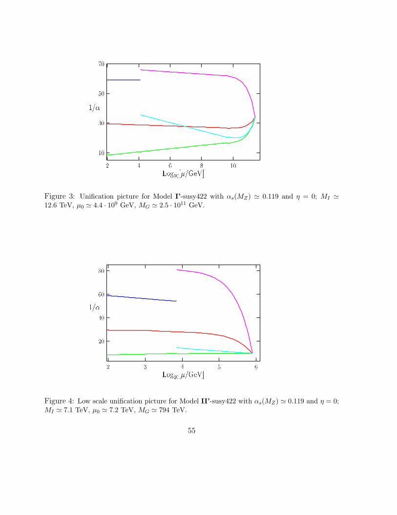
Log10[�=GeV℄1=�

108642

70503010Figure 3: Unification picture for Model I’-susy422 with αs(MZ) ≃ 0.119 and η = 0; MI ≃12.6 TeV, µ0 ≃ 4.4 · 109 GeV, MG ≃ 2.5 · 1011 GeV.

Log10[�=GeV℄1=�

65432

80604020Figure 4: Low scale unification picture for Model II’-susy422 with αs(MZ) ≃ 0.119 and η = 0;MI ≃ 7.1 TeV, µ0 ≃ 7.2 TeV, MG ≃ 794 TeV.

55

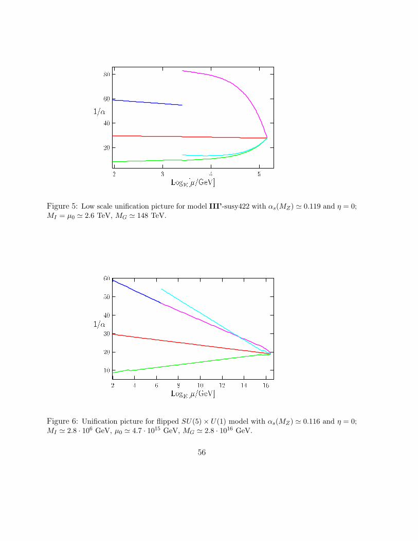
Log10[�=GeV℄1=�

5432

80604020Figure 5: Low scale unification picture for model III’-susy422 with αs(MZ) ≃ 0.119 and η = 0;MI = µ0 ≃ 2.6 TeV, MG ≃ 148 TeV.

Log10[�=GeV℄1=�

161412108642

605040302010Figure 6: Unification picture for flipped SU(5) × U(1) model with αs(MZ) ≃ 0.116 and η = 0;MI ≃ 2.8 · 106 GeV, µ0 ≃ 4.7 · 1015 GeV, MG ≃ 2.8 · 1016 GeV.

56