Galaxy Supercluster Analysis and Visualization: Project Goalstaylorr/Comp715/miller_quammen_final_paper2.pdfGalaxy Supercluster Analysis and Visualization: Project Goals Jameson Miller,

Galaxy Supercluster Analysis and Visualization:Project Goals

Jameson Miller, Cory Quammen - UNC-CH, Computer ScienceMatt Fleenor, Jim Rose - UNC-CH, Physics

May 10, 2005

1 Problem Domain

Determining the large-scale structure of galaxy distribution in the local universe iscurrently an active research area in cosmology. Features called superclusters, whichare global overdensities of galaxies, are of particular interest. Superclusters are com-prised of a collection of galaxy clusters, which are smaller-scale and more dense re-gions of galaxies, along with the regions between these clusters, known as inter-clusterregions. It is currently unknown if the galaxies between clusters, or inter-clustergalaxies, exhibit ordered substructure within the bulk overdensity. The potentialinter-cluster structures, particular those in the Horologium-Reticulum supercluster,are the focus of our astronomer colleagues. Knowledge of supercluster substructuremay help to confirm or refute current models of the universe’s structural evolution.

2 Data Collection Methods

The data used for this visualization project was collected by the UK Schmidt Tele-scope at the Anglo Australian Observatory. Attached to the telescope is an instru-ment, called the 6dF (6-degree field), which is used to perform spectroscopic analysisof the light captured by the telescope from individual galaxies. The galaxies ofinterest are those that make up the Horologium-Reticulum supercluster.

Spectroscopic analysis is used to determine the redshift of light emitted fromeach of the galaxies under study. The redshift provides an estimate of the reces-sional velocity of each galaxy. Since the global trend in the cosmological motion isexpansion proportional to the distance of objects from each other, the recessionalvelocity provides an estimate of each galaxy’s distance from Earth.

Spectroscopic analysis is accomplished by projecting the light from the telescopeonto the 6dF field plate. The location in the sky of each galaxy under study is knowna priori, and a prism is placed upon the 6dF field plate at the locations where each

1

galaxy’s light is received. Optic fiber connects the prism to the spectrometer. Forspeed and accuracy, a robotic arm is employed to place the prisms on the 6dF fieldplate. This allows the redshift of light from up to 150 galaxies to be observed for asingle plate setup, and for many plate setups to be used in a single night [6].

We hoped to use simulation data in this visualization project, but time limitationsprevented that. Further details of the simulation data is provided in the section “DataDescription.”

3 Visualization Goals

3.1 Questions

Our astronomer colleagues have several basic questions they wish to answer withthis visualization project. In order of importance relative to their research goals, thequestions are:

1. Within Horologium-Reticulum, how does one characterize inter-cluster struc-ture? Are there voids, are there spherical lumps, is the structure sponge-likewith highly-connected overdensities?

2. How do observed structures compare with structures in simulated data fromuniverse formation models? Are the same types of shapes found in the ob-served data also found in the simulated data? Are the relative distributions ofstructures the same in observed and simulated data?

3. Within the simulation data, how do true galaxy positions differ from thosethat would be calculated by an observer? Do the true and observed positionsof galaxies contained in some structure vary more than those not contained ina structure? How does density affect observed galaxy position?

The first question has received little attention from the research community. Byanswering it, the astronomers hope to understand how the global overdensity affectsmember galaxy positions. The second question has also received surprisingly littleattention due to lack of interaction among astronomers working with observationaldata and astronomers working on simulations. Answering it would have strong im-plications on the validity of current universe formation models.

3.2 Other Goals

Since determining the member galaxies of inter-cluster structures may be difficultto automate, and there is not currently a good definition of how to define inter-cluster structure, our colleagues requested the ability to manually create groups ofgalaxies. This would involve selecting individual galaxies and adding or removing

2

them from groups. They also require the ability to export selected galaxies to a fileformat accepted by a particular plotting package with which they can make plots forinclusion in publications.

4 Data Description

There are two main types of data used in this project, observation data and simula-tion data. The observation data comes in two forms. The first form consists of 3Dpositional data of galaxies derived from the sky location and redshift data. Out of atotal of 2403 total observed galaxies, 1708 galaxies whose recessional velocities werebetween 12,000 and 27,000 km/sec were chosen. This particular range of recessionalvelocities are those of the galaxies in and around Horologium-Reticulum. The secondform of data consist of the 3D locations of identified cluster centers, derived in thesame way as the individual galaxy position data, but averaged over the locations ofcluster members. Data for 30 clusters are used in this project.

The clusters have been defined in a catalogue created by George Abell in 1958and upated in 1989 [2]. The clustering criteria set forth in [2] considered only thetwo dimensions of the data that define where a galaxy appears in the sky. By takinginto account the third dimension provided by redshift data, our colleagues have find-tuned the members of the clusters by rejecting galaxies whose recessional velocitiesvary by more than 2,000 km/sec from the average cluster membership velocities. Theexact derivation of recessional velocity from redshift data is described later in thispaper.

The galaxies in identified clusters are not of interest to the study at hand. Infact, their presence can actually interfere with determining inter-cluster structure.The interference is a result of each cluster galaxy’s peculiar motion with respect toother members of the cluster, that is, motion caused by the local perturbations of thecluster’s gravitational potential. This peculiar motion causes variations in redshift,making cluster galaxies appear to be either closer or farther than they truly are.Hence, galaxies within a cluster may have a recessional velocity not proportional totheir distance from Earth. This results in those galaxies appearing to interminglewith the true inter-cluster galaxies. For this reason, the galaxies within the clustersare removed from the first data set. However, the known cluster locations can serve aspositional signposts in the remaining data, so it is desirable to have this informationavailable.

The simulation data that we were going to look at consists of 3D positions andvelocities of dark matter particles, each of which represent a mass slightly smallerthan a typical galactic mass. In addition to the position data, the data set has vectordata representing particle velocities. The simulation data has 2563 particles total [4].

As structure identification proceeds on both observation and simulation data,nominal data describing structure membership is created. This data may come from

3

an automatic method or from human selection. In either case, this data is essentialfor characterizing inter-cluster structure.

In addition, the galaxy position data is averaged to produce a rectilinear gridwith a ratio scalar density field. Density can be useful as another means to studystructure in the data.

All told, we had available three non-field data sets (observed galaxy position,observed cluster position, and simulated galaxy position), two nominal data sets(observed and simulated), and two scalar fields (observed density and simulateddensity).

4.1 Observation Data

The observational data describes the locations of galaxies in a particular region of thesky in the southern hemisphere. The data files are formatted as 2D arrays of spatialvalues describing the angular positions of galaxies relative to Earth’s orientation andposition in space, plus a recessional velocity component, derived from redshift, whichcan be taken roughly as a third dimension. One of the two angular positions describesright ascension (RA) and the other describes declination (DEC). Each galaxy hasassociated with it a scalar value representing its recessional speed (cz). The data isstored in ASCII files consisting of floating-point data with between 2 and 6 decimaldigits of precision.

RA describes the position of an object in the sky along the celestial equator,a conceptual plane that sweeps out into space from Earth’s equator. It is akin tolongitude in surface navigation. RA is measured in terms of hours, minutes, andseconds. With the exception of the two rotational poles, a given point on Earthsweeps through all RA positions in a 24-hour span [8].

DEC describes the position above or below the celestial equator. It is measuredin terms of degrees, arcminutes, and arcseconds. The equatorial position correspondsto 0o while the north pole is at +90o and the south pole is at -90o. There are 60arcminutes in a degree and 60 arcseconds in an arcminute [8].

The cz value consists of two components: c, the velocity of light, and z, the ratiobetween the observed wavelength of a galaxy and the emitted wavelength minus 1.Thus, z = λ(observed)

λ(emitted)− 1 [10].

4.2 Observational Data Issues

The set of galaxies chosen for redshift measurement represent approximately 70% ofthe known galaxies above a given apparent brightness (bJ < 17.5) in the observedfield of view. To perform the sampling, a grid was overlayed on top of an equal-areaplot of known galaxies. 70% of the samples within each grid box were chosen atrandom to determine the end random distribution. Sampling in this way reflectedthe distribution of galaxies with respect to RA and DEC.

4

As described above, galaxies that are members of known clusters are removedfrom the main galaxy data. They are not completely missing, however, as the posi-tions of the clusters are kept.

The 6dF instrument provides a precise method of measuring galactic redshiftdata. Each fiber has a 6.7 arcsecond diameter and can be positioned to an accuracyof 1 arcsecond. Redshift data is accurate to within 50km/s [3]. Unfortunately,there is a great deal of uncertainty in deriving distance from redshift data. First,conversion from redshift data depends on the choice of Hubble constant. The Hubbleconstant is currently unknown and estimates of it vary. Our astronomer colleagueshave chosen to set the Hubble constant at 70 km s−1/Mpc, where Mpc stands formegaparsec (one million parsecs). Second, gravity affects the redshift of light as ittravels through the universe in non-obvious ways, causing uncertainty in the redshiftvalues. No attempt to correct for these uncertainties is undertaken in this project.

Redshift is also affected by the peculiar motion of galaxies, that is, motion withinthe supercluster. A galaxy’s peculiar motion affects its observed redshift and hencethe estimated position of the galaxy. For example, a peculiar motion of a galaxyaway from Earth combined with the general expansion of the universe would makethat galaxy appear farther away while a peculiar motion toward Earth would makethe galaxy appear closer than its true distance. For the inter-cluster galaxies understudy, the error induced by peculiar motion was assumed to be negligible, within 1%of the motion caused by the general expansion of the universe.

Finally, the quantization level of the data has no effect on its interpretation.Each data value has 6 or 7 significant digits, about as good as one could expect fromobservational data.

4.3 Simulation Data

The simulation data comes from computations carried out by the Virgo Supercom-puting Consortium using computers at the Computing Centre of the Max-PlanckSociety in Garching, Germany. The data were generated by a low density cold darkmatter model of universe formation. The lambda CDM model used 2563 cold par-ticles with mass on the order of a small galaxy, that is, 4.8 × 1010 solar masses [4].The Hubble constant was assumed to be 70 km s−1/Mpc, the same value as our as-tronomer colleagues are assuming. The simulation code HYDRA was run on a CrayT3D using 64 processors [7]. As in the observational data, the simulation data con-tains 3D positions of these cold particles. In addition, the velocities of each galaxyare available.

4.4 Simulation Data Issues

In the simulation data, all positions and velocities of the particles are known precisely.This is in contrast to the observational data, where only a galaxy’s apparent position

5

is known. This poses a challenge when trying to compare the simulated data withthe observed data. To make a useful comparison, a reference observation point wouldneed to be chosen in the simulation domain, and the simulation data would need tobe converted to RA-DEC-cz values as seen from the observation point. Then, theRA-DEC-cz values would need to be converted back to the same 3D space to whichthe observation data were projected.

The number of particles, 2563, is many orders of magnitude higher than thenumber of galaxies in the observed data. Therefore, data reduction would be requiredto make meaningful comparisons between the two. Our colleagues have typically usedonly one eighth of the simulation data, reducing the data to 1283 particles. Theyfurther sample the particles down to 1/1000 the number of particles in the originaleight of the data set, giving approximately the same number of samples as in theobservational data.

In addition, the clusters are not removed from the simulation data, making usefulcomparisons with the observed data difficult. In the observed data, clusters wouldneed to be determined by an automatic clustering selection algorithm such as the C4algorithm in [5]. We would need to convert the data to RA-DEC-cz values and runthis clustering algorithm on the simulated data, removing the clusters that it foundfrom the data set.

5 Visualization Design

In this section, we detail our ideal visualization strategy for this data and, moreimportantly, for achieving our colleagues’ research goals. We did not consider con-straints, either time-wise or resource-wise, on implementation of the techniques wechose, but rather focused on what would be the best for reaching the research goals.

5.1 General Visualization Techniques

A common thread through the various questions we attempted to answer was the needto accurately perceive 3D shape. According to Ware, stereo depth and structure-from-motion are very important for 3D structure perception [9]. Taking this intoaccount our system should provide support for stereoscopic displays. Users should beable to adjust eye-separation parameters to fit their particular preferences. In addi-tion we should provide interactive view control. This would allow rotation, zooming,and panning. Users who have control over the view have a better understanding of 3Dshape. Sometimes, however, we thought it might have been beneficial to automatea torsional rocking motion for showing structure-from-motion. This would allow theuser to concentrate on the structure information he or she was seeing instead of ondriving the interaction.

Another option useful for answering each of the questions would be the ability tolimit the visualization volume. Only the galaxies located in the specified visualization

6

volume would be viewable, allowing for the user’s concentration on smaller scalestructures. This would remove galaxies from the background that might distract theviewer from the local structure. The boundaries of the viewing volume should alsobe interactively adjustable.

5.2 Identifying and Characterizing Structure in ObservedData

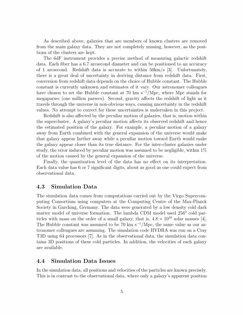
There are several visualization techniques that could be applied to the problem ofidentifying and characterizing inter-cluster structure. We would chose to use iso-surfaces with screen door transparency for exploring the density field, glyphs forrepresenting galaxies and clusters, and to restrict the view volume. After averagingthe point data to a structured grid, isosurfaces could be generated to visualize re-gions of a particular density. It is assumed that regions containing structures were ofhigher density than surrounding regions, and would show up when visualizing withisosurfaces. Since there is no clear density definition for structure, we allowed theisovalue to be adjusted by the user.

The ability to view and select individual galaxies is important to our colleagues.In order to provide the ability to view and select individual galaxies within an iso-surface, a texture that provides screen door transparency should be mapped on theisosurface. The overall structure is expected to be of low frequency, so a screen doortexture with large enough holes to allow viewing of the galaxies would not interferewith perception of the isosurface’s shape. This combination would allow for observingboth the overall structure of the density field and for viewing the individual galaxieswithin the isosurface. Furthermore the texture on the surface would aid in stereo-scopic fusion. The alternative would be to use an opaque or translucent isosurface.An opaque isosurface would have occluded viewing of the galaxies contained within.A translucent isosurface would have interfered with shape and depth perception ofthe isosurface. In addition, a translucent isosurface would have made it difficult todiscern if galaxies were contained within a particular connected component of theisosurface. If a galaxy glyph’s colors had been blended with the isosurface, one couldnot know if the galaxy was behind only one isosurface boundary, making it insidethe volume enclosed by the isosurface, or behind two isosurface boundaries, makingit outside the isosurface.

Glyphs should be used to indicate specific objects in our data set, which includegalaxies and previously-specified clusters. Spherical and cylindrical glyphs shouldbe used to represent galaxies and clusters, respectively, and each should have aperceptually distinct color. Glyphs have two advantages over pixel-sized points inour visualization. First, glyphs have size and take up physical space which allowsfor scaling due to perspective projection. Second, glyphs occlude each other, helpingwith depth perception. If galaxies are represented as pixel points in space, both ofthese depth cues would be lost. To help with the characterization task, the user

7

Figure 1: An example of screen door transparency applied to the density isosurface.

could select galaxies and assign them to different groups. These groups should benominally color-coded. The color mapping scheme should be selected by the programto ensure a suitable selection of colors so that each group can easily be distinguished.The choice of colors should be based on the recommendation in Ware’s book [9].

Another technique that was considered to answer this question was direct volumerendering. While this technique would give an overall impression of density through-out the volume, it would be difficult to perceive 3D structures, such as filaments, inthe data set. If we chose to map opacity to density with, say, a linear ramp, therewould be no sharp surface generated, so shape perception of structures in the dataset would not be easily perceived. If, on the other hand, we chose to map opacityto density gradient, then edges of structures would be easier to see, but at the costof some translucency in the volume. A final strike against direct volume renderingis the fact that the point data are not of sufficient density to justify the cloud-likeeffect direct volume rendering produces. In the end, an isosurface with screen doortransparency will produce a readily perceivable surface to distinguish shapes in thedata set while still allowing users to view galaxies within the isosurface.

5.3 Comparing Observed Data to Simulated Data

Viewing a single 3D data set is challenging. Comparing two 3D data sets in a singlevisualization is even more challenging, depending on the similarity of the two datasets. Comparing two data sets representing the same natural phenomena but whichcome from different sources, all within the same visualization is, to our knowledge,

8

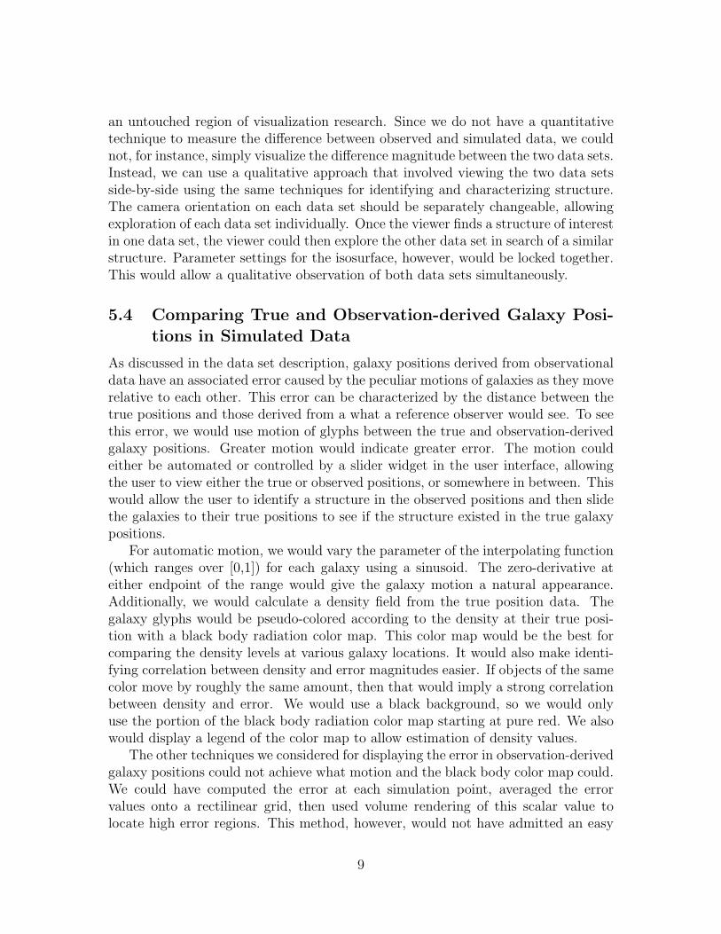
an untouched region of visualization research. Since we do not have a quantitativetechnique to measure the difference between observed and simulated data, we couldnot, for instance, simply visualize the difference magnitude between the two data sets.Instead, we can use a qualitative approach that involved viewing the two data setsside-by-side using the same techniques for identifying and characterizing structure.The camera orientation on each data set should be separately changeable, allowingexploration of each data set individually. Once the viewer finds a structure of interestin one data set, the viewer could then explore the other data set in search of a similarstructure. Parameter settings for the isosurface, however, would be locked together.This would allow a qualitative observation of both data sets simultaneously.

5.4 Comparing True and Observation-derived Galaxy Posi-tions in Simulated Data

As discussed in the data set description, galaxy positions derived from observationaldata have an associated error caused by the peculiar motions of galaxies as they moverelative to each other. This error can be characterized by the distance between thetrue positions and those derived from a what a reference observer would see. To seethis error, we would use motion of glyphs between the true and observation-derivedgalaxy positions. Greater motion would indicate greater error. The motion couldeither be automated or controlled by a slider widget in the user interface, allowingthe user to view either the true or observed positions, or somewhere in between. Thiswould allow the user to identify a structure in the observed positions and then slidethe galaxies to their true positions to see if the structure existed in the true galaxypositions.

For automatic motion, we would vary the parameter of the interpolating function(which ranges over [0,1]) for each galaxy using a sinusoid. The zero-derivative ateither endpoint of the range would give the galaxy motion a natural appearance.Additionally, we would calculate a density field from the true position data. Thegalaxy glyphs would be pseudo-colored according to the density at their true posi-tion with a black body radiation color map. This color map would be the best forcomparing the density levels at various galaxy locations. It would also make identi-fying correlation between density and error magnitudes easier. If objects of the samecolor move by roughly the same amount, then that would imply a strong correlationbetween density and error. We would use a black background, so we would onlyuse the portion of the black body radiation color map starting at pure red. We alsowould display a legend of the color map to allow estimation of density values.

The other techniques we considered for displaying the error in observation-derivedgalaxy positions could not achieve what motion and the black body color map could.We could have computed the error at each simulation point, averaged the errorvalues onto a rectilinear grid, then used volume rendering of this scalar value tolocate high error regions. This method, however, would not have admitted an easy

9

way to correlate error to density. It also would not have allowed comparison ofobservation-derived positions in comparison to the true positions. We could alsohave created isosurfaces, one for error and one for density, but one isosurface couldocclude another, making correlation between error and density difficult to discern.Moreover, isosurfaces would only display how one error value correlated with onedensity value. Finally, cutting planes would not be useful because of occlusion. Ourchoice of using two distinct visual channels that do not interfere with each otherwould allow the relationship between error and density to be conveyed well.

5.5 Keeping Viewers Oriented

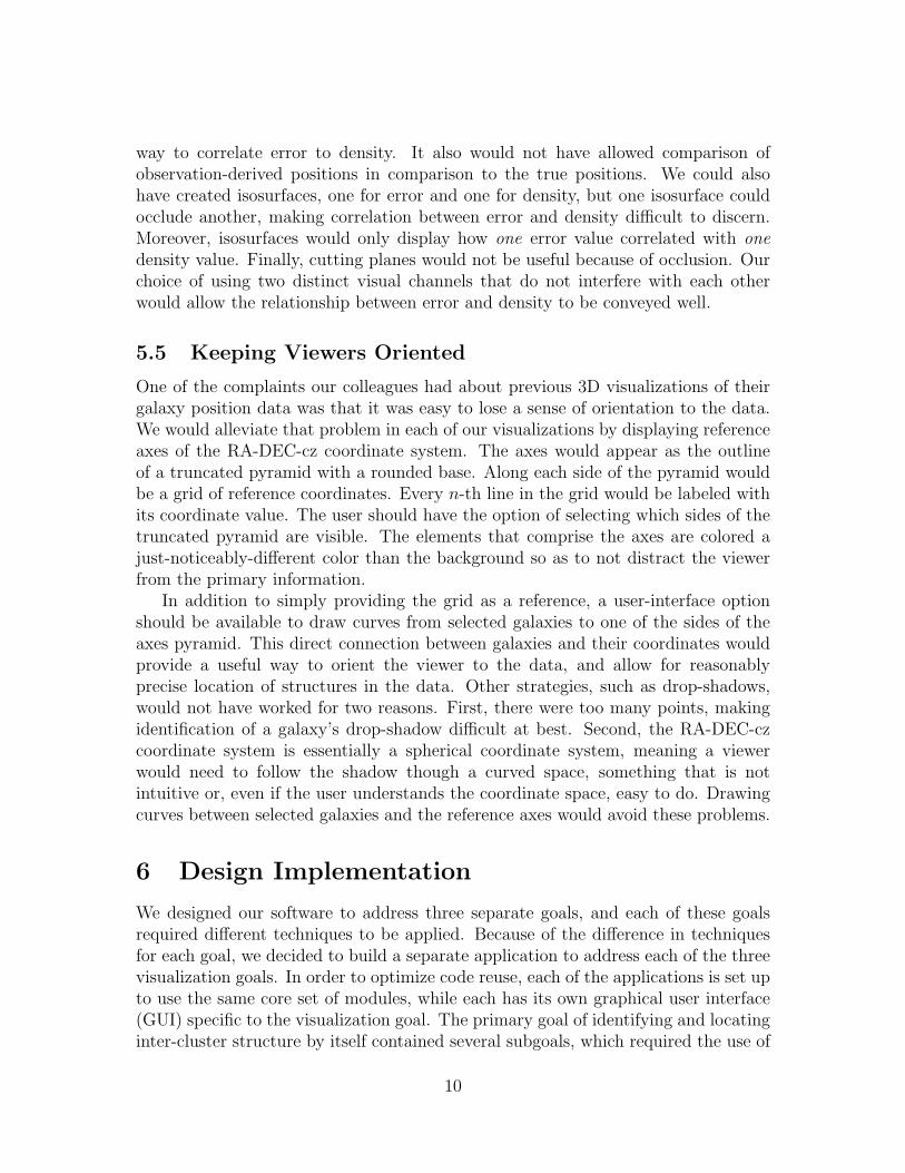
One of the complaints our colleagues had about previous 3D visualizations of theirgalaxy position data was that it was easy to lose a sense of orientation to the data.We would alleviate that problem in each of our visualizations by displaying referenceaxes of the RA-DEC-cz coordinate system. The axes would appear as the outlineof a truncated pyramid with a rounded base. Along each side of the pyramid wouldbe a grid of reference coordinates. Every n-th line in the grid would be labeled withits coordinate value. The user should have the option of selecting which sides of thetruncated pyramid are visible. The elements that comprise the axes are colored ajust-noticeably-different color than the background so as to not distract the viewerfrom the primary information.

In addition to simply providing the grid as a reference, a user-interface optionshould be available to draw curves from selected galaxies to one of the sides of theaxes pyramid. This direct connection between galaxies and their coordinates wouldprovide a useful way to orient the viewer to the data, and allow for reasonablyprecise location of structures in the data. Other strategies, such as drop-shadows,would not have worked for two reasons. First, there were too many points, makingidentification of a galaxy’s drop-shadow difficult at best. Second, the RA-DEC-czcoordinate system is essentially a spherical coordinate system, meaning a viewerwould need to follow the shadow though a curved space, something that is notintuitive or, even if the user understands the coordinate space, easy to do. Drawingcurves between selected galaxies and the reference axes would avoid these problems.

6 Design Implementation

We designed our software to address three separate goals, and each of these goalsrequired different techniques to be applied. Because of the difference in techniquesfor each goal, we decided to build a separate application to address each of the threevisualization goals. In order to optimize code reuse, each of the applications is set upto use the same core set of modules, while each has its own graphical user interface(GUI) specific to the visualization goal. The primary goal of identifying and locatinginter-cluster structure by itself contained several subgoals, which required the use of

10

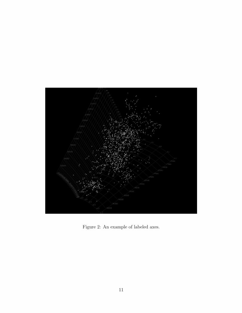
Figure 2: An example of labeled axes.

11

Figure 3: An example of lines connecting galaxies in space to a reference grid.

several visualization techniques. We worked closely with our clients in order togain feedback on each version of our design, and incorporated their suggestions intosuccessive implementations of the design. The end result is an implementation ofall the techniques that we thought would provide the optimal visualization for theprimary goal. The system provides an interactive interface in which to explore theirdata set. The secondary and tertiary goals were not completed, as fully implementingthe techniques that we thought would be optimal for the first visualization took longerthan expected. The issues of implementing these secondary and tertiary goals willbe discussed later in the paper.

Our project did not involve extending a visualization system that was alreadyin place, but rather was designed from the ground up. We first attempted to useJava to develop the software, but quickly changed to Python. We used Pythonbecause it seemed have better integration with VTK, especially under Linux andMac OS X. Tkinter, a Python wrapper for TCL/TK, was used to generate the userinterface. We chose to use VTK as the visualization library. Our choice of VTKand Python means that our system should run on any hardware that supports thesetwo packages. Our current software runs against VTK 4.4, and works with Python2.2 or 2.3. The current binary release of VTK (4.2) requires the use of Python2.1, which is incompatible with our Python code. The system was developed andtested on both a Windows and Linux platform, and was also run under Mac OS X.Some portions of this program were only tested under the Windows environment,such as stereo using the CrystalEyes emitter and goggles. Our clients evaluated

12

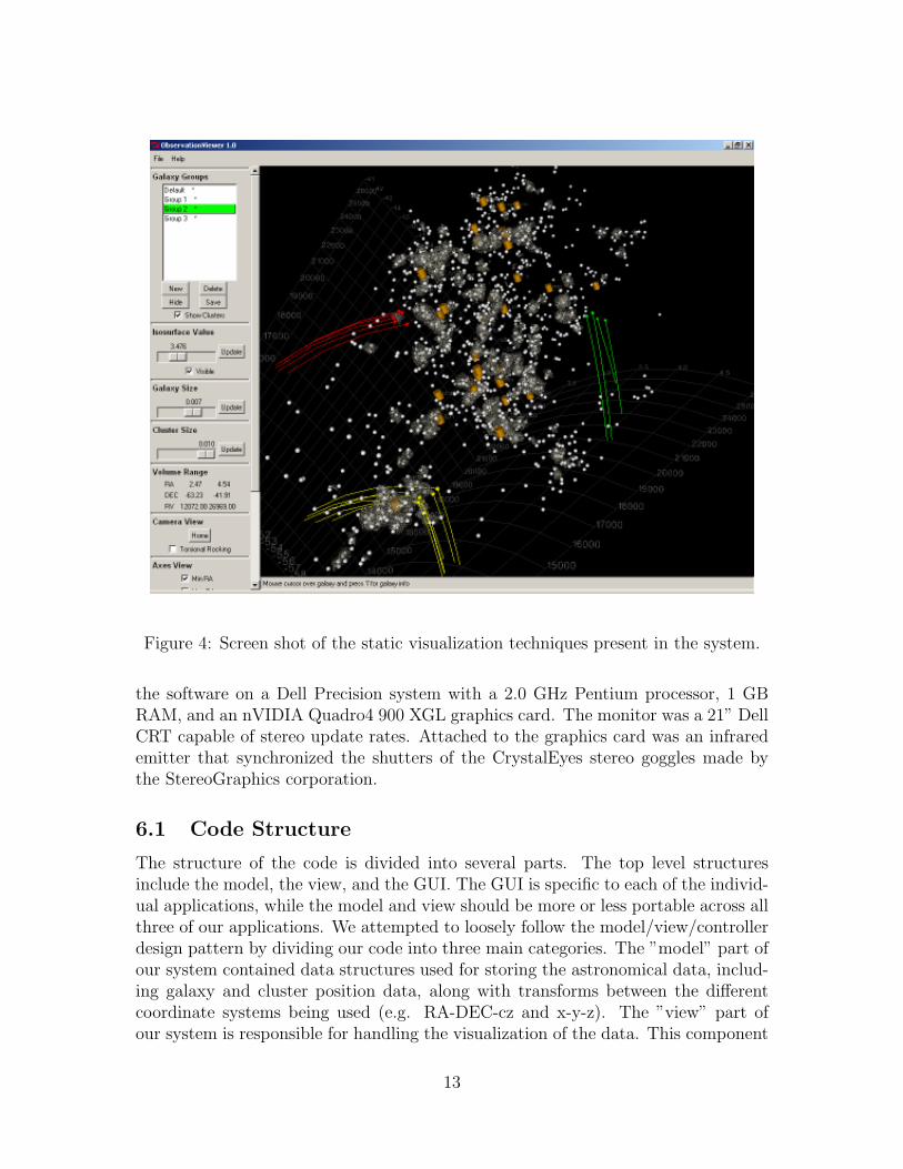
Figure 4: Screen shot of the static visualization techniques present in the system.

the software on a Dell Precision system with a 2.0 GHz Pentium processor, 1 GBRAM, and an nVIDIA Quadro4 900 XGL graphics card. The monitor was a 21” DellCRT capable of stereo update rates. Attached to the graphics card was an infraredemitter that synchronized the shutters of the CrystalEyes stereo goggles made bythe StereoGraphics corporation.

6.1 Code Structure

The structure of the code is divided into several parts. The top level structuresinclude the model, the view, and the GUI. The GUI is specific to each of the individ-ual applications, while the model and view should be more or less portable across allthree of our applications. We attempted to loosely follow the model/view/controllerdesign pattern by dividing our code into three main categories. The ”model” part ofour system contained data structures used for storing the astronomical data, includ-ing galaxy and cluster position data, along with transforms between the differentcoordinate systems being used (e.g. RA-DEC-cz and x-y-z). The ”view” part ofour system is responsible for handling the visualization of the data. This component

13

is responsible for changing the visibility of objects in the visualization. The GUIis responsible for the creation of the user interface, along with communicating userinputs to the view/model.

6.2 Visualization Algorithms

The data files that were read by this application are sets of point data for galaxy andcluster position. The data can be viewed as discrete objects, where each galaxy andcluster is represented by individual glyphs. An isosurface can also be generated usinga particular isovalue in a density field that is computed from the galaxy position data.Each of the objects that can be visualized is created when the data set is loaded,but is not always visible by default. For instance, all of the lines from galaxy glyphsto a particular axis are created when the galaxy data set is loaded, but the visibilityof these actors is turned off. When the user wants to view the lines, the visibility isturned on.

The first step in importing the data is to scale, rotate, and translate the galaxyand cluster positions to fit within a 2x2x2 box centered at the origin of the viewingvolume. The positions are rotated so that the long dimension of the data set, thecz dimension, is aligned with the z-axis in x-y-z space. This is important whencalculating the density field because it allows the data volume to more fully fill theviewing domain, improving the grid-size-to-data-frequency ratio.

6.2.1 Camera Controls

A home button is included to set the camera at a default location in case the user getslost in the visualization and would like to get back to a familiar viewpoint. Anothercamera control is provided to turn on and off torsional rocking of the camera aboutthe up vector. This rocking is accomplished by setting a timer in Python to rotate theimage a certain angle every 1/30 of a second. The angle of rotation is determined by asinusoidal function whose argument is incremented (π/16) for each camera rotation.

6.2.2 Galaxy Glyphs

The galaxies are represented by spherical glyphs. Galaxies are colored according towhich group they have been assigned to by the user. Groups of galaxy glyphs arecontained and controlled by the GalaxyGroupManager class. The GalaxyGroupMan-ager class also controls the assignment of colors to galaxy groups. A vtkSphereSourceis used to create the sphere glyphs. The coordinates of each galaxy in x-y-z spaceis passed to the vtkSphereSource. A vtkGlyph3D object is then created using theoutput of the vtkSphereSource object. A vtkPolyDataMapper takes the output fromvtkGlyph3D object. A vtkActor is assigned to this vtkGlyph3D object, which isthen assigned to the vtkRenderer. These glyphs are color coded according to whichgroup they are assigned. The visibility of these glyphs can be toggled on and off,

14

the size of the glyphs can be set by the user through a slider bar, and lines can bedrawn from the glyph to its location on the axes.

In a second iteration of our implementation, we chose to assign the galaxy glyphsto their own actors. Our first implementation grouped all of the galaxy glyphs intoa single vtkActor. This caused problems when we started to implement the abilityto pick out individual galaxies and assign them to different groups. VTK includesfunctions to query the visualization to see what actors intersect with a line drawnfrom the mouse pointer through the view volume. Since we only had a single actorrepresenting all of the galaxies, this did not tell us what galaxy we were trying topick. Representing all of the galaxies as individual actors was the correct way to dothis, though it adds some memory overhead.

6.2.3 GalaxyGroupManager

The GalaxyGroupManager is used to organize the galaxy groups, and is the mainpoint for accessing the galaxies and galaxy glyphs. The Galaxy Group Manager isresponsible for automatically assigning colors to each of the galaxy groups. The listof available colors is based on Ware’s color selection for nominal coding [?, ware]

6.2.4 GalaxyRenderWidget

This class is a TK widget that provides a rendering window. It subclasses vtk-TkRenderWidget, but adds extra key-bindings. The keys ’m’,’n’,’b’,’v’ are boundto functions that handle the visibility of curves from glyphs to axes. The keys ’p’and ’i’ are bound to functions that pick individual galaxies. Individual galaxies arepicked through the use of vtkPointPicker. The ’p’ key assigns the selected galaxy tothe currently selected group while the ’i’ key displays information about the galaxyin the GUI.

6.2.5 Cluster Glyphs

The locations of previously identified clusters are indicated through the use of cylin-drical glyphs. These glyphs are colored orange, which is perceptually distinct fromany other object in the visualization. The size and visibility of these glyphs canbe easily adjusted by the user through a checkbox and slider bar, respectively. Thepipeline for creating the cluster glyphs is similar to the pipeline for the galaxy glyphs,except that a vtkCylinderSource is used instead of a vtkSphereSource. The ID ofeach glyph is shown next to the cluster in the visualization. The text of the ID is setup to always face the camera through the use of a vtkFollower instead of a vtkActor.

6.2.6 Drop Curves

Another visualization technique we implemented is to have curved lines drawn fromgalaxy glyphs in a particular group to a particular axis. The lines are colored the

15

same as the galaxy glyphs to which they are connected. They are curved to follow agalaxy’s RA or DEC value as it varies in the other dimension to one of the referenceaxes. The commands for drawing lines from galaxies to an axis are bound to keyboardbuttons. Keyboard buttons ’m’, ’n’, ’b’, ’v’ are bound to turning on or off curvesfrom galaxies to the RA-min, RA-max, DEC-min, DEC-max axis.

One problem with using multiple lines to approximate the curves from the galaxiesto the axes is the amount of memory it takes to store all the line segments. Weattempted three different implementations. The first attempt was to draw a straightline from the galaxy to the axis. This required little memory but did not look verygood, and could be confusing as lines could criss-cross. The second attempt usedmultiple vtkLineSources for each curve. The approach looked better and was lessconfusing but also took about 250 MB of memory! To see if the amount of memoryused could be reduced, a third approach was tried using vtkPolyLine objects. Theproblem with this approach is that we also had to create vtkUnstructuredGrid objectsto store each vtkPolyLine. These vtkUnstructuredGrid objects had to be mappedwith the vtkDataSetMapper and then assigned to a vtkActor. This resulted inmemory usage for curved lines alone ballooning to 400 MB! We decided to use thevtkLineSource approach as this provided curved lines at lower memory usage. Thebest way to implement this would have been to generate the curved lines on the flyas they are requested, but this might also slow down the interactivity of turning thelines on and off.

6.2.7 Density Field Generation

To generate the galaxy density field efficiently, we first create a vtkRectilinearGridobject, set its dimensions to 1283, and assign evenly-spaced slice coordinate positionsalong each dimension. We then create a vtkPointLocator object and connect it tothe vtkRectilinearGrid object. This sets up an octree structure to make locatingthe grid nodes within a certain radius of each galaxy position efficient. We set thisradius to be the length of four grid spacings. For each galaxy, we find each grid nodewithin this radius, calculate the distance from the galaxy to the grid node, and usethis distance as a parameter to a 3D Gaussian function. The closer the galaxy is toa grid point, the higher its density contribution to that grid point.

6.2.8 Isosurface generation

To generate the isosurface, we use a vtkContourFilter applied to the density field. Wethen use the vtkPolyDataNormals filter to generate smooth normals at each vertexin the isosurface. To generate the screen door transparency effect, we use a texturemap with circular regions of complete transparency. The 256x256 texture map isshown here. The white region is fully opaque while the black circles represent fullytransparent areas. Using a white texture map allows the color of the isosurface to bemodulated with a color of our choosing, a dull gray color that is perceptually distinct

16

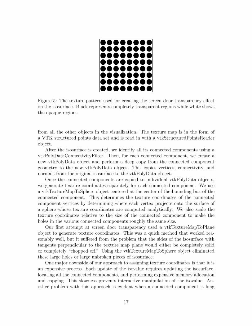
Figure 5: The texture pattern used for creating the screen door transparency effecton the isosurface. Black represents completely transparent regions while white showsthe opaque regions.

from all the other objects in the visualization. The texture map is in the form ofa VTK structured points data set and is read in with a vtkStructuredPointsReaderobject.

After the isosurface is created, we identify all its connected components using avtkPolyDataConnectivityFilter. Then, for each connected component, we create anew vtkPolyData object and perform a deep copy from the connected componentgeometry to the new vtkPolyData object. This copies vertices, connectivity, andnormals from the original isosurface to the vtkPolyData object.

Once the connected components are copied to individual vtkPolyData objects,we generate texture coordinates separately for each connected component. We usea vtkTextureMapToSphere object centered at the center of the bounding box of theconnected component. This determines the texture coordinates of the connectedcomponent vertices by determining where each vertex projects onto the surface ofa sphere whose texture coordinates are computed analytically. We also scale thetexture coordinates relative to the size of the connected component to make theholes in the various connected components roughly the same size.

Our first attempt at screen door transparency used a vtkTextureMapToPlaneobject to generate texture coordinates. This was a quick method that worked rea-sonably well, but it suffered from the problem that the sides of the isosurface withtangents perpendicular to the texture map plane would either be completely solidor completely “chopped off.” Using the vtkTextureMapToSphere object eliminatedthese large holes or large unbroken pieces of isosurface.

One major downside of our approach to assigning texture coordinates is that it isan expensive process. Each update of the isovalue requires updating the isosurface,locating all the connected components, and performing expensive memory allocationand copying. This slowness prevents interactive manipulation of the isovalue. An-other problem with this approach is evident when a connected component is long

17

and narrow. The holes near the center are small while the holes on the far ends ofthe connected component are large. Using a more advanced algorithm for texturecoordinate assignment would fix this problem.

6.2.9 Axes

Four different axes are available in the visualization. The four axes are positioned atthe limits of the volume containing the galaxies. Two of the axes are oriented in theRA-cz coordinate plane, sweeping through the range of DEC values, and the othertwo are oriented in the DEC-cz coordinate plane, sweeping through the RA values.For each of the axes, a grid line is drawn every 1000 cz units. The axes are labeledwith RA and cz or DEC and cz values, depending on the reference axes. The labelsare set to always face the camera, so that they can be read no matter the cameraorientation.

7 Visualization System Evaluation

As we were only able to complete the visualization for answering our colleagues’primary goal of finding structure in their observed data, we limited our evaluationto this system. Before performing our evaluation, we provided a brief overview ofthe various parameter controls our system allowed users to set. Since the goal of thisevaluation was to gauge the effectiveness of our visualization technique and not ouruser interface design, we felt this introduction to the basic parameter controls of ourapplication was appropriate.

As student and advisor, our colleagues Matt and Jim work closely on analyzingtheir data. Because of this, we felt they should work together on our evaluationtasks. During the evaluation, they each took turns as the primary manipulator ofthe system. The person not in control would often make suggestions as to the courseof action to take. This was helpful in analyzing our system’s effectiveness becauseeach of their thought processes was communicated verbally to each other.

For evaluation of our system, we first asked our colleagues to perform three taskswith synthetic data sets. The first task involved identifying shapes and their locationsin a data set. The second task involved identifying voids, or locations where nogalaxies were present, and their locations. Finally, the third task involved countingthe number of galaxies within a connected component of an isosurface. After ourcolleagues finished these tasks based on synthetic data, we observed them as theyviewed their data for the first time with our fully-implemented visualization system.

7.1 Identifying and Locating Structures

For the first task, we inserted familiar shapes, such as spherical shells, cube shells, andcylindrical shells, into a data set consisting of galaxy positions uniformly distributed

18

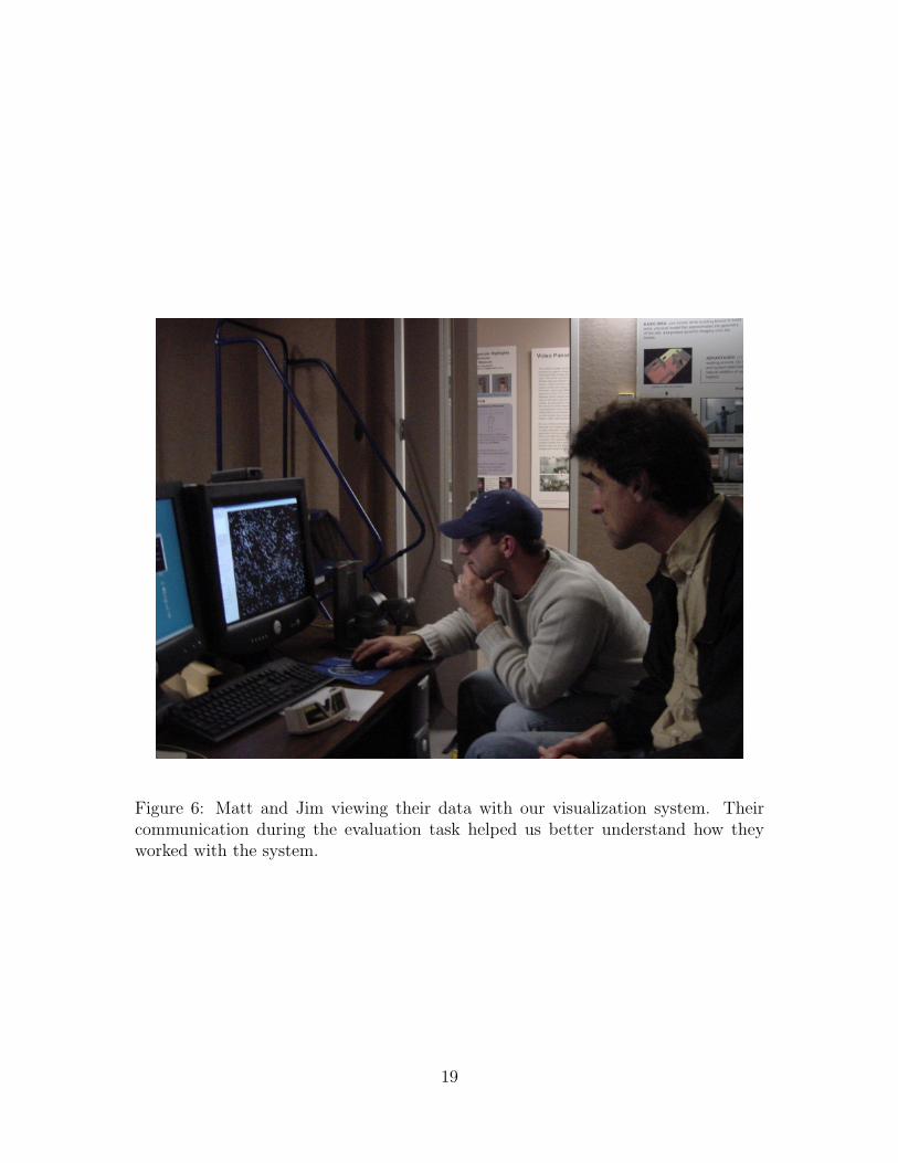
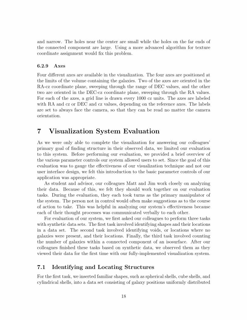
Figure 6: Matt and Jim viewing their data with our visualization system. Theircommunication during the evaluation task helped us better understand how theyworked with the system.

19

in the RA, DEC, and cz dimensions. 1500 random galaxy locations were generatedinside a volume ranging from 2.0 to 4.5 hours in the RA dimension, -5 to 5 degreesin the DEC dimension, and 12000 to 27000 km/sec in the cz dimension. We thenasked our colleagues to identify the shapes we inserted into the random data set.Once the shapes were identified, we asked our colleagues to locate the centers of theshapes in the RA-DEC-cz coordinate system. We had them repeat this task, butwith stereo goggles on the second time. This task was designed to see how effectiveour visualization system was for identifying and locating structure.

For the first task without the stereo goggles, we inserted a spherical shell, a cubeshell, and a cylindrical shell. Our colleagues were able to identify the inserted shapesright away. They were a bit surprised to find such common shapes since they werecoming in with the mindset that they would be looking for cosmological features.After this initial confusion subsided, they set about identifying the centers of theshapes. Right away, they turned some of the reference axes on. After that, theyopted to draw curves from the galaxy positions to the reference axes. Since theyonly wanted a few curves drawn, they chose to create a galaxy group, pick some ofthe galaxies on the shape they were looking at, and draw curves from those galaxiesto the reference axes. There was some confusion when they tried to determine whichpoints would be the best for finding the center of the shapes. They thought that theshapes were filled, but after a few minutes, realized that the shapes were just shells.After a while, they decided to add some representative galaxies distributed aroundthe shape to get an estimate of the center of the shape. Finding the center of thefirst shape they identified took roughly 15 minutes. This was, no doubt, becauseof unfamiliarity with the application and the task, in addition to noise in the labin which we did the evaluation. In fact, Jim made a discouraging comment afterthat first attempt: “This should be easier.” Our colleagues were also very carefulin their estimation, taking the time to be as precise as possible in their answers,more precise than we were expecting them to be. They even joked about providing aplus-or-minus error term in their answers. Identification of the second shape’s centerwent much faster. There were some hiccups due to a small bug in the program andduplicated galaxy position data in the test files, but our colleagues were able to findworkarounds without us intervening and proceeded with the task.

The results for the first task were encouraging. They found the shapes in therandom noise immediately, and their estimates of the shape positions were reasonablyaccurate. Table 1 shows a list of the shapes, their actual centers, and the estimatedcenters.

For the repetition of this task with stereo, we had another data set with threeother shapes added in. This time, there were two cube shells at different locationsand a single warped cylinder. Again, they found the shapes right away. They werea little confused because they thought this new data set was the same as the oldone, and so they second-guessed their identification of a sphere in the first data set.They eventually figured out that this was a different data set. Our colleagues’ initial

20

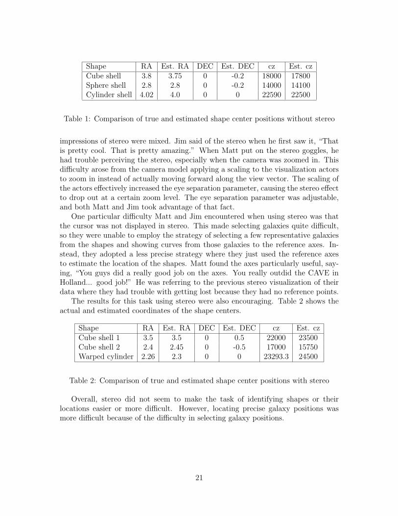
Shape RA Est. RA DEC Est. DEC cz Est. czCube shell 3.8 3.75 0 -0.2 18000 17800Sphere shell 2.8 2.8 0 -0.2 14000 14100Cylinder shell 4.02 4.0 0 0 22590 22500

Table 1: Comparison of true and estimated shape center positions without stereo

impressions of stereo were mixed. Jim said of the stereo when he first saw it, “Thatis pretty cool. That is pretty amazing.” When Matt put on the stereo goggles, hehad trouble perceiving the stereo, especially when the camera was zoomed in. Thisdifficulty arose from the camera model applying a scaling to the visualization actorsto zoom in instead of actually moving forward along the view vector. The scaling ofthe actors effectively increased the eye separation parameter, causing the stereo effectto drop out at a certain zoom level. The eye separation parameter was adjustable,and both Matt and Jim took advantage of that fact.

One particular difficulty Matt and Jim encountered when using stereo was thatthe cursor was not displayed in stereo. This made selecting galaxies quite difficult,so they were unable to employ the strategy of selecting a few representative galaxiesfrom the shapes and showing curves from those galaxies to the reference axes. In-stead, they adopted a less precise strategy where they just used the reference axesto estimate the location of the shapes. Matt found the axes particularly useful, say-ing, “You guys did a really good job on the axes. You really outdid the CAVE inHolland... good job!” He was referring to the previous stereo visualization of theirdata where they had trouble with getting lost because they had no reference points.

The results for this task using stereo were also encouraging. Table 2 shows theactual and estimated coordinates of the shape centers.

Shape RA Est. RA DEC Est. DEC cz Est. czCube shell 1 3.5 3.5 0 0.5 22000 23500Cube shell 2 2.4 2.45 0 -0.5 17000 15750Warped cylinder 2.26 2.3 0 0 23293.3 24500

Table 2: Comparison of true and estimated shape center positions with stereo

Overall, stereo did not seem to make the task of identifying shapes or theirlocations easier or more difficult. However, locating precise galaxy positions wasmore difficult because of the difficulty in selecting galaxy positions.

21

7.2 Identifying and Locating Voids

The second task we gave our colleagues was to identify voids in a synthetic dataset. This task was designed to assess our visualization technique’s ability to revealstructure through displaying “negative” structure, or regions where no galaxies arepresent. Finding these voids and characterizing their shape has important implica-tions on the universe’s topology.

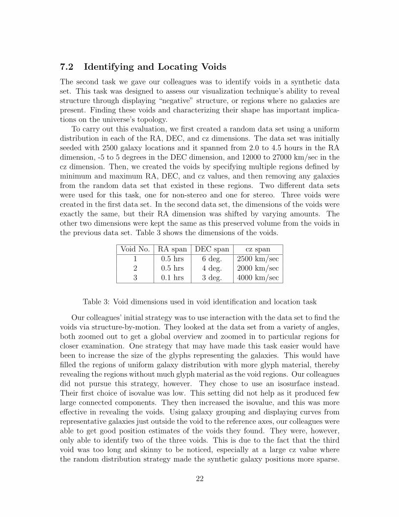
To carry out this evaluation, we first created a random data set using a uniformdistribution in each of the RA, DEC, and cz dimensions. The data set was initiallyseeded with 2500 galaxy locations and it spanned from 2.0 to 4.5 hours in the RAdimension, -5 to 5 degrees in the DEC dimension, and 12000 to 27000 km/sec in thecz dimension. Then, we created the voids by specifying multiple regions defined byminimum and maximum RA, DEC, and cz values, and then removing any galaxiesfrom the random data set that existed in these regions. Two different data setswere used for this task, one for non-stereo and one for stereo. Three voids werecreated in the first data set. In the second data set, the dimensions of the voids wereexactly the same, but their RA dimension was shifted by varying amounts. Theother two dimensions were kept the same as this preserved volume from the voids inthe previous data set. Table 3 shows the dimensions of the voids.

Void No. RA span DEC span cz span1 0.5 hrs 6 deg. 2500 km/sec2 0.5 hrs 4 deg. 2000 km/sec3 0.1 hrs 3 deg. 4000 km/sec

Table 3: Void dimensions used in void identification and location task

Our colleagues’ initial strategy was to use interaction with the data set to find thevoids via structure-by-motion. They looked at the data set from a variety of angles,both zoomed out to get a global overview and zoomed in to particular regions forcloser examination. One strategy that may have made this task easier would havebeen to increase the size of the glyphs representing the galaxies. This would havefilled the regions of uniform galaxy distribution with more glyph material, therebyrevealing the regions without much glyph material as the void regions. Our colleaguesdid not pursue this strategy, however. They chose to use an isosurface instead.Their first choice of isovalue was low. This setting did not help as it produced fewlarge connected components. They then increased the isovalue, and this was moreeffective in revealing the voids. Using galaxy grouping and displaying curves fromrepresentative galaxies just outside the void to the reference axes, our colleagues wereable to get good position estimates of the voids they found. They were, however,only able to identify two of the three voids. This is due to the fact that the thirdvoid was too long and skinny to be noticed, especially at a large cz value wherethe random distribution strategy made the synthetic galaxy positions more sparse.

22

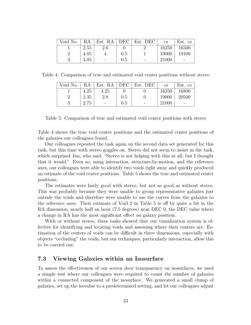
Void No. RA Est. RA DEC Est. DEC cz Est. cz1 2.55 2.6 0 2 16250 165002 4.05 4 0.5 1 19000 191003 3.05 - 0.5 - 21000 -

Table 4: Comparison of true and estimated void center positions without stereo

Void No. RA Est. RA DEC Est. DEC cz Est. cz1 4.25 4.25 0 0 16250 168002 2.35 2.8 0.5 0 19000 205003 2.75 - 0.5 - 21000 -

Table 5: Comparison of true and estimated void center positions with stereo

Table 4 shows the true void center positions and the estimated center positions ofthe galaxies our colleagues found.

Our colleagues repeated the task again on the second data set generated for thistask, but this time with stereo goggles on. Stereo did not seem to assist in the task,which surprised Jim, who said, “Stereo is not helping with this at all, but I thoughtthat it would.” Even so, using interaction, structure-by-motion, and the referenceaxes, our colleagues were able to identify two voids right away and quickly producedan estimate of the void center positions. Table 5 shows the true and estimated centerpositions.

The estimates were fairly good with stereo, but not as good as without stereo.This was probably because they were unable to group representative galaxies justoutside the voids and therefore were unable to use the curves from the galaxies tothe reference axes. Their estimate of Void 2 in Table 5 is off by quite a bit in theRA dimension, nearly half an hour (7.5 degrees) near DEC 0, the DEC value wherea change in RA has the most significant effect on galaxy position.

With or without stereo, these tasks showed that our visualization system is ef-fective for identifying and locating voids and assessing where their centers are. Es-timation of the centers of voids can be difficult in three dimensions, especially withobjects “occluding” the voids, but our techniques, particularly interaction, allow thisto be carried out.

7.3 Viewing Galaxies within an Isosurface

To assess the effectiveness of our screen door transparency on isosurfaces, we useda simple test where our colleagues were required to count the number of galaxieswithin a connected component of the isosurface. We generated a small clump ofgalaxies, set up the isovalue to a predetermined setting, and let our colleagues adjust

23

any other setting except the isovalue and the isosurface visibility. Two evaluationswere performed, one without stereo and the other with. Two different test data setswere used, one with 18 galaxies in the clump and one with 13 galaxies. We wanteda large enough number to make the task challenging, but not so large as to make itimpossible or overly tedious. The galaxy positions were determined randomly.

Without stereo, our colleagues made extensive use of interaction. Sometimes thegalaxies would be occluded by the isosurface, so they would adjust the view to bettersee the galaxy through one of the holes in the isosurface. For their first count, theyfound 17 galaxies. After some more interaction, especially rotation, they found all18. Eventually, they tried the torsional rocking motion. Our colleagues reportedthat this helped to reveal the galaxies “hiding” behind the isosurface, but it made itmore challenging to remember the galaxies they had just counted. A complaint fromour colleagues was that the isosurface was too opaque and hid some of the galaxies.We were surprised that they did not adjust the galaxy glyph size parameter, as thismay have alleviated some of the occlusion problems they were seeing.

During the stereo part of this task, Matt tried to “cheat” and zoom into theisosurface. Since the galaxy clump and isosurface were centered at the origin, thezoom factor could not get large enough to let geometry culling cut away part of theisosurface. At a high enough zoom level, some of the math for the trackball-stylecamera goes haywire, and things start behaving strangely. This occurred duringMatt’s interactions, but he simply used the “Home” key to get himself back to thedefault camera view. This problem of scaling the geometry to zoom in could bealleviated by using a flight-style camera control where the camera actually movesalong the viewing vector. We attempted to use VTK’s flight-style camera, but it isincompatible with the TK rendering widget we use for display.

By Matt’s account, stereo helped a “ton” in this task. He found it easier to keeptrack of previously counted galaxies because of the third dimension. In addition, ifa galaxy was occluded from one eye, it was likely not occluded from the other eye.This helped with the galaxy hiding problem.

Our evaluation showed that the isosurface with screen door transparency waseffective for revealing the galaxies within a connected component. A shortcoming ofour evaluation was that it did not present galaxies outside the isosurface that mightpotentially interfere with counting the galaxies inside the isosurface. We feel thatthe same techniques as those applied to our test data sets would clearly reveal thegalaxies inside and outside the isosurface.

7.4 Real Data Evaluation

Having suffered through our evaluation tasks, Matt said of viewing the real data,“This is much better than that crappy random distribution stuff!” Right away, Mattand Jim identified a particular void they knew well from their previous plottingtechniques. At one point, Jim saw a line of galaxies and said, “Ooh, there’s something

24

right there!” Clearly, our colleagues were excited to see their actual data.After viewing the data set for a while, Jim made this observation: “I don’t

see filaments so much as bubbles.” This observation is exciting because it sayssomething about the topology of the universe and therefore the formation of theuniverse. Further follow up indicated his excitement at comparing the observeddata to the simulation data. Prior visualization work of the simulation data revealsthat the galaxies in simulations tend toward filamentary structures [1]. This is indisagreement with the observational data, according to Jim: “We were impressed bywhat looked like evacuated ’bubbles’ with galaxies defining the surfaces of these voidareas, rather then the 1D filaments that seem to be so prevalent in the numericalsimulations of structure in the universe.”

Matt had some observations of his own to offer. He said, “Viewing it in 3Dmakes it look kind of weird, in a sense.” He has been used to plotting his data intwo-dimensional plots, so it will take a while to get to know his data in 3D. Aboutstereo, he said, “[Stereo] would be helpful on a small scale, where no stereo wouldbe helpful on a larger scale.”

Matt had two requests for us. He requested the ability to display galaxy infor-mation when a particular galaxy is queried. We have since implemented his requestas a TK label widget that displays the RA, DEC, and cz, coordinates, the name ofthe survey that collected that galaxy data, and a galaxy ID. Matt also requestedthat we increase the scale of the cluster glyph relative to the galaxy glyphs to makeit take up more volume. We decided to make the cluster size a separate adjustableparameter and have implemented it as such.

8 Lessons Learned

There were several interesting points that we learned from this project. It wasinteresting to watch scientists actually use the application and hear their comments.The scientists were a little disoriented the first time they looked at their data in3D, as they were so used to viewing their data in 2D plots. The cues that wereincluded in the visualization, such as the cluster glyphs and axes, definitely helpedthem navigate through the visualization, but they were so used to the 2D versionthat the 3D looked weird. Hopefully this new perspective on their data will allowthem to understand it better. Another interesting lesson was how little they usedisosurfaces when visualizing their data. While we were only able to observe themfor a short time while they looked at their own data, they just wanted to look atthe discrete galaxy glyphs. Perhaps when they have more time to explore their datathey will use the isosurface visualization more extensively.

25

9 Future Directions

While we were only able to complete the first goal of our visualization design, theother two are still very interesting to our colleagues. The second goal, the comparisonof simulation data to observational data is an area that does not seem to have beenpaid much attention. The third goal is interesting as it addresses how redshift mightaffect their observation data. The modules provide much of the base frameworkrequired to build visualizations to answer these other questions. For the secondgoal, the simulation data would have to be adjusted so that it matched with theobservation data, and a GUI that sets up two render windows would need to becreated. For the third goal, the extra visualization techniques would need to beimplemented in the visualization code.

By our colleagues’ preliminary findings from our visualization system, we wouldconsider adding user-controlled widgets that could help locate and define the bubblesin the galaxy distribution. These widgets would most likely be in the form of sphereglyphs that the user could position and scale interactively to fill the voids.

Our colleagues are interested in continuing this work in the future, and we areinterested in working with them. Hopefully, with continued interaction, they will beable to leverage our visualization system to find new knowledge about the formationand structure of the universe from their data.

References

[1] Cosmological n-body simulations. http://www.mpa-garching.mpg.de/GIF/

#pics.

[2] G. O. Abell, Jr. H. G. Corwin, and R. P. Olowin. A catalog of rich clusters ofgalaxies. Astrophysical Journal Supplement Series, 70:1–138, May 1989.

[3] M. Colless and Q. Parker. 6df survey plan. http://www2.iap.fr/users/gam/6dF/6dF_survey_plan.html, 2000.

[4] A. Jenkins, C. S. Frenk, F. R. Pearce, P. A. Thomas, J. M. Colberg, S. D. M.White, H. M. P. Couchman, J.A. Peacock, G. Efstathiou, and A.H. Nelson.Evolution of structure in cold dark matter universes. Astrophysical Journal,499(1), May 1998.

[5] R. C. Nichol, C. J. Miller, and T. Goto. The interplay of cluster and galaxyevolution. Astrophysics and Space Science, 285:157–165, 2003.

[6] Q. Parker. 6df: The new automated multi-object fibre-optic spectroscopy systemon the ukst. http://www.roe.ac.uk/ifa/wfau/6df/6df.html, 2001.

26

[7] F. R. Pearce and H. M. P. Couchman. Hydra: a parallel adaptive grid code.New Astronomy, 2:411–427, November 1997.

[8] J. H. Simonetti. How to do astrometry. http://www.phys.vt.edu/~jhs/SIP/astrometry.html.

[9] Colin Ware. Information Visualization: Perception for Design. Morgan Kauff-man, 2nd edition, 2004.

[10] E. L. Wright. Doppler shift. http://www.astro.ucla.edu/~wright/doppler.htm, 2002.

27

10 Appendix A: Evaluation Survey

The following was presented to our colleagues during the evaluation of our visualiza-tion system:

10.1 Evaluation Survey

We have shown you how to manipulate various parameters in GalaxyViewer. Nowwe must assess how useful our visualization techniques are for answering some ofthe questions you wish to answer with this visualization project. We will present aseries of questions for you. Please answer the best that you can. Don’t worry aboutgetting any questions “wrong”. You are not being tested, rather, our visualizationdesign is being tested.

Please feel free to vocalize your thought process. An example statement mightbe, “I am attempting to determine X, so my strategy is to Y. I wish I could do Zto help me in this goal.” In order to provide a fair assessment of our visualizationtechniques, we cannot help you during the evaluation.

At the end of each task, please notify the observers that you are finished. Theywill set up the next task, after which you may proceed.

11 Task 1

Your first task is to identify as many familiar shapes in the data set as you can.Please do not use the stereo goggles for this task. Please list the familiar shapes youfind below, leaving room to the right of each listed shape for Task 2:

12 Task 2

For the shapes you found in Task 1, please locate, as best you can, their centersin RA-DEC-rv coordinates. Please write these coordinates next to the shapes youlisted above.

13 Task 3

Please put on the stereo goggles and repeat Task 1.

28

14 Task 4

Please put on the stereo goggles and repeat Task 2.

15 Task 5

Please take off the stereo goggles. For this task, your goal is to locate voids, or globalunderdensities. For each void you find, please estimate the RA-DEC-rv coordinatesof the center of the void.

16 Task 6

Please put on the stereo goggles and repeat Task 5.

17 Task 7

Please take off the stereo goggles. For this task, we have loaded up a data set andset the isosurface to enclose a set of galaxies. Without turning the isosurface off,how many galaxies are inside the isosurface?

29

18 Task 8

Please put the stereo goggles on and repeat Task 7.

30

19 Appendix B: Evaluation Screenshots

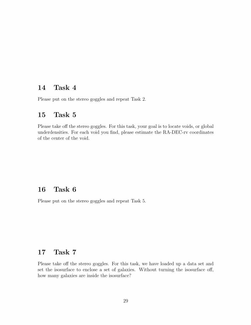
Figure 7: Our application as it appeared for the first evaluation task. Note that inthis and the next three figures, the camera zoom and galaxy glyph size settings areset such that the galaxies are difficult to discern.

31

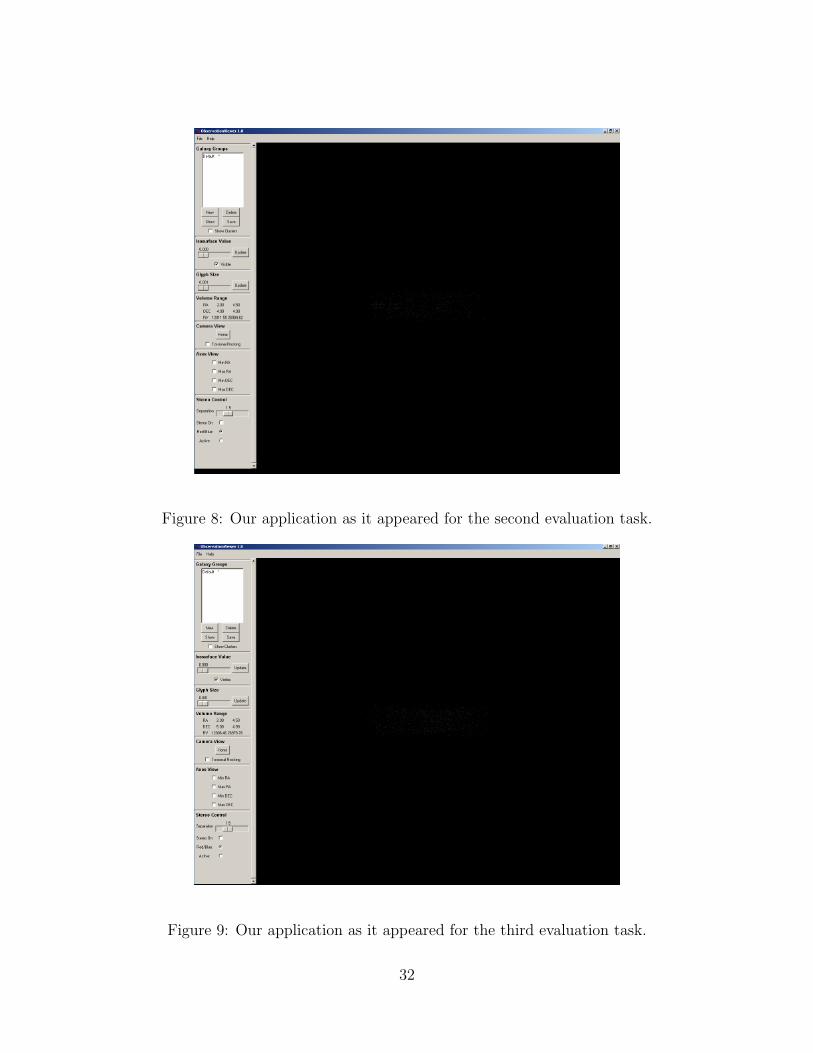
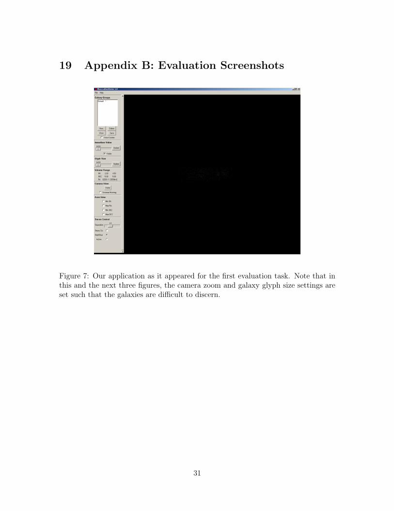
Figure 8: Our application as it appeared for the second evaluation task.

Figure 9: Our application as it appeared for the third evaluation task.

32

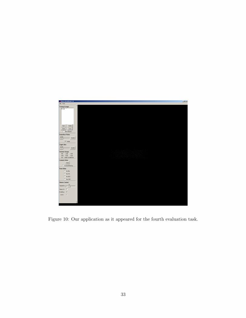
Figure 10: Our application as it appeared for the fourth evaluation task.

33

Figure 11: Our application as it appeared for the fifth evaluation task.

34

Figure 12: Our application as it appeared for the sixth evaluation task.

35