Fundamentals of the multizone air flow model - COMIS - AIVC

LBL-28560

Fundamentals of the Multizone Air Flow Model- COMIS

Edited by: Helmut E Feustel and Alison Raynor-Hoosen

Francis Allard (France) Viktor B Dorer (Switzerland) Helmut E Feustel (USA) Eduardo Rodriguez Garcia (Spain) Mario Grosso (Italy) Magnus K Herrlin (Sweden) Liu Mingsheng (Peoples Republic of China) Hans C Phaff (Netherlands) Yasuo Utsumi (Japan) Hiroshi Yoshino (Japan)

(For current addresses please check the appendix)

C OMIS -I- F u n d a m e n t a l s

© Copyright Oscar Faber PLC 1990

All property rights, Including copyright are vested In the Operating Agent (Oscar Faber Consulting Engineers) on behalf of the International Energy Agency.

In particular, no part of this publication may be reproduced, stored In a retrieval system or transmitted in any form or by any means, electronic, mechanical, photocopying, recording or otherwise, without the prior written permission of the Operating Agent.

Preface

International Energy Agency

The International Energy Agency (IF_A) was established In 1974 within the framework of the Organlsatlon for Economic Co-operation and Development (OECD) to Implement an International Energy Programme. A basic aim of the lEA Is to foster co-operation among the twenty-one lEA Participating Countries to Increase energy security through energy conservation, development of alternative energy sources and energy research development and demonstration (RD&D). This Is achieved In part through a programme of collaborative RD&D consisting of forty-two Implementing Agreements, containing a total of over eighty separate energy RD&D projects. This publication forms one element of this programme.

Energy Conservatlon In Buildings and Communlty Systems

The lEA sponsors research and development In a number of areas related to energy. In one of these areas, energy conservation In buildings, the lEA Is sponsoring various exercises to predict more accurately the energy use of buildings, Including comparison of existing computer programs, building monitoring, comparison of calculation methods, as well as air quality and studies of occupancy. Seventeen countries have elected to participate In this area and have designated contracting parties to the Implementing Agreement covering collaborative research In this area. The designation by governments of a number of private organlsatlons, as well as universities and government laboratories, as contracting parties, has provIdeda broader range of expertise to tackle the projects In the different technology areas than would have been the case if participation was restricted to governments. The Importance of associating Industry with government sponsored energy raseamh and development Is recognized In the lEA, and every effort Is made to encourage this trend.

The Executive Committee

Overall control of the programme Is maintained by an Executive Committee, which not only monitors existing projects but Identifies new areas where collaborative effort may be beneficial. The Executive Committee ensures that all projects fit Into a pre-determlned strategy, without unnecessary overlap or duplication but with effective liaison and communication. The Executive Committee has Initiated the following projects to date (completed projects are Identified by *):

I Load Energy Determination of Buildings * II Ekistics and Advanced Community Energy Systems * III Energy Conservation In Residential Buildings * IV Glasgow Commercial Building Monitoring * V Air Infiltration and Ventilation Centre VI Energy Systems and Design of Communities * VII Local Government Energy Planning * VIII Inhabitant Behavlour with Regard to Ventilation * IX Minimum Ventilation Rates * X Building HVAC Systems Simulation XI Energy Auditing * XII Windows and Fenestration * XIII Energy Management In Hospitals * XIV Condensation XV Energy Efficiency In Schools XVI BEMS - 1 : Energy Management Procedures XVII BEMS - 2: Evaluation and Emulation Techniques XVIII Demand Controlled Ventilating Systems XIX Low Slope Roof Systems XX Air Flow Patterns within Buildings XXI Energy Efficient Communities XXII Thermal Modelling

COMIS -m- Fundamenta l s

Annex V Air Infiltration and Ventilation Centre

The lEA Executive Committee (Building and Community Systems) has highlighted areas where the level of knowledge Is unsatisfactory and there was unanimous agreement that Infiltration was the area about which least was known. An Infiltration group was formed drawing experts from most progressive countries, their long term aim to encourage Joint International research and Increase the world pool of knowledge on Infiltration and ventilation. Much valuable but sporadic and uncoordinated research was already taking place and after some Initial groundwork the experts group recommended to their executive the formation of an Air Infiltration and Ventilation Centre. This recommendation was accepted and proposals for its establishment were Invited Internationally.

The alms of the Centre are the standardleation of techniques, the validation of models, the catalogue and transfer of Information, and the encouragement of research. It Is Intended to be a review body for current world research, to ensure full dissemination of this research and based on a knowledge of work already done to give direction and firm basis for future research In the Participating Countries.

The Participants In this task are Belgium, Canada, Denmark, Federal Republic of Germany, Finland, Italy, Netherlands, New Zealand, Norway, Sweden, Switzerland, United Kingdom and the United States of America.

COMIS Workshop

The COMIS workshop (Conjunction of Multlzone Infiltration Specialists) was a Joint research effort to develop a multlzone Infiltration model. This workshop (October 1988 - September 1989) was hosted by the Energy Performance of Buildings Group at Lawrence Berkeley Laboratory's Applied Science Division. The task of the workshop was to develop a detailed multizone Inflitratlon program taking crack flow, HVAC-systems, single-sided ventilation and transport mechanism through large openings Into account. This work was accomplished not by Investigating Into numerical description of physical phenomena but by reviewing the literature for the best suitable algorithm. The numerical description of physical phenomena Is cleady a task of lEA-Annex XX "Air Flow Patterns In Buildings", which will be finished in September 1991. Multlgas tracer measurements and wind tunnel data will be used to check the model. The agenda Integrated all participants' contributions Into a single model containing a large library of modules. The user-friendly program Is aimed at researchers and building professionals.

From Its announcement In December 1986, COMIS was well received by the research community. Due to the Internationality of the group, several national and International research programmes were co-ordinated with the COMIS workshop. Colleagues from France, Italy, Japan, The Netherlands, Peoples' Republic of China, Spain, Switzerland, and the United States of Amedoa were working together on the development of the model.

Even though this kind of co-operation Is well known In other fields of research, e.g., high energy physics; for the field of building physics it Is a new approach.

The COMIS Fundamentals contains an overview about Infiltration modelling as well as the physics and the mathematics behind the COMIS model.

Helmut E. Feustel COMIS Co-ordinator Berkeley, California January 31, 1990

COMIS -IV- Fundamenta l s

CONTENTS

I.

1.

1.1

1.2

1.3

1.4

1.5

2.

2.1

2.1.1

2.1.2

2.1.2.1

2.1.2.1.1

2.1.2.1.2

2.1.2.1.3

2.1.2.1.4

2.1.2.1.5

2.1.3

2.2

2.2.1

2.2.1.1

2.2.1.2

2.2.1.2.1

2.2.1.2.2

2.2.1.2.3

2.2.1.2.4

2.2.1.2.5

2.2.1.2.6

2.2.1.2.6.1

2.2.1.2.6.2

2.2.1.2.6.3

2.2.1.2.6.4

2.2.1.2.6.4.1

2.2.1.2.6.4.2

2.2.1.3

Nomencla ture ................................................................................ IX

Infiltration Model l ing ..................................................................... 1

Introduction ..................................................................................... 1

History o f Infiltration Model l ing .................................................... 2

Mult izone Infiltration Models ......................................................... 3

Review ............................................................................................ 5

Conclusion ...................................................................................... 8

Physical Fundamenta ls ................................................................... 9

Pressure Distribution ....................................................................... 9

Introduction ..................................................................................... 9

Wind Pressure ................................................................................. 9

Model l ing Wind Pressure Distribution ......................................... 10

Reference Data .............................................................................. 12 Methodology ................................................................................. 12

Analysis ......................................................................................... 15

Calculat ion Model ......................................................................... 19

Out look ......................................................................................... 20

Thermal Buoyancy ........................................................................ 21

Air Flows Through Openings ....................................................... 23

Air F low through Cracks .............................................................. 23

Introduct ion ................................................................................... 23

F low Equat ion ............................................................................... 24

Duct F low ...................................................................................... 24

Crack F low .................................................................................... 25

Temperature Inf luence on Crack F low ......................................... 26

Equat ion Fo rm Influence .............................................................. 27

Regression ..................................................................................... 28

Temperature Equation .................................................................. 29

Classification o f Crack Forms ...................................................... 29

Door os Single-Pane Window ....................................................... 30

Pr ime-and-Storm Window ............................................................ 31

Walls ............................................................................................. 33

Tiny Cracks ................................................................................... 34

Wide Cracks .................................................................................. 35

Conclusion .................................................................................... 36

C O M I S -v- Fundamentals

2.2.2

2.2.2.1

2.2.2.2

2.2.2.2.1

2.2.2.2.2

2.2.2.3

2.2.2.3.1

2.2.2.3.2

2.2.2.3.3

2.2.2.4

2.2.3

2.2.3.1

2.2.3.1

2.2.3.3

2.2.3.4

2.2.3.5

2.2.3.6

2.2.4

2.2.5

2.2.5.1

2.2.5.2

2.3

2.3.1

2.3.2

2.3.3

2.4

2.4.1

2.4.2

2.4.2.1

2.4.3

2.4.4

3.

3.1 3.2

3.3

3.3.1

Air F low through Large Openings ................................................ 39

Introduct ion ................................................................................... 39

Short Rev iew of Literature ........................................................... 39

Steady Flows through Large Openings ......................................... 39

Uns teady Flows through Large Openings .................................... 40

Integration into COMIS ................................................................ 42

Exist ing Solutions ......................................................................... 42

COMIS Contribution .................................................................... 43

Examples o f Solutions .................................................................. 47

Conclusion .................................................................................... 50

HVAC-S ys tems .............................................................................. 51

Pressure Losses through Ducts and Duct Fittings ........................ 51

Friction Losses through the Duct .................................................. 51

Dynamic Losses due to Duct Fittings ........................................... 52

Coefficients o f Flow Equation o f a Duct ...................................... 59

Total Pressure Losses due to T-Junct ion ...................................... 60

Literature Survey .......................................................................... 62

Shafts ............................................................................................. 65

F low Controllers ........................................................................... 66

Types o f F low Controllers ............................................................ 66

Per fo rmance o f Flow Control ler ................................................... 68

Pressure Sources ........................................................................... 71

Fan Per formance ........................................................................... 71

Fan Laws ....................................................................................... 71

Expression o f Fan Curve ............................................................... 72

Pollutant Transport Model ............................................................ 73

Introduction ................................................................................... 73

COMIS Pollutant Transport Model .............................................. 73

Fundamenta ls o f COMIS Pollutant Model ................................... 74

Illustrative Example ...................................................................... 77

Conclusion .................................................................................... 80

Solution Methods for Air Flow Networks .................................... 81

Introduction ................................................................................... 81

Sys tem o f Equations ..................................................................... 81

Special Characterist ics o f the Jacobian Matrix ............................. 82

S y m m e t r y ...................................................................................... 83

C O M I S -VI- Fundamentals

3.4

3.4.1

3.4.2

3.4.3

3.4.4

3.4.5

3.4.6

3.5

3.5.1

3.5.2

3.6

3.6.1

3.6.2

3.6.3

3.6.4

3.7

4.

5.

6.

7.

Linear Solvers ............................................................................... 85

Gaussian-El iminat ion with Back S u b s t i t u t i o n . . . . . . . . . . . . . . . . . . . . . . . . . . . . . . 85

Pivoting ......................................................................................... 86

LU-Factor izat ion ........................................................................... 86

Cho lcsky ' s Method ....................................................................... 86

Band Matices ................................................................................ 87

Skyl ine .......................................................................................... 87

Non-Linear Solvers ....................................................................... 88

Extrapolated Relaxation Coefficients ........................................... 89

Opt imized Relaxat ion Coefficients ............................................... 89

Timing o f Solvers ......................................................................... 91

Chosen Networks .......................................................................... 91

Other Assumptions ........................................................................ 93

Linear Solvers ............................................................................... 93

Non-Linear Solvers ....................................................................... 96

Conclusion .................................................................................... 99

Acknowledgemen t ...................................................................... 101

Disclaimer ................................................................................... 101

References ................................................................................... 103

Appendix .................................................................................... 115

C O M I S -vii- Fundamentals

C O M I S -viii- Fundamentals

I. NOMENCLATURE a ~

b /,, C

corr d d. e

f far g g

h t J k k ,ko

k,:p l td m

md rh n

na pad par, c/ par rbh s t ir

t

U

xl Yc Y, 2

2c

Zref zh

wind direction angle, measuw.A from the normal to each wall [-] density gradient [kg /m 4] turbulent pressure gradient [Pa/m ] specific heat capacity [J /kg ,°C ] corn~tion vector [-] diameter [m ] hydraulic diameter [m ] eigenvalue [-] flow balance function [-] frontal aspect ratio, ratio of model length to model height [-] acceleration of gravity [m/s 2] flow balance function [-] height from the reference level [m ] node number [-] node number, element in ff [-] surface element on building/model wall [-] heat transfer coefficient [-] reactivity Jig / s ] reactivity of pollutant p in zone i It& / s ] duct length [m ] number of pieces of equipment within a section of duct work [-] element in L [-] number of duct fittings within a section of duct work [-] mass flow rate Jig Is ] exponent of flow equation [-] number of ducts within a section of duct work [-] plan area density, representing the density of surrounding buildings [-] reference value forpar [-] parameter [-] relative building height, ratio of model height to the height of surroundings [-] side aspect ratio, ratio of model width to model height [-] temperature [°C ] element in U [-] air velocity [m/s ] relative horizontal position of the surface element k [-] calculated value [-] reference value [-] height above ground [m ] complex number [-] reference height for wind velocity measurements [m ] relative vertical position of the surface element k [-]

C O M I S .Ix- F u n d a m e n t a l s

A A B C C0, Cm CQ CS Cd Cf zh Cpk

Cp,¢ Cpnormsh CF~h D DF F G G H l-t, I J

KQ L L M MM N NF NK NP NZ P P a~n Pi P~ Pro

Pk Poh P atat P,

constant [-] matrix, general [-] constant [-] constant [-1 specific concentration of pollutant p In zone i [kg/kg ] mass flow coefficient [kg /sPa n ] volume flow coefficient [m3/sPa n ] duct shape coefficient [kg" (m 3)l-n/Pa" (m 2) 1-2n s ~ ] discharge coefficient [-] Cp correction factor related to a parameter, at zh [-] pressure coefficient at surface element k [-] pressure coefficient at zh [-] reference pressure coefficient [-] Cp normalized to a reference at zh [-] Cp global correction factor, at zh [-1 constant [-] fan size or impeller diameter [m ] functional form [-] scalar function [-] matrix, triangular [-1 height [m ] specific humidity [kg~,er / kg,~ at, ] matrix, unity [-] Jacobtan matrix [-] temperature correction factor, related to mass flow [-] temperature correction factor, related to volume flow [-] length of crack or tube [-] matrix, lower triangular [-] hall' band width [-] molar mass [g ] number of points for the confidence check [-] fan rotational speed [lls ] number of llnks between two zones [-] number of pollutants in the mixture [-] number of zones [-] reference pressure [Pa ] dynamic pressure [Pa ] pressure at point i in zone m [Pa ] static pressure at height h in the shaR [Pa ] static pressure at reference level in the shaft [Pa ] pressure at point j in zone n [Pa] total pressure at surface element k [Pa ] static pressure at height h of the outdoor air [Pa ] static pressure [Pa] total pressure [Pa ]

C O M I S -x- Fundamentals

P o P~ P, ep Par Par,~ PAR PARre! Q

Re S S~p (t) T U V Vi W XH Z ZN Ot

rl rli,.k Z. x. V

P Po Pai Pi Po Pout

~m A AP AP i aej AP k APp APt 0 0

atmospheric pressure [ P a ] pressure due to stack effect [Pa ] turbulent pressure [Pa ] fan total pressure or fan static pressure [Pa ] parameter [-] reference value for Par [-1 set of parameters [-] set of Par,,/ [-] volume flow [m3/s ] heat transfer [W] Reynolds number [-] source or sink term of pollutant in a zone [kg/s ] source or sink term of pollutant p in zone i [kg/s ] temperature [°K ] matrix, upper triangular [-] volume [m 3] volume of zone i [m 3] width [m ] specific humidity [kgwater /kgdryalr ] vertical position [m ] vertical position of a neutral plane [m ] wind velocity profile exponent, characteristic Of the rouglmess [-] duct roughness factor [m ] filter efficiency 0 < rl < 1 filter efficiency between zone j and t through link k 0 ~: rlji < 1 friction factor [-] relaxation coefficient kinetic viscosity [m 2Is ] air density [kg /m 3] density of dry air [kg/m 3] density of dry air In zone i [k~/m 3] air density in the shaft [kg/m °] air density of the outdoor [kg/m 3] density of the outside air [kg/m 3] local loss coefficient [-] total pressure loss coefficient from point 1 to point 2 [-] difference [-] pressure difference [ P a ] duct total pressure loss [Pa] duct fitting total pressure loss [Pa ] equipment (e.g., coil. fire damper) total pressure loss [Pa ] friction losses tn terms of total pressure [Pa] fitting total pressure loss [Pa 1 dimensionless temperature [-] area reduction factor [-]

C O M I S -xa- Fundamenta l s

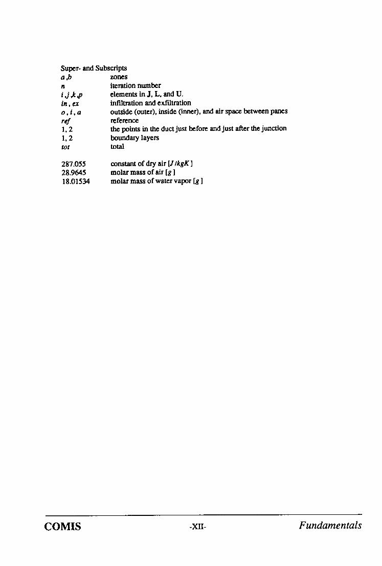
Super- and Subscripts alJ tl

I j , k ~ In, eX

o , t , a

ref 1,2 1,2 tot

/ , o n e s

Iteration number elements in J, L, and U. infiltration and exfiltratlon outside (outer), inside (inner), and air space between panes reference the points in the duct just before and just after the junction boundary layers total

287.055 28.9645 18.01534

constant of dry air [J/kgK ] molar mass of air [g ] molar mass of water vapor [g ]

COMIS -xII- F u n d a m e n t a l s

1. INFILTRATION MODELLING

1.1 Introduction

It is particularly important to be aware of the air flow pattern in a building when determining indoor air quality problems or calculating space conditioning loads for energy consumption. Correct sizing of space conditioning equipment is also dependent upon accurate air flow information. A number of infiltration models have been developed to calculate infiltration-related energy losses and the resulting air flow distribution in both single-zone and multizone buildings. Interna- tional infi trafion research has been conducted since the early twenties - - infiltration modeling, however, is a relatively new task.

-~'='T" I T~,T~,~ NIMI) -DIRECTION DIFFERENCES

I . I I suR..P:OU,D,,~ I I'v~R',,~ ~,.o,,

I RES I STANCES I $HAPE OF THE

BUILDING 1

l I~CHAII ] CAL VENTILATION

$YSTEJ~

,I c~HFAANRA - AJID DUCT

CTERISTICS

t~ [I(DPI~SSlJRE l THEI~AL [ 11q~0SFd) ] DISTRIBUTION BUOYANCY PRESqSI,IR£

o,$,,,,OT,O, I

D,S'R,~T'O" I

Fig. 1: Influences on Air Flow Distribution in Buildings

Awareness of infiltration as a major factor in the overall conditioning load of a building has in many cases led to tighter construction of both building components and the overall building shell. This has decreased the infiltration rate and its related ventilation heat loss but has sometimes created another problem with regard to indoor air quality.

The air-mass flow distribution in a given building is caused by pressure differences evoked by wind, thermal buoyancy, mechanical ventilation systems or a combination of these. Air flow is also influenced by the distribution of openings in the building shell and by the inner pathways. Actions by the occupants can also lead to significant differences in pressure distribution inside a building.

COMIS -1- Fundamenta l s

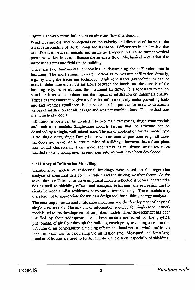
Figure 1 shows various influences on air-mass flow distribution.

Wind pressure distribution depends on the velocity and direction of the wind, the terrain surrounding of the building and its shape. Differences in air density, due to differences between outside and inside air temperatures, cause further vertical pressures which, in turn, influence the air-mass flow. Mechanical ventilation also introduces a pressure field on the building.

There are two fundamental approaches in determining the infiltration rate in buildings. The most straightforward method is to measure infiltration directly, e.g., by using the tracer gas technique. Multizone tracer gas techniques can be used to determine either the air flows between the inside and the outside of the building only, or, in addition, the interzonal air flows. It is necessary to understand the latter so as to determine the impact of infiltration on indoor air quality. Tracer gas measurements give a value for infiltration only under prevailing leakage and weather conditions, but a second technique can be used to determine values of infiltration for all leakage and weather combinations. This method uses mathematical models.

Infiltration models can be divided into two main categories, single-zone models and multizone models. Single-zone models assume that the structure can be described by a single, well-mixed zone. The major application for this model type is the single-story, single-family house with no internal partitions (e.g., all internal doors are open). As a large number of buildings, however, have floor plans that would characterize them more accurately as multizone structures more detailed models, taking internal partitions into account, have been developed.

1.2 History of Infiltration Modelling

Traditionally, models of residential buildings were based on the regression analysis of measured data for infiltration and the driving weather forces. As the regression coefficients for these empirical models reflected structural characteristics as well as shielding effects and occupant behaviour, the regression coefficients between similar residences have varied tremendously. These models may therefore not be appropriate for use as a design tool for building energy analysis.

The next step in residential infiltration modeling was the development of physical single-zone models. The amount of information required for single-zone network models led to the development of simplified models. Their development has been justified by their widespread use. These models are based on the physical phenomena of air flow through the building envelope by assuming a certain distribution of air permeability. Shielding effects and local vertical wind profiles are taken into account for calculating the infiltration rate. Measured data for a large number of houses are used to further fine-tune the effects, especially of shielding.

C O M I S -2- Fundamentals

Following the analysis of an enormous number of measured ventilation rates in houses for which the leakage characteristics have been determined by pressuriza- tion tests, a very simple model has been introduced - - in which the air change rate measured at a given pressure differential is divided by a constant number. This model does not take weather influence or leakage distribution into account.

Even before the advent of physical single-zone models a number of computer models had been developed to calculate the air flow distribution in multizone buildings. The building is described by a set of zones interconnected by flow paths. Each node represents a space with uniform pressure conditions inside or outside the building and the interconnections correspond to impediments to air flow. The network models are usually based on the conservation of mass in each of the zones in the building. The first of these models to be developed was probably the BSRIA-model LEAK which was published in 1970. Since that time many more models have been developed but most of them have been written as research tools and are not available to third parties. As a consequence they are difficult to use and arc, at best, "user-tolerant" rather than "user-friendly".

The In'st very simple multizone model for equipment design calculation for low- rise buildings was the crack model. This model was later refined to cover high- rise buildings. A simplified approach was followed in the development of LBL's infiltration model which allows the calculation of all interzonal air flows by means of a pocket calculator.

While multizone infiltration models have existed for the last two decades some of the thermal building simulation models axe still working with constant rate models. Now that energy conservation and indoor air quality have become important issues this type of model is inadequate.

1.3 Mult izone Infiltration Models

A zone is defined as a fully mixed volume with a constant concentration level of the enclosed gas mixture. Multizone models are required when there are internal partitions in a building, or, in thc case of inhomogcneous concentration in the spacc. Multizone buildings can be either single-room structures (e.g., airplane hangars) single family houses or large building complexes. Figure 2 shows an example of avcry simple multizone building [I].

A number of infiltration programs havc been developed to calculatc air flows penetrating the building's envelope and travelling through the different zones of a multizone structure. Besides being able to simulate infiltration in larger buildings these models are able to calculate mass flow interactions between the different z o n e s .

COMIS -3- Fundamentals

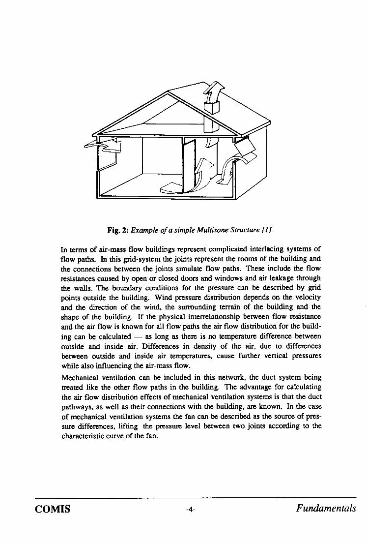
Fig. 2: Example of a simple Mul~zone Structure [1].

In terms of air-mass flow buildings represent complicated interlacing systems of flow paths. In this grid-system the joints represent the rooms of the building and the connections between the joints simulate flow paths. These include the flow resistances caused by open or closed doors and windows and air leakage through the walls. The boundary conditions for the pressure can be described by grid points outside the building. Wind pressure distribution depends on the velocity and the direction of the wind, the surrounding terrain of the building and the shape of the building. If the physical interrelationship between flow resistance and the air flow is known for all flow paths the air flow distribution for the building can be calculated - - as long as there is no temperatur~ difference between outside and inside air. Differences in density of the air, due to differences between outside and inside air temperatures, cause further vertical pressures while also influencing the air-mass flow.

Mechanical ventilation can be included in this network, the duct system being treated like the other flow paths in the building. The advantage for calculating the air flow distribution effects of mechanical ventilation systems is that the duct pathways, as well as their connections with the building, are known. In the case of mechanical ventilation systems the fan can be described as the source of pressure differences, lifting the pressure level between two joints according to the characteristic curve of the fan.


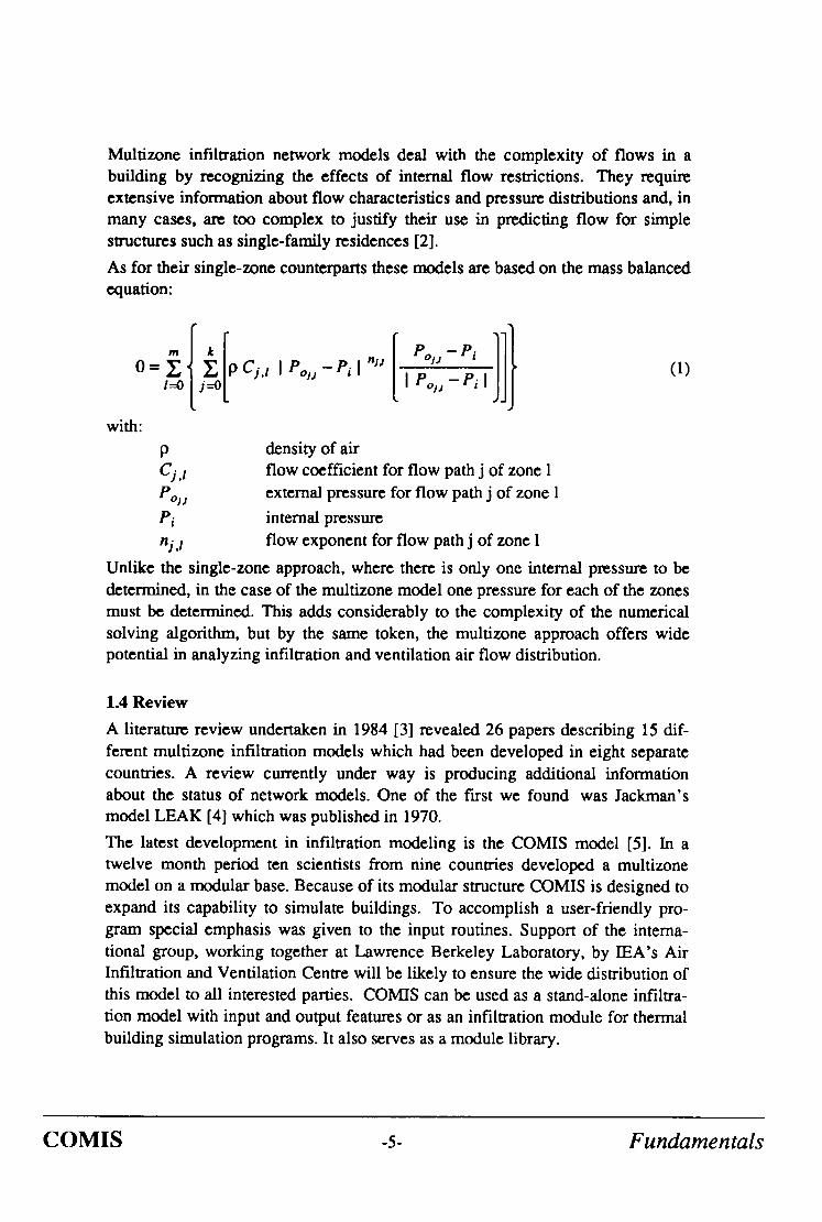
Multizone infiltration network models deal with the complexity of flows in a building by recognizing the effects of internal flow restrictions. They require extensive information about flow characteristics and pressure distributions and, in many cases, are too complex to justify their use in predicting flow for simple structures such as single-family residences [2].

As for their single-zone counterparts these models are based on the mass balanced equation:

with:

P Cy.l Pol~ Pi nj.l

density of air flow coefficient for flow path j of zone 1 external pressure for flow path j of zone 1

internal pressure flow exponent for flow path j of zone 1

(i)

Unlike the single-zone approach, where there is only one internal pressure to be determined, in the case of the multizone model one pressure for each of the zones must be determined. This adds considerably to the complexity of the numerical solving algorithm, but by the same token, the multizone approach offers wide potential in analyzing infiltration and ventilation air flow distribution.

1.4 Review

A literature review undertaken in 1984 [3] revealed 26 papers describing 15 different multizone infiltration models which had been developed in eight separate countries. A review currently under way is producing additional information about the status of network models. One of the first we found was Jackman's model LEAK [4] which was published in 1970.

The latest development in infiltration modeling is the COMIS model [5]. In a twelve month period ten scientists from nine countries developed a multizone model on a modular base. Because of its modular structure COMIS is designed to expand its capability to simulate buildings. To accomplish a user-friendly program special emphasis was given to the input routines. Support of the international group, working together at Lawrence Berkeley Laboratory, by IEA's Air Infiltration and Ventilation Centre will be likely to ensure the wide distribution of this model to all interested parties. COMIS can be used as a stand-alone infiltration model with input and output features or as an infiltration module for thermal building simulation programs. It also serves as a module library.


It was discovered, from the two reviews of the literature above, that most of the models described by program authors use the FORTRAN (75%) programming language, followed, in order of use, by BASIC, HPL and in one case each by PASCAL and C. As most of the programs represent research tools developed at universities they run on main frame or work station type computers (56%).

Because of the nonlinear dependency of the volume flow rate on the pressure difference, the pressure distribution for a building can be calculated only by using a method of iterations. Multizone network models were developed to deal either with simple structures of only a few zones or with buildings having arbitrary floor plans, allowing an unlimited number of zones (limited only by the computer to be used). Many models have been developed which simulate a specific structure only, so allowing for the use of simple solving routines. Models which deal with arbitrarily chosen building types use either a great deal of CPU-space or are equipped with very sophisticated mathematical routines to reduce the storage

need.

Large computer storage was necessary in the past when calculating the air flow distribution of more complicated buildings. Nowadays however, most programs use solver modules which reduce the space requirement, e.g., by band matrices or the skyline method. The Newton method is the most common tool used to solve

the set of non-linear equations.

Although most models have been developed in FORTRAN on main frame computers, many use interactive mode to input the necessary data. Only one of the models, however, allows CAD-input. Three-dimensional building description and schedules for climatic data and occupants are more common today than they were five years ago but a comprehensive way of designing the output seems still to be a problem. Most of the models use the file of arrays to present the calculated result

not really a user-friendly method. Few models use the capabilities of personal computers to show the air flow distribution in two-dimensional graphs.

Twelve of the infiltration models are combined with a thermal model and eight feature a further combination with a pollutant transport model. For seven out of twenty-nine models the authors specify their product as "available to third parties". Eleven authors believe that, lacking user-friendliness, their models would be of no use for third parties. The remainder do not wish to make their tools avail-

able to others.

The multizone models investigated were, in regard to the equations used, very similar to each other. The flow equation used to describe the air flow characteristics of the buildings is similar to the one describing measured results for air flow through building components. Most programs use an empirical power-law expression type of equation even though the pressure exponent may differ from 0.5 to 1.0, depending on the nature of flow. Only few models consider wind

dynamics.


Table 1: Review of Multizone Infiltration Network Models

Program Language:

Computer Type:

Solver:

Input Features:

Output Features:

Miscellaneous:

Program Available?

FORTRAN BASIC PASCAL C HPL

Main Frame Computer Personal Computer

Newton Others

Interactive Input CAD-Input Weather Data from Weather Files 3-D Building Description Schedules (e.g. Occupants)

File of Arrays used by the Model Graphical Output Statistical Functions

Combined with Thermal Model Combined with Pollution Model

Yes

No Yes, but

33 6 1 1 3

23 18

22 8

10 !

18 8

14

23 7 4

12 8

7 11 11

The programs still differ markedly in their ability to simulate mechanical ventilation systems. Twenty of them are able to simulate forced ventilation systems by means of fan and duct characteristics. This is a tremendous change from the last review.

The difficulty of measuring infiltration in buildings under controlled boundary conditions means that none of the models has been validated properly, if at all. The possibility of doing piecemeal validations of certain algorithms has been considered: e.g., the algorithms for air flow through open doorways or air flow through cracks have been tested separately [6]. Measuring a few cells of the whole structure could still provide a severe test for existing models.

These data are important not only for validation purposes but also as a means of further understanding air movement in large mulfizoned buildings. We need to identify the critical variables in different building types in order to develop more accurate input data and, ultimately, more accurate models. Wind pressure


coefficients, for example, represent a factor that needs further study, and the col- lating of existing data should help our efforts in simplifying data requirements.

1.5 Conclusion

Except for the fine-tuning of existing models the development of single-zone models seems to be completed. As multizone models offer much more potential for further investigation, work will probably go on for some time to suit models to

specific needs.

The development of multizone infiltration and ventilation models shows a relatively slow evolution. Lack of exchange of information, restricted distribution of models and the lack of a flexible structure are probably the reasons why models developed in the early seventies are not very different from those developed in

the late eighties.

Although several of the models discovered during this review serve a particular purpose they could have been developed using existing models. The COMIS workshop is trying to overcome these problems by creating a multizone infiltration model with a modular structure which will allow modules to be changed easily. The availability of the program, together with the international author- ship, should help to establish COMIS as an infiltration standard on which specific

applications can be built.

Along with stand-alone infiltration models, network models will also now finally find their way into thermal building simulation models. With the expected advances in the development of the next generation of building simulation programs infiltration modules will be needed for implementation in the program

libraries.

Future tasks include the development of methods to determine the required input parameters, especially the wind pressure distribution. Further work must be done through sensitivity studies to reduce the input requirements and to increase user- friendliness by using the output features of the PC's.

Validation of the models is another essential task. In order to understand physical phenomena related to transport mechanism in buildings, and to develop numerical descriptions, measurements must first be performed under steady state conditions. It is necessary, in order to measure mass flow transport mechanism accurately, to be able to control the pressure level and its fluctuation for each of the outside walls. This is only possible if the building is itseff located in a building. Such a test facility would not only evaluate air flow models as a whole but would also help to validate the tracer gas techniques to be used to evaluate infiltration models in field experiments.


2. PHYSICAL FUNDAMENTALS

2.1. PRESSURE DISTRIBUTION

2.1.1 Introduction

Air flow through the rooms of a building stems from pressure distribution around and within the building itself. Pressure distribution is due to thc combined actions of wind, thermal buoyancy (stack effect) and mechanical ventilation - ff present.

Duc to thc turbulcncc characteristic of the wind flow in the lower layers of the atmosphere [7,8] the pressure field driven by wind on building surface is always unsteady.

Differential pressure due to the stack effect depends on density field; that duc to mechanical vcntilation depends on the characteristics of ducts and exhaust system. While the variation rangc of these phenomena over time is relatively preMictablc it is difficult to simulate the wind pressurc field.

The following pages oudin, the work done on this problem within COMIS. In addition, simple equations calculating the pressure difference due to thermal buoyancy arc given.

2.1.2. Wind Pressure

Wind flows produce a velocity and pressure field around buildings. The relationship, for free stream flow, between velocity and related pressure at different locations of the flow field can be obtained from Bernoulli's equation. Assuming constant density along a streamline at a given height BernouUi's equation can be simplified to:

l Pstat + ~ 9 = const (2)

The shear layer formed by the action of shear stress at a solid boundary is called boundary layer. The velocity in the shcar layer goes from zero at the surface of thc solid boundary to thc speed of the free stream at the outer edge. The flow in the region between both limits is dominated by the effect of viscosity. Depending upon thc Reynolds number thc flow in this region is either laminar or turbulent. Wind flow is characterized by turbulent boundary layer flow with a thickness of a few hundred meters.

The vertical profile of the mean wind speed in the atmospheric boundary layer is primarily dependent upon the roughness of the surface surrounding the building.

The wind velocity profilc can bc calculated by a power law expression [9,10]:


v(z)

V(Zref ) 1 7"rcf J (3)

The value of the exponent o~ increases with increasing roughness of the solid

boundary.

The wind pressure distribution on the building envelope is usually described by dimensionless pressure coefficients - the ratio of the surface dynamic pressure to the dynamic pressure in the undisturbed flow pattern measured at a reference height. The pressure coefficient Cp at point k (x ,y ,z), with reference dynamic pressure Pdyn related at height Zref, for a given wind direction ~ can be described

by:

Pk - P O( z ) (4) CPk (Zref '~) = Pdyn (z,ef )

with

1 Pdyn (Zrtf ) = -2 Po V2(Zref ) (5)

2.1.2.1. Modelling Wind Pressure Distribution

There are a number of variables affecting the pressure distribution around a building due to natural wind. Wall-averaged values of Cp usually do not match the accuracy required for air flow calculation models. More detailed evaluations, taking the Cp distribution on the envelope of buildings into account, can be made in

different ways:

s performing full scale measurements when an existing building is being studied

• carrying out wind tunnel tests on models of existing or designed buildings

• generating Cp values by 3-dimensional numerical air flow models

• generating Cp values by numerical models based on parametrical analysis of wind tunnel test results

The f'u-st is practically impossible to follow unless it is done within expensive and time-consuming experimental plans. The second depends too much on the availability of test equipment and relevant assistance. The third implies time consuming complex calculations. The fourth seems to assure easy access to available Cp data by using a simple algorithm.


The problem is how to combine consistently accurate results with generality of the application range. In COMIS we have tried to find a reliable model able to fulfiU this goal.

Modelling wind surface pressure distribution (wpd) means finding an algorithm describing the variation of Cp on the envelope surfaces of a building when varying wind direction as well as architectural and environmental conditions are taken into account. Because of the stochastic behavior of the phenomenon such an algorithm has to be drawn by empirical correlations, which hold only within the range of variation of the experimental reference data used for the analysis.

Unlike wall-averaged Cp's where tables and graphs are given for large intervals of wind angle [1], [11], a wpd model can yield Cp values at any point on the surface for any wind angle.

On the other hand, unlike wind tunnel or full-scale tests on a specific building-site situation, a wpd model has a high abstraction level, having to match a wide range of climatic and environmental conditions. The accuracy of the model mainly depends on the characteristics of the data on which it is based.

As a first step a literature review was undertaken to check possibly existing wpd models [12-17].

Since no existing algorithms were found which could fulfil the COMIS goal a new model, choosing a parametrical approach, was developed. This means using a systematic analytical process in which each factor (parameter) influencing the variation of a phenomenon, i.e., Cp, is considered as an independent variable while the others are kept constant. Variation curves for each parameter, using statistical regressions, are then defined and the effect on wind pressure distribution evaluated.

For the present analysis three types of parameters have been taken into account:

• climate parameters : wind velocity profile exponent (tx)

• environment parameters :

• building parameters :

wind incident angle (anw)

plan area density (pad) relative building height (rbh)

frontal aspect ratio (far) side aspect ratio (sar) relative vertical position (zh) relative horizontal position (xl)

(For definitions of terms please see Nomenclature)

The specific objective was to find the relationship between variation range of each parameter and change of, Cp on a rectangular-shaped building model in order to develop calculation routines as input for the COMIS program.

COMIS -11- F u n d a m e n t a l s

2.1.2.1.1 Reference Data

As a first stage several wind tunnel test reports were considered in order to find a set of reference data large enough to cover a wide range of variables and struc-

tured in such a way as to allow a parametrical analysis.

One of the criteria in selecting suitable reference tests was to evaluate the various

parameters in relation to the specific influence they have on pressure distribution.

Two parameters have a major effect - - density of surroundings and wind direction. The former is much less studied than the latter so we looked for tests which

emphasised the latter issue.

Two tests were considered, Hussein and Le~ [18] and Akins and Cermak [19].

In three investigations Hussein and Lee measured surface pressure coefficients on block-shaped models of different size, and with different surroundings in an atmospheric boundary layer wind tunnel. All models were referred to a cube-

shaped model with 0.036 m side corresponding to a dimension of 12.6 m in real scale. They measured the vertical pressure distribution on the centerline of the model 's windward and leeward walls with approaching flow normal to the wall.

Pressure coefficients were normalized with respect to the velocity of the gradient wind which, in their case, occurred at a height of 22 times the cube height. They provided a wind velocity profile with a flow exponent ¢x = 0.28 to simulate the

atmospheric wind flow in a low density urban area.

Akins and Cermak performed their test in an industrial aerodynamic wind tunnel measuring surface pressure coefficients at several points on the facades of various block-shaped models. The models were of different size and had two height values, 0.254 and 0.508 m corresponding, in real scale, to 63.5 and 127 m respec-

tively. The effect of the surroundings was not simulated.

They tested 5 different wind directions for each wall - - 0, 20, 40, 70, 90 wind angle degrees with respect to the normal to the wall. Four boundary layer conditions were provided relative to the following values of the wind velocity profile

exponent:

o~ = 0.12, 0.26, 0.34, 0.38.

Pressure coefficients were measured both in vertical and horizontal distribution and normalized with respect to the local wind velocity.

2.1.2.1.2 Methodology

When using different sets of data for a parametrical analysis it is necessary first to

check the similarity of the boundary conditions. The selected tests showed results

related to complementary sets of parameters with a common range of Cp values related to the vertical center line on the windward wall of an isolated cube at

average ¢x = .275 and anw = 0 (Fig. 3).


This similarity allowed for the use of only one set o f data as main reference for the Cp distribution calculation process.

REFERENCE WIND ~ rRs'r,J

CUBE-SHAPED MODEl.

CP CEN'TER LINE VERTICAL PROFI~.

tlp~m • 0.22 PAD = 0 A R • I AI~W M 0

0.07 < = Z H <= 0.93

PA.RAMZTERJI PRODUCT

AKINS & CTr.R.MAK (1976)

CUBE-SHAPED MODPl CP CENTER LiNE V E R T I C A L FROFII.~

• 027J PAD • 0 AR= I A n W • 0

$QUAJ~-PLAN MOD ~1

CP CENI'ER LINE VERTICAL PROFILE

( Ivetl l l l l~ vltlugl I t~0n I dl~emllt modelm lad botmda~ lay•) ~l~ = 0.275 PAD = 0

AR - 0 4 ABW - 0

PLAN AREA } DENSITY

0 <= PAD <= :50

HEIGHT 05 <= RH <= 4

~ SPECT R A ' I 1 0

0J <• AR <...A

COMIS BOUNDARY [ I " -7 L.AYF.R ~ MODEL

~ 0.12 <= ato~ < - 0 3 1 1 ~

MODULE

CPCALC

w l N D "

B O W g ~ ( 1 9 ? 6 )

RECTANOULAR-PLAN MODEL CP WALL DISTRIBUTION

alp, ha = 0.43 P A D • 2S

0.:5 < • AR <= 3 0 < - AnW <= 135

I OUTPL~r . . . . . . . . . . . . . . . . . . . . . . . CHECK

Fig. 3: Allocation of the Reference Tests within the Analysis Framework

With regard to the other conditions, where the two tests dealt with the variation range of different sets of parameters, it was assumed that the variations within one set o f parameters did not affect those within the other.

The method chosen to perform the analysis depends largely on the database structure.

Since Hussein and Lee's test makes use of a wider set o f parameters, including surroundings effect, its Cp center line vertical profile on the windward wall of an isolated cube-shaped model has been taken as main reference.

C O M I S 13- Fundamentals

This profile can be defined analytically as a function of the relative vertical position - zh - of a surface element on the windward wall:

CPref = CPpAR,¢ (zh ) (6)

where PARro, is a set of reference values for the considered parameters.

A polynomial function has been def'med by fitting the profile:

CPPAR,, ¢ (zh ) = a 0 + a 1 (zh ) + a 2 (zh )2 + a 3 (zh )3 (7)

To calculate the deviation of Cp from CPre/, Cp data from several sets related to

each parameter have been normalized, with respect to the reference, at given zh. Different values of zh have been selected - - generally at a regular interval. Should the points differ from these values a linear interpolation is performed.

If par is a specific parameter and par ,~ a reference value of it the normalized

Cp, at zh, can be written:

Cpnorm~ (par)= Cpz h (par)

CPzh (parr4) (8)

The Cp correction factor Cf for the parameter par , at zh, has then been drawn by fitting the curve relevant to the normalized Cp values:

(9)

The value of Cpk at any position ( zh ' , x l ' ) of the surface element k on the wind-

ward wall can be calculated, for a set of given values of each parameter (PAR ' ), by:

CPk (zh'aZ") ( PAR" ) = CPpAR,, t (zh ) CFzh, ( PAR" ) (10)

The global correction factor CFth, is defined by the multiplication of the single

correction factors Cfz h, calculated for a specific value of each parameter :

CFzh, ( P A R " ) = Cf zh' (par l" ) C f zh' (par2") ....... Cf zh" (par,,") (11)

An application range for each parameter has been defined according to the


reference data scope within which the fitting process has been performed.

All curves have been fitted using a very high correlation factor, generally 0.98 - 0.99 and never less than 0.95. A global variance correlation factor has been estimated by:

C =--~{~ [ 'Yc-Yr ' ]2) Yr 02)

Three sample data sets from both the reference tests, related to the parameters pad, rbh, anw and xl, have been chosen. C has been found ranging from 0.013 to 0.0"!. A. corresponding to a balanced average value of 0.024. These values con- f'trm the correlation factors assumed for fitting.

Further tests are foreseen to check the interpolation of more data points and to compare the output of the model to other wind tunnel data sets performed in conditions similar to the reference tests.

2.1.2.1.3 Analysis

It has been difficult to analyze the effect of terrain roughness on pressure distribution due to uncertainty about the evaluation of the mean wind velocity profile. The power law exponent tx has been found unable to represent correctly the pro- fries shown in the reports.

The reference Cp data have been normalized, however, with respect to wind velocity at model height and in relation to recalculated values of ~, using conver- sion expressions obtained by proper manipulation of the Eqs. (3), (4) and (5) (Fig. 4).

By normalization and curve fitting as described above (Eqs. (8) and (9)) functions for Cp correction factors at different zh have been defined with 0.10 < 0t < 0.33 as the application range (Fig. 5).

Two parameters have been used to describe the effect of surrounding buildings on Cp distribution:

• plan area density (pad) defined as the ratio of built area to total area within a radius ranging from 7 to 30 times the reference building height

• relative building height (rbh) ratio of reference building height to the height of the surrounding buildings

Six of Hussein and Lee's data sets have been analyzed. One refers to the windward Cp center line vertical profile on a model with the same height as its surroundings at thirteen different pad with normal pattern layout (Fig. 6). The other five describe the variation of Cp with rbh for five values of pad.


I l O

1 .05

! O0

0 t $

0 ! 0

O. I g

0.7~

e . 7 0 ~

4 0 BY"

n. U

O, 4 0

O 55,

0 . 5 0

0 4 5

0 . 4 0

0 . 1 5

O $C

; 4 t * I J I t I ; t -- 4 . - - ! l - . 4 - - ~ - 4 - - - + - - - ~ . - -

& /

. . . . 41.

I

\

\

j o " \ \

, I

OOO O ~ l e o I g e . 2 0 0 250 ) 0 0 ] ~ 0 4 0 0 4 ~ . $ 0 0 5 ~ 0 600 6 ~ 0 . ? ~ 0 . 7 ~ 0 | 0 0 S ~ 9CO 9 M . O 0

g / H

a l p h a - . 1 0

a l p h a - . 3 1

a l p h a - .22 Huesoin & IAmw A k l n w t C e r m a k A k l n e I C e r m a k

Fig. 4: Cp Cube Center Line Vertical Profiles at Different (x

Cp correction factors, using normalization and curve fitting with respect to the reference profile at different zh, have then been calculated for both area density (Fig. 7) and relative building height.

The pad variation range is 0 to 50% in the case of a model with the same height as its surroundings. This has had to be reduced up to 12.5% in all other cases due to the inconsistency of the data related to higher densities.

Frontal and side aspect ratios have been taken into account in order to evaluate the influence of the model geometry on the Cp center line vertical profile.

Hussein and Lee's data, related to the windward wall of an isolated model, show a decrease of Cp with increase of far almost smoothly distributed along the vertical profile except in the case of the lower and upper part of the model when far = 0.5. On the contrary, sar is shown to have very little influence on the variation of Cp (Fig. 8).

Comparisons among sets of data describing the variation of Cp with pad, at different values for far and sar, show an increase of Cp with aspect ratios at a given pad.

The aspect ratios correction factors have been calculated as above by normalizing Cp values with respect to the cube and fitting the relevant curves at different zh.

Analysis of the horizontal distribution of Cp against wind direction at any vertical position of a surface element has been carried out using data sets from Akins

and Cermak's test.

COMIS .16- Fundamenta ls

I"

" 1 . 1

I"

"~ 1 . 0

M

~ O . t

o, 0 . 0

,g • 0 . ?

I

N

~ 0 . 6

0 .5 -

1.0

o.e

o.6

0,~

0 . 2

0 ,0

I - - I I - - - - - - - - 4 - - - - - I ~ . . . . . 4 - - - - - ' - 4 - I - - 4 - - - I - -

, , , , \ \

0 , 4 ! t t I - - - - t - - - I t t t . . . . , 4 - - - - . - - - . -+ . .~ 0 . 0 ! 0 . 1 0 0 . 1 2 0 . 1 4 0 . 1 6 0 . ) . 8 0 . 2 0 0 . 2 2 0 . 2 4 0 . '~6 0 . 3 8 0 . , )0 0 . 3 2

a l p h a

. . . . . . . g h - . 1 z h - . 3

- - - - z h - . 5 . . . . z h - . 7 . . . . . z h - . 9

Fig. 5: Cp Correction Factor for o~ at Different zh

1 . 4 - -

0.16 0.14 0.12 OJ 0 0.08 OOt 00~ 0.01 0 -0 .02 -OJ)4 cp

Fig . 6: Cp Cube Center Line Vertical Profile at Various Densities [18]


1 l - - - " I ~ + " I I I - I I I I

1 .0"

0 It" ~

O.S '

0 . 7 ;N

0. ~ + ",N\,

- o t ~ - - - I • I ~ I - 4 I , I , I • o ~ 1o 15 ~o ) 5 )o I s 4o * 5

P e r o e n t _ a g e A r e a Denalty

, 0 7 ( £ H ( . 6 5 . 6 5 - - ( ZH ( . 7 5

. . . . . . . . 7 5 ( t H ( . 8 5

. . . . • 0 5 __( Z H ( . g 2

. . . . . . • 9 2 ( S H ( . 9 S

5 0

Fig. 7: Cp Correction Factor for pad at Different zh

0 ~ 0-11 GI 0 3.21 O-10 0.111 0.16 0.14 O.IZ 0.1 0 0.Zl 0.20 Gig ~16 Cp co

Fig. 8: Cp Cube Center Line Vertical Profile at Various Aspect Ratios, pad = 0 [18]

Cp values along horizontal lines on each wall, for given zh and wind incidence angle anw, have been normalized with respect to the Cp center line vertical profile at wind direction normal to the windward wall. The curves of the normalized values drafted by polynomial fitting describe Cp correction factors as a function ofxl at different zh and wind angle. Figure 9 shows an example for zh = 0.5.


tr:

| '

v

O . P

O . t l

0 . 4

0 . 3 .

- 0 . 2 . ~ . ~ . ~ / ~ ~ . ~ - - 4 ~ - _ ~ .

- o . t a ~ " . . . . . . . . . U I . . • . . . -

~ " " . . . . . . . 5 - i r

- 0 . e . ~ . . " " ' " , i t ' ' / " . ( Cl . - • / "

- 1 . o " , , , t l • . -" . ~

- 1 . ~ . . ' " ~ " ~ 1 1 ' . . . . . . i ~ ' ~ •

- 1 4

O . 0 0 0 . 0 5 0 . l O O l~JO. 2 0 0 . 2 5 0 ] 0 0 . ) ~ l O . 4 0 0 . 4 5 0 . 5 0 0 . 5 5 0 . 4 1 0 0 . 4 5 0 . 7 0 0 , 7 ~ 0 . B O O , 1 1 5 0 . 1 1 0 0 . I1*~ ! . O0

X/L

a f l w - O 0 a n w - 20

a D W - - 40

a n y - 70

a n y - 90

a n y - 1 0

a n y - 3 0

a n y - S O

a n y - 6 0

a n w - 8 0

Fig. 9: Cp Correction Factor for xl, at Different anw and at zh = 0.5

2.1.2.1.4 Calculation Model

The Cp calculation program, written as a module of the COMIS model and using the above algorithm, is divided into the following parts:

• handling of geometrical input data related to environment and building

• Cp calculation on vertical and horizontal facades, windward and leeward position

• treatment of fitting coefficients to calculate the Cp correction factors

The main routine first transforms input data, as described in the COMIS User Guide, into parameters as used in the algorithm. Then it deals with the Cp calculation process calling specific subroutines related to the different position of each facade with respect to geometry and wind direction - - vertical windward, vertical leeward, horizontal (roof), horizontal (floor). These subroutines themselves include other subroutines - - one for each parameter to calculate the specific correction factor and others as utility modules searching for coefficients, writing equations, interpolating.

This modular framework allows of adding or changing reference input data by simply operating on the parameter coefficients and/or adding new parameters developing the relevant specific routine.

C 0 M I S - 19- Fundame ntals

The application limits of the model are related to the variation range defined for each parameter. In particular, the model cannot be applied to:

• high terrain roughness (ct > 0.33 )

• surroundings with staggered or irregular pattern layout

• downtown (pad > 50% )

• urban environment ( pad > 12.5 ) when the building to be considered has a different height from its surroundings

• buildings 4 times higher or 0.5 lower than the surroundings

• buildings with irregular shape or overhangs

• regular block-shaped buildings with aspect ratios rather far from a cube (0.5 > fa r >4. ,0.5>sar > 2 . )

Output of the model are single Cp values, each related to a specific two- dimensional position of a surface element on the wall, and to wind direction, as well as an array of Cp, at regular intervals, for locations and wind directions.

Comparisons of the output of the model to results from both full-scale and wind tunnel model-scale performed within COMIS are planned in order to check their discrepancy and estimate the reliability of the model in simulating pressure distribution on buildings.

2.1.2.1.5 Outlook

Analysis has revealed the main problem as being a lack of reference data sets. These are especially needed to show the effect of terrain roughness, the layout of the surroundings and irregular building shapes on wind pressure distribution. More wind tunnel tests will have to be carded out focusing on matters of the greatest uncertainty, i.e.:

• pointing out with higher accuracy the parameter, or set of parameters, describing the effect of boundary layer variation (wind velocity profile exponent and/or terrain roughness length [20]), checking a wide range of configurations [21] and defining the relationship between roughness and surroundings

• testing the shielding effect due to single obstacles and other non-structural elements, i.e., trees

• testing various model forms in order to check the effect of overhangs and irregu-

lar shapes

More experimental work comparing results from wind tunnel tests, full-scale measurements and Cp calculation model must also be done in order to evaluate the differences between these three modelling techniques.

COMIS -2O- Fundamentals

2.1.3. Thermal Buoyancy

The other natural phenomenon driving differential pressure in a building is the effect of thermal buoyancy or stack effect. It is due to density differences between insicl~ and outsicl~ air or between two zones of a building. The density is mainly a function of temperature and the moisture content of air [22].

(P,). Zl

(Pu. Pu, T.) Z M

f f

/ / / /

/ /

/ / / /

z j (P j )

. - zN (PN. PN. TN)

Fig. 10: Stack Effect between Two Points on opposite Side of a Leakage

If M and N are two zones on the opposite sides of a leakage (Fig. 10) and Z,n , Pm ,Tm , Pm , Zn , Pn , Tn , Pn respectively the reference height, pressure, temperature and density in each zone, the local pressure difference between two points Z i , Zj, in the two zones is given by:

Pi - P j =Pro - P n +Pq

Pq represents the stack effect and can be calculated by:

P~;= Pmg (Zm - Z i ) - P . g (Z . - Z j )

(13)

(14)

where Pm and Pn define the values of the air density in each zone due to temperature and moisture content of air.

The air density may be obtained, using psychrometric definition, by the equation:

P P = 461.518 (t + 273.15) (H s + 0.62198)

(1 + H s ) (15)


Thermal buoyancy can have a significant impact on the air flow disuibution in multizone structurcs. This is especially the case when wind effects arc negligible duc to low winds or duc to environmental shielding conditions.


2.2 AIR FLOW THROUGH OPENINGS

2.2.1 Air Flow through Cracks

2.2.1.1 Introduction

Simulation programs require the air leakage characteristics of cracks in order to determine the air flow rate through a crack under real conditions. In order to describe air leakage several parameters must be introduced. Pressure differences across walls arc determined by wind pressure, temperature differences, humidity differences, and mechanical force, all dependent on climate and the operation of HVAC system. The properties of air refer to its density and viscosity. If air is regarded as an ideal gas, its state depends only on temperature and pressure. The air leakage temperature is neither the temperature of the inflow air nor of the out- flow but is the air temperature in the crack. This, in turn, depends on the temperature of the inflowing air, flow rate, heat transfer in the crack, and crack form. The crack form mainly derives from the components of the building and its workman- ship and crack deformation depends on temperature, moisture content and time. The air flow through a crack is always a mixture of laminar, turbulent and transition flow, the proportion of each regime depending on the shape of the crack and pressure difference.

The power law form is widely used to express the leakage characteristics of cracks:

Q = CQ (AP),1 (16)

This form is simple and meaningful, showing clearly that air flow O depends on the pressure difference AP. It is not perfect, however, because it ignores the influence of air properties and flow rate. Major errors can be caused if the air leakage temperature or the moisture content is different from the measurement conditions under which the power law formula was fitted by regression. Many leakage curves arc determined, in laboratory conditions, from new components such as windows, doors and walls, but temperatures there are often 20°C on both sides of the component.

Obtaining a precise description of air leakage characteristics is impossible not only because of the enormous number and variation of cracks and uncertainty about their parameters but also because of the complexity of the expression that would be required.

The description must meet both the requirements of simulation programs and be consistent with measurement results. This chapter therefore deals with air leakage characteristics by classifying crack forms and deducing a modified power law form.


2.2.1.2 Flow Equation

Cracks may appear anywhere in the building envelope and when a pressure difference exists across the building shell air flows through the crack. The cracks may be interconnected by parallel and/or serial patterns but despite the complicated forms of cracks the basic fluid mechanical laws are valid and duct flow can be taken as a starting point.

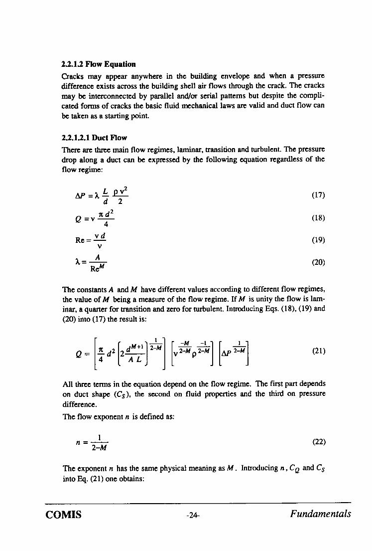
2.2.12.1 Duct Flow

There are three main flow regimes, laminar, transition and turbulent. The pressure drop along a duct can be expressed by the following equation regardless of the flow regime:

AP ) L p v 2 = -- (17) d 2

d 2 Q = v - - (18)

4

v d Re = (19)

V

A ~, = - - (20)

Re M

The constants A and M have different values according to different flow regimes, the value of M being a measure of the flow regime. If M is unity the flow is laminar, a quarter for transition and zero for turbulent. Introducing Eqs. (18), (19) and (20) into (17) the result is:

- dM+l] 2-~ ] 2-Mp (21)

Q-- -TZ-J ] All three terms in the equation depend on the flow regime. The first part depends on duct shape (Cs), the second on fluid properties and the third on pressure

difference.

The flow exponent n is defined as:

1 n = - (22)

2-M

The exponent n has the same physical meaning as M. Introducing n, CQ and C s into Eq. (21) one obtains:


Q = Cs v 1-2~ p-n (AP)n = C a (AP)" (23)

For the three main flow regimes Eqs. (20) and (23) are summarized in Table 2.

Table 2: Summary of Duct Flow

Laminar Transitive Turbulent

Q

64 Re

0.3164 Reo.25

1 (AP)0.57 CS V0.14p0.57

Constant

1 Cs ~ (AP ) °'5

2.2.1.2.2 Crack Flow

Crack flow is more like a flow through a network than a simple duct flow. Meas- urements proved that the relationship between flow rate and pressure difference can be expressed, for a specific crack, by a power law under a certain temperature and pressure difference range. If the crack flow measurement is expressed by power law (16) it can be re-arranged as:

Q = C s f ( p , v, n) (AP) n (24)

Cs and n are constants when the pressure difference is within the pressure range

used to fit the equation to the measurements, the exponent marking the flow regime under the measurements. If we assume that air is an ideal gas and that the influence of pressure is small, the equation can be written as:

Q = C s f ( t , n ) (AP) n (25)

Combining Eq. (20) and Eq. (22) we can write the friction factor as:

~ = A 2n-1

Re n (26)

Since the physical parameters for one specific crack are constant the equation can be rewritten as:


2 n - I f "~t

~.=D / v l n (27) Lvj

If we assume that the crack flow is expressed by Eq. (16) we can use the same procedure to get the crack flow equation:

Q = Cs v 1-2" p-" (AP)" (28)

The coefficient Cs depends on the crack form (duct shape). Here it is treated as a constant because deformation is ignored. Of course it is constant only within a certain pressure difference range.

2.2.1.2.3 Temperature Influence on Crack Flow

In order to make it easier to use Eq. (16) a correction factor KQ is introduced:

KQ = Po L Vo J

(29)

The subscript 0 refers to standard condition. As shown in Eq. (25) the expression (v 1-2" p ~ ) can be expressed in temperature only so that the correction factor is then called temperature factor. The final expression of KQ is:

KQ = T- 136 J (30)

The calculation of Kt2 shows that the main factors influencing KQ are the exponent n and the temperature difference between the actual and the reference

temperature T O = 293.15 ° K .

From the figure below it is obvious that the correction factor might be as large as 1.18 or as low as 0.88. The effect of the exponent is shown clearly. The temperature correction factor must be introduced when n diverges from 0.65. When n is less than 0.65, KQ will increase with temperature difference (T-T0) and vice

versa.

Equation (28) is modified to:


Q = KQ CQ (31)

This equation keeps the basic power law form, is casy to understand and easy to use. It is fitted to measurements by a simple regression method. Furthermore, existing leakage curves can be used if the measurement temperature is known.

L _

0 0

t - O

o (I)

0 0

1.1

l

0 .9

0.8

/ n - 0 . 5

n = 0.65

~ n 0.9 n ~ l . 0

I I 1

-40 -20 0 20 40 80

At [°C]

Fig. 11: Temperature Influence on the Correction Factor for different Values of the Exponent n

2.2.1.2.4 Equation Form Influence

There are three forms of the power law equation. In order to calculate the air flow correctly a temperature correction factor should be introduced in each equation but sometimes it is not known how to get the reference temperature. Which formula gives the best result in, this case? To find the answer the correction factors were deduced, the results being shown in Fig. 12.


. o : f "tn-lf "~2n-I

=I°oi Km LPJ LVJ

n-J- r' "~ 2,1-1

o =Ke % (ae)"

rh = K,a c,a ( A p )"

th = K t C t ,~(A e )"

(32)

The more the actual temperature diverges from the reference temperature the more the correction factor diverges from unity, this trend being the same for all three factors. The closer the exponent is to 0.65 the smaller the divergence from unity for K(2. The exponent n is close to 0.65 in most cases and one can therefore expect KQ to have a minimum of error in the case of no temperature correction.

1.05

I n

0 0 tO U. c- O

m

0 OJ I b

0 0

0.95

0.9

0.85

0.8 0.5

~ Attxt =20*C

Krh

E x p o n e n t , n

I I r - 1 . . . . I

0.6 0.7 0.8 0.9 1

Fig. 12: The Correction Factors for different Exponents

2.2.1.2.5 Regression

Measurements are often made under different temperatures. In order to maintain the simplicity of Eq. (31) it is necessary to introduce a reference temperature. To convert the equation from measurement temperature T,,, to the reference tempera-

ture T O the following equations can be used:


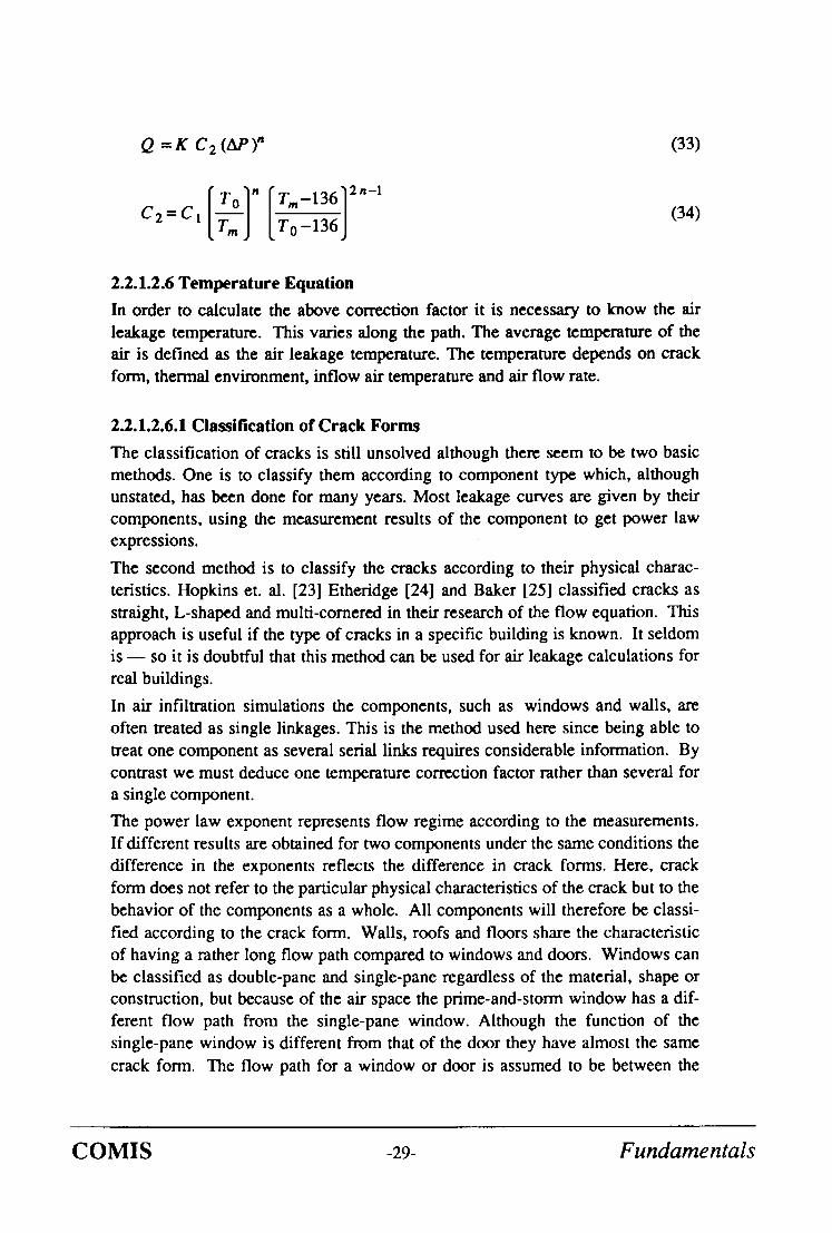
Q = K C 2 (AP) n (33)

C2=CI T0_136 (34)

2.2.1.2.6 Temperature Equation

In order to calculate the above correction factor it is necessary to know the air leakage temperature. This varies along the path. The average temperature of the air is defined as the air leakage temperature. The temperature depends on crack form, thermal environment, inflow air temperature and air flow rate.

2.2.1.2.6.1 Classification of Crack Forms

The classification of cracks is still unsolved although there seem to be two basic methods. One is to classify them according to component type which, although unstated, has been done for many years. Most leakage curves are given by their components, using the measurement results of the component to get power law expressions.

The second method is to classify the cracks according to their physical characteristics. Hopkins et. al. [23] Etheddge [24] and Baker [25] classified cracks as straight, L-shaped and multi-cornered in their research of the flow equation. This approach is useful if the type of cracks in a specific building is known. It seldom is - - so it is doubtful that this method can be used for air leakage calculations for real buildings.

In air infiltration simulations the components, such as windows and walls, axe often treated as single linkages. This is the method used here since being able to treat one component as several serial links requires considerable information. By contrast we must deduce one temperature correction factor rather than several for a single component.

The power law exponent represents flow regime according to the measurements. If different results are obtained for two components under the same conditions the difference in the exponents reflects the difference in crack forms. Here, crack form does not refer to the particular physical characteristics of the crack but to the behavior of the components as a whole. All components will therefore be classified according to the crack form. Walls, roofs and floors share the characteristic of having a rather long flow path compared to windows and doors. Windows can be classified as double-pane and single-pane regardless of the material, shape or construction, but because of the air space the prime-and-storm window has a different flow path from the single-pane window. Although the function of the single-pane window is different from that of the door they have almost the same crack form. The flow path for a window or door is assumed to be between the

C OMIS -29- Fundamentals

openable part and the frame.

2.2.1.2.6.2 Door or Single-Pane Window

There are many types of doors and single-pane windows but although they are of various materials and have different shapes their cracks are similar, i.e., short. The crack surface has little influence on the air leakage temperature and is therefore often ignored. Furthermore, the flow does not mix with the larger volume of air along the flow path.

Heat transfer and air leakage coexist. There are two convective heat transfer boundary layers across a single-pane window or door and the air which leaks through the component originates from the air space very close to the window or door. We can therefore assume that most of the air is coming from the boundary layer.

The air temperature in the boundary layer can be taken as the average temperature of the window surface and of the air outside the boundary layer.

Fig. 13: Air L e a k a g e through S ing le -Pane W i n d o w

The air leakage temperature is expressed as:

OL i tin = t o + (t/ - t o) (35)

2 ( % + ot i)

% (ti - to) (36) t ~ = t i -

2 (% + oq)

C OMIS -3o- Fundamentals

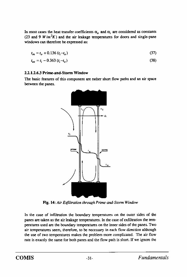
In most cases the heat transfer coefficients a o and 0q are considered as constants

(23 and 9 W/m2K) and the air leakage temperatures for doors and single-pane

windows can therefore be expressed as:

tin = t o + 0.136 ( t i - t o )

t a = t i - 0.363 ( t i - t o )

(37)

(38)

2.2.1.2.6.3 Prime-and-Storm Window

The basic features of this component are rather short flow paths and an air space

between the panes.

t i

Fig. 14: Air EooCiltration through Prime-and-Storm Window

In the case of infiltration the boundary temperatures on the outer sides of the

panes are taken as the air leakage temperatures. In the case of exfilu'ation the temperatures used are the boundary temperatures on the inner sides of the panes. Two air temperatures seem, therefore, to be necessary in each flow direction although the use of two temperatures makes the problem more complicated. The air flow

rate is exactly the same for both panes and the flow path is short. If we ignore the


influence of the flow path we can def'me the average temperature of both boundary temperatures as the air leakage temperature of the window.

According to Guo [26] the heat transfer and air leakage process of the window could be regarded as steady state, the horizontal air temperature in the air space as almost uniform, the vertical air temperature distribution as linear and the air leakage temperature as the boundary temperature on the source side. The inner (prime) and outer (storm) pane form two heating systems along with the room (see Fig. 14) and the infiltration mode equations:

(~tot = ki (ti - ta) + th c (t i - t l)

Qtot = ko (ta - to) + th c (t a - t 2)

(39)

(40)

Similar equations are valid for the exfiltration mode. A dimensionless temperature factor for the infiltration and exfiltration mode can be def'med respectively:

t-to t i - t o

K ao - r h c /2

K ao + K ai - t h c /2

K ai - r h c

K ao + K di - r h c /2

In f i l t ra t ion (41) EJ~filtration

where:

Kao = ko

~ =ki

1 ff~c 2~x o

rhc

(42)

(43)

We can accordingly define the air leakage temperature:

1 t i . /~ = -~ (tl + t2) (44)

The air leakage temperatures becomes,


t i n = t o + - ~ 1 - - - + T 2 + - - + (t i - t o) Oti ~i

(45)

ttx = to + -~ 2 - - ~ ' - / + y 2+--+ot i (ti - to) (46)

From Eqs. (45) and (46) we see that the air leakage temperature depends on the air temperatures of the room and the exterior, the air flow rate and the window thermal performance. The analysis of these equations shows that the influence of thermal performance is small for actual windows. General thermal data is therefore introduced:

tin = to + ( 0.121 + 0.193 T) ( ti - to) (47)

t ,x = to + ( 0.371 + 0.450 ~,) ( t i - t o) (48)

From Eqs. (41), (47) and (48) it is obvious that the calculation of air leakage temperature involves iterative calculations. In solving the problem the basic power law equation is fn-st used to calculate the reference air flow rate. The air flow rate is then used to calculate leakage temperature and to recalculate air flow rate. This procedure is repeated until the desired accuracy is obtained.

2.2.1.2.6.4 Walls

Most walls belong to one of two groups. The first group comprises solid walls, e.g., brick or concrete walls. The second group comprises walls with an air space such as wood or steel frame walls.

A "wide" crack is here defined as a crack where the air penetrating the wall does not have the same temperature as the wall itself. This type of crack appears mostly in comers or at joints. A "tiny" crack is here defined as a crack where the air has almost the same temperature as the wall. Because of the tiny size of these cracks and the low flow velocity the temperature difference between the air and the solid wall is small so that it is reasonable to assume that the air and the wall have the same temperature.


2.2.1.2.6.4.1 Tiny Cracks To obtain a mathematical description one assumes one-dimensional heat and air leakage flow, steady state, unit area air leakage rh, heat resistance R, room tem-

perature t i and outside temperature to.

The wall element of tiny cracks is shown in Figure 15.

0 dx X x

Fig. 15: Wall Element o f Tiny Cracks

From the heat balance of the element dx we obtain:

tin = to + tin.o - to., + - ~ (49)

For the air leakage temperature it is desirable to get one value rather than a curve

and the temperature at x = 0.5X can be used in this case. It is simple, however, to

integrate along x to obtain the average temperature of the air leakage - the air

leakage temperature:


a X i n . o - t o + a X i - t o -

1] - f i r --d--~ [ t i t o e - - - - + - + t i :xtl (50)

To be able to calculate the air leakage temperature we need to know the heat resistance of the wall, room temperature, and the outside temperature.

2.2.1.2.6.4.2 Wide Cracks

The wide crack can take either non-comer or comer form - - the more comers the closer the leakage temperature to the temperature of the wall.

To solve the problem analytically the following is valid. First convert the boun- danes into imaginary wall layers so as to transfer the third boundary condition into a first boundary condition on both the inside and outside of the wall. Secondly assume that the crack surface temperature is not affected by the air leakage. The above is a simple method which can also be used with multi-layer walls. Third use the result of step two as the boundary in solving the temperature distribution in the wall. Forthly use the results from step three to again obtain the air leakage temperature. These first four steps constitute the basic method. This is advantageous in theory but difficult to use. In principle, we can repeat step three and four again and again to get accurate results. The simple method will give reasonable accuracy and the basic method can serve as a standard. Both methods are described by Mingsheng and Herrlin [27]

A crack where the width of the crack is much larger than its height and the length is the same as the thickness of the wail, the wall being a single-layer wall, has been calculated with the following results.

The simple method:

Introduce the dimensionless temperature 0:

t i - - t in 0 - - - -

t i - t o

The air leakage temperature can be expressed as:

0in = ~ 0 dX

(51)

(52)


WE] 1 r h c nlc 01,, = - ~ 1 e (53)

The above is the final equation of the air leakage temperature for the infiltration mode which can also be used as the exfiltration mode. In that case it is necessary

to replace the temperature of the room and the outside temperature with the outside temperature and room temperature respectively.

The basic method:

~, n =inf An tin = C ~a Sinh (n n) Cos n it X

L th c n=0

n =iq B n + ~ e_2n n Cos n n X (e - 2 n r t - 1 )

n--'O 1 +

n =i ,¢ D n y'. Cosh n n X (54)

Cosh n 7I n--O

n =inf An C = t o + - - ~_,

L t h c ,1=0 S inh (n ~)

n:iq" B n ( e - 2 n n _ 1) + ~_~ e -21~n ,I--0 1 +

n =inf D n

- ~ C o s h n n (55) n = 0

We now have the leakage temperature calculation equations for wide cracks. From the formulas above it is clear that although the basic method may give more accurate results it is much more complicated to use. One can similarly deduce formulas for multi-layer walls but as they are too complicated to use in practical cal-

culations they are not given here.

2.2.1.3 Conclusion

Air leakage characteristics can be represented by a power law form based both on theory and measurements. A temperature correction factor should, however, be

introduced to increase the accuracy.


Analysis shows that the volume flow form gives less error should there be no temperature correction. This form is therefore recommended when determining the parameters of the power law.

The air leakage temperature depends on many parameters. Several equations for determining the air leakage temperature are given for windows, doors and walls although more work must be done to simplify the calculation methods.



2.2.2 Air Flow through Large Openings

2.2.2.1. Introduction

Airflow through doorways, windows and other large openings are a significant way in which air, pollutants and thermal energy are transferred from one zone of a building to another or to the outside. In a previous review of multizone inf'dtra- tion models made in 1985, Feustel and Kendon [3] pointed out that no code was able to solve this problem other than dividing the large opening into a series of small ones described by crack flow equations.

The subject of air flows through large openings in fact includes a large number of different problems ranging from steady gravitational flows to fluctuating flows due to wind turbulence, and including recirculating flows caused by boundary layer effects in a thermally driven cavity.

COMIS' contribution has been to describe the various physical problems, review the solutions already developed in the literature and put forward a general propo- sal dealing with most of the large openings included in the pressure network modeling of a multizone building [28].

2.2.2.2. Short Review of Literature

Air may flow differently at the top of a doorway than at the bottom. This bi- directional flow, characteristic of large opening behavior, has a variety of causes which can be classified broadly in two categories - - those which induce steady flow by virtue of their mean value and those whose effect is due to their fluctuating nature.

2.2.2.2.1 Steady Flows through Large Openings

The f'ust category includes the effects of mean wind velocity, the gravitational flows due to density gradients, the effects of boundary layer flows developed in a cavity and the coupling effects induced by ventilation or heating systems.

Many authors have dealt with gravitational flow approach through vertical openings [6], [29-31] and provided elementary solutions based on purely natural or mixed convection. Nevertheless, most of them refer to the basic solution developed analytically by Brown and Solvasson [29]. This solution, based on Bernoulli's assumption, delivers the mass flow through the opening as a function of the main characteristics of air on both sides of it.

Some improvement on this approach has been made by taking into account temperature stratification on each side of the opening.

In the various experimental studies developed by Balcomb et al. [32] Weber [33] Hill et al. [34] and Pelletret [35] it appears that most of the steady state configurations can be well represented by uniform density gradients.


Finally, among the various problems found in defining large opening behavior horizontal openings should be mentioned. The most interesting aspect of horizontal openings is when the fluid above the opening has a greater density than the fluid below. In this case an unstable condition is reached and an exchange occurs between the lighter fluid flowing upward and the heavier fluid flowing down- ward. This problem was first studied by Brown [36] hut few authors have made a consistent contribution towards solving it.

In a recent paper Epstein [37] discusses the buoyancy exchange flow through small openings in horizontal partitions. He presents an experimental study using brine above the partition and fresh water below it and identifies four different regimes as the aspect ratio of the opening is increased. This paper gives a good description of the flow processes but it is limited to purely natural convection effects so that the results are difficult to extend to more general configurations.

Much more work is needed to describe accurately the behavior of horizontal openings in natural or mixed convection configurations. The few papers found in the literature are not sufficient to do so and they do not allow us to include such configurations in a multizone infiltration code.

2.2.2.2.2 Unsteady Flows through Large Openings

The second category usually represents two very different kinds of configurations:

• The transient behavior of flows due to slow evolution of the boundary conditions

• The fluctuating air flows due to fluctuating pressures or velocities

a. Transient Flows

The first type of problem is usually solved with a steady state description of the dynamical process. Bernouilli's flow theory or any other correlation is used to calculate the steady state flow corresponding to the boundary conditions of each time step. The main assumption in this case is that the flow will be fully developed instantaneously and will follow the imposition of new boundary conditions at each time step.

The variation of the boundary conditions can be given by hourly variation of average wind speed and direction, by a schedule of occupancy, or the working of mechanical ventilation systems, or by the evolution in time of the thermal state of the building itself.

The most common way of solving the problem is to combine the air flow model with other models dealing with thermal simulation or any other phenomena driving the air flow process and to give a complete description of the coupled problems. In some cases, however, it is better to use a simpler approach and to give an estimate of the evolution in time of the flow through an opening caused by a

COMIS -4o- Fundamentals

single perturbation. In this way Kiel and Wilson [38] studied the unsteady buoyancy flow that occurs during the door opening or closing period. They investigated the decrease in flow rate that results from the effect of limited interior volume and finally considered the effect of door pumping.

Van der Maas et al. [39] looked at the same problem from a different point of view. They studied the evolution of the air flow rate and temperature in a room when opening a window. Assuming insulated walls and developing the energy balance of the inside air, they show by full-scale experiments that a reasonable agreement is obtained. The main advantage of such a solution is the avoidance of coupling with a real simulation of the thermal behavior of the whole building and the ability to give a quick estimate of the transient evolution of the air flow.

b. Fluctuating Flows through Large Openings Experimental results have shown that the fluctuating effects can be particularly significant in the case of one sided ventilation or when the wind direction is parallel to openings in two parallel facades. Nevertheless, as pointed out by Vandaclc and Wouters [40] in theft review paper very few correlations have been proposed and most of them concern very particular configurations.

The fluctuating flows are mainly created by the effects of turbulence due to local wind characteristics. They depend on the turbulence characteristics of the incoming wind and on the turbulence induced by the building itself. These mechanisms have been studied on scale models or full scale cells and wind tunnel visualiza- tions have been used to describe the main phenomena. Turbulences in the air flow along an opening cause simultaneous positive and negative pressure fluctua- tions of the inside air. The studies of Cockroft et al. [41] Warren [42] Crommclin and Vrins [43] and Ethcridgc [44] illustrate this problem.

Because of the complexity of the problem and the high number of parameters influencing the development of the eddies along the facade of a building very few correlations have been proposed and implemented in multizone air flow models.

Phaff and de Gids [45] propose an empirical correlation deduced from experimental work and give a general definition of the ventilation rate through an open window as a function of temperature difference, wind velocity and fluctuating terms. Since they found an existing flow without either wind or temperature difference a fLXed turbulent term was added to the volummctric flow. This turbulent term is presented as an additional pressure drop written as a function of the flow exponent.

These types of models, combining the effects of wind velocity, temperature difference and turbulence, should bc able to predict the effect of fluctuating wind on the air flow exchange through an external opening in a multizonc pressure network. However, much work is nccdcd in order to give a precise description of the effects of the many parameters influoncing the structure of the local wind at the very location of the opening.


2.2.2.3. Integration into COMIS

A multizone infiltration model like COMIS is defined by a network description of the pressure field in a building. The pressure nodes represent control volumes or zones at thermodynamical equilibrium. They are linked together by nonlinear flow equations expressed in terms of pressure difference. Mass conservation of air in each zone leads to a nonlinear system of pressure equations.

These are two ways of describing the behavior of large openings. Either we can describe the air flow rate through a large opening using a nonlinear equation of the pressure drop, or we can solve the problem separately and include the result as an unbalanced flow in the mass conservation equation of the described zone.

2.2.2.3.1 Existing Solutions

To represent the behavior of a large opening in an air flow model we can take an explicit definition of the flow given by a Bernoulli flow regime assumption, or any other correlation of natural or mixed convection [46] corresponding to the configuration. In the case of both methods the large opening is disconnected from the general pressure network, is solved separately and then represented by an unbalanced flow in the mass conservation equation of each zone. Since the flow is strongly dependent on the pressure field around and inside the building the fast solution will lead to a high number of iterations and a direct approach appears more attractive.

To connect the large openings to the general pressure network it is necessary to define their behavior in terms of nonlinear equations of the pressure drop. The fast possibility is to describe the large opening as a conjunction of parallel small openings, properly located, and with only a one-way flow allowed for each one. Each small opening is then described by a crack flow equation taking into account the local pressure drop. The whole system of nonlinear equations can be introduced directly into the pressure network. This solution was first proposed by Walton [47] and Roldan [48] and has been used in various multizone models developed since (Feustel [49]). It leads to the def'mition of various flow elements in simulating one large opening.

A second way to solve this problem is to interpret the flow equations of large openings in terms of non linear pressure laws. This method leads to the def'mition of new flow equations in pressure characterizing the behavior of large openings.

Walton [50] proposed this solution in the case of a vertical opening between two isothermal zones i and j for steady state flow. Following the approximation of the Bernoulli flow it is assumed that the velocity of the air flow at different heights is given by the orifice equation (Eq. (56)):


]la Vo(Z) = 2

P (56)

where p represents the density of flowing air.

The hydrostatic equation is then used to relate the pressures in each room to the air characteristics at various heights, and the velocity equation becomes:

I (Pi'O-PJ'°)-gz (Pi-PJ)]]p 1/2

(57)

The height of the neutral plane is given by Pi (z) = P j (z) or by setting the interzonal velocity to zero. In the case of a neutral plane being located in the opening, and taking this point as origin for altitude, since Pi (zn) = Pj (zn), the mass flow through the doorway above and below the neutral level zn are given by Eqs. (58) and (59):

z = H - z n

rhzn,t, t = Cd I 19 vq(z) W dz (58) z=O

z--0

rho.zn = Cd f pvij (z) W dz (59) Z

Walton [47] reports that this model of doorways tends to be faster than the multi- ple opening approach. However it complicates the assembly process of the network since one or two flows may exist through the same link between two zones.

2.2.2.3.2 COMIS Contribution

The main objective in proposing a solution for large openings is to fit it easily into the network definition and to go as far as possible in the modeling of the various phenomena influencing the behavior of large openings.

The main assumptions of our model are:

• Steady flow, inviscid and incompressible fluid

• Linear density stratification on both sides of the opening

• Turbulence effects represented by an equivalent pressure difference profile

• Effects of reduction of the effective area of the aperture represented by a single coefficient

C OMIS -43- Fundamentals

a. General Numerical Solution of the Problem

Figure 16 gives a general description of the problem to bc solved.

t Pt (z)-Pto +btz T Z

I I

POl

Pl (z)= Pol+blZ : I

I I

I I

I I

I I

H

z~

ZN]

P2 (z) =

P01 Pto I//'! o P02 P02

1302 +b 2 z

Fig. 16: The General Problem of Gravitational Flow through a Vertical Opening

On each side of the opening, we assume a linear density stratification:

Pi (z) = P0t + bi z (60)

and we introduce a linear pressure difference simulating the effect of turbulence:

APt = Pto + bt z (61)

The reference pressures on each side are given at the bottom of the opening. Assuming Bernoulli hypothesis on both sides of the opening we can define the pressure difference at any level z as:


Z2 Z2)] P l(Z )--P 2(z) = (P 01-P o'z)--g (Pro z + b tT)--(po2 z + b 2--~-- +(Pt 0+bt z ) (62)

The velocity at any level z is then given by:

v(z)= [2

#

Pl(Z) - P2(z) 1/2

(63)

where p represents the density transported by the velocity. The locations of the two possible neutral planes are given by an equilibrium in pressure which leads to a zero velocity point. In a general case we have:

z2[ ] g ( b l - b 2 ) " 7 + g(P01-902) - b t z + ( -Po l + P o 2 - P t o ) = 0 (64)

Equation (64) can have two, one, or zero real solutions. To find the air flows flowing in both ways through the opening, the next step is to integrate Eq. (63) in the intervals defined by the physical limits of the opening and the position of the neutral planes:

z=z 1

rn o.z 1 = Cd 0 I pv(z) W dz (65) Z----0

z=z2

fflz l.z 2 = Cd 0 f Z=Z 1

pv(z) W dz

z = H

rhz 2,/t = Cd 0 I pv(z) W dz Z=Z2

It appears from the preceding equation that the flow through a large opening is directly proportional to an empirical discharge coefficient Cd . This is, in fact, a phenomenological coefficient taking into account the contraction of the flow due to the existence of the opening. Theoretically it depends on the fluid and the local flow characteristics caused by the shape of the opening. Its value goes from 0.61 for sharp-edged orifices to 0.98 for trumpet shaped nozzles. A brief review [51-53] indicates that these values can be as low as 0.25 and higher than 0.75 for large openings. 0 is called area reduction factor. It enables to define the effective opening of a large opening.


Recently Van der Maas et al. [39] reproducing the Lane-Serif et al. [54] experiments, concluded that the discharge coefficient corresponding to the Bernoulli model can reasonably be taken as being between 0.6 and 0.75. However a precise determination remains very difficult. 0 is called an area reduction factor and enables us to define the effective area of the opening through what the air is flowing.

In the more general case these integrals have no analytical solutions and they have to be computed by a numerical mean. In COMIS a classic Simpson integration is used. This numerical solution is general but it is also time-consuming and is reserved for the more general case. As far as Eq. (64) remains a linear one (i.e., when no density gradients exist, an analytical solution does) we can use it to save computational time.

b. Analytical Solution of the Problem without Density Gradients

If we now assume that air density in each zone does not change with the altitude an analytical solution exists. The pressure difference at any given level Z becomes:

Pi (z ) - P 2(z ) = (P ol - P o2) - g (P01 z - po2 z ) + (Pto + b t z ) (66)

The position of the possible neutral plane is then given by:

- (Pol - Po2 + Pro) Zn = (67)

g (POl - P02) - bt

and the velocity at any location Z is given by:

[ " ( P o 1 - P o 2 + P t ° ) - [ g ( P o I - P ° z ) - b t ] v(z )= 2

P

1 / 2

(68)

Taking the position of the neutral plane as origin for the Z axis Eq. (68) becomes:

1 / 2

(69)

and the flows through the large opening are given by direct integration of Eq. (69) between 0 and the limits of the opening. In a general case we have:


1 3

mT~.H =-~ W Cd O'fp g(rhool-Po2)-b t lH -Zn l

and:

l 3

tho.7_~ ='~ W Cd O 4"p g(rhool-PO2)-bt IZnl

(7O)

(71)

In Eqs. (70) and (71) p represents the density transported by the flow.

2.2.2.3.3 Examples of Solutions

a. Influence of the Turbulence Effect

Firstly we test the influence of the turbulence term on the behavior of a large opening when submitted at an increasing pressure reference drop. The opening is a doorway of 0.8 m width and 2.0 m high separating two zones at 20°C without

any water vapor in the air. Its discharge coefficient is equal to 0.65, and the res- triction coefficient is 1, which means that the opening is perpendicular to the flow and completely open.

According to the orders of magnitude given by Phaff and de Gids [45] for the turbulent effect we consider a reference configuration without turbulence effect (Pt = 0) and two additional cases with linear turbulence pressure distributions:

Pt 1 = 0.02 - O.02z and Pt 2 = 0.05 - O.05z (72)

The results obtained using our analytical solution are shown in Fig. 17.

Obviously these two turbulent pressure distributions give a recirculating flow until the reference pressure difference at the bottom of the opening cancels the turbulent effect. Until this threshold we observe a negative flow. When the pressure difference at the bottom is zero, a situation which corresponds to a single- sided ventilation, the values of the recirculating flow due to the turbulent effect reach respectively 227 m3/h and 358 m3/h .

This example is merely a demonstration. Many more studies are necessary to describe precisely the turbulence pressure distributions equivalent to the real effect of wind turbulence. Nevertheless, this effect can be taken into account in an analytical model and this short example demonstrates how significant it can be.


0 . $ -

0 .8 -

0 . 4

"E 0 . 2

0 . 0

-0 .2 0 . 0 0

~ 1 0 . Z N

m Z N , H

" ' i - - '" ,' ' ' i - - I 0 . 0 8 0 . 1 8 0 . 2 0 0 . 1 0

&P [Pal

Fig. 17: Effect of Turbulent Pressure Gradient on a Doorway

b. Influence of Density Gradients

The second example presents the behavior of the same doorway, previously

def'med, but on one side there is a stratified environment. The temperature of zone

2 is set at 20°C and in zone I the reference temperature at the bottom of the

opening is 17.5oc with a density gradient of-.Ikg/m 4 which gives a dry air temperature of 22.5°C at the top of the opening. On the same side the effect of a tur-

bulence effect Pt]=.02- .02z is kept. Figure 18 represents the evolution of the

flows, calculated by our numerical solution, when varying the reference pressure

difference at the bottom of the opening.

For negative pressure differences a negative one way flow is obtained (which

means that air is flowing from zone 2 to zone I) until -0.015 Pa. Beyond this

value a first neutral plane appears at the bottom of the opening. After -0.015 Pa a

two way flow exists until 0.025 Pa where a second neutral plane appears at the

top of the opening. The existence of the second neutral plane increases signifi-

cantly the flow from zone 1 to zone 2. Both neutral planes then disapear and the

negative flow (from zone 2 to zone I) too. Figure 19 shows the evolution of the

position of the two neutral planes in this configuration. This curve is the


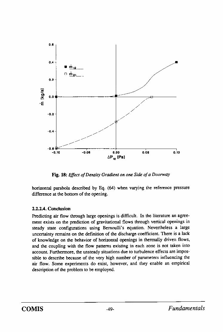
0 .6 -

W

-E

0.4-

0.2

0.0

-0.2

-0.4

-0 .8

• rn12

D r" R i m _

J J

J J

J J

"I-"

-0.10 -0.~08

J J

J J

J J

J J

J /

0.00 APlt IPoI

I

0 . 0 8 0.10

Fig. 18: Effect of Density Gradient on one Side of a Doorway

horizontal parabola described by Eq. (64) when varying the reference pressure difference at the bottom of the opening.

2.2.2.4. Conclusion

Predicting air flow through large openings is difficult. In the literature an agreement exists on the prediction of gravitational flows through vertical openings in steady state configurations using Bemoulli's equation. Nevertheless a large uncertainty remains on the definition of the discharge coefficient. There is a lack of knowledge on the behavior of horizontal openings in thermally driven flows, and the coupling with the flow patterns existing in each zone is not taken into account. Furthermore, the unsteady situations due to turbulence effects are impossible to describe because of the very high number of parameters influencing the air flow. Some experiments do exist, however, and they enable an empirical description of the problem to be employed.


_

l i t

E w

rd

_

H e i g h t o f Door [m] J

J j .

J J

\

J J

Z 1 I I [ F I . . . . I I I l

- 0 .10 - 0 . 0 8 - 0 . 0 6 - 0 . 0 4 - 0 . 0 2 0 . 0 0 0 . 0 2 0 . 0 4 0 . 0 6

~PI. [Pal

Fig. 19: Evolution of Neutral Planes Location

Taking the complexity of the problem into account a general solution to include large openings in the pressure network of a multizone model was proposed.

This model is generally applicable in most of the large openings configuration. It is a combination of the theoretical solutions developed using Bernoulli's assumptions and of empirical knowledge acquired from experiments in real configurations.

Much more work is needed, however, to validate these assumptions. Parametric studies coupled with specific experiments are now necessary to check the validity of this solution and show the effect of the different paranaeters involved in the model.

Further studies should also include the effects of coupling between the large opening flow and other flow patterns caused by natural or mixed convection in buildings.


2.2.3 HVAC-Systems

2.2.3.1 Pressure Ia3sses through Ducts and Duct Fittings

Assuming the specific weight of atmospheric air equals that of air in the duct the relationship for fluid resistance between sections, in terms of pressure, is:

Pt, = Pta + APt (73)

The total pressures at the two sections of a duct are expressed by:

Pq =PI + "P-Vl2 = P 1 2 + PaYn' (74)

Pt2 = P2 + "P-v]2 = P2 + Payn~ (75)

The pressure losses for each section of a duct system can be calculated using Eq. (76):

n~ m~ /~ APt = Z APi + Z APJ + )", APk (76)

i=1 j= l k=l

with the total pressure loss AP t being the sum of the friction losses in the duct APi, the pressure losses due to fittings APj and the pressure losses in the equipment APk-

2.2.3.2 Friction Losses through the Duct

Friction loss for fluid flow in ducts can be calculated by the Darcy equation:

l APp = ~. -~ Pdy. (77)

Within the region of laminar flow (Reynolds numbers less than 2000) the friction is a function of Reynolds number, only, and can be written as:

~ = 6 4 Re (78)

For turbulent flow (Reynolds numbers greater than 10000) the friction factor depends on the Reynolds number, duct surface roughness and internal protuber- ances such as joints and is calculated by Colebrook's equation [55]:

C O M I S -51- Fundamenta l s

251 ] 79, - ~ -~--~- d + R"'e-

Since the equation cannot be solved explicitly for k, we use an approximate explicit equation from Moody [56]:

o61, ~.=0.0055 1+ 0 0 0 0 ~ - + R e J (80)

Bouwman [57] shows, that when Z, is below 0.05, the difference between Moody's equation and Colebrook's equation is less than 5 percent.

ASHRAE [58] divides duct roughness factors into five categories from smooth (0.00003 m) to rough (0.003 m). Manufacturer's data indicate that the absolute roughness for fully extended flexible nonmeu'ic ducts and metal ducts ranges from 0.0011 m to 0.0046 m and 0.00012 m to 0.0021 m, respectively.

Where the length of round and rectangular ducts is equal, with a constant flow in each duct and equal resistance to flow in both ducts, the equivalent round of a rectangular duct is calculated by Eq. (81) found in the literature [58]:

de 1.30 (a b)°"625 = (81) (a + b) °'25°

2.2.3.3 Dynamic Losses due to Duct Fittings

Dynamic losses result from flow disturbances caused by fittings that change the path of the air flow and/or its area. These fittings include entries, exits, transitions and junctions. The dimensionless coefficient zeta (~) is used for fluid resistance. The coefficient zeta has one and the same value in dynamically similar streams, i.e, streams with geometrically similar stretches, equal values of Rey- nolds number and equal values of other criteria necessary for dynamic similarity:

APt APt . . . . (82) .P__V 2 Pdyn

2

The calculation modules for the fittings and equipment prepared for COMIS are shown in Table 3. There are some data available for the local loss coefficients of the fittings and equipment. The values of the local loss coefficients in some fittings, however, differ according to the different literature sources. These values are compared in Figs. 20 to 23.


For round and rectangular hoods the data from ASHRAE [2] is used because that data covers a wide range of angles from 0 to 180 degrees.

There are six data sets available for elbows, each of which differs significantly from the others. One of the reasons for the scatter is probably the difference between the roughness factors of the elbows used for the experiments - - although these were not specified by the authors. In this module the mean value between the data from ASHRAE Handbook of Fundamentals [2] and the data from a Ger- man Handbook [59] is adopted.

Three data sets from the ASHRAE 1985 Handbook of Fundamentals [2] were adopted for round conical diffusors. The data for round contractions was taken from the same source. This data shows the pressure loss coefficient in the wide range of angles from 15 to 180 degrees.

2.2.3.4 Coefficients of the Flow Equation of a Duct

The dependency of the friction loss along the duct, using a Reynolds number is different between the laminar region, the turbulent region and the transitional region as described in 2.2.3.2. For easier calculation in the network model the relationship between the pressure loss and the volume flow rate is assumed to be expressed by the power law function.

The flow coefficient CQ and the exponent n are calculated in our module as follows. Firstly an estimated volume flow rate through a duct is given as input data. If the flow is in the turbulent range (Reynolds number greater than 3500) the duct friction factor is calculated by an approximate explicit equation from Moody instead of by the Colebrook equation which is an implicit expression. If the flow is in the laminar region (Reynolds number less than 2300) the duct friction factor is given as a value, 64, divided by the Reynolds number. In the transitional range the factor is taken as an interpolated value between the two transitional points. The pressure loss along the duct is then calculated, including dynamic pressure losses through duct fittings. Secondly, an alternative volume flow rate is automatically calculated in the module. That value is 10 % higher in the turbulent range and 10 % lower in the laminar range than the value of an initial estimated flow rate. The corresponding friction factor of a duct, and the corresponding pressure loss along a duct with fittings, are calculated to the alternative volume flow rate. Lastly, the flow coefficient CQ and the exponent n are obtained by

the straight line connecting the two points plotted on a log-log chart:

logQ 2 - logQ 1 n = (83)

log(AP2) - log(AP 1)


Table 3. Types of Duct Fitting

2

3

Entries 1.1 Round Duct Mounted in Wall

O---

1.2 Abrupt with Screen

g. 0:--~

1.3 Hood

Exits

2.1 Round Duct Flush with Wall

;= 1.0

2.2 Abrupt with Screen

E lbows

|

;=0.5 ®

C O M I S -54- F u n d a m e n t a l s

Table 3. (continued)

4

5

6

Transitions (Diverging Flow) 4.1 Conical Diffuser, Round

O ~ Transitions (Converging How) 5.1 Contraction, Round

O ~ Obstructions 6.1 Screen in Round Duct

0 6.2 Perforated Round Plate

@ 6.3 Orifice in Round Duct

®

6.4 Damper


I

t-- (U

i m

8 0

O ,--I

i , _

(0 m

L _ n

0 . 8 -

O .6 -

0 , 4 - -

0 . 2 -

0 0

A S H R A E [2 ]

/ /

/

/ /

/ /

]

20

0 j O j

/ /

s /

O ~ / /

/

/ /

/ /

/ /

/

, i /

/ /

O " /

J f I noue [60]

AO . ~ , l l P . v

0 /

I /

/

I I I I I I I I

40 60 80 100 120 140 160 180

Angle of Hood [o]

Fig. 20: Pressure Loss Coefficients for a Hood


I

,k.,,,

I :

i i m

O i i m

O t~ t~ O _1

i . _

t~

I1) i . _

r l

_

0 , 8 - -

0 . 6 -

0 , 4 - -

O . 2 -

o ASHRAE [2]

• _R e c k_ n£cj e_l _/_S p re_n_g_er_ [_5_9_]

o Anon. [61]

• SHASE [62]

o Leuzinger [63]

In Feustel [64]

H D

- ( 7

0 I I I I I

0 1 2 3 4 5

r/D [-]

Fig. 21: Pressure Loss Coefficients for an Elbow


I

e -

i I

i i

¢1

0 _J

L _

L _

0.8 - x~x~

",,

0"4- °',° ~ "''',

• " ~ ~ " \

\

0 , 2 -

0

I 8 deg ASHRAE [2]

[] 12 dog

• 16 deg

O 20 deg

A 30 deg

X 4-5 deg

V 60 deg

+ 90 deg

o 120 deg

O 180 deg

[] 5 deg SHASE [62]

[] 10 de 9

20 deg_ . . . . . . .

[] 30 deg . . . . .

4-0 _d~(~ . . . . . . . . . . . . . . . . . . . . . . . . . .

0.15x(1-X)*~2 Angle < 16 deg

(1-X)* .2 Anqle > 16 deg

180 deg Recknogel/Spreng_e_r [69]

" ~ , ~',, ® v . - - - ~ A 2

~[ ~ "',

_ I I I I •

0 0.2 0.4 0.6 0.8 1 A1/A2 [-]

F i g . 22 : Pressure Loss Coefficients for the Transition of a Diffuser


l

¢ -

(D l l m

0 o n

0

0 . . I (D l l , .

(D l i , .

n

o.,] 0 . 6 ~ ,

0 . 5 - \

0 .4-

0 .3 -

0 .2 -

0.1-

0.0

A] ~ V

\

\

• l _ 5 : _ 4 9 _ d _ e a A_SHRA_E_[_2]_ . . . . . .

(~ 50-60 dog. . . . . . .

• 90 deq

A 150 dog

X 180 d e g _ _

V 30 deg

+ 4.0 deg

O 50 deg

0 60 deg

[] 30 deg SHASE [~21

m 45 deg

60 deg

180 deg

"CF'O'- EF - _ % - - - - I - - - - ~ - - - - < Y . . . . . .

• • J [] + 4- V V []

V

I

0 0.2 0.4

iS ".

i "3 T 0.6 0.8 1

A1/A2 [-]

Fig. 23: Pressure Loss Coefficients for a Contraction


Q1 CQ=

(AP 1)"

As a result, the power law function obtained for the duct is written as:

(84)

Q = cQ (AP)" (85)

2.2.3.5 Total Pressure Losses due to T-Junction

When the flow is diverging, as shown in Fig. 24, the total pressure loss, Ap 12, from the point 1 to the point 2 is expressed by:

(86) T"J T' J

P1 1,2

Fig. 24: Pressures at a Junction of a Tee.

C O M I S -6o- Fundamentals

The pressure loss coefficient is defined by the velocity pressure of point 1 which is just before the junction:

P l 2 12 = 412 "-~-Vl (87)

Therefore:

412 "- AP12

Pl. 2 (88)

When the flow is converging, on the other hand, the pressure loss coefficient is def'med by the velocity pressure of point 2, which is just after the junction:

- P2 2 AP 12 = q12 .-~'v2 (89)

Therefore:

412 = m AP12

132 v 2 (90) "2' 2

The pressure loss coefficient can be expressed as the function of the two volume flow rates just before and after the junction, e.g., the pressure loss coefficient,~l 2,

is expressed as:

412=F[Q~I ] (91)

As the duct systems in this program are combined in the network air flow model the junction is treated as a node, i.e., the static pressure around the junction is calculated iteratively. The static pressures at the two other points, e.g., for the diverging flow, are calculated by Equations (92) and (93):

P lv2 - P2 2 P2=P1 +(1-412) 2 t -~-v2 (92)

C O M I S - 6 1 - Fundamentals

P l . 2 P2 v 2 P 3 = P 1 + (1 - ;13) "~--*1 - - ~ - 3 (93)

Input data in this module are the three volume flow rates through the three ducts connected at the junction as well as the static pressure at the point in a duct just before the junction. The outputs are the static pressures at the two points in the two ducts just after the junction.

2.2.3.6 Literature Survey

There are some available dam of the pressure loss coefficient at the T-junction given [60-71], for example, in the ASHRAE Handbook, the handbooks from Ger- many and The Netherlands and in a paper written by a Japanese researcher. We found, however, that the values of the pressure loss coefficient were significantly different depending on the source. For example, in the case of converging flow, the pressure loss coefficient through the main duct of the T-junction obtained from one source is double the value of the loss coefficient given elsewhere (Fig. 25).

Pressure loss coefficient curves for two cases are shown in Fig. 25 and Fig. 26. Our literature survey will be continued in order to discover the original source and experimental conditions of the pressure loss test.

As a first step, the data prepared by Ito et al., shown in Table 4, was taken since all six pressure loss coefficients in each of the four flow patterns at the T- junction are expressed by the experimental formulae. These values, furthermore, are close to the values presented in the ASHRAE 1985 Handbook of Fundamen- tals [2]. (But only two pressure loss coefficients in the case of the diverging flow are shown in the ASHRAE 1989 Handbook of Fundamentals [58].)


I I I

I I i I

i i N I N I

0

0

(V t . _

QI

1.6-~

1 .4-

1 .2 -

0.8

0.6

0.4

0.2

0

- o 2 t 0

\ \

EK

\ D X

\

\

\

• ASHRAE [2]

[] Recknagel/Spre._nc~r [59]

• JSME [69]

O NEN 5063 [68]

Q1

I to [70]

I EA [ 6 7 ]

In Feustel [ 6 4 ]

Q3

I I' I

0.2 0.4 0.6

Q I / Q 3 [-]

~E3

\ r i

0.8 1

Fig. 25: Pressure Loss Coefficients for T-Junctions


_

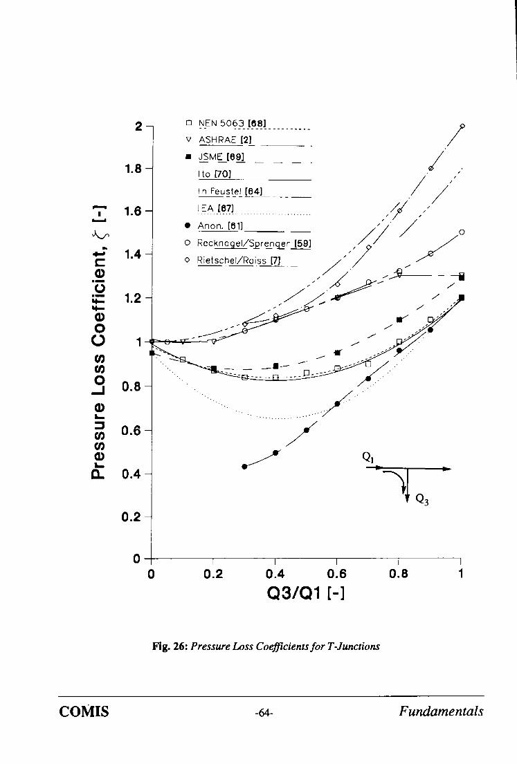
1.8

"T' 1.6

1.4

i 1.2

0 1

O _ 1 0 . 8

(D

:~ 0 . 6

(D t . _

rt 0 . 4

0.2

0

o _NE _N_ _5_0_ 6_3_ _[_681_ . . . . . . . . . . / v ASHRAE [2]

U JSME__[69_.] __ __ __ Z

- rto [70] _ _ / . , ,

t r~ Feu_~teL [04] __ _ / / lEA [67] / /e / ' . ' /

• Anon. [61] ,",~" / " o / / /o

0 R letschel/.OlSS [7]/~~.../..~j ;~

-z:--_ ~- _-7_ . . . . . ~ ... . . --" / / -

" ' - . . . . . . ""

/

I I I I 0 0 . 2 0 . 4 0 . 6 0 . 8 1

Q3/Q1 [-]

Fig. 26: Pressure Loss Coefficients for T-Junctions

CO1VIIS -64- Fundamentals

Table 4: Local Loss Coefficients for Tees

C ~ e l

C ~ e 2

C ~ e 3

C ~ e 4

C ~ e 5

C ~ e 6

1 ---~.--~3

2

1 -.-.>---~3 ,l,

2 --~...-~3 $

2 ~-----~3 "t

,1,

3

,1,

3

~3 = 0.525 + 0.42 Q~ Q1 2

Q3 Q3~

Q3 ~" Q3 • 2 I f 1 > ~ > 0.78 ;1 = 1.55 . - ~ 1 - 0.78

Q5 "2 I f 0.78> {!3 - - - > 0 4~=0.65 0 .78 -

{!1 Qt

O , •48 •

a 1" 2

43 = --0.92 + 3.49--~- - 1 ~ 3

Q 3 ~1=0.59+ 1 . 1 8 Q ~ - 0 . 6 8 Ql

tO ~3 = 0 .80- 0.95 Q1 + 1.34 1

Q3 03

"2

" "2 Q3

41 = 0.99 - 0.82 QQ-~31 + 1.02 Q 1

- 0.03

0.03

2.2.4 Shafts

Where the temperature in the shafts (e.g., staircases, lift shafts) is different from that of outdoor air, the pressure difference occurs between the shafts and the outside due to the buoyancy effect. If the shafts have openings and leaks the outdoor air comes into the shaft and the inside air goes out.


If there is no temperature distribution in the shafts and the friction loss can be ignored due to the air flow in the shafts, the pressures at a height, z, in the shaft and outside can be expressed as:

Piz = Pie - Pi gz (94)

Poz = - P o g z (95)

The pressure difference between the inside of the shaft and the outside is:

AP = - P i o + (Pi - Po)gZ (96)

The pressure difference, Ap, is zero at a height, ZN, which is called a neutral level. At the neutral level, Eq. (96) is modified as:

0 = - P i e + (Pi - Po)gZN (97)

Therefore:

Pie ZN = (98)

(P~ - P o ) g

Using the neutral level, ZN, the pressure difference at a height, z, is expressed by:

A P = (Pi - po) (Z - 7_.N)g (99)

During the heating season, when the indoor temperature is higher than outdoor temperature, the outdoor air infiltrates into the shaft whereas, above the neutral level, the indoor air exfiltrates.

2.2.5 Flow Controllers

2.2.5.1 Types of Flow Controller

Flow controllers ususally have a valve to change the cross-section of the flow path, thereby changing the relation between the flow through and the pressure across the controller (Fig. 27). Flow controllers which have an external input signal for the valve are not covered by the flow controller routine in COMIS. They can be simulated by using the schedules for links.


tO n"

0 l

LL

i

0 >

0.016

0.014

0.012

0.010

0.008

0 .006

0 .004

0 .002

0.000 0

l

I I

/

Q" s

I /

/ /

/ /

/ /

[]

0

A

Curve A

Curve B

Curve C

A

I I

100 200

Pressure Difference [Pal

I

300

Fig. 27: Performance of Flow Controllers


Flow controllers having a characteristic which is a function of the pressure difference across the controller are simulated as follows. There arc four possibilities:

• F1 ideal, symmetric controller

• F2 ideal, nonsymmctric controller

• F3 nonidcal, symmetric controller

• F4 nonidcal, nonsymmetric controller.

Ideal means the controller compensates for parallel leak flows as is explained in the next paragraph. Symmetric means that pressures in both directions give the same valve position. Three ranges of operation are determined.

• Range 1: the pressure is low and the valve will have a fluted position. The characteristic Q =f (AP) is that of a normal crack flow equation

• Range 2: the pressure is within the range where the valve keeps the flow constant or at least, regulated along a polynomial

• Range 3: the pressure is larger than the range where the flow can be maintained at the def'med value of range 2. The flow can either decrease or increase. The characteristic is given by a polinomial.

In case of non-symmetrical controllers the ranges for negative pressures can differ from positive ones.

2.2.5.2 Performance of Flow Controller

As a simplification one might imagine an ideal flow controller for control of infiltration through the facades. This has a setpoint for the flow and also an adjustment knob to compensate for other leaks in the same facade. The adjustment knob is not in the routine. The flow controller of the ideal type looks for flows in the same facade in the same room. The flow controller compensates for these leak flows by decreasing its cross-section, a compensation which works well until the valve is totally closed. An assumption is made that other leaks have the same pressure difference as the flow controller and compensation is made for that part only. If there is a strong stack effect involving low and high leaks the ideal flow controller could fail (also in reality).

The takeover points in the characteristic between range 1 and range 2 is determined by the pressure at which the flow in range 1 will become larger than that of

the polynomial. Therefore no input need be given for this point. The width of range 2, as seen in the pressure axis, is an input. At the end of range 2 the pressure is the width of range 2 added to the pressure for the takeover between range 1 and range 2. The start flow in range 3 is given by the last flow in range 2. The polynomial of range 3 gives only the difference between this last flow in range 2 and the actual flow. The flow will never be opposite to the pressure difference across the controller - - a decreasing characteristic in range 3 can, at most, go to z e r o .


Strongly de.cre.asing flows at increasing positive pressures can spell danger for the solver of the ventilation network. They can spell danger in a real building also, since they may start oscillating. The total flow through a wall ( l~ks plus flow controller) should never decrease with increasing pressure. The ideal flow con- u'oller will not cause this problem.


C O M I S -7o- Fundamentals

2.3 PRESSURE SOURCES

2.3.1 Fan Performance

Fan performance is expressed by the total pressure difference and the volume flow rate. The total pressure difference is the difference of pressure between the entry and the exit in the fan.

2.3.2 Fan Laws

The effect of changing air density and fan rotating speed on volume flow rate and pressure is important for ventilation calculation. The fan laws relating to the effects of fan size, rotating speed and air density are expressed by:

_._ N r . , O' ur.2j ×/v~.---~ (lOO)

2 2

PF"= LOp.2] Lgr.2J P2 (101)

Subscript 1 denotes that the valiable is for the fan under consideration; subscript 2 denotes that the valiable is for the tested fan.

By not taking the fan size into consideration we get:

DFA = DF. 2 (102)

Then, Eqs. (100) and (101) are simplified as:

NF.I Q 1 = Q2 x (103)

NF,2

PF.1 -- rF,2 /.'77":--I m LNp.2J 02

(104)


2.3.3 Expression Of Fan Curve

On the basis of more than three data pairs of the volume flow rate and the pressure difference, the fan performance curve is expressed by the polynomial approximate formula using the least square method. When the pressure difference is outside the normal operation range the fan performance is expressed by the straight line between the two points showing the maximum pressure difference and the minimum pressure difference in the normal operating range. This linearisation is carried out mainly to prevent problems in the ventilation network solver. The input data is a pressure difference. With the correction parameters in the call set to 1 the output is the volume flow rate calculated from the fan curve.

The air density effects and the effect of the fan speed on the fan performance are put into the correction parameters. The module that calculates these correction parameters is FANCONV. In the solving process of the ventilation network, the correction parameter includes the air density. In this way the FAN routine returns the mass flow.


2.4 POLLUTANT TRANSPORT MODEL

2.4.1 Introduction

In the first period of numerical modeling of building physical behavior most of the effort has been devoted to the prediction of energy consumption. In most of the existing models the emphasis has been on the heat transfer phenomena, and strong assumptions are usually made on other transfer problems as multizone air flow or pollutant transport.

This approach has been succesful and significant improvement in the thermal quality of the envelopes of buildings has been made. As the thermal quality of envelopes improves, other phenomena like multizone air flow or pollutant transport become more important in the definition of the air quality and energy conservation of dwellings. This quality can be defined in various ways, energy consumption, comfort and healthy conditions being the most common criteria. Despite the subjectivity connected with comfort conditions these can be evaluated by taking into account a set of physical variables such as surface temperatures, intensity of radiation, air temperature, air humidity, concentration of pollutants and air velocity or pressure.

Unfortunately these variables are not independent - - they are coupled together by non linear laws. It is no longer possible to consider each phenomenon separately and coupled analyses are necessary [72-74] to describe accurately the combined effects of the various transport processes.

In this paper the coupling processes between air flow model and pollutant transport are focussed on. A general formalization of these coupled phenomena is presented along with the pollutant transport using illustrative examples.

2.4.2 COMIS Pollutant Transport Model

The transport of concentrations in a multizone building leads to the definition of mass balance equations for each pollutant considered, in each controlled volume, and at each time step of the period studied. These mass balance equations can be defined, generally as functionals, taking into account all the state variables involved in the definition of the equilibrium.

For instance, the water vapor balance in each zone I of a building is related to the water vapor contents and temperatures of all zones but also to the surface temperatures due to evaporation/condensation phenomena (Eq. (105)):

F W • u l l ,1,1 ,uNZ ,7,1 ,7,1 . . . . . , T N Z , T s 1 . . . . . . T S j , .... ,TsN ] = 0 I L vv , . . . . ,VV ~ . . . . ~VV , ~ , . . . . , ~ (105)

In a general way we can write a similar equation for any kind of pollutant P in zone I:


Ff[t-, 1 r l t',NZ.rl TI TNZ] L,~t , ...... '-4' ...... '-'t' ," ...... " ...... " j : O (106)

The detrmition of all phenomenological laws relating to the state variables delivers an explicit definition of each functional. The last step of the modeling process is to check the closure of the problem showing that the number of unk- nown state variables is the same as the number of balance equations.

2.4.2.1 Fundamentals of COMIS Pollutant Model

In parallel with the development of the multizone air flow model, a multizone transport model defining the mass balance of each pollutant in each zone of a building was developed in COMIS.

The mass variation in time of a specific concentration of a pollutant p in zone i is due to the divergence of the mass flow of pollutant through the boundaries of this control volume increased by any source effect.

The main assumption here is that the concentration is well mixed in a zone and is transported from zone to zone by the flow of air.

Equation (107) describes this mass balance:

d (Pai VI CO, ) j------~z k---NX = E rhay~ (t) ( 1 - Vljik ) Cjp (t)

dt j~-~ k=l

j=NZ k--NK [ ] - ~, Y. rhaijk(t)+kr.o, C ip ( t )+S ip ( t ) (107)

j=o k=~

In Eq. (107), "qjlk represents the filter effect of link k, between zones j and i, on

the incoming concentration. This fdter affects the transported concentration and can represent a solid absorbtion along the path or any kind of reaction (chemical reaction, phase change .... ) due to the contact of the pollutant with a solid material when flowing from one zone to the other.

kr.o, which we call reactivity is a general term taking into account chemical reaction, adsorption or desorption effect in solid materials and phase change or nuclear reactivity of a radioactive pollutant in the considered zone itself.

l]jik and k r,ip can be defined either as constant values or as functions of state vari-

ables other than the concentrations.

S#, (t) represents a source of indoor pollutant p in zone i.

One of the main problems in predicting the pollutant dispersion in a multizone building is the definition of the indoor or outdoor sources and the two terms we called reactivity and filter effect. Good compilation of data has been made by Traynor et al. [75,76] and Tichenor et al. [77] but much more is needed in this


field to reach a precise characterization of the main indoor sources.

The fh'st term of Eq. (107) can be developed in:

d (Pa/Vi Cit, ) d (Pal Vi) dC#, dt = Cip dt + Pal Vi dt (108)

However, in Eq. (108), d (9,2/ Vi)/dt is merely defining the mass balance of dry air in zone i.

This mass balance is also written as Eq. (109):

d (Pal Vi ) j---NZ k-----~g j--.NZ k=NK = Y~ E rha j i k ( t ) - ~, ~-~ rhaijk(t)

dt j--O k=l j=O k=l (109)

If we introduce the definition given by Eq. (109) in Eq. (107) we obtain a general definition of the concentration of pollutant p in zone i involving only the incoming flows:

Pal Vl dCip

dt

j=NZ k=NK = E ~.~ l : a a j i k ( t ) ( 1 - - ' q j i k ) C j p ( t )

j=O k=l

- ~ Y'. rhaj~ k (t) + k,.ip C~p (t) + So, (t) j--o k=~

(llO)

To integrate Eq. (110) over time we use a purely implicit finite difference scheme. This method leads to the definition of a linear system of equations defining the field of concentrations at each time step. Under matrix notation we obtain:

(111)

With:

A (i , j ) = k--NK

-rhajik t+At ( 1 --~j ik ) i ~ j k=l

A (i ,i ) = Pai t VI NZk=NK

+ E Z " '+At ~+~ majik + kr,ip

At j--o k=l

B(i)= Pal t V i

At C i p t .4. Si p t +At -k-

k--4VK • t+At

rna oi k ( 1 - rloik ) Cop k=l

t +At

C O M I S -75- F u n d a m e n t a l s

In the source term B(i), the subscript 0 represents outside characteristics. These terms are introduced here as boundary conditions of the pollutant transport model at each time step.

The coupling of this model with the COMIS air flow model can be divided into two levels:

The

Eq. (110) shows that the concentration is a function of the multizone mass flows of dry air at the same time step

The variation in concentration may modify the density of air in the different zone, influence the stack effect, and then may significantly change the multizone mass flow distribution

air density of moist air with NP pollutants is given by:

i~P ) P I + X H + ~ C i

i=l

[ 18.01534 i--N/ ' 28"9645]mtn (112) P = 28.9645 + ~ Ci 287.055 T 1 + X H " ' '" i

i=1

An important problem when coupling different transfer phenomena is the definition of a reasonable choice for the time step of the simulation.

2.4.2.2 Selection of the Time Step.

As a first approximation we assume that the leading phenomena in Eq. (110) is the transport of concentrations by the interzonal air flows. We neglect the filter effects, the reactivity and the presence of sources in order to get a rough estimate of the concentration in zone i. Given all these assumptions, Eq. (110) has an analytical solution. A good estimate of the concentration of pollutant p in zone i is given by an exponential law:

[[ v, (113)

Co, A

where rhaji represents the total dry air flow coming from zone j to zone i and A is a constant defined by the boundary conditions of the problem.

The time constant of this particular problem is then given by:


Vl Pal (114) ,haj,

j ~

As first approximation the condition to fulfill for the time step can then be taken as:

(115)

2.4.3 Illustrative Examples

In the following examples we consider a simple configuration with two rooms as described in Fig. 28.

I 0,10 Kg/$ 0.045 Kg/$

0.03 Kg/s ~ VI.. 468 m 3 ~ D

0.13 Kg/s 0.015 Kg/s

Fig. 28: Schematic Description of the Reference Case (Air Change Ratio per Hour = 1.)

Room 1 has a volume of 468 m 3 and room 2, 54 m 3. The initial concentrations in both rooms are 1000. 10 -6 g/kg dry air, and the outside concentration is 100. 10 -6 g/kg dry air. The mass flow rates described in Fig. 28 correspond to one air change per hour configuration.


Figure 29 shows the evolution of the indoor concentration during one hour as a function of the air change ratio. In this first configuration, both rooms follow the same evolution in time. This very simple case shows how strong is the coupling between concentration transport and air flow distribution.

When adding a reactivity in zone 1 we consider the evolution in time of the concentration in both rooms. Figure 30 presents the results obtained with no reactivity, 0.1 kg/s and 0.25 kg/s. In Fig. 30, the effect of reactivity in zone 1 affects concentrations in both zones. The concentration decreases in zone 1 and, since zone 2 is strongly coupled to zone 1 by the air flow between the two zones, concentration in zone 2 also decreases significantly.

1000 -

i

el

10 o v

o

o

o

eoo -

000 -

400

IZ00

A C H - 0.5

ACH ,, 1.0

ACH - 2.0

I I - "

0 10 210 310 4 0 El0 810 710

Time [mln]

Fig. 29: Evolution of Concentration in both Rooms with Various Air Change Ratios

Figure 31 shows the influence of a filter effect between zones 1 and 2 on the resulting concentration in zone 2. Since the air is flowing from zone 1 to zone 2 concentration in zone 1 is not affected.

By increasing the filter effect from 0 to 100% the transport of pollutant from zone 1 to zone 2 decreases. This causes a reduction of the concentration in zone 2. When the filter effect between the two zones is 100%, the only concentration affecting the concentration in zone 2 is the outside one. The strong decrease of


1000

e 0 0

t k. "1o Q

Q

o

G

eO0 -

400 -

RO0 -

k r " 0 . 0 Kg/8

k r - 0.1 K 0 / $

k r - 0 . 2 8 Kg /8

- I . . . . . . . I 1

0 10 210 3J0 410 610 6 0 7 0

Time [rain]

Fig. 30: Evolution of Concentration in Room 1 with a Reactivity in Zone I

concentration in zone 2 is duc to the fact that there is no more concentration in

the air flow coming from zone I.


1 0 0 0 -

I 0 0 -

i~ 600-

O

0

o"

4 0 0 -

7 / l l " 0.0

~/12 " 0 . 2 6

the " 0.5

2 0 0 -

~ l t " 1.0

O ] 1 1 1 " ' "

o ,o ,'0 so ,o 6'0 /o ;o Time [mini

Fig. 31: Evolution of Concentration in Room 2 with a Filter Effect between Zone I and 2

2.4.4 Conclusion

In this paragraph the pollutant model developed for coupling with the COMIS mutizone air flow distribution model is described. In the physical description of the model, general terms such as reactivity effect or filter effect are included so as to solve most of the pollutant transport configurations we may find in building physics. We give a general description of the main phenomena and describe the coupling with an air flow model.

In the illustrative examples given at the end of the paper, the significance of these parameters is demonstrated. In most of the cases they represent the interaction between the concentration in a room, or that transported by an air flow, and porous solids such as walls, furnishings or clothing.

Unfortunately we have very little data describing these phenomena for real configurations in buildings. Much more experimental work is needed to define accurately the main characteristics of pollutants flowing through cracks or being par- tially absorbed by furniture or other solid materials in a room.


3. SOLUTION METHODS FOR AIR FLOW NETWORKS

3.1 Introduction

Infiltration programs establish the infiltration and ventilation rates in a building by the solution of a non-linear system of equations. An iterative method can be used in which a linear system of equations is solved in each step of the process.

The Newton-Raphson method is often used for this kind of problem and usually it works satisfactorily although the convergence is sometimes slow. The approach here is to use Newton-Raphson but to modify the method in exceptional cases.

This paper discusses various modifications of the Newton-Raphson method and the special characteristics of the resulting linear system of equations. Two modifications are outlined, coded, and timed. Some direct linear methods are described and several of these are also coded and timed.

3.2 System of Equations

The network consists of pressure nodes and links. A mass flow balance must exist in each node as described by the following flow balance equation:

f (P) = ~./h i - 0 (116) 1

and in vector form for all nodes:

f (P) = 0 (117)

An appropriate function describes the flow rate as a function of pressure difference for each link. Non-linear expressions of the following type are the predom- inant; for a better understanding we here disregard the temperature correction factor K,i introduced in F-xl. (32):

rh = Cjn (AP ) n (118)

where 0.5 < n < 1.0.

Equation (117) is obviously a non-linear system of equations. The system has the following general smacture for two zones, four fLxed pressures and five links:

f aOP)=Cal (P a - P l ) n " +Ca2(Pa -P2)n'2+Cab(Pa - P b ) n~ = 0 (119)

fb (P) = Cab (Pb - Pa )n~ + Cb4(Pb _ p4)~ , + Cb5(Pb _ p 5)~, = 0 (120)


I ! | P , P- a ~ D I

• ! !

\ \ \ \ \ \ ~ \ \ \ \ \ \ \ \

A w

Fig. 32: Two-Zone Builch'ng

The equations are formulated systematically. A flow out from a zone is positive.

The Newton-Raphson method finds the next approximation in the one- dimensional case through the following iteration function h (Pn):

f (Pn) Pn+l =Pn f,(p,,) (121)

where f ' is the derivative o f f . A multi-dimensional case is similar:

f (Pn) Pn+l = Pn J(Pn) (122)

where J is the Jacobian matrix. The Jacobian matrix is obviously similar to f '; the matrix consists of the partial derivatives of all the flow balance equations f regarding all pressures P. Eq. (122) can be rewritten in the following way:

J (P~)corr = - f (Pn) (123)

where corr is the Newton-Raphson corrections of the pressures. Note that this system of equations is linear.

3.3 Special Characteristics of the Jacobian Matrix

Some of the most frequently cited books in Linear Algebra have been reviewed in the preparation of this section [78-83].


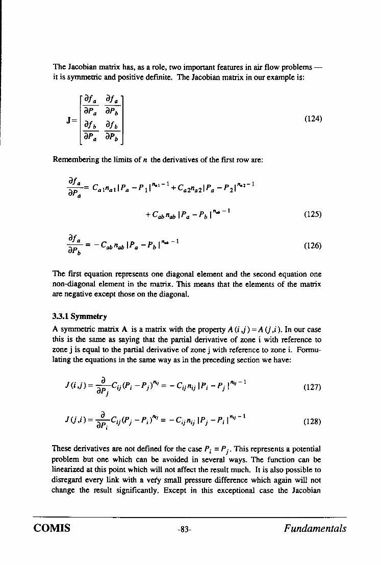
The Jacobian matrix has, as a role, two important features in air flow problems - - it is symmetric and positive definite. The Jacobian matrix in our example is:

j =

~fa ~fa

~)Pa ~Pb

afb ~fb ~Pa ~Pb

(124)

Remembering the limits of n the derivatives of the first row are:

f a

bPa ~ ' = Calnal IP,, - P 1 1 a ' l -1 + Ca2na21Pa - P2I 'h2-1

+ Cab nab I Pa - Pb I ' " - 1 (125)

f a

igpb - Cab nab I Pa - Pb I ~ - 1 (126)

The first equation represents one diagonal element and the second equation one non-diagonal element in the matrix. This means that the elements of the matrix are negative except those on the diagonal.

3.3.1 Symmetry

A symmetric matrix A is a matrix with the property A (i , j ) = A (j ,i ). In our case this is the same as saying that the partial derivative of zone i with reference to zone j is equal to the partial derivative of zone j with reference to zone i. Formu- lating the equations in the same way as in the preceding section we have:

oa p = J(i,j)=-~-fCij( i -P j ) n° -CqnulPi-P/I ' ' -1 (127)

C )"J i,,, j 1 ] (J , i ) = " ~ - i q ( P j - P i = - C i y n q l P / - P i - (128)

These derivatives are not defined for the case PI = Pj . This represents a potential

problem but one which can be avoided in several ways. The function can be linearized at this point which will not affect the result much. It is also possible to disregard every link with a very small pressure difference which again will not change the result significantly. Except in this exceptional case the Jacobian


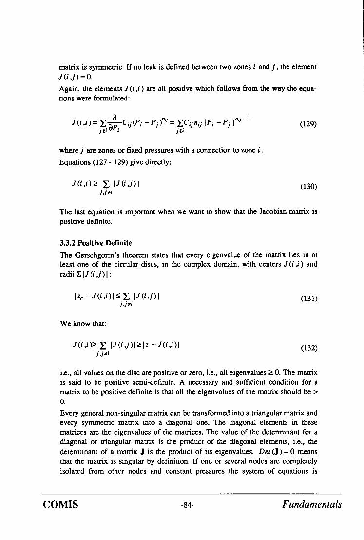
matrix is symmetric. If no leak is defined between two zones i and j , the element J (i , j) =0.

Again, the elements J (i ,i ) are all positive which follows fi'om the way the equations were formulated:

a c J (i , i)= E- F [ j(Pi - j t l "

y cijn o lt'i t'j I = - (129) jti

where j are zones or fixed pressures with a connection to zone i.

Equations (127 - 129) give directly:

Y(i,i)> ~ IJ(i,j)l (130) j d ~ i

The last equation is important when we want to show that the Jacobian matrix is positive definite.

3 .3 .2 P o s i t i v e Definite

The Gerschgorin's theorem states that every eigenvalue of the matrix lies in at least one of the circular discs, in the complex domain, with centers J (i ,i) and

radii g lJ (i , j ) I :

Iz c - J ( i , i ) l < ~ IJ( i , j ) l (131) j .j.i

We know that:

J(i,i)> ~, IJ ( i , j ) l>lz -J(i,i)l j , j ~ i

(132)

i.e., all values on the disc are positive or zero, i.e., all eigenvalues > 0. The matrix is said to be positive semi-definite. A necessary and sufficient condition for a matrix to be positive definite is that all the eigenvalues of the matrix should be > 0.

Every general non-singular matrix can be transformed into a triangular matrix and every symmetric matrix into a diagonal one. The diagonal elements in these matrices are the eigenvalues of the matrices. The value of the determinant for a diagonal or triangular matrix is the product of the diagonal elements, i.e., the determinant of a matrix J is the product of its eigenvalues. Det ( J ) = 0 means that the matrix is singular by definition. If one or several nodes are completely isolated from other nodes and constant pressures the system of equations is


singular.

The conclusion is that the Jacobian matrix must be positive definite except when no unique solution exists.

3.4 Linear Solvers

This section is mainly based on [78] and [84].

A direct method, compared with an iterative method, solves a system of equations in a certain f'mite number of steps. Direct methods are usually the most efficient methods for small to medium size full systems. The number of operations using a direct method is proportional to N 3 and, Using an iterative method, N 2 where N is the order of the matrix. Obviously the iterative methods become more attractive the larger the matrix but these will not be discussed here.

Our concern is with matrices solved by Gaussian-elimination, LU-factorization, and Cholesky's method. This includes studies of general, symmetric, and positive def'mite matrices. Band and skyline methods are used to improve the solvers.

The number of operations required for some methods has been estimated. "Opera- tion" is def'medhere as one multiplication and addition - - a useful measure.

3.4,1 Gausslan-Eilmination with Back Substitution

A triangular matrix can be solved with backward or forward substitution. A general matrix can therefore be solved if it is first reduced to a triangular form.

The Gaussian elimination method reduces a general matrix to a triangular form. The technique is to eliminate corr 1 of the system J con" = - f from the last N - 1 equations by subtracting multiples m of the first equation. Thereafter corr 2 is eliminated in the same way from the last N - 2 equations. This procedure is repeated until we have an upper triangular form with elements u. The diagonal elements are called pivotal elements.

The compact scheme for Gaussian elimination can be written:

k-1 ukj = J k j - - ~ m ~ u p j k = l .... ,N j = k , k + l .... ,N. (133)

p=l

k-I Jtt - E m#, upk

mik= i = k + l .... .N. Ukk

(134)

where j , m, and u are the elements in J, L, and U respectivly.


The backward substitution can be written in compact form:

N - f i - ~.~ Uikc°rrk

t~+l (135) corr i= i = N , N - 1 ..... 1.

Uii

The total number of operations for large N and one right-hand side is approximately N 3 / 3 + N 2 / 2 .

3.4.2 Pivoting

If a pivotal element becomes zero the Gaussian method obviously does not work since division by zero is not a defined mathematical operation. To solve the problem we can interchange rows or columns. In this way it is possible to find a non- zero pivotal element as long as the matrix is non-singular. Pivoting requires a large number of logical operations.

3.4.3 LU-Factorization

The LU-factorization decomposes a matrix A into a lower L and an upper U triangular matrix:

A = LU (136)

Then the system A x = b is equivalent to LUx = b which can be solved as two triangular systems Ly = b and Ux = y. There is an equivalence between Gaus- sian elimination and LU-factorization. The elements in L are the multipliers m and the matrix U is the upper triangular matrix. Equations (133) and (134) are therefore also valid for LU-decomposition.

The LU-decomposition requires N 3 / 3 - N 2 / 2 operations and the two triangular systems N 2 operations, i.e., the same as Gaussian elimination.

3.4.4 Cholesky's Method

For a positive definite matrix Gaussian elimination without pivoting is always possible. We can show that if Gaussian elimination can be carried out without pivoting for a symmetric matrix then there exist transformed elements m and u which form a symmetric matrix. Thus, if the matrix is symmetric positive definite we have only to compute L and the number of operations is approximately halved to N 3 / 6 compared with the general Gaussian elimination without pivoting.


Equations (133) and (134) are now simplified to:

k-1 0.5 mtt = ( j~ - ~ m 2tp )

p=l k = 1,...,N.

k-1

Ji~ - ~ m~,mk 1,

mi t = g.1 ..... i = k + 1, . . . ,N. mkk

(137)

(138)

This is Cholesky's method. The first equation calculates the diagonal elements and the second calculates the elements of the lower triangle.

3.4.5 Band Matrices

The non-zero elements in a band matrix are arranged in a diagonal band of width 2M + 1 where M is the half band width.

In Fig. 33 the LU-factorization method has been adjusted to various matrices and a comparison made of the number of operations involved in solving the system. The curves have been estimated with finite sums. The number of operations for the symmetric case is approximately N M 2 / 2 - M3/3. The number of operations is based on the decomposition only. Administration in the program also is not included so that these curves are very much simplified. Nevertheless we can expect a large reduction in execution time ff we take the special characteristics of the matrix into account.

The lower limits of the sums in Eqs. (137) and (138) are increased according to the band width. The lower limit will not be 1 rather where the band starts for the specific row. This explains the reduction in time.

3.4.6 Skyline

The skyline method, compared with the band method which has constant length, takes into account variable lengths of non-zero rows and columns in a matrix. All the elements below a non-zero element in the upper triangular pan are taken into consideration, these non-zero elements forming a skyline profile. The lower triangular pan is treated in a similar way, all elements to the right of a non-zero element being taken into consideration. If there is one zone that has connections to almost all other zones, the best skyline is achieved ff this common zone is placed as the last zone.

For a symmetric matrix we need only to handle the lower (or upper) pan of the matrix and the diagonal. The skyline is therefore defined by the array of row lengths in the lower pan of the matrix.


Relative Execution Time [-]

1.0

0.9

0.8

0.7

0.6

0.5

0.d

0.3

0.2

0.1

0.0

Full. non-s~anetric o . . - , w

,0 Band, non-symmetric

A, °

o •

o °

o °

Full, )~mmctric 0,

0 o • o o

• o o

0" - Band, symmetric

o • o S

m l ~ ° i l J u • ~

0 10 20 30 40 49 Half Band Width [-]

Fig. 33: Relative Time for LU-Decomposition on DO~ferent Matrices

Again, the lower limits of the sums are changed in Eqs. (137) and (138). The lower limit will follow the skyline. This means that the skyline method always requires equal or less number of operations compared with considering the matrix as a band matrix. The execution time depends on sparsity and cannot easily be generalized as in the ease of the band matrices above. However, some examples are presented in section 3.6.3.

3.5 Non-Linear Solvers

This section is based on the following references: [85-88].

Our links have a type of function that, under certain conditions, creates very slow convergence. Newton-Raphson method can be modified to avoid problems. In principle, most modifications deal with finding an appropriate relaxation coefficient ~ for Eq. (122):

f ( P n ) Pn+l = Pn - ~', ~ (139)

J (Pn)

The Newton-Raphson correction corresponds to Xr = 1.0. Two different methods

COMIS -88- Fundamenta ls

will be discussed that, at times, can accelerate the rate of convergence of Newton-Raphson.

3.5.1 Extrapolated Relaxation Coefficients Steffensen iteration consists of two steps of fixed-point iteration and, thereafter, the use of the three available iterates Pn-1, Pn, and P,,+l to get the starting value

for the next step.

A linear interpolant to the iteration function h (P) in Pn-1 and Pn, i.e., the secant, should be a good approximation to h (P) in the interval ff the slope of h (P) varies a little close to the root. The iteration function given by the secant can therefore be expected to give a good approximation of the root.

Pn + 1 - - Pn = en+l + r e . - Pn-1 ]

I - "L-'~n "~l _----~n J -1 (140)

The method studied here is closely related to this method, the approach above being applied to each node and each node being treated independently of the other nodes. There are, therefore, as many under-relaxation coefficients as there are nodes.

3.5.2 Optimized Relaxation Coefficients To determine the root in a one-dimensional case to the function f is the same as determining the minimum of the function F defined as:

f = F ' (141)

where F" is the derivative of F. To determine the roots in a multidimensional case to the function g is the same as determining the minimum of the scalar function G defined as:

/)(3 ~gG r g = ( ~P'-'~ 'B~P~'"') (142)

G can be expressed as a function in the varible ~'r only. This means that G (Z. r) is a one-xlimensional function. It can be shown that this function has a unique minimum. The function G (~-r) can be approximated with a second order polyno-

mial. The minimum, ~-r,,a,,, of this polynomial is easily determined and can s

represent the minimum of G. The next approximation is taken as:


f ( P . ) P . + I = P . - )'.," .m/,, ~ j ( P n ) (143)

This means that a Newton-Raphson solution

required in each iteration step.

The function F of a one-dimensional function:

and three evaluations of G are

is:

f = ~,Cj IP - Pj I nj (144) J

- - ~ I P pj nj+l F= ~j nj+l - I (145)

where j are zones with fixed pressures and have connections to the zone. A multidimensional case is similar. The function G of the vector function g is:

Cij I ,,,j+l (7 = Y',Y'. IPi-e/ (146) i j ~ nlj

where j are zones or fixed pressures with a connection to zone i. The example given in section 3.2 is:

C1 + 1 C2 1 C3 .3+ 1 G= - - I P a -P I [ n~ + ~ [ P a - P 2 [ "2+ + - - [ P a - P h i

n~ + 1 n 2 + 1 n 3 + 1

C4 +1 C5 +1 "~ - - [ P b -P4[ n" + - - [ P b -P5[ ns (147) n4+l n s + l

where Pa and Pb can be expressed in ~'r" Thc function G is obviously a sum of

non-negative terms. The individual terms are strictly convex functions as long as the matrix is not singular, but a sum of strictly convex functions is also a strictly convex function. A strictly convex function has a unique minimizer. This in turn means that the equation g = 0 has a unique solution.

COMIS -9o- F u n d a m e n t a l s

3.6 Timing of Solvers

The aim here is to provide an overview of the behavior of various solvers in typi- cal air flow examples. Representative networks were selected for the tests which were essentially based on discussions with George Walton from NIST.

The solvers were timed and tested in two programs, AIRNET [89] and MOVECOMP [90], with a special analyzer.

3.6.1 Chosen Networks

1) 2-Network

This network is convenient to use and shows the classical difficulties with Newton-Raphson. All flow exponents are one-half. The ratio between inner and outer links are varied as 10.000, 1000, 100, 10, and 1. The smallest link(s) has the flow coefficient 0.001 kg/s,Pa".

h v2 +50 Pa Aw ,,.,"' O " ~ -50 Pa

0U'IER INNER OUTER LINK LINK LINK

Fig. 34:02-Network

2) 10-Network

This example has been constructed especially to show problems in different non- linear solvers. All flow exponents are one-half. The sizes of the openings are a mixture of large and small with a maximum ratio of 40,000. An additional example, with all links equal to 0.001 kg/s,Pa n , was also used.

3) 45/41- and 27/25-Networks

These buildings consist of 3 and 5 floors with 8 rooms per floor. These examples enable us to study the characteristics of different solvers when the number of nodes is increasing.

The center shaft is simulated in two ways - - as one node at middle floor level (41 and 25) and as one node per floor (45 and 27). The latter takes into account friction losses in the shaft.

C O MIS -91- Fundamentals

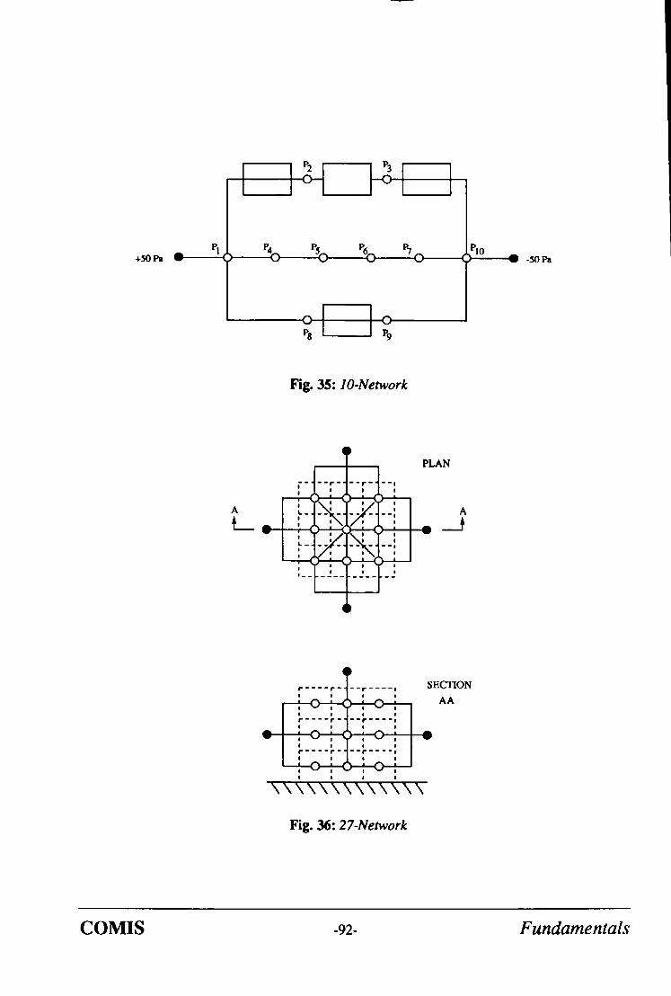
+50 Pa A v

~,J. % ylo

ol I o

A v -50 Pa

Fig. 35: lO-Network

A #

- - - i f - -

I I _ _

..'-r"l _ --l, i LAN

! I

" - r . . . . i

i i

~,:.1 ! !

SECTION

A A

\ \ \ \ \ \ \ \ \ \ \ \ \

Fig. 36: 27-Network


One study proved that the most interesting cases are those with tight floors because they show the greatest difference between a band solver and a skyline

approach.

The buildings contain a mixture of large and small openings. Outer surfaces: 0.001 kg/s,Pa n , Inner surfaces: 0.01, Inner doors: 1, and Shaft: 10. In addition, all flow coefficients are set to 0.001 k g l s , P a 't .

3.6.2 Other Assumptions

The criteria for convergence has to be well specified. In this comparison we use

an absolute flow balance limit of E-6 kg/s or 0.0036 kg/h.

At a very low pressure difference a very steep gradient and large derivative can occur. A leak is therefore linearized when the pressure difference is below 10 -5 Pa.

All air densities were set to 1.20 kg/m 3.

The sizes of the links, i.e., the flow coefficients, are in the range 0.001 - 10 k g / s , P a n or 3.6 - 36,000 kg/h,Pa". The maximum ratio is therefore 10,000. The

flow exponents are 0.5.

3.6,3 Linear Solvers

Four methods were tested: a Gaussian with complete pivoting, a band-Cholesky, a skyline-Cholesky, and an iterative method. All runs were made with MOVECOMP, simply exchanging the linear solvers. The iterative method, Gauss-Seidel, created problems. Although the cause is unclear, too many iterations are needed. Further comparison with this routine is not included here.

The band routine is based on the Cholesky's method as described in section 3.4.4. and 3.4.5. Two features were tested. First, the execution time as a function of the order of the matrix and second, the execution time as a function of the half band width. As a comparison an identical routine, but one with no band features, and two routines from LINPACK [91] were timed.

The result of the influence of the order of matrix is shown in Fig. 37. Two cases are shown, full matrix and diagonal matrix. The benefits of taking the band struc-

ture into consideration increase with the order of matrix. At order 40 a diagonal matrix is solved in 11% of a full matrix. At order 20 the corresponding number is

23 %.

The result of the influence of the half band width for a matrix of order 20 is shown in Fig. 38. The drop in execution time for the band solver with decreasing band width is similar to the curves in Fig. 33. The non-band solver is identical to the band solver except that the band features are removed. We can see that the

administration of the programs is distorting the results.


0.400

0.300

0.200

0.I00

0.000

Execution Time [s]

Full Man'ix

Diagonal Matrix

! ! F m

Order [-] 10 20 30 40

Fig. 37: The Influence of the Order of the Matrix on the Execution Time for the Band Solver

LINPACK(B) is a routine working on a band matrix stored in packed form. LINPACK(NB) is a similar routine without the band features. These routines are generally more time-consuming.

It is not certain that the matrix has a well developed band structure in air flow applications. The skyline approach is therefore interesting. The band solver and the skyline solver were timed on all networks (see Table 5).

The Band column stands for the half-band width. This does not give any information about how well the band is organized. The Ratio column contains this information. The lower the ratio the less organized the band structure.

It can be seen that the increase of time for the Gaussian method is close to the cube of the order of the matrix as predicted in section 3.4.1.

The examples chosen have very poor band structure, the intention being to show the difference between the band and skyline solvers. For more realistic examples, the difference between the band and the skyline methods is likely to be smaller although the skyline approach seems always to equal or be faster than the band method. The skyline does not require significantly more time for even a perfect band or full matrix. The skyline-Cholesky's method has therefore been selected to be incorporated into COMIS.


!

0.60

0.50

0,40

0.30

0.20

0.10

0.00

Execution Time [s] o o ~

o ~

__t...I~.A. ~K.~. . ) . . . - - - . . . . . . . . . . . . . . . . . . . . .

o o °

~ BAND SOLVER

, / - o s

a °

LINPACK (B)

| w

0 5 10 15 19 Half Band Width [.]

Fig. 38: The Influence of the Half Band Width on the Execution Time for the Band Routine and UNPACK

Table 5: Execution Time per Iteration for the Linear Solvers [s]

Matrix-Size Gauss Band Skyline Band Ratio

45 6.1678 0.1437 0.0867 9 0.43 41 5.2004 0.2753 0.1354 20 0.47

27 1.4086 0.0688 0.0400 9 0.46 25 1.2342 0.0748 0.0494 12 0.55

10 0.0839 0.0123 0.0096 7 0.63

02 0.0013 0.0010 0.0010 1.00


3.6.4 Non-Linear Solvers

Relaxation coefficients were selected according to three methods - - Newton- Raphson, extrapolated coefficients and an optimized method. All methods were initialized with 2 conventional Newton-Raphson iterations.

The Newton-Raphson and the optimized method were timed in MOVECOMP. The number of iterations for the extrapolated method was determined in AIR- NET. This method was thereafter assumed to require the same time per iteration as Newton-Raphson.

It was expected that the initialization might influence the number of iterations. If a direct linearization of the original problem is performed, only the exponents are changed to unity. This means, in fact, that the function is linearized through 0 and 1 Pa pressure differences. Such a direct linearization was chosen.

Table 6: Number of lterations for the Non.Linear Solvers

Matrix-Size Newton Extrapolated Optimized

45-10000 45-1 41-1000 41-1

27-10000 27-1 25-1000 25-1

10-40000 10-1

02-10000 02-1000 02-100 02-10 02-1

>1500 24

>1500 21

>1500 25

>1500 22

>1500 8

>1500 946

86 8 1

15 9

15 9

15 9

15 9

19 8

11 11 9 8 2

7 6

5 7 6 5 1

As can be seen in Table 6, the Newton-Raphson method has problems, as expected, at high ratios and is therefore less useful. The number of iterations for the two other methods axe far fewer. The optimized method requires, on averages, 46% less iterations than the extrapolated method. For this comparison, the selected examples are shown in bold in Table 6. There is a linearization of some links at the highest ratios for each matrix size owing to extremely small pressure


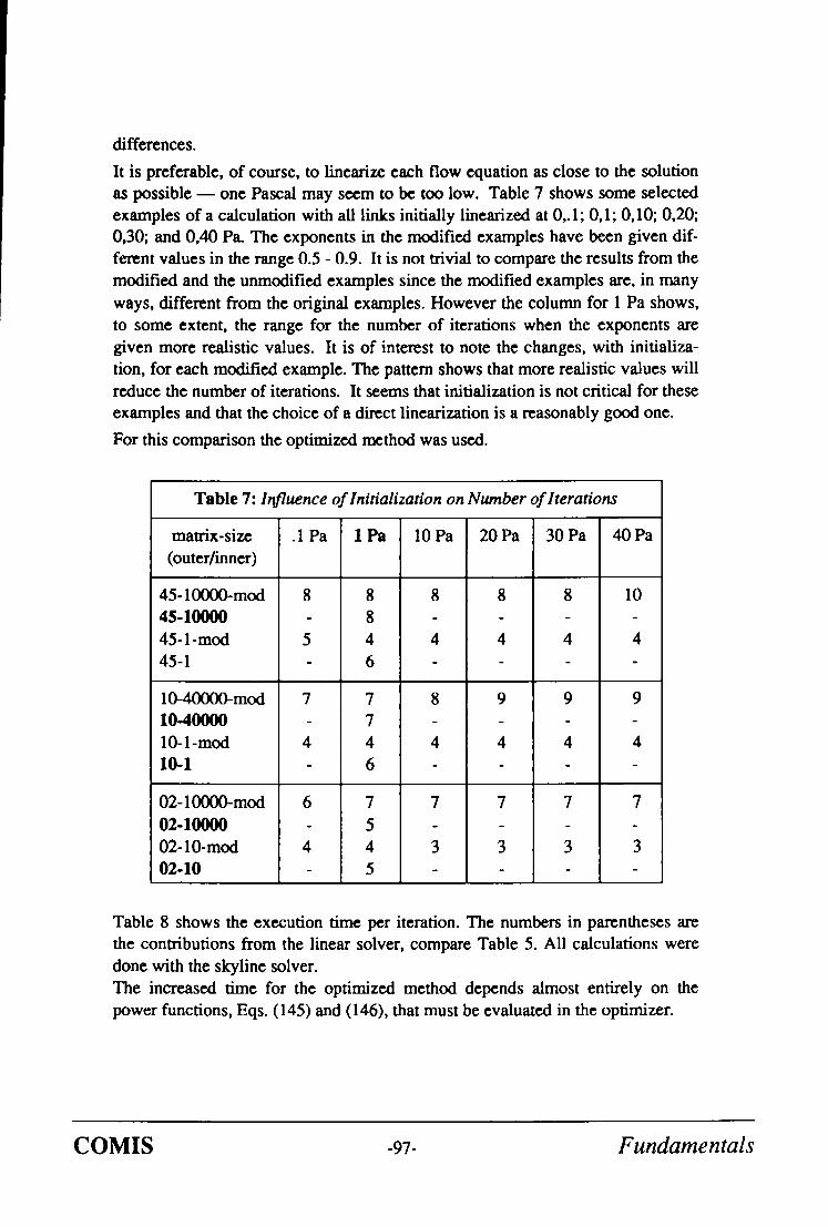
differences.

It is preferable, of course, to linearize each flow equation as close to the solution as possible - - one Pascal may seem to be too low. Table 7 shows some selected examples of a calculation with all links initially linearized at 0,. 1; 0,1; 0,10; 0,20; 0,30; and 0,40 Pa. The exponents in the modified examples have been given different values in the range 0.5 - 0.9. It is not trivial to compare the results from the modified and the unmodified examples since the modified examples are, in many ways, different from the original examples. However the column for 1 Pa shows, to some extent, the range for the number of iterations when the exponents are given more realistic values. It is of interest to note the changes, with initialization, for each modified example. The pattern shows that more realistic values will reduce the number of iterations. It seems that initialization is not critical for these examples and that the choice of a direct linearization is a reasonably good one.

For this comparison the optimized method was used.

Table 7: Influence of lnttializatton on Number of Iterations

matrix-size (outerfmner)

• 1 P a 1 P a 10 P a

45- lO00(Omod 8 8 8 4 5 - 1 0 0 0 0 - 8

45-1-mod 5 4 4 45-1 - 6

10-40000-mod 7 7 8 1 0 - 4 0 0 0 0 - 7 10-1-mod 4 4 4 10-1 - 6

, = ,

02-10000-mod 6 7 7 0 2 - 1 0 0 0 0 - 5

02-10-mod 4 4 3 0 2 - 1 0 - 5

20 Pa 30 Pa

8

4

9

4

7

3

40 Pa

10

4

9

4

7

3

Table 8 shows the execution time per iteration. The numbers in parentheses are the contributions from the linear solver, compare Table 5. All calculations were done with the skyline solver. The increased time for the optimized method depends almost entirely on the power functions, Eqs. (145) and (146), that must be evaluated in the optimizer.


Table 8: Execution Time per Iteration for Complete Solvers [s]

Matrix-Size Newton Optimized Ratio Optimized/Newton

45 0.373 (23%) 0.957 (9%) 2.6 41 0.392 (35%) 0.955 (14%) 2.4

27 0.216 (19%) 0.559 (7%) 2.6 25 0.222 (22%) 0.561 (9%) 2.5

10 0.075 (13%) 0.168 (6%) 2.2

02 0.036 (3%) 0.060 (2%) 1.7

To find the time difference between the complete solvers the number of iterations must be multiplied by the time for each iteration. The optimized method switches to Newton-Raphson if ~ > 0.95. This has two purposes, first, it prevents unnecessary optimization and second, it eliminates the influence of round off errors in the optimizer.

Table 9: Execution Time for Complete Solvers [s]

Matrix-Size Extrapolated Optimized Difference [%]

45-10000 5.707 5.904 -3 41-1 3.599 4.041 -11

27-1 1.983 2.325 -15 25-1000 3.397 3.471 -2

10-40000 1.454 0.897 +62 10-1 0.612 0.636 -4

02-10000 0.404 0.252 +60 02-10 0.294 0.252 +17

If we assume that the extrapolated method does not require any significant extra time relative to Newton-Raphson, then the methods are quite equivalent (see Table 9). In fact the extrapolation method requires about 2% more time than Newton-Raphson. This has been included in the Table.


The choice of a non-linear method is not as obvious as in the case of the linear solver. The optimized method always finds the solution in fewer iterations than the extrapolated method which indicates that the optimized method is more efficient in finding the appropriate under-relaxations. On the other hand, the process of finding the relaxation coefficients is so time-consuming that the methods have almost the same execution time for the test cases based on total time for all exam- pies. The main argument for chosing the optimized method for incorporation as the default in COMIS is that the method itself is more efficient and stable. The time-consuming process of finding the relaxation coefficients is a different matter, a pure numerical or mathematical problem.

3.7 Conclusion

The aim of the present study is to select efficient and robust methods to be used in the COMIS code to solve the non-linear system of equations representing the air flow distribution in multizone buildings.

Taking into account the special characteristics of the Jacobian matrix, we selected a skyline-Cholesky's method for the linear solver. This method can be used in a general way for the problem we are dealing with and it appears to be the more efficient one.

The task is more difficult in regard to the non-linear solver. Even if a generalized Newton-Raphson method is selected, the choice of under-relaxation process to ensure the convergence and efficiency is not obvious. We tested two different methods, an extrapolated method and an optimized method, of finding the under- relaxation coefficients. Although the latter method is more time consuming in finding the relaxation coefficient in each iteration it appears to be safer and more efficient in the resolution of the non-linear system. In testing these two methods on the same sample of test cases we found that they are very similar regarding total time. It is suggested that the optimized one be selected as the default solution method.


C O M I S -lOO- Fundamentals

4. ACKNOWLEDGEMENT

We should like to acknowledge Brian V. Smith from Lawrence Berkeley Labora- tory for his help in designing and processing most of the figures in this publication. We would also like to thank Martin Liddament from Air Infiltration Centre and Reijo Kohonen from Technical Research Centre, Finland for their thorough review.

This publication was supported by the following organizations:

National Scientific Research Center (C.N.R.S.), 75700 Pads, France; French Agency for Energy Management (A.F.M.E.), 75015 Pads, France; Dept. for Environment Science and Technology, Politecnico di Torino, Italy; S.I.V. (Societa' Italiana Vetro) S.p.a., Italy; SECCO S.p.a., Treviso, Italy; Netherlands Organization for Applied Scientific Research, Division of Technology for Society, Department of Indoor Environment, Delft, The Netherlands; Miyagi National College of Technology, Japan; Tohoku University, Japan; Harbin Archi- tectural and Civil Engineering Institute, Harbin, People's Republic of China; CIEMAT-IER, Madrid, Ministerio de Educacion y Ciencia, Madrid, as well as Escuela Superior de Ingenieros Industriales, Sevilla, Spain; The Swedish Council for Building Research, Stockholm, Sweden; F.cole Polytechnique Federale de Lausanne, as well as Eidgenoessische Materialpruefungs- und Versuchsanstalt (EMPA), Abt. 176, Projekt ERL, NEFF, Switzerland; Air Infiltration and Ventila- tion Centre, Warwick, UK; and by the Assistant Secretary for Conservation and Renewable Energy, Office of Building and Community Systems, Building Sys- tems Division of the U.S. Department of Energy under Contract No. DE-AC03- 76SF00098.

5. DISCLAIMER

This document was prepared as an account of work sponsored by the above mentioned agencies. Neither one of these agencies, nor the Regents of the University of California, nor any of their employees or guests, makes any warrenty, express or implied, or assumes any legal liability or responsability for the accuracy, completeness, or usefulness of any information, apparatus, product or process disclosed, or represents that its use would not infringe privately owned rights. References herein to any specific commercial products, process, or service by its trade name, trademark, manufacturer, or otherwise, does not necessarely constitute or imply its endorsement, recommendation, or favoring by any of the sponsoring agencies or the Regents of the University of California. The views and opinions of authors expressed herein do not necessarely state or reflect those of the sponsoring agencies, or the Regents of the University of California, and shall not be used for advertising or product endorsement purposes.

COMIS -lOl- Fundamentals

C O M I S - 102- Fundamen tals

6 . R E F E R E N C E S

. Liddament, M.W.: Air Infiltration Calculation Techniques - an Applica- tions Guide, Air Infiltration and Ventilation.Centre, Bracknell, U.K., 1986

. ASHRAE 1985 Handbook of Fundamentals, Chapter 22, American Society of Heating, Refrigerating and Air-Conditioning Engineers, Atlanta, U.S.A., 1985

. Feustel, H.E. and V.M. Kendon: "Infiltration Models for Multicellular Structures: A Literature Review", Energy and Buildings, Vol. 8, No. 2, Elsevier Sequoia, Lausanne, Switzerland, 1985

. Jackman, P.J.: "A Study of Natural Ventilation of Tall Office Buildings", Journal Inst. Heat Vent. Eng., Vol. 38, pp. 103 - 118, 1970

. Feustel, H.E., F. Allard, V.B. Dorer, M. Grosso, M. Herrlin, M. Liu, J.C. Phaff, Y. Utsumi and H. Yoshino: "The COMIS Infiltration Model", in Proceedings, Building Simulation '89, The International Building Perfor- mance Simulation Association, Vancouver, June 1989

. Shaw, B. H. and W. Whyte: "Air Movement through Doorways - the Influence of Temperature and its Control by Forced Air Flow", BSE Building Services Engineering, Vol. 42, No. 12, pp. 210-218, 1974

. Anon.: "Characteristics of Wind Speed in the Lower Layers of the Atmo- sphere near the Ground: Strong Winds (Neutral Atmosphere)", ESDU Data Item No 72026, Engineering Sciences Data Unit, London, U.K., 1972

. Anon.: "Characteristics of Atmospheric Turbulence near the Ground", ESDU Data Items Nos. 74030, 74031, 75001, Engineering Sciences Data Unit, London, U.K., 1975


. Davenport, A. G.: "Wind Loads on Structures", Technical Paper No. 88, National Research Council, Division of Building Research, Ottawa, Canada, March 1960

10. Torrance, V. B.: "Wind Profiles over a Suburban Site and Wind Effects on a Half Full-Scale Model Building", Building Science, Vol. 7, pp. 1-12, Pergamon Press, London, U.K., 1972

11. Wiren, B.G.: "Effects of Surrounding Buildings on Wind Pressure Distri- butions and Ventilation Losses for Single-Family Houses", Part 1:1 1/2- Storey Detached Houses, Bulletin M85:19, The National Swedish Institute for Building Research, Gavle, Sweden, December 1985

12. Kula, H.G.and H.E. Feustel: "Review of Wind Pressure Distribution as Input Data for Infiltration Models", Lawrence Berkeley Laboratory Report LBL-23886, Berkeley, U.S.A., 1988

13. Anon.: Technical Note AIC 13.1, Wind Pressure Workshop, Proceedings, Air Infiltration and Ventilation.Centre, Bracknell, U.K., November 1984

14. Allen, C.: Wind Pressure Data Requirements for Air Infiltration Calcula- tions, Technical Note AIC 13, Air Infiltration and Ventilation.Centre, Bracknell, U.K., January 1984

15. Bala'zs, K.: "Effect of Some Architectural and Environmental Factors on Air Filtration of Multistorey Buildings", 3rd ICBEM Proceedings, Vol. III, pp. 21 - 28, Lausanne, Switzerland, 1987

16. Swami, M.V.and S. Chandra: Procedures for Calculating Natural Ventila- tion Airflow Rates in Buildings, ASHRAE Research Project 448-RP, Florida Solar Energy.Center Report, Final Report FSEC-CR-163-86, Cape Canaveral, U.S.A., March 1987


17. Bowen, A.J.: '°A Wind Tunnel Investigation using simple Building Models to obtain Mean Surface Wind Pressure Coefficients for Air Infil- tration Estimates", Laboratory Technical Report, LTR-LA-209, N.C., National Aeronautical Establishment, Ottawa, Canada, December 1976

18. Hussein, M. and B.E. Leg: "An Investigation of Wind Forces on Three- dimensional Roughness Elements in a Simulated Atmospheric Boundary Layer", BS 55, Part I, "Flow over isolated Roughness Elements and the Influence of Upstream Fetch", BS 56, Part II, "Flow over Large Arrays of Identical Roughness Elements and the Effect of Frontal and Side Aspect Ratio Variations, BS 57, Part m, "The Effect of.Central Model Hight Variations relative to the Surrounding Roughness Arrays", Department of Building Science, Faculty of Architectural Studies, University of Shef- field, Sheffield, U.K., July 1980

19. Akins, R.E. and J.E..Cerrrmk: "Wind Pressures on Buildings", Fluid Dynamic and Diffusion Laboratory, College of Engineering, Colorado State University, CER76-77REA-JEC15, Colorado, U.S.A., 1976

20. Jensen, M.: "The Model Law for Phenomena in the Natural Wind", Ingenioren - International Edition, Vol. 2, No. 4, Copenhagen, November 1958

21. Cook, N. J.: "On simulating the Atmospheric Boundary Layer in Wind Tunnels", Journal of Industrial Aerodynamics, Vol 2/3, No. 3, pp. 157- 176, Vol 4, No. 2, pp. 311-321, 1978

22. Allard, F. and M., Herrlin: "Wind-Induced Ventilation", to be published in ASHRAE Transactions, Vol. 95, Part 2, American Society of Heating, Refrigerating and Air-Conditioning Engineers, Atlanta, U.S.A., 1989

23. Hopkins, L.P. and B. Hansford: "Air Flow through Cracks", BSE Building Services Engineering, Vol. 42, No. 9, pp. 123 - 131, September 1974


24. Etheridge, D. W.: "Crack Flow Equation and Scale Effects", Building and Environment, Vol. 12, No. 3, pp. 181-189, Pergamon Press, Oxford, U.K., 1977

25. Baker, P. H., S. Sharples and I.C. Ward: "Air Flow through Cracks", Building and Environment, Vol. 22, No. 4, pp. 293 - 304, Pergamon Press, Oxford, U.K., 1987

26. Jun, G. and L. Mingsheng: "The Energy Savings Effect of Double Frame Windows", in Proceedings, Cllma 2000, World Congress on Heating, Ventilating, and Air Conditioning, Vol. 2, Building Design and Perfor- mance, pp. 84 - 97, Copenhagen, Denmark, 1985

27. Mingsheng, L. and M.K. Herrlin: "Crack How Characteristics", to be submitted to Energy and Buildings, Elsevier Sequoia, Lausanne, Switzerland

28. Allard, F. and Y. Utsumi: "Air Flows through Large Openings", submitted to Energy and Buildings, 1989 Elsevier Sequoia, Lausanne, Switzerland

29. Brown, W.G. and K. Solvasson: "Natural Convection through Rectangular Openings in Partitions", Part 1: Vertical Partitions, International Journal Heat and Mass Transfer, Vol. 5, pp. 859-868, 1962

30. Shaw, B.H.: Heat and Mass Transfer by Convection through Large Rec- tangular Openings in Vertical Partitions, Ph. D. Thesis, University of Glasgow, Glasgow, U.K., 1976

31. Lidwell, O.M.: "Air Exchange through Doorways: The Effect of Tempera- ture Difference, Turbulence and Ventilation Flow", J. Hyg. Camb., Vol. 79, pp. 141-154, 1977


32. Balcomb, J.D. and K. Yamaguchi: "Heat Distribution by Natural Convec- tion", in Proceedings, 8th Passive Solar Conference, pp. 289-294, Santa Fe, U.S.A., 1983

33. Weber, D.D.: "Similitude Modeling of Natural Convection Heat Transfer through an Aperture in Passive Solar Heated Building", Ph.D. Thesis, Los Alamos Scientific Laboratory Report, LA8385-T, Los Alamos, U.S.A., 1980

34. Hill, D., A. Kirkpatrick and P. Bums: "Analysis and Measurements of Interzonal Natural Convection Heat Transfer in Buildings", ASME Tran- sactions, Vol. 108, pp. 178-184, ASME American Society of Mechanical Engineers, New York, U.S.A., August 1986

35. Pelletret, R. and H. Khodr: "A new Model to Compute Air Distribution", in Proceedings, Building Simulation '89, IBPSA, pp. 291-295, Vancouver, Canada, June 1989

36. Brown, W.G.: "Natural Convection through Rectangular Openings in Par- tition", Part 2: Horizontal Partitions, International Journal of Heat and Mass Transfer, Vol. 5, pp. 869-878, 1962

37. Epstein, M.: "Buoyancy-Driven Exchange Flow through Small Openings in Horizontal Partitions", Journal of Heat Transfer, Vol. 110, pp. 885-893, November 1988

38. Kiel, D.E., and D.J. Wilson: "Gravity driven Flows through Open Doors", in Proceedings, 7th AIC Conference, Air Infiltration and Ventilation.Centre, Bracknell, U.K., 1986

39. Van der Maas, J., C.-A. Roulet and J.A. Hertig: "Some Aspects of Gravity driven Air Flow through Large Apertures in Buildings", ASHRAE Tran- sactions, Vol. 95, Part 2, American Society of Heating, Refrigerating and Air-Conditioning Engineers, Atlanta, U.S.A., 1989

C O M I S -lO7- Fundamentals

0. Vandaele, L. and P. Wouters: Air Flows through Large Openings. An Overview of Existing Approaches, IEA Annex XX, Subtask 2 Report, International Energy Agency, Paris, France, May 1989

41. Cockroft, J.P. and R. Robertson: "Ventilation of an Enclosure through a Single Opening", Building and Environment, Vol. 11, pp. 29 - 35, Per- gamon Press, Oxford, U.K., 1976

42. Warren, P.: "Ventilation through Openings on One Wall Only", in Proceedings, Int. Heat and Mass Transfer Seminar, pp. 189-206, Hemi- sphere Publishing, Washington D.C., U.S.A., 1977

43. Crommelin, R.D. and E.M.H. Vrins: "Ventilation through a Single Open- ing in a Scale Model", Air Infiltration Review, Vol. 9 , No. 3, pp. 11-15, Air Infiltration and Ventilation.Centre, Warwick, U.K., May 1988

4. Etheridge, D.W.: "Air Leakage Characteristics of Houses. A new Approach", BSERT, Vol. 5, pp. 32-36, 1984

45. Phaff, H. and W. de Gids: "Ventilatie van gebouwen. Onderzoek naar de gevolgen van het openen van ~ raam op het binnenklimat van een kamer", (Building Ventilation. Investigation of the Consequences of Opening one Window on the Internal Climate of a Room.) IMG-TNO report C448, Delft, The Netherlands, 1980

46. Barakat, S.A.: "Inter-zone Convective Heat Transfer in Buildings. A Review ", Journal of Solar Energy Engineering, Vol. 109, pp. 71-78, May 1987

47. Walton, G.N.: "A Computer Algorithm for Predicting Infiltration and Inter-room Air flows", ASHRAE Transactions, Vol. 90, part 1, American Society of Heating, Refrigerating and Air-Conditioning Engineers, Atlanta, U.S.A., 1984


48. Roldan, A.: Etude Thermique et Aa'aulique des Enveloppes de B~timent. Influence des Couplages Int6--ieurs et du Multizonage, Doe. Thesis, INSA de Lyon (France), 1985

9. Feustel, H.E.: "Mathematical Modeling of Infiltration and Ventilation", in Proceedings, I 0th AIVC Conference, Air Infiltration and Vcntilation.Centrc, Warwick, U.K., September 1989

50. Walton, G.N.: "Air Flow Network Models for Element-based Building Air Flow Modeling", to be published in ASHRAE Transactions, American Society of Heating, Refrigerating and Air-Conditioning Engineers, Atlanta, U.S.A., 1989

51. Mahajan, B.M. and D.D. Hill: "Interzonal Natural Convection for Various Aperture Configurations", in Proceedings, ASME Winter Annual Meet- ing, Anaheim, U.S.A., 1986

52. Kiel, D.E.: Measuring and Modeling Air Flow through Doorways, Master Thesis, University of Alberta, Edmonton, Canada, 1985

53. Riffat, S.B.: "A Study of Heat and Mass Transfer through a Doorway in a Conventional House", Research in Building Group,Central London Polytechnic, London, U.K., January 1988

4. Lane-Serif, G.F., J.F. Linden and J.E. Simpson: "Transient Flow through Doorways produced by Temperature Differences", in Proceedings, Room- vent 87, Session 22, 1987

55. Colebrook, C.F.: "Turbulent Flow in Pipes, with particular Reference to Transition Region between the Smooth and Rough Pipe Laws", Journal of the Institution of Civil Engineers, London, U.K., 1938/39

COMIS -I09- Fundamentals

56. Moody, L.F.: "Friction Factors for Pipe Flow", ASME Transactions, Vol.06, ASME American Society of Mechanical Engineers , New York, U.S.A., 1944

57. Bouwman, H.B.: "Optimum Air Duct System Design", Report No. C 512, IMG-TNO, Delft, Netherlands, 1982

58. ASHRAE 1989 Handbook of Fundamentals, American Society of Heat- ing, Refrigerating and Air-Conditioning Engineers, Atlanta, U.S.A., 1989

59. Hocnmann, W.: Taschenbuch flier Heizung und Klimatechnik, R. Olden- burg Verlag, Muenchen, Wien, 1987

60. Inoue, U.: Handbook of Air-Conditioning, Maruzen, Tokyo, Japan, 1982

61. Handbuch der Klimatechnik, Band 2, Berechung und Regelung, 2.Auflage, Verlag C.F.Muller GmbH, Karlsruhe, 1988

62. Anon.: Handbook of Heating, Air-Conditioning and Sanitary Engineering, tenth edition, Vol.2, Society of Heating, Air-Conditioning and Sanitary Engineering, Tokyo, Japan, 1981

63. Leuzinger, R.: "Berechung des Druckverlustes in Luftkanaelen mit pro- grammierbaren Taschenrechnem", Heizung und Lueftung/Chauffage et Ventilation, March 1985

4. Feustel, H.E.: Beitrag zur theoretischen Beschreibung der Druck-und Luftmassenstromverteilung in naturlich und maschinell geluefteten Gebauden, Fortschritt-Berichte der VDI-Zeitschriften, Nr. 151, VDI Ver- lag, Duesseldorf, F.G., 1984


65. Porges, J.: Handbook of Heating Ventilating and Air Conditioning, seventh edition, Newnes-Butterworths, New York, U.S.A., 1976

6. ASHRAE 1977 Handbook of Fundamentals, American Society of Heat- ing, Refrigerating and Air-Conditioning Engineers, Atlanta, U.S.A., 1977

7. Malmstroem, T.G. and L.G. Olsson: "Specification: Ducts", Report of Intematial Energy Agency, Energy Conservation in Buildings and Com- munity Systems Programme, Annex 10, System Simulation, Paris, France, 1989

68. Ventilatie van Oebouwen -- Berekening van het Drukverlies in Lucht- kanalen, Nederlandst Norm, Ontwerp NEN 5063, Publikatie Uitsluitend ter Kritiek, pp.30 and pp.33, April 1988

9. JSME Mechanical Engineer's Handbook, A: Fundamentals, Japanese Society of Mechanical Engineering, Tokyo, Japan, 1986

70. Ito, E. and I. Kiyoshi: "Study on Flow in the Pipes with diverging Flow or converging Flow", Part I: Characteristics of Pressure Losses at the Junc- tion of a Tee, in Proceedings, Meeting of the Mechanical Institute of Japan, Tokyo, Japan, 1971

71. Rietschel/Raiss: Heiz- und Klimatechnik, 15. Aufl., Bd.II, Springer Ver- lag, Berlin/Heidelberg/New York, 1970

72. Rodriguez, E. and F. Allard: "Coupling COMIS Air Flow Model with other Transfer Phenomena" submitted to Energy and Building, Elsevier Sequoia, Lausanne, Switzerland

73. Grot, R. and J. Axley: "The Development of Models for Prediction of Indoor Air Quality in Buildings", in Proceedings, 8th AIVC Conference, Air Infiltration and Ventilation.Centre, Warwick, U.K., 1987


74. Axley J.: "Multi-Zone Dispersal Analysis by Element Assembly", Build- ing and Environment, Vol. 24, No. 2, pp. 113 - 130, Oxford, U.K., 1989

75. Traynor, G.W., J.C. Aceti, M.G. Apte, B.V. Smith, L.L Green, A. Smith- Reiser, K.M. Novak and D.O. Moses: "Maeromodel for Assessing Residential Concentrations of Combustion-Generated Pollutants: Model Development and Preliminary Predictions for CO, NO 2 and Respirable Suspended Particles", Lawrence Berkeley Laboratory Report LBL-25211, Berkeley, U.S.A., 1989

76. Traynor, G.W., M.G. Apte, A. Carruthers, J.F. Dillworth, R.J Drill, D.T. Grimsrud, and B.H. Turk: "The Effects of lntrdtration and Insulation on the Source Strenghts and Indoor Air Pollution from Combustion Space Heating Appliances", JAPCA Journal of the Air & Waste Management Association, Vol. 38, No. 8, pp. 1011-1015, Boulder, U.S.A., 1988

77. Tichenor, B.A., L.E. Sparks, J.B. White and M.D. Jackson: "Evaluating Sources of Indoor Air Pollution", in Proceedings, 81 st Annual Meeting of APCA, Dallas, U.S.A., June 19-24, 1988

78. Dahlquist, G. and A. Bjork: "Numerical Methods", Prentice-Hall Series in Automatic Computation, Prentice-Hall, Englewood Cliffs, U.S.A., 1974

79. Faddeev, D. K. and V.N. Faddeeva: "Computational Methods of Linear Algebra", W.H. Freeman, San Francisco, U.S.A., 1963

80. Forsythe, G. and C.B. Moler: "Computer Solution of Linear Algebraic Systems", Prentice-Hall Series in Automatic Computation, Prentice-Hall, Englewood Cliffs, U.S.A., 1976

81. Schwarz, H. R., et al.: "Numerical Analysis of Symmetric Matrices", Prentice-Hall Series in Automatic Computation, Prentice-Hall, Englewood Cliffs, U.S.A., 1973

c o M I S -112- Fundamentals

82. Wilkinson, J. H. and C. Reinsch: "Linear Algebra", Handbook for Automatic Computation, Vol. 2, Springer-Verlag, New York, 1971

83. Golub, G., C. Van Loan and F. Charles: "Matrix Computations", Johns Hopkins University Press, Baltimore, U.S.A., 1983

84. Dhatt, G., 13. Touzot and 13. Cantin: The Finite Element Method Displayed, John Wiley & Sons, New York, 1984

85. Conte, S. D. and C. de Boor:. Elementary Numerical Analysis - An Algo- rithmic Approach, McGraw-Hill, New York, 1972

86. Ortega, J. M. and W.C. Rheinbolt: Iterative Solution of Non-Linear Equa- tions in Several Variables, Academic Press, New York, 1970

87. Rockafellar, R. T.: Convex Analysis, Princeton University Press, Prince- ton, U.S.A., 1972

88. Gill, P. E., W. Murray, and M.H. Wright: Practical Optimization, Academic Press, New York, U.S.A., 1981

89. Walton, G. N.: AIRNET - A Computer Program for Building Airflow Net- work Modeling, U.S. Department of Commerce, National Institute of Standards and Technology, NISTIR 89-4072, 1989.

0. Herrlin, M. K.: Luftstromnin8 i Byggnader - en Berakningsmodell, Licen- tiate Thesis, Division of Building Services Engineering, Royal Institute of Technology, Stockholm, Sweden, 1987

91. Dongarra, J. J., et al.: LINPACK User's Guide, Society for Industrial and Applied Mathematics, Philadelphia, U.S.A., 1979



7. APPENDIX

Addresses

Francis Allard Centre de Thermique INSA de Lyon URA-CNRS-1372 INSA de Lyon Batiment 307 F-69621 ViUeurbanne Cedex France

Viktor Dorer EMPA ABT 176 CH- 8600 Duebendorf Switzerland

Helmut E. Feustel Lawrence Berkeley Laboratory Building 90, Room 3074 Berkeley, CA 94720, USA

Eduardo Rodriguez Garcia Dpt. Ingenieria Energetica y Fluido Mecanica Escuela Superior de Ingenieros Industriales Avda. Reina Mercedes S/N E-Sevilla, Spain

Mario Grosso Dipartimento di Scienze e Tecniche Per i Processi di Insediamento Politecnico Di Torino Viale Mattioli 39 1-10125 Torino, Italy

Magnus Herrlin Division for Building Services Engineering Royal Institute of Technology S-10044 Stockholm Sweden

Liu Mingsheng Mechanical Engineering Department Texas A&M University College Station, TX 77840, USA

J.C. Phaff MT-TNO POB 217 2600 AE Delft Netherlands

Yasuo Utsumi Department of Architecture Miyagi National College of Technology Medeshima, Natori, Miyagi, Japan

Hiroshi Yoshino Dept. of Architecture Faculty of Engineering Tohoku University Sendal, 980 Japan

C O M I S - 115- Fundamentals

Fundamentals of the multizone air flow model - COMIS - AIVC

Documents