Fundamentals of Queueing Networks - Sharifce.sharif.edu/courses/89-90/1/ce824-1/resources/root/...Fundamentals of Queueing Networks A queueing network model (QNM) of a computer system

Fundamentals of Queueing Networks

A queueing network model (QNM) of a computer system is a collection of service stations connected via directed paths along which the customers of the system move. The stations represent various system resources, and the customer represent jobs, processes, or other active entities. The customers move from one station to another, queueing up at each for service. The service requirement of a customer at a station is a random variable that is described by a probability distribution..

Closed and Open Queueing Networks

• A queueing network in which there is no restriction on the

number of customers is called an open or infinite population model. In such models, the customers initially arrive from an external source and eventually leave the system.

• In models where the number of customers is fixed (i.e., no arrivals from, or departures to, the external world), the model is called a closed or model with the number of circulating customers known as the population.

CPU

DISK1

DISK2 Enter

Exit

p

q

(1-q) 1

3

2

Figure 1

CPU DISK1

DISK2

.

.

1

N

p

(1-p) q

(1-q)

1

23

4

Figure 2

Performance Parameters

• A simple QNM requires the following inputs: (1) Number of stations, henceforth denoted as M, (2) Service-time distribution and scheduling discipline at each station, (3) Routing probabilities of customers among stations, (4) Population (for closed models) or interarrival-time distribution (for open models)

• The output parameters of interest are the various performance measures at each station, such as response time, queue length, throughput, and utilization.

Performance Parameters List:

In the following list, we define certain basic input and output parameters for the stations of a simple queueing network and establish notations for them. The subscript i refers to the station to which the parameters apply. The network in question may be open or closed. In the latter case, it is customary to include the population level N as an argument of the output parameters.

1. Average service time si: Average time spent in serving a customer at station i. We shall often speak of the (average) service rate, denoted μi. This is defined as simply 1/si.

2. External arrival rate Λi: Average rate at which customers arrive to station i, from the external world. This applies to open networks only.

Performance Parameters List (continued):

3. Routing probability qij: Fraction of departures from station i headed to station j next.

4. Throughput λi or λi(N): Average number of service completions per unit time at station i.

5. Average response time Ri or Ri(N): Average time a customer spends at station i, either waiting to be served or receiving service.

6. Average waiting time Wi or Wi(N): Average time a customer spends at station i waiting to be served.

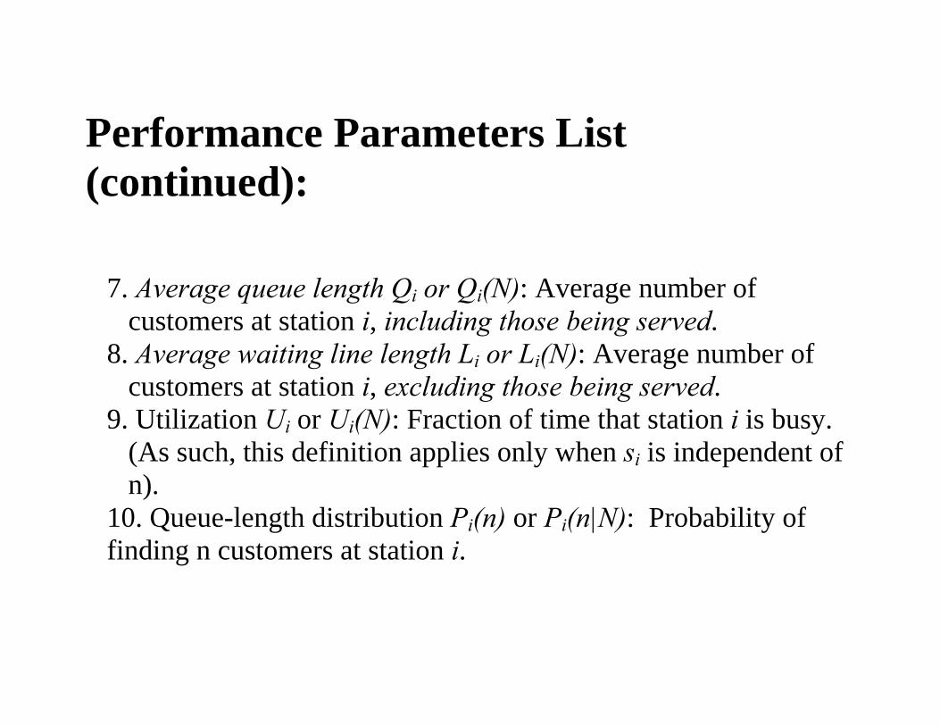
Performance Parameters List (continued):

7. Average queue length Qi or Qi(N): Average number of customers at station i, including those being served.

8. Average waiting line length Li or Li(N): Average number of customers at station i, excluding those being served.

9. Utilization Ui or Ui(N): Fraction of time that station i is busy. (As such, this definition applies only when si is independent of n).

10. Queue-length distribution Pi(n) or Pi(n|N): Probability of finding n customers at station i.

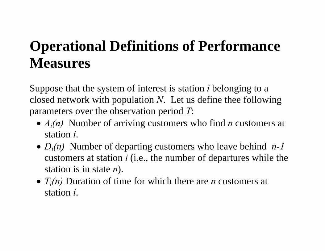
Operational Definitions of Performance Measures

Suppose that the system of interest is station i belonging to a closed network with population N. Let us define thee following parameters over the observation period T: • Ai(n) Number of arriving customers who find n customers at

station i. • Di(n) Number of departing customers who leave behind n-1

customers at station i (i.e., the number of departures while the station is in state n).

• Ti(n) Duration of time for which there are n customers at station i.

Operational Definitions of Performance Measures (continued)

• Note that Ai(N) = 0 and Di(0) = 0, but Ti(n) may be nonzero for all values of n = 1..N. Let Bi denote the total busy period. Obviously,

Bi = T – Ti(0) = 1

( )N

in

T n=∑

• Let Ai and Di denote, respectively, the total number of arrivals

and departures during time T. Then

Ai = 1

0( )

N

in

A n−

=∑ and Di = )

1(

N

in

D n=∑

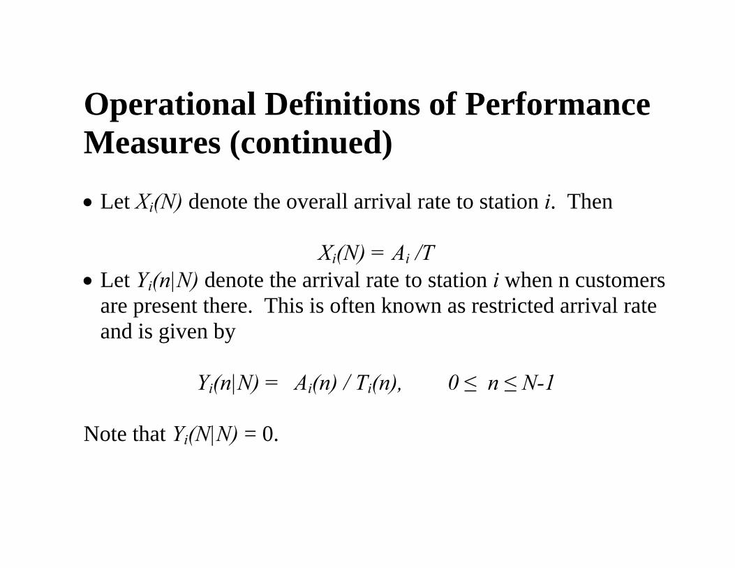
Operational Definitions of Performance Measures (continued) • Let Xi(N) denote the overall arrival rate to station i. Then

Xi(N) = Ai /T • Let Yi(n|N) denote the arrival rate to station i when n customers

are present there. This is often known as restricted arrival rate and is given by

Yi(n|N) = Ai(n) / Ti(n), 0 ≤ n ≤ N-1

Note that Yi(N|N) = 0.

Operational Definitions of Performance Measures (continued) • The departure rate or throughput of station i, denoted λi(N) is

given by λi(N) = Di /T

• The average service time of station I when n customers are

present there, denoted si(n), is given by

si(n|N) = Ti(n) / Di(n), 1 ≤ n ≤ N

In analogy with Yi(n|N), we can think of service rate μi(n) as the restricted departure rate.

Operational Definitions of Performance Measures (continued) • If the services are homogeneous, we denote si(n) and μi(n) as

simply si and μi, respectively. • If the arrivals are homogeneous, Yi(n|N) is independent of n for

n < N and denoted as Yi(N). • Flow balance means that Ai = Di, which implies that Xi(N) = λi(N).

Some Interesting Distributions of the Number of Customers in the System • Distribution seen by an arriving customer, the probability that

an arriver finds n customers in the system, given by

PAi(n|N) = Ai(n) / Ai for 0 ≤ n < N

• Distribution seen by a departing customer, the probability that a departer leaves behind n customers in the system, given by

• PDi(n|N) = Di(n+1) / Di for 0 ≤ n < N

Some Interesting Distributions of the Number of Customers in the System (continued) • Distribution seen by a random observer, a fraction of time the

system contains n customers, given by •

Pi(n|N) = Ti(n) / T for 0 ≤ n ≤ N • As a simple example

Ui(N) = Bi / T = (T – Ti(0)) / T = 1 – Pi(0|N)

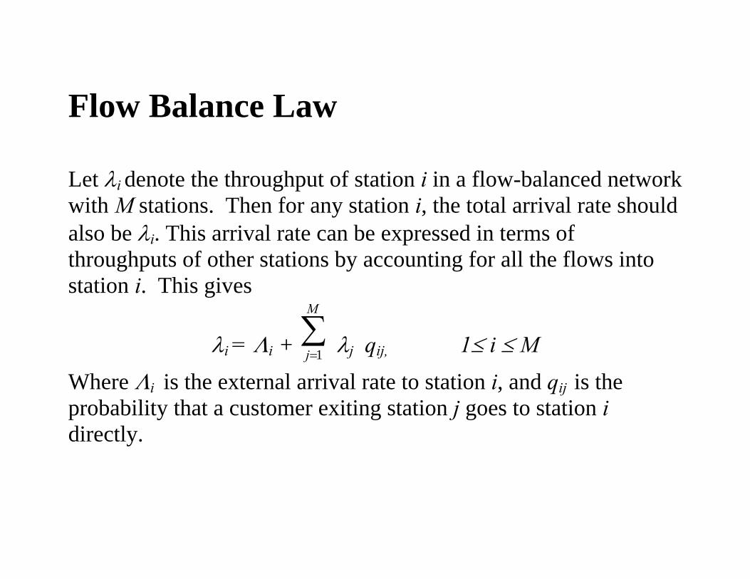
Flow Balance Law Let λi denote the throughput of station i in a flow-balanced network with M stations. Then for any station i, the total arrival rate should also be λi. This arrival rate can be expressed in terms of throughputs of other stations by accounting for all the flows into station i. This gives

λi = Λi + 1

M

j=∑ λj qij, 1≤ i ≤ M

Where Λi is the external arrival rate to station i, and qij is the probability that a customer exiting station j goes to station i directly.

Flow Balance Law (continued)

• If the network is open, the previous system of equations will be non-homogeneous, and will have a unique solution. This means that given the external arrival rates, we can determine the throughputs of all stations exactly.

• If the network is closed, the previous system of equations will become homogeneous and will not have a unique solution. It will in fact include the set of exactly M-1 linearly independent equations, which can be solved to determine the ratios of throughputs.

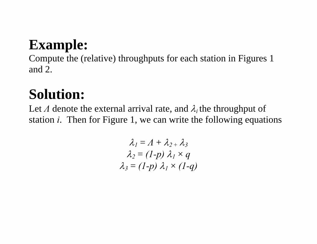
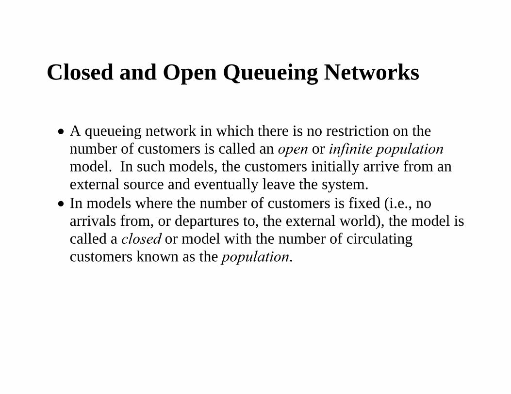
Example: Compute the (relative) throughputs for each station in Figures 1 and 2. Solution: Let Λ denote the external arrival rate, and λi the throughput of station i. Then for Figure 1, we can write the following equations

λ1 = Λ + λ2 + λ3

λ2 = (1-p) λ1 × q λ3 = (1-p) λ1 × (1-q)

Solution (continued)

Suppose that we define visit ratios relative to the external source, i.e., vi = λi /Λ. Then

v1 = 1/p v2 = q (1-p) /p and v3 = (1-q) (1-p) /p

Note that we can determine exact throughputs here. For example, if p = 0.1, q = 0.8, and Λ = 10/sec, then we have:

λ1 = 100/sec, λ2 = 72/sec, and λ3 = 18/sec.

Solution (continued)

For the model of Figure 2, we have

λ2 = λ1 + (1-p) (λ3 + λ4), λ3 = q λ2 , λ4 = (1-q) λ2

It is easy to see that these equations are linearly independent, but we cannot write any more independent equations. Thus, exact throughputs cannot be determined, but visit ratios can. For example, if we let v2 = 1, p = 0.2, and q = 0.6, then v3 = 0.2, v1 = 0.6, and v4 = 0.4.

Some Fundamental Results: λi (N) = iD

T = 1T ) =

1(

N

in

D n=∑

1

( ) ( )( )

Ni i

n i

D n T nT n T=

∑ = 1

( | )( )

Ni

n i

P n Ns n=

∑ Put in standard form, the throughput law then states

λi (N) = 1

( ) ( | )N

i in

n P n Nμ=∑

If the services are homogeneous, i.e., μi(n) = μi for all n > 0, the above equation can be written as

λi (N) = μi [1 – Pi(0|N)],

or, Ui(N) = λi (N) si

Some Fundamental Results: (continued)

A more direct way of obtaining the utilization law is as follows:

Ui(N) = iB

T =

i i

i

B DD T

× = si λi (N)

Like the throughput law, we have the following arrival law: 1

Xi(N) = 0( | ) ( | )

N

i in

Y n N P n N−

=∑

The proof follows trivially from the definition:

Xi(N) = iA

T = 1

0

( ) ( )( )

Ni i

n i

A n T nT n T

−

=∑ =

1

0( | ) ( | )

N

i in

Y n N P n N−

=∑

Some Fundamental Results: (continued) Under flow balance, the arrival rate is the same as throughput, which means that the previous equation is another way of expressing the throughput. If the arrivals are homogeneous, i.e., Yi(n|N) = Yi(N) for all n < N, the previous equation can be written as

Xi(N) = Yi(N) (1- Pi(N|N))

Properties of Queue Length Distributions In general, if arrivals (departures) occur singly, then in any system state n, at most one arrival (departure) can remain unmatched by a departure (arrival). This happens because the system cannot return to state n unless an opposite event occurs. It follows that

∀n |Ai(n) – Di(n+1)| ≤ 1 where Di(n+1) can exceed Ai(n) only if we start with a nonempty system. Under flow balance, we cannot have an arriver who has not departed, or vice versa, and hence the above equation reduces to

Ai(n) = Di(n+1)

Properties of Queue Length Distributions (continued) The earlier equation implies

Ai = Di or

PAi(n|N) = PDi(n|N)

Properties of Queue Length Distributions (continued) We can also get recursive equations for random observer’s and arriver’s distributions under these two assumptions. By definition,

( ) ( ) ( ) ( ) ( 1) ( 1)( | )( ) ( ) ( 1)

i i i i i ii

i i i

T n T n D n T n A n T nP n NT D n T D n T n T

− −= = =

− where we have used the identity Di(n) = Ai(n-1). Recognizing various terms, we get

Pi(n|N) = si(n) Yi(n-1|N) Pi(n-1|N)

Properties of Queue Length Distributions (continued) Similarly, for the arriver’s distribution, we get

( ) ( ) ( ) ( ) ( 1)( | ) ( | ) ( )( ) ( )

i i i i ii i i

i i i i i

A n A n T n D n A nPA n N Y n N s nA T n D n A A

−= = =

which yields

PAi(n|N) = si(n) Yi(n|N) PAi(n-1|N)

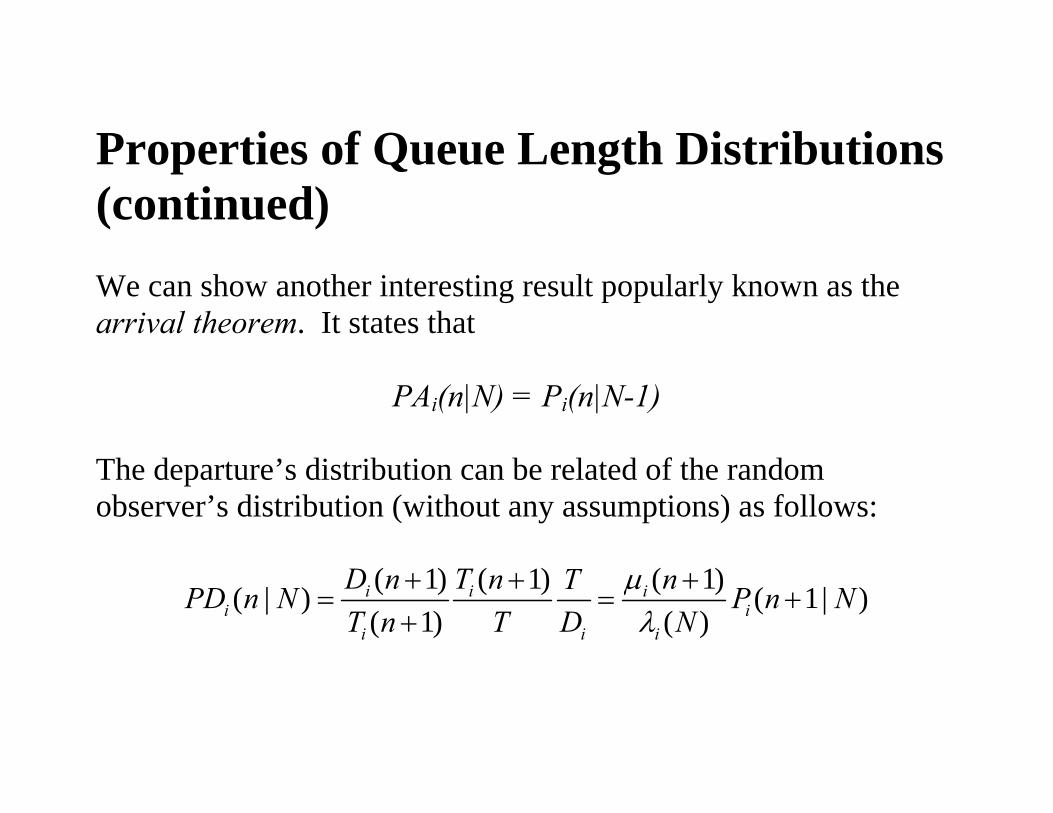
Properties of Queue Length Distributions (continued) We can show another interesting result popularly known as the arrival theorem. It states that

PAi(n|N) = Pi(n|N-1) The departure’s distribution can be related of the random observer’s distribution (without any assumptions) as follows:

( 1) ( 1) ( 1)( | ) ( 1| )( 1) ( )

i i ii i

i i i

D n T n nTPD n N P n NT n T D N

μλ

+ + += = +

+

Properties of Queue Length Distributions (continued) Under flow balance and one-step behavior, we get

PAi(n|N) = μi(n+1) Pi(n+1|N)/λi(N)

Furthermore, using the arrival theorem, we get the so called marginal local balance theorem, which can be restated as

μi(n) Pi(n|N) = λi(N) Pi(n-1|N-1)

Properties of Queue Length Distributions (continued)

In practice, the arrivals are often homogeneous, and we can show some interesting results under this assumption. By definition,

( ) ( ) ( ) ( )( | ) ( | )( ) ( )

i i i ii i

i i i i

A n A n T n Y NTPA n N P n NA T n T A X N

= = = Therefore, we get

( | )( | )1 ( | )

ii

i

P n NPA n NP N N

=−

That is, in a closed network under homogeneous arrivals, the arriver’s distribution is a simple renormalization of the random observer’s distribution

Properties of Queue Length Distributions (continued) For an open network, the previous equation means that the arriver’s and random observer’s distributions are identical. If the system shows one-step behavior and flow balance as well, we get

( ) ( 1| )( | ) ( ) ( 1| )( ) 1 ( | )

i ii i

i i

N P n NP n N n P n Nn P N N

λ αμ

−= −

− This recurrence relation, long with the requirement that all probabilities sum to 1, gives us the following expression

1

1 1

( | ) ( ) 1 ( )n kN

iki j

P n N i jα α−

= =

⎡ ⎤= +⎢ ⎥

⎣ ⎦∑∏ ∏

Properties of Queue Length Distributions (continued) Finally, under homogeneous services, flow balance, and one-step behavior, we can write

Pi(n|N) = Ui(N) PAi(n-1|N) which means that

1 1( ) ( | ) ( ) ( 1| )

N N

i i i in n

Q N nP n N U N nPA n N= =

= −∑ ∑ which along with Little’s law gives the following interesting relationship

Ri(N) = si (1+QAi(N)) Where QAi(N) is the average queue length seen by an arriving customer. Note that by the arrival theorem, QAi(N) = Qi(N-1).

Example:

N(t)

5k-1

Figure 3: A sample behavior sequence.

k-1 k-1

k k k

2

k-1

k

1

k

k1 k-1

1

Tt

Example (continued): n Ai(n) Di(n) Ti(n) Pi(n) PAi(n) PDi(n) Xi(n) si(n)0 4 - 8k 8/15 4/7 4/7 1/(2k) - 1 2 4 4k 4/15 2/7 2/7 1/(2k) k 2 1 2 2k 2/15 1/7 1/7 1/(2k) k 3 - 1 k 1/15 - - - k

Table 1: Performance parameters for the behavior sequence in Figure 3.

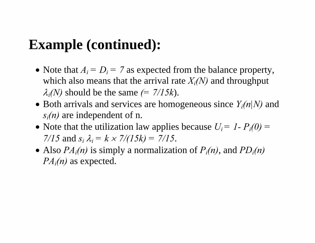
Example (continued): • Note that Ai = Di = 7 as expected from the balance property,

which also means that the arrival rate Xi(N) and throughput λi(N) should be the same (= 7/15k).

• Both arrivals and services are homogeneous since Yi(n|N) and si(n) are independent of n.

• Note that the utilization law applies because Ui = 1- Pi(0) = 7/15 and si λi = k × 7/(15k) = 7/15.

• Also PAi(n) is simply a normalization of Pi(n), and PDi(n) PAi(n) as expected.

Chains: • A real computer system may serve many categories of jobs

such that the level of service provided and/or the routing depends on the category. For example, the characteristics of batch jobs may be different from those of the interactive jobs. This aspect can be represented in a queueing network model by introducing the concept of chains.

• A chain forms a permanent categorization of jobs; a job belonging to one chain cannot switch to another chain.

Classes: • In addition to the permanent categorization of jobs, it is also

desirable to allow customers to go through different phases of processing in the system. This necessarily requires the ability to switch from one phase to another, and thus needs a concept other than chains. We refer to these phases as classes and allow several classes within a chain.

• For example, the execution of both batch and interactive jobs would involve two distinct phases: program loading from disk into the main memory, and the actual execution. We can represent this by having two classes in each chain, such that all customers of a chain start out in class 1 to do program loading, and then switch to class 2 for execution. (In a closed model, class 2 jobs would switch back to class 1 after finishing execution).

Characterization of Classes and Chains We would like to answer the following questions concerning a network with multiple categories of customers:

1.How do we check if the network is consistent, i.e., connected and structurally sound?

2.How do identify the chains, and the classes contained within those chains?

3.How do we check if the network is well-formed, i.e., has a well-defined long-term behavior?

Characterization of Classes and Chains (continued) • To answer the above questions, we use a graph model, known

as the reachability graph (RG). • The nodes of a RG are classes, and an arc from node c to node

d means that a class c customer can switch to class d directly (with a nonzero probability).

• Let S1,…,Sk be the strongly connected components (SCC) of RG. All classes in a SCC must show similar long-term behavior, because any class in a SCC can transform to any other within the same SCC.

Classification of SCC’s: Each SCC can be classified into one of the following four categories: Closed if in the long run it will have a finite number of customers permanently locked in it. Open if it will have both arrivals from and departures to the external world (either directly or via the classes of other SCC’s). Transient if in the long run it will have no customers in it. Unstable if in the long run it receives customers from the external world or classes of other SCC’s, but does not shed any.

Characterization of well-formedness: • A consistent network is well-formed if and only if it does not

have and unstable or transient SCC’s. • In a well-formed network, closed SCC’s can be identified as

closed chains, and open SCC’s can be further grouped into open chains.

Classification algorithm: We start with the reachability graph, of the given model, and proceed as follows:

1.Construct a reduced reachability graph, say Gr, by replacing the SCC’s of G by individual nodes. In Gr, an arc from node i to j indicates that some class in the SCC Si can switch to some class in the SCC Sj with nonzero probability.

2.If class i customers arrive from the external world, regard this as switch from a ``dummy class’’ to class i. Similarly, regard class i departures to the external world as a switch from class i to yet another dummy class. Add nodes and arcs to Gr corresponding to these dummy classes. Let the new graph be denoted as

'. rG

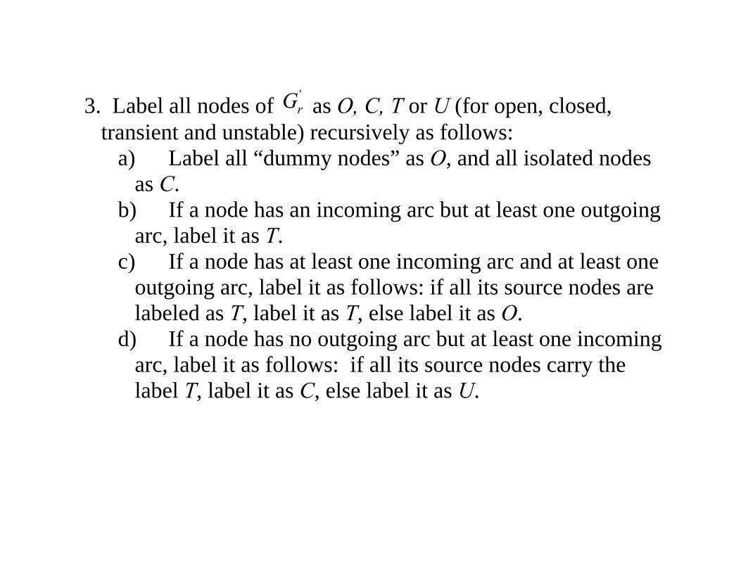
3. Label all nodes of as O, C, T or U (for open, closed, transient and unstable) recursively as follows:

'rG

a) Label all “dummy nodes” as O, and all isolated nodes as C.

b) If a node has an incoming arc but at least one outgoing arc, label it as T.

c) If a node has at least one incoming arc and at least one outgoing arc, label it as follows: if all its source nodes are labeled as T, label it as T, else label it as O.

d) If a node has no outgoing arc but at least one incoming arc, label it as follows: if all its source nodes carry the label T, label it as C, else label it as U.

4.Remove from , all dummy nodes and nodes labeled as T or U. (The corresponding arcs are also removed.) Call the resulting graph " .

'rG

rG

5.All nodes marked as C in must be isolated and represent closed chains (with SCC population as the chain population). Of the remaining nodes, each connected component represents an open chain.

"rG

Example: A computer system model with six categories of jobs

Terminals CPU

DISK1

DISK2

Class 1: Class 4:

Class 2: Class 5:

Class 3: Class 6:

0.2 0.8

0.4

0.6

0.6

0.40.75

.250.7

0.30.8

0.2

0.2

0.3

0.5

Figure 4: A computer system model with six categories of jobs.

Example (continued):

4 8

6 5

7

1

2 3

C

C C

O

U

O

O

T

Figure 5: Reachability graph for the model of Figure 4.

Characteristics of Multiple-Class Ne

• As indicated before, all classes in a well-formed network can

if

•

1 K Ni = ∝ for an open chain.

tworks

be grouped into open and closed chains. • If all chains in the model are closed, we call the mode closed,

all are open, we call the model open, and if some chains are closed and some open, we call the model mixed. For generality, we consider a mixed model with K chains, such that chains 1 .. C are closed, and the rest are open.

• We shall denote the population of chain i as Ni, and the population vector as N = (N , …, N ) where by convention,

C sNe

llowing

nc rM

qυ υ= Λ +∑∑

where

haracteristics of Multiple-Cla s tworks

Under flow balance, the forced-flow law yields the foequation:

( )

1 1irc irc jrd jdicr

j d= =

ircυ denote the visit ratio for class c of chain r at station i,

qjdicr denote the routing probability for a chain r job going to station i as a member of class c after being serviced at station j as a member of class d, and nc(r) denote the number of classes in chain r.

Example: Cr

ompute all visit ratios for the model of Figure 4 (after the emoval of classes 4 and 6).

Solution:

the chain containing classes 1-3 as chain 1, and ng class 5 as chain 2. The class subscript is

edundant for chain 2, and we shall omit it. Suppose (arbitrarily)

212

0.40× v413 = 0.125 + 0.375 + 0.08 =

We shall denotethe one containirthat v111 = v12 =1. Obviously, for chain 2, v22 = 0.8 × v12 = 0.8. Chain 1 contains classes 1-3, which satisfy the following equations: v212 = 0.50× v111 = 0.50 v311 = 0.30× v111 = 0.30 v411 = 0.75× v = 0.375 v413 = 0.20× v111 = 0.20 v312 = 0.25× v212 + v411 +0.580

Operational Analysis of Multiple-Chain N k

more general case as well. We assume the network has M stations and K chains.

i give the number of chain r

n usly, is a

etwor s For simplicity in stating the results, we only consider multiple-chain networks with one class per chain. Similar results can be obtained for the Notations:The state of a station in such a network can be described by a vector, called the occupancy vector. We denote it as n = (n ,…,n ), whose components ni1 iK ircustomers at station i. When there is no confusion, we shall shortethis notation to n with chain r component dented as nr. Obvion can range from 0 to N. We also need the notation er which vector with K elements, of which the rth element is 1 and all others are zero. Suppose that we observe station i for T time units.

Operational Analysis of Multiple-ChainNetworks (continued)

r

ir : Number of chain r departures while the station is in

Then we can introduce the following three measures for each chain ∈ [1..K]:

• Air(n): Number of arriving chain r customers who find n

customers at station i. • D (n)

state n (i.e., the number of departing customers that leavebehind n-er customers).

• Tir(n): Duration of time for which there are n customers at station i.

Operational Analysis of Multiple-Chain Networks (continued)

0 0 0 0 0... ( )

r K

r r r K

N N

ir irn n n n n

A A+

− += = = = =∑ ∑ n

We shall abbreviate summation like this by specifying the range of 0 to N-er for vector n. Thus, we define

n=

Let

1 1 1

...r rN N N− −

= ∑ ∑ ∑1

1 1 1

( )re

ir irA A−

= ∑N

n=0n ( )D D= ∑

N

nr

ir ire

Operational Analysis of Multiple-Chain Networks (cont

Xir(N)= Air / T on

ers are present there. Then

inued) Let Xir(N) denote the total arrival rate of chain r customers to station i. Then

Let Yir(n|N) denote the restricted arrival rate of chain r to statii when n custom

( )irA n( | )Y =n N

λir(N) is given by λir(N) = D / T

( )iriT n , 0 ≤ n ≤ N-er

The throughput of chain r at station i, denoted ir

Operational Analysis of Multiple-Chain Networks (continued)

n r customers at station I hen n customers are present there, be denoted as s*ir(n).

Let the average service time of chaiwObviously,

( )* ( )( ) iir

Ts =nn

irD n , er ≤ n ≤ N It is also convenient to define service rate as simply the inverse of service time, i.e,

μ*ir(n)= 1 / s*ir(n)

Operational Analysis of Multiple-Chain Networks (continued) The three basic distributions for the multiple-chain case can be

r arrivers 0 ≤ n ≤ N - er

0 ≤ n ≤ N - er

≤ n ≤ N

defined as follows: • Distribution seen by chain

PAir(n|N) = Air(n) / Air, • Distribution seen by chain r departers

PAir(n|N) = Dir(n + er) / Dir, • Distribution seen by a random observer

Pi(n|N) = Ti(n) / T, 0

Operational Analysis of Multiple-Chain Networks (continued)

The throughput law holds, since

•

*( ) ( )1D DN N

( ) ( ) ( ) ( | )( )

r r r

ir ir iir ir ir i

e e ei

TD PT T T T

λ μ= = =

= = = =∑ ∑ ∑N

n n n

n nN n n n Nn

Similarly, we can prove the arrival law •

( ) ( )1 e eA A− −N N n n( ) ( ) ( | ) ( | )( )

r r reir ir i

ir ir ir ii

TX A Y PT T T T

−

= = =

= = = =∑ ∑ ∑N

n 0 n 0 n 0

N n n N n Nn