Welcome message from author
This document is posted to help you gain knowledge. Please leave a comment to let me know what you think about it! Share it to your friends and learn new things together.
Transcript

Fundamentals ofGas Dynamics
(2nd Edition)
Cover illustration: Schlieren picture of an under-expanded flow issuingfrom a convergent divergent nozzle. Prandtl-Meyer expansion waves in thedivergent portion as the flow goes around the convex throat can be seen.Expansion fans, reflected oblique shocks and the alternate swelling andcompression of the jet are clearly visible. Courtesy: P. K. Shijin, PhDscholar, Dept. of Mechanical Eng, IIT Madras.
Fundamentals ofGas Dynamics
(2nd Edition)
V. BabuProfessor
Department of Mechanical EngineeringIndian Institute of Technology, Madras,INDIA
Athena Academic Ltd.
John Wiley & Sons Ltd.
Fundamentals of Gas Dynamics, 2nd Edition (2015)
© 2015. V.Babu
First Edition : 2008Reprint : 2009, 2011Second Edition : 2015
This Edition Published byJohn Wiley & Sons LtdThe Atrium, Southern GateChichester, West SussexPO19 8SQ United KingdomTel : +44 (0) 1243 779777Fax : +44 (0) 1243 775878e-mail : [email protected] : www.wiley.com
For distribution in rest of the world other than the Indian sub-continent & Africa.
Under licence from:Athena Academic Ltd.Suite LP24700, Lower Ground Floor145-157 St. John Street, London,ECIV 4PW. United Kingdome-mail : [email protected] : www.athenaacademic.co.uk
ISBN : 978-11-1897-339-4
All rights reserved. No part of this publication may be reproduced, stored in a retrieval system, or transmitted in any form or by any means, electronic, mechanical, photocopying, recording or otherwise, except as permitted by the U.K. Copyright, Designs and Patents Act 1988, without the prior permission of the publisher.
Designations used by companies to distinguish their products are often claimed as trademarks. All brand names and product names used in this book are trade names, service marks, trademarks or registered trademarks of their respective owners. The publisher is not associated with any product or vendor mentioned in this book.
Library Congress Cataloging-in-Publication Data
A catalogue record for this book is available from the British Library
Printed in UK

Dedicated to my wife Chitra and son Aravindh for their enduringpatience and love

Preface
I am happy to come out with this edition of the book Fundamentals of GasDynamics. Readers of the first edition should be able to see changes inall the chapters - changes in the development of the material, new materialand figures as well as more end of chapter problems. In keeping with thespirit of the first edition, the additional exercise problems are drawn frompractical applications to enable the student to make the connection fromconcept to application.
Owing to the ubiquitous nature of steam power plants around the world, itis important for mechanical engineering students to learn the gas dynamicsof steam. With this in mind, a new chapter on the gas dynamics ofsteam has been added in this edition. This is somewhat unusual since thistopic is usually introduced in text books on steam turbines and not in gasdynamics texts. In my opinion, introducing this in a gas dynamics textis logical and in fact makes it easy for the students to learn the concepts.In developing this material, I have assumed that the reader would havegone through a fundamental course in thermodynamics and so would befamiliar with calculations involving steam. Steam tables for use in thesecalculations have also been added at the end of the book. I would like tothank Prof. Korpela of the Ohio State University for generating these tablesand allowing me to include them in the book.
I wish to thank the readers who purchased the first edition and gave memany suggestions as well as for pointing out errors. To the extent possible,the errors have been corrected and the suggestions have been incorporated
iii
iv Fundamentals of Gas Dynamics
in this edition. If there are any errors or if you have any suggestions forimproving the exposition of any topic, please feel free to communicatethem to me via e-mail ([email protected]). I would like to takethis opportunity to thank Prof. S. R. Chakravarthy of IIT Madras for hissuggestion concerning the definition of compressibility. I have taken thisfurther and connected it with Rayleigh flow in the incompressible limit.The effect of different γ on the property changes across a normal shockwave are now included in Chapter 3. The development of the processcurve in Chapters 4 and 5 has been done by directly relating the changes inproperties to changes in stagnation temperature and entropy respectively.In Chapter 6, I have added a figure showing the variation of static pressurealong a CD nozzle as well as the variation of exit static pressure to theambient pressure. Hopefully this will make it easier for the the student tounderstand over- and under-expanded flow.
Once again I would like to express my heartfelt gratitude to my teacherswho taught me so much without expecting anything in return. I can onlyhope that I succeed in giving back at least a fraction of the knowledge andwisdom that I received from them. My advisor, mentor and friend, Prof.Seppo Korpela has been an inspiration to me and his constant and patientcounsel has helped me enormously. I am indebted to my parents for thesacrifices they made to impart a good education to me. This is not a debtthat can be repaid. But for the constant support and encouragement frommy wife and son, this edition and the other books that I have written wouldnot have been possible.
Finally, I would like to thank my former students P. S. Tide, S. Soma-sundaram and Anandraj Hariharan for diligently working out the examplesand exercise problems and my current student P. K. Shijin for carefullyproof reading the manuscript and making helpful suggestions. Thanks aredue in addition to Prof. P. S. Tide for preparing the Solutions Manual.
V. Babu
Contents
Preface iii
1. Introduction 1
1.1 Compressibility of Fluids . . . . . . . . . . . . . . . . . 11.2 Compressible and Incompressible Flows . . . . . . . . . 21.3 Perfect Gas Equation of State . . . . . . . . . . . . . . . 4
1.3.1 Continuum Hypothesis . . . . . . . . . . . . . 51.4 Calorically Perfect Gas . . . . . . . . . . . . . . . . . . 7
2. One Dimensional Flows - Basics 11
2.1 Governing Equations . . . . . . . . . . . . . . . . . . . 112.2 Acoustic Wave Propagation Speed . . . . . . . . . . . . 13
2.2.1 Mach Number . . . . . . . . . . . . . . . . . . 162.3 Reference States . . . . . . . . . . . . . . . . . . . . . 16
2.3.1 Sonic State . . . . . . . . . . . . . . . . . . . . 172.3.2 Stagnation State . . . . . . . . . . . . . . . . . 17
2.4 T-s and P-v Diagrams in Compressible Flows . . . . . . 23Exercises . . . . . . . . . . . . . . . . . . . . . . . . . . . . . 28
3. Normal Shock Waves 31
3.1 Governing Equations . . . . . . . . . . . . . . . . . . . 313.2 Mathematical Derivation of the Normal Shock Solution . 333.3 Illustration of the Normal Shock Solution on T-s and P-v
diagrams . . . . . . . . . . . . . . . . . . . . . . . . . 36
v
vi Fundamentals of Gas Dynamics
3.4 Further Insights into the Normal Shock Wave Solution . 41Exercises . . . . . . . . . . . . . . . . . . . . . . . . . . . . . 45
4. Flow with Heat Addition- Rayleigh Flow 49
4.1 Governing Equations . . . . . . . . . . . . . . . . . . . 494.2 Illustration on T-s and P-v diagrams . . . . . . . . . . . 504.3 Thermal Choking and Its Consequences . . . . . . . . . 604.4 Calculation Procedure . . . . . . . . . . . . . . . . . . 64Exercises . . . . . . . . . . . . . . . . . . . . . . . . . . . . . 67
5. Flow with Friction - Fanno Flow 69
5.1 Governing Equations . . . . . . . . . . . . . . . . . . . 695.2 Illustration on T-s diagram . . . . . . . . . . . . . . . . 705.3 Friction Choking and Its Consequences . . . . . . . . . 755.4 Calculation Procedure . . . . . . . . . . . . . . . . . . 75Exercises . . . . . . . . . . . . . . . . . . . . . . . . . . . . . 81
6. Quasi One Dimensional Flows 83
6.1 Governing Equations . . . . . . . . . . . . . . . . . . . 846.1.1 Impulse Function and Thrust . . . . . . . . . . 84
6.2 Area Velocity Relation . . . . . . . . . . . . . . . . . . 866.3 Geometric Choking . . . . . . . . . . . . . . . . . . . . 886.4 Area Mach number Relation for Choked Flow . . . . . . 906.5 Mass Flow Rate for Choked Flow . . . . . . . . . . . . 926.6 Flow Through A Convergent Nozzle . . . . . . . . . . . 936.7 Flow Through A Convergent Divergent Nozzle . . . . . 976.8 Interaction between Nozzle Flow and Fanno, Rayleigh
Flows . . . . . . . . . . . . . . . . . . . . . . . . . . . 111Exercises . . . . . . . . . . . . . . . . . . . . . . . . . . . . . 122
7. Oblique Shock Waves 127
7.1 Governing Equations . . . . . . . . . . . . . . . . . . . 1297.2 θ-β-M curve . . . . . . . . . . . . . . . . . . . . . . . 1317.3 Illustration of the Weak Oblique Shock Solution on a T-s
diagram . . . . . . . . . . . . . . . . . . . . . . . . . . 1347.4 Detached Shocks . . . . . . . . . . . . . . . . . . . . . 141
Contents vii
7.5 Reflected Shocks . . . . . . . . . . . . . . . . . . . . . 1437.5.1 Reflection from a Wall . . . . . . . . . . . . . . 143
Exercises . . . . . . . . . . . . . . . . . . . . . . . . . . . . . 146
8. Prandtl Meyer Flow 149
8.1 Propagation of Sound Waves and the Mach Wave . . . . 1498.2 Prandtl Meyer Flow Around Concave and Convex Corners 1538.3 Prandtl Meyer Solution . . . . . . . . . . . . . . . . . . 1558.4 Reflection of Oblique Shock From a Constant Pressure
Boundary . . . . . . . . . . . . . . . . . . . . . . . . . 160Exercises . . . . . . . . . . . . . . . . . . . . . . . . . . . . . 163
9. Flow of Steam through Nozzles 165
9.1 T-s diagram of liquid water-water vapor mixture . . . . . 1659.2 Isentropic expansion of steam . . . . . . . . . . . . . . 1689.3 Flow of steam through nozzles . . . . . . . . . . . . . . 171
9.3.1 Choking in steam nozzles . . . . . . . . . . . . 1739.4 Supersaturation and the condensation shock . . . . . . . 179Exercises . . . . . . . . . . . . . . . . . . . . . . . . . . . . . 188
Suggested Reading 191
Table A. Isentropic table for γ = 1.4 193
Table B. Normal shock properties for γ = 1.4 203
Table C. Rayleigh flow properties for γ = 1.4 211
Table D. Fanno flow properties for γ = 1.4 221
Table E. Oblique shock wave angle β in degrees for γ = 1.4 231
Table F. Mach angle and Prandtl Meyer angle for γ = 1.4 237
Table G. Thermodynamic properties of steam, temperature table 243
Table H. Thermodynamic properties of steam, pressure table 247
Table I. Thermodynamic properties of superheated steam 251
viii Fundamentals of Gas Dynamics
Index 259
About the author 263
About the book 265
Chapter 1
Introduction
Compressible flows are encountered in many applications in Aerospaceand Mechanical engineering. Some examples are flows in nozzles,compressors, turbines and diffusers. In aerospace engineering, in additionto these examples, compressible flows are seen in external aerodynamics,aircraft and rocket engines. In almost all of these applications, air (or someother gas or mixture of gases) is the working fluid. However, steam can bethe working substance in turbomachinery applications. Thus, the range ofengineering applications in which compressible flow occurs is quite largeand hence a clear understanding of the dynamics of compressible flow isessential for engineers.
1.1 Compressibility of Fluids
All fluids are compressible to some extent or other. The compressibility ofa fluid is defined as
τ = −1
v
∂v
∂P, (1.1)
where v is the specific volume and P is the pressure. The change inspecific volume corresponding to a given change in pressure, will, ofcourse, depend upon the compression process. That is, for a given changein pressure, the change in specific volume will be different between anisothermal and an adiabatic compression process.
The definition of compressibility actually comes from thermodynamics.
1
Fundamentals of Gas Dynamics, Second Edition. V. Babu.© 2015 V. Babu. Published 2015 by Athena Academic Ltd and John Wiley & Sons Ltd
2 Fundamentals of Gas Dynamics
Since the specific volume v = v(T, P ), we can write
dv =
(
∂v
∂P
)
T
dP +
(
∂v
∂T
)
P
dT .
From the first term, we can define the isothermal compressibility as
−1v
(
∂v∂P
)
Tand, from the second term, we can define the coefficient
of volume expansion as 1v
(
∂v∂T
)
P. The second term represents the
change in specific volume (or equivalently density) due to a change intemperature. For example, when a gas is heated at constant pressure, thedensity decreases and the specific volume increases. This change can belarge, as is the case in most combustion equipment, without necessarilyhaving any implications on the compressibility of the fluid. It thus followsthat compressibility effect is important only when the change in specificvolume (or equivalently density) is due largely to a change in pressure.
If the above equation is written in terms of the density ρ, we get
τ =1
ρ
∂ρ
∂P, (1.2)
The isothermal compressibility of water and air under standard atmo-spheric conditions are 5 × 10⁻¹⁰m2/N and 10−5m2/N . Thus, water (inliquid phase) can be treated as an incompressible fluid in all applications.On the contrary, it would seem that, air, with a compressibility that is fiveorders of magnitude higher, has to be treated as a compressible fluid in allapplications. Fortunately, this is not true when flow is involved.
1.2 Compressible and Incompressible Flows
It is well known from high school physics that sound (pressure waves)propagates in any medium with a speed which depends on the bulkcompressibility. The less compressible the medium, the higher the speedof sound. Thus, speed of sound is a convenient reference speed, when flowis involved. Speed of sound in air under normal atmospheric conditions
Introduction 3
is 330 m/s. The implications of this when there is flow are as follows.Let us say that we are considering the flow of air around an automobiletravelling at 120 kph (about 33 m/s). This speed is 1/10th of the speedof sound. In other words, compared with 120 kph, sound waves travel10 times faster. Since the speed of sound appears to be high comparedwith the highest velocity in the flow field, the medium behaves as thoughit were incompressible. As the flow velocity becomes comparable to thespeed of sound, compressibility effects become more prominent. In reality,the speed of sound itself can vary from one point to another in the flowfield and so the velocity at each point has to be compared with the speedof sound at that point. This ratio is called the Mach number, after ErnstMach who made pioneering contributions in the study of the propagationof sound waves. Thus, the Mach number at a point in the flow can bewritten as
M =u
a, (1.3)
where u is the velocity magnitude at any point and a is the speed of soundat that point.
We can come up with a quantitative criterion to give us an idea about theimportance of compressibility effects in the flow by using simple scalingarguments as follows. From Bernoulli’s equation for steady flow, it followsthat ∆P ∼ ρU2, where U is the characteristic speed. It will be shown inthe next chapter that the speed of sound a =
√
∆P/∆ρ, wherein ∆P and∆ρ correspond to an isentropic process. Thus,
∆ρ
ρ=
1
ρ
∆ρ
∆P∆P =
U2
a2= M2 . (1.4)
On the other hand, upon rewriting Eqn. 1.2 for an isentropic process, weget
∆ρ
ρ= τisentropic∆P .
Comparison of these two equations shows clearly that, in the presence of a
4 Fundamentals of Gas Dynamics
flow, density changes are proportional to the square of the Mach number†.It is customary to assume that the flow is essentially incompressible if thechange in density is less than 10% of the mean value‡. It thus follows thatcompressibility effects are significant only when the Mach number exceeds0.3.
1.3 Perfect Gas Equation of State
In this text, we assume throughout that air behaves as a perfect gas. Theequation of state can be written as
Pv = RT , (1.5)
where T is the temperature§ . R is the particular gas constant and is equal toR/M where R = 8314 J/kmol/K is the Universal Gas Constant and Mis the molecular weight in units of kg/kmol. Equation 1.5 can be written inmany different forms depending upon the application under consideration.A few of these forms are presented here for the sake of completeness. Sincethe specific volume v = 1/ρ, we can write
P = ρRT ,
or, alternatively, as
PV = mRT ,
where m is the mass and V is the volume. If we define the concentration c
as (m/M)(1/V ), then,
P = cRT . (1.6)
Here c has units of kmol/m3. The mass density ρ can be related to the†This is true for steady flows only. For unsteady flows, density changes are proportional
to the Mach number.‡Provided the change is predominantly due to a change in pressure.§In later chapters this will be referred to as the static temperature
Introduction 5
particle density n (particles/m3) through the relationship ρ = nM/NA.Here we have used the fact that 1 kmol of any substance contains Avogadronumber of molecules (NA = 6.023 × 1026). Thus
P = nRNA
T = nkBT , (1.7)
where kB is the Boltzmann constant.
1.3.1 Continuum Hypothesis
In our discussion so far, we have tacitly assumed that properties such aspressure, density, velocity and so on can be evaluated without any ambigu-ity. While this is intuitively correct, it deserves a closer examination.
Consider the following thought experiment. A cubical vessel of a sidedimension L contains a certain amount of a gas. One of the walls ofthe vessel has a view port to allow observations of the contents within afixed observation volume. We now propose to measure the density of thegas at an instant as follows - count the number of molecules within theobservation volume; multiply this by the mass of each molecule and thendivide by the observation volume.
To begin with, let there be 100 molecules inside the vessel. We wouldnotice that the density values measured in the aforementioned mannerfluctuate wildly going down even to zero at some instants. If we increasethe number of molecules progressively to 103, 104, 105 and so on, wewould notice that the fluctuations begin to diminish and eventually die outaltogether. Increasing the number of molecules beyond this limit wouldnot change the measured value for the density.
We can carry out another experiment in which we attempt to measure thepressure using a pressure sensor mounted on one of the walls. Since thepressure exerted by the gas is the result of the collisions of the moleculeson the walls, we would notice the same trend as we did with the densitymeasurement. That is, the pressure measurements too exhibit fluctuationswhen there are few molecules and the fluctuations die out with increasing
6 Fundamentals of Gas Dynamics
number of molecules. The measured value, once again, does not changewhen the number of molecules is increased beyond a certain limit.
We can intuitively understand that, in both these experiments, when thenumber of molecules is less, the molecules travel freely for a considerabledistance before encountering another molecule or a wall. As the numberof molecules is increased, the distance that a molecule on an average cantravel between collisions (which is termed as the mean free path, denotedusually by λ) decreases as the collision frequency increases. Once themean free path decreases below a limiting value, measured property valuesdo not change any more. The gas is then said to behave as a continuum. Thedetermination of whether the actual value for the mean free path is smallor not has to be made relative to the physical dimensions of the vessel. Forinstance, if the vessel is itself only about 1 µm in dimension in each side,then a mean free path of 1 µm is not at all small! Accordingly, a parameterknown as the Knudsen number (Kn) which is defined as the ratio of themean free path (λ) to the characteristic dimension (L) is customarily used.Continuum is said to prevail when Kn ≪ 1. In reality, once the Knudsennumber exceeds 10−2 or so, the molecules of the gas cease to behave as acontinuum.
It is well known from kinetic theory of gases that the mean free path isgiven as
λ =1√
2πd2n, (1.8)
where d is the diameter of the molecule and n is the number density.
Example 1.1. Determine whether continuum prevails in the following twopractical situations: (a) an aircraft flying at an altitude of 10 km where theambient pressure and temperature are 26.5 kPa and 230 K respectively and(b) a hypersonic cruise vehicle flying at an altitude of 32 km where theambient pressure and temperature are 830 Pa and 230 K respectively. Taked = 3.57× 10⁻¹⁰ m.
Solution. In both the cases, it is reasonable to assume the characteristicdimension L to be 1 m.
Introduction 7
(a) Upon substituting the given values of the ambient pressure andtemperature into the equation of state, P = nkBT , we get n = 8.34 ×1024 particles/m3. Hence
λ =1√
2πd2n= 2.12 × 10⁻⁷ m .
Therefore, the Knudsen number Kn = λ/L = 2.12 × 10⁻⁷.
(b) Following the same procedure as before, we can easily obtain Kn =
6.5× 10⁻⁶.
It is thus clear that, in both cases, it is quite reasonable to assume thatcontinuum prevails. �
1.4 Calorically Perfect Gas
In the study of compressible flows, we need, in addition to the equationof state, an equation relating the internal energy to other measurableproperties. The internal energy, strictly speaking, is a function of twothermodynamic properties, namely, temperature and pressure. In reality,the dependence on pressure is very weak for gases and hence is usuallyneglected. Such gases are called thermally perfect and for them e = f(T ).The exact nature of this function is examined next.
From a molecular perspective, it can be seen intuitively that the internalenergy will depend on the number of modes in which energy can be stored(also known as degrees of freedom) by the molecules (or atoms) and theamount of energy that can be stored in each mode. For monatomic gases,the atoms have the freedom to move (and hence store energy in the form ofkinetic energy) in any of the three coordinate directions.
For diatomic gases, assuming that the molecules can be modelled as “dumbbells”, additional degrees of freedom are possible. These molecules, inaddition to translational motion along the three axes, can also rotate about
8 Fundamentals of Gas Dynamics
these axes. Hence, energy storage in the form of rotational kinetic energy isalso possible. In reality, since the moment of inertia about the “dumb bell”axis is very small, the amount of kinetic energy that can be stored throughrotation about this axis is negligible. Thus, rotation adds essentially twodegrees of freedom only. In the “dumb bell” model, the bonds connectingthe two atoms are idealized as springs. When the temperature increasesbeyond 600 K or so, these springs begin to vibrate and so energy can nowbe stored in the form of vibrational kinetic energy of these springs. Whenthe temperature becomes high (> 2000 K), transition to other electroniclevels and dissociation take place and at even higher temperatures theatoms begin to ionize. These effects do not represent degrees of freedom.
Having identified the number of modes of energy storage, we now turnto the amount of energy that can be stored in each mode. The classicalequipartition energy principle states that each degree of freedom, when“fully excited”, contributes 1/2 RT to the internal energy per unit mass ofthe gas. The term “fully excited” means that no more energy can be storedin these modes. For example, the translational mode becomes fully excitedat temperatures as low as 3 K itself. For diatomic gases, the rotational modeis fully excited beyond 600 K and the vibrational mode beyond 2000 K orso. Strictly speaking, all the modes are quantized and so the energy storedin each mode has to be calculated using quantum mechanics. However,the spacing between the energy levels for the translational and rotationalmodes are small enough, that we can assume equipartition principle to holdfor these modes.
We can thus write
e =3
2RT ,
for monatomic gases and
e =3
2RT +RT +
hν/kBT
ehν/kBT − 1RT ,
for diatomic gases. In the above expression, ν is the fundamentalvibrational frequency of the molecule. Note that for large values of T ,the last term approaches RT . We have not derived this term formally as it
Introduction 9
would be well outside the scope of this book. Interested readers may seethe book by Anderson for full details.
The enthalpy per unit mass can now be calculated by using the fact that
h = e+ Pv = e+RT .
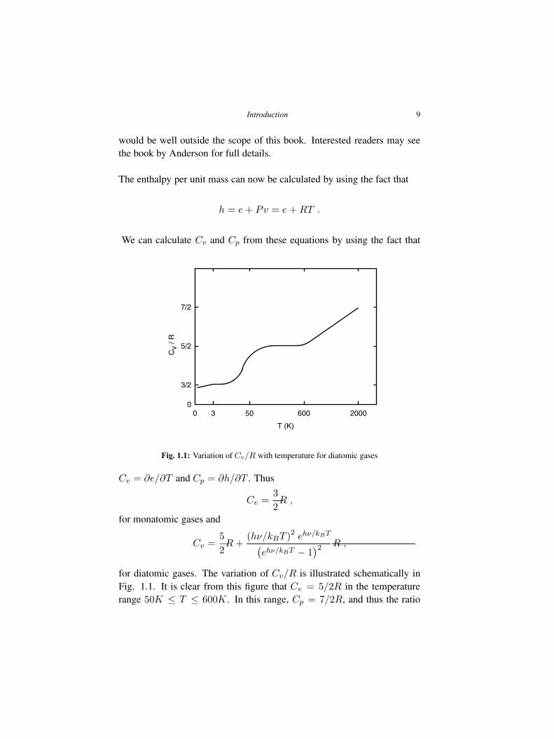
We can calculate Cv and Cp from these equations by using the fact that
T (K)
Cv
/ R
0 3 50 600 20000
3/2
5/2
7/2
Fig. 1.1: Variation of Cv/R with temperature for diatomic gases
Cv = ∂e/∂T and Cp = ∂h/∂T . Thus
Cv =3
2R ,
for monatomic gases and
Cv =5
2R+
(hν/kBT )2 ehν/kBT
(
ehν/kBT − 1)2 R ,
for diatomic gases. The variation of Cv/R is illustrated schematically inFig. 1.1. It is clear from this figure that Cv = 5/2R in the temperaturerange 50K ≤ T ≤ 600K. In this range, Cp = 7/2R, and thus the ratio
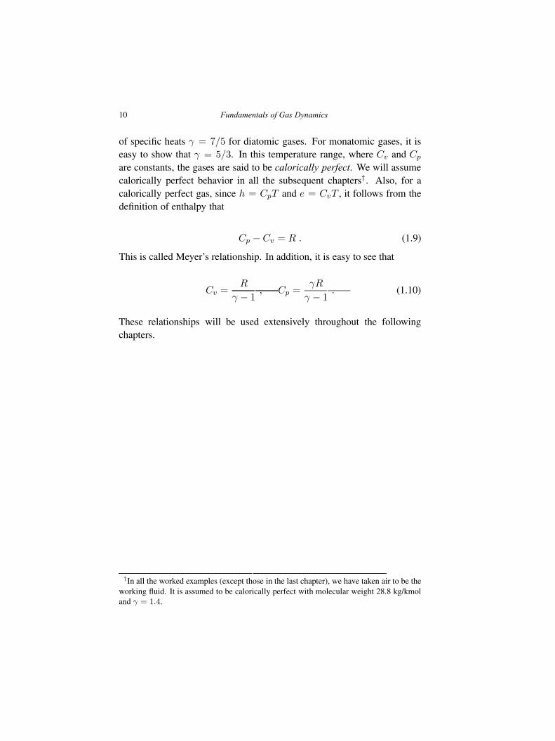
10 Fundamentals of Gas Dynamics
of specific heats γ = 7/5 for diatomic gases. For monatomic gases, it iseasy to show that γ = 5/3. In this temperature range, where Cv and Cp
are constants, the gases are said to be calorically perfect. We will assumecalorically perfect behavior in all the subsequent chapters†. Also, for acalorically perfect gas, since h = CpT and e = CvT , it follows from thedefinition of enthalpy that
Cp − Cv = R . (1.9)
This is called Meyer’s relationship. In addition, it is easy to see that
Cv =R
γ − 1, Cp =
γR
γ − 1. (1.10)
These relationships will be used extensively throughout the followingchapters.
†In all the worked examples (except those in the last chapter), we have taken air to be theworking fluid. It is assumed to be calorically perfect with molecular weight 28.8 kg/kmoland γ = 1.4.
Chapter 2
One Dimensional Flows - Basics
In this chapter, we discuss some fundamental concepts in the study ofcompressible flows. Throughout this book, we assume the flow to beone dimensional or quasi one dimensional. A flow is said to be onedimensional, if the flow properties change only along the flow direction.The fluid can have velocity either along the flow direction or bothalong and perpendicular to it. Oblique shock waves and Prandtl Meyerexpansion/compression waves discussed in later chapters are examples ofthe latter. We begin with a discussion of one dimensional flows whichbelong to the former category i.e., with velocity along the flow directiononly.
2.1 Governing Equations
The governing equations for frictionless, adiabatic, steady, one dimen-sional flow of a calorically perfect gas can be written in differential formas
d(ρu) = 0 , (2.1)
dP + ρudu = 0 , (2.2)
and
dh+ d
(
u2
2
)
= 0 . (2.3)
These equations express mass, momentum and energy conservation respec-tively. In addition, changes in flow properties must also obey the second
11
Fundamentals of Gas Dynamics, Second Edition. V. Babu.© 2015 V. Babu. Published 2015 by Athena Academic Ltd and John Wiley & Sons Ltd
12 Fundamentals of Gas Dynamics
law of thermodynamics. Thus,
ds ≥(
δq
T
)
rev
, (2.4)
where s is the entropy per unit mass and q is the heat interaction, alsoexpressed on a per unit mass basis. The subscript refers to a reversibleprocess. From the first law of thermodynamics, we have
de = CvdT = δqrev − Pdv . (2.5)
Since δqrev = Tds from Eqn. 2.4, and using the equation of statePv = RT , and its differential form Pdv + vdP = RdT , we can write
ds = CvdT
T+R
dv
v= Cv
dP
P+ Cp
dv
v= Cp
dT
T−R
dP
P. (2.6)
Note that Eqn. 2.2 is written in the so-called non-conservative form. Byusing Eqn. 2.1, we can rewrite Eqn. 2.2 in conservative form as follows.
dP + d(
ρu2)
= 0 . (2.7)
Equations 2.1,2.7, 2.3 and 2.4 can be integrated between any two points inthe flow field to give
ρ1u1 = ρ2u2 , (2.8)
P1 + ρ1u21 = P2 + ρ2u
22 , (2.9)
h1 +u212
= h2 +u222
, (2.10)
and
s2 − s1 =
∫ 2
1
δq
T+ σirr . (2.11)
Here, σirr represents entropy generated due to irreversibilities. It is equal
One Dimensional Flows - Basics 13
to zero for an isentropic flow and is greater than zero for all other flows.It follows then from Eqn. 2.11 that entropy change during an adiabaticprocess must increase or remain the same. The latter process, which isadiabatic and reversible is known as an isentropic process. It is importantto realize that while all adiabatic and reversible processes are isentropic,the converse need not be true. This can be seen from Eqn. 2.11, sincewith the removal of appropriate amount of heat, the entropy increase dueto irreversibilities can be offset entirely (at least in principle), therebyrendering an irreversible process isentropic. Equation 2.11 is not in aconvenient form for evaluating entropy change during a process. For thispurpose, we can integrate Eqn. 2.6 from the initial to the final state duringthe process. This gives,
s2 − s1 = Cv lnT2
T1+R ln
v2v1
= Cv lnP2
P1+ Cp ln
v2v1
(2.12)
= Cp lnT2
T1−R ln
P2
P1.
The flow area does not appear in any of the above equations as they stand.When we discuss one dimensional flow in ducts and passages, this canbe introduced quite easily. Also, it is important to keep in mind that, whenpoints 1 and 2 are located across a wave (say, a sound wave or shock wave),the derivatives of the flow properties will be discontinuous.
2.2 Acoustic Wave Propagation Speed
Equations 2.8, 2.9, 2.10 and 2.12 admit different solutions, which we willsee in the subsequent chapters. The most basic solution is the expressionfor the speed of sound, which we will derive in this section.
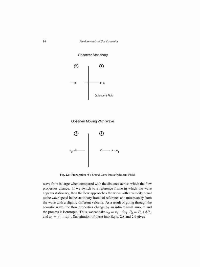
Consider an acoustic wave propagating into quiescent air as shown in Fig.2.1. Although the wave front is spherical, at any point on the wave front,the flow is essentially one dimensional as the radius of curvature of the
14 Fundamentals of Gas Dynamics
Observer Stationary
a
Quiescent Fluid
12
Observer Moving With Wave
a = u1
u2
12
Fig. 2.1: Propagation of a Sound Wave into a Quiescent Fluid
wave front is large when compared with the distance across which the flowproperties change. If we switch to a reference frame in which the waveappears stationary, then the flow approaches the wave with a velocity equalto the wave speed in the stationary frame of reference and moves away fromthe wave with a slightly different velocity. As a result of going through theacoustic wave, the flow properties change by an infinitesimal amount andthe process is isentropic. Thus, we can take u2 = u1+du1, P2 = P1+dP1,and ρ2 = ρ1 + dρ1. Substitution of these into Eqns. 2.8 and 2.9 gives
One Dimensional Flows - Basics 15
ρ1u1 = (ρ1 + dρ1) (u1 + du1) ,
and
P1 + ρ1u21 = P1 + dP1 + (ρ1 + dρ1) (u1 + du1)
2 .
If we neglect the product of differential terms, then we can write
ρ1du1 + u1dρ1 = 0 ,
and
dP1 + 2ρ1u1du1 + u21dρ1 = 0 .
Upon combining these two equations, we get
dP1
dρ1= u21 .
As mentioned earlier, u1 is equal to the speed of sound a and so
a =
√
(
dP
dρ
)
s
, (2.13)
where the subscript 1 has been dropped for convenience. Furthermore,we have also explicitly indicated that the process is isentropic. Since theprocess is isentropic, ds = 0, and so from Eqn. 2.6,
CvdP
P+Cp
dv
v= 0 .
Since ρ = 1/v, dv/v = −dρ/ρ and so
dP
dρ=
Cp
Cv
P
ρ= γRT .
16 Fundamentals of Gas Dynamics
Thus,
a =√
γRT . (2.14)
This expression is valid for a non-reacting mixture of ideal gases as well,with the understanding that γ is the ratio of specific heats for the mixtureand R is the particular gas constant for the mixture†.
2.2.1 Mach Number
The Mach number has already been defined in Eqn. 1.3 and we are now ina position to take a closer look at it. Since it is defined as a ratio, changesin the Mach number are the outcome of either changes in velocity, speedof sound or both. Speed of sound itself varies from point to point and isproportional to the square root of the temperature as seen from Eqn. 2.14.Thus, any deductions of the velocity or temperature variation from a givenvariation of Mach number cannot be made in a straightforward manner.For example, the velocity at the entry to the combustor in an aircraft gasturbine engine may be as high as 200 m/s, but the Mach number is usually0.3 or less due to the high static temperature of the fluid.
2.3 Reference States
In the study of compressible flows and indeed in fluid mechanics, it isconventional to define certain reference states. These allow the governingequations to be simplified and written in dimensionless form so that the
†Equation 2.14 is not valid for a reacting flow, since chemical reactions are by natureirreversible and hence the process across the sound wave cannot be isentropic. However,two limiting conditions can be envisaged and the speed of sound corresponding to theseconditions can still be evaluated using Eqn. 2.14. These are the frozen and equilibriumconditions. In the former case, the reactions are assumed to be frozen and hence the mixtureis essentially non-reacting. The speed of sound for this mixture can be calculated usingEqn. 2.14 appropriately. In the latter case, reactions are still taking place but the mixtureis at chemical equilibrium and hence ds = 0. Once the equilibrium composition andtemperature are known, speed of sound for the equilibrium mixture can be determined,again using Eqn. 2.14. In reality, the reactions neither have to be frozen nor do they have tobe at equilibrium. These are simply two limiting situations, which allow us to get a boundof the speed of sound for the actual case.
One Dimensional Flows - Basics 17
important parameters can be identified. In the context of compressibleflows, the solution procedure can also be made simpler and in additionthe important physics in the flow can be brought out clearly by the use ofthese reference states. Two such reference states are discussed next.
2.3.1 Sonic State
Since the speed of sound plays a crucial role in compressible flows, it isconvenient to use the sonic state as a reference state. The sonic state is thestate of the fluid at that point in the flow field where the velocity is equal tothe speed of sound. Properties at the sonic state are usually denoted with a* viz., P ∗, T ∗, ρ∗ and so on. Of course, u∗ itself is equal to a and so theMach number M = 1 at the sonic state. The sonic reference state can bethought of as a global reference state since it is attained only at one or a fewpoints in the flow field. For example, in the case of choked isentropic flowthrough a nozzle, the sonic state is achieved in the throat section. In someother cases, such as flow with heat addition or flow with friction, the sonicstate may not even be attained anywhere in the actual flow field, but is stilldefined in a hypothetical sense and is useful for analysis. The importanceof the sonic state lies in the fact that it separates subsonic (M < 1) andsupersonic (M > 1) regions of the flow. Since information travels in acompressible medium through acoustic waves, the sonic state separatesregions of flow that are fully accessible (subsonic) and those that are not(supersonic).
Note that the dimensionless velocity u/u∗ at a point is not equal to theMach number at that point since u∗ is not the speed of sound at that point‡.
2.3.2 Stagnation State
Let us consider a point in a one dimensional flow and assume that thestate at this point is completely known. This means that the pressure,temperature and velocity at this point are known. We now carry out athought experiment in which an isentropic, deceleration process takes thefluid from the present state to one with zero velocity. The resulting end
‡Except, of course, at the point where the sonic state occurs
18 Fundamentals of Gas Dynamics
state is called the stagnation state corresponding to the known initial state.Thus, the stagnation state at a point in the flow field is defined as thethermodynamic state that would be reached from the given state at thatpoint, at the end of an isentropic, deceleration process to zero velocity.Note that the stagnation state is a local state contrary to the sonic state.Hence, the stagnation state can change from one point to the next in theflow field. Also, it is important to note that the stagnation process alone isisentropic, and the flow need not be isentropic. Properties at the stagnationstate are usually indicated with a subscript 0 viz., P0, T0, ρ0 and so on.Here P0 is the stagnation pressure, T0 is the stagnation temperature andρ0 is the stagnation density. Hereafter, P and T will be referred to as thestatic pressure and static temperature and the corresponding state point willbe called the static state.
To derive the relationship between the static and stagnation states, we startby integrating Eqn. 2.3 between these two states. This gives,
∫ 0
1dh+
∫ 0
1d
(
u2
2
)
= 0 .
If we integrate this equation and rearrange, we get
h0 = h1 +u212
, (2.15)
after noting that the velocity is zero at the stagnation state. For a caloricallyperfect gas†, dh = CpdT and so
T0,1 − T1 =u212Cp
.
†Equation 2.15 can be used even when the gas is not calorically perfect. This happens, forinstance, when the temperatures encountered in a particular problem are outside the rangein which the calorically perfect assumption is valid. In such cases, either the enthalpy ofthe gas is available as a function of temperature in tabular form or Cp is available in theform of a polynomial in temperature (see for example, http://webbook.nist.gov).If the stagnation and static temperatures are known, then the velocity can be calculatedfrom Eqn. 2.15. On the other hand, if the static temperature and velocity are known, thenthe stagnation temperature has to be calculated either by tabular interpolation or iterativelystarting with a suitable initial guess.
One Dimensional Flows - Basics 19
After using Eqns. 1.10 and 2.12, we can finally write
T0
T= 1 +
γ − 1
2M2 , (2.16)
where the subscript for the static state has been dropped for convenience.Although the stagnation process is isentropic, this fact is not required forthe calculation of stagnation temperature.
Since the stagnation process is isentropic, the static and stagnation stateslie on the same isentrope. If we apply Eqn. 2.12 between the static andstagnation states and use the fact that s0 = s1, we get
P0,1
P1=
(
T0,1
T1
)
γγ − 1
.
If we substitute from Eqn. 2.16, we get
P0
P=
(
1 +γ − 1
2M2
)
γγ − 1
, (2.17)
where, the subscript denoting the static state has been dropped. Thisequation can be derived in an alternative way, in a manner similar to theone used for the derivation of the stagnation temperature. This is somewhatlonger but gives some interesting insights into the stagnation process. Westart by rewriting Eqn. 2.2 in the following form
dP
ρ+ d
(
u2
2
)
= 0 .
By substituting Eqn. 2.3, this can be simplified to read
dP
ρ− dh = 0 .
20 Fundamentals of Gas Dynamics
Integrating this between the static and stagnation states leads to∫ 0
1
dP
ρ−∫ 0
1dh = 0 .
Since the second term is a perfect differential, it can be integrated easily.The first term is not a perfect differential and so the integral depends on thepath used for the integration - in other words, the path connecting states 1and 0. Since this process is isentropic, from Eqn. 2.6 we can show that
CvdP
P+ Cp
dv
v= 0 ⇒ Pvγ = constant = P1v1
γ .
Thus, the above equation reduces to
∫ 0
1
P11/γ
ρ1
dP
P 1/γ= Cp(T0,1 − T1) ,
where we have invoked the calorically perfect gas assumption. With a littlebit of algebra, this can be easily shown to lead to Eqn. 2.17.
The stagnation density can be evaluated by using the equation of stateP0 = ρ0RT0. Thus
ρ0ρ
=
(
1 +γ − 1
2M2
) 1γ − 1
. (2.18)
This derivation brings out the fact that unlike the stagnation temperature,the nature of the stagnation process has to be known in order to evaluate thestagnation pressure. This, in itself, arises from the fact that Eqn. 2.2 is not aperfect differential. It would appear that we could have circumvented thisdifficulty by integrating Eqn. 2.7 instead, which is a perfect differential.This would have led to the following expression
P0,1 = P1 + ρ1u21 .
One Dimensional Flows - Basics 21
If we divide through by P1 and use the fact that P1 = ρ1RT anda1 =
√γRT1, we get
P0
P= 1 + γM2 .
This expression for stagnation pressure is disconcertingly (and erro-neously!) quite different from Eqn. 2.17. The inconsistency arises dueto the use of the continuity equation while deriving Eqn. 2.7. Continuityequation 2.1 is not applicable during the stagnation process, as otherwiseρ0 → ∞ as u → 0. Hence, Eqn. 2.7 is not applicable for the stagnationprocess.
Another important fact about stagnation quantities is that they depend onthe frame of reference unlike static quantities which are frame independent.This is best illustrated through a numerical example.
Example 2.1. Consider the propagation of sound wave into quiescent airat 300 K and 100 kPa. With reference to Fig. 2.1, determine T0,1 and P0,1
in the stationary and moving frames of reference.
Solution. In the stationary frame of reference, u1 = 0 and so, T0,1 = T1
= 300 K and P0,1 = P1 = 100 kPa.
In the moving frame of reference, u1 = a1 and so M1 = 1. Substitutingthis into Eqns. 2.16 and 2.17, we get T0,1 = 360 K and P0,1 = 189 kPa �.
The difference between the values evaluated in different frames becomesmore pronounced at higher Mach numbers.
As already mentioned, stagnation temperature and pressure are localquantities and so they can change from one point to another in the flowfield. Changes in stagnation temperature can be achieved by the additionor removal of heat or work†. Heat addition increases the stagnation†In such cases, the energy equation has to be modified suitably. For example Eqn. 2.3
will read as
22 Fundamentals of Gas Dynamics
temperature, while removal of heat results in a decrease in stagnationtemperature. Changes in stagnation pressure are brought about by workinteraction or irreversibilities. Across a compressor where work is done onthe flow, stagnation pressure increases while across a turbine where workis extracted from the fluid, stagnation pressure decreases. It is for thisreason, that any loss of stagnation pressure in the flow is undesirable asit is tantamount to a loss of work. To see the effect of irreversibilities, westart with the last equality in Eqn. 2.12 and substitute for T2/T1 and P2/P1
as follows:
T2
T1=
T2
T0,2
T0,2
T0,1
T0,1
T1,
andP2
P1=
P2
P0,2
P0,2
P0,1
P0,1
P1.
From Eqn. 2.12
s2 − s1 = R ln
(
T2
T1
)
γγ − 1
/
(
P2
P1
)
.
If we use Eqns. 2.16 and 2.17, we get
s2 − s1 = Cp lnT0,2
T0,1−R ln
P0,2
P0,1. (2.19)
This equation shows that irreversibilities in an adiabatic flow lead to a lossof stagnation pressure, since, for such a flow, s2 > s1 and T0,2 = T0,1
dh+ d
(
u2
2
)
= δq − δw ,
and Eqn. 2.10 will read as
h1 +u2
1
2= h2 +
u2
2
2−Q+W ,
where q (and Q) and w(and W ) refer to the heat and work interaction per unit mass. Wehave also used the customary sign convention from thermodynamics i.e., that heat added toa system is positive and work done by a system is positive.
One Dimensional Flows - Basics 23
and so P0,2 < P0,1. This equation also shows that heat addition in acompressible flow is always accompanied by a loss of stagnation pressure.Since, T0,2 > T0,1 in this case, and s2 > s1, P0,2 has to be less than P0,1.These facts are important in the design of combustors and will be discussedlater. This equation also shows that increase or decrease of stagnationpressure brought about through work interaction leads to a correspondingchange in the stagnation temperature.
2.4 T-s and P-v Diagrams in Compressible Flows
T-s and P-v diagrams are familiar to most of the readers from theirbasic thermodynamics course. These diagrams are extremely useful inillustrating states and processes graphically. Both of these diagramsdisplay the same information, since the thermodynamic state is fully fixedby the specification of two properties, either P, v or T, s. Nevertheless,they are both useful as some processes can be depicted better in one thanthe other.
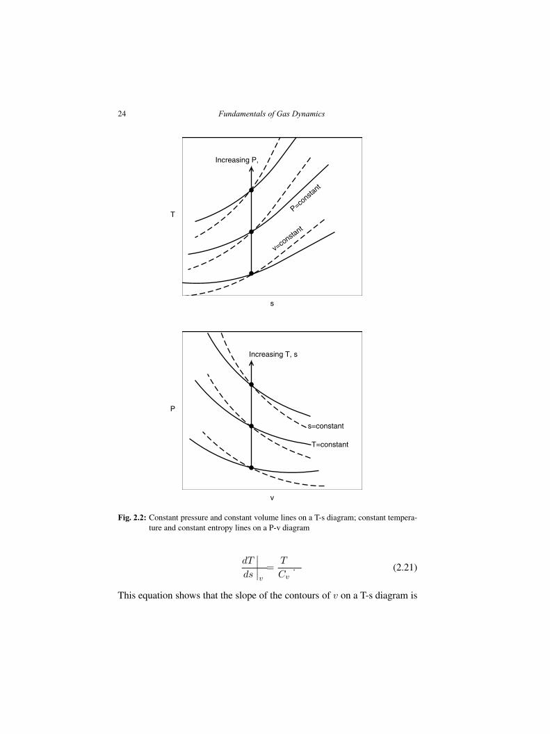
Let us review some basic concepts from thermodynamics in relation to T-sand P-v diagrams. Figure 2.2 shows thermodynamic states (filled circles)and contours of P, v (isobars and isochors) and contours of T, s (isothermsand isentropes). From the first equality in Eqn. 2.6, we can write,
dv =v
Rds− Cv
v
RTdT . (2.20)
From this equation, it is easy to see that, as we move along a s = constant
line in the direction of increasing temperature, v decreases, since, dv =
−(Cv/P )dT , along such a line. Also, the change in v for a given changein T is higher at lower values of pressure than at higher values of pressure.This fact is of tremendous importance in compressible flows as we will seelater.
Since dv = 0 along a v = constant contour, from the above equation,
24 Fundamentals of Gas Dynamics
v
P
T=constant
s=constant
Increasing T, s
s
TP=co
nstant
v=co
nstant
Increasing P, ρ
Fig. 2.2: Constant pressure and constant volume lines on a T-s diagram; constant tempera-ture and constant entropy lines on a P-v diagram
dT
ds
∣
∣
∣
∣
v
=T
Cv. (2.21)
This equation shows that the slope of the contours of v on a T-s diagram is
One Dimensional Flows - Basics 25
always positive and is not a constant. Hence, the contours are not straightlines. Furthermore, the slope increases with increasing temperature and sothe contours are shallow at low temperatures and become steeper at highertemperatures.
Similarly, from the third equality in Eqn. 2.6, it can be shown that
dT
ds
∣
∣
∣
∣
P
=T
Cp, (2.22)
for any isobar. The same observation made above regarding the slope ofthe contours of v on a T-s diagram are applicable to isobars as well. Inaddition, since Cp > Cv, at any state point, isochors are steeper thanisobars on a T-s diagram and pressure increases along a s = constant linein the direction of increasing temperature. These observations regardingisochors and isobars are shown in Fig. 2.2.
From the second equality in Eqn. 2.6, the equation for isentropes on aP-v diagram can be obtained after setting ds = 0. Thus
dP
dv
∣
∣
∣
∣
s
= − Cp
Cv
P
v. (2.23)
By equating the second and the last term in Eqn. 2.6, we get
CvdT
T+R
dv
v= Cp
dT
T−R
dP
P.
This can be rearranged to give (after setting dT = 0)
dP
dv
∣
∣
∣
∣
T
= − P
v. (2.24)
This equation shows that isotherms also have a negative slope on a P-vdiagram and they are less steep than isentropes (Fig. 2.2). Furthermore, sand T increase with increasing pressure as we move along a v = constant
26 Fundamentals of Gas Dynamics
v
P
1’
0,1P0,1
T=T0,1
T=T1
s=s1
T=T**
1P1
M<1
M>1
s
T
T0,1
T*
T1
M=1
M<1
M>1
0,1 P0,1
1
*
u21
/ 2CpP1
1’ P1’
s1
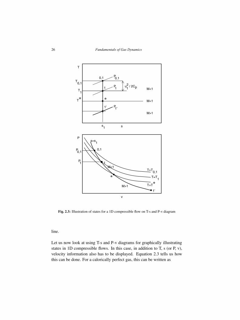
Fig. 2.3: Illustration of states for a 1D compressible flow on T-s and P-v diagram
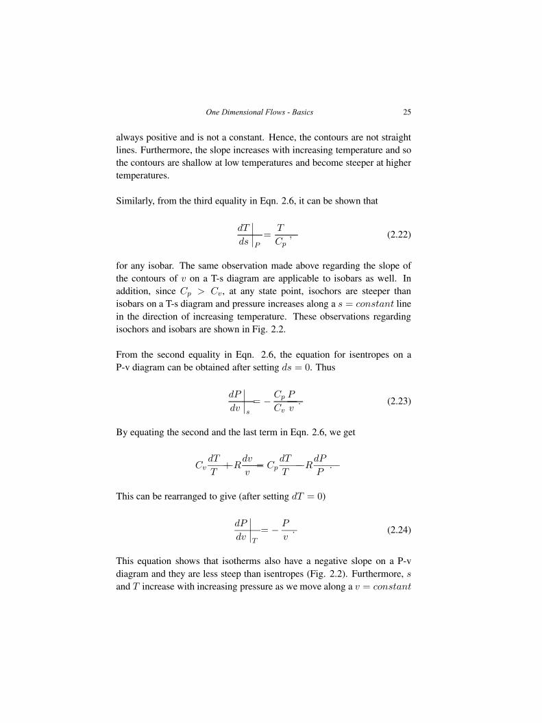
line.
Let us now look at using T-s and P-v diagrams for graphically illustratingstates in 1D compressible flows. In this case, in addition to T, s (or P, v),velocity information also has to be displayed. Equation 2.3 tells us howthis can be done. For a calorically perfect gas, this can be written as
One Dimensional Flows - Basics 27
d
(
T +u2
2Cp
)
= 0 .
Hence, at each state point, the static temperature is depicted as usual, andthe quantity u2/2Cp is added to the ordinate (in case of a T-s diagram).Note that this quantity has units of temperature and the sum T + u2/2Cp
is equal to the stagnation temperature T0 corresponding to this state. Thisis shown in Fig. 2.3 for the subsonic state point marked 1. Also shown inthis figure is the sonic state corresponding to this state. Once T0 is knownT ∗ can be evaluated from Eqn. 2.16 by setting M = 1. Thus
T0
T ∗=
γ + 1
2.
Depicting the sonic state is useful since it tells at a glance whether the flowis subsonic or supersonic. All subsonic states will lie above the sonic stateand all supersonic states will lie below. State point 1′ shown in Fig. 2.3 isa supersonic state. This figure also shows that the stagnation process (1-0or 1′-0) is an isentropic process. All this information is shown in Fig. 2.3on T-s as well as P-v diagram. Although it is conventional to show only T-sdiagram in compressible flows, P-v diagrams are very useful when dealingwith waves (for instance, shock waves and combustion waves). With thisin mind, both the diagrams are presented side by side throughout, to allowthe reader to become familiar with them.
28 Fundamentals of Gas Dynamics
Exercises
(1) Air enters the diffuser of an aircraft jet engine at a static pressure of20 kPa and static temperature 217 K and a Mach number of 0.9. Theair leaves the diffuser with a velocity of 85 m/s. Assuming isentropicoperation, determine the exit static temperature and pressure.[249 K, 32 kPa]
(2) Air is compressed adiabatically in a compressor from a static pressureof 100 kPa to 2000 kPa. If the static temperature of the air at the inletand exit of the compressor are 300 K and 800 K, determine the powerrequired per unit mass flow rate of air. Also, determine whether thecompression process is isentropic or not.[503 kW, Not isentropic]
(3) Air enters a turbine at a static pressure of 2 MPa, 1400 K. It expandsisentropically in the turbine to a pressure of 500 kPa. Determine thework developed by the turbine per unit mass flow rate of air and thestatic temperature at the exit.[460 kW, 942 K]
(4) Air at 100 kPa, 295 K and moving at 710 m/s is decelerated isentrop-ically to 250 m/s. Determine the final static temperature and staticpressure.[515 K, 702 kPa]
(5) Air enters a combustion chamber at 150 kPa, 300 K and 75 m/s.Heat addition in the combustion chamber amounts to 900 kJ/kg. Airleaves the combustion chamber at 110 kPa and 1128 K. Determine thestagnation temperature, stagnation pressure and velocity at the exit andthe entropy change across the combustion chamber.[1198 K, 136 kPa, 376 m/s, 1420 J/kg.K]
(6) Air at 900 K and negligible velocity enters the nozzle of an aircraft jetengine. If the flow is sonic at the nozzle exit, determine the exit statictemperature and velocity. Assume adiabatic operation.
One Dimensional Flows - Basics 29
[750 K, 549 m/s]
(7) Air expands isentropically in a rocket nozzle from P0 = 3.5 MPa, T0 =2700 K to an ambient pressure of 100 kPa. Determine the exit velocity,Mach number and static temperature.[1860 m/s, 2.97, 978 K]
(8) Consider the capture streamtube of an aircraft engine cruising at Mach0.8 at an altitude of 10 km. The capture mass flow rate is 250 kg/s. Atstation 1, which is in the freestream, the static pressure and temperatureare 26.5 kPa and 223 K respectively. At station 2, which is downstreamof station 1, the cross-sectional area is 3 m2. Further downstream atstation 3, the Mach number is 0.4. Determine (a) the cross-sectionalarea at station 1 (usually called the capture area), (b) the Mach numberat station 2, (c) the static pressure and temperature at stations 2 and 3and (d) the cross-sectional at station 3.[a) 2.5213 m2 b) 0.5635 c) Station2: 32.9 kPa, 236.52 K, Station3:36.496 kPa, 243.74 K d) 3.8258 m2]
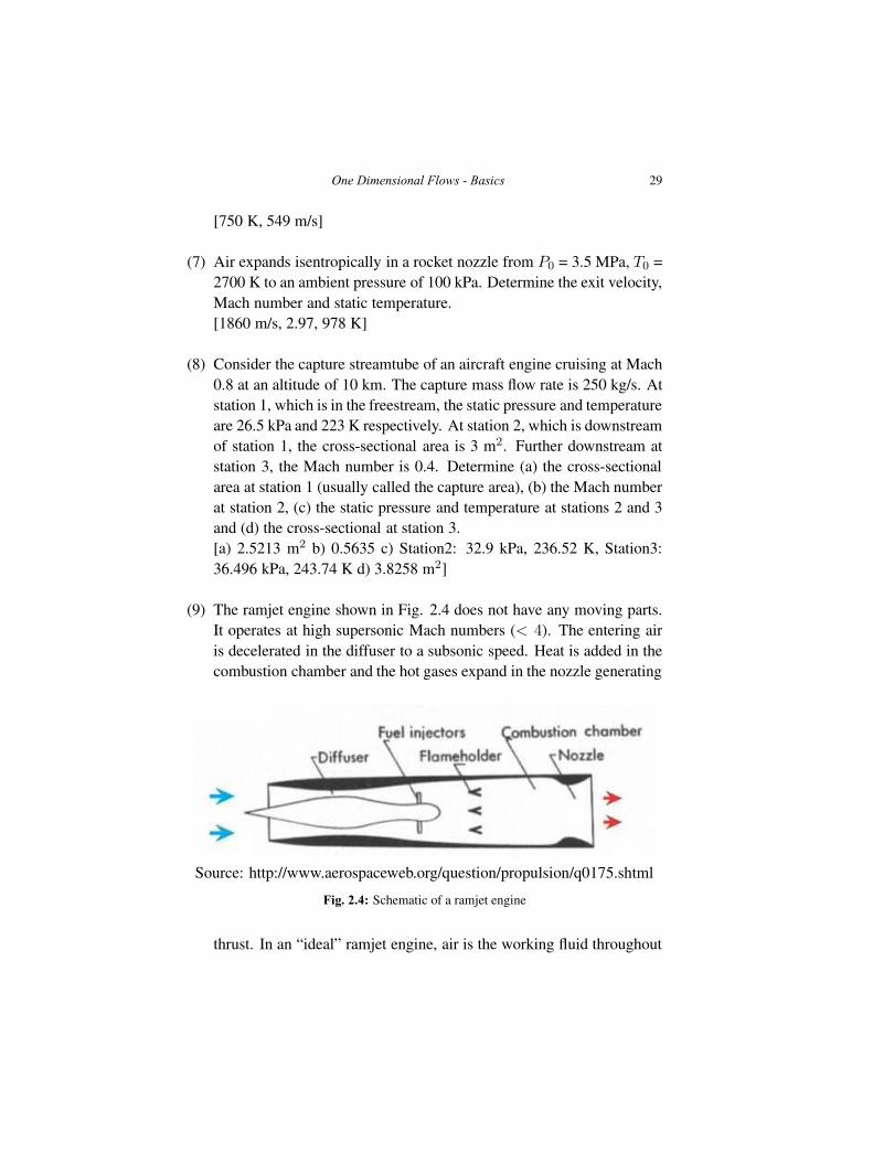
(9) The ramjet engine shown in Fig. 2.4 does not have any moving parts.It operates at high supersonic Mach numbers (< 4). The entering airis decelerated in the diffuser to a subsonic speed. Heat is added in thecombustion chamber and the hot gases expand in the nozzle generating
Source: http://www.aerospaceweb.org/question/propulsion/q0175.shtml
Fig. 2.4: Schematic of a ramjet engine
thrust. In an “ideal” ramjet engine, air is the working fluid throughout
30 Fundamentals of Gas Dynamics
and the compression, expansion processes are isentropic. In addition,there is no loss of stagnation pressure due to the heat addition. The airis expanded in the nozzle to the ambient pressure. Show that the Machnumber of the air as it leaves the nozzle is the same as the Mach numberof the air when it enters the diffuser. Sketch the process undergone bythe air on T-s and P-v diagrams.
Chapter 3
Normal Shock Waves
Normal shock waves are compression waves that are seen in nozzles,turbomachinery blade passages and shock tubes, to name a few. In thefirst two examples, normal shock usually occurs under off-design operatingconditions or during start-up. The compression process across the shockwave is highly irreversible and so it is undesirable in such cases. In the lastexample, normal shock is designed to achieve extremely fast compressionand heating of a gas with the aim of studying highly transient phenomena.Normal shocks are seen in external flows also. The term “normal” is usedto denote the fact that the shock wave is normal (perpendicular) to the flowdirection, before and after passage through the shock wave. This latterfact implies that there is no change in flow direction as a result of passingthrough the shock wave. In this chapter, we take a detailed look at thethermodynamic and flow aspects of normal shock waves.
3.1 Governing Equations
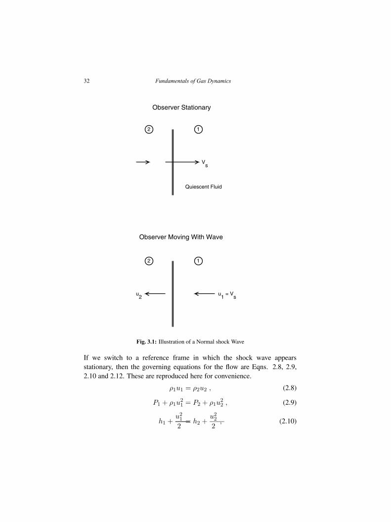
Figure 3.1 shows a normal shock wave propagating into quiescent air. Theshock speed in the laboratory frame of reference is denoted as Vs. Thisfigure is almost identical to Fig. 2.1, where the propagation of an acousticwave is shown. The main differences are: (1) an acoustic wave travels withthe speed of sound, whereas a normal shock travels at supersonic speedsand (2) the changes in properties across an acoustic wave are infinitesimaland isentropic, whereas they are large and irreversible across a normalshock wave.
31
Fundamentals of Gas Dynamics, Second Edition. V. Babu.© 2015 V. Babu. Published 2015 by Athena Academic Ltd and John Wiley & Sons Ltd
32 Fundamentals of Gas Dynamics
Observer Stationary
Vs
Quiescent Fluid
12
Observer Moving With Wave
u1 = V
su2
12
Fig. 3.1: Illustration of a Normal shock Wave
If we switch to a reference frame in which the shock wave appearsstationary, then the governing equations for the flow are Eqns. 2.8, 2.9,2.10 and 2.12. These are reproduced here for convenience.
ρ1u1 = ρ2u2 , (2.8)
P1 + ρ1u21 = P2 + ρ1u
22 , (2.9)
h1 +u212
= h2 +u222
, (2.10)
Normal Shock Waves 33
s2 − s1 = Cv lnT2
T1+R ln
v2v1
= Cv lnP2
P1+ Cp ln
v2v1
(2.12)
= Cp lnT2
T1−R ln
P2
P1.
It can be seen from the energy equation that the stagnation temperature isconstant across the shock wave, as there is no heat addition or removal.
3.2 Mathematical Derivation of the Normal Shock Solution
The continuity equation above can be written as
P2
P1=
√
T2
T1
M1
M2, (3.1)
after using the fact that u = M√γRT and ρ = P/RT . Similarly, we can
get from the momentum equation,
P2
P1=
1 + γM21
1 + γM22
, (3.2)
andT2
T1=
(
1 +γ − 1
2M2
1
)
/
(
1 +γ − 1
2M2
2
)
(3.3)
from the energy equation. Combining these three equations, we get
1 + γ − 12 M2
1
1 +γ − 12 M2
2
=M2
2
M21
(
1 + γM21
1 + γM22
)2
.
This is a quadratic equation in M22 . Given M1, we can solve this equation
to get M2. With M2 known, all the other properties at state 2 can be
34 Fundamentals of Gas Dynamics
evaluated. This equation has only one meaningful solution, namely,
M22 =
2 + (γ − 1)M21
2γM21 − (γ − 1)
. (3.4)
The other solutions are either trivial (M2 = M1) or imaginary. Note that,if we set M1 = 1 in Eqn. 3.4 we get M2 = 1, which is, of course, thesolution corresponding to an acoustic wave. Also, a simple rearrangementof the expression in Eqn. 3.4 shows that
M22 = 1− γ + 1
2γ
M21 − 1
M21 − 1 +
γ + 12γ
. (3.5)
Hence, if M1 > 1, then M2 < 1 and vice versa. Thus, both thecompressive solution M1 > 1,M2 < 1 and the expansion solution M1 <
1,M2 > 1 are allowed by the above equation. We must examine whetherthey are allowed based on entropy considerations. Since the process isadiabatic and irreversible, entropy has to increase across the shock wave.From Eqn. 2.12, the entropy change across the shock wave is given as
s2 − s1 = Cp lnT2
T1−R ln
P2
P1.
Upon substituting the relations obtained above for T2/T1 and P2/P1, weget
s2 − s1 = Cp lnM2
2
M21
(
1 + γM21
1 + γM22
)2
−R ln1 + γM2
1
1 + γM22
.
This can be simplified to read
s2 − s1 = Cp lnM2
2
M21
+Rγ + 1
γ − 1ln
1 + γM21
1 + γM22
.
Substituting for M2 from Eqn. 3.4, we get (after some tedious algebra!)
s2 − s1R
=1
γ − 1ln
[
2γM21 − γ + 1
γ + 1
]
+γ
γ − 1ln
[
2 + (γ − 1)M21
(γ + 1)M21
]
.
Normal Shock Waves 35
With a slight rearrangement, this becomes
s2 − s1R
=1
γ − 1ln
[
1 +2γ
γ + 1(M2
1 − 1)
]
+γ
γ − 1ln
[
1− 2
γ + 1
(
1− 1
M21
)]
.
It is clear from this expression that entropy across the shock wave increaseswhen M1 > 1 and decreases when M1 < 1. Thus, for a normal shock, M1
is always greater than one and M2 is always less than one.
The static pressure and temperature can be seen to increase across theshock wave from Eqns. 3.2 and 3.3. Furthermore, from Eqn. 3.1, it can beinferred that P2/P1 > T2/T1. It follows from this that
ρ2ρ1
=
(
P2
P1
)
/
(
T2
T1
)
> 1 . (3.6)
Of course, due to the irreversibility associated with the shock, there is aloss of stagnation pressure. From Eqn. 2.19, it is easy to show that
s2 − s1 = R lnP0,1
P0,2.
Thus, the stronger† the shock or higher the initial Mach number, the morethe loss of stagnation pressure.
From Eqn. 3.5, we get
M22 = 1− 6
7
M21 − 1
M21 − 1
7
for diatomic gases for which γ = 7/5 and
M22 = 1− 3
5
M21 − 1
M21 − 2
5
†Strength of a shock is usually defined as P2
P1
− 1.
36 Fundamentals of Gas Dynamics
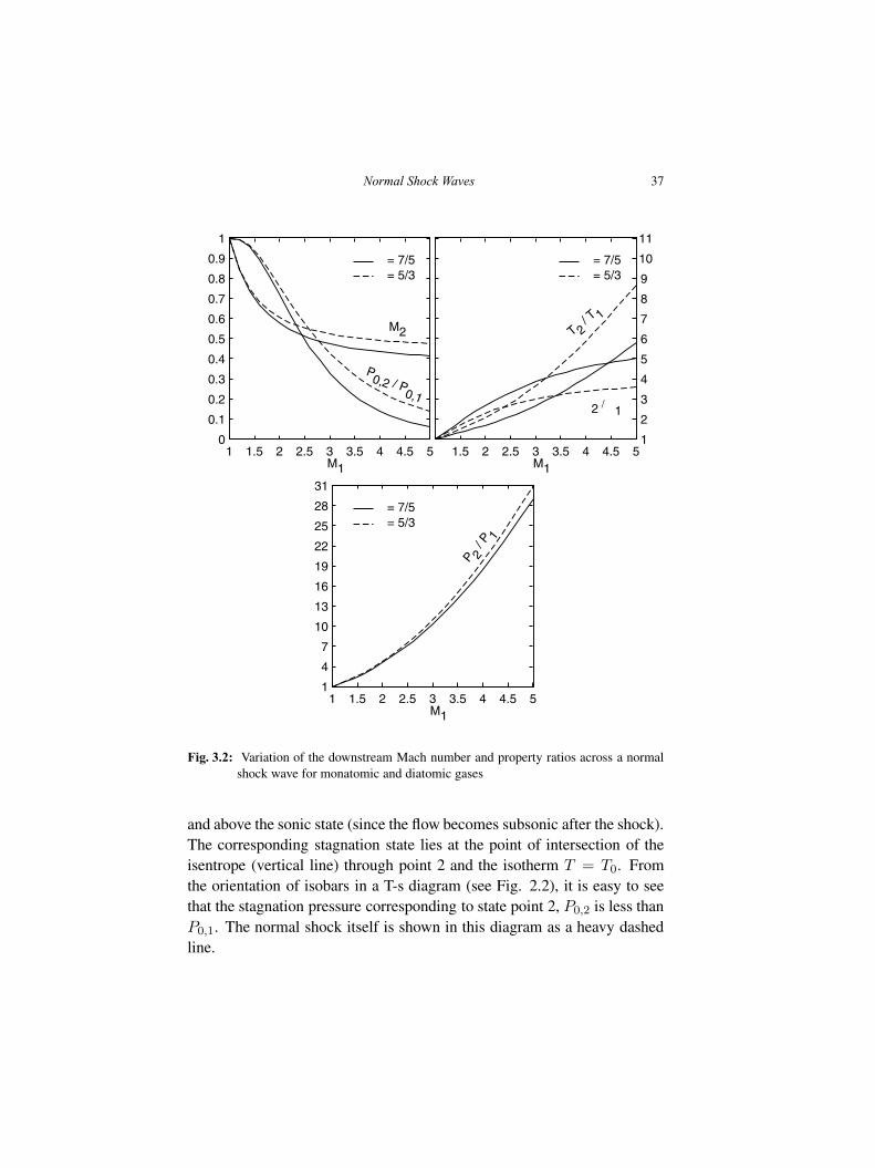
for monatomic gases for which γ = 5/3. A comparison of these twoexpressions suggests that, for a given M1, M2 is higher for monatomicgases than diatomic gases. However, the strength of the shock as wellas the temperature rise at a given M1 is higher in the case of the former.This explains why monatomic gases are used extensively in shock tubes.Equations 3.4, 3.2, 3.3, 3.6 as well as the ratio P0,2/P0,1 are plotted in Fig.3.2 for monatomic and diatomic gases.
In the limiting case when M1 = 1, it is easy to see that the process isisentropic (as it should be, since it corresponds to the propagation of anacoustic wave ). Also, M2 = 1, T2/T1 = 1, P2/P1 = 1 and ρ2/ρ1 = 1 fromEqns. 3.5, 3.3, 3.2 and 3.6.
If we let M1 → ∞ in Eqn. 3.5, then we have
M2 =
√
γ − 1
2γ
P2
P1→ ∞
T2
T1→ ∞
ρ2ρ1
=γ + 1
γ − 1
These trends can be clearly seen in Fig. 3.2.
3.3 Illustration of the Normal Shock Solution on T-s and P-v diagrams
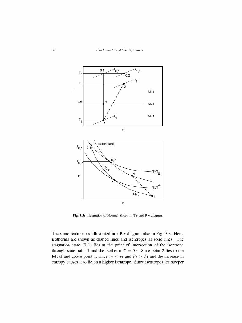
In this section, we will try to draw some insight into the normal shockcompression process through graphical illustrations on the T-s and P-vdiagrams. Figure 3.3 shows the T-s and P-v diagram for the normalshock process. The static (P1, T1), stagnation (P0,1, T0) and sonic state(*) corresponding to state 1 are shown in this figure. State point 2 lies tothe right of state point 1 (owing to the increase in entropy across the shock)
Normal Shock Waves 37
M1
M2
P0,2 / P
0,1
γ = 7/5γ = 5/3
1 1.5 2 2.5 3 3.5 4 4.5 50
0.1
0.2
0.3
0.4
0.5
0.6
0.7
0.8
0.9
1
M1
T 2 / T
1
γ = 7/5
ρ2 / ρ
1
γ = 5/3
1.5 2 2.5 3 3.5 4 4.5 51
2
3
4
5
6
7
8
9
10
11
M1
P 2 /
P 1γ = 7/5γ = 5/3
1 1.5 2 2.5 3 3.5 4 4.5 51
4
7
10
13
16
19
22
25
28
31
Fig. 3.2: Variation of the downstream Mach number and property ratios across a normalshock wave for monatomic and diatomic gases
and above the sonic state (since the flow becomes subsonic after the shock).The corresponding stagnation state lies at the point of intersection of theisentrope (vertical line) through point 2 and the isotherm T = T0. Fromthe orientation of isobars in a T-s diagram (see Fig. 2.2), it is easy to seethat the stagnation pressure corresponding to state point 2, P0,2 is less thanP0,1. The normal shock itself is shown in this diagram as a heavy dashedline.
38 Fundamentals of Gas Dynamics
s
T
T0
M=1
M<1
M>1
0,1 P0,1
T* *
1
P1T
1
2
P2T
2
P0,2
0,2
v
P
1
0,1P0,1
T=T0
s=constant
T=T**
M<1
M>1
2
0,2P0,2
Fig. 3.3: Illustration of Normal Shock in T-s and P-v diagram
The same features are illustrated in a P-v diagram also in Fig. 3.3. Here,isotherms are shown as dashed lines and isentropes as solid lines. Thestagnation state (0, 1) lies at the point of intersection of the isentropethrough state point 1 and the isotherm T = T0. State point 2 lies to theleft of and above point 1, since v2 < v1 and P2 > P1 and the increase inentropy causes it to lie on a higher isentrope. Since isentropes are steeper
Normal Shock Waves 39
than isotherms, the isotherm T = T0 intersects this isentrope at a lowervalue of pressure and so P0,2 < P0,1.
It can also be seen from this diagram that, for given values of v2, v1and P1, normal shock compression results in a higher value for P2 thanisentropic compression albeit with a loss of stagnation pressure. In otherwords, normal shock compression is more effective but less efficient thanisentropic compression. The former attribute is of importance in intakes ofsupersonic vehicles, since it determines the length of the intake. However,the latter attribute is also important and so an optimal operating conditionhas to be determined. An inspection of Fig. 3.2 reveals that the loss ofstagnation pressure is about 20% for M1 = 2 and about 70% for M1 = 3.This suggests that compression using normal shocks is both effective andreasonably efficient for M1 ≤ 2. Accordingly, in supersonic intakes, theflow is decelerated to this value using other means and the compressionprocess is terminated using a normal shock.
Example 3.1. Consider a normal shock wave that moves with a speedof 696 m/s into still air at 100 kPa and 300 K. Determine the static andstagnation properties ahead of and behind the shock wave in stationary andmoving frames of reference.
Solution. In a moving frame of reference in which the shock is stationary(observer moving with shock),
P1 = 100kPa, T1 = 300K, u1 = 696m/s
a1 =√
γRT1 =√1.4× 288 × 300 = 348m/s
M1 = 2, T0,1 = 540K, P0,1 = 782.4kPa
We can use Eqn. 3.4 to evaluate M2 or use the gas tables. The latter choiceallows us to look up pressure ratio, temperature ratio and other ratios, inone go. For M1 = 2, from normal shock table, we get
40 Fundamentals of Gas Dynamics
Observer Stationary
696 m/s
T = 300 K
P = 100 kPa
T0 = 300 K
P0 = 100 kPa
T = 506 K
P = 450 kPa
T0 = 600 K
P0 = 817 kPa
435.2 m/s
12
Observer Moving
T = 300 K
P = 100 kPa
T0 = 540 K
P0 = 782.4 kPa
696 m/s
T = 506 K
P = 450 kPa
T0 = 540 K
P0 = 564 kPa
260.8 m/s
12
Fig. 3.4: Worked example showing static and stagnation properties in stationary andmoving frames of reference
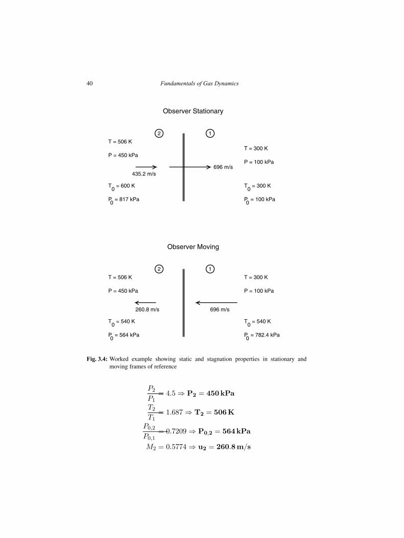
P2
P1= 4.5 ⇒ P2 = 450kPa
T2
T1= 1.687 ⇒ T2 = 506K
P0,2
P0,1= 0.7209 ⇒ P0,2 = 564kPa
M2 = 0.5774 ⇒ u2 = 260.8m/s
Normal Shock Waves 41
Switching now to a stationary frame of reference (observer stationary) inwhich the shock moves with speed Vs = 696m/s,
P1 = 100kPa, T1 = 300K, u1 = 0m/s
P0,1 = 100kPa, T0,1 = 300K
P2 = 450kPa, T2 = 506K
u2 = 696 − 260.8 = 435.2m/s
M2 = 435.2/√1.4× 288 × 506 = 0.9635
T0,2 = 600K, P0,2 = 817kPa
These numbers are shown in Fig. 3.4, to illustrate them more clearly. Notethat, in the moving frame of reference, stagnation temperature remainsconstant while stagnation pressure decreases. On the other hand, inthe stationary frame, both stagnation temperature and stagnation pressureincrease. This clearly shows the frame dependence of the stagnationquantities. �
3.4 Further Insights into the Normal Shock Wave Solution
In this section, further insights into the normal shock wave solution arepresented. The methodology is quite useful in the study of not only normalshock waves, but combustion waves also.
We start by writing the continuity equation Eqn. 2.8 as follows:
ρ1u1 = ρ2u2 = m/A = G , (3.7)
where m is the mass flow rate, A is the cross sectional area and G(> 0) is aconstant. Substituting for u1 and u2 from this equation into the momentumequation Eqn. 2.9, we get
P1 +G2v1 = P2 +G2v2
42 Fundamentals of Gas Dynamics
where we have used the fact that ρ = 1/v. This can be rewritten as
P1 − P2
v1 − v2= −G2 . (3.8)
This is the equation for a straight line with slope −G2 in P-v coordinates.
v
P
1
0,1P0,1
T=T0
s=constant
*
M<1
M>1
2
0,2P0,2
H−curve
Forbidden
states
Forbidden
states Forbidden by
Second Law
2
Rayleigh Line
Rayleigh Line
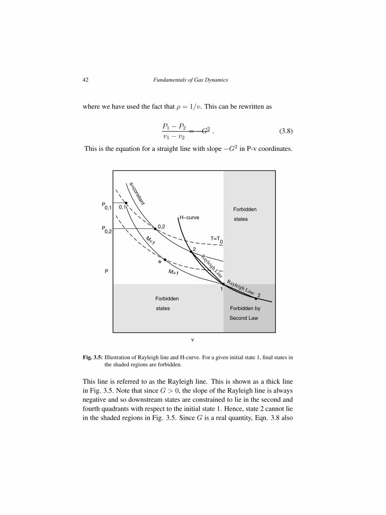
Fig. 3.5: Illustration of Rayleigh line and H-curve. For a given initial state 1, final states inthe shaded regions are forbidden.
This line is referred to as the Rayleigh line. This is shown as a thick linein Fig. 3.5. Note that since G > 0, the slope of the Rayleigh line is alwaysnegative and so downstream states are constrained to lie in the second andfourth quadrants with respect to the initial state 1. Hence, state 2 cannot liein the shaded regions in Fig. 3.5. Since G is a real quantity, Eqn. 3.8 also
Normal Shock Waves 43
allows a compressive solution (P2 > P1 and v2 < v1) which lies in thesecond quadrant and an expansion solution (P2 < P1 and v2 > v1) whichlies in the fourth quadrant. As we already showed in the previous section,only the former solution is allowed by second law of thermodynamics.Thus, state 2 cannot lie in the fourth quadrant also in Fig. 3.5.
If we rewrite the energy equation, Eqn. 2.10 in the same manner in termsof P and v, we get
γR
γ − 1T1 +
1
2v21G
2 =γR
γ − 1T2 +
1
2v22G
2 . (3.9)
Upon rearranging, we get
γR
γ − 1T1
(
1− T2
T1
)
= −1
2(v21 − v22)G
2 .
If we substitute for −G2 from Eqn. 3.8, we get
γR
γ − 1T1
(
1− T2
T1
)
=1
2(v1 + v2)(v1 − v2)
P1 − P2
v1 − v2.
Simplifying
γR
γ − 1T1
(
1− T2
T1
)
=1
2v1
(
1 +v2v1
)
P1
(
1− P2
P1
)
From the equation of state, P1v1 = RT1 and T2/T1 = P2v2/P1v1. Thus,
γ
γ − 1
(
1− P2
P1
v2v1
)
=1
2
(
1 +v2v1
)(
1− P2
P1
)
By rearranging and grouping terms, it is easy to show that
P2
P1=
(
v2v1
− γ + 1
γ − 1
)
/
(
1− v2v1
γ + 1
γ − 1
)
. (3.10)
44 Fundamentals of Gas Dynamics
This equation is called the Rankine-Hugoniot equation. It is the equationfor a quadratic in P-v coordinates, called the H-curve and is shown in Fig.3.5. The points of intersection (state points 1 and 2) of the Rayleigh lineand the H-curve in the P-v diagram represent the normal shock solution.Also, note that the H-curve (Eqn. 3.10), is steeper than the isentrope thatpasses through state 1. So, for a given change in specific volume, thenormal shock process can achieve a higher compression than an isentropicprocess, but with a loss of stagnation pressure, as mentioned earlier.
The H-curve passing through state point 1, is the locus of all possibledownstream states, some allowed and others not allowed. The actualdownstream state for a given value of G, is fixed by the Rayleigh linepassing through state point 1. For some values of G, the Rayleigh linedrawn from point 1 may not intersect the H-curve at all†, which shows thata normal shock solution is not possible for such cases.
†except trivially at point 1 itself
Normal Shock Waves 45
Exercises
(1) A shock wave advances into stagnant air at a pressure of 100 kPa and300 K. If the static pressure downstream of the wave is tripled, what isthe shock speed and the absolute velocity of the air downstream of theshock?[573 m/s, 302 m/s]
(2) Repeat Problem 1 assuming the fluid to be helium instead of air.[1644.97 m/s, 757.49 m/s.]
(3) Air at 2.5 kPa, 221 K approaches the intake of a ramjet engineoperating at an altitude of 25 km. The Mach number is 3.0. Forthis Mach number, a normal shock stands just ahead of the intake.Determine the stagnation pressure, static pressure and temperature ofthe air immediately after the normal shock. Also calculate the percentloss in stagnation pressure. Repeat the calculations for Mach numberequal to 4. The high loss of stagnation pressure that you see from yourcalculations illustrates why the intake of a ramjet has to be designedcarefully to avoid such normal shocks during operation.[30 kPa, 26 kPa, 592 K, 67%; 53 kPa, 46 kPa, 894 K, 86%]
(4) A blast wave passes through still air at 300 K. The velocity of the airbehind the wave is measured to be 180 m/s in the laboratory frameof reference. Determine the speed of the blast wave in the laboratoryframe of reference and the stagnation temperature behind the wave inthe laboratory as well moving frames of reference. You will find thefollowing relations useful:
P2
P1=
γ − 1
γ + 1
[
2γ M21
γ − 1− 1
]
T2
T1=
(
1 +γ − 1
2M2
1
) (
2γ M21
γ − 1− 1
)[
M21
(γ + 1)2
2(γ − 1)
]−1
[472.6 m/s, 411 K, 385 K]
46 Fundamentals of Gas Dynamics
(5) A normal shock wave travels into still air at 300 K. If the statictemperature of the air is increased by 50 K as a result of the passageof the shock wave, determine the speed of the wave in the laboratoryframe of reference.[437.46 m/s]
(6) A shock wave generated due to an explosion travels at a speed of 1.5km/s into still air at 100 kPa and 300 K. Determine the velocity of theair, static and stagnation quantities (with respect to a stationary frameof reference) in the region through which the shock has passed.[1183 m/s, 2.2 MPa, 1370 K, 9.1 MPa, 2067 K]
(7) A bullet travels through air (300 K, 100 kPa) at twice the speed ofsound. Determine the temperature and pressure at the nose of thebullet.Note that although there will be a curved, bow shock ahead of thebullet, in the nose region, normal shock relationships can be used. Alsonote that the nose is a stagnation point![540 K, 565 kPa]
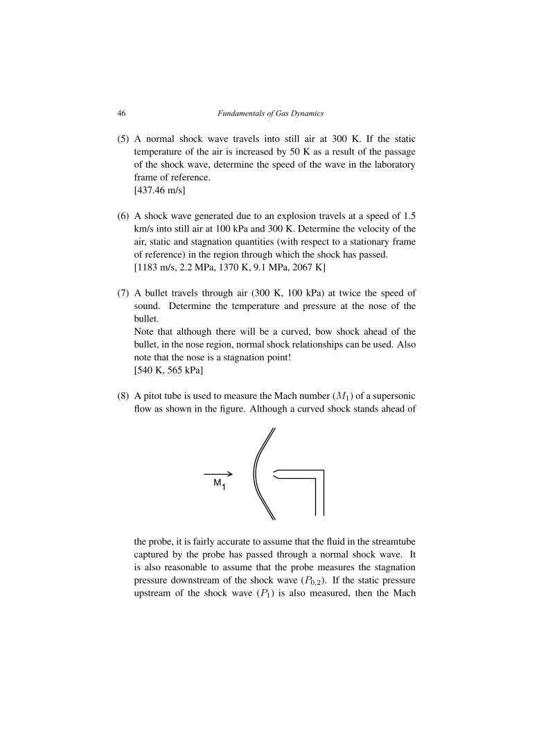
(8) A pitot tube is used to measure the Mach number (M1) of a supersonicflow as shown in the figure. Although a curved shock stands ahead of
M1
the probe, it is fairly accurate to assume that the fluid in the streamtubecaptured by the probe has passed through a normal shock wave. Itis also reasonable to assume that the probe measures the stagnationpressure downstream of the shock wave (P0,2). If the static pressureupstream of the shock wave (P1) is also measured, then the Mach
Normal Shock Waves 47
number M1 can be evaluated. Derive the relation connecting P0,2/P1
and M1 (this is called the Rayleigh pitot formula).

48 Fundamentals of Gas Dynamics
Chapter 4
Flow with Heat Addition- Rayleigh Flow
In this chapter, we look at 1D flow in a constant area duct with heataddition. Heat interaction would be more appropriate, since the theorythat is developed applies equally well to situations where heat is removed.However, such a situation is rarely, if ever, encountered. Hence thepredominant interest is on flows with heat addition, which are encounteredin combustors ranging from those in aviation gas turbine engines throughramjet engines to scramjet engines. The corresponding combustor entryMach number in these applications range from low subsonic through highsubsonic to supersonic.
4.1 Governing Equations
The governing equations for this flow are Eqns. 2.8, 2.9 and 2.12,
ρ1u1 = ρ2u2 , (2.8)
P1 + ρ1u21 = P2 + ρ2u
22 , (2.9)
s2 − s1 = Cv lnP2
P1+ Cp ln
v2v1
. (2.12)
The energy equation, Eqn. 2.10 has to be modified slightly to account forheat interaction and so
h1 +u212
+ q = h2 +u222
, (4.1)
49
Fundamentals of Gas Dynamics, Second Edition. V. Babu.© 2015 V. Babu. Published 2015 by Athena Academic Ltd and John Wiley & Sons Ltd
50 Fundamentals of Gas Dynamics
where q is the heat interaction per unit mass and is positive when heatis added to the flow and negative when heat is removed. Upon usingthe calorically perfect gas assumption and the definition of the stagnationtemperature, T0 = T + u2/2Cp, we get
T0,2 − T0,1 =q
Cp. (4.2)
This equation shows that addition of heat to a flow increases the stagnationtemperature, while heat removal decreases it.
Although the governing equations for this flow resemble those presented inthe previous chapter for normal shock waves, the important difference liesin the solution. The flow properties now change uniformly along the lengthof the duct, whereas in the former case, there is a discontinuity across theshock wave. It is also of interest to note that the spatial coordinate doesnot appear anywhere in the above equations. Thus, state points 1 and 2,represent the conditions at the entrance and the exit of the duct.
4.2 Illustration on T-s and P-v diagrams
Before we discuss the solution procedure for solving the above equations,let us try to get some physical intuition on the solution to Eqns. 2.8,2.9 and 2.12. Starting from the inlet state, we will take a small stepcorresponding to the addition or removal of an incremental amount ofheat δq and try to determine the next state as dictated by these equations.Successive steps will then allow us to determine the locus of all the alloweddownstream states. To this end, we will relate changes in all the propertiesto δq and determine the next state point on the T-s diagram. Since theaddition or removal heat results in a corresponding change in the stagnationtemperature, it is more convenient to relate the change in properties to thechange in the stagnation temperature dT0.
From Eqn. 2.1, we getdρ
ρ= −du
u, (4.3)
Flow with Heat Addition- Rayleigh Flow 51
From Eqn. 2.7, we get
dP = −ρudu .
Since P = ρRT and a2 = γRT , this can be written as
dP
P= −γM2 du
u. (4.4)
From the equation of state P = ρRT , we get
dT =1
ρRdP − T
ρdρ .
Substituting for dP and dρ from above and simplifying, we get
dT
T= (1− γM2)
du
u. (4.5)
Equation 2.6 can be written as
ds = CvdP
P− Cp
dρ
ρ.
If we substitute for dP and dρ from above, we get
ds = Cvγ(1−M2)du
u. (4.6)
From the definition of stagnation temperature,
dT0 = dT +1
Cpudu .
This can be simplified to read as
dT0 = (1−M2)Tdu
u
52 Fundamentals of Gas Dynamics
first and then as
dT0
T0=
1−M2
1 + γ−12 M2
du
u. (4.7)
Finally, from the definition of Mach number, M = u/√γRT , we can write
dM = Mdu
u− M
2
dT
T.
This can be simplified to read
dM
M=
1 + γM2
2
du
u. (4.8)
If we use Eqn. 4.7 to eliminate du/u in favor of dT0/T0 in Eqns. 4.3-4.6and 4.8, we finally get
dρ
ρ= −
1 + γ−12 M2
1−M2
dT0
T0
dP
P= −γM2 1 +
γ−12 M2
1−M2
dT0
T0
dT
T= (1− γM2)
1 + γ−12 M2
1−M2
dT0
T0(4.9)
ds = Cvγ
(
1 +γ − 1
2M2
)
dT0
T0
du
u=
1 + γ−12 M2
1−M2
dT0
T0
dM
M=
1 + γM2
2
1 + γ−12 M2
1−M2
dT0
T0
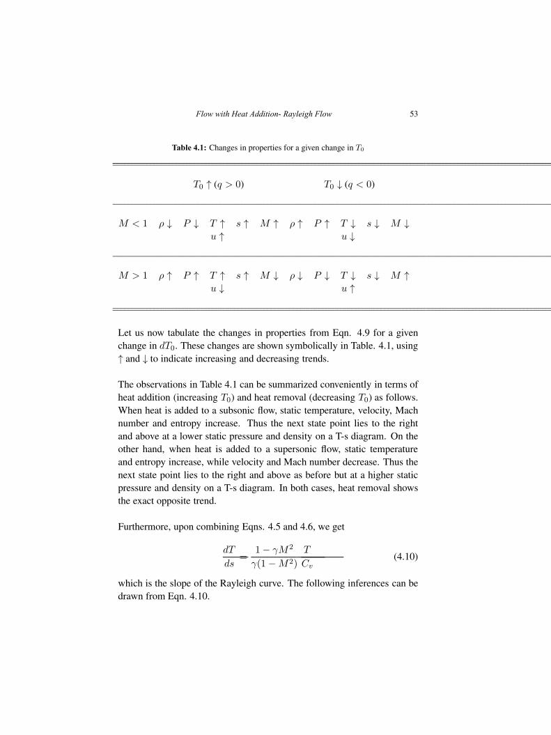
Flow with Heat Addition- Rayleigh Flow 53
Table 4.1: Changes in properties for a given change in T0
T0 ↑ (q > 0) T0 ↓ (q < 0)
M < 1 ρ ↓ P ↓ T ↑ s ↑ M ↑ ρ ↑ P ↑ T ↓ s ↓ M ↓u ↑ u ↓
M > 1 ρ ↑ P ↑ T ↑ s ↑ M ↓ ρ ↓ P ↓ T ↓ s ↓ M ↑u ↓ u ↑
Let us now tabulate the changes in properties from Eqn. 4.9 for a givenchange in dT0. These changes are shown symbolically in Table. 4.1, using↑ and ↓ to indicate increasing and decreasing trends.
The observations in Table 4.1 can be summarized conveniently in terms ofheat addition (increasing T0) and heat removal (decreasing T0) as follows.When heat is added to a subsonic flow, static temperature, velocity, Machnumber and entropy increase. Thus the next state point lies to the rightand above at a lower static pressure and density on a T-s diagram. On theother hand, when heat is added to a supersonic flow, static temperatureand entropy increase, while velocity and Mach number decrease. Thus thenext state point lies to the right and above as before but at a higher staticpressure and density on a T-s diagram. In both cases, heat removal showsthe exact opposite trend.
Furthermore, upon combining Eqns. 4.5 and 4.6, we get
dT
ds=
1− γM2
γ(1−M2)
T
Cv(4.10)
which is the slope of the Rayleigh curve. The following inferences can bedrawn from Eqn. 4.10.
54 Fundamentals of Gas Dynamics
• The slope of the Rayleigh curve is positive for supersonic Machnumbers i.e., dT/ds > 0 when M > 1.
• The supersonic branch of the Rayleigh curve at any point is steeperthan the isobar and the isochor passing through the same point (Eqns.2.21 and 2.22).
• The slope dT/ds → +∞, as M → 1 from an initially supersonicMach number.
• The slope of the Rayleigh curve is positive for subsonic Mach numbersin the range 0 < M ≤ 1/
√γ and negative in the range 1/
√γ < M ≤
1.• The subsonic branch of the Rayleigh curve at any point is less steep
than the isobar and the isochor passing through the same point (Eqns.2.21 and 2.22).
• The slope dT/ds → −∞, as M → 1 from an initially subsonic Machnumber.
• When 1/√γ < M < 1, the static temperature actually decreases with
heat addition.• Entropy reaches a maximum at the sonic state.
These findings allow us to construct the locus of all the possible states (forthe given inlet state or mass flow rate) and ultimately the state at the end ofthe heat interaction process, step by step. This curve is called the Rayleighcurve and is illustrated in Fig. 4.1. This is the same as the Rayleigh lineencountered before, but in the T-s plane instead of the P-v plane.
The sonic state represents a limiting state for both subsonic and supersonicinitial states. The amount of heat necessary to go from a given initial stateto the sonic state represents the maximum amount of heat that can be addedfrom this initial state. Of significance is the fact that such a limitation ispresent only for heat addition, not heat removal.
In principle, starting from a state in the subsonic or supersonic portion ofthe Rayleigh curve, it is possible to traverse through the sonic state onto theother branch with the appropriate combination of heat interaction. Such anarrangement is not practical, however.
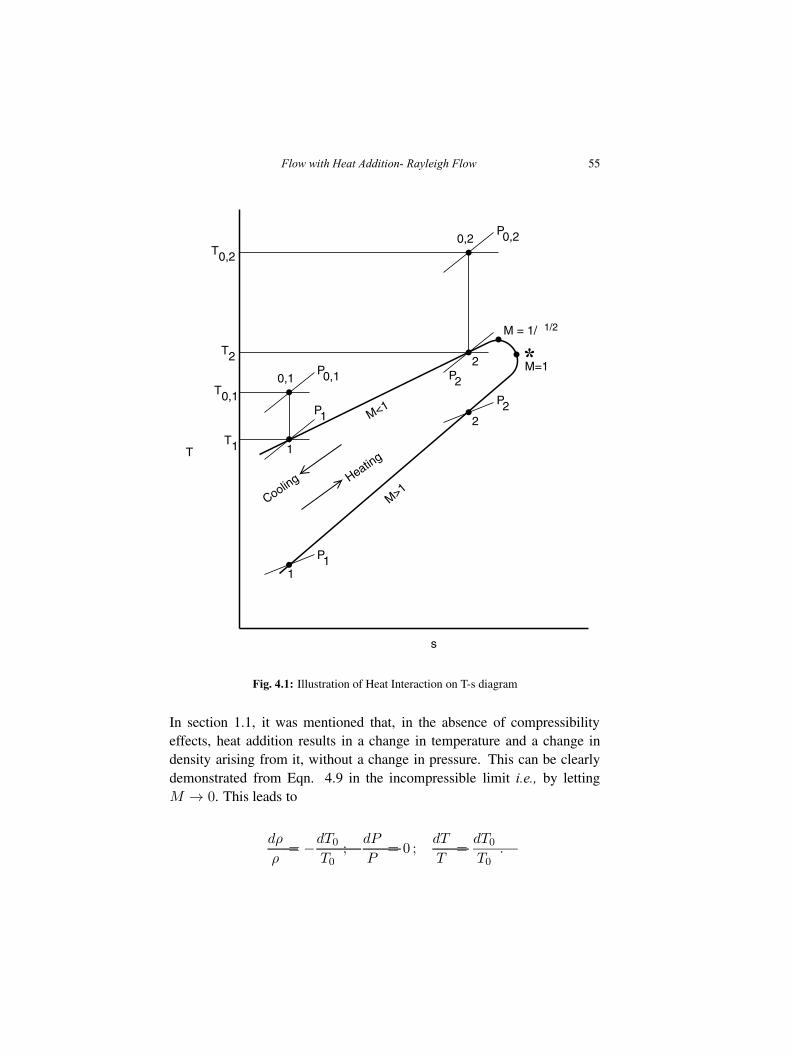
Flow with Heat Addition- Rayleigh Flow 55
s
T
M<1
M>1
T0,1
0,1P0,1
1
P1
T1
1
P1
T0,2
0,2P0,2
2P2
T2
2
P2
*M=1
Heating
Cooling
M = 1/ γ1/2
Fig. 4.1: Illustration of Heat Interaction on T-s diagram
In section 1.1, it was mentioned that, in the absence of compressibilityeffects, heat addition results in a change in temperature and a change indensity arising from it, without a change in pressure. This can be clearlydemonstrated from Eqn. 4.9 in the incompressible limit i.e., by lettingM → 0. This leads to
dρ
ρ= −dT0
T0;
dP
P= 0 ;
dT
T=
dT0
T0.
56 Fundamentals of Gas Dynamics
When compressibility effects are present, Eqn. 4.9 shows that heat additionresults in a change in temperature, density as well as pressure.
An important fact with respect to heat addition is that it always resultsin a loss of stagnation pressure. If we assume that the heat addition is areversible process, then from Eqn. 2.4, we get
ds =CpdT0
T,
where we have used the fact that δq = CpdT0 from Eqn. 4.2. Using Eqn.2.16, the right hand side can be rewritten as
ds = Cp
(
1 +γ − 1
2M2
)
dT0
T0.
From Eqn. 2.19, we can write
ds = Cp lnT0 + dT0
T0−R ln
P0 + dP0
P0,
which, for dT0 ≪ 1 and dP0 ≪ 1, reduces to
ds = CpdT0
T0−R
dP0
P0.
If we eliminate ds from these expressions, we get
dP0
P0= −γM2
2
dT0
T0.
We can also show this in an alternate way by starting with the relationship
P0
P=
(
T0
T
)
γγ − 1
.
Flow with Heat Addition- Rayleigh Flow 57
If we take the logarithm on both sides and rearrange, we get
lnP0 = lnP +γ
γ − 1lnT0 −
γ
γ − 1lnT .
Upon taking the differential of this equation, and substituting for thedifferentials in the right hand side from Eqn. 4.9, we can show after alittle bit of algebra that
dP0
P0= −γM2
2
dT0
T0. (4.11)
From this expression, it is clear that whenever dT0 is positive, dP0 isnegative for both subsonic and supersonic flow. This loss of stagnationpressure is inherent to heat addition and does not arise due to anyirreversibility (it may be recalled that we assumed at the beginning thatthe heat addition process is reversible). Hence, this is an importantfactor in the design of combustors, whether subsonic or supersonic. Goodmixing of the fuel and air is essential for good combustion, but this onlycontributes further to the loss of stagnation pressure since mixing is ahighly irreversible process. Such conflicting factors make the design ofcombustors a very challenging task.
Let us now turn to the illustration of the heat interaction process on a P-v diagram. The equation of the Rayleigh line is the same as before, asthere is no change in the momentum equation. The H-curve derived beforecorresponds to the special case q = 0, whereas, now q can be non-zero.This, however, does not alter the nature of the curve and we now have afamily of H-curves, one for each value of q, as shown in Fig. 4.2. Startingfrom the energy equation 4.1 and using the same algebra as used in theprevious chapter, it is easy to show that, the H-curve is given as
P2
P1=
(
v2v1
− γ + 1
γ − 1− 2q
RT1
)
/
(
1− v2v1
γ + 1
γ − 1
)
. (4.12)
Downstream states that lie in the fourth quadrant are allowed now, consis-tent with the required changes in entropy as a result of the heat interaction.
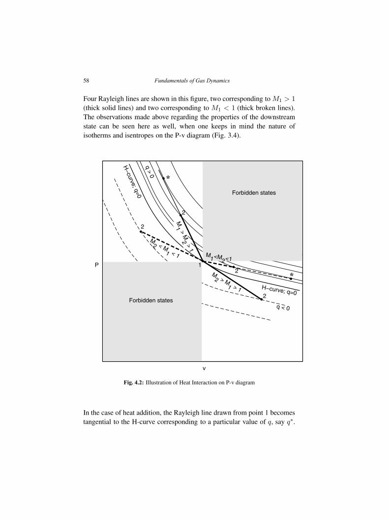
58 Fundamentals of Gas Dynamics
Four Rayleigh lines are shown in this figure, two corresponding to M1 > 1
(thick solid lines) and two corresponding to M1 < 1 (thick broken lines).The observations made above regarding the properties of the downstreamstate can be seen here as well, when one keeps in mind the nature ofisotherms and isentropes on the P-v diagram (Fig. 3.4).
v
P
2
2
M2 > M
1 > 1
*
2
2
M2 < M
1 < 1
*H
−curve; q=0
H−curve; q=0
q > 0
q < 0
1
Forbidden states
Forbidden states
M1 > M
2 > 1
M1<M
2<1
Fig. 4.2: Illustration of Heat Interaction on P-v diagram
In the case of heat addition, the Rayleigh line drawn from point 1 becomestangential to the H-curve corresponding to a particular value of q, say q∗.
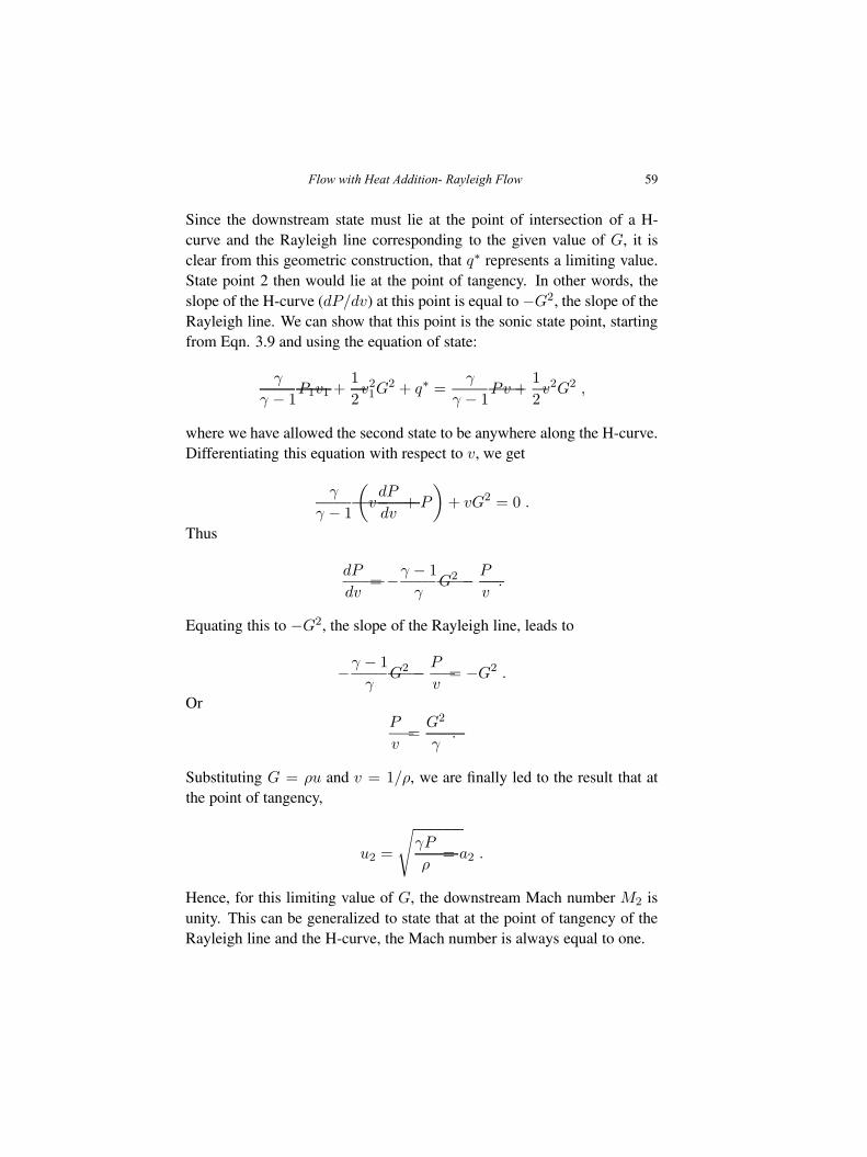
Flow with Heat Addition- Rayleigh Flow 59
Since the downstream state must lie at the point of intersection of a H-curve and the Rayleigh line corresponding to the given value of G, it isclear from this geometric construction, that q∗ represents a limiting value.State point 2 then would lie at the point of tangency. In other words, theslope of the H-curve (dP/dv) at this point is equal to −G2, the slope of theRayleigh line. We can show that this point is the sonic state point, startingfrom Eqn. 3.9 and using the equation of state:
γ
γ − 1P1v1 +
1
2v21G
2 + q∗ =γ
γ − 1Pv +
1
2v2G2 ,
where we have allowed the second state to be anywhere along the H-curve.Differentiating this equation with respect to v, we get
γ
γ − 1
(
vdP
dv+ P
)
+ vG2 = 0 .
Thus
dP
dv= −γ − 1
γG2 − P
v.
Equating this to −G2, the slope of the Rayleigh line, leads to
−γ − 1
γG2 − P
v= −G2 .
OrP
v=
G2
γ.
Substituting G = ρu and v = 1/ρ, we are finally led to the result that atthe point of tangency,
u2 =
√
γP
ρ= a2 .
Hence, for this limiting value of G, the downstream Mach number M2 isunity. This can be generalized to state that at the point of tangency of theRayleigh line and the H-curve, the Mach number is always equal to one.
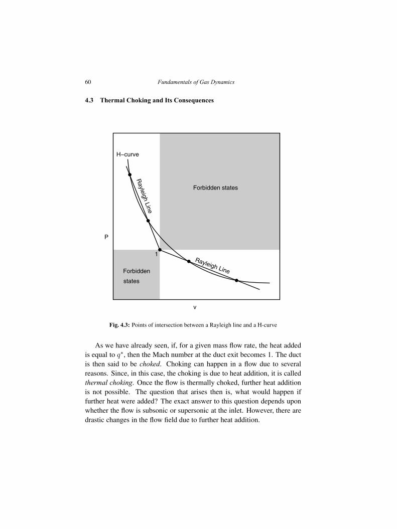
60 Fundamentals of Gas Dynamics
4.3 Thermal Choking and Its Consequences
v
P
H−curve
1
Forbidden states
Forbidden
states
Rayleigh Line
Rayleigh Line
Fig. 4.3: Points of intersection between a Rayleigh line and a H-curve
As we have already seen, if, for a given mass flow rate, the heat addedis equal to q∗, then the Mach number at the duct exit becomes 1. The ductis then said to be choked. Choking can happen in a flow due to severalreasons. Since, in this case, the choking is due to heat addition, it is calledthermal choking. Once the flow is thermally choked, further heat additionis not possible. The question that arises then is, what would happen iffurther heat were added? The exact answer to this question depends uponwhether the flow is subsonic or supersonic at the inlet. However, there aredrastic changes in the flow field due to further heat addition.
Flow with Heat Addition- Rayleigh Flow 61
When the heat added is more than the q∗ for the given inlet conditions,the point of intersection of the Rayleigh line with the H-curve for thisvalue of heat addition lies beyond the point of tangency on the H-curvecorresponding to q∗. In a flow with continuous heat addition such as thepresent one, states on the Rayleigh line beyond the sonic state are notaccessible. Figure 4.3 shows that a Rayleigh line actually intersects a H-curve at two points. The first point alone is accessible through continuousheat addition, for the reason mentioned above. However, in the case ofa discontinuity such as a combustion wave, the other state point is alsoaccessible. Here, we can directly jump to the other state point withoutgoing through any of the intermediate points similar to a normal shockwave.
One way out of this situation is to operate along a Rayleigh line with alesser slope. Since the slope of the Rayleigh line is −G2 = −(m/A)2,this means that the mass flow rate has to be reduced keeping duct areathe same or the duct area has to be increased keeping the mass flow ratethe same. The former, of course, requires the inlet static conditions to bedifferent and so we have to shift to a different Rayleigh curve (in the T-sdiagram) or Rayleigh line (in the P-v diagram). Such a change in inlet staticconditions is possible only if the flow is subsonic. This is illustrated in Fig.4.4(a), where the inlet state moves from state 1 (open circle) to 1′ (filledcircle), to accommodate the heat release. On the other hand, if the flow issupersonic at the inlet, the static pressure increases due to the heat addition,and so a normal shock stands somewhere along the duct. Since the flowis subsonic after the shock, the state point moves to the subsonic portionof the (same) Rayleigh curve. The Mach number continues to increasedue to the heat addition. The exact location of the shock wave dependsupon the inlet Mach number and the amount of heat added. In fact, if theheat addition is high enough, then the normal shock may stand at the ductentrance itself. This is not tantamount to a change in inlet conditions as inthe subsonic case; it means that the required pressure rise can be achievedonly in this manner. The process corresponding to the supersonic inletcases is illustrated in Fig. 4.4(b). Although the exit state is shown to bethe sonic state in Figs. 4.4(a) and (b), the actual exit state will be suchthat the exit static pressure matches the ambient pressure in the region into
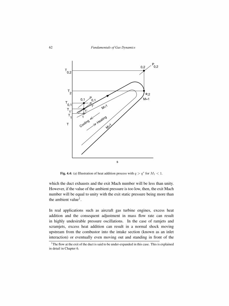
62 Fundamentals of Gas Dynamics
s
T
M<1
M>1
T0,1
0,1 P0,1
1
1’T1’T
1
T0,2
0,2P0,2
T2
P1’
*,2M=1
Heating
Cooling
Fig. 4.4: (a) Illustration of heat addition process with q > q∗ for M1 < 1.
which the duct exhausts and the exit Mach number will be less than unity.However, if the value of the ambient pressure is too low, then, the exit Machnumber will be equal to unity with the exit static pressure being more thanthe ambient value†.
In real applications such as aircraft gas turbine engines, excess heataddition and the consequent adjustment in mass flow rate can resultin highly undesirable pressure oscillations. In the case of ramjets andscramjets, excess heat addition can result in a normal shock movingupstream from the combustor into the intake section (known as an inletinteraction) or eventually even moving out and standing in front of the†The flow at the exit of the duct is said to be under-expanded in this case. This is explained
in detail in Chapter 6.
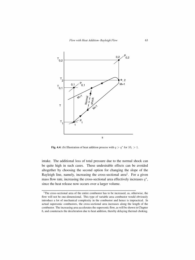
Flow with Heat Addition- Rayleigh Flow 63
s
T
M<1
M>1
T0,1
T1
0,1 P0,1
1
P1
T0,2
0,2 P0,2
*, 2M=1
T2
Nor
mal
shoc
k
Fig. 4.4: (b) Illustration of heat addition process with q > q∗ for M1 > 1.
intake. The additional loss of total pressure due to the normal shock canbe quite high in such cases. These undesirable effects can be avoidedaltogether by choosing the second option for changing the slope of theRayleigh line, namely, increasing the cross-sectional area‡. For a givenmass flow rate, increasing the cross-sectional area effectively increases q∗,since the heat release now occurs over a larger volume.
‡The cross-sectional area of the entire combustor has to be increased, as, otherwise, theflow will not be one-dimensional. This type of variable area combustor would obviouslyintroduce a lot of mechanical complexity in the combustor and hence is impractical. Inactual supersonic combustors, the cross-sectional area increases along the length of thecombustor. The increasing area accelerates the supersonic flow, as will be shown in Chapter6, and counteracts the deceleration due to heat addition, thereby delaying thermal choking.
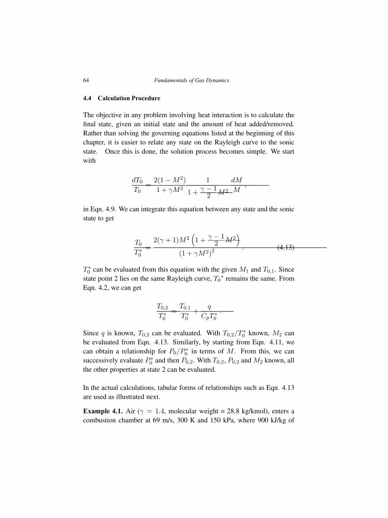
64 Fundamentals of Gas Dynamics
4.4 Calculation Procedure
The objective in any problem involving heat interaction is to calculate thefinal state, given an initial state and the amount of heat added/removed.Rather than solving the governing equations listed at the beginning of thischapter, it is easier to relate any state on the Rayleigh curve to the sonicstate. Once this is done, the solution process becomes simple. We startwith
dT0
T0=
2(1−M2)
1 + γM2
1
1 +γ − 12 M2
dM
M,
in Eqn. 4.9. We can integrate this equation between any state and the sonicstate to get
T0
T ∗0
=2(γ + 1)M2
(
1 +γ − 12 M2
)
(1 + γM2)2. (4.13)
T ∗0 can be evaluated from this equation with the given M1 and T0,1. Since
state point 2 lies on the same Rayleigh curve, T0∗ remains the same. From
Eqn. 4.2, we can get
T0,2
T ∗0
=T0,1
T ∗0
+q
CpT∗0
.
Since q is known, T0,2 can be evaluated. With T0,2/T∗0 known, M2 can
be evaluated from Eqn. 4.13. Similarly, by starting from Eqn. 4.11, wecan obtain a relationship for P0/P
∗0 in terms of M . From this, we can
successively evaluate P ∗0 and then P0,2. With T0,2, P0,2 and M2 known, all
the other properties at state 2 can be evaluated.
In the actual calculations, tabular forms of relationships such as Eqn. 4.13are used as illustrated next.
Example 4.1. Air (γ = 1.4, molecular weight = 28.8 kg/kmol), enters acombustion chamber at 69 m/s, 300 K and 150 kPa, where 900 kJ/kg of
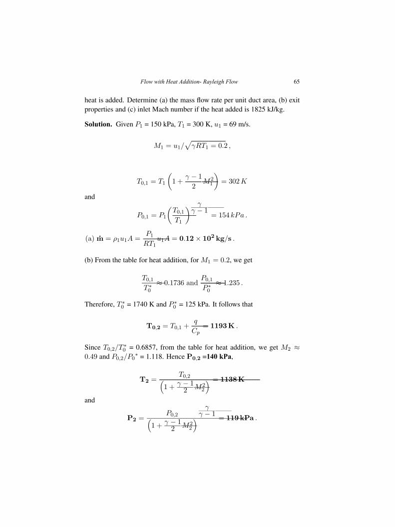
Flow with Heat Addition- Rayleigh Flow 65
heat is added. Determine (a) the mass flow rate per unit duct area, (b) exitproperties and (c) inlet Mach number if the heat added is 1825 kJ/kg.
Solution. Given P1 = 150 kPa, T1 = 300 K, u1 = 69 m/s.
M1 = u1/√
γRT1 = 0.2 ,
T0,1 = T1
(
1 +γ − 1
2M2
1
)
= 302K
and
P0,1 = P1
(
T0,1
T1
)
γγ − 1
= 154 kPa .
(a) m = ρ1u1A =P1
RT1u1A = 0.12× 10² kg/s .
(b) From the table for heat addition, for M1 = 0.2, we get
T0,1
T ∗0
≈ 0.1736 andP0,1
P ∗0
≈ 1.235 .
Therefore, T ∗0 = 1740 K and P ∗
0 = 125 kPa. It follows that
T0,2 = T0,1 +q
Cp= 1193K .
Since T0,2/T∗0 = 0.6857, from the table for heat addition, we get M2 ≈
0.49 and P0,2/P0∗ = 1.118. Hence P0,2 =140 kPa,
T2 =T0,2
(
1 +γ − 12 M2
2
) = 1138K
and
P2 =P0,2
(
1 +γ − 12 M2
2
)
γγ − 1
= 119kPa .
66 Fundamentals of Gas Dynamics
(c) For the given inlet conditions, q∗ = Cp(T∗0 −T0,1) = 1453 kJ/kg. Since
the heat to be added is greater than 1453 kJ/kg, we must find an inlet state(1′) for which q∗ = 1825 kJ/kg. Inlet stagnation conditions remain thesame. Hence,
T ∗0 =
q∗
Cp+ T0,1′ = 2108K .
Thus,
T0,1′
T ∗0
= 0.1432 ⇒ M1′ = 0.18 .�
Flow with Heat Addition- Rayleigh Flow 67
Exercises
(1) Air enters a constant area combustion chamber at 100 m/s and 400 K.Determine the exit conditions if the heat added is (a) 1000 kJ/kg and(b) 2000 kJ/kg. Also determine the ratio of mass flow rates betweenthe two cases. Assume that the inlet stagnation conditions remain thesame for the two cases.[1281 K, 0.67; 1941 K, 1; 1.233]
(2) Air enters a combustion chamber at 75 m/s, 150 kPa and 300 K. Heataddition in the combustor amounts to 900 kJ/kg. Compute (a) the massflow rate, (b) the exit properties and (c) amount of heat to be added tocause the exit Mach number to be unity.[130.7 kg/s; 0.6, 107 kPa, 1123 K; 1173 kJ]
(3) Determine the inlet static conditions and the mass flow rate if the heataddition in the above combustor were 1400 kJ/kg.[0.205, 151 kPa, 300.3 K, 124 kg/s]
(4) Air enters the combustor of a scramjet engine at M = 2.5 and T0 =1500 K and P0 = 1 MPa. Kerosene with calorific value of 45 MJ/kgis used as the fuel. Determine the fuel-air ratio (on a mass basis) thatwill result in the exit Mach number being equal to 1. Also determinethe fuel-air ratio that will result in an “inlet interaction” i.e., a normalshock stands just at the entrance of the combustor.[0.01387, 0.01416]
(5) Air flows from a large reservoir where the pressure and temperatureare 200 kPa, 300 K respectively through a pipe of diameter 0.05 m andexhausts into the atmosphere at 100 kPa. Heat is added to the air in thepipe.
If the heat added is 450 kJ/kg, calculate (a) the inlet and exit Machnumbers, (b) exit static pressure and (c) mass flow rate through thepipe.
68 Fundamentals of Gas Dynamics
If the exit static pressure has to be equal to the ambient pressure,calculate (a) the inlet and exit Mach numbers, (b) maximum amountof heat that can be added and (c) mass flow rate through the pipe.[a) 0.33, 1.0 b) 89.06 kPa c) 0.4898 kg/s][a) 0.66, 1 b) 42 kJ/kg c) 0.812 kg/s]
Chapter 5
Flow with Friction - Fanno Flow
In this chapter, we look at 1D adiabatic flow in a duct with friction atthe walls of the duct. This type of flow occurs, for example, when gasesare transported through pipes over long distances. It is also of practicalimportance when equipment handling gases are connected to high pressurereservoirs which may be located some distance away. Knowledge of thisflow will allow us to determine the mass flow rate that can be handled,pressure drop and so on.
In a real flow, friction at the wall arises due to the viscosity of the fluidand this appears in the form of a shear stress at the wall. So far in ourdiscussion, we have assumed the fluid to be calorically perfect and inviscidas well. Thus, strictly speaking, viscous effects cannot be accounted for inthis formulation. However, in reality, viscous effects are confined to verythin regions (“boundary layers”) near the walls. Effects such as viscousdissipation are also usually negligible. Hence, we can still assume the fluidto be inviscid and take the friction force exerted by the wall as an externallyimposed force. The origin of this force is of no significance to the analysis.
5.1 Governing Equations
The governing equations for this flow are Eqns. 2.8, 2.10 and 2.12,
ρ1u1 = ρ2u2 , (2.8)
h1 +u212
= h2 +u222
, (2.10)
69
Fundamentals of Gas Dynamics, Second Edition. V. Babu.© 2015 V. Babu. Published 2015 by Athena Academic Ltd and John Wiley & Sons Ltd
70 Fundamentals of Gas Dynamics
s2 − s1 = Cv lnP2
P1+ Cp ln
v2v1
. (2.12)
The momentum equation, Eqn. 2.9 has to be modified to take into accountfrictional force at the wall and so
P1 + ρ1u21 = P2 + ρ2u
22 +
PA
∫ L
0τwdx ,
where P is the wetted perimeter, L is the length of the duct and τw is thewall shear stress. The Darcy friction factor f is related to the wall shearstress as f = τw / 1
2ρu2. Upon using this relationship, we can write the
above equation as
P1 + ρ1u21 = P2 + ρ2u
22 +
4
Dh
∫ L
0
1
2ρu2fdx , (5.1)
where Dh = 4A/P is the hydraulic diameter. The friction factor f canbe calculated from Moody’s chart† and is usually assumed to be constantalong the duct (or pipe).
5.2 Illustration on T-s diagram
We follow the same procedure as in the previous chapter and try todetermine the locus of the allowed downstream states, starting from a giveninlet state. From Eqn. 4.3
dρ
ρ= −du
u. (4.2)
†Alternatively, the Colebrook formula can be used for determining the Darcy frictionfactor. Here
1
f1/2= −2 log
(
ǫ/Dh
3.7+
2.51
Ref1/2
)
,
where the Reynolds number is based on the hydraulic diameter and the mean velocity andǫ is the roughness of the pipe surface.
Flow with Friction - Fanno Flow 71
From the definition of stagnation temperature,
dT0 = dT +1
Cpudu .
Since the flow is adiabatic, there is no change in stagnation temperatureand so dT0 = 0 and this equation can be simplified to read
dT
T= −(γ − 1)M2 du
u. (5.2)
From the equation of state P = ρRT , we get
dP = ρRdT +RTdρ .
Substituting for dT and dρ from above and simplifying, we get
dP
P= −
[
1 + (γ − 1)M2] du
u. (5.3)
Equation 2.6 can be written as
ds = CvdP
P− Cp
dρ
ρ.
If we substitute for dP and dρ from above, we get
ds = R(1−M2)du
u. (5.4)
Finally, from the definition of Mach number, M = u/√γRT , we can write
dM = Mdu
u− M
2
dT
T.
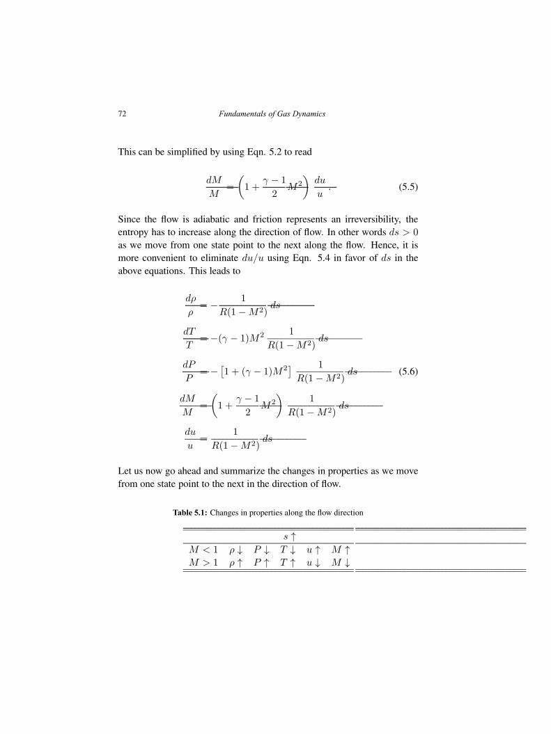
72 Fundamentals of Gas Dynamics
This can be simplified by using Eqn. 5.2 to read
dM
M=
(
1 +γ − 1
2M2
)
du
u. (5.5)
Since the flow is adiabatic and friction represents an irreversibility, theentropy has to increase along the direction of flow. In other words ds > 0
as we move from one state point to the next along the flow. Hence, it ismore convenient to eliminate du/u using Eqn. 5.4 in favor of ds in theabove equations. This leads to
dρ
ρ= − 1
R(1−M2)ds
dT
T= −(γ − 1)M2 1
R(1−M2)ds
dP
P= −
[
1 + (γ − 1)M2] 1
R(1−M2)ds (5.6)
dM
M=
(
1 +γ − 1
2M2
)
1
R(1−M2)ds
du
u=
1
R(1−M2)ds
Let us now go ahead and summarize the changes in properties as we movefrom one state point to the next in the direction of flow.
Table 5.1: Changes in properties along the flow direction
s ↑M < 1 ρ ↓ P ↓ T ↓ u ↑ M ↑M > 1 ρ ↑ P ↑ T ↑ u ↓ M ↓
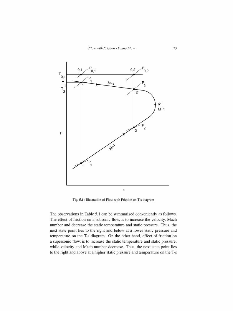
Flow with Friction - Fanno Flow 73
s
T
M<1
M>1
T0,1
0,1 P0,1
1
P1T
1
1P1
0,2 P0,2
2
P2
T2
2
P2
*M=1
Fig. 5.1: Illustration of Flow with Friction on T-s diagram
The observations in Table 5.1 can be summarized conveniently as follows.The effect of friction on a subsonic flow, is to increase the velocity, Machnumber and decrease the static temperature and static pressure. Thus, thenext state point lies to the right and below at a lower static pressure andtemperature on the T-s diagram. On the other hand, effect of friction ona supersonic flow, is to increase the static temperature and static pressure,while velocity and Mach number decrease. Thus, the next state point liesto the right and above at a higher static pressure and temperature on the T-s
74 Fundamentals of Gas Dynamics
diagram.
These findings allow us to construct the locus of all the possible states(for the given inlet state or mass flow rate) and ultimately the state at theend of the duct, step by step. This curve is called the Fanno curve and isillustrated in Fig. 5.1. Furthermore, by combining Eqns. 5.2 and 5.4, wecan get
dT
ds= − M2
1−M2
T
Cv. (5.7)
The following inferences may be drawn from Eqn. 5.7:
• The slope of the subsonic portion of the Fanno curve is negative, whilethe slope of the supersonic portion is positive.
• A comparison of Eqn. 5.7 with Eqns. 2.21 and 2.22 shows that thesupersonic branch of the Fanno curve is steeper than the isochor andisobar.
• dT/ds → ∓∞ as M → 1 and the sonic state occurs at the pointof maximum entropy like the Rayleigh curve. However, unlike theRayleigh curve, it is not possible to move through the sonic state on aFanno curve.
Since friction renders the process irreversible, the stagnation pressurealways decreases in a Fanno flow. This can be seen from Eqn. 2.19, afternoting that T0,2 = T0,1 and s2 > s1. Alternatively, we can follow the stepsused in the previous chapter and show that
dP0
P0=
dP
P− γ
γ − 1
dT
T.
If we substitute from Eqns. 5.2 and 5.3, and then from Eqn. 5.5, we get
dP0
P0= −ds
R=
1−M2
1 + γ−12 M2
dM
M. (5.8)
The first equality makes it clear that there is always a loss of stagnationpressure since ds > 0 regardless of the Mach number.
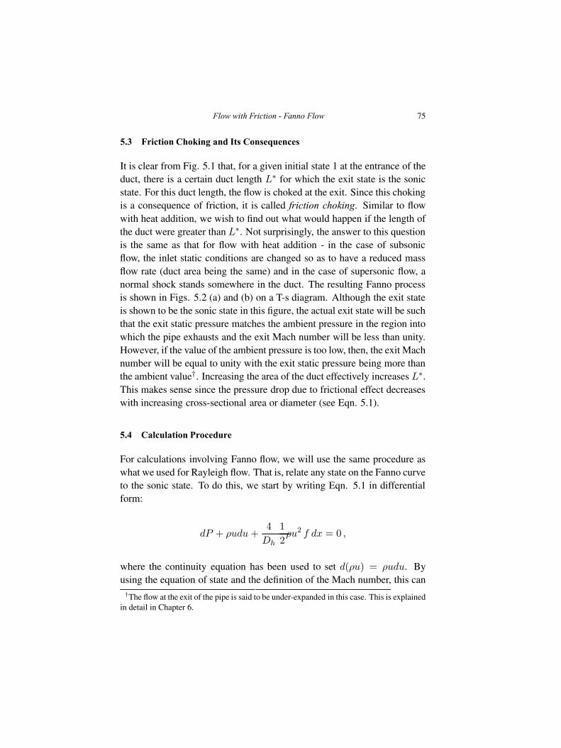
Flow with Friction - Fanno Flow 75
5.3 Friction Choking and Its Consequences
It is clear from Fig. 5.1 that, for a given initial state 1 at the entrance of theduct, there is a certain duct length L∗ for which the exit state is the sonicstate. For this duct length, the flow is choked at the exit. Since this chokingis a consequence of friction, it is called friction choking. Similar to flowwith heat addition, we wish to find out what would happen if the length ofthe duct were greater than L∗. Not surprisingly, the answer to this questionis the same as that for flow with heat addition - in the case of subsonicflow, the inlet static conditions are changed so as to have a reduced massflow rate (duct area being the same) and in the case of supersonic flow, anormal shock stands somewhere in the duct. The resulting Fanno processis shown in Figs. 5.2 (a) and (b) on a T-s diagram. Although the exit stateis shown to be the sonic state in this figure, the actual exit state will be suchthat the exit static pressure matches the ambient pressure in the region intowhich the pipe exhausts and the exit Mach number will be less than unity.However, if the value of the ambient pressure is too low, then, the exit Machnumber will be equal to unity with the exit static pressure being more thanthe ambient value†. Increasing the area of the duct effectively increases L∗.This makes sense since the pressure drop due to frictional effect decreaseswith increasing cross-sectional area or diameter (see Eqn. 5.1).
5.4 Calculation Procedure
For calculations involving Fanno flow, we will use the same procedure aswhat we used for Rayleigh flow. That is, relate any state on the Fanno curveto the sonic state. To do this, we start by writing Eqn. 5.1 in differentialform:
dP + ρudu+4
Dh
1
2ρu2 f dx = 0 ,
where the continuity equation has been used to set d(ρu) = ρudu. Byusing the equation of state and the definition of the Mach number, this can†The flow at the exit of the pipe is said to be under-expanded in this case. This is explained
in detail in Chapter 6.
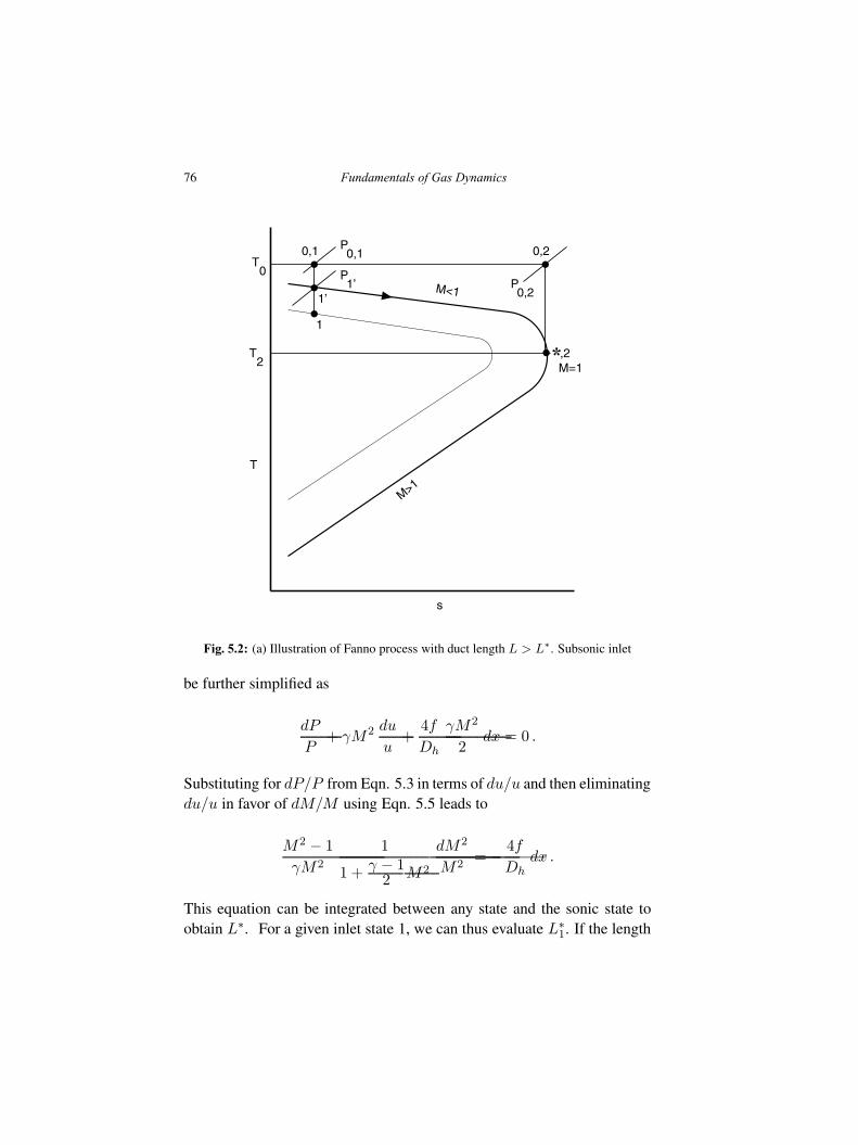
76 Fundamentals of Gas Dynamics
s
T
M<1
M>1
T0
0,1 P0,1
1
1’
P1’
0,2
P0,2
T2 *,2
M=1
Fig. 5.2: (a) Illustration of Fanno process with duct length L > L∗. Subsonic inlet
be further simplified as
dP
P+ γM2 du
u+
4f
Dh
γM2
2dx = 0 .
Substituting for dP/P from Eqn. 5.3 in terms of du/u and then eliminatingdu/u in favor of dM/M using Eqn. 5.5 leads to
M2 − 1
γM2
1
1 +γ − 12 M2
dM2
M2= − 4f
Dhdx .
This equation can be integrated between any state and the sonic state toobtain L∗. For a given inlet state 1, we can thus evaluate L∗
1. If the length
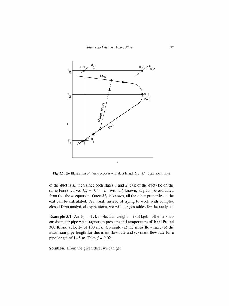
Flow with Friction - Fanno Flow 77
s
T
M<1
M>1
T0
0,1 P0,1
1P1T
1
0,2 P0,2
Nor
mal
sho
ck
*,2M=1
T2
Fig. 5.2: (b) Illustration of Fanno process with duct length L > L∗. Supersonic inlet
of the duct is L, then since both states 1 and 2 (exit of the duct) lie on thesame Fanno curve, L∗
2 = L∗1 − L. With L∗
2 known, M2 can be evaluatedfrom the above equation. Once M2 is known, all the other properties at theexit can be calculated. As usual, instead of trying to work with complexclosed form analytical expressions, we will use gas tables for the analysis.
Example 5.1. Air (γ = 1.4, molecular weight = 28.8 kg/kmol) enters a 3cm diameter pipe with stagnation pressure and temperature of 100 kPa and300 K and velocity of 100 m/s. Compute (a) the mass flow rate, (b) themaximum pipe length for this mass flow rate and (c) mass flow rate for apipe length of 14.5 m. Take f = 0.02.
Solution. From the given data, we can get
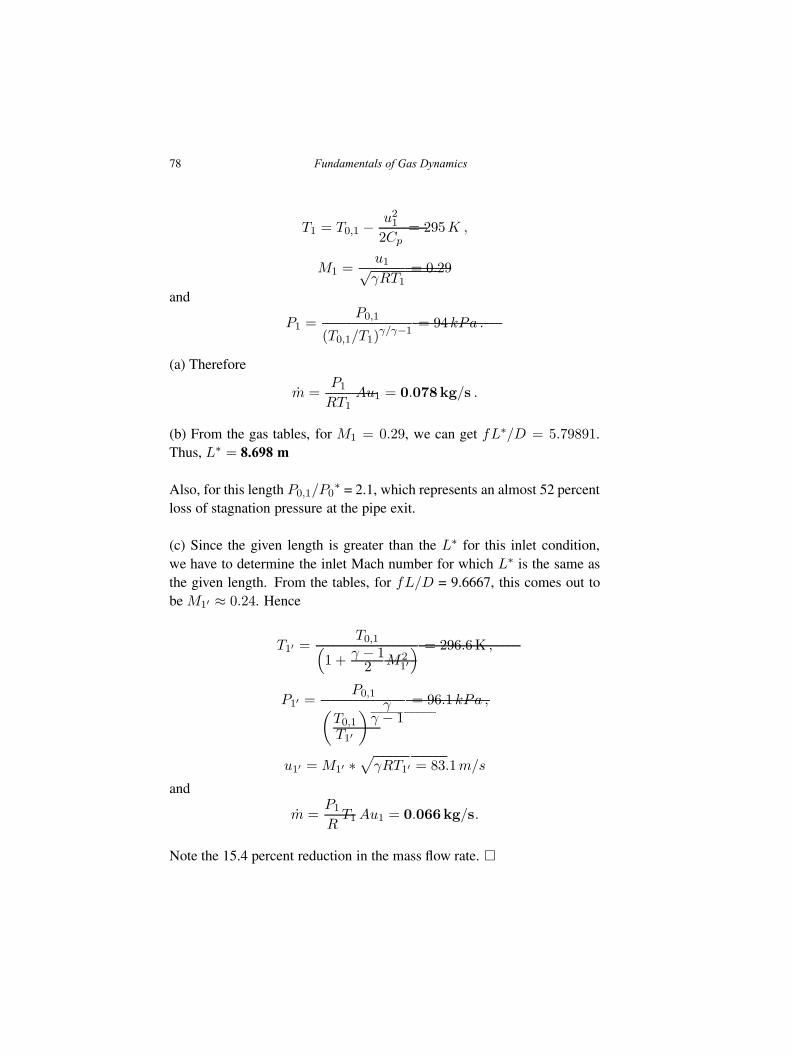
78 Fundamentals of Gas Dynamics
T1 = T0,1 −u212Cp
= 295K ,
M1 =u1√γRT1
= 0.29
and
P1 =P0,1
(T0,1/T1)γ/γ−1
= 94 kPa .
(a) Therefore
m =P1
RT1Au1 = 0.078kg/s .
(b) From the gas tables, for M1 = 0.29, we can get fL∗/D = 5.79891.Thus, L∗ = 8.698 m
Also, for this length P0,1/P0∗ = 2.1, which represents an almost 52 percent
loss of stagnation pressure at the pipe exit.
(c) Since the given length is greater than the L∗ for this inlet condition,we have to determine the inlet Mach number for which L∗ is the same asthe given length. From the tables, for fL/D = 9.6667, this comes out tobe M1′ ≈ 0.24. Hence
T1′ =T0,1
(
1 +γ − 12 M2
1′
) = 296.6K ,
P1′ =P0,1
(
T0,1
T1′
)
γγ − 1
= 96.1 kPa ,
u1′ = M1′ ∗√
γRT1′ = 83.1m/s
and
m =P1
RT1 Au1 = 0.066kg/s.
Note the 15.4 percent reduction in the mass flow rate. �
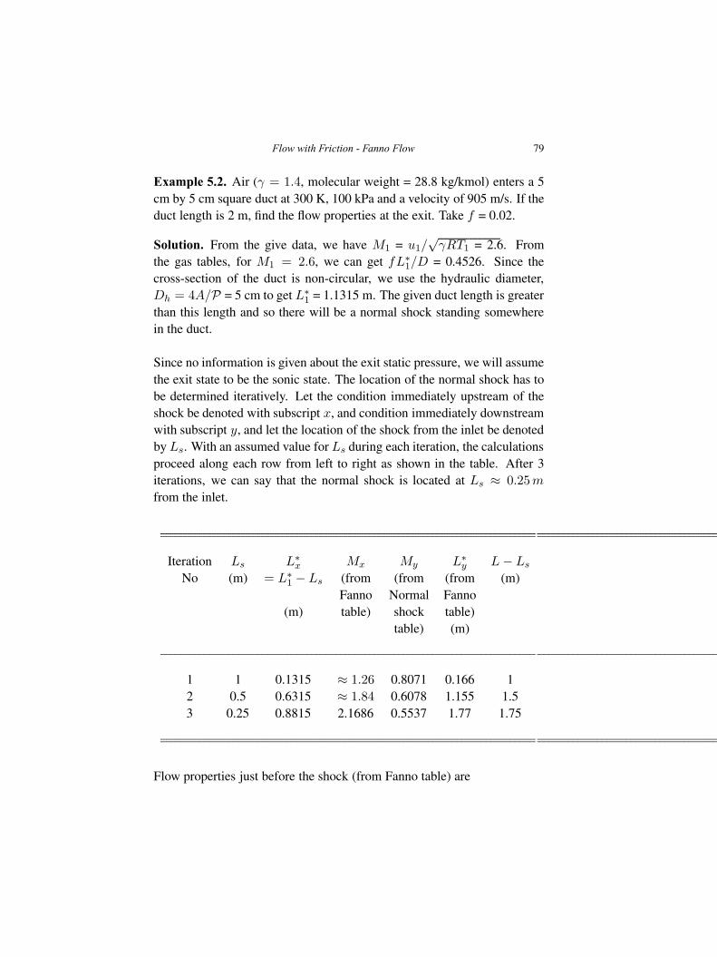
Flow with Friction - Fanno Flow 79
Example 5.2. Air (γ = 1.4, molecular weight = 28.8 kg/kmol) enters a 5cm by 5 cm square duct at 300 K, 100 kPa and a velocity of 905 m/s. If theduct length is 2 m, find the flow properties at the exit. Take f = 0.02.
Solution. From the give data, we have M1 = u1/√γRT1 = 2.6. From
the gas tables, for M1 = 2.6, we can get fL∗1/D = 0.4526. Since the
cross-section of the duct is non-circular, we use the hydraulic diameter,Dh = 4A/P = 5 cm to get L∗
1 = 1.1315 m. The given duct length is greaterthan this length and so there will be a normal shock standing somewherein the duct.
Since no information is given about the exit static pressure, we will assumethe exit state to be the sonic state. The location of the normal shock has tobe determined iteratively. Let the condition immediately upstream of theshock be denoted with subscript x, and condition immediately downstreamwith subscript y, and let the location of the shock from the inlet be denotedby Ls. With an assumed value for Ls during each iteration, the calculationsproceed along each row from left to right as shown in the table. After 3iterations, we can say that the normal shock is located at Ls ≈ 0.25m
from the inlet.
Iteration Ls L∗x Mx My L∗
y L− Ls
No (m) = L∗1 − Ls (from (from (from (m)
Fanno Normal Fanno(m) table) shock table)
table) (m)
1 1 0.1315 ≈ 1.26 0.8071 0.166 12 0.5 0.6315 ≈ 1.84 0.6078 1.155 1.53 0.25 0.8815 2.1686 0.5537 1.77 1.75
Flow properties just before the shock (from Fanno table) are
80 Fundamentals of Gas Dynamics
Tx =
(
Tx
T ∗1
) (
T ∗1
T1
)
T1 =0.6235
0.5102∗ 300 = 366.62K ,
Px =
(
Px
P ∗1
) (
P ∗1
P1
)
P1 =0.3673
0.2747∗ 100 = 133.71 kPa
and
P0,x =
(
P0,x
P ∗0,1
)
(
P ∗0,1
P0,1
) (
P0,1
P1
)
P1
=1.919
2.896∗ 19.95 ∗ 100 = 1322 kPa .
Flow properties just after the shock (from normal shock table) are
Ty =Ty
TxTx = 1.813 ∗ 366.62 = 664.68K
Py =Py
PxPx = 5.226 ∗ 133.71 = 699 kPa
P0,y =P0,y
P0,xP0,x = 0.6511 ∗ 1322 = 860.75 kPa
Flow properties at the exit (from Fanno table) are
T2 = T ∗2 =
T ∗2
TyTy =
664.68
1.1305= 588K ,
P2 = P ∗2 =
P ∗2
PyPy =
699
1.9202= 364kPa ,
P0,2 = P ∗0,2 =
P ∗0,2
P0,yP0,y =
860.75
1.249= 689kPa ,
T0,2 = T0,1 =T0,1
T1T1 = 2.352 ∗ 300 = 705.6K .
Note the 65 percent loss of stagnation pressure at the duct exit.�
Flow with Friction - Fanno Flow 81
Exercises
(1) Redraw Fig. 5.1 in P-v coordinates.
(2) Air enters a 5 cm × 5 cm smooth, insulated square duct with a velocityof 900 m/s and a static temperature of 300 K. If the duct length is 2 m,determine the flow conditions at the exit. Use Colebrook’s formula tocalculate the friction factor.[1.3, 528 K]
(3) Air enters a smooth, insulated circular duct at M = 3. Determinethe stagnation pressure loss in the duct for L/D = 20 and 40. Takef = 0.02.[72.72%, 76.4%]
(4) Air enters a smooth, insulated 3 cm diameter duct with stagnationpressure and temperature of 200 kPa, 500 K and a velocity of 100m/s. Compute (a) the maximum duct length for these conditions (b)the mass flow rate for a duct length of 15 m and 30 m. Take f = 0.02.[16.5 m; 0.097 kg/s, 0.076 kg/s]
(5) Air enters a 3 m long pipe (f = 0.02) of diameter 0.025 m at astagnation temperature of 300 K. If the static pressure of the air at theexit of the pipe is 100 kPa and the Mach number is 0.7, determine thestagnation pressure at entry and the mass flow rate through the pipe.[207.73 kPa, 0.14518 kg/s]
(6) Air enters a pipe (f = 0.02) of diameter 0.05 m with stagnationpressure and temperature equal to 1 MPa and 300 K respectively. Thepipe exhausts into the ambient at 100 kPa. Determine the length of thepipe required to achieve a mass flow rate of 2 kg/s. Assume the flowto be subsonic at the entrance of the pipe.[18.2 m]

82 Fundamentals of Gas Dynamics
Chapter 6
Quasi One Dimensional Flows
In the previous chapters, 1D compressible flow solutions were presented,wherein the flow was either across a wave or through a constant area pas-sage. A very important class of compressible flow is flow through a passageof finite but varying cross-sectional area such as flow through nozzles,diffusers and blade passages in turbomachines. The main difficulty thatarises in this case is that the flow is no longer strictly one dimensional, sincethe variation in the cross-sectional area occurs in a direction normal to themain flow direction (see Fig. 6.1). This means that the velocity componentin the normal direction is non-zero. However, it so happens that in mostof the applications involving such flows, the magnitude of the normalcomponent of velocity is small when compared with the axial component.Hence, as a first approximation, the former is usually neglected and onlythe axial component is considered. Thus, the flow is approximately onedimensional, or, as it is usually called, quasi one dimensional.
Although it is possible to combine effects considered in previous chapters,such as friction and heat addition/removal with area variation, the resultingformulation is too complex to be considered in introductory texts such asthe present one. The interested reader is referred to the books suggested atthe end of the book for such analysis. Here, we assume the flow through avarying area passage to be isentropic (except across normal shocks).
83
Fundamentals of Gas Dynamics, Second Edition. V. Babu.© 2015 V. Babu. Published 2015 by Athena Academic Ltd and John Wiley & Sons Ltd
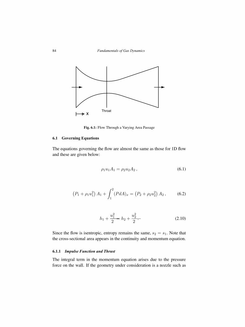
84 Fundamentals of Gas Dynamics
Throatx
Fig. 6.1: Flow Through a Varying Area Passage
6.1 Governing Equations
The equations governing the flow are almost the same as those for 1D flowand these are given below:
ρ1u1A1 = ρ2u2A2 , (6.1)
(
P1 + ρ1u21
)
A1 +
∫ 2
1(PdA)x =
(
P2 + ρ2u22
)
A2 , (6.2)
h1 +u212
= h2 +u222
. (2.10)
Since the flow is isentropic, entropy remains the same, s2 = s1. Note thatthe cross-sectional area appears in the continuity and momentum equation.
6.1.1 Impulse Function and Thrust
The integral term in the momentum equation arises due to the pressureforce on the wall. If the geometry under consideration is a nozzle such as
Quasi One Dimensional Flows 85
in propulsion applications, this would be force exerted on the nozzle† andhence the airframe. To facilitate the evaluation of this force, we define aquantity called Impulse Function, I at any x-location as follows:
I = (P + ρu2)A . (6.3)
The net force exerted is the difference between the value of the impulsefunction at the exit and the inlet, viz.,
T = I2 − I1 .
It is easy to see from this equation and Eqn. 6.2 that T =∫ 21 PdA. Let
us take the reference to propulsion application further and say that we areconsidering an aircraft flying at a speed of u∞. From the above equation,the thrust produced by the engine (in a frame of reference where the aircraftis stationary and the flow approaches with a velocity of u∞) is
T =(
PA+ ρu2A)
exit−(
PA+ ρu2A)
inlet.
If we use subscript ∞ to denote freestream conditions, and subscript e todenote exit conditions, then
T = (PA+ mu)e − (PA+ mu)∞ ,
where we have used m = ρuA. If the static pressures in this equation aremeasured relative to the freestream pressure, then the thrust is given by
T = m (ue − u∞) + (Pe − P∞)Ae . (6.4)
The first term in this equation is called momentum thrust and the second†It should be remembered that thrust force acts in the negative x-direction and drag force
in the positive x-direction. Hence, a negative value for this integral would imply thrust anda positive value, drag.
86 Fundamentals of Gas Dynamics
term is called pressure thrust and is non-zero when the pressure of the fluidat the exit is not equal to the ambient pressure. The negative term, −mu∞,is called intake momentum drag. Note that in the case of a rocket engine,air is not taken in through any inlet and so this term will be absent.
6.2 Area Velocity Relation
The general objective in quasi 1D flows is to determine the Mach numberat any axial location, given the inlet conditions and the area at that location.Once the Mach number is known, all the other properties at that locationcan be determined from the inlet properties using the fact that the flow isisentropic. Before we do this, let us first explore the nature of the flow indetail. The continuity equation for this flow can be written in differentialform as
d(ρuA) = 0 , (6.5)
which simply says that the mass flow rate at any section ρuA is a constant.Momentum and energy equation in differential form are the same as Eqns.2.2 and 2.3, viz.,
dP + ρudu = 0 , (2.2)
dh+ d
(
u2
2
)
= 0 . (2.3)
If we compute the derivative in Eqn. 6.5 using product rule and then divideby ρuA, we get
dρ
ρ+
du
u+
dA
A= 0 . (6.6)
At any point in the flow field, Tvγ−1 = T0v0γ−1. This can be rewritten
as T 1/(γ−1)/ρ = T1/(γ−1)0 /ρ0, since v = 1/ρ. If we take the logarithm of
this expression and then differentiate, we get
dρ
ρ=
1
γ − 1
dT
T.
Quasi One Dimensional Flows 87
Here, we have used the fact that the stagnation quantities remain constantas the flow is isentropic. Since T0 = T + u2/(2Cp), we can write
dT = −γ − 1
γRudu .
Upon dividing both sides by T and rearranging, we get
1
γ − 1
dT
T= − 1
γRTu2
du
u,
which gives†
dρ
ρ= −M2 du
u. (6.7)
If we substitute this into Eqn. 6.6, we get
dA
A= (M2 − 1)
du
u, (6.8)
which is called the area-velocity relationship. The change in velocity fora given change in the area predicted by this equation for subsonic andsupersonic flow is given in Table 6.1. It can be seen that a subsonicflow decelerates in a diverging passage and accelerates in a convergingpassage. In contrast, a supersonic flow accelerates in a diverging passageand decelerates in a converging passage. This conclusion can be reachedthrough a slightly different argument as follows.
We already know from Section 2.4 that changes in v for a given change†Alternatively, we can write
dρ
ρ=
dρ
dP
dP
ρ.
Since dP/dρ = a2, from Eqn. 2.13 and dP = −ρudu from Eqn. 2.2, we can write
dρ
ρ= −M2 du
u.
.
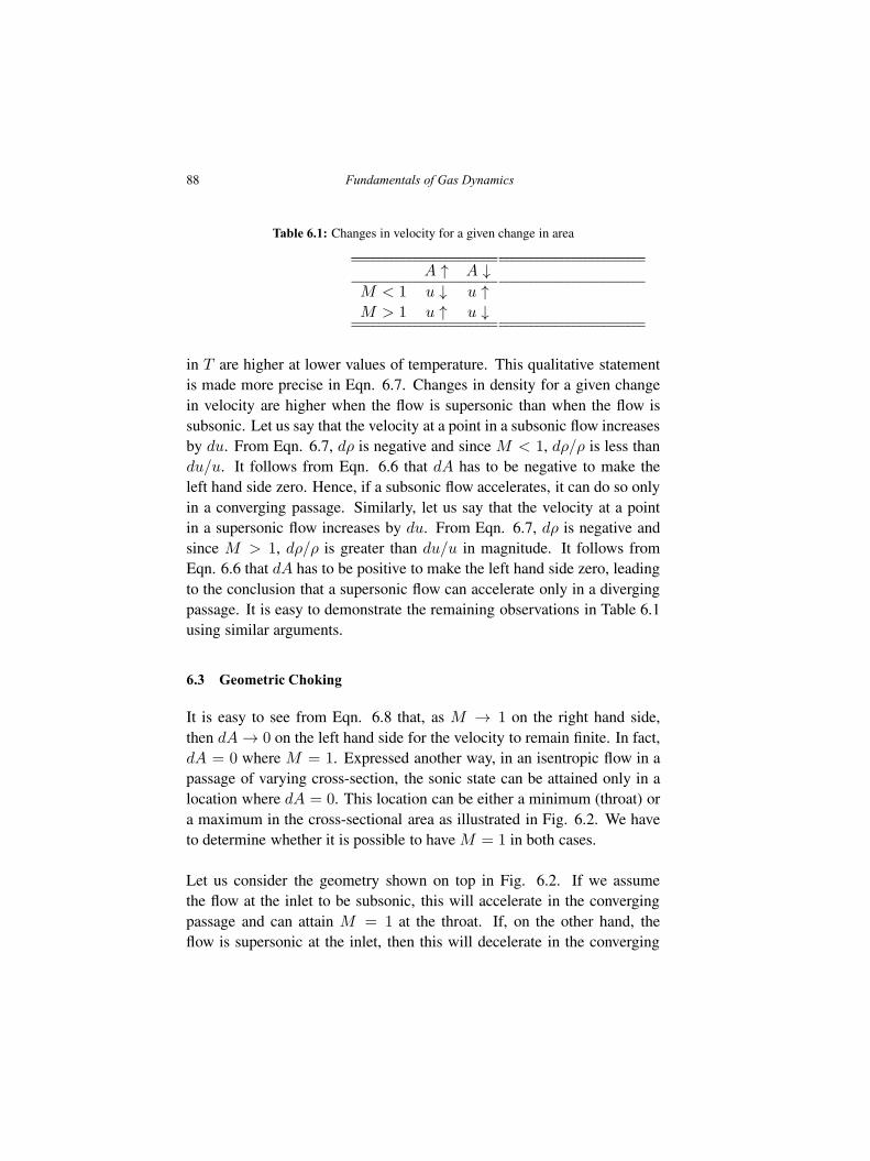
88 Fundamentals of Gas Dynamics
Table 6.1: Changes in velocity for a given change in area
A ↑ A ↓M < 1 u ↓ u ↑M > 1 u ↑ u ↓
in T are higher at lower values of temperature. This qualitative statementis made more precise in Eqn. 6.7. Changes in density for a given changein velocity are higher when the flow is supersonic than when the flow issubsonic. Let us say that the velocity at a point in a subsonic flow increasesby du. From Eqn. 6.7, dρ is negative and since M < 1, dρ/ρ is less thandu/u. It follows from Eqn. 6.6 that dA has to be negative to make theleft hand side zero. Hence, if a subsonic flow accelerates, it can do so onlyin a converging passage. Similarly, let us say that the velocity at a pointin a supersonic flow increases by du. From Eqn. 6.7, dρ is negative andsince M > 1, dρ/ρ is greater than du/u in magnitude. It follows fromEqn. 6.6 that dA has to be positive to make the left hand side zero, leadingto the conclusion that a supersonic flow can accelerate only in a divergingpassage. It is easy to demonstrate the remaining observations in Table 6.1using similar arguments.
6.3 Geometric Choking
It is easy to see from Eqn. 6.8 that, as M → 1 on the right hand side,then dA → 0 on the left hand side for the velocity to remain finite. In fact,dA = 0 where M = 1. Expressed another way, in an isentropic flow in apassage of varying cross-section, the sonic state can be attained only in alocation where dA = 0. This location can be either a minimum (throat) ora maximum in the cross-sectional area as illustrated in Fig. 6.2. We haveto determine whether it is possible to have M = 1 in both cases.
Let us consider the geometry shown on top in Fig. 6.2. If we assumethe flow at the inlet to be subsonic, this will accelerate in the convergingpassage and can attain M = 1 at the throat. If, on the other hand, theflow is supersonic at the inlet, then this will decelerate in the converging
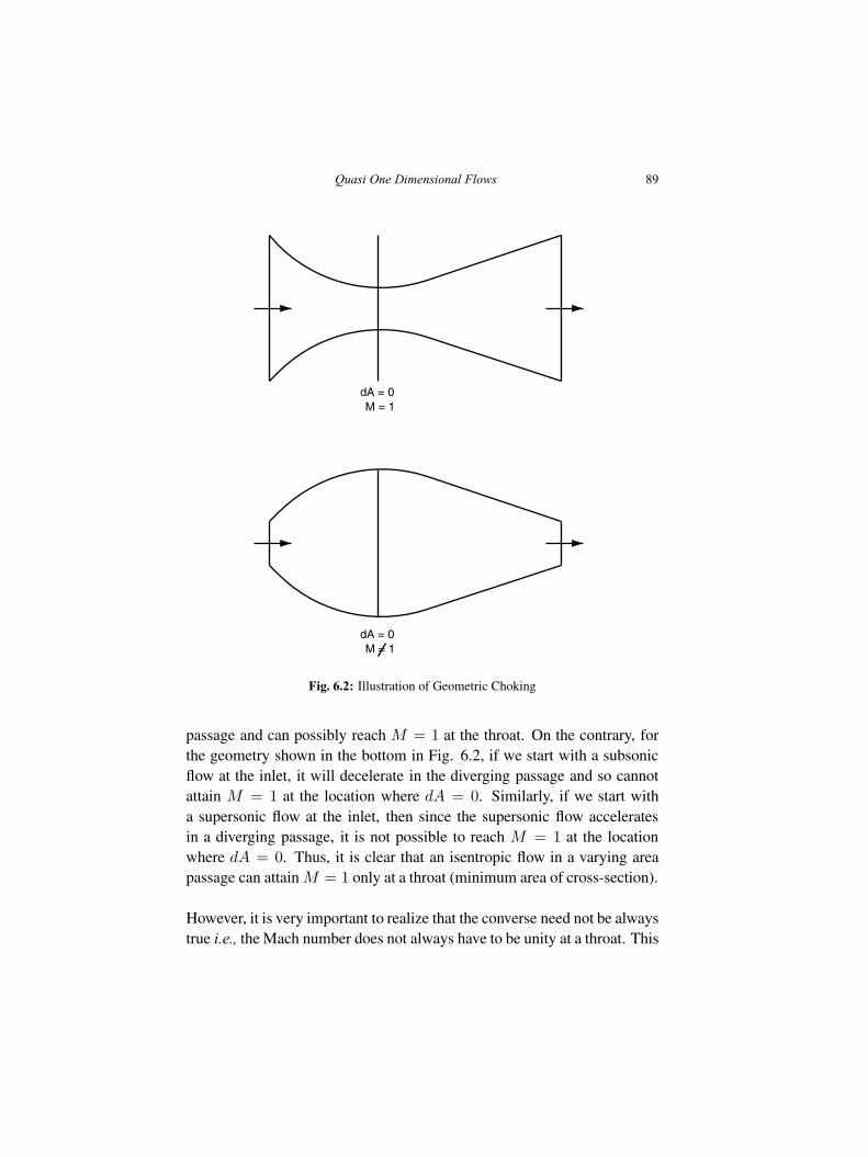
Quasi One Dimensional Flows 89
dA = 0M = 1
dA = 0M = 1
Fig. 6.2: Illustration of Geometric Choking
passage and can possibly reach M = 1 at the throat. On the contrary, forthe geometry shown in the bottom in Fig. 6.2, if we start with a subsonicflow at the inlet, it will decelerate in the diverging passage and so cannotattain M = 1 at the location where dA = 0. Similarly, if we start witha supersonic flow at the inlet, then since the supersonic flow acceleratesin a diverging passage, it is not possible to reach M = 1 at the locationwhere dA = 0. Thus, it is clear that an isentropic flow in a varying areapassage can attain M = 1 only at a throat (minimum area of cross-section).
However, it is very important to realize that the converse need not be alwaystrue i.e., the Mach number does not always have to be unity at a throat. This
90 Fundamentals of Gas Dynamics
can be established from Eqn. 6.8 as follows. If we allow dA → 0 on theleft hand side of Eqn. 6.8, then either M → 1 or du → 0 on the righthand side, since the velocity itself is finite. Of these two possibilities, theone realized in practice depends upon the prevailing operating condition.Hence, for the geometry on the top in Fig. 6.2, a flow, starting from asubsonic Mach number at the inlet can accelerate to a higher Mach number(but less than one) at the throat and decelerate afterwards. Similarly, theflow can start from a supersonic Mach number, decelerate to a value above1 at the throat and accelerate again. The same argument is applicable to thegeometry in the bottom in Fig. 6.2. Two things should thus become clearfrom the arguments given so far:
• Valid compressible flows are possible in both the geometries shownin Fig. 6.2. But, choking, if it occurs, can occur only in a geometricthroat. This is a consequence of the fact that, in Eqn. 6.8, when M →1, dA → 0 for the velocity to be finite.
• Flow need not always choke at a geometric throat. This follows fromthe fact that, in Eqn. 6.8, when dA → 0 at the throat, du → 0, withoutany restriction on the value of M .
When the Mach number does become equal to 1 at the throat, the flow issaid to be choked and this choking is a consequence of the area variationand is called geometric choking†.
6.4 Area Mach number Relation for Choked Flow
In a manner similar to the Rayleigh and Fanno flow problems, in the presentcase also, the state at any point can be conveniently related to the sonicstate. We proceed to derive a relationship between the Mach number andcross-sectional area at any axial location to the area at the location wherethe sonic state occurs. We start by equating the mass flow rates at these
†Mathematically, it is possible to have M = 1 at a location where dA/dx = 0 andd2A/dx2 > 0. These conditions are satisfied at locations where the area reaches a localminimum. Thus, we can have multiple locations where these conditions are satisfied as inFigs. 6.7 and 6.11. However, the Mach number will be equal to one at one or more of theselocations depending upon the actual flow conditions.
Quasi One Dimensional Flows 91
two locations,
m = ρuA = ρ∗u∗A∗ .
We can write
A
A∗=
ρ∗
ρ
u∗
u=
ρ∗
ρ0
ρ0ρ
u∗
u,
where ρ0 is the stagnation density. We know from Eqn. 2.18 that
ρ0ρ
=
(
1 +γ − 1
2M2
)1
γ − 1.
Setting M = 1 in this expression gives
ρ0ρ∗
=
(
γ + 1
2
) 1γ − 1
.
Also, u = Ma = M√γRT and u∗ = a =
√γRT ∗. Substituting these
expressions into the equation above for m, we get
A
A∗=
(
1 +γ − 1
2M2
)1
γ − 1(
2
γ + 1
)1
γ − 1 1
M
√
T ∗
T.
We can write T ∗/T in terms of Mach number as follows.
T ∗
T=
T ∗
T0
T0
T=
2
γ + 1
(
1 +γ − 1
2M2
)
.
If we substitute this into the equation above and simplify, we can finallywrite
(
A
A∗
)2
=1
M2
[
2
γ + 1
(
1 +γ − 1
2M2
)]
γ + 1γ − 1
. (6.9)
This relationship is called the Area Mach number relationship for an
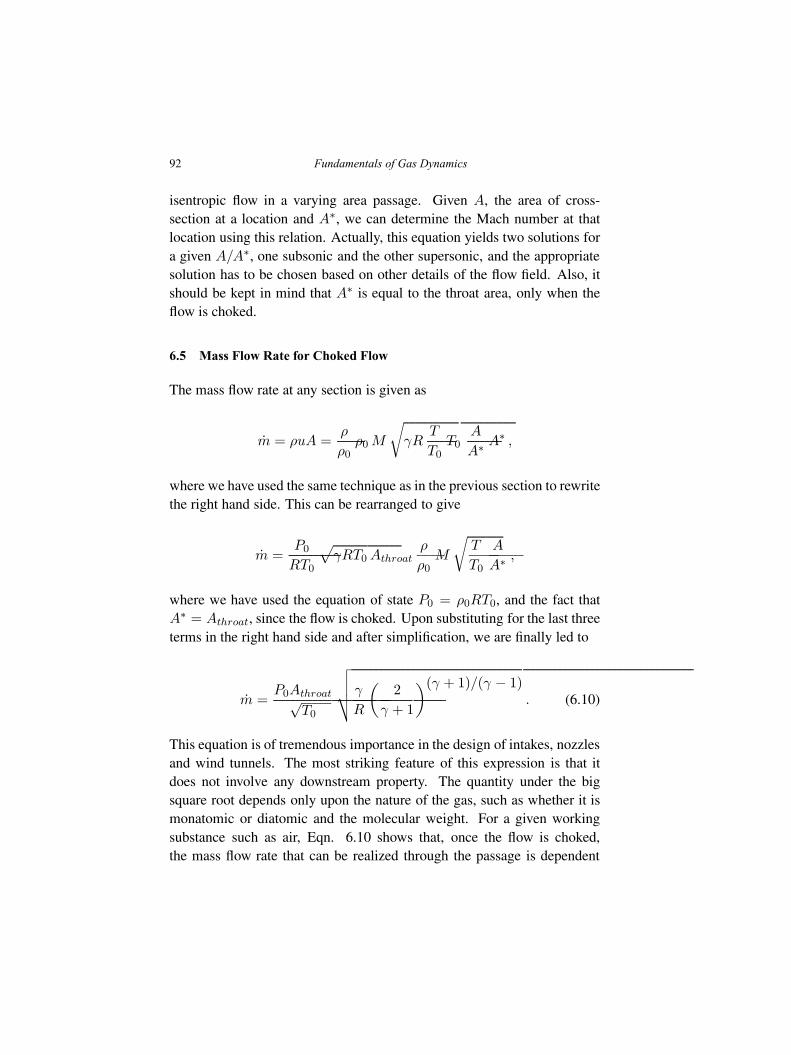
92 Fundamentals of Gas Dynamics
isentropic flow in a varying area passage. Given A, the area of cross-section at a location and A∗, we can determine the Mach number at thatlocation using this relation. Actually, this equation yields two solutions fora given A/A∗, one subsonic and the other supersonic, and the appropriatesolution has to be chosen based on other details of the flow field. Also, itshould be kept in mind that A∗ is equal to the throat area, only when theflow is choked.
6.5 Mass Flow Rate for Choked Flow
The mass flow rate at any section is given as
m = ρuA =ρ
ρ0ρ0 M
√
γRT
T0T0
A
A∗A∗ ,
where we have used the same technique as in the previous section to rewritethe right hand side. This can be rearranged to give
m =P0
RT0
√
γRT0 Athroatρ
ρ0M
√
T
T0
A
A∗,
where we have used the equation of state P0 = ρ0RT0, and the fact thatA∗ = Athroat, since the flow is choked. Upon substituting for the last threeterms in the right hand side and after simplification, we are finally led to
m =P0Athroat√
T0
√
√
√
√γ
R
(
2
γ + 1
)(γ + 1)/(γ − 1). (6.10)
This equation is of tremendous importance in the design of intakes, nozzlesand wind tunnels. The most striking feature of this expression is that itdoes not involve any downstream property. The quantity under the bigsquare root depends only upon the nature of the gas, such as whether it ismonatomic or diatomic and the molecular weight. For a given workingsubstance such as air, Eqn. 6.10 shows that, once the flow is choked,the mass flow rate that can be realized through the passage is dependent
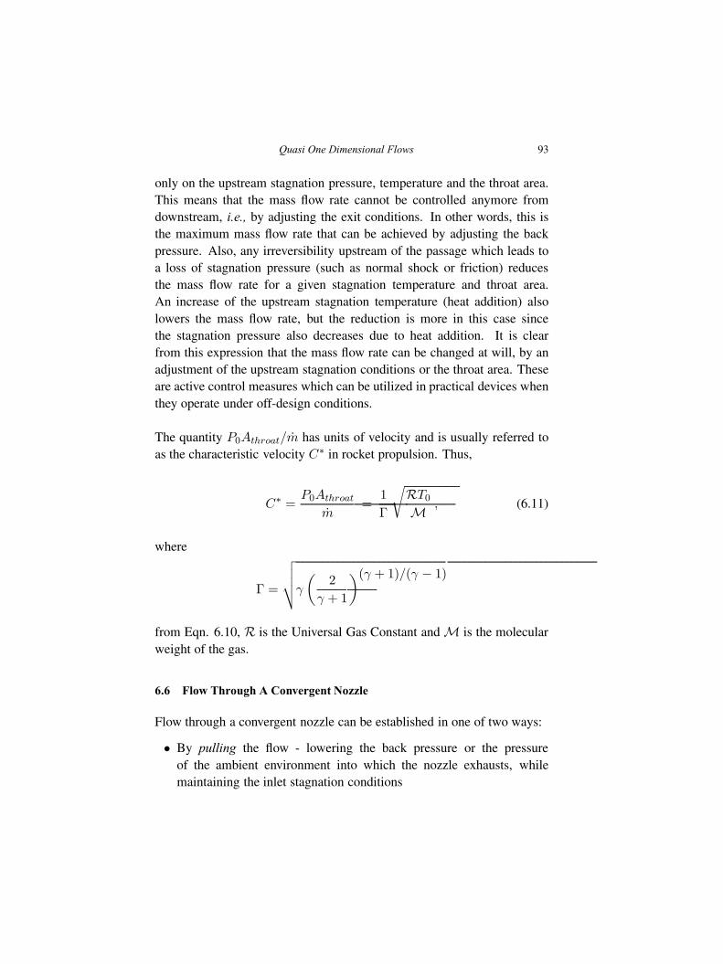
Quasi One Dimensional Flows 93
only on the upstream stagnation pressure, temperature and the throat area.This means that the mass flow rate cannot be controlled anymore fromdownstream, i.e., by adjusting the exit conditions. In other words, this isthe maximum mass flow rate that can be achieved by adjusting the backpressure. Also, any irreversibility upstream of the passage which leads toa loss of stagnation pressure (such as normal shock or friction) reducesthe mass flow rate for a given stagnation temperature and throat area.An increase of the upstream stagnation temperature (heat addition) alsolowers the mass flow rate, but the reduction is more in this case sincethe stagnation pressure also decreases due to heat addition. It is clearfrom this expression that the mass flow rate can be changed at will, by anadjustment of the upstream stagnation conditions or the throat area. Theseare active control measures which can be utilized in practical devices whenthey operate under off-design conditions.
The quantity P0Athroat/m has units of velocity and is usually referred toas the characteristic velocity C∗ in rocket propulsion. Thus,
C∗ =P0Athroat
m=
1
Γ
√
RT0
M , (6.11)
where
Γ =
√
√
√
√
γ
(
2
γ + 1
)(γ + 1)/(γ − 1)
from Eqn. 6.10, R is the Universal Gas Constant and M is the molecularweight of the gas.
6.6 Flow Through A Convergent Nozzle
Flow through a convergent nozzle can be established in one of two ways:
• By pulling the flow - lowering the back pressure or the pressureof the ambient environment into which the nozzle exhausts, whilemaintaining the inlet stagnation conditions
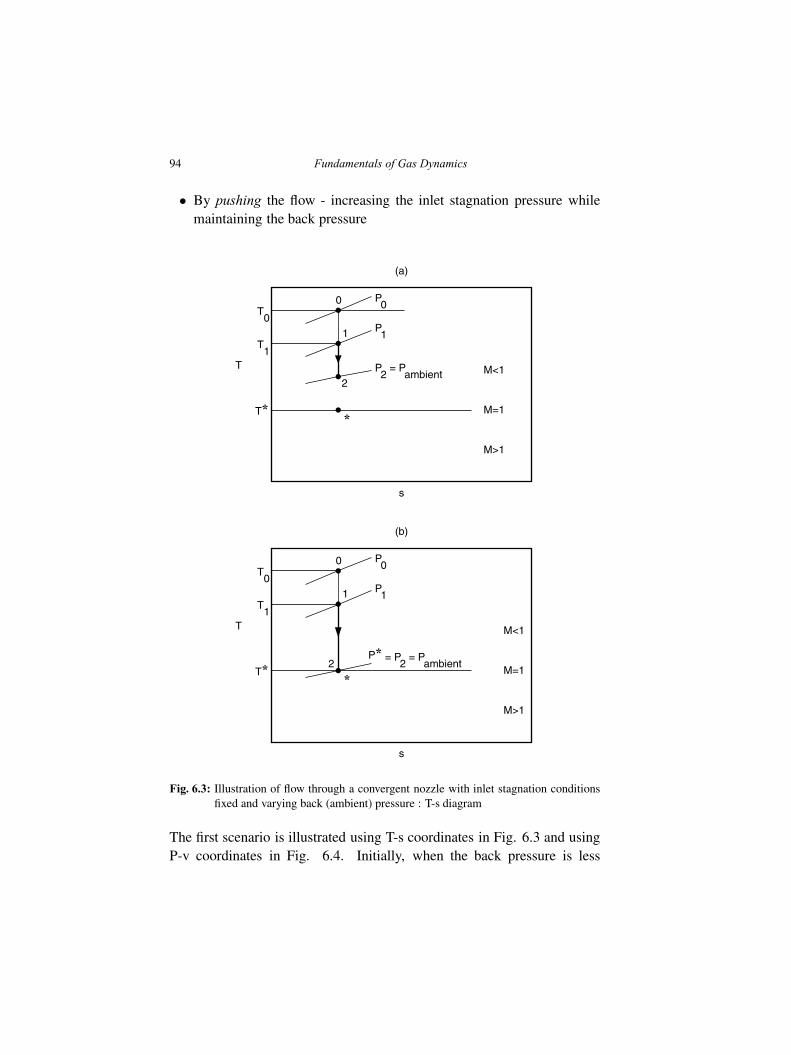
94 Fundamentals of Gas Dynamics
• By pushing the flow - increasing the inlet stagnation pressure whilemaintaining the back pressure
(a)
s
T
T0
M=1
M<1
M>1
0 P0
1 P1
T1
*T*
2P2 = P
ambient
(b)
s
T
T0
M=1
M<1
M>1
0 P0
1 P1
T1
*2
P* = P2 = P
ambientT*
Fig. 6.3: Illustration of flow through a convergent nozzle with inlet stagnation conditionsfixed and varying back (ambient) pressure : T-s diagram
The first scenario is illustrated using T-s coordinates in Fig. 6.3 and usingP-v coordinates in Fig. 6.4. Initially, when the back pressure is less
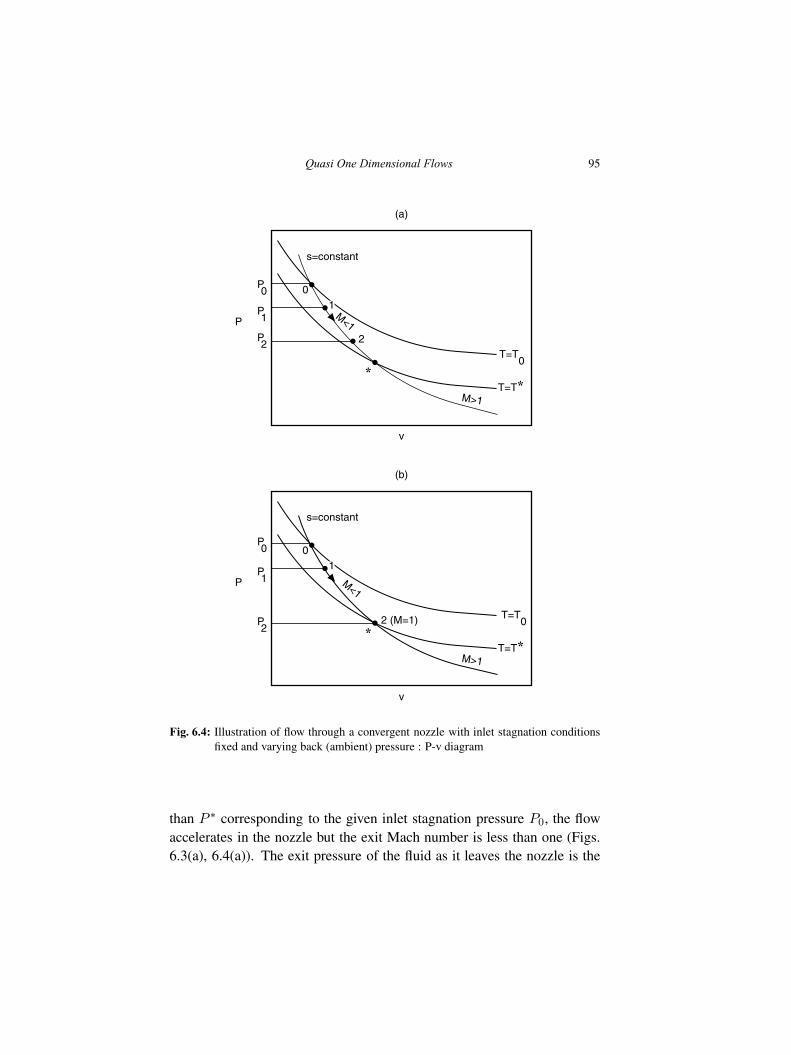
Quasi One Dimensional Flows 95
(a)
v
P
0P0
T=T0
s=constant
T=T**
1P1
2P2
M<1
M>1
(b)
v
P
0P0
T=T0
s=constant
T=T**
1P1
2 (M=1)P2
M<1
M>1
Fig. 6.4: Illustration of flow through a convergent nozzle with inlet stagnation conditionsfixed and varying back (ambient) pressure : P-v diagram
than P ∗ corresponding to the given inlet stagnation pressure P0, the flowaccelerates in the nozzle but the exit Mach number is less than one (Figs.6.3(a), 6.4(a)). The exit pressure of the fluid as it leaves the nozzle is the
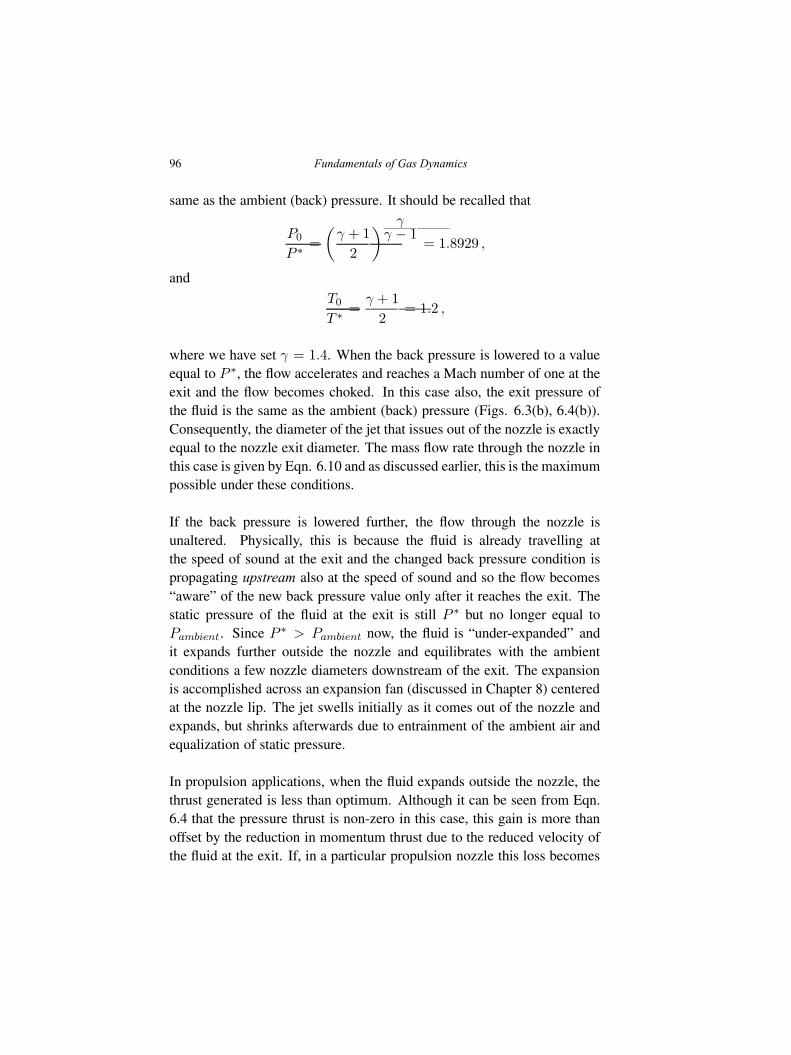
96 Fundamentals of Gas Dynamics
same as the ambient (back) pressure. It should be recalled that
P0
P ∗=
(
γ + 1
2
)
γγ − 1
= 1.8929 ,
and
T0
T ∗=
γ + 1
2= 1.2 ,
where we have set γ = 1.4. When the back pressure is lowered to a valueequal to P ∗, the flow accelerates and reaches a Mach number of one at theexit and the flow becomes choked. In this case also, the exit pressure ofthe fluid is the same as the ambient (back) pressure (Figs. 6.3(b), 6.4(b)).Consequently, the diameter of the jet that issues out of the nozzle is exactlyequal to the nozzle exit diameter. The mass flow rate through the nozzle inthis case is given by Eqn. 6.10 and as discussed earlier, this is the maximumpossible under these conditions.
If the back pressure is lowered further, the flow through the nozzle isunaltered. Physically, this is because the fluid is already travelling atthe speed of sound at the exit and the changed back pressure condition ispropagating upstream also at the speed of sound and so the flow becomes“aware” of the new back pressure value only after it reaches the exit. Thestatic pressure of the fluid at the exit is still P ∗ but no longer equal toPambient. Since P ∗ > Pambient now, the fluid is “under-expanded” andit expands further outside the nozzle and equilibrates with the ambientconditions a few nozzle diameters downstream of the exit. The expansionis accomplished across an expansion fan (discussed in Chapter 8) centeredat the nozzle lip. The jet swells initially as it comes out of the nozzle andexpands, but shrinks afterwards due to entrainment of the ambient air andequalization of static pressure.
In propulsion applications, when the fluid expands outside the nozzle, thethrust generated is less than optimum. Although it can be seen from Eqn.6.4 that the pressure thrust is non-zero in this case, this gain is more thanoffset by the reduction in momentum thrust due to the reduced velocity ofthe fluid at the exit. If, in a particular propulsion nozzle this loss becomes
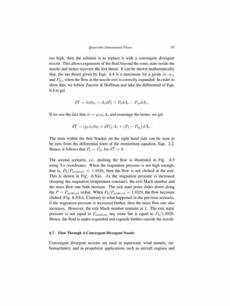
Quasi One Dimensional Flows 97
too high, then the solution is to replace it with a convergent divergentnozzle. This allows expansion of the fluid beyond the sonic state inside thenozzle and hence recovers the lost thrust. It can be shown mathematicallythat, the net thrust given by Eqn. 6.4 is a maximum for a given m, u∞and P∞, when the flow at the nozzle exit is correctly expanded. In order toshow this, we follow Zucrow & Hoffman and take the differential of Eqn.6.4 to get
dT = mdue +AedPe + PedAe − P∞dAe .
If we use the fact that m = ρeueAe and rearrange the terms, we get
dT = (ρeuedue + dPe)Ae + (Pe − P∞) dAe .
The term within the first bracket on the right hand side can be seen tobe zero from the differential form of the momentum equation, Eqn. 2.2.Hence, it follows that Pe = P∞ for dT = 0.
The second scenario, i.e., pushing the flow is illustrated in Fig. 6.5using T-s coordinates. When the stagnation pressure is not high enough,that is, P0/Pambient < 1.8929, then the flow is not choked at the exit.This is shown in Fig. 6.5(a). As the stagnation pressure is increased(keeping the stagnation temperature constant), the exit Mach number andthe mass flow rate both increase. The exit state point slides down alongthe P = Pambient isobar. When P0/Pambient = 1.8929, the flow becomeschoked (Fig. 6.5(b)). Contrary to what happened in the previous scenario,if the stagnation pressure is increased further, then the mass flow rate alsoincreases. However, the exit Mach number remains at 1. The exit staticpressure is not equal to Pambient any more but is equal to P0/1.8929.Hence, the fluid is under-expanded and expands further outside the nozzle.
6.7 Flow Through A Convergent Divergent Nozzle
Convergent divergent nozzles are used in supersonic wind tunnels, tur-bomachinery and in propulsion applications such as aircraft engines and
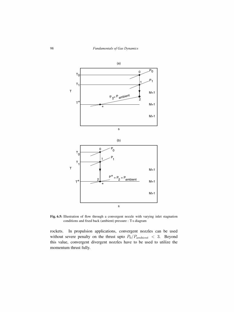
98 Fundamentals of Gas Dynamics
(a)
s
T
T0
M=1
M<1
M>1
0 P0
1P1
T1
*
2P 2= P ambient
T*
(b)
s
T
T0
M=1
M<1
M>1
0 P0
1 P1
T1
*2
P* = P2 = P
ambientT*
Fig. 6.5: Illustration of flow through a convergent nozzle with varying inlet stagnationconditions and fixed back (ambient) pressure : T-s diagram
rockets. In propulsion applications, convergent nozzles can be usedwithout severe penalty on the thrust upto P0/Pambient < 3. Beyondthis value, convergent divergent nozzles have to be used to utilize themomentum thrust fully.
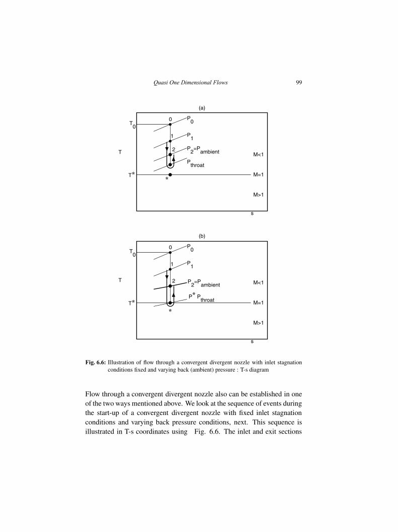
Quasi One Dimensional Flows 99
(a)
s
T
T0
M=1
M<1
M>1
0 P0
1 P1
*T*
Pthroat
2 P2=P
ambient
(b)
s
T
T0
M=1
M<1
M>1
0 P0
1 P1
*T*
P* Pthroat
2 P2=P
ambient
Fig. 6.6: Illustration of flow through a convergent divergent nozzle with inlet stagnationconditions fixed and varying back (ambient) pressure : T-s diagram
Flow through a convergent divergent nozzle also can be established in oneof the two ways mentioned above. We look at the sequence of events duringthe start-up of a convergent divergent nozzle with fixed inlet stagnationconditions and varying back pressure conditions, next. This sequence isillustrated in T-s coordinates using Fig. 6.6. The inlet and exit sections
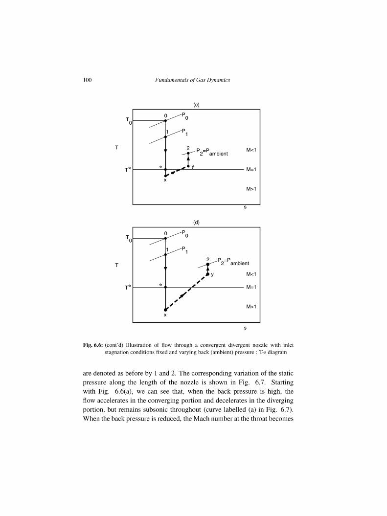
100 Fundamentals of Gas Dynamics
(c)
s
T
T0
M=1
M<1
M>1
0 P0
1 P1
*T*x
y
2 P2=P
ambient
(d)
s
T
T0
M=1
M<1
M>1
0 P0
1 P1
*T*
x
y
2 P2=P
ambient
Fig. 6.6: (cont’d) Illustration of flow through a convergent divergent nozzle with inletstagnation conditions fixed and varying back (ambient) pressure : T-s diagram
are denoted as before by 1 and 2. The corresponding variation of the staticpressure along the length of the nozzle is shown in Fig. 6.7. Startingwith Fig. 6.6(a), we can see that, when the back pressure is high, theflow accelerates in the converging portion and decelerates in the divergingportion, but remains subsonic throughout (curve labelled (a) in Fig. 6.7).When the back pressure is reduced, the Mach number at the throat becomes
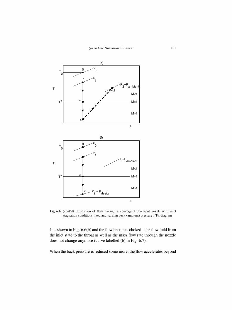
Quasi One Dimensional Flows 101
(e)
s
T
T0
M=1
M<1
M>1
0 P0
1 P1
*T*
x
y,2
P2=P
ambient
(f)
s
T
T0
M=1
M<1
M>1
0 P0
1 P1
*T*
2 P2 = P
design
P=Pambient
Fig. 6.6: (cont’d) Illustration of flow through a convergent divergent nozzle with inletstagnation conditions fixed and varying back (ambient) pressure : T-s diagram
1 as shown in Fig. 6.6(b) and the flow becomes choked. The flow field fromthe inlet state to the throat as well as the mass flow rate through the nozzledoes not change anymore (curve labelled (b) in Fig. 6.7).
When the back pressure is reduced some more, the flow accelerates beyond
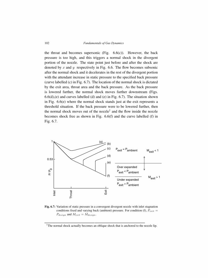
102 Fundamentals of Gas Dynamics
the throat and becomes supersonic (Fig. 6.6(c)). However, the backpressure is too high, and this triggers a normal shock in the divergentportion of the nozzle. The state point just before and after the shock aredenoted by x and y respectively in Fig. 6.6. The flow becomes subsonicafter the normal shock and it decelerates in the rest of the divergent portionwith the attendant increase in static pressure to the specified back pressure(curve labelled (c) in Fig. 6.7). The location of the normal shock is dictatedby the exit area, throat area and the back pressure. As the back pressureis lowered further, the normal shock moves further downstream (Figs.6.6(d),(e) and curves labelled (d) and (e) in Fig. 6.7). The situation shownin Fig. 6.6(e) where the normal shock stands just at the exit represents athreshold situation. If the back pressure were to be lowered further, thenthe normal shock moves out of the nozzle† and the flow inside the nozzlebecomes shock free as shown in Fig. 6.6(f) and the curve labelled (f) inFig. 6.7.
P/ P
0
(a)(b)
(c)
(d)
(e)
(f)
Pexit = Pambient Mexit < 1
Over expandedPexit < Pambient
Under expandedPexit > Pambient
Mexit > 1
Inle
t
Thr
oat
Exi
t
0.53
1
Fig. 6.7: Variation of static pressure in a convergent divergent nozzle with inlet stagnationconditions fixed and varying back (ambient) pressure. For condition (f), Pexit =
Pdesign and Mexit = Mdesign.
†The normal shock actually becomes an oblique shock that is anchored to the nozzle lip.
Quasi One Dimensional Flows 103
Two things should be noted in Figs. 6.6(c)-(e). Firstly, the Machnumber before the shock keeps increasing as the shock moves downstream.Consequently, the loss of stagnation pressure across the shock wave alsokeeps increasing. Secondly, the flow field upstream of the shock wave doesnot change as the back pressure is lowered, since the flow is supersonicahead of the shock wave. Finally, when the back pressure is decreasedto the design value, the flow through the nozzle becomes shock free(isentropic) and the flow is supersonic throughout the divergent portion(Fig. 6.6(f) and curve labelled (f) in Fig. 6.7). Since the exit area and thethroat area are known, and M = 1 at the throat, the exit Mach number canbe calculated from Eqn. 6.9.
If the back pressure is lowered below the design value, the nozzle exitpressure does not change. The jet is now said to be “under-expanded” (asin the case of the convergent nozzle) and further expansion takes placeoutside the nozzle.
In contrast to a convergent nozzle, it is possible to operate a convergentdivergent nozzle in an “over-expanded” mode. This happens when theback pressure is higher than the design value, but lower than the valuefor which a normal shock would stand just at the exit (Fig. 6.7). Sincethe static pressure of the jet as it comes out of the nozzle is less than theambient value, it undergoes compression through oblique shocks outsidethe nozzle.
The variation of thrust due to under-expanded and over-expanded mode ofoperation is a difficult issue with rocket engines, designed for a particularoperational altitude. The jet is over-expanded at altitudes below the designaltitude and under-expanded at higher altitudes. Altitude compensatingnozzles are a better alternative under such circumstances.
The start-up sequence described above remains the same when the backpressure is fixed and the inlet stagnation pressure is varied. This meansthat the normal shock that occurs in the divergent portion is inevitable andcannot be avoided. This is undesirable since the loss of stagnation pressure
104 Fundamentals of Gas Dynamics
across the normal shock can be quite high. It is for these reasons, thatconvergent divergent nozzles are not used in propulsion applications unlessthe pressure ratio P0/Pambient is high enough.
Example 6.1. A converging diverging nozzle with an exit to throat ratio of3.5, operates with inlet stagnation conditions 1 MPa and 500 K. Determinethe exit conditions when the back pressure is (a) 20 kPa (b) 500 kPa.Assume air to be the working fluid (γ = 1.4, Mol. wt = 28.8 kg/kmol).
Solution. Given P0,1 = 1 MPa, T0 = 500 K and Aexit/Athroat = 3.5. Fora correctly expanded flow, the exit conditions for this area ratio are (fromthe isentropic table)
P0,1
Pexit= 27.14 ,
T0
Texit= 2.568 and Mexit = 2.8 .
Therefore, Pexit = 36.85 kPa and Texit = 194.7 K
(a) Since the given exit static pressure of 20 kPa is less than the designvalue of 36.85 kPa, the flow is under-expanded. The values for the exitproperties are the same as the design values.
(b) For a back pressure of 500 kPa, we have to see whether the flow iscompletely subsonic in the divergent portion or there is a normal shock. Ifwe assume that the nozzle is still choked, then, for fully subsonic flow inthe divergent portion, from the isentropic table, for an area ratio of 3.5,
1.01803 <P0,1
Pexit< 1.02038 ⇒ 980 kPa < Pexit < 982.29 kPa .
Since the given Pexit is less than this value, there is a normal shock in thedivergent portion. The mass flow rate through the nozzle is the same at thethroat and the exit sections. Thus,
m = ρ∗ u∗Athroat = ρexit uexit Aexit
⇒ P ∗
RT ∗
√
γRT ∗Athroat =Pexit
RTexitMexit
√
γRTexitAexit
Quasi One Dimensional Flows 105
P ∗
P0,1
P0,1
Pexit
√
T0
T ∗
Athroat
Aexit= Mexit
√
T0
Texit
⇒ P ∗
P0,1
P0,1
Pexit
√
γ + 1
2
Athroat
Aexit= Mexit
√
1 +γ − 1
2M2
exit
⇒ 1
1.893
1000
500
√1.2
1
3.5= Mexit
√
1 + 0.2M2exit
⇒ 0.2756 = Mexit
√
1 + 0.2M2exit
Therefore, Mexit = 0.2735,
Texit =Texit
T0T0 =
1
1.015500 = 493K
and
P0,exit =P0
PexitPexit = 1.056 × 500 = 528kPa .
The loss of stagnation pressure due to the normal shock is almost 50percent.
Let x, y denote the states just ahead of and behind the normal shock.For P0,y/P0,x = 528/1000 = 0.528, from the normal shock table we getMx = 2.43. From the isentropic table, A/A∗ corresponding to this valueof Mach number is 2.4714. Thus, the normal shock stands at a location inthe divergent portion where A/Athroat is 2.4714. �
The occurrence of the normal shock during start-up of a convergentdivergent nozzle leads to difficulties in non-propulsion applications also.Consider the supersonic wind tunnel shown in Fig. 6.8, where a convergent
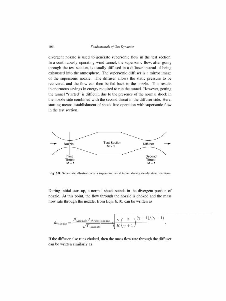
106 Fundamentals of Gas Dynamics
divergent nozzle is used to generate supersonic flow in the test section.In a continuously operating wind tunnel, the supersonic flow, after goingthrough the test section, is usually diffused in a diffuser instead of beingexhausted into the atmosphere. The supersonic diffuser is a mirror imageof the supersonic nozzle. The diffuser allows the static pressure to berecovered and the flow can then be fed back to the nozzle. This resultsin enormous savings in energy required to run the tunnel. However, gettingthe tunnel “started” is difficult, due to the presence of the normal shock inthe nozzle side combined with the second throat in the diffuser side. Here,starting means establishment of shock free operation with supersonic flowin the test section.
FirstThroatM = 1
SecondThroatM = 1
Test SectionM > 1
Nozzle Diffuser
Fig. 6.8: Schematic illustration of a supersonic wind tunnel during steady state operation
During initial start-up, a normal shock stands in the divergent portion ofnozzle. At this point, the flow through the nozzle is choked and the massflow rate through the nozzle, from Eqn. 6.10, can be written as
mnozzle =P0,nozzleAthroat,nozzle
√
T0,nozzle
√
√
√
√γ
R
(
2
γ + 1
)(γ + 1)/(γ − 1).
If the diffuser also runs choked, then the mass flow rate through the diffusercan be written similarly as
Quasi One Dimensional Flows 107
mdiffuser =P0,diffuserAthroat,diffuser
√
T0,diffuser
√
√
√
√γ
R
(
2
γ + 1
)(γ + 1)/(γ − 1).
There is no change in stagnation temperature between the nozzle and thediffuser section. However, because of the normal shock, there is a loss ofstagnation pressure and so P0,diffuser < P0,nozzle. If the throat areas ofthe nozzle and the diffuser are the same, then the maximum mass flow ratethat the diffuser can handle is less than the mass flow rate coming fromthe nozzle. The only way to accommodate the higher mass flow rate is toincrease the diffuser throat area. If we equate the mass flow rates throughthe nozzle and diffuser, we get,
Athroat,diffuser
Athroat,nozzle=
P0,nozzle
P0,diffuser.
The loss of stagnation pressure is the highest when the normal shock standsin the test section as the Mach number is the highest there. The diffuserthroat should be sized for this condition. This allows the normal shockto be “swallowed” by the diffuser throat and the shock then moves intothe divergent portion of the diffuser. It will eventually sit in the diffuserthroat. At this point, the tunnel is shock free with supersonic flow in thetest section and the tunnel is said to be “started”. The diffuser throat areanow has to be reduced. During steady state operation, the diffuser throatarea is equal to the nozzle throat area, although in reality it will be larger.
Example 6.2. Diffusers are commonly used in the intakes of supersonicvehicle to decelerate the incoming supersonic free stream to the appropriateMach number before entry into the combustor. Consider a convergingdiverging diffuser in Fig. 6.9 (usually called an internal compressionintake) that is designed for shock free operation at a free stream Machnumber of 2. Determine the ratio of the mass flow rate through the diffuserwhen the free stream Mach number is 1.5, to that at design condition. Alsodetermine the stagnation pressure recovery. Assume the intake geometryto be fixed and the throat Mach number to be 1 in all the cases. Free streamstatic conditions also remain the same.
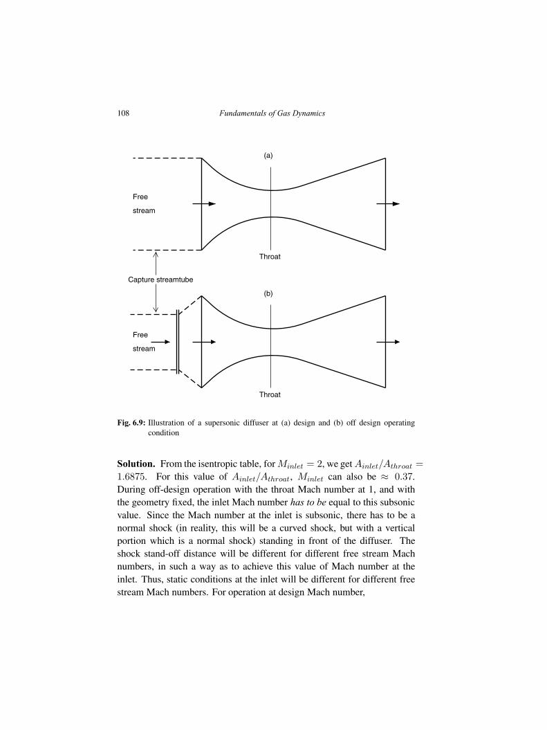
108 Fundamentals of Gas Dynamics
Throat
(b)
Free
stream
Throat
(a)
Free
stream
Capture streamtube
Fig. 6.9: Illustration of a supersonic diffuser at (a) design and (b) off design operatingcondition
Solution. From the isentropic table, for Minlet = 2, we get Ainlet/Athroat =
1.6875. For this value of Ainlet/Athroat, Minlet can also be ≈ 0.37.During off-design operation with the throat Mach number at 1, and withthe geometry fixed, the inlet Mach number has to be equal to this subsonicvalue. Since the Mach number at the inlet is subsonic, there has to be anormal shock (in reality, this will be a curved shock, but with a verticalportion which is a normal shock) standing in front of the diffuser. Theshock stand-off distance will be different for different free stream Machnumbers, in such a way as to achieve this value of Mach number at theinlet. Thus, static conditions at the inlet will be different for different freestream Mach numbers. For operation at design Mach number,
Quasi One Dimensional Flows 109
mdesign =P0,∞Athroat√
T0,∞
√
γ
R
(
2
γ + 1
)(γ+1)/(γ−1)
,
where the subscript ∞ denotes free stream condition. From isentropictable, for M∞ = 2, we get,
P0,∞
P∞
= 7.82445 andT0,∞
T∞
= 1.8 .
⇒ mdesign = 5.832P∞Athroat√
T∞
√
γ
R
(
2
γ + 1
)(γ+1)/(γ−1)
.
For operation with M∞ = 1.5,
m(M∞ = 1.5) =P0,inletAthroat√
T0,inlet
√
γ
R
(
2
γ + 1
)(γ+1)/(γ−1)
.
From the normal shock table, for M = 1.5, we get
P0,inlet
P0,∞= 0.929787 .
From the isentropic table, for M∞ = 1.5, we get
P0,∞
P∞
= 3.67103 andT0,∞
T∞
= 1.45 .
Therefore,
P0,inlet =P0,inlet
P0,∞
P0,∞
P∞
P∞ = 3.4133P∞ ,
T0,inlet =T0,inlet
T0,∞
T0,∞
T∞
T∞ = 1.45T∞
110 Fundamentals of Gas Dynamics
and
m(M∞ = 1.5) = 2.8346P∞Athroat√
T∞
√
γ
R
(
2
γ + 1
)(γ+1)/(γ−1)
.
Therefore,
m(M∞ = 1.5)
mdesign= 0.486
and the total pressure recovery is 93 percent.
Shock free operation even under off-design operating conditions can beachieved by having a variable area throat. The intake can be “started” byincreasing the throat area such that
Athroat(M∞ = 1.5)
Athroat(design)=
1
0.486= 2.058 .
During shock free operation, the throat area should be reduced such that
Athroat(M∞ = 1.5)
Athroat(design)=
1.6875
1.17617= 1.435 .
Thus, by adjusting the throat area to match the mass flow rate that the intakecan “swallow”, the normal shock in front of the intake under off-designoperating conditions can be avoided. However, the required area variationis too large for such internal compression intakes to be of practical use.
Capture area of an intake is an important performance metric of supersonicintakes. The capture area is the freestream cross-sectional area of thestreamtube that enters the intake. From Fig. 6.9, it is clear that the capturearea for design operating condition is equal to the inlet area. For off-design operating condition, since the mass flow rate is less, capture areaalso decreases. For the above example,
Quasi One Dimensional Flows 111
For operation with M∞ = 1.5,
A∞
Athroat=
2.8346
M∞
√
(
2
γ + 1
)(γ+1)/(γ−1)
= 1.1 .
For comparison, at design operating condition, A∞/Athroat = 1.6875 �
6.8 Interaction between Nozzle Flow and Fanno, Rayleigh Flows
So far, we have looked at flow through a constant area passage with friction,with heat addition and isentropic flow through nozzles in isolation. In reallife applications, there will always be an interaction, since a nozzle has tobe connected to a high pressure reservoir located upstream through pipes,or heat addition in a combustion chamber is followed by expansion in anozzle and so on. From Eqn. 6.10, we know that the mass flow rate througha nozzle is affected by any upstream changes in stagnation pressure andtemperature. Since Fanno flow and Rayleigh flow both result in changesin stagnation pressure (and stagnation temperature in the latter case), it isimportant to study the interaction between these flows.
Figure 6.10(a) shows a constant area passage followed by a convergentnozzle. In keeping with what we have discussed so far, we will assumefrictional flow in the constant area passage and isentropic flow in thenozzle. The process is illustrated using T-s coordinates in Fig. 6.10(b).State points 1 and 2 lie on the Fanno curve. The isentropic process in thenozzle is indicated by the vertical line going down to the sonic isotherm.Here, without any loss of generality, we have assumed the exit state to besonic, but it need not be. As long as the exit Mach number is subsonic orjust becoming sonic, the exit static pressure will be equal to the ambientpressure. Thus, it is possible to have geometric choking in this case, butnot friction choking. Owing to the loss of stagnation pressure due to theeffect of friction ahead of the nozzle, the choked mass flow rate throughthe nozzle is less now by a factor of 1−P0,2/P0,1. The longer the distancebetween the nozzle and the reservoir i.e., longer the pipe connecting the
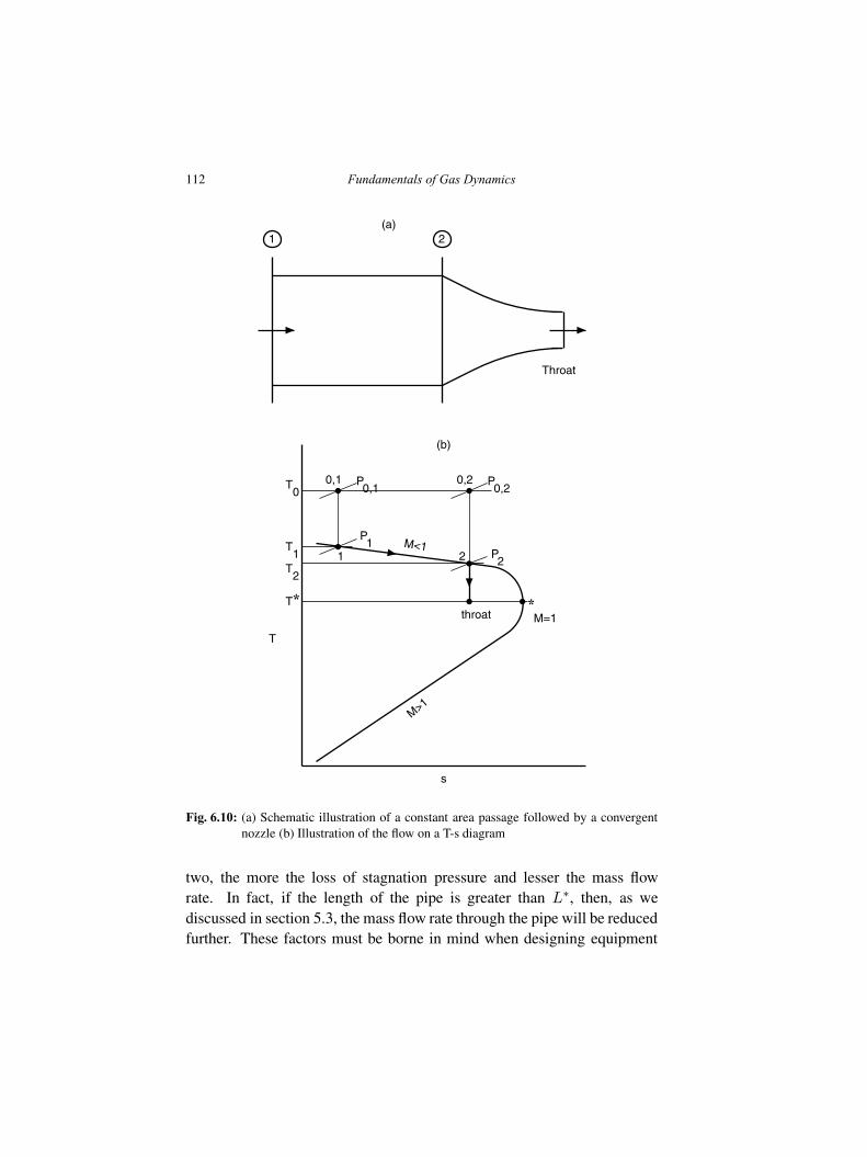
112 Fundamentals of Gas Dynamics
Throat
1 2(a)
(b)
s
T
M<1
M>1
T0
0,1 P0,1
1
P1T
1
0,2 P0,2
2 P2
T2
throat*T*M=1
Fig. 6.10: (a) Schematic illustration of a constant area passage followed by a convergentnozzle (b) Illustration of the flow on a T-s diagram
two, the more the loss of stagnation pressure and lesser the mass flowrate. In fact, if the length of the pipe is greater than L∗, then, as wediscussed in section 5.3, the mass flow rate through the pipe will be reducedfurther. These factors must be borne in mind when designing equipment
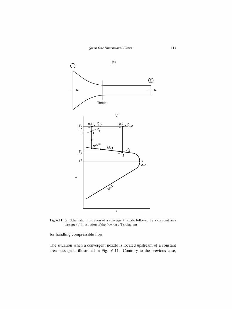
Quasi One Dimensional Flows 113
Throat
1
2
(a)
(b)
s
T
M<1
M>1
T00,1 P0,1
1P1T1
throat
0,2 P0,2
2
P2T2
*T*M=1
Fig. 6.11: (a) Schematic illustration of a convergent nozzle followed by a constant areapassage (b) Illustration of the flow on a T-s diagram
for handling compressible flow.
The situation when a convergent nozzle is located upstream of a constantarea passage is illustrated in Fig. 6.11. Contrary to the previous case,
114 Fundamentals of Gas Dynamics
now, the Mach number at the nozzle throat cannot reach 1, since the Machnumber has to increase further in the constant area section due to friction.Hence, it is possible to have friction choking but not geometric choking inthis case. Since the nozzle cannot choke, the mass flow rate is less thanthe maximum value possible for the given stagnation conditions at section1 and throat area. Thus, in this case also, the mass flow rate is reduced dueto the effect of friction.
Figure 6.12(a) shows a converging diverging nozzle feeding a constantarea passage. The process is shown on a T-s diagram in Fig. 6.12(b),when the length of the passage is less than L∗ corresponding to the Machnumber at the inlet of the passage. The isentropic expansion in the nozzle isdenoted by the vertical line 1-2 in this figure, and the Fanno process in theconstant area passage by 2-3 in supersonic branch of the Fanno curve. Ifthe length of the constant area passage is greater than the L∗ correspondingto M2, then a normal shock occurs somewhere in the passage and the flowbecomes subsonic. This is illustrated in Fig. 6.12(c). There is no change inthe mass flow rate, however. As the passage length is increased, this shockmoves upstream and can even go into the divergent portion of the nozzle.
The interaction between flow with heat addition and isentropic flow ina nozzle can be developed along the same lines as discussed above. Ifthe heat addition takes place before the nozzle, then the reduction in themass flow rate is even higher, since heat addition not only increases thestagnation temperature but decreases the stagnation pressure as well. It isleft as an exercise to the reader to illustrate the interaction on T-s diagramssimilar to Figs. 6.10-6.12. These considerations are important in practicalpropulsion applications such as combustors and afterburners. Most of theaircraft engines used in military applications have an afterburner for shortduration thrust augmentation. The basic principle in an afterburner is toinject and burn fuel in the tail pipe portion located just before the nozzle.This increases the velocity of the fluid as it comes out of the nozzle, therebyincreasing the thrust. Usually, a convergent nozzle is used with or withoutthe afterburner in operation. However, the throat area of the nozzle has tobe increased when the afterburner is in operation, if the mass flow rate isto be maintained, due to the above mentioned factors. Consequently, such
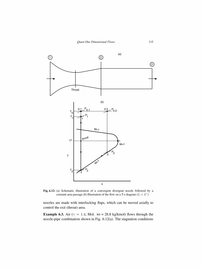
Quasi One Dimensional Flows 115
Throat
1 2
3
(a)
(b)
s
T
M<1
M>1
T0
0,1 P0,1
1P1T1
throat
2P2T2
3P3
*T*M=1
0,3 P0,3
Fig. 6.12: (a) Schematic illustration of a convergent divergent nozzle followed by aconstant area passage (b) Illustration of the flow on a T-s diagram (L < L∗)
nozzles are made with interlocking flaps, which can be moved axially tocontrol the exit (throat) area.
Example 6.3. Air (γ = 1.4, Mol. wt = 28.8 kg/kmol) flows through thenozzle-pipe combination shown in Fig. 6.12(a). The stagnation conditions
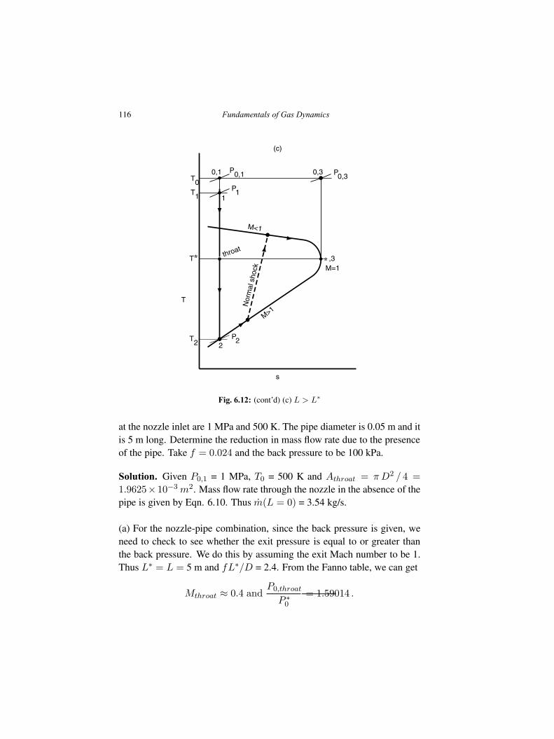
116 Fundamentals of Gas Dynamics
(c)
s
T
M<1
M>1
T0
0,1 P0,1
1P1T1
throat
2P2T2
* ,3T*M=1
0,3 P0,3
Nor
mal
sho
ck
Fig. 6.12: (cont’d) (c) L > L∗
at the nozzle inlet are 1 MPa and 500 K. The pipe diameter is 0.05 m and itis 5 m long. Determine the reduction in mass flow rate due to the presenceof the pipe. Take f = 0.024 and the back pressure to be 100 kPa.
Solution. Given P0,1 = 1 MPa, T0 = 500 K and Athroat = πD2 / 4 =
1.9625×10⁻³ m2. Mass flow rate through the nozzle in the absence of thepipe is given by Eqn. 6.10. Thus m(L = 0) = 3.54 kg/s.
(a) For the nozzle-pipe combination, since the back pressure is given, weneed to check to see whether the exit pressure is equal to or greater thanthe back pressure. We do this by assuming the exit Mach number to be 1.Thus L∗ = L = 5 m and fL∗/D = 2.4. From the Fanno table, we can get
Mthroat ≈ 0.4 andP0,throat
P ∗0
= 1.59014 .
Quasi One Dimensional Flows 117
Therefore,
P ∗ =P ∗0
P0,throatP0,throat
P ∗
P ∗0
=1
1.59014(1000)
1
1.89293= 332 kPa ,
where we have used M = 1 at the exit. Since P ∗ is greater than the backpressure, it is clear that the flow at the exit is under-expanded and the Machnumber at the exit is indeed equal to one. Proceeding further,
m(L = 5m) = ρthroat uthroat Athroat
=Pthroat
RTthroatMthroat
√
γRTthroat Athroat
=Pthroat
P0,1P0,1
√
γ
RT0
√
T0
TthroatMthroatAthroat
=1
1.1117
106
(3.1143 × 10⁻³)
√1.032 (0.4) (1.9635 × 10⁻³)
= 2.235kg/s
The reduction in mass flow rate is about 37 percent.
Example 6.4. In an aircraft jet engine fitted with a constant area after-burner and a converging nozzle, post-combustion gas enters the nozzle witha stagnation temperature and pressure of 900 K and 0.5 MPa, when theafterburner is not lit. With the afterburner lit, the stagnation temperatureincreases to 1900 K with a 15 percent loss in stagnation pressure at thenozzle inlet. If the mass flow rate has to be maintained at 90 kg/s, determinethe required nozzle exit area in both cases. Also, determine the thrustaugmentation with afterburner operation, assuming that the engine is on astatic test stand at sea level (ambient pressure 0.1 MPa). Assume isentropicprocess for the nozzle. For the gas, take γ = 4/3 and Cp = 1.148 kJ/kg.K
Solution. When the afterburner is not lit, the stagnation pressure at entryto the nozzle is P0 = 0.5 MPa. The critical pressure corresponding to this
118 Fundamentals of Gas Dynamics
stagnation pressure is
P ∗ = P0
(
2
γ + 1
)γ
γ−1
= 0.27MPa .
Since the ambient pressure P∞ = 0.1 MPa is less than P ∗, the nozzle ischoked and so the exit static pressure Pe = P ∗ = 0.27 MPa. The massflow rate is thus given by
m =P0Athroat√
T0
√
γ
R
(
2
γ + 1
)(γ+1)/(γ−1)
.
When the afterburner is not lit, P0 = 0.5 MPa and T0 = 900 K. Substitutingthese values, we get
Athroat = 0.1359m2 .
Also, the exit static temperature can be evaluated as
Te = T ∗ = T0
(
2
γ + 1
)
= 771K
and the exit velocity is thus
ue =√
γRTe = 543m/s .
When the afterburner is lit, P0 = 0.5 × 0.85 = 0.425 MPa and the criticalpressure corresponding to this stagnation pressure is
P ∗ = P0
(
2
γ + 1
)γ
γ−1
= 0.229MPa .
Since the ambient pressure P∞ = 0.1 MPa is less than P ∗, the nozzle ischoked in this case also and so the exit static pressure Pe = P ∗ = 0.229
Quasi One Dimensional Flows 119
MPa. With T0 = 1900 K, we can get
Athroat = 0.1359
(
0.5
0.425
)
√
1900
900= 0.3817m2 .
The exit static temperature Te and the exit velocity ue can be calculated tobe 1629 K and 789 m/s in the same manner as before.
From Eqn. 6.4, thrust developed is given as
T = m ue + (Pe − P∞)Ae ,
where we have set u∞ = 0, since the engine is on a static thrust stand.Therefore,
Thrust (no afterburner) = 48.87 kN + 23.103 kN = 71.973 kN
and Thrust (with afterburner) = 71 kN + 30 kN = 101 kN
Thrust augmentation due to afterburner is about 40 percent. Note thatthe pressure thrust in both the cases is non-zero due to under-expandedoperation of the nozzle.
Example 6.5. In the above example, if a converging diverging nozzle isused instead of a convergent nozzle during normal operation without anafterburner, what would be the thrust?
Solution. Assuming that the flow is correctly expanded, exit pressure withthe converging diverging nozzle is 0.1 MPa. Thus,
P0
Pe= 5 =
(
1 +γ − 1
2M2
e
)γ
γ−1
.
This can be solved easily to give the exit Mach number Me = 1.73. The
120 Fundamentals of Gas Dynamics
exit static temperature Te can be calculated using
Te =T0
1 + γ−12 M2
e
= 602K .
The exit velocity,
ue = Me
√
γRTe = 830m/s .
Therefore, Thrust (no afterburner) = 74.7 kN + 0 kN = 74.7 kN. It is clearthat the increase in thrust is minimal when we use a convergent divergentnozzle in this case.
Example 6.6. We close this chapter with a very interesting exampleinvolving nozzle-nozzle interaction, adapted from White’s book (whoattributes this problem to a book by Thompson). The schematic is shownin Fig. 6.13. The arrangement consists of two tanks, with the one in theleft being larger and two identical converging nozzles. The pressure in thelarge tank remains constant at 1 MPa and the ambient pressure is 0.1 MPa.We wish to find out whether the nozzles are choked or not under steadystate operation (neglecting heat losses).
Solution. To begin with, based on the numerical values given, it is easyto conclude that the static pressure (and the stagnation pressure) in thesmaller tank will be well above the critical value of 0.18929 MPa. In fact,it is likely to be close to 1 MPa. Consequently, the nozzle on the smallertank will be choked. Although we can safely assume that the nozzlesoperate isentropically, the mixing process in the smaller tank introducessome irreversibility in the flow. Due to this irreversibility, the stagnationpressure for the downstream nozzle is less than that for the one locatedon the larger tank. In addition, T0, Athroat are also the same for both thenozzles. Since, during steady state operation, the mass flow rates throughboth the nozzles have to be equal, we can conclude from Eqn. 6.10 that thenozzle on the larger tank is not choked.
Note that, during start-up, the nozzle on the larger tank is choked, while
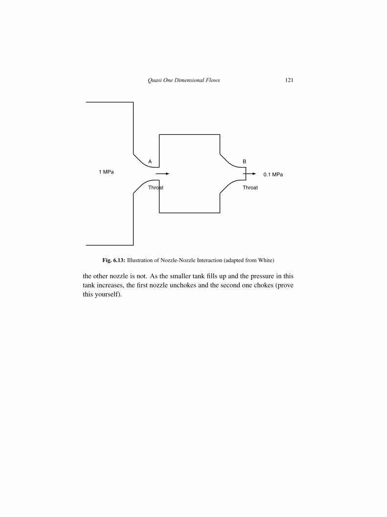
Quasi One Dimensional Flows 121
Throat
A
1 MPa
Throat
B
0.1 MPa
Fig. 6.13: Illustration of Nozzle-Nozzle Interaction (adapted from White)
the other nozzle is not. As the smaller tank fills up and the pressure in thistank increases, the first nozzle unchokes and the second one chokes (provethis yourself).
122 Fundamentals of Gas Dynamics
Exercises
(1) Consider the two tank system in Fig. 6.13. Assume, in addition,the stagnation temperature to be 300 K and the throat diameter of thenozzles to be 2.54 cm. Initially, the pressure in the small tank is equalto the ambient pressure. Sketch the variation of the exit pressure,mass flow rate and the exit Mach number of nozzles A and B withtime starting from time 0+ until steady state is reached. Althoughthe profiles can be qualitative, key instants should be marked withnumerical values for these quantities. The pressure profiles must beshown together in same figure using the same axes.
(2) Consider again the two tank system in Fig. 6.13. Assume that onlynozzle A is present and that it is a convergent-divergent nozzle of exit-to-throat area ratio 2 with the same throat diameter as before. Sketchthe variation of the exit pressure, mass flow rate, exit Mach number andthe ambient pressure of nozzle A with time starting from time 0+ untilsteady state is reached. Although the profiles can be qualitative, keyinstants should be marked with numerical values for these quantities.The pressure profiles must be shown together in same figure using thesame axes.
(3) Air enters a convergent-divergent nozzle of a rocket engine at astagnation temperature of 3200 K. The nozzle exhausts into an ambientpressure of 100 kPa and the exit-to-throat area ratio is 10. The thrustproduced is 1300 kN. Assume the expansion process to be completeand isentropic. Determine (a) the exit velocity and static temperature(b) mass flow rate (c) stagnation pressure (d) throat and exit areas.[2207 m/s, 777 K; 589.2 kg/s; 14.2 MPa; 0.0595 m2, 0.595 m2]
(4) A reservoir of volume V initially contains air at pressure Pi andtemperature Ti. A hole of cross-sectional area A develops in thereservoir and the air begins to leak out. Develop an expression for thetime taken for half of the initial mass of air in the reservoir to escape.Assume that, during the process, the pressure in the reservoir is muchhigher than the ambient pressure and also that the temperature remains
Quasi One Dimensional Flows 123
constant.
(5) Consider a CD nozzle with exit and throat areas of 0.5 m2 and 0.25m2 respectively. The inlet reservoir pressure is 100 kPa and the exitstatic pressure is 60 kPa. Determine the exit Mach number.[0.46]
(6) Air at a pressure and temperature of 400 kPa and 300 K contained in alarge vessel is discharged through an isentropic nozzle into a spaceat a pressure of 100 kPa. Find the mass flow rate if the nozzle is(a) convergent and (b) convergent-divergent with optimum expansionratio. In both cases, the minimum cross-sectional area of the nozzlemay be taken to be 6.5 cm2.[0.6067 kg/s in both cases]
(7) Air flows in a frictionless, adiabatic duct at M=0.6 and P0 = 500 kPa.The cross-sectional area of the duct is 6 cm2 and the mass flow rate is0.5 kg/s. If the area of the duct near the exit is reduced so as to form aconvergent nozzle, what is the minimum area possible without alteringthe flow properties in the duct? If the area is reduced to 3/4th of thisvalue, determine the change (if any) in the mass flow rate and the staticand stagnation pressure in the duct.[5.051 cm2; 0.125 kg/s, 447.8 kPa and stagnation pressure remains thesame]
(8) A student is trying to design an experimental set-up to produce acorrectly expanded supersonic stream at a Mach number of 2 issuinginto ambient at 100 kPa. For this purpose, the student wishes to usea CD nozzle with the largest possible exit area. There is a 10 m3
reservoir containing air at 1 MPa and 300 K available in the lab. Thenozzle is connected to the reservoir through a settling chamber. Thesettling chamber is reasonably large and allows the stagnation pressurejust ahead of the nozzle to be fixed at the desired value. Determine thelargest possible exit area for the nozzle that will allow the student to runthe experiment continuously for at least 15 minutes. Neglect frictionallosses in the pipes and assume that the temperature of the air remains
124 Fundamentals of Gas Dynamics
constant ahead of the nozzle.[9.34 × 10⁻⁵m2]
(9) What is the stagnation pressure required to run the nozzle described inthe previous question at the desired Mach number?[782.4 kPa]What is the stagnation pressure required if the nozzle discharges intoa duct (Fig. 6.11a) instead of directly into the ambient? Assume thatthe duct discharges into the ambient and that there is a normal shockstanding at the duct exit. Neglect frictional loss in the duct.[173.9 kPa]If a supersonic diffuser is now connected to the end of the duct todiffuse the air to ambient pressure (thereby eliminating the normalshock), what is the stagnation pressure required to drive the flow?[100 kPa]
(10) A rocket nozzle produces 1 MN of thrust at sea level (ambient pressureand temperature 100 kPa and 300 K). The stagnation pressure andtemperature are 5 MPa and 2800 K. Determine (a) the exit to throatarea ratio (b) exit Mach number (c) exit velocity (d) mass flow rateand (e) exit area. Determine the thrust developed by the nozzle at analtitude of 20 km, where the ambient pressure and temperature are 5.46kPa and 217 K. Assume the working fluid to be air with γ = 1.4.[5.12; 3.2; 1944 m/s; 514.4 kg/s; 0.6975 m2; 1.066 MN]
(11) Assume that the rocket nozzle of the previous problem is designed todevelop a thrust of 1 MN at an altitude of 10 km. Determine the thrustdeveloped by the nozzle at 20 km, for the same stagnation conditionsin the thrust chamber. Take the ambient pressure and temperature at 10km to be 26.15 kPa and 223 K. Do you expect to see a normal shockin the nozzle divergent portion during sea level operation?[1.033 MN]
(12) An aircraft engine is operating at an ambient pressure and temperatureof P∞ and T∞. The mass flow rate through the engine is m and the airenters with a velocity of u∞. Consider the following two choices for
Quasi One Dimensional Flows 125
the nozzle:
• Convergent with the flow choked at the exit and• Convergent divergent with the flow at the exit correctly expanded
In each case, express the thrust in terms of the quantities given aboveas well the stagnation pressure P0 and temperature T0 in the nozzle.Simplify the expressions by substituting γ = 4/3. Demonstrate that thethrust produced by the convergent divergent nozzle is always greater.You may assume the flow in the nozzle to be isentropic.
(13) A supersonic diffuser is designed to operate at a freestream Machnumber of 1.7. Determine the ratio of mass flow rate through thediffuser when it operates at a freestream Mach number of 2 with anormal shock in front (see Fig. 6.9) to that at the design condition.Assume M=1 at the throat for both cases. Also assume that thefreestream static conditions remain the same. What is the ratio of thecapture area to the throat area in each case?[1.073; 1.338, 1.218]
(14) Air enters the combustion chamber of a ramjet engine (Fig. 2.4) at T0
= 1700 K and M = 0.3. How much can the stagnation temperaturebe increased in the combustion chamber without affecting the inletconditions? Assume that the combustion chamber has a constant areaof cross-section.[3157 K]
(15) Air enters a constant area combustor followed by a convergent nozzle.Heat addition takes place in the combustor and the flow is isentropic inthe nozzle. The inlet Mach number is 0.3, and the throat-to-inlet arearatio is 0.9.(a) If the stagnation temperature is doubled in the combustor, deter-mine the exit Mach number.(b) Determine the stagnation temperature rise that will just cause thenozzle to choke.(c) If the actual rise in stagnation temperature is 10 percent higher thanthe value obtained in (b), determine the inlet Mach number.
126 Fundamentals of Gas Dynamics
(d) If the mass flow rate is the same, determine the required change inthe inlet stagnation pressure.[0.58, 2.55, 0.285, 0.953]
(16) Consider an arrangement consisting of a converging nozzle followedby a smooth, 1 m long pipe. The diameter of the pipe is 0.04 m. Thestagnation conditions upstream of the nozzle are 2.5 MPa and 500 K.Determine the mass flow rate if the Mach number at the exit is 1.Assume the flow in the nozzle to be isentropic and that in the pipeto be Fanno flow. Take f = 0.01.[5.11 kg/s]
(17) A converging diverging frictionless nozzle is connected to a large airreservoir by means of a 20 m long pipe of diameter 0.025 m. Theinlet, throat and exit diameters of the nozzle are, respectively, 0.025 m,0.0125 m and 0.025 m. If the air is expanded to the ambient pressureof 100 kPa and f = 0.02 in the pipe, determine the stagnation pressurein the reservoir.[4064 kPa]
(18) In the previous problem, if the nozzle and pipe were interchanged, thendetermine the stagnation pressure in the reservoir.[757.76 kPa]
Chapter 7
Oblique Shock Waves
Oblique shock waves are generated in compressible flows whenever asupersonic flow is turned into itself through a finite angle. In someapplications such as intakes of supersonic vehicles, ramjet and scramjetengines, the intended objective is to decelerate and compress the incomingair through a series of such oblique shocks thereby eliminating the needfor the compressor and the turbine. In other applications, the dynamics ofthe flow triggers oblique shock waves. This is the case, for instance, whenan over-expanded supersonic jet issues from a nozzle into the ambient.Oblique shocks are generated from the corners in the exit plane of thenozzle to compress the jet and increase the static pressure to the ambientvalue.
Oblique shocks are similar to normal shocks, in that, the flow undergoesa compression process in both cases. However, in the case of the obliqueshock wave, unlike a normal shock wave, the flow changes direction afterpassing through the shock wave. In both cases, the velocity componentnormal to the shock wave decreases. Since the normal component ofvelocity is always less than the magnitude of the velocity itself, for a givenvelocity and temperature of the fluid before the shock, the actual Machnumber of the flow as “seen” by the shock wave is less for an obliqueshock. Consequently, the stagnation pressure loss across an oblique shockis also lower.
Consider a shock wave moving with speed Vs into quiescent air as shownin the top in Fig. 7.1 (this is the same scenario as shown in Fig. 3.1). If
127
Fundamentals of Gas Dynamics, Second Edition. V. Babu.© 2015 V. Babu. Published 2015 by Athena Academic Ltd and John Wiley & Sons Ltd
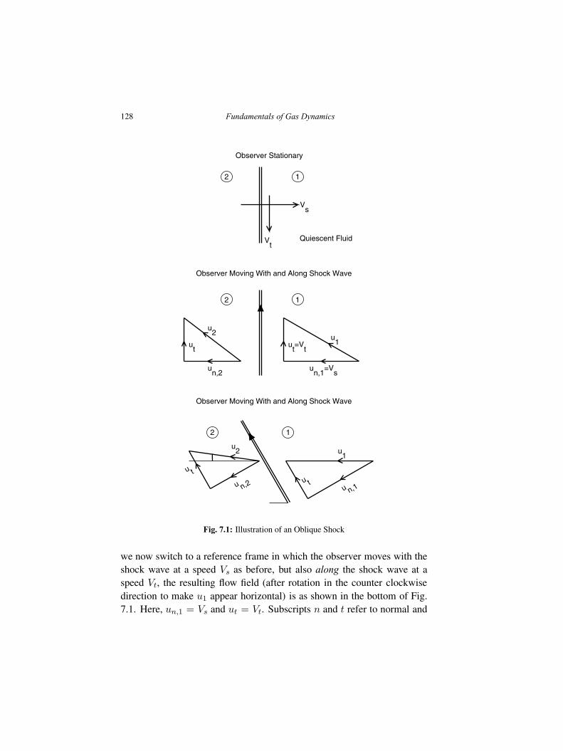
128 Fundamentals of Gas Dynamics
Observer Stationary
Vs
Vt
Quiescent Fluid
12
Observer Moving With and Along Shock Wave
12
un,1
=Vs
ut=V
t
u1
β
un,2
ut
u2
Observer Moving With and Along Shock Wave
β
12
u n,1u t
u1
β
u n,2
u t
u2
θ
Fig. 7.1: Illustration of an Oblique Shock
we now switch to a reference frame in which the observer moves with theshock wave at a speed Vs as before, but also along the shock wave at aspeed Vt, the resulting flow field (after rotation in the counter clockwisedirection to make u1 appear horizontal) is as shown in the bottom of Fig.7.1. Here, un,1 = Vs and ut = Vt. Subscripts n and t refer to normal and
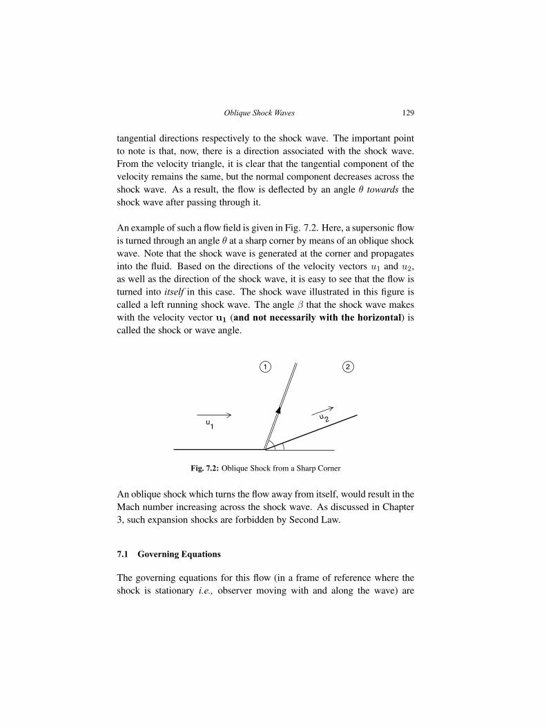
Oblique Shock Waves 129
tangential directions respectively to the shock wave. The important pointto note is that, now, there is a direction associated with the shock wave.From the velocity triangle, it is clear that the tangential component of thevelocity remains the same, but the normal component decreases across theshock wave. As a result, the flow is deflected by an angle θ towards theshock wave after passing through it.
An example of such a flow field is given in Fig. 7.2. Here, a supersonic flowis turned through an angle θ at a sharp corner by means of an oblique shockwave. Note that the shock wave is generated at the corner and propagatesinto the fluid. Based on the directions of the velocity vectors u1 and u2,as well as the direction of the shock wave, it is easy to see that the flow isturned into itself in this case. The shock wave illustrated in this figure iscalled a left running shock wave. The angle β that the shock wave makeswith the velocity vector u1 (and not necessarily with the horizontal) iscalled the shock or wave angle.
1 2
u1
u 2
θβ
Fig. 7.2: Oblique Shock from a Sharp Corner
An oblique shock which turns the flow away from itself, would result in theMach number increasing across the shock wave. As discussed in Chapter3, such expansion shocks are forbidden by Second Law.
7.1 Governing Equations
The governing equations for this flow (in a frame of reference where theshock is stationary i.e., observer moving with and along the wave) are
130 Fundamentals of Gas Dynamics
almost the same as those for normal shock wave. These can be writtenas
ρ1un,1 = ρ2un,2 , (7.1)
P1 + ρ1 u2n,1 = P2 + ρ2 u
2n,2 , (7.2)
h1 +1
2u2n,1 +
1
2u2t = h2 +
1
2u2n,2 +
1
2u2t . (7.3)
As before, T0,2 = T0,1. Comparison of these equations with the governingequations for a normal shock wave shows that u1 and u2 from the latter arenow replaced by un,1 and un,2.
From the velocity triangles in Fig. 7.1, it is easy to see that
un,1 = u1 sin β , un,2 = u2 sin(β − θ) ,
and
ut = u1 cosβ = u2 cos(β − θ) .
It follows thatun,1un,2
=tan β
tan(β − θ).
Butun,1un,2
=ρ2ρ1
,
from Eqn. 7.1. This can be rewritten as follows:
un,1un,2
=P2
P1
T1
T2.
The right hand side can be written in terms of Mach numbers by using therelations given in Section 3.2, after replacing M1 and M2 by Mn,1 andMn,2. Thus
un,1un,2
=(γ + 1)M2
n,1
2 + (γ − 1)M2n,1
.
Oblique Shock Waves 131
If we equate the two expressions for un,1/un,2, we get
tan β
tan(β − θ)=
(γ + 1)M2n,1
2 + (γ − 1)M2n,1
.
From the velocity triangles in Fig. 7.1,
Mn,1 = M1 sin β , Mn,2 = M2 sin(β − θ) .
Upon substituting this into the above relationship, we get
tan β
tan(β − θ)=
(γ + 1)M21 sin
2 β
2 + (γ − 1)M21 sin2 β
.
With a little of algebra, this can be written as
tan θ = 2cot β
(
M21 sin
2 β − 1
M21 (γ + cos 2β) + 2
)
. (7.4)
This relation is known as the θ − β − M relation. Given any two of thethree quantities, M1, θ and β, this relation can be used to determine thethird quantity.
7.2 θ-β-M curve
Solutions of the θ − β −M equation for different values of the upstreamMach number M1 are illustrated in Fig. 7.3. This figure is meant to be anillustration for elucidating the important features of the θ−β−M relation.For calculation purposes, a more accurate representation in graphical ortabular form is usually available in gas tables. Several important featuresthat emerge from this illustration are:
• For any upstream Mach number M1, there exists a maximum value ofdeflection angle θ = θmax (indicated in Fig. 7.3 by filled circles). If
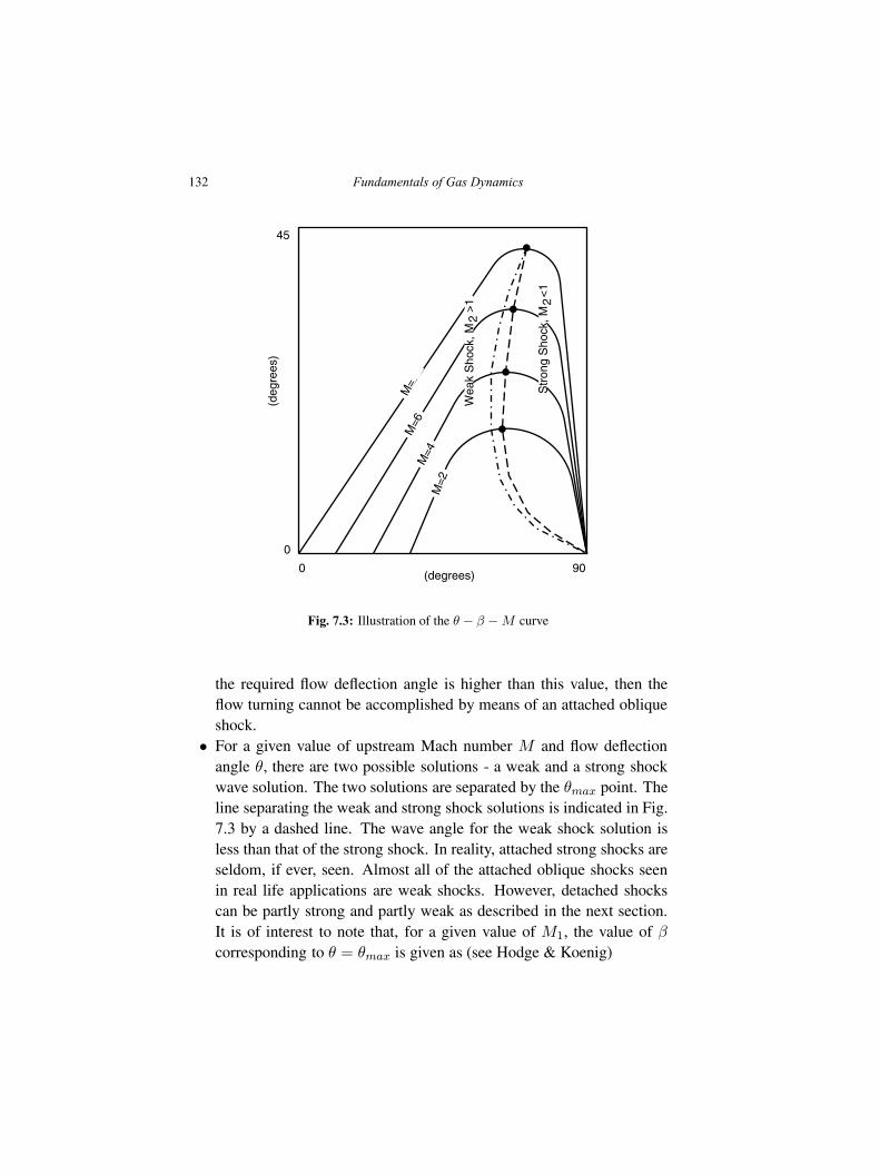
132 Fundamentals of Gas Dynamics
β (degrees)
θ (d
egre
es)
M=2
M=4
M=6
M=
∞
Wea
k S
hock
, M2
>1
Str
ong
Sho
ck, M
2<
1
0 90
0
45
Fig. 7.3: Illustration of the θ − β −M curve
the required flow deflection angle is higher than this value, then theflow turning cannot be accomplished by means of an attached obliqueshock.
• For a given value of upstream Mach number M and flow deflectionangle θ, there are two possible solutions - a weak and a strong shockwave solution. The two solutions are separated by the θmax point. Theline separating the weak and strong shock solutions is indicated in Fig.7.3 by a dashed line. The wave angle for the weak shock solution isless than that of the strong shock. In reality, attached strong shocks areseldom, if ever, seen. Almost all of the attached oblique shocks seenin real life applications are weak shocks. However, detached shockscan be partly strong and partly weak as described in the next section.It is of interest to note that, for a given value of M1, the value of βcorresponding to θ = θmax is given as (see Hodge & Koenig)
Oblique Shock Waves 133
sin2 βθ=θmax =1
γM21
[
γ + 1
4M2
1 − 1
+
√
(γ + 1)
(
1 +γ − 1
2M2
1 +γ + 1
16M4
1
)
]
.
Using this value for β, the corresponding value for θmax can beobtained from Eqn. 7.4.
• For the strong shock solution, M2 is always less than one. For theweak shock, however, M2 is almost always greater than one, exceptwhen the flow deflection angle is close to θmax. This region, whereM2 is less than one for the weak shock, lies between the dashed andthe dot-dashed line in Fig. 7.3. Note that even when M2 is greater thanone, Mn,2 is less than one, since Mn,1 and Mn,2 are related throughthe normal shock relationship.
• The strong shock portion of all the M = constant curves intersect theabscissa at β = 90◦. This corresponds to a deflection angle of 0◦ withthe shock wave normal to the flow direction, which is nothing but thenormal shock solution.
• The weak shock portion of the M = constant curves, on theother hand, intersect the abscissa at different points. The point ofintersection represents an infinitesimally weak shock wave (called aMach wave) which deflects the flow through an infinitesimally smallangle. The compression process is isentropic in this case, and thistype of compression wave is the subject matter of the next chapter.The wave angle corresponding to the point of intersection is called theMach angle, µ, and is equal to sin−1(1/M). The significance of thisangle is discussed in the next chapter.
• Each M = constant curve wherein µ ≤ β ≤ 90◦ in Fig. 7.3, depictsall possible compressive wave solutions, namely, Mach wave → WeakOblique shock wave → Strong Oblique shock wave → Normal shockwave in sequence.
Based on the above observations, we can make some inferences on the lossof stagnation pressure and entropy change across a shock wave. From Eqn.2.17, we can write
134 Fundamentals of Gas Dynamics
P0,2
P0,1=
P0,2
P2
P2
P1
P1
P0,1=
1 +γ − 12 M2
2
1 +γ − 12 M2
1
γγ − 1
P2
P1.
From this expression, it is easy to see that, for a given value of M1 and P1,loss of stagnation pressure (P0,1 −P0,2) increases with decreasing M2 andincreasing P2. Note that, since M2 and P2 are related, a decrease in theformer automatically results in an increase in the latter. With this in mind,if we follow a M = constant curve in Fig. 7.3, we can see that since M2
decreases along this curve, the loss of stagnation pressure increases fromzero for β = µ to a maximum for β = 90◦. It is easy to see from Eqn.2.19, that entropy change follows the same trend.
7.3 Illustration of the Weak Oblique Shock Solution on a T-s diagram
Although Fig. 7.3 is very informative, it is not possible to depictthermodynamic states in this figure. Since oblique shock waves are en-countered extensively, it would be worthwhile depicting the correspondingthermodynamic states on a T-s diagram. Of course, the strong obliqueshock solution is almost identical to the normal shock solution illustratedin Fig. 3.3 from a thermodynamic perspective and hence the T-s diagramfor the strong oblique shock solution will not be presented here. However,the weak oblique shock wave solution differs substantially and we turn tothe illustration of the same on a T-s diagram.
Based on the discussion in the previous section, for a weak oblique shockwave, M1 > M2 > 1, Mn,1 > 1 > Mn,2, P2 > P1, T2 > T1,T0,2 = T0,1 = T0 and P0,2 < P0,1. Note that from Eqn. 7.3,
T0 = T +1
2u2n +
1
2u2t = T +
1
2u2 ,
where the last equality follows from the velocity triangles shown in Fig.7.1.
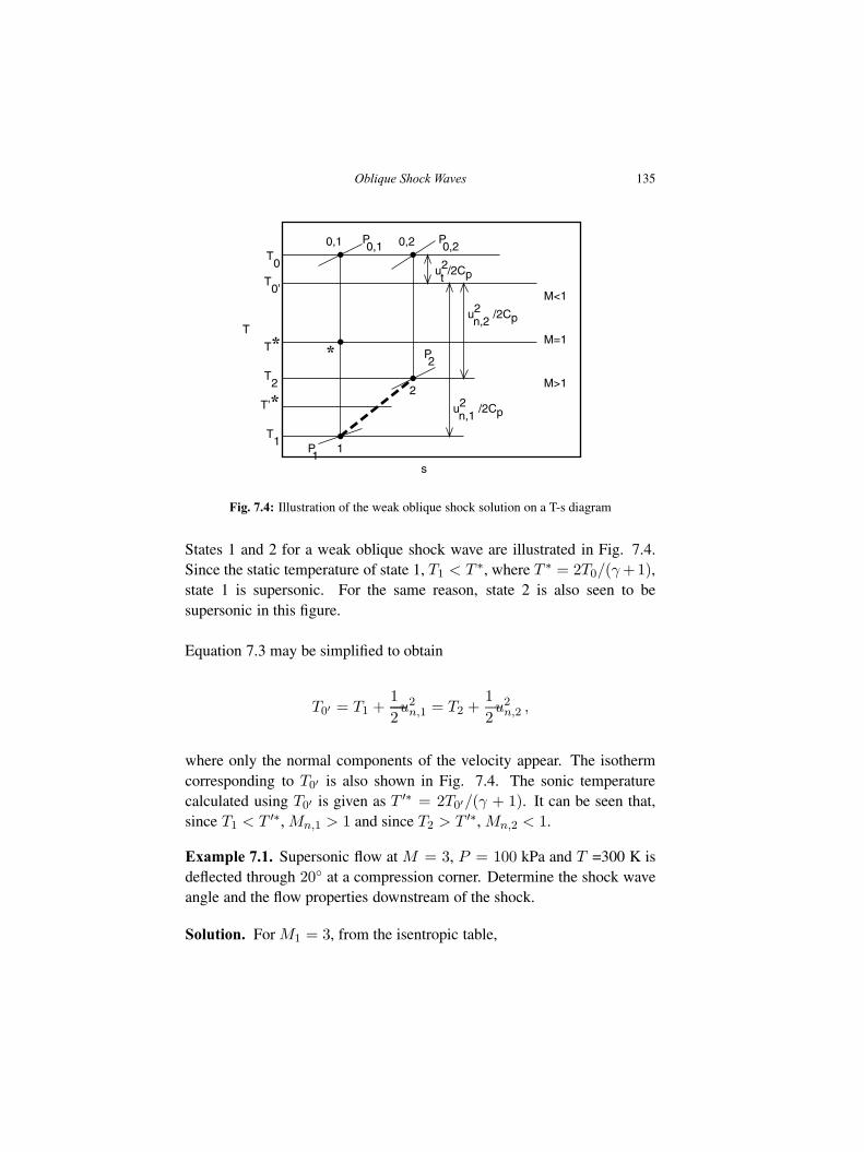
Oblique Shock Waves 135
s
T
T0
M=1
M<1
M>1
0,1 P0,1
T* *
1P1
T1
2
P2
T2
P0,20,2
T0’
T’*
u2t
/2Cp
u2n,1
/2Cp
u2n,2
/2Cp
Fig. 7.4: Illustration of the weak oblique shock solution on a T-s diagram
States 1 and 2 for a weak oblique shock wave are illustrated in Fig. 7.4.Since the static temperature of state 1, T1 < T ∗, where T ∗ = 2T0/(γ+1),state 1 is supersonic. For the same reason, state 2 is also seen to besupersonic in this figure.
Equation 7.3 may be simplified to obtain
T0′ = T1 +1
2u2n,1 = T2 +
1
2u2n,2 ,
where only the normal components of the velocity appear. The isothermcorresponding to T0′ is also shown in Fig. 7.4. The sonic temperaturecalculated using T0′ is given as T ′∗ = 2T0′/(γ + 1). It can be seen that,since T1 < T ′∗, Mn,1 > 1 and since T2 > T ′∗, Mn,2 < 1.
Example 7.1. Supersonic flow at M = 3, P = 100 kPa and T =300 K isdeflected through 20◦ at a compression corner. Determine the shock waveangle and the flow properties downstream of the shock.
Solution. For M1 = 3, from the isentropic table,
136 Fundamentals of Gas Dynamics
P0,1
P1= 36.73 and
T0,1
T1= 2.8 .
Thus, P0,1 = 3.673 MPa and T0,1 = 840 K.
For M1 = 3 and θ = 20◦, from the oblique shock table, we getβ = 37.76◦. Therefore, Mn,1 = M1 sin β = 1.837.
From the normal shock table, for Mn,1 = 1.837, we get
P2
P1= 3.77036 ,
T2
T1= 1.56702 and Mn,2 = 0.608 .
Hence,
M2 =Mn,2
sin(β − θ)= 2.0 ,
P2 = 377 kPa and T2 = 470 K. Also,
P0,2 =P0,2
P2P2 = (7.82445)(377) = 2.95MPa
and T0,2 = T0,1 = 840 K.
The loss of stagnation pressure for this case is about 20 percent. Had thisbeen a normal shock, the loss of stagnation pressure would have been 67percent. �
Example 7.2. Mixed compression supersonic intakes (Fig. 7.5) arewidely used in supersonic vehicles, ramjet and scramjet engines owingto their superior off-design performance when compared with internalcompression intakes. Here, external compression is achieved by meansof oblique shocks generated from properly designed ramps and terminatedby a normal shock. This is followed by internal compression. The intakeshown in Fig. 7.5 is designed for operation at M∞ = 3, P∞ = 15 kPaand T∞ = 135 K. The ramp angles are 15◦ and 30◦ respectively. For thecritical mode of operation, determine the mass flow rate through the intake,cross-sectional area at the beginning of internal compression and the totalpressure recovery.
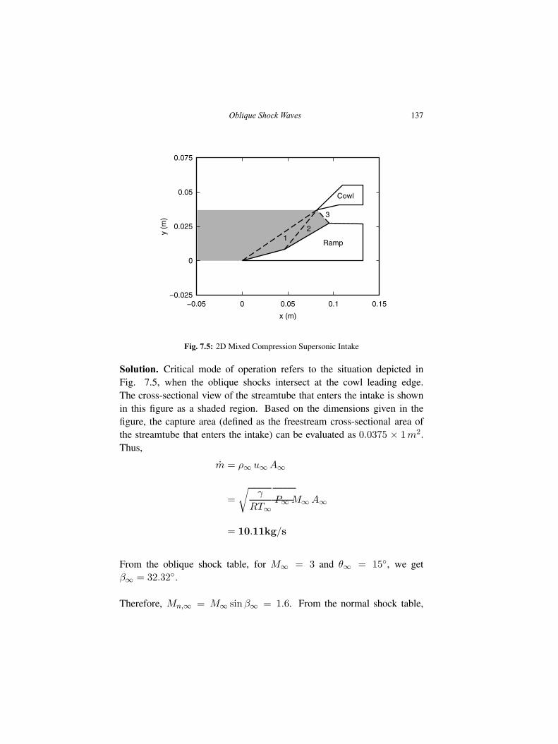
Oblique Shock Waves 137
x (m)
y (m
)
∞ 12
3
−0.05 0 0.05 0.1 0.15−0.025
0
0.025
0.05
0.075
Cowl
Ramp
Fig. 7.5: 2D Mixed Compression Supersonic Intake
Solution. Critical mode of operation refers to the situation depicted inFig. 7.5, when the oblique shocks intersect at the cowl leading edge.The cross-sectional view of the streamtube that enters the intake is shownin this figure as a shaded region. Based on the dimensions given in thefigure, the capture area (defined as the freestream cross-sectional area ofthe streamtube that enters the intake) can be evaluated as 0.0375 × 1m2.Thus,
m = ρ∞ u∞A∞
=
√
γ
RT∞P∞ M∞A∞
= 10.11kg/s
From the oblique shock table, for M∞ = 3 and θ∞ = 15◦, we getβ∞ = 32.32◦.
Therefore, Mn,∞ = M∞ sin β∞ = 1.6. From the normal shock table,
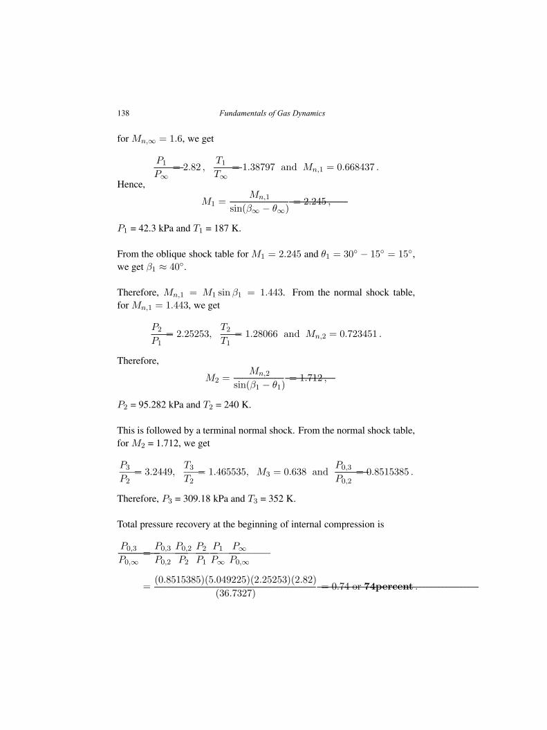
138 Fundamentals of Gas Dynamics
for Mn,∞ = 1.6, we get
P1
P∞
= 2.82 ,T1
T∞
= 1.38797 and Mn,1 = 0.668437 .
Hence,
M1 =Mn,1
sin(β∞ − θ∞)= 2.245 ,
P1 = 42.3 kPa and T1 = 187 K.
From the oblique shock table for M1 = 2.245 and θ1 = 30◦ − 15◦ = 15◦,we get β1 ≈ 40◦.
Therefore, Mn,1 = M1 sin β1 = 1.443. From the normal shock table,for Mn,1 = 1.443, we get
P2
P1= 2.25253,
T2
T1= 1.28066 and Mn,2 = 0.723451 .
Therefore,
M2 =Mn,2
sin(β1 − θ1)= 1.712 ,
P2 = 95.282 kPa and T2 = 240 K.
This is followed by a terminal normal shock. From the normal shock table,for M2 = 1.712, we get
P3
P2= 3.2449,
T3
T2= 1.465535, M3 = 0.638 and
P0,3
P0,2= 0.8515385 .
Therefore, P3 = 309.18 kPa and T3 = 352 K.
Total pressure recovery at the beginning of internal compression is
P0,3
P0,∞=
P0,3
P0,2
P0,2
P2
P2
P1
P1
P∞
P∞
P0,∞
=(0.8515385)(5.049225)(2.25253)(2.82)
(36.7327)= 0.74 or 74percent .
Oblique Shock Waves 139
At the beginning of internal compression, the mass flow rate is
m = ρ3 u3 A3
=
√
γ
RT3P3 M3A3
⇒ A3 = 0.0138m2�
Example 7.3. A converging diverging nozzle with an exit to throat arearatio of 2.637 operates in an over-expanded mode and exhausts into anambient pressure of 100 kPa (see Fig. 7.6). The inlet stagnation conditionsare 300 K and 854.5 kPa. Determine the flow properties at states 2, 3 and4. Also, find out the angle made by the edge of the jet with the horizontal.(Adapted from Hodge and Koenig).
Throat
1
2
3
3
4
P=Pambient
Fig. 7.6: Illustration for worked example
Solution. Given A2/A∗ = 2.637, P0,1 = P0,2 = 854.5 kPa and T0 =
300K.
From the isentropic table, for the given area ratio, we get
140 Fundamentals of Gas Dynamics
M2 = 2.5 ,P0,2
P2= 17.09 and
T0
T2= 2.25 .
Therefore, P2 = 50 kPa and T2 = 133 K.
Since the jet is over-expanded, it undergoes compression outside the nozzleby the oblique shocks generated from the trailing edge of the nozzle. Staticpressure in region 3 is the same as the ambient pressure. Therefore, P3 =100 kPa.
From the normal shock table, for P3/P2 = 2, we get
Mn,2 = 1.36 , Mn,3 = 0.7572 andT3
T2= 1.229 .
Since Mn,2 = M2 sin β2, we can get β2 = 33◦.
Also, T3 = 164 K from above. Since, T0,3 = 300 K, we get T0,3/T3 =1.8308. From the isentropic table, for this value of T0,3/T3, we can getM3 ≈ 2.04. It follows that
P0,3 =P0,3
P3P3 = (8.32731)(100) = 832.731kPa .
From
M3 =Mn,3
sin(β2 − θ2),
we get θ2 = 11.2118◦. The edge of the jet makes an angle of 11.2118◦
(clockwise) with the horizontal.
Since the flow is deflected through 11.2118◦ in region 3, the shock waveangle for calculation of properties in region 4 is β3 = 33◦ + 11.2118◦ =
44.2118◦. Thus, with respect to this wave, Mn,3 = M3 sin β3 = 1.4225.
Oblique Shock Waves 141
From the normal shock table, for Mn,3 = 1.4225, we get
Mn,4 = 0.729425 ,P4
P3= 2.2024 and
T4
T3= 1.27085 .
Hence, P4 = 220.24 kPa and T4 = 208 K. Since T0,4 = 300 K, it followsthat T0,4/T4 = 1.441, and from the isentropic table, we get M4 ≈ 1.48. Itfollows that
P0,4 =P0,4
P4P4 = (3.56649)(220.24) = 785.48kPa .
From
M4 =Mn,4
sin(β3 − θ3),
we get θ3 = 14.6834◦. Since the pressure in region 4 is higher thanatmospheric, the flow expands further downstream. This sequence ofalternate expansion and compressions goes on for a few jet diameters,producing the characteristic “shock diamond” pattern in the jet. �
7.4 Detached Shocks
So far, we have looked at examples involving attached oblique shocks. Inreal life applications in aerodynamics such as flow around blunt bodies, thisis no longer possible and the shock becomes detached. It is of interest tolook at the structure of such detached shocks to gain a better understandingof the flow field.
Figure 7.7 illustrates the flow around a wedge† with freestream Machnumber M1. When the wedge half-angle θ is less than θmax, the obliqueshocks on the upper and lower surface remain attached to the tip of thewedge. When θ becomes greater than θmax, the shocks detach and a†It is possible to look at the cross-sectional view in this figure and assume that it might
also represent flow around a cone. The resemblance is only superficial, for the flow arounda wedge is two-dimensional, whereas, flow around a cone is inherently three-dimensional.
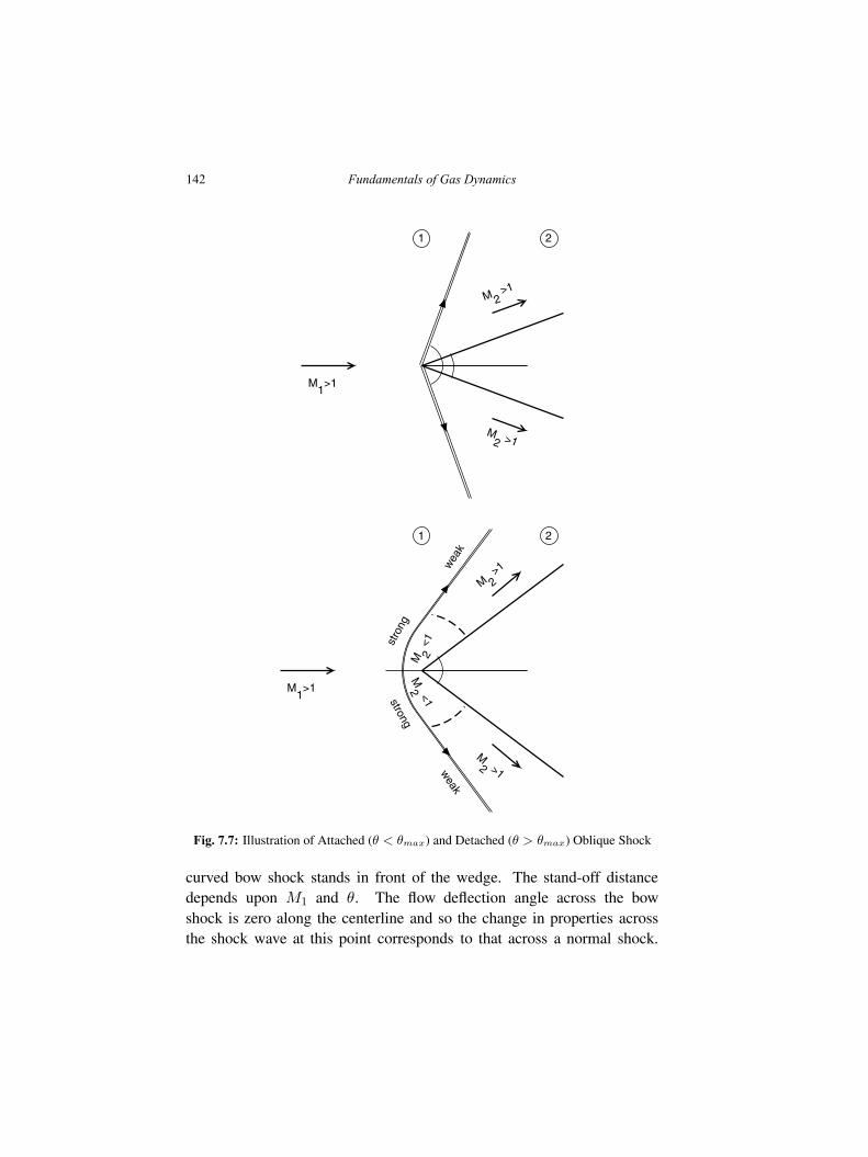
142 Fundamentals of Gas Dynamics
1 2
M1>1
M 2 >1
M2 >1
θ
β
θβ
1 2
M1>1
M 2 >1
M2 >1
M 2 <
1
M2 <1
stro
ng
strong
wea
k
weak
θθ
Fig. 7.7: Illustration of Attached (θ < θmax) and Detached (θ > θmax) Oblique Shock
curved bow shock stands in front of the wedge. The stand-off distancedepends upon M1 and θ. The flow deflection angle across the bowshock is zero along the centerline and so the change in properties acrossthe shock wave at this point corresponds to that across a normal shock.
Oblique Shock Waves 143
Consequently, the shock is also the strongest at this location‡ . Far awayfrom the centerline, where the free stream does not feel the presence ofthe wedge, the bow shock becomes infinitesimally weak and the flowdeflection angle also becomes infinitesimally small. It thus becomes clearthat the strength of the shock decreases as one moves outwards alongthe shock from the centerline. Furthermore, flow deflection angle whichis zero at the centerline increases, reaches a maximum and then againdecreases to zero upon reaching the undisturbed free stream. Based uponthese considerations, the structure of the bow shock can be surmised tobe as follows: Normal shock → Strong oblique shock → Weak obliqueshock. This is illustrated in Fig. 7.7. The sonic line which separates thestrong and weak shock portion is shown in this figure as a dashed line.Interestingly enough, the same structure can be seen in Fig. 7.3 if wefollow the M1 = constant curve, from β = 90◦ to β = µ. It is interestingsince the solution shown in Fig. 7.3, is for attached shocks. In the case ofa bow shock, the property changes and the flow field has to be calculatedby means of computational techniques, but the similarity to the attachedshock solution allows us to make quick estimates of these quantities.
7.5 Reflected Shocks
Whenever an oblique shock impinges on a boundary, it is reflected fromthe boundary in some manner. This boundary can either be a wall or a jetboundary as in Fig. 7.6. We consider the former case here and defer thelatter case to the next chapter, as it requires knowledge of expansion fans.
7.5.1 Reflection from a Wall
Reflection of an oblique shock wave is illustrated in Fig. 7.8. Here, anoblique shock is generated from a concave corner on the bottom wall andimpinges on the top wall. The flow is deflected upward by an angle θ (i.e.,towards the shock wave). If we now consider the flow in a region very‡Increase in temperature due to shock heating is also quite high in this region. In
some cases such as the space shuttle when it re-enters the atmosphere, for instance, thetemperature rise is high enough to ionize the air. Reentry vehicles thus require specialthermal protection such as ceramic or ablative coatings in the nose region to withstandsuch high temperatures.
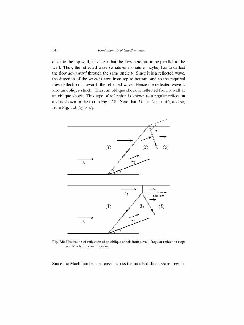
144 Fundamentals of Gas Dynamics
close to the top wall, it is clear that the flow here has to be parallel to thewall. Thus, the reflected wave (whatever its nature maybe) has to deflectthe flow downward through the same angle θ. Since it is a reflected wave,the direction of the wave is now from top to bottom, and so the requiredflow deflection is towards the reflected wave. Hence the reflected wave isalso an oblique shock. Thus, an oblique shock is reflected from a wall asan oblique shock. This type of reflection is known as a regular reflectionand is shown in the top in Fig. 7.8. Note that M1 > M2 > M3 and so,from Fig. 7.3, β2 > β1.
1 2 3
u1
u 2
θβ1
β2− θθ
1 2 3
u1
u 2
u1
θβ1
slip line
Fig. 7.8: Illustration of reflection of an oblique shock from a wall. Regular reflection (top)and Mach reflection (bottom).
Since the Mach number decreases across the incident shock wave, regular
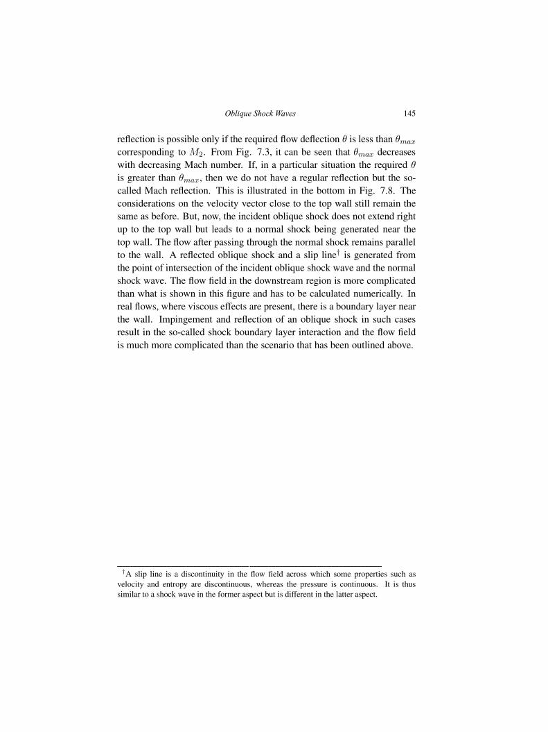
Oblique Shock Waves 145
reflection is possible only if the required flow deflection θ is less than θmax
corresponding to M2. From Fig. 7.3, it can be seen that θmax decreaseswith decreasing Mach number. If, in a particular situation the required θ
is greater than θmax, then we do not have a regular reflection but the so-called Mach reflection. This is illustrated in the bottom in Fig. 7.8. Theconsiderations on the velocity vector close to the top wall still remain thesame as before. But, now, the incident oblique shock does not extend rightup to the top wall but leads to a normal shock being generated near thetop wall. The flow after passing through the normal shock remains parallelto the wall. A reflected oblique shock and a slip line† is generated fromthe point of intersection of the incident oblique shock wave and the normalshock wave. The flow field in the downstream region is more complicatedthan what is shown in this figure and has to be calculated numerically. Inreal flows, where viscous effects are present, there is a boundary layer nearthe wall. Impingement and reflection of an oblique shock in such casesresult in the so-called shock boundary layer interaction and the flow fieldis much more complicated than the scenario that has been outlined above.
†A slip line is a discontinuity in the flow field across which some properties such asvelocity and entropy are discontinuous, whereas the pressure is continuous. It is thussimilar to a shock wave in the former aspect but is different in the latter aspect.
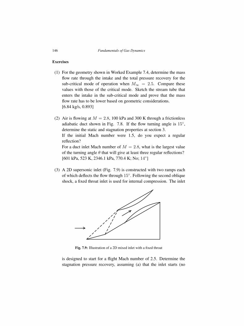
146 Fundamentals of Gas Dynamics
Exercises
(1) For the geometry shown in Worked Example 7.4, determine the massflow rate through the intake and the total pressure recovery for thesub-critical mode of operation when M∞ = 2.5. Compare thesevalues with those of the critical mode. Sketch the stream tube thatenters the intake in the sub-critical mode and prove that the massflow rate has to be lower based on geometric considerations.[6.84 kg/s, 0.893]
(2) Air is flowing at M = 2.8, 100 kPa and 300 K through a frictionlessadiabatic duct shown in Fig. 7.8. If the flow turning angle is 15◦,determine the static and stagnation properties at section 3.If the initial Mach number were 1.5, do you expect a regularreflection?For a duct inlet Mach number of M = 2.8, what is the largest valueof the turning angle θ that will give at least three regular reflections?[601 kPa, 523 K, 2346.1 kPa, 770.4 K; No; 14◦]
(3) A 2D supersonic inlet (Fig. 7.9) is constructed with two ramps eachof which deflects the flow through 15◦. Following the second obliqueshock, a fixed throat inlet is used for internal compression. The inlet
Fig. 7.9: Illustration of a 2D mixed inlet with a fixed throat
is designed to start for a flight Mach number of 2.5. Determine thestagnation pressure recovery, assuming (a) that the inlet starts (no
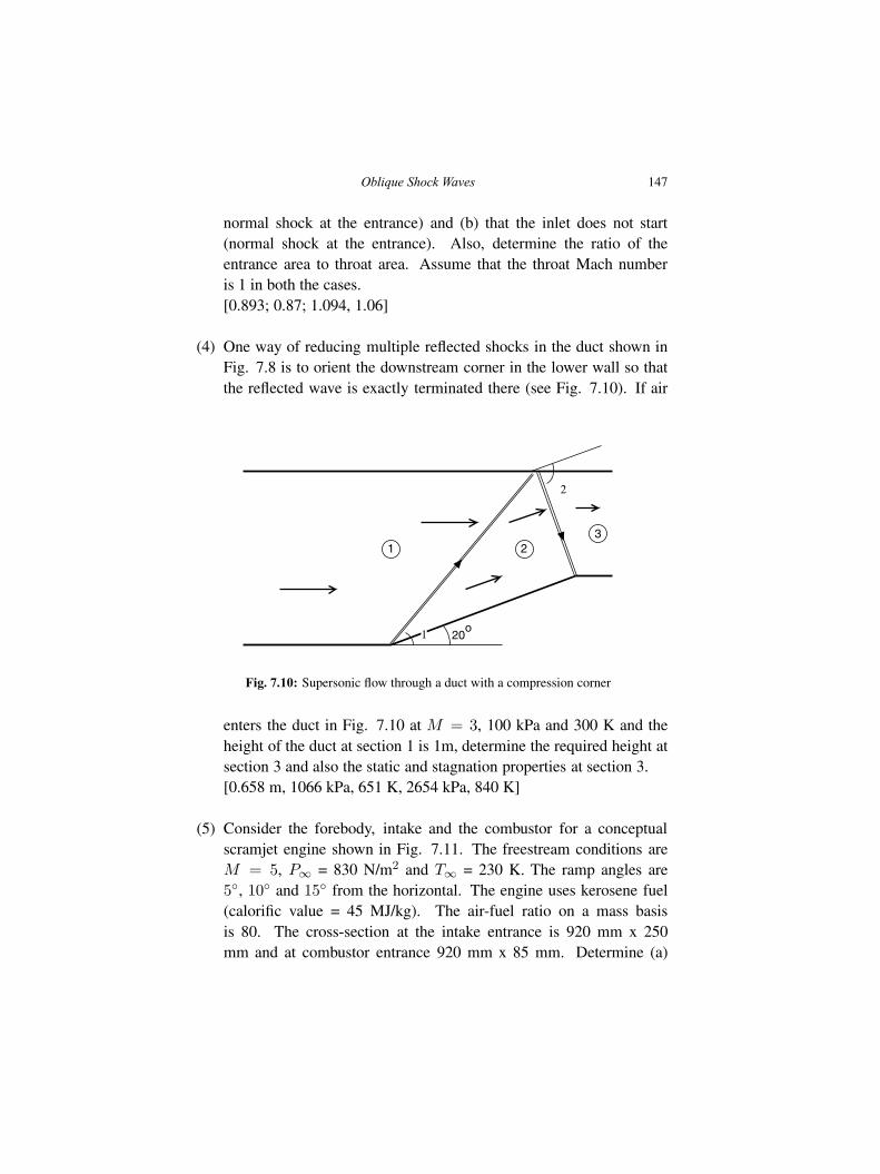
Oblique Shock Waves 147
normal shock at the entrance) and (b) that the inlet does not start(normal shock at the entrance). Also, determine the ratio of theentrance area to throat area. Assume that the throat Mach numberis 1 in both the cases.[0.893; 0.87; 1.094, 1.06]
(4) One way of reducing multiple reflected shocks in the duct shown inFig. 7.8 is to orient the downstream corner in the lower wall so thatthe reflected wave is exactly terminated there (see Fig. 7.10). If air
1 23
20oβ1
β2
Fig. 7.10: Supersonic flow through a duct with a compression corner
enters the duct in Fig. 7.10 at M = 3, 100 kPa and 300 K and theheight of the duct at section 1 is 1m, determine the required height atsection 3 and also the static and stagnation properties at section 3.[0.658 m, 1066 kPa, 651 K, 2654 kPa, 840 K]
(5) Consider the forebody, intake and the combustor for a conceptualscramjet engine shown in Fig. 7.11. The freestream conditions areM = 5, P∞ = 830 N/m2 and T∞ = 230 K. The ramp angles are5◦, 10◦ and 15◦ from the horizontal. The engine uses kerosene fuel(calorific value = 45 MJ/kg). The air-fuel ratio on a mass basisis 80. The cross-section at the intake entrance is 920 mm x 250mm and at combustor entrance 920 mm x 85 mm. Determine (a)
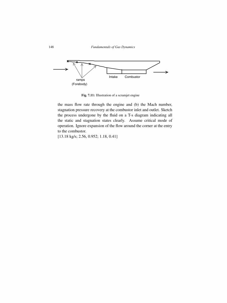
148 Fundamentals of Gas Dynamics
CombustorIntakeramps
(Forebody)
Fig. 7.11: Illustration of a scramjet engine
the mass flow rate through the engine and (b) the Mach number,stagnation pressure recovery at the combustor inlet and outlet. Sketchthe process undergone by the fluid on a T-s diagram indicating allthe static and stagnation states clearly. Assume critical mode ofoperation. Ignore expansion of the flow around the corner at the entryto the combustor.[13.18 kg/s; 2.56, 0.952; 1.18, 0.41]
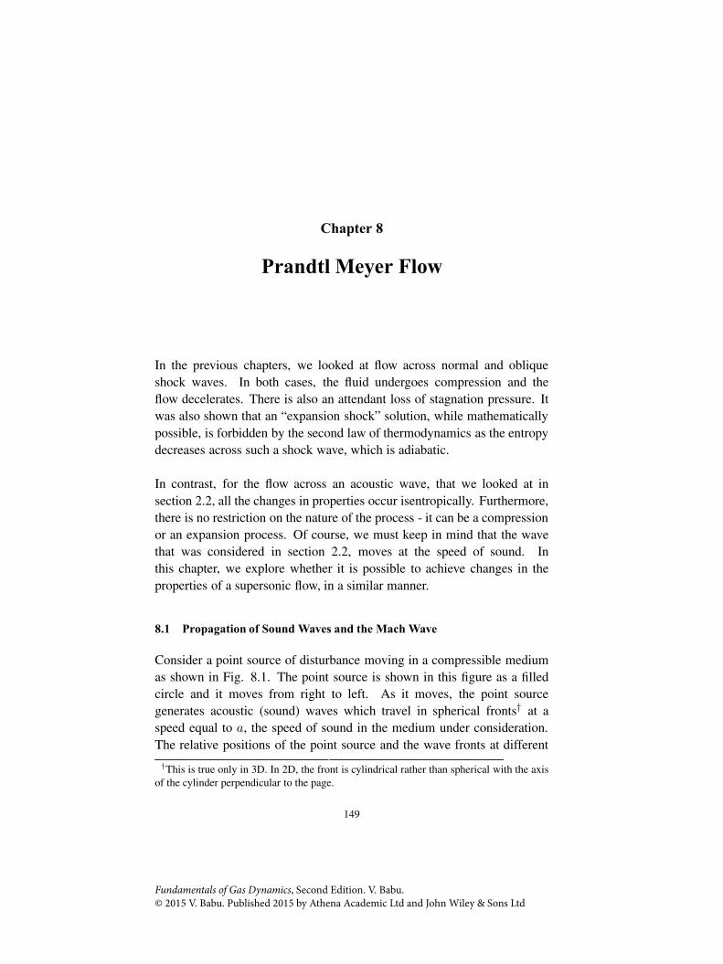
Chapter 8
Prandtl Meyer Flow
In the previous chapters, we looked at flow across normal and obliqueshock waves. In both cases, the fluid undergoes compression and theflow decelerates. There is also an attendant loss of stagnation pressure. Itwas also shown that an “expansion shock” solution, while mathematicallypossible, is forbidden by the second law of thermodynamics as the entropydecreases across such a shock wave, which is adiabatic.
In contrast, for the flow across an acoustic wave, that we looked at insection 2.2, all the changes in properties occur isentropically. Furthermore,there is no restriction on the nature of the process - it can be a compressionor an expansion process. Of course, we must keep in mind that the wavethat was considered in section 2.2, moves at the speed of sound. Inthis chapter, we explore whether it is possible to achieve changes in theproperties of a supersonic flow, in a similar manner.
8.1 Propagation of Sound Waves and the Mach Wave
Consider a point source of disturbance moving in a compressible mediumas shown in Fig. 8.1. The point source is shown in this figure as a filledcircle and it moves from right to left. As it moves, the point sourcegenerates acoustic (sound) waves which travel in spherical fronts† at aspeed equal to a, the speed of sound in the medium under consideration.The relative positions of the point source and the wave fronts at different
†This is true only in 3D. In 2D, the front is cylindrical rather than spherical with the axisof the cylinder perpendicular to the page.
149
Fundamentals of Gas Dynamics, Second Edition. V. Babu.© 2015 V. Babu. Published 2015 by Athena Academic Ltd and John Wiley & Sons Ltd
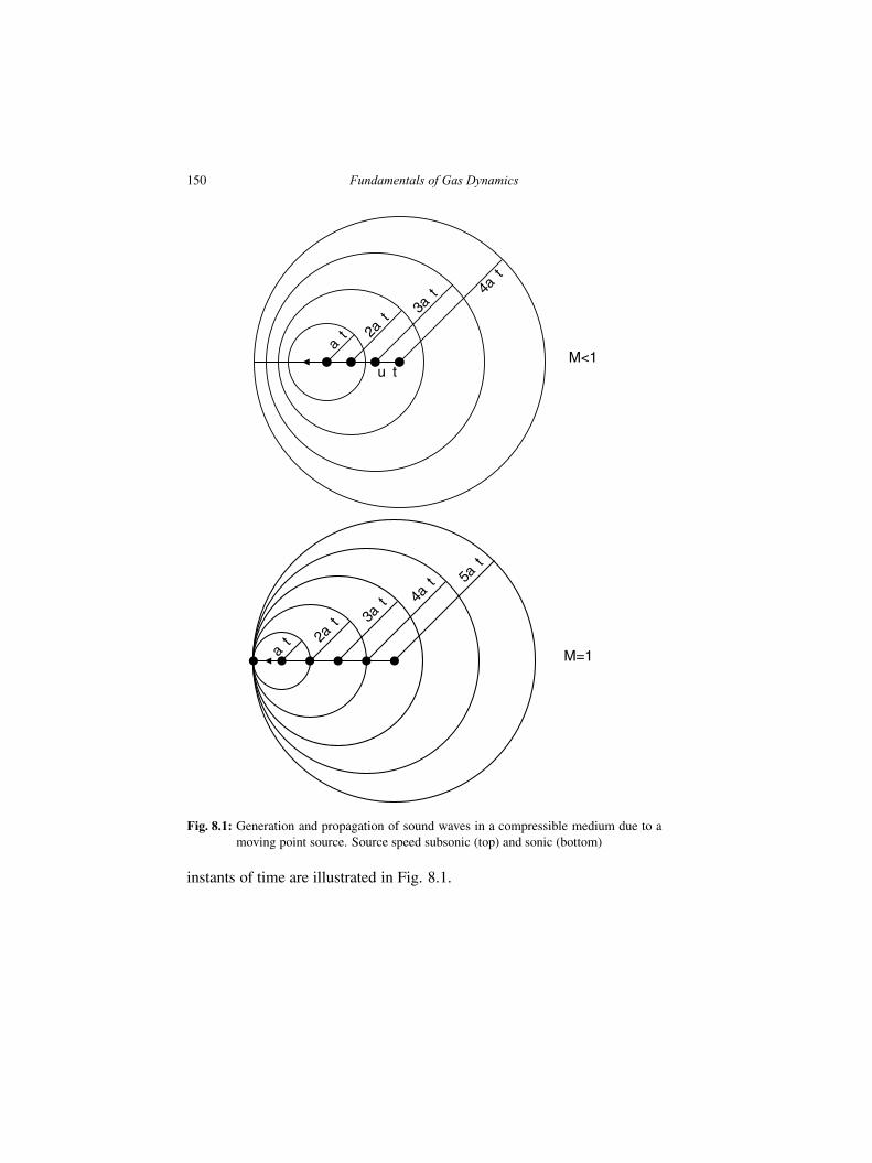
150 Fundamentals of Gas Dynamics
M<1
4a∆t
3a∆t
2a∆t
a∆t
u∆t
5a∆t
4a∆t
3a∆t
2a∆t
a∆tM=1
Fig. 8.1: Generation and propagation of sound waves in a compressible medium due to amoving point source. Source speed subsonic (top) and sonic (bottom)
instants of time are illustrated in Fig. 8.1.
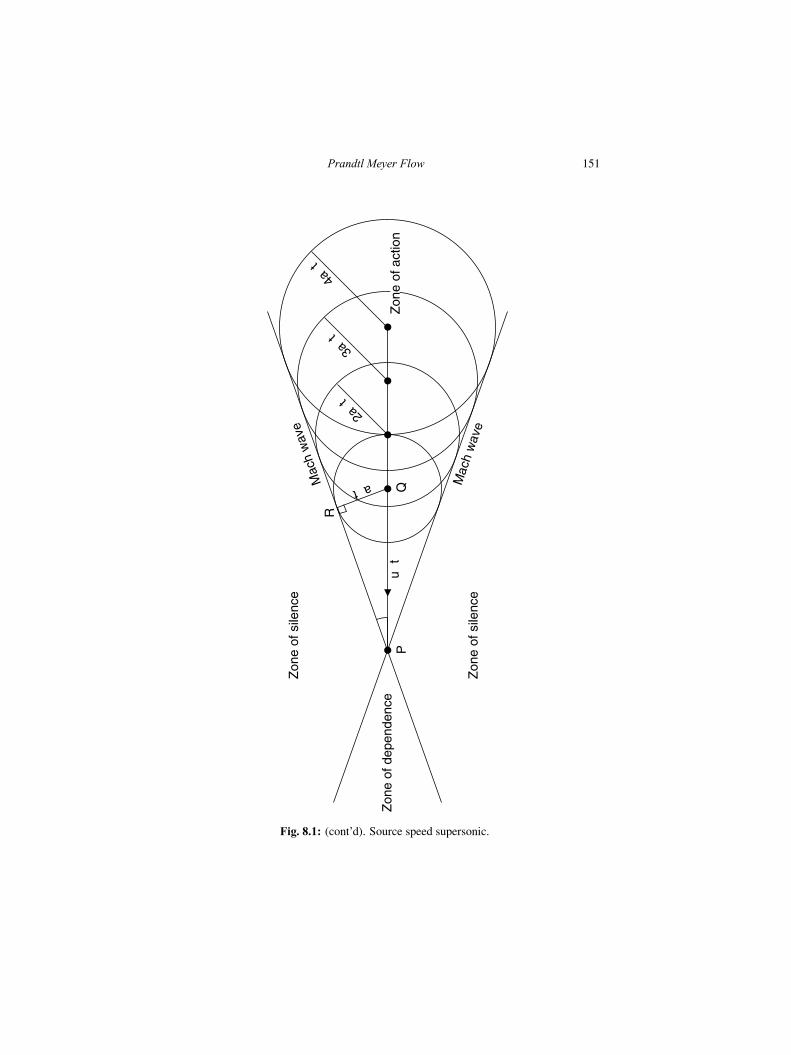
Prandtl Meyer Flow 151
PQ
R
Zon
e of
sile
nce
Zon
e of
sile
nce
Zon
e of
dep
ende
nce
Zon
e of
act
ion
Mac
h w
ave
Mac
h w
ave
4a∆t
3a∆t
2a∆t
a∆t
u∆t
µ
Fig. 8.1: (cont’d). Source speed supersonic.
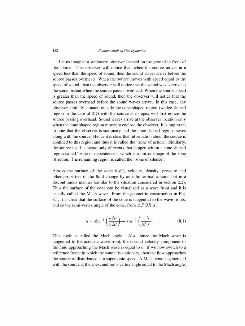
152 Fundamentals of Gas Dynamics
Let us imagine a stationary observer located on the ground in front ofthe source. This observer will notice that, when the source moves at aspeed less than the speed of sound, then the sound waves arrive before thesource passes overhead. When the source moves with speed equal to thespeed of sound, then the observer will notice that the sound waves arrive atthe same instant when the source passes overhead. When the source speedis greater than the speed of sound, then the observer will notice that thesource passes overhead before the sound waves arrive. In this case, anyobserver, initially situated outside the cone shaped region (wedge shapedregion in the case of 2D) with the source at its apex will first notice thesource passing overhead. Sound waves arrive at the observer location onlywhen the cone shaped region moves to enclose the observer. It is importantto note that the observer is stationary and the cone shaped region movesalong with the source. Hence it is clear that information about the source isconfined to this region and thus it is called the “zone of action”. Similarly,the source itself is aware only of events that happen within a cone shapedregion called “zone of dependence”, which is a mirror image of the zoneof action. The remaining region is called the “zone of silence”.
Across the surface of the cone itself, velocity, density, pressure andother properties of the fluid change by an infinitesimal amount but in adiscontinuous manner (similar to the situation considered in section 2.2).Thus the surface of the cone can be visualized as a wave front and it isusually called the Mach wave. From the geometric construction in Fig.8.1, it is clear that the surface of the cone is tangential to the wave fronts,and so the semi-vertex angle of the cone, from △PQR is,
µ = sin−1
(
a∆t
u∆t
)
= sin−1
(
1
M
)
. (8.1)
This angle is called the Mach angle. Also, since the Mach wave istangential to the acoustic wave front, the normal velocity component ofthe fluid approaching the Mach wave is equal to a. If we now switch to areference frame in which the source is stationary, then the flow approachesthe source of disturbance at a supersonic speed. A Mach cone is generatedwith the source at the apex, and semi-vertex angle equal to the Mach angle,
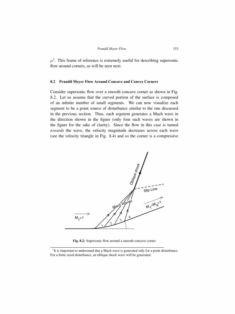
Prandtl Meyer Flow 153
µ†. This frame of reference is extremely useful for describing supersonicflow around corners, as will be seen next.
8.2 Prandtl Meyer Flow Around Concave and Convex Corners
Consider supersonic flow over a smooth concave corner as shown in Fig.8.2. Let us assume that the curved portion of the surface is composedof an infinite number of small segments. We can now visualize eachsegment to be a point source of disturbance similar to the one discussedin the previous section. Thus, each segment generates a Mach wave inthe direction shown in the figure (only four such waves are shown inthe figure for the sake of clarity). Since the flow in this case is turnedtowards the wave, the velocity magnitude decreases across each wave(see the velocity triangle in Fig. 8.4) and so the corner is a compressive
M1>1
M 1>M 4
>1
θµ1 µ2µ 3
µ 4
Mach Waves
Obl
ique
sho
ck
Slip Line
Fig. 8.2: Supersonic flow around a smooth concave corner
†It is important to understand that a Mach wave is generated only for a point disturbance.For a finite sized disturbance, an oblique shock wave will be generated.
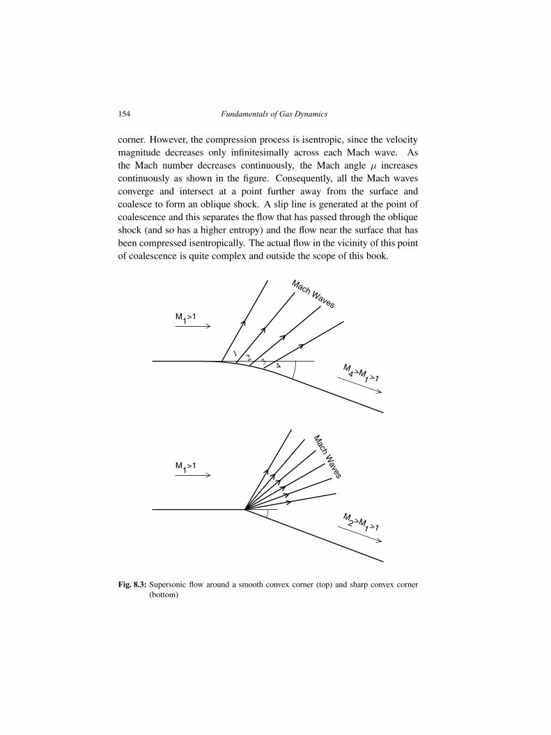
154 Fundamentals of Gas Dynamics
corner. However, the compression process is isentropic, since the velocitymagnitude decreases only infinitesimally across each Mach wave. Asthe Mach number decreases continuously, the Mach angle µ increasescontinuously as shown in the figure. Consequently, all the Mach wavesconverge and intersect at a point further away from the surface andcoalesce to form an oblique shock. A slip line is generated at the point ofcoalescence and this separates the flow that has passed through the obliqueshock (and so has a higher entropy) and the flow near the surface that hasbeen compressed isentropically. The actual flow in the vicinity of this pointof coalescence is quite complex and outside the scope of this book.
M1>1
M4 >M
1 >1θ
µ1 µ2 µ 3 µ 4
Mach Waves
M1>1
M2 >M
1 >1θ
Mach W
aves
Fig. 8.3: Supersonic flow around a smooth convex corner (top) and sharp convex corner(bottom)
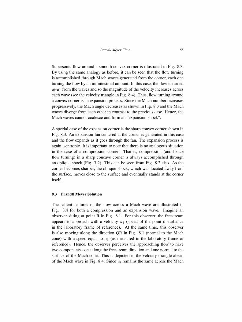
Prandtl Meyer Flow 155
Supersonic flow around a smooth convex corner is illustrated in Fig. 8.3.By using the same analogy as before, it can be seen that the flow turningis accomplished through Mach waves generated from the corner, each oneturning the flow by an infinitesimal amount. In this case, the flow is turnedaway from the waves and so the magnitude of the velocity increases acrosseach wave (see the velocity triangle in Fig. 8.4). Thus, flow turning arounda convex corner is an expansion process. Since the Mach number increasesprogressively, the Mach angle decreases as shown in Fig. 8.3 and the Machwaves diverge from each other in contrast to the previous case. Hence, theMach waves cannot coalesce and form an “expansion shock”.
A special case of the expansion corner is the sharp convex corner shown inFig. 8.3. An expansion fan centered at the corner is generated in this caseand the flow expands as it goes through the fan. The expansion process isagain isentropic. It is important to note that there is no analogous situationin the case of a compression corner. That is, compression (and henceflow turning) in a sharp concave corner is always accomplished throughan oblique shock (Fig. 7.2). This can be seen from Fig. 8.2 also. As thecorner becomes sharper, the oblique shock, which was located away fromthe surface, moves close to the surface and eventually stands at the corneritself.
8.3 Prandtl Meyer Solution
The salient features of the flow across a Mach wave are illustrated inFig. 8.4 for both a compression and an expansion wave. Imagine anobserver sitting at point R in Fig. 8.1. For this observer, the freestreamappears to approach with a velocity u1 (speed of the point disturbancein the laboratory frame of reference). At the same time, this observeris also moving along the direction QR in Fig. 8.1 (normal to the Machcone) with a speed equal to a1 (as measured in the laboratory frame ofreference). Hence, the observer perceives the approaching flow to havetwo components - one along the freestream direction and one normal to thesurface of the Mach cone. This is depicted in the velocity triangle aheadof the Mach wave in Fig. 8.4. Since ut remains the same across the Mach
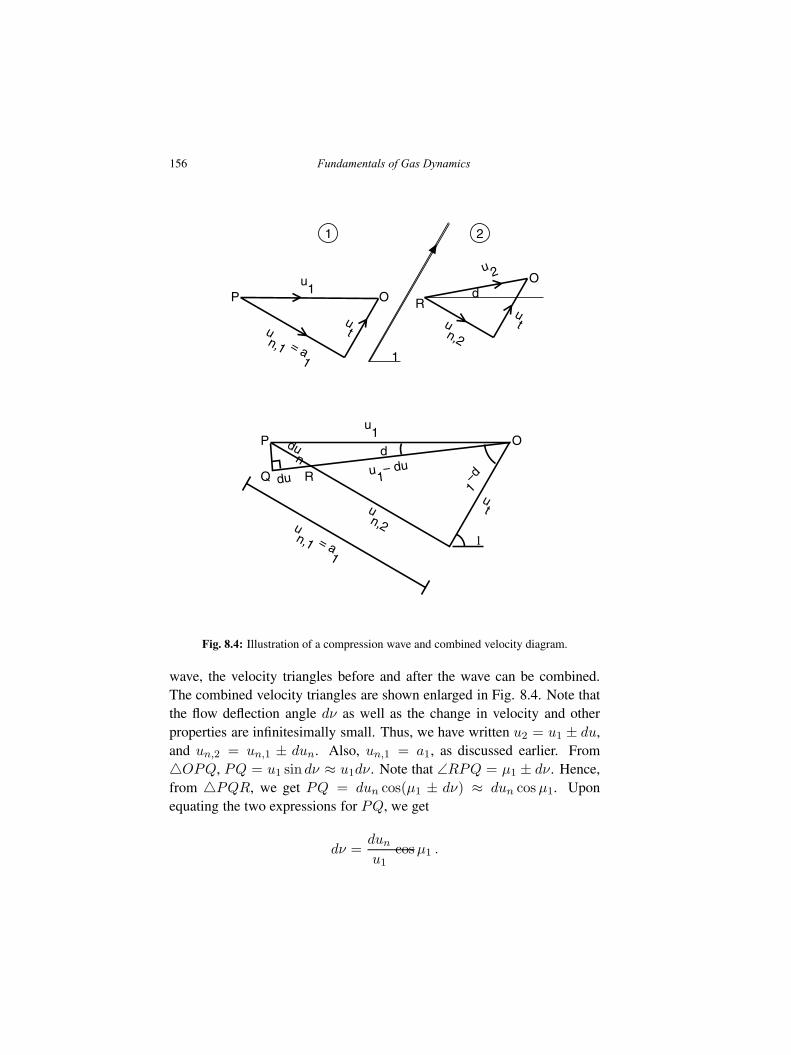
156 Fundamentals of Gas Dynamics
µ1
21
un,1 = a
1
ut
u1
P O
un,2
ut
u 2 O
Rdν
un,1 = a
1
u1
un,2
dun
ut
u1− du
du
µ1
dν
µ 1−d
ν
P
Q R
O
Fig. 8.4: Illustration of a compression wave and combined velocity diagram.
wave, the velocity triangles before and after the wave can be combined.The combined velocity triangles are shown enlarged in Fig. 8.4. Note thatthe flow deflection angle dν as well as the change in velocity and otherproperties are infinitesimally small. Thus, we have written u2 = u1 ± du,and un,2 = un,1 ± dun. Also, un,1 = a1, as discussed earlier. From△OPQ, PQ = u1 sin dν ≈ u1dν. Note that ∠RPQ = µ1 ± dν. Hence,from △PQR, we get PQ = dun cos(µ1 ± dν) ≈ dun cosµ1. Uponequating the two expressions for PQ, we get
dν =dunu1
cosµ1 .
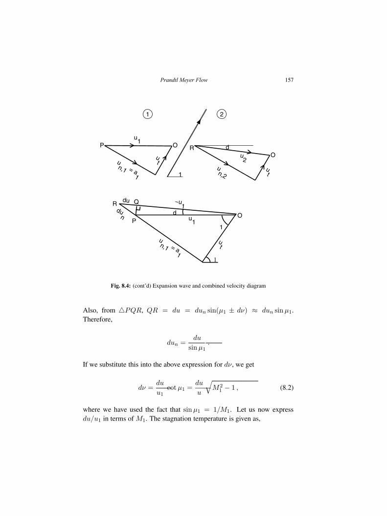
Prandtl Meyer Flow 157
µ1
21
un,1 = a
1
ut
u1
P O
un,2
ut
u2
OR dν
un,1 = a
1
dun
~u1
du
ut
u1
µ1
dν
µ1
R Q
PO
Fig. 8.4: (cont’d) Expansion wave and combined velocity diagram
Also, from △PQR, QR = du = dun sin(µ1 ± dν) ≈ dun sinµ1.Therefore,
dun =du
sinµ1.
If we substitute this into the above expression for dν, we get
dν =du
u1cotµ1 =
du
u
√
M21 − 1 , (8.2)
where we have used the fact that sinµ1 = 1/M1. Let us now expressdu/u1 in terms of M1. The stagnation temperature is given as,
158 Fundamentals of Gas Dynamics
T0 = T1 +u212Cp
.
If we take the differential of this expression (keeping in mind that T0 is aconstant), we get
dT +γ − 1
γRu1du = 0 ,
where the subscripts have been dropped from the differentials. This can bewritten as,
dT
T1= −(γ − 1)M2
1
du
u1,
where we have used M1 = u1/√γRT1. Further, if we take the differential
of this expression for the Mach number, we get
dM
M1=
du
u1− dT
T1.
If we combine the last two expressions, we get
dM
M1= 2
(
1 +γ − 1
2M2
1
)
du
u1.
This can be simplified to yield
du
u1=
dM21
2M21
(
1 +γ − 12 M2
1
) .
Equation (8.1) can thus be written as
dν =
√
M21 − 1 dM2
1
2M21
(
1 +γ − 12 M2
1
) .
Prandtl Meyer Flow 159
Note that dν = 0, when M1 = 1, which is consistent with what wediscussed in Section 2.2. If we now integrate this equation from M1 = 1
to any M , we get
ν =
√
γ + 1
γ − 1tan−1
√
γ − 1
γ + 1(M2 − 1)− tan−1
√
M2 − 1 . (8.3)
This angle is called the Prandtl Meyer angle and it is the angle throughwhich a sonic flow has to be turned (away from itself) to reach a supersonicMach number M . Alternatively, it is the angle through which a supersonicflow at a Mach number M has to be turned (towards itself) to reachM = 1. Both the expansion and the compression process are isentropic.Also note that ν is a monotonically increasing function of M . Thus, if asupersonic flow is deflected through an angle θ in a compression corner,then θ = ν1 − ν2. On the contrary, if it is deflected through the same anglein an expansion corner, then θ = ν2 − ν1. Both the Prandtl-Meyer angleand the Mach angle are tabulated for Mach numbers ranging from 1 to 5and γ = 1.4 in Table F.
Two limiting cases for ν can be considered, namely, as M → 1 andM → ∞. In the former case, ν → 0 and µ → 90◦, as already mentioned.In the latter case, it is easy to show from the above equation that,
νmax =π
2
(√
γ + 1
γ − 1− 1
)
(8.4)
and µ → 0◦. For γ = 1.4, νmax is equal to 130.45◦. This maximum valueis only of academic interest, since, long before the flow is deflected throughthis angle (and correspondingly expanded), the continuum assumptionwould have become invalid owing to the static pressure attaining very lowvalues.
Example 8.1. Supersonic flow at M = 3, P = 100 kPa and T = 300K is deflected through 20◦ at a compression corner. Determine the flowproperties downstream of the corner, assuming the process to be isentropic.
160 Fundamentals of Gas Dynamics
Solution. For M1 = 3, the Prandtl Meyer angle ν1 = 49.7568◦ , fromTable F. Since this is a compression corner,
θ = ν1 − ν2 and so ν2 = 29.7568◦ .
From Table F, it can be seen that this value of ν corresponds to M2 = 2.125.From the isentropic table,
T2 =T2
T0
T0
T1T1 =
0.5254575
0.35714× 300 = 441K
P2 =P2
P0
P0
P1P1 =
36.7327
9.509016× 100 = 386.3kPa
Comparison of these numbers with those given in Worked Example 7.1reveals that the Mach number at the end of the compression process ishigher and there is no loss of stagnation pressure now. Since the Machnumber is higher, the static temperature is lower (since the stagnationtemperature is the same in both the cases).�
8.4 Reflection of Oblique Shock From a Constant Pressure Boundary
A constant pressure boundary is a physically distinct surface in a fluid,across (and along) which the static pressure is the same. This type ofboundary is usually encountered in the study of jets and mixing layers.As can be seen in Fig. 8.5, the surface of the jet is a constant pressureboundary. We now wish to find out what happens when the oblique shocksemanating from the top and bottom corners of the nozzle impinge on thisboundary.
If we consider the point of impingement which is located right on the jetboundary, then there is an increase in pressure due to the shock wave. Butthe pressure at this point cannot be different from the ambient pressureand so the pressure rise due to the impingement of the shock waveis immediately nullified by the generation of an expansion fan. Thus,an oblique shock is reflected from a constant pressure boundary as an
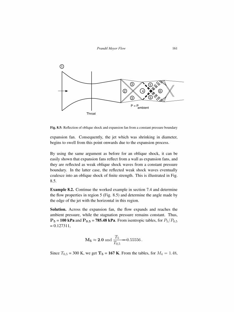
Prandtl Meyer Flow 161
Throat
1
2
3
3
4
P = Pambient
5
5
6
Fig. 8.5: Reflection of oblique shock and expansion fan from a constant pressure boundary
expansion fan. Consequently, the jet which was shrinking in diameter,begins to swell from this point onwards due to the expansion process.
By using the same argument as before for an oblique shock, it can beeasily shown that expansion fans reflect from a wall as expansion fans, andthey are reflected as weak oblique shock waves from a constant pressureboundary. In the latter case, the reflected weak shock waves eventuallycoalesce into an oblique shock of finite strength. This is illustrated in Fig.8.5.
Example 8.2. Continue the worked example in section 7.4 and determinethe flow properties in region 5 (Fig. 8.5) and determine the angle made bythe edge of the jet with the horizontal in this region.
Solution. Across the expansion fan, the flow expands and reaches theambient pressure, while the stagnation pressure remains constant. Thus,P5 = 100 kPa and P0,5 = 785.48 kPa. From isentropic tables, for P5/P0,5
= 0.127311,
M5 ≈ 2.0 andT5
T0,5= 0.55556 .
Since T0,5 = 300 K, we get T5 = 167 K. From the tables, for M4 = 1.48,
162 Fundamentals of Gas Dynamics
ν4 = 11.3168◦. Similarly, ν5 = 26.3795◦. Since this is an expansionprocess, flow deflection angle is 26.3795◦ − 11.3168◦ = 15.0627◦. Theangle made by the edge of the jet with the horizontal is
15.0627◦ + 14.6834◦ − 11.2118◦=18.5343◦ (counter clockwise).
Continuing the calculations beyond this point is somewhat difficult, as weneed to look at the effect of the expansion fans intersecting each other. Thereader may consult Zucrow and Hoffman for calculations involving suchinteractions. �
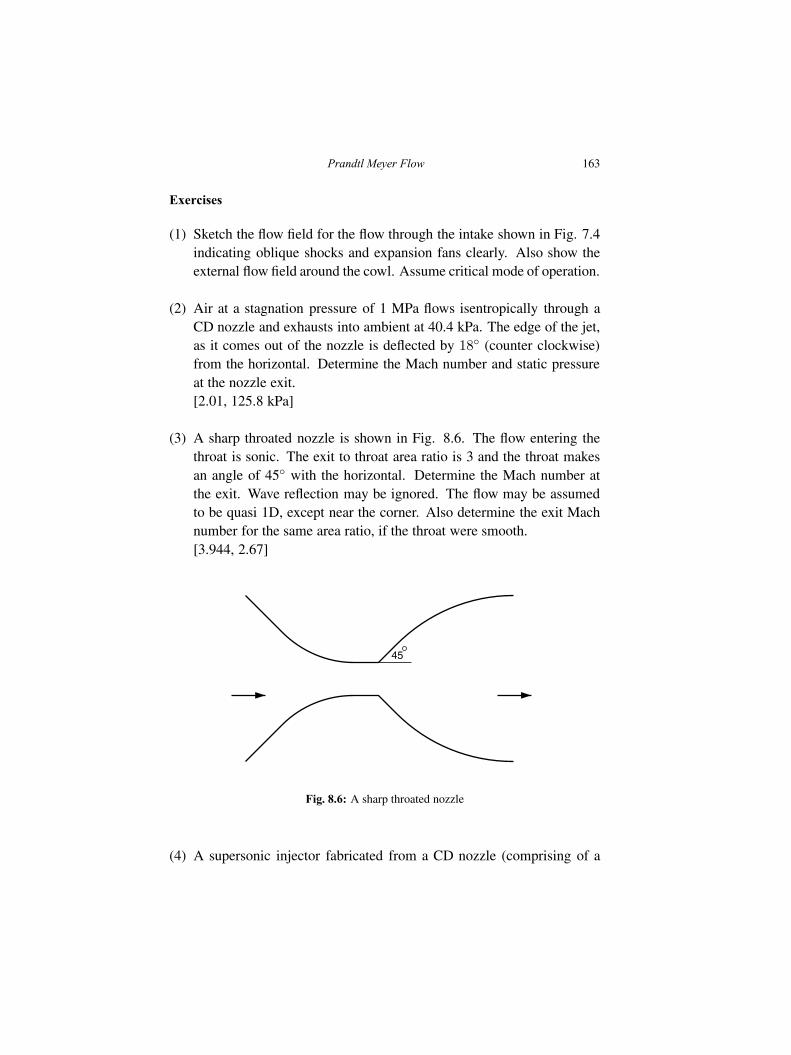
Prandtl Meyer Flow 163
Exercises
(1) Sketch the flow field for the flow through the intake shown in Fig. 7.4indicating oblique shocks and expansion fans clearly. Also show theexternal flow field around the cowl. Assume critical mode of operation.
(2) Air at a stagnation pressure of 1 MPa flows isentropically through aCD nozzle and exhausts into ambient at 40.4 kPa. The edge of the jet,as it comes out of the nozzle is deflected by 18◦ (counter clockwise)from the horizontal. Determine the Mach number and static pressureat the nozzle exit.[2.01, 125.8 kPa]
(3) A sharp throated nozzle is shown in Fig. 8.6. The flow entering thethroat is sonic. The exit to throat area ratio is 3 and the throat makesan angle of 45◦ with the horizontal. Determine the Mach number atthe exit. Wave reflection may be ignored. The flow may be assumedto be quasi 1D, except near the corner. Also determine the exit Machnumber for the same area ratio, if the throat were smooth.[3.944, 2.67]
45
Fig. 8.6: A sharp throated nozzle
(4) A supersonic injector fabricated from a CD nozzle (comprising of a
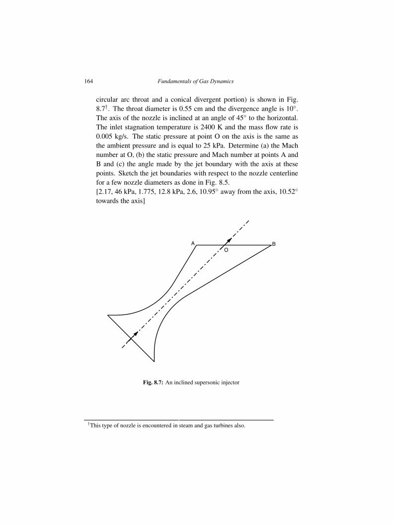
164 Fundamentals of Gas Dynamics
circular arc throat and a conical divergent portion) is shown in Fig.8.7†. The throat diameter is 0.55 cm and the divergence angle is 10◦.The axis of the nozzle is inclined at an angle of 45◦ to the horizontal.The inlet stagnation temperature is 2400 K and the mass flow rate is0.005 kg/s. The static pressure at point O on the axis is the same asthe ambient pressure and is equal to 25 kPa. Determine (a) the Machnumber at O, (b) the static pressure and Mach number at points A andB and (c) the angle made by the jet boundary with the axis at thesepoints. Sketch the jet boundaries with respect to the nozzle centerlinefor a few nozzle diameters as done in Fig. 8.5.[2.17, 46 kPa, 1.775, 12.8 kPa, 2.6, 10.95◦ away from the axis, 10.52◦
towards the axis]
OA B
Fig. 8.7: An inclined supersonic injector
†This type of nozzle is encountered in steam and gas turbines also.
Chapter 9
Flow of Steam through Nozzles
In the earlier chapters, we studied the gas dynamics of a perfect gas. Inthis chapter, we will study the dynamics of the flow of steam throughnozzles. Historically, the theory of the flow of steam through nozzles wasdeveloped first in the late 1800s and early 1900s. The convergent divergentnozzle to accelerate steam to high speeds for use in impulse steam turbineswas designed by de Laval in 1888. The importance of studying the flowof steam arises from the fact that steam turbines, even today, are usedextensively in power generation. A clear understanding of the dynamics ofthe flow of steam through the blade passages of the steam turbines as wellas through the nozzles which precede the blades is thus very important. Thetheory developed in Chapter 6 for calorically perfect gases can be carriedover for steam with a few modifications, which will be mentioned shortly.First, a brief review of the thermodynamic states of water in the pressureand temperature range of interest is presented.
9.1 T-s diagram of liquid water-water vapor mixture
The thermodynamic state of a liquid water-water vapor mixture can beillustrated on a T-s diagram as shown in Fig. 9.1. The most salient featurein this diagram is the “dome” shaped region bounded by the curve ACB.The state of a mixture of liquid water and water vapor will lie inside thisregion. Curve CA is the saturated liquid line and curve CB is the saturatedvapor line. The term saturated is used to highlight the fact that these linesindicate the beginning or termination of a change of phase. An examinationof the isobars shown in this diagram makes it clear that the pressure and
165
Fundamentals of Gas Dynamics, Second Edition. V. Babu.© 2015 V. Babu. Published 2015 by Athena Academic Ltd and John Wiley & Sons Ltd
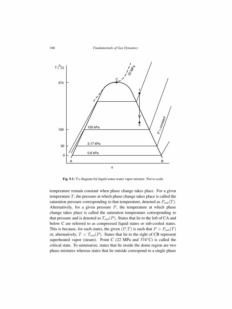
166 Fundamentals of Gas Dynamics
s
T (o
C)
A
C
B
374
22 M
Pa
0
30
100
0.6 kPa
3.17 kPa
100 kPa
P =
con
stan
t
1
2
Fig. 9.1: T-s diagram for liquid water-water vapor mixture. Not to scale
temperature remain constant when phase change takes place. For a giventemperature T , the pressure at which phase change takes place is called thesaturation pressure corresponding to that temperature, denoted as Psat(T ).Alternatively, for a given pressure P , the temperature at which phasechange takes place is called the saturation temperature corresponding tothat pressure and is denoted as Tsat(P ). States that lie to the left of CA andbelow C are referred to as compressed liquid states or sub-cooled states.This is because, for such states, the given (P, T ) is such that P > Psat(T )
or, alternatively, T < Tsat(P ). States that lie to the right of CB representsuperheated vapor (steam). Point C (22 MPa and 374◦C) is called thecritical state. To summarize, states that lie inside the dome region are twophase mixtures whereas states that lie outside correspond to a single phase
Flow of Steam through Nozzles 167
(liquid or vapor).
Since pressure and temperature are not independent inside the two phaseregion, an additional property is required to fix the state. For this purpose,a new property called the dryness fraction (x) is introduced. This is definedas
x =mg
m=
mg
mf +mg(9.1)
where the subscripts f and g refer to the liquid and vapor phase respectivelyand m denotes the mass. It is easy to see that x = 0 corresponds to asaturated liquid and x = 1 corresponds to a saturated vapor state. Thus,the saturated liquid line CA is the locus of all states for which x = 0 and thesaturated vapor line CB is the locus of states for which x = 1. The drynessfraction is indeterminate at the critical state C. Physically, this means that,when a substance exits at the critical state, it is impossible to distinguishwhether it is in the liquid or vapor state. It is important to realize that theconcept of dryness fraction is meaningless outside the dome region.
Any specific property of the two phase mixture can be evaluated as theweighted sum of the respective values at the saturated liquid and vaporstates, where the weights can be expressed in terms x. For instance, let atwo phase mixture of mass m contain mf and mg of saturated liquid andvapor respectively. The specific volume of the mixture (v) is given as
v =V
m
=mfvf +mgvg
m
= (1− x)vf + xvg
= vf + x(vg − vf )
Any specific property of the mixture (φ) in the two phase region can be
168 Fundamentals of Gas Dynamics
written in the same manner as
φ = φf + x(φg − φf ) , (9.2)
where, φ can be the specific volume v, specific internal energy u, specificenthalpy h or the specific entropy s. Property values of superheated statescan be retrieved either from tables or the Mollier diagram (h− s diagram).We mention in passing that, in contrast to the earlier chapters, here, we willuse u to denote the internal energy instead of e.
9.2 Isentropic expansion of steam
In the earlier chapters, the development assumed the fluid to be a calori-cally perfect gas. It may be recalled that this model assumes that
• the gas obeys the ideal gas equation of state, Pv = RT and• the internal energy is a linear function of temperature.
In the case of steam (as well as a two phase saturated mixture of liquidand vapor), both these assumptions are unrealistic and must be abandoned.The T-v diagram shown in Fig. 9.2 illustrates how well superheated steamobeys the ideal gas equation of state. Thermodynamic states that lie withinthe shaded region in this figure are such that Pv/(RT ) − 1 ≤ 1 percent.States that lie outside this region show greater departure from ideal gasbehaviour. States near the critical point, C, show the maximum departure.In an actual application, there is no guarantee that the initial state of thesteam (before expansion in the nozzle) will lie within the shaded region inFig. 9.2. More importantly, the state at the end of the isentropic expansionprocess in the nozzle (process 1-2 in Figs. 9.1 and 9.2) will most likely liein the two phase region.
The internal energy of water in the two-phase region as well as thesuperheated region is a function of temperature and pressure, i.e., u =
u(T, P ). Hence, even the thermally perfect assumption is invalid let alonethe calorically perfect assumption.
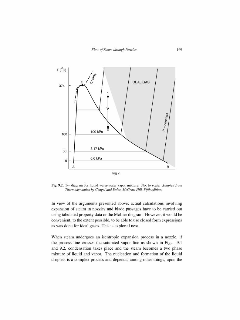
Flow of Steam through Nozzles 169
log v
T (o
C)
IDEAL GAS
A
C
B
37422
MP
a
0
30
100
0.6 kPa
3.17 kPa
100 kPa P =
con
stan
t
1
2
Fig. 9.2: T-v diagram for liquid water-water vapor mixture. Not to scale. Adapted fromThermodynamics by Cengel and Boles, McGraw Hill, Fifth edition.
In view of the arguments presented above, actual calculations involvingexpansion of steam in nozzles and blade passages have to be carried outusing tabulated property data or the Mollier diagram. However, it would beconvenient, to the extent possible, to be able to use closed form expressionsas was done for ideal gases. This is explored next.
When steam undergoes an isentropic expansion process in a nozzle, ifthe process line crosses the saturated vapor line as shown in Figs. 9.1and 9.2, condensation takes place and the steam becomes a two phasemixture of liquid and vapor. The nucleation and formation of the liquiddroplets is a complex process and depends, among other things, upon the
170 Fundamentals of Gas Dynamics
purity of the steam. Depending upon their radii, the droplets will tend tomove with velocities different from the vapor phase owing to inertia force.Furthermore, as mentioned in section 6.7, normal shocks tend to occur inthe divergent portion of a convergent divergent nozzle. At this point, thesteam would have undergone a considerable amount of expansion and islikely to be quite wet. As a result of the increase in pressure, temperatureand entropy across the normal shock, the steam will become dry andsaturated or even superheated. The gas dynamics of a two phase mixtureis complex and beyond the scope of this book. However, if the drynessfraction does not become too low i.e., the steam does not become too wet,then the aforementioned complications can be ignored. We assume this tobe the case in the rest of this chapter. In addition, we will assume that theflow is shock free and hence isentropic.
We know that isentropic expansion of an ideal gas obeys Pvγ = constant.Isentropic expansion of steam can be represented using a similar expressionof the form
Pvn = constant , (9.3)
where the exponent n has to be determined from experimental data througha curve fit. This is given as
n =
{
1.3 if superheated1.035 + 0.1x1 saturated mixture
(9.4)
where x1 is the initial dryness fraction. The exponent for superheatedsteam is due to Callendar and the expression for the saturated mixture isdue to Zeuner. It will be demonstrated later through numerical examplesthat Eqn. 9.3 with the exponent given by Eqn. 9.4 is an excellentdescription of the isentropic expansion process of steam in nozzles.
Since the propagation of an acoustic wave through a medium causeschanges in the properties of the medium that are governed by an isentropicprocess, the speed of sound a, in superheated steam or a saturated mixturecan be calculated using Eqns. 2.13 and 9.4 as follows:
Flow of Steam through Nozzles 171
a =
√
dP
dρ
∣
∣
∣
∣
s
(2.13)
=√nPv (9.5)
9.3 Flow of steam through nozzles
The theory developed in Chapter 6 for the flow of a calorically perfectgas is applicable for the flow of steam as well, subject to the constraintsmentioned above. In view of this, this material will not be repeated inthis chapter. However, the material will be developed along the linescustomarily adopted in the context of steam nozzles.
The continuity equation for this flow can be written in differential formas
d(ρV A) = 0 , (6.3)
where, in contrast to the earlier chapters, we have used V to denote thevelocity†. Momentum and energy equation in differential form are thesame as Eqns. 2.2 and 2.3, viz.,
dP + ρV dV = 0 , (2.2)
dh+ d
(
V 2
2
)
= 0 . (2.3)
If we integrate the momentum equation, we get, for expansion betweenstates 1 and 2,
V 22 − V 2
1
2= −
∫ 2
1v dP .
†Since we have used u to denote the internal energy now.
172 Fundamentals of Gas Dynamics
Since Pvn = constant, the integral on the right hand can be evaluated. Thisleads to
V 22 − V 2
1
2=
n
n− 1(P1v1 − P2v2) .
This can be rewritten as
V2 =
√
V 21 +
2n
n− 1P1v1
[
1− P2v2P1v1
]
=
√
√
√
√V 21 +
2n
n− 1P1v1
[
1−(
P2
P1
)(n−1)/n]
, (9.6)
where we have used P1vn1 = P2v
n2 . If the steam expands from a steam
chest, where stagnation conditions prevail, then V1 = 0, P1 = P0 andv1 = v0. Thus,
V2 =
√
√
√
√
2n
n− 1P0v0
[
1−(
P2
P0
)(n−1)/n]
.
If we integrate Eqn. 2.3 between states 1 and 2, we get
h1 − h2 =V 22 − V 2
1
2.
Upon substituting for V2 from Eqn. 9.6, we get
h1 − h2 =n
n− 1P1v1
[
1−(
P2
P1
)(n−1)/n]
. (9.7)
Without any loss of generality, if we simply assume that the steam is
Flow of Steam through Nozzles 173
expanded from the chest to a final pressure of P , then the subscript 2 canbe dropped from the above equation and we thus get the velocity at the endof the expansion process to be
V =
√
√
√
√
2n
n− 1P0v0
[
1−(
P
P0
)(n−1)/n]
. (9.8)
In contrast to nozzle flows involving perfect gases where the Area-Machnumber relation is used extensively (and perhaps exclusively), Eqn. 9.8 isused extensively in applications involving flow of steam through nozzles† .
9.3.1 Choking in steam nozzles
The mass flow rate at any section in a nozzle is given as
m =AV
v.
If we use the fact that Pvn = P0vn0 in the above expression, we get
m =AV
v0
(
P
P0
)1/n
.
Upon substituting for V from Eqn. 9.8, we are led to
m = A
√
√
√
√
2n
n− 1
P0
v0
[
(
P
P0
)2/n
−(
P
P0
)(n+1)/n]
.
For a given value of A, P0 and v0, it is easy to show that the mass flow rateis a maximum when the steam is expanded to a pressure P given by
P
P0=
(
2
n+ 1
)n/(n−1)
. (9.9)
†Most likely due to the almost exclusive use of steam nozzles in steam turbines.
174 Fundamentals of Gas Dynamics
We can rewrite Eqn. 9.8 as
V =
√
√
√
√
2n
n− 1Pv
[
(
P0
P
)n/(n−1)
− 1
]
.
If we substitute for P from Eqn. 9.9, then, at the section where the pressureis given by this equation, the velocity of the steam is given as
V =√nPv .
It follows from Eqn. 9.5 that this velocity is equal to the local speed ofsound. Hence, Eqn. 9.9 may be rewritten as
P ∗
P0=
(
2
n+ 1
)n/(n−1)
. (9.10)
It is worthwhile emphasizing that Eqns. 9.8, 9.9 and 9.10 have been derivedwith the sole assumption that the isentropic expansion process of steamin the nozzle can be described by Pvn = constant and without using thecalorically perfect assumption.
Example 9.1. Dry, saturated steam enters a convergent nozzle at a staticpressure of 500 kPa and is expanded to 300 kPa. If the inlet and throatdiameters are 0.05 m and 0.025 m respectively, determine the velocity atthe inlet and exit and the stagnation pressure.
Solution. Given P1 = 500 kPa and x1 = 1, we can get v1 = 0.3748 m3/kg,h1 = 2748.49 kJ/kg and s1 = 6.8215 kJ/kg.K. Since the steam is initiallydry and saturated, n = 1.135 from Eqn. 9.4. From Eqn. 9.3, we can get
ve = v1
(
Pe
P1
)−1/n
= 0.5878m3/kg
Flow of Steam through Nozzles 175
and from Eqn. 9.7
h1 − he =n
n− 1P1v1
[
1−(
Pe
P1
)(n−1)/n]
= 92.88 kJ/kg
=V 2e − V 2
1
2
Also, since the mass flow rates at the inlet and outlet are the same, we have
V1 =Ae
A1
v1ve
Ve .
(a) We can thus obtain the exit velocity Ve = 436.6 m/s. It follows that theinlet velocity V1 = 69.6 m/s. Note that the speed of sound at the exit canbe calculated from Eqn. 9.5 to be 447.4 m/s. Hence, the flow is not choked.
(b) The stagnation enthalpy can be evaluated using
h0 = h1 +V 21
2= 2751 kJ/kg .
Since s0 = s1 = 6.8215 kJ/kg.K, we can get the stagnation pressure P0 =507 kPa from the steam table. For this value of P0, we can obtain P ∗ =294 kPa from Eqn. 9.10. The given exit pressure is higher than this valueconfirming our earlier observation that the flow is not choked. �
Example 9.2. Dry, saturated steam at 1 MPa in a steam chest expandsthrough a nozzle to a final pressure of 100 kPa. Determine (a) if thenozzle is convergent or convergent-divergent, (b) the exit velocity, (c) thedryness fraction at the exit and (c) the exit to throat area ratio. Assume theexpansion to be isentropic throughout.
Solution. We have P0 = 1 MPa and we can get v0 = 0.19436 m3/kg fromthe steam table.
176 Fundamentals of Gas Dynamics
(a) Since the steam is initially dry and saturated, n = 1.135 from Eqn.9.4. From Eqn. 9.10, we have P ∗ = 0.58P0 = 580 kPa. Since the flowis expanded to a final pressure of 100 kPa in the nozzle, it is clear that thenozzle is convergent-divergent.
(b) We have from Eqn. 9.7
h0 − he =n
n− 1P0v0
[
1−(
Pe
P0
)(n−1)/n]
,
where the subscript e denotes the exit. Upon substituting numerical values,we get
h0 − he = 391.48 kJ/kg .
Therefore
Ve =√
2(h0 − he) = 885m/s .
(c) From Eqn. 9.3, we can get
ve = v0
(
Pe
P0
)−1/n
= 1.478m3/kg .
Using steam tables, the dryness fraction at the exit can now be calculatedas 0.87.
(d) From Eqn. 9.3, we can get
v∗ = v0
(
P ∗
P0
)−1/n
= 0.3141m3/kg
and
V ∗ =√nP ∗v∗ = 454.7m/s .
Since
m =A∗V ∗
v∗=
AeVe
ve,
Flow of Steam through Nozzles 177
we can obtain Ae/A∗ = 2.42.
An alternative solution method is to use the Mollier diagram or the steamtable. From the steam table, for dry saturated vapor at 1 MPa, we can geth0 = 2778.1 kJ/kg and s0 = 6.5865 kJ/kg.K. Since the expansion processis isentropic, we have at the exit, se = 6.5865 kJ/kg.K and Pe = 100 kPa.From steam tables, we can get xe = 0.872 and thus he = 2387.3 kJ/kg andve = 1.4773 m3/kg. Therefore
Ve =√
2(h0 − he) = 884m/s�
Example 9.3. Steam at 700 kPa, 250◦C in a steam chest expands througha nozzle to a final pressure of 100 kPa. The mass flow rate is 0.076 kg/s.Determine (a) if the nozzle is convergent or convergent-divergent (b) thethroat diameter (c) the exit diameter and (d) the dryness fraction at theexit. Assume the expansion process to be isentropic and in equilibriumthroughout.
Solution. From the steam table, it is easy to establish that for the givensteam chest conditions of P0 = 700 kPa and T0 = 250◦C the steamis initially superheated. Also, v0 = 0.336343 m3/kg and s0 = 7.1062
kJ/kg.K.
(a) Since the steam is initially superheated, n = 1.3 from Eqn. 9.4. FromEqn. 9.10, we have P ∗ = 0.545P0 = 380 kPa. Since the flow is expandedto a final pressure of 100 kPa in the nozzle, it is clear that the nozzle isconvergent-divergent.
(b) From Eqn. 9.3, we can get
v∗ = v0
(
P ∗
P0
)−1/n
= 0.53648m3/kg
and
V ∗ =√nP ∗v∗ = 514.8m/s .
Since
A∗ =mv∗
V ∗= 7.92 × 10⁻⁵ m2 ,
178 Fundamentals of Gas Dynamics
the throat diameter D∗ = 10 mm.
(c) Since the expansion process is isentropic, the process line crosses thesaturated vapor line at Pg = 212 kPa. With n = 1.3 (as the flow issuperheated until it crosses the saturated vapor line), we can get
h0 − hg =n
n− 1P0v0
[
1−(
Pg
P0
)(n−1)/n]
= 245.8 kJ/kg ,
and
vg = v0
(
Pg
P0
)−1/n
= 0.843m3/kg .
It follows that Vg =√
2(h0 − hg) = 701.14 m/s. Once the flow crossesthe saturated vapor line, n = 1.135 (this implies that the flow continues tobe in equilibrium after crossing the saturated vapor line). Hence
hg − he =n
n− 1Pgvg
[
1−(
Pe
Pg
)(n−1)/n]
= 127.77 kJ/kg ,
and
ve = vg
(
Pe
Pg
)−1/n
= 1.6344m3/kg .
Therefore
Ve =√
V 2g + 2(hg − he) = 864m/s .
For the given mass flow rate, the exit area can be calculated as
Ae =mveVe
= 1.44 × 10⁻⁴ m2
and the exit diameter can be calculated as De = 13.5 mm.
(d) From the given value of the exit pressure Pe and the calculated value of
Flow of Steam through Nozzles 179
ve, we can get the dryness fraction at the exit to be 0.96 using steam tables.
Alternatively, we can use the steam table (or Mollier diagram) to solvethe problem. For the given steam chest condition, we can get h0 = 2954
kJ/kg and s0 = 7.1062 kJ/kg.K.
The pressure at the throat P ∗ = 0.545P0 = 380 kPa. Since theexpansion is isentropic, s∗ = s0 = 7.1062 kJ/kg.K. Therefore, the fluidis superheated at the throat with v∗ = 0.537 m3/kg and h∗ = 2820 kJ/kg.It follows that
V ∗ =√
2 (h0 − h∗) = 518m/s
and
A∗ =mv∗
V ∗= 7.86 × 10⁻⁵ m2 .
Thus, the throat diameter D∗ = 10 mm.
We have Pe = 100 kPa and se = s0 = 7.112 kJ/kg.K. It can be determinedthat the fluid at the exit is a saturated mixture. The dryness fraction xe canbe evaluated as 0.96. Also, he = 2581 kJ/kg and ve = 1.623 m3/kg. Hence
Ve =√
2 (h0 − he) = 864m/s
and
Ae =mveVe
= 1.43 × 10⁻⁴ m2 .
Thus, the exit diameter De = 13.5 mm. �
9.4 Supersaturation and the condensation shock
When thermodynamic states and processes are depicted in diagrams suchas the ones in Figs. 9.1 and 9.2, an important assumption is that equilibriumprevails during the process. In other words, the underlying implication is
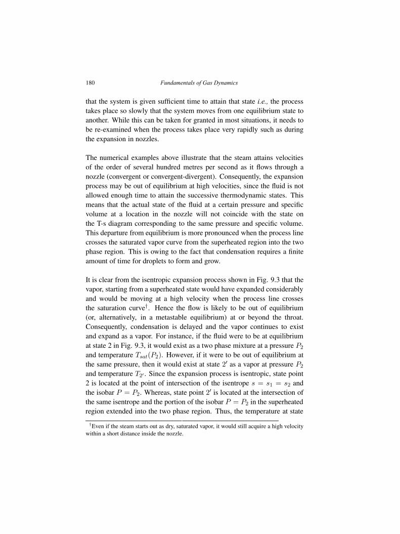
180 Fundamentals of Gas Dynamics
that the system is given sufficient time to attain that state i.e., the processtakes place so slowly that the system moves from one equilibrium state toanother. While this can be taken for granted in most situations, it needs tobe re-examined when the process takes place very rapidly such as duringthe expansion in nozzles.
The numerical examples above illustrate that the steam attains velocitiesof the order of several hundred metres per second as it flows through anozzle (convergent or convergent-divergent). Consequently, the expansionprocess may be out of equilibrium at high velocities, since the fluid is notallowed enough time to attain the successive thermodynamic states. Thismeans that the actual state of the fluid at a certain pressure and specificvolume at a location in the nozzle will not coincide with the state onthe T-s diagram corresponding to the same pressure and specific volume.This departure from equilibrium is more pronounced when the process linecrosses the saturated vapor curve from the superheated region into the twophase region. This is owing to the fact that condensation requires a finiteamount of time for droplets to form and grow.
It is clear from the isentropic expansion process shown in Fig. 9.3 that thevapor, starting from a superheated state would have expanded considerablyand would be moving at a high velocity when the process line crossesthe saturation curve†. Hence the flow is likely to be out of equilibrium(or, alternatively, in a metastable equilibrium) at or beyond the throat.Consequently, condensation is delayed and the vapor continues to existand expand as a vapor. For instance, if the fluid were to be at equilibriumat state 2 in Fig. 9.3, it would exist as a two phase mixture at a pressure P2
and temperature Tsat(P2). However, if it were to be out of equilibrium atthe same pressure, then it would exist at state 2′ as a vapor at pressure P2
and temperature T2′ . Since the expansion process is isentropic, state point2 is located at the point of intersection of the isentrope s = s1 = s2 andthe isobar P = P2. Whereas, state point 2′ is located at the intersection ofthe same isentrope and the portion of the isobar P = P2 in the superheatedregion extended into the two phase region. Thus, the temperature at state
†Even if the steam starts out as dry, saturated vapor, it would still acquire a high velocitywithin a short distance inside the nozzle.
Flow of Steam through Nozzles 181
s
T
A
C
B
1
2
2’
3
eP
= P
sat (
T2’
)
P =
P2P
= P
1
Tsat
( P2
)
Fig. 9.3: Illustration of supersaturated flow on a T-s diagram. Note that 2′ is a metastablestate and P2′ = P2. The dashed line connecting 2′-3 represents the condensationshock.
2′ is not Tsat(P2) but is given as
T2′ = T1
(
P2
P1
)(n−1)/n
, (9.11)
where we have used the fact that P2′ = P2. It must be noted that in writingEqn. 9.11 from Eqn. 9.3, we have used the ideal gas equation of state forthe supersaturated vapor. This is only an approximation as evident fromFig. 9.2, but an acceptable one for practical purposes.
Two quantities are customarily used to characterize supersaturated steam.
182 Fundamentals of Gas Dynamics
These are the degree of supersaturation or supersaturation ratio denotedby S and the degree of supercooling. The degree of supersaturation isdefined as the ratio of the pressure P of the supersaturated vapor to the(equilibrium) saturation pressure corresponding to its temperature. Thus,
S =P
Psat(T ). (9.12)
The degree of supercooling of a supersaturated vapor is defined as the dif-ference between the actual temperature T and the (equilibrium) saturationtemperature corresponding to its pressure. Thus,
∆T = Tsat(P )− T . (9.13)
Figure 9.3 illustrates how these quantities are to be evaluated. It shouldalso be clear from this figure that S > 1 and ∆T > 0 for a supersaturatedvapor. The degree of supercooling is the exact opposite of the more familiardegree of superheat. It may be recalled that the latter quantity is defined inthe same manner except that T > Tsat(P ).
When steam exists in this unnaturally dry, supersaturated state, its densityis higher than that of the saturated vapor at the same pressure by a factorof approximately 5-8. Moreover, since the latent heat of condensation hasnot been released owing to the delayed condensation, the enthalpy dropand hence the velocity (Eqn. 9.7) is also less. This reduction is usually nothigh as the velocity is dependent on the square root of the enthalpy drop.However, if the flow were to be supersaturated at the nozzle throat, thenthe combined effect of these two factors is to increase the mass flow ratethrough the nozzle for a given steam chest pressure and throat area.
Example 9.4. For the same steam chest condition and exit pressure in theprevious example, determine the exit velocity, the supersaturation ratio andthe degree of supercooling, if the flow is out of equilibrium.
Solution. In this case, we use n = 1.3 for the entire expansion process.Therefore,
ve = v0
(
Pe
P0
)−1/n
= 4.2209m3/kg ,
Flow of Steam through Nozzles 183
Te = T0
(
Pe
P0
)(n−1)/n
= 333.8K = 60.8◦C
and
h0 − he =n
n− 1P0v0
[
1−(
Pe
P0
)(n−1)/n]
= 369.1 kJ/kg .
The exit velocity Ve =√
2 (h0 − he) = 859 m/s.
The saturation pressure corresponding to Te = 60.8◦C is 20.7 kPa. Hence,the supersaturation ratio S = Pe/Psat(Te) = 4.83.
The saturation temperature corresponding to Pe = 100 kPa is 100◦C.Hence, the degree of supercooling ∆T = Tsat(Pe)− Te = 39.2◦ C. �
As the supersaturated steam expands, both the degree of supersaturationand the degree of supercooling increase. However, there is a limit to thedegree of supersaturation that can be allowed and once this limit is reached,the supersaturated vapor condenses almost instantaneously, triggering acondensation shock (Fig. 9.4). The pressure, temperature and entropyincrease across the condensation shock as shown in Fig. 9.3. The limitingvalue of the degree of supersaturation is 5 and it depends upon, amongother things, the purity of the vapor. If impurities such as dissolvedsalts are present, then nucleation of droplets begins early. Remarkably,experimental evidence suggests that the condensation shock is almostalways initiated once the process line reaches the 96% dryness fractionline. This line is called the Wilson line . The term “shock” is somewhat ofa misnomer since the condensation process occurs over a small but finitedistance and is not a discontinuity.
The flow attains equilibrium downstream of the condensation shock andmay continue to expand until the nozzle exit (denoted as the state pointe in Fig. 9.3). However, if the back pressure at the exit is high, thena normal shock will stand somewhere in the divergent part of the nozzleas mentioned in section 6.7. As before, the pressure, temperature andentropy increase across the shock wave. As a result, the two phase mixtureupstream of the shock wave may attain the saturated vapor state or even
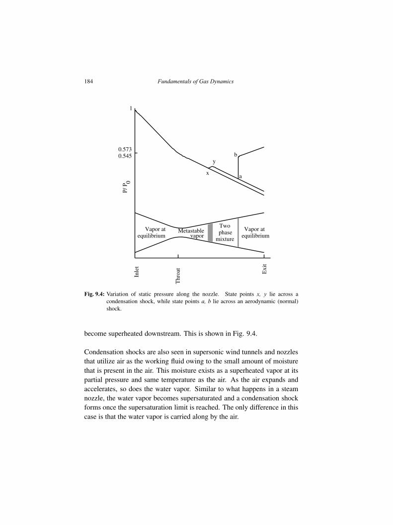
184 Fundamentals of Gas Dynamics
P/ P
0In
let
Thr
oat
Exi
t
0.5730.545
1
x
y
a
b
Vapor atequilibrium
Metastablevapor
Twophase
mixture
Vapor atequilibrium
Fig. 9.4: Variation of static pressure along the nozzle. State points x, y lie across acondensation shock, while state points a, b lie across an aerodynamic (normal)shock.
become superheated downstream. This is shown in Fig. 9.4.
Condensation shocks are also seen in supersonic wind tunnels and nozzlesthat utilize air as the working fluid owing to the small amount of moisturethat is present in the air. This moisture exists as a superheated vapor at itspartial pressure and same temperature as the air. As the air expands andaccelerates, so does the water vapor. Similar to what happens in a steamnozzle, the water vapor becomes supersaturated and a condensation shockforms once the supersaturation limit is reached. The only difference in thiscase is that the water vapor is carried along by the air.
Flow of Steam through Nozzles 185
The development in sections 9.2 and 9.3 cannot be used downstream ofstate point x shown in Fig. 9.4, as two phase effects are significant. Acomprehensive and unified theory of condensation as well as aerodynamic(normal) shocks in flows with or without a carrier gas was developed byGuha†. Interested readers may refer this work for the details of how toincorporate two phase effect and droplet nucleation and growth effect intothe quasi one dimensional theory developed above in sections 9.2 and 9.3.
Example 9.5. Steam expands in a convergent-divergent nozzle from astagnation pressure and temperature of P0 = 144 kPa and T0 = 118.7◦Crespectively. The steam expands until a supersaturation ratio of 5 is reachedat which point a condensation shock occurs. Determine the pressure,velocity and degree of supercooling just ahead of the condensation shock.
Solution. It can be established that, for the given stagnation conditions,the steam is superheated at the inlet and v0 = 1.234 m3/kg. Let x denotethe state point just ahead of the condensation shock. The supersaturationratio is defined as
S =Px
Psat(Tx).
If the flow is assumed to be isentropic until the onset of the condensationshock, then
Tx = T0
(
Px
P0
)(n−1)/n
, (9.14)
with n = 1.3 for superheated steam.
The task is to determine Px and Tx from these two equations for theprescribed value of S. This can be accomplished quite easily in an iterativemanner starting with a guessed value for Px. The initial guess should bemade keeping in mind that Px should be less than Pthroat = 0.58P0 =
78584 Pa. The procedure is illustrated in the following table.
†“A unified theory of aerodynamic and condensation shock waves in vapor-droplet flowswith or without a carrier gas”, Physics of Fluids, Vol. 6, No. 5, May 1994, pp. 1893-1913.
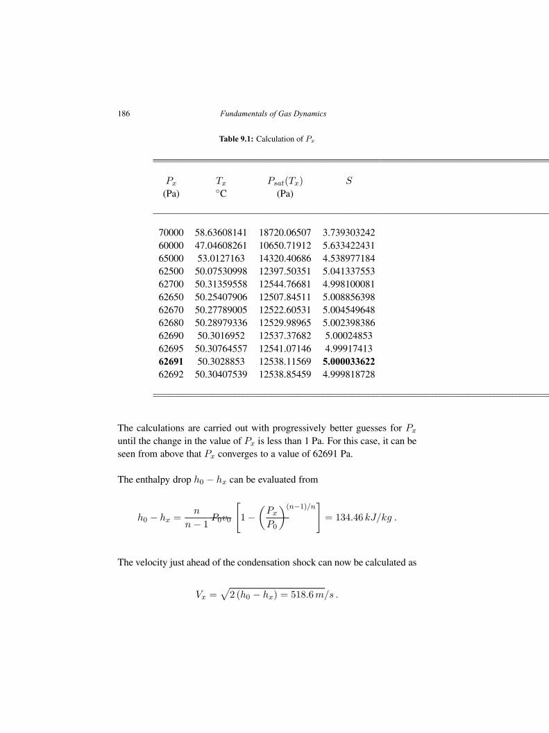
186 Fundamentals of Gas Dynamics
Table 9.1: Calculation of Px
Px Tx Psat(Tx) S
(Pa) ◦C (Pa)
70000 58.63608141 18720.06507 3.73930324260000 47.04608261 10650.71912 5.63342243165000 53.0127163 14320.40686 4.53897718462500 50.07530998 12397.50351 5.04133755362700 50.31359558 12544.76681 4.99810008162650 50.25407906 12507.84511 5.00885639862670 50.27789005 12522.60531 5.00454964862680 50.28979336 12529.98965 5.00239838662690 50.3016952 12537.37682 5.0002485362695 50.30764557 12541.07146 4.9991741362691 50.3028853 12538.11569 5.00003362262692 50.30407539 12538.85459 4.999818728
The calculations are carried out with progressively better guesses for Px
until the change in the value of Px is less than 1 Pa. For this case, it can beseen from above that Px converges to a value of 62691 Pa.
The enthalpy drop h0 − hx can be evaluated from
h0 − hx =n
n− 1P0v0
[
1−(
Px
P0
)(n−1)/n]
= 134.46 kJ/kg .
The velocity just ahead of the condensation shock can now be calculated as
Vx =√
2 (h0 − hx) = 518.6m/s .
Flow of Steam through Nozzles 187
From steam tables, we can get Tsat(Px) = 87◦C. Hence, the degree ofsupercooling ∆T = Tsat(Px)− Tx = 36.7◦C. �
188 Fundamentals of Gas Dynamics
Exercises
(1) Dry, saturated steam enters a convergent nozzle at a static pressureof 800 kPa and is expanded to the sonic state. If the inlet and throatdiameters are 0.05 m and 0.025 m respectively, determine the velocityat the inlet and exit and the stagnation pressure.[70.6 m/s, 453 m/s, 806 kPa]
(2) Dry saturated steam at 1.1 MPa is expanded in a nozzle to a pressureof 15 kPa. Assuming the expansion process to be isentropic and inequilibrium throughout, determine (a) if the nozzle is convergent orconvergent-divergent, (b) the exit velocity, (c) the dryness fraction atthe exit and (c) the exit to throat area ratio.[convergent-divergent,1146 m/s, 0.8, 11]
(3) Superheated steam at 700 kPa, 220◦C in a steam chest is expandedthrough a nozzle to a final pressure of 20 kPa. The throat diameteris 10 mm. Assuming the expansion process to be isentropic and inequilibrium throughout, determine (a) the mass flow rate, (b) the exitvelocity, (c) the dryness fraction at the exit and (c) the exit diameter.[0.0781 kg/s, 1085 m/s, 0.87, 24.5 mm]
(4) Dry saturated steam at 1.2 MPa is expanded in a nozzle to 20 kPa. Thethroat diameter of the nozzle is 6 mm. If the total mass flow rate is 0.5kg/s, determine how many nozzles are required and the exit diameterof the nozzle. Assume the expansion process to be isentropic and inequilibrium throughout.[10,0.18.2 mm]
(5) Superheated steam at 850 kPa, 200◦C expands in a convergent nozzleuntil it becomes a saturated vapor. Determine the exit velocity,assuming the expansion process to be isentropic and in equilibriumthroughout.[407 m/s]
(6) Steam which is initially saturated and dry expands from 1400 kPa to
Flow of Steam through Nozzles 189
700 kPa. Assuming the expansion to be in equilibrium (n=1.135),determine the final velocity and specific volume. If the expansion is outof equilibrium (n=1.3), determine the final velocity, specific volume,supersaturation ratio and the degree of undercooling.[512 m/s, 0.2593 m3/kg; 502 m/s, 0.24 m3/kg, 3.41, 39◦C]
(7) Superheated steam at 500 kPa, 180◦C is expanded in a nozzle topressure of 170 kPa. Assuming the expansion process to be isentropicand in equilibrium determine the exit velocity. Assuming the flowto be isentropic and supersaturated, determine the the exit velocity,supersaturation ratio and the degree of supercooling.[627 m/s, 621 m/s, 3.59, 34◦C]
(8) For each of the stagnation condition given below, determine thepressure, velocity and degree of supercooling just before the onset ofcondensation shock for a limiting value of supersaturation ratio of 5.Assume the expansion process to be isentropic. (a) 87000 Pa, 96◦C,(b) 70727 Pa, 104◦C and (c)25000 Pa, 85◦C.[45037 Pa, 453 m/s, 35◦C; 29918 Pa, 518.6 m/s, 33◦C; 10127 Pa, 518m/s, 28◦C]

190 Fundamentals of Gas Dynamics
Suggested Reading
Gas Dynamics Vol. 1 by M. J. Zucrow and J. D. Hoffman, John Wiley &Sons, 1976.
Dynamics and Thermodynamics of Compressible Fluid Flow by A. H.Shapiro, Krieger Publications Company, Reprint Edition, 1983.
Elements of Gas Dynamics by H. W. Liepmann and A. Roshko, DoverPublications, 2002.
Modern Compressible Flow With Historical Perspective by J. D. Ander-son, Third Edition, McGraw-Hill Series in Aeronautical and AerospaceEngineering, 2003.
Compressible Fluid Dynamics by B. K. Hodge and K. Koenig, PrenticeHall Inc, 1995.
Elements of Gas Turbine Propulsion by J. D. Mattingly, McGraw-HillSeries in Aeronautical and Aerospace Engineering, 1996.
191
Fundamentals of Gas Dynamics, Second Edition. V. Babu.© 2015 V. Babu. Published 2015 by Athena Academic Ltd and John Wiley & Sons Ltd
192 Fundamentals of Gas Dynamics
Compressible Fluid Flow by M. Saad, Second Edition, Prentice Hall Inc,1985.
Fluid Mechanics by F. M. White, Fifth Edition, McGraw-Hill HigherEducation, 2003.
Steam Turbine Theory and Practice by W. J. Kearton, Seventh Edition, SirIsaac Pitman & Sons Ltd, London, 1958. Reprinted with permissionin India by CBS Publishers and Distributors Pvt. Ltd, 2004.
Principles of Turbomachinery by S. A. Korpela, First Edition, John Wiley& Sons, 2011.
Table A. Isentropic table for γ = 1.4
193
Fundamentals of Gas Dynamics, Second Edition. V. Babu.© 2015 V. Babu. Published 2015 by Athena Academic Ltd and John Wiley & Sons Ltd
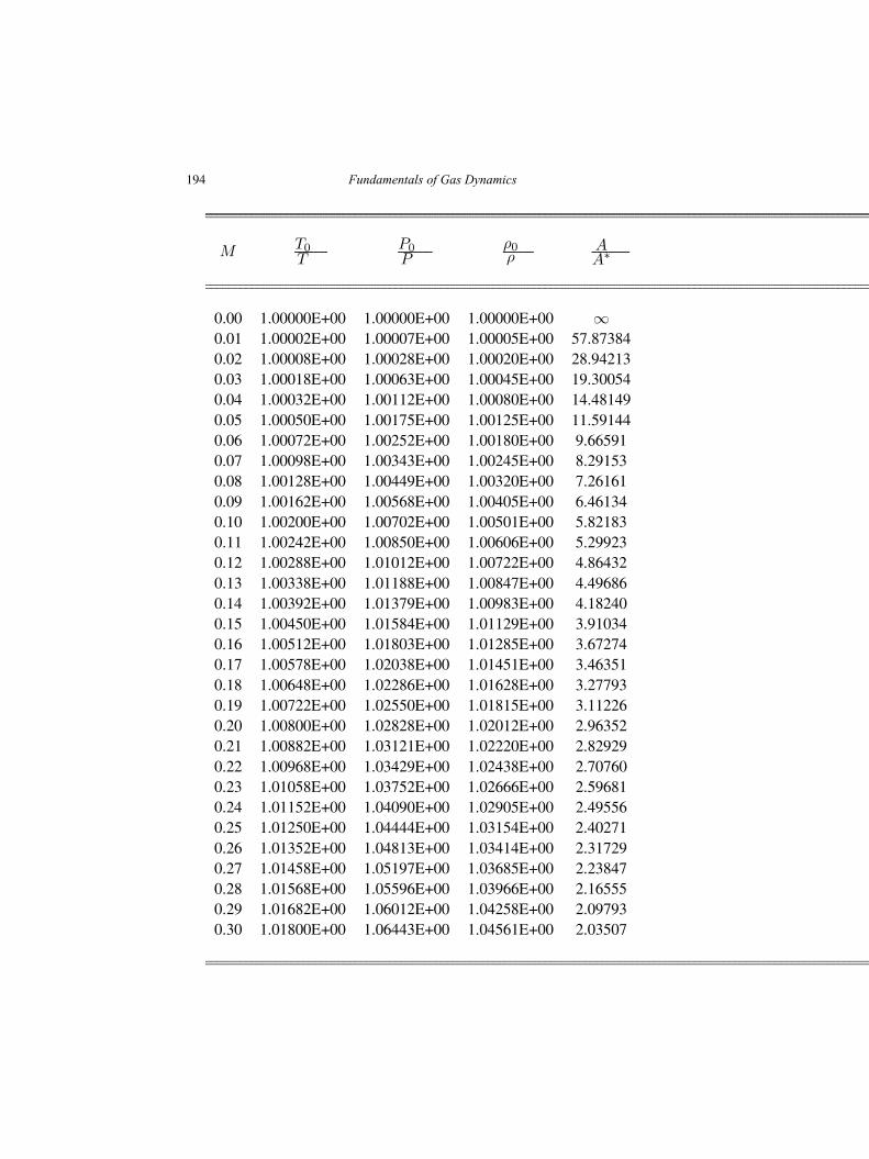
194 Fundamentals of Gas Dynamics
M T0T
P0P
ρ0ρ
AA∗
0.00 1.00000E+00 1.00000E+00 1.00000E+00 ∞0.01 1.00002E+00 1.00007E+00 1.00005E+00 57.873840.02 1.00008E+00 1.00028E+00 1.00020E+00 28.942130.03 1.00018E+00 1.00063E+00 1.00045E+00 19.300540.04 1.00032E+00 1.00112E+00 1.00080E+00 14.481490.05 1.00050E+00 1.00175E+00 1.00125E+00 11.591440.06 1.00072E+00 1.00252E+00 1.00180E+00 9.665910.07 1.00098E+00 1.00343E+00 1.00245E+00 8.291530.08 1.00128E+00 1.00449E+00 1.00320E+00 7.261610.09 1.00162E+00 1.00568E+00 1.00405E+00 6.461340.10 1.00200E+00 1.00702E+00 1.00501E+00 5.821830.11 1.00242E+00 1.00850E+00 1.00606E+00 5.299230.12 1.00288E+00 1.01012E+00 1.00722E+00 4.864320.13 1.00338E+00 1.01188E+00 1.00847E+00 4.496860.14 1.00392E+00 1.01379E+00 1.00983E+00 4.182400.15 1.00450E+00 1.01584E+00 1.01129E+00 3.910340.16 1.00512E+00 1.01803E+00 1.01285E+00 3.672740.17 1.00578E+00 1.02038E+00 1.01451E+00 3.463510.18 1.00648E+00 1.02286E+00 1.01628E+00 3.277930.19 1.00722E+00 1.02550E+00 1.01815E+00 3.112260.20 1.00800E+00 1.02828E+00 1.02012E+00 2.963520.21 1.00882E+00 1.03121E+00 1.02220E+00 2.829290.22 1.00968E+00 1.03429E+00 1.02438E+00 2.707600.23 1.01058E+00 1.03752E+00 1.02666E+00 2.596810.24 1.01152E+00 1.04090E+00 1.02905E+00 2.495560.25 1.01250E+00 1.04444E+00 1.03154E+00 2.402710.26 1.01352E+00 1.04813E+00 1.03414E+00 2.317290.27 1.01458E+00 1.05197E+00 1.03685E+00 2.238470.28 1.01568E+00 1.05596E+00 1.03966E+00 2.165550.29 1.01682E+00 1.06012E+00 1.04258E+00 2.097930.30 1.01800E+00 1.06443E+00 1.04561E+00 2.03507
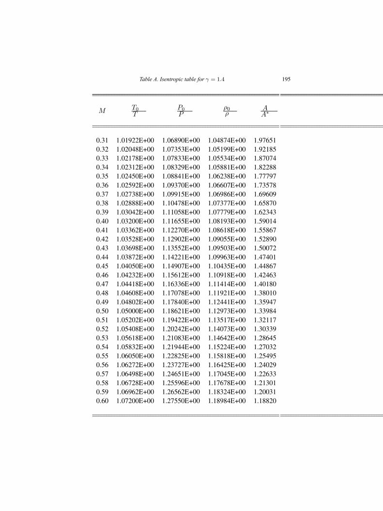
Table A. Isentropic table for γ = 1.4 195
M T0T
P0P
ρ0ρ
AA∗
0.31 1.01922E+00 1.06890E+00 1.04874E+00 1.976510.32 1.02048E+00 1.07353E+00 1.05199E+00 1.921850.33 1.02178E+00 1.07833E+00 1.05534E+00 1.870740.34 1.02312E+00 1.08329E+00 1.05881E+00 1.822880.35 1.02450E+00 1.08841E+00 1.06238E+00 1.777970.36 1.02592E+00 1.09370E+00 1.06607E+00 1.735780.37 1.02738E+00 1.09915E+00 1.06986E+00 1.696090.38 1.02888E+00 1.10478E+00 1.07377E+00 1.658700.39 1.03042E+00 1.11058E+00 1.07779E+00 1.623430.40 1.03200E+00 1.11655E+00 1.08193E+00 1.590140.41 1.03362E+00 1.12270E+00 1.08618E+00 1.558670.42 1.03528E+00 1.12902E+00 1.09055E+00 1.528900.43 1.03698E+00 1.13552E+00 1.09503E+00 1.500720.44 1.03872E+00 1.14221E+00 1.09963E+00 1.474010.45 1.04050E+00 1.14907E+00 1.10435E+00 1.448670.46 1.04232E+00 1.15612E+00 1.10918E+00 1.424630.47 1.04418E+00 1.16336E+00 1.11414E+00 1.401800.48 1.04608E+00 1.17078E+00 1.11921E+00 1.380100.49 1.04802E+00 1.17840E+00 1.12441E+00 1.359470.50 1.05000E+00 1.18621E+00 1.12973E+00 1.339840.51 1.05202E+00 1.19422E+00 1.13517E+00 1.321170.52 1.05408E+00 1.20242E+00 1.14073E+00 1.303390.53 1.05618E+00 1.21083E+00 1.14642E+00 1.286450.54 1.05832E+00 1.21944E+00 1.15224E+00 1.270320.55 1.06050E+00 1.22825E+00 1.15818E+00 1.254950.56 1.06272E+00 1.23727E+00 1.16425E+00 1.240290.57 1.06498E+00 1.24651E+00 1.17045E+00 1.226330.58 1.06728E+00 1.25596E+00 1.17678E+00 1.213010.59 1.06962E+00 1.26562E+00 1.18324E+00 1.200310.60 1.07200E+00 1.27550E+00 1.18984E+00 1.18820
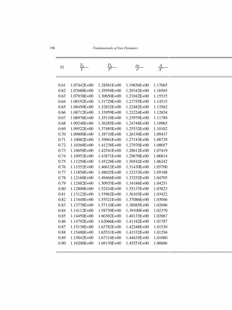
196 Fundamentals of Gas Dynamics
M T0T
P0P
ρ0ρ
AA∗
0.61 1.07442E+00 1.28561E+00 1.19656E+00 1.176650.62 1.07688E+00 1.29594E+00 1.20342E+00 1.165650.63 1.07938E+00 1.30650E+00 1.21042E+00 1.155150.64 1.08192E+00 1.31729E+00 1.21755E+00 1.145150.65 1.08450E+00 1.32832E+00 1.22482E+00 1.135620.66 1.08712E+00 1.33959E+00 1.23224E+00 1.126540.67 1.08978E+00 1.35110E+00 1.23979E+00 1.117890.68 1.09248E+00 1.36285E+00 1.24748E+00 1.109650.69 1.09522E+00 1.37485E+00 1.25532E+00 1.101820.70 1.09800E+00 1.38710E+00 1.26330E+00 1.094370.71 1.10082E+00 1.39961E+00 1.27143E+00 1.087290.72 1.10368E+00 1.41238E+00 1.27970E+00 1.080570.73 1.10658E+00 1.42541E+00 1.28812E+00 1.074190.74 1.10952E+00 1.43871E+00 1.29670E+00 1.068140.75 1.11250E+00 1.45228E+00 1.30542E+00 1.062420.76 1.11552E+00 1.46612E+00 1.31430E+00 1.057000.77 1.11858E+00 1.48025E+00 1.32333E+00 1.051880.78 1.12168E+00 1.49466E+00 1.33252E+00 1.047050.79 1.12482E+00 1.50935E+00 1.34186E+00 1.042510.80 1.12800E+00 1.52434E+00 1.35137E+00 1.038230.81 1.13122E+00 1.53962E+00 1.36103E+00 1.034220.82 1.13448E+00 1.55521E+00 1.37086E+00 1.030460.83 1.13778E+00 1.57110E+00 1.38085E+00 1.026960.84 1.14112E+00 1.58730E+00 1.39100E+00 1.023700.85 1.14450E+00 1.60382E+00 1.40133E+00 1.020670.86 1.14792E+00 1.62066E+00 1.41182E+00 1.017870.87 1.15138E+00 1.63782E+00 1.42248E+00 1.015300.88 1.15488E+00 1.65531E+00 1.43332E+00 1.012940.89 1.15842E+00 1.67314E+00 1.44433E+00 1.010800.90 1.16200E+00 1.69130E+00 1.45551E+00 1.00886
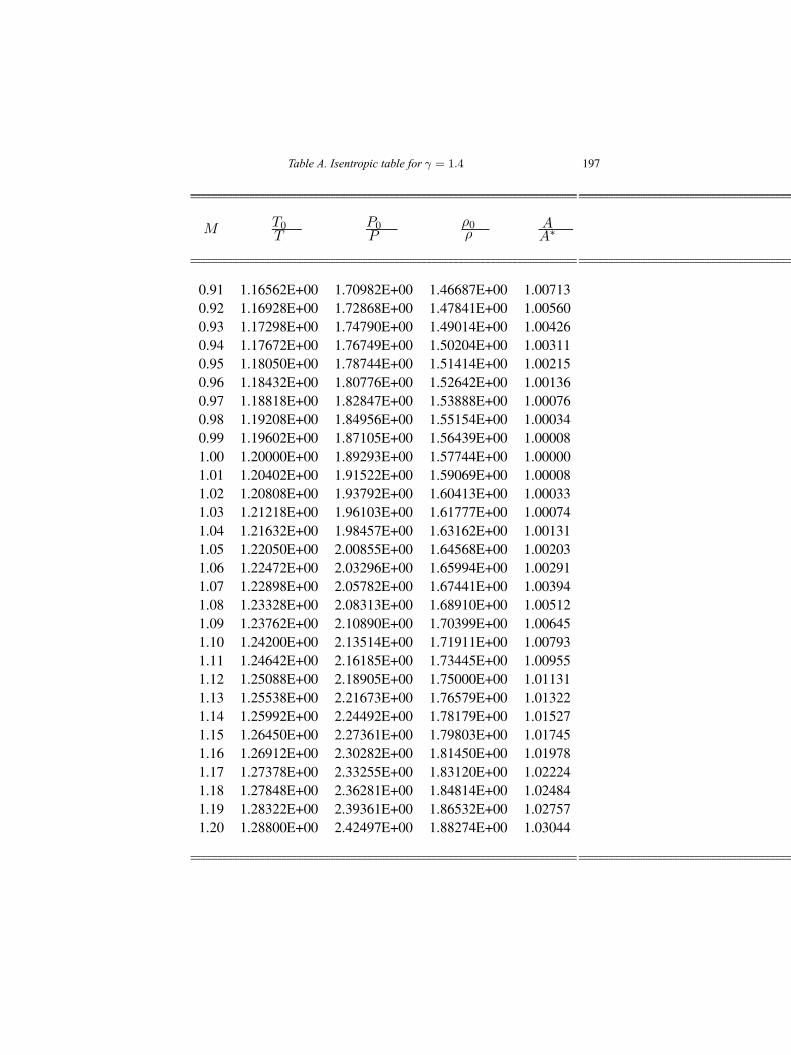
Table A. Isentropic table for γ = 1.4 197
M T0T
P0P
ρ0ρ
AA∗
0.91 1.16562E+00 1.70982E+00 1.46687E+00 1.007130.92 1.16928E+00 1.72868E+00 1.47841E+00 1.005600.93 1.17298E+00 1.74790E+00 1.49014E+00 1.004260.94 1.17672E+00 1.76749E+00 1.50204E+00 1.003110.95 1.18050E+00 1.78744E+00 1.51414E+00 1.002150.96 1.18432E+00 1.80776E+00 1.52642E+00 1.001360.97 1.18818E+00 1.82847E+00 1.53888E+00 1.000760.98 1.19208E+00 1.84956E+00 1.55154E+00 1.000340.99 1.19602E+00 1.87105E+00 1.56439E+00 1.000081.00 1.20000E+00 1.89293E+00 1.57744E+00 1.000001.01 1.20402E+00 1.91522E+00 1.59069E+00 1.000081.02 1.20808E+00 1.93792E+00 1.60413E+00 1.000331.03 1.21218E+00 1.96103E+00 1.61777E+00 1.000741.04 1.21632E+00 1.98457E+00 1.63162E+00 1.001311.05 1.22050E+00 2.00855E+00 1.64568E+00 1.002031.06 1.22472E+00 2.03296E+00 1.65994E+00 1.002911.07 1.22898E+00 2.05782E+00 1.67441E+00 1.003941.08 1.23328E+00 2.08313E+00 1.68910E+00 1.005121.09 1.23762E+00 2.10890E+00 1.70399E+00 1.006451.10 1.24200E+00 2.13514E+00 1.71911E+00 1.007931.11 1.24642E+00 2.16185E+00 1.73445E+00 1.009551.12 1.25088E+00 2.18905E+00 1.75000E+00 1.011311.13 1.25538E+00 2.21673E+00 1.76579E+00 1.013221.14 1.25992E+00 2.24492E+00 1.78179E+00 1.015271.15 1.26450E+00 2.27361E+00 1.79803E+00 1.017451.16 1.26912E+00 2.30282E+00 1.81450E+00 1.019781.17 1.27378E+00 2.33255E+00 1.83120E+00 1.022241.18 1.27848E+00 2.36281E+00 1.84814E+00 1.024841.19 1.28322E+00 2.39361E+00 1.86532E+00 1.027571.20 1.28800E+00 2.42497E+00 1.88274E+00 1.03044
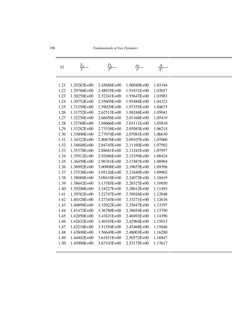
198 Fundamentals of Gas Dynamics
M T0T
P0P
ρ0ρ
AA∗
1.21 1.29282E+00 2.45688E+00 1.90040E+00 1.033441.22 1.29768E+00 2.48935E+00 1.91831E+00 1.036571.23 1.30258E+00 2.52241E+00 1.93647E+00 1.039831.24 1.30752E+00 2.55605E+00 1.95488E+00 1.043231.25 1.31250E+00 2.59029E+00 1.97355E+00 1.046751.26 1.31752E+00 2.62513E+00 1.99248E+00 1.050411.27 1.32258E+00 2.66058E+00 2.01166E+00 1.054191.28 1.32768E+00 2.69666E+00 2.03111E+00 1.058101.29 1.33282E+00 2.73338E+00 2.05083E+00 1.062141.30 1.33800E+00 2.77074E+00 2.07081E+00 1.066301.31 1.34322E+00 2.80876E+00 2.09107E+00 1.070601.32 1.34848E+00 2.84745E+00 2.11160E+00 1.075021.33 1.35378E+00 2.88681E+00 2.13241E+00 1.079571.34 1.35912E+00 2.92686E+00 2.15350E+00 1.084241.35 1.36450E+00 2.96761E+00 2.17487E+00 1.089041.36 1.36992E+00 3.00908E+00 2.19653E+00 1.093961.37 1.37538E+00 3.05126E+00 2.21849E+00 1.099021.38 1.38088E+00 3.09418E+00 2.24073E+00 1.104191.39 1.38642E+00 3.13785E+00 2.26327E+00 1.109501.40 1.39200E+00 3.18227E+00 2.28612E+00 1.114931.41 1.39762E+00 3.22747E+00 2.30926E+00 1.120481.42 1.40328E+00 3.27345E+00 2.33271E+00 1.126161.43 1.40898E+00 3.32022E+00 2.35647E+00 1.131971.44 1.41472E+00 3.36780E+00 2.38054E+00 1.137901.45 1.42050E+00 3.41621E+00 2.40493E+00 1.143961.46 1.42632E+00 3.46545E+00 2.42964E+00 1.150151.47 1.43218E+00 3.51554E+00 2.45468E+00 1.156461.48 1.43808E+00 3.56649E+00 2.48003E+00 1.162901.49 1.44402E+00 3.61831E+00 2.50572E+00 1.169471.50 1.45000E+00 3.67103E+00 2.53175E+00 1.17617
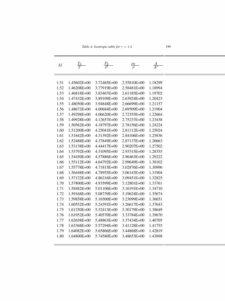
Table A. Isentropic table for γ = 1.4 199
M T0T
P0P
ρ0ρ
AA∗
1.51 1.45602E+00 3.72465E+00 2.55810E+00 1.182991.52 1.46208E+00 3.77919E+00 2.58481E+00 1.189941.53 1.46818E+00 3.83467E+00 2.61185E+00 1.197021.54 1.47432E+00 3.89109E+00 2.63924E+00 1.204231.55 1.48050E+00 3.94848E+00 2.66699E+00 1.211571.56 1.48672E+00 4.00684E+00 2.69509E+00 1.219041.57 1.49298E+00 4.06620E+00 2.72355E+00 1.226641.58 1.49928E+00 4.12657E+00 2.75237E+00 1.234381.59 1.50562E+00 4.18797E+00 2.78156E+00 1.242241.60 1.51200E+00 4.25041E+00 2.81112E+00 1.250241.61 1.51842E+00 4.31392E+00 2.84106E+00 1.258361.62 1.52488E+00 4.37849E+00 2.87137E+00 1.266631.63 1.53138E+00 4.44417E+00 2.90207E+00 1.275021.64 1.53792E+00 4.51095E+00 2.93315E+00 1.283551.65 1.54450E+00 4.57886E+00 2.96463E+00 1.292221.66 1.55112E+00 4.64792E+00 2.99649E+00 1.301021.67 1.55778E+00 4.71815E+00 3.02876E+00 1.309961.68 1.56448E+00 4.78955E+00 3.06143E+00 1.319041.69 1.57122E+00 4.86216E+00 3.09451E+00 1.328251.70 1.57800E+00 4.93599E+00 3.12801E+00 1.337611.71 1.58482E+00 5.01106E+00 3.16191E+00 1.347101.72 1.59168E+00 5.08739E+00 3.19624E+00 1.356741.73 1.59858E+00 5.16500E+00 3.23099E+00 1.366511.74 1.60552E+00 5.24391E+00 3.26617E+00 1.376431.75 1.61250E+00 5.32413E+00 3.30179E+00 1.386491.76 1.61952E+00 5.40570E+00 3.33784E+00 1.396701.77 1.62658E+00 5.48863E+00 3.37434E+00 1.407051.78 1.63368E+00 5.57294E+00 3.41128E+00 1.417551.79 1.64082E+00 5.65866E+00 3.44868E+00 1.428191.80 1.64800E+00 5.74580E+00 3.48653E+00 1.43898
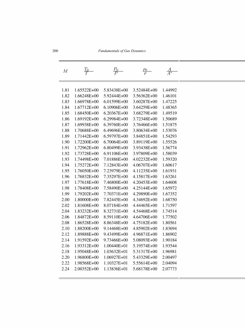
200 Fundamentals of Gas Dynamics
M T0T
P0P
ρ0ρ
AA∗
1.81 1.65522E+00 5.83438E+00 3.52484E+00 1.449921.82 1.66248E+00 5.92444E+00 3.56362E+00 1.461011.83 1.66978E+00 6.01599E+00 3.60287E+00 1.472251.84 1.67712E+00 6.10906E+00 3.64259E+00 1.483651.85 1.68450E+00 6.20367E+00 3.68279E+00 1.495191.86 1.69192E+00 6.29984E+00 3.72348E+00 1.506891.87 1.69938E+00 6.39760E+00 3.76466E+00 1.518751.88 1.70688E+00 6.49696E+00 3.80634E+00 1.530761.89 1.71442E+00 6.59797E+00 3.84851E+00 1.542931.90 1.72200E+00 6.70064E+00 3.89119E+00 1.555261.91 1.72962E+00 6.80499E+00 3.93438E+00 1.567741.92 1.73728E+00 6.91106E+00 3.97809E+00 1.580391.93 1.74498E+00 7.01886E+00 4.02232E+00 1.593201.94 1.75272E+00 7.12843E+00 4.06707E+00 1.606171.95 1.76050E+00 7.23979E+00 4.11235E+00 1.619311.96 1.76832E+00 7.35297E+00 4.15817E+00 1.632611.97 1.77618E+00 7.46800E+00 4.20453E+00 1.646081.98 1.78408E+00 7.58490E+00 4.25144E+00 1.659721.99 1.79202E+00 7.70371E+00 4.29890E+00 1.673522.00 1.80000E+00 7.82445E+00 4.34692E+00 1.687502.02 1.81608E+00 8.07184E+00 4.44465E+00 1.715972.04 1.83232E+00 8.32731E+00 4.54468E+00 1.745142.06 1.84872E+00 8.59110E+00 4.64706E+00 1.775022.08 1.86528E+00 8.86348E+00 4.75182E+00 1.805612.10 1.88200E+00 9.14468E+00 4.85902E+00 1.836942.12 1.89888E+00 9.43499E+00 4.96871E+00 1.869022.14 1.91592E+00 9.73466E+00 5.08093E+00 1.901842.16 1.93312E+00 1.00440E+01 5.19574E+00 1.935442.18 1.95048E+00 1.03632E+01 5.31317E+00 1.969812.20 1.96800E+00 1.06927E+01 5.43329E+00 2.004972.22 1.98568E+00 1.10327E+01 5.55614E+00 2.040942.24 2.00352E+00 1.13836E+01 5.68178E+00 2.07773
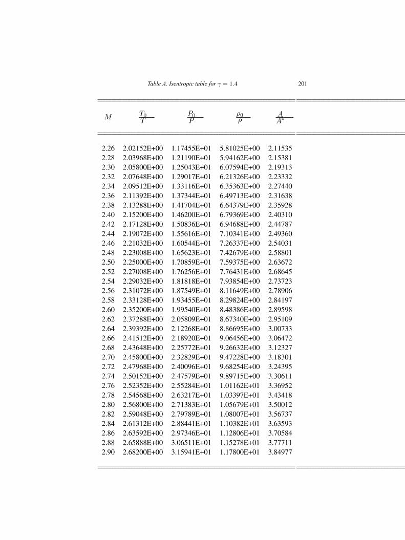
Table A. Isentropic table for γ = 1.4 201
M T0T
P0P
ρ0ρ
AA∗
2.26 2.02152E+00 1.17455E+01 5.81025E+00 2.115352.28 2.03968E+00 1.21190E+01 5.94162E+00 2.153812.30 2.05800E+00 1.25043E+01 6.07594E+00 2.193132.32 2.07648E+00 1.29017E+01 6.21326E+00 2.233322.34 2.09512E+00 1.33116E+01 6.35363E+00 2.274402.36 2.11392E+00 1.37344E+01 6.49713E+00 2.316382.38 2.13288E+00 1.41704E+01 6.64379E+00 2.359282.40 2.15200E+00 1.46200E+01 6.79369E+00 2.403102.42 2.17128E+00 1.50836E+01 6.94688E+00 2.447872.44 2.19072E+00 1.55616E+01 7.10341E+00 2.493602.46 2.21032E+00 1.60544E+01 7.26337E+00 2.540312.48 2.23008E+00 1.65623E+01 7.42679E+00 2.588012.50 2.25000E+00 1.70859E+01 7.59375E+00 2.636722.52 2.27008E+00 1.76256E+01 7.76431E+00 2.686452.54 2.29032E+00 1.81818E+01 7.93854E+00 2.737232.56 2.31072E+00 1.87549E+01 8.11649E+00 2.789062.58 2.33128E+00 1.93455E+01 8.29824E+00 2.841972.60 2.35200E+00 1.99540E+01 8.48386E+00 2.895982.62 2.37288E+00 2.05809E+01 8.67340E+00 2.951092.64 2.39392E+00 2.12268E+01 8.86695E+00 3.007332.66 2.41512E+00 2.18920E+01 9.06456E+00 3.064722.68 2.43648E+00 2.25772E+01 9.26632E+00 3.123272.70 2.45800E+00 2.32829E+01 9.47228E+00 3.183012.72 2.47968E+00 2.40096E+01 9.68254E+00 3.243952.74 2.50152E+00 2.47579E+01 9.89715E+00 3.306112.76 2.52352E+00 2.55284E+01 1.01162E+01 3.369522.78 2.54568E+00 2.63217E+01 1.03397E+01 3.434182.80 2.56800E+00 2.71383E+01 1.05679E+01 3.500122.82 2.59048E+00 2.79789E+01 1.08007E+01 3.567372.84 2.61312E+00 2.88441E+01 1.10382E+01 3.635932.86 2.63592E+00 2.97346E+01 1.12806E+01 3.705842.88 2.65888E+00 3.06511E+01 1.15278E+01 3.777112.90 2.68200E+00 3.15941E+01 1.17800E+01 3.84977
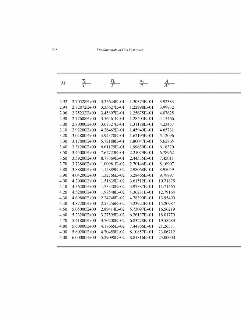
202 Fundamentals of Gas Dynamics
M T0T
P0P
ρ0ρ
AA∗
2.92 2.70528E+00 3.25644E+01 1.20373E+01 3.923832.94 2.72872E+00 3.35627E+01 1.22998E+01 3.999322.96 2.75232E+00 3.45897E+01 1.25675E+01 4.076252.98 2.77608E+00 3.56461E+01 1.28404E+01 4.154663.00 2.80000E+00 3.67327E+01 1.31188E+01 4.234573.10 2.92200E+00 4.26462E+01 1.45949E+01 4.657313.20 3.04800E+00 4.94370E+01 1.62195E+01 5.120963.30 3.17800E+00 5.72188E+01 1.80047E+01 5.628653.40 3.31200E+00 6.61175E+01 1.99630E+01 6.183703.50 3.45000E+00 7.62723E+01 2.21079E+01 6.789623.60 3.59200E+00 8.78369E+01 2.44535E+01 7.450113.70 3.73800E+00 1.00981E+02 2.70146E+01 8.169073.80 3.88800E+00 1.15889E+02 2.98068E+01 8.950593.90 4.04200E+00 1.32766E+02 3.28466E+01 9.798974.00 4.20000E+00 1.51835E+02 3.61512E+01 10.718754.10 4.36200E+00 1.73340E+02 3.97387E+01 11.714654.20 4.52800E+00 1.97548E+02 4.36281E+01 12.791644.30 4.69800E+00 2.24748E+02 4.78390E+01 13.954904.40 4.87200E+00 2.55256E+02 5.23924E+01 15.209874.50 5.05000E+00 2.89414E+02 5.73097E+01 16.562194.60 5.23200E+00 3.27595E+02 6.26137E+01 18.017794.70 5.41800E+00 3.70200E+02 6.83278E+01 19.582834.80 5.60800E+00 4.17665E+02 7.44766E+01 21.263714.90 5.80200E+00 4.70459E+02 8.10857E+01 23.067125.00 6.00000E+00 5.29090E+02 8.81816E+01 25.00000

Table B. Normal shock properties forγ = 1.4
203
Fundamentals of Gas Dynamics, Second Edition. V. Babu.© 2015 V. Babu. Published 2015 by Athena Academic Ltd and John Wiley & Sons Ltd
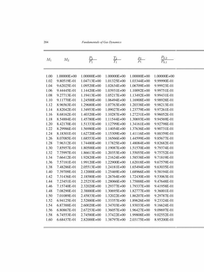
204 Fundamentals of Gas Dynamics
M1 M2P2P1
T2T1
ρ2ρ1
P0,2
P0,1
1.00 1.00000E+00 1.00000E+00 1.00000E+00 1.00000E+00 1.00000E+001.02 9.80519E-01 1.04713E+00 1.01325E+00 1.03344E+00 9.99990E-011.04 9.62025E-01 1.09520E+00 1.02634E+00 1.06709E+00 9.99923E-011.06 9.44445E-01 1.14420E+00 1.03931E+00 1.10092E+00 9.99751E-011.08 9.27713E-01 1.19413E+00 1.05217E+00 1.13492E+00 9.99431E-011.10 9.11770E-01 1.24500E+00 1.06494E+00 1.16908E+00 9.98928E-011.12 8.96563E-01 1.29680E+00 1.07763E+00 1.20338E+00 9.98213E-011.14 8.82042E-01 1.34953E+00 1.09027E+00 1.23779E+00 9.97261E-011.16 8.68162E-01 1.40320E+00 1.10287E+00 1.27231E+00 9.96052E-011.18 8.54884E-01 1.45780E+00 1.11544E+00 1.30693E+00 9.94569E-011.20 8.42170E-01 1.51333E+00 1.12799E+00 1.34161E+00 9.92798E-011.22 8.29986E-01 1.56980E+00 1.14054E+00 1.37636E+00 9.90731E-011.24 8.18301E-01 1.62720E+00 1.15309E+00 1.41116E+00 9.88359E-011.26 8.07085E-01 1.68553E+00 1.16566E+00 1.44599E+00 9.85677E-011.28 7.96312E-01 1.74480E+00 1.17825E+00 1.48084E+00 9.82682E-011.30 7.85957E-01 1.80500E+00 1.19087E+00 1.51570E+00 9.79374E-011.32 7.75997E-01 1.86613E+00 1.20353E+00 1.55055E+00 9.75752E-011.34 7.66412E-01 1.92820E+00 1.21624E+00 1.58538E+00 9.71819E-011.36 7.57181E-01 1.99120E+00 1.22900E+00 1.62018E+00 9.67579E-011.38 7.48286E-01 2.05513E+00 1.24181E+00 1.65494E+00 9.63035E-011.40 7.39709E-01 2.12000E+00 1.25469E+00 1.68966E+00 9.58194E-011.42 7.31436E-01 2.18580E+00 1.26764E+00 1.72430E+00 9.53063E-011.44 7.23451E-01 2.25253E+00 1.28066E+00 1.75888E+00 9.47648E-011.46 7.15740E-01 2.32020E+00 1.29377E+00 1.79337E+00 9.41958E-011.48 7.08290E-01 2.38880E+00 1.30695E+00 1.82777E+00 9.36001E-011.50 7.01089E-01 2.45833E+00 1.32022E+00 1.86207E+00 9.29787E-011.52 6.94125E-01 2.52880E+00 1.33357E+00 1.89626E+00 9.23324E-011.54 6.87388E-01 2.60020E+00 1.34703E+00 1.93033E+00 9.16624E-011.56 6.80867E-01 2.67253E+00 1.36057E+00 1.96427E+00 9.09697E-011.58 6.74553E-01 2.74580E+00 1.37422E+00 1.99808E+00 9.02552E-011.60 6.68437E-01 2.82000E+00 1.38797E+00 2.03175E+00 8.95200E-01
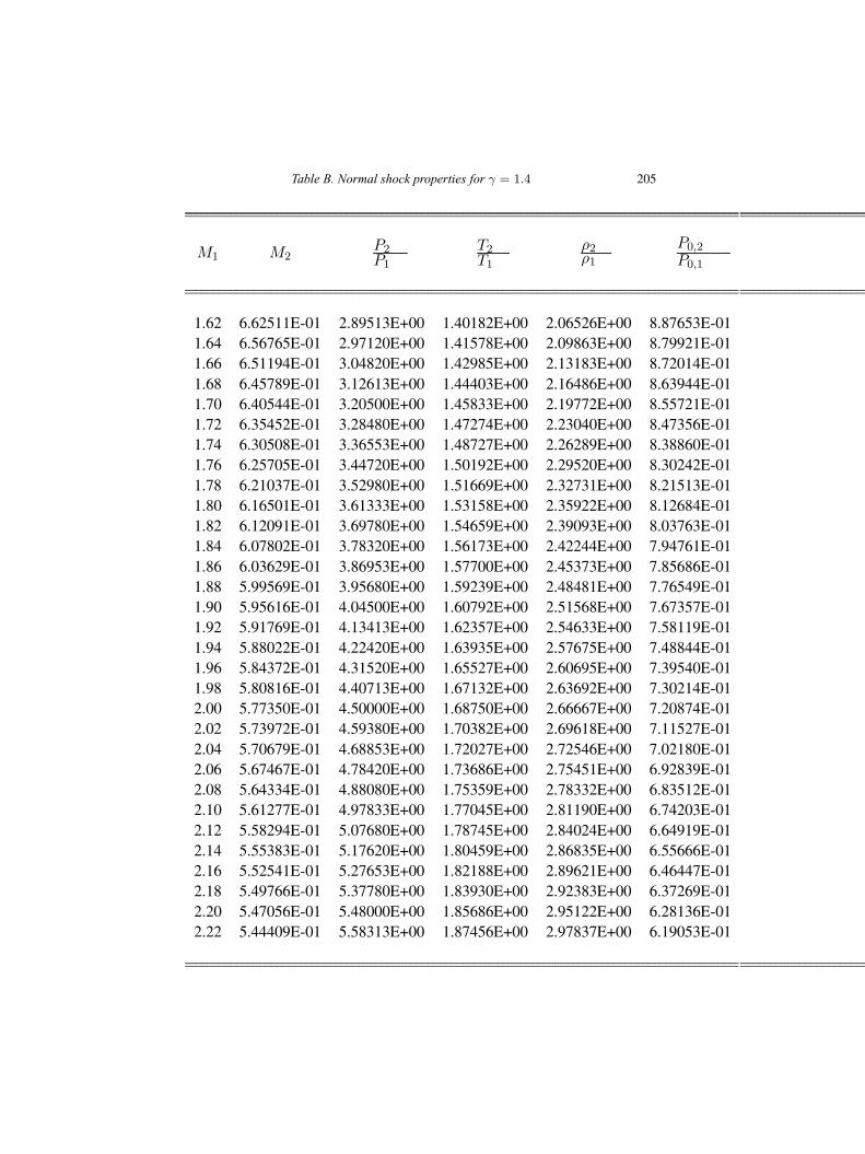
Table B. Normal shock properties for γ = 1.4 205
M1 M2P2P1
T2T1
ρ2ρ1
P0,2
P0,1
1.62 6.62511E-01 2.89513E+00 1.40182E+00 2.06526E+00 8.87653E-011.64 6.56765E-01 2.97120E+00 1.41578E+00 2.09863E+00 8.79921E-011.66 6.51194E-01 3.04820E+00 1.42985E+00 2.13183E+00 8.72014E-011.68 6.45789E-01 3.12613E+00 1.44403E+00 2.16486E+00 8.63944E-011.70 6.40544E-01 3.20500E+00 1.45833E+00 2.19772E+00 8.55721E-011.72 6.35452E-01 3.28480E+00 1.47274E+00 2.23040E+00 8.47356E-011.74 6.30508E-01 3.36553E+00 1.48727E+00 2.26289E+00 8.38860E-011.76 6.25705E-01 3.44720E+00 1.50192E+00 2.29520E+00 8.30242E-011.78 6.21037E-01 3.52980E+00 1.51669E+00 2.32731E+00 8.21513E-011.80 6.16501E-01 3.61333E+00 1.53158E+00 2.35922E+00 8.12684E-011.82 6.12091E-01 3.69780E+00 1.54659E+00 2.39093E+00 8.03763E-011.84 6.07802E-01 3.78320E+00 1.56173E+00 2.42244E+00 7.94761E-011.86 6.03629E-01 3.86953E+00 1.57700E+00 2.45373E+00 7.85686E-011.88 5.99569E-01 3.95680E+00 1.59239E+00 2.48481E+00 7.76549E-011.90 5.95616E-01 4.04500E+00 1.60792E+00 2.51568E+00 7.67357E-011.92 5.91769E-01 4.13413E+00 1.62357E+00 2.54633E+00 7.58119E-011.94 5.88022E-01 4.22420E+00 1.63935E+00 2.57675E+00 7.48844E-011.96 5.84372E-01 4.31520E+00 1.65527E+00 2.60695E+00 7.39540E-011.98 5.80816E-01 4.40713E+00 1.67132E+00 2.63692E+00 7.30214E-012.00 5.77350E-01 4.50000E+00 1.68750E+00 2.66667E+00 7.20874E-012.02 5.73972E-01 4.59380E+00 1.70382E+00 2.69618E+00 7.11527E-012.04 5.70679E-01 4.68853E+00 1.72027E+00 2.72546E+00 7.02180E-012.06 5.67467E-01 4.78420E+00 1.73686E+00 2.75451E+00 6.92839E-012.08 5.64334E-01 4.88080E+00 1.75359E+00 2.78332E+00 6.83512E-012.10 5.61277E-01 4.97833E+00 1.77045E+00 2.81190E+00 6.74203E-012.12 5.58294E-01 5.07680E+00 1.78745E+00 2.84024E+00 6.64919E-012.14 5.55383E-01 5.17620E+00 1.80459E+00 2.86835E+00 6.55666E-012.16 5.52541E-01 5.27653E+00 1.82188E+00 2.89621E+00 6.46447E-012.18 5.49766E-01 5.37780E+00 1.83930E+00 2.92383E+00 6.37269E-012.20 5.47056E-01 5.48000E+00 1.85686E+00 2.95122E+00 6.28136E-012.22 5.44409E-01 5.58313E+00 1.87456E+00 2.97837E+00 6.19053E-01
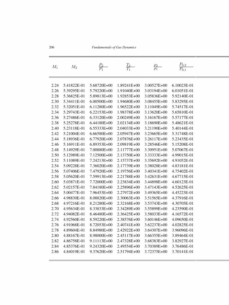
206 Fundamentals of Gas Dynamics
M1 M2P2P1
T2T1
ρ2ρ1
P0,2
P0,1
2.24 5.41822E-01 5.68720E+00 1.89241E+00 3.00527E+00 6.10023E-012.26 5.39295E-01 5.79220E+00 1.91040E+00 3.03194E+00 6.01051E-012.28 5.36825E-01 5.89813E+00 1.92853E+00 3.05836E+00 5.92140E-012.30 5.34411E-01 6.00500E+00 1.94680E+00 3.08455E+00 5.83295E-012.32 5.32051E-01 6.11280E+00 1.96522E+00 3.11049E+00 5.74517E-012.34 5.29743E-01 6.22153E+00 1.98378E+00 3.13620E+00 5.65810E-012.36 5.27486E-01 6.33120E+00 2.00249E+00 3.16167E+00 5.57177E-012.38 5.25278E-01 6.44180E+00 2.02134E+00 3.18690E+00 5.48621E-012.40 5.23118E-01 6.55333E+00 2.04033E+00 3.21190E+00 5.40144E-012.42 5.21004E-01 6.66580E+00 2.05947E+00 3.23665E+00 5.31748E-012.44 5.18936E-01 6.77920E+00 2.07876E+00 3.26117E+00 5.23435E-012.46 5.16911E-01 6.89353E+00 2.09819E+00 3.28546E+00 5.15208E-012.48 5.14929E-01 7.00880E+00 2.11777E+00 3.30951E+00 5.07067E-012.50 5.12989E-01 7.12500E+00 2.13750E+00 3.33333E+00 4.99015E-012.52 5.11089E-01 7.24213E+00 2.15737E+00 3.35692E+00 4.91052E-012.54 5.09228E-01 7.36020E+00 2.17739E+00 3.38028E+00 4.83181E-012.56 5.07406E-01 7.47920E+00 2.19756E+00 3.40341E+00 4.75402E-012.58 5.05620E-01 7.59913E+00 2.21788E+00 3.42631E+00 4.67715E-012.60 5.03871E-01 7.72000E+00 2.23834E+00 3.44898E+00 4.60123E-012.62 5.02157E-01 7.84180E+00 2.25896E+00 3.47143E+00 4.52625E-012.64 5.00477E-01 7.96453E+00 2.27972E+00 3.49365E+00 4.45223E-012.66 4.98830E-01 8.08820E+00 2.30063E+00 3.51565E+00 4.37916E-012.68 4.97216E-01 8.21280E+00 2.32168E+00 3.53743E+00 4.30705E-012.70 4.95634E-01 8.33833E+00 2.34289E+00 3.55899E+00 4.23590E-012.72 4.94082E-01 8.46480E+00 2.36425E+00 3.58033E+00 4.16572E-012.74 4.92560E-01 8.59220E+00 2.38576E+00 3.60146E+00 4.09650E-012.76 4.91068E-01 8.72053E+00 2.40741E+00 3.62237E+00 4.02825E-012.78 4.89604E-01 8.84980E+00 2.42922E+00 3.64307E+00 3.96096E-012.80 4.88167E-01 8.98000E+00 2.45117E+00 3.66355E+00 3.89464E-012.82 4.86758E-01 9.11113E+00 2.47328E+00 3.68383E+00 3.82927E-012.84 4.85376E-01 9.24320E+00 2.49554E+00 3.70389E+00 3.76486E-012.86 4.84019E-01 9.37620E+00 2.51794E+00 3.72375E+00 3.70141E-01
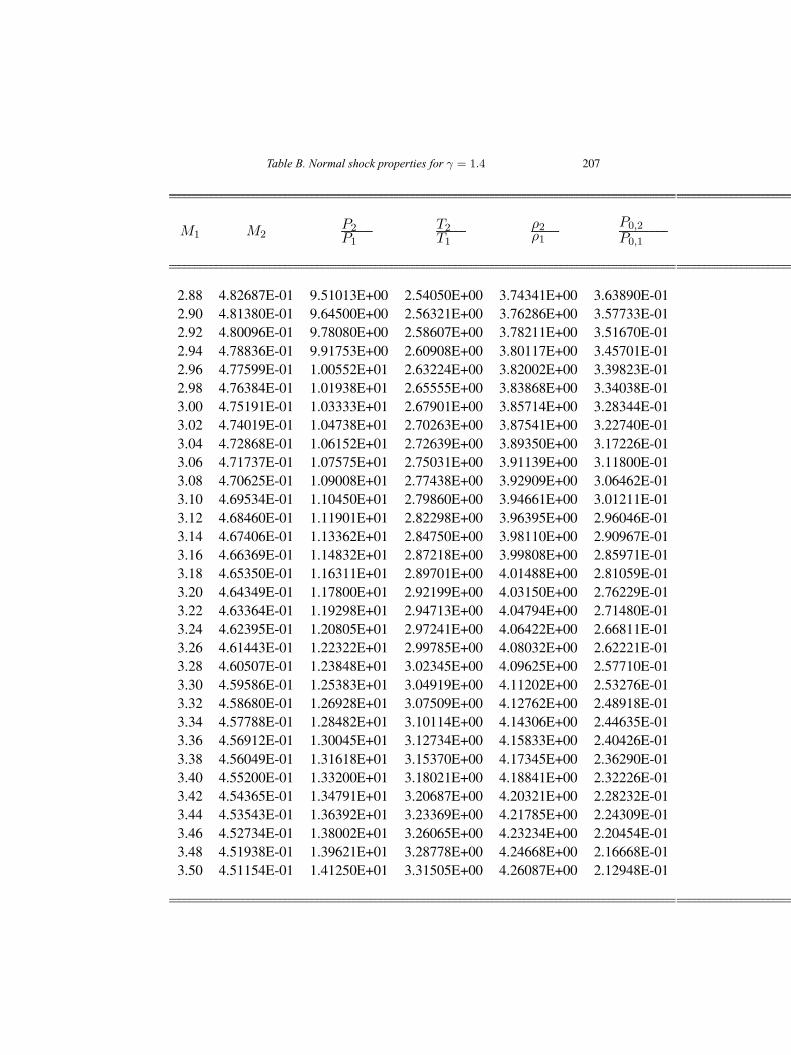
Table B. Normal shock properties for γ = 1.4 207
M1 M2P2P1
T2T1
ρ2ρ1
P0,2
P0,1
2.88 4.82687E-01 9.51013E+00 2.54050E+00 3.74341E+00 3.63890E-012.90 4.81380E-01 9.64500E+00 2.56321E+00 3.76286E+00 3.57733E-012.92 4.80096E-01 9.78080E+00 2.58607E+00 3.78211E+00 3.51670E-012.94 4.78836E-01 9.91753E+00 2.60908E+00 3.80117E+00 3.45701E-012.96 4.77599E-01 1.00552E+01 2.63224E+00 3.82002E+00 3.39823E-012.98 4.76384E-01 1.01938E+01 2.65555E+00 3.83868E+00 3.34038E-013.00 4.75191E-01 1.03333E+01 2.67901E+00 3.85714E+00 3.28344E-013.02 4.74019E-01 1.04738E+01 2.70263E+00 3.87541E+00 3.22740E-013.04 4.72868E-01 1.06152E+01 2.72639E+00 3.89350E+00 3.17226E-013.06 4.71737E-01 1.07575E+01 2.75031E+00 3.91139E+00 3.11800E-013.08 4.70625E-01 1.09008E+01 2.77438E+00 3.92909E+00 3.06462E-013.10 4.69534E-01 1.10450E+01 2.79860E+00 3.94661E+00 3.01211E-013.12 4.68460E-01 1.11901E+01 2.82298E+00 3.96395E+00 2.96046E-013.14 4.67406E-01 1.13362E+01 2.84750E+00 3.98110E+00 2.90967E-013.16 4.66369E-01 1.14832E+01 2.87218E+00 3.99808E+00 2.85971E-013.18 4.65350E-01 1.16311E+01 2.89701E+00 4.01488E+00 2.81059E-013.20 4.64349E-01 1.17800E+01 2.92199E+00 4.03150E+00 2.76229E-013.22 4.63364E-01 1.19298E+01 2.94713E+00 4.04794E+00 2.71480E-013.24 4.62395E-01 1.20805E+01 2.97241E+00 4.06422E+00 2.66811E-013.26 4.61443E-01 1.22322E+01 2.99785E+00 4.08032E+00 2.62221E-013.28 4.60507E-01 1.23848E+01 3.02345E+00 4.09625E+00 2.57710E-013.30 4.59586E-01 1.25383E+01 3.04919E+00 4.11202E+00 2.53276E-013.32 4.58680E-01 1.26928E+01 3.07509E+00 4.12762E+00 2.48918E-013.34 4.57788E-01 1.28482E+01 3.10114E+00 4.14306E+00 2.44635E-013.36 4.56912E-01 1.30045E+01 3.12734E+00 4.15833E+00 2.40426E-013.38 4.56049E-01 1.31618E+01 3.15370E+00 4.17345E+00 2.36290E-013.40 4.55200E-01 1.33200E+01 3.18021E+00 4.18841E+00 2.32226E-013.42 4.54365E-01 1.34791E+01 3.20687E+00 4.20321E+00 2.28232E-013.44 4.53543E-01 1.36392E+01 3.23369E+00 4.21785E+00 2.24309E-013.46 4.52734E-01 1.38002E+01 3.26065E+00 4.23234E+00 2.20454E-013.48 4.51938E-01 1.39621E+01 3.28778E+00 4.24668E+00 2.16668E-013.50 4.51154E-01 1.41250E+01 3.31505E+00 4.26087E+00 2.12948E-01
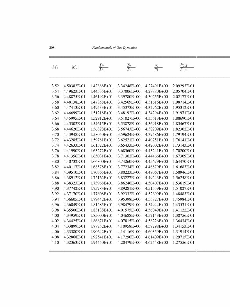
208 Fundamentals of Gas Dynamics
M1 M2P2P1
T2T1
ρ2ρ1
P0,2
P0,1
3.52 4.50382E-01 1.42888E+01 3.34248E+00 4.27491E+00 2.09293E-013.54 4.49623E-01 1.44535E+01 3.37006E+00 4.28880E+00 2.05704E-013.56 4.48875E-01 1.46192E+01 3.39780E+00 4.30255E+00 2.02177E-013.58 4.48138E-01 1.47858E+01 3.42569E+00 4.31616E+00 1.98714E-013.60 4.47413E-01 1.49533E+01 3.45373E+00 4.32962E+00 1.95312E-013.62 4.46699E-01 1.51218E+01 3.48192E+00 4.34294E+00 1.91971E-013.64 4.45995E-01 1.52912E+01 3.51027E+00 4.35613E+00 1.88690E-013.66 4.45302E-01 1.54615E+01 3.53878E+00 4.36918E+00 1.85467E-013.68 4.44620E-01 1.56328E+01 3.56743E+00 4.38209E+00 1.82302E-013.70 4.43948E-01 1.58050E+01 3.59624E+00 4.39486E+00 1.79194E-013.72 4.43285E-01 1.59781E+01 3.62521E+00 4.40751E+00 1.76141E-013.74 4.42633E-01 1.61522E+01 3.65433E+00 4.42002E+00 1.73143E-013.76 4.41990E-01 1.63272E+01 3.68360E+00 4.43241E+00 1.70200E-013.78 4.41356E-01 1.65031E+01 3.71302E+00 4.44466E+00 1.67309E-013.80 4.40732E-01 1.66800E+01 3.74260E+00 4.45679E+00 1.64470E-013.82 4.40117E-01 1.68578E+01 3.77234E+00 4.46879E+00 1.61683E-013.84 4.39510E-01 1.70365E+01 3.80223E+00 4.48067E+00 1.58946E-013.86 4.38912E-01 1.72162E+01 3.83227E+00 4.49243E+00 1.56258E-013.88 4.38323E-01 1.73968E+01 3.86246E+00 4.50407E+00 1.53619E-013.90 4.37742E-01 1.75783E+01 3.89281E+00 4.51559E+00 1.51027E-013.92 4.37170E-01 1.77608E+01 3.92332E+00 4.52699E+00 1.48483E-013.94 4.36605E-01 1.79442E+01 3.95398E+00 4.53827E+00 1.45984E-013.96 4.36049E-01 1.81285E+01 3.98479E+00 4.54944E+00 1.43531E-013.98 4.35500E-01 1.83138E+01 4.01575E+00 4.56049E+00 1.41122E-014.00 4.34959E-01 1.85000E+01 4.04688E+00 4.57143E+00 1.38756E-014.02 4.34425E-01 1.86871E+01 4.07815E+00 4.58226E+00 1.36434E-014.04 4.33899E-01 1.88752E+01 4.10958E+00 4.59298E+00 1.34153E-014.06 4.33380E-01 1.90642E+01 4.14116E+00 4.60359E+00 1.31914E-014.08 4.32868E-01 1.92541E+01 4.17290E+00 4.61409E+00 1.29715E-014.10 4.32363E-01 1.94450E+01 4.20479E+00 4.62448E+00 1.27556E-01
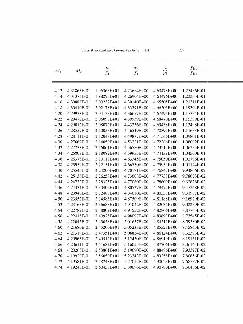
Table B. Normal shock properties for γ = 1.4 209
M1 M2P2P1
T2T1
ρ2ρ1
P0,2
P0,1
4.12 4.31865E-01 1.96368E+01 4.23684E+00 4.63478E+00 1.25436E-014.14 4.31373E-01 1.98295E+01 4.26904E+00 4.64496E+00 1.23355E-014.16 4.30888E-01 2.00232E+01 4.30140E+00 4.65505E+00 1.21311E-014.18 4.30410E-01 2.02178E+01 4.33391E+00 4.66503E+00 1.19304E-014.20 4.29938E-01 2.04133E+01 4.36657E+00 4.67491E+00 1.17334E-014.22 4.29472E-01 2.06098E+01 4.39939E+00 4.68470E+00 1.15399E-014.24 4.29012E-01 2.08072E+01 4.43236E+00 4.69438E+00 1.13498E-014.26 4.28559E-01 2.10055E+01 4.46549E+00 4.70397E+00 1.11633E-014.28 4.28111E-01 2.12048E+01 4.49877E+00 4.71346E+00 1.09801E-014.30 4.27669E-01 2.14050E+01 4.53221E+00 4.72286E+00 1.08002E-014.32 4.27233E-01 2.16061E+01 4.56580E+00 4.73217E+00 1.06235E-014.34 4.26803E-01 2.18082E+01 4.59955E+00 4.74138E+00 1.04500E-014.36 4.26378E-01 2.20112E+01 4.63345E+00 4.75050E+00 1.02796E-014.38 4.25959E-01 2.22151E+01 4.66750E+00 4.75953E+00 1.01124E-014.40 4.25545E-01 2.24200E+01 4.70171E+00 4.76847E+00 9.94806E-024.42 4.25136E-01 2.26258E+01 4.73608E+00 4.77733E+00 9.78673E-024.44 4.24732E-01 2.28325E+01 4.77060E+00 4.78609E+00 9.62828E-024.46 4.24334E-01 2.30402E+01 4.80527E+00 4.79477E+00 9.47268E-024.48 4.23940E-01 2.32488E+01 4.84010E+00 4.80337E+00 9.31987E-024.50 4.23552E-01 2.34583E+01 4.87509E+00 4.81188E+00 9.16979E-024.52 4.23168E-01 2.36688E+01 4.91022E+00 4.82031E+00 9.02239E-024.54 4.22789E-01 2.38802E+01 4.94552E+00 4.82866E+00 8.87763E-024.56 4.22415E-01 2.40925E+01 4.98097E+00 4.83692E+00 8.73545E-024.58 4.22045E-01 2.43058E+01 5.01657E+00 4.84511E+00 8.59580E-024.60 4.21680E-01 2.45200E+01 5.05233E+00 4.85321E+00 8.45865E-024.62 4.21319E-01 2.47351E+01 5.08824E+00 4.86124E+00 8.32393E-024.64 4.20963E-01 2.49512E+01 5.12430E+00 4.86919E+00 8.19161E-024.66 4.20611E-01 2.51682E+01 5.16053E+00 4.87706E+00 8.06164E-024.68 4.20263E-01 2.53861E+01 5.19690E+00 4.88486E+00 7.93397E-024.70 4.19920E-01 2.56050E+01 5.23343E+00 4.89258E+00 7.80856E-024.72 4.19581E-01 2.58248E+01 5.27012E+00 4.90023E+00 7.68537E-024.74 4.19245E-01 2.60455E+01 5.30696E+00 4.90780E+00 7.56436E-02
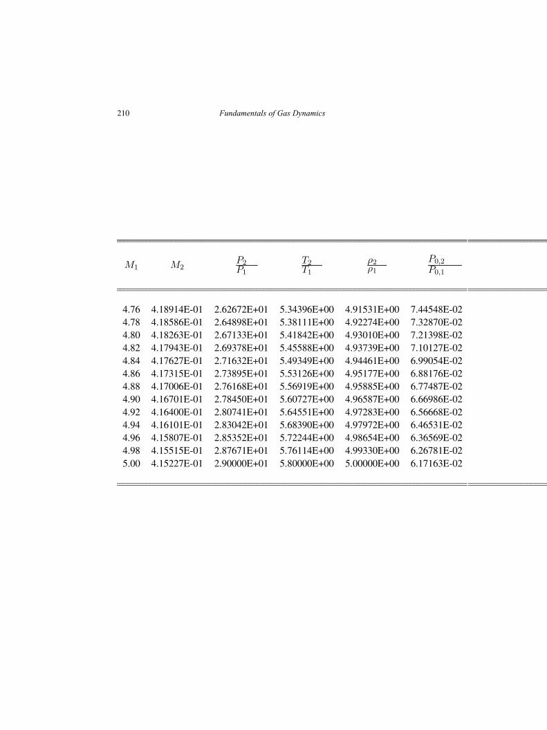
210 Fundamentals of Gas Dynamics
M1 M2P2P1
T2T1
ρ2ρ1
P0,2
P0,1
4.76 4.18914E-01 2.62672E+01 5.34396E+00 4.91531E+00 7.44548E-024.78 4.18586E-01 2.64898E+01 5.38111E+00 4.92274E+00 7.32870E-024.80 4.18263E-01 2.67133E+01 5.41842E+00 4.93010E+00 7.21398E-024.82 4.17943E-01 2.69378E+01 5.45588E+00 4.93739E+00 7.10127E-024.84 4.17627E-01 2.71632E+01 5.49349E+00 4.94461E+00 6.99054E-024.86 4.17315E-01 2.73895E+01 5.53126E+00 4.95177E+00 6.88176E-024.88 4.17006E-01 2.76168E+01 5.56919E+00 4.95885E+00 6.77487E-024.90 4.16701E-01 2.78450E+01 5.60727E+00 4.96587E+00 6.66986E-024.92 4.16400E-01 2.80741E+01 5.64551E+00 4.97283E+00 6.56668E-024.94 4.16101E-01 2.83042E+01 5.68390E+00 4.97972E+00 6.46531E-024.96 4.15807E-01 2.85352E+01 5.72244E+00 4.98654E+00 6.36569E-024.98 4.15515E-01 2.87671E+01 5.76114E+00 4.99330E+00 6.26781E-025.00 4.15227E-01 2.90000E+01 5.80000E+00 5.00000E+00 6.17163E-02

Table C. Rayleigh flow properties forγ = 1.4
211
Fundamentals of Gas Dynamics, Second Edition. V. Babu.© 2015 V. Babu. Published 2015 by Athena Academic Ltd and John Wiley & Sons Ltd
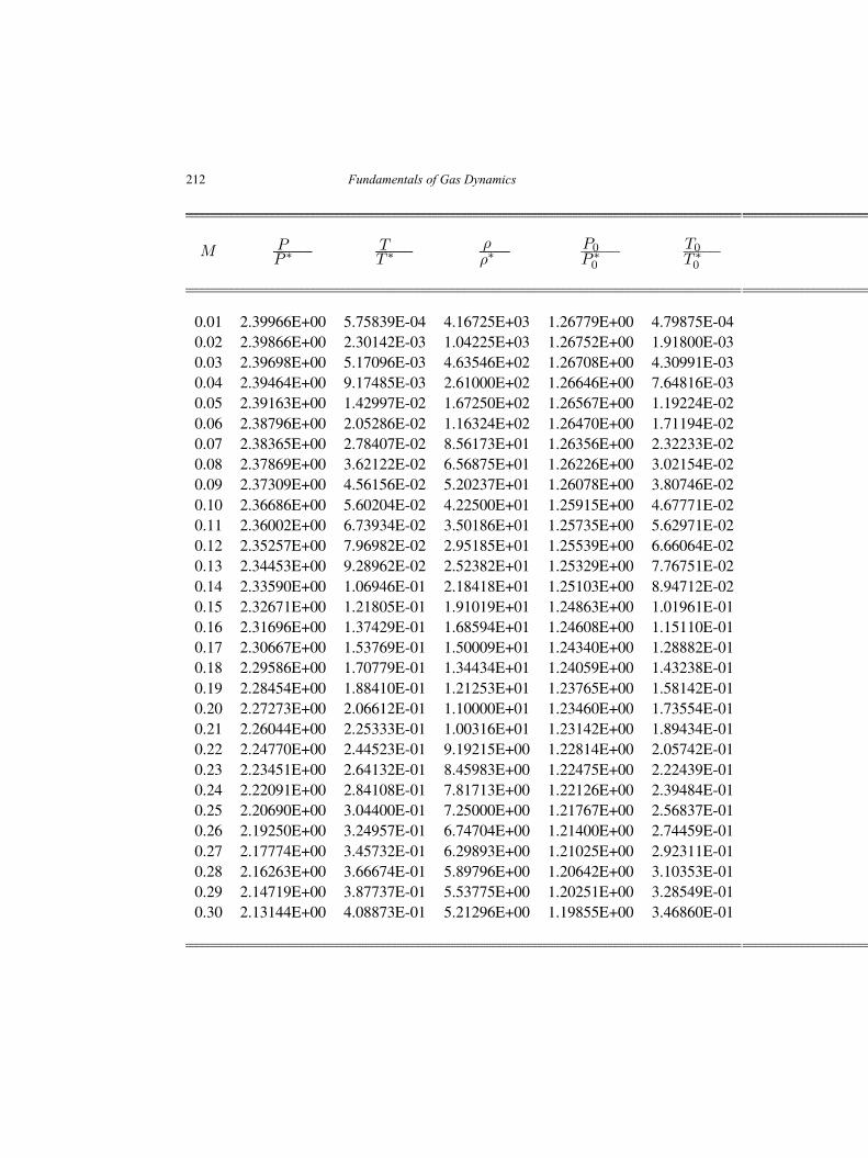
212 Fundamentals of Gas Dynamics
M PP ∗
TT ∗
ρρ∗
P0P ∗0
T0T ∗0
0.01 2.39966E+00 5.75839E-04 4.16725E+03 1.26779E+00 4.79875E-040.02 2.39866E+00 2.30142E-03 1.04225E+03 1.26752E+00 1.91800E-030.03 2.39698E+00 5.17096E-03 4.63546E+02 1.26708E+00 4.30991E-030.04 2.39464E+00 9.17485E-03 2.61000E+02 1.26646E+00 7.64816E-030.05 2.39163E+00 1.42997E-02 1.67250E+02 1.26567E+00 1.19224E-020.06 2.38796E+00 2.05286E-02 1.16324E+02 1.26470E+00 1.71194E-020.07 2.38365E+00 2.78407E-02 8.56173E+01 1.26356E+00 2.32233E-020.08 2.37869E+00 3.62122E-02 6.56875E+01 1.26226E+00 3.02154E-020.09 2.37309E+00 4.56156E-02 5.20237E+01 1.26078E+00 3.80746E-020.10 2.36686E+00 5.60204E-02 4.22500E+01 1.25915E+00 4.67771E-020.11 2.36002E+00 6.73934E-02 3.50186E+01 1.25735E+00 5.62971E-020.12 2.35257E+00 7.96982E-02 2.95185E+01 1.25539E+00 6.66064E-020.13 2.34453E+00 9.28962E-02 2.52382E+01 1.25329E+00 7.76751E-020.14 2.33590E+00 1.06946E-01 2.18418E+01 1.25103E+00 8.94712E-020.15 2.32671E+00 1.21805E-01 1.91019E+01 1.24863E+00 1.01961E-010.16 2.31696E+00 1.37429E-01 1.68594E+01 1.24608E+00 1.15110E-010.17 2.30667E+00 1.53769E-01 1.50009E+01 1.24340E+00 1.28882E-010.18 2.29586E+00 1.70779E-01 1.34434E+01 1.24059E+00 1.43238E-010.19 2.28454E+00 1.88410E-01 1.21253E+01 1.23765E+00 1.58142E-010.20 2.27273E+00 2.06612E-01 1.10000E+01 1.23460E+00 1.73554E-010.21 2.26044E+00 2.25333E-01 1.00316E+01 1.23142E+00 1.89434E-010.22 2.24770E+00 2.44523E-01 9.19215E+00 1.22814E+00 2.05742E-010.23 2.23451E+00 2.64132E-01 8.45983E+00 1.22475E+00 2.22439E-010.24 2.22091E+00 2.84108E-01 7.81713E+00 1.22126E+00 2.39484E-010.25 2.20690E+00 3.04400E-01 7.25000E+00 1.21767E+00 2.56837E-010.26 2.19250E+00 3.24957E-01 6.74704E+00 1.21400E+00 2.74459E-010.27 2.17774E+00 3.45732E-01 6.29893E+00 1.21025E+00 2.92311E-010.28 2.16263E+00 3.66674E-01 5.89796E+00 1.20642E+00 3.10353E-010.29 2.14719E+00 3.87737E-01 5.53775E+00 1.20251E+00 3.28549E-010.30 2.13144E+00 4.08873E-01 5.21296E+00 1.19855E+00 3.46860E-01
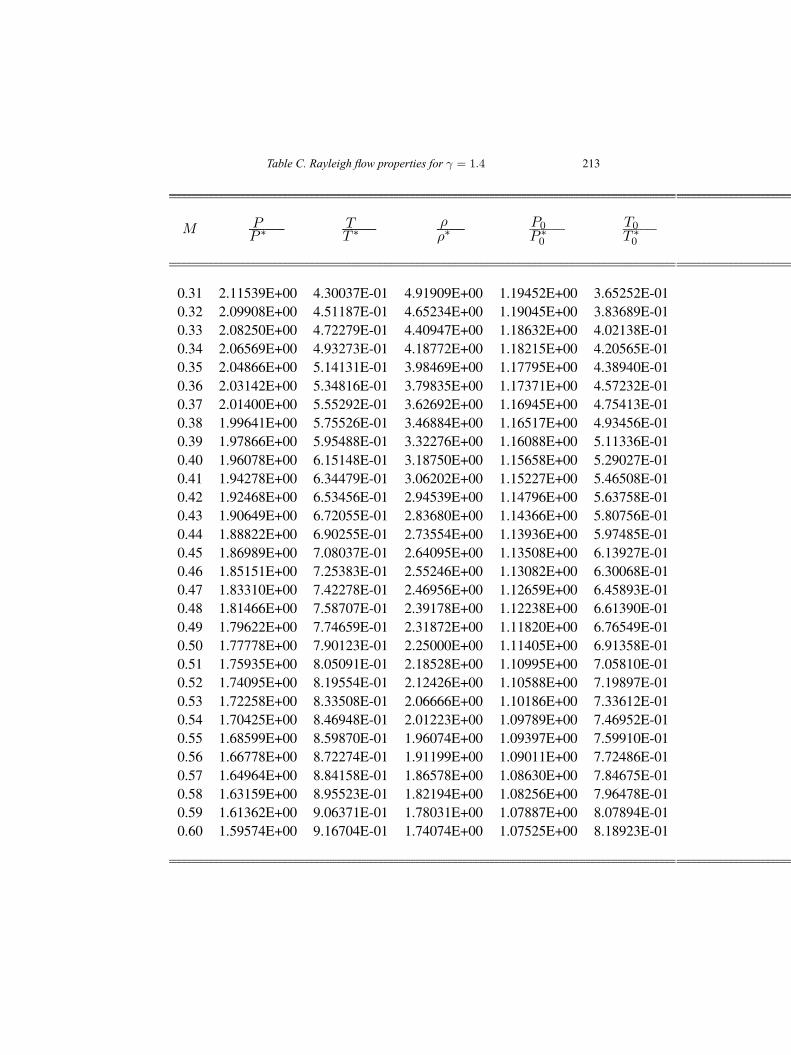
Table C. Rayleigh flow properties for γ = 1.4 213
M PP ∗
TT ∗
ρρ∗
P0P ∗0
T0T ∗0
0.31 2.11539E+00 4.30037E-01 4.91909E+00 1.19452E+00 3.65252E-010.32 2.09908E+00 4.51187E-01 4.65234E+00 1.19045E+00 3.83689E-010.33 2.08250E+00 4.72279E-01 4.40947E+00 1.18632E+00 4.02138E-010.34 2.06569E+00 4.93273E-01 4.18772E+00 1.18215E+00 4.20565E-010.35 2.04866E+00 5.14131E-01 3.98469E+00 1.17795E+00 4.38940E-010.36 2.03142E+00 5.34816E-01 3.79835E+00 1.17371E+00 4.57232E-010.37 2.01400E+00 5.55292E-01 3.62692E+00 1.16945E+00 4.75413E-010.38 1.99641E+00 5.75526E-01 3.46884E+00 1.16517E+00 4.93456E-010.39 1.97866E+00 5.95488E-01 3.32276E+00 1.16088E+00 5.11336E-010.40 1.96078E+00 6.15148E-01 3.18750E+00 1.15658E+00 5.29027E-010.41 1.94278E+00 6.34479E-01 3.06202E+00 1.15227E+00 5.46508E-010.42 1.92468E+00 6.53456E-01 2.94539E+00 1.14796E+00 5.63758E-010.43 1.90649E+00 6.72055E-01 2.83680E+00 1.14366E+00 5.80756E-010.44 1.88822E+00 6.90255E-01 2.73554E+00 1.13936E+00 5.97485E-010.45 1.86989E+00 7.08037E-01 2.64095E+00 1.13508E+00 6.13927E-010.46 1.85151E+00 7.25383E-01 2.55246E+00 1.13082E+00 6.30068E-010.47 1.83310E+00 7.42278E-01 2.46956E+00 1.12659E+00 6.45893E-010.48 1.81466E+00 7.58707E-01 2.39178E+00 1.12238E+00 6.61390E-010.49 1.79622E+00 7.74659E-01 2.31872E+00 1.11820E+00 6.76549E-010.50 1.77778E+00 7.90123E-01 2.25000E+00 1.11405E+00 6.91358E-010.51 1.75935E+00 8.05091E-01 2.18528E+00 1.10995E+00 7.05810E-010.52 1.74095E+00 8.19554E-01 2.12426E+00 1.10588E+00 7.19897E-010.53 1.72258E+00 8.33508E-01 2.06666E+00 1.10186E+00 7.33612E-010.54 1.70425E+00 8.46948E-01 2.01223E+00 1.09789E+00 7.46952E-010.55 1.68599E+00 8.59870E-01 1.96074E+00 1.09397E+00 7.59910E-010.56 1.66778E+00 8.72274E-01 1.91199E+00 1.09011E+00 7.72486E-010.57 1.64964E+00 8.84158E-01 1.86578E+00 1.08630E+00 7.84675E-010.58 1.63159E+00 8.95523E-01 1.82194E+00 1.08256E+00 7.96478E-010.59 1.61362E+00 9.06371E-01 1.78031E+00 1.07887E+00 8.07894E-010.60 1.59574E+00 9.16704E-01 1.74074E+00 1.07525E+00 8.18923E-01

214 Fundamentals of Gas Dynamics
M PP ∗
TT ∗
ρρ∗
P0P ∗0
T0T ∗0
0.61 1.57797E+00 9.26527E-01 1.70310E+00 1.07170E+00 8.29566E-010.62 1.56031E+00 9.35843E-01 1.66727E+00 1.06822E+00 8.39825E-010.63 1.54275E+00 9.44657E-01 1.63314E+00 1.06481E+00 8.49703E-010.64 1.52532E+00 9.52976E-01 1.60059E+00 1.06147E+00 8.59203E-010.65 1.50801E+00 9.60806E-01 1.56953E+00 1.05821E+00 8.68329E-010.66 1.49083E+00 9.68155E-01 1.53987E+00 1.05503E+00 8.77084E-010.67 1.47379E+00 9.75030E-01 1.51153E+00 1.05193E+00 8.85473E-010.68 1.45688E+00 9.81439E-01 1.48443E+00 1.04890E+00 8.93502E-010.69 1.44011E+00 9.87391E-01 1.45850E+00 1.04596E+00 9.01175E-010.70 1.42349E+00 9.92895E-01 1.43367E+00 1.04310E+00 9.08499E-010.71 1.40701E+00 9.97961E-01 1.40989E+00 1.04033E+00 9.15479E-010.72 1.39069E+00 1.00260E+00 1.38709E+00 1.03764E+00 9.22122E-010.73 1.37452E+00 1.00682E+00 1.36522E+00 1.03504E+00 9.28435E-010.74 1.35851E+00 1.01062E+00 1.34423E+00 1.03253E+00 9.34423E-010.75 1.34266E+00 1.01403E+00 1.32407E+00 1.03010E+00 9.40095E-010.76 1.32696E+00 1.01706E+00 1.30471E+00 1.02777E+00 9.45456E-010.77 1.31143E+00 1.01970E+00 1.28609E+00 1.02552E+00 9.50515E-010.78 1.29606E+00 1.02198E+00 1.26819E+00 1.02337E+00 9.55279E-010.79 1.28086E+00 1.02390E+00 1.25096E+00 1.02131E+00 9.59754E-010.80 1.26582E+00 1.02548E+00 1.23438E+00 1.01934E+00 9.63948E-010.81 1.25095E+00 1.02672E+00 1.21840E+00 1.01747E+00 9.67869E-010.82 1.23625E+00 1.02763E+00 1.20300E+00 1.01569E+00 9.71524E-010.83 1.22171E+00 1.02823E+00 1.18816E+00 1.01400E+00 9.74921E-010.84 1.20734E+00 1.02853E+00 1.17385E+00 1.01241E+00 9.78066E-010.85 1.19314E+00 1.02854E+00 1.16003E+00 1.01091E+00 9.80968E-010.86 1.17911E+00 1.02826E+00 1.14670E+00 1.00951E+00 9.83633E-010.87 1.16524E+00 1.02771E+00 1.13382E+00 1.00820E+00 9.86069E-010.88 1.15154E+00 1.02689E+00 1.12138E+00 1.00699E+00 9.88283E-010.89 1.13801E+00 1.02583E+00 1.10936E+00 1.00587E+00 9.90282E-010.90 1.12465E+00 1.02452E+00 1.09774E+00 1.00486E+00 9.92073E-01
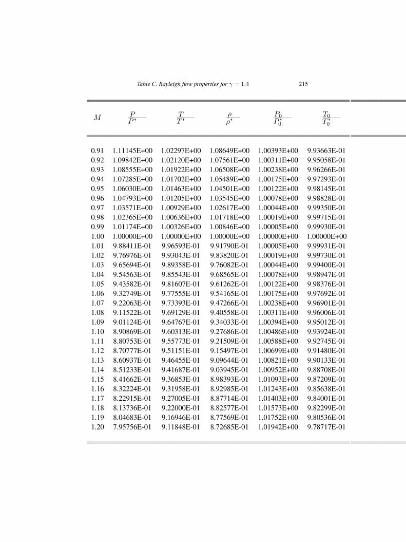
Table C. Rayleigh flow properties for γ = 1.4 215
M PP ∗
TT ∗
ρρ∗
P0P ∗0
T0T ∗0
0.91 1.11145E+00 1.02297E+00 1.08649E+00 1.00393E+00 9.93663E-010.92 1.09842E+00 1.02120E+00 1.07561E+00 1.00311E+00 9.95058E-010.93 1.08555E+00 1.01922E+00 1.06508E+00 1.00238E+00 9.96266E-010.94 1.07285E+00 1.01702E+00 1.05489E+00 1.00175E+00 9.97293E-010.95 1.06030E+00 1.01463E+00 1.04501E+00 1.00122E+00 9.98145E-010.96 1.04793E+00 1.01205E+00 1.03545E+00 1.00078E+00 9.98828E-010.97 1.03571E+00 1.00929E+00 1.02617E+00 1.00044E+00 9.99350E-010.98 1.02365E+00 1.00636E+00 1.01718E+00 1.00019E+00 9.99715E-010.99 1.01174E+00 1.00326E+00 1.00846E+00 1.00005E+00 9.99930E-011.00 1.00000E+00 1.00000E+00 1.00000E+00 1.00000E+00 1.00000E+001.01 9.88411E-01 9.96593E-01 9.91790E-01 1.00005E+00 9.99931E-011.02 9.76976E-01 9.93043E-01 9.83820E-01 1.00019E+00 9.99730E-011.03 9.65694E-01 9.89358E-01 9.76082E-01 1.00044E+00 9.99400E-011.04 9.54563E-01 9.85543E-01 9.68565E-01 1.00078E+00 9.98947E-011.05 9.43582E-01 9.81607E-01 9.61262E-01 1.00122E+00 9.98376E-011.06 9.32749E-01 9.77555E-01 9.54165E-01 1.00175E+00 9.97692E-011.07 9.22063E-01 9.73393E-01 9.47266E-01 1.00238E+00 9.96901E-011.08 9.11522E-01 9.69129E-01 9.40558E-01 1.00311E+00 9.96006E-011.09 9.01124E-01 9.64767E-01 9.34033E-01 1.00394E+00 9.95012E-011.10 8.90869E-01 9.60313E-01 9.27686E-01 1.00486E+00 9.93924E-011.11 8.80753E-01 9.55773E-01 9.21509E-01 1.00588E+00 9.92745E-011.12 8.70777E-01 9.51151E-01 9.15497E-01 1.00699E+00 9.91480E-011.13 8.60937E-01 9.46455E-01 9.09644E-01 1.00821E+00 9.90133E-011.14 8.51233E-01 9.41687E-01 9.03945E-01 1.00952E+00 9.88708E-011.15 8.41662E-01 9.36853E-01 8.98393E-01 1.01093E+00 9.87209E-011.16 8.32224E-01 9.31958E-01 8.92985E-01 1.01243E+00 9.85638E-011.17 8.22915E-01 9.27005E-01 8.87714E-01 1.01403E+00 9.84001E-011.18 8.13736E-01 9.22000E-01 8.82577E-01 1.01573E+00 9.82299E-011.19 8.04683E-01 9.16946E-01 8.77569E-01 1.01752E+00 9.80536E-011.20 7.95756E-01 9.11848E-01 8.72685E-01 1.01942E+00 9.78717E-01
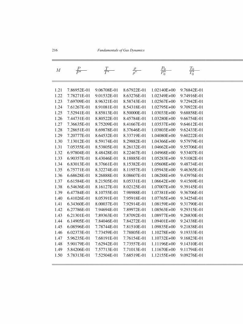
216 Fundamentals of Gas Dynamics
M PP ∗
TT ∗
ρρ∗
P0P ∗0
T0T ∗0
1.21 7.86952E-01 9.06708E-01 8.67922E-01 1.02140E+00 9.76842E-011.22 7.78271E-01 9.01532E-01 8.63276E-01 1.02349E+00 9.74916E-011.23 7.69709E-01 8.96321E-01 8.58743E-01 1.02567E+00 9.72942E-011.24 7.61267E-01 8.91081E-01 8.54318E-01 1.02795E+00 9.70922E-011.25 7.52941E-01 8.85813E-01 8.50000E-01 1.03033E+00 9.68858E-011.26 7.44731E-01 8.80522E-01 8.45784E-01 1.03280E+00 9.66754E-011.27 7.36635E-01 8.75209E-01 8.41667E-01 1.03537E+00 9.64612E-011.28 7.28651E-01 8.69878E-01 8.37646E-01 1.03803E+00 9.62433E-011.29 7.20777E-01 8.64532E-01 8.33719E-01 1.04080E+00 9.60222E-011.30 7.13012E-01 8.59174E-01 8.29882E-01 1.04366E+00 9.57979E-011.31 7.05355E-01 8.53805E-01 8.26132E-01 1.04662E+00 9.55706E-011.32 6.97804E-01 8.48428E-01 8.22467E-01 1.04968E+00 9.53407E-011.33 6.90357E-01 8.43046E-01 8.18885E-01 1.05283E+00 9.51082E-011.34 6.83013E-01 8.37661E-01 8.15382E-01 1.05608E+00 9.48734E-011.35 6.75771E-01 8.32274E-01 8.11957E-01 1.05943E+00 9.46365E-011.36 6.68628E-01 8.26888E-01 8.08607E-01 1.06288E+00 9.43976E-011.37 6.61584E-01 8.21505E-01 8.05331E-01 1.06642E+00 9.41569E-011.38 6.54636E-01 8.16127E-01 8.02125E-01 1.07007E+00 9.39145E-011.39 6.47784E-01 8.10755E-01 7.98988E-01 1.07381E+00 9.36706E-011.40 6.41026E-01 8.05391E-01 7.95918E-01 1.07765E+00 9.34254E-011.41 6.34360E-01 8.00037E-01 7.92914E-01 1.08159E+00 9.31790E-011.42 6.27786E-01 7.94694E-01 7.89972E-01 1.08563E+00 9.29315E-011.43 6.21301E-01 7.89363E-01 7.87092E-01 1.08977E+00 9.26830E-011.44 6.14905E-01 7.84046E-01 7.84272E-01 1.09401E+00 9.24338E-011.45 6.08596E-01 7.78744E-01 7.81510E-01 1.09835E+00 9.21838E-011.46 6.02373E-01 7.73459E-01 7.78805E-01 1.10278E+00 9.19333E-011.47 5.96235E-01 7.68191E-01 7.76154E-01 1.10732E+00 9.16823E-011.48 5.90179E-01 7.62942E-01 7.73557E-01 1.11196E+00 9.14310E-011.49 5.84206E-01 7.57713E-01 7.71013E-01 1.11670E+00 9.11794E-011.50 5.78313E-01 7.52504E-01 7.68519E-01 1.12155E+00 9.09276E-01
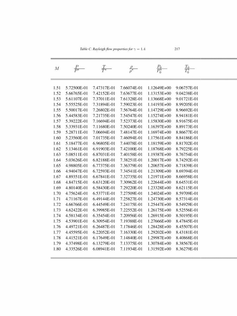
Table C. Rayleigh flow properties for γ = 1.4 217
M PP ∗
TT ∗
ρρ∗
P0P ∗0
T0T ∗0
1.51 5.72500E-01 7.47317E-01 7.66074E-01 1.12649E+00 9.06757E-011.52 5.66765E-01 7.42152E-01 7.63677E-01 1.13153E+00 9.04238E-011.53 5.61107E-01 7.37011E-01 7.61328E-01 1.13668E+00 9.01721E-011.54 5.55525E-01 7.31894E-01 7.59023E-01 1.14193E+00 8.99205E-011.55 5.50017E-01 7.26802E-01 7.56764E-01 1.14729E+00 8.96692E-011.56 5.44583E-01 7.21735E-01 7.54547E-01 1.15274E+00 8.94181E-011.57 5.39222E-01 7.16694E-01 7.52373E-01 1.15830E+00 8.91675E-011.58 5.33931E-01 7.11680E-01 7.50240E-01 1.16397E+00 8.89173E-011.59 5.28711E-01 7.06694E-01 7.48147E-01 1.16974E+00 8.86677E-011.60 5.23560E-01 7.01735E-01 7.46094E-01 1.17561E+00 8.84186E-011.61 5.18477E-01 6.96805E-01 7.44078E-01 1.18159E+00 8.81702E-011.62 5.13461E-01 6.91903E-01 7.42100E-01 1.18768E+00 8.79225E-011.63 5.08511E-01 6.87031E-01 7.40158E-01 1.19387E+00 8.76754E-011.64 5.03626E-01 6.82188E-01 7.38251E-01 1.20017E+00 8.74292E-011.65 4.98805E-01 6.77375E-01 7.36379E-01 1.20657E+00 8.71839E-011.66 4.94047E-01 6.72593E-01 7.34541E-01 1.21309E+00 8.69394E-011.67 4.89351E-01 6.67841E-01 7.32735E-01 1.21971E+00 8.66958E-011.68 4.84715E-01 6.63120E-01 7.30962E-01 1.22644E+00 8.64531E-011.69 4.80140E-01 6.58430E-01 7.29220E-01 1.23328E+00 8.62115E-011.70 4.75624E-01 6.53771E-01 7.27509E-01 1.24024E+00 8.59709E-011.71 4.71167E-01 6.49144E-01 7.25827E-01 1.24730E+00 8.57314E-011.72 4.66766E-01 6.44549E-01 7.24175E-01 1.25447E+00 8.54929E-011.73 4.62422E-01 6.39985E-01 7.22552E-01 1.26175E+00 8.52556E-011.74 4.58134E-01 6.35454E-01 7.20956E-01 1.26915E+00 8.50195E-011.75 4.53901E-01 6.30954E-01 7.19388E-01 1.27666E+00 8.47845E-011.76 4.49721E-01 6.26487E-01 7.17846E-01 1.28428E+00 8.45507E-011.77 4.45595E-01 6.22052E-01 7.16330E-01 1.29202E+00 8.43181E-011.78 4.41521E-01 6.17649E-01 7.14840E-01 1.29987E+00 8.40868E-011.79 4.37498E-01 6.13279E-01 7.13375E-01 1.30784E+00 8.38567E-011.80 4.33526E-01 6.08941E-01 7.11934E-01 1.31592E+00 8.36279E-01
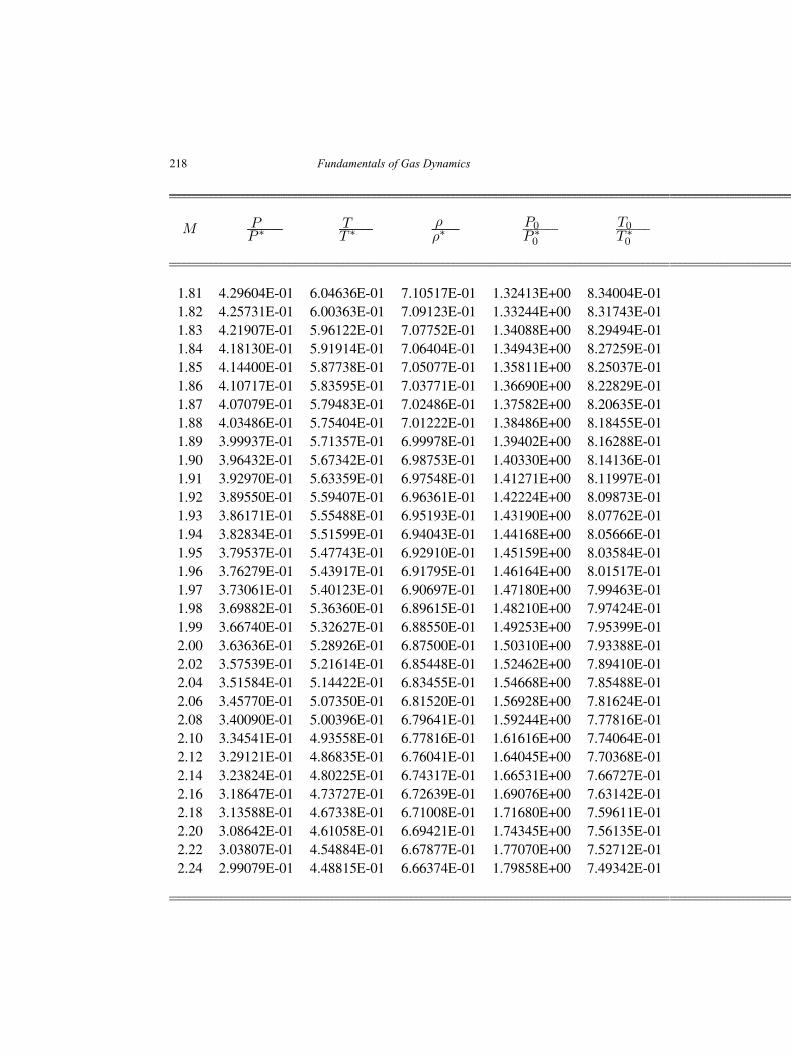
218 Fundamentals of Gas Dynamics
M PP ∗
TT ∗
ρρ∗
P0P ∗0
T0T ∗0
1.81 4.29604E-01 6.04636E-01 7.10517E-01 1.32413E+00 8.34004E-011.82 4.25731E-01 6.00363E-01 7.09123E-01 1.33244E+00 8.31743E-011.83 4.21907E-01 5.96122E-01 7.07752E-01 1.34088E+00 8.29494E-011.84 4.18130E-01 5.91914E-01 7.06404E-01 1.34943E+00 8.27259E-011.85 4.14400E-01 5.87738E-01 7.05077E-01 1.35811E+00 8.25037E-011.86 4.10717E-01 5.83595E-01 7.03771E-01 1.36690E+00 8.22829E-011.87 4.07079E-01 5.79483E-01 7.02486E-01 1.37582E+00 8.20635E-011.88 4.03486E-01 5.75404E-01 7.01222E-01 1.38486E+00 8.18455E-011.89 3.99937E-01 5.71357E-01 6.99978E-01 1.39402E+00 8.16288E-011.90 3.96432E-01 5.67342E-01 6.98753E-01 1.40330E+00 8.14136E-011.91 3.92970E-01 5.63359E-01 6.97548E-01 1.41271E+00 8.11997E-011.92 3.89550E-01 5.59407E-01 6.96361E-01 1.42224E+00 8.09873E-011.93 3.86171E-01 5.55488E-01 6.95193E-01 1.43190E+00 8.07762E-011.94 3.82834E-01 5.51599E-01 6.94043E-01 1.44168E+00 8.05666E-011.95 3.79537E-01 5.47743E-01 6.92910E-01 1.45159E+00 8.03584E-011.96 3.76279E-01 5.43917E-01 6.91795E-01 1.46164E+00 8.01517E-011.97 3.73061E-01 5.40123E-01 6.90697E-01 1.47180E+00 7.99463E-011.98 3.69882E-01 5.36360E-01 6.89615E-01 1.48210E+00 7.97424E-011.99 3.66740E-01 5.32627E-01 6.88550E-01 1.49253E+00 7.95399E-012.00 3.63636E-01 5.28926E-01 6.87500E-01 1.50310E+00 7.93388E-012.02 3.57539E-01 5.21614E-01 6.85448E-01 1.52462E+00 7.89410E-012.04 3.51584E-01 5.14422E-01 6.83455E-01 1.54668E+00 7.85488E-012.06 3.45770E-01 5.07350E-01 6.81520E-01 1.56928E+00 7.81624E-012.08 3.40090E-01 5.00396E-01 6.79641E-01 1.59244E+00 7.77816E-012.10 3.34541E-01 4.93558E-01 6.77816E-01 1.61616E+00 7.74064E-012.12 3.29121E-01 4.86835E-01 6.76041E-01 1.64045E+00 7.70368E-012.14 3.23824E-01 4.80225E-01 6.74317E-01 1.66531E+00 7.66727E-012.16 3.18647E-01 4.73727E-01 6.72639E-01 1.69076E+00 7.63142E-012.18 3.13588E-01 4.67338E-01 6.71008E-01 1.71680E+00 7.59611E-012.20 3.08642E-01 4.61058E-01 6.69421E-01 1.74345E+00 7.56135E-012.22 3.03807E-01 4.54884E-01 6.67877E-01 1.77070E+00 7.52712E-012.24 2.99079E-01 4.48815E-01 6.66374E-01 1.79858E+00 7.49342E-01
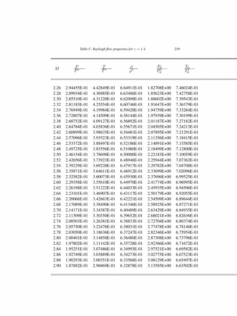
Table C. Rayleigh flow properties for γ = 1.4 219
M PP ∗
TT ∗
ρρ∗
P0P ∗0
T0T ∗0
2.26 2.94455E-01 4.42849E-01 6.64911E-01 1.82708E+00 7.46024E-012.28 2.89934E-01 4.36985E-01 6.63486E-01 1.85623E+00 7.42758E-012.30 2.85510E-01 4.31220E-01 6.62098E-01 1.88602E+00 7.39543E-012.32 2.81183E-01 4.25554E-01 6.60746E-01 1.91647E+00 7.36379E-012.34 2.76949E-01 4.19984E-01 6.59428E-01 1.94759E+00 7.33264E-012.36 2.72807E-01 4.14509E-01 6.58144E-01 1.97939E+00 7.30199E-012.38 2.68752E-01 4.09127E-01 6.56892E-01 2.01187E+00 7.27182E-012.40 2.64784E-01 4.03836E-01 6.55671E-01 2.04505E+00 7.24213E-012.42 2.60899E-01 3.98635E-01 6.54481E-01 2.07895E+00 7.21291E-012.44 2.57096E-01 3.93523E-01 6.53319E-01 2.11356E+00 7.18415E-012.46 2.53372E-01 3.88497E-01 6.52186E-01 2.14891E+00 7.15585E-012.48 2.49725E-01 3.83556E-01 6.51080E-01 2.18499E+00 7.12800E-012.50 2.46154E-01 3.78698E-01 6.50000E-01 2.22183E+00 7.10059E-012.52 2.42656E-01 3.73923E-01 6.48946E-01 2.25944E+00 7.07362E-012.54 2.39229E-01 3.69228E-01 6.47917E-01 2.29782E+00 7.04708E-012.56 2.35871E-01 3.64611E-01 6.46912E-01 2.33699E+00 7.02096E-012.58 2.32582E-01 3.60073E-01 6.45930E-01 2.37696E+00 6.99525E-012.60 2.29358E-01 3.55610E-01 6.44970E-01 2.41774E+00 6.96995E-012.62 2.26198E-01 3.51222E-01 6.44033E-01 2.45935E+00 6.94506E-012.64 2.23101E-01 3.46907E-01 6.43117E-01 2.50179E+00 6.92055E-012.66 2.20066E-01 3.42663E-01 6.42221E-01 2.54509E+00 6.89644E-012.68 2.17089E-01 3.38490E-01 6.41346E-01 2.58925E+00 6.87271E-012.70 2.14171E-01 3.34387E-01 6.40489E-01 2.63429E+00 6.84935E-012.72 2.11309E-01 3.30350E-01 6.39652E-01 2.68021E+00 6.82636E-012.74 2.08503E-01 3.26381E-01 6.38833E-01 2.72704E+00 6.80374E-012.76 2.05750E-01 3.22476E-01 6.38031E-01 2.77478E+00 6.78146E-012.78 2.03050E-01 3.18636E-01 6.37247E-01 2.82346E+00 6.75954E-012.80 2.00401E-01 3.14858E-01 6.36480E-01 2.87308E+00 6.73796E-012.82 1.97802E-01 3.11142E-01 6.35728E-01 2.92366E+00 6.71672E-012.84 1.95251E-01 3.07486E-01 6.34993E-01 2.97521E+00 6.69582E-012.86 1.92749E-01 3.03889E-01 6.34273E-01 3.02775E+00 6.67523E-012.88 1.90293E-01 3.00351E-01 6.33568E-01 3.08129E+00 6.65497E-012.90 1.87882E-01 2.96869E-01 6.32878E-01 3.13585E+00 6.63502E-01
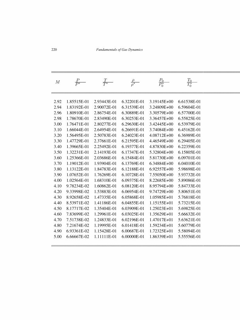
220 Fundamentals of Gas Dynamics
M PP ∗
TT ∗
ρρ∗
P0P ∗0
T0T ∗0
2.92 1.85515E-01 2.93443E-01 6.32201E-01 3.19145E+00 6.61538E-012.94 1.83192E-01 2.90072E-01 6.31539E-01 3.24809E+00 6.59604E-012.96 1.80910E-01 2.86754E-01 6.30889E-01 3.30579E+00 6.57700E-012.98 1.78670E-01 2.83490E-01 6.30253E-01 3.36457E+00 6.55825E-013.00 1.76471E-01 2.80277E-01 6.29630E-01 3.42445E+00 6.53979E-013.10 1.66044E-01 2.64954E-01 6.26691E-01 3.74084E+00 6.45162E-013.20 1.56495E-01 2.50783E-01 6.24023E-01 4.08712E+00 6.36989E-013.30 1.47729E-01 2.37661E-01 6.21595E-01 4.46549E+00 6.29405E-013.40 1.39665E-01 2.25492E-01 6.19377E-01 4.87830E+00 6.22359E-013.50 1.32231E-01 2.14193E-01 6.17347E-01 5.32804E+00 6.15805E-013.60 1.25366E-01 2.03686E-01 6.15484E-01 5.81730E+00 6.09701E-013.70 1.19012E-01 1.93904E-01 6.13769E-01 6.34884E+00 6.04010E-013.80 1.13122E-01 1.84783E-01 6.12188E-01 6.92557E+00 5.98698E-013.90 1.07652E-01 1.76269E-01 6.10728E-01 7.55050E+00 5.93732E-014.00 1.02564E-01 1.68310E-01 6.09375E-01 8.22685E+00 5.89086E-014.10 9.78234E-02 1.60862E-01 6.08120E-01 8.95794E+00 5.84733E-014.20 9.33998E-02 1.53883E-01 6.06954E-01 9.74729E+00 5.80651E-014.30 8.92658E-02 1.47335E-01 6.05868E-01 1.05985E+01 5.76818E-014.40 8.53971E-02 1.41186E-01 6.04855E-01 1.15155E+01 5.73215E-014.50 8.17717E-02 1.35404E-01 6.03909E-01 1.25023E+01 5.69825E-014.60 7.83699E-02 1.29961E-01 6.03025E-01 1.35629E+01 5.66632E-014.70 7.51738E-02 1.24833E-01 6.02196E-01 1.47017E+01 5.63621E-014.80 7.21674E-02 1.19995E-01 6.01418E-01 1.59234E+01 5.60779E-014.90 6.93361E-02 1.15428E-01 6.00687E-01 1.72325E+01 5.58094E-015.00 6.66667E-02 1.11111E-01 6.00000E-01 1.86339E+01 5.55556E-01
Table D. Fanno flow properties for γ = 1.4
221
Fundamentals of Gas Dynamics, Second Edition. V. Babu.© 2015 V. Babu. Published 2015 by Athena Academic Ltd and John Wiley & Sons Ltd
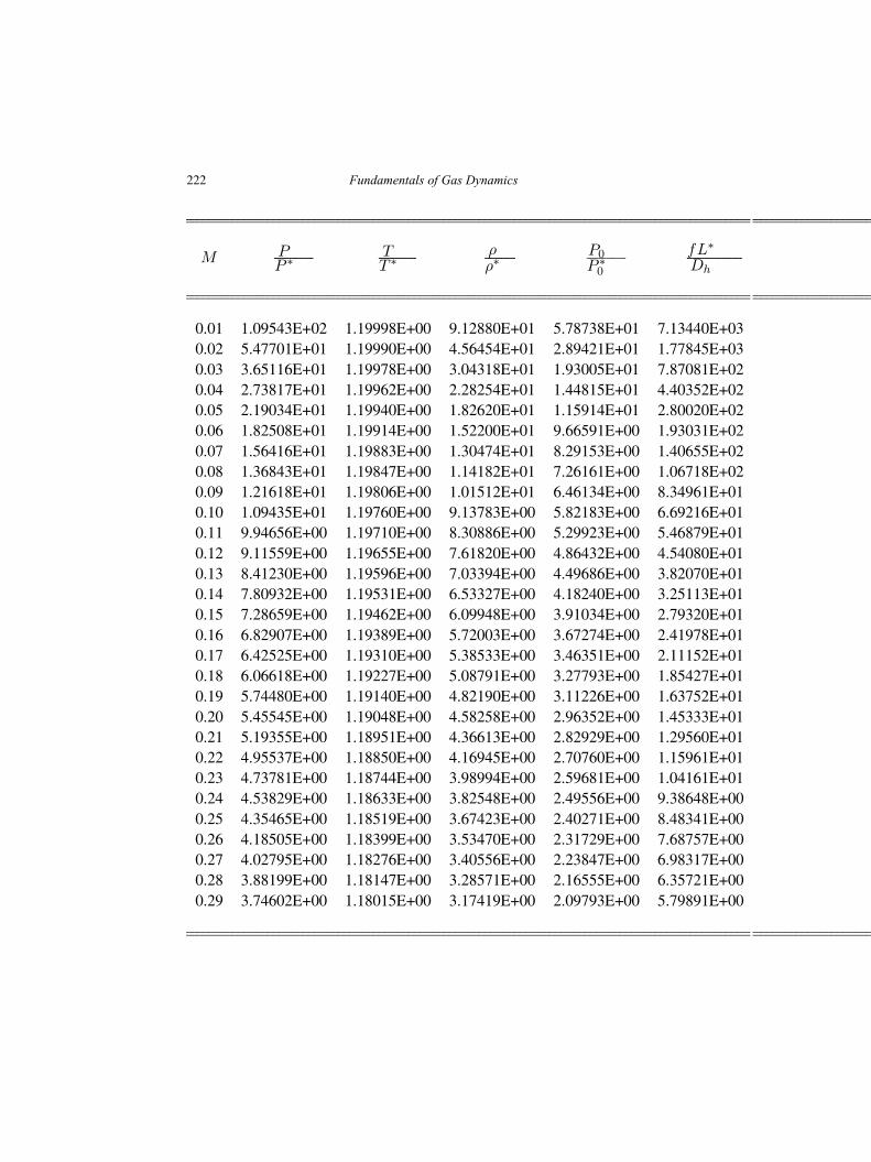
222 Fundamentals of Gas Dynamics
M PP ∗
TT ∗
ρρ∗
P0P ∗0
fL∗
Dh
0.01 1.09543E+02 1.19998E+00 9.12880E+01 5.78738E+01 7.13440E+030.02 5.47701E+01 1.19990E+00 4.56454E+01 2.89421E+01 1.77845E+030.03 3.65116E+01 1.19978E+00 3.04318E+01 1.93005E+01 7.87081E+020.04 2.73817E+01 1.19962E+00 2.28254E+01 1.44815E+01 4.40352E+020.05 2.19034E+01 1.19940E+00 1.82620E+01 1.15914E+01 2.80020E+020.06 1.82508E+01 1.19914E+00 1.52200E+01 9.66591E+00 1.93031E+020.07 1.56416E+01 1.19883E+00 1.30474E+01 8.29153E+00 1.40655E+020.08 1.36843E+01 1.19847E+00 1.14182E+01 7.26161E+00 1.06718E+020.09 1.21618E+01 1.19806E+00 1.01512E+01 6.46134E+00 8.34961E+010.10 1.09435E+01 1.19760E+00 9.13783E+00 5.82183E+00 6.69216E+010.11 9.94656E+00 1.19710E+00 8.30886E+00 5.29923E+00 5.46879E+010.12 9.11559E+00 1.19655E+00 7.61820E+00 4.86432E+00 4.54080E+010.13 8.41230E+00 1.19596E+00 7.03394E+00 4.49686E+00 3.82070E+010.14 7.80932E+00 1.19531E+00 6.53327E+00 4.18240E+00 3.25113E+010.15 7.28659E+00 1.19462E+00 6.09948E+00 3.91034E+00 2.79320E+010.16 6.82907E+00 1.19389E+00 5.72003E+00 3.67274E+00 2.41978E+010.17 6.42525E+00 1.19310E+00 5.38533E+00 3.46351E+00 2.11152E+010.18 6.06618E+00 1.19227E+00 5.08791E+00 3.27793E+00 1.85427E+010.19 5.74480E+00 1.19140E+00 4.82190E+00 3.11226E+00 1.63752E+010.20 5.45545E+00 1.19048E+00 4.58258E+00 2.96352E+00 1.45333E+010.21 5.19355E+00 1.18951E+00 4.36613E+00 2.82929E+00 1.29560E+010.22 4.95537E+00 1.18850E+00 4.16945E+00 2.70760E+00 1.15961E+010.23 4.73781E+00 1.18744E+00 3.98994E+00 2.59681E+00 1.04161E+010.24 4.53829E+00 1.18633E+00 3.82548E+00 2.49556E+00 9.38648E+000.25 4.35465E+00 1.18519E+00 3.67423E+00 2.40271E+00 8.48341E+000.26 4.18505E+00 1.18399E+00 3.53470E+00 2.31729E+00 7.68757E+000.27 4.02795E+00 1.18276E+00 3.40556E+00 2.23847E+00 6.98317E+000.28 3.88199E+00 1.18147E+00 3.28571E+00 2.16555E+00 6.35721E+000.29 3.74602E+00 1.18015E+00 3.17419E+00 2.09793E+00 5.79891E+00
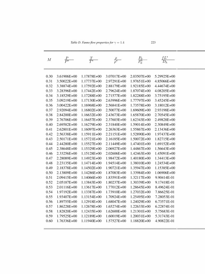
Table D. Fanno flow properties for γ = 1.4 223
M PP ∗
TT ∗
ρρ∗
P0P ∗0
fL∗
Dh
0.30 3.61906E+00 1.17878E+00 3.07017E+00 2.03507E+00 5.29925E+000.31 3.50022E+00 1.17737E+00 2.97291E+00 1.97651E+00 4.85066E+000.32 3.38874E+00 1.17592E+00 2.88179E+00 1.92185E+00 4.44674E+000.33 3.28396E+00 1.17442E+00 2.79624E+00 1.87074E+00 4.08205E+000.34 3.18529E+00 1.17288E+00 2.71577E+00 1.82288E+00 3.75195E+000.35 3.09219E+00 1.17130E+00 2.63996E+00 1.77797E+00 3.45245E+000.36 3.00422E+00 1.16968E+00 2.56841E+00 1.73578E+00 3.18012E+000.37 2.92094E+00 1.16802E+00 2.50077E+00 1.69609E+00 2.93198E+000.38 2.84200E+00 1.16632E+00 2.43673E+00 1.65870E+00 2.70545E+000.39 2.76706E+00 1.16457E+00 2.37603E+00 1.62343E+00 2.49828E+000.40 2.69582E+00 1.16279E+00 2.31840E+00 1.59014E+00 2.30849E+000.41 2.62801E+00 1.16097E+00 2.26363E+00 1.55867E+00 2.13436E+000.42 2.56338E+00 1.15911E+00 2.21151E+00 1.52890E+00 1.97437E+000.43 2.50171E+00 1.15721E+00 2.16185E+00 1.50072E+00 1.82715E+000.44 2.44280E+00 1.15527E+00 2.11449E+00 1.47401E+00 1.69152E+000.45 2.38648E+00 1.15329E+00 2.06927E+00 1.44867E+00 1.56643E+000.46 2.33256E+00 1.15128E+00 2.02606E+00 1.42463E+00 1.45091E+000.47 2.28089E+00 1.14923E+00 1.98472E+00 1.40180E+00 1.34413E+000.48 2.23135E+00 1.14714E+00 1.94514E+00 1.38010E+00 1.24534E+000.49 2.18378E+00 1.14502E+00 1.90721E+00 1.35947E+00 1.15385E+000.50 2.13809E+00 1.14286E+00 1.87083E+00 1.33984E+00 1.06906E+000.51 2.09415E+00 1.14066E+00 1.83591E+00 1.32117E+00 9.90414E-010.52 2.05187E+00 1.13843E+00 1.80237E+00 1.30339E+00 9.17418E-010.53 2.01116E+00 1.13617E+00 1.77012E+00 1.28645E+00 8.49624E-010.54 1.97192E+00 1.13387E+00 1.73910E+00 1.27032E+00 7.86625E-010.55 1.93407E+00 1.13154E+00 1.70924E+00 1.25495E+00 7.28053E-010.56 1.89755E+00 1.12918E+00 1.68047E+00 1.24029E+00 6.73571E-010.57 1.86228E+00 1.12678E+00 1.65274E+00 1.22633E+00 6.22874E-010.58 1.82820E+00 1.12435E+00 1.62600E+00 1.21301E+00 5.75683E-010.59 1.79525E+00 1.12189E+00 1.60019E+00 1.20031E+00 5.31743E-010.60 1.76336E+00 1.11940E+00 1.57527E+00 1.18820E+00 4.90822E-01
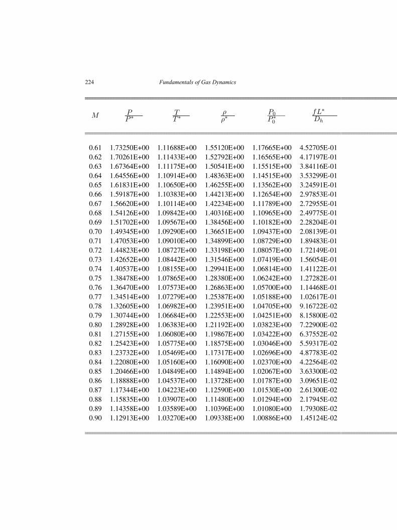
224 Fundamentals of Gas Dynamics
M PP ∗
TT ∗
ρρ∗
P0P ∗0
fL∗
Dh
0.61 1.73250E+00 1.11688E+00 1.55120E+00 1.17665E+00 4.52705E-010.62 1.70261E+00 1.11433E+00 1.52792E+00 1.16565E+00 4.17197E-010.63 1.67364E+00 1.11175E+00 1.50541E+00 1.15515E+00 3.84116E-010.64 1.64556E+00 1.10914E+00 1.48363E+00 1.14515E+00 3.53299E-010.65 1.61831E+00 1.10650E+00 1.46255E+00 1.13562E+00 3.24591E-010.66 1.59187E+00 1.10383E+00 1.44213E+00 1.12654E+00 2.97853E-010.67 1.56620E+00 1.10114E+00 1.42234E+00 1.11789E+00 2.72955E-010.68 1.54126E+00 1.09842E+00 1.40316E+00 1.10965E+00 2.49775E-010.69 1.51702E+00 1.09567E+00 1.38456E+00 1.10182E+00 2.28204E-010.70 1.49345E+00 1.09290E+00 1.36651E+00 1.09437E+00 2.08139E-010.71 1.47053E+00 1.09010E+00 1.34899E+00 1.08729E+00 1.89483E-010.72 1.44823E+00 1.08727E+00 1.33198E+00 1.08057E+00 1.72149E-010.73 1.42652E+00 1.08442E+00 1.31546E+00 1.07419E+00 1.56054E-010.74 1.40537E+00 1.08155E+00 1.29941E+00 1.06814E+00 1.41122E-010.75 1.38478E+00 1.07865E+00 1.28380E+00 1.06242E+00 1.27282E-010.76 1.36470E+00 1.07573E+00 1.26863E+00 1.05700E+00 1.14468E-010.77 1.34514E+00 1.07279E+00 1.25387E+00 1.05188E+00 1.02617E-010.78 1.32605E+00 1.06982E+00 1.23951E+00 1.04705E+00 9.16722E-020.79 1.30744E+00 1.06684E+00 1.22553E+00 1.04251E+00 8.15800E-020.80 1.28928E+00 1.06383E+00 1.21192E+00 1.03823E+00 7.22900E-020.81 1.27155E+00 1.06080E+00 1.19867E+00 1.03422E+00 6.37552E-020.82 1.25423E+00 1.05775E+00 1.18575E+00 1.03046E+00 5.59317E-020.83 1.23732E+00 1.05469E+00 1.17317E+00 1.02696E+00 4.87783E-020.84 1.22080E+00 1.05160E+00 1.16090E+00 1.02370E+00 4.22564E-020.85 1.20466E+00 1.04849E+00 1.14894E+00 1.02067E+00 3.63300E-020.86 1.18888E+00 1.04537E+00 1.13728E+00 1.01787E+00 3.09651E-020.87 1.17344E+00 1.04223E+00 1.12590E+00 1.01530E+00 2.61300E-020.88 1.15835E+00 1.03907E+00 1.11480E+00 1.01294E+00 2.17945E-020.89 1.14358E+00 1.03589E+00 1.10396E+00 1.01080E+00 1.79308E-020.90 1.12913E+00 1.03270E+00 1.09338E+00 1.00886E+00 1.45124E-02
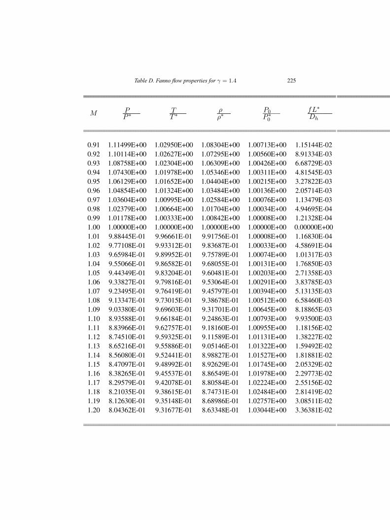
Table D. Fanno flow properties for γ = 1.4 225
M PP ∗
TT ∗
ρρ∗
P0P ∗0
fL∗
Dh
0.91 1.11499E+00 1.02950E+00 1.08304E+00 1.00713E+00 1.15144E-020.92 1.10114E+00 1.02627E+00 1.07295E+00 1.00560E+00 8.91334E-030.93 1.08758E+00 1.02304E+00 1.06309E+00 1.00426E+00 6.68729E-030.94 1.07430E+00 1.01978E+00 1.05346E+00 1.00311E+00 4.81545E-030.95 1.06129E+00 1.01652E+00 1.04404E+00 1.00215E+00 3.27822E-030.96 1.04854E+00 1.01324E+00 1.03484E+00 1.00136E+00 2.05714E-030.97 1.03604E+00 1.00995E+00 1.02584E+00 1.00076E+00 1.13479E-030.98 1.02379E+00 1.00664E+00 1.01704E+00 1.00034E+00 4.94695E-040.99 1.01178E+00 1.00333E+00 1.00842E+00 1.00008E+00 1.21328E-041.00 1.00000E+00 1.00000E+00 1.00000E+00 1.00000E+00 0.00000E+001.01 9.88445E-01 9.96661E-01 9.91756E-01 1.00008E+00 1.16830E-041.02 9.77108E-01 9.93312E-01 9.83687E-01 1.00033E+00 4.58691E-041.03 9.65984E-01 9.89952E-01 9.75789E-01 1.00074E+00 1.01317E-031.04 9.55066E-01 9.86582E-01 9.68055E-01 1.00131E+00 1.76850E-031.05 9.44349E-01 9.83204E-01 9.60481E-01 1.00203E+00 2.71358E-031.06 9.33827E-01 9.79816E-01 9.53064E-01 1.00291E+00 3.83785E-031.07 9.23495E-01 9.76419E-01 9.45797E-01 1.00394E+00 5.13135E-031.08 9.13347E-01 9.73015E-01 9.38678E-01 1.00512E+00 6.58460E-031.09 9.03380E-01 9.69603E-01 9.31701E-01 1.00645E+00 8.18865E-031.10 8.93588E-01 9.66184E-01 9.24863E-01 1.00793E+00 9.93500E-031.11 8.83966E-01 9.62757E-01 9.18160E-01 1.00955E+00 1.18156E-021.12 8.74510E-01 9.59325E-01 9.11589E-01 1.01131E+00 1.38227E-021.13 8.65216E-01 9.55886E-01 9.05146E-01 1.01322E+00 1.59492E-021.14 8.56080E-01 9.52441E-01 8.98827E-01 1.01527E+00 1.81881E-021.15 8.47097E-01 9.48992E-01 8.92629E-01 1.01745E+00 2.05329E-021.16 8.38265E-01 9.45537E-01 8.86549E-01 1.01978E+00 2.29773E-021.17 8.29579E-01 9.42078E-01 8.80584E-01 1.02224E+00 2.55156E-021.18 8.21035E-01 9.38615E-01 8.74731E-01 1.02484E+00 2.81419E-021.19 8.12630E-01 9.35148E-01 8.68986E-01 1.02757E+00 3.08511E-021.20 8.04362E-01 9.31677E-01 8.63348E-01 1.03044E+00 3.36381E-02
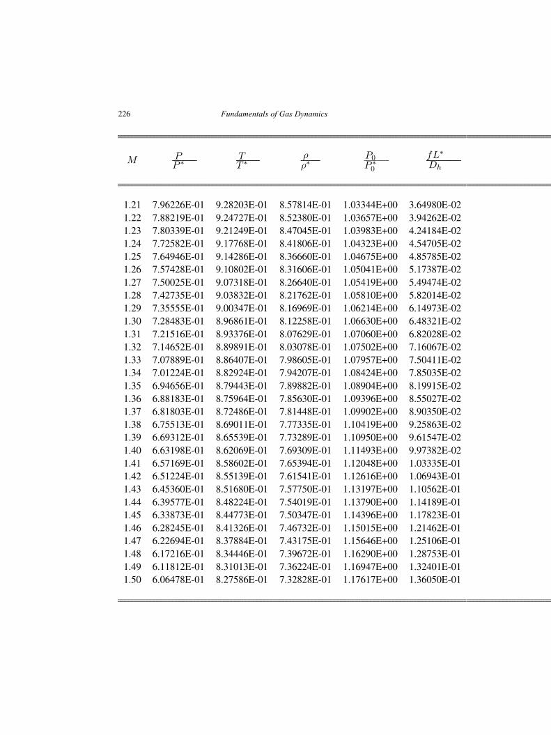
226 Fundamentals of Gas Dynamics
M PP ∗
TT ∗
ρρ∗
P0P ∗0
fL∗
Dh
1.21 7.96226E-01 9.28203E-01 8.57814E-01 1.03344E+00 3.64980E-021.22 7.88219E-01 9.24727E-01 8.52380E-01 1.03657E+00 3.94262E-021.23 7.80339E-01 9.21249E-01 8.47045E-01 1.03983E+00 4.24184E-021.24 7.72582E-01 9.17768E-01 8.41806E-01 1.04323E+00 4.54705E-021.25 7.64946E-01 9.14286E-01 8.36660E-01 1.04675E+00 4.85785E-021.26 7.57428E-01 9.10802E-01 8.31606E-01 1.05041E+00 5.17387E-021.27 7.50025E-01 9.07318E-01 8.26640E-01 1.05419E+00 5.49474E-021.28 7.42735E-01 9.03832E-01 8.21762E-01 1.05810E+00 5.82014E-021.29 7.35555E-01 9.00347E-01 8.16969E-01 1.06214E+00 6.14973E-021.30 7.28483E-01 8.96861E-01 8.12258E-01 1.06630E+00 6.48321E-021.31 7.21516E-01 8.93376E-01 8.07629E-01 1.07060E+00 6.82028E-021.32 7.14652E-01 8.89891E-01 8.03078E-01 1.07502E+00 7.16067E-021.33 7.07889E-01 8.86407E-01 7.98605E-01 1.07957E+00 7.50411E-021.34 7.01224E-01 8.82924E-01 7.94207E-01 1.08424E+00 7.85035E-021.35 6.94656E-01 8.79443E-01 7.89882E-01 1.08904E+00 8.19915E-021.36 6.88183E-01 8.75964E-01 7.85630E-01 1.09396E+00 8.55027E-021.37 6.81803E-01 8.72486E-01 7.81448E-01 1.09902E+00 8.90350E-021.38 6.75513E-01 8.69011E-01 7.77335E-01 1.10419E+00 9.25863E-021.39 6.69312E-01 8.65539E-01 7.73289E-01 1.10950E+00 9.61547E-021.40 6.63198E-01 8.62069E-01 7.69309E-01 1.11493E+00 9.97382E-021.41 6.57169E-01 8.58602E-01 7.65394E-01 1.12048E+00 1.03335E-011.42 6.51224E-01 8.55139E-01 7.61541E-01 1.12616E+00 1.06943E-011.43 6.45360E-01 8.51680E-01 7.57750E-01 1.13197E+00 1.10562E-011.44 6.39577E-01 8.48224E-01 7.54019E-01 1.13790E+00 1.14189E-011.45 6.33873E-01 8.44773E-01 7.50347E-01 1.14396E+00 1.17823E-011.46 6.28245E-01 8.41326E-01 7.46732E-01 1.15015E+00 1.21462E-011.47 6.22694E-01 8.37884E-01 7.43175E-01 1.15646E+00 1.25106E-011.48 6.17216E-01 8.34446E-01 7.39672E-01 1.16290E+00 1.28753E-011.49 6.11812E-01 8.31013E-01 7.36224E-01 1.16947E+00 1.32401E-011.50 6.06478E-01 8.27586E-01 7.32828E-01 1.17617E+00 1.36050E-01
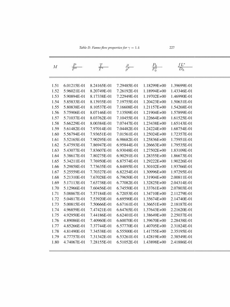
Table D. Fanno flow properties for γ = 1.4 227
M PP ∗
TT ∗
ρρ∗
P0P ∗0
fL∗
Dh
1.51 6.01215E-01 8.24165E-01 7.29485E-01 1.18299E+00 1.39699E-011.52 5.96021E-01 8.20749E-01 7.26192E-01 1.18994E+00 1.43346E-011.53 5.90894E-01 8.17338E-01 7.22949E-01 1.19702E+00 1.46990E-011.54 5.85833E-01 8.13935E-01 7.19755E-01 1.20423E+00 1.50631E-011.55 5.80838E-01 8.10537E-01 7.16608E-01 1.21157E+00 1.54268E-011.56 5.75906E-01 8.07146E-01 7.13509E-01 1.21904E+00 1.57899E-011.57 5.71037E-01 8.03762E-01 7.10455E-01 1.22664E+00 1.61525E-011.58 5.66229E-01 8.00384E-01 7.07447E-01 1.23438E+00 1.65143E-011.59 5.61482E-01 7.97014E-01 7.04482E-01 1.24224E+00 1.68754E-011.60 5.56794E-01 7.93651E-01 7.01561E-01 1.25024E+00 1.72357E-011.61 5.52165E-01 7.90295E-01 6.98682E-01 1.25836E+00 1.75951E-011.62 5.47593E-01 7.86947E-01 6.95844E-01 1.26663E+00 1.79535E-011.63 5.43077E-01 7.83607E-01 6.93048E-01 1.27502E+00 1.83109E-011.64 5.38617E-01 7.80275E-01 6.90291E-01 1.28355E+00 1.86673E-011.65 5.34211E-01 7.76950E-01 6.87574E-01 1.29222E+00 1.90226E-011.66 5.29858E-01 7.73635E-01 6.84895E-01 1.30102E+00 1.93766E-011.67 5.25559E-01 7.70327E-01 6.82254E-01 1.30996E+00 1.97295E-011.68 5.21310E-01 7.67028E-01 6.79650E-01 1.31904E+00 2.00811E-011.69 5.17113E-01 7.63738E-01 6.77082E-01 1.32825E+00 2.04314E-011.70 5.12966E-01 7.60456E-01 6.74550E-01 1.33761E+00 2.07803E-011.71 5.08867E-01 7.57184E-01 6.72053E-01 1.34710E+00 2.11279E-011.72 5.04817E-01 7.53920E-01 6.69590E-01 1.35674E+00 2.14740E-011.73 5.00815E-01 7.50666E-01 6.67161E-01 1.36651E+00 2.18187E-011.74 4.96859E-01 7.47421E-01 6.64765E-01 1.37643E+00 2.21620E-011.75 4.92950E-01 7.44186E-01 6.62401E-01 1.38649E+00 2.25037E-011.76 4.89086E-01 7.40960E-01 6.60070E-01 1.39670E+00 2.28438E-011.77 4.85266E-01 7.37744E-01 6.57770E-01 1.40705E+00 2.31824E-011.78 4.81490E-01 7.34538E-01 6.55500E-01 1.41755E+00 2.35195E-011.79 4.77757E-01 7.31342E-01 6.53261E-01 1.42819E+00 2.38549E-011.80 4.74067E-01 7.28155E-01 6.51052E-01 1.43898E+00 2.41886E-01
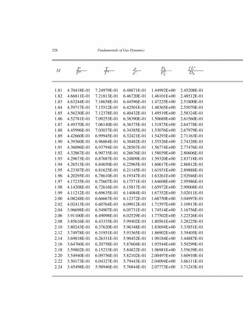
228 Fundamentals of Gas Dynamics
M PP ∗
TT ∗
ρρ∗
P0P ∗0
fL∗
Dh
1.81 4.70418E-01 7.24979E-01 6.48871E-01 1.44992E+00 2.45208E-011.82 4.66811E-01 7.21813E-01 6.46720E-01 1.46101E+00 2.48512E-011.83 4.63244E-01 7.18658E-01 6.44596E-01 1.47225E+00 2.51800E-011.84 4.59717E-01 7.15512E-01 6.42501E-01 1.48365E+00 2.55070E-011.85 4.56230E-01 7.12378E-01 6.40432E-01 1.49519E+00 2.58324E-011.86 4.52781E-01 7.09253E-01 6.38390E-01 1.50689E+00 2.61560E-011.87 4.49370E-01 7.06140E-01 6.36375E-01 1.51875E+00 2.64778E-011.88 4.45996E-01 7.03037E-01 6.34385E-01 1.53076E+00 2.67979E-011.89 4.42660E-01 6.99945E-01 6.32421E-01 1.54293E+00 2.71163E-011.90 4.39360E-01 6.96864E-01 6.30482E-01 1.55526E+00 2.74328E-011.91 4.36096E-01 6.93794E-01 6.28567E-01 1.56774E+00 2.77476E-011.92 4.32867E-01 6.90735E-01 6.26676E-01 1.58039E+00 2.80606E-011.93 4.29673E-01 6.87687E-01 6.24809E-01 1.59320E+00 2.83718E-011.94 4.26513E-01 6.84650E-01 6.22965E-01 1.60617E+00 2.86812E-011.95 4.23387E-01 6.81625E-01 6.21145E-01 1.61931E+00 2.89888E-011.96 4.20295E-01 6.78610E-01 6.19347E-01 1.63261E+00 2.92946E-011.97 4.17235E-01 6.75607E-01 6.17571E-01 1.64608E+00 2.95986E-011.98 4.14208E-01 6.72616E-01 6.15817E-01 1.65972E+00 2.99008E-011.99 4.11212E-01 6.69635E-01 6.14084E-01 1.67352E+00 3.02011E-012.00 4.08248E-01 6.66667E-01 6.12372E-01 1.68750E+00 3.04997E-012.02 4.02413E-01 6.60764E-01 6.09012E-01 1.71597E+00 3.10913E-012.04 3.96698E-01 6.54907E-01 6.05731E-01 1.74514E+00 3.16756E-012.06 3.91100E-01 6.49098E-01 6.02529E-01 1.77502E+00 3.22526E-012.08 3.85616E-01 6.43335E-01 5.99402E-01 1.80561E+00 3.28225E-012.10 3.80243E-01 6.37620E-01 5.96348E-01 1.83694E+00 3.33851E-012.12 3.74978E-01 6.31951E-01 5.93365E-01 1.86902E+00 3.39405E-012.14 3.69818E-01 6.26331E-01 5.90452E-01 1.90184E+00 3.44887E-012.16 3.64760E-01 6.20758E-01 5.87604E-01 1.93544E+00 3.50299E-012.18 3.59802E-01 6.15233E-01 5.84822E-01 1.96981E+00 3.55639E-012.20 3.54940E-01 6.09756E-01 5.82102E-01 2.00497E+00 3.60910E-012.22 3.50173E-01 6.04327E-01 5.79443E-01 2.04094E+00 3.66111E-012.24 3.45498E-01 5.98946E-01 5.76844E-01 2.07773E+00 3.71243E-01
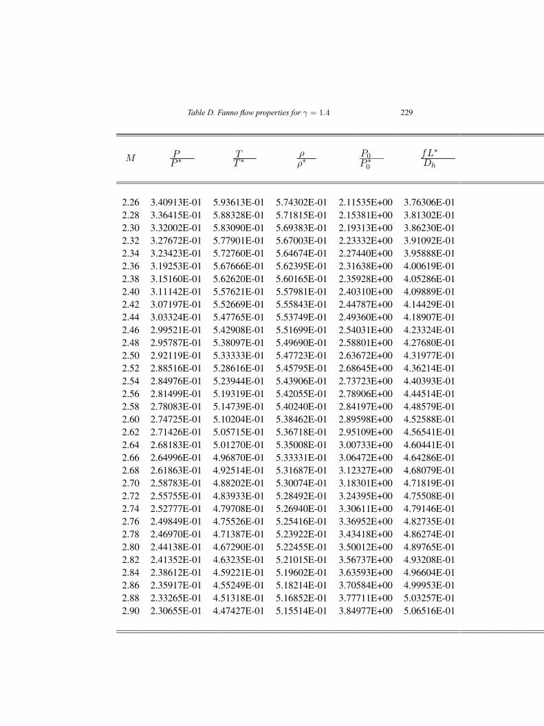
Table D. Fanno flow properties for γ = 1.4 229
M PP ∗
TT ∗
ρρ∗
P0P ∗0
fL∗
Dh
2.26 3.40913E-01 5.93613E-01 5.74302E-01 2.11535E+00 3.76306E-012.28 3.36415E-01 5.88328E-01 5.71815E-01 2.15381E+00 3.81302E-012.30 3.32002E-01 5.83090E-01 5.69383E-01 2.19313E+00 3.86230E-012.32 3.27672E-01 5.77901E-01 5.67003E-01 2.23332E+00 3.91092E-012.34 3.23423E-01 5.72760E-01 5.64674E-01 2.27440E+00 3.95888E-012.36 3.19253E-01 5.67666E-01 5.62395E-01 2.31638E+00 4.00619E-012.38 3.15160E-01 5.62620E-01 5.60165E-01 2.35928E+00 4.05286E-012.40 3.11142E-01 5.57621E-01 5.57981E-01 2.40310E+00 4.09889E-012.42 3.07197E-01 5.52669E-01 5.55843E-01 2.44787E+00 4.14429E-012.44 3.03324E-01 5.47765E-01 5.53749E-01 2.49360E+00 4.18907E-012.46 2.99521E-01 5.42908E-01 5.51699E-01 2.54031E+00 4.23324E-012.48 2.95787E-01 5.38097E-01 5.49690E-01 2.58801E+00 4.27680E-012.50 2.92119E-01 5.33333E-01 5.47723E-01 2.63672E+00 4.31977E-012.52 2.88516E-01 5.28616E-01 5.45795E-01 2.68645E+00 4.36214E-012.54 2.84976E-01 5.23944E-01 5.43906E-01 2.73723E+00 4.40393E-012.56 2.81499E-01 5.19319E-01 5.42055E-01 2.78906E+00 4.44514E-012.58 2.78083E-01 5.14739E-01 5.40240E-01 2.84197E+00 4.48579E-012.60 2.74725E-01 5.10204E-01 5.38462E-01 2.89598E+00 4.52588E-012.62 2.71426E-01 5.05715E-01 5.36718E-01 2.95109E+00 4.56541E-012.64 2.68183E-01 5.01270E-01 5.35008E-01 3.00733E+00 4.60441E-012.66 2.64996E-01 4.96870E-01 5.33331E-01 3.06472E+00 4.64286E-012.68 2.61863E-01 4.92514E-01 5.31687E-01 3.12327E+00 4.68079E-012.70 2.58783E-01 4.88202E-01 5.30074E-01 3.18301E+00 4.71819E-012.72 2.55755E-01 4.83933E-01 5.28492E-01 3.24395E+00 4.75508E-012.74 2.52777E-01 4.79708E-01 5.26940E-01 3.30611E+00 4.79146E-012.76 2.49849E-01 4.75526E-01 5.25416E-01 3.36952E+00 4.82735E-012.78 2.46970E-01 4.71387E-01 5.23922E-01 3.43418E+00 4.86274E-012.80 2.44138E-01 4.67290E-01 5.22455E-01 3.50012E+00 4.89765E-012.82 2.41352E-01 4.63235E-01 5.21015E-01 3.56737E+00 4.93208E-012.84 2.38612E-01 4.59221E-01 5.19602E-01 3.63593E+00 4.96604E-012.86 2.35917E-01 4.55249E-01 5.18214E-01 3.70584E+00 4.99953E-012.88 2.33265E-01 4.51318E-01 5.16852E-01 3.77711E+00 5.03257E-012.90 2.30655E-01 4.47427E-01 5.15514E-01 3.84977E+00 5.06516E-01
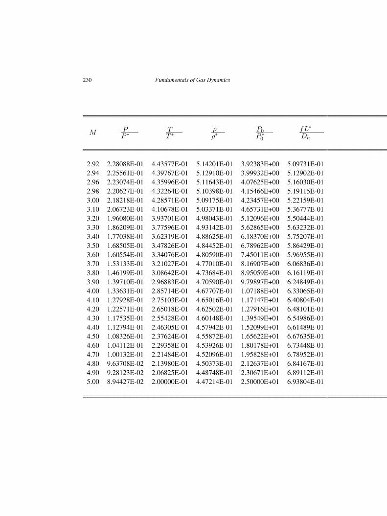
230 Fundamentals of Gas Dynamics
M PP ∗
TT ∗
ρρ∗
P0P ∗0
fL∗
Dh
2.92 2.28088E-01 4.43577E-01 5.14201E-01 3.92383E+00 5.09731E-012.94 2.25561E-01 4.39767E-01 5.12910E-01 3.99932E+00 5.12902E-012.96 2.23074E-01 4.35996E-01 5.11643E-01 4.07625E+00 5.16030E-012.98 2.20627E-01 4.32264E-01 5.10398E-01 4.15466E+00 5.19115E-013.00 2.18218E-01 4.28571E-01 5.09175E-01 4.23457E+00 5.22159E-013.10 2.06723E-01 4.10678E-01 5.03371E-01 4.65731E+00 5.36777E-013.20 1.96080E-01 3.93701E-01 4.98043E-01 5.12096E+00 5.50444E-013.30 1.86209E-01 3.77596E-01 4.93142E-01 5.62865E+00 5.63232E-013.40 1.77038E-01 3.62319E-01 4.88625E-01 6.18370E+00 5.75207E-013.50 1.68505E-01 3.47826E-01 4.84452E-01 6.78962E+00 5.86429E-013.60 1.60554E-01 3.34076E-01 4.80590E-01 7.45011E+00 5.96955E-013.70 1.53133E-01 3.21027E-01 4.77010E-01 8.16907E+00 6.06836E-013.80 1.46199E-01 3.08642E-01 4.73684E-01 8.95059E+00 6.16119E-013.90 1.39710E-01 2.96883E-01 4.70590E-01 9.79897E+00 6.24849E-014.00 1.33631E-01 2.85714E-01 4.67707E-01 1.07188E+01 6.33065E-014.10 1.27928E-01 2.75103E-01 4.65016E-01 1.17147E+01 6.40804E-014.20 1.22571E-01 2.65018E-01 4.62502E-01 1.27916E+01 6.48101E-014.30 1.17535E-01 2.55428E-01 4.60148E-01 1.39549E+01 6.54986E-014.40 1.12794E-01 2.46305E-01 4.57942E-01 1.52099E+01 6.61489E-014.50 1.08326E-01 2.37624E-01 4.55872E-01 1.65622E+01 6.67635E-014.60 1.04112E-01 2.29358E-01 4.53926E-01 1.80178E+01 6.73448E-014.70 1.00132E-01 2.21484E-01 4.52096E-01 1.95828E+01 6.78952E-014.80 9.63708E-02 2.13980E-01 4.50373E-01 2.12637E+01 6.84167E-014.90 9.28123E-02 2.06825E-01 4.48748E-01 2.30671E+01 6.89112E-015.00 8.94427E-02 2.00000E-01 4.47214E-01 2.50000E+01 6.93804E-01

Table E. Oblique shock wave angle β indegrees for γ = 1.4
231
Fundamentals of Gas Dynamics, Second Edition. V. Babu.© 2015 V. Babu. Published 2015 by Athena Academic Ltd and John Wiley & Sons Ltd
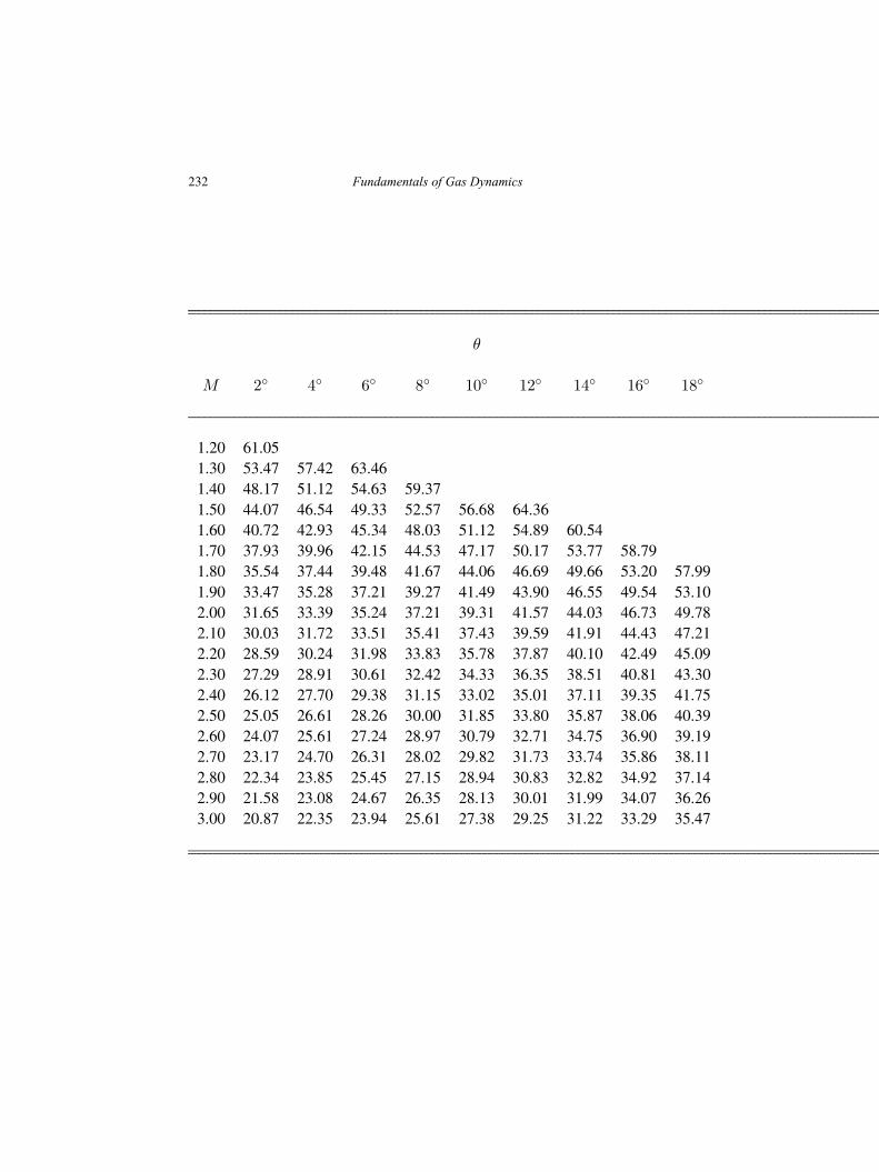
232 Fundamentals of Gas Dynamics
θ
M 2◦ 4◦ 6◦ 8◦ 10◦ 12◦ 14◦ 16◦ 18◦
1.20 61.051.30 53.47 57.42 63.461.40 48.17 51.12 54.63 59.371.50 44.07 46.54 49.33 52.57 56.68 64.361.60 40.72 42.93 45.34 48.03 51.12 54.89 60.541.70 37.93 39.96 42.15 44.53 47.17 50.17 53.77 58.791.80 35.54 37.44 39.48 41.67 44.06 46.69 49.66 53.20 57.991.90 33.47 35.28 37.21 39.27 41.49 43.90 46.55 49.54 53.102.00 31.65 33.39 35.24 37.21 39.31 41.57 44.03 46.73 49.782.10 30.03 31.72 33.51 35.41 37.43 39.59 41.91 44.43 47.212.20 28.59 30.24 31.98 33.83 35.78 37.87 40.10 42.49 45.092.30 27.29 28.91 30.61 32.42 34.33 36.35 38.51 40.81 43.302.40 26.12 27.70 29.38 31.15 33.02 35.01 37.11 39.35 41.752.50 25.05 26.61 28.26 30.00 31.85 33.80 35.87 38.06 40.392.60 24.07 25.61 27.24 28.97 30.79 32.71 34.75 36.90 39.192.70 23.17 24.70 26.31 28.02 29.82 31.73 33.74 35.86 38.112.80 22.34 23.85 25.45 27.15 28.94 30.83 32.82 34.92 37.142.90 21.58 23.08 24.67 26.35 28.13 30.01 31.99 34.07 36.263.00 20.87 22.35 23.94 25.61 27.38 29.25 31.22 33.29 35.47
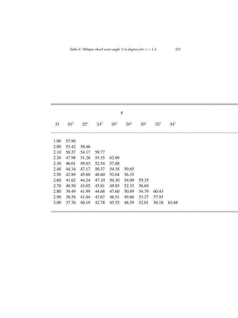
Table E. Oblique shock wave angle β in degrees for γ = 1.4 233
θ
M 20◦ 22◦ 24◦ 26◦ 28◦ 30◦ 32◦ 34◦
1.90 57.902.00 53.42 58.462.10 50.37 54.17 59.772.20 47.98 51.28 55.35 62.692.30 46.01 49.03 52.54 57.082.40 44.34 47.17 50.37 54.18 59.652.50 42.89 45.60 48.60 52.04 56.332.60 41.62 44.24 47.10 50.30 54.09 59.352.70 40.50 43.05 45.81 48.85 52.33 56.692.80 39.49 41.99 44.68 47.60 50.89 54.79 60.432.90 38.58 41.04 43.67 46.51 49.66 53.27 57.933.00 37.76 40.19 42.78 45.55 48.59 52.01 56.18 63.68
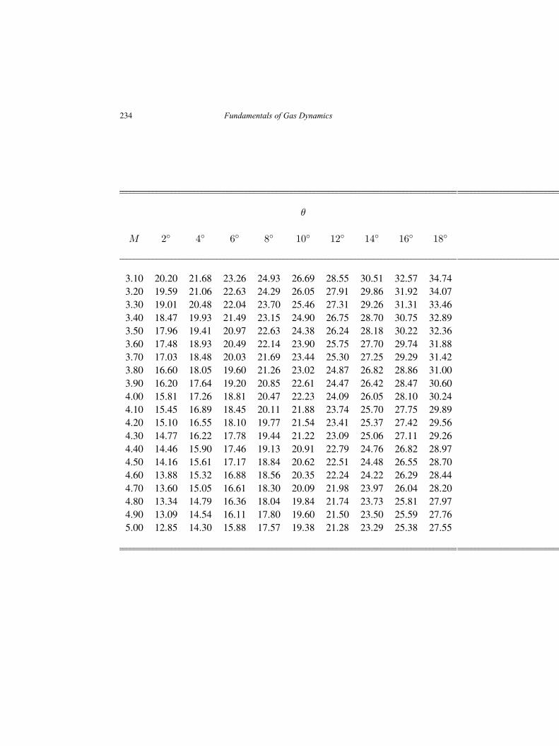
234 Fundamentals of Gas Dynamics
θ
M 2◦ 4◦ 6◦ 8◦ 10◦ 12◦ 14◦ 16◦ 18◦
3.10 20.20 21.68 23.26 24.93 26.69 28.55 30.51 32.57 34.743.20 19.59 21.06 22.63 24.29 26.05 27.91 29.86 31.92 34.073.30 19.01 20.48 22.04 23.70 25.46 27.31 29.26 31.31 33.463.40 18.47 19.93 21.49 23.15 24.90 26.75 28.70 30.75 32.893.50 17.96 19.41 20.97 22.63 24.38 26.24 28.18 30.22 32.363.60 17.48 18.93 20.49 22.14 23.90 25.75 27.70 29.74 31.883.70 17.03 18.48 20.03 21.69 23.44 25.30 27.25 29.29 31.423.80 16.60 18.05 19.60 21.26 23.02 24.87 26.82 28.86 31.003.90 16.20 17.64 19.20 20.85 22.61 24.47 26.42 28.47 30.604.00 15.81 17.26 18.81 20.47 22.23 24.09 26.05 28.10 30.244.10 15.45 16.89 18.45 20.11 21.88 23.74 25.70 27.75 29.894.20 15.10 16.55 18.10 19.77 21.54 23.41 25.37 27.42 29.564.30 14.77 16.22 17.78 19.44 21.22 23.09 25.06 27.11 29.264.40 14.46 15.90 17.46 19.13 20.91 22.79 24.76 26.82 28.974.50 14.16 15.61 17.17 18.84 20.62 22.51 24.48 26.55 28.704.60 13.88 15.32 16.88 18.56 20.35 22.24 24.22 26.29 28.444.70 13.60 15.05 16.61 18.30 20.09 21.98 23.97 26.04 28.204.80 13.34 14.79 16.36 18.04 19.84 21.74 23.73 25.81 27.974.90 13.09 14.54 16.11 17.80 19.60 21.50 23.50 25.59 27.765.00 12.85 14.30 15.88 17.57 19.38 21.28 23.29 25.38 27.55
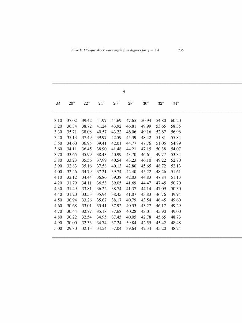
Table E. Oblique shock wave angle β in degrees for γ = 1.4 235
θ
M 20◦ 22◦ 24◦ 26◦ 28◦ 30◦ 32◦ 34◦
3.10 37.02 39.42 41.97 44.69 47.65 50.94 54.80 60.203.20 36.34 38.72 41.24 43.92 46.81 49.99 53.65 58.353.30 35.71 38.08 40.57 43.22 46.06 49.16 52.67 56.963.40 35.13 37.49 39.97 42.59 45.39 48.42 51.81 55.843.50 34.60 36.95 39.41 42.01 44.77 47.76 51.05 54.893.60 34.11 36.45 38.90 41.48 44.21 47.15 50.38 54.073.70 33.65 35.99 38.43 40.99 43.70 46.61 49.77 53.343.80 33.23 35.56 37.99 40.54 43.23 46.10 49.22 52.703.90 32.83 35.16 37.58 40.13 42.80 45.65 48.72 52.134.00 32.46 34.79 37.21 39.74 42.40 45.22 48.26 51.614.10 32.12 34.44 36.86 39.38 42.03 44.83 47.84 51.134.20 31.79 34.11 36.53 39.05 41.69 44.47 47.45 50.704.30 31.49 33.81 36.22 38.74 41.37 44.14 47.09 50.304.40 31.20 33.53 35.94 38.45 41.07 43.83 46.76 49.944.50 30.94 33.26 35.67 38.17 40.79 43.54 46.45 49.604.60 30.68 33.01 35.41 37.92 40.53 43.27 46.17 49.294.70 30.44 32.77 35.18 37.68 40.28 43.01 45.90 49.004.80 30.22 32.54 34.95 37.45 40.05 42.78 45.65 48.734.90 30.00 32.33 34.74 37.24 39.84 42.55 45.42 48.485.00 29.80 32.13 34.54 37.04 39.64 42.34 45.20 48.24
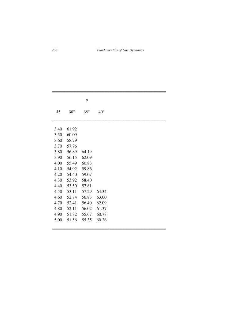
236 Fundamentals of Gas Dynamics
θ
M 36◦ 38◦ 40◦
3.40 61.923.50 60.093.60 58.793.70 57.763.80 56.89 64.193.90 56.15 62.094.00 55.49 60.834.10 54.92 59.864.20 54.40 59.074.30 53.92 58.404.40 53.50 57.814.50 53.11 57.29 64.344.60 52.74 56.83 63.004.70 52.41 56.40 62.094.80 52.11 56.02 61.374.90 51.82 55.67 60.785.00 51.56 55.35 60.26

Table F. Mach angle and Prandtl Meyerangle for γ = 1.4
237
Fundamentals of Gas Dynamics, Second Edition. V. Babu.© 2015 V. Babu. Published 2015 by Athena Academic Ltd and John Wiley & Sons Ltd
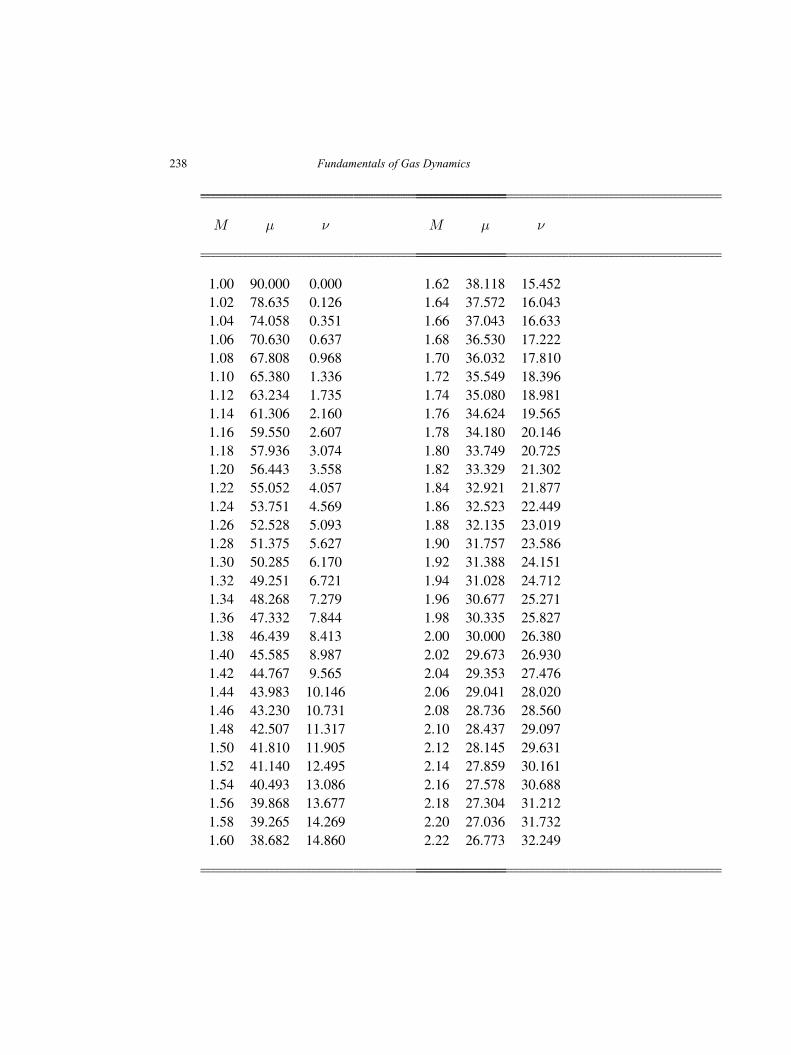
238 Fundamentals of Gas Dynamics
M µ ν
1.00 90.000 0.0001.02 78.635 0.1261.04 74.058 0.3511.06 70.630 0.6371.08 67.808 0.9681.10 65.380 1.3361.12 63.234 1.7351.14 61.306 2.1601.16 59.550 2.6071.18 57.936 3.0741.20 56.443 3.5581.22 55.052 4.0571.24 53.751 4.5691.26 52.528 5.0931.28 51.375 5.6271.30 50.285 6.1701.32 49.251 6.7211.34 48.268 7.2791.36 47.332 7.8441.38 46.439 8.4131.40 45.585 8.9871.42 44.767 9.5651.44 43.983 10.1461.46 43.230 10.7311.48 42.507 11.3171.50 41.810 11.9051.52 41.140 12.4951.54 40.493 13.0861.56 39.868 13.6771.58 39.265 14.2691.60 38.682 14.860
M µ ν
1.62 38.118 15.4521.64 37.572 16.0431.66 37.043 16.6331.68 36.530 17.2221.70 36.032 17.8101.72 35.549 18.3961.74 35.080 18.9811.76 34.624 19.5651.78 34.180 20.1461.80 33.749 20.7251.82 33.329 21.3021.84 32.921 21.8771.86 32.523 22.4491.88 32.135 23.0191.90 31.757 23.5861.92 31.388 24.1511.94 31.028 24.7121.96 30.677 25.2711.98 30.335 25.8272.00 30.000 26.3802.02 29.673 26.9302.04 29.353 27.4762.06 29.041 28.0202.08 28.736 28.5602.10 28.437 29.0972.12 28.145 29.6312.14 27.859 30.1612.16 27.578 30.6882.18 27.304 31.2122.20 27.036 31.7322.22 26.773 32.249
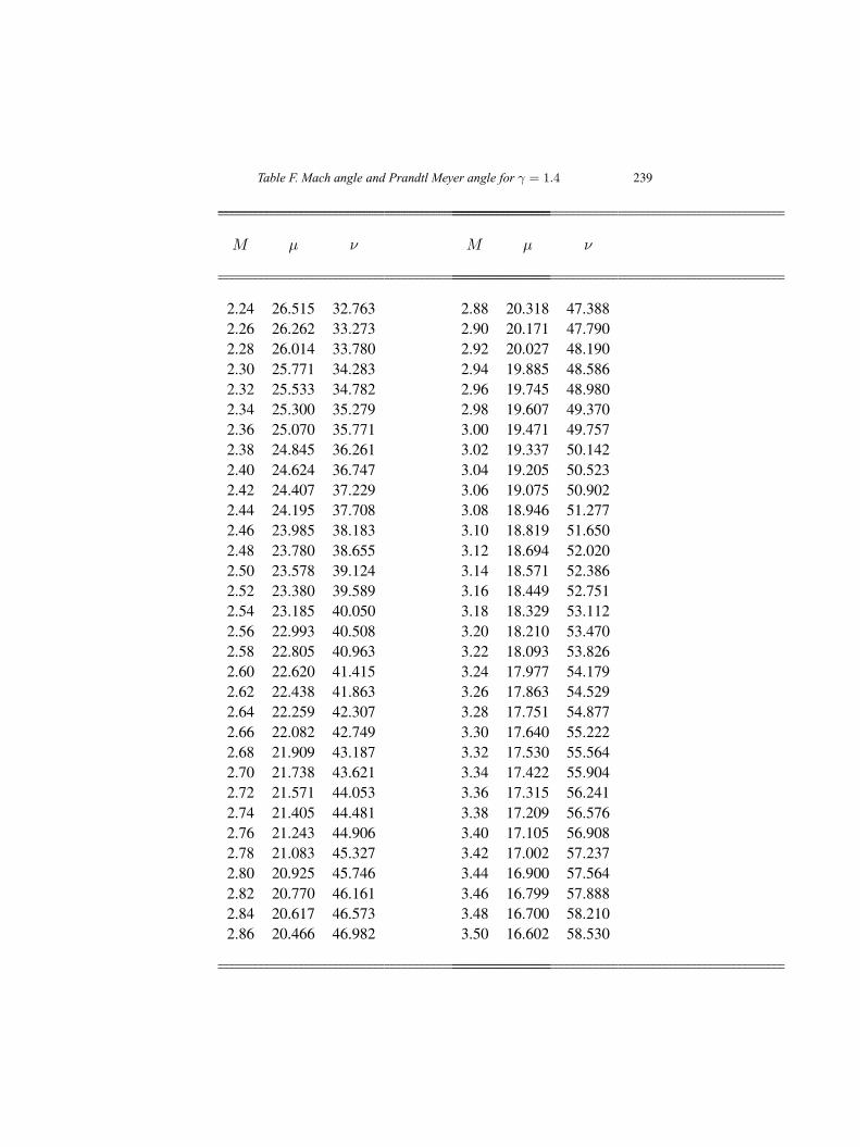
Table F. Mach angle and Prandtl Meyer angle for γ = 1.4 239
M µ ν
2.24 26.515 32.7632.26 26.262 33.2732.28 26.014 33.7802.30 25.771 34.2832.32 25.533 34.7822.34 25.300 35.2792.36 25.070 35.7712.38 24.845 36.2612.40 24.624 36.7472.42 24.407 37.2292.44 24.195 37.7082.46 23.985 38.1832.48 23.780 38.6552.50 23.578 39.1242.52 23.380 39.5892.54 23.185 40.0502.56 22.993 40.5082.58 22.805 40.9632.60 22.620 41.4152.62 22.438 41.8632.64 22.259 42.3072.66 22.082 42.7492.68 21.909 43.1872.70 21.738 43.6212.72 21.571 44.0532.74 21.405 44.4812.76 21.243 44.9062.78 21.083 45.3272.80 20.925 45.7462.82 20.770 46.1612.84 20.617 46.5732.86 20.466 46.982
M µ ν
2.88 20.318 47.3882.90 20.171 47.7902.92 20.027 48.1902.94 19.885 48.5862.96 19.745 48.9802.98 19.607 49.3703.00 19.471 49.7573.02 19.337 50.1423.04 19.205 50.5233.06 19.075 50.9023.08 18.946 51.2773.10 18.819 51.6503.12 18.694 52.0203.14 18.571 52.3863.16 18.449 52.7513.18 18.329 53.1123.20 18.210 53.4703.22 18.093 53.8263.24 17.977 54.1793.26 17.863 54.5293.28 17.751 54.8773.30 17.640 55.2223.32 17.530 55.5643.34 17.422 55.9043.36 17.315 56.2413.38 17.209 56.5763.40 17.105 56.9083.42 17.002 57.2373.44 16.900 57.5643.46 16.799 57.8883.48 16.700 58.2103.50 16.602 58.530
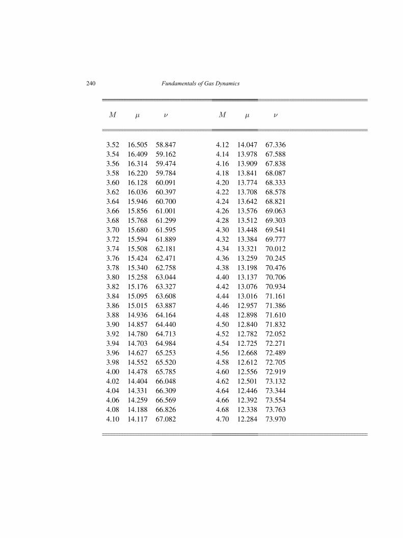
240 Fundamentals of Gas Dynamics
M µ ν
3.52 16.505 58.8473.54 16.409 59.1623.56 16.314 59.4743.58 16.220 59.7843.60 16.128 60.0913.62 16.036 60.3973.64 15.946 60.7003.66 15.856 61.0013.68 15.768 61.2993.70 15.680 61.5953.72 15.594 61.8893.74 15.508 62.1813.76 15.424 62.4713.78 15.340 62.7583.80 15.258 63.0443.82 15.176 63.3273.84 15.095 63.6083.86 15.015 63.8873.88 14.936 64.1643.90 14.857 64.4403.92 14.780 64.7133.94 14.703 64.9843.96 14.627 65.2533.98 14.552 65.5204.00 14.478 65.7854.02 14.404 66.0484.04 14.331 66.3094.06 14.259 66.5694.08 14.188 66.8264.10 14.117 67.082
M µ ν
4.12 14.047 67.3364.14 13.978 67.5884.16 13.909 67.8384.18 13.841 68.0874.20 13.774 68.3334.22 13.708 68.5784.24 13.642 68.8214.26 13.576 69.0634.28 13.512 69.3034.30 13.448 69.5414.32 13.384 69.7774.34 13.321 70.0124.36 13.259 70.2454.38 13.198 70.4764.40 13.137 70.7064.42 13.076 70.9344.44 13.016 71.1614.46 12.957 71.3864.48 12.898 71.6104.50 12.840 71.8324.52 12.782 72.0524.54 12.725 72.2714.56 12.668 72.4894.58 12.612 72.7054.60 12.556 72.9194.62 12.501 73.1324.64 12.446 73.3444.66 12.392 73.5544.68 12.338 73.7634.70 12.284 73.970
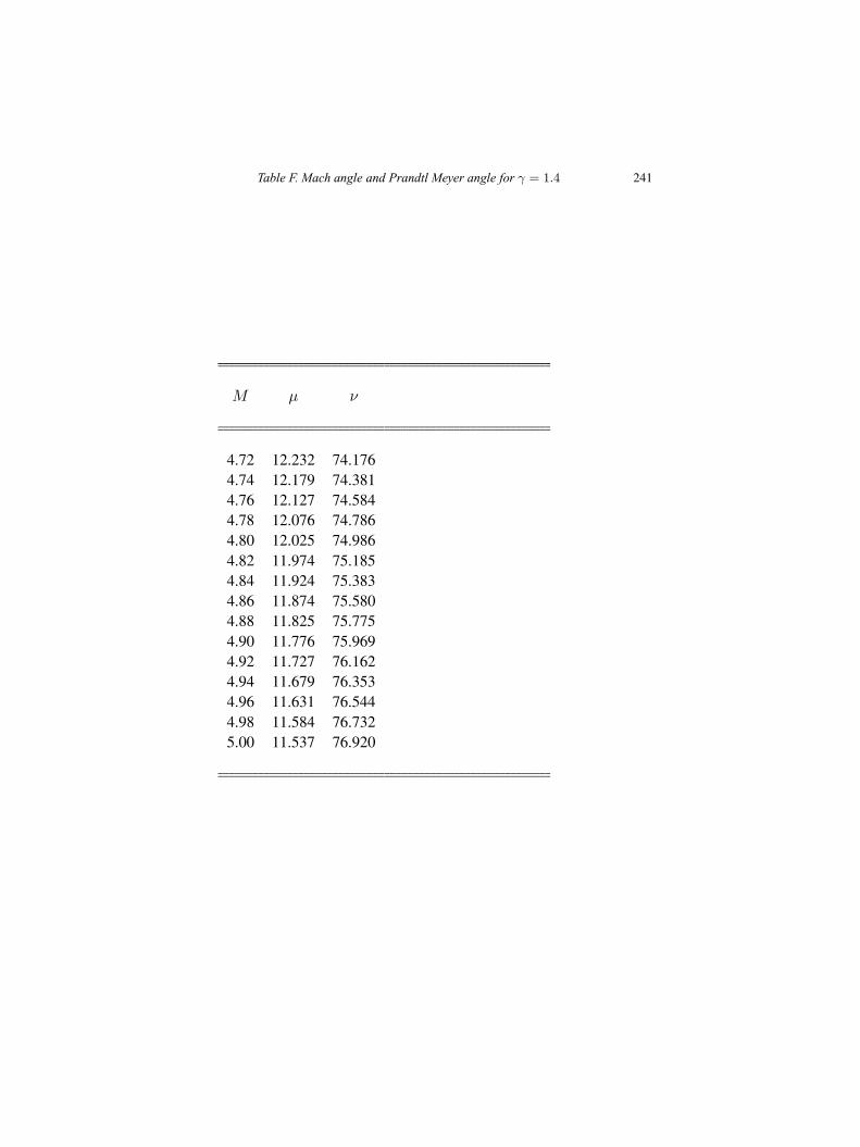
Table F. Mach angle and Prandtl Meyer angle for γ = 1.4 241
M µ ν
4.72 12.232 74.1764.74 12.179 74.3814.76 12.127 74.5844.78 12.076 74.7864.80 12.025 74.9864.82 11.974 75.1854.84 11.924 75.3834.86 11.874 75.5804.88 11.825 75.7754.90 11.776 75.9694.92 11.727 76.1624.94 11.679 76.3534.96 11.631 76.5444.98 11.584 76.7325.00 11.537 76.920

242 Fundamentals of Gas Dynamics
Table G. Thermodynamic properties ofsteam, temperature table
243
Fundamentals of Gas Dynamics, Second Edition. V. Babu.© 2015 V. Babu. Published 2015 by Athena Academic Ltd and John Wiley & Sons Ltd
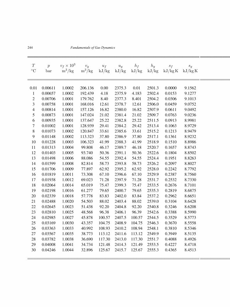
244 Fundamentals of Gas Dynamics
T p vf × 103 vg uf ug hf hg sf sg◦C bar m3/kg m3/kg kJ/kg kJ/kg kJ/kg kJ/kg kJ/kgK kJ/kgK
0.01 0.00611 1.0002 206.136 0.00 2375.3 0.01 2501.3 0.0000 9.15621 0.00657 1.0002 192.439 4.18 2375.9 4.183 2502.4 0.0153 9.12772 0.00706 1.0001 179.762 8.40 2377.3 8.401 2504.2 0.0306 9.10133 0.00758 1.0001 168.016 12.61 2378.7 12.61 2506.0 0.0459 9.07524 0.00814 1.0001 157.126 16.82 2380.0 16.82 2507.9 0.0611 9.04925 0.00873 1.0001 147.024 21.02 2381.4 21.02 2509.7 0.0763 9.02366 0.00935 1.0001 137.647 25.22 2382.8 25.22 2511.5 0.0913 8.99817 0.01002 1.0001 128.939 29.41 2384.2 29.42 2513.4 0.1063 8.97298 0.01073 1.0002 120.847 33.61 2385.6 33.61 2515.2 0.1213 8.94799 0.01148 1.0002 113.323 37.80 2386.9 37.80 2517.1 0.1361 8.9232
10 0.01228 1.0003 106.323 41.99 2388.3 41.99 2518.9 0.1510 8.898611 0.01313 1.0004 99.808 46.17 2389.7 46.18 2520.7 0.1657 8.874312 0.01403 1.0005 93.740 50.36 2391.1 50.36 2522.6 0.1804 8.850213 0.01498 1.0006 88.086 54.55 2392.4 54.55 2524.4 0.1951 8.826314 0.01599 1.0008 82.814 58.73 2393.8 58.73 2526.2 0.2097 8.802715 0.01706 1.0009 77.897 62.92 2395.2 62.92 2528.0 0.2242 8.779216 0.01819 1.0011 73.308 67.10 2396.6 67.10 2529.9 0.2387 8.756017 0.01938 1.0012 69.023 71.28 2397.9 71.28 2531.7 0.2532 8.733018 0.02064 1.0014 65.019 75.47 2399.3 75.47 2533.5 0.2676 8.710119 0.02198 1.0016 61.277 79.65 2400.7 79.65 2535.3 0.2819 8.687520 0.02339 1.0018 57.778 83.83 2402.0 83.84 2537.2 0.2962 8.665121 0.02488 1.0020 54.503 88.02 2403.4 88.02 2539.0 0.3104 8.642822 0.02645 1.0023 51.438 92.20 2404.8 92.20 2540.8 0.3246 8.620823 0.02810 1.0025 48.568 96.38 2406.1 96.39 2542.6 0.3388 8.599024 0.02985 1.0027 45.878 100.57 2407.5 100.57 2544.5 0.3529 8.577325 0.03169 1.0030 43.357 104.75 2408.9 104.75 2546.3 0.3670 8.555826 0.03363 1.0033 40.992 108.93 2410.2 108.94 2548.1 0.3810 8.534627 0.03567 1.0035 38.773 113.12 2411.6 113.12 2549.9 0.3949 8.513528 0.03782 1.0038 36.690 117.30 2413.0 117.30 2551.7 0.4088 8.492629 0.04008 1.0041 34.734 121.48 2414.3 121.49 2553.5 0.4227 8.471830 0.04246 1.0044 32.896 125.67 2415.7 125.67 2555.3 0.4365 8.4513
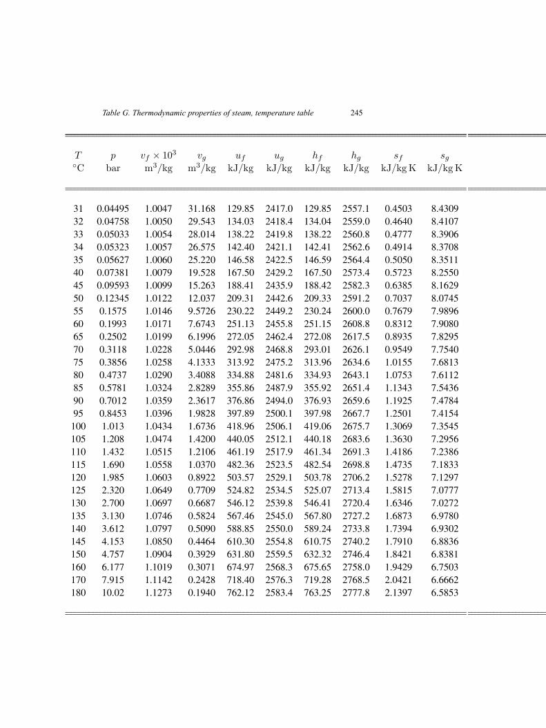
Table G. Thermodynamic properties of steam, temperature table 245
T p vf × 103 vg uf ug hf hg sf sg◦C bar m3/kg m3/kg kJ/kg kJ/kg kJ/kg kJ/kg kJ/kgK kJ/kgK
31 0.04495 1.0047 31.168 129.85 2417.0 129.85 2557.1 0.4503 8.430932 0.04758 1.0050 29.543 134.03 2418.4 134.04 2559.0 0.4640 8.410733 0.05033 1.0054 28.014 138.22 2419.8 138.22 2560.8 0.4777 8.390634 0.05323 1.0057 26.575 142.40 2421.1 142.41 2562.6 0.4914 8.370835 0.05627 1.0060 25.220 146.58 2422.5 146.59 2564.4 0.5050 8.351140 0.07381 1.0079 19.528 167.50 2429.2 167.50 2573.4 0.5723 8.255045 0.09593 1.0099 15.263 188.41 2435.9 188.42 2582.3 0.6385 8.162950 0.12345 1.0122 12.037 209.31 2442.6 209.33 2591.2 0.7037 8.074555 0.1575 1.0146 9.5726 230.22 2449.2 230.24 2600.0 0.7679 7.989660 0.1993 1.0171 7.6743 251.13 2455.8 251.15 2608.8 0.8312 7.908065 0.2502 1.0199 6.1996 272.05 2462.4 272.08 2617.5 0.8935 7.829570 0.3118 1.0228 5.0446 292.98 2468.8 293.01 2626.1 0.9549 7.754075 0.3856 1.0258 4.1333 313.92 2475.2 313.96 2634.6 1.0155 7.681380 0.4737 1.0290 3.4088 334.88 2481.6 334.93 2643.1 1.0753 7.611285 0.5781 1.0324 2.8289 355.86 2487.9 355.92 2651.4 1.1343 7.543690 0.7012 1.0359 2.3617 376.86 2494.0 376.93 2659.6 1.1925 7.478495 0.8453 1.0396 1.9828 397.89 2500.1 397.98 2667.7 1.2501 7.4154
100 1.013 1.0434 1.6736 418.96 2506.1 419.06 2675.7 1.3069 7.3545105 1.208 1.0474 1.4200 440.05 2512.1 440.18 2683.6 1.3630 7.2956110 1.432 1.0515 1.2106 461.19 2517.9 461.34 2691.3 1.4186 7.2386115 1.690 1.0558 1.0370 482.36 2523.5 482.54 2698.8 1.4735 7.1833120 1.985 1.0603 0.8922 503.57 2529.1 503.78 2706.2 1.5278 7.1297125 2.320 1.0649 0.7709 524.82 2534.5 525.07 2713.4 1.5815 7.0777130 2.700 1.0697 0.6687 546.12 2539.8 546.41 2720.4 1.6346 7.0272135 3.130 1.0746 0.5824 567.46 2545.0 567.80 2727.2 1.6873 6.9780140 3.612 1.0797 0.5090 588.85 2550.0 589.24 2733.8 1.7394 6.9302145 4.153 1.0850 0.4464 610.30 2554.8 610.75 2740.2 1.7910 6.8836150 4.757 1.0904 0.3929 631.80 2559.5 632.32 2746.4 1.8421 6.8381160 6.177 1.1019 0.3071 674.97 2568.3 675.65 2758.0 1.9429 6.7503170 7.915 1.1142 0.2428 718.40 2576.3 719.28 2768.5 2.0421 6.6662180 10.02 1.1273 0.1940 762.12 2583.4 763.25 2777.8 2.1397 6.5853
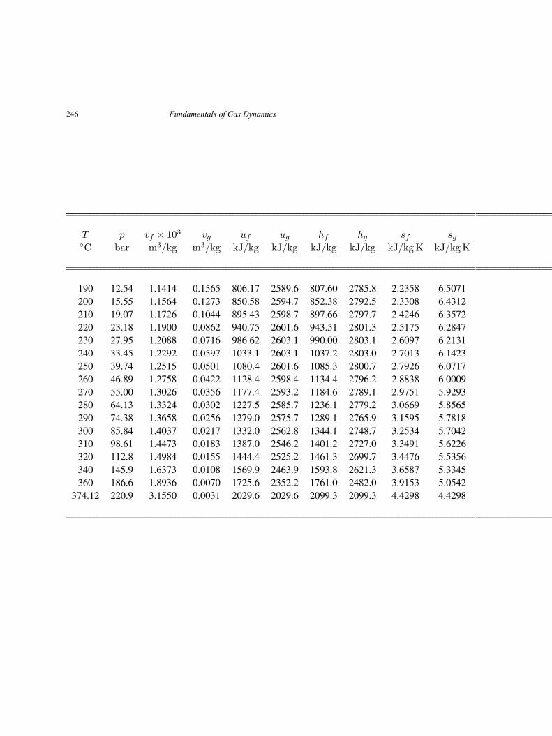
246 Fundamentals of Gas Dynamics
T p vf × 103 vg uf ug hf hg sf sg◦C bar m3/kg m3/kg kJ/kg kJ/kg kJ/kg kJ/kg kJ/kgK kJ/kgK
190 12.54 1.1414 0.1565 806.17 2589.6 807.60 2785.8 2.2358 6.5071200 15.55 1.1564 0.1273 850.58 2594.7 852.38 2792.5 2.3308 6.4312210 19.07 1.1726 0.1044 895.43 2598.7 897.66 2797.7 2.4246 6.3572220 23.18 1.1900 0.0862 940.75 2601.6 943.51 2801.3 2.5175 6.2847230 27.95 1.2088 0.0716 986.62 2603.1 990.00 2803.1 2.6097 6.2131240 33.45 1.2292 0.0597 1033.1 2603.1 1037.2 2803.0 2.7013 6.1423250 39.74 1.2515 0.0501 1080.4 2601.6 1085.3 2800.7 2.7926 6.0717260 46.89 1.2758 0.0422 1128.4 2598.4 1134.4 2796.2 2.8838 6.0009270 55.00 1.3026 0.0356 1177.4 2593.2 1184.6 2789.1 2.9751 5.9293280 64.13 1.3324 0.0302 1227.5 2585.7 1236.1 2779.2 3.0669 5.8565290 74.38 1.3658 0.0256 1279.0 2575.7 1289.1 2765.9 3.1595 5.7818300 85.84 1.4037 0.0217 1332.0 2562.8 1344.1 2748.7 3.2534 5.7042310 98.61 1.4473 0.0183 1387.0 2546.2 1401.2 2727.0 3.3491 5.6226320 112.8 1.4984 0.0155 1444.4 2525.2 1461.3 2699.7 3.4476 5.5356340 145.9 1.6373 0.0108 1569.9 2463.9 1593.8 2621.3 3.6587 5.3345360 186.6 1.8936 0.0070 1725.6 2352.2 1761.0 2482.0 3.9153 5.0542
374.12 220.9 3.1550 0.0031 2029.6 2029.6 2099.3 2099.3 4.4298 4.4298
Table H. Thermodynamic properties ofsteam, pressure table
247
Fundamentals of Gas Dynamics, Second Edition. V. Babu.© 2015 V. Babu. Published 2015 by Athena Academic Ltd and John Wiley & Sons Ltd
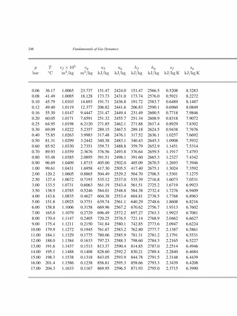
248 Fundamentals of Gas Dynamics
p T vf × 103 vg uf ug hf hg sf sgbar ◦C m3/kg m3/kg kJ/kg kJ/kg kJ/kg kJ/kg kJ/kgK kJ/kgK
0.06 36.17 1.0065 23.737 151.47 2424.0 151.47 2566.5 0.5208 8.32830.08 41.49 1.0085 18.128 173.73 2431.0 173.74 2576.0 0.5921 8.22720.10 45.79 1.0103 14.693 191.71 2436.8 191.72 2583.7 0.6489 8.14870.12 49.40 1.0119 12.377 206.82 2441.6 206.83 2590.1 0.6960 8.08490.16 55.30 1.0147 9.4447 231.47 2449.4 231.49 2600.5 0.7718 7.98460.20 60.05 1.0171 7.6591 251.32 2455.7 251.34 2608.9 0.8318 7.90720.25 64.95 1.0198 6.2120 271.85 2462.1 271.88 2617.4 0.8929 7.83020.30 69.09 1.0222 5.2357 289.15 2467.5 289.18 2624.5 0.9438 7.76760.40 75.85 1.0263 3.9983 317.48 2476.1 317.52 2636.1 1.0257 7.66920.50 81.31 1.0299 3.2442 340.38 2483.1 340.43 2645.3 1.0908 7.59320.60 85.92 1.0330 2.7351 359.73 2488.8 359.79 2652.9 1.1451 7.53140.70 89.93 1.0359 2.3676 376.56 2493.8 376.64 2659.5 1.1917 7.47930.80 93.48 1.0385 2.0895 391.51 2498.1 391.60 2665.3 1.2327 7.43420.90 96.69 1.0409 1.8715 405.00 2502.0 405.09 2670.5 1.2693 7.39461.00 99.61 1.0431 1.6958 417.30 2505.5 417.40 2675.1 1.3024 7.35922.00 120.2 1.0605 0.8865 504.49 2529.2 504.70 2706.5 1.5301 7.12752.50 127.4 1.0672 0.7193 535.12 2537.0 535.39 2716.8 1.6073 7.05313.00 133.5 1.0731 0.6063 561.19 2543.4 561.51 2725.2 1.6719 6.99233.50 138.9 1.0785 0.5246 584.01 2548.8 584.38 2732.4 1.7276 6.94094.00 143.6 1.0835 0.4627 604.38 2553.4 604.81 2738.5 1.7768 6.89635.00 151.8 1.0925 0.3751 639.74 2561.1 640.29 2748.6 1.8608 6.82166.00 158.8 1.1006 0.3158 669.96 2567.2 670.62 2756.7 1.9313 6.76027.00 165.0 1.1079 0.2729 696.49 2572.2 697.27 2763.3 1.9923 6.70818.00 170.4 1.1147 0.2405 720.25 2576.5 721.14 2768.9 2.0462 6.66279.00 175.4 1.1211 0.2150 741.84 2580.1 742.85 2773.6 2.0947 6.6224
10.00 179.9 1.1272 0.1945 761.67 2583.2 762.80 2777.7 2.1387 6.586111.00 184.1 1.1329 0.1775 780.06 2585.9 781.31 2781.2 2.1791 6.553112.00 188.0 1.1384 0.1633 797.23 2588.3 798.60 2784.3 2.2165 6.522713.00 191.6 1.1437 0.1513 813.37 2590.4 814.85 2787.0 2.2514 6.494614.00 195.1 1.1488 0.1408 828.60 2592.2 830.21 2789.4 2.2840 6.468415.00 198.3 1.1538 0.1318 843.05 2593.9 844.78 2791.5 2.3148 6.443916.00 201.4 1.1586 0.1238 856.81 2595.3 858.66 2793.3 2.3439 6.420817.00 204.3 1.1633 0.1167 869.95 2596.5 871.93 2795.0 2.3715 6.3990
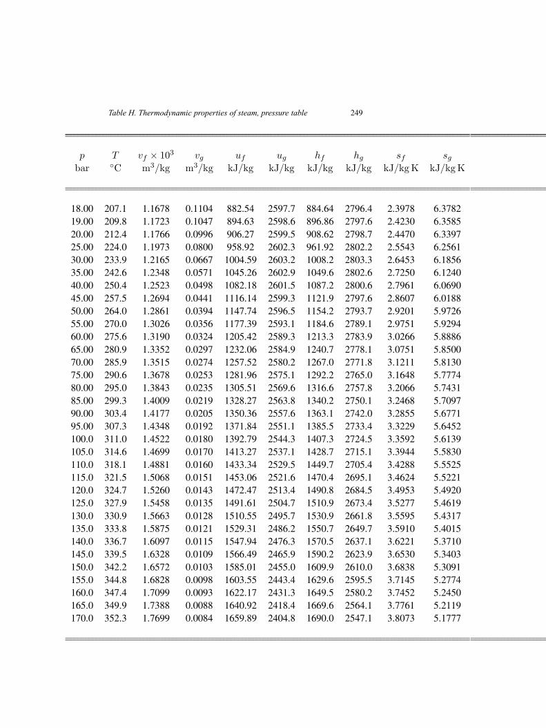
Table H. Thermodynamic properties of steam, pressure table 249
p T vf × 103 vg uf ug hf hg sf sgbar ◦C m3/kg m3/kg kJ/kg kJ/kg kJ/kg kJ/kg kJ/kgK kJ/kgK
18.00 207.1 1.1678 0.1104 882.54 2597.7 884.64 2796.4 2.3978 6.378219.00 209.8 1.1723 0.1047 894.63 2598.6 896.86 2797.6 2.4230 6.358520.00 212.4 1.1766 0.0996 906.27 2599.5 908.62 2798.7 2.4470 6.339725.00 224.0 1.1973 0.0800 958.92 2602.3 961.92 2802.2 2.5543 6.256130.00 233.9 1.2165 0.0667 1004.59 2603.2 1008.2 2803.3 2.6453 6.185635.00 242.6 1.2348 0.0571 1045.26 2602.9 1049.6 2802.6 2.7250 6.124040.00 250.4 1.2523 0.0498 1082.18 2601.5 1087.2 2800.6 2.7961 6.069045.00 257.5 1.2694 0.0441 1116.14 2599.3 1121.9 2797.6 2.8607 6.018850.00 264.0 1.2861 0.0394 1147.74 2596.5 1154.2 2793.7 2.9201 5.972655.00 270.0 1.3026 0.0356 1177.39 2593.1 1184.6 2789.1 2.9751 5.929460.00 275.6 1.3190 0.0324 1205.42 2589.3 1213.3 2783.9 3.0266 5.888665.00 280.9 1.3352 0.0297 1232.06 2584.9 1240.7 2778.1 3.0751 5.850070.00 285.9 1.3515 0.0274 1257.52 2580.2 1267.0 2771.8 3.1211 5.813075.00 290.6 1.3678 0.0253 1281.96 2575.1 1292.2 2765.0 3.1648 5.777480.00 295.0 1.3843 0.0235 1305.51 2569.6 1316.6 2757.8 3.2066 5.743185.00 299.3 1.4009 0.0219 1328.27 2563.8 1340.2 2750.1 3.2468 5.709790.00 303.4 1.4177 0.0205 1350.36 2557.6 1363.1 2742.0 3.2855 5.677195.00 307.3 1.4348 0.0192 1371.84 2551.1 1385.5 2733.4 3.3229 5.6452100.0 311.0 1.4522 0.0180 1392.79 2544.3 1407.3 2724.5 3.3592 5.6139105.0 314.6 1.4699 0.0170 1413.27 2537.1 1428.7 2715.1 3.3944 5.5830110.0 318.1 1.4881 0.0160 1433.34 2529.5 1449.7 2705.4 3.4288 5.5525115.0 321.5 1.5068 0.0151 1453.06 2521.6 1470.4 2695.1 3.4624 5.5221120.0 324.7 1.5260 0.0143 1472.47 2513.4 1490.8 2684.5 3.4953 5.4920125.0 327.9 1.5458 0.0135 1491.61 2504.7 1510.9 2673.4 3.5277 5.4619130.0 330.9 1.5663 0.0128 1510.55 2495.7 1530.9 2661.8 3.5595 5.4317135.0 333.8 1.5875 0.0121 1529.31 2486.2 1550.7 2649.7 3.5910 5.4015140.0 336.7 1.6097 0.0115 1547.94 2476.3 1570.5 2637.1 3.6221 5.3710145.0 339.5 1.6328 0.0109 1566.49 2465.9 1590.2 2623.9 3.6530 5.3403150.0 342.2 1.6572 0.0103 1585.01 2455.0 1609.9 2610.0 3.6838 5.3091155.0 344.8 1.6828 0.0098 1603.55 2443.4 1629.6 2595.5 3.7145 5.2774160.0 347.4 1.7099 0.0093 1622.17 2431.3 1649.5 2580.2 3.7452 5.2450165.0 349.9 1.7388 0.0088 1640.92 2418.4 1669.6 2564.1 3.7761 5.2119170.0 352.3 1.7699 0.0084 1659.89 2404.8 1690.0 2547.1 3.8073 5.1777
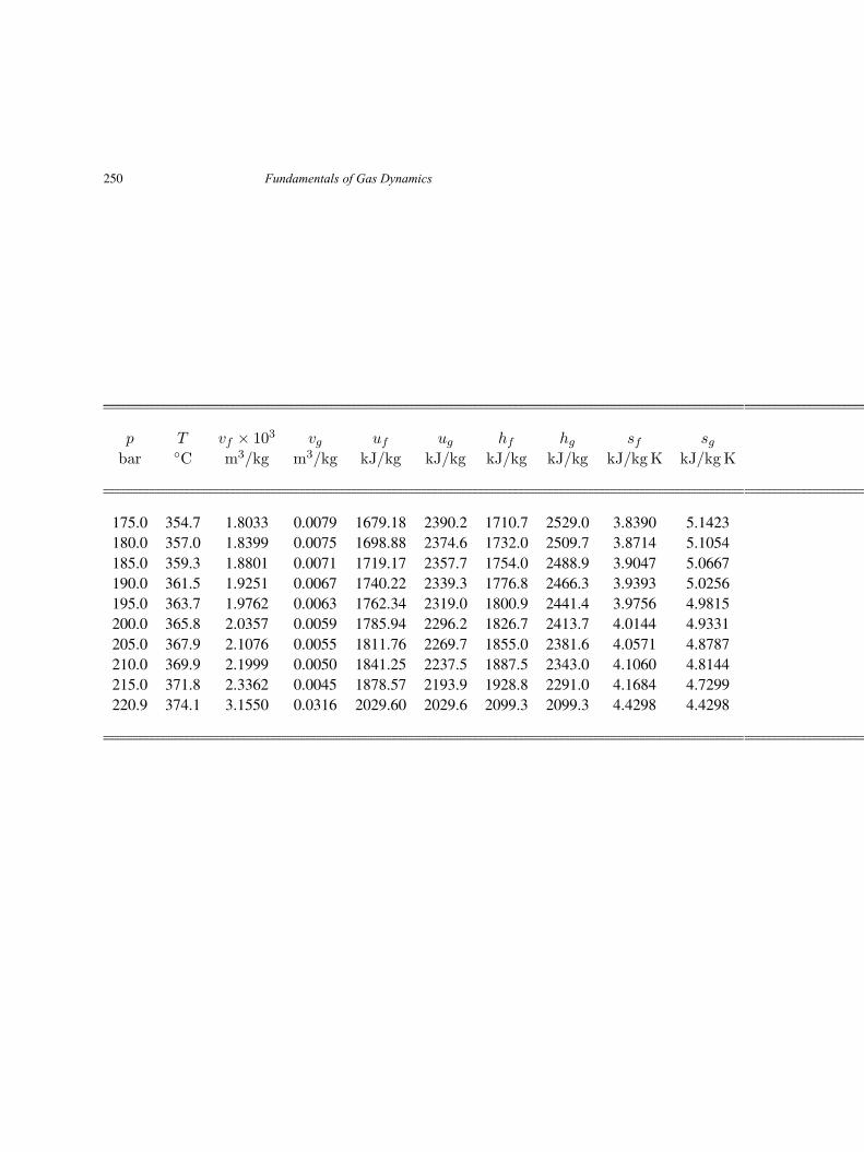
250 Fundamentals of Gas Dynamics
p T vf × 103 vg uf ug hf hg sf sgbar ◦C m3/kg m3/kg kJ/kg kJ/kg kJ/kg kJ/kg kJ/kgK kJ/kgK
175.0 354.7 1.8033 0.0079 1679.18 2390.2 1710.7 2529.0 3.8390 5.1423180.0 357.0 1.8399 0.0075 1698.88 2374.6 1732.0 2509.7 3.8714 5.1054185.0 359.3 1.8801 0.0071 1719.17 2357.7 1754.0 2488.9 3.9047 5.0667190.0 361.5 1.9251 0.0067 1740.22 2339.3 1776.8 2466.3 3.9393 5.0256195.0 363.7 1.9762 0.0063 1762.34 2319.0 1800.9 2441.4 3.9756 4.9815200.0 365.8 2.0357 0.0059 1785.94 2296.2 1826.7 2413.7 4.0144 4.9331205.0 367.9 2.1076 0.0055 1811.76 2269.7 1855.0 2381.6 4.0571 4.8787210.0 369.9 2.1999 0.0050 1841.25 2237.5 1887.5 2343.0 4.1060 4.8144215.0 371.8 2.3362 0.0045 1878.57 2193.9 1928.8 2291.0 4.1684 4.7299220.9 374.1 3.1550 0.0316 2029.60 2029.6 2099.3 2099.3 4.4298 4.4298
Table I. Thermodynamic properties ofsuperheated steam
251
Fundamentals of Gas Dynamics, Second Edition. V. Babu.© 2015 V. Babu. Published 2015 by Athena Academic Ltd and John Wiley & Sons Ltd
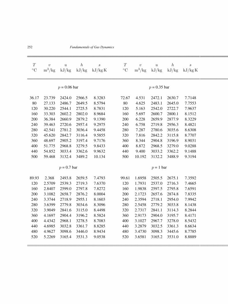
252 Fundamentals of Gas Dynamics
T v u h s T v u h s◦C m3/kg kJ/kg kJ/kg kJ/kgK ◦C m3/kg kJ/kg kJ/kg kJ/kgK
p = 0.06 bar p = 0.35 bar
36.17 23.739 2424.0 2566.5 8.3283 72.67 4.531 2472.1 2630.7 7.714880 27.133 2486.7 2649.5 8.5794 80 4.625 2483.1 2645.0 7.7553
120 30.220 2544.1 2725.5 8.7831 120 5.163 2542.0 2722.7 7.9637160 33.303 2602.2 2802.0 8.9684 160 5.697 2600.7 2800.1 8.1512200 36.384 2660.9 2879.2 9.1390 200 6.228 2659.9 2877.9 8.3229240 39.463 2720.6 2957.4 9.2975 240 6.758 2719.8 2956.3 8.4821280 42.541 2781.2 3036.4 9.4458 280 7.287 2780.6 3035.6 8.6308320 45.620 2842.7 3116.4 9.5855 320 7.816 2842.2 3115.8 8.7707360 48.697 2905.2 3197.4 9.7176 360 8.344 2904.8 3196.9 8.9031400 51.775 2968.8 3279.5 9.8433 400 8.872 2968.5 3279.0 9.0288440 54.852 3033.4 3362.6 9.9632 440 9.400 3033.2 3362.2 9.1488500 59.468 3132.4 3489.2 10.134 500 10.192 3132.2 3488.9 9.3194
p = 0.7 bar p = 1 bar
89.93 2.368 2493.8 2659.5 7.4793 99.61 1.6958 2505.5 2675.1 7.3592120 2.5709 2539.3 2719.3 7.6370 120 1.7931 2537.0 2716.3 7.4665160 2.8407 2599.0 2797.8 7.8272 160 1.9838 2597.5 2795.8 7.6591200 3.1082 2658.7 2876.2 8.0004 200 2.1723 2657.6 2874.8 7.8335240 3.3744 2718.9 2955.1 8.1603 240 2.3594 2718.1 2954.0 7.9942280 3.6399 2779.8 3034.6 8.3096 280 2.5458 2779.2 3033.8 8.1438320 3.9049 2841.6 3115.0 8.4498 320 2.7317 2841.1 3114.3 8.2844360 4.1697 2904.4 3196.2 8.5824 360 2.9173 2904.0 3195.7 8.4171400 4.4342 2968.1 3278.5 8.7083 400 3.1027 2967.7 3278.0 8.5432440 4.6985 3032.8 3361.7 8.8285 440 3.2879 3032.5 3361.3 8.6634480 4.9627 3098.6 3446.0 8.9434 480 3.4730 3098.3 3445.6 8.7785520 5.2269 3165.4 3531.3 9.0538 520 3.6581 3165.2 3531.0 8.8889
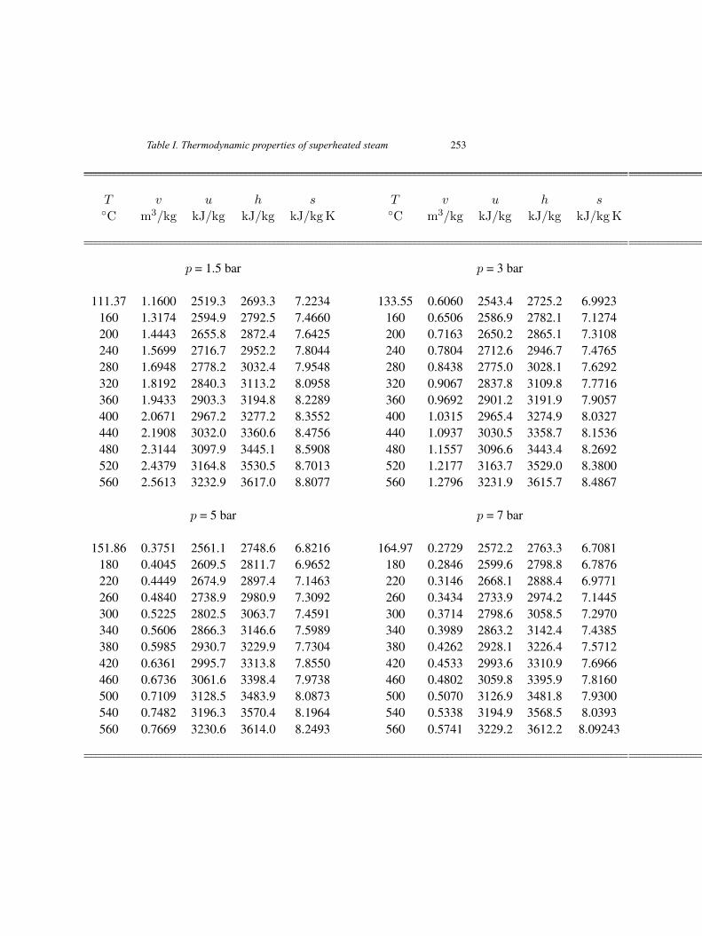
Table I. Thermodynamic properties of superheated steam 253
T v u h s T v u h s◦C m3/kg kJ/kg kJ/kg kJ/kgK ◦C m3/kg kJ/kg kJ/kg kJ/kgK
p = 1.5 bar p = 3 bar
111.37 1.1600 2519.3 2693.3 7.2234 133.55 0.6060 2543.4 2725.2 6.9923160 1.3174 2594.9 2792.5 7.4660 160 0.6506 2586.9 2782.1 7.1274200 1.4443 2655.8 2872.4 7.6425 200 0.7163 2650.2 2865.1 7.3108240 1.5699 2716.7 2952.2 7.8044 240 0.7804 2712.6 2946.7 7.4765280 1.6948 2778.2 3032.4 7.9548 280 0.8438 2775.0 3028.1 7.6292320 1.8192 2840.3 3113.2 8.0958 320 0.9067 2837.8 3109.8 7.7716360 1.9433 2903.3 3194.8 8.2289 360 0.9692 2901.2 3191.9 7.9057400 2.0671 2967.2 3277.2 8.3552 400 1.0315 2965.4 3274.9 8.0327440 2.1908 3032.0 3360.6 8.4756 440 1.0937 3030.5 3358.7 8.1536480 2.3144 3097.9 3445.1 8.5908 480 1.1557 3096.6 3443.4 8.2692520 2.4379 3164.8 3530.5 8.7013 520 1.2177 3163.7 3529.0 8.3800560 2.5613 3232.9 3617.0 8.8077 560 1.2796 3231.9 3615.7 8.4867
p = 5 bar p = 7 bar
151.86 0.3751 2561.1 2748.6 6.8216 164.97 0.2729 2572.2 2763.3 6.7081180 0.4045 2609.5 2811.7 6.9652 180 0.2846 2599.6 2798.8 6.7876220 0.4449 2674.9 2897.4 7.1463 220 0.3146 2668.1 2888.4 6.9771260 0.4840 2738.9 2980.9 7.3092 260 0.3434 2733.9 2974.2 7.1445300 0.5225 2802.5 3063.7 7.4591 300 0.3714 2798.6 3058.5 7.2970340 0.5606 2866.3 3146.6 7.5989 340 0.3989 2863.2 3142.4 7.4385380 0.5985 2930.7 3229.9 7.7304 380 0.4262 2928.1 3226.4 7.5712420 0.6361 2995.7 3313.8 7.8550 420 0.4533 2993.6 3310.9 7.6966460 0.6736 3061.6 3398.4 7.9738 460 0.4802 3059.8 3395.9 7.8160500 0.7109 3128.5 3483.9 8.0873 500 0.5070 3126.9 3481.8 7.9300540 0.7482 3196.3 3570.4 8.1964 540 0.5338 3194.9 3568.5 8.0393560 0.7669 3230.6 3614.0 8.2493 560 0.5741 3229.2 3612.2 8.09243
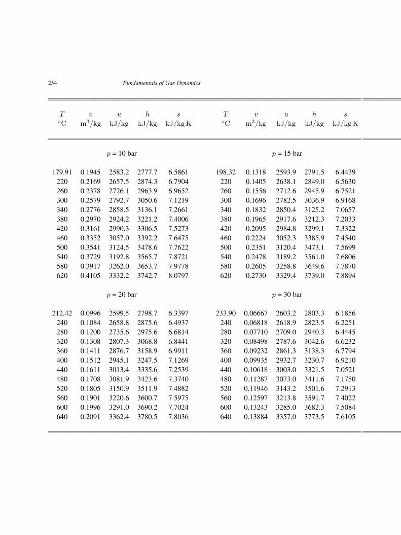
254 Fundamentals of Gas Dynamics
T v u h s T v u h s◦C m3/kg kJ/kg kJ/kg kJ/kgK ◦C m3/kg kJ/kg kJ/kg kJ/kgK
p = 10 bar p = 15 bar
179.91 0.1945 2583.2 2777.7 6.5861 198.32 0.1318 2593.9 2791.5 6.4439220 0.2169 2657.5 2874.3 6.7904 220 0.1405 2638.1 2849.0 6.5630260 0.2378 2726.1 2963.9 6.9652 260 0.1556 2712.6 2945.9 6.7521300 0.2579 2792.7 3050.6 7.1219 300 0.1696 2782.5 3036.9 6.9168340 0.2776 2858.5 3136.1 7.2661 340 0.1832 2850.4 3125.2 7.0657380 0.2970 2924.2 3221.2 7.4006 380 0.1965 2917.6 3212.3 7.2033420 0.3161 2990.3 3306.5 7.5273 420 0.2095 2984.8 3299.1 7.3322460 0.3352 3057.0 3392.2 7.6475 460 0.2224 3052.3 3385.9 7.4540500 0.3541 3124.5 3478.6 7.7622 500 0.2351 3120.4 3473.1 7.5699540 0.3729 3192.8 3565.7 7.8721 540 0.2478 3189.2 3561.0 7.6806580 0.3917 3262.0 3653.7 7.9778 580 0.2605 3258.8 3649.6 7.7870620 0.4105 3332.2 3742.7 8.0797 620 0.2730 3329.4 3739.0 7.8894
p = 20 bar p = 30 bar
212.42 0.0996 2599.5 2798.7 6.3397 233.90 0.06667 2603.2 2803.3 6.1856240 0.1084 2658.8 2875.6 6.4937 240 0.06818 2618.9 2823.5 6.2251280 0.1200 2735.6 2975.6 6.6814 280 0.07710 2709.0 2940.3 6.4445320 0.1308 2807.3 3068.8 6.8441 320 0.08498 2787.6 3042.6 6.6232360 0.1411 2876.7 3158.9 6.9911 360 0.09232 2861.3 3138.3 6.7794400 0.1512 2945.1 3247.5 7.1269 400 0.09935 2932.7 3230.7 6.9210440 0.1611 3013.4 3335.6 7.2539 440 0.10618 3003.0 3321.5 7.0521480 0.1708 3081.9 3423.6 7.3740 480 0.11287 3073.0 3411.6 7.1750520 0.1805 3150.9 3511.9 7.4882 520 0.11946 3143.2 3501.6 7.2913560 0.1901 3220.6 3600.7 7.5975 560 0.12597 3213.8 3591.7 7.4022600 0.1996 3291.0 3690.2 7.7024 600 0.13243 3285.0 3682.3 7.5084640 0.2091 3362.4 3780.5 7.8036 640 0.13884 3357.0 3773.5 7.6105
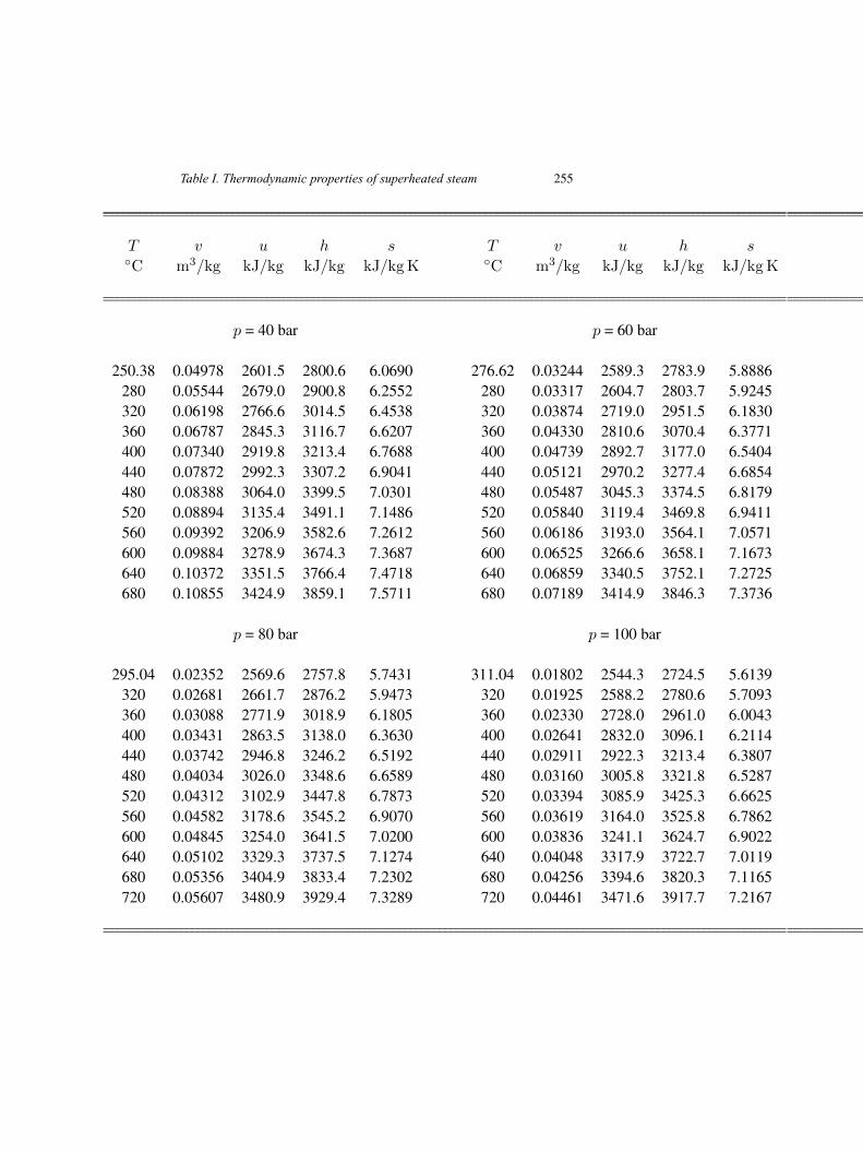
Table I. Thermodynamic properties of superheated steam 255
T v u h s T v u h s◦C m3/kg kJ/kg kJ/kg kJ/kgK ◦C m3/kg kJ/kg kJ/kg kJ/kgK
p = 40 bar p = 60 bar
250.38 0.04978 2601.5 2800.6 6.0690 276.62 0.03244 2589.3 2783.9 5.8886280 0.05544 2679.0 2900.8 6.2552 280 0.03317 2604.7 2803.7 5.9245320 0.06198 2766.6 3014.5 6.4538 320 0.03874 2719.0 2951.5 6.1830360 0.06787 2845.3 3116.7 6.6207 360 0.04330 2810.6 3070.4 6.3771400 0.07340 2919.8 3213.4 6.7688 400 0.04739 2892.7 3177.0 6.5404440 0.07872 2992.3 3307.2 6.9041 440 0.05121 2970.2 3277.4 6.6854480 0.08388 3064.0 3399.5 7.0301 480 0.05487 3045.3 3374.5 6.8179520 0.08894 3135.4 3491.1 7.1486 520 0.05840 3119.4 3469.8 6.9411560 0.09392 3206.9 3582.6 7.2612 560 0.06186 3193.0 3564.1 7.0571600 0.09884 3278.9 3674.3 7.3687 600 0.06525 3266.6 3658.1 7.1673640 0.10372 3351.5 3766.4 7.4718 640 0.06859 3340.5 3752.1 7.2725680 0.10855 3424.9 3859.1 7.5711 680 0.07189 3414.9 3846.3 7.3736
p = 80 bar p = 100 bar
295.04 0.02352 2569.6 2757.8 5.7431 311.04 0.01802 2544.3 2724.5 5.6139320 0.02681 2661.7 2876.2 5.9473 320 0.01925 2588.2 2780.6 5.7093360 0.03088 2771.9 3018.9 6.1805 360 0.02330 2728.0 2961.0 6.0043400 0.03431 2863.5 3138.0 6.3630 400 0.02641 2832.0 3096.1 6.2114440 0.03742 2946.8 3246.2 6.5192 440 0.02911 2922.3 3213.4 6.3807480 0.04034 3026.0 3348.6 6.6589 480 0.03160 3005.8 3321.8 6.5287520 0.04312 3102.9 3447.8 6.7873 520 0.03394 3085.9 3425.3 6.6625560 0.04582 3178.6 3545.2 6.9070 560 0.03619 3164.0 3525.8 6.7862600 0.04845 3254.0 3641.5 7.0200 600 0.03836 3241.1 3624.7 6.9022640 0.05102 3329.3 3737.5 7.1274 640 0.04048 3317.9 3722.7 7.0119680 0.05356 3404.9 3833.4 7.2302 680 0.04256 3394.6 3820.3 7.1165720 0.05607 3480.9 3929.4 7.3289 720 0.04461 3471.6 3917.7 7.2167
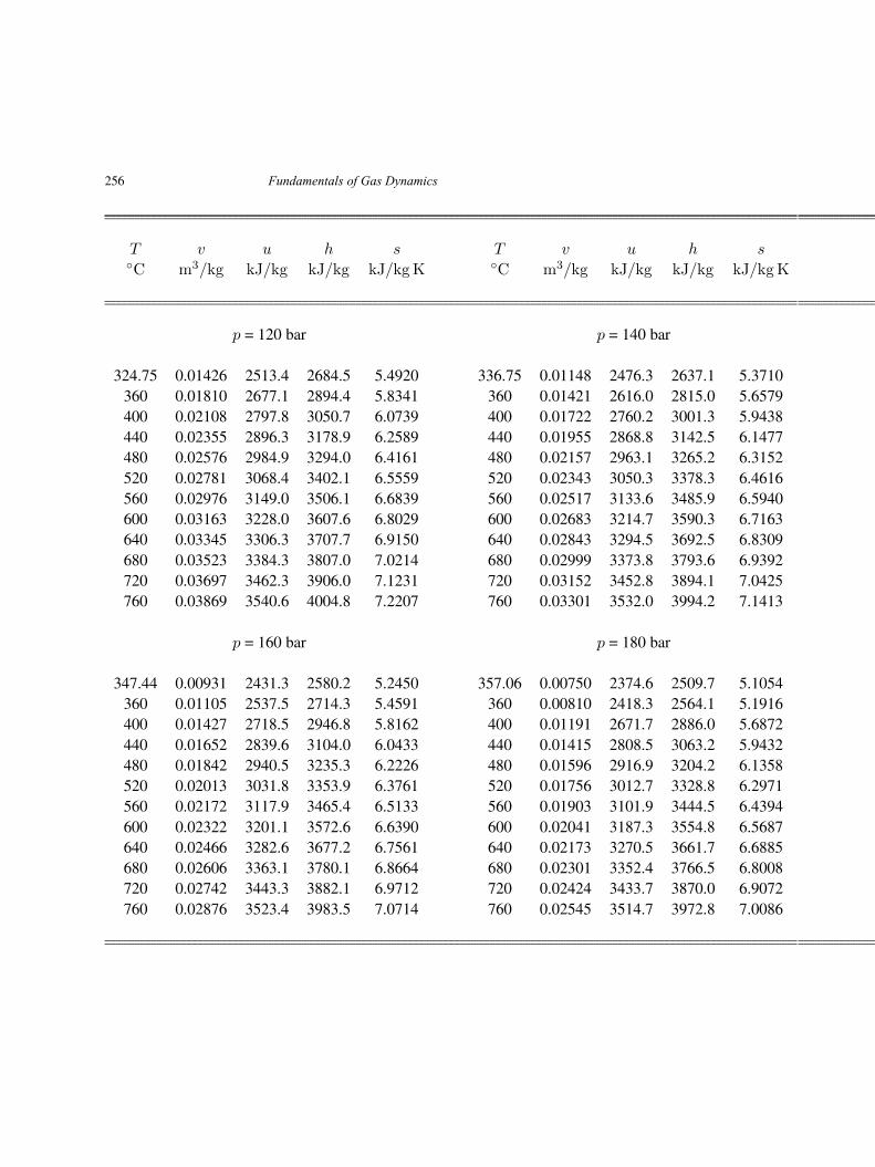
256 Fundamentals of Gas Dynamics
T v u h s T v u h s◦C m3/kg kJ/kg kJ/kg kJ/kgK ◦C m3/kg kJ/kg kJ/kg kJ/kgK
p = 120 bar p = 140 bar
324.75 0.01426 2513.4 2684.5 5.4920 336.75 0.01148 2476.3 2637.1 5.3710360 0.01810 2677.1 2894.4 5.8341 360 0.01421 2616.0 2815.0 5.6579400 0.02108 2797.8 3050.7 6.0739 400 0.01722 2760.2 3001.3 5.9438440 0.02355 2896.3 3178.9 6.2589 440 0.01955 2868.8 3142.5 6.1477480 0.02576 2984.9 3294.0 6.4161 480 0.02157 2963.1 3265.2 6.3152520 0.02781 3068.4 3402.1 6.5559 520 0.02343 3050.3 3378.3 6.4616560 0.02976 3149.0 3506.1 6.6839 560 0.02517 3133.6 3485.9 6.5940600 0.03163 3228.0 3607.6 6.8029 600 0.02683 3214.7 3590.3 6.7163640 0.03345 3306.3 3707.7 6.9150 640 0.02843 3294.5 3692.5 6.8309680 0.03523 3384.3 3807.0 7.0214 680 0.02999 3373.8 3793.6 6.9392720 0.03697 3462.3 3906.0 7.1231 720 0.03152 3452.8 3894.1 7.0425760 0.03869 3540.6 4004.8 7.2207 760 0.03301 3532.0 3994.2 7.1413
p = 160 bar p = 180 bar
347.44 0.00931 2431.3 2580.2 5.2450 357.06 0.00750 2374.6 2509.7 5.1054360 0.01105 2537.5 2714.3 5.4591 360 0.00810 2418.3 2564.1 5.1916400 0.01427 2718.5 2946.8 5.8162 400 0.01191 2671.7 2886.0 5.6872440 0.01652 2839.6 3104.0 6.0433 440 0.01415 2808.5 3063.2 5.9432480 0.01842 2940.5 3235.3 6.2226 480 0.01596 2916.9 3204.2 6.1358520 0.02013 3031.8 3353.9 6.3761 520 0.01756 3012.7 3328.8 6.2971560 0.02172 3117.9 3465.4 6.5133 560 0.01903 3101.9 3444.5 6.4394600 0.02322 3201.1 3572.6 6.6390 600 0.02041 3187.3 3554.8 6.5687640 0.02466 3282.6 3677.2 6.7561 640 0.02173 3270.5 3661.7 6.6885680 0.02606 3363.1 3780.1 6.8664 680 0.02301 3352.4 3766.5 6.8008720 0.02742 3443.3 3882.1 6.9712 720 0.02424 3433.7 3870.0 6.9072760 0.02876 3523.4 3983.5 7.0714 760 0.02545 3514.7 3972.8 7.0086
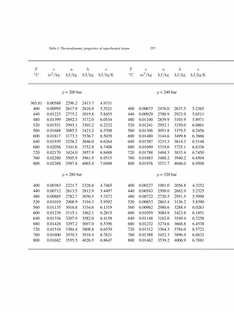
Table I. Thermodynamic properties of superheated steam 257
T v u h s T v u h s◦C m3/kg kJ/kg kJ/kg kJ/kgK ◦C m3/kg kJ/kg kJ/kg kJ/kgK
p = 200 bar p = 240 bar
365.81 0.00588 2296.2 2413.7 4.9331400 0.00995 2617.9 2816.9 5.5521 400 0.00673 2476.0 2637.5 5.2365440 0.01223 2775.2 3019.8 5.8455 440 0.00929 2700.9 2923.9 5.6511480 0.01399 2892.3 3172.0 6.0534 480 0.01100 2839.9 3103.9 5.8971520 0.01551 2993.1 3303.2 6.2232 520 0.01241 2952.1 3250.0 6.0861560 0.01688 3085.5 3423.2 6.3708 560 0.01366 3051.8 3379.5 6.2456600 0.01817 3173.3 3536.7 6.5039 600 0.01480 3144.6 3499.8 6.3866640 0.01939 3258.2 3646.0 6.6264 640 0.01587 3233.3 3614.3 6.5148680 0.02056 3341.6 3752.8 6.7408 680 0.01690 3319.6 3725.1 6.6336720 0.02170 3424.0 3857.9 6.8488 720 0.01788 3404.3 3833.4 6.7450760 0.02280 3505.9 3961.9 6.9515 760 0.01883 3488.2 3940.2 6.8504800 0.02388 3587.8 4065.4 7.0498 800 0.01976 3571.7 4046.0 6.9508
p = 280 bar p = 320 bar
400 0.00383 2221.7 2328.8 4.7465 400 0.00237 1981.0 2056.8 4.3252440 0.00712 2613.5 2812.9 5.4497 440 0.00543 2509.0 2682.9 5.2325480 0.00885 2782.7 3030.5 5.7472 480 0.00722 2720.5 2951.5 5.5998520 0.01019 2908.9 3194.3 5.9592 520 0.00853 2863.4 3136.2 5.8390560 0.01135 3016.8 3334.6 6.1319 560 0.00962 2980.6 3288.4 6.0263600 0.01239 3115.1 3462.1 6.2815 600 0.01059 3084.9 3423.8 6.1851640 0.01336 3207.9 3582.0 6.4158 640 0.01148 3182.0 3549.4 6.3258680 0.01428 3297.2 3697.0 6.5390 680 0.01232 3274.6 3668.8 6.4538720 0.01516 3384.4 3808.8 6.6539 720 0.01312 3364.3 3784.0 6.5722760 0.01600 3470.3 3918.4 6.7621 760 0.01388 3452.3 3896.4 6.6832800 0.01682 3555.5 4026.5 6.8647 800 0.01462 3539.2 4006.9 6.7881

258 Fundamentals of Gas Dynamics
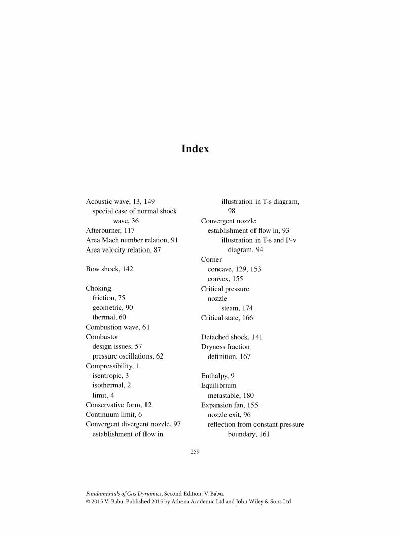
Index
Acoustic wave, 13, 149special case of normal shock
wave, 36Afterburner, 117Area Mach number relation, 91Area velocity relation, 87
Bow shock, 142
Chokingfriction, 75geometric, 90thermal, 60
Combustion wave, 61Combustor
design issues, 57pressure oscillations, 62
Compressibility, 1isentropic, 3isothermal, 2limit, 4
Conservative form, 12Continuum limit, 6Convergent divergent nozzle, 97
establishment of flow in
illustration in T-s diagram,98
Convergent nozzleestablishment of flow in, 93
illustration in T-s and P-vdiagram, 94
Cornerconcave, 129, 153convex, 155
Critical pressurenozzle
steam, 174Critical state, 166
Detached shock, 141Dryness fraction
definition, 167
Enthalpy, 9Equilibrium
metastable, 180Expansion fan, 155
nozzle exit, 96reflection from constant pressure
boundary, 161
259
Fundamentals of Gas Dynamics, Second Edition. V. Babu.© 2015 V. Babu. Published 2015 by Athena Academic Ltd and John Wiley & Sons Ltd
260 Fundamentals of Gas Dynamics
Fanno curve, 74Fanno flow, 69
changes in properties, 74illustration in T-s diagram, 74interaction with nozzle flow, 111sonic state, 76
Frictioneffect of, 69factor, 70
H-curveNormal shock wave, 44Rayleigh flow, 57sonic state, 59
Heat addition, 49
Impulse function, 84Intake
capture area, 137critical mode, 137supersonic, 107, 136
Internal energydistribution, 8modes, 7
Isentropic process, 13illustraion in T-s and P-v
diagram, 27relation, 20
steam, 170
Knudsen number, 6
Machangle, 133, 153cone, 152number, 3
reflection, 145wave, 133, 152
flow across, 155Mass flow rate
choked, 92
Normal shock, 31entropy change, 35illustration in P-v diagram, 44illustration in T-s and P-v
diagram, 37loss of stagnation pressure, 35moving, 39special case of oblique shock,
133strength, 35
Oblique shock, 127θ − β −M relation, 131flow deflection angle, 129from nozzle exit, 139reflection
from constant pressureboundary, 160
from wall, 143Over expanded flow, 103
Perfect gascalorically perfect, 7Equation of state, 4
alternative forms, 5Specific heats, 9
Prandtl Meyerangle, 159flow, 153

Index 261
Quasi one-dimensional, 83
Ramjet engineinlet interaction, 63intake, 136schematic, 29
Rankine-Hugoniot equation, 44Rayleigh curve, 54Rayleigh flow, 49
changes in properties, 53illustration in P-v diagram, 57ilustration in T-s diagram, 54interaction with nozzle flow, 114sonic state, 64
Rayleigh linenormal shock, 42sonic state, 59
Reference states, 17sonic state, 17stagnation state, 18
Saturationpressure, 166temperature, 166
Scramjet engineinlet interaction, 63intake, 136
Second lawdifferential form, 12Entropy change for a process, 13TdS relation, 12
Shockcondensation, 183
Shock angle, 129Shock diamond, 141Slip line, 145, 154
Sonic state, 17, 54Fanno flow, 76illustration in T-s, P-v diagram,
27nozzle
steam, 174nozzle flow, 90Rayleigh flow, 64Rayleigh line, 59
Speed of sound, 15mixture of gases, 16Perfect gas, 16reacting flow, 16steam, 170
Stagnation density, 20Stagnation pressure
changes in, 22definition, 19loss, 35, 57, 74, 127, 133
Stagnation statedefinition, 18illustration in T-s, P-v diagram,
27Stagnation temperature
changes in, 21definition, 19
Strong oblique shock, 132Supersaturated flow
degree of supercooling, 182degree of supersaturation, 182Wilson line, 183
Thrustloss of, 96momentum, 85pressure, 85
262 Fundamentals of Gas Dynamics
Under expanded flow, 62, 75, 96,103
Velocity triangle, 129, 156
Wave angle, 129Weak oblique shock, 132Wilson line, 183Wind tunnel
supersonic, 105
Related Documents