Fundamental Theorems of Optimization 1

Welcome message from author
This document is posted to help you gain knowledge. Please leave a comment to let me know what you think about it! Share it to your friends and learn new things together.
Transcript

Fundamental Theorems of Optimization
1

Fundamental Theorems of Math Prog.
CS 101, Ec 101 Mathematical Programming 26 January 2005 2
Maximizing a concave function over a convex set.Maximizing a convex function over a closed bounded convex set.

Maximizing Concave Functions
CS 101, Ec 101 Mathematical Programming 26 January 2005 3
The problem is to maximize a concave function over a convex set.
FUNDAMENTAL THEOREM 1: A local optimum is a global optimum.

Proof
CS 101, Ec 101 Mathematical Programming 26 January 2005 4
Assume the contrary.Let point x be a local optimum that is NOT a global optimum, and let point y be a global optimum.
Consider the line segment between points x and y.

Proof
CS 101, Ec 101 Mathematical Programming 26 January 2005 5
Local max but not global max
Global max
x y

Proof
CS 101, Ec 101 Mathematical Programming 26 January 2005 6
Since f(y) > f(x), the value of f for every point on the line segment between x and y other than x itself, is strictly greater than f(x).

Proof
CS 101, Ec 101 Mathematical Programming 26 January 2005 7
Line segment lies strictly abovef(x) for points other than x
f(x)
x y

Proof
CS 101, Ec 101 Mathematical Programming 26 January 2005 8
Since the curve is concave, the value of f for every point on the line segment is greater than or equal to the value of f on the line segment between points:
(x, f(x)) and (y, f(y))

Proof
CS 101, Ec 101 Mathematical Programming 26 January 2005 9
Greater than f(x)
x yCurve lies strictly above
the line segment for points other than x
Proof by Contradiction
CS 101, Ec 101 Mathematical Programming 26 January 2005 10
Greater than f(x)
Cannot be local maximum
x yCurve lies strictly above
the line segment for points other than x

Maximizing Convex Functions
CS 101, Ec 101 Mathematical Programming 26 January 2005 11
Problem: Maximizing convex functions over closed bounded convex sets.Because the feasible region is a closed bounded convex set, the feasible region is the set of points that are convex combinations of extreme points.

Feasible Region and Extreme Points
CS 101, Ec 101 Mathematical Programming 26 January 2005 12
The extreme points.
Feasible region
Convex combinations of extreme points
Feasible region is the set of all convex combinations of extreme points

Maximizing Convex Functions
CS 101, Ec 101 Mathematical Programming 26 January 2005 13
Fundamental Theorem 2
There exists an extreme point which is the global maximum of a convex function
over a closed bounded convex set.

Proof by Contradiction
CS 101, Ec 101 Mathematical Programming 26 January 2005 14
Assume the contrary.So there is a global maximum at a point p that is not an extreme point, and no global maximum occurs at an extreme point.Therefore for every extreme point q:
f(p) > f(q)Point p is a convex combination of some set of extreme points. So there exists extreme points x_1, x_2, …,x_k and positive scalars r_1, … ,r_k, that sum to 1 such that:
p = sum over j of r_j * x _j

Proof
CS 101, Ec 101 Mathematical Programming 26 January 2005 15
Since f is a convex function:f(sum over j of r_j * x_j)
=<Sum over j of r_j * f(x_j)
If for every j, f(x_j) is strictly less than the global maximum, then the right hand side of the above inequality is strictly less than the global maximum, and so the left hand side is also strictly less than the global maximum. But, the left hand side is f(p). Hence p is not a global maximum. Contradiction!

Remembering the Fundamental Theorems Graphically
CS 101, Ec 101 Mathematical Programming 26 January 2005 16
Local maximum is
global maximum
There exists an extreme pointwhich is a global maximum

Introduction to Linear Programming
17

Maximizing Linear Functions
CS 101, Ec 101 Mathematical Programming 26 January 2005 18
Which of the fundamental theorems can we apply if the objective function is linear?

Maximizing Linear Functions
CS 101, Ec 101 Mathematical Programming 26 January 2005 19
Which of the fundamental theorems can we apply if the objective function is linear?BOTH fundamental theorems because linear functions are both concave functions and convex functions!

Maximizing Linear Functions
CS 101, Ec 101 Mathematical Programming 26 January 2005 20
Maximizing linear functions over closed bounded convex sets allows us to use both theorems. So:
Every local maximum is a global maximum, andThere exists an extreme point that is a global maximum.

Algorithm for Linear Objective Functions
CS 101, Ec 101 Mathematical Programming 26 January 2005 21
Start at an extreme point.While the extreme point is not a local maximum do
traverse along the boundary of the feasible region to a better neighboring extreme point, i.e., a point with a higher value of the objective function.

Linear Feasible Regions
CS 101, Ec 101 Mathematical Programming 26 January 2005 22
Can we simplify the problem if the feasible region is bounded by hyperplanes?The feasible region is a polyhedron with a finite number of extreme points.So, we know the algorithm will stop because the while loop never returns to the same extreme point.So, the loop can iterate at most N times where N is the number of extreme points of the polyhedron representing the feasible region.

Algorithm for Linear Problems
CS 101, Ec 101 Mathematical Programming 26 January 2005 23
Start at an extreme point.If it is not a local maximum find a direction of improvement along a boundary to a neighboring better extreme point.

Algorithm for Linear Problems
CS 101, Ec 101 Mathematical Programming 26 January 2005 24
Start at an extreme point.If it is not a local maximum find a direction of improvement along a boundary to a neighboring better extreme point.

Algorithm for Linear Problems
CS 101, Ec 101 Mathematical Programming 26 January 2005 25
If the extreme point is not a local maximum find a direction of improvement along a boundary to a neighboring better extreme point.

Algorithm for Linear Problems
CS 101, Ec 101 Mathematical Programming 26 January 2005 26
If the extreme point is a local maximum, stop.
Linear Programming
CS 101, Ec 101 Mathematical Programming 26 January 2005 27
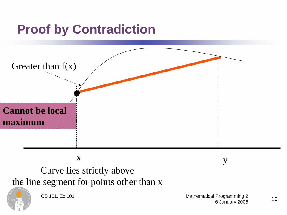
Linear programming is mathematical programming where the objective function and constraints are linear.
Example:Maximize zWhere 3x0 + 2x1 = zSubject to:
2x0 + x1 =< 4x0 + 2x1 =< 6
x0, x1 >= 0

Canonical Form
CS 101, Ec 101 Mathematical Programming 26 January 2005 28
For now, we restrict ourselves to problems of the form:
Maximize z wherec.x = zSubject to:A.x =< bx >= 0Where:• c is an row vector of length n, • x is a column vector of length n, • A is an m x n matrix, and • b is a column vector of length m with all values non-negative

Example of Canonical Form
CS 101, Ec 101 Mathematical Programming 26 January 2005 29
C = [ 3, 2]
2 11 2
A =
46b =
x0
x1x =
Example:Maximize zWhere 3x0 + 2x1 = zSubject to:
2x0 + x1 =< 4x0 + 2x1 =< 6
x0, x1 >= 0

Another Canonical Form
CS 101, Ec 101 Mathematical Programming 26 January 2005 30
Convert the inequalities to equalities.
Example:Maximize zWhere 3x0 + 2x1 = zSubject to:
2x0 + x1 =< 4x0 + 2x1 =< 6
x0, x1 >= 0
Example:Maximize zWhere 3x0 + 2x1 + 0s0 + 0s1 = zSubject to:
2x0 + x1 + s0 + 0s1 = 4x0 + 2x1 + 0s0 + s1 = 6
x0, x1, s0, s1 >= 0

The Alternative Canonical Form
CS 101, Ec 101 Mathematical Programming 26 January 2005 31
Max zWhere c.x = z
Subject to:A. x =< b
x >= 0
Max zWhere c.x + 0.s = z
Subject to:A. x + I.s = b
x, s >= 0
Here I is the identity matrix

Relationship to Economics
CS 101, Ec 101 Mathematical Programming 26 January 2005 32
The constraints represent constraints on resources.The columns represent activities.The objective function represents revenue.

Relationship to Economics
CS 101, Ec 101 Mathematical Programming 26 January 2005 33
Maximize zWhere 4x0 + 5x1 + 9x2 = zSubject to:
2x0 + x1 + 3x2 =< 6x0 + 2x1 + 4x2 =< 9
x0, x1 >= 0
Example: A furniture maker has two scarce resources: wood and labor. The company has 6 units of wood and 9 units of labor. The company can make small tables, chairs, or cupboards. A table requires 2 units of wood and 1 unit of labor and produces revenue of 4 units. A chair requires 1 unit of wood and 2 units of labor and produces a revenue of 5 units. A cupboards requires 3 units of wood, 4 of labor and produces a revenue of 9 units. How many tables, chairs and cupboards should the company make to maximize revenue?

Definition: Basic Feasible Solution
CS 101, Ec 101 Mathematical Programming 26 January 2005 34
A feasible solution is a vector X such that:A.X =< b, and X >= 0.
A basic solution is one in which at most m variables are non-zero (and so at least n-m variables are strictly zero), and the m, possibly non-zero variables correspond to linearly independent columns.Let B be the matrix obtained by putting together the columns of the possibly non-zero variables. Let the m-vector formed by putting these variables together be xB. Then the basic solution is
xB = B-1.b, and all other variables are strictly zero.

Examples of Basic Solutions
CS 101, Ec 101 Mathematical Programming 26 January 2005 35
Maximize zWhere 4x0 + 5x1 + 9x2 + 0s0 + 0s1 = zSubject to:
2x0 + x1 + 3x2 + s0 + 0s1 = 6x0 + 2x1 + 4x2 + 0s0 + s1 = 9
x0, x1 >= 0
Example 1:Basic variables are s0, s1.Non-basic variables are x0, x1 , x2.The columns corresponding to the
basic variables are the last two columns, i.e.,
1 00 1
So, the basic solution is s0, s1 = 6, 9 and x0, x1 , x2 = 0, 0, 0

Examples of Basic Solutions
CS 101, Ec 101 Mathematical Programming 26 January 2005 36
Maximize zWhere 4x0 + 5x1 + 9x2 + 0s0 + 0s1 = zSubject to:
2x0 + x1 + 3x2 + s0 + 0s1 = 6x0 + 2x1 + 4x2 + 0s0 + s1 = 9
x0, x1 >= 0
Example 2:Basic variables are x0, x1.Non-basic variables are x2, s0 , s1.The columns corresponding to the
basic variables are the first two columns, i.e.,
2 11 2
So, the basic solution is x0, x1 = 1, 4 and x2, s0 , s1 = 0, 0, 0

Examples of Basic Solutions
CS 101, Ec 101 Mathematical Programming 26 January 2005 37
Maximize zWhere 4x0 + 5x1 + 9x2 + 0s0 + 0s1 = zSubject to:
2x0 + x1 + 3x2 + s0 + 0s1 = 6x0 + 2x1 + 4x2 + 0s0 + s1 = 9
x0, x1 >= 0
Example 3:Basic variables are x1, s0.Non-basic variables are x0, x2 , s1.The columns corresponding to the
basic variables are the first two columns, i.e.,
1 12 0
So, the basic solution is x1, s0 = 4.5, 1.5 and x0, x2 , s1 = 0, 0, 0

Economic Meaning of Positive Slack Variables
CS 101, Ec 101 Mathematical Programming 26 January 2005 38
The slack variable is the variable we added to turn a constraint into an equality.We have one slack variable for every constraint.If a slack variable is positive in a solution, that means that the inequality constraint is not tight. In other words, we are not using all of that resource. This implies that the resource is not scarce.

Theorem
CS 101, Ec 101 Mathematical Programming 26 January 2005 39
A solution is an extreme point of the feasible region if and only if it is a basic feasible solution.Proof:First prove that every basic feasible solution is an extreme point.Then prove that every feasible solution that is not a basic solution, is not an extreme point.

Every basic feasible solution is extreme
CS 101, Ec 101 Mathematical Programming 26 January 2005 40
Proof:Let p be a basic feasible solution. Let u and v be two feasible solutions, distinct from p, such that the line segment between u and v passes through p.Thus p is a weighted average of u and v with positive weights.Since u and v are feasible, their elements are non-negative.The only way that weighted average (with positive weights) of non-negative numbers is strictly zero is for the numbers themselves to be strictly zero too.

Proof continued
CS 101, Ec 101 Mathematical Programming 26 January 2005 41
Hence the values of non-basic variables in u and v are strictly zero.Therefore, the values of the basic variables in both u and v must be: B-1.bThis is the same as the solution for p.Hence u and v are not distinct from p: contradiction!

Theorem: Non-basic is not Extreme
CS 101, Ec 101 Mathematical Programming 26 January 2005 42
Proof:Assume there are m+1 or more variables that are strictly positive in a solution p.The column corresponding to at least one of these variables, say , is linearly dependent on the remaining columns.Consider a solution u obtained by perturbing solution p by increasing xk by arbitrarily small positive epsilon and adjusting m positive variables in p so that u is feasible.Consider a solution v, obtained in the same way by decreasing xk by arbitrarily small positive delta.Show that p can be obtained by a linear combination of u and v.

Theorem
CS 101, Ec 101 Mathematical Programming 26 January 2005 43
Consider the problem:Max z where c.x = z subject to A.x + I.s = b, and x,s>=0.
The basic feasible solution x = 0, s = b is locally optimum if all the elements of c are non-positive.Proof: c.x is non-positive since c is non-positive and x is non-negative. Hence z = 0 is an optimal solution.

The Algorithm
CS 101, Ec 101 Mathematical Programming 26 January 2005 44
Start with a basic feasible solution: say x = 0, s = b, where s is the vector of slacks.While locally-optimum extreme point is not found: do:
Increase the value of a non-basic variable that improves the objective function until a basic variable becomes zero.Modify the basis as follows: Replace the basic variable that hasbecome zero by the variable that became positive.

The Algorithm: Computational Steps
CS 101, Ec 101 Mathematical Programming 26 January 2005 45
Start with a basic feasible solution: say x = 0, s = b, where s is the vector of slacks.Always maintain a problem in the canonical form: max z where c.x + 0.s = z, subject to A.x + I.s = b, and x, s >= 0While an element of c is positive: do:
Increase the value of a non-basic variable corresponding to a positive c until a basic variable becomes zero.Modify the basis as follows: Replace the basic variable that hasbecome zero by the variable corresponding to the positive element of c. Convert to canonical form.

Examples of Simplex Algorithm
CS 101, Ec 101 Mathematical Programming 26 January 2005 46
Problem is in canonical form:Max zWhere c.x + 0.s = zSubject to:A.x + I.s = bx, s >= 0And where b is non-negative.
A basic feasible solution (and hence an extreme point) is s = b, x = 0
There are coefficients of c that are positive. Increase any variable with a positive coefficient, say x0
Maximize zWhere 4x0 + 5x1 + 9x2 + 0s0 + 0s1 = zSubject to:
2x0 + x1 + 3x2 + s0 + 0s1 = 6x0 + 2x1 + 4x2 + 0s0 + s1 = 9
x0 , x1 , x2 , s0 , s1 >= 0

Examples of Simplex Algorithm
CS 101, Ec 101 Mathematical Programming 26 January 2005 47
Maximize zWhere 4x0 + 5x1 + 9x2 + 0s0 + 0s1 = zSubject to:
2x0 + x1 + 3x2 + s0 + 0s1 = 6x0 + 2x1 + 4x2 + 0s0 + s1 = 9
x0 , x1 , x2 , s0 , s1 >= 0
Keep increasing x0 until some currently basic variable decreases in value to 0.
How large can we make x0?
Which basic variable decreases to 0 first?

Examples of Simplex Algorithm
CS 101, Ec 101 Mathematical Programming 26 January 2005 48
Maximize zWhere 4x0 + 5x1 + 9x2 + 0s0 + 0s1 = zSubject to:
2x0 + x1 + 3x2 + s0 + 0s1 = 6x0 + 2x1 + 4x2 + 0s0 + s1 = 9
x0 , x1 , x2 , s0 , s1 >= 0
Keep increasing x0 until some currently basic variable decreases in value to 0.
How large can we make x0?
Which basic variable decreases to 0 first?
When x0 increases to 3, s0 decreases to 0 while s1 is still positive. So, at the next basic feasible solution (and hence extreme point) the basic variables are x0 and s1, while the other variables, x1, x2 and s0 are strictly 0.

Examples of Simplex Algorithm
CS 101, Ec 101 Mathematical Programming 26 January 2005 49
Maximize zWhere 4x0 + 5x1 + 9x2 + 0s0 + 0s1 = zSubject to:
2x0 + x1 + 3x2 + s0 + 0s1 = 6x0 + 2x1 + 4x2 + 0s0 + s1 = 9
x0 , x1 , x2 , s0 , s1 >= 0
Old basic variables: s0, s1.
New basic variables: x0, s1.
Convert to canonical form for new basic variables.
Convert to canonical form by pivoting on the element in the column of the incoming basic variable (column 1) and in the row of the outgoing basic variable (row 1).

Examples of Simplex Algorithm
CS 101, Ec 101 Mathematical Programming 26 January 2005 50
Maximize zWhere 4x0 + 5x1 + 9x2 + 0s0 + 0s1 = zSubject to:
2x0 + x1 + 3x2 + s0 + 0s1 = 6x0 + 2x1 + 4x2 + 0s0 + s1 = 9
x0 , x1 , x2 , s0 , s1 >= 0
Old basic variables: s0, s1.
New basic variables: x0, s1.
Convert to canonical form for new basic variables.
Convert to canonical form by pivoting on the element in the column of the incoming basic variable (column 1) and in the row of the outgoing basic variable (row 1).
pivot

Examples of Simplex Algorithm
CS 101, Ec 101 Mathematical Programming 26 January 2005 51
Maximize zWhere 4x0 + 5x1 + 9x2 + 0s0 + 0s1 = zSubject to:
2x0 + x1 + 3x2 + s0 + 0s1 = 6x0 + 2x1 + 4x2 + 0s0 + s1 = 9
x0 , x1 , x2 , s0 , s1 >= 0
To pivot, our goal is to make the column vector into a unit vector. So we want to transform the column [4, 2, 1] to [0, 1, 0]. So, divide first constraint by 2.
pivot
Examples of Simplex Algorithm
CS 101, Ec 101 Mathematical Programming 26 January 2005 52
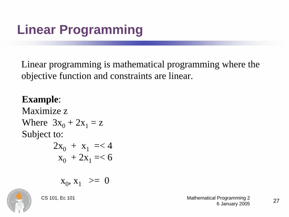
Maximize zWhere 4x0 + 5x1 + 9x2 + 0s0 + 0s1 = zSubject to:
1.x0 + 0.5x1 + 1.5x2 + 0.5s0 + 0s1 = 3x0 + 2x1 + 4x2 + 0s0 + s1 = 9
x0 , x1 , x2 , s0 , s1 >= 0
To pivot, our goal is to make the column vector into a unit vector. So we want to transform the column
[4, 1, 1] to [0, 1, 0]. So, subtract 4 times first constraint from objective function.
pivot

Examples of Simplex Algorithm
CS 101, Ec 101 Mathematical Programming 26 January 2005 53
To pivot, our goal is to make the column vector into a unit vector. So we want to transform the column
[0, 1, 1] to [0, 1, 0]. So, subtract first constraint from second.
Maximize zWhere 0x0 + 3x1 + 3x2 – 2s0 + 0s1 = z - 12Subject to:
1.x0 + 0.5x1 + 1.5x2 + 0.5s0 + 0s1 = 3x0 + 2x1 + 4x2 + 0s0 + s1 = 9
x0 , x1 , x2 , s0 , s1 >= 0
pivot

Examples of Simplex Algorithm
CS 101, Ec 101 Mathematical Programming 26 January 2005 54
To pivot, our goal is to make the column vector into a unit vector. So we want to transform the column
[0, 1, 1] to [0, 1, 0]. So, subtract first constraint from second.
Maximize zWhere 0x0 + 3x1 + 3x2 – 2s0 + 0s1 = z - 12Subject to:
1.x0 + 0.5x1 + 1.5x2 + 0.5s0 + 0s1 = 30.x0 + 1.5x1 + 2.5x2 - 0.5s0 + s1 = 6
x0 , x1 , x2 , s0 , s1 >= 0
pivot

Examples of Simplex Algorithm
CS 101, Ec 101 Mathematical Programming 26 January 2005 55
The problem is again in canonical form.
A basic feasible solution is x0 = 3 and s1 = 6
Are there elements of c that are positive?
Yes, coefficient of x1 is positive. So, increase x1.
Maximize zWhere 0x0 + 3x1 + 3x2 – 2s0 + 0s1 = z - 12Subject to:
1.x0 + 0.5x1 + 1.5x2 + 0.5s0 + 0s1 = 30.x0 + 1.5x1 + 2.5x2 - 0.5s0 + s1 = 6
x0 , x1 , x2 , s0 , s1 >= 0
pivot

Examples of Simplex Algorithm
CS 101, Ec 101 Mathematical Programming 26 January 2005 56
Maximize zWhere 0x0 + 3x1 + 3x2 – 2s0 + 0s1 = z - 12Subject to:
1.x0 + 0.5x1 + 1.5x2 + 0.5s0 + 0s1 = 30.x0 + 1.5x1 + 2.5x2 - 0.5s0 + s1 = 6
x0 , x1 , x2 , s0 , s1 >= 0
What basic variable drops to 0 first when x1 is increased?
pivot

Examples of Simplex Algorithm
CS 101, Ec 101 Mathematical Programming 26 January 2005 57
What basic variable drops to 0 first when x1 is increased?
Maximize zWhere 0x0 + 3x1 + 3x2 – 2s0 + 0s1 = z - 12Subject to:
1.x0 + 0.5x1 + 1.5x2 + 0.5s0 + 0s1 = 30.x0 + 1.5x1 + 2.5x2 - 0.5s0 + s1 = 6
x0 , x1 , x2 , s0 , s1 >= 0
pivot When x1 is increased to 4, s1 drops to 0 while x0remains positive. So, the new basic variables are x0 and x1.

Examples of Simplex Algorithm
CS 101, Ec 101 Mathematical Programming 26 January 2005 58
Old basic variables:x0, s1
New basic variables:x0, x1
Convert to canonical form with new basic variables.
Pivot on column of incoming basic variable and row of outgoing basic variables
Maximize zWhere 0x0 + 3x1 + 3x2 – 2s0 + 0s1 = z - 12Subject to:
1.x0 + 0.5x1 + 1.5x2 + 0.5s0 + 0s1 = 30.x0 + 1.5x1 + 2.5x2 - 0.5s0 + s1 = 6
x0 , x1 , x2 , s0 , s1 >= 0

Examples of Simplex Algorithm
CS 101, Ec 101 Mathematical Programming 26 January 2005 59
Pivot on column of incoming basic variable and row of outgoing basic variables
Maximize zWhere 0x0 + 3x1 + 3x2 – 2s0 + 0s1 = z - 12Subject to:
1.x0 + 0.5x1 + 1.5x2 + 0.5s0 + 0s1 = 30.x0 + 1.5x1 + 2.5x2 - 0.5s0 + s1 = 6
x0 , x1 , x2 , s0 , s1 >= 0
pivot

Examples of Simplex Algorithm
CS 101, Ec 101 Mathematical Programming 26 January 2005 60
Maximize zWhere 0x0 + 0x1 - 2x2 – 5s0 - 2s1 = z - 24Subject to:
1.x0 + 0x1 + 2/3x2 + 1/3s0 - 1/3s1 = 10.x0 + 1x1 + 5/3x2 - 1/3s0 + 2/3s1 = 4
x0 , x1 , x2 , s0 , s1 >= 0
Problem is once again in canonical form.
The basic feasible solution for this canonical form is x0 = 1, x1 = 4, with all other variables x2, s0, s1 being 0.
Since all coefficients of c are now negative, the solution is a local (and hence global) maximum.
Related Documents