Motivation: Fundamental Theorems of Vector Calculus Our goal as we close out the semester is to give several “Fundamental Theorem of Calculus”-type theorems which relate volume integrals of derivatives on a given domain to line and surface integrals about the boundary of the domain. The general form of these theorems, which we collectively call the fundamental theorems of vector calculus, is the following: The integral of a “derivative-type object” on a given domain D may be computed using only the function values along the boundary of D .

Welcome message from author
This document is posted to help you gain knowledge. Please leave a comment to let me know what you think about it! Share it to your friends and learn new things together.
Transcript

Motivation: Fundamental Theorems of Vector Calculus
Our goal as we close out the semester is to give several“Fundamental Theorem of Calculus”-type theorems which relatevolume integrals of derivatives on a given domain to line andsurface integrals about the boundary of the domain.
The general form of these theorems, which we collectively call thefundamental theorems of vector calculus, is the following:
The integral of a “derivative-type object” on a given domain Dmay be computed using only the function values along theboundary of D.

Motivation: Fundamental Theorems of Vector Calculus
As an overview, we will roughly and informally summarize the content of thefundamental theorems of vector calculus. First let’s start with the ones we havealready seen:
1. FTC: An area integral of the form∫ b
af ′(x)dx
may be computed by evaluating f at the boundary points a and b of the1-dimensional domain interval [a, b].
2. Fundamental Theorem for Conservative Vector Fields: A line integralof the form ∫
C ∇Vds
may be computed by evaluating V at the boundary points of the1-dimensional parametrized curve domain C.

Fundamental Theorems of Vector Calculus, contd.
Now here are the new ones.
1. Green’s Theorem: A volume integral of the form∫ ∫D
(δF2
δx−δF1
δy
)d(x, y)
may be computed by line integrating ~F = (F1, F2) along the boundary of the 2-dimensional
domain D.
2. Stokes’ Theorem: A surface integral of the form∫ ∫S curl(~F )dS
may be computed by line integrating ~F along the boundary of the 2-dimensional domain S.
Note: The “curl” of ~F is a derivative-type object we will define later.
3. Divergence Theorem: A volume integral of the form∫ ∫ ∫W div(~F )d(x, y , z)
may be computed by surface integrating ~F along the boundary of the 3-dimensional domain
W.
Note: The ”divergence” of ~F is another soon-to-be-introduced derivative-type object.

Definitions and Terminology
DefinitionLet D be a region in R2. Recall that a point (x , y) is called a boundarypoint of D if every open disk about (x , y) intersects both D and theexterior of D. Denote the set of all boundary points of D by δD. We callδD the boundary of D.
Suppose C may be parametrized by a continuous one-to-one R2-valuedfunction ~c with domain [a, b], where ~c(a) = ~c(b). Then we call C asimple closed curve.
If δD is a simple closed curve, then we choose to orient δD in thecounterclockwise direction. This is called the boundary orientation.

Green’s Theorem
Theorem (Green’s Theorem)
Let D be a domain whose boundary δD is a simple closed curve.Let F = (F1,F2) be a vector field over R2. Then∮
δD
~F · ds =
∫ ∫D
(δF2
δx− δF1
δy
)d(x , y).
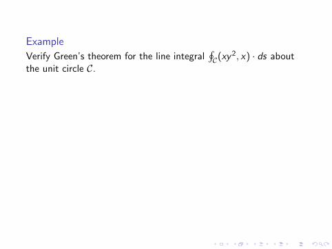
Example
Verify Green’s theorem for the line integral∮C(xy 2, x) · ds about
the unit circle C.
If (F1,F2) = (xy 2, x), then
δF2δx −
δF1δy = 1− 2xy 2,
and hence we are being asked to show that∮C(xy 2, x) · ds =
∫ ∫R(1− 2xy)d(x , y),
where R is the interior of the unit circle.

Example
Verify Green’s theorem for the line integral∮C(xy 2, x) · ds about
the unit circle C.
If (F1,F2) = (xy 2, x), then
δF2δx −
δF1δy = 1− 2xy 2,
and hence we are being asked to show that∮C(xy 2, x) · ds =
∫ ∫R(1− 2xy)d(x , y),
where R is the interior of the unit circle.

Solution: The Line Integral
Goal:∮C(xy
2, x) · ds =∫ ∫
R(1− 2xy)d(x , y)
We start with the line integral on the left. Parametrize C by
~c(t) = (cos t, sin t) for 0 ≤ t ≤ 2π.
We have ~c ′(t) = (− sin t, cos t).Now compute:∮
C(xy 2, x) · ds =
∫ 2π
0
(cos t sin2 t, sin t) · (− sin t, cos t)dt
=
∫ 2π
0
(− cos t sin3 t + cos2 t)dt
=
[−1
4sin4 t +
1
2t +
1
4sin(2t)
]2π
0
= (0 + π + 0)− (0 + 0 + 0)
= π.

Solution: The Line Integral
Goal:∮C(xy
2, x) · ds =∫ ∫
R(1− 2xy)d(x , y)
We start with the line integral on the left. Parametrize C by
~c(t) = (cos t, sin t) for 0 ≤ t ≤ 2π.
We have ~c ′(t) = (− sin t, cos t).
Now compute:∮C(xy 2, x) · ds =
∫ 2π
0
(cos t sin2 t, sin t) · (− sin t, cos t)dt
=
∫ 2π
0
(− cos t sin3 t + cos2 t)dt
=
[−1
4sin4 t +
1
2t +
1
4sin(2t)
]2π
0
= (0 + π + 0)− (0 + 0 + 0)
= π.

Solution: The Line Integral
Goal:∮C(xy
2, x) · ds =∫ ∫
R(1− 2xy)d(x , y)
We start with the line integral on the left. Parametrize C by
~c(t) = (cos t, sin t) for 0 ≤ t ≤ 2π.
We have ~c ′(t) = (− sin t, cos t).Now compute:∮
C(xy 2, x) · ds =
∫ 2π
0
(cos t sin2 t, sin t) · (− sin t, cos t)dt
=
∫ 2π
0
(− cos t sin3 t + cos2 t)dt
=
[−1
4sin4 t +
1
2t +
1
4sin(2t)
]2π
0
= (0 + π + 0)− (0 + 0 + 0)
= π.

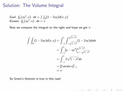
Solution: The Volume Integral
Goal:∮C(xy
2, x) · ds =∫ ∫
R(1− 2xy)d(x , y)
Known:∮C(xy
2, x) · ds = π
Now we compute the integral on the right and hope we get π:
∫ ∫R
(1− 2xy)d(x , y) =
∫ 1
−1
∫ √1−x2
−√
1−x2
(1− 2xy)dydx
=
∫ 1
−1
[y − xy 2]
√1−x2
y=−√
1−x2
=
∫ 1
−1
2√
1− x2dx
= [2 arcsin x ]1−1
= π.
So Green’s theorem is true in this case!

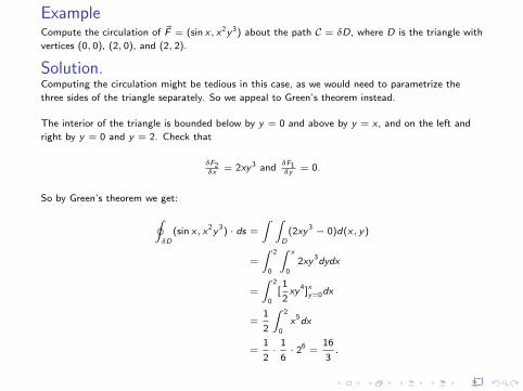
ExampleCompute the circulation of ~F = (sin x, x2y 3) about the path C = δD, where D is the triangle with
vertices (0, 0), (2, 0), and (2, 2).
Solution.Computing the circulation might be tedious in this case, as we would need to parametrize the
three sides of the triangle separately. So we appeal to Green’s theorem instead.
The interior of the triangle is bounded below by y = 0 and above by y = x , and on the left and
right by y = 0 and y = 2. Check that
δF2δx = 2xy 3 and
δF1δy = 0.
So by Green’s theorem we get:
∮δD
(sin x, x2y 3) · ds =
∫ ∫D
(2xy 3 − 0)d(x, y)
=
∫ 2
0
∫ x
0
2xy 3dydx
=
∫ 2
0
[1
2xy 4]x
y=0dx
=1
2
∫ 2
0
x5dx
=1
2·
1
6· 26 =
16
3.

Corollary (Area Formula)Let D be a region in R2 and assume C = δD is a simple closed curve.Then the area of D is equal to
12
∮C(−y , x) · ds.
Proof.Set ~F = (F1,F2) = 1
2 (−y , x) and check that δF2
δx −δF1
δy = 12 − (− 1
2 ) = 1.
Now apply Green’s theorem:
Area of D =
∫ ∫D
1d(x , y)
=
∫ ∫D
(δF2
δx− δF1
δy)d(x , y)
=
∮C~F · ds
=1
2
∮C
(−y , x) · ds.
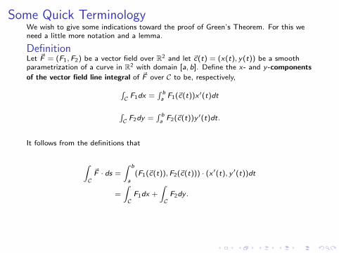
Some Quick TerminologyWe wish to give some indications toward the proof of Green’s Theorem. For this weneed a little more notation and a lemma.
DefinitionLet ~F = (F1,F2) be a vector field over R2 and let ~c(t) = (x(t), y(t)) be a smoothparametrization of a curve in R2 with domain [a, b]. Define the x- and y-components
of the vector field line integral of ~F over C to be, respectively,∫C F1dx =
∫ ba F1(~c(t))x ′(t)dt
∫C F2dy =
∫ ba F2(~c(t))y ′(t)dt.
It follows from the definitions that
∫C~F · ds =
∫ b
a(F1(~c(t)),F2(~c(t))) · (x ′(t), y ′(t))dt
=
∫C
F1dx +
∫C
F2dy .
LemmaThe values of the x- and y-components of a vector field line integral are independentof the choice of parametrization ~c.

Proof of a Special Case of Green’s Theorem
Goal: Show∮δD~F · ds =
∫ ∫D
(δF2
δx− δF1
δy
)d(x , y).
We are unable to give a proof of Green’s theorem in its full generality,but we can prove it if we make the following very special simplifyingassumptions:
I the boundary δD may be described as the union of two graphs ofthe form y = T (x) with B(x) ≤ T (x) for a ≤ x ≤ b; and
I δD may also be described as the union of two graphs of the formx = L(y) and x = R(y) with L(y) ≤ R(y) for c ≤ y ≤ d .
(Picture on whiteboard!)

Proof of a Special Case, contd.
Goal: Show∮δD~F · ds =
∫ ∫D
(δF2
δx− δF1
δy
)d(x , y).
In order to observe Green’s theorem, we will break it up into two parts.
Since∮δD~F · ds =
∮δD
F1dx +∮δD
F2dy , it suffices for us to show thefollowing two equalities:∮
δDF1dx = −
∫ ∫DδF1
δy d(x , y)∮δD
F2dy =∫ ∫
DδF2
δx d(x , y).
We begin by parametrizing the bottom C1 and top C2 of δD.
C1: ~c1(t) = (x1(t), y1(t)) = (t,B(t))C2: ~c2(t) = (x2(t), y2(t)) = (t,T (t))
Note ~c1 traverses C1 along the boundary orientation but ~c2 goes
clockwise, i.e. ~c2 parametrizes −C2.

Proof of a Special Case, contd.
Mid-Goal: Show that∮δD
F1dx = −∫ ∫
DδF1δy
d(x , y)
Now we compute∫ ∫
D
δF1
δyd(x , y).
∫ ∫D
δF1
δyd(x , y) =
∫ b
a
∫ T (x)
B(x)
δF1
δydydx
=
∫ b
a
[F1(x ,T (x))− F1(x ,B(x))]dx
=
∫ b
a
F1(c2(t))x′2(t)dt −
∫ b
a
F1(c1(t))x′1(t)dt
=
∫−C2
F1dx −∫C1
F1dx
= −∮δD
F1dx .
This completes the proof of the mid-goal.
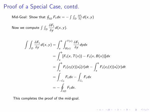

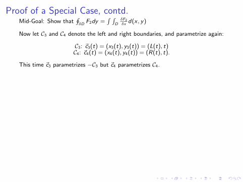
Proof of a Special Case, contd.Mid-Goal: Show that
∮δD
F2dy =∫ ∫
DδF2δx
d(x , y)
Now let C3 and C4 denote the left and right boundaries, and parametrize again:
C3: ~c3(t) = (x3(t), y3(t)) = (L(t), t)C4: ~c4(t) = (x4(t), y4(t)) = (R(t), t).
This time ~c3 parametrizes −C3 but ~c4 parametrizes C4.
∫ ∫D
δF2
δxd(x , y) =
∫ d
c
∫ R(y)
L(y)
δF2
δxdxdy
=
∫ d
c
F2(R(y), y)dy −∫ d
c
F2(L(y), y)dy
=
∫ d
c
F2(~c4(t))y′4(t)dt −
∫ d
c
F2(~c3(t))y′3(t)dt
=
∫C4
F2dy −∫−C3
F2dy
=
∮δD
F2dy .

Proof of a Special Case, contd.
We conclude by observing that, as promised:∮δD
~F · ds =
∮δD
F1dx +
∮δD
F2dy
= −∫ ∫
D
δF1
δyd(x , y) +
∫ ∫D
δF2
δxd(x , y)
=
∫ ∫D
(δF2
δx− δF1
δy
)d(x , y).
Related Documents