Functional segmentation of the brain cortex using high model order group PICA

For Peer Review

Functional segmentation of the brain cortex using high model order group ICA

Journal: Human Brain Mapping

Manuscript ID: HBM-08-0444.R2

Wiley - Manuscript type: Research Article

Date Submitted by the Author:

01-Apr-2009

Complete List of Authors: Kiviniemi, Vesa; Oulu University Hospital, Diagnostic Radiology Starck, Tuomo; Oulu University Hospital, Radiology Remes, Jukka; Oulu University Hospital, Radiology Long, Xiang-Yu; Beijing Normal University, State Key Laboratory of Cognitive Neuroscience

Nikkinen, Juha; Oulu University Hospital, Radiology Veijola, Juha; Oulu University Hospital, Psychiatry Moilanen, Irma; Oulu University Hospital, Child Psychiatry Haapea, Marianne; Oulu University Hospital, Radiology; Oulu University Hospital, Psychiatry Zang, Yu-Feng; Beijing Normal University, State Key Laboratory of Cognitive Neuroscience and Learning Isohanni, Matti; Oulu University Hospital, Psychiatry Tervonen, Osmo; Oulu University Hospital, Radiology

Keywords: ICA, fMRI, resting state, brain cortex

John Wiley & Sons, Inc.

Human Brain Mapping

For Peer Review

Functional segmentation of the brain cortex using high model

order group PICA.

Kiviniemi Vesa1, Starck Tuomo

1, Jukka Remes

1, Xiangyu Long

1,2, Nikkinen Juha

1, Haapea

Marianne1,3

, Veijola Juha3, Moilanen Irma

4, Matti Isohanni

3, Yu-Feng Zang

2, Tervonen Osmo

1

1Department of Diagnostic Radiology, Oulu University Hospital

2 State Key Laboratory of Cognitive Neuroscience, Beijing Normal University, China

3Department of Psychiatry, Oulu University Hospital

4 Department of Child Psychiatry, Oulu University Hospital

Abstract: Baseline activity of resting state brain networks (RSN) in a resting subject has become

one of the fastest growing research topics in neuroimaging. It has been shown that up to 12 RSNs

can be differentiated using an independent component analysis (ICA) of the blood oxygen level

dependent (BOLD) resting state data. In this study, we investigate how many RSN signal sources

can be separated from the entire brain cortex using high dimension ICA analysis from a group

dataset. Group data from 55 subjects was analysed using temporal concatenation and a

probabilistic ICA (PICA) algorithm. ICA repeatability testing (ICASSO) verified that 60 of the

70 computed components were robustly detectable. Forty-two independent signal sources were

identifiable as RSN, and 28 were related to artifacts or other non-interest sources (non-RSN).

The depicted RSNs bore a closer match to functional neuroanatomy than the previously reported

RSN components. The non-RSN sources have significantly lower temporal inter-source

connectivity than the RSN (p< 0.0003). We conclude that the high model order ICA of the group

BOLD data enables functional segmentation of the brain cortex. The method enables new

approaches to causality and connectivity analysis with more specific anatomical details.

Page 1 of 53

John Wiley & Sons, Inc.

Human Brain Mapping

123456789101112131415161718192021222324252627282930313233343536373839404142434445464748495051525354555657585960

For Peer Review

Introduction

Since the discovery of functionally connected low frequency fluctuations of the blood oxygen

dependent (BOLD) with a functional MRI by Biswal and colleagues, the detection of baseline

activity within functional brain networks has become a fast growing interest area in brain

imaging research [Biswal et al., 1995; Fox & Raichle 2007,Vincent et al., 2007]. Intra-cortical

local field potential and multiunit activity fluctuations partly correlate with the fluctuations of the

BOLD signal with a 6 second lag in anesthetized conditions [Logothetis et al., 2001; Shmuel et

al., 2008]. In addition to electrophysiological activity, metabolic, and vasomotor effects partly

explain the detected BOLD fluctuation changes [Fukunaga et al., 2008; Kannurpatti et al., 2008;

Kiviniemi 2008].

The combined effects of these fluctuations in neuronal networks have been shown to be

differentiable from noise during normal, awake resting conditions. Independent component

analysis (ICA) is an effective tool in separating statistically independent source signals of the

BOLD data. ICA separates various sources of the fMRI signal by maximizing the non-

Gaussianity of the source signals. Spatial domain ICA (sICA) can separate BOLD signal sources

that represent reactions to externally cued task-activations, background activity within functional

brain (i.e. resting state) networks (RSN), and various physiological noise and artifact sources

[Beckmann et al., 2004 & 2005; Calhoun et al., 2001; Kiviniemi et al., 2003; McKeown et al.,

1998; Van de Ven 2004]. ICA methodology yields results that are equally accurate to other

contemporary methods of detecting large scale temporally coherent networks from the BOLD

signal data [Long et al., 2008].

Page 2 of 53

John Wiley & Sons, Inc.

Human Brain Mapping

123456789101112131415161718192021222324252627282930313233343536373839404142434445464748495051525354555657585960

For Peer Review

It has been suggested that 10 to 12 RSNs can be detected from the brain cortex from resting state

BOLD data, using ICA with a component dimensionality, i.e. a model order, around 25-40

components [Beckmann et al. 2005, De Luca et al., 2006, Damoiseaux et al., 2006]. However,

the most recent reports on topographic delineation of cortex and functional connectivity nodes

show that there should be more than a dozen detectable functional networks on the brain cortex

[Bartels & Zeki 2005; Cohen et al., 2008; Di Martino et al., 2008; Malinen et al., 2007, Mezer et

al., 2008; Pawela et al., 2008]. When the model order of the ICA estimation is increased, the

separated BOLD signal sources have been shown to split into several functional nodes [Li et al.,

2007; Ma et al., 2007, Malinen et al., 2007, Eichele et al., 2008]. McKeown and co-workers have

shown that the detected ICA components of BOLD data actually represent deterministic signal

sources of the data, even in very high model orders [McKeown et al., 2002].

In this study, we evaluate how many independent RSN signal sources of baseline brain activity

can be detected from the brain cortex using a fairly large group of subjects and a relatively high

order group ICA. We show that the previously detected RSN signal sources can be differentiated

into a more finely tuned functional anatomy by extending the use of temporal connectivity, the

frequency power spectral and the anatomical clustering characteristics of the signal sources into

group analysis data. We show that over 60 of the detected signal sources can be robustly detected

with repeatability analysis (ICASSO-software package) from group data. We found supporting

evidence for our hypothesis that true RSN sources have increased temporal inter-source

connectivity compared to noise sources. Spatial overlap of the RSN components, and predefined

Page 3 of 53

John Wiley & Sons, Inc.

Human Brain Mapping

123456789101112131415161718192021222324252627282930313233343536373839404142434445464748495051525354555657585960

For Peer Review

anatomical structures are presented. The possible functional and clinical implications of the

results are discussed.

Materials and Methods

The ethical committee of Oulu University Hospital has approved the studies for which the

subjects have been recruited, and informed consent has been obtained from each subject

individually according the Helsinki declaration. Fifty-five control subjects were chosen (age

24.96 ± 5.25 years, 32 ♀, 23 ♂) from three resting state studies: an At Risk Mental Stage

(ARMS) 1986 birth cohort study of ADHD and schizophrenia; a 1966 birth cohort study of

schizophrenia; brain tumor resting state study, total n = 200. Subjects were imaged on a GE 1.5T

HDX scanner equipped with an 8-channel head coil using parallel imaging with an acceleration

factor 2. The scanning was done during January 2007- May 2008. All subjects received identical

instructions: to simply rest and focus on a cross on an fMRI dedicated screen which they saw

through the mirror system of the head coil. Hearing was protected using ear plugs, and motion

was minimized using soft pads fitted over the ears.

The functional scanning was performed using an EPI GRE sequence. The TR used was 1800 ms

and the TE was 40 ms. The whole brain was covered, using 28 oblique axial slices 4 mm thick

with a 0.4 mm space between the slices. FOV was 25.6 cm x 25.6 cm with a 64 x 64 matrix, and

a flip angle of 90 degrees. The resting state scan consisted of 253 functional volumes. The first

three images were excluded due to T1 equilibrium effects. In all three studies, the resting state

scanning started the protocols, and lasted 7 minutes and 36 seconds. In addition to resting-state

fMRI, T1-weighted scans were taken with 3D FSPGR BRAVO sequence (FOV 24.0 cm, matrix

Page 4 of 53

John Wiley & Sons, Inc.

Human Brain Mapping

123456789101112131415161718192021222324252627282930313233343536373839404142434445464748495051525354555657585960

For Peer Review

256 x 256, slice thickness 1.0 mm, TR 12.1ms, TE 5.2 ms, and flip angle 20 degrees) in order to

obtain anatomical images for co-registration of the fMRI data to standard space coordinates.

Pre-processing of imaging data

Head motion in the fMRI data was corrected using multi-resolution rigid body co-registration of

volumes, as implemented in FSL 3.3 MCFLIRT software [Jenkinson et al. 2002]. The default

settings used were: middle volume as reference, a three-stage search (8 mm rough + 4 mm,

initialized with 8 mm results + 4 mm fine grain, initialized with the previous 4 mm step results)

with final tri-linear interpolation of voxel values, and normalized spatial correlation as the

optimization cost function. Brain extraction was carried out for motion corrected BOLD volumes

with optimization of the deforming smooth surface model, as implemented in FSL 3.3 BET

software [Smith 2002] using threshold parameters f = 0.5 and g = 0; and for 3D FSPGR volumes,

using parameters f = 0.25 and g = 0. After brain extraction, the BOLD volumes were spatially

smoothed, 7 mm FWHM Gaussian kernel and voxel time series were detrended using a Gaussian

linear high-pass filter with a 125 second cutoff. The FSL 4.0 fslmaths tool was used for these

steps.

Multi-resolution affine co-registration as implemented in the FSL 4.0 FLIRT software

[Jenkinson et al. 2002] was used to co-register mean non-smoothed fMRI volumes to 3D FSPGR

volumes of corresponding subjects, and 3D FSPGR volumes to the Montreal Neurological

Institute (MNI) standard structural space template (MNI152_T1_2mm_brain template included

in FSL). Tri-linear interpolation was used, a correlation ratio was used as the optimization cost

function, and regarding the rotation parameters a search was done in the full [-π π] range. The

Page 5 of 53

John Wiley & Sons, Inc.

Human Brain Mapping

123456789101112131415161718192021222324252627282930313233343536373839404142434445464748495051525354555657585960

For Peer Review

resulting transformations and the tri-linear interpolation were used to spatially standardize

smoothed and filtered BOLD volumes to the 2 mm MNI standard space. Because an sICA was

run later on fMRI data concatenated from the 55 subjects, in practice the spatial resolution of

spatially standardized BOLD volumes had to be lowered to 4 mm.

Spatial domain analysis

Analysis was carried out using Probabilistic Independent Component Analysis (PICA)

[Beckmann et al., 2004] on pre-processed and spatially standardized BOLD data, temporally

concatenated from data sets of individual subjects. The implementation of PICA and temporal

concatenation in FSL 4.0 MELODIC software was used in this study. The default processing

provided in MELODIC, and used in this study, starts on the subject level. Intensities of voxel

time courses in pre-processed fMRI volumes are converted to percentages of change with respect

to the mean intensity in those voxels. This is followed by group level joined normalization of

voxel time course variances. The mean 4D fMRI data set is averaged from individual data sets,

and the variance estimate is computed from it. The variance estimate used in normalization is

computed so that 1) data with respect to its time points (temporal dimensions) is whitened, 2) in

whitened space, large values corresponding to variance, possibly not originating from Gaussian

processes, are noted with some threshold value, and their influence excluded from data in the

original space, after which 3) variance is computed ordinarily on resulting residual data. Within

MELODIC implementation and in its joined normalization scheme, this threshold value was set

to 3.1. Fourth, voxels with insufficient variances (<0.0001) are set to zero because they contain

nearly constant time courses, and in that sense a bad signal-to-noise ratio that would (after

Page 6 of 53

John Wiley & Sons, Inc.

Human Brain Mapping

123456789101112131415161718192021222324252627282930313233343536373839404142434445464748495051525354555657585960

For Peer Review

variance normalization) contribute too much to the analysis. Each individual subject fMRI data

set is divided voxel-wise with a standard deviation corresponding to the voxel-wise variance

estimate. A whitening matrix corresponding to the whitening mean 4D fMRI data set is

computed and used for group-level joined whitening and dimensionality reduction of each

individual subject fMRI data sets. The number of resulting dimensions corresponds to the model

order of ICA that is intended to be used. In this study, the model order was chosen to be 70, in

correspondence to the high order sICA modeling of the resting state BOLD data. Since PPCA

estimation suggested 73 components in an initial test, we reduced it to 70 components due to

better extraction of extracranial voxels after using a more sensitive BET algorithm outside the

MELODIC framework.

The jointly whitened and reduced individual fMRI data sets are further whitened, and then

temporally concatenated. Further dimensionality reduction is performed with principal

components analysis (PCA) on the concatenated data. The number of dimensions in the

concatenated data (number of subjects times 70) is reduced to the number of independent

components to be computed, 70 in this study. Finally, FastICA [Hyvärinen 1999] is performed

using voxel values as samples, and PCA reduced and whitened temporal dimensions as variables.

In this study, we used the default settings in the MELODIC software: symmetric

orthogonalization and skewness (“pow3”) as the contrast function.

In a PICA framework, estimated intensity maps (independent components) are converted to Z-

scores by dividing intensity values by voxel-wise standard deviations of noise distribution.

Standard deviations are estimated through calculation of corresponding voxel-wise variances of

Page 7 of 53

John Wiley & Sons, Inc.

Human Brain Mapping

123456789101112131415161718192021222324252627282930313233343536373839404142434445464748495051525354555657585960

For Peer Review

the original pre-processed data in the subspace left out by dimensionality reduction steps.

Probability distributions of values in individual resulting score maps are modeled using a

mixture of functions, a zero mean Gaussian function and two gamma functions. The Gaussian

function corresponds to the effects due to chance, and the gamma functions model outliers not

observed by chance. For a given Z-score, the sum of gamma function values divided by the sum

of all function values can be used to calculate the probability of actually observing an effect with

that score. With regard to these probabilities, a probability threshold (P-value) is set to leave out

(set to zero) those voxel values in score maps that are presumed to be observed in the PICA

results by chance. In this study, we used P = 0.5, attributing equal relevance to both false

negatives and false positives.

The Juelich histological atlas [Eickhoff et al. 2007], and the Harvard -Oxford cortical and

subcortical atlases (Harvard Center for Morphometric Analysis) which are provided with the

FSL4 software package were used to quantify anatomical characteristics of thresholded Z-score

maps. For this purpose, maps were upsampled back to 2 mm resolution MNI standard space.

Individual anatomical regions in the probabilistic atlases were binarized, and used as masks to

extract the corresponding regions in maps. An FSL4 fslstats tool was used to calculate mean and

maximum intensity in regions, as well as the location of maximum intensity. The number of

voxels in the masked PICA maps was also calculated, and divided by number of voxels in the

whole anatomical masking region, to provide a percentage of the coverage of different

anatomical areas by individual maps.

Page 8 of 53

John Wiley & Sons, Inc.

Human Brain Mapping

123456789101112131415161718192021222324252627282930313233343536373839404142434445464748495051525354555657585960

For Peer Review

A neuroradiologist (VK) depicted the thresholded PICA maps corresponding to the RSNs by

choosing anatomically clustered sources in the cortical regions, in the vicinity of functional brain

regions. The sources were further classified into three regions for illustration purposes with a

scheme modified from Salvador and co-workers [2005] (peri-sylvian = rolandic and temporal,

frontal, occipito-parietal). In each of the selected sources, 1) sources presented clustered voxel

groups, 2) sources were focused on cortical structures, and 3) time courses in the ICA mixing

matrix corresponding to the maps showed elevated low frequency (<0.1 Hz) power. Artifactual

non-RSNs were identified based on their motion related location at the borders of the brain, in

cerebrospinal fluid (CSF), at the proximity of large blood vessels, in white matter, and in the

vicinity of areas shown to be susceptible to physiological pulsations with relatively increased or

mixed high frequency power [Birn et al., 2006; Lund et al., 2006].

Repeatability analysis: The data from the final step prior to FastICA was also subjected to ICA

repeatability analysis (ICASSO) [Himberg, Hyvärinen & Esposito 2004]. Since ICA is sensitive

to its initialization, this framework runs FastICA multiple times on the same data, with random

initializations and clusters with a hierarchical clustering algorithm, on the results from individual

runs. The number of clusters is the same as the number of components, and provides statistics

about the quality of the clusters, reflecting the stability of the ICA results. In this study, we used

the provided Matlab implementation [Himberg, Hyvärinen & Esposito 2004] with 100 runs, and

a low epsilon threshold (0.0000001) so that optimization would not converge too soon before

reaching extrema. Symmetric orthogonalization and skewness (“skew”) as the contrast function

were also used in this setting. The conservative cluster quality index Iq was used to estimate

individual component repeatability [Himberg, Hyvärinen & Esposito 2004]. Iq is one for an ideal

Page 9 of 53

John Wiley & Sons, Inc.

Human Brain Mapping

123456789101112131415161718192021222324252627282930313233343536373839404142434445464748495051525354555657585960

For Peer Review

cluster, and decreases when component clusters become less compact and isolated in repeated

ICA runs.

Time domain analysis

A mixing matrix estimated in an sICA contains time courses corresponding to estimated spatial

maps (independent components). The time courses represent the behavior of non-artifact

components in time more accurately than the average BOLD time courses computed from the

same spatial area as in the maps; this is because the most dominant effects of cardiac, respiratory,

CSF-pulsation and motion, and other artifacts are eliminated into separate components. This

offers preprocessed time courses for temporal correlation analysis of BOLD signal sources [Jafri

et al., 2008; Sorg et al., 2007].

In a temporal concatenation scheme, the mixing matrix can be divided into subject specific

consecutive segments, reflecting subject-wise temporal behavior of components. In this study,

these subject specific 250 point time courses were used to assess pair-wise inter component

connectivity on the group level. The time courses were first de-trended, and then correlated with

each other on the subject level with the Pearson product-moment correlation coefficient with a

zero lag. The group level average and standard deviation of the results were calculated for each

correlation pair’s absolute values.

In addition, the mean of these group-level absolute correlation coefficients was calculated per

component within the group of components corresponding to RSNs, and within the group

corresponding to non-RSNs. These values were tested for differences with a two-sample t-test

between RSNs and non-RSNs.

Page 10 of 53

John Wiley & Sons, Inc.

Human Brain Mapping

123456789101112131415161718192021222324252627282930313233343536373839404142434445464748495051525354555657585960

For Peer Review

Frequency domain analysis

The subject-wise time courses extracted from the mixing matrix were (after detrending) also

converted to power spectra, to assess contribution of low frequency power in them. For each

time course, a spectrogram was computed with 128-point rectangular windowing in Matlab

(R2008a) with the similarly named function. Rectangular windowing was sufficient, since no

sinc-interpolation (e.g. no zero padding) was used in the Discrete Fourier Transform. The

absolute values of the resulting 123 spectra were raised to the second power to approximate

power spectra, and they were averaged to obtain a final power spectrum estimate for each time

course.

For the group-level analysis, each power spectrum was normalized by dividing its values by its

total power. Normalized power spectra from individual subjects were averaged for each

component, to produce a group-level representation of temporal power. In addition, Singular

Value Decomposition was used for each component to produce, on a group-level, a rank-1

approximation of subject-specific power spectra for that component. Rank-1 approximation

depicts frequencies with the most commonly elevated power in subject-level time courses.

Page 11 of 53

John Wiley & Sons, Inc.

Human Brain Mapping

123456789101112131415161718192021222324252627282930313233343536373839404142434445464748495051525354555657585960

For Peer Review

Results

Repeatability measures

An ICASSO algorithm was run on the pre-whitened PCA-data matrix provided by the

MELODIC. After 100 repeated runs of the group ICA, significantly clustered components were

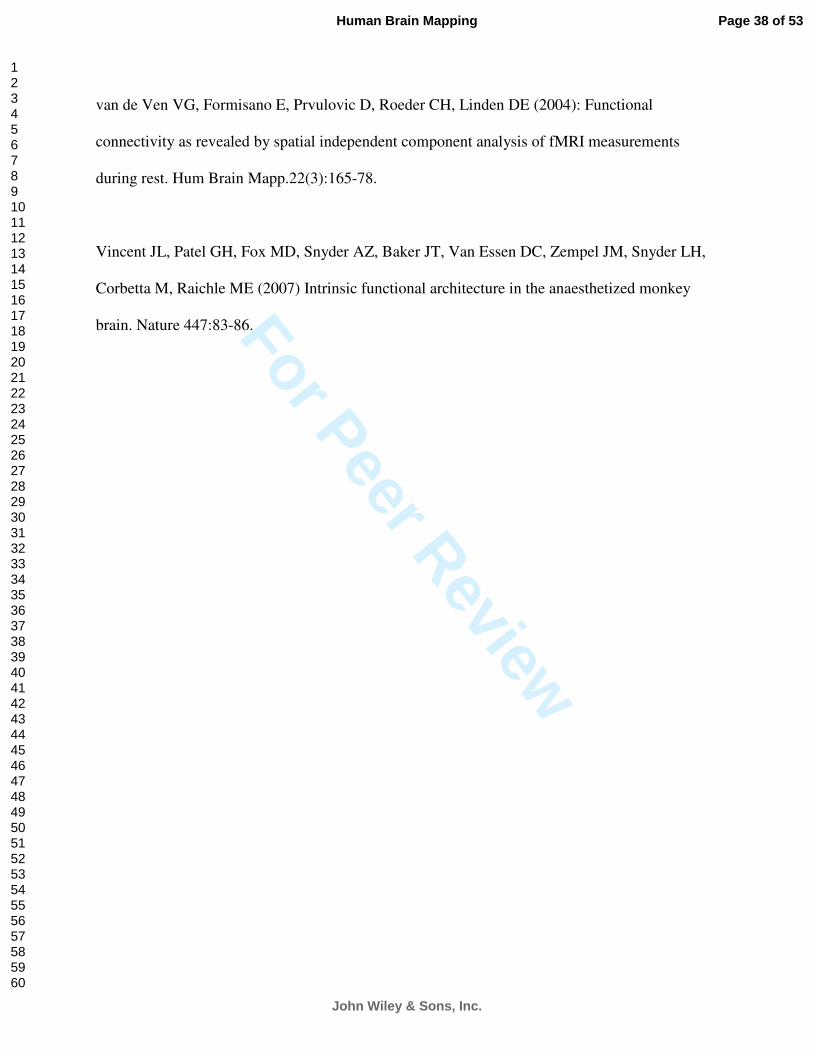
detected. Fifty-one of the 70 ICs had an Iq over 0.8, and 60 ICs still had an Iq of at least 0.7.

Figure 1 shows clustering of the centroid components and stability indexes in reducing the

stability order. PICA estimation of the group data yielded 73 components. We made 7 separate

runs altering the basic spatial smoothening parameters (3-7mm FWHM), temporal high (100-420

s) and low-pass filtering. In essence, the spatial correlation between the detected ICA

components of separate runs was always > 0.7.

< Fig.1 can be here >

RSN-identification

The group PICA separated 42 components that were identified as RSN. These 42 components

cover most of the brain cortex excluding areas having susceptibility artefacts due to air sinuses.

The corresponding RSN components had an average Iq = 0.83 (±0.13) in the ICASSO analysis.

The RSN components had elevated low frequency fluctuation power and, spatially, were

clustered components located in the cortex. Figures 2 to 4 show fused maps and separate spatial

distributions of 25 of the different signal sources on both sides of the Sylvian fissure and the

Page 12 of 53

John Wiley & Sons, Inc.

Human Brain Mapping

123456789101112131415161718192021222324252627282930313233343536373839404142434445464748495051525354555657585960

For Peer Review

central sulcus (Peri-Sylvian), in the frontal lobe (Frontal), and in the occital and parietal regions

(Occipito-Parietal). The remaining signal sources are shown in Fig. 5 in more optimal 3D

presentations.

Twenty-eight ICs were related to non-RSN sources. Eighteen non-RSN components were

identified as motion/realignment artifacts, and physiological noise sources such as arterial and

CSF pulsation. Ten of the discarded components were detected as large voxel clusters in the

white matter, and were not further analysed. Ten examples of the non-RSN sources are shown in

Fig.6.

Anatomical parcellation

In practice, most of the cerebral cortex can be shown to be segmented with the IC components

(c.f. the upper rows in Figures 2-4). On average, the maximal spatial correlation between

detected RSN components and other sources was 0.2 (sd 0.04). This can be seen in Figures 2-4

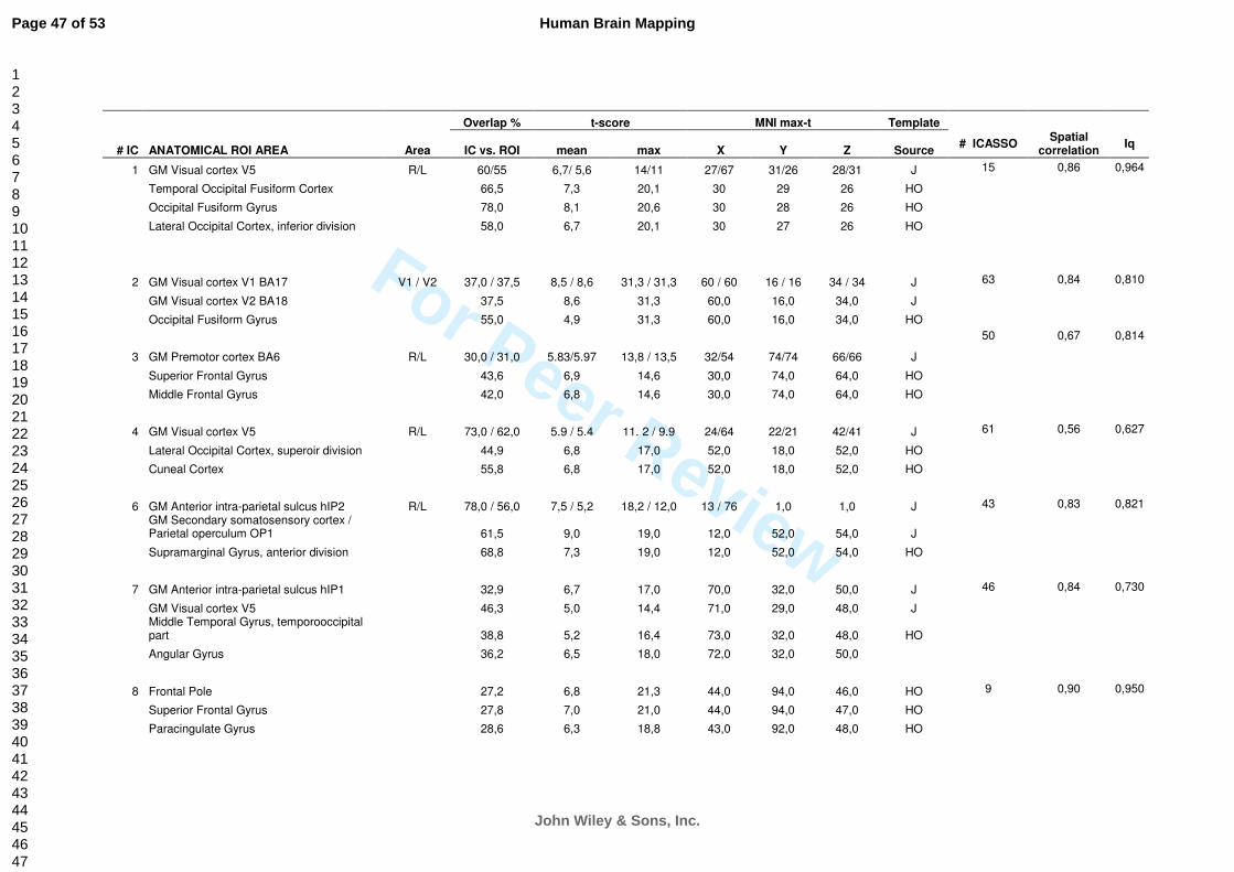
as a limited spatial overlap of separate signal source components. Table 1 lists the first 3-5

largest overlapping anatomical segments used in FSL4 (Juelich and Oxford atlases) in

comparison with the selected RSN signal sources. The RSN components actually show more

connectivity nodes to multiple other anatomical structures, and the complete table is presented in

the supplementary material (Supplementary: Extended Table 1.2 ). In the following, the

individual RSN sources are evaluated, based on spatial overlap with pre-existing anatomical

segments. Temporal inter-source synchrony of the sources, and the highest spatial correlation

with ICASSO components are also presented.

Page 13 of 53

John Wiley & Sons, Inc.

Human Brain Mapping

123456789101112131415161718192021222324252627282930313233343536373839404142434445464748495051525354555657585960

For Peer Review

Rolandic signal sources

Figure 2 shows six signal sources identified as peri-rolandic, situated at or in the vicinity of the

central sulcus. Although most of the sources have strong localized connectivity, some have long

range connectivity to other primary and secondary sensory areas, such as to the visual and

auditory regions.

The motor cortex was divided into two different signal sources resembling the classical

separation of upper cortical structures representing the hand areas (IC 27) and midline feet areas

(IC 19). Similar to the original discovery of Biswal et al., there was a midline connectivity node

posterior to the typical SMA seen during activation studies [Biswal et al., 1995]. Another motor

cortex component, IC 24, was depicted, but it was not clear whether such parcellation is due to

physiological factors, or if the results are split due to positioning differences in the original

BOLD axial slices. Anterior to motor areas there were unilateral components (IC’s 53 & 60) with

positive connectivity to the cerebellum. The right anterior motor IC 60 was spatially larger than

the left IC 53.

Primary and secondary somatosensory cortices were separated into signal sources of their own

(IC 6 and, 43, respectively). Posterior to these, there was a symmetrical, bilateral post-

somatosensory cluster (Fig ure 5, IC 40). The somatosensory signal source also showed smaller

clusters of connectivity to anatomical visual, auditory and Broca’s areas (c.f. Table 1_2

[supplementary]). The signal source IC 14 was situated below the somatosensory cortex in the

white-grey matter boundary. The secondary somatosensory source (IC 43) also showed

Page 14 of 53

John Wiley & Sons, Inc.

Human Brain Mapping

123456789101112131415161718192021222324252627282930313233343536373839404142434445464748495051525354555657585960

For Peer Review

connectivity with structures in the cerebellum, in addition to secondary somatosensory, auditory,

motor and pre-motor anatomical structures. The supplementary motor area (SMA, i.e.

juxtapositional lobule) area had bilateral connectivity clusters in IC 49, primarily involving the

insular cortices, and partly involving the secondary somatosensory area, resembling mirror

neuron networks. Interestingly, both pre-motor areas BA6 also presented unilateral components,

i.e. IC’s 53 & 60 (Fig 5). There was a tendency that the farther a source was from the central

sulcus, the longer the distances were between detected connectivity clusters.

< Fig 2 can be here >

Temporal lobe signal sources

In figure 2, the primary auditory cortex was identified as a bilateral component of its own, with a

right brain dominance (IC 25). As with the peri-rolandic sources, this large network presented

connectivity with other sources in distant regions, in both the motor and visual areas. A Broca’s

area on the left and an homologous right hemisphere Broca’s area were detected in a unique

bilateral component, with a clear, functionally connected cluster in the right paracingulate areas,

posterior cingulate gyrus, and bilateral occipital poles (IC 30). The the fronto-insular cortex of

the salience network was detected in a bilateral IC 15 with a partial Broca’s area and inferior

frontal gyrus involvement, in addition to paracingulate gyrus connectivity [Shihadran et al.,

2008]. IC 49 showing connectivity to SMA could be differentiated from the salience network.

The temporal poles (IC 13, Fig. 5) were also detected in a unique signal source, with

connectivity to midline structures to bilateral hippocampi.

Page 15 of 53

John Wiley & Sons, Inc.

Human Brain Mapping

123456789101112131415161718192021222324252627282930313233343536373839404142434445464748495051525354555657585960

For Peer Review

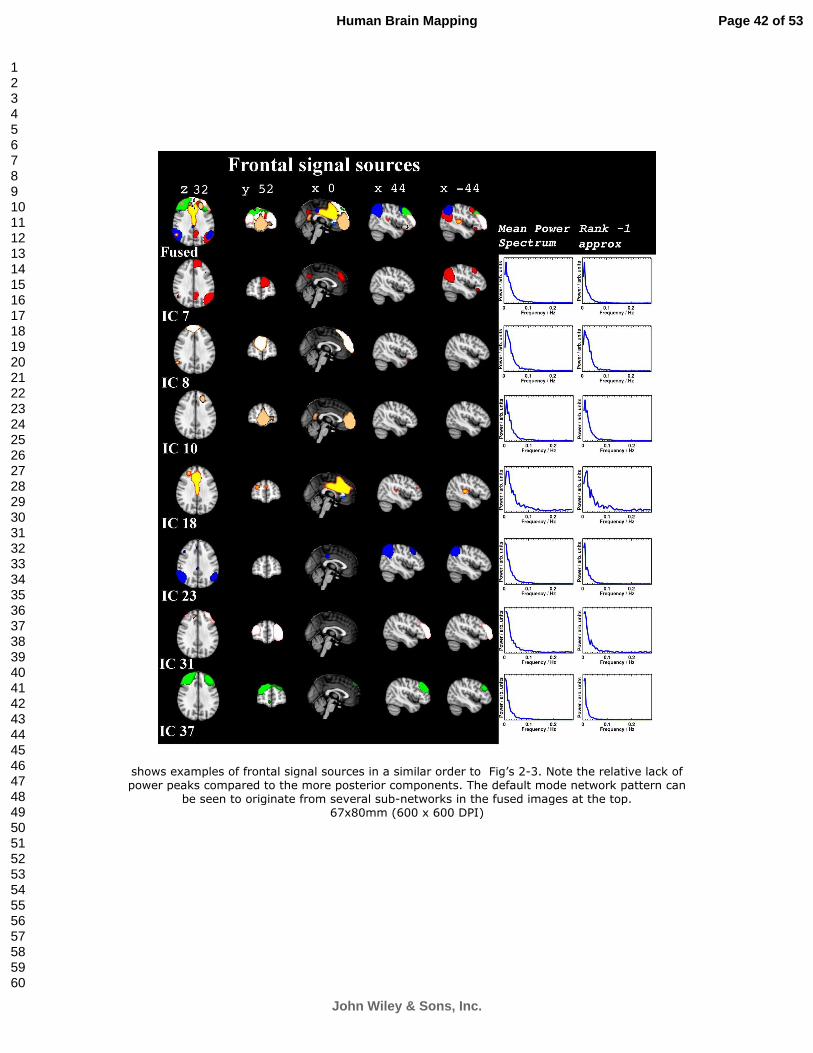
Frontal signal sources

The frontal lobe had eleven RSN signal sources, seven of which are presented in Figure 3. In five

sources (ICs 7, 10, 18, 31 and 37), connectivity to language-related areas, such as the auditory

cortex, inferior frontal gyrus and/or Broca’s anatomical areas, was detected. In addition to these

areas, IC 7 and 10 were also connected to the anterior cingulate and paracingulate gyri. IC 7 had

connectivity to the angular gyri and the visual cortex. IC 10 was present at the lower frontal pole

and medial frontal cortex, and IC 8 was related to the upper frontal pole, and the middle and

superior frontal and angular gyri. IC 18 was connected to the superior frontal gyrus,

paracingulate, and cingulate gyri. IC 23 was connected to the angular and supramarginal gyri,

along with the visual cortex. IC 37 was related to the superior and medial frontal gyri, and the

paracingulate gyri.

< Fig.3 can be here>

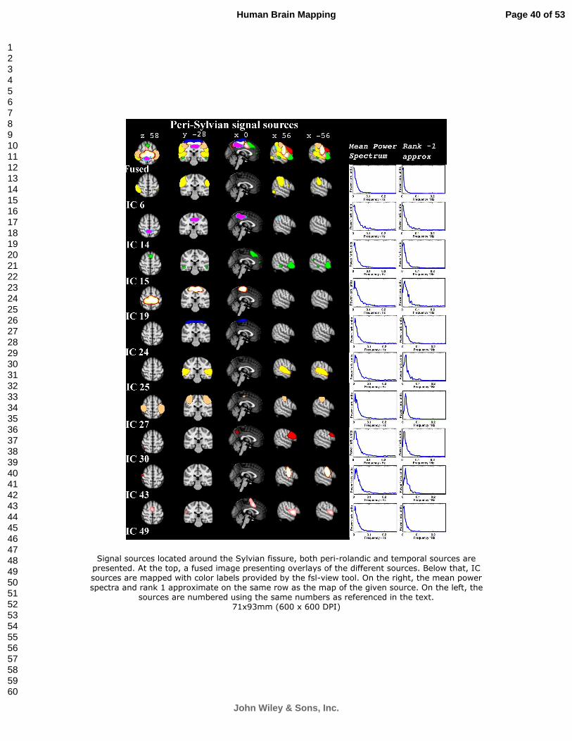
Occipital and Parietal signal sources

There were seven separated signal source clusters in the occipital lobe, all spatially connected to

visual areas (c.f. Figure 4). IC 2 was situated at the lateral part of the primary visual cortex (V1),

as in the lateral visual component in previous papers. Above and lateral to it was IC 4, with

midline connectivity in V5. IC 39 was also comprised of bilateral V5 areas, yet different V5

areas from those in IC 4, with connectivity to V1&2 and the inferior and medial temporal gyrus.

IC 59 typically presented the previously detected medial visual resting state network, comprising

almost completely of the intracalcarine and supracalcarine cortex, the lingual cortex, and the

Page 16 of 53

John Wiley & Sons, Inc.

Human Brain Mapping

123456789101112131415161718192021222324252627282930313233343536373839404142434445464748495051525354555657585960

For Peer Review

major parts of V1&2 and the cuneal cortex. An anterior medial visual component IC 32 in V2,

with hippocampal and geniculate body connectivity, was also detected. A posterior component

IC 21 was separated from the medial central IC 59. The cuneal and precuneal cortex were

dominant in IC 63, along with V1&2, with clear retrosplenial connectivity. In addition, there

were two anti-correlated components in the visual areas (IC’s 52 & 61) showing positive z-

scores caudally on the other visual cortex, and negative z-scores on the contra-lateral side more

cranially.

< Fig. 4-6 can be here >

Default mode and frontal attention control sources

Several ICA sources were detected in the areas known to be related to the default mode network

(DMN). IC 10 = ventromedial prefrontal cortex (vmPFC), IC 38 = precuneus & parietal lobule

(PCC). ICs 7, 10, 23, 18, and 37 were closely related to anatomical structures of the DMN (c.f.

Figures 3-4). The regions usually detected as anti-correlated to DMN in correlation analysis were

also detected as sources of their own, i.e. IC’s 6, 40 and 49 [Fox et al., 2007,Buckner et al.,

2008]. IC 17 resembles the frontal areas central executive network [Shihadran et al., 2008].

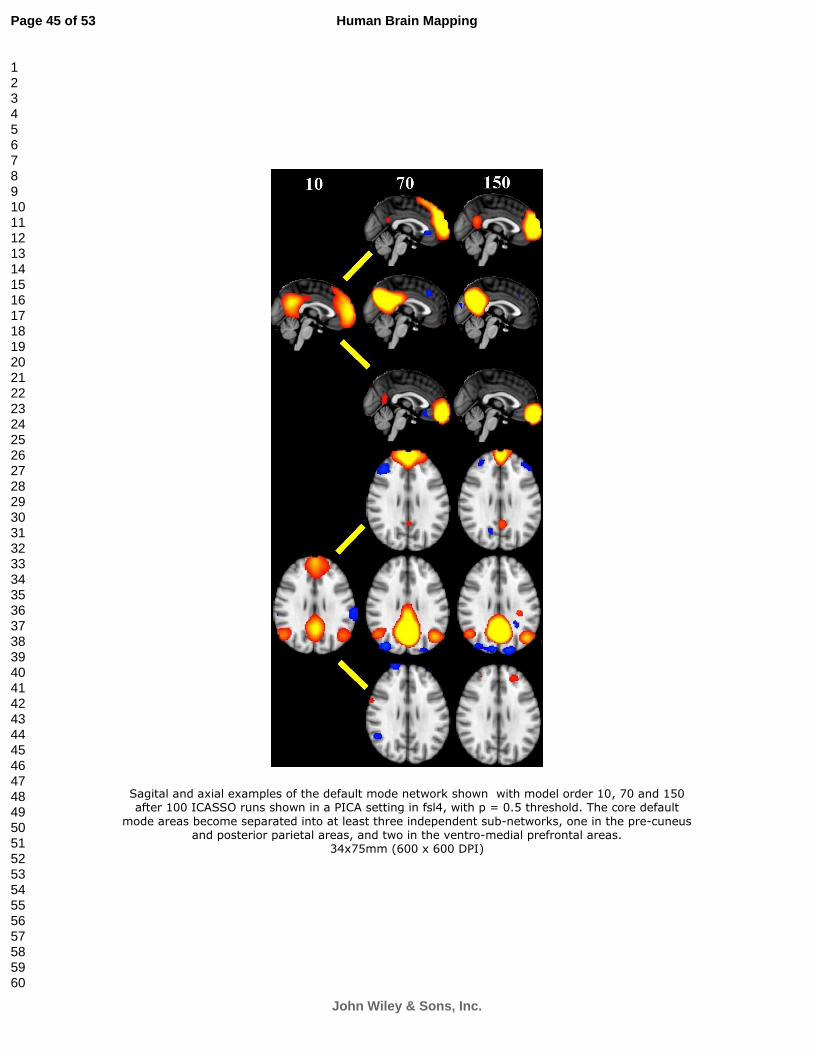
Figure 7 shows an example of PICA images calculated with 100 repeated ICASSO runs with

model orders 10, 70 and 150. Please note how the core areas of the default mode divide into

smaller sub-networks with increasing model order.

< Fig. 7 can be here>

Page 17 of 53

John Wiley & Sons, Inc.

Human Brain Mapping

123456789101112131415161718192021222324252627282930313233343536373839404142434445464748495051525354555657585960

For Peer Review

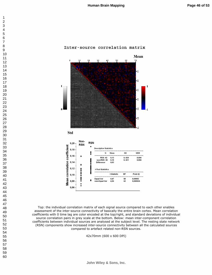
Time domain synchrony

The inter-source connectivity between all the calculated ICs are presented in a matrix in Figure

8. The graph shows how the individual sources are connected to the other sources on average

with zero time lag. The correlation coefficients range from 0.64 to -0.66 ( ± 0.21). The mean

correlation coefficients of each component provide an overall assessment of general inter-source

connectivity of a given IC. The overall connectivity of the non-RSN sources was statistically

significantly lower than the connectivity of the RSN sources (t = 4.6, p< 0.000024, c.f. Figure 8

bottom). Eight out of the ten lowest values of summed correlation were depicted in non-RSN

sources. There is, however, some overlap in the correlation values between the RSN and non-

RSN sources, and temporal zero-lagged correlation alone cannot be used to separate the sources

with absolute certainty.

< Fig.8 can be here>

Frequency domain

The mean power spectra of the individual ICA time courses extracted from the group data

mixing matrix had increased low frequency power with 1/f distribution characteristics (see also

Figures 2-4). The first rank approximate of the power spectra shows the most contributing

frequencies, mostly presenting the same proportional distribution as the mean power spectra. In

the majority of the components, the dominant feature is the 1/f characteristic trend. However, in

ICs 7, 18, 19, 21, 25, 27, 30, 32, 38, 43, 59, and 63, there is a distinct peak in lower frequencies.

That is, the lowest frequency is not with the largest power. The peaks were almost absent from

frontal sources, with the exception of DFM related IC 18. Primary auditory IC 25,

Page 18 of 53

John Wiley & Sons, Inc.

Human Brain Mapping

123456789101112131415161718192021222324252627282930313233343536373839404142434445464748495051525354555657585960

For Peer Review

somatosensory IC 43, motor ICs 19 and 27, and visual sources 21, 32 and 59 showed peaks. In

the visual cortex, IC 59 in the medial areas had an exceptional 0.045 Hz frequency peak at the

most dominant approximate. Default mode IC 38 and the Broca area source IC 30 also presented

peaks in their power spectra.

Discussion

The results of this study represent functional segmentation of the human brain cortex, using the

statistical independence of spontaneous brain activity sources as a delineating feature. We have

shown that the intrinsic baseline activity of the brain cortex can be separated into 42 independent

sources, having resting state network features, using a high model order PICA approach. These

sources cover virtually the whole brain cortex, excluding the sources affected by susceptibility

artefacts near air-sinus interfaces. The dominant low frequency power characteristics of rank-1

approximates in the RSN support the idea that the sources represent low frequency background

activity of the RSN. All of the RSN sources have increased LFF power in the mean power

spectra (c.f. Figures 2-4).

The utilization of continuous in vivo baseline activity information on brain activity offers a

complementary method to previous anatomical/histological dissection studies, as well as imaging

data-based segmentation studies, which currently form the basis of spatial localization schemes.

The introduction of functional segmentation offers a more accurate tool for delineating

functional activity that traverses presently used tissue segmentation borders in connected

neuronal networks. In addition, these IC source maps can be used as data driven, statistically

independent, functional seed regions for further correlation analyses.

Page 19 of 53

John Wiley & Sons, Inc.

Human Brain Mapping

123456789101112131415161718192021222324252627282930313233343536373839404142434445464748495051525354555657585960

For Peer Review

Using present 1.5 T MRI scanning methodology our group has identified 42 signal sources over

the whole brain cortex. The results of this study are in excellent agreement with the recent results

of Cohen et al. [2008], who showed several small functionally connected areas within the same

cortical regions. The work of Malinen and co-workers convincingly shows that during natural

stimuli there are all together at least twenty task and non-task related signal sources detectable in

the brain [Malinen et al., 2007]. Compared to a higher resolution fMRI scan on a rat, the results

of this study seem conservative, since rats were shown to have some 20 connectivity hubs

detectable in the somatosensory and visual systems alone [Pawela et al., 2008]. Two groups have

been able to identify separate regions from the striatum and thalamus with distinct functional

connectivity to the brain cortex in human subjects [DiMartino et al., 2008, Mezer et al, 2008].

On a sub-millimeter scale, anatomical structures of the visual field columns and cortical layers

can be identified based on the spontaneous electrophysiological activity of sub-second time

scales. This suggests that an even greater number of spontaneous signal sources will be

detectable with increased spatiotemporal accuracy in the future [Kenet et al., 2003; Pelled &

Goelman 2004].

The previously detected 12 signal sources that were found in smaller datasets are basically

summations of some of the sources presented here [Beckmann, et al., 2005; Damoiseaux et al.,

2006; Sorg et al., 2007; Jafri et al., 2008]. An example of this can be seen in the Figure 7, where

the DMN is initially presented as one single source with the model order 10, and, after increasing

the model order, becomes divided into several sources. It seems that low model orders provide

information on large scale networks, whereas higher model orders, at least in group-data settings,

Page 20 of 53

John Wiley & Sons, Inc.

Human Brain Mapping

123456789101112131415161718192021222324252627282930313233343536373839404142434445464748495051525354555657585960

For Peer Review

provide sub-network accuracy. We are currently analyzing the effect of model order on the

dividing of RSN’s into sub-networks. We suggest that the 42 group-PICA signal sources

depicted in this study represent a more finely-tuned and segmented version of the functional

neuro-anatomy of the RSN’s in the brain cortex, and therefore we strongly support using high

model order in large group datasets.

The distinction of components into two categories of either RSN or non-RSN may be somewhat

arbitrary although there have been some successful attempts towards automated noise removal

that basically also delineates IC’s into neuronal and artifactual originated ones [De Martino et al.,

2007; Tohka et al., 2008]. One might justifiably speculate in the absence of definite exclusion

criteria that there exist a “borderline” between RSN sources and non-RSN sources. Some IC’s

have features of cortical signal source overlapping with regions often presenting artifacts. For

example IC’s 3, 24 and 40 all are situated within the cranial brain cortex and somewhat resemble

sources seen in individual ICA results as motion artefact/partial volume effects. However at least

IC 40 seems to be a RSN based on further studies not shown here. On the other hand IC’s 8, 52

and 61 are situated very close to sagital or transverse sinuses and one might speculate that the

source has some contribution from pulsation from sagital sinus. However the sagital sinus at

least was shown to have an even more confined source of its own (IC 46) c.f. Fig 6. It would be

beneficial to obtain a more quantitative criteria than anatomical positioning and low frequency

fluctuation of the sources in order to differentiate true RSN sources from artefacts.

The signal sources depicted here accurately follow the known functional anatomy of the sensory

and motor networks. Sources IC 19 and 27 together cover 89 % of the right and 86 % of the left

Page 21 of 53

John Wiley & Sons, Inc.

Human Brain Mapping

123456789101112131415161718192021222324252627282930313233343536373839404142434445464748495051525354555657585960

For Peer Review

primary motor cortices when compared to MNI atlases in fsl4. Primary sensorimotor areas were

shown to have spatial connectivity with fourteen IC’s, twelve of which were the same (IC

3,4,6,14,19,24,27,40,43,53,60,66). The M1 anatomical area was uniquely connected to IC’s 41 &

45 , while S1 was connected to IC 9 & 35, c.f. Table 1_2 in the supplement. Somatosensory S1

had a spatial overlap of 61 % (IC 6) and S2 72 % (IC 43). The supplementary motor area (i.e.

juxtapositional lobule) activity was differentiated from the primary sensorimotor components,

although it was shown to have connectivity to them. SMA was shown to be connected to 12

RSN’s, the largest share being detected in IC 49 (58%). Also IC’s 53 (24 %), IC 60 (34%), IC 18

(30%), IC 19 (36%) had relatively high spatial overlaps with the SMA template. The unilateral

and somewhat anterior pre-motor sources (IC’s 53 & 60: Broadman area BA6, 42 % and 55%,

respectively) could be related functional differences of the subjects pre-motor areas [Longcamp

et al, 2005].

Visual sources are separated into multiple sources, and not only into medial and lateral

components as before. The primary and secondary visual cortices V1 & V 2 were detected in 10

IC’s (IC’s 1,2,4,21,32,38,52,59,61,63),and, the largest overlap for V1 was in IC’s 21 and 55,

both having 55.5 %. The secondary V2 had the largest overlaps in IC’s 21 (51%) and IC 59

(54%). The multiple components have a strong resemblance to natural viewing (V1-V5, lateral

occipital complexes) and listening-related components in the occipital and temporal regions

[Bartels & Zeki 2005, Malinen et al., 2007]. The positive/negative IC’s 52 and 61 resemble

visual fields seen in visual hemifield activation study using the frequency based group ICA

[Calhoun et al., 2003].

Page 22 of 53

John Wiley & Sons, Inc.

Human Brain Mapping

123456789101112131415161718192021222324252627282930313233343536373839404142434445464748495051525354555657585960

For Peer Review

IC 25 was most overlapping with the primary auditory cortex ( 90.5% with the right TE 1.0 and

89.7 % with TE 1.2 on the left) and is left-dominant. The primary auditory cortex was connected

to ten IC’s (IC’s 1,15,18,25,29,37,39,43,47,68). Broca’s area had connectivity with sixteen

sources (IC’s 3,4,7,8,9,10,15,30,31,35,37,39,43,49,66,68) with largest nodes in IC 30 (77 % right

side), IC 35 (97 % left side). Several other frontal and temporal sources have interesting and

complex connectivity with various functional regions related to attention, language and other

cognitive functions. Their spatial overlapping with presently known anatomical regions are rich,

just like those of the primary sensory and motor cortices, and they are presented more precisely

in the Supplement: Extended Table 1.2.

Recent findings show that the DMN nodes have separate causality and connectivity

characteristics [Sridharan et al., 2008; Uddin et al., 2008]. Also researchers using ICA have

noticed the separation of the DMN into at least two sub-networks [Calhoun et al., 2008;

Damoiseaux et al., 2006]. The results of this study shows that the DMN is functionally

differentiated into anterior and posterior parts. There are also “DMN-type” components (IC 7,

10, 23, 18, and 37) with clear spatial overlap with DMN related areas [Buckner et al, 2008]. The

detection of these areas is particularly sensitive to model order of the ICA and we are currently

investigating this phenomenon.

The regions detected as anti-correlated with the DMN in correlation analyses using global mean

regression were also detected as sources of their own (IC’s 6, 40, 49). The use of ICA avoids the

problematic regression of the global mean signal, although the PCA mean subtraction step in

pre-processing of PICA also alters the data to some extent [Murphy et al., 2008]. Based on the

Page 23 of 53

John Wiley & Sons, Inc.

Human Brain Mapping

123456789101112131415161718192021222324252627282930313233343536373839404142434445464748495051525354555657585960

For Peer Review

present results, the areas anti-correlated to DMN in correlation analyses are also present as

independent signal sources and therefore may not be completely a by-product of global mean

signal regression of BOLD signal.

In order to maximize the chances of effective treatment, it is crucially important to identify

diseases at the earliest stage possible. Functional alterations often present themselves as

symptoms prior to irreversible tissue damage. For clinical brain research, function-based tissue

segmentation is of pivotal importance in the early detection and characterization of diseases.

Greicius and co-workers [2004, 2007] have already shown that minimally impaired memory

deficiency or depression are related to the function of a brain network. ICA analyses detecting

multiple brain networks have shown that, while some networks show no changes, others may be

more affected by diseases such as Alzheimer’s and schizophrenia [Calhoun et al., 2008; Jafri et

al., 2008; Sorg et al., 2007]. The high model order ICA segmentation increases functional and

anatomical specificity in the connectivity analysis of the networks and so may enhance our

ability to detect disease-related network alterations.

The ICA methodology in this study is widely used by other researchers, and we suggest that the

relatively high number of detected RSN components is due to increased signal-to-noise ratio

related to the large dataset used in the group analysis. How inter-subject variance affects the

results is, however, an important question; are we seeing more fringe components that are only

present on sub-populations within the group [Schmidthorst & Holland, 2004]? For example,

bored, anxious or enthusiastic subjects might have different strengths of fluctuations in default

Page 24 of 53

John Wiley & Sons, Inc.

Human Brain Mapping

123456789101112131415161718192021222324252627282930313233343536373839404142434445464748495051525354555657585960

For Peer Review

mode sub-networks. The answer to this problem is also related to model order of a large group

dataset and therefore this issue may not be entirely handled within the scope of this manuscript.

The only minor alteration compared to general trends in ICA analyses was the utilization of 70

components. The high model order is supported by the works of McKeown et al. [2002] and

some recent ones as well [De Martino et al., 2007, Malinen et al., 2007]. One can always

speculate on the effects of over-fitting in the detected components, if there are any. It should be

noted that model order estimation with PPCA also yielded high model order numbers, i.e. 73 in

this dataset, which strongly speaks against major overfitting. Two of the original 73 components

were related to non-accurate extra-brain tissue removal, and this was corrected by utilizing

another bet-algorithm outside the MELODICA automated tool.

In order to validate the stability of the method, we employed ICASSO on the pre-processed

MELODIC data matrix. In doing so, 60 out of 70 components were shown to have a stability

value of at least 0.7 in the group analysis, especially when the ICASSO was computed using a

low epsilon threshold. Higher epsilon thresholds led to less clustered components in repeated

runs due to less demanding convergence of the ICA algorithm around local maxima. It should be

interesting to see how the repeated ICASSO analysis results differentiate from single subject run

PICA results. We are currently exploring the benefits of using both PICA and ICASSO in a

combined analysis setting. Another unclear issue is how the RSN’s detected in the group data

can be used in individual settings. Based on the results shown here, a familiar ICA related issue

re-emerges; what is the optimal model order of ICA in datasets with increased subject numbers,

and how are pre-processing schemes influencing the results? We are currently investigating

Page 25 of 53

John Wiley & Sons, Inc.

Human Brain Mapping

123456789101112131415161718192021222324252627282930313233343536373839404142434445464748495051525354555657585960

For Peer Review

whether it is still possible to detect more accurate RSN components with bigger data samples and

higher model orders.

The temporal correlation matrix of the ICA enables the assessment of connectivity between all

the detected signal sources. It can be seen that some of the sources have limited correlation to

practically all the other sources, which becomes visible as a dark row in the mean connectivity

matrix (c.f. Figure 5). These dark lines tend to be non-RSNs sources related to noise/artefacts

and, indeed, their mean temporal inter-source connectivity is significantly lower than those of

the RSN sources. The temporal correlation structure could perhaps be used as a feature in

differentiating the non-RSN and RSN sources with different lag periods. The non-RSN sources

are thus temporally more independent than the connected RSN sources, and therefore their

automated separation seems feasible from this point of view [De Martino et al., 2007; Tohka et

al., 2008].

There have been concerns about the uncontrolled nature of the resting state regarding attention

and free thinking induced alterations. In this study, we used a semi-resting state by instructing

the subject to fixate on a cross shown on the screen. The subject is not completely at rest and

tries to sustain attention on the cross. On the other hand, no restrictions on the fixation or mental

imagery were given either. The fixation reduces motion artefacts and still offers some cognitive

baseline function in order to reduce some of the variability of free thinking. McAvoy et al

recently presented rather similar spatial distribution of areas where BOLD fluctuation frequency

is dependent on whether the subject has eyes open, closed or is fixating on a cross. We found a

similar distribution of areas, and in addition differences in power spectral densities between the

Page 26 of 53

John Wiley & Sons, Inc.

Human Brain Mapping

123456789101112131415161718192021222324252627282930313233343536373839404142434445464748495051525354555657585960

For Peer Review

visual area sources. The V1 related medial (IC 59) and dorsal (IC 21) components in this study

have somewhat different rank-1 approximates from the other occipital sources. It would be

interesting to see how these sources differ in subjects with eyes closed in a large number of

subjects.

Importantly, it has been shown that the effective estimation and removal of underlying

oscillations significantly improves the signal-to-noise ratio in the task activation studies [Fox et

al., 2006]. In addition, baseline activity oscillations preceding stimuli explains the major share

of the subsequent stimulus response variability [Boly et al., 2007; Fox et al., 2006, Eichele et al.,

2008]. There may be stimulus-locked connectivity alterations that can be masked by the baseline

oscillations, rendering the hemodynamic response functions and correlation based connectivity

measurement inaccurate. After establishing the cortical oscillatory activity within each of the

networks with high model order ICA, one may be able to utilize these baseline oscillations in a

regression analysis in a more accurate manner, and obtain increased signal-to-noise ratios in

stimulus related effective connectivity analyses of brain networks. Also, due to the fact that ICA

separates noise sources, the mixing matrix signals seem to yield effective measures for

connectivity and causality measurements, without biasing physiological or motion related

correlations [Eichele, et al.2008, Sorg et al., 2008, Calhoun et al., 2008].

Mantini and co-workers were able to distinguish EEG power distribution fingerprints of

different RSNs [Mantini et al., 2007]. Although the frequency resolution of fMRI alone is not as

good as that of EEG, one is able to depict differences between the power distributions and first

rank approximates of the RSNs (c.f. Figures 2-4). Primary sensory and motor sources, default

Page 27 of 53

John Wiley & Sons, Inc.

Human Brain Mapping

123456789101112131415161718192021222324252627282930313233343536373839404142434445464748495051525354555657585960

For Peer Review

mode, Broca’s area and some occipital visual sources present some prominent frequency peaks

in addition to the 1/f trend in the spectrum. The frontal sources predominantly have 1/f

distributions without clear peaks. The functional significance of this difference in peak frequency

distributions needs further elucidation.

Conclusion

The brain cortex can be robustly segmented into 42 independent RSNs by utilizing the group-

ICA of baseline BOLD data. This method offers complementary information on tissue

characteristics of cortical structures compared to previous post-mortem histological and

microanatomic dissection of structures. Utilization of a relatively high model order and multi-

subject group data enables increased accuracy of functional segmentation of brain tissue due to

increased signal-to-noise ratio. The method reveals multiple interlinked connectivity sub-

networks enabling more fine-tuned characterization of seed regions for further causality and

connectivity analyses.

Grants: Finnish Academy-Chinese NSFC Collaboration NEURO-program grant # 117111,

Finnish Medical Foundation, and Finnish Neurological Association grants were used in the

production of this research.

Acknowledgements: The authors cordially thank Dr. Christian Beckmann for his assistance in

PICA mixing matrix and bet analyses, and, Dr Gordon Roberts for editorial assistance. The

Page 28 of 53

John Wiley & Sons, Inc.

Human Brain Mapping

123456789101112131415161718192021222324252627282930313233343536373839404142434445464748495051525354555657585960

For Peer Review

authors would also like to express their deep gratitude to the reviewers and handling editor for

their excellent suggestions and corrections on the manuscript.

References

Bartels A, Zeki S (2005): The chronoarchitecture of the cerebral cortex. Philos Trans R Soc

Lond B Biol Sci. 360(1456):733-50.

Beckmann CF, Smith SM (2004): Probabilistic independent component analysis for functional

magnetic resonance imaging. IEEE Trans Med Imaging. 23(2):137-52.

Beckmann CF, DeLuca M, Devlin JT, Smith SM (2005): Investigations into resting-state

connectivity using independent component analysis. Philos Trans R Soc Lond B Biol Sci.

29:360(1457):1001-13.

Biswal BB, Yetkin FZ, Haughton VM, Hyde JS (1995): Functional connectivity in the motor

cortex of resting human brain using echo-planar MRI. Magn Reson Med 34:537-541.

Birn RM, Diamond JB, Smith MA, Bandettini PA. (2006): Separating respiratory-variation-

related fluctuations from neuronal-activity-related fluctuations in fMRI. Neuroimage.

15;31(4):1536-48.

Boly M, Balteau E, Schnakers C, Degueldre C, Moonen G, Luxen A, Phillips C, Peigneux P,

Page 29 of 53

John Wiley & Sons, Inc.

Human Brain Mapping

123456789101112131415161718192021222324252627282930313233343536373839404142434445464748495051525354555657585960

For Peer Review

Maquet P, Laureys S. (2007): Baseline brain activity fluctuations predict somatosensory

perception in humans. Proc Natl Acad Sci 17;104(29):12187-92.

Calhoun VD, Adali T, Pearlson GD, Pekar JJ (2001): A method for making group inferences

from functional MRI data using independent component analysis, Hum Brain Map 14(3):140–

151.

Calhoun VD, Adali T, Pekar JJ, Pearlson GD (2003): Latency (in)sensitive ICA. Group

independent component analysis of fMRI data in the temporal frequency domain.

Neuroimage. 20(3):1661-9

Calhoun VD, Kiehl KA, Pearlson GD (2008): Modulation of temporally coherent brain networks

estimated using ICA at rest and during cognitive tasks. Hum Brain Mapp. 29(7):828-38.

Cohen AL, Fair DA, Dosenbach NU, Miezin FM, Dierker D, Van Essen DC, Schlaggar BL,

Petersen SE (2008): Defining functional areas in individual human brains using resting

functional connectivity MRI. NeuroImage 15;41(1):45-57.

Damoiseaux JS, Rombouts SA, Barkhof F, Scheltens P, Stam CJ, Smith SM, Beckmann CF

(2006) Consistent resting-state networks across healthy subjects. Proc Natl Acad Sci

12;103(37):13848-53.

Page 30 of 53

John Wiley & Sons, Inc.

Human Brain Mapping

123456789101112131415161718192021222324252627282930313233343536373839404142434445464748495051525354555657585960

For Peer Review

De Martino F, Gentile F, Esposito F, Balsi M, Di Salle F, Goebel R, Formisano E (2007):

Classification of fMRI independent components using IC-fingerprints and support vector

machine classifiers NeuroImage, Volume 34 (1):177-194.

De Luca M, Beckmann CF, De Stefano N, Matthews PM, Smith SM (2006): fMRI resting state

networks define distinct modes of long-distance interactions in the human brain. Neuroimage.

29(4):1359-67.

Di Martino A, Scheres A, Margulies DS, Kelly AM, Uddin LQ, Shehzad Z, Biswal B, Walters

JR, Castellanos FX, Milham MP (2008): Functional Connectivity of Human Striatum: A Resting

State fMRI Study. Cereb Cortex. 18(12):2735-47.

Eichele T, Debener S, Calhoun VD, Specht K, Engel AK, Hugdahl K, von Cramon DY,

Ullsperger M (2008): Prediction of human errors by maladaptive changes in event-related brain

networks. Proc Natl Acad Sci 105:6173-6178.

Eickhoff SB, Paus T, Caspers S, Grosbras MH, Evans AC, Zilles K, Amunts K (2007):

Assignment of functional activations to probabilistic cytoarchitectonic areas revisited.

NeuroImage, 36(3): 511-521.

Fox MD, Snyder AZ, Zacks JM, Raichle ME (2006): Coherent spontaneous activity accounts for

trial-to-trial variability in human evoked brain responses. Nat Neurosci. 9(1):23-5.

Page 31 of 53

John Wiley & Sons, Inc.

Human Brain Mapping

123456789101112131415161718192021222324252627282930313233343536373839404142434445464748495051525354555657585960

For Peer Review

Fox MD, Raichle ME (2007): Spontaneous fluctuations in brain activity observed with

functional magnetic resonance imaging. Nat Rev Neurosci. 8(9):700-11.

Fukunaga M, Horovitz SG, de Zwart JA, van Gelderen P, Balkin TJ, Braun AR, Duyn JH

(2008): Metabolic origin of BOLD signal fluctuations in the absence of stimuli.J Cereb Blood

Flow Metab. 28(7):1377-87.

Greicius MD, Srivastava G, Reiss AL, Menon V (2004): Default-mode network activity

distinguishes Alzheimer's disease from healthy aging: Evidence from functional MRI. Proc Natl

Acad Sci 101(13):4637-4642.

Greicius MD, Flores BH, Menon V, Glover GH, Solvason HB, Kenna H, Reiss AL, Schatzberg

AF (2007): Resting-state functional connectivity in major depression: abnormally increased

contributions from subgenual cingulate cortex and thalamus. Biol Psychiatry. 62(5):429-37.

Himberg J, Hyvärinen A, Esposito F (2004): Validating the independent components of

neuroimaging time series via clustering and visualization. Neuroimage 22(3):1214-22.

Hyvärinen, A (1999): Fast and Robust Fixed-Point Algorithms for Independent Component

Analysis. IEEE Trans. on Neural Networks, 10(3):626-634,

Page 32 of 53

John Wiley & Sons, Inc.

Human Brain Mapping

123456789101112131415161718192021222324252627282930313233343536373839404142434445464748495051525354555657585960

For Peer Review

Jafri MJ, Pearlson GD, Stevens M, Calhoun VD (2008): A method for functional network

connectivity among spatially independent resting-state components in schizophrenia.

Neuroimage. 15;39(4):1666-81.

Jenkinson M, Bannister PR, Brady JM, Smith SM (2002): Improved optimisation for the robust

and accurate linear registration and motion correction of brain images. NeuroImage, 17(2):825-

841.

Kannurpatti SS, Biswal BB, Kim YR, Rosen BR (2008): Spatio temporal characteristics of low

frequency BOLD signal fluctuations in isoflurane anesthetized rat brain. NeuroImage

40(4):1738-47.

Kenet T, Bibitchkov D, Tsodyks M, Grinvald A, Arieli A (2003): Spontaneously emerging

cortical representations of visual attributes. Nature 425(6961):954-6.

Kiviniemi V, Kantola J-H, Jauhiainen J, Hyvärinen A, Tervonen O (2003): Independent

Component Analysis of Non-deterministic fMRI Signal Sources. NeuroImage 19:253-260.

Kiviniemi V (2008): Endogenous brain fluctuations and diagnostic imaging.

Hum Brain Mapp. 2008 Jul;29(7):810-7. Review

Page 33 of 53

John Wiley & Sons, Inc.

Human Brain Mapping

123456789101112131415161718192021222324252627282930313233343536373839404142434445464748495051525354555657585960

For Peer Review

Kleinfeld D, Mitra PP, Helmchen F, Denk W 1998. Fluctuations and stimulus-induced changes

in blood flow observed in individual capillaries in layers 2 through 4 of rat neocortex. Proc Natl

Acad Sci 95:15741-15746.

Li YO, Adali T, Calhoun VD (2007): Estimating the number of independent components for

functional magnetic resonance imaging data. Hum Brain Mapp. (11):1251-66.

Logothetis NK, Pauls J, Augath M, Trinath T, Oelterman A (2001): Neurophysiological

investigation of the basis of the fMRI signal. Nature 412:150-157.

Long XY, Zuo XN, Kiviniemi V, Yang Y, Zou QH, Zhu CZ, Jiang TZ, Yang H, Gong QY,

Wang L, Li KC, Xie S, Zang YF (2008): Default mode network as revealed with multiple

methods for resting-state functional MRI analysis. J Neurosci Methods. 30;171(2):349-55.

Longcamp M, Anton JL, Roth M, Velay JL (2005): Premotor activations in response to visually

presented single letters depend on the hand used to write: a study on left-handers.

Neuropsychologia. 43(12):1801-9.

Lund TE, Madsen KH, Sidaros K, Luo WL, Nichols TE (2006): Non-white noise in fMRI: does

modelling have an impact? Neuroimage 29(1):54-66.

Ma L, Wang B, Chen X, Xiong J (2007): Detecting functional connectivity in the resting brain: a

comparison between ICA and CCA.Magn Reson Imaging. 25(1):47-56.

Page 34 of 53

John Wiley & Sons, Inc.

Human Brain Mapping

123456789101112131415161718192021222324252627282930313233343536373839404142434445464748495051525354555657585960

For Peer Review

Malinen S, Hlushchuk Y, Hari R (2007): Towards natural stimulation in fMRI--issues of data

analysis. NeuroImage 35:131-139.

Mantini D, Perrucci MG, Del Gratta C, Romani GL, Corbetta M. (2007): Electrophysiological

signatures of resting state networks in the human brain.Proc Natl Acad Sci 7;104(32):13170-5.

McAvoy M, Larson-Prior L, Nolan TS, Vaishnavi SN, Raichle ME, d'Avossa G (2008) Resting

states affect spontaneous BOLD oscillations in sensory and paralimbic cortex. Journal of

Neurophysiology 100:922-931.

McKeown MJ, Jung TP, Makeig S, Brown G, Kindermann SS, Lee TW, Sejnowski TJ (1998):

Spatially independent activity patterns in functional MRI data during the stroop color-naming

task. Proc Natl Acad Sci 95(3):803-10.

McKeown MJ, Varadarajan V, Huettel S, McCarthy G. (2002): Deterministic and stochastic

features of fMRI data: implications for analysis of event-related experiments. J Neurosci

Methods. 118(2):103-13.

Mezer A, Yovel Y, Pasternak O, Gorfine T, Assaf Y. (2008) Cluster analysis of resting-state

fMRI time series. Neuroimage. doi:10.1016/j.neuroimage.2008.12.015

Page 35 of 53

John Wiley & Sons, Inc.

Human Brain Mapping

123456789101112131415161718192021222324252627282930313233343536373839404142434445464748495051525354555657585960

For Peer Review

Murphy K, Birn RM, Handwerker DA, Jones TB, Bandettini PA.(2008) The impact of global

signal regression on resting state correlations: Are anti-correlated networks introduced?

Neuroimage. [epub ahead of print].

Onton J, Westerfield M, Townsend J, Makeig S (2006) Imaging human EEG dynamics using

independent component analysis. Neurosci Biobehav Rev 30:808-822.

Pawela CP, Biswal BB, Cho YR, Kao DS, Li R, Jones SR, Schulte ML, Matloub HS, Hudetz

AG, Hyde JS (2008): Resting-state functional connectivity of the rat brain. Magn Reson Med.

59(5):1021-9.

Pelled G, Goelman G (2004): Different physiological MRI noise between cortical layers. Magn

Res Med 52:913-916

Salvador R, Suckling J, Coleman MR, Pickard JD, Menon D, Bullmore E (2005):

Neurophysiological architecture of functional magnetic resonance images of human brain. Cereb

Cortex 15(9):1332-42.

Schmithorst VJ, Holland SK (2004) Comparison of three methods for generating group statistical

inferences from independent component analysis of functional magnetic resonance imaging data.

J Magn Reson Imaging 19:365-368.

Page 36 of 53

John Wiley & Sons, Inc.

Human Brain Mapping

123456789101112131415161718192021222324252627282930313233343536373839404142434445464748495051525354555657585960

For Peer Review

Shmuel A, Leopold DA (2008):Neuronal correlates of spontaneous fluctuations in fMRI signals

in monkey visual cortex: Implications for functional connectivity at rest. Hum Brain Mapp.

29(7):751-61.

Smith SM. (2002): Fast robust automated brain extraction. Human Brain Mapping, 17(3):143-

155,

Sorg C, Riedl V, Mühlau M, Calhoun VD, Eichele T, Läer L, Drzezga A, Förstl H, Kurz A,

Zimmer C, Wohlschläger AM (2007): Selective changes of resting-state networks in individuals

at risk for Alzheimer's disease. Proc Natl Acad Sci 104(47):18760-5.

Sridharan D, Levitin DJ, Menon V (2008): A critical role for the right fronto-insular cortex in

switching between central-executive and default mode networks. Proc Natl Acad Sci

105(34):12569-12574.

Tohka J, Foerde K, Aron AR, Tom SM, Toga AW, Poldrack RA (2008): Automatic independent

component labeling for artifact removal in fMRI. Neuroimage. 39(3):1227-45.

Uddin LQ, Clare Kelly AM, Biswal BB, Xavier Castellanos F, Milham MP (2008): Functional

connectivity of default mode network components: Correlation, anticorrelation, and causality.

Hum Brain Mapp. epub ahead of print

Page 37 of 53

John Wiley & Sons, Inc.

Human Brain Mapping

123456789101112131415161718192021222324252627282930313233343536373839404142434445464748495051525354555657585960

For Peer Review

van de Ven VG, Formisano E, Prvulovic D, Roeder CH, Linden DE (2004): Functional

connectivity as revealed by spatial independent component analysis of fMRI measurements

during rest. Hum Brain Mapp.22(3):165-78.

Vincent JL, Patel GH, Fox MD, Snyder AZ, Baker JT, Van Essen DC, Zempel JM, Snyder LH,

Corbetta M, Raichle ME (2007) Intrinsic functional architecture in the anaesthetized monkey

brain. Nature 447:83-86.

Page 38 of 53

John Wiley & Sons, Inc.

Human Brain Mapping

123456789101112131415161718192021222324252627282930313233343536373839404142434445464748495051525354555657585960

For Peer Review

On the left, the clustering of group PICA-derived components in ICASSO after 100 repeated runs. On the right, ICASSO run components in descending clustering index values, showing that in 60/70 components the clusters are repeatedly detectable (Iq ≥ 0.7). Please note that the ICASSO cluster

numbers are not the same as the PICA numbers in the text and other images. 18x9mm (600 x 600 DPI)

Page 39 of 53

John Wiley & Sons, Inc.

Human Brain Mapping

123456789101112131415161718192021222324252627282930313233343536373839404142434445464748495051525354555657585960

For Peer Review

Signal sources located around the Sylvian fissure, both peri-rolandic and temporal sources are presented. At the top, a fused image presenting overlays of the different sources. Below that, IC sources are mapped with color labels provided by the fsl-view tool. On the right, the mean power spectra and rank 1 approximate on the same row as the map of the given source. On the left, the

sources are numbered using the same numbers as referenced in the text. 71x93mm (600 x 600 DPI)

Page 40 of 53

John Wiley & Sons, Inc.

Human Brain Mapping

123456789101112131415161718192021222324252627282930313233343536373839404142434445464748495051525354555657585960

For Peer Review

The occipital and parietal RSN signal sources presented in the same way as in Fig.2 with power

spectra and rank 1 approximates. The DMN posterior part is depicted in IC 38.

78x124mm (600 x 600 DPI)

Page 41 of 53

John Wiley & Sons, Inc.

Human Brain Mapping

123456789101112131415161718192021222324252627282930313233343536373839404142434445464748495051525354555657585960

For Peer Review

shows examples of frontal signal sources in a similar order to Fig’s 2-3. Note the relative lack of power peaks compared to the more posterior components. The default mode network pattern can

be seen to originate from several sub-networks in the fused images at the top. 67x80mm (600 x 600 DPI)

Page 42 of 53

John Wiley & Sons, Inc.

Human Brain Mapping

123456789101112131415161718192021222324252627282930313233343536373839404142434445464748495051525354555657585960

For Peer Review

Shows examples of the remaining 17 RSN in coronal, axial and sagital views on an MNI template. The MNI coordinates are shown in the image. Red-yellow positive z-scores, and blue negative z-

scores. 67x86mm (600 x 600 DPI)

Page 43 of 53

John Wiley & Sons, Inc.

Human Brain Mapping

123456789101112131415161718192021222324252627282930313233343536373839404142434445464748495051525354555657585960

For Peer Review

Ten artefactual non-RSN sources, from top left: brain stem pulsation (IC 11), motion artefact (IC18), two white matter sources (IC’s 16,17), cerebral artery related (IC 28), Sagital sinus (IC 46),

two CSF-ventricle pulsation sources (IC 51,56) and temporal motion related source (IC 65) and frontal sinus susceptibility artefacts (IC 66).

38x27mm (600 x 600 DPI)

Page 44 of 53

John Wiley & Sons, Inc.

Human Brain Mapping

123456789101112131415161718192021222324252627282930313233343536373839404142434445464748495051525354555657585960

For Peer Review

Sagital and axial examples of the default mode network shown with model order 10, 70 and 150 after 100 ICASSO runs shown in a PICA setting in fsl4, with p = 0.5 threshold. The core default

mode areas become separated into at least three independent sub-networks, one in the pre-cuneus and posterior parietal areas, and two in the ventro-medial prefrontal areas.

34x75mm (600 x 600 DPI)

Page 45 of 53

John Wiley & Sons, Inc.

Human Brain Mapping

123456789101112131415161718192021222324252627282930313233343536373839404142434445464748495051525354555657585960

For Peer Review

Top: the individual correlation matrix of each signal source compared to each other enables assessment of the inter-source connectivity of basically the entire brain cortex. Mean correlation

coefficients with 0 time lag are color encoded at the top/right, and standard deviations of individual source correlation pairs in grey scale at the bottom. Below: mean inter-component correlation

coefficients between individual sources are analysed at the subject level. The resting state network (RSN) components show increased inter-source connectivity between all the calculated sources

compared to artefact related non-RSN sources.

42x70mm (600 x 600 DPI)

Page 46 of 53

John Wiley & Sons, Inc.

Human Brain Mapping

123456789101112131415161718192021222324252627282930313233343536373839404142434445464748495051525354555657585960

For Peer Review

Overlap % t-score MNI max-t Template

# IC ANATOMICAL ROI AREA Area IC vs. ROI mean max X Y Z Source # ICASSO

Spatial correlation

Iq

1 GM Visual cortex V5 R/L 60/55 6,7/ 5,6 14/11 27/67 31/26 28/31 J 15 0,86 0,964

Temporal Occipital Fusiform Cortex 66,5 7,3 20,1 30 29 26 HO

Occipital Fusiform Gyrus 78,0 8,1 20,6 30 28 26 HO

Lateral Occipital Cortex, inferior division 58,0 6,7 20,1 30 27 26 HO

2 GM Visual cortex V1 BA17 V1 / V2 37,0 / 37,5 8,5 / 8,6 31,3 / 31,3 60 / 60 16 / 16 34 / 34 J 63 0,84 0,810

GM Visual cortex V2 BA18 37,5 8,6 31,3 60,0 16,0 34,0 J

Occipital Fusiform Gyrus 55,0 4,9 31,3 60,0 16,0 34,0 HO

50 0,67 0,814

3 GM Premotor cortex BA6 R/L 30,0 / 31,0 5.83/5.97 13,8 / 13,5 32/54 74/74 66/66 J

Superior Frontal Gyrus 43,6 6,9 14,6 30,0 74,0 64,0 HO

Middle Frontal Gyrus 42,0 6,8 14,6 30,0 74,0 64,0 HO

4 GM Visual cortex V5 R/L 73,0 / 62,0 5.9 / 5.4 11. 2 / 9.9 24/64 22/21 42/41 J 61 0,56 0,627

Lateral Occipital Cortex, superoir division 44,9 6,8 17,0 52,0 18,0 52,0 HO

Cuneal Cortex 55,8 6,8 17,0 52,0 18,0 52,0 HO

6 GM Anterior intra-parietal sulcus hIP2 R/L 78,0 / 56,0 7,5 / 5,2 18,2 / 12,0 13 / 76 1,0 1,0 J 43 0,83 0,821

GM Secondary somatosensory cortex / Parietal operculum OP1 61,5 9,0 19,0 12,0 52,0 54,0 J

Supramarginal Gyrus, anterior division 68,8 7,3 19,0 12,0 52,0 54,0 HO

7 GM Anterior intra-parietal sulcus hIP1 32,9 6,7 17,0 70,0 32,0 50,0 J 46 0,84 0,730

GM Visual cortex V5 46,3 5,0 14,4 71,0 29,0 48,0 J

Middle Temporal Gyrus, temporooccipital part 38,8 5,2 16,4 73,0 32,0 48,0 HO

Angular Gyrus 36,2 6,5 18,0 72,0 32,0 50,0

8 Frontal Pole 27,2 6,8 21,3 44,0 94,0 46,0 HO 9 0,90 0,950

Superior Frontal Gyrus 27,8 7,0 21,0 44,0 94,0 47,0 HO

Paracingulate Gyrus 28,6 6,3 18,8 43,0 92,0 48,0 HO

Page 47 of 53

John Wiley & Sons, Inc.

Human Brain Mapping

123456789101112131415161718192021222324252627282930313233343536373839404142434445464748495051525354555657585960

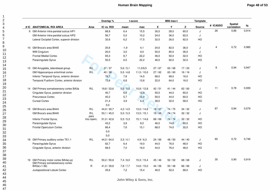
For Peer Review

Overlap % t-score MNI max-t Template

# IC ANATOMICAL ROI AREA Area IC vs. ROI mean max X Y Z Source # ICASSO

Spatial correlation

Iq

9 GM Anterior intra-parietal sulcus hIP1 68,9 6,4 15,5 30,0 28,0 60,0 J 26 0,86 0,914

GM Anterior intra-parietal sulcus hIP2 56,7 5,0 10,2 24,0 36,0 62,0 J

Lateral Occipital Cortex, superoir division 32,6 6,2 17,5 32,0 26,0 62,0 HO

10 GM Broca's area BA45 20,6 -1,9 4,1 24,0 82,0 36,0 J 4 0,72 0,982

WM Cingulum 20,0 3,0 9,0 50,0 85,0 36,0 J

Frontal Medial Cortex 65,3 8,7 22,2 46,0 92,0 32,0 HO

Paracingulate Gyrus 50,5 6,5 22,2 46,0 92,0 32,0 HO

13 GM Amygdala_laterobasal group R/L 37 / 37 5,6 / 5,1 11,0/9,5 27 / 67 63 / 68 17 / 20 J 8 0,94 0,947

GM Hippocampus entorhinal cortex R/L 40 / 38 5,5 / 4,8 11,5 / 10,0 27 / 62 63 / 60 16 / 16 J

Inferior Temporal Gyrus, anterior division 76,7 7,8 14,5 68,0 68,0 16,0 HO

Temporal Fusiform Cortex, anterior division 73,8 6,8 13,6 22,0 64,0 16,0 HO

14 GM Primary somatosensory cortex BA3a R/L 19,8 / 33,6 5,0 / 5,5 10,8 / 12,8 42 / 51 41 / 44 62 / 60 J 11 0,78 0,939

Cingulate Gyrus, posterior division 40,7 6,6 12,9 50,0 44,0 60,0 HO

Precuneous Cortex 40,2 5,7 12,9 50,0 44,0 60,0 HO

Cuneal Cortex 21,4 3,9 6,4 38,0 32,0 58,0 HO

0,0

15 GM Broca's area BA44 R/L 44,9 / 30,7 4,2 / 4,5 13,0 / 14,6 18 / 67 74 / 75 34 / 32 J 67 0,84 0,579

GM Broca's area BA45 R/L 53,1 / 45,5 5,0 / 5,3 13,5 / 15,1 19 / 68 74 / 74 32 / 32 J

Inferior Frontal Gyrus, pars

tria./operc. 51,0 / 42,6 5,5 / 5,3 15,1 / 14,6 68 / 69 74 / 74 32 / 32 HO

Paracingulate Gyrus 43,2 3,9 8,2 46,0 74,0 60,0 HO

Frontal Operculum Cortex 66,4 7,6 15,1 68,0 74,0 32,0 HO

0,0

0,0

18 GM Primary auditory cortex TE1.1 R/L 44,0 / 64,0 3,3 / 4,1 4,9 / 6,3 24 / 66 48 / 50 44 / 40 J 60 0,72 0,746

Paracingulate Gyrus 62,7 6,4 19,0 44,0 76,0 48,0 HO

Cingulate Gyrus, anterior division 68,5 7,0 19,0 44,0 76,0 48,0 HO

19 GM Primary motor cortex BA4a(+p) R/L 50,2 / 50,8 7,4 / 8,0 15,3 / 15,4 45 / 46 52 / 52 68 / 68 J 35 0,90 0,919

GM Primary somatosensory cortex BA3a(+1-3b) R 41,0 / 39,8 7,8 / 7,7 14,6 / 15,0 44 / 56 50 / 48 66 / 66 J

Juxtapositional Lobule Cortex 35,6 7,2 15,4 46,0 52,0 68,0 HO

Page 48 of 53

John Wiley & Sons, Inc.

Human Brain Mapping

123456789101112131415161718192021222324252627282930313233343536373839404142434445464748495051525354555657585960

For Peer Review

Overlap % t-score MNI max-t Template

# IC ANATOMICAL ROI AREA Area IC vs. ROI mean max X Y Z Source # ICASSO

Spatial correlation

Iq

21 GM Visual cortex V1 BA17 V1/V2 55,5 / 51,2 8,7 / 7,7 26,8 / 26,8 42 / 42 18 / 18 36 / 36 J 66 0,91 0,645

Intracalcarine Cortex 51,5 10,3 26,8 42,0 18,0 36,0 HO

Occipital Pole 52,3 8,3 26,8 42,0 18,0 36,0 HO

23 GM Anterior intra-parietal sulcus hIP1-2 R/L 47,5 / 38,1 8,0 / 5,6 19,0 / 12,5 20 / 69 34 / 34 59 / 60 J 30 0,81 0,859

Supramarginal Gyrus, posterior division 35,2 6,8 19,8 18,0 36,0 58,0 HO

Angular Gyrus 50,4 7,8 19,8 18,0 36,0 58,0 HO

Lateral Occipital Cortex, superoir division 29,3 5,7 19,8 18,0 36,0 58,0 HO

24 GM Primary motor cortex BA4a+p R/L 38,6 / 35,8 7,0 / 5,8 12,7 / 13,5 40 / 50 56 / 57 74 / 74 J 58 0,67 0,907

GM Primary somatosensory cortex BA1 R/L 34,4 / 31,1 6,4 / 4,7 12,1 / 11,6 30 / 50 50 / 51 72 / 74 J

GM Premotor cortex BA6 R R/L 27,0 / 27,5 6,6 / 5,8 12,7 / 13,6 40 / 52 56 / 58 74 / 74 J

Juxtapositional Lobule Cortex (SMA) 26,0 4,7 13,5 50,0 58,0 74,0 HO

25 GM Primary auditory cortex TE1.0 (-1.2) R/L 90,5 / 87,6 8,1 / 8,9 17,7 / 19,3 14 / 76 52 / 50 40 / 40 J 14 0,94 0,925

GM Secondary somatosensory cortex / Parietal operculum OP1 R/L 39,7 / 52,9 6,7 / 9,2 17,0 / 19,3 14 / 76 53 / 50 40 / 40 J

Heschl's Gyrus (includes H1 and H2) 90,6 8,7 19,4 76,0 50,0 40,0 HO

27 GM Anterior intra-parietal sulcus hIP2 R/L 49,3 / 48,9 7,0 / 7,9 17,9 / 18,7 22 / 70 50 / 48 63 / 61 J 69 0,88 0,578

GM Primary motor cortex BA4p (+a) 35,3 7,9 18,3 22,0 51,0 64,0 J

GM Primary somatosensory cortex BA2 R/L 55,6 / 59,8 7,6 / 9,9 18,3 / 19,8 22 / 66 52 / 52 64 / 66 J

Supramarginal Gyrus, anterior division 56,3 6,4 19,3 68,0 48,0 63,0 HO

29 GM Amygdala_centromedial group R/L 68,6 / 40,1 5,0 / 4,5 11,6 / 9,6 24 / 62 61 / 54 26 / 31 J 23 0,90 0,940

GM Hippocampus cornu ammonis R/L 41,0 / 32,6 5,2 / 5,3 12,9 / 13,7 24 / 65 57 / 54 29 / 30 J

GM Lateral geniculate body R/L 54,4 / 42,7 3,5 / 3,4 5,8 / 5,7 30 / 60 55 / 53 32 / 30 J

Planum Polare 64,5 7,7 15,6 66,0 56,0 30,0 HO

30 GM Anterior intra-parietal sulcus hIP1 R/L 37,9 / 21,6 3,8 / 3,7 6,2 / 5,8 26 / 24 34 / 36 60 / 60 J 33 0,84 0,923

GM Broca's area BA44 (+BA45) R/L 77,5 / 33,9 6,7 / 4,4 13,1 / 8,3 20 / 68 70 / 72 48 / 48 J

GM Secondary somatosensory cortex / Parietal operculum OP3 (+OP2,4) R 55,3 4,5 10,5 22,0 65,0 46,0 J

Inferior Frontal Gyrus, pars opercularis 63,9 6,3 13,1 20,0 70,0 48,0 HO

Right Caudate 20,0 3,1 4,2 34,0 61,0 46,0 HO

Page 49 of 53

John Wiley & Sons, Inc.

Human Brain Mapping

123456789101112131415161718192021222324252627282930313233343536373839404142434445464748495051525354555657585960

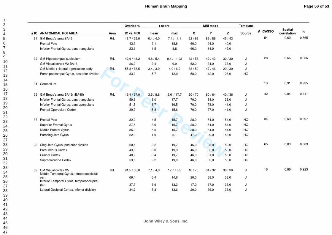
For Peer Review

Overlap % t-score MNI max-t Template

# IC ANATOMICAL ROI AREA Area IC vs. ROI mean max X Y Z Source # ICASSO

Spatial correlation

Iq

31 GM Broca's area BA45 R/L 16,7 / 29,0 0,4 / 4,0 7,4 / 11,1 22 / 66 86 / 86 45 / 43 54 0,69 0,665

Frontal Pole 42,5 5,1 18,6 60,0 94,0 40,0

Inferior Frontal Gyrus, pars triangularis 22,3 1,5 8,8 66,0 84,0 45,0

32 GM Hippocampus subiculum R/L 42,9 / 48,2 4,8 / 5,4 9,4 / 11,02 32 / 58 42 / 43 30 / 30 J 28 0,66 0,936

GM Visual cortex V2 BA18 26,0 3,4 9,9 52,0 34,0 38,0 J

GM Medial (+lateral ) geniculate body R/L 55,8 / 88,5 3,4 / 3,9 4,9 / 6,2 38 / 50 47 / 46 29 / 30 J

Parahippocampal Gyrus, posterior division 83,3 5,7 12,0 58,0 42,0 28,0 HO

34 Cerebellum 13 0,91 0,935

35 GM Broca's area BA45(+BA45) R/L 19,4 / 97,0 3,5 / 8,8 5,6 / 17,7 20 / 70 80 / 84 40 / 36 J 42 0,84 0,811

Inferior Frontal Gyrus, pars triangularis 59,6 8,0 17,7 70,0 84,0 36,0 J

Inferior Frontal Gyrus, pars opercularis 51,5 6,7 16,5 70,0 78,0 41,0 J

Frontal Operculum Cortex 39,7 5,8 15,6 70,0 77,0 41,0 J

37 Frontal Pole 32,2 4,5 15,7 28,0 84,0 54,0 HO 34 0,69 0,897

Superior Frontal Gyrus 27,5 3,9 15,7 28,0 84,0 54,0 HO

Middle Frontal Gyrus 36,9 5,5 15,7 28,0 84,0 54,0 HO

Paracingulate Gyrus 22,9 1,0 5,1 41,0 90,0 53,0 HO

38 Cingulate Gyrus, posterior division 50,5 8,2 19,7 46,0 33,0 50,0 HO 65 0,83 0,883

Precuneous Cortex 43,8 8,0 19,9 46,0 32,0 50,0 HO

Cuneal Cortex 40,2 8,4 19,7 46,0 31,0 50,0 HO

Supracalcarine Cortex 53,6 9,2 19,9 46,0 32,0 50,0 HO

39 GM Visual cortex V5 R/L 91,5 / 56,0 7,1 / 4,0 12,7 / 6,2 18 / 70 34 / 32 38 / 36 J 16 0,86 0,923

Middle Temporal Gyrus, temporooccipital part 69,4 6,4 14,6 20,0 38,0 38,0 J

Inferior Temporal Gyrus, temporooccipital part 37,7 5,9 13,3 17,0 37,0 36,0 J

Lateral Occipital Cortex, inferior division 34,2 5,3 13,6 20,0 36,0 38,0 J

Page 50 of 53

John Wiley & Sons, Inc.

Human Brain Mapping

123456789101112131415161718192021222324252627282930313233343536373839404142434445464748495051525354555657585960

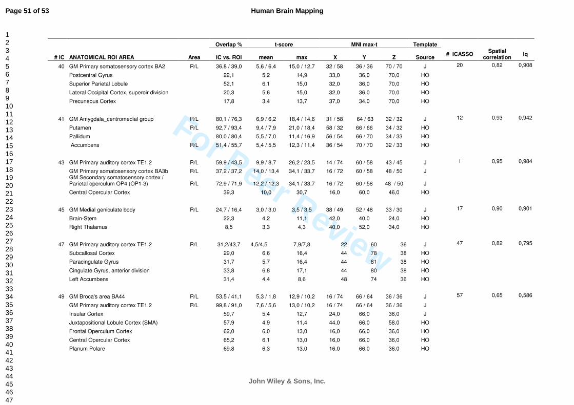
For Peer Review

Overlap % t-score MNI max-t Template

# IC ANATOMICAL ROI AREA Area IC vs. ROI mean max X Y Z Source # ICASSO

Spatial correlation

Iq

40 GM Primary somatosensory cortex BA2 R/L 36,8 / 39,0 5,6 / 6,4 15,0 / 12,7 32 / 58 36 / 36 70 / 70 J 20 0,82 0,908

Postcentral Gyrus 22,1 5,2 14,9 33,0 36,0 70,0 HO

Superior Parietal Lobule 52,1 6,1 15,0 32,0 36,0 70,0 HO

Lateral Occipital Cortex, superoir division 20,3 5,6 15,0 32,0 36,0 70,0 HO

Precuneous Cortex 17,8 3,4 13,7 37,0 34,0 70,0 HO

41 GM Amygdala_centromedial group R/L 80,1 / 76,3 6,9 / 6,2 18,4 / 14,6 31 / 58 64 / 63 32 / 32 J 12 0,93 0,942

Putamen R/L 92,7 / 93,4 9,4 / 7,9 21,0 / 18,4 58 / 32 66 / 66 34 / 32 HO

Pallidum 80,0 / 80,4 5,5 / 7,0 11,4 / 16,9 56 / 54 66 / 70 34 / 33 HO

Accumbens R/L 51,4 / 55,7 5,4 / 5,5 12,3 / 11,4 36 / 54 70 / 70 32 / 33 HO

43 GM Primary auditory cortex TE1.2 R/L 59,9 / 43,5 9,9 / 8,7 26,2 / 23,5 14 / 74 60 / 58 43 / 45 J 1 0,95 0,984

GM Primary somatosensory cortex BA3b R/L 37,2 / 37,2 14,0 / 13,4 34,1 / 33,7 16 / 72 60 / 58 48 / 50 J

GM Secondary somatosensory cortex / Parietal operculum OP4 (OP1-3) R/L 72,9 / 71,9 12,2 / 12,3 34,1 / 33,7 16 / 72 60 / 58 48 / 50 J

Central Opercular Cortex 39,3 10,0 30,7 16,0 60,0 46,0 HO

45 GM Medial geniculate body R/L 24,7 / 16,4 3,0 / 3,0 3,5 / 3,5 38 / 49 52 / 48 33 / 30 J 17 0,90 0,901

Brain-Stem 22,3 4,2 11,1 42,0 40,0 24,0 HO

Right Thalamus 8,5 3,3 4,3 40,0 52,0 34,0 HO

47 GM Primary auditory cortex TE1.2 R/L 31,2/43,7 4,5/4,5 7,9/7,8 22 60 36 J 47 0,82 0,795

Subcallosal Cortex 29,0 6,6 16,4 44 78 38 HO

Paracingulate Gyrus 31,7 5,7 16,4 44 81 38 HO

Cingulate Gyrus, anterior division 33,8 6,8 17,1 44 80 38 HO

Left Accumbens 31,4 4,4 8,6 48 74 36 HO

49 GM Broca's area BA44 R/L 53,5 / 41,1 5,3 / 1,8 12,9 / 10,2 16 / 74 66 / 64 36 / 36 J 57 0,65 0,586

GM Primary auditory cortex TE1.2 R/L 99,8 / 91,0 7,6 / 5,6 13,0 / 10,2 16 / 74 66 / 64 36 / 36 J

Insular Cortex 59,7 5,4 12,7 24,0 66,0 36,0 J

Juxtapositional Lobule Cortex (SMA) 57,9 4,9 11,4 44,0 66,0 58,0 HO

Frontal Operculum Cortex 62,0 6,0 13,0 16,0 66,0 36,0 HO

Central Opercular Cortex 65,2 6,1 13,0 16,0 66,0 36,0 HO

Planum Polare 69,8 6,3 13,0 16,0 66,0 36,0 HO

Page 51 of 53

John Wiley & Sons, Inc.

Human Brain Mapping

123456789101112131415161718192021222324252627282930313233343536373839404142434445464748495051525354555657585960

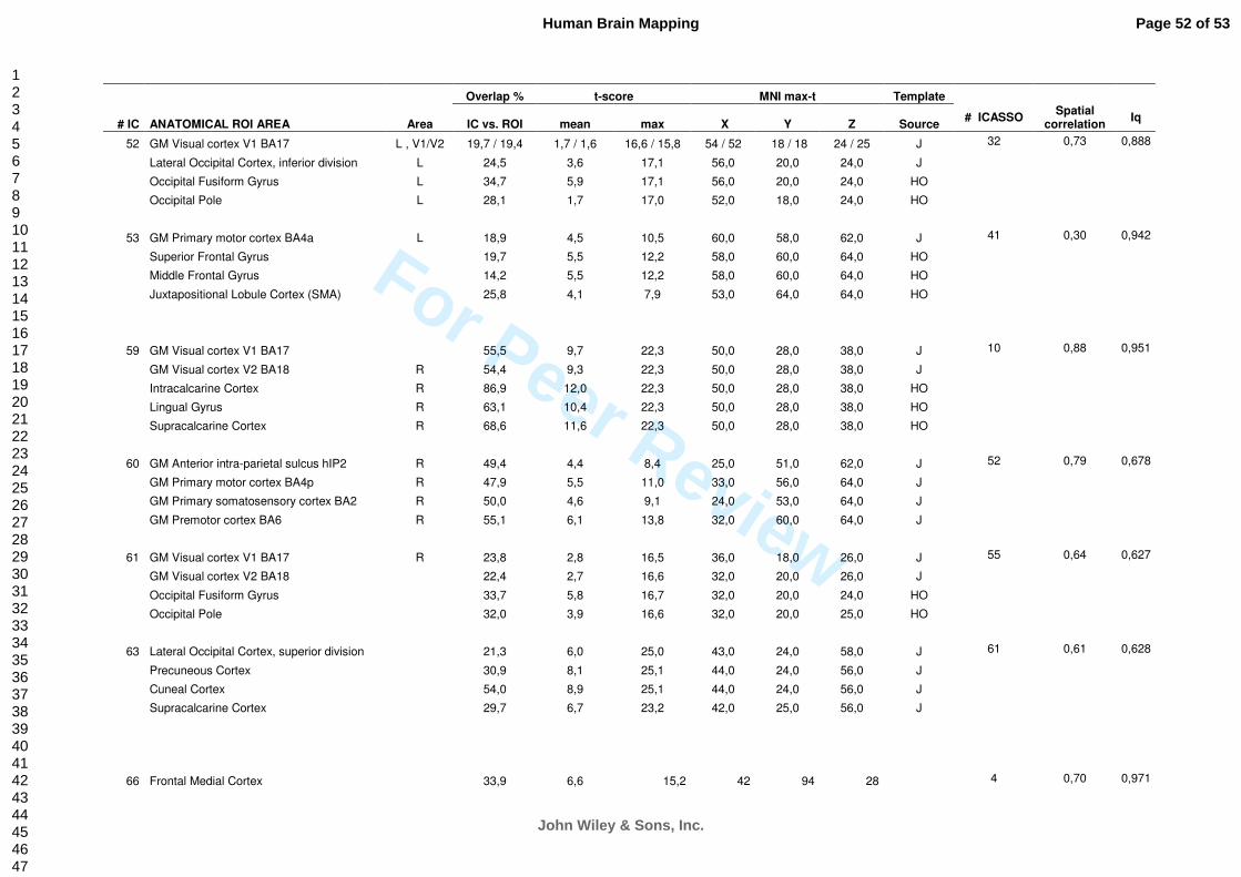
For Peer Review

Overlap % t-score MNI max-t Template

# IC ANATOMICAL ROI AREA Area IC vs. ROI mean max X Y Z Source # ICASSO

Spatial correlation

Iq

52 GM Visual cortex V1 BA17 L , V1/V2 19,7 / 19,4 1,7 / 1,6 16,6 / 15,8 54 / 52 18 / 18 24 / 25 J 32 0,73 0,888

Lateral Occipital Cortex, inferior division L 24,5 3,6 17,1 56,0 20,0 24,0 J

Occipital Fusiform Gyrus L 34,7 5,9 17,1 56,0 20,0 24,0 HO

Occipital Pole L 28,1 1,7 17,0 52,0 18,0 24,0 HO

53 GM Primary motor cortex BA4a L 18,9 4,5 10,5 60,0 58,0 62,0 J 41 0,30 0,942

Superior Frontal Gyrus 19,7 5,5 12,2 58,0 60,0 64,0 HO

Middle Frontal Gyrus 14,2 5,5 12,2 58,0 60,0 64,0 HO

Juxtapositional Lobule Cortex (SMA) 25,8 4,1 7,9 53,0 64,0 64,0 HO

59 GM Visual cortex V1 BA17 55,5 9,7 22,3 50,0 28,0 38,0 J 10 0,88 0,951

GM Visual cortex V2 BA18 R 54,4 9,3 22,3 50,0 28,0 38,0 J

Intracalcarine Cortex R 86,9 12,0 22,3 50,0 28,0 38,0 HO

Lingual Gyrus R 63,1 10,4 22,3 50,0 28,0 38,0 HO

Supracalcarine Cortex R 68,6 11,6 22,3 50,0 28,0 38,0 HO

60 GM Anterior intra-parietal sulcus hIP2 R 49,4 4,4 8,4 25,0 51,0 62,0 J 52 0,79 0,678

GM Primary motor cortex BA4p R 47,9 5,5 11,0 33,0 56,0 64,0 J

GM Primary somatosensory cortex BA2 R 50,0 4,6 9,1 24,0 53,0 64,0 J

GM Premotor cortex BA6 R 55,1 6,1 13,8 32,0 60,0 64,0 J

61 GM Visual cortex V1 BA17 R 23,8 2,8 16,5 36,0 18,0 26,0 J 55 0,64 0,627

GM Visual cortex V2 BA18 22,4 2,7 16,6 32,0 20,0 26,0 J

Occipital Fusiform Gyrus 33,7 5,8 16,7 32,0 20,0 24,0 HO

Occipital Pole 32,0 3,9 16,6 32,0 20,0 25,0 HO

63 Lateral Occipital Cortex, superior division 21,3 6,0 25,0 43,0 24,0 58,0 J 61 0,61 0,628

Precuneous Cortex 30,9 8,1 25,1 44,0 24,0 56,0 J

Cuneal Cortex 54,0 8,9 25,1 44,0 24,0 56,0 J

Supracalcarine Cortex 29,7 6,7 23,2 42,0 25,0 56,0 J

66 Frontal Medial Cortex 33,9 6,6 15,2 42 94 28 4 0,70 0,971

Page 52 of 53

John Wiley & Sons, Inc.

Human Brain Mapping

123456789101112131415161718192021222324252627282930313233343536373839404142434445464748495051525354555657585960

For Peer Review

Overlap % t-score MNI max-t Template

# IC ANATOMICAL ROI AREA Area IC vs. ROI mean max X Y Z Source # ICASSO

Spatial correlation

Iq

Juxtapositional Lobule Cortex (SMA) 25,7 3,4 5,2 48 64 58

Middle Temporal Gyrus, temporooccipital part 19,6 3,6 6,0 72 36 40

68 GM Broca's area BA44 20,7 4,6 24,5 29,0 68,0 56,0 J 68 0,70 0,602

GM Primary auditory cortex TE1.2 24,4 3,1 74,7 78,0 53,0 42,0 J

GM Visual cortex V5 33,2 3,6 19,2 20,0 28,0 47,0 J

Superior Frontal Gyrus 21,8 5,6 33,6 32,0 70,0 56,0 HO

max 0,95 0,984

mean 0,79 0,829

std 0,13 0,132

#IC = number of selected component, Anatomical ROI Area = Name of anatomical template from fsl4, Area = side or other anatomical specification R = right, L= left,

Overlap % = anatomical overlap percentage of components vs. anatomical structure, t-score = t-value (mean, maximum [Max], minimum[Min]), MNI max-t = maximum t-

value x, y & z-direction Montreal Neurologic Institute 152 coordinates, Template source = anatomical ROI source in fsl4: J= Juelich, HO=Harvard-Oxford template, #

ICASSO = icasso run equivalent to selected IC, spatial correlation = spatial correlation between ICASSO and selected IC, Iq = ICASSO clustering index.

Page 53 of 53

John Wiley & Sons, Inc.

Human Brain Mapping

123456789101112131415161718192021222324252627282930313233343536373839404142434445464748495051525354555657585960