Topology correction in brain cortex segmentation using a multiscale, graph-based algorithm

IEEE TRANACTIONS ON MEDICAL IMAGING, VOL. XX, NO. Y, MONTH 2002 1

Topology Correction in Brain Cortex SegmentationUsing a Multiscale, Graph-Based Algorithm

Xiao Han, Chenyang Xu, Member, Ulisses Braga-Neto, Member and Jerry L. Prince,� Senior Member

Abstract— Reconstructing an accurate and topologically correct repre-sentation of the cortical surface of the brain is an important objectivein various neuroscience applications. Most cortical surface reconstruc-tion methods either ignore topology or correct it using manual editing ormethods that lead to inaccurate reconstructions. Shattuck and Leahy re-cently reported a fully-automatic method that yields a topologically cor-rect representation with little distortion of the underlying segmentation.We provide an alternate approach that has several advantages over theirapproach, including the use of arbitrary digital connectivities, a flexiblemorphology-based multiscale approach, and the option of foreground-onlyor background-only correction. A detailed analysis of the method's perfor-mance on 15 magnetic resonance brain images is provided.

Keywords— Digital Topology, Segmentation, Brain Imaging, GraphAnalysis, Cortical Surface Extraction.

I. INTRODUCTION

Reconstruction of the brain cortical surface from magneticresonance (MR) images is an important goal in medicine andneuroscience. Reconstructed cortical surfaces can be used tostudy brain geometry and quantify geometric variations acrosspopulations, in normal growth, and disease [1], [2]. They canalso be used to assist in brain registration by sulcal match-ing [3], [4], and to visualize functional data acquired throughother imaging techniques [5], [6].

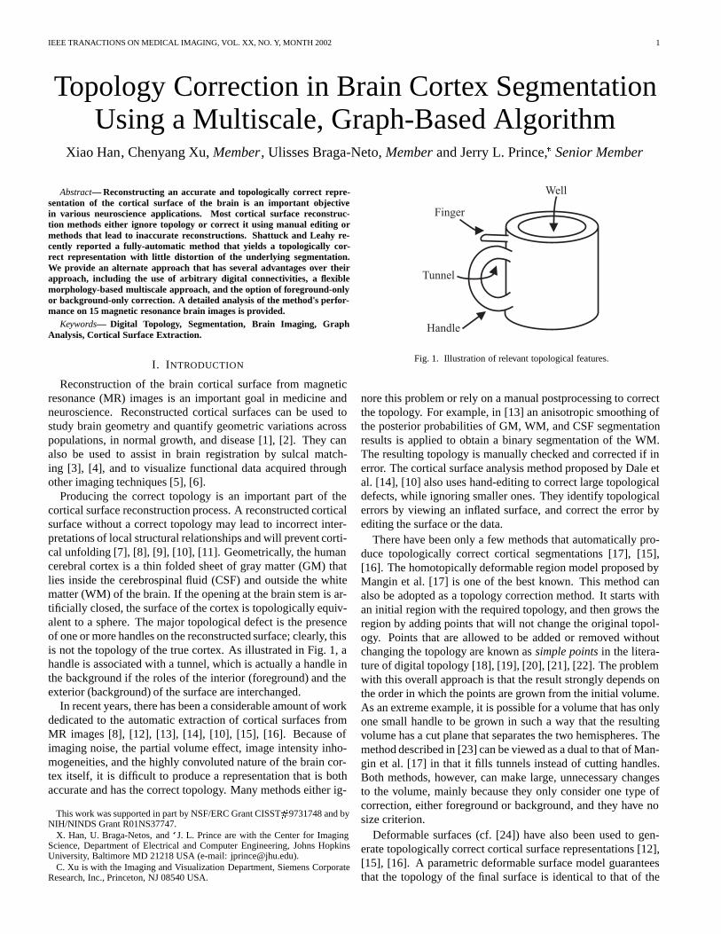
Producing the correct topology is an important part of thecortical surface reconstruction process. A reconstructed corticalsurface without a correct topology may lead to incorrect inter-pretations of local structural relationships and will prevent corti-cal unfolding [7], [8], [9], [10], [11]. Geometrically, the humancerebral cortex is a thin folded sheet of gray matter (GM) thatlies inside the cerebrospinal fluid (CSF) and outside the whitematter (WM) of the brain. If the opening at the brain stem is ar-tificially closed, the surface of the cortex is topologically equiv-alent to a sphere. The major topological defect is the presenceof one or more handles on the reconstructed surface; clearly, thisis not the topology of the true cortex. As illustrated in Fig. 1, ahandle is associated with a tunnel, which is actually a handle inthe background if the roles of the interior (foreground) and theexterior (background) of the surface are interchanged.

In recent years, there has been a considerable amount of workdedicated to the automatic extraction of cortical surfaces fromMR images [8], [12], [13], [14], [10], [15], [16]. Because ofimaging noise, the partial volume effect, image intensity inho-mogeneities, and the highly convoluted nature of the brain cor-tex itself, it is difficult to produce a representation that is bothaccurate and has the correct topology. Many methods either ig-

This work was supported in part by NSF/ERC Grant CISST�9731748 and byNIH/NINDS Grant R01NS37747.

X. Han, U. Braga-Netos, and �J. L. Prince are with the Center for ImagingScience, Department of Electrical and Computer Engineering, Johns HopkinsUniversity, Baltimore MD 21218 USA (e-mail: [email protected]).

C. Xu is with the Imaging and Visualization Department, Siemens CorporateResearch, Inc., Princeton, NJ 08540 USA.

Tunnel

Finger

Well

Handle

Fig. 1. Illustration of relevant topological features.

nore this problem or rely on a manual postprocessing to correctthe topology. For example, in [13] an anisotropic smoothing ofthe posterior probabilities of GM, WM, and CSF segmentationresults is applied to obtain a binary segmentation of the WM.The resulting topology is manually checked and corrected if inerror. The cortical surface analysis method proposed by Dale etal. [14], [10] also uses hand-editing to correct large topologicaldefects, while ignoring smaller ones. They identify topologicalerrors by viewing an inflated surface, and correct the error byediting the surface or the data.

There have been only a few methods that automatically pro-duce topologically correct cortical segmentations [17], [15],[16]. The homotopically deformable region model proposed byMangin et al. [17] is one of the best known. This method canalso be adopted as a topology correction method. It starts withan initial region with the required topology, and then grows theregion by adding points that will not change the original topol-ogy. Points that are allowed to be added or removed withoutchanging the topology are known as simple points in the litera-ture of digital topology [18], [19], [20], [21], [22]. The problemwith this overall approach is that the result strongly depends onthe order in which the points are grown from the initial volume.As an extreme example, it is possible for a volume that has onlyone small handle to be grown in such a way that the resultingvolume has a cut plane that separates the two hemispheres. Themethod described in [23] can be viewed as a dual to that of Man-gin et al. [17] in that it fills tunnels instead of cutting handles.Both methods, however, can make large, unnecessary changesto the volume, mainly because they only consider one type ofcorrection, either foreground or background, and they have nosize criterion.

Deformable surfaces (cf. [24]) have also been used to gen-erate topologically correct cortical surface representations [12],[15], [16]. A parametric deformable surface model guaranteesthat the topology of the final surface is identical to that of the

2 IEEE TRANACTIONS ON MEDICAL IMAGING, VOL. XX, NO. Y, MONTH 2002

initial one. (We note that since a parametric surface can developself-intersections, the topological correctness of the correspond-ing volume implied by the surface is still not guaranteed.) Theproblem then becomes one of how to generate a topologicallycorrect initial surface that is close enough to the cortex so thatthe deformable surface will correctly converge to the cortex. Xuet al. [15] used an adaptive fuzzy c-means algorithm to get aninitial segmentation of the white matter, which was then suc-cessively filtered with median filters until its isosurface had thecorrect topology. There are two problems with this approach.First, it is not guaranteed to converge. Second, it changes theentire white matter volume when there may only be a local prob-lem. We have found that this method can generate new handles,sometimes very large ones, while working to correct smallerhandles in other regions of the volume.

Geometric deformable surface models have also been usedto generate cortical surfaces [25]. While there are many ad-vantages in the use of geometric deformable models over para-metric ones, their topological flexibility is a liability rather thanan advantage in the brain mapping application. The method in[25], for example, finds the inner and outer gray matter surfacessimultaneously, but cannot guarantee their topological correct-ness. Recent development of topology preserving geometricmodels [26], [27] shows promise for the refinement of a topo-logically correct initial surface; but does not solve the problemof finding a topologically correct initial surface close enough tothe final surface to avoid poor convergence behavior.

When the initial volume segmentation or surface reconstruc-tion has an incorrect topology, a topology correction algorithmis needed to detect and remove handles/tunnels from the ini-tial volume or surface. Two approaches in the literature oper-ate directly on the triangulated surface meshes rather than theunderlying digital volumes [11], [28]. The method reported in[11] replaces the manual editing strategy in [14] with an auto-matic procedure in which handles are detected as overlappingtriangles on the surface after it is inflated to a sphere. Thehandles are then removed by deleting the overlapping triangles.This method is slow because of the surface inflation step, andthe removal of overlapping triangles generally removes a muchlarger part of the surface than is actually necessary in order toachieve the correct topology — i.e., instead of requiring onlya small cut to break the handle, a large portion of the handlemay be removed. A second surface-based approach describedin [28] removes small handles by simulating wavefront prop-agation within a certain neighborhood surrounding each meshvertex. A handle that is smaller than the size of the neighbor-hood is detected when the wavefronts meet. It is then brokenby cutting the mesh along a closed path that encloses the handleand re-tessellating the mesh to seal the resulting holes. This cor-rection will always fill the tunnel associated with a given han-dle rather than cutting the handle itself, which may not be thebest strategy, especially with long, thin handles. Furthermore,the method is computationally intensive, and the final correc-tion strongly depends on the vertex used to identify the defect.In short, it is not a desirable overall strategy for the cortical re-construction application.

Shattuck and Leahy have recently described an algorithm todetect and correct handles in a digital volume [29], [30]. In-

stead of region-growing or global filtering, their approach ex-amines the connectivity of the binary white matter segmentationto find regions that give rise to incorrect topology. Then, ratherthan simply removing these regions, their method carefully ed-its the underlying volume to make the smallest possible changes(within the limits of their overall approach) that will correct thetopology. Their method is elegant and effective, but there is stillroom for significant improvement. First, the authors acknowl-edge that their “cuts” are not very natural since they can only beoriented along the Cartesian axes. They also describe a particu-lar topological problem in which “slice duplication” is required.Finally, their approach requires 6-connectivity of the digital ob-ject, and has not been generalized for any other digital connec-tivity. This limits the performance and appearance of the finalresult as well.

In this paper, we develop a new volumetric topology correc-tion algorithm, which we refer to as the graph-based topologycorrection algorithm (GTCA). GTCA removes all handles froma binary object, which in our case is the largest connected com-ponent of a white matter segmentation, filled to remove cavi-ties1. As in [29], [30], we rely on a connection graph to detecthandles, but our graph construction and editing procedures arequite different. Our graph is constructed by using a morpho-logical opening operation, applied to either the foreground orthe background, producing both body and residue parts of theoriginal object. A conditional topological expansion procedure,similar to the region-growing procedure of Mangin et al. [17],is used to replace residue parts that do not involve handles. Agraph is then constructed by analyzing the connectivity of thebody and residue pieces, and one or more residue pieces are re-moved to break the cycles in the graph, thus removing handles inthe volume. Since small corrections are desirable, we apply thisprocedure on both the object and its background starting with asmall structuring element to cut “thin” handles and fill “narrow”tunnels. We then increase the scale of the filter by using largerstructuring elements, which guarantees that topological defectsare always corrected at the smallest possible scale.

Although similar in broad concept to the method of Shattuckand Leahy, our method is quite different in the details. Ourmethod is intrinsically three-dimensional, and “cuts” are notforced to be oriented along cardinal axes. It does not require theintroduction of half-thickness slices, and any (consistent) dig-ital connectivity definition can be used. A final distinction ofour approach is that correct topology can be assured through ap-plication of either foreground or background filters alone. Thisprocedure would result in either handles being cut or tunnels be-ing filled exclusively, which is not a good option in brain map-ping, but may be of use in other applications. In the followingsections, we give necessary background, describe the algorithm,and provide experimental results that show the overall charac-teristics and performance of our new method.

We note that a preliminary version of this work has been pub-lished in a conference proceedings [31].

�Cavities, unlike handles, are background regions completely surrounded bythe object; they are easily removed using standard region-growing.

HAN et al.: TOPOLOGY CORRECTION IN BRAIN CORTEX SEGMENTATION 3

II. BACKGROUND

In this section, we present some basic notions about 3D dis-crete topology that will be used in describing the topology cor-rection algorithm (see [18], [19], [21], [20], [22] for more de-tails). We also discuss the relation between digital connectivitiesand isosurface algorithms. This relationship allows us to com-pute the genus of a digital object by computing the Euler numberof its surface representation. Note that in the application of braincortical surface reconstruction, we desire a topologically correctsurface; the topology correction, however, is performed on thevolume data. Thus, we must make sure that the isosurface algo-rithm gives a topologically correct surface representation of theobject.

A. 3D discrete topology

A 3D digital image V � Z� is defined as a cubic arrayof lattice points. We follow the conventional definition of n-neighborhood and n-adjacency, where n � f�� g. Wedenote the n-neighborhood of a point x by Nn�x�, and the setcomprising the neighborhood of x with x removed by N �

n�x�.An n-path of length l � � from p to q in X , where X � V ,

means a sequence of distinct points p � p�� p�� pl � q inX such that pi is n-adjacent to pi��, for i � �� l� �. Ann-path p�� p�� pl is an n-closed path if and only if p� is n-adjacent to pl. Two points p� q � X are n-connected if and onlyif there exists an n-path from p to q in X . The set X is calledn-connected if every two points p� q � X are n-connected in X .An n-connected component of X is a non-empty n-connectedsubset of X that is not n-adjacent to any other point in X . Wedenote the set of all n-connected components of X by Cn�X�.

In order to avoid a connectivity paradox, different connec-tivities, n and n, must be used in a binary image comprisingan object (foreground) X and a background X. For example,(�� ) and (�� ) are two pairs of compatible connectivities.The following definitions are from [21]:

Definition 1 (Geodesic Neighborhood) Let X � V and x �V . The geodesic neighborhood of x with respect to X of or-der k is the set Nk

n�x�X� defined recursively by: N�n�x�X� �

N�

n�x� � X and Nkn�x�X� � �fNn�y� � N�

��x� � X� y �Nk��

n �x�X�g�

Definition 2 (Topological Numbers) Let X � V and x �V . The topological numbers of the point x relative to theset X are: T��x�X� � C��N

�� x�X��, T��x�X� �

C��N�� x�X��, T��x�X� � C��N

��x�X��, and

T��x�X� � C��N��x�X��, where denotes cardinality

of a set.

Topological numbers are used to classify the topology type of alattice point; their efficient computation is described in [21]. Wenote that in the definition of topological numbers there are twonotations for 6-connectivity. This follows the convention intro-duced in [21], wherein the notation “6+” implies 6-connectivitywhose dual connectivity is 18, while the notation “6” implies6-connectivity whose dual connectivity is 26. This distinction is

(a) (c)

(d) (e) (f)

(b)

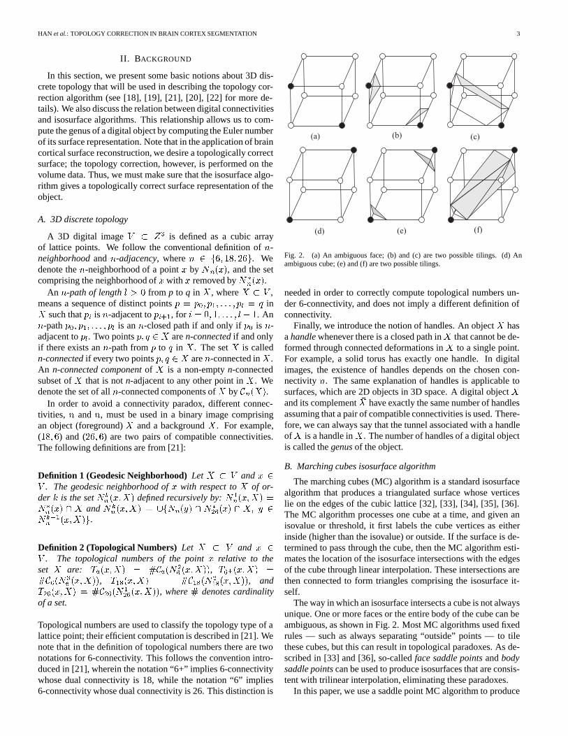
Fig. 2. (a) An ambiguous face; (b) and (c) are two possible tilings. (d) Anambiguous cube; (e) and (f) are two possible tilings.

needed in order to correctly compute topological numbers un-der 6-connectivity, and does not imply a different definition ofconnectivity.

Finally, we introduce the notion of handles. An object X hasa handle whenever there is a closed path in X that cannot be de-formed through connected deformations in X to a single point.For example, a solid torus has exactly one handle. In digitalimages, the existence of handles depends on the chosen con-nectivity n. The same explanation of handles is applicable tosurfaces, which are 2D objects in 3D space. A digital object Xand its complement X have exactly the same number of handlesassuming that a pair of compatible connectivities is used. There-fore, we can always say that the tunnel associated with a handleof X is a handle in X. The number of handles of a digital objectis called the genus of the object.

B. Marching cubes isosurface algorithm

The marching cubes (MC) algorithm is a standard isosurfacealgorithm that produces a triangulated surface whose verticeslie on the edges of the cubic lattice [32], [33], [34], [35], [36].The MC algorithm processes one cube at a time, and given anisovalue or threshold, it first labels the cube vertices as eitherinside (higher than the isovalue) or outside. If the surface is de-termined to pass through the cube, then the MC algorithm esti-mates the location of the isosurface intersections with the edgesof the cube through linear interpolation. These intersections arethen connected to form triangles comprising the isosurface it-self.

The way in which an isosurface intersects a cube is not alwaysunique. One or more faces or the entire body of the cube can beambiguous, as shown in Fig. 2. Most MC algorithms used fixedrules — such as always separating “outside” points — to tilethese cubes, but this can result in topological paradoxes. As de-scribed in [33] and [36], so-called face saddle points and bodysaddle points can be used to produce isosurfaces that are consis-tent with trilinear interpolation, eliminating these paradoxes.

In this paper, we use a saddle point MC algorithm to produce


a surface representation of a binary object (1=object, 0=back-ground). Note that selection of the isovalue, which can take onany real value in the range �� , due to the interpolation implicitin the isosurface algorithm, has a direct effect on the underly-ing digital connectivity that the algorithm can represent. Forinstance, it is straightforward to verify that standard MC algo-rithms, which do not consider saddle points, can only be madeconsistent with 6-connectivity by choosing an isovalue greaterthan 0.5. In order to be consistent with other connectivities, itis necessary to consider both face and body saddle points. Fur-thermore, following the computation of face/body saddle pointsas in [36], it is easy to see that for 0-1 valued binary volumes,to yield 26-connectivity we must choose an isovalue less than0.25; to yield 18-connectivity we must set the isovalue between0.25 and 0.5; and to be consistent with 6-connectivity, we needan isovalue above 0.5. All of these object connectivities haveconsistent background connectivities according to the previousdiscussion.

C. Topology of surface meshes

The genus g of a surface mesh is computed from the Eulernumber � as follows [37]

g � �� (1)

where � � V � E F and V , E, and F are the number ofvertices, edges, and faces, respectively, of the surface mesh. Inthis paper, due to preprocessing steps we need only considersurface meshes consisting of a single connected set of vertices.Such a surface is topologically equivalent to a sphere when g ��. However, neither the Euler number nor the genus providesinformation about the size or location of a handle.

Given a topologically consistent isosurface algorithm, thereis a one-to-one correspondence between the handles on a binarydigital object with n-connectivity and that of its triangulated sur-face representation. Thus, if we remove all the handles on a bi-nary digital object, its boundary surface will be homeomorphicto a sphere. Since direct computation of the genus of a digitalobject is difficult, and since our final objective is a surface rep-resentation of the brain cortex, we always check the topologyof the object by computing the Euler number of its surface ex-tracted using the correct MC algorithm. To save time, our MCalgorithm can omit the computation of triangle positions whenonly the Euler number is needed.

III. GRAPH-BASED TOPOLOGY CORRECTION ALGORITHM

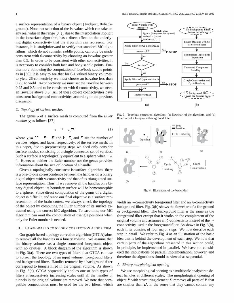
Our graph-based topology correction algorithm (GTCA) aimsto remove all the handles in a binary volume. We assume thatthe binary volume has a single connected foreground objectwith no cavities. A block diagram of the algorithm is shownin Fig. 3(a). There are two types of filters that GTCA can useto correct the topology of an input volume: foreground filtersand background filters. Handles removed by a background filtercorrespond to tunnels filled in the original volume. As shownin Fig. 3(a), GTCA sequentially applies one or both types offilters at successively increasing scales until all the handles ortunnels in the original volume are removed. We note that com-patible connectivities must be used for the two filters, which

If a Background Filter,Invert the Volume

Binary Opening with SEat Selected Scale

Conditional TopologicalExpansion

Connected ComponentLabeling

Graph Construction andCycle Breaking

If a Background Filter,Invert the Volume Back

STOP= 0 ?genus

No

Yes

Yes

Increase Scale

InitializationType

Switch

Scale

{ foreground, background}

{yes, no}

{1, 2, }

�

�

� �

Apply Filter of andType Scale

Input Volume with> 0genus

Switch ?

Apply Filter of andType Scale

= 0 ?genus STOPYes

No

No

(a) (b)

Fig. 3. Topology correction algorithm: (a) flowchart of the algorithm, and (b)flowchart of a foreground/background filter.

Opening

CTE + labeling2

1

3

4

56

7

BodyResidue

1

235

6

7

4 Graph

Construction

Cycle

Breaking

(b)(a) (c)

(d)(f) (e)

23

4

1

7

6

Fig. 4. Illustration of the basic idea.

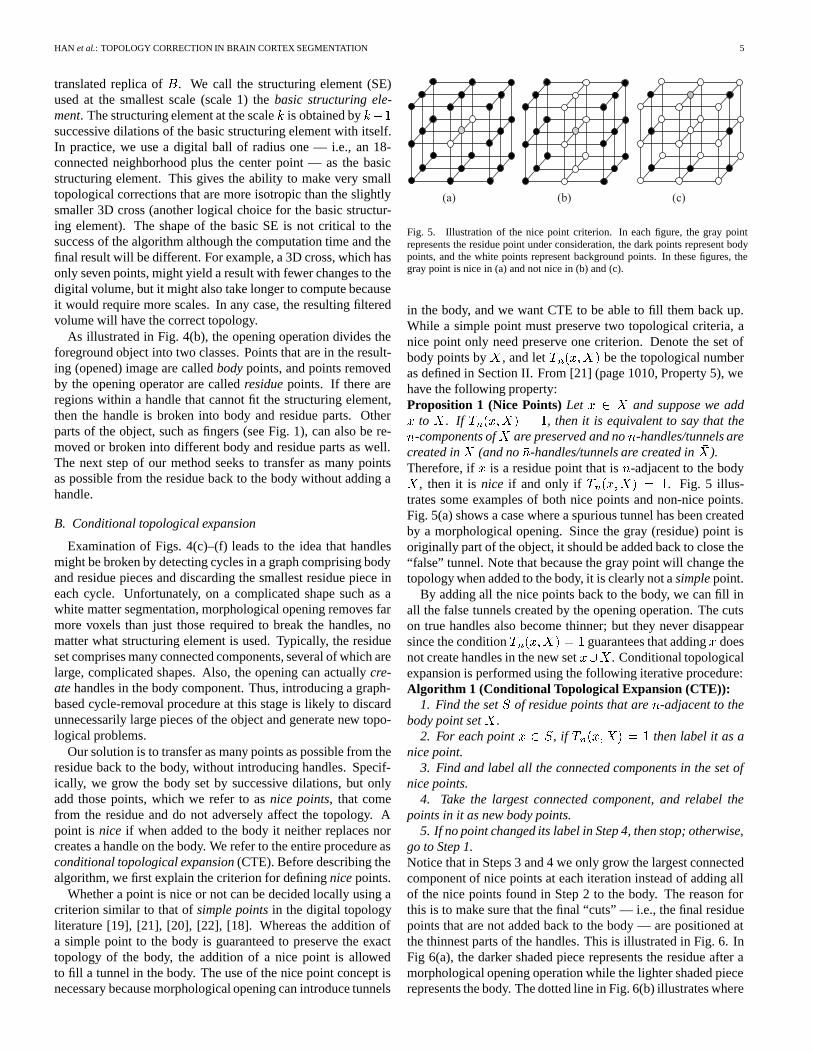
yields an n-connectivity foreground filter and an n-connectivitybackground filter. Fig. 3(b) shows the flowchart of a foregroundor background filter. The background filter is the same as theforeground filter except that it works on the complement of theoriginal volume and assumes an n-connectivity instead of the n-connectivity used in the foreground filter. As shown in Fig. 3(b),each filter consists of four major steps. We now describe eachstep in detail. We refer to Fig. 4 as an illustration of the basicidea that is behind the development of each step. We note thatcertain parts of the algorithms presented in this section could,in principle, be implemented in parallel. We have not consid-ered the implications of parallel implementation, however, andtherefore the algorithms should be viewed as sequential.

A. Binary morphological opening

We use morphological opening as a multiscale analyzer to de-tect handles at different scales. The morphological opening ofobject F with structuring element B removes all parts of F thatare smaller than B, in the sense that they cannot contain any


translated replica of B. We call the structuring element (SE)used at the smallest scale (scale 1) the basic structuring ele-ment. The structuring element at the scale k is obtained by k��successive dilations of the basic structuring element with itself.In practice, we use a digital ball of radius one — i.e., an 18-connected neighborhood plus the center point — as the basicstructuring element. This gives the ability to make very smalltopological corrections that are more isotropic than the slightlysmaller 3D cross (another logical choice for the basic structur-ing element). The shape of the basic SE is not critical to thesuccess of the algorithm although the computation time and thefinal result will be different. For example, a 3D cross, which hasonly seven points, might yield a result with fewer changes to thedigital volume, but it might also take longer to compute becauseit would require more scales. In any case, the resulting filteredvolume will have the correct topology.

As illustrated in Fig. 4(b), the opening operation divides theforeground object into two classes. Points that are in the result-ing (opened) image are called body points, and points removedby the opening operator are called residue points. If there areregions within a handle that cannot fit the structuring element,then the handle is broken into body and residue parts. Otherparts of the object, such as fingers (see Fig. 1), can also be re-moved or broken into different body and residue parts as well.The next step of our method seeks to transfer as many pointsas possible from the residue back to the body without adding ahandle.

B. Conditional topological expansion

Examination of Figs. 4(c)–(f) leads to the idea that handlesmight be broken by detecting cycles in a graph comprising bodyand residue pieces and discarding the smallest residue piece ineach cycle. Unfortunately, on a complicated shape such as awhite matter segmentation, morphological opening removes farmore voxels than just those required to break the handles, nomatter what structuring element is used. Typically, the residueset comprises many connected components, several of which arelarge, complicated shapes. Also, the opening can actually cre-ate handles in the body component. Thus, introducing a graph-based cycle-removal procedure at this stage is likely to discardunnecessarily large pieces of the object and generate new topo-logical problems.

Our solution is to transfer as many points as possible from theresidue back to the body, without introducing handles. Specif-ically, we grow the body set by successive dilations, but onlyadd those points, which we refer to as nice points, that comefrom the residue and do not adversely affect the topology. Apoint is nice if when added to the body it neither replaces norcreates a handle on the body. We refer to the entire procedure asconditional topological expansion (CTE). Before describing thealgorithm, we first explain the criterion for defining nice points.

Whether a point is nice or not can be decided locally using acriterion similar to that of simple points in the digital topologyliterature [19], [21], [20], [22], [18]. Whereas the addition ofa simple point to the body is guaranteed to preserve the exacttopology of the body, the addition of a nice point is allowedto fill a tunnel in the body. The use of the nice point concept isnecessary because morphological opening can introduce tunnels

(a) (c)(b)

Fig. 5. Illustration of the nice point criterion. In each figure, the gray pointrepresents the residue point under consideration, the dark points represent bodypoints, and the white points represent background points. In these figures, thegray point is nice in (a) and not nice in (b) and (c).

in the body, and we want CTE to be able to fill them back up.While a simple point must preserve two topological criteria, anice point only need preserve one criterion. Denote the set ofbody points by X , and let Tn�x�X� be the topological numberas defined in Section II. From [21] (page 1010, Property 5), wehave the following property:Proposition 1 (Nice Points) Let x � X and suppose we addx to X . If Tn�x�X� � �, then it is equivalent to say that then-components of X are preserved and no n-handles/tunnels arecreated in X (and no n-handles/tunnels are created in X).Therefore, if x is a residue point that is n-adjacent to the bodyX , then it is nice if and only if Tn�x�X� � �. Fig. 5 illus-trates some examples of both nice points and non-nice points.Fig. 5(a) shows a case where a spurious tunnel has been createdby a morphological opening. Since the gray (residue) point isoriginally part of the object, it should be added back to close the“false” tunnel. Note that because the gray point will change thetopology when added to the body, it is clearly not a simple point.

By adding all the nice points back to the body, we can fill inall the false tunnels created by the opening operation. The cutson true handles also become thinner; but they never disappearsince the condition Tn�x�X� � � guarantees that adding x doesnot create handles in the new set x�X . Conditional topologicalexpansion is performed using the following iterative procedure:Algorithm 1 (Conditional Topological Expansion (CTE)):

1. Find the set S of residue points that are n-adjacent to thebody point set X .

2. For each point x � S, if Tn�x�X� � � then label it as anice point.

3. Find and label all the connected components in the set ofnice points.

4. Take the largest connected component, and relabel thepoints in it as new body points.

5. If no point changed its label in Step 4, then stop; otherwise,go to Step 1.Notice that in Steps 3 and 4 we only grow the largest connectedcomponent of nice points at each iteration instead of adding allof the nice points found in Step 2 to the body. The reason forthis is to make sure that the final “cuts” — i.e., the final residuepoints that are not added back to the body — are positioned atthe thinnest parts of the handles. This is illustrated in Fig. 6. InFig 6(a), the darker shaded piece represents the residue after amorphological opening operation while the lighter shaded piecerepresents the body. The dotted line in Fig. 6(b) illustrates where


(a) (b)

Fig. 6. Illustration of CTE on a simple handle (surface rendering). (a) Originalbody (light) and residue (dark) after opening; (b) the final cut (dark) after CTE.The dashed line illustrates a non-optimal cut position.

Labeling Body ConnectedComponents (BCCs)

Remove individual residue pointthat forms handle with a BCC

Labeling Residue ConnectedComponents (RCCs)

Compute number of connections betweeneach RCC and BCC pair by strongly-

connected component (SCC) labeling

Repeat until no more changes

Break multiple connections between RCCand BCC by eliminating multiple SCCs

Merge RCCs if necessary

Fig. 7. Connected component labeling and connection analysis.

the final cut would be if all the nice points were added back tothe body after each conditional dilation. The dark line illustrateswhere the actual cut is placed using CTE. We note that CTEcan be made computationally efficient by using a first-in-first-out queue data structure [38].

C. Connected component labeling

After CTE, any tunnels in the body that were created bymorphological opening are filled in, and the remaining residuepieces form thin “cuts” that separate body components. Thissituation is illustrated in Figs. 4(b)–(c). Removing all the re-maining cuts would certainly eliminate all the handles at thisscale, but would also disconnect large portions of the body thatwe refer to as fingers, such as the parts labeled “6” and “3” inFig. 4(c). Detecting and removing cuts that belong to handles

a

b c d

e

f

1

2

Fig. 8. Illustration of the strong and the weak connectivity definitions (n=18).The gray points belonging to one RCC, the dark disks and the squares representpoints belonging to two separate BCCs, and the rest are background points. Itcan be seen that a handle exists in the RCC.

and rejoining to the body those that are not part of handles isthe aim of the graph analysis to be described in the next sec-tion. It turns out, however, that without further analysis of theremaining residue pieces, graph analysis might lead to unnec-essary removal or, worse, the accidental inclusion of handles.In this section, we prepare for graph analysis by grouping thebody and residue points into sets of connected components withdistinct labels. We then compute the number of connections be-tween each pair of body and residue components. When multi-ple connections are found, they are broken in order to break thecorresponding handle(s). Special care is taken both to detect andbreak handles inside a residue component and to merge suitableresidue components in order to avoid false cycles in the subse-quent graph analysis. The overall processing strategy describedin this section is illustrated in Fig. 7. We note that the final setof body and residue components become the nodes for the graphanalysis described in the following section.

We begin by labeling the connected components of bodypoints using n-connectivity; these form the body connectedcomponents or BCCs. Each residue point that forms a handleby itself with a single BCC is then removed (changed to back-ground). These are the residue points x for which Tn�x�X� � �for some BCC X (see Fig. 5(c) for an example). This preventsresidue connected components that are merged to the body laterfrom forming handles that could not be detected by graph analy-sis. In some unusual configurations, a point removed in this stepwould not have actually formed a handle in the merged body. Inthis case, however, the last step of our algorithm (another CTEafter graph analysis) adds these points back to the body.

Next, we compute the n-connected components in the re-maining residue points; these form the residue connected com-ponents or RCCs. We must now compute the number of connec-tions between each RCC and each of its adjacent BCCs. Thiscomputation is important because an RCC being connected toa BCC more than once indicates that there is at least one han-dle formed between them (e.g., see the nodes labeled “1” and“7” in Fig. 4(d)). The way we define the number of connectionsbetween an RCC and an adjacent BCC can be considered as ageneralization of the definition of topological numbers, whichcharacterize the number of connections between a single point


and its adjacent object components. This generalization leads tothe concept of strong connectivity and strongly connected com-ponent (SCC) labeling as will be presented later. A subtletyexists when a handle is entirely contained within the RCC itself,as illustrated in Fig. 8. In this case, calculation of the number ofconnections between the RCC and its adjacent BCCs does notreveal the “hidden handle”. The definition of a weak connectiv-ity is aimed to resolve this problem. We found that if a handleis contained fully in the RCC but not in the BCC as in Fig. 8(otherwise, the handle is not yet broken by the opening at thecurrent scale), then there will be two neighboring points in theRCC that are not weakly connected but would be assigned tothe same SCC (e.g., points with label a and f in Fig. 8). Thus,by removing one point from each non-weakly connected pair ofneighboring points, we break handles within an RCC. We firstpresent the two definitions (which are new as far as we know):

Definition 3 (Strong Connectivity) Let X�Y � V . Twopoints x�� x� � X that are n-adjacent to Y are stronglynk-connected with respect to Y if x� � Nk

n�x�� X� (orequivalently, x� � Nk

n�x�� X�) and their geodesic neighbor-hoods of order k inside Y intersect each other — i.e. Nk

n�x�� Y �and Nk

n�x�� Y � share at least one common point.

Definition 4 (Weak Connectivity) Let X�Y � V . Twopoints x�� x� � X that are n-adjacent to Y are weaklynk-connected with respect to Y if there exists another pointx� in X that is strongly nk-connected to both x� and x�.

In the above definitions, k is chosen with respect to n as in thedefinition of topological numbers. For example, if n is ��, thenk is 3. We note that strong connectivity implies weak connec-tivity.

An illustration of the above definitions is shown in Fig. 8.Suppose we consider the strong or weak connectivity relation-ship among the gray RCC points with respect to the BCC con-sisting of all the dark squares, and assume that the digital con-nectivity rule is n � ��. It is easy to check that the pairs such as�a� b�, �b� c�, �c� d�, �d� e�, and �e� f� are all strongly-connectedpairs of residue points. Points a and f are ��-neighbors to eachother and both ��-adjacent to the BCC, but they are not weakly-connected by the above definition. This signals a hidden handleinside the RCC itself. We can break the handle by removing ei-ther point a or f to background. Note that if the point with label� is also a residue point, then the handle does not exist, but thena and f become weakly-connected. Another variation is whenpoint � is a foreground point, and thus belongs to the BCC ofdark squares. In this case, the handle is contained in the BCCalso, which says that the handle is not yet broken at the currentscale. Whether we can detect the handle in the RCC is no longera relevant issue.

Now let Ri be an RCC and Bj be a BCC that is n-adjacent toRi. The number of connections between Ri and Bj is definedto be the number of strongly connected components (SCCs)formed with respect toBj by the points inRi that are n-adjacentto Bj . There are handles formed between Ri and Bj if Ri isconnected to Bj more than once or, equivalently, if the pointsof Ri that are n-adjacent to Bj form more than one strongly

1 1

111

1

1 1 1

1

2 2

3 3 3

3

4 4

1

2

4

3(a) (b)

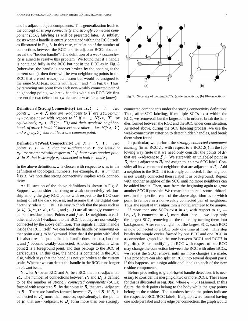
Fig. 9. Necessity of merging RCCs. (a) 6-connectivity; (b) 18-connectivity.

connected components under the strong connectivity definition.Thus, after SCC labeling, if multiple SCCs exist within theRCC, we remove all but the largest one in order to break the han-dles formed between the RCC and the BCC under consideration.As noted above, during the SCC labeling process, we use theweak-connectivity criterion to detect hidden handles, and breakthem when found.

In particular, we perform the strongly connected componentlabeling (in an RCC Ri with respect to a BCC Bj) in the fol-lowing way (note that we need only consider the points of Ri

that are n-adjacent to Bj). We start with an unlabeled point inRi that is adjacent to Bj and assign to it a new SCC label. Con-sider all its n-connected neighbors that are adjacent to Bj . Adda neighbor to the SCC if it is strongly connected. If the neighboris not weakly connected then relabel it as background. Repeatwith another neighbor of the SCC until no more neighbors canbe added into it. Then, start from the beginning again to growanother SCC if possible. We remark that there is some arbitrari-ness in the specific result of the above algorithm as to whichpoint to remove in a non-weakly connected pair of neighbors.Thus, the result of this algorithm is not guaranteed to be unique.

If more than one SCCs exist in Ri with respect to Bj —i.e., Ri is connected to Bj more than once — we keep onlythe largest SCC, removing all the others by turning them intobackground. After removing all but the largest SCC, each RCCis now connected to a BCC only one time at most. This stepbreaks the simple cycles formed by one BCC and one RCC ina connection graph like the one between BCC1 and RCC7 inFig. 4(d). Since modifying an RCC with respect to one BCCmay change the connection between the RCC with other BCCs,we repeat the SCC removal until no more changes are made.This procedure can also split an RCC into several disjoint parts.If this happens, we assign additional labels to each of the newresidue components.

Before proceeding to graph-based handle detection, it is nec-essary to consider the merging of two or more RCCs. The reasonfor this is illustrated in Fig. 9(a), where n � � is assumed. In thisfigure, the dark points belong to the body while the gray pointsbelong to the residue. The numbers beside the points indicatethe respective BCC/RCC labels. If a graph were formed havingone node per label and one edge per connection, the graph would


contain the cycle 1-3-2-4-1. Graph analysis would require thateither RCC 3 or 4 be removed in order to break the cycle, anapparent handle. Yet careful scrutiny of the figure shows that inreality the body and residue points taken together form a solidobject without any handles. No residue need be removed sincethere is no handle to break. A similar situation can occur in thecase of 18-connectivity, as illustrated in Fig. 9(b).

To resolve the problem, we merge the RCCs that represent thesame cut between two body components. Two RCCs are saidto represent the same cut with respect to two BCCs if the twoRCCs are 18-connected at the face (if n � �) or 26-connectedat the cube (if n � ��) where the separation between the twoBCCs occurs, such as RCC3 and RCC4 in Fig. 9(a) or 9(b). It iseasily seen that in such cases, there can be no background pathpassing through the junction where the four components (twoRCCs and two BCCs) meet. Thus, the two RCCs need to bemerged as one single RCC since the cycle otherwise formed bythe four components does not represent a true handle. In ourimplementation, we merge two RCCs Ri and Rj if there aretwo points x � Ri and y � Rj such that x � N��y� and xand y have two common n-neighbors that belong to two distinctBCCs. An RCC can be merged with more than one RCCs if itsatisfies this criteria with each one of them.

D. Graph construction and cycle breaking

After considerable preparation, we are now in position tobuild a graph whose nodes represent the RCCs and BCCs andwhose edges represent the connections between them, as illus-trated in Fig. 4(d). Note that at this stage, there can be at mostone edge between an RCC node and a BCC node. That is, cycles(handles) involving one RCC and one BCC with two or moreedges between them, like BCC1 and RCC7 in Fig. 4(d), are al-ready broken in the previous step by removing multiple SCCs.The remaining handles appear as cycles in the graph that areformed by more than two nodes. The graph analysis in this stepaims to find such cycles and break them by removing one nodefrom each cycle. Because of the conditional topological expan-sion, it is reasonable to assume that the RCCs are much smallerin size than the BCCs. Accordingly, our strategy is to removeone RCC from each cycle in order to break it, which breaksthe corresponding object handle in the volume. Since we breakcycles by removing nodes from the graph rather than edges asin [29], [30], the maximum spanning tree algorithm (see [38])cannot be applied in our approach. A different strategy must beused.

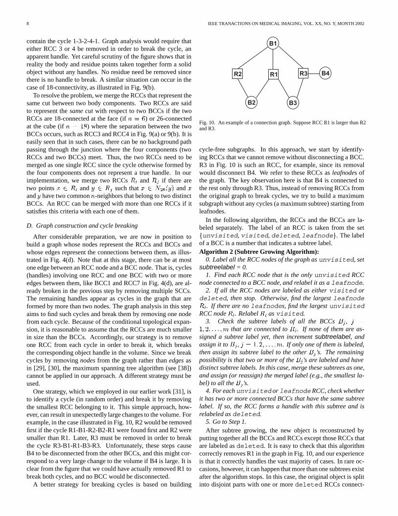
One strategy, which we employed in our earlier work [31], isto identify a cycle (in random order) and break it by removingthe smallest RCC belonging to it. This simple approach, how-ever, can result in unexpectedly large changes to the volume. Forexample, in the case illustrated in Fig. 10, R2 would be removedfirst if the cycle R1-B1-R2-B2-R1 were found first and R2 weresmaller than R1. Later, R3 must be removed in order to breakthe cycle R3-B1-R1-B3-R3. Unfortunately, these steps causeB4 to be disconnected from the other BCCs, and this might cor-respond to a very large change to the volume if B4 is large. It isclear from the figure that we could have actually removed R1 tobreak both cycles, and no BCC would be disconnected.

A better strategy for breaking cycles is based on building

B2

R2 R1 R3 B4

B1

B3

Fig. 10. An example of a connection graph. Suppose RCC R1 is larger than R2and R3.

cycle-free subgraphs. In this approach, we start by identify-ing RCCs that we cannot remove without disconnecting a BCC.R3 in Fig. 10 is such an RCC, for example, since its removalwould disconnect B4. We refer to these RCCs as leafnodes ofthe graph. The key observation here is that B4 is connected tothe rest only through R3. Thus, instead of removing RCCs fromthe original graph to break cycles, we try to build a maximumsubgraph without any cycles (a maximum subtree) starting fromleafnodes.

In the following algorithm, the RCCs and the BCCs are la-beled separately. The label of an RCC is taken from the setfunvisited, visited, deleted, leafnodeg. The labelof a BCC is a number that indicates a subtree label.Algorithm 2 (Subtree Growing Algorithm):

0. Label all the RCC nodes of the graph as unvisited, setsubtreelabel = 0.

1. Find each RCC node that is the only unvisited RCCnode connected to a BCC node, and relabel it as a leafnode.

2. If all the RCC nodes are labeled as either visited ordeleted, then stop. Otherwise, find the largest leafnodeRi. If there are no leafnodes, find the largest unvisitedRCC node Ri. Relabel Ri as visited.

3. Check the subtree labels of all the BCCs Bj , j �� m that are connected to Ri. If none of them are as-signed a subtree label yet, then increment subtreelabel, andassign it to Bj , j � �� m. If only one of them is labeled,then assign its subtree label to the other Bj 's. The remainingpossibility is that two or more of the Bj 's are labeled and havedistinct subtree labels. In this case, merge these subtrees as one,and assign (or reassign) the merged label (e.g., the smallest la-bel) to all the Bj 's.

4. For eachunvisited or leafnodeRCC, check whetherit has two or more connected BCCs that have the same subtreelabel. If so, the RCC forms a handle with this subtree and isrelabeled as deleted.

5. Go to Step 1.After subtree growing, the new object is reconstructed by

putting together all the BCCs and RCCs except those RCCs thatare labeled as deleted. It is easy to check that this algorithmcorrectly removes R1 in the graph in Fig. 10, and our experienceis that it correctly handles the vast majority of cases. In rare oc-casions, however, it can happen that more than one subtrees existafter the algorithm stops. In this case, the original object is splitinto disjoint parts with one or more deleted RCCs connect-


ing them. Ideally, one would like to connect the subtrees so thatno body component is lost; but the development of a systematicapproach for this process turns out to be a challenging task. Itinvolves splitting one or more deleted RCC into appropriatepieces, some of which are removed to break the handles whileothers are kept so that the subtrees can be jointed together. Wehave no algorithm for doing this at present. Instead, for thesecases we simply remove all the deleted RCCs and retain thelargest resulting subtree as the reconstructed object. In our ex-periments, this situation occurs very infrequently and this sim-ple strategy has never brought about a drastic change to the cor-rected volume. We also note that removing a whole RCC nodecan sometimes remove good points if the points do not belongto the edges of the cycle to be broken. We run a final pass ofCTE after the graph analysis to bring these points back, whichwill be discussed in the next section.

E. Final stages

There are several steps that must be performed after graph re-construction. First, it is usually possible to append points thatwere unnecessarily removed during the connected componentlabeling and the graph analysis. To do this we apply anotherpass of CTE using Algorithm 1 with the new object as the bodyset and the removed points as the residue set. Second, if thepresent filter is a background filter, the volume is inverted sothat background becomes foreground and vice versa. Third, weapply the saddle point MC algorithm to this volume using anisovalue corresponding to the selected connectivity. Last, wecompute the genus of the resulting surface. This finishes onepass of the foreground or background filter. If the genus is zero,then the topology of the new volume is correct, and we stop.Otherwise, the proposed algorithm either switches to the oppo-site filter (background vs. foreground) at the same scale (if notalready applied) or increases the scale of the current filter, andrepeat the topology correction on the new volume (see Fig. 3(a)).The algorithm is guaranteed to converge because at some scale,the morphological opening must completely break all the han-dles, and the CTE and the graph algorithms that follows can thenproduce a handle-free new object.

IV. RESULTS

A. Simple demonstration

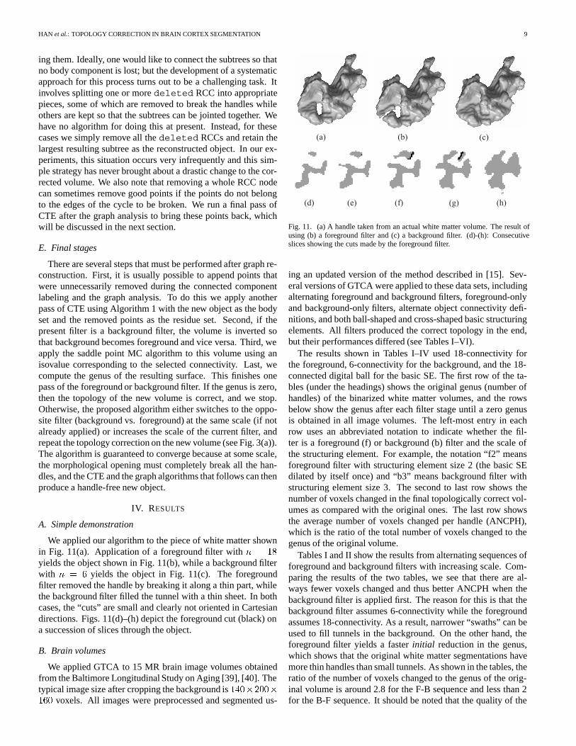
We applied our algorithm to the piece of white matter shownin Fig. 11(a). Application of a foreground filter with n � ��yields the object shown in Fig. 11(b), while a background filterwith n � � yields the object in Fig. 11(c). The foregroundfilter removed the handle by breaking it along a thin part, whilethe background filter filled the tunnel with a thin sheet. In bothcases, the “cuts” are small and clearly not oriented in Cartesiandirections. Figs. 11(d)–(h) depict the foreground cut (black) ona succession of slices through the object.

B. Brain volumes

We applied GTCA to 15 MR brain image volumes obtainedfrom the Baltimore Longitudinal Study on Aging [39], [40]. Thetypical image size after cropping the background is �� voxels. All images were preprocessed and segmented us-

(a) (c)(b)

(h)(d) (e) (f) (g)

Fig. 11. (a) A handle taken from an actual white matter volume. The result ofusing (b) a foreground filter and (c) a background filter. (d)-(h): Consecutiveslices showing the cuts made by the foreground filter.

ing an updated version of the method described in [15]. Sev-eral versions of GTCA were applied to these data sets, includingalternating foreground and background filters, foreground-onlyand background-only filters, alternate object connectivity defi-nitions, and both ball-shaped and cross-shaped basic structuringelements. All filters produced the correct topology in the end,but their performances differed (see Tables I–VI).

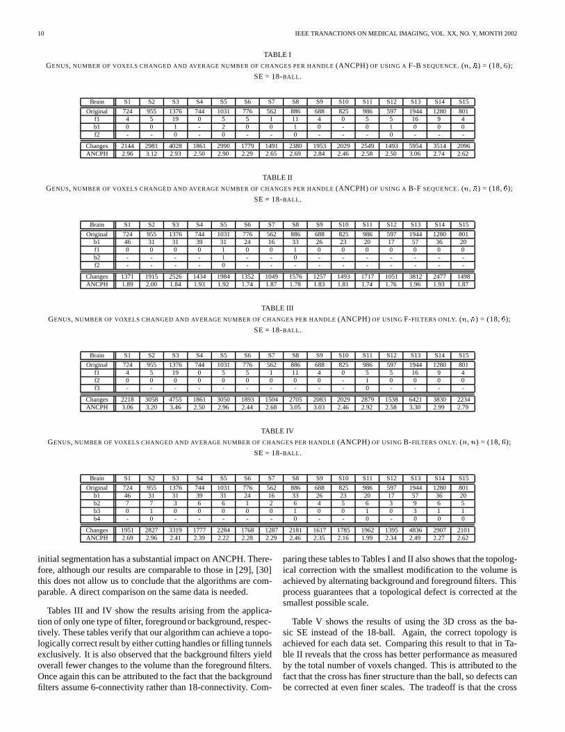
The results shown in Tables I–IV used 18-connectivity forthe foreground, 6-connectivity for the background, and the 18-connected digital ball for the basic SE. The first row of the ta-bles (under the headings) shows the original genus (number ofhandles) of the binarized white matter volumes, and the rowsbelow show the genus after each filter stage until a zero genusis obtained in all image volumes. The left-most entry in eachrow uses an abbreviated notation to indicate whether the fil-ter is a foreground (f) or background (b) filter and the scale ofthe structuring element. For example, the notation “f2” meansforeground filter with structuring element size 2 (the basic SEdilated by itself once) and “b3” means background filter withstructuring element size 3. The second to last row shows thenumber of voxels changed in the final topologically correct vol-umes as compared with the original ones. The last row showsthe average number of voxels changed per handle (ANCPH),which is the ratio of the total number of voxels changed to thegenus of the original volume.

Tables I and II show the results from alternating sequences offoreground and background filters with increasing scale. Com-paring the results of the two tables, we see that there are al-ways fewer voxels changed and thus better ANCPH when thebackground filter is applied first. The reason for this is that thebackground filter assumes 6-connectivity while the foregroundassumes 18-connectivity. As a result, narrower “swaths” can beused to fill tunnels in the background. On the other hand, theforeground filter yields a faster initial reduction in the genus,which shows that the original white matter segmentations havemore thin handles than small tunnels. As shown in the tables, theratio of the number of voxels changed to the genus of the orig-inal volume is around 2.8 for the F-B sequence and less than 2for the B-F sequence. It should be noted that the quality of the


TABLE I

GENUS, NUMBER OF VOXELS CHANGED AND AVERAGE NUMBER OF CHANGES PER HANDLE (ANCPH) OF USING A F-B SEQUENCE. (n, �n) = (18, �);

SE = 18-BALL.

Brain S1 S2 S3 S4 S5 S6 S7 S8 S9 S10 S11 S12 S13 S14 S15

Original 724 955 1376 744 1031 776 562 886 688 825 986 597 1944 1280 801f1 4 5 19 0 5 5 1 11 4 0 5 5 16 9 4b1 0 0 1 - 2 0 0 1 0 - 0 1 0 0 0f2 - - 0 - 0 - - 0 - - - 0 - - -

Changes 2144 2981 4028 1861 2990 1779 1491 2380 1953 2029 2549 1493 5954 3514 2096ANCPH 2.96 3.12 2.93 2.50 2.90 2.29 2.65 2.69 2.84 2.46 2.58 2.50 3.06 2.74 2.62

TABLE II

GENUS, NUMBER OF VOXELS CHANGED AND AVERAGE NUMBER OF CHANGES PER HANDLE (ANCPH) OF USING A B-F SEQUENCE. (n, �n) = (18, �);

SE = 18-BALL.


Original 724 955 1376 744 1031 776 562 886 688 825 986 597 1944 1280 801b1 46 31 31 39 31 24 16 33 26 23 20 17 57 36 20f1 0 0 0 0 1 0 0 1 0 0 0 0 0 0 0b2 - - - - 1 - - 0 - - - - - - -f2 - - - - 0 - - - - - - - - - -

Changes 1371 1915 2526 1434 1984 1352 1049 1576 1257 1493 1717 1051 3812 2477 1498ANCPH 1.89 2.00 1.84 1.93 1.92 1.74 1.87 1.78 1.83 1.81 1.74 1.76 1.96 1.93 1.87

TABLE III

GENUS, NUMBER OF VOXELS CHANGED AND AVERAGE NUMBER OF CHANGES PER HANDLE (ANCPH) OF USING F-FILTERS ONLY. (n, �n) = (18, �);

SE = 18-BALL.


Original 724 955 1376 744 1031 776 562 886 688 825 986 597 1944 1280 801f1 4 5 19 0 5 5 1 11 4 0 5 5 16 9 4f2 0 0 0 0 0 0 0 0 0 - 1 0 0 0 0f3 - - - - - - - - - - 0 - - - -

Changes 2218 3058 4755 1861 3050 1893 1504 2705 2083 2029 2879 1538 6421 3830 2234ANCPH 3.06 3.20 3.46 2.50 2.96 2.44 2.68 3.05 3.03 2.46 2.92 2.58 3.30 2.99 2.79

TABLE IV

GENUS, NUMBER OF VOXELS CHANGED AND AVERAGE NUMBER OF CHANGES PER HANDLE (ANCPH) OF USING B-FILTERS ONLY. (n, �n) = (18, �);

SE = 18-BALL.


Original 724 955 1376 744 1031 776 562 886 688 825 986 597 1944 1280 801b1 46 31 31 39 31 24 16 33 26 23 20 17 57 36 20b2 7 7 3 6 6 1 2 6 4 5 6 3 9 6 5b3 0 1 0 0 0 0 0 1 0 0 1 0 3 1 1b4 - 0 - - - - - 0 - - 0 - 0 0 0

Changes 1951 2827 3319 1777 2284 1768 1287 2181 1617 1785 1962 1395 4836 2907 2101ANCPH 2.69 2.96 2.41 2.39 2.22 2.28 2.29 2.46 2.35 2.16 1.99 2.34 2.49 2.27 2.62

initial segmentation has a substantial impact on ANCPH. There-fore, although our results are comparable to those in [29], [30]this does not allow us to conclude that the algorithms are com-parable. A direct comparison on the same data is needed.

Tables III and IV show the results arising from the applica-tion of only one type of filter, foreground or background, respec-tively. These tables verify that our algorithm can achieve a topo-logically correct result by either cutting handles or filling tunnelsexclusively. It is also observed that the background filters yieldoverall fewer changes to the volume than the foreground filters.Once again this can be attributed to the fact that the backgroundfilters assume 6-connectivity rather than 18-connectivity. Com-

paring these tables to Tables I and II also shows that the topolog-ical correction with the smallest modification to the volume isachieved by alternating background and foreground filters. Thisprocess guarantees that a topological defect is corrected at thesmallest possible scale.

Table V shows the results of using the 3D cross as the ba-sic SE instead of the 18-ball. Again, the correct topology isachieved for each data set. Comparing this result to that in Ta-ble II reveals that the cross has better performance as measuredby the total number of voxels changed. This is attributed to thefact that the cross has finer structure than the ball, so defects canbe corrected at even finer scales. The tradeoff is that the cross


TABLE V

GENUS, NUMBER OF VOXELS CHANGED AND AVERAGE NUMBER OF CHANGES PER HANDLE (ANCPH) OF USING A B-F SEQUENCE. (n, �n) = (18, �),

SE = 6-CROSS.


Original 724 955 1376 744 1031 776 562 886 688 825 986 597 1944 1280 801b1 130 166 144 98 108 94 66 103 94 108 103 77 249 169 85f1 2 9 12 4 3 3 7 11 6 3 6 5 8 8 7b2 1 4 5 3 1 0 3 5 2 0 3 1 3 3 5f2 0 0 1 0 1 - 0 0 0 - 0 0 0 0 0b3 - - 0 - 0 - - - - - - - - - -

Changes 1270 1714 2335 1346 1782 1238 972 1497 1126 1296 1573 993 3734 2136 1283ANCPH 1.75 1.79 1.70 1.81 1.73 1.60 1.73 1.69 1.64 1.57 1.60 1.66 1.92 1.67 1.60

TABLE VI

GENUS, NUMBER OF VOXELS CHANGED AND AVERAGE NUMBER OF CHANGES PER HANDLE (ANCPH) OF USING A F-B SEQUENCE (n, �n) = (26, 6);

SE = 18-BALL.


Original 1049 1354 2008 1075 1522 1132 863 1313 979 1201 1438 854 2726 1843 1186f1 12 11 35 0 13 12 2 14 8 5 12 9 21 11 12b1 1 0 1 - 2 0 0 2 0 0 0 1 1 0 0f2 0 - 0 - 0 - - 0 - - - 0 0 - -

Changes 3046 4004 5559 2612 4080 2541 2115 3240 2642 2817 3516 2051 8221 4655 2859ANCPH 2.90 2.96 2.77 2.43 2.68 2.24 2.45 2.47 2.70 2.34 2.44 2.40 3.02 2.52 2.41

requires five scales instead of four — and therefore more com-putation time — in order to guarantee topological correctness ofall 15 volumes.

Table VI shows the result from application of 26-connectivityto the foreground and 6-connectivity to the background. Asexpected, GTCA successfully corrects the topology of all 15brain volumes. Comparison with Table I, however, shows thatit does not perform as well as the (18,6) topological pair, asmeasured by the number of voxels changed in the final volume.It is also interesting to note that use of 26-connectivity yieldsa much larger genus in the original volume than does use of18-connectivity. These facts taken together suggest that use of(18,6) connectivity rather than (26,6) connectivity will producea more delicate topological correction.

C. Visualization and computation

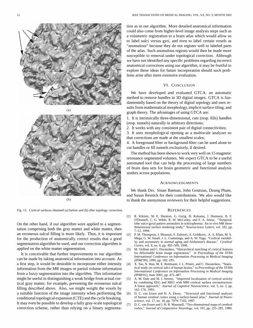
Fig. 12 shows one part of a WM/GM surface before and aftertopology correction using a background-foreground sequencewith 6 connectivity for the background and 18-connectivity forthe foreground. The basic structuring element used in this ex-periment is the 18-ball. All handles seen in panel (a) are clearlyremoved in panel (b).

The processing time of GTCA depends on the total number offoreground/background filters required. For the results shownin Tables I–VI, each filter took less than 3 minutes on an SGIOnyx2 workstation with a 250-MHz R10000 processor, and thetotal processing time for each brain volume took less than 10minutes.

V. DISCUSSION

We have experimentally shown that our topology correctionalgorithm works successfully on brain volumes having largenumbers of handles. Furthermore, it works successfully with

different choices of connectivity rules, different filtering se-quences, and different structuring elements. It is clear from thetheory that it will always produce a topologically correct finalvolume; however, we make no claim that our result is optimalby any criteria. Instead, our approach can be considered to bea (presumably) sub-optimal solution to the goal of producinga topologically correct object by making the fewest number ofchanges to the voxels in the original volume.

It might be asked, however, whether the criterion of makingthe fewest number of changes to the original volume is a sen-sible one. The primary rationale behind this criterion is thattopology defects are caused by image noise, and are primarilyof a fine scale. Our strategy to alternate between foreground andbackground, then go from fine to coarse scales acknowledgesthe fact that such noise can either “add” or “remove” parts ofthe object and that noise can sometimes group together to formlarger defects.

But this focus and strategy does not necessarily make changesthat are concordant with the actual anatomy. For example, sup-pose two opposing banks of a sulcus were wrongly “bridged”near its gyral lips. The two possible corrections to this topolog-ical defect are to remove the bridge or to fill the entire sulcus. Ifthe sulcus were very narrow and the bridge were very thick, thenit is possible that our algorithm would erroneously fill the sul-cus. Fortunately, this situation is unlikely to exist when correct-ing the white matter volume, since the sulcal separation includesboth the sulcal gap itself and both sulcal banks comprising cor-tical gray matter. Therefore, it is unlikely that such bridges willexist, assuming a good segmentation algorithm is used. Further-more, it is much more likely that the scale of any such bridgewill be smaller than the scale of the sulcus. In this case, thebridge will be cut first and the correct result will be achieved re-gardless of the order of background and foreground alternation.


(a)

(b)

Fig. 12. Cortical surfaces obtained (a) before and (b) after topology correction.

On the other hand, if our algorithm were applied to a segmen-tation comprising both the gray matter and white matter, thenan erroneous sulcal filling is more likely. Thus, it is importantfor the production of anatomically correct results that a goodsegmentation algorithm be used, and our correction algorithm isapplied on the white matter segmentation.

It is conceivable that further improvements to our algorithmcan be made by taking anatomical information into account. Asa first step, it would be desirable to incorporate either intensityinformation from the MR images or partial volume informationfrom a fuzzy segmentation into the algorithm. This informationmight be useful in distinguishing a weak bridge from actual cor-tical gray matter, for example, preventing the erroneous sulcalfilling described above. Also, we might weight the voxels bya suitable function of the image intensity when performing theconditional topological expansion (CTE) and the cycle breaking.It may even be possible to develop a fully gray-scale topologicalcorrection scheme, rather than relying on a binary segmenta-

tion as in our algorithm. More detailed anatomical informationcould also come from higher-level image analysis steps such asa volumetric registration to a brain atlas which would allow usto label sulci versus gyri, and even to label certain voxels as“anomalous” because they do not register well to labeled partsof the atlas. Such anomalous regions would then be made moresusceptible to removal under topological correction. Althoughwe have not identified any specific problems regarding incorrectanatomical corrections using our algorithm, it may be fruitful toexplore these ideas for future incorporation should such prob-lems arise after more extensive evaluation.

VI. CONCLUSION

We have developed and evaluated GTCA, an automaticmethod to remove handles in 3D digital images. GTCA is fun-damentally based on the theory of digital topology and uses re-sults from mathematical morphology, implicit surface tiling, andgraph theory. The advantages of using GTCA are:1. It is intrinsically three-dimensional, cuts (resp. fills) handles(resp. tunnels) naturally in arbitrary directions;2. It works with any consistent pair of digital connectivities;3. It uses morphological opening as a multiscale analyzer sothat corrections are made at the smallest scales;4. A foreground filter or background filter can be used alone tocut handles or fill tunnels exclusively, if desired.

The method has been shown to work very well on 15 magneticresonance segmented volumes. We expect GTCA to be a usefulautomated tool that can help the processing of large numbersof brain data sets for brain geometric and functional analysisstudies across populations.

ACKNOWLEDGMENTS

We thank Drs. Sinan Batman, John Goutsias, Dzung Pham,and Susan Resnick for their contributions. We also would liketo thank the anonymous reviewers for their helpful suggestions.

REFERENCES

[1] R. Kikinis, M. E. Shenton, G. Gerig, H. Kokama, J. Haimson, B. F.O'Donnell, C. G. Wible, R. W. McCarley, and F. A. Jolesz, “Temporallobe sulco-gyral pattern anomalies in schizophrenia: An in vivo MR three-dimensional surface rendering study,” Neuroscience Letters, vol. 182, pp.7–12, 1994.

[2] P. M. Thompson, J. Moussai, S. Zohoori, A. Goldkorn, A. A. Khan, M. S.Mega, G. W. Small, J. L. Cummings, and A. W. Toga, “Cortical variabil-ity and asymmetry in normal aging and Alzheimer's disease,” CerebralCortex, vol. 8, no. 6, pp. 492–509, 1998.

[3] M. Vaillant and C. Davatzikos, “Hierarchical matching of cortical featuresfor deformable brain image registration,” in Proceedings of the XVIthInternational Conference on Information Processing in Medical Imaging(IPMI'99), 1999, pp. 182–195.

[4] X. Tao, X. Han, M. E. Rettmann, J. L. Prince, and C. Davatzikos, “Statis-tical study on cortical sulci of human brains,” in Proceedings of the XVIIthInternational Conference on Information Processing in Medical Imaging(IPMI'01), June 2001, pp. 475–487.

[5] A. M. Dale and M. I. Sereno, “Improved localization of cortical activityby combining EEG and MEG with MRI cortical surface reconstruction:A linear approach,” Journal of Cognitive Neuroscience, vol. 5, no. 2, pp.162–176, 1993.

[6] D. C. van Essen and H. A. Drury, “Structural and functional analysesof human cerebral cortex using a surface-based atlas,” Journal of Neuro-science, vol. 17, no. 18, pp. 7079–7102, 1997.

[7] D. C. van Essen and J. H. R. Maunsell, “Two dimensional maps of cerebralcortex,” Journal of Comparative Neurology, vol. 191, pp. 255–281, 1980.


[8] G. J. Carman, H. A. Drury, and D. C. van Essen, “Computational methodsfor reconstructing and unfolding the cerebral cortex,” Cerebral Cortex,vol. 5, pp. 506–517, 1995.

[9] B. Wandell, S. Engel, and H. Hel-Or, “Creating images of the flattenedcortical sheet,” Investigative Ophthalmology and Visual Science, vol. 36,pp. S612, 1996.

[10] B. Fischl, M. I. Sereno, and A. M. Dale, “Cortical surface-based analysisII: Inflation, flattening, and a surface-based coordinate system,” NeuroIm-age, vol. 9, pp. 195–207, 1999.

[11] B. Fischl, A. Liu, and A. M. Dale, “Automated manifold surgery: Con-structing geometrically accurate and topologically correct models of thehuman cerebral cortex,” IEEE Transactions on Medical Imaging, vol. 20,no. 1, pp. 70–80, 2001.

[12] C. Davatzikos and N. Bryan, “Using a deformable surface model to ob-tain a shape representation of the cortex,” IEEE Transactions on MedicalImaging, vol. 15, no. 6, pp. 785–795, 1996.

[13] P. C. Teo, G. Sapiro, and B. A. Wandell, “Creating connected represen-tations of cortical gray matter for functional MRI visualization,” IEEETransactions on Medical Imaging, vol. 16, no. 6, pp. 852–863, 1997.

[14] A. M. Dale, B. Fischl, and M. I. Sereno, “Cortical surface-based analysisI: Segmentation and surface reconstruction,” NeuroImage, vol. 9, pp. 179–194, 1999.

[15] C. Xu, D. L. Pham, M. E. Rettmann, D. N. Yu, and J. L. Prince, “Recon-struction of the human cerebral cortex from magnetic resonance images,”IEEE Transactions on Medical Imaging, vol. 18, no. 6, pp. 467–480, 1999.

[16] D. MacDonald, N. Kabsni, D. Avis, and A. C. Evans, “Automated 3-D extraction of inner and outer surfaces of cerebral cortex from MRI,”NeuroImage, vol. 12, pp. 340–355, 2000.

[17] J.-F. Mangin, V. Frouin, I. Bloch, J. Regis, and J. Lopez-Krahe, “From3D magnetic resonance images to structural representations of the cortextopography using topology preserving deformations,” Journal of Mathe-matical Imaging and Vision, vol. 5, pp. 297–318, 1995.

[18] T. Y. Kong and A. Rosenfeld, “Digital topology: Introduction and survey,”Computer Vision, Graphics, and Image Processing, vol. 48, pp. 357–393,1989.

[19] G. Malandain, G. Bertrand, and N. Ayache, “Topological segmentation ofdiscrete surfaces,” International Journal of Computer Vision, vol. 10, no.2, pp. 183–197, 1993.

[20] G. Bertrand and G. Malandain, “A new characterization of three dimen-sional simple points,” Pattern Recognition Letters, vol. 15, pp. 169–175,1994.

[21] G. Bertrand, “Simple points, topological numbers and geodesic neighbor-hoods in cubic grids,” Pattern Recognition Letters, vol. 15, pp. 1003–1011,1994.

[22] P. K. Saha and B. B. Chaudhuri, “Detection of 3D simple points for topol-ogy preserving transformations with application to thinning,” IEEE Trans-actions on Pattern Analysis and Machine Intelligence, vol. 16, pp. 1028–1032, 1994.

[23] Z. Aktouf, G. Bertrand, and L. Perroton, “A 3D-hole closing algorithm,”in 6th Int. Workshop on Discrete Geometry for Computer Imagery, Lyon,France, 1996, pp. 36–47.

[24] T. McInerney and D. Terzopoulos, “Deformable models in medical imageanalysis: A survey,” Medical Image Analysis, vol. 1, no. 2, pp. 91–108,1996.

[25] X. Zeng, L. H. Staib, R. T. Schultz, and J. S. Duncan, “Segmentationand measurement of the cortex from 3D MR images,” in Proceedingsof Medical Image Computing and Computer-Assisted Intervention (MIC-CAI). 1998, pp. 519–530, Springer-Verlag.

[26] X. Han, C. Xu, and J. L. Prince, “A topology preserving deformable modelusing level sets,” in Proc. IEEE CS Conf. Computer Vision Pattern Recog-nition (CVPR2001), Hawaii, USA, December 2001.

[27] X. Han, C. Xu, D. Tosun, and J. L. Prince, “Cortical surface reconstruc-tion using a topology preserving geometric deformable model,” in Proc.IEEE Workshop on Mathematical Methods in Biomedical Image Analysis(MMBIA2001), Hawaii, USA, December 2001.

[28] I. Guskov and Z. J. Wood, “Topological noise removal,” in Proceedingsof Graphics Interface 2001, 2001, pp. 19–26.

[29] D. W. Shattuck and R. M. Leahy, “Topological refinement of volumetricdata,” in Proceedings of the SPIE, San Diego, USA, February 1999, vol.3661, pp. 204–213.

[30] D. W. Shattuck and R. M. Leahy, “Topologically constrained cortical sur-faces from MRI,” in Proceedings of the SPIE, San Diego, USA, February2000, vol. 3979, pp. 747–758.

[31] X. Han, C. Xu, U. Braga-Neto, and J. L. Prince, “Graph-based topologycorrection for brain cortex segmentation,” in Proceedings of the XVIIthInternational Conference on Information Processing in Medical Imaging(IPMI'01), June 2001, pp. 395–401.

[32] W. E. Lorensen and H. E. Cline, “Marching cubes: A high-resolution 3Dsurface construction algorithm,” ACM Computer Graphics, vol. 21, no. 4,pp. 163–170, 1987.

[33] G. M. Nielson and B. Hamann, “The asymptotic decider: Resolving theambiguity in marching cubes,” in Proceedings of IEEE Visualization 1991,Los Alamitos, Calif., 1991, pp. 83–91.

[34] P. Ning and J. Bloomenthal, “An evaluation of implicit surface tilers,”IEEE Computer Graphics and Applications, vol. 13, no. 6, pp. 33–41,1993.

[35] A. van Gelder and J. Wilhelms, “Topological considerations in isosurfacegeneration,” ACM Transactions on Graphics, vol. 13, no. 4, pp. 337–375,1994.

[36] B. K. Natarajan, “On generating topologically consistent isosurfaces fromuniform samples,” Visual Computer, vol. 11, no. 1, pp. 52–62, 1994.

[37] M. K. Agoston, Algebraic Topology — A first course, Marcel Dekker, Inc.,New York, 1976.

[38] R. Sedgewick, Algorithms in C, Addison-Wesley, MA, 1990.[39] N. W. Shock, R. C. Greulich, R. Andres, D. Arenberg, P. T. Costa Jr.,

E. Lakatta, and J. D. Tobin, “Normal human aging: The Baltimore lon-gitudinal study of aging,” U.S. Government Printing Office, Washington,D.C., 1984.

[40] S. M. Resnick, A. F. Goldszal, C. Davatzikos, S. Golski, M. A. Kraut, E. J.Metter, R. N. Bryan, and A. B. Zonderman, “One-year age changes inMRI brain volumes in older adults,” Cerebral Cortex, vol. 10, no. 5, pp.464–472, 2000.

[41] M. Vaillant and C. Davatzikos, “Finding parametric representations of thecortical sulci using an active contour model,” Medical Image Analysis,vol. 1, no. 4, pp. 295–315, 1997.

Topology correction in brain cortex segmentation using a multiscale, graph-based algorithm

Documents