FULLTEXT01.pdf - uu .diva

Vol.:(0123456789)

Environmental Fluid Mechanics (2019) 19:719–750https://doi.org/10.1007/s10652-018-9650-4

1 3

ORIGINAL ARTICLE

On possibilities to estimate local concentration variations with CFD‑LES in real urban environments

Jan Burman1,3 · Lage Jonsson1,2 · Anna Rutgersson3

Received: 3 October 2017 / Accepted: 13 November 2018 / Published online: 24 November 2018 © The Author(s) 2018

AbstractApplied studies with Large Eddy Simulation (LES) of hazardous gas dispersion around buildings in cities have become increasingly feasible due to rapid advancements in com-puting technology. However, there is little extant literature investigating how each model’s results compare with others, as well as their ability to predict near-field dispersion in a real city. In this study, three typical LES sub-grid-scale models are used to simulate gas disper-sion, utilizing alternatively constant values and synthetic turbulence at inflow boundaries. The results are compared with data from the Joint Urban 2003 Atmospheric Dispersion Study in Oklahoma City. Flow and turbulence statistics of the simulation is presented at two probe locations, one inside the city-core and one outside. In addition, comparisons with the measured mean concentration and maximum concentration values are conducted. It was found that in the core of the city, simulated turbulence is mainly determined by buildings and their configurations, and is only weakly affected by model type and assumed turbulence at the inflow boundaries. On the other hand, outside and upwind the city center the turbulence set at the inflow boundaries is very important if realistic turbulence statis-tics is to be achieved. Downstream of the source, all tested models produce similar pre-dictions of maximum concentration values, which in turn are similar to the experimental data. Thus, the results indicate that it could be better to use the LES calculated maximum-concentration instead of the calculated mean-concentration when developing methods for hazard area estimation.

Keywords Gas dispersion · Urban area · LES · SIGMA · CFD · Synthetic boundary condition · Turbulence statistics · Contaminant statistics · JU2003

* Lage Jonsson [email protected]

1 Division of CBRN Defence and Security, FOI, Swedish Defence Research Agency, 901 82 Umeå, Sweden

2 KTH, Royal Institute of Technology, 100 44 Stockholm, Sweden3 Department of Earth Sciences, Uppsala University, Uppsala, Sweden

http://crossmark.crossref.org/dialog/?doi=10.1007/s10652-018-9650-4&domain=pdf

720 Environmental Fluid Mechanics (2019) 19:719–750

1 3

1 Introduction

Since performing applied studies with Computational Fluid Dynamic (CFD) of gas disper-sion in cities has constituted a major challenge for researchers, the aim of this investigation is to test the current potential of typical CFD-LES simulations to predict near-field hazard-ous gas dispersion in urban environments. A previous review on past achievements and future challenges concluded that more effective efforts should be invested in the numerical simulation of fluctuating flow fields and the numerical evaluation of peak values of varia-bles [1]. For practical applications, this is accentuated in Tolias [2]. In addition, in a recent review [3] it was asserted that, for near-field pollutant dispersion around buildings, it is still necessary to discern the applicability of CFD. Also, in their review Lateb et al. [4] con-clude that the topic of micro-scale dispersion still requires further investigations to under-stand the effect of all the parameters on wind flow and pollutant dispersion in urban areas. In addition, Tolias [2] recognised that higher order statistics and grid evaluations are miss-ing in several of previous LES-studies. Furthermore, Park et al. [5] who performed LES of a densely built-up area of Seoul found that strong ejections are dominant at building-top heights and that downdrafts along the windward walls of high-rise buildings are distinct below building-tops inducing high turbulent kinetic energy and winding flow around the high buildings near the ground surface, transporting momentum downward and intermit-tently into nearby streets. Specifically, in their conclusion they state that an in-depth inves-tigation of turbulence coherent structures behind typical urban buildings is required to bet-ter understand complex turbulent flow in a densely built-up urban area and, in addition, they point out that dispersion in urban areas are reported to be more accurate when data from a mesoscale model, or from measurement at a high tower, are used as inflow data [6]. This conclusion was also drawn by Nakayama [7–12] who developed a local-scale high-resolution atmospheric dispersion model using LES to assess the safety at nuclear facili-ties and to respond to emergency situations resulting from accidental or deliberate releases of radioactive materials. They also conclude that LES simulates reasonably the unsteady behavior of turbulent flows and plume dispersion even for complex heterogeneous urban areas. Likewise, Li et al. [13] used a scheme which employs the turbulence-reconstruc-tion method to couple mesoscale model data with LES to simulate dispersion in a real city. They found improvements in the prediction of the wind direction, especially near the source, as well as of the r.m.s. concentration and the concentration maximum. Though to date most LES studies of dispersion in cities are for neutral stratification, there are cases when LES is applied for an unstable atmospheric boundary layer as well, for example [14]. In this case both inlet velocity fluctuations and inlet temperature fluctuations are necessary to prescribe. An overview of previous and present LES computations of atmospheric dis-persion in actual urban areas can be found in Gousseau et al. [15].

To evaluate the consequences of gas dispersion in a city center, it may be necessary to predict spatiotemporal fluctuations since, for many toxic gases, acute poisoning occurs during the first concentration peak, which typically has duration of less than 1 min. How-ever, due to their stochastic nature, single real eddies cannot be predicted. Specifically, large local variations exist and in a short time interval, i.e., in less than a couple of min-utes, the concentration varies widely. As Schatzmann [16] revealed, near the ground within the Urban Canopy Layer (UCL), the meteorological and concentration fields are obviously inhomogeneous. Moreover, gradients of flow properties are considerable. For example, measurements taken a few meters apart from each other can obtain largely different results, and measurements taken under apparently identical conditions can also differ significantly.

721Environmental Fluid Mechanics (2019) 19:719–750

1 3

Correspondingly, Liu et al. [17] analyzed fluctuations around a high-rise building in wind-tunnel experiments, and found that variations in fluctuation intensity are quite sensitive to both source location and wind direction. Therefore, in order to analyze the consequences of hazardous gas dispersion, a trend exists in which increasingly complex CFD models, including LES [18, 19], are utilized to describe intermittency and fluctuations in wind and concentration fields. Since spatiotemporal fluctuations of local wind and concentra-tion fields are impossible to be directly predicted, as a basis for the consequences analy-sis, flow- and concentration-statistics resulting from the CFD simulations must be used. Furthermore, to evaluate the consequences of hazardous gas dispersion it is more realis-tic to rely on dosage calculated from concentration levels resolved in time. This could be performed by use of eddy resolving simulations. An alternative method is to establish the concentration cumulative distribution (cdf) assuming a certain shape of the concentration probability density function [20–22] and use this to predict the maximum instantaneous concentration from the simulation results. Also, Xie [23] used extreme value theory (EVT) to model the upper tail of the probability density function of the concentration time series collected from LES with remarkable success. Recording the maximum values spatially, as discussed in this investigation, gives support to hazard area estimation. It is critical to thoroughly elucidate the magnitude and features of differences in dispersion-characteristics and analyze results produced by typical LES Sub-Grid-Scale (SGS) models that might be used for applied dispersion simulations in urban areas and, furthermore, check how these results compare with full-scale experiments. The maximum dosage can also be estimated by a methodology presented by Bartzis [24] where they introduced an approach relating maximum dosage to parameters such as concentration variance and turbulence integral time scale. The methodology has been implemented by Efthimiou [25] for a point source in a RANS CFD model. Efthimiou [26, 27] also simulated part of the MUST experiment [28, 29] and found that their model gave satisfactory estimates of short time maximum exposure. Furthermore, Bartzis et al. [30] presented an attempt to approximate on generic terms, the statistical behavior of the stochastic nature of turbulence with a beta distribu-tion probability density function (beta-pdf). The extreme concentration value in beta-pdf seemed to be properly addressed by the proposed correlation [24] in which global values of its associated constants are proposed, since the wind tunnel experiment and the MUST experiment gave support to the theory. Later [31], a continuously emitting source in the MUST experiment was used for the selection of the best performing statistical model between the Gamma and the Beta distributions. They found that the performance of the Beta distribution was slightly better than that of the Gamma distribution.

In summary, as stated by Bogen [32] who statistically analyzed the impact of spatiotem-poral fluctuations in airborne chemicals on toxic hazard assessment; these fluctuations will need to be reflected one way or the other in chemical threat assessment models.

The scope of the present study is to demonstrate and discuss the usefulness and differ-ences in dispersion characteristics and results produced by some typical LES SGS-models. Specifically, the aim is to investigate the usefulness of the CFD results for gas dispersion by illustration, discussion, and comparison of results and turbulence statistics in two city-areas, one inside of a dense building area and one outside of a dense building area. The simulations are mimicking part of the Joint Urban 2003 Atmospheric Dispersion Study in Oklahoma City 2003 (JU2003) using both constant and dynamic settings for turbulence at inflow boundaries with acceptable resolution and a reasonable size of the computational domain for applied studies considering the computational effort.

With the objective to determine how well the models compare with each other and determine their ability to predict experimental results in a real city without specific tuning,


1 3

three typical LES SGS-models were chosen: (1) the standard static Smagorinsky model [33]; (2) the WALE model [34]; and (3) the SIGMA model [35]. Though important for developing LES based dispersion models, this type of comparison has not been presented before, and, to the authors’ knowledge, among the studied models the SIGMA model has not earlier been used for studies of dispersion in a real city. Moreover, in order to inves-tigate the influence of Boundary Conditions (BC) on important parameters, one type of dynamic setting for turbulence (synthetic BC) at inflow boundaries was examined using the SIGMA model.

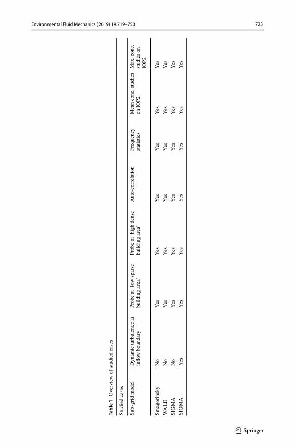
A summary of the studied cases is presented in Table 1.

2 Joint urban 2003 atmospheric dispersion study

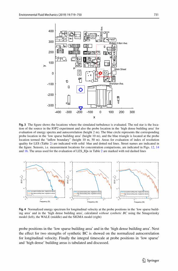
The DOE-DTRA JU2003 field experiment was performed in Oklahoma City in July 2003. In JU2003, street canyon experiments were conducted in which a large number of wind and tracer sensors were placed at the street level, on towers, and at the roof level within a section of a street canyon on Park Avenue, which is located within the downtown core of Oklahoma City. In the experiment, sulphur hexafluoride (SF6) tracer dissemination and data collection were performed during 10 Intensive Observation Periods (IOPs). The IOP:s included three quasi-continuous (30 min) point releases (17 daytime, 12 nocturnal) and 40 puff (instantaneous) releases (25 daytime and 15 nocturnal). The experiment is described in several studies [36–40]. Several model comparisons have also been performed with the data, among them [11, 13, 41, 42]. One of the objectives of the experiment was to collect flow and tracer concentration data at various distances from the release point, including in and around a single block, in and around several blocks in the downtown central busi-ness district, and to investigate tracer exchange through a building envelope. Among the conclusions drawn by analysis of the sampler data are: (1) concentrations measured at the street level often exceeded rooftop-level measurements by a factor of three or greater; (2) tracer released at the street level during moderate winds rapidly disperses to rooftop levels near the release location; (3) tracer released at the street level can be channeled down street canyons at angles approaching 60°–80° from the downwind direction; and (4) street-level turbulence measurements can constitute useful predictors of tracer dissipation rates. In this investigation, data from IOP2, continuous release, have been used for comparison with the simulations. The location of the source, and the different probes and sensors used in this study are shown in Figs. 3, 12, 14 and 16. Details regarding the comparisons of current model dispersion results and measurements are presented in the Sect. 4.

3 Modeling

In this research, CFD was utilized to investigate the accuracy and feasibility of simu-lated flow and concentration statistics for an urban environment, and comparison with the results of the JU2003 campaign. For three LES SGS-models, i.e., WALE [34], SIGMA [35] and standard static Smagorinsky [33], the commercial code PHOENICS© [43] was used to solve the equations for both constant and dynamic settings of turbulence at inflow boundaries.

Numerical details for the simulations are presented in Sect. 3.1, used turbulence calcula-tions in Sect. 3.2 and dispersion of gas in Sect. 3.3.


1 3

Tabl

e 1

Ove

rvie

w o

f stu

died

cas

es

Stud

ied

case

s

Sub-

grid

mod

elD

ynam

ic tu

rbul

ence

at

inflo

w b

ound

ary

Prob

e at

‘low

spar

se

build

ing

area

’Pr

obe

at ‘h

igh

dens

e bu

ildin

g ar

ea’

Aut

o-co

rrel

atio

nFr

eque

ncy

stat

istic

sM

ean

conc

. stu

dies

on

IOP2

Max

. con

c.

studi

es o

n IO

P2

Smag

orin

sky

No

Yes

Yes

Yes

Yes

Yes

Yes

WA

LEN

oYe

sYe

sYe

sYe

sYe

sYe

sSI

GM

AN

oYe

sYe

sYe

sYe

sYe

sYe

sSI

GM

AYe

sYe

sYe

sYe

sYe

sYe

sYe

s


1 3

3.1 Numerical details for simulations in a city‑center

Presented below are numerical details of calculation domain, grid, equations, numerical schemes and other details for the simulations.

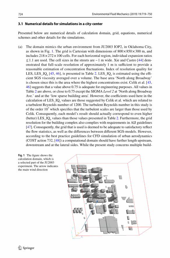
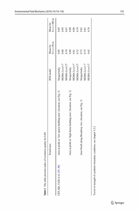
(a) The domain mimics the urban environment from JU2003 IOP2, in Oklahoma City, as shown in Fig. 1. The grid is Cartesian with dimensions of 800 × 850 × 300 m, and includes 218 × 272 × 100 cells. For each horizontal region, individual expansion ratios ≤ 1.1 are used. The cell sizes in the streets are ~ 1 m wide. Xie and Castro [44] dem-onstrated that full-scale resolution of approximately 1 m is sufficient to provide a reasonable estimation of concentration fluctuations. Index of resolution quality for LES, LES_IQν [45, 46], is presented in Table 2. LES_IQν is estimated using the effi-cient SGS viscosity averaged over a volume. The base area ‘North along Broadway’ is chosen since this is the area where the highest concentrations exist. Celik et al. [45, 46] suggests that a value above 0.75 is adequate for engineering purposes. All values in Table 2 are above, or close to 0.75 except the SIGMA Level 2 at ‘North along Broadway Ave.’ and at the ‘low sparse building area’. However, the coefficients used here in the calculation of LES_IQν values are those suggested by Celik et al. which are related to a turbulent Reynolds number of 1200. The turbulent Reynolds number in this study is of the order 107 which specifies that the turbulent scales are larger than those used by Celik. Consequently, each model’s result should actually correspond to even higher (better) LES_IQν values than those values presented in Table 2. Furthermore, the grid resolution for the building complex also complies with requirements in AIJ guidelines [47]. Consequently, the grid that is used is deemed to be adequate to satisfactory reflect the flow statistics, as well as the differences between different SGS-models. However, according to the best practice guidelines for CFD simulation of urban aerodynamics (COST action 732, [48]) a computational domain should have further length upstream, downstream and at the lateral sides. While the present study concerns multiple build-

Fig. 1 The figure shows the calculation domain, which is a selected part of the JU2003 experiment. The arrow indicates the main wind direction


1 3

Tabl

e 2

The

tabl

e pr

esen

ts in

dex

of re

solu

tion

qual

ity fo

r LES

a Leve

l of s

treng

th o

f syn

thet

ic b

ound

ary

cond

ition

, see

cha

pter

3.2

.2

Teste

d ar

eaSG

S m

odel

Mea

n fo

r 0 <

z <

50 m

Mea

n fo

r 0 <

z <

300

m

LES_

IQν,

Cel

ik e

t al.

[45,

46]

Are

a at

pro

be a

t ‘lo

w sp

arse

bui

ldin

g ar

ea’ (

loca

tion,

see

Fig.

3)

Smag

orin

sky

0.85

0.85

SIG

MA

Lev

el 1

a0.

880.

95SI

GM

A L

evel

2a

0.70

0.67

Are

a at

pro

be a

t ‘hi

gh d

ense

bui

ldin

g ar

ea’ (

loca

tion,

see

Fig.

3)

Smag

orin

sky

0.80

0.88

SIG

MA

Lev

el 1

a0.

810.

89SI

GM

A L

evel

2a

0.72

0.79

Are

a N

orth

alo

ng B

road

way

Ave

. (lo

catio

n, se

e Fi

g. 3

)Sm

agor

insk

y0.

720.

81SI

GM

A L

evel

1a

0.75

0.81

SIG

MA

Lev

el 2

a0.

620.

70


1 3

ings and, according to the recommendations, lateral, then upwind and downwind dis-tances might then be chosen smaller. Moreover, one of the purposes of the survey is to investigate if, and to what extent, synthetic boundary conditions can replace the proposed extensions of the domain when performing applied studies.

(b) The balance equation used is finite volume, and the solution method is whole field.(c) The equation formulation utilized is elliptic-staggered.(d) The solution algorithm used for velocity and pressure is the Semi-Implicit Method for

Pressure-Linked Equations Shortened, abbreviated as the SIMPLEST method [43], which is a modified version of the well-known SIMPLE method [49].

(e) The advection discretization schema employed is the Monotone Upstream-centered Schemes for Conservation Laws (MUSCL) [50]. MUSCL is a bounded higher-order advection Total Variation Diminishing (TVD) schema [51] with low dispersive error.

(f) The temporal scheme used is a 3rd-order implicit Adams–Moulton [52].(g) In the studied area of the domain, y+ is typically in the range 30 < y+ < ≈ 15,000, where

y+ is the dimensionless distance to the wall, i.e., the distance to the wall multiplied by friction velocity divided by the viscosity of air. There are typically around 40 cells along larger buildings in the x- and y-directions, and around 20 cells along smaller buildings.

(h) Cells partly filled with fluid are handled by a built-in cut-cell method in PHOENICS [43].

(i) Convergence is considered to be obtained when all residuals have decreased by at least a factor of < 10−5. Point values are monitored (all solved variables) both graphically and numerically and checked for stability. Typical changes are between zero and 10−7 at the end of a time-step. The %-error for each variable is then of the order 10−6 and the change of the order 10−9.

(j) Boundary and inlet conditions are given in Table 3. SIGMA simulations have been performed with synthetic turbulence at inflow bound-

aries (paragraph 2.3), as well as with static boundary conditions without any inlet turbulence quantities added. Smagorinsky and WALE simulations are reported without any inlet turbulence quantities added.

(k) Start of evaluation for all flow variables and spectra begins at 60 s. After 60 s the set properties of the inlet boundary at the roof top height has passed over the release point and thereby influences the vertical dispersion [53]. At the ground level, the urban boundary layer turbulence dominates the dispersion.

3.2 Turbulence

In this section, the turbulence approaches used in the investigation are presented. Specifi-cally, LES [54] was chosen since numerous researchers consider it to be the existing state-of-the-art model for calculating turbulence and wind in urban areas.

3.2.1 Sub‑grid scale modelling

Large Eddy Simulation makes use of large eddies that within turbulent flow are dependent on geometry, while smaller scales are more universal [55]. This makes it possible to explic-itly solve for large eddies and implicitly account for small eddies by a SGS-model.

In this study, the standard Smagorinsky model [33] and two other model implemen-tations of static SGS-modelling using the eddy-viscosity concept have been employed to


1 3

illustrate the results of the model approaches: (1) the WALE model proposed by Nicoud and Ducros [34], which possesses the property that the SGS-viscosity is always positive, it decays as the distance to a solid boundary to the third power, and vanishes in pure shear as well as in a flow in solid rotation; and (2) the SIGMA model proposed by Nicoud et al. [35] which, in addition to the SGS-viscosity properties of the WALE model, has the property that the SGS-viscosity is zero where the resolved scales are either in pure axisymmetric or isotropic expansion/contraction, as well as for any two dimensional and/or two component flows.

SGS-viscosity is expressed as:

where Cm is the model constant; Δ is a characteristic scale; and Dm is the model operator acting on the resolved velocity field.

For the Smagorinsky model, Dm is defined as:

where

where ui is the velocity components and xi is the coordinates.For the WALE model, Dm is defined as:

(1)𝜈SGSm = (CmΔ)2Dm( �u)

(2)Dm = (2SijSij)1

2

(3)Sij =1

2

(

�ui

�xj+

�uj

�xi

)

Table 3 The table shows boundary conditions and initial values for simulations of dispersion in JU2003 IOP2

Velocities, z0, and wind direction in the table are from Hanna et al. [41]

Property Condition

Top boundary Flat and frictionless at 300 mGround surface Roughness height z0 for the logarithmic velocity

profile set to 0.02 m to account for variability of surface structure

Building surface Smooth surfaceOutlet boundaries Static pressure boundary conditionsInlet velocity X = 1.97 m/s, Y = 2.82 m/s at 10 m height, loga-

rithmic profile, roughness height (z0) 0.6 mDomain size 800 × 850 × 300 mSource From JU2003 IOP2 dataset (5 g/s)Sensor locations From JU2003 IOP2 dataset, see Figs. 12, 14, 16Buildings From JU2003 dataset, see Fig. 1Initial velocities at time 0 (m/s) U = 0, V = 0, W = 0Start of evaluation for all flow variables and spectra After 60-s simulated timeInitial pressure field, initial concentrations and initial

value for turbulent properties0

Coordinate system Origin is located in the lower-left corner of the domain


1 3

where Sdij=

1

2

(

A2

ij+ A2

ji

)

−1

3A2

kk𝛿ij with A2

ij= AikAkj ; and Aij = �ui∕�xj

Similarly, for the SIGMA model, Dm is defined as:

where �i are the singular values of the tensor Gij, i.e., the appropriately ordered square-roots

(

�1≥ �

2≥ �

3≥ 0

)

of the eigenvalues of Gij = Δ2AikAjk.In this study, in the implementation of the Smagorinsky model, explicit filtering was

applied to the discretized Navier–Stokes equations. The numerical filter width used is:

where Δ is the characteristic scale of the computational cell; Δxi is the cell extension in direction i. The product is taken over the three coordinate directions.

The Smagorinsky model applies wall damping according to Van-Driest [56] to partially take wall effects into account by appropriately reducing the length scale in the proximity of walls. The Smagorinsky constant was set to 0.1.

3.2.2 Synthetic turbulence at inflow boundaries

In many flows it is critical to prescribe suitable turbulent fluctuations. There are several ways to create turbulence boundary conditions. One way, limited to fairly low Reynolds numbers, is to use a pre-cursor DNS of channel flow. Another method, which is able to reproduce first- and second-order statistics, as well as two-point correlations, is the vortex method [57] based on a superposition of coherent eddies in which each eddy is described by a shape function localized in space. A similar method was used by Aristodemou [58] where the level of turbulence at the inflow boundary was varied from zero to the values from the wind tunnel experiment, for comparison purposes. A third method is to take resolved fluctuations at a plane downstream of the inlet plane, re-scale them, and use them as inlet fluctuations, as used by Li et al. [13]. As noted by Hertwig [59], for validation exer-cises of fast atmospheric dispersion models, it can also be appropriate to use cyclic bound-ary conditions. In this investigation, in the cases of simulations where inlet fluctuations are used, synthesized inlet fluctuations, according to a method that was first developed by Billson [60–62], are utilized for creating turbulence. This method was first established for generating noise, and later developed for inflow boundary conditions [63–65].

A mean velocity profile is prescribed, which is taken from the log law. Instantaneous turbulent fluctuations taken from synthesized, isotropic turbulence are created by using a

(4)Dm =

(

SdijSdij

)3∕2

(

SdijSdij

)5∕2

+(

SdijSdij

)5∕4

(5)Dm =�3

(

�1− �

2

)(

�2− �

3

)

�2

1

(6)Δ =

(

∏

i

Δxi

)1

3


1 3

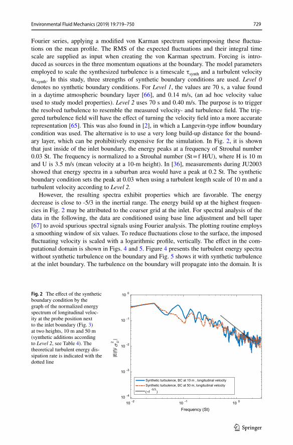
Fourier series, applying a modified von Karman spectrum superimposing these fluctua-tions on the mean profile. The RMS of the expected fluctuations and their integral time scale are supplied as input when creating the von Karman spectrum. Forcing is intro-duced as sources in the three momentum equations at the boundary. The model parameters employed to scale the synthesized turbulence is a timescale τsynth and a turbulent velocity u*synth. In this study, three strengths of synthetic boundary conditions are used. Level 0 denotes no synthetic boundary conditions. For Level 1, the values are 70 s, a value found in a daytime atmospheric boundary layer [66], and 0.14 m/s, (an ad hoc velocity value used to study model properties). Level 2 uses 70 s and 0.40 m/s. The purpose is to trigger the resolved turbulence to resemble the measured velocity- and turbulence field. The trig-gered turbulence field will have the effect of turning the velocity field into a more accurate representation [65]. This was also found in [2], in which a Langevin-type inflow boundary condition was used. The alternative is to use a very long build-up distance for the bound-ary layer, which can be prohibitively expensive for the simulation. In Fig. 2, it is shown that just inside of the inlet boundary, the energy peaks at a frequency of Strouhal number 0.03 St. The frequency is normalized to a Strouhal number (St = f H/U), where H is 10 m and U is 3.5 m/s (mean velocity at a 10-m height). In [36], measurements during JU2003 showed that energy spectra in a suburban area would have a peak at 0.2 St. The synthetic boundary condition sets the peak at 0.03 when using a turbulent length scale of 10 m and a turbulent velocity according to Level 2.

However, the resulting spectra exhibit properties which are favorable. The energy decrease is close to -5/3 in the inertial range. The energy build up at the highest frequen-cies in Fig. 2 may be attributed to the coarser grid at the inlet. For spectral analysis of the data in the following, the data are conditioned using base line adjustment and bell taper [67] to avoid spurious spectral signals using Fourier analysis. The plotting routine employs a smoothing window of six values. To reduce fluctuations close to the surface, the imposed fluctuating velocity is scaled with a logarithmic profile, vertically. The effect in the com-putational domain is shown in Figs. 4 and 5. Figure 4 presents the turbulent energy spectra without synthetic turbulence on the boundary and Fig. 5 shows it with synthetic turbulence at the inlet boundary. The turbulence on the boundary will propagate into the domain. It is

Fig. 2 The effect of the synthetic boundary condition by the graph of the normalized energy spectrum of longitudinal veloc-ity at the probe position next to the inlet boundary (Fig. 3) at two heights, 10 m and 50 m (synthetic additions according to Level 2, see Table 4). The theoretical turbulent energy dis-sipation rate is indicated with the dotted line

10 -2 10 -1 10 0

Frequency (St)

10 -4

10 -3

10 -2

10 -1

10 0

|E(f)

/2 U

|

Synthetic turbulence, BC at 10 m , longitudinal velocitySynthetic turbulence, BC at 50 m, longitudinal velocity

(~f-5/3

)


1 3

also clear that the properties endure until the flow encounters buildings that will force the flow to break up into smaller turbulent eddies.

3.3 Dispersion of gas

In this investigation, the transport and diffusion of dispersed gas are modeled according to Patankar [68]:

where the first term expresses the rate of change of ϕ with respect to time; the second term expresses convection (transport due to fluid-flow); and the third term expresses diffusion (transport due to the variation of ϕ from point to point), where Γϕ is the exchange coef-ficient of the entity ϕ in the phase. Please note that Γ� is defined differently for the different turbulence approaches (e.g., Pope [69]). The fourth term expresses source terms (associ-ated with the creation or destruction of ϕ). The source term is specified in the JU2003 IOP2 dataset [38].

4 Results

To compare the SGS-models and to illustrate the influence of synthetic boundary condi-tions, frequency statistics and autocorrelations of data produced by the Smagorinsky, WALE and the SIGMA model are presented in Sect. 4.1 at two probe locations, one inside of the dense building area and one outside of the dense area. In addition, for the SIGMA model two different levels of dynamic settings for turbulence at inflow boundaries are used and the results presented.

With the objective to determine the ability of each of the models to predict experimental results without specific tuning, comparisons with measured mean concentration and meas-ured maximum concentration are presented in Sect. 4.2.

Figure 3 shows where, in the calculation domain, the statistics and autocorrelations (Figs. 4, 5, 6, 7, 8 and Tables 4, 5) are evaluated.

4.1 Frequency statistics and autocorrelations

The objective of this section is to check how well the Smagorinsky model, the WALE and the SIGMA model corresponds with each other without any specific tuning since, if the results are similar and their dispersion results also correlate well with field measurements, it points to that the models are useful.

First, illustrated is the normalized energy spectrum of longitudinal velocity at the probe positions in the ‘low sparse building area’ and in the ‘high dense building area’ with static BC using the Smagorinsky model, the WALE and the SIGMA model.

Thereafter influence of synthetic BC on the normalized energy spectrum for longitudi-nal velocity is exemplified at both probe positions, followed by the power spectra demon-strated and compared with and without synthetic BC.

Then the resolved TKE is compared between the different SGS-models followed by comparative illustration of the normalized autocorrelation for longitudinal velocity at

(7)�

�t(��) +

�

�xi(��ui) =

�

�xi

(

Γ�

��

�xi

)

+ S�


1 3

probe positions in the ‘low sparse building area’ and in the ‘high dense building area’. Next the effect for two strengths of synthetic BC is showed on the normalized autocorrelation for longitudinal velocity. Finally the integral timescale at probe positions in ‘low sparse’ and ‘high dense’ building areas is tabulated and discussed.

Fig. 3 The figure shows the locations where the simulated turbulence is evaluated. The red star is the loca-tion of the source in the IOP2 experiment and also the probe location in the ‘high dense building area’ for evaluation of energy spectra and autocorrelation (height 2 m). The blue circle represents the corresponding probe location in the ‘low sparse building area’ (height 10 m), and the blue triangle is located at the probe location termed the “inflow boundary” (height 10 m, 50 m). Areas for evaluation of index of resolution quality for LES (Table 2) are indicated with solid blue and dotted red lines. Street names are indicated in the figure. Sensors, i.e. measurement locations for concentration comparisons, are indicated in Figs. 12, 14 and 16. The areas used for the evaluation of LES_IQν in Table 2 are marked with red dashed lines

10 -2 10 -1 10 010 -4

10 -3

10 -2

10 -1

10 0

|E(f

)/2 U

|

(~f -5/3)

Frequency (St)

High dense building area, longitudinal velocityLow sparse building area, longitudinal velocity

10 -2 10 -1 10 0

Frequency (St)

10 -4

10 -3

10 -2

10 -1

10 0

|E(f

)/2 U

|

Low sparse building area, longitudinal velocityHigh dense building area, longitudinal velocity(~f-5/3

)

10 -2 10 -1 10 010 -4

10 -3

10 -2

10 -1

10 0

|E(f

)/2 U

|

(~f -5/3)

High dense building area, longitudinal velocityLow sparse building area, longitudinal velocity

Frequency (St)

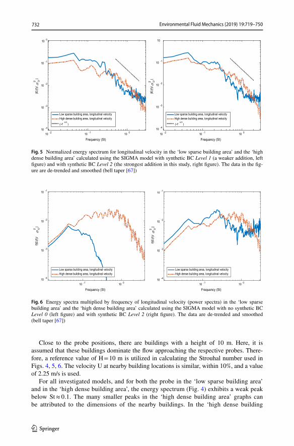
Fig. 4 Normalized energy spectrum for longitudinal velocity at the probe positions in the ‘low sparse build-ing area’ and in the ‘high dense building area’, calculated without synthetic BC using the Smagorinsky model (left), the WALE (middle) and the SIGMA model (right)


1 3

Close to the probe positions, there are buildings with a height of 10 m. Here, it is assumed that these buildings dominate the flow approaching the respective probes. There-fore, a reference value of H = 10 m is utilized in calculating the Strouhal number used in Figs. 4, 5, 6. The velocity U at nearby building locations is similar, within 10%, and a value of 2.25 m/s is used.

For all investigated models, and for both the probe in the ‘low sparse building area’ and in the ‘high dense building area’, the energy spectrum (Fig. 4) exhibits a weak peak below St ≈ 0.1. The many smaller peaks in the ‘high dense building area’ graphs can be attributed to the dimensions of the nearby buildings. In the ‘high dense building

10 -2 10 -1 10 0

Frequency (St)

10 -4

10 -3

10 -2

10 -1

10 0|E

(f)/

2 U|

Low sparse building area, longitudinal velocityHigh dense building area, longitudinal velocity

(~f-5/3

)

10 -2 10 -1 10 0

Frequency (St)

10 -4

10 -3

10 -2

10 -1

10

|E(f

)/2 U

|


(~f-5/3

)

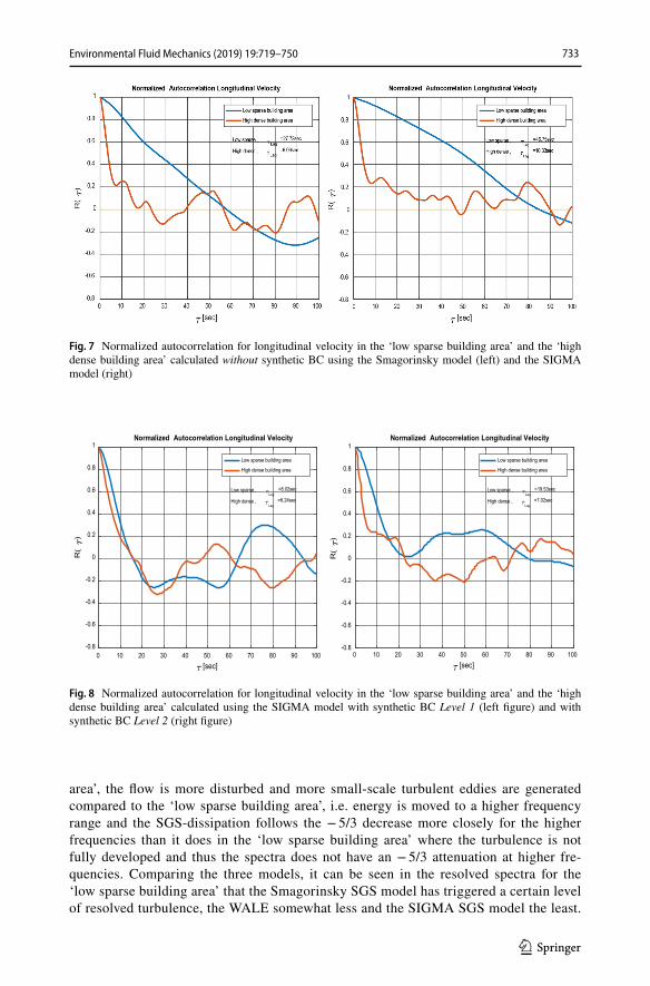
Fig. 5 Normalized energy spectrum for longitudinal velocity in the ‘low sparse building area’ and the ‘high dense building area’ calculated using the SIGMA model with synthetic BC Level 1 (a weaker addition, left figure) and with synthetic BC Level 2 (the strongest addition in this study, right figure). The data in the fig-ure are de-trended and smoothed (bell taper [67])

10 -1 10 0

Frequency (St)

10 -4

10 -3

10 -2

10 -1

f|E(f

)/2 U

|


10 -1 10 0

Frequency (St)

10 -4

10 -3

10 -2

10-1

f|E(f

)/2 U

|


Fig. 6 Energy spectra multiplied by frequency of longitudinal velocity (power spectra) in the ‘low sparse building area’ and the ‘high dense building area’ calculated using the SIGMA model with no synthetic BC Level 0 (left figure) and with synthetic BC Level 2 (right figure). The data are de-trended and smoothed (bell taper [67])


1 3

area’, the flow is more disturbed and more small-scale turbulent eddies are generated compared to the ‘low sparse building area’, i.e. energy is moved to a higher frequency range and the SGS-dissipation follows the − 5/3 decrease more closely for the higher frequencies than it does in the ‘low sparse building area’ where the turbulence is not fully developed and thus the spectra does not have an − 5/3 attenuation at higher fre-quencies. Comparing the three models, it can be seen in the resolved spectra for the ‘low sparse building area’ that the Smagorinsky SGS model has triggered a certain level of resolved turbulence, the WALE somewhat less and the SIGMA SGS model the least.

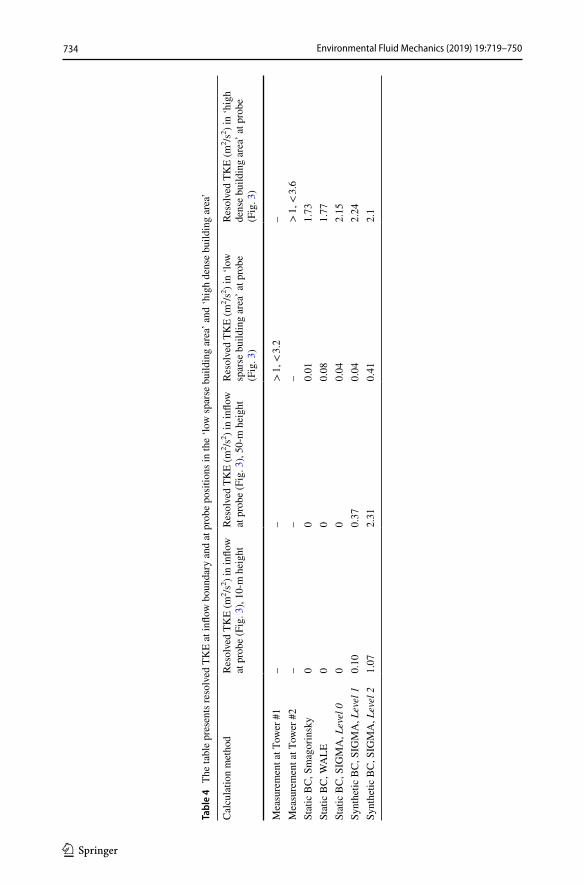
Fig. 7 Normalized autocorrelation for longitudinal velocity in the ‘low sparse building area’ and the ‘high dense building area’ calculated without synthetic BC using the Smagorinsky model (left) and the SIGMA model (right)

[sec]

-0.8

-0.6

-0.4

-0.2

0

0.2

0.4

0.6

0.8

1

R(

)

Normalized Autocorrelation Longitudinal Velocity

Low sparse ,Lag

=8.02sec

High dense ,Lag

=6.24sec

Low sparse building area

High dense building area

0 10 20 30 40 50 60 70 80 90 100

Normalized Autocorrelation Longitudinal Velocity

Low sparse ,Lag

=19.53sec

High dense ,Lag

=7.02sec

Low sparse building area

High dense building area

-0.8

-0.6

-0.4

-0.2

0

0.2

0.4

0.6

0.8

1

R(

)

[sec]0 10 20 30 40 50 60 70 80 90 100

Fig. 8 Normalized autocorrelation for longitudinal velocity in the ‘low sparse building area’ and the ‘high dense building area’ calculated using the SIGMA model with synthetic BC Level 1 (left figure) and with synthetic BC Level 2 (right figure)


1 3

Tabl

e 4

The

tabl

e pr

esen

ts re

solv

ed T

KE

at in

flow

bou

ndar

y an

d at

pro

be p

ositi

ons i

n th

e ‘lo

w sp

arse

bui

ldin

g ar

ea’ a

nd ‘h

igh

dens

e bu

ildin

g ar

ea’

Cal

cula

tion

met

hod

Reso

lved

TK

E (m

2 /s2 ) i

n in

flow

at

pro

be (F

ig. 3

), 10

-m h

eigh

tRe

solv

ed T

KE

(m2 /s

2 ) in

inflo

w

at p

robe

(Fig

. 3),

50-m

hei

ght

Reso

lved

TK

E (m

2 /s2 ) i

n ‘lo

w

spar

se b

uild

ing

area

’ at p

robe

(F

ig. 3

)

Reso

lved

TK

E (m

2 /s2 ) i

n ‘h

igh

dens

e bu

ildin

g ar

ea’ a

t pro

be

(Fig

. 3)

Mea

sure

men

t at T

ower

#1

––

> 1,

< 3.

2–

Mea

sure

men

t at T

ower

#2

––

–>

1, <

3.6

Stat

ic B

C, S

mag

orin

sky

00

0.01

1.73

Stat

ic B

C, W

ALE

00

0.08

1.77

Stat

ic B

C, S

IGM

A, L

evel

00

00.

042.

15Sy

nthe

tic B

C, S

IGM

A, L

evel

10.

100.

370.

042.

24Sy

nthe

tic B

C, S

IGM

A, L

evel

21.

072.

310.

412.

1


1 3

For the probe at the ‘high dense building area’, the differences are mostly model related. A pile-up of energy at higher frequencies is seen for the Smagorinsky model but not for the other models. There are also some local peaks at different frequencies which are dif-ferent between the models. This is linked to differences in the resolved flow-fields and mostly a representation of the differences between the models.

In Fig. 5, the different levels of RMS of the fluctuations supplied as input when creat-ing the von Karman spectrum are labeled as “Level Nr.”. Level 0 stands for zero addition, Level 1 is a weaker addition, and Level 2 denotes the strongest addition in this study. The figure shows that, for the weaker imposed BC fluctuations (Level 1), the probe in the ‘low sparse building area’ and the probe in the ‘high dense building area’ both exhibit peaks in the energy spectrum at St ≈ 0.05. The stronger imposed BC fluctuations do not seem to affect the peak frequency in the energy spectrum. Furthermore, the turbulence dissipates following the − 5/3 characteristics. Moreover, for both stronger BC fluctuations (Level 2) and weaker imposed BC fluctuations (Level 1), it is shown that lower frequencies domi-nate in the ‘low sparse building area’, and higher frequencies take a larger part in the ‘high dense building area’. For the ‘low sparse building area’, the dissipation is not effective at high frequencies, which might be explained by that this area not being as well resolved as the ‘high dense building area’.

The effect on resolved Turbulent Kinetic Energy (TKE) can be found in Table 4.In Fig. 6 it can be seen that the frequency peak at St ≈ 0.05, shown in Figs. 4 and 5, is

preserved. For the stronger BC fluctuations (Level 2), the power spectra in the ‘low sparse building area’ exhibit an additional peak at St = 0.25 which originates from the synthetic BC. It is also shown that, at the probe in the ‘high dense building area’, the power spectra show a peak at St ≈ 0.5, both for the static BC (Level 0) and for stronger BC fluctuations (Level 2). Garvey et al. [36] found that the frequency difference between peak values at suburban and urban locations was approximately 0.3 St. Thus, when the scenario lacks objects to trigger turbulence, the synthetic BC seems to be able to establish a rather realis-tic turbulent energy distribution comparing Fig. 6 left pane and right pane.

Although the values in Table 4 only represent values at two specific probe locations, some conclusions could be drawn from the data. In the ‘low sparse building area’, it is important to introduce fluctuating inflow BC to obtain a realistic resolved TKE. Further-more, in the ‘high dense building area’, the resolved TKE between the tested cases is closely similar. In addition, it is only weakly affected by synthetic BC. This means that, in the ‘high dense building area’, the turbulence is mainly determined by the buildings and their configurations, and only weakly affected by SGS-model type and assumed turbulence at inflow boundaries. This was also seen in [58].

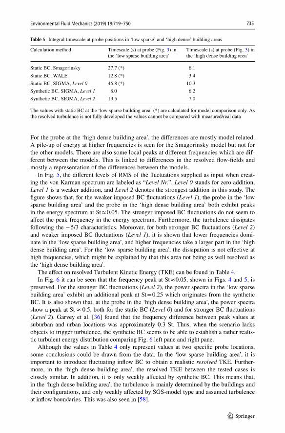
Table 5 Integral timescale at probe positions in ‘low sparse’ and ‘high dense’ building areas

The values with static BC at the ‘low sparse building area’ (*) are calculated for model comparison only. As the resolved turbulence is not fully developed the values cannot be compared with measured/real data

Calculation method Timescale (s) at probe (Fig. 3) in the ‘low sparse building area’

Timescale (s) at probe (Fig. 3) in the ‘high dense building area’

Static BC, Smagorinsky 27.7 (*) 6.1Static BC, WALE 12.8 (*) 3.4Static BC, SIGMA, Level 0 46.8 (*) 10.3Synthetic BC, SIGMA, Level 1 8.0 6.2Synthetic BC, SIGMA, Level 2 19.5 7.0


1 3

Measurements at Tower #1 and Tower #2, which are located outside of the computa-tional domain, are 10 min average values at 2.5 m, 5 m, and 10 m height. Tower positions and data can be found in Garvey et al. [36].

In Fig. 7 it can be seen that the autocorrelation for longitudinal velocity appears to be similar for both the Smagorinsky model and the SIGMA model. However, in the ‘low sparse building area’, the autocorrelation decreases to the level R(τ) ≈ 0 more rapidly for the Smagorinsky model, at τ ≈ 58 compared to at τ ≈ 85 for the SIGMA model, i.e., eddies calculated with the SIGMA model in the ‘low sparse building area’ might have a more “lasting memory” (lacking dissipation). For the ‘high dense building area’, the autocor-relation reaches zero more rapidly for the Smagorinsky model (τ ≈ 23) than it does for the SIGMA model (τ ≈ 47). However, it should be noted that these values pertain to only two separate probe points (Fig. 3).

Figure 8 shows the autocorrelation for longitudinal velocity for both the weaker syn-thetic BC (Level 1) and the stronger synthetic BC (Level 2). The integral time scale in the ‘low sparse building area’ is ≈ 8 s and ≈ 20 s for weaker synthetic BC (Level 1) and stronger synthetic BC (Level 2), respectively. The integral time scale in the ‘high dense building area’ is ≈ 6 s and ≈ 7 s for weaker synthetic BC (Level 1) and stronger synthetic BC (Level 2), respectively. Obviously, the integral time scale is not much affected by the level of synthetic BC in the ‘high dense building area’. In the ‘low sparse building area’ the synthetic BC contributes to increased turbulence and also a shorter time scale compared to the case with static BC. The autocorrelation plot for the ‘low sparse building area’ in the right pane of Fig. 8 indicates that an occurrence of a large eddy exists that increases the value.

The integral time scale at probe positions shown in Fig. 3 is tabulated in Table 5. The cases at the ‘low sparse building area’ with static BC are only included for comparison between models at that position. As the atmospheric boundary layer is not fully developed there, it cannot directly be compared with measurements.

At the ‘high dense building area’ the Smagorinsky and WALE models exhibit lower values of the integral time scale than the SIGMA model. This is probably an effect of the SGS-model itself. The Smagorinsky model creates sub-grid eddy viscosity in a simple wall flow, as it is in the ‘low sparse building area’, whereas the SIGMA model does not. Fur-thermore, in the ‘high dense building area’, the introduced level on synthetic BC does not seem to be very important, i.e., the introduced level of synthetic BC does not significantly change the integral time scale in the ‘high dense building area’, indicating that the time scale is mainly determined by the buildings in the area.

4.2 Calculated dispersion characteristics and comparisons between measurements and simulations

In this section comparison between field measurements and simulations are presented.First, the dispersion is illustrated by contour plots using a Smagorinsky, WALE and

SIGMA model, with and without synthetic BC.Thereafter, presented is a comparison of experimental and simulation point results and

experimental and simulation maximum values using the three SGS-models, with and with-out synthetic inflow BC.

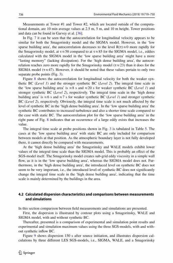
Figure 9 shows dispersion 150 s after source initiation, and illustrates dispersion cal-culations by three different LES SGS-models, i.e., SIGMA, WALE, and a Smagorinsky


1 3

Fig. 9 Dispersion illustrated by contour plots at ground level (2 m) overlaid by surface plots at 2.5 × 10−7 kg/m3 from the continuous source (IOP2), 150 s after initiation, calculated by using static bound-ary conditions and three different LES SGS-models, i.e., SIGMA, WALE, and a Smagorinsky model


1 3

model. It can be seen that, although some differences exist, the dispersion patterns are similar. In addition, the SIGMA model generates more updrafts, and as a result, higher concentration at higher heights than does the Smagorinsky model, which thus exhibits a higher concentration closer to the ground. The WALE model seems to have characteristics in between the SIGMA model and the Smagorinsky model.

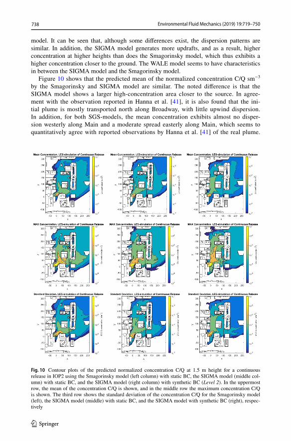
Figure 10 shows that the predicted mean of the normalized concentration C/Q sm−3 by the Smagorinsky and SIGMA model are similar. The noted difference is that the SIGMA model shows a larger high-concentration area closer to the source. In agree-ment with the observation reported in Hanna et al. [41], it is also found that the ini-tial plume is mostly transported north along Broadway, with little upwind dispersion. In addition, for both SGS-models, the mean concentration exhibits almost no disper-sion westerly along Main and a moderate spread easterly along Main, which seems to quantitatively agree with reported observations by Hanna et al. [41] of the real plume.

Fig. 10 Contour plots of the predicted normalized concentration C/Q at 1.5 m height for a continuous release in IOP2 using the Smagorinsky model (left column) with static BC, the SIGMA model (middle col-umn) with static BC, and the SIGMA model (right column) with synthetic BC (Level 2). In the uppermost row, the mean of the concentration C/Q is shown, and in the middle row the maximum concentration C/Q is shown. The third row shows the standard deviation of the concentration C/Q for the Smagorinsky model (left), the SIGMA model (middle) with static BC, and the SIGMA model with synthetic BC (right), respec-tively


1 3

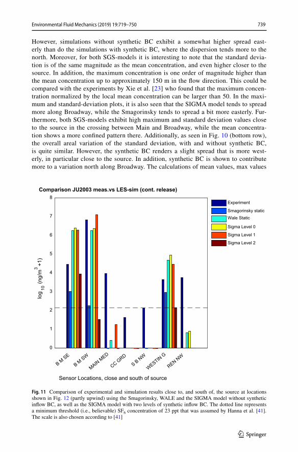
However, simulations without synthetic BC exhibit a somewhat higher spread east-erly than do the simulations with synthetic BC, where the dispersion tends more to the north. Moreover, for both SGS-models it is interesting to note that the standard devia-tion is of the same magnitude as the mean concentration, and even higher closer to the source. In addition, the maximum concentration is one order of magnitude higher than the mean concentration up to approximately 150 m in the flow direction. This could be compared with the experiments by Xie et al. [23] who found that the maximum concen-tration normalized by the local mean concentration can be larger than 50. In the maxi-mum and standard-deviation plots, it is also seen that the SIGMA model tends to spread more along Broadway, while the Smagorinsky tends to spread a bit more easterly. Fur-thermore, both SGS-models exhibit high maximum and standard deviation values close to the source in the crossing between Main and Broadway, while the mean concentra-tion shows a more confined pattern there. Additionally, as seen in Fig. 10 (bottom row), the overall areal variation of the standard deviation, with and without synthetic BC, is quite similar. However, the synthetic BC renders a slight spread that is more west-erly, in particular close to the source. In addition, synthetic BC is shown to contribute more to a variation north along Broadway. The calculations of mean values, max values

Comparison JU2003 meas.vs LES-sim (cont. release)

B M SE

B M SW

MAIN MED

CC GRD

S B NW

WESTIN G

REN NW

Sensor Locations, close and south of source

0

1

2

3

4

5

6

7

8

log

10(n

g/m

3+1

)

Experiment

Smagorinsky staticWale Static

Sigma Level 0

Sigma Level 1

Sigma Level 2

Fig. 11 Comparison of experimental and simulation results close to, and south of, the source at locations shown in Fig. 12 (partly upwind) using the Smagorinsky, WALE and the SIGMA model without synthetic inflow BC, as well as the SIGMA model with two levels of synthetic inflow BC. The dotted line represents a minimum threshold (i.e., believable) SF6 concentration of 23 ppt that was assumed by Hanna et al. [41]. The scale is also chosen according to [41]


1 3

and standard deviation are performed from 115 s after the release until 360 s after the release, i.e., during a period of 245 s.

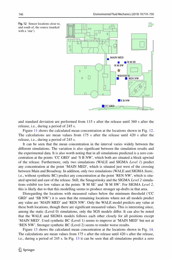
Figure 11 shows the calculated mean concentration at the locations shown in Fig. 12. The calculations are mean values from 175 s after the release until 420 s after the release, i.e., during a period of 245 s.

It can be seen that the mean concentration in the interval varies widely between the different simulations. The variation is also significant between the simulation results and the experimental data. It is also worth noting that in all simulations predicted is a zero con-centration at the points ‘CC GRD’ and ‘S B NW’, which both are situated a block upwind of the release. Furthermore, only two simulations (WALE and SIGMA Level 1) predict any concentration at the point ‘MAIN MED’, which is situated just west of the crossing between Main and Broadway. In addition, only two simulations (WALE and SIGMA Static, i.e., without synthetic BC) predict any concentration at the point ‘REN NW’, which is situ-ated upwind and east of the release. Still, the Smagorinsky and the SIGMA Level 2 simula-tions exhibit too low values at the points ‘B M SE’ and ‘B M SW’. For SIGMA Level 2, this is likely due to that this modelling seems to produce stronger up-drafts in that area.

Disregarding the locations with measured values below the minimum threshold (‘CC GRD’ and ‘SB NW’) it is seen that the remaining locations where not all models predict any value are ‘MAIN MED’ and ‘REN NW’. Only the WALE model predicts any value at these both locations, though there are significant measured values. This is interesting since, among the static (Level 0) simulations, only the SGS models differ. It can also be noted that the WALE and SIGMA models follows each other closely for all positions except ‘MAIN MED’. Used synthetic BC (Level 1) seems to improve at ‘MAIN MED’ but not at ‘REN NW’. Stronger synthetic BC (Level 2) seems to render worse results.

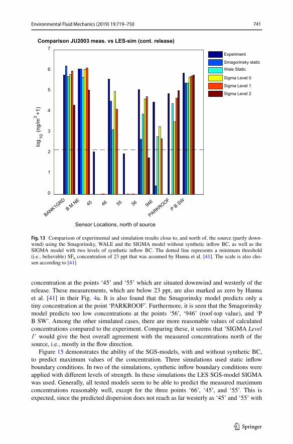
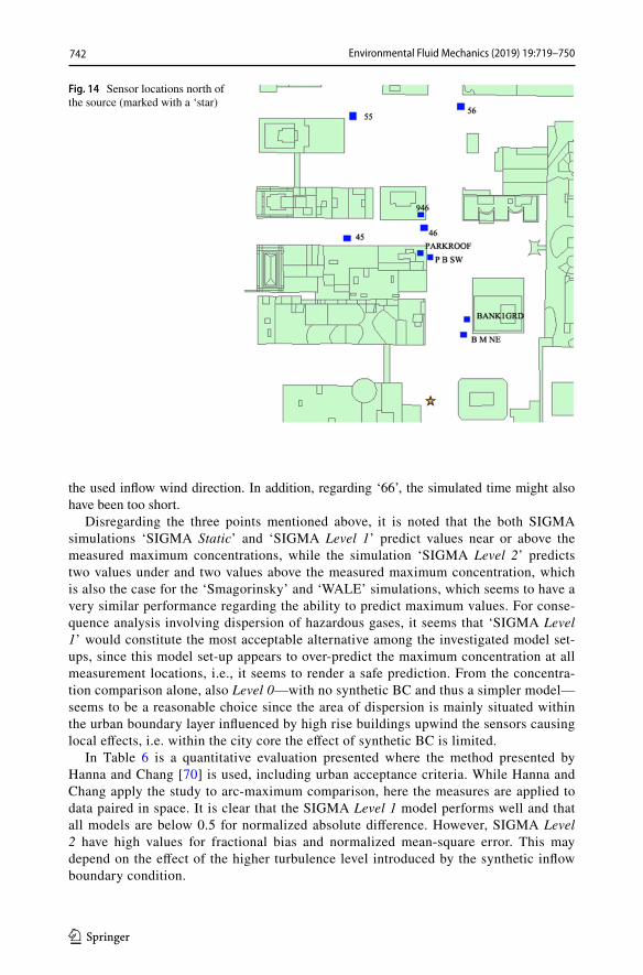
Figure 13 shows the calculated mean concentration at the locations shown in Fig. 14. The calculations are mean values from 175 s after the release until 420 s after the release, i.e., during a period of 245 s. In Fig. 13 it can be seen that all simulations predict a zero

Fig. 12 Sensor locations close to, and south of, the source (marked with a ‘star’)


1 3

concentration at the points ‘45’ and ‘55’ which are situated downwind and westerly of the release. These measurements, which are below 23 ppt, are also marked as zero by Hanna et al. [41] in their Fig. 4a. It is also found that the Smagorinsky model predicts only a tiny concentration at the point ‘PARKROOF’. Furthermore, it is seen that the Smagorinsky model predicts too low concentrations at the points ‘56’, ‘946’ (roof-top value), and ‘P B SW’. Among the other simulated cases, there are more reasonable values of calculated concentrations compared to the experiment. Comparing these, it seems that ‘SIGMA Level 1’ would give the best overall agreement with the measured concentrations north of the source, i.e., mostly in the flow direction.

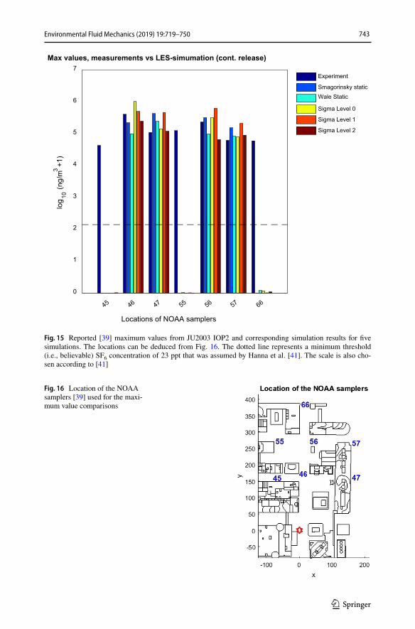
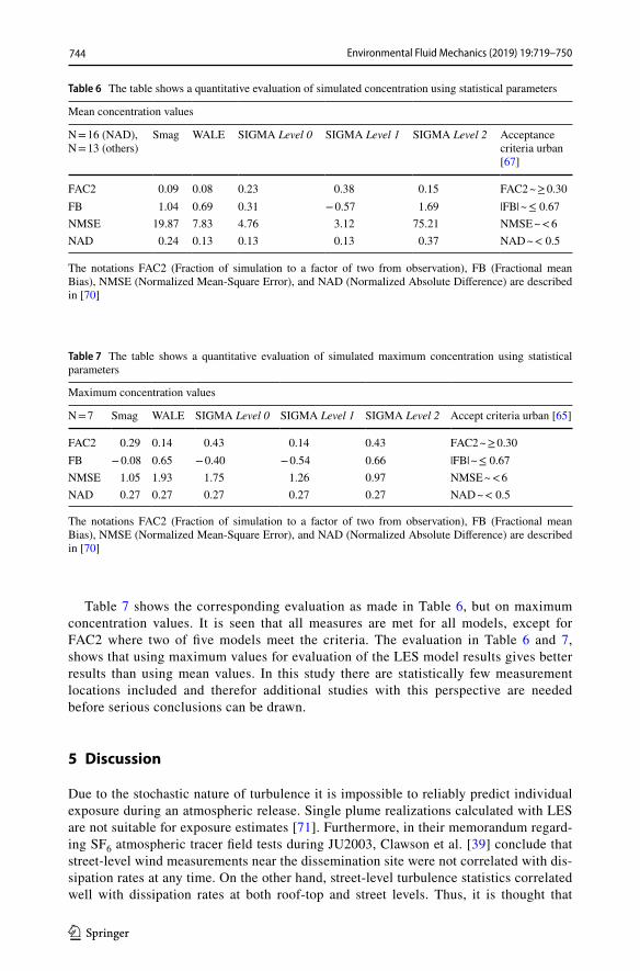
Figure 15 demonstrates the ability of the SGS-models, with and without synthetic BC, to predict maximum values of the concentration. Three simulations used static inflow boundary conditions. In two of the simulations, synthetic inflow boundary conditions were applied with different levels of strength. In these simulations the LES SGS-model SIGMA was used. Generally, all tested models seem to be able to predict the measured maximum concentrations reasonably well, except for the three points ‘66’, ‘45’, and ‘55’. This is expected, since the predicted dispersion does not reach as far westerly as ‘45’ and ‘55’ with

Comparison JU2003 meas. vs LES-sim (cont. release)

BANK1GRD

B M NE

45

46

55

56

946

PARKROOF

P B SW

Sensor Locations, north of source

0

1

2

3

4

5

6

7

log

10(n

g/m

3+1

)

Experiment


Sigma Level 0

Sigma Level 1

Sigma Level 2

Fig. 13 Comparison of experimental and simulation results close to, and north of, the source (partly down-wind) using the Smagorinsky, WALE and the SIGMA model without synthetic inflow BC, as well as the SIGMA model with two levels of synthetic inflow BC. The dotted line represents a minimum threshold (i.e., believable) SF6 concentration of 23 ppt that was assumed by Hanna et al. [41]. The scale is also cho-sen according to [41]


1 3

the used inflow wind direction. In addition, regarding ‘66’, the simulated time might also have been too short.

Disregarding the three points mentioned above, it is noted that the both SIGMA simulations ‘SIGMA Static’ and ‘SIGMA Level 1’ predict values near or above the measured maximum concentrations, while the simulation ‘SIGMA Level 2’ predicts two values under and two values above the measured maximum concentration, which is also the case for the ‘Smagorinsky’ and ‘WALE’ simulations, which seems to have a very similar performance regarding the ability to predict maximum values. For conse-quence analysis involving dispersion of hazardous gases, it seems that ‘SIGMA Level 1’ would constitute the most acceptable alternative among the investigated model set-ups, since this model set-up appears to over-predict the maximum concentration at all measurement locations, i.e., it seems to render a safe prediction. From the concentra-tion comparison alone, also Level 0—with no synthetic BC and thus a simpler model—seems to be a reasonable choice since the area of dispersion is mainly situated within the urban boundary layer influenced by high rise buildings upwind the sensors causing local effects, i.e. within the city core the effect of synthetic BC is limited.

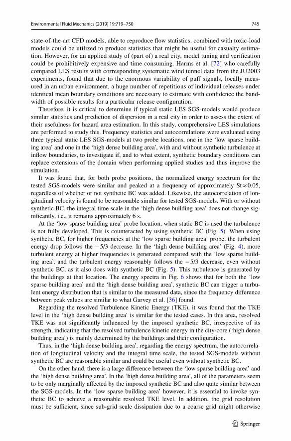
In Table 6 is a quantitative evaluation presented where the method presented by Hanna and Chang [70] is used, including urban acceptance criteria. While Hanna and Chang apply the study to arc-maximum comparison, here the measures are applied to data paired in space. It is clear that the SIGMA Level 1 model performs well and that all models are below 0.5 for normalized absolute difference. However, SIGMA Level 2 have high values for fractional bias and normalized mean-square error. This may depend on the effect of the higher turbulence level introduced by the synthetic inflow boundary condition.

Fig. 14 Sensor locations north of the source (marked with a ‘star)


1 3

Max values, measurements vs LES-simumation (cont. release)

45 46 47 55 56 57 66

Locations of NOAA samplers

0

1

2

3

4

5

6

7lo

g 10(n

g/m

3+1

)

Experiment


Sigma Level 0

Sigma Level 1

Sigma Level 2

Fig. 15 Reported [39] maximum values from JU2003 IOP2 and corresponding simulation results for five simulations. The locations can be deduced from Fig. 16. The dotted line represents a minimum threshold (i.e., believable) SF6 concentration of 23 ppt that was assumed by Hanna et al. [41]. The scale is also cho-sen according to [41]

Fig. 16 Location of the NOAA samplers [39] used for the maxi-mum value comparisons


1 3

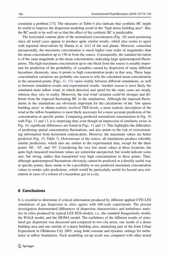
Table 7 shows the corresponding evaluation as made in Table 6, but on maximum concentration values. It is seen that all measures are met for all models, except for FAC2 where two of five models meet the criteria. The evaluation in Table 6 and 7, shows that using maximum values for evaluation of the LES model results gives better results than using mean values. In this study there are statistically few measurement locations included and therefor additional studies with this perspective are needed before serious conclusions can be drawn.

5 Discussion

Due to the stochastic nature of turbulence it is impossible to reliably predict individual exposure during an atmospheric release. Single plume realizations calculated with LES are not suitable for exposure estimates [71]. Furthermore, in their memorandum regard-ing SF6 atmospheric tracer field tests during JU2003, Clawson et al. [39] conclude that street-level wind measurements near the dissemination site were not correlated with dis-sipation rates at any time. On the other hand, street-level turbulence statistics correlated well with dissipation rates at both roof-top and street levels. Thus, it is thought that

Table 6 The table shows a quantitative evaluation of simulated concentration using statistical parameters

The notations FAC2 (Fraction of simulation to a factor of two from observation), FB (Fractional mean Bias), NMSE (Normalized Mean-Square Error), and NAD (Normalized Absolute Difference) are described in [70]

Mean concentration values

N = 16 (NAD), N = 13 (others)

Smag WALE SIGMA Level 0 SIGMA Level 1 SIGMA Level 2 Acceptance criteria urban [67]

FAC2 0.09 0.08 0.23 0.38 0.15 FAC2 ~ ≥ 0.30FB 1.04 0.69 0.31 − 0.57 1.69 |FB| ~ ≤ 0.67NMSE 19.87 7.83 4.76 3.12 75.21 NMSE ~ < 6NAD 0.24 0.13 0.13 0.13 0.37 NAD ~ < 0.5

Table 7 The table shows a quantitative evaluation of simulated maximum concentration using statistical parameters

The notations FAC2 (Fraction of simulation to a factor of two from observation), FB (Fractional mean Bias), NMSE (Normalized Mean-Square Error), and NAD (Normalized Absolute Difference) are described in [70]

Maximum concentration values

N = 7 Smag WALE SIGMA Level 0 SIGMA Level 1 SIGMA Level 2 Accept criteria urban [65]

FAC2 0.29 0.14 0.43 0.14 0.43 FAC2 ~ ≥ 0.30FB − 0.08 0.65 − 0.40 − 0.54 0.66 |FB| ~ ≤ 0.67NMSE 1.05 1.93 1.75 1.26 0.97 NMSE ~ < 6NAD 0.27 0.27 0.27 0.27 0.27 NAD ~ < 0.5


1 3

state-of-the-art CFD models, able to reproduce flow statistics, combined with toxic-load models could be utilized to produce statistics that might be useful for casualty estima-tion. However, for an applied study of (part of) a real city, model tuning and verification could be prohibitively expensive and time consuming. Harms et al. [72] who carefully compared LES results with corresponding systematic wind tunnel data from the JU2003 experiments, found that due to the enormous variability of puff signals, locally meas-ured in an urban environment, a huge number of repetitions of individual releases under identical mean boundary conditions are necessary to estimate with confidence the band-width of possible results for a particular release configuration.

Therefore, it is critical to determine if typical static LES SGS-models would produce similar statistics and prediction of dispersion in a real city in order to assess the extent of their usefulness for hazard area estimation. In this study, comprehensive LES simulations are performed to study this. Frequency statistics and autocorrelations were evaluated using three typical static LES SGS-models at two probe locations, one in the ‘low sparse build-ing area’ and one in the ‘high dense building area’, with and without synthetic turbulence at inflow boundaries, to investigate if, and to what extent, synthetic boundary conditions can replace extensions of the domain when performing applied studies and thus improve the simulation.

It was found that, for both probe positions, the normalized energy spectrum for the tested SGS-models were similar and peaked at a frequency of approximately St ≈ 0.05, regardless of whether or not synthetic BC was added. Likewise, the autocorrelation of lon-gitudinal velocity is found to be reasonable similar for tested SGS-models. With or without synthetic BC, the integral time scale in the ‘high dense building area’ does not change sig-nificantly, i.e., it remains approximately 6 s.

At the ‘low sparse building area’ probe location, when static BC is used the turbulence is not fully developed. This is counteracted by using synthetic BC (Fig. 5). When using synthetic BC, for higher frequencies at the ‘low sparse building area’ probe, the turbulent energy drop follows the − 5/3 decrease. In the ‘high dense building area’ (Fig. 4), more turbulent energy at higher frequencies is generated compared with the ‘low sparse build-ing area’, and the turbulent energy reasonably follows the − 5/3 decrease, even without synthetic BC, as it also does with synthetic BC (Fig. 5). This turbulence is generated by the buildings at that location. The energy spectra in Fig. 6 shows that for both the ‘low sparse building area’ and the ‘high dense building area’, synthetic BC can trigger a turbu-lent energy distribution that is similar to the measured data, since the frequency difference between peak values are similar to what Garvey et al. [36] found.

Regarding the resolved Turbulence Kinetic Energy (TKE), it was found that the TKE level in the ‘high dense building area’ is similar for the tested cases. In this area, resolved TKE was not significantly influenced by the imposed synthetic BC, irrespective of its strength, indicating that the resolved turbulence kinetic energy in the city-core (‘high dense building area’) is mainly determined by the buildings and their configuration.

Thus, in the ‘high dense building area’, regarding the energy spectrum, the autocorrela-tion of longitudinal velocity and the integral time scale, the tested SGS-models without synthetic BC are reasonable similar and could be useful even without synthetic BC.

On the other hand, there is a large difference between the ‘low sparse building area’ and the ‘high dense building area’. In the ‘high dense building area’, all of the parameters seem to be only marginally affected by the imposed synthetic BC and also quite similar between the SGS-models. In the ‘low sparse building area’ however, it is essential to invoke syn-thetic BC to achieve a reasonable resolved TKE level. In addition, the grid resolution must be sufficient, since sub-grid scale dissipation due to a coarse grid might otherwise


1 3

constitute a problem [73]. The measures in Table 6 also indicate that synthetic BC might be useful to improve the dispersion modeling result in the “high dense building area”. But, the BC needs to be well set so that the effect of the synthetic BC is predictable.

The horizontal contour plots of the normalized concentration (Fig. 10) seem promising since all tested cases appear to produce quite similar results, which also seems to agree with reported observations by Hanna et al. [41] of the real plume. However, somewhat unexpectedly, the maximum concentration is much higher (one order of magnitude) than the mean concentration up to 150 m from the source. Consequently, the standard deviation is of the same magnitude as the mean concentration, indicating large spatiotemporal fluctu-ations. The high maximum concentration up to one block from the source is notably impor-tant for prediction of the probability of casualties caused by dispersion of many different hazardous chemicals, since it points to high concentration peaks in that area. These large concentration variations are probably one reason to why the calculated mean concentration at the measured points (Figs. 11, 13) varies widely between different simulations, as well as between simulation results and experimental results. Another reason is most likely the simulated main inflow wind, in which direction and speed for the static cases are steady, whereas they vary in reality. Moreover, the real wind variation could be stronger and dif-ferent from the imposed fluctuating BC in the simulations. Although the imposed fluctu-ations in the simulations are obviously important for the calculations of the ‘low sparse building areas’ to obtain realistic resolved TKE-levels, a more realistic description of the wind at the inflow boundaries is most likely necessary for a more accurate prediction of the concentration at specific points. Comparing predicted normalized concentration in Fig. 10 with Figs. 11 and 13, it is surprising that, even though an impression of similarity exists in Fig. 10, significant differences are found in Figs. 11 and 13. This highlights the difficulties of predicting spatial concentration fluctuations, and also points to the risk of overestimat-ing information from horizontal contour-plots. However, the maximum values are better predicted (Fig. 15, Table 7). Downstream of the source, all simulations produce tolerably similar predictions, which also are similar to the experimental data, except for the three points ‘66’, ‘45’, and ‘55’. Considering the very low mean values at these locations, the quite high measured maximum values are somewhat unexpected, but would indicate some rare, but strong, eddies that transported very high concentrations to these points. Thus, although spatiotemporal fluctuations obviously cannot be predicted in a directly useful way at specific points, there seems to be a possibility to use predicted maximum concentration values to render safer predictions, which would be particularly useful for hazard area esti-mation in cases of a release of a hazardous gas in a city.

6 Conclusions

It is essential to determine if critical information produced by different applied CFD-LES simulations of gas dispersion in cities agrees with full-scale experiments. The present investigation demonstrated differences of dispersion characteristics and turbulence statis-tics in cities produced by typical LES SGS-models, i.e., the standard Smagorinsky model, the WALE model, and the SIGMA model. The usefulness of the different results of simu-lated gas dispersion was discussed and compared in two city-areas, one inside of a dense building area and one outside of a dense building area, mimicking part of the Joint Urban Experiment in Oklahoma City 2003, using both constant and dynamic settings for turbu-lence at inflow boundaries. Each modelling set-up result was compared with other tested


1 3

set-up results, and the ability of each of the set-ups to predict experimental results was examined.

It was found that:

1. In the ‘high dense building area’, the overall result is that the tested SGS-models without synthetic BC are reasonably similar regarding the energy spectrum, the autocorrelation of longitudinal velocity, and the integral time scale. Therefore, the SGS-models could be useful, even without synthetic BC, in the city center. This indicates that, in the ‘high dense building area’, the turbulence is mainly determined by the buildings and their configuration, and only weakly affected by SGS-model type and assumed turbulence at inflow boundaries.

2. While all studied parameters seem to be only marginally affected by the imposed syn-thetic BC in the ‘high dense building area’, and also quite similar between the SGS-models, there is a difference in the integral time scale and resolved TKE level between different modelling approaches in the ‘low sparse building area’. In this area, it is essen-tial to invoke synthetic BC to achieve a reasonable resolved TKE level and a mean wind profile that is linked to the up-wind atmospheric properties. Thus, it was found that it is necessary to apply synthetic BC whenever dispersion calculations in similar areas as the here tested ‘low sparse building areas’ are to be performed.

3. All tested SGS-models appear to produce quite similar horizontal contour plots of the normalized concentration, which also seems to agree with reported observations of the real plume.

4. The maximum concentration is much higher (one order of magnitude) than the mean concentration up to 150 m from the source, and the standard deviation is of the same magnitude as the mean concentration.

5. Downwind from the source, all tested modelling-approaches produce reasonably similar predictions of maximum values, which in turn are reasonably similar to the experi-mental data. Thus, the results indicate that it could be better to use the LES calculated maximum-concentration instead of the calculated mean-concentration when developing methods for hazard area estimation.

6. The applied performance measures show that all models comply with the normalized absolute difference criteria (NAD) and the SIGMA Level 1 SGS-model complies with all of the presented measures for the urban area.

Open Access This article is distributed under the terms of the Creative Commons Attribution 4.0 Interna-tional License (http://creat iveco mmons .org/licen ses/by/4.0/), which permits unrestricted use, distribution, and reproduction in any medium, provided you give appropriate credit to the original author(s) and the source, provide a link to the Creative Commons license, and indicate if changes were made.

References

1. Stathopoulos T (2002) The numerical wind tunnel for industrial aerodynamics: real or virtual in the new millennium? Wind Struct 5:193–208

2. Tolias IC, Koutsourakis N, Hertwig D, Efthimiou GG, Venetsanos AG, Bartzis JG (2018) Large Eddy Simulation study on structure of turbulent flow in a complex city. J Wind Eng Ind Aerodyn 177:101–116

http://creativecommons.org/licenses/by/4.0/


1 3

3. Tominaga Y, Stathopoulos T (2013) CFD simulation of near-field pollutant dispersion in the urban environment: a review of current modeling techniques. Atmos Environ 79:716–730

4. Lateb M, Meroney RN, Yataghene M, Fellouah H, Saleh F, Boufadel MC (2016) On the use of numer-ical modelling for near-field pollutant dispersion in urban environments: a review. Environ Pollut 271–283:0269–7491. https ://doi.org/10.1016/j.envpo l.2015.07.039

5. Park S-B, Baik J-J, Han B-S (2015) Large-eddy simulation of turbulent flow in a densely built-up urban area. Environ Fluid Mech 15:235–250. https ://doi.org/10.1007/s1065 2-013-9306-3

6. Xie ZT (2011) Modelling street-scale flow and dispersion in realistic winds—towards coupling with mesoscale meteorological models. Bound Layer Meteorol 141:53–75

7. Nakayama H, Nagai H (2009) Development of local-scale high-resolution atmospheric dispersion model using large-eddy simulation part 1: turbulent flow and plume dispersion over a flat terrain. J Nucl Sci Technol 46:1170–1177

8. Nakayama H, Nagai H (2011) Development of local-scale high-resolution atmospheric dispersion model using large-eddy simulation part 2: turbulent flow and plume dispersion around a cubical build-ing. J Nucl Sci Technol 48:374–383

9. Nakayama H, Takemi T, Nagai H (2012) Large-eddy simulation of urban boundary-layer flows by gen-erating turbulent inflows from mesoscale meteorological simulations. Atmos Sci Lett 13:180–186

10. Nakayama H, Jurcakova K, Nagai H (2013) Development of local-scale high-resolution atmospheric dispersion model using large-eddy simulation part 3: turbulent flow and plume dispersion in building arrays. J Nucl Sci Technol 50:503–519

11. Nakayama H, Leitl B, Harms F, Nagai H (2014) Development of local-scale high-resolution atmos-pheric dispersion model using large-eddy simulation part 4: turbulent flows and plume dispersion in an actual urban area. J Nucl Sci Technol 51:626–638

12. Nakayama H, Takemi T, Nagai H (2016) Development of LOcal-scale High-resolution atmospheric DIspersion Model using large-eddy simulation. Part 5: detailed simulation of turbulent flows and plume dispersion in an actual urban area under real meteorological condition. J Nucl Sci Technol 53:887–908

13. Li H, Cui G, Zhang Z (2018) A new scheme for the simulation of microscale flow and dispersion in urban areas by coupling large-eddy simulation with mesoscale models. Bound Layer Meteorol 167:145–170

14. Jiang G, Yoshie R (2018) Large-eddy simulation of flow and pollutant dispersion in a 3D urban street model located in an unstable boundary layer. Build Environ 142:47–57

15. Gousseau P, Blocken B, Stathopoulos T, van Heijst GJF (2011) CFD simulation of near-field pollutant dispersion on a high-resolution grid: a case study by LES and RANS for a building group in downtown Montreal. Atmos Environ 45:428–438. https ://doi.org/10.1016/j.atmos env.2010.09.065

16. Schatzmann M, Leitl B (2011) Issues with validation of urban flow and dispersion CFD models. J Wind Eng Ind Aerodyn 99:169–186

17. Liu XP, Niu JL, Kwok KCS (2011) Analysis of concentration fluctuations in gas dispersion around high-rise building for different incident wind directions. J Hazard Mater 192:1623–1632

18. Li X-X, Liu C-H, Leung D, Lam K (2006) Recent progress in CFD modelling of wind field and pol-lutant transport in street canyons. Atmos Environ 40:5640–5658. https ://doi.org/10.1016/j.atmos env.2006.04.055

19. Salim SM, Buccolieri R, Chan A, Di Sabatino S (2011) Numerical simulation of atmospheric pollutant dispersion in an urban street canyon: comparison between RANS and LES. J Wind Eng Ind Aerodyn 99:103–113. https ://doi.org/10.1016/j.jweia .2010.12.002

20. Mylne KR, Davidson MJ et al (1996) Concentration fluctuation measurements in tracer plumes using high and low frequency response detectors. Bound Layer Meteorol 79(3):225–242

21. Yee E, Chan R (1997) A simple model for the probability density function of concentration fluctua-tions in atmospheric plumes. Atmos Environ 31(7):991–1002

22. Lung T, Muller HJ et al (2002) Measurements and modelling of full-scale concentration fluctuations. Agratechnische Forschung 8(1):5–15

23. Xie Z, Hayden P, Voke PR, Robins AG (2011) Large-eddy simulation of dispersion: comparison between elevated and ground-level sources. J Turbul 5:1. https ://doi.org/10.1088/1468-5248/5/1/031

24. Bartzis JG, Sfetsos A et al (2008) On the individual exposure from airborne hazardous releases: the effect of atmospheric turbulence. J Hazard Mater 150(1):76–82

25. Efthimiou GC, Bartzis JG, Andronopoulos S, Sfetsos A (2011) Air dispersion modelling for individual exposure studies. Int J Environ Pollut 47(1–4):302–316

26. Efthimiou GC, Bartzis JG, Koutsourakis N (2011) Modelling concentration fluctuations and individual exposure in complex urban environments. J Wind Eng Ind Aerodyn 99(4):349–356

https://doi.org/10.1016/j.envpol.2015.07.039

https://doi.org/10.1007/s10652-013-9306-3

https://doi.org/10.1016/j.atmosenv.2010.09.065



https://doi.org/10.1016/j.jweia.2010.12.002

https://doi.org/10.1088/1468-5248/5/1/031


1 3

27. Efthimiou GC, Bartzis JG (2011) Atmospheric dispersion and individual exposure of hazardous mate-rials. J Hazard Mater 188:375–383

28. Biltoft CA (2001) Customer report for mock urban setting test, technical report DPG document No. WDTCFR-01-121. West Desert Test Center, U.S. Army Dugway Proving Ground, Dugway, Utah, p 55

29. Yee E, Biltoft C (2004) Concentration fluctuation measurements in a plume dispersing through a regu-lar array of obstacles. Bound Layer Meteorol 111(3):363–415

30. Bartzis JG, Efthimiou GC, Andronopoulos S (2015) Modelling short term individual exposure from airborne hazardous releases in urban environments. J Hazard Mater 300:182–188

31. Efthimiou GC, Andronopoulos S, Bartzis JG (2017) Evaluation of probability distributions for concen-tration fluctuations in a building array. Physica A 484:104–116

32. Bogen KT, Gouveia FJ (2008) Impact of spatiotemporal fluctuations in airborne chemical concentra-tion on toxic hazard assessment. J Hazard Mater 152(1):228–240

33. Smagorinsky J (1963) General circulation experiments with the primitive equations. Mon Weather Rev 91:99–164

34. Nicoud F, Ducros F (1999) Sub-grid-scale stress modelling based on the square of the velocity gradi-ent tensor flow. Turbul Combust 62:183–200

35. Nicoud F, Baya HT, Cabrit O, Bose S, Lee J (2011) Using singular values to build a sub-grid-scale model for large eddy simulations. Phys Fluids 23:085106

36. Garvey D, Bustillos M, Chang S, Cionco R, Creegan E, Elliott D, Huynh G, Klipp C, Ligon D, Measure E, Quintis D, Torres M, Vaucher, G, Vidal E, Wang Y, Williamson C, Yarbrough J, Yee Y (2009) U.S. army research laboratory meteorological measurements for joint urban 2003. Army Research Laboratory, Adelpi, ARL-TR-4989

37. Nelson MA, Pardyjak ER, Klein P (2011) Momentum and turbulent kinetic energy budgets within the Park Avenue Street Canyon during the joint urban 2003 field campaign. Bound Layer Meteorol 140:143–162. https ://doi.org/10.1007/s1054 6-011-9610-8

38. Allwine KJ, Flaherty JE (2006) Joint urban 2003: study overview and instrument locations. Pacific Northwest National Laboratory, PNNL-15967

39. Clawson KL, Carter RG, Lacroix DI, Biltoft CA, Hukari NE, Johnson RC, Rich JD, Beard SA, Strong T (2005) JOINT URBAN 2003 (JU2003) SF6 atmospheric tracer field tests. Air Resource Laboratory, Silver Spring, Maryland, NOAA technical memorandum OAR ARL-254

40. Leach MJ (2005) Final report for the joint urban 2003 atmospheric dispersion study in Oklahoma City: Lawrence Livermore National Laboratory Participation, UCRL-TR-216437

41. Hanna S, White J, Trolier J, Vernot R, Brown M, Gowardhan A, Kaplan H, Alexander Y, Mous-safir J, Wang Y, Williamson C, Hannan J, Hendrick E (2011) Comparisons of JU2003 observations with four diagnostic urban wind flow and Lagrangian particle dispersion models. Atmos Environ 45:4073–4081

42. Lundquist JK, Chan ST (2005) Analysis of joint URBAN 2003 wind and turbulence profiles and comparison with FEM3MP simulations. In: 9th annual conference on atmospheric transport and dispersion modeling, Fairfax, VA, United States, UCRL-PROC-213530

43. Cham (2014) CHAM TR/326, PHOENICS-VR reference guide. Wimbledon, London 44. Xie ZT, Castro IP (2009) Large-eddy simulation for flow and dispersion in urban streets. Atmos

Environ 43(13):2174–2185 45. Celik IB, Cehreli ZN, Yavuz I (2005) Index of resolution quality for large eddy simulations. J Flu-

ids Eng T ASME 127:949–958. https ://doi.org/10.1115/1.19902 01 46. Celik I, Klein M, Janicka J (2009) Assessment measures for engineering LES applications. J Fluids

Eng T ASME 131:1–10 47. Tominaga Y, Mochida A, Yoshie R, Kataoka H, Nozu T, Yoshikawa M, Shirasawa T (2008) AIJ

guidelines for practical applications of CFD to pedestrian wind environment around buildings. J Wind Eng Ind Aerodyn 96:1749–1761. https ://doi.org/10.1016/j.jweia .2008.02.058

48. Franke J, Hellsten A, Schlünzen KH, Carissimo B (2007) Best practice guideline for the CFD simu-lation of flows in the urban environment. COST Office, Brussels

49. Patankar SV, Spalding DB (1972) A calculation procedure for heat, mass and momentum transfer in three-dimensional parabolic flows. Int J Heat Mass Transf 15(10):1787–1806

50. Van Leer B (1974) Towards the ultimate conservative difference scheme. II. Monotonicity and con-servation combined in a second-order scheme. J Comput Phys 14(4):361–370

51. Harten A (1984) On a class of high resolution total-variation-stable finite-difference schemes. SIAM J Numer Anal 21(1):1–23

52. Ochoa JS (2004) Large eddy simulation of a flow past a square cylinder. In: Fueyo N (ed) 17th, efficiency, costs, optimization, simulation and environmental impact of energy on process systems; ECOS, pp 37–50

https://doi.org/10.1007/s10546-011-9610-8

https://doi.org/10.1115/1.1990201

https://doi.org/10.1016/j.jweia.2008.02.058


1 3

53. Hertwig D (2013) On aspects of large-eddy simulation validation for near-surface atmospheric flows. University of Hamburg, Hamburg

54. Berselli LC, IIiescu T, Layton WJ (2006) Mathematics of large eddy simulation of turbulent flows. Springer, Berlin. ISBN-10 3-540-26316-0

55. Kolmogorov A (1991) The local structure of turbulence in incompressible viscous fluid for very large reynolds numbers, London. Proc R Soc Lond Ser A Math Phys Sci 434:9–13

56. Van Driest YEAR (1956) On turbulent flow near a wall (AIAA): AIAA ARC. J Aeronaut Sci (Insti-tute of the Aeronautical Sciences) 23(11):1007–1011

57. Jarrin N, Benhamadouche S, Laurence D, Prosser R (2006) A synthetic-eddy method for generating inflow conditions for large-eddy simulations. Int J Heat Fluid Flow 27(4):585–593

58. Aristodemou E, Boganegra LM, Mottet L, Pavlidis D, Constantinou A, Pain C, Robins A, ApSimon H (2018) How tall buildings affect turbulent air flows and dispersion of pollution within a neigh-bourhood. Environ Pollut 233:782–796

59. Hertwig D, Soulhac L, Fuka V, Auerswald T, Carpentieri M, Hayden P, Robins A, Xie ZT, Coceal O (2018) Evaluation of fast atmospheric dispersion models in a regular street network. Environ Fluid Mech 18:1007–1044

60. Billson M (2004) Computational techniques for turbulence generated noise. Ph.D. thesis, Depart-ment of Thermo and Fluid Dynamics, Chalmers University of Technology, Göteborg, Sweden

61. Billson M, Eriksson LE, Davidson L (2003) Jet noise prediction using stochastic turbulence modeling. In: AIAA paper 2003-3282, 9th AIAA/CEAS aeroacoustics conference

62. Davidson L, Billson M (2006) Hybrid LES/RANS using synthesized turbulence for forcing at the interface. Int J Heat Fluid Flow 27(6):1028–1042

63. Davidson L (2005) Hybrid LES-RANS: inlet boundary conditions. In: Skallerud B, Andersson HI (eds) 3rd national conference on computational mechanics—MekIT’05 (invited paper), Trondheim, Norway, pp 7–22

64. Davidson L (2007) Hybrid LES-RANS: inlet boundary conditions for flows with recirculation. In: Sec-ond symposium on hybrid RANS-LES methods, Corfu island, Greece

65. Davidson L (2007) Using isotropic synthetic fluctuations as inlet boundary conditions for unsteady simulations. Adv Appl Fluid Mech 1(1):1–35

66. Hanna SR (1980) Lagrangian and Eulerian time-scale relations in the daytime boundary layer. J Appl Meteorol 20:242–249

67. Stull RB (1988) An introduction to boundary layer meteorology. Kluwer Academic Publishers, Dordrecht

68. Patankar SV (1980) Numerical heat transfer and fluid flow. Hemispere Publishing Corporation, New York

69. Pope SB (2000) Turbulent flows. Cambridge University Press, Cambridge 70. Hanna S, Chang J (2012) Acceptance criteria for urban dispersion model evaluation. Meteorol Atmos

Phys 116:133–146 71. Burman J, Jonsson L (2015) Issues when linking computational fluid dynamics for urban mod-

eling to toxic load models: the need for further research. Atmos Environ 104:112–124. https ://doi.org/10.1016/j.atmos env.2014.12.068

72. Harms F, Leitl B, Schatzmann M, Patnik G (2011) Validating LES-based flow and dispersion models. J Wind Eng Ind Aerodyn 99:289–295

73. Davidson L (2009) Large eddy simulations: how to evaluate resolution. Int J Heat Fluid Flow 30(5):1016–1025

Publisher’s Note Springer Nature remains neutral with regard to jurisdictional claims in published maps and institutional affiliations.



FULLTEXT01.pdf - uu .diva

Documents