Institutionen f¨ or Datavetenskap Department of Computer and Information Science Master’s thesis Automated Reasoning Support for Invasive Interactive Parallelization by Kianosh Moshir Moghaddam LIU-IDA/LITH-EX-A–12/050–SE 2012-10-18 ✬ ✫ ✩ ✪ Link¨ opings universitet SE-581 83 Link¨ oping, Sweden Link¨ opings universitet 581 83 Link¨ oping

Welcome message from author
This document is posted to help you gain knowledge. Please leave a comment to let me know what you think about it! Share it to your friends and learn new things together.
Transcript
Institutionen for DatavetenskapDepartment of Computer and Information Science
Master’s thesis
Automated Reasoning Support forInvasive Interactive Parallelization
by
Kianosh Moshir Moghaddam
LIU-IDA/LITH-EX-A–12/050–SE
2012-10-18'
&
$
%Linkopings universitet
SE-581 83 Linkoping, Sweden
Linkopings universitet
581 83 Linkoping

Institutionen for DatavetenskapDepartment of Computer and Information Science
Master’s thesis
Automated Reasoning Support forInvasive Interactive Parallelization
by
Kianosh Moshir Moghaddam
LIU-IDA/LITH-EX-A–12/050–SE
2012-10-18
Supervisor: Christoph Kessler
Examiner: Christoph Kessler
Linköping University Electronic Press
Upphovsrätt
Detta dokument hålls tillgängligt på Internet – eller dess framtida ersättare –från
publiceringsdatum under förutsättning att inga extraordinära omständigheter
uppstår.
Tillgång till dokumentet innebär tillstånd för var och en att läsa, ladda ner,
skriva ut enstaka kopior för enskilt bruk och att använda det oförändrat för icke-
kommersiell forskning och för undervisning. Överföring av upphovsrätten vid
en senare tidpunkt kan inte upphäva detta tillstånd. All annan användning av
dokumentet kräver upphovsmannens medgivande. För att garantera äktheten,
säkerheten och tillgängligheten finns lösningar av teknisk och administrativ art.
Upphovsmannens ideella rätt innefattar rätt att bli nämnd som upphovsman i
den omfattning som god sed kräver vid användning av dokumentet på ovan be-
skrivna sätt samt skydd mot att dokumentet ändras eller presenteras i sådan form
eller i sådant sammanhang som är kränkande för upphovsmannens litterära eller
konstnärliga anseende eller egenart.
För ytterligare information om Linköping University Electronic Press se för-
lagets hemsida http://www.ep.liu.se/
Copyright
The publishers will keep this document online on the Internet – or its possible
replacement –from the date of publication barring exceptional circumstances.
The online availability of the document implies permanent permission for
anyone to read, to download, or to print out single copies for his/hers own use
and to use it unchanged for non-commercial research and educational purpose.
Subsequent transfers of copyright cannot revoke this permission. All other uses
of the document are conditional upon the consent of the copyright owner. The
publisher has taken technical and administrative measures to assure authenticity,
security and accessibility.
According to intellectual property law the author has the right to be
mentioned when his/her work is accessed as described above and to be protected
against infringement.
For additional information about the Linköping University Electronic Press
and its procedures for publication and for assurance of document integrity,
please refer to its www home page: http://www.ep.liu.se/.
© Kianosh Moshir Moghaddam
Abstract
To parallelize a sequential source code, a parallelization strategy must bedefined that transforms the sequential source code into an equivalent paral-lel version. Since parallelizing compilers can sometimes transform sequentialloops and other well-structured codes into parallel ones automatically, weare interested in finding a solution to parallelize semi-automatically codesthat compilers are not able to parallelize automatically, mostly because ofweakness of classical data and control dependence analysis, in order to sim-plify the process of transforming the codes for programmers.
Invasive Interactive Parallelization (IIP) hypothesizes that by using anintelligent system that guides the user through an interactive process one canboost parallelization in the above direction. The intelligent system’s guid-ance relies on a classical code analysis and pre-defined parallelizing transfor-mation sequences. To support its main hypothesis, IIP suggests to encodeparallelizing transformation sequences in terms of IIP parallelization strate-gies that dictate default ways to parallelize various code patterns by usingfacts which have been obtained both from classical source code analysis anddirectly from the user.
In this project, we investigate how automated reasoning can supportthe IIP method in order to parallelize a sequential code with an accept-able performance but faster than manual parallelization. We have looked attwo special problem areas: Divide and conquer algorithms and loops in thesource codes. Our focus is on parallelizing four sequential legacy C programssuch as: Quick sort, Merge sort, Jacobi method and Matrix multipliationand summation for both OpenMP and MPI environment by developing aninteractive parallelizing assistance tool that provides users with the assis-tance needed for parallelizing a sequential source code.
iii

iv

Dedicated to my parents with love and gratitude.
v
Acknowledgements
First of all, I would like to offer my sincerest gratitude to my examinerProfessor Christoph Kessler who always had time for me and my questions.His advice and comments to my technical questions, implementation andeven my report by proof-reading were very precise and useful. Thank youDr.Kessler for your invaluable guidance and support during my thesis work.
I’m also very grateful to Professor Anders Haraldsson who was the firstperson that made me familiar to the world of Lisp programming. Thank youDr.Haraldsson, I will never forget your kindness and our fruitful discussions.
I would like to thank Mikhail Chalabine, who was my supervisor in thefirst phase of my thesis and made me familiar with the concept of IIP. Hiscomments were very instructive. It was a pity that I couldn’t have hiscollaboration for the rest of this project.
Thanks also to PELAB group at IDA department of Linkoping Univer-sity that made this project possible for me.
I would like to express my gratitude to the National SupercomputerCenter in Linkoping Sweden (NSC) for giving me access permission to theirservers.
Last, but certainly not least, I would like to thank my family members.Without your encouragement and support throughout my life none of thiswould have happened.
vi
Contents
1 Introduction 21.1 Motivation . . . . . . . . . . . . . . . . . . . . . . . . . . . . 21.2 Overview and Contributions . . . . . . . . . . . . . . . . . . 31.3 Research questions . . . . . . . . . . . . . . . . . . . . . . . . 51.4 Scope of this Thesis . . . . . . . . . . . . . . . . . . . . . . . 5
1.4.1 Limitations . . . . . . . . . . . . . . . . . . . . . . . . 51.4.2 Thesis Assumptions . . . . . . . . . . . . . . . . . . . 6
1.5 Evaluation Methods . . . . . . . . . . . . . . . . . . . . . . . 61.6 Outline . . . . . . . . . . . . . . . . . . . . . . . . . . . . . . 6
2 Foundations and Background 82.1 Compiler Structure . . . . . . . . . . . . . . . . . . . . . . . . 82.2 Dependence analysis . . . . . . . . . . . . . . . . . . . . . . . 9
2.2.1 GCD Test . . . . . . . . . . . . . . . . . . . . . . . . . 132.2.2 Banerjee Test . . . . . . . . . . . . . . . . . . . . . . . 14
2.3 Artificial intelligence . . . . . . . . . . . . . . . . . . . . . . . 142.3.1 Knowledge representation and Reasoning . . . . . . . 142.3.2 Inference . . . . . . . . . . . . . . . . . . . . . . . . . 152.3.3 Planning, deductive reasoning and problem solving . . 152.3.4 Machine Learning . . . . . . . . . . . . . . . . . . . . 15
2.3.4.1 Classification and statistical learning methods 162.3.4.2 Decision Tree . . . . . . . . . . . . . . . . . . 16
2.3.5 Logic programming and AI languages . . . . . . . . . 162.4 Parallelization mechanisms . . . . . . . . . . . . . . . . . . . 172.5 Parallel Computers . . . . . . . . . . . . . . . . . . . . . . . . 182.6 Parallel Programming Models . . . . . . . . . . . . . . . . . . 202.7 Performance Metrics . . . . . . . . . . . . . . . . . . . . . . . 212.8 Code Parallelization . . . . . . . . . . . . . . . . . . . . . . . 21
2.8.1 Loop Parallelization . . . . . . . . . . . . . . . . . . . 232.8.1.1 OpenMP . . . . . . . . . . . . . . . . . . . . 252.8.1.2 MPI . . . . . . . . . . . . . . . . . . . . . . . 302.8.1.3 Different methods for loop parallelization in
MPI . . . . . . . . . . . . . . . . . . . . . . . 302.8.2 Function Parallelization . . . . . . . . . . . . . . . . . 35
vii
viii CONTENTS
2.9 Divide and Conquer Algorithms . . . . . . . . . . . . . . . . . 352.9.1 Parallelization of Divide and Conquer Algorithms . . . 36
2.10 Sorting algorithms . . . . . . . . . . . . . . . . . . . . . . . . 372.10.1 Sequential Quick sort . . . . . . . . . . . . . . . . . . 372.10.2 Parallel Quick sort . . . . . . . . . . . . . . . . . . . . 39
2.11 Jacobi method . . . . . . . . . . . . . . . . . . . . . . . . . . 402.12 Software composition techniques . . . . . . . . . . . . . . . . 41
2.12.1 Aspect-Oriented Programming (AOP) . . . . . . . . . 422.12.2 Template Metaprogramming . . . . . . . . . . . . . . 432.12.3 Invasive Software Composition . . . . . . . . . . . . . 43
2.13 Invasive Interactive Parallelization . . . . . . . . . . . . . . . 43
3 System Architecture 453.1 Code Analysis . . . . . . . . . . . . . . . . . . . . . . . . . . . 453.2 Dependence Analysis . . . . . . . . . . . . . . . . . . . . . . . 473.3 Strategy Selection . . . . . . . . . . . . . . . . . . . . . . . . 483.4 Weaving . . . . . . . . . . . . . . . . . . . . . . . . . . . . . . 49
4 Implementation 514.1 System Overview . . . . . . . . . . . . . . . . . . . . . . . . . 514.2 Implemented Predicates and Functions . . . . . . . . . . . . . 54
4.2.1 Code Analysis . . . . . . . . . . . . . . . . . . . . . . 544.2.2 Dependency Analysis . . . . . . . . . . . . . . . . . . . 584.2.3 Strategy Selection and Weaving . . . . . . . . . . . . . 62
4.2.3.1 OpenMP . . . . . . . . . . . . . . . . . . . . 624.2.3.2 MPI . . . . . . . . . . . . . . . . . . . . . . . 64
5 Evaluation 785.1 System Parallelization of Test Programs . . . . . . . . . . . . 78
5.1.1 Quick sort . . . . . . . . . . . . . . . . . . . . . . . . . 785.1.2 Jacobi method . . . . . . . . . . . . . . . . . . . . . . 855.1.3 Other test programs . . . . . . . . . . . . . . . . . . . 87
5.2 Correctness of the parallelized test programs . . . . . . . . . 915.3 Performance of the parallelized test programs . . . . . . . . . 92
5.3.1 Quick sort . . . . . . . . . . . . . . . . . . . . . . . . . 925.3.2 Jacobi method . . . . . . . . . . . . . . . . . . . . . . 985.3.3 Other test programs . . . . . . . . . . . . . . . . . . . 101
5.4 Usefulness . . . . . . . . . . . . . . . . . . . . . . . . . . . . . 106
6 Related Work 1076.1 Dependency analysis in parallelizing sequential code . . . . . 1076.2 Parallelizing by using Skeletons . . . . . . . . . . . . . . . . . 1086.3 Automatically parallelizing sequential code . . . . . . . . . . 1086.4 Semi-automatically parallelizing sequential code . . . . . . . . 1096.5 Summary . . . . . . . . . . . . . . . . . . . . . . . . . . . . . 110
CONTENTS ix
7 Conclusion 111
8 Future work 1138.1 Header files . . . . . . . . . . . . . . . . . . . . . . . . . . . . 1138.2 Graphical user interface . . . . . . . . . . . . . . . . . . . . . 1138.3 Extension of loop parallelization . . . . . . . . . . . . . . . . 1148.4 Add profiler’s support . . . . . . . . . . . . . . . . . . . . . . 1148.5 Pointer analysis . . . . . . . . . . . . . . . . . . . . . . . . . . 1148.6 Extension for D&C algorithms parallelization . . . . . . . . . 114
Appendix A Divide and Conquer Templates 115A.1 MPI . . . . . . . . . . . . . . . . . . . . . . . . . . . . . . . . 115A.2 OpenMP . . . . . . . . . . . . . . . . . . . . . . . . . . . . . . 117
Appendix B Source Codes 118B.1 Quick sort . . . . . . . . . . . . . . . . . . . . . . . . . . . . . 118
B.1.1 Sequential Code(code example1) . . . . . . . . . . . . 118B.1.2 Sequential Code with better pivot selection(code ex-
ample2) . . . . . . . . . . . . . . . . . . . . . . . . . . 120B.1.3 System-generated MPI Parallel code . . . . . . . . . . 122B.1.4 System-generated OpenMP Parallel code . . . . . . . 126
B.2 Merge sort . . . . . . . . . . . . . . . . . . . . . . . . . . . . . 128B.2.1 Sequential Code . . . . . . . . . . . . . . . . . . . . . 128B.2.2 System-generated MPI Parallel code . . . . . . . . . . 130B.2.3 System-generated OpenMP Parallel code . . . . . . . 134
B.3 Jacobi method . . . . . . . . . . . . . . . . . . . . . . . . . . 137B.3.1 Sequential Code . . . . . . . . . . . . . . . . . . . . . 137B.3.2 Manual MPI Parallel Code . . . . . . . . . . . . . . . 139B.3.3 System-generated MPI Parallel code . . . . . . . . . . 142B.3.4 Manual OpenMP Parallel Code . . . . . . . . . . . . . 146B.3.5 System-generated OpenMP Parallel code . . . . . . . 148
B.4 Matrix multiplication and summation . . . . . . . . . . . . . 150B.4.1 Sequential Code . . . . . . . . . . . . . . . . . . . . . 150B.4.2 System-generated MPI Parallel code . . . . . . . . . . 152B.4.3 System-generated OpenMP Parallel code . . . . . . . 159
x CONTENTS
List of Figures
1.1 Overview of our system . . . . . . . . . . . . . . . . . . . . . 3
2.1 Compiler Front end and Back end concept. . . . . . . . . . . 92.2 Dominance Relations . . . . . . . . . . . . . . . . . . . . . . . 102.3 Data Dependence Graph . . . . . . . . . . . . . . . . . . . . . 112.4 Distributed Memory Architecture. . . . . . . . . . . . . . . . 192.5 Shared Memory Architecture, here with a shared bus as in-
terconnection network. . . . . . . . . . . . . . . . . . . . . . . 192.6 Fork/Join Concept . . . . . . . . . . . . . . . . . . . . . . . . 202.7 Foster’s PCAM methodology for parallel programs . . . . . . 222.8 Index Set Splitting . . . . . . . . . . . . . . . . . . . . . . . . 242.9 Parallel nested loops . . . . . . . . . . . . . . . . . . . . . . . 262.10 Distributing loop iterations . . . . . . . . . . . . . . . . . . . 312.11 Quick sort data division . . . . . . . . . . . . . . . . . . . . . 382.12 Jacobi Method . . . . . . . . . . . . . . . . . . . . . . . . . . 41
3.1 System Architecture Steps . . . . . . . . . . . . . . . . . . . . 453.2 Example of code analysis decision tree . . . . . . . . . . . . . 463.3 Code Analyzer Structure . . . . . . . . . . . . . . . . . . . . . 483.4 Strategy Selection . . . . . . . . . . . . . . . . . . . . . . . . 493.5 Weaving . . . . . . . . . . . . . . . . . . . . . . . . . . . . . . 50
4.1 Implementation work flow . . . . . . . . . . . . . . . . . . . . 524.2 The system asks for a sequential code and reads it . . . . . . 524.3 The system will save the result . . . . . . . . . . . . . . . . . 534.4 Loop dependency analysis . . . . . . . . . . . . . . . . . . . . 604.5 Function parallelization analysis . . . . . . . . . . . . . . . . 63
5.1 Data division between processors . . . . . . . . . . . . . . . . 815.2 Processors division . . . . . . . . . . . . . . . . . . . . . . . . 815.3 Quick sort MPI parallelization . . . . . . . . . . . . . . . . . 825.4 Quick sort OpenMP parallelization . . . . . . . . . . . . . . . 845.5 Processors communications . . . . . . . . . . . . . . . . . . . 855.6 Jacobi method MPI parallelization . . . . . . . . . . . . . . . 88
xi
xii LIST OF FIGURES
5.7 Jacobi method OpenMP parallelization . . . . . . . . . . . . 895.8 Merge sort . . . . . . . . . . . . . . . . . . . . . . . . . . . . . 905.9 Matrix multiplication and summation . . . . . . . . . . . . . 905.10 System-parallelized MPI Quick sort (code example1) speedup
for the problem size 107 . . . . . . . . . . . . . . . . . . . . . 945.11 System-parallelized OpenMP Quick sort (code example1) speedup
for the problem size 107 . . . . . . . . . . . . . . . . . . . . . 955.12 System-parallelized MPI Quick sort (code example2) speedup
for the problem size 107 . . . . . . . . . . . . . . . . . . . . . 965.13 System-parallelized OpenMP Quick sort (code example2) speedup
for the problem size 107 . . . . . . . . . . . . . . . . . . . . . 975.14 System-parallelized MPI Jacobi method speedup for the prob-
lem size 10000 ∗ 1000 . . . . . . . . . . . . . . . . . . . . . . 995.15 System-parallelized OpenMP Jacobi method speedup for the
problem size 10000 ∗ 1000 . . . . . . . . . . . . . . . . . . . . 1015.16 System-parallelized MPI Merge sort speedup for the problem
size 107 . . . . . . . . . . . . . . . . . . . . . . . . . . . . . . 1035.17 System-parallelized OpenMP Merge sort speedup for the prob-
lem size 107 . . . . . . . . . . . . . . . . . . . . . . . . . . . . 1035.18 System-parallelized MPI Matrix multiplication and summa-
tion speedup for the problem size 10000 ∗ 1000× 1000 ∗ 10000. . . . . . . . . . . . . . . . . . . . . . . . . . . . . . . . . . . 105
5.19 System-parallelized OpenMP Matrix multiplication and sum-mation speedup for the problem size 10000∗1000×1000∗10000 106
List of Tables
4.1 Expression analysis . . . . . . . . . . . . . . . . . . . . . . . 554.2 For-loop analysis . . . . . . . . . . . . . . . . . . . . . . . . . 564.3 Function definition analysis . . . . . . . . . . . . . . . . . . . 574.4 Function call analysis . . . . . . . . . . . . . . . . . . . . . . 57
5.1 Sequential Quick sort (code example1) execution time (in sec-onds) . . . . . . . . . . . . . . . . . . . . . . . . . . . . . . . . 93
5.2 System-parallelized MPI Quick sort (code example1) execu-tion time (in seconds) . . . . . . . . . . . . . . . . . . . . . . 93
5.3 System-parallelized OpenMP Quick sort (code example1) ex-ecution time (in seconds) . . . . . . . . . . . . . . . . . . . . 94
5.4 Sequential Quick sort (code example2) execution time (in sec-onds) . . . . . . . . . . . . . . . . . . . . . . . . . . . . . . . . 95
5.5 System-parallelized MPI Quick sort (code example2) execu-tion time (in seconds) . . . . . . . . . . . . . . . . . . . . . . 96
5.6 System-parallelized OpenMP Quick sort (code example2) ex-ecution time (in seconds) . . . . . . . . . . . . . . . . . . . . 97
5.7 Sequential Jacobi method execution time (in seconds) . . . . 985.8 System-parallelized MPI Jacobi method execution time (in
seconds) . . . . . . . . . . . . . . . . . . . . . . . . . . . . . 985.9 Hand-parallelized MPI Jacobi method execution time (in sec-
onds) . . . . . . . . . . . . . . . . . . . . . . . . . . . . . . . 995.10 System-parallelized OpenMP Jacobi method execution time
(in seconds) . . . . . . . . . . . . . . . . . . . . . . . . . . . 1005.11 Hand-parallelized OpenMP Jacobi method execution time (in
seconds) . . . . . . . . . . . . . . . . . . . . . . . . . . . . . 1005.12 Sequential Merge sort execution time (in seconds) . . . . . . . 1015.13 System-parallelized MPI Merge sort execution time (in seconds)1025.14 System-parallelized OpenMP Merge sort execution time (in
seconds) . . . . . . . . . . . . . . . . . . . . . . . . . . . . . . 1025.15 Sequential Matrix multiplication and summation execution
time (in seconds) . . . . . . . . . . . . . . . . . . . . . . . . . 1045.16 System-parallelized MPI Matrix multiplication and summa-
tion execution time (in seconds) . . . . . . . . . . . . . . . . 104
xiii
xiv LIST OF TABLES
5.17 System-parallelized OpenMP Matrix multiplication and sum-mation execution time (in seconds) . . . . . . . . . . . . . . 105
Listings
2.1 OpenMP for-loop parallelization . . . . . . . . . . . . . . . . 272.2 OpenMP shared vs. private variables . . . . . . . . . . . . . . 272.3 OpenMP firstprivate variable . . . . . . . . . . . . . . . . . . 272.4 OpenMP lastprivate variable . . . . . . . . . . . . . . . . . . 282.5 OpenMP nested for-loop parallelization . . . . . . . . . . . . 282.6 OpenMP keeping the order of for-loop execution . . . . . . . 282.7 OpenMP reduction for-loop . . . . . . . . . . . . . . . . . . . 292.8 OpenMP multiple loops parallelization . . . . . . . . . . . . . 292.9 OpenMP schedule(static) parallelization . . . . . . . . . . . . 302.10 Sequential for-loop to calculate the sum of all array elements 322.11 Sequential for-loop to increase all elements of an array by one 322.12 MPI for-loop parallelization method1 . . . . . . . . . . . . . . 322.13 MPI for-loop parallelization method2 . . . . . . . . . . . . . . 332.14 MPI for-loop parallelization method3 . . . . . . . . . . . . . . 342.15 MPI for-loop parallelization method4 . . . . . . . . . . . . . . 352.16 Sequential Quick sort . . . . . . . . . . . . . . . . . . . . . . . 382.17 Jacobi iteration, sequential code . . . . . . . . . . . . . . . . 413.1 Dependency Example . . . . . . . . . . . . . . . . . . . . . . 484.1 For-loop code example . . . . . . . . . . . . . . . . . . . . . . 714.2 For-loop parallelization by using method2 . . . . . . . . . . . 724.3 Optimized for-loop parallelization . . . . . . . . . . . . . . . . 765.1 MPI parallel Quick sort (pseudocode) . . . . . . . . . . . . . 795.2 OpenMP parallel Quick sort function . . . . . . . . . . . . . . 835.3 MPI pseudocode of implemented Jacobi algorithm . . . . . . 865.4 OpenMP implemented Jacobi algorithm . . . . . . . . . . . . 87A.1 MPI D&C template . . . . . . . . . . . . . . . . . . . . . . . 115A.2 OpenMP D&C template . . . . . . . . . . . . . . . . . . . . . 117B.1 Sequential Quick sort source code example1 . . . . . . . . . . 118B.2 Sequential Quick sort source code example2 . . . . . . . . . . 120B.3 System-parallelized MPI Quick sort source code . . . . . . . . 122B.4 System-parallelized OpenMP Quick sort source code . . . . . 126B.5 Sequential Merge sort source code . . . . . . . . . . . . . . . 128B.6 System-parallelized MPI Merge sort source code . . . . . . . 130B.7 System-parallelized OpenMP Merge sort source code . . . . . 134
xv
xvi LISTINGS
B.8 Sequential Jacobi method source code . . . . . . . . . . . . . 137B.9 Hand-parallelized MPI Jacobi method source code . . . . . . 139B.10 System-parallelized MPI Jacobi method source code . . . . . 142B.11 Hand-parallelized OpenMP Jacobi method source code . . . . 146B.12 System-parallelized OpenMP Jacobi method source code . . . 148B.13 Sequential Matrix multiplication and summation source code 150B.14 System-parallelized MPI Matrix multiplication and summa-
tion source code . . . . . . . . . . . . . . . . . . . . . . . . . 152B.15 System-parallelized OpenMP Matrix multiplication and sum-
mation source code . . . . . . . . . . . . . . . . . . . . . . . . 159
LISTINGS 1
Chapter 1
Introduction
Computers were originally developed with one single processor. With in-creased demand for faster computation and processing larger amounts ofdata for scientific and engineering problems over the years, single proces-sor computers were unable to process all amounts of incoming data or ulti-mately processed them with low performance. To overcome the performanceproblem, computers’ architectures have changed towards Multi-processor ar-chitectures. For these multi-processor computers we need to write specialprograms in such a way to be able to run in parallel on a number of proces-sors in order to achieve the targeted performance.
Since there exists a large number of sequential legacy programs, andmost of the times it is not possible or economic to write parallel code fromscratch, we should find a way to convert them into parallel. There are severalways for this conversion with their own advantages and disadvantages, andwe will discuss them more in the following pages.
1.1 Motivation
The use of multi-core computers spreads over different science areas and eachday we encounter more requests for parallel applications which are able torun on multi-core computers. In creating parallel programs we encountertwo approaches. The first refers to the situation where there is no parallelprogram for our problem and we should write one from scratch. The sec-ond approach indicates that there exists a serial program which should bechanged into parallel to be able to execute on multi-processor computers.In this thesis our focus is on the second approach.
There exist several methods for parallelizing serial programs (see sec-tion 2.4); among these methods manual parallelization is more precise sincethe programmer based on the character of the program can decide how toadd and merge code statements in a way to reach better performance, butbasically this is an exhausting task for a programmer. Manual paralleliza-
2
1.2. OVERVIEW AND CONTRIBUTIONS 3
tion needs extensive parallelization knowledge for analysis and implemen-tation, and, since it has limited reusability in implementation, takes lotsof time. Compiler-based automatic parallelization by automatically paral-lelizing some parts of the problem can increase the speed of parallelizationbut is restricted to special code structures and sometimes it is not able toparallelize some codes such as recursion problems [47].
In the semi-automatic parallelization method, to some extent the steps ofparallelization become easier for the user by combining automatic and userinteractive tasks for converting a specific part of sequential code into parallelcode. But still this method is not capable of assisting the user in analyzingthe program and it can increase the speed just by avoiding repetitive tasks.
Our remedy to this problem is using invasive interactive parallelization(IIP), see section 2.13, together with a reasoning system that will assist theuser in the analysis of the code and help to make better decisions based onexisting rules. We believe these methods will increase reusability and speedof parallelization. Our research now focuses on parallelizing four differentkinds of test programs, Quick sort and Merge sort which both programsuse the divide and conquer paradigm , the Jacobi method that consists ofseveral loops and a Matrix multiplication and summation which has a loopand a reduction statement. All require deep understanding of the code andreasoning.
Our motivation for choosing these two programs is as follows: if we arecapable of parallelizing them with the same quality as a manual paralleliza-tion method but faster, we can be able to generalize it, e.g., to other divideand conquer programs and also programs which consist of loops.
1.2 Overview and Contributions
This thesis contributes to Invasive Interactive Parallelization (IIP) - a semi-automatic approach to parallelization of legacy code rooted in static invasivecode refactoring and separation of concerns.
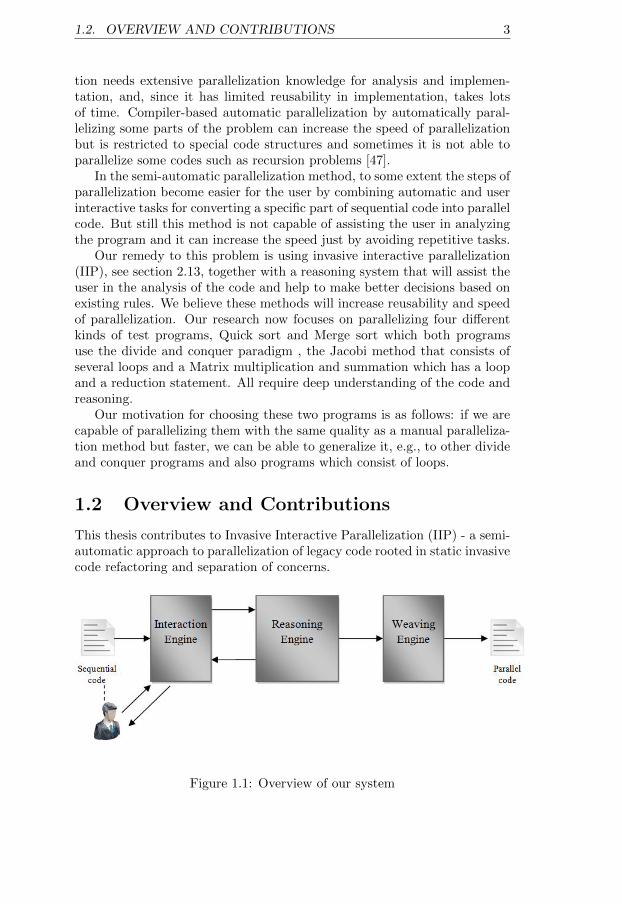
Figure 1.1: Overview of our system
4 CHAPTER 1. INTRODUCTION
Chalabine [13] suggests that an IIP system should comprise three corecomponents - interaction engine, reasoning engine, and weaving engine.
• The interaction engine is in interaction with the user and the reasoningengine in three steps: first, through it the user will load a sequentialprogram into the system. Second, the user will ask for parallelizationby pinpointing a part of the code, indicating a specific defined par-allelization strategy and a target architecture. Third, the reasoningengine’s suggestions will be shown to the user and the user will selectthe best suggestion among them.
• The reasoning engine is in interaction with the two other components,interaction engine and weaving engine. It will preprocess the code andanalyze the user’s request that was entered through the interactionengine and tries to give parallelization suggestions based on definedrules.
• The weaving engine contributes to the system in two ways. Initially,it will refactor the code based on the user’s selected suggestion anddefined IIP strategies. Finally, it, based on software composition tech-nology, will combine the refactored codes in a right order. The resultof this component will be a complete parallel program.
In this project initially we focus on IIP parallelization strategies for semi-automatic refactoring of one loop-based iterative function (Jacobi method)and one recursion-based divide and conquer function (Quick sort) both writ-ten in C.
Our first goal is to construct a prototype of an interactive reasoning en-gine by implementing a set of IIP strategies which are capable of guidingthe user through the parallelization of the two functions above by followingpatterns formulated as Lisp programs. We will build a list of predicates andfunctions alike isArray(), hasDependencies(), etc. Then, user interactioncan proceed as follows (U=user, S=system):
U: [Want to parallelize]S: [Select the sequential code]U: [Filename]S: [Select the target architecture (currently, either SHMEM or DMEM)]U: [Architecture name, e.g. SHMEM]S: [Present system analysis result, e.g. system can : parallelize part B1 andB2][Select part of the code to be parallelized]U: . . .
Our second goal is to investigate how the use of the developed prototypeaffects the productivity of a typical parallelization expert.
1.3. RESEARCH QUESTIONS 5
1.3 Research questions
In our research we try to answer the following questions: How can we helpa user with an intermediate knowledge of parallelization to parallelize se-quential codes such as Quick sort and Jacobi method? In this respect, howwould an IIP parallelization system be helpful? How can we define the factsin this system? What reasoning strategy should we use for selecting thefacts? What is the best strategy for refactoring the code?
These questions lead us toward the following hypothesis:
HypothesisWhile manual parallelization is a time consuming tedious task and whilecompilers have difficulties in automatically parallelizing recursive constructs,we are, by encoding IIP strategies using decision trees and letting the pro-grammer interact with the system, capable of parallelizing Quick sort andJacobi method achieving an acceptable level of performance but simpler andfaster than manual parallelization.
1.4 Scope of this Thesis
1.4.1 Limitations
This thesis prototype is implemented in Common Lisp language. It acceptsa sequential C code as an input and converts it to a parallel code. In orderto be able to do this conversion, it must be able to understand and retrievethe C syntax in Common Lisp; therefore, we have implemented a C parser inLisp as much as we needed for our job but we did not provide a full compilerfor C in Lisp.
In our implementation we did not restrict ourselves to specific hard-ware architecture and this system is able to be used for both shared anddistributed memory architecture.
In nested loop parallelization for two-dimensional arrays in distributedmemory, we have not implemented column-wise parallelization in our pro-totype, since arrays in C are stored in row-wise order and parallelization ofarrays in column-wise order needs several loops and more communications.Later on, in section 4.2.3.2 we will describe one method for column-wiseparallelization of two-dimensional arrays.
For divide and conquer (D&C) algorithms and specifically Quick sortwe have investigated different methods and load balancing issues but wedid not implement our system based on the best mentioned load balancingtechnique, because this technique can be used just for some sort of D&Calgorithms and we cannot generalize it.
6 CHAPTER 1. INTRODUCTION
1.4.2 Thesis Assumptions
For simplicity, the following assumptions have been made:
• We assume that all relevant code for parallelization of sequential codeexists in a single file and all statements, even “{” and “}” symbols,are in separate lines.
• For both examples we assume that we have more data items thanprocessors, which means that sizes of arrays and matrices are biggerthan the number of processors.
• We suppose that the sequential Quick sort uses the best pivot selectingmethod.
• In the end both examples are output in C language.
1.5 Evaluation Methods
We evaluate our approach based on the following metrics:Correctness: We evaluate the correctness of our system for the two exam-ples Quick sort and Jacobi method in two ways. At first, we will use testingto compare the result of execution of the sequential code with that of theparallel code that we will get from the system; in principle, they should bothbe the same for any legal input which means parallelization will not changethe semantics (input-output behavior) of the sequential code.
Second, we will by inspection compare the result of manual paralleliza-tion of the sequential code with the parallel code that we will get from thesystem, both should be basically the same.Performance: We evaluate the system’s performance by comparing theexecution time of the sequential code on one processor with the executiontime of the parallel code on multi-processors and calculating the speedup.We will show for a large amount of data items that we reach considerablyhigh speedup.Usefulness: We will show that our system will increase the speed of par-allelization for users with an intermediate knowledge of parallelization.
1.6 Outline
The rest of this thesis is organized as follows:Chapter 2 explains foundations and background to this thesis.Chapters 3 and 4 describe the contributions in terms of both the model andthe algorithms used to construct the structures that make up the model.Chapter 5 contains an evaluation of the usefulness of the model.Chapter 6 describes related work in the area of automatic and semi-automaticparallelization of sequential codes.
1.6. OUTLINE 7
Chapter 7 and 8 summarize the contributions of this work and propose somesuggestions for extending this research.
Chapter 2
Foundations andBackground
This chapter provides background necessary to understand the research de-scribed in this master thesis. It begins with a description of compiler struc-ture and continues with dependence analysis, some notions of artificial in-telligence, parallelization, software engineering techniques and finally, it fin-ishes with invasive interactive parallelization. The order of the mentionedsections is based on their priority for implementing the selected method.
2.1 Compiler Structure
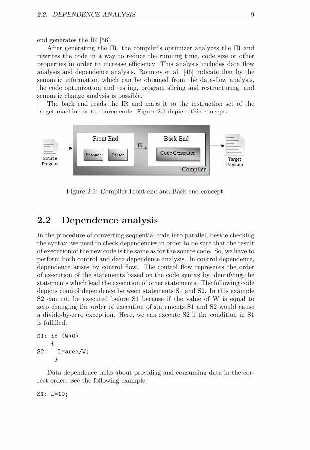
A compiler is a software system which receives a program in one high levellanguage as an input and then processes and translates it to a program inanother high level or lower level language usually with the same behavior asthe input program [56].
As presented in e.g. Cooper et al. [56], the compilation process is tradi-tionally decomposed into two parts, front end and back end. The front endtakes the source program as an input and concentrates on understandingthe language (both syntax and semantics) and encoding it into an interme-diate representation (IR). In order to complete this procedure, the inputprogram’s syntax and semantics must be well formed. Each language hasits own grammar which is a finite set of rules. The language is an infiniteset of strings defined by a grammar. Scanner and parser check the inputcode and determine its validity based on the defined grammar. The scannerdiscovers and classifies words in a string of characters. The parser, in a num-ber of steps, applies the grammar rules. These rules specify the syntax forthe input language. It may happen that sentences are syntactically correctbut they are meaningless; therefore, beside syntax, the compiler also checkssemantics of programs based on contextual knowledge. Finally, the front
8
2.2. DEPENDENCE ANALYSIS 9
end generates the IR [56].After generating the IR, the compiler’s optimizer analyzes the IR and
rewrites the code in a way to reduce the running time, code size or otherproperties in order to increase efficiency. This analysis includes data flowanalysis and dependence analysis. Rountev et al. [46] indicate that by thesemantic information which can be obtained from the data-flow analysis,the code optimization and testing, program slicing and restructuring, andsemantic change analysis is possible.
The back end reads the IR and maps it to the instruction set of thetarget machine or to source code. Figure 2.1 depicts this concept.
Figure 2.1: Compiler Front end and Back end concept.
2.2 Dependence analysis
In the procedure of converting sequential code into parallel, beside checkingthe syntax, we need to check dependencies in order to be sure that the resultof execution of the new code is the same as for the source code. So, we have toperform both control and data dependence analysis. In control dependence,dependence arises by control flow. The control flow represents the orderof execution of the statements based on the code syntax by identifying thestatements which lead the execution of other statements. The following codedepicts control dependence between statements S1 and S2. In this exampleS2 can not be executed before S1 because if the value of W is equal tozero changing the order of execution of statements S1 and S2 would causea divide-by-zero exception. Here, we can execute S2 if the condition in S1is fulfilled.
S1: if (W>0)
{
S2: L=area/W;
}
Data dependence talks about providing and consuming data in the cor-rect order. See the following example:
S1: L=10;
10 CHAPTER 2. FOUNDATIONS AND BACKGROUND
S2: W=5;
S3: area= L* W;
Statement S3 can not be moved before either S1 or S2. There is no con-straint in the order of execution of S1 and S2. To understand both thesedependencies we can use a dependence graph. The dependence graph is adirected graph whose vertices are statements and arcs show control and datadependency [51, 5].
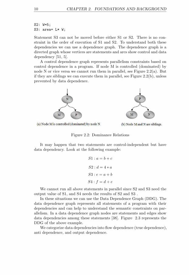
A control dependence graph represents parallelism constraints based oncontrol dependence in a program. If node M is controlled (dominated) bynode N or vice versa we cannot run them in parallel, see Figure 2.2(a). Butif they are siblings we can execute them in parallel, see Figure 2.2(b), unlessprevented by data dependence.
Figure 2.2: Dominance Relations
It may happen that two statements are control-independent but havedata dependency. Look at the following example:
S1 : a = b+ c
S2 : d = 4 ∗ a
S3 : e = a+ b
S4 : f = d+ e
We cannot run all above statements in parallel since S2 and S3 need theoutput value of S1, and S4 needs the results of S2 and S3 .
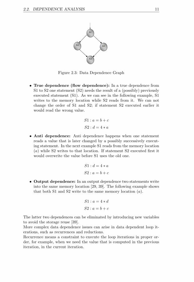
In these situations we can use the Data Dependence Graph (DDG). Thedata dependence graph represents all statements of a program with theirdependencies and can help to understand the semantic constraints on par-allelism. In a data dependence graph nodes are statements and edges showdata dependencies among these statements [38]. Figure 2.3 represents theDDG of the above example.
We categorize data dependencies into flow dependence (true dependence),anti dependence, and output dependence.
2.2. DEPENDENCE ANALYSIS 11
Figure 2.3: Data Dependence Graph
• True dependence (flow dependence): In a true dependence fromS1 to S2 one statement (S2) needs the result of a (possibly) previouslyexecuted statement (S1). As we can see in the following example, S1writes to the memory location while S2 reads from it. We can notchange the order of S1 and S2; if statement S2 executed earlier itwould read the wrong value.
S1 : a = b+ c
S2 : d = 4 ∗ a
• Anti dependence: Anti dependence happens when one statementreads a value that is later changed by a possibly successively execut-ing statement. In the next example S1 reads from the memory location(a) while S2 writes to that location. If statement S2 executed first itwould overwrite the value before S1 uses the old one.
S1 : d = 4 ∗ a
S2 : a = b+ c
• Output dependence: In an output dependence two statements writeinto the same memory location [29, 39]. The following example showsthat both S1 and S2 write to the same memory location (a).
S1 : a = 4 ∗ d
S2 : a = b+ c
The latter two dependences can be eliminated by introducing new variablesto avoid the storage reuse [39].More complex data dependence issues can arise in data dependent loop it-erations, such as recurrences and reductions.Recurrence means a constraint to execute the loop iterations in proper or-der, for example, when we need the value that is computed in the previousiteration, in the current iteration.
12 CHAPTER 2. FOUNDATIONS AND BACKGROUND
A reduction operation is used to reduce the elements of one array byusing operations such as sum, multiply, min, max, etc. into a single value.For example, in the case of a loop summing the elements of one array, in eachiteration the value of the sum variable is updated to add a new element. Ifwe parallelize this loop, in the parallel version we divide the loop iterationsbetween the active processors and each processor will calculate sum as abovefor its own subset; therefore, the processors may interfere with each otherand overwrite each other’s values in the same memory location. To overcomethis problem we have to consider that at each time only one processor beable to execute the summation which again serializes the loop execution.Data dependency in loops can in some cases be eliminated by rewriting theloops, for more information see [2].
Loop execution is one of the situations where we need to do data depen-dency analysis. There are two kinds of loop dependencies, loop-independentdependences and loop-carried dependences.
Loop-independent dependence means that the dependence occurs in thesame loop iteration. For example, assume we have two statements S1 andS2 in the same loop that both access the same memory location (a[i]) ineach iteration but the memory location in each iteration is different. Sincewe have a distinct memory location in each iteration the iterations are in-dependent of each other, see the following example.
for (i=0;i<10;++i)
{
S1: a[i]=2*i;
S2: e[i]=a[i]-2;
}
Loop-carried dependence occurs when one statement accesses a memorylocation in one iteration and in another iteration there is a second accessto that memory location and at least one of these accesses is a write access[29]. The following example demonstrates this idea, as we can see that inevery iteration statement S2 uses an element of a that was computed in theprevious iteration by S1.
for(i=0;i<10;++i)
{
S1: a[i]=2*i;
S2: e[i]=a[i-1]-2;
}
Most compilers can perform control and data dependency analyses butin a limited scale and mostly for loops.In our project we use both control and data dependency analysis for selectedparts of the code that include control statements such as if-statements, it-eration (for-loops, nested for-loops) and recursive functions.
2.2. DEPENDENCE ANALYSIS 13
In order to determine whether data dependences may exist among thecode statements inside a loop or not, there exist several tests such as ZIV(zero index variable), SIV (single index variable), MIV (multiple index vari-able), GCD test, Banerjee test, etc. All these tests are based on the indexvariables of the loops enclosing the statements and the arrays’ indices thatoccur inside the statements. We refer the reader to [5] for details concerningthese tests.
The two traditionally most well known tests that find dependenciesamong loop statements are GCD and Banerjee tests. In [5] Allen et al.mention that most compilers for automatic parallelization use these twotests to find dependencies.
2.2.1 GCD Test
Both GCD and Banerjee test are based on solving Linear Diophantine equa-tions, and they determine whether a dependence equation of the form (2.1)may have an integer solution which satisfies the constraint (2.2) or not. [5]
f(I1, I2, · · · , In) = a0 + a1I1 + a2I2 + · · ·+ anIn
g(J1, J2, · · · , Jn) = b0 + b1J1 + b2J2 + · · ·+ bnJn
f(I1, I2, · · · , In) = g(J1, J2, · · · , Jn)
a1I1 − b1J1 + · · ·+ anIn − bnJn = b0 − a0 (2.1)
Lk ≤ Ik, Jk ≤ Hk ∀k, 1 ≤ k ≤ n (2.2)
In equation 2.2 in a sequence Lk and Hk show the lower and upper limitsfor the loop index variable of loop k in a loop nest with n levels.
The GCD test does not consider the loop index limits and it only checkswhether there may exist an integer solution that fulfills 2.1 or not. TheGCD test is calculated by calculating the gcd (greatest common divisor) ofall the coefficients of the loop index variables (gcd(a1, · · · , an, b1, · · · , bn))and testing if it divides the constant terms (b0−a0). If not it means there isno solution for the equation and definitely no dependence; otherwise, theremay be a dependence. Here, if there is a solution for the test, we are still notsure about the existence of a dependence, because it may happen that theinteger solutions may not fulfill the iteration space constraint (2.2).[5, 43]
In this situation we can run another dependency test and for this thesiswe have selected the Banerjee test.
14 CHAPTER 2. FOUNDATIONS AND BACKGROUND
2.2.2 Banerjee Test
In contrast to the GCD test, the Banerjee test considers the loop indexlimits for its computations. It uses the loop index limits to calculate themin and max values on the left-hand side of equation (2.3).
a1I1 + a2I2 + · · ·+ anIn = a0 (2.3)
Lk ≤ Ik ≤ Hk ∀k, 1 ≤ k ≤ n
Assume that in equation 2.3, min and max are calculated as follows:
min =
n∑i=1
(a+i Li − a−i Hi) max =
n∑i=1
(a+i Hi − a−i Li)
Where
a+ = if a ≥ 0 then a else 0
a− = if a ≥ 0 then 0 else -a
Now, if a0 is not between min and max (min ≤ a0 ≤ max) there isdefinitely no dependence; otherwise, there may be a dependence [5, 43, 44].In the situation that both GCD and Banerjee tests reach to “maybe”, wewill consider that there is a dependency.
2.3 Artificial intelligence
Artificial intelligence (AI) is an area of computer science. Among differentexisting definitions we will define it as, simulation of human intelligence on acomputer in a way that enables it to make efficient decisions to solve complexproblems with incomplete knowledge. Such a system must be capable ofplanning in order to select and execute suitable tasks at each step. AI is awide research area and many researchers are working on different aspects ofit. Now we will describe some of them.
2.3.1 Knowledge representation and Reasoning
Knowledge representation’s (KR) focus is on understanding requirements,capturing required knowledge, representing this knowledge in symbols andautomatically making it available based on reasoning strategies. A KR sys-tem is responsible for analyzing the user’s queries and answering them in areasonable time. KR is a part of a larger system which interacts with otherparts by answering their queries and letting them add and modify concepts,roles and assertions, for more details see [7].
2.3. ARTIFICIAL INTELLIGENCE 15
2.3.2 Inference
In our daily life it may happen that, according to the existing facts or ourexperiences, we draw a conclusion for some problems, in these situations weinfer the result. For example if the ground is wet in autumn we usually inferthat it was raining. This notion is expanded in different areas and we alsohave it in AI. Inference is classified into two groups, deductive and inductive.
The deductive inference infers in two steps: at first, by assigning thetruth values to the sentences, it specifies the premises. In the second step,it provides an inference procedure based on given premises which is leadto the certain conclusions. The inductive inference, similarly to deductiveinference, infers in two steps: at first, it specifies premises by assigningprobability values to the sentences and in the second step, it provides aninference procedure based on given premises which is lead to most possibleconclusions. Since the inductive inference is only probable, even in thesituation that the evidence is accurate, the conclusion can be wrong. Fromthe mathematical point of view, how to specify the conclusions based onpremises is the difference between inductive and deductive inferences, formore details see [36].
2.3.3 Planning, deductive reasoning and problem solv-ing
An intelligent agent must be able to set the goals and predict the necessarystates to achieve the successful goals by reasoning about the effect of eachstate in an efficient manner. Deductive reasoning means to take decisionsbased on existing facts, and intelligent agents use this method for creat-ing step by step a plan to solve a specific problem even with incompleteinformation.
2.3.4 Machine Learning
We can define learning as improving some tasks with experience. The field ofmachine learning includes studies of designing the computer programs thatimprove their performance at some tasks through learning from the previ-ous experience or history. In machine learning we encounter two concepts,supervised and unsupervised learning. In supervised or inductive learning,similar to human learning that gains knowledge from the past experiencesto improve the human’s ability to perform the real world tasks, the machinelearns from the past experiences data.
In this concept we have a set of inputs, outputs, and algorithms thatmap these inputs to outputs. For mapping data, supervised learning at firstwill classify the data based on their similarities and then it will executethe set of functions which lead to reaching the specified outputs from theexisting inputs. Here input data must be complete otherwise the systemcannot be able to infer correctly. One of the most common techniques of
16 CHAPTER 2. FOUNDATIONS AND BACKGROUND
supervised learning is decision tree learning which creates a decision treebased on predefined training data.
Unsupervised learning is a technique with emphasis in computer abilityto solve a classification problem from a chain of observations; therefore, itis able to solve more complex problems. In this technique we do not needtraining data [48].
2.3.4.1 Classification and statistical learning methods
In supervised learning we have the notion of class which is defined as adecision to be made, and patterns belong to these classes. AI applicationsare grouped into classifiers and controllers. Classifiers are functions thatbased on pattern matching methods, find the closest pattern, and controllersinfer actions [48]. Classifiers are used in support vector machine (SVM), k-nearest neighbor algorithm, decision tree, etc.
2.3.4.2 Decision Tree
Decision tree learning is a method of supervised learning. It uses a tree-like graph or model of decisions. In a decision tree, the internal nodes testattributes, branches represent the values corresponding to the attributes andclassifications are assigned by leaf nodes [53].
Interpretability, flexibility and usability make this model transparent andunderstandable to human experts, applicable to a wide range of problemsand accessible to non-specialists. This model is also highly scalable and theresult is accurately predictable, for more details we refer the reader to [53].
2.3.5 Logic programming and AI languages
Logic programming is a part of the AI research area. In logic program-ming we categorize languages into two groups, declarative and imperativelanguages. A declarative language describes what the problem is while animperative language describes how to solve the problem. A declarative state-ment is also called a declarative sentence. It is a complete expression innatural language which is true or false. A declarative program consists of aset of declarative statements and shows the relationship between them. Animperative sentence or command says what to do. An imperative programconsists of a sequence of commands, for more information see [40].
Two main logic languages that are mostly used in AI are Lisp and Prologwhich both are declarative languages.
Lisp was born in 1958; it seems that after Fortran it is the second oldestsurviving language. Lisp is a functional language which is based on defin-ing functions. In Lisp all symbolic expressions and other information arerepresented by a list structure, which makes manipulation easy [37].
2.4. PARALLELIZATION MECHANISMS 17
Prolog is a special-purpose language which is based on first order logicand mostly used for logic and reasoning. It is a declarative language. It hasa limited number of key words which makes it easy to learn.
2.4 Parallelization mechanisms
There are four different methods for parallelizing a program:
• Manual parallelization: Traditionally, parallel programs have beenmanually written by expert programmers. The programmer is respon-sible for identification and implementation of parallelism. This mech-anism is flexible since the programmer can decide how to implementit. However, the programmer must have a good knowledge about thecharacteristics of the architecture where the program is intended to berun and take decisions about the ways to decompose and map data,and how the scheduling and synchronization procedures must be [19].Since the programmer is responsible for doing all of the above tasksby him/herself and it also may happen that we have repetitive tasks,this method is time consuming, complex and error-prone [9].
• Compiler-based automatic parallelization: In this method com-pilers automatically generate a parallel version of the sequential code.This method is less flexible than the previous method. Here, most fo-cus is on loop level parallelization since most of the program executiontime is spent in executing loop iterations. Compilers parallelize loopsbased on data dependence analysis. However, it is not always possibleto detect data dependency at compile time. Overall we can say thatthe compilers can parallelize the loops with the situations mentionedin section 2.8.1.Different parallel algorithms for the same sequential code may presentdifferent parallelism degrees. As Gonzalez-Escribano et al. [19] men-tion, many compilers will not parallelize a loop when the overhead ofthe parallel execution is expected to exceed the gained performance.Some compilers have problems with parallelizing divide and conqueralgorithms and generally recursive procedures due to dependenciesthat may exist among the recursive calls [47].
• Skeletons: Algorithmic skeletons which were introduced by Cole [15]is another approach for parallel programming. In this method, de-tails for parallel implementations are abstracted in skeleton which canincrease programmer’s productivity. But, this method restricts paral-lelization, since it is only suitable for well structured parallelism andthe source code also must be rewritten according to existing templates.
• Semi-automatic: The semi-automatic method provides an interme-diate alternative between manual and compiler-based automatic par-allelization [33] as a method for locality-optimization [54]. In this

18 CHAPTER 2. FOUNDATIONS AND BACKGROUND
method the programmer conducts the compiler how to parallelize thecode. For example, if we have a simple loop or a nested loop and wewant to parallelize it, we can specify how the compiler distributes databetween different processors in such a way that each processor executesoperations on a specific amount of data. For loops with accumulativeoperations where two concurrent iterations update the same variablesimultaneously, we will lose one of the updates due to overwriting thevalue by other iteration; in this case, the programmer annotates thespecific parts of the code as a critical section and the compiler willparallelize it accordingly.
Semi-automatic parallelization uses directives which means to insertpragmas before the selected statement or block of statements such as“#pragma omp parallel for” in OpenMP.
#pragma omp parallel for
for(i=0;i<n;++i)
{
...
}
2.5 Parallel Computers
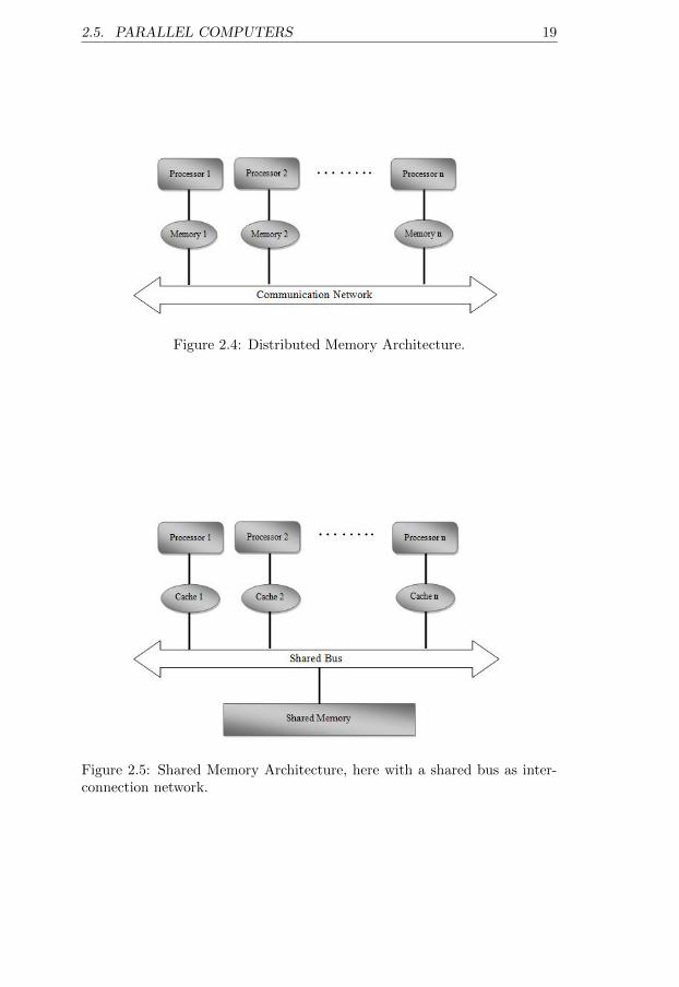
Parallel computers are computers with multiple processor units. There aretwo architecture models for these computers, multicomputer and multipro-cessor.In multicomputer or distributed memory model, a number of computers areinterconnected to each other through a network and memory is distributedamong the processors, which improves scalability. Each processor has directaccess to its local memory, and in order to access data in other processors’memory they use message passing (Figure 2.4). There are two models fordistributed memory: Message passing architecture, and Distributed sharedmemory where the global address space is shared among multiple proces-sors and an operating system helps to give the shared memory view to theprogrammer, see [52, 27] for more information.
In the second model, which is called multiprocessor or shared memory,a number of processors are connected to a common memory through a net-work, such as a shared bus or a switch. Memory is located at a centralizedlocation and all processors have direct access to that place (Figure 2.5).We have two designs for shared memory multiprocessors: symmetric mul-tiprocessor (SMP) with UMA (uniform memory access) architecture styleand Cc-NUMA (cache-coherent NUMA1 ) [52, 27].
1Non-uniform memory access: Access mechanism and time to various parts of a mem-ory is varying for a processor.
2.5. PARALLEL COMPUTERS 19
Figure 2.4: Distributed Memory Architecture.
Figure 2.5: Shared Memory Architecture, here with a shared bus as inter-connection network.
20 CHAPTER 2. FOUNDATIONS AND BACKGROUND
2.6 Parallel Programming Models
As we have described in the previous section, there are two different memoryarchitectures, shared memory and distributed memory for parallel comput-ers. Each architecture has its own design and programming model; therefore,before beginning to program we should define our architecture.
The Message Passing Interface (MPI) standard supports distributed mem-ory architectures and is defined for C/C++ and Fortran programs. In thismodel, during run time the number of tasks is fixed [10]. In MPI all proces-sors run the same code. The programmer’s parallelizing skills are requiredin order to write a parallel program.
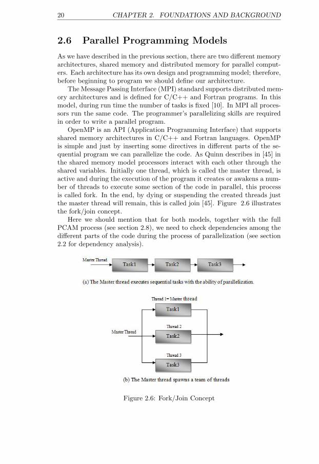
OpenMP is an API (Application Programming Interface) that supportsshared memory architectures in C/C++ and Fortran languages. OpenMPis simple and just by inserting some directives in different parts of the se-quential program we can parallelize the code. As Quinn describes in [45] inthe shared memory model processors interact with each other through theshared variables. Initially one thread, which is called the master thread, isactive and during the execution of the program it creates or awakens a num-ber of threads to execute some section of the code in parallel, this processis called fork. In the end, by dying or suspending the created threads justthe master thread will remain, this is called join [45]. Figure 2.6 illustratesthe fork/join concept.
Here we should mention that for both models, together with the fullPCAM process (see section 2.8), we need to check dependencies among thedifferent parts of the code during the process of parallelization (see section2.2 for dependency analysis).
Figure 2.6: Fork/Join Concept
2.7. PERFORMANCE METRICS 21
In contrast with MPI where the number of active processes during theexecution of the program is fixed and all of them are active, in this methodthe number of active threads during the execution will change. As we havementioned above, at the start and end of the code execution we have justone active thread.
2.7 Performance Metrics
Speedup and efficiency are two metrics to evaluate the performance of par-allel programs.Speedup measures the gain we get by running certain parts of the programin parallel to solve a specific problem. There are several concepts for calcu-lating speedup and among them we will describe the two most well-knownconcepts; absolute and relative speedup [34].
• Absolute speedup: is calculated by dividing the time taken to run thebest known serial algorithm on one processor (Tser) by the time takento run the parallel algorithm on p processors (Tpar).
Sabs =TserTpar
• Relative speedup: The relative speedup is calculated by dividing theexecution time of the parallel algorithm on one processor (T1) by theexecution time for the same parallel algorithm on p processors (Tpar).
Srel =T1Tpar
Efficiency (E) is the ratio between speedup and the number p of processorsused, which indicates the resource utilization of the parallel machine by theparallel algorithm.
E =S
p
In the ideal situation the efficiency is equal to one which means S = p whereall processors use their maximum potential, but practically this cannot beachieved. Usually the performance decreases for several reasons and typi-cally will cause efficiency to be less than one. For more details we refer thereader to [34].
2.8 Code Parallelization
As we have discussed before, the aim of parallelization of sequential code isincreasing the speed of computations. Thus, our strategy for parallelizationis based on parallelizing parts of the codes which use most of CPU times
22 CHAPTER 2. FOUNDATIONS AND BACKGROUND
Figure 2.7: Foster’s PCAM methodology for parallel programs
2.8. CODE PARALLELIZATION 23
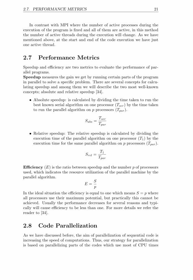
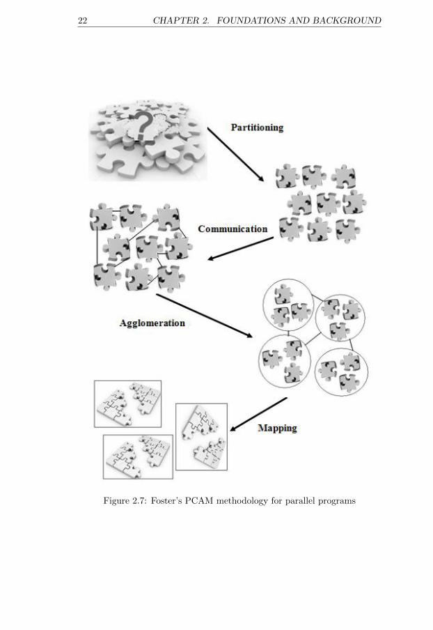
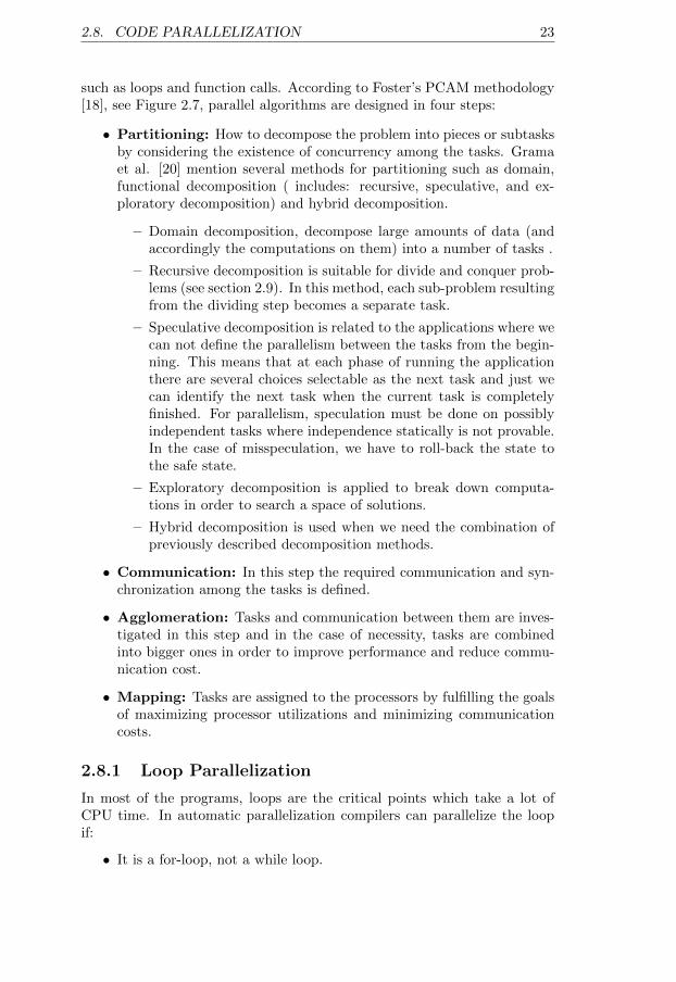
such as loops and function calls. According to Foster’s PCAM methodology[18], see Figure 2.7, parallel algorithms are designed in four steps:
• Partitioning: How to decompose the problem into pieces or subtasksby considering the existence of concurrency among the tasks. Gramaet al. [20] mention several methods for partitioning such as domain,functional decomposition ( includes: recursive, speculative, and ex-ploratory decomposition) and hybrid decomposition.
– Domain decomposition, decompose large amounts of data (andaccordingly the computations on them) into a number of tasks .
– Recursive decomposition is suitable for divide and conquer prob-lems (see section 2.9). In this method, each sub-problem resultingfrom the dividing step becomes a separate task.
– Speculative decomposition is related to the applications where wecan not define the parallelism between the tasks from the begin-ning. This means that at each phase of running the applicationthere are several choices selectable as the next task and just wecan identify the next task when the current task is completelyfinished. For parallelism, speculation must be done on possiblyindependent tasks where independence statically is not provable.In the case of misspeculation, we have to roll-back the state tothe safe state.
– Exploratory decomposition is applied to break down computa-tions in order to search a space of solutions.
– Hybrid decomposition is used when we need the combination ofpreviously described decomposition methods.
• Communication: In this step the required communication and syn-chronization among the tasks is defined.
• Agglomeration: Tasks and communication between them are inves-tigated in this step and in the case of necessity, tasks are combinedinto bigger ones in order to improve performance and reduce commu-nication cost.
• Mapping: Tasks are assigned to the processors by fulfilling the goalsof maximizing processor utilizations and minimizing communicationcosts.
2.8.1 Loop Parallelization
In most of the programs, loops are the critical points which take a lot ofCPU time. In automatic parallelization compilers can parallelize the loopif:
• It is a for-loop, not a while loop.
24 CHAPTER 2. FOUNDATIONS AND BACKGROUND
• There is no loop-carried dependence between iterations. In order tobe able to parallelize the loops we have to do dependency analysisfor all statements inside the loop body. If there exists loop-carrieddependence we can not parallelize the code unless we remove thesedependencies [39].
• The function calls inside the loops do not affect the variables accessedin other iterations and not the loop index.
• The loop index variable must be integer [2].
Together with the above constraints, two points are really important andthey should be considered while parallelizing the code. First, the numberof loop iterations must be known since we usually divide the loop iterationsbetween the processors.
The second point refers to conditional statements inside the body of theloop where for every iteration we have to execute one branch of the condi-tional statements. Sometimes, these statements cause different behavior inloops that makes the loop not able to be parallelized. Therefore, we shouldfind them by analyzing the code and if it is possible remove them.
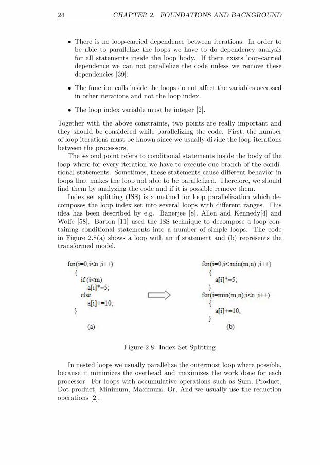
Index set splitting (ISS) is a method for loop parallelization which de-composes the loop index set into several loops with different ranges. Thisidea has been described by e.g. Banerjee [8], Allen and Kennedy[4] andWolfe [58]. Barton [11] used the ISS technique to decompose a loop con-taining conditional statements into a number of simple loops. The codein Figure 2.8(a) shows a loop with an if statement and (b) represents thetransformed model.
Figure 2.8: Index Set Splitting
In nested loops we usually parallelize the outermost loop where possible,because it minimizes the overhead and maximizes the work done for eachprocessor. For loops with accumulative operations such as Sum, Product,Dot product, Minimum, Maximum, Or, And we usually use the reductionoperations [2].
2.8. CODE PARALLELIZATION 25
Where we are sure that there is no loop-carried dependency inside theloop, based on the selected parallel programming model (MPI / OpenMP)we can parallelize the code as follows.
2.8.1.1 OpenMP
Quinn [45] has mentioned that in the OpenMP programming model, thecompiler is responsible for generating the code for fork/join of threads andalso allocating the iterations to threads. In a shared memory architecturethe user interacts with the compiler through the compiler directives (inC: Pragmas, pragmatic information). The syntax of OpenMP pragmas inC/C++ is as follows:
#pragma omp <rest of pragma>
By inserting pragmas in different parts of the code the user will indicate tothe compiler which parts he/she wants to parallelize.
In order to parallelize a for-loop, the loop must be in canonical shape.
for(index=start; index
<≤≥>
end; step)
The for-loop is in canonical shape if :
• The initial expression has one of the following formats:loop-variable= lower-bound (e.g. i=0)integer-data-type loop-variable= lower-bound (e.g. int i=0)
• It contains a loop exit-condition.
• The incremental expression step be in one of the following formats:++ loop-variable (e.g.++i)loop-variable ++ (e.g. i++)−− loop-variable (e.g. −−i)loop-variable −−(e.g. i−−)loop-variable += integer-value (e.g. i+=2)loop-variable -= integer-value (e.g. i-=2)loop-variable= loop-variable + integer-value (e.g. i= i+2)loop-variable = integer-value + loop-variable (e.g. i=2+ i)loop-variable = loop-variable - integer-value (e.g. i=i - 2)
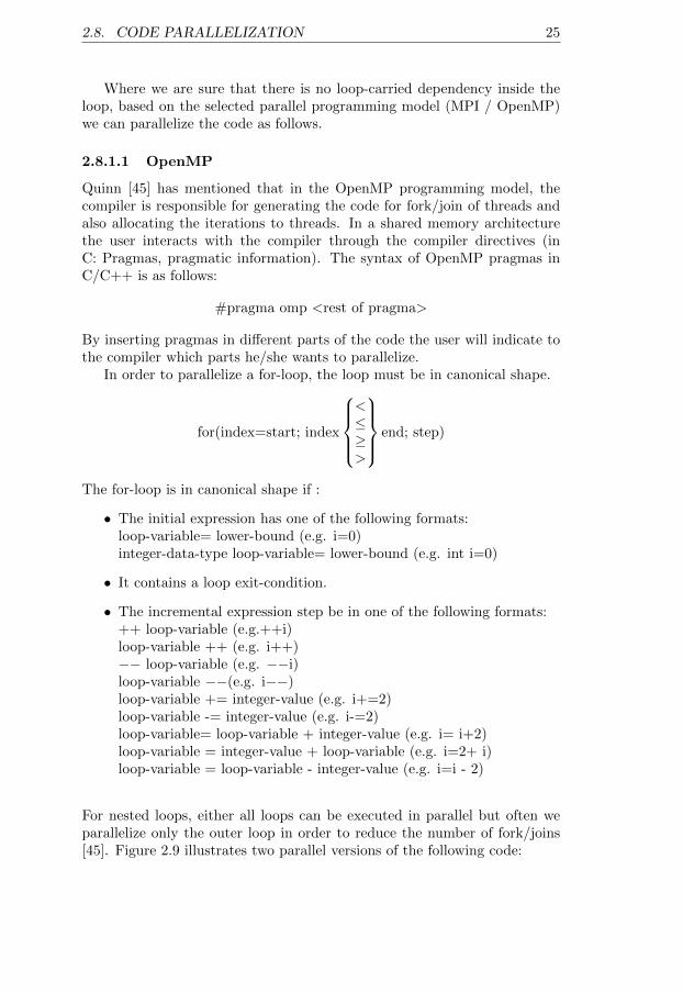
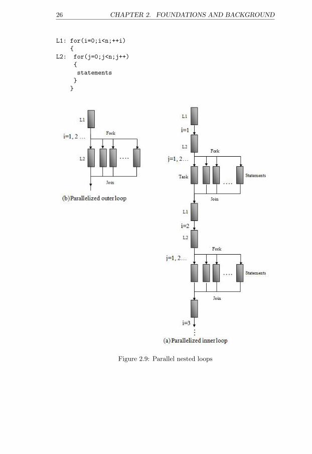
For nested loops, either all loops can be executed in parallel but often weparallelize only the outer loop in order to reduce the number of fork/joins[45]. Figure 2.9 illustrates two parallel versions of the following code:
26 CHAPTER 2. FOUNDATIONS AND BACKGROUND
L1: for(i=0;i<n;++i)
{
L2: for(j=0;j<n;j++)
{
statements
}
}
Figure 2.9: Parallel nested loops
2.8. CODE PARALLELIZATION 27
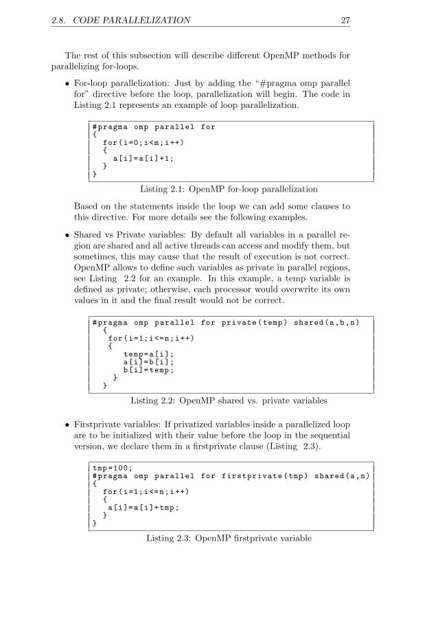
The rest of this subsection will describe different OpenMP methods forparallelizing for-loops.
• For-loop parallelization: Just by adding the “#pragma omp parallelfor” directive before the loop, parallelization will begin. The code inListing 2.1 represents an example of loop parallelization.
#pragma omp parallel for{
for(i=0;i<m;i++){
a[i]=a[i]+1;}
}
Listing 2.1: OpenMP for-loop parallelization
Based on the statements inside the loop we can add some clauses tothis directive. For more details see the following examples.
• Shared vs Private variables: By default all variables in a parallel re-gion are shared and all active threads can access and modify them, butsometimes, this may cause that the result of execution is not correct.OpenMP allows to define such variables as private in parallel regions,see Listing 2.2 for an example. In this example, a temp variable isdefined as private; otherwise, each processor would overwrite its ownvalues in it and the final result would not be correct.
#pragma omp parallel for private(temp) shared(a,b,n){for(i=1;i<=n;i++){
temp=a[i];a[i]=b[i];b[i]=temp;
}}
Listing 2.2: OpenMP shared vs. private variables
• Firstprivate variables: If privatized variables inside a parallelized loopare to be initialized with their value before the loop in the sequentialversion, we declare them in a firstprivate clause (Listing 2.3).
tmp =100;#pragma omp parallel for firstprivate(tmp) shared(a,n){
for(i=1;i<=n;i++){a[i]=a[i]+tmp;
}}
Listing 2.3: OpenMP firstprivate variable
28 CHAPTER 2. FOUNDATIONS AND BACKGROUND
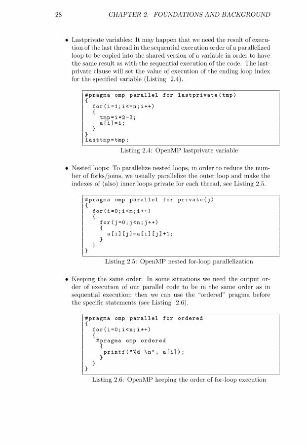
• Lastprivate variables: It may happen that we need the result of execu-tion of the last thread in the sequential execution order of a parallelizedloop to be copied into the shared version of a variable in order to havethe same result as with the sequential execution of the code. The last-private clause will set the value of execution of the ending loop indexfor the specified variable (Listing 2.4).
#pragma omp parallel for lastprivate(tmp){
for(i=1;i<=n;i++){
tmp=i*2-3;a[i]=i;
}}lasttmp=tmp;
Listing 2.4: OpenMP lastprivate variable
• Nested loops: To parallelize nested loops, in order to reduce the num-ber of forks/joins, we usually parallelize the outer loop and make theindexes of (also) inner loops private for each thread, see Listing 2.5.
#pragma omp parallel for private(j){
for(i=0;i<m;i++){
for(j=0;j<n;j++){
a[i][j]=a[i][j]+1;}
}}
Listing 2.5: OpenMP nested for-loop parallelization
• Keeping the same order: In some situations we need the output or-der of execution of our parallel code to be in the same order as insequential execution; then we can use the “ordered” pragma beforethe specific statements (see Listing 2.6).
#pragma omp parallel for ordered{
for(i=0;i<n;i++){#pragma omp ordered{printf("%d \n", a[i]);
}}
}
Listing 2.6: OpenMP keeping the order of for-loop execution
2.8. CODE PARALLELIZATION 29
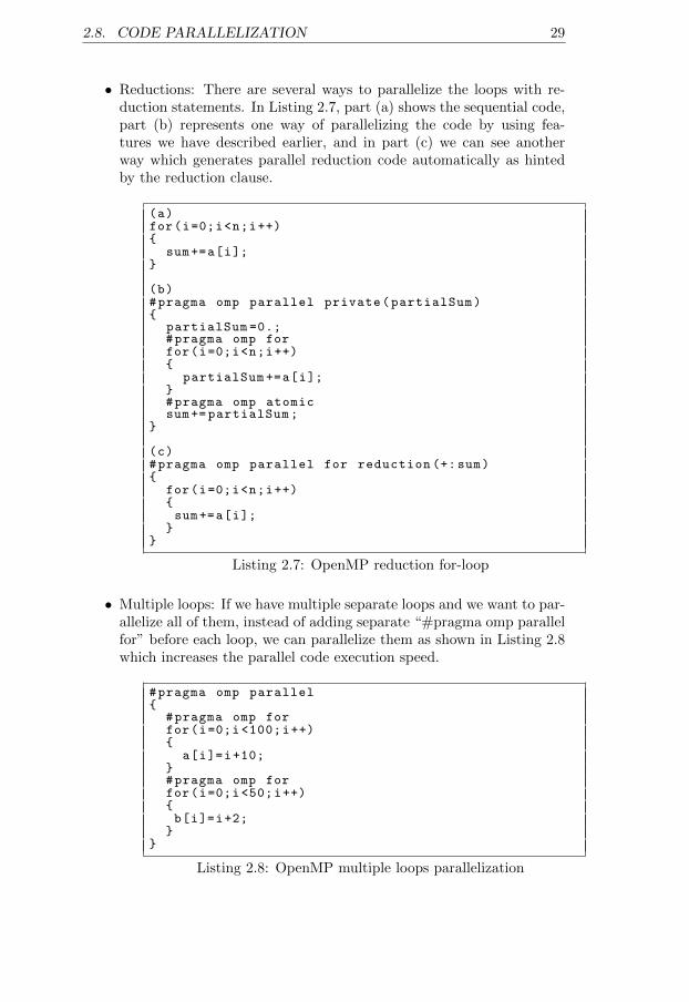
• Reductions: There are several ways to parallelize the loops with re-duction statements. In Listing 2.7, part (a) shows the sequential code,part (b) represents one way of parallelizing the code by using fea-tures we have described earlier, and in part (c) we can see anotherway which generates parallel reduction code automatically as hintedby the reduction clause.
(a)for(i=0;i<n;i++){
sum+=a[i];}
(b)#pragma omp parallel private(partialSum){
partialSum =0.;#pragma omp forfor(i=0;i<n;i++){
partialSum +=a[i];}#pragma omp atomicsum+= partialSum;
}
(c)#pragma omp parallel for reduction (+:sum){
for(i=0;i<n;i++){sum+=a[i];
}}
Listing 2.7: OpenMP reduction for-loop
• Multiple loops: If we have multiple separate loops and we want to par-allelize all of them, instead of adding separate “#pragma omp parallelfor” before each loop, we can parallelize them as shown in Listing 2.8which increases the parallel code execution speed.
#pragma omp parallel{
#pragma omp forfor(i=0;i <100;i++){
a[i]=i+10;}#pragma omp forfor(i=0;i<50;i++){b[i]=i+2;
}}
Listing 2.8: OpenMP multiple loops parallelization
30 CHAPTER 2. FOUNDATIONS AND BACKGROUND
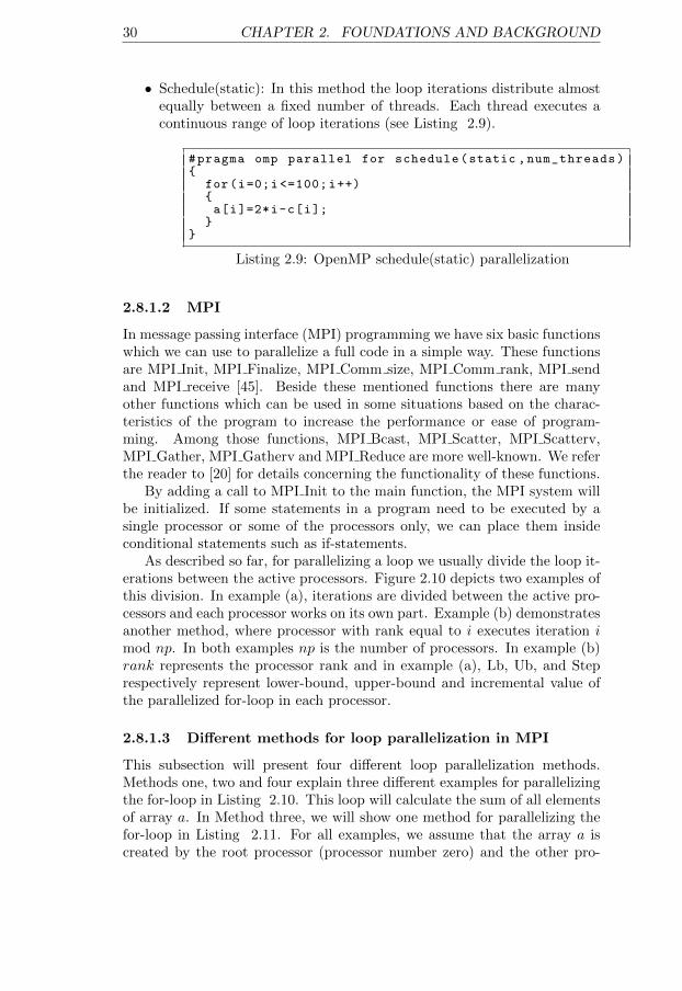
• Schedule(static): In this method the loop iterations distribute almostequally between a fixed number of threads. Each thread executes acontinuous range of loop iterations (see Listing 2.9).
#pragma omp parallel for schedule(static ,num_threads){
for(i=0;i <=100;i++){a[i]=2*i-c[i];
}}
Listing 2.9: OpenMP schedule(static) parallelization
2.8.1.2 MPI
In message passing interface (MPI) programming we have six basic functionswhich we can use to parallelize a full code in a simple way. These functionsare MPI Init, MPI Finalize, MPI Comm size, MPI Comm rank, MPI sendand MPI receive [45]. Beside these mentioned functions there are manyother functions which can be used in some situations based on the charac-teristics of the program to increase the performance or ease of program-ming. Among those functions, MPI Bcast, MPI Scatter, MPI Scatterv,MPI Gather, MPI Gatherv and MPI Reduce are more well-known. We referthe reader to [20] for details concerning the functionality of these functions.
By adding a call to MPI Init to the main function, the MPI system willbe initialized. If some statements in a program need to be executed by asingle processor or some of the processors only, we can place them insideconditional statements such as if-statements.
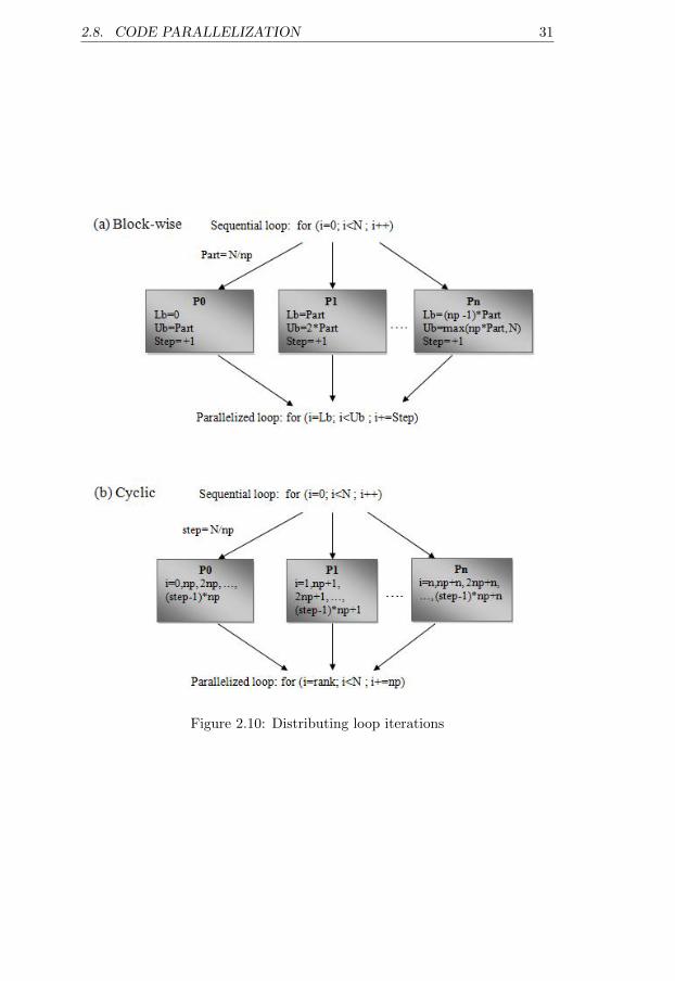
As described so far, for parallelizing a loop we usually divide the loop it-erations between the active processors. Figure 2.10 depicts two examples ofthis division. In example (a), iterations are divided between the active pro-cessors and each processor works on its own part. Example (b) demonstratesanother method, where processor with rank equal to i executes iteration imod np. In both examples np is the number of processors. In example (b)rank represents the processor rank and in example (a), Lb, Ub, and Steprespectively represent lower-bound, upper-bound and incremental value ofthe parallelized for-loop in each processor.
2.8.1.3 Different methods for loop parallelization in MPI
This subsection will present four different loop parallelization methods.Methods one, two and four explain three different examples for parallelizingthe for-loop in Listing 2.10. This loop will calculate the sum of all elementsof array a. In Method three, we will show one method for parallelizing thefor-loop in Listing 2.11. For all examples, we assume that the array a iscreated by the root processor (processor number zero) and the other pro-
2.8. CODE PARALLELIZATION 31
Figure 2.10: Distributing loop iterations
32 CHAPTER 2. FOUNDATIONS AND BACKGROUND
cessors do not have access to it. In these examples np holds the number ofactive processors and MyRank the rank of the specified processor.
for(i=0;i<n;++i){
sum+=a[i];}
Listing 2.10: Sequential for-loop to calculate the sum of all array elements
for(i=0;i<n;++i){
a[i]=a[i]+1;}
Listing 2.11: Sequential for-loop to increase all elements of an array by one
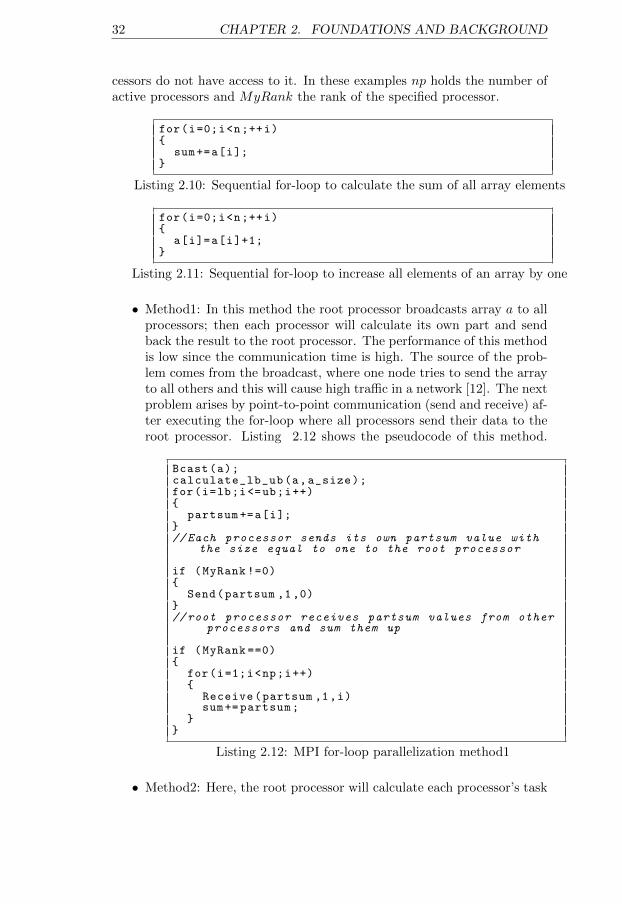
• Method1: In this method the root processor broadcasts array a to allprocessors; then each processor will calculate its own part and sendback the result to the root processor. The performance of this methodis low since the communication time is high. The source of the prob-lem comes from the broadcast, where one node tries to send the arrayto all others and this will cause high traffic in a network [12]. The nextproblem arises by point-to-point communication (send and receive) af-ter executing the for-loop where all processors send their data to theroot processor. Listing 2.12 shows the pseudocode of this method.
Bcast(a);calculate_lb_ub(a,a_size);for(i=lb;i<=ub;i++){
partsum +=a[i];}//Each processor sends its own partsum value with
the size equal to one to the root processor
if (MyRank !=0){
Send(partsum ,1,0)}//root processor receives partsum values from other
processors and sum them up
if (MyRank ==0){
for(i=1;i<np;i++){
Receive(partsum ,1,i)sum+= partsum;
}}
Listing 2.12: MPI for-loop parallelization method1
• Method2: Here, the root processor will calculate each processor’s task
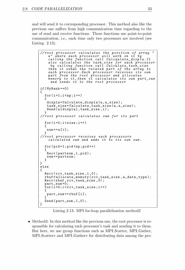
2.8. CODE PARALLELIZATION 33
and will send it to corresponding processor. This method also like theprevious one suffers from high communication time regarding to theuse of send and receive functions. These functions use point-to-pointcommunication, i.e., each time only two processors are involved (seeListing 2.13).
//root processor calculates the position of array "a" where each processor will work on it bycalling the function call Calcaulate_displa.Italso calculates the task_size for each processorby calling function call Calculate_task_size
then it sends the related part of the array toeach processor.Each processor receives its ownpart from the root processor and allocatesmemory to it,then it calculates its own part_sumand sends it to the root processor
if(MyRank ==0){
for(i=1;i<np;i++){displa=Calculate_displa(a,a_size);task_size=Calculate_task_size(a,a_size);Send(a[displa],task_size ,i);
}//root processor calculates sum for its part
for(i=0;i<size;i++){sum+=a[i];
}//root processor receives each processors
calculated sum and adds it to its own sum.
for(pid=1;pid <np;pid ++){Recv(partsum ,1,pid);sum+= partsum;
}}else{
Recv(rcv_task_size ,1,0);rbuf=allocate_memory(rcv_task_size ,a_data_type);Recv(rbuf ,rcv_task_size ,0);part_sum =0;for(i=0;i<rcv_task_size;i++){part_sum +=rbuf[i];
}Send(part_sum ,1,0);
}
Listing 2.13: MPI for-loop parallelization method2
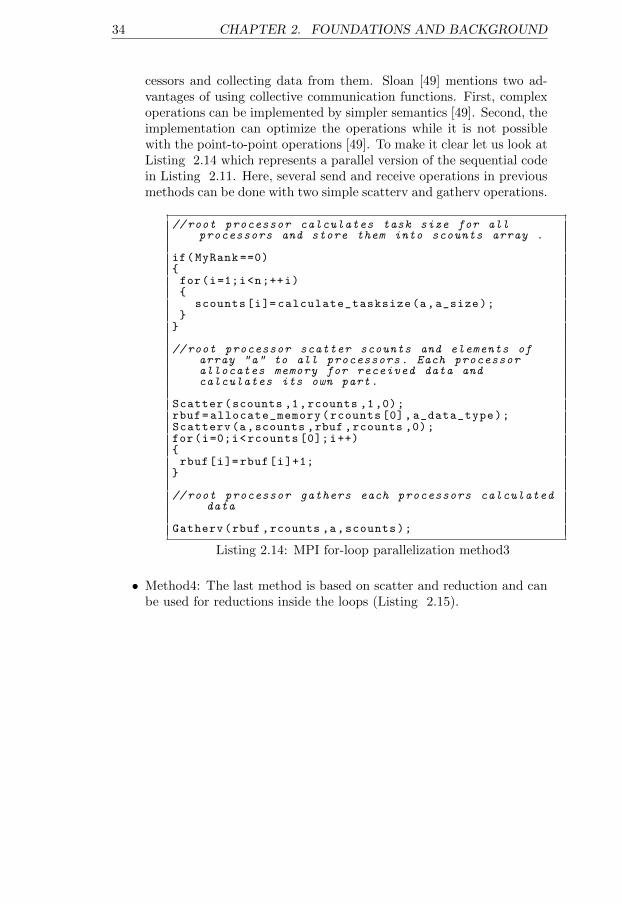
• Method3: In this method like the previous one, the root processor is re-sponsible for calculating each processor’s task and sending it to them.But here, we use group functions such as MPI Scatter, MPI Gather,MPI Scatterv and MPI Gatherv for distributing data among the pro-
34 CHAPTER 2. FOUNDATIONS AND BACKGROUND
cessors and collecting data from them. Sloan [49] mentions two ad-vantages of using collective communication functions. First, complexoperations can be implemented by simpler semantics [49]. Second, theimplementation can optimize the operations while it is not possiblewith the point-to-point operations [49]. To make it clear let us look atListing 2.14 which represents a parallel version of the sequential codein Listing 2.11. Here, several send and receive operations in previousmethods can be done with two simple scatterv and gatherv operations.
//root processor calculates task size for allprocessors and store them into scounts array .
if(MyRank ==0){for(i=1;i<n;++i){
scounts[i]= calculate_tasksize(a,a_size);}
}
//root processor scatter scounts and elements ofarray "a" to all processors. Each processorallocates memory for received data andcalculates its own part.
Scatter(scounts ,1,rcounts ,1,0);rbuf=allocate_memory(rcounts [0], a_data_type);Scatterv(a,scounts ,rbuf ,rcounts ,0);for(i=0;i<rcounts [0];i++){rbuf[i]=rbuf[i]+1;
}
//root processor gathers each processors calculateddata
Gatherv(rbuf ,rcounts ,a,scounts);
Listing 2.14: MPI for-loop parallelization method3
• Method4: The last method is based on scatter and reduction and canbe used for reductions inside the loops (Listing 2.15).
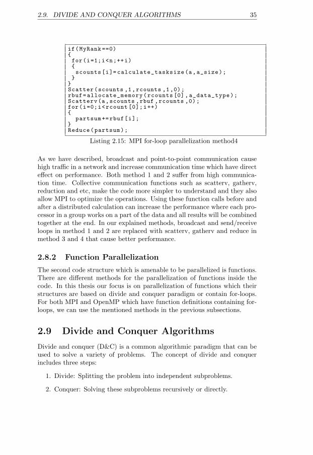
2.9. DIVIDE AND CONQUER ALGORITHMS 35
if(MyRank ==0){for(i=1;i<n;++i){scounts[i]= calculate_tasksize(a,a_size);
}}Scatter(scounts ,1,rcounts ,1,0);rbuf=allocate_memory(rcounts [0], a_data_type);Scatterv(a,scounts ,rbuf ,rcounts ,0);for(i=0;i<rcount [0];i++){
partsum +=rbuf[i];}Reduce(partsum);
Listing 2.15: MPI for-loop parallelization method4
As we have described, broadcast and point-to-point communication causehigh traffic in a network and increase communication time which have directeffect on performance. Both method 1 and 2 suffer from high communica-tion time. Collective communication functions such as scatterv, gatherv,reduction and etc, make the code more simpler to understand and they alsoallow MPI to optimize the operations. Using these function calls before andafter a distributed calculation can increase the performance where each pro-cessor in a group works on a part of the data and all results will be combinedtogether at the end. In our explained methods, broadcast and send/receiveloops in method 1 and 2 are replaced with scatterv, gatherv and reduce inmethod 3 and 4 that cause better performance.
2.8.2 Function Parallelization
The second code structure which is amenable to be parallelized is functions.There are different methods for the parallelization of functions inside thecode. In this thesis our focus is on parallelization of functions which theirstructures are based on divide and conquer paradigm or contain for-loops.For both MPI and OpenMP which have function definitions containing for-loops, we can use the mentioned methods in the previous subsections.
2.9 Divide and Conquer Algorithms
Divide and conquer (D&C) is a common algorithmic paradigm that can beused to solve a variety of problems. The concept of divide and conquerincludes three steps:
1. Divide: Splitting the problem into independent subproblems.
2. Conquer: Solving these subproblems recursively or directly.
36 CHAPTER 2. FOUNDATIONS AND BACKGROUND
3. Combine: Appropriately combining the results of the subproblems inorder to solve the original problem.
2.9.1 Parallelization of Divide and Conquer Algorithms
The structure of divide and conquer is adaptable for executing in parallel.As we described, the D&C technique is based on three steps ; divide, con-quer and combine. During the divide phase we obtain several independentsubtasks which can be executed in parallel. The parallelization steps of thesealgorithms are thus as follows:
1. Divide: In this step we must divide both processors and tasks. Pro-cessors are divided into subgroups of processors and tasks are dividedinto independent subtasks. For each subgroup of processors we willassign a number of subtasks. Here, we have to set a condition beforethe dividing phase such that when the condition fulfills the executionof the code switches to serial solution. Then, we will use the serialD&C algorithm.
2. Conquer: Solve in parallel.
3. Combine: After all subgroups solved their assigned tasks recursivelyor directly, their results will be combined.
In order to reach an optimized level of parallelization we have to considerbalance of workload between subgroups of processors. Without this con-sideration, it may happen that some processors finish their assigned taskssooner while others are still busy. In this situation the execution time willnot be as we expected because, for calculating it we consider the time fromthe beginning step until all engaged processors finish their jobs. By consid-ering this calculation, we have to focus more on division phase.
There exist several load balancing strategies for D&C. For instance, in[17], Eriksson et al. have discussed the benefits and drawbacks of task-queue, manager load balancing and overpartitioning strategies. This paperalso suggests a simplified variant for parallel Quick sort.
Binary tree division is a special case of dividing tasks between a numberof processors which is based on hierarchical division of tasks and processors.In this algorithm processors are divided into two equal sized subgroups thatwill each be assigned a number of tasks recursively. This method, besideseveral benefits such as fast computation of subtasks has some drawbacksand the most important one returns to load balancing, where as it works wellfor balanced D&C algorithms (the subtasks created by D&C algorithms areequal in size). For unbalanced D&C algorithms such as Quick sort where thesize of subtasks can be different it will cause bad load balancing; therefore, itmay happen that some processors work more while others have less work todo or they are idle. To solve this problem, Hardwick [25] defined the team-parallel model which overcomes the above mentioned problem by matchingthe teams’ sizes to the subtask sizes.
2.10. SORTING ALGORITHMS 37
2.10 Sorting algorithms
Sorting is the process of ordering a collection of data according to somekey, e.g. alphabetically or numerically. There are several sorting algorithms(Bubble sort, Merge sort, Insertion sort, Quick sort,. . . ) each one with itsown characteristics. To select one of these algorithms we should focus on afeature which is important for us. For example if efficiency is important itis better to choose Quick sort rather than Bubble sort since it has expectedless data movement and comparisons.
2.10.1 Sequential Quick sort
Quick sort is the fastest comparison-based sorting algorithm which was de-veloped by Tony Hoare in 1961. Time complexity of this algorithm is fluc-tuating between O(n log n) in the best case and O(n2) for the worst case.Quick sort is based on the divide and conquer paradigm and recursivelysorts data.
In the case of Quick sort the algorithm can be formulated as follows:
1. Select an element as a pivot.
2. divide the list into two sublists. One list includes data less than orequal to pivot and the other includes data higher than or equal topivot.
3. Sort the sublists recursively until no more division is possible.
Listing 2.16 represents an example of sequential Quick sort and Figure 2.11illustrates this concept.
In this algorithm selecting the pivot is a key point to reach the bestcomplexity. For the best performance result, the pivot must be selected ina way that the number of the elements in the created sublists be balanced.
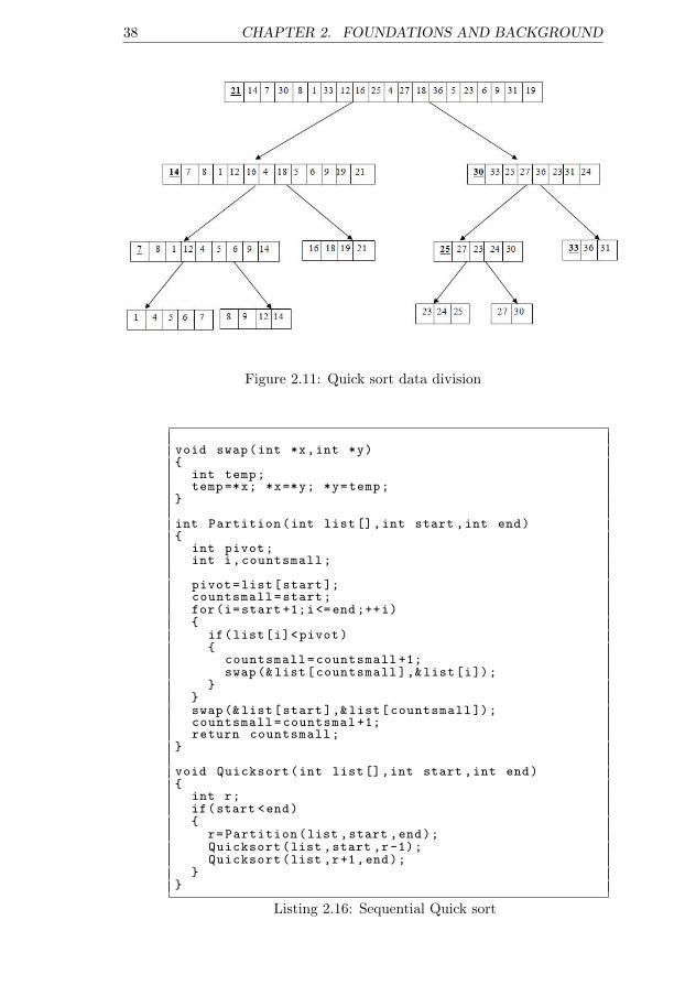
38 CHAPTER 2. FOUNDATIONS AND BACKGROUND
Figure 2.11: Quick sort data division
void swap(int *x,int *y){
int temp;temp=*x; *x=*y; *y=temp;
}
int Partition(int list[],int start ,int end){
int pivot;int i,countsmall;
pivot=list[start ];countsmall=start;for(i=start +1;i<=end ;++i){
if(list[i]<pivot){
countsmall=countsmall +1;swap(&list[countsmall ],&list[i]);
}}swap(&list[start],&list[countsmall ]);countsmall=countsmal +1;return countsmall;
}
void Quicksort(int list[],int start ,int end){
int r;if(start <end){
r=Partition(list ,start ,end);Quicksort(list ,start ,r-1);Quicksort(list ,r+1,end);
}}
Listing 2.16: Sequential Quick sort
2.10. SORTING ALGORITHMS 39
2.10.2 Parallel Quick sort
Quick sort is one of the sequential sorting algorithms which is suitable to beexecuted in parallel because of its D&C structure. In this algorithm the sub-lists recursively can be sorted in parallel. We considered two approaches forparallelizing the algorithm; MPI (message passing interface) for distributedmemory and OpenMP for shared memory (section 5.1.1 shows the OpenMPversion of this code).
There exists several methods for parallelizing Quick sort in MPI. In therest of this section we will describe three different MPI algorithms and dis-cuss advantages and disadvantages of them. These algorithms are takenfrom Quinn [45].
1. Algorithm1-Parallel Quick sortThis algorithm consists of the following steps:
(a) Divide data equally among processes.
(b) Process P0 randomly selects the pivot and broadcasts it to theother processes.
(c) All processes divide their unsorted list into two sublists: one listwith the elements smaller than or equal to pivot and another listwith the elements greater than or equal to pivot.
(d) Each process exchanges “lower list” and “upper list” values withits partner in the process list. For example, a process in the upperhalf of the process list (p(i+n/2): where i + n/2 is equal to thatprocess rank and n is the problem size) sends its lower sublist toits partner process (pi) in the lower half of the process list andreceives an upper list in return.
(e) Now our processes are divided into two groups and we recursivelyrepeat this algorithm for each half separately. After log p recur-sion steps, each process sorts its list by using sequential quicksort.
Poor load balancing is the weakness of this algorithm, since if theselected pivot element is not the median, the list will not be dividedinto two equal-sized sublists.
2. Algorithm2 - Hyperquick sortThis algorithm looks to some extent like the previous algorithm butthe selected pivot is more likely to be close to the true median.
(a) Divide data equally among processes. Each process locally sortsits assigned values.
(b) Process P0 selects its median value as a pivot and broadcasts itto the other processes.
40 CHAPTER 2. FOUNDATIONS AND BACKGROUND
(c) As in the previous algorithm, the processes exchange their lowand high sublists with their partners.
(d) Each process merges and sorts its values with the received list’svalues.
(e) Now, like in the previous algorithm, our processes are dividedinto two groups and we recursively apply this algorithm for eachhalf separately in parallel. After log p exchange steps our list willbe sorted.
Although this algorithm is better than the previous one in load bal-ancing it still may happen that the selected pivot is not the truemedian. The initial Quick sort step has complexity time equal toO((n/p) log(n/p)) and the total communication time for this algorithmfor log p exchange steps is O((n/p) log p)) [45].
3. Algorithm 3 - Parallel Sorting by Regular Sampling (PSRS)Compared to the two other algorithms this algorithm has the best listsize balance. It can be done in the following steps.
(a) Divide the data equally among the processes. Each process lo-cally sorts the assigned values.
(b) Each process selects elements 0, n/p2, 2n/p2, . . . , (p − 1)n/p2 ofits list
(c) One process will gather and sort the p2 selected elements fromall processes. (p − 1) pivots will be selected by this process andbroadcasted to others.
(d) Each process divides its list into p partitions. It keeps the parti-tion whose index is equal to its process rank and sends the otherpartitions to their corresponding processes.
(e) Each process will merge the (p − 1) received partitions with itsown partition.
In the two previous algorithms the number of processors must be apower of 2, but in this algorithm we do not have such a restriction.This algorithm has the best load balancing among these three. Thetotal communication time for this algorithm is O((n/p)(log n+log p)+p2 log p) [45].
2.11 Jacobi method
In this thesis, we have selected an example for loop-based parallelizationwhich is based on the Jacobi iteration example in [50]. Figure 2.12 depictsthis concept.
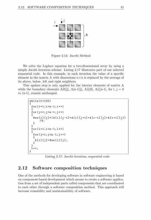
2.12. SOFTWARE COMPOSITION TECHNIQUES 41
Figure 2.12: Jacobi Method
We solve the Laplace equation for a two-dimensional array by using asimple Jacobi iteration scheme. Listing 2.17 illustrates part of our selectedsequential code. In this example, in each iteration the value of a specificelement in the matrix A with dimensions n ∗n is replaced by the average ofits above, below, left and right neighbors.
This update step is only applied for the interior elements of matrix Awhile the boundary elements A[0][j], A[n-1][j], A[i][0], A[i][n-1], for i, j = 0to (n-1), remain unchanged.
while(t <100){for(i=1;i<n-1;i++){for(j=1;j<n-1;j++){New[i][j]=(A[i][j-1]+A[i][j+1]+A[i-1][j]+A[i+1][j])
/4;}
}for(i=1;i<n-1;i++){for(j=1;j<n-1;j++){A[i][j]=New[i][j];
}}t++;
}
Listing 2.17: Jacobi iteration, sequential code
2.12 Software composition techniques
One of the methods for developing software in software engineering is basedon component-based development which means to create a software applica-tion from a set of independent parts called components that are coordinatedto each other through a software composition method. This approach willincrease reusability and maintainability of software.
42 CHAPTER 2. FOUNDATIONS AND BACKGROUND
A software component is an independent executable unit which can beused as a part of a system [55]. Meta Group [21] defines software componentsas “ prefabricated, pre-tested, self-contained, reusable software modules -bundles of data and procedures - that perform specific functions”. We candivide components into three different categories:
• Blackbox component: the internal structure of the component is in-visible to programmer, its content is fixed and not changeable. Theprogrammer can get information about its functionality through somepredefined documents.
• Whitebox component: the internal structure is readable to the pro-grammer and its content is directly changeable.
• Graybox component: is between Blackbox and Whitebox componentswhich means that the user is able to change some specific parts of thecomponent.
A notion of component without composition is meaningless. According toHeineman [26], “Composition is the combination of two or more softwarecomponents yielding a new component behavior at a different level of ab-straction.”
After we defined our components we need glue code to join them.Graybox component composition is what we want to apply in our project,controlled by user interaction. We have defined some templates throughstrategies and a user is able to change parts of them. We want our user tobe able to inject parallelization code into a selected part of the sequentialcode.
Among the known Graybox composition models the most well-knownones are: Aspect-Oriented Programming, View-based Programming and In-vasive Software Composition.
2.12.1 Aspect-Oriented Programming (AOP)
Before going through AOP, we define the notion of crosscut. Crosscut meanscomposition of concerns “such as: exception handling, real-time constraints,distribution and concurrency control” with the application core in differentways while they are coordinated [42]. Properties may crosscut components.A system property can be implemented either as a component if it is possibleto encapsulate it as a generalized procedure (class, method or procedure) oras an aspect if it “affects classes in a systematic way” [42].
The goal of Aspect-Oriented Programming (AOP) is to help the devel-oper to separate and modularize crosscutting concerns and find the “mech-anisms to compose them to produce the desired system ” [24, 42]. By spec-ifying how and at what points an aspect influences other modules we canencapsulate code that spreads throughout other modules into one aspect.We call these points join points and for describing them we usually usecrosscut languages such as Aspect-J [24].
2.13. INVASIVE INTERACTIVE PARALLELIZATION 43
2.12.2 Template Metaprogramming
Template metaprogramming is based on static metaprogramming by usingtemplates. A metaprogram is a program that can analyze, and possiblychange or manipulate other programs in such a way that new programs willbe generated. In template metaprogramming the compiler uses templates(as in C++) in order to create new source codes and merge and compilethem with the rest of the codes [57].
2.12.3 Invasive Software Composition
Invasive Software Composition (ISC) is a static metaprogramming method.It aims to improve components’ reusability by transformation, which meansthat ISC adapts, extends and transforms components at hooks during com-position. We encapsulate (source-level) components as fragment boxes, codeanchor points as hooks and the composition operators as composers.
Hooks are arbitrary program elements or variation points of a box (com-ponent), i.e. code fragments or positions which are subject to change. Thereare two kinds of hooks, implicit and declared hooks. An implicit hook is aprogram element that is implied by the syntax and/or semantics of the un-derlying programming language (e.g. method entry/exit). A declared hookis a program element defined by the box writer as a placeholder that issubject to change (e.g. generic types of parameters) [6].
Composers are program generators and transformers. A composer’s maintasks are to prepare pattern matching (e.g., navigate through the serial pro-gram to find matching statements), modify (e.g., parallelize) the statement(e.g. introduce data distribution, introduce data collection, introduce workload sharing), adapt the surrounding function by declaring necessary vari-ables, and adapt the whole program (include necessary libraries, initializeinter-process communication, clean up). The composition is invasive, as theoperators change invasively the fragments in the components [6].
2.13 Invasive Interactive Parallelization
Invasive Interactive Parallelization (IIP) is a method for parallelizing sequen-tial code which is based on separation of concerns and invasive composition[13]. In this method, parallelizing code will be injected into sequential codebased on defined rules and strategies and with user hints. The program-mer will pinpoint parts of the code to be parallelized and the system willsupport him/her by giving suggestions based on defined strategies. Thisinteraction will continue until the programmer stops it. The semantics ofthe output (parallelized code) is the same as the sequential code unless theuser explicitly advised the system to change it.
As we described in section 1.2, an IIP system consists of three corecomponents - interaction engine, reasoning engine, and weaving engine. The
44 CHAPTER 2. FOUNDATIONS AND BACKGROUND
interaction engine implements the communication between the programmerand the system by accepting the user’s requests.
The reasoning engine which has a main role in parallelizing the codewill accept the user’s requests for automated reasoning and give suggestionsbased on defined strategies and rules.
At last the weaving engine will inject all advices of aspects (selectedparallelization code parts) at the right place based on a specific definedorder or default system order.
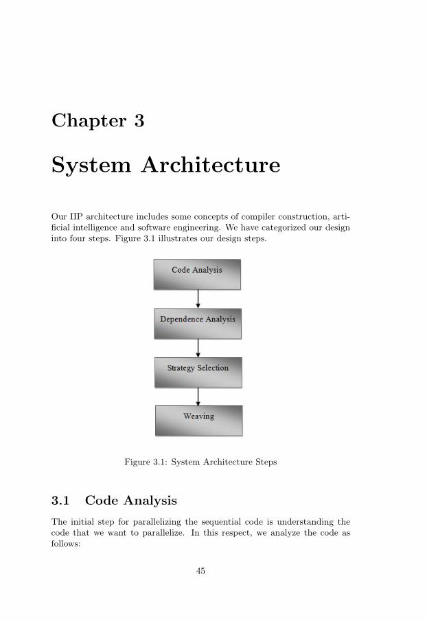
Chapter 3
System Architecture
Our IIP architecture includes some concepts of compiler construction, arti-ficial intelligence and software engineering. We have categorized our designinto four steps. Figure 3.1 illustrates our design steps.
Figure 3.1: System Architecture Steps
3.1 Code Analysis
The initial step for parallelizing the sequential code is understanding thecode that we want to parallelize. In this respect, we analyze the code asfollows:
45
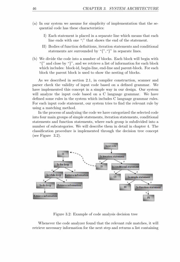
46 CHAPTER 3. SYSTEM ARCHITECTURE
(a) In our system we assume for simplicity of implementation that the se-quential code has these characteristics:
I) Each statement is placed in a separate line which means that eachline ends with one “;” that shows the end of the statement.
II) Bodies of function definitions, iteration statements and conditionalstatements are surrounded by “{”,“}” in separate lines.
(b) We divide the code into a number of blocks. Each block will begin with“{” and close by “}”, and we retrieve a list of information for each blockwhich includes: block-id, begin-line, end-line and parent-block. For eachblock the parent block is used to show the nesting of blocks.
As we described in section 2.1, in compiler construction, scanner andparser check the validity of input code based on a defined grammar. Wehave implemented this concept in a simple way in our design. Our systemwill analyze the input code based on a C language grammar. We havedefined some rules in the system which includes C language grammar rules.For each input code statement, our system tries to find the relevant rule byusing a matching method.
In the process of analyzing the code we have categorized the selected codeinto four main groups of simple statements, iteration statements, conditionalstatements and function statements, where each group is subdivided into anumber of subcategories. We will describe them in detail in chapter 4. Theclassification procedure is implemented through the decision tree concept(see Figure 3.2).
Figure 3.2: Example of code analysis decision tree
Whenever the code analyzer found that the relevant rule matches, it willretrieve necessary information for the next step and returns a list containing
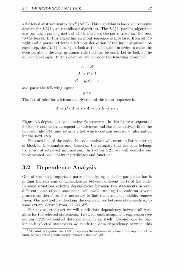
3.2. DEPENDENCE ANALYSIS 47
a flattened abstract syntax tree2 (AST). This algorithm is based on recursivedescent for LL(1), an established algorithm. The LL(1) parsing algorithmis a top-down parsing method which traverses the parse tree from the rootto the leaves. In this algorithm an input sequence is processed from left toright and a parser retrieves a leftmost derivation of the input sequence. Ateach step, the LL(1) parser just look at the next token in order to make thedecision about the next grammar rule that can be used. Let us look at thefollowing example. In this example, we consider the following grammar:
A→ B
A→ B ∗A
B → y|z| · · · |ε
and parse the following input:y ∗ z
The list of rules for a leftmost derivation of the input sequence is:
A→ B ∗A→ y ∗A→ y ∗B → y ∗ z
Figure 3.3 depicts our code analyzer’s structure. In this figure a sequentialfor-loop is selected as a sequential statement and the code analyzer finds therelevant rule (R4) and returns a list which contains necessary informationfor the next step.
For each line of the code, the code analyzer will create a list consistingof block-id, line-number and, based on the category that the code belongsto, a list of retrieved information. In section 4.2.1 we will describe ourimplemented code analyzer predicates and functions.
3.2 Dependence Analysis
One of the most important parts of analyzing code for parallelization isfinding the relations or dependencies between different parts of the code.In some situations existing dependencies between two statements or evendifferent parts of one statement, will avoid running the code on severalprocessors; therefore, it is necessary to find them and, if possible, removethem. Our method for checking the dependences between statements is, tosome extent, derived from [22, 23, 32].
For any selected part we will check data dependency between all vari-ables for the selected statements. First, for each assignment expression (seesection 4.2.2) we control data dependency on itself. Second, one by one,for each selected statements we check the data dependency between this
2“An abstract syntax tree (AST) captures the essential structure of the input in a treeform, while omitting unnecessary syntactic details” [30].
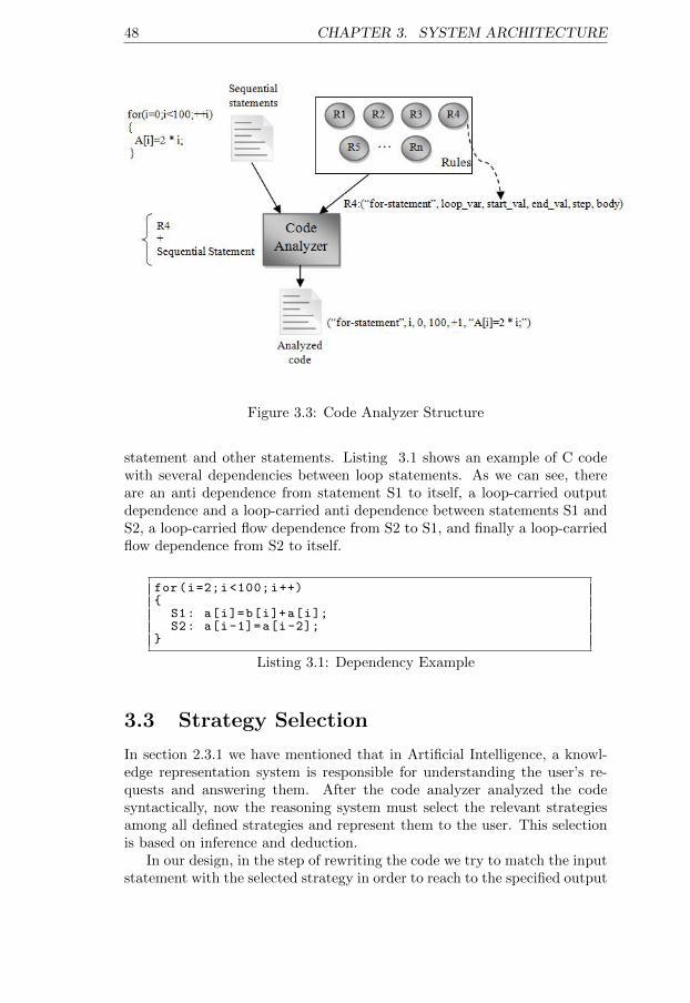
48 CHAPTER 3. SYSTEM ARCHITECTURE
Figure 3.3: Code Analyzer Structure
statement and other statements. Listing 3.1 shows an example of C codewith several dependencies between loop statements. As we can see, thereare an anti dependence from statement S1 to itself, a loop-carried outputdependence and a loop-carried anti dependence between statements S1 andS2, a loop-carried flow dependence from S2 to S1, and finally a loop-carriedflow dependence from S2 to itself.
for(i=2;i <100;i++){
S1: a[i]=b[i]+a[i];S2: a[i-1]=a[i-2];
}
Listing 3.1: Dependency Example
3.3 Strategy Selection
In section 2.3.1 we have mentioned that in Artificial Intelligence, a knowl-edge representation system is responsible for understanding the user’s re-quests and answering them. After the code analyzer analyzed the codesyntactically, now the reasoning system must select the relevant strategiesamong all defined strategies and represent them to the user. This selectionis based on inference and deduction.
In our design, in the step of rewriting the code we try to match the inputstatement with the selected strategy in order to reach to the specified output
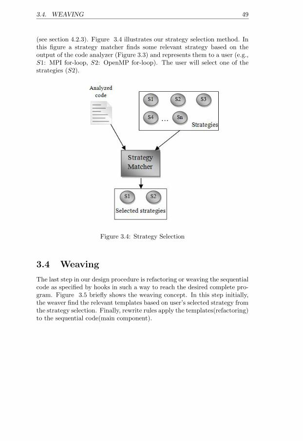
3.4. WEAVING 49
(see section 4.2.3). Figure 3.4 illustrates our strategy selection method. Inthis figure a strategy matcher finds some relevant strategy based on theoutput of the code analyzer (Figure 3.3) and represents them to a user (e.g.,S1: MPI for-loop, S2: OpenMP for-loop). The user will select one of thestrategies (S2).
Figure 3.4: Strategy Selection
3.4 Weaving
The last step in our design procedure is refactoring or weaving the sequentialcode as specified by hooks in such a way to reach the desired complete pro-gram. Figure 3.5 briefly shows the weaving concept. In this step initially,the weaver find the relevant templates based on user’s selected strategy fromthe strategy selection. Finally, rewrite rules apply the templates(refactoring)to the sequential code(main component).
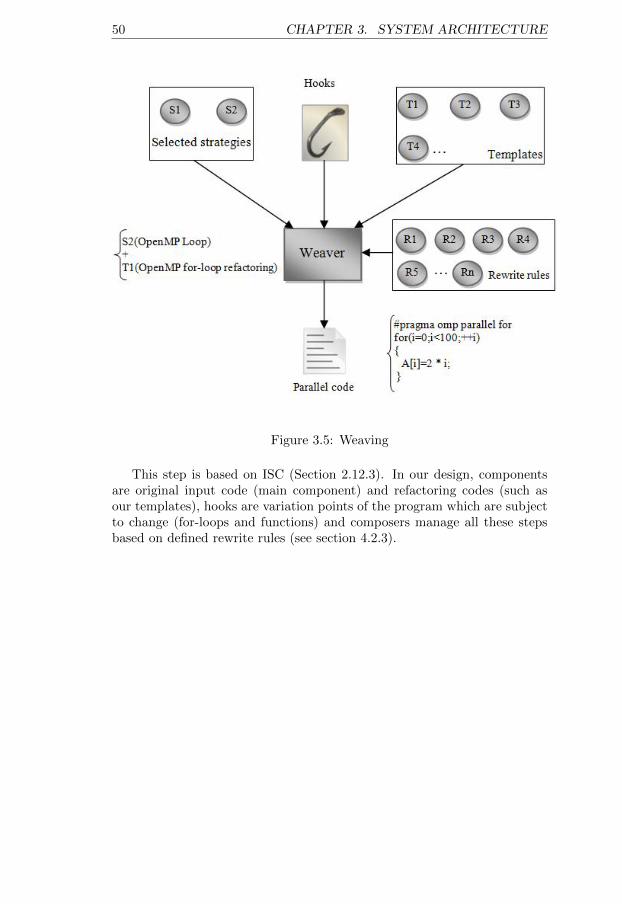
50 CHAPTER 3. SYSTEM ARCHITECTURE
Figure 3.5: Weaving
This step is based on ISC (Section 2.12.3). In our design, componentsare original input code (main component) and refactoring codes (such asour templates), hooks are variation points of the program which are subjectto change (for-loops and functions) and composers manage all these stepsbased on defined rewrite rules (see section 4.2.3).
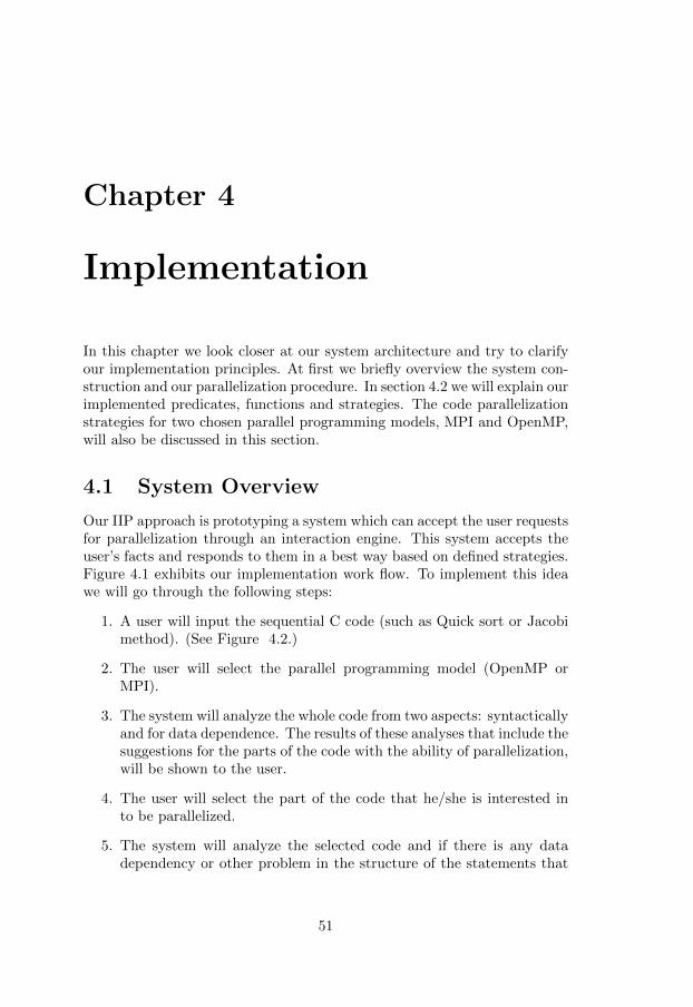
Chapter 4
Implementation
In this chapter we look closer at our system architecture and try to clarifyour implementation principles. At first we briefly overview the system con-struction and our parallelization procedure. In section 4.2 we will explain ourimplemented predicates, functions and strategies. The code parallelizationstrategies for two chosen parallel programming models, MPI and OpenMP,will also be discussed in this section.
4.1 System Overview
Our IIP approach is prototyping a system which can accept the user requestsfor parallelization through an interaction engine. This system accepts theuser’s facts and responds to them in a best way based on defined strategies.Figure 4.1 exhibits our implementation work flow. To implement this ideawe will go through the following steps:
1. A user will input the sequential C code (such as Quick sort or Jacobimethod). (See Figure 4.2.)
2. The user will select the parallel programming model (OpenMP orMPI).
3. The system will analyze the whole code from two aspects: syntacticallyand for data dependence. The results of these analyses that include thesuggestions for the parts of the code with the ability of parallelization,will be shown to the user.
4. The user will select the part of the code that he/she is interested into be parallelized.
5. The system will analyze the selected code and if there is any datadependency or other problem in the structure of the statements that
51
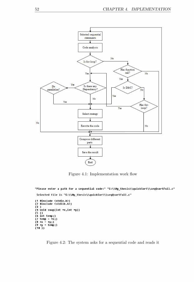
52 CHAPTER 4. IMPLEMENTATION
Figure 4.1: Implementation work flow
Figure 4.2: The system asks for a sequential code and reads it
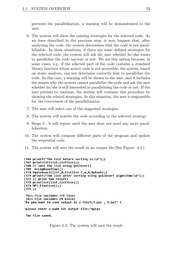
4.1. SYSTEM OVERVIEW 53
prevents the parallelization, a warning will be demonstrated to theuser.
6. The system will show the existing strategies for the selected code. Aswe have described in the previous step, it may happen that, afteranalyzing the code, the system determines that the code is not paral-lelizable. In these situations, if there are some defined strategies forthe selected code, the system will ask the user whether he/she wantsto parallelize the code anyway or not. We set this option because, insome cases, e.g. if the selected part of the code contains a standardlibrary function whose source code is not accessible, the system, basedon static analysis, can not determine correctly how to parallelize thecode. In this case, a warning will be shown to the user, and it includesthe reason why the system cannot parallelize the code and ask the userwhether he/she is still interested in parallelizing the code or not. If theuser persists to continue, the system will continue this procedure byshowing the related strategies. In this situation, the user is responsiblefor the correctness of the parallelization.
7. The user will select one of the suggested strategies.
8. The system will rewrite the code according to the selected strategy.
9. Steps 4 - 8 will repeat until the user does not need any more paral-lelization.
10. The system will compose different parts of the program and updatethe sequential code.
11. The system will save the result in an output file.(See Figure 4.3.)
Figure 4.3: The system will save the result
54 CHAPTER 4. IMPLEMENTATION
4.2 Implemented Predicates and Functions
In the previous section we described our parallelization procedure. Since thesystem is built for both message passing and OpenMP, from the implemen-tation point of view we decompose our predicates and functions into twogroups, namely common predicates and functions which are independent ofthe target programming model (such as code analysis and dependence anal-ysis predicates and functions), and target-specific predicates and functionswhich include both strategy selection and weaving predicates and functions.
We have chosen Lisp which is one of the programming languages in AI(see section 2.3.5) as our implementation language. All our implementationsare done in the Allegro CL development system [28].
4.2.1 Code Analysis
As we have mentioned in section 3.1, we have divided the code statementsinto four main groups where each group is subdivided into several subcate-gories. These groups and their subdivisions are the base of our code analysisand we will explain them in this subsection. But first of all, we point toone important function which is used in all four groups’ analysis, “variabletype”.
• Variable type: Different variables need different treatment in theprocedure of code generation. We have divided variables into threegroups:
1. Constants: Constants are numerical terms with the data typesinteger, float, double, etc. whose values never change.
2. Scalars: These variables are usually identified by an identifier andthey have just one value at a time.
3. Arrays: Arrays are defined by name, dimensions and number ofelements where each element has a specific value.
• Simple statement: In this project we have grouped directives (e.g.,#include, #define, . . . ), declaration statements (such statements con-sist of a variable name and its data type e.g.,“int x;” ), jump statements(the statements that may change the control to some other point inthe code, such as return, goto, break, and continue), comments, andexpressions as simple statements.
Among these statements, the expressions have a more important rolein the parallelization process. They consist of one or more operandsand at least one operator. We have grouped expressions into sixsubcategories: assignment expressions, relational expressions, binaryexpressions, auto-increment/auto-decrement expressions, variable ac-cesses and function calls.
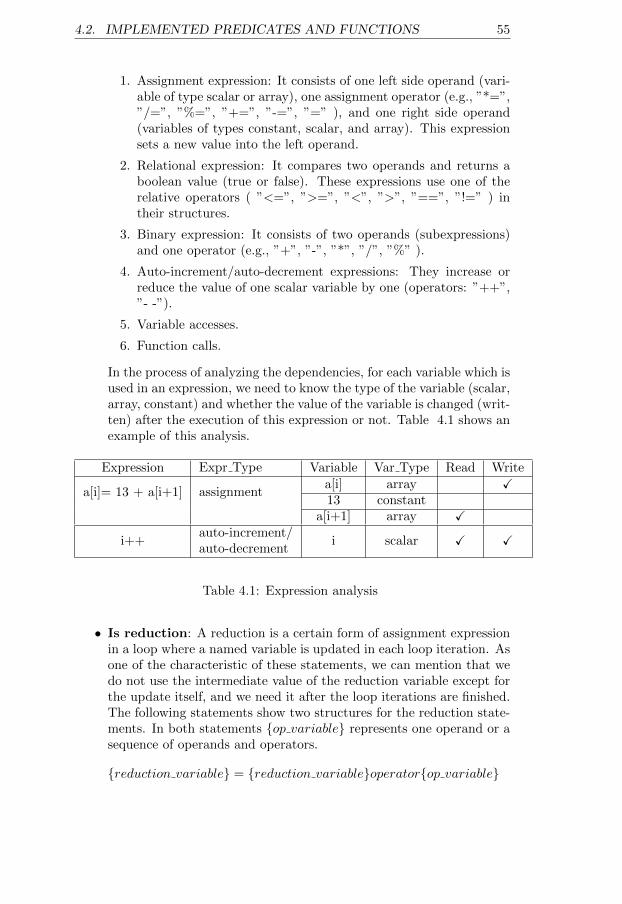
4.2. IMPLEMENTED PREDICATES AND FUNCTIONS 55
1. Assignment expression: It consists of one left side operand (vari-able of type scalar or array), one assignment operator (e.g., ”*=”,”/=”, ”%=”, ”+=”, ”-=”, ”=” ), and one right side operand(variables of types constant, scalar, and array). This expressionsets a new value into the left operand.
2. Relational expression: It compares two operands and returns aboolean value (true or false). These expressions use one of therelative operators ( ”<=”, ”>=”, ”<”, ”>”, ”==”, ”!=” ) intheir structures.
3. Binary expression: It consists of two operands (subexpressions)and one operator (e.g., ”+”, ”-”, ”*”, ”/”, ”%” ).
4. Auto-increment/auto-decrement expressions: They increase orreduce the value of one scalar variable by one (operators: ”++”,”- -”).
5. Variable accesses.
6. Function calls.
In the process of analyzing the dependencies, for each variable which isused in an expression, we need to know the type of the variable (scalar,array, constant) and whether the value of the variable is changed (writ-ten) after the execution of this expression or not. Table 4.1 shows anexample of this analysis.
Expression Expr Type Variable Var Type Read Write
a[i]= 13 + a[i+1] assignmenta[i] array X13 constant
a[i+1] array X
i++auto-increment/auto-decrement
i scalar X X
Table 4.1: Expression analysis
• Is reduction: A reduction is a certain form of assignment expressionin a loop where a named variable is updated in each loop iteration. Asone of the characteristic of these statements, we can mention that wedo not use the intermediate value of the reduction variable except forthe update itself, and we need it after the loop iterations are finished.The following statements show two structures for the reduction state-ments. In both statements {op variable} represents one operand or asequence of operands and operators.
{reduction variable} = {reduction variable}operator{op variable}
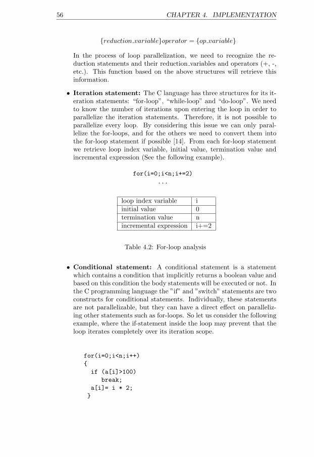
56 CHAPTER 4. IMPLEMENTATION
{reduction variable}operator = {op variable}
In the process of loop parallelization, we need to recognize the re-duction statements and their reduction variables and operators (+, -,etc.). This function based on the above structures will retrieve thisinformation.
• Iteration statement: The C language has three structures for its it-eration statements: “for-loop”, “while-loop” and “do-loop”. We needto know the number of iterations upon entering the loop in order toparallelize the iteration statements. Therefore, it is not possible toparallelize every loop. By considering this issue we can only paral-lelize the for-loops, and for the others we need to convert them intothe for-loop statement if possible [14]. From each for-loop statementwe retrieve loop index variable, initial value, termination value andincremental expression (See the following example).
for(i=0;i<n;i+=2)
...
loop index variable iinitial value 0termination value nincremental expression i+=2
Table 4.2: For-loop analysis
• Conditional statement: A conditional statement is a statementwhich contains a condition that implicitly returns a boolean value andbased on this condition the body statements will be executed or not. Inthe C programming language the ”if” and ”switch” statements are twoconstructs for conditional statements. Individually, these statementsare not parallelizable, but they can have a direct effect on paralleliz-ing other statements such as for-loops. So let us consider the followingexample, where the if-statement inside the loop may prevent that theloop iterates completely over its iteration scope.
for(i=0;i<n;i++)
{
if (a[i]>100)
break;
a[i]= i * 2;
}
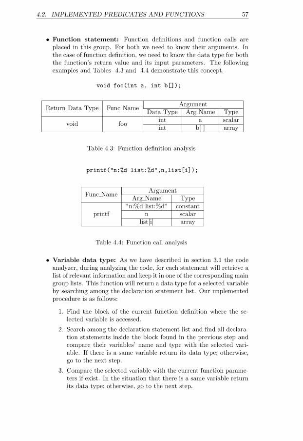
4.2. IMPLEMENTED PREDICATES AND FUNCTIONS 57
• Function statement: Function definitions and function calls areplaced in this group. For both we need to know their arguments. Inthe case of function definition, we need to know the data type for boththe function’s return value and its input parameters. The followingexamples and Tables 4.3 and 4.4 demonstrate this concept.
void foo(int a, int b[]);
Return Data Type Func NameArgument
Data Type Arg Name Type
void fooint a scalarint b[ ] array
Table 4.3: Function definition analysis
printf("n:%d list:%d",n,list[i]);
Func NameArgument
Arg Name Type
printf”n:%d list:%d” constant
n scalarlist[i] array
Table 4.4: Function call analysis
• Variable data type: As we have described in section 3.1 the codeanalyzer, during analyzing the code, for each statement will retrieve alist of relevant information and keep it in one of the corresponding maingroup lists. This function will return a data type for a selected variableby searching among the declaration statement list. Our implementedprocedure is as follows:
1. Find the block of the current function definition where the se-lected variable is accessed.
2. Search among the declaration statement list and find all declara-tion statements inside the block found in the previous step andcompare their variables’ name and type with the selected vari-able. If there is a same variable return its data type; otherwise,go to the next step.
3. Compare the selected variable with the current function parame-ters if exist. In the situation that there is a same variable returnits data type; otherwise, go to the next step.
58 CHAPTER 4. IMPLEMENTATION
4. In the case that the selected variable is a global variable, oursystem will try to find the data type by checking the declarationstatements inside the parent block of the function found in thefirst step .
4.2.2 Dependency Analysis
• Dependency from one statement to itself: In the process of de-pendency analysis, given an expression statement, we usually checkdependencies on itself. Zima et al. [60] divide each statement’s ac-cessed variables into two different sets, “Definition” and “Use”. TheDefinition set includes all variables of the statement that are writtenduring the execution of the statement and the Use set holds variablesthat are read. A dependency exists from one expression to itself if thereare common variables in both mentioned sets. We find dependenciesas follows:
– Create a Definition set and a Use set for the statement.
– Based on constraint 4.1, our system will determine the existenceof a dependence.
S.Definition ∩ S.Use 6= φ. (4.1)
– After the data dependence analysis is completed, if the output ofconstraint 4.1 is a list of variables, this list will be checked. Anydata dependence between scalar variables is a self-dependence.For array accesses, we have to calculate the distance betweentheir indices. Here let IndexA be an array index expression in aDefinition set and IndexB an index expression of the same arrayin a Use set:
If indexA-indexB < 0; there exists forward dependenceIf indexA-indexB > 0; there exists backward dependenceIf indexA-indexB = 0; there exists self-dependence
Let us look at the following example:
S: a[i]=a[i]+1
As we can see, there is a self-dependence from S to S.
• Dependency between two statements: This predicate will checkthe dependency between two statements of the code. We can use thispredicate in several situations. For example, if we want to parallelizea for-loop, we need to consider dependencies between different state-ments of its body, or when we want to parallelize a function which
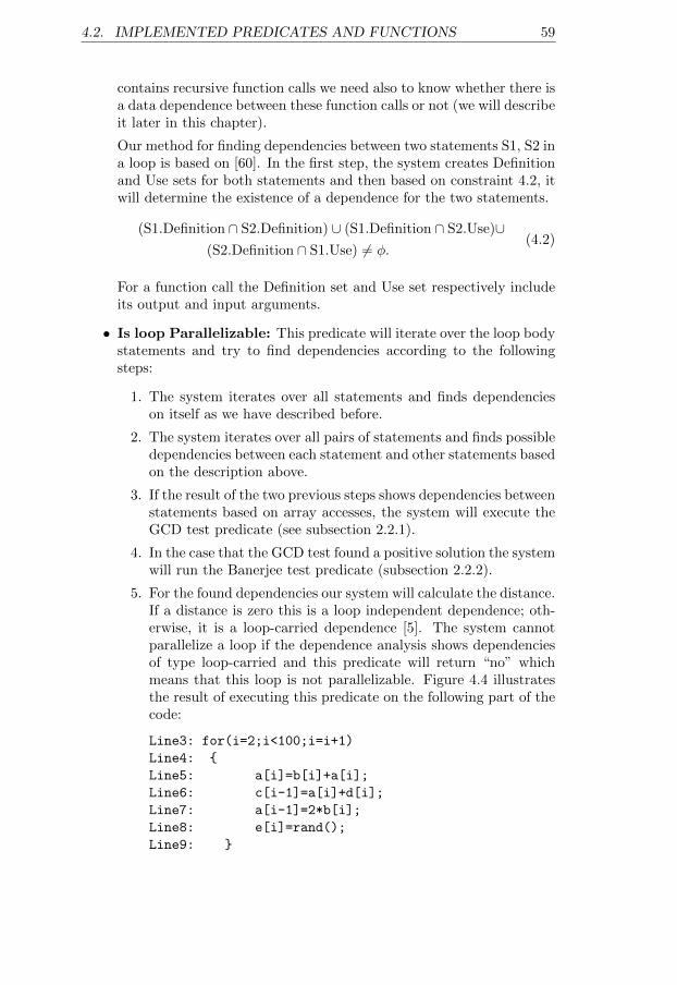
4.2. IMPLEMENTED PREDICATES AND FUNCTIONS 59
contains recursive function calls we need also to know whether there isa data dependence between these function calls or not (we will describeit later in this chapter).
Our method for finding dependencies between two statements S1, S2 ina loop is based on [60]. In the first step, the system creates Definitionand Use sets for both statements and then based on constraint 4.2, itwill determine the existence of a dependence for the two statements.
(S1.Definition ∩ S2.Definition) ∪ (S1.Definition ∩ S2.Use)∪(S2.Definition ∩ S1.Use) 6= φ.
(4.2)
For a function call the Definition set and Use set respectively includeits output and input arguments.
• Is loop Parallelizable: This predicate will iterate over the loop bodystatements and try to find dependencies according to the followingsteps:
1. The system iterates over all statements and finds dependencieson itself as we have described before.
2. The system iterates over all pairs of statements and finds possibledependencies between each statement and other statements basedon the description above.
3. If the result of the two previous steps shows dependencies betweenstatements based on array accesses, the system will execute theGCD test predicate (see subsection 2.2.1).
4. In the case that the GCD test found a positive solution the systemwill run the Banerjee test predicate (subsection 2.2.2).
5. For the found dependencies our system will calculate the distance.If a distance is zero this is a loop independent dependence; oth-erwise, it is a loop-carried dependence [5]. The system cannotparallelize a loop if the dependence analysis shows dependenciesof type loop-carried and this predicate will return “no” whichmeans that this loop is not parallelizable. Figure 4.4 illustratesthe result of executing this predicate on the following part of thecode:
Line3: for(i=2;i<100;i=i+1)
Line4: {
Line5: a[i]=b[i]+a[i];
Line6: c[i-1]=a[i]+d[i];
Line7: a[i-1]=2*b[i];
Line8: e[i]=rand();
Line9: }
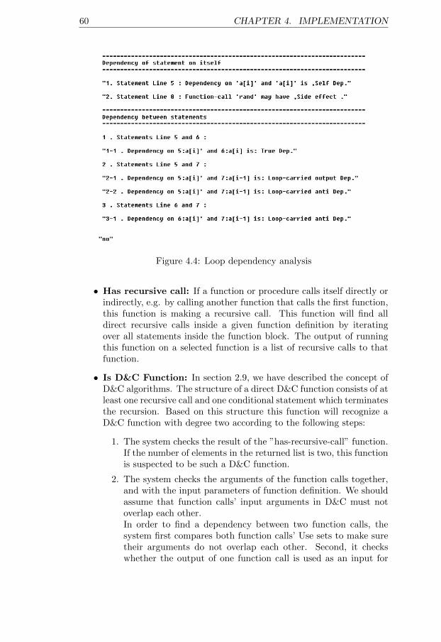
60 CHAPTER 4. IMPLEMENTATION
Figure 4.4: Loop dependency analysis
• Has recursive call: If a function or procedure calls itself directly orindirectly, e.g. by calling another function that calls the first function,this function is making a recursive call. This function will find alldirect recursive calls inside a given function definition by iteratingover all statements inside the function block. The output of runningthis function on a selected function is a list of recursive calls to thatfunction.
• Is D&C Function: In section 2.9, we have described the concept ofD&C algorithms. The structure of a direct D&C function consists of atleast one recursive call and one conditional statement which terminatesthe recursion. Based on this structure this function will recognize aD&C function with degree two according to the following steps:
1. The system checks the result of the ”has-recursive-call” function.If the number of elements in the returned list is two, this functionis suspected to be such a D&C function.
2. The system checks the arguments of the function calls together,and with the input parameters of function definition. We shouldassume that function calls’ input arguments in D&C must notoverlap each other.In order to find a dependency between two function calls, thesystem first compares both function calls’ Use sets to make suretheir arguments do not overlap each other. Second, it checkswhether the output of one function call is used as an input for
4.2. IMPLEMENTED PREDICATES AND FUNCTIONS 61
the other or not. In this respect, it finds the common variablesbetween the first function call’s Definition set and the secondfunction call’s Use set.
3. There should be a conditional statement that, whenever its valueis true, prevents the execution of the program from going intodivide phase and recursive calls.
Based on the above mentioned procedure, this function will determinewhether the function is D&C or not. In the case that the systemanalysis finds out that the selected function is D&C, it will show amessage to the user and wait for his/her confirmation (see Figure5.3). If the user accepts that the function is D&C, this function willreturn the line numbers of the recursive calls and a partition variableif it exists. The partition variable is a scalar variable (index of arrayoperand) that splits the problem into subproblems.
• Retrieve D&C Function parameters: In order to parallelize theD&C functions we need to identify three parts: divide part, recursivecalls and combine part.By executing “Is D&C Function” function, we will have the partitionvariable and the positions of the two recursive calls inside the code.In order to find the divide part we have to check all the statements be-fore the first recursive call. If there is just one assignment expressionor function call which calculates this partition variable, the systemassumes this statement as the divide part. Otherwise, it considers allthe statements before the first recursive call as the divide part and,for simplicity of later use, it creates a new function, copies all thesestatements into this new function and names it as “partition func-tion”. Here we should mention that, before copying the statements,the system will show a message which contains the found partitionlines to the user and, if he/she confirms it, our system will copy thecode; otherwise, it will ask the user to give the line numbers and thenit will copy the mentioned lines. For more details the reader may lookat the system-parallelized MPI Quick sort in Figure 5.3.The combine statements are usually placed after the last recursive call.As we have done for the divide part, for the combine part also, thesystem will find the combine statement(s). In the situation that thereare several statements in the combine part, it refactors them in a newfunction which is called “combine function”.
• Is function Parallelizable: Parallelizing independent function callsmay have a completely positive effect on the performance. In contrast,a function call itself is just a single statement, thus our judgment aboutits parallelizability is based on its function definition. Since we do nothave access to the source code of the system library functions (e.g.printf, scanf,. . . ) we can not predict their side effects in dependence
62 CHAPTER 4. IMPLEMENTATION
analysis with respect to this definition.This predicate receives a function call as an input and determines itsparallelizability in the following steps:
1. Find the relevant function definition by checking the name, thenumber of the arguments and the arguments’ types.
2. Check if the function definition is a D&C function or not, byexecuting the “ is D&C Function” function.
3. If the selected function is not a D&C function, the system willlook for for-loops and run the “is loop Parallelizable” predicateto check whether any loop exists inside this function definitionwhich is possible to be parallelized or not.
4. If the system does not find any solution, the result of this predi-cate is “no” which means that this function is not parallelizable.
Let us look at the following example, where we want to check theparallelizability of the function call foo() in line 14. Figure 4.5 depictsthe result of executing this predicate on the following code.
Line1: #include<stdio.h>
Line2: void foo()
Line3: {
Line4: int i,a[100],b[100],e[100];
Line5: for(i=2;i<100;i=i+1)
Line6: {
Line7: a[i]=b[i]+a[i];
Line8: a[i-1]=2*b[i];
Line9: e[i]=rand();
Line10: }
Line11: }
Line12: int main()
Line13: {
Line14: foo();
Line15: }
4.2.3 Strategy Selection and Weaving
All of the above defined predicates and functions can be used for both MPIand OpenMP models. In this part our focus is on the predicates and func-tions which implement both for-loop and function parallelization strategiesfor each of these models.
4.2.3.1 OpenMP
As we have described, in OpenMP the whole program will be executed justby one thread (master thread) unless we put the code in a parallel region. In
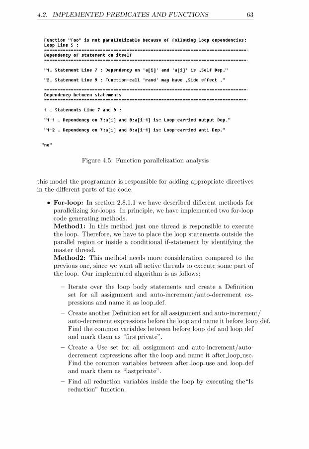
4.2. IMPLEMENTED PREDICATES AND FUNCTIONS 63
Figure 4.5: Function parallelization analysis
this model the programmer is responsible for adding appropriate directivesin the different parts of the code.
• For-loop: In section 2.8.1.1 we have described different methods forparallelizing for-loops. In principle, we have implemented two for-loopcode generating methods.Method1: In this method just one thread is responsible to executethe loop. Therefore, we have to place the loop statements outside theparallel region or inside a conditional if-statement by identifying themaster thread.Method2: This method needs more consideration compared to theprevious one, since we want all active threads to execute some part ofthe loop. Our implemented algorithm is as follows:
– Iterate over the loop body statements and create a Definitionset for all assignment and auto-increment/auto-decrement ex-pressions and name it as loop def.
– Create another Definition set for all assignment and auto-increment/auto-decrement expressions before the loop and name it before loop def.Find the common variables between before loop def and loop defand mark them as “firstprivate”.
– Create a Use set for all assignment and auto-increment/auto-decrement expressions after the loop and name it after loop use.Find the common variables between after loop use and loop defand mark them as “lastprivate”.
– Find all reduction variables inside the loop by executing the“Isreduction” function.
64 CHAPTER 4. IMPLEMENTATION
– For the variables in loop def, if they are not defined as first/lastprivate and they are not array accesses that contain the loopindex variable as part of their indices mark them as “private”.
– For nested loops, if we want to parallelize the outer loop, declarethe loop index variable of the inner loop as “private”.
– Ask the user whether the order of loop execution for each state-ment is important or not. If yes, add a “#pragma omp ordered”before it.
– Place the loop inside a “#pragma omp parallel for ” directive.
– If we have some variables which are marked as “private”, “first-private”, “ lastprivate”, and “reduction” add the relevant clauseto the for-loop statement. For more detailed information, we referthe reader to section 2.8.1.1.
• Functions: As indicated in section 2.8.2, our focus in this thesis is onparallelization of functions which have D&C paradigms or for-loops intheir structures. These ideas lead us to the following algorithm:
– For for-loop statements, parallelize the loops according to thementioned methods.
– For the D&C functions, we create a new function for the parallelversion of the code based on our defined OpenMP D&C template,see Appendix A.2. This template has the following structure:
∗ There is a conditional statement such that, whenever it istrue the sequential code (old version) will be executed.
∗ In the situation that the condition is not fulfilled, we dividethe team of threads into two groups and assign to each grouppart of the tasks.
∗ Place the two recursive function calls inside the “#pragmaomp parallel sections” directive.
∗ Before each recursive call add a “#pragma omp section” di-rective.
∗ Recursively call the parallel function for each group.
∗ End of the parallel sections directive scope.
∗ Combine the subsolutions.
4.2.3.2 MPI
As we have described, in the Message passing interface the MPI environmentwill be initialized by adding a MPI Init call to the sequential code before anyother MPI routine call. Here, in contrast to OpenMP, all active processorswill execute all the code statements until they reach to the MPI Finalizecall and the end of the program. Hence, it is the programmer’s job to dividethe work between several processors.
4.2. IMPLEMENTED PREDICATES AND FUNCTIONS 65
• For-loop: So far, in section 2.8.1.2 we have talked about the differentmethods for parallelizing MPI for-loops, now we explain our imple-mented strategies.As we have already mentioned, the programmer makes the decisionhow to parallelize the code based on the code behavior. Like for theOpenMP model, for MPI, we have implemented two for-loop code gen-erating methods.Method1: As indicated in section 2.8.1.2, some statements or loopshould be executed by a few or just one processor. In this situationwe place the statements or loop inside a conditional statement.Method2: Here, each processor is responsible for executing somepart of the loop iterations. This method is more complicated than theprevious one and consists of the following steps:
1. Find all the array variables inside the loop body by iterating overall statements inside the loop and run the“Is array” function forall variables. Create a Definition set and a Use set for found arrayaccesses and respectively name them as arr Def and arr Use.
Let us consider the following formalization for the situation wherethere is a single statement inside the loop and all accessed arraysinside the loop are one dimensional arrays:
for(i = lb; i ≤ ub; i+ +){
A0
[exp0 (i)
]= f(A1
[exp1 (i)
], · · · , Ak
[expk (i)
], Al
[expl (j)
], · · · , a1, · · · , aq);
}
Where exp0 (i) , exp1 (i) , · · · are index expressions. Here our re-trieved lists are as follows:
scalar list = {a1, · · · , aq}
arr list = {A0
[exp0 (i)
], A1
[exp1 (i)
], · · · , Ak
[expk (i)
],
Al
[expl (j)
], · · · }
arr Def = {A0
[exp0 (i)
]}
arr Use = {A1
[exp1 (i)
], · · · , Ak
[expk (i)
], Al
[expl (j)
], · · · }
2. Find all the reduction statements and their reduction variablesby executing the “Is reduction” function.
66 CHAPTER 4. IMPLEMENTATION
3. A root processor broadcasts all accessed scalars in scalar list ex-cept the reduction variables.
4. For each referenced array in arr list and reduction variable re-trieve the data type by executing the“Variable data type” func-tion. This information can be used for making decision about theMPI Datatype for MPI functions such as MPI Send, MPI Receive,MPI Scatterv, MPI Reduce, etc.
5. For all referenced arrays in arr list retrieve the array size by ex-ecuting the“Variable type” function.
6. Now, we have to divide loop iterations and all referenced arrays’elements between the active processors, such that each processorwill work approximately on an equal number of elements andhas all elements that it will need to read. Our implementationprocedure is as follows:
(a) The root processor is responsible for dividing arrays elements.
(b) In this phase it is important to know the array dimension inorder to determine how to divide the array elements.
(c) For each referenced array in arr list find the dimension wherethe loop index variable occurs in the index expression.
(d) If the loop index variable is not part of the array indicesthen the root processor will broadcast the mentioned arrayto other processors by adding a MPI Bcast before the loop.In our example the broadcast list consists of the followingarrays:
Bcast list = {Al
[expl (j)
], · · · }
(e) In the case of linear array A0 where the loop index variableis used as part of the index, the root processor will specifyeach processor’s working part by calculating the range of in-dex positions of the array where each processor is supposedto work on (begin index and end index in the following ex-amples).
k=0
array_division=size_of_array/number_of_processors;
remain=size_of_array% number_of_processors;
for(pid=0;pid<number_of_processors;++pid)
{
if(pid<remain)
part=array_division+1 ;
else
part=array_division;
begin_index=k;
4.2. IMPLEMENTED PREDICATES AND FUNCTIONS 67
end_index=k+part;
k=k+part;
}
(f) For two-dimensional arrays A0 in arr list in order to find therange of index positions, we have to find the dimension wherethe loop index variable occurs in the index expression. If theloop index variable is used in the dimension zero our divisionof A0 is row-wise and each processor’s part will be calculatedas follows:
k=0
array_division=number_of_rows/number_of_processors;
remain=number_of_rows% number_of_processors;
for(pid=0;pid<number_of_processors;++pid)
{
if(pid<remain)
part=array_division+1 ;
else
part=array_division;
begin_index=k * number_of_columns;
end_index=(k+part) * number_of_columns;
k=k+part;
}
Finally, in the case that the loop index variable occurs indimension 1 each processor’s part will be calculated as:
k=0
array_division=number_of_columns/number_of_processors;
remain=number_of_columns% number_of_processors;
for(pid=0;pid<number_of_processors;++pid)
{
if(pid<remain)
part=array_division+1 ;
else
part=array_division;
begin_index=k * number_of_rows;
end_index=(k+part) * number_of_rows;
k=k+part;
}
(g) Each processor needs a range of array elements from each ex-isting array in arr Use in order to work on its own part. Theroot processor will calculate this range for each referenced ar-ray in arr Use for all processors based on the following steps.
– For each referenced array in arr Use create two lists,min list and max list.
68 CHAPTER 4. IMPLEMENTATION
– Find the set of all index expressions of the dimensionwhere the loop index variable is used and copy them intomin list. Replace the loop variable index in min list bybegin index and evaluate symbolically.
xr min list = 〈expr : xr ε arr Use ∧ i occurs in expr ,
rε{1, · · · , k}〉
xr min list = {expr (max(begin index, lb))}
– Find the set of all index expressions of the dimensionwhere the loop index variable is used and copy them intomax list. Replace the loop index variable in max list byend index and evaluate symbolically.
xr max list = 〈expr : xr ε arr Use ∧ i occurs in expr ,
rε{1, · · · , k}〉
xr max list = {expr (end index)}
– Find the minimum value in the min list and the maxi-mum value in the max list and copy them into the min valand max val variables, respectively. If the min val is lessthan zero, set the min val value to zero and if the max valis greater than the upper bound of selected dimension forthe referenced array, set the max val to upper bound.
xr min val = max(min(xr min list), 0);xr max val = min(max(xr max list), xr.list size);
– The root processor will calculate the amount of array el-ements that each processor needs by subtracting min valfrom max val.
xr need part = xr max val − xr min val
– Each processor will create a new array with size equal tothe size of referenced array in arr Use in order to placethe received data.
– In section 2.8.1.3, we have described that the collectivecommunications have often better performance than equiv-alent point-to-point communications; therefore, for lin-ear arrays and two-dimensional arrays with loop indexvariable in dimension zero the root processor sends eachprocessor’s part of the array by adding a MPI Scatterv
4.2. IMPLEMENTED PREDICATES AND FUNCTIONS 69
function call before the loop.
Scatterv(p0, xr, xr need part)
For two dimensional arrays that the loop index variableoccurs in dimension one, we use the method which willbe described later in item i.
(h) Each processor will write to a range of array elements of eachexisting array in arr Def. The root processor will calculatethis range for each referenced array in arr Def for all proces-sors based on the following steps.
– For each referenced array in arr Def create two lists,min list and max list.
– Find the set of all indices of the dimension where the loopindex variable is used and copy them into min list. Re-place the loop index variable in min list by begin indexand evaluate symbolically.
ys min list = 〈exps : ys ε arr Def ∧ i occurs in exps ,
s = 0〉
ys min list = {exps (begin index)}
– Find the set of all indices of the dimension where theloop index variable is used and copy them into max list.Replace the loop index variable in max list by end indexand evaluate symbolically.
y0 max list = 〈exp0 : y0 ε arr Def ∧ i occurs in exp0〉y0 max list = {exp0 (end index)}
– Find the minimum value in the min list and the maxi-mum value in the max list and copy them into the min valand max val variables, respectively. If the min val is lessthan zero, set the min val value to zero and if the max valis greater than the upper bound of selected dimension forthe referenced array, set the max val to the upper bound.
y0 min val = max(min(y0 min list), 0);y0 max val = min(max(y0 max list), y0.list size));
– The root processor will calculate the amount of arrayelements that each processor will write by subtracting
70 CHAPTER 4. IMPLEMENTATION
min val from max val and send this value to the corre-sponding processor.
y0 write part = y0 max val − y0 min val
– Each processor will create a new array with size equal tothe size of referenced array in arr Def in order to calculateits own part.
– Each processor will write back the written part througha MPI Gatherv function call after the loop, for lineararrays and two-dimensional arrays with loop index vari-able in dimension zero. We assume for simplicity thatthe written partitions of A0 are disjoint for different pro-cessors.
∀ pqε P, q ε {0, 1, · · · , np− 1}Gatherv(pq, y0, y0 write part)
Where P and np are the set of processors and the numberof processors, respectively.
(i) In contrast to Fortran, the C language linearizes matrices inrow-wise order; therefore, in the situation of a two-dimensionalarray where the loop index variable is used in dimension onewe need to change our sending methods. There may existseveral methods for dividing the matrix elements column-wise and here, we describe one method.In our column-wise division, after we calculated each proces-sor’s part we will copy those related elements in a linear array.Then by using MPI Send, the root processor sends this arrayto the corresponding processor and the target processor willexecute the MPI Receive command in order to receive it. Thetarget processors will put the elements of the received arrayin their own places in the matrix. All these communicationsmust be done before the loop execution. This procedure willrepeat again but in the opposite way (sending data from thetarget processor to the root processor) after executing theloop body.
7. For each reduction variable found in step two, we define a newlocal accumulator variable and in the reduction statement replacethe reduction variable with the corresponding new one. In thissituation each processor will calculate its own part and store itsresult in the new variable. We add a MPI Reduce function call af-ter the loop iteration by considering the reduction variable as theaddress of the receive buffer and the corresponding new definedvariable as the address of the send buffer.
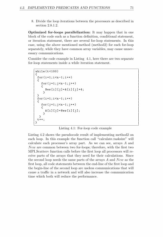
4.2. IMPLEMENTED PREDICATES AND FUNCTIONS 71
8. Divide the loop iterations between the processors as described insection 2.8.1.2.
Optimized for-loops parallelization: It may happen that in oneblock of the code such as a function definition, conditional statement,or iteration statement, there are several for-loop statements. In thiscase, using the above mentioned method (method2) for each for-loopseparately, while they have common array variables, may cause unnec-essary communications.
Consider the code example in Listing 4.1, here there are two separatefor-loop statements inside a while iteration statement.
while(t<100){for(i=1;i<n-1;i++){
for(j=1;j<n-1;j++){
New[i][j]=A[i][j]+4;}
}for(i=1;i<n-1;i++){
for(j=1;j<n-1;j++){
A[i][j]=New[i][j];}
}t++;
}
Listing 4.1: For-loop code example
Listing 4.2 shows the pseudocode result of implementing method2 oneach loop. In this example the function call “calculate tasksize” willcalculate each processor’s array part. As we can see, arrays A andNew are common between two for-loops; therefore, with the first twoMPI Scatterv function calls before the first loop all processors will re-ceive parts of the arrays that they need for their calculations. Sincethe second loop needs the same parts of the arrays A and New as thefirst loop, all code statements between the end-line of the first loop andthe begin-line of the second loop are useless communications that willcause a traffic in a network and will also increase the communicationtime which both will reduce the performance.
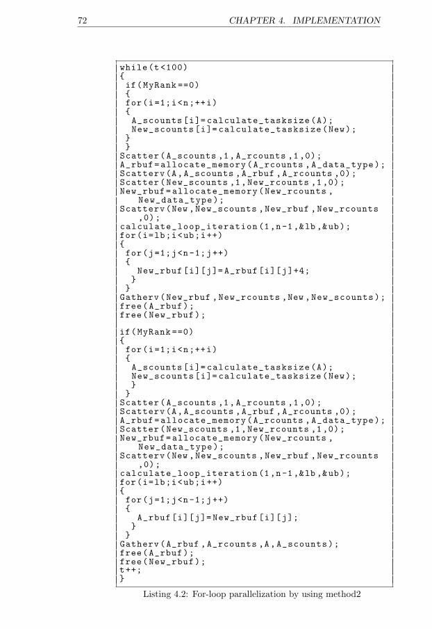
72 CHAPTER 4. IMPLEMENTATION
while(t <100){if(MyRank ==0){for(i=1;i<n;++i){A_scounts[i]= calculate_tasksize(A);New_scounts[i]= calculate_tasksize(New);
}}
Scatter(A_scounts ,1,A_rcounts ,1,0);A_rbuf=allocate_memory(A_rcounts ,A_data_type);Scatterv(A,A_scounts ,A_rbuf ,A_rcounts ,0);Scatter(New_scounts ,1,New_rcounts ,1,0);New_rbuf=allocate_memory(New_rcounts ,
New_data_type);Scatterv(New ,New_scounts ,New_rbuf ,New_rcounts
,0);calculate_loop_iteration (1,n-1,&lb ,&ub);for(i=lb;i<ub;i++){for(j=1;j<n-1;j++){
New_rbuf[i][j]= A_rbuf[i][j]+4;}
}Gatherv(New_rbuf ,New_rcounts ,New ,New_scounts);free(A_rbuf);free(New_rbuf);
if(MyRank ==0){for(i=1;i<n;++i){A_scounts[i]= calculate_tasksize(A);New_scounts[i]= calculate_tasksize(New);}
}Scatter(A_scounts ,1,A_rcounts ,1,0);Scatterv(A,A_scounts ,A_rbuf ,A_rcounts ,0);A_rbuf=allocate_memory(A_rcounts ,A_data_type);Scatter(New_scounts ,1,New_rcounts ,1,0);New_rbuf=allocate_memory(New_rcounts ,
New_data_type);Scatterv(New ,New_scounts ,New_rbuf ,New_rcounts
,0);calculate_loop_iteration (1,n-1,&lb ,&ub);for(i=lb;i<ub;i++){for(j=1;j<n-1;j++){
A_rbuf[i][j]= New_rbuf[i][j];}
}Gatherv(A_rbuf ,A_rcounts ,A,A_scounts);free(A_rbuf);free(New_rbuf);t++;}
Listing 4.2: For-loop parallelization by using method2
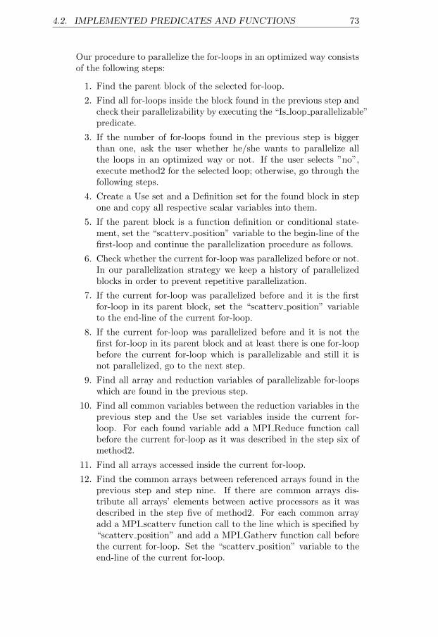
4.2. IMPLEMENTED PREDICATES AND FUNCTIONS 73
Our procedure to parallelize the for-loops in an optimized way consistsof the following steps:
1. Find the parent block of the selected for-loop.
2. Find all for-loops inside the block found in the previous step andcheck their parallelizability by executing the “Is loop parallelizable”predicate.
3. If the number of for-loops found in the previous step is biggerthan one, ask the user whether he/she wants to parallelize allthe loops in an optimized way or not. If the user selects ”no”,execute method2 for the selected loop; otherwise, go through thefollowing steps.
4. Create a Use set and a Definition set for the found block in stepone and copy all respective scalar variables into them.
5. If the parent block is a function definition or conditional state-ment, set the “scatterv position” variable to the begin-line of thefirst-loop and continue the parallelization procedure as follows.
6. Check whether the current for-loop was parallelized before or not.In our parallelization strategy we keep a history of parallelizedblocks in order to prevent repetitive parallelization.
7. If the current for-loop was parallelized before and it is the firstfor-loop in its parent block, set the “scatterv position” variableto the end-line of the current for-loop.
8. If the current for-loop was parallelized before and it is not thefirst for-loop in its parent block and at least there is one for-loopbefore the current for-loop which is parallelizable and still it isnot parallelized, go to the next step.
9. Find all array and reduction variables of parallelizable for-loopswhich are found in the previous step.
10. Find all common variables between the reduction variables in theprevious step and the Use set variables inside the current for-loop. For each found variable add a MPI Reduce function callbefore the current for-loop as it was described in the step six ofmethod2.
11. Find all arrays accessed inside the current for-loop.
12. Find the common arrays between referenced arrays found in theprevious step and step nine. If there are common arrays dis-tribute all arrays’ elements between active processors as it wasdescribed in the step five of method2. For each common arrayadd a MPI scatterv function call to the line which is specified by“scatterv position” and add a MPI Gatherv function call beforethe current for-loop. Set the “scatterv position” variable to theend-line of the current for-loop.
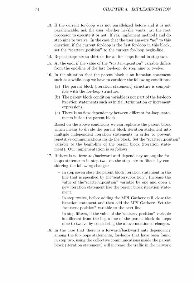
74 CHAPTER 4. IMPLEMENTATION
13. If the current for-loop was not parallelized before and it is notparallelizable, ask the user whether he/she wants just the rootprocessor to execute it or not. If yes, implement method1 and dostep nine to twelve. In the case that the user answers “no” to thisquestion, if the current for-loop is the first for-loop in this block,set the “scatterv position” to the current for-loop begin-line.
14. Repeat steps six to thirteen for all for-loops found in step two.
15. At the end, if the value of the “scatterv position” variable differsfrom the end-line of the last for-loop, do step nine to twelve.
16. In the situation that the parent block is an iteration statementsuch as a while-loop we have to consider the following conditions:
(a) The parent block (iteration statement) structure is compat-ible with the for-loop structure.
(b) The parent block condition variable is not part of the for-loopiteration statements such as initial, termination or incrementexpressions.
(c) There is no flow dependency between different for-loop state-ments inside the parent block.
Based on the above conditions we can replicate the parent blockwhich means to divide the parent block iteration statement intomultiple independent iteration statements in order to preventrepetitive communications inside the block. Set the “scatterv position”variable to the begin-line of the parent block (iteration state-ment). Our implementation is as follows:
17. If there is no forward/backward anti dependency among the for-loops statements in step two, do the steps six to fifteen by con-sidering the following changes:
– In step seven close the parent block iteration statement in theline that is specified by the“scatterv position”. Increase thevalue of the“scatterv position” variable by one and open anew iteration statement like the parent block iteration state-ment.
– In step twelve, before adding the MPI Gatherv call, close theiteration statement and then add the MPI Gatherv. Set the“scatterv position” variable to the next line.
– In step fifteen, if the value of the“scatterv position” variableis different from the begin-line of the parent block do stepsnine to twelve by considering the above mentioned changes.
18. In the case that there is a forward/backward anti dependencyamong the for-loops statements, for-loops that have been foundin step two, using the collective communications inside the parentblock (iteration statement) will increase the traffic in the network
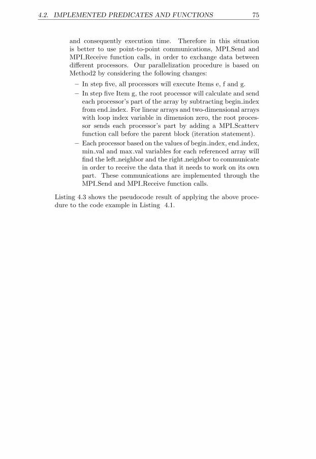
4.2. IMPLEMENTED PREDICATES AND FUNCTIONS 75
and consequently execution time. Therefore in this situationis better to use point-to-point communications, MPI Send andMPI Receive function calls, in order to exchange data betweendifferent processors. Our parallelization procedure is based onMethod2 by considering the following changes:
– In step five, all processors will execute Items e, f and g.
– In step five Item g, the root processor will calculate and sendeach processor’s part of the array by subtracting begin indexfrom end index. For linear arrays and two-dimensional arrayswith loop index variable in dimension zero, the root proces-sor sends each processor’s part by adding a MPI Scattervfunction call before the parent block (iteration statement).
– Each processor based on the values of begin index, end index,min val and max val variables for each referenced array willfind the left neighbor and the right neighbor to communicatein order to receive the data that it needs to work on its ownpart. These communications are implemented through theMPI Send and MPI Receive function calls.
Listing 4.3 shows the pseudocode result of applying the above proce-dure to the code example in Listing 4.1.
76 CHAPTER 4. IMPLEMENTATION
if(MyRank ==0){for(i=1;i<n;++i){A_scounts[i]= calculate_tasksize(A);New_scounts[i]= calculate_tasksize(New);
}}Scatter(A_scounts ,1,A_rcounts ,1,0);A_rbuf=allocate_memory(A_rcounts ,A_data_type);Scatterv(A,A_scounts ,A_rbuf ,A_rcounts ,0);
Scatter(New_scounts ,1,New_rcounts ,1,0);New_rbuf=allocate_memory(New_rcounts ,New_data_type)
;Scatterv(New ,New_scounts ,New_rbuf ,New_rcounts ,0);t=0;while(t <100){calculate_loop_iteration (1,n-1,&lb ,&ub);
for(i= lb;i<ub;i++){
for(j=1; j<n-1;j++){
New_rbuf[i][j]= A_rbuf[i][j]+4;}
}calculate_loop_iteration (1,n-1,&lb ,&ub);
for(i=lb;i<ub;i++){
for(j=1;j<n-1;j++){
A_rbuf[i][j]= New_rbuf[i][j];}
}t++;
}Gatherv(A_rbuf ,A_rcounts ,A,A_scounts);Gatherv(New_rbuf ,New_rcounts ,New ,New_scounts);free(A_rbuf);free(New_rbuf);
Listing 4.3: Optimized for-loop parallelization
• Functions: As for OpenMP, for MPI also our focus is on parallelizingthe functions that are D&C or they have for-loops. Our algorithm forparallelizing functions consists of the following steps:
– For functions with for-loops, parallelize the loops as mentionedbefore.
– For D&C functions our implementation method is based on theteam parallel model (see section 2.9.1).
∗ Create a new function for the parallel version of the functionbased on our defined MPI D&C template, see Appendix A.1.This template has the following structure:
4.2. IMPLEMENTED PREDICATES AND FUNCTIONS 77
∗ It has a conditional statement such that whenever it is truethe sequential code (old version) will be executed.
∗ In the situation that the condition is not fulfilled and theproblem is large enough, we divide the problem and splitthe group of processors into two subgroups and assign toeach subgroup a subset of the tasks. For this assignment weneed communication between the subgroups of the processorsand in this template, we have used the MPI Send and theMPI Receive function calls for the communication.
∗ Recursively call the function for each group.
∗ End sub groups.
∗ Combine subsolutions.
One execution example of this algorithm for a Quick sort program willbe discussed later in section 5.1.1.
Chapter 5
Evaluation
So far, in the previous chapters we have talked about the thesis researchquestions, the hypothesis and our design and implementation solution. Now,it is time to evaluate whether our implemented system fulfilled our require-ments or not. In order to answer this question we have chosen two testprograms, Quick sort and Jacobi method. First, in section 5.1, we will de-scribe these two examples and our system parallelization methods, then thenext three sections, 5.2, 5.3 and 5.4 will evaluate our results based on thethree metrics correctness, performance and usefulness.
5.1 System Parallelization of Test Programs
We have already mentioned that our first test examples are Quick sort andJacobi method. Quick sort is an example of a D&C function, and Jacobimethod has nested loops. In the rest of this section we will talk more aboutthem.
5.1.1 Quick sort
In section 2.10.2 we have explained three different methods for parallelizingQuick sort. In this project our selected algorithm for both hand-parallelizedand system-parallelized versions of the selected sequential code is based onteam parallel model of Hardwick [25]. We have discussed that Eriksson etal. [17] suggest a simplified variant strategy for Quick sort. We have pre-ferred the concept of team parallel model rather than Eriksson’s strategy,because this model can be used for other D&C algorithms such as Mergesort and Pairwise summation algorithms and this will lead us to the conceptof generalized parallel D&C algorithms. Now we will go through two parallelversions (MPI, OpenMP) of sequential Quick sort which is demonstrated inListing 2.16.
78
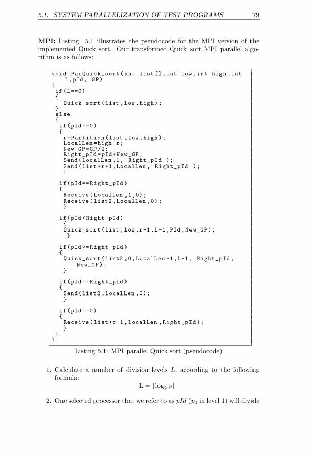
5.1. SYSTEM PARALLELIZATION OF TEST PROGRAMS 79
MPI: Listing 5.1 illustrates the pseudocode for the MPI version of theimplemented Quick sort. Our transformed Quick sort MPI parallel algo-rithm is as follows:
void ParQuick_sort(int list[],int low ,int high ,intL,pId , GP)
{if(L==0){
Quick_sort(list ,low ,high);}else{if(pId ==0){r=Partition(list ,low ,high);LocalLen=high -r;New_GP=GP/2;Right_pId=pId+New_GP;Send(LocalLen ,1, Right_pId );Send(list+r+1,LocalLen , Right_pId );}
if(pId== Right_pId){Receive(LocalLen ,1,0);Receive(list2 ,LocalLen ,0);}
if(pId <Right_pId){Quick_sort(list ,low ,r-1,L-1,PId ,New_GP);}
if(pId >= Right_pId){Quick_sort(list2 ,0,LocalLen -1,L-1, Right_pId ,
New_GP);}
if(pId== Right_pId){Send(list2 ,LocalLen ,0);}
if(pId ==0){Receive(list+r+1,LocalLen ,Right_pId);}
}}
Listing 5.1: MPI parallel Quick sort (pseudocode)
1. Calculate a number of division levels L, according to the followingformula:
L = dlog2 pe
2. One selected processor that we refer to as pId (p0 in level 1) will divide
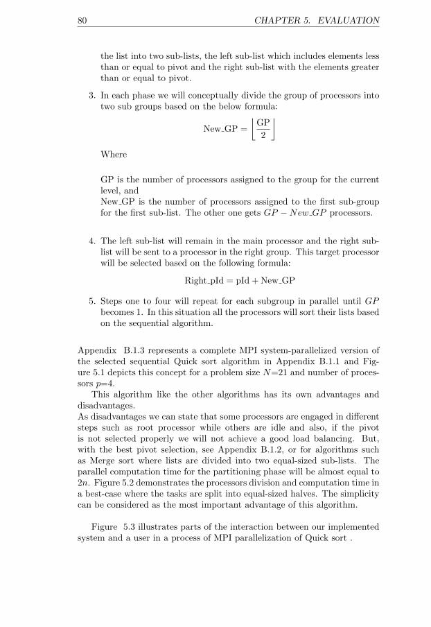
80 CHAPTER 5. EVALUATION
the list into two sub-lists, the left sub-list which includes elements lessthan or equal to pivot and the right sub-list with the elements greaterthan or equal to pivot.
3. In each phase we will conceptually divide the group of processors intotwo sub groups based on the below formula:
New GP =
⌊GP
2
⌋Where
GP is the number of processors assigned to the group for the currentlevel, andNew GP is the number of processors assigned to the first sub-groupfor the first sub-list. The other one gets GP −New GP processors.
4. The left sub-list will remain in the main processor and the right sub-list will be sent to a processor in the right group. This target processorwill be selected based on the following formula:
Right pId = pId + New GP
5. Steps one to four will repeat for each subgroup in parallel until GPbecomes 1. In this situation all the processors will sort their lists basedon the sequential algorithm.
Appendix B.1.3 represents a complete MPI system-parallelized version ofthe selected sequential Quick sort algorithm in Appendix B.1.1 and Fig-ure 5.1 depicts this concept for a problem size N=21 and number of proces-sors p=4.
This algorithm like the other algorithms has its own advantages anddisadvantages.As disadvantages we can state that some processors are engaged in differentsteps such as root processor while others are idle and also, if the pivotis not selected properly we will not achieve a good load balancing. But,with the best pivot selection, see Appendix B.1.2, or for algorithms suchas Merge sort where lists are divided into two equal-sized sub-lists. Theparallel computation time for the partitioning phase will be almost equal to2n. Figure 5.2 demonstrates the processors division and computation time ina best-case where the tasks are split into equal-sized halves. The simplicitycan be considered as the most important advantage of this algorithm.
Figure 5.3 illustrates parts of the interaction between our implementedsystem and a user in a process of MPI parallelization of Quick sort .
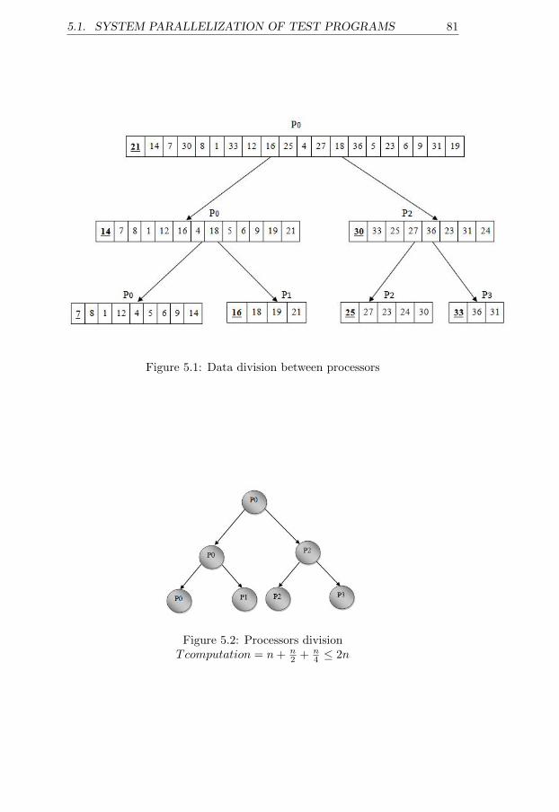
5.1. SYSTEM PARALLELIZATION OF TEST PROGRAMS 81
Figure 5.1: Data division between processors
Figure 5.2: Processors divisionTcomputation = n+ n
2 + n4 ≤ 2n
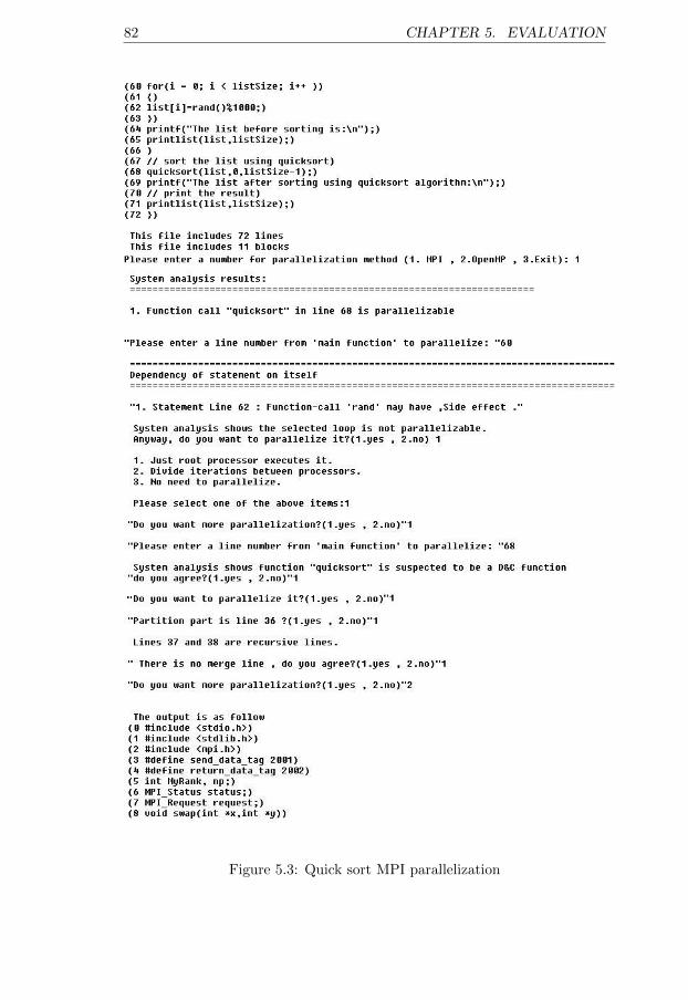
82 CHAPTER 5. EVALUATION
Figure 5.3: Quick sort MPI parallelization
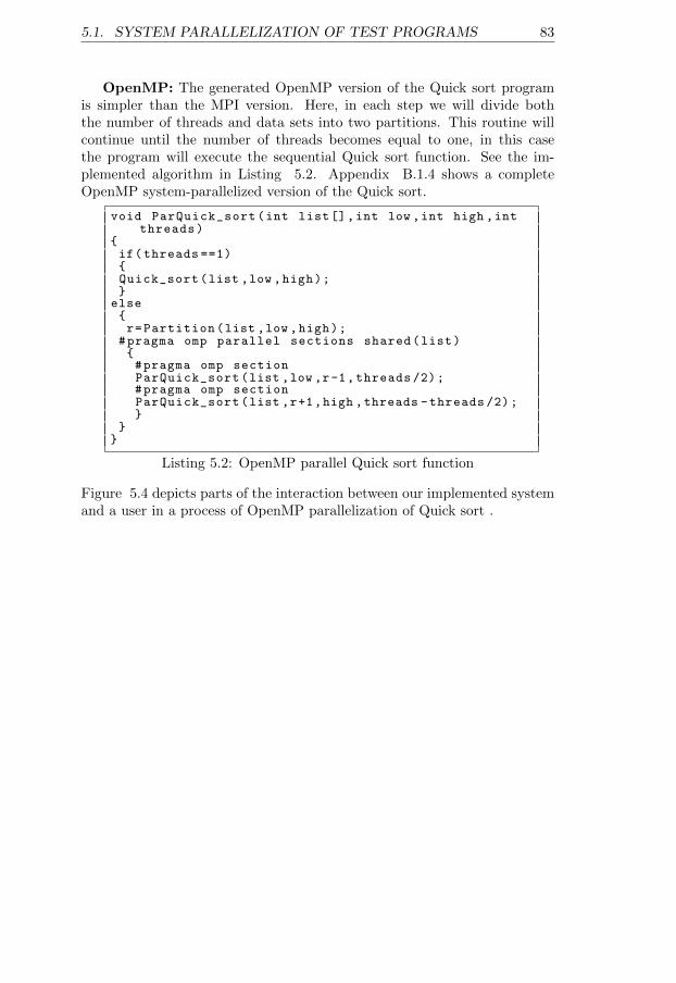
5.1. SYSTEM PARALLELIZATION OF TEST PROGRAMS 83
OpenMP: The generated OpenMP version of the Quick sort programis simpler than the MPI version. Here, in each step we will divide boththe number of threads and data sets into two partitions. This routine willcontinue until the number of threads becomes equal to one, in this casethe program will execute the sequential Quick sort function. See the im-plemented algorithm in Listing 5.2. Appendix B.1.4 shows a completeOpenMP system-parallelized version of the Quick sort.
void ParQuick_sort(int list[],int low ,int high ,intthreads)
{if(threads ==1){Quick_sort(list ,low ,high);}
else{r=Partition(list ,low ,high);
#pragma omp parallel sections shared(list){#pragma omp sectionParQuick_sort(list ,low ,r-1,threads /2);#pragma omp sectionParQuick_sort(list ,r+1,high ,threads -threads /2);}
}}
Listing 5.2: OpenMP parallel Quick sort function
Figure 5.4 depicts parts of the interaction between our implemented systemand a user in a process of OpenMP parallelization of Quick sort .
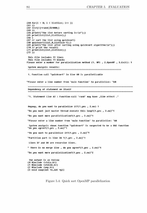
84 CHAPTER 5. EVALUATION
Figure 5.4: Quick sort OpenMP parallelization
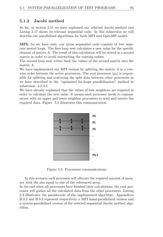
5.1. SYSTEM PARALLELIZATION OF TEST PROGRAMS 85
5.1.2 Jacobi method
So far, in section 2.11 we have explained our selected Jacobi method andListing 2.17 shows its relevant sequential code. In this subsection we willdescribe our parallelized algorithms for both MPI and OpenMP model.
MPI: As we have seen, our given sequential code consists of two sepa-rate nested loops. The first loop nest calculates a new value for the specificelement of matrix A. The result of this calculation will be stored in a secondmatrix in order to avoid overwriting the existing values.The second loop nest writes back the values of the second matrix into thematrix A.We have implemented our MPI version by splitting the matrix A in a row-wise order between the active processors. The root processor (p0) is respon-sible for splitting and scattering the split data between other processors aswe have described in the “optimized for-loops parallelization” method insubsection 4.2.3.2.We have already explained that the values of four neighbors are required inorder to calculate the new value. It means each processor needs to commu-nicate with its upper and lower neighbor processors to send and receive therequired data. Figure 5.5 illustrates this communication.
Figure 5.5: Processors communications
In this scenario each processor will allocate the required amount of mem-ory with the size equal to size of the referenced array.In the end when all processors have finished their calculations, the root pro-cessor will gather all the calculated data from the other processors. Listing5.3 illustrates the pseudocode of the implemented algorithm. AppendicesB.3.2 and B.3.3 represent respectively a MPI hand-parallelized version anda system-parallelized version of the selected sequential Jacobi method algo-rithm.
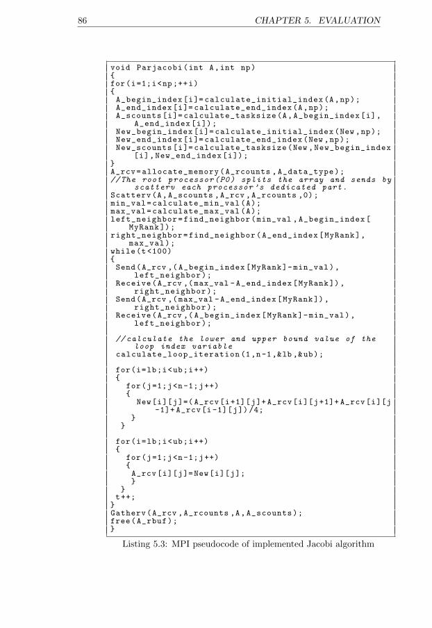
86 CHAPTER 5. EVALUATION
void Parjacobi(int A,int np){for(i=1;i<np;++i){A_begin_index[i]= calculate_initial_index(A,np);A_end_index[i]= calculate_end_index(A,np);A_scounts[i]= calculate_tasksize(A,A_begin_index[i],
A_end_index[i]);New_begin_index[i]= calculate_initial_index(New ,np);New_end_index[i]= calculate_end_index(New ,np);New_scounts[i]= calculate_tasksize(New ,New_begin_index
[i],New_end_index[i]);}A_rcv=allocate_memory(A_rcounts ,A_data_type);//The root processor(P0) splits the array and sends by
scatterv each processor ’s dedicated part.Scatterv(A,A_scounts ,A_rcv ,A_rcounts ,0);min_val=calculate_min_val(A);max_val=calculate_max_val(A);left_neighbor=find_neighbor(min_val ,A_begin_index[
MyRank ]);right_neighbor=find_neighbor(A_end_index[MyRank],
max_val);while(t <100){Send(A_rcv ,( A_begin_index[MyRank]-min_val),
left_neighbor);Receive(A_rcv ,(max_val -A_end_index[MyRank ]),
right_neighbor);Send(A_rcv ,(max_val -A_end_index[MyRank ]),
right_neighbor);Receive(A_rcv ,( A_begin_index[MyRank]-min_val),
left_neighbor);
// calculate the lower and upper bound value of theloop index variable
calculate_loop_iteration (1,n-1,&lb ,&ub);
for(i=lb;i<ub;i++){
for(j=1;j<n-1;j++){
New[i][j]=( A_rcv[i+1][j]+ A_rcv[i][j+1]+ A_rcv[i][j-1]+ A_rcv[i-1][j])/4;
}}
for(i=lb;i<ub;i++){
for(j=1;j<n-1;j++){A_rcv[i][j]=New[i][j];}
}t++;
}Gatherv(A_rcv ,A_rcounts ,A,A_scounts);free(A_rbuf);}
Listing 5.3: MPI pseudocode of implemented Jacobi algorithm
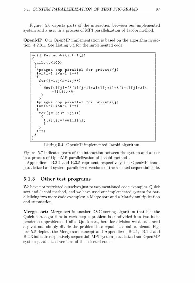
5.1. SYSTEM PARALLELIZATION OF TEST PROGRAMS 87
Figure 5.6 depicts parts of the interaction between our implementedsystem and a user in a process of MPI parallelization of Jacobi method.
OpenMP: Our OpenMP implementation is based on the algorithm in sec-tion 4.2.3.1. See Listing 5.4 for the implemented code.
void Parjacobi(int A[]){while(t<100){#pragma omp parallel for private(j)for(i=1;i<n-1;i++){for(j=1;j<n-1;j++){
New[i][j]=(A[i][j-1]+A[i][j+1]+A[i-1][j]+A[i+1][j])/4;
}}
#pragma omp parallel for private(j)for(i=1;i<n-1;i++){for(j=1;j<n-1;j++){A[i][j]=New[i][j];}
}t++;
}}
Listing 5.4: OpenMP implemented Jacobi algorithm
Figure 5.7 indicates parts of the interaction between the system and a userin a process of OpenMP parallelization of Jacobi method .
Appendices B.3.4 and B.3.5 represent respectively the OpenMP hand-parallelized and system-parallelized versions of the selected sequential code.
5.1.3 Other test programs
We have not restricted ourselves just to two mentioned code examples, Quicksort and Jacobi method, and we have used our implemented system for par-allelizing two more code examples: a Merge sort and a Matrix multiplicationand summation.
Merge sort: Merge sort is another D&C sorting algorithm that like theQuick sort algorithm in each step a problem is subdivided into two inde-pendent subproblems. Unlike Quick sort, here for division we do not needa pivot and simply divide the problem into equal-sized subproblems. Fig-ure 5.8 depicts the Merge sort concept and Appendices B.2.1, B.2.2 andB.2.3 indicate respectively sequential, MPI system-parallelized and OpenMPsystem-parallelized versions of the selected code.
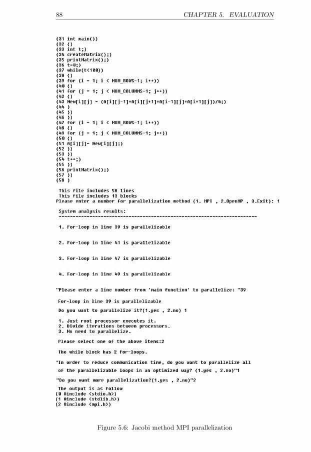
88 CHAPTER 5. EVALUATION
Figure 5.6: Jacobi method MPI parallelization
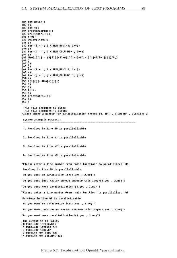
5.1. SYSTEM PARALLELIZATION OF TEST PROGRAMS 89
Figure 5.7: Jacobi method OpenMP parallelization
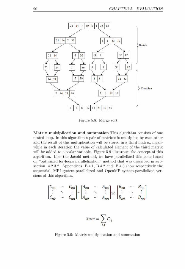
90 CHAPTER 5. EVALUATION
Figure 5.8: Merge sort
Matrix multiplication and summation This algorithm consists of onenested loop. In this algorithm a pair of matrices is multiplied by each otherand the result of this multiplication will be stored in a third matrix, mean-while in each iteration the value of calculated element of the third matrixwill be added to a scalar variable. Figure 5.9 illustrates the concept of thisalgorithm. Like the Jacobi method, we have parallelized this code basedon “optimized for-loops parallelization” method that was described in sub-section 4.2.3.2. Appendices B.4.1, B.4.2 and B.4.3 show respectively thesequential, MPI system-parallelized and OpenMP system-parallelized ver-sions of this algorithm.
Figure 5.9: Matrix multiplication and summation
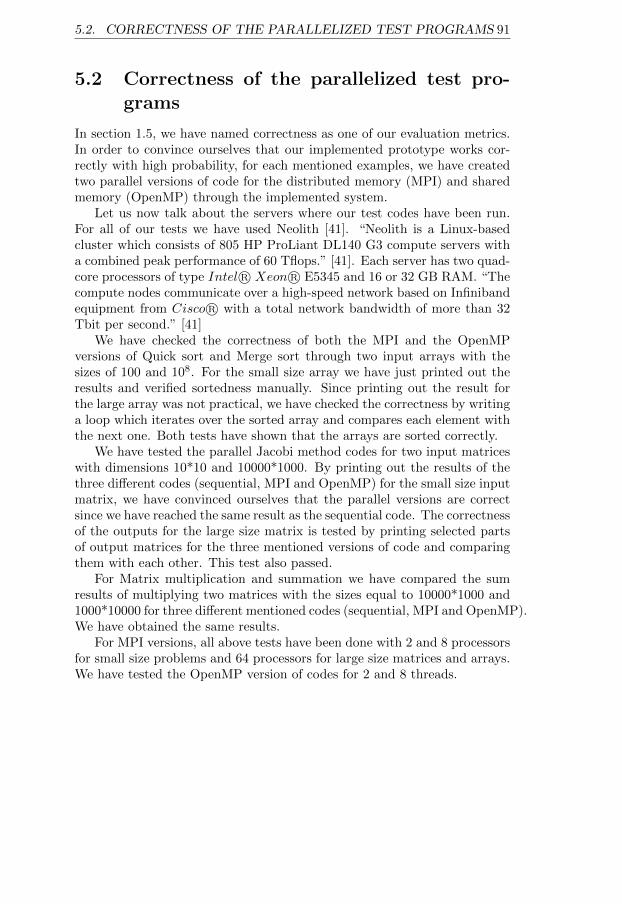
5.2. CORRECTNESS OF THE PARALLELIZED TEST PROGRAMS 91
5.2 Correctness of the parallelized test pro-grams
In section 1.5, we have named correctness as one of our evaluation metrics.In order to convince ourselves that our implemented prototype works cor-rectly with high probability, for each mentioned examples, we have createdtwo parallel versions of code for the distributed memory (MPI) and sharedmemory (OpenMP) through the implemented system.
Let us now talk about the servers where our test codes have been run.For all of our tests we have used Neolith [41]. “Neolith is a Linux-basedcluster which consists of 805 HP ProLiant DL140 G3 compute servers witha combined peak performance of 60 Tflops.” [41]. Each server has two quad-core processors of type Intel R© Xeon R© E5345 and 16 or 32 GB RAM. “Thecompute nodes communicate over a high-speed network based on Infinibandequipment from Cisco R© with a total network bandwidth of more than 32Tbit per second.” [41]
We have checked the correctness of both the MPI and the OpenMPversions of Quick sort and Merge sort through two input arrays with thesizes of 100 and 108. For the small size array we have just printed out theresults and verified sortedness manually. Since printing out the result forthe large array was not practical, we have checked the correctness by writinga loop which iterates over the sorted array and compares each element withthe next one. Both tests have shown that the arrays are sorted correctly.
We have tested the parallel Jacobi method codes for two input matriceswith dimensions 10*10 and 10000*1000. By printing out the results of thethree different codes (sequential, MPI and OpenMP) for the small size inputmatrix, we have convinced ourselves that the parallel versions are correctsince we have reached the same result as the sequential code. The correctnessof the outputs for the large size matrix is tested by printing selected partsof output matrices for the three mentioned versions of code and comparingthem with each other. This test also passed.
For Matrix multiplication and summation we have compared the sumresults of multiplying two matrices with the sizes equal to 10000*1000 and1000*10000 for three different mentioned codes (sequential, MPI and OpenMP).We have obtained the same results.
For MPI versions, all above tests have been done with 2 and 8 processorsfor small size problems and 64 processors for large size matrices and arrays.We have tested the OpenMP version of codes for 2 and 8 threads.
92 CHAPTER 5. EVALUATION
5.3 Performance of the parallelized test pro-grams
Note that the main goal of this research is not prototyping a system whichproduces a parallel version of the mentioned sequential codes with high per-formance; instead it is aimed to make the parallelization steps faster andsimpler for users by implementing IIP strategies. The results of executionof the system-parallelized test programs have shown that we have attainedacceptable performance. The rest of this section will explain our perfor-mance results for both MPI and OpenMP system-parallelized versions ofQuick sort, Jacobi method and the two other test programs. We have mea-sured the performance for both MPI and OpenMP implementations of thementioned examples by calculating the absolute speedup using 1, 8, 16, 32and 64 cores for MPI and 1 to 8 threads for OpenMP.
5.3.1 Quick sort
We have measured the Quick sort performance for two sequential code ex-amples in Appendices B.1.1 and B.1.2 for problem sizes 105, 106 and 107.In order to show the effect of the pivot selection method on Quick sortexecution time we have chosen two code examples.
• Code example1: Listing 2.16 represents the concept of this example.In this method the first element of the list is selected as the pivot (seeAppendix B.1.1 for the complete code).
• Code example2: In this example, see Appendix B.1.2, we have used abetter pivot selection method. In order to select the pivot we will gothrough the following steps:
1. Calculate the average of the first and the last indices and nameit as “mid”.
2. Select the list element in index “mid”.
3. Compare the value of the element found in previous step by thevalue of the first element. If it is smaller than the first elementswap their values.
4. Compare the value of the first element by the value of the lastelement. In the case it is larger than the last element swap theirvalues.
5. Compare the value of the element found in step one by the valueof the last element. If it is larger than the first element swap theirvalues.
6. Set the value of the pivot to the value of the list element in index“mid”.
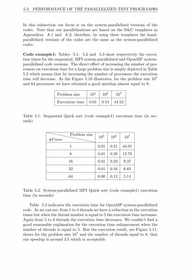
5.3. PERFORMANCE OF THE PARALLELIZED TEST PROGRAMS93
In this subsection our focus is on the system-parallelized versions of thecodes. Note that our parallelizations are based on the D&C templates inAppendices A.1 and A.2; therefore, by using these templates the hand-parallelized versions of the codes are the same as the system-parallelizedcodes.
Code example1: Tables 5.1, 5.2 and 5.3 show respectively the execu-tion times for the sequential, MPI system-parallelized and OpenMP system-parallelized code versions. The direct effect of increasing the number of pro-cessors on execution time for a large problem size is simply depicted in Table5.2 which means that by increasing the number of processors the executiontime will decrease. As the Figure 5.10 illustrates, for the problem size 107
and 64 processors we have obtained a good speedup almost equal to 9.
Problem size 105 106 107
Execution time 0.01 0.54 44.53
Table 5.1: Sequential Quick sort (code example1) execution time (in sec-onds)
````````````#CoresProblem size
105 106 107
1 0.01 0.51 44.01
8 0.01 0.28 12.78
16 0.01 0.23 9.37
32 0.01 0.16 6.83
64 0.00 0.12 5.14
Table 5.2: System-parallelized MPI Quick sort (code example1) executiontime (in seconds)
Table 5.3 indicates the execution time for OpenMP system-parallelizedcode. As we can see, from 1 to 4 threads we have a reduction in the executiontimes but when the thread number is equal to 5 the execution time increases.Again from 5 to 8 threads the execution time decreases. We couldn’t find agood reasonable explanation for the execution time enhancement when thenumber of threads is equal to 5. But the execution result, see Figure 5.11,shows for the problem size 107 and the number of threads equal to 8, thatour speedup is around 3.5 which is acceptable.
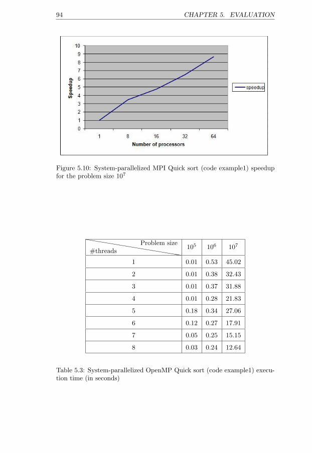
94 CHAPTER 5. EVALUATION
Figure 5.10: System-parallelized MPI Quick sort (code example1) speedupfor the problem size 107
hhhhhhhhhhhhhhh#threadsProblem size
105 106 107
1 0.01 0.53 45.02
2 0.01 0.38 32.43
3 0.01 0.37 31.88
4 0.01 0.28 21.83
5 0.18 0.34 27.06
6 0.12 0.27 17.91
7 0.05 0.25 15.15
8 0.03 0.24 12.64
Table 5.3: System-parallelized OpenMP Quick sort (code example1) execu-tion time (in seconds)
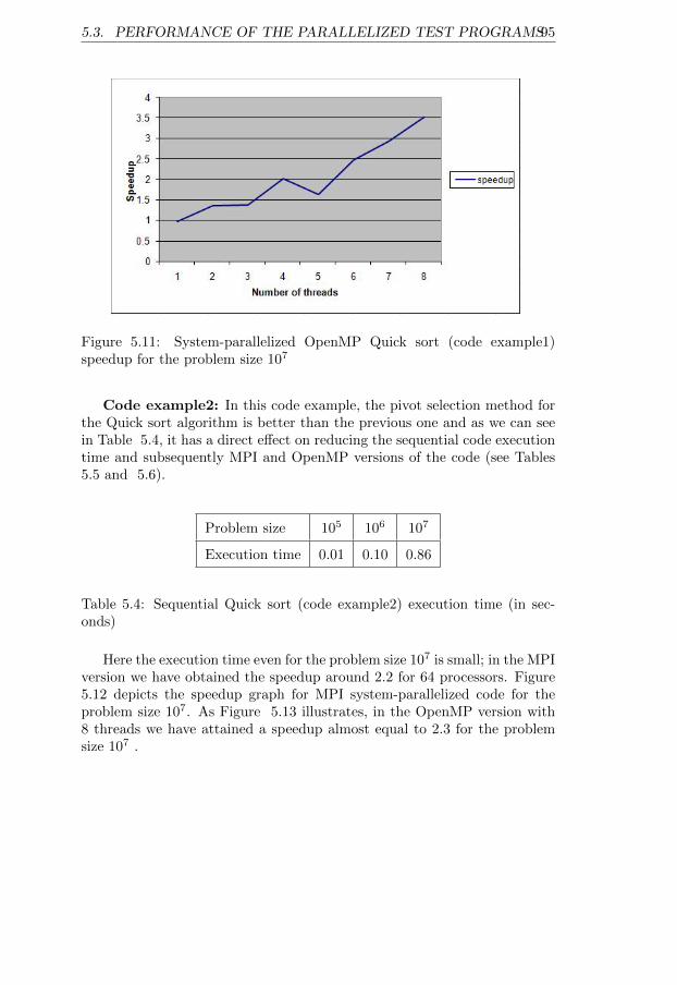
5.3. PERFORMANCE OF THE PARALLELIZED TEST PROGRAMS95
Figure 5.11: System-parallelized OpenMP Quick sort (code example1)speedup for the problem size 107
Code example2: In this code example, the pivot selection method forthe Quick sort algorithm is better than the previous one and as we can seein Table 5.4, it has a direct effect on reducing the sequential code executiontime and subsequently MPI and OpenMP versions of the code (see Tables5.5 and 5.6).
Problem size 105 106 107
Execution time 0.01 0.10 0.86
Table 5.4: Sequential Quick sort (code example2) execution time (in sec-onds)
Here the execution time even for the problem size 107 is small; in the MPIversion we have obtained the speedup around 2.2 for 64 processors. Figure5.12 depicts the speedup graph for MPI system-parallelized code for theproblem size 107. As Figure 5.13 illustrates, in the OpenMP version with8 threads we have attained a speedup almost equal to 2.3 for the problemsize 107 .
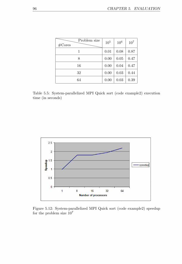
96 CHAPTER 5. EVALUATION
````````````#CoresProblem size
105 106 107
1 0.01 0.08 0.87
8 0.00 0.05 0.47
16 0.00 0.04 0.47
32 0.00 0.03 0.44
64 0.00 0.03 0.39
Table 5.5: System-parallelized MPI Quick sort (code example2) executiontime (in seconds)
Figure 5.12: System-parallelized MPI Quick sort (code example2) speedupfor the problem size 107
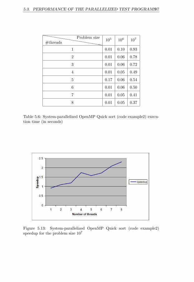
5.3. PERFORMANCE OF THE PARALLELIZED TEST PROGRAMS97
hhhhhhhhhhhhhhh#threadsProblem size
105 106 107
1 0.01 0.10 0.93
2 0.01 0.06 0.78
3 0.01 0.06 0.72
4 0.01 0.05 0.49
5 0.17 0.06 0.54
6 0.01 0.06 0.50
7 0.01 0.05 0.41
8 0.01 0.05 0.37
Table 5.6: System-parallelized OpenMP Quick sort (code example2) execu-tion time (in seconds)
Figure 5.13: System-parallelized OpenMP Quick sort (code example2)speedup for the problem size 107
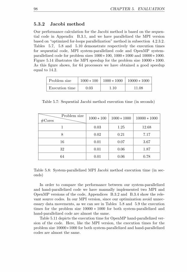
98 CHAPTER 5. EVALUATION
5.3.2 Jacobi method
Our performance calculation for the Jacobi method is based on the sequen-tial code in Appendix B.3.1, and we have parallelized the MPI versionbased on “optimized for-loops parallelization” method in subsection 4.2.3.2.Tables 5.7, 5.8 and 5.10 demonstrate respectively the execution timesfor sequential code, MPI system-parallelized code and OpenMP system-parallelized code for problem sizes 1000 ∗ 100, 1000 ∗ 1000 and 10000 ∗ 1000.Figure 5.14 illustrates the MPI speedup for the problem size 10000 ∗ 1000.As this figure shows, for 64 processors we have obtained a good speedupequal to 14.2.
Problem size 1000 ∗ 100 1000 ∗ 1000 10000 ∗ 1000
Execution time 0.03 1.10 11.08
Table 5.7: Sequential Jacobi method execution time (in seconds)
````````````#CoresProblem size
1000 ∗ 100 1000 ∗ 1000 10000 ∗ 1000
1 0.03 1.25 12.68
8 0.02 0.21 7.17
16 0.01 0.07 3.67
32 0.01 0.06 1.87
64 0.01 0.06 0.78
Table 5.8: System-parallelized MPI Jacobi method execution time (in sec-onds)
In order to compare the performance between our system-parallelizedand hand-parallelized code we have manually implemented two MPI andOpenMP versions of the code, Appendices B.3.2 and B.3.4 show the rele-vant source codes. In our MPI version, since our optimization avoid unnec-essary data movements, as we can see in Tables 5.8 and 5.9 the executiontimes for the problem size 10000 ∗ 1000 for both system-parallelized andhand-parallelized code are almost the same.
Table 5.11 depicts the execution time for OpenMP hand-parallelized ver-sion of the code. Here, like the MPI version, the execution times for theproblem size 10000∗1000 for both system-parallelized and hand-parallelizedcodes are almost the same.
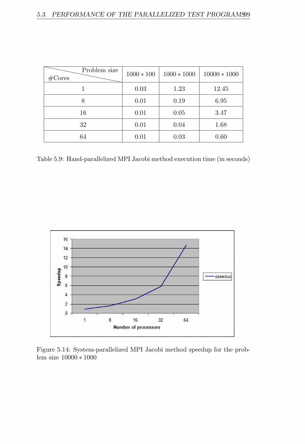
5.3. PERFORMANCE OF THE PARALLELIZED TEST PROGRAMS99
````````````#CoresProblem size
1000 ∗ 100 1000 ∗ 1000 10000 ∗ 1000
1 0.03 1.23 12.45
8 0.01 0.19 6.95
16 0.01 0.05 3.47
32 0.01 0.04 1.68
64 0.01 0.03 0.60
Table 5.9: Hand-parallelized MPI Jacobi method execution time (in seconds)
Figure 5.14: System-parallelized MPI Jacobi method speedup for the prob-lem size 10000 ∗ 1000
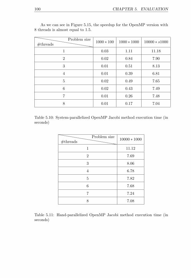
100 CHAPTER 5. EVALUATION
As we can see in Figure 5.15, the speedup for the OpenMP version with8 threads is almost equal to 1.5.
hhhhhhhhhhhhhhh#threadsProblem size
1000 ∗ 100 1000 ∗ 1000 10000 ∗ s1000
1 0.03 1.11 11.18
2 0.02 0.84 7.90
3 0.01 0.51 8.13
4 0.01 0.39 6.81
5 0.02 0.49 7.65
6 0.02 0.43 7.49
7 0.01 0.26 7.48
8 0.01 0.17 7.04
Table 5.10: System-parallelized OpenMP Jacobi method execution time (inseconds)
hhhhhhhhhhhhhhh#threadsProblem size
10000 ∗ 1000
1 11.12
2 7.69
3 8.06
4 6.78
5 7.82
6 7.68
7 7.24
8 7.08
Table 5.11: Hand-parallelized OpenMP Jacobi method execution time (inseconds)
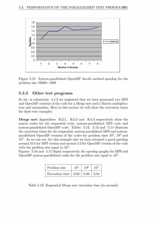
5.3. PERFORMANCE OF THE PARALLELIZED TEST PROGRAMS101
Figure 5.15: System-parallelized OpenMP Jacobi method speedup for theproblem size 10000 ∗ 1000
5.3.3 Other test programs
So far, in subsection 5.1.3 we explained that we have generated two MPIand OpenMP versions of the code for a Merge sort and a Matrix multiplica-tion and summation. Here in this section we will show the execution timesfor these two examples.
Merge sort Appendices B.2.1, B.2.2 and B.2.3 respectively show thesource codes for the sequential code, system-parallelized MPI code andsystem-parallelized OpenMP code. Tables 5.12, 5.13 and 5.14 illustratethe execution times for the sequential, system-parallelized MPI and system-parallelized OpenMP versions of the codes for problem sizes 105, 106 and107. As we can see, for this example also we have attained a good speeduparound 10.5 for MPI version and around 4.2 for OpenMP version of the codewith the problem size equal to 107.Figures 5.16 and 5.17 depict respectively the speedup graphs for MPI andOpenMP system-parallelized codes for the problem size equal to 107.
Problem size 105 106 107
Execution time 0.02 0.26 2.54
Table 5.12: Sequential Merge sort execution time (in seconds)
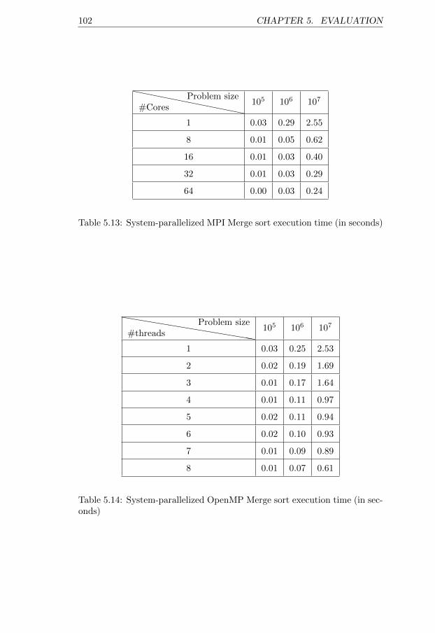
102 CHAPTER 5. EVALUATION
````````````#CoresProblem size
105 106 107
1 0.03 0.29 2.55
8 0.01 0.05 0.62
16 0.01 0.03 0.40
32 0.01 0.03 0.29
64 0.00 0.03 0.24
Table 5.13: System-parallelized MPI Merge sort execution time (in seconds)
hhhhhhhhhhhhhhh#threadsProblem size
105 106 107
1 0.03 0.25 2.53
2 0.02 0.19 1.69
3 0.01 0.17 1.64
4 0.01 0.11 0.97
5 0.02 0.11 0.94
6 0.02 0.10 0.93
7 0.01 0.09 0.89
8 0.01 0.07 0.61
Table 5.14: System-parallelized OpenMP Merge sort execution time (in sec-onds)
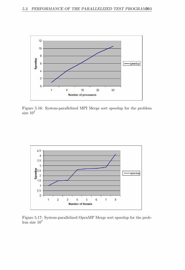
5.3. PERFORMANCE OF THE PARALLELIZED TEST PROGRAMS103
Figure 5.16: System-parallelized MPI Merge sort speedup for the problemsize 107
Figure 5.17: System-parallelized OpenMP Merge sort speedup for the prob-lem size 107
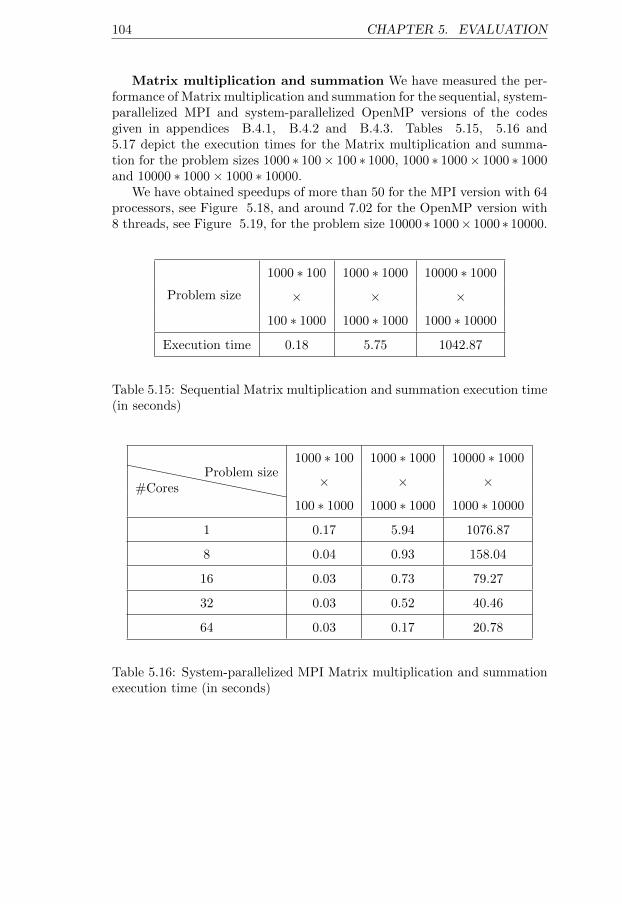
104 CHAPTER 5. EVALUATION
Matrix multiplication and summation We have measured the per-formance of Matrix multiplication and summation for the sequential, system-parallelized MPI and system-parallelized OpenMP versions of the codesgiven in appendices B.4.1, B.4.2 and B.4.3. Tables 5.15, 5.16 and5.17 depict the execution times for the Matrix multiplication and summa-tion for the problem sizes 1000 ∗ 100× 100 ∗ 1000, 1000 ∗ 1000× 1000 ∗ 1000and 10000 ∗ 1000× 1000 ∗ 10000.
We have obtained speedups of more than 50 for the MPI version with 64processors, see Figure 5.18, and around 7.02 for the OpenMP version with8 threads, see Figure 5.19, for the problem size 10000 ∗ 1000× 1000 ∗ 10000.
Problem size
1000 ∗ 100 1000 ∗ 1000 10000 ∗ 1000
× × ×
100 ∗ 1000 1000 ∗ 1000 1000 ∗ 10000
Execution time 0.18 5.75 1042.87
Table 5.15: Sequential Matrix multiplication and summation execution time(in seconds)
````````````#CoresProblem size
1000 ∗ 100 1000 ∗ 1000 10000 ∗ 1000
× × ×
100 ∗ 1000 1000 ∗ 1000 1000 ∗ 10000
1 0.17 5.94 1076.87
8 0.04 0.93 158.04
16 0.03 0.73 79.27
32 0.03 0.52 40.46
64 0.03 0.17 20.78
Table 5.16: System-parallelized MPI Matrix multiplication and summationexecution time (in seconds)
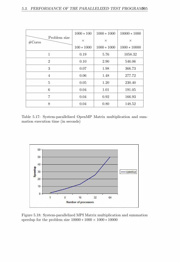
5.3. PERFORMANCE OF THE PARALLELIZED TEST PROGRAMS105
````````````#CoresProblem size
1000 ∗ 100 1000 ∗ 1000 10000 ∗ 1000
× × ×
100 ∗ 1000 1000 ∗ 1000 1000 ∗ 10000
1 0.19 5.76 1058.32
2 0.10 2.90 546.06
3 0.07 1.98 366.73
4 0.06 1.48 277.72
5 0.05 1.20 230.40
6 0.04 1.01 191.05
7 0.04 0.92 166.93
8 0.04 0.80 148.52
Table 5.17: System-parallelized OpenMP Matrix multiplication and sum-mation execution time (in seconds)
Figure 5.18: System-parallelized MPI Matrix multiplication and summationspeedup for the problem size 10000 ∗ 1000× 1000 ∗ 10000
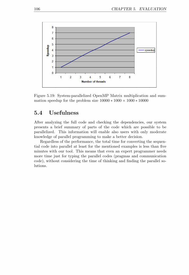
106 CHAPTER 5. EVALUATION
Figure 5.19: System-parallelized OpenMP Matrix multiplication and sum-mation speedup for the problem size 10000 ∗ 1000× 1000 ∗ 10000
5.4 Usefulness
After analyzing the full code and checking the dependencies, our systempresents a brief summary of parts of the code which are possible to beparallelized. This information will enable also users with only moderateknowledge of parallel programming to make a better decision.
Regardless of the performance, the total time for converting the sequen-tial code into parallel at least for the mentioned examples is less than fiveminutes with our tool. This means that even an expert programmer needsmore time just for typing the parallel codes (pragmas and communicationcode), without considering the time of thinking and finding the parallel so-lutions.
Chapter 6
Related Work
Parallelizing sequential code is widely recognized as a quite interesting re-search topic in computer science over the past decades and different researchgroups work on different aspects of it. In this chapter, we will mention anumber of related projects and highlight the differences to our work in sec-tion 6.5.
6.1 Dependency analysis in parallelizing se-quential code
Dependency analysis is a technique which shows the relation among differentstatements of a program and has been used since the 1970’s to vectorizeFortran loops automatically. Therefore, it is one of the important topics thatwe must consider in parallelizing sequential code, especially for recurrences,reductions, and data dependent loop iterations.
In this respect, Hsieh [59] has presented techniques for parallelizingnested do loops and blocks of codes based on constrained forward controldependence analysis in the PTRAN system at IBM Research. Control anddata dependence information have been used in order to compute the con-strained forward control dependence graph. As an input language he uses alanguage similar to Fortran. He claims that his techniques generate nestedparallelism. His proposed techniques have two main weaknesses. At first,since they produce too much fine-grained parallelism, the generated outputprogram runs slowly. Second, his techniques are not able to perform loopparallelization upon arrays
Another attempt refers to dependency analysis tests for parallelizing se-quential codes that were proposed by Jacobson and Stubbendieck [29]. Theyhave used dependency analysis techniques to identify different ways of trans-forming sequential code into parallel and producing coarse grained parallelcode from sequential C code to be able to execute on a cluster of work-
107
108 CHAPTER 6. RELATED WORK
stations. In their approach they have addressed a number of dependencyanalysis tests in order to determine existing dependences in for-loops.
Dependence analysis is now commonplace in many modern compilerframeworks, such as Cetus [16] and Open64 [1].
6.2 Parallelizing by using Skeletons
Regarding parallelizing recursive functions there exist several approaches.Gonzalez-Escribano et al. [19] suggest skeletons for parallelizing these kindsof functions. Ahn and Han [3] have implemented it by dividing the taskof parallelizing recursive functions into two different tasks: converting thesequential program into several parallel skeletons and implementing theseskeletons. They have indicated that the analytical approach and parallelskeletons made possible the parallelization of recursive functions with com-plex data flows.
6.3 Automatically parallelizing sequential code
In automatic parallelization the emphasis is mostly on producing a com-piler which can parallelize sequential code automatically. In this approachmost focus is on parallelizing control and data structures, as Nikhil [39] hasmentioned.
Gonzalez-Escribano et al. [19] explain that most compilers focus onloop-level parallelization and will avoid it if the execution overhead for loopparallelization exceeds the expected performance gain.
With respect to parallelizing recursive functions we should consider spe-cial techniques to be able to parallelize codes automatically by compilers.Rugina and Rinard [47] discuss that recursive programs are not suitablefor traditional parallelizing compilers since recursive algorithms are usuallycoded as recursive procedures and use pointers into dynamically allocatedmemory blocks. Their remedy to this problem was designing a compilerwhich was able to parallelize algorithms that use pointers to access disjointregions of dynamically allocated arrays by extracting symbolic expressionsfor the regions of the memory accessed during the divide and conquer algo-rithm implementation. Finally, this compiler ran dependence analysis on theextracted expressions, and if the result proved disjoint regions of memory itconcluded that recursive function calls can be executed in parallel.
In [23] Gupta et al. presented a framework for automatically parallelizingrecursive procedures by using compile-time analysis to prove independenceof multiple recursive calls. Their approach is capable of parallelizing pro-grams for which compile-time analysis alone is not sufficient, by exploiting atechnique for speculative parallelization of recursive procedures. They par-allelized programs like Quick sort and Merge sort, written in C, for parallel
6.4. SEMI-AUTOMATICALLY PARALLELIZING SEQUENTIALCODE 109
execution on an IBM G30 SMP, and their experimental results have showngood speedups.
In order to make it possible for a programmer to specify vector and ar-ray operations explicitly (like for Fortran90) for existing Fortran programs,Allen and Kennedy [4] have implemented a translator, PFC (Parallel FOR-TRAN Converter), which automatically rewrites the implicitly discoveredparallelism in a Fortran program into Fortran8x (Fortran90). This transla-tor works extremely fast for uncovering parallelism and its performance hasbeen a pleasant surprise.
6.4 Semi-automatically parallelizing sequen-tial code
Semi-automatic parallelization tries to parallelize the code by combiningautomatic techniques and human knowledge. Ishihara et al. [35] devel-oped an interactive parallelizing assistance tool which is called iPat/OMP.IPat/OMP is a combination of an Emacs editor mode, Java functions andshell scripts which assists in manual parallelization by using OpenMP. Byusing the PowerTest for dependence analysis this tool is capable of analyz-ing data dependence relations in a for-loop. All communications betweenthe implemented system and a programmer are text-based. In this system,the programmer is responsible for modifying the code manually based ondependency reports generated by the tool.
ParaScope Editor, PED, is a tool developed by Kennedy et al. [31]with the aim of assisting scientists in parallelizing sequential code. Theyclaim that “PED overcomes the imprecision of dependence analysis and theinflexibility of automatic parallel code generation techniques”[31], so it isconsidered as an interactive programming tool that facilitates parallel pro-gramming by involving the user. This tool determines dependences, advicesthe programmer and performs transformations. The programmer interactswith system by selecting valid dependences and required transformations.This tool supports the programmer’s incremental change by analyzing theedited texts. PED accepts and generates code for Fortran77, IBM parallelFortran and parallel Fortran for the Sequent Symmetry.
Another attempt in this respect is extending the iblOpt programmingtool [54] which semi-automatically parallelizes the code. In this project, alocal search algorithm is developed that automatically parallelize the codeby distributing the code statements across a number of processors. This al-gorithm, for code distribution, simulates memory access time and the resultshows that this method optimizes program for parallel execution.
110 CHAPTER 6. RELATED WORK
6.5 Summary
In this master thesis, we developed an interactive system that assists a userin the parallelization of selected C code blocks for shared and distributedmemory architectures. This work advances previous approaches. Each ofthe above mentioned approaches provides parts of our approach’s featuresbut none of them provides all the features. Jacobson and Stubbendieckhave mostly focused on parallelizing for-loops by using data dependencyanalysis, and although they were successful in their attempts it is not obviouswhether their method is capable of parallelizing recursive procedures or not.Unlike Jacobson et al.[29]; Gonzalez-Escribano et al.[19], Ahn and Han [3],Rugina and Rinard [47], and Gupta et al.[23] put their efforts on parallelizingrecursive functions by using skeleton-based parallelization or compiler-basedparallelization methods. These two methods restrict parallelization, sincethe skeleton-based method is only suitable for well structured code and acompiler-based method is inflexible in generating parallel code for all codestructures.
IPat/OMP and PED are interactive tools that assist users in paralleliz-ing sequential code. IPat/OMP by Ishihara et al. [35] is a compositionalapproach and it only supports OpenMP. Kennedy et al. [31] have proposedPED, a semi-automatically parallelizing tool with useful features that ac-cepts and generates Fortran code for shared memory architecture.
Although the semi-automatic method for locality optimization is ableto optimize the code statements, but it has some performance issues. Thistool can not support different memory organizations (e.g. NUMA) or otherparallel architectures such as clusters.
In our approach, we develop an interactive system which is able to paral-lelize both loops and certain recursive procedures for both MPI and OpenMPin the C language. We propose a system to assist users in both advisingand transforming the code with the help of a reasoning system. By using areasoning system, consistency, availability, productivity, and quality of theparallelization process will increase.
Chapter 7
Conclusion
Nowadays, the requirement for utilizing multi-processor computers is in-creasing more and more; meanwhile, a lot more efforts are being done tocreate tools with the ability of producing parallel codes which exploit thefull computation power of existing hardware.
This thesis is an attempt towards finding a software solution to fulfillparts of these requirements. In order to do so, it presents techniques forsemi-automatically parallelizing the code by prototyping a system which isbased on IIP and reasoning concepts.
Our focus in this project was on parallelizing loops (e.g., Jacobi method)and D&C algorithms (e.g., Quick sort). We can enumerate two reasons forselecting these two programs. First, loops are often performance criticalpoints in programs which consume a lot of CPU time and we can estimatethat a large number of programs have loops in their structures. Therefore,finding a solution to parallelizing them in an effective way will increase theperformance. Second, D&C algorithms are common algorithms that can beused to solve a variety of problems.
Our proposed approach has the advantage that the output parallel pro-gram can have high performance if the parallelization strategies and reason-ing engine are defined properly. Our implemented parallelization strategiesare not the best possible ones but our experimental results show that wehave obtained good speedups. This can support the claim that by selectinga better strategy we can have even better performance.
Another important aspect of this approach is simplicity and extensibilityin creating new strategies. Since all strategies in this system are defined byusing the concept of a decision tree, it can be easy to implement new ones.At the same time, we can point to one important aspect of software de-velopment, which is time-to-market. In software engineering, it is reallyimportant that the output product will be ready in appropriate time andsince it is mentioned in section 5.4 the time for converting sequential codeinto parallel code with this system is really low; at least for the mentioned
111
112 CHAPTER 7. CONCLUSION
test examples, the proposed system fulfills this requirement.In chapter 5, we have shown that beyond the two test examples Quick
sort and Jacobi method, our tool is capable of parallelizing other codeswhich have D&C (e.g., Merge sort), for-loop and reduction statements (e.g.,Matrix multiplication and summation) in their structures. This means thatour system is not just restricted to two test examples but also has the abilityto parallelize other codes.
Although implementing a complete system has its own costs and diffi-culties, when we look at its benefits we conclude that this effort will haveits valuable results.
Finally, we hope that the proposed methods in this thesis open a newway toward finding efficient and correct ways for interactively parallelizingsequential codes.
Chapter 8
Future work
In this last chapter, we point out and suggest some directions for continuingthis work.
8.1 Header files
Our implemented system prototype is not a complete C compiler and wehave just implemented some compiler concepts as far as we have needed, alsothe C language’s standard library functions are not defined in our system.If our system, during the code analysis, has reached a function call thatdoes not have any function definition in the given code, it will consider thefunction as a system library function.
Our prototype expects a single input source file. Hence, if we have a codewhich accesses some functions through the header files we must accuratelychange the code in a way that all the related files are placed in a singlefile in order to be able to parallelize the relevant functions. In a long-termrespective whole-program analysis should be performed for multi-moduleprograms.
Adding these features will increase the ability of the system to covermore programs.
8.2 Graphical user interface
Here it should be mentioned that the purpose of this thesis is not implement-ing a complete IIP system, but we have just implemented a prototype whichshows the correctness of our hypothesis. Therefore, we did not implementa graphical user interface. Instead users can pinpoint their selected code bytyping the line number which is displayed next to each statement; therefore,it is necessary to place each statement in a separate line of code. The systemusability will increase by implementing a graphical user interface.
113
114 CHAPTER 8. FUTURE WORK
8.3 Extension of loop parallelization
Our implemented system is able to recognize different C code structuressuch as loops. In our implementation, in order to parallelize the loops ourfocus was just on for-loops. In the C language, there are two other forms ofloops, “while” and “do”, that also may take a lot of CPU time. By addingthe ability to convert these loops into an equivalent for-loop structure wherepossible we may have further opportunities for reducing the execution time.
We have not implemented column-wise array distribution, this featurealso is important to be added.
8.4 Add profiler’s support
Our system’s loop parallelizability judgement is just based on dependenceanalysis while some parallelizable loops are so small that parallelizing themwill consume more time than running them sequentially. By using the pro-filer’s abilities that statistically records the time spent in different parts ofthe program we can give recommendations for not parallelizing such loops,which can further improve our system’s output performance.
8.5 Pointer analysis
This system can recognize the pointers in a code block. However, it is notyet capable of finding dependencies between statements which use pointers.Since pointers are one of the fundamental concepts in the C language, itseems really important to add this feature to the implemented system.
8.6 Extension for D&C algorithms paralleliza-tion
In our system prototype, we implemented just one special parallelizationstrategy for D&C functions, which is suitable for the algorithms with tworecursive calls. Since this system should be able to recognize many D&Calgorithms, by defining more strategies for this kind of algorithms, we canincrease the ability of the system to cover more D&C patterns and program-ming styles.
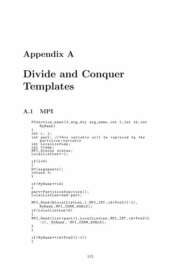
Appendix A
Divide and ConquerTemplates
A.1 MPI
Pfunction_name(f_arg_dty arg_name ,int l,int id,intMyRank)
{int i, j;int part; //this variable will be replaced by the
partition -variableint LocalListLen;int *temp;MPI_Status status;LocalListLen =-1;
if(l=0){DC(arguments);return 0;}
if(MyRank ==id){part=Partitionfunction ();LocalListLen=end -part;
MPI_Send (& LocalListLen ,1,MPI_INT ,id+Pow2(l-1),MyRank ,MPI_COMM_WORLD);
if(LocalListLen >0){MPI_Send(list+part+1,LocalListLen ,MPI_INT ,id+Pow2(l
-1), MyRank , MPI_COMM_WORLD);}}
if(MyRank ==id+Pow2(l-1)){
115
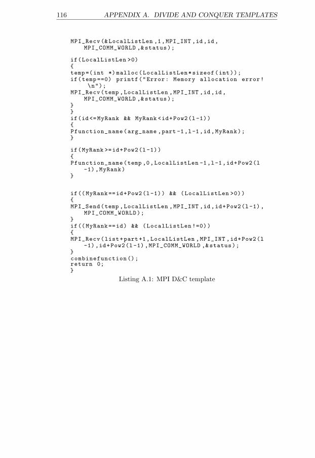
116 APPENDIX A. DIVIDE AND CONQUER TEMPLATES
MPI_Recv (& LocalListLen ,1,MPI_INT ,id,id,MPI_COMM_WORLD ,& status);
if(LocalListLen >0){temp=(int *) malloc(LocalListLen*sizeof(int));if(temp ==0) printf("Error: Memory allocation error!
\n");MPI_Recv(temp ,LocalListLen ,MPI_INT ,id,id,
MPI_COMM_WORLD ,& status);}}if(id <= MyRank && MyRank <id+Pow2(l-1)){Pfunction_name(arg_name ,part -1,l-1,id,MyRank);}
if(MyRank >=id+Pow2(l-1)){Pfunction_name(temp ,0,LocalListLen -1,l-1,id+Pow2(l
-1),MyRank)}
if(( MyRank ==id+Pow2(l-1)) && (LocalListLen >0)){MPI_Send(temp ,LocalListLen ,MPI_INT ,id,id+Pow2(l-1),
MPI_COMM_WORLD);}if(( MyRank ==id) && (LocalListLen !=0)){MPI_Recv(list+part+1,LocalListLen ,MPI_INT ,id+Pow2(l
-1),id+Pow2(l-1),MPI_COMM_WORLD ,& status);}combinefunction ();return 0;}
Listing A.1: MPI D&C template
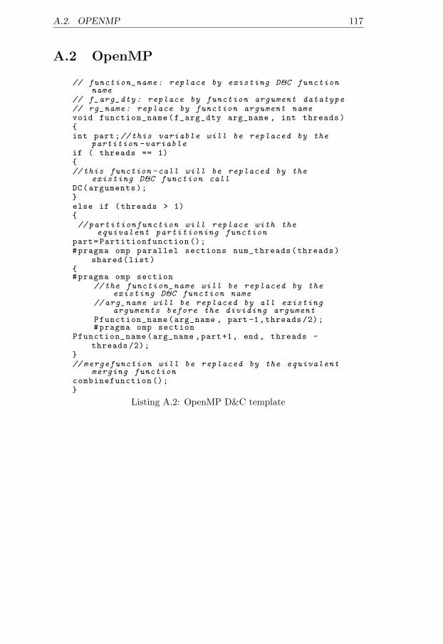
A.2. OPENMP 117
A.2 OpenMP
// function_name: replace by existing D&C functionname
// f_arg_dty: replace by function argument datatype// rg_name: replace by function argument namevoid function_name(f_arg_dty arg_name , int threads){int part;//this variable will be replaced by the
partition -variableif ( threads == 1){//this function -call will be replaced by the
existing D&C function callDC(arguments);}else if (threads > 1){// partitionfunction will replace with the
equivalent partitioning functionpart=Partitionfunction ();#pragma omp parallel sections num_threads(threads)
shared(list){#pragma omp section
//the function_name will be replaced by theexisting D&C function name
// arg_name will be replaced by all existingarguments before the dividing argument
Pfunction_name(arg_name , part -1,threads /2);#pragma omp section
Pfunction_name(arg_name ,part+1, end , threads -threads /2);
}// mergefunction will be replaced by the equivalent
merging functioncombinefunction ();}
Listing A.2: OpenMP D&C template
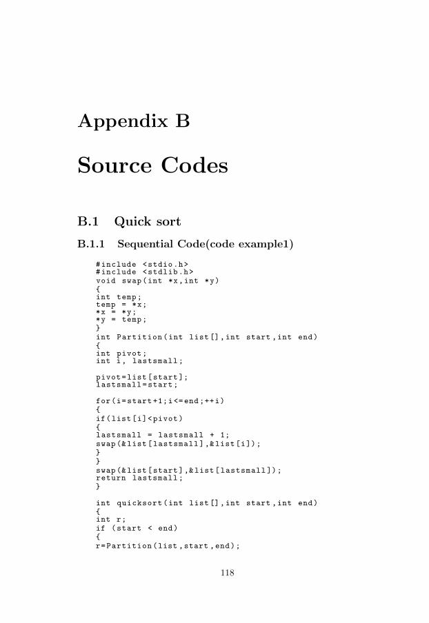
Appendix B
Source Codes
B.1 Quick sort
B.1.1 Sequential Code(code example1)
#include <stdio.h>#include <stdlib.h>void swap(int *x,int *y){int temp;temp = *x;*x = *y;*y = temp;}int Partition(int list[],int start ,int end){int pivot;int i, lastsmall;
pivot=list[start];lastsmall=start;
for(i=start +1;i<=end ;++i){if(list[i]<pivot){lastsmall = lastsmall + 1;swap(&list[lastsmall ],&list[i]);}}swap(&list[start],&list[lastsmall ]);return lastsmall;}
int quicksort(int list[],int start ,int end){int r;if (start < end){r=Partition(list ,start ,end);
118
B.1. QUICK SORT 119
quicksort(list ,start , r-1);quicksort(list ,r + 1, end);}return 0;}void printlist(int list[],int n){int i;for(i=0;i<n;i++){printf("%d\t",list[i]);}printf("\n");}
int main(){const int listSize = 100;int list[listSize ];
int i = 0;srand (396);// generate random numbers and fill them to the
listfor(i = 0; i < listSize; i++ ){list[i]=rand() %1000;}printf("The list before sorting is:\n");printlist(list ,listSize);
// sort the list using quicksortquicksort(list ,0,listSize -1);printf("The list after sorting using quicksort
algorithm :\n");// print the resultprintlist(list ,listSize);}
Listing B.1: Sequential Quick sort source code example1
120 APPENDIX B. SOURCE CODES
B.1.2 Sequential Code with better pivot selection(codeexample2)
#include <stdio.h>#include <stdlib.h>#include <stdbool.h>#include <time.h>
void swap(int *x,int *y){int temp;temp = *x;*x = *y;*y = temp;}int Partition(int list[],int start ,int end){int pivot;int i,j;int lastsmall;
int mid = (start + end) / 2;
lastsmall =0;
if (list[mid] < list[start ]) swap (&list[mid], &list[start ]);
if (list[end] < list[start ]) swap (&list[end], &list[start ]);
if (list[end] < list[mid]) swap (&list[end], &list[mid]);
pivot=list[mid];i=start -1;j=end+1;while (true) {while (list [++i] < pivot) {;} // scan right until
list[i] >= pivotwhile (list[--j] > pivot) {;} // scan left until
list[j] <= pivotif (i < j){swap(&list[i], &list[j]);
}elsebreak;
}lastsmall=j;
return lastsmall;}
int quicksort(int list[],int start ,int end){int r;if (start < end){r=Partition(list ,start ,end);
B.1. QUICK SORT 121
quicksort(list ,start , r);quicksort(list ,r +1, end);}return 0;}void printlist(int list[],int n){int i;for(i=0;i<n;i++){printf("%d\t",list[i]);}printf(" \n");}
int main(){const int listSize = 100;int list[listSize ];struct timespec stime , etime;
int i = 0;srand (396);
for(i = 0; i < listSize; i++ ){list[i]=rand() %1000;}printf("The list before sorting is:\n");printlist(list ,listSize);
// sort the list using quicksortclock_gettime(CLOCK_REALTIME , &stime);quicksort(list ,0,listSize -1);clock_gettime(CLOCK_REALTIME , &etime);
printf("Execution time: %5.2f\n", (etime.tv_sec -stime.tv_sec)+ 1e-9*( etime.tv_nsec - stime.tv_nsec)) ;
printf("The list after sorting using quicksortalgorithm :\n");
printlist(list ,listSize);}
Listing B.2: Sequential Quick sort source code example2
122 APPENDIX B. SOURCE CODES
B.1.3 System-generated MPI Parallel code
#include <stdio.h>#include <stdlib.h>#include <stdbool.h>#include <mpi.h>#define send_data_tag 2001#define return_data_tag 2002int MyRank , np;MPI_Status status;MPI_Request request;void swap(int *x,int *y){int temp;temp = *x;*x = *y;*y = temp;}int Partition(int list[],int start ,int end){int pivot;int i, lastsmall;
pivot=list[start];lastsmall=start;
for(i=start +1;i<=end ;++i){if(list[i]<pivot){lastsmall = lastsmall + 1;swap(&list[lastsmall ],&list[i]);}}swap(&list[start],&list[lastsmall ]);return lastsmall;}
void printlist(int list[],int n){int i;for(i=0;i<n;i++){printf("%d\t",list[i]);}printf(" \n");}
int Pow2(int num){int i;
i=1;
while(num >0){num --;i=i*2;}
B.1. QUICK SORT 123
return i;}int Log2(int num){int i, j;
i=1;j=2;
while(j<num){j=j*2;i++;}
if(j>num)i--;
return i;}int Pquicksort(int list[],int start ,int end ,int l,
int id ,int MyRank){int i, j;int r;int LocalListLen;int *temp;MPI_Status status;LocalListLen =-1;
if(l==0){quicksort(list ,start ,end);return 0;}
if(MyRank ==id){r=Partition(list ,start ,end);LocalListLen=end -r;
MPI_Send (& LocalListLen ,1,MPI_INT ,id+Pow2(l-1),MyRank ,MPI_COMM_WORLD);
if(LocalListLen >0)
MPI_Send(list+r+1,LocalListLen ,MPI_INT ,id+Pow2(l-1),MyRank ,MPI_COMM_WORLD);
}
if(MyRank ==id+Pow2(l-1)){MPI_Recv (& LocalListLen ,1,MPI_INT ,id,id,
MPI_COMM_WORLD ,& status);
if(LocalListLen >0){temp=(int *) malloc(LocalListLen*sizeof(int));if(temp ==0) printf("Error: Memory allocation error
!\n");
124 APPENDIX B. SOURCE CODES
MPI_Recv(temp ,LocalListLen ,MPI_INT ,id,id,MPI_COMM_WORLD ,& status);
}}if(id <= MyRank && MyRank <id+Pow2(l-1)){Pquicksort(list ,start ,r,l-1,id ,MyRank);}
if(MyRank >=id+Pow2(l-1)){Pquicksort(temp ,0,LocalListLen -1,l-1,id+Pow2(l-1),
MyRank);}
if(( MyRank ==id+Pow2(l-1)) && (LocalListLen >0))
MPI_Send(temp ,LocalListLen ,MPI_INT ,id,id+Pow2(l-1),MPI_COMM_WORLD);
if(( MyRank ==id) && (LocalListLen >0)){MPI_Recv(list+r+1,LocalListLen ,MPI_INT ,id+Pow2(l-1)
,id+Pow2(l-1),MPI_COMM_WORLD ,& status);
}return 0;}int main(int argc ,char *argv []){const int listSize = 100;int level;int list[listSize ];MPI_Init (&argc ,&argv);MPI_Comm_rank(MPI_COMM_WORLD ,& MyRank);MPI_Comm_size(MPI_COMM_WORLD ,&np);int i = 0;double startTime , endTime;srand (396);// generate random numbers and fill them to the
listif(MyRank ==0){for(i = 0; i < listSize; i++ ){list[i]=rand() %1000;}}printf("The list before sorting is:\n");printlist(list ,listSize);// sort the list using quicksortlevel=Log2(np);MPI_Barrier(MPI_COMM_WORLD);startTime = MPI_Wtime ();Pquicksort(list ,0,listSize -1,m,0,MyRank);MPI_Barrier(MPI_COMM_WORLD);endTime = MPI_Wtime ();
B.1. QUICK SORT 125
if (MyRank == 0){printf("Execution time: %5.2f\n", (endTime -
startTime));printlist(list ,listSize);}MPI_Finalize ();}
Listing B.3: System-parallelized MPI Quick sort source code
126 APPENDIX B. SOURCE CODES
B.1.4 System-generated OpenMP Parallel code
#include <stdio.h>#include <stdlib.h>#include <time.h>#include <omp.h>int tid;void swap(int *x,int *y){int temp;temp = *x;*x = *y;*y = temp;}int Partition(int list[],int start ,int end){int pivot;int i, lastsmall;pivot=list[start];lastsmall=start;for(i=start +1;i<=end ;++i){if(list[i]<pivot){lastsmall = lastsmall + 1;swap(&list[lastsmall ],&list[i]);}}swap(&list[start],&list[lastsmall ]);return lastsmall;}int quicksort(int list[],int start ,int end){int r;if (start < end){r=Partition(list ,start ,end);quicksort(list ,start , r-1);quicksort(list ,r + 1, end);}return 0;}void printlist(int list[],int n){int i;for(i=0;i<n;i++){printf("%d\t",list[i]);}printf(" \n");}
int Pquicksort(int list[],int start ,int end ,intthreads)
{int r;
if ( threads == 1)
B.1. QUICK SORT 127
{quicksort(list ,start ,end);}else if (threads > 1){r=Partition(list ,start ,end);#pragma omp parallel num_threads(threads){#pragma omp sections{#pragma omp sectionPquicksort(list ,start , r-1,threads /2);#pragma omp sectionPquicksort(list ,r+1, end , threads - threads /2);}}}return 0;}int main(int argc ,char *argv []){const int listSize = 100;int list[listSize ];int threads ,tid;double stime , etime;omp_set_dynamic (0);omp_set_nested (1);
threads=omp_get_max_threads ();tid=omp_get_thread_num ();int i = 0;srand (396);// generate random numbers and fill them to the
listfor(i = 0; i < listSize; i++ ){list[i]=rand() %1000;}
printf("The list before sorting is:\n");printlist(list ,listSize);
// sort the list using quicksort#pragma omp barrierstime=omp_get_wtime ();Pquicksort(list ,0,listSize -1,threads);#pragma omp barrieretime=omp_get_wtime ();
printf("sorting took: %5.2f \n", (etime -stime)) ;printlist(list ,listSize);
}
Listing B.4: System-parallelized OpenMP Quick sort source code
128 APPENDIX B. SOURCE CODES
B.2 Merge sort
B.2.1 Sequential Code
#include <stdio.h>#include <stdlib.h>void merge(int lstA[], int lstA_size , int lstB[],
int lstB_size){int cntA ,cntB ,cnttmp ,i;int *tmp;int tmp_size = lstA_size+lstB_size;
cntA =0;cntB =0;cnttmp =0;
tmp = (int *) malloc(tmp_size*sizeof(int));while ((cntA < lstA_size) && (cntB < lstB_size)){if (lstA[cntA] <= lstB[cntB]){tmp[cnttmp] = lstA[cntA];cnttmp ++;cntA ++;} else{tmp[cnttmp] = lstB[cntB];cnttmp ++;cntB ++;}}
if (cntA >= lstA_size)for (i = cnttmp; i < tmp_size; i++){tmp[i] = lstB[cntB];cntB ++;}else if (cntB >= lstB_size)for (i = cnttmp; i < tmp_size; i++){tmp[i] = lstA[cntA];cntA ++;}for (i = 0; i < lstA_size; i++)lstA[i] = tmp[i];for (i = 0; i < lstB_size; i++)lstB[i] = tmp[lstA_size+i];free(tmp);tmp=NULL;}
int mergesort(int list[], int start , int end){int mid;if(start <end){
B.2. MERGE SORT 129
mid=( start+end)/2;
mergesort(list ,start ,mid);mergesort(list ,mid+1,end);
merge(list + start , mid -start+1, list+ mid + 1, end-mid);
}return 0;}
void printlist(int list[],int n){int i;for(i=0;i<n;i++)printf("%d\t",list[i]);printf(" \n");}int main(){const int listSize = 21;int list[listSize ];int i = 0;srand (396);
for(i = 0; i < listSize; i++ ){list[i]=rand() %1000;}printf("The list before sorting is:\n");printlist(list ,listSize);
mergesort(list ,0,listSize -1);
printf("The list after sorting using quicksortalgorithm :\n");
printlist(list ,listSize);}
Listing B.5: Sequential Merge sort source code
130 APPENDIX B. SOURCE CODES
B.2.2 System-generated MPI Parallel code
#include <stdio.h>#include <stdlib.h>#include <mpi.h>#define send_data_tag 2001#define return_data_tag 2002int MyRank , np;MPI_Status status;MPI_Request request;void merge(int lstA[], int lstA_size , int lstB[],
int lstB_size){int cntA ,cntB ,cnttmp ,i;int *tmp;int tmp_size = lstA_size+lstB_size;
cntA =0;cntB =0;cnttmp =0;
tmp = (int *) malloc(tmp_size*sizeof(int));while ((cntA < lstA_size) && (cntB < lstB_size)){if (lstA[cntA] <= lstB[cntB]){tmp[cnttmp] = lstA[cntA];cnttmp ++;cntA ++;} else{tmp[cnttmp] = lstB[cntB];cnttmp ++;cntB ++;}}
if (cntA >= lstA_size)for (i = cnttmp; i < tmp_size; i++){tmp[i] = lstB[cntB];cntB ++;}else if (cntB >= lstB_size)for (i = cnttmp; i < tmp_size; i++){tmp[i] = lstA[cntA];cntA ++;}for (i = 0; i < lstA_size; i++)lstA[i] = tmp[i];for (i = 0; i < lstB_size; i++)lstB[i] = tmp[lstA_size+i];free(tmp);tmp=NULL;}
int mergesort(int list[], int start , int end){int mid;
B.2. MERGE SORT 131
if(start <end){mid=( start+end)/2;mergesort(list ,start ,mid);mergesort(list ,mid+1,end);merge(list + start , mid -start+1, list+ mid + 1, end
-mid);}return 0;}void printlist(int list[],int n){int i;if(MyRank ==0){for(i=0;i<n;i++)printf("%d\t",list[i]);printf(" \n");}}int partition_func(int start ,int end){int mid;mid=( start+end)/2;return mid;}
int Pow2(int num){int i;
i=1;
while(num >0){num --;i=i*2;}
return i;}int Log2(int num){int i, j;
i=1;j=2;
while(j<num){j=j*2;i++;}
if(j>num)i--;
return i;}
132 APPENDIX B. SOURCE CODES
int Pmergesort(int list[], int start , int end ,int l,int id,int MyRank)
{int i, j;int mid;int LocalListLen;int *temp;MPI_Status status;LocalListLen =-1;
if(l==0){mergesort(list ,start ,end);return 0;}
if(MyRank ==id){mid=partition_func(start ,end);LocalListLen=end -mid;
MPI_Send (& LocalListLen ,1,MPI_INT ,id+Pow2(l-1),MyRank ,MPI_COMM_WORLD);
if(LocalListLen >0)
MPI_Send(list+mid+1,LocalListLen ,MPI_INT ,id+Pow2(l-1),MyRank ,MPI_COMM_WORLD);
}
if(MyRank ==id+Pow2(l-1)){MPI_Recv (& LocalListLen ,1,MPI_INT ,id,id,
MPI_COMM_WORLD ,& status);
if(LocalListLen >0){temp=(int *) malloc(LocalListLen*sizeof(int));if(temp ==0) printf("Error: Memory allocation error!
\n");MPI_Recv(temp ,LocalListLen ,MPI_INT ,id,id,
MPI_COMM_WORLD ,& status);}}if(id <= MyRank && MyRank <id+Pow2(l-1)){Pmergesort(list ,start ,mid ,l-1,id ,MyRank);}
if(MyRank >=id+Pow2(m-1)){Pmergesort(temp ,0,LocalListLen -1,l-1,id+Pow2(l-1),
MyRank);}
if(( MyRank ==id+Pow2(l-1)) && (LocalListLen >0))
B.2. MERGE SORT 133
MPI_Send(temp ,LocalListLen ,MPI_INT ,id,id+Pow2(l-1),MPI_COMM_WORLD);
if(( MyRank ==id) && (LocalListLen >0)){MPI_Recv(list+mid+1,LocalListLen ,MPI_INT ,id+Pow2(l
-1),id+Pow2(l-1),MPI_COMM_WORLD ,& status);merge(list + start , mid -start+1, list+ mid + 1, end
-mid);}return 0;}int main(int argc ,char *argv []){const int listSize = 100;int level;int list[listSize ];MPI_Init (&argc ,&argv);MPI_Comm_rank(MPI_COMM_WORLD ,& MyRank);MPI_Comm_size(MPI_COMM_WORLD ,&np);int i = 0;srand (396);
if(MyRank ==0){for(i = 0; i < listSize; i++ ){list[i]=rand() %1000;}}if (MyRank ==0){printf("The list before sorting is:\n");printlist(list ,listSize);}
level=Log2(np);Pmergesort(list ,0,listSize -1,level ,0,MyRank);
if (MyRank ==0){printf("The list after sorting using quicksort
algorithm :\n");printlist(list ,listSize);}
MPI_Finalize ();}
Listing B.6: System-parallelized MPI Merge sort source code
134 APPENDIX B. SOURCE CODES
B.2.3 System-generated OpenMP Parallel code
#include <stdio.h>#include <stdlib.h>#include <omp.h>void merge(int lstA[], int lstA_size , int lstB[],
int lstB_size){int cntA ,cntB ,cnttmp ,i;int *tmp;int tmp_size = lstA_size+lstB_size;
cntA =0;cntB =0;cnttmp =0;
tmp = (int *) malloc(tmp_size*sizeof(int));while ((cntA < lstA_size) && (cntB < lstB_size)){if (lstA[cntA] <= lstB[cntB]){tmp[cnttmp] = lstA[cntA];cnttmp ++;cntA ++;} else{tmp[cnttmp] = lstB[cntB];cnttmp ++;cntB ++;}}
if (cntA >= lstA_size)for (i = cnttmp; i < tmp_size; i++){tmp[i] = lstB[cntB];cntB ++;}else if (cntB >= lstB_size)for (i = cnttmp; i < tmp_size; i++){tmp[i] = lstA[cntA];cntA ++;}for (i = 0; i < lstA_size; i++)lstA[i] = tmp[i];for (i = 0; i < lstB_size; i++)lstB[i] = tmp[lstA_size+i];free(tmp);tmp=NULL;}
int mergesort(int list[], int start , int end){int mid;if(start <end){mid=( start+end)/2;mergesort(list ,start ,mid);
B.2. MERGE SORT 135
mergesort(list ,mid+1,end);merge(list + start , mid -start+1, list+ mid + 1, end
-mid);}return 0;}void printlist(int list[],int n){int i;#pragma omp master{for(i=0;i<n;i++)printf("%d\t",list[i]);printf(" \n");}}int partition_func(int start ,int end){int mid;mid=( start+end)/2;return mid;}
int Pmergesort(int list[], int start , int end ,intthreads)
{int mid;if ( threads == 1){mergesort(list ,start ,end);}else if (threads > 1){mid=partition_func(start ,end);#pragma omp parallel sections num_threads(threads)
shared(list){#pragma omp sectionPmergesort(list ,start , mid ,threads /2);#pragma omp sectionPmergesort(list ,mid+1, end , threads - threads /2);}merge(list + start , mid -start+1, list+ mid + 1, end
-mid);}return 0;}int main(int argc ,char *argv []){const int listSize = 100;omp_set_dynamic (0);omp_set_nested (1);int list[listSize ];int threads ,tid;threads=omp_get_max_threads ();tid=omp_get_thread_num ();int i = 0;double stime , etime;
136 APPENDIX B. SOURCE CODES
srand (396);
for(i = 0; i < listSize; i++ ){list[i]=rand() %1000;}
printf("The list before sorting is:\n");printlist(list ,listSize);stime=omp_get_wtime ();Pmergesort(list ,0,listSize -1,threads);etime=omp_get_wtime ();printf("sorting took: %5.2f \n", (etime -stime)) ;printf("The list after sorting using quicksort
algorithm :\n");printlist(list ,listSize);}
Listing B.7: System-parallelized OpenMP Merge sort source code
B.3. JACOBI METHOD 137
B.3 Jacobi method
B.3.1 Sequential Code
#include <stdio.h>#include <stdlib.h>#include <time.h>#define NUM_ROWS 4#define NUM_COLUMNS 4int i, j, k;
double A[NUM_ROWS ][ NUM_COLUMNS ];double New[NUM_ROWS ][ NUM_COLUMNS ];void createMatrix (){for (i = 0; i < NUM_ROWS; i++){for (j = 0; j < NUM_COLUMNS; j++){A[i][j]=rand() % 10000;}}}void printMatrix (){for (i = 0; i < NUM_ROWS; i++){printf("\n");for (j = 0; j < NUM_COLUMNS; j++){printf("%8.2f ", A[i][j]);}}printf("\n");}
int main(){int t;struct timespec stime , etime;createMatrix ();printMatrix ();t=0;clock_gettime(CLOCK_REALTIME , &stime);while(t <100){for (i = 1; i < NUM_ROWS -1; i++){for (j = 1; j < NUM_COLUMNS -1; j++){New[i][j] = (A[i][j-1]+A[i][j+1]+A[i-1][j]+A[i+1][j
])/4;
}}for (i = 1; i < NUM_ROWS -1; i++){
138 APPENDIX B. SOURCE CODES
for (j = 1; j < NUM_COLUMNS -1; j++){A[i][j]= New[i][j];}}t++;}clock_gettime(CLOCK_REALTIME , &etime);printf("Execution time: %5.2f\n", (etime.tv_sec -
stime.tv_sec)+ 1e-9*( etime.tv_nsec - stime.tv_nsec)) ;
printMatrix ();}
Listing B.8: Sequential Jacobi method source code
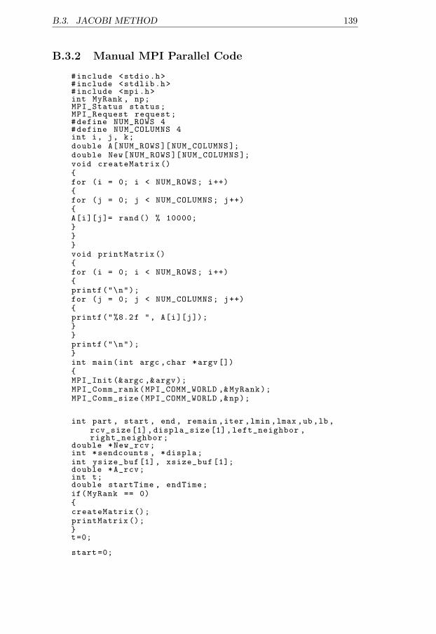
B.3. JACOBI METHOD 139
B.3.2 Manual MPI Parallel Code
#include <stdio.h>#include <stdlib.h>#include <mpi.h>int MyRank , np;MPI_Status status;MPI_Request request;#define NUM_ROWS 4#define NUM_COLUMNS 4int i, j, k;double A[NUM_ROWS ][ NUM_COLUMNS ];double New[NUM_ROWS ][ NUM_COLUMNS ];void createMatrix (){for (i = 0; i < NUM_ROWS; i++){for (j = 0; j < NUM_COLUMNS; j++){A[i][j]= rand() % 10000;}}}void printMatrix (){for (i = 0; i < NUM_ROWS; i++){printf("\n");for (j = 0; j < NUM_COLUMNS; j++){printf("%8.2f ", A[i][j]);}}printf("\n");}int main(int argc ,char *argv []){MPI_Init (&argc ,&argv);MPI_Comm_rank(MPI_COMM_WORLD ,& MyRank);MPI_Comm_size(MPI_COMM_WORLD ,&np);
int part , start , end , remain ,iter ,lmin ,lmax ,ub ,lb ,rcv_size [1], displa_size [1], left_neighbor ,right_neighbor;
double *New_rcv;int *sendcounts , *displa;int ysize_buf [1], xsize_buf [1];double *A_rcv;int t;double startTime , endTime;if(MyRank == 0){createMatrix ();printMatrix ();}t=0;
start =0;
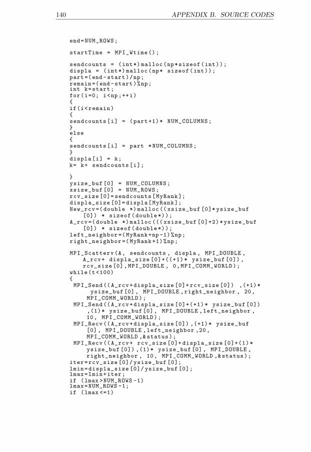
140 APPENDIX B. SOURCE CODES
end=NUM_ROWS;
startTime = MPI_Wtime ();
sendcounts = (int*) malloc(np*sizeof(int));displa = (int*) malloc(np* sizeof(int));part=(end -start)/np;remain =(end -start)%np;int k=start;for(i=0; i<np;++i){if(i<remain){sendcounts[i] = (part +1)* NUM_COLUMNS;}else{sendcounts[i] = part *NUM_COLUMNS;}displa[i] = k;k= k+ sendcounts[i];
}ysize_buf [0] = NUM_COLUMNS;xsize_buf [0] = NUM_ROWS;rcv_size [0]= sendcounts[MyRank ];displa_size [0]= displa[MyRank ];New_rcv =( double *) malloc (( xsize_buf [0]* ysize_buf
[0]) * sizeof(double *));A_rcv=( double *) malloc ((( xsize_buf [0]+2)*ysize_buf
[0]) * sizeof(double *));left_neighbor =( MyRank+np -1)%np;right_neighbor =( MyRank +1)%np;
MPI_Scatterv(A, sendcounts , displa , MPI_DOUBLE ,A_rcv+ displa_size [0]+((+1)* ysize_buf [0]),rcv_size [0],MPI_DOUBLE , 0,MPI_COMM_WORLD);
while(t <100){MPI_Send ((A_rcv+displa_size [0]+ rcv_size [0]) ,(+1)*
ysize_buf [0], MPI_DOUBLE ,right_neighbor , 20,MPI_COMM_WORLD);
MPI_Send ((A_rcv+displa_size [0]+(+1)* ysize_buf [0]),(1)* ysize_buf [0], MPI_DOUBLE ,left_neighbor ,10, MPI_COMM_WORLD);
MPI_Recv ((A_rcv+displa_size [0]) ,(+1)* ysize_buf[0], MPI_DOUBLE ,left_neighbor ,20,MPI_COMM_WORLD ,& status);
MPI_Recv ((A_rcv+ rcv_size [0]+ displa_size [0]+(1)*ysize_buf [0]) ,(1)* ysize_buf [0], MPI_DOUBLE ,right_neighbor , 10, MPI_COMM_WORLD ,& status);
iter=rcv_size [0]/ ysize_buf [0];lmin=displa_size [0]/ ysize_buf [0];lmax=lmin+iter;if (lmax >NUM_ROWS -1)lmax=NUM_ROWS -1;if (lmax <=1)
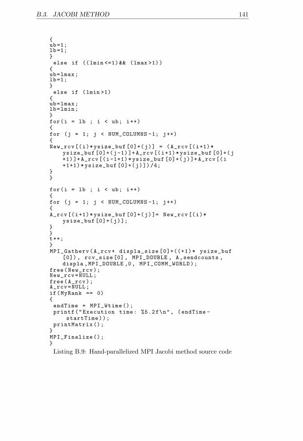
B.3. JACOBI METHOD 141
{ub=1;lb=1;}else if ((lmin <=1)&& (lmax >1))
{ub=lmax;lb=1;}else if (lmin >1)
{ub=lmax;lb=lmin;}for(i = lb ; i < ub; i++){for (j = 1; j < NUM_COLUMNS -1; j++){New_rcv [(i)*ysize_buf [0]+(j)] = (A_rcv[(i+1)*
ysize_buf [0]+(j-1)]+ A_rcv[(i+1)*ysize_buf [0]+(j+1)]+ A_rcv[(i -1+1)*ysize_buf [0]+(j)]+ A_rcv[(i+1+1)*ysize_buf [0]+(j)])/4;
}}
for(i = lb ; i < ub; i++){for (j = 1; j < NUM_COLUMNS -1; j++){A_rcv[(i+1)*ysize_buf [0]+(j)]= New_rcv [(i)*
ysize_buf [0]+(j)];}}t++;}MPI_Gatherv(A_rcv+ displa_size [0]+((+1)* ysize_buf
[0]), rcv_size [0], MPI_DOUBLE , A,sendcounts ,displa ,MPI_DOUBLE ,0, MPI_COMM_WORLD);
free(New_rcv);New_rcv=NULL;free(A_rcv);A_rcv=NULL;if(MyRank == 0){endTime = MPI_Wtime ();printf("Execution time: %5.2f\n", (endTime -
startTime));printMatrix ();
}MPI_Finalize ();}
Listing B.9: Hand-parallelized MPI Jacobi method source code
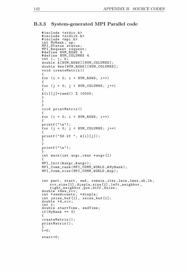
142 APPENDIX B. SOURCE CODES
B.3.3 System-generated MPI Parallel code
#include <stdio.h>#include <stdlib.h>#include <mpi.h>int MyRank , np;MPI_Status status;MPI_Request request;#define NUM_ROWS 4#define NUM_COLUMNS 4int i, j, k;double A[NUM_ROWS ][ NUM_COLUMNS ];double New[NUM_ROWS ][ NUM_COLUMNS ];void createMatrix (){for (i = 0; i < NUM_ROWS; i++){for (j = 0; j < NUM_COLUMNS; j++){A[i][j]=rand() % 10000;}}}void printMatrix (){for (i = 0; i < NUM_ROWS; i++){printf("\n");for (j = 0; j < NUM_COLUMNS; j++){printf("%8.2f ", A[i][j]);}}printf("\n");}int main(int argc ,char *argv []){MPI_Init (&argc ,&argv);MPI_Comm_rank(MPI_COMM_WORLD ,& MyRank);MPI_Comm_size(MPI_COMM_WORLD ,&np);
int part , start , end , remain ,iter ,lmin ,lmax ,ub ,lb ,rcv_size [1], displa_size [1], left_neighbor ,right_neighbor ,pos ,diff ,Ssize;
double *New_rcv;int *sendcounts , *displa;int ysize_buf [1], xsize_buf [1];double *A_rcv;int t;double startTime , endTime;if(MyRank == 0){createMatrix ();printMatrix ();}t=0;
start =0;
B.3. JACOBI METHOD 143
end=NUM_ROWS;
startTime = MPI_Wtime ();
sendcounts = (int*) malloc(np*sizeof(int));displa = (int*) malloc(np* sizeof(int));part=(end -start)/np;remain =(end -start)%np;int k=start;for(i=0; i<np;++i){if(i<remain){sendcounts[i] = (part +1)* NUM_COLUMNS;}else{sendcounts[i] = part *NUM_COLUMNS;}displa[i] = k;k= k+ sendcounts[i];
}ysize_buf [0] = NUM_COLUMNS;xsize_buf [0] = NUM_ROWS;rcv_size [0]= sendcounts[MyRank ];displa_size [0]= displa[MyRank ];New_rcv =( double *) malloc (( xsize_buf [0]* ysize_buf
[0]) * sizeof(double *));A_rcv=( double *) malloc ((( xsize_buf [0]+2)*ysize_buf
[0]) * sizeof(double *));Ssize=ysize_buf [0]* xsize_buf [0];diff = displa_size [0] -(+1);if(diff <0)pos= ysize_buf [0]* xsize_buf [0]+ diff;if(diff >0)pos=diff;
for(i=0; i<np;++i){if ((pos >= displa[i])&& (pos <= displa[i]+ sendcounts[i
])){left_neighbor=i;}}
diff=displa_size [0]+ rcv_size [0]+(+1);if(diff >Ssize)pos=diff -Ssize;if(diff <Ssize)pos=diff;for(i=0; i<np;++i){if((pos >= displa[i])&& (pos <= displa[i]+ sendcounts[i
])){right_neighbor=i;
144 APPENDIX B. SOURCE CODES
}}MPI_Scatterv(New , sendcounts , displa , MPI_DOUBLE ,
New_rcv+ displa_size [0], rcv_size [0], MPI_DOUBLE ,0,MPI_COMM_WORLD);
MPI_Scatterv(A, sendcounts , displa , MPI_DOUBLE ,A_rcv+ displa_size [0]+((+1)* ysize_buf [0]),rcv_size [0],MPI_DOUBLE , 0,MPI_COMM_WORLD);
while(t <100){MPI_Send ((A_rcv+displa_size [0]+ rcv_size [0]) ,(+1)*
ysize_buf [0], MPI_DOUBLE ,right_neighbor , 20,MPI_COMM_WORLD);
MPI_Send ((A_rcv+displa_size [0]+(+1)* ysize_buf [0]),(1)* ysize_buf [0], MPI_DOUBLE ,left_neighbor ,10, MPI_COMM_WORLD);
MPI_Recv ((A_rcv+displa_size [0]) ,(+1)* ysize_buf[0], MPI_DOUBLE ,left_neighbor ,20,MPI_COMM_WORLD ,& status);
MPI_Recv ((A_rcv+ rcv_size [0]+ displa_size [0]+(1)*ysize_buf [0]) ,(1)* ysize_buf [0], MPI_DOUBLE ,right_neighbor , 10, MPI_COMM_WORLD ,& status);
iter=rcv_size [0]/ ysize_buf [0];lmin=displa_size [0]/ ysize_buf [0];lmax=lmin+iter;if (lmax >NUM_ROWS -1)lmax=NUM_ROWS -1;if (lmax <=1){ub=1;lb=1;}else if ((lmin <=1)&& (lmax >1))
{ub=lmax;lb=1;}else if (lmin >1)
{ub=lmax;lb=lmin;}for(i = lb ; i < ub; i++){for (j = 1; j < NUM_COLUMNS -1; j++){New_rcv [(i)*ysize_buf [0]+(j)] = (A_rcv[(i+1)*
ysize_buf [0]+(j-1)]+ A_rcv[(i+1)*ysize_buf [0]+(j+1)]+ A_rcv[(i -1+1)*ysize_buf [0]+(j)]+ A_rcv[(i+1+1)*ysize_buf [0]+(j)])/4;
}}iter=rcv_size [0]/ ysize_buf [0];lmin=displa_size [0]/ ysize_buf [0];lmax=lmin+iter;if (lmax >NUM_ROWS -1)lmax=NUM_ROWS -1;
B.3. JACOBI METHOD 145
if (lmax <=1){ub=1;lb=1;}else if ((lmin <=1)&& (lmax >1))
{ub=lmax;lb=1;}else if (lmin >1)
{ub=lmax;lb=lmin;}for(i = lb ; i < ub; i++){for (j = 1; j < NUM_COLUMNS -1; j++){A_rcv[(i+1)*ysize_buf [0]+(j)]= New_rcv [(i)*
ysize_buf [0]+(j)];}}t++;}MPI_Gatherv(New_rcv+ displa_size [0], rcv_size [0],
MPI_DOUBLE , New ,sendcounts , displa ,MPI_DOUBLE ,0,MPI_COMM_WORLD);
MPI_Gatherv(A_rcv+ displa_size [0]+((+1)* ysize_buf[0]), rcv_size [0], MPI_DOUBLE , A,sendcounts ,displa ,MPI_DOUBLE ,0, MPI_COMM_WORLD);
free(New_rcv);New_rcv=NULL;free(A_rcv);A_rcv=NULL;if(MyRank == 0){endTime = MPI_Wtime ();printf("Execution time: %5.2f\n", (endTime -
startTime));printMatrix ();}MPI_Finalize ();}
Listing B.10: System-parallelized MPI Jacobi method source code
146 APPENDIX B. SOURCE CODES
B.3.4 Manual OpenMP Parallel Code
#include <stdio.h>#include <stdlib.h>#include <omp.h>#define NUM_ROWS 4#define NUM_COLUMNS 4int i, j, k;double A[NUM_ROWS ][ NUM_COLUMNS ];double New[NUM_ROWS ][ NUM_COLUMNS ];void createMatrix (){for (i = 0; i < NUM_ROWS; i++){for (j = 0; j < NUM_COLUMNS; j++){A[i][j]=rand() % 10000;}}}}void printMatrix (){for (i = 0; i < NUM_ROWS; i++){printf("\n");for (j = 0; j < NUM_COLUMNS; j++){printf("%8.2f ", A[i][j]);}}
printf("\n");}int main(int argc ,char *argv []){int t;int threads ,tid;double stime , etime;
omp_set_dynamic (0);threads=omp_get_max_threads ();omp_set_num_threads( threads );
tid=omp_get_thread_num ();createMatrix ();printMatrix ();t=0;#pragma omp barrierstime=omp_get_wtime ();while(t <100){#pragma omp parallel private(j){#pragma omp forfor (i = 1; i < NUM_ROWS -1; i++){for (j = 1; j < NUM_COLUMNS -1; j++)
B.3. JACOBI METHOD 147
{New[i][j] = (A[i][j-1]+A[i][j+1]+A[i-1][j]+A[i+1][j
])/4;}}#pragma omp forfor (i = 1; i < NUM_ROWS -1; i++){for (j = 1; j < NUM_COLUMNS -1; j++){A[i][j]= New[i][j];}}}t++;}#pragma omp barrieretime=omp_get_wtime ();printf("it takes: %5.2f \n", (etime -stime)) ;printMatrix ();}
Listing B.11: Hand-parallelized OpenMP Jacobi method source code
148 APPENDIX B. SOURCE CODES
B.3.5 System-generated OpenMP Parallel code
#include <stdio.h>#include <stdlib.h>#include <omp.h>#define NUM_ROWS 4#define NUM_COLUMNS 4int i, j, k;double A[NUM_ROWS ][ NUM_COLUMNS ];double New[NUM_ROWS ][ NUM_COLUMNS ];void createMatrix (){for (i = 0; i < NUM_ROWS; i++){for (j = 0; j < NUM_COLUMNS; j++){A[i][j]=rand() % 10000;}}}void printMatrix (){for (i = 0; i < NUM_ROWS; i++){printf("\n");for (j = 0; j < NUM_COLUMNS; j++){printf("%8.2f ", A[i][j]);}}printf("\n");}int main(int argc ,char *argv []){int t;int threads ,tid;double stime , etime;
omp_set_dynamic (0);threads=omp_get_max_threads ();omp_set_num_threads( threads );
tid=omp_get_thread_num ();createMatrix ();printMatrix ();t=0;#pragma omp barrierstime=omp_get_wtime ();while(t <100){#pragma omp parallel for private(j)for (i = 1; i < NUM_ROWS -1; i++){for (j = 1; j < NUM_COLUMNS -1; j++){New[i][j] = (A[i][j-1]+A[i][j+1]+A[i-1][j]+A[i+1][j
])/4;}
B.3. JACOBI METHOD 149
}#pragma omp parallel for private(j)for (i = 1; i < NUM_ROWS -1; i++){for (j = 1; j < NUM_COLUMNS -1; j++){A[i][j]= New[i][j];}}t++;}#pragma omp barrieretime=omp_get_wtime ();
printf("it takes: %5.2f \n", (etime -stime)) ;printMatrix ();}
Listing B.12: System-parallelized OpenMP Jacobi method source code
150 APPENDIX B. SOURCE CODES
B.4 Matrix multiplication and summation
B.4.1 Sequential Code
#include <stdio.h>#include <time.h>
#define NUM_ROWS_A 4#define NUM_COLUMNS_A 4#define NUM_ROWS_B 4#define NUM_COLUMNS_B 4
int i, j, k;int mat_a[NUM_ROWS_A ][ NUM_COLUMNS_A ];int mat_b[NUM_ROWS_B ][ NUM_COLUMNS_B ];int mat_result[NUM_ROWS_A ][ NUM_COLUMNS_B ];
void makeAB (){for (i = 0; i < NUM_ROWS_A; i++){for (j = 0; j < NUM_COLUMNS_A; j++){mat_a[i][j] = i + j;}}for (i = 0; i < NUM_ROWS_B; i++){for (j = 0; j < NUM_COLUMNS_B; j++){mat_b[i][j] = i*j;}}}void printArray (){for (i = 0; i < NUM_ROWS_A; i++){printf("\n");for (j = 0; j < NUM_COLUMNS_A; j++){printf("%d ", mat_a[i][j]);}}printf("\n");for (i = 0; i < NUM_ROWS_B; i++){printf("\n");for (j = 0; j < NUM_COLUMNS_B; j++){printf("%d ", mat_b[i][j]);}}printf("\n");for (i = 0; i < NUM_ROWS_A; i++){printf("\n");
B.4. MATRIX MULTIPLICATION AND SUMMATION 151
for (j = 0; j < NUM_COLUMNS_B; j++){printf("%d ", mat_result[i][j]);}}printf("\n\n");}int main(){int sum =0;struct timespec stime , etime;
makeAB ();clock_gettime(CLOCK_REALTIME , &stime);
for (i = 0; i < NUM_ROWS_A; i++){for (j = 0; j < NUM_COLUMNS_B; j++){for (k = 0; k < NUM_ROWS_B; k++){mat_result[i][j] += (mat_a[i][k] * mat_b[k][j]);sum+= mat_result[i][j];}}}
clock_gettime(CLOCK_REALTIME , &etime);printf("Execution time: %5.2f\n", (etime.tv_sec -
stime.tv_sec)+ 1e-9*( etime.tv_nsec - stime.tv_nsec)) ;
printArray ();printf("sum:%d \n", sum);
return 0;}
Listing B.13: Sequential Matrix multiplication and summation source code
152 APPENDIX B. SOURCE CODES
B.4.2 System-generated MPI Parallel code
#include <stdio.h>#include <mpi.h>int MyRank , np;MPI_Status status;MPI_Request request;#define NUM_ROWS_A 4#define NUM_COLUMNS_A 4#define NUM_ROWS_B 4#define NUM_COLUMNS_B 4int i, j, k;int mat_a[NUM_ROWS_A ][ NUM_COLUMNS_A ];int mat_b[NUM_ROWS_B ][ NUM_COLUMNS_B ];int mat_result[NUM_ROWS_A ][ NUM_COLUMNS_B ];void makeAB (){for (i = 0; i < NUM_ROWS_A; i++){for (j = 0; j < NUM_COLUMNS_A; j++){mat_a[i][j] = i + j;}}for (i = 0; i < NUM_ROWS_B; i++){for (j = 0; j < NUM_COLUMNS_B; j++){mat_b[i][j] = i*j;}}}void printArray (){for (i = 0; i < NUM_ROWS_A; i++){printf("\n");for (j = 0; j < NUM_COLUMNS_A; j++){printf("%d ", mat_a[i][j]);}}printf("\n");for (i = 0; i < NUM_ROWS_B; i++){printf("\n");for (j = 0; j < NUM_COLUMNS_B; j++){printf("%d ", mat_b[i][j]);}}printf("\n");for (i = 0; i < NUM_ROWS_A; i++){printf("\n");for (j = 0; j < NUM_COLUMNS_B; j++){
B.4. MATRIX MULTIPLICATION AND SUMMATION 153
printf("%d ", mat_result[i][j]);}}printf("\n\n");}
int find_min(int *array , int size) {
int i;int val = array [0];for (i = 1; i < size; ++i) {if (val > array[i]) {val = array[i];}}return val;}int find_max(int *array , int size) {
int i;int val = array [0];for (i = 1; i < size; ++i) {if (val < array[i]) {val = array[i];}}return val;}int main(int argc ,char *argv []){MPI_Init (&argc ,&argv);MPI_Comm_rank(MPI_COMM_WORLD ,& MyRank);MPI_Comm_size(MPI_COMM_WORLD ,&np);
double startTime , endTime;
int iter ,ub ,lb;int part ,k,remain ,lmin ,lmax ,dis_part ,dis_min ,
dis_max ,dis_lb ,dis_ub;int *mat_a_rcv;int mat_a_start ,mat_a_end ,mat_a_ysize_buf [1],
mat_a_xsize_buf [1], mat_a_rcv_size [1],mat_a_displa_size [1], mat_a_rcv_size2 [1],mat_a_displa_size2 [1];
int *mat_a_sendcounts , *mat_a_displa , *mat_a_sendcounts2 , *mat_a_displa2;
int *mat_result_rcv;int mat_result_start ,mat_result_end ,
mat_result_ysize_buf [1], mat_result_xsize_buf[1], mat_result_rcv_size [1],mat_result_displa_size [1], mat_result_rcv_size2[1], mat_result_displa_size2 [1];
int *mat_result_sendcounts , *mat_result_displa , *mat_result_sendcounts2 , *mat_result_displa2;
int parsum;parsum =0;int sum =0;if(MyRank == 0){
154 APPENDIX B. SOURCE CODES
makeAB ();}mat_a_start =0;mat_a_end=NUM_ROWS_A;startTime = MPI_Wtime ();
if(MyRank == 0){mat_a_sendcounts = (int*) malloc(np*sizeof(int));mat_a_displa = (int*) malloc(np* sizeof(int));mat_a_sendcounts2 = (int*) malloc(np*sizeof(int));mat_a_displa2 = (int*) malloc(np* sizeof(int));part=(mat_a_end -mat_a_start)/np;remain =(mat_a_end -mat_a_start)%np;k=mat_a_start;for(i=0; i<np;++i){if(i<remain){dis_part=part +1;}else{dis_part=part;}dis_lb=k;dis_ub=dis_lb+dis_part;k=dis_ub;
mat_a_displa2[i] = dis_lb* NUM_COLUMNS_A;mat_a_sendcounts2[i] = dis_part* NUM_COLUMNS_A;}mat_a_ysize_buf [0] = NUM_COLUMNS_A;mat_a_xsize_buf [0] = NUM_ROWS_A;}
MPI_Bcast(mat_a_ysize_buf , 1, MPI_INT , 0,MPI_COMM_WORLD);
MPI_Bcast(mat_a_xsize_buf , 1, MPI_INT , 0,MPI_COMM_WORLD);
MPI_Scatter(mat_a_displa2 , 1, MPI_INT ,mat_a_displa_size2 , 1, MPI_INT , 0,MPI_COMM_WORLD);
MPI_Scatter(mat_a_sendcounts2 , 1, MPI_INT ,mat_a_rcv_size2 , 1, MPI_INT , 0, MPI_COMM_WORLD);
mat_a_rcv =(int *) malloc (( mat_a_xsize_buf [0] *mat_a_ysize_buf [0]) * sizeof(int*));
if(MyRank == 0){for(i=0; i<np;++i){dis_lb=mat_a_displa2[i]/ mat_a_ysize_buf [0];dis_ub =( mat_a_displa2[i]+ mat_a_sendcounts2[i])/
mat_a_ysize_buf [0];int mat_a_min_lst70 []={ dis_lb };int mat_a_max_lst70 []={ dis_ub };dis_min= find_min(mat_a_min_lst70 ,1);
B.4. MATRIX MULTIPLICATION AND SUMMATION 155
dis_max= find_max(mat_a_max_lst70 ,1);if(dis_min <0)dis_min =0;if(dis_max >mat_a_end)dis_max=mat_a_end;mat_a_displa[i] = dis_min*mat_a_ysize_buf [0];mat_a_sendcounts[i] = (dis_max -dis_min)*
mat_a_ysize_buf [0];}}MPI_Scatter(mat_a_sendcounts , 1, MPI_INT ,
mat_a_rcv_size , 1, MPI_INT , 0, MPI_COMM_WORLD);MPI_Scatter(mat_a_displa , 1, MPI_INT ,
mat_a_displa_size , 1, MPI_INT , 0, MPI_COMM_WORLD);
MPI_Scatterv(mat_a , mat_a_sendcounts , mat_a_displa ,MPI_INT , mat_a_rcv+ mat_a_displa_size [0],
mat_a_rcv_size [0],MPI_INT , 0,MPI_COMM_WORLD);
mat_result_start =0;mat_result_end=NUM_ROWS_A;
if(MyRank == 0){mat_result_sendcounts = (int*) malloc(np*sizeof(int)
);mat_result_displa = (int*) malloc(np* sizeof(int));mat_result_sendcounts2 = (int*) malloc(np*sizeof(int
));mat_result_displa2 = (int*) malloc(np* sizeof(int));part=( mat_result_end -mat_result_start)/np;remain =( mat_result_end -mat_result_start)%np;k=mat_result_start;for(i=0; i<np;++i){if(i<remain){dis_part=part +1;}else{dis_part=part;}dis_lb=k;dis_ub=dis_lb+dis_part;k=dis_ub;
mat_result_displa2[i] = dis_lb* NUM_COLUMNS_B;mat_result_sendcounts2[i] = dis_part* NUM_COLUMNS_B
;}mat_result_ysize_buf [0] = NUM_COLUMNS_B;mat_result_xsize_buf [0] = NUM_ROWS_A;}
MPI_Bcast(mat_result_ysize_buf , 1, MPI_INT , 0,MPI_COMM_WORLD);
156 APPENDIX B. SOURCE CODES
MPI_Bcast(mat_result_xsize_buf , 1, MPI_INT , 0,MPI_COMM_WORLD);
MPI_Scatter(mat_result_displa2 , 1, MPI_INT ,mat_result_displa_size2 , 1, MPI_INT , 0,MPI_COMM_WORLD);
MPI_Scatter(mat_result_sendcounts2 , 1, MPI_INT ,mat_result_rcv_size2 , 1, MPI_INT , 0,MPI_COMM_WORLD);
mat_result_rcv =(int *) malloc (( mat_result_xsize_buf[0] *mat_result_ysize_buf [0]) * sizeof(int*));
if(MyRank == 0){for(i=0; i<np;++i){dis_lb=mat_result_displa2[i]/ mat_result_ysize_buf
[0];dis_ub =( mat_result_displa2[i]+
mat_result_sendcounts2[i])/mat_result_ysize_buf[0];
int mat_result_min_lst70 []={ dis_lb };int mat_result_max_lst70 []={ dis_ub };dis_min= find_min(mat_result_min_lst70 ,1);dis_max= find_max(mat_result_max_lst70 ,1);if(dis_min <0)dis_min =0;if(dis_max >mat_result_end)dis_max=mat_result_end;mat_result_displa[i] = dis_min*mat_result_ysize_buf
[0];mat_result_sendcounts[i] = (dis_max -dis_min)*
mat_result_ysize_buf [0];}}MPI_Scatter(mat_result_sendcounts , 1, MPI_INT ,
mat_result_rcv_size , 1, MPI_INT , 0,MPI_COMM_WORLD);
MPI_Scatter(mat_result_displa , 1, MPI_INT ,mat_result_displa_size , 1, MPI_INT , 0,MPI_COMM_WORLD);
MPI_Scatterv(mat_result , mat_result_sendcounts ,mat_result_displa , MPI_INT , mat_result_rcv+mat_result_displa_size [0], mat_result_rcv_size[0],MPI_INT , 0,MPI_COMM_WORLD);
MPI_Bcast(mat_b ,( NUM_ROWS_B*NUM_COLUMNS_B), MPI_INT,0, MPI_COMM_WORLD);
iter=mat_a_rcv_size2 [0]/ mat_a_ysize_buf [0];lmin=mat_a_displa_size2 [0]/ mat_a_ysize_buf [0];lmax=lmin+iter;if (lmax >NUM_ROWS_A)lmax=NUM_ROWS_A;if (lmax <=0){ub=0;lb=0;}else if ((lmin <=0)&& (lmax >0)){
B.4. MATRIX MULTIPLICATION AND SUMMATION 157
ub=lmax;lb=0;}else if (lmin >0){ub=lmax;lb=lmin;}for(i = lb ; i < ub; i++){for (j = 0; j < NUM_COLUMNS_B; j++){for (k = 0; k < NUM_ROWS_B; k++){mat_result_rcv [(i)*mat_result_ysize_buf [0]+(j)] +=
(mat_a_rcv [(i)*mat_a_ysize_buf [0]+(k)] * mat_b[k][j]);
parsum += mat_result_rcv [(i)*mat_result_ysize_buf[0]+(j)];
}}}MPI_Gatherv(mat_a_rcv+mat_a_displa_size2 [0],
mat_a_rcv_size2 [0], MPI_INT , mat_a ,mat_a_sendcounts2 , mat_a_displa2 ,MPI_INT ,0,MPI_COMM_WORLD);
MPI_Gatherv(mat_result_rcv+mat_result_displa_size2[0], mat_result_rcv_size2 [0], MPI_INT , mat_result,mat_result_sendcounts2 , mat_result_displa2 ,MPI_INT ,0, MPI_COMM_WORLD);
MPI_Reduce (&parsum ,&sum ,1,MPI_INT ,MPI_SUM ,0,MPI_COMM_WORLD);
if(MyRank ==0){free(mat_a_sendcounts);mat_a_sendcounts=NULL;free(mat_a_displa);mat_a_displa=NULL;free(mat_a_sendcounts2);mat_a_sendcounts2=NULL;free(mat_a_displa2);mat_a_displa2=NULL;free(mat_result_sendcounts);mat_result_sendcounts=NULL;free(mat_result_displa);mat_result_displa=NULL;free(mat_result_sendcounts2);mat_result_sendcounts2=NULL;free(mat_result_displa2);mat_result_displa2=NULL;}
if(MyRank == 0){endTime = MPI_Wtime ();
158 APPENDIX B. SOURCE CODES
printf("Execution time: %5.2f\n", (endTime -startTime));
printArray ();printf("sum:%d \n ", sum);}free(mat_a_rcv);mat_a_rcv=NULL;free(mat_result_rcv);mat_result_rcv=NULL;
MPI_Finalize ();return 0;}
Listing B.14: System-parallelized MPI Matrix multiplication andsummation source code
B.4. MATRIX MULTIPLICATION AND SUMMATION 159
B.4.3 System-generated OpenMP Parallel code
#include <stdio.h>#include <omp.h>#define NUM_ROWS_A 4#define NUM_COLUMNS_A 4#define NUM_ROWS_B 4#define NUM_COLUMNS_B 4int i, j, k;int mat_a[NUM_ROWS_A ][ NUM_COLUMNS_A ];int mat_b[NUM_ROWS_B ][ NUM_COLUMNS_B ];int mat_result[NUM_ROWS_A ][ NUM_COLUMNS_B ];void makeAB (){for (i = 0; i < NUM_ROWS_A; i++){for (j = 0; j < NUM_COLUMNS_A; j++){mat_a[i][j] = i + j;}}for (i = 0; i < NUM_ROWS_B; i++){for (j = 0; j < NUM_COLUMNS_B; j++){mat_b[i][j] = i*j;}}}void printArray (){for (i = 0; i < NUM_ROWS_A; i++){printf("\n");for (j = 0; j < NUM_COLUMNS_A; j++){printf("%d ", mat_a[i][j]);}}printf("\n");for (i = 0; i < NUM_ROWS_B; i++){printf("\n");for (j = 0; j < NUM_COLUMNS_B; j++){printf("%d ", mat_b[i][j]);}}printf("\n");for (i = 0; i < NUM_ROWS_A; i++){printf("\n");for (j = 0; j < NUM_COLUMNS_B; j++){printf("%d ", mat_result[i][j]);}}
160 APPENDIX B. SOURCE CODES
printf("\n\n");}int main(int argc ,char *argv []){double stime , etime;int sum=0;int threads ,tid;threads=omp_get_max_threads ();tid=omp_get_thread_num ();makeAB ();stime=omp_get_wtime ();
#pragma omp parallel for private(j,k) reduction (+:sum)
for (i = 0; i < NUM_ROWS_A; i++){for (j = 0; j < NUM_COLUMNS_B; j++){for (k = 0; k < NUM_ROWS_B; k++){mat_result[i][j] += (mat_a[i][k] * mat_b[k][j]);sum+= mat_result[i][j];}}}
etime=omp_get_wtime ();printf("sorting took: %5.2f \n", (etime -stime)) ;printArray ();printf("int:%d \n ", sum);return 0;}
Listing B.15: System-parallelized OpenMP Matrix multiplication andsummation source code
Bibliography
[1] Open64. Computer Architecture and Parallel Systems Laboratory(CAPSL). http://www.open64.net/, Accessed August 2012.
[2] Sparc: Parallelization. Sun Microsystems, Inc., 2000.http://caligari.dartmouth.edu/doc/solaris-forte/manuals/
fortran/prog_guide/10_parallel.html, Accessed June 2012.
[3] Joonseon Ahn and Taisook Han. An analytical method for paralleliza-tion of recursive functions. Parallel Processing Letters, pages 359–370,December 2000.
[4] Randy Allen and Ken Kennedy. Automatic translation of Fortran pro-grams to vector form. ACM Trans. Program. Lang. Syst., 9(4):491–542,October 1987.
[5] Randy Allen and Ken Kennedy. Optimizing Compilers for Modern Ar-chitectures: A Dependence-Based Approach. Morgan Kaufmann, 2002.
[6] U. Assmann. Invasive Software Composition. Springer-Verlag NewYork, Inc., Secaucus, NJ, USA, 2003.
[7] Franz Baader and Werner Nutt. The description logic handbook. chap-ter Basic description logics, pages 43–95. Cambridge University Press,New York, NY, USA, 2003.
[8] Utpal Banerjee. Speedup of ordinary programs. PhD thesis, Universityof Illinois at Urbana-Champaign, Champaign, IL, USA, 1979.
[9] Blaise Barney. Introduction to parallel computing. Lawrence LivermoreNational Laboratory. https://computing.llnl.gov/tutorials/
parallel_comp, Accessed June 2012.
[10] Blaise Barney. Message passing interface(MPI). Lawrence LivermoreNational Laboratory. https://computing.llnl.gov/tutorials/mpi,Accessed June 2012.
[11] Christopher Barton, Arie Tal, Bob Blainey, and Jose Nelson Amaral.Generalized index-set splitting. In Proceedings of the 14th international
161
162 BIBLIOGRAPHY
conference on Compiler Construction, CC’05, pages 106–120, Berlin,Heidelberg, 2005. Springer-Verlag.
[12] Songluan Cang and Jie Wu. Minimizing total communication distanceof time-step optimal broadcast in mesh networks. In IPPS/SPDP, pages10–17, Los Alamitos, CA, USA, 1998. IEEE Computer Society.
[13] Mikhail Chalabine. Invasive Interactive Parallelization. Licentiate the-sis, Linkoping university press, 2007.
[14] Rohit Chandra, Leonardo Dagum, Dave Kohr, Dror Maydan, and JeffMcDonald. Parallel programming in OpenMP. Morgan and Kaufmann,San Diego, CA, 2001.
[15] Murray Cole. Algorithmic skeletons: structured management of parallelcomputation. MIT Press, Cambridge, MA, USA, 1991.
[16] Chirag Dave, Hansang Bae, Seung-Jai Min, Seyong Lee, Rudolf Eigen-mann, and Samuel Midkiff. Cetus: A source-to-source compiler infras-tructure for multicores. Computer, 42(12):36–42, December 2009.
[17] Mattias Eriksson, Christoph Kessler, and Mikhail Chalabine. Loadbalancing of irregular parallel divide-and-conquer algorithms in Group-SPMD programming environments. In Proc. 8th Workshop on ParallelSystems and Algorithms (PASA 2006), Frankfurt am Main, Germany,March 2006.
[18] Ian Foster. Designing and Building Parallel Programs. Addison Wesley,1995.
[19] A Gonzalez-Escribano, D Llanos, D Orden, and B Palop. Parallelizationalternatives and their performance for the convex hull problem. AppliedMathematical Modelling, 30(7):563–577, 2006.
[20] Ananth Grama, Anshul Gupta, George Karypis, and Vipin Kumar.Introduction to Parallel Computing. Addison Wesley, 2003.
[21] Meta Group. Component software. Meta Group, Inc., White Paper,1994.
[22] Junjie Gu, Zhiyuan Li, and Gyungho Lee. Symbolic array dataflowanalysis for array privatization and program parallelization. In Proceed-ings of the 1995 ACM/IEEE conference on Supercomputing (CDROM),Supercomputing ’95, New York, NY, USA, 1995. ACM.
[23] Manish Gupta, Sayak Mukhopadhyay, and Navin Sinha. Automaticparallelization of recursive procedures. Int. J. Parallel Program.,28:537–562, December 2000.
BIBLIOGRAPHY 163
[24] Kris Gybels and Johan Brichau. Arranging language features for morerobust pattern-based crosscuts. In Proceedings of the 2nd internationalconference on Aspect-oriented software development, AOSD ’03, pages60–69, New York, NY, USA, 2003. ACM.
[25] Jonathan Hardwick. Practical Parallel Divide-and-Conquer Algorithms.PhD thesis, Carnegie Mellon University, Pittsburgh, PA 15213, Decem-ber 1997.
[26] George T. Heineman and William T. Councill, editors. Component-based software engineering: putting the pieces together. Addison-WesleyLongman Publishing Co., Inc., Boston, MA, USA, 2001.
[27] John L. Hennessy and David A. Patterson. Computer Architecture,Fourth Edition: A Quantitative Approach. Morgan Kaufmann Publish-ers Inc., San Francisco, CA, USA, 2006.
[28] Franz Inc. Allegro cl 8.2, 2012. http://www.franz.com/products/
allegrocl/, Accessed June 2012.
[29] Tim Jacobson and Gregg Stubbendieck. Dependency analysis of for-loop structures for automatic parallelization of C code. In 36th AnnualMidwest Instruction and Computing Symposium, MICS 2003.
[30] Joel Jones. Abstract syntax tree implementation idioms. In Proceedingsof the 10th Conference on Pattern Languages of Programs (PLoP2003),2003.
[31] Ken Kennedy, Kathryn S. McKinley, and Chau-Wen Tseng. Interactiveparallel programming using the parascope editor. IEEE TRANSAC-TIONS ON PARALLEL AND DISTRIBUTED SYSTEMS, 2(3):329–341, 1991.
[32] K. Ashwin Kumar, Aasish Kumar Pappu, K. Sarath Kumar, and SudipSanyal. Hybrid approach for parallelization of sequential code withfunction level and block level parallelization. In Proceedings of the in-ternational symposium on Parallel Computing in Electrical Engineer-ing, PARELEC ’06, pages 161–166, Washington, DC, USA, 2006. IEEEComputer Society.
[33] Claudia Leopold. Arranging statements and data of program instancesfor locality. Future Gener. Comput. Syst., 14(5-6):293–311, December1998.
[34] Calvin Lin and Larry Snyder. Principles of Parallel Programming.Addison-Wesley Publishing Company, USA, 1st edition, 2008.
[35] Toshitsugu Yuba Makoto Ishihara, Hiroki Honda and Mitsuhisa Sato.Interactive parallelizing assistance tool for OpenMP: iPat/OMP. In
164 BIBLIOGRAPHY
Fifth European Workshop on OpenMP , EWOMP ‘03, Aachen Univer-sity, Germany, September 22-26 2003.
[36] John Mariana. Deductive arguments and inductive arguments: Howto tell the difference. Mathematics and computer science depart-ment, Michigan State University. https://www.msu.edu/~marianaj/
DedInd.htm, Accessed June 2012.
[37] John McCarthy. Lisp - notes on its past and future. In Proceedings ofthe 1980 ACM conference on LISP and functional programming, LFP’80, pages .5–viii, New York, NY, USA, 1980. ACM.
[38] L.E. Moser. Data dependency graphs for ada programs. IEEE Trans-actions on Software Engineering, 16:498–509, 1990.
[39] Rishiyur S. Nikhil. Notes on automatic parallelization. Laboratory forcomputer science, Massachusetts Institute of Technology, Cambridge,July 1990.
[40] Ulf Nilsson and Jan Maluszynski. Logic, Programming, and PROLOG.John Wiley & Sons, Inc., New York, NY, USA, 2nd edition, 1995.
[41] NSC. User guide. National Supercomputer Centre in Sweden. http:
//www.nsc.liu.se/systems/snic/, Accessed June 2012.
[42] Eduardo Kessler Piveta and Luiz Carlos Zancanella. Aspect weavingstrategies. Journal of Universal Computer Science, 9(8):970–983, Au-gust 2003.
[43] K. Psarris. Program analysis techniques for transforming programs forparallel execution. Parallel Comput., 28(3):455–469, March 2002.
[44] Kleanthis Psarris. The Banerjee-Wolfe and gcd tests on exact datadependence information. J. Parallel Distrib. Comput., 32(2):119–138,February 1996.
[45] Michael J. Quinn. Parallel Programming in C with MPI and OpenMP.McGraw-Hill Education Group, 2003.
[46] Atanas Rountev, Barbara G. Ryder, and William Landi. Data-flowanalysis of program fragments. In Proceedings of the 7th Europeansoftware engineering conference held jointly with the 7th ACM SIG-SOFT international symposium on Foundations of software engineer-ing, ESEC/FSE-7, pages 235–252, London, UK, 1999. Springer-Verlag.
[47] Radu Rugina and Martin Rinard. Automatic parallelization of divideand conquer algorithms. In Proceedings of the 7th ACM SIGPLANSymposium on Principles and Practice of Parallel Programming, pages72–83, Atlanta, May 1999.
BIBLIOGRAPHY 165
[48] Stuart J. Russell and Peter Norvig. Artificial intelligence: a modernapproach (2nd ed.). Prentice-Hall, Inc., Upper Saddle River, NJ, USA,2003.
[49] Joseph D. Sloan. High Performance Linux Clusters: With OSCAR,Rocks, openMosix, and MPI (Nutshell Handbooks). O’Reilly Media,Inc., 2004.
[50] Marc Snir, Steve W. Otto, David W. Walker, Jack Dongarra, andSteven Huss-Lederman. MPI: The Complete Reference. MIT Press,Cambridge, MA, USA, 1995.
[51] Judith Alyce Stafford. A formal, language-independent, and compo-sitional approach to interprocedural control dependence analysis. PhDthesis, University of Colorado at Boulder, Boulder, CO, USA, 2000.
[52] William Stallings. Computer Organization and Architecture: Designingfor Performance (8th Edition). Prentice Hall, 2009.
[53] Amos Storkey. Learning from data: Decision trees. School of informat-ics, University of Edinburgh, September 2004.
[54] Michael Suß. Automatic parallelization and minimization of com-munication costs of program instances. In Proceedings of 5. GI-Informatiktage 2003, pages 206–209, Bad Schussenried, Germany.
[55] Clemens Szyperski. Component Software: Beyond Object-Oriented Pro-gramming. Addison-Wesley Longman Publishing Co., Inc., Boston,MA, USA, 2nd edition, 2002.
[56] Linda Torczon and Keith Cooper. Engineering A Compiler. MorganKaufmann Publishers Inc., San Francisco, CA, USA, 2nd edition, 2011.
[57] Todd Veldhuizen. C++ gems. chapter Using C++ template metapro-grams, pages 459–473. SIGS Publications, Inc., New York, NY, USA,1996.
[58] Michael Joseph Wolfe. Optimizing Supercompilers for Supercomputers.MIT Press, Cambridge, MA, USA, 1990.
[59] Wilson Cheng yi Hsieh. Extracting parallelism from sequential pro-grams. Technical report, Department of Electrical Engineering andComputer Science, Massachusetts Institute of Technology, 1988.
[60] Hans Zima and Barbara Chapman. Supercompilers for parallel andvector computers. ACM, New York, NY, USA, 1991.

166 BIBLIOGRAPHY
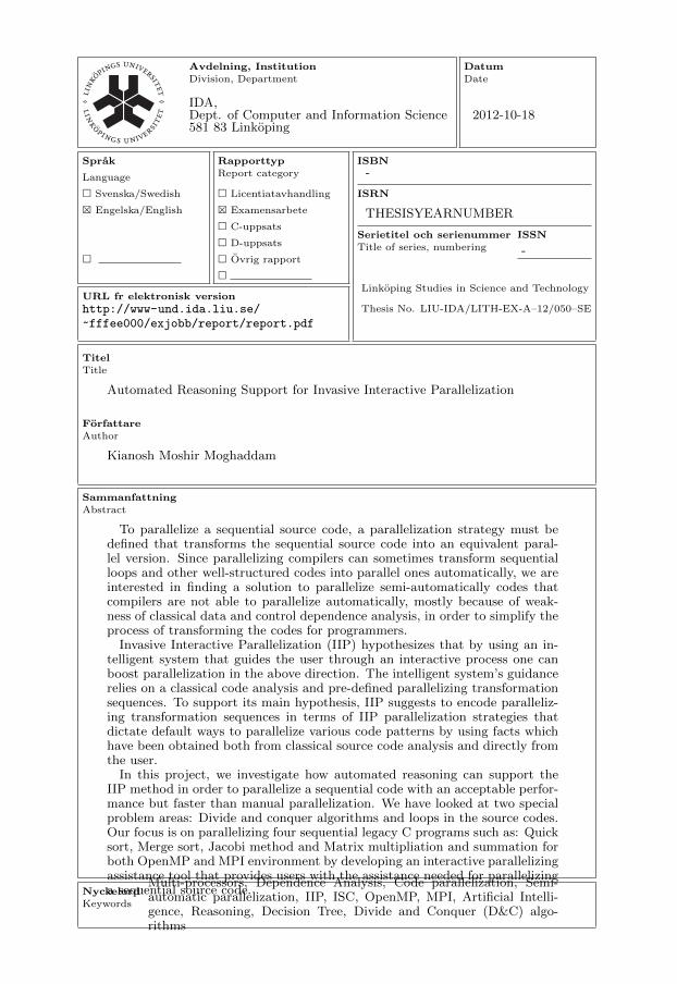
Avdelning, InstitutionDivision, Department
DatumDate
Sprak
Language
� Svenska/Swedish
� Engelska/English
�
RapporttypReport category
� Licentiatavhandling
� Examensarbete
� C-uppsats
� D-uppsats
� Ovrig rapport
�
URL fr elektronisk version
ISBN
ISRN
Serietitel och serienummerTitle of series, numbering
ISSN
Linkoping Studies in Science and Technology
Thesis No. LIU-IDA/LITH-EX-A–12/050–SE
TitelTitle
ForfattareAuthor
SammanfattningAbstract
NyckelordKeywords
To parallelize a sequential source code, a parallelization strategy must bedefined that transforms the sequential source code into an equivalent paral-lel version. Since parallelizing compilers can sometimes transform sequentialloops and other well-structured codes into parallel ones automatically, we areinterested in finding a solution to parallelize semi-automatically codes thatcompilers are not able to parallelize automatically, mostly because of weak-ness of classical data and control dependence analysis, in order to simplify theprocess of transforming the codes for programmers.
Invasive Interactive Parallelization (IIP) hypothesizes that by using an in-telligent system that guides the user through an interactive process one canboost parallelization in the above direction. The intelligent system’s guidancerelies on a classical code analysis and pre-defined parallelizing transformationsequences. To support its main hypothesis, IIP suggests to encode paralleliz-ing transformation sequences in terms of IIP parallelization strategies thatdictate default ways to parallelize various code patterns by using facts whichhave been obtained both from classical source code analysis and directly fromthe user.
In this project, we investigate how automated reasoning can support theIIP method in order to parallelize a sequential code with an acceptable perfor-mance but faster than manual parallelization. We have looked at two specialproblem areas: Divide and conquer algorithms and loops in the source codes.Our focus is on parallelizing four sequential legacy C programs such as: Quicksort, Merge sort, Jacobi method and Matrix multipliation and summation forboth OpenMP and MPI environment by developing an interactive parallelizingassistance tool that provides users with the assistance needed for parallelizinga sequential source code.
IDA,Dept. of Computer and Information Science581 83 Linkoping
2012-10-18
-
THESISYEARNUMBER
-
http://www-und.ida.liu.se/
~fffee000/exjobb/report/report.pdf
2012-10-18
Automated Reasoning Support for Invasive Interactive Parallelization
Kianosh Moshir Moghaddam
××
Multi-processors, Dependence Analysis, Code parallelization, Semi-automatic parallelization, IIP, ISC, OpenMP, MPI, Artificial Intelli-gence, Reasoning, Decision Tree, Divide and Conquer (D&C) algo-rithms
Related Documents